The Multiobjective Traveling Salesman Problem

The Multiobjective Traveling Salesman

Problem: A Survey and a New Approach.

Thibaut Lust⋆ and Jacques Teghem

Faculte Polytechnique de MonsLaboratory of Mathematics and Operational Research9, rue de Houdain7000 Mons, [email protected], [email protected]

Summary. The traveling salesman problem (TSP) is a challenging problem in com-binatorial optimization. In this paper we consider the multiobjective TSP for whichthe aim is to obtain or to approximate the set of efficient solutions. In a first step,we classify and describe briefly the existing works, that are essentially based on theuse of metaheuristics. In a second step, we propose a new method, called two-phasePareto local search. In the first phase of this method, an initial population com-posed of an approximation to the extreme supported efficient solutions is generated.The second phase is a Pareto local search applied to all solutions of the initial pop-ulation. The method does not use any numerical parameter. We show that usingthe combination of these two techniques—good initial population generation andPareto local search—gives, on the majority of the instances tested, better resultsthan state-of-the-art algorithms.

1 Introduction

Since the 70ies, multiobjective optimization problems (MOP) became an im-portant field of operations research. In many real applications, there existseffectively more than one objective to be taken into account to evaluate thequality of the feasible solutions.

A MOP is defined as follows:

“min” z(x) = zk(x) k = 1, . . . , p (MOP)

s.t x ∈ X ⊂ Rn+

where n is the number of variables, zk(x) : Rn+ → R represents the kth

objective function and X is the set of feasible solutions. We will denote byZ = {z(x) : x ∈ X} ⊂ R

p the image of X in the objective space.

⋆ T. Lust thanks the “Fonds National de la Recherche Scientifique” for a researchfellow grant (Aspirant FNRS).

2 Thibaut Lust and Jacques Teghem

Due to the typically conflictive objectives, the notion of optimal solutiondoes not exist generally anymore for MOPs. However, based on the dominancerelation of Pareto (see definition 1), the notion of optimal solution can be re-placed by the notion of efficient (or Pareto optimal) solution (see definition 2).

Definition 1. A vector z ∈ Z dominates a vector z′ ∈ Z if, and only if,

zk ≤ z′k, ∀ k ∈ {1, . . . , p}, with at least one index k for which the inequality is

strict. We denote this dominance relation by z ≺ z′.

Definition 2. A feasible solution x ∈ X is efficient if there does not exist

any other solution x′ ∈ X such that z(x′) ≺ z(x). The image of an efficient

solution in objective space is called a non-dominated point.

In the following, we will denote by XE , called efficient set, the set of allefficient solutions and by ZN , called the Pareto front, the image of XE in theobjective space.

The following additional definitions have been introduced by Hansen [22].

Definition 3. Equivalent solutions: two solutions x1, x2 ∈ XE are equivalent

if z(x1) = z(x2).

Definition 4. Complete set: a complete set XEc is a subset of XE such that

each x ∈ X \XEc is either dominated by or equivalent to at least one x ∈ XEc.

In other words, for each non-dominated point z ∈ ZN there exists at least one

x ∈ XEc with z(x) = z.

Definition 5. Minimal complete set: a minimal complete set XEm is a com-

plete set without equivalent solutions. Any complete set contains at least a

minimal complete set.

Even if other approaches exist to tackle a MOP problem (aggregation ofthe objectives with a utility function, hierarchy of the objectives, goal pro-gramming, interactive method to generate a “ good compromise ”: see [53]), inthis paper we are only interested in the determination, or the approximation,of XE and ZN . It should be noted that in all heuristics presented in this work,only an approximation of a minimal complete set is determined: no equivalentsolution generated will thus be retained.

It is first the problems with continuous variables which called the atten-tion of the researchers: see the book of Steuer [52] for multiobjective linear

programming (MOLP) problems and of Miettinen [43] for multiobjective non-

linear programming [43] (MONLP) problems.However it is well-known that discrete variables are often unavoidable in

the modeling of many applications and for such problems the determinationof XE and ZN becomes more difficult.

Let us consider for instance a multiobjective integer linear programming

(MOILP) problem of the form:

The Multiobjective Traveling Salesman Problem 3

“min” z(x) = zk(x) = ckx k = 1, . . . , p (MOILP)

s.t x ∈ X = {x ∈ Zn+ : Ax = b}

In such case, we can distinguish two types of efficient solutions:

• The supported efficient solutions are optimal solutions of the weightedsingle-objective problem

min

p∑

k=1

λkzk(x)

s.t x ∈ X

where λ ∈ Rp+ is a weight vector with all positive components λk, k =

1, . . . , p. We denote by XSE and ZSN respectively the set of supportedefficient solutions and the set of corresponding non-dominated points inR

p. The points of ZSN are located on the frontier of the convex hull of Z.• Contradictorily with a MOLP problem ZSN is generally a proper subset

of ZN due to the non-convex character of Z: there exist efficient solutionswhich are non-supported. We denote by XNE = XE\XSE and ZNN =ZN\ZSN respectively the set of non-supported efficient solutions and theset of the corresponding non-dominated points in R

p.

Inside XSE , it is useful to distinguish the extreme supported efficient so-lutions, i.e., the solutions x ∈ XSE such that z(x) is a vertex of the convexhull of Z, and the others, the non-extreme supported solutions. We denoteby XSE1 and XSE2 = XSE\XSE1 respectively the set of extreme and non-extreme supported solutions and by ZSE1 and ZSE2 the corresponding setsof non-dominated points in the objective space.

Already in the 80ies, several methods have been proposed to generate XE

for MOILP problems [54]. The two main difficulties to overcome are that:

• The sets XE and ZN , formed of discrete points, can be of very largecardinality;

• The sets XNE and ZNN are more difficult to determine.

Later, various multiobjective combinatorial optimization (MOCO) prob-lems have been considered. Most of them are of the type

“min” z(x) = ck(x) k = 1, . . . , p (MOCO)

s.t x ∈ X = D ∩ {0, 1}n

where D is a specific polytope characterizing the particular CO problem.During the last 15 years, there has been a notable increase of the number

of studies on MOCO problems. From the first survey [55] in 1994 till [8] in2002, a lot of papers have been published and this flow is still increasing. Themain reason of this phenomenon is the success story of the metaheuristics [16].

Effectively, it is quite difficult to determine exactly the sets XE and ZN

for MOCO problems. This is a NP-hard problem even for CO problems for


which a polynomial algorithm for the single-objective version exists such aslinear assignment problem. Therefore, there exist only few exact methods ableto determine the sets XE and ZN and we can expect to apply these methodsonly for small instances. For this reason, many methods are heuristic methodswhich produce approximations XE and ZN to the sets XE and ZN . Due to thesucces of metaheuristics for single-objective CO, multiobjective metaheuristics

(MOMH) became quickly a classic tool to tackle MOCO problems and it ispresently a real challenge for the researchers to improve the results previouslyobtained.

The two main difficulties of MOMH are related to the basic needs of anymetaheuristics [16]:

• To assure sufficient intensity, i.e. to produce an approximation ZN as closeas possible to ZN ;

• To assure sufficient diversity, i.e. to cover with ZN all the parts of ZN .

Unfortunately, measuring the quality of an approximation or to comparethe approximations obtained by various methods remains a difficult task: theproblem of the quality assessment of the results of a MOMH method is in factalso a multicriteria problem. Consequently, several indicators have been intro-duced in the literature to measure the quality of an approximation (see [60]for instance).

Some of them are unary indicators:

• The hypervolume H (to be maximized) [59]: the volume of the dominated

space defined by ZN , limited by a reference point.• The R measure (normalized between 0 and 1, to be maximized) [26]: eval-

uation of ZN by the expected value of the weighted Tchebycheff utilityfunction over a set of normalized weight vectors.

• The average distance D1 and maximal distance D2 (to be minimized) [7,

57] between the points of a reference set and the points of ZN , by usingthe Euclidean distance. Ideally, the reference set is ZN itself, but generallyit is not available ; otherwise, it can be the non-dominated points existingamong the union of various sets ZN generated by several methods, or alower bound of ZN [9].

Other indicators are introduced to compare two approximation sets Aand B of ZN . In particular, the Iǫ(A, B) [61] indicator gives the ǫ factor bywhich the approximation A is worse (if ǫ > 1) or better (if ǫ < 1) than theapproximation B with respect to all objectives:

Iǫ(A, B) = infǫ∈R+

{∀ z ∈ B, ∃ z′ ∈ A : z′k ≤ ǫ · zk, k = 1, . . . , p}

If B is a reference set, this indicator can also be used as a unary indicator,denoted by Iǫ1.

Unfortunately, none of these indicators allows to conclude that an ap-proximation is better than another one (see [61] for details). Nevertheless,


an approximation that finds better values for these indicators is generallypreferred to others.

In the first time, the MOCO problems treated in the literature are those forwhich there exist efficient algorithms in the single-objective case, essentiallylinear assignment problem, shortest path problem or knapsack problem.

More recently, a large attention has been devoted to the multiobjectivetraveling salesman problem (MOTSP). In the next section, we survey brieflythe existing MOTSP literature. Section 3 is dedicated to a new heuristicmethod applied to the biobjective TSP. Its results are presented in section4 before a short conclusion in section 5.

2 The multiobjective TSP literature

The traveling salesman problem is certainly the best-known and most studiedNP-hard single-objective CO problem.

The book of Gutin and Punnen [18] analyzes various methods for the TSPand for some of its variants; the chapters of Johnson and McGeoch [29, 30] aredevoted to heuristics respectively for the symmetric and asymmetric versionsof the TSP.

Other interesting reviews are related to the use of metaheuristics for theTSP: [28] is a survey of local search (LS) methods, [35] of genetic algorithms(GA) and [42] of memetic algorithms applied to TSP.

We recall the formulation of the MOTSP: given N cities and p costscki,j (k = 1, . . . , p) to travel from city i to city j, the MOTSP consists of

finding a tour, i.e. a cyclic permutation ρ of the N cities, minimizing

“ min ”zk(ρ) =

N−1∑

i=1

ckρ(i),ρ(i+1) + ck

ρ(N),ρ(1), k = 1, . . . , p

The majority of the instances treated in the following cited papers concernthe symmetric biobjective case (p = 2); sometimes p = 3.

One of the first paper concerning MOTSP is the study of Borges andHansen [6]. It is devoted to the “global convexity” in MOCO problems ingeneral, MOTSP in particular. The authors analyzed the landscape of localoptima, considering the classical 2-opt neighborhood (two edges are deletedand replaced with the only possible pair of new edges that does not break thetour) and using well-known scalarizing functions like the weighted sum of theobjectives or the Tchebycheff function. They indicated the implications of thedistribution of local optima in building MOMH to approximate ZN .

Almost all the existing methods are MOMH. In these methods, a set XE ≡XEc of potential efficient solutions is updated each time a new solution x isgenerated: x is added to XE if no solution of XE dominates x or is equivalentto x and all the solutions of XE dominated by x are removed. At the end ofthe procedure, XE is the proposed approximation.


In order to present the MOMH suited to solve the MOTSP, we made adistinction between MOMH based on evolutionary algorithms, based on localsearch and we finally present particular studies and variants of the MOTSP.

2.1 Evolutionary Algorithms (EAs)

We first present MOMH essentially based on EAs.

• One of the best performing MOMH is the MOGLS (multiple objectivegenetic local search) method proposed by Jaszkiewicz [26] so that theperformance of MOGLS is often taken as reference for comparisons.MOGLS combines GA and LS and works as follows:– An initial population P is built: each solution is optimized by a local

search applied to a weighted sum of the objectives.– At each iteration, a random utility function is selected. The best so-

lutions in P for this function form a temporary population TP. InsideTP, two solutions x1 and x2 are randomly selected and recombinedto generate a solution x3; the local search is applied to x3 obtainingx′

3. If x′3 is better that the worst solution of P according to the ran-

dom utility function, x′3 is added to P . To treat a MOTSP problem,

the local search is a standard 2-opt exchange and the recombinationoperator is the distance preserving crossover DPX: all edges commonto both parents are put in the offspring which is then completed byrandomly selected edges to form a Hamiltonian cycle. The consideredinstances—with two or three objectives—are based on the TSPLIBlibrary [49].

• The memetic random key genetic algorithm described in [51] is inspiredby MOGLS. The crossover operator is different: first a random number isassociated to each city of each parent and the chromosome is representedalternatively by these numbers. A classical one-point crossover is appliedbut the random numbers are used as “sort keys” to decode the new solu-tions: the cities are sorted in the ascending order of their correspondingkeys to indicate the travel order of the salesman. Unfortunately, the resultsare not compared with those of [26] (but are better than those of [20]).

• Very recently, Jaszkiewicz and Zielniewicz [27] analyzed the idea of path re-linking (search for new efficient solutions along path in the decision spaceconnecting two potential efficient solutions) for MOTSP. Whenever twoparents are selected for recombination, a path in the decision space link-ing the two solutions is built by the local search that starts from one ofthe parents. The local search uses lexicographic objective function: first itminimizes the distance (measured by the number of common arcs) to thesecond parent. In case of several solutions having the same distance theyare compared with the current scalarizing function. This Pareto memeticalgorithm (PMA) with path-relinking is further extended with the use ofone iteration of the Pareto local search method of Paquete et al. [45] (see


section 2.2). Both Pareto local search and path-relinking use a simple 2-optneighborhood. However, they use for the generation of the initial popula-tion and for improving the solutions after recombination a greedy versionof the Lin-Kernighan algorithm [37]. The results of PMA improve those ofPD-TPLS [46] (see section 2.3) but with higher running time and highernumber of parameters.

• A quite different MOEA is proposed by Yan et al. [58].The main characteristics are that:– A reproduction operator, called “inver-over”, is defined to replace the

tradional crossover and mutation operators: a son is created from afather solution making use of a particular comparison with a solutionrandomly selected in the population.

– Niches are defined with a sharing function (see chapter 6 of [8]) topreserve the diversity of the population.

– Rather than assigning a fitness value to solutions, a boolean function“better” is defined to sort the individuals of the population, from thesubset of best solutions to the subset of worst solutions.

– To generate a new population, a competition is chosen randomly, basedon a fixed probability, between two types: a “family competition”, toreplace the father solution by the son solution if the second is betterthan the first; a “population competition” which compares the sonsolution with a randomly chosen solution in the population.

Various two objectives instances are randomly generated and the resultsobtained with this new MOEA outperforms those obtained by the classicalMOEA called SPEA (see chapter 6 of [8]).

• Kumar and Singh [34] proposed a Pareto converging genetic algorithm(PCGA) which is a hybridization of Pareto-rank GA with a LS.Each solution of the population is evaluated by its rank equal to one plusthe number of individuals dominating it. Then two individuals are de-termined by a conventional roulette wheel selection and are crossed-overusing the DPX operator to produce offspring. The offspring is insertedinto the population according to its rank against the whole set of indi-viduals. Mutation is also applied. An original convergence criterion basedon “rank-histograms” is defined. Inside a population, the rank of an in-dividual is equal to one plus the number of individuals dominating it sothat all the non-dominated individuals are assigned to one. Two successivepopulations Pt−1 and Pt are considered and the union Pt−1∪Pt is ranked.Taking each rank in turn, the histogram is the fraction of the solutionsfrom Pt among those from Pt−1 ∪ Pt having this rank. The perfect con-vergence corresponds to a rank histogram equal to a single non-zero entryof 0.5 for rank equal to 1 indicating that no solutions superior to those inPt−1 have been generated in evolving the later generation Pt.The hybridization of the PCGA is made with the 3-opt LS. To form theinitial population, the LS is applied with each objective separately from in-


dividuals generated randomly. For the other populations, the LS considersthe objectives simultaneously and uses Pareto-ranking.Comparison is made with the results of MOGLS and PD-TPLS (see nextsection) and, roughly speaking, the results appear equivalent between thethree methods.

• Very recently, Elaoud et al. [10] proposed a multiple crossover GA for theMOTSP. As many types of crossover and mutation operators have beenproposed for TSP (see [35]), all of them are included in the algorithm.At each iteration of the GA, a pair (crossover, mutation) is randomlyselected based on a probability distribution. At the beginning, this distri-bution is uniform. Then, depending on the performance of the iteration—measured by the numbers of new solutions entering in XE and solutionsrejected from XE— the probability distribution is modified into a dy-namic scheme to reward or not the selected pair of operators. Experimen-tal results and comparison with those of MOGLS show the synergy effectsamong the different operators and prove the efficiency of the proposed ap-proach.

• Another more recent and quite different metaheuristic is ant colony opti-mization (ACO) which also has been adapted to a multiobjective frame-work. Recently in [14], the authors review and classify the different exist-ing MOACO algorithms by proposing a taxonomy and developing a largeand systematic experimental study, comparing them with two well-knownMOEA algorithms (see chapter 6 of [8]) on several MOTSP instances.From this paper, it results that MOACO algorithms are very competitiveagainst those two MOEA algorithms. Among their conclusions, the authorspropose as future development to add a local search to the MOACO algo-rithms with the aim to compare their performance with those of MOGLS.

2.2 Local search algorithms

Another class of metaheuristics abundantly applied to MOTSP are sophisti-cated local search algorithms.

• In [3], Angel et al. consider a so-called “dynasearch neighborhood”. Givena solution σ and a neighborhood N (σ), the first idea is to determine the setUN (σ) containing all neighboring solutions not dominated by σ. The au-thors apply this idea to the particular ds-2opt (dynasearch) neighborhoodNdyna(σ) which consists to apply a series of independent 2-opt moves: twosuch moves are independent if the edges involved do not overlap. They usea dynamic programming method to compute UNdyna(σ) in an efficientway.The neighborhood is integrated in a Pareto local search method, that wecall PLS1. The method starts with an initial population P and UNdyna(σ)


is determined for each solution σ ∈ P . The next population is formed ofall the new potentially efficient solutions. With each new solution, XE

is possibly updated. In this algorithm, neighbors are generated from allσ ∈ P even if σ does not belong anymore to XE (i.e. if σ is dominated bya new neighbor). The initial population is composed of only one randomsolution. The authors also use a rounding technique to limit the numberof potential non-dominated points generated. The results on biobjectiveinstances are of good quality but obtained in a high resolution time.

• The Pareto local search of Paquete et al. [45], noted PLS2, is very similar

to PLS1. The method starts with a randomly generated solution, and XE

is initialized with this solution. At each iteration a solution σ is chosenrandomly in XE and its neighborhood N (σ) is completely explored. If a

non-dominated solution σ′ ∈ N (σ) is found, XE is updated. When all the

neighborhood N (σ) has been examined, a new solution σ is chosen in XE .Therefore, contrary to PLS1, in PLS2 the neighbors are never generatedfrom a dominated solution. The method stops when all the solutions σ ofXE have been examined. The results depend on the order in which thesolutions of XE are examined. Three neighborhoods are considered: 2-opt,a so-called 2h-opt (considering in addition of 2-opt, moves of a single cityfrom its position to another inside the tour) and 3-opt. With this lastneighborhood, the results are a little bit better than those of MOGLS butat the price of a higher computation time.

• Paquete and Stutzle [46] presented three versions of a local search method,all presenting two phases. The methods are called two-phase LS (TPLS),double two-phase LS (P-TPLS) and Pareto double two-phase LS (PD-TPLS). The two phases are as follows. In the first phase, the TPLS methodgenerates a single initial solution by optimizing only the first objective (z1)with a LS (the weight of z1 is 1 and the weight of z2 is equal to zero). Inthe second phase, the LS is applied with a sequence of different weightedsum ai forming a chain. The LS with the function ai+1 starts with thebest solution found at the preceding iteration i, the function ai+1 is aslight modification of ai: the weight of objective z1 is decremented and theweight of objective z2 is incremented.P-TPLS is simply TPLS applied two times, considering for the first phaserespectively z1 and z2.PD-TPLS tries to determine additional potential non-dominated pointswhich are missed by the aggregation used. For this, a LS that acceptssolutions which are not dominated by the current local optimum in bothobjectives, is applied after a local optimum is found with each function ai.The neighborhood used is 2-opt exchange.


A comparison of the results obtained shows that they are competitive withthose of MOGLS on biobjective instances.

• A quite different approach is proposed by Li [36], based on the notion of“attractor” of each objective. Such attractor contains a set of the bestsolutions found for the corresponding objective. The number of hits ofeach edge in all these solutions is recorded. Using this information, theprocedure combines these edges to produce potential efficient solutions.Results are provided for randomly generated costs, but no comparison withother algorithms, either assessments of the quality of the approximationsis realized.

2.3 Particular studies and variants of the MOTSP

To be as far as possible exhaustive, we mention here other papers related tothe MOTSP.

• Gupta and Warburton [17] described a heuristic method to approximatean optimal solution minimizing a weighted Tchebycheff function.

• Tung [50] proposed an exact labeling method to determine XE . Of course,only very small instances can be treated.

• Special models are also treated by different authors:– Fisher and Richter [12] considered a biobjective particular TSP, in

which the first objective is a classical sum objective but the secondis a multiplicative reliability objective, and they proposed a dynamicprogramming approach.

– In the biobjective problem treated by Melamed and Sigal [41] the firstobjective is also a classical sum objective but the second is the max-imum of the cost of the edges selected for the tour; their method isbased on the linear convolution of the two objective functions.

– The TSP model treated by Angel et al. [2] is called TSP(1,2) becausethe cost associated to each edge can only take the two values 1 and 2.For a biobjective TSP(1,2), the authors proposed a LS based on 2-opt

to obtain an approximation ZN with a guarantee of performance equalto 3/2.

– Manthey and Ram [40] also described heuristics with performanceguarantees for a MOTSP in the particular case where the costs sat-isfied the γ−triangle inequality:

ckij ≤ γ(ck

il + cklj) ∀ i, j, l ∈ {1, . . . , n}, ∀ k ∈ {1, . . . , p}, γ ∈ [

1

2, 1].


They also treat the case of MOTSP(1,2).

Some variants of the MOTSP are also considered.

• An interesting variant of the TSP is the TSP with profits. In such a prob-lem, the traveling salesman is not required to visit all cities, but a profitis associated to each visited city. It can thus be modelized as a biobjectiveproblem: it is necessary to find a cyclic permutation over a subset of then cities such that the collected prize is maximized while the travel cost isminimized. The old paper of Keller and Goodchild [33] already introducedsuch a model for which a heuristic is proposed. Very recently, Berube et

al. [15] proposed an exact ǫ-constraint method to generate XE and Joze-fowiez et al. [31] developed a MOEA combined with an ejection chain localsearch to approximate XE .

• Other related models are analyzed: Jozefowiez et al. [32] considered multi-objective vehicle routing problems and Huang et al. [25] a multiobjectiveroute planning problem.

3 New approach: the Two-Phase Pareto Local Search

Method

3.1 Presentation

From the preceding survey about MOMH, we have seen that many methods,using sometimes complex components, have been developed for approximatingXE . We show here that it is however possible to produce very good approxima-tions XE for different types of instances of the MOTSP, by using simple com-ponents coming from state-of-the-art results for the single-objective TSP. Thenew method, called two-phase Pareto local search (2PPLS) [39], thoroughlymakes use of the Lin-Kernighan heuristic [37] and speed-up techniques [28].

The 2PPLS method presents no numerical parameters and is mainly basedon the conclusion of Borges and Hansen [6] in their work about the globalconvexity in MOTSP: efficient solutions of the MOTSP are very close in thedecision space and 2-opt moves from efficient solutions allow to generate manyother efficient solutions. To take this fact into account, the 2PPLS methodis decomposed into two phases: in the first, an approximation of supportedefficient solutions is generated and in the second, a local search is used togenerate non-supported efficient solutions. The spirit of the two phases ofthe 2PPLS method is thus similar to that of the exact two-phase methoddeveloped by Ulungu and Teghem [56], but here, approximation methods areused in both phases. The adaptation of the two phases in the case of findingapproximations to the efficient solutions of the biobjective TSP (bTSP) is asfollows:


1. Phase 1: Find a good approximation of the supported efficient solutions.These solutions can be generated by resolution of weighted sum single-objective problems obtained by applying a linear aggregation of the objec-tives. Only a good approximation of a minimal complete set of the extremesupported efficient solutions is sought. To this aim, we have heuristicallyadapted the method of Aneja and Nair [1], initially proposed for the res-olution of a biobjective transportation problem. The method consists ingenerating all the weight sets which make it possible to obtain a minimalcomplete set of extreme supported efficient solutions of a biobjective prob-lem. Each single-objective problem is solved with one of the best heuristicsfor the single-objective TSP: the Lin-Kernighan heuristic [37]. Two dif-ferent improvements of the original version of Lin and Kernighan, with apublished implementation, are well-known : the version of Helsgaun [23]and the version of Applegate et al. [4]. We use the chained Lin-Kernighanversion of Applegate since as shown in [39], the results obtained withthese two versions are similar but with the version of Applegate et al.,no numerical parameters have to be tuned to keep reasonable resolutiontimes.

2. Phase 2: Find non-supported efficient solutions located between the sup-ported efficient solutions. In this phase, we use the Pareto local search(PLS) method, used and developed by different authors [3, 5, 45]. Twodifferent versions of PLS are known depending on how the populationis updated: the version of Angel et al. [3] and the version of Paquete et

al. [45] (see section 2.2). We use the version of PLS of Angel et al. (PLS1),which has also been used by Basseur [5] as local search in a memetic algo-rithm. In PLS, we use the well-known 2-opt neighborhood, as suggested byBorges and Hansen in their work about the global convexity in bTSP [6].

It should be noted that 2PPLS is close to the method of Hamacher andRuhe [19], developed in 1994, to find a well distributed approximation ofthe efficient solutions of the multiobjective spanning tree problem. However,two differences can be noticed: they use the exact set of extreme efficientsolutions in phase 1 and a stop criterion related to the distance between twoconsecutive solutions is applied in phase 2. This method has only been appliedto the multiobjective spanning tree problem.

3.2 Speed-up technique

As generating all the 2-opt moves for each solution of the population will be

very time-consuming (N(N−3)2 neighbors to generate for each solution), we will

only consider a small proportion of all the possible 2-opt moves. Otherwise,large instances could not be solved in a reasonable time [38]. We show belowhow to select the 2-opt moves to make.


Data analysis

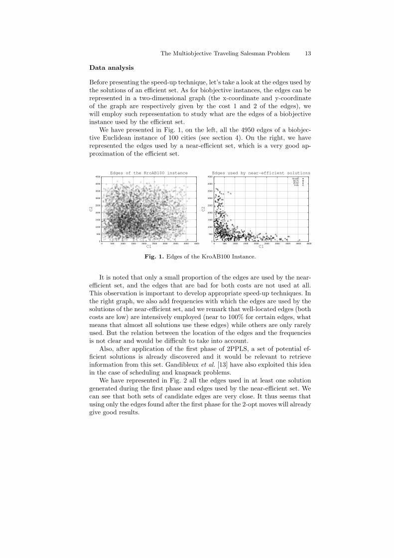
Before presenting the speed-up technique, let’s take a look at the edges used bythe solutions of an efficient set. As for biobjective instances, the edges can berepresented in a two-dimensional graph (the x-coordinate and y-coordinateof the graph are respectively given by the cost 1 and 2 of the edges), wewill employ such representation to study what are the edges of a biobjectiveinstance used by the efficient set.

We have presented in Fig. 1, on the left, all the 4950 edges of a biobjec-tive Euclidean instance of 100 cities (see section 4). On the right, we haverepresented the edges used by a near-efficient set, which is a very good ap-proximation of the efficient set.

0

500

1000

1500

2000

2500

3000

3500

4000

4500

0 500 1000 1500 2000 2500 3000 3500 4000 4500

C2

C1

Edges of the KroAB100 instance

0

500

1000

1500

2000

2500

3000

3500

4000

4500

0 500 1000 1500 2000 2500 3000 3500 4000 4500

C2

C1

Edges used by near-efficient solutions

75-10050-7525-50

0-25

Fig. 1. Edges of the KroAB100 Instance.

It is noted that only a small proportion of the edges are used by the near-efficient set, and the edges that are bad for both costs are not used at all.This observation is important to develop appropriate speed-up techniques. Inthe right graph, we also add frequencies with which the edges are used by thesolutions of the near-efficient set, and we remark that well-located edges (bothcosts are low) are intensively employed (near to 100% for certain edges, whatmeans that almost all solutions use these edges) while others are only rarelyused. But the relation between the location of the edges and the frequenciesis not clear and would be difficult to take into account.

Also, after application of the first phase of 2PPLS, a set of potential ef-ficient solutions is already discovered and it would be relevant to retrieveinformation from this set. Gandibleux et al. [13] have also exploited this ideain the case of scheduling and knapsack problems.

We have represented in Fig. 2 all the edges used in at least one solutiongenerated during the first phase and edges used by the near-efficient set. Wecan see that both sets of candidate edges are very close. It thus seems thatusing only the edges found after the first phase for the 2-opt moves will alreadygive good results.


0

500

1000

1500

2000

2500

3000

3500

4000

4500

0 500 1000 1500 2000 2500 3000 3500 4000 4500

C2

C1

Edges used by near-efficient solutions

75-10050-7525-500-25

0

500

1000

1500

2000

2500

3000

3500

4000

4500

0 500 1000 1500 2000 2500 3000 3500 4000 4500

C2

C1

Edges used after phase 1

75-10050-7525-50

0-25

Fig. 2. Edges used by a near-efficient set and by the set obtained after the firstphase (KroAB100 instance).

2-opt moves with candidate lists

We will explain now how to take into account the reduced set of edges usedby the efficient solutions.

We have represented in Fig. 3 a 2-opt move, where (t1, t2) and (t3, t4)are the leaving edges and (t1, t4) and (t2, t3) are the entering edges. For theleaving edge (t1, t2), if we intend to generate all the 2-opt moves, they are(n − 3) possibilities for the city t3.

t t

t

tt

t�

t1 t2

t3 ?

t1 t2

t3

t t

t

tt

t

t4

Fig. 3. 2-exchange move.

In order to limit the number of possibilities for t3, a classic speed-up tech-nique for solving the TSP is the candidate list. For a starting city t1, with t2the next city in the tour, to consider candidates for t3, we only need to startat the beginning of the candidate list of t2 and proceed down it until the endof the list has been reached. The size of the list is limited to a reasonable size,compromise between quality and running time. For example, in [28], Johnsonand McGeoch recommend a size equal to 15.

In the single-objective case, the candidate lists are created on the basisof the single cost. In the biobjective case, as there is no more a total order


between the cost vectors c, the candidate lists are created on the basis of theedges used by the solutions found during the phase 1 of the 2PPLS method.To do that, we explore the set of candidate edges of phase 1, and for eachcandidate edge {vi, vj}, we add the city vj to the candidate list of the cityvi, if vi is not already in the candidate list of vj (to avoid to realize the samemove twice).

All the cities are considered as starting cities for the 2-opt moves.

4 Results

We test 2PPLS with the speed-up technique on several biobjective TSP in-stances. We consider four types of instances:

• Euclidean instances: the costs between the edges correspond to the Eu-clidean distance between two points in a plane.

• Random instances: the costs between the edges are randomly generatedfrom a uniform distribution.

• Mixed instances: the first cost corresponds to the Euclidean distance be-tween two points in a plane and the second cost is randomly generatedfrom a uniform distribution.

• Clustered instances: the points are randomly clustered in a plane, and thecosts between the edges correspond to the Euclidean distance.

In this work, we use the following biobjective symmetric instances:

• Euclidean instances: three Euclidean instances of respectively 100, 300 and500 cities called EuclAB100, EuclAB300 and EuclAB500.

• Random instances: three random instances of respectively 100, 300 and500 cities called RdAB100, RdAB300 and RdAB500.

• Mixed instances: three mixed instances of respectively 100, 300 and 500cities called MixedAB100, MixedAB300 and MixedAB500.

• Clustered instances: three clustered instances of respectively 100, 300 and500 cities called ClusteredAB100, ClusteredAB300 and ClusteredAB500.

We have generated ourselves the clustered instances with the generatoravailable from the 8th DIMACS Implementation Challenge site2 with thefollowing property: the number of clusters is equal to the number of citiesdivided by 25 and the maximal coordinate for a city is equal to 3163 (asdone by Paquete for the Euclidean instances). The other instances have beengenerated and published by Paquete [44]. Paquete and Stutzle [47] have veryrecently published the results of the comparison of their PD-TPLS method toMOGLS on these instances and they show that they obtain better results onmost of the instances.

2 http://www.research.att.com/~dsj/chtsp/download.html


All the algorithms tested in this work have been run on a Pentium IV with3 Ghz CPUs and 512 MB of RAM. We present the average of the indicatorson 20 executions. The resolution time of our implementation of the algorithmscorresponds to the wall clock time.

To compute the distances D1 and D2 (see section 1), reference sets basedon the notion of ideal set [39] have been generated for all the instances ex-perimented. The ideal set is defined as the best potential Pareto front thatcan be produced from the extreme supported non-dominated points. This isa lower bound of the Pareto front [9]. For generating the extreme supportednon-dominated points, we have used the method proposed by Przybylski et

al. [48]. However, for the instances of more than 200 cities, numerical problemswere encountered. Thus, for these instances, we have generated the extremesupported non-dominated points of the biobjective minimum spanning treeproblem (bMST) associated to the same data than the bTSP. The ideal set isthen produced on the basis of the extreme supported non-dominated pointsof the bMST. As the biobjective minimum spanning tree problem is a relax-ation of the bTSP, all feasible solutions of the bTSP remain dominated orequivalent to the solutions of the ideal set of the bMST.

For the computation of the R and H indicators, the reference points aredetermined according to the reference sets. For the R indicator, the numberof weight sets used is equal to 101 for all instances. This indicator has beennormalized between 0 and 1, where 1 corresponds to the best value.

As state-of-the-art results are not known for all the instances used in thiswork, we have implemented ourselves the PD-TPLS method of Paquete andStutzle [46], a method presenting few parameters contrarily to MOEA al-gorithms. This allows to produce a comparison as fair as possible with thePD-TPLS method, since 2PPLS and PD-TPLS are run on the same com-puter and share the same data structures. However, our implementation ofPD-TPLS is presumable not as good as the original implementation and theexecution time has to be seen as an indicator but not as an objective com-parison factor. For this implementation, we have fixed the parameters of thismethod as follows, as done in [46]:

• The number of iterations for the number of perturbation steps of the it-erated local search method used in PD-TPLS is equal to the number ofcities n minus 50.

• The number of aggregations is equal to n, except for the 100 cities instanceswhere the number of aggregations is higher than n in order to obtaincomparable running times between 2PPLS and PD-TPLS. The number ofaggregations is equal to 250 for the 100 cities instances, excepted for theClusterredAB100 instance where this number has been set to 400.

4.1 Comparison based on the mean of indicators

We use five different indicators to measure the quality of the approximationsobtained: the H, Iǫ1, R, D1 and D2 indicators (see section 1). We also add


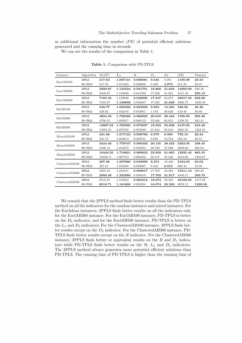
as additional information the number |PE| of potential efficient solutionsgenerated and the running time in seconds.

We can see the results of the comparison in Table 1.

Table 1. Comparison with PD-TPLS.

Instance Algorithm H(108) Iǫ1 R D1 D2 |PE| Time(s)

EuclAB1002PPLS 217.62 1.007141 0.930081 0.345 5.091 1196.90 25.53

PD-TPLS 217.55 1.013423 0.930009 0.460 4.072 811.35 29.47

EuclAB3002PPLS 2309.67 1.124524 0.941701 16.868 21.633 14050.90 258.56

PD-TPLS 2308.97 1.124950 0.941598 17.020 21.921 4415.40 255.13

EuclAB5002PPLS 7165.35 1.129026 0.948995 17.247 22.072 33017.30 692.88

PD-TPLS 7163.87 1.128899 0.948927 17.395 21.829 9306.75 1056.43

RdAB1002PPLS 529.77 1.025300 0.953339 0.932 14.325 438.30 25.46

PD-TPLS 528.92 1.042416 0.953061 1.195 30.620 419.40 30.89

RdAB3002PPLS 4804.48 1.728586 0.966925 20.910 36.424 1766.95 305.36

PD-TPLS 4790.35 1.893817 0.966152 22.848 60.815 1238.70 305.41

RdAB5002PPLS 13987.92 1.790290 0.973697 19.502 55.098 3127.85 816.40

PD-TPLS 13951.01 2.057356 0.972940 21.954 95.618 2081.55 1324.55

MixedAB1002PPLS 331.96 1.017122 0.936782 0.579 6.006 793.10 26.24

PD-TPLS 331.74 1.032013 0.936741 0.659 12.754 585.10 30.15

MixedAB3002PPLS 3410.40 1.778747 0.956492 20.135 28.422 5202.05 238.45

PD-TPLS 3406.12 1.943372 0.956254 20.722 37.980 2299.80 288.04

MixedAB5002PPLS 10440.35 1.710601 0.960652 22.858 31.865 12925.40 865.55

PD-TPLS 10429.11 1.907713 0.960452 23.517 35.546 4816.00 1303.07

ClusteredAB1002PPLS 267.28 1.007686 0.949999 0.274 10.426 2184.05 50.02

PD-TPLS 267.21 1.019305 0.949887 0.442 6.015 989.45 53.56


PD-TPLS 2566.38 1.232286 0.956616 17.702 21.917 4540.15 293.72


PD-TPLS 8516.71 1.181800 0.962394 16.974 23.230 9678.15 1239.56

We remark that the 2PPLS method finds better results than the PD-TPLSmethod on all the indicators for the random instances and mixed instances. Forthe Euclidean instances, 2PPLS finds better results on all the indicators onlyfor the EuclAB300 instance. For the EuclAB100 instance, PD-TPLS is betteron the D2 indicator, and for the EuclAB500 instance, PD-TPLS is better onthe Iǫ1 and D2 indicators. For the ClusteredAB100 instance, 2PPLS finds bet-ter results except on the D2 indicator. For the ClusteredAB300 instance, PD-TPLS finds better results except on the R indicator. For the ClusteredAB500instance, 2PPLS finds better or equivalent results on the R and D1 indica-tors while PD-TPLS finds better results on the H, Iǫ1 and D2 indicators.The 2PPLS method always generates more potential efficient solutions thanPD-TPLS. The running time of PD-TPLS is higher than the running time of


2PPLS, except on the EuclAB300, ClusteredAB300 and ClusteredAB500 in-stances where the running time of PD-TPLS is slightly lower. The PD-TPLSmethod appears thus more performing than 2PPLS on the clustered instances.

4.2 Mann-Whitney test

To take into account the variations in the results of the algorithms, as we donot know the distributions of the indicators, we carried out the non-parametricstatistical test of Mann-Whitney [11]. This test allows to compare the distri-butions of the indicators of 2PPLS with these of PD-TPLS.

We test the following hypothesis: “the two samples come from identicalpopulations” for the H, Iǫ1, R, D1 or D2 indicators on a given instance. Whenthe hypothesis is satisfied, the result “=” is indicated (no differences betweenthe indicators of the algorithms). When the hypothesis is not satisfied, thereare differences between the indicators of the algorithms: the sign “>” indicatesthat the mean value obtained with 2PPLS is better than the mean valueobtained with PD-TPLS and the sign “<” indicates that the mean valueobtained with 2PPLS is worse than the mean value obtained with PD-TPLS.

As five hypothesis are tested simultaneously, the levels of risk α of thetests have been adjusted with the Holm sequential rejective method [24]. Thismethod works as follows: the p-values obtained with the Mann-Whitney testfor each indicator are sorted by increasing value and the smallest p-value iscompared to α/k (where k is the number of indicators, equal to five in ourcase). If that p-value is less than α/k, the hypothesis related to this p-valueis rejected. The second smallest p-value is then compared to α/(k − 1), thethird to α/(k−2), etc. The procedure proceeds until each hypothesis has beenrejected or when a hypothesis cannot be rejected. The starting level of risk ofthe test has been fixed to 1%.

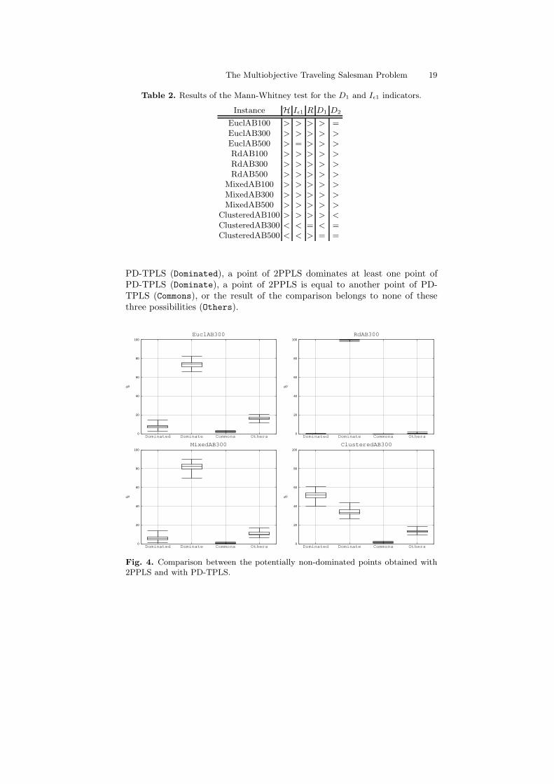
The results of the comparison of 2PPLS with PD-TPLS are given in Ta-ble 2. The results show that we can affirm with a very low risk that, for theindicators considered in this work, 2PPLS is better or equal to PD-TPLS onall the instances tested in this work, except for the ClusteredAB100 instance(on D2), for the ClusteredAB300 instance (on H, Iǫ1 and D1) and for theClusteredAB500 instance (on H and Iǫ1).

4.3 Outperformance relations

We now compare the solutions obtained with 2PPLS and PD-TPLS in termof outperformance relations [21].

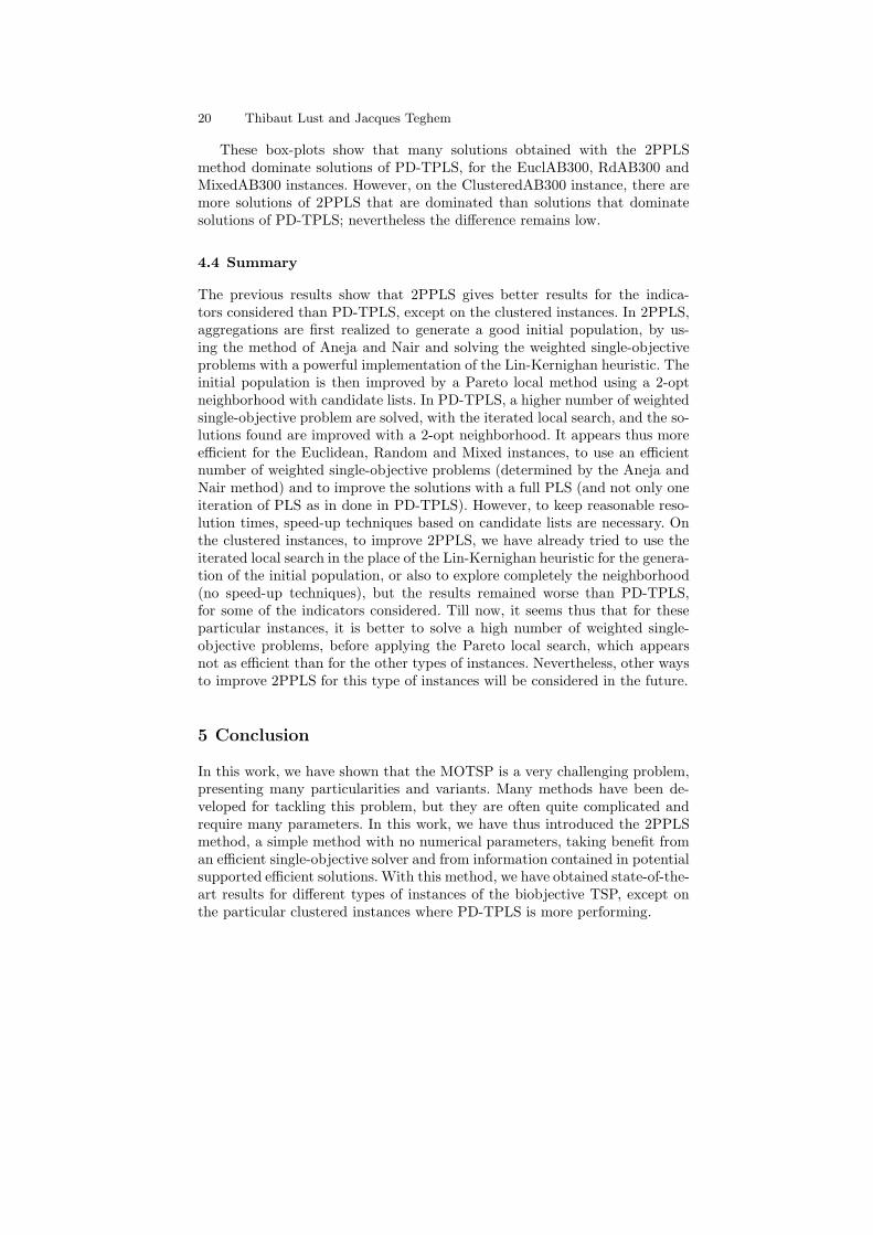
We show in Fig. 4 the results of the comparison between the potentialnon-dominated points obtained with 2PPLS and by PD-TPLS, for the 300cities instances.

To create these box-plot graphs, we compare the points obtained withthe 2PPLS method to the points obtained with the PD-TPLS method. Fourcases can occur: a point of 2PPLS is dominated by at least one point of


Table 2. Results of the Mann-Whitney test for the D1 and Iǫ1 indicators.

Instance H Iǫ1 R D1 D2

EuclAB100 > > > > =EuclAB300 > > > > >

EuclAB500 > = > > >

RdAB100 > > > > >

RdAB300 > > > > >

RdAB500 > > > > >

MixedAB100 > > > > >

MixedAB300 > > > > >

MixedAB500 > > > > >

ClusteredAB100 > > > > <

ClusteredAB300 < < = < =ClusteredAB500 < < > = =

PD-TPLS (Dominated), a point of 2PPLS dominates at least one point ofPD-TPLS (Dominate), a point of 2PPLS is equal to another point of PD-TPLS (Commons), or the result of the comparison belongs to none of thesethree possibilities (Others).

0

20

40

60

80

100

Dominated Dominate Commons Others

%

EuclAB300

0

20

40

60

80

100


%

RdAB300

0

20

40

60

80

100


%

MixedAB300

0

20

40

60

80

100


%

ClusteredAB300

Fig. 4. Comparison between the potentially non-dominated points obtained with2PPLS and with PD-TPLS.


These box-plots show that many solutions obtained with the 2PPLSmethod dominate solutions of PD-TPLS, for the EuclAB300, RdAB300 andMixedAB300 instances. However, on the ClusteredAB300 instance, there aremore solutions of 2PPLS that are dominated than solutions that dominatesolutions of PD-TPLS; nevertheless the difference remains low.

4.4 Summary

The previous results show that 2PPLS gives better results for the indica-tors considered than PD-TPLS, except on the clustered instances. In 2PPLS,aggregations are first realized to generate a good initial population, by us-ing the method of Aneja and Nair and solving the weighted single-objectiveproblems with a powerful implementation of the Lin-Kernighan heuristic. Theinitial population is then improved by a Pareto local method using a 2-optneighborhood with candidate lists. In PD-TPLS, a higher number of weightedsingle-objective problem are solved, with the iterated local search, and the so-lutions found are improved with a 2-opt neighborhood. It appears thus moreefficient for the Euclidean, Random and Mixed instances, to use an efficientnumber of weighted single-objective problems (determined by the Aneja andNair method) and to improve the solutions with a full PLS (and not only oneiteration of PLS as in done in PD-TPLS). However, to keep reasonable reso-lution times, speed-up techniques based on candidate lists are necessary. Onthe clustered instances, to improve 2PPLS, we have already tried to use theiterated local search in the place of the Lin-Kernighan heuristic for the genera-tion of the initial population, or also to explore completely the neighborhood(no speed-up techniques), but the results remained worse than PD-TPLS,for some of the indicators considered. Till now, it seems thus that for theseparticular instances, it is better to solve a high number of weighted single-objective problems, before applying the Pareto local search, which appearsnot as efficient than for the other types of instances. Nevertheless, other waysto improve 2PPLS for this type of instances will be considered in the future.

5 Conclusion

In this work, we have shown that the MOTSP is a very challenging problem,presenting many particularities and variants. Many methods have been de-veloped for tackling this problem, but they are often quite complicated andrequire many parameters. In this work, we have thus introduced the 2PPLSmethod, a simple method with no numerical parameters, taking benefit froman efficient single-objective solver and from information contained in potentialsupported efficient solutions. With this method, we have obtained state-of-the-art results for different types of instances of the biobjective TSP, except onthe particular clustered instances where PD-TPLS is more performing.


Despite of these good results, the MOTSP still needs further study: veryfew results are known for the TSP with more than two objectives (at theexception of some results for the three objective case), and no efficient exactmethod has been developed for solving this problem, even in the biobjectivecase. Moreover, the instances size for which approximations have been gen-erated with a reasonable running time are still small compared to the size ofthe single-objective instances that we can approximate.

References

1. Y.P. Aneja and K.P.K. Nair. Bicriteria transportation problem. ManagementScience, 25:73–78, 1979.

2. E. Angel, E. Bampis, and L. Gourves. Approximating the Pareto curve withlocal search for the bicriteria TSP(1,2) problem. Theoritical Computer Science,310:135–146, 2004.

3. E. Angel, E. Bampis, and L. Gourves. A dynasearch neighborhood for the bi-criteria traveling salesman problem. In X. Gandibleux, M. Sevaux, K. Sorensen,and V. T’kindt, editors, Metaheuristics for Multiobjective Optimisation, pages153–176. Springer. Lecture Notes in Economics and Mathematical Systems Vol.535, Berlin, 2004.

4. D. Applegate. Chained Lin-Kernighan for large traveling salesman problems.INFORMS Journal on Computing, 15:82–92, 2003.

5. M. Basseur. Design of cooperative algorithms for multi-objective optimization:application to the flow-shop scheduling problem. 4OR, 4(3):255–258, 2006.

6. P.C. Borges and M.P. Hansen. A study of global convexity for a multiple objec-tive travelling salesman problem. In C.C Ribeiro and P. Hansen, editors, Essaysand surveys in metaheuristics, pages 129–150. Kluwer, 2000.

7. P. Czyzak and A. Jaszkiewicz. Pareto simulated annealing—a metaheuristictechnique for multiple-objective combinatorial optimization. Journal of Multi-Criteria Decision Analysis, 7:34–47, 1998.

8. M. Ehrgott and X. Gandibleux. Multiobjective Combinatorial Optimization—Theory, Methodology, and Applications. In Matthias Ehrgott and XavierGandibleux, editors, Multiple Criteria Optimization: State of the Art AnnotatedBibliographic Surveys, pages 369–444. Kluwer Academic Publishers, Boston,2002.

9. M. Ehrgott and X. Gandibleux. Bound sets for biobjective combinatorial opti-mization problems. Computers and Operations Research, 34:2674–2694, 2007.

10. S. Elaoud, J. Teghem, and T. Loukil. Multiple crossover genetic algorithmfor the multiobjective traveling salesman problem: University of Sfax (tunisia).Submitted for publication, 2008.

11. T.S. Ferguson. Mathematical Statistics, a decision theoretic approach. AcademicPress, New-York and London, 1967.

12. R. Fisher and K. Richter. Solving a multiobjective traveling salesman problemby dynamic programming. Mathematische Operationsforschung und Statistik,Series Optimization, 13(2):247–252, 1982.

13. X. Gandibleux, H. Morita, and N. Katoh. The supported solutions used as a ge-netic information in a population heuristics. In Eckart Zitzler, Kalyanmoy Deb,


Lothar Thiele, Carlos A. Coello Coello, and David Corne, editors, Evolution-ary Multi-Criterion Optimization. Second International Conference, EMO 2003,volume 1993 of Lecture Notes in Computer Science, pages 429–442. Springer,2001.

14. C. Garcia-Martinez, O. Cordon, and F. Herrera. A taxonomy and an empiricalanalysis of multiple objective ant colony optimization algorithms for the bi-criteria TSP. European Journal of Operational Research, 180(1):116 – 148, June2007.

15. M. Gendreau, J-F. Berube, and J-Y. Potvin. An exact epsilon-constraint methodfor bi-objective combinatorial optimization problems: Application to the travel-ing salesman problem with profits. European Journal of Operational Research,194(1):39–50, 2009.

16. F. Glover and G. Kochenberger. Handbook of Metaheuristics. Kluwer, Boston,2003.

17. A. Gupta and A. Warburton. Approximation methods for multiple criteriatraveling salesman problems, towards interactive and intelligent decision supportsystems. In Y. Sawaragi, editor, Proc. 7th Internat. Conf. on Multiple CriteriaDecision Making, pages 211–217, Berlin, 1986. Springer.

18. G. Gutin and A. Punnen. The Traveling Salesman Problem and its Variations.Kluwer, Dordrecht / Boston / London, 2002.

19. H.W. Hamacher and G. Ruhe. On spanning tree problems with multiple objec-tives. Annals of Operations Research, 52:209–230, 1994.

20. M.P. Hansen. Use of Substitute Scalarizing Functions to Guide a Local SearchBased Heuristic: The Case of moTSP. Journal of Heuristics, 6(3):419–430, 2000.

21. M.P. Hansen and A. Jaszkiewicz. Evaluating the quality of approximationsof the nondominated set. Technical report, Technical University of Denmark,Lingby, Denmark, 1998.

22. P. Hansen. Bicriterion path problems. Lecture Notes in Economics and Mathe-matical Systems, 177:109–127, 1979.

23. K. Helsgaun. An effective implementation of the lin-kernighan traveling sales-man heuristic. European Journal of Operational Research, 126:106–130, 2000.

24. S. Holm. A simple sequentially rejective multiple test procedure. ScandinavianJournal of Statistics, 6:65–70, 1979.

25. B. Huang, L. Yao, and K. Raguraman. Bi-level GA and GIS for multi-objectiveTSP route planning. Transportation Planning and Technology, 29(2):105–124,April 2006.

26. A. Jaszkiewicz. On the Performance of Multiple-Objective Genetic Local Searchon the 0/1 Knapsack Problem—A Comparative Experiment. IEEE Transactionson Evolutionary Computation, 6(4):402–412, August 2002.

27. A. Jaszkiewicz and P. Zielniewicz. Pareto memetic algorithm with path-relinkingfor biobjective traveling salesman problem. European Journal of OperationalResearch, 193(3):885–890, 2009.

28. D.S. Johnson and L.A. McGeoch. The Traveling Salesman Problem: A CaseStudy in Local Optimization. In E. H. L. Aarts and J.K. Lenstra, editors, LocalSearch in Combinatorial Optimization, pages 215–310. John Wiley and SonsLtd, 1997.

29. D.S. Johnson and L.A. McGeoch. Experimental analysis of heuristics for theATSP. In G. Gutin and A. Punnen, editors, The Traveling Salesman Problemand its Variations. Kluwer, 2002.


30. D.S. Johnson and L.A. McGeoch. Experimental analysis of heuristics for theSTSP. In G. Gutin and A. Punnen, editors, The Traveling Salesman Problemand its Variations. Kluwer, 2002.

31. N. Jozefowiez, F. Glover, and M. Laguna. Multi-objective meta-heuristics forthe traveling salesman problem with profits. Journal of Mathematical Modellingand Algorithms, 7(2):177–195, 2008.

32. N. Jozefowiez, F. Semet, and E-G. Talbi. Multi-objective vehicle routing prob-lems. European Journal of European Research, 189(2):293–309, 2008.

33. C.P. Keller and M. Goodchild. The multiobjective vending problem: A gen-eralization of the traveling salesman problem. Environment and Planning B:Planning and Design, 15:447–460, 1988.

34. R. Kumar and P.K. Singh. Pareto evolutionary algorithm hybridized with localsearch for biobjective TSP. In C. Grosan, A. Abraham, and H. Ishibuchi, editors,Hybrid Evolutionary Algorithms, chapter 14. Springer-Verlag, 2007.

35. P. Larranaga, C.M.H. Kuijpers, R.H. Murga, I. Inza, and S. Dizdarevic. Geneticalgorithms for the travelling salesman problem: A review of representations andoperators. Artificial Intelligence Review, 13(2):129–170, 1999.

36. W. Li. Finding Pareto-optimal set by merging attractors for a bi-objectivetraveling salesmen problem. In Carlos A. Coello Coello, Arturo HernandezAguirre, and Eckart Zitzler, editors, Evolutionary Multi-Criterion Optimization.Third International Conference, EMO 2005, volume 3410 of Lecture Notes inComputer Science, pages 797–810. Springer, 2005.

37. S. Lin and B.W. Kernighan. An effective heuristic algorithm for the traveling-salesman problem. Operations Research, 21:498–516, 1973.

38. T. Lust and A. Jaszkiewicz. Speed-up techniques for solving large-scale biob-jective TSP. To appear in Computers and Operations Research, 2009.

39. T. Lust and J. Teghem. Two-phase Pareto local search for the biobjectivetraveling salesman problem. To appear in Journal of Heuristics, 2009.

40. B. Manthey and L. Shankar Ram. Approximation algorithms for multi-criteriatraveling salesman problems. CoRR, arxiv:abs/cs/0606040, 2007.

41. I.I. Melamed and K.I. Sigal. The linear convolution of criteria in the bicrite-ria traveling salesman problem. Computational Mathematics and MathematicalPhysics, 37(8):902–905, 1997.

42. P. Merz and B. Freisleben. Memetic algorithms for the traveling salesman prob-lem. Complex Systems, 13:297–345, 2001.

43. K. Miettinen. Nonlinear multiobjective optimization. Kluwer, Boston, 1999.44. L. Paquete. Stochastic Local Search Algorithms for Multiobjective Combina-

torial Optimization: Methods and Analysis. PhD thesis, FB Informatik, TUDarmstadt, 2005.

45. L. Paquete, M. Chiarandini, and T. Stutzle. Pareto Local Optimum Setsin the Biobjective Traveling Salesman Problem: An Experimental Study. InX. Gandibleux, M. Sevaux, K. Sorensen, and V. T’kindt, editors, Metaheuristicsfor Multiobjective Optimisation, pages 177–199, Berlin, 2004. Springer. LectureNotes in Economics and Mathematical Systems Vol. 535.

46. L. Paquete and T. Stutzle. A Two-Phase Local Search for the Biobjective Trav-eling Salesman Problem. In C. M. Fonseca, P. J. Fleming, E. Zitzler, K. Deb,and L. Thiele, editors, Evolutionary Multi-Criterion Optimization. Second In-ternational Conference, EMO 2003, pages 479–493, Faro, Portugal, April 2003.Springer. Lecture Notes in Computer Science Vol. 2632.


47. L. Paquete and T. Stutzle. Design and analysis of stochastic local search forthe multiobjective traveling salesman problem. Computers and Operations Re-search, 36(9):2619–2631, 2009.

48. A. Przybylski, X. Gandibleux, and M. Ehrgott. Two-phase algorithms for thebiobjective assignement problem. European Journal of Operational Research,185(2):509–533, 2008.

49. G. Reinelt. Tsplib - a traveling salesman problem library. ORSA Journal ofComputing, 3(4):376–384, 1991.

50. F. Samanlioglu, W.G. Ferrell Jr., and M.E. Kurz. A multicriteria Pareto-optimalalgorithm for the traveling salesman problem. Asia-Pacific Journal of Opera-tional Research, 11:103–115, 1994.

51. F. Samanlioglu, W.G. Ferrell Jr., and M.E. Kurz. A hybrid random-key ge-netic algorithm for a symmetric travelling salesman problem. Computers andIndustrial Engineering, 55(2):439–449, 2008.

52. R. Steuer. Multiple Criteria Optimization: Theory, Computation and Applica-tions. John Wiley & Sons, New-York, 1986.

53. J. Teghem. La programmation lineaire multicritere. In D. Dubois and M. Pirlot,editors, Concepts et methodes pour l’aide a la decision, pages 215–288. Hermes,2006.

54. J. Teghem and P. Kunsch. A survey of techniques for finding efficient solutions tomulti-objective integer linear programming. Asia-Pacific Journal of OperationalResearch, 3(2):95–108, 1986.

55. E.L. Ulungu and J. Teghem. Multiobjective combinatorial optimization prob-lems: A survey. Journal of Multi-Criteria Decision Analysis, 3:83–104, 1994.

56. E.L. Ulungu and J. Teghem. The two phases method: An efficient procedure tosolve biobjective combinatorial optimization problems. Foundation of Comput-ing and Decision Science, 20:149–156, 1995.

57. E.L. Ulungu, J. Teghem, Ph. Fortemps, and D. Tuyttens. MOSA Method: ATool for Solving Multiobjective Combinatorial Optimization Problems. Journalof Multi-Criteria Decision Analysis, 8(4):221–236, 1999.

58. Z. Yan, L. Zhang, L. Kang, and G. Lin. A new MOEA for multiobjective TSPand its convergence property analysis. In C.M. Fonseca, P.J. Fleming, E. Zitzler,K. Deb, and L. Thiele, editors, EMO, volume 2632 of Lecture Notes in ComputerScience, pages 342–354. Springer, 2003.

59. E. Zitzler. Evolutionary Algorithms for Multiobjective Optimization: Methodsand Applications. PhD thesis, Swiss Federal Institute of Technology (ETH),Zurich, Switzerland, November 1999.

60. E. Zitzler, M. Laumanns, L. Thiele, C.M. Fonseca, and V. Grunert da Fonseca.Why Quality Assessment of Multiobjective Optimizers Is Difficult. In W.B.Langdon, E. Cantu-Paz, K. Mathias, R. Roy, D. Davis, R. Poli, K. Balakrishnan,V. Honavar, G. Rudolph, J. Wegener, L. Bull, M.A. Potter, A.C. Schultz, J.F.Miller, E. Burke, and N. Jonoska, editors, Proceedings of the Genetic and Evolu-tionary Computation Conference (GECCO’2002), pages 666–673, San Francisco,California, July 2002. Morgan Kaufmann Publishers.

61. E. Zitzler, L. Thiele, M. Laumanns, C.M. Fonseca, and V. Grunert da Fonseca.Performance Assessment of Multiobjective Optimizers: An Analysis and Review.IEEE Transactions on Evolutionary Computation, 7(2):117–132, April 2003.

The Multiobjective Traveling Salesman Problem

Documents