A Constraint Programming Based Hadoop Scheduler for Handling MapReduce Jobs with Deadlines on Clouds Norman Lim Dept. of Systems and Computer Engineering Carleton University Ottawa, ON, Canada [email protected] Shikharesh Majumdar Dept. of Systems and Computer Engineering Carleton University Ottawa, ON, Canada [email protected] Peter Ashwood-Smith Huawei, Canada Kanata, ON, Canada ABSTRACT A novel MapReduce constraint programming based matchmaking and scheduling algorithm (MRCP) that can handle MapReduce jobs with deadlines and achieve high system performance is devised. The MRCP algorithm is incorporated into Hadoop, which is a widely used open source implementation of the MapReduce programming model, as a new scheduler called the CP-Scheduler. This paper originates from the collaborative research with our industrial partner concerning the engineering of resource management middleware for high performance. It describes our experiences and the challenges that we encountered in designing and implementing the prototype CP-based Hadoop scheduler. A detailed performance evaluation of the CP-Scheduler is conducted on Amazon EC2 to determine the CP-Scheduler’s effectiveness as well as to obtain insights into system behaviour and performance. In addition, the CP-Scheduler’s performance is also compared with an earliest deadline first (EDF) Hadoop scheduler, which is implemented by extending Hadoop’s default FIFO scheduler. The experimental results demonstrate the effectiveness of the CP- Scheduler’s ability to handle an open stream of MapReduce jobs with deadlines in a Hadoop cluster. Categories and Subject Descriptors C.2.4 [Computer-Communication Networks]: Distributed Systems. C.4 [Performance of Systems]: performance attributes, modeling techniques. Keywords Resource management on clouds; MapReduce with deadlines; Hadoop scheduler; Constraint programming. 1. INTRODUCTION Cloud computing has rapidly gained popularity and is now being used extensively by various types of users including enterprises as well as engineering and scientific institutions around the world. Some of the attractive features of the cloud that make it desirable to use include the “pay-as-you-go” model, scalability, and elasticity that lets a user dynamically increase or shrink the number of resources allocated. In cloud computing, hardware resources (including computing, storage, and communication), as well as software resources are exposed as on- demand services, and can be accessed by users over a network such as the Internet. Cloud computing environments that provide resources on demand are of great importance and interest to service providers and consumers as well as researchers and system builders. Cloud service providers (e.g. Amazon) deploy large pools of resources that include computing, storage, and communication resources for consumers to acquire on demand. An effective resource management technique needs to be deployed for harnessing the power of the underlying resource pool, and efficiently provide resources on demand to consumers. Effective management of the resources on a cloud is also crucial for achieving user satisfaction and high system performance leading to high revenue for the cloud service provider. The important operations performed by a resource manager in a cloud include: matchmaking and scheduling. The matchmaking operation, when given a pool of requests, determines the resource or resources to be allocated to each request. Once a number of requests are allocated to a specific resource, a scheduling algorithm is used to determine the order in which each of the requests are to be executed for achieving the desired system objectives. Both matchmaking and scheduling are performed in a single step in Hadoop [1] by an entity referred to as the Hadoop scheduler in the literature [2]. A further discussion of Hadoop is provided in Section 2.2. Since such a single step operation is performed by the resource manager described in this paper, we refer to it as a Hadoop scheduler. Two important components of performance engineering are performance optimization and performance modeling. One of the goals of this research is to engineer resource management middleware that can make resource management decisions that achieve high system performance, while also maintaining a low processing overhead. This paper describes how optimization theory and constraint programming (CP) [3] is used to devise a matchmaking and scheduling algorithm. Particular emphasis is placed on discussing our design and implementation experience and the performance implications of various system and workload parameters. CP is a well-known theoretical technique used to solve optimization problems, and is capable of finding optimal solutions with regards to maximizing or minimizing an objective function (see Section 2.1 for a further discussion). A majority of the existing research on resource management on clouds has focused mainly on workloads that are characterized by requests requiring a best effort service. In this paper, workloads that comprise of requests with an associated quality of service often specified in a service level agreement (SLA) are considered. Most of the research on resource management for requests characterized by an SLA has only considered: (1) requests requiring service from a single resource and (2) a batch workload comprising a fixed number of requests. The focus of this research is on requests that need to be processed by multiple resources (called multi-stage requests) with SLAs specifying a required execution time, an earliest start time (release time), and an end-to-end deadline. Note that in line with the existing Hadoop Permission to make digital or hard copies of all or part of this work for personal or classroom use is granted without fee provided that copies are not made or distributed for profit or commercial advantage and that copies bear this notice and the full citation on the first page. Copyrights for components of this work owned by others than ACM must be honored. Abstracting with credit is permitted. To copy otherwise, or republish, to post on servers or to redistribute to lists, requires prior specific permission and/or a fee. Request permissions from [email protected]. ICPE'15, Jan. 31–Feb. 4, 2015, Austin, TX, USA Copyright 2015 ACM 978-1-4503-3248-4/15/01…$15.00 http://dx.doi.org/10.1145/2668930.2688058 111

Welcome message from author
This document is posted to help you gain knowledge. Please leave a comment to let me know what you think about it! Share it to your friends and learn new things together.
Transcript

A Constraint Programming Based Hadoop Scheduler for Handling MapReduce Jobs with Deadlines on Clouds
Norman Lim Dept. of Systems and Computer
Engineering Carleton University
Ottawa, ON, Canada
Shikharesh Majumdar Dept. of Systems and Computer
Engineering Carleton University
Ottawa, ON, Canada
Peter Ashwood-Smith Huawei, Canada
Kanata, ON, Canada
ABSTRACT
A novel MapReduce constraint programming based matchmaking
and scheduling algorithm (MRCP) that can handle MapReduce
jobs with deadlines and achieve high system performance is
devised. The MRCP algorithm is incorporated into Hadoop, which
is a widely used open source implementation of the MapReduce
programming model, as a new scheduler called the CP-Scheduler.
This paper originates from the collaborative research with our
industrial partner concerning the engineering of resource
management middleware for high performance. It describes our
experiences and the challenges that we encountered in designing
and implementing the prototype CP-based Hadoop scheduler. A
detailed performance evaluation of the CP-Scheduler is conducted
on Amazon EC2 to determine the CP-Scheduler’s effectiveness as
well as to obtain insights into system behaviour and performance.
In addition, the CP-Scheduler’s performance is also compared
with an earliest deadline first (EDF) Hadoop scheduler, which is
implemented by extending Hadoop’s default FIFO scheduler. The
experimental results demonstrate the effectiveness of the CP-
Scheduler’s ability to handle an open stream of MapReduce jobs
with deadlines in a Hadoop cluster.
Categories and Subject Descriptors
C.2.4 [Computer-Communication Networks]: Distributed
Systems. C.4 [Performance of Systems]: performance attributes,
modeling techniques.
Keywords
Resource management on clouds; MapReduce with deadlines;
Hadoop scheduler; Constraint programming.
1. INTRODUCTION Cloud computing has rapidly gained popularity and is now
being used extensively by various types of users including
enterprises as well as engineering and scientific institutions
around the world. Some of the attractive features of the cloud that
make it desirable to use include the “pay-as-you-go” model,
scalability, and elasticity that lets a user dynamically increase or
shrink the number of resources allocated. In cloud computing,
hardware resources (including computing, storage, and
communication), as well as software resources are exposed as on-
demand services, and can be accessed by users over a network
such as the Internet.
Cloud computing environments that provide resources on
demand are of great importance and interest to service providers
and consumers as well as researchers and system builders. Cloud
service providers (e.g. Amazon) deploy large pools of resources
that include computing, storage, and communication resources for
consumers to acquire on demand. An effective resource
management technique needs to be deployed for harnessing the
power of the underlying resource pool, and efficiently provide
resources on demand to consumers. Effective management of the
resources on a cloud is also crucial for achieving user satisfaction
and high system performance leading to high revenue for the
cloud service provider. The important operations performed by a
resource manager in a cloud include: matchmaking and
scheduling. The matchmaking operation, when given a pool of
requests, determines the resource or resources to be allocated to
each request. Once a number of requests are allocated to a specific
resource, a scheduling algorithm is used to determine the order in
which each of the requests are to be executed for achieving the
desired system objectives. Both matchmaking and scheduling are
performed in a single step in Hadoop [1] by an entity referred to
as the Hadoop scheduler in the literature [2]. A further discussion
of Hadoop is provided in Section 2.2. Since such a single step
operation is performed by the resource manager described in this
paper, we refer to it as a Hadoop scheduler.
Two important components of performance engineering are
performance optimization and performance modeling. One of the
goals of this research is to engineer resource management
middleware that can make resource management decisions that
achieve high system performance, while also maintaining a low
processing overhead. This paper describes how optimization
theory and constraint programming (CP) [3] is used to devise a
matchmaking and scheduling algorithm. Particular emphasis is
placed on discussing our design and implementation experience
and the performance implications of various system and workload
parameters. CP is a well-known theoretical technique used to
solve optimization problems, and is capable of finding optimal
solutions with regards to maximizing or minimizing an objective
function (see Section 2.1 for a further discussion).
A majority of the existing research on resource management
on clouds has focused mainly on workloads that are characterized
by requests requiring a best effort service. In this paper,
workloads that comprise of requests with an associated quality of
service often specified in a service level agreement (SLA) are
considered. Most of the research on resource management for
requests characterized by an SLA has only considered: (1)
requests requiring service from a single resource and (2) a batch
workload comprising a fixed number of requests. The focus of
this research is on requests that need to be processed by multiple
resources (called multi-stage requests) with SLAs specifying a
required execution time, an earliest start time (release time), and
an end-to-end deadline. Note that in line with the existing Hadoop
Permission to make digital or hard copies of all or part of this work for personal or
classroom use is granted without fee provided that copies are not made or distributed
for profit or commercial advantage and that copies bear this notice and the full
citation on the first page. Copyrights for components of this work owned by others
than ACM must be honored. Abstracting with credit is permitted. To copy
otherwise, or republish, to post on servers or to redistribute to lists, requires prior
specific permission and/or a fee. Request permissions from [email protected].
ICPE'15, Jan. 31–Feb. 4, 2015, Austin, TX, USA
Copyright 2015 ACM 978-1-4503-3248-4/15/01…$15.00
http://dx.doi.org/10.1145/2668930.2688058
111

scheduler [2], the earliest start time of a job is set to its arrival
time in this research. Meeting an end-to-end deadline for requests
that require processing by multiple system resources increases the
complexity of the problem significantly. In addition, this paper
considers a workload comprising an open stream of request
arrivals (and not a workload with a fixed number of requests) that
characterizes typical workloads on cloud data centres. Both the
matchmaking and scheduling operations are well known to be
computationally hard problems when they need to satisfy user
requirements for a quality of service while also considering
system objectives, such as high resource utilization and adequate
revenue for the service provider.
A popular multi-stage application that is deployed by
enterprises and institutions for processing and analyzing very
large and complex data sets (for performing Big Data analytics for
example) is MapReduce [4]. MapReduce, proposed by Google, is
a programming model whose purpose is to simplify performing
massively distributed parallel processing so that very large data
sets can be processed and analyzed efficiently. In such cases, it is
necessary to distribute the computation among multiple machines
to facilitate parallel processing and reduce the total processing
time. One of the benefits of MapReduce is that it provides an
abstraction to hide the complex details and issues of
parallelization. As its name suggests, the MapReduce
programming model has two key functions [4]: map and reduce.
The map function accepts a set of input key/value pairs and
generates a new set of intermediate key/value pairs. These
intermediary key/value pairs are grouped together and then passed
to the reduce function, which is typically called the shuffle phase.
The reduce function processes these intermediate key/value pairs
to generally produce a smaller set of values.
A typical MapReduce application (or job) is comprised of
multiple map tasks and multiple reduce tasks as illustrated in
Figure 1. Reduce tasks cannot complete their execution until all
the map tasks have finished. Many computations can be expressed
using the MapReduce programming model. For example, a
MapReduce application can be developed to process the logs of
web servers to count the number of distinct URL accesses. This
type of application is often referred to as a WordCount
application. In this case, the input into the map function would be
the logs of the web servers, and the map function would produce
the following intermediate key/value pairs: {URL, 1}. This
key/value pair indicates that one instance of a URL is found. Note
that the intermediate data set may contain many duplicate
key/value pairs (e.g. {www.google.com, 1} can appear multiple
times). The reduce function sums all the values with the same key
to emit the new data set: {URL, total count}.
t1
t2
t3t5
t4
Output
Map Tasks Reduce Tasks
Input
Shuffling
Figure 1. Directed Acyclic Graph for a MapReduce job.
More recently, resource management on clusters that execute
MapReduce jobs with an associated completion time guarantee
(deadline) has begun receiving attention from researchers (e.g.,
see [5] to [9]). Executing MapReduce jobs that have an associated
end-to-end deadline is required for latency-sensitive applications
such as live business intelligence, personalized advertising,
spam/fraud detection, and real-time event log analysis
applications [5]. By allowing users to specify deadlines, the
system can also prioritize jobs and ensure that time-critical jobs
are completed on time. Developing an efficient resource
management middleware on such an environment is the focus of
attention for this research performed in collaboration with our
industrial partners Huawei, Canada.
More specifically, in this paper we focus on devising a
scheduler for Hadoop [1] that can effectively perform
matchmaking and scheduling of an open stream of MapReduce
jobs with SLAs comprising an execution time for the map and
reduce tasks, an earliest start time, and an end-to-end deadline.
Hadoop is a widely used open source implementation of the
MapReduce programming model (discussed in more detail in
Section 2.2). The formulation of the matchmaking and scheduling
problem of MapReduce jobs with SLAs is achieved using
constraint programming (CP) as discussed in Section 3. In our
preliminary work [10], a detailed comparison of different resource
management approaches based on CP as well as linear
programming is presented. The results of the investigation showed
the superiority of the CP-based approach implemented and solved
using IBM ILOG CPLEX [11], including its more intuitive and
simple formulation of constraints, lower processing overhead, and
its ability to handle larger workloads.
In addition, our previous work [12] describes a novel
MapReduce Constraint Programming based Resource
Management (MRCP-RM) algorithm that can effectively perform
matchmaking and scheduling of an open stream of MapReduce
jobs with end-to-end deadlines. Using simulation a performance
evaluation of MRCP-RM was conducted that demonstrated its
effectiveness in generating a schedule where there is a low
number of late jobs. The strong performance of MRCP-RM in
simulation experiments has motivated this research that focuses
on devising a revised version of the MRCP-RM algorithm and
implementing the algorithm on a real system (i.e. Hadoop). A new
CP-based Hadoop scheduler, named CP-Scheduler, which can
handle matchmaking and scheduling an open stream of
MapReduce jobs with deadlines is devised and implemented. To
the best of our knowledge, there is no existing research describing
a CP-based scheduler for Hadoop that can handle matchmaking
and scheduling an open stream of MapReduce jobs with
deadlines. The devising of the CP-Scheduler is based on the
objective of providing user satisfaction while achieving high
system performance. The main contributions of this paper include:
A prototype CP-based Hadoop scheduler (called CP-
Scheduler) for matchmaking and scheduling an open stream
of MapReduce jobs with end-to-end deadlines.
o A discussion of our experiences and challenges that were
encountered in designing and implementing the CP-
Scheduler is provided.
A detailed performance evaluation of the CP-Scheduler was
conducted on Amazon EC2. Insights into system behavior
and performance are described.
o This includes a discussion of the impact of various
system and workload parameters on performance and a
performance comparison of the CP-scheduler compared
to an earliest deadline first (EDF) based Hadoop
scheduler, which was implemented by extending
Hadoop’s default FIFO scheduler.
Experimental demonstration of the effectiveness of the CP-
Scheduler’s ability to handle an open stream of MapReduce
jobs with deadlines in a Hadoop cluster for a number of
different workloads.
The results of this research will be of interest to researchers, cloud
providers, as well as developers of resource management
middleware for clouds and Hadoop-based systems.
112

The rest of the paper is organized as follows. In Section 2,
background information is provided and related work is discussed.
Section 3 discusses the problem formulation and how the
MapReduce Constraint Program (MRCP) is devised. The focus of
Section 4 is on the design and implementation of the Hadoop EDF
and CP based schedulers, and includes a discussion of our
experiences and challenges. In Section 5, the results of the
experiments performed on Amazon EC2 to evaluate the EDF-
Scheduler and CP-Scheduler are presented. Insights into system
behavior and performance are described. Lastly, Section 6
concludes the paper and provides directions for future work.
2. BACKGROUND AND RELATED WORK A brief overview of constraint programming (CP), Hadoop,
and Amazon EC2 are provided in Sections 2.1 to 2.3, respectively.
In addition, related research is discussed in Section 2.4.
2.1 Constraint Programming (CP) CP is a theoretical technique for solving optimization
problems that was developed by computer science researchers in
the mid-1980s using knowledge from artificial intelligence, logic
and graph theory, and computer programming languages [3]. A
typical CP problem consists of three key parts: decision variables,
objective function, and constraints. The decision variables are the
variables in the CP problem that need to be assigned values. The
objective function is a mathematical function that generates the
value that needs to be optimized (i.e. minimized or maximized).
Lastly, the constraints are a set of mathematical formulas that
restrict the values that the decision variables can be assigned. In
summary, when solving a CP problem, a solver will assign values
to the decision variables that optimize the objective function,
while ensuring that none of the constraints are violated.
2.2 Apache Hadoop Apache Hadoop [1][13] is an open-source software
framework (written in Java) that implements the MapReduce
programming model, and is aimed at data-intensive distributed
computing applications. Hadoop’s software framework contains
three sub-frameworks: Hadoop Common, Hadoop Distributed File
System (HDFS), and Hadoop MapReduce. Hadoop Common
provides utility functions including remote procedure call (RPC)
and object serialization libraries. HDFS and Hadoop MapReduce
are based on Google’s MapReduce programming model [4] and
Google’s File System (a distributed file system implementation),
respectively.
A typical Hadoop cluster comprises a single master node and
one or more slave nodes. In Hadoop 1.2.1, which implements the
MapReduce version one (MRv1) architecture, the master node
comprises of two entities (which are often called Hadoop
daemons): NameNode and JobTracker. Each slave node also
consists of two Hadoop daemons: a DataNode and a TaskTracker.
The NameNode and DataNodes are the Hadoop daemons in
charge of managing HDFS. Each file that is written to HDFS is
split into blocks (64MB by default) and each block is stored on
the storage device where a DataNode is running. Each block is
replicated multiple times (by default three times) and stored on
different DataNodes. It is the job of NameNode to keep track of
which DataNode stores the blocks of a particular file (which is
called the metadata of the HDFS). Another important function of
NameNode is to direct DataNodes (slaves) to perform HDFS I/O
operations (read, write, delete). DataNodes keep in constant
contact with NameNode to receive I/O instructions.
JobTracker is the link between user applications and the
Hadoop cluster. In addition, JobTracker is the Hadoop daemon
responsible for managing TaskTrackers. Some of the main
responsibilities of JobTracker include: initialize jobs and prepare
them for execution, determine when the map and reduce tasks of
jobs should be executed and which TaskTrackers should execute
them (i.e. perform matchmaking and scheduling), as well as
monitor all tasks that are currently running. TaskTrackers function
as the JobTracker’s slaves, and their primary purpose is to execute
the map or reduce tasks that they are assigned. Another
responsibility of TaskTracker is to periodically send polling/
update messages (called heartbeats) to JobTracker. If JobTracker
does not receive a heartbeat message from a TaskTracker within a
specified time period (by default one minute), JobTracker will
assume that the TaskTracker has been lost, and re-map all the
tasks that was assigned to the lost TaskTracker.
2.3 Amazon EC2 Amazon Elastic Compute Cloud (abbreviated Amazon EC2)
is a public cloud that provides Infrastructure-as-a-Service (IaaS).
Amazon EC2 allows consumers to launch virtual machines (VMs)
called instances. After launching these instances, consumers can
connect to the instance, and deploy and run their own
applications. Amazon EC2 also provides various instance types,
which are pre-configured VMs that have various predetermined
CPU, memory, storage, and networking capacity. The cost of
running the instance depends on the type of instance deployed,
and users are charged by the hour. As expected, Amazon EC2
provides the benefits of cloud computing including elasticity
(scale up/scale down computing capacity dynamically), and pay-
as-you-go (no upfront investment).
2.4 Related Work The focus of this research is on developing resource
management techniques for handling MapReduce applications,
which are used by many companies and institutions to facilitate
Big Data analytics [14]. A representative set of related work is
provided next.
In [15] a MapReduce framework for heterogeneous and load-
imbalanced environments is described. The research presented in
[16] and [17] focuses on a formulation of the MapReduce
matchmaking and scheduling problem using linear programming.
In these works, the objective is to find a schedule that minimizes
the completion time of jobs in the cluster. In [5] the authors
present a resource allocation policy based on earliest deadline first
(EDF) that attempts to allocate to each job the minimum number
of task slots required for completing the job before its deadline.
Dong et al. [6], describe a technique that can handle scheduling of
MapReduce workloads that contain best-effort jobs as well as jobs
with deadlines. Similar to [5], the proposed technique executes
jobs at their minimum degree of parallelism to meet its deadline
(i.e. attempts to use all of a job’s slack time). Mattess et al. [7],
propose an approach that uses a cloud to dynamically provision
resources to execute MapReduce jobs that cannot meet their
deadlines on a local set of resources. Investigation of resource
management algorithms for minimizing the cost of allocating
virtual machines to execute MapReduce applications with
deadlines is presented in [8]. The authors of [9] describe an
execution cost model for MapReduce that considers the following
job attributes: execution time of the map and reduce tasks, and the
size of input data. A scheduler for Hadoop that could handle
scheduling a fixed number of jobs was developed based on this
concept.
The approaches described in [15], [16], and [17] do not
consider jobs with end-to-end deadlines and focus on other
aspects of MapReduce jobs. Furthermore, the works described in
[5] to [9], which do consider MapReduce jobs with deadlines, use
heuristic-based techniques for matchmaking and scheduling the
113

jobs. Handling of workloads comprising an open stream of
MapReduce jobs with deadlines is not considered by [6] to [9],
which the CP-Scheduler can effectively handle. The existing
default schedulers for Hadoop that handle a fixed number of
resources do not consider jobs with deadlines. To the best of our
knowledge, no existing paper has proposed a CP-based Hadoop
scheduler that can effectively perform matchmaking and
scheduling of an open stream of MapReduce jobs with end-to-end
deadlines on a cluster with a fixed number of processing
resources, which is described in this paper.
3. MAPREDUCE CONSTRAINT
PROGRAM (MRCP) The MapReduce Constraint Program (MRCP) is a model of
the MapReduce matchmaking and scheduling problem formulated
using constraint programming. MRCP was discussed in full detail
in our previous work [10]. In this section, a brief summary of
MRCP is provided, along with a discussion of the new
modifications made in this paper to improve MRCP and make it
work with Hadoop. The objective of MRCP is to meet SLAs
while achieving high system performance.
Table 1 shows the formulation of the improved MRCP. The
inputs required include: a set of MapReduce jobs, J and a set of
resources, R, on which to map J. Each job j in J has the following:
an earliest start time (sj), a set of map tasks (Tjmp), a set of reduce
tasks (Tjrd), and a deadline (dj). The tasks t in each job has an
estimated execution time in seconds (et), and resource capacity
requirement (qt) that specifies the number of resources the task
requires to execute (typically set to one for most map and reduce
tasks). Note that the estimated task execution times includes the
time required to read the input data, and exchange data (e.g.
intermediate keys) between the map and reduce phases. The
resources are modelled after Hadoop’s TaskTrackers. Each
resource r in R has a map task capacity (no. of map slots), crmp,
and a reduce task capacity (no. of reduce slots), crrd. The map and
reduce task capacity specifies the number of map tasks and reduce
tasks, respectively, that the resource can execute in parallel
simultaneously.
The decision variables of MRCP are outlined below. Note that
the set T contains the tasks for all the jobs in J.
Matchmaking, xtr: a binary variable. If task t is assigned to
resource r, xtr=1, otherwise xtr=0. Each task t in T has an xtr
variable for each resource r in R
Scheduling, at: an integer variable. Each task t in T, has an at
variable that specifies the assigned start time of t.
Nj: a binary variable. If a job j misses its deadline Nj is set to
one. Each job j in J has an Nj that is initialized to zero.
Cj (new): an integer variable that stores the completion time of
job j. Each job j in J has a Cj variable.
The objective function of MRCP has been modified from previous
work that focused only on the minimization of late jobs. The first
part of the objective function minimizes the number of late jobs;
whereas, the second part of the objective function minimizes the
maximum turnaround time of all jobs. The net effect of the second
part of the objective function is to distribute the tasks more evenly
among the resources (i.e. load balancing). This is confirmed to be
achieved by examining the output schedule generated after MRCP
is solved.
A summary of the purpose of each of MRCP’s constraints
outlined in Table 1 is provided. Constraint (1) states that each task
t in the set of tasks, T, can only be assigned to one resource. The
second constraint ensures that each job’s map task has an assigned
start time that is after the job’s earliest start time. Constraint (3)
enforces that each job’s reduce tasks are scheduled to start after
all of the job’s map tasks are completed. The fourth constraint,
which is a new constraint that was not described in previous work
states that the completion time of the job is set to the completion
time of the job’s latest finishing reduce task. Constraint (5) makes
sure that Nj for all the jobs that miss their deadlines is set to one.
The next two constraints (6) and (7) are the resource capacity
constraints, and enforce that the map and reduce task capacities of
each resource are not violated at any point in time. Note that
constraints (6) and (7) make use of CP’s global constraint function
cumulative. Lastly, constraints (8)-(10) specify the valid values
that the decision variables can be assigned.
Table 1. MapReduce Constraint Program (MRCP)
𝑀𝑖𝑛𝑖𝑚𝑖𝑧𝑒 (∑ 𝑁𝑗
𝑗∈𝐽
+ 1) × 𝑚𝑎𝑥𝑗∈𝐽(𝐶𝑗 − 𝑠𝑗)
such that
∑ 𝑥𝑡𝑟
𝑟∈𝑅
= 1 ∀ 𝑡 ∈ 𝑇 (1)
(𝑎𝑡 ≥ 𝑠𝑗 ∀𝑡 ∈ 𝑇𝑗𝑚𝑝
) ∀ 𝑗 ∈ 𝐽 (2)
(𝑎𝑡′ ≥ max𝑡 ∈ 𝑇𝑗
𝑚𝑝 (𝑎𝑡 + 𝑒𝑡) ∀𝑡′ ∈ 𝑇𝑗
𝑟𝑑) ∀𝑗 ∈ 𝐽 (3)
(𝐶𝑗 = max𝑡 ∈ 𝑇𝑗
𝑟𝑑 (𝑎𝑡 + 𝑒𝑡)) ∀𝑗 ∈ 𝐽 (4)
(𝐶𝑗 > 𝑑𝑗 ⟹ 𝑁𝑗 = 1 ) ∀𝑗 ∈ 𝐽 (5)
(𝑐𝑢𝑚𝑢𝑙𝑎𝑡𝑖𝑣𝑒((𝑎𝑡|𝑥𝑡𝑟 = 1), (𝑒𝑡|𝑥𝑡𝑟 = 1), (𝑞𝑡|𝑥𝑡𝑟 = 1),
𝑐𝑟𝑚𝑝
) ∀𝑡 ∈ 𝑇𝑗𝑚𝑝
)∀𝑟 ∈ 𝑅 (6)
( 𝑐𝑢𝑚𝑢𝑙𝑎𝑡𝑖𝑣𝑒((𝑎𝑡|𝑥𝑡𝑟 = 1), (𝑒𝑡|𝑥𝑡𝑟 = 1), (𝑞𝑡|𝑥𝑡𝑟 = 1),
𝑐𝑟𝑟𝑑) ∀𝑡 ∈ 𝑇𝑗
𝑟𝑑) ∀𝑟 ∈ 𝑅 (7)
(𝑥𝑡𝑟 ∈ {0, 1} ∀ 𝑡 ∈ 𝑇) ∀𝑟 ∈ 𝑅 (8) 𝑁𝑗 ∈ {0, 1} ∀ 𝑗 ∈ 𝐽 (9)
𝑎𝑡 ∈ ℤ ∀ 𝑡 ∈ 𝑇 (10)
3.1 Implementing and Solving MRCP The software chosen to solve MRCP is IBM ILOG CPLEX
Optimization Studio v12.5 [11] (abbreviated CPLEX). CPLEX is
used because in our preliminary work [10] it was found that it was
the most effective (had lower overhead and able to handle larger
workloads) in solving MRCP. Before MRCP can be solved by
CPLEX’s CP solving engine, called the CP Optimizer [18],
MRCP needs to be implemented (modelled) using CPLEX’s
Optimization Programming Language (OPL) [11]. OPL is an
algebraic language that is specifically designed for developing and
expressing optimization models. Note that the implementation of
MRCP using OPL is referred to as the OPL model.
4. HADOOP EDF-SCHEDULER AND CP-
SCHEDULER As indicated in Section 1, a Hadoop scheduler performs both
matchmaking and scheduling. This section discusses the design
and implementation of two new Hadoop schedulers that can
handle matchmaking and scheduling of an open stream of
MapReduce jobs with deadlines. The first is the earliest deadline
first scheduler, EDF-Scheduler, which was devised by extending
Hadoop’s default FIFO scheduler (see Section 4.2). The second is
a more advanced constraint programming based scheduler, called
CP-Scheduler (see Sections 4.3-4.4), that performs matchmaking
and scheduling by solving MRCP, which was discussed in Section
3.1. Our experiences and challenges in implementing these
schedulers are discussed. The main challenge encountered is
114

understanding the Hadoop source code and determining which of
the Hadoop classes need to be modified to implement the
schedulers. A summary of the challenges encountered is provided.
Determining the Hadoop classes that need to be modified to:
(1) support user-specified job deadlines (discussed in Section
4.1), and (2) allow users to define the estimated task execution
times of their jobs (see Section 4.3.2).
Determining how to implement a custom scheduler for
Hadoop’s JobTracker (see Section 4.2.1). Examining the source
code of Hadoop’s default FIFO scheduler to learn the
intricacies of how job scheduling in Hadoop is performed
(discussed in Section 4.2.2).
The main challenges of implementing the Hadoop CP-
Scheduler include: (1) determining how to create the input data
for MRCP from Hadoop classes (see Section 4.3.1), (2)
integrating IBM CPLEX into Hadoop (see Section 4.3.3), (3)
investigating how to handle IBM CPLEX’s lack of support for
long values to represent timestamps (see Section 4.4.2 and
4.3.1), and (4) developing an approach to ensure that a specific
TaskTracker executes the task it has been assigned in the
MRCP solution (see Section 4.4.1).
During testing a bug was discovered where the reduce tasks
would stall and take a very long time to complete (discussed in
Section 4.4.1.1).
4.1 Adding Support for Job Deadlines in
Hadoop This section discusses the Hadoop classes that were modified
to support user-specified job deadlines. First, in Hadoop’s org.
apache.hadoop.mapred.JobInProgress class a new private
field, long deadline, was added to store a job’s deadline. The
value stored in the deadline field represents the number of
milliseconds elapsed from midnight, January 1, 1970 UTC. The
JobInProgress (JIP) class represents a MapReduce job that is
being tracked by JobTracker. The JIP class maintains all the
information for a MapReduce job including: the job’s map and
reduce tasks, its state (e.g. running, succeeded, failed), as well as
accounting information (e.g. launch time and finish time). JIP’s
deadline field is initialized via the JIP constructor by invoking
conf.getJobDeadline() where conf is an object that is an
instance of the org.apache.hadoop.mapred.JobConf class, and
getJobDeadline() is a new method that was implemented in the
JobConf class to retrieve the job’s deadline.
The JobConf class represents a MapReduce job configuration.
It is an interface for users to specify the properties (e.g. job name
and number of map and reduce tasks) for their MapReduce job
before submission to the Hadoop cluster. Two new methods are
added to the JobConf class: getJobDeadline() and setJob
Deadline(). The method setJobDeadline(long deadline) sets
the job configuration property, mapred.job.deadline, to the
supplied parameter. Similarly, the getJobDeadline() method is
used to retrieve the value assigned to the mapred.job.deadline
property.
The last Hadoop class that needs to be modified to support
user-specified job deadlines is the org.apache.hadoop.
mapreduce.Job class. The Job class is the main user API that is
used to create and submit jobs to the Hadoop cluster (more
specifically JobTracker). The Job class is the user’s view of the
MapReduce job, and it provides methods to allow the user to
create, configure, and submit a job, as well as control its
execution, and obtain status information (e.g. state of the job).
Similar to the JobConf class, the two new methods added to the
Job class are: setJobDeadline(), and getJobDeadline(). These
two methods in turn invoke conf.setJobDeadline() and
conf.getJobDeadline(), respectively, where conf is an instance
of a JobConf object. Note that conf is one of the private fields of
the Job class and is initialized when a Job object is created. The
sequence of calls for setting the deadline of a job is illustrated in
the sequence diagram shown in Figure 2.
:Job :JobConf
setJobDeadline
(deadline)
setJobDeadline
(deadline)
Note: deadline=System.currentTime()+20000
set key �mapred.job.deadline
to value deadline
Figure 2. Sequence diagram for setJobDeadline().
4.2 Hadoop EDF-Scheduler An earliest deadline first scheduler called EDF-Scheduler is
implemented by extending Hadoop’s default FIFO (first-in-first-
out) scheduler. This is done to investigate if the naïve solution of
using the commonly known EDF policy is effective for handling
an open stream of MapReduce jobs with deadlines (see Section 5).
This section briefly discusses the key classes that were modified
to implement the EDF-Scheduler, but first an overview of how to
implement a custom scheduler for Hadoop is discussed in Section
4.2.1, and in Section 4.2.2, a discussion of the key classes of
Hadoop’s FIFO Scheduler is provided.
4.2.1 Implementing a Custom Hadoop Scheduler Hadoop provides a pluggable scheduler framework [2] that
allows developers to implement custom schedulers using their
own scheduling logic and algorithms. The key to implementing a
custom scheduler for Hadoop is to extend Hadoop’s abstract class
org.apache.hadoop.mapred.TaskScheduler and implement the
abstract method List<Task> assignTasks(TaskTracker tt).
The assignTasks() method returns a list of tasks (including both
map and reduce tasks) that the supplied TaskTracker should
execute as soon as it receives the list. Note that the returned list
can be empty meaning that there are no new tasks to assign to the
TaskTracker at the moment.
The Hadoop org.apache.hadoop.mapred.JobTracker class
implements the Hadoop JobTracker daemon, which is responsible
for scheduling the tasks of the MapReduce jobs that are
submitted. The JobTracker class has a TaskScheduler private
field named taskScheduler which stores the reference to the
scheduler (e.g. FIFO, EDF or CP) that is used to assign and
schedule tasks on TaskTrackers. More specifically, the
JobTracker class invokes taskScheduler.assignTasks() each
time JobTracker receives and processes a heartbeat message from
a TaskTracker (i.e. within the JobTracker class’ heartbeat()
method). Recall that heartbeats are the periodic status messages
that TaskTrackers send to JobTracker.
4.2.2 Hadoop FIFO Scheduler Hadoop’s default FIFO scheduler is implemented in the
org.apache.hadoop.mapred.JobQueueTaskScheduler class
(abbreviated JQTS), which extends Hadoop’s TaskScheduler
abstract class. The JQTS class keeps jobs that are ready to execute
in priority order and by default, this order is FIFO. There are two
other key classes required by JQTS: (1) JobQueueJobIn
ProgressListener (JQ-JIPL) and (2) EagerTaskInitialization
Listener (ETIL). The JQ-JIPL class represents the job queue
manager, and by default, it sorts the jobs in the queue in FIFO
order, but it is possible to implement a custom ordering strategy
such as EDF. JQ-JIPL extends Hadoop’s abstract class JobIn
115

ProgressListener (JIPL), which is a class that is used by the
JobTracker class to listen for when a job's lifecycle in JobTracker
changes. The JIPL class has three key methods: jobAdded(),
jobRemoved(), and jobUpdated(), which are invoked when
JobTracker sees that a job is added, removed, or updated,
respectively. For example, when a user submits a job to
JobTracker, JQ-JIPL’s jobAdded() method is invoked by the
JobTracker class to add the submitted job to JQ-JIPL’s queue.
The ETIL class prepares a submitted job for execution by
initializing/creating the job’s tasks. A thread pool with four
worker threads is deployed by the ETIL class to concurrently
initialize jobs. Similar to JQ-JIPL, the ETIL class also extends the
JIPL abstract class. Thus, as soon as a job is submitted to
JobTracker, ETIL places the submitted job into its job
initialization queue called jobInitQueue (sorted using FIFO by
default). The job remains in the queue until there is a worker
thread available to initialize the job.
4.2.3 Implementation of Hadoop EDF-Scheduler The EDF-Scheduler is implemented in a class called
EDF_Scheduler (stored in the package org.apache.hadoop.
mapred), and is based closely on the implementation of Hadoop’s
FIFO scheduler (discussed in Section 4.2.2). The major changes
that are made are in the JQ-JIPL and ETIL classes. More
specifically, in the ETIL class the resortInitQueue() method is
modified to sort the queue with priority given to the jobs with an
earlier deadline (i.e. earliest deadline first). Moreover, the JQ-
JIPL class’ JobSchedulingInfo Comparator was also modified
to place jobs with an earlier deadline first. In Java, a Comparator
is an interface used by Java collection objects to sort elements of
the collection in a specified order. The JobSchedulingInfo is a
static nested class of JQ-JIPL that assembles all the necessary job-
related information (e.g. job id and deadline) for the EDF-
Scheduler to schedule jobs.
4.3 Hadoop CP-Scheduler Figure 3 shows an overview of the CP-Scheduler being
deployed on a Hadoop cluster. There is a single master node and
m slave nodes (defined in Section 2.2). Users submit jobs to
JobTracker which uses the CP-Scheduler to schedule the jobs onto
TaskTrackers. CP-Scheduler uses three IBM CPLEX Java library
packages (discussed in Section 4.3.3), and performs matchmaking
and scheduling by creating a MRCP OPL model and using
CPLEX’s CP Optimizer (a CP solving engine) to solve the OPL
Model (discussed in detail in Section 4.4).
CPLEX CP
Optimzer
ilog.concert
ilog.opl
ilog.cp
OPL Model
Master Node
NameNodeJobTracker
CP-Scheduler
<<uses>>
<<create>><<solves>>
Slave Node 1
DataNode TaskTracker
Submit jobs
Users
Slave Node m
DataNode TaskTracker
Cloud
...
Figure 3. Overview of a Hadoop cluster deploying the CP-
Scheduler.
Similar to the EDF-Scheduler the implementation of the CP-
Scheduler starts with creating a class, called CP_Scheduler (in the
package org.apache.hadoop.mapred) which extends Hadoop’s
TaskScheduler abstract class. In addition, The CP-Scheduler also
has two classes: JobQueueManager and JobInitializer that
extend Hadoop’s JIPL class, and have similar functionality as the
EDF-Scheduler’s JQ-JIPL and ETIL classes, respectively.
4.3.1 Entity Classes The CP_Scheduler class also uses three entity classes:
Job_CPS, Task_CPS, and Resource_CPS. These classes represent
how the CP-Scheduler views MapReduce jobs, tasks, and
TaskTrackers (resources), respectively, and stores the necessary
information required by MRCP (discussed in Section 3) for
scheduling the MapReduce tasks onto TaskTrackers. An
abbreviated class diagram showing the important attributes and
methods of the three entity classes is presented in Figure 4. Note
that a discussion of the key attributes and methods of the
CP_Scheduler class is provided in Section 4.3.
+ Resource_CPS(tts : TaskTrackerStatus)+ addScheduledTask(t : Task_CPS) : void + removeScheduledTask(t : Task_CPS) : void + scheduledTaskCompleted(t : Task_CPS): void
- id : String- numMapSlots : int- numReduceSlots : int
Resource_CPS
CP_Scheduler
+ Job_CPS(jip:JobInProgress)+ normalizeAndConvertTimes(baseTime : long) : void
- id : JobID- releaseTime : long - deadline : long - origReleaseTime : long- isTimeNormalized : boolean
Job_CPS
+ Task_CPS(tip:TaskInProgress, parentJob:Job_CPS, execTime:int)
- id : TaskID- executionTime : int- isReduceTask : boolean- numSlotsReq : int- scheduledStart : int- isExecuting : boolean
Task_CPS
1..*
parentJob
mapTasks
0..*assignedResource
schedMapTasks
0..*
jobsToSchedule
0..*resources
0..*
parentJob
reduceTasks
0..*assignedResource
schedRedTasks
Figure 4. Class diagram (abbreviated) of CP-Scheduler’s
entity classes.
The Job_CPS class contains information required by the
CP_Scheduler to map jobs onto TaskTrackers (resources). This
information is retrieved from Hadoop’s JobInProgress class, and
includes the job’s: id, release time, deadline, map tasks, and
reduce tasks. Note that both the release time and deadline fields
store the number of milliseconds elapsed from midnight, January
1, 1970 UTC. Since the release time field is constantly updated
depending on when the job is being scheduled (discussed in
Section 4.4), the origReleaseTime field stores the time of when
the job is first received by JobTracker. The isTimeNormalized
field indicates if the following calculations have been performed:
releaseTime = releaseTime – REFERENCE_TIME, and deadline
= deadline - REFERENCE_TIME (referred to as time
normalization). REFERENCE_TIME is a field in the CP_Scheduler
class that stores a timestamp which is taken when the CP-
Scheduler maps a job for the first time. The job’s release time and
deadline have to be normalized because CPLEX does not support
values of type long (only int is supported). Normalization of the
times is discussed in more detail in Section 4.4.2.
The Task_CPS class holds the information that the
CP_Scheduler uses for matchmaking and scheduling tasks
including: the task’s id, estimated execution time (in seconds),
task type, and the number of slots (resource capacity) required.
This information, except the estimated task execution times
(discussed in Section 4.3.2), is retrieved from Hadoop’s
TaskInProgress class. Once a task has been mapped, its
assignedResource and scheduledStart fields are initialized to
the resource that the task is scheduled to execute on, and the time
the task is to start running, respectively. The isExecuting field is
set to true if the task is currently executing.
The Resource_CPS class contains TaskTracker information
(retrieved from Hadoop’s TaskTrackerStatus class), including:
116
id, the number of map slots, and the number of reduce slots. The
tasks that are assigned to the resource are placed in either the
schedMapTasks list or the schedRedTasks list, depending on the
task type. Note that both these lists keep tasks sorted by earliest
scheduled start time. The methods addScheduledTask() and
removeScheduledTask() are used to add, and remove tasks from
the scheduled tasks lists, respectively. The last method,
schedTaskCompleted(), is called when a task has completed its
execution. Completed tasks are moved from the scheduled tasks
lists to the completed tasks lists.
4.3.2 Adding Support for Estimated Task Execution
Times One of the inputs that MRCP (discussed in Section 3) requires
is the estimated task execution times. Note that the estimation of
task execution times can be accomplished by analyzing historical
data such as system logs, and workload traces of previously
executed tasks (discussed in Section 5.1.2). Similar to how
support for job deadlines was added to Hadoop (discussed in
Section 4.1), support to allow users to specify the estimated task
execution times of their submitted jobs is accomplished by adding
two new methods: setEstimatedTaskExecutionTimes() and
getEstimatedTaskExecutionTimes() (abbreviated setET and
getET, respectively) to Hadoop’s Job and JobConf classes.
The setET method accepts two parameters: a comma
delimitated string of task execution times in seconds (e.g.
“2,2,3”), and the task type (map or reduce). Depending on the task
type, the setET method assigns either the mapred.job.mapTask
ExecTimes property or the mapred.job.reduceTaskExecTimes
property to the supplied string. The getET method accepts a single
parameter the task type (map or reduce), and returns a string array
containing the values assigned to the corresponding property.
4.3.3 Integration of IBM CPLEX As discussed in Section 3.1, MRCP is solved using IBM
CPLEX. Therefore, to model and solve MRCP, the CP-Scheduler
requires importing IBM CPLEX’s Java libraries to make use of
the following Java APIs [11]: ILOG Concert Technology
(abbreviated Concert), ILOG OPL, and ILOG CP. These APIs
allow the CP-Scheduler to embed CPLEX’s CP Optimizer solving
engine and the MRCP OPL model into the CP_Scheduler class.
To use these APIs, the following CPLEX Java library packages
need to be imported: ilog.concert, ilog.opl, and ilog.cp.
Before being able to import the required CPLEX Java
libraries, IBM CPLEX v12.5 was installed on the machine where
the master node executes. The IBM CPLEX v12.5 JAR (Java
archive) file, named oplall12.5.jar, was placed in Hadoop’s
/hadoop/lib folder. In addition, a modification is made to
Hadoop’s /hadoop/bin/hadoop script so that the JobTracker
would be able to locate the CPLEX libraries. More specifically,
the java.library.path variable of the hadoop script is modified
to include the folder <IBM_CPEX_Install_dir>/opl/bin/x86-
64_sles10_4.1.
Two additional classes that are used by the CP_Scheduler for
aiding in the integration of CPLEX are: OPLModelSource and
OPLModelData. The former stores the implementation of MRCP
written in CPLEX’s Optimization Programming Language (OPL),
which is referred to as the OPL model. The latter class is used by
the CP_Scheduler class to create the input data for the OPL
model. OPLModelData extends the OPL APIs ilog.opl.Ilo
CustomOplDataSource class [11] and converts the
CP_Scheduler’s resources and jobsToSchedule lists to a format
that the OPL model can read (i.e. generates the OPL model’s
input sets: Jobs, Tasks, and Resources).
4.4 CP-Scheduler Algorithm This section provides details on the CP-Scheduler algorithm.
A class diagram of the CP_Scheduler showing its key fields and
methods is presented in Figure 5. Note that these fields and
methods are discussed in Sections 4.4.1-4.4.3.
+ CP_Scheduler()+ assignTasks(tt : TaskTracker) : List<Task>- generateAndSolve() : void- createNewModelDefinition() : void- addConstraints(modelText:String, r:Resource_CPS, t:Task_CPS) : void- extractSolution(keepLateTasks : boolean) : void- createResourcesForCP() : void- createJobsToScheduleForCP() : void- removeTask(Task_CPS t) : void
- REFERENCE_TIME : long - jobQueueManager : JobQueueManager- jobInitializer : JobInitializer- oplFactory : IloOplFactory - settings : IloOplSettings - modelDefinition : IloOplModelDefinition - cpSolver : IloCP - oplModel : IloOplModel
CP_Scheduler
Figure 5. Abbreviated class diagram of CP_Scheduler.
4.4.1 assignTasks() Table 2 shows the CP-Scheduler algorithm which is
implemented in the CP_Scheduler class’ assignTasks() method.
The input required by the algorithm is a TaskTracker to assign
tasks to. The algorithm returns a list of tasks for the supplied
TaskTracker to execute (includes both map and reduce tasks). The
first step (line 1) is to calculate the currently available map and
reduce slots of the supplied TaskTracker (e.g. availMapSlots =
mapCapacity – runningMaps). The next step (lines 2-3) is to
create the Resource_CPS list (called resources) and Job_CPS list
(called jobsToSchedule), which are required as input to the OPL
model. The createResourcesForCP() method (abbreviated CR)
invokes the JobTracker class’ activeTaskTrackers() method to
return a collection of TaskTrackerStatus (TTS) objects. The CR
method then uses the TTS objects to create Resource_CPS objects
via its constructor (recall Figure 4). The createJobsToSchedule
ForCP() method (abbreviated CJ) checks the JobQueueManager’s
jobQueue (a collection of JobInProgress objects) for new jobs
in the running state (i.e. setup is complete and tasks are
initialized), and creates a new Job_CPS object for each one. If
there are new jobs or resources, the CP_Scheduler’s hasNewJob
and hasNewResources flags are set to true.
The next step is to check if CP_Scheduler’s jobsToSchedule
list is empty. If this condition is true, then an empty task list is
returned (line 4). If either hasNewJobs or hasNewResources flags
are true CP_Scheduler’s generateAndSolve() method (discussed
in Section 4.4.2) is invoked (see lines 5-7). The two flags are used
to prevent unnecessarily invoking generateAndSolve()when a
MRCP solution for the same input (jobs and resources) has
already been found. Once a solution is found, the next step (line 8)
is to retrieve the assigned map and reduce tasks from the
Resource_CPS object in resources (named res) that has the same
id as the supplied TaskTracker.
In lines 9-19, each available map slot of the supplied
TaskTracker is assigned the map task with the earliest scheduled
start time. This is accomplished by first retrieving the task (a
Task_CPS object) from res, as well as retrieving the task’s
corresponding TaskInProgress (TIP) (lines 10 and 11). Before
assigning the task, TIP is checked to see if the task has completed,
and if true, the CP_Scheduler’s removeTask() method is invoked
(lines 12-13). The removeTask() method performs a number of
operations including: moving the task from its assigned resource’s
scheduled tasks list to the completed tasks list, and moving the
task from its parent job’s tasks to schedule lists to the completed
task lists. Recall that a task’s assigned resource and parent job are
117

Resource_CPS and Job_CPS objects, respectively. Furthermore,
removeTask() also checks if the job’s mapTasks and
reduceTasks lists are empty (i.e. job has completed executing). If
this is true, the job’s release time is reset to its original release
time, and the job is moved from the CP_Scheduler’s
jobsToSchedule list to the completedJobs list. Otherwise, if the
task has not completed executing, the task is assigned to a
TaskTracker for execution (lines 14-18). This is accomplished by
invoking a new method named obtainSpecificMapTask()
(abbreviated OSMT) that is implemented in Hadoop’s
JobInProgress class. As the name suggests, given a
TaskInProgress object, OSMT returns the corresponding Task
object (i.e. Task that has the same id). The task that is returned by
OSMT is added to the assignedTasks list.
Table 2. CP-Scheduler algorithm (implemented in
CP_Scheduler::assignTasks()).
Input: TaskTracker tt Output: List of Tasks for the supplied TaskTracker to execute, named assignedTasks.
1: Get currently available map and reduce slots of tt. 2: call createResourcesForCP() 3: call createJobsToScheduleForCP() 4: if no jobs to schedule return empty list 5: if new jobs to schedule or new resources in cluster then 6: call generateAndSolve() 7: end if 8: res get Resource_ CPS object from resources with same
id as tt 9: for each available map slot in tt do 10: Task_CPS t get scheduled map task with earliest start
time from res 11: tip t.getTaskInProgress() 12: if tip is complete then 13: call removeTask() 14: else 15: jip t.getParentJob().getJobInProgress() 16: call jip.obtainSpecificMapTask(tip) returning
mapTask 17: Add mapTask to assignedTasks. 18: end if 19: end for 20: Repeat lines 9 to 19 but this time for reduce slots and
reduce tasks with one change to Line 14: the new condition is “else if all map tasks of t’s parent job are completed then”
21: return assignedTasks
Next, the same logic is executed for the TaskTracker’s
reduce slots (line 20), except with one change to the else
statement (line 14). The else statement is changed to an else if
statement, which checks if all the map tasks of the job has
completed before assigning reduce tasks (see Section 4.4.1.1). A
new obtainSpecificReduceTask() method is implemented in
JobInProgress that returns the reduce task (Task object) with the
same id as the supplied TIP. Lastly, the assignedTasks list which
now contains the tasks that the supplied TaskTracker should
execute is returned (line 16).
4.4.1.1 Reduce Task Stalling Problem During preliminary testing it was found that in some
situations the reduce tasks of a job j would take a very long time
to complete because its map tasks were not being executed in a
timely fashion. This can be caused, for example, when the CP-
Scheduler schedules the map tasks of a job with an earlier
deadline before j’s tasks. It was observed that the reason j’s
reduce task could not finish executing is because not all of j’s map
task were finished executing. In fact, it was discovered that
Hadoop permits reduce tasks of a job to start executing once a few
of its map tasks have finished executing (and does not wait until
all the job’s map tasks have completed).
One approach to solve this problem is to give execution
priority to all of j’s map tasks so that they can execute before
other tasks. Initially, this approach was used, and implemented by
adding constraints to the OPL model that stated that these task
should be scheduled to execute at their originally scheduled times
(and not be rescheduled). However, further testing showed that
this solution is not ideal when it comes to minimizing the number
of late jobs because jobs that have an earlier deadline may have to
wait for execution. On the other hand, a problem with not
ensuring that j’s reduce tasks can complete its execution in a
timely manner, is that j’s reduce tasks will remain idle and
unnecessarily consume reduce task slots of TaskTrackers. This
can in turn also delay the execution of jobs that already have their
map tasks completed. The solution that was used to avoid these
problems is to prevent the CP-Scheduler from assigning reduce
tasks to TaskTrackers until all the job’s map tasks are completed
(recall Section 4.4.1). This guarantees that reduce tasks assigned
to a TaskTracker can complete its execution.
4.4.2 generateAndSolve() Table 3 presents CP-Scheduler’s generateAndSolve()
algorithm whose purpose is to generate the MRCP OPL model,
and solve it. The first step is to initialize the CP_Scheduler’s
REFERENCE_TIME (abbreviated RT) if it has not already been done,
and initialize the mrcpCurrentTime variable to zero (line 1-3).
Recall that RT is required to normalize the Job_CPS’ release time
and deadline fields as discussed in Section 4.3.1. If RT has already
been initialized, then the mrcpCurrentTime variable is set to the
current time minus RT, and the value is converted into seconds
(lines 4-7). As the name suggests, mrcpCurrentTime is the current
time value used when solving MRCP. Recall from Section 4.3.1
that OPL does not support values of type long.
Table 3. CP-Scheduler algorithm, generateAndSolve().
Input: none. Output: none.
1: if REFERENCE_TIME = -1 then 2: REFERENCE_TIME System.currentTimeMillis() 3: mrcpCurrentTime 0 4: else 5: mrcpCurrentTime System.currentTimeMillis() –
REFERENCE_TIME 6: Convert mrcpCurrentTime to seconds. 7: end if 8: for each job j in jobsToSchedule do 9: call j. normalizeAndConvertTimes (REFERENCE_ 10: TIME) 11: if mrcpCurrentTime > j.getReleaseTime() then
j.setTempReleaseTime(mrcpCurrentTime ) 12: end for 13: call createNewModelDefinition() 14: Create a new OPL model and attach the data source
containing jobsToSchedule and resources. 15: Generate and solve the OPL model. 16: call extractSolution()
In the next steps (lines 8-12), each job (a Job_CPS object) in
CP_Scheduler’s jobsToSchedule list has its release time and
deadline normalized by invoking Job_CPS’ normalizeAnd
ConvertTimes() method (discussed in Section 4.3.1). In addition,
each job’s release time is updated to mrcpCurrentTime because a
job cannot start before mrcpCurrentTime. In line 13, a new OPL
model definition is created by invoking CP_Scheduler’s
118

createNewModelDefinition() method, which is discussed in
Section 4.4.3. After a new model definition has been created, a
new OPL model is produced (line 14), and then solved (line 15)
using CPLEX. After a solution is found, it is extracted by
invoking CP_Scheduler’s extractSolution() (line 16). This
method retrieves values from MRCP’s decision variables: xtr and
at (discussed in Section 3), and assigns the values to the Task_CPS
objects’ assignedResource and scheduledStart fields,
respectively. In addition, the tasks (Task_CPS objects) that are
assigned to a particular resource r (a Resource_CPS object) are
added to r’s scheduledMapTasks or scheduledRedTasks lists
depending on its task type.
4.4.3 createNewModelDefinition() Table 4 presents the CP-Scheduler’s createNewModel
Definition() algorithm. The first step is to initialize the variable
modelSrc with a string value containing the OPL model’s source
code, which is obtained from OPLModelSource (discussed in
Section 4.3.3) The next step is to process all scheduled tasks
(Task_CPS objects) to check the state of the task’s corresponding
TaskInProgress (TIP) object (lines 2 to 11). If the task’s TIP
state is running then the Task_CPS’ isExecuting field is set to
true, and the CP_Scheduler’s addConstraints() method is
called (line 11). This method, as the name suggests, adds a new
constraint to modelSrc that specifies the assigned start time, end
time, and assigned resource of the task that is currently executing.
The purpose of the new constraint is to prevent the solver from
scheduling new tasks on the same resource slot during the same
time interval. In addition, the task’s isExecuting field is also set,
which will be passed on to the OPL model (via OPLModelData
class), to tell the CP solver that enforcing Constraint 2 is not
required for tasks that are already executing. Conversely, if the
task’s TIP state is completed then the CP_Scheduler’s remove
Task() method (discussed in Section 4.4.1) is invoked (line 9).
The final step (line 13) is to create the new OPL model definition
object from the updated OPL model source, modelSrc.
Table 4. CP-Scheduler algorithm,
createNewModelDefinition().
Input: none. Output: none.
1: modelSrc OPLModelSource.getSource() 2: for each resource r in resources do 3: for each task t in r.getAllScheduledTasks() do 4: tip t.getTaskInProgress() 5: if tip is currently executing then 6: t.setCurrentlyExecuting(true) 7: call addConstraints(modelSrc, t, r) 8: else if tip is finished executing then 9: call removeTask(t) 10: end if 11: end for 12: end for 13: modelDefinition Create new OPL model definition using
the updated OPL model source, modelSrc.
5. PERFORMANCE EVALUATION This section describes the experiments that were conducted to
evaluate the performance of the CP-Scheduler and EDF-Scheduler
developed for Hadoop. In addition, a discussion of the
experimental results and insights into system performance and
behavior are provided.
5.1 Experimental Setup
5.1.1 System The experiments were performed on an Amazon EC2 Hadoop
cluster comprising one master node, and four slave nodes
configured to have one map and one reduce slot each. Recall from
Section 2.2 and Figure 3 the definitions of the master and slave
nodes. Each node is an Amazon EC2 m3.medium instance. The
m3.medium instances are fixed performance instances that
provide a good balance of compute, memory, and network
resources. Each m3.medium instance is launched with a 2.5GHz
Intel Xeon E5-2670 v2 (Ivy Bridge) CPU, 3.75 GB of RAM, and
runs Ubuntu 13.04. The cost of running an m3.medium instance is
$0.07 per hour. Our experiments were performed on this cluster
because it allowed us to confirm the functionality of the new
prototype Hadoop CP-Scheduler by viewing the output of
JobTracker and each TaskTracker in real-time. In addition, the
chosen cluster fits within our current experimental budget. For
future work, the plan is to perform experiments on a cluster with
more nodes.
Initially, our experiments used Amazon’s t2 instances;
however, it was discovered that t2 instances are susceptible to
performance degradation over time if the CPU usage is
continuously high. This is because t2 instances are burstable
performance instances and do not provide a fixed (consistent)
performance. The t2 instances continuously receive CPU Credits
at a fixed rated depending on the instance size. A CPU Credit
supplies the instance with the performance of a full CPU core for
one minute. If the instance is idle, it accumulates CPU Credits
whereas the instance consumes CPU Credits when it is active. As
a result of this, the m3.medium fixed performance instances are
used in the experiments.
5.1.2 Workload A Hadoop WordCount application (as discussed in Section 1)
with three different input data sizes (i.e. job size) were used in the
experiments: small: 3 files (~3MB), med: 10 files (~5MB), and
large: 20 files (~10MB), to investigate the impact of different
workload sizes on the performance of the system. The files are e-
books (in plain text format) that are obtained from Project
Gutenberg (www.gutenberg.org). Note that each job size has a
number of map tasks that corresponds to the number of files it
has, and one reduce task. For example, the medium workload job
comprises ten map tasks and one reduce task. In these
experiments, our goal is to use workloads with real input data,
which is why e-books from Project Gutenberg were chosen. The
number of files in each job was selected so that the cluster could
execute the MapReduce job within a reasonable amount of time
(small: ~50s, med: ~80s, large: ~100s) when there is no
contention for resources. The reasonable execution time of these
jobs results in a reasonable run time when conducting experiments
with an open stream of job arrivals. The Hadoop/MapReduce
framework is used with a variety of different data intensive
applications. These include Big Data applications as well as
applications processing data with sizes of 10s of megabytes (see
[19] for example). This is in line with the size of data files we
have experimented with. Analyzing the performance of the CP-
Scheduler with other workloads characterized by large volumes of
data forms a direction for future research.
A JobSubmitter (which runs on its own m3.medium
instance) was implemented in Java to submit an open stream of
WordCount jobs at a specified arrival rate (λ) to the Amazon
EC2 Hadoop cluster. The arrival of jobs was generated using a
Poisson process. The earliest start time (sj) of the jobs is equal to
its arrival time, and the job’s deadline (dj) is calculated as the sum
of sj and the maximum execution time of the job multiplied by an
execution time multiplier (em). The purpose of em is to give the job
slack time, and it is generated using a uniform distribution within
the interval [1, 5]. These parameters for the jobs are generated in a
119
similar manner to [5]. Note that the sample execution times of the
jobs are obtained by performing a dry run—executing the jobs on
the cluster when there is no resource contention.
Four different types of experiments were performed and each
experiment type was conducted for the CP-Scheduler as well as
for the EDF-Scheduler. In the first three experiment types, the
JobSubmitter was configured to submit only a single job type:
small, medium, or large. In the fourth experiment type, the
JobSubmitter submits a mix of the three job types with each job
type having an equal probability of being submitted. Note that the
JobSubmitter is initialized with a predetermined seed for its
random number generator so that the same sequence of jobs is
submitted during the CP-Scheduler experiments and EDF-
Scheduler experiments. Each experiment was run for at least five
hours so that the system reached steady state.
5.1.3 Performance Metrics The performance metrics that are considered in each
experiment to evaluate the effectiveness and performance of the
schedulers include:
Proportion of late jobs (P): calculated as the ratio of the
number of late jobs (N) and the number of jobs executed (NE).
Recall that a job j is considered late if its completion time (Cj)
is after its deadline (dj).
Average job turnaround time (T): calculated as ∑ (𝐶𝑗 − 𝑠𝑗)𝑗∈𝐽
divided by NE.
Average matchmaking and scheduling time of a job (O):
calculated as the total time required to perform matchmaking
and scheduling of jobs during an experiment divided by NE.
Note that O is a measure of the schedulers’ processing
overhead.
5.2 Experimental Results
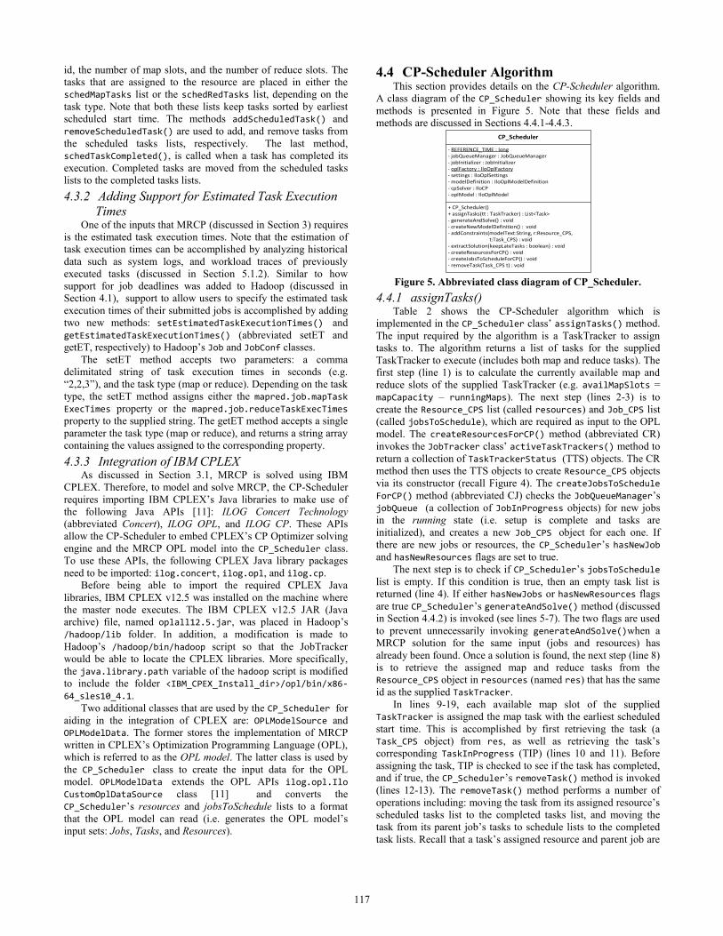
5.2.1 Mixed Workload Figure 6 and Figure 7 demonstrate that CP is able to
effectively handle a complex workload with different types of
jobs. CP outperforms EDF by a large margin in terms of P (up to
91%) and T (up to 57%). The CP-Scheduler is able to effectively
interleave the execution of the tasks of multiple jobs such that
jobs do not miss their deadlines. The EDF-Scheduler’s poor
performance in terms of P and T can be attributed to its focus on
only scheduling a single job at a time (i.e. the job with the earliest
deadline), and not interleaving the execution of jobs.
Figure 6. Mixed Workload: P.
The results in Figure 7 show that CP’s O is larger (changing
from 590ms to 3.5s as λ increases), compared to EDF’s O which
remains close to 12ms for all λ. CP’s O is higher and is observed
to increase with λ because the CP-Scheduler requires generating
an OPL model that represents MRCP, and solving the OPL model
using IBM’s CP Optimizer (see Section 4.4). When there are more
jobs in the OPL model’s input, more time is required to generate
and solve the OPL model because of the higher number of
decision variables and constraints that need to be processed by the
CP Optimizer. On the other hand, EDF’s O tends not to change
significantly with λ because the EDF-Scheduler selects the job to
schedule by retrieving the first job in its job queue (i.e. the job
with the earliest deadline). Although, CP’s O is high, the O/T ratio
which is an indication of a scheduler’s processing overhead in
relation to the average job turnaround time, is still relatively low
in all cases (less than 0.393%).
Figure 7. Mixed Workload: T and O.
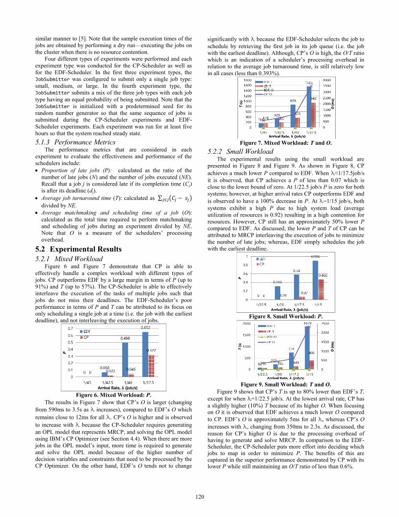
5.2.2 Small Workload The experimental results using the small workload are
presented in Figure 8 and Figure 9. As shown in Figure 8, CP
achieves a much lower P compared to EDF. When λ<1/17.5job/s
it is observed, that CP achieves a P of less than 0.07 which is
close to the lower bound of zero. At 1/22.5 job/s P is zero for both
systems; however, at higher arrival rates CP outperforms EDF and
is observed to have a 100% decrease in P. At λ=1/15 job/s, both
systems exhibit a high P due to high system load (average
utilization of resources is 0.92) resulting in a high contention for
resources. However, CP still has an approximately 50% lower P
compared to EDF. As discussed, the lower P and T of CP can be
attributed to MRCP interleaving the execution of jobs to minimize
the number of late jobs; whereas, EDF simply schedules the job
with the earliest deadline.
Figure 8. Small Workload: P.
Figure 9. Small Workload: T and O.
Figure 9 shows that CP’s T is up to 80% lower than EDF’s T,
except for when λ=1/22.5 job/s. At the lowest arrival rate, CP has
a slightly higher (10%) T because of its higher O. When focusing on O it is observed that EDF achieves a much lower O compared
to CP. EDF’s O is approximately 5ms for all λ, whereas CP’s O
increases with λ, changing from 350ms to 2.3s. As discussed, the
reason for CP’s higher O is due to the processing overhead of having to generate and solve MRCP. In comparison to the EDF-Scheduler, the CP-Scheduler puts more effort into deciding which jobs to map in order to minimize P. The benefits of this are captured in the superior performance demonstrated by CP with its lower P while still maintaining an O/T ratio of less than 0.6%.
120
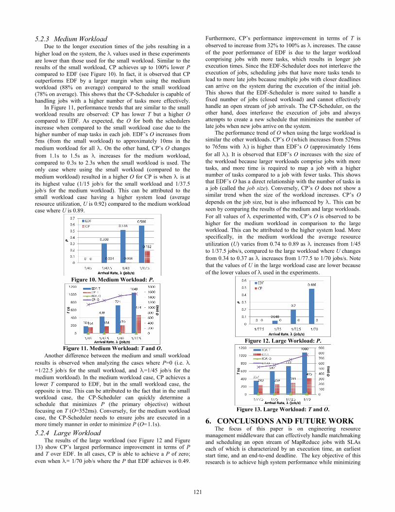
5.2.3 Medium Workload Due to the longer execution times of the jobs resulting in a
higher load on the system, the λ values used in these experiments
are lower than those used for the small workload. Similar to the
results of the small workload, CP achieves up to 100% lower P
compared to EDF (see Figure 10). In fact, it is observed that CP
outperforms EDF by a larger margin when using the medium
workload (88% on average) compared to the small workload
(78% on average). This shows that the CP-Scheduler is capable of
handling jobs with a higher number of tasks more effectively.
In Figure 11, performance trends that are similar to the small
workload results are observed: CP has lower T but a higher O
compared to EDF. As expected, the O for both the schedulers
increase when compared to the small workload case due to the
higher number of map tasks in each job. EDF’s O increases from
5ms (from the small workload) to approximately 10ms in the
medium workload for all λ. On the other hand, CP’s O changes
from 1.1s to 1.5s as λ increases for the medium workload,
compared to 0.3s to 2.3s when the small workload is used. The
only case where using the small workload (compared to the
medium workload) resulted in a higher O for CP is when λ is at
its highest value (1/15 job/s for the small workload and 1/37.5
job/s for the medium workload). This can be attributed to the
small workload case having a higher system load (average
resource utilization, U is 0.92) compared to the medium workload
case where U is 0.89.
Figure 10. Medium Workload: P.
Figure 11. Medium Workload: T and O.
Another difference between the medium and small workload
results is observed when analyzing the cases where P=0 (i.e. λ
=1/22.5 job/s for the small workload, and λ=1/45 job/s for the
medium workload). In the medium workload case, CP achieves a
lower T compared to EDF, but in the small workload case, the
opposite is true. This can be attributed to the fact that in the small
workload case, the CP-Scheduler can quickly determine a
schedule that minimizes P (the primary objective) without
focusing on T (O=352ms). Conversely, for the medium workload
case, the CP-Scheduler needs to ensure jobs are executed in a
more timely manner in order to minimize P (O=1.1s).
5.2.4 Large Workload The results of the large workload (see Figure 12 and Figure
13) show CP’s largest performance improvement in terms of P
and T over EDF. In all cases, CP is able to achieve a P of zero;
even when λ= 1/70 job/s where the P that EDF achieves is 0.49.
Furthermore, CP’s performance improvement in terms of T is
observed to increase from 32% to 100% as λ increases. The cause
of the poor performance of EDF is due to the larger workload
comprising jobs with more tasks, which results in longer job
execution times. Since the EDF-Scheduler does not interleave the
execution of jobs, scheduling jobs that have more tasks tends to
lead to more late jobs because multiple jobs with closer deadlines
can arrive on the system during the execution of the initial job.
This shows that the EDF-Scheduler is more suited to handle a
fixed number of jobs (closed workload) and cannot effectively
handle an open stream of job arrivals. The CP-Scheduler, on the
other hand, does interleave the execution of jobs and always
attempts to create a new schedule that minimizes the number of
late jobs when new jobs arrive on the system.
The performance trend of O when using the large workload is
similar the other workloads. CP’s O (which increases from 529ms
to 765ms with λ) is higher than EDF’s O (approximately 16ms
for all λ). It is observed that EDF’s O increases with the size of
the workload because larger workloads comprise jobs with more
tasks, and more time is required to map a job with a higher
number of tasks compared to a job with fewer tasks. This shows
that EDF’s O has a direct relationship with the number of tasks in
a job (called the job size). Conversely, CP’s O does not show a
similar trend when the size of the workload increases. CP’s O
depends on the job size, but is also influenced by λ. This can be
seen by comparing the results of the medium and large workloads.
For all values of λ experimented with, CP’s O is observed to be
higher for the medium workload in comparison to the large
workload. This can be attributed to the higher system load. More
specifically, in the medium workload the average resource
utilization (U) varies from 0.74 to 0.89 as λ increases from 1/45
to 1/37.5 jobs/s, compared to the large workload where U changes
from 0.34 to 0.37 as λ increases from 1/77.5 to 1/70 jobs/s. Note
that the values of U in the large workload case are lower because
of the lower values of λ used in the experiments.
Figure 12. Large Workload: P.
Figure 13. Large Workload: T and O.
6. CONCLUSIONS AND FUTURE WORK The focus of this paper is on engineering resource
management middleware that can effectively handle matchmaking
and scheduling an open stream of MapReduce jobs with SLAs
each of which is characterized by an execution time, an earliest
start time, and an end-to-end deadline. The key objective of this
research is to achieve high system performance while minimizing
121

resource management overhead. More specifically, a MapReduce
constraint programming based matchmaking and scheduling
algorithm (MRCP) is devised and solved using IBM CPLEX.
Furthermore, a new constraint programming based scheduler for
Hadoop, which is a popular open source implementation of the
MapReduce programming model, is devised and implemented.
The new scheduler for Hadoop, called CP-Scheduler, generates
and solves an MRCP model to perform matchmaking and
scheduling of an open stream of MapReduce jobs with deadlines.
Our experiences and the challenges that we encountered in
devising the CP-Scheduler and implementing the algorithm in
Hadoop are described in this paper. A performance evaluation of
the CP-scheduler is conducted on an Amazon EC2 cluster running
Hadoop and its performance is compared with that of an EDF-
Scheduler, which is implemented by extending Hadoop’s default
FIFO scheduler. The experimental results demonstrate the CP-
Scheduler’s effectiveness to map an open stream of MapReduce
jobs with deadlines in a Hadoop cluster. Some of the key insights
into system behaviour and performance are summarized:
In all the experiments, the CP-Scheduler generated a schedule
that leads to a lower or equal P compared to the EDF-
Scheduler, and close to the lower bound of zero when the
system utilization is reasonable. The best performance observed
is in the large workload experiments where the CP-Scheduler
generated a P of zero in all cases. In other experiments, the
percentage improvement of the CP-Scheduler’s P compared to
the EDF-Scheduler’s P is observed to be as low as 48% and as
high as 100%.
In most cases, the CP-Scheduler generated a schedule with a
lower T compared to the EDF-Scheduler. The CP-Scheduler is
outperformed by the EDF-Scheduler by a small margin when
the system is lightly loaded (i.e. small workload and small
arrival rate, which can be attributed to the CP-Scheduler’s O
having a larger impact on T.
Although, the CP-Scheduler demonstrates a much superior P
and T in comparison to EDF-Scheduler, this performance
improvement is accompanied by an increase in O. However, it
is still observed that the ratio O/T for the CP-Scheduler is still
very small in all cases experimented with (less than 0.69%).
o The CP-Scheduler’s O depends on the number of tasks in a
job (i.e. job size), as well as the job arrival rate, and thus for
a given workload type O increases as the job arrival rate
increases. Conversely, the EDF-Scheduler’s O increases
with job size, and remains relatively the same as job arrival
rate increases.
Overall, the experimental results show that the CP-Scheduler can
effectively perform matchmaking and scheduling of an open
stream of MapReduce jobs with deadlines in a Hadoop cluster
leading to a schedule with a small proportion of late jobs. The
EDF-Scheduler; however, seems to be more suited to handle a
fixed (closed) workload because of the fact that it does not
interleave the execution of jobs, which can lead to very poor
performance on an open system. This can happen, for example,
when the execution times of jobs are long and multiple jobs arrive
on the system with earlier deadlines (see Section 5.2.4). For future research, we plan to perform more extensive
experiments, which includes experiments that use larger
workloads and more nodes. Moreover, techniques for estimating task execution times and handling errors associated with the
estimated times warrants further investigation.
7. ACKNOWLEDGMENTS We are grateful to Huawei, Canada and the Government of
Ontario for supporting this research.
8. REFERENCES [1] The Apache Software Foundation. Hadoop. Available:
http://hadoop.apache.org.
[2] Jones, M. 2011. Scheduling in Hadoop. Available: http://www.ibm.com/developerworks/library/os-hadoop-scheduling/
[3] Rossi, F., Beek, P., and Walsh, T. 2008. Chapter 4: Constraint Programming. Handbook of Knowledge Representation (2008). 181-211.
[4] Dean, J. and Ghemawat, S. 2004. MapReduce: Simplified data processing on large clusters. Int’l Symp. on Operating System Design and Implementation (Dec. 2004). 137–150.
[5] Verma, A., Cherkasova, L., Kumar, V.S., and Campbell, R.H. 2012. Deadline-based workload management for MapReduce environments: Pieces of the performance puzzle. In Proc. of Network Operations and Management Symposium (16-20 April 2012). 900-905.
[6] Dong, X., Wang, Y., and Liao, H. 2011. Scheduling Mixed Real-Time and Non-real-Time Applications in MapReduce Environment. Int’l Conf. on Parallel and Distributed Systems (7-9 Dec. 2011). 9-16.
[7] Mattess, M., Calheiros, R.N., and Buyya, R. 2013. Scaling MapReduce Applications Across Hybrid Clouds to Meet Soft Deadlines. Int’l Conf. on Advanced Information Networking and Applications (25-28 March 2013). 629-636.
[8] Hwang, E. and Kim, K. H. 2012. Minimizing Cost of Virtual Machines for Deadline-Constrained MapReduce Applications in the Cloud. Int’l Conf. on Grid Computing (20-23 Sept. 2012).130-138.
[9] Kc, K., and Anyanwu, K. 2010. Scheduling Hadoop Jobs to Meet Deadlines. Int’l Conf. on Cloud Computing Technology and Science (Nov. 30 2010-Dec. 3 2010). 388-392.
[10] Lim, N., Majumdar, S., and Ashwood-Smith, P. 2014.Engineering Resource Management Middleware for Optimizing the Performance of Clouds Processing MapReduce Jobs with Deadlines. Int’l Conf. on Performance Engineering (Mar. 24-26 2014). 161-172.
[11] IBM. IBM ILOG CPLEX Optimization Studio V12.5 Reference Manual. Available: http://pic.dhe.ibm.com/ infocenter/cosinfoc/ v12r5/index.jsp
[12] Lim, N., Majumdar, S., and Ashwood-Smith, P. 2014. A Constraint Programming-Based Resource Management Technique for Processing MapReduce Jobs with SLAs on Clouds. Int’l Conf. on Parallel Processing (Sept 9-12 2014).
[13] White, T. 2011. Hadoop: The Definitive Guide, 2nd
Edition. O’Reilly Media, Inc., Sebastopol, CA, USA.
[14] Apache. Hadoop Wiki. Available: http://wiki.apache.org/ hadoop/PoweredBy
[15] Fadika, Z., Dede, E., Hartog, J., and Govindaraju, M. 2012. MARLA: MapReduce for Heterogeneous Clusters. IEEE/ACM Int’l Symp. on Cluster, Cloud and Grid Computing (13-16 May 2012). 49-56.
[16] Chang, H., Kodialam, M., Kompella, R.R., Lakshman, T.V. Lee, M., and Mukherjee, S. 2011. Scheduling in mapreduce like systems for fast completion time. IEEE INFOCOM (10-15 April 2011). 3074-3082.
[17] Gao, X., Chen, Q., Chen, Y., Sun, Q., Liu, Y., and Li, M. 2012. A Dispatching-Rule-Based Task Scheduling Policy for MapReduce with Multi-type Jobs in Heterogeneous Environments. ChinaGrid Annual Conference (20-23 Sept. 2012). 17 -24.
[18] IBM. 2010. Detailed Scheduling in IBM ILOG CPLEX Optimization Studio with IBM ILOG CPLEX CP Optimizer. White Paper. IBM Corporation (2010).
[19] Zujie, R., Wan, J., Shi, W., Xu, X., and Zhou, M. 2014. Workload Analysis, Implications, and Optimization on a Production Hadoop Cluster: A Case Study on Taobao. IEEE Transactions Services Computing (vol.7, no.2, April-June 2014). 307-321.
122
Related Documents