Constraint Programming

SOLVING POLYNOMIAL SYSTEMS USING A BRANCHAND PRUNE APPROACH∗

PASCAL VAN HENTENRYCK† , DAVID MCALLESTER‡ , AND DEEPAK KAPUR§

SIAM J. NUMER. ANAL. c© 1997 Society for Industrial and Applied MathematicsVol. 34, No. 2, pp. 797–827, April 1997 019

Abstract. This paper presents Newton, a branch and prune algorithm used to find all isolatedsolutions of a system of polynomial constraints. Newton can be characterized as a global searchmethod which uses intervals for numerical correctness and for pruning the search space early. Thepruning in Newton consists of enforcing at each node of the search tree a unique local consistencycondition, called box-consistency, which approximates the notion of arc-consistency well known inartificial intelligence. Box-consistency is parametrized by an interval extension of the constraint andcan be instantiated to produce the Hansen–Sengupta narrowing operator (used in interval methods)as well as new operators which are more effective when the computation is far from a solution. Newtonhas been evaluated on a variety of benchmarks from kinematics, chemistry, combustion, economics,and mechanics. On these benchmarks, it outperforms the interval methods we are aware of andcompares well with state-of-the-art continuation methods. Limitations of Newton (e.g., a sensitivityto the size of the initial intervals on some problems) are also discussed. Of particular interest is themathematical and programming simplicity of the method.

Key words. system of equations, global methods, interval and finite analysis

AMS subject classifications. 65H10, 65G10

PII. S0036142995281504

1. Introduction. Many applications in science and engineering (e.g., chemistry,robotics, economics, mechanics) require finding all isolated solutions to a system ofpolynomial constraints over real numbers. This problem is difficult due to its inherentcomputational complexity (i.e., it is NP-hard) and due to the numerical issues involvedto guarantee correctness (i.e., finding all solutions) and to ensure termination. Severalinteresting methods have been proposed in the past for this task, including two funda-mentally different methods: interval methods (e.g., [4, 5, 7, 8, 11, 13, 14, 15, 19, 25, 29])and continuation methods (e.g., [24, 35]). Continuation methods have been shown tobe effective for problems for which the total degree is not too high, since the numberof paths explored depends on the estimation of the number of solutions. Intervalmethods are generally robust but tend to be slow.

The purpose of this paper is to propose and study a novel interval algorithmimplemented in a system called Newton. From a user standpoint, Newton receives asinput a system of polynomial constraints over, say, variables x1, . . . , xn and a box, i.e.,an interval tuple 〈I1, . . . , In〉 specifying the initial range of these variables; it returnsa set of small boxes of specified accuracy containing all solutions with typically onesolution per box returned.

Operationally, Newton uses a branch and prune algorithm which was inspiredby the traditional branch and bound approach used to solve combinatorial optimiza-

∗Received by the editors February 10, 1995; accepted for publication (in revised form) July 10,1995.

http://www.siam.org/journals/sinum/34-2/28150.html†Brown University, Department of Computer Science, Box 1910, Providence, RI 02912 (pvh@cs.

brown.edu). The research of this author was supported in part by Office of Naval Research grantN00014-94-1-1153, National Science Foundation grant CCR-9357704, and a National Science Foun-dation National Young Investigator Award with matching funds of Hewlett-Packard.‡MIT AI Lab, Technology Square, 545, Cambridge, MA 02139 ([email protected]).§SUNY at Albany, Department of Computer Science, Albany, NY 12222 ([email protected]).

The research of this author was supported in part by United States Air Force Office of ScientificResearch grant AFOSR-91-0361.

797

798 P. VAN HENTENRYCK, D. MCALLESTER, AND D. KAPUR

tion problems. Newton uses intervals to address the two fundamental problems listedabove. Numerical reliability is obtained by evaluating functions over intervals usingoutward rounding (as in interval methods). The complexity issue is addressed byusing constraints to reduce the intervals early in the search. The pruning in Newton isachieved by enforcing a unique local consistency condition, called box-consistency, ateach node of the search tree. Box-consistency is an approximation of arc-consistency,a notion well known in artificial intelligence [16, 18] and used to solve discrete combi-natorial problems in several systems (e.g., [31, 32]). Box-consistency is parametrizedby an interval extension operator for the constraint and can be instantiated to producevarious narrowing operators. In particular, box-consistency on the Taylor extensionof the constraint produces a generalization of the Hansen–Sengupta operator [8], wellknown in interval methods. In addition, box-consistency on the natural extension pro-duces narrowing operators which are more effective when the algorithm is not near asolution. Newton has the following properties:

• Correctness. Newton finds all isolated solutions to the system in the followingsense: if 〈v1, . . . , vn〉 is a solution, then Newton returns at least one box〈I1, . . . , In〉 such that vi ∈ Ii (1 ≤ i ≤ n). In addition, Newton may guaranteethe existence of a unique solution in some or all of the boxes in the result.If the solutions are not isolated (e.g., the floating-point system is not preciseenough to separate two solutions), then the boxes returned by the algorithmmay contain several solutions.• Termination. Newton always terminates.• Effectiveness. Newton has been evaluated on a variety of benchmarks from

kinematics, chemistry, combustion, economics, and mechanics. It outper-forms the interval methods we are aware of and compares well with state-of-the-art continuation methods on many problems. Interestingly, Newton solvesthe Broyden banded function problem [8] and More–Cosnard discretizationof a nonlinear integral equation [22] for several hundred variables.• Simplicity and uniformity. Newton is based on simple mathematical results

and is easy to use and to implement. It is also based on a single concept:box-consistency.

The rest of this paper is organized as follows. Section 2 gives an overview ofthe approach. Section 3 contains the preliminaries. Section 4 presents an abstractversion of the branch and prune algorithm. Section 5 discusses the implementation ofthe box-consistency. Section 6 describes the experimental results. Section 7 discussesrelated work and the development of the ideas presented here. Section 8 concludesthe paper. A short version of this paper is available in [33].

2. Overview of the approach. As mentioned, Newton is a global search al-gorithm which solves a problem by dividing it into subproblems which are solvedrecursively. In addition, Newton is a branch and prune algorithm which means thatit is best viewed as an iteration of two steps:

1. pruning the search space;2. making a nondeterministic choice to generate two subproblems

until one or all solutions to a given problem are found.The pruning step ensures that some local consistency conditions are satisfied. It

consists of reducing the intervals associated with the variables so that every constraintappears to be locally consistent. The local consistency condition of Newton is calledbox-consistency, an approximation of arc-consistency, a notion well known in artificialintelligence [16, 18] and used in many systems (e.g., [32, 34, 30]) to solve discretecombinatorial search problems. Informally speaking, a constraint is arc-consistent if

SOLVING POLYNOMIAL SYSTEMS USING BRANCH AND PRUNE 799

for each value in the range of a variable there exist values in the ranges of the othervariables such that the constraint is satisfied. Newton approximates arc-consistencywhich cannot be computed on real numbers in general.

The pruning step either fails, showing the absence of solution in the intervals, orsucceeds in enforcing the local consistency condition. Sometimes, local consistencyalso implies global consistency as in the case of the Broyden banded function, i.e.,

fi(x1, . . . , xn) = xi(2 + 5x2i ) + 1−

∑j∈Ji

xj(1 + xj) (1 ≤ i ≤ n)

where Ji = {j | j 6= i and max(1, i − 5) ≤ j ≤ min(n, i + 1)}. The pruning step ofNewton solves this problem in essentially linear time for initial intervals of the form[−108, 108] and always proves the existence of a solution in the final box. However,in general, local consistency does not imply global consistency either because thereare multiple solutions or simply because the local consistency condition is too weak.Consider the intersection of a circle and a parabola:{

x21 + x2

2 = 1,x2

1 − x2 = 0

with initial intervals in [−108, 108] and assume that we want the resulting intervalsto be of size 10−8 or smaller. The pruning step returns the intervals

x1 ∈ [−1.0000000000012430057,+1.0000000000012430057],x2 ∈ [−0.0000000000000000000,+1.0000000000012430057].

Informally speaking, Newton obtains the above pruning as follows. The first constraintis used to reduce the interval of x1 by searching for the leftmost and rightmost “zeros”of the interval function

X21 + [−108, 108]2 = 1.

These zeros are −1 and 1 and hence the new interval for x1 becomes [−1,1] (modulothe numerical precision).1 The same reasoning applies to x2. The second constraintcan be used to reduce further the interval of x2 by searching for the leftmost andrightmost zeros of

[−1, 1]2 −X2 = 0

producing the interval [0,1] for x2. No more reduction is obtained by Newton andbranching is needed to make progress. Branching on x1 produces the intervals

x1 ∈ [−1.0000000000012430057,+0.0000000000000000000],x2 ∈ [−0.0000000000000000000,+1.0000000000012430057].

Further pruning is obtained by taking the Taylor extension of the polynomials in theabove equations around (−0.5, 0.5), the center of the above box, and by condition-ing the system. Newton then uses these new constraints to find their leftmost andrightmost zeros, as was done previously to obtain

x1 ∈ [−1.0000000000000000000,−0.6049804687499998889],x2 ∈ [+0.3821067810058591529,+0.8433985806150308129].

1The precision of the pruning step depends both on the numerical precision and the improvementfactor selected (see section 5.6) which explains the digits 12430057 in the above results.


Additional pruning using the original statement of the constraints leads to the firstsolution

x1 ∈ [−0.7861513777574234974,−0.7861513777574231642],x2 ∈ [+0.6180339887498946804,+0.6180339887498950136].

Backtracking on the choice for x1 produces the intervals

x1 ∈ [−0.0000000000000000000,+1.0000000000012430057],x2 ∈ [−0.0000000000000000000,+1.0000000000012430057]

and to the second solution

x1 ∈ [+0.7861513777574231642,+0.7861513777574233864],x2 ∈ [+0.6180339887498946804,+0.6180339887498950136].

Note that, in this case, Newton makes the smallest number of choices to isolate thesolutions.2 To conclude this motivating section, let us illustrate Newton on a largerexample which describes the inverse kinematics of an elbow manipulator [11]:

s2c5s6 − s3c5s6 − s4c5s6 + c2c6 + c3c6 + c4c6 = 0.4077,c1c2s5 + c1c3s5 + c1c4s5 + s1c5 = 1.9115,s2s5 + s3s5 + s4s5 = 1.9791,c1c2 + c1c3 + c1c4 + c1c2 + c1c3 + c1c2 = 4.0616,s1c2 + s1c3 + s1c4 + s1c2 + s1c3 + s1c2 = 1.7172,s2 + s3 + s4 + s2 + s3 + s2 = 3.9701,s2i + c2i = 1 (1 ≤ i ≤ 6)

and assumes that the initial intervals are in [−108, 108] again. The pruning stepreturns the intervals

[− 1.0000000000000000000,+1.0000000000000000000],[− 1.0000000000000000000,+1.0000000000000000000],[ + 0.3233666666666665800,+1.0000000000000000000],[− 1.0000000000000000000,+1.0000000000000000000],[− 0.0149500000000000189,+1.0000000000000000000],[− 1.0000000000000000000,+1.0000000000000000000],[− 0.0209000000000001407,+1.0000000000000000000],[− 1.0000000000000000000,+1.0000000000000000000],[ + 0.6596999999999998420,+1.0000000000000000000],[− 0.7515290480087772896,+0.7515290480087772896],[− 1.0000000000000000000,+1.0000000000000000000],[− 1.0000000000000000000,+1.0000000000000000000]

showing already some interesting pruning. After exactly 12 branchings and in lessthan a second, Newton produces the first box with a proof of existence of a solutionin the box.

3. Preliminaries. In this section, we review some basic concepts needed forthis paper, including interval arithmetic and the representation of constraints. Moreinformation on interval arithmetic can be found in many places (e.g., [1, 8, 7, 19, 20]).Our definitions are slightly nonstandard.

2This example can also be solved by replacing x21 in the first equation by x2 to obtain a univariate

constraint in x2 which can be solved independently. However, this cannot always be done and thediscussion here is what Newton would do, without making such optimizations.


3.1. Interval arithmetic. We consider <∞ = < ∪ {−∞,∞} the set of realnumbers extended with the two infinity symbols and the natural extension of therelation < to this set. We also consider a finite subset F of <∞ containing −∞,∞, 0.In practice, F corresponds to the floating-point numbers used in the implementation.

DEFINITION 1 [Interval]. An interval [l, u] with l, u ∈ F is the set of real numbers

{r ∈ < | l ≤ r ≤ u}.

The set of intervals is denoted by I and is ordered by set inclusion.3

DEFINITION 2 [Enclosure and hull]. Let S be a subset of <. The enclosure of S,denoted by S or box{S}, is the smallest interval I such that S ⊆ I. We often write rinstead of {r} for r ∈ <. The interval hull of I1 and I2, denoted by I1 ] I2, is definedas box{I1 ∪ I2}.

We denote real numbers by the letters r, v, a, b, c, d, F -numbers by the lettersl,m, u, intervals by the letter I, real functions by the letters f, g, and interval functions(e.g., functions of signature I → I) by the letters F,G, all possibly subscripted. Weuse l+ (resp., l−) to denote the smallest (resp., largest) F -number strictly greater(resp., smaller) than the F -number l. To capture outward rounding, we use dre(resp., brc) to return the smallest (resp., largest) F -number greater (resp., smaller) orequal to the real number r. We also use ~I to denote a box 〈I1, . . . , In〉 and ~r to denotea tuple 〈r1, . . . , rn〉. Q is the set of rational numbers and N is the set of naturalnumbers. Finally, we use the following notations:

left([l, u]) = l,right([l, u]) = u,center([a, b]) = b(a+ b)/2c.

The fundamental concept of interval arithmetic is the notion of interval extension.DEFINITION 3 [Interval extension]. F : In → I is an interval extension of f :

<n → < iff

∀I1 . . . In ∈ I : r1 ∈ I1, . . . , rn ∈ In ⇒ f(r1, . . . , rn) ∈ F (I1, . . . , In).

An interval relation C : In → Bool is an interval extension of a relation c : <n → Booliff

∀I1 . . . In ∈ I : [ ∃r1 ∈ I1, . . . , ∃rn ∈ In c(r1, . . . , rn) ]⇒ C(I1, . . . , In).

Example 1. The interval function ⊕ defined as

[a1, b1]⊕ [a2, b2] = [ba1 + a2c, db1 + b2e]

is an interval extension of addition of real numbers. The interval relation = definedas

I1=I2 ⇔ (I1 ∩ I2 6= ∅)

is an interval extension of the equality relation on real numbers.It is important to stress that a real function (resp., relation) can be extended in

many ways. For instance, the interval function ⊕ is the most precise interval extension

3Our intervals are usually called floating-point intervals in the literature.


of addition (i.e., it returns the smallest possible interval containing all real results)while a function always returning [−∞,∞] would be the least accurate.

In the following, we assume fixed interval extensions for the basic real operators+,−,× and exponentiation (for instance, the interval extension of + is defined by⊕) and the basic real relations =,≥. In addition, we overload the real symbols anduse them for their interval extensions. Finally, we denote relations by the letter cpossibly subscripted, interval relations by the letter C possibly subscripted. Notethat constraints and relations are used as synonyms in this paper.

3.2. Division and unions of intervals. Even though many basic real opera-tors can be naturally extended to work on intervals, division creates problems if thedenominator interval includes zero. A tight extension of division to intervals can bebest expressed if its result is allowed to be a union of intervals [10, 6, 12]. Assumingthat c ≤ 0 ≤ d and c < d, [a, b]/[c, d] is defined as follows:

[bb/cc,∞] if b ≤ 0 and d = 0,[−∞, db/de] ∪ [bb/cc,∞] if b ≤ 0 and c < 0 < d,[−∞, db/de] if b ≤ 0 and c = 0,[−∞,∞] if a < 0 < b,[−∞, da/ce] if a ≥ 0 and d = 0,[−∞, da/ce] ∪ [bb/cc,∞] if a ≥ 0 and c < 0 < d,[ba/dc,∞] if a ≥ 0 and c = 0.

When [c, d] = [0, 0], [a, b]/[c, d] = [−∞,∞]. The case where 0 /∈ [c, d] is easy to define.Note also that other operations such as addition and subtraction can also be extendedto work with unions of intervals.

A typical use of unions of intervals in interval arithmetic is the intersection of aninterval I with the result of an operation of the form Ic − In/Id to produce a newinterval I ′. To increase precision, Ic − In/Id is computed with unions of intervalsproducing a result of the form I1 or I1 ∪ I2. This result should be intersected withI to produce a single interval as result (i.e., not a union of intervals). A generalizedintersection operation u defined as

(I1 ∪ · · · ∪ In) u (I ′1 ∪ · · · ∪ I ′m) = (I1 ∩ I ′1) ] (I1 ∩ I ′2) ] · · · ] (In ∩ I ′m)

is used for this purpose, i.e., we compute

I u (Ic − In/Id).

This result may be more precise than

(I1 ] · · · ] In) ∩ (I ′1 ] · · · ] I ′m).

To illustrate the gain of precision, consider I = [−5,−1], I1 = [−∞,−3], and I2 =[3,∞]. The expression I u (I1 ∪ I2) evaluates to the interval [−5,−3], while theexpression I ∩ (I1 ] I2) returns the interval [−5,−1], since I1 ] I2 = [−∞,∞].

3.3. Constraint representations. It is well known that different computerrepresentations of a real function may produce different results when evaluated withfloating-point numbers on a computer. As a consequence, the way constraints arewritten may have an impact on the behavior of the algorithm. For this reason, a con-straint or a function in this paper is considered to be an expression written in someformal language by composing real variables, rational numbers, some predefined real


numbers (e.g., π), arithmetic operations such as +,−,×, and exponentiation to a nat-ural number, parentheses, and relation symbols such as ≤,=.4 We will abuse notationby denoting functions (resp., constraints) and their representations by the same sym-bol. Real variables in constraints will be taken from a finite (but arbitrary large) set{x1, . . . , xn}. Similar conventions apply to interval functions and constraints. Intervalvariables will be taken from a finite (but arbitrary large) set {X1, . . . , Xn}, intervalfunctions will be denoted by the letter F , and interval constraints by the letter C.For simplicity of exposition, we restrict attention to equations. It is straightforwardto generalize our results to inequalities (see section 5.6).

4. The branch and prune algorithm. This section describes the branch andprune algorithm Newton. Section 4.1 defines box-consistency, the key concept behindour algorithm. Section 4.2 shows how box-consistency can be instantiated to producevarious pruning operators achieving various trade-offs between accuracy and efficiency.Section 4.3 defines a conditioning operator used in Newton to improve the effectivenessof box-consistency. Section 4.4 specifies the pruning in Newton. Section 4.5 describesthe algorithm. Recall that we assume that all constraints are defined over variablesx1, . . . , xn.

4.1. Box consistency. Box-consistency [2] approximates arc-consistency, a no-tion well known in artificial intelligence [16] which states a simple local condition ona constraint c and the set of possible values for each of its variables, say D1, . . . , Dn.Informally speaking, a constraint c is arc-consistent if none of the Di can be reducedby using projections of c.

DEFINITION 4 [Projection constraint]. A projection constraint 〈c, i〉 is a pair ofa constraint c and an index i (1 ≤ i ≤ n). Projection constraints are denoted by theletter p, possibly subscripted.

Example 2. Consider the constraint x21 + x2

2 = 1. Both 〈x21 + x2

2 = 1 , 1〉 and〈x2

1 + x22 = 1 , 2〉 are projection constraints.

DEFINITION 5 [Arc-consistency]. A projection constraint 〈c, i〉 is arc-consistentwith respect to ~D = 〈D1, . . . , Dn〉 iff

Di = Di∩{ri | ∃r1 ∈ D1, . . . , ri−1 ∈ Di−1, ri+1 ∈ Di+1, . . . , rn ∈ Dn : c(r1, . . . , rn)}.

A constraint c is arc-consistent with respect to ~D if each of its projections is arc-consistent with respect to ~D. A system of constraints S is arc-consistent with respectto ~D if each constraint in S is arc-consistent with respect to ~D.

Example 3. Let c be the constraint x21 + x2

2 = 1. c is arc-consistent with respectto 〈 [−1, 1], [−1, 1] 〉 but is not arc-consistent with respect to 〈 [−1, 1], [−2, 2] 〉 since,for instance, there is no value r1 for x1 in [−1, 1] such that r2

1 + 22 = 1.Given some initial domains 〈D0

1, . . . , D0n〉, an arc-consistency algorithm computes

the largest domains 〈D1, . . . , Dn〉 included in 〈D01, . . . , D

0n〉 such that all constraints

are arc-consistent. These domains always exist and are unique. Enforcing arc-consistency is very effective on discrete combinatorial problems. However, it cannotbe computed in general when working with real numbers and polynomial constraints.Moreover, simple approximations to take into account numerical accuracy are veryexpensive to compute (the exact complexity is an open problem). For instance, asimple approximation of arc-consistency consists of working with intervals and ap-

4It is easy to extend the language to include functions such as sin, cos, e, . . . .


proximating the set computed by arc-consistency to return an interval, i.e.,

Ii = box{Ii ∩ { ri | ∃r1 ∈ I1, . . . , ri−1 ∈ Ii−1, . . . , ri+1 ∈ Ii+1, rn ∈ In : c(r1, . . . , rn) }}.

This condition, used in systems like [26, 3], is easily enforced on simple constraintssuch as

x1 = x2 + x3, x1 = x2 − x3, x1 = x2 × x3,

but it is also computationally very expensive for complex constraints with multipleoccurrences of the same variables. Moreover, decomposing complex constraints intosimple constraints entails a substantial loss in pruning, making this approach imprac-tical on many applications. See [2] for experimental results on this approach and theircomparison with the approach presented in this paper.

The notion of box-consistency introduced in [2] is a coarser approximation of arc-consistency which provides a much better trade-off between efficiency and pruning.It consists of replacing the existential quantification in the above condition by theevaluation of an interval extension of the constraint on the intervals of the existentialvariables. Since there are many interval extensions for a single constraint, we definebox-consistency in terms of interval constraints.

DEFINITION 6 [Interval projection constraint]. An interval projection constraint〈C, i〉 is the association of an interval constraint C and of an index i (1 ≤ i ≤ n).Interval projection constraints are denoted by the letter P , possibly subscripted.

DEFINITION 7 [Box-consistency]. An interval projection constraint 〈C, i〉 is box-consistent with respect to ~I = 〈I1, . . . , In〉 iff

C(I1, . . . , Ii−1, [l, l+], Ii+1, . . . , In) ∧ C(I1, . . . , Ii−1, [u−, u], Ii+1, . . . , In)

where l = left(Ii) and u = right(Ii). An interval constraint is box-consistent withrespect to ~I if each of its projections is box-consistent with respect to ~I. A system ofinterval constraints is box-consistent with respect to ~I iff each interval constraint inthe system is box-consistent with respect to ~I.

Intuitively speaking, the above condition states that the ith interval cannot bepruned further using the unary interval constraint obtained by replacing all variablesbut Xi by their intervals, since the boundaries satisfy the unary constraint. Note alsothat the above condition is equivalent to

Ii = box{ ri ∈ Ii | C(I1, ..., Ii−1, ri, Ii+1, ..., In) }

which shows clearly that box-consistency is an approximation of arc-consistency.5

The difference between arc-consistency and box-consistency appears essentially whenthere are multiple occurrences of the same variable.

Example 4. Consider the constraint x1 + x2 − x1 = 0. The constraint is notarc-consistent with respect to 〈[−1, 1], [−1, 1]〉 since there is no value r1 for x1 whichsatisfies r1 + 1− r1 = 0. On the other hand, the interval constraint X1 +X2−X1 = 0is box-consistent, since ([−1, 1] + [−1,−1+] − [−1, 1]) ∩ [0, 0] and ([−1, 1] + [1−, 1] −[−1, 1]) ∩ [0, 0] are nonempty.

5It is interesting to note that this definition is also related to the theorem of Miranda [25]. Inthis case, box-consistency can be seen as replacing universally quantified variables by the intervalson which they range.


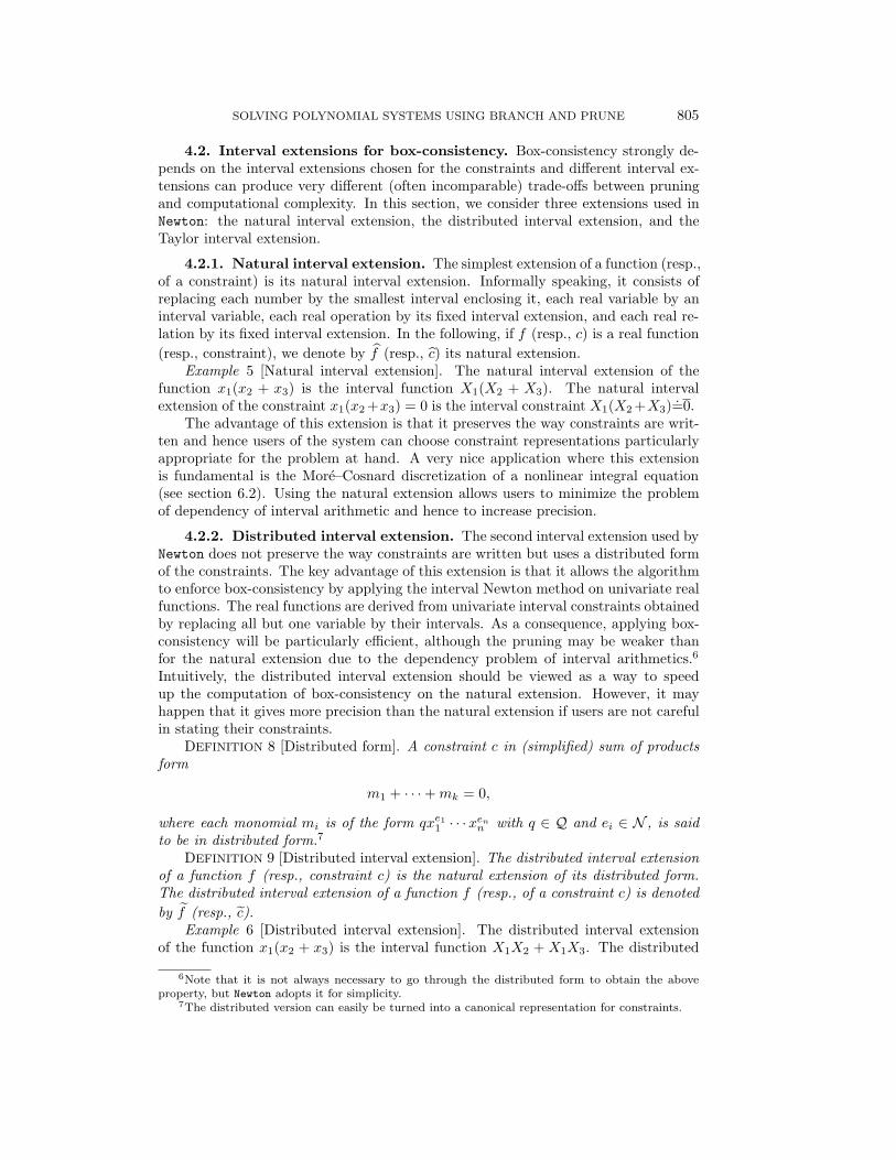
4.2. Interval extensions for box-consistency. Box-consistency strongly de-pends on the interval extensions chosen for the constraints and different interval ex-tensions can produce very different (often incomparable) trade-offs between pruningand computational complexity. In this section, we consider three extensions used inNewton: the natural interval extension, the distributed interval extension, and theTaylor interval extension.

4.2.1. Natural interval extension. The simplest extension of a function (resp.,of a constraint) is its natural interval extension. Informally speaking, it consists ofreplacing each number by the smallest interval enclosing it, each real variable by aninterval variable, each real operation by its fixed interval extension, and each real re-lation by its fixed interval extension. In the following, if f (resp., c) is a real function(resp., constraint), we denote by f (resp., c) its natural extension.

Example 5 [Natural interval extension]. The natural interval extension of thefunction x1(x2 + x3) is the interval function X1(X2 + X3). The natural intervalextension of the constraint x1(x2 +x3) = 0 is the interval constraint X1(X2 +X3)=0.

The advantage of this extension is that it preserves the way constraints are writ-ten and hence users of the system can choose constraint representations particularlyappropriate for the problem at hand. A very nice application where this extensionis fundamental is the More–Cosnard discretization of a nonlinear integral equation(see section 6.2). Using the natural extension allows users to minimize the problemof dependency of interval arithmetic and hence to increase precision.

4.2.2. Distributed interval extension. The second interval extension used byNewton does not preserve the way constraints are written but uses a distributed formof the constraints. The key advantage of this extension is that it allows the algorithmto enforce box-consistency by applying the interval Newton method on univariate realfunctions. The real functions are derived from univariate interval constraints obtainedby replacing all but one variable by their intervals. As a consequence, applying box-consistency will be particularly efficient, although the pruning may be weaker thanfor the natural extension due to the dependency problem of interval arithmetics.6

Intuitively, the distributed interval extension should be viewed as a way to speedup the computation of box-consistency on the natural extension. However, it mayhappen that it gives more precision than the natural extension if users are not carefulin stating their constraints.

DEFINITION 8 [Distributed form]. A constraint c in (simplified) sum of productsform

m1 + · · ·+mk = 0,

where each monomial mi is of the form qxe11 · · ·xenn with q ∈ Q and ei ∈ N , is saidto be in distributed form.7

DEFINITION 9 [Distributed interval extension]. The distributed interval extensionof a function f (resp., constraint c) is the natural extension of its distributed form.The distributed interval extension of a function f (resp., of a constraint c) is denotedby f (resp., c).

Example 6 [Distributed interval extension]. The distributed interval extensionof the function x1(x2 + x3) is the interval function X1X2 + X1X3. The distributed

6Note that it is not always necessary to go through the distributed form to obtain the aboveproperty, but Newton adopts it for simplicity.

7The distributed version can easily be turned into a canonical representation for constraints.


interval extension of the constraint x1(x2 + x3) = 0 is the interval constraint X1X2 +X1X3 = 0.

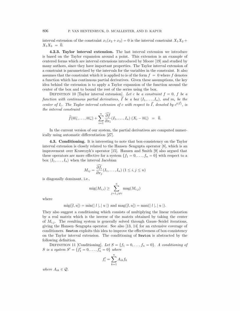
4.2.3. Taylor interval extension. The last interval extension we introduceis based on the Taylor expansion around a point. This extension is an example ofcentered forms which are interval extensions introduced by Moore [19] and studied bymany authors, since they have important properties. The Taylor interval extension ofa constraint is parametrized by the intervals for the variables in the constraint. It alsoassumes that the constraint which it is applied to is of the form f = 0 where f denotesa function which has continuous partial derivatives. Given these assumptions, the keyidea behind the extension is to apply a Taylor expansion of the function around thecenter of the box and to bound the rest of the series using the box.

DEFINITION 10 [Taylor interval extension]. Let c be a constraint f = 0, f be afunction with continuous partial derivatives, ~I be a box (I1, . . . , In), and mi be thecenter of Ii. The Taylor interval extension of c with respect to ~I, denoted by ct(~I), isthe interval constraint

f(m1, . . . ,mn) +n∑i=1

∂f

∂xi(I1, . . . , In) (Xi −mi) = 0.

In the current version of our system, the partial derivatives are computed numer-ically using automatic differentiation [27].

4.3. Conditioning. It is interesting to note that box-consistency on the Taylorinterval extension is closely related to the Hansen–Sengupta operator [8], which is animprovement over Krawczyk’s operator [15]. Hansen and Smith [9] also argued thatthese operators are more effective for a system {f1 = 0, . . . , fn = 0} with respect to abox 〈I1, . . . , In〉 when the interval Jacobian

Mij =∂fi∂xj

(I1, . . . , In) (1 ≤ i, j ≤ n)

is diagonally dominant, i.e.,

mig(Mi,i) ≥n∑

j=1,j 6=imag(Mi,j)

where

mig([l, u]) = min(| l |, | u |) and mag([l, u]) = max(| l |, | u |).They also suggest a conditioning which consists of multiplying the linear relaxationby a real matrix which is the inverse of the matrix obtained by taking the centerof Mi,j . The resulting system is generally solved through Gauss–Seidel iterations,giving the Hansen–Sengupta operator. See also [13, 14] for an extensive coverage ofconditioners. Newton exploits this idea to improve the effectiveness of box-consistencyon the Taylor interval extension. The conditioning of Newton is abstracted by thefollowing definition.

DEFINITION 11 [Conditioning]. Let S = {f1 = 0, . . . , fn = 0}. A conditioning ofS is a system S′ = {f ′1 = 0, . . . , f ′n = 0} where

f ′i =n∑k=1

Aikfk

where Aik ∈ Q.


In its present implementation, Newton uses a conditioning cond({f1 = 0, . . . , fn =0},~I) which returns a system {f ′1 = 0, . . . , f ′n = 0} such that

f ′i =n∑k=1

Aikfk

where

Mij =∂fi∂xj

(I1, . . . , In) (1 ≤ i, j ≤ n),

Bij = center(Mij),

A =

{B−1 if B is not singular,I otherwise.

Note that the computation of the inverse of B is obtained by standard floating-pointalgorithms and hence it is only an approximation of the actual inverse.

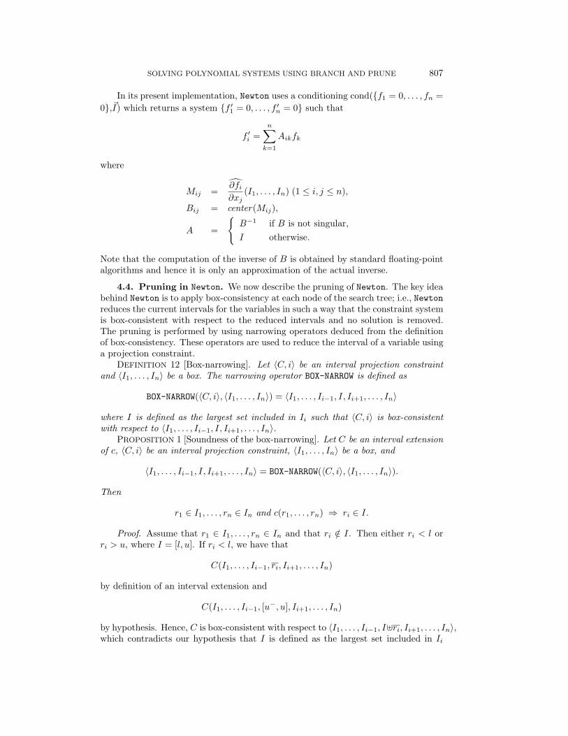
4.4. Pruning in Newton. We now describe the pruning of Newton. The key ideabehind Newton is to apply box-consistency at each node of the search tree; i.e., Newtonreduces the current intervals for the variables in such a way that the constraint systemis box-consistent with respect to the reduced intervals and no solution is removed.The pruning is performed by using narrowing operators deduced from the definitionof box-consistency. These operators are used to reduce the interval of a variable usinga projection constraint.

DEFINITION 12 [Box-narrowing]. Let 〈C, i〉 be an interval projection constraintand 〈I1, . . . , In〉 be a box. The narrowing operator BOX-NARROW is defined as

BOX-NARROW(〈C, i〉, 〈I1, . . . , In〉) = 〈I1, . . . , Ii−1, I, Ii+1, . . . , In〉

where I is defined as the largest set included in Ii such that 〈C, i〉 is box-consistentwith respect to 〈I1, . . . , Ii−1, I, Ii+1, . . . , In〉.

PROPOSITION 1 [Soundness of the box-narrowing]. Let C be an interval extensionof c, 〈C, i〉 be an interval projection constraint, 〈I1, . . . , In〉 be a box, and

〈I1, . . . , Ii−1, I, Ii+1, . . . , In〉 = BOX-NARROW(〈C, i〉, 〈I1, . . . , In〉).

Then

r1 ∈ I1, . . . , rn ∈ In and c(r1, . . . , rn) ⇒ ri ∈ I.

Proof. Assume that r1 ∈ I1, . . . , rn ∈ In and that ri /∈ I. Then either ri < l orri > u, where I = [l, u]. If ri < l, we have that

C(I1, . . . , Ii−1, ri, Ii+1, . . . , In)

by definition of an interval extension and

C(I1, . . . , Ii−1, [u−, u], Ii+1, . . . , In)

by hypothesis. Hence, C is box-consistent with respect to 〈I1, . . . , Ii−1, I]ri, Ii+1, . . . , In〉,which contradicts our hypothesis that I is defined as the largest set included in Ii


procedure PRUNE(in S: Set of Constraint; inout ~I : In)begin

repeat~Ip := ~I;

BOX-PRUNE({〈c, i〉 | c ∈ S and 1 ≤ i ≤ n} ∪ {〈c, i〉 | c ∈ S and 1 ≤ i ≤ n},~I);BOX-PRUNE({〈ct(~I), i〉 | c ∈ cond(S, ~I) and 1 ≤ i ≤ n},~I);

until ~I = ~Ip;end

procedure BOX-PRUNE(in P: Set of Interval Projection Constraint; inout ~I : In)begin

repeat~Ip := ~I;~I :=

⋂{BOX-NARROW(P, ~I) | P ∈ P }

until ~I = ~Ip;end

FIG. 1. Pruning in Newton.

such that 〈C, i〉 is box-consistent with respect to 〈I1, . . . , Ii−1, I, Ii+1, . . . , In〉. Thecase ri > u is similar.

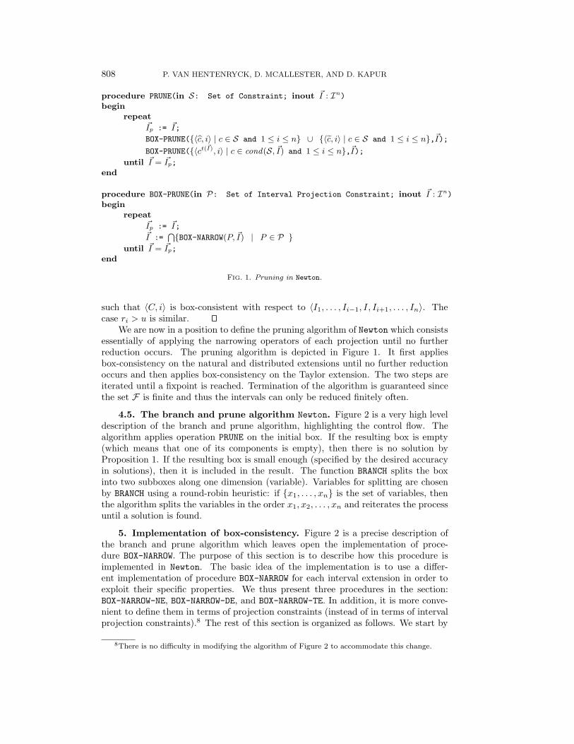
We are now in a position to define the pruning algorithm of Newton which consistsessentially of applying the narrowing operators of each projection until no furtherreduction occurs. The pruning algorithm is depicted in Figure 1. It first appliesbox-consistency on the natural and distributed extensions until no further reductionoccurs and then applies box-consistency on the Taylor extension. The two steps areiterated until a fixpoint is reached. Termination of the algorithm is guaranteed sincethe set F is finite and thus the intervals can only be reduced finitely often.

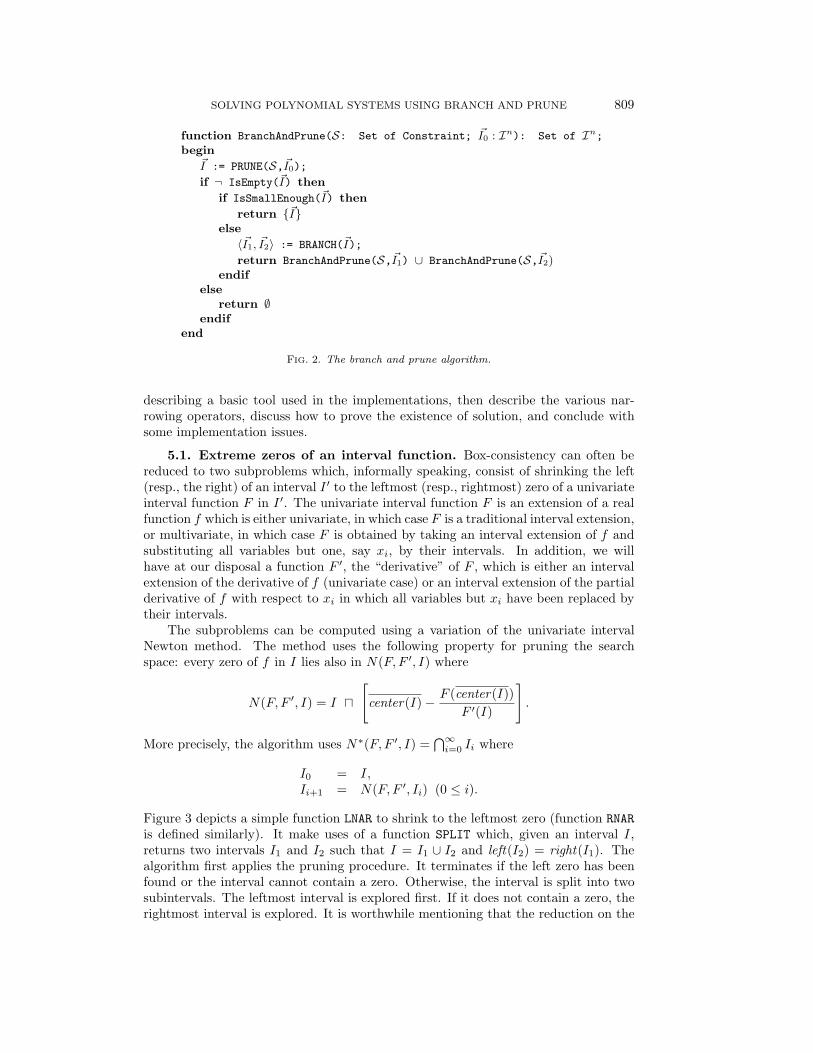
4.5. The branch and prune algorithm Newton. Figure 2 is a very high leveldescription of the branch and prune algorithm, highlighting the control flow. Thealgorithm applies operation PRUNE on the initial box. If the resulting box is empty(which means that one of its components is empty), then there is no solution byProposition 1. If the resulting box is small enough (specified by the desired accuracyin solutions), then it is included in the result. The function BRANCH splits the boxinto two subboxes along one dimension (variable). Variables for splitting are chosenby BRANCH using a round-robin heuristic: if {x1, . . . , xn} is the set of variables, thenthe algorithm splits the variables in the order x1, x2, . . . , xn and reiterates the processuntil a solution is found.

5. Implementation of box-consistency. Figure 2 is a precise description ofthe branch and prune algorithm which leaves open the implementation of proce-dure BOX-NARROW. The purpose of this section is to describe how this procedure isimplemented in Newton. The basic idea of the implementation is to use a differ-ent implementation of procedure BOX-NARROW for each interval extension in order toexploit their specific properties. We thus present three procedures in the section:BOX-NARROW-NE, BOX-NARROW-DE, and BOX-NARROW-TE. In addition, it is more conve-nient to define them in terms of projection constraints (instead of in terms of intervalprojection constraints).8 The rest of this section is organized as follows. We start by

8There is no difficulty in modifying the algorithm of Figure 2 to accommodate this change.


function BranchAndPrune(S: Set of Constraint; ~I0 : In): Set of In;begin

~I := PRUNE(S,~I0);if ¬ IsEmpty(~I) then

if IsSmallEnough(~I) thenreturn {~I}

else〈~I1, ~I2〉 := BRANCH(~I);

return BranchAndPrune(S,~I1) ∪ BranchAndPrune(S,~I2)endif

elsereturn ∅

endifend

FIG. 2. The branch and prune algorithm.

describing a basic tool used in the implementations, then describe the various nar-rowing operators, discuss how to prove the existence of solution, and conclude withsome implementation issues.

5.1. Extreme zeros of an interval function. Box-consistency can often bereduced to two subproblems which, informally speaking, consist of shrinking the left(resp., the right) of an interval I ′ to the leftmost (resp., rightmost) zero of a univariateinterval function F in I ′. The univariate interval function F is an extension of a realfunction f which is either univariate, in which case F is a traditional interval extension,or multivariate, in which case F is obtained by taking an interval extension of f andsubstituting all variables but one, say xi, by their intervals. In addition, we willhave at our disposal a function F ′, the “derivative” of F , which is either an intervalextension of the derivative of f (univariate case) or an interval extension of the partialderivative of f with respect to xi in which all variables but xi have been replaced bytheir intervals.

The subproblems can be computed using a variation of the univariate intervalNewton method. The method uses the following property for pruning the searchspace: every zero of f in I lies also in N(F, F ′, I) where

N(F, F ′, I) = I u[

center(I)− F (center(I))F ′(I)

].

More precisely, the algorithm uses N∗(F, F ′, I) =⋂∞i=0 Ii where

I0 = I,Ii+1 = N(F, F ′, Ii) (0 ≤ i).

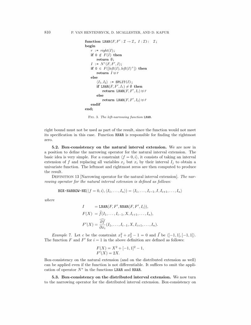
Figure 3 depicts a simple function LNAR to shrink to the leftmost zero (function RNARis defined similarly). It make uses of a function SPLIT which, given an interval I,returns two intervals I1 and I2 such that I = I1 ∪ I2 and left(I2) = right(I1). Thealgorithm first applies the pruning procedure. It terminates if the left zero has beenfound or the interval cannot contain a zero. Otherwise, the interval is split into twosubintervals. The leftmost interval is explored first. If it does not contain a zero, therightmost interval is explored. It is worthwhile mentioning that the reduction on the


function LNAR(F, F ′ : I → I, I : I): I;begin

r := right(I);if 0 /∈ F (I) then

return ∅;I := N∗(F, F ′, I);if 0 ∈ F ([left(I), left(I)+]) then

return I ] relse〈I1, I2〉 := SPLIT(I);if LNAR(F, F ′, I1) 6= ∅ then

return LNAR(F, F ′, I1) ] relse

return LNAR(F, F ′, I2) ] rendif

end;

FIG. 3. The left-narrowing function LNAR.

right bound must not be used as part of the result, since the function would not meetits specification in this case. Function RNAR is responsible for finding the rightmostzero.

5.2. Box-consistency on the natural interval extension. We are now ina position to define the narrowing operator for the natural interval extension. Thebasic idea is very simple. For a constraint 〈f = 0, i〉, it consists of taking an intervalextension of f and replacing all variables xj but xi by their interval Ij to obtain aunivariate function. The leftmost and rightmost zeros are then computed to producethe result.

DEFINITION 13 [Narrowing operator for the natural interval extension]. The nar-rowing operator for the natural interval extension is defined as follows:

BOX-NARROW-NE(〈f = 0, i〉, 〈I1, . . . , In〉) = 〈I1, . . . , Ii−1, I, Ii+1, . . . , In〉

where

I = LNAR(F, F ′, RNAR(F, F ′, Ii)),

F (X) = f(I1, . . . , Ii−1, X, Ii+1, . . . , In),

F ′(X) =∂f

∂xi(I1, . . . , Ii−1, X, Ii+1, . . . , In).

Example 7. Let c be the constraint x21 + x2

2 − 1 = 0 and ~I be 〈[−1, 1], [−1, 1]〉.The function F and F ′ for i = 1 in the above definition are defined as follows:

F (X) = X2 + [−1, 1]2 − 1,F ′(X) = 2X.

Box-consistency on the natural extension (and on the distributed extension as well)can be applied even if the function is not differentiable. It suffices to omit the appli-cation of operator N∗ in the functions LNAR and RNAR.

5.3. Box-consistency on the distributed interval extension. We now turnto the narrowing operator for the distributed interval extension. Box-consistency on


the distributed interval extension can be enforced by using the univariate intervalfunction

F (X) = f(I1, . . . , Ii−1, X, Ii+1, . . . , In)

and by searching its extreme zeros. However, since the function is in distributed form,it is possible to do better by using an idea from [11]. The key insight is to sandwichF exactly between two univariate real functions fl and fu defined as follows:

fl(x) = left(F (x)),fu(x) = right(F (x)).

Note that box-consistency can now be enforced by searching the leftmost and right-most zeros of some interval extensions, say Fl and Fu, of fl and fu using intervalextensions, say F ′l and F ′u, of their derivatives f ′l and f ′u. Of course, LNAR and RNARcan be used to find these extreme zeros.

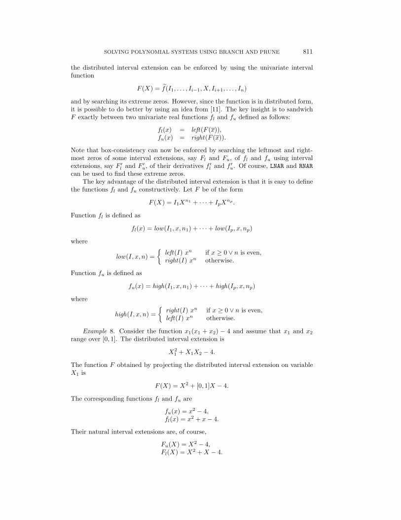
The key advantage of the distributed interval extension is that it is easy to definethe functions fl and fu constructively. Let F be of the form

F (X) = I1Xn1 + · · ·+ IpX

np .

Function fl is defined as

fl(x) = low(I1, x, n1) + · · ·+ low(Ip, x, np)

where

low(I, x, n) ={

left(I) xn if x ≥ 0 ∨ n is even,right(I) xn otherwise.

Function fu is defined as

fu(x) = high(I1, x, n1) + · · ·+ high(Ip, x, np)

where

high(I, x, n) ={

right(I) xn if x ≥ 0 ∨ n is even,left(I) xn otherwise.

Example 8. Consider the function x1(x1 + x2) − 4 and assume that x1 and x2range over [0, 1]. The distributed interval extension is

X21 +X1X2 − 4.

The function F obtained by projecting the distributed interval extension on variableX1 is

F (X) = X2 + [0, 1]X − 4.

The corresponding functions fl and fu are

fu(x) = x2 − 4,fl(x) = x2 + x− 4.

Their natural interval extensions are, of course,

Fu(X) = X2 − 4,Fl(X) = X2 +X − 4.


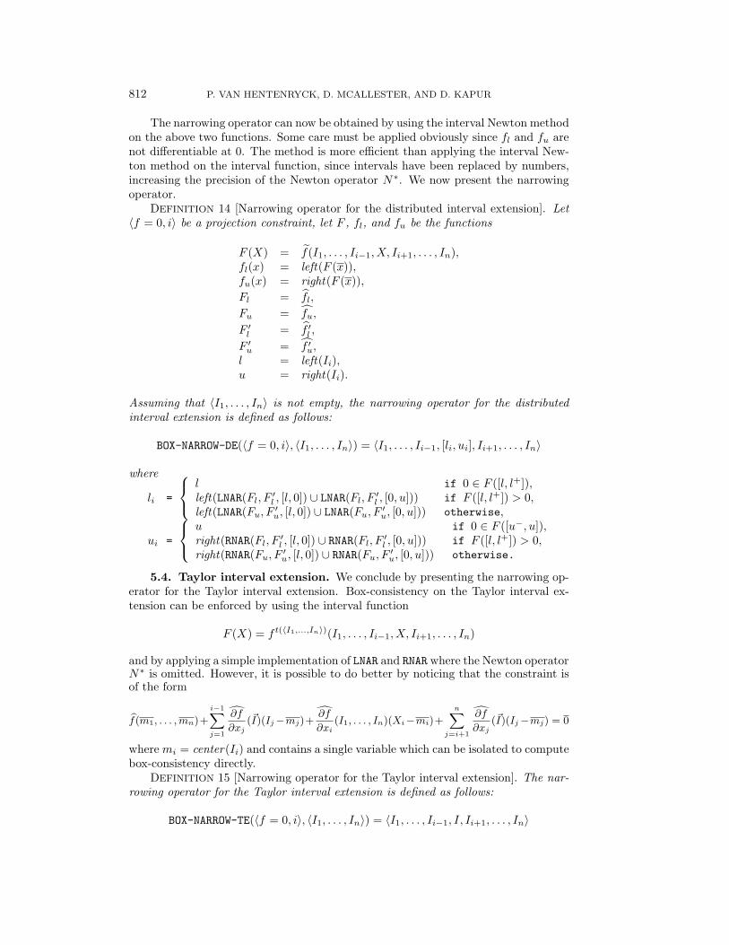
The narrowing operator can now be obtained by using the interval Newton methodon the above two functions. Some care must be applied obviously since fl and fu arenot differentiable at 0. The method is more efficient than applying the interval New-ton method on the interval function, since intervals have been replaced by numbers,increasing the precision of the Newton operator N∗. We now present the narrowingoperator.

DEFINITION 14 [Narrowing operator for the distributed interval extension]. Let〈f = 0, i〉 be a projection constraint, let F , fl, and fu be the functions

F (X) = f(I1, . . . , Ii−1, X, Ii+1, . . . , In),fl(x) = left(F (x)),fu(x) = right(F (x)),Fl = fl,

Fu = fu,

F ′l = f ′l ,

F ′u = f ′u,l = left(Ii),u = right(Ii).

Assuming that 〈I1, . . . , In〉 is not empty, the narrowing operator for the distributedinterval extension is defined as follows:

BOX-NARROW-DE(〈f = 0, i〉, 〈I1, . . . , In〉) = 〈I1, . . . , Ii−1, [li, ui], Ii+1, . . . , In〉

where

li =

l if 0 ∈ F ([l, l+]),left(LNAR(Fl, F ′l , [l, 0]) ∪ LNAR(Fl, F ′l , [0, u])) if F ([l, l+]) > 0,left(LNAR(Fu, F ′u, [l, 0]) ∪ LNAR(Fu, F ′u, [0, u])) otherwise,

ui =

u if 0 ∈ F ([u−, u]),right(RNAR(Fl, F ′l , [l, 0]) ∪ RNAR(Fl, F ′l , [0, u])) if F ([l, l+]) > 0,right(RNAR(Fu, F ′u, [l, 0]) ∪ RNAR(Fu, F ′u, [0, u])) otherwise.

5.4. Taylor interval extension. We conclude by presenting the narrowing op-erator for the Taylor interval extension. Box-consistency on the Taylor interval ex-tension can be enforced by using the interval function

F (X) = f t(〈I1,...,In〉)(I1, . . . , Ii−1, X, Ii+1, . . . , In)

and by applying a simple implementation of LNAR and RNAR where the Newton operatorN∗ is omitted. However, it is possible to do better by noticing that the constraint isof the form

f(m1, . . . ,mn)+i−1∑j=1

∂f

∂xj(~I)(Ij−mj)+

∂f

∂xi(I1, . . . , In)(Xi−mi)+

n∑j=i+1

∂f

∂xj(~I)(Ij−mj) = 0

where mi = center(Ii) and contains a single variable which can be isolated to computebox-consistency directly.

DEFINITION 15 [Narrowing operator for the Taylor interval extension]. The nar-rowing operator for the Taylor interval extension is defined as follows:

BOX-NARROW-TE(〈f = 0, i〉, 〈I1, . . . , In〉) = 〈I1, . . . , Ii−1, I, Ii+1, . . . , In〉


where

I = Iiu

mi −1

∂f∂xi

(I1, . . . , In)

n∑j=1,j 6=i

∂f

∂xj(I1, . . . , In) (Ij −mj) + f(m1, . . . ,mn)

and mi = center(Ii).

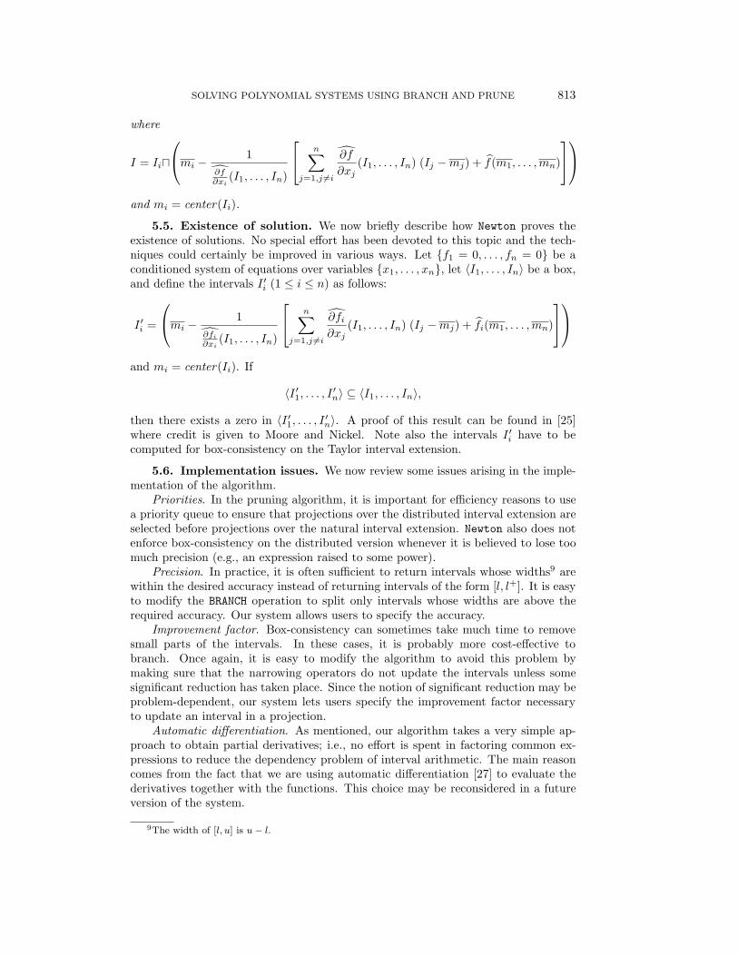
5.5. Existence of solution. We now briefly describe how Newton proves theexistence of solutions. No special effort has been devoted to this topic and the tech-niques could certainly be improved in various ways. Let {f1 = 0, . . . , fn = 0} be aconditioned system of equations over variables {x1, . . . , xn}, let 〈I1, . . . , In〉 be a box,and define the intervals I ′i (1 ≤ i ≤ n) as follows:

I ′i =

mi −1

∂fi∂xi

(I1, . . . , In)

n∑j=1,j 6=i

∂fi∂xj

(I1, . . . , In) (Ij −mj) + fi(m1, . . . ,mn)

and mi = center(Ii). If

〈I ′1, . . . , I ′n〉 ⊆ 〈I1, . . . , In〉,

then there exists a zero in 〈I ′1, . . . , I ′n〉. A proof of this result can be found in [25]where credit is given to Moore and Nickel. Note also the intervals I ′i have to becomputed for box-consistency on the Taylor interval extension.

5.6. Implementation issues. We now review some issues arising in the imple-mentation of the algorithm.

Priorities. In the pruning algorithm, it is important for efficiency reasons to usea priority queue to ensure that projections over the distributed interval extension areselected before projections over the natural interval extension. Newton also does notenforce box-consistency on the distributed version whenever it is believed to lose toomuch precision (e.g., an expression raised to some power).

Precision. In practice, it is often sufficient to return intervals whose widths9 arewithin the desired accuracy instead of returning intervals of the form [l, l+]. It is easyto modify the BRANCH operation to split only intervals whose widths are above therequired accuracy. Our system allows users to specify the accuracy.

Improvement factor. Box-consistency can sometimes take much time to removesmall parts of the intervals. In these cases, it is probably more cost-effective tobranch. Once again, it is easy to modify the algorithm to avoid this problem bymaking sure that the narrowing operators do not update the intervals unless somesignificant reduction has taken place. Since the notion of significant reduction may beproblem-dependent, our system lets users specify the improvement factor necessaryto update an interval in a projection.

Automatic differentiation. As mentioned, our algorithm takes a very simple ap-proach to obtain partial derivatives; i.e., no effort is spent in factoring common ex-pressions to reduce the dependency problem of interval arithmetic. The main reasoncomes from the fact that we are using automatic differentiation [27] to evaluate thederivatives together with the functions. This choice may be reconsidered in a futureversion of the system.

9The width of [l, u] is u− l.


Inequalities. It is straightforward to generalize the above algorithms for inequal-ities. In general, it suffices to test if the inequality is satisfied at the end points ofthe interval. If it is not, then the problem reduces once again to finding the leftmostand/or rightmost zeros.

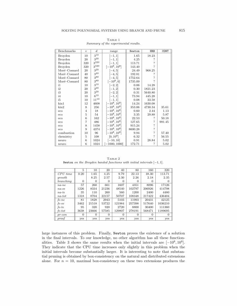
6. Experimental results. This section reports experimental results of Newtonon a variety of standard benchmarks. The benchmarks were taken from paperson numerical analysis [22], interval analysis [8, 11, 21], and continuation methods[35, 24, 23, 17]. We also compare Newton with a traditional interval method us-ing the Hansen–Sengupta operator, range testing, and branching. This method usesthe same implementation technology as Newton and is denoted by HRB in the fol-lowing.10 Finally, we compare Newton with a state-of-the-art continuation method[35], denoted by CONT in the following. Note that all results given in this sec-tion were obtained by running Newton on a Sun Sparc 10 workstation to obtainall solutions. In addition, the final intervals must have widths smaller than 10−8

and Newton always uses an improvement factor of 10%. The results are summa-rized in Table 1. For each benchmark, we give the number of variables (n), thetotal degree of the system (d), the initial range for the variables, and the resultsof each method in seconds. Note that the times for the continuation method areon a DEC 5000/200. A space in a column means that the result is not availablefor the method. A question mark means that the method does not terminate ina reasonable time (greater than one hour). The rest of the section describes eachbenchmark and the results in much more detail. For each benchmark, we report theCPU times in seconds, the growth of the CPU time, the number of branch operationsbranching, the number of narrowings on the various extensions na-ne, na-ee, na-te,the total number of narrowings na-tot, the number of function evaluations (includ-ing evaluation of derivatives which are counted as normal function evaluations) foreach of the extensions fe-ne, fe-ee, fe-te, and the total number of function evalua-tions fe-tot. We also indicate the number of preconditionings by pr-con and whetherthe algorithm can prove the existence of the solutions in the resulting intervals byproof.

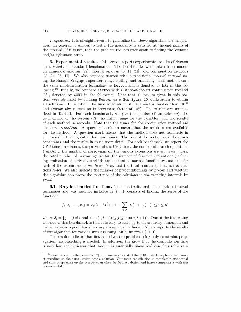
6.1. Broyden banded functions. This is a traditional benchmark of intervaltechniques and was used for instance in [7]. It consists of finding the zeros of thefunctions

fi(x1, . . . , xn) = xi(2 + 5x2i ) + 1−

∑j∈Ji

xj(1 + xj) (1 ≤ i ≤ n)

where Ji = {j | j 6= i and max(1, i− 5) ≤ j ≤ min(n, i+ 1)}. One of the interestingfeatures of this benchmark is that it is easy to scale up to an arbitrary dimension andhence provides a good basis to compare various methods. Table 2 reports the resultsof our algorithm for various sizes assuming initial intervals [−1, 1].

The results indicate that Newton solves the problem using only constraint prop-agation: no branching is needed. In addition, the growth of the computation timeis very low and indicates that Newton is essentially linear and can thus solve very

10Some interval methods such as [7] are more sophisticated than HRB, but the sophistication aimsat speeding up the computation near a solution. Our main contribution is completely orthogonaland aims at speeding up the computation when far from a solution and hence comparing it with HRBis meaningful.


TABLE 1Summary of the experimental results.

Benchmarks v d range Newton HRB CONT

Broyden 10 310 [−1, 1] 1.65 18.23Broyden 20 320 [−1, 1] 4.25 ?Broyden 320 3320 [−1, 1] 113.71 ?Broyden 320 3320 [−108, 108] 143.40 ?More–Cosnard 20 320 [−4, 5] 24.49 968.25More–Cosnard 40 340 [−4, 5] 192.81 ?More–Cosnard 80 380 [−4, 5] 1752.64 ?More–Cosnard 80 380 [−108, 0] 1735.09 ?i1 10 310 [−2, 2] 0.06 14.28i2 20 320 [−1, 2] 0.30 1821.23i3 20 320 [−2, 2] 0.31 5640.80i4 10 610 [−1, 1] 73.94 445.28i5 10 1110 [−1, 1] 0.08 33.58kin1 12 4608 [−108, 108] 14.24 1630.08kin2 8 256 [−108, 108] 353.06 4730.34 35.61eco 4 18 [−108, 108] 0.60 2.44 1.13eco 5 54 [−108, 108] 3.35 29.88 5.87eco 6 162 [−108, 108] 22.53 ? 50.18eco 7 486 [−108, 108] 127.65 ? 991.45eco 8 1458 [−108, 108] 915.24 ?eco 9 4374 [−108, 108] 8600.28 ?combustion 10 96 [−108, 108] 9.94 ? 57.40chemistry 5 108 [0, 108] 6.32 ? 56.55neuro 6 1024 [−10, 10] 0.91 28.84 5.02neuro 6 1024 [−1000, 1000] 172.71 ? 5.02

TABLE 2Newton on the Broyden banded functions with initial intervals [−1, 1].

5 10 20 40 80 160 320CPU time 0.20 1.65 4.25 9.79 22.13 48.30 113.71growth 8.25 2.57 2.30 2.26 2.18 2.35branching 0 0 0 0 0 0 0na-ne 57 260 661 1607 4351 8096 17126na-ee 1226 8334 21236 48540 102797 206926 414798na-te 35 110 260 560 1200 2400 4480na-tot 1318 8704 22157 50707 108348 217422 436404fe-ne 81 1828 2943 5103 11993 20431 42125fe-ee 3462 21518 53722 121984 257398 517640 1036210fe-te 95 320 920 2720 8800 30400 111360fe-tot 3638 23666 57585 129807 278191 568471 1189695pr-con 0 0 0 0 0 0 0proof yes yes yes yes yes yes yes

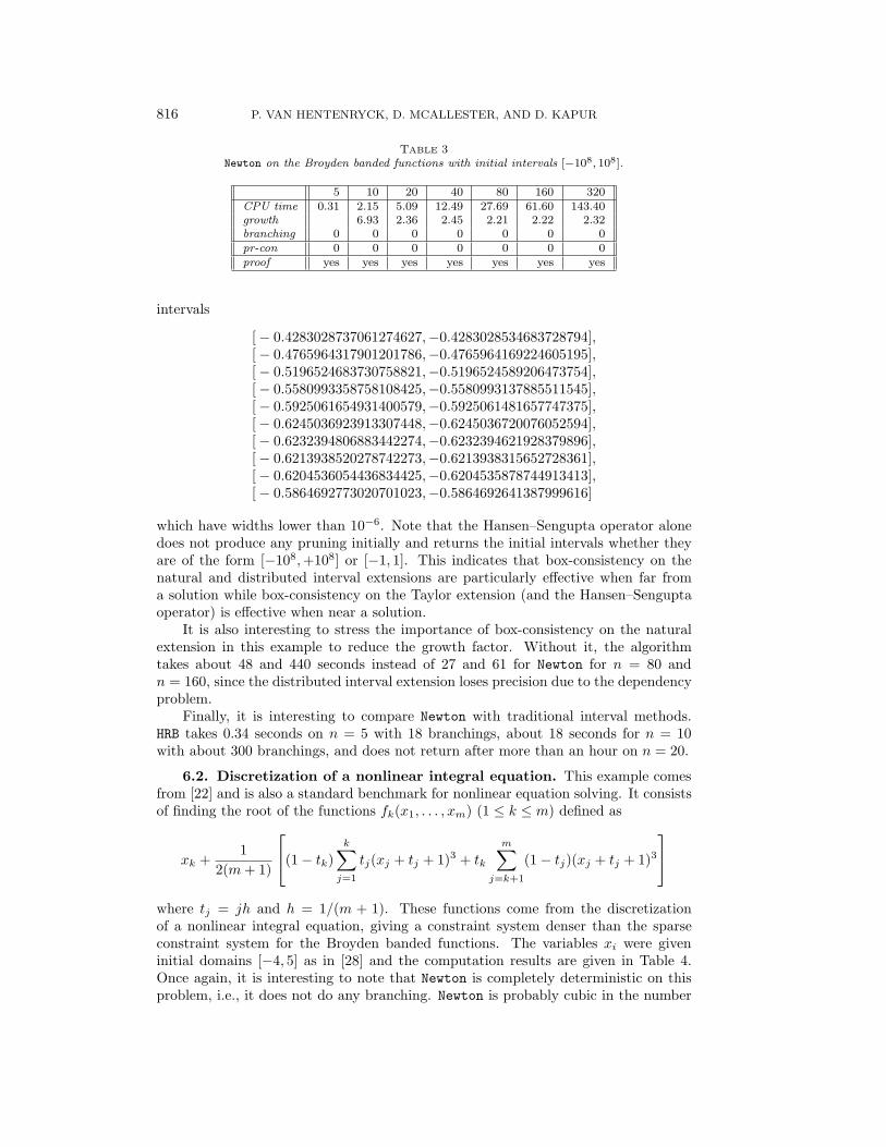
large instances of this problem. Finally, Newton proves the existence of a solutionin the final intervals. To our knowledge, no other algorithm has all these function-alities. Table 3 shows the same results when the initial intervals are [−108, 108].They indicate that the CPU time increases only slightly in this problem when theinitial intervals become substantially larger. It is interesting to note that substan-tial pruning is obtained by box-consistency on the natural and distributed extensionsalone. For n = 10, maximal box-consistency on these two extensions produces the


TABLE 3Newton on the Broyden banded functions with initial intervals [−108, 108].

5 10 20 40 80 160 320CPU time 0.31 2.15 5.09 12.49 27.69 61.60 143.40growth 6.93 2.36 2.45 2.21 2.22 2.32branching 0 0 0 0 0 0 0pr-con 0 0 0 0 0 0 0proof yes yes yes yes yes yes yes

intervals

[− 0.4283028737061274627,−0.4283028534683728794],[− 0.4765964317901201786,−0.4765964169224605195],[− 0.5196524683730758821,−0.5196524589206473754],[− 0.5580993358758108425,−0.5580993137885511545],[− 0.5925061654931400579,−0.5925061481657747375],[− 0.6245036923913307448,−0.6245036720076052594],[− 0.6232394806883442274,−0.6232394621928379896],[− 0.6213938520278742273,−0.6213938315652728361],[− 0.6204536054436834425,−0.6204535878744913413],[− 0.5864692773020701023,−0.5864692641387999616]

which have widths lower than 10−6. Note that the Hansen–Sengupta operator alonedoes not produce any pruning initially and returns the initial intervals whether theyare of the form [−108,+108] or [−1, 1]. This indicates that box-consistency on thenatural and distributed interval extensions are particularly effective when far froma solution while box-consistency on the Taylor extension (and the Hansen–Senguptaoperator) is effective when near a solution.

It is also interesting to stress the importance of box-consistency on the naturalextension in this example to reduce the growth factor. Without it, the algorithmtakes about 48 and 440 seconds instead of 27 and 61 for Newton for n = 80 andn = 160, since the distributed interval extension loses precision due to the dependencyproblem.

Finally, it is interesting to compare Newton with traditional interval methods.HRB takes 0.34 seconds on n = 5 with 18 branchings, about 18 seconds for n = 10with about 300 branchings, and does not return after more than an hour on n = 20.

6.2. Discretization of a nonlinear integral equation. This example comesfrom [22] and is also a standard benchmark for nonlinear equation solving. It consistsof finding the root of the functions fk(x1, . . . , xm) (1 ≤ k ≤ m) defined as

xk +1

2(m+ 1)

(1− tk)k∑j=1

tj(xj + tj + 1)3 + tk

m∑j=k+1

(1− tj)(xj + tj + 1)3

where tj = jh and h = 1/(m + 1). These functions come from the discretizationof a nonlinear integral equation, giving a constraint system denser than the sparseconstraint system for the Broyden banded functions. The variables xi were giveninitial domains [−4, 5] as in [28] and the computation results are given in Table 4.Once again, it is interesting to note that Newton is completely deterministic on thisproblem, i.e., it does not do any branching. Newton is probably cubic in the number


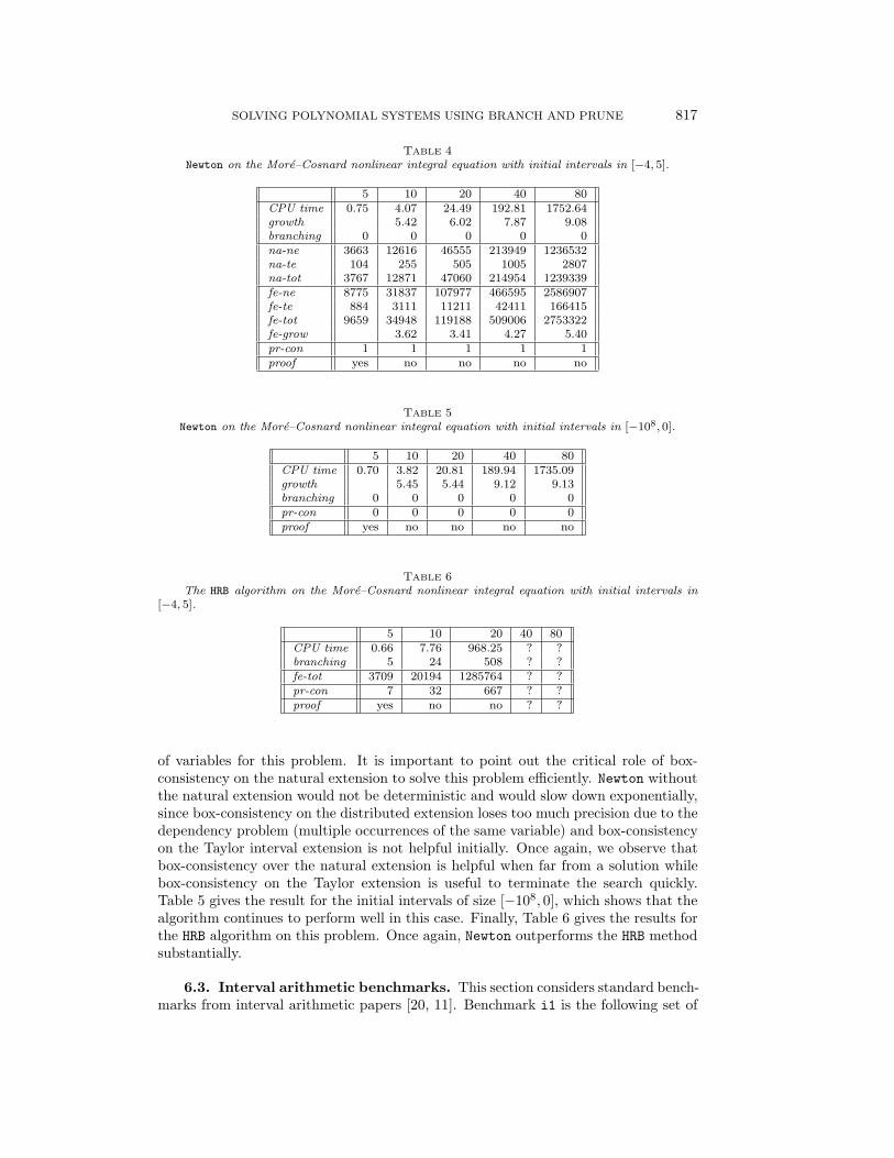
TABLE 4Newton on the More–Cosnard nonlinear integral equation with initial intervals in [−4, 5].

5 10 20 40 80CPU time 0.75 4.07 24.49 192.81 1752.64growth 5.42 6.02 7.87 9.08branching 0 0 0 0 0na-ne 3663 12616 46555 213949 1236532na-te 104 255 505 1005 2807na-tot 3767 12871 47060 214954 1239339fe-ne 8775 31837 107977 466595 2586907fe-te 884 3111 11211 42411 166415fe-tot 9659 34948 119188 509006 2753322fe-grow 3.62 3.41 4.27 5.40pr-con 1 1 1 1 1proof yes no no no no

TABLE 5Newton on the More–Cosnard nonlinear integral equation with initial intervals in [−108, 0].

5 10 20 40 80CPU time 0.70 3.82 20.81 189.94 1735.09growth 5.45 5.44 9.12 9.13branching 0 0 0 0 0pr-con 0 0 0 0 0proof yes no no no no

TABLE 6The HRB algorithm on the More–Cosnard nonlinear integral equation with initial intervals in

[−4, 5].

5 10 20 40 80CPU time 0.66 7.76 968.25 ? ?branching 5 24 508 ? ?fe-tot 3709 20194 1285764 ? ?pr-con 7 32 667 ? ?proof yes no no ? ?

of variables for this problem. It is important to point out the critical role of box-consistency on the natural extension to solve this problem efficiently. Newton withoutthe natural extension would not be deterministic and would slow down exponentially,since box-consistency on the distributed extension loses too much precision due to thedependency problem (multiple occurrences of the same variable) and box-consistencyon the Taylor interval extension is not helpful initially. Once again, we observe thatbox-consistency over the natural extension is helpful when far from a solution whilebox-consistency on the Taylor extension is useful to terminate the search quickly.Table 5 gives the result for the initial intervals of size [−108, 0], which shows that thealgorithm continues to perform well in this case. Finally, Table 6 gives the results forthe HRB algorithm on this problem. Once again, Newton outperforms the HRB methodsubstantially.

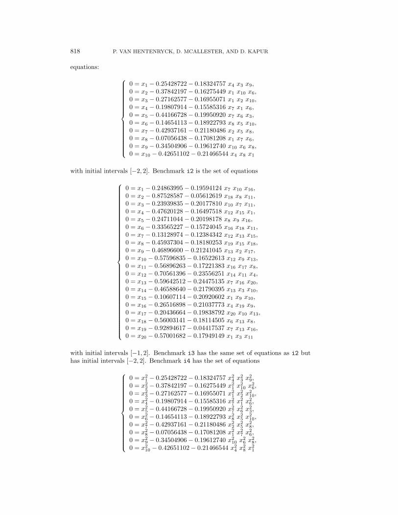
6.3. Interval arithmetic benchmarks. This section considers standard bench-marks from interval arithmetic papers [20, 11]. Benchmark i1 is the following set of


equations:

0 = x1 − 0.25428722− 0.18324757 x4 x3 x9,0 = x2 − 0.37842197− 0.16275449 x1 x10 x6,0 = x3 − 0.27162577− 0.16955071 x1 x2 x10,0 = x4 − 0.19807914− 0.15585316 x7 x1 x6,0 = x5 − 0.44166728− 0.19950920 x7 x6 x3,0 = x6 − 0.14654113− 0.18922793 x8 x5 x10,0 = x7 − 0.42937161− 0.21180486 x2 x5 x8,0 = x8 − 0.07056438− 0.17081208 x1 x7 x6,0 = x9 − 0.34504906− 0.19612740 x10 x6 x8,0 = x10 − 0.42651102− 0.21466544 x4 x8 x1

with initial intervals [−2, 2]. Benchmark i2 is the set of equations

0 = x1 − 0.24863995− 0.19594124 x7 x10 x16,0 = x2 − 0.87528587− 0.05612619 x18 x8 x11,0 = x3 − 0.23939835− 0.20177810 x10 x7 x11,0 = x4 − 0.47620128− 0.16497518 x12 x15 x1,0 = x5 − 0.24711044− 0.20198178 x8 x9 x16,0 = x6 − 0.33565227− 0.15724045 x16 x18 x11,0 = x7 − 0.13128974− 0.12384342 x12 x13 x15,0 = x8 − 0.45937304− 0.18180253 x19 x15 x18,0 = x9 − 0.46896600− 0.21241045 x13 x2 x17,0 = x10 − 0.57596835− 0.16522613 x12 x9 x13,0 = x11 − 0.56896263− 0.17221383 x16 x17 x8,0 = x12 − 0.70561396− 0.23556251 x14 x11 x4,0 = x13 − 0.59642512− 0.24475135 x7 x16 x20,0 = x14 − 0.46588640− 0.21790395 x13 x3 x10,0 = x15 − 0.10607114− 0.20920602 x1 x9 x10,0 = x16 − 0.26516898− 0.21037773 x4 x19 x9,0 = x17 − 0.20436664− 0.19838792 x20 x10 x13,0 = x18 − 0.56003141− 0.18114505 x6 x13 x8,0 = x19 − 0.92894617− 0.04417537 x7 x13 x16,0 = x20 − 0.57001682− 0.17949149 x1 x3 x11

with initial intervals [−1, 2]. Benchmark i3 has the same set of equations as i2 buthas initial intervals [−2, 2]. Benchmark i4 has the set of equations

0 = x21 − 0.25428722− 0.18324757 x2

4 x23 x

29,

0 = x22 − 0.37842197− 0.16275449 x2

1 x210 x

26,

0 = x23 − 0.27162577− 0.16955071 x2

1 x22 x

210,

0 = x24 − 0.19807914− 0.15585316 x2

7 x21 x

26,

0 = x25 − 0.44166728− 0.19950920 x2

7 x26 x

23,

0 = x26 − 0.14654113− 0.18922793 x2

8 x25 x

210,

0 = x27 − 0.42937161− 0.21180486 x2

2 x25 x

28,

0 = x28 − 0.07056438− 0.17081208 x2

1 x27 x

26,

0 = x29 − 0.34504906− 0.19612740 x2

10 x26 x

28,

0 = x210 − 0.42651102− 0.21466544 x2

4 x28 x

21


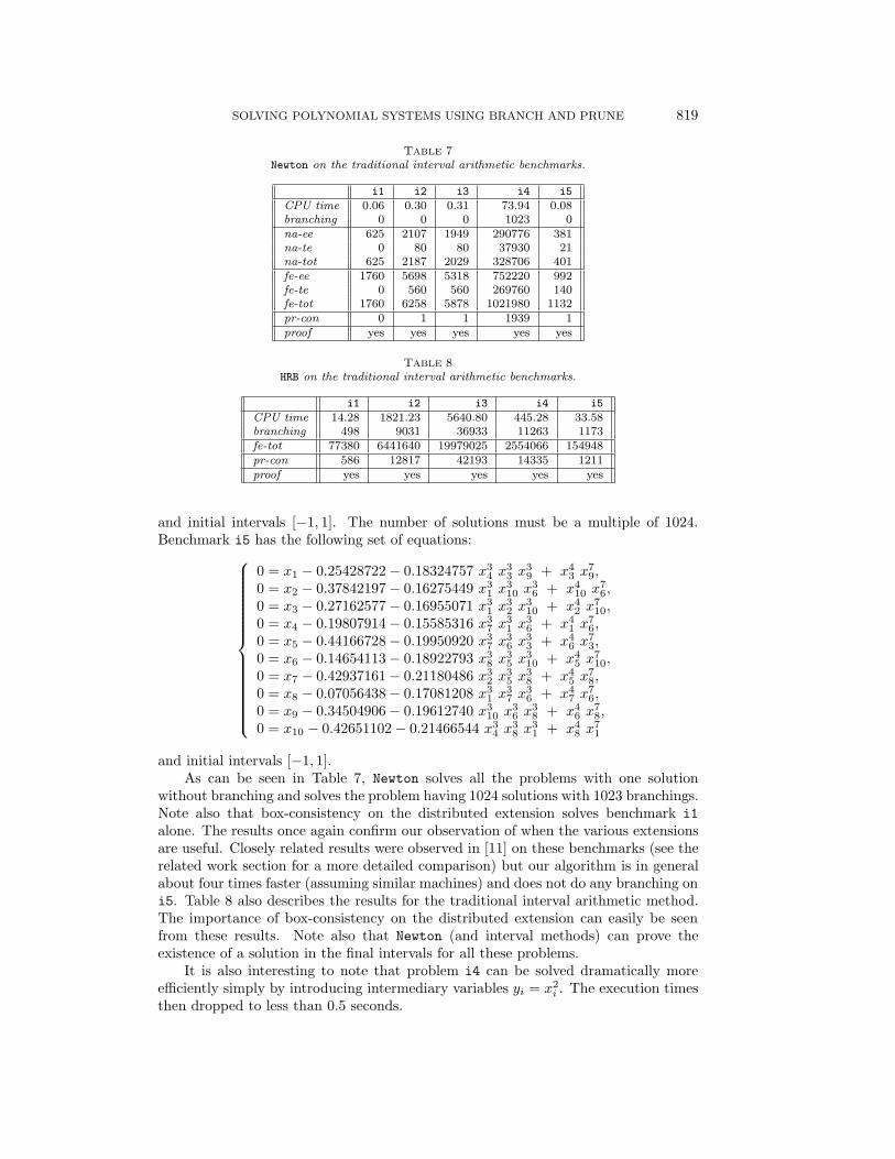
TABLE 7Newton on the traditional interval arithmetic benchmarks.

i1 i2 i3 i4 i5CPU time 0.06 0.30 0.31 73.94 0.08branching 0 0 0 1023 0na-ee 625 2107 1949 290776 381na-te 0 80 80 37930 21na-tot 625 2187 2029 328706 401fe-ee 1760 5698 5318 752220 992fe-te 0 560 560 269760 140fe-tot 1760 6258 5878 1021980 1132pr-con 0 1 1 1939 1proof yes yes yes yes yes

TABLE 8HRB on the traditional interval arithmetic benchmarks.

i1 i2 i3 i4 i5CPU time 14.28 1821.23 5640.80 445.28 33.58branching 498 9031 36933 11263 1173fe-tot 77380 6441640 19979025 2554066 154948pr-con 586 12817 42193 14335 1211proof yes yes yes yes yes

and initial intervals [−1, 1]. The number of solutions must be a multiple of 1024.Benchmark i5 has the following set of equations:

0 = x1 − 0.25428722− 0.18324757 x34 x

33 x

39 + x4

3 x79,

0 = x2 − 0.37842197− 0.16275449 x31 x

310 x

36 + x4

10 x76,

0 = x3 − 0.27162577− 0.16955071 x31 x

32 x

310 + x4

2 x710,

0 = x4 − 0.19807914− 0.15585316 x37 x

31 x

36 + x4

1 x76,

0 = x5 − 0.44166728− 0.19950920 x37 x

36 x

33 + x4

6 x73,

0 = x6 − 0.14654113− 0.18922793 x38 x

35 x

310 + x4

5 x710,

0 = x7 − 0.42937161− 0.21180486 x32 x

35 x

38 + x4

5 x78,

0 = x8 − 0.07056438− 0.17081208 x31 x

37 x

36 + x4

7 x76,

0 = x9 − 0.34504906− 0.19612740 x310 x

36 x

38 + x4

6 x78,

0 = x10 − 0.42651102− 0.21466544 x34 x

38 x

31 + x4

8 x71

and initial intervals [−1, 1].As can be seen in Table 7, Newton solves all the problems with one solution

without branching and solves the problem having 1024 solutions with 1023 branchings.Note also that box-consistency on the distributed extension solves benchmark i1alone. The results once again confirm our observation of when the various extensionsare useful. Closely related results were observed in [11] on these benchmarks (see therelated work section for a more detailed comparison) but our algorithm is in generalabout four times faster (assuming similar machines) and does not do any branching oni5. Table 8 also describes the results for the traditional interval arithmetic method.The importance of box-consistency on the distributed extension can easily be seenfrom these results. Note also that Newton (and interval methods) can prove theexistence of a solution in the final intervals for all these problems.

It is also interesting to note that problem i4 can be solved dramatically moreefficiently simply by introducing intermediary variables yi = x2

i . The execution timesthen dropped to less than 0.5 seconds.


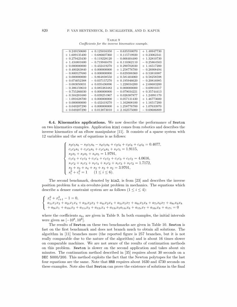
TABLE 9Coefficients for the inverse kinematics example.

− 0.249150680 + 0.125016350 − 0.635550070 + 1.48947730+ 1.609135400 − 0.686607360 − 0.115719920 + 0.23062341+ 0.279423430 − 0.119228120 − 0.666404480 + 1.32810730+ 1.434801600 − 0.719940470 + 0.110362110 − 0.25864503+ 0.000000000 − 0.432419270 + 0.290702030 + 1.16517200+ 0.400263840 + 0.000000000 + 1.258776700 − 0.26908494− 0.800527680 + 0.000000000 − 0.629388360 + 0.53816987+ 0.000000000 − 0.864838550 + 0.581404060 + 0.58258598+ 0.074052388 − 0.037157270 + 0.195946620 − 0.20816985− 0.083050031 + 0.035436896 − 1.228034200 + 2.68683200− 0.386159610 + 0.085383482 + 0.000000000 − 0.69910317− 0.755266030 + 0.000000000 − 0.079034221 + 0.35744413+ 0.504201680 − 0.039251967 + 0.026387877 + 1.24991170− 1.091628700 + 0.000000000 − 0.057131430 + 1.46773600+ 0.000000000 − 0.432419270 − 1.162808100 + 1.16517200+ 0.049207290 + 0.000000000 + 1.258776700 + 1.07633970+ 0.049207290 + 0.013873010 + 2.162575000 − 0.69686809

6.4. Kinematics applications. We now describe the performance of Newtonon two kinematics examples. Application kin1 comes from robotics and describes theinverse kinematics of an elbow manipulator [11]. It consists of a sparse system with12 variables and the set of equations is as follows:

s2c5s6 − s3c5s6 − s4c5s6 + c2c6 + c3c6 + c4c6 = 0.4077,c1c2s5 + c1c3s5 + c1c4s5 + s1c5 = 1.9115,s2s5 + s3s5 + s4s5 = 1.9791,c1c2 + c1c3 + c1c4 + c1c2 + c1c3 + c1c2 = 4.0616,s1c2 + s1c3 + s1c4 + s1c2 + s1c3 + s1c2 = 1.7172,s2 + s3 + s4 + s2 + s3 + s2 = 3.9701,s2i + c2i = 1 (1 ≤ i ≤ 6).

The second benchmark, denoted by kin2, is from [23] and describes the inverseposition problem for a six-revolute-joint problem in mechanics. The equations whichdescribe a denser constraint system are as follows (1 ≤ i ≤ 4): x2

i + x2i+1 − 1 = 0,

a1ix1x3 + a2ix1x4 + a3ix2x3 + a4ix2x4 + a5ix5x7 + a6ix5x8 + a7ix6x7 + a8ix6x8+ a9ix1 + a10ix2 + a11ix3 + a12ix4 + a13ix5a14ix6 + a15ix7 + a16ix8 + a17i = 0

where the coefficients aki are given in Table 9. In both examples, the initial intervalswere given as [−108, 108].

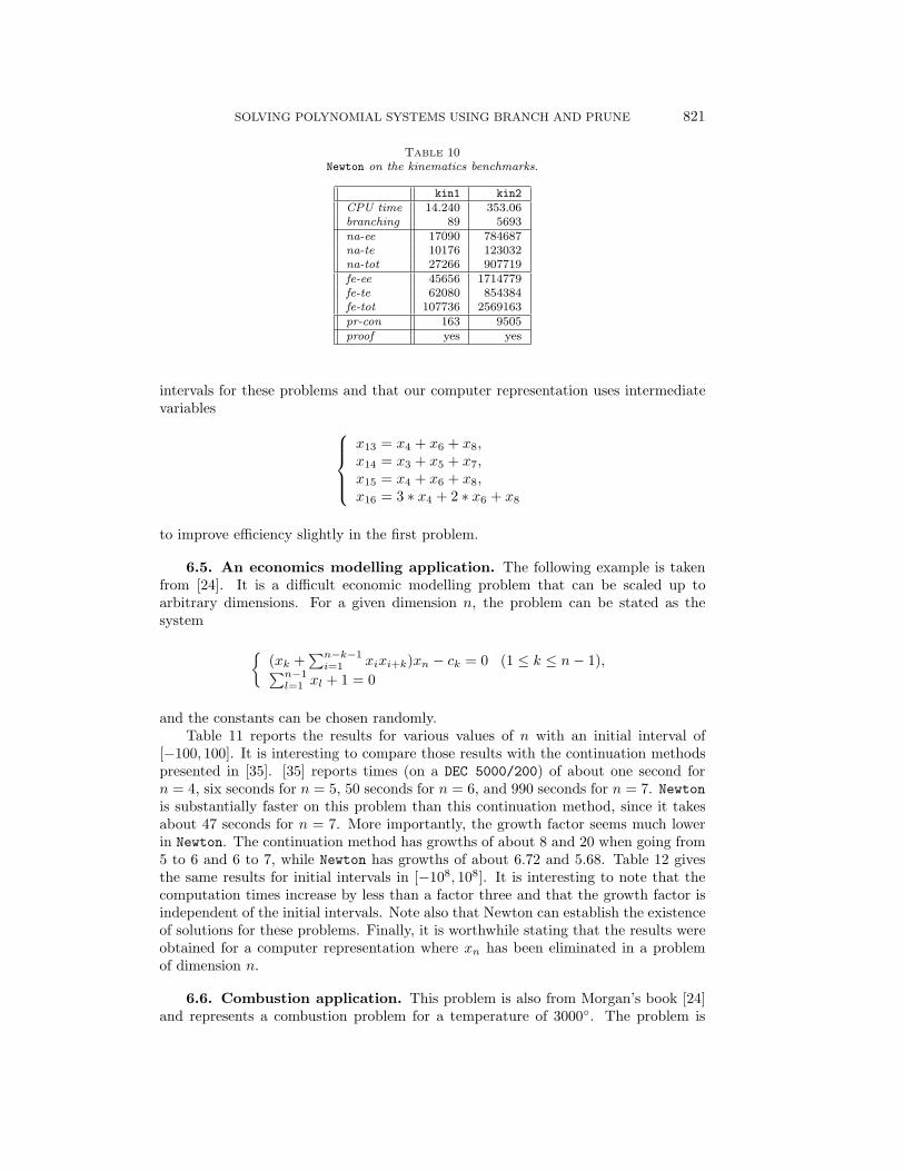
The results of Newton on these two benchmarks are given in Table 10. Newton isfast on the first benchmark and does not branch much to obtain all solutions. Thealgorithm in [11] branches more (the reported figure is 257 branches, but it is notreally comparable due to the nature of the algorithm) and is about 16 times sloweron comparable machines. We are not aware of the results of continuation methodson this problem. Newton is slower on the second application and takes about sixminutes. The continuation method described in [35] requires about 30 seconds on aDEC 5000/200. This method exploits the fact that the Newton polytopes for the lastfour equations are the same. Note that HRB requires about 1630 and 4730 seconds onthese examples. Note also that Newton can prove the existence of solutions in the final


TABLE 10Newton on the kinematics benchmarks.

kin1 kin2CPU time 14.240 353.06branching 89 5693na-ee 17090 784687na-te 10176 123032na-tot 27266 907719fe-ee 45656 1714779fe-te 62080 854384fe-tot 107736 2569163pr-con 163 9505proof yes yes

intervals for these problems and that our computer representation uses intermediatevariables

x13 = x4 + x6 + x8,x14 = x3 + x5 + x7,x15 = x4 + x6 + x8,x16 = 3 ∗ x4 + 2 ∗ x6 + x8

to improve efficiency slightly in the first problem.

6.5. An economics modelling application. The following example is takenfrom [24]. It is a difficult economic modelling problem that can be scaled up toarbitrary dimensions. For a given dimension n, the problem can be stated as thesystem

{(xk +

∑n−k−1i=1 xixi+k)xn − ck = 0 (1 ≤ k ≤ n− 1),∑n−1

l=1 xl + 1 = 0

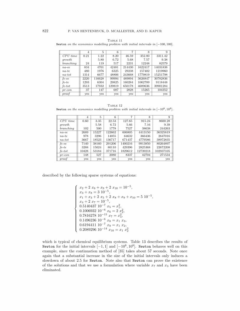
and the constants can be chosen randomly.Table 11 reports the results for various values of n with an initial interval of

[−100, 100]. It is interesting to compare those results with the continuation methodspresented in [35]. [35] reports times (on a DEC 5000/200) of about one second forn = 4, six seconds for n = 5, 50 seconds for n = 6, and 990 seconds for n = 7. Newtonis substantially faster on this problem than this continuation method, since it takesabout 47 seconds for n = 7. More importantly, the growth factor seems much lowerin Newton. The continuation method has growths of about 8 and 20 when going from5 to 6 and 6 to 7, while Newton has growths of about 6.72 and 5.68. Table 12 givesthe same results for initial intervals in [−108, 108]. It is interesting to note that thecomputation times increase by less than a factor three and that the growth factor isindependent of the initial intervals. Note also that Newton can establish the existenceof solutions for these problems. Finally, it is worthwhile stating that the results wereobtained for a computer representation where xn has been eliminated in a problemof dimension n.

6.6. Combustion application. This problem is also from Morgan’s book [24]and represents a combustion problem for a temperature of 3000◦. The problem is


TABLE 11Newton on the economics modelling problem with initial intervals in [−100, 100].

4 5 6 7 8 9CPU time 0.21 1.22 8.20 46.59 352.80 3311.42growth 5.80 6.72 5.68 7.57 9.38branching 24 119 517 2231 12248 82579na-ee 834 4701 42481 214430 1622417 14031838na-te 480 1976 6325 29238 157402 1219960na-tot 1314 6677 48806 243668 1779819 15251798fe-ee 2220 116628 99994 489894 3626847 30782836fe-te 1293 6304 29825 160284 1062789 9118448fe-tot 3513 17932 129819 650178 4689636 39901284pr-con 37 147 687 2828 15265 104352proof yes yes yes yes yes yes

TABLE 12Newton on the economics modelling problem with initial intervals in [−108, 108].

4 5 6 7 8 9CPU time 0.60 3.35 22.53 127.65 915.24 8600.28growth 5.58 6.72 5.66 7.16 9.39branching 102 500 1778 7527 38638 244263na-ee 2689 15227 122662 606805 4413150 36325819na-te 978 3296 14055 64632 366436 2647016na-tot 3667 18523 136717 671437 4779586 38972835fe-ee 7140 38160 291206 1400216 9913850 80264897fe-te 3288 15024 80110 429396 2825368 22672208fe-tot 10428 53184 371716 1829612 12739218 102937105pr-con 148 527 2080 8337 42704 271534proof yes yes yes yes yes yes

described by the following sparse systems of equations:

x2 + 2 x6 + x9 + 2 x10 = 10−5,x3 + x8 = 3 10−5,x1 + x3 + 2 x5 + 2 x8 + x9 + x10 = 5 10−5,x4 + 2 x7 = 10−5,0.5140437 10−7 x5 = x2

1,0.1006932 10−6 x6 = 2 x2

2,0.7816278 10−15 x7 = x2

4,0.1496236 10−6 x8 = x1 x3,0.6194411 10−7 x9 = x1 x2,0.2089296 10−14 x10 = x1 x

22

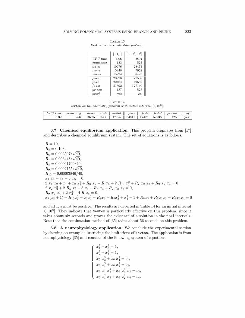
which is typical of chemical equilibrium systems. Table 13 describes the results ofNewton for the initial intervals [−1, 1] and [−108, 108]. Newton behaves well on thisexample, since the continuation method of [35] takes about 57 seconds. Note onceagain that a substantial increase in the size of the initial intervals only induces aslowdown of about 2.5 for Newton. Note also that Newton can prove the existenceof the solutions and that we use a formulation where variable x7 and x3 have beeneliminated.


TABLE 13Newton on the combustion problem.

[−1,1] [−108,108]CPU time 4.06 9.94branching 183 523na-ee 10676 28473na-te 5248 7952na-tot 15924 36425fe-ee 28928 77508fe-te 22464 49632fe-tot 51392 127140pr-con 187 527proof yes yes

TABLE 14Newton on the chemistry problem with initial intervals [0, 108].

CPU time branching na-ee na-te na-tot fe-ee fe-te fe-tot pr-con proof6.32 256 13725 3400 17125 34811 17425 52236 425 yes

6.7. Chemical equilibrium application. This problem originates from [17]and describes a chemical equilibrium system. The set of equations is as follows:

R = 10,R5 = 0.193,R6 = 0.002597/

√40,

R7 = 0.003448/√

40,R8 = 0.00001799/40,R9 = 0.0002155/

√40,

R10 = 0.00003846/40,x1 x2 + x1 − 3 x5 = 0,2 x1 x2 + x1 + x2 x

23 +R8 x2 −R x5 + 2 R10 x

22 +R7 x2 x3 +R9 x2 x4 = 0,

2 x2 x23 + 2 R5 x

23 − 8 x5 +R6 x3 +R7 x2 x3 = 0,

R9 x2 x4 + 2 x24 − 4 R x5 = 0,

x1(x2 + 1) +R10x22 + x2x

23 +R8x2 +R5x

23 + x2

4 − 1 +R6x3 +R7x2x3 +R9x2x4 = 0

and all xi’s must be positive. The results are depicted in Table 14 for an initial interval[0, 108]. They indicate that Newton is particularly effective on this problem, since ittakes about six seconds and proves the existence of a solution in the final intervals.Note that the continuation method of [35] takes about 56 seconds on this problem.

6.8. A neurophysiology application. We conclude the experimental sectionby showing an example illustrating the limitations of Newton. The application is fromneurophysiology [35] and consists of the following system of equations:

x21 + x2

3 = 1,x2

2 + x24 = 1,

x5 x33 + x6 x

34 = c1,

x5 x31 + x6 x

32 = c2,

x5 x1 x23 + x6 x

24 x2 = c3,

x5 x21 x3 + x6 x

22 x4 = c4.


TABLE 15Newton on the neurophysiology problem.

[−10, 10] [−102, 102] [−103, 103] [−104, 104]CPU time 0.91 11.69 172.71 2007.51growth 12.84 14.77 11.62branching 52 663 9632 115377na-ee 4290 57224 645951 6541038na-te 810 6708 96888 1173456na-tot 5100 63932 742839 7714494fe-ee 11012 144843 1620538 16647442fe-te 4104 48804 769056 9376632fe-tot 15116 193647 2389594 26024074pr-con 69 983 15980 195270proof yes yes yes yes

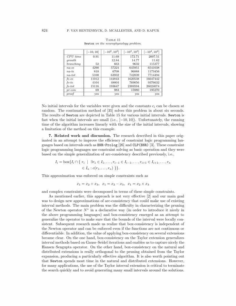
No initial intervals for the variables were given and the constants ci can be chosen atrandom. The continuation method of [35] solves this problem in about six seconds.The results of Newton are depicted in Table 15 for various initial intervals. Newton isfast when the initial intervals are small (i.e., [−10, 10]). Unfortunately, the runningtime of the algorithm increases linearly with the size of the initial intervals, showinga limitation of the method on this example.

7. Related work and discussion. The research described in this paper orig-inated in an attempt to improve the efficiency of constraint logic programming lan-guages based on intervals such as BNR-Prolog [26] and CLP(BNR) [3]. These constraintlogic programming languages use constraint solving as basic operation and they werebased on the simple generalization of arc-consistency described previously, i.e.,

Ii = box{Ii ∩ { ri | ∃r1 ∈ I1, . . . , ri−1 ∈ Ii−1, . . . , ri+1 ∈ Ii+1, . . . , rn

∈ In : c(r1, . . . , rn) }}.

This approximation was enforced on simple constraints such as

x1 = x2 + x3, x1 = x2 − x3, x1 = x2 × x3

and complex constraints were decomposed in terms of these simple constraints.As mentioned earlier, this approach is not very effective [2] and our main goal

was to design new approximations of arc-consistency that could make use of existinginterval methods. The main problem was the difficulty in characterizing the pruningof the Newton operator N∗ in a declarative way (in order to introduce it nicely inthe above programming languages) and box-consistency emerged as an attempt togeneralize the operator to make sure that the bounds of the interval were locally con-sistent. Subsequent research made us realize that box-consistency is independent ofthe Newton operator and can be enforced even if the functions are not continuous ordifferentiable. In addition, the value of applying box-consistency on several extensionsbecame clear. On the one hand, box-consistency on the Taylor extension generalizesinterval methods based on Gauss–Seidel iterations and enables us to capture nicely theHansen–Sengupta operator. On the other hand, box-consistency on the natural anddistributed extensions is really orthogonal to the pruning obtained from the Taylorexpansion, producing a particularly effective algorithm. It is also worth pointing outthat Newton spends most time in the natural and distributed extensions. However,for many applications, the use of the Taylor interval extension is critical to terminatethe search quickly and to avoid generating many small intervals around the solutions.


As a general observation, box-consistency on the natural and distributed extensionsseem effective when far from a solution while box-consistency on the Taylor expan-sion seems effective when near a solution. It is worth mentioning that the intervalcommunity has spent much effort to design additional techniques to speed up furtherthe computation when near a solution but have not considered techniques to improvepruning when far from a solution.

It is interesting to note that the idea of using approximations of arc-consistencywas also used independently by Hong and Stahl [11], who were also exposed to re-search on constraint logic programming. Their use of projections is, however, quitedifferent from ours. The key idea is to work with a set of boxes and to use projectionsto split a box into several subboxes by isolating all zeros of a projection. This gives analgorithm of a very different nature which cannot easily be characterized as a branchand prune algorithm since constraints are used to branch. Our approach seems to bemore effective in practice, since their use of projections may generate many subboxesthat may all need to be pruned away later on, implying much redundant work. Ourapproach postpones the branching until no pruning takes place and generates onlysubboxes when they are strictly necessary to progress. It is also very interesting toreport that, on all benchmarks that we tested, the projection never contained morethan two zeros. This seems to indicate that searching for all zeros may not be worth-while in most cases and that box-consistency may be the right trade-off here. Finally,note that their approach seems to use implicitly a distributed extension,11 but they donot make use of the natural extension which is very important for some applications.

Note also that our current implementation does not use some of the novel tech-niques of the interval community such as the more advanced conditioners and splittingtechniques of [13]. It is of course possible to include them easily, since the overall recur-sive structure of the implementations is essentially similar. Integrating these resultswould obviously be of benefit, since these techniques are complementary to ours.

The research described here also provides a uniform framework to integrate thesetechniques in constraint logic programming, to understand the importance of thevarious pruning operators and their relationships, and to suggest further researchdirections. For instance, higher notions of consistency such as path-consistency [18]may be worth investigating for some applications.

8. Conclusion. In this paper, we presented a branch and prune algorithm tofind all isolated solutions to a system of polynomial constraints over the reals. Ifthe solution are not isolated, the algorithm will return boxes that contain severalsolutions. The algorithm is based on a single concept, box-consistency, which isan approximation of arc-consistency, a notion well known in artificial intelligence.Box-consistency can be instantiated to produce the Hansen–Sengupta operator aswell as other narrowing operators which are more effective when the computationis far from a solution. The algorithm and its mathematical foundations are simple.Moreover, the algorithm is shown to behave well on a variety of benchmarks fromkinematics, mechanics, chemistry, combustion, and economics. It outperforms theinterval methods we know of and compares well with continuation methods on theirbenchmarks. In addition, problems such as the Broyden banded function and theMore–Cosnard discretization of a nonlinear integral equation can be solved for severalhundred variables. Limitations of the method (e.g., a sensitivity to the size of theinitial intervals on some problems) have also been identified.

11The idea of sandwiching the interval function in between two real functions is described there.


Acknowledgments. We would like to thank the referees for their help in makingthe paper accessible to a wider audience, for pointing out several related works, andfor their careful comments on the manuscript. We would like to thank F. Benhamou,A. Colmerauer, and B. Le Charlier for many interesting discussions on this topic.

REFERENCES

[1] G. ALEFELD AND J. HERZBERGER, Introduction to Interval Computations, Academic Press,New York, 1983.

[2] F. BENHAMOU, D. MCALLESTER, AND P. VAN HENTENRYCK, CLP (intervals) revisited, inProceedings of the International Symposium on Logic Programming (ILPS-94), Ithaca,NY, November 1994, pp. 124–138.

[3] F. BENHAMOU AND W. OLDER, Applying interval arithmetic to real, integer and Booleanconstraints, J. Logic Programming, to appear.

[4] R. HAMMER, M. HOCKS, M. KULISCH, AND D. RATZ, Numerical Toolbox for Verified Com-puting I – Basic Numerical Problems, Theory, Algorithms, and PASCAL-XSC Programs,Springer-Verlag, Heidelberg, 1993.

[5] E. HANSEN, Global Optimization Using Interval Analysis, Marcel Dekker, New York, 1992.[6] E. R. HANSEN, Global optimization using interval analysis: The multi-dimensional case,

Numer. Math, 34 (1980), pp. 247–270.[7] E. R. HANSEN AND R. I. GREENBERG, An interval Newton method, Appl. Math. Comput., 12

(1983), pp. 89–98.[8] E. R. HANSEN AND S. SENGUPTA, Bounding solutions of systems of equations using interval

analysis, BIT, 21 (1981), pp. 203–211.[9] E. R. HANSEN AND R. R. SMITH, Interval arithmetic in matrix computation: Part II, SIAM

J. Numer. Anal., 4 (1967), pp. 1–9.[10] R. J. HANSON, Interval Arithmetic as a Closed Arithmetic System on a Computer, Jet Propul-

sion Laboratory Report 197, Pasadena, CA, 1968.[11] H. HONG AND V. STAHL, Safe starting regions by fixed points and tightening, Computing,

53 (1994), pp. 323–335.[12] W. M. KAHAN, A More Complete Interval Arithmetic, Lecture notes, University of Michigan,

Ann Arbor, MI, Summer 1968.[13] R. B. KEARFOTT, Preconditioners for the interval Gauss-Seidel method, SIAM J. Numer.

Anal., 27 (1990), pp. 804–822.[14] R. B. KEARFOTT, A Review of preconditioners for the interval Gauss-Seidel method, Interval

Comput., 1 (1991), pp. 59–85.[15] R. KRAWCZYK, Newton-Algorithmen zur Bestimmung von Nullstellen mit Fehlerschranken,

Computing, 4 (1969), pp. 187–201.[16] A. K. MACKWORTH, Consistency in networks of relations, Artificial Intelligence, 8 (1977),

pp. 99–118.[17] K. MEINTJES AND A. P. MORGAN, Chemical equilibrium systems as numerical test problems,

ACM Trans. Math. Software, 16 (1990), pp. 143–151.[18] U. MONTANARI, Networks of constraints: Fundamental properties and applications to picture

processing, Inform. Sci., 7 (1974), pp. 95–132.[19] R. E. MOORE, Interval Analysis, Prentice–Hall, Englewood Cliffs, NJ, 1966.[20] R. E. MOORE, Methods and Applications of Interval Analysis, SIAM, Philadelphia, PA, 1979.[21] R. E. MOORE AND S. T. JONES, Safe starting regions for iterative methods, SIAM J. Numer.

Anal., 14 (1977), pp. 1051–1065.[22] J. J. MORE AND M. Y. COSNARD, Numerical solution of nonlinear equations, ACM Trans.

Math. Software, 5 (1979), pp. 64–85.[23] A. P. MORGAN, Computing all solutions to polynomial systems using homotopy continuation,

Appl. Math. Comput., 24 (1987), pp. 115–138.[24] A. P. MORGAN, Solving Polynomial Systems Using Continuation for Scientific and Engineering

Problems, Prentice–Hall, Englewood Cliffs, NJ, 1987.[25] A. NEUMAIER, Interval methods for systems of equations, Prentice–Hall Internat. Ser. Comput.

Sci., Cambridge University Press, Cambridge, 1990.[26] W. OLDER AND A. VELLINO, Extending prolog with constraint arithmetics on real intervals,

in Canadian Conference on Computer and Electrical Engineering, Ottawa, 1990.[27] L. B. RALL, Automatic differentiation: Techniques and applications, Lecture Notes in Comput.

Sci., Springer-Verlag, New York, 1981.


[28] H. RATSCHEK AND J. ROKNE, New Computer Methods for Global Optimization, Ellis HorwoodLimited, Chichester, 1988.

[29] S. M. RUMP, Verification methods for dense and sparse systems of equations, in Topics inValidated Computations, J. (Ed.) Herzberger, ed., Elsevier, New York, 1988, pp. 217–231.

[30] J. SISKIND AND D. MCALLESTER, Nondeterministic lisp as a substrate for constraint logicprogramming, in AAAI-93, 1993, pp. 133–138.

[31] P. VAN HENTENRYCK, A logic language for combinatorial optimization, Ann. Oper. Res.,21 (1989), pp. 247–274.

[32] P. VAN HENTENRYCK, Constraint Satisfaction in Logic Programming, Logic ProgrammingSeries, MIT Press, Cambridge, MA, 1989.

[33] P. VAN HENTENRYCK, D. MCALLESTER, AND D. KAPUR, Interval Methods Revisited, Tech.report No. 1524, MIT AI Lab, MIT, Cambridge, MA, 1995.

[34] P. VAN HENTENRYCK, V. SARASWAT, AND Y. DEVILLE, The design, implementation, andevaluation of the constraint language cc(FD), in Constraint Programming: Basics andTrends, Springer-Verlag, New York, 1995.

[35] J VERSCHELDE, P. VERLINDEN, AND R. COOLS, Homotopies exploiting Newton polytopes Forsolving sparse polynomial systems, SIAM J. Numer. Anal., 31 (1994), pp. 915–930.

Constraint Programming

Documents