A Comparison of Three Stochastic Multi-Site Precipitation Occurrence Generators

Journal of Hydrology (2006) 331, 280–292

ava i lab le at www.sc iencedi rec t . com

journal homepage: www.elsevier .com/ locate / jhydro l

A comparison of three stochasticmulti-site precipitation occurrence generators

R. Mehrotra a,*,1, R. Srikanthan b, Ashish Sharma a

a Civil and Environmental Engineering, The University of New South Wales, Kensington, Sydney, NSW 2052, Australiab Bureau of Meteorology, Melbourne, Australia

Received 26 May 2005; received in revised form 15 May 2006; accepted 16 May 2006

Summary This paper presents a comparison of three multi-site stochastic weather generatorsfor simulation of point rainfall occurrences at a network of 30 raingauge stations around Syd-ney, Australia. The approaches considered include a parametric hidden Markov model (HMM),a multi-site stochastic precipitation generation model (proposed by [Wilks, D.S., 1998. Multi-site generalization of a daily stochastic precipitation model, J. Hydrol. 210, 178–191.]) anda non-parametric K-nearest neighbour (KNN) model. The HMM generates the precipitation dis-tribution conditional on a discrete weather state representing certain identified spatial rainfalldistribution patterns. The spatial dependence is maintained by assumption of a commonweather state across all stations while the temporal dependence is simulated by assumingthe weather state to be Markovian in nature. The Wilks model preserves serial dependencethrough the assumption of an order one Markov dependence at each location. The spatialdependence is simulated by prescribing a dependence pattern on the uniform random variatesused to generate the rainfall occurrence at each location from the associated conditional prob-ability distribution. The K-nearest neighbour approach simulates spatial dependence by simul-taneously generating precipitation occurrence at all locations. Temporal persistence issimulated through Markovian assumptions on the rainfall occurrence process.

The three methods are evaluated for their ability to model spatial and temporal dependencein the rainfall occurrence field and also the relative ease with which the assumptions of spatialand temporal dependence can be accommodated. Our results indicate that all the approachesare successful in reproducing spatial dependence in the multi-site rainfall occurrence field.However, the different orders of assumed Markovian dependence in the observed data limittheir ability in representing temporal dependence at time scales longer than a few days. Whileeach approach comes with its own advantages and disadvantages, the alternative proposed byWilks has an overall advantage in offering a mechanism for modelling varying orders of serial

KEYWORDSRainfall generation;Rainfall occurrence;Multi-site stochasticweather generator;Spatial and temporaldependence;Aggregated time scalecharacteristics;Australia

0d

* Corresponding author. Tel.: +61 293855064; fax: +61 293856139.E-mail address: [email protected] (R. Mehrotra).

1 Also at National Institute of Hydrology, Roorkee, India.

A comparison of three stochastic multi-site precipitation occurrence generators 281

dependence at each point location, while still maintaining the observed spatial dependencewith sufficient accuracy.

�c 2006 Elsevier B.V. All rights reserved.

Introduction

Stochastic models, sometimes also known as ‘stochasticweather generators’, are commonly used to generate syn-thetic sequences of weather variables that are statisticallyconsistent with the observed characteristics of the histori-cal record in time. These synthetic sequences provide aset of alternate realisations that can be used for risk andreliability assessment in the design and operation of agricul-tural and water resource systems. Stochastic models gener-ating weather at a single point location are easy toformulate and implement, and thus remain popular. A com-mon approach to modelling single-site daily rainfall hasbeen to develop models describing the rainfall occurrence(wet-dry) process and to describe the distribution of rainfallamounts on wet days independently (Woolhiser, 1992).Rainfall occurrence is represented in two ways: either as aMarkov process (Gabriel and Neumann, 1962; Salas, 1993;Katz and Zheng, 1999) or as an alternating renewal processfor wet and dry sequences (Buishand, 1978; Sharma andLall, 1999). Rainfall amount is generated once a day hasbeen specified as wet, the amount being generated eitherunconditionally or conditional to appropriately specifiedvariables. The rainfall amount and rainfall occurrence canalso be modelled as a single process using a multi-state Mar-kov chain, the rainfall being treated as a mixed discrete andcontinuous variable, and transition probabilities being pre-scribed to model the dependence structure present (Haanet al., 1976; Srikanthan and McMahon, 1985; Gregoryet al., 1993). There exist more generalized model catego-ries, for example, generalized linear models (Chandler andWheater, 2002) and cluster point process based models rep-resenting the physical aspects of precipitation (e.g., Brasand Rodriguez-Iturbe, 1976; Waymire et al., 1984; Nor-throp, 1998; Onof et al., 2000; Wheater et al., 2000; Pe-gram and Clothier, 2001; Koutsoyiannis et al., 2003). Inaddition to the above, a related class of widely used modelsare non-parametric alternatives for stochastic weather gen-eration (Lall et al., 1996; Rajagopalan and Lall, 1999; Harr-old et al., 2003). These differ from parametric stochasticweather generators in their use of the observed weather re-cord as the basis for generating new realisations. A limita-tion of commonly used single site rainfall models is theirinability to represent spatial attributes. The spatial correla-tion of weather variables, specially the precipitation, canhave a significant impact on any flow generation applica-tions the rainfall sequences are used for.

A number of space–time parametric stochastic modelshave addressed this important issue of spatial dependenceamong weather variables at multiple locations, both withand without conditioning on exogenous atmospheric predic-tors. These models have been developed to generate multi-ple realizations of selected weather variables (primarily forprecipitation) simultaneously at multiple locations, mostlyat daily time step (e.g., Bardossy and Plate, 1992; Bogardi

et al., 1993; Bras and Rodriguez-Iturbe, 1976; Hay et al.,1991; Hughes et al., 1993; Hughes and Guttorp, 1994;Hughes et al., 1999; Qian et al., 2002; Stehlık and Bardossy,2002; Waymire et al., 1984; Wilson et al., 1992; Wilks,1998).

The non-homogeneous hidden Markov model (NHMM) asproposed by Hughes and Guttorp (1994) represents a generalclass of weather state downscaling/generation models, andrelates a small set of exogenous predictors to daily precip-itation occurrence at multiple locations via a finite numberof hidden or unobserved weather states. The selected pre-dictors may include atmospheric variables indicative ofthe large-scale atmospheric forcings that affect weatherat a local scale. If atmospheric variables are not included,the model reduces to the hidden Markov model (HMM) of Ra-biner and Juang (1986). The NHMM or HMM identifies themost distinct spatial patterns in the multi-station, daily pre-cipitation occurrence record. In this way, it captures muchof the spatial variability in daily precipitation and approxi-mately the temporal variability through persistence in theweather states. These stochastic weather generators tryto represent some of the physical aspects of the complexbehavior of the rainfall generation mechanism in a simpleyet realistic manner. However, these kinds of models (incor-porating more and more realistic processes) require exten-sive parameter estimation and statistical verification(Georgakakos and Kavvas, 1987; Mehrotra et al., 2004). Thisoften limits their use for common operational applications.

To overcome the difficulty of parameter estimation ofmulti-site weather generators, Wilks (1998) proposed a sim-ple extension of commonly used single-site weather gener-ators for precipitation, to multiple sites by joining acollection of individual single-site models through a tempo-rally independent but spatially correlated sequence of ran-dom numbers representing the probability of non-exceedence of the random variable being generated. Thespatial correlation structure associated with these randomnumbers is empirically estimated so as to ensure an appro-priate representation of observed spatial dependence in theprecipitation field. Wilks (1999a) also proposed a straight-forward full extension of Richardson (1981) model for dailyprecipitation, daily maximum temperature, daily minimumtemperature, and daily solar radiation to multiple sites. Fur-ther, Wilks (1999b) applied a stochastic weather generatorfor downscaling of precipitation at multiple locations condi-tioning on atmospheric variables. Qian et al. (2002) ex-tended Wilks (1998) model for simultaneous simulations ofdaily precipitation, and daily maximum and minimum tem-peratures at multiple sites conditional on daily circulationpatterns.

Non-parametric models offer a different rational for gen-eration of climate variables and have been used extensivelyfor this problem in recent years (Rajagopalan and Lall, 1999;Brandsma and Buishand, 1998; Sharma and Lall, 1999; Harr-old et al., 2003; Buishand and Brandsma, 2001; Mehrotra

282 R. Mehrotra et al.

et al., 2004). These models offer an alternative of develop-ing the temporal and spatial relationship among weathervariables without a priori assumptions on the joint probabil-ity distribution associated with these variables. These areparsimonious, provide a flexible framework, can easily bemodified to incorporate new form of conditional depen-dence and have the ability to reproduce any observed func-tional relationship. The lack of any assumptions defining thejoint distribution of the weather variables helps ensure anaccurate representation of features such as non-linearity,asymmetry or multi-modality in the observed record ofthe variables being modelled.

The K-nearest neighbour bootstrap (KNN) is a techniquethat conditionally resamples the values from the observedrecord based on the conditional relationship specified. Formulti-site resampling, since the variables at these locationsare simulated concurrently, dependence across space isaccurately preserved. An algorithm for bootstrapping timeseries considering Markovian dependence was developedby Lall and Sharma (1996). Buishand and Brandsma (2001)used nearest neighbour resampling for multi-site generationof daily precipitation and temperature at 25 stations in theGerman part of the Rhine basin. Mehrotra et al. (2004) ap-plied KNN technique to simulate rainfall conditional onatmospheric variables simultaneously at 30 stations aroundSydney. Further, Mehrotra and Sharma (2005) applied aweather-state based non-parametric model and to simulaterainfall occurrence simultaneously at 30 locations around,Sydney, Australia and successfully simulated various tempo-ral and spatial rainfall characteristics at multiple locations.

Recognising the importance of reproduction of spatialand temporal behaviour of the weather variables, recently,Clark et al. (2004a) and Clark et al. (2004b) introduced areshuffling procedure to reconstruct the observed spatial(intersite) and temporal correlation statistics among multi-ple locations by reordering the generated weather variablesat individual locations. The reshuffled generated series ofweather variables were shown to be consistent with the ob-served series in terms of the various temporal and spatialcharacteristics.

This paper discusses applications of three stochasticweather generators for simultaneous simulation of rainfalloccurrences at multiple locations. These include (a) hiddenMarkov model (HMM) of Rabiner and Juang (1986) and fur-ther extended by Hughes and Guttorp (1994) as non-homo-geneous hidden Markov model (NHMM); (b) multi-siteMarkov process model of Wilks (1998); and (c) a non-para-metric K-nearest neighbour multi-site model (Lall and Shar-ma, 1996; Buishand and Brandsma, 2001). These selectedmodels represent three distinct modeling configurationsand hence justify their selection for a comparative analysis.The HMM is a parametric alternative that is sensitive to theparameteric relationships assumed, the Wilks approach is ageneric alternative for simulating spatial dependence in anexisting single-site Markovian parametric representation,and, the KNN modeling approach represents a non-paramet-ric framework based on simple Markovian considerations.

Each of the methods is assessed based on its ability tosimulate sequences with statistical attributes that are sim-ilar to those observed. A 43-year long record of daily rainfalloccurrence at a network of 30 locations near Sydney, Aus-tralia, is used to compare the various methods. Note that,

unless otherwise stated, a reference to rainfall or precipita-tion in the remainder of the paper refers to precipitationoccurrence and not to the combined precipitation occur-rence-amount process.

The paper is organised as follows. The methodology andthe models used are discussed in Section ‘Methodology’. De-tails on the application of the various models considered,the data and the study region used, and a comparison ofthe various results obtained, are presented in Section‘Application of model and simulation results’. We concludethe paper by presenting the summary and conclusions drawnfrom the results in Section ‘Conclusions’.

Methodology

Hidden Markov model (HMM)

The hidden Markov model (HMM) was first proposed by Rabi-ner and Juang (1986) and later modified by Hughes and Gut-torp (1994) for use in climate related studies. Hughes andGuttorp (1994) extended the HMM by including exogenousatmospheric predictors for rainfall simulation and referredthe model as non-homogeneous hidden Markov model(NHMM). The unifying feature of NHMM or HMM, in the con-text of multi-site weather variables, is the hypothesis of anunobserved discrete weather state that corresponds to cer-tain distinguished spatial rainfall distribution patterns overthe ground. The word ‘hidden’ refers to the fact that theweather state process is an unobserved quantity. Thus, alldays of the multi-site rainfall occurrences are classified intoa few discrete weather states based on the rainfall distribu-tion patterns. The multi-site daily rainfall occurrences areconditional on a weather state and the daily transition ofweather state is defined using a first-order Markov model.Thus, temporal dependence is maintained by assumptionof an order one model for the weather state and spatialdependence is reproduced by allowing at site rainfall tobe associated with a weather state that is common acrossall sites and represents certain similar rainfall distributionpatterns. In the discussions that follow, we denote all matri-ces and vector as bold, a ns site rainfall occurrence vector attime t as Rt, a discrete weather state at time t as St and thetotal number of observations as n. In the most simplifiedform a HMM is defined by the following assumptions:

Assumption 1 :PðRtjSn; Sn�1; . . . ; St; St�1; . . . ; S1;Rt�1;

Rt�2; . . . . . . ;R1Þ ¼ PðRtjStÞ ð1Þ

and

Assumption 2 : PðStjSt�1; St�2; . . . ; S1Þ ¼ PðStjSt�1Þ ð2Þ

According to Assumption (1), given the current weatherstate, the rainfall occurrence pattern is assumed indepen-dent of all past rainfall occurrence patterns and weatherstates. Assumption (2) asserts that the weather state attime t depends only on the state at the previous time step.It may be noted that apart from introducing simplicity,Assumption (1) is also necessary when using the model forgeneration/prediction as future time step values areunknown.

To parameterize P(RtjSt), Hughes et al. (1999) adoptedthe autologistic model for multivariate binary data:

A comparison of three stochastic multi-site precipitation occurrence generators 283

PðRt ¼ rjSt ¼ sÞ / expXnsi¼1

asiri þXj<i

bsijrirj

!ð3Þ

where ri is the rainfall occurrence for site i, i = 1, ns, bsij isthe ‘conditional log-odds ratio’ of rain at station i to rain atstation j (in state s) based on the probability distributionP(ri,rjjr�i,�j, St = s) where r�i,�j is the vector of rainfalloccurrences at all stations other than i and j. It may benoted that (3) describes the probability of a vector of rain-fall occurrences (r) at a network of stations under a discreteweather state (s) at a given time t. This formulation forP(RtjSt = s) also considers the spatial correlation of rainfalloccurrences Ri

t at stations in each weather state. Theparameter asi is estimated from the psi, the probability ofrain at station i in weather state s, using the expressionasi = log[psi/(1 � psi)]. An important case of (3) arises whenbsij = 0 for all i, j and s. Then

PðRt ¼ rjSt ¼ sÞ ¼Ynsi¼1

pri

sið1� psiÞ1�ri ð4Þ

This formulation assumes the rainfall occurrences Rit as spa-

tially independent given the weather state. Uncondition-ally, however, the Ri

t will be correlated owing to theinfluence of the common weather state. Hughes and Gut-torp (1994) found this model to be working well for spatiallysparse network of raingauge stations. Without introducingadditional complexity, in the present paper this simplemodel structure is considered.

The P(StjSt�1) is defined by the following:

PðSt ¼ jjSt�1 ¼ iÞ ¼ cij ð5Þ

where cij is the transition probability of weather state whenthe state of the weather at the previous time step was i andthe current state of the weather is j. It is necessary to im-pose the constraints

Pjcij ¼ 1 in order to ensure identifi-

ability of the parameters.The parameters for P(RtjSt) in (4) are estimated using a

modified two step EM algorithm (Hughes et al., 1999) to ob-tain maximum likelihood estimates using numerical optimi-zation techniques and the forward–backward algorithm(Juang and Rabiner, 1991). Model parameters for P(StjSt�1)are estimated using the adaptive Metropolis (AM) samplingapproach (Haario et al., 2001; Marshall et al., 2004; Mehro-tra et al., 2004).

Wilks’ approach

Wilks (1998) extended the familiar first-order Markovchain single site model of rainfall occurrences to multi-site by driving a collection of single-site models with seri-ally independent but spatially correlated random num-bers. Individual models are fitted to each of the ns sitesfirst. Each such model enables specification of the condi-tional probability distribution of the at site rainfall occur-rences. Simulation proceeds by sampling from theconditional cumulative distribution function (CDF), whichis equivalent to sampling the quantile equivalent to a ran-domly generated probability of non-exceedence, and isobtained as a Uniform random variate between 0 and 1.Non-zero correlations among the pre-specified random

numbers result in intersite correlations between the gen-erated rainfall sequences. The following describes in briefthe procedure followed to generate the spatially corre-lated random numbers and their use in the generationof rainfall occurrences at multiple locations.

Denote ut as a vector of uniform [0,1] variates oflength ns at time step t. Given a network of ns raingaugesites, there are ns (ns � 1)/2 pairwise correlations thatshould be maintained in the uniform random numbers(ut) forcing the occurrence process. The vector ut is de-fined such that corr[ut, ut+1] = 0 (or, each vector is inde-pendent across time), but for locations k and l,corr[ut(k), ut(l)] 5 0. As a result, there is spatial depen-dence between individual elements of the vector, thisdependence being introduced to induce observed spatialdependence in the rainfall occurrences they are used togenerate.

Denoting the rainfall occurrence at ns locations as Rt,with variables for locations k and l as Rt(k) and Rt(l) respec-tively, the sample coefficient of correlation between thetwo variables (rainfall occurrence series at locations k andl) is written as:

nðk; lÞ ¼ Corr½RtðkÞ;RtðlÞ� ð6Þ

The spatial dependence between the uniform random vari-ates ut(k), ut(l) is specified such that the resulting quantilesfrom the conditional CDF exhibit a correlation equivalent ton(k, l). This spatial dependence is specified by first trans-forming the uniform random variates to those of a standardnormal distribution:

utðkÞ ¼ U½wtðkÞ� ð7Þ

where U[.] indicates the standard normal CDF. Let the cor-relation between the standard normal variates be denotedas:

xðk; lÞ ¼ Corr½wtðkÞ;wtðlÞ� ð8Þ

Our aim then becomes to find a value for x(k, l) such thatthe Uniform random variates ut(k), ut(l) generated basedon it, lead to rainfall occurrences Rt(k), Rt(l) that exhibita correlation of no(k, l), which denotes the observed valueof n(k, l), which will have been estimated from the observedbinary series Ro

t ðkÞ and Rot ðlÞ at stations k and l. Estimating

x(k, l) involves an empirical procedure that is describedbelow.

Direct computation of x(k, l) from no(k, l) is not possibleas wt(k) corresponding to observed rainfall occurrence ser-ies Ro

t ðkÞ cannot be computed. However, as noted by Wilks(1998), there exists a monotonic relationship betweenx(k, l)and the generated n(k, l) for a given station pair kand l. Therefore, in practice, one obtains x(k, l) using a trialand error procedure by assuming a reasonable value forx(k, l), generating the series Rt(k) and Rt(l) at stations kand l using x(k, l), evaluating n(k, l) and comparing it withno(k, l). The process is repeated with different values ofx(k, l) till an acceptable value of n(k, l), reasonably closeto no(k, l), is obtained. It is also possible to invert the rela-tionship between x(k, l) and n(k, l) using a non-linear rootfinding algorithm. Further details on the methodology areavailable in Wilks (1998).

284 R. Mehrotra et al.

k-nearest-neighbour resampling

In the context of multi-site generation of rainfall occur-rences, the K-nearest-neighbour approach considers sam-pling with replacement of the rainfall occurrences atmultiple locations, from the historical rainfall record. Thisinvolves identifying days (nearest neighbours) in the histor-ical record that have similar characteristics as the previousday, and using observations for the current day as the basisfor resampling. To simulate temporal dependence, a Mar-kov order (one or more lags) conditional resampling proce-dure is implemented. The spatial rainfall distributionstructure is maintained by resampling simultaneously atall the stations. Denoting the vector of conditioning vari-ables as Xt (also referred to as the feature or state vector),the problem reduces to identifying the nearest neighboursof this vector in the historical record. This conditioningvector may be designed to include standardized values ofrainfall occurrences for previous day(s) (Rajagopalan andLall, 1999) or standardised summary statistics of rainfalland/or other weather variables (Buishand and Brandsma,2001; Beersma and Buishand, 2003; Mehrotra et al.,2004). In the present application, Xt consists of previousday average rainfall state ðRt�1Þ and thus includes a solovariable Rt�1 only. The K nearest neighbours of Xt are se-lected in terms of a weighted Euclidean distance betweenthe conditioning vector Xt at time t and a vector Xi formedfrom the ith day rainfall of the observed record. The i + 1day rainfall vector of the K most nearest Xi vectors formthe most probable values of rainfall for the current dayt. For two m-dimensional vectors, Xt and Xi, this distanceis defined as:

Ei ¼ffiffiffiffiffiffiffiffiffiffiffiffiffiffiffiffiffiffiffiffiffiffiffiffiffiffiffiffiffiffiffiffiffiffiffiffiffiffiffiffiffiffiffiffiXm

j¼1sjbjðXj;i � Xj;tÞ2

rð9Þ

where sj and bj, respectively, are the scaling weight andthe influence weight associated with the jth predictor;and Xj,i and Xj,t, respectively, are the jth elements of vec-tors Xt and Xi. Scaling weights s(s = [sj], j = 1, . . . ,m) areused to convert the values of each predictor to a commonscale in estimation of the distance. Influence weights, b(b = [bj],j = 1, . . . ,m), define the information content ofeach predictor in estimating the conditional probabilitydensity (see for details, Mehrotra and Sharma, 2006). Itis also possible to use other distance measures (for exam-ple see Yates et al., 2003; Souza Filho and Lall, 2003; Woj-cik and Buishand, 2003). The scaling or influence weightcan also be a function of the time t to impart the effectof seasonality in the predictor–predictand relationship.In the application presented in later sections, a movingwindow of a specified length is used for scaling weight esti-mation and for conditional resampling, the predictorsbeing standardised using standard deviation of the observa-tions lying within the moving window, thereby ensuring anappropriate representation of seasonal variations in therelationship being modelled. Similarly, the sample usedto specify the conditional probability distribution is alsothe subset of observations that fall within the movingwindow.

For simulations of the variables of the time series, a dis-crete probability distribution or kernel as recommended by

Lall and Sharma (1996) that gives higher weight to the closerneighbours is adopted. For this decreasing kernel the prob-ability, pj that can be assigned to the jth closest neighbouris given by:

pi ¼1=iPKj¼11=j

ð10Þ

where i represents the ith nearest neighbour of the condi-tioning vector Xt, and K is the number of nearest neighboursused. The conditional cumulative probability distributioncan then be written as:

P1 ¼ p1 and Pi ¼ Pi�1 þ pi for i > 1; ð11Þ

where Pi is the cumulative probability for the ith nearestneighbour.

Simulation proceeds by first forming a conditioning vec-tor Xt for the current day on the basis of average rainfallstate of the previous day and calculating Euclidean dis-tances, E of all the days lying within the moving windowand vector Xt, using Eq. (9). For each day, the subsequentday rainfall vector is tagged to the calculated Euclideandistance. In the second step, these distances are rankedfrom lowest to highest and the tagged rainfall vectors ofthe first K days having the smallest distances are pickedup. In the final step a uniform random number u between0 and 1 is generated and the i*th neighbour or rainfall vec-tor (from the pre-identified K rainfall vectors using Eqs.(10) and (11)) is identified such that Pi��1 < u 6 Pi� . Thisidentified rainfall vector (rainfall at all locations) formsthe rainfall of the day t. Use of the above logic enablesresampling of rainfall at all locations on a given day (i*)simultaneously, with replacement. Further details on theapproach are available in Rajagopalan and Lall (1999);Brandsma and Buishand (1998); Sharma and Lall (1999);Harrold et al. (2003); Buishand and Brandsma (2001) andMehrotra et al. (2004).

Computer programmes (in Fortran language) of all themodels used in the study are available with the authorsand can be provided on request.

Application of model and simulation results

Data and study area

The study region is located around Sydney, eastern Austra-lia spanning between 147�E–153�E longitude and 31�S–36�S latitude (Fig. 1). Most significant rainfall events inwinter in this region involve air masses that have beenbrought over the region from the east-coast low-pressuresystems. Orographic uplift of these air masses when theystrike coastal ranges or the Great Dividing Range oftenproduces very heavy rain. For this study, a 43-year contin-uous record (from 1960 to 2002) of daily rainfall occur-rences at 30 stations around Sydney, eastern Australia(see Fig. 1) was used. The inter-station distances betweenstation pairs vary approximately from 20 to 340 km. Missingvalues at some stations (<0.5%), were estimated using therecords of nearby stations. A day was considered as a wetor dry depending on whether the rainfall amount on thatday was greater than or equal to, or less than 0.3 mm,respectively.

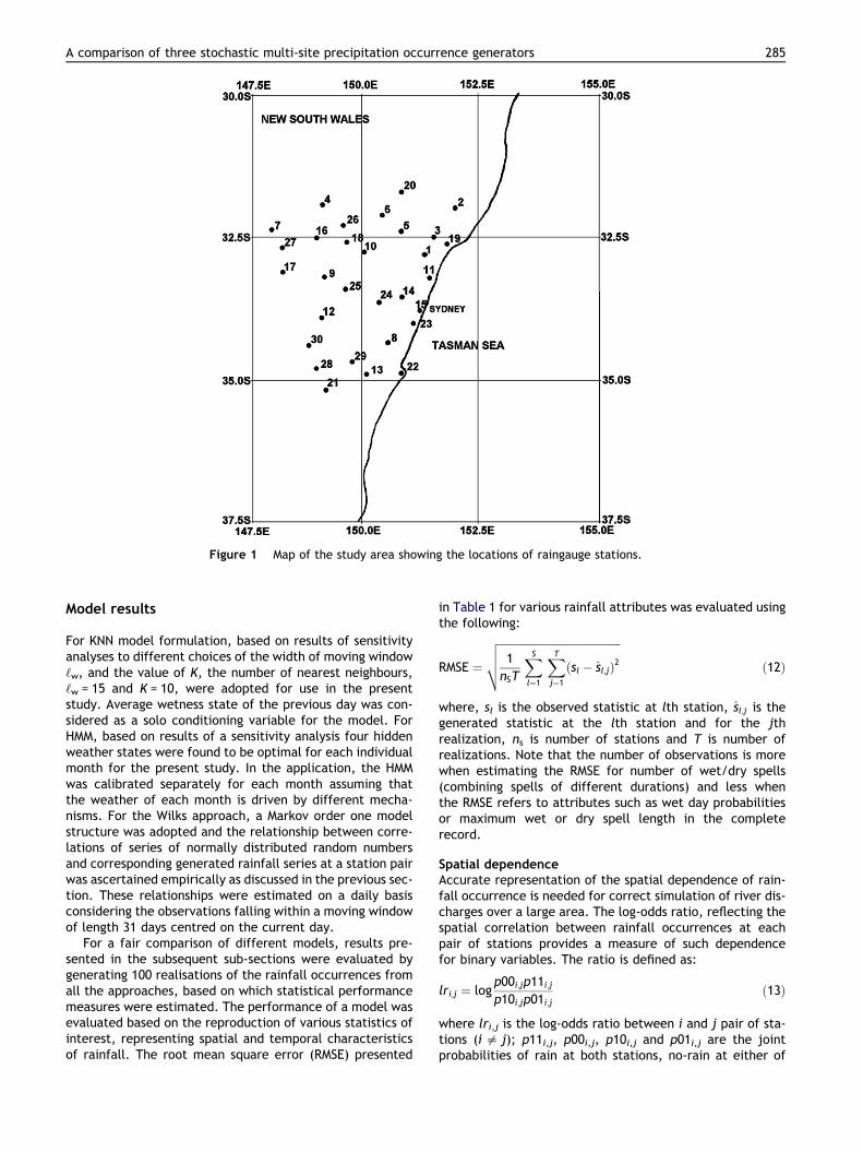
Figure 1 Map of the study area showing the locations of raingauge stations.

A comparison of three stochastic multi-site precipitation occurrence generators 285

Model results

For KNN model formulation, based on results of sensitivityanalyses to different choices of the width of moving window‘w, and the value of K, the number of nearest neighbours,‘w = 15 and K = 10, were adopted for use in the presentstudy. Average wetness state of the previous day was con-sidered as a solo conditioning variable for the model. ForHMM, based on results of a sensitivity analysis four hiddenweather states were found to be optimal for each individualmonth for the present study. In the application, the HMMwas calibrated separately for each month assuming thatthe weather of each month is driven by different mecha-nisms. For the Wilks approach, a Markov order one modelstructure was adopted and the relationship between corre-lations of series of normally distributed random numbersand corresponding generated rainfall series at a station pairwas ascertained empirically as discussed in the previous sec-tion. These relationships were estimated on a daily basisconsidering the observations falling within a moving windowof length 31 days centred on the current day.

For a fair comparison of different models, results pre-sented in the subsequent sub-sections were evaluated bygenerating 100 realisations of the rainfall occurrences fromall the approaches, based on which statistical performancemeasures were estimated. The performance of a model wasevaluated based on the reproduction of various statistics ofinterest, representing spatial and temporal characteristicsof rainfall. The root mean square error (RMSE) presented

in Table 1 for various rainfall attributes was evaluated usingthe following:

RMSE ¼

ffiffiffiffiffiffiffiffiffiffiffiffiffiffiffiffiffiffiffiffiffiffiffiffiffiffiffiffiffiffiffiffiffiffiffiffiffiffiffiffiffiffiffiffiffi1

nST

XSl¼1

XTj¼1ðsl � sl;jÞ2

vuut ð12Þ

where, sl is the observed statistic at lth station, sl;j is thegenerated statistic at the lth station and for the jthrealization, ns is number of stations and T is number ofrealizations. Note that the number of observations is morewhen estimating the RMSE for number of wet/dry spells(combining spells of different durations) and less whenthe RMSE refers to attributes such as wet day probabilitiesor maximum wet or dry spell length in the completerecord.

Spatial dependenceAccurate representation of the spatial dependence of rain-fall occurrence is needed for correct simulation of river dis-charges over a large area. The log-odds ratio, reflecting thespatial correlation between rainfall occurrences at eachpair of stations provides a measure of such dependencefor binary variables. The ratio is defined as:

lri;j ¼ logp00i;jp11i;jp10i;jp01i;j

ð13Þ

where lri,j is the log-odds ratio between i and j pair of sta-tions (i 5 j); p11i,j, p00i,j, p10i,j and p01i,j are the jointprobabilities of rain at both stations, no-rain at either of

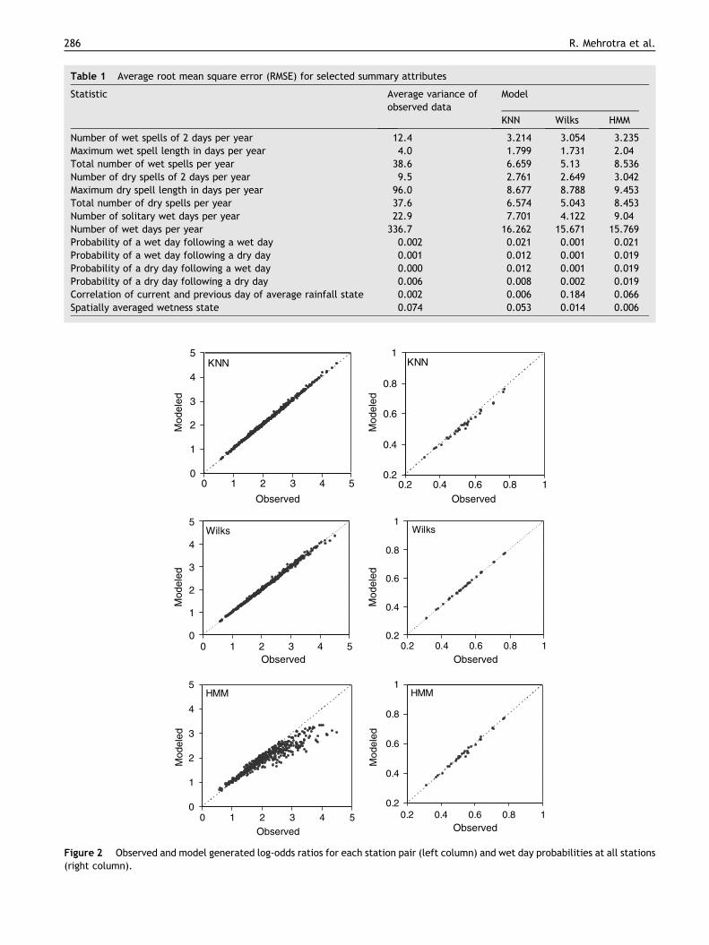
Table 1 Average root mean square error (RMSE) for selected summary attributes

Statistic Average variance ofobserved data

Model

KNN Wilks HMM

Number of wet spells of 2 days per year 12.4 3.214 3.054 3.235Maximum wet spell length in days per year 4.0 1.799 1.731 2.04Total number of wet spells per year 38.6 6.659 5.13 8.536Number of dry spells of 2 days per year 9.5 2.761 2.649 3.042Maximum dry spell length in days per year 96.0 8.677 8.788 9.453Total number of dry spells per year 37.6 6.574 5.043 8.453Number of solitary wet days per year 22.9 7.701 4.122 9.04Number of wet days per year 336.7 16.262 15.671 15.769Probability of a wet day following a wet day 0.002 0.021 0.001 0.021Probability of a wet day following a dry day 0.001 0.012 0.001 0.019Probability of a dry day following a wet day 0.000 0.012 0.001 0.019Probability of a dry day following a dry day 0.006 0.008 0.002 0.019Correlation of current and previous day of average rainfall state 0.002 0.006 0.184 0.066Spatially averaged wetness state 0.074 0.053 0.014 0.006

KNN

0

1

2

3

4

5

0 1 2 3 4 5

Observed Observed

Observed

Observed

Observed

Observed

Mod

eled

Mod

eled

Mod

eled

KNN

0.2

0.4

0.6

0.8

1

0.2 0.4 0.6 0.8 1

Wilks

0

1

2

3

4

5

0 1 2 3 4 5

Wilks

0.2

0.4

0.6

0.8

1

0.2 0.4 0.6 0.8 1

HMM

0

1

2

3

4

5

0 1 2 3 4 5

HMM

0.2

0.4

0.6

0.8

1

0.2 0.4 0.6 0.8 1

Mod

eled

Mod

eled

Mod

eled

Figure 2 Observed and model generated log-odds ratios for each station pair (left column) and wet day probabilities at all stations(right column).

286 R. Mehrotra et al.

A comparison of three stochastic multi-site precipitation occurrence generators 287

the station, rain at station i and no-rain at station j, and no-rain at station i and rain at station j, respectively. This mea-sure of spatial dependence is more apt for representingdependence between discrete variables such as rainfalloccurrence. A high value is indicative of better-defined spa-tial dependence between the variables.

A similar measure of spatial dependence is the compari-son of the spatially averaged wetness state of observed andmodel generated rainfall series. To compare the statistic,following discrete classes of wetness state were formed:equal to zero, 0.1–0.2, . . . , and 0.9–1.0 and percent occur-rence of days falling within each class in the observed andmodelled series were noted.

Fig. 2 presents the observed and modelled log-odds ra-tios at all stations. Each point on the graph indicates the ra-tio evaluated for a pair of rain gauge stations. The last rowof Table 1 provides the RMSE associated with the percentoccurrences of observed and modeled series in the discreteclasses of wetness state. The RMSE is the lowest for the KNNmodel followed by the Wilks approach and HMM.

KNN

0

4

8

12

16

0 84 12 16Observed

Mod

elle

dM

odel

led

Wilks

0

4

8

12

16

HMM

0

4

8

12

16

Mod

elle

d

0 84 12 16Observed

0 84 12 16Observed

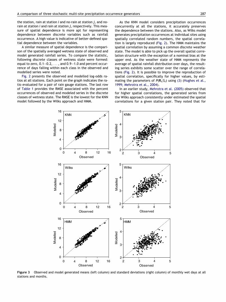
Figure 3 Observed and model generated means (left column) andstations and months.

As the KNN model considers precipitation occurrencesconcurrently at all the stations, it accurately preservesthe dependence between the stations. Also, as Wilks modelgenerates precipitation occurrences at individual sites usingspatially correlated random numbers, the spatial correla-tion is largely reproduced (Fig. 2). The HMM maintains thespatial correlation by assuming a common discrete weatherstate. The model is able to pick up the overall spatial corre-lation structure with the exception of a nominal bias at theupper end. As the weather state of HMM represents theaverage of spatial rainfall distribution over days, the result-ing series exhibits some scatter over the range of correla-tions (Fig. 2). It is possible to improve the reproduction ofspatial correlation, specifically for higher values, by esti-mating the parameters of P(RtjSt) using (3) (Hughes et al.,1999; Mehrotra et al., 2004).

In an earlier study, Mehrotra et al. (2005) observed thatfor higher spatial correlations, the generated series fromthe Wilks approach consistently under estimated the spatialcorrelations for a given station pair. They noted that for

Observed

Mod

elle

dKNN

22

3

3

4

4

5

5

Mod

elle

d

Wilks

2

3

4

5

HMM

2

3

4

5

Mod

elle

d

Observed2 3 4 5

Observed2 3 4 5

standard deviations (right column) of monthly wet days at all

288 R. Mehrotra et al.

highly correlated observations, a large change in the corre-lation between series of normal distributed random num-bers resulted in corresponding small change in thecorrelation between resulting series of rainfall occurrences.They opined that perhaps the trial and error procedureadopted was not efficient enough to pick up those minorchanges for highly correlated station pairs and suggestedeither to use more efficient technique to estimate the rela-tionship between the correlations of the generated seriesand corresponding normal deviates for a given station pairor to use some adjustment factor. Accordingly, in the pres-ent study, we applied a finer termination criterion to esti-mate the relationship using trial and error and alsomodified the correlation matrix of the normal deviates byusing a multiplication factor of 1.05. These adjustmentshelped in fixing the bias in the correlations (Fig. 2).

Wetness fractionReproduction of total number of wet days in a season or thefrequency of a wet day and day to day occurrence of therainfall is essential in simulating the seasonal water balancein any modelling exercise in which the generated rainfallmay be used. Fig. 2 also presents the scatter plots of ob-served and modelled wetness fraction (total wet days di-vided by the total number of days) at all stations. TheRMSE associated with the total number of wet days per yearis presented in Table 1. KNN and Wilks models reproduce thisstatistic accurately for all stations. The HMM also performswell with the exception of some scatter for some stations.All models are also evaluated for their ability to representmonthly statistics. Fig. 3 presents the scatter plots of meannumber of wet days per month and standard deviation of wet

Wet spell probabilities of a day

0.05

0.075

0.1

0.125

0.05 0.075 0.1 0.125

Mod

eled

Wilks KNN HMM

Wet spell probabilities of 7-13 days

0

0.02

0.04

0.06

0.08

0 0.02 0.04 0.06 0.08Observed

Mod

eled

Wilks KNN HMM

Observed

Figure 4 Observed and model generated wet spell probabilities of13 days at all stations.

days per month for all stations and months. In general, allmethods are able to simulate the monthly means fairly well,but have difficulties in representing the monthly standarddeviations. This deficiency is roughly equivalent in all mod-els, and is likely to be the result of the use of a Markov orderone dependence structure, whereas the true persistencemay be of a higher order. The under-representation of theinterannual variability of wet days, as indicated for exampleby the year-to-year variations in monthly or seasonal wetdays, is typically smaller than in the real climate. This isone of the well known problems of daily rainfall generationmodels of the class considered in the present study, (Gregoryet al., 1993; Katz and Parlange, 1993, 1998; Wilks, 1999c)and is not the focus of the present study. However, the useof a mixture of a low and a high order Markovian representa-tion, as outlined in Harrold et al. (2003), in the context ofthe Wilks and KNN models presented here, is expected toincorporate the longer time scale characteristic also in thegenerated rainfall series.

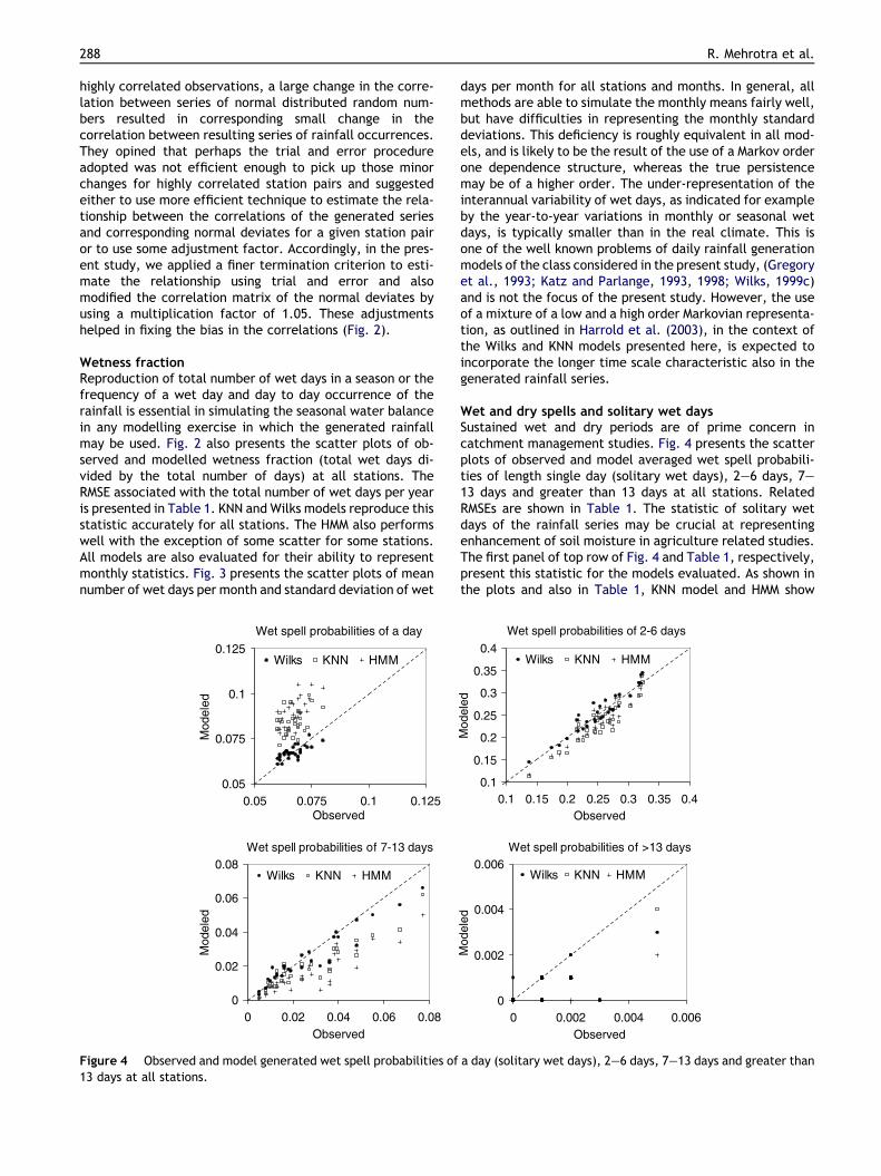
Wet and dry spells and solitary wet daysSustained wet and dry periods are of prime concern incatchment management studies. Fig. 4 presents the scatterplots of observed and model averaged wet spell probabili-ties of length single day (solitary wet days), 2–6 days, 7–13 days and greater than 13 days at all stations. RelatedRMSEs are shown in Table 1. The statistic of solitary wetdays of the rainfall series may be crucial at representingenhancement of soil moisture in agriculture related studies.The first panel of top row of Fig. 4 and Table 1, respectively,present this statistic for the models evaluated. As shown inthe plots and also in Table 1, KNN model and HMM show

Wet spell probabilities of 2-6 days

0.1

0.15

0.2

0.25

0.3

0.35

0.4

0.1 0.15 0.2 0.25 0.3 0.35 0.4

Mod

eled

Wilks KNN HMM

Wet spell probabilities of >13 days

0

0.002

0.004

0.006

0 0.002 0.004 0.006Observed

Observed

Mod

eled

Wilks KNN HMM

a day (solitary wet days), 2–6 days, 7–13 days and greater than

A comparison of three stochastic multi-site precipitation occurrence generators 289

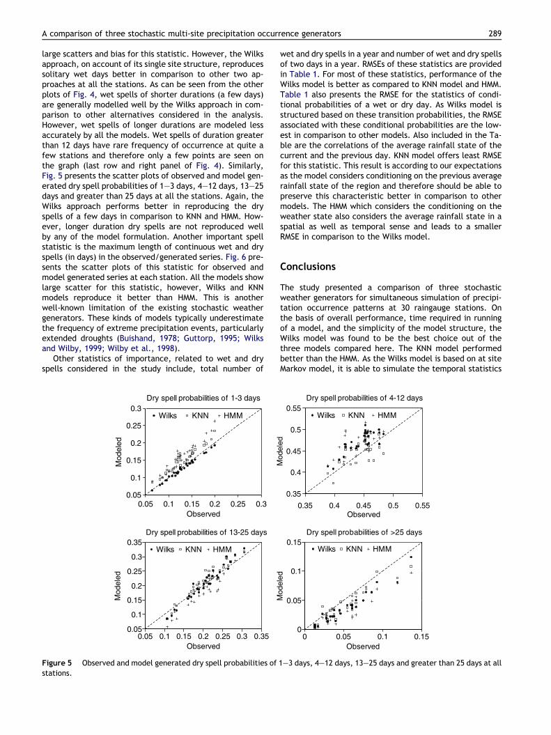
large scatters and bias for this statistic. However, the Wilksapproach, on account of its single site structure, reproducessolitary wet days better in comparison to other two ap-proaches at all the stations. As can be seen from the otherplots of Fig. 4, wet spells of shorter durations (a few days)are generally modelled well by the Wilks approach in com-parison to other alternatives considered in the analysis.However, wet spells of longer durations are modeled lessaccurately by all the models. Wet spells of duration greaterthan 12 days have rare frequency of occurrence at quite afew stations and therefore only a few points are seen onthe graph (last row and right panel of Fig. 4). Similarly,Fig. 5 presents the scatter plots of observed and model gen-erated dry spell probabilities of 1–3 days, 4–12 days, 13–25days and greater than 25 days at all the stations. Again, theWilks approach performs better in reproducing the dryspells of a few days in comparison to KNN and HMM. How-ever, longer duration dry spells are not reproduced wellby any of the model formulation. Another important spellstatistic is the maximum length of continuous wet and dryspells (in days) in the observed/generated series. Fig. 6 pre-sents the scatter plots of this statistic for observed andmodel generated series at each station. All the models showlarge scatter for this statistic, however, Wilks and KNNmodels reproduce it better than HMM. This is anotherwell-known limitation of the existing stochastic weathergenerators. These kinds of models typically underestimatethe frequency of extreme precipitation events, particularlyextended droughts (Buishand, 1978; Guttorp, 1995; Wilksand Wilby, 1999; Wilby et al., 1998).

Other statistics of importance, related to wet and dryspells considered in the study include, total number of

Dry spell probabilities of 1-3 days

0.05

0.1

0.15

0.2

0.25

0.3

0.05 0.1 0.15 0.2 0.25 0.3Observed

Mod

eled

Wilks KNN HMM

Dry spell probabilities of 13-25 days

0.05

0.1

0.15

0.2

0.25

0.3

0.35

0.05 0.1 0.15 0.2 0.25 0.3 0.35Observed

Mod

eled

Wilks KNN HMM

Figure 5 Observed and model generated dry spell probabilities ofstations.

wet and dry spells in a year and number of wet and dry spellsof two days in a year. RMSEs of these statistics are providedin Table 1. For most of these statistics, performance of theWilks model is better as compared to KNN model and HMM.Table 1 also presents the RMSE for the statistics of condi-tional probabilities of a wet or dry day. As Wilks model isstructured based on these transition probabilities, the RMSEassociated with these conditional probabilities are the low-est in comparison to other models. Also included in the Ta-ble are the correlations of the average rainfall state of thecurrent and the previous day. KNN model offers least RMSEfor this statistic. This result is according to our expectationsas the model considers conditioning on the previous averagerainfall state of the region and therefore should be able topreserve this characteristic better in comparison to othermodels. The HMM which considers the conditioning on theweather state also considers the average rainfall state in aspatial as well as temporal sense and leads to a smallerRMSE in comparison to the Wilks model.

Conclusions

The study presented a comparison of three stochasticweather generators for simultaneous simulation of precipi-tation occurrence patterns at 30 raingauge stations. Onthe basis of overall performance, time required in runningof a model, and the simplicity of the model structure, theWilks model was found to be the best choice out of thethree models compared here. The KNN model performedbetter than the HMM. As the Wilks model is based on at siteMarkov model, it is able to simulate the temporal statistics

Dry spell probabilities of 4-12 days

0.35

0.4

0.45

0.5

0.55

0.35 0.4 0.45 0.5 0.55Observed

Mod

eled

Wilks KNN HMM

Dry spell probabilities of >25 days

0

0.05

0.1

0.15

0 0.05 0.1 0.15Observed

Mod

eled

Wilks KNN HMM

1–3 days, 4–12 days, 13–25 days and greater than 25 days at all

KNN

5

10

15

20

5 10 15 20ObservedObserved

Observed

Observed Observed

ObservedM

odel

led

Mod

elle

dM

odel

led

Mod

elle

d

Mod

elle

dM

odel

led

KNN

20

30

40

50

60

70

80

20 30 40 50 60 70 80

Wilks

5

10

15

20

5 10 15 20

Wilks

20

30

40

50

60

70

80

20 30 40 50 60 70 80

5

10

15

20

5 10 15 20

HMMHMM

20

30

40

50

60

70

80

20 30 40 50 60 70 80

Figure 6 Scatter plots of observed and model generated maximum wet (left column) and dry (right column) spell lengths in days atall stations.

290 R. Mehrotra et al.

at individual sites adequately, while use of spatially corre-lated uniform random variables imparts spatial depen-dence. As can be expected, longer time dependence is notpreserved by either Wilks or the other approaches com-pared. A few important findings of the study are summarisedas follows:

The KNN approach considers simultaneous resamplingwith replacement at all stations and therefore is capable ofreproducing the spatial correlation structure quite well.The model used in the study considered the conditioning onaverage wetness fraction of the previous day and reproducedsatisfactorily the various temporal statistics. However, itwas found that the conditioning on average wetness fractionof previous day was not enough to capture the individual sta-tion characteristic like the solitary wet days.

The KNN logic as presented in this paper resamples therainfall at all locations on a given day with replacementand, therefore, results in responses that cannot be differentfrom what was observed. This limitation can be serious ifthe aim is to study changes in extreme rainfall amounts,in which case a different non-parametric method based on

kernel density estimation (Sharma and O’Neill, 2002) canbe used. As our aim is to generate a response that was dis-crete (rainfall occurrence), the above limitation was notrelevant.

The HMM explains the spatial rainfall correlation struc-ture by defining the existence of a weather state. The modelfinds similar spatial rainfall distribution in the rainfall re-cord, and expresses the averaged spatial rainfall distribu-tion as a weather state. As such the model is expected toreproduce the average spatial structure of the weatherstate. The temporal persistence is maintained by assumingthe weather state to be following an order one Markovstructure. As such, with enough number of weather statescapturing all significant rainfall distribution patterns, themodel is expected to reproduce adequately the short termtemporal dependence. The results of the present study con-firm these observations.

In the Wilks approach, some better ways of estimatingthe relationship between correlations of series of normaldeviates and correlations of generated rainfall occurrenceseries are needed. For example, a direct root finding

A comparison of three stochastic multi-site precipitation occurrence generators 291

algorithm as outlined in Press et al. (1986) might be moreconvenient and useful.

Parametric models like HMM and Wilks require largenumber of parameters to maintain the spatial and temporalstructures. For example, in case of HMM with four weatherstates and 30 raingauge stations, number of parametersneeded were 132 for each month. The Wilks approachmakes use of correlated random numbers to maintain spa-tial correlation structure, however, required the wet dayprobability as the solo parameter for each day and stationto reproduce the temporal dependence. For these modelswith the increase in the number of stations and, weatherstates for HMM, the number of parameters of the model al-most grows exponentially. The non-parametric alternativeslike the KNN, on the other hand, do not require specificparameters to be estimated. However, the model requiredvalues of K, number of nearest neighbours; ‘w, length ofmoving window; s, standard deviation of the variables usedin the conditioning vector for each day and b, the values ofinfluence weights for each conditioning variable as the basicinformation to be supplied. Several possible improvementsto these models are worth investigating, including morerealistic spatial dependence structure of HMM and reducedparameterization of HMM and Wilks approach. Some sortof simplicity in HMM can be gained by dividing the study areainto number of homogeneous sub-regions and assigning acommon parameter set to all stations within the sub-region.Combining the days having similar meteorological condi-tions i.e., estimation of wet day probabilities on a monthlyor seasonal basis in the Wilks approach would help in reduc-ing the number of parameters.

The statistics related to longer time scale memory arenot preserved adequately by either of the formulation con-sidered in the study (Figs. 5 and 6). It has been reported thatdaily attributes of precipitation series (e.g., mean, median,variance, mean wet-/dry-spell persistence, etc.) are satis-factorily reproduced, but lower-frequency variations (e.g.,monthly, seasonal and annual means, variances and wet-day frequencies, etc.) are poorly resolved by the type ofstochastic weather generators used in the study (e.g., Buis-hand, 1978; Gregory et al., 1993; Katz and Parlange, 1998;Wilks, 1999c; Wilby et al., 1998; Wilks and Wilby, 1999).This deficiency has wider implications for the generationof realistic hydrological scenarios. Future work will focuson replacing the single-site Markov order one dependencemodel within the Wilks’ framework with an approach thatcan model longer term variability, such as is suggested inHarrold et al. (2003).

Acknowledgements

This work was partially funded by the Australian ResearchCouncil. We acknowledge the constructive comments ofProf. Demetris Koutsoyiannis, whose inputs greatly bene-fited the quality of our presentation.

References

Bardossy, A., Plate, E.J., 1992. Space–time models for daily rainfallusing atmospheric circulation patterns. Water Resour. Res. 28,1247–1259.

Beersma, J.J., Buishand, T.A., 2003. Multi-site simulation of dailyprecipitation and temperature conditional on the atmosphericcirculation. Clim. Res. 25, 121–133.

Bogardi, I., Matyasovszky, I., Bardossy, A., Duckstein, L., 1993.Application of a space–time stochastic model for daily precip-itation using atmospheric circulation patterns. J. Geophys. Res.98 (D6), 16653–16667.

Brandsma, T., Buishand, T.A., 1998. Simulation of extreme precip-itation in the Rhine basin by nearest neighbour resampling.Hydrol. Earth Syst. Sci. 2, 195–209.

Bras, R., Rodriguez-Iturbe, I., 1976. Rainfall generation: a non-stationary time varying multi-dimensional model. Water Resour.Res. 12, 450–456.

Buishand, T.A., 1978. Some remarks on the use of daily rainfallmodels. J. Hydrol. 36, 295–308.

Buishand, T.A., Brandsma, T., 2001. Multi-site simulation of dailyprecipitation and temperature in the Rhine basin by nearest-neighbour resampling. Water Resour. Res. 37, 2761–2776.

Chandler, R.E., Wheater, H.S., 2002. Analysis of rainfall variabilityusing generalized linear models: a case study from the west ofIreland. Water Resour. Res. 38 (10), 1192. doi:10.1029/2001WR00090.

Clark, M.P., Gangopadhyay, S., Hay, L.E., Rajagopalan, B., Wilby,R.L., 2004a. The Schaake shuffle: a method for reconstructingspace–time variability in forecasted precipitation and temper-ature fields. J. Hydrometeorol. 5, 243–262.

Clark, M.P., Gangopadhyay, S., Brandon, D., Werner, K., Hay, l.,Rajagopalan, B., Yates, D., 2004b. A resampling procedure forgenerating conditioned daily weather sequences. Water Resour.Res. W04304. doi:10.1029/2003WR00274.

Gabriel, K.R., Neumann, J., 1962. A Markov chain model for dailyrainfall occurrence at Tel Aviv. J. R. Meteorol. Soc. 88, 90–95.

Georgakakos, K.P., Kavvas, M.L., 1987. Precipitation analysis,modeling, and prediction in hydrology. Rev. Geophys. 25, 163–178.

Gregory, J.M., Wigley, T.M.L., Jones, P.D., 1993. Application ofMarkov models to area-average daily precipitation series andinterannual variability of seasonal totals. Clim. Dyn. 8, 299–310.

Guttorp, P., 1995. Stochastic Modeling of Scientific Data. Chapmanand Hall, London (Chapter 2).

Haan, C.T., Allen, D.M., Street, J.D., 1976. A Markov chain model ofdaily rainfall. Water Resour. Res. 12 (3), 443–449.

Haario, H., Saksman, E., Tamminem, J., 2001. An adaptiveMetropolis algorithm. Bernoulli 7 (2), 223–242.

Harrold, T.I., Sharma, A., Sheather, S.J., 2003. A non-parametricmodel for stochastic generation of daily rainfall occurrence.Water Resour. Res. 39 (10), 1300. doi:10.1029/2003WR00218.

Hay, L., McCabe, J., Wolock, D.M., Ayers, M.A., 1991. Simulation ofprecipitation by weather type analysis. Water Resour. Res. 27,493–501.

Hughes, J.P., Guttorp, P., 1994. A class of stochastic models forrelating synoptic atmospheric patterns to regional hydrologicphenomena. Water Resour. Res. 30 (5), 1535–1546.

Hughes, J.P., Lettenmaier, D.P., Guttorp, P., 1993. A stochasticapproach for assessing the regional circulation patterns to localprecipitation. Water Resour. Res. 29, 3303–3315.

Hughes, J.P., Guttorp, P., Charles, S., 1999. A non-homogeneoushidden Markov model for precipitation occurrence. Appl. Stat.48 (1), 15–30.

Juang, B.H., Rabiner, L.R., 1991. Hidden Markov models for speechrecognition. Technometrics 33, 251–272.

Katz, R.W., Parlange, M.B., 1993. Effects of an index of atmo-spheric circulation on stochastic properties of precipitation.Water Resour. Res. 29, 2335–2344.

Katz, R.W., Parlange, M.B., 1998. Overdispersion phenomenon instochastic modeling of precipitation. J. Clim. 11, 591–601.

Katz, R.W., Zheng, X., 1999. Mixture model for overdispersion ofprecipitation. J. Clim. 12, 2528–2537.

292 R. Mehrotra et al.

Koutsoyiannis, D., Onof, C., Wheater, H.S., 2003. Multivariaterainfall disaggregation at a fine time scale. Water Resour. Res.39 (7), 1173. doi:10.1029/2002WR00160, 1–18.

Lall, U., Sharma, A., 1996. A nearest neighbour bootstrap for timeseries resampling. Water Resour. Res. 32, 679–693.

Lall, U., Rajagopalan, B., Tarboton, D.G., 1996. A non-parametricwet/dry spell model for resampling daily precipitation. WaterResour. Res. 32 (9), 2803–2823.

Marshall, L., Nott, D., Sharma, A., 2004. A comparative study ofMarkov chain Monte Carlo methods for conceptual rainfall-runoffmodelling. Water Resour. Res. 40, W02501. doi:10.1029/2003WR00237.

Mehrotra, R., Sharma, A., 2005. A non-parametric non-homoge-neous hidden Markov model for downscaling of multi-site dailyrainfall occurrences. J. Geophys. Res. 110, D16108.doi:10.1029/2004JD00567.

Mehrotra, R., Sharma, A., 2006. Conditional resampling of hydro-logic time series using multiple predictor variables: A K-nearestneighbour approach. Adv. Water Resour. 29, 987–999.doi:10.1016/j.advwaters.2005.08.007.

Mehrotra, R., Sharma, A., Cordery, I., 2004. A comparison of twoapproaches for downscaling synoptic atmospheric patterns tomulti-site precipitation occurrence. J. Geophys. Res. 109,D14107. doi:10.1029/2004JD00482.

Mehrotra, R., Srikanthan, R., Sharma, A., 2005. Comparison ofthree approaches for stochastic simulation of multi-site precip-itation occurrence. In: Twenty-ninth hydrology and waterresources symposium, Engineers Australia, 21–23 February2005, Canberra, Australia.

Northrop, P.J., 1998. A clustered spatial-temporal model ofrainfall. Proc. R. Soc. Lond. A454, 1875–1888.

Onof, C., Chandler, R.E., Kakou, A., Northrop, P., Wheater, H.S.,Isham, V., 2000. Rainfallmodelling using Poisson-cluster processes:a review of developments. Stoch Env Res Risk A 14, 384–411.

Pegram, G.G.S., Clothier, A.N., 2001. High-resolution space–timemodelling of rainfall: the ‘‘String of Beads’’ model. J. Hydrol.241, 26–41.

Press, W.H., Flannery, B.P., Teukolsky, S.A., Vetterling, W.T.,1986. Numerical Recipes, the Art of Scientific Computing.Cambridge, pp. 818.

Qian, B., Corte-Real, J., Xu, H., 2002. Multi-site stochastic weathermodels for impact studies. Int. J. Climatol 22, 1377–1397.

Rabiner, L.R., Juang, B.H., 1986. An introduction to hidden Markovmodels. IEEE Trans. Acoust. Speech Signal Process. 3, 4–16.

Rajagopalan, B., Lall, U., 1999. A K-nearest neighbour simulator fordaily precipitation and other weather variables. Water Resour.Res. 35 (10), 3089–3101.

Richardson, C.W., 1981. Stochastic simulation of daily precipita-tion, temperature, and solar radiation. Water Resour. Res. 17,182–190.

Salas, J.D., 1993. Analysis and modelling of hydrologic time series.In: Maidment, D.R. (Ed.), Handbook of Hydrology. McGraw-Hill,New York, pp. 19.1–19.72.

Sharma, A., Lall, U., 1999. A non-parametric approach for dailyrainfall simulation. Math. Comput. Simulat. 48, 361–371.

Sharma, A., O’Neill, R., 2002. A non-parametric approach forrepresenting interannual dependence in monthly streamflowsequences. Water Resour. Res. 38 (7), 5.1–5.10.

Souza Filho, F.A., Lall, U., 2003. Seasonal to interannual ensemblestreamflow forecasts for Ceara, Brazil: applications of a multi-variate, semiparametric algorithm. Water Resour. Res. 39 (11),1307. doi:10.1029/2002WR00137.

Srikanthan, R., McMahon, T.A., 1985. Stochastic generation ofrainfall and evaporation data. Technical paper 84, AustralianWater Resources Council, Canberra.

Stehlık, J., Bardossy, A., 2002. Multivariate stochastic downscalingmodel for generating daily precipitation series based on atmo-spheric circulation. J. Hydrol. 256, 120–141.

Waymire, E., Gupta, V.K., Rodriguez-Iturbe, I., 1984. A spectraltheory of rainfall at the meso-b scale. Water Resour. Res. 20,1453–1465.

Wheater, H.S., Isham, V.S., Cox, D.R., Chandler, R.E., Kakou, A.,Northrop, P.J., Oh, L., Onof, C., Rodriguez-Iturbe, I., 2000.Spatial-temporal rainfall fields: modelling and statisticalaspects. Hydrol. Earth Syst. Sci. 4, 581–601.

Wilby, R.L., Wigley, T.M.L., Conway, D., Jones, P.D., Hewiston,B.C., Main, J., Wilks, D.S., 1998. Statistical downscaling ofgeneral circulation model output: a comparison of methods.Water Resour. Res. 34, 2995–3008.

Wilks, D.S., 1998. Multi-site generalization of a daily stochasticprecipitation model. J. Hydrol. 210, 178–191.

Wilks, D.S., 1999a. Simultaneous stochastic simulation of dailyprecipitation, temperature and solar radiation at multiplesites in complex terrain. Agri. Forest Meteorol. 96, 85–101.

Wilks, D.S., 1999b. Multi-site downscaling of daily precipitationwith a stochastic weather generator. Clim. Res. 11, 125–136.

Wilks, D.S., 1999c. Interannual variability and extreme-valuecharacteristics of several stochastic daily precipitation models.Agri. Forest Meteorol. 93, 153–169.

Wilks, D.S., Wilby, R.L., 1999. The weather generator game: areview of stochastic weather models. Prog. Phys. Geogr. 23 (3),329–357.

Wilson, L.L., Lettenmaier, D.P., Skyllingstad, E., 1992. A hierar-chical stochastic model of large-scale atmospheric circulationpatterns and multiple station daily precipitation. J. Geophys.Res. D3, 2791–2809.

Wojcik, R., Buishand, T.A., 2003. Simulation of 6-h rainfall andtemperature by two resampling schemes. J. Hydrol. 273, 69–80.

Woolhiser, D.A., 1992. Modeling daily precipitation – progress andproblems. In: Walden, A.T., Guttorp, P. (Eds.), Statistics in theEnvironmental and Earth Sciences. Wiley, New York, pp. 71–89.

Yates, D., Gangopaghyay, S., Rajagopalan, B., Strzepek, K., 2003. Atechnique for generating regional climate scenarios using anearest-neighbour algorithm. Water Resour. Res. 39 (7),SWC7(1–15).