A Comparison of New Factor Models in the Korean Stock · PDF fileA Comparison of New Factor Models in the Korean ... we report the results from our empirical analyses. ... three-factor

A Comparison of New Factor Models in the Korean

Stock Market

Hankil Kang*

Jangkoo Kang†

Wooyeon Kim‡

Abstract

We compare empirical performance of the Fama and French (2015) five-factor model, the Hou,

Xue, and Zhang (2014) q-factor model, and their variations in the Korean stock market. Among

the models considered, we show that the adjusted five-factor model, which includes the

quarterly-based profitability factor instead of the yearly-based one, best explains the size, value,

investment, and profitability sorted portfolio returns. The adjusted five-factor model

outperforms the other factor models in digesting various anomalies in the Korean market.

JEL classification: G12

Keywords: the Fama-French five-factor model; the Hou-Xue-Zhang four-factor model; cross-

section of stock returns

* College of Business, Korea Advanced Institute of Science and Technology (KAIST), Seoul, Korea. E-mail: [email protected]. † Graduate School of Finance & Accounting, College of Business, Korea Advanced Institute of Science and Technology (KAIST), Seoul, Korea. E-mail: [email protected]. ‡ Corresponding author: College of Business, Korea Advanced Institute of Science and Technology (KAIST), Seoul, Korea. Phone+82-2-958-3693, Fax+82-959-4645, E-mail:[email protected].

A Comparison of New Factor Models in the Korean

Stock Market

Abstract

We compare empirical performance of the Fama and French (2015) five-factor model, the Hou,

Xue, and Zhang (2014) q-factor model, and their variations in the Korean stock market. Among

the models considered, we show that the adjusted five-factor model, which includes the

quarterly-based profitability factor instead of the yearly-based one, best explains the size, value,

investment, and profitability sorted portfolio returns. The adjusted five-factor model

outperforms the other factor models in digesting various anomalies in the Korean market.

JEL classification: G12

Keywords: the Fama-French five-factor model; the Hou-Xue-Zhang four-factor model; cross-

section of stock returns

3

1 Introduction

After the failure of the capital asset pricing model (CAPM) to explain the cross-section of stock

returns, a host of previous literature has sought to uncover its behavior. Fama and French (1992) show

that size and book-to-market equity do a major role in explaining the cross-section of average stock

returns in the U.S. stock market. Continuing from this result, Fama and French (1993) (FF henceforth)

build a three-factor model to capture the relation between average return and size, and the relation

between average return and book-to-market. Although the FF three-factor model summarizes the

cross-section of average stock returns better than the CAPM, it appears that the model fails to capture

myriad market anomalies.1

In recent years, a number of factor models based on the q-theory of firm investment are introduced.

Cooper, Gulen and Schill (2008) document that asset growth, which is a proxy for firm’s investment,

is closely related to the expected returns. Chen, Novy-Marx and Zhang (2011) suggest an alternative

three-factor model from the q-theory with the market, investment-to-assets, and return-on equity as its

factors. Hou, Xue and Zhang (2014) (HXZ henceforth) propose an empirical q-factor model

consisting of the market factor, a size factor, an investment-to-assets factor, and a return-on-equity

factor. They argue that the q-factor model performs better than the FF three-factor model and the

Carhart (1997) four-factor model in explaining stock market anomalies in the U.S. market.

Motivated by Novy-Marx (2013) gross profitability premium and Miller and Modigliani (1961),

Fama and French (2015) add a profitability factor and an investment factor to their three-factor model

and propose the FF five-factor model. They show that the FF five-factor model outperforms the FF

three-factor model. Hou, Xue and Zhang (2016), however, sustain their empirical q-factor model in

the sense that the q-factor model outperforms the FF five-factor model in digesting a number of

market anomalies.

Researchers try to examine whether the well-known cross-sectional patterns in the U.S. stock

1Examples include Ang, Hodrick, Xing and Zhang (2006); Cooper, Gulen and Schill (2008); Daniel and Titman (2006); Fama and French (1996).

4

market also exist in the Korean stock market, and they try to find an asset pricing model that best

explains the cross-section of expected returns. Kim, Kim and Shin (2012) compare performance of

various asset pricing models including variations of CAPM and CCAPM, the FF three-factor model,

and the Chen-Novy-Marx-Zhang three-factor model. Kim (2014) tests empirical asset pricing models

which work well in the Korean stock market based on FF (2015). Lee and Ohk (2015) compares the

FF three-factor model and the Chen, Novy-Marx and Zhang (2011) three-factor model, focusing on

the models’ ability to explain the various anomalies in the Korean market. However, the empirical

evidence of the cross-section of the stock returns in the Korean market is mixed across various sample

periods and data management methodologies.

This paper aims to compare performances of the FF five-factor model and the HXZ q-factor model,

and their variations using the Korean stock data. First, we test whether the size, book-to-market,

profitability, or investment effect exists in the Korean market. Second, we discuss the performance of

alternative asset pricing models in describing the cross-section of portfolio returns sorted on size,

book-to-market, profitability, and investment. Third, we consider a variety of anomaly variables in the

U.S. market, and test whether our candidate models well explains the significant anomalies in the

Korean market.

Our empirical findings can be summarized as follows. First, we find that in our July 2002 to June

2014 sample, we observe the value, profitability, and investment effect in the Korean market.

Especially for the profitability effect, we find that the profitability variable should be based on

quarterly earnings data following Hou, Xue and Zhang (2014) instead of annual profitability measure

in Fama and French (2015) to exhibit strong cross-sectional pattern. Second, the adjusted FF five-

factor model with the quarterly profitability factor outperforms the FF three-factor model, the FF five-

factor model, and the HXZ four-factor model in explaining the portfolio returns sorted on the size,

book-to-market, profitability, or investment-sorted portfolios and significant anomaly portfolios.

This paper makes further contribution especially in the following three points. First, we examine

whether the size, value, profitability, or investment effect exists in the Korean market. Second, we

5

cover the FF five-factor model and its subordinate models as well as the HXZ q-factor model.

Specifically, we suggest the adjusted five-factor model which shows better performance than the FF

five-factor model and the HXZ model. We show that the quarterly-based profitability measure is

closely related to the cross-section of returns and that the HML factor has strong explanatory power

unlike the U.S. market. Third, we investigate which model performs well in digesting significant

anomalies. By doing this, we also examine whether various stock market anomalies exist in the

Korean market. Compared to Lee and Ohk (2015), we only use significant anomalies to our asset

pricing tests.

This paper is organized as follows. Section 2 describes the dataset, the asset pricing models, and

empirical methodology including measure construction, factor construction, and portfolio formation.

In section 3, we report the results from our empirical analyses. Section 4 concludes.

2 Data and Empirical Methodology

2.1 Data Source and New Factor Models

Monthly stock returns and accounting information are from FN-DataGuide. We use all non-financial

stocks in the KOSPI and KOSDAQ market. We exclude stocks with negative book equity and stocks

with non-December fiscal year-ends. Our sample period is from July 2002 to June 2015 with the

following two reasons. First, we need to include KOSDAQ stocks, which have been listed since 1996,

to have enough number of firms in our portfolios. Second and more importantly, we use quarterly-

based accounting information, which is available after 2000, to construct the quarterly profitability

measure. We use the one-year monetary stabilization bond yields from the Economic Statistic System

(ECOS) in the Bank of Korea as the risk-free rate.

2.1.1 The FF (2015) five-factor Model

Fama and French (2015) add a profitability factor (RMW) and an investment factor (CMA) to their

6

three-factor model in Fama and French (1993) to capture the variation in average returns related to

profitability and investment. This five-factor model is written as the following:

E (1)

in which E is the expected excess return, is the market excess return, (small-

minus-big) is the difference between the returns on diversified portfolios of small and big stocks,

(high-minus-low) is the difference between the returns on diversified portfolios of high and low

book-to-market stocks, (robust-minus-weak) is the difference between the returns on

diversified portfolios of robust and weak profitability stocks, and (conservative-minus-

aggressive) is the difference between the returns on diversified portfolios of low and high investment

stocks. The slopes , , , and are the exposures to the five factors.

2.1.1 The HXZ (2014) q-factor Model

Hou, Xue and Zhang (2014) construct a new empirical model inspired by investment-based asset

pricing, which is built on the q-theory of investment. They argue that the expected excess return is

described by the market factor, the size factor, the investment factor, and the profitability factor. Their

q-factor model is formally written as the following:

E E E / E / E (2)

In the equation, E is the expected excess return. is the market excess return,

is the difference between the returns on diversified portfolios of small and big stocks, / is the

difference between the returns on diversified portfolios of low and high investment-to-assets stocks,

and is the difference between the returns on diversified portfolios of high and low ROE stocks.

The factor loadings on , , / , and are denoted as , , / , and ,

respectively. In the subsequent paper, Hou, Xue and Zhang (2016) conclude that the four-factor q-

factor model outperforms the Fama-French five factor model in digesting a number of anomalies in

the U.S. stock market.

7

2.2 Measure Construction and Empirical Properties

We measure Size as the market capitalization. We measure B/M as book equity at the end of the fiscal

year ending in 1 divided by the market capitalization at the end of December of year t 1.

Investment, Inv, is measured as the annual change of total assets from the fiscal year ending in year

2 to the year 1 divided by total assets at the fiscal year ending in year 2. We follow

Fama and French (2015) to construct operating profitability (OP), which is measured as operating

profit divided by book equity for the fiscal year ending in year 1.2

Hou, Xue and Zhang (2016) argue that the most recent quarterly earnings announcement contains

the latest information on future profitability. To incorporate their argument, we measure quarterly

operating profitability (OPq) in the same way we did to construct OP, except that we use operating

profit and book equity of the last quarter, not the last year. To avoid possible problems due to the late

announcement of quarterly earnings, we apply one more lag both on earnings and book equity.3

Before we construct factor portfolios, we first examine whether the average returns of our

portfolios in the Korean market formed on size, book-to-market, investment, and profitability exhibit

the known patterns in the U.S. stock market. The reported portfolio returns are in excess of the

implied monthly returns of one-year monetary stabilization bond yields. Following Fama and French

(1993), at the end of June each year, we sort stocks by Size, B/M, Inv, OP, and OPq using the KOSPI

breakpoints. We choose 4 by 4 double sorts instead of 5 by 5 sorts to have enough number of firms in

each portfolio.

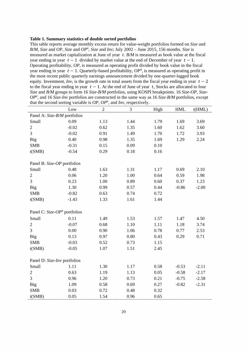
Table 1 depicts average monthly excess returns of value-weight portfolios formed on (1) Size and

B/M, and (2) Size and OP, and (3) Size and OPq, and (4) Size and Inv. In each Panel of Table 1, we

2 Although HXZ (2014, 2016) use income before extraordinary items instead of operating profits to measure ROE, we mainly follow FF (2015) here for the numerator of the profitability measure. 3 In Korea, for firms whose fiscal year-end is December, Q1, Q2, Q3 and Q4 earnings reports should be submitted to Financial Supervisory Service (FSS) before/on May 16, August 16, November 14, and March 30, respectively, and are announced few days later. For example, in April of year , we use quarterly data reported for Q3 of year 1 instead of those reported for Q4 of year 1 to take account of possible delays in quarterly reports.

8

report monthly excess returns of 16 double-sorted portfolios, together with the small-minus-big and

high-minus-low excess returns and their t-statistics.

Panel A of Table 1 shows the pattern of average excess returns of 16 Size-B/M portfolios. In each

size quartile, average excess return increases from low B/M stocks to high B/M stocks, and high-

minus-low excess returns are significantly positive. This clearly indicates that there exists the value

effect in our sample. However, in the lowest B/M quartile, the average small-minus-big excess return

is negative. In the other B/M quartiles, small-minus-big excess returns are positive but insignificant.

This result is robust in Panels B, C, and D of Table 1. Out of 16 small-minus-big excess returns, three

are negative, and only one excess return in Panel C is significantly positive with 1.15% of monthly

average. Therefore, we see no size effect in our sample.

Panel B of Table 1 shows average monthly excess percent returns for 16 Size-OP portfolios. Except

for the last row, high-minus-low excess returns are positive. However, only high-minus-low returns in

the two smaller quartiles are significant. Moreover, for the biggest stocks, the pattern of returns is in

reverse direction and high-minus-low excess return is significantly negative (-0.86% a month). Thus,

it is in doubt that there is the profitability effect in the Korean stock market when the sorting variable

is annual OP.

Panel C of Table 1 reports average monthly excess percent returns for 16 Size-OPq portfolios.

Compared to the Size-OP portfolios in Panel B, we see stronger evidence that the profitability effect

exists in the Size-OPq portfolios. High-minus-low returns are positive and significant with one

exception, again the biggest stocks. Motivated by this observation, we measure the profitability as

OPq rather than OP, since quarterly profitability measure generates stronger expected return patterns

in the Korean market.

Panel D of Table 1 shows average monthly excess percent returns for 16 Size-Inv portfolios. The

investment effect appears in the Korean stock market, because high-minus-low excess return is

significantly negative for each size row with values from -0.53% to -0.82%. This result implies that

there is strong investment effect in the Korean market.

9

To summarize the performance of portfolios sorted on Size, B/M, Inv, OP, and OPq in our sample,

we observe strong return patterns sorted on B/M, OPq, and Inv. However, we find weaker evidence

that Size and OP are closely related to the cross-section of stock returns in the Korean market.

3.3 Factor Construction

FF (2015) construct the size, B/M, profitability and investment factors in three different ways: (1)

2 3 sorts on Size and B/M, or Size and OP, or Size and Inv, and (2) 2 2 sorts on Size and B/M, or

Size and OP, or Size and Inv, and (3) 2 2 2 2 sorts on Size, B/M, OP, and Inv. We follow their

approach to construct factors in the Korean stock market. However, as shown in the previous

subsection, portfolios formed on OP have weak patterns of average returns, while portfolios formed

on OPq have stronger empirical patterns in our sample. Therefore, we substitute OPq in place of OP in

our factor construction.

The 2 3 sort is a familiar and usual way as Fama and French (1993) did. Taking the intersection

of the two Size and three B/M groups, six portfolios are formed. The Size breakpoint is the KOSPI

median and the B/M breakpoint is the 30th and 70th percentiles of the KOSPI stocks. We define

SMBB/M as the average of three small size portfolios minus three big size portfolios and the value

factor, HML, as the average of two high B/M portfolios minus two low B/M portfolios. Repeating the

same procedure, SMBOPq and the profitability factor RMWq, SMBInv and the investment factor CMA

can be similarly defined. Lastly, the size factor SMB is defined as the average of the size factors from

each 2 3 sort: SMBB/M, SMBOPq, and SMBInv. The 2 2 sort is not different from the 2 3 sort,

except that the breakpoint of B/M (or OPq, Inv) is the KOSPI median instead of the 30th and 70th

percentiles (or OPq, Inv, respectively).

In the 2 2 2 2 sort, Size, B/M, OPq, and Inv are jointly controlled, taking intersection of the

two Size, two B/M, two OPq, and two Inv groups. For each variable, the breakpoint is the KOSPI

median. SMB is defined as the average of 8 small portfolios minus 8 big portfolios. HML, RMWq,

and CMA are similarly defined. In the 2 2 2 2 sorts, each factor better isolates the premium in

10

average returns related to the other three factors.

Table 2 reports summary statistics of average factor returns following FF (2015). Panel A of Table 2

shows means, standard deviations, and t-statistics for the five factors in each version of factor

construction. Panel B of Table 2 shows the correlation matrices across the five factors in each version

of factor construction. Panel C of Table 2 shows the correlation matrices between different versions of

each factor.

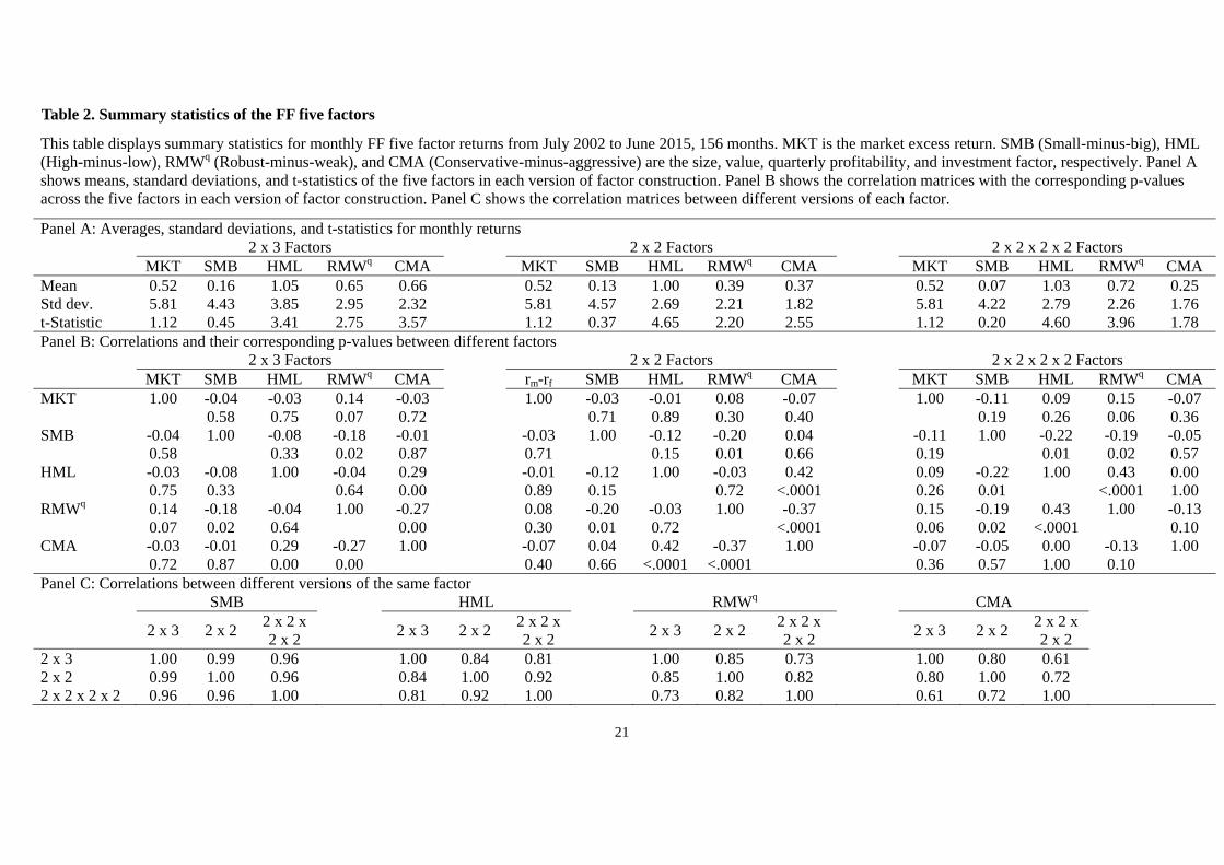
In Panel A of Table 2, we report the averages, standard deviations, and the corresponding t-statistics

of the FF factors. The average SMB return is 0.16% in the 2 3 sort, which is not statistically

significant. Consistent with the results in Table 1, we observe no significant size premium in our

sample, which is robust across the sorting method. HML earns more than monthly 1% returns, which

is highly significant and robust to the sorting method. In the 2 3 sort, RMWq and CMA earn about

0.65% monthly and highly significant. However, the mean returns of RMWq and CMA vary

significantly with their sorting method. Specifically, RMWq earns 0.39% and 0.72% in the 2 2 and

2 2 2 2 sorts, and CMA earns 0.37% and 0.25% in the 2 2 and 2 2 2 2 sorts.

In Panel B of Table 2, we show correlations of the FF factors. Notably, we find high correlation of

CMA and RMWq to the other factors in the double sorts. CMA is positively correlated with HML and

negatively correlated with RMWq, and RMWq is negatively correlated with SMB. Given that

correlations, we understand the results that RMWq and CMA returns are quite different in the

2 2 2 2 sorts because they are highly correlated with the others. In addition, we report

correlations between different versions of the same factor in Panel C of Table 2. As shown in Panel A,

SMB and HML seem quite robust across the sorting method. RMWq is less robust with its lowest

correlation of 0.73, and CMA is the least robust with its lowest correlation of 0.61.

To summarize, the mean excess returns of the factors are highest in the 2 3 sort with an

exception of RMWq. Especially, CMA earns much higher return in the 2 3 sort. Therefore, we use

the factors from the classical 2 3 sort in our subsequent analyses. We use this 2 3 sorted

measure not only to follow FF (2015), but also to reflect the empirical properties in the Korean market.

11

Although not reported in Table 2, RMW from the annual OP measure earns insignificant average

returns.

HXZ (2014) construct the q-factors from an independent 2 3 3 sort on Size, OPq, and Inv in

order to control for size when constructing the investment and the profitability factors. Taking the

intersection of the two Size, the three Inv, and the three OPq groups, total 18 portfolios are formed.

The Size breakpoint is the KOSPI median. The OPq and Inv breakpoints are the 30th and 70th

percentiles of KOSPI stocks, respectively. The size factor, , is the difference between the average

return of 9 small size portfolios and the average return of 9 big size portfolios. The investment factor,

/ , is the difference between the average return of 6 low Inv portfolios and the average return of 6

high Inv portfolios. Lastly, the profitability factor, , is the difference between the average return

of 6 high OPq portfolios and the average return of 6 low OPq portfolios.

According to Hou, Xue and Zhang (2016), the empirical difference between the HXZ factors and

the FF factors is twofold. First, the quarterly ROE measure is different from the annual OP measure.

Second, HXZ use triple sort, whereas FF use 2 3 double sort. In this paper, we use the same

sorting variable in constructing FF and HXZ profitability factors. Therefore, we do not have the first

difference, and the only difference between SMB, HML, and RMWq and , / and in this

paper is in the sorting method.

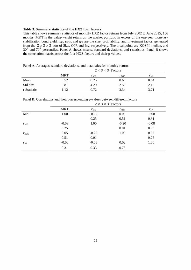
Table 3 reports the summary statistics of the q-factors in the Korean market. In Panel A, the

overall average returns are quite similar to those in Table 2. Although earns 0.25% monthly,

which is greater than 0.16% of SMB from the 2 3 sort, it is still statistically insignificant. In Panel

B, except for the -0.20 correlation between and , we find modest correlations among the

factors, with their absolute values less than 0.1.

12

3 Empirical Evidence

3.1 Performance of the Alternative Models

In this subsection, we report the performance of alternative asset pricing models to explain the

cross section of portfolios in the Korean market. If an asset pricing model describes the expected

returns well, the intercept from a time-series regression of excess asset returns on the factors should

be indistinguishable from zero. To test whether the intercepts are not jointly different from zero for all

portfolios, we employ the GRS tests developed by Gibbons, Ross and Shanken (1989). The GRS

statistic is computed as follows:

GRS (3)

In the GRS statistic, and represent the number of test portfolios and factors, respectively. is

an 1 vector of estimated intercepts, is an unbiased estimate of the residual covariance matrix,

is an 1 vector of the factor portfolios’ sample means where is the number of factors, and

is an unbiased estimate of the factor portfolios’ covariance matrix. Under the null hypothesis that all

intercepts of the assets are jointly zero, the GRS statistics have the F-distribution with degree of

freedom and . In this paper, the GRS statistic and the corresponding p-value are used

to measure model performances.

As documented in the previous section, the annual profitability factor, RMW, earns insignificant

average returns in our sample. Therefore, we focus on the FF five-factor model with the quarterly

profitability factor, RMWq. We call this five factor model as the adjusted FF five-factor model

throughout this paper.

Table 4 reports the model performance summary of (1) the FF three-factor model, (2) three four-

factor models with MKT, SMB, and two factors of HML, RMWq, and CMA, (3) the adjusted FF five-

factor model with MKT, SMB, HML, RMWq, and CMA. The test assets in Panel A, B, C, and D are

16 value-weight portfolios sorted on Size-B/M, Size-OP, Size-OPq, and Size-Inv, respectively. We

13

report the GRS statistic with its corresponding p-value, together with the average absolute value of the

intercept. In each column, we use the factors with different sorting methods, namely, the 2 3,

2 2, and 2 2 2 2 sorts. The regression equations are as follows:

(4)

where denotes the vector of factors. For example, for the FF three-factor model,

. In every regression in this paper, we use Newey and West (1987) standard

errors with four lags to adjust for possible heteroscedasticity and autocorrelations to calculate the t-

statistics and the GRS statistics.

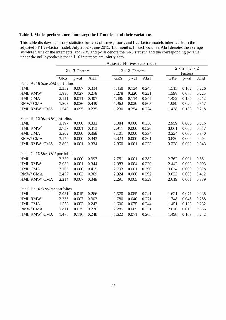
We summarize the results in Table 4 in the following three observations. First, the adjusted FF five-

factor model outperforms the FF three-factor model and the four-factor models. The GRS statistic

tends to attain its minimum value when the five factors are used. Especially, we cannot reject the five-

factor model in Panel A and D in 5% level of significance. This implies that the profitability and

investment factors help explaining the cross-section of returns in the Korean market. Second, unlike

Fama and French (2015) in the U.S. market, the HML factor is not redundant in the Korean market.

Comparing the fourth and fifth rows of each Panel, we observe the GRS statistic and the average

absolute intercept decrease when HML is introduced. Third, the quarterly profitability factor, RMWq,

has an important role in explaining the Size-B/M, Size-OP, and Size-OPq portfolios. We find large

decreases of the GRS statistic and the average absolute intercept in the fifth rows of Panel A, B, and C,

compared the third rows where RMWq is missing. This confirms that our use of the quarterly

profitability factor is important in capturing the expected returns in the Korean market, compared to

the results in Kim (2014) who uses annual profitability factor and finds weak evidence for its

explanatory power.

Hou, Xue and Zhang (2016) argue that the empirical performance of their four-factor model is

better than that of the FF five-factor model. Lee and Ohk (2015) show that the three-factor Chen,

Novy-Marx and Zhang (2011) model with the market, investment, and profitability factors

outperforms the FF three-factor model in the Korean market. Hence, we compare the FF three-factor

14

model, the original and adjusted FF five-factor model, and the HXZ four-factor model in Table 5. We

introduce one more variation of the HXZ model, which is the augmented HXZ model. The augmented

HXZ model uses MKT, , , / , and HML as its factors. We compare this model and the

adjusted FF five-factor model to see the effect of different sorting method in factor construction. As

noted in the last section, the only difference between the HXZ factors and the FF factors in this paper

is in sorting method. Since Hou, Xue and Zhang (2016) argue that the joint control in sorting stocks is

important and affects the empirical performance, we test whether the triple sort is better in the Korean

market.

In Panel A, B, C, and D of Table 5, we use Size-B/M, Size-OP, Size-OPq, and Size-Inv portfolios as

test assets, respectively. We use five competing asset pricing models: the FF three-factor model (FF3),

the FF five-factor model which uses annual RMW as its profitability factor (FF5), the FF five-factor

model with quarterly RMWq factor (AdjFF5), the HXZ four-factor model (HXZ), and the augmented

HXZ model which uses MKT, HML, , / , and as its factors (AugHXZ). Similar to Table

4, we report the GRS statistic with its p-value, and the average absolute intercept for each model. All

factors used in the FF models are 2 3 sorted.

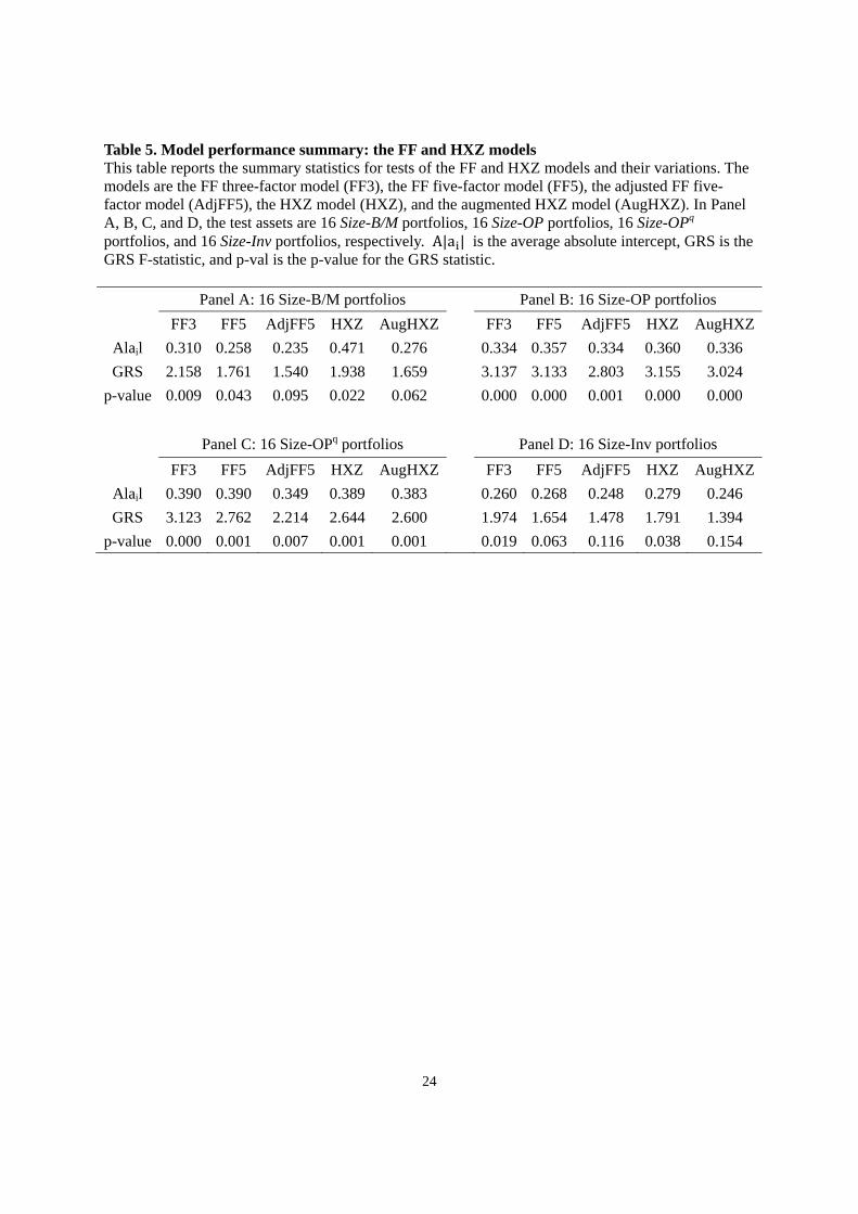
In Table 5, we first observe that the adjusted FF five-factor model always performs better than the

original FF five-factor model. The adjusted model generates lower GRS statistics and average

absolute intercepts. Therefore, the use of quarterly profitability factor instead of the annual one is

crucial in explaining the cross-section of stock returns in the Korean market. This result is consistent

with one of the critiques in Hou, Xue and Zhang (2016) that more recent profitability data have more

correct information about the firm’s profitability. Second, the adjusted FF five-factor model and

augmented HXZ five-factor model always perform better than the HXZ four-factor model.

Specifically, in Panel A and D, the adjusted FF five-factor model and augmented HXZ model are not

rejected in the GRS test, whereas the original HXZ model is rejected in every Panel. This verifies that

unlike the U.S. market, the HML factor is not redundant and helps explaining the cross-section of

expected returns even in the existence of the other factors. Third, the adjusted FF five-factor model is

15

better than the augmented HXZ five-factor model in Panels A, B, and C. The only difference between

the two models is in the sorting method to construct the size, profitability, and investment factors.

Although Hou, Xue and Zhang (2016) argue that their triple sort does a better job in empirical tests,

that is not the case in our sample.

The results from the asset pricing tests in Table 5 indicate that HML, RMWq, and CMA have their

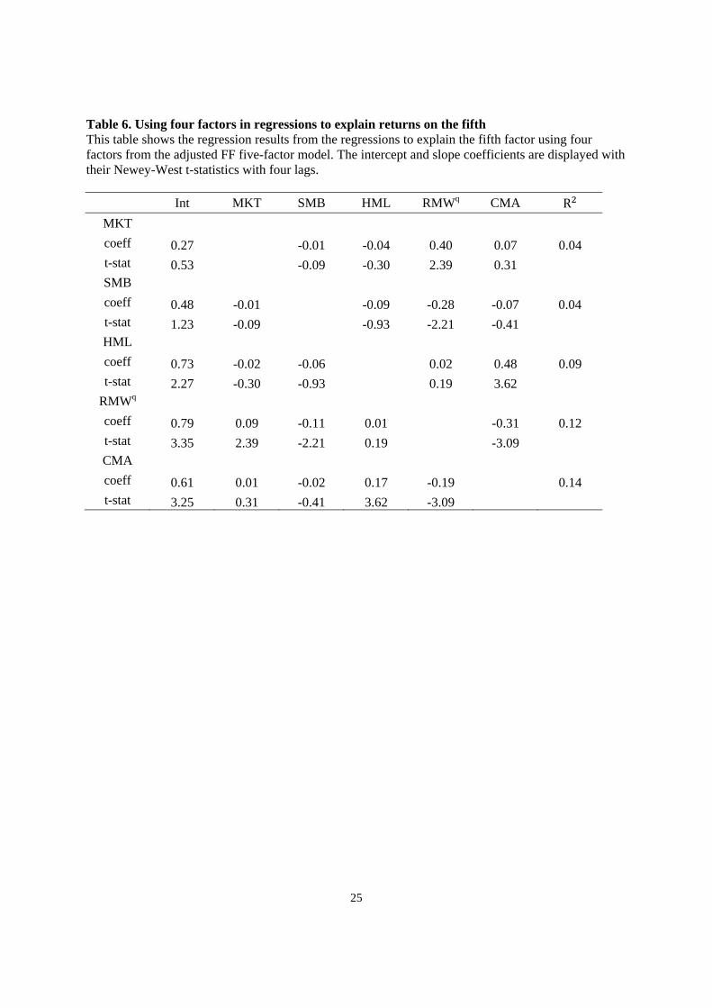
own roles in pricing the cross-section of returns. We take a further step to test this argument. In Table

6, we regress one of the adjusted FF five factors (MKT, SMB, HML, RMWq, and CMA) on the other

four factors. We focus on the intercepts, which are the factor returns unexplained by the remaining

four. If the intercept of one dependent variable is insignificant, it means that the other four factors

span the factor, which also implies that the factor is redundant in explaining the cross-section of

returns in existence of the others.

The intercepts of HML, RMWq, and CMA in Table 6 are positive and significant. The estimated

intercepts are 0.73%, 0.79%, 0.61% per month, respectively. Compared to their time-series averages

in Table 2, which are 1.05%, 0.65%, 0.66%, the unexplained parts of the factors are still substantial.

In the RMWq case, the intercept is even greater than its time-series average. In contrast, the intercepts

from the regressions of MKT and SMB are 0.27% and 0.48%. The SMB intercept is three times

greater than its original time-series mean (0.16%). However, it is still statistically insignificant. The

overall level of the s is quite low, with the maximum value of 0.14. In sum, the unexplained

portion of the factors is quite large and it is only significantly positive in HML, RMWq, and CMA

cases. Therefore, we assure that those three factors are not subsumed by the others, so that each of

them has its own role in explaining the cross-section of expected returns.

To summarize our horse-racing results in this subsection, we find that the adjusted FF five-factor

model best explains the cross-section of portfolios sorted in Size, B/M, OP (OPq), or Inv. Especially, it

is not rejected when the test assets are sorted by Size-B/M or Size-Inv. In addition, the HML, RMWq,

and CMA are not redundant in the Korean market in presence of the other factors. In the next

subsection, we further investigate the performance of the asset pricing models in this paper to explain

16

a broad collection of anomalies in the Korean stock market.

3.2 Digesting Anomalies

In this subsection, we perform empirical horse races with the FF3, FF5, adjusted FF5, and HXZ

models in capturing various anomalies in the Korean market. We consider a subset of anomalies

discussed in Hou, Xue and Zhang (2014). The list of 34 anomalies and their definitions are in

Appendix. The selected anomalies are categorized into five groups: value, investment, profitability,

intangibles, and momentum. For each anomaly, we construct value-weight decile portfolios with

KOSPI breakpoints, and examine whether the tenth-minus-first excess returns are significantly

positive.

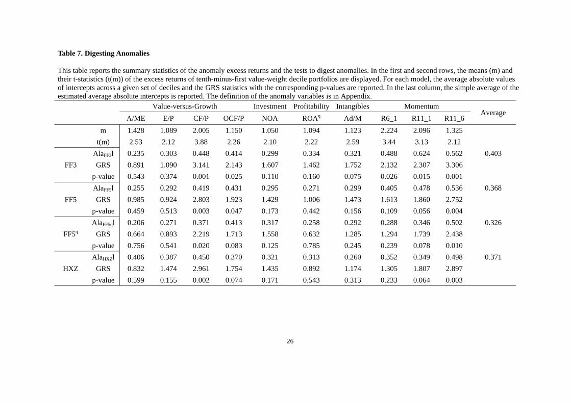
Table 7 reports the results of digesting 10 anomalies which are significant in our sample. In the first

and second rows, we report the mean of the tenth-minus-first excess returns for each anomaly and its

t-statistics. We report the average absolute alphas from 10 portfolios, the GRS statistics and their p-

values for each asset pricing model.

The monthly anomaly excess returns exhibit 1.05% to 2.23%. In momentum portfolio returns, Ri_j

stands for the one-month returns calculated from the portfolios sorted on the holding period returns

from 1 to 1 . We observe strong momentum returns in our sample with various

specifications of formation periods (R6_1, R11_1, and R11_6). The significant R11_6 excess return is

called the intermediate term momentum, which is documented in Novy-Marx (2012).

The average absolute alphas from the FF three-factor model range in 0.23% ~ 0.62% with the mean

of 0.4%, and the GRS statistic cannot reject the model in three anomalies. Although the FF three-

factor model helps explaining some anomalies, it is not enough to digest the anomalies. The FF five-

factor model shows some improvement from the FF three-factor model. The mean of average absolute

alphas is 0.37%, and we cannot reject the FF five-factor model with 5% level of significance in 7 out

of 10 anomalies. The adjusted FF five-factor model shows the best performance among the tested

17

models. Its mean of average absolute alphas is 0.32%, and it cannot be rejected in 8 out of 10

anomalies. The performance of the HXZ model is comparable to that of the FF five-factor model. The

mean of average absolute intercepts is 0.37%, and it is not rejected in 8 anomalies.

Comparing the adjusted FF five-factor model and the HXZ model, the adjusted FF five-factor

model dominates the HXZ model in six anomalies in the sense that it generates lower average

absolute intercepts and lower GRS statistics, whereas the HXZ model dominates only in one anomaly.

The two anomaly portfolios that are not explained by the tested models are those sorted on cash flow-

to-price (CF/P) and R11_6. Although the adjusted five-factor model cannot digest the intermediate

term momentum, it helps explaining various anomaly portfolio returns which are related to size, value,

investment, profitability, and momentum. Also, its ability to digest anomalies is stronger than that of

the FF three-factor model, the FF five-factor model, and the HXZ four-factor model. The results from

the analysis in this section confirm the superiority of the adjusted FF five-factor model in capturing

the cross-section of expected returns in the Korean stock market.

4 Conclusion

This paper compares newly introduced asset pricing models in the Korean stock market. The asset

pricing models tested are the FF three-factor model, the FF five-factor model, the HXZ q-factor model

and their variations. To evaluate asset pricing models, we mainly perform time-series regressions of

test portfolios sorted on size, book-to-market, profitability, investment, and other anomaly variables.

We use the average absolute intercepts the GRS F-statistics as our criteria to compare the pricing

performance.

The overall results show that the adjusted FF five-factor model with the quarterly-based

profitability factor best describes the cross-section of stock returns in Korea. The results indicate that

the value factor, HML, is an important factor under the existence of the investment and profitability

factors, and that the use of RMWq, the quarterly-based profitability factor is crucial in improving the

18

asset pricing performance. In addition, we find strong evidence that the adjusted five-factor model

shows best performance in digesting various anomaly returns in the Korean market including

momentum.

19

References

Ang, Andrew, Robert J Hodrick, Yuhang Xing, and Xiaoyan Zhang, 2006, The cross‐section of volatility and expected returns, The Journal of Finance 61, 259-299.

Carhart, Mark M, 1997, On persistence in mutual fund performance, Journal of finance 52, 57-82. Chen, Long, Robert Novy-Marx, and Lu Zhang, 2011, An alternative three-factor model, Working

Paper. Cooper, Michael J, Huseyin Gulen, and Michael J Schill, 2008, Asset growth and the cross‐section of

stock returns, The Journal of Finance 63, 1609-1651. Daniel, Kent, and Sheridan Titman, 2006, Market reactions to tangible and intangible information,

The Journal of Finance 61, 1605-1643. Fama, Eugene F, and Kenneth R French, 1992, The cross‐section of expected stock returns, Journal of

Finance 47, 427-465. Fama, Eugene F, and Kenneth R French, 1993, Common risk factors in the returns on stocks and

bonds, Journal of Financial Economics 33, 3-56. Fama, Eugene F, and Kenneth R French, 1996, Multifactor explanations of asset pricing anomalies,

The journal of finance 51, 55-84. Fama, Eugene F, and Kenneth R French, 2015, A five-factor asset pricing model, Journal of Financial

Economics 116, 1-22. Gibbons, Michael R, Stephen A Ross, and Jay Shanken, 1989, A test of the efficiency of a given

portfolio, Econometrica 1121-1152. Hou, Kewei, Chen Xue, and Lu Zhang, 2014, Digesting anomalies: An investment approach, Review

of Financial Studies hhu068. Hou, Kewei, Chen Xue, and Lu Zhang, 2016, A comparison of new factor models, Working Paper. Kim, Dong Hoe, 2014, Asset pricing model in korean stock market, The Korean Journal of Financial

Engineering 13, 87-119. Kim, Soon-Ho, Dongcheol Kim, and Hyun-Soo Shin, 2012, Evaluating asset pricing models in the

korean stock market, Pacific-Basin Finance Journal 20, 198-227. Lee, Minkyu, and Ki Yool Ohk, 2015, Market anomalies and multifactor models: Comparison

between the ff model and the cnz model, Korean Journal of Financial Studies 44. Miller, Merton H, and Franco Modigliani, 1961, Dividend policy, growth, and the valuation of shares,

the Journal of Business 34, 411-433. Newey, Whitney K, and Kenneth D West, 1987, A simple, positive semi-definite, heteroskedasticity

and autocorrelation consistent covariance matrix, Econometrica 55, 703-708. Novy-Marx, Robert, 2012, Is momentum really momentum?, Journal of Financial Economics 103,

429-453. Novy-Marx, Robert, 2013, The other side of value: The gross profitability premium, Journal of

Financial Economics 108, 1-28.

20

Table 1. Summary statistics of double sorted portfolios This table reports average monthly excess return for value-weight portfolios formed on Size and B/M, Size and OP, Size and OPq, Size and Inv; July 2002 – June 2015, 156 months. Size is measured as market capitalization at June of year . B/M is measured as book value at the fiscal year ending in year 1 divided by market value at the end of December of year 1. Operating profitability, OP, is measured as operating profit divided by book value in the fiscal year ending in year 1. Quarterly-based profitability, OPq, is measured as operating profit in the most recent public quarterly earnings announcement divided by one-quarter-lagged book equity. Investment, Inv, is the growth rate in total assets from the fiscal year ending in year 2 to the fiscal year ending in year 1. At the end of June of year , Stocks are allocated to four Size and B/M groups to form 16 Size-B/M portfolios, using KOSPI breakpoints. 16 Size-OP, Size- OPq, and 16 Size-Inv portfolios are constructed in the same way as 16 Size-B/M portfolios, except that the second sorting variable is OP, OPq, and Inv, respectively.

Low 2 3 High HML t(HML) Panel A: Size-B/M portfolios Small 0.09 1.13 1.44 1.79 1.69 3.69 2 -0.02 0.62 1.35 1.60 1.62 3.60 3 -0.02 0.91 1.49 1.70 1.72 3.93 Big 0.40 0.98 1.35 1.69 1.29 2.24 SMB -0.31 0.15 0.09 0.10 t(SMB) -0.54 0.29 0.18 0.16

Panel B: Size-OP portfolios Small 0.48 1.63 1.31 1.17 0.69 2.10 2 0.06 1.20 1.00 0.64 0.59 1.98 3 0.23 1.00 0.89 0.60 0.37 1.23 Big 1.30 0.99 0.57 0.44 -0.86 -2.00 SMB -0.82 0.63 0.74 0.72 t(SMB) -1.43 1.33 1.61 1.44

Panel C: Size-OPq portfolios

Small 0.11 1.49 1.53 1.57 1.47 4.50 2 -0.07 0.68 1.10 1.11 1.18 3.74 3 0.00 0.90 1.06 0.78 0.77 2.53 Big 0.13 0.97 0.80 0.43 0.29 0.71 SMB -0.03 0.52 0.73 1.15 t(SMB) -0.05 1.07 1.51 2.45

Panel D: Size-Inv portfolios Small 1.11 1.30 1.17 0.58 -0.53 -2.11 2 0.63 1.19 1.13 0.05 -0.58 -2.17 3 0.96 1.20 0.73 0.21 -0.75 -2.58 Big 1.09 0.58 0.69 0.27 -0.82 -2.31 SMB 0.03 0.72 0.48 0.32 t(SMB) 0.05 1.54 0.96 0.65

21

Table 2. Summary statistics of the FF five factors

This table displays summary statistics for monthly FF five factor returns from July 2002 to June 2015, 156 months. MKT is the market excess return. SMB (Small-minus-big), HML (High-minus-low), RMWq (Robust-minus-weak), and CMA (Conservative-minus-aggressive) are the size, value, quarterly profitability, and investment factor, respectively. Panel A shows means, standard deviations, and t-statistics of the five factors in each version of factor construction. Panel B shows the correlation matrices with the corresponding p-values across the five factors in each version of factor construction. Panel C shows the correlation matrices between different versions of each factor.

Panel A: Averages, standard deviations, and t-statistics for monthly returns 2 x 3 Factors 2 x 2 Factors 2 x 2 x 2 x 2 Factors

MKT SMB HML RMWq CMA MKT SMB HML RMWq CMA MKT SMB HML RMWq CMA Mean 0.52 0.16 1.05 0.65 0.66 0.52 0.13 1.00 0.39 0.37 0.52 0.07 1.03 0.72 0.25 Std dev. 5.81 4.43 3.85 2.95 2.32 5.81 4.57 2.69 2.21 1.82 5.81 4.22 2.79 2.26 1.76 t-Statistic 1.12 0.45 3.41 2.75 3.57 1.12 0.37 4.65 2.20 2.55 1.12 0.20 4.60 3.96 1.78 Panel B: Correlations and their corresponding p-values between different factors

2 x 3 Factors 2 x 2 Factors 2 x 2 x 2 x 2 Factors MKT SMB HML RMWq CMA rm-rf SMB HML RMWq CMA MKT SMB HML RMWq CMA

MKT 1.00 -0.04 -0.03 0.14 -0.03 1.00 -0.03 -0.01 0.08 -0.07 1.00 -0.11 0.09 0.15 -0.07 0.58 0.75 0.07 0.72 0.71 0.89 0.30 0.40 0.19 0.26 0.06 0.36

SMB -0.04 1.00 -0.08 -0.18 -0.01 -0.03 1.00 -0.12 -0.20 0.04 -0.11 1.00 -0.22 -0.19 -0.05 0.58 0.33 0.02 0.87 0.71 0.15 0.01 0.66 0.19 0.01 0.02 0.57

HML -0.03 -0.08 1.00 -0.04 0.29 -0.01 -0.12 1.00 -0.03 0.42 0.09 -0.22 1.00 0.43 0.00 0.75 0.33 0.64 0.00 0.89 0.15 0.72 <.0001 0.26 0.01 <.0001 1.00

RMWq 0.14 -0.18 -0.04 1.00 -0.27 0.08 -0.20 -0.03 1.00 -0.37 0.15 -0.19 0.43 1.00 -0.13 0.07 0.02 0.64 0.00 0.30 0.01 0.72 <.0001 0.06 0.02 <.0001 0.10

CMA -0.03 -0.01 0.29 -0.27 1.00 -0.07 0.04 0.42 -0.37 1.00 -0.07 -0.05 0.00 -0.13 1.00 0.72 0.87 0.00 0.00 0.40 0.66 <.0001 <.0001 0.36 0.57 1.00 0.10 Panel C: Correlations between different versions of the same factor

SMB HML RMWq CMA

2 x 3 2 x 2 2 x 2 x 2 x 2

2 x 3 2 x 2 2 x 2 x 2 x 2

2 x 3 2 x 2 2 x 2 x 2 x 2

2 x 3 2 x 2 2 x 2 x 2 x 2

2 x 3 1.00 0.99 0.96 1.00 0.84 0.81 1.00 0.85 0.73 1.00 0.80 0.61 2 x 2 0.99 1.00 0.96 0.84 1.00 0.92 0.85 1.00 0.82 0.80 1.00 0.72 2 x 2 x 2 x 2 0.96 0.96 1.00 0.81 0.92 1.00 0.73 0.82 1.00 0.61 0.72 1.00

22

Table 3. Summary statistics of the HXZ four factors This table shows summary statistics of monthly HXZ factor returns from July 2002 to June 2015, 156 months. MKT is the value-weight return on the market portfolio in excess of the one-year monetary stabilization bond yield. rME, rROE, and rI/A are the size, profitability, and investment factor, generated from the 2 3 3 sort of Size, OPq, and Inv, respectively. The breakpoints are KOSPI median, and 30th and 70th percentiles. Panel A shows means, standard deviations, and t-statistics. Panel B shows the correlation matrix across the four HXZ factors and their p-values.

Panel A: Averages, standard deviations, and t-statistics for monthly returns 2 3 3 Factors

MKT rME rROE rI/A

Mean 0.52 0.25 0.68 0.64 Std dev. 5.81 4.29 2.53 2.15 t-Statistic 1.12 0.72 3.34 3.71

Panel B: Correlations and their corresponding p-values between different factors 2 3 3 Factors

MKT rME rROE rI/A

MKT 1.00 -0.09 0.05 -0.08 0.25 0.51 0.31

rME -0.09 1.00 -0.20 -0.08 0.25 0.01 0.33

rROE 0.05 -0.20 1.00 0.02 0.51 0.01 0.78

rI/A -0.08 -0.08 0.02 1.00

0.31 0.33 0.78

23

Table 4. Model performance summary: the FF models and their variations

This table displays summary statistics for tests of three-, four-, and five-factor models inherited from the adjusted FF five-factor model; July 2002 - June 2015, 156 months. In each column, Alail denotes the average absolute value of the intercepts, and GRS and p-val denote the GRS statistic and the corresponding p-value under the null hypothesis that all 16 intercepts are jointly zero.

Adjusted FF five-factor model

2 3 Factors

2 2 Factors

2 2 2 2

Factors GRS p-val Alail GRS p-val Alail GRS p-val AlailPanel A: 16 Size-B/M portfolios HML 2.232 0.007 0.334 1.458 0.124 0.245 1.515 0.102 0.226HML RMWq 1.886 0.027 0.278 1.278 0.220 0.221 1.598 0.077 0.225HML CMA 2.111 0.011 0.307 1.486 0.114 0.247 1.432 0.136 0.212RMWq CMA 1.805 0.036 0.439 1.962 0.020 0.505 1.959 0.020 0.517HML RMWq CMA 1.540 0.095 0.235 1.230 0.254 0.224 1.438 0.133 0.218

Panel B: 16 Size-OP portfolios HML 3.197 0.000 0.331 3.084 0.000 0.330 2.959 0.000 0.316HML RMWq 2.737 0.001 0.313 2.911 0.000 0.320 3.061 0.000 0.317HML CMA 3.502 0.000 0.359 3.101 0.000 0.334 3.224 0.000 0.340RMWq CMA 3.150 0.000 0.343 3.323 0.000 0.361 3.826 0.000 0.404HML RMWq CMA 2.803 0.001 0.334 2.850 0.001 0.323 3.228 0.000 0.343

Panel C: 16 Size-OPq portfolios HML 3.220 0.000 0.397 2.751 0.001 0.382 2.762 0.001 0.351HML RMWq 2.636 0.001 0.344 2.383 0.004 0.320 2.442 0.003 0.003HML CMA 3.105 0.000 0.415 2.793 0.001 0.390 3.034 0.000 0.378RMWq CMA 2.477 0.002 0.369 2.924 0.000 0.392 3.022 0.000 0.412HML RMWq CMA 2.214 0.007 0.349 2.291 0.005 0.329 2.619 0.001 0.339

Panel D: 16 Size-Inv portfolios HML 2.031 0.015 0.266 1.570 0.085 0.241 1.621 0.071 0.238HML RMWq 2.233 0.007 0.303 1.780 0.040 0.271 1.748 0.045 0.258HML CMA 1.578 0.083 0.243 1.606 0.075 0.244 1.451 0.128 0.232RMWq CMA 1.811 0.035 0.270 2.285 0.005 0.331 2.076 0.013 0.356HML RMWq CMA 1.478 0.116 0.248 1.622 0.071 0.263 1.498 0.109 0.242

24

Table 5. Model performance summary: the FF and HXZ models This table reports the summary statistics for tests of the FF and HXZ models and their variations. The models are the FF three-factor model (FF3), the FF five-factor model (FF5), the adjusted FF five-factor model (AdjFF5), the HXZ model (HXZ), and the augmented HXZ model (AugHXZ). In Panel A, B, C, and D, the test assets are 16 Size-B/M portfolios, 16 Size-OP portfolios, 16 Size-OPq portfolios, and 16 Size-Inv portfolios, respectively. A|a | is the average absolute intercept, GRS is the GRS F-statistic, and p-val is the p-value for the GRS statistic. Panel A: 16 Size-B/M portfolios Panel B: 16 Size-OP portfolios

FF3 FF5 AdjFF5 HXZ AugHXZ FF3 FF5 AdjFF5 HXZ AugHXZ

Alail 0.310 0.258 0.235 0.471 0.276 0.334 0.357 0.334 0.360 0.336

GRS 2.158 1.761 1.540 1.938 1.659 3.137 3.133 2.803 3.155 3.024

p-value 0.009 0.043 0.095 0.022 0.062 0.000 0.000 0.001 0.000 0.000

Panel C: 16 Size-OPq portfolios Panel D: 16 Size-Inv portfolios

FF3 FF5 AdjFF5 HXZ AugHXZ FF3 FF5 AdjFF5 HXZ AugHXZ

Alail 0.390 0.390 0.349 0.389 0.383 0.260 0.268 0.248 0.279 0.246

GRS 3.123 2.762 2.214 2.644 2.600 1.974 1.654 1.478 1.791 1.394

p-value 0.000 0.001 0.007 0.001 0.001 0.019 0.063 0.116 0.038 0.154

25

Table 6. Using four factors in regressions to explain returns on the fifth This table shows the regression results from the regressions to explain the fifth factor using four factors from the adjusted FF five-factor model. The intercept and slope coefficients are displayed with their Newey-West t-statistics with four lags.

Int MKT SMB HML RMWq CMA R

MKT

coeff 0.27 -0.01 -0.04 0.40 0.07 0.04 t-stat 0.53 -0.09 -0.30 2.39 0.31 SMB

coeff 0.48 -0.01 -0.09 -0.28 -0.07 0.04 t-stat 1.23 -0.09 -0.93 -2.21 -0.41 HML

coeff 0.73 -0.02 -0.06 0.02 0.48 0.09 t-stat 2.27 -0.30 -0.93 0.19 3.62

RMWq

coeff 0.79 0.09 -0.11 0.01 -0.31 0.12 t-stat 3.35 2.39 -2.21 0.19 -3.09 CMA

coeff 0.61 0.01 -0.02 0.17 -0.19 0.14 t-stat 3.25 0.31 -0.41 3.62 -3.09

26

Table 7. Digesting Anomalies

This table reports the summary statistics of the anomaly excess returns and the tests to digest anomalies. In the first and second rows, the means (m) and their t-statistics (t(m)) of the excess returns of tenth-minus-first value-weight decile portfolios are displayed. For each model, the average absolute values of intercepts across a given set of deciles and the GRS statistics with the corresponding p-values are reported. In the last column, the simple average of the estimated average absolute intercepts is reported. The definition of the anomaly variables is in Appendix.

Value-versus-Growth Investment Profitability Intangibles Momentum Average

A/ME E/P CF/P OCF/P NOA ROAq Ad/M R6_1 R11_1 R11_6

m 1.428 1.089 2.005 1.150 1.050 1.094 1.123 2.224 2.096 1.325

t(m) 2.53 2.12 3.88 2.26 2.10 2.22 2.59 3.44 3.13 2.12

FF3

AlaFF3l 0.235 0.303 0.448 0.414 0.299 0.334 0.321 0.488 0.624 0.562 0.403

GRS 0.891 1.090 3.141 2.143 1.607 1.462 1.752 2.132 2.307 3.306

p-value 0.543 0.374 0.001 0.025 0.110 0.160 0.075 0.026 0.015 0.001

FF5

AlaFF5l 0.255 0.292 0.419 0.431 0.295 0.271 0.299 0.405 0.478 0.536 0.368

GRS 0.985 0.924 2.803 1.923 1.429 1.006 1.473 1.613 1.860 2.752

p-value 0.459 0.513 0.003 0.047 0.173 0.442 0.156 0.109 0.056 0.004

FF5q

AlaFF5ql 0.206 0.271 0.371 0.413 0.317 0.258 0.292 0.288 0.346 0.502 0.326

GRS 0.664 0.893 2.219 1.713 1.558 0.632 1.285 1.294 1.739 2.438

p-value 0.756 0.541 0.020 0.083 0.125 0.785 0.245 0.239 0.078 0.010

HXZ

AlaHXZl 0.406 0.387 0.450 0.370 0.321 0.313 0.260 0.352 0.349 0.498 0.371

GRS 0.832 1.474 2.961 1.754 1.435 0.892 1.174 1.305 1.807 2.897

p-value 0.599 0.155 0.002 0.074 0.171 0.543 0.313 0.233 0.064 0.003

27

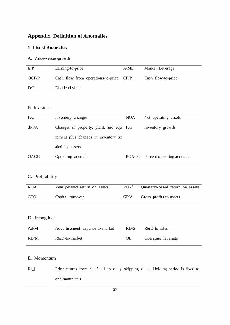
Appendix. Definition of Anomalies

1. List of Anomalies

A. Value-versus-growth

E/P

OCF/P

D/P

Earning-to-price

Cash flow from operations-to-price

Dividend yield

A/ME

CF/P

Market Leverage

Cash flow-to-price

B. Investment

IvC

dPI/A

OACC

Inventory changes

Changes in property, plant, and equ

ipment plus changes in inventory sc

aled by assets

Operating accruals

NOA

IvG

POACC

Net operating assets

Inventory growth

Percent operating accruals

C. Profitability

ROA

CTO

Yearly-based return on assets

Capital turnover

ROAq

GP/A

Quarterly-based return on assets

Gross profits-to-assets

D. Intangibles

Ad/M

RD/M

Advertisement expense-to-market

R&D-to-market

RD/S

OL

R&D-to-sales

Operating leverage

E. Momentum

Ri_j Prior returns from 1 to , skipping 1. Holding period is fixed to

one-month at .

28

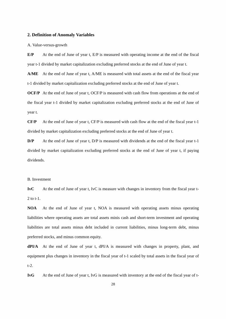
2. Definition of Anomaly Variables

A. Value-versus-growth

E/P At the end of June of year t, E/P is measured with operating income at the end of the fiscal

year t-1 divided by market capitalization excluding preferred stocks at the end of June of year t.

A/ME At the end of June of year t, A/ME is measured with total assets at the end of the fiscal year

t-1 divided by market capitalization excluding preferred stocks at the end of June of year t.

OCF/P At the end of June of year t, OCF/P is measured with cash flow from operations at the end of

the fiscal year t-1 divided by market capitalization excluding preferred stocks at the end of June of

year t.

CF/P At the end of June of year t, CF/P is measured with cash flow at the end of the fiscal year t-1

divided by market capitalization excluding preferred stocks at the end of June of year t.

D/P At the end of June of year t, D/P is measured with dividends at the end of the fiscal year t-1

divided by market capitalization excluding preferred stocks at the end of June of year t, if paying

dividends.

B. Investment

IvC At the end of June of year t, IvC is measure with changes in inventory from the fiscal year t-

2 to t-1.

NOA At the end of June of year t, NOA is measured with operating assets minus operating

liabilities where operating assets are total assets minis cash and short-term investment and operating

liabilities are total assets minus debt included in current liabilities, minus long-term debt, minus

preferred stocks, and minus common equity.

dPI/A At the end of June of year t, dPI/A is measured with changes in property, plant, and

equipment plus changes in inventory in the fiscal year of t-1 scaled by total assets in the fiscal year of

t-2.

IvG At the end of June of year t, IvG is measured with inventory at the end of the fiscal year of t-

29

1 divided by inventory at the end of the fiscal year of t-1, minus one. In other word, it is the growth

rate of inventory from the fiscal year t-2 to t-1.

OACC At the end of June of year t, OACC is measured with net incomes minus cash flow from

operation at the end of the fiscal year of t-1 divided by one-year-lagged total assets.

POACC At the end of June of year t, POACC is measured with net incomes minus cash flow from

operations at the end of the fiscal year of t-1 divided by net incomes at the end of the fiscal year of t-1.

C. Profitability

ROA At the end of June of year t, ROA is measured with operating profit at the end of the fiscal

year of t-1 divided by total assets at the end of the fiscal year of t-1.

ROAq In each month, ROAq is measured with operating profit in the most recent public quarterly

earnings announcement divided by one-quarter-lagged total assets.

CTO At the end of June of year t, CTO is measured with sales at the end of the fiscal year of t-1

divided by one-year-lagged total assets.

GP/A At the end of June of year t, GP/A is measured with sales minus cost of good sold scaled by

total assets at the end of the fiscal year of t-1.

D. Intangibles

Ad/M At the end of June of year t, Ad/M is measured with advertisement expenses at the end of the

fiscal year of t-1 divided by market capitalization at the end of June of year t.

RD/S At the end of June of year t, RD/S is measured with R&D expenses divided by sales at the

end of the fiscal year of t-1, if R&D expenses are positive.

RD/M At the end of June of year t, RD/M is measured with R&D expenses at the end of the fiscal

year of t-1 divided by market capitalization at the end of June of year t.

OL At the end of June of year t, OL is measured with cost of goods sold plus selling, general, and administrative expenses, all divided by total assets at the end of the fiscal year of t-1.