An Empirical Comparison of Predictive Power of One-Factor Yield Curve Models Hideaki Ishibashi Doctoral Program in Quantitative Finance and Management Advised by Isao Shoji Submitted to the Graduate School of System and Information Engineering in Partial Ful¯llment of the Requirements for the Degree of Master of Quantitative Finance and Management at the University of Tsukuba January 2002

Welcome message from author
This document is posted to help you gain knowledge. Please leave a comment to let me know what you think about it! Share it to your friends and learn new things together.
Transcript

An Empirical Comparison of PredictivePower of One-Factor Yield Curve Models
Hideaki Ishibashi
Doctoral Program in Quantitative Finance andManagement
Advised by Isao Shoji
Submitted to the Graduate School ofSystem and Information Engineering
in Partial Ful¯llment of the Requirementsfor the Degree of Master of
Quantitative Finance and Managementat the
University of Tsukuba
January 2002

An Empirical Comparison of PredictivePower of One-Factor Yield Curve Models 1
Hideaki Ishibashi 2
Abstract
The main goal of this paper is to compare the predictive power ofone-factor term structure models of short-term interest rate. Thosemodels are focused on the class of one-factor models proposed byChan, Karolyi, Longsta®, and Sanders (1992,hereafter CKLS) thatincludes a wide range of notable one-factor models, though the classdoes not include all possible one-factor models. The conclusion isdi®erent from prior evidence of short-term interest rates analysis. I¯nd strong evidence for the mean reverting feature in short-term yieldcurves. And the volatility of interest rates should be proportional tothe level of the rate in the models built in mean reverting process inthe drift term.
Keywords: Equilibrium term structure models, Spot rate models.
1I gratefully acknowledge the constructive comments and suggestions from I.Shoji andH.Takamizawa.
2Graduate School of System and Information Engineering University of Tsukuba,[email protected]

Contents1 Introduction 2
2 Spot Rate Models 122.1 The continuous-time spot rate models . . . . . . . . . . . . . . 122.2 Estimation method . . . . . . . . . . . . . . . . . . . . . . . . 162.3 The Spot Rate Data . . . . . . . . . . . . . . . . . . . . . . . 182.4 Empirical Results . . . . . . . . . . . . . . . . . . . . . . . . . 19
3 The Term Structure Models 213.1 Market Price of Risk . . . . . . . . . . . . . . . . . . . . . . . 213.2 Closed Form Solutions . . . . . . . . . . . . . . . . . . . . . . 22
3.2.1 A±ne Models . . . . . . . . . . . . . . . . . . . . . . . 223.2.2 Merton Model . . . . . . . . . . . . . . . . . . . . . . . 233.2.3 The Vasicek Model . . . . . . . . . . . . . . . . . . . . 243.2.4 The Cox, Ingersoll, Ross Model . . . . . . . . . . . . . 25
3.3 Approximation by the Local Linear Method . . . . . . . . . . 263.4 The In-sample Yield Data . . . . . . . . . . . . . . . . . . . . 273.5 The Empirical Results . . . . . . . . . . . . . . . . . . . . . . 27
4 Forecasting 284.1 Root Mean Squared Forecast Error . . . . . . . . . . . . . . . 284.2 The Out-of-sample Yield Data . . . . . . . . . . . . . . . . . . 284.3 The Principal Components Analysis of yields . . . . . . . . . . 294.4 Empirical Results . . . . . . . . . . . . . . . . . . . . . . . . . 29
5 Concluding Remarks 33
1

1 Introduction
The term structure of interest rates models are important in many ¯-
nancial economics models, such as interest rate-related bets in ¯xed income
portfolio( e.g. duration bets and yield curve bets), bond pricing models,
derivative securities pricing models, careful selections of assumptions of in-
terest rates, e®ective risk management including value-at-risk calculations
and yield curves models to make reasonable assumptions about how each
rate moves relative to others. The dynamics of ¯xed income instruments
are essentially the dynamics of a curve rather than the dynamics of a sin-
gle stochastic process. Particularly, short-term interest rates are taken as
reference rates for other interest rates and also an essential feature of the
monetary transmission mechanism described in Duguay (1994). More over,
Barry Cozier and Greg Tkacz (1994) described that the term structure of
interest rates has been used to forecast a plethora of economic variables; fu-
ture levels of interest, the in°ation rate, consumption growth, and output
growth. In the present paper we focus primarily on the term structure's
ability to forecast short-term yield curve.
There are two di®erent type of term structure model, equilibrium mod-
els and arbitrage-free models. Equilibrium models usually start to assume
2

economic variables and a process for the short-term rate. Examples of the
equilibrium models include the models of Vasicek (1977), Dothan (1978),
Cox, Ingersoll, and Ross (1985), Brennan and Schwartz (1979) and Longsta®
and Schwartz (1992). Equilibrium models don't take bond prices as given
and don't constrain the model's prices to match the markets. Therefore,
Equilibrium models are criticized because they do not ¯t the existing term
structure. Although parameters can be chosen to minimize errors from to-
day's yield curve, the ¯t will not be perfect. Whereas, when a trader want
to buy a set of Treasury bonds and to sell another set, he uses °attening or
steepening of the term structure by using some models to determine which
bonds to buy and which to sell. What is called yield curve bet trading.
Arbitrage-free models are of no use for this purpose. And more, the simplest
approach to risk reduction, duration hedging, is widely used in practice.
Hedging exposure to parallel changes in the yield curve is the most typical
use of duration hedging in ¯xed income markets.
Wesley Phoa (2000) described that since parallel and slope shifts are the
dominant yield curve risk factors, it makes sense to focus on measures of
parallel and slope risk; to structure limits in terms of maxi-mum parallel and
slope risk rather than more rigid limits for each point of the yield curve; and
3

to design °exible hedging strategies based on matching parallel and slope
risk. If the desk as a whole takes proprietary interest rate risk positions,
it is most e±cient to specify these in terms of target exposures to parallel
and slope risk, and leave it to individual traders to structure their exposures
using speci¯c instruments.
The parameters of equilibrium models are estimated from historical data
or generated by market views and they don't change from day to day largely.
Therefore, their use over time, is internally consistent.
On the other hand, arbitrage-free models which assume that ¯nancial
markets have no arbitrage opportunities. Heath, Jarrow, Morton (1992, here-
after HJM) generalize the arbitrage-free framework by modeling the forward
rates derived from the current yield curve. The continuous time model of Ho
and Lee (1986, hereafter Ho-Lee) is the simplest case of the HJM framework.
Neftci(2000) described that the HJM approach is clearly the more appro-
priate philosophy to adopt from the point of arbitrage-free pricing. However,
it appears that market practice still prefers the Equilibrium term structure
approach and continues to use spot-rate modeling one way or another. It
is also true that there are signi¯cant resources invested in spot-rate models
both ¯nancially and time-wise. There is a great deal of familiarity with the
4

spot-rate models, and it may be that they provide good approximations to
arbitrage-free prices anyway.
One-factor models assume that movements of the entire term structure
can be summarized by the movements of short-term rate. But given the
change in the short-term rate, the change in any other long yield can be easily
determined from the model. This is a major weakness of the one-factor yield
curve model. Therefore, those models will fail to protect against changes in
the shape of the yield curve, whether against °attening, steepening or other
twists.
While much of the recent academic literature we review focuses on one-
factor models, it is widely known, at least since Litterman and Scheinkman
(1991), that at least three factors are needed fully to capture the variability of
interest rates. And many multifactor traditional a±ne models are proposed
as follows. Longsta® and Schwartz, (1992), Brown and Schaefer(1994), Singh,
Manoj (1995), Balduzzi, Das, Foresi, and Sundaram. (1996), Chen, L. (1996),
Gong, F. F. and Remolona. (1996). Anderson and Lund (1997), Qiang
Dai and Kenneth Singleton(1997), Kobayashi and Ochi(1997), Du®ee(2000).
Those main conclusion is that multifactor models are desired to describe
yield curve's level, slope, twist including long-term yield.
5

But these empirical studies are about long-term yield curve. Then, how
about short-term yield curve? Is it not same as long-term yield curve?
Why then consider one-factor models? As documented in Litterman and
Scheinkman (1991), roughly ninety percent of the variation in Treasury rates
can be explained by the ¯rst factor, which can be interpreted as corresponding
to changes in the general level of interest rates. Thus, any relation between
the level of interest rates and their expected changes and volatilities will be
dominated by the in°uence of this ¯rst factor. In one-factor models, this
factor is typically identi¯ed with the instantaneous or short rate of interest.
The recent academic literature studying(e.g. Chapman and Pearson(2001))
the behavior of the yields on short-term bonds or deposits can be interpreted
as a detailed explanation of the ¯rst factor, using the yield on a particu-
lar instrument (1-month yield )as a proxy for the short rate. Particularly,
dramatic changes in the yield curve can typically be attributed almost to
the ¯rst principal component. The assumption of a single factor is not as
restrictive as it might appear. An one-factor model implies that all move in
the same direction over any short time interval, but not that they all move
by the same amount. It does not imply that the term structure always has
the same shape. A fairly rich pattern of term structure can describe under a
6

one-factor model. And for purposes of comparing the CKLS results, we use
one-factor models better.
Gregory R. Du®ee (2000) describes as follows.The reason why only a sin-
gle factor will a®ect long-maturity bond yields is practical, not theoretical.
There are a variety of types of shocks that a®ect the term structure (e.g.,
level, slope, twist), and multifactor models capture this variety through fac-
tors that die out at di®erent rates under the equivalent martingale measure.
In principle, we could construct a model with multiple factors a®ecting long-
bond yields. The only requirement is to force the factors to share the same
low speed of mean reversion. But by doing so, we weaken the major ad-
vantage of multifactor models-the ability to ¯t di®erent kinds of shocks to
the term structure. Thus such a model would produce a poor ¯t of term
structure data relative to a model in which each factor had its own speed of
mean reversion.
George J. Jiang(1997) indicated as follows. The strongest implication of
the one-factor term structure model is that the whole yield curve is endoge-
nous. Even though the one-factor model is criticized for various reasons, it
is still very attractive to both practitioners and academics mainly because:
First, it promises to o®er a consistent model, with parsimonious structure,
7

for the fundamental behavior of interest rates and term structure; Second, it
provides an unifying tool for the pricing of many interest rate derivative se-
curities; and Third, most importantly, the model is easy to implement from a
computational point of view since the underlying model is a one-dimensional
Markov process.
Above all, we focus on one-factor term structure models to analyze short-
term yield curve. Then how do we compare the performance of models?
We compared by the predictive power in this paper. Term structure mod-
els are used as a yield curve bet trading in which a trader positions himself to
pro¯t from a steepnig or °attening of the term structure. Though it is impor-
tant to know its forecast power, there are a few papers that did research and
compare it.For example, Fama(1984),(1987), Mishkin(1988), Kobayashi and
Ochi(1997), Du®ee(2000) discussed that the predictive power of a±ne mod-
els, like CIR and Vasicek, is not rich. The main conclusion of Du®ee(2000)
is that the class of a±ne models studied most extensively to date fails at
forecasting. He refer to this class, which includes multifactor generalizations
of both Vasicek (1977) and Cox, Ingersoll, and Ross (1985),and is extensively
analyzed in Dai and Singleton (2000). He ¯t general three-factor completely
a±ne models to the Treasury term structure (with maturities ranging from
8

three months to ten years) over the period 1952 through 1994. But there is
no paper that compare the predictive power of short-term benchmark term
structure models listed in CKLS(1992). Then, which models to be selected
? How about previous work for spot-rate models needed for driving term
structure models?
CKLS (1992) estimated and compared several models of short-term inter-
est rates to explain U.S. 1-month Treasury bill yields. The results indicated
that models that allowed the variability of interest rates to depend upon the
level of interest rates captured the dynamic behaviour of short-term interest
rates more successfully. The level e®ect was such that interest rate volatility
was positively correlated with the level of interest rates. Du®ee (1993), Ball
and Torous (1994) , Broze et al (1995), Elerian, Chib, and Sheperd (2000)
and Jones (2000) also and the evidence on mean reversion in the short rate
to be inconclusive. Tse (1995) and Dahlquist (1996) extended the analysis
of CKLS to international short-term interest rates. Their results indicated
that in many countries the impact of the level of rates upon the volatility
of interest rates was also positive, though lower than in the United States.
The conditional volatility of interest rates is signi¯cantly related to the level
of the short rate. Therefore the models that best described the dynamics of
9

interest rate changes to be highly dependent on the level of the interest rate.
The notation of short-term is sometimes not clearly de¯ned. Most em-
pirical work focused on a single rate with maturity between one to three
months. On the other hand, we commonly use short-term interest rates less
than one year in maturity. Therefore it is important to be able to charac-
terize the behavior of short-term yield curve.This paper answers following
questions.
1. Are the mean reverting models poor?
2. Does the variability of interest rates depend on the level of interest
rates captured the dynamic behavior of short-term yield curve more
rich?
Though CKLS considered eight short-term interest rate models, the closed
form solutions are Merton, CIR-SR, Vasiceck model only. The other models
have to calculate numerically by solving a series of partial di®erential equa-
tions (PDE) of bond price. Finite di®erence method and binomial trees are
useful. But these methods are time consuming and have no computational
tractability. An alternative to numerical procedure is approximating PDE.
Shoji and Ozaki (1997), Takamizawa and Shoji (2001) presented a new useful
10

approximating method. That is the Local Linear Method (LLM).
The paper is organized as follows: Section 2 discusses the CKLS one-
factor models for short-term interest rates, describing the discrete-time mod-
els. And we estimate those parameters by using both 1-month U.S. treasury
yield data as spot rate and the general method of moments (hereafter GMM).
Section 3 explains term structure models and estimates those parameters by
using both 2-month through 11-month Treasury bill data and GMM. Section
4 presents the results of comparison of forecasting errors by using out-of-
sample data. Finally, Summary concludes.
11

2 Spot Rate Models
2.1 The continuous-time spot rate models
Before presenting the interest rate models, we discussed some general fea-
tures of interest rate movements. Kevin C. Ahlgrim et al (1999) incicated
some intuitive form for an interest rate model as follows.
1. The volatility of yields at di®erent maturities varies. In particular,
long-term rates do not vary as much as shorter term rates.
2. Interest rates are mean-reverting. Interest rate increases tend to be
followed by rate decreases; conversely, when rates drop, they tend to
be followed by rate increases.
3. Rates of di®erent maturities are positively correlated. Rates for matu-
rities that are closer together have higher correlations than maturities
that are farther apart.
4. Interest rates should not be allowed to become negative.
5. Based on the results reported in CKLS, the volatility of interest rates
should be proportional to the level of the rate.
12

No known model captures all of the features mentioned above. Therefore,
one of the ¯rst steps in choosing an interest rate model is to understand
which of these characteristics are important based on the use of the model.
CKLS(1992) specify the well-known generalized di®usion model that al-
lows for mean-reversion and speci¯es the instantaneous change in the interest
rate as:
drt = (® + ¯rt)dt + ¾r°t dzt (1)
In this model, dz is the increment to a Weiner process, the parameters
®, ¾ and ° are assumed to be non-negative and r0 is assumed to be a ¯xed
positive constant. The model allows for mean reversion and speci¯es the
instantaneous variance as a function of the level of interest rates. The pa-
rameter ¯ captures the speed of adjustment while α is the product of the
speed of adjustment and the long-run mean. For estimation purposes equa-
tion 1 can be discretised as
rt+1 ¡ rt = ® + ¯rt + ²t+1 (2)
where
²t+1 » N(0; ¾2r2°t )
13

From equation (2), the mean reversion feature can be easily seen if ¯ is
negative. Rewriting ® + ¯r as ¯(r ¡ (¡®=¯)) shows that the more negative
the value of ¯, the faster r responds to deviations from (¡®=¯). Condi-
tional heteroscedasticity is introduced through a positive value of °. The
generalised model allows for various volatility functions through °. Most
theoretical interest rate models can be captured by imposing restrictions on
the model including Brennan and Schwartz (1980), Cox, Ingersoll and Ross
(1985), Cox and Ross (1976), Merton (1973) and Vasicek (1977). Table 1
shows the parameter restrictions implied in equation 2 by various theoretical
models.
From table 1, the advantages of the speci¯cation in equation 2 can be
seen. Alternative interest rate models can be nested within the generalized
model. This approach has been used before in CKLS (1992) and Dahlquist
(1996).
CKLS is the unrestricted model which allows for mean reversion and
changing variance which can be non-linear with respect to the level of in-
terest rates (as in CKLS. 1992). Merton is a Brownian motion with drift
(from Merton 1973). Vasicek is the Ornstein-Uhlenbeck process re°ecting an
elastic random walk (from Vasicek 1977). Both of these models assume a
14

constant variance. The other models allow for changing variance by speci-
fying the instantaneous variance as a function of the level of interest rates.
CIR-SR is the Cox-Ingersoll-Ross (1985) mean reverting square root process
which restricts γ to 0.5 thereby imposing a linear relationship between the
instantaneous variance and the level of the interest rate. GBM is from Black
and Scholes (1973) and is the geometric Brownian motion model . Bre-Sch
is from Brennan and Schwartz (1980) and extends GBM to allow the full
features of mean reversion. CIR-VR is from Cox, Ingersoll and Ross (1980)
which allows a non-linear relationship between the instantaneous variance
and the level of the interest rate but has no mean reversion features. CEV is
the constant elasticity of variance model proposed by Cox and Ross (1976)
which does not impose restrictions on the variance but does restrict the mean
reversion term.
More over, we add following 4 models to know the tendency of above 9
models. Merton-dash is set α= 0 in Merton model. Vasicek-dash is also set
α= 0 in Vasicek model. CEV-dash is set β= 0 in CEV model. CIR-SR-dash
is also set β= 0 in CIR-SR model.
15

2.2 Estimation method
The general method of moments (GMM) of Hansen (1982) is appealing
in that no parametric assumptions need be made about the distribution of
the errors, and the GMM errors are asymptotically consistent. GMM is
closely related to the classical method of moments and instrumental variable
estimation. The classical method of moments uses moment restrictions to
estimate model parameters. These restrictions can be written as population
moments whose expectation is zero when evaluated at the true parameter
values. One of the key concepts behind GMM is that there is a set of moment
conditions involving the parameter vector such that the expected value of
these conditions at the true parameter vector is zero. In instrumental variable
estimation, the key idea is to ¯nd a set of instruments that is correlated with
the regressors but uncorrelated with the error terms. In other words, the
instrument vector must be orthogonal to the errors. Instrumental variable
estimation can be cast in a GMM framework where the momentum conditions
are given by the requirement that the instrument vector be orthogonal to the
errors. Consequently, the moment conditions are also referred to as following
orthogonality conditions.
16
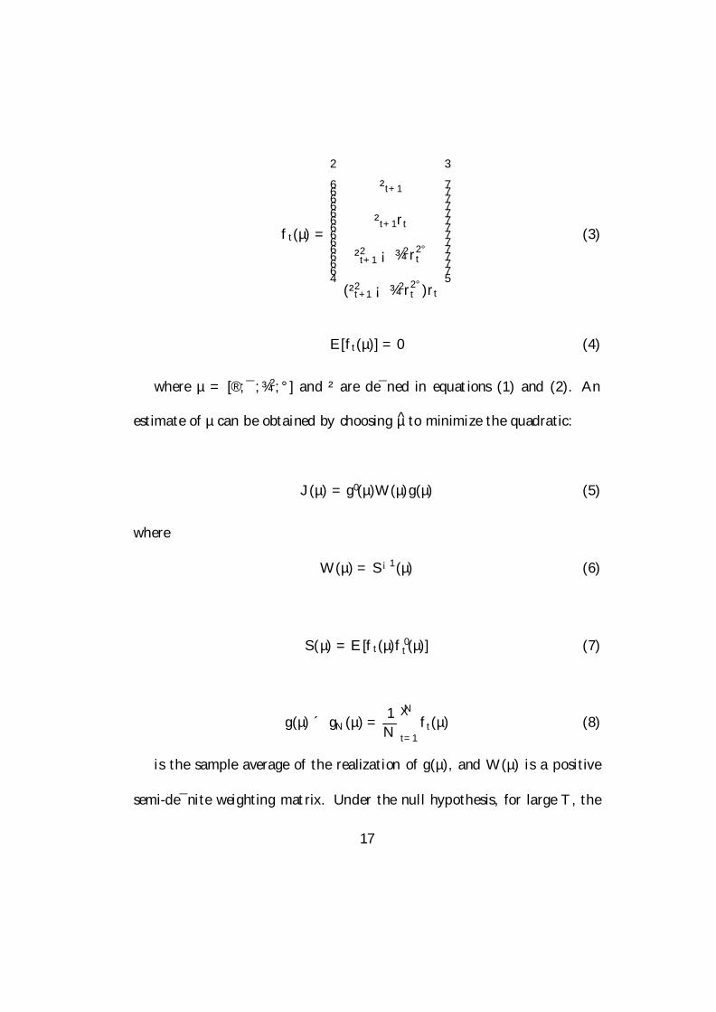
ft(µ) =
266666666666664
²t+1
²t+1rt
²2t+1 ¡ ¾2r2°
t
(²2t+1 ¡ ¾2r2°
t )rt
377777777777775
(3)
E[ft(µ)] = 0 (4)
where µ = [®; ¯; ¾2; °] and ² are de¯ned in equations (1) and (2). An
estimate of µ can be obtained by choosing µ to minimize the quadratic:
J(µ) = g0(µ)W (µ)g(µ) (5)
where
W (µ) = S¡1(µ) (6)
S(µ) = E [ft(µ)f 0t(µ)] (7)
g(µ) ´ gN(µ) = 1N
NX
t=1ft(µ) (8)
is the sample average of the realization of g(µ), and W (µ) is a positive
semi-de¯nite weighting matrix. Under the null hypothesis, for large T , the
17

sample average gT will converge to zero when evaluated at the true values of
µ. Newey and West (1987), the test statistic is
R = N [JN(¹µ) ¡ JN(µ)] (9)
where JN(¹µ) is the unrestricted model's objective function value and
gN(µ), JN(µ) is the restricted model's objective function value where the
unrestricted model's weighting matrix is used in both cases. Newey and
West (1987) point out that this procedure is analogous to a likelihood ratio
test. Under the null hypothesis that the restrictions are not binding, the test
statistic, R, has a  -squared distribution with degrees of freedom equal to
the number of restrictions under the alternative hypothesis.
2.3 The Spot Rate Data
For purposes of comparing the CKLS and other results, we use the 1-
month Treasury bill series taken from the 12-month Fama Treasury bill Files
included in the Center for Research in Security Prices (CRSP) 12-month
Government Bond Files. We study to the June 1964 through March 1996
period. This data series is not ideal for two reasons. Firstly, the maturity
of the nominal 1-month Treasury bill in the 12-month ¯le varies between 10
18

to 41 days. This is an artifact of the construction of the series. A more
constant-maturity 1-month series is the 1-month Treasury bill rate found in
the 6-month Treasury bill ¯le, which varies in maturity from 21 to 39 days
(23 to 35 for all but two months).
2.4 Empirical Results
In this section, the GMM approach of CKLS (1992) is used. The initial
purpose is to compare the nested models within the generalised di®usion
model. Maximum likelihood estimation(MLE) cannot be used as the models
are strictly non-nested and hence formal comparison tests are not possible to
construct. From table 3, the ® and ¯ parameters give us the mean reversion
term in CKLS, Vasicek, CIR-SR, and Bre-Sch models. We ¯nd that the sign
of ¯ is satis¯ed with the negative constraint, but not statistically signi¯cant
in the all mean revering models. This indicates that the mean reversion term
is not a very important feature for interest rates of 1-month maturity.
Table 4 indicated that models that allowed the variability of interest rates
to depend upon the level of interest rates captured the dynamic behaviour
of short-term interest rates more successfully. The level e®ect was such that
interest rate volatility was positively correlated with the level of interest
19

rates.
These results are consistent with the ¯ndings in CKLS(1992) and Tse(1995).
When restrictions are placed on ° , almost estimates of ¾2 are signi¯cant ex-
cept for CKLS, CEV, CEV-dash models. However, when ° is unrestricted
in the models of CKLS, CEV and CEV-dash, the coe±cient estimate on
¾2 is insigni¯cant. Nevertheless, potential estimation problems with GMM,
the value of ° in the unrestricted model is signi¯cant and about 1.46 which
is generally consistent with other evidence (CKLS 1992). A more formal
comparison of the models can be made using the tests of Newey and West
(1987). A signi¯cant test statistic suggests that the model is misspeci¯ed.
Four models being the Merton, Vasicek, CIR-SR, Merton-dash, Vasicek-dash
can be rejected at the 5% level. However, other models are accepted such as
Dothan, GBM, Bre-Sch, CIR-VR, and CEV. The two models which stand-out
are Dothan, GBM process. These models are clearly accepted and cannot be
distinguished from the unrestricted CKLS model. Nevertheless, diagnostic
tests of the residuals indicate that both skewness and excess kurtosis remain.
20

3 The Term Structure Models
3.1 Market Price of Risk
This section discusses the market price of risk. To keep the absence of
arbitrage opportunities, we have to evaluate bond price under an equiva-
lent probability measure. Therefore we consider the market price of risk to
guarantee the existence of the equivalent martingale measure.
In the traditional models, the functional forms of the market price of risk
are also speci¯ed for pure simplicity and computational tractability, examples
are ¸(rt) = ¸ in Merton(1973) and Vasicek (1977), ¸(rt) = ¸r(¯+0:5)t in CIR
(1985).
George J. Jiang(1997) indicated that as CIR (1985) point out, the arbi-
trage approach does not imply that every choice of the functional form for
the market price of risk will lead to bond prices which do not admit arbi-
trage opportunities. Indeed CIR (1985) showed with an example that a linear
functional form for ¸(rt)¾(rt) can lead to internal inconsistency. In addition
to condition, Du±e (1988, pp.227-228) provided regularity conditions that
the market price of risk must satisfy in order for the model to be consistent,
i.e.,¸(rt) must be a predictable process satisfying.
21

Z u
t¸2(r(s))ds < 1; a:s:8u ¸ t; E
"expf1
2
Z T
t¸2(r(s))dsg
#< 1 (10)
On the other hand, other models have no well-known the functional forms
of the market price of risk. Therefore, from the view point of comparing CIR-
SR model, we de¯ne ¸(rt) = ¸r(°+0:5)t in other models as Takamizawa and
Shoji (2001). The same approach for deriving the risk premium function is
taken in Longsta® (1989) and Beaglehole and Tenney (1992).
3.2 Closed Form Solutions
3.2.1 A±ne Models
When general A±ne model formulates the interest rate model in terms of
changes in the short-term (or instantaneous) interest rate:
drt = (® + ¯rt)dt + ¾r°t dzt (11)
The price of a bond, P (t; T ), is then dependent on the expected path of
future interest rates. Bond prices can be presented the following form:
P (t; T ) = A(t; T )e¡r(t)B(t;T) (12)
22

where A(t; T ) and B(t; T ) are functions of only ®, ¯, and ¾ and indepen-
dent of the current spot rate, rt. Bond yields, Y (t; T ) are then related to
prices by:
Y (t; T ) = ¡ 1T ¡ t
ln P (t; T ) (13)
3.2.2 Merton Model
Merton(1973) formulates the interest rate model in terms of changes in the
short-term (or instantaneous) interest rate with the market price of risk:
drt = (® ¡ ¾¸)dt + ¾dzt (14)
Bond yields:
Y (t; T ) = ¡ 1T ¡ t
lnA(t; T ) +1
T ¡ tB(t; T )rt (15)
where
A(t; T ) = ¡16(T ¡ t)2(3® ¡ (T ¡ t)¾2 ¡ 3¾¸)
B(t; T ) = ¡(T ¡ t)
It was used to derive the value of pure discount bonds.
23

3.2.3 The Vasicek Model
Vasicek(1977) formulates the interest rate model in terms of changes in
the short-term (or instantaneous) interest rate with the market price of risk:
drt = (® ¡ ¾¸ + ¯rt)dt + ¾dzt (16)
Vasicek shows that bond yields:
Y (t; T ) = ¡ 1T ¡ t
lnA(t; T ) +1
T ¡ tB(t; T )rt (17)
where
A(t; T ) = exp"(B(t; T ) ¡ (T ¡ t))(a2b ¡ ¾2=2)
a2 ¡ ¾2B(t; T )2
4a
#
B(t; T ) =1 ¡ exp¡a(T¡t)
a; a = ¡¯; b = ¡®
¯+
¾¯
¸
Vasicek model is very tractable and provides convenient closed-form solu-
tions for many interest rate-dependent instruments. However, the model has
some serious drawbacks including restricted dynamics of the term structure
and constant conditional volatility.
24

3.2.4 The Cox, Ingersoll, Ross Model
Another model of interest rates was formulated by Cox, Ingersoll, and Ross
(1985) (CIR-SR). The model is as follows:
drt = (® + (¯ ¡ ¸)rt)dt + ¾p
rtdzt (18)
CIR shows that Bond yields:
Y (t; T ) = ¡ 1T ¡ t
lnA(t; T ) +1
T ¡ tB(t; T )r(t) (19)
A(t; T ) ="
2°e(¸¡¯+°)(T¡t)=2
(° + ¸ ¡ ¯)(e°(T ¡ t) ¡ 1) + 2°¡
#2®=¾2
B(t; T ) =2(e°(T¡t) ¡ 1)
(° + ¸ ¡ ¯)(e°(T ¡t) ¡ 1) + 2°
The CIR-SR model is also known as the square-root process because the
volatility is related to the square root of the current level of the interest rate.
Unlike the Vasicek model, the CIR-SR model relates the conditional volatility
to the level of the short rate. A second improvement of the CIR-SR model
over the Vasicek model is that interest rates cannot be negative. Although
CKLS ¯nd that interest rate volatility is more sensitive to the level of interest
25
rates than proposed by the CIR-SR speci¯cation, other researchers defend
the model by commenting on the estimation approaches employed by CKLS
(see Eom, 1994).
3.3 Approximation by the Local Linear Method
In the previous section, the three models have closed from solutions. But
the other models listed in Table 1 have to calculate numerically by solving a
series of partial di®erential equations (PDE) of bond price. Finite di®erence
method and binomial trees are useful. But these methods are time consuming
and have no computational tractability. An alternative to numerical proce-
dure is approximating PDE. Shoji and Ozaki (1997), Takamizawa and Shoji
(2001) presented a new useful approximating method. That is the Local
Linear Method (LLM). The advantage of their model is that we can capture
actual behavior of the short-rate and yield curve by specifying its process
generally and that we obtain an analytical solution for the term structure of
interest rates.
26

3.4 The In-sample Yield Data
The data set that we use contains monthly data on T-bill yields that are
drawn from the the same data source in section 2.3. (CRSP Files), and
consist of interest rates of maturities ranging from 2-month to 11-month.
We use in-sample data, June 1964 through March 1996, consisting of 382
observations in each yield. In table 4 some basic in-sample statistics of data
are presented. We exclude data on the 12-month yield since almost a quarter
of the data are missing in our in-sample period.
3.5 The Empirical Results
Since we use the 2- through 11-month yield data, we need twenty orthog-
onality conditions for estimating ¸ by the GMM and the result in Table 6.
The sign of all estimated ¸ are negative and their values are signi¯cant. The
t-statistics are in parentheses. Table7 shows overidentifying restrictions. The
more near to 0
27
4 Forecasting
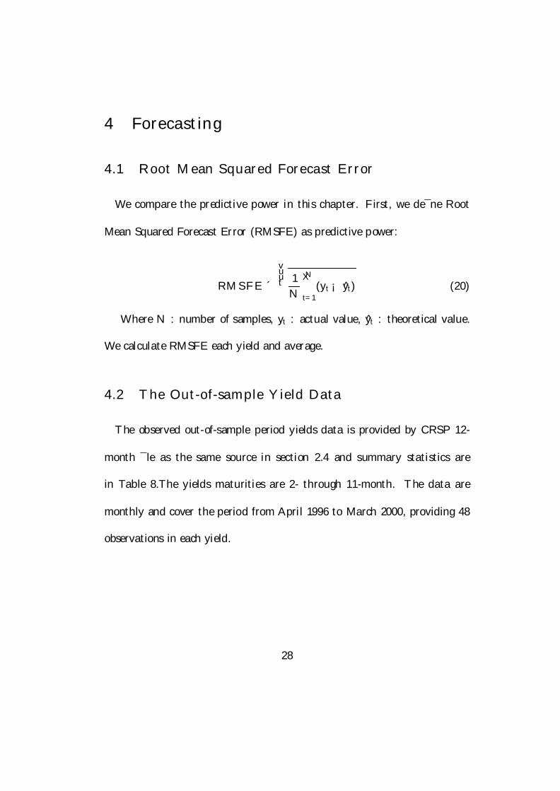
4.1 Root Mean Squared Forecast Error
We compare the predictive power in this chapter. First, we de¯ne Root
Mean Squared Forecast Error (RMSFE) as predictive power:
RMSFE ´vuut 1
N
NX
t=1(yt ¡ yt) (20)
Where N : number of samples, yt : actual value, yt : theoretical value.
We calculate RMSFE each yield and average.
4.2 The Out-of-sample Yield Data
The observed out-of-sample period yields data is provided by CRSP 12-
month ¯le as the same source in section 2.4 and summary statistics are
in Table 8.The yields maturities are 2- through 11-month. The data are
monthly and cover the period from April 1996 to March 2000, providing 48
observations in each yield.
28

4.3 The Principal Components Analysis of yields
Table 9 shows the result of a principal component analysis carried out on
actual Treasury bill yield data from 1964-2000. In this case the dominant
¯rst factor is parallel shift, which explains over 90% of observed °uctuations
in bond yields. The second factor is a slope and the third factor is a kind of
curvature. Therefore, our focus on models of the short rate was motivated by
the evidence that approximately 90% of the variation in T-bill yields could
be attributed to the ¯rst factor alone.
4.4 Empirical Results
We ¯nd some implications from following results. Table 10 presents the
results of comparison based on RMSFE, which is decomposed into bias and
standard deviation (Std Dev). Figure 1 plots the RMSFE. Models are listed
in the order in Table 9. The notations of following tables and ¯gures are
basis point(bp) Firstly, we ¯nd that the predictive powers of the model built
in mean reverting process are rich relatively. Secondly, if the drift term has
mean reversion process, then the higher γ is the higher predictive power(or
vice versa). Though their di®erences between CKLS model are under 1bp.
These results are di®erent from prior evidence of short-term interest rates
29

analysis. CKLS(1992) ¯nd only weak evidence of mean reversion but the
model rankings generally depend upon the level of °. Speci¯cally, those
models with a value of ° less than one are rejected while those with a value
of ° greater than one are preferred. Moreover in a forecasting test which
examines the variation in the volatility of the ex-post yield changes explained
by the conditional expected volatility of yield changes, CEV model has the
highest explanatory power. Du®ee (1993), Bliss and Smith (1994), and other
analysis provide similar evidence.
Thirdly, the predictive power of Merton model is relative rich, though the
model is a simple random walk model. This result is seemed to be surprising.
But Du®ee(2000) describes as follows. The class of a±ne models, which
includes multifactor generalizations of both Vasicek (1977), CIR(1985),and is
extensively analyzed in Dai and Singleton (2000), studied most extensively to
date fails at forecasting. He ¯t general three-factor completely a±ne models
to the Treasury term structure (with maturities ranging from three months
to ten years) over the period 1952 through 1994. Yield forecasts produced
with these estimated models are typically worse than forecasts produced by
simply assuming yields follow random walks. This conclusion holds for both
in-sample forecasts and out-of-sample (1995 through 1998) forecasts.
30

Figure 2 plots the Std Deviations and models are listed in the order in
Table 12. From the graph, we quickly ¯nd that the longer maturity is the
higher Std Deviation. And Table 12 indicates that the di®erences between
CKLS are not larger than RMSFE's one. The largest di®erence is at most
1.7bp.
Figure 3 plots the bias and models are listed in the order in Table 13. We
¯nd that the models built in mean reverting process in the drift term have
following point. Their biases are smaller than no mean reverting model's
one. They tend to overvalue relative to long maturity yields. The models
without mean reverting process undervalue in all yields. This result implies
that if we use the models built in mean reverting process to try yield curve
bet trading and we have long position in a short-term maturity yield and
short position in long-term one, we will get money.
31

5 Concluding Remarks
We compared the predictive power of one-factor term structure models of
short-term interest rate. Our main empirical ¯ndings are as follows and at
the same time, previous questions in the introduction are answered. Firstly,
section 2.4 indicated that the mean reversion term is not a very important
feature for spot rate models. These results are consistent with the ¯ndings in
the prior evidences. However we ¯nd strong evidence for the mean reverting
feature in short-term yield curves.
Secondly, the models built in mean reverting process in the drift term
have following point.
² Their predictive powers are rich relatively.
² Their biases are smaller than no mean reverting model's one.
² They tend to overvalue relative to long maturity yields (or vice versa).
33

Table 1: Speci¯cation and Prameter Restrictions
Number Model Speci¯cation ® ¯ ¾2 °1 CKLS drt = (® + ¯rt)dt + ¾r°
t dzt2 Merton drt = ®dt + ¾dzt 0 03 Vasicek drt = (® + ¯rt)dt + ¾dzt 04 CIR-SR drt = (® + ¯rt)dt + ¾prtdzt 0.55 Dothan drt = ¾rtdzt 0 0 16 GBM drt = ¯rtdt + ¾rtdzt 0 17 Bren-Sch drt = (® + ¯rt)dt + ¾rtdzt 18 CIR-VR drt = ¾r1:5
t dzt 0 0 1.59 CEV drt = ¯rtdt + ¾r°
t dzt 010 Merton-dash drt = ¾dzt 0 0 011 Vasicek-dash drt = ¯rtdt + ¾dzt 0 012 CIR-SR-dash drt = ¯rtdt + ¾prtdzt 0 0.513 CEV-dash drt = ¾r°
t dzt 0 0
Table 2: Summary Statistics:Spot Rate Data
Variable N Mean Std.Dev. Skewness Excess Kurt.rt 382 0.0525 0.0218 1.2516 1.7214
rt+1 ¡ rt 381 -0.00004 0.0063 1.0740 10.6969
34

Table 3: Estimates of Altanative Models for the Short-Term Interest Rate
Model ® ¯ ¾2 ° ¡®=¯ R-stat. d.f.(t-value) =Rev. rate (p-value)CKLS 0.0281 -0.5266 1.7137 1.4660 0.0534
(1.83) (-1.55) (1.52) (6.25)Merton 0.0034 0.0003 0 7.3838 2
(1.25) (16.09) (0.0249)Vasicek 0.0100 -0.1487 0.0003 0 0.0670 9.2429 1
(0.73) (-0.49) (15.54) (0.0024)CIR-SR 0.0124 -0.1984 0.0058 0.5 0.0625 6.4588 1
(0.92) (-0.65) (16.68) (0.0110)Dothan 0 0 0.1170 1 5.2442 3
(17.46) (0.1548)GBM 0 0.0810 0.1186 1 3.1839 2
(1.34) (17.63) (0.2035)Bre-Sch 0.0187 -0.3270 0.1176 1 0.0572 2.5522 1
(1.36) (-1.07) (17.62) (0.1101)CIR-VR 0 0 1.9759 1.5 6.0082 3
(17.46) (0.1112)CEV 0 0.0842 0.5553 1.2685 2.9673 1
(1.39) (1.26) (4.55) (0.0849)Merton-dash 0 0 0.0003 0 9.3303 3
(16.19) (0.0252)Vasicek-dash 0 0.0697 0.0003 0 7.3651 2
(1.15) (16.07) (0.0252)CIR-SR-dash 0 0.0731 0.0060 0.5 5.3730 2
(1.21) (16.98) (0.0681)CEV-dash 0 0 0.4378 1.2297 4.9977 2
(1.22) (-4.30) (0.0822)
The t-statistics are in parentheses.The R-statistic is from Newey and West (1987) and is approximately.
35

Table 4: Spot:p-value and °
Model p-value °GBM 0.2035 1
Dothan 0.1548 1CIR-VR 0.1112 1.5Bre-Sch 0.1101 1CEV 0.0849 1.2685
CEV-dash 0.0822 1.2297CIR-SR-dash 0.0681 0.5Merton-dash 0.0252 0Vasicek-dash 0.0252 0
Merton 0.0249 0CIR-SR 0.0110 0.5Vasicek 0.0024 0
Table 5: Summary Statistics : Sample Period Monthly Yield Data
Maturity 2m 3m 4m 5m 6m 7m 8m 9m 10m 11mMax 0.135 0.134 0.134 0.135 0.138 0.135 0.136 0.136 0.137 0.137Min 0.023 0.023 0.023 0.024 0.024 0.024 0.024 0.025 0.025 0.025
Mean 0.054 0.055 0.056 0.057 0.057 0.058 0.058 0.059 0.059 0.059Std Dev 0.022 0.022 0.022 0.022 0.022 0.022 0.022 0.022 0.022 0.022
Skew 1.243 1.232 1.214 1.184 1.175 1.142 1.124 1.117 1.107 1.092Kurt 1.657 1.592 1.517 1.414 1.388 1.273 1.224 1.215 1.175 1.124
36

Table 6: The Market Price of Risk
Model the functional form ¾ ° ¸ the value of the(t-value) market price of risk
CKLS ¸r°+0:5 1.4660 -2.7142 -0.00828(-27.16)
Merton ¸¾ 0.0163 -0.4082 -0.00663(-17.44)
Vasicek ¸¾ 0.0160 -0.011 -0.00018(-18.70)
CIR-SR ¸r°+0:5 0.5 -0.1482 -0.00778(-20.38)
Dothan ¸r°+0:5 1 -0.5178 -0.00623(-17.50)
GBM ¸r°+0:5 1 -0.2217 -0.00267(-7.72)
Bre-Sch ¸r°+0:5 1 -0.651 -0.00784(-22.60)
CIR-VR ¸r°+0:5 1.5 -1.425 -0.00393(-12.69)
CEV ¸r°+0:5 1.2685 -0.328 -0.00179(-5.67)
Merton-dash ¸¾ 0.0163 -0.6157 -0.01001(-26.38)
Vasicek-dash ¸¾ 0.0163 -0.00003 -0.00003(-17.42)
CIR-SR-dash ¸r°+0:5 0.5 -0.09 -0.00455(-12.21)
CEV-dash ¸r°+0:5 1.2297 -0.84 -0.00516(-15.17)
37

Table 7: Overidentifying Restrictions
Order Model Speci¯cation Over.Res.
1 CKLS drt = (® + ¯rt)dt + ¾r°=1:47t dzt 174.917
2 Bre-Sch drt = (® + ¯rt)dt + ¾rtdzt 177.7233 CIR-SR drt = (® + ¯rt)dt + ¾prtdzt 178.4524 Vasicek drt = (® + ¯rt)dt + ¾dzt 179.2735 Merton-dash drt = ¾dzt 183.2686 Merton drt = ®dt + ¾dzt 183.2747 Vasicek-dash drt = ¯rtdt + ¾dzt 189.4688 CIR-SR-dash drt = ¯rtdt + ¾
prtdzt 198.643
9 GBM drt = ¯rtdt + ¾rtdzt 205.09610 CEV drt = ¯rtdt + ¾r°=1:27
t dzt 208.66311 Dothan drt = ¾rtdzt 211.09512 CEV-dash drt = ¾r°=1:23
t dzt 218.34313 CIR-VR drt = ¾r1:5
t dzt 227.519
Table 8: Summary Statistics : Out of Sample Period Monthly Yield Data
Maturity 2m 3m 4m 5m 6m 7m 8m 9m 10m 11mMax 0.048 0.048 0.048 0.049 0.05 0.051 0.051 0.051 0.051 0.051Min 0.033 0.035 0.036 0.036 0.036 0.036 0.035 0.035 0.035 0.035
Mean 0.041 0.042 0.042 0.043 0.043 0.043 0.043 0.044 0.044 0.044Std Dev 0.003 0.003 0.003 0.003 0.003 0.003 0.004 0.004 0.004 0.004
Skew -0.332 -0.283 -0.317 -0.36 -0.31 -0.275 -0.284 -0.273 -0.285 -0.404Kurt 0.547 0.163 0.009 0.179 0.218 0.015 0.105 -0.02 -0.126 -0.02
Note : There are 48 monthly observations of the yields with ten kinds ofmaturities. The data is obtained from the same CRSP bond les, rangingfrom April 1996 to March 2000.
38
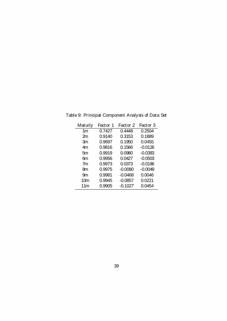
Table 9: Principal Component Analysis of Data Set
Matuity Factor 1 Factor 2 Factor 31m 0.7427 0.4448 0.25042m 0.9140 0.3153 0.18893m 0.9697 0.1950 0.04554m 0.9816 0.1566 -0.01265m 0.9919 0.0980 -0.03836m 0.9956 0.0427 -0.05037m 0.9973 0.0373 -0.01868m 0.9975 -0.0080 -0.00499m 0.9981 -0.0468 0.004610m 0.9945 -0.0857 0.022111m 0.9905 -0.1027 0.0454
39

Table 10: The Forecasting Results (basis point)
2m 3m 4m 5m 6m 7m 8m 9m 10m 11mCKLS 17.16 20.22 21.49 21.54 23.11 23.58 25.30 27.05 28.50 28.84StdDev 17.34 20.27 21.66 21.73 23.35 23.63 25.14 26.52 27.54 27.22Bias 0.40 2.59 1.61 1.25 0.38 -3.07 -4.62 -6.58 -8.34 -10.32
Merton 17.70 21.34 22.81 23.02 24.57 24.47 25.97 27.36 28.49 28.5117.79 21.04 22.65 22.84 24.50 24.71 26.24 27.57 28.56 28.291.86 4.68 4.26 4.40 3.98 0.91 -0.32 -2.02 -3.57 -5.40
Vasicek 17.37 20.57 21.93 22.02 23.62 24.14 25.93 27.75 29.29 29.8117.56 20.64 22.12 22.24 23.87 24.10 25.60 26.94 27.94 27.610.32 2.43 1.35 0.86 -0.15 -3.78 -5.52 -7.70 -9.69 -11.93
CIR-SR 17.59 21.12 22.54 22.71 24.24 24.23 25.76 27.20 28.38 28.4517.71 20.90 22.46 22.63 24.27 24.49 26.01 27.33 28.32 28.031.58 4.28 3.76 3.80 3.29 0.15 -1.14 -2.90 -4.49 -6.35
Dothan 19.07 24.37 26.85 28.46 30.95 30.70 32.59 34.02 35.25 35.3418.04 21.47 23.22 23.51 25.23 25.47 27.05 28.40 29.43 29.266.71 11.93 13.89 16.38 18.29 17.53 18.60 19.17 19.87 20.27
GBM 18.82 23.84 26.11 27.44 29.70 29.31 31.01 32.27 33.33 33.2018.03 21.45 23.19 23.48 25.20 25.43 27.01 28.36 29.38 29.215.99 10.85 12.45 14.59 16.14 15.03 15.73 15.95 16.29 16.34
Bre-Sch 17.44 20.80 22.16 22.27 23.80 23.92 25.49 27.02 28.28 28.4317.58 20.67 22.17 22.30 23.93 24.16 25.67 27.01 28.00 27.691.24 3.78 3.12 3.04 2.42 -0.83 -2.20 -4.02 -5.67 -7.58
CIR-VR 19.61 25.50 28.48 30.76 33.84 34.05 36.47 38.40 40.20 40.9517.97 21.35 23.05 23.32 25.02 25.24 26.81 28.15 29.16 28.978.28 14.28 17.04 20.35 23.07 23.14 25.03 26.44 27.98 29.24
CEV 18.95 24.12 26.51 28.02 30.43 30.12 31.94 33.31 34.48 34.4918.00 21.41 23.14 23.42 25.13 25.35 26.92 28.27 29.29 29.106.45 11.54 13.37 15.75 17.54 16.67 17.62 18.08 18.68 18.98
Merton-dash 17.70 21.34 22.81 23.02 24.57 24.47 25.97 27.36 28.49 28.5117.79 21.04 22.65 22.84 24.50 24.71 26.24 27.57 28.56 28.291.86 4.67 4.26 4.40 3.98 0.91 -0.32 -2.02 -3.58 -5.40
Vasicek-dash 17.89 21.76 23.32 23.65 25.23 24.95 26.39 27.64 28.64 28.5117.90 21.24 22.90 23.14 24.82 25.04 26.59 27.93 28.93 28.702.51 5.64 5.51 5.93 5.76 2.94 1.94 0.46 -0.89 -2.53
CIR-SR-dash 18.51 23.14 25.14 26.07 28.02 27.50 28.99 30.09 30.95 30.6118.05 21.50 23.25 23.55 25.27 25.50 27.09 28.44 29.47 29.304.84 9.12 10.14 11.69 12.64 10.93 11.04 10.65 10.39 9.82
CEV-dash 19.33 24.92 27.63 29.57 32.34 32.29 34.43 36.08 37.57 37.9618.01 21.42 23.15 23.44 25.15 25.38 26.95 28.30 29.32 29.157.49 13.09 15.45 18.34 20.65 20.30 21.77 22.75 23.87 24.69
40

17.00
22.00
27.00
32.00
37.00
42.00
2M 3M 4M 5M 6M 7M 8M 9M 10M 11M
CIR-VR
CEV-dash
Dothan
CEV
GBM
CIR-SR-dash
Vasicek-dash
Merton
Merton-dash
Vasicek
CIR-SR
Bre-Sch
CKLS
Figure 1: Root Mean Squared Forecast Error (in basis point)
Table 11: The Order of Root Mean Squared Forecast Error
RMSFE The Di®erenceOrder Model Speci¯cation (average) bewteen CKLS
1 CKLS drt = (® + ¯rt)dt + ¾r°=1:47t dzt 23.6808 0
2 Bre-Sch drt = (® + ¯rt)dt + ¾rtdzt 23.9624 0.28153 CIR-SR drt = (® + ¯rt)dt + ¾prtdzt 24.2229 0.54214 Vasicek drt = (® + ¯rt)dt + ¾dzt 24.2443 0.56345 Merton-dash drt = ¾dzt 24.4231 0.74236 Merton drt = ®dt + ¾dzt 24.4232 0.74237 Vasicek-dash drt = ¯rtdt + ¾dzt 24.7981 1.11738 CIR-SR-dash drt = ¯rtdt + ¾prtdzt 26.9024 3.22159 GBM drt = ¯rtdt + ¾rtdzt 28.5034 4.822610 CEV drt = ¯rtdt + ¾r°=1:27
t dzt 29.2366 5.555811 Dothan drt = ¾rtdzt 29.7597 6.078812 CEV-dash drt = ¾r°=1:23
t dzt 31.2112 7.530313 CIR-VR drt = ¾r1:5
t dzt 37.1532 13.4723
41

17
19
21
23
25
27
29
31
2M 3M 4M 5M 6M 7M 8M 9M 10M 11M
CIR-SR-dashDothan
GBM
CEV-dashCEV
CIR-VRVasicek-dash
Merton
Merton-dashCIR-SR
Bre-SchVasicek
CKLS
Figure 2: The Std Deviation (in basis point)
Table 12: The Order of Std Deviation
The Di®erenceOrder Model Speci¯cation Std Dev bewteen CKLS
1 CKLS drt = (® + ¯rt)dt + ¾r°=1:47t dzt 23.4395 0
2 Vasicek drt = (® + ¯rt)dt + ¾dzt 23.8614 0.42193 Bre-Sch drt = (® + ¯rt)dt + ¾rtdzt 23.9173 0.47784 CIR-SR drt = (® + ¯rt)dt + ¾
prtdzt 24.2138 0.7743
5 Merton-dash drt = ¾dzt 24.4186 0.97916 Merton drt = ®dt + ¾dzt 24.4186 0.97917 Vasicek-dash drt = ¯rtdt + ¾dzt 24.7190 1.27958 CIR-VR drt = ¾r1:5
t dzt 24.9038 1.46439 CEV drt = ¯rtdt + ¾r°=1:27
t dzt 25.0035 1.563910 CEV-dash drt = ¾r°=1:23
t dzt 25.0265 1.587011 GBM drt = ¯rtdt + ¾rtdzt 25.0742 1.634712 Dothan drt = ¾rtdzt 25.1082 1.668713 CIR-SR-dash drt = ¯rtdt + ¾
prtdzt 25.1400 1.7005
42

-13.00
-8.00
-3.00
2.00
7.00
12.00
17.00
22.00
27.00
2M 3M 4M 5M 6M 7M 8M 9M 10M 11M
CIR-VRCEV-dashDothanCEVGBMCIR-SR-dashVasicek-dashMertonMerton-dashCIR-SRBre-SchCKLSVasicek
Figure 3: Average Bias of Absolute Value (in basis point)
Table 13: The Order of Average Bias of Absolute Value
The Di®erenceOrder Model Speci¯cation Ave.Bias bewteen No.1
1 Merton-dash drt = ¾dzt 3.1404 02 Merton drt = ®dt + ¾dzt 3.1406 0.00023 CIR-SR drt = (® + ¯rt)dt + ¾prtdzt 3.1748 0.03454 Bre-Sch drt = (® + ¯rt)dt + ¾rtdzt 3.3888 0.24855 Vasicek-dash drt = ¯rtdt + ¾dzt 3.4122 0.27196 CKLS drt = (® + ¯rt)dt + ¾r°=1:47
t dzt 3.9160 0.77577 Vasicek drt = (® + ¯rt)dt + ¾dzt 4.3740 1.23368 CIR-SR-dash drt = ¯rtdt + ¾prtdzt 10.1258 6.98549 GBM drt = ¯rtdt + ¾rtdzt 13.9359 10.795510 CEV drt = ¯rtdt + ¾r°=1:27
t dzt 15.4667 12.326411 Dothan drt = ¾rtdzt 16.2636 13.123212 CEV-dash drt = ¾r°=1:23
t dzt 18.8392 15.698913 CIR-VR drt = ¾r1:5
t dzt 21.4850 18.3446
43

References
Andersen, T. G. and J. Lund. 1997. "Estimating Continuous-TimeStochastic Volatility Models of the short Term Interest Rate.ls Journal ofEconometrics 77, no. 2 (April): 343-377.
Ball, C.A. & Torous, W.N. 1994, A stochastic volatility model for short-term interest rates and the detection of structural shifts, Working paper,Vanderbilt University.
Beaglehole, David and Mark Tenney. "Corrections and Additions to 'ANonlinear Equilibrium Model of the Term Structure of Interest Rates.'" Jour-nal of Financial Economics 32 (December, 1992), 345-353.
Golub, Bennett W., Tilman, Leo M.2000 " Risk management : ap-proaches for ¯xed income markets" New York : Wiley
Brennan, M. J., and E. S. Schwartz, 1979, " A Continuous-Time Approachto the Pricing of Bonds," Journal of Banking and Finance, 3, 133-155.
Brennan, M. and E. Schwartz. 1980. "Analyzing covertible bond" Journalof Financial and Quantitative Analysis 15, 907-929.
Broze L., Scaillet O. & Zakoian J.-M., 1995a, "Testing for Continuous-Time Models of the Short-Term Interest Rate", Journal of Empirical Finance2(3), 199-223.
Balduzzi, Pierluigi, Sanjiv Rajan Das, Silverio Foresi and RangarajanSundaram. "A Simple Approach to Three-Factor Term Structure Models."The Journal of Fixed Income 6 (December, 1996), 43-53.
Canabarro,E. 1993." Where do one-factor interest rate models fail" Jour-nal of Fixed Income (September): 31-52.
Chan, K. C., G. A. Karolyi, F. A. Longsta®, and A. B. Sanders, 1992, "An Empirical Comparison of Alternative Models of the Short-Term InterestRate," Journal of Finance, 47, 1209-1227.
Cheng, J.W. 1996, "The intertemporal behavior of short-term interestrates in Hong Kong" Journal of Business Finance and Accounting, vol. 23,pp. 1059-68.
Chen, L. 1996. Stochastic Mean and Stochastic Volatility Three-FactorModel of the Term Structure of Interest Rates and Its Applications in Deriva-tives Pricing and Risk Management.Financial Mar-kets,Institutions & Instru-ments 5(1): 18.
Chen, R-R., and L. Scott. 1993. "Maximum Likelihood Estimation fora Multifactor Equilibrium Model of the Term Structure of Interest Rates"Journal of Fixed Income 3. no. 3 (December): 14-31.
44

Cox, J. C., J. E. Ingersoll, and S. A. Ross, 1985, " A Theory of the TermStructure of Interest Rates," Econometrica, 53, 385-407.
Cox, J. C., J. E. Ingersoll, and S. A. Ross, 1980, "An analysis of variablerate loan contractse"Journal of Finance, 35, 389-403.
Dai, Q. and K. J. Singleton. 1997. "Speci¯cation Analysis of A±ne TermStructure Models." NBER Work-ing Paper 6128.
Dahlquist, M. 1996, "On alternative interest rate processes", Journal ofBanking and Finance,vol. 20, pp. 1093-19.
David A. Chapman-Neil D. Pearson(2001)"Recent Advances in Estimat-ing Models of the Term Structure" Forthcoming in the Financial AnalystsJournal
Dothan, U. L., 1978, " On the Term Structure of Interest Rates," Journalof Financial Economics, 7, 59-69.
Driessen,J. Melenberg,B. Nijman,T.,2000,"Common Factors in Interna-tional Bond Returns" Tilburg University Center for Economic Research No.2000-91
Du±e, D., 1988, Security Markets: Stochastic Models. Academic Press,Boston, MA.
Du®ee, G.R. 1993, "On the relation between the level and volatilityof short-term interest rates: A comment on Chan, Karolyi, Longsta® andSanders', Working paper, Federal Reserve Board, Washington.
Duguay, P. 1994. "Empirical Evidence on the Strength of the MonetaryTransmission Mechanism in Canada: An Aggregate Approach."Journal ofMonetary Economics 33: 39-1.
Engle, R.F., Lilien, D. & Robins, R. 1987, "Estimating time varying riskpremia in the term structure: The ARCH-M model', Econometrica, vol. 55,pp. 391-407.
Engle, R.F. & Ng, V. 1993a, "Time-varying volatility and the dynamicbehaviour of the term structure', Journal of Money, Credit and Banking, vol.25, pp. 336-49.
Elerian, O., S. Chib, and N. Shepherd. 2000. "Likelihood Inference forDis-cretely Observed Non-linear Diusions." Econometrica,69, 959-993.
Eom, Y.H., 1994, "In Defense of the Cox, Ingersoll, and Ross Model:Some Empirical Evidence," Working Paper, New York University.
Fama,E.,"The Information in the Term Structure," Journal of FinancialEconomics, (December 1984).
Fama,E.,"The Information in Long-Maturity Forward Rates," (with RobertR. Bliss), American Economic Review, (September 1987).
45

Gibbons, M. R., and K. Ramaswamy, 1993, " A Test of the Cox, Ingersolland Ross Model of the Term Structure," Review of Financial Studies, 6, 619-658.
Golub, Bennett W., Tilman, Leo M.2000 " Risk management : ap-proaches for ¯xed income markets" New York : Wiley
Gong, F. F. and E. M. Remolona. 1996. "A Three-Factor Economet-ric Model of the U.S. Term Structure." Federal Reserve Bank of New YorkResearch Paper No. 9619.
Gregory R. Du®ee 2001."Term premia and interest rate forecasts in a±nemodels" This used to be called "Forecasting future interest rates: Are a±nemodels failures?" Forthcoming, Journal of Finance.
Hansen, L.P. 1982, "Large sample properties of generalised method ofmoments estimators" Econometrica, vol. 50, pp. 1029-54.
Hansen, L. P., and J. A. Scheinkman, 1995, " Back to the Future: Gener-ating Moment Implications for Continuous Time Markov Processes," Econo-metrica, 63, 767-804.
Harvey, A. C., 1993, "Time Series Models (2nd ed.)", MIT Press, Cam-bridge, Mass. Hiraki, T., Shiraishi, N. and Takezawa, N., "Cointegration,common factors and the term structure of Yen o®shore interest rates", J.Fixed Income, December 1996.
Hiraki, T. and N. Takezawa, "How Sensitive Is Short-Term Japanese In-terest Rate Volatility to the Level of the Interest Rate?" Economics Letters,Vol.56, 1997, pp.325-332.
Kevin C. Ahlgrim-Stephen P. D'Arcy-Richard W. Gorvett .1999 "Param-eterizing Interest Rate Models" Casualty Actuarial Society Dynamic Finan-cial Analysis Seminar
Kobayashi,T. and Ochi,A 1997, "Forecasting Interest Rates using Va-sicek's Term Structure Model" Faculty of Economics, University of Tokyo inits series CIRJE J-Series as number 97-J-2
Litterman, R. and J. Scheinkman. 1991. "Common Factors Aecting BondReturns." Journal of Fixed Income 3, no. 3 (December): 54-61.
Longsta®, Francis. "A Nonlinear General Equlibrium Model of the TermStructure of Interest Rates." Journal of Financial Economics 23 (August,1989), 195-224.
Longsta®, F. A., and E. S. Schwartz, 1992, Interest Rate Volatility andthe Term Structure: A Two-Factor General Equilibrium Model",Journal ofFinance, 47, 1259282.
46

Merton, R., 1973. Rational theory of option pricing. Bell Journal ofEconomics and Management Science 4, 141-183.
Mishkin, F, 1988, The information in the term structure: Some furtherresults, Journal of Applied Econometrics, 3, 307-314.
Newey, W. & West, K. 1987, "Hypothesis testing with e±cient method ofmoments estimation" International Economic Review, vol. 28, pp. 777-787.
Pearson, N. D. and T-s. Sun. 1994. "Exploiting the conditional densityin estimating the term structure: an application to the Cox, Ingersoll, andRoss Model" Journal of Finance 49, no. 4 (September): 1279-1304.
Stambaugh, R. F. 1988. "The Information in Forward Rates.lt Journalof Financial Economics 21, no. 1 (May): 41-70.
Shoji, I. and Ozaki, T., 1997, Comparative study of estimation methodsfor continuous time stochastic processes, Journal of Time Series Analysis 18,485-506.
Takamizawa, H. and Shoji, I., 2001, Approximation of nonlinear termstructure models, Journal of Derivatives 8, 44-51.
Y.K.Tes .1995 Some international evidence on the stochastic behavior ofinterest rates, Journal of International Money and Finance, 14,721-738
Vasicek, O.A., "An Equilibrium Characterization of the Term Structure,"Journal of Financial Economics, Vol.5, 1977, pp.177-188.
Wesley Phoa, Yield Curve Risk Factors Domestic And Global ContextsThe Practitioner's Handbook of Financial Risk Management,2000,Chaper 5
Wong, E., 1971, Stochastic Processes in Information and Dynamical Sys-tems, McGraw-Hill,New York.
Zhang,H.,1993,"Treasury yield curves and cointegration" Applied Econo-metrics,25, 361-367.
47
Related Documents


![[Salomon Brothers] Understanding the Yield Curve, Part 5 - Convexity Bias and the Yield Curve](https://static.cupdf.com/doc/110x72/577d26641a28ab4e1ea111d0/salomon-brothers-understanding-the-yield-curve-part-5-convexity-bias-and.jpg)