A comparison of direct and iterated multistep AR methods ...mwatson/papers/Marcellino_Stock_Watson_JoE_2006.pdfThe relative performance of the iterated forecasts improves with the

ARTICLE IN PRESS

Journal of Econometrics 135 (2006) 499–526

0304-4076/$ -

doi:10.1016/j

�CorrespoE-mail ad

www.elsevier.com/locate/jeconom

A comparison of direct and iterated multistepAR methods for forecasting macroeconomic

time series

Massimiliano Marcellinoa, James H. Stockb, Mark W. Watsonc,�

aIstituto di Economia Politica, Universita Bocconi and IGIER, ItalybDepartment of Economics, Harvard University, and the NBER, USA

cDepartment of Economics and Woodrow Wilson School, Princeton University,

and the NBER, Princeton, NJ 08544, USA

Available online 24 August 2005

Abstract

‘‘Iterated’’ multiperiod-ahead time series forecasts are made using a one-period ahead

model, iterated forward for the desired number of periods, whereas ‘‘direct’’ forecasts are

made using a horizon-specific estimated model, where the dependent variable is the

multiperiod ahead value being forecasted. Which approach is better is an empirical matter:

in theory, iterated forecasts are more efficient if the one-period ahead model is correctly

specified, but direct forecasts are more robust to model misspecification. This paper compares

empirical iterated and direct forecasts from linear univariate and bivariate models by applying

simulated out-of-sample methods to 170 U.S. monthly macroeconomic time series spanning

1959–2002. The iterated forecasts typically outperform the direct forecasts, particularly, if the

models can select long-lag specifications. The relative performance of the iterated forecasts

improves with the forecast horizon.

r 2005 Elsevier B.V. All rights reserved.

JEL: C32; E37; E47

Keywords: Multistep forecasts; Var forecasts; Forecast comparisons

see front matter r 2005 Elsevier B.V. All rights reserved.

.jeconom.2005.07.020

nding author. Tel.: +1609 258 4811; fax: +1 609 258 5533.

dress: [email protected] (M.W. Watson).

www.elsevier.com/locate/jeconom

ARTICLE IN PRESS

M. Marcellino et al. / Journal of Econometrics 135 (2006) 499–526500

1. Introduction

A forecaster making a multiperiod time series forecast—for example, forecastingthe unemployment rate six months hence—confronts a choice between using a one-period model iterated forward, or instead using a multiperiod model estimated witha loss function tailored to the forecast horizon. In the case of univariate linearmodels and quadratic loss, the ‘‘iterated’’ forecast (sometimes called a ‘‘plug-in’’forecast) entails first estimating an autoregression, then iterating upon thatautoregression to obtain the multiperiod forecast. In contrast, the forecast basedon the multiperiod model—which, following the literature, we shall call the ‘‘direct’’forecast—entails regressing a multiperiod-ahead value of the dependent variable oncurrent and past values of the variable. For example, the direct forecast of theunemployment rate six months from now might entail the regression of theunemployment rate, six months hence, against a constant and current and pastvalues of the unemployment rate. But which forecast, the iterated or the direct,should the forecaster use in practice?

The theoretical literature on this problem tends to emphasize the advantages of thedirect over indirect forecasts. The idea that direct multiperiod forecasts can be moreefficient than iterated forecasts dates at least to Cox (1961), who made the suggestionin the context of exponential smoothing, and to Klein (1968), who suggested directmultiperiod estimation of dynamic forecasting models. Contributions to the theoryof iterated vs. direct forecasts include Findley (1983, 1985), Weiss (1991), Tiao andXu (1993), Lin and Granger (1994), Tiao and Tsay (1994), Clements and Hendry(1996), Bhansali (1996, 1997), Kang (2003), Chevillon and Hendry (2005), andSchorfheide (2005). Bhansali (1999) provides a nice survey of this theoreticalliterature, and Ing (2003) gives a complete treatment of first-order asymptotics forstationary autoregressions.

Choosing between iterated and direct forecasts involves a trade-off between biasand estimation variance: the iterated method produces more efficient parameterestimates than the direct method, but it is prone to bias if the one-step-ahead modelis misspecified. Ignoring estimation uncertainty, if both the iterated model and thedirect model have p lags of the dependent variable but the true autoregressive orderexceeds p, then the asymptotic mean squared forecast error (MSFE) of the directforecast typically is less than (and cannot exceed) the MSFE of the iterated forecast(e.g. Findley, 1983). On the other hand, if the true autoregressive order is p or less,then (still ignoring estimation uncertainty) the MSFEs of the direct and iteratedmethods are the same; because the iterated parameter estimator is more efficient, theMSFE including estimation uncertainty is less for the iterated method when theautoregressive order is correctly specified. Because it seems implausible that typicallylow-order autoregressive models are correctly specified, in the sense of estimating thebest linear predictor, the theoretical literature tends to conclude that the robustnessof the direct forecast to model misspecification makes it a more attractive procedurethan the bias-prone iterated forecast (Bhansali, 1999; Ing, 2003).

Because the relative efficiency of iterated vs. direct forecasts is theoreticallyambiguous and depends on the unknown population best linear projection, the

ARTICLE IN PRESS

M. Marcellino et al. / Journal of Econometrics 135 (2006) 499–526 501

question of which method to choose is an empirical one. Given the practicalimportance of the question, there are surprisingly few empirical studies of the relativeperformance of iterated vs. direct forecasts. Findley (1983, 1985) studies univariatemodels of two of Box and Jenkins’s (1976) series (chemical process temperature andsunspots), and Liu (1996) studies univariate autoregressive forecasts of foureconomic time series. Ang et al. (2005) find that, at least during the 1990s, iteratedforecasts of U.S. GDP growth outperform direct forecasts using a measure of short-term interest rates and the term spread. The largest empirical study we are aware ofis Kang (2003), who studied univariate autoregressive models of nine U.S. economictime series with mixed results, concluding that the direct method ‘‘may or may notimprove forecast accuracy’’ relative to the iterated method (Kang, 2003, p. 398).

This paper undertakes a large-scale empirical comparison of iterated vs. directforecasts using data on 170 U.S. macroeconomic time series variables, availablemonthly from 1959 to 2002. Rather than narrowing in on individual series, this studyconsiders the larger questions of whether the iterated or direct forecasts are moreaccurate on average for the population of U.S. macroeconomic time series, andwhether the distribution of MSFEs for direct forecasts is statistically andsubstantively below the distribution of MSFEs for iterated forecasts. Using thesedata, we compare iterated and direct forecasts based on univariate autoregressionsand bivariate vector autoregressions; in both cases, we consider models with fixed lagorder and models with data-dependent lag order choices, using the AkaikeInformation Criterion (AIC) or, alternatively, the Bayes Information Criterion(BIC).1 Multiperiod forecasts are computed for horizons of 3, 6, 12, and 24 months.2

The experimental design uses a pseudo-out-of-sample (or ‘‘recursive’’) forecastingframework; for example, forecasts for the 12 months from January 1985 toDecember 1985 are computed from models estimated and selected using only dataavailable through December 1984.

This study yields surprisingly sharp results. First, iterated forecasts tend to havelower sample MSFEs than direct forecasts, particularly if the lag length in the one-period ahead model is selected by AIC. Second, these improvements tend to bemodest, as one would expect if the main source of the improvements is reduction inestimating uncertainty of the parameters. Third, direct forecasts become increasinglyless desirable as the forecast horizon lengthens; this too is consistent with theefficiency of the iterated forecasts outweighing the robustness of the direct forecasts.Fourth, for series measuring wages, prices, and money, direct forecasts improveupon iterated forecasts based on low-order autoregressions, but not upon iteratedforecasts from high-order autoregressions, a finding that is consistent with theseseries having, in effect, a large moving average root (or long lags in the optimal linear

1Because possible model misspecification is central to this comparison, data-dependent lag order choice

can play an important role: selecting a high-order one-period model can reduce bias but increase

estimation uncertainty, and thus increase total MSFE, relative to a lower order direct model (Bhansali,

1997).2Following the literature we consider direct h-step versus one-step-ahead iterated forecasts. In principle,

it would also be possible to construct iterated forecasts from k-step-ahead models, where koh, and h/k is

an integer.

ARTICLE IN PRESS


predictor), as suggested by Nelson and Schwert (1977) and Schwert (1987). Incontrast, iterated forecasts from low-order autoregressive models outperform directforecasts for real activity measures and the other macroeconomic variables in ourdata set.

2. Forecasting models and methods of comparison

This section describes the iterated and direct forecasting models and estimators.We begin with two general observations.

First, many macroeconomic time series appear to be nonstationary in the sense ofhaving one or more unit roots, while the literature surveyed above focuses onstationary variables.3 The strategy adopted here is to transform the series of interestto approximate stationarity by taking its first or second difference as needed, toestimate the forecasting model, then to compute the h-step-ahead forecast of theoriginal series produced by that model. For example, the logarithm of real GDP isfirst transformed by taking its first difference, DlogGDPt, the forecasting models areestimated using DlogGDPt, and these models are then used to compute the forecastof the level of the logarithm of GDP, h periods ahead. The transformations used foreach series are discussed in the next section and in the data appendix.

Second, all forecasts are recursive (pseudo-out-of-sample), that is, forecasts arebased only on values of the series up to the date on which the forecast is made.Parameters are then reestimated in each period, for each forecasting model, usingdata from the beginning of the sample through the current forecasting date. Forforecasts entailing data-based model selection, the order of the model is also selectedrecursively, and thus can change over the sample as new information is added to theforecast data set.

2.1. Univariate models

Let Xt denote the level or logarithm of the series of interest. The objective is tocompute forecasts of Xt+h, using information at time t. Let yt denote the stationarytransformation of the series after taking first or second differences. Specifically,suppose that Xt is integrated of order d (is IðdÞ); then yt ¼ DdXt, where d ¼ 0, 1, or 2as appropriate.

2.1.1. Iterated AR forecasts

The one-step-ahead AR model for yt is

ytþ1 ¼ aþXp

i¼1

fiytþ1�i þ �t: (1)

3A notable exception is Chevillon and Hendry (2005), which compares iterated and direct forecasts for

Ið1Þ autoregressions. Long-horizon iterated forecasts in the local-to-unity autoregression are studied in

Stock (1997), and these methods appear well-suited for studying direct forecasts as well.

ARTICLE IN PRESS


For the iterated AR forecasts, the parameters a, f1; . . . ;fp in (1) are estimatedrecursively by OLS, and the forecasts of yt+h are constructed recursively as,

yItþh=t ¼ aþ

Xp

i¼1

fi yItþh�i=t, (2)

where yj=t ¼ yj for jpt. Forecasts of Xt+h are then computed by accumulating thevalues of yI

tþk=t as appropriate in the I(0), I(1) and I(2) cases:

XI

tþhjt ¼

yItþhjt if X t is Ið0Þ;

X t þPhi¼1

yItþijt ifX t is Ið1Þ;

X t þ hDX t þPhi¼1

Pi

j¼1

yItþjjt ifX t is Ið2Þ:

8>>>>>>><>>>>>>>:

(3)

2.1.2. Direct forecasts

The direct estimates of the parameters are the recursive minimizers of the meansquared error of the h-step-ahead criterion function. Accordingly, the parameters areestimated by the OLS regression in which the regressors are a constant andyt; . . . ; yt2pþ1 and the dependent variable is yh

tþh, where

yhtþh ¼

X tþh if X t is Ið0Þ;

X tþh � X t ifX t is Ið1Þ;

Phi¼1

Pi

j¼1

D2X tþj ¼ X tþh � X t � hDX t ifX t is Ið2Þ:

8>>>><>>>>:

(4)

The direct forecasting regression model is,

yhtþh ¼ bþ

Xp

i¼1

riytþ1�i þ �tþh. (5)

The direct estimator of the coefficients is obtained by the recursive estimation of(5) by OLS, where data through period t are used (so that the last observationincludes yh

t on the left-hand side of the regression). The direct forecasts of yhtþh

are

yD;htþh ¼ bþ

Xp

i¼1

riytþ1�i. (6)

Forecasts of Xt+h are then computed from the yD;htþh as appropriate in the I(0), I(1)

and I(2) cases: XD

tþh=t ¼ yD;htþh=t

for I(0), XD

tþh=t ¼ yD;htþh þ X t for I(1) and X

D

tþh=t ¼

yD;htþh þ X t þ hDX t for I(2).4

4As an alternative, direct forecasts could be computed by first estimating regressions of yt+i onto (1, yt,

yt�1, y, yt+1�p) for i ¼ 1, y, h, and then accumulating the forecasts of yt+i to form forecasts of yhtþh.

Because each regression uses the same set of regressors, these forecasts will be identical to those in (6) when

data over the sample period are used.

ARTICLE IN PRESS


2.1.3. Lag-length determination

Four different methods were used to determine the lag order p: (1) p ¼ 4 (fixed);(2) p ¼ 12 (fixed); (3) p chosen by the AIC, with 0ppp12, and (4) p chosen by theBIC, with 0ppp12. For the iterated forecasts, the AIC and BIC were computedusing the standard formulas based on the sum of squared residuals (SSR) from theone-step-ahead regression. For the direct forecasts, the AIC and BIC were computedusing the SSR from the estimated h-step-ahead regression (5). The AIC and BICwere recomputed at each date, so the order of the selected forecasting model canchange from one period to the next, where the model selection and parameterestimates are based only on data through the date of the forecast (period t).

These four choices cover leading cases of theoretical interest. If the true lag orderp0 is finite and if the maximum lag considered exceeds p0, then the BIC provides aconsistent estimator of p0 and the iterated estimator with BIC is asymptoticallyefficient. If p0 is infinite, then the direct estimator with AIC model selection achievesan efficiency bound for direct estimators and this bound is below that for all iteratedestimators (see Bhansali (1996) for a precise statement of this result; he shows thatthe direct estimator bound also is achieved using Shibata’s (1980) lag-lengthselector). In finite samples, however, BIC and AIC lag-length selection introducesadditional sampling uncertainty and the short (4 lag) and long (12 lag) fixed-lagautoregressions provide benchmarks against which to compare the BIC and AICforecasts.5

2.2. Multivariate models

We also consider iterated and direct forecasts computed using bivariate vectorautoregressions (VARs). For two series i and j, the iterated VARs are specified interms of the stationary transforms yit and yjt. The iterated forecast is then obtainedby iterating forward the VAR and then applying the transformation (3). The h-stepdirect forecast for series i is obtained from the OLS regression of yh

i;tþh against aconstant and p lags each of yit and yjt. In both the iterated and direct models, thesame number of lags p is used for both regressors. The same four methods of lagdetermination are used as in the analysis of the univariate models.

2.3. Estimation and forecast sample periods

Let T0 denote the first observation used in estimation of the regressions, T1 denotethe date at which the first pseudo-out-of-sample forecast is made, and T2 denote thedate at which the final pseudo-out-of-sample forecast is made. The date T0 is the dateat which the first observation is available (for most series, 1959:1), plus 12 (because12 lags are used for the long-lagged models), plus the order of integration of the

5Other possible lag-length selection methods are possible but are not pursued here. For example,

Bhansali (1999) and Schorfheide (2005) suggest selecting the order of the iterated model based on the h-

step-ahead SSR of the iterated forecasts, rather than (as is conventional and as we do) based on the one-

step-ahead SSR.

ARTICLE IN PRESS


series (to allow for first and second differences). For most series, the initial forecastdate T1 is 1979:1; for series that start after 1959:1, T1 is the later of 1979:1 or the firstobservation for which all regressions can be estimated using a minimum of 120observations. The final forecast date depends on the forecast horizon, and is the dateof the last available observation (2002:12) minus the forecast horizon h. Thus, formost series, pseudo-out-of-sample forecasts X tþh were computed for t ¼ 1979:1 to2002:12–h.

The pseudo-out-of-sample forecast error is etþh ¼ X tþh � X tþh, and the sampleMSFE is,

MSFE ¼1

T2 � T1 þ 1

XT2

t¼T1

e2tþh. (7)

The sample MSFE is computed for each series (170 series), for each forecastingmethod (iterated, with 4 lag choices, and direct, with 4 lags choices), and for eachhorizon (3, 6, 12, and 24 months). For a given series and horizon, the empiricalefficiency of comparable direct and indirect forecasts is assessed by comparing therespective MSFEs.

2.4. Parametric bootstrap method for comparing iterated vs. direct forecasts

The sample MSFE might be less for a direct than an iterated forecast eitherbecause the direct forecast is more efficient in population or because of samplingvariability. For a single series, the null hypothesis that a direct forecast fails toimprove upon an indirect forecast can be tested using suitable versions of testsproposed by West (1996) and Clark and McCracken (2001) for comparing simulatedout-of-sample forecasts. Our focus, however, is on whether the direct methodimproves upon the iterated method on average over the population of macro-economic variables of interest. Thus the objects of interest in this study are summarymeasures of the distribution of the relative MSFEs, for example, the mean relativeMSFE of the direct estimator, relative to the iterated estimator, across thepopulation of U.S. macroeconomic series, from which we have a sample of 170series. This comparison of empirical distributions of direct and iterated estimatorsgoes beyond the theoretical results available in the forecast evaluation literature.

To assess the statistical significance of our summary statistics, we thereforeimplemented a parametric bootstrap that examined the spread of the distribution ofrelative MSFEs under the null hypothesis that the iterated forecasting model iscorrectly specified, so that the iterated forecast is efficient. The parametric bootstraphas the following steps:

(1)
For each series i, i ¼ 1, y, 170, an autoregressive model of order pi is estimatedusing the full sample, producing the (one-step ahead) residuals eit.
(2)
Previous research suggests that these series are well-modeled by a factor modelwith a small number of factors (e.g. Stock and Watson, 2002a, b). Accordingly, astatic factor model with four factors is fit to these residuals, where the factor

ARTICLE IN PRESS


loadings and error variances are estimated using principal components. Separatefactor models (different factor loadings and idiosyncratic variances) wereestimated in the pre-1982:12 and post-1983:1 periods, where the break pointwas chosen approximately to coincide with the decline in volatility of many U.S.macroeconomic time series (McConnell and Perez-Quiros, 2000; Kim andNelson, 1999).

(3)
Using the estimated parameters from the dynamic factor models, a pseudo-random data set consisting of 170 series was computed, where the sample periodsfor the pseudo-data are the same as the actual data. From these pseudo-randomdata, recursive iterated and direct forecasts are computed as described above,along with their MSFEs. This process is repeated 200 times. This produces anempirical distribution of direct MSFEs, relative to iterated MSFEs, under thehypothesis that the true AR lag length is pi, i ¼ 1, y, 170.
(4)
This procedure is repeated for each of the four-lag selection methods. For p ¼ 4(fixed), pi is fixed at 4, and similarly for p ¼ 12 (fixed). For the AIC method, pi isdetermined by AIC prior to estimation in step #1, and similarly for the BIC method.
This algorithm provides an estimate of the distribution of relative MSFEs underthe null hypothesis that the iterated model is correctly specified (so that the iteratedmodel is asymptotically efficient), where this distribution allows for both samplinguncertainty in the MSFEs and heterogeneity among and time variation of theautoregressive processes. This distribution allows for a comparison of the observeddistribution of relative MSFEs to their null distribution. This distribution also canbe used to compute bootstrap p-values. For example, consider the comparison of thedirect estimator with p ¼ 4 to the iterated estimator with p ¼ 4. The bootstrapp-value of the hypothesis that the median relative MSFE (where the median iscomputed across all 170 series for the given horizon) equals its population value thatwould obtain were the iterated model correctly specified so that the iteratedestimator is efficient, against the alternative that the direct estimator is moreefficient, is the fraction of the 200 bootstrap draws of the median that are less thanthe median ratio actually observed in the data.

3. The data

The data set consists of 170 major monthly U.S. macroeconomic time series. Thefull data set spans 1959:1–2002:12, and most series are available over this full sample.The data set consists of five categories of series:

(A)
Income, output, sales, and capacity utilization (38 series); (B) Employment and unemployment (27 series); (C) Construction, inventories and orders (37 series); (D) Interest rates and asset prices (33 series); and (E) Nominal prices, wages, and money (35 series).
The series and their spans are listed in the data appendix.

ARTICLE IN PRESS


The series were subject to three transformations and manipulations. First, seriesthat represent quantities, indexes, and price levels were transformed to logarithms;interest rates, unemployment rates, etc. were left in the original levels; this yields theXit series in the notation of Section 2.

Second, these series were then differenced so that the resulting series wereintegrated of order zero, yielding the yit series in the notation of Section 2. Generallyspeaking, real quantities and real prices were treated as I(1). For our primary set ofresults, we treated nominal prices, wages, and money as I(1). There is a disagreementamong practitioners about whether it is best to treat these series as I(1) or I(2);however, so we repeated the analysis treating the series in category (E), prices, wages,and money, as I(2). The results of this sensitivity analysis are discussed briefly inSection 4.

Third, a few of the resulting yit series contained large outliers. So that theseoutliers would not dominate the results, observations were dropped when |yit|exceeded its median by more than six times its interquartile range.

4. Results for univariate autoregressions

Table 1 summarizes the distributions of the ratios of the MSFE of the directforecast to the MSFE of the iterated forecast, where the forecasts are based on thesame method of lag selection, for different forecast horizons. For example, acrossthe 170 series, when p ¼ 4 lags are used for both the iterated and direct forecast andthe forecast horizon is h ¼ 3, the mean relative MSFE is 0.99, indicating that thedirect estimator on average makes a very slight improvement over the indirectestimator, at least by this measure. In 10% of the 170 series, relative MSFE is lessthan 0.97 at this horizon, while in 10% of the series the relative MSFE exceeds 1.02.The numbers in parentheses in Table 1 are the bootstrap p-values for the test of thehypothesis that the iterated estimator is efficient, computed as described in Section2.4. For example, the bootstrap p-value of the mean relative MSFE for the p ¼ 4 lagmodel at horizon h ¼ 3 is o0.005; according to the bootstrap null distribution, werethe iterated model correctly specified, the probability of observing a mean relativeMSFE of 0.99 or less is less than 0.5%.6

Inspection of Table 1 suggests that whether the iterated or direct estimator ispreferred depends on the method of lag selection. For the short-lag selectionmethods (p ¼ 4 and BIC), the direct estimator is preferred; this is particularly truefor the BIC, where the improvements in the lower tail of the distribution aresubstantial, at least through the 12-month horizon. According to the bootstrap p-values, these improvements generally are statistically significant. In contrast, withinthe long-lag models, the iterated estimator is preferable, and the direct estimatortypically does not improve substantially upon the iterated estimator. At the longer24-month horizon, the iterated forecast is generally preferable to the direct forecastfor all four lag selection methods. Indeed, at this horizon the direct forecasts can be

6If the iterated model is correctly specified, then the direct estimator is inefficient and the relative MSFE

ratio would tend to exceed one.

ARTICLE IN PRESS

Table 1

Distributions of relative MSFEs of direct vs. iterated univariate forecasts based on the same lag selection

method: all series

Lag selection Mean/percentile Forecast horizon

3 6 12 24

AR(4) Mean 0.99 (o0.005) 0.99 (o0.005) 1.00 (o0.005) 1.05 (0.83)

0.10 0.97 (o0.005) 0.92 (o0.005) 0.90 (o0.005) 0.85 (o0.005)

0.25 0.99 (o0.005) 0.98 (o0.005) 0.98 (o0.005) 0.97 (0.04)

0.50 1.00 (0.01) 1.00 (0.03) 1.01 (0.25) 1.05 (40.995)

0.75 1.01 (0.85) 1.02 (0.83) 1.04 (0.55) 1.12 (40.995)

0.90 1.02 (0.83) 1.04 (0.86) 1.08 (0.82) 1.23 (0.99)

AR(12) Mean 1.01 (40.995) 1.01 (40.995) 1.03 (40.995) 1.10 (40.995)

0.10 0.98 (40.995) 0.97 (40.995) 0.95 (40.995) 0.93 (40.995)

0.25 1.00 (40.995) 0.99 (40.995) 1.00 (40.995) 1.02 (40.995)

0.50 1.00 (40.995) 1.01 (40.995) 1.03 (40.995) 1.09 (40.995)

0.75 1.01 (40.995) 1.02 (40.995) 1.06 (40.995) 1.17 (40.995)

0.90 1.02 (0.99) 1.05 (40.995) 1.11 (40.995) 1.29 (40.995)

AR(BIC) Mean 0.98 (o0.005) 0.97 (o0.005) 0.99 (0.21) 1.05 (0.99)

0.10 0.92 (o0.005) 0.86 (o0.005) 0.86 (0.01) 0.88 (0.06)

0.25 0.97 (o0.005) 0.96 (o0.005) 0.97 (0.02) 0.98 (0.50)

0.50 1.00 (o0.005) 1.00 (0.01) 1.01 (0.56) 1.04 (40.995)

0.75 1.01 (0.99) 1.02 (0.91) 1.03 (0.76) 1.12 (40.995)

0.90 1.03 (40.995) 1.05 (40.995) 1.10 (40.995) 1.20 (0.98)

AR(AIC) Mean 1.00 (40.995) 1.01 (40.995) 1.02 (40.995) 1.09 (40.995)

0.10 0.97 (0.51) 0.95 (0.99) 0.94 (40.995) 0.91 (0.97)

0.25 0.98 (0.08) 0.98 (0.90) 0.98 (0.97) 1.00 (40.995)

0.50 1.00 (0.22) 1.00 (40.995) 1.02 (40.995) 1.07 (40.995)

0.75 1.01 (40.995) 1.03 (40.995) 1.06 (40.995) 1.18 (40.995)

0.90 1.04 (40.995) 1.06 (40.995) 1.11 (40.995) 1.29 (40.995)

Notes: The first entry in each cell is the indicated summary measure of the distribution of the ratio of the

MSFE for the direct forecast to the MSFE of the iterated forecast for the lag selection method listed in the

first column and the horizon indicated in the column heading. For each cell, the distribution and summary

measure are computed over the 170 series being forecasted. The entry in parentheses is the p-value of the

test of the hypothesis that the iterated model is efficient, against the alterative that the direct model is more

efficient, computed using the parametric bootstrap algorithm described in Section 2.


markedly worse than the iterated forecasts: the 90th percentile of the distribution ofrelative MSFEs at h ¼ 24 exceeds 1.2 for all four lag methods. These results suggestthat the robustness of the direct estimator is outweighed by its larger variance.7

7As a check of this interpretation of the results, a referee suggested that we compute the results

separately for the first and second half of the out-of-sample period. The variance component of the MSFE

should be smaller in the second half because of the increased sample used for estimation, so that the

relative performance of the direct forecast should improve. Indeed, the forecast errors did show a slight

improvement in the relative forecast performance of the direct forecast in the second half of the out-of-

sample period.

ARTICLE IN PRESS


Table 2 breaks down the overall results in Table 1 into two categories of series, the35 series on nominal prices, wages, and money, and the remaining 135 series. Theconclusions are substantially different for these two sets of series. Once the price,wage, and money series are excluded, the iterated forecast is universally preferred tothe direct forecast at all horizons. Even in the few cases that the direct estimator hasa small p-value, the actual MSFE ratio is one or very nearly so, indicating that theimprovement from the direct forecast is too small to be of practical forecasting value.In contrast, for the price, wage, and money series, the direct estimator providesstatistically significant improvements over the indirect estimator at all horizons, andat all points in the distribution, for both short-lag models; in some cases, theseimprovements are large from a practical perspective (for example, the mean relativeMSFE at h ¼ 6 and 12 for the BIC model is 0.86). But using longer lags in theiterated model eliminates most if not all of the advantages of the direct forecast; forexample, at h ¼ 12, the mean relative MSFE for the 4 lag forecasts is 0.87, but thisrises to 1.00 for the 12-lag forecasts, a value that is statistically significant butprovides no practical improvement from using the direct method.

Table 3 summarizes the mean and median relative MSFEs of the various forecasts,all relative to the iterated 4-lag forecasts (so the entry for the iterated AR(4) columnis 1.00 by construction), for all series together (part A) and for the two groups ofnonprice and price series separately (parts B and C). Also reported are the fraction ofseries among the 170 series for which a given forecast has the smallest MSFE at thathorizon among the eight competitors. Several results stand out. If prices, wages, andmoney are excluded, then the iterated forecasts produce the lowest MSFEs in theclear majority of cases; the forecasts that are most frequently best are the short-lagiterated forecasts. On average, direct forecasts produce higher MSFEs than theiterated AR(4), sometimes by a substantial margin. The relative performance ofthe iterated forecasts improves as the horizon lengthens. For the price, wage, andmoney series, the short-lag iterated forecasts are not successful, and for nearly halfthese series the direct forecasts are better at short horizons. As the horizon lengthens,however, the iterated forecasts become more desirable.

The fact that short-lag iterated forecasts are most successful for the nonprice seriesand long-lag iterated forecasts are most successful for the price series suggests thatiterated forecasts with a data-dependent lag choice that can select long-laggedmodels should be best in some average sense. This is in fact the case. For all seriescombined (Table 3, part A), the mean and median MSFE of the iterated AICforecast, relative to the iterated AR(4), is as small or smaller than the relative MSFEsof all the other forecasts, at all horizons.

As a sensitivity check, the results for the price, wage, and money variables (thevariables in category E in the data appendix) were recomputed, treating thesevariables as I(2) instead of I(1). The results are summarized in part D of Table 3; fullresults are available on the Web.8 In the I(2) specification, the iterated AR(4)forecasts have larger MSFEs, relative to the other forecasts, than they do in the I(1)specification, so that the mean relative MSFEs are smaller in part D than in part C.

8www.wws.princeton.edu/�mwatson/

http://www.wws.princeton.edu/~mwatson/

http://www.wws.princeton.edu/~mwatson/

ARTICLE IN PRESS

Table 2

Distributions of relative MSFEs of direct vs. iterated univariate forecasts based on the same lag selection

method, by category of series

Model Mean/percentile Forecast horizon

3 6 12 24

(A) Excluding prices, wages, and money

AR(4) Mean 1.00 (0.01) 1.01 (0.51) 1.03 (0.97) 1.09 (40.995)

0.10 0.98 (o0.005) 0.97 (o0.005) 0.96 (0.07) 0.94 (0.25)

0.25 1.00 (0.01) 0.99 (0.06) 0.99 (0.09) 1.01 (40.995)

0.50 1.00 (0.47) 1.01 (0.84) 1.02 (0.82) 1.06 (40.995)

0.75 1.01 (0.93) 1.02 (0.89) 1.05 (0.91) 1.14 (40.995)

0.90 1.02 (0.96) 1.05 (0.94) 1.10 (0.98) 1.33 (4.995)

AR(12) Mean 1.01 (40.995) 1.01 (40.995) 1.03 (40.995) 1.11 (40.995)

0.10 0.99 (40.995) 0.97 (0.97) 0.96 (40.995) 0.93 (0.79)

0.25 1.00 (40.995) 0.99 (40.995) 1.00 (40.995) 1.03 (40.995)

0.50 1.00 (40.995) 1.01 (0.99) 1.03 (40.995) 1.11 (40.995)

0.75 1.01 (0.96) 1.02 (0.95) 1.06 (40.995) 1.18 (40.995)

0.90 1.02 (0.97) 1.04 (0.94) 1.12 (40.995) 1.31 (40.995)

BIC Mean 1.00 (o0.005) 1.00 (0.01) 1.03 (0.94) 1.07 (0.99)

0.10 0.96 (o0.005) 0.95 (o0.005) 0.97 (0.30) 0.94 (0.28)

0.25 0.98 (o0.005) 0.99 (o0.005) 0.99 (0.14) 1.00 (0.98)

0.50 1.00 (0.04) 1.01 (0.22) 1.02 (0.86) 1.05 (40.995)

0.75 1.01 (0.97) 1.02 (0.90) 1.05 (0.94) 1.13 (40.995)

0.90 1.03 (40.995) 1.05 (0.98) 1.11 (40.995) 1.26 (0.99)

AIC Mean 1.01 (40.995) 1.01 (40.995) 1.04 (40.995) 1.11 (40.995)

0.10 0.97 (0.08) 0.95 (0.17) 0.96 (0.88) 0.95 (0.83)

0.25 0.99 (o0.005) 0.99 (0.77) 0.99 (0.78) 1.02 (40.995)

0.50 1.00 (0.20) 1.01 (0.98) 1.02 (40.995) 1.10 (40.995)

0.75 1.02 (40.995) 1.03 (40.995) 1.07 (40.995) 1.18 (40.995)

0.90 1.04 (40.995) 1.06 (40.995) 1.12 (40.995) 1.32 (40.995)

(B) Prices, wages, and money only

AR(4) Mean 0.96 (o0.005) 0.90 (o0.005) 0.87 (o0.005) 0.90 (o0.005)

0.10 0.90 (o0.005) 0.68 (o0.005) 0.57 (o0.005) 0.64 (o0.005)

0.25 0.95 (o0.005) 0.87 (o0.005) 0.78 (o0.005) 0.77 (o0.005)

0.50 0.98 (o0.005) 0.95 (o0.005) 0.92 (o0.005) 0.95 (o0.005)

0.75 0.99 (o0.005) 0.98 (o0.005) 1.00 (o0.005) 1.04 (0.04)

0.90 1.01 (0.15) 1.01 (o0.005) 1.04 (0.04) 1.10 (0.17)

AR(12) Mean 1.00 (40.995) 1.01 (40.995) 1.00 (40.995) 1.04 (40.995)

0.10 0.98 (40.995) 0.96 (40.995) 0.92 (40.995) 0.89 (40.995)

0.25 0.99 (40.995) 0.98 (40.995) 0.95 (40.995) 0.96 (40.995)

0.50 1.00 (40.995) 1.01 (40.995) 1.01 (40.995) 1.04 (40.995)

0.75 1.01 (40.995) 1.03 (40.995) 1.04 (40.995) 1.13 (40.995)

0.90 1.02 (0.98) 1.06 (40.995) 1.07 (0.96) 1.20 (0.99)

BIC Mean 0.93 (o0.005) 0.86 (o0.005) 0.86 (o0.005) 0.96 (0.63)

0.10 0.74 (o0.005) 0.56 (o0.005) 0.56 (o0.005) 0.68 (0.12)

0.25 0.91 (o0.005) 0.81 (o0.005) 0.72 (o0.005) 0.79 (0.01)

0.50 0.95 (o0.005) 0.88 (o0.005) 0.91 (0.02) 0.97 (0.20)


ARTICLE IN PRESS

Table 2 (continued )


3 6 12 24

0.75 1.00 (0.01) 0.98 (o0.005) 1.00 (0.06) 1.09 (40.995)

0.90 1.04 (40.995) 1.02 (0.82) 1.06 (0.87) 1.14 (0.92)

AIC Mean 0.98 (0.86) 0.98 (40.995) 0.96 (40.995) 1.00 (40.995)

0.10 0.92 (0.39) 0.87 (00.99) 0.85 (4.995) 0.81 (0.98)

0.25 0.95 (0.19) 0.96 (40.995) 0.89 (0.99) 0.90 (0.95)

0.50 0.99 (0.54) 0.99 (40.995) 0.99 (4.995) 1.00 (0.99)

0.75 1.01 (40.995) 1.01 (40.995) 1.03 (0.99) 1.07 (0.99)

0.90 1.02 (40.995) 1.06 (40.995) 1.06 (0.94) 1.18 (0.97)

Notes: See the notes to Table 1.


Adjusting for this difference in the denominators, however, one can see that thegeneral pattern in part D is the same as in the I(1) specifications in part C. Inparticular, the long-lag specifications outperform the short-lag specifications, and theiterated long-lag forecasts tend to have the best average performance, especially asthe horizon increases.

The different results for the wage and price series suggest that the population bestlinear projections for the nonprice series tend to be short, whereas they tend to belong for the price, wage, and money series. In particular, there could be large movingaverage root in ARIMA models of prices, wages, and money, where the number ofautoregressive lags is short. This possibility has been previously suggested by Nelsonand Schwert (1977) and Schwert (1987) and is consistent with the long-lag lengths forbackward-looking Phillips curve specifications that Brayton et al. (1999) argue isappropriate for postwar U.S. data. To examine this possibility, Table 4 reportsestimated ARIMA(2,1,1) and ARIMA(1,2,1) models for the eight wage and priceinflation series for which a direct forecast exhibited the greatest improvement,relative to the iterated AR(4) forecast. In all cases, the MA coefficient is large, in afew cases exceeding 0.9. This large moving average root occurs in both the I(1)specifications and the I(2) specifications for these series, so it is not a simpleconsequence of overdifferencing. These large moving average coefficients areconsistent with a slow decay in the coefficients of the optimal linear predictor forthe price and wage series and are consistent with the relatively poor performance ofthe short-lag iterated estimators, and the relatively good performance of the long-lagdirect and iterated estimators, for these series.

5. Results for bivariate forecasts

This data set contains a total of 170� 169 ¼ 28,730 different possible pairs ofseries. To keep the computations tractable, we used a stratified random subsample of

ARTICLE IN PRESS

Table

3

RelativeMSFEsofeach

univariate

forecast

method,relativeto

iteratedAR(4),andthefractionoftimes

each

forecast

methodisbest

Forecast

horizon

Summary

statistic

Iterated

Direct

AR(4)

AR(12)

BIC

AIC

Sum

AR(4)

AR(12)

BIC

AIC

Sum

(A)

All

seri

es

3Mean

1.00

0.99

1.01

0.99

0.99

0.99

0.99

0.99

Median

1.00

1.00

1.00

1.00

1.00

1.00

1.00

1.00

Fractionbest

0.15

0.22

0.21

0.12

0.70

0.06

0.14

0.06

0.08

0.33

6Mean

1.00

0.97

1.00

0.97

0.99

0.98

0.98

0.98

Median

1.00

1.00

1.00

1.00

1.00

1.01

1.01

1.00

Fractionbest

0.15

0.25

0.15

0.19

0.75

0.05

0.14

0.05

0.06

0.31

12

Mean

1.00

0.98

1.00

0.97

1.00

1.01

1.00

1.00

Median

1.00

1.01

1.01

1.00

1.01

1.03

1.02

1.02

Fractionbest

0.25

0.23

0.14

0.17

0.79

0.07

0.09

0.05

0.05

0.25

24

Mean

1.00

1.01

1.00

1.00

1.05

1.10

1.05

1.08

Median

1.00

1.01

1.00

1.00

1.05

1.09

1.04

1.08

Fractionbest

0.22

0.22

0.16

0.21

0.81

0.09

0.05

0.05

0.04

0.22

(B)

Ex

clu

din

gp

rice

s,w

ag

es,

an

dm

on

ey

3Mean

1.00

1.02

1.01

1.02

1.00

1.03

1.01

1.02

Median

1.00

1.02

1.00

1.01

1.00

1.01

1.00

1.01

Fractionbest

0.19

0.19

0.25

0.11

0.75

0.06

0.10

0.07

0.05

0.28

6Mean

1.00

1.01

1.02

1.01

1.01

1.03

1.02

1.02

Median

1.00

1.02

1.00

1.00

1.01

1.02

1.02

1.01

Fractionbest

0.19

0.21

0.18

0.21

0.79

0.06

0.10

0.05

0.05

0.27

12

Mean

1.00

1.03

1.01

1.01

1.03

1.06

1.04

1.05

Median

1.00

1.02

1.01

1.00

1.02

1.05

1.03

1.03

Fractionbest

0.30

0.19

0.17

0.16

0.82

0.08

0.05

0.06

0.03

0.22

24

Mean

1.00

1.05

1.01

1.02

1.09

1.15

1.09

1.13

Median

1.00

1.01

1.00

1.00

1.06

1.12

1.06

1.10

Fractionbest

0.26

0.19

0.16

0.21

0.81

0.10

0.03

0.05

0.04

0.22


ARTICLE IN PRESS

(C)

Pri

ces,

wag

es,

an

dm

on

ey

3Mean

1.00

0.85

0.98

0.88

0.96

0.85

0.91

0.86

Median

1.00

0.87

0.99

0.89

0.98

0.87

0.91

0.87

Fractionbest

0.00

0.34

0.03

0.14

0.51

0.06

0.29

0.00

0.17

0.51

6Mean

1.00

0.79

0.96

0.82

0.90

0.79

0.83

0.80

Median

1.00

0.81

0.98

0.83

0.95

0.82

0.85

0.83

Fractionbest

0.00

0.40

0.06

0.14

0.60

0.03

0.29

0.06

0.09

0.46

12

Mean

1.00

0.80

0.95

0.83

0.87

0.79

0.83

0.80

Median

1.00

0.84

0.99

0.85

0.92

0.86

0.87

0.86

Fractionbest

0.06

0.40

0.03

0.20

0.69

0.03

0.23

0.00

0.11

0.37

24

Mean

1.00

0.88

0.95

0.91

0.90

0.89

0.92

0.89

Median

1.00

0.88

0.99

0.90

0.95

0.92

0.95

0.92

Fractionbest

0.09

0.34

0.17

0.20

0.80

0.03

0.11

0.03

0.06

0.23

(D)

Pri

ces,

wa

ges

,a

nd

mo

ney

(I(2)

spec

ifica

tion)

3Mean

1.00

0.85

0.91

0.85

0.97

0.85

0.87

0.85

6Mean

1.00

0.78

0.88

0.79

0.91

0.79

0.80

0.78

12

Mean

1.00

0.77

0.88

0.78

0.89

0.77

0.79

0.77

24

Mean

1.00

0.79

0.89

0.80

0.88

0.79

0.81

0.79

No

tes:

Theentriesin

the‘‘mean’’rowsare

themeanrelativeMSFE

fortheindicatedgroupofseries

attheindicatedhorizon,forthecolumnforecasting

method,relativeto

theMSFEfortheiteratedAR(4)benchmark

forecast,wherethemeaniscomputedacross

the170series.Theentriesin

the‘‘median’’rows

are

themedianofthis

relativeMSFE

across

the170series.The‘‘fractionbest’’row

reportsthefractionofthe170series

inwhichthecolumnforecasting

methodhasthesm

allestMSFEamongtheeightpossibilities;thesum

ofthesefractionsisreported

inthe‘‘sum’’columnsrespectivelyforalliteratedandforall

directforecasts.Thesum

offractionbestexceeds1.0

insomecasesbecause

ofties.


ARTICLE IN PRESS

Table 4

ARIMA(2,1,1) and ARIMA(1,2,1) models for selected price and wage series

Series (1–f1L–f2L2)DXt ¼ (1–yL)et (1–fL)D2Xt ¼ (1–yL)et

f1 f2 y f y

Wages, construction (lehcc) 0.57 (0.04) 0.41 (0.04) 0.93 (0.02) �0.42 (0.04) 0.93 (0.02)

Wages, trade and utilities (lehtu) 0.78 (0.05) 0.21 (0.05) 0.91 (0.02) �0.21 (0.05) 0.92 (0.02)

PPI, int. materials (pwimsa) 0.76 (0.09) 0.13 (0.07) 0.50 (0.09) �0.05 (0.06) 0.66 (0.05)

CPI, food (pu81) 1.27 (0.7) �0.30 (0.06) 0.87 (0.05) 0.32 (0.05) 0.93 (0.02)

CPI, housing (puh) 1.12 (0.08) �0.15 (0.07) 0.77 (0.06) 0.17 (0.07) 0.81 (0.04)

CPI, apparel (pu83) 1.04 (0.05) �0.04 (0.05) 0.94 (0.02) 0.03 (0.05) 0.93 (0.02)

CPI, services (pus) 0.91 (0.07) 0.06 (0.06) 0.69 (0.05) �0.02 (0.06) 0.76 (0.04)

PCE, durables (gmdcd) 1.04 (0.06) �0.06 (0.06) 0.82 (0.04) 0.08 (0.05) 0.85 (0.03)

Notes: Entries are estimated ARIMA coefficients and standard errors (in parentheses); series mnemonics

appear in parentheses in the first column.


these VARs. There are five categories of series, listed as (A) through (E), in Section 3.This produces 10 possible pairs of nonrepeated series categories (AB, AC, y, BC,BD,y,DE). From each pair of categories, 200 pairs of series are randomly drawn(one from each category, with replacement), for a total of 2000 pairs of series. Thisset of 2000 pairs of series constitutes the data set for the bivariate forecasts. At eachhorizon and for each forecasting method (iterated or direct, four-lag selectionmethods), a total of 4000 forecasts are computed from the 2000 pairs, one for eachseries in the pair.

The iterated and direct forecasts are compared, for the same lag-length selectionmethod, in Table 5, for all the series combined (this is the bivariate counterpart ofTable 1). The conclusions are similar to those for the univariate models. Generallyspeaking, the long-lag (p ¼ 12 or AIC) direct forecasts offer little or no averageimprovements over the long-lag iterated forecasts. For a subset of the pairs, thedirect forecasts have lower MSFEs than the iterated forecasts for the short-lagselection methods.

Table 6 summarizes the performance of the various forecasting methods, relativeto the iterated VAR(4) benchmark (this is the bivariate counterpart of Table 3). Theresults are qualitatively similar to those found using the univariate models. For thepairs that do not contain a nominal price, wage or money series (part B of Table 3),the short-lag iterated methods are most frequently the best, and the iterated methodsoutperform the direct methods in approximately three-fourths of the series. For theprice, wage, and money series (part D), the short-lag iterated methods areinfrequently best, and are beaten by the long-lag iterated methods and, at shorthorizons, the long-lag direct methods. At long horizons, the direct methods stilloutperform the iterated AR(4) benchmark for these series, but do not outperformthe long-lag iterated method. Looking across all variables, the iterated method withAIC lag selection tends to produce the lowest, or nearly lowest, MSFE on averageacross all horizons.

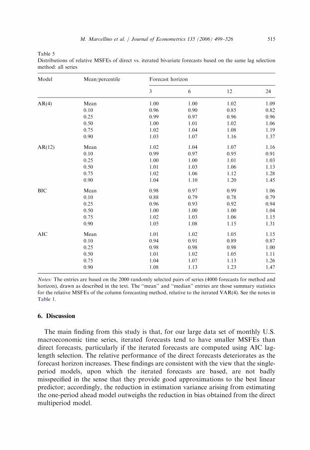
ARTICLE IN PRESS

Table 5

Distributions of relative MSFEs of direct vs. iterated bivariate forecasts based on the same lag selection

method: all series


3 6 12 24

AR(4) Mean 1.00 1.00 1.02 1.09

0.10 0.96 0.90 0.85 0.82

0.25 0.99 0.97 0.96 0.96

0.50 1.00 1.01 1.02 1.06

0.75 1.02 1.04 1.08 1.19

0.90 1.03 1.07 1.16 1.37

AR(12) Mean 1.02 1.04 1.07 1.16

0.10 0.99 0.97 0.95 0.91

0.25 1.00 1.00 1.01 1.03

0.50 1.01 1.03 1.06 1.13

0.75 1.02 1.06 1.12 1.28

0.90 1.04 1.10 1.20 1.45

BIC Mean 0.98 0.97 0.99 1.06

0.10 0.88 0.79 0.78 0.79

0.25 0.96 0.93 0.92 0.94

0.50 1.00 1.00 1.00 1.04

0.75 1.02 1.03 1.06 1.15

0.90 1.05 1.08 1.15 1.31

AIC Mean 1.01 1.02 1.05 1.15

0.10 0.94 0.91 0.89 0.87

0.25 0.98 0.98 0.98 1.00

0.50 1.01 1.02 1.05 1.11

0.75 1.04 1.07 1.13 1.26

0.90 1.08 1.13 1.23 1.47

Notes: The entries are based on the 2000 randomly selected pairs of series (4000 forecasts for method and

horizon), drawn as described in the text. The ‘‘mean’’ and ‘‘median’’ entries are those summary statistics

for the relative MSFEs of the column forecasting method, relative to the iterated VAR(4). See the notes in

Table 1.


6. Discussion

The main finding from this study is that, for our large data set of monthly U.S.macroeconomic time series, iterated forecasts tend to have smaller MSFEs thandirect forecasts, particularly if the iterated forecasts are computed using AIC lag-length selection. The relative performance of the direct forecasts deteriorates as theforecast horizon increases. These findings are consistent with the view that the single-period models, upon which the iterated forecasts are based, are not badlymisspecified in the sense that they provide good approximations to the best linearpredictor; accordingly, the reduction in estimation variance arising from estimatingthe one-period ahead model outweighs the reduction in bias obtained from the directmultiperiod model.

ARTICLE IN PRESS

Table 6

Relative MSFEs of each bivariate forecast method, relative to iterated VAR(4), and the fraction of times

each forecast method is best

Forecast horizon Percentile Iterated forecasts Direct forecasts

AR(4) AR(12) BIC AIC Sum AR(4) AR(12) BIC AIC Sum

(A) All variables

3 Mean 1.00 1.03 1.04 1.00 1.00 1.04 1.01 0.01

Median 1.00 1.04 1.01 1.00 1.00 1.05 1.01 0.02

Fraction best 0.15 0.14 0.27 0.13 0.69 0.08 0.07 0.10 0.08 0.33

6 Mean 1.00 1.00 1.06 0.99 0.99 1.03 1.01 0.01

Median 1.00 1.03 1.02 1.00 1.01 1.05 1.01 0.02

Fraction best 0.18 0.20 0.24 0.14 0.75 0.07 0.07 0.07 0.06 0.26

12 Mean 1.00 1.00 1.06 0.99 1.01 1.07 1.03 0.04

Median 1.00 1.03 1.03 1.00 1.02 1.09 1.03 0.05

Fraction best 0.21 0.21 0.19 0.16 0.77 0.06 0.08 0.06 0.04 0.25

24 Mean 1.00 1.03 1.04 0.99 1.09 1.19 1.09 0.15

Median 1.00 1.03 1.02 1.00 1.06 1.15 1.07 0.11

Fraction best 0.22 0.22 0.19 0.19 0.81 0.05 0.07 0.06 0.04 0.21

(B) Pairs not including wages, prices, or money

3 Mean 1.00 1.06 1.03 1.02 1.01 1.08 1.02 0.04

Median 1.00 1.05 1.00 1.01 1.01 1.06 1.01 0.02

Fraction best 0.18 0.10 0.29 0.13 0.71 0.09 0.04 0.11 0.07 0.31

6 Mean 1.00 1.04 1.04 1.01 1.02 1.08 1.03 0.05

Median 1.00 1.05 1.01 1.01 1.01 1.07 1.02 0.03

Fraction best 0.22 0.16 0.25 0.14 0.77 0.08 0.05 0.08 0.04 0.25

12 Mean 1.00 1.05 1.04 1.01 1.05 1.12 1.05 0.08

Median 1.00 1.04 1.02 1.00 1.03 1.11 1.03 0.06

Fraction best 0.24 0.17 0.20 0.17 0.78 0.06 0.06 0.08 0.04 0.24

24 Mean 1.00 1.07 1.02 1.01 1.12 1.23 1.10 0.18

Median 1.00 1.04 1.01 1.00 1.08 1.18 1.07 0.12

Fraction best 0.23 0.17 0.22 0.19 0.81 0.05 0.06 0.07 0.03 0.22

(C) Nonprice, wage, money variables in pairs that include a price, wage, money variable

3 Mean 1.00 1.08 1.01 1.03 1.01 1.09 1.01 1.06

Median 1.00 1.07 1.00 1.02 1.01 1.08 1.01 1.05

Fraction best 0.18 0.04 0.41 0.09 0.73 0.08 0.02 0.14 0.04 0.28

6 Mean 1.00 1.07 1.01 1.02 1.03 1.10 1.03 1.08

Median 1.00 1.06 1.00 1.02 1.02 1.09 1.02 1.06

Fraction best 0.22 0.07 0.41 0.13 0.82 0.06 0.02 0.06 0.04 0.18

12 Mean 1.00 1.08 1.02 1.03 1.07 1.16 1.07 1.13

Median 1.00 1.07 1.02 1.02 1.05 1.14 1.05 1.11

Fraction best 0.30 0.10 0.29 0.13 0.83 0.07 0.03 0.05 0.02 0.18

24 Mean 1.00 1.09 1.03 1.04 1.16 1.32 1.16 1.28

Median 1.00 1.07 1.02 1.02 1.13 1.26 1.12 1.23

Fraction best 0.31 0.14 0.23 0.18 0.86 0.04 0.04 0.04 0.03 0.16

(D) Price, wage, money variables

3 Mean 1.00 0.88 1.11 0.92 0.97 0.88 1.01 0.89

Median 1.00 0.89 1.05 0.94 0.98 0.89 1.01 0.91

Fraction best 0.01 0.38 0.03 0.16 0.58 0.07 0.20 0.02 0.14 0.43


ARTICLE IN PRESS

Table 6 (continued )

Forecast horizon Percentile Iterated forecasts Direct forecasts

AR(4) AR(12) BIC AIC Sum AR(4) AR(12) BIC AIC Sum

6 Mean 1.00 0.80 1.15 0.88 0.90 0.82 0.93 0.83

Median 1.00 0.82 1.11 0.89 0.92 0.84 0.95 0.84

Fraction best 0.01 0.47 0.03 0.14 0.64 0.04 0.17 0.04 0.12 0.37

12 Mean 1.00 0.79 1.15 0.87 0.87 0.81 0.92 0.82

Median 1.00 0.81 1.12 0.89 0.89 0.84 0.95 0.84

Fraction best 0.06 0.44 0.04 0.15 0.69 0.04 0.21 0.01 0.07 0.33

24 Mean 1.00 0.85 1.10 0.90 0.91 0.93 0.97 0.92

Median 1.00 0.83 1.08 0.91 0.92 0.93 0.98 0.92

Fraction best 0.13 0.44 0.04 0.17 0.78 0.03 0.12 0.03 0.07 0.25

Notes: The entries are based on the 2000 randomly selected pairs of series (4000 forecasts for method and

horizon), drawn as described in the text. The ‘‘mean’’ and ‘‘median’’ entries are those summary statistics

for the relative MSFEs of the column forecasting method, relative to the iterated VAR(4). See the notes to

Table 3.


There is considerable heterogeneity in these data with respect to the best lag orderof the one-period model: for nominal price, wage, and money series, a long-lag orderis indicated, whereas for the other series a short-lag order is more appropriate.Overall, this heterogeneity appears to be handled adequately by using AIC lag-lengthselection when specifying the model for the iterated forecast.

It is interesting to note that these findings in favor of the iterated forecasts are atodds with some of the theoretical literature, which emphasizes the robustness andbias reduction of the direct forecasts in contrast to the special parametric, finite-lagassumptions that underlie optimality properties for the iterated forecasts (cf.Bhansali, 1999; Ing, 2003). It appears that, in practice, the robustness and biasreduction obtained using direct forecasts do not justify the price paid in terms ofincreased sampling variance.

Acknowledgments

The authors thank Jin-Lung Lin, Frank Schorfheide, Ken West, and two refereesfor comments. This research was funded in part by NSF grant SBR-0214131.

Appendix A. Data Appendix

This appendix lists the time series used in the empirical analysis. The series wereeither taken directly from the DRI-McGraw Hill Basic Economics database, inwhich case the original mnemonics are used, or they were produced by authors’calculations based on data from that database, in which case the authors’calculations and original DRI/McGraw series mnemonics are summarized in thedata description field. Following the series name is a transformation code, the

ARTICLE IN PRESS


sample period for the data series, and a short data description. The transformationsare (Lev) level of the series; (D) first difference; (Ln) logarithm of the series; (DLn)first difference of the logarithm. The following abbreviations appear in thedata descriptions: SA ¼ seasonally adjusted; NSA ¼ not seasonally adjusted;SAAR ¼ seasonally adjusted at an annual rate; AC ¼ authors’ calculations.

Series
Trans. Sample period Description
(A) Income, output, sales, capacity utilization
Msmq DLn 1967: 1–2001: 7 Sales, business—manufacturing
(chained)
ips11 DLn 1959: 1–2002: 12 Industrial production index—products,
total
ips299 DLn 1959: 1–2002: 12 Industrial production index—final
products
ips12 DLn 1959: 1–2002: 12 Industrial production index—consumer
goods
ips13 DLn 1959: 1–2002: 12 Industrial production index—durable
consumer goods
ips18 DLn 1959: 1–2002: 12 Industrial production index—
nondurable consumer goods
ips25 DLn 1959: 1–2002: 12 Industrial production index—business
equipment
ipi DLn 1959: 1–2002: 10 industrial production: intermediate
products (1992 ¼ 100, sa)
ips32 DLn 1959: 1–2002: 12 Industrial production index—materials ips34 DLn 1959: 1–2002: 12 Industrial production index—durable
goods materials
nondurable goods materials
manufacturing (sic)
ipd DLn 1959: 1–2002: 10 Industrial production: durable
manufacturing (1992 ¼ 100, sa)
ipn DLn 1959: 1–2002: 10 Industrial production: nondurable
manufacturing (1992 ¼ 100, sa)

ipmin
DLn 1959: 1–2002: 10 Industrial production: mining(1992 ¼ 100, sa)
iput
DLn 1959: 1–2002: 10 Industrial production: utilities(1992 ¼ 100, sa)
utl10
Lev 1967: 1–2002: 12 Capacity utilization—total index utl11 Lev 1959: 1–2002: 12 Capacity utilization—manufacturing (sic) utl13 Lev 1967: 1–2002: 12 Capacity utilization—durable
manufacturing (naics)

ARTICLE IN PRESS


utl25
Lev 1967: 1–2002: 12 Capacity utilization—nondurablemanufacturing (naics)
utl35
Lev 1967: 1–2002: 12 Capacity utilization—mining naics ¼ 21 utl36 Lev 1967: 1–2002: 12 Capacity utilization—electric and gas
utilities
gmpyq DLn 1959: 1–2002: 12 Personal income (chained, series #52,
bil 92$, saar)
gmyxpq DLn 1959: 1–2002: 12 Personal income less transfer payments
(chained, series #51, bil 92$, saar)
gmcq DLn 1967: 1–2002: 12 Personal consumption expenditure
(chained)—total (bil 92$, saar)
gmcdq DLn 1967: 1–2002: 12 Personal consumption expenditure
(chained)—total durables (bil 1996$,saar)

gmcnq
DLn 1967: 1–2002: 12 Personal consumption expenditure(chained)—nondurables (bil 96$,saar)
gmcsq
DLn 1967: 1–2002: 12 Personal consumption expenditure(chained)—services (bil 92$, saar)
gmcanq
DLn 1967: 1–2002: 12 Personal consumption expenditure(chained)—new cars (bil 1996$, saar)
wtq
DLn 1959: 1–2001: 7 Merch wholesalers: total (mil of chained1996 dollars, sa)
wtdq
DLn 1959: 1–2001: 7 Merch wholesalers: durable goods total(mil of chained 1996 dollars, sa)
msdq
DLn 1959: 1–2001: 7 Mfg. and trade: mfg.; durable goods (milof chained 1996 dollars, sa)
msmtq
DLn 1959: 1––2001: 7 Mfg. and trade: total (mil of chained1996 dollars, sa)
msnq
DLn 1959: 1–2001: 7 Mfg. and trade: mfg.;nondurable goods(mil of chained 1996 dollars, sa)
wtnq
DLn 1959: 1–2001: 7 Merch. wholesalers: nondurable goods(mil of chained 1996 dollars, sa)
rtdrq
DLn 1967: 1–2001: 4 Retail sales durables, real (rtdr/pucd,AC)
rtnrq
DLn 1967: 1–2001: 4 Retail sales nondurables, real (rtnr/pu882, AC)
ips10
DLn 1959: 1–2002: 12 Industrial production index—total index
(B) Employment and unemployment
lpnag DLn 1959: 1–2002: 12 Employees on nonag. payrolls: total
(thous., sa)
lhu26 Lev 1959: 1–2002: 12 Unemployed by duration: persons
unemployed 15–26 wks (thous., sa)
lpgd DLn 1959: 1–2002: 12 Employees on nonag. payrolls: goods-
producing (thous., sa)

ARTICLE IN PRESS


lhu15
Lev 1959: 1–2002: 12 Unemployed by duration: personsunemployed 15 wks+(thous., sa)
lp
DLn 1959: 1–2002: 12 Employees on nonag payrolls: total,private (thous., sa)
lpcc
DLn 1959: 1–2002: 12 Employees on nonag. payrolls: contractconstruction (thous., sa)
lhelx
Ln 1959: 1–2002: 12 Employment: ratio; help-wanted ads: no.unemployed clf
lhu5
Lev 1959: 1–2002: 12 Unemployed by duration: personsunemployed less than 5 wks (thous., sa)
lhu14
Lev 1959: 1–2002: 12 Unemployed by duration: personsunemployed 5–14 wks (thous., sa)
lpsp
DLn 1959: 1–2002: 12 Employees on nonag. payrolls: service-producing (thous., sa)
lptu
DLn 1959: 1–2002: 12 Employees on nonag. payrolls: trans.and public utilities (thous., sa)
lpt
DLn 1959: 1–2002: 12 Employees on nonag. payrolls: wholesaleand retail trade (thous., sa)
lpfr
DLn 1959: 1–2002: 12 Employees on nonag. payrolls: finance,insur. and real estate (thous., sa)
lps
DLn 1959: 1–2002: 12 Employees on nonag. payrolls: services(thous., sa)
lpgov
DLn 1959: 1–2002: 12 Employees on nonag. payrolls:government (thous., sa)
lw
Dif 1964: 1–2002: 12 Avg. weekly hrs. of prod. wkrs.: totalprivate (sa)
lphrm
Lev 1959: 1–2002: 12 Avg. weekly hrs. of production wkrs.:manufacturing (sa)
lpmosa
Lev 1959: 1–2002: 12 Avg. weekly hrs. of prod. wkrs.: mfg.,overtime hrs. (sa)
lhu680
Lev 1959: 1–2002: 12 Unemployed by duration: average(mean) duration in weeks (sa)
lhur
Lev 1959: 1–2002: 12 Unemployment rate: all workers, 16years and over (%, sa)
lpen
DLn 1959: 1–2002: 12 Employees on nonag. payrolls:nondurable goods (thous., sa)
lpem
DLn 1959: 1–2002: 12 Employees on nonag. payrolls:manufacturing (thous., sa)
lhel
DLn 1959: 1–2002: 12 Index of help-wanted advertising innewspapers (1967 ¼ 100; sa)
lped
DLn 1959: 1–2002: 12 Employees on nonag. payrolls: durablegoods (thous., sa)
lhem
DLn 1959: 1–2002: 12 Civilian labor force: employed, total(thous., sa)

ARTICLE IN PRESS


lhnag
DLn 1959: 1–2002: 12 Civilian labor force: employed, nonagric.industries (thous., sa)
lpmi
DLn 1959: 1–2002: 12 Employees on nonag. payrolls: mining(thous., sa)
(C) Construction, inventories and orders
hssou Ln 1959: 1–2002: 12 Housing starts: south (thous.u., s.a.) contc DLn 1964: 1–2002: 12 Construct.put in place: total priv and
public 1987 $ (mil$, saar)
conpc DLn 1964: 1–2002: 12 Construct. put in place: total private
1987 $ (mil$, saar)
conqc DLn 1964: 1–2002: 12 New construction put in place—public
(c30)
condo9 Ln 1963: 1–2002: 12 Construct.contracts: comm’l and
indus.bldgs (mil.sq.ft.floor sp.;sa)
hniv Ln 1963: 1–2002: 12 New 1-family houses for sale at end of
month (thous, sa)
hnr Ln 1963: 1–2002: 12 New 1-family houses, month’s supply @
current sales rate (ratio)
hns Ln 1963: 1–2002: 12 New 1-family houses sold during month
(thous, saar)
hsbr Ln 1959: 1–2002: 12 Housing authorized: total new priv
housing units (thous., saar)
hswst Ln 1959: 1–2002: 12 Housing starts: west (thous.u.) s.a. hmob Ln 1959: 1–2002: 12 Mobile homes: manufacturers’
shipments (thous.of units, saar)
hsmw Ln 1959: 1–2002: 12 Housing starts: midwest (thous.u.) s.a. hsne Ln 1959: 1–2002: 12 Housing starts: northeast (thous.u.) s.a. hsfr Ln 1959: 1–2002: 12 Housing starts: nonfarm (1947–58);total
farm and nonfarm (1959-, thous., sa)
ivmtq DLn 1959: 1–2001: 7 Mfg. and trade inventories: total (mil of
chained 1996, sa)
ivmfgq DLn 1959: 1–2001: 7 Inventories, business, mfg. (mil of
chained 1996 dollars, sa)
ivmfdq DLn 1959: 1–2001: 7 Inventories, business durables (mil of
chained 1996 dollars, sa)
ivmfnq DLn 1959: 1–2001: 7 Inventories, business, nondurables (mil
of chained 1996 dollars, sa)
ivwrq DLn 1959: 1–2001: 7 Mfg. and trade inv: merchant
wholesalers (mil of chained 1996dollars, sa)

ivrrq
DLn 1959: 1–2001: 7 Mfg. and trade inv: retail trade (mil ofchained 1996 dollars, sa)
ivsrq
DLn 1959: 1–2001: 7 Ratio for mfg. and trade: inventory/sales(chained 1996 dollars, sa)

ARTICLE IN PRESS


ivsrmq
DLn 1959: 1–2001: 7 Ratio for mfg. and trade: mfg.;inventory/sales (1996 $ s.a.)
ivsrwq
DLn 1959: 1–2001: 7 Ratio for mfg. and trade: wholesaler;inventory/sales (1996 $ s.a.)
ivsrrq
DLn 1959: 1–2001: 7 Ratio for mfg. and trade: retailtrade;inventory/sales(1996 $ s.a.)
pmi
Lev 1959: 1–2002: 12 Purchasing managers’ index (sa) pmp Lev 1959: 1–2002: 12 Napm production index (percent) pmno Lev 1959: 1–2002: 12 Napm new orders index (percent) pmdel Lev 1959: 1–2002: 12 Napm vendor deliveries index (percent) pmnv Lev 1959: 1–2002: 12 Napm inventories index (percent) pmemp Lev 1959: 1–2002: 12 Napm employment index (percent) pmcp Lev 1959: 1–2002: 12 Napm commodity prices index (percent) mocmq DLn 1959: 1–2002: 12 New orders (net)—consumer goods and
materials, 1996 dollars (bci)
msondq DLn 1959: 1–2002: 12 New orders, nondefense capital goods, in
1996 dollars (bci)
moq DLn 1959: 1–2001: 5 Mfg. new orders: all manufacturing
industries, total, real (mo/pwfsa, AC)
mdoq DLn 1959: 1–2001: 5 Mfg. new orders: durable goods
industries, total, real (mdo/pwfsa, AC)
muq DLn 1959: 1–2001: 5 Mfg. unfilled orders: all manufacturing
industries, total (mu/pwfsa, AC)
mduq DLn 1959: 1–2001: 5 Mfg. unfilled orders: durable goods
industries, total (mdu/pwfsa, AC)

(D) Interest rates and asset prices
fygt10 D 1959: 1–2002: 12 Interest rate: U.S. treasury const
maturities, 10-yr.(% per ann, nsa)
fclnq DLn 1959: 1–2002: 12 Commercial and industrial loans
oustanding in 1996 dollars (bci)
fsncom DLn 1959: 1–2002: 12 Nyse common stock price index:
composite (12/31/65 ¼ 50)
fsnin DLn 1966: 1–2002: 12 Nyse common stock price index:
industrial (12/31/65 ¼ 50)
fsntr DLn 1966: 1–2002: 12 Nyse common stock price index:
transportation (12/31/65 ¼ 50)
fsnut DLn 1966: 1–2002: 12 Nyse common stock price index: utility
(12/31/65 ¼ 50)
fsnfi DLn 1966: 1–2002: 12 Nyse common stock price index: finance
(12/31/65 ¼ 50)
fspcom DLn 1959: 1–2002: 12 S&p’s common stock price index:
composite (1941-43 ¼ 10)
fspin DLn 1959: 1–2002: 12 S&p’s common stock price index:
industrials (1941-43 ¼ 10)

ARTICLE IN PRESS


fsdxp
Lev 1959: 1–2002: 12 S&p’s composite common stock:dividend yield (% per annum)
fspxe
Lev 1959: 1–2002: 12 S&p’s composite common stock: price-earnings ratio (%, nsa)
fyff
D 1959: 1–2002: 12 Interest rate: federal funds (effective)(% per annum, nsa)
fygm3
D 1959: 1–2002: 12 Interest rate: U.S. treasury bills, sec mkt,3-mo. (% per ann, nsa)
fygm6
D 1959: 1–2002: 12 Interest rate: U.S. treasury bills, sec mkt,6-mo. (% per ann, nsa)
fygt1
D 1959: 1–2002: 12 Interest rate: U.S. treasury constmaturities, 1-yr. (% per ann, nsa)
fygt5
D 1959: 1–2002: 12 Interest rate: U.S. treasury constmaturities, 5-yr. (% per ann, nsa)
fm2dq
DLn 1959: 1–2002: 2 Money supply—m2 in 1996 dollars (bci) fyaaac D 1959: 1–2002: 12 Bond yield: moody’s aaa corporate
(% per annum)
fybaac D 1959: 1–2002: 12 Bond yield: moody’s baa corporate
(% per annum)
fymcle D 1963: 1–2002: 12 Effective interest rate: conventional
home mtge loans closed (%)
sfygm3 Lev 1959: 1–2002: 12 Fygm3-fyff (AC) sfygm6 Lev 1959: 1–2002: 12 Fygm6-fyff (AC) sfygt1 Lev 1959: 1–2002: 12 Fygt1-fyff (AC) sfygt5 Lev 1959: 1–2002: 12 Fygt5-fyff (AC) sfygt10 Lev 1959: 1–2002: 12 Fygt10-fyff (AC) sfyaaac Lev 1959: 1–2002: 12 Fyaaac-fyff (AC) sfybaac Lev 1959: 1–2002: 12 Fybaac-fyff (AC) sfymcle Lev 1963: 1–2002: 12 Fymcle-fyff (AC) exrus DLn 1959: 1–2002: 12 United states; effective exchange rate
(merm, index no.)
exrsw DLn 1959: 1–2002: 12 Foreign exchange rate: switzerland (swiss
franc per U.S. $)
exrjan DLn 1959: 1–2002: 12 Foreign exchange rate: japan (yen per
U.S. $)
exruk DLn 1959: 1–2002: 12 Foreign exchange rate: united kingdom
(cents per pound)
exrcan DLn 1959: 1–2002: 12 Foreign exchange rate: canada (canadian
$ per U.S. $)

(E) Nominal prices, wages, and money
fm1 DLn 1959: 1–2002: 12 Money stock: m1(curr, trav. cks, dem
dep, other ck’able dep, bil$, sa)
fm2 DLn 1959: 1–2002: 12 Money stock: m2 (m1+o’nite rps, euro$,
g/p&b/d mmmfs & sav & sm time dep, bil$)

ARTICLE IN PRESS


fm3
DLn 1959: 1–2002: 12 Money stock: m3 (m2+lg time dep, termrp’s & inst only mmmfs, bil$, sa)
fmfba
DLn 1959: 1–2002: 12 Monetary base, adj for reserverequirement changes (mil$, sa)
fmrra
DLn 1959: 1–2002: 12 Depository inst reserves: total, adj forreserve req chgs (mil$, sa)
leh
DLn 1964: 1–2002: 12 Avg hr earnings of prod. wkrs.: totalprivate nonagric ($, sa)
lehcc
DLn 1959: 1–2002: 12 Avg hr earnings of constr. wkrs.:construction ($, sa)
lehm
DLn 1959: 1–2002: 12 Avg hr earnings of prod. wkrs.:manufacturing ($, sa)
lehtu
DLn 1964: 1–2002: 12 Avg hr earnings of nonsupv. wkrs.: trans& public util($, sa)
lehtt
DLn 1964: 1–2002: 12 Avg hr earnings of prod. wkrs.:wholesale & retail trade (sa)
lehfr
DLn 1964: 1–2002: 12 Avg hr earnings of nonsupv. wkrs.:finance, insur, real est ($, sa)
lehs
DLn 1964: 1–2002: 12 Avg hr earnings of nonsupv. wkrs.:services ($, sa)
pwfsa
DLn 1959: 1–2002: 12 Producer price index: finished goods(82 ¼ 100, sa)
pwfcsa
DLn 1959: 1–2002: 12 Producer price index: finished consumergoods (82 ¼ 100, sa)
pwimsa
DLn 1959: 1–2002: 12 Producer price index: intermedmat.supplies and components(82 ¼ 100, sa)
pwcmsa
DLn 1959: 1–2002: 12 Producer price index: crude materials(82 ¼ 100, sa)
pwfxsa
DLn 1967: 1–2002: 12 Producer price index: finishedgoods,excl. foods (82 ¼ 100, sa)
psm99q
DLn 1959: 1–2002: 12 Index of sensitive materials prices(1990 ¼ 100, bci-99a)
punew
DLn 1959: 1–2002: 12 Cpi-u: all items (82–84 ¼ 100, sa) pu81 DLn 1967: 1–2002: 12 Cpi-u: food and beverages
(82–84 ¼ 100, sa)
puh DLn 1967: 1–2002: 12 Cpi-u: housing (82–84 ¼ 100, sa) pu83 DLn 1959: 1–2002: 12 Cpi-u: apparel and upkeep
(82–84 ¼ 100, sa)
pu84 DLn 1959: 1–2002: 12 Cpi-u: transportation (82–84 ¼ 100, sa) pu85 DLn 1959: 1–2002: 12 Cpi-u: medical care (82–84 ¼ 100, sa) pu882 DLn 1959: 1–2002: 12 Cpi-u: nondurables (1982–84 ¼ 100, sa) puc DLn 1959: 1–2002: 12 Cpi-u: commodities (82–84 ¼ 100, sa) pucd DLn 1959: 1–2002: 12 Cpi-u:durables (82–84 ¼ 100, sa) pus DLn 1959: 1–2002: 12 Cpi-u: services (82–84 ¼ 100, sa)

ARTICLE IN PRESS


puxf
DLn 1959: 1–2002: 12 Cpi-u: all items less food(82–84 ¼ 100, sa)
puxhs
DLn 1959: 1–2002: 12 Cpi-u: all items less shelter(82–84 ¼ 100, sa)
puxm
DLn 1959: 1–2002: 12 Cpi-u: all items less midical care(82–84 ¼ 100, sa)
gmdc
DLn 1959: 1–2002: 12 Pce, impl pr defl: pce (1987 ¼ 100) gmdcd DLn 1959: 1–2002: 12 Pce, impl pr defl: pce; durables
(1987 ¼ 100)
gmdcn DLn 1959: 1–2002: 12 Pce, impl pr defl: pce; nondurables
(1996 ¼ 100)
gmdcs DLn 1959: 1–2002: 12 Pce, impl pr defl: pce; services
(1987 ¼ 100)

References

Ang, A., Piazzesi, M., Wei, M., 2005. What does the yield curve tell us about GDP growth? Journal of

Econometrics (forthcoming).

Bhansali, R.J., 1996. Asymptotically efficient autogressive model selection for multistep prediction. Annals

of the Institute of Statistical Mathematics 48 (3), 577–602.

Bhansali, R.J., 1997. Direct autoregressive predictions for multistep prediction: order selection and

performance relative to the plug in predictors. Statistica Sinca 7, 425–449.

Bhansali, R.J., 1999. Parameter estimation and model selection for multistep prediction of a time series: a

review. In: Ghosh, S. (Ed.), Asymptotics, Nonparametrics, and Time Series. Marcel Dekker, New

York, pp. 201–225.

Box, G.E.P., Jenkins, G.M., 1976. Time Series Analysis: Forecasting and Control, 2nd ed. Holden Day,

New York.

Brayton, F., Roberts, J., Williams, J., 1999. What’s Happened to the Phillips Curve? manuscript, FRB

Working Paper 1999-49, U.S. Federal Reserve Board.

Chevillon, G., Hendry, D.F., 2005. Non-parametric direct multi-step estimation for forecasting economic

processes. International Journal of Forecasting 21, 201–218.

Clark, T.E., McCracken, M.W., 2001. Tests of equal forecast accuracy and encompassing for nested

models. Journal of Econometrics 105, 85–100.

Clements, M.P., Hendry, D.F., 1996. Multi-step estimation for forecasting. Oxford Bulletin of Economics

and Statistics 58, 657–684.

Cox, D.R., 1961. Prediction by exponentially weighted moving averages and related methods. JRSS, B 23,

414–422.

Findley, D.F., 1983. On the use of multiple models for multi-period forecasting. Proceedings of the

Business and Statistics Section, American Statistical Association, 528–531.

Findley, D.F., 1985. Model selection for multi-step-ahead forecasting. In: Baker, H.A., Young, P.C.

(Eds.), Proceedings of the Seventh Symposium on Identification and System Parameter Estimation.

Pergamon, Oxford, pp. 1039–1044.

Ing., C.-K., 2003. Multistep prediction in autoregressive processes. Econometric Theory 19, 254–279.

Kang, I.-B., 2003. Multi-period forecasting using different models for different horizons: an application to

U.S. economic time series data. International Journal of Forecasting 19, 387–400.

Kim, Chang-Jin., Charles, R. Nelson., 1999. Has the U.S. economy become more stable? a Bayesian

approach based on a Markov-switching model of the business cycle. The Review of Economics and

Statistics 81, 608–616.

ARTICLE IN PRESS


Klein, L.R., 1968. An Essay on the Theory of Economics Prediction. Sanomaprint, Helsinki, Finland

(Yrjo Jansen lectures).

Lin, J.-L., Granger, C.W.G., 1994. Forecasting from non-linear models in practice. Journal of Forecasting

13, 1–9.

Liu, S.-I., 1996. Model selection for multiperiod forecasts. Biometrika 83, 861–873.

McConnell, M.M., Perez-Quiros, G., 2000. Output fluctuations in the United States: what has changed

since the early 1980s. American Economic Review 90 (5), 1464–1476.

Nelson, C.R., Schwert, G.W., 1977. On testing the hypothesis that the real rate of interest is constant.

American Economic Review 67, 478–486.

Schorfheide, F., 2005. VAR forecasting under misspecification. Journal of Econometrics (forthcoming).

Schwert, G.W., 1987. Effects of model misspecification on tests for unit roots in macroeconomic data.

Journal of Monetary Economics 20, 73–103.

Shibata, R., 1980. Asymptotically efficient selection of the order of the model for estimating parameters of

a linear process. Annals of Statistics 8 (1), 1464–1470.

Stock, J.H., 1997. Cointegration, long-run comovements, and long-horizon forecasting. In: Kreps, D.,

Wallis, K.F. (Eds.), Advances in Econometrics: Proceedings of the Seventh World Congress of the

Econometric Society, vol. III. Cambridge, Cambridge University Press, pp. 34–60.

Stock, J.H., Watson, M.W., 2002a. Forecasting using principal components from a large number of

predictors. Journal of the American Statistical Association 97, 1167–1179.

Stock, J.H., Watson, M.W., 2002b. Macroeconomic forecasting using diffusion indexes. Journal of

Business and Economic Statistics 20 (2), 147–162.

Tiao, G.C., Xu, D., 1993. Robustness of MLE for multi-step predictions: the exponential smoothing case.

Biometrika 80, 623–641.

Tiao, G.C., Tsay, R.S., 1994. Some advances in non-linear and adaptive modelling in time-series. Journal

of Forecasting 13, 109–131.

Weiss, A.A., 1991. Multi-step estimation and forecasting in dynamic models. Journal of Econometrics 48,

135–149.

West, K.D., 1996. Asymptotic inference about predictive ability. Econometrica 64, 1067–1084.

A comparison of direct and iterated multistep AR methods ...mwatson/papers/Marcellino_Stock_Watson_JoE_2006.pdfThe relative performance of the iterated forecasts improves with the

Documents