Iterated Filtering

arX

iv:0

902.

0347

v2 [

mat

h.ST

] 2

2 N

ov 2

012

The Annals of Statistics

2011, Vol. 39, No. 3, 1776–1802DOI: 10.1214/11-AOS886c© Institute of Mathematical Statistics, 2011

ITERATED FILTERING1

By Edward L. Ionides, Anindya Bhadra,

Yves Atchade and Aaron King

University of Michigan and Fogarty International Center, NationalInstitutes of Health, University of Michigan, University of Michigan,

and University of Michigan and Fogarty International Center,National Institutes of Health

Inference for partially observed Markov process models has been alongstanding methodological challenge with many scientific and engi-neering applications. Iterated filtering algorithms maximize the likeli-hood function for partially observed Markov process models by solvinga recursive sequence of filtering problems. We present new theoreticalresults pertaining to the convergence of iterated filtering algorithmsimplemented via sequential Monte Carlo filters. This theory comple-ments the growing body of empirical evidence that iterated filteringalgorithms provide an effective inference strategy for scientific mod-els of nonlinear dynamic systems. The first step in our theory involvesstudying a new recursive approach for maximizing the likelihood func-tion of a latent variable model, when this likelihood is evaluated viaimportance sampling. This leads to the consideration of an iteratedimportance sampling algorithm which serves as a simple special caseof iterated filtering, and may have applicability in its own right.

1. Introduction. Partially observed Markov process (POMP) models areof widespread importance throughout science and engineering. As such, theyhave been studied under various names including state space models [Durbin

Received September 2010; revised March 2011.1Supported by NSF Grants DMS-08-05533 and EF-04-30120, the Graham Environ-

mental Sustainability Institute, the RAPIDD program of the Science & Technology Direc-torate, Department of Homeland Security, and the Fogarty International Center, NationalInstitutes of Health.

This work was conducted as part of the Inference for Mechanistic Models WorkingGroup supported by the National Center for Ecological Analysis and Synthesis, a Centerfunded by NSF Grant DEB-0553768, the University of California, Santa Barbara and theState of California.

MSC2010 subject classification. 62M09.Key words and phrases. Dynamic systems, sequential Monte Carlo, filtering, impor-

tance sampling, state space model, partially observed Markov process.

This is an electronic reprint of the original article published by theInstitute of Mathematical Statistics in The Annals of Statistics,2011, Vol. 39, No. 3, 1776–1802. This reprint differs from the original inpagination and typographic detail.

1

http://arxiv.org/abs/0902.0347v2

http://www.imstat.org/aos/

http://dx.doi.org/10.1214/11-AOS886

http://www.imstat.org

http://www.imstat.org

http://www.imstat.org/aos/

http://dx.doi.org/10.1214/11-AOS886

2 IONIDES, BHADRA, ATCHADE AND KING

and Koopman (2001)], dynamic models [West and Harrison (1997)] and hid-den Markov models [Cappe, Moulines and Ryden (2005)]. Applications in-clude ecology [Newman et al. (2009)], economics [Fernandez-Villaverde andRubio-Ramırez (2007)], epidemiology [King et al. (2008)], finance [Johannes,Polson and Stroud (2009)], meteorology [Anderson and Collins (2007)], neu-roscience [Ergun et al. (2007)] and target tracking [Godsill et al. (2007)].

This article investigates convergence of a Monte Carlo technique for esti-mating unknown parameters of POMPs, called iterated filtering, which wasproposed by Ionides, Breto and King (2006). Iterated filtering algorithmsrepeatedly carry out a filtering procedure to explore the likelihood surfaceat increasingly local scales in search of a maximum of the likelihood func-tion. In several case-studies, iterated filtering algorithms have been showncapable of addressing scientific challenges in the study of infectious diseasetransmission, by making likelihood-based inference computationally feasiblein situations where this was previously not the case [King et al. (2008); Bretoet al. (2009); He, Ionides and King (2010); Laneri et al. (2010)]. The par-tially observed nonlinear stochastic systems arising in the study of diseasetransmission and related ecological systems are a challenging environmentto test statistical methodology [Bjørnstad and Grenfell (2001)], and manystatistical methodologies have been tested on these systems in the past fiftyyears [e.g., Cauchemez and Ferguson (2008); Toni et al. (2008); Keeling andRoss (2008); Ferrari et al. (2008); Morton and Finkenstadt (2005); Grenfell,Bjornstad and Finkenstadt (2002); Kendall et al. (1999); Bartlett (1960);Bailey (1955)]. Since iterated filtering has already demonstrated potentialfor generating state-of-the-art analyses on a major class of scientific models,we are motivated to study its theoretical justification. The previous the-oretical investigation of iterated filtering, presented by Ionides, Breto andKing (2006), did not engage directly in the Monte Carlo issues relating topractical implementation of the methodology. It is relatively easy to checknumerically that a maximum has been attained, up to an acceptable level ofMonte Carlo uncertainty, and therefore one can view the theory of Ionides,Breto and King (2006) as motivation for an algorithm whose capabilitieswere proven by demonstration. However, the complete framework presentedin this article gives additional insights into the potential capabilities, limi-tations and generalizations of iterated filtering.

The foundation of our iterated filtering theory is a Taylor series argu-ment which we present first in the case of a general latent variable model inSection 2. This leads us to propose and analyze a novel iterated importancesampling algorithm for maximizing the likelihood function of latent variablemodels. Our motivation is to demonstrate a relatively simple theoretical re-sult which is then extended to POMP models in Section 3. However, thisresult also demonstrates the broader possibilities of the underlying method-ological approach.

ITERATED FILTERING 3

The iterated filtering and iterated importance sampling algorithms thatwe study have an attractive practical property that the model for the un-observed process enters the algorithm only through the requirement thatrealizations can be generated at arbitrary parameter values. This propertyhas been called plug-and-play [Breto et al. (2009); He, Ionides and King(2010)] since it permits simulation code to be simply plugged into the in-ference procedure. A concept closely related to plug-and-play is that of im-plicit models for which the model is specified via an algorithm to generatestochastic realizations [Diggle and Gratton (1984); Breto et al. (2009)]. Inparticular, evaluation of the likelihood function for implicit models is con-sidered unavailable. Implicit models arise when the model is represented bya “black box” computer program. A scientist investigates such a model byinputting parameter values, receiving as output from the “black box” inde-pendent draws from a stochastic process, and comparing these draws to thedata to make inferences. For an implicit model, only plug-and-play statisti-cal methodology can be employed. Other plug-and-play methods proposedfor partially observed Markov models include approximate Bayesian com-putations implemented via sequential Monte Carlo [Liu and West (2001);Toni et al. (2008)], an asymptotically exact Bayesian technique combiningsequential Monte Carlo with Markov chain Monte Carlo [Andrieu, Doucetand Holenstein (2010)], simulation-based forecasting [Kendall et al. (1999)],and simulation-based spectral analysis [Reuman et al. (2006)]. Further dis-cussion of the plug-and-play property is included in the discussion of Sec-tion 4.

2. Iterated importance sampling. Let fXY (x, y; θ) be the joint densityof a pair of random variables (X,Y ) depending on a parameter θ ∈R

p. Wesuppose that (X,Y ) takes values in some measurable space X × Y, andfXY (x, y; θ) is defined with respect to some σ-finite product measure whichwe denote by dxdy. We suppose that the observed data consist of a fixedvalue y∗ ∈ Y, with X being unobserved. Therefore, fXY (x, y; θ), θ ∈ R

pdefines a general latent variable statistical model. We write the marginaldensities ofX and Y as fX(x; θ) and fY (y; θ), respectively. Themeasurementmodel is the conditional density of the observed variable given the latentvariable X , written as fY |X(y | x; θ). The log likelihood function is definedas ℓ(θ) = log fY (y

∗; θ). We consider the problem of calculating the maximum

likelihood estimate, defined as θ = argmaxθ ℓ(θ).We consider an iterated importance sampling algorithm which gives a

plug-and-play approach to likelihood based inference for implicit latent vari-able models, based on generating simulations at parameter values in a neigh-borhood of the current parameter estimate to refine this estimate. Thisshares broadly similar goals with other Monte Carlo methods proposed for


latent variable models [e.g., Johansen, Doucet and Davy (2008); Qian andShapiro (2006)], and in a more general context has similarities with evo-lutionary optimization strategies [Beyer (2001)]. We emphasize that thepresent motivation for proposing and studying iterated importance sam-pling is to lay the groundwork for the results on iterated filtering in Sec-tion 3. However, the successes of iterated filtering methodology on POMPmodels also raise the possibility that related techniques may be useful inother latent variable situations.

We define the stochastically perturbed model to be a triplet of randomvariables (X, Y , Θ), with perturbation parameter τ and parameter θ, havinga joint density on X×Y×R

p specified as

gX,Y ,Θ(x, y, ϑ; θ, τ) = fXY (x, y; ϑ)τ−pκτ ((ϑ− θ)/τ).(1)

Here, κτ , τ > 0 is a collection of mean-zero densities on Rp (with respect

to Lebesgue measure) satisfying condition (A1) below:

(A1) For each τ > 0, κτ is supported on a compact set K0 ⊂Rp indepen-

dent of τ .

Condition (A1) can be satisfied by the arbitrary selection of κτ . At firstreading, one can imagine that κτ is fixed, independent of τ . However, theadditional generality will be required in Section 3.

We start by showing a relationship between conditional moments of Θ andthe derivative of the log likelihood function, in Theorem 1. We write Eθ,τ [·]to denote expectation with respect to the stochastically perturbed model.We write u ∈ R

p to specify a column vector, with u′ being the transposeof u. For a function f = (f1, . . . , fm)′ :Rp → R

m, we write∫f(u)du for the

vector (∫f1(u)du, . . . ,

∫fm(u)du)′ ∈ R

m; For any function f :Rp → R, wewrite ∇f(u) to denote the column vector gradient of f , with ∇2f(u) beingthe second derivative matrix. We write | · | for the absolute value of a vectoror the largest absolute eigenvalue of a square matrix. We write B(r) = u ∈Rp : |u| ≤ r for the ball of radius r in R

p. We assume the following regularitycondition:

(A2) ℓ(θ) is twice differentiable. For any compact set K1 ⊂Rp,

supθ∈K1

|∇ℓ(θ)|<∞ and supθ∈K1

|∇2ℓ(θ)|<∞.

Theorem 1. Assume conditions (A1), (A2). Let h :Rp →Rm be a mea-

surable function possessing constants α≥ 0, c > 0 and ε > 0 such that, when-ever u ∈B(ε),

|h(u)| ≤ c|u|α.(2)


Define τ0 = supτ :K0 ⊂B(ε/τ). For any compact set K2 ⊂Rp there exists

C1 <∞ and a positive constant τ1 ≤ τ0 such that, for all 0< τ ≤ τ1,

supθ∈K2

∣∣∣∣Eθ,τ [h(Θ− θ) | Y = y∗]−∫h(τu)κτ (u)du

− τ

∫h(τu)u′κτ (u)du

∇ℓ(θ)

∣∣∣∣(3)

≤C1τ2+α.

Proof. Let gY |Θ(y | ϑ; θ, τ) denote the conditional density of Y given Θ.

We note that gY |Θ does not depend on either τ or θ, and so we omit these de-

pendencies below. Then, gY |Θ(y∗ | ϑ) =

∫fXY (x, y

∗; ϑ)dx= exp(ℓ(ϑ)). Chang-

ing variable to u= (ϑ− θ)/τ , we calculate

Eθ,τ [h(Θ− θ) | Y = y∗] =

∫h(ϑ− θ)gY |Θ(y

∗ | ϑ)τ−pκτ ((ϑ− θ)/τ)dϑ∫gY |Θ(y

∗ | ϑ)τ−pκτ ((ϑ− θ)/τ)dϑ(4)

=

∫h(τu) expℓ(θ + τu)− ℓ(θ)κτ (u)du∫

expℓ(θ+ τu)− ℓ(θ)κτ (u)du.

Applying the Taylor expansion ex = 1 + x+ (∫ 10 (1 − t)etx dt)x2 to the nu-

merator of (4) gives∫

expℓ(θ+ τu)− ℓ(θ)h(τu)κτ (u)du

=

∫h(τu)κτ (u)du+

∫ℓ(θ+ τu)− ℓ(θ)h(τu)κτ (u)du(5)

+

∫ (∫ 1

0(1− t)et(ℓ(θ+τu)−ℓ(θ)) dt

)ℓ(θ+ τu)− ℓ(θ)2h(τu)κτ (u)du.

We now expand the second term on the right-hand side of (5) by makinguse of the Taylor expansion

ℓ(θ+ τu)− ℓ(θ) = τu′∫ 1

0∇ℓ(θ+ tτu)dt

(6)

= τu′∇ℓ(θ) + τu′∫ 1

0∇ℓ(θ+ tτu)−∇ℓ(θ)dt

and defining ψτ,h(θ) =∫h(τu)κτ (u)du + τ

∫h(τu)u′κτ (u)du∇ℓ(θ). This

allows us to rewrite (5) as∫

expℓ(θ + τu)− ℓ(θ)h(τu)κτ (u)du= ψτ,h(θ) +R1(θ, τ),(7)


where

R1(θ, τ)

= τ

∫h(τu)u′

(∫ 1

0∇ℓ(θ+ tτu)−∇ℓ(θ)dt

)κτ (u)du

+

∫ (∫ 1

0(1− t)et(ℓ(θ+τu)−ℓ(θ)) dt

)ℓ(θ+ τu)− ℓ(θ)2h(τu)κτ (u)du.

As a consequence of (A2), we have

supθ∈K2

supu∈K0

supt∈[0,τ0]

(|∇ℓ(θ+ tu)|+ |∇2ℓ(θ+ tu)|)<∞.(8)

Combining (8) with the assumption that K0 ⊂B(ε/τ), we deduce the exis-tence of a finite constant C2 such that

supθ∈K2

|R1(θ, τ)| ≤C2τ2+α.(9)

We bound the denominator of (4) by considering the special case of (7) inwhich h is taken to be the unit function, h(u) = 1. Noting that

∫uκτ (u)du=

0, we see that ψτ,1(θ) = 1 and so (7) yields∫

expℓ(θ + τu)− ℓ(θ)κτ (u)du= 1+R2(θ, τ)

with R2(θ, τ) having a bound

supθ∈K2

|R2(θ, τ)| ≤C3τ2(10)

for some finite constant C3. We now note the existence of a finite constantC4 such that

supθ∈K2

|ψτ,h(θ)| ≤C4τα(11)

implied by (2), (A1) and (A2). Combining (9), (10) and (11) with the identity

Eθ,τ (h(Θ− θ) | Y = y∗)−ψτ,h(θ) =R1(θ, τ)−R2(θ, τ)ψτ,h(θ)

1 +R2(θ, τ),

and requiring τ1 < (2C3)−1/2, we obtain that

supθ∈K2

|Eθ,τ (h(Θ− θ) | Y = y∗)−ψτ,h(θ)| ≤C5τ2+α(12)

for some finite constant C5. Substituting the definition of ψτ,h(θ) into (12)gives (3) and hence completes the proof.


One natural choice is to take h(u) = u in Theorem 1. Supposing that κτhas associated positive definite covariance matrix Σ, independent of τ , thisleads to an approximation to the derivative of the log likelihood given by

|∇ℓ(θ)− (τ2Σ)−1(Eθ,τ [Θ | Y = y∗]− θ)| ≤C6τ(13)

for some finite constant C6, with the bound being uniform over θ in anycompact subset of Rp. The quantity Eθ,τ [Θ | Y = y∗] does not usually havea closed form, but a plug-and-play Monte Carlo estimate of it is availableby importance sampling, supposing that one can draw from fX(x; θ) andevaluate fY |X(y∗ | x; θ). Numerical approximation of moments is generallymore convenient than approximating derivatives, and this is the reason thatthe relationship in (13) may be useful in practice. However, one might sus-pect that there is no “free lunch” and therefore the numerical calculationof the left-hand side of (13) should become fragile as τ becomes small. Wewill see that this is indeed the case, but that iterated importance samplingmethods mitigate the difficulty to some extent by averaging numerical errorover subsequent iterations.

A trade-off between bias and variance is to be expected in any MonteCarlo numerical derivative, a classic example being the Kiefer–Wolfowitzalgorithm [Kiefer and Wolfowitz (1952); Spall (2003)]. Algorithms whichare designed to balance such trade-offs have been extensively studied un-der the label of stochastic approximation [Kushner and Yin (2003); Spall(2003); Andrieu, Moulines and Priouret (2005)]. Algorithm 1 is an exam-ple of a basic stochastic approximation algorithm taking advantage of (13).As an alternative, the derivative approximation in (13) could be combinedwith a stochastic line search algorithm. In order to obtain the plug-and-playproperty, we consider an algorithm that draws from fX(x; θ) for iterativelyselected values of θ. This differs from other proposed iterative importancesampling algorithms which aim to construct improved importance samplingdistributions [e.g., Celeux, Marin and Robert (2006)]. In principle, a pro-cedure similar to Algorithm 1 could take advantage of alternative choicesof importance sampling distribution: the fundamental relationship in The-orem 1 is separate from the numerical issues of computing the requiredconditional expectation by importance sampling. Theorem 2 gives sufficientconditions for the convergence of Algorithm 1 to the maximum likelihoodestimate. To control the variance of the importance sampling weights, wesuppose:

(A3) For any compact set K3 ⊂Rp,

supθ∈K3,x∈X

fY |X(y∗ | x; θ)<∞.

We also adopt standard sufficient conditions for stochastic approximationmethods:


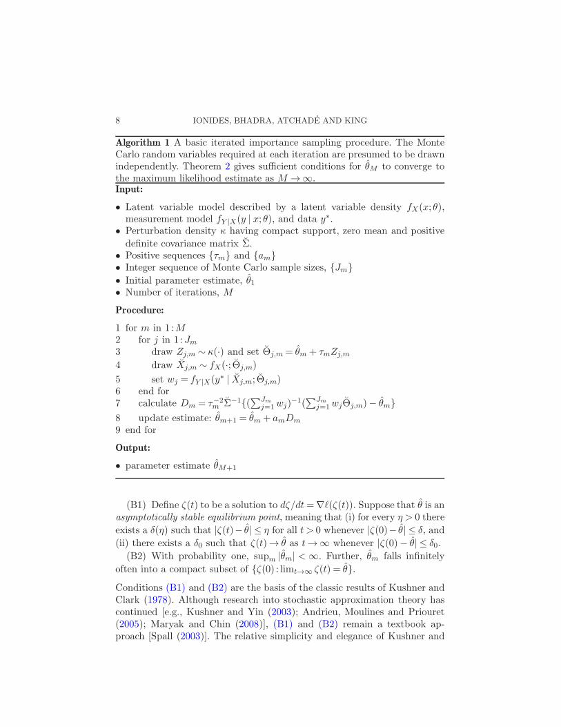
Algorithm 1 A basic iterated importance sampling procedure. The MonteCarlo random variables required at each iteration are presumed to be drawnindependently. Theorem 2 gives sufficient conditions for θM to converge tothe maximum likelihood estimate as M →∞.Input:

• Latent variable model described by a latent variable density fX(x; θ),measurement model fY |X(y | x; θ), and data y∗.

• Perturbation density κ having compact support, zero mean and positive

definite covariance matrix Σ.• Positive sequences τm and am• Integer sequence of Monte Carlo sample sizes, Jm• Initial parameter estimate, θ1• Number of iterations, M

Procedure:

1 for m in 1 :M2 for j in 1 :Jm3 draw Zj,m ∼ κ(·) and set Θj,m = θm + τmZj,m

4 draw Xj,m ∼ fX(·; Θj,m)

5 set wj = fY |X(y∗ | Xj,m; Θj,m)6 end for7 calculate Dm = τ−2

m Σ−1(∑Jm

j=1wj)−1(∑Jm

j=1wjΘj,m)− θm8 update estimate: θm+1 = θm + amDm

9 end for

Output:

• parameter estimate θM+1

(B1) Define ζ(t) to be a solution to dζ/dt=∇ℓ(ζ(t)). Suppose that θ is anasymptotically stable equilibrium point, meaning that (i) for every η > 0 there

exists a δ(η) such that |ζ(t)− θ| ≤ η for all t > 0 whenever |ζ(0)− θ| ≤ δ, and

(ii) there exists a δ0 such that ζ(t)→ θ as t→∞ whenever |ζ(0)− θ| ≤ δ0.

(B2) With probability one, supm |θm| <∞. Further, θm falls infinitely

often into a compact subset of ζ(0) : limt→∞ ζ(t) = θ.Conditions (B1) and (B2) are the basis of the classic results of Kushner andClark (1978). Although research into stochastic approximation theory hascontinued [e.g., Kushner and Yin (2003); Andrieu, Moulines and Priouret(2005); Maryak and Chin (2008)], (B1) and (B2) remain a textbook ap-proach [Spall (2003)]. The relative simplicity and elegance of Kushner and


Clark (1978) makes an appropriate foundation for investigating the linksbetween iterated filtering, sequential Monte Carlo and stochastic approxi-mation theory. There is, of course, scope for variations on our results basedon the diversity of available stochastic approximation theorems. Althoughneither (B1) and (B2) nor alternative sufficient conditions are easy to verify,stochastic approximation methods have nevertheless been found effectivein many situations. Condition (B2) is most readily satisfied if θm is con-

strained to a neighborhood in which θ is a unique local maximum, whichgives a guarantee of local rather than global convergence. Global convergenceresults have been obtained for related stochastic approximation procedures[Maryak and Chin (2008)] but are beyond the scope of this current paper.The rate assumptions in Theorem 2 are satisfied, for example, by am =m−1,τ2m =m−1 and Jm =m(δ+1/2) for δ > 0.

Theorem 2. Let am, τm and Jm be positive sequences with τm →0, Jmτm →∞, am → 0,

∑m am =∞ and

∑m a

2mJ

−1m τ−2

m <∞. Let θm be de-fined via Algorithm 1. Assuming (A1)–(A3) and (B1) and (B2),

limm→∞ θm = θ with probability one.

Proof. The quantity Dm in line 7 of Algorithm 1 is a self-normalizedMonte Carlo importance sampling estimate of

(τ2mΣ)−1Eθm,τm[Θ | Y = y∗]− θm.

We can therefore apply Corollary 8 from Section A.2, writing EMC andVarMC for the Monte Carlo expectation and variance resulting from carryingout Algorithm 1 conditional on the data y∗. This gives

|EMC [Dm − (τ2mΣ)−1Eθm,τm[Θ | Y = y∗]− θm]|

(14)

≤C7(supx∈X fY |X(y∗ | x; θm))2

τmJm(fY (y∗; θm))2,

|VarMC (Dm)| ≤C8(supx∈X fY |X(y∗ | x; θm))2

τ2mJm(fY (y∗; θm))2(15)

for finite constants C7 and C8 which do not depend on J , θm or τm. Havingassumed the conditions for Theorem 1, we see from (13) and (14) that Dm

provides an asymptotically unbiased Monte Carlo estimate of ∇ℓ(θm) in thesense of (B5) of Theorem 6 in Section A.1. In addition, (15) justifies (B4) ofTheorem 6. The remaining conditions of Theorem 6 hold by hypothesis.

3. Iterated filtering for POMP models. Let X(t), t ∈ T be a Markovprocess [Rogers and Williams (1994)] with X(t) taking values in a mea-surable space X. The time index set T ⊂ R may be an interval or a dis-


crete set, but we are primarily concerned with a finite subset of timest1 < t2 < · · · < tN at which X(t) is observed, together with some initialtime t0 < t1. We write X0 :N = (X0, . . . ,XN ) = (X(t0), . . . ,X(tN )). We writeY1 :N = (Y1, . . . , YN ) for a sequence of random variables taking values in ameasurable space YN . We assume that X0 :N and Y1 :N have a joint den-sity fX0 : N ,Y1 : N

(x0 : n, y1 : n; θ) on XN+1 ×YN , with θ being an unknown pa-rameter in R

p. A POMP model may then be specified by an initial den-sity fX0(x0; θ), conditional transition densities fXn|Xn−1

(xn | xn−1; θ) for1≤ n≤N , and the conditional densities of the observation process which areassumed to have the form fYn|Y1 : n−1,X0 : n

(yn | y1 : n−1, x0 : n; θ) = fYn|Xn(yn |

xn; θ). We use subscripts of f to denote the required joint and conditionaldensities. We write f without subscripts to denote the full collection ofdensities and conditional densities, and we call such an f the generic den-sity of a POMP model. The data are a sequence of observations by y∗1 :N =(y∗1 , . . . , y

∗N ) ∈YN , considered as fixed. We write the log likelihood function

of the data for the POMP model as ℓN (θ) where

ℓn(θ) = log

∫fX0(x0; θ)

n∏

k=1

fXk,Yk|Xk−1(xk, y

∗k | xk−1; θ)dx0 : n

for 1 ≤ n ≤ N . Our goal is to find the maximum likelihood estimate, θ =argmaxϑ ℓN (θ).

It will be helpful to construct a POMP model f which expands the modelf by allowing the parameter values to change deterministically at each timepoint. Specifically, we define a sequence ϑ0 :N = (ϑ0, . . . , ϑN ) ∈ RpN+1. Wethen write (X0 :N , Y 1 :N ) ∈XN+1 ×YN for a POMP with generic density fspecified by the joint density

fX0 : N ,Y 1 : N(x0 :N , y1 :N ;ϑ0 : n)

(16)

= fX0(x0;ϑ0)

N∏

k=1

fYk,Xk|Xk−1(yk, xk | xk−1;ϑk).

We write the log likelihood of y∗1 : n for the model f as ℓn(ϑ0 : n) =log fY 1 : n

(y∗1 : n;ϑ0 : n). We write θ[k] to denote k copies of θ ∈ Rp, concate-

nated in a column vector, so that ℓn(θ) = ℓn(θ[n+1]). We write ∇iℓn(ϑ0 : n)

for the partial derivative of ℓn with respect to ϑi, for i= 0, . . . , n. An appli-cation of the chain rule gives the identity

∇ℓn(θ) =n∑

i=0

∇iℓn(θ[n+1]).(17)

The regularity condition employed for Theorem 3 below is written in termsof this deterministically perturbed model:


(A4) For each 1≤ n≤N , ℓn(θ0 : n) is twice differentiable. For any compactsubset K of Rpn+1 and each 0≤ i≤ n,

supθ0 : n∈K

|∇iℓn(θ0 : n)|<∞ and supθ0 : n∈K

|∇2i ℓn(θ0 : n)|<∞.(18)

Condition (A4) is a nonrestrictive smoothness assumption. However, therelationship between smoothness of the likelihood function, the transitiondensity fXk|Xk−1

(xk | xk−1; θ), and the observation density fYk|Xk(yk | xk; θ)

is simple to establish only under the restrictive condition that X is a compactset. Therefore, we note an alternative to (A4) which is more restrictive butmore readily checkable:

(A4′) X is compact. Both fXk|Xk−1(xk | xk−1; θ) and fYk|Xk

(yk | xk; θ) aretwice differentiable with respect to θ. These derivatives are continuous withrespect to xk−1 and xk.

Iterated filtering involves introducing an auxiliary POMP model in whicha time-varying parameter process Θn,0≤ n≤N is introduced. Let κ be aprobability density function on R

p having compact support, zero mean andcovariance matrix Σ. Let Z0, . . . ,ZN be N independent draws from κ. Weintroduce two perturbation parameters, σ and τ , and construct a processΘ0 :N by setting Θ0 = ϑ0 + τZ0 and Θk = ϑk + τZ0 + σ

∑kj=1Zj for 1 ≤

k ≤N . The joint density of Θ0 :N is written as gΘ0 : N(ϑ0 :N ;ϑ0 :N , σ, τ). We

define the stochastically perturbed POMP model g with a Markov process(Xn, Θn),0≤n≤N, observation process Y1 :N and parameter (ϑ0 :N , σ, τ)by the joint density

gX0 : N ,Θ0 : N ,Y1 : N(x0 :N , ϑ0 :N , y1 :N ;ϑ0 :N , σ, τ)

= gΘ0 : N(ϑ0 :N ;ϑ0 :N , σ, τ)fX0 : N ,Y 1 : N

(x0 :N , y1 :N ; ϑ0 :N ).

We seek a result analogous to Theorem 1 which takes into account thespecific structure of a POMP. Theorem 3 below gives a way to approximate∇ℓN (θ) in terms of moments of the filtering distributions for g. We write

Eϑ0 : n,σ,τ and Varϑ0 : n,σ,τ for the expectation and variance, respectively, forthe model g. We will be especially interested in the situation where ϑ0 : n =θ[n+1], which leads us to define the following filtering means and predictionvariances:

θFn = θFn (θ,σ, τ) = Eθ[n+1],σ,τ [Θn | Y1 : n = y∗1 : n]

=

∫ϑngΘn|Y1 : n

(ϑn | y∗1 : n; θ[n+1], σ, τ)dϑn,(19)

V Pn = V P

n (θ,σ, τ) = Varθ[n+1],σ,τ (Θn | Y1 : n−1 = y∗1 : n−1)

for n= 1, . . . ,N , with θF0 = θ.


Theorem 3. Suppose condition (A4). Let σ be a function of τ withlimτ→0 σ(τ)/τ = 0. For any compact set K4 ⊂ R

p, there exists a finite con-stant C9 such that for all τ small enough,

supθ∈K4

|τ−2Σ−1(θFN − θ)−∇ℓN (θ)| ≤C9(τ + σ2/τ2)(20)

and

supθ∈K4

∣∣∣∣∣

N∑

n=1

(V Pn )−1(θFn − θFn−1)−∇ℓN(θ)

∣∣∣∣∣≤C9(τ + σ2/τ2).(21)

Proof. For each n ∈ 1, . . . ,N, we map onto the notation of Sec-

tion 2 by setting X = X0 : n, Y = Y 1 : n, θ = ϑ0 : n, Θ = Θ0 : n, y∗ = y∗1 : n

and h(ϑ0 : n) = ϑn. We note that, by construction, this implies X = X0 : n,

Y = Y1 : n, and κτ (ϑ0 : n) = κ(ϑ0)∏n

i=1(σ/τ)−pκ((ϑi − ϑi−1)/(σ/τ)). For this

choice of h, the integral τ∫h(τu)u′κτ (u)du is a p × p(n + 1) matrix for

which the ith p× p sub-matrix is Eϑ0 : n,σ,τ [(Θn −ϑn)(Θi−1−ϑi−1)′] = τ2+

(i− 1)σ2Σ. Thus,(τ

∫h(τu)u′κτ (u)du

)∇ℓn(ϑ0 : n)

=

n∑

i=0

Eϑ0 : n,σ,τ [(Θn − ϑn)(Θi − ϑi)′]∇iℓn(ϑ0 : n)(22)

=n∑

i=0

(τ2Σ+ iσ2Σ)∇iℓn(ϑ0 : n).

Applying Theorem 1 in this context, the second term in (3) is zero and thethird term is given by (22). We obtain that for any compact K5 ⊂ R

p(n+1)

there is a C10 <∞ such that

supϑ0 : n∈K5

∣∣∣∣∣τ−2Σ−1(Eϑ0 : n,σ,τ [Θn | Y1 : n = y∗1 : n]− ϑn)

−n∑

i=0

(1 + σ2τ−2i)∇iℓn(ϑ0 : n)

∣∣∣∣∣(23)

≤C10τ.

Applying (23) to the special case of ϑ0 : n = θ[n+1], making use of (17) and(19), we infer the existence of finite constants C11 and C12 such that

supθ∈K4

|τ−2Σ−1(θFn − θ)−∇ℓn(θ)| ≤C11τ + supθ∈K4

σ2τ−2n∑

i=1

i|∇iℓn(θ[n+1])|

(24)≤C12(τ + σ2τ−2),


which establishes (20). To show (21), we write

n∑

k=1

V Pk −1(θFk − θFk−1)

=

n∑

k=1

τ−2Σ−1(θFk − θFk−1) + τ−2n∑

k=1

(τ−2V Pk −1 −Σ−1)(θFk − θFk−1)(25)

= τ−2Σ−1(θFn − θ) + τ−2n∑

k=1

(τ−2V Pk −1 −Σ−1)(θFk − θFk−1).

We note that (24) implies the existence of a bound

|θFn − θ| ≤C13τ2.(26)

Combining (25), (24) and (26), we deduce

supθ∈K4

∣∣∣∣∣

n∑

k=1

V Pk −1(θFk − θFk−1)−∇ℓn(θ)

∣∣∣∣∣

≤C14(τ + σ2τ−2) +C15

n∑

k=1

supθ∈K4

|τ−2V Pk −1 −Σ−1|

for finite constants C14 and C15. For invertible matrices A and B, we havethe bound

|A−1 −B−1| ≤ |B−1|2(1− |(B −A)B−1|)−1|B −A|(27)

provided that |(B−A)B−1|< 1. Applying (27) with A= τ−2V Pk and B =

Σ, we see that the theorem will be proved once it is shown that

supθ∈K4

|τ−2V Pk −Σ| ≤C0(τ + σ2τ−2).

Now, it is easy to check that

τ−2V Pn −Σ= τ−2

Eθ[n+1],σ,τ [(Θn−1 − θ)(Θn−1 − θ)′ | Y1 : n−1 = y∗1 : n−1]−Σ

− τ−2(θFn−1 − θ)(θFn−1 − θ)′ + σ2τ−2Σ.

Applying Theorem 1 again with h(ϑ0 : n) = (ϑn − θ)(ϑn − θ)′, and makinguse of (26), we obtain

supθ∈K4

|τ−2Eθ[n+1],σ,τ [(Θn − θ)(Θn − θ)′ | Y1 : n = y∗1 : n]−Σ|

(28)≤C16(τ + σ2τ−2),

which completes the proof.


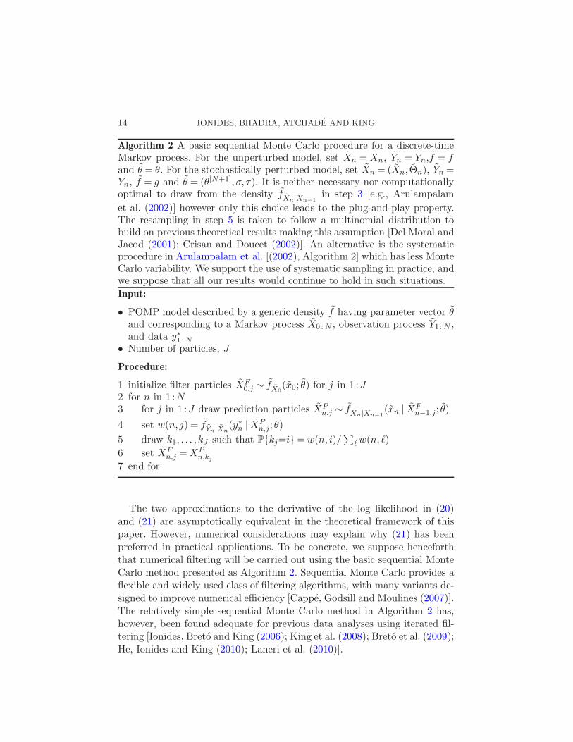
Algorithm 2 A basic sequential Monte Carlo procedure for a discrete-timeMarkov process. For the unperturbed model, set Xn =Xn, Yn = Yn,f = fand θ = θ. For the stochastically perturbed model, set Xn = (Xn, Θn), Yn =Yn, f = g and θ = (θ[N+1], σ, τ). It is neither necessary nor computationallyoptimal to draw from the density fXn|Xn−1

in step 3 [e.g., Arulampalam

et al. (2002)] however only this choice leads to the plug-and-play property.The resampling in step 5 is taken to follow a multinomial distribution tobuild on previous theoretical results making this assumption [Del Moral andJacod (2001); Crisan and Doucet (2002)]. An alternative is the systematicprocedure in Arulampalam et al. [(2002), Algorithm 2] which has less MonteCarlo variability. We support the use of systematic sampling in practice, andwe suppose that all our results would continue to hold in such situations.

Input:

• POMP model described by a generic density f having parameter vector θand corresponding to a Markov process X0 :N , observation process Y1 :N ,and data y∗1 :N

• Number of particles, J

Procedure:

1 initialize filter particles XF0,j ∼ fX0

(x0; θ) for j in 1 :J2 for n in 1 :N3 for j in 1 :J draw prediction particles XP

n,j ∼ fXn|Xn−1(xn | XF

n−1,j; θ)

4 set w(n, j) = fYn|Xn(y∗n | XP

n,j; θ)

5 draw k1, . . . , kJ such that Pkj=i=w(n, i)/∑

ℓw(n, ℓ)

6 set XFn,j = XP

n,kj7 end for

The two approximations to the derivative of the log likelihood in (20)

and (21) are asymptotically equivalent in the theoretical framework of thispaper. However, numerical considerations may explain why (21) has been

preferred in practical applications. To be concrete, we suppose henceforth

that numerical filtering will be carried out using the basic sequential Monte

Carlo method presented as Algorithm 2. Sequential Monte Carlo provides aflexible and widely used class of filtering algorithms, with many variants de-

signed to improve numerical efficiency [Cappe, Godsill and Moulines (2007)].

The relatively simple sequential Monte Carlo method in Algorithm 2 has,

however, been found adequate for previous data analyses using iterated fil-tering [Ionides, Breto and King (2006); King et al. (2008); Breto et al. (2009);

He, Ionides and King (2010); Laneri et al. (2010)].


When carrying out filtering via sequential Monte Carlo, the resamplinginvolved has a consequence that all surviving particles can descend from onlyfew recent ancestors. This phenomenon, together with the resulting shortageof diversity in the Monte Carlo sample, is called particle depletion and canbe a major obstacle for the implementation of sequential Monte Carlo tech-niques [Arulampalam et al. (2002); Andrieu, Doucet and Holenstein (2010)].The role of the added variation on the scale of σm in the iterated filteringalgorithm is to rediversify the particles and hence to combat particle deple-tion. Mixing considerations suggest that the new information about θ in thenth observation may depend only weakly on y∗1 : n−k for sufficiently large k[Jensen and Petersen (1999)]. The actual Monte Carlo particle diversity ofthe filtering distribution, based on (21), may therefore be the best guidewhen sequentially estimating the derivative of the log likelihood. Futuretheoretical work on iterated filtering algorithms should study formally therole of mixing, to investigate this heuristic argument. However, the theorypresented in Theorems 3, 4 and 5 does formally support using a limit randomwalk perturbations without any mixing conditions. Two influential previousproposals to use stochastic perturbations to reduce numerical instabilitiesarising in plug-and-play inference for POMPS via sequential Monte Carlo[Kitagawa (1998); Liu and West (2001)] lack even this level of theoreticalsupport.

To calculate Monte Carlo estimates of the quantities in (19), we apply

Algorithm 2 with f = g, Xn = (Xn, Θn), θ = (θ[N+1], σ, τ) and J particles.

We write XPn,j = (XP

n,j,ΘPn,j) and XF

n,j = (XFn,j,Θ

Fn,j) for the Monte Carlo

samples from the prediction and filtering and calculations in steps 3 and 6of Algorithm 2. Then we define

θFn = θFn (θ,σ, τ, J) =1

J

J∑

j=1

ΘFn,j,

(29)

V Pn = V P

n (θ,σ, τ, J) =1

J − 1

J∑

j=1

(ΘPn,j − θFn−1)(Θ

Pn,j − θFn−1)

′.

In practice, a reduction in Monte Carlo variability is possible by modifying(29) to estimate θFn and V P

n from weighted particles prior to resampling[Chopin (2004)]. We now present, as Theorem 4, an analogue to Theorem 3in which the filtering means and prediction variances are replaced by theirMonte Carlo counterparts. The stochasticity in Theorem 4 is due to MonteCarlo variability, conditional on the data y∗1 :N , and we write EMC andVarMC to denote Monte Carlo means and variances. The Monte Carlo ran-dom variables required to implement Algorithm 2 are presumed to be drawnindependently each time the algorithm is evaluated. To control the MonteCarlo bias and variance, we assume:


(A5) For each n and any compact set K6 ⊂Rp,

supθ∈K6,x∈X

fYn|Xn(y∗n | xn; θ)<∞.

Theorem 4. Let σm, τm and Jm be positive sequences with τm → 0,

σmτ−1m → 0 and τmJm → ∞. Define θFn,m = θFn (θ,σm, τm, Jm) and V P

n,m =

V Pn (θ,σm, τm, Jm) via (29). Suppose conditions (A4) and (A5) and let K7

be an arbitrary compact subset of Rp. Then,

limm→∞

supθ∈K7

∣∣∣∣∣EMC

[N∑

n=1

(V Pn,m)−1(θFn,m − θFn−1,m)

]−∇ℓN (θ)

∣∣∣∣∣= 0,(30)

limm→∞

supθ∈K7

∣∣∣∣∣τ2mJmVarMC

(N∑

n=1

(V Pn,m)−1(θFn,m − θFn−1,m)

)∣∣∣∣∣<∞.(31)

Proof. Let K8 be a compact subset of R2 containing (σm, τm),m =1,2, . . .. Set θ ∈K7 and (σ, τ) ∈K8. Making use of the definitions in (19) and

(29), we construct un = (θFn − θFn−1)/τ and vn = V Pn /τ

2, with corresponding

Monte Carlo estimates un = (θFn − θFn−1)/τ and vn = V Pn /τ

2. We look to

apply Theorem 7 (presented in Section A.2) with f = g, Xn = (Xn, Θn),

Yn = Yn, θ = (θ[n+1], σ, τ), J particles, and

φ(Xn, Θn) = (Θn − θ)/τ.

Using the notation from (44), we have un = φFn −φFn−1 and un = φFn − φFn−1.By assumption, κ(u) is supported on some set u : |u|<C17 from which wederive the bound |φ(Xn, Θn)| ≤C17(1+nσ/τ). Theorem 7 then provides forthe existence of a C18 and C19 such that

EMC [|un − un|2]≤ C18/J,(32)

|EMC [un − un]| ≤ C19/J.(33)

The explicit bounds in (47) of Theorem 7, together with (A4) and (A5),assure us that C18 =C18(θ,σ, τ) and C19 =C19(θ,σ, τ) can be chosen so that(32) and (33) hold uniformly over (θ,σ, τ) ∈K7 ×K8. The same argument

applied to vn = V Pn /τ

2 and vn = V Pn /τ

2 gives

|EMC [vn − vn]| ≤C20/J, EMC [|vn − vn|2]≤C21/J(34)

uniformly over (θ,σ, τ) ∈K7 ×K8. We now proceed to carry out a Taylorseries expansion:

v−1n un = v−1

n un + v−1n (un − un)v

−1n (vn − vn)v

−1n un +R3,(35)


where |R3|< C22(|un − un|2 + |vn − vn|2) for some constant C22. The exis-tence of such a C22 is guaranteed since the determinant of vn is boundedaway from zero. Taking expectations of both sides of (35) and applying(32)–(34) gives

|EMC [v−1n un]− v−1

n un| ≤C23/J(36)

for some constant C23 <∞. Another Taylor series expansion,

v−1n un = v−1

n un +R4

with |R4|<C24(|un − un|+ |vn − vn|) implies

VarMC (v−1n un)≤C25/J.(37)

Rewriting (36) and (37), defining θFn,m = θFn (θ,σm, τm) and V Pn,m = V P

n (θ,σm, τm), we deduce that

τmJm|EMC [(VPn,m)−1(θFn,m − θFn−1,m)]− (V P

n,m)−1(θFn,m − θFn−1,m)| ≤C23

(38)and

τ2mJmVarMC [(VPn,m)−1(θFn,m − θFn−1,m)]≤C25.(39)

Combining (38) with Theorem 3, and summing over n, leads to (30). Sum-ming (39) over n justifies (30).

Theorem 4 suggests that a Monte Carlo method which leans on Theo-rem 3 will require a sequence of Monte Carlo sample sizes, Jm, which in-creases faster than τ−1

m . Even with τmJm →∞, we see from (31) that theestimated derivative in (30) may have increasing Monte Carlo variability asm→∞. Theorem 5 gives an example of a stochastic approximation proce-dure, defined by the recursive sequence θm in (40), that makes use of theMonte Carlo estimates studied in Theorem 4. Because each step of this re-cursion involves an application of the filtering procedure in Algorithm 2,we call (40) an iterated filtering algorithm. The rate assumptions in The-orem 5 are satisfied, for example, by am =m−1, τ2m =m−1, σ2m =m−(1+δ)

and Jm =m(δ+1/2) for δ > 0.

Theorem 5. Let am, σm, τm and Jm be positive sequences withτm → 0, σmτ

−1m → 0, Jmτm →∞, am → 0,

∑m am =∞ and

∑m a

2mJ

−1m τ−2

m <

∞. Specify a recursive sequence of parameter estimates θm by

θm+1 = θm + am

N∑

n=1

(V Pn,m)−1(θFn,m − θFn−1,m),(40)

where θFn,m = θFn (θm, σm, τm, Jm) and V Pn,m = V P

n,m(θm, σm, τm, Jm) are de-fined in (29) via an application of Algorithm 2. Assuming (A4), (B1) and

(B2), limm→∞ θm = θ with probability one.


Proof. Theorem 5 follows directly from a general stochastic approxi-mation result, Theorem 6 of Section A.1, applied to ℓN (θ). Conditions (B4)and (B5) of Theorem 6 hold from Theorem 4 and the remaining assumptionsof Theorem 6 hold by hypothesis.

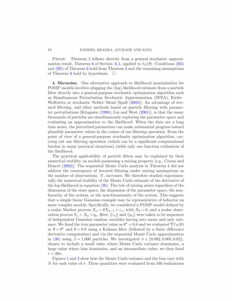
4. Discussion. One alternative approach to likelihood maximization forPOMP models involves plugging the (log) likelihood estimate from a particlefilter directly into a general-purpose stochastic optimization algorithm suchas Simultaneous Perturbation Stochastic Approximation (SPSA), Kiefer–Wolfowitz or stochastic Nelder–Mead [Spall (2003)]. An advantage of iter-ated filtering, and other methods based on particle filtering with parame-ter perturbations [Kitagawa (1998); Liu and West (2001)], is that the manythousands of particles are simultaneously exploring the parameter space andevaluating an approximation to the likelihood. When the data are a longtime series, the perturbed parameters can make substantial progress towardplausible parameter values in the course of one filtering operation. From thepoint of view of a general-purpose stochastic optimization algorithm, car-rying out one filtering operation (which can be a significant computationalburden in many practical situations) yields only one function evaluation ofthe likelihood.

The practical applicability of particle filters may be explained by theirnumerical stability on models possessing a mixing property [e.g., Crisan andDoucet (2002)]. The sequential Monte Carlo analysis in Theorem 4 did notaddress the convergence of iterated filtering under mixing assumptions asthe number of observations, N , increases. We therefore studied experimen-tally the numerical stability of the Monte Carlo estimate of the derivative ofthe log likelihood in equation (30). The role of mixing arises regardless of thedimension of the state space, the dimension of the parameter space, the non-linearity of the system, or the non-Gaussianity of the system. This suggeststhat a simple linear Gaussian example may be representative of behavior onmore complex models. Specifically, we considered a POMP model defined bya scalar Markov process Xn = θXn−1 + εn, with X0 = 0, and a scalar obser-vation process Yn =Xn+ηn. Here, εn and ηn were taken to be sequencesof independent Gaussian random variables having zero mean and unit vari-ance. We fixed the true parameter value as θ∗ = 0.8 and we evaluated ∇ℓN (θ)at θ = θ∗ and θ = 0.9 using a Kalman filter (followed by a finite differencederivative computation) and via the sequential Monte Carlo approximationin (30) using J = 1,000 particles. We investigated σ ∈ 0.002,0.005,0.02,chosen to include a small value where Monte Carlo variance dominates, alarge value where bias dominates, and an intermediate value; we then fixedτ = 20σ.

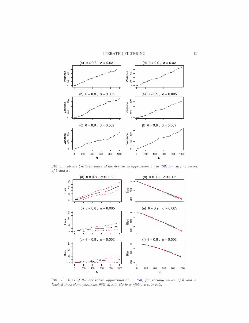
Figures 1 and 2 show how the Monte Carlo variance and the bias vary withN for each value of σ. These quantities were evaluated from 100 realizations


Fig. 1. Monte Carlo variance of the derivative approximation in (30) for varying valuesof θ and σ.

Fig. 2. Bias of the derivative approximation in (30) for varying values of θ and σ.Dashed lines show pointwise 95% Monte Carlo confidence intervals.


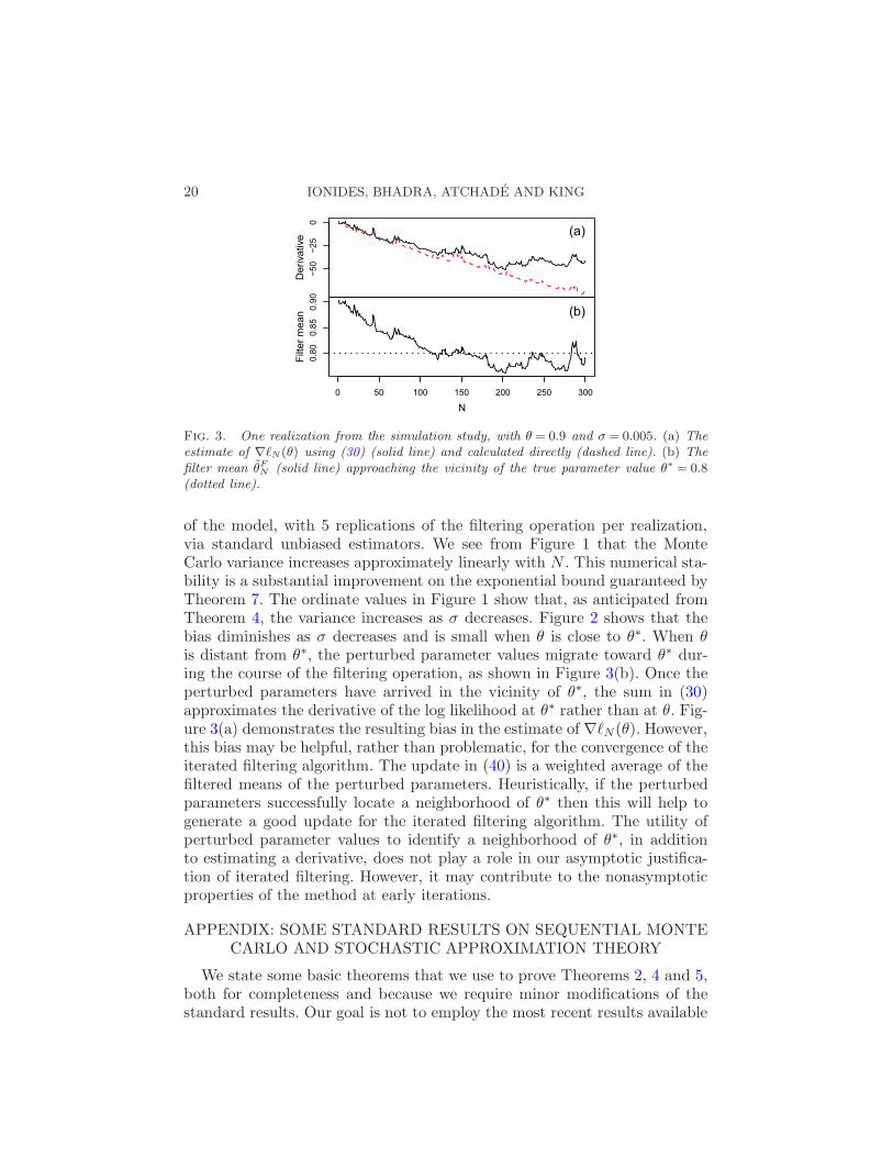
Fig. 3. One realization from the simulation study, with θ = 0.9 and σ = 0.005. (a) Theestimate of ∇ℓN(θ) using (30) (solid line) and calculated directly (dashed line). (b) Thefilter mean θ

FN (solid line) approaching the vicinity of the true parameter value θ

∗ = 0.8(dotted line).

of the model, with 5 replications of the filtering operation per realization,via standard unbiased estimators. We see from Figure 1 that the MonteCarlo variance increases approximately linearly with N . This numerical sta-bility is a substantial improvement on the exponential bound guaranteed byTheorem 7. The ordinate values in Figure 1 show that, as anticipated fromTheorem 4, the variance increases as σ decreases. Figure 2 shows that thebias diminishes as σ decreases and is small when θ is close to θ∗. When θis distant from θ∗, the perturbed parameter values migrate toward θ∗ dur-ing the course of the filtering operation, as shown in Figure 3(b). Once theperturbed parameters have arrived in the vicinity of θ∗, the sum in (30)approximates the derivative of the log likelihood at θ∗ rather than at θ. Fig-ure 3(a) demonstrates the resulting bias in the estimate of ∇ℓN (θ). However,this bias may be helpful, rather than problematic, for the convergence of theiterated filtering algorithm. The update in (40) is a weighted average of thefiltered means of the perturbed parameters. Heuristically, if the perturbedparameters successfully locate a neighborhood of θ∗ then this will help togenerate a good update for the iterated filtering algorithm. The utility ofperturbed parameter values to identify a neighborhood of θ∗, in additionto estimating a derivative, does not play a role in our asymptotic justifica-tion of iterated filtering. However, it may contribute to the nonasymptoticproperties of the method at early iterations.

APPENDIX: SOME STANDARD RESULTS ON SEQUENTIAL MONTECARLO AND STOCHASTIC APPROXIMATION THEORY

We state some basic theorems that we use to prove Theorems 2, 4 and 5,both for completeness and because we require minor modifications of thestandard results. Our goal is not to employ the most recent results available


in these research areas, but rather to show that some fundamental andwell-known results from both areas can be combined with our Theorems 1and 3 to synthesize a new theoretical understanding of iterated filtering anditerated importance sampling.

A.1. A version of a standard stochastic approximation theorem. Wepresent, as Theorem 6, a special case of Theorem 2.3.1 of Kushner andClark (1978). For variations and developments on this result, we refer thereader to Kushner and Yin (2003), Spall (2003), Andrieu, Moulines andPriouret (2005) and Maryak and Chin (2008). In particular, Theorem 2.3.1of Kushner and Clark (1978) is similar to Theorem 4.1 of Spall (2003) andto Theorem 2.1 of Kushner and Yin (2003).

Theorem 6. Let ℓ(θ) be a continuously differentiable function Rp →R

and let Dm(θ),m≥ 1 be a sequence of independent Monte Carlo estimators

of the vector of partial derivatives ∇ℓ(θ). Define a sequence θm recursively

by θm+1 = θm + amDm(θm). Assume (B1) and (B2) of Section 2 togetherwith the following conditions:

(B3) am > 0, am → 0,∑

m am =∞.(B4)

∑m a

2m sup|θ|<rVarMC (Dm(θ))<∞ for every r > 0.

(B5) limm→∞ sup|θ|<r |EMC [Dm(θ)]−∇ℓ(θ)|= 0 for every r > 0.

Then θm converges to θ = argmax ℓ(θ) with probability one.

Proof. The most laborious step in deducing Theorem 6 from Kushnerand Clark (1978) is to check that (B1)–(B5) imply that, for all ε > 0,

limn→∞

P

[supj≥1

∣∣∣∣∣

n+j∑

m=n

amDm(θm)−EMC [Dm(θm) | θm]∣∣∣∣∣≥ ε

]= 0,(41)

which in turn implies condition A2.2.4′′ and hence A2.2.4 of Kushner andClark (1978). To show (41), we define ξm =Dm(θm)− EMC [Dm(θm) | θm]and

ξkm =

ξm, if |θm| ≤ k,

0, if |θm|> k.(42)

Define processes Mnj =∑n+j

m=n amξm, j ≥ 0 and Mn,kj =

∑n+jm=n amξ

km, j ≥

0 for each k and n. These processes are martingales with respect to the fil-tration defined by the Monte Carlo stochasticity. From the Doob–Kolmogorovmartingale inequality [e.g., Grimmett and Stirzaker (1992)],

P

[supj

|Mn,kj | ≥ ε

]≤ 1

ε2

∞∑

m=n

a2m sup|θ|<k

VarMC (Dm(θ)).(43)


Define events Fn = supj |Mnj | ≥ ε and Fn,k = supj |Mn,k

j | ≥ ε. It followsfrom (B4) and (43) that limn→∞PFn,k = 0 for each k. In light of thenondivergence assumed in (B2), this implies limn→∞PFn = 0 which isexactly (41).

To expand on this final assertion, let Ω = supm |θm| < ∞ and Ωk =

supm |θm|< k. Assumption (B2) implies that P(Ω) = 1. Since the sequenceof events Ωk is increasing up to Ω, we have limk→∞P(Ωk) = P(Ω) = 1. Nowobserve that Ωk ∩ Fn,j =Ωk ∩ Fn for all j ≥ k, as there is no truncation of

the sequence ξjm,m= 1,2, . . . for outcomes in Ωk when j ≥ k. Then,

limn→∞

P[Fn]≤ limn→∞

P[Fn ∩Ωk] + 1− P[Ωk]

= limn→∞

P[Fn,k ∩Ωk] + 1− P[Ωk]

≤ limn→∞

P[Fn,k] + 1− P[Ωk]

= 1− P[Ωk].

Since k can be chosen to make 1 − P[Ωk] arbitrarily small, it follows thatlimn→∞P[Fn] = 0.

A.2. Some standard results on sequential Monte Carlo and importance

sampling. A general convergence result on sequential Monte Carlo combin-ing results by Crisan and Doucet (2002) and Del Moral and Jacod (2001)is stated in our notation as Theorem 7 below. The theorem is stated for aPOMP model with generic density f , parameter vector θ, Markov processX0 :N taking values in XN+1, observation process Y1 :N taking values in YN ,

and data y∗1 :N . For application to the unperturbed model one sets f = f ,

Xn =Xn, X = X, Yn = Yn and θ = θ. For application to the stochasticallyperturbed model one sets f = g, Xn = (Xn, Θn), X= X×R

p, Yn = Yn andθ = (θ[N+1], σ, τ). When applying Theorem 7 in the context of Theorem 4,the explicit expressions for the constants C26 and C27 are required to showthat the bounds in (45) and (46) apply uniformly for a collection of modelsindexed by the approximation parameters τm and σm.

Theorem 7 [Crisan and Doucet (2002); Del Moral and Jacod (2001)].Let f be a generic density for a POMP model having parameter vectorθ, unobserved Markov process X0 :N , observation process Y1 :N and datay∗1 :N . Define XF

n,j via applying Algorithm 2 with J particles. Assume that

fYn|Xn(y∗n | xn; θ) is bounded as a function of xn. For any φ : X→R, denote

the filtered mean of φ(Xn) and its Monte Carlo estimate by

φFn =

∫φ(xn)fXn|Y1 : n

(xn | y∗1 : n; θ)dxn, φFn =1

J

J∑

j=1

φ(XFn,j).(44)


There are constants C26 and C27, independent of J , such that

EMC [(φFn − φFn )

2]≤ C26 supx |φ(x)|2J

,(45)

|EMC [φFn − φFn ]| ≤

C27 supx |φ(x)|J

.(46)

Specifically, C26 and C27 can be written as linear functions of 1 and ηn,1, . . . ,ηn,n defined as

ηn,i =

n∏

k=n−i+1

(supxk

fYk|Xk(y∗k | xk; θ)

fYk|Y1 : k−1(y∗k | y∗1 : k−1; θ)

)2

.(47)

Proof. Theorem 2 of Crisan and Doucet (2002) derived (45), and herewe start by focusing on the assertion that the constant C26 in equation(45) can be written as a linear function of 1 and the quantities ηn,1, . . . , ηn,ndefined in (47). This was not explicitly mentioned by Crisan and Doucet(2002) but is a direct consequence of their argument. Crisan and Doucet[(2002), Section V] constructed the following recursion, for which cn|n is theconstant C26 in equation (45). For n= 1, . . . ,N and c0|0 = 0, define

cn|n = (√C +

√cn|n)

2,(48)

cn|n = 4cn|n−1

( ‖fYn|Xn‖

fYn|Y1 : n−1(y∗n | y∗1 : n−1; θ)

)2

,(49)

cn|n−1 = (1+√cn−1|n−1)

2,(50)

where ‖fYn|Xn‖= supxn

fYn|Xn(y∗n | xn; θ). Here, C is a constant that depends

on the resampling procedure but not on the number of particles J . Now,(48)–(50) can be reformulated by routine algebra as

cn|n ≤K1 +K2cn|n,(51)

cn|n ≤K3qncn|n−1,(52)

cn|n−1 ≤K4 +K5cn−1|n−1,(53)

where qn = ‖fYn|Xn‖2[fYn|Y1 : n−1

(y∗n | y∗1 : n−1; θ)]−2 and K1, . . . ,K5 are con-

stants which do not depend on f , θ, y∗1 :N or J . Putting (52) and (53)into (51),

cn|n ≤K1 +K2K3qncn|n−1(54)

≤K1 +K2K3K4qn +K2K3K5qncn−1|n−1.

Since ηn,i = qnηn−1,i for i < n, and ηn,n = qn, the required assertion followsfrom (54).


To show (46), we introduce the unnormalized filtered mean φUn and its

Monte Carlo estimate φUn , defined by

φUn = φFn

n∏

k=1

fYk|Y1 : k−1(y∗k | y∗1 : k−1; θ), φ

Un = φFn

n∏

k=1

1

J

J∑

j=1

w(k, j),(55)

where w(k, j) is computed in step 4 of Algorithm 2 when evaluating φFn .Then, Del Moral and Jacod (2001) showed that

EMC [φUn ] = φUn ,(56)

EMC [(φUn − φUn )

2]≤ (n+ 1) supx |φ(x)|2J

n∏

k=1

(supxk

fYk|Xk(y∗k | xk; θ)

)2.(57)

We now follow an approach of Del Moral and Jacod [(2001), equation 3.3.14],

by defining the unit function 1(x) = 1 and observing that φFn = φUn /1Un and

φFn = φUn /1Un . Then (56) implies the identity

EMC [φFn − φFn ] =EMC

[(φFn − φFn )

(1− 1Un

1Un

)].(58)

Applying the Cauchy–Schwarz inequality to (58), making use of (45) and(57), gives (46).

We now give a corollary to Theorem 7 for a latent variable model (X, Y ),as defined in Section 2, having generic density f , parameter vector θ, un-

observed variable X taking values in X, observed variable Y taking valuesin Y, and data y∗. Importance sampling for such a model is a special caseof sequential Monte Carlo, with N = 1 and no resampling step. We presentand prove a separate result, which takes advantage of the simplified situa-tion, to make Section 2 and the proof of Theorem 2 self-contained. In thecontext of Theorem 2, one sets f = g, X = (X, Θ), X=X×R

p, Yn = Y andθ = (θ, τ).

Corollary 8. Let f be a generic density for the latent variable model(X, Y ) with parameter vector θ and data y∗. Let Xj , j = 1, . . . , J be J

independent Monte Carlo draws from fX(x; θ) and let wj = fY |X(y∗ | Xj ; θ).

Letting φ : X→R be a bounded function, write the conditional expectation ofφ(X) and its importance sampling estimate as

φC =

∫φ(xn)fX|Y (x | y∗; θ)dx, φC =

∑Jj=1wjφ(Xj)∑J

j=1wj

.(59)


Assume that fY |X(y∗ | x; θ) is bounded as a function of x. Then,

VarMC (φC)≤

4 supx |φ(x)|2 supx(fY |X(y∗ | x; θ))2

J(fY (y∗; θ))2

,(60)

|EMC [φC ]− φC | ≤

2 supx |φ(x)| supx(fY |X(y∗ | x; θ))2

J(fY (y∗; θ))2

.(61)

Proof. We introduce normalized weights wj =wj/fY (y∗; θ) and a nor-

malized importance sampling estimator φC = 1J

∑Jj=1 wjφ(Xj) to compare

to the self-normalized estimator in (59). It is not hard to check that EMC [φC ] =

φC and VarMC (φC) ≤ 1

J (supx |φ(x)| supx fY |X(y∗ | x; θ)/fY (y∗; θ))2. Now,

VarMC (φC)≤ 2VarMC (φ

C − φC) + VarMC (φC) and

VarMC (φC − φC)≤ EMC

[((1/J)

∑Jj=1 wjφ(Xj)

(1/J)∑J

j=1 wj

− 1

J

J∑

j=1

wjφ(Xj)

)2]

= EMC

[((1/J)

∑Jj=1 wjφ(Xj)

(1/J)∑J

j=1 wj

)2(1− 1

J

J∑

j=1

wj

)2]

≤ supx

|φ(x)|2EMC

[1− 1

J

J∑

j=1

wj

]2

≤supx |φ(x)|2 supx(fY |X(y∗ | x; θ))2

J(fY (y∗; θ))2

.

This demonstrates (60). To show (61), we write

|EMC [φC ]− φC |= |EMC [φ

C − φC ]|

=

∣∣∣∣∣EMC

[(φC −EMC [φ

C ])

(1− 1

J

J∑

j=1

wj

)]∣∣∣∣∣

≤

√√√√VarMC (φC)VarMC

(1− 1

J

J∑

j=1

wj

)

≤2 supx |φ(x)| supx(fY |X(y∗ | x; θ))2

J(fY (y∗; θ))2

.

Acknowledgments. The authors are grateful for constructive advice fromthree anonymous referees and the Associate Editor.


REFERENCES

Anderson, J. L. and Collins, N. (2007). Scalable implementations of ensemble filter

algorithms for data assimilation. Journal of Atmospheric and Oceanic Technology 24

1452–1463.

Andrieu, C., Doucet, A. and Holenstein, R. (2010). Particle Markov chain Monte

Carlo methods. J. R. Stat. Soc. Ser. B Stat. Methodol. 72 269–342.

Andrieu, C., Moulines, E. and Priouret, P. (2005). Stability of stochastic approxi-

mation under verifiable conditions. SIAM J. Control Optim. 44 283–312. MR2177157

Arulampalam, M. S., Maskell, S., Gordon, N. and Clapp, T. (2002). A tutorial

on particle filters for online nonlinear, non-Gaussian Bayesian tracking. IEEE Trans.Signal Process. 50 174–188.

Bailey, N. T. J. (1955). Some problems in the statistical analysis of epidemic data.

J. Roy. Statist. Soc. Ser. B 17 35–58; Discussion 58–68. MR0073090

Bartlett, M. S. (1960). Stochastic Population Models in Ecology and Epidemiology.

Methuen, London. MR0118550

Beyer, H.-G. (2001). The Theory of Evolution Strategies. Springer, Berlin. MR1930756

Bjørnstad, O. N. and Grenfell, B. T. (2001). Noisy clockwork: Time series analysis

of population fluctuations in animals. Science 293 638–643.

Breto, C., He, D., Ionides, E. L. and King, A. A. (2009). Time series analysis via

mechanistic models. Ann. Appl. Stat. 3 319–348. MR2668710

Cappe, O., Godsill, S. and Moulines, E. (2007). An overview of existing methods and

recent advances in sequential Monte Carlo. Proceedings of the IEEE 95 899–924.

Cappe, O., Moulines, E. and Ryden, T. (2005). Inference in Hidden Markov Models.

Springer, New York. MR2159833

Cauchemez, S. and Ferguson, N. M. (2008). Likelihood-based estimation of continuous-

time epidemic models from time-series data: Application to measles transmission in

London. Journal of the Royal Society Interface 5 885–897.

Celeux, G., Marin, J.-M. and Robert, C. P. (2006). Iterated importance sampling in

missing data problems. Comput. Statist. Data Anal. 50 3386–3404. MR2236856

Chopin, N. (2004). Central limit theorem for sequential Monte Carlo methods and its

application to Bayesian inference. Ann. Statist. 32 2385–2411. MR2153989

Crisan, D. and Doucet, A. (2002). A survey of convergence results on particle filtering

methods for practitioners. IEEE Trans. Signal Process. 50 736–746. MR1895071

Del Moral, P. and Jacod, J. (2001). Interacting particle filtering with discrete obser-vations. In Sequential Monte Carlo Methods in Practice (A. Doucet, N. de Freitas

and N. J. Gordon, eds.) 43–75. Springer, New York. MR1847786

Diggle, P. J. and Gratton, R. J. (1984). Monte Carlo methods of inference for implicit

statistical models. J. Roy. Statist. Soc. Ser. B 46 193–227. MR0781880

Durbin, J. and Koopman, S. J. (2001). Time Series Analysis by State Space Methods.

Oxford Statist. Sci. Ser. 24. Oxford Univ. Press, Oxford. MR1856951

Ergun, A., Barbieri, R., Eden, U. T., Wilson, M. A. and Brown, E. N. (2007). Con-

struction of point process adaptive filter algorithms for neural systems using sequential

Monte Carlo methods. IEEE Trans. Biomed. Eng. 54 419–428.

Fernandez-Villaverde, J. and Rubio-Ramırez, J. F. (2007). Estimating macroeco-

nomic models: A likelihood approach. Rev. Econom. Stud. 74 1059–1087. MR2353620

Ferrari, M. J., Grais, R. F., Bharti, N., Conlan, A. J. K., Bjornstad, O. N.,

Wolfson, L. J.,Guerin, P. J.,Djibo, A. andGrenfell, B. T. (2008). The dynamics

of measles in sub-Saharan Africa. Nature 451 679–684.

http://www.ams.org/mathscinet-getitem?mr=2177157














Godsill, S., Vermaak, J., Ng, W. and Li, J. (2007). Models and algorithms for tracking

of maneuvering objects using variable rate particle filters. Proceedings of the IEEE 95

925–952.

Grenfell, B. T., Bjornstad, O. N. and Finkenstadt, B. F. (2002). Dynamics of

measles epidemics: Scaling noise, determinism, and predictability with the TSIR model.

Ecological Monographs 72 185–202.

Grimmett, G. R. and Stirzaker, D. R. (1992). Probability and Random Processes, 2nd

ed. The Clarendon Press/Oxford Univ. Press, New York. MR1199812

He, D., Ionides, E. L. and King, A. A. (2010). Plug-and-play inference for disease

dynamics: Measles in large and small towns as a case study. Journal of the Royal

Society Interface 7 271–283.

Ionides, E. L., Breto, C. and King, A. A. (2006). Inference for nonlinear dynamical

systems. Proc. Natl. Acad. Sci. USA 103 18438–18443.

Jensen, J. L. and Petersen, N. V. (1999). Asymptotic normality of the maximum

likelihood estimator in state space models. Ann. Statist. 27 514–535. MR1714719

Johannes, M., Polson, N. and Stroud, J. (2009). Optimal filtering of jump diffusions:

Extracting latent states from asset prices. Review of Financial Studies 22 2759–2799.

Johansen, A. M., Doucet, A. and Davy, M. (2008). Particle methods for maximum

likelihood estimation in latent variable models. Stat. Comput. 18 47–57. MR2416438

Keeling, M. and Ross, J. (2008). On methods for studying stochastic disease dynamics.

Journal of the Royal Society Interface 5 171–181.

Kendall, B. E., Briggs, C. J., Murdoch, W. W., Turchin, P., Ellner, S. P.,

McCauley, E., Nisbet, R. M. and Wood, S. N. (1999). Why do populations cycle?

A synthesis of statistical and mechanistic modeling approaches. Ecology 80 1789–1805.

Kiefer, J. and Wolfowitz, J. (1952). Stochastic estimation of the maximum of a re-

gression function. Ann. Math. Statist. 23 462–466. MR0050243

King, A. A., Ionides, E. L., Pascual, M. and Bouma, M. J. (2008). Inapparent infec-

tions and cholera dynamics. Nature 454 877–880.

Kitagawa, G. (1998). A self-organising state-space model. J. Amer. Statist. Assoc. 93

1203–1215.

Kushner, H. J. and Clark, D. S. (1978). Stochastic Approximation Methods for

Constrained and Unconstrained Systems. Appl. Math. Sci. 26. Springer, New York.

MR0499560

Kushner, H. J. and Yin, G. G. (2003). Stochastic Approximation and Recursive Al-

gorithms and Applications, 2nd ed. Applications of Mathematics: Stochastic Modelling

and Applied Probability 35. Springer, New York. MR1993642

Laneri, K., Bhadra, A., Ionides, E. L., Bouma, M., Yadav, R., Dhiman, R. and

Pascual, M. (2010). Forcing versus feedback: Epidemic malaria and monsoon rains in

NW India. PLoS Comput. Biol. 6 e1000898.

Liu, J. and West, M. (2001). Combined parameter and state estimation in simulation-

based filtering. In Sequential Monte Carlo Methods in Practice (A. Doucet,N. de Fre-

itas and N. J. Gordon, eds.) 197–223. Springer, New York. MR1847793

Maryak, J. L. and Chin, D. C. (2008). Global random optimization by simultaneous

perturbation stochastic approximation. IEEE Trans. Automat. Control 53 780–783.

MR2401029

Morton, A. and Finkenstadt, B. F. (2005). Discrete time modelling of disease incidence

time series by using Markov chain Monte Carlo methods. J. Roy. Statist. Soc. Ser. C

54 575–594. MR2137255











Newman, K. B., Fernandez, C., Thomas, L. and Buckland, S. T. (2009). MonteCarlo inference for state-space models of wild animal populations. Biometrics 65 572–583. MR2751482

Qian, Z. and Shapiro, A. (2006). Simulation-based approach to estimation of latentvariable models. Comput. Statist. Data Anal. 51 1243–1259. MR2297520

Reuman, D. C., Desharnais, R. A., Costantino, R. F., Ahmad, O. S. and Co-

hen, J. E. (2006). Power spectra reveal the influence of stochasticity on nonlinearpopulation dynamics. Proc. Natl. Acad. Sci. USA 103 18860–18865.

Rogers, L. C. G. and Williams, D. (1994). Diffusions, Markov Processes, and Martin-gales. Vol. 1: Foundations, 2nd ed. Wiley, Chichester. MR1331599

Spall, J. C. (2003). Introduction to Stochastic Search and Optimization: Estimation,Simulation, and Control. Wiley-Interscience, Hoboken, NJ. MR1968388

Toni, T., Welch, D., Strelkowa, N., Ipsen, A. and Stumpf, M. P. (2008). Approx-imate Bayesian computation scheme for parameter inference and model selection indynamical systems. Journal of the Royal Society Interface 6 187–202.

West, M. and Harrison, J. (1997). Bayesian Forecasting and Dynamic Models, 2nd ed.Springer, New York. MR1482232

E. L. Ionides

Department of Statistics

University of Michigan

Ann Arbor, Michigan 48109

USA

and

Fogarty International Center

National Institutes of Health

Bethesda, Maryland 20892

USA

E-mail: [email protected]

A. Bhadra

Y. Atchade

Department of Statistics


Ann Arbor, Michigan

USA

E-mail: [email protected]@umich.edu

A. King

Department of Ecology and

Evolutionary Biology


Ann Arbor, Michigan

USA

and

Fogarty International Center

National Institutes of Health

Bethesda, Maryland 20892

USA

E-mail: [email protected]






mailto:[email protected]




Iterated Filtering

Documents