ECONOMIC ANALYSIS AND POLICY IMPLICATIONS OF FARM AND OFF-FARM EMPLOYMENT: A CASE STUDY IN THE TIGRAY REGION OF NORTHERN ETHIOPIA

Welcome message from author
This document is posted to help you gain knowledge. Please leave a comment to let me know what you think about it! Share it to your friends and learn new things together.
Transcript

ECONOMIC ANALYSIS AND POLICY IMPLICATIONS OF FARM AND
OFF-FARM EMPLOYMENT: A CASE STUDY IN THE TIGRAY REGION
OF NORTHERN ETHIOPIA

Promotor: dr.ir. A.J. Oskam
Hoogleraar in de Agrarische Economie en Plattelandsbeleid
Co-promotor: dr. C.P.J. Burger
Hoofdonderzoeker Economisch en Sociaal Instituut
Vrije Universiteit, Amsterdam

Tassew Woldehanna
ECONOMIC ANALYSIS AND POLICY IMPLICATIONS OF FARM AND
OFF-FARM EMPLOYMENT: A CASE STUDY IN THE TIGRAY REGION
OF NORTHERN ETHIOPIA
Proefschrift ter verkrijging van de graad van doctor op gezag van de rector magnificus van Wageningen Universiteit, dr. C.M. Karssen, in het openbaar te verdedigen op 9 mei 2000 des namiddags te 16.00 uur in de Aula.

ISBN 90-6754-601-1

To the memory of my parents
Woldehanna Kahsay (1905-1985) and
Tsehaynesh Hadgay (1928-1986)


i
ABSTRACT
The central item of this research is the impact of off-farm employment and income on
farm households and agricultural production. The interaction between farm and non-
farm activities, the adjustment of labour demand and supply, the performance of the
labour market, and wage determination are analysed using a farm household model
with liquidity constraints. The analysis provides a new insight into the role of off-farm
income in risky and less dynamic agriculture (as opposed to dynamic and less risky
agriculture).
The study shows that off-farm income can be complementary to farm income
if farm households are constrained in their borrowing. Imposing liquidity constraints
into the standard farm household model proves this theoretically. This is tested
empirically using farm household survey data collected from Tigray, Northern
Ethiopia. Farm households with more diversified sources of income have a higher
agricultural productivity. Expenditure on farm input is dependent not only on
agricultural production, but also on off-farm income because of capital market
imperfections (borrowing constraints). Farmers involved in better paying off-farm
activities such as masonry, carpentry and trading are in a better position to hire farm
labour.
The wage rates for off-farm work vary across agricultural seasons and skill
requirements. Hence, wage rates respond to forces of demand and supply. Increased
expenditure on variable farm inputs is found to increase the demand for and supply of
farm labour. The farm households have an upward sloping off-farm labour supply, but
the supply of off-farm labour is wage inelastic. Due to entry barriers, relatively
wealthy farm households dominate the most lucrative rural non-farm activities such as
masonry, carpentry and petty trade.
Although the study focuses on Northern Ethiopia, most conclusions can have a
wider application in the other parts of the country and in many of the Sub-Saharan
African countries where agriculture is not dynamic and the capital market is highly
imperfect.
Keywords: off-farm employment, labour market, wage determination, liquidity
constraint, crop choice, marketing surplus, growth linkages, farm household model.

ii
ACKNOWLEDGMENTS In the course of undertaking this study, several institutions and individuals have contributed to its successful completion. The Netherlands Foundation for the Advancement of Tropical Research (WOTRO) provided a subsidy by WB 45-139 to undertake the research and also supplied funds to visit Michigan State University, USA. The Agricultural Economics and Rural Policy Group, Wageningen University (WU) provided additional support for finishing following the courses of the Network of General and Quantitative Economics (NAKE) and for finishing the PhD thesis. Special thanks go also to Mekelle University College, Ethiopia for the institutional support given during the fieldwork and the Department of Agricultural Economics, Michigan State University, USA for allowing me to visit the department.
Both supervisors contributed to all topics of the study. My sincere gratitude goes to my promoter Professor Dr. Ir. Arie Oskam of the Agricultural Economics and Rural Policy Group, Wageningen Agricultural University without whom it would have been impossible to accomplish this study. Arie Oskam is the initiator of the project. His intellectual stimulation, professional guidance and encouragement have been very useful. My co-promoter Dr. Kees Burger of the Free University of Amsterdam is greatly appreciated for his professional guidance and constructive comments throughout the course of this study. My special thanks also go to Dr. Thomas Reardon of the Department of Agricultural Economics, Michigan State University (MSU), USA, for his invitation to visit MSU and for his valuable advice. I am benefited from the discussions I had with Prof. Stefan Dercon, Dr. Pramila Krishnan and Dr. Simon Appelton at the Centre for the Study of African Economies, Oxford University, UK and from the comments of Dr. Peter Lanjouw of the World Bank. I thank also Dr. Mitiku Haile for his encouraging advice and Dr. Berhanu Gebremedhin for facilitating my communication with Dr. Thomas Reardon.
The contribution of colleagues in the Agricultural Economics and Rural Policy Group and other groups of WU were very helpful. I highly appreciate Wilbert Houweling for making the necessary software available and for the financial and other administrative services and Dineke Wemmenhove for the secretariat assistance and facilitating all my travelling in relation to my work. Dr. Sudha Loman edited my English, Marrit van den Berg translated the summary into Dutch and Rien Komen edited the translation.
I thank the offices of Enderta Woreda and Hintalo Wejirat Woreda administration and the Regional Government of Tigray, Ethiopia for facilitating my contact with Tabia (Peasant Association) chairmen and providing a list of farmers under their administration. I thank Tabia chairmen and farmers who were willing to offer their time to be interviewed. Without their cooperation this book would never have been written.
The contribution of my family has been enormous. I wish to thank my wife Mehret Terefe for her constant encouragement and personal sacrifices during the course of this work. I also thank my daughter Berhan Tassew who valued my study and my thirteen-month old daughter, Veronica Tassew, who missed her father’s care. Finally, I like to thank my friends Gebremedhin Woldewahid and Habtu Lemma and my contact family in the Netherlands, Wim, Aghat, Emiel and Wessel Norel, for their encouragement. Tassew Woldehanna Wageningen, March 2000

iii
TABLE OF CONTENTS
PAGE
ABSTRACT i
ACKNOWLEDGMENTS ii
LIST OF FIGURES vi
LIST OF TABLES vii
CHAPTER 1. INTRODUCTION 1 1.1 Background 1
1.2 Problem statement 4
1.3 Objective of the book 6
1.4 Outline of the book 8
CHAPTER 2. DESCRIPTION OF THE STUDY AREA AND THE SURVEY DATA 13 2.1 Introduction 13
2.2 Overview of the region’s economic policy and farming systems 13
2.2.1 The region’s natural and social environment 13
2.2.2 The performance of the regional economy and farming systems 16
2.2.3 National and regional policy 19
2.2.4 The role of non-governmental organisations 22
2.3 Survey setting and description of the survey data 24
2.3.1 Survey setting and area description 24
2.3.2 Description of the data set 26
2.4 Summary and conclusions 35
CHAPTER 3. AN AGRICULTURAL HOUSEHOLD MODEL WITH INCOMPLETE MARKETS: THEORY AND IMPLICATIONS 39
3.1 Introduction 39
3.2 Farm household modelling: theoretical background and analysis 41
3.3 Implication for the labour, product and input markets 49
3.3.1 Off-farm work, labour market and food security 49
3.3.2 Product and factor market and crop choice decision 56
3.4 Conclusions 60
CHAPTER 4. THE WORKING OF LABOR MARKET AND WAGE DETERMINATION 61
4.1 Introduction 61

iv
4.2 Theoretical framework 63
4.3 Model specification and the data 66
4.4 Analysis of the labour market 68
4.4.1 Farm labour market 69
4.4.2 Non-farm labour market 78
4.5 Determinants of wages 83
4.6 Discussion and conclusions 90
CHAPTER 5. INCOME DIVERSIFICATION, OFF-FARM INCOME AND FARM PRODUCTIVITY 93
5.1 Introduction 93
5.2 Conceptual framework 95
5.3 Model specification and estimation 99
5.4 Description of the farming system 102
5.5 Results and discussion 103
5.6 Conclusions 108
CHAPTER 6. TIME ALLOCATION, LABOR DEMAND AND LABOR SUPPLY OF FARM HOUSEHOLDS 111
6.1 Introduction 111
6.2 Description of households’ time allocation 112
6.3 Theoretical model 114
6.4 Econometric model specification and estimation 117
6.5 Estimation results and discussion 121
6.6 Conclusions 126
CHAPTER 7. OFF-FARM EMPLOYMENT, ENTRY BARRIERS AND INCOME INEQUALITY 129
7.1 Introduction 129
7.2 The nature of off-farm employment 131
7.3 Theoretical consideration 134
7.4 Gini decomposition, econometric model specification and estimation 137
7.5 Income inequality and income sources 141
7.6 Estimation results and discussion 145
7.7 Conclusions 151

v
CHAPTER 8. CROP CHOICES, MARKET PARTICPATION AND OFF-FARM EMPLOYMENT 155
8.1 Introduction 155
8.2 Description of crop choice and market participation 157
8.3 Theoretical background 160
8.4 Model specification and estimation method 163
8.5 Estimation results and discussion 166
8.6 Conclusions 173
CHAPTER 9. PRODUCTION AND CONSUMPTION LINKAGES AND THE DEVELOPMENT OF RURAL NON-FARM ENTERPRISES 175
9.1 Introduction 175
9.2 Theoretical background 177
9.3 Performance of rural small-scale enterprises and constraints for development 181
9.3.1 Developments of micro and small-scale enterprises 181
9.3.2 Constraints to the development of micro and small-scale enterprises 186
9.4 Production and consumption linkages 188
9.4.1 Production linkages 188
9.4.2 Consumption linkages 190
9.5 Summary and conclusions 195
CHAPTER 10. SUMMARY OF RESULTS, POLICY IMPLICATIONS AND CONCLUSIONS 197
10.1 Introduction 197
10.2 Summary of results 199
10.3 Program and policy implications 208
10.4 Suggestion for future research 212
10.5 Summary and conclusions 215
REFERENCES 221
SAMENVATTING (SUMMARY IN DUTCH) 239
APPENDICES 245
vi
LIST OF FIGURES
PAGE
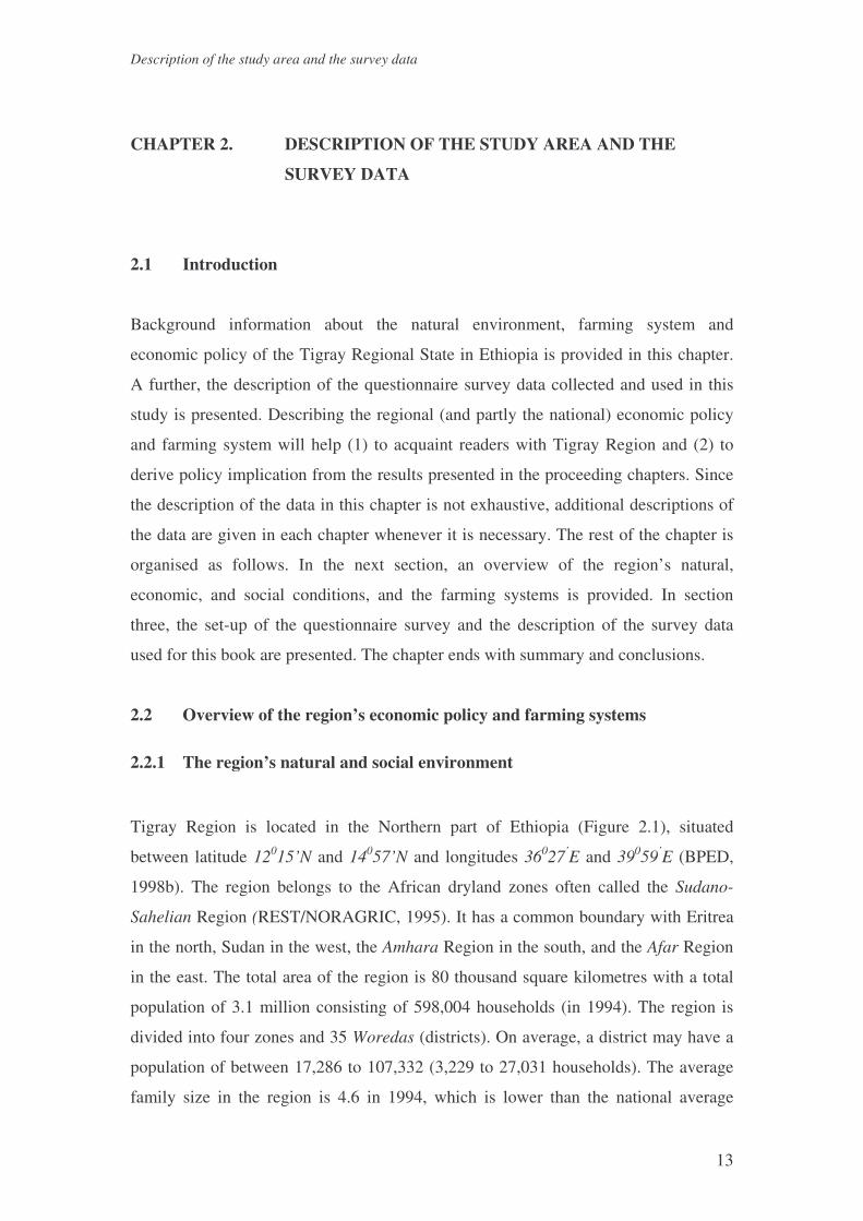
Figure 2.1 Map of Tigray Regional State, Ethiopia 14
Figure 3.1a Sale of skilled labour and purchase of farm labour under
transaction cost 53
Figure 3.1b Market failure in the sale of skilled labour and purchase of farm
labour under higher transaction cost 53
Figure 3.2 Market failure in the sale and purchase of unskilled labour due to
transaction cost 54
Figure 4.1 Kernel density estimates of area of land owned and cultivated 72
Figure 4.2 Wage rates (Birr/day) at Mekelle 81
Figure 9.1 Development of Small Scale Manufacturing Enterprises in Tigray
Region 182

vii
LIST OF TABLES
PAGE
Table 2.1 Regional (Tigray) gross domestic product by economic activity at
constant factor cost in 1994/95 and 1995/96 (in million Birr
except for per capita GDP) 17
Table 2.2. National and regional statistics of crops and livestock husbandry
(in thousands) 17
Table 2.3 National and Regional area (000 hectare) and production (000
quintals) figure in 1995/1996 18
Table 2.4 Household number (‘000) and family size (‘000) by the size of
land holding (in hectare) 19
Table 2.5 The distribution of the sample across districts, tabias and kushets 25
Table 2.6 Description of the data set (n=402 and values are measured in
Birr) 27
Table 2.7 Description of variables – value per year in Birr- (n=402) 28
Table 2.8 Farm household participation in off-farm activities 29
Table 2.9 Reasons for farm household to receive credit 32
Table 2.10 Distribution of household meeting their consumption through
Purchase 33
Table 2.11 Classification of farm households by labour regimes (%) 34
Table 2.12 Proportion of farm households who hired farm labour under
different off-farm activities 35
Table 2.13 Distribution of expenditure (in Birr) 35
Table 4.1 Seasonal distribution of farm labour, off-farm work participation
and wage rates 70
Table 4.2 Sources of farm labour and seasonal allocation in 1996 and 1997
(household average) 70
Table 4.3 Absolute and relative factor endowments across farm size classes 75
Table 4.4 Use of labour and return to land and labour across farm size
classes 76
Table 4.5 Farm households’ probability of hiring farm labour (n=402) 78

viii
Table 4.6 Motivations to work in non-farm activities 79
Table 4.7 Average off-farm wage and participation rates in off-farm wage-
employment 84
Table 4.8 OLS estimates of wage offer equation of farm households (Dep
variable = household wage Birr/hour) 85
Table 4.9 OLS estimates of wage offer equations of husband and wife
(Birr/day) 88
Table 4.10 OLS estimates of wage offer equations of other male and female
members (Birr/day) 89
Table 5.1 Description of important variables 102
Table 5.2 Parameters estimation of production function (dependent variable
Ln = value of farm output in Birr) 104
Table 5.3 Tobit estimation of expenditure on variable farm inputs 105
Table 5.4 Parameter estimates off-farm labour supply (in hours) 107
Table 6.1 Description of variables related to time allocation 113
Table 6.2 Marginal effects on the demand for total farm labour and hired
farm labour 123
Table 6.3 The marginal product of farm labour for participant and non-
participant in off-farm work 124
Table 6.4 Elasticity of on-farm and off-farm labour supply of male and
female members 125
Table 7.1 Off-farm work Participation rates (%) by type and season in two
districts 132
Table 7.2 Average (median) farm and off-farm return to family labour
(Birr/hour) by districts 133
Table 7.3 Labour allocation and availability of an average household 134
Table 7.4 Gini Decomposition by income sources 144
Table 7.5 Estimates of wage offer equations for off-farm wage employment
and self-employment 146
Table 7.6 Elasticity for the probability and level of participation in off-farm
wage and self-employment 150
Table 7.7 Elasticity for the probability and level of participation in off-farm
wage and self-employment including both the direct and indirect
effects 150

ix
Table 8.1 Cropping pattern: percent of farm household growing crops 157
Table 8.2 Cropping pattern on average farm household (one tsimdi = one-
fourth hectare) 158
Table 8.3 Distribution of market regimes in crop and livestock outputs in
Enderta (EN) and Adigudom (AD) Districts 159
Table 8.4 Off-farm activities and marketing surplus (in Birr) of average
farmers 159
Table 8.5 Off-farm income and participation in the product market of
average farmers 160
Table 8.6 Elasticity for the probability of growing crops using instrumental
variables 167
Table 8.7 Elasticity of share of land allocated to crops at mean values 169
Table 8.8 Average land share, marginal land share and total land elasticity
of land allocation 170
Table 8.9 Elasticities of labour allocation across crops 171
Table 8.10 Elasticities of market participation and the level of purchase and
sales in the product market 172
Table 9.1 Distribution of small-scale manufacturing enterprises in Tigray in
1996/97 182
Table 9.2 Characteristics of the distributive trade in Tigray 184
Table 9.3 Value added (Birr) and employment potential for non-farm
activities in Tigray 186
Table 9.4 Problems faced by small and micro enterprises in Tigray,
Ethiopia 188
Table 9.5 Forward and backward production linkages agriculture with non-
farm sectors 189
Table 9.6 District level Correlation between farm income, population
density and capital invested in non-farm income in Tigray 190
Table 9.7 Food and non-food expenditure behaviour of farm households in
Tigray. 194
Table 10.1 Direct and indirect effects of off-farm income on farm income
(elasticities) 200
Table 10.2 Effects of a 1% increase in farm inputs on farm employment
(elasticity) 201

x
Table 10.3 Effects of a 1% increase in farm inputs on the hours of on and
off-farm employment 201
Table 10.4 Summary of wage and income elasticities for farm and off-farm
labour supply 202
Table 10.5 Comparison of elasticities with other studies 203
Table 10.6 The effect of a 1% increase in the market wage rate on the supply
of labour hours and household income 203
Table 10.7 Effect of farm and off-farm incomes on marketing surplus crop
output (elasticity) 204
Table 10.8 The marginal and percentage effect of an increase in family size
by one person 206
Table 10.9 The effects of education on logarithm of wage rate 207
Table 10.10 Marginal effects of education on the hours of labour supply 208

Introduction
1
CHAPTER 1. INTRODUCTION
1.1 Background
In most of the world historically, and in much of the world today, the economics of
agriculture is the economics of subsistence. It is about the effort of the rural people
who try to obtain the food necessary for survival from limited (and uncertain)
resources such as soil, water, etc. The focus of economics is, therefore, on how
individuals carry out such efforts (and how families, villages or other social entities
organise their members for doing so). Economic development begins when agriculture
generates production in excess of farm family requirements. Historically, the ability of
agriculture to generate surplus food is credited for the creation not only of markets but
also of such elements of civilisation as cities. Key innovations relating to crop and
animal production, mechanisation and information, and trade and specialisation form
an important part of agricultural economics research.
One of the most striking, and still to some extent controversial findings, in the
economics of traditional agriculture is the wide extent to which farmers in the poorest
circumstance (in the least developed countries) act consistently according to basic
microeconomic principles (Schultz, 1964). Schultz shows that farmers in traditional
agriculture follow economic rationality in the sense of getting the most economic
value possible with the resources at hand; but innovation and investment that would
generate economic growth are missing. In his view, farmers can break out of the poor
but efficient equilibrium by means of investment in high-income streams – mainly
physical, capital and improved production methods embodying new knowledge and
investment in human capital (Schultz, 1961; Becker, 1964) that would foster
innovation in technology and the effective adoption of innovations.
It is a long debated issue whether agriculture is an ‘engine of growth’ in which
investment is an important source of economic development (Johnston and Mellor,
1961); or the other way round, whether agriculture is an economically stagnant ‘sink’
of labour to mobilise more productively elsewhere as the economy grows (see
Timmer, 1988 for a survey). The latter issue is explicitly addressed in a dual economy
model (Lewis, 1954). The dual economy approach has evolved towards a neo-

Chapter 2
2
classical general equilibrium approach in which agriculture differs only in possessing
a specific factor, land, resulting in price and income inelastic output, and a possibly
different rate of technical progress (with no presumption that agriculture’s is lower).
Such a neo-classical model can account for the observed huge out-migration from
agriculture (traditional sector), as has occurred in all the industrial economies (such as
Japan, Taiwan and Denmark), together with increases in wage and income levels in
rural areas rising towards that of urban levels (Hayami and Ruttan, 1985). But they do
not provide useful guidance about the underlying stimuli to growth, or for fostering
economic development in least developing countries.
In the dual economy model1, emphasis is given to the role of a capital-
intensive large-scale industry, and mechanical and commercial agriculture which
results in the accumulation of capital in the modern sector and withdrawal of labour
from the traditional sector. This creates a growing imbalance between agriculture and
industry. It leaves little direct place for peasants, small-scale non-farm enterprises, or
the poor. Agriculture is not considered to be a high priority sector for fostering growth
in developing countries2.
Because of the experience from the Indian green revolution, export pessimism
and the balanced growth theory (Nurkes, 1953), agricultural development has become
a priority sector in economic development. It is now considered (at least) to have
equal priority with the industrial expansion (balanced growth) in the sense that
agricultural and industrial development are both simultaneously to be promoted
(Mellor, 1976). The purchasing power of the rural people as a valuable means to
1 In a dual economy model (Lewis, 1954; Fei and Ranis, 1964), an economy is divided into a traditional sector (which is mainly agricultural, but also includes the rural manufacturing and trading - rural non-farm- activities) and modern (capitalist) sector (which includes industrial and large-scale commercial agriculture). The dual economy model argues that the transformation of the traditional sector must occur by absorbing the traditional sector into the modern sector, which is often called transformation by displacement (Bruton, 1985). In fact, Fei and Ranis do see a positive role for the traditional sector to play if productivity in the traditional sector can be increased, in which case expansion of the modern sector is easier and the transformation process can occur much more rapidly. 2 This is espoused mainly by the unbalanced growth theory (Hirschman, 1958) which proposes public investment in the non-agricultural sectors, which is thought to have greater production linkages with rest of the economy. Early studies on economic linkages between sectors focused on production linkages only, namely forward and backward production linkages. Agricultural growth (subsistence agriculture) was thought not to have strong backward and foreword production linkages, hence it stimulates little new demand for intermediate inputs or new investment in down stream activities. Rural non-farm activities (traditional manufacturing and services giving activities) faced the same problem as the traditional agriculture. An anti-agriculture attitude was also encouraged by the elasticity pessimism debate on the export of agricultural products. The Malthusian concern with diminishing marginal productivity in agriculture was also a factor for the investment bias against agriculture.

Introduction
3
stimulate industrial development (Johnston and Mellor, 1961) is recognised3. As a
result, the attention of policy makers has shifted from a capital-intensive strategy to a
rural led employment-oriented strategy (Mellor, 1976). The rural led employment-
oriented strategy is intended to increase employment in agriculture (rather than
withdrawing labour from agriculture) and leads to the growth of industry and trade
through production (backward and forward) and consumption linkages with
agriculture. This approach places agriculture at the centre of economic development.
The roles of traditional sector rural non-farm activities in the development of
agricultural sector via backward, forward and consumption linkages (Delgado et al.,
1998; Haggblade and Hazell, 1989; Haggblade, Hazell, and Brown 1989) are also
well recognised.
Linkages can also run from the traditional sector rural non-farm activities to
agricultural production (Ranis and Stewart, 1987; Reardon, 1997; Evans and Ngau,
1991): demand, supply, motivational, and liquidity related linkages. Expansion of
rural based manufacturing stimulates the development of markets for agricultural
production, and as these markets expand, it allows agricultural producers to diversify
into non-food agricultural production (demand linkage). Production of manufacturing
goods in the traditional sector will provide the supply of inputs necessary to increase
agricultural production (supply linkage). If farmers are engaged in rural based non-
farm activities (such as manufacturing and trading), they are likely to intensify
production efforts and increase agricultural productivity to provide the resources
necessary for investment in the rural based non-agricultural activities. In areas where
agriculture is risky, income diversification (into rural non-farm activities) for farmers
will reduce the risk associated with innovation (motivational linkage). In a situation
where insurance and credit markets are limited (or do not exist), income
diversification for farmers will help to finance agricultural production (liquidity
linkage). Hence through the interaction of farm and non-farm activities, a virtuous
circle of traditional sector development can arise, but this requires further empirical
evidence.
3 The purchasing power of peasants and their families could increase when labor productivity of agriculture improves. Increases in labor productivity will increase the marketing surplus of agricultural production, which can be diverted to industrialization and development of infrastructure (through fiscal and monetary policies such as taxation or encouraging saving through monetary polices) essential for the economy as a whole at the early stages of economic development.

Chapter 2
4
The concentration of non-farm sectors in a few urban areas, and the wage gap
between rural and urban areas result in a huge rural-urban migration and
concentration of unemployed workers in urban areas (Todaro, 1980)4. The rapid
urbanisation and growing number of unemployment in urban areas necessitates
finding a way to create jobs outside agriculture and outside cities focusing on a
growth process that would boost the demand for rural non-agricultural activities.
Hence creating demand in rural areas for locally produced non-food goods and
services becomes an important element in the process of economic development (Bell
and Hazell, 1980; Mellor, 1976).
1.2 Problem statement
Considering agriculture as the centre of economic development, governments in
developing countries may intervene in the rural economy (farm and non-farm sectors)
through pricing policies and investment projects. Such policies can influence
production and consumption (the livelihood) of farm households. However, the
manner in which agricultural households respond to such interventions and the
magnitude and nature of the linkages that exist between the rural non-farm activities
and the industrial sector on the one hand and the farm sector on the other hand are
crucial in determining the relative merits of these policies (Singh et al., 1986; Strauss
and Thomas, 1995; Strauss and Thomas, 1998).
Two main policies can be identified with a view to increasing employment and
reducing poverty in Ethiopia (TGE, 1991). The first policy is to improve productivity
in agriculture and promote self-sufficiency in food. Second policy is to promote
investment in the rural non-farm sector in order to provide alternative income earning
opportunities. The success of investments in the agricultural and industrial sectors and
the extent to which the benefits trickle down to the landless and/or poor households
depend on the adjustment of labour supply and demand, the smooth functioning of the
labour market, and wage determination (Collier and Lal, 1986). Whether the
introduction of an improved technology increases the demand for labour and whether
the increased demand for labour is met from the household’s own resource or from
4 Unemployment in urban areas is also the result of wage rigidity imposed by minimum wage legislation and efficiency wage (Stiglitz, 1988).

Introduction
5
hired labour depend on the microeconomic behaviour of farm households and the
extent of market imperfection in general and on the demand and supply of labour in
particular. If the labour market is highly imperfect, the transaction costs of hiring and
selling labour (such as supervision and search costs, and shirking) will be very high.
This will retard or hinder investment or make capital relatively cheap and eventually
results in lower employment opportunities. If the transaction costs of labour make
capital cheap relative to labour, investment will be more capital-intensive, which is
not appropriate to the factor endowments (factor proportions) prevailing in developing
countries. If the capital market is highly imperfect such that farmers are constrained
with respect to liquidity and credit, the use of purchased inputs and hired labour will
be very limited. This has negative repercussions on the expansion of employment and
the transfer of income from landed (large farm size) to landless (small farm size)
households.
Off-farm employment is thought to have a negative impact on farm income at
the household level. It increases the cash resources of farm households and decreases
the availability of family labour for farming activities (Burger, 1989). The demand for
leisure increases (and farms income decreases) when off-farm income increases due to
both a substitution effect and an income effect. However, if there is surplus labour (or
farming is not able to absorb the idle family labour), off-farm employment may not
have a negative impact on farming activities. In the case of surplus labour, off-farm
employment may not be able to compete with farming activities for labour. If the
capital market is highly imperfect and farmers are liquidity constrained, off-farm
employment may help farmers to diversify their income sources and break the
financial constraints they face in hiring labour and purchasing capital farm inputs
(Collier and Lal, 1986). In the cases of capital market imperfection and liquidity
constraints, therefore, off-farm employment may increase farm income.
One of the basic assumptions of diversifying income sources into off-farm
activities is to supplement farm income for the poor and reduce income inequality in
rural areas. This is because the motivation to diversify income sources into off-farm
activities is higher for poor than for rich farm households (Reardon, 1997). However,
if there is an entry barrier in the off-farm labour market, diversifying income sources
into off-farm activities will be more difficult for poor farm households than for rich
farm households. Off-farm activities may require investment on equipment purchase
or rent, skill acquisition and license fees. Because of collateral requirements and

Chapter 2
6
differences in repayment capacity, the credit constraint is more severe for poorer farm
households than for richer farm households. The poor households face a binding
credit constraint, and so can not afford the investment required in the off-farm labour
market, while this would not be a problem for rich. As a result off-farm employment
may exacerbate income inequality rather than reducing it.
Previous studies in Africa focus more on characterising rural micro enterprises
(Liedholm, McPherson, and Chuta, 1994), and on the impact of agricultural growth on
the rural non-farm economy (Haggblade, Hazell and Brown, 1989; Delgado et al.,
1994; Delgado et al., 1998). The attention is on the effect of agricultural growth on
rural non-farm activities rather than on the effect of off-farm income on farm income.
Literature on the effect of off-farm employment on farm income mainly discusses
theories and postulates hypotheses about the contribution of off-farm income to farm
income (Reardon, 1997). Empirical evidence based on actual data of farm households
is scarce in the literature. Empirical studies done on the effect of off-farm
employment on farm income are concerned with a dynamic agricultural sector where
cash crops are grown widely (Burger, 1994; Evans and Ngau, 1991). Despite the
general scarcity of literature on farm and non-farm linkages, there has been no
systematic study done on marginal areas in the Ethiopian context. Furthermore,
analysis of the rural labour market and wage determination in Africa are scarce in the
literature (Reardon, 1997), especially in Ethiopia. This forms the motivation to
analyse the interaction between farm and non-farm activities, the adjustment of labour
demand and supply, the performance of the labour market and wage determination in
the context of Ethiopia, with particular focus on Tigray. Although the main focus is
on Northern Ethiopia, most conclusions can have a wider application in the other parts
of the country and in many of the Sub-Saharan African countries where agriculture is
not dynamic and capital market is highly imperfect.
1.3 Objective of the book
The objective of this study is to analyse farm non-farm linkages at the household
level, particularly focusing on the impact of off-farm employment on agricultural
productivity and marketing surplus and on the role of off-farm employment in
alleviating rural poverty. The study identifies the microeconomic determinants of
labour use and allocation and assesses the factors that affect labour productivity. The
Introduction
7
determinants of on-farm and off-farm labour demand and supply including social,
cultural and economic determinants are investigated as well. The labour market is
assumed to be a non-separable link between the consumption and production
decisions of an agricultural household.
Specifically the objectives of the book are summarised as follows.
1 To determine the magnitude and direction of the relationship between off-farm
employment on the one hand and farm income, factor inputs, marketing surplus
and crop choice on the other hand.
2 To identify the factors determining farm households’ demand (for total and hired
farm labour) and supply of labour for farm and off-farm activities and the relative
importance of these factors.
3 To evaluate the functioning of the farm and non-farm labour markets and the wage
determination process.
4 To enumerate and quantify the production, consumption and labour market
linkages between the farm and non-farm sectors.
5 To assess the development of and the constraints of rural small scale and micro
enterprises (SME).
6 To integrate and generalise the results obtained in separate chapters, and derive
policy implications.
In answering these research questions, a non-separable agricultural household
model (Cailavet, Guyomard, and Lifran, 1994; Singh, Squire and Strauss, 1986;
Strauss and Thomas, 1995; Strauss and Thomas, 1998) is developed. The agricultural
households model is adopted to handle various problems such as a missing market for
capital, transaction costs in the input and product markets and transaction cost and
rationing in the labour market (De Janvry, Fafchamps, and Sadoulet, 1991; De Janvry
et al., 1992). Econometric estimation of labour demand and supply equations is done
accounting for the sample selection biases that might be introduced due to truncation
(Maddala, 1983). The farm-non-farm linkages are analysed at a micro level
(Haggblade and Hazell, 1989; Haggblade, Hazell, and Brown 1989; Reardon, 1997).
In doing so, this study provides microeconomic evidence on the farm-non-farm
growth linkages and the adjustment of labour demand and labour supply, which has
macroeconomic policy implications (Binswanger and Deininger, 1997).
The study uses data collected from a questionnaire survey of 201 farm
households for two years, 1996 and 1997, from two districts of the Tigray Region in

Chapter 2
8
Northern Ethiopia and from a small informal survey of the labour market, labourers
and major employers in the towns of Mekelle, Quiha and Adigudom (see Chapter 2 for
the set-up of the questionnaire survey and the description of data). Secondary data
from the government ministries such as the Central Statistics Authority of Ethiopia
(CSA, 1997a, 1997b, 1997c, 1997d) and the Industry, Trade, and Transport Bureau of
Tigray Regional State (ITTB, 1998) are also used.
Because of the limited panel nature of the data set, econometric models
estimation was done in a cross section context. In fact the data has two observations
per household which enables to use e.g. a fixed effect estimator. Fixed effect
estimator helps to capture unobserved individual effects (see Deaton, 1997 for a
discussion in the context of survey data). Then variables that do not change over the
period of observation (such as - in our case - soil depth indicators, soil type dummy,
education dummy, income diversification index, family size5, location dummies, etc.)
have to be dropped. Because of the limited panel characteristics of the data, the use of
a fixed effect estimator will result in a huge loss of information. The loss of efficiency
is the greatest when there are only two observations per household (Deaton, 1997, pp.
105-110). Using a fixed effect estimator means that we can not test all of the
hypotheses of the book. Furthermore, fixed effect estimation results in biased
estimates for most of the models which involve a limited dependent variable
(Chamberlain, 1984).
1.4 Outline of the book
In addition to the introductory chapter, the book contains nine chapters. Chapters 3-8
present the analyses at household level while chapters 9 and 10 present the analyses at
the regional level. Particularly chapters 5-8 are brought together to derive policy
implications at a higher (regional) level. The details of the estimation results are given
in the appendix at the end. The chapters are organised as follows. Chapter 2 is a
descriptive chapter that helps to acquaint readers with the Tigray Region, Ethiopia,
which is the area under study. It includes an overview of the region’s natural,
economic, social and policy environments as well as the role of governmental and
non-governmental organisations in rural development. The chapter also presents the
5 Family size changes over the period observation for only three-percent of the sample.

Introduction
9
set-up of the sampling strategy and the description of the survey data used for the
study.
In chapter 3, a model is developed that reflects the observed patterns in the
sample of farm households described in section 2.3.2. A non-separable agricultural
household model with missing markets for factors of production such as capital (De
Janvry, Fafchamps and Sadoulet, 1991) is used. The model includes rationing and
transaction costs in the labour market. Testable implications are derived for off-farm
employment, hiring of farm labour and product market under transaction cost,
liquidity constraint and rationing in the labour market. The links between liquidity
constraints and off-farm employment are analysed.
In chapter 4, the working of farm and non-farm labour markets is analysed.
The initial differences in absolute and relative factor endowments such as labour/land
ratio and labour/capital ratio among farm size classes are assessed. Then the extent to
which the farm labour market equalises the return to labour and land across different
farm sizes is analysed. The factors that determine the hiring probability of farm labour
and their relative importance are identified. We also see to what extent the seasonal
character of agricultural production influences the use of hired labour. The working of
the non-farm labour market is analysed based on our observation of the non-farm
labour market in formal and informal interviews with labourers and major employers.
Recruitment procedures and the criteria used to hire farm labour, information sources
in the labour markets, the relative power of employers and employees, and wage
determination are discussed. Finally, based on the farm survey data, the factors that
determine the farm household members’ wages and their relative importance are
identified. The concepts from the competitive theory of labour markets accounting for
the heterogeneity of labour and efficiency wage theory are used in analysing the
labour market and wage determination.
Chapter 5 deals with the link between farm and non-farm income. Specifically,
it looks at the impact of off-farm income on production technology and on the
financing of farm activities. To see the impact of income diversification on production
technology, Simpson’s index of income diversification is constructed and used as an
explanatory variable in the production function. To assess the impact of off-farm
income on the financing of farming activities, the demand for variable inputs, with
off-farm income as an explanatory variable, is estimated. Off-farm work participation

Chapter 2
10
and off-farm labour supply (without dissagregating off-farm labour by sex or by type
of off-farm activities) are also estimated in this chapter.
In chapter 6, the structural equations of demand as well as the on and off-farm
labour supply of family labour, dissaggregated into male and female household
members, are estimated. The demand equations for total farm labour and hired farm
labour are estimated. The shadow wages of family farm labour is derived from a
Cobb-Douglas production function. Finally own and cross wage elasticities and
income elasticities of labour supply are calculated.
Chapter 7 deals with off-farm work dissaggregated into wage employment and
self-employment. It assesses the impact of off-farm income on income inequality. The
income category includes crop income, livestock income, non-labour income, and off-
farm income. Off-farm income is sub-divided further into off-farm wage employment
and off-farm self-employment. Off-farm wage employment is further categorised into
paid development work (food for work program), non-farm unskilled wage work and
non-farm skilled wage work. The Gini index of inequality and the relative
contribution of income sources to total inequality for total household income and
various categories of household income are calculated. The Gini elasticity of various
income sources is also calculated. The factors that determine a farm household’s
choice among different types of off-farm work and the relative importance of these
factors are analysed using a multinomial logit model. The supply of labour for off-
farm wage employment and non-farm self-employment is estimated.
In chapter 8, crop choice and land and labour allocation decisions of farm
households, market participation and its relation to off-farm employment are
analysed. The crop choice decision is analysed using a binomial logit model for each
crop. Tobit models of labour and the proportion of land allocated to each crop are
estimated for each crop. In the labour allocation model, non-farm labour hours
supplied is used as an explanatory variable. In the land allocation model, the level of
off-farm income earned by a farm household is used as an explanatory variable. The
output marketing decision of farm households is modelled in order to assess the
factors that determine the probability and level of participation in the product market.
In this model, farm households face a two-stage decision problem. The first is a
discrete decision whether or not to trade (depending on the cost of market
participation) and in which direction (either as buyer or as a seller). The second
(continuous decision) is how much to trade conditional on participation as a buyer or

Introduction
11
seller. Therefore, first the bivariate probit equations of participation as a buyer and as
a seller in the product market are estimated. Using the selectivity term derived from
the probit equations, the level of sales and purchase equations are estimated using
3SLS estimation method. In all cases off-farm income and farm outputs are
considered as endogenous variables.
Chapter 9 brings two different, but similar issues together in order to complete
the discussion of farm-non-farm income linkages. The first part deals with the
problem and development of small and micro enterprises (SME) as well as the link
between the farm and non-farm sectors in the Tigray Regional State. The analysis of
the farm-non-farm linkages and the constraints and the development of SME is done
using secondary data collected by the Central Statistical Authority of Ethiopia and the
Tigray Regional Bureau of Trade and Transport. The second part deals with
enumerating and quantifying the production and consumption linkages that exist
between farm and non-farm sectors. For this purpose the survey data collected from a
sample of 201farm household in the two districts of the Tigray Regional State is used.
In chapter 10, the link between farm and off-farm income is explicitly
determined using the results from Chapter 5 to 8. The relationship between farm
inputs, farm labour and marketing surplus on the one hand and off-farm employment
on the other hand is analysed. The impact of an increase in family size on various
categories of labour, and the role of education in the farm household’s earnings and
labour supply are summarised. The program and policy implications of the main
findings, and suggestion for future research are discussed. Finally, the general
conclusion of the book is presented.

Description of the study area and the survey data
13
CHAPTER 2. DESCRIPTION OF THE STUDY AREA AND THE
SURVEY DATA
2.1 Introduction
Background information about the natural environment, farming system and
economic policy of the Tigray Regional State in Ethiopia is provided in this chapter.
A further, the description of the questionnaire survey data collected and used in this
study is presented. Describing the regional (and partly the national) economic policy
and farming system will help (1) to acquaint readers with Tigray Region and (2) to
derive policy implication from the results presented in the proceeding chapters. Since
the description of the data in this chapter is not exhaustive, additional descriptions of
the data are given in each chapter whenever it is necessary. The rest of the chapter is
organised as follows. In the next section, an overview of the region’s natural,
economic, and social conditions, and the farming systems is provided. In section
three, the set-up of the questionnaire survey and the description of the survey data
used for this book are presented. The chapter ends with summary and conclusions.
2.2 Overview of the region’s economic policy and farming systems
2.2.1 The region’s natural and social environment
Tigray Region is located in the Northern part of Ethiopia (Figure 2.1), situated
between latitude 12015’N and 14057’N and longitudes 36027’E and 39059’E (BPED,
1998b). The region belongs to the African dryland zones often called the Sudano-
Sahelian Region (REST/NORAGRIC, 1995). It has a common boundary with Eritrea
in the north, Sudan in the west, the Amhara Region in the south, and the Afar Region
in the east. The total area of the region is 80 thousand square kilometres with a total
population of 3.1 million consisting of 598,004 households (in 1994). The region is
divided into four zones and 35 Woredas (districts). On average, a district may have a
population of between 17,286 to 107,332 (3,229 to 27,031 households). The average
family size in the region is 4.6 in 1994, which is lower than the national average
Chapter 2
14
(5.15). Each district is subdivided into Tabia (peasant associations). One Tabia
consist of up to 1500 households on average. The Tabia is the lowest official
administration unit in the region. Each Tabia is divided into Kushets. One Tabia can
have up to eight Kushets. In most cases Kushets, not Tabias, own the pasture area,
woodland and irrigation schemes. Eight-five percent of the population resides in
purely rural areas and the other 15 % lives in towns: either in the capital city of the
region, or district centres, or rural centres. There are 74 rural centres registered as
rural towns: 35 of them are Woreda centres.
Figure 2.1 Map of Tigray Regional State, Ethiopia
The topography of the region is characterised by highly variable landforms
and different altitudes (BPED, 1998b). It ranges from flat lowland to ragged and
mountain plateau. The altitude of the region ranges from 500 meters in the eastern
part of the region (Erob) to 3900 meters in the southern zone near Kisad Kudo. Kiremt
(summer) is the main rainy season of the region. The rain usually starts in late June or
early July. It ends in late August or early September.
The natural resources of Tigray are under extreme stress to support the over
increasing population (REST/NORAGRIC, 1995). Much of the steep slopes have lost
Ethiopia

Description of the study area and the survey data
15
their protective cover. They are highly overused for cultivation and grazing of
livestock. Grasslands have been overexploited. Soil run-off from slopes has caused
severe erosion. Most of the soil is eroded by water and wind (BPED, 1998b). The
natural forest of the region has been destroyed mainly through encroachment of
subsistence cultivation. Crop production and animal husbandry potential of the region
has declined severely mainly due to the degradation of natural resources. Agricultural
productivity has declined due to soil erosion. Aridification has increased due to
clearing of natural vegetation such as forest, woodland and bushland.
The region does not have a well-developed infrastructure (BPED, 1998b).
Most areas of Tigray are difficult to reach by mechanised transport. There are not
enough roads to connect places and the quality of the available roads has deteriorated
greatly. The regional average road density is below the national average. In 1992, the
regional road density was 10.3 km/1000km2, while the national average was
25km/1000km2. In 1995, the regional road density became 15km/1000km2,which was
still lower than the 1992’s national average road density. Until 1997, the region did
not have 24 hours supply of electricity in the towns. Since May 1998, most towns
located on the main highway have 24 hours of electricity supply from
hydroelectricity. The supply of telephone lines and postal services is far below the
level of demand and of low quality.
Farmers do not have full access to formal financial institutions such as
commercial, insurance and construction banks. The financial institutions that are
found in the region mostly serve only the town people. The 12 branches of the
Commercial Bank of Ethiopia are located in 11 towns; two Development Banks, one
Business and Construction Bank, and two private banks are located in Mekelle. These
banks require collateral and involve time consuming screening processes before they
provide loans to individuals.
The region does not have enough institutions to improve the educational level
and technical skills of its population. Most of the schools are basic schools such as
elementary, secondary and high schools. These schools lack even the basic
equipment. Furthermore, the increasing number of students is not matched by a
corresponding increase in the number of teachers and adequate facilities. There are
three higher learning institutions that teach agriculture, engineering and business
economics and administration. There are technical vocational training centres in
Mekelle, Korem, Adigrat and Axum town that are run by the Bureau of Labour and

Chapter 2
16
Social Affairs. There are also five technical training centres run by non-governmental
organisations. Two of them, administered by TDA (Tigray Development Association),
are designed for low-level academic background people. The other three are designed
to train medium level technicians in building, mechanical fields, business and
agriculture. The demand for high, medium and low level technicians in building and
other mechanical fields is not yet fully satisfied. However, trainees from the schools
designed for low level training have a hard time getting a job or starting their own
business. This is because of financial constraints in starting their own business and the
lack of information about the labour market.
2.2.2 The performance of the regional economy and farming systems
The magnitude and growth of the regional economy is given in Table 2.1. Tigray
region constitutes 22% of the national GDP1. Agriculture is the dominant sector, both
at the national and regional levels. Based on the 1995/1996 estimate, agriculture,
forestry and fishing constitute 64% of the regional GDP and 90% of the employment.
Industry, distributive service, and other services constitute 23%, 4%, and 9%
respectively. In 1995/96, the overall regional GDP had grown by 7.3%. The
distributive service sector is the fastest growing sector in the region. The second
fastest growing sector is the industrial sector. The industrial sector includes, among
others, the manufacturing sub sector and the large and medium as well as the small-
scale industry and the handicraft sub-sub sector.
Agriculture in Tigray consists of crop husbandry, livestock husbandry and
mixed farming. Mixed farming is the dominant type of farming system both at the
regional and national levels (Table 2.2). The region’s agricultural production is mostly
for domestic consumption. Products for export include oil crops such as sesame,
pulses such as horse bean and field peas, and skin and hides (CSA, 1997a). The region
produces circa 555,320 skins and hides per year most of which is for the export
market. The production of skins and hides has grown by 27% per year over the last
three years.
1 The figure appears a little exaggerated and it is hard to believe. The region’s population and total area is roughly 5.6 and 7.1 percent of the national population and total area, respectively.

Description of the study area and the survey data
17
Table 2.1 Regional (Tigray) gross domestic product by economic activity at constant factor cost in 1994/95 and 1995/96 (in million Birr except for per capita GDP)
Gross value Growth rate % Economic activity 1994/95 1995/96 Nominal Real 1. Agriculture, forestry and fishing 1797.6 1917.5 17 7 2. Industry 648.7 693.7 12 7 2.1. Mining and quarrying 155.0 175.7 10 13 2.2. Manufacturing 73.1 92.3 26 26 Large and medium scale 13.2 29.6 123 124 Small scale industry and handcraft 59.9 62.7 4 5 2.3. electricity and water 23.9 25.8 13 8 2.4. construction 396.7 399.8 11 1 3. Distributive service 123.4 143.4 16 16 3.1. Trade, hotel & restaurant 88.0 102.1 15 16 3.2. Transport and communication. 35.4 41.4 16 17 4. Other services 247.9 269.1 13 9 Regional GDP 2817.7 3023.7 16 7 Population (million) 3.1 3.2 2.5 Regional Per capita GDP (Birr) 904.8 946.9 13 5 Source: Regional Bureau of planning and economic development of Tigray Region.
Table 2.2. National and regional statistics of crops and livestock husbandry (in thousands) National Tigray Region
Total cropped area hectares (%) 8687 (100.0%) 484 (100%) Temporary crops only 8114 (93.4%) 483 (99.7%) Permanent crops only 573 (6.6%) 1 (0.3%) Number of households (%) With crops only 1504 (17.3%) 107 (18.5%) With livestock only 179 (2.1 %) 19 (3.3 %) With crops and livestock 7030 (80.7%) 454 (78.2%) Source: Crop utilization, Statistical Bulletin no. 152, CSA, Addis Ababa, September 1997
Farming systems in Tigray are characterised by a traditional technology,
completely based on animal traction and rain-fed. Cereals are the dominant crops with
pulses being of secondary importance (Table 2.3). A variety of crops such as cereals,
pulses and oil crops are grown in the region. The major crops are sorghum, teff,
barley and wheat. Arable land is getting scarce, leading to an extremely intensive land
use pattern. Farmlands are owned and run by small farms that are divided into minor
plots scattered over an extensive area. The production process is family based with
little hired labour. Livestock (except for plow-oxen) play an important but secondary
role (REST/NORAGRIC, 1995).
Farming activities start right after harvest, usually between September and
December. Farmers plow their lands two to four times before planting depending on
the type of soil and crop. The first plowing and in some places the second plowing
takes place in the dry season right after harvest. The rest of the plowing activities is

Chapter 2
18
done immediately after a rain shower. Planting is done from late June to early July.
The plowing intensity is higher for cereals than for pulses and oil crops. The land is
plowed not more than twice for legumes and oil crops, while it is plowed up to four
times in case of cereals, especially for teff and wheat.
Table 2.3 National and Regional area (000 hectare) and production (000 quintals*) figure in 1995/1996
National Regional Crop Type Area Production Yield qt/ha Area production yield qt/ha
Cereals 6,652.56 82,697.14 12.43 436.76 4,926.92 11.28 Teff 2,097.40 17,523.75 8.35 87.88 608.27 6.92 Barley 825.54 8725.32 10.57 87.35 817.11 9.35 Wheat 882.06 10,763.04 12.20 84.55 846.53 10.01 Maize 1,280.68 25,392.92 19.83 45.05 679.63 15.09 Sorghum 1,252.41 17,226.52 13.75 96.14 1,729.68 17.99 Millet 269.35 2,413.42 8.96 35.78 245.70 6.87 Oats 45.11 652.17 14.46 NA NA NA Pulses 904.39 8,141.44 9.00 36.91 329.27 8.92 Others 391.58 1,952.61 4.99 7.76 22.03 2.84 All Crops 7,948.53 92,791.19 11.67 481.43 5,278.22 10.96 Source: CSA (1997a). Statistical Bulletin number 152, volume IV. NA= not available; *one quintal equals 100 kilograms
Tigray region is relatively less productive in agriculture compared to the
southern and central part of the country. Agricultural production in the region is
below the national average. For example, in a good year (1996), the average yield per
hectare is 1,167 kilogram at the national level and 1,096 kilogram at the regional
level. The region gets a lower amount of rainfall with a higher inter-year variability of
rainfall compared to the national average. While the regional average rainfall (from
1968 to 1988) is 578 mm with a coefficient of variation (CV) of 28%, the national
average rainfall is 921 mm with a CV of 8%2.
The most basic constraints for crop production are unreliable rainfall, lack of
oxen for plowing, low soil fertility, and outbreak of crop pest. In the Central Zone, for
example, unreliable rainfall is perceived by farm households to be the most important
problem followed by crop pest and lack of oxen (REST/NORAGRIC). Lack of
pasture and fodder are the main constraints in animal production. Scarcity of
veterinary clinics is also an important constraint in livestock development. The revival
2 Using CV to compare the national inter-year rainfall variability with those of regions could be misleading because the CV of the national average rainfall could underestimate the national inter-year rainfall variability.

Description of the study area and the survey data
19
of livestock farming after a drought period is very difficult due to the fact that a great
number of cattle die during the drought period.
The growth in population has resulted in a decrease in the farm size. The
average farm size in the region is 0.97 hectares. Seventy percent of the farm
households in the region own less than one hectare (Table 2.4). Livestock husbandry
in Tigray is constrained by a shortage of grazing land. The forage supplies come from
unimproved and overgrazed pasture, and crop residue. Animal dung is used as fuel for
cooking in the region, not for enriching the soil. Because of the growing population,
expansion into marginal areas and areas with steeper slopes is widespread. The result
has been wide loss of massive highlands due to erosion. Increasing the area of land
under cultivation in the region is difficult due to land scarcity and malaria in the low
land areas of the western zone. Labour absorption in agriculture can only be possible
through the intensification of agricultural production and use of irrigation. Reducing
the farm size would not necessarily result in underemployment if a transition can be
made to intensive land use and irrigation. However, agriculture intensification and use
of irrigation has been adopted at a very slow pace and it is unlikely to show faster
progress in the near future. As a result, it is becoming very difficult to increase
employment in agriculture. The non-farm sectors have also not yet developed well
enough to absorb the growing population. The majority of non-farm enterprises are
small and often one-person enterprises (CSA, 1997d).
Table 2.4 Household number (‘000) and family size (‘000) by the size of land holding (in hectare) Size of holding Number of
households Number of household members
Average household size
Under 0.1 41.8 146.3 3.5 0.1 – 0.50 199.6 841.9 4.2 0.51-1.00 161.3 823.8 5.1 1.01-2.00 127.6 687.7 5.4 2.01-5.00 36.3 221.7 6.1 5.01-10.00 4.3 NA NA > 10.0 NA NA NA Total 571.3 2,754.2 4.8 National average household size is 5.15. Source: CSA (1997a). Statistical Bulletin number 152, volume IV; * NA = not available.
2.2.3 National and regional policy
National Policy. The 1974 revolution resulted in a series of policy measures aimed at
expanding collective and state owned farm and non-farm enterprises and managing

Chapter 2
20
the economy through central planning. The military government overthrew the
Emperor Haileselasie and declared socialism. Consequently the government
nationalised all banks, insurance companies, the industrial sector such as commercial
farms and non-farm enterprises, and houses. The government implemented major land
reforms so that land became state property. The government imposed restrictions so
that an individual could have only one type of occupation. Especially farmers were
not allowed to engage in off-farm activities. Hiring of labour was restricted. The
establishment of private dealers in the labour market was considered illegal. Farmers
were forced to become members of producer’s and service cooperatives. These
cooperatives were given priority for most types of financial assistance and extension
services. Industrial products were distributed through the service cooperatives. Private
traders in the rural areas were officially non-existent. The products of farmers were
sold at lower prices to the marketing board through the service cooperatives.
Public institutions were given the responsibility to promote the non-farm
sector. These institutions were the Rural Technology Promotion Department (RTPD)
of the Ministry of Agriculture; the Handcraft and Small Industrial Development
Agency (HASIDA) of the Ministry of Industry; and the Adult Training Centres (ATC)
of the Ministry of Agriculture. HASIDA was in charge of issuing licenses, organising
cooperatives and assisting in the marketing of products. However, these activities
were limited to urban areas. RTPD was entrusted with the task of developing and
promoting improved farm and non-farm tools as well as food processing and
preservation of technologies, which was quite far from the needs of the peasant
farmers. ATC of the Ministry of Education attempted to introduce various handicrafts,
construction, and farming skills into urban and rural areas. Their efforts were,
however, constrained by policy and institutional factors from the very beginning. All
promotional activities were aimed at cooperatives. Individuals trained in crafts were
unable to set themselves up due to lack of credit, tools, raw materials, demand and
business advice.
After the collapse of the military government, a market-based economy
replaced the centrally planned economy. In 1991 the coalition of rebellion groups
called the Ethiopian People’s Revolutionary Democratic Front (EPRDF) overthrew
the military government and immediately formed the Transitional Government of
Ethiopia (TGE). The TGE took new initiatives to limit the role of the government to

Description of the study area and the survey data
21
specific economic services, encouraging private investment, improving the
bureaucracy and pursuing appropriate macro and sectoral policies (TGE, 1991).
After the formulation of the Federal Democratic Republic of Ethiopia (FDRE)
in 1995, the government tried to liberalise the economy and promote investment in the
agricultural and industrial sector. The FDRE intended to continue the economic policy
agenda of the TGE. The present policy of Ethiopia gives emphasis to both the
agricultural and industrial sectors, but with a less clear focus on the rural non-farm
sector.
The main objective of the agricultural policy of the present FDRE is to ensure
adequate food security by increasing agricultural production and employment. A
broad based Agricultural Development-led Industrialization (ADLI) strategy
(Adelman, 1984)3 has been formulated that concentrates on three priority areas: (1)
acceleration of growth through the supply of fertiliser, improved seeds, and other
inputs; (2) expansion of small scale industries to interact with agriculture; (3)
expansion of exports to pay for capital goods import. Under the framework of ADLI,
a new system of agricultural extension, termed as participatory demonstration and
training extension system, was launched in 1994/1995. It provides agricultural inputs
in a package form together with extension advice.
However, the reform process, particularly the structural adjustment, has
affected the institutions that were in charge of promoting non-farm activities4. RTPD,
for instance, has been brought under the regional Bureau of Agriculture. Budget and
manpower are the major problems currently facing the centres. Most of them (for
example in Tigray) are still establishing themselves. HASIDA is offering technical
and managerial services to small-scale industry and handicrafts. Its operations are
financed through the revenue generated by charging fees for the service rendered. It is
still under reform and yet its services cover only selected urban areas, and no rural
areas at all. Most of the Adults Training Centres of the Ministry of Education have
been inactive since 1991. In some areas (Tigray) they have been transferred to local
NGOs (Tigray Development Agency, TDA).
3 See Adelman and Vogel (1995) and Adelman, Bournieux, and Waelbroeck (1995) for further discussion on ADLI. 4 The strategy for the small non-farm sector is not clearly mentioned in the national economic policy, it is yet to be elaborated.

Chapter 2
22
Despite the liberalisation process, the ownership of land has not changed. The
land is state property and farmers do not have the right to sell or buy land or give land
as a gift. However, farmers are given user’s rights. They can lease their holdings, hire
labour and can transfer land to their children.
Regional policy. Regions (states) in Ethiopia do not have different policies as
such, but their priorities can differ from one region to another. Given the national
policy, Tigray Regional State focuses more on environmental rehabilitation and food
security. Specifically, a conservation-based agricultural development strategy is
followed. The land tenure system in Tigray is the same as the national system, that is,
public ownership of land. The present land policy was first devised by TPLF (Tigray
People’s Liberation Front) and was applied first in the liberated areas of Tigray
during the war against the Mengistu regime. According to the policy, a person whose
livelihood is dependent on agriculture and who normally resides in the area for at least
six months is entitled to have land. The land was allocated to farm households based
on the size of the family (see also Table 2.4). No land distribution has been done since
1990. The regional government has recently (1997) decided to stop land distribution.
2.2.4 The role of non-governmental organisations
Non-governmental organisations in the Tigray Region are directly involved in
providing technical assistance to farm and non-farm communities. These NGOs are
internationally, nationally, or regionally based. The internationally based NGOs are
Farm Africa, Irish Aid, World Vision, and Evangelical Church. They provide farmers
with a variety of services mainly focused on agricultural development, afforestation,
and soil and water conservation activities, as well as rural water supply on a project
basis. They also provide credit for all income generating activities including petty
trade and handicraft. However, their focus on rural non-farm activities is minimal.
The nationally based NGOs are Catholic and Orthodox churches. They are engaged in
a number of programs including rural afforestation and water supply programs, but do
not have programs that focus on rural non-farm activities.
The regionally based NGOs are Relief Society of Tigray (REST) and Tigray
Development Association (TDA). REST and TDA are more active and are engaged in
more diversified activities (especially REST) than those of internationally and
Description of the study area and the survey data
23
nationally based NGOs. REST is the most active NGO in the region. It participates in
a wide array of activities: environmental rehabilitation such as afforestation and
development plantation forestry; soil and water conservation activities; rural water
supply, agricultural development such as irrigation development; emergency food aid;
construction and maintenance of rural roads; and development of rural credit systems.
REST’s involvement in the rural non-farm sector is mainly through its rural
credit and savings program. Its service is quite well distributed all over the region.
They have 12 main branches and 103 sub-branches. REST provides loans for various
cottages and small agro-based industry artisans engaged in rural arts, crafts, shoats,
horticulture and cash crops. The specific activities for which loans are provided are:
(1) crafts such as embroidery, pottery, basket making, spinning, weaving, carpentry,
metal work, and especially making of agricultural implements; (2) petty trade such as
buying and selling in the open market, shop keeping, barber shops, tailoring, and
preparing local food and drugs; (3) agriculture such as livestock rearing, bee keeping,
horticulture, and cereal production. The maximum loan amount is 5000 Birr and the
minimum is 50 Birr. The duration of the loan is up to one year depending on the
repayment capacity of the borrower and the nature of the activities. The loan is
provided on a group basis, charging 12.5% interest which is much higher than the
inflation rate5. The credit program of REST has improved farmers access to the
financial market. However, they still can not satisfy the farm households’ demand for
credit.
TDA is primarily involved in improving basic education and technical
training. Initially, it was also involved in the Integrated Rural Development Program.
Since 1996, its focus has been on urban and rural education. TDA is financially
dependent on membership contribution. They also solicit funds from international
governmental and non-governmental organisations.
TDA runs four technical training centres, two in the Central Zone (Shire and
Axum) and two in Mekelle. School dropouts, ex-soldiers, farmers, women, and
individuals without jobs are allowed to join the training program. The training is
given in basic construction (masonry and carpentry), metal work, woodwork,
electricity and auto-mechanics. Handicraft skills such as carpet making are provided
5 Inflation is contained below 10 percent. The average annual inflation over the last six years is 3.6 percent (MEDC, 1999).

Chapter 2
24
to a limited extent. Graduates are provided with the necessary tools and credit to start
their own business. However, their capacity is very limited. They have both financial
and accommodation problems.
In summary, it is not clearly known either now or in the past which government
organisation is responsible for the promotion of non-farm activities in rural areas
particularly for those activities carried out by farm households. The Agricultural
Research Centre and the Bureau of Agriculture concentrate on farming activities. The
Industry and Commerce Bureaus focus on non-farm activities in the urban areas.
Their activities are not well organised and do not clearly target the rural non-farm
activities carried out by farm households. The Bureau of Agriculture does some
activities through the Rural Technology Promotion department (RTPD) but it is not
well coordinated to reach the rural areas. The Handcraft and Small Industrial
Development Agency of the Bureau of Industry (HASIDA) does not target rural non-
farm activities in general or rural non-farm activities carried out by farm households
in particular. Substantial promotional work for farm and rural non-farm activities is
done by the non-governmental organisations. The non-governmental organisations
(especially REST and TDA) are more active and are better targeted at rural poor and
rural non-farm activities than the governmental organisations. However, their
activities still require more coordination with government organisations in order to
ensure efficient assistance programs and avoid duplication of activities.
2.3 Survey setting and description of the survey data
2.3.1 Survey setting and area description
A questionnaire survey was conducted in the Enderta and Adigudom6 Districts (see
Figure 2.1 in section 2.2.1 for the location) located in the Southern Zone of the Tigray
Region, Northern Ethiopia. The survey includes 201 farm households chosen
randomly from a stratified sample area. The choice of the districts was not random,
nor were they designed to be representative of the region as a whole. To select
districts that represent the whole region, a massive survey covering all districts would
6 Adigudom was formerly a district, and is now part of Hintalo Wejirat District.

Description of the study area and the survey data
25
have been required, which is far beyond the available budget and time of the research
project. Instead, given the nature of the gaps in our understanding of off-farm
employment and its linkage with farm employment, the present survey placed greater
emphasis on depth than on coverage. The two districts were selected because of the
following reasons. First, there are off-farm activities undertaken in the area. Second,
there are substantial variations in the nature and availability of off-farm activities.
Third, there are variations between the two districts in their access to information,
market, and infrastructure facilities. However, the choice of Tabias, Kushets, and
households were done randomly. The distribution of Tabias and Kushets are shown in
Table 2.5. To support the survey, additional information has been collected from
labourers and major employers in the off-farm labour market at Adigudom, Quiha,
and Mekelle towns.
Table 2.5 The distribution of the sample across districts, tabias and kushets District (Tabia) Kushet Sample households 1. ENDERTA 100 (Felegeselam) 35 Ashegoda 14 Emba 11 Maekeladi 10 (Maytsedo) 31 Egrihariba 11 Embafekadu 20 (Shebta) 34 Egrewenber 8 Gergenbes 8 Makel Adi 9 Randa 9 2. ADIGUDOM 101 (Araasegda) 49 Ara 25 Hedmo 24 (Fekrealem) 52 Aderak 18 Beleat 22 Mayifo 12 Total 201 Farm households were selected from each Kushet proportional to the population (4.2%).
Enderta is near the central city (Mekelle) of the regional government.
Adigudom is 40 kilometres from Mekelle. There are lots of opportunities for
households to work for off-farm wage employment in Enderta District. This
opportunity is very low in Adigudom District except for food for work in Adigudom.
Enderta District has an annual rainfall of 625.5mm with 26% CV, and while that of
Adigudom is 471.5mm with a CV of 49%. During the 1996 cropping calendar,
Adigudom received an annual rainfall of 596 mm. Enderta received a better

Chapter 2
26
distribution of rainfall in 19967. In 1997, both districts received poorly distributed
rainfall. In August, the amount of rainfall was 49% less than the average in Enderta
and 70% percent less than the average in Adigudom.
2.3.2 Description of the data set
Information on various activities of farm households including home, farm and off-
farm activities was collected using a survey questionnaire (see the outline of the
questionnaire in Appendix A2)8. The survey data provides detailed information on
seasonal labour allocation (for home, farm, off-farm activities and for each crop),
income sources (crop, livestock, wage employment, off-farm self employment, non-
labour income), purchase of farm outputs and inputs (including hired labour), sales of
farm outputs, expenditure on the consumption of home grown and purchased goods
and services, credit, household compositions, and anthropometrics. Local units are
partly used for the description of the survey data set. Area is measured in tsimdi,
which is equivalent to 0.25 hectare. Weight is measured in kilograms. Values are
measured in the Ethiopian currency called Birr. One US dollar is equivalent to seven
Ethiopian Birr during the survey period9.
The main data set characterising the households is given in Table 2.6 and
Table 2.7. On the average, the family size is 5.6, which is slightly above the regional
(4.8) and national average (5.15). The average dependency ratio (number of
dependants over family size) is computed to be 58.4%.
Farm households participate in a variety of farm, off-farm, and home
activities. The farming activities include crop production, livestock husbandry and
mixed farming. Mixed farming is the dominant type of farming system, and includes
both crop production and animal husbandry. The proportion of farm households
engaged in crop production only, in livestock husbandry only and in mixed farming
are 20%, 6% and 69%, respectively. The farming technology is traditional: simple
hand tools, oxen driven implements, and labour. The use of purchased capital inputs
7 The full rainfall record of 1996 for Enderta District and for both Enderta and Adigudom Districts in 1997 were not available. 8 The whole questionnaire is put at the following web site: www.sls.wau.nl/twoldehanna/. It was found too big to annex the questionnaire. The data set can be obtained from the author upon request. 9 The official rate for US dollar is 6.98 Birr, while the black market rate for one US dollar is 7.30 Birr.

Description of the study area and the survey data
27
such as fertiliser, improved seeds, and pesticides is very low. Labour is the dominant
type of farm input. Most of the labour input comes from the family (78%). The
remaining labour comes from hired labour (15%) and shared labour (7%).
Table 2.6 Description of the data set (n=402 and values are measured in Birr) Variables Mean Std. Dev. Min Max Family size 5.58 2.15 1 11 Number of dependants 3.26 1.91 0 7 Age of the household head 48 11.83 25 76 Area of land cultivated (in tsimdi)* 7.06 4.7 0 24 Number of plots cultivated 3.65 2.11 0 14 Area of land owned (in tsimdi) 5.88 2.42 1 15 Number of plots owned 3.06 0.95 1 7 Value of owned farm implements 237.62 185.71 0 1,427 Value of non-farm equipment 8.13 56.34 0 700 Total livestock wealth 3,616 5,298 0 63,700 Market wage rate per hour 1.18 1.61 0.10 14.73 Food expenditure 3,003 1,517 809 15,239 Share of high value crop 0.42 0.26 0 0.99 Percent single households (divorced or widows) 13.7 - - - Percent female headed households 11.44 - - - Percent orthodox households 98.5 - - - Percent Muslim households 1.5 - - - *TSIMDI is a local area measurement unit (one hectare = 4 TSIMDIs); One USD equals seven Ethiopian Birr in 1997.
The four most important crops in order of their importance in production and
the number of households growing a crop are barley, wheat, teff and sorghum. Other
crops such as lentils, vetch, linseed, and vegetables also have considerable
importance. Most households grow low value crops such as oat, sorghum, finger
millet, maize, barley and vetch (latyrus). The average share of high value crop is 42%.
Wheat, teff, linseed, lentils, chickpea, beans and vegetables are considered high value
crops. This is determined on the basis on their long-term market price in the region.
While 16.2% of the households grow only low value crops, 2.2% of the households
grow only high value crops.
Most farmers produce under rain-fed agriculture. The average area under
irrigation is 0.01 hectare. About six percent of the farm households use irrigation to
produce vegetables and some food crops. Seventy-eight percent of the vegetable-
growing households are located near the centre of the region, Mekelle. Households
that live further from Mekelle use irrigation to grow maize and pepper rather than
vegetables.

Chapter 2
28
Table 2.7 Description of variables – value per year in Birr- (n=402) Variables Mean Std. Dev. Min Max Crop output 1,962.04 1,911.46 0 15,000 Output of livestock products 497.40 681.9 0 5900 Net crop income 1,339.65 1,342.79 -1082.7 10,770 Off-farm labour income 1121 1340 0 9948 Non-labour income 271.62 902.51 0 10,000 Variable farm inputs 446.07 388.65 0 2,517 Hired farm labour input in hours 92.6 199.84 0 1486 On-farm family labour hours 491.54 325.73 0 1,968 On-farm labour hours from labour sharing 47.00 134.38 0 1,420 Total off-farm labour hours 1347 1402 0 9,920 Non-farm self-employment income 262.50 584.02 0 4000 Income from paid community work 437.89 624.34 0 5,400 Non-farm unskilled wage employ income 284.58 786.03 0 8,340 Skilled non-farm wage employ income 136.29 860.01 0 8,730 Food expenditure 3,003.21 1,516.99 808.5 15,239 Non-food expenditure 800.24 615.41 41 5,525 Labour hours supplied for paid community work 811.64 1,047.45 0 8,640 Labour hours supplied for unskilled non-farm work 385.73 1,072.48 0 9,920 Labour hours supplied for skilled non-farm work 51.66 296.43 0 2,916 Labour hours supplied for non-farm self-employ. 97.56 234.38 0 1,475 Credit received (Birr) 224.29 438.13 0 2,240 One USD equals seven Ethiopian Birr in 1997.
Farm households are involved in two types of off-farm activities: wage
employment and self-employment (own business activities). Wage employment
includes paid community development work (often called food-for-work), farm work,
and manual work in construction, masonry, and carpentry. Self-employment includes
petty trading, transporting by pack animal, fuel wood selling, charcoal making, selling
fruits, making pottery and handicrafts and stone-mining. The majority of farm
households participate in off-farm activities (81%). Most of the farm households work
in their Tabia (48%) and few go outside their Tabia (18%) and Woreda (1%). Most of
the off-farm works are temporary and do not require any professional qualification
with the exception of masonry and carpentry. The proportion of households that do
not participate in off-farm wage employment is 27.9%, and the proportion of
households that do not participate in off-farm self-employment is 72.14% (Table 2.8).
In most farm households, more than one member participates in off-farm
activities. For reasons of simplicity family members are categorised into four groups:
household head, wife, other male member, other female member. The dominant type
of off-farm work is paid development work. The household heads work in paid
development work in 55% of the households, in bricks making and carpentry in 4% of
the households, and in manual work in 11% of the households. The household wives
work only in paid development work (34%) and other manual work (2%). Other male

Description of the study area and the survey data
29
members work partly for paid development work (12%) and partly for other manual
work (8%). Other female members work for paid development work only (6%). The
main participants in non-farm own business are household heads (80%) and
household wives (12%).
Table 2.8 Farm household participation in off-farm activities Type of off-farm activities Participation rate (%) Off-farm own-business 27.9 Total wage employment 71.5 Non-farm wage employment 21.6 Manual non-farm wage employment 19.2 Masonry and carpentry 3.5 Food for work 57.7 Off-farm work participation excluding food for work 43.0 Over all off-farm work participation 81
Paid development work is the dominant type of off-farm work. Unless a
person is unable to work, the provision of food aid (in case of drought) is linked to the
participation of households in development activities such as terracing, reforestation,
dam and road construction and maintenance, and the rehabilitation of social services
like clinics and schools. Regardless of crop failure, terrace construction and
maintenance is done every year until the whole area that needs terracing is covered.
Every person above 18 years old has an obligation to provide 20 person days per year
for community development works. If a person works more than 20 days, three
kilogram of wheat grain is given per person day. If the community development work
is limited, priority is given to the poorer households. However, in the years 1996 and
1997, there were many micro dam constructions in the two districts. Hence, any
farmer who wanted to work was able to work for paid development work.
Farm household income is composed of farm income, off-farm labour income
and non-labour income. In the household’s total income, farm income accounts for
57% with livestock contributing 16% and crop production 41 %. Off-farm labour
income accounts for 35% and non-labour income accounts for 8% of the total income.
The amount of non-labour income that households obtain is very small compared to
the farm and off-farm income received. Non-labour income includes remittance
(47%), food aid (20%), and gifts and inheritance from relatives (19%).
Most of the people are illiterate, and only few can read and write as a result of
attendance in regular schools, adult education or church schools. In the sample, 35%
of the household heads can read and write. Of these 62 % attended modern school, 9%

Chapter 2
30
attended an adult education program and 29 % did not attend school. The other 65
percent of the household heads are illiterate. The illiteracy is higher for wives than for
husbands.
Farm households allocate their labour between farm and off-farm activities as
well as homework. The farm activities that farm households perform are plowing by
the male members of the household, usually by the head; weeding and harvesting by
all members of the household, and cattle keeping by male and female family members
who are less than 15 years old. The off-farm activities are public unpaid work, paid
community work, farm wage employment, non-farm wage employment and own non-
farm business. The main activity of the household heads is farm work (88%). They
also engage in off-farm wage employment (7%), working at home (8%)10, and trading
(21%). The main activities of household wives are food preparation, child caring, and
water and fuel wood fetching. Most of the other male members of the households are
engaged mainly in cattle keeping (52%). In Only a few households, other male
members engage in farm (25%) and off-farm (5%) activities. The rest are either
students or elderly people who are not able to work. Other female members are
engaged in homework activities (preparing food and child caring, 17%); cattle
keeping; farm work (2%) and off-farm work (2%).
Farm household heads work up to 11 hours per day for farm work and up to
eight hours for off-farm work. Household wives work usually for 4 hours per day on
the farm, but for 11 hours during peak agricultural seasons for weeding and harvesting
seasons. However, farm households in Tigray do not work every day due to the
Ethiopian Coptic-church holidays. On the average, including Saturdays and Sundays,
farm households do not work for 15 days a month for farming activities and for 12
days a month for off-farm activities11. Violation of Christian holidays is very rare.
Fifty-eight percent of the households have never violated any of the holidays. The
proportion of households that violated holidays for home work is 39%, for threshing
is 3%, and for harvesting and weeding is 1%. Plowing during holidays is considered a
great sin, and hence no one responded to having violated holidays for plowing
10 A household head works at home when the head of the household is female. About 11.4% of the households in the sample are female headed. All female household heads are either unmarried, widows or divorced. 11 This means that at most a household spends 15 days per month on farm work and 18 days per month on off-farm work. In the Ethiopian calendar, one year is divided into 13 months. Each month has 30 days, except the 13th month which has 5 days (6 days in a leap year).

Description of the study area and the survey data
31
farmland. Furthermore, the number of holidays does not have any correlation or
dependence with either the educational level or age of the household head. Farm
households allocate their time partly for other social services such as church service,
social ceremonies, going to towns for legal cases, shopping and other marketing
activities. Most households allocate their time for social services during the holidays.
The general wealth of the households is very low. A low level of capital is
involved on the farm. The types of capital involved in farming activities are small
hand tools and oxen driven equipment. The modal value of agricultural equipment per
household is 160 Birr. The majority of the households (96%) have their own farm
implements. Almost all farm households (98%) live in their own houses. The houses
are made of stone wall and mud roofs. Quite a few farm households construct the roof
from tin, which is a sign of wealth in most cases12. Most households (53%) also have
separate grain stores, made of wooden wall. Those farm households that participate in
relatively skilled non-farm wage employment have their own non-farm equipment
(5%). On the average, these farm households have 182 Birr worth of non-farm
equipment. Other assets of farm households include household goods (64% of
household) and valuables (11% of the households) such as jewellery, watch, radio etc.
Most households also have separate housing for livestock, sheep, goats and donkeys
(69%), which is worth on the average 347 Birr.
The level of saving is very low and sometimes negative. Most farm
households usually hold their savings in the form of livestock, sheep and goats as well
as grain such as teff, barley and wheat. A few farm households also store teff, barley
and wheat for future sale (43%).
Almost all farm households have land because of the egalitarian type of land
distribution. The land tenure system does not allow farm households to sell their land.
Nevertheless, it allows farm households to lease out their land. Consequently, 11% of
the households do not cultivate land. The size of land holding is very small and the
land is divided into many parcels. On the average land cultivated per household is
seven tsimdis (1.75 hectare), which is higher than the regional average (see Table 2.4).
The proportion of farm households in the sample who rent land is 45%, and those who
rent out land is 17%.
12 Some houses have roofs made of mud, which are more expensive than roofs made of tin.

Chapter 2
32
There are only few opportunities for farm households to borrow money for
farm and non-farm activities. The main suppliers of credit are public financial
institutions. Credit is given for off-farm activities on a group basis by the Relief
Society of Tigray, REST. Most of the farm credit is tied to farm inputs, but the public
financial institutions do not provide credit to hire farm labour (Table 2.9). Private
supply of credit and credit for consumption is almost absent. The suppliers of credit
for consumption purposes are individual moneylenders and relatives. The proportion
of farm households who receive credit from the extension program is 37%, from
private moneylenders 2% and from relatives 1%. The credit obtained from the
extension program is used for the purchase of fertiliser and oxen. Most farmers do not
want to take credit from the extension program (52%) because it is closely tied to the
purchase of fertiliser. While 14% of the households do not take credit because they
fear they can not repay it, 17% of the households want to take credit but they do not
have access to credit. The demand for credit is satisfied for only 17% of the
households.
Table 2.9. Reasons for farm household to receive credit Reasons to borrow Percent of farm households* To buy farm implements 0.7 To buy seeds, fertiliser, and pesticides 23.1 To by oxen and livestock 12.7 To hire farm labour 0.0 To pay rent, tax and loans 1.0 To start off-farm business 1.5 For consumption 2.5 Not received loan at all 61.0 * They do not add up to 100 because farm households were allowed to respond to more than one reason.
A farm household tends to be risk averse since the area is drought prone.
About fifty-six percent of the farm households fear that there will be crop failure, of
which 84% fear that very much and the rest 16% fear that moderately. When
households face crop failure the coping mechanisms are looking for off-farm work,
selling household goods and cattle, looking for food aid, and migration.
The majority of the farm households participate in the market through the sale
and purchase of grains and livestock products. They sell and buy cereals, pulses, oil
crops, vegetables and livestock products (Table 2.10). The crops sold by farm
households are wheat, barley, and teff. Most of the produced vegetables are sold on
the market although only few households grow it. In the grain market, 44% of the

Description of the study area and the survey data
33
farm households sell part of their output for the market in a good year and 56% of the
households do not sell their output even in good years. The average level of
commercialisation (defined as the ratio of output sold to output produced) at
household level is 14%. The proportion of autarkic farm households is 4% (neither
sells nor buys food products), the proportion of net buyers is 61% and net sellers 35%.
In livestock husbandry, only 35% of the households sell livestock products to the
market. These products include milk, butter, eggs and chicken. The level of
commercialisation in the livestock husbandry is 14.5%. Most farm households are net
buyers in both the grain (61%) and livestock product markets (69%). Two percent of
the farm households are autarkic, 69% are net buyer and 28% are net sellers. In
general farm households’ participation in the market is higher in the grain market than
in the livestock product market. The participation of farm households is lower in the
input market than in the output market. The proportion of farm households that hire
farm labour and purchase variable capital inputs is 39% and 32%, respectively.
Table 2.10 Distribution of household meeting their consumption through Purchase % of FHH purchase Ratio own-produced
consumption to total cons. % Ratio purchased
cons. to total cons. %
Cereals 45 78 13 Pulse 71 51 46 Oil 23 31 69 Animal products 96 61 37 Beverage 48 60 40 Coffee, tea and sugar 96 1 96 Salt, spices and pepper 97 2 96 FHH stands for farm households The majority of farm households are actively engaged in the labour market as
sellers and buyers of labour services (Table 2.11). Seventy-two percent of the
households sell labour and 40% hire labour. Only 10% of the farm households are not
involved in the selling and hiring of farm labour. Farm households can be categorised
into four labour regimes, namely labour selling, labour buying, both labour buying
and selling, and autarkic (neither sell nor buy). Most of the farm households are in the
labour-selling regime in all seasons. The percentage of farm households in the labour-
selling regime is highest during the slack season (plowing period). The percentage of
farm households in the labour-selling regime is lowest during harvesting. Most of the
hiring of labour is done during the harvesting season. The percentage of labour-hiring
households is lowest during the slack season. A considerable proportion of farm

Chapter 2
34
households is engaged in both the labour selling and labour hiring regimes, especially
during the harvesting seasons. A small proportion of farm households is also involved
in the autarkic labour regime. Farm households that are involved in the skilled non-
farm labour market hire more labour than the farm households that are involved in
manual work (Table 2.12). Those involved in non-farm self-employment also have a
substantial role in the hiring of farm labour.
Table 2.11 Classification of farm households by labour regimes (%) Type of labour regime wage employment only Wage and non-farm self-
employment 1. Total Selling and hiring 25.6 30.8 Selling only 46.5 50.00 Hiring only 14.2 9.0 Neither sell nor hire (autarkic) 13.7 10.2 2. Seasonal 2.1. Plowing period Selling and hiring 4.7 6.0 Selling only 66.4 74.1 Hiring only 4.5 3.2 Neither sell nor hire (autarkic) 24.4 16.7 2.2. Planting and weeding Selling and hiring 12.2 13.4 Selling only 57.7 62.0 Hiring only 11.2 10.0 Neither sell nor hire (autarkic) 18.9 14.7 2.3. Harvesting and threshing Selling and hiring 13.7 17.2 Selling only 38.8 42.8 Hiring only 20.4 16.9 Neither sell nor hire (autarkic) 27.1 23.1
The consumption of farm households (total expenditure) includes food crops
(such as cereals, oil crops, pulses), beverages (such as alcohol, coffee and tea), salt,
paper, spices, sugar, and honey as well as household goods, clothing, ceremonial
expenditures, taxes and contributions to governmental and non-governmental
organisations (Table 2.13). Most of the consumption expenditure is on food grains.
While the expenditure on food accounts for 79% of the total household expenditure,
expenditure on food grains accounts for 49% of the total household expenditure. Of
the total expenditure on cereals, 13% is purchased from the nearby market, and the
rest comes from their own harvest and food aid. Most of the consumption expenditure
on pulses and oil crops comes from purchases. Almost all consumption expenditure
on beverages (coffee and tea), honey, and salt results from purchases.

Description of the study area and the survey data
35
Table 2.12 Proportion of farm households who hired farm labour under different off-farm activities Type of off-farm activities involved % hiring farm labour Food for work 31 Unskilled non-farm work 30 Skilled non-farm work 79 Non-farm self employment 46
The distribution of private expenditures within the household appears to be not
biased against females. The average private expenditures of women and girls are
higher than that of men and boys, respectively. Expenditures on household equipment,
tax, religious and other ceremonies are public in nature; and expenditures on food,
clothing, cosmetics and entertainment are private in nature. Since household members
eat together from one plate, it is very difficult to know the distribution of food
expenditures across household members. However, we were able to identify the intra-
household distribution of expenditures on clothing, cosmetics, entertainment and other
private expenditure (Table 2.13).
Table 2.13 Distribution of expenditure (in Birr) Type of expenditure Mean Std dev Min Max Total expenditure 3803.45 1822.32 1076.5 15484 Food expenditure 3003.21 1516.99 808.5 15239 Cereal 1857.19 1220.74 325 14440 Pulses 191.05 137.64 0 1973 Oil 13.56 31.68 0 260 Animal products 406.34 443.86 0 4305 Vegetables 3.67 7.95 0 60 Coffee, sugar, tea, salt, spices 531.41 311.61 0 1825 Other expenditure (total –food expenditure) 800.24 615.41 41 5525 Public goods (durable) 17.58 35.98 0 308 Other public goods (social expenditure). 196.61 325.09 0 3585 Private expenditure of men 150.17 161.43 0 1456 Private expenditure of women 296.17 184.62 0 1320 Private expenditure of boys 64.79 91.80 0 700 Private expenditure of girls 74.92 109.87 0 600
2.4 Summary and conclusions
The growth in population has reduced farm size. Crop production in the Tigray region
is highly constrained by moisture and soil fertility. Livestock husbandry is constrained
by the shortage of grazing land. Due to the growing population, expansion into
marginal and steeper slopes is widely practised. Increasing the area of cultivated land
in the region is not possible due to land scarcity. The reduced farm size need not
necessarily result in underemployment since more intensive land use and irrigation

Chapter 2
36
agriculture can ease the pressure on land. However, the adoption of agricultural
intensification and use of irrigation is very slow and it is unlikely to show faster
progress in the near future. Hence, it is risky to rely only on the agricultural sector for
employment opportunities. Also the non-farm sectors have not yet developed
sufficiently to absorb the growing population. It is not clearly known now or in the
past which government organisation is responsible for the promotion of non-farm
activities in rural areas particularly those activities carried out by farm households.
To provide dependable employment opportunities for the rural people,
promotion of off-farm activities is a very reasonable option. However, the nature and
determinants of off-farm activities and their link to farming activities are not well
known. Furthermore, no systematic study has been done so far on off-farm activities
in the country in general and in the region in particular (see Chapter 1). Hence it is not
clear how the promotion of off-farm employment is related to the national policy of
the Agricultural Development-Led Industrialization (ADLI) in general and to the
objective of food self-sufficiency in particular.
Farm households participate in three types of farming activities in the region:
crop production, livestock husbandry and mixed farming. Mixed farming is the
dominant type of farming system, and includes both crop production and animal
husbandry. Most farmers produce under rain-fed agriculture with very limited use of
irrigation. The majority of the farm households participate in the market through the
sale and purchase of grains and livestock products. They are, however, still at a
subsistence level. Most of the farm households are net buyers in the product market
and net sellers in the labour market. Most of the production is for own consumption.
Farm households engage substantially in off-farm activities.
The general wealth of the households is very low. A low level of capital is
involved on the farm. Capital involved in farming activities is in the form of small
hand tools and oxen driven implements. There are only few opportunities for farm
households to borrow money for farm and non-farm activities. The main suppliers of
credit are public financial institutions. Credit is given for off-farm activities on a
group basis by the Relief Society of Tigray, REST. Most of the farm credit (public) is
tied to farm inputs, but is not available for the hiring of farm labour and consumption
purposes. Private supplies of credit and credit for consumption purposes are very
limited. The suppliers of credit for consumption are individual moneylender and
relatives.

Description of the study area and the survey data
37
Policies designed to increase self-sufficiency in food and alleviate rural
poverty and unemployment must take the microeconomic behaviour of farm
households into consideration. In order to assess the microeconomic behaviour of
farm households, therefore, a farm household model that combines production and
consumption decisions needs to be used. Most of the farmers face a liquidity
constraint for purchasing farm inputs. Rationing prevails in the labour market, and
transaction costs are involved in the labour, input and output markets. So the farm
household model to be developed should be able to handle these specific features.


An agricultural household model with incomplete markets: theory and implications
39
CHAPTER 3. AN AGRICULTURAL HOUSEHOLD MODEL WITH
INCOMPLETE MARKETS: THEORY AND
IMPLICATIONS
3.1 Introduction
Modelling of the farm household economy requires not only a model that uses both
consumption and production theory simultaneously, but also a model that incorporates
transaction cost and rationing in the labour market. An agricultural household model
incorporates the agricultural producer, consumer and the labour supply decision of an
agricultural household into a single unit (Singh et. al., 1986). It is versatile in the
sense that it can model a range of units from purely subsistence farm households to
commercial family farms Nakajima (1969, 1986). However, the capital, product, input
and labour markets in developing countries are usually partial or incomplete (De
Janvry et al., 1991). Farm households are typically characterised by differential
endowments of labour and assets that influence their family labour supply (farm or
off-farm based on differential labour skill) and their demand for farm labour
(depending on land, fixed asset and liquidity constraints). As a result farm households
could sell labour service, hire farm labour, or opt for labour self-sufficiency. The
labour market they deal with may involve large transaction costs so that the effective
wage received when selling labour may diverge significantly from the effective wage
paid when hiring labour, thus creating a wide idiosyncratic price band around the
market wage (De Janvry et al., 1991). Furthermore, farm households could have
differential access to off-farm activities if there is rationing and entry barriers in the
off-farm labour market. Therefore the farm household model must be amended to
handle transaction cost and rationing in the labour market.
The presence of transaction cost and rationing in the labour market has
important consequences for the analysis of labour allocation decisions. If farm
households are fully integrated in the labour market (for purchase and sale of labour),
family labour can be substituted for by hired labour and the opportunity cost of family
labour is the effective wage received when they sell labour and pay the wage for
labour employed. If there is no market failure, the production decision can be taken
independently from the consumption decision. The solution to the household model is

Chapter 3
40
recursive, with production being solved before the consumption problem, and the two
are linked through the income level achieved in production (Singh et al., 1986). If, in
contrast, the household is self-sufficient in labour or not fully integrated with the
labour market due to rationing and liquidity constraints, the production and
consumption (include leisure) decisions are linked; and hence the production and
consumption decision must be considered simultaneously. The determinants of
consumption choices need to be included in the analysis of the production decision
mainly in the crop choice decision. Differential labour integration by farm households
implies differential response to policy interventions that affect the market wage,
transaction costs, liquidity constraint (credit provision), and rationing of labour
(employment creation).
Farmers in Ethiopia, particularly in Tigray, can be considered as farm
households, which are not fully integrated into the market. As indicated in the
previous chapter, households consume most of the crops produced and are net buyers.
Only 35% of the farmers are net sellers and eight percent are neither sellers nor buyers
(autarkic) in the grain market. Farmers use a traditional type of agricultural
technology composed of small hand tools and oxen driven farm implements. The use
of purchased capital input such as fertiliser, improved seeds and pesticides is very
minimal. The dominant type of farm input is labour. Most of the farm labour comes
from the family members and the use of hired labour is very limited. Farm households
responded in the survey that their demand for credit is not fully satisfied. Private
supply of credit and consumption credit is almost absent. The available credit is
supplied by public organisations and is strongly linked to extension activities. Farm
households have limited access to off-farm work and are particularly rationed in the
non-farm labour market. Their participation in the off-farm labour market is mostly
limited to paid development work such as ‘food for work program’.
As seen from the data in chapter two, all household members eat from the
same plate. The distribution of private expenditure within the household does not
show any discrimination against women and children. In traditional societies,
moreover, it may be very hard to believe that bargaining (collective models) drives
labour divisions within the household. Rather, the social norms, religion and customs
may motivate it (Jones, 1986, p. 105). The most important issue seems rather the
integration of farm households with the product, inputs and labour markets. Hence the

An agricultural household model with incomplete markets: theory and implications
41
focus in this study is on the transaction costs and rationing in the labour and other
input markets rather than focusing on the intra-household issues.
Farm household models that have been developed so far (Singh et. al., 1986)
cannot handle all the problems facing an area-specific farm household economy. They
do not handle transaction costs in the product, input and labour markets, a liquidity
constraint, and rationing in the labour market simultaneously. The objective of this
chapter is, therefore, to model and derive testable hypotheses about a household’s
choice to work on and/or off the farm given transaction costs in the product, input and
labour market as well as rationing in the labour market. Specifically, the objectives
are as follows. First, to derive testable implications for off-farm employment, hiring
of farm labour, and product market under transaction costs, liquidity constraint and
rationing in the labour market. Second, to analyse how the liquidity constraint creates
a link between farm and non-farm income. A model is developed to mimic the
observed patterns in the sample of farm households described in the previous chapter.
It uses a non-separable agricultural household model with imperfect market for
labour, outputs and inputs (De Janvry et al., 1991). The novel element is that the
model includes rationing and transaction cost, specifically, in the labour market.
The rest of the chapter is organised as follows. In the next section, the theory
of farm households with an imperfect market is presented. In section three, testable
implications for the product, input and labour markets are derived. The chapter ends
with some concluding comments.
3.2 Farm household modelling: theoretical background and analysis
Basically there are two classes of household models: unitary and collective household
models. The collective model includes the non co-operative model (Bourguignon,
1984; Ulph, 1988; Lunderberg and Pollak, 1993), the efficient co-operative model
(Chiappori, 1992) and the Nash bargained co-operative model (Manser and Brown,
1980; McElroy and Horney, 1981; McElroy, 1990). The unitary household model
includes separable and non-separable agricultural household models (Alderman et al.,
1995; Chiappori, 1992). The unitary models in general represent a household as
though it is a single individual and as a unit of decision making in the production and
consumption decisions. The advantage of following this model is that it fits exactly
into the familiar consumer choice framework and fulfils integrability so that it is

Chapter 3
42
possible to recover the preferences from market behaviour (reduced form equations).
However, there are some serious difficulties with this type of models (Chiappori,
1992). The first problem is that it violates the basic rule of neo-classical
microeconomics analysis which is based on the requirement that individuals have to
be characterised by their own preferences (individualism) rather than being
aggregated within the decision unit, the household. The second problem is that it
considers a household as a black box such that nothing can be said about the internal
decision process (Alderman et al., 1995). The collective model relaxes these
assumptions and treats individuals as the unit of decision making rather than the
household1. Empirically, however, this requires a considerable amount of data to be
collected for each member of a household and hence is not realistic given the data set
available nowadays (Kapteyn and Kooreman, 1992). It is also difficult and costly to
collect accurate information from survey on the distribution of resources within the
household.
In separable agricultural household models, the production and consumption
decision of a farm household can be modelled as being separable (Singh et. al., 1986)
under some restrictive assumptions. The assumptions are that there are perfectly
competitive markets for labour and other inputs and outputs, the family and hired labour
are perfect substitutes in production, and that there is no specific disutility associated
with working off the farm. Under the separability assumption, the decision can be made
in two stages (Benjamin, 1992; De Janvry et al., 1992). First, a household decides how
much total labour to use on its farm so as to maximise profits from production without
any consideration of its consumption or leisure preferences. Second, based on its farm
profits and the market prices and wages, it decides how much to consume, how much
labour to supply, and how much labour to hire. Thus under separability, the market wage
provides an exogenous measure of the value of family labour time, irrespective of
whether they work on or off the farm. The production decision of the household
influences family labour supply only through the income effect of changes in farm
profits.
In a non-separable household model, production and consumption decisions
are interrelated. The non-separability of production and consumption decisions might
1 See Chiappori, 1992 and Alderman et al., 1995 for an excellent review and exposition of unitary and collective household models; and Hoddinot and Haddad (1994) for implications.
An agricultural household model with incomplete markets: theory and implications
43
arise for several reasons. Binding constraints in off-farm employment may prevent
complete adjustment in the agricultural labour market (Singh et. al., 1986; Ozane,
1992; Benjamin, 1992). Family and hired labour may be imperfect substitutes in
agricultural production (Jacoby, 1993, Skoufias, 1994). Farmers may have preference
towards working on or off the farm (Lopez, 1986). Farmers may also be rationed in
the credit market (Stiglitz and Weiss, 1981) and the interest rate charged to the
household may depend on how much they borrow as well as on household
characteristics (Singh et al., 1986). Farmers may be risk-averse (Moscardi and De
Janvry, 1977; Dillon and Scandizzo, 1978; Binswanger, 1980) so that the expected
utility of profit is maximised (Roe and Graham-Tomasi, 1986). Moreover, markets
may fail for some particular product, or for certain inputs and households (De Janvry
et al., 1991). Under any of the preceding circumstances, the production and the
consumption decisions of farm households can be treated as non-separable in the
sense that not only production decisions affect consumption decisions, but also
consumption decisions (preference) affect the production decisions. Furthermore,
labour supply choices cannot be considered independent of the labour used on the
family farm and vice-versa (Singh et al., 1986).
In this study, a non-separable agricultural household model is used for the
following reasons. In traditional societies, it is very hard to believe that bargaining
(collective models) drive divisions of labour within the household. Rather, social
norms, religion and customs in traditional society govern division of labour within the
household (Jones, 1986, p. 105). It is also very difficult and costly to collect
information on the intra-household resource distribution. Field observations and the
available data on individual expenditure within the household do not support the
existence of bargaining within the household (see chapter two). Therefore a unitary
household model in which production and consumption decisions are inter-related is
used. It is assumed that the resource distribution within the household is governed by
social norms and cultures and is given for the household.
The agricultural household model developed here is mainly aimed at capturing
farm households’ decisions to allocate labour for farm and off-farm activities under
transaction costs and rationing in the labour market. Farm households follow a utility
function (U) composed of a vector of consumption goods (C), Leisure (H) and a taste
shifter (a), which includes, for example, age, education, and other characteristics:

Chapter 3
44
);,( aCHUU = (3.1)
The utility function is assumed to be quasi-concave, continuous and non-decreasing in
consumption goods and leisure. The level of utility attainable by the farm household
is subject to the constraints imposed by: its resource endowments, cash (liquidity), the
production technology, household time, rationing in the labour market, and the
equilibrium condition for goods (commodity balance).
The farm production technology is represented by a closed, bounded and
convex production possibility set (Q):
0),,,,,,( ≥ZLKALXqQ fh (3.2)
where, qi represents the ith output; X represents farm variable capital farm inputs (such
as seeds, fertiliser and pesticides), Lh is hired farm labour; Lfi is on-farm labour hours
supplied by the household to output (crop) i, K is the capital employed on the farm, Ai
is the land allocated for crop i, Z indicates farm characteristics such as soil type and
location.
Hired labour is paid a wage rate (denoted as wh) and it involves supervision cost
(sp). The supervision cost of hired labour is decomposed into supervision time cost
(sph) and supervising cash cost (spc).
Land is assumed to be given and fixed for the household. The sum of land
allocated for each crop (Ai (i=1, 2, 3, . . ., . I)) is equal to the total area of land the
household cultivates:
AAI
ii =�
=1
(3.3)
Labour allocated for each crop (Lfi) is equal to the total on-farm family labour
supplied: f
I
ifi LL =�
=1
The farm household sells labour for off-farm work at the market wage rate
(wm). The market wage is determined by the off-farm labour demand or off-farm wage
equation (wage offer equation): ),,,( FCLCSKEDwwm = . The market wage rate
depends on the marketable human capital (Mincer, 1974; Huffman, 1991) such as
education (ED), skill and experience (SK); local labour market characteristics (LC)
and family characteristics (FC), but is independent of the hours worked.
Off-farm work involves transaction cost (tc) such as commuting, search and
information cost. The transaction in the off-farm labour market can be decomposed

An agricultural household model with incomplete markets: theory and implications
45
into transaction time cost (tch) and transaction cash cost (tcc). The farm household
faces rationing and an entry barrier in the off-farm labour market such that the level of
labour allocated for off-farm work is less than or equal to the level of off-farm labour
willing to be allocated, Lmp:
mpm LL ≤ (3.4)
The household allocates its endowment of time (T) among farm work, off-farm
work, leisure, supervising hired farm labour, and transacting in the off-farm labour
market:
TtchLsphLHLL mhm
I
ifi =++++�
=
..1
. (3.5)
The household’s endowment of time is dependent on family size (FS) and number of
dependants (NDS). It increases with family size and decreases with the number of
dependants.
The household incurs marketing cost (d) such as transport and information
cost when buying and selling farm outputs (Omamo, 1998).
The cash constraint2 that the household faces is
0..][][11
≥−−−−+−++− ��==
hmhhx
J
jjjjjmm
I
iiiii LspcLtccLwXPbdbPvLwsdsP
(3.6)
where Pi is the price of the ith farm output; Pj is the price of the jth consumption good;
v is non-labour income, d is marketing cost such as transport and information costs in
the sale of farm output and purchase of consumption goods, s is the quantity of farm
output sold, b is the quantity of consumption goods purchased; and Px is the price of
variable capital farm inputs.
The following equilibrium condition (commodity balance) must hold for all n
goods for the combined set of I farm outputs (qi) and J consumer goods (Cj).
nnnn sbqC −+= (3.7)
The non-negativity constraints are given by
0;0;0;0;0;0;0;0;0;0 ≥>≥≥≥≥≥≥≥≥ XLHLLAsqbC hmfiiiijj (3.8)
2 Later on we shift to the wording ‘liquidity constraint’, but without focusing on a credit constraint. For the treatment of liquidity constraint including credit, see Eswaran and Kotwal (1985a, 1986) and Dasgupta (1993, pp.257-259) in which they relate a liquidity constraint with land holding. However, the association of liquidity constraint with land holding may not apply in areas where there is an egalitarian type of land distribution among farm households.

Chapter 3
46
Prices (Pi, Pj and Px), wh, and marketing costs (di) are given.
The household, therefore, chooses the level of consumption goods, purchase of
consumption goods, farm and off-farm hours or leisure, quantity of inputs and
outputs, sale of farm output in order to maximise utility (3.1) given the constraints
(3.2)-(3.8). The lagrangian expression associated with the constrained maximisation
problem is given by:
[ ]
[ ][ ]� −−+
−+���
��� −−−−�−+
���
��� �−+
��
���
� −−−−� +−++� −
+=
=
==
==
+N
nnnnnn
mmpmhm
I
iifi
I
i
hmhhx
J
jjjjjmm
I
iiiii
fh
Csbq
LLtchLsphLHLLTiAA
LspcLtccLwXPbdbPvLwsdsP
ZLKALXqQaCHUL
1
1
11][][
),,,,,,();,(
η
µγδ
λ
ψ
(3.9)
where λ and γ are the lagrangian multipliers for the marginal value of household’s
cash (or the marginal utility of liquidity) and household’s time, respectively; µ is the
lagrangian multiplier for the rationing of labour i.e. the shadow value of additional
off-farm jobs available; ηn is the shadow value of commodity balance for good n; ψ is
the marginal utility of the technology constraint, and δ is the shadow value of one unit
of land. The Kuhn-Tucker conditions for the interior solutions (except for specific
outputs, sales, purchases, crop specific land and labour, off-farm work, and hired farm
labour) are3:
0(.) =−
∂∂=
∂∂
jjj C
UCL η (3.10)
0=−= γ∂∂
∂∂
HU
HL
(3.11)
�
�
�
=+≥
≤+=
0)(.)(0
0(.)/*
/
iiii
iii
Qqandq
QqL
ψη
ψη∂∂
(3.12)
�
�
�
=−−≥
≤−−=
0))((0
0)(*
iiiii
iiii
dPsands
dPsL
ηλ
ηλ∂∂
(3.13)
3 See Chiang (1984, pp. 726-728) for the interpretation of the Kuhn-Tucker conditions.

An agricultural household model with incomplete markets: theory and implications
47
�
�
�
=+−≥
≤+−=∂∂
+
+
0))((0
0)(
*ijjjj
ijjj
dPbandb
dPbL
ηλ
ηλ (3.14)
��
��
�
=��
����
�−≥
≤−�=
0(.)
0
0(.)
0
* δ∂
∂ψ
δ∂
∂ψ∂∂
iii
ii
AQ
AandA
AQ
AL
(3.15)
0(.)
1
=−= xPX
QXL λ
∂∂ψ
∂∂
(3.16)
��
��
�
=��
�
��
�
�−≥
≤−=
0(.)
0
0(.)
* γ∂∂ψ
γ∂∂ψ
∂∂
fififi
fifi
LQ
LandL
LQ
LL
(3.17)
��
��
�
=��
����
�−+−≥
≤−+−=
0)((.)
0
,0)((.)
* sphspcwL
QLandL
sphspcwL
QLL
hh
hh
hhh
γλ∂
∂ψ
γλ∂
∂ψ∂∂
(3.18)
( )�
�
�
=−+−−≥
≤−+−−=∂∂
0)1()(0
,0)1()(* µγλ
µγλ
tchtccwLandL
tchtccwLL
mmm
mm
(3.19)
000 =∂∂≥≥
∂∂
µµµ
µL
andL
(3.20)
0..][][11
=−−−−+−++−=∂∂
��==
hmhhx
J
jjjjjmm
I
iiiii LspcLtccLwXPbdbPvLwsdsP
Lλ
(3.21)
0.. =−−−−�−=∂∂
=tchLsphLHLLT
Lmhm
I
iifiγ
(3.22)
0),,,,,,( ==∂∂
ZLKALXqQL
fhiψ (3.23)
0=−−+=∂∂
nnnnn
CsbqL
η (3.24)
01
=−=∂∂
�=
I
iiAA
Lδ
(3.25)
The superscripts * indicate the optimum level.

Chapter 3
48
Given the assumptions of the utility function and production possibility set,
and that the other inequality constraints are linear, the Kuhn-Tucker conditions are
both necessary and sufficient conditions for the maximisation of the objective
function (Chiang, 1984, pp. 738-740).
Equation (3.10) show the optimality condition for consumption goods. It
depends on the marginal utility of the commodity balance. Equation (3.11) and (3.17)
are conditions that must be met for optimal allocation of the household’s time.
Equation (3.11) is equality because households are assumed to have positive leisure
time. Equation (3.12) and (3.16) show the optimality conditions for farm output and
variable capital farm inputs. Equation (3.13) and (3.14) are Kuhn-Tucker conditions
that sow the optimality conditions for the sale of farm output and purchase of
consumer goods, respectively. Equation (3.15) and (3.17) are Kuhn-Tucker conditions
that show the optimality conditions for the optimal allocation of crop specific land and
labour, respectively. Equation (3.18) is a Kuhn-Tucker condition that shows the
optimality condition for hired farm labour. Equation (3.19) is a Kuhn-Tucker
condition that shows the optimality conditions for off-farm work. If it is less than
zero, the optimal hours of off-farm work is negative or zero, whereas if equation
(3.19) is an equality, the optimal hours of off-farm work is positive. Unlike the
standard farm household model (Singh et al., 1986), the first-order condition for off-
farm work not only depends on the marginal value of household time and income, but
also depends on transaction costs, and the marginal values of the liquidity constraint
and rationing. As a result, at positive optimal hours of off-farm work, the virtual off-
farm wage rate (internal wage) is not equal to the marginal productivity of family
labour on the farm (details will be discussed in the next section). Equation (3.21),
(3.22), (3.23) and (3.24) indicate the restrictions on liquidity, household’s time, off-
farm employment and commodity balance, respectively.
Since the production and consumption decisions are not separable, an optimal
set of farm output (qi*); sale of farm output (si*); demand for leisure (H*),
consumption goods (C*), purchase of consumer goods (bj*); on-farm labour demand;
on farm labour supply, off-farm labour supply (Huffman, 1980), and crop specific
area (Ai*) and labour (Lfi
*) should be derived by simultaneously solving the first-order
conditions. However, the solution may not be analytically tractable (Sadoulet and De
Janvry, 1995) although testable implications can be derived.

An agricultural household model with incomplete markets: theory and implications
49
3.3 Implication for the labour, product and input markets
In a non-separable farm household model, the solutions for the household
optimisation are not analytically tractable. Therefore, structural equations derived
from a utility function can not be used. To circumvent this problem, there are two
choices. One is to estimate the reduced form equations, and to use the utility
maximisation and first-order conditions to select variables for the equations to be
estimated and interpreted (Jacoby, 1993; Skoufias, 1994). The second choice is to
specify the utility functions (indirect utility function) and solve the optimisation
numerically by applying some restrictive assumptions (Sadoulet and De Janvry, 1995;
De Janvry et al., 1992). This option is useful in analysing alternative policy options,
but functional forms need to be specified while no tested utility function exists. Here
the first option is followed and the model formulated is used to derive testable
implications and to select variables for econometric model estimation and
interpretation. The first option is accessible and gives wider possibilities to test
hypotheses, which has wider policy implications.
In this section, part of the model related to the labour allocation is discussed.
The effects of transaction costs and rationing in the labour market and the liquidity
constraint on the off-farm labour allocation are analysed. Next the effect of off-farm
income on market participation, crop choice, and the use of purchased capital inputs
are discussed.
3.3.1 Off-farm work, labour market and food security
In the standard farm household model, a household participates in off-farm work
when the market wage is equal to the shadow value of its time weighted by the
marginal utility of income. However, when households face a liquidity constraint and
transaction costs and rationing in the labour market, two opposing forces act on the
allocation of labour for off-farm work apart from the marginal value of on-farm
labour (γ). On the one hand, the transaction costs of looking for an off-farm job and
the rationing in the labour market decrease the level of labour allocated for off-farm
work (hereafter called the transaction-rationing effect). On the other hand, a
household allocates more for off-farm work when farm households face a binding

Chapter 3
50
liquidity constraint (hereafter-called liquidity constraint effect). The net effect
depends on the relative strength of the transaction-rationing effect and the liquidity
constraint effect.
The first-order condition (19) captures the effects of the liquidity constraint,
and transaction costs and rationing on the labour market on the household’s
willingness to participate in off-farm activities. When condition (19) is less than zero,
that is, 0)1()( <−+−− µγλ tchtccwm , the optimal off-farm work is less than or
equal to zero (a corner solution). When 0)1()( =−+−− µγλ tchtccwm , the optimal
number of hours for off-farm work is potentially positive. From equation (3.19),
virtual wage (w∗m) can be derived as:
λµγλ +++= )1(.
*tchtcc
w m . (3.26)
This shows that the marginal values of time (γ), the liquidity constraint (λ) and
rationing (µ), transaction cash cost (tcc) and transaction time cost (tch) in the labour
market influence the virtual wage and hence households’ participation in off-farm
activities. For households that are not rationed in the off-farm labour market, µ is
zero. Hence the µ affects the virtual wage of the rationed farm households only. The
virtual wage is not equal to the shadow value of on-farm labour because of the
liquidity constraint, and transaction costs in the labour market. It is the difference
between the virtual wage and the market wage offered that determines a farm
household’s participation in off-farm activities. When the market wage (wm) is greater
than or equal to the virtual wage (w∗m), the household will be willing to participate in
off-farm activities. Transaction cash cost (tcc) and transaction time cost (tch) increase
the virtual wage and discourage the farm household from participating in off-farm
activities. The effect of a binding liquidity constraint on the virtual wage and off-farm
employment is clear. It decreases the virtual wage and increases the households’
willingness to participate in off-farm activities.
Increased off-farm income may have a positive effect on the demand for hired
farm labour. From the first-order condition (3.18), the virtual benefit of hired farm
labour (w*h) is derived as
λλγψ spcsphLQ
w hh
../(.)* −−∂∂= . (3.27)

An agricultural household model with incomplete markets: theory and implications
51
This virtual benefit of using hired farm labour is dependent on the marginal value
product of hired labour, supervision cost, marginal utility of liquidity, and household
time. It is the difference between this virtual benefit from hired farm labour and the
wage paid for a unit of hired labour that determines the farm household’s decision to
hire farm labour. Any policy change, external factors, that increases (reduces) the
supervision cost and reduces (increases) liquidity reduces (increases) the virtual
benefit of hired labour and hence reduces (increases) the willingness to hire farm
labour. Off-farm income, through the liquidity constraint, decreases the marginal
value of the liquidity constraint and increases the virtual benefit of hired farm labour.
As a result, off-farm employment will increase the household’s willingness to hire
farm labour.
When farm households decide to hire farm labour and are still restricted by the
liquidity constraint, the level of hired farm labour used can also be dependent on the
level of off-farm income obtained. This can be shown from the marginal value
product of hired labour derived from the first-order condition (3.18)
as sphspcwLQ hh γλ∂∂ ++= )(/(.) . It implies that the marginal value product of
hired farm labour is higher when there is a binding liquidity constraint and when the
supervision cash cost and supervision time needed for hired labour increase. If
farmers work off-farm, the liquidity constraint may be lowered, which will result in a
decrease in the marginal value product of hired farm labour and an increase in the use
of hired farm labour.
Farm households may hire farm labour while at the same time selling their
labour outside their farm. Two conditions must be fulfilled simultaneously for farm
households to simultaneously hire farm labour and sell labour for off-farm work.
First, the market wage received must be greater than or equal to the virtual wage, i.e.
wm ≥ w*m. Second, the wage premium the households receive over and above the
virtual wage of hired farm labour (w*h) must be greater than or equal to zero, wm - w*
h
≥ 0.
Those farm households who are relatively skilled have a comparative
advantage in hiring farm labour and selling labour for off-farm work at the same time
(Yang, 1997). Relatively educated farm households can get a sufficient wage
premium over and above the wage paid for the hired farm labour. Suppose that a farm

Chapter 3
52
household’s supply of labour for off-farm work is positively sloped, and the
household faces a negatively sloped demand curve to hire farm labour. Let us assume
also that the wage rate for a skilled off-farm work (Wmk) is higher than the wage rate
paid for a hired farm labour (Wh) and the wage rate for a manual off-farm work (Wmu)
is the same as the wage rate paid for a hired farm labour. Hence the farm household
fetches higher wage when he is involved in skilled off-farm work and fetches lower
wage when he is involved in a manual off-farm work. Figure 3.1a and Figure 3.1b
compare the effective wage rate received by the household in a skilled off-farm work
and the effective wage rate paid by the household for a hired farm labour. Figure 3.2
compares the effective wage rate received by the farm household in a manual off-farm
work and the effective wage rate paid by the farm household for a hired farm labour.
Skilled workers receive a positive effective wage premium enabling them to hire and
sell labour: [wmk – tcc -tch] – [whu + spc + sph] > 0 (Figure 3.1a). When the
transaction costs of looking for off-farm work and the supervision costs of hiring
labour increase from (tcc +tch) to (tcc’ +tch’) and from (spc + sph) to (spc’ + sph’),
respectively, a skilled worker can receive a negative wage premium, which does not
enable them to hire and sell labour simultaneously (Figure 3.1b). The manual workers
who have relatively low skill and perhaps lower education levels can not hire and sell
labour simultaneously because the effective wage premium is negative: [wmu–tcc-tch)]
– [whu+spc+sph] < 0 (Figure 3.2). Hence if the transaction costs in the labour market
is not excessively high, it is the relatively skilled (educated) worker who can hire farm
labour and sell his labour off-farm.

An agricultural household model with incomplete markets: theory and implications
53
Figure 3.1a Sale of skilled labour and purchase of farm labour under transaction cost
Figure 3.1b Market failure in the sale of skilled labour and purchase of farm labour under higher
transaction cost
Wage rate per hour
Labor hours
Wmk
Wh
Wh+spc+sph
Lh Lmk
(+) Wage premium
Supply of labor
Demand for hired farm labor
Wmk -tcc-tch
Labor hours
Wage rate per hour
Labor hours
Wmk
Wh
Wmk –tcc’-tch’
Lmk
(-) Wage premium
Supply of labor
Demand for hired farm labor
Wh+spc’+sph’
Labor hours
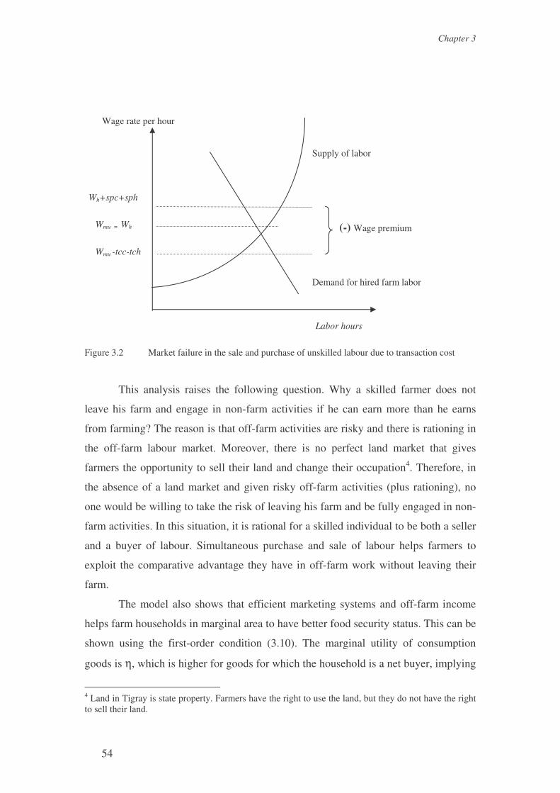
Chapter 3
54
Figure 3.2 Market failure in the sale and purchase of unskilled labour due to transaction cost
This analysis raises the following question. Why a skilled farmer does not
leave his farm and engage in non-farm activities if he can earn more than he earns
from farming? The reason is that off-farm activities are risky and there is rationing in
the off-farm labour market. Moreover, there is no perfect land market that gives
farmers the opportunity to sell their land and change their occupation4. Therefore, in
the absence of a land market and given risky off-farm activities (plus rationing), no
one would be willing to take the risk of leaving his farm and be fully engaged in non-
farm activities. In this situation, it is rational for a skilled individual to be both a seller
and a buyer of labour. Simultaneous purchase and sale of labour helps farmers to
exploit the comparative advantage they have in off-farm work without leaving their
farm.
The model also shows that efficient marketing systems and off-farm income
helps farm households in marginal area to have better food security status. This can be
shown using the first-order condition (3.10). The marginal utility of consumption
goods is η, which is higher for goods for which the household is a net buyer, implying
4 Land in Tigray is state property. Farmers have the right to use the land, but they do not have the right to sell their land.
Wage rate per hour
Labor hours
Wh+spc+sph
Wmu = Wh
Wmu -tcc-tch
(-) Wage premium
Supply of labor
Demand for hired farm labor

An agricultural household model with incomplete markets: theory and implications
55
that the level of consumption is lower for these commodities. In other words, the
marginal utility of consumption for the purchased commodity is higher than that of
the own produced commodity because of marketing costs. When farm households
face a binding liquidity constraint, it is not possible for them to purchase consumer
goods. Therefore, if the liquidity constraint is released through, among others, off-
farm income, the level of consumption could be increased. Therefor, any policy that
improves the efficiency of the market systems (decrease the marketing margin) and
liquidity (promoting off-farm employment) will improve the food security status of
those farm households that are net buyers of food.
The model in general implies that farm households choose to work more for
off-farm work than the standard farm household model (Singh et al., 1986) predicts. It
also implies that farm and off-farm income will have a positive relationship. Off-farm
income will support farm activities through the financing of farming activities and
consumption. If there is a binding liquidity constraint, farm households work off-farm
in order to buy farm input and hire farm labour. Most importantly, off-farm income
helps farm household to attain better food security in marginal areas. Consequently,
the following generalisations (hypotheses) can be drawn, which can be tested latter to
answer the research questions (objectives) presented in Section 1.3:
1. Rationing and transaction cost in the labour market inhibit farm households from
participating in off-farm activities. As a result policy change (any external factors)
that increases the availability of off-farm employment and reduces the transaction
costs in the labour market increases farmers’ participation in off-farm activities;
2. While the liquidity constraint increases the farm household’s desire to participate
in off-farm activities, the transaction costs in the labour market reduces the desire
to hire farm labour;
3. Off-farm employment increases liquidity, and hence increases the willingness to
hire farm-labour.
4. Those farm households, which are relatively skilled and capable of getting
attractive off-farm activities, can be better off by simultaneously hiring farm
labour and selling labour off-farm.
5. Off-farm income helps a liquidity-constrained farm household to have better food
security status.
All of these generalisations (hypotheses) are explicitly tested in the coming
chapters, except for the direct test on the motivation effect of liquidity constraint on
Chapter 3
56
off-farm work participation, which is found to be difficult. The first hypothesis is
tested partly in chapter 7. Chapter 4 tests the second and the fourth hypotheses.
Hypothesis three and five are tested in chapter 6 and chapter 8, respectively.
3.3.2 Product and factor market and crop choice decision
A household can be either autarkic (self-sufficient), a net buyer, or a net seller in a
product market good i. The opportunity cost of production is different in each case.
The opportunity cost depends on the potential impact of trading cost (transportation
cost, profit margin by merchants, and others) on the equilibrium output (Omamo,
1998; Sadoulet, De Janvry and Benjamin, 1996). This opportunity cost is the shadow
value of the commodity balance equation given by η. From (3.14), when the
household is a buyer, the purchase price is given by (η i/λ=Pi + di) and the first-order
condition in equation (3.12) for a buyer can be rewritten as ).(),( iii dPzqQ +−=′ λψ
From equation (3.13), when the household is a seller of a good in the market, the sales
price is (η i/λ=Pi - di) and the first-order condition in equation (3.12) becomes
)(),( iii dPzqQ −−=′ λψ . When the household is not trading, the prices of goods are
internal to the household and are endogenous determined by η i. The implication of
these conditions is that due to the trading cost, the optimal response will be greater for
the production of goods for which the farm household is a net buyer and smaller for
production of items for which the household is a net seller (Omamo, 1998). In
general, the household becomes more self-sufficient (autarkic) as the marketing costs
increase.
The presence of a liquidity constraint also has important implications for the
determination of optimal output. When there is a binding liquidity constraint - that is,
λ>0 – the decision price for liquidity using and generating factor inputs and products
are affected. The first-order conditions (3.12) and (3.13) imply that the presence of a
liquidity constraint does affect the relative magnitude of the marginal value product of
crops that differ in their need for liquidity. The marginal value product will be higher
for crops that require liquidity than for crops that do not require liquidity. Higher
marginal value product of liquidity using crops means less production of these crops.
Therefore, off-farm employment which releases the liquidity constraint makes farm
households shift from lower liquidity using crops to higher liquidity using crops.

An agricultural household model with incomplete markets: theory and implications
57
The first-order condition in equation (3.16) implies that xPXQ λ∂∂ψ =(.)
for the purchased variable capital farm inputs. This means that the marginal value
product of purchased variable capital farm inputs is higher and the level of purchased
variable capital farm input use is lower when there is a binding liquidity constraint
(λ>0). Therefore, when the liquidity constraint is released through, for instance, off-
farm income, the marginal value product of purchased variable farm inputs could be
lowered through the use of additional purchased variable capital farm inputs such as
fertiliser, improved seeds, insecticide and pesticide.
The land allocation decision for different crops can be derived from the first-
order condition (3.15):
δ∂
∂ψ =iA
Q(.) (3.28)
It implies that the marginal value product of land for each crop is equal to the shadow
value of land. Corner solutions could also exist in crop specific land allocation. If
equation (3.15) is less than zero for some crops, corner solutions exist, i.e., some
crops receive zero amount of land. This means that the marginal value product of land
for crops receiving zero amount of land is less than the marginal value product of land
for crops receiving positive amount of land. Furthermore, off-farm income may affect
land allocation cross crops because the marginal product of land depends on the
complementary inputs used on the farm whose use depends on the liquidity constraint.
Hence, off-farm income, by affecting the use of inputs, may affect the relative product
of land allocated to different crops. Therefore, the decision to allocate land across
crops may depend on the total availability of land for cultivation, household taste
preferences, crop profitability, off-farm income, farm characteristics, and agronomic
conditions and risk considerations.
A farmer allocates labour for a crop i if
0(.) =−γ
∂∂ψ
fiLQ
(3.29)
This implies that the optimal level of labour allocated for each crop will be
determined at a point where the marginal product labour for each crop is equal. Hence
the labour use for each crop is dependent on the marginal value product of labour.
It may be interesting to elaborate on the link that exists between crop choice
and off-farm income beyond what the model (first-order condition) clearly shows

Chapter 3
58
because the crop specific marginal product of land and labour implicitly reveal the
impact of various complementary inputs and liquidity constraints. The influence of
off-farm income on crop choice mainly arises when households face an imperfect
capital market. Land and labour are allocated among various crops such that the
marginal product of labour and land are equal across all crops grown by farmers in a
perfect capital market. When households are liquidity constrained, however, more
land may be allocated for crops that use less liquidity. Since, in the model employed,
off-farm income increases liquidity (or eases the liquidity constraints), land will be
reallocated to crops that are liquidity using when a household is more involve in off-
farm employment. Off-farm employment can have two contrasting effects on the
allocation of labour among crops. When households are more involved in off-farm
employment, on the one hand, more labour will be allocated to liquidity using crops in
order to take advantage of the purchased inputs used on the crops. On the other hand,
more off-farm income results in the reallocation of labour towards crops that use less
labour and are less liquidity using because off-farm employment competes with
labour on the farm. Therefore, the net effect of off-farm employment on the
reallocation of labour among crops is difficult to know a priori.
Farmers may not specialise in growing specific crops; rather they may grow a
variety of crops. If their decision is not rational, they lose the benefit they would have
achieved from specialisation. Farmers’ decision to grow a variety of crops at the same
time may be rational due to many reasons. If there is constant returns to scale, two or
more crops can be grown to make use of the available resources (Burger, 1994). If
there is increasing or decreasing returns to scale, the choice that can rationally be
made depends on the farm size. Due to transaction costs in the output market, the
shadow price of products may be between the selling price and the purchase price, i.e.
within the price band. Then the shadow price of crops for a household is internally
determined by their relative marginal utility of crops grown, not by equation (3.28)
and (3.29). When the price band is wide enough, adjustment of crop choices and
labour and land allocations are determined by household preference. When more food
becomes available, with decreasing marginal returns of food, the increasing use of
land and labour for a given crop leads to a decline in the shadow price of that crop. At
some point, substituting for that crop by another more attractive crop would become
inevitable.

An agricultural household model with incomplete markets: theory and implications
59
The following generalisations (hypotheses) can be drawn from the analysis of
market participation, crop choices and land and labour allocation among crops.
1. The optimal response will be greater for the production of same goods for
which the farm household is a net buyer, and smaller for the production of
items for which the household is a net seller due to the trading cost.
2. The presence of a liquidity constraint increases the marginal value of a
liquidity-using product implying a lower level of output. For products that are
not liquidity using, the marginal value of the product is lower implying higher
level of output produced. Therefore, off-farm employment can release the
liquidity constraint and enable the farm household to shift from the production
of lower liquidity using crops to higher liquidity using crops. As a result, off-
farm employment can increase the production of crops that require liquidity
and decrease the production of crops that do not require liquidity.
3. Off-farm employment releases the liquidity constraint and increases the use of
purchased capital inputs such as fertiliser, improved seeds, and pesticides.
4. The direction of the impact of off-farm employment on the allocation of
labour among various crops is not known a priori. On the one hand, more
labour will be allocated to liquidity using crops when households are more
involved in off-farm employment in order to take advantage of the purchased
inputs used. On the other hand, more off-farm income results the reallocation
of labour towards crops that use less labour, and are less liquidity using
because off-farm employment competes with labour on the farm.
5. When a farm household is not involved in the market due to high transaction
costs, the reallocation of land and labour is determined by a shadow price,
which in turn is determined by household preferences.
6. Off-farm employment fosters commercialisation in the rural household
economy by promoting the production of liquidity using crops and purchased
capital inputs.
Some of these hypotheses are similar to those presented in 3.3.1. Off-farm
employment increases the use of purchased inputs such as labour (in 3.3.1) and capital
farm inputs (in 3.3.2). Hypothesis three is tested in chapters 5 and 6. Chapter 8 tests
hypothesis four and six.

Chapter 3
60
3.4 Conclusions
The farm household model derived considers liquidity constraint, transaction cost and
rationing in the labour market simultaneously. It generates testable implications on the
farm households’ participation in off-farm work. The model predicts that off-farm
income may have positive effects on farm income through its effect on the liquidity
constraint. The participation of farm households in off-farm activities not only
depends on farming and household characteristics, but also on the transaction costs
and rationing that exist in the labour market. The liquidity constraint induces farm
households to join the off-farm labour market and thereby helps them to buy more
capital farm inputs and farm labour. Those farm households which are relatively
skilled and capable of working in lucrative off-farm activities hire more farm labour
than those which are relatively less skilled and educated. Furthermore, off-farm
income helps farm households to attain better food security status in marginal areas.
Farm households can be either buyers or sellers in the product market not only
depending on production and consumption preferences, but also depending on the
transaction cost involved in buying and selling goods. Trading cost makes the optimal
response greater for production of goods for which the farm household is a net buyer,
and smaller for production of items for which the household is a net seller. Assuming
positive production, if the transaction cost is very high, farm households may be
prohibited from being sellers in the output market and they might be better off being
self-sufficient.
Off-farm employment, by releasing the liquidity constraint, may affect
participation in the factor and product market. A farm household with more off-farm
income could finance its farm activities such as hiring labour and purchasing capital
input and thus produce more market oriented crops so as to maximise profit. On the
other hand, a farm household whose off-farm income is high could simply satisfy his
cash requirement from the off-farm income he receives and grow crops for own
consumption and sell less of his output (Burger, 1994).
The working of labor market and wage determination
61
CHAPTER 4. THE WORKING OF LABOR MARKET AND WAGE
DETERMINATION
4.1 Introduction
Governments in developing countries interfere in agricultural sectors, among others,
through the promotion of public and/or private investment projects, technological
innovations and off-farm employment. Particularly, the focus of policy makers in
Ethiopia is to increase productivity and attain food self sufficiency and food security
on the one hand and to promote investment in the non-farm sector or industrial sector
in order to provide alternative income earning opportunities on the other hand. The
success of investment in the agricultural and industrial sectors and the extent to which
the benefits of technological innovations in agriculture and the investments in the
non-farm sector trickle down to the landless and/or poor household depend on the
smooth functioning of the labour market, wage determination and the factor bias of
technological development. If the labour market is imperfect, the transaction cost of
hiring labour will be high, which hinders investment or makes capital relatively
cheaper and eventually generates lower employment. If the transaction cost of labour
makes capital relatively cheaper than labour, investment will tend to be more capital-
intensive, which is not appropriate given the factor endowments (factor proportions)
prevailing in developing countries. If there is a smooth functioning of the labour
market coupled with labour using technological innovation, the benefit of rural
investment will go to the landless and poor households.
Wage rates in rural areas are usually thought to be determined by either
subsistence or nutritional requirement or else by the forces of supply and demand. The
first class of theories rests on the assumption that, because labour supply is excessive
in relation to the complementary factors, wage will be held at a subsistence level. The
further assumption that labour supply is perfectly elastic led to a prediction that real
wage will be constant over some range regardless of the demand (Sen, 1966).
However, this prediction has not been fulfilled. Wages in rural areas may be low, but
they are generally observed to vary over both time and space. This observed variation
in wage across time, especially over seasons, is attributed to changes in demand and
supply (Squire, 1981).
Chapter 4
62
Another variant of the subsistence hypothesis focuses on the relation between
nutrition and work efficiency. A positive relation between wage and the efficiency of
labour may make it profitable for employers to pay labour more than the subsistence
wage (Mazumdar, 1959). This model is known as nutrition-based efficiency wage
model in labour economics literature.
The third variant is a model that assumes farm households are partially or
wholly integrated in the market and that the labour market operates competitively
(Rosenzweig, 1980; 1988). In this model the wage rate depends on supply and
demand forces. Wage can also be dependent on marketable human capital (Mincer,
1974) such as experience, education, skill and the physical characteristics of an
individual. The evidence that farm households participate extensively in the labour
market as both buyers and sellers of labour points to the likelihood of competitive,
although not perfect, labour markets.
In a farm labour market where large commercial farms are absent or rare, the
main participants as employers as well as employees are farm households. Exchange
of labour among farm household can be triggered by the initial differences in absolute
and relative factor endowments. Shortage of labour, particularly in peak seasons, can
be one of the reasons for farm households to hire farm labour. The other reason could
be that allocating their labour for non-farm activities and hiring farm labour
simultaneously may be beneficial for farm households. Therefore, the level of farm
and non-farm income and other household characteristics may have a substantial
influence on household participation in the farm labour market.
The integration of farm households in the market (and the participation of
farm households in the labour market as employers) has considerable policy
implications regarding the distribution of the benefits that arises from technological
innovations in agriculture. If the technological innovations are of the more labour-
intensive type, farm households will hire farm labour and the benefits of technological
innovations will trickle down to those who do not have land.
Analyses of the labour market in general and the rural labour market in
particular and wage determination in Africa are scarce in literature (Reardon, 1997),
especially for Ethiopia, and they are absent for Tigray despite their importance for
policy makers. Policy makers have little knowledge whether the benefit of the
investment is going to the poor who are endowed with labour. Furthermore, the
motivations for a farm household to hire farm labour is not well known as well,

The working of labor market and wage determination
63
especially when a farm household hires farm labour and also sells labour
simultaneously.
The objectives of this chapter are the following. First, to describe how the
farm and non-farm labour market work, and to analyse the process of wage
determination and recruitment of labour. Second, to identify the determinants of farm
households’ participation in farm labour markets as an employer and the determinants
of farm household member’s wages in the farm and non-farm labour markets.
Descriptive statistics and simple statistical tests are used to explain the workings of
the labour market in both the farm and non-farm labour markets. A probit model,
consistent with an agricultural household model, is used in order to identify the
determinants of a farm household’s participation in the farm labour market as an
employer. Wage offer equations, correcting for sample selection bias, are estimated to
identify the determinants of household members’ wage.
The rest of the chapter is organised as follows. In section two, the theoretical
framework is outlined. In section three, the data and model specifications are
described. In section four, the analysis and estimation results are presented. The
chapter ends with conclusions.
4.2 Theoretical framework
There are three basic approaches in the development literature concerning the wage
determination and labour market in developing countries (Rosenzweig, 1988). The
first approach raised by Chayanov (1925, 1966) and expressed by Sen (1966) is an
autarkic model that assumes the non-existence of a labour market. If there is surplus
labour in the household, family workers can be removed from the household without a
loss in output. In the autarkic model, labour is in surplus only if the removal of a
family member leaves the marginal rate of substitution between consumption and
leisure unchanged. If family members, by increasing their labour supply, can fully
compensate for the lost hours of work associated with a reduction in the number of
family workers, labourers can be removed from the household (Agriculture) without
any loss in output. Consequently, because labour supply is excessive in relation to the
complementary factors, the wage will remain at a subsistence level.
The second model hypothesises that there are agricultural agents willing to or
seeking work, but they are unable to find employment. It focuses on the relation

Chapter 4
64
between nutrition and work efficiency. Employers try to capture the benefits of
greater work efficiency by improving nutrition through higher wages. A positive
relation between wage and the efficiency of labour may make it profitable for
employers to pay labour more than the subsistence wage (Leibenstein, 1957,
Mazumdar, 1959). This theory led to several testable predictions about the wage
payment system: labour-tying (the use of contracts of relatively long duration); an
inverse relationship between wage and the earner-dependency ratio, and payment in
the form of meals for workers. In labour economics literature, this model is known as
nutrition-based efficiency wage model. The other kinds of efficiency wage models are
the shirking model (Shapiro and Stiglitz, 1984); the labour turnover model (Salop,
1979); the adverse selection model (Weiss, 1980); and the sociological model
(Akerlof, 1982). All of the efficiency wage models have in common that in
equilibrium, an individual firm’s production costs are reduced if it pays a wage more
than market clearing, and thus there is equilibrium involuntary unemployment.
The main idea of the efficiency wage model is that labour productivity
depends on the real wage paid by an employer. If wage cuts lower farm productivity,
then cutting wages may actually result in higher labour cost. According to the
efficiency wage model, a higher wage payment in general has five benefits (Akerlof
and Yellen, 1986). Firstly, it improves the nutritional status of workers (from the
nutrition based efficiency wage model). Secondly, it reduces shirking of work by
employees due to the higher cost of job losses (from the shirking model). Thirdly, it
lowers the turnover of workers (from the labour turnover model). Fourthly, it
improves the average quality of job applicants (adverse selection model). Fifthly, it
improves workers morale (from the sociological models).
Rosenzweig (1988), however, argues that it is only the nutrition-based
efficiency wage model (Leibenstein, 1957; Mirrles, 1975; Stiglitz, 1976) which
provides an important explanation for the downward rigidity of rural wages, although
direct empirical tests of the relationship between nutritional level and effort are
extremely rare and perhaps difficult. Binswanger and Rosenzweig (1984) also have
reservations about the applicability of all types of efficiency wage models and suggest
that it is less likely to be applied to explain rural daily-based wage employment.
The third approach assumes that farm households are partially or fully
integrated in the market and that the labour market operates competitively
(Rosenzweig, 1980; 1988). Then the wage that an individual or farm household

The working of labor market and wage determination
65
receives depends on demand and supply forces. This model is called a competitive
model in the labour market literature (Collier and Lal, 1986). It has four inherent
assumptions: perfect information on the supply and demand side of the labour market,
no uncertainty (or perfect future markets), no transaction costs in achieving a
competitive market equilibrium, and homogenous labour inputs. Given a convex
preference structure of labour-leisure choices of individuals, profit maximisation by
the producers and utility maximisation by the consumers, the competitive model leads
to a general equilibrium condition in which wage equals the marginal value product of
labour, which also equals the labourer’s marginal rate of substitution between income
and leisure. However, modern neo-classical theorists have tried to relax the
assumptions. The introduction of human capital into the neo-classical theory of the
labour market helps to take account of some of the factors that leads to the
heterogeneity of labour on the supply side of the labour market. Human capital
consists of skills acquired through formal and informal education and on-the-job
training. This gives rise to differentials in the productivity of different labourers.
Since the acquisition of skills involves costs, the skills will be acquired if the skilled
wage rate is higher than that the unskilled wage rate. The actual difference is
determined by supply and demand considerations and the relative value marginal
productivity of different skills.
The neo-classical model has also been extended to include non-separability of
production and consumption decisions (Singh, Squire and Strauss, 1986; Caillavet,
Guyomard and Lifran, 1994) labour market imperfections (Lopez, 1986; Benjamin,
1992), risk (Roe and Graham-Tomasi, 1986), and imperfection in the input and output
markets (De Janvry, Fafchamps, and Sadoulet, 1991) in a farm household economy.
The evidence that farm households participate extensively in the labour market
both as buyers and as sellers of labour points to the likelihood of a competitive labour
market, although not a perfect labour market. Since there can be unobservable
characteristics of a worker which may be an important determinant of workers
marginal productivity and hence the demand for labour, exclusive reliance on the neo-
classical theory of competitive model would be misleading (Collier and Lal, 1986).
Hence, it will be worth to consider other theories such as the efficiency wage theory
in explaining the wage structure.
Exchange of labour among farm households arises from initial differences in
absolute and relative factor endowments (Collier and Lal, 1986). If the labour market

Chapter 4
66
is smooth, differences in the inequality in factor proportions and marginal
productivity will trigger farm households to undertake labour transactions among
themselves. In a farm household model setting, a farm household’s willingness to hire
farm labour depends on the farm characteristics and household composition (such as
the availability of family labour). If the household has sufficient family labour, it is
obvious that the need for farm labour can be satisfied without hiring labour from
outside. If the farm household’s benefit from allocating their labour outside the farm
is greater than the cost incurred in hiring labour, they will sell labour for off-farm
work and hire farm labour simultaneously. This can be easily derived from an
agricultural household model (see the theoretical chapter).
4.3 Model specification and the data
Econometric models specification. In this sub-section, econometric models for the
probability of hiring farm labour and for the wage offer equations of farm household
members are specified. Following chapter three of this book, the decision to hire farm
labour (Hi) is modelled as a dichotomous mode (Amemiya, 1981, p. 1486):
�
>+≥==
<=≥=
),0(~);0Pr()Pr()1(Pr
0;1
2/
*
**
uiii
hihii
hihiihihii
NuuXwwH
wwifHwwifH
σγ
(4.1)
where wh is wage paid for hired labour; wh* is the virtual benefit the farm household
gets from hiring farm labour; Pr (.) is probability of an event occurring; X is a column
vector of explanatory variables; γ / is a row vector of parameters; ui is the error term.
The vector of explanatory variables includes those factors that affect the virtual wage
rate and the market wage rate for hired labour.
In modelling the market wage rate that a household receives from working in
off-farm activities (wm), one needs to consider the truncated nature of household’s
participation in off-farm activities. Market wage rates are observed only for
households who participate in off-farm activities. The participation decision of a
household to work off-farm (Di), can be modelled as
�
>+≤==
>=≤=
),0(~);0Pr()(Pr
)1(Pr
0;1
2111
/uiii
imrii
imiriimrii
NuuXww
D
wwifDwwifD
σα
(4.2)

The working of labor market and wage determination
67
where wr and wm are the reservation wage rate and the market wage rate, respectively ;
X is a vector of variables that affects the market and the reservation wage rates; u1i is
the error term.
The wage offer equation is given by:
1,),0(~,/
=+=
imi
eiiimiDifobservedisw
NeeZw σβ (4.3)
where Z is a column vector of variables that affect the market wage; β’ is a row vector
of parameters; ei is the error term of the wage offer equation. Furthermore, we assume
that the error terms of the participation equation (u1i) and the error terms of the wage
offer equation (ei) have a bivariate normal distribution with zero mean and correlation
ρ. Consequently, the expected market wage rate, E(wm), and the truncated market
wage rate, E(wm|D1=1), are given by (Amemiya, 1984; pp. 31-33; Maddala, 1983, pp.
174-189, 231-233):
)()()( / zfzFZwE em σρβ += (4.4)
and
)(/)()1|( / zFzfZDwE eim σρβ +== (4.5)
where z=β’ Z/σ1u, σ is the standard error of u, f(z) is the density function, F(z) is the
cumulative distribution function and f(z)/F(z) is the hazard ratio or inverse mills ratio.
In an agricultural household model (Huffman, 1991) off-farm labour demand
or the off-farm wage equation (wage offer equation) facing farm household depends
on their marketable human capital (Mincer, 1974), demand influences, earning
differential attributes and efficiency wage attributes. Human capital attributes include
education, experience, skill health status, and physical strength of individuals.
Demand influencing attributes consist of location, year and seasonal dummies.
Earning differential attributes include participation in different types of off-farm
employment and gender composition of the participants in off-farm activities.
Efficiency wage attributes may include the dependency ratio and per capita land
cultivated.
The data and estimation. This chapter uses (1) the 201 randomly selected
farm household survey done in Enderta and Hintalo Wojerat districts, (2) the small
informal survey done in Mekelle, Quiha and Adigudom towns. The latter includes 24
labourers working in construction works and major employers (big public and private

Chapter 4
68
companies as well as small employers). The labourers and employers were
interviewed to get insight into how the labour market works.
The initial differences in factor endowment and the exchange of labour among
different farm size classes, the actual process of selection, wage determination and
movement of wage over seasons are analysed using descriptive statistics. A probit
equation (4.1) is estimated in order to identify the factors that determine the
probability of hiring farm labour and the relative importance of these factors.
The determinants of farm household members’ wage are identified from wage
offer equations using the farm household survey data. Wage rates are defined as off-
farm labour income divided by off-farm labour hours supplied. Farm household
members are categorised into four categories: the household head, wife, other male
members, other female members. Because not all households participate in the labour
market, there could be a sample selection bias. To circumvent this problem,
Heckman’s two-stage method (Maddala, 1983) is used. First the willingness of farm
households to participate in off-farm work is estimated from a probit model (2). Then
the inverse mills ratios are derived from the probit estimates. Finally the wage offer
equations (4.5) for a household in general and for each household member in
particular are estimated incorporating their respective inverse mills ratios in the list of
the explanatory variables. In all cases, T-ratios and significance level are calculated
based on White’s heteroscedasticity consistent standard errors (Greene, 1997, pp. 547-
548).
4.4 Analysis of the labour market
Both the farm and non-farm labour markets adapt themselves to the seasonal nature of
agriculture. Agricultural activities in the area are highly seasonal. One cropping
calendar takes approximately 12 months. It can be divided roughly into four (or three)
seasons: plowing, planting, weeding and harvesting (except that planting and weeding
can overlap and be considered as one season). The calendar begins with plowing in
December (except for land lying fallow from September of the previous year). Land
can be plowed up to four times before planting depending on the type of soil and crop.
While teff and wheat fields are plowed four times, a linseed field is plowed once. For
the majority of the crops, planting is done at the onset of the rainy season, early June
to late July. Chickpeas and latyrus (vetch) are planted in late August. Hand weeding is
The working of labor market and wage determination
69
done on cereals once or twice during the rainy seasons, mid July to early September.
Harvesting is done from October to November. Threshing starts right after harvest and
ends before the end of December.
Table 4.1 summarises the seasonal nature of labour use both on and off-farm.
Most of the labour use on the farm is during harvesting and threshing. Farm
households sell their labour off-farm, in a counter cyclical pattern to the use of farm
labour. The participation and extent of off-farm employment is the highest during the
slack agricultural season, January to April, and lowest in the peak agricultural season,
September to December.
4.4.1 Farm labour market
There are three sources of farm labour, namely, family labour, labour sharing
arrangements and hired labour. Hired labour comes mostly from the same village. A
labour sharing arrangement is done between neighbours and between farm
households. Shared labour can be either reciprocal or non-reciprocal. It is reciprocal
in the sense that the household has to repay it in the form of labour or in another
implicit form. It can be non-reciprocal in the sense that there is no obligation to pay it
immediately in the form of labour. Nevertheless, it is usually expected that the
household will help the other at times when the other is short of labour. It is common
and polite to offer hired and shared-labourers with food and sewa (local brewed drink)
during work or after the end of the day. Providing labourers with food and sewa
during work stimulates them to work hard (boost their morale) according to the
sociological model of efficiency wage (Akerlof and Yellen, 1986).
Most farm labour comes from family labour. Family labour accounts for 84.2
% of the farm labour, while the share of hired labour is 10.2 % and shared labour is
5.6%. The highest proportion of farm labour (hired, family and shared labour) is used
for harvesting. The second highest use of hired labour and shared labour is for
weeding, while the second highest use of family labour is for plowing. About 12% of
the hired labour is also used for plowing, during the slack season.

Chapter 4
70
Table 4.1 Seasonal distribution of farm labour, off-farm work participation and wage rates Seasons
Type of employment Total January-April
(plowing) May – August (planting and weeding)
Sep.–Dec. (harvest and thresh)
Labour use on the farm 631.13 141.30 191.46 298.37 Off-farm wage employment Percent of participation 72.1 71.1 69.9 52.5 Hours supplied 1249.02 573.98 424.25 250.81 Income earned 858.75 367.99 306.04 184.72 Wage received per hour 0.72 0.69 0.75 0.74 Off-farm self-employment Percent of participation 27.9 24.6 20.6 14.7 Hours supplied 97.56 55.87 26.72 14.97 Income earned 262.50 148.30 75.59 38.61 Wage received per hour 4.69 3.60 5.03 2.89 Both wage and self employ. Percent of participation 80.9 80.1 75.4 60.0 Hours supplied 1346.58 629.83 450.97 265.77 Income earned 1121.24 516.29 381.63 223.32 Wage received per hour 1.18 1.15 1.20 1.10 There are seasonal variations in the use of total farm labour and wage rates.
Harvesting takes the highest proportion of total labour and offers the highest wage
rate (Table 4.2). Weeding takes the second highest proportion of total labour, but
offers the lowest wage rate. The wage rate paid for harvesting is 1.1 Birr/hour, for
planting it is 0.93 Birr/hour, for plowing 0.89 Birr/hour and for weeding 0.78
Birr/hour. One would expect that the wage rate during the slack season to be lower
than that in the peak season. The reason is that plowing is a difficult job and needs
some level of skill, while weeding can be done using relatively lower skill level and is
not as intensive as plowing. Besides, rain can interrupt a weeding activity reducing the
effective working hours. The reason that the harvesting wage is the highest of all is
the urgency of the work and the higher non-farm labour demand during the harvesting
season.
Table 4.2 Sources of farm labour and seasonal allocation in 1996 and 1997 (household average) Type of farm labour Hours Plowing Planting Weeding Harvesting Family labour 491.53 26% 14% 15% 45% Hired labour 92.60 9% 5% 26% 60% Shared labour 47.00 11% 8% 35% 46% Hired wage rate (Birr/hour) 0.96 0.89 0.93 0.78 1.09
Spot contracts dominate the labour market. Only few farm households hire
permanent labour for farm work and homework. Two farm households (one percent)
were found who hire a permanent farm worker. One household (0.5%) hires a house
maidservant, and eight farm households (3.9 %) hire a cattle keeper boy. Permanent

The working of labor market and wage determination
71
labour contracts are absent in the farm labour market because of the counter-cyclical
nature of non-farm employment, the seasonal nature of farm labour demand and the
risk associated with agriculture. The participation of labourers in non-farm
employment (either wage or self-employment) during the slack season reduces the
labourers’ exposure to wage uncertainty (Rosenzweig, 1988). If the employers can not
fully use permanent labour during the slack season, and the wage uncertainty during
the peak season is very low, the employer may prefer casual labour to permanent
labour (Bardhan, 1983). For this reason, most of the permanent-labour contracts are
on activities that are not seasonal such as homework and cattle keeping.
If permanent labour exists, farm households hire the permanent labour from
relatives. Of the households who hire permanent workers, 65 % hire relatives. The
search for people to hire for permanent work is done through friends and relatives.
There is no agent either formally or informally who mediates in the hiring process1.
Of the farm households who hire a permanent worker, only one household has
responded that he just picked up a worker from the open labour market area without
prior information about the person.
Exchange of labour among farm households arises due to initial differences in
absolute and relative factor endowments. The difference in absolute and relative
factor endowments could be due to demographic, ecological and economic processes
(Collier and Lal, 1986). Land was distributed among the farm household in 1990
based on their family size. Given the egalitarian type of land distribution, there should
not be initial difference in land ownership. However, the fact is that there is a
difference in land endowment among farm households. Figure 4.1 provides a kernel
density estimate of area of land owned and area of land cultivated (on per adult
equivalent family size and per working family member bases). The figure shows that
distributions of land owned and cultivated are skewed towards the upper tail. The
amount of land cultivated is different from the amount of land owned (Table 4.3)
because farm household could either rent-in land or rent-out land. Only one household
out of the 201 (sampled farm households) did not own land at all. However, after
transactions in the land market, about 11% of the farm households did not cultivate
1 The Ethiopian law does not allow agents to mediate between employees and employers. The law was drafted during the communist regime, and the present government, which is relatively liberal, has not yet reviewed it.

Chapter 4
72
land. Most of the farm households who do not cultivate land also do not own oxen and
farm implements.
Table 4.3 gives the distribution of land cultivated per working family
member (i.e., initial land labour ratio, see bolded row), farm capital per working
family member, and transport animal per working family member. These ratios are
positively related to farm size indicating that there are differences in the initial
endowment of factor proportions among farm households (between small and larger
farms). There are also differences in absolute factor endowment among different farm
sizes. The total amount of land cultivated and owned as well as the amount of farm
capital and number of transport animals owned increases with farm size. The family
labour used per unit of land decreases across farm size classes (Table 4.4). Because of
the differentiation in both absolute and relative factor endowments, a difference in the
marginal productivity of labour and thus inequality among farm households could
arise if the labour market performs poorly. Potentially the difference in marginal
productivity must create a profitable transaction in a factor market such as labour.
Figure 4.1 Kernel density estimates of area of land owned and cultivated
-0.452 13.702
0
0.697 Land owned per adult equivalent family size
Land cultivated per working family size
Land owned per working family size
Land cultivated per adult equivalent family sizeKerneldensity

The working of labor market and wage determination
73
The differences in factor proportions and marginal productivity have triggered
farm households to make labour transactions among themselves. The results show that
labour exchange increases with farm size. Hired labour per unit of land cultivated and
per working family members increase with farm size (see bolded rows in Table 4.4).
The proportion of farm households which hire farm labour also increase from 7.14%
for smaller farms to 100% in the largest farm. However, the extent of hiring farm
labour is very small either because of one or a combination of the following reasons:
liquidity constraint, transaction cost (Collier and Lal, 1986) or smaller farm size. The
absolute shared labour and the relative shared labour with respect to land cultivated
and working family member increases with farm size. This could be an indication of
an alternative means of labour exchange when farmers face a liquidity constraint and
a high transaction cost in monitoring hired farm labour. Since labour-sharing
arrangements are made among neighbours who trust each other, the transaction cost of
monitoring shared labour could be lower than that of hired labour. Since a labour-
sharing arrangement is not a spot contract, shirking would not be a problem. The
renting of land (hiring-in and hiring-out land) among farm households could also be
an outcome of the transaction cost in the farm labour market. The level of rent paid
for the land leased-in increases and the level of rent received from the land leased-out
decreases across farm size classes (Table 4.4).
Nevertheless, the exchange of labour equalises the labour/land ratio (see
bolded rows in Table 4.4), the returns to land and to labour among different farm size
classes. There are no visible differences in the observed mean level of labour/land
ratio, return to land and to labour between smaller and larger farm size classes. This
implies that the farm labour market operates well enough to make agricultural growth
trickle down to the poorer segment of the population.
Farm households also equalise their earnings (marginal productivity of labour)
by selling their labour for non-farm (off-farm) activities in response to the differences
in the relative factor endowments. The amount of labour sold per working family
member and per unit of land cultivated declines as we go from smaller to larger farm
sizes. Labour sales, therefore, narrow the differences in the labour input per unit of
land and thereby reduces inequality by equalising the payment for family labour.
Because there could be an entry barriers (skill and capital requirement) in the non-
farm labour market, the unskilled employment labour market contributes substantially
towards equalising the differences in factor proportions, inequality and poverty. This

Chapter 4
74
effect is substantial compared to the contribution made by hired labour. Most of the
farm households are net sellers of labour. Only farm households who cultivate more
than 16 tsimdi of land are net buyers of labour on a per unit of land basis.
Furthermore, the majority of the households are net sellers in the labour
market. For example, the proportion of farm households who sell labour but do not
hire labour at all is 50%. The proportion of farm households who simultaneously sell
and buy labour is 31 %. Only 10 % are autarkic (neither sell nor buy labour) in the
labour market. Of those who simultaneously hire and sell labour, the majority (78.2
%) are of the middle farm size class (cultivate 4-12 tsimdis). This implies that the
middle farm size classes are liquidity constrained and thereby sell labour in order to
finance their farming activities (such as hiring of farm labour).
Therefore, it can be concluded that the exchange of labour tends to reduce the
absolute and relative gap in labour use per unit of land that exists between smaller and
larger farms. However, the extent of hired labour use is small due to the high
transaction cost for unmonitored effort, liquidity constraints and smaller farm size.
Since most farmers are net sellers of labour, the non-farm labour market, particularly
the wage employment contributes greatly to reducing the differences in factor
endowments and marginal productivity of labour (as well as poverty and inequality).

The working of labor market and wage determination
75
Table 4.3 Absolute and relative factor endowments across farm size classes
Farm size class (area of land cultivated in tsimdi*) Total [0] (0-2] (2-4] (4-8] (8-12] (12-16] >16
Total land cultivated 7.09 0 1.75 3.61 6.35 10.12 13.90 22. 0 Total land owned 5.88 4.91 3.04 3.59 5.67 7.26 7.86 9.11 Farm implement owned 237.62 39.92 138.64 164.08 218.24 301.72 379.52 732.0 Value of oxen owned 1433.88 62.79 385.71 1034.31 1352.5 1872.87 2419.13 4270.0 Value of transport animals owned 437.51 68.61 121.43 199.61 353.4 606.34 880.44 1745 Family size 5.80 3.3 4.0 4.8 5.9 6.4 6.3 6.9 Working family members 2.30 1.7 1.5 2.1 2.3 2.5 2.6 2.8 Land owned per working family member 2.70 3.2 1.5 1.7 2.6 3.1 3.2 3.3 Oxen owned per unit of land owned 0.22 0.05 0.19 0.26 0.21 0.25 0.29 0.41 Hired-in farm labour hours 92.60 0 0.86 13.75 43.35 141.79 196.83 778.64 Farm labour hours from share labour arrangement 47.00 0 11.07 21.97 36.33 60.05 78.44 291.57 Family labour use on the farm 551.95 0.00 185.85 335.10 495.78 652.63 862.39 1071.36 Total labour use on the farm 676.39 0.00 180.5 325.65 536.24 815.80 1110.96 2243.57 Hired out labour hours (off-farm labour hour) 1346.58 2171.49 1358.46 1099.41 1331.49 1352.72 1081.7 260.43 Farm capital per unit of land cultivated ** 251.60 102.71 301.05 336.60 251.40 216.35 199.77 234.29 Farm capital per family size 314.23 48.69 167.28 293.48 292.06 398.28 455.22 761.24 Farm capital per working family member 730.72 88.67 254.57 567.55 715.09 927.89 1131.84 1865.89 Land cultivated per family size 1.32 0 0.53 0.92 1.22 1.84 2.32 3.34 Land cultivated per of working family member 3.09 0 0.85 1.77 2.90 4.36 5.64 8.35 Land owned per adult equivalent family size 1.47 2.14 1.04 1.06 1.34 1.58 1.65 1.72 Land owned per family size 1.21 1.92 0.92 0.90 1.08 1.27 1.30 1.37 Transport animals owned per unit of land cultivated 58.47 68.61 60.71 54.85 56.36 58.61 65.98 79.60 Transport animals owned per family size 75.98 17.93 25.30 46.43 60.56 108.51 128.65 263.31 Transport animals owned per working family member
182.59 26.59 41.07 92.25 159.91 246.16 325.8 691.19
*Land size is measures in tsimdi, a local measure for area. One tsimdi is equivalent to one-fourth of a hectare. ** Farm capital is defined as farm implement plus oxen owned and the average farm capital is put as farm capital per unit of land cultivated for the landless group.

Chapter 4
76
Table 4.4 Use of labour and return to land and labour across farm size classes
Farm size class (area of land cultivated in tsimdi*) Total 0 (0-2] (2-4] (4-8] (8-12] (12-16] >16
Percent of farm household 100.0 10.7 3.48 12.69 38.81 25.12 5.72 3.48 Percent of farm household who hired farm labour 39.801 0 7.14 19.61 33.33 67.33 65.22 100.00 Percent farm household selling labour 80.85 86.05 85.71 80.39 82.05 83.17 73.91 42.86 Percent of farm household who get share labour 23.88 0 21.43 13.73 22.44 35.64 30.43 57.14 Hired-in farm labour hours per unit of land cultivated
9.81 0 0.429 3.88 6.96 13.871 14.23 36.070
Hired-in farm labour hours per working family member
39.59 0 0.429 8.37 20.73 59.311 86.21 305.37
Hired-out labour hours per unit of land cultivated 211.9 2171.49** 729.77 311.05 220.40 134.96 77.75 13.44 Hired-out labour hours per working family member 608.09 1212.11 550.09 534.52 575.09 554.36 447.91 97.36 Share labour received per unit of land cultivated 6.17 0 5.54 6.42 5.81 5.93 6.06 11.76 Share labour received per working family member 22.03 0 4.33 13.27 19.58 27.82 33.71 105.52 Family labour use on the farm per unit of land cultivated
75.68 0 104.83 93.43 78.78 64.69 62.75 50.11
Total labour use on the farm per unit of land cultivated
85.748 0 107.85 90.89 84.77 80.58 81.55 101.51
Value of crop output per unit of land cultivated (Birr)
265.19 - 250.54 284.65 268.10 246.03 260.86 321.56
Value of output per labour hour used (Birr) 3.41 - 2.56 3.49 3.34 3.43 4.07 3.38 Rent paid for land leased-in (Birr) 203.70 0 0.0 50.539 103.375 255.236 560.760 1750.68 Rent received from land leased-out (Birr) 77.80 549.72 225 24.117 16.570 6.693 0 0 *Land size is measures in tsimdi, a local measure for area. One tsimdi is equivalent to one-fourth of a hectare. ** Since the denominator (land size) is zero, the mean value of hired-out labour is put

The working of labor market and wage determination
77
Apart from the differences in factor endowment, household and farming
characteristics may affect farm labour transaction. A probit model (4.1) is used to identify
the factors affecting the decision of farm households to hire farm labour. The decision to
hire farm labour depends on variables (factors) that affect both the virtual wage and the
market wage of hired farm labour. These variables include household composition
(family size and number of dependants) and characteristics (age, age-squared, and
education dummies), farm income, farm size (area of land cultivated) and non-labour
income, location and year dummies, and household participation in off-farm activities.
All variables, except farm income, are assumed to be exogenous. A Hausman
specification test (Greene, 1997, pp. 763-764; Spencer and Berk, 1981; Pindyck and
Rubinfeld, 1991, pp. 303-301) was conducted to test if farm income is endogenous to the
model. The test rejects the null hypothesis that farm income is exogenous to the model at
1% level. Therefore, fixed farm inputs are used as instrumental variables for farm
income.
The estimation result is summarised in (Table 4.5). The predicted probability for a
farm household to be an employer in the farm labour market is 37 percent. The
probability depends on the level of farm income, household participation in a relatively
skilled non-farm wage employment, and family composition, and year dummy. When
farm income increases, the probability of hiring farm labour increases. The probability of
hiring farm labour increases also with farm size. Farm households who participate in
mason and carpentry work have higher probability of hiring farm labour. Therefore, it
appears that farm households hire farm labour in order to sell their labour for a better
paying non-farm activities. This also confirms the proposition in chapter three (see Figure
3.1) that the skilled workers receives a positive effective wage premium enabling them to
hire and sell labour simultaneously. The probability of hiring labour is also dependent on
the household endowment of labour. It increases with decreasing family size and with
increasing number of dependants. The proportion of households which hires labour is
higher in 1996 than in 1997 because 1997 was a relatively dry year. The effects of
participation in unskilled non-farm wage employment and non-farm self-employment,
education level of the household head and wife, age of the household head on the
probability of hiring farm labour are not significantly different from zero. However, the
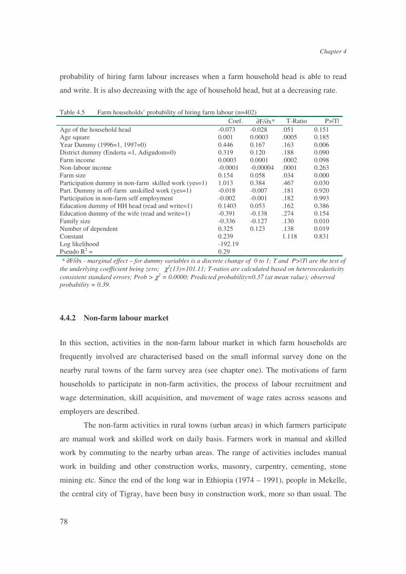
Chapter 4
78
probability of hiring farm labour increases when a farm household head is able to read
and write. It is also decreasing with the age of household head, but at a decreasing rate.
Table 4.5 Farm households’ probability of hiring farm labour (n=402) Coef. ∂F/∂x* T-Ratio P>|T| Age of the household head -0.073 -0.028 .051 0.151 Age square 0.001 0.0003 .0005 0.185 Year Dummy (1996=1, 1997=0) 0.446 0.167 .163 0.006 District dummy (Enderta =1, Adigudom=0) 0.319 0.120 .188 0.090 Farm income 0.0003 0.0001 .0002 0.098 Non-labour income -0.0001 -0.00004 .0001 0.263 Farm size 0.154 0.058 .034 0.000 Participation dummy in non-farm skilled work (yes=1) 1.013 0.384 .467 0.030 Part. Dummy in off-farm unskilled work (yes=1) -0.018 -0.007 .181 0.920 Participation in non-farm self employment -0.002 -0.001 .182 0.993 Education dummy of HH head (read and write=1) 0.1403 0.053 .162 0.386 Education dummy of the wife (read and write=1) -0.391 -0.138 .274 0.154 Family size -0.336 -0.127 .130 0.010 Number of dependent 0.325 0.123 .138 0.019 Constant 0.239 1.118 0.831 Log likelihood -192.19 Pseudo R2 = 0.29 * ∂F/∂x - marginal effect – for dummy variables is a discrete change of 0 to 1; T and P>|T| are the test of the underlying coefficient being zero; χ2(13)=101.11; T-ratios are calculated based on heteroscedasticity consistent standard errors; Prob > χ2 = 0.0000; Predicted probability=0.37 (at mean value); observed probability = 0.39.
4.4.2 Non-farm labour market
In this section, activities in the non-farm labour market in which farm households are
frequently involved are characterised based on the small informal survey done on the
nearby rural towns of the farm survey area (see chapter one). The motivations of farm
households to participate in non-farm activities, the process of labour recruitment and
wage determination, skill acquisition, and movement of wage rates across seasons and
employers are described.
The non-farm activities in rural towns (urban areas) in which farmers participate
are manual work and skilled work on daily basis. Farmers work in manual and skilled
work by commuting to the nearby urban areas. The range of activities includes manual
work in building and other construction works, masonry, carpentry, cementing, stone
mining etc. Since the end of the long war in Ethiopia (1974 – 1991), people in Mekelle,
the central city of Tigray, have been busy in construction work, more so than usual. The

The working of labor market and wage determination
79
boom in construction work and public work programs has created a demand for non-farm
wage employment.
The motivation to participate in non-farm activities is summarised in Table 4.6.
Most of the labourers work in non-farm activities because they do not have land or the
land they have is insufficient. Some labourers participate in non-farm activities because
they find it more profitable than farm work, farm work is insufficient for earning a
livelihood, or they are not totally interested in farming activities.
Table 4.6 Motivations to work in non-farm activities Reasons to work off the farm Percent of households I don’t have land or enough land 80 Farm work is insufficient for livelihood 33 non-farm work is more profitable than farm work 21 I am not interested to work in farming 4 The response percentage does not add up to 100 because the respondents were allowed to have multiple responses.
The participation of farm households is substantial in urban non-farm work. Forty
five percent of those who participate in manual work are farmers. Most of the manual
workers are illiterate, only few can write and read. Skilled workers, especially the
carpenters, can at least read and write.
Most of the skilled labour workers acquire the skill without training, only one
person in the sample (4%) gets training in building work. This is not a surprising figure
as there are no schools that train people in building, carpentry and other technical work
except a limited training given by the Tigray Development Agency, TDA. Most acquire
the skill gradually during their employment as a manual worker in construction works. It
is not only ability that limits the manual worker from becoming a mason or carpenter, but
also the lack of equipment required for masonry and carpentry. If they are beginners, they
rarely get employment as a mason or carpenter. To be a mason or carpenter in a short
period, they have to find someone who is an experienced mason/carpenter under whose
supervision they can work as an assistant. Then after a few months, they can get
recognition as mason/carpenter. In general, job seekers have to pass through a long
search process, usually done via friends and relatives. There is no agent who mediates
between an employer and employees. Eighty eight percent of the respondent responded
that it is difficult to get a job when you want to.
Chapter 4
80
Labourers have to fulfil few additional criteria before they qualify for the job. For
the manual labourers, physical fitness is the most important criterion, and for masons and
carpenters, experience supported by a certificate is the most important criterion.
Labourers who have their own equipment are the most preferred one. For masons and
carpenters, it is impossible to get a job if they do not have their own equipment. The
average required investment in equipment for a manual labourer is 40-50 Birr, and for
masons and carpenters it is 250-350 Birr. Kinship between the employees and employer
and an informal referee are helpful to be employed as labourers and masons. In a private
house construction, a referee is needed to verify that he is an experienced mason or
carpenter. Sometimes the employers want to see a house built by an applicant worker (or
work done by the applicants) before hiring the worker.
It seems that there is an implicit agreement in providing workers with food before,
during or after work. Labourers negotiate for the wage during recruitment, but not for the
food they receive during work. However, every employer, except government
organisations, provides workers local beer once to twice a day while they are working.
When workers are supplied local beer, they get stimulated and work relatively quickly
and cheerfully. There is a debate in the efficiency wage literature about whether a higher
wage can increase effort in the long-run, but not in the short-run (Binswanger and
Rosenzweig, 1984). However, the observed reality is that when workers are given food
and drink, especially local beer, they just immediately get stimulated and work hard with
relatively little supervision. When workers were asked why they work hard when they get
food and local beer, they responded that it increases their morale and they work harder
and little longer hours than the usual. This supports the proposition made by the
sociological model of efficiency wage theory (Akerlof and Yellen, 1986).
The demand for non-farm work is not the same throughout the year. Building
work is done during the period when there is no rainfall, particularly during the months of
September to June. Hence, masons have a hard time getting a job during the rainy
seasons between end of June and beginning of September. For manual labourers, it is
difficult to get a job from January to March (the slack season and when the supply of
manual labour is relatively higher). In the rainy season, some manual labourers can get a
job in farming activities (weeding). The peak period for farm and non-farm work is
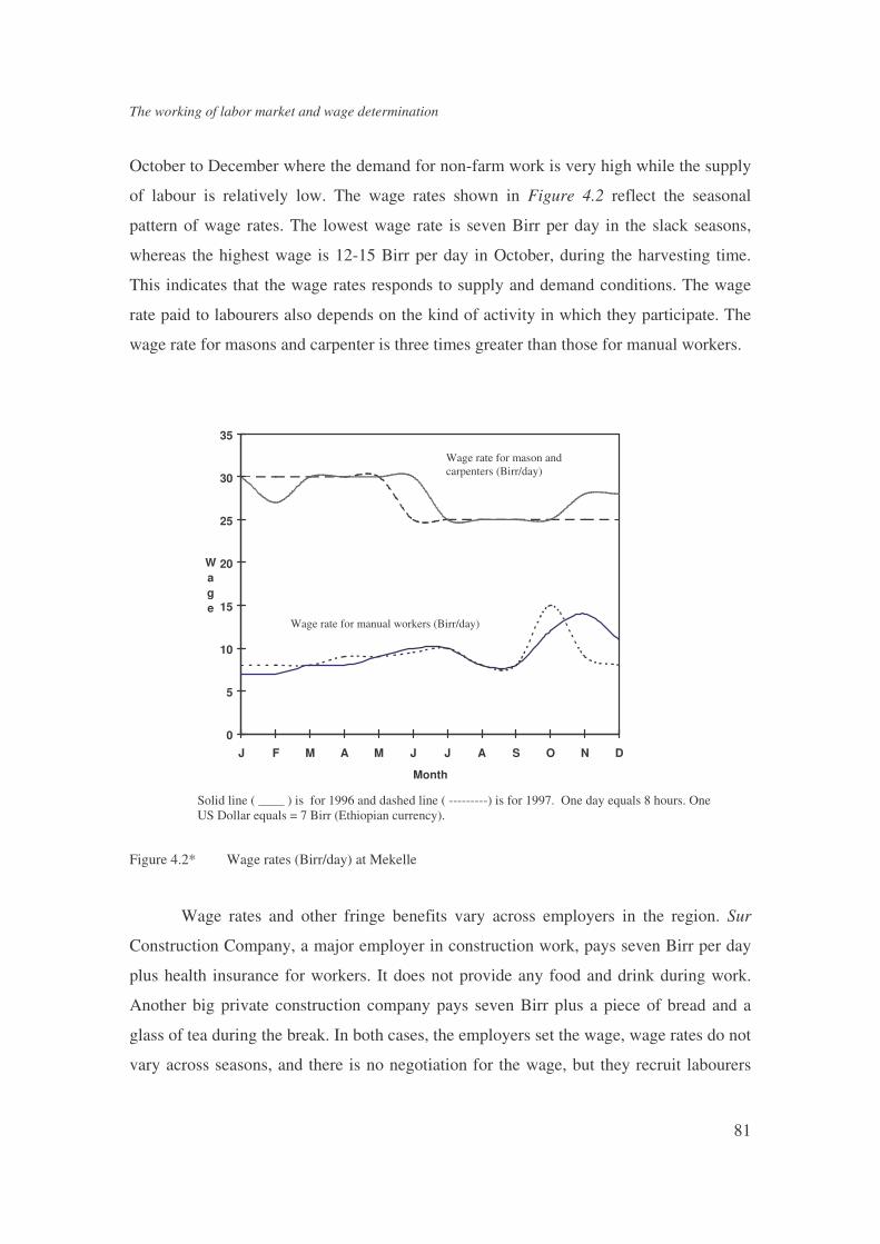
The working of labor market and wage determination
81
October to December where the demand for non-farm work is very high while the supply
of labour is relatively low. The wage rates shown in Figure 4.2 reflect the seasonal
pattern of wage rates. The lowest wage rate is seven Birr per day in the slack seasons,
whereas the highest wage is 12-15 Birr per day in October, during the harvesting time.
This indicates that the wage rates responds to supply and demand conditions. The wage
rate paid to labourers also depends on the kind of activity in which they participate. The
wage rate for masons and carpenter is three times greater than those for manual workers.
0
5
10
15
20
25
30
35
J F M A M J J A S O N D
Month
Wage
Figure 4.2* Wage rates (Birr/day) at Mekelle
Wage rates and other fringe benefits vary across employers in the region. Sur
Construction Company, a major employer in construction work, pays seven Birr per day
plus health insurance for workers. It does not provide any food and drink during work.
Another big private construction company pays seven Birr plus a piece of bread and a
glass of tea during the break. In both cases, the employers set the wage, wage rates do not
vary across seasons, and there is no negotiation for the wage, but they recruit labourers
Solid line ( ____ ) is for 1996 and dashed line ( ---------) is for 1997. One day equals 8 hours. One US Dollar equals = 7 Birr (Ethiopian currency).
Wage rate for mason and carpenters (Birr/day)
Wage rate for manual workers (Birr/day)

Chapter 4
82
who are physically more fit and masons and carpenters with a certificate of experience.
The wages do not vary across seasons and workers do not request an increase in salary
during the busy seasons because workers fear that the employer will retaliate against
them by not hiring them during the slack season.
For small private employers, the wage rate varies from 8 to 12 Birr depending on
the season and the labourer’s physical fitness. Small private sector employers decrease
the wage they offer during the slack season and employees can increase their wage they
demand during the peak season. Usually the wage rate is higher than that paid by the big
employers. Small private employers offer workers with local beer once or twice a day,
but the duration of the work is not longer than a week. Therefore, labourers have to
choose between higher wage and shorter duration on one hand and lower wage and
longer duration on the other hand. This choice depends on the capacity of workers to
absorb risk and the risk aversion of the labourer. However, the queuing line to get
employment with big employers is longer than for small employers, implying that it is
risky for labourers to work for small employers.
Wage rates also differ across labourers depending on their loyalty and physical
fitness. If a labourer is loyal and found to work well without supervision, his wage could
go up to 20% higher than the normal. The employers give these types of labourers an
additional assignment of supervising the labourers. Likewise, labourers who are physical
more fit get a job easily and receive higher wages than normal. Especially loyal and
physically strong workers are relatively in a better position than the rest of the workers
when the demand for labour is very low.
Almost all employers responded that shirking is the most important problem when
they hire casual labourers. The measure they took when they caught workers shirking is
firing. The other way to control shirking may be to pay wages on a piece rate basis, but
there are complaints from the employers that the quality of work is not good.
Labourers are also employed as manual workers for community development
work. The payment is in kind, in the form of wheat, and no additional food and other
fringe benefits are given. This payment is equivalent to six Birr per day (25 % less than
the wage rate paid for other type of work). Usually employment in the community
development work is given to poorer households on a priority basis when there is

The working of labor market and wage determination
83
insufficient demand for hired labour. In the years 1996 and 1997, there was a lot
community development work with the construction of micro dams, soil and water
conservation projects, school and clinic construction, etc. Hence, everyone who was
willing to be employed interested could find work. Most of the labourers in the
community development work are women implying that women occupy the low paying
wage activities. For the other type of wage employment, most of the labourers are men.
4.5 Determinants of wages
In this section, the determinants of the wage rates received by farm households in the
survey area and their relative importance are identified. Household members are
categorised into four groups: husband (household head), wife (household head if she is
unmarried, widowed or divorced), other male members and other female members. Farm
households substantially participate in the wage labour market as sellers and buyers
(Table 4.7). Nearly 72 % of the household participate in off-farm wage-employment. The
previous section shows also that 39 % of the households participate in the labour market
as employers. The husbands (the household heads) have the highest participation rates in
off-farm wage employment. A considerable proportion of the wives (35%) and other
male members (18%) in the sample participated in off-farm wage employment but the
participation of the wives is limited to the food for work program. The participation of
other female members is very small (6%).
Table 4.7 summarises the distribution of wage rates across household members. It
seems that there is a difference in the wage rate received by a household head and other
male members on the one hand and that of the wife and other female member on the
other hand. The mean separation test shows that the wage rate received by the household
head is significantly higher than that received by the wife. Nevertheless, the difference in
wage rate received by other male members and other female members is neither
significantly different from zero nor greater than zero. The fact that there is a difference
in wage rate between husband and wife does not in itself mean that there is
discrimination. If there is discrimination between men and women, the effect of other

Chapter 4
84
confounding factors have accounted for and this is dealt with next in the estimates wage
offer equations.
Table 4.7 Average off-farm wage and participation rates in off-farm wage-employment Member type Wage rate (Birr/hour) Participation rate (%) Head 0.73 67 Wife 0.62 35 Other male member 0.72 18 Other female member 0.62 6 Household 0.72 72 Wage offer equation (4.5) for the households in general as well as separately for
husbands, wives, other male members and other female members are estimated. The
independent variable comes from the following sources: human capital attributes
(individual or household characteristics), demand influences, earning differential
attributes and efficiency wage attributes. Human capital attributes include education,
health status, physical strength of individuals (weight and height dummies) age and age
squared. Demand influencing attributes consist of location, year and seasonal dummies.
Earning differential attributes include dummies for participation in paid community
development work, unskilled and skilled wage employment as well as dummies for
participation of male household members in wage employment. Explanatory variables
that reflect efficiency wages are the dependency ratio (dependency earners ratio) and per
capita land cultivated. Inverse mills ratio, derived from a probit equation (4.2), are also
included in all wage offer equations. Variables that indicate individual health, off-farm
work participation, and per capita consumption are not included in the estimation of the
probit equations. The probit models include household characteristics (age, age-squared,
education), household composition (family size, number of dependants), location and
year dummies, and variables that affects farm productivity such farm capital, area of land
cultivated, variable inputs (fertiliser, seeds and pesticides), etc.
Estimates of the wage offer equation of off-farm work for the household in
general are given in Table 4.8. The result does not show a statistically significant wage
differential between male and female members of a household. However, controlling for
other factors such as human capital attributes, demand influences and type of non-farm
employment involved, the dummy for the participation of household heads shows a

The working of labor market and wage determination
85
positive effect on the wage offer equation of the household. Demand-influencing
variables such as seasonal, year and location dummies and a few earning differential
variables such as the type of off-farm activities involved are more important in explaining
the variation in wage than the human capital attributes (household characteristics) and
efficiency wage attributes.
Table 4.8 OLS estimates of wage offer equation of farm households (Dep variable = household wage Birr/hour)
Full model Restricted model Explanatory Variables Coef. T-ratio P>|T| Coef. T-ratio P>|T|
Age of the household head -0.006 -0.518 0.605 -0.006 -0.492 0.623 Age squared 0.00003 0.232 0.817 0.00003 0.205 0.838 District dummy (Enderta=1) 0.090 1.790 0.074 0.093 1.863 0.063 Year dummy (1996=1, 1997=0) 0.175 3.366 0.001 0.171 3.456 0.001 Value of off-farm equip. owned 0.0005 1.154 0.249 0.0005 1.170 0.243 Education dummy of HH head -0.018 -0.410 0.682 -0.012 -0.278 0.781 Education dummy of the wife 0.011 0.213 0.832 0.002 0.044 0.965 Health condition of head (1=ill) -0.028 -0.668 0.505 -0.032 -0.777 0.438 health condition of wife (1=ill) -0.030 -0.773 0.440 -0.030 -0.778 0.437 Dummy for Part. in unskilled wage work 0.172 2.095 0.037 0.160 2.044 0.042 Dummy for part. Skilled wage work 1.382 5.277 0.000 1.383 5.298 0.000 head participation in wage work 0.083 0.863 0.388 0.081 0.864 0.388 Other male member part. in wage work -0.058 -1.040 0.299 -0.057 -1.027 0.305 Dummy for part.in wage work in May-August 0.372 2.682 0.008 0.357 2.727 0.007 Dummy for part. in wage work in Sep-Dec. 0.012 0.157 0.876 0.012 0.160 0.873 Dependency earners ratio 0.035 0.422 0.673 Land cultivated per capita 0.016 0.733 0.464 Inverse mills ratio 0.131 1.938 0.053 0.138 2.173 0.03 Constant 0.191 0.765 0.445 0.245 0.914 0.362 Adjusted R2 0.56 0.57 T-ratios are calculated based on heteroscedasticity consistent standard errors; P>|T| is the lowest significance level that the underlying coefficient is different from zero. Estimates of wage offer equations of the heads, wives, other male members and
other female members are presented in Table 4.9 and Table 4.10. In all the cases, wage
rates are explained more by demand influencing attributes than by individual
characteristics and efficiency wage considerations. Wages were higher in 1996 than in
1997 because 1996 was a good harvest year when the farm sector achieved remarkable
growth. Consequently, the growth of the farm sector has increased the demand for off-
farm work in rural areas through the labour market linkages (Haggblade and Hazell,
1989) resulting in an increase in the wage rate. Except for the other male members,
wages are higher in Enderta district than in Adigudom district indicating the
responsiveness of wages to demand. The availability of jobs is usually higher in Enderta

Chapter 4
86
district than in Adigudom district. The seasonality of demand for off-farm work also has a
strong influence on the variation in wages. For example, husbands receive a wage, which
is by 0.21 Birr/hour higher in the peak period (September-December) than in the slack
season (January-April).
The results show that there is a very high earning differential across off-farm job
types. Participation in non-farm activities instead of the food for work program enables
household members to get higher wages. Compared to working in the food for work
program, household heads get wages 1.62 Birr/hour higher when they work in non-farm
skilled jobs and 0.18 Birr/hour higher when they work in non-farm manual jobs. Wives
and other male members also get a wage which is 0.10 Birr/hour higher when they
participate in non-farm unskilled wage work in contrast to the food for work program.
The wage differential across activities reflects the skills required to perform the activities.
It is not surprising if the wage paid for labour in the food for work program is low. The
food for work program is designed to have a lower wage and to improve the access of the
poor to off-farm jobs.
Age, age squared, education, health status, physical strength of individuals,
dependency ratio and per capita land cultivated do not show statistically significant
effects on the wage rates except for other female members. Other female members who
are heavier in weight receive higher wage, while those who are shorter receive a lower
wage. Although the ownership of equipment increases the wage rate of all types
household members, the coefficients are not statistically significant perhaps because of
multicollinearity. However, it is quite common to see (during the informal survey at the
Mekelle labour market) farmers who are trained (in a state sponsored training centre)
working in low paying non-farm activities because they could not find credit to buy the
equipment required to enable them to work in a better paying non-farm jobs.
Furthermore, employers in a spot market contract prefer labourers who have equipment,
and they are willing to offer slightly higher wages for workers who come with
equipment. The employers in the spot contract market do not want to buy their own
equipment because they do not have work that lasts for a long period (house construction)
or the kind of activity for which they hire labour is seasonal (such as harvesting).
Education is affects the wage rate positively, but the effect of education is very small and

The working of labor market and wage determination
87
statistically insignificant. This may be because most of the off-farm jobs are manual and
do not require education at all (Rosenzweig, 1978, 1984, 1988). If some off-farm jobs
require education, reading and writing without any other technical skills may not be able
to make a substantial change to the wage rate received by the farm households.
The parameter estimates for the dependency ratio and per capital land cultivated
(reflecting the efficiency wage theory) are not entirely consistent with the efficiency
wage theory. First, they are not statistical significant from zero. Second, the positive
effect of per capita land cultivated on the wage rate is quite contrary to the efficiency
wage theory. Adjusted R2 increases when the wage offer equations are estimated without
the dependency ratio and per capital land cultivated. Since we are dealing with casual
labour, it is not surprising to get results not consistent with the nutrition-based efficiency
wage theory. If efficiency wage exists, the nutrition based efficiency wage can only be
observed for permanent labour contracts (Binswanger and Rosenzweig, 1984; Bardhan,
1979).

Chapter 4
88
Table 4.9 OLS estimates of wage offer equations of husband and wife (Birr/day)* Dep var. = Husband's wage rate Dep var. = wife’s wage rate
Full model Restricted model Full model Restricted model Explanatory variables
Coef. T-ratio P>|T| Coef. T-ratio P>|T| Coef. T-ratio P>|T| Coef. T-ratio P>|T| Age -0.013 -0.975 0.330 -0.011 -0.845 0.399 0.001 0.176 0.861 0.001 0.251 0.802 Age squared 0.0001 0.627 0.531 0.0001 0.489 0.625 -0.00003 -0.497 0.619 -0.00004 -0.581 0.562 District dummy (Enderta=1) 0.160 2.827 0.005 0.164 2.841 0.005 -0.046 -1.513 0.131 -0.046 -1.563 0.119 Year dummy (1996=1, 1997=0) 0.160 3.109 0.002 0.159 3.241 0.001 0.151 5.514 0.000 0.151 5.585 0.000 Value of off-farm equip. owned* 0.0001 0.474 0.636 0.0001 0.497 0.619 0.0001 0.561 0.575 0.0001 0.627 0.531 Education dummy (read and write=1) 0.004 0.084 0.933 0.008 0.182 0.856 0.072 0.806 0.421 0.073 0.806 0.421 health condition (ill=1) 0.005 0.122 0.903 0.001 0.028 0.977 -0.025 -1.009 0.314 -0.025 -1.007 0.315 weight dummy (low=1) -0.053 -1.207 0.228 -0.055 -1.242 0.215 -0.025 -0.907 0.365 -0.024 -0.894 0.372 weight dummy (high=1) -0.059 -1.041 0.298 -0.062 -1.073 0.284 -0.088 -2.185 0.030 -0.087 -2.127 0.034 height dummy (short=1) 0.012 0.215 0.830 0.010 0.178 0.859 -0.045 -1.488 0.138 -0.046 -1.587 0.113 Height Dummy (long=1) -0.019 -0.398 0.691 -0.021 -0.448 0.654 0.021 0.588 0.557 0.021 0.591 0.555 Dummy for part. in unskilled wage work 0.182 2.310 0.021 0.174 2.325 0.021 0.100 2.167 0.031 0.101 2.227 0.027 Dummy for Part. skill wage work 1.695 7.319 0.000 1.696 7.329 0.000 Dummy for part.in wage work May-Aug. 0.195 1.933 0.054 0.191 2.044 0.042 0.323 3.156 0.002 0.324 3.179 0.002 Dummy for part. in wage work Sep-Dec. 0.211 2.345 0.020 0.213 2.371 0.018 0.060 0.867 0.387 0.061 0.880 0.379 Dependency earners ratio 0.056 0.705 0.481 0.010 0.162 0.871 Land cultivated per capita 0.007 0.296 0.767 -0.002 -0.134 0.893 Inverse mills ratio 0.193 3.418 0.001 0.194 3.718 0.000 0.172 3.710 0.000 0.171 3.750 0.000 Constant 0.419 1.499 0.135 0.426 1.430 0.154 0.076 0.716 0.474 0.070 0.678 0.498 Adjusted R2 0.60 0.61 0.577 0.579 * T-ratios are calculated based on heteroscedasticity consistent standard errors; P>|T| is the lowest significance level that the underlying coefficient is different from zero.

The working of labor market and wage determination
89
Table 4.10 OLS estimates of wage offer equations of other male and female members (Birr/day)*
Dep var. = other male members’ wage rate Dep var. = other female members’ wage rate Full model Restricted model Full model Restricted model
Explanatory variables
Coef. T-ratio P>|T| Coef. T-ratio P>|T| Coef. T-ratio P>|T| Coef. T-ratio P>|T| District dummy (Enderta=1) -0.007 -0.314 0.754 -0.005 -0.245 0.807 0.003 0.370 0.712 0.004 0.552 0.581 Year dummy (1996=1, 1997=0) 0.044 1.632 0.104 0.043 1.597 0.111 0.018 2.016 0.044 0.018 2.021 0.044 Value of off-farm equip. owned 0.001 1.292 0.197 0.001 1.292 0.197 -0.0001 -1.036 0.301 -0.0001 -1.068 0.286 Weight dummy (low=1) 0.081 1.473 0.141 0.081 1.483 0.139 0.046 0.776 0.438 0.045 0.772 0.441 Weight dummy (high=1) 0.008 0.141 0.888 0.011 0.207 0.836 0.133 1.863 0.063 0.131 1.851 0.065 Height dummy (short=1) -0.019 -0.275 0.784 -0.018 -0.262 0.794 -0.067 -1.723 0.086 -0.068 -1.719 0.086 Height Dummy (long=1) -0.009 -0.132 0.895 -0.009 -0.130 0.896 0.045 0.966 0.335 0.043 0.910 0.363 Dummy for part. in unskilled wage work 0.104 1.896 0.059 0.098 1.966 0.050 -0.009 -0.474 0.636 -0.011 -0.578 0.563 Dummy for part.in wage work May-Aug. 0.742 6.307 0.000 0.737 6.374 0.000 0.606 6.298 0.000 0.605 6.301 0.000 Dummy for part. in wage work Sep-Dec. 0.042 0.351 0.726 0.041 0.343 0.732 -0.013 -0.105 0.917 -0.013 -0.109 0.914 Dependency earners ratio 0.053 1.181 0.238 -0.003 -0.175 0.861 Land cultivated per capita 0.003 0.302 0.763 0.003 0.794 0.428 Inverse mills ratio -0.054 -0.748 0.455 -0.050 -0.708 0.479 -0.005 -1.137 0.256 -0.005 -1.131 0.259 Constant -0.089 -2.168 0.031 -0.056 -1.864 0.063 -0.012 -0.863 0.388 -0.009 -1.934 0.054 Adjusted R2 0.57 0.58 0.72 0.721 * T-ratios are calculated based on heteroscedasticity consistent standard errors; P>|T| is the lowest significance level that the underlying coefficient is different from zero.

Chapter 4
90
4.6 Discussion and conclusions
In response to initial differences in factor proportions, farm households integrate
themselves into the labour market as employers or as labourers. The exchange of
labour tends to reduce the absolute and relative gap in the farm-labour used per unit of
land among farm households. However, the extent of use of hired labour is small due
to the high transaction cost for monitoring the work effort, liquidity constraints and
limited farm size. Nevertheless, the exchange of labour has equalised the returns per
labour and land among different farm size classes. This implies that the farm labour
market is capable of making agricultural growth trickle down to the poorer segment of
the population. Since most farmers are net sellers of labour, the non-farm labour
market contributes greatly towards reducing the differences in factor endowments and
marginal productivity of labour (thus alleviating poverty and inequality). Although
labour exchanges among farm households show seasonal variations, there is also a
substantial demand for hired labour in the slack season. This implies that the public
work program usually scheduled for the slack seasons is not without an opportunity
cost.
Spot contracts dominate the labour market. Permanent labour does not exist in
the farm labour market because of the seasonality of farm labour demand, the counter-
cyclic nature of off-farm employment, and the risks associated with agriculture. Farm
households in the farm labour market and other employers in the non-farm labour
market rely on relatives and friends to hire labour. Most workers also rely on relatives
and friends to get information about where to find a job. This considerably increase
the transaction cost associated with hiring labour and searching for jobs. Hence, there
should be assistance from the government to encourage the setting up of dealer who
can negotiate between employers and labourers. At least the law that prohibits the
establishment of dealers in the labour market should be repealed. Probably, public
provision of labour market information might be necessary in the short-run until the
market supports the emergence of dealers in the labour market. Such information may
include wage rates, the magnitude and type of labour demand (type of skill required)
by specific sites and lists of job seekers by skill.
The wage rate in the non-farm labour market varies across agricultural seasons
and skill requirements implying that supply and demand forces affect wage rates.

The working of labor market and wage determination
91
Demand factors are very important in explaining the variations in wages. Individual
differences are slightly important for those who find off-farm work in the non-farm
sector. There is an efficiency wage in the farm and the non-farm labour market. Most
employers provide workers with food during work to stimulate their morale. Most of
the people working as masons and carpenters acquire their skill after long time
practice, which is very slow and unproductive. This has led to the short supply of
well-qualified masons and carpenters for construction and other investment activities.
To enable the investment activities and infrastructure works to perform better, there
should be some kind of organised on-location training of workers for building and
other construction works. The establishment of training programs in addition to those
established by the Tigray Development Agency might be necessary. Vocational
schools or local master craftsmen can give training programs as well. The most
important feature of a successful training program is one linked with the labour
market. Unless a training establishment is responsive to changing labour market
conditions, their graduates will encounter difficulties in finding employment and the
investment in training will be socially unproductive.
Location, type of wage employment and year influence the non-farm wage
rate farm households receive. The wage rate varies across location implying that there
is lack of mobility of labour, which requires further investigation. Education affects
the wage rate positively, but the effect of education is very small and statistically
insignificant. This may be because most jobs do not require education (Rosenzweig,
1978, 1984, 1988). Wage rates vary across seasons and activities implying that the
wage rates reflect the demand and supply of labour as well as the amount of effort
required to perform the job. The efficiency wage in the labour market is not very
relevant. Rather, the wage is determined more or less by marginal productivity; farm
households are partially engaged in the labour market; and the labour market operates
competitively (Rosenzweig, 1988), but is constrained by transaction costs.


Income diversification, off-farm income and farm productivity
93
CHAPTER 5. INCOME DIVERSIFICATION, OFF-FARM INCOME
AND FARM PRODUCTIVITY
5.1 Introduction
Empirical attention has been given more to the effect of agricultural growth on rural
non-farm activities (Bagachwa and Stewart, 1992; Hazell and Hojjati, 1995;
Haggblade, Hazell and Brown, 1989) than to the effect of off-farm income on farm
income. Literature that looks at the effect of off-farm income on farm income deals
mainly with a theoretical explanation, postulation of hypotheses and a research
agenda (Reardon, 1994, 1997). Few studies that have been made at the household
level do not introduce the linkages systematically into a farm household model (Evans
and Ngau, 1991). In general empirical evidence on how off-farm income affects farm
income at micro level is scarce.
Traditionally, diversification of income sources and crops is thought to reduce
farm productivity. However, income and crop diversification can have both positive
and negative impact on farm productivity and farm income, and their net impact
cannot be determined a priori. The lack of specialisation may reduce farm
productivity because of inefficiency in management and competition for some
complementary inputs such as labour and capital. In case of a credit or capital
constraint, farm and off-farm activities can be complementary to each other as sources
of cash so that income from off-farm activities can be used to finance purchase of
farm inputs (see Chapter 3). Involvement of farm households in various activities may
increase their managerial skill and reduce the pressure on land that in turn increases
farm productivity. Hence, the net effect of income diversification on production and
farm income is a priori ambiguous.
Farm households may also diversify their crops because of natural conditions
or to reduce the overall income risk. Crop diversification might increase agricultural
productivity and farm income if diversification of crop is done in order to keep the
crop rotation sequence and match crop with soil type. If diversification of crop is done
to reduce the overall income and consumption risk, it will certainly decrease farm
income because of the inefficiency introduced from lack of specialisation.

Chapter 5
94
The effect of agricultural growth on the rural non-farm activities is well
documented in development economics literature. A rising agricultural income
stimulates the growth of rural non-farm activities through production, consumption,
and labour market linkages (Haggblade and Hazell, 1989; Reardon, 1997; Reardon et
al., 1997). On the other hand, off-farm income also has an important role in the farm
household economy. In case of credit constraint and risky environment, off-farm
income can increase households’ farm productivity by mitigating risk and promoting
farm investment (Evans and Ngau, 1991) and financing consumption. Off-farm
income provides farm households with insurance against the risk of farming and
thereby enables them to adopt new technologies. Off-farm activities help farm
household to hire farm labour, purchase farm implements, livestock and other inputs
such as fertiliser, pesticides and seeds. Off-farm income reduces the variance of
household income, improves food security and smoothes consumption thereby
keeping farmers healthy and productive. Off-farm income can also serve as collateral
and thus facilitate access to credit (Reardon, Crawford and Kelly, 1994).
The neo-classical farm household model predicted that a farm household
chooses to work either on the farm or off-farm depending on the marginal return from
farm and off-farm work (Becker, 1965; Singh et al., 1986; Huffman, 1991). When the
market wage rate is above the shadow or reservation wage, off-farm income
substitutes for farm income, whereas when marginal return to labour is greater than
the market wage rate, farm income substitutes for off-farm income. Low and unstable
yields, a short growing season, lack of irrigation or drought, credit/capital market
failure and land constraint may push farm households into off-farm activities
(Reardon, Delgado and Malton 1992). Most importantly, when off-farm and farm
returns are less than perfectly correlated, farm households can reduce the overall
income risk by diversifying their income sources into various farm and non-farm
activities (Reardon et. al. 1994).
In Ethiopia, the policy focus is to increase agricultural productivity and farm
income so as attain food self-sufficiency at a national and regional level. While
substantial resources have been spent on agricultural research and extension to
alleviate food shortage in the nation, no research and extension have been done on the
issue of off-farm employment versus farm employment. Despite this fact, farmers are
engaged in a variety of off-farm activities to diversify their income and enable them to
feed themselves during crop failures. The main question and worry of policy makers
Income diversification, off-farm income and farm productivity
95
may be whether it is possible to support farmers to enable them to participate in off-
farm activities without sacrificing the farm productivity and food self-sufficiency
objectives. Hence, looking into the link between farm and off-farm activities and their
determinants is necessary before policy measures are taken to promote off-farm
activities.
This chapter has the following objectives: (1) to investigate the effect of crop
and income diversification on farm productivity; and (2) to identify the determinants
and the relative importance of the determinants of off-farm income. The agricultural
household model developed in chapter three of this book is used as a conceptual
framework to explain and derive variable input demand and the households’ choice
between farm and off-farm work.
The rest of the chapter is organised as follows. In section two, the theoretical
framework is presented. In section three, the econometric models and the
methodologies are described. In section four, a description of the survey area and data
set are provided. In section five, the results are explained. Finally, some concluding
remarks are given.
5.2 Conceptual framework
I follow the agricultural household model developed in Chapter 3. However, the
production technology is modified to include diversification indices (Sakurai and
Reardon, 1997). The production function is specified as
),,,,;,,( zINDCDKALLXQQ fh= (5.1)
where Q if farm output, Q(.) is production function concave in inputs; X variable
inputs such as hired labour, seed, fertiliser and pesticides; Lf is on-farm labour hours
supplied by the household; A is area of land cultivated; K is capital (one-year
depreciation of farm equipment and livestock); z contains farm characteristics; CD is
Simpson’s crop diversification index and IND is Simpson’s income diversification
index. Crop and income diversification indices (Patil and Taillie, 1982) are defined as:
�=
��
����
�−=
K
i cultivatedareatotalplantedicropofarea
CD1
2
1 (5.2)
2
1 '1 �
=��
����
�−=
K
i incometotalshouseholdiactivityfromincome
IND (5.3)

Chapter 5
96
where i = 1, 2, ...K; i=1 is off-farm income; 2, 3, ...K are other sources of income; K
is the number of crops grown by a household or the number of income sources of a
household. Simpson’s index is zero when K=1, and one when K is infinity.
Crop diversification and income diversification are included in the production
function because diversification can directly affect the efficiency of production. The
lack of specialisation may reduce farm productivity because of inefficiency in
management and competition for some complementary input such as labour, capital,
and cash. However, income diversification may increase agricultural productivity. In
case of a credit or liquidity constraint, farm and off-farm activities can be
complementary to each other as sources of cash so that income from off-farm
activities can be used to finance purchase of farm inputs. The involvement of farm
households in various farm activities and non-farm activities will increase their
managerial skill because of learning by doing. Involvement in off-farm activities may
also reduce the pressure on land and enable farm households to use better farming
practices such as fallowing and crop rotation.
If farm households are constrained by the lack of opportunities to work in off-
farm activities, crop diversification is another option for reducing the overall income
and consumption risks. This will certainly decrease agricultural productivity because
of the inefficiency introduced from the lack of specialisation. Farmers may diversify
their crops in order to keep the crop rotation sequences and match crops with
appropriate soil type. If farm households cultivate plots of land scattered across
different soil types, they will have higher crop diversification. This type of
diversification most likely increases agricultural productivity and farm income rather
than creating inefficiency. The net effect of crop diversification can be, therefore,
either negative or positive.
Farm household’s decision to choose between working on farm or off-farm
activities depends on the first-order conditions (3.17) and (3.19) in chapter 3. If the
marginal value of leisure or marginal value of on-farm work exceeds the off-farm
wage offered, the optimal off-farm work is less than or equal to zero (corner solution).
If off-farm wage is greater or equal to the marginal value of leisure time or marginal
return from working on the farm, the optimal hours of off-farm work is potentially
positive. Hence the participation in and allocation of labour to off-farm activities
depends on the factors that affect both the farm and off-farm activities (Huffman,
1991).
Income diversification, off-farm income and farm productivity
97
In our model, off-farm income affects farm productivity in two ways: through
the purchase of farm inputs and through the income diversification index. The income
diversification index can be used to determine the differential impact of off-farm
income and net farm income on agricultural productivity. The marginal effect of
diversifying income sources into off-farm activities on farm productivity is dependent
on the marginal contribution of off-farm income to the income diversification index
and the effect of diversification on farm production. Given the equation that defines
the income diversification index (3), the marginal effect of off-farm income and net
farm income on agricultural production is given by:
3
22
)()(2)(22
.).(
).().(
incometotalincometotalYYincometotalY
INDQ
YIND
INDQ
YQ
ooo
oo
−−+∂∂=
∂∂
∂∂=
∂∂
(5.4)
and
3
22
)()(2)(22
.).(
).().(
incometotalincometotalYYincometotalY
INDQ
YIND
INDQ
YQ
FFF
FF
−−+∂∂=
∂∂
∂∂=
∂∂
(5.5)
where Yo is non-farm income and YF is net farm income. Hence, whether off-farm
income and net farm income have positive or negative impact on farm productivity
depends on the sign of the income diversification effect on production and the
marginal effect of off-farm and net farm income on the diversification index. The
impact of diversifying income sources into off-farm activities compensated for the
loss of net farm income can be determined by subtracting (5.5) from (5.4).
The factors that determine input demand and labour supply depend on whether
the production decision is separable from the consumption decision. When there is no
full participation of households in off-farm work, the household’s production and
consumption decisions are not separable (Huffman, 1991). Therefore, solving the
first-order condition simultaneously, the off-farm labour supply and demand for
variable input can be found to be a function of market wages, prices, non-labour
income, farm characteristics and household characteristics (Huffman, 1991)1. In
addition, off-farm labour supply also depends on the total time endowment of a
1 For the derivation of optimal input, output and farm and off-farm labor supply, see Huffman (1991, pp. 92-98).

Chapter 5
98
household (Singh et al., 1986) and location characteristics (Lass, Findeis and
Hallberg, 1991).
Based on the foregoing conceptual model some hypotheses can be drawn. In
the production function, both variable and fixed inputs are expected to have a positive
sign. The crop diversification and income diversification indexes can have either
positive or negative impact on the productivity of agriculture depending on the
relative strength of the opposing forces discussed above. Farm output has a positive
impact on input demand. If farm households face either a liquidity or credit constraint,
off-farm income can have a positive impact on the demand for purchased variable
inputs such as hired farm labour fertiliser, seeds, and pesticides. While farm
households with higher family size are expected to have a lower level of hired farm
labour, those who have a higher number of dependants are expected to hire more farm
labour.
Factor inputs that increase farm income are expected to have a negative effect
on the off-farm labour supply because of substitution and income effects. When farm
income increases, the value of farm labour increases, and household allocate more
labour to farm than to off-farm activities. Farm income raises the marginal value of
consumption (leisure) and as a result households allocate less labour to off-farm
activities. Higher non-labour income is expected to decrease the amount of labour
allocated to off-farm work because of income effect resulting an increase in the
marginal value of consumption of leisure.
Family characteristics can have diverse effects on the off-farm work decision
of farm households. The effect of human capital variable (education) cannot be
determined a priori as it affects both farm income (which increases the marginal value
of farm labour) and off-farm income. Age and age squared can capture the life cycle
effect (Sumner, 1982). Households are expected to work more during their younger
age and save, and reach a peak at a certain age level. When they reach a certain age
level, they start working less and consume what they have saved. Hence, we expect
age and age squared to have a positive and a negative effect on off-farm work,
respectively. Farm households with a larger family size are expected to allocate more
hours for off-farm work because an increase in family size will decrease the marginal
value of consumption of leisure. On the supply side, a greater family size increases
household’s time available for off-farm work. The effect of the number of dependants
on the off-farm work decision is ambiguous to determine a priori. The number of

Income diversification, off-farm income and farm productivity
99
dependants in a farm household may reduce the marginal value of consumption and
hence increase off-farm work participation, or it may reduce the household’s time
available for work, especially those of wives, and so reduce the probability and level
of participation in off-farm work. The off-farm work decision of a farm household is
affected not only by their willingness and their ability to supply labour, but also by the
demand for off-farm labour. Location characteristics can capture the impact of access
to and availability of employment opportunity. Farm households that are located
closer to a bigger town are expected to have higher participation and to allocate more
labour for off-farm work.
5.3 Model specification and estimation
In cross section data where prices do not vary, the econometric estimation of the full
set of optimal farm input demand and labour supply is problematic. Hence it is
necessary to make some simplifications in empirical modelling. An important feature
in our data is that there are several observations where farm output, variable farm
inputs, and off-farm labour hours supplied are zero. As this feature destroys the
linearity assumption, the least square method of estimation is clearly inappropriate
(Amemiya, 1984, p. 5). Consequently, the following tobit models are specified, which
correspond to the theoretical model developed in chapter 3 (household indicator i is
suppressed for easy readability).
otherwiseQQifQQNeezINDCDKALXQQ ef
0,0),0(~,),,,,,;,(
**
2111
*
=>== σ
(5.6)
otherwiseXXifXXNeeazYQXX eo
0;0),0(~),,,,,(
**
2222
*
=>== σ
(5.7)
otherwiseLLifLLNeeazwKAXLL
mmmm
emmm
0;0),,0(~),,,,,,,(
**
233
*
=>== σ (5.8)
where Q and Q* are observed and latent output, respectively; X and X* are observed
and latent variable farm inputs, respectively; Yo is off-farm income composed of
income from off-farm labour and non-labour income, Lm and Lm* are observed and
latent off-farm labour hours supplied off-farm, respectively; wm is the market wage
rate received by farm households; e1, e2, and e3 are error terms and σ2e1, σ2
e2, and σ2e3 are
their variances, respectively.

Chapter 5
100
This specification is a simultaneous equation (tobit model) which requires a
two stage estimation method (Maddala, 1983). Equation (5.6) is a production function
in which production is measured in monetary term. It is specified to be dependent on
family labour, variable farm inputs (hired labour, seed, fertiliser and pesticides), land,
one-year depreciation value of farm implements and livestock, soil depth index,
location dummies and a year dummy. Because the dependent variable in the
production function is in monetary term, the share of high value crop is added to the
production function as an explanatory variable in order to pick up the higher values
that might be imposed on the value of farm output2. The production function is
specified as a Cobb-Douglas production function and final estimation is made per unit
of land.
The Cobb-Douglas production function is used because it is linear,
homogenous and it yields a reasonable estimate of the marginal productivity of family
farm labour. It has an advantage of being easily interpreted in economic term.
However, it is more restrictive than a translog production function (Lau, 1986). In our
case, the translog production function does not meet the required properties:
increasing in inputs, and concave in variable inputs (Christensen, Jorgenson and Lau,
1975). As a result, it yields a negative production elasticity of family farm labour (and
the shadow value of family farm labour) for more than half of the households. Despite
its apparent complexity for estimation, the constant elasticity of substitution (CES)
production function (which is a general case of Cobb-Douglas production function) is
only perfectly adequate for two inputs. To use it for more than two inputs,
unreasonable restrictions on the substitution possibilities of inputs must be made
(McFadden, 1963; Uzawa, 1962)3.
In the estimation of the production function estimation, family labour hours
used at the farm and variable farm inputs are considered as endogenous variables
because they may depend on agricultural output. Instrumental variables for family
labour used at the farm and variable farm inputs are family size, number of
dependants, education dummy, age and age squared of the household head, and soil
2 Wheat, teff, linseed, lentils, chickpea, beans and vegetables are considered as high value crops, whereas oat, sorghum, finger millet, maize, barley and latyrus (vetch) are considered as low value crops. This is determined based on their long-term market price in the region. 3 To use more than two inputs in CES production function, factor inputs are divided into classes such that the direct elasticity of substitution between any pair of inputs within a class is one, and between any two inputs drawn from any two different classes is some single value (McFadden, 1963, p.74).

Income diversification, off-farm income and farm productivity
101
types. Since the crop diversification index, the income diversification index and the
share of high value crops may also depend on farm output, they may be correlated
with the error term, which can result in biased estimates of the parameters. The
number of plots a household cultivates, the soil depth index, the share of different soil
types, the dependency ratio, and the value of non-farm equipment owned are used as
instrumental variables for the crop diversification index, the income diversification
index and the share of high value crops. However, location dummies, year dummies,
the one-year depreciation value of farm implements, and the total values of livestock
wealth are assumed to be exogenous for the household. The farm implements and
livestock wealth is not likely to vary in the short-run. The survey shows that the
purchase of farm capital and livestock was not done every year in the study area.
Equation (5.7) and (5.8) refer to the demand for the variable farm inputs, and
off-farm hours of labour supply, respectively. The demand for the variable farm
inputs is dependent on gross farm income, off-farm income, year and location
dummies, the soil index and household characteristics (family size and number of
dependants). Since farm and non-farm incomes are assumed to be endogenous,
instrumental variable estimation is used. Total labour used on the farm, land, value of
farm implements, animal wealth, the share of high value crops, and location dummies
are used as instrumental variables for farm income. The instrumental variables used
for off-farm income are family size, number of dependants, value of off-farm
equipment owned, animal wealth, year dummy and location dummies.
Off-farm hours of labour supply are assumed to be dependent on the wage rate
received by a household, farm inputs (such as variable inputs), farm characteristics
such as land cultivated, farm implements and livestock wealth owned, non-labour
income, human capital variables (education, age, age squared), household
composition (family size and number of dependants), location dummies and year
dummy. Variable farm inputs and market wage rates are assumed to be endogenous.
The area of land cultivated, soil depth, soil type and availability of credit are the
instrumental variables used for variable farm inputs. The market wage is defined as
off-farm labour income divided by off-farm labour hours supplied. The market wage
rate is predicted from a wage offer equation correcting for a sample selectivity bias
using Heckman’s two-stage method (Maddala, 1983, p. 205, pp. 241-242). Age, age
squared, the education dummy, off-farm equipment owned, a district dummy and the
inverse mills ratio are used to predict the market wage rate. The inverse mills ratio is

Chapter 5
102
derived from a probit equation of participation in off-farm work. The independent
variables in the probit equations are the farm inputs, household assets, age, age
squared, family composition, education dummies, year and location dummies.
5.4 Description of the farming system
The data set characterising the households is described in Table 2.6 and 2.7 of chapter
2. A description of important variables is provided in Table 5.1. Farm households in
the sample area have two agricultural income sources and three off-farm income
sources. The complete list of income sources includes crop husbandry, livestock
production, food for work program, unskilled wage employment, skilled wage
employment, off-farm self-employment and non-labour income. Farm households
participate in two types of farm activities: crop and livestock husbandry. Crop
husbandry is the major income source of farm households. In the household’s total
income, total farm production accounts for 57 % which consists of livestock 16 % and
crop production 41 %. Off-farm labour income accounts for 35% and non-labour
income accounts for 8 % of the total income. Based on equation (5.3), the average
income diversification index is calculated as 0.5.
Table 5.1 Description of important variables Variable Median Mean Std. Dev. Min Max Income diversification index 0.517 0.500 0.197 0 0.91 Crop diversification index 0.651 0.634 0.208 0 0.99 Soil depth index 0.9 0.669 0.317 0 0.9 Proportion of farmers who receive credit - 0.393 0.489 0 1.0 Prop. of farmers who use the extension service - 0.209 0.407 0 1.0 Share of high value crop 0.44 0.418 0.260 0 1.0 Proportion of black soil cultivated 0.25 0.305 0.282 0 1.0 Proportion of sandy soil cultivated 0.286 0.328 0.305 0 1.0 Proportion of loam soil cultivated 0.357 0.364 0.282 0 1.0 Total value of farm output (Birr) 2057.5 2382.0 2129.6 30 20528 Expenditure on total variable farm input 543.5 745.1 845.4 0 5311 Value of farm implements owned 210.5 237.6 185.7 0 1427 Total animal wealth 2770.0 3615.6 5297.5 0 63700 Off-farm labour hours supplied 1045 1346.58 1402.43 0 9920
Land and labour are the most important factors in agricultural production.
About 84 % of the total farm labour used come from the family. Of the rest 10 % and
6% come from hired labour and labour sharing arrangements, respectively. Farmers in
the sample area classify the soil into three types: black soil (walka), loam soil (bakel)
and sandy soil (hutsa). The use of fixed (such as Farm implements) and variable

Income diversification, off-farm income and farm productivity
103
capital farm inputs is very limited. Farm implements comprise of traditional plow, hoe
and sickles. Variable capital input includes fertiliser, pesticides and seeds. The use of
credit to finance farming activities and extension services is very restricted. Few of
the farm households acknowledged using extension services (21%) and credit to
finance their farming activities (39%). Farmers plant a variety of crops, namely
cereals such as wheat, barley, teff, sorghum and finger millet; legumes such as vetch,
lentils and chick pea; and oil crops such as linseed. Using equation (5.2), the crop
diversification index is calculated to be 0.6 on the average.
They also participate in a variety of off-farm activities like non-farm self
employment and off-farm wage employment. Off-farm wage employment includes
paid work in community development projects (food for work); and non-farm wage
employment such as manual work, mason and carpentry. Non-farm self-employment
includes petty trade, transportation service using pack animals, wood and charcoal
making, selling fruits, making pottery and handcrafts, stone mining etc. In general,
about 81% of the farm households participate in off-farm activities.
5.5 Results and discussion
Income diversification and farm productivity. Table 5.2 summarises the results of
the production function estimation. The production function fits the data quite well.
The result shows that family labour, variable farm inputs and farm implements and
livestock used on the farm explain agricultural production to a significant extent. The
parameter estimates of all factor inputs have the expected sign and are significantly
different from zero at a one-percent level, except for livestock, which is significant at
a 10% level. Variable farm input has the highest output elasticity of all factor inputs.
When variable inputs increase by 10%, farm output increases by 3.2 %. The elasticity
of output with respect to livestock is very low, that is, 0.05. Family labour and farm-
equipment have comparable elasticity. When family labour increases by 10%, farm
output increases by 2.6% (and in case of farm implements, by 2.7 %). The elasticity of
output with respect to total land cultivated is calculated to be 0.124 which is greater
than the contribution of livestock, but less than that of family labour and farm
4 Since we use constant return to scale, land elasticity of farm output is given by one minus the sum of elasticities of output with respect to all other inputs (1-0.255-0.316-0.265 = 0.117).

Chapter 5
104
implements and variable inputs. The share of high value crops is not significantly
different from zero although the sign is positive. The year dummy shows that
agricultural output was higher in 1996 than in 1997, which makes sense as the 1997
was a relatively drought year. Location dummies too are very important and capture
the difference in rainfall and other environmental (location) factors.
The crop diversification and income diversification indexes show a remarkable
result. Income diversification resulted in higher agricultural output per unit of land.
When income diversification increases by 10%, farm productivity increases by 8.6%.
Using the formula in equation (5.4), on the average, when off-farm income increases
by one Birr, agricultural production increases by 1.7 Birr. Whereas the shift of income
from farm income to off-farm income by one Birr increases farm output by 1.5 Birr.
This shows that the managerial skill that comes from learning by doing in various
activities and the better farming practices effect dominate the effect of competition for
input uses and reduction in efficiency that comes from the lack of specialisation. Crop
diversification has a positive impact on agricultural output per unit of land. This
shows that farm households diversify their crops in order to match the type of crop
with the soil type and perhaps to follow crop rotation sequences. Therefore, crop
diversification does not result in inefficiency in production.
Table 5.2 Parameters estimation of production function (dependent variable Ln = value of farm output in Birr)
Explanatory variables Coefficient Marginal effect (Elasticity for inputs)
∂Y/∂X
Ln (family labour hour) 0.362*** 0.255 1.17 Birr/hr Ln (total variable inputs in Birr) 0.448*** 0.316 1.04 Birr Ln (P2V2ND) 0.375*** 0.265 2.65 Birr Ln (TANIMND) 0.066* 0.047 0.21 Birr Share of high value crop 1.253 0.883 Crop diversification index 2.42*** 1.710 Income diversification index 2.454* 1.729 Soil depth index 0.337 0.238 Year dummy (1996=1, 1997=0) 0.291** 0.205 Dummy for Tabia Araasegda 0.905*** 0.638 Dummy for Tabia Fekre alem 1.488*** 1.049 Dummy for Tabia Felegeselam -0.168 -0.119 Dummy for Tabia Mytsedo -0.126 -0.090 *** The parameter is significantly different from zero at 1 % ; ** the parameter is significantly different from zero at 5 %; * the parameter is significant different from zero at 10 %; Ln = natural logarithm; P2V2ND = one-year depreciation value of agricultural equipment Birr per unit of land cultivated; TANIMND = one-year depreciation value of livestock Birr per unit of land cultivated; Elasticity of output with respect to land = 0.12 and the marginal effect is 41.8 Birr per tsimdi of land (one hectare =four tsimdi).

Income diversification, off-farm income and farm productivity
105
Off-farm income and the use of variable inputs in agricultural production. The
estimation result for demand for variable inputs is summarised in Table 5.3. Soil
types, location, farm and non-farm incomes are the most important factors that
determine variable input use on the farm. The effect of household composition
(dependency ratio) and inter-year environmental factors (year dummy) are not
significantly different from zero at any reasonable level of significance. Off-farm
income makes the same contribution as farm income to the financing of farming
activities. Controlling for other factors, the use of variable farm input is highly
influenced by off-farm income. The effect is significantly different from zero at a one-
percent level. This implies that farmers are liquidity constrained to finance their
farming activities. If farmers were not liquidity constrained, off-farm income would
have no effect on the use of variable inputs. When off-farm income increases by 10%,
expenditure on farm variable inputs increases by 1.3 percent.
Table 5.3 Tobit estimation of expenditure on variable farm inputs Explanatory variables Coefficient Marginal effect+
Dependency ratio 0.28 0.251 District dummy (Enderta=1, Adigudom=0) 0.93*** 0.825 Year dummy (1996=1, 1997=0) -0.16 -0.142 Proportion of black soil 5.89*** 5.230 Proportion of sandy soil 5.78*** 5.129 Proportion of loam soil 6.04*** 5.366 Ln (land cultivated) 0.081 0.072 Ln (off-farm income) 0.15*** 0.133 Ln (farm income) 0.16*** 0.132 Constant -2.91*** *** The parameter is significantly different from zero at 1 % ; ** the parameter is significantly different from zero at 5 %; * the parameter is significant different from zero at 10 %; Ln = natural logarithm. +See appendix A5.4 for the derivation of marginal effects.
Off-farm labour supply. Table 5.4 summarises the estimation results of off-
farm labour supply of farm households5. The probability and level of participation of
farm households’ in off-farm work is highly dependent on the wage rate they
received. The year dummy, variable input used in agricultural production, livestock
wealth, land cultivated, non-labour income, wage rate, family composition, and
locations explain the variation in the off-farm labour supply. Farm households have an
upward-sloping off-farm labour supply curve. The own wage elasticity of off-farm
labour supply is inelastic. When the wage rate increases by 10 %, the probability of
5 Estimates of the probability of participation in off-farm work can be obtained by dividing the parameter estimates of the off-farm labor-supply by the standard error (see Appendix A5.4).

Chapter 5
106
participation in off-farm work and the level of off-farm labour supply increase by
1.9% and 5.3%, respectively6. Non-labour income has a negative effect on the supply
of off-farm labour signifying the fact that leisure time of the households is a normal
good.
Variable input use, farm implements, and land cultivated decrease the supply
of off-farm labour. This is due to the income and substitution effects. These variables
increase agricultural output and hence the marginal value of farm-labour. When the
marginal value of farm labour increases, households substitute farm work for off-farm
work (substitution effect). When agricultural income increases, due to the increment in
factor inputs, the household’s demand for leisure time increases (income effect) and
hence the supply of off-farm labour decreases. However, the effect of livestock wealth
on off-farm labour supply is positive and significantly different from zero at a 5%
level. This could be due to many reasons. First, since livestock production is less
labour intensive and can be done by child labour, it is less likely that livestock
husbandry competes with off-farm work for labour. Second, some of the livestock
wealth (donkey, mules and horses) can be used to do business in the non-farm sectors
such as petty trading, fuel-wood and charcoal selling, stone mining and transport by
pack animals.
Household composition and characteristics show some influence on the off-
farm work decision. Family size and the number of dependants greatly influence the
off-farm work decision. Those with larger family size and greater number of
dependants have a higher probability and level of participation in off-farm work. This
is because a larger family size increases the availability of labour and reduces the
marginal utility of consumption. The education dummy and age of the household head
and off-farm equipment owned are modelled to affect off-farm work directly and
indirectly through the wage rate. Farm households where the household head can read
and write have a lower probability and level of participation in off-farm work. The
direct elasticity of off-farm labour supply with respect to education is positive, 0.001.
The indirect effect that acts via the wage rate is negative (-0.12). The indirect effect
dominates and the net elasticity turns out to be negative (-0.12). The direct effect is
not statistically significant at any reasonable level. This is because that substantial
6 Elasticities are calculated based on the marginal effects on unconditional expected value. These elasticities are always higher than those calculated based on the marginal effect conditional on being uncensored (see Table A5.3 in the appendix).

Income diversification, off-farm income and farm productivity
107
proportion of the off-farm work (60%) is on food for work program where education
is not required at all. The value of off-farm equipment owned shows a positive net
effect on off-farm labour supply. While the direct effect is negative, the indirect effect
that works via the wage rate is positive. The net elasticity of off-farm work with
respect to the value of off-farm equipment owned is calculated as 0.1. The direct
effect of the age of the household head on the off-farm labour supply is not
significantly different from zero. Nevertheless, the indirect effect that acts via the
wage rate is significantly different from zero and has a quadratic pattern. A household
head receives highest wage at the age 30.
The probability and level of participation in off-farm activity is also highly
influenced by location characteristics and the year dummy, which reflect the demand
for off-farm labour. The location dummies show that the probability of off-farm
employment is stronger in locations, which are near to construction sites. In general,
the participation and the level of off-farm work are higher in 1996 than in 1997.
Table 5.4 Parameter estimates off-farm labour supply (in hours) Marginal effect+
Explanatory variables Coefficient Unconditional
Expected value Conditional on being uncensored
Probability uncensored
Age of the household head -32.44 -26.22 -19.20 -0.007 Age squared 0.503 0.41 0.30 0.0001 Year dummy (1996=1, 1997=0) -346.57** -280.19 -205.16 -0.077 Education dummy (read and write=1) 4.25 3.43 2.51 0.001 Ln (variable farm input) -144.32** -116.68 -85.43 -0.032 Ln (farm implement owned) -105.20 -85.05 -62.28 -0.023 Ln (livestock wealth) 101.24** 81.85 59.93 0.022 Ln (off-farm equipment owned) -45.79 -37.01 -27.11 -0.010 Ln (land cultivated) -602.18*** -486.84 -356.48 -0.133 Ln (non-labour income) -154.40*** -124.83 -91.40 -0.034 Ln (market wage rate received) 887.39*** 717.42 525.32 0.196 Family size 620.65*** 501.77 367.42 0.137 Number of dependants -500.43*** -404.57 -296.24 -0.110 Dummy for Tabia Araasegda 1236.75*** 999.86 732.134 0.273 Dummy for Tabia Fekre alem 52.86 42.74 31.29 0.012 Dummy for Tabia Felegeselam 616.8*** 498.69 365.16 0.136 Dummy for Tabia Mytsedo 722.39*** 584.026 427.65 0.160 Constant 1863.16 +Marginal effects conditional on being uncensored means the marginal effect on the level of off-farm work being off-farm work is positive. Marginal effects on probability being uncensored means the marginal effect on the probability of participation in off-farm activities. *** The parameter is significantly different from zero at 1 % ; ** the parameter is significantly different from zero at 5 %; * the parameter is significant different from zero at 10 %; Ln stands for natural logarithm.

Chapter 5
108
5.6 Conclusions
In a risk free and perfect capital market environment, diversification can make farm
households loose the gains that they could have achieved from specialisation.
However, in an environment where agriculture is risky and the credit market is nearly
non-existent, diversification, especially income diversification increases the farm
households capacity to undertake risk at farm level and to use more variable inputs in
production which will eventually lead to higher return in agriculture. The foregoing
analysis has made clear that income diversification increases productivity, that is,
increases production per unit of land. It also reveals that off-farm income helps to
finance farming activities such as purchase of farm labour and other inputs such as
seeds, fertiliser, and pesticides. Since crop diversification is done to match the type of
crop with the soil type, it does not result inefficiency in production. Therefore, there is
a substantial potential for increasing farm income of farm households by diversifying
their income sources in general and by promoting off-farm employment in particular.
The supply of labour for off-farm work (and hence off-farm income) is largely
determined by farm characteristics, market wage rate and household compositions. It
increases with market wage rate, livestock wealth, and family size, and decreases with
non-labour income, farm assets, variable farm inputs, and area of land cultivated.
Farm households have an upward-sloping off-farm labour supply curve.
However, an increase in the wage rate does not necessarily lead farmers to leave the
farm and work off-farm. Since agricultural production is seasonal, farm households
can work off-farm during the slack seasons and work on their farm in peak seasons. If
the labour market is smooth and farmers do not have a liquidity constraint, they can
hire labour in case of labour shortages. By enabling farm households to engage in
both farm and off-farm activities, it might be possible to make farmers more efficient
thereby increasing the productivity of agriculture.
Therefore, increasing agricultural output and raising agricultural productivity
cannot be seen in isolation. Complementary policies and programs must be developed
to strengthen the link between farm and non-farm activities. The current agricultural
extension program should encompass both farm and non-farm activities and

Income diversification, off-farm income and farm productivity
109
encourage the growth of small-scale business and create non-farm employment
opportunities in rural areas.


Time allocation, labor demand and labor supply of farm households
111
CHAPTER 6. TIME ALLOCATION, LABOR DEMAND AND LABOR
SUPPLY OF FARM HOUSEHOLDS
6.1 Introduction
The government in a developing country may intervene in the agricultural sector
through pricing policies and investment projects. Such policies can influence
production and consumption as well as the livelihood of farm households. These
policies may be designed to generate revenue, secure self-sufficiency, improve rural
incomes, etc. However, the way in which agricultural households respond to such
interventions is a critical factor in determining the relative merits of alternative
policies (Singh et al., 1986). To explore the possible responses to government
interventions, therefore, it is necessary to understand the microeconomic behaviour of
agricultural households.
Two main policy approaches can be identified with a view to increasing
employment and reducing poverty. The first one is to improve productivity in
agriculture and produce enough food to meet the growing demand, that is, to promote
self-sufficiency in food. The second one is to promote investment in the rural non-
farm sector in order to provide alternative income earning opportunities. The extent to
which the benefit of rural investment strategies, technological innovations in
agriculture and the provision of off-farm employment are transmitted through the
labour market to the landless and poor households depends substantially on how farm
households adjust their labour supply and demand.
Investment in rural non-farm activities will increase the off-farm employment
of farm households. However, it can conflict with the objective of increasing food
production. If there is surplus labour in the region, providing off-farm employment
may have no adverse effect on agricultural production (Sen, 1966). If, however, there
is no surplus labour in agriculture, the allocation of labour between farm and off-farm
income will depend on the relative return to family labour (Becker, 1965; Gronau,
1977). If farmers find that off-farm employment is more profitable than farming, they
will allocate their labour to off-farm activities at the expense of agricultural
production. In this case the program of self-sufficiency in food production may not be

Chapter 6
112
achieved. On the other hand, off-farm employment can help to achieve self-
sufficiency in food if off-farm income has a positive effect on agricultural production.
With the income from the off-farm employment a farmer can buy inputs and thus
improve agricultural productivity (Evans and Ngau, 1991).
The objective of this chapter is to identify the determinants of farm labour
demand and supply of farm households for farm and non-farm activities and their
relative importance; and to assess the role of off-farm income on hired farm labour in
Tigray, Northern Ethiopia. The chapter also describes the household’s time allocation
among its various activities: leisure, home and farming activities and social
obligations. The chapter uses an agricultural household model elaborated in Chapter
3, in which production and consumption decisions are interrelated (Singh et al., 1986).
Household’s labour supply is decomposed into farm and off-farm labour on the one
hand, and into male and female members’ labour on the other hand. Then a set of
structural equations consisting of the production function, labour demand and labour
supply equations is specified and estimated using the tobit estimation method
(Maddala, 1983).
The rest of the chapter is organised as follows. In the next section, the
description of household time allocation among home, farm, non-farm and social
activities is presented. The theoretical model is described in section three. In section
four, the econometric model and estimation methods are described. The estimation
results of labour demand and supply of farm households are presents in section five.
The chapter ends with conclusions.
6.2 Description of households’ time allocation
The data set includes a sample of farm households from two districts and five Peasant
Tabias (Peasant associations) as described in Chapter 2. The main occupation of the
households is farming activities. Descriptions of additional variables are also given in
Table 6.1 (see also Table 2.6 and Table 2.7 in Chapter two). On average, 42% of the
family members are working. The household heads and wives sleep eight to ten hours
a day. The rest of their time is allocated for various home, farm and off-farm activities
as well as for social activities. Home activities include food preparation, childcare,
fuel wood gathering and water fetching. Female members mainly do the home
activities, but male members sometimes gather fuel wood. In about 51% of the

Time allocation, labor demand and labor supply of farm households
113
households, the head participates in fuel wood gathering. Food preparation and
childcare are exclusively the female members’ duty.
Farm activities include plowing, planting, weeding and harvesting as well as
cattle keeping. Male members do all plowing and planting and most harvesting and
weeding. Female members participate to a substantial extent in weeding and
harvesting activities. In about 80% of the households, male members work for eight to
ten hours on the farm, while female members work 4-6 hours during weeding and
harvesting time. Child labour is used for cattle keeping. Out of the total labour used in
agriculture, 78% comes from family members. The rest of the labour used on the farm
comes from hired labour (15%) and labour-sharing arrangement among neighbours
(7%). There is a difference in the two districts regarding the source of farm labour. In
Enderta, hired and shared labour make a substantial contribution to farming activities.
Hired labour constitutes 18% and shared labour accounts for 11% of the farm labour
used. In Adigudom farm households are close to self-sufficient in labour. The
contribution of hired labour (9%) and labour from labour sharing arrangements
(1.3%) is very low. In general about 40% of the farm households in the sample hire
farm labour. Comparing the district, 50% of the farm households in Enderta district
hire farm labour, whereas 31% hire farm labour in Adigudom District.
Table 6.1 Description of variables related to time allocation Variables Mean St.dev. Minimum Maximum Number of holidays for farm work 15 1.8 11 20 Number of holidays for off-farm work 11.8 1.7 5 15 Hour of sleeping per day for head and wife 8.7 1.18 7 13 Working hours per day on the farm (head) 7.9 2.9 0 11 Working hours per day for farm wife 4.0 3.3 0 10 Total farm labour used in hours 631.1 491.00 0 2909 Family labour used on the farm in hours 491.5 235.73 0 1968 Hired labour used on the farm in hours 92.6 199.84 0 1486 Share labour used on the farm in hours 47.0 134.38 0 1420 Off-farm labour supplied by male members 997.2 1209.6 0 (30)* 9920 Off-farm labour supplied by female members 349.4 604.6 0 (40)* 3840 Market wage rate of male members (n=316) 1.23 1.6 0.20 14.74 Market wage rate of female members (n=167) 0.82 1.03 0.23 9.33 * Figures in parenthesis are the minimum next to zero.
The male members, particularly the head, are the main participants in off-farm
activities. The female participation rate in off-farm activities (42%) is lower than the
male participation rate (79%). They all work seven to eight hours per day. The male
members’ participation rate is higher in Enderta District than in Adigudom District,
Chapter 6
114
whereas the female members’ participation is higher in Adigudom than in Enderta.
Households engaged in two types of off-farm activities: wage employment and self-
employment. Wage employment includes paid work on soil and water conservation,
manual work, and masonry and carpentry in construction site. Self-employment in
non-farm activities includes petty trade, stone mining, manufacturing of handicrafts
(weaving, blacksmith work and pottery); and selling prepared foods, drinks, charcoal,
and fuel wood. Wage employment is the dominant type of off-farm activity. It
accounts for about 92 % of the male members’ off-farm working hours and 97% of
female members’ off-farm working hours.
Apart from home, farm and off-farm activities, households spend substantial
time on various social obligations. Every adult member of the household (whose age
is greater than 18 years) has to provide 20 person-days per year free labour for public
soil and water conservation work. The household head also spends 3.5 hours per week
on other social obligations such as church and ceremonial services. Farm households
also do not work on farm and off-farm activities during Coptic Church holidays (or
Saint days). These holidays have decreased the available time for work by almost
50%. On the average, the Orthodox Christian does not work for 15 days per month on
farming activities such as plowing, weeding and harvesting and for 12 days per month
on off-farm activities. However, most of the social obligations such as church and
ceremonial services and marketing activities are done during the holidays1.
6.3 Theoretical model
Households maximise utility subject to cash income, time and non-negativity
constraints as indicated in chapter two. However, few modifications are made to the
household preference and cash and time constraints of chapter two. The farm
household derives utility (U) from a combination of consumption goods, on farm
labour (Lf) and off-farm labour (Lm) given household characteristic (a) such as
education, family size, number of dependants and age. Consumption has a positive,
and farm and off-farm labour time have negative impact on utility:
; aLLCU mf ),, ( U −−= (6.1)
1 About 98.5 % of the farm households are Orthodox Christian in the study area and 1.5 % are Muslims.

Time allocation, labor demand and labor supply of farm households
115
where C is a vector of consumption goods, Lf and Lm are vectors of on-farm family
labour hours and off-farm labour hours, respectively; a is household characteristics.
The cash constraint is substituted for by the following income constraint:
YvLw Z) (q; LCPm
jmjmifc ≡++≤ �
=1
,π (6.2)
where Pc is price vector of consumption goods; q is a price vector of net outputs; Lfj
is a vector on on-farm labour hours supplied by household members; Z is fixed inputs
(land, capital and technology) and farm characteristics such as soil type and location;
wmj is the market wage rate received by household member j; Lmj is off-farm labour
hours supplied by the j-th household member; v is non labour income; Y is full
income; and π(q; Lf , Z) is restricted profit function. The profit function is given by
))T, Z Q : (Q; L( q Z) = (q; L fT
f ∈max,π (6.3)
where Q is a column vector of net outputs;T is a closed, bounded and convex
production possibility set.
The condition that the profit is dependent on fixed inputs (such as family
labour), and that the preference is allowed to be affected by on-farm and off-farm
labour shows that the farm household utility and profit maximisation decisions are not
separable (Lopez, 1984). This interdependence arises because the shadow wage rate
of farm labour is endogenous, depending on the production and consumption sides of
the model.
However the budget constraint is non-linear so that it is not possible to use
traditional demand theory. In order to circumvent this problem, the budget constraint
is approximated around the optimal level of on-farm labour (Thijssen, 1992) as
vLwLw + Y C P + + mjmj
m
jfjfj
m
jOc ��
==
≤11
(6.4)
where wfj is the shadow wage rate of on-farm labour of the jth household member
given by
mjL
Lqw
fj
fjfj .....,,2,1;
);(=
∂∂
=π
(6.5)
and
. mj L. w - Z),L (q; = Y fjfj
m
1=ifjO ,...,2,1;** =�π (6.6)

Chapter 6
116
The superscript * indicates the optimum amount. Hence the budget constraint can be
rearranged for convenience (Elhorst, 1994) as:
SvYLwLw C P + omjmj
m
jfjfj
m
jc ≡=�−�
==
−11
(6.7)
where S is called unearned income hereafter.
Substituting the linear budget constraint, the household maximises the
following Lagrangian function2:
])11
[,, ( U SLwLwC P ; aLLCL mjmj
m
jfjfj
m
jcmjfj −�−�
==
−+−−= µ (6.8)
where µ is the marginal value of income. Then solving the Lagrangian function, a
reduced form of demand for farm labour (Ld) on the production side, and a system of
demand for consumption goods (C) and on farm family labour supply (Lfj) and off-
farm labour supply (Lmj) on the consumption side can be obtained:
),,( azqfLd = (6.9)
. aSwwf = L mjfjfj ),,,( (6.10)
. aSwwf = L mjfjmj ),,,( (6.11)
where Ld is total farm labour hours demanded; Lfj is on-farm labour hour supplied by
the j-th household member; Lmj is off-farm labour hour supplied by the j-th household
member. This means that the farm household operates according to the following two-
stage process. In the first stage farm households maximise short-run profit. In the
second stage they maximise their utility and make a choice between on-farm profit
and on-farm labour time (Elhorst, 1994). This two stage process signifies that the
household can only be in equilibrium if the demand for on-farm labour is equal to the
supply of on-farm labour, and the marginal value of on-farm labour is equated with
the marginal rate of substitution between on-farm labour and consumption.
Theoretically, the marginal productivity of farm labour and the effective off-
farm wage rate received must be equal if households are involved in both farm and
off-farm activities. Empirically, however, the estimated marginal productivity of farm
labour (shadow wage rate) and off-farm wage rate may not be equal for various
reasons. First, mis-specification may arise in the production function, which may
2 Maximizing utility with labor hours as argument instead of leisure hours avoids the problem of assigning arbitrary values for the total households’ endowments of time (Elhorst, 1994, p. 262).
Time allocation, labor demand and labor supply of farm households
117
result in errors in estimating marginal productivity. Second, if there is rationing and
transaction cost in the labour market, the marginal productivity of farm labour and the
market wage rate may be different (Skoufias, 1994). Third, due to liquidity constraints
and the seasonality of agricultural production, farmers may be involved in off-farm
activities in the slack season to finance farming activities during the peak season
(Skoufias, 1993). Hence the market wage rate cannot be a substitute for the shadow
wage rate in the estimation of labour supply.
6.4 Econometric model specification and estimation
In this section, the production function, labour supply and demand equations are
specified. There are two ways to specify the labour supply equations. The first
approach is to derive a system of structural demand equations from a particular form
of the utility model: for example, the almost ideal demand systems (Deaton and
Muellbauer, 1980a, 1980b) or the translog indirect utility model (Christensen,
Jorgenson and Lau, 1975). The second approach is to directly specify the reduced
form of the labour supply equations, which are often called ad hoc models. Structural
demand equations have an advantage over the ad hoc models in that they can be used
to evaluate alternative policy measures through simulation. However, it is not easy to
derive the structural equations, especially in non-separable household models.
Furthermore, elasticity estimates from a structural model also depend on the choice of
functional form of the utility model. Deriving own and cross wage elasticity is much
easier with ad hoc models. Since the objective here is to derive the elasticity, we
follow the second approach.
Since the price vector q is constant across households, the empirical model we
employ here is slightly different from the theoretical model mentioned above. In
addition to the variables included in the theoretical model (6.9), we include variable
capital farm inputs and non-farm income in the list of the explanatory variables for the
demand for farm labour and hired labour. Non-farm income is included to account for
the liquidity needed to hire farm labour (see Chapter 3 for argument). An we noted
earlier, there are several observations in our data where farm output, hired labour
hours and family labour supplied on and off-farm are zero. As this feature destroy the
linearity assumption, the least square method of estimation is clearly inappropriate
(Amemiya, 1984, p. 5). Consequently, the following tobit models for the production

Chapter 6
118
function (Q), reduced form demand for total farm labour hours (which includes hired
labour) and for hired labour hours (Ld), the supply of on-farm family labour hours
(Lfj), and the supply of off-farm labour hours (Lmj) are constructed (* denotes latent
variable and without * denotes observed variable; household indicator subscript i is
dropped to improve readability):
otherwiseQQifQQNeeDXQQ e
0,0),0(~,),,,(
**
2111
*
=>== σβ
(6.12)
otherwiseLLifLLNeeazYXfL
dddd
eofpd
0,0),0(~,),,,,(
**
2222
*
=>== σ (6.13)
otherwiseLLifLLNeeaSwwfL
fjfjfjfj
emjfjfj
0,0),0(~,),,,,(
**
2333
*
=>== σ
(6.14)
otherwiseLLifLLNeeaSwwfL
mjmjmjmj
emjfjmj
0,0),0(~),,,,,(
**
2444
*
=>== σ
(6.15)
where Q is the total value of crop output; β is a vector of parameters; X is a vector
farm input used by the farm household (which includes hours of family labour; hours
of hired labour; variable capital inputs such as fertiliser, seed, pesticides; the level of
land cultivated; one year depreciation value of farm equipment and of livestock
wealth); D in the production function includes location and year dummies as well as
the share of high value crops; Xp is expenditure on variable capital inputs; Yof is non-
farm income; z is a vector of fixed inputs (such as area of land cultivated, value of
farm implements and livestock wealth) and farm characteristics (such as location and
year dummies); a denotes household characteristics such as education, family size,
number of dependants and age; and e1, e2, e3, and e4 are error terms summarising the
influence of other omitted variables and σ2e1, σ2
e2, σ2e3 and σ2
e4 are the variance of the
error terms, respectively. Because the dependent variables in the production function
are in monetary terms, the share of high value crop is added to the production function
as an explanatory variable in order to pick up the higher values that may be imposed
on the value of farm output3.
The absence of variation in the prices of inputs and outputs can make the
identification of the demand for and the supply of labour very problematic. The
observed hours of labour use on the farm is the result of an equilibrium between the
demand and the supply of labour. Hence to identify the demand for and the supply of
3 For the definition of the share of high value crops, see chapter five.
Time allocation, labor demand and labor supply of farm households
119
labour on the farm, it is necessary to examine variables that shift the demand for and
supply of labour. Fortunately we have enough variables that shift the demand for farm
labour (such as non-farm income, household compositions, year and location
dummies) and the supply of labour (household composition, household characteristics
such as age, age squared, education, year and location dummies). Furthermore, the
dependent variables in the demand for and supply of farm labour are different in our
specification. On the demand side, we estimate total labour demand and hired labour
demand, which are influenced more by demand factors than by supply factors. The
most important factors for farm labour demand are not only the availability of family
labour, but also expected output (which is dependent on the use of farm inputs) and
liquidity (such as off-farm income). If there is a need for farm labour, farm
households can hire labour and allocate their labour off the farm. On the supply side,
we estimate the supply of family farm labour, which is influenced largely by supply
factors. As long as farmers have the opportunity to join the off-farm labour market,
the most important factors for farmers to supply farm labour are the relative return to
family labour on and off the farm, and household preferences and opportunities to
work off-farm. Hence family labour used on the farm is influenced more by supply
factors than by demand factors. In our estimation, therefore, it is possible to identify
the demand for farm labour and the supply of family farm labour.
The log linear model of the production function (6.12)4 and farm labour demand
(6.13), as well as the linear model of the labour supply equation (6.14) and (6.15) are
estimated using the instrumental variable approach, often called the two stage tobit
estimation method (Maddala, 1983, p. 245). Here in our case we have one on-farm
labour supply equation and two off-farm labour supply equations for the male and
female members. It was difficult to decompose on-farm family labour into those for
male and female members. For off-farm labour supply (Lmj) j=1 refers to off-farm
labour supply for the male members and j=2 refers to off-farm labour supply for the
female members.
4 The Cobb-Douglas production function is used because it linear, homogenous and it produces a reasonable estimate of marginal productivity of family farm labor. It has an advantage of being easily interpreted economically. However, it is more restrictive than a translog production function (Lau, 1986). If the coefficients of the translog function on the interaction terms are jointly significant, use of Cobb-Douglas function may represent mis-specification. In our case, in addition to the problem of multicollinearity, the estimated elasticity of family labor on the farm (and the shadow value of family farm labor) turned out to be negative for more than half of the households (53%) when the translog production function is used.

Chapter 6
120
The shadow wage rate for household i (wfi) is derived based on the Cobb-
Douglas production function using the expression:
ffi
ifi L
Qw β(.)ˆ
= (6.16)
where Q̂ i(.) is the fitted value of output by farm household i, Lfi is family labour
supplied for farm work by household i, and βf is estimated coefficient of family labour
in the production function. Market wage rates are defined as off-farm labour income
divided by off-farm labour hour supplied.
In the production function, family farm labour, hired farm labour, variable
capital inputs are considered as endogenous variables. In the equation of demand for
farm family labour and hired labour, non-farm income and expenditure on purchased
farm inputs are considered as endogenous variables. In the labour supply equation, the
shadow wage rate of on-farm family labour (wf) and unearned income (S) are
endogenous to the model. The shadow wage rate of on-farm family labour time is a
function of the shadow value of household time and income. Hence any change in the
exogenous variables in the system will lead to a new optimal value for the shadow
value of households time and thus in turn leads to a new optimal value for the shadow
wage rate. This implies that both the shadow wage rate and unearned income are
correlated with the unobserved variables summarised by the error term in an
econometric estimation of labour supply. One possible way to control for the
endogeneity of unearned income and the shadow wage rate is to estimate the labour
supply equations (6.14) and (6.15) using the instrumental variables estimation method
(Greene, 1993).
With cross section data, getting appropriate instruments, correlated with the
endogenous variable but uncorrelated with the error term, is very difficult. However,
we have managed to get instruments for the endogenous variables in the production
function, labour demand and labour supply equations. The following instruments are
used for the endogenous variables in the production function. Instruments used for
family farm labour are age, age squared, an education dummy, location dummies,
family size, number of dependants; and market wage rate. For hired labour, the
instrumental variables used are family size, number of depends, non-farm income, and
soil types. For other variable inputs, the level of credit obtained, soil types, a district
dummy, and non-farm income are used as instruments.
Time allocation, labor demand and labor supply of farm households
121
The instrumental variables used in the labour demand equation are age, age
squared, education, location and year dummies, off-farm equipment and transport
animals owned for the endogenous variable non-farm income; and the amount of
credit obtained, soil type, the share of high value crops, a dummy for participation in
extension, and a district dummy for the endogenous variable expenditure on
purchased farm inputs.
In the labour supply equations, the instruments used for shadow wage and
unearned income (S) are all of the farm inputs (except family labour), a district
dummy, share of high value crops and soil types. Wage rates of off-farm work are
predicted from wage offer equations. Market wage rates are predicted from wage offer
equations, which are estimated using Heckman’s two-stage estimation method
(Maddala, 1983, pp. 231-234) in order to correct for any sample selection bias that
might be created. Independent variables in the wage offer equations are age, age
squared, ownership off-farm equipment and transport animals, education dummies,
year and location (village) dummies, and the inverse mills ratio. Inverse mills ratios
are derived from the probit equations for participation in off-farm work. The
independent variables in the probit equations are all farm inputs, household assets,
age, age squared, family composition, education dummies, year and location (district)
dummies.
6.5 Estimation results and discussion
The production function (6.12) is first estimated using the instrumental variable
estimation method. The labour demand equation (6.13) for total farm labour and hired
farm labour is similarly estimated using instrumental variables. Then the shadow
value of farm labour is calculated using the estimated parameters of the production
function. The shadow value of farm labour is tested to see if it is equal to the off-farm
wage rate received by the farm households following the method used by Jacoby
(1993) and Skoufias (1994, pp. 225-226). Instrumental variable estimation is used to
test the equality of the wages. There is a strong positive relationship between the
market wage rate and the marginal product of farm labour. The test rejects the null
hypothesis that they are equal at a one- percent level of significance. Farm labour and
off-farm labour supply of farm households are estimated using off-farm wage rates

Chapter 6
122
and shadow wage of farm labour, among others, as explanatory variables. The
detailed estimation results for all equations are presented in the appendix.
Farm labour demand. The most important variables that affect total farm
labour demand are the area of land cultivated, value of farm equipment, expenditure
on purchased capital inputs, non-farm income, year and location dummies (Table 6.2;
see also Table A6.3 and Table A6.4 in the appendix). The demand for total farm
labour responds positively to the area of land cultivated, the value of variable farm
inputs used and off-farm income, and negatively to farm implement and animal
wealth. When land area increases by 10%, the demand for total farm labour increases
by 4%. Variable inputs appear to be a gross complement to the total farm labour
demand with an elasticity of 0.8. The elasticity of farm labour demand with respect to
off-farm income is 0.15. Farm implement shows a negative impact signifying the fact
that it is a gross substitute with total farm labour. Although the coefficient of livestock
wealth is not significantly different from zero at any reasonable level, the negative
sign could be due to competition for family labour between livestock husbandry and
crop production.
The demand for hired farm labour responds positively to the area of land
cultivated, off-farm income, variable farm inputs used and livestock wealth, and
negatively to the value of farm implement. The most significant response is to the area
of land cultivated and off-farm income. The demand for hired labour is unitary elastic
with respect to the areas of land cultivated and non-farm income. One normally
expects off-farm income to show no impact on the demand for total and hired farm
labour if there is a perfect capital markets (i.e. no borrowing constraint). If, however,
farmers face a borrowing constraint, they may depend on off-farm income to finance
the hiring of farm labour during peak agricultural seasons. The positive impact of off-
farm income on the total and hired farm labour demands supports the latter view that
farm households face a borrowing constraint in financing their farming activities. The
impact of livestock wealth on the demand for hired labour is positive and significant
unlike that of the demand for total farm labour demand. The possible interpretations
for this are that (1) livestock production may help farmers generate income that can be
used for the purchase of farm labour and (2) hired labour is used exclusively for crop
husbandry such that there is no competition for hired labour between livestock
husbandry and crop production. Although the sign of the variable farm inputs on the
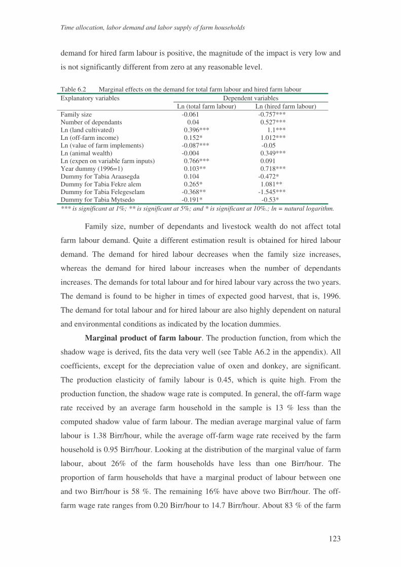
Time allocation, labor demand and labor supply of farm households
123
demand for hired farm labour is positive, the magnitude of the impact is very low and
is not significantly different from zero at any reasonable level.
Table 6.2 Marginal effects on the demand for total farm labour and hired farm labour
Dependent variables Explanatory variables Ln (total farm labour) Ln (hired farm labour)
Family size -0.061 -0.757*** Number of dependants 0.04 0.527*** Ln (land cultivated) 0.396*** 1.1*** Ln (off-farm income) 0.152* 1.012*** Ln (value of farm implements) -0.087*** -0.05 Ln (animal wealth) -0.004 0.349*** Ln (expen on variable farm inputs) 0.766*** 0.091 Year dummy (1996=1) 0.103** 0.718*** Dummy for Tabia Araasegda 0.104 -0.472* Dummy for Tabia Fekre alem 0.265* 1.081** Dummy for Tabia Felegeselam -0.368** -1.545*** Dummy for Tabia Mytsedo -0.191* -0.53* *** is significant at 1%; ** is significant at 5%; and * is significant at 10%.; ln = natural logarithm. Family size, number of dependants and livestock wealth do not affect total
farm labour demand. Quite a different estimation result is obtained for hired labour
demand. The demand for hired labour decreases when the family size increases,
whereas the demand for hired labour increases when the number of dependants
increases. The demands for total labour and for hired labour vary across the two years.
The demand is found to be higher in times of expected good harvest, that is, 1996.
The demand for total labour and for hired labour are also highly dependent on natural
and environmental conditions as indicated by the location dummies.
Marginal product of farm labour. The production function, from which the
shadow wage is derived, fits the data very well (see Table A6.2 in the appendix). All
coefficients, except for the depreciation value of oxen and donkey, are significant.
The production elasticity of family labour is 0.45, which is quite high. From the
production function, the shadow wage rate is computed. In general, the off-farm wage
rate received by an average farm household in the sample is 13 % less than the
computed shadow value of farm labour. The median average marginal value of farm
labour is 1.38 Birr/hour, while the average off-farm wage rate received by the farm
household is 0.95 Birr/hour. Looking at the distribution of the marginal value of farm
labour, about 26% of the farm households have less than one Birr/hour. The
proportion of farm households that have a marginal product of labour between one
and two Birr/hour is 58 %. The remaining 16% have above two Birr/hour. The off-
farm wage rate ranges from 0.20 Birr/hour to 14.7 Birr/hour. About 83 % of the farm

Chapter 6
124
households receive less than one Birr/hour. Among those farm households who
engage in off-farm work, about 31% of them have male members’ market wage rate
greater than the marginal product of farm labour. The majority (69 %) has a marginal
product of farm labour higher than the market wage rate received by male members.
In general, there is a difference in the magnitude of the marginal product of farm
labour between those farm households engage in off-farm work and those who do not
(Table 6.3). The marginal product of labour is 28% higher for the non-participants
than for the participants in off-farm activity.
Table 6.3 The marginal product of farm labour for participant and non-participant in off-farm work
Birr*/hour Non-participant in off-farm work 1.77 Participant in off-farm work 1.28 Total 1.38
* One US Dollar was equivalent to seven Ethiopian Birr.
Labour supply. The estimation results for farm and off-farm labour supply
are summarised in Table 6.4 (see also Table A6.5 - Table A6.7 in the appendix). The
shadow wage of farm labour, male household members’ market wage rate, the
household head’s education and wife’s education, year dummy and some location
dummies significantly influence the farm labour supply of family members. The own
wage elasticity for on-farm family labour supply is found to be slightly greater than
unity (1.24). The influence of the male members’ market (off-farm) wage rate is
negative signifying the fact that farm labour and off-farm labour are substitutes, but it
is small (-0.03). Education has two contrasting effects on the supply of farm labour.
On the one hand, households when the head can read and write supply more labour on
the farm than those when the head cannot read and write. On the other hand,
households when the wife cannot read and write supply less labour on the farm than
those when the wife cannot read and write. The fact that less labour was supplied in
1996 than in 1997 and that the labour supply differs across location show that natural
conditions such as soil type and the amount of rainfall influence the labour supplied
on the farm. The income effect is positive, but not significant. The result is
inconsistent with the estimates of off-farm labour supply of male and female
members’ (see below), which might be due to mis-specification. Although the
parameter estimates of family composition (size and the number of dependants) are

Time allocation, labor demand and labor supply of farm households
125
not significantly different from zero, the supply of labour on the farm increases with
both family size the numbers of dependants. The age of the household shows a
quadratic pattern, but the parameter estimates are not significantly different from zero.
Family labour supply increases with age, reaches its maximum at the age of 43 years
and decreases thereafter.
Table 6.4 Elasticity of on-farm and off-farm labour supply of male and female members Explanatory variables On-farm labour Male off-farm labour Female off-farm labour Shadow wage of on-farm family labour
1.238*** -1.264** -0.680**
Male Off-farm wage rate -0.026* 0.701*** -0.038 Female off-farm wage rate -0.0001 -0.049* 0.813*** non-labour income plus Yo
= (S) 0.007 -0.048 -0.143** Education dummy of head 0.051** -0.030 0.045 Education dummy of house wife -0.025** 0.054** -0.043 Age of the household head -0.078 0.285 0.858 Family size 0.198 2.396*** 0.167 Number of dependants -0.098 -1.079*** 0.439 Elasticities are calculated based on the unconditional expected marginal effects. For the derivation see Appendix A6.2. *** is significant at 1%; ** is significant at 5%; and * is significant at 10%.. = Yo is the constant term (intercept) of the linearised budget constraint.
Wage rate and family composition are the main determining factors in the off-
farm labour supply of male members, whereas female members’ off-farm labour
supply is influenced by the wage rate and non-labour income. The own wage
elasticities of male and female members are positive and significant suggesting an
upward sloping labour supply. The off-farm labour supply of both male and female
members is decreasing with the non-labour income (exogenous income) indicating
that leisure time is a normal good. But the parameter estimate of the income effect on
the male labour supply is not significantly different from zero. The own wage
elasticity of male members’ off-farm labour supply is less elastic (0.7) than that of
female members’ (0.8). The estimated own wage elasticity of both male and female
members in this study is higher than those estimated for Indian (Skoufias, 1994) and
Peruvian (Jacoby, 1993) households. They are also slightly higher than that estimated
for the Northern Ghana (Abdulai and Delgado, 1999). The cross wage elasticity
between male and female off-farm labour supply is small5 and negative indicating that
they are substitutes. The off-farm labour supply of male and female members
increases with family size and the numbers of dependants. This indicates that family
5 But they are not symmetric. The effect of the female wage rate on the male wage rate is higher than that of male on female.

Chapter 6
126
size reduces the marginal value of households’ leisure time and hence increases the
marginal value of households’ home time. However, the parameter estimates of
family composition on the female members’ off-farm labour supply are not
significantly different from zero.
When household heads are able to read and write, male members supply less
labour for off-farm work and female members (wife) supply more labour for off-farm
work. Similarly, when household wives are able to read and write male members
supply more labour for off-farm work and female members (wife) supply less labour
for off-farm work. The supply of off-farm labour was higher in 1996 than in 1997
although the parameter estimates are not significantly different from zero. Location
dummies also have a significant influence on both the male and female labour
supplies. However, the age and age squared variables do not show a significant effect
on off-farm labour supply (except for the effect of age squared on the male members’
off-farm labour supply). Off-labour labour supply of both male and female members
decrease with age, but at a decreasing rate when the household grows older.
6.6 Conclusions
The estimated models provide important findings that can be used to derive policy
implications. Increased expenditure on purchased farm inputs increases the demand
for farm labour, and non-farm-farm income makes a significant positive contribution
to the hired farm labour demand. Off-farm labour supply is reasonably responsive to
own wage rate. Farm labour supply is a substitute to off-farm labour supply, but it is
low enough for off-farm work to discourage farming activities. On the other hand, the
effect of the return to farm labour on off-farm work is high enough to make farmers
reduce the amount of labour supplied for off-farm work. The own wage elasticities of
off-farm labour supply are found to be higher than those estimated for other countries
such as India (Skoufias, 1994) and Peruvian Sierra (Jacoby, 1993). They are also
slightly higher than that estimated for the Northern Ghana (Abdulai and Delgado,
1999). Male and female members of a household have different wage elasticity. The
own wage elasticity of female members is higher than that of male members. The
cross wage elasticity between male and female off-farm labour supply is negative, but
very low. The shadow value of farm labour and the wage rate received from off-farm

Time allocation, labor demand and labor supply of farm households
127
work are not equal perhaps due to the imperfect labour market that arises due to
transaction cost and rationing of labour in off-farm work.
These findings may have some policy implications. First, the effect of policies
aimed at shifting the supply of off-farm labour will have a differential impact on
household labour income depending on the gender composition of households.
Second, creating off-farm employment opportunities for female women will only have
a small negative impact on the male members’ off-farm labour supply. Third,
increasing the return to off-farm work (wage rate) can be used as one of the policy
instruments to promote off-farm employment with only a small negative impact on
the supply of farm labour. Fourth, increasing off-farm employment can help to release
the farmers’ liquidity constraints and promote commercialisation of agriculture by
increasing the use of hired labour on the farm. Fifth, increased use of fertiliser and
improved seeds help to increase on-farm employment and absorb idle family labour.


Off-farm employment, entry barriers and income inequality
129
CHAPTER 7. OFF-FARM EMPLOYMENT, ENTRY BARRIERS AND
INCOME INEQUALITY
7.1 Introduction
One of the basic assumptions of diversifying income sources into off-farm activities is
to supplement the farm income of the poor and reduce the income inequality that
exists in rural areas. The incentive to diversify income sources into off-farm activities
is stronger for poor than for rich farm households because the relative return to off-
farm work is greater for the poor than for the rich. The risk aversion motives to
diversify income into off-farm declines as farm household’s wealth increases if risk
aversion is negatively related with wealth (Newbery and Stiglitz, 1981). However, if
there are entry barriers and rationing in the labour market, diversifying income into
off-farm activities will be more difficult for poor farm households than for rich farm
households (Reardon, 1997). The presence of a credit (liquidity) constraint may make
it difficult for poor farm households to finance investment (such as equipment
purchase or rent, skill acquisition, capital for initial investment and a license fee)
needed to participate in off-farm activities. Community level barriers can also exist
that prevent farm households from participating in off-farm activities. Due to poor
infrastructure there is limited labour market integration (Sadoulet and De Janvry,
1995). The lack of labour market integration leads to rationing of off-farm jobs in
some communities. The lack of infrastructural facilities may restrict the movement of
labour between communities or make it costly to move to towns. As a result off-farm
employment may worsen income inequality rather than reducing it.
Analysing off-farm work participation without making a distinction between
self-employment and wage employment is valid only if the nature of off-farm wage
and self-employment are quite similar. But the nature and determinants of off-farm
wage employment and off-farm self-employment are different. Off-farm wage
employment is a temporary employment contract in which the employer gives a direct
order, whereas off-farm self-employment involves ownership of a firm that produces
goods and services, and buyers who do not give direct orders (Reardon, 1997). The
input requirements of wage and self-employment may also be different. Wage

Chapter 7
130
employment generally does not require as much capital as self-employment. If there is
a credit constraint and own capital is limited, then undertaking self-employment may
be more difficult than wage employment. Self-employment also requires managerial
skill to run the business. On the other hand, wage employment is more available in
areas nearer to towns and commercialised agriculture. In areas far from urban centres,
farm households can engage in petty trade, as the competition from urban traders is
very low. Near urban centres, off-farm self-employment may face serious competition
from urban areas. Hence, the determinants of participation in off-farm self-
employment and wage employment and their relative importance will be different. As
a result, the relative contribution of off-farm wage and self-employment for reducing
poverty and income inequality is different within and across communities. Most of the
studies have analysed off-farm employment as a whole without making a distinction
between wage and self-employment (Abdulai and Delgado, 1999; Jacoby, 1993;
Skoufias, 1994). The relative contributions of off-farm wage employment and off-
farm self-employment to household total income and poverty alleviation is seldom
known (Reardon, 1997). Given the general lack of studies on off-farm activities,
analysing the relative importance of wage and self-employment is crucial for a better
targeting of programs designed to alleviate poverty.
The objective of this chapter is, therefore, (1) to identify the determinants of
farm households’ choice between wage and self-employment, and (2) to analyse the
relative importance of wage and self-employment in overall household income and
income inequality. The total farm household income is decomposed into various
categories of farm and non-farm incomes. The income categories used are crop
income, livestock income, off-farm self-employment, off-farm wage employment
(paid food for work, non-farm manual wage employment and non-farm skilled wage
employment) and non-labour income. The relative contributions of these income
sources to the overall income inequality are assessed using the Gini decomposition
method (Lerman and Yitzhaki, 1985). Probit and tobit models as well as a
multinomial logit model, consistent with a non-separable agricultural household
model, were estimated to identify the factors that determine the labour allocation
decisions of farm households.
The rest of the chapter is organised as follows. The nature of off-farm work in
the study areas is described in the next section. In section three, a Gini-decomposition
technique and an econometric model specification are described. A brief theoretical

Off-farm employment, entry barriers and income inequality
131
background is provided in section four. The impact of off-farm income on overall
income inequality is presented in section five. Estimation results are discussed in
section six. The paper ends with some concluding comments.
7.2 The nature of off-farm employment
The types of off-farm activities in which farm households participate can be
categorised into wage employment and self-employment. Three types of wage
employment can be distinguished, namely paid development work, manual non-farm
work, and non-manual (skilled) non-farm work. Paid development work involves jobs
in community micro dam construction, community soil and water conservation works
such as construction of terraces and afforestation, and other community works done
under the food for work program. Manual non-farm work is an activity in which farm
households work for private and public construction companies in urban and near
urban areas. Non-manual (skilled) non-farm work involves masonry, carpentry and
cementing in public and private construction sites. Off-farm self-employment
comprises mainly petty trade, transporting by pack animals, stone mining, pottery and
handicraft, selling of wood and charcoal, local brewery and selling of fruit such as
beles.
The participation rates for different off-farm activities are presented in Table
7.1. The dominant type of off-farm work is wage employment. Paid development
work (food for work) is the major source of wage employment in both districts. The
overall average participation rate in wage employment is 72%. The participation rate
in off-farm self-employment is approximately 28% of which more than half comes
from the Enderta district. Manual non-farm wage employment is the second most
important type of wage employment in Enderta district. Non-manual (skilled) wage
work is done by 7 % of the households in Enderta district. Non-farm wage
employment (both manual and non-manual) is almost non-existent in Adigudom
District. The food for work program is the sole provider of wage employment in
Adigudom. There is a remarkable difference in the seasonal distribution of
participation in off-farm activities between the two districts. In Enderta, farm
households’ participation in off-farm work is higher during the slack season, twice
that of the peak season. In Adigudom, farm households’ participation is uniform in all
seasons. This implies that there is more surplus labour in Adigudom than in Enderta.
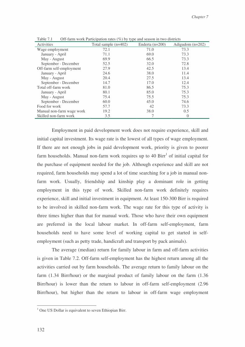
Chapter 7
132
Table 7.1 Off-farm work Participation rates (%) by type and season in two districts Activities Total sample (n=402) Enderta (n=200) Adigudom (n=202) Wage employment 72.1 71.0 73.3 January - April 71.1 69.0 73.3 May - August 69.9 66.5 73.3 September - December 52.5 32.0 72.8 Off-farm self-employment 27.9 42.5 13.4 January - April 24.6 38.0 11.4 May - August 20.4 27.5 13.4 September - December 14.7 17.0 12.4 Total off-farm work 81.0 86.5 75.3 January - April 80.1 85.0 75.3 May - August 75.4 75.5 75.3 September - December 60.0 45.0 74.6 Food for work 57.7 42 73.3 Manual non-farm wage work 19.2 38.0 0.5 Skilled non-farm work 3.5 7 0
Employment in paid development work does not require experience, skill and
initial capital investment. Its wage rate is the lowest of all types of wage employment.
If there are not enough jobs in paid development work, priority is given to poorer
farm households. Manual non-farm work requires up to 40 Birr1 of initial capital for
the purchase of equipment needed for the job. Although experience and skill are not
required, farm households may spend a lot of time searching for a job in manual non-
farm work. Usually, friendship and kinship play a dominant role in getting
employment in this type of work. Skilled non-farm work definitely requires
experience, skill and initial investment in equipment. At least 150-300 Birr is required
to be involved in skilled non-farm work. The wage rate for this type of activity is
three times higher than that for manual work. Those who have their own equipment
are preferred in the local labour market. In off-farm self-employment, farm
households need to have some level of working capital to get started in self-
employment (such as petty trade, handicraft and transport by pack animals).
The average (median) return for family labour in farm and off-farm activities
is given in Table 7.2. Off-farm self-employment has the highest return among all the
activities carried out by farm households. The average return to family labour on the
farm (1.34 Birr/hour) or the marginal product of family labour on the farm (1.36
Birr/hour) is lower than the return to labour in off-farm self-employment (2.96
Birr/hour), but higher than the return to labour in off-farm wage employment
1 One US Dollar is equivalent to seven Ethiopian Birr.

Off-farm employment, entry barriers and income inequality
133
(0.72Birr/hour). It is also higher than the wage rate paid for hired farm labour (1.08
Birr/hour). The structure of wage rate looks different when off-farm employment is
decomposed into specific categories. The return to labour in paid development work
(0.45 Birr/hour) is the lowest among all the activities. The return to labour in manual
non-farm work (0.89 Birr/hour) is lower than the payment to family labour on the
farm and the wage rate paid for hired farm labour. However, skilled non-farm wage
employment has a return (2.8 Birr/hour) higher than the return to family labour on the
farm and the wage rate paid for hired farm labour. It has a return close to that of off-
farm self-employment. The return to labour in general seems to be higher in Enderta
District than in the Adigudom District, although the marginal product of labour is
almost equal in both districts. Non-farm wage employment is mainly found in the
Enderta District. No skilled non-farm activity is observed and only one household
was found to be involved in manual non-farm work in the sample drawn from
Adigudom district.
Table 7.2 Average (median) farm and off-farm return to family labour (Birr‡/hour) by districts Activity Enderta Adigudom‡‡ Total average Average product of family labour on the farm* 2.76 2.56 2.73 Return to family labour on the farm** 1.50 1.26 1.34 Marginal product of family labour*** 1.36 1.37 1.36 Wage rate paid for hired farm work 1.11 1.04 1.08 Wage rate for wage employment 0.89 0.55 0.72 Wage rate for food for work 0.62 0.55 0.45 Wage rate for manual non-farm wage work 0.90 0.85 0.89 Wage rate for skilled non-farm work 2.8 - 2.8 Return from off-farm self-employment 3.66 1.52 2.96 Return to family labour on the farm Non-participant in off-farm work 1.76 1.93 1.87 Participant in off-farm work 1.44 1.07 1.22 Percent participants earn less relative to non-participants -18.2% -44.6% -34.8% Marginal product of family labour Non-participant 1.96 1.74 1.77 Participant 1.27 1.30 1.28 Percent participants earn less relative to non-participants -35.2% -25.3% -27.7% * The average product of family labour is calculated as the total value of farm output divided by the hours of family labour used on the farm; ** The average return of farm labour is computed as crop income minus variable inputs and one year depreciation of farm equipment and livestock wealth divided by the family labour hours used on the farm. *** The marginal product of family labour is calculated from a Cobb-Douglas production function. ‡ One US Dollar is equivalent to seven Ethiopian Birr. ‡‡ No one participated in skilled non-farm work in Adigudom District.
There is a differential return for farm work between those households that
participate in off-farm activities and those that do not. The median return to family
labour on the farm for the participating farm households is 35% lower than the return

Chapter 7
134
for the non-participating farm households. The difference in return to family labour on
the farm between the off-farm work participants and the non-participants is higher in
Adigudom than in Enderta. In Enderta participants earn 18% less for family labour on
the farm than those who do not participate, whereas in Adigudom participants earn
44% less than those who do not participate.
Despite the high return to labour on the farm, the amount of labour supplied to
farming activities is much lower than the amount supplied to off-farm work (Table
7.3). Given the number of people who can work on the farm and off-farm (Table 7.3),
farm households could still allocate more labour to off-farm activities if there were
enough jobs. Given that an average household has 2.5 working members who work 16
days per month2 and assuming they can work for eight hours per day, an average
household can have 3893 hours available for farm and off-farm work. However, an
average household uses only 2148 labour hours (Table 7.3) for farm and off farm
work, which is 55 % of their time. Furthermore, when farmers are asked for the
reason why they do not work more in off-farm activities, about 60 % of them
responded that they could not get off-farm employment around their district. This
shows that agriculture is not able to absorb the available labour and there is
potentially rationing in the off-farm labour market. Hence we can conclude that off-
farm employment can be expanded without reducing the amount of labour available
for agricultural activities.
Table 7.3 Labour allocation and availability of an average household Enderta Adigudom Total Farm labour hours supplied by family members
544 439 492
Off-farm wage employment labour hours 1455 1045 1249 Off-farm self-employment labour hours 148 47 98 Family size 5.8 5.5 5.6 No. people working on farm 2.5 2.7 2.6 No. people working off-farm 1.4 1.4 1.4 Number of dependants 3.3 3.2 3.3
7.3 Theoretical consideration
2 Due to Coptic Church holidays, farmers use only 53% of their available time for farm and off-farm work.
Off-farm employment, entry barriers and income inequality
135
In a farm household economy with a perfect market, labour is allocated between farm
and off-farm activities in such a way that the marginal value of farm labour equals the
wage rate for off-farm activities (Becker, 1965; Gronau, 1973; Huffman and Lange,
1989). This means that individuals are willing to participate in off-farm work as long
as their marginal value of farm labour (or reservation wage) is less than the off-farm
wage rate they command. This implies that poorer farm households have a stronger
incentive to diversify their income sources into off-farm activities because they have a
lower marginal value of farm labour. One of the motives to diversify income sources
into off-farm activities is to manage the risk associated with agricultural production.
The extent of the risk motive to diversify income depends critically on risk aversion.
Because risk aversion varies inversely with wealth (Newbery and Stiglitz, 1981), the
risk incentive to diversify income sources is stronger for poor than for rich. However,
there can be entry barriers in the off-farm labour market because off-farm activities
may require investment on equipment purchase or rent, skill acquisition and license
fees. If households face binding liquidity and credit constraints, poor households
could not afford the investment required in the off-farm labour market. Hence if there
are entry barriers in the off-farm labour market, the capacity to diversify income
sources into off-farm activities is lower for poorer farm households. Individual assets
and wealth can affect the type of non-farm activities a household picks up and can
worsen the income distribution (Reardon and Taylor, 1996). As a result less wealthy
farmers spend most of their time in low paying off-farm activities for which the entry
barrier is very low. If there is rationing in the labour market, we may not observe a
farm household participating in an off-farm labour market even if the marginal value
of farm labour (or reservation wage rate) is less than the marginal value of off-farm
labour (Blundell and Meghir, 1987). Therefore, the actual participation of a farm
household in off-farm activities (income diversification of household) depends on the
incentive and the capacity to participate (Reardon et al., 1998).
A farm household’s choice among different types of off-farm activities (wage
and non-farm self-employment) can be seen as a two-stage process. In the first stage,
a farm household’s choice of whether or not to work off-farm depends on the
reservation wage rate (see Chapter three of this book for details). If the reservation
wage rate is less than the prevailing market wage rate net of commuting cost, the
household will participate in off-farm activities. If there is rationing and transaction
cost in the labour market and the household faces a binding credit constraint, the

Chapter 7
136
reservation wage rate of that household will be very high and hence it will choose for
less off-farm work participation. In the second stage, if the reservation wage rate is
less than the prevailing off-farm market wage rate, a farm household will choose
among the available off-farm activities depending on the relative wage rates.
Obviously, a farm household chooses to work in the off-farm activity with the highest
effective market wage rate. If agriculture is risky (and households are risk averse), the
household will choose an occupation that is negatively correlated with agricultural
income (Newbery and Stiglitz, 1981). If the farmer faces a liquidity (or credit)
constraint, he will prefer the one that requires less initial capital. Most probably, the
credit constrained farm household will choose wage employment above off-farm self-
employment. A farm household with a better asset position may face relatively less
credit constraints and hence may prefer to work in off-farm self-employment.
A farm household can participate in more than one off-farm activity. If there
are other family members in the household who can participate in off-farm activities,
participation in two kinds of off-farm activities is possible. The wife and husband can
choose (ex-ante) different off-farm activities with rewards that are negatively
correlated in order to stabilise their income. Farm households can also work in both
wage employment and off-farm self-employment at different times of the year
depending on the availability of jobs. Hence we can observe two types of off-farm
occupation in a given household.
Empirical studies have documented that the reservation wage rate that
determines the households’ participation in off-farm activities is an endogenous
variable (Huffman, 1980; Lass, Findeis and Hallberg, 1991). It depends on farm
characteristics, family characteristics, locations, and endogenous and exogenous
household incomes. Farm characteristics include the farm size (amount of land
cultivated), livestock wealth, and the number of animals used for transportation
(donkey and horse). Family characteristics include age and educational level of family
members, family size, and the number of dependants. Endogenous household income
consists of farm income, which depends on farm and location characteristics
(Huffman, 1980; Woldehanna et al., 2000). Exogenous household income consists of
non-labour income such as transfer income (remittance, gift, food aid) and income
from property rent. Off-farm wage is also an endogenous variable, which depends on
individual and location characteristics (Huffman, 1980). Variables that raise the
reservation wage reduce the probability and level of participation in off-farm work,

Off-farm employment, entry barriers and income inequality
137
but variables that raise the off-farm wage rate increase the participation. Age,
educational status, location, farm and non-farm equipment may affect both the
reservation and off-farm wage. Hence the direction of influence on off-farm work
participation depends on the relative strength of these forces. Farm income, livestock
wealth and other income may also improve farm households’ access to off-farm work
if there is a credit constraint. Hence their impact on the off-farm work participation
can be positive.
7.4 Gini decomposition, econometric model specification and estimation
Gini decomposition. Gini decomposition is used to analyse the contribution of
alternative income sources to overall income inequality (Lerman and Yotzhaki, 1985;
Reardon and Taylor, 1996). The conventional Gini coefficient (G) is given by
Y)]Y(F,Y[cov2
G = (7.1)
where cov[Y, F(Y)] is the covariance of total income with its cumulative distribution
of income (F(Y)), Y is total household income, and Y is mean household income .
Decomposing total household income into K sources (yk), the overall Gini coefficient
can be rewritten as
Y
)]Y(F,y[cov2G
K
1kk�
== (7.2)
Then dividing and multiplying each component k by cov(yk, Fk) and the mean income
of source k (yk) yields Gini decomposition by income source as
��==
=××=K
kkkk
k
k
kkK
k kk
k SGRYy
yFy
FyYFy
G11
),(cov2
),(cov)](,[cov
(7.3)
where Fk is the cumulative distribution of income from source k, Rk is the Gini
correlation between income from source k and total household income, Gk is the
relative Gini of income from source k, Sk is the income from source k’s share of total
household income.
To analyse how changes in particular income sources will affect overall
income inequality, consider a change in each household’s income from source k equal
to ekyk where ek is close to one. The partial derivative of the overall Gini (G) with
Chapter 7
138
respect to a percentage change (e) in income source k is given by (Lerman and
Yotzhaki, 1985, p. 152):
)( GGRSeG
kkkk
−=∂∂
(7.4)
Then dividing (4) by G, the relative effect of a marginal change in source k’s income
on the Gini for total income is given by
kkkk
kkkk
SG
GRSG
GGRSGe
eG −=−= 1
)(∂∂
. (7.5)
This is equal to the relative contribution of income from source k to the overall
income inequality minus the share of income from source k in total income.
Econometric model specification. Two sets of models can be used to analyse
off-farm employment: off-farm labour supply of farm households and farm
households’ choices between off-farm activities. The first model involves specifying
the hourly supply of labour for off-farm wage employment and off-farm self-
employment in order to identify the factors that determine them and their relative
importance. For this purpose, we need to specify equations that determine the labour
hours supplied to the off-farm activities at the ruling wage rate, conditional on
individual participation.
Let latent variable off-farm labour hour be denoted by L*m and observed off-
farm labour hour by Lm. In an agricultural household model an individual is willing to
participate in off-farm work when his/her reservation wage (wri) is less than the off-
farm wage net of commuting cost (wmi) offered:
imiriimrii wwifDwwifD >=≤= 0;1 (7.6)
where Di is the participation decision of a household to work off-farm. Consequently
the latent variable off-farm labour hours (L*m) and observed off-farm labour hours
(Lm) can be specified by a tobit model:
�
===
+=
001
),0(~;*
2/*
i
iimi
eiiimi
DifDifLL
NeeXL σβ (7.7)
where β/ is a row vector of parameters; X is a column vector of variables that affect
the reservation and market wage; ei is the error term. Following the lines of Maddala

Off-farm employment, entry barriers and income inequality
139
(1983), Amemiya (1984, p. 9) and Blundell and Meghir (1987, p. 181), the log
likelihood function of the tobit model can be written as3:
�� −+−+−=1
eimieei0
)]/)X'L((loglog[))/X'(1(logLlog σβφσσβΦ (7.8)
where the subscript 0 indicates summation over observations with zero off-farm
labour hours, 1 indicates summation over observation with positive observed off-farm
labour hours, and φ(.) and Φ(.) refer to the standard normal density and probability
functions, respectively. The tobit model assumes, however, that the same stochastic
process affects both the participation decision and the off-farm labour income. A zero
realisation for a dependent variable represents a corner solution or a negative value for
the underlying latent dependent variable (Cragg, 1971; Lin and Schmidt, 1984).
The second model is a farm household’s choice between off-farm activities.
Basically the off-farm work choices available for farm households in the study area
can be categorised into four: not participating in off-farm activities at all, participating
in off-farm wage employment only, participating in off-farm self-employment only,
and participating in both off-farm wage and self-employment. This can be easily
modelled using a multinomial logit model (Cramer, 1991; Maddala, 1983). Let Uij
denote the utility that a farm household i gets from choosing alternative j and
ijjijijijij eXeuU +=+= γ (7.9)
where γj varies and Xi remains constant across alternatives; and eij is a random
disturbance reflecting intrinsically random choice behaviour, measurement or
specification error and unobserved attributes of the alternatives. Let also Pij (j =
0,1,2,3) denote the probability associated with the four choices available for farm
household i with
j = 0 if the farm household does not participate in off-farm work at all,
j= 1 if the farm household participates in off-farm wage employment only,
j= 2 if the farm household participates in off-farm self-employment only and
j= 3 if the farm household participate in both off-farm wage employment and
self-employment.
3 The likelihood function of a Tobit model is
)/(
)/)(1
)/(1
)]/(1[0
)0(Pr)0|(1
)0(Pr0
eX
eXmiLe
eXeX
miLmiLmiLfmiLL
σβ
σβφσ
σβσβ′Φ
′−
′ΦΠ′Φ−Π=
>>Π=Π=
.

Chapter 7
140
Then the multinomial logit model4 is given by
�=
= 3
0jji
jiij
)Xexp(
)Xexp(P
γ
γ. (7.10)
Setting γ0=0, the multinomial logit model can be rewritten as
)3,2,1j()Xexp(1
)Xexp(P 3j
1jji
jiij =
′+
′=
�=
=
γ
γ and
�=
=
′+= 3
1
0
)exp(1
1j
jji
i
XP
γ (7.11)
which can be estimated using the maximum likelihood estimation method.
Estimation procedure. The tobit (7.7) models for off-farm wage employment
and off-farm self-employment are estimated to determine the relative importance of
factors that affect the off-farm wage employment and off-farm self employment. The
multinomial logit model (7.11) is estimated to identify the factors that determine farm
households’ choices between off-farm wage employment and off-farm self-
employment. Explanatory variables used in the probit, tobit and logit model are age,
age squared and dummy for education status of the household head, location (district)
dummy, year dummy, family size, number of dependants, livestock wealth, ownership
of animals used for transportation (such as donkey and horses), value of owned
equipment for off-farm work, amount of cultivated land by the household, farm
income, non-labour income, and wage rates received by the households. Two
education dummies have been constructed: a dummy for those who have traditional
education and a dummy for modern (basic) education. They are compared with those
who can not read and write at all.
The predicted wage and farm income (rather than observed wage and farm
income) are used in order to remove endogeneity. Estimation of farm income is based
on a Cobb-Douglas production function (see Chapter 5). Heckman’s two stage
method (Maddala, 1983) for correcting the sample selection bias is used to estimate
the wage rate received by farm households. The wage rate of off-farm wage
employment is defined as income from off-farm wage employment divided by the
4 Assume that farm household i prefers, for example, alternative 1 to alternative 0 and 3:
)1313121231211 (Pr)Pr( iiiiiiiiiiiii eXXeandeXXeUandUUUP +−<−<=>>= + γγγγ .
Assuming eij are independently and identically distributed with Weibull density function, the cumulative distribution function has the form .))exp((exp)(Pr εε −−=≤ije The difference between
any two random variables with this type of distribution has a logistic distribution function (Judge et al., 1985, p. 770). The probability arising from this kind of model is given by a multinomial logit model.

Off-farm employment, entry barriers and income inequality
141
number of hours supplied for off-farm wage employment. For off-farm self
employment, wage is defined as the net income (profit) from off-farm self
employment divided by the number of hours supplied for off-farm self employment.
The explanatory variables used for the estimation of wage equations are age, age
squared, year and education dummies, value of off-farm equipment and transport
animals, location dummies and inverse mills ratio. The inverse mills ratios are derived
from the probit equations for participation in off-farm wage employment and off-farm
self-employment. The independent variables in the estimation of the probit equations
are age, age squared, family size, number of dependants, farm inputs and year,
education and location dummies.
All variables measured in monetary terms are used in logarithm form. These
variables include farm income, non-labour income, the wage rate for off-farm wage
and self-employment and the value of off-farm equipment owned5. Elasticities of off-
farm work participation are computed at sample means.
7.5 Income inequality and income sources
In this section, Gini coefficients for the total household (7.1) and various farm and
non-farm incomes (7.3) are calculated. Total household income is decomposed into
livestock income, crop income, income from off-farm wage employment, income
from off-farm self-employment and non-labour income. Income from off-farm wage
employment is further decomposed into income from paid development work (food
for work), income from non-farm manual work, and income from non-manual
(skilled) non-farm work. Then the income sources elasticity of the overall Gini index
is computed using equation (7.5).
Gini coefficients for total income as well as the share of income from various
sources and their marginal contribution to overall Gini coefficients are presented in
Table 7.4. There is no change in the Gini coefficients when they are calculated from
incomes stated in per capita terms. Crop income has the highest contribution to
overall income inequality (as measured by Gini coefficients) followed by wage
employment and livestock income. Crop, livestock and off-farm wage incomes reduce
income inequality. The results are mixed when wage income is decomposed into
5 Since the logarithm of zero does not exist, zero observations are replaced with a value of one.

Chapter 7
142
various categories. Paid food for work program is the only type of off-farm wage
income that reduces income inequality. It is unequally distributed by itself, but
favours the poor. The elasticity of total income inequality with respect to food for
work income is the highest of all the other income sources’ elasticity. Non-farm wage
and self-employment incomes have non-equalising effect. Income from unskilled
(manual) and skilled (non-manual) non-farm work increases overall income
inequality. Non-labour income (such as gifts, remittances, and property rent) is also
increases income inequality. The marginal effect on income inequality is higher for
non-labour income than for non-farm wage and self-employment income.
There are no consistent findings among previous studies regarding the impact
of off-farm income on rural income inequality. Comparison of the results is not easy
either, as most empirical studies do not use the same type of income definition and
income decomposition and methodology. In Palanpur (India), Lanjouw and Stern
(1993) found that off-farm income in general has increased income inequality in
1983/84 and reduced it in 1981/82. Stark, Taylor and Yitzhaki (1986) found that
remittance from domestic and international sources has both positive and negative
effects on income inequality in two villages of Mexico. In rural Pakistan, Adams
(1994) found that non-farm income makes a small contribution to income inequality
despite its large share in total income. Non-farm income also has a low Gini
coefficient and is poorly correlated with total income. When non-farm income is
decomposed into different categories, income from government employment and off-
farm self-employment is found to increase income inequality while income from
unskilled labour reduces income inequality. In Philippines, Leones and Feldman
(1998) found that while income from remittance, trading and skilled labour increases
inequality, income from agricultural wage labour and gathering activities such as
fishing and logging reduces inequality. All these studies have one common result.
Income sources that need skill and capital to enter (such as non-farm self-employment
and income from skilled wage labour) increase income inequality. The same goes for
the results obtained from this study: off-farm activities that have entry barriers and
require capital to start have a negative impact on income inequality. It is only income
from food for work programs that have a positive effect on rural income inequality.
This is because the food for work jobs do not need skill and capital and are initially
targeted to provide employment for the poorer farm households. However, there is a
peculiar finding in this study that unskilled non-farm wage work increases income

Off-farm employment, entry barriers and income inequality
143
inequality. Although unskilled non-farm wage work does not require education and
skill, it involves very high transaction cost (such as search and commuting cost)
unaffordable by poor farmers. Farmers are required to have their own equipment
(worth at least 40 Birr) and be able to commute to towns in order to get jobs in the
unskilled non-farm labour market.
The possible reason for non-farm income to have a dis-equalising effect from
an investment perspective (Reardon, Crawford and Kelly, 1994) is that there is an
entry barrier for the poor. Skilled non-farm wage employment and off-farm self-
employment require skill and capital to start. In the absence of a perfect credit market,
it is only the rich households that can afford to enter into self-employment. Even in
the unskilled non-farm labour market, the transaction cost of looking for jobs in the
nearby urban areas coupled with rationing in the labour market gives richer farm
households an advantage in the non-farm labour market. As a result income from the
non-farm labour market increases income inequality. This implies that unless rural
non-farm activities are promoted that particularly target the poor, wealthy farm
households will dominate the most lucrative form of non-farm activities such as
masonry, carpentry and trading.

Chapter 7
144
Table 7.4 Gini Decomposition by income sources Household Income components Mean Sk Rk Gk Gk*Rk Sk*Rk*Gk (Sk*Rk*Gk )/G (Sk*Rk*Gk )/G - Sk
Off-farm self-employ income 262.50 0.068 0.598 0.836 0.500 0.034 0.103 0.035
Off-farm wage income 858.75 0.280 0.489 0.628 0.308 0.086 0.261 -0.019
Income from food for work 437.89 0.174 0.183 0.664 0.122 0.021 0.064 -0.110
Manual non-farm wag income 284.58 0.085 0.406 0.883 0.358 0.030 0.092 0.007
Skilled non-farm wage income 136.28 0.022 0.794 0.978 0.777 0.017 0.053 0.031
Non-labour income 194.31 0.039 0.707 0.951 0.672 0.026 0.080 0.041
Net farm crop income 1339.65 0.448 0.698 0.442 0.308 0.138 0.419 -0.029
Livestock income 497.40 0.164 0.425 0.643 0.273 0.045 0.136 -0.028
Total household income 3152.60 0.330
Sk is the average share of income from source k in total income;
Gk is Gini index of inequality for income from source k;
Rk is Gini correlation with total income ranking;
G is the Gini index of total income inequality;
G
**Sk kk GR is the relative contribution of income from source k to the Gini index of total income inequality;
kk S-
G**S kk GR
is elasticity of Gini index of inequality with respect to income source k.

Off-farm employment, entry barriers and income inequality
145
7.6 Estimation results and discussion
Wage offer equations for off-farm wage employment and off-farm self-employment,
off-farm work participation and intensity of participation in wage employment and
self-employment and a multinomial model of off-farm works have been estimated.
Farm output is found to be the source of heteroscedasticity in the tobit model off-farm
labour supply for off-farm wage and self-employment. No heteroscedaticity problem
is found in the wage offer equations and multinomial logit model estimations. A
Ramsey’s RESET test is used to detect heteroscedasticity and a White’s test is used to
identify the variables causing heteroscedasticity (Maddala, 1992; p. 204).
Multiplicative heteroscedasticity model is used to remedy the heteroscedasticity found
(Greene, 1997).
Wage offer equations. Estimates of the wage offer equations of off-farm
wage employment and off-farm self-employment are given in Table 5. The wage rates
households receive are highly influenced by age of the household head, location and
year dummies, value of off-farm equipment and number of own animals used for
transportation. The age of the household head showed a quadratic pattern consistent
with a life cycle hypothesis (Sumner, 1982) for wage employment, and inconsistent
with a life cycle hypothesis for off-farm self-employment. The wage rate in off-farm
wage employment first increases with the age of the household head, reaches its peak
at the age of 30 and then decreases, whereas the wage rate decreases with age for off-
farm self-employment. Education seems to favour the wage rate for off-farm self-
employment. Those farm households of which the heads have a modern or traditional
education receive a lower wage rate in off-farm wage employment and a higher wage
rate in off-farm self-employment than those farm households that do not have an
education at all. The reason for the negative impact of education on the wage rate for
off-farm wage employment could be that most of the off-farm wage work is manual
work, which does not require education at all. The effect of traditional education on
the wage rate for wage employment and the effect of modern education on the wage
rate for off-farm self-employment are statistically insignificant at any reasonable
level. Wage rates are higher in Enderta district than in Adigudom district for both off-
farm wage employment and off-farm self-employment. The wage rate for off-farm
wage employment was lower in 1996 than in 1997, while the wage rate for off-farm

Chapter 7
146
self-employment was higher in 1996 than in 1997. The return to off-farm self-
employment was higher in 1996 than in 1997 because 1996 was a good harvest year
and a year when the farm sector achieved remarkable growth. As a result, the growth
of the farm sector has favoured off-farm self-employment in rural areas through the
consumption linkages (Haggblade and Hazell, 1989; see also Chapter 9). An increase
in the number of animals used for transportation increases the wage rate for off-farm
self-employment and reduces the wage rate for off-farm wage employment. An
increase in the value of owned off-farm equipment reduces the wage rate for self-
employment and increases the wage rate for off-farm wage employment. This is
consistent with the fact that farmers require transport animals to work in off-farm self
employment such as trading, stone mining, wood and charcoal selling. Farmers are
also required to have their own equipment in order to get job in the off-farm labour
market. Equipment and transport animals may increase the productivity of labour and
hence the return to labour. The results reveal also that those farm households who
participate in off-farm work receive higher wage rates than those who do not
participate in both off-farm wage employment and self-employment.
Table 7.5 Estimates of wage offer equations for off-farm wage employment and self-employment * Ln (wage rate received Birr/hour) Elasticity of wage
Explanatory variables Wage employ. Self-employ. Wage emp. Self-emp.
Constant -4.78 (-4.43) -2.513 (-2.26) Age of the household head 0.189 (4.17) -0.190 (-4.06) Age square -0.0024 (-5.14) 0.002 (3.57) Year dummy(1996=1; 1997=0) -1.272 (-8.79) 2.096 (14.02) Dummy for District (Enderta=1) 0.261 (1.69) 2.435 (15.27) Dummy for trad. edu. -0.009 (-0.042) 0.81 (3.56) Dummy for modern edu. -1.046 (-5.65) 0.043 (0.22) No. of owned of transport animals -0.347 (-5.69) 0.394 (6.26) -0.43 0.487 Ln (value of off-farm equip. owned) 0.403 (5.34) -0.263 (-3.37) 0.403 -0.056 Inverse mills ratio 3.50 (32.92) 4.272 (37.409) Adjusted R2 0.76 0.83 *Figures in parenthesis are T-ratios.
Off-farm wage employment. The elasticities of off-farm labour supply for
wage employment at mean values are summarised in Table 7.6. Table 7.7 summarises
the elasticities including the indirect effect that arises via the wage rates because the
variables entered in the wage offer equations are also used in the off-farm labour
supply equations. Table 7.7 also includes the indirect elasticity of land that arises via
the farm output. The direct estimation results are presented in Table A7.2 in the
appendix.
Off-farm employment, entry barriers and income inequality
147
The wage rate, age of the household head, farm output, livestock wealth, non-
labour income, family size and the number of dependants are the main factors which
determine off-farm wage employment. The impact of traditional and modern
education on the supply of labour for off-farm wage employment is negative, but
statistically the effects are not significantly different from zero. The possible
interpretation for the negative sign of education may be (1) an increase in education
increases the productivity of the individual on the farm or in the household more than
it increases the productivity in off-farm employment or (2) off-farm employment in
the rural areas of Tigray may not require education at all and hence no special demand
in the labour market for relatively educated farm households.
For most of the variables, the results obtained meet our expectations. The
impact of farm size (area of land cultivated) on the supply of labour for off-farm wage
employment is negative, but statistically not significantly different from zero. The
negative impact of farm size (land cultivated) on off-farm wage employment is what
the theory and empirical evidence support (Huffman, 1980). Farm households who
have a smaller farm depend on off-farm employment to escape from poverty by
supplementing farm income, but perhaps due to multicollinearity its coefficient is not
significantly different from zero. Own-wage elasticity of the labour supply for off-
farm wage employment is positive, but inelastic (0.46). The elasticity of the labour
supply with respect to wage rate for off-farm self-employment is small and positive
(0.02), but not significantly different from zero. The results confirm that the farm
households’ participation in off-farm wage employment is driven by the availability
of surplus family labour, lower farm size and low farm and non-labour incomes. The
supply of labour for wage employment reduces farm income due to the substitution
and income effects. The reason for the negative impact of gross farm income is that
farm income increases the shadow value of farm labour and the demand for leisure.
The hours worked for off-farm wage employment also decrease with an increase in
the amount of non-labour income, livestock wealth, horses and donkeys due to the
income effects. Even though most of the wage employment is in the food for work
program, which does not require labourers to have their own equipment, farm
households still need to have their own equipment to work off-farm. Considering the
direct and indirect effect that arises via the wage rate, an increase in the value of
owned off-farm equipment increases the supply of labour for wage employment. This
supports the observation that farm households who have their own equipment are

Chapter 7
148
preferred in the labour market. An increase in the number of owned transport animals
reduces the supply of labour for off-farm wage employment because (1) transport
animals are not required for most wage work and (2) the ownership of transport
animals captures the wealth effect and hence affects the supply of labour negatively
(due to the income effect). Farm households’ probability and level of participation in
off-farm wage employment increases with family size and the number of dependants.
These results imply that farm households are involved in off-farm wage employment
due to push factors (insufficient farm and non-farm income as well as surplus labour).
In other words, off-farm wage employment is considered to be a residual employment
that absorbs the surplus family labour, which cannot be fully employed on the farm.
Then it would also contribute to reduce income inequality (see Table 7.4).
The age of the household head (including the indirect effect through the wage
rate) does not show a quadratic pattern for off-farm labour supply, which is contrary
to the predictions of a life cycle hypothesis (Sumner, 1982). The supply of labour for
off-farm wage employment is higher for younger households than for older
households. The supply of off-farm hours was expected to be directly related to the
age of the household head based on the assumption that older individuals have more
off-farm work experience and information, and therefore older individuals are able to
supply more hours for off-farm employment. The negative impact of age on hours-
worked in off-farm wage-employment may be explained by the fact that off-farm
work requires more physical effort. And older individuals may not have the strength
to work off-farm. Most importantly, due to high population pressure, young farm
households can not get enough land to support their livelihood compared to older farm
households. Hence the younger households have to rely on off-farm employment to
support their livelihood. The off-farm wage employment decision of farm households
is also found to be dependent on location and year dummies. There is higher off-farm
wage employment in the Enderta district than in the Adigudom district. The off-farm
wage employment was lower in 1996 than in 1997.
Off-farm self-employment. The participation decision in off-farm self-
employment is significantly influenced by the level of farm output, wage rates, area of
land cultivated, livestock wealth and the value of owned off-farm equipment (Table
7.6 and Table 7.7, see also Table A7.3 in the Appendix). The influence of year and
location dummies, educational status, donkey and horses owned are not significantly
different from zero statistically at any reasonable significance level. The supply of
Off-farm employment, entry barriers and income inequality
149
labour for off-farm self-employment responds positively to its own wage rate. The
own wage elasticity of labour supply for off-farm self-employment is calculated to be
inelastic, 0.41, and slightly lower than that of the supply of labour for off-farm wage
employment. The elasticity of off-farm self-employment labour supply with respect to
the wage rate for wage employment is negative and inelastic, but not significantly
different from zero. Family size and the number of dependants do not significantly
affect the probability or level of participation, but the signs of the parameter estimates
are plausible.
Increases in the level of farm output, livestock wealth, non-labour income and
cultivated land are thought to increase the reservation wage rate and reduce off-farm
employment. The result partly confirms this hypothesis. An increase in the area of
cultivated land reduces the probability and level of off-farm self-employment. When
cultivated land increases by one percent, the probability and level of self-employment
decreases by 0.34 and 0.89%, respectively. A rise in the level of livestock wealth also
increases the reservation wage and affects off-farm self-employment negatively,
perhaps through the income effect. However, farm output is found to affect self-
employment positively. The elasticity of labour supply for off-farm self-employment
with respect to farm output is 0.17. This implies that farm households with more farm
output have the capacity to join off-farm self-employment since they can overcome
the liquidity and credit constraint. In other words, the liquidity-constraint effect
outweighs the reservation wage effect of farm output. The level of non-labour income
has a negative, but insignificant effect. The value of owned off-farm equipment and
the number of owned transport animals used for transportation increase farmers’
access to off-farm self-employment and hence increase the supply of labour, although
the effect of transport animals is statistically not significantly different from zero. The
fact that family size and number of dependants do not affect the decision to work in
off-farm self employment and the strong positive contribution of farm income explain
the fact that farmers are motivated to work in off-farm self-employment due to push
factors. Farm households with a higher output enter into off-farm self-employment to
benefit from (reap) the attractive return.
The results do not provide a clear indication concerning the effect of education
and age of the household heads on off-farm self-employment. Farmers with modern
education work less and farmers with traditional education work more in off-farm
self-employment than those farmers who are not educated at all, but the estimates of

Chapter 7
150
the parameters are not significantly different from zero. This contradicts the previous
studies (e.g. Burger, 1994), which state that those who are more educated participate
in off-farm activities. An increase in the age of the household head seems to reduce
the level and probability of participation in off-farm self-employment, but the
estimates of the parameters are not significantly different from zero.
Table 7.6 Elasticity for the probability and level of participation in off-farm wage and self-employment
Wage employment Off-farm self-employment
Probability (DWP)
Labour hours DWH1)
Probability (OBP)
Labour hour (OBH1)
Farm output in Birr -0.030*** -0.06*** 0.064*** 0.171*** Cultivated land -0.020 -0.04 -0.339*** -0.879*** Livestock wealth in Birr -0.026** -0.060** -0.057*** -0.154*** Number of donkey and horses owned -0.080** -0.168** -0.003 -0.005 Equipment for off-farm work in Birr -0.065*** -0.138*** 0.092*** 0.247*** Non-labour income -0.038*** -0.080*** -0.017 -0.044 Wage rate for wage employment 0.220*** 0.464*** -0.013 -0.035 Wage rate for off-farm self-employ. 0.009 0.018 0.152*** 0.41*** Family size 1.435*** 3.06*** 0.279 0.748 Number of dependent -0.69*** -1.45*** -0.163 -0.501 *** Stands for significant at 1%; ** stands significant at 5%; * stands significant at 10%; + it includes the indirect effect through the farm income (0.12). Elasticities are calculated based on the unconditional expected marginal effects (see Table A5.2 in the appendix for the derivation of marginal effects).
Table 7.7 Elasticity for the probability and level of participation in off-farm wage and self-employment including both the direct and indirect effects *
Wage employment Off-farm self-employment Probability (DWP)
Labour hours DWH1)
Probability (OBP)
Labour hour (OBH1)
Farm output in Birr -0.030 -0.06 0.064 0.171 Cultivated land -0.020 -0.04 -0.339 -0.879 Livestock wealth in Birr -0.026 -0.060 -0.057 -0.154 Number of donk. And horses owned -0.175 -0.368 0.071 0.195 Equipment for off-farm work in Birr 0.024 0.05 0.083 0.224 Non-labour income -0.038 -0.080 -0.017 -0.044 Wage rate for wage employment 0.220 0.464 -0.013 -0.035 Wage rate for off-farm self-employ. 0.009 0.018 0.152 0.41 Family size 1.435 3.06 0.279 0.748 Number of dependants -0.69 -1.45 -0.163 -0.501 * Land includes the indirect effect through the farm income (0.12). Age, year and district dummies, education dummies, No of transport animals and owned off-farm equipment include an indirect effect through the wage rates. Elasticities are calculated based on the unconditional expected marginal effects (see McDonald and Moffit, 1980 for the derivation of marginal effects). Off-farm wage employment versus self-employment. The multinomial logit
model is used to explain farmers’ choices between off-farm wage employment and
self-employment. The most important factors that explain farmers’ choices between
the two types of off-farm employment are farm income, ownership of transport
animals, area of land cultivated, family size and location (see Table A7.4-Table A7.7

Off-farm employment, entry barriers and income inequality
151
in the appendix). Farm households prefer working in off-farm self-employment to off-
farm wage employment when they have a higher amount of farm income and a greater
number of transport animals1. On the other hand, they prefer off-farm wage
employment to off-farm self-employment when they have a larger family size and
more livestock wealth. Off-farm self-employment is also more preferred to wage
employment in Enderta district than in Adigudom district and in a good harvest year
(1996) than in a bad harvest year (1997). Off-farm self-employment is preferred to
wage employment by farm households who are closer to a big market (such as
Mekelle) and at times of stronger consumption linkages (demand for food and non-
food products). Farm households who participate in both wage and self-employment
tend to leave wage employment and focus on off-farm self-employment when their
farm income and number of transport animals owned increase. Farm households who
live in Enderta district prefer either self-employment or both self and wage
employment to wage employment only. On the other hand, farmers who engaged in
both wage and self-employment tend to focus only on wage employment when they
have a larger family size and more cultivated land. The fact that self-employment is
preferred to wage employment when farm output increases and family size decreases
confirms that self-employment is undertaken by farm households to reap the attractive
return, while wage employment serves as a residual employer and is undertaken due
to push factors.
7.7 Conclusions
If there are entry barriers in labour markets, off-farm employment may not reduce
income inequality among farm households in rural areas. Our results show that there
are entry barriers in the non-farm labour market. Off-farm self-employment increases
with increased ownership of off-farm equipment and transport animals, and off-farm
wage employment increases with the increased ownership of off-farm equipment. As
a result the wealthy farm households are able to dominate the most lucrative form of
non-farm activity such as masonry, carpentry and trading. This has resulted in
increasing income but also inequality among farm households in the rural areas. The
1 So farm district dummy is assumed to affect the intercept only. However, when it is allowed to change the slop, farm households in Adigudom district prefer wage employment to self-employment when they have higher farm income, but the parameter estimate is not significantly different from zero.
Chapter 7
152
main sources of the inequality are non-farm activities such as non-farm skilled wage
work and non-farm self-employment. The present public work program is unequally
distributed but it favours the poor and hence reduces the income inequality that exists
in the rural areas.
This chapter, by distinguishing between wage and self-employment, enables
us to identify (1) the influence of liquidity constraints on labour supply and (2) the
motives of farm households to join in various labour markets. While higher farm
output discourages farmers from working in off-farm wage employment, it improves
the capacity of farm households to participate in the labour market and so increases
the level of labour supply for off-farm self-employment. As a result, off-farm wage
employment decreases and off-farm self-employment increases with the level of farm
output. Off-farm wage employment increases with family size and decreases with the
number of dependants. Whereas off-farm self-employment increases when
agricultural production increases, it is unaffected by family size and the number of
dependants. The fact that self-employment is preferred to wage employment when
farm output is larger and family size is smaller reconfirms that self-employment is
undertaken by farm households in order to reap the attractive return, and wage
employment serves as a residual employment and is undertaken by farm households
due to push factors. The supply of labour for off-farm wage employment is slightly
more elastic than that for off-farm self-employment. There is no significant cross
wage elasticity between off-farm wage and self-employment labour supply. At this
stage of economic development in the area, the off-farm activities are not significant
enough to create competition for labour in farming activities. Households still have
opportunities to work outside their farm without affecting their agricultural
production.
The regional rural economy can be expanded to a greater extent through the
promotion of off-farm activities. Increasing the availability of off-farm activities and
improving the wage rates received by farm households can increase farm households’
involvement in off-farm activities. Certain measures can be taken in order to reduce
the income inequality effect of non-farm activities. First, rural non-farm investment
programs need to focus on non-farm activities in which the poor would participate
more than the rich. Second, the underlying factors that hinder farm households’
participation in non-farm activities must be addressed and removed. The
establishment of training centres to tackle skill barriers, the provision of credit for the
Off-farm employment, entry barriers and income inequality
153
poor together with business-extension advice and the expansion of public employment
schemes could be of use. Public provision of information on the labour market could
also be helpful to reduce the transaction cost of searching for non-farm jobs.
Improving rural infrastructure can also reduce spatial income inequality. Improved
infrastructure such as roads can be a double-edged sword for rural inequality.
Improving the quantity and quality of infrastructure will reduce income inequality by
increasing farmers’ income earning opportunities, most probably, through off-farm
activities.


Crop choices, market participation and off-farm employment
155
CHAPTER 8. CROP CHOICES, MARKET PARTICIPATION AND
OFF-FARM EMPLOYMENT
8.1 Introduction
The objective of Ethiopian agricultural policy is to achieve food self-sufficiency and
increase the marketing surplus on the one hand and to increase on and off-farm
employment on the other hand. The latter two-fold objective is to be achieved by
increasing the capacity of agriculture to absorb more labour and by providing
alternative employment opportunities. Food security is also one of the prime strategies
of Ethiopian agricultural policy in general and marginal states such as the Tigray
Regional State in particular.
The possible policy instruments to achieve food self-sufficiency and increased
marketing surplus are by guaranteeing a producer floor price and by improving the
distribution of inputs. However, Goetz (1992) shows the difficulty of using a producer
floor price in Sub-Saharan Africa to encourage farmers to produce more. The reason
is that most farmers are net buyers of food (Asfaw et al., 1998) and some fail to
participate in a cash market altogether (Goetz, 1992).
The concern of the government to protect producers from the domestic price
instability is very high, while the concern to protect the consumers from the price
instability is very low. It is assumed that most farmers are sellers of farm output and
receive a low farm income when there is a good harvest due to the fall in price.
Farmer-consumers who purchase farm output for consumption are thought to be
insignificant in number. As a result a price floor is thought to be the only good policy
instrument to stabilise farm output prices. However the social usefulness of a price
floor is under question. When the majority of the farm households are net buyers,
looking at price stability from the point of view of consumers might also be as
important as looking at it from the point of view of the producers. If the majority of
farm households do not participate in the product market, a price policy to raise prices
of agricultural output beyond the market clearing point may not be effective in
increasing agricultural output. Pricing policy may also aggravate income inequality
among farm households as raising the prices of agricultural output benefits the net

Chapter 8
156
sellers which are assumed to be richer (Jamal, 1995). Improving the access of farm
households to markets will be very important if farmers are restricted from market
participation. Possible reasons that prevents farm households from participating in the
market are the subsistence nature of production and transaction cost (Goetz, 1992). In
areas with a thin market, it is time-consuming to discover trading opportunities. Poor
market access due to lack of transport, distance, and other barriers such as lack of
information may increase a farm household’s cost of observing market prices in order
to make transaction decisions. Output and price risk may also prevent farmers from
participating in the product market.
Off-farm employment may substantially complicate farm management, for it
can introduce the possibility of simultaneously having more cash and less labour.
Farm households who strive for subsistence using labour-intensive techniques may
choose to work off-farm and use the income to finance farming so as to make farm
work less onerous or increase the return to farm labour. They may also rearrange their
crop choices to suit off-farm work. If there is unemployment or underemployment,
off-farm jobs may have practically no effect on farming systems.
The level of off-farm income may increase or reduce the market participation.
A farm household with more off-farm income may use it to finance its farm activities
such as hiring of farm labour and purchasing of capital input and may engage in farm
production on the basis of profit maximisation motive. On the other hand a farmer
whose off-farm income is high can meet his cash requirement from the off-farm
income he receives and grow crops for own consumption and sell less of his output.
In general, achieving the objectives of food self-sufficiency, increasing
marketing surplus and promoting on and off-farm employment may depend greatly on
the farmers crop choice decision and market participation and their link to off-farm
employment. It is therefore interesting to look at the farmers’ crop choice, land and
labour allocation decisions, and market participation, and the impact of off-farm
employment on the cropping systems and marketing behaviour.
The objectives of this chapter are, therefore, (1) to identify the determinants of
land and labour allocations to crops and their relative importance; (2) to analyse the
determinants of farm households’ participation in the sale and purchase of farm
output; and (3) to analyse the relationship between off-farm income and crop choice,
land and labour allocations and marketing behaviour.

Crop choices, market participation and off-farm employment
157
The rest of the chapter is organised as follows. The description of crop choice
and market participation in the study area is described in the next section. In section
three, the theoretical background is presented. Formulation of econometric models
and methods of estimation are discussed in section four. In section five, the result of
econometric estimation are discussed. The chapter ends with conclusions.
8.2 Description of crop choice and market participation
Farmers in the study area grow a variety of cereals, legumes and oil crops. The types
of crops grown and their labour and land allocations are given in Table 8.1 and Table
8.2. The most important crop in the study area is barley, covering, on average 36.4%
of the total area cultivated despite its lower market price. It is also a crop grown by
most of the farmers: about 80% of the farmers grow barley. The share of barley in
total expenditure is the highest of all the crops. The possible reason that barley is the
dominant crop is that it is relatively drought resistant, the labour requirement is low
and it can grow on relatively less fertile land. In general it is a less risky crop. For
example, there was no crop failure on barley fields during the 1997 cropping season,
whereas about 4% of the teff fields faced crop failure due to drought. Wheat and teff
are the second and the third most important crops, respectively. They fetch a higher
price than barley. Teff is considered to be a cash crop for farmers in the study area. In
terms of the share in total expenditure, teff wins on the third place. However, its
labour requirement is very high. The land has to be plowed more than three times and
weeded at least twice. The amount of labour required to harvest and thresh teff is also
higher than the amount of labour required by other crops. Sorghum and finger millets,
which fetch a low price in the market, are also grown by 14% of the household mainly
concentrated in Adigudom District.
Table 8.1 Cropping pattern: percent of farm household growing crops Crop type Enderta Adigudom Total Teff 63.5 65.4 64.4 Wheat 71.0 64.4 67.7 Barley 78.5 82.7 80.6 Sorghum and finger millet 6.0 22.3 14.2 Legumes 42.5 39.1 40.8 Oil crop 7.5 10.9 9.2 Vegetables 9.5 4.9 7.2

Chapter 8
158
Latyrus (a kind of vetch locally known as Enguaya) is the most popular
legume crop grown in the area. It constitutes about 74 % of the legume production of
the average farm household. In addition to its food value as a source of protein, it has
an important place in the crop rotation sequence. It is used to fix nitrogen in the soil.
However, it is considered to be an inferior crop. Its price is the lowest of all crops
grown in the area. Oil crops such as linseed are also grown by 9.2 % of the farm
households. The share of oil crops in the total expenditure is only 0.3%. The
production of vegetables is very limited and 70 % of the households growing
vegetables are found in villages (in Enderta District) nearer to Mekelle where there is
sufficient demand for vegetables. Almost all of the vegetable production is for sale. Its
share in total expenditure is negligible. The fact that farm households are risk-averse
and the income elasticity of oil and vegetable crops is high (see Chapter eight) imply a
higher expected utility of farm households from the price variability (Fafchamps,
1992). On the other hand the expected utility gain from price variability of cereals is
very low, as the income elasticity is very low. As a result, the probability that farm
households grow oil and vegetable crops is lower, while the probability that they grow
cereals is higher.
Table 8.2 Cropping pattern on average farm household (one tsimdi = one-fourth hectare) Crop type Share of
land Labour hour/
tsimdi Var. input Birr/tsimdi
Yield KG/ Tsimdi
Yield Birr/tsimdi
Share in total expen
Teff 0.197 167.94 34.70 113.31 241.33 0.15 Wheat 0.250 76.42 87.46 146.73 298.05 0.16 Barley 0.364 71.05 77.13 199.72 279.34 0.18 SFM*. 0.049 83.26 11.49 179.77 275.70 0.01 Legumes 0.110 70.64 48.24 195.77 104.92 0.05 Oil crop 0.018 69.76 29.46 81.54 179.76 0.003 Vegetables 0.010 185.24 61.89 1056.03 1465.37 0.001 *SFM is sorghum and finger millet.
Households’ participation in the product market is described in Table 8.3. The
majority of households participate in the product market through the sale and
purchase of agricultural products. Only 5% of the households are autarkic in the grain
market. With regard to crop outputs and animal products, all farm households
participate in the product market. However, farm households participate more actively
in the purchase than in the sale of agricultural output. The majority of the households
are net buyers in both the crop and animal products market. The net sellers constitute
about 35 and 28 % for crop and animal products, respectively.
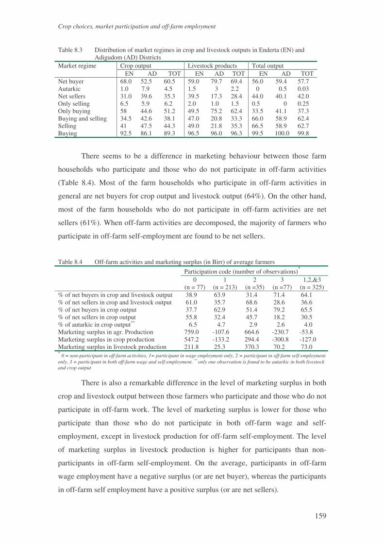
Crop choices, market participation and off-farm employment
159
Table 8.3 Distribution of market regimes in crop and livestock outputs in Enderta (EN) and Adigudom (AD) Districts
Crop output Livestock products Total output Market regime EN AD TOT EN AD TOT EN AD TOT Net buyer 68.0 52.5 60.5 59.0 79.7 69.4 56.0 59.4 57.7 Autarkic 1.0 7.9 4.5 1.5 3 2.2 0 0.5 0.03 Net sellers 31.0 39.6 35.3 39.5 17.3 28.4 44.0 40.1 42.0 Only selling 6.5 5.9 6.2 2.0 1.0 1.5 0.5 0 0.25 Only buying 58 44.6 51.2 49.5 75.2 62.4 33.5 41.1 37.3 Buying and selling 34.5 42.6 38.1 47.0 20.8 33.3 66.0 58.9 62.4 Selling 41 47.5 44.3 49.0 21.8 35.3 66.5 58.9 62.7 Buying 92.5 86.1 89.3 96.5 96.0 96.3 99.5 100.0 99.8
There seems to be a difference in marketing behaviour between those farm
households who participate and those who do not participate in off-farm activities
(Table 8.4). Most of the farm households who participate in off-farm activities in
general are net buyers for crop output and livestock output (64%). On the other hand,
most of the farm households who do not participate in off-farm activities are net
sellers (61%). When off-farm activities are decomposed, the majority of farmers who
participate in off-farm self-employment are found to be net sellers.
Table 8.4 Off-farm activities and marketing surplus (in Birr) of average farmers Participation code (number of observations)*
0 (n = 77)
1 (n = 213)
2 (n =35)
3 (n =77)
1,2,&3 (n = 325)
% of net buyers in crop and livestock output 38.9 63.9 31.4 71.4 64.1 % of net sellers in crop and livestock output 61.0 35.7 68.6 28.6 36.6 % of net buyers in crop output 37.7 62.9 51.4 79.2 65.5 % of net sellers in crop output 55.8 32.4 45.7 18.2 30.5 % of autarkic in crop output** 6.5 4.7 2.9 2.6 4.0 Marketing surplus in agr. Production 759.0 -107.6 664.6 -230.7 -53.8 Marketing surplus in crop production 547.2 -133.2 294.4 -300.8 -127.0 Marketing surplus in livestock production 211.8 25.3 370.3 70.2 73.0 * 0 = non-participant in off-farm activities, 1= participant in wage employment only, 2 = participant in off-farm self-employment only, 3 = participant in both off-farm wage and self-employment. ** only one observation is found to be autarkic in both livestock and crop output
There is also a remarkable difference in the level of marketing surplus in both
crop and livestock output between those farmers who participate and those who do not
participate in off-farm work. The level of marketing surplus is lower for those who
participate than those who do not participate in both off-farm wage and self-
employment, except in livestock production for off-farm self-employment. The level
of marketing surplus in livestock production is higher for participants than non-
participants in off-farm self-employment. On the average, participants in off-farm
wage employment have a negative surplus (or are net buyer), whereas the participants
in off-farm self employment have a positive surplus (or are net sellers).

Chapter 8
160
The average off-farm income (off-farm labour income and non-labour income)
of net buyers is higher than those of net sellers (Table 8.5). However, the average
income from self-employment is higher for net sellers than for net buyers. This may
be due to the fact that those who participate in off-farm self-employment have higher
farm output or their production is more oriented towards the market. Since farmers are
often borrowing or liquidity constrained, only those who have enough capital (with
higher farm income) have the capacity to join off-farm self-employment. This type of
income can be one of the sources of income inequality in rural areas (see Chapter 7). Table 8.5 Off-farm income and participation in the product market of average farmers Net sellers Net buyers Off-farm self-employment income 345 222 Off-farm wage-employment income 632 974 Non-labour income 172 206
8.3 Theoretical background
Crop choice and allocation of land and labour. In a farm household model setting,
a farm household’s decision to grow a crop involves a discrete choice on whether to
grow a particular crop (see Chapter 3 for a mathematical exposition). This decision
depends on the marginal productivity of land across crops. If corner solutions exist,
i.e., some crops receive a zero amount of land, the marginal productivity of land for
crops receiving a zero amount of land is less than the marginal productivity of land for
crops receiving a positive amount of land.
When the production and consumption decisions are separable (Singh et al.,
1986) and there are perfect input and output markets, farms should grow the most
profitable crops. There is no need to have enough family labour and land to run a
farm. In the presence of a perfect insurance market, production choice, particularly
crop choice, should not depend on the consumption and risk preferences of the
producers (Sandmo, 1971; Fafchamps, 1992). In most developing countries, however,
agriculture is highly risky and the insurance and credit markets are far from perfect
(Fafchamps, 1992). It is also known that farmers are risk averse (Binswanger, 1980),
and their risk aversion depends on the level of wealth. Poor farmers in developing
countries attempt to minimise their exposure to risk by growing their own food
(Roumasset, 1976, Fafchamps, 1992). Furthermore, the price and production risk
Crop choices, market participation and off-farm employment
161
associated with crops might also induce households to grow a particular type of food
crop that is not profitable, but dependable (Fafchamps, 1992). Under any of these
market imperfections, the production and consumption decisions of farm households
are not separable (Benjamin, 1992; Roe and Graham-Tomasi, 1986). As a result, crop
choice and land and labour allocation to crops depend on consumption preferences,
household composition, and risk considerations.
A risk-averse household reduces the production of food crops for which
income elasticities are large. This is because high-income elasticity leads to expected
utility gain from price variability (Turnovsky, Shalit and Schmitz, 1980).
Consequently a farm household with high-income elasticity for the crop will find it in
its interest to be less insured and therefore, grows less of that crop (Fafchamps, 1992,
p. 93). Hence the production of crops with high-income elasticity such as vegetables,
fruits, meat, dairy, oilseeds and spices will be proportionally lower than other crops
whose income elasticity is lower, such as cereals. More risk-averse farmers will seek
also to insure themselves against consumption price risk by increasing the production
of consumption crops.
The decision on how much labour to apply to each crop grown can be updated
regularly depending on the changing current and expected future conditions. This
decision to allocate labour for each crop depends on the demand for labour by each
crop if the production and consumption decisions of households are separable.
However, the production and consumption decisions of farm households in
developing countries are far from separable. Hence, the labour allocations for crops
not only depend on the demand for labour, but also on factors affecting the supply of
labour. In other words, the labour allocation decision of farm households for crops
depends on factors that affect both the demand for and supply of labour. These factors
include the level of land allocated to each crop, agronomic conditions, expected yield,
household composition (which affect the time available for work and leisure),
household taste shifters (such as education and age), risk consideration and off-farm
employment.
Most farmers do not specialise in growing a specific crop; rather they grow a
variety of crops. If their decision is not rational, they lose the gain they would have
achieved from specialisation. A farmer’s decision to grow a variety of crops at the
same time may be rational for many reasons. If there is constant returns to scale, two
or more crops can be grown to make use of the available resources (Burger, 1994). If

Chapter 8
162
there is increasing and decreasing returns to scale, the choice that can rationally be
made depends on the farm size. Due to transaction costs in the output market, the
shadow price of products may lie between the selling price and the purchase price, i.e.
within the price band. Then the shadow price of crops for a household is internally
determined by the relative marginal utility of crops grown. When the price band is
wide enough, crop choices and labour and land allocations are determined by
household preference. When an increasing amount of food becomes available, with
decreasing marginal utility of food, increasing use of land and labour for a given crop
leads to a decline in the shadow price of that crop. At some point, substituting that
crop with another more attractive crop would be inevitable.
Off-farm employment may substantially complicate farm management
because it can introduce the possibility of simultaneously having more cash and less
labour. Farm households who strive for subsistence using labour-intensive techniques
may choose to work off-farm and use the income to finance farming so as to make
working on the farm less onerous or increase the return to farm labour. They may also
rearrange their crop choices to suit off-farm work. As a result they may prefer to grow
crops that need less labour, for example cereals rather than vegetables. On the other
hand, farm households with adequate capital but excess family labour may not modify
their farming practices; rather they may simply boost their level of consumption. If
there is disguised unemployment or underemployment, off-farm jobs may have
practically no effect on farming systems. When farm households are not able to find
permanent off-farm jobs and have to choose among low-paying occasional off-farm
jobs, they may suit off-farm work schedule to the labour demand of their farm instead
of the other way round. Off-farm income may also lower risk aversion. As a result,
off-farm income may induce farm households to grow crops that are risky but
remunerative or that require more purchased input.
Marketing of farm output. Farmers face a decision problem of whether or
not to participate in the sale and purchase of farm outputs, and if they participate, how
much to sell and buy. A farm household can be either autarkic (self-sufficient), buyer,
or seller in a product market for agricultural goods. When the production and
consumption decisions are made simultaneously, the purchase and sale of agricultural
output (Strauss, 1984; Goetz, 1992) are determined by a vector of prices, wage rates,
household characteristics affecting taste and availability of time for work and leisure,
exogenous income, farm characteristics including fixed inputs, and a vector of

Crop choices, market participation and off-farm employment
163
production technology. However, farm households may fail to participate in the
market due to transaction cost. In areas with a sparse market, it is time consuming to
discover trading opportunities. Poor market access due to lack of transport, distance,
and other barriers such as low information may increases a farm household’s cost of
observing market prices in order to make transaction decisions.
Off-farm work participation and the level of farm income may also affect their
participation in the product market. The level of off-farm income may increase or
reduce market participation. A farm household with more off-farm income may use it
to finance its farm activities such as hiring of farm labour and purchasing of capital
input and may engage in farm production on the basis of the profit maximisation
motive. On the other hand, a farmer whose off-farm income is high can meet his cash
requirement from the off-farm income he receives and grow crops for own
consumption and sell less of his output. A farmer with more off-farm income can
participate actively in the product market as a buyer. A farmer who works more in
off-farm activities may produce less and meet his consumption through the purchase
of farm output. Therefore participation of farmers in the product market as seller will
be higher for those with higher off-farm income than those with lower off-farm
income.
8.4 Model specification and estimation method
Model specification. The following sets of econometric models are constructed to
model the crop choice, labour and land allocation decisions of farm households. A
household i’s choice of crop j (crij) can be modelled using a logit model (for
application see Burger, 1994). The assumption underlying the logit model is that the
error term of the utility that households attach to each choice has a cumulative
distribution of the hyperbolic-secant square (sech2) distribution (Maddala, 1983, p. 9),
which implies that the optimal choice is distributed as a logistic statistic:
�=
j ij
ijij x
xcrpr
)exp(
)exp()(
αα
(8.1)
Chapter 8
164
where pr(crij) is the probability household i chooses crop j, α is a parameter, xi is a
vector of explanatory variables1. The share of land (GC) a household i allocates for
crop j is given by
00
,0),(
==
>=
ijij
ijijijij
crifGC
crifexfGC γ (8.2)
where γ is a parameter xi is a vector of explanatory variables and e is the error term.
The allocation of labour hours (LC) by household i for crop j is given by
otherwiseLCLCifexfLC ijijijijij 0,0),( =>= β (8.3)
where β is a parameter, xi as a vector of explanatory variables and e is the error term.
With regard to product market participation, farm households face a two-stage
decision problem. The first is a discrete decision whether or not to trade (depending
on the cost of market participation) and in which direction (either as buyer or as a
seller). The second is (continuous decision) how much to trade conditional on
participation as a buyer or seller. Let the utility attained if the household sells output
be Usi, if he buys output be Ub
i, when he does not sell be UNSi, does not buy be UNB
i.
Let also D1 be the index of participation in a product market as a seller; D2 be the
index of participation in the product market as a buyer, S* be the potential level of
farm output the household can sell, B* be the potential level of farm outputs the
household can purchase; and S and B are observed sales and purchase levels,
respectively. Then the household’s probability and level of participation in the
product market can be modelled as:
)0Pr()(Pr)1(Pr0;1
11/
11
11
>+=>==≤=>=
iNS
iS
ii
NSi
Sii
NSi
Sii
uXUUDUUifDUUifD
α (8.4)
)0Pr()(Pr)1(Pr0;1
22/
22
22
>+=>==≤=>=
iNB
iS
ii
NBi
Bii
NBi
Bii
uXUUDUUifDUUifD
α (8.5)
00;1
),0(~;)(
11*
21111
/111
*
====
+=+=
iiiii
eiiiii
DifSDifSS
NeeXeXSS σβ (8.6)
00;1
),0(~;)(
221*
22222
/222
*
====
+=+=
iiiii
eiiiii
DifSDifBB
NeeXeXSB σβ (8.7)
where X is a vector of explanatory variables, u’s are the error term of the participation
decision, e’s are the error term of the continuous variable decisions and α and β are
1 The vector of explanatory variables (xj) is constant across crops.

Crop choices, market participation and off-farm employment
165
parameters to be estimated. When the error terms of the participation decision and
continuous decision are correlated (Amemiya 1984, p. 31-32; and Blundell and
Meghir, 1987, p. 187), the sales (8.6) and purchase (8.7) equations can be written
respectively as:
iiei euXS 1*
1111/
1* ++= σρβ (8.8)
iiei euXB 2*
2222/
2* ++= σρβ (8.9)
where ρ1 and ρ2 are the correlation coefficients between the error terms of the
participation decision and the extent of participation decision in the sales and
purchase equations. Equation (8.8) and (8.9) can be estimated using either a two-stage
process or using the generalised tobit model (Amemiya, 1984).
Estimation Method. The logit models of crop choice (8.1) and the tobit
models of land (8.2) and labour allocation (8.3) are estimated using the maximum
likelihood estimation method. The estimations are done for seven categories of crops
namely teff, wheat, barley, sorghum and finger millet, legumes, oil crops and
horticultural crops.
Variables that reflect profitability, agronomic conditions, consumption
preferences and risk consideration are used as explanatory variables in the logit model
of crop choice, land and labour allocation equations. Age and age square of the
household head, family size, dependency ratio, year dummy, location dummies,
dummies for soil types, soil depth index and value of farm implements and number of
oxen owned are used as explanatory variables in both the logit model of crop choice
and labour allocation equations. Besides, off-farm income, total land cultivated and
share of crop in total expenditure are also used as explanatory variables in the crop
choice model. In the land allocation equation (8.2), off-farm income, total animal
wealth, total land cultivated, value of output expected2, number of dependants, family
size, value of farm and non-farm equipment owned, education and year dummies, the
proportion of clay soil and sandy soil cultivated and soil depth indicator are used as
explanatory variables. In the labour allocation equation (8.3), off-farm labour hours,
level of land allocated and variable inputs used are included in the list of explanatory
variables. In all equations, off-farm income, off-farm hours worked, share of crops in
total consumption, and expected yield are treated as endogenous variables. The rest of
2 The value of actual output is used as a proxy for the expected value of farm output.

Chapter 8
166
the explanatory variables are assumed to be exogenous. For all endogenous variables,
their predicted values are used in place of their observed values. Off-farm income and
off-farm hours worked are predicted from a tobit model. This is equivalent to using a
two stage tobit model (Maddala, 1983, pp. 245-246).
The following strategy is followed to estimate the market participation. First
the bivariate probit equations of participation as buyer or seller in the product market
(equation 8.4 and 8.5) are estimated jointly (which is analogous to Zellner’s
seemingly unrelated regression, SUR). This estimate is compared with the single
probit estimates of equation 8.4 and 8.5. Then the selectivity term or inverse mills
ratios are constructed from the best estimates. Second, using the selectivity term
derived from the probit equations, the level of sales (8.8) and purchase (8.9) equations
are estimated using 3SLS estimation method. Age, age square, education dummies,
year dummy, family size, dependency ratio, value of transport animals, value of farm
output, off-farm income and variables that reflect transaction cost such as location
dummies are used as explanatory variables in both the purchase and sales decision.
Off-farm income and farm outputs are considered to be endogenous and the rest are
assumed as exogenous variables. Instrumental variables, which are included and
excluded in turn in the model, are used to predict the off-farm income and farm
output. The instrumental variables used that are excluded from the model are farm
labour used, area of land cultivated, variable inputs, off-farm wage rates, livestock
wealth and farm and non-farm equipment.
8.5 Estimation results and discussion
Crop choice. The probability of growing a particular crop is influenced by agronomic
conditions such as soil type and depth, the level of land cultivated and partly by the
availability of equipment and number of oxen owned (Table 8.6, see also Appendix
A8.2). As one usually expects, the amount of land cultivated has significantly
increased the probability of growing crops for all seven types of crop. The availability
of sandy type soil (hutsa) has increased the probability of growing wheat and
vegetables. The probability of growing teff is higher for households who have black
and deep soil. The availability of black soil has also increased the probability of
growing vegetables. While the value of farm implements owned increases the
probability of growing teff, it decreases the probability of growing barley. The

Crop choices, market participation and off-farm employment
167
ownership of oxen has significantly increased the probability of growing barley, but
its parameters are insignificant from zero at 10% for the rest of the crops.
The year dummy shows a significant influence on the probability of growing
teff and finger millet and sorghum. It may have captured the timing of rainfall. The
growing of teff and finger millet and sorghum depends on the timing of rainfall. If
there is rainfall in May, farmers grow sorghum, whereas if there is no rain in the
month of May, farmers grow teff in place of sorghum. In May 1996 there was
sufficient rainfall to grow sorghum, where as in May 1997 the level of rainfall was not
sufficient to grow sorghum and finger millet. As a result the probability of growing
teff was lower in 1996 than in 1997 while the probability of growing finger millet and
sorghum was higher in 1996 than in 1997.
Table 8.6 Elasticity for the probability of growing crops using instrumental variables Crops/variables Teff wheat Barley Sorghum Legume Oil crops Veg Family size 0.118 0.155 0.090 0.061 0.178 0.006 -0.092** Dependency ratio -0.090 0.085 -0.008 -0.051 -0.099 0.075 0.046 Soil depth index 0.247*** 0.099 0.10*** 0.014 0.076 0.044 0.045 Off-farm income 0.096 -0.193 -0.114 -0.014 -0.039 -0.107** 0.040 Value of farm implements 0.162** -0.025 -0.09** -0.002 -0.035 -0.042 0.005 Number of oxen owned -0.012 0.069 0.082** 0.001 -0.074 0.000 -0.011 Land cultivated 0.271*** 0.33*** 0.20*** 0.037** 0.580*** 0.032 -0.002 Share in total consumption 0.223 0.025 0.161 -0.093 0.156 0.000 -0.087*** *** stands for significance at 1 %; ** stands for significance at 5 % and * stands for significance at 10 % level.
The results also show that non-farm income, share of crops in total
expenditure, age, education, location dummies and household compositions such
family size and dependency ratio do not affect the probability of growing crops by
farm households in the sample. It is not surprising to see that off-farm income has
insignificant influence on crop choice because in areas with a substantial under-
employment, farm households are expected to adjust their off-farm activities to their
farming conditions. The parameters of the share in total consumption are not
significantly different from zero for all crops except vegetables. Besides the
parameters for the share in total expenditure are negative for sorghum and vegetables,
contrary to our expectation. The impact of family size is positive for all crops except
for vegetables and is higher for teff, wheat and legumes. When the dependency ratio
increases the probability of growing wheat and oil crops increases while the
probabilities for teff, barley, sorghum and legumes decline. However, none of the

Chapter 8
168
parameters for household composition and consumption preference variables are
significantly different from zero.
Land allocation. The share of land allocated to crops is greatly dependent on
factors affecting profitability (yield), risk bearing ability (livestock, wealth, and value
of equipment owned), off-farm income, and availability of land (Table 8.7, see also
Appendix A8.3). The share of land allocated to all crop types declines when the area
of total land cultivated increases. However, the level of land increases for all crops
when total land cultivated increases. The average land shares, the marginal land
shares and the elasticity of land allocated for each crop with respect to the total land
are summarised in Table 8.8. All crops have positive elasticity, but less than unity3.
The highest land elasticity for land allocation goes to vegetables and oil crops, which
are less productive.
As theory and empirical evidence suggest (Chavas and Holt, 1990), land
allocation is significantly influenced by the economic return. The expected yield has
increased the share of land allocated to all crop types. The highest response of land
allocation to the expected return is in case of teff followed by wheat and barley. These
crops are the main food crops and the sources of cash in the area. Off-farm income
and wealth also show some influence on the land allocation. While off-farm income
decreases the share of land allocated to teff, wheat, barley and finger millet and
sorghum, it increases the share of land allocated for legumes and oil crops, which
require less labour per unit of land. The influence of off-farm income on land
allocated for sorghum and finger millet and oil crops is not significantly different
from zero at any reasonable level of significance. The positive impact of off-farm
income on the level and share of land allocated to legumes shows that off-farm
income helps farmers to exercise land-augmenting practices. Legumes are usually
planted after a series of cereals in order to improve the productivity of land (by fixing
nitrogen to the soil). The wealth variables show mixed result on land allocation.
Livestock wealth increases the share of land allocated for wheat, finger millet and
sorghum and legumes but decreases the share of land allocated for teff, barley, oil
crops and vegetables. Farm and non-farm implements reduce the share of land
allocated for teff, wheat, barley, legumes and vegetables, but increase the share of
3 If all farm households were growing all crops, marginal budget shares would add up to one and the elasticity of all crops would not be leas than one. Farm households must be shifting to a new crop when area of land under cultivation increases.

Crop choices, market participation and off-farm employment
169
land allocated to finger millet and sorghum and oil crops. In general the result of
wealth variables is not consistent regarding the response of crop choice to risk. The
expectation was that wealth variables would increase the share of land allocated to
relatively risky crops (such as teff and wheat) and decrease the share of land allocated
to relatively less risky crops (such as barley, finger millet and sorghum).
The results on the influence of consumption preference also do not coincide
with our expectation. When farm household’s consumption and production decisions
are inseparable, one normally expects consumption preferences to influence crop
choice decision. However, consumption preference does not affect the land allocation
decision of farm household at all. For all crop types, the influence of the share of
crops in total consumption on land allocation is not significantly different from zero at
any reasonable significance level. Besides, the impact of the shares in total
consumption is negative for finger millet and sorghum and vegetables.
Table 8.7 Elasticity of share of land allocated to crops at mean values Teff Wheat Barley SFM Legumes Oil crops Veget. Off-farm income -0.2263*** -0.1989*** -0.3645*** -0.1151 0.0923 0.0590 -0.0512 Total animal wealth -0.0052 0.0037 -0.0469*** 0.0251 0.0005 -0.0091 -0.0045 Equipment owned (Birr) -0.0625** -0.0465** -0.0736*** 0.0008 -0.0001** 0.0240 -0.0559 Total land cultivated -0.6146*** -0.5891*** -0.3099*** -0.5407*** -0.4344*** -0.277* -0.0435 Expected yield 0.7749*** 0.5685*** 0.5339*** 0.2701*** 0.5783*** 0.1856*** 0.1751*** Share in total expenditure -0.0197 0.2773 0.0929 -0.0521 -0.7716 -0.1751 -0.3397 Number of dependants -0.1386 -0.3116** -0.1787** -0.3436 -0.2634 0.2637 -0.0099 Family size 0.4226*** 0.7492*** 0.4542** 0.6168 0.4590 -0.5554 0.1857 Proportion of clay soil 0.1191*** 0.0502*** 0.0320** 0.0426 0.1046** 0.0764 0.1893*** Proportion of sandy soil 0.0799*** 0.1049*** 0.0777** 0.0379 0.0105 0.0062 0.2991*** Soil depth index 0.2821*** 0.3867*** 0.4446 0.1643 0.3530*** 0.2222 0.1152*** *** Stands for significance at 1 %; ** stands for significance at 5 % and * stands for significance at 10 % level. SFM is sorghum and finger millet.
Land allocation is greatly influenced by family composition. Family size
shows a significant and positive influence on the share of land allocated to teff, wheat
and barley. This may imply that farm households allocate more land to the main food
crops, which require relatively higher amount of labour in production. Teff, wheat and
barley are crops that require higher amount of labour and are the main food crops in
the area. The influence of the number of dependants is negative and significant for
wheat only. The allocation of land is also greatly influenced by natural environmental
conditions such as rainfall and soil types. More land is allocated in 1996 than in 1997
for sorghum and finger millet. This is due to the favourable rainfall conditions in
1996. The share of land for barley is higher when the soil is deep and sandy. Legume

Chapter 8
170
crops receive a higher share when the share of black soil cultivated increases. Teff and
wheat receive a higher share of land in deep, black and sandy soils.
No meaningful result is obtained regarding the effect of education on land
allocation decisions. The education dummy of the household head show positive
impact on the land allocation for wheat, finger millet and sorghum, and negative
impact for teff, barley and vegetables. However, none of the parameters are
significantly different from zero at 10% level, except for teff and vegetables.
Table 8.8 Average land share, marginal land share and total land elasticity of land allocation Crop type Average land
share Marginal land share
Elasticity land with respect to total land cultivated
Teff 0.197 0.089 0.45 Wheat 0.250 0.118 0.47 Barley 0.364 0.263 0.72 Sorghum and F. millet 0.049 0.035 0.51 Legumes 0.110 0.067 0.61 Oil crop 0.018 0.013 0.76 Vegetables 0.010 0.010 0.93 Labour allocation. The most important factors that influence the labour
allocation decision of farm households are soil type, soil depth, area land allocated,
the level of labour supplied off-farm, farm equipment and oxen (Table 8.9, see also
Appendix A8.4). Household composition and labour availability also has limited
influence on the labour allocation of farm households. Controlling for agronomic and
other social and economic factors, off-farm employment show a significant negative
impact on the level of labour allocated for teff, wheat, barley and vegetables. The
impact for sorghum, finger millet, legumes and oil crops is not significantly different
from zero.
The amount of labour allocated to all crops increase with the amount of land
allocated except for vegetables. It also increases with increasing soil depth for all
crops except for sorghum, oil crops and vegetables. Households with a higher
proportion of sandy soil use a higher amount of labour for wheat and barley. Family
size (showing the availability of labour) shows a positive and significant impact only
on the level of labour allocated to wheat. Its impact for the rest of the crops is
insignificant. While the level of farm implements owned increases the use of labour
for teff, it reduces the use of labour for wheat. Its impact on the rest of the crops is
statistically insignificant. The ownership of oxen shows a significant positive effect
on the labour use for wheat only.

Crop choices, market participation and off-farm employment
171
The use of variable farm inputs such as fertiliser, insecticide and improved
varieties increases the use of labour for wheat, barley, sorghum, finger millet and
legumes. Its impact on the use of labour for teff, oil crops and vegetables is not
significantly different from zero. The positive impact of farm variable inputs implies
that the intensive use of commercial inputs can be used as a means to promote on-
farm employment. Purchased capital inputs such as fertiliser and improved seeds can
increase on-farm employment not only because they are labour using, but because
they are also land augmenting. Hence the intensive use of variable farm inputs can
increase the return to family labour on the farm and encourage family members to use
more labour on the farm.
Table 8.9 Elasticities of labour allocation across crops Teff Wheat Barley SFM Legum Oil Vege Family size 0.108 0.308** 0.085 0.470 0.133 -0.775 0.414 Dependency ratio -0.019 -0.020 -0.034 -0.664 0.016 0.521 0.786 Soil depth index 0.255*** 0.240*** 0.129*** 0.532 0.273*** -0.192 0.160 Hours worked off-farm -0.27*** -0.254** -0.149** -0.490 -0.180 -0.311 -2.403** Value of farm implements 0.133*** -0.112** 0.026 -0.381 0.007 0.244 0.186 Value of oxen owned -0.004 0.088* -0.017 0.063 -0.049 -0.168 -0.671 Land cult. with spec. crop 0.525*** 0.439*** 0.459*** 0.24*** 0.339*** 0.31*** 0.309*** Variable farm inputs used 0.012 0.102*** 0.137*** 0.10*** 0.114*** 0.027 0.028 *** Stands for significance at 1 %; ** stands for significance at 5 % and * stands for significance at 10 % level.
Product marketing behaviour. Single equation and full information
maximum likelihood bivariate probit equations were estimated. But the estimates of
the cross equation correlation in the bivariate probit model is not significantly
different from zero at any reasonable level. So single equations probit estimates are
sufficient to construct the selectivity term (inverse mills ratio). Hence the results of
the single probit equations are used for the rest of the discussion.
The probability and level of participating in the product market both as a buyer
and as a seller is significantly influenced by transaction cost, level of output and off-
farm income (Table 8.10, see also Appendix A8.5). The variables reflecting
consumption preferences (such as dependency ratio), family size, education and age
do not affect the market behaviour of farm households. Those villages that are far
from market areas have a low probability and level of buying and selling agricultural
outputs than those villages nearer to market area signifying the importance of
transaction cost. The level of output reduces the probability and the level of
participation in the market as a buyer and increases the probability and level of

Chapter 8
172
participation in the market as a seller. The magnitudes of the impact are higher for
sellers than for buyers. The output elasticity of sales is greater than unity (1.3) while
the output elasticity of purchase is inelastic (-0.354).
The off-farm income affects the marketing behaviour of households through
its influence on the sale and purchase of farm outputs in the opposite way. While off-
farm income increases the probability and level of purchase of agricultural output, it
reduces the probability and level of sales of agricultural outputs. However, the impact
on the level of sales is very small and not significantly different from zero. This
implies that when off-farm income increases, the marketing surplus of farm output
decreases, but very small. To elaborate more, for most of the small farmers who do
not have another source of income (such as off-farm income), the main source of cash
income is the sale of farm output. To buy compulsory food and non-food items, which
cannot be produced on their farm (such as salt, spices, clothes and taxes), farm
households have to sell farm output. When the farm households obtain off-farm
income, they can stop selling farm output and use the cash obtained from off-farm
work to purchase the food and non-food items required. However, off-farm
employment can help farm households finance their farming activities through the
purchase of farm inputs such as hired labour, fertiliser, and improved seeds. In a
drought prone area, off-farm income can help to purchase food for consumption and
keep farmers productive on their farm. As a result, off-farm employment can increase
farm output and its negative impact on the sale of farm output can be very low.
Therefore, in a less dynamic agricultural area, the impact of off-farm employment on
the marketing surplus of farm outputs could be very minimal.
Table 8.10 Elasticities of market participation and the level of purchase and sales in the product
market Variable Probability of
being Buyer Probability of being Seller
Purchase Sales
Family size -0.080 0.125 0.260 -0.160 Dependency ratio 0.098* -0.013 0.240 0.113 value of transport animals owned -0.004 0.049 -0.020 0.016 total value of crop yield -0.040** 0.253*** -0.354*** 1.303*** Off-farm income 0.053** -0.057** 0.153*** -0.018 *** Stands for significance at 1 %; ** stands for significance at 5 % and * stands for significance at 10 % level.
The selectivity terms (inverse mills ratio) show that buying and selling
households sell and buy more than the households selected at random. This result
suggests that those who participate in the product market have a comparative
Crop choices, market participation and off-farm employment
173
advantage in the market either as buyers or sellers, due to lower transaction cost and
unobservable factors such as farmers’ skill and access to information and information
sources.
8.6 Conclusions
Crop choice and land and labour allocation decisions of farm households and their
relation with off-farm employment are modelled in a non-separable agricultural
household model setting. Due to the existence of substantial underemployment in the
area, the influence of off-farm employment on the crop choices of farm households is
not substantial. Instead farm households adjust their off-farm activities to their
farming condition in most of the cases. The influence of off-farm employment is
rather slightly stronger on the land and labour allocation decisions of farm
households. It increases the allocation of land for legumes and oil crops, which are
less productive, less labour using and land improving. Off-farm employment also
reduces the use of labour for cereals implying that off-farm employment competes
with farming activities for labour. The results also show that crop choice, land and
labour allocation decisions of farm households are influenced by agronomic
conditions (such as soil type and depth), the area of land cultivated, risk
considerations and partly by the availability of equipment and number of oxen owned.
Furthermore, off-farm employment influences the marketing behaviour of
farm households. While the probability and level of purchase of food increases with
increasing off-farm income, the probability of grain sales decreases with increasing
off-farm income. The negative impact of off-farm income on the marketing surplus of
farm outputs is found to be very minimal. Farmers are restricted from participating in
the product market because of lower farm output and off-farm income, higher
transaction cost and lack of access to information and information sources. Although
the majority of farm households are reasonably linked to a product market, the
majority of them are net buyers, which limits the use of pricing policy as a means to
raise the income of farm households in the region. Given that the majority of farmers
are net buyers, pricing policy in order to protect consumers is as important as pricing
policy to protect producers. In general there is little relevance for pricing policy in the
area. Rather it will be beneficial to take measures to reduce the transaction costs by
improving the infrastructure. Proximity to market and alternative income
opportunities such as off-farm activity will improve the link of farmers to the market.

Chapter 8
174
Improving the link of farmers to the market means that the government has alternative
policy instruments to achieve its desired objectives.

Production and consumption linkages and the development of rural non-farm enterprises
175
CHAPTER 9. PRODUCTION AND CONSUMPTION LINKAGES AND
THE DEVELOPMENT OF RURAL NON-FARM
ENTERPRISES
9.1 Introduction
The foregoing chapters have demonstrated that there is underemployment in the rural
areas of Tigray. Farm households are endowed more with labour than with capital and
land. They employ a low level of capital and operate small farms. As a result the
present farming system is not dynamic enough to absorb the growing population. On
the average, farm households use not more than 53% of their available time working
on and off-farm (see Chapter 6 and Chapter 7). Due to the seasonality of agricultural
production, rural labour cannot be employed fully unless irrigation agriculture or rural
non-farm activities are widely adopted. Neither irrigation facilities nor non-farm
activities are developed sufficiently to employ the surplus rural labour at the moment.
Irrigation development alone cannot be relied upon to reduce under-employment in
rural areas because its development is too slow to tackle the problem. Labour under-
utilisation can be attacked on either the supply side or the demand side of a labour
market. In practice, little can be done to bring about a supply-side adjustment. The
labour force is currently growing faster than employment. The only real supply-side
alternative is to reduce the growth of labour supply by limiting the population growth,
which is quite difficult in developing countries at the moment. Hence policy must
concentrate on the demand side of the labour market in order to reduce or ameliorate
underemployment of the rural labour force. Among others, the promotion of micro
and small-scale enterprises (MSE) in rural areas can reduce the problem of rural
underemployment.
Despite their importance, development policies usually neglect the role of
rural non-farm activities and their link to agriculture. This might be due to the fact
that the role of the rural non-farm sector in the rural economy is poorly understood.
The knowledge gap in the role of the rural non-farm sector is reflected in the policies
of the developing countries. Particularly in Ethiopia, there is no development policy
that identifies and includes the rural non-farm sector as an important component of the
economy and a source of employment. The agricultural ministries have focused on

Chapter 9
176
farming and the industry ministries have focused on industries. Rural non-farm
activities and their link to farm activities are completely neglected. The neglect of the
rural non-farm sector as well as their link to the agricultural sector is socially costly
(Lanjouw and Lanjouw, 1997). Without recognising the importance of the rural non-
farm sectors, the sector’s potential role in absorbing the growing rural labour force, in
reducing rural-urban migration, in contributing to the national economy and
promoting a more equitable distribution of income cannot be materialised. It is
crucial, therefore, to identify the contribution of micro and small- scale enterprises to
development (to employment, income generation and poverty alleviation) and to make
policy makers aware of the roles played by MSEs.
The contribution of agricultural production to rural non-farm activities is well-
documented (Haggblade, Hazell and Brown, 1989; Bagachwa and Stewart, 1992;
Reardon, 1997). A rising agricultural income stimulates the growth of rural non-farm
activities through production, consumption, and labour market linkages. A growing
agricultural sector can increase employment in the non-farm sector through the
demand for purchased agricultural inputs (backward production linkages) and
consumption goods and services (consumption linkages) and the supply of raw
materials for processing and distribution (forward production linkages). An increase
in agricultural income raises the opportunity cost of labour in non-farm activities
(labour market linkages), and thereby induces farm households to shift from very
labour-intensive, low return off-farm activities into more skilled, higher-investment,
high-return activities. In fragile and marginal areas, non-farm income can reduce the
incidence of poverty and the direct dependence on land which affects the
environmental quality, crop mix and cropping potentials (Reardon et al., 1998;
Reardon and Vosti, 1995). However, the magnitude and relative strength of the
production and consumption linkages are not well known in Ethiopia, particularly in
Tigray.
The objective of this chapter is (1) to analyse the developments and constraints
of rural small-scale enterprises and their link to the agricultural sector; and (2) to
examine the production and consumption linkages as well as their relative strength.
The contribution of this chapter is, therefore, to fill the gap in understanding about the
type and magnitude of the linkages that exist between the farm and non-farm sectors
in the region using already well established methodology (Hazell and Roëll, 1983).

Production and consumption linkages and the development of rural non-farm enterprises
177
We try to explain and quantify the linkages that have not been examined so far in any
of the preceding chapters for the sake of completeness.
This chapter brings two different issues together each of which could have
been treated separately. However, because of lack of space and time, I choose to do
them in one chapter briefly. The first part deals with the problem and development of
micro and small-scale enterprises (MSE) as well as the general link that exists
between the farm and non-farm sectors in the Tigray Regional State. The analysis of
farm and non-farm linkages and constraints and development of MSE are based on
secondary data collected by the Central Statistical Authority of Ethiopia and the
Tigray Regional Bureau of Trade and Transport. The second issue is enumerating and
if possible, quantifying the production and consumption linkages that exist between
the farm and non-farm sectors. These linkages are enumerated and quantified using
the survey data obtained from a sample of 201 farm households in the two districts of
the Tigray Regional State. The development and constraints of rural micro and small-
scale enterprises are discussed in section three. In section four, production and
consumption linkages are assessed. The paper ends with some concluding comments.
9.2 Theoretical background
To bring economic growth to developing countries, it is advisable to adopt
technologies more appropriate to the factor endowment of the area (Gills, et al., 1992;
Hayami and Ruttan, 1985). Farm households in developing countries are endowed
more with labour than with capital. Land is also becoming the scarcest resource in
some African countries such as Ethiopia. As a result, wide underemployment of
labour is observed. Labour under-utilisation can be attacked on the supply side or the
demand side of a labour market, but little can be done to bring about a supply-side
adjustment. The labour force is growing faster than employment creation. It is quite
hard to discourage people from seeking work. The only real supply-side option is to
reduce the growth of labour supply by limiting population growth, which takes at least
15-20 years to stabilise the growth of the labour force. Hence policy has to
concentrate on the demand side of the labour market in order to reduce or ameliorate
underemployment of the rural labour force.
On the demand side, there are two different approaches to employment
creation. The first is to stimulate output, especially in relatively high-productivity and
Chapter 9
178
high wage sectors of the economy. The second one is to increase the amount of labour
used to produce a given amount of output (Berry, 1974). The first one deals with the
growth of export, output and industry (see chapter 17, 18, and 20 in Gills et al., 1992
for details). The second one implies making production more labour intensive.
Production can be made more labour-intensive by changing the relative prices and
thus creating incentives for businesses to substitute labour for capital. Certain
restrictions should be avoided in order to provide incentives for businesses to
substitute labour for capital. The restrictions include the imposition of artificially high
wages on the modern sector, which can result from the minimum wage laws of the
government and lobbying of trade unions; social security taxes on modern sector
payrolls; interest rate ceiling; overvaluation of domestic currency; import licensing;
and investment incentives proportional to the amount of capital invested. Such
restrictions could be avoided by deregulation and exposure to open competition or
could be offset by taxes and subsidies if the restrictions cannot be removed.
Production can be made more labour-intensive by developing technologies
more appropriate to the factor proportions prevailing in the area. In fact it is
controversial as to how such appropriate technology be acquired. However, broad-
based acquisition of technological capacity has to be developed gradually through
learning by doing. Income distribution in favour of the poor may sometimes
accelerate job creation because the goods consumed by the poor are more labour
intensive than the goods consumed by those who are better off (Mellor, 1966).
Seeking investments that complement labour rather than substitute for it can help to
increase employment. Examples of labour intensive investment are promoting
irrigation rather than large-scale plantation farming and providing training to fill the
skill gap so as to increase employment through increased absorption of
complementary unskilled labour. Most importantly, the promotion of micro and
small-scale enterprises (MSE) can ameliorate rural under-employment (Mead and
Liedholm, 1998; Liedholm, McPherson and Chuta, 1994) because most of the
products of MSE are more labour intensive than the products of large and medium
scale industries.
Agriculture plays a crucial role in rural enterprises employment generation.
Rising agricultural income stimulates the growth of non-farm activities in both rural
areas and towns (Reardon et al., 1998). When agriculture is dynamic enough to bring
about substantial change in household income and employment, it affects non-farm

Production and consumption linkages and the development of rural non-farm enterprises
179
activities (Reardon, 1997) in at least three ways (Haggblade and Hazell, 1989):
through production, through consumption, and through labour market linkages. On the
production side, a growing agricultural sector requires farm inputs such as fertiliser,
insecticide, pumps, equipment, and repair services -either produced or distributed by
non-farm enterprises (backward linkages). Increased agricultural output stimulates
rural non-farm activities (forward production linkages) by providing raw materials
that require milling, processing and distribution by non-farm enterprises.
Consumption linkages arise when growing farm income boosts the demand for
basic consumer goods and services and results in the diversification of consumption
spending on products other than food. Non-farm enterprises in rural areas or in rural
towns can meet most of the demand by farm households for purchased farm inputs,
basic non-farm consumption goods and services that are either produced or distributed
locally. Average and marginal budget shares as well as the income elasticity of
consumption goods can help to determine the magnitude of consumption linkages in
an economy (Hazell and Hojjati, 1995). In particular, the decomposition of budget
shares and elasticity can provide useful information on how expenditure is distributed
across locations. To analyse the relative importance of different commodity groups in
the demand linkages, marginal budget shares and expenditure elasticity can be derived
from an Engel function with a non-linear relationship between consumption and
income.
The third linkage is labour market interactions. A growing agricultural sector
can raise agricultural wages and this in turn raises the opportunity cost of labour in
non-farm activities. This induces farm households to alter the composition of non-
farm activities and move out of very labour-intensive, low return activities into more
skilled, higher-investment, high-return activities. In general raising agricultural
productivity can be an instrument to induce structural transformation of the rural non-
farm economy.
With a dynamic agriculture, these linkages can bring about a virtuous spiral of
growth, employment and income for rural households (Reardon, et al., 1998). These
linkages are minimal in marginal areas or in areas where the agroclimate is poor, and
agriculture is risky and less dynamic. In marginal areas, the non-farm sector is rather
important since it enables rural households economy to cope with risks such as a poor
harvest. The non-farm sector can provide cash for buying food and farm inputs, and

Chapter 9
180
so alleviates a vicious circle of poverty-extensification-degradation-poverty (Reardon,
1998; Reardon and Vosti, 1995).
If agriculture is stagnant and lacks the growth impulses that operate via
demand-supply inter-linkages to the non-farm sector, the development of micro and
small-scale enterprises could be the result of under-employment in the agricultural
sector. In other words, the development of non-farm activities could be an outcome of
excessive demographic pressure coupled with the inability of agriculture to absorb the
expanding labour force rather than an outcome of transmission of positive growth
from the farm to the non-farm sectors. They call this a residual sector hypothesis in
Indian economic literature (Vaidyanathan, 1986; Verma and Verma, 1995; Shylendra
and Thomas, 1995), which is similar to the push and pull motives of income
diversification of farm households (Reardon, Delgado and Malton 1992; Reardon,
1997; Reardon et al. 1994). If the residual sector hypothesis is true, the development
of the agricultural and rural non-farm sectors will be negatively correlated.
In addition to the performance of the agriculture sector, other factors such as
the level of infrastructure, population density and growth, development of rural towns
(Haggblade, Hazell and Brown, 1989), policies and government regulations, human
capital, skill, caste, tradition, and the availability of non-agricultural raw materials as
well as social and political environment influence the performance and development
of the non-farm economy. The development of rural towns is very important for the
centralised and cost effective way of providing key infrastructure and services.
Infrastructure development reduces the cost of information and transportation which
in turn improves the efficiency with which rural labour and financial markets channel
inputs into activities yielding the highest returns. It also opens rural resources and
markets to viable exploitation, and facilitates a change to a more specialised and
productive rural economy. A higher density of population helps to attain a minimum
efficient scale for non-farm production and service delivery. It may also limit the
number of households that should survive from agriculture alone thereby forcing
some of the rural households into non-farm activities.
Location, nearby urbanisation and competition from imports also influence the
performance and growth of the rural non-farm sector (Haggblade, Hazell and Brown,
1989). The evidence from some African countries (for example, Ivory Coast) suggests
that rural manufacturing is most vulnerable from urban and imported substitutes,

Production and consumption linkages and the development of rural non-farm enterprises
181
while services and commerce are better insulated from urban competition (Haggblade,
1995).
9.3 Performance of rural small-scale enterprises and constraints for
development
9.3.1 Developments of micro and small-scale enterprises
In this section the development of small-scale non-farm activities will be discussed
based on the information obtained from the Central Statistics Authority (CSA, 1997b,
1997c, 1997d) of Ethiopia and Tigray Regional State Bureau of Industry, Trade, and
Transport (ITTB, 1998). This does not include the informal non-farm sector, as it is
difficult to get data on this sector. A discussion about the rural informal non-farm
activities as off-farm activities will be presented in the next section.
The following CSA classification of non-farm activities is used: (1)
distributive and service trade and (2) manufacturing industries. Distributive and
service trade is defined as an economic sector, which includes wholesale, retail trade
and commercial services. Manufacturing industries are divided into three: (1) large
and medium manufacturing industries are those which engage 10 or more persons and
use power-driven machines; (2) small scale manufacturing establishments that engage
less than 10 persons and use power driven machines such as bakeries, candy factory,
electric workshop, edible oil extraction etc.; (3) cottage/handicrafts manufacturing
establishments which perform their major activities manually (using mainly non-
power-driven machines). Here in this study, small scale manufacturing industries,
cottage/handicraft manufacturing establishment and distributive and service trade
(that are formally registered by government offices) are considered to be micro and
small-scale enterprises (MSE).
Statistics from ITTB (1998) show that small-scale manufacturing enterprises have
been flourishing for the last seven years. In 1991, small-scale industry was almost
non-existent except for cottage industries. In 1994 they showed a remarkable growth
and were 206 in number. In 1997, they number 599 (Figure 9.1). These small-scale
manufacturing enterprises provide employment for approximately five people per

Chapter 9
182
establishment. The average capital investment per establishment is 153 thousand Birr.
The most successful type of small-scale industry is a grain mill. About 20 % of the
small-scale manufacturing enterprises are found in Mekelle, Capital City of the
region. The rest (80%) are found in other zonal and district towns (Table 9.1). Most of
the raw materials used for production is locally produced. Imported raw materials
constitute about 14 % of the total raw materials used on the average. The ratio of
imported raw materials to total raw materials for publishing and printing enterprises,
manufacturing of machinery and metal products, and manufacturing of wearing
apparels are 83%, 61% and 53%, respectively.
Table 9.1. Distribution of small-scale manufacturing enterprises in Tigray in 1996/97 Count Investment (000’Birr) Employment Tigray 599 91651 2957 Mekelle 117 34253 842 Southern zone 117 15551 765 East zone 93 20873 521 Central zone 105 9370 373 Western zone 168 11983 558 Source: Bureau of Industry and Trade and Transport of Tigray Region, Statistical Bulletin 1, February 1998.
Figure 9.1 Development of Small Scale Manufacturing Enterprises in Tigray Region
0
100
200
300
400
500
600
700
1990
/91
1991
/92
1992
/93
1993
/94
1994
/95
1995
/96
1996
/97
Year
The
num
ber o
f ent
erpr
ises

Production and consumption linkages and the development of rural non-farm enterprises
183
The Central Statistics Authority has estimated cottage/handicraft enterprises to
be 25,012 in number, of which nine percent are found in the metropolitan city of
Mekelle. The rest is found in the other towns. Cottage industries are known to use
more locally produced raw material in production than small-scale manufacturing
industries. The cottage industry in the region covers a variety of industrial groups
including the following major products: manufacturing of food products and
beverages, manufacturing of textiles, and manufacturing of non-metallic mineral
products. These three groups constitute 90 % of the overall regional cottage industry.
The average initial capital invested per establishment for rural areas is 376 Birr, while
it is 276 Birr for urban areas. Most of the finance for initial investment comes from
own saving (44%). Assistance from friends and relatives is the second most important
source of capital for initial investment. The dependence of small establishments like
cottage industries on banks for investment is very minimal due to the high collateral
requirement.
Distributive trade is the most common non-farm activity and has grown very
fast over the last seven years. In 1995 the growth rate of this sector was 16 %. If the
unlicensed trade activities undertaken by farm households were included (which are
often underestimated in the GNP calculation), the growth rate estimate of the
distributive trade would have been higher than 16 %. Here three kinds of trade are
included: wholesale trade, retail trade and service rendering trade. The service
rendering trade establishments include bars, barbers, beauty salons, building
contractors, laundries, and typing and veterinary schools. About 16 % of them are
found in the metropolitan city of Mekelle. The rest are found in the zonal and Woreda
centres. The initial capital required for retail trade is lower than that for wholesale and
service rendering trades. The educational statuses of the owners of wholesale and
retail trades are comparable. People who have only elementary level education are the
owners of the majority of the trade establishments. Most of the wholesale and retail
trades establishments are owned by men (Table 9.2). Women own most (71%) of the
service-rendering establishment such as bars, beauty salons and local drink houses,
where the value added per unit of investment is the lowest. Most of the bars (86%),
beauty salon (94) and meisse1 houses (97 %) are owned by women. When these three
1 Meisse is local liquor mainly made from honey and/or sugar.

Chapter 9
184
trade establishments are excluded, women own only 20 % of the service rendering
trade.
The dominant type of ownership is the sole-proprietorship. Share company
and partnership are not well developed in business activity. In Mekelle wholesale
trades are all individual proprietorships; in other urban areas 10.8% are individual
proprietorships, 4.8% are partnerships. In retail trade in Mekelle, 98 % are individual
proprietorships; the rest (2%) are partnerships and publicly owned. In other urban
areas of Tigray, the retail trade consists of 97 % individual ownership, and the rest are
partnerships, public owned and cooperatives. For service trade in Mekelle, 99% are
individual proprietorships; the rest (one percent) are public owned and cooperatives.
In other urban areas of the service trade, 99.8% are individual proprietorships and the
rest (0.2%) are publicly owned. One possible reason for a sole-proprietorship to
dominate is fear of friction and the transaction costs that would be involved during
dispute. It takes several months to settle a dispute in a court. This coupled with the
problem of working capital reported imply that if the share companies or partnerships
are encouraged, the problem of lack of working capital and initial capital investment
could have been solved.
Table 9.2 Characteristics of the distributive trade in Tigray Wholesale trade Retail trade Service rendering trade Number of establishments 2734 11765 2799 Initial capital per establishment (Birr) 31,301 4,326 14,922 % of female owners 11 25 71 % of owners illiterate 16 22 34 % of owners % grade 1-6 56 61 42 % of owners high school 22 21 20 % of owners >12 grade 1.3 1.3 3.1 Source: Calculated from table provided by Industry, Trade and Transport Bureau of Tigray Regional State.
The cottage industry and small scale manufacturing industry have a more
important role than the distributive trade in providing employment and generating
income (Table 9.3). In Tigray, cottage and small scale manufacturing industry require
269 and 3,509 Birr capital investment per unit of employment, respectively. In the
distributive trade, 202, 075 Birr capital investment is required to employ one person.
The value added per unit of investment is also smaller for the distributive trade, which
generates 0.004 Birr per Birr of initial investment. The cottage and small-scale
industry generate 2.21 and 1.42 Birr per Birr of initial investment, respectively. In

Production and consumption linkages and the development of rural non-farm enterprises
185
terms of the value added per employee, small-scale industry performs the best
followed by the distributive trade.

Chapter 9
186
Table 9.3 Value added (Birr) and employment potential for non-farm activities in Tigray Type of non-farm activity
Initial capital investment per unit of employment provided
Value added per Birr of investment
Value added per person engaged
Cottage industry 269 2.210 595 Small scale industry 3,508 1.420 4,966 Total distributive trade 202,075 0.004 804 Wholesale trade 156,941 0.040 6,023 Retail trade 18,000 ---- ---- Service rendering 426,406 0.004 1,828
Source: Calculated from CSA Statistical Bulletin no. 182
9.3.2 Constraints to the development of micro and small-scale enterprises
Constraints to the development of small and micro enterprises can be categorised as:
(1) general infrastructure problem and (2) firm-specific financial and economic
problems. The infrastructure problem arises from the low quality and insufficient
supplies of roads, electric power and telephone lines. The region has very bad roads.
Even the main road that connects other regions and the central government is not well
maintained. There was no supply of electricity until May 1998 in most urban areas of
the region for the manufacturing industry. The electric power in the regional centre,
Mekelle, was not sufficient to run all the manufacturing industries. Since May 1998,
most towns have hydroelectricity supply. Even then it takes several months to get
electricity power due to the shortage of electrical equipment. The capacity of the
government office responsible for the service is also very limited. The telephone line
is not well developed. For these reasons businessmen have to spend a lot of time to
order and get raw materials and other commodities.
The statistical abstracts of the Central Statistics Authority have documented
the specific problems that exist in cottage and small scale manufacturing industries as
well as the distributive and service trade. The problems are summarised in Table 9.4.
In cottage/handicrafts and small scale manufacturing enterprises, the first major
problem is lack of sufficient initial capital. Forty-eight percent and 36 % of the
establishments in cottage and small-scale enterprises, respectively, are reported to
have this problem. The second problem is lack of adequate skills to start the enterprise
for cottage manufacturing enterprises and lack of supply of raw materials and working
premises in small-scale enterprises. A few small-scale and cottage-manufacturing
industries are not working at full capacity. The main reasons stated (in order of
importance) were absence of market demand for the products, shortage of supply of
Production and consumption linkages and the development of rural non-farm enterprises
187
raw materials and lack of working capital. The main problems in operating cottage
and small-scale enterprises (in order of importance) are absence of market demand,
lack of working capital and shortage of supply of raw materials.
The main problems for trade enterprises during operation are lack of working
premises, shortage of supply of raw material and lack of working capital. About 6 %
of the establishments in retail trade and 4.2 % in service trade reported that
government regulations were a problem in starting business. In the service trade, 9 %
of the establishments in Tigray has reported government harassment during operation.
The above problems seem less acute in wholesale trade. About forty-six percent of
establishments responded that they do not have any problem in starting wholesale
business enterprises.
To summarise, small and micro enterprises in Tigray have grown fast over the
last seven years. Their finance comes from own saving and assistance from friends
and relatives. The use of loans from formal financial institutions such as banks is very
limited, especially for cottage industries due to the high collateral requirement. In
general, the distributive trade is flourishing better than the small scale and cottage
manufacturing industries. It is only recently that cottage and small-scale
manufacturing have started to grow. Cottage and small-scale enterprises are very
important for both employment and income generation, although the cottage industry
has the lowest value added per person employed. Distributive trade requires more
capital to generate employment. Among the distributive service trades, wholesale
trade has better income generating capacity. Most women are engaged in the service
rendering trade where the value added per unit of capital is the lowest. However, the
development of MSE are extremely constrained by low quality and insufficient supply
of infrastructure such as roads, telephones and electric power, lack of working capital,
absence of demand for their products, and limited supply of raw materials. Promoting
share companies together with the improvement of the judiciary system and the
bureaucracy might help to solve the problem of working capital. Improving the
quality and the level of supply of urban and rural roads as well as the supply of
electric power and telephone lines can improve the supply of raw materials needed for
the MSEs. Improving the quality of products of the MSEs through subcontracting
with either domestic or foreign large firms may increase the product demand. The
problem is less acute for relatively larger trade establishments such as wholesale
trade. Since most of the products of MSEs have relatively higher income elasticity

Chapter 9
188
(see Table 9.4), their demand can increase in the long run through the development of
the agricultural sector (that is, through improvement of the consumption linkages with
agriculture).
Table 9.4 Problems faced by small and micro enterprises in Tigray, Ethiopia Business type Problems to start business (response %) Operational difficulties Cottage/handcraft enterprises
Lack of sufficient initial capital (36%) Lack of continuous supply of raw materials (15%) Lack of working premises (12%)
Insufficient initial capital (48.1%) Lack of adequate skill (11.4%)
Small-scale enterprises
Lack of sufficient initial capital (36%) Lack of continuous supply of raw materials (15%) Lack of working premises (12%)
Absence of market demand (42%) Lack of working capital (16.7%) Short supply of raw materials (11.2%)
Wholesale Lack of sufficient own capital (21.6%) Lack of working premises (19.8 %) No problem (45.7%)
Limited market (29.1%) Shortage of working capital (18.8%) Lack of working pace (9.4%) No problem (16.2%)
Retail trade Lack of sufficient own capital (36.6%) Lack of working premises (17 %) Government regulations (6.3%)
Shortage of working capital (37.7%) Limited market (30.9%) Lack of working pace (5.5%)
Service trade Lack of working premises (17%) Lack of sufficient own capital (8.8%) Access to raw materials (6.9%) Government regulations (4.2%)
Lack of working premises (37%) Shortage of working capital (24.1%) State harassment (9%)
Source: calculated from Central Statistics Authority Statistical Bulletin no. 172, 179, 182, 9.4 Production and consumption linkages
9.4.1 Production linkages
The backward and forward production linkages of the agricultural sector with the non-
farm sector in the region are small (Table 9.5). The amount of farm inputs purchased
such as fertiliser and pesticides is very low. For example, the average fertiliser use in
the sample of farm household drawn from two districts is 62 Birr per household,
which is only a very small percentage of farm output (3.2%). Similarly, the use of
veterinary medicine is very low. The sale of crop and livestock is still at a very low
level. Households consume most of their farm production. On the average a farm
household sells only 13% of their crop, and 15% of their production from animal
husbandry. At this stage, agriculture seems unable to support large-scale agro-
processing industries. This could be one of the reasons for the existence of only two
large-scale agro-industries in the region: one edible extraction industry and one
tannery.

Production and consumption linkages and the development of rural non-farm enterprises
189
Table 9.5 Forward and backward production linkages agriculture with non-farm sectors Birr/household % of household using
Backward production linkages 64.27 Expenditure on fertiliser 61.78 29.6 Expenditure on insecticide 0.62 3.7 Expenditure on veterinary medicine 1.87 15.4 Labour market linkages Expenditure on hired farm labour 89.85 39.6 Forward production Linkages Sale of crop output 252.64 44.3 Sale of livestock products 72.94 18.2 Sale of livestock 176.99 23.1 Source: survey of 201 farm households
Consider the general relationship between farm and non-farm activities at
district level. The data for district level farm income is obtained from the Tigray
Bureau of Agriculture. The district level non-farm activities are obtained from the
Industry, Trade, and Transport Bureau of Tigray Region. Since the non-farm activities
include only those formally registered, the result should be interpreted cautiously. The
correlation coefficients in Table 9.6 show that the district level non-farm activities
(using capital invested as a proxy) are strongly related to population density. The
correlation with farm income is very weak. This is due to the fact that agriculture has
very limited backward and forward production linkages. The correlation of
distributive trade with agricultural income is much higher than of service trade and
small manufacturing industries. This indicates that the consumption linkage is
stronger than the production linkages and the majority of the users of the distributive
trade are the farming population. The service trade and micro and small-scale
enterprises are negatively correlated with farm output. This is perhaps due the fact
that when agriculture is unable to support the growing population, farmers are forced
into non-farm activities. This supports the residual sector hypothesis that non-farm
activities act a sponge that soaks up the workers that cannot be readily absorbed in
agriculture or vice versa (Vaidyanathan, 1986). Rural centres are also an important
stimulus for the performance of micro and small-scale enterprises. Districts that are
nearer to the metropolitan city enjoy some of the services needed to run small scale
manufacturing industries such as roads, energy and telephone lines. When districts are
far from the metropolitan zone (Mekelle) and rural towns, a smaller amount of capital
is invested on service rendering trade and small scale manufacturing enterprises.
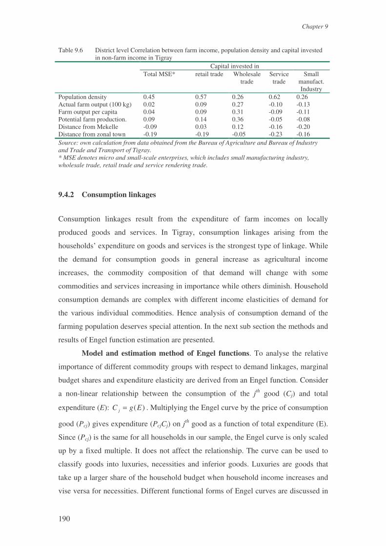
Chapter 9
190
Table 9.6 District level Correlation between farm income, population density and capital invested in non-farm income in Tigray
Capital invested in Total MSE* retail trade Wholesale
trade Service trade
Small manufact. Industry
Population density 0.45 0.57 0.26 0.62 0.26 Actual farm output (100 kg) 0.02 0.09 0.27 -0.10 -0.13 Farm output per capita 0.04 0.09 0.31 -0.09 -0.11 Potential farm production. 0.09 0.14 0.36 -0.05 -0.08 Distance from Mekelle -0.09 0.03 0.12 -0.16 -0.20 Distance from zonal town -0.19 -0.19 -0.05 -0.23 -0.16 Source: own calculation from data obtained from the Bureau of Agriculture and Bureau of Industry and Trade and Transport of Tigray. * MSE denotes micro and small-scale enterprises, which includes small manufacturing industry, wholesale trade, retail trade and service rendering trade.
9.4.2 Consumption linkages
Consumption linkages result from the expenditure of farm incomes on locally
produced goods and services. In Tigray, consumption linkages arising from the
households’ expenditure on goods and services is the strongest type of linkage. While
the demand for consumption goods in general increase as agricultural income
increases, the commodity composition of that demand will change with some
commodities and services increasing in importance while others diminish. Household
consumption demands are complex with different income elasticities of demand for
the various individual commodities. Hence analysis of consumption demand of the
farming population deserves special attention. In the next sub section the methods and
results of Engel function estimation are presented.
Model and estimation method of Engel functions. To analyse the relative
importance of different commodity groups with respect to demand linkages, marginal
budget shares and expenditure elasticity are derived from an Engel function. Consider
a non-linear relationship between the consumption of the jth good (Cj) and total
expenditure (E): )(EgC j = . Multiplying the Engel curve by the price of consumption
good (Pcj) gives expenditure (PcjCj) on jth good as a function of total expenditure (E).
Since (Pcj) is the same for all households in our sample, the Engel curve is only scaled
up by a fixed multiple. It does not affect the relationship. The curve can be used to
classify goods into luxuries, necessities and inferior goods. Luxuries are goods that
take up a larger share of the household budget when household income increases and
vise versa for necessities. Different functional forms of Engel curves are discussed in

Production and consumption linkages and the development of rural non-farm enterprises
191
Deaton and Muellbauer (1980). Double logarithmic, sem-logarithmic and log
reciprocal forms of the Engel curves were investigated by Praise and Houthakker
(1955). More complex forms such as a cumulative distribution function of the log
normal distribution has been suggested, which combines many of the desirable
properties of the simpler forms explained above. However, none of these forms are
consistent with the adding up restriction. The adding up restriction is crucial for a
demand analysis since it implies that demand functions satisfy the budget constraint
that households face. The useful form of Engel curve that satisfies the adding up
restriction is the one first estimated by Working (1943) and successfully used by
Leser (1963). This function2 relates budget shares to the logarithm of outlays.
jjjj Ew εββ ++= ln21 (9.1)
where wj (= Cj * Pcj/E) is the budget share of the jth good, E is total household
expenditure and β1 and β2 are parameters to be estimated and ε is the error term
distributed. Adding up requires Σwj= 1, which is satisfied provided that Σβ1j = 1 and
Σβ2j = 0. When equation (9.1) is estimated equation by equation for each category of
expenditure, the adding up restriction will be automatically satisfied (Deaton and
Muellbauer, 1980, p. 84). When both sides of equation (9.1) are multiplied by the total
expenditure and after adding an intercept, the Engel curve can be written as
jjjjj EEEC εβββ +++= ln210 . (9.2)
Households differ in size, age composition, educational level and other characteristics.
Households with different characteristics have different expenditure patterns (Deaton
and Muellbauer, 1980). The Engel curve (9.2) with household characteristics included
is given by
jjjjjj mEEEC εαβββ ++++= )(ln210 . (9.3)
where m(α) is household characteristics. The most important household
characteristics are household composition, and the number, types and ages of the
household members. For simplicity, m(α) is modelled as
EDUCDEPRATj 4j3j2j1j ageFS )m( ααααα +++= (9.4)
where DEPRAT is dependency ratio, FS is family size, AGE is age of the household
head, EDUC is dummy for the education level of the household head. Family size is
2 This model is consistent with Almost Ideal Demand Systems (AIDS) if it is extended to include prices (Deaton and Muellbauer, 1980).
Chapter 9
192
put in adult equivalent term with household members below the age of 15 weighted
by 0.63. This weight is calculated from the food composition table prepared by West
(1987). Since a substantial part of the household income consists of food grown on the
farm, subsistence ratio must be included in the list of explanatory variables (Massell,
1969). Combining equation (9.3) and equation (9.4) and adding taste shifters such as
location dummies, the Engel curve can be written as
j
m
kkjj
jjjjj
LDDYEAREDUC
DEPRATEEEC
εααα
αααβββ
++++
+++++=
�−
=
1
1654j
3j2j1210 AGEFSln. (9.5)
where YEARD is year dummy (1996=1 and 1997=0) and LD are village (location)
dummies. Using OLS to estimate the Engel function could result in biased estimates
of parameters when total consumption expenditure is used as a measure of income.
Furthermore biases are likely to be introduced by the correlation of independent
variables and the error term. Considering total consumption expenditure as an
endogenous variable, therefore, the Engel function can be estimated using the
instrumental variable estimation method. The instrumental variables used to predict
total consumption expenditure are total land cultivated, farm equipment, non-farm
income, location dummies and family size.
Then the average budget share (ABS), marginal budget share (MBS) and
expenditure elasticities (EEL) are calculated using the following formulas respectively
as:
E
CABS j
j = ;
EEC
MBS jjjj ln221 βββ ++=∂∂= ;
j
jj ABS
MBSEEL = .
The total consumption expenditure variable used in the regression is composed
of the value of any purchased and own-produced foods and non-food goods consumed
by the households. The local market price is used to impute the values of the own
produced consumption foods.
Estimation results of the Engel functions. The estimation results of the
Engel functions for different category of consumption goods is given in the Appendix.
The parameter estimates of OLS have far higher t-ratios than the parameters

Production and consumption linkages and the development of rural non-farm enterprises
193
estimated by instrumental variable method. This could be due to multicollinearity.
Hazell and Röell (1983) reported the same problem. The coefficients of
determinations are also in general higher for the OLS estimates than for the
instrumental variable estimates. The OLS results are, therefore, used for the
computation of marginal budget shares and elasticities. For comparison, the
estimation results for both the OLS and the instrumental variable method are given in
the appendix.
The data fit very well and the adjusted coefficient of determination is higher
for most of the commodities ranging from 0.21 for consumption expenditure on oil
crops to 0.94 for total food expenditure (Table A9.1). The standard errors are
calculated using White heteroscedasticity consistent estimators (Greene, 1997, p.
505). Variables such as total expenditure, year dummy and subsistence ratio and
location dummies have a significant effect on the consumption demand for all
commodity groups. Family size and dependency ratio show a significant effect on the
consumption of non-food commodity groups. Age and education of the household
head do not significantly affect the consumption demand of all commodity groups.
There was significant difference in the consumption pattern of all commodity groups
between 1996 and 1997. Consumption of purchase non-food products was higher in
1996 than in 1997, which illustrates the strong consumption link between farm and
non-farm sectors.
Table 9.7. summarises the expenditure behaviour of an average farm
household. The results are obtained by evaluating the average budget share, marginal
budget share and the expenditure elasticity at the sample mean value. The
commodities consumed are categorised in to: (1) food and non-food items groups and
(2) locational groups. The food items include cereals, pulses, oil crops, vegetables and
animal products such as milk, butter and cheese as well as sugar, tea and salts. The
non-food items are grouped into social expenses like services and ceremonial
expenditure, contributions for local organisation and taxes, and industrial products
such as household durable and clothing and footwear.
Food and non-food commodity groups. Total food accounts for 79% of
household expenditure, leaving only a small share of the budget for non-foods. The
marginal budget share of food items is 73%, which is less than its average budget
share. The expenditure elasticity is also less than unity (0.91) implying that the budget
share of food items will decline when total income rises. The result is comparable to

Chapter 9
194
(slightly less than) those reported by Hazell and Hojjati (1995) for Zambia, and Hazell
and Roëll (1983) for the Gusau Region of Northern Nigeria. The estimated
expenditure elasticity for food items were 0.88 for the Eastern Province, Zambia and
0.81 for Northern Nigeria.
Among the food items, cereals account for a substantial share of the budget
(0.50), but their importance declines as income rises. The expenditure elasticity is
0.52 and the marginal budget share is 0.26, that is, half of the average budget share.
The food items group (which includes pulses, oil crops, animal products, vegetables
and sugar, tea and salts) consists of relatively high value foods. Their expenditure
elasticity is very high implying that their share will increase dramatically if the total
income of the household increases. However, at the moment their average budget
shares are very low. Expenditure on animal products and oil crops is in particular
potentially very important and will grow fast if the income of the farm household
rises.
Table 9.7 Food and non-food expenditure behaviour of farm households in Tigray. Average budget
share Marginal budget share
Expenditure elasticity
Total food expenditure 0.80 0.73 0.91 Cereals 0.50 0.26 0.52 Pulses 0.05 0.06 1.2 Oil crops 0.003 0.007 2.33 Vegetables 0.001 0.0001 0.10 Animal products 0.10 0.23 2.30 Coffee, sugar, tea, salt, spices 0.14 0.16 1.14 Total non food expenditure 0.20 0.28 1.40 Service, ceremonial and other social expense 0.05 0.09 2.25 Industrial products 0.16 0.19 1.19 Household goods 0.01 0.03 3.0 Clothes, shoes and cosmetics 0.15 0.18 1.2 Locational Group Own produced food 0.51 0.46 0.90 Purchased food local 0.15 0.11 0.75 Purchased non-local food 0.14 0.16 1.14 Industrial products non-food (not locally produced) 0.16 0.19 1.19 Purchased locally non-food 0.04 0.09 2.25
All non-food items group have an expenditure elasticity that is highly elastic
implying that their importance in the budget share will increase as farm households’
income rises. The relative increase will be greatest for expenditures on services,
ceremonial and other social expenses, and expenditure on clothes and footwear. This
clearly shows that agriculture has the potential to strengthen the local demand for non-
food in Tigray, Northern Ethiopia.

Production and consumption linkages and the development of rural non-farm enterprises
195
Locational groups. The results of locational linkages in Table 9.7 show that
about 70% of the total expenditure is on regionally produced food and non-food
items, leaving the rest 30% for regionally imported food and non-food items. But the
expenditure elasticity for imported items is higher than that for non-imported items.
This implies that there are strong household demand linkages to the local economy
which predominantly benefit the agricultural sector in the short-run, but these linkages
will diminish if the income of the farm households rises. The average budget share
and expenditure elasticity of the local products of the non-farm service sector is 0.04
and 2.2, respectively. The household demand linkages with the local non-farm sector
through expenditures such as services and ceremonial expenses is very low at the
moment, but it will increase substantially when farm households’ income rises.
Purchased food items imported from outside the region (such as sugar, coffee and
salt) are also potentially important.
9.5 Summary and conclusions
The liberalisation of the economy has favoured non-farm activities in the urban areas
of the region over the last seven years. Distributive and service trade are the dominant
non-farm activities in the remote rural centres in the region. Small-scale
manufacturing industries and handicraft are more concentrated in big towns and they
are potentially very important for employment and income generation in the region.
The involvement of women in the non-farm sector is mainly confined to activities
with low value added per unit of capital invested such as service rendering trade like
hotels, beauty salon, bar and restaurants. The development of micro and small-scale
enterprises (MSE) is highly constrained by poor infrastructure due to low quality,
inadequacy of urban and rural roads, and insufficient energy supplies. Lack of
working capital, absence of a market for the products of MSE and insufficient supply
of raw materials are the main problems that constrain the existing MSE. Share-
company and partnership are not well developed in the non-farm sector due to the
high transaction costs of settling disputes and ineffective judiciary systems. Rural
centres or towns act as a focal point in providing infrastructure services to the rural
areas. They also act as a centre for business enterprises that serve the rural population.
However, the majority of the users of the small-scale manufacturing industries and
handicraft are from urban population. Currently it is the distributive trade that serves

Chapter 9
196
the rural as well as the urban population. In general rural non-farm activities act as a
residual sector that absorbs the workers who cannot be readily absorbed in agriculture.
When agriculture is unable to support the growing population, farmers are forced to
be engaged in non-farm activities.
Consumption linkages are much higher than the production linkages in the region.
The production linkages between the farm and non-farm sectors are very small. At the
moment most of the consumption expenditure is focused on locally produced food
items. In the long run, more of the incremental income of farm households will be
spent on livestock products and on regionally imported food and non-food items as
well on local non-food products, particularly on services and ceremonial expenditures.
Therefore, if rural farm and non-farm enterprises are to achieve their full
potential for income generation and economic decentralisation, policy makers need to
review their development policies, laws and institutions which hinders small farmers
and small rural non-farm enterprises. Rural towns should be viewed as important focal
points in the development of the rural economy. Through the rural towns, most of the
soft and hard infrastructure services can be provided to farmers relatively easily.
Other measures to improve the efficiency of the economy such as improving the
bureaucratic and judiciary system may also help to develop partnership and share
companies in the business communities which in turn will resolve the problem of
working capital. A program of direct assistance can also facilitate the growth of the
rural non-farm economy.
Summary of results, policy implications and conclusions
197
CHAPTER 10. SUMMARY OF RESULTS, POLICY IMPLICATIONS
AND CONCLUSIONS
10.1 Introduction
The foregoing chapters (Chapter 4 to chapter 8) deal with specific issues in order to
answer the research questions raised in Chapter 1. On the one hand, some of the
questions raised in the introductory chapter exceed the scope of the separate chapters.
On the other hand, the results of the different chapters need to be integrated. The link
between farm and off-farm income; the relationship between factor inputs, marketing
surplus and off-farm employment; the differential impact of family size and education
on various categories of labour demand and supply; and the overall policy implication
of the results are not yet made clear. Hence the objective of this chapter is to integrate
and summarise the results presented in the foregoing chapters and to explain the
issues concerning farm and off-farm linkages.
Farm off-farm income linkages at a household level are modelled in such a way
that off-farm income (employment) affects agricultural production through income
diversification, through the purchase of farm inputs and through the substitution of
farm work by off-farm work. If there is disguised unemployment and agricultural
activities are seasonal, the negative effect of off-farm employment on the farming
activities can be very small. The net impact of off-farm employment on agricultural
production can be positive or negative depending on the relative strength and
direction of the forces. On the other hand, farm income in our model affects off-farm
income (employment) through the return to family labour on the farm (shadow wage
rate of farm labour or farm output).
The results indicate that off-farm income affects agricultural production positively
through income diversification and the financing of farm activities such as purchase
of farm labour, fertiliser, seeds and pesticides and negatively through on-farm labour
supply. Farming activities also affect off-farm employment negatively through the
competition for family labour and positively through the provision of liquidity for off-
farm self-employment.

Chapter 10
198
Family size also shows to have a positive effect on the farm and off-farm hours of
labour supply, but with varying magnitude. The magnitude of the family size effects
on farm and off-farm employment is found to be dependent on the gender
composition of the household and the type of off-farm activities involved. The effect
of education on the wage rates depends on the type of off-farm activities involved and
on the kind of education farm households have acquired.
The questions dealt with in this chapter are the following:
1 What is the total net impact of off-farm income on farm income?
2 What is the net impact of farm income on off-farm employment in general and on
off-farm wage employment versus self-employment and male-female off-farm
work in particular?
3 What is the impact of off-farm income on the purchase and sale of farm output?
4 What is the general effect of an increase in family size?
5 What are the effects of education on the market wage rate and on the supply of
labour for various activities?
6 What kind of program and policy implications can be drawn from the results of
the study in general?
To answer these questions, the marginal effects and elasticities estimated in
the foregoing chapters are combined and a simulation exercise is done to calculate the
effect of farm income on the shadow value of family farm labour. The summary of the
results regarding (1) the direct and indirect impact of off-farm income on farm
income; (2) the impact of factor inputs and farm income on off-farm employment; (3)
the impact of factor inputs and off-farm income on the marketing surplus of farm
outputs; and (4) the impact of family size and education on farm and non-farm
activities and on the marketing surplus of farm outputs are presented.
The direct impact of off-farm income on farm income consists of the
production technology effect of diversifying income sources into off-farm activities.
The indirect impact includes the contribution of off-farm income towards purchasing
of farm inputs such as farm labour, fertiliser, seeds and pesticides. It also includes the
competition for labour via the response of on-farm labour supply to the market wage
rate. The impact of off-farm income on the marketing surplus is assumed to act in two
ways: (1) directly on the sale and purchase of farm output by proving liquidity and (2)
indirectly on the sale and purchase of farm output by supplementing farm output.

Summary of results, policy implications and conclusions
199
The impact of farm inputs and farm income on off-farm employment is
analysed through their effect on the shadow wage rate and from there to the off-farm
labour supply for various categories of off-farm employment and household members.
The rest of the chapter is organised as follows. In the next section a summary
of the results from previous chapters and new simulations are presented. The program
and policy implications of the book results are discussed in section three. In section
four, issues that need further research are described. In the final section, the general
summary and conclusions of the book are presented.
10.2 Summary of results
Farm off-farm income linkage. A substantial proportion of farm households (81%)
diversifies their income into off-farm activities. The diversification of income sources
into off-farm activities increases farm output directly by increasing their managerial
skill and indirectly through the purchase of farm inputs such as hired labour, fertiliser
and pesticides (see Chapter 5). Table 10.1 summarises the effect of off-farm income
on farm income for an average farm household in the sample. When off-farm income
increases by 10% (compensating for farm income), farm household’s income
diversification, measured by Simpson’s index (see Chapter 5), increases by 1.4% and
farm output increases by 1.2%.
The purchase of farm labour and variable capital farm inputs increases by
10.2% and 1.3%, respectively, when off-farm income increases by 10%.
Consequently, an increase in off-farm income by 10% increases farm productivity by
1.2% via the hiring of farm labour and by 0.2% via the purchase of variable capital
farm inputs. The increase in the use of hired labour is greater than the increase in the
use of purchased variable capital farm inputs. Off-farm income is more important for
the hiring of farm labour than for the purchase of capital inputs because of the bias of
the public credit scheme against the hiring of farm labour. The public supply of credit
is tied to the purchase of capital farm inputs only, so that farm households can get
credit for the purchase of capital farm inputs (such as improved seeds, fertiliser and
pesticides), but not for the hiring of farm labour (see Table 1.9 in chapter 1)1.
1 The bias in the public provision of credit against the hiring of farm labor may have come from the assumption that farm households are not constrained by labor. However, the fact that quite a lot of farmers (39%) are found to hire farm labor indicates that farm households are labor constrained.
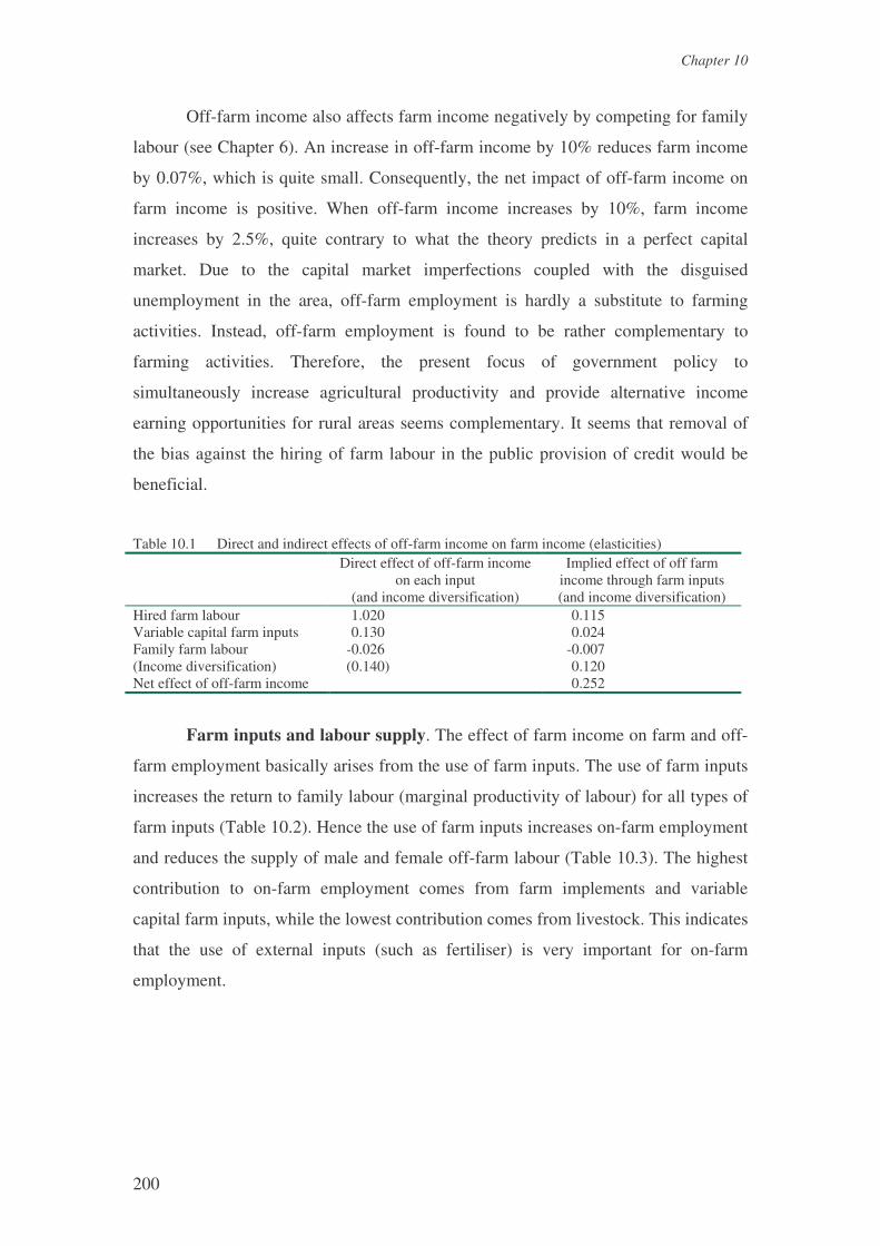
Chapter 10
200
Off-farm income also affects farm income negatively by competing for family
labour (see Chapter 6). An increase in off-farm income by 10% reduces farm income
by 0.07%, which is quite small. Consequently, the net impact of off-farm income on
farm income is positive. When off-farm income increases by 10%, farm income
increases by 2.5%, quite contrary to what the theory predicts in a perfect capital
market. Due to the capital market imperfections coupled with the disguised
unemployment in the area, off-farm employment is hardly a substitute to farming
activities. Instead, off-farm employment is found to be rather complementary to
farming activities. Therefore, the present focus of government policy to
simultaneously increase agricultural productivity and provide alternative income
earning opportunities for rural areas seems complementary. It seems that removal of
the bias against the hiring of farm labour in the public provision of credit would be
beneficial.
Table 10.1 Direct and indirect effects of off-farm income on farm income (elasticities) Direct effect of off-farm income
on each input (and income diversification)
Implied effect of off farm income through farm inputs (and income diversification)
Hired farm labour 1.020 0.115 Variable capital farm inputs 0.130 0.024 Family farm labour -0.026 -0.007 (Income diversification) (0.140) 0.120 Net effect of off-farm income 0.252
Farm inputs and labour supply. The effect of farm income on farm and off-
farm employment basically arises from the use of farm inputs. The use of farm inputs
increases the return to family labour (marginal productivity of labour) for all types of
farm inputs (Table 10.2). Hence the use of farm inputs increases on-farm employment
and reduces the supply of male and female off-farm labour (Table 10.3). The highest
contribution to on-farm employment comes from farm implements and variable
capital farm inputs, while the lowest contribution comes from livestock. This indicates
that the use of external inputs (such as fertiliser) is very important for on-farm
employment.
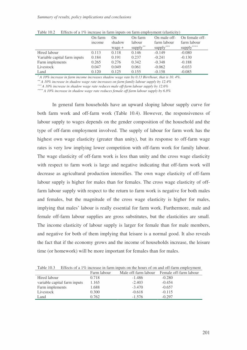
Summary of results, policy implications and conclusions
201
Table 10.2 Effects of a 1% increase in farm inputs on farm employment (elasticity)
On farm income
On shadow wage +
On farm labour supply++
On male off-farm labour supply+++
On female off-farm labour supply++++
Hired labour 0.113 0.118 0.146 -0.149 -0.080 Variable capital farm inputs 0.184 0.191 0.237 -0.241 -0.130 Farm implements 0.265 0.276 0.342 -0.348 -0.188 Livestock 0.047 0.049 0.061 -0.062 -0.033 Land 0.120 0.125 0.155 -0.158 -0.085 + A 10% increase in farm income increases shadow wage rate by 0.13 Birr/hour, that is 10. 4%. ++ A 10% increase in shadow wage rate increases on farm family labour supply by 12.4% +++ A 10% increase in shadow wage rate reduces male off-farm labour supply by 12.6% ++++ A 10% increase in shadow wage rate reduces female off-farm labour supply by 6.8% In general farm households have an upward sloping labour supply curve for
both farm work and off-farm work (Table 10.4). However, the responsiveness of
labour supply to wages depends on the gender composition of the household and the
type of off-farm employment involved. The supply of labour for farm work has the
highest own wage elasticity (greater than unity), but its response to off-farm wage
rates is very low implying lower competition with off-farm work for family labour.
The wage elasticity of off-farm work is less than unity and the cross wage elasticity
with respect to farm work is large and negative indicating that off-farm work will
decrease as agricultural production intensifies. The own wage elasticity of off-farm
labour supply is higher for males than for females. The cross wage elasticity of off-
farm labour supply with respect to the return to farm work is negative for both males
and females, but the magnitude of the cross wage elasticity is higher for males,
implying that males’ labour is really essential for farm work. Furthermore, male and
female off-farm labour supplies are gross substitutes, but the elasticities are small.
The income elasticity of labour supply is larger for female than for male members,
and negative for both of them implying that leisure is a normal good. It also reveals
the fact that if the economy grows and the income of households increase, the leisure
time (or homework) will be more important for females than for males.
Table 10.3 Effects of a 1% increase in farm inputs on the hours of on and off-farm employment Farm labour Male off-farm labour Female off-farm labour Hired labour 0.718 -1.486 -0.280 variable capital farm inputs 1.165 -2.403 -0.454 Farm implements 1.688 -3.470 -0.657 Livestock 0.300 -0.618 -0.115 Land 0.762 -1.576 -0.297

Chapter 10
202
There is a difference in the nature of off-farm labour supply for wage and self-
employment. When farm income increases, the supply of labour for off-farm wage
employment decreases and the supply of labour for off-farm self-employment
increases (Table 10.2). This can be explained by the fact that off-farm self-
employment is undertaken by a relatively rich household while poorer farm
households face entry barriers (Reardon, 1997). The results also reveal that the wage
elasticities of off-farm labour supply of households for wage and self-employment is
positive but inelastic. Income elasticity is negative for both types of labour supply, but
the magnitude is higher for wage employment than for self-employment. The larger
income elasticity for wage employment relative to that for self-employment implies
that households will work less for wage employment than for self-employment when
the economy grows.
Table 10.4 Summary of wage* and income elasticities for farm and off-farm labour supply Ws Wmm Wmf Wmw Wmo S
On-farm labour supply 1.24 -0.026 -0.0001 Male members’ off-farm labour supply -1.26 0.701 -0.049 -0.048 Female members’ off-farm labour supply -0.68 -0.038 0.813 -0.143 Off-farm labour supply for wage employ. 0.46 0.02 -0.080 Off-farm labour Supply of self-employ. -0.04 0.41 -0.044 * Wage elasticity is calculated based on the expected marginal effects of natural logarithm of wage rates on a labour supply. Ws = shadow wage rate of family labour on the farm; Wmm = market wage rate of male members; Wmf = Market wage rate of female members; Wmw = market wage rate for wage employment; Wmo = Market wage rate for off-farm self-employment; S = non-labour income;
The elasticity estimates of this study are higher than those estimated for Asian
countries for both men and females, and closer to (but still lower than) Ghanaian farm
households (Table 10.5). Unlike Asian farm households, females have a higher own
wage elasticity of off-farm labour supply than males in Tigray, which is similar to that
for Ghanaian farm households. However, the difference in own wage elasticity
between females and males is smaller for the Tigryan farm households than for the
Ghanaian farm households. The magnitude of the cross wage elasticity of labour
supply between male and female is the same as that for Indian farm households, but
smaller than and opposite in sign to that for Ghanaian farm households. The income
elasticity estimate is also the same as those for India and Peruvian Sierra, but much
lower than that for Ghana.

Summary of results, policy implications and conclusions
203
Table 10.5 Comparison of elasticities with other studies Own wage elasticity Income elasticity
Study area [author(s)] Cross wage Male to female (female to male)
Male Female Male Female
Tigray, Ethiopia (this study) -0.049 (-0.38) 0.701 0.813 -0.048 -0.143 For India (Skoufias, 1994) -0.076 (0.056) 0.107 -0.0.69 -0.05 -0.013 Peruvian Sierra (Jacoby, 1993) -0.010 (0.006) 0.102 0.079 -0.058 -0.058 Ghana (Abdulai and Delgado, 1999) 0.187 (-0.198) 0.33 0.66 -0.272 -2.08
Market wage rate and household income. The aforementioned results show
that farm and off-farm labour supply are substitutes in the sense that when the return
to off-farm work (market wage rate) increases, the supply of labour for farm work
decreases and the supply of labour for off-farm work increases. But what happens to
total household income when the market wage rate increases? To answer this
question, the effect of a one-percent increase in the market wage rate on off-farm
income and farm income and on total household income is calculated using the
estimated labour supply functions (Table 10.6). In our estimate, the effect of the
market wage on the supply of farm labour is very low. As a result, the increase in off-
farm income is much higher than the decrease in farm income when the market wage
rate increases by one percent. The net effect of an increase in the market wage rate by
one percent on total household income (compensating for an income effect) is
calculated to be 8.13 Birr. This implies that improving the market wage rate is an
important policy instrument for increasing household incomes in rural areas.
Table 10.6 The effect of a 1% increase in the market wage rate on the supply of labour hours and household income
Substitution effect Income effect Net effect Hours off-farm labour 7.174 Hours of on-farm labour -0.247 Off-farm income (Birr) 13.057 -4.592 8.466 Farm income (Birr) -0.347 0.010 -0.337 Household income (Birr) 12.710 -4.581 8.129
Off-farm income and marketing surplus. If farm households do not have
another source of income (such as off-farm income), the main source of cash income
is the sale of farm output. To buy the necessary food and non-food items that cannot
be produced on their farm (such as salt, spices, clothes and taxes), farm households
have to sell farm output. When the farm households obtain off-farm income, they can
stop selling farm output and use the cash obtained from off-farm work to purchase the

Chapter 10
204
food and non-food items required. The results show, however, that off-farm
employment can help farm households to finance their farming activities through the
purchase of farm inputs such as hired labour, fertiliser, and improved seeds.
In a drought prone area, off-farm income can help to purchase food for
consumption and keep farmers productive on their farm. As a result, off-farm
employment increases farm output and its negative impact on the sale of farm output
could be very low. Therefore, in a less dynamic agricultural area, the impact of off-
farm employment on the marketing surplus of farm outputs could be positive. The
results support the view that off-farm income increases the marketing surplus of farm
outputs (Table 10.7, see also Chapter 8). Hence off-farm income in marginal areas
should not been seen as a substitute for farm income. Instead off-farm employment is
complementary to farming activities and it helps to achieve the objective of food self-
sufficiency.
The effect of farm output on the marketing surplus basically comes from the
use of farm inputs such as variable capital farm inputs, hired labour, family labour,
land, and farm implements. Since these farm inputs affect the farm output positively
(see Chapter 5), their effect on the market surplus of farm output is positive. The
relative contribution of the various farm inputs to the market surplus is, however,
different. The highest contribution to the marketing surplus comes from the use of
variable capital farm inputs followed by farm implements (capital) and family labour
used. The contribution of livestock to the marketing surplus is the lowest among all
the farm inputs. The fact that variable capital farm inputs contribute more to the
marketing surplus implies that the promotion of external inputs is effective in
achieving the objective of food self-sufficiency.
Table 10.7 Effect of farm and off-farm incomes on marketing surplus crop output (elasticity) Farm income Purchase Sales Surplus Hired labour 0.113 -0.040 0.147 0.187 Variable capital farm inputs 0.184 -0.065 0.240 0.305 Family labour 0.255 -0.090 0.332 0.422 Farm implements 0.265 -0.094 0.345 0.439 Livestock 0.047 -0.017 0.061 0.078 Land 0.120 -0.043 0.156 0.199 Off-farm income (=direct + indirect)
0.228 0.064 (=-0.089 + 0.153)
0.310 (=0.328 -0.018)
0.246
The elasticity of purchase and sales with respect to farm output is -0.354 and 1.303, respectively. The effect of off-farm income on purchase and sale of farm output includes also the indirect effect through the farm income (0.252 times -0.354 on the purchase function and 0.252 times 1.303 on the sales function).

Summary of results, policy implications and conclusions
205
Family size and labour allocation. With population growing at 3.1% per
annum in Ethiopia, family size will not remain constant in the future. If appropriate
family planning measures are not implemented, or if labour is not withdrawn from
agriculture, most probably family size and thus the pressure on agriculture will
increase. The increased family size will have an impact on farm size, the supply of
labour for farm and off-farm work, and household income.
The effect on the labour allocation of an average household as a result of an
increase in family size by one person is given in Table 10.8. The result in general
indicates that family size increases the supply of labour for both farm and off-farm
work, but the magnitude of the increase depends on the sex (gender) composition of
the household and the type of off-farm activities involved. The effect of an increase in
family size is smaller for farm work than for off-farm work. The effect is also larger
for wage employment than for off-farm self-employment, and for male members’
hours of labour supply than for female members’ hours of labour supply. The effect of
family size on farm work is lower in magnitude than that on off-farm work because
the opportunity to work on the farm is very limited by the small farm size. Therefore,
given the current trend in population growth, the better option seems to be to promote
off-farm employment so as to increase employment in rural areas. The effect of
family size on off-farm wage-employment is larger than that on off-farm self-
employment because off-farm self-employment requires more capital and it is less
labour intensive than off-farm wage employment. When family size increases, female
labour is more important than male labour in home activities (such as preparing meals
and childcare). As a result, the response of female members’ off-farm labour supply is
smaller than that of male members.
Family size also affects the demand for hired farm labour and the marketing
surplus of farm outputs negatively, although the effect on the marketing surplus is
statistically not significant. This suggests that with the ever-increasing population, the
long-term prospect for improving national food self-sufficiency is under question. To
resolve this problem, considerable effort must be made to increase off-farm
employment on one hand and agricultural productivity on the other hand. If the
population grows unabated or alternative employment opportunities are not designed,
farm households may become more subsistence-oriented producers instead of being
more commercially oriented producers.

Chapter 10
206
Table 10.8 The marginal and percentage effect of an increase in family size by one person Marginal increase Percentage increase Hours of off-farm employment 501.77 37.26 Probability of off-farm employment 0.14 0.14 Hours of off-farm wage employment 687.23 55.02 Probability of off-farm wage employment 0.26 0.26 Hours of off-farm self employment 13.09 13.42 Probability of off-farm self employment 0.05 0.05 Hours of male members off-farm work 428.27 42.95 Probability of male members off-farm work 0.15 0.15 Hours of female members off-farm work 10.49 3.00 Probability of female members off-farm work 0.02 0.02 Hours of demand for hired farm labour -67.39 -75.7 Hours of supply for farm work 19.09 3.55 Marketing surplus (Birr) -26.23 -2.31
Education, market wage rate and labour supply. The effect of education on
wages is summarised in Table 10.9. The education of the household head (measured
by the ability to read and write) is associated with a lower wage rate for both male and
female members of a household, which is quite contrary to the theory of human
capital (Schultz, 1961; Becker, 1964). The results reveal a remarkable picture when
the wage for wage-employment and self-employment are considered individually, and
when education is decomposed into traditional education (can read and write without
going to formal school) and modern education (has attended elementary school). On
the one hand, the wage rate a household receives from off-farm wage employment is
lower (but only little and statistically insignificant) when a head is able to read and
write through a traditional education and is higher when a head has attended a modern
school. The lack of a relationship between education (particularly traditional
education) and the wage rate for off-farm wage employment may be that most of the
off-farm wage work is manual work, which does not require education at all. If the
activities involved in wage-employment require education, merely reading and
writing without other literacy skills might not help to increase productivity
(Rosenzweig, 1988). If there is no demand for traditional education by the employers
in the local labour market or if traditional education is not marketable (even if it is
productive), traditional education may not result in higher wage rate. To benefit from
the knowledge acquired from traditional education, therefore, one has to be self-
employed. If education does not have any influence on the market wage or on the
return to own business activities, education must be obtained by households for
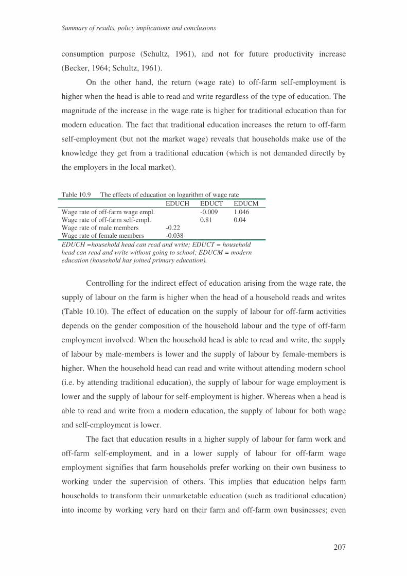
Summary of results, policy implications and conclusions
207
consumption purpose (Schultz, 1961), and not for future productivity increase
(Becker, 1964; Schultz, 1961).
On the other hand, the return (wage rate) to off-farm self-employment is
higher when the head is able to read and write regardless of the type of education. The
magnitude of the increase in the wage rate is higher for traditional education than for
modern education. The fact that traditional education increases the return to off-farm
self-employment (but not the market wage) reveals that households make use of the
knowledge they get from a traditional education (which is not demanded directly by
the employers in the local market).
Table 10.9 The effects of education on logarithm of wage rate EDUCH EDUCT EDUCM Wage rate of off-farm wage empl. -0.009 1.046 Wage rate of off-farm self-empl. 0.81 0.04 Wage rate of male members -0.22 Wage rate of female members -0.038 EDUCH =household head can read and write; EDUCT = household head can read and write without going to school; EDUCM = modern education (household has joined primary education).
Controlling for the indirect effect of education arising from the wage rate, the
supply of labour on the farm is higher when the head of a household reads and writes
(Table 10.10). The effect of education on the supply of labour for off-farm activities
depends on the gender composition of the household labour and the type of off-farm
employment involved. When the household head is able to read and write, the supply
of labour by male-members is lower and the supply of labour by female-members is
higher. When the household head can read and write without attending modern school
(i.e. by attending traditional education), the supply of labour for wage employment is
lower and the supply of labour for self-employment is higher. Whereas when a head is
able to read and write from a modern education, the supply of labour for both wage
and self-employment is lower.
The fact that education results in a higher supply of labour for farm work and
off-farm self-employment, and in a lower supply of labour for off-farm wage
employment signifies that farm households prefer working on their own business to
working under the supervision of others. This implies that education helps farm
households to transform their unmarketable education (such as traditional education)
into income by working very hard on their farm and off-farm own businesses; even

Chapter 10
208
though a low level of primary education is not expected to bring about a significant
change in attitude and productivity. Studies show that at least elementary education
above the 4th grade is necessary for an increase in agricultural productivity
(Colclough, 1982; Wier, 1999). For education to be beneficial in traditional farming
areas, fundamental economic and, possibly, social changes are needed (Schultz,
1964). When the change in economic conditions creates a disequilibrium, therefore,
educated individuals could exploit the benefits of economic development more
effectively (Schultz, 1975). Hence for substantial rural development, it is quite
necessary to create a demand for educated people and improve the ‘traditional sector’
of the economy.
Table 10.10 Marginal effects of education on the hours of labour supply Directly
EDUCH EDUCT (EDUCM)
Indirectly via wage
Total Increase
On-farm labour supply 77.2 0.036 77.24 Male mem. off-farm labour supply -83.8 -1.538 -85.34 Female mem. off-farm labour supply 44.08 -0.108 43.97 Off-farm wage empl. labour supply -197.6
(220.8) -0.052 (-6.06)
-197.65 (-3.853)
Off-farm self-empl. labour supply -15.1 (-2.7)
0.323 (0.016)
14.77 (-2.68)
EDUCH =household head can read and write; EDUCT = household head can read and write without going to school; EDUCM = modern education (household has attended primary education).
The results of this study could not confirm that education helps the labour
force to participate in non-farm activities (Huffman, 1980; Burger, 1994) because the
study has been conducted in an area where traditional farming and non-farm activities
are dominant and the demand for education is very low. However, the study confirms
that education is very helpful in motivating farmers to work on their own farm and
non-farm businesses. Further study is necessary to investigate the role of education in
traditional farm and non-farm activities in the region.
10.3 Program and policy implications
In this section, program and policy implications of the main findings are discussed.
The policy implications are categorised based on the policies required to tackle
problems. The program and policy implications discussed here are (1) the need for

Summary of results, policy implications and conclusions
209
alternative employment opportunities, (2) development of complementary policies,
(3) exploitation of potential farm-non-farm linkage, (4) targeting of the vulnerable
groups, (5) the role of rural towns in rural development, and (6) updating the existing
policies and institutions.
The need for alternative employment opportunities. It is becoming very
difficult to increase regional employment in agriculture. The growth in population has
resulted in a smaller farm size. Because of the growing population, expansion into
marginal land and steeper slopes is widely practised. The result has been wide
degradation of hills due to erosion. Crop residue and animal dung is used as fuel for
cooking in the region, not for enriching the soil. Increasing the land under cultivation
in the region is difficult because of land scarcity and malaria in low land areas such as
the western zone of Tigray. Livestock production is not promising either. The forage
supplies come from unimproved and overgrazed pastures and crop residue competing
with food crops. Poverty is forcing farmers to search for wage employment. The
reduction in farm size would not result unemployment if a transition is made to
intensive land use and irrigation agriculture. However, the use of irrigation (which
requires high investment cost) and agricultural intensification is so slow that it is
unlikely to absorb the growing population in the near future. It is therefore necessary
to reduce the dependence on land. To reduce the pressure on land, rural non-farm
activities have to be expanded. The results indicate that diversifying income sources
into off-farm activities increases agricultural production and productivity. Employing
the rural population in rural non-farm activities may have additional advantages: it
helps to keep farmers in the rural areas and reduces rural-urban migration (Todaro,
1969; Harris and Todaro, 1970). It provides farmers with additional income and
reduces the pressure on land (Reardon et al., 1998; Reardon and Vosti, 1995).
Development of complementary policies and organised promotional
activities. Off-farm income has an important role in the rural economy in the Tigray
Regional State. Farm households with a more diversified source of income realise a
higher productivity in agriculture. Expenditure on farm inputs is dependent not only
on agricultural production, but also on off-farm income because off-farm income
helps to finance farming activities. Farmers who are involved in relatively high wage
jobs such as masonry and carpentry are in a better position to hire farm labour. Off-
farm income also helps farm households to increase the marketing surplus of farm
outputs. In general, the positive link between farm and off-farm income implies that

Chapter 10
210
increased agricultural output and raising agricultural productivity cannot be seen in
isolation in the Tigray Region. Complementary policies and programs could be
developed to strengthen the link between farm and non-farm activities. The current
agricultural extension program should encompass both farm and non-farm activities
and encourage the growth of small-scale business and create non-farm employment
opportunities in rural areas. However, agricultural growth still remains central to
attack rural poverty and to promote rural non-farm activities by generating demand
(Mellor, 1976).
There are attempts in the region to promote rural non-farm activities in order
to provide farm households with alternative income sources and to supplement farm
income. For example, public employment schemes such as ‘food for work’ has
increased farm households’ access to off-farm work. However, the efforts are
disorganised and insufficient, and the links between farm and non-farm activities are
not fully recognised. Because the majority of the population is engaged in agriculture,
most governmental and non-governmental organisations have focused exclusively on
agriculture. Promotion of non-farm activities should not be confined to urban areas
and should not be left to the industry and trade ministries.
Institutional support might be necessary as well to create an enabling
environment for rural non-farm enterprises. Therefore, some sort of government
organisation must be established to coordinate the presently dispersed and
unorganized promotion of rural non-farm activities. Then this organisation can be
responsible for formulating, upgrading, coordinating, and implementing enabling
measures such as economic and financial policies as well as assistance programs to
promote rural non-farm activities. Since rural non-farm enterprise owners do not have
the capacity to organize themselves because they are many in number and are less
prosperous, the new institution can lobby for policies that favour the rural non-farm
activities and the development of assistance programs (Binswanger and Deininger,
1997).
Exploiting the potential farm non-farm linkage. The results show that the
consumption linkage dominates the production linkage. This implies that the
government should focus on commerce (distributive and service trade) as the main
non-farm activities in the short-run. To exploit this potential, infrastructure such as
roads and telephone connections should be improved. Other measures that improve
the efficiency of the economy such as improving the bureaucratic and judiciary

Summary of results, policy implications and conclusions
211
system may also help. Improving the efficiency of the distributive and service trade
means creating a favorable market for industrial products especially for the products
of small-scale and cottage manufacturing industries.
Service-providing enterprises are scarce and the demand for the services of
non-farm activities are to a great extent not satisfied. This implies that there is quite
some potential to increase the economic activity of the region in rural areas by
promoting rural non-farm activities. On the one hand, there is still a huge unsatisfied
demand for industrial and agricultural products that are not produced locally in the
rural areas. Farmers have to travel several hours or even days to shop for many
commodities. On the other hand, there is surplus labour in some places and disguised
unemployment in most of the rural areas. There is no labour shortage in farming
except in the peak agricultural seasons such as harvesting and threshing. There is still
rationing in the farm and non-farm labour market. Agriculture is not dynamic enough
to provide sufficient employment for the rural communities. If basic facilities are
provided such as infrastructure, credit provision, technical and management training,
and sufficient business advice, the enormous potential can be easily exploited2.
Targeting of the vulnerable group. Women participate to a considerable
extent in non-farm activities. However, they are engaged in activities with lower value
added per unit of investment and lower wage non-farm activities such as public work
programs and manual work in construction sites. The wealthy farm households
dominate the most lucrative forms of non-farm activity, particularly masonry,
carpentry and non-farm self-employment such as trading. So poverty-focused rural
non-farm investment should need to focus on non-farm activities, which are
accessible to the poor and to women. The underlying factors that hinder entry into
non-farm activities must be removed.
The need for reviewing and updating the existing policies and institutions.
Government policies affect not only the magnitude of agricultural growth but also the
ability of rural non-farm enterprises to respond to agriculturally induced increase in
demand. Rural non-farm enterprises are the second most important sources in
generating employment in the country and the nation (next to agriculture). If rural
non-farm enterprises are to achieve their full potential for income generation and
2 Although our analysis does not include all of the proposed improvement, it quite clear that credit provision for liquidity constrained households, and technical and management training and business advice for traditional farmers are very important.

Chapter 10
212
economic decentralisation, policy makers need to review their agricultural,
investment, commercial and infrastructure development policies that stands against
small farmers and small rural non-farm enterprises. A specific policy that should be
reformed is the proclamation that provides investment incentives such as income tax
relief to local investors with over 250, 000 Birr capital. This tax relief does not
encourage rural non-farm activities that require smaller capital investment. Likewise,
policies should be formulated to improve small rural non-farm enterprises’ access to
formal financial institutions such as commercial and development banks (Binswanger
and Deininger, 1997).
The role of rural towns in rural development. Rural towns act as a focal
point in the development of the rural non-farm economy. The results indicate that
vegetable production, off-farm employment, and rural non-farm enterprises perform
better in locations nearer to bigger towns and rural centres because of their access to
infrastructure. It is essential to assure adequate economic and social infrastructure to
develop the demand for high value agricultural products such as vegetables and to
support the nascent modern rural non-farm activities and to renovate and develop the
already available traditional non-farm activities. Efficient rural institutional
infrastructures centred in rural towns may be critical for fostering the transition to a
more productive rural farm and non-farm economy.
10.4 Suggestion for future research
There are other important issues that are less well explored in this study and hence
require further investigation: the general equilibrium effects of a change in farm and
non-farm incomes, rural towns as a focal point in rural development, and
consideration of risk in analysing the farm non-farm linkages.
The need for a general equilibrium (CGE) analysis. The approach used in
this book is a partial equilibrium analysis, which does not deal with the general
equilibrium feed back effect of income changes. In our study, we use a non-separable
farm household model with missing markets which assumes that a farm household
faces an internal general-equilibrium constrained by time and liquidity (De Janvry et
al., 1992). Outputs and virtual prices adjust to ensure that the household is in
equilibrium when the markets for labour, inputs or outputs are missing (De Janvry et
Summary of results, policy implications and conclusions
213
al., 1991). However, an agricultural household model does not explicitly deal with the
interaction among households within and outside a village (community) and the
general equilibrium effects of a change in income (income linkages) that can
influence the outcome of policy change (Taylor and Adelman, 1996).
The level of economic interaction among farm households can be categorised
into three situations. The first extreme situation is when all farm households are self-
sufficient and all goods are non-tradable. Under this situation, production and
expenditure linkages among households (within and outside their village) would be
non-existent. Therefore, a non-separable farm household model would be able to deal
with the analysis of the production and consumption decisions of farm households.
The other extreme situation is when all farm households are perfectly integrated with
the goods and factors market within and outside the village, and all goods and factor
inputs are village tradable. In this situation, the production and expenditure linkages
among village households will be the same as the linkage among household outside
the village (at the regional, national and global level). Hence the standard computable
general equilibrium (CGE) model would be sufficient to deal with the feed-back
effects of policies and economic activities in rural areas. The third situation is
between these two extreme situations. If goods and factors inputs are exchanged
among households within the community (village), but not between the village and
the outside (village non-tradable), prices are determined neither by the internal
equilibrium conditions within a household (as in a self-sufficient household) nor by
the regional, national, or world markets. Instead prices are determined within a
village. In this case, a village (micro) computable general equilibrium (VCGE) model
(Taylor and Adelman, 1996) is quite necessary to deal with the growth linkages in
rural areas.
However, in most developing countries, particularly in our study area, a
combination of goods could exist whose prices are determined either by the internal
equilibrium of a household, or by the interaction of households within a village, or by
the interaction of households outside the village (regional, national, or global).
Therefore, when interaction among farm households exists at all levels of markets, a
model that combines a farm household model, a village-wide economic model, and
general equilibrium model has to be developed. Future research must focus on
formulating and using an applied model that makes use of a non-separable farm
household model (Singh et al., 1986; De Janvry et al., 1992), a village-wide model

Chapter 10
214
(Taylor, 1995; Taylor and Adelman, 1996) and a computable general equilibrium
model (Shoven and Whalley, 1984) in analysing the farm and non-farm growth
linkages in developing countries.
The importance of rural towns in rural development. The market town
approach has long been recognised as a means of taking jobs to rural areas (to the
rural labour force) and consequently reducing social overhead investment in urban
centres and tapping provincial sources of capital (Mellor, 1976). However, the market
town approach has failed in the past because the basic strategy of growth (capital
intensive, industrial oriented growth) did not provide the essential foundation for
raising rural income. As pointed out by Mellor (1976), with changes in the strategy,
the market towns can become the cornerstone of the development effort. Within the
rural-led employment-oriented context of development, the market town (small or
rural towns) could be the focal point for organisation and decision making. Evans
(1992), using data from Kenya, finds that small towns help to raise agricultural
productivity by allowing farmers to diversify income and by increasing the demand
for farm outputs.
Nevertheless, a rural development strategy which focuses attention on small
towns still rests on the assumption that rural towns are scattered over a wide area and
are integrated with the countryside. The idea is that the benefit derived from increased
economic activity within the rural towns will trickle down to the surrounding area.
However, development in a wider economy and globalisation may reduce the
economic linkages between the towns and the surrounding rural people and weaken
local multipliers to such an extent as to lead to the death of the local economy (Curran
and Blackburn, 1994). Hence if the ‘small town’ option for rural development is to be
given serious consideration, it is important to assess whether there is a strong
economic linkage between the rural town and the surrounding rural areas, and if rural
towns are spatially well distributed to provide efficient services for rural people.
Risk consideration. Since the study area is located in the semi-arid zone
where there is recurrent drought and incidences of crop pests and diseases,
incorporation of risk in the production and consumption analysis might be useful
(Dillon and Scandizzo, 1978; Newbery and Stiglitz, 1981; Reo and Graham-Tomasi,
1986). However, analysis of production and consumption with risk consideration
requires time series data on each individual in a sample, which is very difficult to get
from this survey. Another possibility is to use hypothetical questions to measure

Summary of results, policy implications and conclusions
215
farmers’ attitude towards risk (Dillon and Scandizzo, 1978; Binswanger, 1980;
Binswanger and Sillers, 1983). Using the information on households’ attitude towards
risk, one can study the structural production decision of farm households. However,
the risk characteristics of hypothetical or experimental decisions do not necessarily
correspond to the actual production decision taken by farmers (Buschena and
Zilberman, 1994). Moreover, it is not clearly known how and to what extent the
findings of the hypothetical method which abstracts from farmers' actual production
decisions are relevant to the analysis of producer behaviour or to policy analysis
(Antle, 1988). The data set we have in this study is not equipped to incorporate risk in
the analysis. Therefore, establishment of panel data should be the task of future
research in the area of farm labour market and farm non-farm income linkage.
10.5 Summary and conclusions
The analyses on farm and off-farm employment for the Tigray Region, Northern
Ethiopia, and the review of the policy implications give clear directions for policy
makers and practitioners interested in understanding the labour market and
strengthening the farm non-farm growth linkages. It provides a new insight into the
role of off-farm income in a less dynamic and risky agriculture (as opposed to
dynamic and less risky agriculture).
In response to initial differences in relative factor endowment, farm
households integrate themselves in the labour market as employers and as labourers.
The exchange of labour tends to reduce the absolute and relative gap in the farm-
labour used per unit of land among farm households. However, the extent of hired
labour is small due to the high transaction cost for monitoring work effort, liquidity
constraints and limited farm size. Nevertheless, the exchange of labour has equalised
the returns per unit of labour and land among different farm size classes implying that
the farm labour market is capable of making agricultural growth trickle down to the
poor.
Spot contracts dominate the labour market. Permanent labour does not exist in
the farm labour market because of the seasonality of farm labour demand, the counter-
cyclic nature of off-farm employment, and the risk associated with agriculture. The
wage rate in the non-farm labour market varies across agricultural seasons and skill
Chapter 10
216
requirements implying that the wage rates respond to forces of demand and supply.
Despite the absence of permanent contracts in the labour market, an efficiency wage
is observed in both the farm and non-farm labour market. Most employers provide
workers with food during work to stimulate their morale (effort). Most of the people
working as masons and carpenters acquire their skill after a long time of practice,
which is very slow and unproductive.
Agricultural productivity increases with increased use of farm inputs such as
family labour, variable farm inputs, fixed capital inputs and livestock wealth. Variable
farm inputs (such as fertiliser, pesticides, improved seed and hired labour) have the
highest output elasticity of all the factor inputs used on the farm. When variable
capital inputs increase by 10%, farm output increases by 3.2 %. The elasticity of
output with respect to livestock is very low, that is, 0.05. Family labour and farm-
equipment have comparable elasticities. When family labour increases by 10%, farm
output increases by 2.6% (and in case of farm implements, by 2.7 %). The elasticity of
output with respect to total land cultivated is calculated to be 0.12, which is greater
than the contribution of livestock, but less than that of family labour and farm
implements and variable inputs.
Off-farm income plays an important role in the rural economy of the region.
Farm households with more diversified sources of income have a higher agricultural
productivity. Expenditure on farm input is dependent not only on agricultural
production, but also on off-farm income because of capital market imperfections
(borrowing constraints). Farmers involved in better paying off-farm activities such as
masonry and carpentry are in a better position to hire farm labour. Because of the bias
in the public provision of credit against the hiring of farm labour, off-farm income is
found to be more important for the hiring of farm labour than for the purchasing of
other variable inputs.
Off-farm labour supply is reasonably responsive to the own wage rate. Farm
labour supply has a wage elasticity greater than unity (1.24) and is a substitute for off-
farm labour supply, but the cross wage elasticity is very small. Nevertheless, the
effect of the return to farm labour on off-farm work is high enough to make farmers
reduce the amount of labour supplied for off-farm work. The own wage elasticities for
off-farm labour supply are found to be higher than those estimated for other countries
such as India (Skoufias, 1994) and Peruvian Sierra (Jacoby, 1993). They are also
slightly higher than that estimated for Northern Ghana (Abdulai and Delgado, 1999).

Summary of results, policy implications and conclusions
217
The income elasticity estimate is the same as those for India and Peruvian Sierra, but
much lower than that for Ghana. The supply of labour for off-farm activities depends
on the gender composition of the household and the type of off-farm activities
involved. Male and female members of a household have different wage elasticities.
The own wage elasticity of female members (0.8) is higher than that of male members
(0.7). The cross wage elasticity between male and female off-farm labour supply is
negative, but very small. Off-farm self-employment increases with increasing
ownership of off-farm equipment and transport animals, and off-farm wage
employment increases with the ownership of off-farm equipment. As a result wealthy
farm households have been able to dominate the most lucrative form of non-farm
activity such as masonry, carpentry and trading. This has resulted in an increase in
income inequality among farm households in the rural areas. The main source of the
inequality is non-farm activities namely non-farm skilled and unskilled wage work
and non-farm self-employment. The present public work program is unequally
distributed but it favours the poor and hence helps to reduce the income inequality
that exists in the rural areas.
Self-employment is undertaken by farm households in order to reap the
attractive return, and wage employment serves as residual employment and is
undertaken by farm households due to push factors. The supply of labour for off-farm
wage employment is slightly more elastic than that for off-farm self-employment.
There is no significant cross wage elasticity between off-farm wage and self-
employment labour supply.
Off-farm employment does not strongly influence the crop choices of farm
households. Instead farm households adjust their off-farm activities to their farming
conditions. However, off-farm employment influences the land and labour allocation
decisions of farm households. It increases the allocation of land for legumes and oil
crops, which are less productive, less labour using and land improving. Off-farm
employment also reduces the use of labour for cereals implying that off-farm
employment competes with farming activities for labour. Although off-farm
employment competes with farming activities for family labour, the net impact of off-
farm income on farm income is positive. It also has a positive impact on the
marketing surplus of farm outputs because of capital market imperfections and risky
agriculture and the seasonality of farming activities.

Chapter 10
218
The present structure of the economy indicates that the distributive and service
sectors dominate the non-farm activities in rural centres (towns) in the region. Small-
scale manufacturing and handicrafts are more concentrated in big towns and they are
potentially very important for employment and income generation in the region. The
development of small scale and micro enterprises (SME) is highly constrained by the
poor infrastructure: low quality urban and rural roads, and insufficient roads and
energy supplies. Lack of working capital, absence of markets for the products, and
insufficient supply of raw materials are the main problems that constrain the
development of SME. Rural centres or towns act as a focal point in providing
infrastructure services to the rural areas. They also act as a centre for business
enterprises that serve the rural population. In general rural non-farm activities act as
residual sector which absorbs the workers who cannot be readily absorbed in
agriculture.
Consumption linkages are much stronger than the production linkages in the
region. At the moment most of the consumption expenditure is on locally produced
food items. In the long run, more of the incremental income of farm households will
be spent on livestock products and on regionally imported food and non-food items as
well as on local non-food products, particularly on services and ceremonial
expenditures. Even though the production linkages between agricultural and non-
farming sectors is very small at the household level, farm income can support
considerable non-farm activities at an aggregate level. Therefore, agriculture is an
engine of growth for economic development (Mellor, 1976). However, given the
considerable underemployment in rural areas, agriculture is still a source of labour for
industrial development (Lewis, 1954; Fei and Ranis, 1964), but it is not economically
stagnant. Agricultural production can be increased through the intensive use of fixed
and variable capital inputs.
The positive link between farm and off-farm income indicates that
complementary policies and programs must be developed to strengthen the link
between farm and non-farm activities. Hence, the current agricultural research and
extension program, which focuses only on agricultural activities, should encompass
both farm and non-farm activities and encourage the growth of small-scale business
and create non-farm employment opportunities in rural areas.
If rural farm and non-farm enterprises are to achieve their full potential for
income generation and economic decentralisation, policy makers need to review their

Summary of results, policy implications and conclusions
219
development policies, laws and institutions to ensure that they benefit small farmers
and small rural non-farm enterprises. The efficiency of the distributive and service
trade must be improved so as to create a favourable market for agricultural and
industrial products especially for the products of small-scale and cottage
manufacturing industries. Public provision of labour market information such as wage
rates and the magnitude and type of labour demand (type of skill required) by specific
sites and a list of job seekers by skill might be necessary in the short-run until the
market supports the emergence of dealers in the labour market.
In order to reduce the income inequality effect of non-farm activities certain
measures need to be taken. First, rural non-farm investments intended to attack rural
poverty need to focus on non-farm activities in which the poor can participate.
Second, the underlying factors that hinder farm households’ participation in non-farm
activities must be eliminated. This requires the establishment of training centres to
eliminate the skill barrier, provision of credit for the poor together with business-
extension advice, and expansion of public employment schemes.
Education does not have any significant association with the market wage rate
because most of the off-farm wage work is manual work and the level of education is
too low to be productive. However, education has a positive effect on the return to
labour on own business. Although studies show that at least the 4th grade is necessary
for education to increase agricultural productivity, a lower level education still helps
farm households to transform their unmarketable education (such as traditional
education) into income by working very hard on their farm and off-farm own
businesses. Substantial rural development might be necessary to create a demand for
educated people and improve the ‘traditional sector’ of the economy (Schultz, 1961,
1964). In fact, further study is necessary to investigate the role of education in
traditional farm and non-farm activities in the region.
Three broad areas for future research are suggested by this study. First, future
research may focus on formulating an applied model that combines a non-separable
farm household model, a village-wide model, and a computable general equilibrium
model so as to analyse the general equilibrium effects of a change in income in the
study area. Second, it is important to assess whether there is a strong economic
linkage between the rural town and the surrounding rural areas and whether rural
towns are spatially well distributed to provide efficient services for rural people
before adopting ‘the development of small towns’ as a focal point for rural

Chapter 10
220
development. Third, future research activities should be able to develop a panel data
set in order to incorporate risk into the analysis of the production and consumption
decisions of farm households.

References
221
REFERENCES
Abdulai, A., and Delgado, C. L. (1999). Determinants of Nonfarm Earnings of Farm
Based Husbands and Wives in Northern Ghana. American Journal of Agricultural
Economics 81(1): 117-130.
Adams, R. H. (1994). Non-farm Income and Inequality in Rural Pakistan: A
Decomposition Analysis. Journal of Development Studies 31(1): 110-133.
Adelman, I. (1984). Beyond Export-led Growth. World Development 12(9): 937-949.
Adelman, I. and Vogel, S. J. (1995). The Relevance of ADLI for Sub-Saharan Africa.
In I. Adelman (ed.), Institutions and Development Strategies: The Selected Essays
of Irma Adelman, Volume 1. England: Edward Elgar Publishing Company, pp.
323-344.
Adelman, I., Bournieux, Jean-Marc, and Waelbroeck, J. (1995). Agricultural
Development-led Industrialization in a Global Perspective. In I. Adelman (ed.),
Institutions and Development Strategies: The Selected Essays of Irma Adelman,
Volume 1. England: Edward Elgar Publishing Company, pp. 320-339.
Akerlof, G.A. (1982). Labour Contracts as Partial Gift Exchange. Quarterly Journal
of Economics 97: 543-569.
Akerlof, G.A., and Yellen, J.L. (1986). Efficiency Wage Models of Labour Market.
Cambridge: Cambridge University Press.
Alderman, H., Chiappori, P., Haddad, L., Hoddinott, J., and Kanbur, R. (1995).
Unitary versus Collective Models of the Household: Is It Time to Shift the
Burden of Proof? World Bank Research Observer 10(1): 1-19.
Alderman, H., Chiappori, P., Haddad, L., Hoddinott, J., and Vosti, S. (1994).
Strengthening Agricultural and Natural Resource Policy Through Intrahousehold
Analysis: An Introduction. American Journal of Agricultural Economics 76:
1208-1212.
Amemiya, T. (1981). Qualitative Response Models: A Survey. Journal of Economic
Literature 19(4): 1483-1536.
Amemiya, T. (1984). Tobit Models: A Survey. Journal of Econometrics 24:3-61.
Antle, J. M. (1988). Pesticide Policy, Production Risk, and Producer Welfare: An
Econometric Approach to Applied Welfare Economics. Washington D.C.:
Resource for the Future.

References
222
Asfaw, A., Jayne, T.S., Amha, W., Vallee, J.C. Le, Weber, M.T. and Shaffer, J.
(1998). Grain Market Liberalisation in Ethiopia. Working Paper 11, Grain Market
Research Project. Addis Ababa: Ministry of Economic Development and
Cooperation.
Bagachwa, M.S.D., and Stewart, F. (1992). Rural Industries and Rural Linkages in
Sub-Saharan Africa: A Survey. In F. Stewart, S. Lall, and S. Wangwe (eds.),
Alternative Development Strategies in Sub-Saharan Africa, pp. 145-184.
Bardhan, P.K. (1983). Labour Tying in a Poor Agrarian Economy: A Theoretical and
Empirical Analysis. Quarterly Journal of Economics 98(3): 501-514.
Bardhan, P.K. (1979). Wages and Unemployment in a Poor Agrarian Economy: A
Theoretical and Empirical Analysis. Journal of Political Economy 87(3): 479-
500.
Becker, G.S. (1964). Human Capital. New York: NBER, Columbia University Press.
Becker, G. S. (1965). The Theory of Allocation of Time. Economic Journal 75: 493-
517.
Bell, C.L.G. and Hazell, P.B.R. (1980). Measuring the Indirect Effects of an
Agricultural Investment Project on Its Surrounding Region. American Journal of
Agricultural Economics 62(1): 75-86.
Benjamin, D. (1992). Household Composition, Labour Market, and Labour Demand:
Testing for Separation in Household Models. Econometrica 60: 287-322.
Berry, R.A. (1974). Factor Proportion and Urban Employment in Developing
Countries. International Labour Review 109 (3): 217-233.
Bevan, D., Collier, P., and Gunning, J.W. (1989). Peasants and Governments: An
Economic Analysis. Oxford: Clarendon Press.
Binswanger, H. P. (1980). Attitude Towards Risk: Experimental Measurement in
Rural India. American Journal of Agricultural Economics 62: 395-407.
Binswanger, H.P., and Deininger, K. (1997). Explaining Agricultural and Agrarian
Policies in Developing Countries. Journal of Economic Literature. 35:1958-2005.
Binswanger, H. P., and Rosenzweig, M. R. (1986). Behavioural and Material
Determinants of Production Relations in Agriculture. Journal of Development
Studies 22:503-539.
Binswanger, H. P., Deininger, K. (1997). Explaining Agricultural and Agrarian
Policies in Developing Countries. Journal of Economic Literature 35(4): 1958-
2005.

References
223
Binswanger, H., and Sillers, D. (1983). Risk Aversion and Credit Constraints in
Farmers’ Decision Making: A Reinterpretation. Journal of Development Studies
20(1): 5-21.
Binswanger, H.P. and Rosenzweig, M.R., eds., (1984). Contractual Arrangements,
Employment, and Wage in Rural Labour Market in Asia. New Haven: Yale
University Press.
Bliss, C., and Stern, N.H. (1978). Productivity, Wage and Nutrition, Part I and Part II,
Journal of Development Economics 5:331-398.
Blundell, R., and Meghir, C. (1987). Bivariate Alternatives to the Tobit Model.
Journal of Econometrics 34:179-200.
Bourguignon, F. (1984). Rationalite individuelle ou rationalite strategique: le cas de
l'offre familiale de travail (Individual or Strategic Rationality: The Case of
Family Labour Supply). Revue Economique 35(1): 147-162.
Bourguignon, F., and Chiappori, P. (1992). Collective Models of Household
Behaviour: An Introduction. European Economic Review 36: 355-364.
BPED (1998a). Estimation of Gross Domestic Product of Tigray National Regional
Administration (1994/95-1995/96), Phase One Report, November 1997. Mekelle:
Bureau of Planning and Economic Development (BPED) of Tigray Region,
Ethiopia.
BPED (1998b). Atlas of Tigray. Mekelle: Bureau of Planning and Economic
development (BPED) of National Regional State of Tigray, Ethiopia.
Bruton, H. (1985). The Search for Development Economics. World Development 13:
1099-1124.
Burger, K. (1989). Off-Farm Income and the Farm-Household: The Case of Kenyan
Smallholders. Research-Memoranda 1990-5. Amsterdam: Free University.
Burger, K. (1994). Farm Households, Cash Income and Food Production: The Case
of Kenyan Smallholdings. Academisch Proefschrift, Free University of
Amterdam.
Buschena, D. E., and Zilberman, D. (1994). What Do We Know about Decision
Making under Risk and Where Do We Go from Here? Journal of Agricultural
and Resource Economics 19(2): 425-445.
Cailavet, F., Guyomard, H., and Lifran, R. eds. (1994). Agricultural Household
Modelling and Family Economics. Amsterdam: Elsevier Science B.V.
References
224
Chamberlain, G. (1984). Panel Data. In Griliches, Zvi, Intriligator, Michael D. (eds.),
Handbook of Econometrics. Volume II. Handbooks in Economics Series, Book 2.
Amsterdam; New York and Oxford: North-Holland; Elsevier Science, pp. 1248-
1318.
Chavas, J., and Holt, M.T.( 1990). Acreage Decisions under Risk: the Case of Corn
and Soybeans. American Journal of Agricultural Economics 72(3): 529-38.
Chayanov, A. K. (1925, 1966). The Theory of the Peasant Economy. Homewood, IL:
Irwin Press.
Chiang, A. C. (1984). Fundamental Methods of Mathematical Economics. Auckland:
McGraw-Hill Book Co.
Chiappori, P. (1988a). Nash-Bargained Households Decisions: A Comment.
International Economic Review 29(4): 791-796.
Chiappori, P. (1988b). Rational Household Supply. Econometrica 56(1): 63-89.
Chiappori, P. (1991). Nash-Bargained Households Decisions: A Rejoinder.
International Economic Review 32(3): 791-796.
Chiappori, P. (1992). Collective Labour Supply. Journal of Political Economy 100(3):
437-467.
Christensen, L.R. Jorgenson, D.W., and Lau, L.J. (1975). Transcendental Logarithmic
Utility Functions. American Economic Review 65(3): 367-383.
Colclough, C. (1982). The Impact of Primary Schooling on Economic Development:
A Review of the Evidence. World Development 10(3): 167-185.
Collier, P., and Lal, D. (1986). Labour and Poverty in Kenya: 1900 - 1980. Oxford:
Clarendon Press.
Cragg, J.G. (1971). Some Statistical Model for Limited Dependent Variables with
Application to the Demand for Durable Goods. Econometrica 39:829-844.
Cramer, J.S. (1991). The Logit Model: An Introduction for Economists. London:
Edward Arnold.
CSA (1997a). Agricultural Sample Survey 1995/1996, Volume IV, Report on Crop
Land Utilisation. Statistical Bulletin No. 152. Addis Ababa: Central Statistical
Authority of the Federal Democratic Republic of Ethiopia.
CSA (1997b). Report on Cottage/Handicraft Manufacturing Industries Survey.
Statistical Bulletin No. 182. Addis Ababa: Central Statistical Authority of the
Federal Democratic Republic of Ethiopia.

References
225
CSA (1997c). Report on Distributive and Service Trade Survey. Statistical Bulletin
No. 179. Addis Ababa: Central Statistical Authority of the Federal Democratic
Republic of Ethiopia.
CSA (1997d). Report on Small Scale Manufacturing Industries Survey. Statistical
Bulletin No. 172. Addis Ababa: Central Statistical Authority of the Federal
Democratic Republic of Ethiopia.
Curran, J., and Blackburn, R. (1994). Small Firms and Local Economic Networks:
The Death of Local Economy. London: Paul Chapman.
Dasgupta, P. (1993). An Inquiry into Well-being and Destitution. Oxford, New York,
Toronto and Melbourne: Oxford University Press, Clarendon Press.
De Janvry, A., Fafchamps, M, and Sadoulet, E. (1991). Peasant Household Behaviour
with Missing Markets: Some Paradoxes Explained. The Economic Journal 101:
1400-1417.
De Janvry, A., Sadoulet, E. Fafchamps, M., and Raki, M. (1992). Structural
Adjustment and Peasantry in Morocco: A Computable Household Model.
European Review of Agricultural Economics 19(4): 427-453.
Deaton, A. (1997). The Analysis of Household Surveys: A Microeconometric
Approach to Development Policy. Baltimore and London: Johns Hopkins
University Press for the World Bank
Deaton, A., and Muellbauer, J. 1980a. An Almost Ideal Demand System. American
Economic Review 70: 312-326.
Deaton, A., and Muellbauer, J. 1980b. Economics and Consumer Behaviour.
Cambridge: Cambridge University Press.
Delgado, C. L., Hazell, P., Hopkins, J., and Kelly, V.A. (1994). Promoting
Intersectoral Growth Linkages in Rural Africa through Agricultural Technology
and Policy Reform. American Journal of Agricultural Economics 76: 1166-1171.
Delgado, C. L., Hopkins, J., and Kelly, V.A. with Hazell, P., McKenna, A.A., Gruhn,
P., Hojjati, B., Sil, J., and Courbois , C. (1998). Agricultural Growth Linkages in
Sub-Saharan Africa. Research Report 107. Washington, D.C.: International Food
Policy Research Institute.
Dennis, A. (1982). Small Industry in Developing Countries: A Discussion of Issues.
World Development 10: 214.

References
226
Dillon, J., and Scandizzo, P. L. (1978). Risk Attitude of Subsistence Farmers in
Northeast Brazil: A sampling Approach. American Journal of Agricultural
Economics 60: 425-435.
Elhorst, J. P. (1994). Firm-household Interrelationships on Dutch Dairy Farms.
European Review of Agricultural Economics 21: 259-276.
Eswaran, M., and Kotwal, A. (1985a). A Theory of Contractual Structure in
Agriculture. The American Economic Review 75 (3): 352-367.
Eswaran, M., and Kotwal, A. (1985b). A Theory of Two-Tier Labour Market in
Agrarian Economies. The American Economic Review 75(1): 162-177.
Eswaran, M., and Kotwal, A. (1986). Access to Capital and Agrarian Production
Organisation. Economic Journal 96(382): 482-98.
Evans, H. E. (1989). National Development and Rural-Urban Policy: Past Experience
and New Directions in Kenya. Urban Studies 26(2): 253-66.
Evans, H. E. (1992). A Virtuous Circle Model of Rural-Urban Development:
Evidence from a Kenyan Small Town and Its Hinterland. Journal of Development
Studies 28(4): 640-667.
Evans, H. E., and Ngau, P. (1991). Rural-Urban Relations, Household Income
Diversification and Agricultural Productivity. Development and Change 22: 519-
545.
Fafchamps, M. (1992). Cash Crop Production, Food Price Volatility, and Rural
Market Integration in the Third World. American Journal of Agricultural
Economics 74: 90-99
Fei, J.C.H, and Ranis, G. (1964). Development of the Labour Surplus Economy.
Homewood, Ill.: Irwin.
Finkelshtain, I., and Chalfant, J. A. (1991). Market Surplus Under Risk: Do Peasant
Agree with Sandmo? American Journal of Agricultural Economics 73(1): 557-
567.
Gills, M., Perkins, D.H., Roemer, M., and Snodgrass, D.R. (1992). Economics of
Development. New York: W. W. Norton and Company, Inc.
Goetz, S. J. (1992). A Selectivity Model of Household Food Marketing Behaviour in
Sub-Saharan Africa. American Journal of Agricultural Economics 74:444-452.
Grabowski, R. and Shields, M.P. (1996). Development Economics. Cambridge:
Blackwell Publishers, Inc.

References
227
Greene, W. H. (1993). Econometric Analysis. New York: Macmillan Publishing
Company.
Greene, W. H. (1997). Econometric Analysis. London: Prentice-Hall International
(UK) Limited.
Gronau, R. (1977). Leisure, Home, Production, and Work: The Theory of the
Allocation of Time. Journal of Political Economy 85(6): 1099-1123.
Gronau, R. (1973). The Intrafamily Allocation of Time: The Value of the
Housewive’s Time. American Economic Review 63:634-651.
Haggblade, S. (1995). Promoting Rural Industrial Linkages Within Agrarian
Economies for Rural Poverty alleviation: A Report Prepared for the United
Nations Industrial Development Organisation, April, 17, 1995 (draft).
Haggblade, S., and Hazell, P. (1989). Agricultural Technology and Farm-Nonfarm
Growth Linkages. Agricultural Economics, 3: 345-364.
Haggblade, S., and Liedholm, C. (1991). Agriculture, Rural Labour Markets, and the
Evolution of the Rural Non-farm Economy. Prepared for the 21st Conference for
the International Association of Agricultural Economists, August 22-29, 1991,
Tokyo, Japan.
Haggblade, S., Hazell, P., and Brown, J. (1989). Farm-Non-farm Linkages in Rural
Sub-Saharan Africa. World Development 17(8): 1173-1201.
Hallberg, M. C., Findeis, J. L., and Lass, D. A. editors, (1991). Multiple Job-holding
Among Farm Families. Ames: Iowa State University Press.
Harris, J.R., and Todaro, M.P. (1970). Migration, Unemployment and Development:
A Two-Sector Analysis. American Economic Review 60(1): 126-42.
Hayami, Y., and Ruttan, V.W. (1985). Agricultural Development: An International
Perspective. Baltimore and London: The Johns Hopkins University Press.
Hazell, P., and Röell, A. (1983). Rural Growth Linkages: Household Expenditure
Patterns in Malaysia and Nigeria. Research Report 41, International Food Policy
Research Institute.
Hazell, P. B. R., Hojjati, B. (1995). Farm/Non-farm Growth Linkages in Zambia.
Journal of African Economies 4(3): 406-435.
Hirschman, A. (1958). The Strategy of Economic Development. New Haven: Conn.,
USA.

References
228
Ho, Y. M., and Huddle, D. (1976). Traditional and Small-Scale Culture Goods in
International Trade and Employment. Journal of Development Studies 12: 232-
251.
Huffman W.E., and Lange, M.D. (1989). Off-farm Work Decision of Husband and
Wives: Joint Decision Making. Review of Economics and Statistics 71(3): 471-
480.
Huffman, W. E. (1980). Farm and Off-Farm Work Decisions: The Role of Human
Capital. Review of Economics and Statistics 62: 14-23.
Huffman, W. E. (1991). Agricultural Household Models: Survey and Critique. In: M.
C. Hallberg, J. L Findeis,. and D. A Lass (eds.), Multiple Job-holding Among
Farm Families. Ames: Iowa State University, 79-110.
Hymer, S., and Resnick, S. (1969). A model of Agrarian Economy with Non-
Agricultural Activities. American Economic Review 59: 493-506.
ITTB (1998). Statistical Bulletin No. 1, February 1998. Mekelle: Industry, Trade and
Transport Bureau (ITTB) of Tigray, Ethiopia.
Jacoby, H. (1993). Shadow Wages and Peasant Family Labour Supply: An
Econometrics Application to the Peruvian Sierra. Review of Economic Studies 60:
903-22.
Jamal, V. (1995). Adjustment Programmes and Adjustment: Confronting the New
Parameters of African Economies. In V. Jamal (ed.), Structural Adjustment and
Labour Market in Africa, New York: St. Martin's Press, pp 1-37.
Johnston, B.F., and Mellor, J.W. (1961). The Role of Agriculture in Economic
Development. American Economic Review 51(4): 566-293.
Jones, C.W. (1986). Intra-Household Bargaining in Response to the Introduction of
New Crops: A Case Study from North Cameroon. In J.L. Moock (ed.),
Understanding Africa's Rural Households and Farming systems. Boulder and
London: Westview Press, pp. 105-123.
Judge, G.G., Griffiths, W.E., Hill, R.C., Lutkepohl, H., and Lee, T. (1985). The
Theory and Practice of Econometrics. New York: John Wiley and Sons.
Kapteyn, A., and Kooreman, P. (1992). Household Labour Supply: What Kind of
Data Can Tell Us How Many Decision Makers There Are? European Economic
Review 36(2-3): 365-371.
References
229
Kimhi, A. (1994). Participation of Farm Owners in Farm and Non Farm Work
Including the Option of Full-Time Off-Farm Work. Journal of Agricultural
Economics 45(2): 232-239.
Lanjouw, J, and Lanjouw, P. (1997). The Rural Non-Farm Employment: a Survey.
Policy Research Working paper No.1463, The World Bank.
Lanjouw, P., and Stern, N. (1993). Agricultural Change and Inequality in Palanpur. In
K. Hoff, A. Braverman, and J. E. Stiglitz (eds.), The Economics of Rural
Organisation: Theory, Practice, and Policy. Oxford: Oxford University Press for
the World Bank, pp. 543-568.
Lass, D. A, Findeis, J. L., and Hallberg, M. C. (1991). Factors Affecting the Supply of
Off-farm Labour: a Review of Empirical Evidence. In: M. C. Hallberg, J. L
Findeis,. and D. A. Lass (eds.), Multiple Job-holding Among Farm Families.
Ames: Iowa State University Press, pp. 239-262.
Lau, L. J. (1986). Functional Forms in Econometric Model Building. In Z. Griliches,
and M.D. Intriligator (eds.), Handbook of Econometrics. Volume 3, Amsterdam,
Oxford and Tokyo: Elsevier Science BV, pp. 1515-1566.
Leibenstein, H. (1957). Economic Backwardness and Economic Growth: Studies in
the Theory of Economic Growth. New York: Wiley.
Leones, J. P., and Feldman, S. (1998). Nonfarm Activity and Rural Household
Income: Evidence from Philippine Microdata. Economic Development and
Cultural Change 46(4): 789-806.
Lerman, R., and Yitzhaki, S. (1985). Income Inequality Effects by Income Sources: A
New Approach and Applications to the United States. Review of Economics and
Statistics 67(1): 151-156.
Leser, C.E.V. (1963). Forms of Engel Functions. Econometrica 31: 694-703.
Lewis, A.W. (1954). Economic Development with Unlimited Supplies of Labour.
Manchester School of Economics and Social Studies 22: 139-191.
Liedholm, C., McPherson, M. and Chuta, E. (1994). Small Enterprise Employment
Growth in Rural Africa. American Journal of Agricultural Economics 76(5):
1177-1182.
Lin, T., and Schmidt, P. (1984). A Test of Tobit Specification Against an Alternative
Suggested By Cragg. The Review of Economics and Statistics 66: 174-177.
Lopez, R. (1984). Estimating Labour Supply and Production Decision of Self-
Employed Farm Producer. European Economic Review 24:61-82.

References
230
Lopez, R. E. (1986). Structural Models of Farm Household that Allows for
Interdependent Utility and Profit Maximisation Decision. In I. Singh, L. Squire,
and J. Strauss (eds.). Agricultural Household Models: Extensions, Applications,
and Policy. Baltimore: The Johns Hopkins University Press, pp 306-26.
Lundberg, S., and Pollak, R. A. (1993). Separate Spheres Bargaining and the Marriage
Market. Journal of Political Economy 101(6): 988-1010.
Maddala, G. S. (1983). Limited-Dependent and Qualitative Variables in
Econometrics. Cambridge: Cambridge University Press.
Maddala, G.S. (1992). Introduction to Econometrics. New York: Macmillan
Publishing Company.
Manser, M, and Brown, M. (1980). Marriage and Household Decision-Making: A
Bargaining Analysis. International Economic Review 21(1):31-44.
Massell, B.F. (1969). Consistent Estimation of Expenditure Elasticities from Cross-
Section Data on Households Producing Partly for Subsistence. Review of
Economics and Statistics 51(1969): 136-142.
Mazumdar, D. (1959). The Marginal Productivity Theory of Wages and Disguised
Unemployment. Review of Economic Studies 26: 190-197.
McDonald, J. F., and Moffitt, R. A. (1980). The Uses of Tobit Analysis. Review of
Economics and Statistics 62(2): 318-321.
McElroy, M. B. (1990). The Empirical Content of Nash-Bargained Household
Behaviour. The Journal of Human Resources 25(4): 559- 583.
McElroy, M. B., and Horney, M. J. (1981). Nash-Bargained Household Decisions:
Towards a Generalization of the Theory of Demand. International Economic
Review 22(2): 333-348.
McElroy, M. B., and Horney, M. J. (1990). Nash-Bargained Household Decisions:
Reply. International Economic Review 31(1): 237-242.
McFadden, D.L. (1963). Further Results with C.E.S. Production Functions. Review of
Economic Studies 30: 73-83.
Mead, D.C., and Liedholm, C. (1998). The Dynamics of Micro and Small Enterprises
in Developing Countries. World Development 26(1): 61-74.
MEDC (1999). An Overview of Socio-Economic Development in Ethiopia: 1st
Quarter, 1999. Addis Ababa, Ministry of Economic Development and
Cooperation (MEDC), Abridged by Walta Information Centre. Retrieved

References
231
November 8, 1999.
http://www.telecom.net.et/~walta/profile/articles/article26.html.
Mellor, J.W. (1966). The Economics of Agricultural Development. London: Cornell
University Press.
Mellor, J.W. (1976). The New Economics of Growth: A Strategy for India and the
Developing World. Ithaca and London: Cornell University Press.
Mellor, J.W. (1995). Agriculture on the Road to Industrialization. Baltimore: Johns
Hopkins University Press.
Mincer, J. (1974). Schooling, Experience and Earning. New York: National Bureau of
Economic Research, Columbia University Press.
Mirrles, J. (1975). A Pure Theory of Underdeveloped Economy. In L. Reynolds (ed.),
Agriculture in the Development Theory. New Haven, CT: Yale University Press.
Moscardi, E., and De Janvry, A. (1977). Attitude Towards Risk among Peasants: An
Econometric Approach. American Journal of Agricultural Economics 59: 710-
716.
Nakajima, C. (1969). Subsistence and Commercial Family Farms: Some Theoretical
Models of Subjective Equilibrium. In C. R. Wharton (ed.), Subsistent Agriculture
and Economic Development. Chicago: Aldine publishing Company.
Nakajima, C. (1986). Subjective Equilibrium Theory of the Farm Household.
Amsterdam: Elsevier.
Newbery, D. M. G., and Stiglitz, J. E. (1981). The Theory of Commodity Price
Stabilization: A Study in the Economics of Risk. Oxford, England: Clarendon
Press.
Norman, D.W., Simmons, E.B., and Hays, H.M. (1982). Farming Systems in the
Nigerian Savanna: Research and Strategies for Development. Boulders:
Westview press.
Nurkes, R. (1953). Problem of Capital Formation in Underdeveloped Countries.
Oxford: Basil Blackwell.
Omamo, S.W. (1998). Transport Costs and Smallholder Cropping Choices: An
Application to Siaya District, Kenya. American Journal of Agricultural
Economics, 80: 116-123.
Ozane, A. (1992). Perverse Supply Response in Agriculture. Averbury: Aldershot.
Patil, G.P., and Taillie, C. (1982). Diversity as a Concept and its Measurement.
Journal of American Statistical Association 77 (September): 548-568.

References
232
Pindyck, R.S., and Rubinfeld, D.L. (1991). Econometric Models and Economic
Forecasts. New York: McGraw-Hill, Inc.
Pollak, R. (1977). Price Dependent Preference. American Economic Review 67(2): 64-
75.
Reardon, T. (1997). Using Evidence of Household Income Diversification to Inform
Study of the Rural Non-farm Labour Market in Africa. World Development
25(50): 735-747.
Reardon, T., and Stamoulis, K., Cruz, M.E., Balisacan, A., Berdegue, J., Savadogo, K.
(1998). Diversification of Household Incomes into Nonfarm Sources: Patterns,
Determinants, and Effects. Paper no. 4, Prepared for IFPRI Conference on
Strategies for Stimulating Growth of the Rural Non-farm Economy in Developing
Countries, 17-21 May 1998 at Airlie Hose, Virginia.
Reardon, T., and Taylor, J.E. (1996). Agroclimatic Shock, Income Inequality, and
Poverty: Evidence from Burkina Faso. World Development 24(5): 901-914.
Reardon, T., and Vosti, S. A. (1995). Links between Rural Poverty and the
Environment in Developing Countries: Asset Categories and Investment Poverty.
World Development 23(9): 1495-1506.
Reardon, T., Crawford, E., and Kelly, V. (1994). Link Between Non-Farm Income
and Farm Investment in African Households: Adding the Capital Market
Perspective. American Journal of Agricultural Economics 76 (5): 1172-1176.
Reardon, T., Delgado, C. and Malton, P. (1992). Determinants and Effects of Income
Diversification among Farm Households in Burkina Faso. Journal of
Development Studies 28(2): 264-296.
REST/NORAGRIC (1995). Farming Systems, Resource Management and Household
Coping Strategies in Northern Ethiopia: Report of a Social and Agro-Ecological
Baseline Study in Central Tigray. Addis Ababa, Ethiopia.
Roe, T., and Graham-Tomasi, T. (1986). Yield Risk in Dynamic Model of the
Agricultural Household. In I. Singh, L. Squire, and J. Strauss (eds.). Agricultural
Household Models: Extensions, Applications, and Policy. Baltimore: The Johns
Hopkins University Press, pp. 255-276.
Rosenzweig, M.R. (1978). Rural Wage, Labour Supply and Land Reform: A
Theoretical and Empirical Analysis. American Economic Review 68(5): 847-861.

References
233
Rosenzweig, M.R. (1980). Neoclassical Theory and the Optimizing Peasant: An
Econometric Analysis of Market Family Labour Supply in Developing Country.
Quarterly Journal of Economics 94: 31-55.
Rosenzweig, M.R. (1984). Determinants of Wage Rate and Labour supply Behaviour
in the Rural Sector of a Developing Country. In H.P. Binswanger and M.R.
Rosenzweig (eds.), Contractual Arrangements, Employment, and Wage in Rural
Labour Market in Asia. New Haven: Yale University Press, 211-241.
Rosenzweig, M. R. (1988). Labour Market in Low Income Countries. In H. Chenery
and T.N. Srinivasan (eds.), Handbook of Development Economics, Volume 1,
Amsterdam: Elsevier Science Publisher B.V, pp. 713-762.
Roumasset, J. A. (1976). Rice and Risk: Decision Among Low Income Farmers.
Amsterdam: North-Holland Publishing.
Ranis, G. and Stewart, F. (1987). Rural Linkages in Philippines and Taiwan. In F.
Stewart (ed.), Macro-Policies for Appropriate Technology in Developing
Countries, pp. 140-171.
Sadoulet, E., and De Janvry, A. (1995). Quantitative Development Policy Analysis.
Baltimore: Johns Hopkins University Press.
Sadoulet, E., De Janvry, A., and Benjamin, C. (1996). Household Behaviour with
Imperfect Labour Market. Working papers No. 786, Department of Agricultural
and Resource Economics Division of Agriculture and Natural Resource,
University of California at Berkeley.
Sakurai, T., and Reardon, T. (1997). Potential Demand for Drought Insurance in
Burkina Faso and its Determinants. American Journal of Agricultural Economics
79(4): 1193-1207.
Salop, S. (1979). A Model of the Natural Rate of Unemployment. American
Economic Review 69: 117-125.
Sandmo, A. (1971). On the Theory of the Competitive Firm Under Price Uncertainty.
American Economic Review 61: 65-73.
Schultz , T.W. (1964). Transforming Traditional Agriculture. New Haven and
London: Yale University Press.
Schultz, T. W. (1961). Investment in Human Capital. American Economic Review
51(1):1-17.
Schultz, T. W. (1975). The Value of the Ability to Deal with Disequilibria. Journal of
Economic Literature 13(3): 827-8.46.

References
234
Sen, A. (1966). Peasant and Dualism With and Without Surplus Labour. Journal of
Political Economy 74(5): 425-450.
Shapiro, C., and Stiglitz, J. E. (1984). Equilibrium Unemployment as a Worker
Discipline Devise. American Economic Review 74(3): 433-444.
Shoven, J.B., and Whalley, J. (1984). Applied General-Equilibrium Models of
Taxation and International Trade: An Introduction and Survey. Journal of
Economic Literature 22(3): 1007-1051.
Shylendra, H.S., and Thomas, P. (1995). Non-Farm Employment: Nature, Magnitude
and Determinants in a Semi-Arid Village of Western India. Indian Journal of
Agricultural Economics 50(3): 410-416.
Singh, I., Squire, L., and Strauss, J. eds., (1986). Agricultural Household Models:
Extensions, Applications, and Policy. Baltimore: The Johns Hopkins University
Press.
Skoufias, E. (1993). Seasonal Labour Utilisation in Agriculture: Theory and Evidence
from Agrarian Households in India. American Journal of Agricultural Economics
75: 20-32.
Skoufias, E. (1994). Using Shadow Wages to Estimate Labour Supply of Agricultural
Households. American Journal of Agricultural Economics 76: 215-227.
Spencer , D.C., and Berk, K.N. (1981). A limited Information Specification Test.
Econometrica 49: 1079-1085.
Squire, L. (1981). Employment Policy in Developing Countries: A survey of Issues
and Evidences. Oxford: Oxford University Press.
Staley, E, and Mores, R. (1965). Modern Small-Scale Industry for Developing
Countries. New York: McGraw-Hill.
Stark, O. Taylor, J. E., and Yitzhaki, S. (1988). Migration, Remittances and
Inequality: A Sensitivity Analysis Using the Extended Gini Index. Journal of
Development Economics 28(3): 309-322.
Stark, O., Taylor, J. E., and Yitzhaki, S. (1986). Remittances and Inequality.
Economic Journal 96(383): 722-740.
Stiglitz, J., and Weiss, A. (1981). Credit Rationing in Market with Imperfect
Information. American Economic Review 71(3): 393-410.
Stiglitz, J.E. (1974). Alternative Theories of Wage Determination and Unemployment
in LDC’s: The Labour Turnover Model. Quarterly Journal of Economics 88 (2):
194-227.

References
235
Stiglitz, J.E. (1974). Alternative Theories of Wage Determination and
Unemployment: The Efficiency Wage Model. In M. Gersovitz, E. Diaz-Alejand,
G. Ranisand, and M. Rosenweig (eds.), The Theory and Experience of Economic
Development. London: George Allen and Unwin.
Stiglitz, J.E. (1976). The efficiency Wage Hypothesis, Surplus Labour and the
Distribution of Income in LDCs’. Oxford Economic Papers 28(2): 185-207.
Stiglitz, J.E. (1988). Economic Organisation, Information, and Development. In H.
Chenery, and T. N. Srinivasan (eds.). Handbook of Development Economics, Vol.
1. Amsterdam: Elsevier Science, B.V, pp. 93-160.
Strauss, J. (1984). Marketed Surpluses of Agricultural Households in Sierra Leone.
American Journal of Agricultural Economics 66: 321-331.
Strauss, J., and Thomas, D. (1995). Human Resources: Empirical Modeling of
Household and Family Decisions. In J. Behrman, and T. N. Srinivasan (eds.).
Handbook of Development Economics, Vol. 3A. Handbooks in Economics, vol. 9.
Amsterdam; New York and Oxford: Elsevier Science, North Holland, pp. 1883-
2023.
Strauss, J., and Thomas, D. (1998). Health, Nutrition, and Economic Development.
Journal of Economic Literature 36(2): 766-817.
Sumner, D.A. (1982). The Off-Farm Labour Supply of Farmers. American Journal of
Agricultural Economics 64(3):499-509.
Taylor, J.E. (1995). Micro-Economywide Model for Migration and Policy Analysis:
An Application to Mexico. Paris: Organisation for Economic Cooperation and
Development.
Taylor, J.E., and Adelman, I. (1996). Village Economies: the Design, Estimation, and
Use of Village-wide Economic Models. Cambridge: Cambridge University Press.
TGE (Transitional Government of Ethiopia) (1991). Ethiopia’s Economic Policy
During the Transitional Period. Addis Ababa, Ethiopia.
Thijssen, G.J., 1992. Microeconomic Models of Dutch Dairy Farms. Wageningen
Economic Studies No. 25. Wageningen Agricultural University.
Thomas, D. (1990). Intra-Household Resource Allocation: An Inferential Approach.
The Journal of Human Resources 25: 635-664.
Timmer, C. P. (1988). The Agricultural Transformation. In H. Chenery, and T. N.
Srinivasan, (eds.). Handbook of Development Economics, Vol. 1. Amsterdam:
Elsevier Science, B.V, pp.275-331.

References
236
Todaro, M. P. (1980). Internal Migration, Urban Population Growth and
Unemployment in Developing Nations: Issues and Controversies. Journal of
Economic Development 5(1): 7-23.
Todaro, M.P. (1969). A Model for Labour Migration and Urban Unemployment in
Less Developed Countries. American Economic Review 59(1): 38-48.
Turnovsky, S.J., Shalit, H., and Schmitz, A. (1980). Consumer’s Surplus, Price
Instability, and Consumer Welfare. Econometrica 48: 135-152.
Uzawa, H. (1962). Production Function with Constant Elasticity of Substitution.
Review of Economic Studies 29: 291-299.
Ulph, D. (1988). General Noncooperative Nash Model of Household Consumption
Behaviour. Discussion Paper 88-205. University of Bristol, Department of
Economics, Bristol, UK Processed.
Vaidyanathan, A. (1986). Labour Use in Rural India: A study of Spatial and Temporal
Variations. Economic and Political Weekly 21(52): 130-146.
Verma, B.N., and Verma, N. (1995). Distress Diversification from Farm to Non-Farm
Rural Employment Sector in the Eastern Region. Indian Journal of Agricultural
Economics 50(3): 422-429.
Von Braun, J., and Kennedy, E. (1994). Agricultural Commercialization, Economic
Development, and Nutrition. Baltimore, London: The Johns Hopkins University
press.
Weir, S. (1999). The Effects of Education on Farmer Productivity in Rural Ethiopia.
Working Paper Series 99.7. Centre for the Study of African Economies,
Department of Economics, University of Oxford.
Weiss, A. (1980). Job Queues and Layoffs in Labour Markets with Flexible Wages.
Journal of Political Economy 88: 526-538.
West, C. (1987). Food Composition Tables, mimeo. De Dreijen: Department of
Human Nutrition, Wageningen Agricultural University,
Wiggins, V. (1998). Dtobit2: Stata Module to Estimate a Tobit Model with Marginal
effects at Observed Censoring Rate. Retrieved July 21, 1999.
http://ideas.uqam.ca/ideas/data/Softwares/bocbocodeS338401.html.
Woldehanna, T., Oude Lansink, A., Peerlings , J. (2000) Off-Farm Work Decisions
on Dutch Cash Crop Farms and the 1992 and Agenda 2000 CAP Reforms.
Agricultural Economics 22(2): pp. 163-171.
References
237
Working, H. (1943). Statistical Laws of Family Expenditure. Journal of American
Statistical Association 38: 43-56.
Yang, D. T. (1997). Education and Off-farm Work. Economic Development and
Cultural Change 45(3): 613-632.


Samenvatting
239
SAMENVATTING (SUMMARY IN DUTCH)
Overheden van ontwikkelingslanden beschouwen de landbouw als het centrum
van economische ontwikkeling. Om de productiviteit van de landbouw te verbeteren,
zelfvoorziening in voedsel te bevorderen en om boeren alternatieve
inkomensmogelijkheden te bieden, mengen zij zich in de rurale economie (agrarische
en niet-agrarische sectoren) met prijsbeleid en investeringsprojecten. Het succes van
investeringen in de landbouw en de industrie en de mate waarin de baten doordringen
tot de landlozen en/of armen hangen af van de harmonisering van arbeidsvraag en –
aanbod, het probleemloos functioneren van de arbeidsmarkt, en de loonvorming
(Collier and Lal, 1986). Het doel van dit proefschrift is het analyseren van de
agrarische en niet-agrarische arbeidsmarkten, de relaties tussen landbouw en niet-
landbouw op het niveau van de huishoudens, waarbij speciaal aandacht wordt besteed
aan het effect van externe werkgelegenheid op de landbouwproductiviteit, en het
bestrijden van rurale armoede. Het proefschrift gebruikt data die zijn verzameld door
middel van interviews met 201 boerenhuishoudens in twee jaren, 1996 en 1997, in
twee districten in de Tigray regio in noord Ethiopië. Verder wordt er gebruik gemaakt
van een informeel onderzoek naar de arbeidsmarkt, arbeiders en belangrijke
werkgevers in de steden Mekelle, Quiha en Adigudom. Een bron van secundaire data
zijn overheidsinstellingen zoals de ‘Central Statistics Authority of Ethiopia’ (CSA,
1997a, 1997b, 1997c, 1997d) en de ‘Industry, Trade, and Transport Bureau of Tigray
Regional State’ (ITTB, 1998).
Er wordt een niet-separeerbaar agrarisch huishoudensmodel ontwikkeld
(Cailavet, Guyomard, and Lifran, 1994; Singh, Squire and Strauss, 1986; Strauss and
Thomas, 1995; Strauss and Thomas, 1998). Het model wordt gebruikt voor het
analyseren van verschillende problemen, zoals een afwezige kapitaalmarkt,
transactiekosten in input- en productmarkten en transactiekosten en rantsoenering in
de arbeidsmarkt (De Janvry, Fafchamps, and Sadoulet, 1991; De Janvry et al., 1992).
Er worden econometrische schattingen verricht die rekening houden met de
steekproef selectiebias die mogelijk ontstaat door aftopping van de data (Maddala,
1983). De landbouw-niet-landbouw relaties worden geanalyseerd op micro niveau
(Haggblade and Hazell, 1989; Haggblade, Hazell, and Brown 1989; Reardon, 1997).
De analyses voor de Tigray regio, noord Ethiopië, over werkgelegenheid in en buiten
het landbouwbedrijf en het overzicht van de beleidsimplicaties geven duidelijke
richtlijnen voor beleidsmakers en –uitvoerders die geïnteresseerd zijn in de

Samenvatting
240
arbeidsmarkt en het versterken van koppelingen tussen groei in de landbouw en de
niet-landbouw. Het proefschrift levert nieuw inzicht in de rol van extern inkomen in
een weinig dynamische, risicovolle landbouw (in tegenstelling tot dynamische en
weinig risicovolle landbouw).
Als reactie op initiële verschillen in de verhouding tussen de
productiefactoren, mengen boerenhuishoudens zich in de arbeidsmarkt als werkgevers
en werknemers. De uitwisseling van arbeid verlaagt het absolute en relatieve verschil
tussen boerenhuishoudens in de hoeveelheid arbeid die gebruikt wordt per eenheid
land. Het aandeel van gehuurde arbeid is echter klein als gevolg van hoge
transactiekosten voor het controleren van de arbeidsinspanning, liquiditeits-
beperkingen en een beperkte bedrijfsgrootte. Desondanks heeft de uitwisseling van
arbeid de opbrengsten per eenheid arbeid en land gelijkgetrokken tussen de
verschillende bedrijfsklassen. Dit betekent dat de agrarische arbeidsmarkt in staat is
om agrarische groei door te sluizen naar de armen.
Loco-contracten domineren de arbeidsmarkt. Vanwege de seizoens-
gebondenheid van de agrarische arbeidsvraag, het anticyclische karakter van niet-
agrarische werkgelegenheid en het aan landbouw gerelateerde risico, zijn er geen
vaste contracten in de agrarische arbeidsmarkt. Het feit dat de niet-agrarische
loonvoet varieert met de agrarische seizoenen en met vaardigheden, betekent dat
loonvoeten reageren op de krachten van vraag en aanbod. Ondanks de afwezigheid
van vaste contracten in de arbeidsmarkt, is er een efficiëntieloon in zowel de
agrarische- als de niet-agrarische arbeidsmarkt. De meeste werkgevers verschaffen
hun arbeiders maaltijden tijdens werktijd om hun moreel (inzet) te stimuleren. De
meeste metselaars en timmerlieden verkrijgen hun vakmanschap na een langdurige
periode van oefening, die traag en onproductief is.
De productiviteit van de landbouw neemt toe met het gebruik van agrarische
inputs zoals familiearbeid, variabele inputs, vast kapitaal en veebezit. Variabele inputs
(zoals kunstmest, pesticiden, verbeterd zaaizaad en gehuurde arbeid) hebben de
hoogste output elasticiteit van alle op het bedrijf gebruikte factorinputs. Als de
variabele kapitaalgoederen met 10% toenemen, stijgt de output met 3,2%. De
elasticiteit van output met betrekking tot de veevoorraad is erg laag, namelijk 0,05.
Familiearbeid en gereedschap hebben vergelijkbare elasticiteiten. Als familiearbeid
met 10% toeneemt, neemt de output toe met 2,6% (en in het geval van gereedschap
met 2,7%). De elasticiteit van de output met betrekking tot het oppervlak gecultiveerd

Samenvatting
241
land is 0,2. Dit is groter dan de bijdrage van vee, maar kleiner dan die van
familiearbeid, gereedschap en variabele inputs.
Inkomen van buiten het boerenbedrijf speelt een belangrijke rol in de rurale
economie van de regio. Boerenhuishoudens met meer diverse inkomensbronnen
hebben een hogere agrarische productiviteit. Door imperfecties in de kapitaalmarkt
(beperkte leningen) wordt niet alleen de landbouwproductie beïnvloedt, maar ook het
extern inkomen en de uitgaven voor agrarische inputs. Boeren die actief zijn in goed-
betalende niet-landbouwactiviteiten zoals metselen en timmeren verkeren in een
betere positie om arbeid te huren. Vanwege de bias in de publieke verschaffing van
krediet tegen het huren van agrarische arbeid, is inkomen van buiten het bedrijf
belangrijker voor het huren van arbeid dan voor het aanschaffen van andere variabele
inputs.
Het aanbod van arbeid buiten de landbouw reageert redelijk goed op de eigen
loonvoet. De loonelasticiteit van het arbeidsaanbod in de landbouw is groter dan één
(1,24). Arbeid op het eigen landbouwbedrijf is een substituut voor externe arbeid,
maar de kruisloonelasticiteit is erg laag. Desondanks is het effect van de opbrengsten
van landbouwarbeid op externe arbeid groot genoeg om boeren de hoeveelheid arbeid
die geleverd wordt voor externe activiteiten te doen verlagen. De eigen
loonelasticiteiten voor arbeidsaanbod buiten het boerenbedrijf zijn lager dan die
geschat voor landen zoals India (Skoufias, 1994) en de Peruviaanse Sierra (Jacoby,
1993). Ze zijn bovendien lager dan de geschatte elasticiteit voor noord Ghana
(Abdulai and Delgado, 1999). De inkomenselasticiteit is vergelijkbaar met die voor
India en de Peruviaanse Sierra, maar veel lager dan die voor Ghana. Het aanbod van
arbeid voor activiteiten buiten het boerenbedrijf hangt af van de
geslachtsverhoudingen binnen het huishouden en van het type activiteiten. Mannelijke
en vrouwelijke leden van een huishouden hebben verschillende loonelasticiteiten. De
eigen loonelasticiteit van vrouwen (0,8) is hoger dan die van mannen (0,7). De
kruisloonelasticiteit tussen mannelijke en vrouwelijke arbeid buiten het
landbouwbedrijf is negatief, maar erg laag. Er is een toename van zelfstandige
activiteiten buiten het boerenbedrijf met een stijging in eigendom van niet-landbouw
werktuigen en transportdieren, en een toename van loonarbeid met een stijging in
niet-landbouw werktuigen. Hierdoor domineren rijke boerenhuishoudens de meest
lucratieve niet-agrarische activiteiten, zoals metselen, timmeren en handel. Dit heeft
geresulteerd in een toename van de inkomensongelijkheid tussen boerenhuishoudens

Samenvatting
242
in rurale gebieden. De belangrijkste bron van ongelijkheid is niet-agrarische
activiteiten, namelijk niet-agrarische gekwalificeerde en niet gekwalificeerde
loonarbeid en niet-agrarische zelfstandige activiteiten. Het huidige programma voor
arbeidsverschaffing is onevenwichtig verdeeld, maar het bevoorrecht de armen en
helpt daardoor de inkomensongelijkheid in rurale gebieden te verlagen.
Boerenhuishoudens ondernemen zelfstandige activiteiten vanwege de
aantrekkelijke opbrengsten. Loonarbeid dient als restactiviteit die huishoudens
ondernemen vanwege ‘push’ factoren. Het arbeidsaanbod voor loonarbeid is iets
elastischer dan dat voor zelfstandige activiteiten buiten het boerenbedrijf. Er bestaat
geen significante kruisloonelasticiteit tussen loonarbeid en zelfstandige activiteiten.
Werkgelegenheid buiten het boerenbedrijf heeft geen sterk effect op de
gewaskeuze van boerenhuishoudens. Daarentegen passen huishoudens hun externe
activiteiten aan hun agrarische omstandigheden aan. Externe activiteiten beïnvloeden
bovendien huishoudensbeslissingen met betrekking tot de allocatie van land en arbeid.
Ze vergroten de toewijzing van land aan leguminosen en oliegewassen, die weinig
productief zijn, weinig arbeid behoeven en het land verbeteren. Activiteiten buiten het
boerenbedrijf verminderen bovendien het gebruik van arbeid voor granen. Dit
betekent dat activiteiten buiten het bedrijf met de eigen landbouwproductie
concurreren om arbeid. Hoewel activiteiten binnen en buiten het boerenbedrijf dus
concurreren om familiearbeid, is het netto effect van extern inkomen op inkomen van
het boerenbedrijf positief. Vanwege imperfecties in de kapitaalmarkt, het risico van
landbouw en de seizoensgebondenheid van landbouwactiviteiten heeft extern
inkomen ook een positief effect op het verhandelde surplus van landbouwproducten.
In de huidige economische structuur domineren de distributie- en de
servicesector de niet-agrarische activiteiten in de rurale centra (kleine en middelgrote
steden) van de regio. Kleinschalige industrie en handvaardigheid zijn sterker
geconcentreerd in de grote steden en ze zijn potentieel erg belangrijk voor de
werkgelegenheid en inkomensverwerving in de regio. De ontwikkeling van
kleinschalige bedrijfjes wordt sterk belemmerd door de slechte infrastructuur: slechte
kwaliteit van urbane en rurale wegen en onvoldoende wegen en energieaanbod.
Gebrek aan werkkapitaal, de afwezigheid van productmarkten en onvoldoende aanbod
van ruwe materialen zijn de belangrijkste problemen die de ontwikkeling van
kleinschalige bedrijfjes beperken. Rurale centra of steden dienen vaak als restsector
die de arbeiders opneemt die niet vlot worden opgenomen in de landbouw.

Samenvatting
243
De consumptiekoppelingen in de regio zijn veel sterker dan de
productiekoppelingen. Momenteel worden de meeste consumptieve uitgaven gedaan
aan locaal geproduceerde goederen. Op de lange termijn zal meer van het extra
inkomen van boerenhuishoudens worden besteed aan veeproducten en regionaal
geïmporteerde voedings- en niet-voedingsartikelen zowel als aan locale niet-voedsel
producten, in het bijzonder diensten en ceremoniële uitgaven. Ook al zijn de
produktiekoppelingen tussen landbouw en niet-landbouw op huishoudniveau erg
klein, op geaggregeerd niveau kan landbouwinkomen niet-landbouwactiviteiten
aanzienlijk ondersteunen. Landbouw is dan ook een motor voor groei van de
economische ontwikkeling (Mellor, 1976). Gegeven de onvolledige werkgelegenheid
in rurale gebieden is landbouw nog steeds een bron van arbeid voor industriële
ontwikkeling (Lewis, 1954; Fei and Ranis, 1964). De landbouw stagneert echter niet
en de agrarische productie kan worden verhoogd door het intensieve gebruik van
vaste en variabele kapitaalinputs.
Het positieve verband tussen inkomen van binnen en buiten het bedrijf wijst
op de noodzaak om complementaire programma’s en beleid te ontwikkelen teneinde
de koppeling tussen beide bronnen van inkomsten te versterken. Het agrarische
onderzoeks- en voorlichtingsprogramma zou zowel agrarische- als niet-agrarische
activiteiten moeten omvatten, de groei van kleinschalige bedrijven moeten
aanmoedigen en niet-agrarische werkgelegenheid in rurale gebieden moeten creëren.
Het huidige programma richt zich echter uitsluitend op agrarische activiteiten.
Beleidsmakers dienen hun ontwikkelingsbeleid, wetten en instituties te herzien
om er zeker van te zijn dat deze ten gunste komen van kleine boeren en kleine rurale
niet-agrarische ondernemingen. Alleen dan kunnen rurale agrarische en niet-
agrarische ondernemingen hun volle potentieel voor inkomensvorming en
economische decentralisatie bereiken. De efficiëntie van distributie en de handel in
diensten moeten worden verhoogd om een gunstige markt voor agrarische en
industriële producten te creëren. Dit geldt met name voor de producten van
kleinschalige bedrijven en huisvlijt. Totdat de markt het opkomen van handelaren in
de arbeidsmarkt ondersteunt, kan het publiek verschaffen van arbeidsmarktinformatie
op korte termijn noodzakelijk zijn. Hierbij wordt gedacht aan loonvoeten, grootte en
type arbeidsvraag (benodigde vaardigheden) per specifieke locatie en aan een lijst van
werkzoekenden per vaardigheid.
Samenvatting
244
Het verminderen van het effect van niet-landbouw activiteiten op de
inkomensongelijkheid vergt bepaalde activiteiten. In de eerste plaats dienen rurale
niet-agrarische investeringen, die bedoeld zijn om de rurale armoede aan te pakken,
zich toespitsen op die activiteiten waaraan de armen kunnen deelnemen. Ten tweede
moeten de onderliggende factoren die boerenhuishoudens belemmeren in hun
participatie in niet-agrarische activiteiten geëlimineerd worden. Dit vereist de
oprichting van trainingscentra voor het uitbannen van de vaardigheidsbarrière, het
verschaffen van krediet aan de armen in combinatie met bedrijfsvoorlichting, en de
uitbreiding van publieke werkgelegenheidsprogramma’s.
Scholing heeft geen significant verband met het marktloon omdat het meeste
werk buiten het landbouwbedrijf handwerk is en omdat het scholingsniveau te laag is
om productief te zijn. Scholing heeft echter wel een positief effect op de opbrengst
van arbeid in de eigen onderneming. Hoewel studies aantonen dat minstens de vierde
klas nodig is om de agrarische productiviteit te verhogen, helpt ook een lager
opleidingsniveau boerenhuishoudens om hun niet vermarktbare scholing (zoals
traditionele scholing) in inkomen om te zetten door erg hard te werken op hun
boerenbedrijf en andere privé-ondernemingen. Substantiële rurale ontwikkeling zou
noodzakelijk kunnen zijn om een vraag naar opgeleide mensen te creëren en om de
‘traditionele sector’ van de economie te verbeteren (Schultz, 1961, 1964). In feite is
verder onderzoek naar de rol van onderwijs in traditionele agrarische en niet-
agrarische activiteiten in de regio noodzakelijk.
Deze studie suggereert drie brede velden voor toekomstig onderzoek. Ten
eerste kan toekomstig onderzoek zich richten op het formuleren van een toegepast
model dat een niet-separeerbaar agrarisch huishoudensmodel, een dorpsmodel en een
toegepast algemeen evenwichtsmodel met elkaar combineert om op die manier de
algemene evenwichtseffecten van een verandering in inkomen in het studiegebied te
analyseren. Ten tweede is het belangrijk om te bepalen of er een sterk economisch
verband is tussen de stad in het rurale gebied en de omringende rurale gebieden en of
rurale steden ruimtelijk goed verdeeld zijn om efficiënte diensten te verschaffen voor
de rurale bevolking. Pas dan is het zinvol om ‘de ontwikkeling van kleine steden’ te
lanceren als een kernpunt voor rurale ontwikkeling. Ten derde, toekomstige
onderzoeksactiviteiten dienen een paneldataset te ontwikkelen om risico te kunnen
incorporeren in de analyse van productie en consumptie beslissingen van
boerenhuishoudens.
Appendices
245
APPENDICES
Appendix A21. Outline of Tigray Rural Household Survey (1996-1997) Questionnaire for Farm and
Off-Farm Employment Study
A questionnaire survey was conducted in the Enderta and Adigudom Districts located in the Southern Zone of the Tigray Region, Northern Ethiopia. The survey includes 201 farm households chosen randomly from a stratified sample area. The survey was conducted for two years (1996 and 1997) with the help of two enumerators recruited from the survey area. The respondents were the heads of the households. The survey data includes detailed information on the seasonal allocation of labour (for home, farm, off-farm activities and for each crop), the sources of income (crop, livestock, wage employment, off-farm self employment, non-labour income), the purchase of farm outputs and inputs (including hired labour), the sale of farm outputs, expenditure on the consumption of home grown and purchased goods and services, credit, household compositions, and anthropometrics. Since it was found too big to annex the 42-pages survey questionnaire, we give the outline of the questionnaire below. The whole questionnaire is available at the following web site: www.sls.wau.nl/twoldehanna/.
OUTLINE OF THE QUESTIONAIRE INTRODUCTION PART ONE: HOUSEHOLD DEMOGRAPHIC, EDUCATION AND TIME ALLOCATION
SECTION 1: HOUSEHOLD CHARACTERISTICS SECTION 2: HOLYDAYS SECTION 3: HOUSEHOLD TIME ALLOCATION SHEET
PART TWO: HOUSEHOLD ASSET, CREDIT AND NON-FOOD EXPENDITURE SECTION 1. HOUSEHOLD ASSET SECTION 2: CREDIT
PART THREE: NON-FARM EMPLOYMENT AND INCOME SECTION 1: EMPLOYMENT FOR WAGE SECTION 2: OWN BUSINESS ACTIVITIES SECTION 2.1. SPECIAL: MONTHLY OFF-FARM EMPLOYMENT RECORD SECTION 3: TRANSFERS (REMITTANCE AND AID) SECTION 4: MIGRATION AND INCOME
PART FOUR: AGRICULTURE SECTION 1. LAND USE INFORMATION SECTION 2: CROP AND PERSON SPECIFIC INPUTS SECTION 3: GENERAL INPUTS SECTION 4: LABOR ALLOCATION ROSTER SECTION 5: CROP OUTPUT AND SALES SECTION 6: LAND RENTED TO OTHER HOUSEHOLDS
PART FIVE: LIVESTOCK OWNERSHIP, EXPENDITURE AND INCOME SECTION 1: LIVESTOCK OWNERSHIP SECTION 2: LIVESTOCK EXPENDITURE AND INCOME
PART SIX: FOOD CONSUMPTION, HEALTH AND WOMEN’S ACTIVITIES SECTION 1: ANTHROPOMETRICS SECTION 2: CONSUMPTION HABIT SECTION 3: FOOD EXPENDITURE AND CONSUMPTION SECTION 4: NON-FOOD EXPENDITURE SECTION 5: ENERGY, WATER AND HOUSEHOLD CONSUMABLE
PART SEVEN: FARMERS EVALUATION OF CROP PERFORMANCE RECORD
1 Appendix starts with A2 in order to match with the numbering of chapters.

Appendices
246
Appendix A5 Estimation results of production function, demand for variable input and off-farm labour supply presented in Chapter 5
Table A5.1 Parameters estimation of a Cobb-Douglas production function (tobit model)
Marginal effects Coefficient
Std. Err.
T-ratio
P>|T| Unconditional Uncensored Prob. uncensored
Lfmshlnf 0.362 0.096 3.766 0.000 0.324 0.255 0.091 Lvrinpnf 0.448 0.142 3.147 0.002 0.401 0.316 0.112 LP2V2ND 0.375 0.072 5.228 0.000 0.336 0.265 0.094 LTANIMND 0.066 0.037 1.779 0.076 0.0595 0.047 0.017 SHVCBF 1.253 1.458 0.859 0.391 1.122 0.883 0.314 CDF 2.42 0.925 2.624 0.009 2.173 1.710 0.609 INDF 2.454 1.026 2.392 0.017 2.197 1.729 0.616 SOILI 0.337 0.302 1.117 0.265 0.302 0.238 0.085 DYEAR 0.291 0.118 2.462 0.014 0.261 0.205 0.073 DTAA 0.905 0.188 4.801 0.000 0.810 0.638 0.227 DTAF 1.488 0.202 7.359 0.000 1.332 1.049 0.373 DTEF -0.168 0.241 -0.696 0.487 -0.151 -0.119 -0.042 DTEM -0.126 0.2019 -0.634 0.526 -0.114 -0.090 -0.032 Constant -3.309 1.052 -3.148 0.002 Standard error
0.722 0.027
Lfmshlnf = natural log of family labour used on the farm (instrumented); Lvrinpnf = natural log of total variable input used on the farm (instrumented); LP2V2ND = natural log of one-year depreciation value of agricultural equipment per unit of land cultivated; LTANIMN = natural log of one-year depreciation value of livestock per unit of land cultivated; DTAA, DTAF, DTEF, DTEM, are location dummies; DYEAR = Year dummy (1996=1); SHVCB = share of high value crop; CDF = crop diversification index (instrumented); INDF = income diversification index (instrumented). Table A5.2 Tobit estimation of expenditure on variable farm inputs
Marginal effect Coefficient Std. Err. T-ratio P>|T-ratio| unconditional Uncensored Prob. Uncensored
Deprat 0.28 0.29 0.971 0.332 0.251 0.196 0.051 Dden 0.93 0.16 5.808 0.000 0.825 0.644 0.168 Dyear -0.16 0.12 -1.386 0.166 -0.142 -0.111 -0.029 Walkap 5.89 0.41 14.528 0.000 5.230 4.083 1.065 Hutsap 5.78 0.38 15.182 0.000 5.129 4.004 1.044 Bakelp 6.04 0.40 15.177 0.000 5.366 4.189 1.092 Llandc 0.081 0.13 0.616 0.538 0.072 0.056 0.015 Lnfinf 0.15 0.056 2.677 0.008 0.133 0.104 0.027 Lfarmqf 0.16 0.047 3.184 0.002 0.132 0.103 0.027 Constant -2.91 0.432 -6.736 0.000 Standard error 1.053 0.040 Deprat = dependency ratio; Dyear = year dummy (1996=1); Dden = district dummy (enderta=1); Walkap=proportion of black soil; Hutsap = proportion of sandy soil; Bakelp = proportion of loam soil; Llandc = natural log of land cultivated; Lnfinf = natural log of non-farm income (instrumented); Lfarmqf = natural log of farm income (instrumented).

Appendices
247
Table A5.3 Off-farm hours of labour supply (NFH1)
Marginal effects at observed censoring rate Coefficient
Std. Err.
T-ratio
P>|T|
Unconditional expected value
Conditional on being Uncensored
Probability uncensored
Age -32.437 50.076 -0.648 0.518 -26.22 -19.20 -0.007 age2 .503 0.514 0.978 0.329 0.41 0.30 0.0001 Dyear -346.569 136.63 -2.537 0.012 -280.19 -205.16 -0.077 Educh 4.245 153.54 0.028 0.978 3.43 2.51 0.001 Lvarinpf -144.32 60.87 -2.371 0.018 -116.68 -85.43 -0.032 lp2v2 -105.20 81.26 -1.295 0.196 -85.05 -62.28 -0.023 Ltanim 101.24 47.16 2.147 0.032 81.85 59.93 0.022 lp2v3 -45.788 69.80 -0.656 0.512 -37.01 -27.11 -0.010 Llandc -602.18 139.93 -4.303 0.000 -486.84 -356.48 -0.133 Ltranin1 -154.40 35.331 -4.370 0.000 -124.826 -91.40 -0.034 Lwage1f 887.39 79.68 11.137 0.000 717.42 525.32 0.196 p1v5 620.65 106.50 5.828 0.000 501.77 367.42 0.137 p1v63 -500.43 117.47 -4.260 0.000 -404.57 -296.24 -0.110 Dtaa 1236.75 246.69 5.013 0.000 999.86 732.134 0.273 Dtaf 52.86 236.928 0.223 0.824 42.74 31.29 0.012 Dtef 616.8 233.123 2.646 0.008 498.69 365.16 0.136 Dtem 722.39 253.448 2.850 0.005 584.026 427.65 0.160 _cons 1863.16 1190.474 1.565 0.118 _se 1235.30 48.581 Age = age of the household head; Age2 = age of the household head squared; Dyear = Year dummy (1996=1); Educh = dummy for the education of the household head; Lvarinpf= natural log of expenditure on variable farm inputs; Lp2v2 = natural log of value of farm implements; Lp2v3 = log of value of non-agricultural equipment; Llandc = log of land cultivated; Ltranin1 = natural log of non-labour income; Lwage1f = log of predicted market wage rate; p1v5 = family size; p1v63 = number of dependent; Dtaa, Dtaf, Dtef, Dtem, are location dummies.

Appendices
248
Appendix A5.4 Derivation of marginal effects in a Tobit model The marginal effects on the unconditional expected value, on conditional being uncensored and on the probability uncensored can be calculated at the observed censoring rate of the dependent variable (McDonald and Moffitt, 1980). Given the off-farm labour supply of farm households
00;0 ==>+= miLifLandmiLifuXmiL miβ ,
the expected value of off-farm hours of work is (individual subscript are suppressed for notational convenience).
)()( zzXmEL σφβ +Φ=
where σβ /Xz =
σ is the standard error of u (.)φ is unit normal density
(.)Φ is cumulative normal distribution function The expected value of off-farm hours worked for observations with the limit is
)(/)()0/( zzXmiLmiLE Φ+=> σφβ .
From these basic relationships, we can calculate the marginal effect at mean values of the explanatory variables. 1. The marginal effect on unconditional expected value of the dependent variable:
)()(
zX
mLEj
j
Φ=∂
∂β .
2. The marginal effect on the dependent variable conditional on being uncensored:
]2
)(/2
)()(/)(1[)0/(
zzzzzX
mLmLEj
j
Φ−Φ−=∂
>∂φφβ .
3. The marginal effect on the probability of being uncensored:
)()(
zj
jX
z φσ
β=
∂
Φ∂.
To give an example, let us see how marginal effect of log of market wage rate (lwage1f) on the supply of labour for off-farm work is calculated in Table A5.3. The observed censoring rate of the dependent variable, )(zΦ , in our sample is 0.8085, the scaling factor used to get the marginal effects on the unconditional expected value of the dependent variable. The inverse of cumulative normal distribution of 0.808 is given by z = 0.872. The normal probability density )(zφ is calculated as 0.2727. The other scaling factor used to get the marginal effects explanatory variables on the dependent variable conditional on being uncensored is given by:
592.0]2
)(/2
)()(/)(1[ =Φ−Φ− zzzzz φφ .
Consequently, (1) the marginal effect of log of market wage rate on the unconditional expected value of off-farm labour supply is
42.7178085.039.8871
)(=×=
∂
∂
flwage
mLE;
(2) the marginal effect of log wage on the supply of labour for off-farm work conditional on being uncensored is :
32.525592.039.8871
)0/(=×=
∂
>∂
flwage
mLmLE,
(3).the marginal effect of log wage on the probability of being uncensored is
196.02727.03.12335
887.0
1
)(=×=
∂
Φ∂
flwage
z.
See Wiggins (1998) for an application in Stata, statistical software.

Appendices
249
Appendix A6 Estimation results of production function, labour demand and labour supply equations presented in Chapter 6
Table A6.1 Description of variables used in the econometric estimations Variables Descriptions Age Age of the household head Age2 Age squared of household head Dtaa Dummy for Tabia Araasegda Dtaf Dummy for Tabia fekre alem Dtef Dummy for Tabia Felegeselam Dtem Dummy for Tabia Mytsedo Dyear Year dummy (1996=1, 1997=0) Educh Education dummy (head read and write=1, 0 otherwise) Educw Education dummy (wife read and write=1, 0 otherwise) Lfmshlaf Ln of family labour supplied on the farm Lhirlabf Ln of hired farm labour used Linqbf Ln of variable farm input excluding hired farm labour Llandc Ln of land cultivated in Tsimid (4 tsimdi = one hectare) lp2v2d Ln of one-year depreciation value of farm implement lp6v2d Ln of one-year depreciation of oxen owned Lshdnewf Ln of Shadow wage of on-farm family labour Lwagegmf Predicted ln of market wage rate of male members Lwagegnf Predicted ln of market wage rate of female members Lyof Ln of non-labour income plus intercept of the linearized profit function Fmshla On-farm family labour supplied Nfh1gf Female members’ off-farm family labour supplied Nfh1gm Male members’ off-farm family labour supplied P1v5 Family size p1v63 Number of dependants Shvcbf Share of high value crops Ln stands for natural logarithm Table A6.2 Parameter estimates of production function (dependent variable log of value of crop output) Explanatory variables Coef. Std.Err. P>|t| Marginal effect Lfmshlaf 0.648 0.184 0.000 0.451*** Lhirlabf 0.163 0.088 0.066 0.113* Linqbf 0.265 0.166 0.113 0.184 Lp2v2d -0.035 0.060 0.558 -0.025 Lp6v2d -0.012 0.035 0.723 -0.009 Llandc 0.431 0.166 0.010 0.300*** Shvcbf 3.393 0.921 0.000 2.365*** Dyear 0.435 0.101 0.000 0.303*** Dtaa 0.196 0.159 0.218 0.136 Dtaf 0.279 0.196 0.155 0.194 Dtef 0.191 0.176 0.278 0.133 Dtem -0.407 0.167 0.015 -0.284** Constant -1.109 0.229 0.000 Sigma 0.790 0.030 Log likelihood = - 445.16; χ2=971.04; Prob > χ2 = 0.000

Appendices
250
Table A6.3 Estimates of demand for total farm labour [dependent variable = ln (total farm labour)
Coef. Std. Err. P>|t| Marginal p1v5 -0.088 0.06 0.144 -0.061 p1v63 0.058 0.051 0.263 0.04 Llandc 0.568 0.058 0.000 0.396*** Dyear 0.147 0.064 0.022 0.103** Dtaa -0.15 0.094 0.114 -0.104 Dtaf 0.38 0.213 0.076 0.265* Dtef -0.528 0.17 0.002 -0.368** Dtem -0.274 0.128 0.032 -0.191* Lnfinf 0.217 0.097 0.026 0.152* lp2v2 -0.124 0.039 0.001 -0.087*** Ltanim -0.006 0.029 0.84 -0.004 Linqbf 1.099 0.038 0 0.766*** Constant -1.462 0.581 0.012 _Sigma 0.552 0.021 Log likelihood = -312.02; χ2=1126.91; Prob > χ2 = 0.000 Table A6.4 Estimates of demand for hired labour [dependent variable = ln (hired farm labour)] Coef. Std. Err. P>|t| Marginal p1v5 -2.435 0.519 0 -0.757*** p1v63 1.697 0.455 0 0.527*** Llandc 3.538 0.528 0 1.1*** Dyear 2.309 0.548 0 0.718*** Dtaa -1.519 0.801 0.059 -0.472* Dtaf 3.477 1.718 0.044 1.081** Dtef -4.972 1.349 0 -1.545*** Dtem -1.706 1 0.089 -0.53* Lnfinf 3.256 0.759 0 1.012*** lp2v2 -0.16 0.36 0.657 -0.05 Ltanim 1.124 0.28 0 0.349*** Linqbf 0.291 0.422 0.491 0.091 _cons -26.671 4.843 0 _se 4.019 0.258 Log likelihood = -566.92; χ2=168.29; Prob > χ2 = 0.000

Appendices
251
Table A6.5 Parameter estimates of on-farm family labour supply (Fmshla)
Marginal effects* Coef.
Std. Err.
P>|t|
Unconditional Expected value
Conditional on being uncensored
Probability uncensored
Lshdnewf 748.567 59.571 0.000 666.634 521.80 0.502 Lwagegmf -15.515 9.581 0.106 -13.816 -10.81 -0.01 Lwagegnf -0.047 8.106 0.995 -0.042 -0.032 -0.00003 Lyof 4.408 13.614 0.746 3.925 3.07 0.003 Educh 86.712 33.907 0.011 77.221 60.44 0.058 Educw -118.050 51.615 0.023 -105.129 -82.29 -0.079 Age 11.236 10.642 0.292 10.007 7.83 0.008 Age2 -0.130 0.109 0.234 -0.116 -0.09 -0.0001 P1v5 21.433 28.038 0.445 19.087 14.94 0.014 P1v63 -18.135 34.766 0.602 -16.150 -12.64 -0.012 Dyear -190.288 34.325 0.000 -169.460 -132.64 -0.128 Dtaa -185.352 97.745 0.059 -165.064 -129.20 -0.124 Dtaf -225.350 98.300 0.022 -200.685 -157.08 -0.151 Dtef 172.130 60.691 0.005 153.290 119.99 0.115 Dtem 58.911 55.904 0.293 52.463 41.065 0.04 Constant 125.821 253.606 0.620 Sigma 279.341 10.489 Log likelihood = - 2543.09; χ2=350.8; Prob > χ2 = 0.000; *Marginal effects on conditional on being uncensored means the marginal effect on level of off-farm work being off-farm work is positive. Marginal effects on probability being uncensored means the marginal effect on the probability of participation in off-farm activities. Table A6.6 Parameter estimates of male members’ off-farm family labour supply (Nfh1gm)
Marginal effects*
Coef.
Std. Err.
P>|t| Unconditional Expected value
Conditional on being uncensored
Probability uncensored
Lshdnewf -1603.62 236.784 0.000 -1260.554 -912.09 -0.431 Lwagegmf 889.494 109.834 0.000 699.204 505.918 0.239 Lwagegnf -61.755 32.491 0.058 -48.544 -35.124 -0.017 Lyof -60.567 59.996 0.313 -47.610 -34.449 -0.016 Educh -106.607 146.844 0.468 -83.801 -60.635 -0.029 Educw 533.617 226.604 0.019 419.460 303.506 0.143 Age -64.643 45.901 0.16 -50.814 -36.767 -0.017 Age2 0.7699 0.4781 0.108 0.605 0.438 0.0002 p1v5 544.828 118.462 0.000 428.273 309.882 0.146 p1v63 -419.916 145.307 0.004 -330.083 -238.836 -0.113 Dyear 5.160 146.918 0.972 4.056 2.935 0.0013 Dtaa 813.510 432.977 0.061 639.476 462.701 0.218 Dtaf 789.656 455.734 0.084 620.725 449.133 0.212 Dtef -256.372 255.27 0.316 -201.526 -145.817 -0.069 Dtem 176.681 241.801 0.465 138.883 100.490 0.047 Constant 1137.256 1065.45 0.286 Sigma 1084.749 43.241 Log likelihood = -2662.15; χ2=329.89; Prob > χ2 = 0.000; *Marginal effects on conditional on being uncensored means the marginal effect on level of off-farm work being off-farm work is positive. Marginal effects on probability being uncensored means the marginal effect on the probability of participation in off-farm activities.

Appendices
252
Table A6.7 Parameter estimates of female members’ off-farm family labour supply (Nfh1gf)
Marginal effects*
Coef.
Std. Err.
P>|t| Unconditional Expected value
Conditional on being uncensored
Probability uncensored
Lshdnewf -571.944 246.995 0.021 -237.599 -182.692 -0.349 Lwagegmf -32.332 52.824 0.541 -13.431 -10.328 -0.020 Lwagegnf 683.740 86.900 0.000 284.041 218.402 0.417 Lyof -120.534 54.206 0.027 -50.073 -38.501 -0.074 Educh 106.108 122.406 0.387 44.080 33.893 0.065 Educw -278.660 220.114 0.206 -115.762 -89.010 -0.170 Age -14.291 38.691 0.712 -5.937 -4.565 -0.008 Age2 0.31504 0.402 0.433 0.131 0.1006 0.0002 p1v5 25.245 100.032 0.801 10.487 8.064 0.015 p1v63 113.309 125.948 0.369 47.071 36.193 0.069 Dyear 117.230 123.206 0.342 48.700 37.446 0.072 Dtaa 928.195 417.258 0.027 385.593 296.486 0.566 Dtaf 823.097 442.642 0.064 341.933 262.916 0.502 Dtef 245.052 288.067 0.395 101.800 78.275 0.150 Dtem 249.742 283.649 0.379 103.749 79.773 0.152 Constant 696.404 912.394 0.446 Sigma 639.121 35.065 Log likelihood = -1318.22; χ2=484.28; Prob > χ2 = 0.000 *Marginal effects on conditional on being uncensored means the marginal effect on level of off-farm work being off-farm work is positive. Marginal effects on probability being uncensored means the marginal effect on the probability of participation in off-farm activities.

Appendices
253
Appendix A7 Estimation results of labour supply for off-farm wage employment and
off-farm self-employment presented in Chapter 7 Table A7.1 Description of variables Variables Description Age Age of the household head Age2 Age of the household head squared Dden District dummy with Enderta district = 1 and Adigudom = 0 DWH1 Hours supplied for off-farm wage employment per year DWP Participation dummy in off-farm wage employment Dyear Year dummy with 1996=1 and 1997=0 Educm Education dummy with read and write through formal education =1 and 0 otherwise Educt Education dummy with read and write through informal learning =1 and 0 otherwise Group one Households who do participate in off-farm wage employment only Group two Households who do participate in off-farm self-employment only Group zero Households who do not participate in off-farm employment at all Groupthree Households who do participate in both off-farm wage employment and off-farm self-employment landc Amount of cultivated land in Tsimdi (one hectare = 4 Tsimdi) Ldwage1f Predicted log of wage rate for off-farm wage employment Lfarmqf2 Predicted log of farm income in Birr Lobwge1f Predicted log of wage rate for off-farm self employment lp2v3 Log of owned equipment for off-farm work measured in Birr ltanim1 Log of livestock wealth in Birr Ltranin1 Log of non-labour income OBH1 Hours supplied for off-farm self-employment per year OBP Participation dummy in off-farm self-employment p1v5 Family size p1v63 Number of dependent p6v25 Number of donkeys and horses owned.

Appendices
254
Table A7.3 Tobit model of labour supply for off-farm employment in hours (dwh1)
Marginal effects+
Coef.
Std. Err.
T-ratio
P>|T| Unconditional Expected value
Conditional on being uncensored
Probability uncensored
Age -142.080 56.497 -2.515 0.012 -102.495 -72.470 -0.038 age2 1.567 0.583 2.689 0.007 1.131 0.799 0.0005 Dyear -742.270 180.968 -4.102 0.000 -535.469 -378.608 -0.204 Dden 146.190 185.022 0.790 0.430 105.460 74.567 0.040 Educt -273.900 225.238 -1.216 0.225 -197.590 -139.707 -0.075 Educm 306.080 201.116 1.522 0.129 220.804 156.122 0.084 Lfarmqf2 -110.401 32.813 -3.365 0.001 -79.642 -56.312 -0.030 Landc -7.543 5.245 -1.438 0.151 -5.442 -3.847 -0.002 Ltanim1 -95.203 46.059 -2.067 0.039 -68.679 -48.560 -0.026 p6v25 -236.243 104.180 -2.268 0.024 -170.424 -120.499 -0.065 lp2v3 -238.312 81.833 -2.912 0.004 -171.916 -121.555 -0.065 Ltranin1 -139.172 39.341 -3.538 0.000 -100.398 -70.989 -0.038 Ldwage1f 803.201 88.664 9.059 0.000 579.423 409.687 0.220 Lobwge1f 31.058 25.544 1.216 0.225 22.405 15.841 0.009 p1v5 952.641 121.675 7.829 0.000 687.229 485.911 0.261 p1v63 -773.470 128.356 -6.026 0.000 -557.976 -394.522 -0.212 Constant 5010.859 1292.673 3.876 0.000 Std. Error 1226.226 51.075 Log likelihood = -2478.15; χ2 = 412.22; pseudo R2 = 0.0768. +Marginal effects on conditional on being uncensored means the marginal effect on level of off-farm work being off-farm work is positive. Marginal effects on probability being uncensored means the marginal effect on the probability of participation in off-farm activities. Table A7.5 Tobit model of labour supply off-farm self-employment (OBH1),
Marginal effects +
Coef.
Std. Err.
T-ratio
P>|t| Unconditional Expected value
Conditional on being uncensored
Probability uncensored
Age -15.667 20.516 -0.764 0.446 -4.36 -3.990 -0.017 Age2 0.128 0.212 0.602 0.547 0.036 .0325 0.0001 Dyear 62.607 69.557 0.900 0.369 17.443 15.947 0.067 Dden 87.496 76.569 1.143 0.254 24.377 22.287 0.093 Educt -54.196 88.099 -0.615 0.539 -15.100 -13.804 -0.058 Educm -9.695 80.080 -0.121 0.904 -2.701 -2.469 -0.010 Lfarmqf2 59.840 14.857 4.028 0.000 16.672 15.2425 0.064 Landc -40.902 10.539 -3.881 0.000 -11.395 -10.418 -0.043 Ltanim1 -53.725 20.262 -2.652 0.008 -14.968 -13.685 -0.057 P6v25 -1.488 26.977 -0.055 0.956 -0.415 -0.379 -0.002 Lp2v3 86.398 25.446 3.395 0.001 24.071 22.007 0.092 Ltranin1 -15.524 13.321 -1.165 0.245 -4.325 -3.954 -0.017 Ldwage1f -12.114 11.386 -1.064 0.288 -3.375 -3.088 -0.013 Lobwge1f 143.219 13.119 10.917 0.000 39.902 36.481 0.152 P1v5 46.980 40.678 1.155 0.249 13.089 11.967 0.050 P1v63 -53.843 46.439 -1.159 0.247 -15.001 -13.715 -0.057 Constant 201.450 473.995 0.425 0.671 Std. Error 315.554 21.31955 *P value is the minimum significant level that rejects the null hypothesis that the parameter is zero; Log likelihood = -816.79; χ2 = 381.67; pseudo R2 = 0.19; +Marginal effects on conditional on being uncensored means the marginal effect on level of off-farm work being off-farm work is positive. Marginal effects on probability being uncensored means the marginal effect on the probability of participation in off-farm activities.
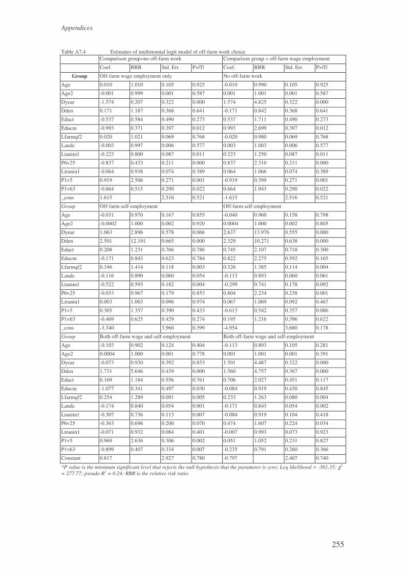
Appendices
255
Table A7.4 Estimates of multinomial logit model of off-farm work choice Comparison group=no off-farm work Comparison group = off-farm wage employment
Coef. RRR Std. Err. P>|T| Coef. RRR Std. Err. P>|T|
Group Off-farm wage employment only No off-farm work
Age 0.010 1.010 0.105 0.925 -0.010 0.990 0.105 0.925
Age2 -0.001 0.999 0.001 0.587 0.001 1.001 0.001 0.587
Dyear -1.574 0.207 0.322 0.000 1.574 4.825 0.322 0.000
Dden 0.171 1.187 0.368 0.641 -0.171 0.842 0.368 0.641
Educt -0.537 0.584 0.490 0.273 0.537 1.711 0.490 0.273
Educm -0.993 0.371 0.397 0.012 0.993 2.699 0.397 0.012
Lfarmqf2 0.020 1.021 0.069 0.768 -0.020 0.980 0.069 0.768
Landc -0.003 0.997 0.006 0.577 0.003 1.003 0.006 0.577
Ltanim1 -0.223 0.800 0.087 0.011 0.223 1.250 0.087 0.011
P6v25 -0.837 0.433 0.211 0.000 0.837 2.310 0.211 0.000
Ltranin1 -0.064 0.938 0.074 0.389 0.064 1.066 0.074 0.389
P1v5 0.919 2.506 0.271 0.001 -0.919 0.399 0.271 0.001
P1v63 -0.664 0.515 0.290 0.022 0.664 1.943 0.290 0.022
_cons 1.615 2.516 0.521 -1.615 2.516 0.521
Group Off-farm self-employment Off-farm self-employment
Age -0.031 0.970 0.167 0.855 -0.040 0.960 0.158 0.798
Age2 -0.0002 1.000 0.002 0.920 0.0004 1.000 0.002 0.805
Dyear 1.063 2.896 0.578 0.066 2.637 13.976 0.555 0.000
Dden 2.501 12.191 0.665 0.000 2.329 10.271 0.638 0.000
Educt 0.208 1.231 0.766 0.786 0.745 2.107 0.718 0.300
Educm -0.171 0.843 0.623 0.784 0.822 2.275 0.592 0.165
Lfarmqf2 0.346 1.414 0.118 0.003 0.326 1.385 0.114 0.004
Landc -0.116 0.890 0.060 0.054 -0.113 0.893 0.060 0.061
Ltanim1 -0.522 0.593 0.182 0.004 -0.299 0.741 0.178 0.092
P6v25 -0.033 0.967 0.179 0.853 0.804 2.234 0.238 0.001
Ltranin1 0.003 1.003 0.096 0.974 0.067 1.069 0.092 0.467
P1v5 0.305 1.357 0.390 0.433 -0.613 0.542 0.357 0.086
P1v63 -0.469 0.625 0.429 0.274 0.195 1.216 0.396 0.622
_cons -3.340 3.960 0.399 -4.954 3.680 0.178
Group Both off-farm wage and self-employment Both off-farm wage and self-employment
Age -0.103 0.902 0.124 0.404 -0.113 0.893 0.105 0.281
Age2 0.0004 1.000 0.001 0.778 0.001 1.001 0.001 0.391
Dyear -0.073 0.930 0.392 0.853 1.501 4.487 0.322 0.000
Dden 1.731 5.646 0.439 0.000 1.560 4.757 0.367 0.000
Educt 0.169 1.184 0.556 0.761 0.706 2.027 0.451 0.117
Educm -1.077 0.341 0.497 0.030 -0.084 0.919 0.430 0.845
Lfarmqf2 0.254 1.289 0.091 0.005 0.233 1.263 0.080 0.004
Landc -0.174 0.840 0.054 0.001 -0.171 0.843 0.054 0.002
Ltanim1 -0.307 0.736 0.113 0.007 -0.084 0.919 0.104 0.418
P6v25 -0.363 0.696 0.200 0.070 0.474 1.607 0.224 0.034
Ltranin1 -0.071 0.932 0.084 0.401 -0.007 0.993 0.073 0.923
P1v5 0.969 2.636 0.306 0.002 0.051 1.052 0.231 0.827
P1v63 -0.899 0.407 0.334 0.007 -0.235 0.791 0.260 0.366
Constant 0.817 2.927 0.780 -0.797 2.407 0.740
*P value is the minimum significant level that rejects the null hypothesis that the parameter is zero; Log likelihood = -361.35; χ2 = 277.77; pseudo R2 = 0.24; RRR is the relative risk ratio.

Appendices
256
Table A7.5 Estimates of multinomial logit model of off-farm work choice Comparison group is off-farm self-employment
only Comparison group = off-farm wage and self
employment Coef. RRR Std. Err. P>|T| Coef. RRR Std. Err. P>|T|
Group No off-farm work No off-farm work Age 0.031 1.031 0.167 0.855 0.103 1.109 0.124 0.404
age2 0.0002 1.000 0.002 0.920 -0.0004 1.000 0.001 0.778
Dyear -1.063 0.345 0.578 0.066 0.073 1.075 0.392 0.853
Dden -2.501 0.082 0.665 0.000 -1.731 0.177 0.439 0.000
Educt -0.208 0.812 0.766 0.786 -0.169 0.844 0.556 0.761
Educm 0.171 1.186 0.623 0.784 1.077 2.936 0.497 0.030
Lfarmqf2 -0.346 0.707 0.118 0.003 -0.254 0.776 0.091 0.005
Landc 0.116 1.123 0.060 0.054 0.174 1.191 0.054 0.001
ltanim1 0.522 1.686 0.182 0.004 0.307 1.359 0.113 0.007
p6v25 0.033 1.034 0.179 0.853 0.363 1.437 0.200 0.070
Ltranin1 -0.003 0.997 0.096 0.974 0.071 1.073 0.084 0.401
p1v5 -0.305 0.737 0.390 0.433 -0.969 0.379 0.306 0.002
p1v63 0.469 1.599 0.429 0.274 0.899 2.458 0.334 0.007
_cons 3.340 3.960 0.399 -0.817 2.927 0.780
Group Off-farm wage employment only Off-farm wage employment only
Age 0.040 1.041 0.158 0.798 0.113 1.120 0.105 0.281
age2 -0.0004 1.000 0.002 0.805 -0.001 0.999 0.001 0.391
Dyear -2.637 0.072 0.555 0.000 -1.501 0.223 0.322 0.000
Dden -2.329 0.097 0.638 0.000 -1.560 0.210 0.367 0.000
Educt -0.745 0.475 0.718 0.300 -0.706 0.493 0.451 0.117
Educm -0.822 0.440 0.592 0.165 0.084 1.088 0.430 0.845
Lfarmqf2 -0.326 0.722 0.114 0.004 -0.233 0.792 0.080 0.004
Landc 0.113 1.119 0.060 0.061 0.171 1.186 0.054 0.002
ltanim1 0.299 1.349 0.178 0.092 0.084 1.088 0.104 0.418
p6v25 -0.804 0.448 0.238 0.001 -0.474 0.622 0.224 0.034
Ltranin1 -0.067 0.935 0.092 0.467 0.007 1.007 0.073 0.923
p1v5 0.613 1.846 0.357 0.086 -0.051 0.951 0.231 0.827
p1v63 -0.195 0.823 0.396 0.622 0.235 1.265 0.260 0.366
_cons 4.954 3.680 0.178 0.797 2.407 0.740
Group Both ff-farm wage and self-employment Off-farm self-employment only
Age -0.073 0.930 0.158 0.645 0.073 1.075 0.158 0.645
age2 0.001 1.001 0.002 0.747 -0.001 0.999 0.002 0.747
Dyear -1.136 0.321 0.566 0.045 1.136 3.115 0.566 0.045
Dden -0.770 0.463 0.651 0.237 0.770 2.159 0.651 0.237
Educt -0.039 0.962 0.696 0.956 0.039 1.040 0.696 0.956
Educm -0.906 0.404 0.603 0.133 0.906 2.475 0.603 0.133
Lfarmqf2 -0.093 0.912 0.116 0.424 0.093 1.097 0.116 0.424
Landc -0.058 0.943 0.071 0.413 0.058 1.060 0.071 0.413
Ltanim1 0.215 1.240 0.173 0.214 -0.215 0.806 0.173 0.214
p6v25 -0.329 0.719 0.204 0.106 0.329 1.390 0.204 0.106
Ltranin1 -0.074 0.929 0.092 0.424 0.074 1.077 0.092 0.424
p1v5 0.664 1.942 0.357 0.063 -0.664 0.515 0.357 0.063
p1v63 -0.430 0.651 0.396 0.278 0.430 1.537 0.396 0.278
_cons 4.157 3.622 0.251 -4.157 3.622 0.251
*P value is the minimum significant level that rejects the null hypothesis that the parameter is zero; Log likelihood = -361.35; χ2 = 277.77; pseudo R2 = 0.24; RRR is the relative risk ratio.

Appendices
257
Table A7.6 Estimates of marginal effect in a multinomial logit model of off-farm work
choices (group zero and one as comparison groups) Comparison group=no off-farm group Comparison group = off-farm wage
employment only Wage employment No off-farm work Coef. Std. Err. T P>|T| Coef. Std. Err. T P>|T| Group Wage employment No off-farm work Age 0.011 0.019 0.586 0.558 0.001 0.016 0.093 0.926 age2 -0.0002 0.0002 -0.804 0.421 0.0001 0.0002 0.411 0.681 Dyear -0.370 0.060 -6.124 0 0.201 0.051 3.932 0.000 Dden -0.144 0.067 -2.136 0.033 -0.079 0.056 -1.417 0.156 Educt -0.140 0.088 -1.593 0.111 0.064 0.075 0.853 0.394 Educm -0.135 0.074 -1.825 0.068 0.157 0.060 2.625 0.009 lfarmqf2 -0.022 0.013 -1.683 0.092 -0.011 0.011 -1.019 0.308 landc 0.015 0.004 4.300 0 0.005 0.002 3.483 0.000 ltanim1 -0.017 0.017 -0.990 0.322 0.039 0.013 2.921 0.003 p6v25 -0.161 0.045 -3.588 0 0.118 0.032 3.741 0.000 ltranin1 -0.009 0.014 -0.640 0.522 0.010 0.011 0.899 0.369 p1v5 0.125 0.046 2.709 0.007 -0.145 0.041 -3.537 0.000 p1v63 -0.070 0.050 -1.393 0.164 0.111 0.044 2.524 0.012 _cons 0.355 0.451 0.786 0.432 -0.214 0.385 -0.555 0.579 Group Self-employment only Self-employment only Age -0.001 0.004 -0.157 0.876 -0.001 0.004 -0.157 0.876 age2 0.000004 0.00004 0.105 0.916 0.000004 0.00004 0.105 0.916 Dyear 0.051 0.020 2.525 0.012 0.051 0.020 2.525 0.012 Dden 0.052 0.020 2.599 0.009 0.052 0.020 2.599 0.009 Educt 0.013 0.017 0.769 0.442 0.013 0.017 0.769 0.442 Educm 0.015 0.014 1.097 0.273 0.015 0.014 1.097 0.273 Lfarmqf2 0.007 0.003 2.416 0.016 0.007 0.003 2.416 0.016 Landc -0.002 0.001 -1.678 0.093 -0.002 0.001 -1.678 0.093 ltanim1 -0.008 0.004 -1.839 0.066 -0.008 0.004 -1.839 0.066 p6v25 0.014 0.007 2.034 0.042 0.014 0.007 2.034 0.042 ltranin1 0.001 0.002 0.631 0.528 0.001 0.002 0.631 0.528 p1v5 -0.010 0.009 -1.150 0.25 -0.010 0.009 -1.150 0.250 p1v63 0.002 0.009 0.236 0.814 0.002 0.009 0.236 0.814 _cons -0.109 0.088 -1.240 0.215 -0.109 0.088 -1.240 0.215 Group Both off-farm wage and self-employment Both off-farm wage and self-employment Age -0.012 0.011 -1.107 0.268 -0.012 0.011 -1.107 0.268 age2 0.0001 0.0001 0.769 0.442 0.0001 0.0001 0.769 0.442 Dyear 0.118 0.040 2.983 0.003 0.118 0.040 2.983 0.003 Dden 0.170 0.042 4.022 0 0.170 0.042 4.022 0.000 Educt 0.062 0.048 1.304 0.192 0.062 0.048 1.304 0.192 Educm -0.037 0.046 -0.810 0.418 -0.037 0.046 -0.810 0.418 Lfarmqf2 0.025 0.007 3.392 0.001 0.025 0.007 3.392 0.001 Landc -0.019 0.004 -4.558 0 -0.019 0.004 -4.558 0.000 Ltanim1 -0.014 0.011 -1.298 0.194 -0.014 0.011 -1.298 0.194 p6v25 0.029 0.022 1.293 0.196 0.029 0.022 1.293 0.196 Ltranin1 -0.003 0.008 -0.345 0.73 -0.003 0.008 -0.345 0.730 p1v5 0.031 0.024 1.284 0.199 0.031 0.024 1.284 0.199 p1v63 -0.044 0.028 -1.582 0.114 -0.044 0.028 -1.582 0.114 _cons -0.032 0.253 -0.126 0.9 -0.032 0.253 -0.126 0.900 *P value is the minimum significant level that rejects the null hypothesis that the parameter is zero; Log likelihood = -361.35; χ2 = 138.29; pseudo R2 = 0.24;

Appendices
258
Table A7.7 Estimates of marginal effect in a multinomial logit model of off-farm work choices (group two and three as comparison groups)
Comparison group = off-farm self-employment only Comparison group = both wage and self-employment
Coef. Std. Err. T P>|T| Coef. Std. Err. T P>|T| Group no off-farm work No off-arm work Age 0.001 0.016 0.093 0.926 0.001 0.016 0.093 0.926 age2 0.0001 0.0002 0.411 0.681 0.0001 0.0002 0.411 0.681 dyear 0.201 0.051 3.932 0.000 0.201 0.051 3.932 0.000 dden -0.079 0.056 -1.417 0.156 -0.079 0.056 -1.417 0.156 educt 0.064 0.075 0.853 0.394 0.064 0.075 0.853 0.394 educm 0.157 0.060 2.625 0.009 0.157 0.060 2.625 0.009 lfarmqf2 -0.011 0.011 -1.019 0.308 -0.011 0.011 -1.019 0.308 landc 0.005 0.002 3.483 0.000 0.005 0.002 3.483 0.000 ltanim1 0.039 0.013 2.921 0.003 0.039 0.013 2.921 0.003 p6v25 0.118 0.032 3.741 0.000 0.118 0.032 3.741 0.000 ltranin1 0.010 0.011 0.899 0.369 0.010 0.011 0.899 0.369 p1v5 -0.145 0.041 -3.537 0.000 -0.145 0.041 -3.537 0.000 p1v63 0.111 0.044 2.524 0.012 0.111 0.044 2.524 0.012 _cons -0.214 0.385 -0.555 0.579 -0.214 0.385 -0.555 0.579 Group Off-farm wage employment only Off-farm wage employment only Age 0.011 0.019 0.586 0.558 0.011 0.019 0.586 0.558 age2 -0.000 0.000 -0.804 0.421 -0.0002 0.0002 -0.804 0.421 Dyear -0.370 0.060 -6.124 0.000 -0.370 0.060 -6.124 0.000 Dden -0.144 0.067 -2.136 0.033 -0.144 0.067 -2.136 0.033 Educt -0.140 0.088 -1.593 0.111 -0.140 0.088 -1.593 0.111 Educm -0.135 0.074 -1.825 0.068 -0.135 0.074 -1.825 0.068 Lfarmqf2 -0.022 0.013 -1.683 0.092 -0.022 0.013 -1.683 0.092 Landc 0.015 0.004 4.300 0.000 0.015 0.004 4.300 0.000 ltanim1 -0.017 0.017 -0.990 0.322 -0.017 0.017 -0.990 0.322 p6v25 -0.161 0.045 -3.588 0.000 -0.161 0.045 -3.588 0.000 Ltranin1 -0.009 0.014 -0.640 0.522 -0.009 0.014 -0.640 0.522 p1v5 0.125 0.046 2.709 0.007 0.125 0.046 2.709 0.007 p1v63 -0.070 0.050 -1.393 0.164 -0.070 0.050 -1.393 0.164 _cons 0.355 0.451 0.786 0.432 0.355 0.451 0.786 0.432 Group both off-farm wage and self employment Off-farm self-employment only Age -0.012 0.011 -1.107 0.268 -0.001 0.004 -0.157 0.876 age2 0.0001 0.0001 0.769 0.442 0.000004 0.00004 0.105 0.916 Dyear 0.118 0.040 2.983 0.003 0.051 0.020 2.525 0.012 Dden 0.170 0.042 4.022 0.000 0.052 0.020 2.599 0.009 Educt 0.062 0.048 1.304 0.192 0.013 0.017 0.769 0.442 Educm -0.037 0.046 -0.810 0.418 0.015 0.014 1.097 0.273 Lfarmqf2 0.025 0.007 3.392 0.001 0.007 0.003 2.416 0.016 Landc -0.019 0.004 -4.558 0.000 -0.002 0.001 -1.678 0.093 ltanim1 -0.014 0.011 -1.298 0.194 -0.008 0.004 -1.839 0.066 p6v25 0.029 0.022 1.293 0.196 0.014 0.007 2.034 0.042 ltranin1 -0.003 0.008 -0.345 0.730 0.001 0.002 0.631 0.528 p1v5 0.031 0.024 1.284 0.199 -0.010 0.009 -1.150 0.250 p1v63 -0.044 0.028 -1.582 0.114 0.002 0.009 0.236 0.814 _cons -0.032 0.253 -0.126 0.900 -0.109 0.088 -1.240 0.215 *P value is the minimum significant level that rejects the null hypothesis that the parameter is zero; Log likelihood = -361.35; χ2 = 138.29; pseudo R2 = 0.24;

Appendices
259
Appendix A8 Estimation of crop choice, labour and land allocation equations presented in Chapter 8 AppendixA8.1 Description of variables used in the econometric estimations Variables Description AGE Age of the household head AGE2 Age squared of household head BAKELP Proportion of loam (bakel) soil cultivated BARCSH Share of barley in total consumption BARVINB Value of variable input used for barley BARYKF Barley yield in kilogram DEPRAT Dependency ratio DFMYKF Sorghum and finger millet yield in kilogram DTAA Dummy for Tabia Araasegda DTAF Dummy for Tabia Fekre alem DTEF Dummy for Tabia Felegeselam DTEM Dummy for Tabia Mytsedo DYEAR Year dummy (1996=1, 1997=0) EDUCH Education dummy (head read and write=1, 0 otherwise) EDUCW Education dummy (wife read and write=1, 0 otherwise) HUTSAP Proportion of sandy soil (Hutsa) cultivated IMR Inverse mills ratio LEGCSHF Share of legumes in total consumption LEGLAN Land allocated to legumes LEGVINB Value of variable input used for legumes LEGYKF Legume crops yield in kilogram NFHF Hours worked off the farm (fitted value) NFIN1 Non-farm income (Birr) NFIN1F Non-farm income NFIN1F0 Non-farm income in 100 Birr (fitted value) OILCSHF Share of oil crop in total consumption OILVINB Value of variable input used for oil crops OILYKF Oil crops yield in kilogram P1V5 Family size P1V63 Number of dependants P2V2 Value of farm implements (replacement cost in Birr) P5V67 Land allocated to barley P5V68 Labour hours allocated to barley P5V79 Land allocated to oil crops P5V80 Labour hours allocated to oil crops P6V1 The number of oxen owned P6V2 Value of oxen owned IN Birr (at replacement cost) P6V26 Value of transport animal owned (at replacement cost) RHO(1,2) Correlation between the error terms of the probability of buying and selling farm outputs SFMCSHF Share of sorghum and finger millet in total consumption SFMLAN Land allocated to sorghum and finger millet SFMVINB Value of variable input used for sorghum and finger millet Sigma Standard error SOILI Soil depth index TANIM Total livestock wealth TANIM0 Total livestock wealth in 1000 Birr TEFCSHF Share of teff in total consumption TEFLAN Land allocated to teff TEFVINB Value of variable input used for teff TEFYKF Teff yield in kilogram TEQUIP Total value of equipment households own in Birr TEQUIP0 Total value of equipment households own in 1000 Birr TLANDCR Total land allocated to crops in tsimdi (one hectare = 4 tsimdi) TYLDB1F Fitted value of crop output in Birr VEGCSHF Share of vegetables in total consumption VEGLAN Land allocated to vegetables VEGVINB Value of variable input used for vegetables VEGYKF Vegetables yield in kilogram WALKAP Proportion of clay (walka) soil cultivated WHTCSHF Share of wheat in total consumption WHTLAN Land allocated to wheat WHTVINB Value of variable input used for wheat WHTYKF Wheat yield in kilogram One US Dollar was equivalent to seven Birr during the time of surveying

Appendices
260
Appendix A8.2 Logit model of probability of growing crops using instrumental variable approach Table A8.2.1 Logit Model of Probability of growing teff
Coef. Std. Err. T-ratio P>|T| Marginal Age 0.091 0.106 0.860 0.390 0.019 age2 -0.001 0.001 -1.366 0.172 -0.0003 p1v5 0.100 0.130 0.767 0.443 0.021 Deprat -0.804 0.990 -0.812 0.417 -0.171 Dyear -0.986 0.337 -2.925 0.003 -0.209 Dtaa 0.490 0.546 0.898 0.369 0.104 Dtaf 0.972 0.704 1.380 0.168 0.206 Dtef -0.720 0.521 -1.381 0.167 -0.153 Dtem 0.305 0.582 0.524 0.601 0.065 Walkap 1.250 0.618 2.023 0.043 0.265 Hutsap 0.079 0.491 0.160 0.873 0.017 Soili 1.738 0.561 3.096 0.002 0.369 Nfin1f 0.0003 0.001 0.629 0.529 0.0001 p2v2 0.003 0.002 2.003 0.045 0.001 p6v1 -0.035 0.118 -0.296 0.767 -0.007 Tlandcr 0.180 0.053 3.406 0.001 0.038 Tefcshf 7.279 6.352 1.146 0.252 1.545 Constant -5.022 2.574 -1.951 0.051 -1.066 Table A8.2.2 Logit Model of Probability of growing wheat
Coef. Std. Err. T P>|T| Marginal Age -0.138 0.101 -1.365 0.172 -0.026 age2 0.002 0.001 1.551 0.121 0.0003 p1v5 0.147 0.145 1.018 0.308 0.028 Deprat 0.848 1.019 0.832 0.405 0.160 Dyear 0.206 0.344 0.601 0.548 0.039 Dtaa -0.680 0.582 -1.167 0.243 -0.128 Dtaf -1.196 0.798 -1.499 0.134 -0.225 Dtef -0.181 0.588 -0.308 0.758 -0.034 Dtem 0.541 0.636 0.851 0.395 0.102 Walkap -0.226 0.593 -0.382 0.702 -0.043 Hutsap 1.040 0.513 2.028 0.043 0.196 Soili 0.786 0.537 1.463 0.143 0.148 nfin1f -0.001 0.001 -1.213 0.225 -0.0001 p2v2 -0.001 0.002 -0.340 0.733 -0.0001 p6v1 0.231 0.192 1.202 0.229 0.044 Tlandcr 0.249 0.060 4.150 0.000 0.047 Whtcshf 0.842 6.696 0.126 0.900 0.159 Constant 0.948 2.817 0.337 0.736 0.179 Table A8.2.3 Logit Model of Probability of growing barley
Coef. Std. Err. T P>|T| Marginal Age 0.046 0.123 0.378 0.706 0.004 age2 -0.001 0.001 -0.462 0.644 -0.00004 p1v5 0.207 0.186 1.110 0.267 0.016 Deprat -0.185 1.219 -0.152 0.879 -0.014 Dyear 0.093 0.486 0.192 0.848 0.007 Dtaa -0.919 0.798 -1.152 0.249 -0.071 Dtaf -1.726 1.165 -1.481 0.139 -0.134 Dtef -0.630 0.807 -0.780 0.435 -0.049 Dtem -0.496 0.817 -0.607 0.544 -0.038 Walkap 0.337 0.802 0.420 0.675 0.026 Hutsap 0.961 0.628 1.532 0.125 0.075 Soili 1.846 0.687 2.687 0.007 0.143 nfin1f -0.001 0.001 -1.155 0.248 -0.0001 p2v2 -0.005 0.002 -2.533 0.011 -0.0004 p6v1 0.662 0.269 2.458 0.014 0.051 Tlandcr 0.372 0.094 3.948 0.000 0.029 Barcshf 11.259 6.885 1.635 0.102 0.873 Constant -3.419 3.327 -1.028 0.304 -0.265

Appendices
261
Table A8.2.4 Logit Model of Probability of growing sorghum and finger millet Coef. Std. Err. T P>|T| Marginal
Age 0.067 0.132 0.505 0.614 0.003 age2 -0.001 0.001 -0.655 0.513 -0.00004 p1v5 0.241 0.172 1.405 0.160 0.011 Deprat -2.098 1.431 -1.466 0.143 -0.096 Dyear 2.663 0.554 4.804 0.000 0.121 Dtaa 1.317 0.659 1.999 0.046 0.060 Dtaf 1.069 0.898 1.190 0.234 0.049 Dtef -2.708 1.137 -2.383 0.017 -0.123 Dtem -1.957 0.974 -2.009 0.045 -0.089 Walkap -1.151 0.823 -1.398 0.162 -0.052 Hutsap 0.892 0.651 1.370 0.171 0.041 Soili 0.450 0.712 0.632 0.527 0.020 nfin1f -0.0002 0.001 -0.329 0.743 -0.00001 p2v2 -0.0001 0.001 -0.119 0.905 -0.00001 p6v1 0.015 0.197 0.077 0.938 0.001 Tlandcr 0.116 0.053 2.184 0.029 0.005 Sfmcshf -17.542 36.637 -0.479 0.632 -0.799 Constant -5.985 3.505 -1.707 0.088 -0.273 Table A8.2.5 Logit Model of Probability of growing legumes
Coef. Std Err. T P>|T| Marginal Age 0.006 0.103 0.055 0.956 0.001 age2 -0.0003 0.001 -0.285 0.776 -0.0001 p1v5 0.137 0.124 1.106 0.269 0.032 Deprat -0.803 1.063 -0.755 0.450 -0.187 Dyear -0.110 0.313 -0.352 0.725 -0.026 Dtaa -0.003 0.512 -0.006 0.995 -0.001 Dtaf -0.526 0.660 -0.796 0.426 -0.122 Dtef -0.039 0.498 -0.079 0.937 -0.009 Dtem 0.111 0.521 0.214 0.831 0.026 Walkap 1.845 0.576 3.202 0.001 0.429 Hutsap 0.135 0.525 0.258 0.796 0.031 Soili 0.491 0.601 0.816 0.414 0.114 nfin1f -0.0001 0.0005 -0.257 0.797 -0.00003 p2v2 -0.001 0.001 -0.525 0.599 -0.0001 p6v1 -0.200 0.163 -1.227 0.220 -0.046 Tlandcr 0.352 0.054 6.527 0.000 0.082 Legcshf 13.245 96.826 0.137 0.891 3.077 Constant -3.639 5.525 -0.659 0.510 -0.845 Table A8.2.6 Logit Model of Probability of growing oil crops
Coef. Std Err. T P>|T| Marginal Age 0.060 0.170 0.350 0.726 0.004 age2 -0.0005 0.002 -0.280 0.779 -0.00003 p1v5 0.017 0.180 0.096 0.924 0.001 Deprat 2.356 1.772 1.330 0.184 0.141 Dyear -0.037 0.438 -0.085 0.933 -0.002 Dtaa 0.029 0.741 0.039 0.969 0.002 Dtaf -1.194 0.910 -1.311 0.190 -0.071 Dtef 0.223 0.763 0.293 0.770 0.013 Dtem 0.866 0.779 1.112 0.266 0.052 Walkap 0.893 0.824 1.084 0.278 0.053 Hutsap 1.057 0.758 1.394 0.163 0.063 Soili 1.094 0.884 1.237 0.216 0.065 nfin1f -0.001 0.001 -1.999 0.046 -0.0001 p2v2 -0.003 0.002 -1.560 0.119 -0.0002 p6v1 -0.001 0.190 -0.003 0.998 -0.00003 Tlandcr 0.077 0.054 1.408 0.159 0.005 Oilcshf -0.587 168.442 -0.003 0.997 -0.035 Constant -4.869 4.418 -1.102 0.270 -0.291

Appendices
262
Table A8.2.7 Logit Model of Probability of growing vegetables Coef. Std Err. T P>|T| Marginal
Age 0.645 0.284 2.269 0.023 0.021 Age2 -0.006 0.003 -2.307 0.021 -0.0002 p1v5 -0.503 0.272 -1.847 0.065 -0.016 Deprat 2.644 1.927 1.372 0.170 0.087 Dyear -0.632 0.531 -1.189 0.234 -0.021 Dtaa -1.095 0.820 -1.336 0.182 -0.036 Dtaf -1.989 1.135 -1.752 0.080 -0.065 Dtem -1.286 0.862 -1.491 0.136 -0.042 Walkap 2.830 1.131 2.501 0.012 0.093 Hutsap 3.504 0.977 3.587 0.000 0.115 Soili 2.055 1.283 1.601 0.109 0.067 Nfin1f 0.001 0.001 0.927 0.354 0.00003 p2v2 0.001 0.001 0.445 0.656 0.00002 p6v1 -0.208 0.276 -0.755 0.450 -0.007 Tlandcr -0.007 0.074 -0.088 0.929 -0.0002 Vegcshf -2647.5 884.577 -2.993 0.003 -86.782 Constant -17.090 7.132 -2.396 0.017 -0.560

Appendices
263
Appendix A8.3 Parameter estimates of Tobit model for the land allocation of different crops Table A8.3.1 Parameter estimates of share of land allocated to teff
Coef. Std. Err. T P>|t| Marginal Nfin1f0 -0.0043 0.0015 -2.9490 0.0030 -0.0028 Tanim0 -0.0004 0.0019 -0.2130 0.8320 -0.0003 Tequip0 -0.0339 0.0140 -2.4240 0.0160 -0.0219 Tlandcr -0.0236 0.0024 -9.7610 0.0000 -0.0152 Tefykf 0.0015 0.0001 21.3990 0.0000 0.0009 Tefcshf -0.0371 0.2926 -0.1270 0.8990 -0.0239 p1v63 -0.0116 0.0124 -0.9330 0.3520 -0.0075 p1v5 0.0206 0.0118 1.7440 0.0820 0.0133 Educh -0.0032 0.0169 -0.1880 0.8510 -0.0021 Dyear -0.1485 0.0176 -8.4530 0.0000 -0.0957 Walkap 0.1194 0.0331 3.6120 0.0000 0.0769 Hutsap 0.0746 0.0286 2.6110 0.0090 0.0481 Soili 0.1150 0.0309 3.7250 0.0000 0.0741 Constant 0.0309 0.0492 0.6280 0.5310 Sigma 0.1318 0.0061 Table A8.3.2 Parameter estimates of share of land allocated to wheat
Coef. Std. Err. T P>|t| marginal Nfin1f0 -0.0046 0.0016 -2.9240 0.0040 -0.0031 Tanim0 0.0003 0.0017 0.1980 0.8430 0.0002 Tequip -0.0306 0.0149 -2.0620 0.0400 -0.0207 Tlandcr -0.0275 0.0029 -9.4000 0.0000 -0.0186 Whtykf 0.0007 0.0000 20.6170 0.0000 0.0005 Whtcshf 0.5818 0.3870 1.5030 0.1340 0.3922 p1v63 -0.0317 0.0129 -2.4590 0.0140 -0.0214 p1v5 0.0445 0.0126 3.5320 0.0000 0.0300 Educh 0.0140 0.0178 0.7860 0.4320 0.0095 Dyear -0.0658 0.0183 -3.6020 0.0000 -0.0444 Walkap 0.0612 0.0357 1.7120 0.0880 0.0412 Hutsap 0.1190 0.0296 4.0170 0.0000 0.0802 Soili 0.1916 0.0321 5.9770 0.0000 0.1292 Constant -0.1189 0.0821 -1.4470 0.1490 Sigma 0.1449 0.0067 Table A8.3.3 Parameter estimates of share of land allocated to barley
Coef. Std. Err. T P>|t| marginal nfin1f0 -0.0104 0.0022 -4.8190 0.0000 -0.0084 Tanim0 -0.0053 0.0024 -2.1460 0.0330 -0.0042 Tequip -0.0593 0.0207 -2.8600 0.0040 -0.0476 Tlandcr -0.0177 0.0038 -4.7040 0.0000 -0.0142 Barykf 0.0004 0.0000 12.6300 0.0000 0.0003 Barcshf 0.2037 0.3747 0.5440 0.5870 0.1637 p1v63 -0.0222 0.0181 -1.2240 0.2220 -0.0178 p1v5 0.0329 0.0172 1.9160 0.0560 0.0265 educh -0.0123 0.0249 -0.4960 0.6210 -0.0099 dyear -0.0937 0.0255 -3.6700 0.0000 -0.0753 walkap 0.0475 0.0495 0.9610 0.3370 0.0382 hutsap 0.1078 0.0415 2.5940 0.0100 0.0866 soili 0.2690 0.0446 6.0370 0.0000 0.2161 Constant 0.0783 0.0898 0.8720 0.3840 Sigma 0.2084 0.0086

Appendices
264
Table A8.3.4 Parameter estimates of share of land allocated to sorghum and f millet Coef. Std. Err. T P>|t| marginal nfin1f0 -0.0025 0.0035 -0.7140 0.4760 -0.0004 tanim0 0.0022 0.0037 0.5880 0.5570 0.0003 tequip 0.0005 0.0460 0.0110 0.9910 0.0001 tlandcr -0.0237 0.0058 -4.1200 0.0000 -0.0034 sfmykf 0.0015 0.0001 12.4920 0.0000 0.0002 sfmcshf -1.3995 3.7026 -0.3780 0.7060 -0.1984 p1v63 -0.0328 0.0260 -1.2600 0.2080 -0.0046 p1v5 0.0344 0.0248 1.3870 0.1660 0.0049 educh 0.0070 0.0354 0.1990 0.8420 0.0010 dyear 0.0704 0.0460 1.5310 0.1270 0.0100 walkap 0.0487 0.0711 0.6850 0.4940 0.0069 hutsap 0.0403 0.0571 0.7060 0.4810 0.0057 soili 0.0764 0.0588 1.3000 0.1940 0.0108 Constant -0.3196 0.0895 -3.5720 0.0000 Sigma 0.1486 0.0149 Table A8.3.5 Parameter estimates of share of land allocated to legumes
Coef. Std. Err. T P>|t| Marginal nfin1f0 0.0016 0.0016 0.9500 0.3430 0.0006 tanim0 0.00003 0.0020 0.0160 0.9870 0.00001 Tequip -0.0368 0.0171 -2.1480 0.0320 -0.00002 Tlandcr -0.0147 0.0028 -5.2230 0.0000 -0.0060 Legykf 0.0015 0.0001 18.5990 0.0000 0.0006 Legcshf -3.6485 3.9717 -0.9190 0.3590 -1.4884 p1v63 -0.0194 0.0146 -1.3310 0.1840 -0.0079 p1v5 0.0198 0.0139 1.4190 0.1570 0.0081 Educh 0.0227 0.0193 1.1750 0.2410 0.0093 Dyear -0.0728 0.0188 -3.8600 0.0000 -0.0297 Walkap 0.0924 0.0389 2.3770 0.0180 0.0377 Hutsap 0.0086 0.0342 0.2510 0.8020 0.0035 Soili 0.1268 0.0371 3.4130 0.0010 0.0517 Constant 0.0105 0.1968 0.0530 0.9580 Sigma 0.1332 0.0080 Table A8.3.6 Parameter estimates of share of land allocated to oil crops
Coef. Std. Err. T P>|t| marginal nfin1f0 0.0007 0.0023 0.3100 0.7570 0.0001 tanim0 -0.0004 0.0015 -0.2980 0.7660 -0.00004 tequip 0.0082 0.0196 0.4170 0.6770 0.0008 tlandcr -0.0067 0.0039 -1.7210 0.0860 -0.0006 oilykf 0.0038 0.0003 11.6580 0.0000 0.0004 oilcshf -9.5240 7.3016 -1.3040 0.1930 -0.8766 p1v63 0.0139 0.0204 0.6790 0.4980 0.0013 p1v5 -0.0171 0.0197 -0.8650 0.3880 -0.0016 educh 0.0233 0.0211 1.1070 0.2690 0.0021 dyear -0.0507 0.0246 -2.0610 0.0400 -0.0047 walkap 0.0482 0.0390 1.2360 0.2170 0.0044 hutsap 0.0036 0.0397 0.0920 0.9270 0.0003 soili 0.0570 0.0457 1.2460 0.2130 0.0052 Constant -0.1093 0.0630 -1.7370 0.0830 Sigma 0.0748 0.0091 Table A8.3.7 Parameter estimates of share of land allocated to vegetables Coef. Std. Err. T P>|t| Marginal nfin1f0 -0.0004 0.0025 -0.1750 0.8610 -0.00003 tanim0 -0.0001 0.0036 -0.0410 0.9670 -0.00001 tequip -0.0133 0.0175 -0.7590 0.4480 -0.0010 tlandcr -0.0007 0.0038 -0.1910 0.8490 -0.0001 vegykf 0.0004 0.0000 8.0170 0.0000 0.00003 vegcshf -38.6948 47.8076 -0.8090 0.4190 -2.7914 p1v63 -0.0004 0.0231 -0.0160 0.9870 -0.00003 p1v5 0.0040 0.0227 0.1750 0.8610 0.0003 educh -0.0515 0.0292 -1.7640 0.0790 -0.0037 dyear -0.0572 0.0267 -2.1470 0.0320 -0.0041 walkap 0.0831 0.0562 1.4790 0.1400 0.0060 hutsap 0.1222 0.0515 2.3730 0.0180 0.0088 soili 0.0205 0.0568 0.3610 0.7180 0.0015 Constant -0.1901 0.0953 -1.9940 0.0470 Sigma 0.0823 0.0120
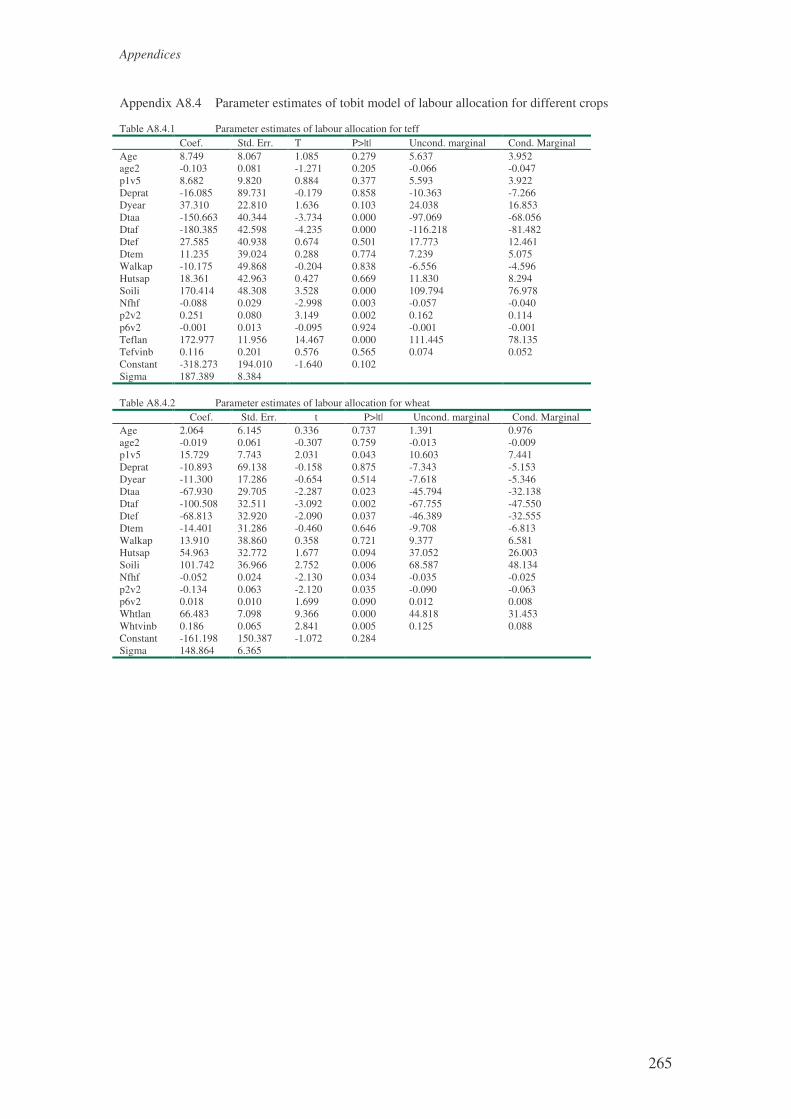
Appendices
265
Appendix A8.4 Parameter estimates of tobit model of labour allocation for different crops Table A8.4.1 Parameter estimates of labour allocation for teff Coef. Std. Err. T P>|t| Uncond. marginal Cond. Marginal Age 8.749 8.067 1.085 0.279 5.637 3.952 age2 -0.103 0.081 -1.271 0.205 -0.066 -0.047 p1v5 8.682 9.820 0.884 0.377 5.593 3.922 Deprat -16.085 89.731 -0.179 0.858 -10.363 -7.266 Dyear 37.310 22.810 1.636 0.103 24.038 16.853 Dtaa -150.663 40.344 -3.734 0.000 -97.069 -68.056 Dtaf -180.385 42.598 -4.235 0.000 -116.218 -81.482 Dtef 27.585 40.938 0.674 0.501 17.773 12.461 Dtem 11.235 39.024 0.288 0.774 7.239 5.075 Walkap -10.175 49.868 -0.204 0.838 -6.556 -4.596 Hutsap 18.361 42.963 0.427 0.669 11.830 8.294 Soili 170.414 48.308 3.528 0.000 109.794 76.978 Nfhf -0.088 0.029 -2.998 0.003 -0.057 -0.040 p2v2 0.251 0.080 3.149 0.002 0.162 0.114 p6v2 -0.001 0.013 -0.095 0.924 -0.001 -0.001 Teflan 172.977 11.956 14.467 0.000 111.445 78.135 Tefvinb 0.116 0.201 0.576 0.565 0.074 0.052 Constant -318.273 194.010 -1.640 0.102 Sigma 187.389 8.384 Table A8.4.2 Parameter estimates of labour allocation for wheat
Coef. Std. Err. t P>|t| Uncond. marginal Cond. Marginal Age 2.064 6.145 0.336 0.737 1.391 0.976 age2 -0.019 0.061 -0.307 0.759 -0.013 -0.009 p1v5 15.729 7.743 2.031 0.043 10.603 7.441 Deprat -10.893 69.138 -0.158 0.875 -7.343 -5.153 Dyear -11.300 17.286 -0.654 0.514 -7.618 -5.346 Dtaa -67.930 29.705 -2.287 0.023 -45.794 -32.138 Dtaf -100.508 32.511 -3.092 0.002 -67.755 -47.550 Dtef -68.813 32.920 -2.090 0.037 -46.389 -32.555 Dtem -14.401 31.286 -0.460 0.646 -9.708 -6.813 Walkap 13.910 38.860 0.358 0.721 9.377 6.581 Hutsap 54.963 32.772 1.677 0.094 37.052 26.003 Soili 101.742 36.966 2.752 0.006 68.587 48.134 Nfhf -0.052 0.024 -2.130 0.034 -0.035 -0.025 p2v2 -0.134 0.063 -2.120 0.035 -0.090 -0.063 p6v2 0.018 0.010 1.699 0.090 0.012 0.008 Whtlan 66.483 7.098 9.366 0.000 44.818 31.453 Whtvinb 0.186 0.065 2.841 0.005 0.125 0.088 Constant -161.198 150.387 -1.072 0.284 Sigma 148.864 6.365

Appendices
266
Table A8.4.3 Parameter estimates of labour allocation for barley Coef. Std. Err. T P>|t| Uncond. marginal Cond. Marginal
Age 2.261 3.182 0.711 0.478 1.822 1.332 age2 -0.024 0.032 -0.738 0.461 -0.019 -0.014 p1v5 4.374 3.970 1.102 0.271 3.525 2.577 Deprat -18.418 35.177 -0.524 0.601 -14.844 -10.854 Dyear 18.701 9.221 2.028 0.043 15.072 11.021 Dtaa -38.506 15.667 -2.458 0.014 -31.035 -22.692 Dtaf -50.054 17.245 -2.903 0.004 -40.342 -29.497 Dtef -4.187 16.633 -0.252 0.801 -3.375 -2.468 Dtem 13.537 16.075 0.842 0.400 10.910 7.977 Walkap 26.560 20.003 1.328 0.185 21.407 15.652 Hutsap 42.936 16.793 2.557 0.011 34.605 25.303 Soili 55.177 18.583 2.969 0.003 44.471 32.517 Nfhf -0.031 0.012 -2.469 0.014 -0.025 -0.018 p2v2 0.032 0.034 0.931 0.352 0.026 0.019 p6v2 -0.003 0.005 -0.607 0.544 -0.003 -0.002 p5v67 52.610 3.364 15.638 0.000 42.402 31.004 Barvinb 0.203 0.032 6.352 0.000 0.164 0.120 Constant -91.153 77.629 -1.174 0.241 Sigma 80.126 3.158 Table A8.4.4 Parameter estimates of labour allocation for sorghum and finger millet
Coef. Std. Err. T P>|t| Uncond. marginal Cond. Marginal Age 19.547 11.016 1.774 0.077 2.772 3.731 age2 -0.200 0.111 -1.808 0.071 -0.028 -0.038 p1v5 8.913 12.409 0.718 0.473 1.264 1.701 Deprat -132.501 103.686 -1.278 0.202 -18.787 -25.287 Dyear 63.597 32.026 1.986 0.048 9.017 12.137 Dtaa -0.201 41.343 -0.005 0.996 -0.028 -0.038 Dtaf -68.407 49.309 -1.387 0.166 -9.700 -13.055 Dtef -141.196 69.112 -2.043 0.042 -20.020 -26.947 Dtem -78.878 56.285 -1.401 0.162 -11.184 -15.054 Walkap -26.794 61.919 -0.433 0.665 -3.799 -5.114 Hutsap 42.544 49.008 0.868 0.386 6.032 8.119 Soili 84.080 55.493 1.515 0.131 11.922 16.046 Nfhf -0.037 0.036 -1.027 0.305 -0.005 -0.007 p2v2 -0.169 0.109 -1.550 0.122 -0.024 -0.032 p6v2 0.005 0.015 0.304 0.761 0.001 0.001 Sfmlan 77.274 12.101 6.386 0.000 10.957 14.748 Sfmvinb 2.922 0.779 3.751 0.000 0.414 0.558 Constant -629.139 269.711 -2.333 0.020 Sigma 132.254 13.812 Table A8.4.5 Parameter estimates of labour allocation for legumes
Coef. Std. Err. T P>|t| Uncond. marginal Cond. Marginal Age -2.380 4.033 -0.590 0.555 -0.983 -0.757 age2 0.010 0.041 0.252 0.801 0.004 0.003 p1v5 4.417 4.976 0.888 0.375 1.824 1.405 Deprat 5.694 46.362 0.123 0.902 2.351 1.812 Dyear 7.866 10.738 0.733 0.464 3.248 2.503 Dtaa 1.447 19.181 0.075 0.940 0.598 0.460 Dtaf 0.906 21.350 0.042 0.966 0.374 0.288 Dtef -19.548 20.668 -0.946 0.345 -8.072 -6.220 Dtem 12.088 19.518 0.619 0.536 4.992 3.846 Walkap -3.598 25.031 -0.144 0.886 -1.486 -1.145 Hutsap 16.693 21.984 0.759 0.448 6.893 5.312 Soili 75.402 25.635 2.941 0.003 31.136 23.992 Nfhf -0.024 0.015 -1.605 0.109 -0.010 -0.008 p2v2 0.006 0.036 0.156 0.876 0.002 0.002 p6v2 -0.006 0.007 -0.961 0.337 -0.003 -0.002 Leglan 70.540 6.579 10.722 0.000 29.129 22.445 Legvinb 0.497 0.100 4.965 0.000 0.205 0.158 Constant -50.586 94.721 -0.534 0.594 Sigma 78.807 4.401

Appendices
267
Table A8.4.6 Parameter estimates of labour allocation for oil crops (linseed) Coef. Std. Err. T P>|t| Uncond. marginal Cond. Marginal
Age 0.741 4.444 0.167 0.868 0.068 0.122 age2 -0.002 0.044 -0.047 0.962 0.000 0.000 p1v5 -6.277 5.804 -1.081 0.280 -0.578 -1.034 Deprat 44.383 52.276 0.849 0.396 4.085 7.310 Dyear -3.391 12.403 -0.273 0.785 -0.312 -0.558 Dtaa 37.785 25.994 1.454 0.147 3.478 6.223 Dtaf 40.728 25.107 1.622 0.106 3.749 6.708 Dtef -19.943 32.487 -0.614 0.540 -1.836 -3.284 Dtem 40.151 26.276 1.528 0.127 3.695 6.613 Walkap 16.940 23.645 0.716 0.474 1.559 2.790 Hutsap 18.823 23.031 0.817 0.414 1.732 3.100 Soili -12.976 27.776 -0.467 0.641 -1.194 -2.137 Nfhf -0.010 0.018 -0.547 0.585 -0.001 -0.002 p2v2 0.046 0.042 1.099 0.272 0.004 0.008 p6v2 -0.005 0.007 -0.751 0.453 0.000 -0.001 p5v79 114.724 13.541 8.472 0.000 10.559 18.894 Oilvinb 0.339 0.315 1.076 0.283 0.031 0.056 Constant -139.051 109.367 -1.271 0.204 Sigma 44.639 5.651 Table A8.4.7 Parameter estimates of labour allocation for vegetables
Coef. Std. Err. T P>|t| Uncond. marginal Cond. Marginal Age 41.522 24.530 1.693 0.091 3.099 6.413 age2 -0.407 0.240 -1.695 0.091 -0.030 -0.063 p1v5 4.890 18.535 0.264 0.792 0.365 0.755 Deprat 97.788 173.268 0.564 0.573 7.298 15.103 Dyear 23.768 39.435 0.603 0.547 1.774 3.671 Dtaa 42.353 58.419 0.725 0.469 3.161 6.541 Dtaf -165.948 74.085 -2.240 0.026 -12.384 -25.631 Dtef -570.251 . . . -42.556 -88.076 Dtem -30.003 55.545 -0.540 0.589 -2.239 -4.634 Walkap -181.797 110.227 -1.649 0.100 -13.567 -28.079 Hutsap 147.911 77.941 1.898 0.058 11.038 22.845 Soili 15.801 93.928 0.168 0.866 1.179 2.440 Nfhf -0.114 0.053 -2.163 0.031 -0.008 -0.018 P2v2 0.052 0.112 0.461 0.645 0.004 0.008 P6v2 -0.031 0.028 -1.118 0.264 -0.002 -0.005 Veglan 339.750 49.511 6.862 0.000 25.355 52.475 Vegvinb 0.562 0.354 1.590 0.113 0.042 0.087 Constant -1197.379 622.938 -1.922 0.055 Sigma 119.864 16.330

Appendices
268
Appendix A8.5 Estimates of buying and selling equations Table A8.5.1 Bivariate probit estimation of being Buyer and Seller (line 1-14 for buyers and 15 – 30 for sellers)
Variable Coeffici S.E T-ratio P>|T| Constant 2.86210 1.68590 1.69800 0.08958 DTAA -0.82876 0.49693 -1.66800 0.09536 DTAF -0.73943 0.49648 -1.48900 0.13639 DTEF -0.45957 0.53932 -0.85200 0.39414 DTEM -0.53466 0.53124 -1.00600 0.31421 DYEAR 0.20726 0.25698 0.80600 0.41996 AGE -0.05091 0.07244 -0.70300 0.48220 AGE2 0.00058 0.00074 0.78500 0.43261 EDUCH -0.25803 0.21558 -1.19700 0.23134 P1V5 -0.11136 0.08968 -1.24200 0.21435 DEPRAT 1.43710 0.80619 1.78300 0.07466 P6V26 -0.00008 0.00011 -0.72600 0.46775 TYLDB1F -0.00016 0.00009 -1.80600 0.07090 NFIN1 0.00032 0.00015 2.17400 0.02968 Constant -1.42470 1.17600 -1.21100 0.22572 DTAA -0.59702 0.23822 -2.50600 0.01220 DTAF 0.05711 0.25456 0.22400 0.82248 DTEF 0.00057 0.26203 0.00200 0.99825 DTEM -0.28210 0.27685 -1.01900 0.30822 DYEAR -0.07513 0.16040 -0.46800 0.63950 AGE 0.04408 0.05115 0.86200 0.38887 AGE2 -0.00042 0.00052 -0.82300 0.41072 EDUCH 0.04999 0.16444 0.30400 0.76114 P1V5 0.06218 0.05802 1.07200 0.28387 DEPRAT -0.06697 0.53782 -0.12500 0.90091 P6V26 0.00031 0.00031 0.98200 0.32600 TYLDB1F 0.00037 0.00008 4.67600 0.00000 NFIN1 -0.00012 0.00006 -1.97300 0.04846 RHO(1,2) 0.00703 0.14657 0.04800 0.96175 Table A8.5.2 Probit model of probability of being a buyer
Variable Coefficient Marginal Std. Error T-ratio. P>|T| Constant 2.85640 0.36610 1.60920 1.77500 0.07590 DTAA -0.82853 -0.10619 0.38610 -2.14600 0.03188 DTAF -0.73979 -0.09482 0.38711 -1.91100 0.05600 DTEF -0.45866 -0.05879 0.44212 -1.03700 0.29954 DTEM -0.53407 -0.06845 0.41671 -1.28200 0.19997 DYEAR 0.20781 0.02664 0.20685 1.00500 0.31508 AGE -0.05065 -0.00649 0.06896 -0.73400 0.46267 AGE2 0.00058 0.00007 0.00070 0.82900 0.40698 EDUCH -0.25751 -0.03301 0.19304 -1.33400 0.18221 P1V5 -0.11165 -0.01431 0.07623 -1.46500 0.14301 DEPRAT 1.43890 0.18442 0.74693 1.92600 0.05405 P6V26 -0.00008 -0.00001 0.00010 -0.75500 0.45054 TYLDB1F -0.00016 -0.00002 0.00008 -2.18000 0.02929 NFIN1 0.00032 0.00004 0.00013 2.52900 0.01145 Table A8.5.3 Probit model of probability of being a seller Variable Coefficient Marginal Std. Error T-ratio. P>|T| Constant -1.42470 -0.51422 1.10970 -1.28400 0.19919 DTAA -0.59696 -0.21546 0.23268 -2.56600 0.01030 DTAF 0.05705 0.02059 0.24583 0.23200 0.81650 DTEF 0.00024 0.00009 0.25420 0.00100 0.99925 DTEM -0.28169 -0.10167 0.26896 -1.04700 0.29495 DYEAR -0.07518 -0.02714 0.15764 -0.47700 0.63341 AGE 0.04409 0.01591 0.04760 0.92600 0.35436 AGE2 -0.00043 -0.00015 0.00048 -0.88500 0.37598 EDUCH 0.04966 0.01792 0.15948 0.31100 0.75551 P1V5 0.06220 0.02245 0.05323 1.16900 0.24257 DEPRAT -0.06753 -0.02437 0.50311 -0.13400 0.89323 P6V26 0.00031 0.00011 0.00025 1.25800 0.20845 TYLDB1F 0.00037 0.00013 0.00008 4.88200 0.00000 NFIN1 -0.00012 -0.00004 0.00006 -2.11200 0.03467
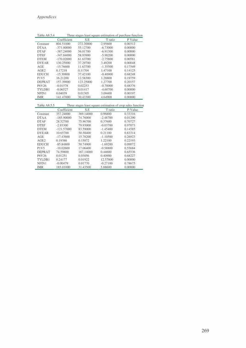
Appendices
269
Table A8.5.4 Three stages least square estimation of purchase function
Coefficient S.E T ratio P Value Constant 804.51000 272.20000 2.95600 0.00312 DTAA -371.00000 55.12700 -6.73000 0.00000 DTAF -387.24000 56.01700 -6.91300 0.00000 DTEF -347.84000 58.93900 -5.90200 0.00000 DTEM -170.02000 61.63700 -2.75800 0.00581 DYEAR 130.25000 37.29700 3.49200 0.00048 AGE -15.76600 11.63700 -1.35500 0.17549 AGE2 0.17218 0.11704 1.47100 0.14125 EDUCH -15.30800 37.42100 -0.40900 0.68248 P1V5 16.21200 12.58300 1.28800 0.19759 DEPRAT 157.39000 123.25000 1.27700 0.20157 P6V26 -0.01578 0.02253 -0.70000 0.48376 TYLDB1 -0.06527 0.01417 -4.60700 0.00000 NFIN1 0.04039 0.01305 3.09400 0.00197 IMR 141.47000 30.43300 4.64900 0.00000 Table A8.5.5 Three stages least square estimation of crop sales function
Coefficient S.E T ratio P-Value Constant 357.24000 369.14000 0.96800 0.33316 DTAA -185.90000 74.76000 -2.48700 0.01290 DTAF 28.52700 75.96700 0.37600 0.70727 DTEF -2.93300 79.93000 -0.03700 0.97073 DTEM -121.57000 83.59000 -1.45400 0.14585 DYEAR 10.65700 50.58400 0.21100 0.83314 AGE -17.43600 15.78200 -1.10500 0.26923 AGE2 0.19386 0.15872 1.22100 0.22193 EDUCH -85.84800 50.74900 -1.69200 0.09072 P1V5 -10.02600 17.06400 -0.58800 0.55684 DEPRAT 74.59800 167.14000 0.44600 0.65536 P6V26 0.01251 0.03056 0.40900 0.68227 TYLDB1 0.24177 0.01922 12.57800 0.00000 NFIN1 -0.00479 0.01770 -0.27100 0.78675 IMR 185.01000 31.43500 5.88600 0.00000

Appendices
270
Appendix A9 Estimated results of Engel functions for different categories of consumption goods presented in Chapter 9
Table A9.1. Description of variables used in estimation Variables Descriptions _cons Constant (intercept) Adeqfs Adult equivalent family size Age Age of the household head Deprat Dependency ratio Dtaa Dummy for Tabia Araasegda Dtaf Dummy for Tabia fekre alem Dtef Dummy for Tabia Felegeselam Dtem Dummy for Tabia Mytsedo Dyear Year dummy (1996=1, 1997=0) Educm Education dummy (1 if the household head has modern education and 0 otherwise) Educt Education dummy (1 if household has traditional education and 0 otherwise Lsubrat Log of subsistence ratio Texpbirr Total consumption expenditure Ylny Total expenditure times the natural log of total consumption expenditure Table A9.2 Estimation result of Engel function for total food consumption (Expfood) Ordinary least square Instrumental variable estimation Coef. Std. Err. T RATIO P>|t| Coef. Std. Err. T ratio P>|t| Texpbirr -1.386 0.501 -2.768 0.006 8.592 3.425 2.509 0.013 Ylny 0.231 0.054 4.294 0.000 -0.836 0.363 -2.302 0.022 Deprat 102.673 118.68 0.865 0.388 -291.173 270.638 -1.076 0.283 Adeqfs -9.146 19.539 -0.468 0.640 -44.283 99.955 -0.443 0.658 Age -1.327 2.030 -0.654 0.514 6.263 5.302 1.181 0.238 Dyear -254.446 34.097 -7.462 0.000 672.927 137.762 4.885 0.000 Educt 1.058 50.986 0.021 0.983 -163.090 146.138 -1.116 0.265 Educm -68.612 66.834 -1.027 0.305 163.046 158.373 1.030 0.304 Dtaa -468.613 68.105 -6.881 0.000 -242.835 331.929 -0.732 0.465 Dtaf -290.121 48.863 -5.937 0.000 -82.130 365.409 -0.225 0.822 Dtef -51.294 53.153 -0.965 0.335 -499.612 344.050 -1.452 0.147 Dtem -44.011 51.954 -0.847 0.397 -616.266 340.075 -1.812 0.071 Lsubrat 226.551 62.332 3.635 0.000 715.978 228.959 3.127 0.002 _cons 1466.942 223.63 6.560 0.000 -3064.752 1435.83 -2.134 0.033 R2 0.94 0.29 Table A9.3 Estimation result of Engel function for total non-food consumption (Expother) Ordinary least square Instrumental variable estimation
Coef. Std. Err. T RATIO P>|t| Coef. Std. Err. T RATIO P>|t| Texpbirr 2.386 0.501 4.766 0.000 2.770 1.643 1.686 0.093 Ylny -0.231 0.054 -4.294 0.000 -0.264 0.175 -1.507 0.133 Deprat -102.673 118.679 -0.865 0.388 -255.187 142.280 -1.794 0.074 Adeqfs 9.146 19.539 0.468 0.640 -10.485 36.638 -0.286 0.775 Age 1.327 2.030 0.654 0.514 2.782 2.482 1.121 0.263 Dyear 254.446 34.097 7.462 0.000 512.936 43.975 11.664 0.000 Educt -1.058 50.986 -0.021 0.983 0.534 65.315 0.008 0.993 Educm 68.612 66.834 1.027 0.305 117.331 88.419 1.327 0.185 Dtaa 468.613 68.105 6.881 0.000 622.603 75.711 8.223 0.000 Dtaf 290.121 48.863 5.937 0.000 469.818 56.475 8.319 0.000 Dtef 51.294 53.153 0.965 0.335 -4.116 65.322 -0.063 0.950 Dtem 44.011 51.954 0.847 0.397 -13.423 59.811 -0.224 0.823 Lsubrat -226.551 62.332 -3.635 0.000 -136.245 66.118 -2.061 0.040 _cons -1466.942 223.627 -6.560 0.000 -1998.771 717.106 -2.787 0.006 R2 0.64 0.49

Appendices
271
Table A9.4 Estimation result of Engel function for purchased non-local food consumption (other2)
(coffee, sugar, salt and spices) Ordinary least square Instrumental variable estimation
Coef. Std. Err. T RATIO P>|t| Coef. Std. Err. T RATIO P>|t| Texpbirr 1.450 0.186 7.817 0.000 1.018 0.816 1.248 0.213 Ylny -0.141 0.020 -7.215 0.000 -0.086 0.087 -0.994 0.321 Deprat 134.036 54.099 2.478 0.014 47.607 69.741 0.683 0.495 Adeqfs -34.383 9.675 -3.554 0.000 -59.664 17.232 -3.462 0.001 Age 1.517 0.919 1.650 0.100 2.262 1.169 1.935 0.054 Dyear 96.013 18.929 5.072 0.000 238.690 22.002 10.848 0.000 Educt -15.761 27.097 -0.582 0.561 -8.727 33.431 -0.261 0.794 Educm 67.011 26.079 2.570 0.011 84.947 32.527 2.612 0.009 Dtaa 228.706 28.570 8.005 0.000 323.196 34.576 9.347 0.000 Dtaf 257.206 27.751 9.268 0.000 372.766 33.494 11.129 0.000 Dtef 107.275 27.008 3.972 0.000 71.076 36.264 1.960 0.051 Dtem 40.629 25.492 1.594 0.112 7.785 29.469 0.264 0.792 Lsubrat -109.633 29.818 -3.677 0.000 -64.85 33.964 -1.909 0.057 _cons -759.135 95.573 -7.943 0.000 -853.64 357.279 -2.389 0.017 R2 0.68 0.52 Table A9.5 Estimation result of Engel function for service, ceremonial and other social expenses (Expsoc)
(ceremonial expenditure, taxes, contribution to churches, local institutions and organisation) Ordinary least square Instrumental variable estimation
Coef. Std. Err. T ratio P>|t| Coef. Std. Err. T ratio P>|t| Texpbirr 0.460 0.369 1.244 0.214 0.630 0.963 0.655 0.513 Ylny -0.041 0.040 -1.021 0.308 -0.064 0.101 -0.630 0.529 Deprat -50.560 68.091 -0.743 0.458 -72.742 76.197 -0.955 0.340 Adeqfs -6.995 14.258 -0.491 0.624 14.043 27.722 0.507 0.613 Age 1.822 1.320 1.380 0.168 2.609 1.588 1.643 0.101 Dyear 135.280 22.214 6.090 0.000 234.019 27.843 8.405 0.000 Educt 49.805 35.926 1.386 0.166 42.145 42.028 1.003 0.317 Educm 59.833 50.703 1.180 0.239 97.135 64.895 1.497 0.135 Dtaa 269.418 54.328 4.959 0.000 305.457 53.001 5.763 0.000 Dtaf 177.596 24.891 7.135 0.000 209.174 25.862 8.088 0.000 Dtef 62.541 30.975 2.019 0.044 37.306 32.338 1.154 0.249 Dtem 33.907 18.307 1.852 0.065 5.235 22.550 0.232 0.817 Lsubrat -126.398 47.460 -2.663 0.008 -76.171 43.623 -1.746 0.082 _cons -574.106 150.491 -3.815 0.000 -660.533 428.184 -1.543 0.124 R2 0.42 0.32 Table A9.6 Estimation result of Engel function for purchased industrial products (Indus)
(household goods, building materials, clothes shoes and cosmetics) Ordinary least square Instrumental variable estimation
Coef. Std. Err. T RATIO P>|t| Coef. Std. Err. T RATIO P>|t| Texpbirr 1.926 0.236 8.154 0.000 2.139 1.142 1.874 0.062 Ylny -0.190 0.025 -7.637 0.000 -0.200 0.122 -1.638 0.102 Deprat -52.113 86.022 -0.606 0.545 -182.445 94.200 -1.937 0.053 Adeqfs 16.142 14.028 1.151 0.251 -24.527 22.399 -1.095 0.274 Age -0.495 1.250 -0.396 0.692 0.173 1.363 0.127 0.899 Dyear 119.166 25.280 4.714 0.000 278.918 29.032 9.607 0.000 Educt -50.863 40.216 -1.265 0.207 -41.611 43.939 -0.947 0.344 Educm 8.779 36.839 0.238 0.812 20.196 43.636 0.463 0.644 Dtaa 199.195 41.321 4.821 0.000 317.146 45.154 7.024 0.000 Dtaf 112.525 37.729 2.982 0.003 260.645 40.760 6.395 0.000 Dtef -11.247 40.716 -0.276 0.783 -41.422 46.473 -0.891 0.373 Dtem 10.104 46.598 0.217 0.828 -18.659 49.229 -0.379 0.705 Lsubrat -100.152 26.948 -3.716 0.000 -60.074 33.864 -1.774 0.077 _cons -892.836 120.012 -7.440 0.000 -1338.238 475.573 -2.814 0.005 R2 0.57 0.46

Appendices
272
Table A9.7 Estimation result of Engel function for clothes, shoes and cosmetics (Expcloth) Ordinary least square Instrumental variable estimation
Coef. Std. Err. T ratio P>|t| Coef. Std. Err. T ratio P>|t| Texpbirr 1.852 0.230 8.057 0.000 1.906 1.113 1.712 0.088 Ylny -0.183 0.024 -7.551 0.000 -0.176 0.119 -1.477 0.141 Deprat -61.606 86.086 -0.716 0.475 -184.425 92.720 -1.989 0.047 Adeqfs 18.832 14.030 1.342 0.180 -21.466 22.077 -0.972 0.331 Age -0.279 1.224 -0.228 0.820 0.354 1.319 0.268 0.788 Dyear 100.369 24.933 4.026 0.000 252.517 28.326 8.915 0.000 Educt -56.648 38.911 -1.456 0.146 -46.740 42.142 -1.109 0.268 Educm 2.352 36.456 0.065 0.949 12.263 42.639 0.288 0.774 Dtaa 178.742 40.661 4.396 0.000 292.302 43.974 6.647 0.000 Dtaf 92.472 37.084 2.494 0.013 235.600 39.392 5.981 0.000 Dtef -19.659 39.824 -0.494 0.622 -49.486 44.873 -1.103 0.271 Dtem -3.178 46.030 -0.069 0.945 -30.687 48.345 -0.635 0.526 Lsubrat -85.504 26.014 -3.287 0.001 -47.775 32.390 -1.475 0.141 _cons -841.355 118.422 -7.105 0.000 -1212.733 462.527 -2.622 0.009 R2 0.55 0.44 Table A9.8 Estimation result of Engel function for cereal consumption (p7v17) Ordinary least square Instrumental variable estimation
Coef. Std. Err. T ratio P>|t| Coef. Std. Err. T RATIO P>|t| Texpbirr -5.620 0.942 -5.967 0.000 2.338 2.533 0.923 0.357 Ylny 0.643 0.101 6.357 0.000 -0.237 0.268 -0.883 0.378 Deprat -120.218 161.981 -0.742 0.458 -171.704 182.579 -0.940 0.348 Adeqfs 92.793 25.539 3.633 0.000 160.304 86.756 1.848 0.065 Age -2.347 2.719 -0.863 0.389 3.397 3.624 0.938 0.349 Dyear -147.507 56.738 -2.600 0.010 368.350 120.165 3.065 0.002 Educt 58.814 60.245 0.976 0.330 -112.575 107.497 -1.047 0.296 Educm -156.444 83.764 -1.868 0.063 42.113 126.473 0.333 0.739 Dtaa -739.690 77.299 -9.569 0.000 -792.834 314.955 -2.517 0.012 Dtaf -729.178 74.418 -9.798 0.000 -869.247 349.149 -2.490 0.013 Dtef -277.005 86.101 -3.217 0.001 -635.244 323.361 -1.965 0.050 Dtem -112.116 68.699 -1.632 0.103 -584.375 320.859 -1.821 0.069 Lsubrat 242.114 67.887 3.566 0.000 617.986 217.972 2.835 0.005 _cons 3260.887 392.153 8.315 0.000 405.507 1083.290 0.374 0.708 R2 0.84 0.21 Table A9.9 Estimation result of Engel function for pulses consumption (p7v25) Ordinary least square Instrumental variable estimation
Coef. Std. Err. T ratio P>|t| Coef. Std. Err. T ratio P>|t| Texpbirr 0.561 0.127 4.426 0.000 0.310 0.436 0.711 0.478 Ylny -0.055 0.012 -4.384 0.000 -0.025 0.046 -0.529 0.597 Deprat 12.840 25.307 0.507 0.612 -18.367 25.606 -0.717 0.474 Adeqfs -6.745 8.850 -0.762 0.446 -15.351 8.043 -1.909 0.057 Age 0.079 0.689 0.114 0.909 0.393 0.697 0.565 0.572 Dyear 8.718 23.089 0.378 0.706 65.983 12.284 5.372 0.000 Educt -5.493 12.035 -0.456 0.648 -2.673 14.090 -0.190 0.850 Educm -27.531 20.437 -1.347 0.179 -19.319 17.933 -1.077 0.282 Dtaa -7.557 13.801 -0.548 0.584 29.361 12.479 2.353 0.019 Dtaf -2.249 13.458 -0.167 0.867 42.454 12.925 3.285 0.001 Dtef 21.241 14.163 1.500 0.134 6.041 14.684 0.411 0.681 Dtem 55.414 33.095 1.674 0.095 41.914 34.968 1.199 0.231 Lsubrat 1.507 10.253 0.147 0.883 20.421 15.850 1.288 0.198 _cons -202.144 33.028 -6.120 0.000 -202.380 155.060 -1.305 0.193 R2 0.35 0.22

Appendices
273
Table A9.10 Estimation result of Engel function for oil crops consumption (p7v33) Ordinary least square Instrumental variable estimation
Coef. Std. Err. T ratio P>|t| Coef. Std. Err. T RATIO P>|t| Texpbirr 0.087 0.016 5.542 0.000 0.196 0.074 2.659 0.008 Ylny -0.009 0.002 -5.462 0.000 -0.021 0.008 -2.648 0.008 Deprat -5.154 8.680 -0.594 0.553 -10.842 9.269 -1.170 0.243 Adeqfs -2.836 1.182 -2.399 0.017 -2.098 1.586 -1.323 0.187 Age 0.359 0.138 2.592 0.010 0.386 0.144 2.672 0.008 Dyear 9.639 2.204 4.374 0.000 15.930 2.698 5.904 0.000 Educt -6.715 3.428 -1.959 0.051 -6.926 3.438 -2.014 0.045 Educm -6.173 3.205 -1.926 0.055 -4.396 3.324 -1.322 0.187 Dtaa 21.216 3.530 6.010 0.000 25.320 3.763 6.729 0.000 Dtaf 25.559 3.884 6.581 0.000 30.035 4.192 7.166 0.000 Dtef -0.576 2.143 -0.269 0.788 0.179 2.211 0.081 0.935 Dtem -3.229 1.957 -1.650 0.100 -2.905 1.973 -1.472 0.142 Lsubrat -0.643 3.647 -0.176 0.860 1.198 3.701 0.324 0.746 _cons -56.802 10.416 -5.454 0.000 -107.422 35.358 -3.038 0.003 R2 0.33 0.29 Table A9.11 Estimation result of Engel function for animal product consumption (p7v41) Ordinary least square Instrumental variable estimation
Coef. Std. Err. T ratio P>|t| Coef. Std. Err. T ratio P>|t| Texpbirr 2.142 0.371 5.774 0.000 4.711 1.491 3.160 0.002 Ylny -0.209 0.038 -5.429 0.000 -0.465 0.159 -2.922 0.004 Deprat 80.360 98.651 0.815 0.416 -138.023 104.587 -1.320 0.188 Adeqfs -58.062 17.495 -3.319 0.001 -127.233 24.845 -5.121 0.000 Age -0.951 1.843 -0.516 0.606 -0.193 2.043 -0.094 0.925 Dyear -223.141 52.178 -4.277 0.000 -18.049 38.470 -0.469 0.639 Educt -29.050 49.576 -0.586 0.558 -31.270 56.588 -0.553 0.581 Educm 52.750 57.145 0.923 0.357 58.054 59.564 0.975 0.330 Dtaa 32.227 46.914 0.687 0.493 175.677 47.847 3.672 0.000 Dtaf 161.179 45.792 3.520 0.000 344.495 50.469 6.826 0.000 Dtef 98.738 68.226 1.447 0.149 59.514 72.539 0.820 0.412 Dtem -28.793 45.367 -0.635 0.526 -82.356 47.365 -1.739 0.083 Lsubrat 94.215 37.830 2.490 0.013 142.179 38.327 3.710 0.000 _cons -778.889 169.823 -4.586 0.000 -2299.124 591.273 -3.888 0.000 R2 0.42 0.28 Table A9.12 Estimation result of Engel function for vegetables consumption (p7v81) Ordinary least square Instrumental variable estimation
Coef. Std. Err. T ratio P>|t| Coef. Std. Err. T RATIO P>|t| Texpbirr -0.005 0.005 -1.018 0.309 0.019 0.025 0.766 0.444 Ylny 0.001 0.001 1.070 0.285 -0.002 0.003 -0.750 0.454 Deprat 0.808 2.172 0.372 0.710 0.156 2.052 0.076 0.940 Adeqfs 0.086 0.345 0.250 0.803 -0.240 0.633 -0.379 0.705 Age 0.016 0.039 0.403 0.687 0.016 0.037 0.437 0.662 Dyear 1.833 0.774 2.369 0.018 2.024 0.701 2.887 0.004 Educt -0.736 0.612 -1.203 0.230 -0.919 0.616 -1.492 0.136 Educm 1.774 1.194 1.486 0.138 1.646 1.234 1.335 0.183 Dtaa -3.515 1.180 -2.978 0.003 -3.556 1.239 -2.871 0.004 Dtaf -2.638 1.151 -2.291 0.022 -2.633 1.206 -2.184 0.030 Dtef -0.967 1.166 -0.829 0.407 -1.179 1.199 -0.983 0.326 Dtem 4.083 1.832 2.228 0.026 3.672 1.827 2.010 0.045 Lsubrat -1.010 1.647 -0.613 0.540 -0.954 1.678 -0.569 0.570 _cons 3.026 4.196 0.721 0.471 -7.693 12.601 -0.610 0.542 R2 0.153 0.148

Appendices
274
Table A9.13 Estimation result of Engel function for the consumption of household durable goods (p7v94) Ordinary least square Instrumental variable estimation
Coef. Std. Err. T ratio P>|t| Coef. Std. Err. T ratio P>|t| Texpbirr 0.074 0.018 4.062 0.000 0.233 0.091 2.572 0.01 Ylny -0.007 0.002 -3.887 0.000 -0.024 0.010 -2.516 0.012 Deprat 9.493 7.829 1.213 0.226 1.980 8.599 0.230 0.818 Adeqfs -2.690 1.441 -1.867 0.063 -3.061 2.232 -1.371 0.171 Age -0.216 0.133 -1.631 0.104 -0.182 0.139 -1.305 0.193 Dyear 18.797 3.120 6.025 0.000 26.401 3.194 8.265 0 Educt 5.785 4.816 1.201 0.230 5.129 4.933 1.040 0.299 Educm 6.428 5.069 1.268 0.206 7.934 5.419 1.464 0.144 Dtaa 20.452 4.079 5.014 0.000 24.844 4.252 5.844 0 Dtaf 20.053 4.291 4.673 0.000 25.045 4.612 5.430 0 Dtef 8.412 3.831 2.196 0.029 8.063 4.129 1.953 0.052 Dtem 13.283 4.682 2.837 0.005 12.028 4.680 2.570 0.011 Lsubrat -14.648 4.251 -3.446 0.001 -12.299 4.413 -2.787 0.006 _cons -51.481 11.072 -4.650 0.000 -125.505 39.204 -3.201 0.001 R2 0.31 0.28 Table A9.14 Estimation result of Engel function for own produced food consumption (Ownfood) Ordinary least square Instrumental variable estimation
Coef. Std. Err. T ratio P>|t| Coef. Std. Err. T ratio P>|t| Texpbirr -3.464 0.595 -5.820 0.000 3.378 3.030 1.115 0.266 Ylny 0.429 0.064 6.706 0.000 -0.309 0.322 -0.957 0.339 Deprat -54.990 150.257 -0.366 0.715 -244.596 218.811 -1.118 0.264 Adeqfs 8.034 21.659 0.371 0.711 -1.474 85.272 -0.017 0.986 Age -4.182 2.359 -1.773 0.077 2.071 4.202 0.493 0.622 Dyear -279.127 42.503 -6.567 0.000 393.339 121.806 3.229 0.001 Educt 37.257 57.327 0.650 0.516 -111.820 124.284 -0.900 0.369 Educm -72.018 74.244 -0.970 0.333 114.913 135.988 0.845 0.399 Dtaa -388.861 77.183 -5.038 0.000 -304.709 302.472 -1.007 0.314 Dtaf -241.277 68.417 -3.527 0.000 -197.736 335.514 -0.589 0.556 Dtef -60.202 64.710 -0.930 0.353 -462.519 313.043 -1.477 0.14 Dtem -20.760 62.426 -0.333 0.740 -526.679 310.713 -1.695 0.091 Lsubrat 1109.093 135.561 8.182 0.000 1511.880 256.446 5.896 0 _cons 2621.661 256.062 10.238 0.000 -285.106 1226.495 -0.232 0.816 R2 0.91 0.33 Table A9.15 Estimation result of Engel function for purchased locally produced food consumption (Purfloc) Ordinary least square Instrumental variable estimation
Coef. Std. Err. T ratio P>|t| Coef. Std. Err. T ratio P>|t| Texpbirr 0.628 0.235 2.671 0.008 4.196 1.101 3.812 0 Ylny -0.057 0.025 -2.308 0.022 -0.441 0.117 -3.759 0 Deprat 23.627 84.448 0.280 0.780 -94.185 87.309 -1.079 0.281 Adeqfs 17.203 13.887 1.239 0.216 16.855 20.951 0.805 0.422 Age 1.338 1.196 1.118 0.264 1.929 1.283 1.504 0.133 Dyear -71.331 28.803 -2.477 0.014 40.898 27.430 1.491 0.137 Educt -20.437 38.893 -0.525 0.600 -42.543 39.814 -1.069 0.286 Educm -63.606 34.601 -1.838 0.067 -36.815 36.440 -1.010 0.313 Dtaa -308.458 46.987 -6.565 0.000 -261.322 51.958 -5.029 0 Dtaf -306.050 46.053 -6.646 0.000 -257.160 50.997 -5.043 0 Dtef -98.368 43.223 -2.276 0.023 -108.169 47.788 -2.264 0.024 Dtem -63.880 47.458 -1.346 0.179 -97.372 51.437 -1.893 0.059 Lsubrat -772.910 94.846 -8.149 0.000 -731.050 90.613 -8.068 0 _cons -395.584 116.090 -3.408 0.001 -1926.006 450.424 -4.276 0 R2 0.64 0.57

Appendices
275
Table A9.16 Estimation result of Engel function for public good consumption (Hhgood)
(household goods and building materials) Ordinary least square Instrumental variable estimation
Coef. Std. Err. T ratio P>|t| Coef. Std. Err. T ratio P>|t| Texpbirr 0.272 0.085 3.214 0.001 0.609 0.357 1.708 0.088 Ylny -0.027 0.008 -3.163 0.002 -0.064 0.037 -1.701 0.09 Deprat 10.024 21.436 0.468 0.640 -7.907 19.464 -0.406 0.685 Adeqfs -9.525 5.623 -1.694 0.091 -5.629 6.840 -0.823 0.411 Age -0.592 0.373 -1.586 0.113 -0.443 0.379 -1.170 0.243 Dyear 25.708 13.722 1.873 0.062 52.199 9.290 5.619 0 Educt 37.953 25.418 1.493 0.136 36.449 26.297 1.386 0.167 Educm 13.684 11.414 1.199 0.231 22.019 11.888 1.852 0.065 Dtaa 45.921 11.559 3.973 0.000 60.279 10.458 5.764 0 Dtaf 46.621 9.840 4.738 0.000 61.518 9.843 6.250 0 Dtef 29.342 18.503 1.586 0.114 28.888 19.956 1.448 0.149 Dtem 19.654 7.683 2.558 0.011 17.504 7.466 2.345 0.02 Lsubrat -32.277 9.758 -3.308 0.001 -22.443 10.359 -2.167 0.031 _cons -153.083 29.268 -5.230 0.000 -308.333 151.088 -2.041 0.042 R2 0.25 0.19


Curriculum Vitae
277
CURRICULUM VITAE
Tassew was born on June 5, 1964 at a village called Sesela, which is located near the
town of Korem, Ethiopia. His parents sent him to school at the age of six. After
finishing primary and secondary education at Korem, he studied General Agriculture
at Ambo Institute of Agriculture and was awarded a diploma with the grade ‘great
distinction’. He worked for seven years in the Ministry of Agriculture as an
Agronomist. In 1988, he joined Alemaya University of Agriculture (AUA) and
obtained a BSc degree in Agricultural Economics with ‘great distinction’. He obtained
the Chancellor’s medal for that academic year. Immediately afterwards he was
employed by AUA as a Graduate Assistant, which is a rare chance given to
outstanding students. From September 1993 to January 1995, he studied Agricultural
and Environmental Economics and Policy at Wageningen Agricultural University, the
Netherlands and obtained an MSc degree in Agricultural Economics and Marketing
with distinction. In February 1995, he joined the Agricultural Economics and Rural
Policy Group of Wageningen University as a PhD student to study Farm Household
Economics and obtained a WOTRO research grant. During his PhD period he
obtained the diploma the Netherlands Network of Economics (NAKE). Moreover, he
stayed two years at Mekelle University College – where he combined research and
teaching - and three months at Michigan State University. After finishing his work on
the thesis he spends three months at the Centre for the Study of African Economies,
Oxford University, UK.
Related Documents