A BUNDLE OF JOY: DOES PARENTING REALLY …journalistsresource.org/wp-content/uploads/2011/08/parenting.pdfA BUNDLE OF JOY: DOES PARENTING REALLY MAKE US ... conclusion has been adopted

Electronic copy available at: http://ssrn.com/abstract=1883839

A BUNDLE OF JOY: DOES PARENTING REALLY MAKE US MISERABLE?*

Chris M. Herbst School of Public Affairs Arizona State University

411 N. Central Ave., Ste. 450 Phoenix, AZ 85004-0687

(602) 496-0459 Email: [email protected]

John Ifcher Department of Economics Leavey School of Business

Santa Clara University 500 El Camino Real

Santa Clara, California 95053 (408) 554-5579

Email: [email protected]

Abstract

A large literature suggests that parents are less happy than non-parents. We critically assess this literature and reexamine the relationship between parenthood and well-being. We find that: parental- happiness-gap estimates are highly sensitive to the inclusion of standard covariates; parents are happier than non-parents in many specifications; and parents became happier over time relative to non-parents. Results are consistent across two datasets, most sub-groups, and numerous specification checks. We also present evidence that parenthood may inoculate parents against forces that are reducing well-being. Our research demonstrates the need for new identification strategies to determine whether parenting really makes us miserable.

Draft: August 2011 JEL classification codes: D60, D10

Keywords: parents, happiness, life satisfaction, subjective well-being, General Social Survey (GSS), and DDB Lifestyle Survey (LSS)

*We wish to thank seminar participants at the WEAI annual meeting (San Diego) as well as Rafael Di Tella, Richard Easterlin, Ori Heffetz, John Helliwell, Andrew Oswald, and Stephen Wu for their helpful comments and suggestions. All opinions and errors are those of the authors. The authors contributed equally to this work.

Electronic copy available at: http://ssrn.com/abstract=1883839

2

I. Introduction

Social scientists have seemingly determined that the proverbial “bundle of joy” is nothing of

the sort. Indeed, over the past few decades a large body of accumulated research almost universally

finds that parents are less happy, experience more depression and anxiety, and have less fulfilling

marriages than their childless counterparts (e.g., Alesina et al., 2004; Clark, 2006; Clark et al., 2008;

Di Tella et al., 2003; Evenson & Simon, 2005; Glenn & McLanahan, 1982; Margolis & Myrskyla,

2011; McLanahan & Adams, 1989; Nomaguchi & Milkie, 2003). Such findings are perhaps

unsurprising given that parents enjoy providing child care only slightly more than housework and

commuting (Kahneman et al., 2004). This “parental happiness gap” is evident across new and veteran

parents, working and non-working parents, and holds regardless of marital status. In addition, the gap

is just as likely to show up in studies of U.S. parents as it is in studies of Europeans. This unhappy

conclusion has been adopted as conventional wisdom and become the focus of countless pieces in

high-profile media outlets including the New York Times, Wall Street Journal, Slate, Time, National

Public Radio, New York Magazine, and the Freakonomics blog.1 In fact, the presumed parental

happiness gap is used by Caplan (2011) in the book Selfish Reasons to Have More Kids to champion

the supposition that parents should seek more tranquility and devote fewer resources to childrearing.

Yet despite—or perhaps because of—the widespread acceptance of this conclusion, we know

of no attempt to critically assess previous research on the relationship between parental status and

happiness. The first goal of this paper, therefore, is to undertake such an investigation. Our review

uncovers a number of potentially serious problems. First, most previous research estimates simple

associations between parental status and happiness, rather than demonstrating a causal link. A

concern with such studies is that parents’ happiness may differ from that of non-parents in ways that

cannot be accounted for using even a rich set of observable characteristics. If the unobserved

determinants of happiness are correlated with the decision to become a parent, a classic case of

1 Some recent pieces include, but are not limited to, the following: “Does Having Children Make You Unhappy?” by Lisa Belkin (New York Times, April 1, 2009); “Older Parents Find More Joy in Their Bundles” by Pamela Paul (New York Times, April 7, 2011); “Delayed Child Rearing, More Stressful Lives” by Steven Greenhouse (New York Times, December 1, 2010); “The Breeder’s Cup” by Bryan Caplan (Wall Street Journal, June 19, 2010); “Parents are Junkies: If Parenthood Sucks, Why Do We Love It? Because We’re Addicted” by Shankar Vedantam (Slate, November 12, 2010); “The Only Child: Debunking the Myths” by Lauren Sandler (Time, July 8, 2010); “Kid Crazy: Why We Exaggerate the Joys of Parenthood” by John Cloud (Time, March, 2011); “Having Kids Makes You Unhappy, Right?” by Betsey Stevenson (National Public Radio’s Marketplace, May 6, 2010); “All Joy and No Fun: Why Parents Hate Parenting” by Jennifer Senior (New York Magazine, July 4, 2010); and “Parents Are Less Happy. So What?” by Justin Wolfers (Freakonomics blog, May 26, 2011). Economists and sociologists have also advanced this argument in other outlets, for example, “Parents are Unhappy. But Why? And Should We Care?” by Betsey Stevenson (Cato Unbound, May 10, 2011); “Think Having Children Will Make You Happy?” by Nattavudh Powdthavee (The Psychologist, April 2009); and “The Joys of Parenthood, Reconsidered” by Robin Simon (Contexts, Spring 2008). Freakonomics Radio took up the topic in a discussion of parenting and parental happiness entitled “The Economist’s Guide to Parenting” (Freakonomics Radio, June 16, 2011).

3

omitted variable bias arises, in which the estimated effect of parental status on happiness is

confounded. For example, if highly altruistic individuals are, on average, happier and more likely to

have children, then failing to condition on altruism and other personality traits would bias the

estimated effect of parental status on happiness. Our concern appears to be justified: the few studies

that attempt to address the omitted variables problem find that parents are actually happier than

comparable non-parents (Kohler et al., 2005; Clark & Oswald, 2002).

Another critique applies to studies that use repeated cross-sections of happiness data. They

typically specify an empirical model that yields an estimate of the average parental happiness gap

over several decades. Implicit in this framework is the assumption that the happiness gap remained

constant over time. If, however, parents’ happiness followed a different time trend from that of non-

parents, this assumption would be violated, leading previous work to seriously misinterpret how the

parental happiness gap shifted over time. Finally, our review finds that even the most recent studies

rely on survey data from the late-1980s and early-1990s to draw conclusions about the effect of

parental status on happiness. An obvious concern is whether the estimated parental happiness gap in

these datasets remains applicable in the contemporary period, or whether it was an artifact of social

and economic forces that are no longer decisive.

In light of these concerns, the second goal of this paper is to conduct a careful reexamination

of the relationship between parental status and happiness in the U.S. Our analysis uses data from the

General Social Survey (GSS) and DDB Needham Life Style Survey (LSS), two nationally

representative datasets that have tracked self-reported happiness and life satisfaction, respectively,

over the past few decades. These surveys are well-suited to reassess the parental happiness gap and

have been used by happiness researchers studying a variety of related questions. We begin the

analysis by estimating a standard happiness equation in which detailed background characteristics are

gradually added. The goal of this exercise is to determine whether the parental happiness gap is

robust to the inclusion of a standard set of observable correlates of happiness. Next, we focus the

analysis on those who are most likely to be parents by restricting the sample to respondents ages 45

and under. Finally, we exploit the extensive time coverage in the GSS (1972-2008) and LSS (1985-

2005) to assess whether the parental happiness gap persists over time—as implied by previous

research—or whether it is sensitive to the time-period analyzed. To do so, we first compare estimates

of the parental happiness gap across the first and second half of the study period, followed by a time-

trend analysis of parents’ and non-parents’ happiness. In all analyses, the large sample sizes in the

4

GSS and LSS allow us to examine a number of narrowly defined demographic sub-groups that have

garnered substantial scholarly and popular attention (e.g., working mothers).

Our results are striking and can be summarized as follows. We first show that the

unconditional parental happiness gap is smaller than other known happiness gaps, for example, the

gap between married and single and high- and low-income individuals. Second, estimates of the

parental happiness gap are highly sensitive to the inclusion of standard demographic covariates, and

in many specifications, we find that parents are happier than comparable non-parents. The estimates

are also sensitive to the age-group and time-period analyzed. Specifically, the parental happiness gap

is only present when older individuals (who are unlikely to be parents) are included in the analysis

and in the first half of the study period. Indeed, when the sample is limited to individuals in their

prime parenting years (ages 45 and under) and to the contemporary period, we find strong evidence

that parents are happier than non-parents. Consistent with this finding, our time-trend analysis

suggests that parents’ happiness increased over time relative to non-parents. The relative

improvement among parents is the result of an absolute decline in non-parents’ happiness over the

study period. These findings are remarkably consistent across two nationally representative datasets,

apply to virtually every demographic sub-group analyzed, and are robust to numerous specification

checks.

To put it conservatively, we find little evidence that parents are less happy than their childless

peers. In fact, contrary to most previous research, our results often reveal a happiness gap in favor of

parents—a “parental happiness surplus”—which appears to be the product of increasing parental

happiness over the past several decades. This secular improvement partially explains why previous

studies, which estimated average happiness gaps or used outdated surveys, have mischaracterized the

relationship between parental status and happiness. In addition, the instability of the estimated

parental happiness gap is of concern, as it highlights the possibility that unobserved differences

between parents and non-parents may have confounded prior estimates of the parental happiness gap.

Future research should therefore attempt to identify exogenous variation in parental status that can be

used to estimate the causal effect of parenting on happiness.

Our findings have important implications for the scholarly and popular debate regarding

parental happiness. Specifically, our results call into question the central tenet of the literature: that

being a parent leads to a reduction in happiness. This is important because happy individuals are

known to be more energetic, flexible and creative; absent from work less, less depressed; and less

likely to need psychology counseling (Frey & Stutzer, 2002). Furthermore, Diener (2011) states that

5

there is now sufficient evidence to conclude that happier people are healthier and live longer. It is

also important to recognize the critical role that parents play in shaping child well-being. Indeed, it is

well-documented that family income (e.g., Blau, 1999; Dahl & Lochner, 2008) and time inputs (e.g.,

Morrill, 2011; Ruhm, 2004) affect child outcomes. Moreover, we are aware of at least one study

finding that parents’ happiness is a key determinant of child outcomes (Berger & Spiess, 2011).

Insofar as happy parents raise happy and healthy children, it is important for the parental happiness

literature to not only produce credible estimates of the effect of parental status on happiness, but also

investigate the deeper forces at work in the parent-child relationship that may enhance the parenting

experience.

Our results are also interesting in light of recent studies documenting widespread declines in

happiness over the past few decades in the U.S. (Herbst, 2010a; Stevenson & Wolfers, 2009). In

contrast to these papers, we find that parents are one of the few demographic groups that have not

experienced an absolute drop in happiness, and in fact, parents are becoming happier relative to their

childless peers.2 Does being a parent inoculate adults against a growing number of social and

economic forces—including the reduction in social and political trust, the fraying of community ties,

rising income inequality, and increasing narcissism—that appear to be reducing well-being in the

U.S. (Putnam, 2000; Twenge & Campbell, 2009)? That children and the family environment might

offer protection against such powerful forces is provocative and stands in contrast to the conventional

view that being a parent reduces happiness.

Finally, the existence of a parental happiness gap has naturally led researchers to wonder why

people continue to have children given that it makes people unhappy.3 Two explanations are

commonly provided: either parents do not behave according to utility maximizing principles, or

survey-based measures of happiness do not fully capture the complex benefits of being a parent.

While either explanation may be correct, our findings do not support the notion that having children

is a “bad” choice.

The rest of the paper proceeds as follows. Section II provides an overview and critical

assessment of the parental happiness literature. Section III introduces the two datasets used in the

analysis. Section IV discusses the results. Section V concludes.

II. Parental Well-Being: A Review of Previous Research

2 In previous research that focused exclusively on single mother, Herbst (2010b) and Ifcher and Zarghamee (2010) find that single mothers’ absolute and relative happiness (i.e., compared to single childless women) increased over the past few decades. 3 For example, in a recent commentary for National Public Radio’s Marketplace (entitled “Having Kids Makes You Unhappy, Right?”), Betsey Stevenson accepts that there is a parental happiness gap and discusses why individuals might still become parents.

6

There is a substantial body of evidence on the relationship between parental status and

psychological well-being. The earliest studies come from sociologists, who focus primarily on

parental depression, anxiety, and social relationships. Much of this work is thoroughly reviewed in

McLanahan and Adams (1987), Ross et al. (1990), and Umberson and Williams (1999). In recent

years, economists interested in subjective well-being have begun to explore the relationship between

parental status and happiness. The happiness economics literature is summarized in Blanchflower

(2008) and Clark et al. (2008). Our intent here is to highlight some of the key findings that have

emerged over the past few decades and to identify weaknesses in the parental happiness literature.

The sociological literature provides fairly consistent evidence that parents are worse off than

non-parents across a variety of psychological domains (e.g., Barnett & Baruch, 1985; Everson &

Simon, 2005; Glenn & McLanahan, 1981, 1982; Glenn & Weaver, 1978; 1979, Nomaguchi &

Milkie, 2003, Pearlin, 1974).4 Parents report higher levels of stress and anxiety, increased anger and

depression, and lower levels of happiness and life satisfaction. Although the negative mental health

effects are concentrated among parents with children currently in the home (fullnest parents), recent

studies find that well-being does not rebound substantially after children leave (emptynest parents)

(Evenson & Simon, 2005). Furthermore, it appears that parents of young children are unhappier still

(Umberson & Williams, 1999), and that each successive child in the home is associated with steeper

reductions in well-being (Glenn & McLanahan, 1982).

Other studies indicate that parents are not a monolith with respect to the mental health

consequences of being a parent. For example, female parents are found to worry more and experience

lower levels of well-being than their male counterparts (Bird & Rogers, 1998), and employed

parents—especially working women—experience lower mental health than unemployed childless

adults (Simon, 1998). The negative effects of parental status appear to be concentrated among young

parents, as a number of studies find that older parents have similar or even higher levels of well-

being than comparable non-parents (Koropeckyj-Cox et al., 2007; Margolis & Myrskyla, 2011).

Finally, single parents are substantially more likely to experience stress and depression than their

married counterparts (Aneshensel et al., 1981).

A smaller sociological literature examines the effect of parental status on marital satisfaction

and social connectedness. This research finds that marital satisfaction decreases after the birth of the

first child and does not return to pre-child levels after the departure of the last child (Lavee et al.,

4 It should be noted that a few studies find inconsistent or neutral effects (e.g., Cleary & Mechanic, 1983; Gore & Mangione, 1983), while others find positive effects (e.g., Ross & Huber, 1985; Aassve et al., 2009).

7

1996; MacDermid et al., 1990; Menaghan, 1982). On the other hand, parents report higher levels of

self-esteem than non-parents (Hansen et al., 2009). Furthermore, a related set of papers highlights the

social benefits of parenthood through increased connectedness to friends, family, and the community

(Gallagher & Gerstel, 2001; Umberson & Gove, 1989). Finally, a recent paper by Nomaguchi and

Milkie (2003) finds that new parents experience greater social integration (defined as the frequency

of contact with friends and relatives) than non-parents, even though these parents are worse off than

non-parents across a variety of psychological dimensions.

Economists have largely reached the same conclusion: that being a parent decreases well-

being. Most of this work focuses on global measures of happiness and life satisfaction, and provides

only indirect evidence of well-being differences between parents and non-parents. That is, these

papers typically include a control for the presence or number of children in a happiness equation

focusing on another topic, such as the macroeconomic determinants of well-being. Nevertheless,

these studies consistently find that being a parent is associated with reductions in happiness and life

satisfaction, although they do not carefully scrutinize or confirm the robustness of such results (e.g.,

Alesina et al., 2004; Di Tella et al., 2001; 2003; Clark, 2006; Clark et al., 2008a; 2008b).5

This paper contributes to the literature by carefully examining the parental happiness gap and

demonstrating that it is neither robust, nor constant over time. Specifically, we address several

weaknesses found in the extant literature. First, few studies attempt to establish a causal relationship

between parental status and happiness, and instead estimate simple associations between the two. A

concern with such an approach is that parents’ happiness could differ from that of non-parents for

reasons that are difficult to capture using standard survey datasets. If the unobserved determinants of

happiness are correlated with an individual’s decision to become a parent, then the estimated “effect”

of parental status on happiness is biased. In addition, previous work does not account for the

possibility of a simultaneous relationship between parental status and happiness; that is, adults’

happiness is likely to be shaped by and a determinant of fertility decisions.6 The small number of

studies that attempt to account for the endogeneity of fertility decisions using twin (Kohler et al.,

2005) or individual (Clark & Oswald, 2002) fixed effects finds that being a parent increases

5 Once again, there is some disagreement in the literature, with some studies finding neutral or positive effects of parental status on happiness (e.g., Frey & Stutzer, 2006). In addition, a related paper by Helliwell and Wang (2011) finds that the elevated levels of well-being during the weekend are more pronounced for those in their prime parenting years (i.e., those ages 26 to 45) presumably because the stress and time constraints associated with being a parent are lessened during the weekend. 6 Furthermore, previous studies have not adequately considered the impact of large compositional differences between parents and non-parents on estimates of the parental happiness gap. In particular, adding a rich set of covariates to the analysis–as previous studies do—may not fully correct for compositional differences if there are omitted variables or endogeneity among the independent variables. For example, parents are over a decade younger on average than are non-parents. If the relationship between age and happiness is different for parents and non-parents, then adding age as a covariate will not fully adjust for this difference.

8

happiness. Rather than attempt to identify the causal effect of parental status, we carefully test the

robustness of the parental-happiness-gap, first by gradually adding standard demographic covariates

to the analysis, and then by focusing the analysis on respondents who are most likely to be parents

(that is, we restrict the sample to respondents ages 45 and under). Our results indicate that two

covariates—family income and marital status—and the age-restriction each have a striking effect on

estimates of the parental happiness gap.

Another concern focuses on studies using repeated cross-sections of happiness data. In

particular, the standard empirical specification yields an estimate of the average parental happiness

gap over a substantial time period. For example, Di Tella et al. (2001; 2003) estimate the average

effect of parental status over approximately 17 years of Eurobarometer data, and Margolis and

Myrskyla (2011) estimate the average effect over 24 years of World Values Survey data. Implicit in

this framework is the assumption that the parental happiness gap has remained constant over time. If,

however, parents and non-parents followed different happiness time trends, then previous research

may seriously misinterpret whether and how the parental happiness gap changed. To highlight our

concern, it is useful to consider McLanahan and Adams (1989), which uses the 1957 and 1976 waves

of the Americans View Their Mental Health survey to examine parental well-being. Although the

authors find few well-being differences between parents and non-parents in 1957, the former became

increasingly unhappy, less efficacious, and more worried by 1976. This change in parental well-

being would have been obscured had the authors used the standard empirical approach of averaging

well-being differences over the entire study period. Furthermore, the average well-being difference

would not have accurately reflected the well-being difference in either period. In the current paper,

we do several things to allow the parental happiness gap to vary over time. We first compare

estimates of the parental happiness gap across the early and latter halves of the study period, and then

we estimate linear happiness time trends for parents and non-parents, thus enabling us to examine

whether parents’ happiness has changed over time.

Third, even the most recent studies rely on outdated data to draw conclusions about parental

happiness gap. For example, Evenson and Simon (2005) and Nomaguchi and Milkie (2003) use the

1987-1988 and 1992-1994 waves of the National Survey of Families and Households, respectively.

In the economics literature, Alesina et al. (2004) and Di Tella et al. (2001; 2003) use GSS and

Eurobarometer data through the early- to mid-1990s. The question naturally arises to whether the

parental happiness gap found in these earlier periods is transitory or whether it continues to persist. In

this study, we use GSS and LSS data through 2008 and 2005, respectively. Our findings suggest that

9

the happiness gap had disappeared by the late-1990s, calling into question the applicability of

previous results for the contemporary period.

III. Data

We examine parental subjective well-being (SWB) using two nationally representative

surveys: the GSS and LSS.7 The GSS is a standard data source for studying the happiness of the U.S.

population. The GSS was administered annually to approximately 1,500 individuals between 1972

and 1993 (with the exception of 1979, 1981, and 1992) and was administered biennially to

approximately 4,500 individuals thereafter. For this study we have obtained GSS data through 2008.

In addition to the detailed demographic and labor market data collected in the GSS, it includes a

standard question about global happiness. Specifically, it asks respondents “Taken all together, how

would you say things are these days–would you say that you are very happy, pretty happy, or not too

happy?” This question has remained intact since 1972, providing us with approximately 35 years and

45,000 observations over which to study the happiness of parents and non-parents in the U.S.

However, there have been some changes to the survey and sampling that might impact self-

reported happiness trends. Stevenson and Wolfers (2008, 2009, & 2010) have written a series of

papers examining SWB trends using the GSS. We largely follow their methodology for creating a

consistent measure of self-reported happiness. This includes (i) dropping the black oversample in the

1982 and 1987 GSS; (ii) dropping surveys that were conducted in Spanish (and could not have been

completed if English was the only language in which the survey was offered) in the 2006 GSS; and

(iii) using the GSS weight WTSSALL to help ensure that the survey includes a nationally

representative sample of U.S. adults [see Appendix A of Stevenson and Wolfers (2008) for additional

details]. Our weighting strategy does diverge from Stevenson and Wolfers in one way. Specifically,

the questionnaire item that directly preceded the happiness question was different in the 1972 and

1985 GSS.8 We adjust for this by dropping all observations from the 1972 and 1985 GSS as well as

all observations from the split-ballot experiments that were conducted in the 1980, 1986, and 1987

GSS in an attempt to identify the question-order effect. In contrast, Stevenson and Wolfers create a

weight to adjust for the question-order effect using the split-ballot experiments. We chose our

approach because we believe it is more conservative. Furthermore, given the large number of waves

in the GSS, dropping these observations should not affect the results. Indeed, we demonstrate in a

7 Until this point, we primarily used the word “happiness” to discuss well-being differences between parents and non-parents. We now transition to the phrase “subjective well-being” to account for the slightly different measures included in the GSS and LSS. In particular, the GSS inquires about happiness, while the LSS inquires about life satisfaction. 8 Dillman et al (1996) and Schuman and Presser (1981) find that there is a question-order effect.

10

robustness check that the results are not materially affected if we instead use Stevenson and Wolfers’

weights.

Our second data source is the LSS.9 Each year since 1975, the advertising agency DDB

Needham has commissioned Market Facts, a commercial polling firm, to administer the LSS on a

sample of approximately 3,500 Americans. The questionnaire covers a diverse set of topics, ranging

from consumer behavior and product preferences to recreational activities and political attitudes.

Importantly for the current study, the LSS contains a standard item that inquires about respondents’

life satisfaction: “I am very satisfied with the way things are going in my life these days” (response

categories include 6=definitely agree, 5=generally agree, 4=moderately agree, 3=moderately

disagree, 2=generally disagree, and 1=definitely disagree). This question has remained intact since

1983. In auxiliary analyses, we examine several other SWB items inquiring about self-confidence,

regrets about the past, self-reported physical condition, and a variety of stress-related health issues

(e.g., sleep quality and frequency of headaches). These alternative measures are examined to confirm

the robustness of our findings. Finally, between 1975 and 1984, the LSS was administered

exclusively to married individuals. Thus, we are only able to use the LSS data between 1985 and

2005, providing us with approximately 20 years and 75,000 observations over which to study the life

satisfaction of parents and non-parents in the U.S.10

For the purposes of this study, we define “parents” as respondents who report having children

ages 0 to 17 residing in the household.11 While this definition enables us to focus on the subset of

parents who are of primary interest—those who are actively and regularly parenting—we recognize

that this definition commingles the following groups as “non-parents:” adults without children,

parents with children ages 18 and over, and parents whose children do not live in the household. To

investigate the sensitivity of the results to our definition of parents, we reestimate the models using

the following alternative definition of parents: respondents who report both having children and

having children residing in the household. Our main results are robust to this alternative definition.

Another concern is that we are not able to determine whether a given child is the respondent’s own

biological, adoptive, or step child, or whether another household member claims legal guardianship

over the child. Although it would be ideal to examine parental well-being across each parent-child

9 See Putnam and Yonish (1999), Groeneman (1994), and Herbst (2010a) for an extensive introduction to and evaluation of the LSS. The LSS is a proprietary data archive, although the 1975-1998 surveys are freely available on Robert Putnam’s Bowling Alone website. 10 The LSS includes a weight, but there is insufficient documentation on how the weight is constructed. Therefore, we conduct the LSS analyses using unweighted data. However, applying the weight does not change the results discussed in the text. 11 The main results include parents of all ages. In auxiliary analyses we restrict the sample to respondents ages 45 and under. When we do this we find consistent evidence that there is a parental happiness surplus.

11

custody arrangement, it is somewhat reassuring that parents in most arrangements are found to report

similar SWB (Evenson & Simon, 2005).12

IV. Is There Really A Parental SWB Gap?

A seemingly well-founded consensus has developed that parents’ SWB is lower than that of

non-parents’. In this section, we provide strong evidence that this conclusion is ill-founded.

Specifically, we illustrate that (i) the unconditional “parental SWB gap” is small when compared to

other known “SWB gaps;” (ii) the demographic characteristics of parents and non-parents are

materially different along dimensions that are correlated with SWB; (iii) estimates of the parental

SWB gap are sensitive to the covariates, age-group, and time-period included in the analysis; (iv)

there appears to be a parental SWB surplus in many specifications; (v) parents’ SWB is increasing

relative to non-parents’ SWB over time; and (vi) non-parents’ SWB is declining absolutely over

time. These findings are consistent across the GSS and LSS and robust to numerous specification

checks.

The Unconditional Parental SWB Gap Is Relatively Small

The unconditional parental happiness gap is only -0.018. That is, parents’ average happiness

is only 0.018 “happiness points” lower than non-parents’ average happiness (2.221 versus 2.239) in

the GSS [compare Columns (2) and (3) of Table 1]. While this gap is statistically significant, it is

small in magnitude. For example, consider the happiness gaps associated with other well-established

correlates of happiness: the “unmarried happiness gap” is -0.284 points and the “bottom-top income

quartile happiness gap” is -0.239 points, 15 and 13 times the size of the parental happiness gap,

respectively. In the LSS, the pattern is similar, although the “parental life satisfaction gap” slightly

larger than it is in the GSS. Specifically, the “unmarried life satisfaction gap” is -0.859 points, and

12 Generally speaking, previous research does not dedicate sufficient attention to the definition of “parent.” Moreover, previous studies generally do not discuss which groups of parents fall within their definition (for example, full-nest or empty-nest, parents of biological children versus parents of adoptive, step, or foster children, etc.), nor the advantages and disadvantages of their chosen definition. For example, Alesina et al. (2004) and Di Tella et al. (2001; 2003) do not explicitly define their “parent” variable, making it difficult to draw conclusions about whether differences in the definition of parent may explain divergent results. Among papers that do explicitly define parent, there is considerable variation in the way parent is defined. For example, Margolis and Myrskyla’s (2011) definition is based on the survey question “Have you had any children?” which is arguably narrow in scope (in that it presumably captures adults’ own biological children and omits, for example, adopted and step children) and does not allow one to distinguish between full-nest and empty-nest parents. This distinction is potentially important in light of previous research that indicates that the presence or absence of a child in the home can lead to different conclusions about parental well-being (e.g., Evenson & Simon, 2005). The survey used in Kohler et al.’s (2005) analysis asked explicitly about respondents’ biological children, thereby explicitly excluding adopted, step, and foster children. Moreover, it is unclear whether their analysis captures full-nest parents exclusively or whether empty-nest parents are captured as well. As a final example, Nomaguchi and Milkie’s (2003) definition includes only “new parents,” defined as those who became a parent within the last five to seven years, that is, between waves of the National Survey of Families and Households, as inclusion in the sample is conditioned on not having had a child at the time the earlier wave was administered. Thus, their analysis focuses only on parents with young children.

12

the “bottom-top income quartile life satisfaction gap” is -0.431 points, 5 and 2 times the size of the

parental life satisfaction gap (-0.187 points), respectively [compare Columns (5) and (6) of Table 1].

Parents and Non-Parents’ Demographic Characteristics are Materially Different

Even if the unconditional parental SWB gap were negative and large, one should not

necessarily conclude that there is a parental SWB gap because, as shown in Table 1, parents and non-

parents’ demographic characteristics are materially different along dimensions that are correlated

with SWB. For example, parents’ SWB might be lower than non-parents’ SWB, since (i) parents’

average family income (equivalency scaled) is substantially less than non-parents’ average income

(GSS: $30,767 versus $38,959; LSS: $27,973 versus $39,445), and (ii) income and SWB are

positively correlated in cross-sectional studies (Clark et al., 2008).13 Conversely, parents’ SWB

might be greater than non-parents’ SWB, since (i) parents are substantially more likely to be married

than non-parents (GSS: 73 versus 54 percent; LSS: 86 versus 60 percent), and (ii) being married and

SWB are positively correlated in cross-sectional studies (Frey & Stutzer, 2002).

Thus, one needs to carefully consider the influence of demographic characteristics on SWB

before determining whether the small, unconditional parental SWB gap indicates that parents’ SWB

is lower than non-parents’ SWB. Furthermore, given that parents’ and non-parents’ demographic

characteristics are materially different, it is likely that their unobserved characteristics will differ as

well. If the unobserved characteristics are correlated with both happiness and the decision to become

a parent, then conditioning even on a rich set of observable characteristics will not eliminate the

problem of omitted variables. Thus the estimated parental SWB gap might be biased in an unknown

direction.

Adjusting SWB for Observable Characteristics

To test whether the parental SWB gap is sensitive to conditioning on parents’ and non-

parents’ demographic characteristics, we estimate a standard SWB equation that regresses measures

of SWB (happiness in the GSS and life satisfaction in the LSS) on a parent dummy variable as well

as a standard set of demographic and labor market covariates. Formally, we estimate an equation of

the following form:

(1) yirt = β0 + β1parentirt + Dirtγ + μr + ηy + (μr × ηy) + εirt,

13 For GSS the OECD equivalency scale is used where the first adult is equal to 1, additional adults are equal to 0.5, and each child (under the age of 18) is equivalent to 0.3. For LSS first adult is equal to 1, and additional household members are equal to 0.4 (LSS household size data does indicate the age of the household members).

13

for i = 1, …, I; r = 1, …, R; and t = 1, …, T, where i indexes individuals, r indexes region of

residence, and t indexes years. The dependent variable, y, is the SWB of the ith respondent in region r

and year t (recall that SWB is measured with a question regarding happiness in the GSS and life

satisfaction in the LSS). The independent variable, parent, is a dummy variable that equals one if the

ith respondent in region r and year t reports having at least one child ages 0 to 17 residing in the

household. The vector, D, is a set of exogenous and endogenous demographic variables for the ith

respondent in region r and year t.14 The model also includes dummy variables for the nine Census

regions (μr), a vector of year dummy variables (ηy), and vector of region-by-year interactions (μr ×

ηy).

The β1 is the parameter of primary interest. It captures the average SWB difference between

parents and non-parents over the study period (1972-2008 in the GSS and 1985-2005 in the LSS). If

the estimate of β1 is negative then it indicates that there is a parental SWB gap, that is, parents’ SWB

is lower than that of non-parents’. In contrast, a positive estimate of β1 indicates that there is a

parental SWB surplus, that is, parents’ SWB is greater than that of non-parents’. Estimates of β1 are

commonly reported in the parental well-being literature, and the findingthat there is a parental SWB

gapis based on such estimates.

Given the ordered nature of the dependent variable, we use an ordered probit to estimate

equation (1). Standard errors are adjusted for arbitrary forms of heteroskedasticity as well as the non-

random clustering of observations by year. We also estimate equation (1) using binary indicators of

high- and low-levels of SWB using a probit.15 Following Stevenson and Wolfers (2009), we begin by

estimating equation (1) using no covariates, followed by a model that adds the exogenous control

variables (age, age-squared, gender, and race/ethnicity). Next, we gradually add the endogenous

control variables (education, employment, income, and marital status). Finally, we add the region,

year, and region-year controls (μr, ηy, μr × ηy, respectively). By progressively adding the covariates,

we are able to demonstrate that the parental SWB gap is not robust to the inclusion and exclusion of

many demographic and labor market characteristics.

14 For each covariate we set missing observations to zero and add a dummy variable that equals one if the observation is missing and zero otherwise. 15 In the GSS, the top happiness category is “very happy” and the bottom category is “not too happy.” In the LSS, the top life satisfaction category includes those who “definitely agree” with the life satisfaction statement, and the bottom category includes those who “definitely disagree” with the statement.

14

The Parental SWB Gap is Not Robust

In an attempt to understand the influence of demographic characteristics on the parental SWB

gap, equation (1) is estimated with various sets of control variables. Starting with the GSS data and

no covariates, the coefficient on the parent dummy, β1, is negative and significant. This reconfirms

that there is an unconditional parental happiness gap (see Column (1) of Table 2a).

The results change markedly, however, as control variables are added. The β1 switches from

negative and significant to positive and insignificant when the exogenous control variables (age, age-

squared, gender, and race) are added. Moreover, β1 is positive and significant when the endogenous

control variables (education and income) are entered individually or jointly (in addition to the

exogenous controls) (see Columns (2) – (6) of Table 2a). That is, there is now a “parental happiness

surplus.”

The same pattern emerges when using the LSS data. The parental life satisfaction gap

becomes a surplus as control variables are included in the model. The β1 is negative and significant

when no covariates are used, and positive and significant when the exogenous control variables and

income are used (see Columns (1) – (6) of Table 2b).16 The parental life satisfaction surplus

continues to be present when the full set of endogenous controls (education, employment, and

income) is entered. Compared to the GSS, one observes in the LSS that β1 does not become positive

and significant until income is used as a control variable. Using the exogenous control variables

alone reduces the β1‘s magnitude by over 80 percent (compared to using no covariates), and the

addition of education or employment as control variables makes β1 statistically insignificant.

The impact of using income as a control variable is striking. The β1 is positive, large, and

highly significant when it is used with either dataset, indicating that there is a parental SWB surplus

not a parental SWB gap. This impact is perhaps not surprising given (i) that non-parents’ income is

over 25 percent greater than parents’ income and (ii) that income and SWB are positively correlated.

Interestingly, the parental SWB surplus appears to be “symmetric.” That is, parents (relative to non-

parents) have a significantly higher probability of reporting a high level of SWB and a significantly

lower probability of reporting a low level of SWB (see probit results in Column (6) of Tables 2a and

2b). Finally, it should be noted that income is an endogenous variable, as are education and

16 Note that the coefficient on the (logged) first-order family income term is positive using the GSS, but negative using the LSS (see Tables 2a and 2b). In LSS results, available upon request, we find that the coefficient on the squared (logged) income term is positive and statistically significant. In addition, when the model is estimated with non-logged family income polynomials the first-order income coefficient is positive and statistically significant.

15

employment. Thus, one must use caution interpreting the estimates if endogenous control variables

are used.

The final endogenous control variable, marital status, also has a striking impact. The β1

becomes negative and highly significant when it is used with either dataset (in addition to the

exogenous control variables) (see Column (7) of Tables 2a and 2b).17 Again, this impact is perhaps

not surprising given (i) that parents are over 35 percent more likely to be married than non-parents

and (ii) that being married and SWB are positively correlated. Similar to the parental SWB surplus

above, the parental SWB gap appears to be symmetric. That is, parents (relative to non-parents) have

a significantly lower probability of reporting a high level of SWB and a significantly higher

probability of reporting a low level of SWB (see probit results in Column (7) of Tables 2a and 2b).

Given that there is no indication of “asymmetry” in the estimated gaps and surpluses across all

results, we do not discuss the probit results hereafter; however, we present them in Tables 3, 4, and 5.

Finally, these results are robust to the inclusion of region, year, and region-year interaction dummies

(see Columns (8) and (9) of Tables 2a and 2b).

Caution must also be used when interpreting the estimates above, as marital status is an

endogenous variable. In fact, decisions regarding marriage and fertility are inextricably linked for

many individuals. For example, in a recent survey 59 percent of married individuals reported that

having children is a “very important” reason to marry (Pew Research Center, 2010). Thus, using

marital status as a control variable is clearly problematic, as it is highly correlated with both SWB

and parental status. In particular, if marital status is included as a covariate along with the parent

dummy, the strong correlation between the two makes it difficult to identify the independent

contribution of each to parents’ and non-parents’ SWB. Conversely, if marital status is not included

as a covariate, some of the SWB benefits of marriage could load onto the parent coefficient,

positively biasing β1.18 Our intent here is not to advocate for the inclusion or exclusion of income or

marital status, but rather to point out the ways in which these observed factors influence estimates of

the parental SWB gap. It is likely that unobserved correlates of SWB and parental status, e.g.,

altruism, would lead to similar instability in β1.

In summary, the parental SWB gap is not robust. Using GSS data, β1 is negative and

17 The β1s presented in Columns (7) – (9) of Tables 2a and 2b are consistent with those found previously. 18 Simply repeating the analysis with the sample restricted to married or single respondents will not resolve the endogeneity problem either. For example, if becoming a parent increases the likelihood that one marries, then the effect of becoming a parent will be commingled with the SWB boost that one receives from the increased likelihood of being married. Thus, limiting the sample to married individuals potentially negates one of the benefits of becoming a parent: a higher likelihood of being married. Again, without exogenous variation in parental status, or another appropriate identification strategy, the effect of parental status on SWB cannot be estimated.

16

significant when no covariates are used and when marital status is used as a covariate, positive and

insignificant when only the exogenous control variables are used and when the exogenous control

variables are used with employment, and positive and significant when the exogenous control

variables are used with education or income. Using LSS data, the results are similar. The β1 can be

positive or negative and significant or not, depending on which control variables are used. Finally,

our analysis raises doubts about the validity of prior parental SWB research, as those studies did not

adequately consider the impact that observable and unobservable characteristics have on the estimate

of the parental SWB gap.

Focusing on Those Who are Most Likely to be Parents

Parents are also much younger, on average, than non-parents (GSS: 37 versus 49 years old;

LSS: 37 versus 53 years old). Moreover, the likelihood of being a parent is substantially greater for

those ages 45 and under as compared to those over 45 (GSS: 56 versus 16 percent; LSS: 62 versus 12

percent). These differences are important given that there appears to be a U-shaped relationship

between age and SWB, with the trough estimated to be between 40 and 50 years old (e.g., Frey &

Stutzer, 2002; Stone et al., 2010). To focus the analysis on respondents who are most likely to be

parents, or comparable to parents, the sample is restricted to respondents ages 45 and under.19 Similar

age restrictions are often used for analogous reasons when studying the impact of social welfare

programs on parents (e.g., Grogger, 2004; Meyer & Rosenbaum, 2001) but have not been used

previously in the parental SWB literature. Thus, prior estimates of β1 represent the average parental

SWB gap across respondents of all ages, many of whom are past their prime childbearing and

parenting years. Furthermore, this age restriction should prevent the large number of older non-

parents—as well as emptynest parents—from pushing up the average SWB of all non-parents.

Estimating equation (1) with the sample restricted to those ages 45 and under yields a β1 that

is positive and statistically significant in seven of eight specifications across the GSS and LSS in

Table 3 [see Columns (2) and (5) of Panels (A) to (D)]. The β1 is positive and insignificant only

when all covariates including marital status are used with the GSS data. In the LSS, β1 remains

positive and statistically significant even after controls for marital status are included. In contrast, the

results indicate that there is a parental SWB gap for those ages 46 and over. These estimates clearly

corroborate our finding—that the parental SWB gap is spurious—as previous studies neglected to

estimate the SWB equation on a sample of likely parents. When the GSS and LSS samples are

19 The results are robust to restricting the sample to those ages 40 and under and 50 and under.

17

limited to those who are most likely to be parents—or comparable to parents—there is a parental

SWB surplus.

Parents’ SWB is Improving Over Time

In recent years, researchers have become increasingly interested in SWB trends. For

example, Souza-Poza and Souza-Poza (2003) study gender-specific trends in job satisfaction, and

Blanchflower and Oswald (2004) and Stevenson and Wolfers (2009) examine gender-specific trends

in happiness and life satisfaction. In the case of the parental SWB research, not only has prior

research incorrectly concluded that there is a parental SWB gap, but it has also implicitly assumed

that the parental SWB gap is constant over time. That is, the parental SWB gap has been modeled, as

in equation (1), as a single parameter, β1, even though the datasets typically pool data from multiple

cross-sections (e.g., Alesina et al., 2004; Di Tella et al., 2001; 2003; Margolis & Myrskyla, 2011).20

In this section, we relax this assumption by allowing the effect of parental status on SWB to vary

over time. Our results indicate that previous research mischaracterized this relationship. There is

strong evidence that the parental SWB gap has not remained constant. Rather, parents’ SWB appears

to have increased relative to non-parents’ over the past few decades.

Parents’ SWB Before and After 1995

To examine whether parents’ SWB (relative to non-parents’ SWB) is the same in the first and

second half of the study period, a pre1995 dummy is interacted with the parent dummy in equation

(1).21 The pre1995 dummy equals one if the survey was administered prior to 1995, and zero

otherwise; the pre1995 dummy is used as a covariate as well to allow for a pre1995-period effect.

Results from this analysis are shown in Table 4.

In the earlier period, β1 is negative and statistically significant in five of eight specifications

across the GSS and LSS. The β1 is only positive when all covariates except marital status are used

with either dataset. In the latter period, β1 is positive and statistically significant in four of eight

specifications across the GSS and LSS. The β1 is only negative when no covariates are used with the

LSS dataset. Furthermore, each latter-period β1 is significantly greater than each earlier-period β1,

indicating that parents’ SWB (relative to non-parents’ SWB) is significantly greater in the latter

period than in the earlier period. Finally, in results not reported in the table, estimating this model 20 A notable exception is McLanahan & Adams (1989), in which the authors compare the parental SWB gap across two cross-sections of the Americans View Their Mental Health Survey (from 1957 and 1976) that were both old at the time the paper was published and were conducted 19 years apart. 21 1995 is the midpoint of the LSS data. The results using the GSS data are robust to using 1990 (the midpoint of the GSS data) as the cutoff.

18

with the sample restricted to those who are most likely to be parents (i.e., those age 45 and below), β1

is positive and statistically significant in all eight specifications across the GSS and LSS. In

summary, there appears to be a parental SWB gap in the earlier period and a parental SWB surplus in

the latter period.

Trends in Parents’ and Non-Parents’ SWB

To examine trends in parents’ and non-parents’ SWB, we utilize the empirical framework

outlined in Souza-Poza and Souza-Poza (2003) and Blanchflower and Oswald (2004) and formalized

in Stevenson and Wolfers (2009). In particular, we estimate an equation of the following form:

(2) yirt = β0 + β1parentirt + β2(parentirt × trendt) + β3(non-parentirt × trendt) + Dirtγ + μr + εirt

where y, parent, and D are defined as before. A linear time trend, trend, is set to equal the year the

survey was administered, t, minus the first year the survey was administered (1972 for the GSS and

1985 for the LSS) divided by 100. Dividing by 100 scales-up the coefficient so that it represents the

net change in SWB one would expect to see over the course of a century.

The β2 and β3 are the parameters of interest. They capture parents’ and non-parents’ linear

SWB time trend, respectively. If the estimate of β2 or β3 is negative, then it indicates that parents’ or

non-parents’ SWB is decreasing on average over time, respectively. Conversely, if the estimate of β2

or β3 is positive, then it indicates that parents’ or non-parents’ SWB is increasing over time,

respectively. A useful parameter is (β2 – β3), which captures the difference between parents’ and non-

parents’ linear SWB time trend, that is, the change in the parental SWB gap or surplus over time. If

the estimate of (β2 – β3) is positive (negative), then it indicates that parents’ SWB increased

(decreased) over time relative to non-parents’ SWB. In addition to presenting the estimated

difference in SWB trends, we conduct a formal test of the null hypothesis that parents’ and non-

parents did not experience differential SWB trends over the past few decades.22

Looking at Table 5, one observes that the difference between parents’ and non-parents’ linear

SWB time trend, β2 – β3, is positive and statistically significant in all specifications, irrespective of

whether controls for marital status are included [see Columns (3) and (6) of Panels (A) to (D)]. This

indicates that parents’ SWB is increasing relative to the non-parents’ SWB over the study period

(GSS: 1973–2008; LSS: 1985–2005). Interestingly, parents’ SWB does not appear to be increasing or

22 Again, we (i) use an ordered probit to estimate equation (2); (ii) estimate equation (2) using binary indicators of high- and low-levels of SWB using a probit; (iii) calculate robust standard errors by clustering observations by year; and (iv) begin by estimating equation (2) using no covariates and then progressively add covariates. Finally, note that year fixed effects are not included in equation (2) as we are estimating time trends in this analysis.

19

decreasing (absolutely) during this period, that is, no clear pattern emerges in the estimates of β2

across the eight specifications. In contrast, there is strong evidence that non-parents’ SWB is

decreasing (absolutely) during the study period. The β3 is negative and statistically significant in all

eight specifications. We discuss this robust and unanticipated result in the final section of the paper.

Together, the results presented in Tables 4 and 5 indicate that parents’ relative SWB shifted from a

SWB gap to a surplus over time. This shift calls into question the relevance of previous findings that

use “average-effects” estimates or outdated datasets.

Robustness of Results

The central findings of this paper are that: (i) the parental SWB gap is not robust, (ii) there is

a parental SWB surplus in many specifications, (iii) parents witnessed a relative improvement in

SWB over time, and (iv) non-parents’ SWB decreased (absolutely) over time. These findings are

consistent across two nationally representative surveys and are highly robust. Below is a discussion

of the robustness checks that we perform.

“Intense” Parenting Amplifies the Parental Happiness Surplus

A parental happiness surplus is particularly evident for parents who are engaged in more

“intense” parenting, that is, for parents with younger children and more children. To illustrate, the

following analyses are performed: First, a set of youngest-child-age-group dummies are interacted

with the parent dummy in equations (1) and (2). The youngest-child-age-groups are: (i) ages 0-6

years (LSS: ages 0-5), (ii) ages 7-12 (LSS: ages 6-11), and (iii) ages 13-17 (LSS: ages12-17).23 The

youngest-child-age-group dummies equal one if the youngest child in the household is in a given age

group, and zero for non-parents. When estimating equation (2) the set of youngest-child-age-group

dummies are included as covariates to allow for youngest-child-age-group level effects in the time-

trends analysis.

As shown in Panel A of Table 6a, the results of estimating equation (1) indicate that parents

with younger children have higher SWB than those with older children and non-parents. The β1

monotonically increases as the age group it is interacted with decreases in seven of eight

specifications. For example, when all covariates except marital status are used, the parental SWB

surplus, β1, is 0.002, 0.042, and 0.121 in the GSS and -0.027, 0.060, and 0.166 in the LSS when

interacted with the oldest, middle, and youngest age-group dummy, respectively. In Column (4), β1 is

roughly the same regardless of which age-group dummy it is interacted with. Furthermore, β1 is

23 There are minor differences in the construction of the age groups in the GSS and LSS.

20

positive and statistically significant in five of eight specifications when it is interacted with the

youngest age-group dummy and negative (and statistically significant) in seven (five) of eight

specifications when it is interacted with the oldest age-group dummy. Finally, the excluding and

including of marital status as a covariate has its customary impact, changing the number of

specifications in which β1 is positive from five of six to one of six, respectively.

As shown in Panel (A) of Table 6b, the results of estimating equation (2) using the GSS data

indicate that the relative improvement in parents’ SWB overall is most pronounced among those

parents with young children. That is, the difference between parents and non-parents’ linear SWB

time trend, β2 – β3, monotonically increases as the age-group it is interacted with decreases [see

Columns (3) and (6)]. Furthermore, the estimate of (β2 – β3) is positive and statistically significant for

parents with children in the youngest and middle age-groups, and negative and insignificant in

households with children in the oldest age-group. Using the LSS data, the difference between

parents’ and non-parents’ linear SWB time trend, β2 – β3, is positive, statistically significant, and

roughly constant regardless of the age-group of the youngest child in the household, suggesting that

the relative improvement in SWB has been experienced by parents with children of all ages [see

Columns (9) and (12)].

Second, a set of number-of-children dummies are interacted with the parent dummy in

equations (1) and (2). The number-of-children categories are: (i) one child living in the household,

and (ii) two or more children living in the household.24 The number-of-children dummies equal one

if the household size is in the number-of-children range, and zero for non-parents. When estimating

equation (2) the set of number-of-children dummies are included as covariates to allow for number-

of-children level effects in the time-trends analysis.

The results of estimating equation (1) indicate that parents with two or more children have

greater SWB than households with one child and, in many specifications, greater SWB than non-

parents. Specifically, β1 is greater when interacted with the larger number-of-children dummy than

when interacted with the smaller number-of-children dummy in all eight specifications [see Panel (B)

of Table 6a]. Furthermore, β1 is positive and statistically significant in four of eight specifications—

and negative and significant in only one of eight specifications—when it is interacted with the larger

number-of-children dummy. In contrast, β1 is negative (and statistically significant) in six (five) of

eight specifications when it is interacted with the smaller number-of-children dummy. 24 In the LSS data it is not possible to determine the number of children in a household beyond two. Thus, this categorization of number-of-children is used with both datasets. The findings are similar when an additional number-of-children category is added for the GSS data.

21

The results from equation (2) indicate that parents’ SWB is consistently increasing (relative

to non-parents’ SWB) more over time in households with two or more children than in households

with one child and non-parents. Specifically, the difference between parents and non-parents’ linear

SWB time trend, β2-β3, is greater when interacted with the larger number-of-children dummy than

when interacted with the smaller number-of-children dummy in all specifications, suggesting that the

SWB gains experienced by parents have disproportionately accrued to those with more children [see

Columns (3), (6), (9), and (12) of Panel (B) of Table 6b]. In summary, more intense parenting is

associated with greater parental SWB and a more positive (relative) parental SWB time trend.

The Findings are Consistent across Sub-Groups

The parental SWB gap or surplus, β1, and the difference between parents and non-parents’

linear SWB time trend, β2 – β3, are estimated for a series of sub-groups: men and women, employed

and unemployed, working men and working women, non-white and white, and more educated and

less educated adults. As shown in Table 7, results from the sub-group analyses are remarkably

consistent with the main results.

Examining the parental SWB gap or surplus by sub-group, one observes that β1 is always

positive and often statistically significant (for 14 of 20 sub-groups) when all covariates except for

marital status are used [see Columns (3) and (7) of Panels (B) to (F)]. In contrast, β1 is often negative

(for 15 of 20 subgroups), although rarely statistically significant (for 6 of 20 subgroups) when all

covariates including marital status are used [see Columns (4) and (8) of Panels (B) to (F)]. Thus, the

sub-group analysis appears to confirm that the parental SWB gap is not robust and that there is a

parental SWB surplus in many specifications.

Examining the linear SWB time trend by sub-group (Table 8), one observes: (i) that (β2 – β3)

is always positive and often statistically significant (for 24 of 40 specifications); (ii) that β3 (non-

parents’ linear SWB time trend) is very often negative (for 35 of 40 specifications) and often

statistically significant (for 29 of 40 specifications); and (iii) that there is no clear pattern in the

estimates of β2 (parents’ linear SWB time trend). Indeed, β2 is positive in 20 of 40 specifications and

negative in 20 of 40 specifications. Thus, the subgroup analysis appears to confirm that the parents’

SWB is increasing (relative to non-parents’ SWB) over time and that non-parents’ SWB is

decreasing absolutely over time.

22

The Findings are Corroborated by Alternate Measures of Self-Reported Well-Being

As shown in Table 9, estimating equations (1) and (2) with additional subjective measures of

well-being, one finds that the results generally corroborate our findings based on measures of global

happiness and life satisfaction. For example, parents’ perceive their financial situation as improving

relative to non-parents during the study period [see Q1 and Q2 in Columns (5) to (8)]. Furthermore,

parents report (relative to non-parents): (i) being in better health, (ii) being less likely to want to alter

their lives, and (iii) being more confident and physically fit [see Q3, Q4, Q5, Q6, and Q10 in

Columns (1) to (4)]. In addition, it appears that parents’ well-being is improving over time relative to

non-parents’ using these measures [see Q3, Q4, Q5, Q6, and Q10 in Columns (5) to (8)]. Parents,

however, may experience more stress than non-parents, and their general health appears to be

deteriorating. They report (relative to non-parents) more headaches, difficulty relaxing, and trouble

falling asleep as well as declining general health over the study period [see Q3, Q7, Q8, and Q9 in

Columns (1) to (8)].

Additional Specification Checks

Finally, a series of specification checks are performed. The breakpoint for the pre- and post-

period is changed to 1990 for the GSS data (1995 was chosen as the breakpoint because it is the

midpoint of the LSS data; 1990 is the midpoint of the GSS data). Stevenson and Wolfers’ (2008)

weights (discussed in the data section) are used with the GSS data. The definition of parent is

changed to those who report both having children and having children residing in the household

(from those who report having children residing in the household) with the GSS data.25 Alternate age

restrictions are used (i.e., ages 40 and under and ages 50 and under). Finally, we use a quadratic of

the linear time trend when estimating equation (2). The main results remain largely the same when

any of these specification checks are implemented.

V. Discussion

The past few decades have witnessed a flurry of parental happiness research from nearly

every corner of the social sciences. Much of this research finds that parents are worse off than non-

parents across many psychological domains. In this paper, we critically assess and provide a careful

reexamination of this body of work. Our results call into question the well-documented and highly

publicized parental happiness gap. Specifically, we demonstrate that the parental happiness gap is not

robust. Indeed, the coefficient on parent in a standard happiness equation can be positive and 25 This alternate definition cannot be implemented using the LSS.

23

significant, negative and significant, or somewhere in between depending on the covariates, age-

group, or study period that is used. In addition, we find that in many specifications there is a parental

happiness surplus. This is especially true for those most likely to be parents (ages 45 and under), for

the latter half of the study period, and for those who have young and multiple children. Finally, we

show that parents’ relative happiness is increasing over time, a finding that is driven by the strong

absolute decline in non-parents’ happiness. All of these finding are robust to various specification

checks and consistent across two nationally representative surveys and a host of sub-groups.

Our findings raise an interesting question: why have parents experienced a relative increase

in happiness over the past few decades? This question is provocative in light of recent studies

documenting widespread declines in most indicators of SWB (Herbst, 2010a; Stevenson & Wolfers,

2009). One potential explanation is that having children may inoculate parents against social and

economic factors that increasingly reduce well-being. Examples of such factors include the decline in

community and political involvement, growing disconnectedness from family and friends, and the

growth in economic insecurity. Indeed, many of these themes were studied extensively by Robert

Putnam in Bowling Alone (2000), which documents the causes and consequences of the erosion of

Americans’ social connectedness over the past few decades. In Putnam’s view, these changes are

important because they have had profound effects on outcomes ranging from national economic

prosperity and community health to individual happiness. Added to these societal changes is the rise

in narcissism and the growing obsession with beauty and youthfulness. Indeed, in The Narcissism

Emidemic (2009), Twenge and Campbell document Americans’ increasing narcissism and its

destructive effect on individuals and society.

Our contention is that parents—because of their children—may not have been as vulnerable

to these changes, and as a result, have been buffered against the decline in SWB that has been so

pervasive for many other demographic groups. Indeed, previous research finds that one of the few

benefits associated with parenthood is increased social connectedness through regular contact with

friends and family and community organizations (e.g., Gallagher & Gerstel, 2001; Nomaguchi &

Milkie, 2003). To explore this possibility, we estimate equation (2), the trend analysis, replacing the

dependent variables with measures organized around the themes of (i) social and political

connectedness, (ii) social and political trust, (iii) economic well-being, and (iv) balancing multiple

responsibilities. In these models, the coefficient on parents’ and non-parents’ linear time trends

captures the change in these social and economic domains over the past few decades.

24

Consistent with Putnam’s (2000) work, Table 10 provides evidence in favor of the steady

erosion in Americans’ social and civic connectedness, interpersonal trust, and economic security.

Across virtually every outcome, however, the reduction has been substantially less dramatic among

parents. Indeed, parents over time have become relatively more likely to visit friends, to get the news

every day, and to remain engaged in politics. Interestingly, these relative improvements apply to the

economic realm as well: parents are increasingly likely relative to non-parents to agree that “family

income is high enough to satisfy nearly all important desires,” and perhaps because of this, have

become less likely to confide that “our family is too heavily in debt.” Finally, even the indicator of

balancing multiple responsibilities, as shown in Panel D, favors parents. Parents and non-parents

alike are increasingly likely to agree with the statement “I feel like I am so busy trying to make

everybody else happy that I don’t have control of my own life,” but the upward trend among non-

parents has greatly exceeded that of parents. Together, this evidence strongly suggests that parents

have not experienced the growing social disconnectedness and economic insecurity to the same

extent as non-parents. Insofar as these social and economic factors are related to SWB, such

differential changes over time provide a plausible explanation for why parents absolute SWB has not

deteriorated, and has improved relative to non-parents.

Lastly, and perhaps most importantly, our results highlight the need to identify a source of

exogenous variation in parental status before attempting to determine the effect of parental status on

SWB. Decisions regarding parental status are potentially endogenous in a model of SWB, and even a

rich set of demographic and labor market controls is not likely to eliminate the unobserved

differences between parents and non-parents. Therefore, future research should attempt to isolate

plausibly exogenous variation in fertility choices so that credible estimates of the impact of parental

status on SWB can be obtained. In addition, our work shows that simply excluding or including

commonly used—but clearly endogenous—control variables generates substantial instability in the

estimated effect of parental status. Thus, future research should use more care when estimating

parental SWB equations. Of course, our concerns are not limited to the parental SWB literature, but

rather apply to research on SWB in general, where few studies use exogenous variation to

demonstrate causal effects. In fact, while economists in most specialties are required to attempt to

demonstrate causation, economists who study happiness are generally not.26 Perhaps happiness

economics is now mature enough to be held to such a standard as well.

26 We thank Andrew Oswald and Dan Benjamin for helping us crystallize this point.

25

References

Aassve, A., Goisis, A., & Sironi, M. (2009). Happiness and childbearing across Europe. Working

Paper No. 10. Carlo F. Dondena Centre for Research on Social Dynamics. Alesina, A., Di Tella, R., & McCulloch, R. (2004). Inequality and happiness: Are European and

Americans different? Journal of Public Economics, 88, 2009–2042. Aneshensel, C. S., Frerichs, R. R., & Clark, V. A. (1981). Family roles and sex differences in

depression. Journal of Health and Social Behavior, 22, 379-393. Barnett, R. C., & Baruch, G. K. (1985). Women’s involvement in multiple roles and psychological

distress. Journal of Personality and Social Psychology, 49, 135-145. Berger, E. & Spiess. K. (2011). Maternal life satisfaction and child outcomes: Are they related?

Journal of Economic Psychology, 32, 142-158. Bird, C. & Roger, M. (1998). Parenting and depression: The impact of the division of labor within

couplkes and perceptions of equity. PSTC Working Paper No. 98-09. Population Studies and Training Center. Providence, RI: Brown University.

Blau, D. (1999). The effect of income on child development. Review of Economics and Statistics, 81,

261-276.

Blanchflower, D. (2008). International evidence on subjective well-being. NBER Working Paper No. 14318. Cambridge, MA: National Bureau of Economic Research.

Blanchflower, D. & Oswald, A. (2004). Well-being over time in Britain and the USA. Journal of

Public Economics, 88, 1359-1386. Clark, A. (2006). Born to be mild? Cohort effects don’t explain why well-being is U-shaped in

age. Working paper 2006-35, Paris-Jourdan Sciences Economiques. Clark, A., Frijters, P., & Shields, M. (2008a). Relative Income, Happiness, and Utility: An

Explanation for the Easterlin Paradox and Other Puzzles. Journal of Economic Literature, 46, 95-144.

Clark, A., Diener, E., Georgellis, Y., & Lucas, R, (2008b). Lags and leads in life satisfaction: A test

of the baseline hypothesis. The Economic Journal, 118, F222–F243. Clark, A. & Oswald, A. (2002). Well-being in panels. Working Paper. Cleary, P. D., & Mechanic, D. (1983). Sex differences in psychological distress among married

people. Journal of Health and Social Behavior, 24, 111-121. Dahl, G. & Lochner, L. (2008). The impact of family income on child achievement: Evidence from

the Earned Income tax Credit. NBER Working Paper No. 14599. Cambridge, MA: NBER.

26

Di Tella, R., MacCulloch, R., & Oswald, A. J. (2003). Preferences over inflation and unemployment:

Evidence from surveys of happiness. American Economic Review, 91, 335–341. Di Tella, R., MacCulloch, R., & Oswald, A. J. (2003). The macroeconomics of happiness. Review of

Economics and Statistics, 85, 809–827. Dillman, D., Sangster, R., Tarnai, J., & Rockwood, T. (1996). Understanding differences in people’s

answers to telephone and mail surveys. New Directions for Evaluation, 70, 45-61. Everson, R. & Simon, R. (2005). Clarifying the relationship between parenthood and depression.

Journal of Health and Social Behavior, 46, 341-358. Frey, B., & Stutzer, A. (2002). “Happiness & Economics.” Princeton, NJ: Princeton University Press. Frey, B., & Stutzer, A. (2006). Does marriage make people happy or do happy people get married?

The Journal of Socio-Economics, 35, 326–347. Gallagher, S. K., & Gerstel, N. (2001). Connections and constraints: The effects of children on

caregiving. Journal of Marriage and the Family, 63, 265- 275. Glenn, N. D. & McLanahan, S. (1981). The effects of children on the psychological well-being of

older adults. Journal of Marriage and the Family, 43, 409-421. Glenn, N. D., & McLanahan, S. (1982). Children and marital happiness: A further specification of

the relationship. Journal of Marriage and the Family, 44, 63-72. Glenn, N. D. & Weaver, C. (1978). A multi-variate, multisurvey study of marital happiness. Journal

of Marriage and Family, 40, 269-281. Glenn, N. D. & Weaver, C. (1979). A note on family situation and global happiness. Social Forces,

57, 269-282. Gore, S., & Mangione, T. W. (1983). Social roles, sex roles, and psychological distress: Additive and

interactive models of sex differences. Journal of Health and Social Behavior, 24, 300-312. Groeneman, S. (1994). Multi-purpose household panels and general samples: How similar and how

different? Paper presented at the Annual Meeting of the American Association for Public opinion Research. Danvers, MA.

Hansen, T., Slagsvold, B., Moun, T. (2009). Childlessness and psychological well-being in midlife

and old age: An examination of parental status effects across a range of outcomes. Social Indicators Research, 94, 343-362.

Helliwell, J. & Wang, S. (2011). Weekends and subjective well-being. NBER Working Paper No.

17180. Cambridge, MA: National Bureau of Economic Research.

27

Herbst, C.M. (2010a). ‘Paradoxical’ decline? Another look at the relative reduction in women’s happiness. Forthcoming in Journal of Economic Psychology.

Herbst, C.M. (2010b). Footloose and fancy free? Two decades of single mothers’ subjective well- being. Working Paper: School of Public Affairs, Arizona State University. Kahneman, D., Krueger, A., Schkade, D., Schwarz, N., & Stone, A. (2004). A survey method for

characterizing daily life experience: The day reconstruction method. Science, 306, 1776-1780. Kohler, H.-P., Behrman, J., & Skytthe, A. (2005). Partner + children = happiness? The effects of

partnerships and fertility on well-being. Population and Development Review, 31, 407-445. Lavee, Y., Sharlin, S., & Katz, R. (1996). The effect of parenting stress on marital quality: An

integrated mother-father model. Journal of Family Issues, 17, 114-135. Margolis, R. & Myrskyla, M. (2011). A global perspective on happiness and fertility. Population and

Development Review, 37, 29-56. McLanahan, S., & Adams, J. (1987). Parenthood and psychological well-being. Annual Review of

Sociology, 13, 237-257. McLanahan, S. & Adams, J. (1989). The effects of children on adults’ psychological well-being:

1957-1976. Social Forces, 68, 124-146. MacDermid, S. M., Huston, T. L., & McHale, S. M. (1990). Changes in marriage associated with the

transition to parenthood: Individual differences as a function of sex-role attitudes and changes in the division of household labor. Journal of Marriage and the Family, 52, 475-486.

Menaghan, E. (1982). Assessing the impact of family transitions on marital experience. In Family

Stress, Coping, and Social Support, ed. H.I. McCubbin, A.E. Cauble, J. M. Patterson, pp. 90-108. Springfield, IL: Charles C. Thomas.

Morrill, M. (2011). The effects of maternal employment on the health of school-age children. Journal of Health Economics, 30, 240-257.

Nomaguchi, K. & Milie, M. (2003). Costs and rewards of children: The effects of becoming a parent

on adults’ lives. Journal of Marriage and the Family, 65, 356-374. Pearlin, L. (1974). Sex roles and depression. In Life Span Developmental Psychology Conference:

Normative Life Crises, ed. N. Datan, L. Ginsberg, pp. 191-207. New York: Academic Press. Putnam, R. & Yonish, S. (1999). How important is response rate? An evaluation of a “mail panel”

survey archive. Working Paper. Cambridge: MA: JFK School of Government, Harvard University.

Ross, C. E., & Huber, J. (1985). Hardship and depression. Journal of Health and Social Behavior,

26, 312-327. Ross, C. E., Mirowsky, J., & Goldsteen, K. (1990). The impact of the family on health: The decade

28

in review. Journal of Marriage and the Family, 52, 1059-1078. Ruhm, C. (2004). Parental employment and child cognitive development. Journal of Human

Resources, 39, 155-192.

Schuman, H. & Presser, S. (1981). Questions and answers in attitude surveys: experiments on question form, wording, and context. New York: Academic Press. Simon, R. W. (1998). Assessing sex differences in vulnerability among employed parents: The

importance of marital status. Journal of Health and Social Behavior, 39, 38-54. Sousa-Poza, A. & Sousa-Poza, A. A. (2003). Gender differences in job satisfaction in Great

Britain, 1991-2000: Permanent or transitory? Applied Economics Letters, 10, 691-694. Stevenson, B. & Wolfers, J. (2008). Happiness inequality in the United States. Journal of Legal

Studies, 37, S33-S79. Stevenson, B. & Wolfers, J. (2009). The paradox of declining female happiness. American Economic

Journal: Economic Policy, 1, 190-225. Stevenson, B. & Wolfers, J. (2010). Subjective and objective indicators of racial progress. Working

paper. Twenge, J. & Campbell, W.K. (2009). The Narcissism Epidemic. New York: Free Press. Umberson, D., & Gove, W. (1989). Parenthood and psychological well-being: Theory, measurement,

and stage in the family life course. Journal of Family Issues, 10, 440-462. Umberson, D., & Williams,K. (1999). Family Status and mental health. In C. S. Aneshensel & J. C.

Phelan (Eds.), Handbook of the Sociology of Mental Health (pp. 225-253). New York: Kluwer Academic/Plenum.

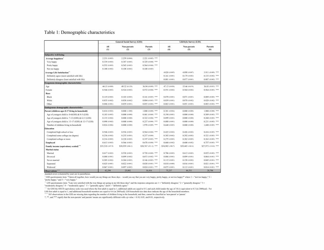
Table 1: Demographic characteristics

Subjective well-being

Average happiness+ 2.231 (0.003) 2.239 (0.004) 2.221 (0.005) ***

Very happy 0.339 (0.003) 0.347 (0.003) 0.329 (0.004) ***

Pretty happy 0.553 (0.003) 0.545 (0.003) 0.564 (0.004) ***

Not too happy 0.108 (0.002) 0.108 (0.002) 0.108 (0.003)

Average Life Satisfaction++ 4.026 (0.005) 4.098 (0.007) 3.911 (0.009) ***

Definitely agree (most satisfied with life) 0.161 (0.001) 0.179 (0.002) 0.133 (0.002) ***

Definitely disagree (least satisfied with life) 0.081 (0.001) 0.077 (0.001) 0.087 (0.002) ***

Exogenous demographic characteristics Age 44.15 (0.089) 49.32 (0.129) 36.94 (0.099) *** 47.13 (0.058) 53.46 (0.074) 36.85 (0.053) ***

Female 0.544 (0.003) 0.524 (0.003) 0.572 (0.004) *** 0.551 (0.002) 0.544 (0.002) 0.564 (0.003) ***

Race Black 0.119 (0.002) 0.103 (0.002) 0.141 (0.003) *** 0.078 (0.001) 0.071 (0.001) 0.089 (0.002) ***

White 0.835 (0.002) 0.858 (0.002) 0.804 (0.003) *** 0.859 (0.001) 0.878 (0.002) 0.828 (0.002) ***

Other 0.046 (0.001) 0.039 (0.001) 0.055 (0.002) *** 0.063 (0.001) 0.051 (0.001) 0.083 (0.002) ***

Endogenous demographic characteristicsParent (children ages 0-17 living in household) 0.414 (0.003) 0.000 (1.000) 1.000 (0.000) *** 0.381 (0.002) 0.000 (0.000) 1.000 (0.000) ***

Age of youngest child is: 0-6(GSS) & 0-5 (LSS) 0.183 (0.002) 0.000 (0.000) 0.441 (0.004) *** 0.194 (0.001) 0.000 (0.000) 0.509 (0.003) ***

Age of youngest child is: 7-12 (GSS) & 6-11 (LSS) 0.133 (0.002) 0.000 (0.000) 0.322 (0.004) *** 0.099 (0.001) 0.000 (0.000) 0.260 (0.003) ***

Age of youngest child is: 13-17 (GSS) & 12-17 (LSS) 0.098 (0.002) 0.000 (0.000) 0.237 (0.004) *** 0.088 (0.001) 0.000 (0.000) 0.231 (0.002) ***

Number of children living in household 0.816 (0.006) 0.000 (0.000) 1.970 (0.009) *** 0.640 (0.003) 0.000 (0.000) 1.680 (0.005) ***

Education Completed high school or less 0.546 (0.003) 0.536 (0.003) 0.564 (0.004) *** 0.422 (0.002) 0.426 (0.002) 0.416 (0.003) ***

Completed some college (no degree) 0.236 (0.002) 0.235 (0.003) 0.237 (0.004) 0.303 (0.002) 0.292 (0.002) 0.321 (0.003) ***

Completed college or more 0.216 (0.002) 0.228 (0.003) 0.197 (0.003) *** 0.275 (0.002) 0.282 (0.002) 0.263 (0.003) ***

Employed 0.613 (0.003) 0.566 (0.003) 0.678 (0.004) *** 0.660 (0.002) 0.600 (0.002) 0.757 (0.003) ***

Family income (equivalency scaled)+++ $35,518 (167.9) $38,959 (244.1) $30,767 (211.2) *** $34,985 (100.7) $39,445 (142.6) $27,973 (118.0) ***

Marital status Married 0.617 (0.003) 0.538 (0.003) 0.728 (0.004) *** 0.706 (0.002) 0.613 (0.002) 0.855 (0.002) ***

Divorced 0.088 (0.001) 0.099 (0.002) 0.073 (0.002) *** 0.086 (0.001) 0.099 (0.001) 0.064 (0.001) ***

Never married 0.203 (0.002) 0.244 (0.003) 0.146 (0.003) *** 0.115 (0.001) 0.158 (0.002) 0.045 (0.001) ***

Separated 0.025 (0.001) 0.022 (0.001) 0.030 (0.001) *** 0.018 (0.000) 0.016 (0.001) 0.021 (0.001) ***

Widowed 0.067 (0.001) 0.097 (0.002) 0.024 (0.001) *** 0.075 (0.001) 0.113 (0.001) 0.014 (0.001) ***

Observations++++

standard errors (clustered by year) are in parentheses.

++++ 265 observations in the GSS are missing data regarding the number of children living in the household, and thus, cannot be classified as 'non-parent' or 'parent.'*, **, and *** signify that the non-parents' and parents' means are significantly different with a p-value < 0.10, 0.05, and 0.01, respectively.

42,298

+ GSS questionnaire item: "Taken all together, how would you say things are these days – would you say that you are very happy, pretty happy, or not too happy?" where 1 = "not too happy," 2 = "pretty happy," and 3 = "very happy."

+++ for GSS the OECD equivalency scale was used where the first adult is equal to 1, additional adults are equal to 0.5, and each child (under the age of 18) is equivalent to 0.3 (in 2008usd). For LSS first adult is equal to 1, and additional household members are equal to 0.4 (in 2005usd); LSS household size data does indicate the age of the household members.

Non-parents (5)

Parents (6)

75,237 46,531 28,70625,882 16,416

++ LSS questionnaire item: "I am very satisfied with the way things are going in my life these days" and the response categories are 1 = "definitely disagree," 2 = "generally disagree," 3 = "moderately disagree," 4 = "moderately agree," 5 = "generally agree," and 6 = "definitely agree."

General Social Survey (GSS) LifeStyle Survey (LSS)

All (4)

All (1)

Non-parents (2)

Parents (3)

30

Table 2a: Coefficients from estimating equation (1) with GSS data

Coefficient on parent - ordered probit(happy) -0.032 (0.013) ** 0.016 (0.015) 0.035 (0.015) ** 0.020 (0.015) 0.064 (0.015) *** 0.069 (0.015) *** -0.099 (0.012) *** -0.045 (0.013) *** -0.043 (0.013) **

Marginal effect of being parent - probit(very happy) -0.018 (0.006) *** 0.007 (0.007) 0.012 (0.007) * 0.007 (0.007) 0.023 (0.007) *** 0.023 (0.007) *** -0.037 (0.006) *** -0.021 (0.006) *** -0.020 (0.006) ***

Marginal effect of being parent - probit(not too happy) -0.001 (0.003) -0.002 (0.004) -0.007 (0.004) * -0.004 (0.004) -0.013 (0.004) *** -0.015 (0.004) *** 0.016 (0.004) *** 0.002 (0.004) 0.001 (0.003)

Exogenous demographic characteristics Age 0.011 (0.002) *** 0.008 (0.002) *** 0.007 (0.002) *** -0.003 (0.002) -0.004 (0.002) ** -0.012 (0.003) *** -0.024 (0.003) *** -0.023 (0.003) ***

Age squared 0.000 (0.000) *** 0.000 (0.000) * 0.000 (0.000) * 0.000 (0.000) *** 0.000 (0.000) *** 0.000 (0.000) *** 0.000 (0.000) *** 0.000 (0.000) ***

Female 0.036 (0.014) *** 0.044 (0.015) *** 0.055 (0.015) *** 0.064 (0.015) *** 0.070 (0.016) *** 0.080 (0.015) *** 0.110 (0.017) *** 0.113 (0.018) ***

Race Black -0.398 (0.026) *** -0.376 (0.028) *** -0.394 (0.026) *** -0.312 (0.026) *** -0.308 (0.027) *** -0.282 (0.029) *** -0.220 (0.030) *** -0.235 (0.030) ***

Other -0.129 (0.043) *** -0.145 (0.043) *** -0.128 (0.044) *** -0.091 (0.046) ** -0.102 (0.046) ** -0.090 (0.044) ** -0.078 (0.046) * -0.056 (0.047)

Endogenous demographic characteristics Education Completed high school or less -0.120 (0.015) *** -0.056 (0.014) *** -0.086 (0.014) *** -0.094 (0.014) ***

Completed college or more 0.117 (0.018) *** 0.056 (0.017) *** 0.044 (0.017) ** 0.045 (0.017) **

Employed 0.110 (0.017) *** 0.026 (0.015) * 0.059 (0.016) *** 0.056 (0.016) ***

Ln family income (equivalency scaled in 2008 usd)++ 8.372 (4.362) * 6.507 (4.170) 7.509 (4.078) * 5.875 (4.214)

Marital status Divorced -0.582 (0.019) *** -0.548 (0.019) *** -0.546 (0.019) ***

Never married -0.461 (0.041) *** -0.443 (0.042) *** -0.430 (0.043) ***

Separated -0.753 (0.036) *** -0.692 (0.036) *** -0.682 (0.036) ***

Widowed -0.653 (0.022) *** -0.622 (0.022) *** -0.627 (0.023) ***

Region, year, and region*year dummies

Observations+++


+++ 265 observations in the GSS are missing data regarding the number of children living in the household, and thus, cannot be classified as 'non-parent' or 'parent.' `*, **, and *** signify that the coefficient is significantly different than zero with a p-value < 0.10, 0.05, and 0.01, respectively.

No No

All (6)

All (3)

All (4)

All (5)

General Social Survey (GSS) - Dependent variable: happy+

All (2)

All (9)

YesNo

All (1)

All (8)

All (7)

No No42,033 42,033

++ includes quartic of ln family income but only the first coefficient is reported; also, use OECD equivalency scale where the first adult is equal to 1, additional adults are equal to 0.5, and each child (under the age of 18) is equivalent to 0.3.

42,03342,033 42,033


No No No42,03342,03342,033 42,033

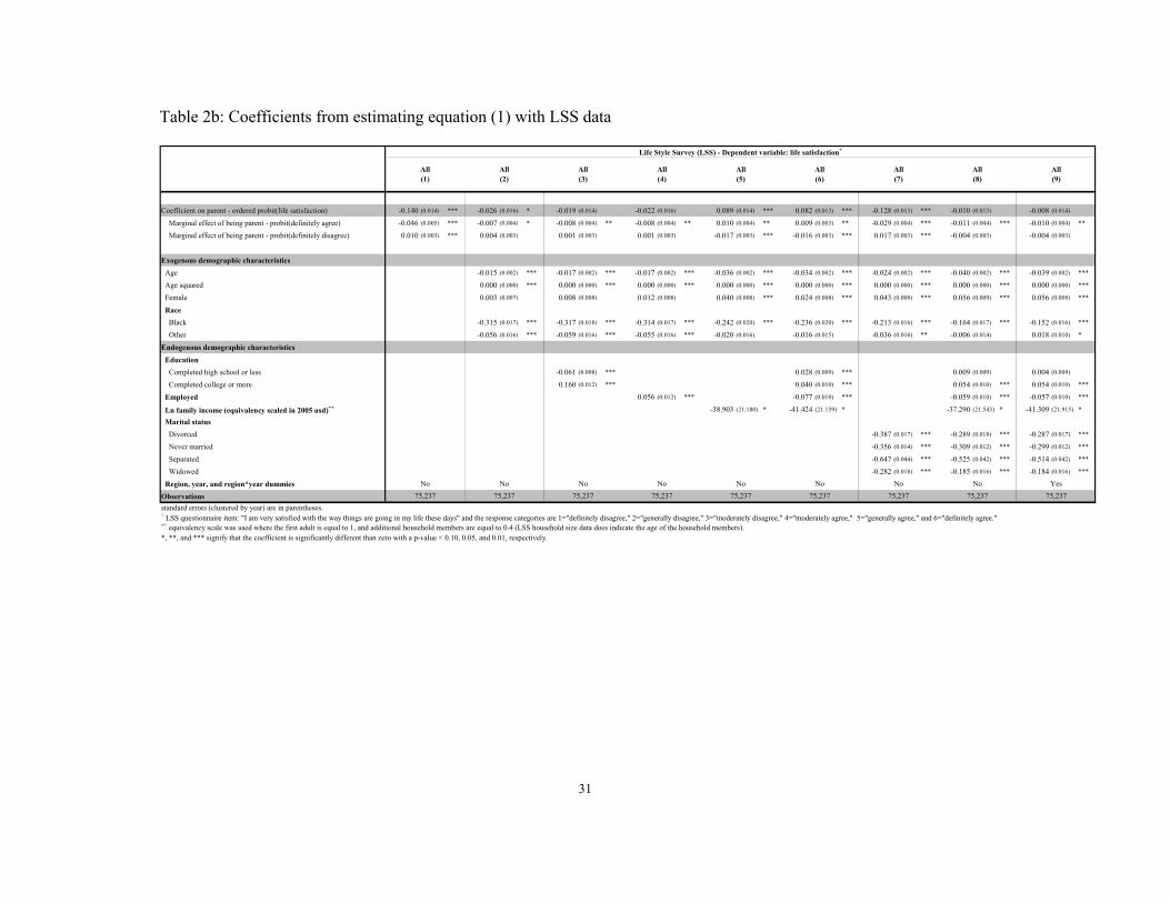
31

Table 2b: Coefficients from estimating equation (1) with LSS data

Coefficient on parent - ordered probit(life satisfaction) -0.140 (0.014) *** -0.026 (0.016) * -0.019 (0.014) -0.022 (0.016) 0.089 (0.014) *** 0.082 (0.013) *** -0.128 (0.013) *** -0.010 (0.013) -0.008 (0.014)

Marginal effect of being parent - probit(definitely agree) -0.046 (0.005) *** -0.007 (0.004) * -0.008 (0.004) ** -0.008 (0.004) ** 0.010 (0.004) ** 0.009 (0.003) ** -0.029 (0.004) *** -0.011 (0.004) *** -0.010 (0.004) **

Marginal effect of being parent - probit(definitely disagree) 0.010 (0.003) *** 0.004 (0.003) 0.001 (0.003) 0.001 (0.003) -0.017 (0.003) *** -0.016 (0.003) *** 0.017 (0.003) *** -0.004 (0.003) -0.004 (0.003)

Exogenous demographic characteristics Age -0.015 (0.002) *** -0.017 (0.002) *** -0.017 (0.002) *** -0.036 (0.002) *** -0.034 (0.002) *** -0.024 (0.002) *** -0.040 (0.002) *** -0.039 (0.002) ***

Age squared 0.000 (0.000) *** 0.000 (0.000) *** 0.000 (0.000) *** 0.000 (0.000) *** 0.000 (0.000) *** 0.000 (0.000) *** 0.000 (0.000) *** 0.000 (0.000) ***

Female 0.003 (0.007) 0.008 (0.008) 0.012 (0.008) 0.040 (0.008) *** 0.024 (0.008) *** 0.043 (0.008) *** 0.056 (0.009) *** 0.056 (0.008) ***

Race Black -0.315 (0.017) *** -0.317 (0.018) *** -0.314 (0.017) *** -0.242 (0.020) *** -0.236 (0.020) *** -0.213 (0.016) *** -0.164 (0.017) *** -0.152 (0.016) ***

Other -0.056 (0.016) *** -0.059 (0.016) *** -0.055 (0.016) *** -0.020 (0.016) -0.016 (0.015) -0.036 (0.016) ** -0.006 (0.014) 0.018 (0.010) *

Endogenous demographic characteristics Education Completed high school or less -0.061 (0.008) *** 0.028 (0.009) *** 0.009 (0.009) 0.004 (0.009)

Completed college or more 0.160 (0.012) *** 0.040 (0.010) *** 0.054 (0.010) *** 0.054 (0.010) ***

Employed 0.056 (0.012) *** -0.077 (0.010) *** -0.059 (0.010) *** -0.057 (0.010) ***

Ln family income (equivalency scaled in 2005 usd)++ -38.903 (21.180) * -41.424 (21.159) * -37.290 (21.543) * -41.309 (21.915) *

Marital status Divorced -0.387 (0.017) *** -0.289 (0.018) *** -0.287 (0.017) ***

Never married -0.356 (0.014) *** -0.309 (0.012) *** -0.299 (0.012) ***

Separated -0.647 (0.044) *** -0.525 (0.042) *** -0.514 (0.042) ***

Widowed -0.282 (0.018) *** -0.185 (0.016) *** -0.184 (0.016) ***

Region, year, and region*year dummiesObservationsstandard errors (clustered by year) are in parentheses.

*, **, and *** signify that the coefficient is significantly different than zero with a p-value < 0.10, 0.05, and 0.01, respectively.

+ LSS questionnaire item: "I am very satisfied with the way things are going in my life these days" and the response categories are 1="definitely disagree," 2="generally disagree," 3="moderately disagree," 4="moderately agree," 5="generally agree," and 6="definitely agree."

Yes

All (8)

No No

++ equivalency scale was used where the first adult is equal to 1, and additional household members are equal to 0.4 (LSS household size data does indicate the age of the household members).

Life Style Survey (LSS) - Dependent variable: life satisfaction+

All (2)

All (3)

75,237

All (4)

75,237No No No

All (1)

75,237 75,237

All (6)

75,237No

All (5)

75,237

All (7)

75,237No

75,237 75,237No

All (9)

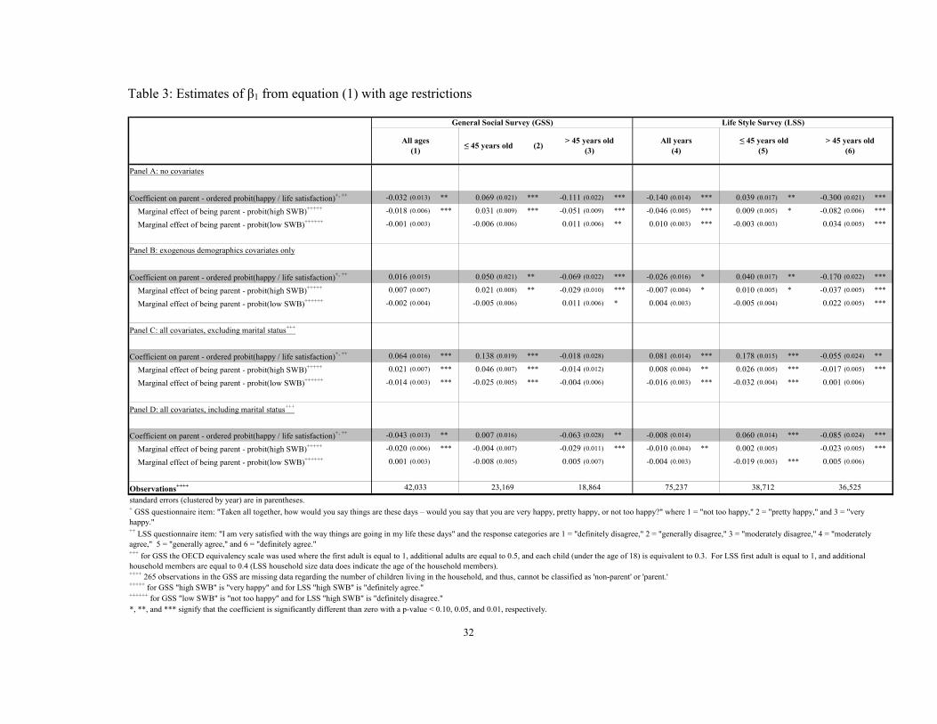
32

Table 3: Estimates of β1 from equation (1) with age restrictions

Panel A: no covariates

Coefficient on parent - ordered probit(happy / life satisfaction)+, ++ -0.032 (0.013) ** 0.069 (0.021) *** -0.111 (0.022) *** -0.140 (0.014) *** 0.039 (0.017) ** -0.300 (0.021) ***

Marginal effect of being parent - probit(high SWB)+++++ -0.018 (0.006) *** 0.031 (0.009) *** -0.051 (0.009) *** -0.046 (0.005) *** 0.009 (0.005) * -0.082 (0.006) ***

Marginal effect of being parent - probit(low SWB)++++++ -0.001 (0.003) -0.006 (0.006) 0.011 (0.006) ** 0.010 (0.003) *** -0.003 (0.003) 0.034 (0.005) ***

Panel B: exogenous demographics covariates only

Coefficient on parent - ordered probit(happy / life satisfaction)+, ++ 0.016 (0.015) 0.050 (0.021) ** -0.069 (0.022) *** -0.026 (0.016) * 0.040 (0.017) ** -0.170 (0.022) ***

Marginal effect of being parent - probit(high SWB)+++++ 0.007 (0.007) 0.021 (0.008) ** -0.029 (0.010) *** -0.007 (0.004) * 0.010 (0.005) * -0.037 (0.005) ***

Marginal effect of being parent - probit(low SWB)++++++ -0.002 (0.004) -0.005 (0.006) 0.011 (0.006) * 0.004 (0.003) -0.005 (0.004) 0.022 (0.005) ***

Panel C: all covariates, excluding marital status+++

Coefficient on parent - ordered probit(happy / life satisfaction)+, ++ 0.064 (0.016) *** 0.138 (0.019) *** -0.018 (0.028) 0.081 (0.014) *** 0.178 (0.015) *** -0.055 (0.024) **

Marginal effect of being parent - probit(high SWB)+++++ 0.021 (0.007) *** 0.046 (0.007) *** -0.014 (0.012) 0.008 (0.004) ** 0.026 (0.005) *** -0.017 (0.005) ***

Marginal effect of being parent - probit(low SWB)++++++ -0.014 (0.003) *** -0.025 (0.005) *** -0.004 (0.006) -0.016 (0.003) *** -0.032 (0.004) *** 0.001 (0.006)

Panel D: all covariates, including marital status+++

Coefficient on parent - ordered probit(happy / life satisfaction)+, ++ -0.043 (0.013) ** 0.007 (0.016) -0.063 (0.028) ** -0.008 (0.014) 0.060 (0.014) *** -0.085 (0.024) ***

Marginal effect of being parent - probit(high SWB)+++++ -0.020 (0.006) *** -0.004 (0.007) -0.029 (0.011) *** -0.010 (0.004) ** 0.002 (0.005) -0.023 (0.005) ***

Marginal effect of being parent - probit(low SWB)++++++ 0.001 (0.003) -0.008 (0.005) 0.005 (0.007) -0.004 (0.003) -0.019 (0.003) *** 0.005 (0.006)

Observations++++


++++ 265 observations in the GSS are missing data regarding the number of children living in the household, and thus, cannot be classified as 'non-parent' or 'parent.'+++++ for GSS "high SWB" is "very happy" and for LSS "high SWB" is "definitely agree."++++++ for GSS "low SWB" is "not too happy" and for LSS "high SWB" is "definitely disagree."*, **, and *** signify that the coefficient is significantly different than zero with a p-value < 0.10, 0.05, and 0.01, respectively.

General Social Survey (GSS) Life Style Survey (LSS)

75,23742,033

All ages (1)

> 45 years old (3)

> 45 years old (6)

All years (4)

≤ 45 years old (5) ≤ 45 years old (2)

36,52538,712

+++ for GSS the OECD equivalency scale was used where the first adult is equal to 1, additional adults are equal to 0.5, and each child (under the age of 18) is equivalent to 0.3. For LSS first adult is equal to 1, and additional household members are equal to 0.4 (LSS household size data does indicate the age of the household members).



23,169 18,864

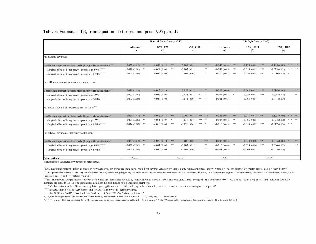
33

Table 4: Estimates of β1 from equation (1) for pre- and post-1995 periods


Coefficient on parent - ordered probit(happy / life satisfaction)+, ++ -0.032 (0.013) ** -0.059 (0.012) *** 0.009 (0.024) ^^ -0.140 (0.014) *** -0.173 (0.022) *** -0.105 (0.013) *** ^^^

Marginal effect of being parent - probit(high SWB)+++++ -0.018 (0.006) *** -0.028 (0.006) *** -0.003 (0.011) ^^ -0.046 (0.005) *** -0.058 (0.007) *** -0.033 (0.005) *** ^^^

Marginal effect of being parent - probit(low SWB)++++++ -0.001 (0.003) 0.004 (0.004) -0.008 (0.005) ^ 0.010 (0.003) *** 0.010 (0.004) ** 0.009 (0.004) **


Coefficient on parent - ordered probit(happy / life satisfaction)+, ++ 0.016 (0.015) -0.012 (0.013) 0.059 (0.025) ** ^^ -0.026 (0.016) * -0.062 (0.022) *** 0.014 (0.011) ^^^

Marginal effect of being parent - probit(high SWB)+++++ 0.007 (0.007) -0.003 (0.007) 0.021 (0.011) * ^ -0.007 (0.004) * -0.020 (0.007) *** 0.006 (0.004) ^^^

Marginal effect of being parent - probit(low SWB)++++++ -0.002 (0.004) 0.003 (0.004) -0.011 (0.005) ** ^^ 0.004 (0.003) 0.005 (0.004) 0.001 (0.004)

Panel C: all covariates, excluding marital status+++

Coefficient on parent - ordered probit(happy / life satisfaction)+, ++ 0.064 (0.016) *** 0.038 (0.011) *** 0.109 (0.026) *** ^^^ 0.081 (0.014) *** 0.045 (0.021) ** 0.123 (0.010) *** ^^^

Marginal effect of being parent - probit(high SWB)+++++ 0.021 (0.007) *** 0.011 (0.007) * 0.038 (0.012) *** ^^ 0.008 (0.004) ** -0.005 (0.006) 0.024 (0.005) *** ^^^

Marginal effect of being parent - probit(low SWB)++++++ -0.014 (0.003) *** -0.010 (0.003) *** -0.020 (0.005) *** ^ -0.016 (0.003) *** -0.015 (0.003) *** -0.017 (0.004) ***

Panel D: all covariates, including marital status+++

Coefficient on parent - ordered probit(happy / life satisfaction)+, ++ -0.043 (0.013) ** -0.072 (0.014) *** 0.008 (0.024) ^^^ -0.008 (0.014) -0.043 (0.018) ** 0.033 (0.013) ** ^^^

Marginal effect of being parent - probit(high SWB)+++++ -0.020 (0.006) *** -0.031 (0.007) *** -0.002 (0.011) ^^ -0.010 (0.004) ** -0.023 (0.006) *** 0.006 (0.005) ^^^

Marginal effect of being parent - probit(low SWB)++++++ 0.001 (0.003) 0.006 (0.004) * -0.007 (0.005) ^^ -0.004 (0.003) -0.004 (0.003) -0.005 (0.004)

Observations++++


++++ 265 observations in the GSS are missing data regarding the number of children living in the household, and thus, cannot be classified as 'non-parent' or 'parent.'+++++ for GSS "high SWB" is "very happy" and for LSS "high SWB" is "definitely agree."++++++ for GSS "low SWB" is "not too happy" and for LSS "high SWB" is "definitely disagree."*, **, and *** signify that the coefficient is significantly different than zero with a p-value < 0.10, 0.05, and 0.01, respectively.^, ^^, ^^^ signify that the coefficients for the earlier later periods are significantly different with a p-value < 0.10, 0.05, and 0.01, respectively (compare Columns (2) to (3), and (5) to (6))


75,237 75,23742,033


All years (1)

1995 - 2008 (3)

1995 - 2005 (6)

42,033

All years (4)

1985 - 1994 (5)

1973 - 1994 (2)



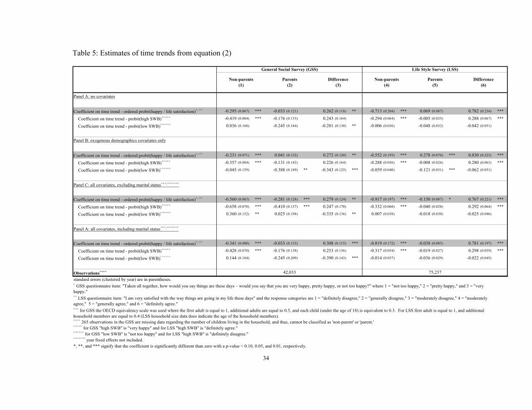
34

Table 5: Estimates of time trends from equation (2)


Coefficient on time trend - ordered probit(happy / life satisfaction)+, ++ -0.295 (0.067) *** -0.033 (0.121) 0.262 (0.118) ** -0.713 (0.204) *** 0.069 (0.087) 0.782 (0.234) ***

Coefficient on time trend - probit(high SWB)+++++ -0.419 (0.084) *** -0.176 (0.133) 0.243 (0.164) -0.294 (0.064) *** -0.005 (0.025) 0.288 (0.067) ***

Coefficient on time trend - probit(low SWB)++++++ 0.036 (0.160) -0.245 (0.184) -0.281 (0.130) ** -0.006 (0.036) -0.048 (0.032) -0.042 (0.051)


Coefficient on time trend - ordered probit(happy / life satisfaction)+, ++ -0.231 (0.071) *** 0.041 (0.132) 0.272 (0.120) ** -0.552 (0.193) *** 0.278 (0.076) *** 0.830 (0.223) ***


Coefficient on time trend - probit(low SWB)++++++ -0.045 (0.159) -0.388 (0.189) ** -0.343 (0.125) *** -0.059 (0.040) -0.121 (0.031) *** -0.062 (0.051)

Panel C: all covariates, excluding marital status+++,+++++++

Coefficient on time trend - ordered probit(happy / life satisfaction)+, ++ -0.560 (0.063) *** -0.281 (0.128) *** 0.279 (0.124) ** -0.917 (0.197) *** -0.150 (0.087) * 0.767 (0.221) ***

Coefficient on time trend - probit(high SWB)+++++ -0.658 (0.078) *** -0.410 (0.137) *** 0.247 (0.170) -0.332 (0.060) *** -0.040 (0.028) 0.292 (0.064) ***

Coefficient on time trend - probit(low SWB)++++++ 0.360 (0.152) ** 0.025 (0.198) -0.335 (0.136) ** 0.007 (0.038) -0.018 (0.030) -0.025 (0.046)

Panel A: all covariates, including marital status+++,+++++++

Coefficient on time trend - ordered probit(happy / life satisfaction)+, ++ -0.341 (0.080) *** -0.033 (0.133) 0.308 (0.115) *** -0.819 (0.172) *** -0.038 (0.085) 0.781 (0.197) ***


Coefficient on time trend - probit(low SWB)++++++ 0.144 (0.184) -0.245 (0.209) -0.390 (0.143) *** -0.014 (0.037) -0.036 (0.029) -0.022 (0.045)

Observations++++


++++ 265 observations in the GSS are missing data regarding the number of children living in the household, and thus, cannot be classified as 'non-parent' or 'parent.'+++++ for GSS "high SWB" is "very happy" and for LSS "high SWB" is "definitely agree."++++++ for GSS "low SWB" is "not too happy" and for LSS "high SWB" is "definitely disagree."+++++++ year fixed effects not included.*, **, and *** signify that the coefficient is significantly different than zero with a p-value < 0.10, 0.05, and 0.01, respectively.

++ LSS questionnaire item: "I am very satisfied with the way things are going in my life these days" and the response categories are 1 = "definitely disagree," 2 = "generally disagree," 3 = "moderately disagree," 4 = "moderately agree," 5 = "generally agree," and 6 = "definitely agree."+++ for GSS the OECD equivalency scale was used where the first adult is equal to 1, additional adults are equal to 0.5, and each child (under the age of 18) is equivalent to 0.3. For LSS first adult is equal to 1, and additional household members are equal to 0.4 (LSS household size data does indicate the age of the household members).

75,237

Non-parents (4)

Parents (5)

Parents (2)


Life Style Survey (LSS)General Social Survey (GSS)

42,033

Non-parents (1)

Difference (3)

Difference (6)

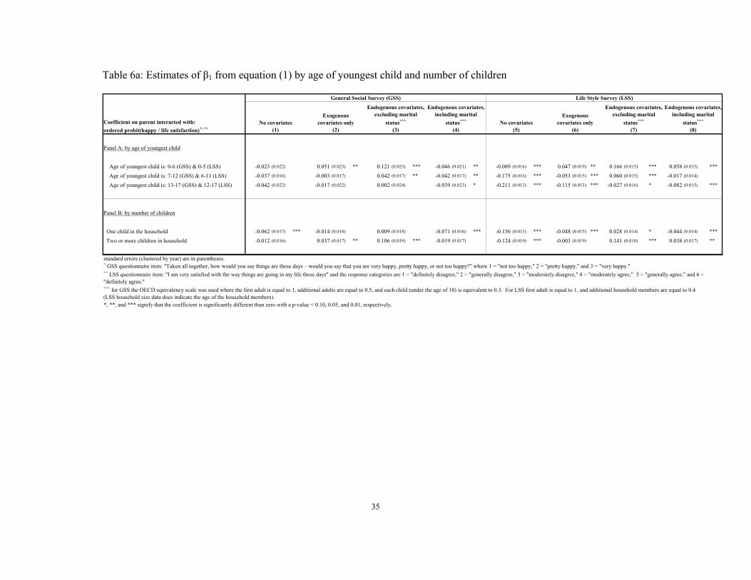
35

Table 6a: Estimates of β1 from equation (1) by age of youngest child and number of children

Panel A: by age of youngest child

Age of youngest child is: 0-6 (GSS) & 0-5 (LSS) -0.023 (0.022) 0.051 (0.023) ** 0.121 (0.023) *** -0.046 (0.021) ** -0.089 (0.016) *** 0.047 (0.019) ** 0.166 (0.015) *** 0.058 (0.015) ***

Age of youngest child is: 7-12 (GSS) & 6-11 (LSS) -0.037 (0.016) -0.003 (0.017) 0.042 (0.017) ** -0.042 (0.017) ** -0.175 (0.016) *** -0.053 (0.015) *** 0.060 (0.015) *** -0.017 (0.014)

Age of youngest child is: 13-17 (GSS) & 12-17 (LSS) -0.042 (0.022) -0.017 (0.022) 0.002 (0.024) -0.039 (0.023) * -0.211 (0.013) *** -0.115 (0.013) *** -0.027 (0.016) * -0.082 (0.015) ***

Panel B: by number of children

One child in the household -0.062 (0.017) *** -0.014 (0.018) 0.009 (0.018) -0.071 (0.016) *** -0.156 (0.013) *** -0.048 (0.015) *** 0.028 (0.014) * -0.044 (0.014) ***

Two or more children in household -0.012 (0.016) 0.037 (0.017) ** 0.106 (0.019) *** -0.019 (0.017) -0.124 (0.019) *** -0.003 (0.019) 0.141 (0.018) *** 0.038 (0.017) **



No covariates (5)

Exogenous covariates only

(6)

Endogenous covariates, excluding marital

status+++

(7)


Endogenous covariates, including marital

status+++

(8)

++ LSS questionnaire item: "I am very satisfied with the way things are going in my life these days" and the response categories are 1 = "definitely disagree," 2 = "generally disagree," 3 = "moderately disagree," 4 = "moderately agree," 5 = "generally agree," and 6 = "definitely agree."+++ for GSS the OECD equivalency scale was used where the first adult is equal to 1, additional adults are equal to 0.5, and each child (under the age of 18) is equivalent to 0.3. For LSS first adult is equal to 1, and additional household members are equal to 0.4 (LSS household size data does indicate the age of the household members).

Coefficient on parent interacted with: ordered probit(happy / life satisfaction)+, ++


No covariates (1)


(2)


status+++

(3)


status+++

(4)

36

Table 6b: Estimates of time trends from equation (2) by age of youngest child and number of children

Panel A: by age of youngest child

Age of youngest child is: 0-6 (GSS) & 0-5 (LSS) -0.295 (0.067) *** 0.141 (0.172) 0.436 (0.160) *** -0.339 (0.080) *** 0.240 (0.179) 0.579 (0.147) *** -0.713 (0.204) *** 0.082 (0.119) 0.795 (0.267) *** -0.831 (0.172) *** -0.036 (0.092) 0.795 (0.211) ***

Age of youngest child is: 7-12 (GSS) & 6-11 (LSS) -0.057 (0.114) 0.238 (0.129) * -0.115 (0.096) 0.224 (0.124) * -0.027 (0.129) 0.686 (0.273) ** -0.234 (0.156) 0.597 (0.245) **

Age of youngest child is: 13-17 (GSS) & 12-17 (LSS) -0.309 (0.235) -0.015 (0.234) -0.392 (0.252) -0.053 (8.000) -0.044 (0.134) 0.669 (0.188) *** -0.080 (0.132) 0.750 (0.180) ***

Panel B: by number of children

One child in the household -0.295 (0.067) *** -0.150 (0.173) 0.145 (0.168) -0.344 (0.079) *** -0.090 (0.171) 0.254 (0.161) -0.713 (0.204) *** -0.129 (0.135) 0.584 (0.229) ** -0.826 (0.172) *** -0.182 (0.144) 0.645 (0.197) ***

Two or more children in household 0.068 (0.112) 0.363 (0.112) *** 0.024 (0.134) 0.368 (0.115) *** 0.251 (0.132) * 0.964 (0.278) *** 0.082 (0.116) 0.908 (0.239) ***



Parents (2)

Non-parents (4)

Parents (5)

General Social Survey (GSS)No covariates All covariates++++


Life Style Survey (LSS)No covariates All covariates++++

Non-parents (7)

Parents (8)

Difference (9)

++++ year fixed effects not included. The difference between parents' and non-parents' SWB time trend is similar regardless of which covariates are included, so only two specification are reported: no covariates and all covariates.

Difference (6)

Parents (11)

Difference (12)



Non-parents (10)Coefficient on time trend interacted with:

ordered probit(happy / life satisfaction)+, ++

Non-parents (1)

Difference (3)

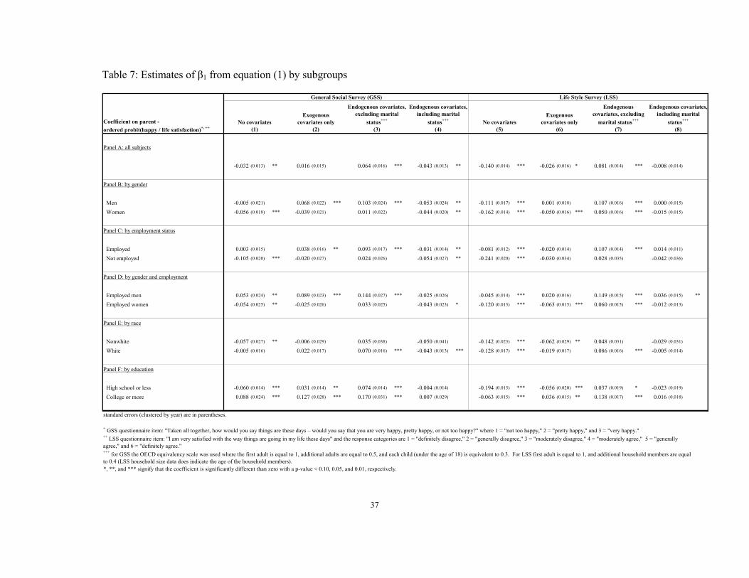
37

Table 7: Estimates of β1 from equation (1) by subgroups

Panel A: all subjects

-0.032 (0.013) ** 0.016 (0.015) 0.064 (0.016) *** -0.043 (0.013) ** -0.140 (0.014) *** -0.026 (0.016) * 0.081 (0.014) *** -0.008 (0.014)

Panel B: by gender

Men -0.005 (0.021) 0.068 (0.022) *** 0.103 (0.024) *** -0.053 (0.024) ** -0.111 (0.017) *** 0.001 (0.018) 0.107 (0.016) *** 0.000 (0.015)

Women -0.056 (0.018) *** -0.039 (0.021) 0.011 (0.022) -0.044 (0.020) ** -0.162 (0.014) *** -0.050 (0.016) *** 0.050 (0.016) *** -0.015 (0.015)

Panel C: by employment status

Employed 0.003 (0.015) 0.038 (0.016) ** 0.093 (0.017) *** -0.031 (0.014) ** -0.081 (0.012) *** -0.020 (0.014) 0.107 (0.014) *** 0.014 (0.011)

Not employed -0.105 (0.020) *** -0.020 (0.027) 0.024 (0.026) -0.054 (0.027) ** -0.241 (0.020) *** -0.030 (0.034) 0.028 (0.035) -0.042 (0.036)

Panel D: by gender and employment

Employed men 0.053 (0.024) ** 0.089 (0.023) *** 0.144 (0.027) *** -0.025 (0.026) -0.045 (0.014) *** 0.020 (0.016) 0.149 (0.015) *** 0.036 (0.015) **

Employed women -0.054 (0.025) ** -0.025 (0.026) 0.033 (0.025) -0.043 (0.023) * -0.120 (0.013) *** -0.063 (0.015) *** 0.060 (0.015) *** -0.012 (0.013)

Panel E: by race

Nonwhite -0.057 (0.027) ** -0.006 (0.029) 0.035 (0.038) -0.050 (0.041) -0.142 (0.023) *** -0.062 (0.029) ** 0.048 (0.031) -0.029 (0.031)

White -0.005 (0.016) 0.022 (0.017) 0.070 (0.016) *** -0.043 (0.013) *** -0.128 (0.017) *** -0.019 (0.017) 0.086 (0.016) *** -0.005 (0.014)

Panel F: by education

High school or less -0.060 (0.014) *** 0.031 (0.014) ** 0.074 (0.014) *** -0.004 (0.014) -0.194 (0.015) *** -0.056 (0.020) *** 0.037 (0.019) * -0.023 (0.019)

College or more 0.088 (0.024) *** 0.127 (0.028) *** 0.170 (0.031) *** 0.007 (0.029) -0.063 (0.015) *** 0.036 (0.015) ** 0.138 (0.017) *** 0.016 (0.018)




General Social Survey (GSS)

No covariates (1)


Life Style Survey (LSS)

Endogenous covariates, excluding

marital status+++

(7)


status+++

(8)



status+++

(3)


(2)


status+++

(4)No covariates

(5)


(6)Coefficient on parent - ordered probit(happy / life satisfaction)+, ++

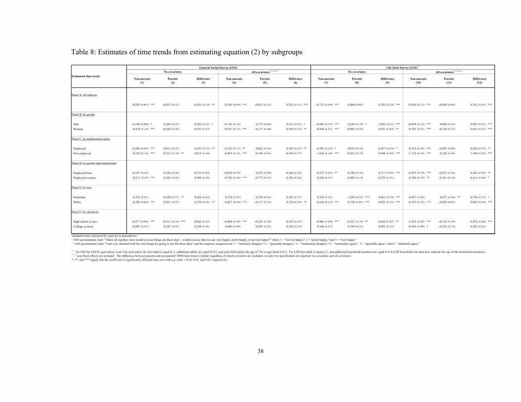
38

Table 8: Estimates of time trends from estimating equation (2) by subgroups

Panel A: all subjects

-0.295 (0.067) *** -0.033 (0.121) 0.262 (0.118) ** -0.358 (0.076) *** -0.033 (0.133) 0.325 (0.111) *** -0.713 (0.204) *** 0.069 (0.087) 0.782 (0.234) *** -0.819 (0.172) *** -0.038 (0.085) 0.781 (0.197) ***

Panel B: by gender

Men -0.158 (0.094) * 0.228 (0.191) 0.385 (0.211) * -0.136 (0.116) 0.177 (0.200) 0.313 (0.187) * -0.842 (0.183) *** 0.250 (0.138) * 1.092 (0.213) *** -0.878 (0.112) *** 0.069 (0.153) 0.947 (0.181) ***

Women -0.419 (0.110) *** -0.228 (0.145) 0.191 (0.167) -0.527 (0.117) *** -0.177 (0.148) 0.350 (0.178) ** -0.604 (0.231) *** -0.063 (0.103) 0.541 (0.269) ** -0.781 (0.231) *** -0.130 (0.112) 0.651 (0.251) ***

Panel C: by employment status

Employed -0.286 (0.093) *** 0.011 (0.155) 0.297 (0.135) ** -0.243 (0.117) ** 0.062 (0.164) 0.305 (0.125) ** -0.383 (0.223) * 0.074 (0.110) 0.457 (0.234) * -0.515 (0.193) *** -0.087 (0.096) 0.428 (0.195) **

Not employed -0.325 (0.110) *** -0.313 (0.138) ** 0.012 (0.168) -0.455 (0.112) *** -0.186 (0.156) 0.269 (0.177) -1.016 (0.189) *** -0.021 (0.175) 0.995 (0.282) *** -1.119 (0.182) *** 0.130 (0.185) 1.249 (0.281) ***

Panel D: by gender and employment

Employed men -0.107 (0.143) 0.226 (0.190) 0.333 (0.264) -0.010 (0.158) 0.255 (0.200) 0.264 (0.236) -0.527 (0.224) ** 0.190 (0.136) 0.717 (0.243) *** -0.475 (0.139) *** -0.013 (0.162) 0.463 (0.189) **

Employed women -0.511 (0.192) *** -0.203 (0.243) 0.308 (0.258) -0.528 (0.196) *** -0.172 (0.233) 0.356 (0.234) -0.244 (0.257) -0.009 (0.178) 0.235 (0.251) -0.594 (0.272) ** -0.181 (0.158) 0.413 (0.245) *

Panel E: by race

Nonwhite 0.352 (0.241) 0.620 (0.271) ** 0.268 (0.228) 0.178 (0.297) 0.359 (0.282) 0.182 (0.271) 0.338 (0.332) 1.299 (0.225) *** 0.961 (0.370) *** -0.057 (0.289) 0.677 (0.264) ** 0.734 (0.375) *

White -0.288 (0.065) *** 0.051 (0.132) 0.339 (0.141) ** -0.427 (0.070) *** -0.117 (0.138) 0.310 (0.129) ** -0.616 (0.219) *** 0.336 (0.091) *** 0.952 (0.253) *** -0.923 (0.181) *** -0.058 (0.091) 0.865 (0.210) ***

Panel F: by education

High school or less -0.577 (0.089) *** -0.511 (0.134) *** 0.066 (0.143) -0.460 (0.108) *** -0.225 (0.158) 0.235 (0.143) -0.986 (0.204) *** -0.321 (0.138) ** 0.664 (0.265) ** -1.011 (0.205) *** -0.135 (0.154) 0.876 (0.268) ***

College or more -0.007 (0.147) 0.247 (0.187) 0.254 (0.181) 0.046 (0.164) 0.282 (0.226) 0.236 (0.219) 0.166 (0.277) 0.168 (0.151) 0.002 (0.323) -0.365 (0.209) * -0.163 (0.178) 0.202 (0.261)






Estimated time trendNon-parents

(1)Difference

(3)Parents

(2)Non-parents

(4)

General Social Survey (GSS)+

No covariates All covariates+++,++++

Parents (5)

Difference (6)

++++ year fixed effects not included. The difference between parents and non-parents' SWB time trend is similar regardless of which covariates are included, so only two specification are reported: no covariates and all covariates.

Life Style Survey (LSS)++

No covariates All covariates+++,++++

Non-parents (7)

Parents (8)

Difference (9)

Non-parents (10)

Parents (11)

Difference (12)

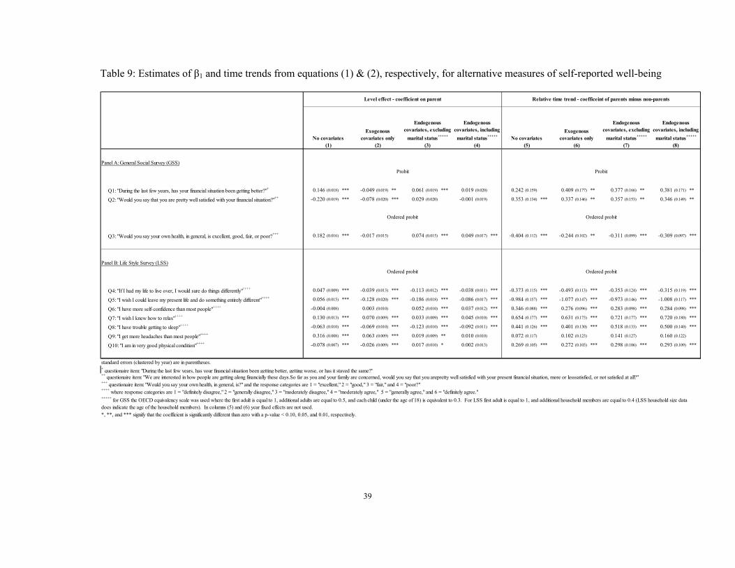
39

Table 9: Estimates of β1 and time trends from equations (1) & (2), respectively, for alternative measures of self-reported well-being

Panel A: General Social Survey (GSS)

Q1: "During the last few years, has your financial situation been getting better?"+ 0.146 (0.018) *** -0.049 (0.019) ** 0.061 (0.019) *** 0.019 (0.020) 0.242 (0.159) 0.409 (0.177) ** 0.377 (0.166) ** 0.381 (0.171) **

Q2: "Would you say that you are pretty well satisfied with your financial situation?"++ -0.220 (0.019) *** -0.078 (0.020) *** 0.029 (0.020) -0.001 (0.019) 0.353 (0.134) *** 0.337 (0.146) ** 0.357 (0.153) ** 0.346 (0.149) **

Q3: "Would you say your own health, in general, is excellent, good, fair, or poor?+++ 0.182 (0.016) *** -0.017 (0.015) 0.074 (0.015) *** 0.049 (0.017) *** -0.404 (0.112) *** -0.244 (0.102) ** -0.311 (0.099) *** -0.309 (0.097) ***

Panel B: Life Style Survey (LSS)

Q4: "If I had my life to live over, I would sure do things differently"++++ 0.047 (0.009) *** -0.039 (0.013) *** -0.113 (0.012) *** -0.038 (0.011) *** -0.373 (0.115) *** -0.493 (0.113) *** -0.353 (0.124) *** -0.315 (0.119) ***

Q5: "I wish I could leave my present life and do something entirely different"++++ 0.056 (0.015) *** -0.128 (0.020) *** -0.186 (0.018) *** -0.086 (0.017) *** -0.984 (0.157) *** -1.077 (0.147) *** -0.973 (0.146) *** -1.008 (0.117) ***

Q6: "I have more self-confidence than most people"++++ -0.004 (0.008) 0.003 (0.010) 0.052 (0.010) *** 0.037 (0.012) *** 0.346 (0.088) *** 0.276 (0.096) *** 0.283 (0.098) *** 0.284 (0.098) ***

Q7: "I wish I knew how to relax"++++ 0.130 (0.013) *** 0.070 (0.009) *** 0.033 (0.009) *** 0.045 (0.010) *** 0.654 (0.177) *** 0.631 (0.173) *** 0.721 (0.177) *** 0.720 (0.180) ***

Q8: "I have trouble getting to sleep"++++ -0.063 (0.010) *** -0.069 (0.010) *** -0.123 (0.010) *** -0.092 (0.011) *** 0.441 (0.126) *** 0.401 (0.130) *** 0.518 (0.133) *** 0.500 (0.140) ***

Q9: "I get more headaches than most people"++++ 0.316 (0.008) *** 0.063 (0.009) *** 0.019 (0.009) ** 0.010 (0.010) 0.072 (0.117) 0.102 (0.123) 0.141 (0.127) 0.160 (0.122)

Q10: "I am in very good physical condition"++++ -0.078 (0.007) *** -0.026 (0.009) *** 0.017 (0.010) * 0.002 (0.013) 0.269 (0.105) *** 0.272 (0.103) *** 0.298 (0.106) *** 0.293 (0.109) ***

standard errors (clustered by year) are in parentheses.+ questionaire item: "During the last few years, has your financial situation been getting better, getting worse, or has it stayed the same?"


Level effect - coefficient on parent Relative time trend - coefficeint of parents minus non-parents

No covariates (5)


marital status+++++

(7)

Endogenous covariates, including marital status+++++

(8)No covariates

(1)

Endogenous covariates, including marital status+++++

(4)


marital status+++++

(3)


(2)


(6)

+++++ for GSS the OECD equivalency scale was used where the first adult is equal to 1, additional adults are equal to 0.5, and each child (under the age of 18) is equivalent to 0.3. For LSS first adult is equal to 1, and additional household members are equal to 0.4 (LSS household size data does indicate the age of the household members). In columns (5) and (6) year fixed effects are not used.

Ordered probit Ordered probit

+++ questionaire item: "Would you say your own health, in general, is?" and the response categories are 1 = "excellent," 2 = "good," 3 = "fair," and 4 = "poor?"++++ where response categories are 1 = "definitely disagree," 2 = "generally disagree," 3 = "moderately disagree," 4 = "moderately agree," 5 = "generally agree," and 6 = "definitely agree."

Probit

++ questionaire item: "We are interested in how people are getting along financially these days.So far as you and your family are concerned, would you say that you arepretty well satisfied with your present financial situation, more or lesssatisfied, or not satisfied at all?"

Probit

Ordered probit Ordered probit

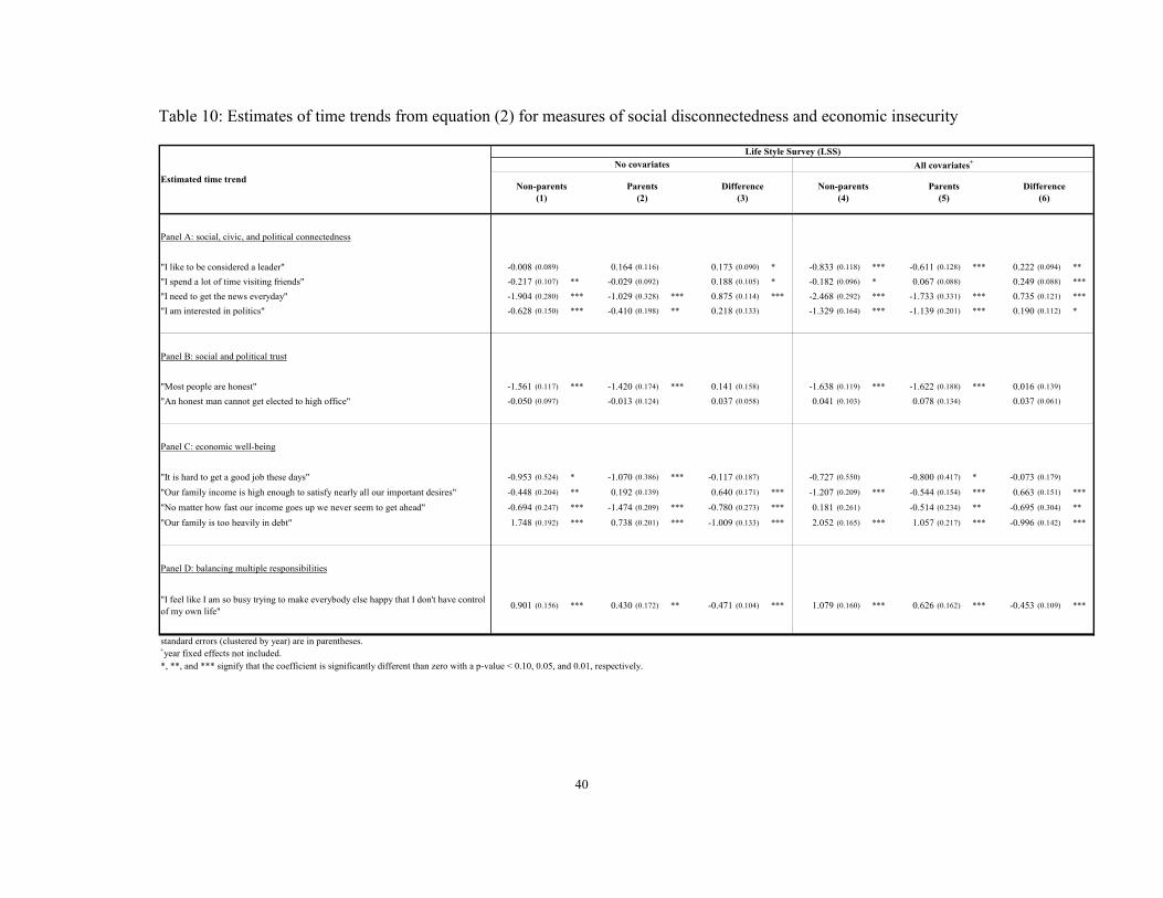
40

Table 10: Estimates of time trends from equation (2) for measures of social disconnectedness and economic insecurity

Panel A: social, civic, and political connectedness

"I like to be considered a leader" -0.008 (0.089) 0.164 (0.116) 0.173 (0.090) * -0.833 (0.118) *** -0.611 (0.128) *** 0.222 (0.094) **

"I spend a lot of time visiting friends" -0.217 (0.107) ** -0.029 (0.092) 0.188 (0.105) * -0.182 (0.096) * 0.067 (0.088) 0.249 (0.088) ***

"I need to get the news everyday" -1.904 (0.280) *** -1.029 (0.328) *** 0.875 (0.114) *** -2.468 (0.292) *** -1.733 (0.331) *** 0.735 (0.121) ***

"I am interested in politics" -0.628 (0.150) *** -0.410 (0.198) ** 0.218 (0.133) -1.329 (0.164) *** -1.139 (0.201) *** 0.190 (0.112) *

Panel B: social and political trust

"Most people are honest" -1.561 (0.117) *** -1.420 (0.174) *** 0.141 (0.158) -1.638 (0.119) *** -1.622 (0.188) *** 0.016 (0.139)

"An honest man cannot get elected to high office" -0.050 (0.097) -0.013 (0.124) 0.037 (0.058) 0.041 (0.103) 0.078 (0.134) 0.037 (0.061)

Panel C: economic well-being

"It is hard to get a good job these days" -0.953 (0.524) * -1.070 (0.386) *** -0.117 (0.187) -0.727 (0.550) -0.800 (0.417) * -0.073 (0.179)

"Our family income is high enough to satisfy nearly all our important desires" -0.448 (0.204) ** 0.192 (0.139) 0.640 (0.171) *** -1.207 (0.209) *** -0.544 (0.154) *** 0.663 (0.151) ***

"No matter how fast our income goes up we never seem to get ahead" -0.694 (0.247) *** -1.474 (0.209) *** -0.780 (0.273) *** 0.181 (0.261) -0.514 (0.234) ** -0.695 (0.304) **

"Our family is too heavily in debt" 1.748 (0.192) *** 0.738 (0.201) *** -1.009 (0.133) *** 2.052 (0.165) *** 1.057 (0.217) *** -0.996 (0.142) ***

Panel D: balancing multiple responsibilities

"I feel like I am so busy trying to make everybody else happy that I don't have control of my own life" 0.901 (0.156) *** 0.430 (0.172) ** -0.471 (0.104) *** 1.079 (0.160) *** 0.626 (0.162) *** -0.453 (0.109) ***

standard errors (clustered by year) are in parentheses.+year fixed effects not included.*, **, and *** signify that the coefficient is significantly different than zero with a p-value < 0.10, 0.05, and 0.01, respectively.

Estimated time trend

Life Style Survey (LSS)No covariates All covariates+

Non-parents (1)

Parents (2)

Difference (3)

Non-parents (4)

Parents (5)

Difference (6)

A BUNDLE OF JOY: DOES PARENTING REALLY …journalistsresource.org/wp-content/uploads/2011/08/parenting.pdfA BUNDLE OF JOY: DOES PARENTING REALLY MAKE US ... conclusion has been adopted

Documents