A Brownian dynamics algorithm for colloids in curved manifolds

A Brownian dynamics algorithm for colloids in curved manifoldsPavel Castro-Villarreal, Alejandro Villada-Balbuena, José Miguel Méndez-Alcaraz, Ramón Castañeda-Priego,

and Sendic Estrada-Jiménez

Citation: The Journal of Chemical Physics 140, 214115 (2014); doi: 10.1063/1.4881060 View online: http://dx.doi.org/10.1063/1.4881060 View Table of Contents: http://scitation.aip.org/content/aip/journal/jcp/140/21?ver=pdfcov Published by the AIP Publishing Articles you may be interested in Dynamic Monte Carlo simulations of anisotropic colloids J. Chem. Phys. 137, 054107 (2012); 10.1063/1.4737928 Tracking the Brownian diffusion of a colloidal tetrahedral cluster Chaos 21, 041103 (2011); 10.1063/1.3665984 Structural and dynamical analysis of monodisperse and polydisperse colloidal systems J. Chem. Phys. 133, 224901 (2010); 10.1063/1.3506576 Effects of polydispersity on Brownian dynamics of concentrated colloidal suspensions AIP Conf. Proc. 469, 180 (1999); 10.1063/1.58498 Grand canonical Brownian dynamics simulation of colloidal adsorption J. Chem. Phys. 107, 9157 (1997); 10.1063/1.475207

This article is copyrighted as indicated in the article. Reuse of AIP content is subject to the terms at: http://scitation.aip.org/termsconditions. Downloaded to IP:

148.214.16.175 On: Fri, 06 Jun 2014 16:47:18

THE JOURNAL OF CHEMICAL PHYSICS 140, 214115 (2014)

A Brownian dynamics algorithm for colloids in curved manifoldsPavel Castro-Villarreal,1,a) Alejandro Villada-Balbuena,2,b)

José Miguel Méndez-Alcaraz,2,c) Ramón Castañeda-Priego,3,d)

and Sendic Estrada-Jiménez1,e)

1Centro de Estudios en Física y Matemáticas Básicas y Aplicadas, Universidad Autónoma de Chiapas,Carretera Emiliano Zapata, Km. 8, Rancho San Francisco, C. P. 29050, Tuxtla Gutiérrez, Chiapas, México2Departamento de Física, Cinvestav, Av. IPN 2508, Col. San Pedro Zacatenco, 07360 México, D. F., México3Departamento de Ingeniería Física, División de Ciencias e Ingenierías, Campus León, Universidad deGuanajuato, Loma del Bosque 103, 37150 León, Guanajuato, México

(Received 5 March 2014; accepted 21 May 2014; published online 6 June 2014)

The many-particle Langevin equation, written in local coordinates, is used to derive a Browniandynamics simulation algorithm to study the dynamics of colloids moving on curved manifolds. Thepredictions of the resulting algorithm for the particular case of free particles diffusing along a circleand on a sphere are tested against analytical results, as well as with simulation data obtained by meansof the standard Brownian dynamics algorithm developed by Ermak and McCammon [J. Chem. Phys.69, 1352 (1978)] using explicitly a confining external field. The latter method allows constrainingthe particles to move in regions very tightly, emulating the diffusion on the manifold. Additionally,the proposed algorithm is applied to strong correlated systems, namely, paramagnetic colloids alonga circle and soft colloids on a sphere, to illustrate its applicability to systems made up of interactingparticles. © 2014 AIP Publishing LLC. [http://dx.doi.org/10.1063/1.4881060]

I. INTRODUCTION

Diffusion processes occur in a wide diversity of physi-cal areas, including elementary particle physics,1 condensedmatter physics,2 and astrophysics.3 In the latter case, suchprocesses are relevant within the framework of special andgeneral relativity (see, e.g., Ref. 4 and references therein). Ad-ditionally, in biophysics the diffusion processes on curved sur-faces have gained increasing attention over the last decade.5

The transport phenomena of proteins occurring inside cellmembranes are interesting since they determine the flux ofnutrients between the cell and its exterior affecting, in con-sequence, the cell functionality.6 In particular, the lateral dif-fusion of integral proteins or lipids on a biological cell is acomplex phenomenon mainly because the interactions withthe remaining components of the membrane and the proteinfinite-size effects.7, 8 In addition, there are membrane cur-vature contributions9 and thermal fluctuations that produceshape undulations in the membrane10, 11 and, thus, have a cru-cial contribution to the transport phenomena.12 Protein diffu-sion is also affected when changes in the membrane thick-ness are present.13, 14 The simplest approach to study thiscomplex problem is grounded on the Smoluchowski equa-tion for a point particle on curved manifolds, see, e.g., Refs. 9and 15–21.

The statistical mechanics of fluids in manifolds has beenrecently discussed and reviewed by Tarjus et al.22 In softcondensed matter, rather than the exception, dynamical phe-

a)Electronic mail: [email protected])Electronic mail: [email protected])Electronic mail: [email protected])Electronic mail: [email protected])Electronic mail: [email protected]

nomena take place commonly in curved manifolds. A fewparticular examples, among others, are the diffusion of ad-sorbed particles on a curved substrate,23, 24 the dynamics ofconfined polymer chains,25–27 the single-file diffusion in nar-row cavities,28 and the dynamics of colloidal halos.29, 30 Manyof these transport processes have been subjects of accuratemeasurements, and, nowadays, a considerable amount of ex-perimental results is available, however, not all of them havebeen fully understood yet.

The theoretical treatment of the diffusion phenomenamentioned in the previous paragraph often resides on localapproximations, where the dynamics is assumed to happenin an Euclidean plane or along a straight line (see, for in-stance, Ref. 31 in the case of single-file diffusion). This kindof approximations captures the right physics as long as theparticles diffuse only short distances as compared with thecurvature radius of the supporting manifold. Nevertheless,within a general description, one has to take into accountthe contributions of the geometry on the particle dynamics.Such geometrical effects have led to a growing set of theoret-ical frameworks that have explicitly considered the curvatureeffects.9, 12, 18, 20, 21, 23, 25, 32

Ermak and McCammon33 derived a Brownian dynamicssimulation algorithm that has been widely used for studyingthe dynamics of colloids in Euclidean spaces and in the over-damped limit. This algorithm applies typically to colloidalbulk systems that have no physical interfaces, where thereare non-trivial changes in both the hydrodynamic mobilitytensors and the direct particle interactions. However, it hasbeen successfully used to study interacting particles diffus-ing on an almost ideal two-dimensional gas-liquid interface34

and particles confined to lines and surfaces by means oflaser tweezers.37 However, extensions of the Ermak and

0021-9606/2014/140(21)/214115/10/$30.00 © 2014 AIP Publishing LLC140, 214115-1

This article is copyrighted as indicated in the article. Reuse of AIP content is subject to the terms at: http://scitation.aip.org/termsconditions. Downloaded to IP:

148.214.16.175 On: Fri, 06 Jun 2014 16:47:18

214115-2 Castro-Villarreal et al. J. Chem. Phys. 140, 214115 (2014)

McCammon algorithm treat mainly with its optimizationwhen hydrodynamic interactions (HI) are included35 and withthe development of nonlinear schemes that ensure the stabilityof the particle trajectories for robust time steps.36

Algorithms to study dynamical processes occurring oncurved manifolds are typically implemented by using theErmak-McCammon algorithm for the open Euclidean space,but applying external fields able to confine the particles inregions very tightly that, approximately, emulate the mani-fold under consideration.37–39 Nonetheless, a few algorithms,mainly based on the diffusion equation on curved mani-folds, have been developed to include the intrinsic featuresof the surfaces or lines of interest, see, e.g., Refs. 18 and32. Recently, Elvingson and collaborators40, 41 have proposeda Brownian dynamics algorithm for curved manifolds. Thisscheme first solves the diffusion equation on the correspond-ing manifold and its solution is introduced into a finitedifference (Langevin) equation adapted to the manifold. Elv-ingson et al.40, 41 tested their algorithm by studying thedynamics of both free and repulsive particles on a three-dimensional sphere.

Then, by using some ideas and approximations similarto the ones mentioned above,20, 33, 40 in this work we reporton the derivation of a Brownian dynamics computer simu-lation algorithm to study the dynamics of colloidal particlesdiffusing on curved surfaces and lines, as in the case of spher-ical colloidal halos29 and circular optical traps,42 respectively.This is done according to the following two steps:

(i) A holonomic constraint is included in the many-particleLangevin equation (MPLE) to enforce the particles tomove on the given manifold. The MPLE is first ex-pressed in global coordinates, but, after an appropriateparametrization, it is rewritten in local coordinates forboth lines and surfaces.

(ii) The MPLE in local coordinates is used to derivea Brownian dynamics simulation algorithm by ap-plying the same method developed by Ermak andMcCammon,33 however, the geometry of the subspace,where the particles can diffuse, is included into theequation of motion. The latter is then parametrized inorder to be adapted to the particular cases of circles andspheres.

This algorithm is based only on the finite difference equa-tion resulting from the MPLE adapted to the manifold. Inparticular, the algorithm derived in this paper does not needany particular solution of the diffusion equation on the corre-sponding manifold in contrast with previous algorithms. Also,it is shown that the short-time dynamics occurs in the tangen-tial plane and that the long-time dynamics can be constructedby combining those tangential parts. In other words, the re-sulting algorithm captures the regime where the particles dif-fuse over long distances, as compared to the curvature radiusof the supporting manifold, but the hydrodynamic interactionsare neglected at this stage of our calculations. The derivationof the algorithm is explained in Appendixes A–C.

The details of the numerical implementation of the algo-rithm are explained by studying the diffusion of free parti-cles moving along a circle and on a sphere. The simulation

results are then compared with the analytical solution of thediffusion equation on curved manifolds, which is obtained inAppendix D. In addition, both cases are also contrastedagainst simulation results obtained by means of the standardBrownian dynamics algorithm with a confining external field,which constrains the particles to move in regions very tightlylocated around either the trace of the circle or the positionof the surface of the sphere. In order to emphasize the po-tential application of the algorithm, two cases of strong cor-related systems are also explored, namely, paramagnetic col-loids along a circle30 and soft colloids on a sphere.29

Regarding the organization of the paper, after this generalIntroduction, it is split in two related, but independent parts.The first one, contained in Secs. II, III, and IV presents the al-gorithm, the results of its implementation, and some generalconcluding remarks, respectively. The second one, containedin Appendixes A–C, explains the derivation of the algorithm.There is also an Appendix D dedicated to the diffusion equa-tion and to its analytical solution. The first part emphasizesthe application of the algorithm, which is of importance andinterest for the soft condensed matter community, whereas thesecond part is of general character and requires more abstractmathematical methods.

II. THE ALGORITHM

According to Ermak and McCammon,33 the MPLE canbe rewritten as the stochastic finite differences equation

ri(t + �t) = ri(t) + β

N∑j=1

Dij · fj (t)�t

+∇j · Dij�t + δRi , (1)

provided the time step �t is restricted to τB � �t � τ I, whereτB and τ I are, respectively, the momentum and structure re-laxation times. ri(t) denotes the position vector of particle iat the time t, Dij is the diffusion tensor, fj(t) is the instanta-neous force acting on the particle j due to its direct interactionwith all other particles in the system, δRi is the Brownian ran-dom displacement due to solvent-particle interactions, and β

= 1/kBT the inverse of the thermal energy kBT, with kB andT being the Boltzmann’s constant and the absolute tempera-ture, respectively. The Cartesian components of δRi are ran-dom variables with a multi-variate Gaussian distribution withzero means, and covariance matrix 〈δRiδRj〉 = 2Dij�t. If hy-drodynamic interactions are neglected, Dij must be replacedby D0δij1, where D0 is the free-particle diffusion coefficient,δij the Kronecker’s delta, and 1 is the three-dimensional unitmatrix.

An external force Fi acting on the particles can be in-cluded into Eq. (1) by adding it to fi(t), given that Fi does notappreciably change in distances of the order of the Brownianrandom displacements. Thus, the diffusion in curved mani-folds can be emulated by including, for instance, an harmonicexternal force that enforces the particles to stay around thesubspace occupied by the manifold. In the case of spheres ofradius R, for instance, it takes the simple form

Fi = −κ(ri − R)ni , (2)

This article is copyrighted as indicated in the article. Reuse of AIP content is subject to the terms at: http://scitation.aip.org/termsconditions. Downloaded to IP:

148.214.16.175 On: Fri, 06 Jun 2014 16:47:18

214115-3 Castro-Villarreal et al. J. Chem. Phys. 140, 214115 (2014)

written in spherical coordinates, where ni = ri/ri is the nor-mal vector. The emulation is effective as long as the parti-cles do not diffuse much more than their own diameter awayfrom the manifold; this requirement demands very large val-ues of κ . This is hard to combine with the small values of κ

required to have slow varying forces. Therefore, this methodhas strong limitations, which become more evident at long-times when the curvature and interaction effects are expectedto be manifested.38 This is, however, not an issue for free par-ticles, since Eq. (1) displays only one time regime and allowstherefore for arbitrary, although perhaps not physical, valuesof �t.

The above difficulties do not longer appear if the MPLEis written down in the corresponding manifold, as explained inAppendixes B and C. A stochastic finite differences equationsimilar to Eq. (1) is then obtained, but for the local coordi-nates xα

i (t) of particle i, with α = 1, . . . , d

xαi (t + �t) = xα

i (t) + βD0fT,αi (t)�t + δXα

i , (3)

where fT,αi (t) is the projection of fi(t) on the tangential space

to the manifold in the point P where the particle is instan-taneously located. Because we are looking for the dynamicsin a small neighbourhood of P , it is convenient to use Rie-mann normal coordinates (RNC)47 centered at xα(t). The tan-gential displacement δXα

i is a Brownian random variable witha mono-variate Gaussian distribution with zero mean, and co-variance 〈δXα

i δXβ

j 〉 = 2D0δij δαβ�t . No hydrodynamic inter-

actions are included in Eq. (3). The displacement in RNCcan be written as �s(�t) = √

δαβ�xα�xβ , hence, the mean-square displacement (MSD) is given by 〈�s2(�t)〉 = 2dDo�t,where d is the dimension of the manifold.

Equation (3) allows us to observe that, first, the short-time dynamics (τB � t � τ I) occurs in the tangential planeto the manifold, and, second, that the long-time dynamics (t� τ I) can be constructed by combining those tangential parts.

The algorithm can be implemented in the following formin the cases of circles and spheres:

� The force fi(t) is calculated; its projection f Ti (t) on the

tangential space in the position of particle i is calcu-lated and, therefore, the corresponding deterministicdisplacement βD0f

Ti (t)�t is calculated.

� A d + 1-dimensional Gaussian random displacementin Cartesian coordinates δRi is generated in the posi-tion of particle i; its projection, δXi, on the tangentialspace is calculated.

� Both projected displacements are summed; the anglebetween the two radial lines passing through the initialand final positions defines the angular displacement�αi of particle i; the new angular position is thereforeobtained.

� This is put in terms of the polar angle φi in polar coor-dinates for circles, and in polar and azimuthal anglesθ i and ϕi in spherical coordinates for spheres. Finally,the geodesic displacement is obtained through �si

= R�αi, where R is the radius of the circle or sphere.

All the previous steps are carried out for all particles at everytime step.

We should stress that more complicated manifolds re-quire a more careful implementation of Eq. (3), which willbe reported elsewhere. In Sec. III, Eq. (3) is used to simulatethe diffusion of free and interacting particles along circles andon spheres, both of radius R. The diameter σ of the particlesallows for the definition of the time scale τ = σ 2/D0; the timeneeded for a particle to diffuse a distance similar to its ownsize. In terms of this time scale, we use values of �t of theorder of 10−4τ , and let the program run over eight orders ofmagnitude after thermalization to reduce statistical uncertain-ties. In terms of the time τG = R2/D0; the time needed for aparticle to diffuse a distance similar to the size of the circleor sphere, �t is of the order of 10−6τG, and a time windowof the order of 100τG is used in our simulations. This meansthat the particles are able to diffuse several times around themanifold before the simulation run is stopped.

III. APPLICATIONS: FREE-PARTICLESAND SOFT-PARTICLES

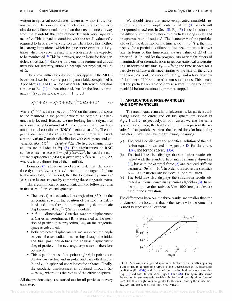
The mean-square angular displacements for particles dif-fusing along the circle and on the sphere are shown inFigs. 1 and 2, respectively. In both cases, we use the sametype of lines. Then, the bold and thin lines represent the re-sults for free particles whereas the dashed lines for interactingparticles. Bold lines have the following meanings:

(a) The bold line displays the analytical solution of the dif-fusion equation derived in Appendix D; for the circle,(D4), and for the sphere, (D6).

(b) The bold line also displays the simulation results ob-tained with the standard Brownian dynamics algorithm(1), but with the external force (2) and reduced stiffnessparameter βR2κ = 105. In order to improve the statisticsN = 1000 particles are included in the simulation.

(c) The bold line also displays the simulation results ob-tained with our Brownian dynamics algorithm (3). In or-der to improve the statistics N = 1000 free particles areused in the simulation.

The differences between the three results are smaller than thethickness of the bold line; that is the reason why the same lineis used to represent all of them.

10−3

10−2

10−1

100

101

10−3 10−2 10−1 100 101 102

<[Δφ(

t)]2 >

tD0/R2

π2/3 2D0t/R2

FIG. 1. Mean-square angular displacement for free particles diffusing alonga circle: The bold black line represents the superposition of the theoreticalprediction (Eq. (D4)) with the simulation results, both with our algorithm(Eq. (3)) and with its emulation (Eqs. (1) and (2)). The figure also showsthe results for paramagnetic particles obtained with our algorithm (dashedline). The thin straight lines are guides for the eyes, showing the short-times,2D0t/R2, and the geometrical limit, π2/3, values.

This article is copyrighted as indicated in the article. Reuse of AIP content is subject to the terms at: http://scitation.aip.org/termsconditions. Downloaded to IP:

148.214.16.175 On: Fri, 06 Jun 2014 16:47:18

214115-4 Castro-Villarreal et al. J. Chem. Phys. 140, 214115 (2014)

10−3

10−2

10−1

100

101

10−4 10−3 10−2 10−1 100 101

<[θ

(t)]

2 >

tD0/R2

(π2−4)/2 4D0t/R2

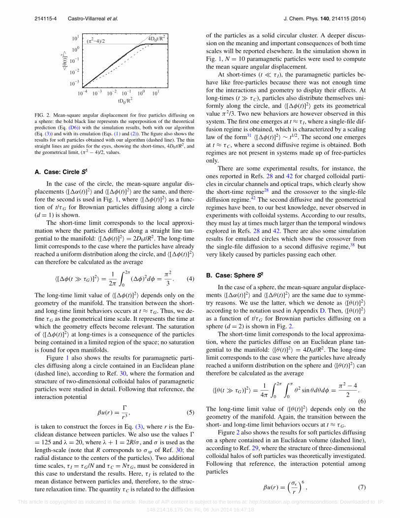
FIG. 2. Mean-square angular displacement for free particles diffusing ona sphere: the bold black line represents the superposition of the theoreticalprediction (Eq. (D6)) with the simulation results, both with our algorithm(Eq. (3)) and with its emulation (Eqs. (1) and (2)). The figure also shows theresults for soft particles obtained with our algorithm (dashed line). The thinstraight lines are guides for the eyes, showing the short-times, 4D0t/R2, andthe geometrical limit, (π2 − 4)/2, values.

A. Case: Circle S1

In the case of the circle, the mean-square angular dis-placements 〈[�α(t)]2〉 and 〈[�φ(t)]2〉 are the same, and there-fore the second is used in Fig. 1, where 〈[�φ(t)]2〉 as a func-tion of t/τG for Brownian particles diffusing along a circle(d = 1) is shown.

The short-time limit corresponds to the local approxi-mation where the particles diffuse along a straight line tan-gential to the manifold: 〈[�φ(t)]2〉 = 2D0t/R2. The long-timelimit corresponds to the case where the particles have alreadyreached a uniform distribution along the circle, and 〈[�φ(t)]2〉can therefore be calculated as the average

〈[�φ(t � τG)]2〉 = 1

2π

∫ 2π

0(�φ)2dφ = π2

3. (4)

The long-time limit value of 〈[�φ(t)]2〉 depends only on thegeometry of the manifold. The transition between the short-and long-time limit behaviors occurs at t ≈ τG. Thus, we de-fine τG as the geometrical time scale. It represents the time atwhich the geometry effects become relevant. The saturationof 〈[�φ(t)]2〉 at long-times is a consequence of the particlesbeing contained in a limited region of the space; no saturationis found for open manifolds.

Figure 1 also shows the results for paramagnetic parti-cles diffusing along a circle contained in an Euclidean plane(dashed line), according to Ref. 30, where the formation andstructure of two-dimensional colloidal halos of paramagneticparticles were studied in detail. Following that reference, theinteraction potential

βu(r) =

r3, (5)

is taken to construct the forces in Eq. (3), where r is the Eu-clidean distance between particles. We also use the values

= 125 and λ = 20, where λ + 1 = 2R/σ , and σ is used as thelength-scale (note that R corresponds to σ sp of Ref. 30; theradial distance to the centers of the particles). Two additionaltime scales, τ I = τG/N and τC = NτG, must be considered inthis case to understand the results. Here, τ I is related to themean distance between particles and, therefore, to the struc-ture relaxation time. The quantity τC is related to the diffusion

of the particles as a solid circular cluster. A deeper discus-sion on the meaning and important consequences of both timescales will be reported elsewhere. In the simulation shown inFig. 1, N = 10 paramagnetic particles were used to computethe mean square angular displacement.

At short-times (t � τ I), the paramagnetic particles be-have like free-particles because there was not enough timefor the interactions and geometry to display their effects. Atlong-times (t � τC), particles also distribute themselves uni-formly along the circle, and 〈[�φ(t)]2〉 gets its geometricalvalue π2/3. Two new behaviors are however observed in thissystem. The first one emerges at t ≈ τ I, where a single-file dif-fusion regime is obtained, which is characterized by a scalinglaw of the form31 〈[�φ(t)]2〉 ∼ t1/2. The second one emergesat t ≈ τC, where a second diffusive regime is obtained. Bothregimes are not present in systems made up of free-particlesonly.

There are some experimental results, for instance, theones reported in Refs. 28 and 42 for charged colloidal parti-cles in circular channels and optical traps, which clearly showthe short-time regime28 and the crossover to the single-filediffusion regime.42 The second diffusive and the geometricalregimes have been, to our best knowledge, never observed inexperiments with colloidal systems. According to our results,they must lay at times much larger than the temporal windowsexplored in Refs. 28 and 42. There are also some simulationresults for emulated circles which show the crossover fromthe single-file diffusion to a second diffusive regime,38 butvery likely caused by particles passing each other.

B. Case: Sphere S2

In the case of a sphere, the mean-square angular displace-ments 〈[�α(t)]2〉 and 〈[�θ (t)]2〉 are the same due to symme-try reasons. We use the latter, which we denote as 〈[θ (t)]2〉according to the notation used in Appendix D. Then, 〈[θ (t)]2〉as a function of t/τG for Brownian particles diffusing on asphere (d = 2) is shown in Fig. 2.

The short-time limit corresponds to the local approxima-tion, where the particles diffuse on an Euclidean plane tan-gential to the manifold: 〈[θ (t)]2〉 = 4D0t/R2. The long-timelimit corresponds to the case where the particles have alreadyreached a uniform distribution on the sphere and 〈[θ (t)]2〉 cantherefore be calculated as the average

〈[θ (t � τG)]2〉 = 1

4π

∫ 2π

0

∫ π

0θ2 sin θdθdφ = π2 − 4

2.

(6)The long-time limit value of 〈[θ (t)]2〉 depends only on thegeometry of the manifold. Again, the transition between theshort- and long-time limit behaviors occurs at t ≈ τG.

Figure 2 also shows the results for soft particles diffusingon a sphere contained in an Euclidean volume (dashed line),according to Ref. 29, where the structure of three-dimensionalcolloidal halos of soft particles was theoretically investigated.Following that reference, the interaction potential amongparticles

βu(r) =(σε

r

)6, (7)

This article is copyrighted as indicated in the article. Reuse of AIP content is subject to the terms at: http://scitation.aip.org/termsconditions. Downloaded to IP:

148.214.16.175 On: Fri, 06 Jun 2014 16:47:18

214115-5 Castro-Villarreal et al. J. Chem. Phys. 140, 214115 (2014)

is taken to construct the forces in Eq. (3), where r is theEuclidean distance between particles. We also use the val-ues 2R/σ ε = 1 and 2R/σ = 20, σ being used as the length-scale. This case does not exhibit the dynamical behavior ∼t1/2,which is characteristic of the single-file behavior, since mu-tual passage is possible. The additional time scales τ I andτC are also important here, but the dynamics is much richerand the interplay between time scales much more complicatedthan in the case of the circle. This topic will be further ex-plored, but here we only report on the straightforward appli-cation of the algorithm (3) to the particular case of interact-ing particles moving along circles and on spheres. We shouldpoint out that Fig. 2 displays one of the most simple situationsfor a sphere, where only an intermediate diffusive regime isfound between both short- and long-time limits. N = 10 softparticles were used in the simulations to numerically evaluatethe mean square angular displacement.

IV. CONCLUDING REMARKS

An algorithm to simulate Brownian motion in curvedmanifolds was introduced. It was derived from the over-damped many-particle Langevin equation by means of thesame procedure developed by Ermak and McCammon.33 Itsapplicability was demonstrated by studying four different sys-tems: (i) Free-particles along a circle, (ii) free-particles ona sphere, (iii) paramagnetic particles along a circle, and (iv)soft-particles on a sphere.

The first two cases were used to validate the algorithm;we compared its predictions with the analytical solution ofthe diffusion equation, also obtained here, and with simula-tion data generated by the standard Ermak-McCammon al-gorithm with an external field emulating the manifolds. Thelast two cases were used to illustrate the way in which thealgorithm can be straightforward used to study strong corre-lated systems. These systems are important, for example, tounderstand the transport mechanisms in interacting proteinsattached to the surface of the cell.

The aim of this paper was, on one hand, to present thealgorithm and, on the other hand, to explain its use. We didnot discuss in detail the physics behind the performed simu-lations. Nevertheless, the few results shown in the figures al-lowed us for a short view of a very rich dynamics, which wasexpressed in terms of the time scales τ I, τG, and τC. We willfurther report on this point in future works, where the algo-rithm will be extensively applied to study the phenomenon ofsingle-file diffusion and the dynamics of colloidal halos undervery specific circumstances.

Although only circles and spheres were studied in thepresent work, our algorithm can also be applied to more so-phisticated manifolds, like ellipsoids, toroids, and sponges, aslong as the radius of curvature is very large, on every pointof the manifold, as compared with the random Brownian dis-placements. This is, however, the subject of future work.

Hydrodynamic interactions were neglected in this work.Thus, a Brownian dynamics algorithm with HI in curved man-ifolds is still missing. It clearly represents a very importantchallenge, since particles moving close to surfaces can be verystrong correlated through solvent-mediated interactions.34, 43

Such effects may be still enhanced if the particles are enforcedto diffuse in small spatial regions.44

ACKNOWLEDGMENTS

Financial support by PIFI-2011, PIEC, PROMEP(1035/08/3291), and CONACyT (through Grant Nos.61418/2007, 102339/2008, 60595 and Red Temática de laMateria Condensada Blanda) is kindly acknowledged. Theauthors also thank to the General Coordination of Informa-tion and Communications Technologies (CGSTIC) at Cinves-tav for providing HPC resources on the Hybrid Cluster Super-computer “Xiuhcoatl,” which have contributed to the researchresults reported in this paper.

APPENDIX A: GEOMETRICAL NOTATION

In this appendix, we provide our geometrical notation;we follow Ref. 45. In a level set approach, a hypersurface canbe defined as a set M = {X ∈ Rd+1|�(X) = 0}. In particular,the normal vector is defined by N = ∇�/|∇�|. This formu-lation is useful for the global description of the many-particleLangevin equation.

An alternative approach to describe the geometry of thehypersurface is using a parametrized map X : U ⊂ Rd → M,where a particular point in M is given by X(xα), being xα

the local coordinates (α = 1, . . . , d). In this description, theset {eα ≡ ∂αX} defines a basis for the tangent space TX(M)in the point X. The normal vector can also be obtained bysolving the set of equations eα · N = 0 and N2 = 1. It is alsouseful to introduce the metric tensor gαβ = eα · eβ and theextrinsic curvature tensor Kαβ = eα · ∂βN. Riemann tensor isgiven by Rαβγ δ = Kαγ Kβδ − KαδKβγ and Ricci scalar cur-vature, which is twice the Gaussian curvature, is given byRg = gαγ gβδRαβγ δ . In each point of the hypersurface, theWeingarten-Gauss structure equations are satisfied

∂αeβ = γ

βαeγ − KβαN, (A1)

where the Chrystoffel symbols γ

βα are defined by

γ

βα = 1

2gγ ε(∂βgαε + ∂αgβε − ∂εgβα). (A2)

In particular, for planar curves parametrized by the arc-length s, one has only a unit tangent vector T(s) = X′(s)= dX(s)/ds. In this case, the structure equations are given bythe Frenet-Serret equations

T′(s) = κ(s)N(s),(A3)

N′(s) = −κ(s)T(s),

where k(s) is the curvature of the curve.Additionally, one has the following identities for curves

and surfaces:

κ(s) = TtGT, (A4)

and

Kαβ = etαGeβ, (A5)

This article is copyrighted as indicated in the article. Reuse of AIP content is subject to the terms at: http://scitation.aip.org/termsconditions. Downloaded to IP:

148.214.16.175 On: Fri, 06 Jun 2014 16:47:18

214115-6 Castro-Villarreal et al. J. Chem. Phys. 140, 214115 (2014)

respectively, where G is the Hessian of � divided by |∇�|and superindex t means transposed. These identities establisha connection between the level and local descriptions46 andthey turn out to describe the normal part of the many-particleLangevin equation (B4).

Furthermore, it is useful to introduce the Riemann nor-mal coordinates47 centered at point P , which have the featurethat geodesic curves that pass through P look equal to theequations of straight lines passing through the origin (P) ofa Euclidean space. These coordinates are defined by mappinga point on the manifold to the origin of Rd and the followingconditions:

gαβ(0) = δαβ, xαgαβ(x) = δαβ. (A6)

These conditions imply that the Chrystoffel symbols can beexpanded as

αμν(x) = 1

3Rα

(μβν)(0)xβ + · · · , (A7)

where Rα(μβν) = Rα

μβν + Rανβμ, among other results.

APPENDIX B: THE MANY-PARTICLELANGEVIN EQUATION

The many-particle Langevin equation on curved surfacescan be derived using holonomic constraints, �(Xi) = 0, thatbind the particles on the hypersurface M. The position of theith particle is denoted by Xi in Rd+1. Following the stan-dard procedure,48 the addition of the term λi�(Xi) to thefree-particle Lagrangian allows us to impose a holonomicconstraint on M. Indeed, the resulting equation of motion isXi = λi∇�(Xi) and the required constraint is �(Xi) = 0. Thefirst derivative with respect to time is denoted by U ≡ dU/dt .

For the many-particle Langevin equation defined on M,one simply includes the previous constraint, a friction term, astochastic force fi(t), and the forces, Fij, due to the rest of theparticles

Xi = −ζ Xi/M + λi∇�(Xi) + 1

M

⎛⎝fi(t) +

∑j �=i

Fji

⎞⎠ .

(B1)

The second term of the r.h.s. of Eq. (B1) represents the forcedue to the holonomic constraint. ζ and M denote the solventfriction and the mass of the colloidal particle, respectively.

The Lagrange multiplier λi can be obtained by using theconstraint as follows. The velocity of each particle is tangentto M, i.e., Xi = eαxα

i , and since Ni · eα = 0 (where it is un-derstood that eα is the tangent vector at point Xi), one has

∇�(Xi) · Xi = 0. (B2)

The second derivative with respect to time on Eq. (B2) gives

Ni · Xi = −XtiGXi , (B3)

where Gij = ∂ i∂ j�/|∇�|. Now, one gets λi by equating (B3)and the normal projection of (B1). Then,

λi = − XtiGXi

|∇�| −Ni ·

(fi + ∑

j �=i Fji

)M|∇�| .

By substituting this Lagrange multiplier in Eq. (B1), the re-sulting equations of motion, without HI, take the followingform:

Xi + XtiGXiNi = − ζ

MXi + 1

MP

⎛⎝fi(t) +

∑j �=i

Fij

⎞⎠ .

(B4)

The last term in the r.h.s. of Eq. (B4) is the tangent projec-tion of the stochastic force, fi, and the interaction force be-tween the ith particle with the rest of the particles, Fij, whereP ≡ 1 − NiNj is the tangent projector. It is worthy to men-tion that for those interaction forces Fij which depend only onthe Euclidean distance rij between particles, one has rij = |Xi

− Xj|. Note that the standard Langevin equation, without HI,is recovered for a flat geometry i.e., when the constraint is alinear function of the position.

In addition, the stochastic forces are chosen such thatthey satisfy the standard fluctuation-dissipation theorem,33

〈fi(t)〉 = 0,(B5)

〈fi(t)fj (t ′)〉 = �δij1δ(t − t ′),

where � = 2ζ /β, with β = (kBT)−1 being the inverse of thethermal energy, and kB and T are the Boltzmann constant andabsolute temperature, respectively. The unit matrix 1 has size(d + 1) × (d + 1).

In what follows, a simplified form of the many-particleLangevin equation using local coordinates adapted to curvesand surfaces is explicitly derived.

1. Langevin equation for colloids diffusing along lines

In order to simplify Eq. (B4) for lines, let us considera planar curve Xi(si) parametrized by the arc-length si. Inthis case, the velocity of the ith particle can be written asXi = siT(si), where si is the local velocity. Now, the secondderivative with respect to time is Xi = siT(si) + s2

i κ(si)N(si),where we have used the Frenet-Serret equations (A3). Next,we substitute this equation into (B4), and then we projectalong the tangential part. Note that the term coming from theforces is already tangential due to the projector P . Hence, thetangential component of the many-particle Langevin equation(B4) is given by

si = − ζ

Msi + ji(si, t), (B6)

where

ji(si, t) = 1

MT(si) ·

⎛⎝fi(t) +

∑j �=i

Fij

⎞⎠ , (B7)

while the normal counterpart turns out to be the identity (A4).These equations represent the general many-particle Langevinequation adapted to curved lines. Then, the recipe to find theequation of motion on a particular planar curve is: give an arc-length parametrization Xi(si), find the tangent vector T(si),and substitute it into Eqs. (B6) and (B7).

This article is copyrighted as indicated in the article. Reuse of AIP content is subject to the terms at: http://scitation.aip.org/termsconditions. Downloaded to IP:

148.214.16.175 On: Fri, 06 Jun 2014 16:47:18

214115-7 Castro-Villarreal et al. J. Chem. Phys. 140, 214115 (2014)

2. Langevin equation for colloids diffusingon surfaces

In order to simplify Eq. (B4) for surfaces, we introduce alocal parametrization Xi. In this case, the acceleration of theith particle can be written as Xi = ∂βeαxα

i xβ

i + eαxαi , where

xαi are the local velocities. Now, we use the Weingarten-Gauss

equations (A1). Next, the resulting Xi is substituted in (B4),and then we project along the tangential directions. Hence, thetangential component of the many-particle Langevin equation(B4) is given by

xγ

i + γ

βαxβ

i xαi = − ζ

Mx

γ

i + jγ

i (xi, t), (B8)

with

jγ

i (xi, t) = 1

Meγ (xi) ·

⎛⎝fi(t) +

∑j �=i

Fji

⎞⎠ , (B9)

while the normal projection gives the identity for the extrin-sic curvature tensor (A5). Thus, these equations represent thegeneral many-particle Langevin equation adapted to surfaces.The recipe to find the equation of motion for a particular sur-face is similar to the one explained above for curved lines. Inaddition, the Riemann normal coordinates will give anothersimplification.

APPENDIX C: BROWNIAN DYNAMICS ALGORITHMFOR CURVED SURFACES

The structure of Eqs. (B6) and (B8) allows us to ap-ply the same procedure used by Ermak and McCammon,33

originally developed for open Euclidean spaces, and, thus, toderive a Brownian dynamics algorithm for curves and sur-faces. According to the authors in Ref. 33, a perturbativeexpansion is performed of the source terms in powers of�xα

i = xαi (t) − xα

i (0). Then, to calculate the mean and mean-square displacements of the particle to first order in �t ≡ t− 0, it is only necessary to keep the zeroth order term of thesource. In the curved case, the difference with the Ermak andMcCammon’s33 original contribution is the tangential projec-tion in the source term and the additional term involving theChrystoffel symbols in Eq. (B8) for surfaces. Because we arelooking for the dynamics in a small neighbourhood of the ini-tial point xα

i (0), it is convenient to use Riemann normal coor-dinates centered at xα

i (0).Following Ref. 33, one has the identity

e− ζ

Mt d

dt

(e

ζ

Mt xα

i

)= xα

i + ζ

Mxα

i , (C1)

and using the RNC centered at xα(0) we expand Chrystoffelsymbols in powers of �xα

i . Thus, one has immediately theidentity (A7). Now, we substitute (C1) and (A7) into (B8);the resulting equation is integrated by the same method usedby Ermak and McCammon.33 Hence, one obtains

�xα(t) = βD0

∫ t

0dτh(ζ (t − τ )/M)jα

i (xi(0), τ )

− M

3ζRα

(μβν)(0)I (t,�x, x), (C2)

where h(x) ≡ (1 − e−x) and

I (t,�x, x) =∫ t

0dτh(ζ (t − τ )/M)�xδ(τ )xβ(τ )xγ (τ ).

(C3)

In the overdamped limit, i.e., t � τB ≡ M/ζ , one has thath(ζ (t − τ )/M) ≈ 1. Thus, by using the mean-value theoremfor integration, the last integral can be written as

I (t,�x, x) = �xδ(τ ′)xβ(τ ′)xγ (τ ′)t/τB, (C4)

where τ ′ ∼ t. In addition, we use the approximations�xα ∼ (D0t)1/2 and xα ∼ (kBT /m)1/2. Then, one has that�xα(τ )xβ(τ ) ∼ (kBT /m)(t/τB). Therefore, the last integralis of order (t/τB)2, which is entirely neglected in our descrip-tion. Taking into account all these considerations, one arisesto the expression,

�xαi (t) = βD0

∑j �=i

F0ij · eα

i (0)�t

+ 1

ζ

∫ t

0dτ

(1 − e− ζ

M(t−τ )

)fi(τ ) · eα

i (0), (C5)

where D0 = kBT/ζ and the upper-script 0 means that the corre-sponding quantity is evaluated at the initial time step. Besides,using the fluctuation-dissipation relations (B5) one can verifythat ⟨

�xαi (t)

⟩ = βD0

∑j �=i

F0ij · eα

i (0)�t, (C6)

and ⟨�xα

i (t)�xβ

j (t)⟩ ≈ 2D0δij g

αβ(0)t, (C7)

where gαβ(0) = eα(0) · eβ(0) = δαβ due to the RNC and eα(0)is the tangent vector evaluated at the initial time step. Forlines, one simply replaces �xα by �s and eα by T. Finally,Eq. (C5) can be written more concisely as

�xαi (t) = βD0

∑j �=i

F0ij · eα

i (0)t + δRi · eαi (0), (C8)

where δR is a random displacement with a Gaussian dis-tribution function with a mean-value zero and covariance〈δRi(�t)δRj (�t)〉 = 2D0δij1�t , where 1 is the unit matrixof size (d + 1) × (d + 1), with d being the dimension ofthe manifold. In addition, it is also convenient to introduceδXα(�t) ≡ δRi · eα

i (0), that is a random displacement pro-jected along the tangential plane with mean-value zero andcovariance 〈δXα

i (�t)δXβ

j (�t)〉 = 2D0δij δαβ�t .

Furthermore, the geodesic displacement s(�t) ofthe Brownian particle can be written in RNC as �s

= √gαβ(0)�xα�xβ = √

δαβ�xα�xβ . Hence, for the mean-square displacement one has⟨

�s2i (�t)

⟩ = 2dD0�t, (C9)

where d = 1 for lines and d = 2 for surfaces.

1. Colloids diffusing along a circle

In the case of the circle, the arc-length is given by si

= Rϕi, where R is the radius of the circle and ϕi is the angle

This article is copyrighted as indicated in the article. Reuse of AIP content is subject to the terms at: http://scitation.aip.org/termsconditions. Downloaded to IP:

148.214.16.175 On: Fri, 06 Jun 2014 16:47:18

214115-8 Castro-Villarreal et al. J. Chem. Phys. 140, 214115 (2014)

measured from the positive horizontal axis. Then, the tangentvector in the point ϕi is

T(ϕi) = (− sin ϕi, cos ϕi). (C10)

Thus, the Brownian dynamics algorithm for the circle, i.e.,equation of motion for ϕi(t), is obtained by simply substitut-ing T(ϕi) into Eq. (C8). In addition, the Euclidean distance, r,between two particles placed at ϕi and ϕj is given by

r =√

2R√

1 − cos(ϕi − ϕj ). (C11)

2. Colloids diffusing on a sphere

In the case of the sphere, the Riemann distance depends,in general, on the chosen local coordinates. In particular, weuse polar coordinates (θ i, ϕi), where θ i is the azimuthal angleand ϕi is the polar angle. The tangent vectors on a point (θ i,ϕi) of the sphere are

eθ = R(cos θ cos ϕ, cos θ sin ϕ,− sin θ ), (C12)

eϕ = R(− sin θ sin ϕ, sin θ cos ϕ, 0). (C13)

For convenience, one chooses one point on the equator (θ i

= π /2, ϕi) as the starting point at t = 0 where eθ (0) = (0,0, −1) and eϕ(0) = (−sin ϕi, cos ϕi, 0). In addition, the Eu-clidean distance r, between two particles placed at (θ1, ϕ1)and (θ2, ϕ2) is

r =√

2R√

1 − cos α, (C14)

where cos α = sin θ1sin θ2cos (ϕ1 − ϕ2) + cos θ1cos θ2.

APPENDIX D: FREE-PARTICLE DIFFUSIONON CURVED SURFACES

We turn now to the alternative approach based on theSmoluchowski’s equation defined for curved surfaces in orderto validate the Ermak-McCammon algorithm derived above.This approach is equivalent to the previous one in the over-damped limit,49 i.e., t � τB. In particular, we focus on theparticular case of the free-particle diffusion. Then, the single-particle Smoluchowski’s equation reads as20

∂P (x, x ′, t)∂t

= D0�gP (x, x ′, t), (D1)

where �g· = 1√g∂a(

√ggab∂b·) is the Laplace-Beltrami oper-

ator, gab is the inverse metric tensor, and g = det gab. Thisequation is subjected to the boundary condition P (x, x ′, 0)= δ(d)(x − x ′)/

√g. As usual, P (x, x ′, t)dv is the probabil-

ity to find a diffusing particle in the volume element dv

= √gddx, centered in x, at time t, when the particle started

in x′ at t = 0. In addition, the expectation value of any observ-able O(x) is defined in the standard fashion,

〈O(x(t))〉 =∫M

dvO(x)P (x, x ′, t), (D2)

and 〈O(x(t))〉 depends, in general, on the initial point x′.

1. Smoluchowski’s equation for the circle

The circle S1 is the mapping X : [0, 2π ] → R2, whereX(φ) = (R cos φ, R sin φ), with R being the circle radius. TheLaplace-Beltrami operator is the one-dimensional Laplacian�S1 = 1

R2∂2

∂φ2 with periodic boundary conditions. The eigen-functions of this operator form the complete orthonormal set{eimφ|m ∈ Z} in L2(S1) and their corresponding eigenvaluesare λm = −m2/R2.

In order to study Brownian motion on S1, we choose thefollowing initial and boundary conditions: φ′(0) = 0 and P(φ,0, 0) = δ(φ)/2πR. After some simplifications, the explicit so-lution of the diffusion equation (D1) is

P (φ, t) = 1

2πR

(1 + 2

∞∑m=1

e−m2 D0 t

R2 cos(mφ)

). (D3)

In this case, the distribution is normalized with the perimeterof the circle, i.e.,

∫IdsP(φ, t) = 1, where I = (−π , π ) and

ds = Rdφ. The distribution is also symmetric under the inter-change φ → −φ. By a straightforward calculation, the secondmoment for the arc-length, 〈s2(t)〉, is given by

〈s2(t)〉R2

= π2

3+ 4

∞∑m=1

(−1)me−m2 D0 t

R2

m2. (D4)

On one hand, the MSD given by Eq. (D4) reduces to 〈s2(t)〉= 2D0t for short times (τB � t < τG). On the other hand, atlong times (t � tG = R2/D0) we have 〈s2(t)〉 =π2R2/3. In thegeometric regime, the dependence is only on the size of thecircle.

We should point out that although the MSD in (D4) devi-ates from the planar result, this difference is due to the finitesize of the circle and not to curvature effects. In Figure 1, weexplicitly compared the predictions of Eq. (D4) with thoseobtained using the Brownian dynamics algorithm for curvedlines described above.

2. Smoluchowski’s equation for the sphere

The geometry of a sphere is encoded into the metric ten-sor whose components are gθϕ = gϕθ = 0, gθθ = R2, and gϕϕ

= R2sin 2θ , where R, θ , and ϕ are the radius, polar, and az-imuthal coordinates of the sphere, respectively. The Laplace-Beltrami operator on the sphere has eigenvalues and eigen-vectors given by λ� = �(� + 1) and {Y�m(θ , ϕ)}, respectively,with � = 0, . . . , ∞ and m = −�, . . . , �, where Y�m(θ , ϕ) arethe spherical harmonics.

We choose x′ to be on the north pole and take advan-tage of the azimuthal invariance. The solution of the diffusionequation is then

P (θ, t) =∞∑

�=0

2� + 1

4πR2P�(cos θ )e− D0�(�+1)

R2 t, (D5)

where P� is the Legendre polynomial of order �.As in the previous case, we look for the information pro-

vided by 〈s2(t)〉. Thus, the solution of the Smoluchowski’s

This article is copyrighted as indicated in the article. Reuse of AIP content is subject to the terms at: http://scitation.aip.org/termsconditions. Downloaded to IP:

148.214.16.175 On: Fri, 06 Jun 2014 16:47:18

214115-9 Castro-Villarreal et al. J. Chem. Phys. 140, 214115 (2014)

equation for 〈s2(t)〉 is given by the expression

〈s2(t)〉R2

= 1

2

∞∑�=0

(2� + 1)gθ2 (�)e−D0�(�+1)t/R2, (D6)

where gθ2 (�) is the projection of θ2 along the basis of the Leg-endre polynomials. We explicitly show the functional form ofgθ2 (�) further below. The behavior of Eq. (D6) was shown inFigure 2.

By means of the operator method defined in Ref. 20, it ispossible to show that the short-time behavior of the MSD is

〈s2(t)〉 = 4D0t − 2

3Rg(D0t)

2 − 2

45R2

g(D0t)3 + · · · , (D7)

where Rg/2 = 1/R2 is the Gaussian curvature of the sphere.Note that the terms in the MSD that depend on the Gaussiancurvature are always negative. This means that curvature ef-fects only contribute to reduce the particle’s diffusion.

In the geometric regime, t � τG = 3R2/D0, it is not diffi-cult to show that

〈s2(t)〉R2

= π2 − 4

2

(1 − 3π2

4π2 − 16e−2 D0 t

R2 + · · ·)

. (D8)

Then, the particle diffusion on the sphere can be explainedas follows. At the beginning, the particles move around theirinitial position. After a long time, much larger than τG, theMSD 〈s2〉 moves toward the saturation value (π2 − 4)R2/2.In this regime, the particle has visited all the points on thesurface and confinement dominates entirely the diffusive be-havior; the saturation values depend only on the size of thesphere.

a. Expectation value of s2(t)

In what follows we discuss the mean values of the func-tions s = Rθ and s2. In order to have a more manageable formfor such expectation values, we use the following identity:

P�(cos θ ) = (−1)��∑

k=0

(− 12

�

)( − 12

� − k

)cos[(� − 2k)θ ],

where (x

n

)= x(x − 1)(x − 2) . . . (x − n + 1)/n!,

is the binomial coefficient.50 Now, we perform the integrationfor even and odd values of �. After performing the elementaryintegrations, we obtain the following results. For s = Rθ , gs(�)is zero for even values of �, and for odd values of � it takesthe form

gs(2p + 1) = π

2

(− 12

p

) ( − 12

p + 1

)

−π

2p+1∑k=0

(− 12

k

) ( − 12

2p + 1 − k

)(2(p − k) + 1)2 − 1

,

where the last sum does not take the values k = p and k = p+ 1. For s2 = R2θ2, it is not difficult to show that the identity

gs2 (2p + 1) = πgs(2p + 1) holds for odd values of �. How-ever, for even values of � we find

gs2 (2p) =2p∑k=0

(− 12

k

) ( − 12

2p + 1 − k

)H (2(p − k)),

(D9)

where H is a function defined as

H (z) ≡ 12z2 + 4 − π2(z2 − 1)2

(z2 − 1)3.

1B. Svetitsky, Phys. Rev. D 37, 2484 (1988).2E. Frey and K. Kroy, Ann. Phys. 14, 20–50 (2005).3B. L. Hu and E. Verdaguer, Living Rev. Relat. 11, 3 (2008).4J. Dunkel and P. Hänggi, Phys. Rep. 471, 1–73 (2009).5M. Weiss, H. Hashimoto, and T. Nilsson, Biophys. J. 84, 4043 (2003); V. M.Sukhorukov and J. Bereiter-Hahn, PLoS ONE 4, e4604 (2009); N. Malchusand M. Weiss, Biophys. J. 99, 1321 (2010).

6B. Alberts, A. Johnson, J. Lewis, M. Raff, K. Roberts, and P. Walter, Molec-ular Biology of the Cell, 4th ed. (Garland Science, 2002).

7F. Córdoba-Valdés, C. Fleck, and R. Castañeda-Priego, Rev. Mex. Fis. 53,475 (2007).

8A. Naji, P. J. Atzberger, and F. L. H. Brown, Phys. Rev. Lett. 102, 138102(2009).

9J. Faraudo, J. Chem. Phys. 116, 5831 (2002).10S. Gustafsson and B. Halle, J. Chem. Phys. 106, 1880 (1997).11E. Reister and U. Seifert, Europhys. Lett. 71, 859 (2005).12E. Reister-Gottfried, S. M. Leitenberg, and U. Seifert, Phys. Rev. E 81,

031903 (2010).13N. S. Gov, Phys. Rev. E 73, 041918 (2006).14N. Ogawa, Phys. Rev. E 81, 061113 (2010).15B. M. Aizenbud and N. D. Gershon, Biophys. J. 38, 287 (1982).16D. Anderson and H. Wennerström, J. Phys. Chem. 94, 8683 (1990).17J. Balakrishnan, Phys. Rev. E 61, 4648 (2000).18R. Hołyst, D. Plewczynski, A. Aksimentiev, and K. Burdzy, Phys. Rev. E

60, 302 (1999).19T. Yoshigaki, Phys. Rev. E 75, 041901 (2007).20P. Castro-Villarreal, J. Stat. Mech. (2010) P08006.21P. Castro-Villarreal, J. Stat. Mech. 2014, P05017.22G. Tarjus, F. Sausset, and P. Viot, Adv. Chem. Phys. 148, 251 (2011).23G. Chacón-Acosta, I. Pineda, and L. Dagdug, J. Chem. Phys. 139, 214115

(2013).24J. P. Vest, G. Tarjus, and P. Viot, Mol. Phys. 112, 1330 (2014).25R. P. Mondescu and M. Muthukumar, Phys. Rev. E 57, 4411 (1998).26J. J. Kasianowicz, M. Kellermayer, and D. E. Deamer, Structure and Dy-

namics of Confined Polymers, NATO Science Series 3, Vol. 87 (KluwerAcademic Publishers, 2002).

27P. J. Rasmark, T. Ekholm, and C. Elvingson, J. Chem. Phys. 122, 184110(2005).

28Q.-H. Wei, C. Bechinger, and P. Leiderer, Science 287, 625 (2000).29P. X. Viveros-Méndez, J. M. Méndez-Alcaraz, and P. González-Mozuelos,

J. Chem. Phys. 128, 014701 (2008).30P. X. Viveros-Méndez, J. M. Méndez-Alcaraz, and P. González-Mozuelos,

J. Chem. Phys. 136, 164902 (2012).31M. Kollmann, Phys. Rev. Lett. 90, 180602 (2003).32M. Christensen, J. Comput. Phys. 201, 421–438 (2004).33D. L. Ermak and J. A. McCammon, J. Chem. Phys. 69, 1352 (1978).34K. Zahn, J. M. Méndez-Alcaraz, and G. Maret, Phys. Rev. Lett. 79, 175

(1997).35T. Geyer and U. Winter, J. Chem. Phys. 130, 114905 (2009).36A. C. Branka and D. M. Heyes, Phys. Rev. E 60, 2381 (1999).37E. C. Euán-Díaz, V. R. Misko, F. M. Peeters, S. Herrera-Velarde, and R.

Castañeda-Priego, Phys. Rev. E 86, 031123 (2012).38D. Lucena, D. V. Tkachenko, K. Nelissen, V. R. Misko, W. P. Ferreira, G.

A. Farias, and F. M. Peeters, Phys. Rev. E 85, 031147 (2012).39J. C. N. Carvalho, K. Nelissen, W. P. Ferreira, G. A. Farias, and F. M.

Peeters, Phys. Rev. E 85, 021136 (2012).40J. Nissfolk, T. Ekholm, and C. Elvingson, J. Chem. Phys. 119, 6423 (2003).41T. Carlsson, T. Ekholm, and C. Elvingson, J. Phys. A 43, 505001 (2010).

This article is copyrighted as indicated in the article. Reuse of AIP content is subject to the terms at: http://scitation.aip.org/termsconditions. Downloaded to IP:

148.214.16.175 On: Fri, 06 Jun 2014 16:47:18

214115-10 Castro-Villarreal et al. J. Chem. Phys. 140, 214115 (2014)

42C. Lutz, M. Kollmann, and C. Bechinger, Phys. Rev. Lett. 93, 026001(2004).

43M. D. Carbajal-Tinoco, R. López-Fernández, and J. L. Arauz-Lara, Phys.Rev. Lett. 99, 138303 (2007).

44E. Kosheleva, B. Leahy, H. Diamant, B. Lin, and S. A. Rice, Phys. Rev. E86, 041402 (2012).

45T. Frankel, The Geometry of Physics (Cambridge University Press,2004).

46R. Goldman, Comput. Aided Geom. Des. 22, 632 (2005).47U. Müller, C. Schubert, and A. E. M. van de Ven, Gen. Rel. Grav. 31, 1759

(1999).48H. Goldstein, C. Poole, and J. Safko, Classical Mechanics, 3rd ed.

(Addison-Wesley, 2000).49M. Polettini, J. Stat. Mech. (2013) P07005.50I. S. Gradshteyn and I. M. Ryzhik, Table of Integrals, Series, and Products,

7th ed. (Academic Press, 2007).

This article is copyrighted as indicated in the article. Reuse of AIP content is subject to the terms at: http://scitation.aip.org/termsconditions. Downloaded to IP:

148.214.16.175 On: Fri, 06 Jun 2014 16:47:18