A Balanced System of Industry Accounts for the U.S. and ...

A Balanced System of Industry Accounts for the U.S. and Structural Distribution of Statistical Discrepancy*

Baoline Chen

Bureau of Economic Analysis 1441 L Street, NW

Washington, DC 20230 Email: [email protected]

November 1, 2006

(Do not quote without permission)

Abstract

This paper describes and illustrates a generalized least squares (GLS) reconciliation method that can efficiently incorporate all available information on initial data in reconciling a large system of disaggregated accounts and can accurately estimate industry distribution of statistical discrepancy. The GLS reconciliation method is applied to reconciling the 1997 GDP-by-industry accounts and the Input-output accounts. The former measure GDP by industry using industry gross income, and the latter measure GDP by industry as the residual between gross output and intermediate inputs. The GLS method produced balanced estimates and estimated the industry distribution of the statistical discrepancy. The results show that using reliability to reconcile different accounts produces statistically meaningful balanced estimates. The study demonstrates that reconciling a large system of disaggregated accounts is empirically feasible and computationally efficient. ________ *This paper represents the author’s views and does not necessarily represent official positions of the Bureau of Economic Analysis. I would like to thank Professors Dale Jorgenson, Williams Nordhaus and other participants for their helpful comments at the BEA Advisory Committee Meeting on May 19, 2006. I would also like to thank Tarek M. Harchaoui from Statistics Canada for his excellent discussion and helpful comments at the 2006 NBER_CIRW summer workshop on July 19. Thanks also go to the participants during the presentation at the 2006 joint meetings of the American Statistical Association. I would like to express my appreciation to my colleagues at BEA for their comments on the paper and to all staff members at BEA who provided data and other assistance in this project. I would like to express my appreciation to Zhi Wang who brought up the discussion of the subject and helped with computer programs at the beginning stage of the project.

1

I. Introduction

The Bureau of Economic Analysis (BEA) estimates GDP based

on production, final expenditure, and income data. The National

Income and Product Accounts (NIPA) estimate GDP based on final

expenditures and gross income. The industry input-output

accounts estimate GDP based on by-industry estimates of value-

added measured as the residual between industry gross output and

intermediate inputs. The GDP-by-industry accounts estimate GDP

based on by-industry estimates of value-added measured as the sum

of all items of gross business income.

BEA publishes GDP based on final expenditures and Gross

Domestic Income (GDI). Although the two estimates are

conceptually equivalent, the actual estimates are inconsistent.

The residual between estimated GDP and GDI is the aggregate

statistical discrepancy, and it is recorded as an income

component that reconciles the income side with the expenditure

side of the accounts.

The presence of inconsistency between different measures of

GDP is due to different sources of errors in the initial data

used in different accounts. The main errors include errors

induced by inconsistency between initial data from different

sources, sampling and non-sampling errors. Over the years,

compilers of national and industry accounts at BEA have made

consistent efforts to reduce errors in initial data in order to

reduce inconsistency between different measures of GDP. However,

currently there are no estimates of statistical discrepancy by

industry or by expenditure category. Lack of such information

hinders a good understanding of the sources of aggregate

inconsistency and makes it difficult to identify improvements in

source data and estimation methods needed to minimize the

statistical discrepancy.

Traditionally, in the GDP-by-industry accounts the

aggregate statistical discrepancy is treated as a separate

industry, such that estimates of nominal value-added by industry

2

sum up to the aggregate nominal GDP. During the 2003

comprehensive revision, BEA decided to distribute the aggregate

statistical discrepancy to each industry as part of

reconciliation between the 1997 benchmark input-output accounts

and the 1997 GDP-by-industry accounts (Lawson et al., 2004). The

reconciliation proceeded in four steps: 1) Some adjustments were

separately made in the estimates of gross operating surplus by

industry in the input-output and GDP-by-industry accounts based

on GDP estimates from the 2003 benchmark revision; 2) the

aggregate statistical discrepancy was distributed to each

industry in the GDP-by-industry accounts according to industry

shares of gross operating surplus; 3) the inconsistency between

estimates of value-added from the two accounts was reconciled by

computing the final estimates as a weighted average of the two

estimates; and 4) the final estimates of some industries were

readjusted manually in order to satisfy industry accounting

constraints.

There are several concerns over this reconciliation method.

First of all, the method used to allocate the statistical

discrepancy suggests that reliability of initial data plays no

role in the allocation, and it implies the assumption that

industries that have large shares of total gross operating

surplus contribute more to the aggregate statistical discrepancy.

However, data provide little empirical support to this

assumption. Secondly, the weights used to compute the final

estimates were based on an assumed distribution and on

subjectively assigned standard deviations of the initial

estimates of gross operating surplus. Thirdly, the multi-step

reconciliation procedure is complicated and difficult to

replicate. Therefore, there is strong interest in developing an

alternative method to achieve a statistically meaningful

reconciliation of the accounts.

The objective of this study is to propose a generalized

least squares (GLS) method that can efficiently incorporate all

available information on initial data in reconciling different

3

sets of accounts, and that can correctly estimate the industry

distribution of the aggregate statistical discrepancy according

to reliabilities of the initial estimates in the input-output and

GDP-by-industry accounts.

The GLS method proposed here has two empirical advantages.

The first advantage is that it has a firm Bayesian foundation.

It allows information on relative reliabilities of the initial

data to be used efficiently in the reconciliation process. Using

this method, reconciliation is achieved by trading off relative

degrees of uncertainty of all data items in the system in order

to adjust the initial estimates to satisfy the accounting

constraints. This is essentially what is usually done during the

final stages of compiling national and industry accounts when

major discrepancies exit between data from different sources that

need to be reconciled within the accounting framework. The

difference is that here it is done in a framework that allows

reliabilities of the initial estimates to be used systematically

in a procedure to remove inconsistencies between the accounts.

This technique is an enhancement of the knowledge about the

initial data. It allows producing fully balanced accounts with

adjustments that reflect the quality of the initial data.

The second advantage is that it provides great flexibility

to the balancing process. For example, reconciliation can be

conducted in a hierarchical manner (Dagum and Cholette, 2005).

In a first round of reconciliation, the initial estimates at a

relatively aggregated level are reconciled (e.g. 2-digit industry

classification). In a second round of reconciliation, the

initial estimates at a more disaggregated level (e.g. 4-digits)

are reconciled, and these reconciled estimates add up to the

previously reconciled aggregates. This method also allows

additional constraints or restrictions to be easily imposed. For

example, upper and lower bounds can be placed on unknown

elements, inequality constraints can be added, or a penalty

function can be incorporated to restrict solutions to be in the

feasible set. Such flexibility is important in order to improve

4

the information content of the balanced estimates. Moreover,

this method allows unobserved or unallocated initial estimates to

be estimated (Barker et al., 1984).

The idea of incorporating data reliability in data

reconciliation dates back to Stone (1942) when he developed the

procedures for compiling national income accounts. Byron (1978)

introduced a more efficient alternative procedure based on a

conjugate gradient algorithm, and, thus, made it empirically

feasible to implement the GLS method to reconciling large

accounting systems. Since then, the GLS method has been further

developed (Stone, 1982; van der Ploeg, 1982a, b; and Weale,

1982). The GLS method has been applied to balancing small

consolidated and large disaggregated systems of accounts (Stone,

1982; Barker et al, 1984), and to developing an accounting matrix

for transactions of the world economy (Weale, 1984).

However, despite of these developments, there were two

obstacles to the implementation of the GLS method in national

accounts. The first one was the limited computer capacity,

software capability, and the large computer memory required for

reconciling a large disaggregated accounting system. With the

advances in computer technology and software, this obstacle has

been removed. The second obstacle was, and still is, the

availability of objective information on the reliability of

initial data. In fact, in the previous applications of balancing

national accounts for a given year, reliabilities of the initial

data are assigned subjectively. Because initial estimates are

adjusted according to their relative reliabilities, subjectively

assigned reliabilities may lead to incorrectly reconciled

accounts and improperly estimated industry distribution of

statistical discrepancy. Tremendous effort has been made in this

research to obtain all available information on sampling and non-

sampling errors in the initial estimates in order to properly

estimate their reliabilities.

In this study the GLS method is applied to reconciling the

1997 U.S. input-output and GDP-by-industry accounts with the

5

expenditure-based GDP estimates at the details of 65 industries,

69 commodity groups, 3 value-added components, 11 final demand

categories, exports and imports. The initial estimates on gross

output and intermediate inputs are from the benchmark Input-

output accounts, and the initial estimates of value-added are

from the GDP-by-industry accounts prior to the allocation of the

aggregate statistical discrepancy. The initial estimates of

final expenditures are from the 2003 comprehensive revision.

Data on sampling errors are provided by the Census Bureau and

Statistics of Income (SOI) of the IRS.

The plan for the remainder of the paper is as follows.

Section II discusses the major data problems identified in the

initial data used in the 1997 accounts. Section III describes

the GLS method and the accounting system to be balanced. Section

IV discusses reliabilities of the initial estimates. Section V

presents the balanced estimates and the industry distribution of

the statistical discrepancy. Section VI discusses future

research and concludes the paper.

II. Major Data Problems Identified in the 1997 Accounts

Data used in the national and industry accounts are subject

to various sources of errors. There are four types of major data

problems identified in the initial estimates of the 1997 input-

output and GDP-by-industry accounts.

1) Inconsistency between Initial Data from Different Sources.

The primary source data for the 1997 benchmark input-output

accounts were from the 1997 Economic Census collected by the

Census Bureau. For manufacturing industries, except for selected

purchased services, and for the Mining industry, data were

compiled directly from the Economic Census data. The selected

purchased services for manufacturing industries were estimated

using data collected through a sampling survey. For most

6

services, retail and wholesale trade industries, estimates were

compiled using data from the Business Expense Survey (BES). Data

for some transportation industries, communication, and

construction industries were compiled, respectively, from

information collected in the 1997 Transportation Survey, Annual

Communication Survey, and Construction Survey. These surveys

were related to Economic Census programs.

However, the Census Bureau did not provide production data

for all industries. Data for the farm industry were provided by

the Department of Agriculture (USDA); data for the utility

industry were from the Department of Energy; rail transportation

data were from Amtrak and the American Rail Road Association; air

transportation data were from the Department of Transportation

(DOT) and some trade companies; data for financial industries

were partially based on information collected by the Federal

Reserve Bank, investment for pension plans, and SOI of the IRS;

and data for the insurance industry were provided by a trade

company.

The GDP-by-industry accounts contain estimates of value-

added by industry based on gross business income. There are

three aggregate components in the GDP-by-industry accounts:

compensation, taxes and subsidies, and gross operating surplus.

Primary source data on wages and salaries, which accounted for

80% of compensation, were largely based on state unemployment

insurance reports (UI) tabulated by the Bureau of Labor

Statistics (BLS). Data on taxes and subsidies on production and

imports were compiled using data from BEA, the Census Bureau,

Department of Transportation, IRS, Department of Treasury, and

other state government agencies. A major portion of the initial

data on gross operating surplus was from SOI provided by the IRS.

In addition, data from the Federal Reserve Bank, Census Bureau,

some regulatory agencies and some trade companies were also used.

7

2) Sampling and Non-Sampling Errors in the Source Data.

Production data from BES and from various annual surveys

used to construct the input-output accounts were estimated from

sampling surveys, and SOI data used to construct the GDP-by-

industry accounts were estimates from samples of business income

tax returns. Thus, there were sampling errors in these

estimates. The Census Bureau and SOI of the IRS provided data on

the coefficient of variation (CV) for all their published

estimates. In addition, the IRS also provided correlation

coefficients for SOI estimates.

In addition to sampling errors, source data for the input-

output and GDP-by-industry accounts also suffer from non-sampling

errors such as double counting, misallocation, misreporting,

misspecification, omission, or simple mistakes. Double counting

was encountered in both product and income side of the accounts.

For some industries, double counting was a serious source of

errors in the source data. For example, gross output of the

rental and leasing industry (NAICS 532RL) was primarily based on

royalty income data from SOI. However, SOI royalty income

overlaps with receipts from the Economic Census for some

industries, where these receipts were classified as miscellaneous

receipts or receipts for non-employer establishments, and they

were not classified as secondary products for those industries.

Consequently, this resulted in double counting of royalty income,

creating a large gap between initial estimates of industry gross

output and total inputs.

Historically, under-reporting and misreporting on income

tax returns have consistently been serious sources of non-

sampling errors in the national and industry accounts. Non-

filers and non-employer establishments contribute additional

errors to the income and product side of the accounts.

Misallocation of source data is another example of non-sampling

error which occurs in both sides of the accounts. For instance,

for some industries whose production data were not provided by

8

the Census Bureau, the only source data available were total

receipts. To construct the use table analysts had to allocate

total receipts to expense items subjectively. The allocated

expenses were inevitably subject to misallocation error.

3) Errors in the Adjustments to the Source Data

Various adjustments were made to source data in both

accounts in order to correct non-sampling errors. The

adjustments could be categorized into five different types: i)

definitional adjustments to reconcile differences between the

definitions of income and product used in the source data and

used in the national and industry accounts; ii) misreporting

adjustments to adjust for under-reporting and misreporting on

business income tax returns, and for non-filers’ income or

receipts; iii) double counting adjustments to correct double

counting according to NIPA concepts; iv) depreciation adjustments

to account for definitional differences in depreciation that

exist between source data and national accounts; and v)

imputation adjustment to account for portions of income,

intermediate inputs and gross output that can not be directly

measured using source data.

However, adjustment data themselves introduce additional

uncertainty in initial estimates. Some adjustments were based on

studies conducted many years ago or based on ad hoc methods. For

example, the 1997 misreporting adjustments were primarily based

on TCMP Audit Adjustment and Information Return Program

Adjustment (IRP) provided by the IRS. Apart from the fact that

TCMP and IRP programs were based on a 1986 study using data from

1976, misreporting adjustments were not available at industry

level. The industry allocation of misreporting adjustments was

conducted in an ad hoc manner. Consequently, misallocation of

misreporting adjustments occurred in both product and income side

of the accounts. Moreover, some adjustments were based purely on

analysts’ subjective judgments, inevitably introducing additional

9

errors in the initial estimates. In sum, adjustments intended to

correct non-sampling errors in the source data are also subject

to errors, and some errors could be quite significant.

4. The Official Residual Errors.

The official errors between income and expenditure measures

of GDP, i.e., the aggregate statistical discrepancy, were a major

inconsistency to be removed. The aggregate statistical

discrepancy was recorded as a separate item in the GDP-by-

industry accounts.

III. A GLS Method of Accounts Reconciliation

The objective here is to reconcile the 1997 input-output

and GDP-by-industry accounts with the final expenditure-based

GDP. Because the expenditure-based GDP estimate was from the

2003 comprehensive revision, it was considered the most accurate

measure of GDP. Thus, initial estimates of final expenditures,

exports and imports were considered final and were not to be

adjusted1. The mathematical problem is then to minimize the

reliability weighted sum of squares of adjustments of all

components of initial estimates in gross output, intermediate

inputs and value-added of all industries and all commodities,

subject to accounting constraints and restrictions.

Let x, z and v denote initial estimates of gross output,

intermediate inputs, and value-added. Let wx, wz and wv denote

reliabilities of corresponding initial estimates measured by the

variances of the initial estimates. Let y, e and m denote final

demand by expenditure category, exports and imports. Let YE and YI

denote aggregate GDP and GDI. Let subscripts i, k, f and d

indicate indexes for industry, commodity group, value-added

1 BEA decided not to adjust expenditure-based GDP in the reconciliation of the 1997 accounts, because recent studies have shown that expenditure-based GDP estimates are very reliable (small revisions) over time (Fixler and Grimm, 2005). However, the mathematical model can be easily modified to allow initial estimates of all elements in all accounts to be adjusted. See the appendix A.

10

component and final expenditure category, and let superscript “o”

indicate the initial estimates. Formally, the reconciliation

problem is to minimize

(3.1) Min S{x,z,v) = fi

ifif

i fik

ikik

1=k1=iik

ik

ki wv

vv

wzzz

wx

xxik )()()( 065

1

3

1

2069652069

1

65

1

−+

−+ ∑ ∑∑∑∑∑

= =

−

==,

subject to

(3.2) = 0, f

ifik1=kk

ik vz x ∑∑∑==

−−3

1

6969

1

for i = 1, …, 65,

(3.3) = 0, ok

ok

okd

1=dki

1=iki

1=imeyz x +−−− ∑∑∑

116565

for k = 1, …, 69,

(3.4) - = 0, ∑ ∑= =

65

1

3

1i fifv ][

1169

1

ok

ok

okd

1=dkmey +−∑∑

=

with the initial conditions that satisfy

(3.5) = Y][1169

1

ok

ok

okd

1=dkmey +−∑∑

=

E0,

(3.6) = Y∑ ∑= =

65

1

3

1i f

oifv I0.

The industry constraint (3.2) says that for each industry,

final estimates of intermediate inputs and value-added must sum

up to final estimate of industry gross output. The commodity

11

constraint (3.3) states that for each commodity, final estimates

of commodities used as intermediate inputs and of commodities

sold as final demand must sum up to final estimate of commodity

output. Aggregation constraint (3.4) says that value-added

estimates of all industries must sum up to total GDP estimate,

removing the aggregate statistical discrepancy. Equations (3.5)

and (3.6) state the initial conditions that initial estimate of

total GDP differs from the initial estimate of total GDI, and the

difference between the two initial estimates, YE0 - YI0, is the

aggregate statistical discrepancy.

The GLS reconciliation model described above has a unique

solution. Proof of the solution’s uniqueness can be found in

Byron (1978). Van der Ploeg (1982b) discusses the treatment of

account items with zero variance.

The system of accounts described here consists of 10062

variables to be solved for and 135 accounting constraints to be

satisfied. The reconciliation model is solved using the CPLEX

solver of the optimization software package GAMS, a powerful tool

for handling large linear or quadratic constrained programming

problems. Using this software, the system of accounts described

above can be successfully reconciled in less than one second.

IV. Reliability of the Data

This section discusses how reliabilities of the initial

estimates were estimated. As pointed out earlier, various types

of adjustments were made at national and industry accounts to

correct non-sampling errors in the source data. Therefore,

initial estimates of gross output, intermediate inputs, and

value-added can be decomposed into two components: source data

value and adjustment value. Specifically, an item of initial

estimate of gross output, intermediate inputs, and value-added in

the accounts can be expressed as

12

xik = Sikx +

Aikx , zik = +

Sikz A

ikz , vif = + Sifv A

ifv ,

where superscripts “S” and “A” indicate source and adjustment

component of the initial estimate.

Reliabilities of source data were measured by their

estimated variances. In the input-output accounts, for data from

BES and other annual surveys, the Census Bureau provided

coefficients of variation (CV) of all published estimates. For

data compiled from the Economic Census, such as gross output, CV

= 0 because there were no sampling errors. Thus, variances of

source data items used to construct the input-output accounts

were estimated using the published estimates and their

corresponding CVs.

In the GDP-by-industry accounts, source data on wages and

salaries were from the state UI reports compiled from quarterly

Census data. Data on taxes and subsidies were provided by

federal, state and local governments. Thus, source data on wages

and salaries and on taxes and subsidies were treated in the same

fashion as data from the Economic Census that had no sampling

errors. For the SOI portion of the initial estimates of gross

operating surplus (GOS), IRS provided correlation coefficients in

addition to CVs of all components of GOS. Therefore, variances

of the SOI portion of the GOS estimates were estimated using

published SOI estimates, their corresponding CVs and estimated

correlation coefficients.

However, estimating reliabilities of adjustment data was

less straightforward, because there was little information

available about the degrees of uncertainty in the adjustment

data. Based on how they were obtained, adjustment data are

divided into three categories and are ranked in a decreasing

order of reliability: 1) adjustments estimated using data from

major source data agencies, such as the Census Bureau, IRS and

other regulatory agencies; 2) adjustments estimated using

established procedures or fairly reliable sources; and 3)

13

adjustments estimated using incomplete data or using methods that

have serious known problems.

An example of adjustments in category 1 is inventory change

in the input-output accounts using data from the Census Bureau.

An example of adjustments in category 2 is the depreciation

adjustment of both the income and product sides of the accounts

estimated using a procedure developed by the National Accounts.

One example of adjustment in category 3 is misreporting

adjustments based on TCMP and IRP and allocated to each industry

using an ad hoc procedure. Another such example is the

adjustments base purely on analysts’ subjective judgments.

Adjustment data in percentage of total initial estimates

and the composition of different categories of adjustments vary

largely across industries (see Figure 1 for some details). For a

few industries, more than 50% of the initial estimates of gross

output or intermediate inputs were from estimated adjustments.

Data items from SOI were estimated from company-based business

income tax returns, whereas data from the Economic Census were on

an establishment basis. To achieve consistency between accounts,

company-based SOI estimates were converted into establishment-

based estimates. However, the method used for conversion was

based on some very strong assumptions about the behavior of the

estimates across industries. Consequently, conversion introduced

additional uncertainty. Figure 1 shows that for some industries,

the converted estimates were hugely different from the pre-

converted values.

Since inconsistencies are removed according to relative

reliabilities of initial estimates, different degrees of

uncertainty in adjustments across industries should be taken into

account. However, because there is little information about how

most of the adjustments were estimated, objective measures of

uncertainty in the adjustments were impossible to obtain. Thus,

reliability of the adjustments was assessed subjectively based on

the reliability rankings of the adjustment data. Let θ = (1, 2,

14

3) be the reliability rankings of the adjustment data in

categories 1, 2, and 3; let Aθ be an item of adjustment data in

an account; and let c be the minimum CV of adjustment data

assessed by experienced analysts. The CV of an adjustment data

item in each category is assumed to be a linear function of the

reliability ranking and the minimum CV2 is

(4.1) CV(Aθ) = ƒ(c, θ) = θc.

In this study, the minimum CV is set to 10%. Thus, the CVs of

adjustment data in categories 1, 2, 3 are 10%, 20%, and 30%. The

variance of estimated adjustments in each category is computed as

the product of θc and the estimated adjustments. Correlations

between different categories of adjustment are ignored due to

lack of information.

Total reliability of each initial estimate in gross output,

intermediate inputs, and value-added is thus measured by the

variance of the sum of the source data and adjustment data.

Correlations between source data and adjustments are ignored,

because no information is available on how these two components

are correlated. For example, the variance of a gross output item

in the input-output account is computed as

(4.2) wxik = var(Sikx +

Aikx ) = var( S

ikx ) + var( Aikx )

= (cv(xik) Sikx )2 + . ∑ =

31

2)(θθθ Acx

2 The CV of adjustment data are assigned subjectively because of insufficient information about the actual uncertainty in the data. The number of categories of adjustments should depend on the analysts’ knowledge about the details of the relative reliability of the adjustments according to the sources and methods used to obtain them. Functional forms other than linear could be used if more information is available about the relative degrees of uncertainty in the adjustments in different categories.

15

Alternatively, we may contrast the reliability measure with

a neutral variant defined as the absolute value of initial

estimates. Neutral variants of gross output, intermediate

inputs, and value-added are estimated as

wxik = abs(xik), wzik = abs(zik), wvif = abs(vif).

Reconciliation according to neutral variants does not take into

account reliabilities of initial estimates. Using neutral

variants is equivalent to assigning identical reliability to each

initial estimate, and it implies the assumption that

inconsistency between accounts should be removed according to

relative sizes of initial estimates. In other words, larger

industries should account for larger shares of the aggregate

statistical discrepancy. Such neutral variants have been used in

previous studies to derive weights for accounts reconciliation

(Beaulieu and Bartelsman, 2004). For the purpose of a

comparative study, both relative reliability and neutral variant

weights were used in this study to reconcile the input-output and

GDP-by-industry accounts with the benchmark expenditure-based

GDP.

V. Balanced System of Industry Accounts

We now present and discuss the two sets of final estimates.

The first set is estimated using weights derived from

reliabilities measured by variances of initial estimates and the

second set is estimated using weights derived from neutral

variants of initial estimates. The main results are: 1) GLS

reconciliation model produced two sets of balanced estimates and

removed aggregate statistical discrepancies; 2) the sizes of

initial gaps between estimates from the input-output and GDP-by-

industry accounts affect the sizes of adjustments in initial

estimates; and 3) balanced estimates based on relative

reliabilities of the initial estimates can be substantially

16

different from balanced estimates based on neutral variants of

the initial estimates. Moreover, using reliability weights to

reconcile the accounts, relative reliabilities of initial

estimates determine adjustments in the initial estimates and in

the industry distribution of the statistical discrepancy. On the

contrary, using neutral variants to reconcile the accounts, the

relative sizes of the initial estimates and the shares of

industry value-added of GDP determine the outcome.

Next, we shall discuss the results in details. Note that

the word “adjustment” used in this section refers to the

difference between balanced and initial estimate. It is

customary to use “adjustment” in the reconciliation literature.

All tables and figures of the results are at the end of the

paper. A table that contains NAICS codes and the description of

the 65 industries is also included at the end of the paper.

1) Balanced Estimates for the 65 Industries and 69 Commodities.

Table 1 contains initial estimates and two sets of balanced

estimates for the 65 industries. The left panel shows the

initial estimates of gross output, x, intermediate inputs, z, and

value-added, v, by industry. It also shows the percentage gap by

industry between gross output and total inputs (sum of z and v).

Initial gaps reflect degrees of violation of industry constraints

across industries. The middle panel displays balanced estimates

according to relative reliabilities of the initial estimates.

The right panel displays balanced estimates according to neutral

variants of the initial estimates. Zeros in the last column in

the middle and right panel indicate that 65 industry constraints

stated in equation (3.2) are all satisfied.

There are three features to note from the balanced

estimates in Table 1. First, if the gap between initial gross

output and total inputs is large for an industry, the adjustments

will be large, at least for some components, in order to satisfy

the industry accounting constraint. Second, the two sets of

17

balanced estimates for a given industry can be substantially

different. Third, percentage adjustments in different components

in the account can be quite disproportional if relative

reliabilities are used to remove inconsistencies in an industry

or a commodity account, whereas percentage adjustments in

different components in an account tend to be more proportional

if neutral variants are used to remove inconsistencies. This

feature shows the potential importance of incorporating

information about degrees of uncertainty in the initial data.

Third, the aggregate statistical discrepancy is removed. The

last row of the column labeled “value-added” in the middle and

right panel in Table 1 shows that the sum of value-added of the

65 industries equals GDP, indicating that the aggregation

constraint stated in equation (3.4) is satisfied.

In order to see these features and have a flavor of the

details, consider the Paper (NAICS 322) and the Electric

Equipment industries (NAICS 335) as examples. The initial gap

between gross output and total inputs is .32% for industry 322

and 33.18% for industry 335. The balanced estimates for industry

322 show very small changes from the initial estimates in all

three components, whereas for industry 335, the adjustments

needed to remove the inconsistency are much larger, especially in

some components. The balanced estimates based on relative

reliabilities can be very different from balanced estimates based

on neutral variants. For industry 335, the differences between

the two sets of balanced estimates for gross output, intermediate

inputs and value-added are, respectively, -8.984, 10.908 and

-19.892 billion dollars.

Furthermore, adjustments in different components can be

quite disproportionate when relative reliabilities are used to

remove inconsistencies. For industry 335, the initial estimates

of gross output, intermediate inputs and value-added are adjusted

by .17%, -2.08% and -44.39% respectively. This is not surprising

because reliability of each component for a given industry can be

quite different. For industry 335, variances of initial gross

18

output, intermediate inputs and value-added are, respectively,

6.15x105, 4.81x106 and 1.89x108. In contrast, adjustments in

different components tend to be more proportional when neutral

variants are used to remove inconsistency in initial estimates.

Again for industry 335, percentage adjustments in the initial

estimates of gross output, intermediate inputs and value-added

are, respectively, 2.89%, -18.27% and -18.9%. The adjustments

are more proportional when neutral variants are used because

different components in the account for an industry tend to be

more proportional to the overall size of the industry.

Table 2 shows the initial and balanced estimates for the 69

commodities. The initial estimates of final uses from the input-

output accounts are much closer to the final expenditures from

the benchmark revised GDP, and, thus, the initial gaps between

gross commodity output, xk, and total uses of commodities (sum of

zk, yk, ek and mk) are in general smaller.

Balanced commodity estimates in Table 2 show similar

features as those observed from balanced industry estimates in

Table 1. To see these features, consider the Wholesale (NAICS

42) and the Air transportation industries (NAICS 481) as

examples. The sizes of initial commodity gaps affect the sizes

of adjustments in the initial estimates. The initial gap is .03%

for industry 42 and 8.65% for industry 481. Consequently, the

adjustments needed to close the gap are larger for industry 481.

Balanced estimates based on relative reliabilities are quite

different from balanced estimates based on neutral variants, and

adjustments in different components could be more

disproportionate when relative reliabilities are used to remove

inconsistencies. Recall that the initial estimates of final uses

are considered fixed and are adjusted. For industry 481,

differences between the two balanced estimates for gross

commodity output and intermediate inputs uses are both -6.432

billion dollars. When adjustments in the initial estimates are

based on their relative reliabilities, the percentage adjustments

19

in the initial estimates of gross commodity output and

intermediate inputs uses are -7.92% and -15.3%.

The last row of the column labeled “final uses” shows that

the sum of final uses from 69 commodities equals GDP. Because

commodity uses as final demand are not adjusted, the identical

values in the columns labeled “final uses” indicate that the

restriction on final expenditures is respected.

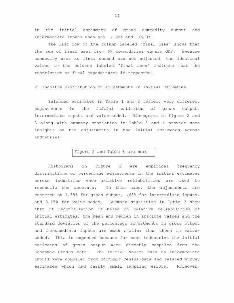
2) Industry Distribution of Adjustments in Initial Estimates.

Balanced estimates in Table 1 and 2 reflect very different

adjustments in the initial estimates of gross output,

intermediate inputs and value-added. Histograms in Figure 2 and

3 along with summary statistics in Table 3 and 4 provide some

insights on the adjustments in the initial estimates across

industries.

Figure 2 and Table 3 are here

Histograms in Figure 2 are empirical frequency

distributions of percentage adjustments in the initial estimates

across industries when relative reliabilities are used to

reconcile the accounts. In this case, the adjustments are

centered on 1.39% for gross output, .63% for intermediate inputs,

and 8.25% for value-added. Summary statistics in Table 3 show

that if reconciliation is based on relative reliabilities of

initial estimates, the mean and median in absolute values and the

standard deviation of the percentage adjustments in gross output

and intermediate inputs are much smaller than those in value-

added. This is expected because for most industries the initial

estimates of gross output were directly compiled from the

Economic Census data. The initial source data on intermediate

inputs were compiled from Economic Census data and related survey

estimates which had fairly small sampling errors. Moreover,

20

except for a few industries, adjustments made to correct non-

sampling errors in the source data were a small fraction of the

total initial estimates. Therefore, initial estimates of gross

output and intermediate inputs had fairly high reliabilities. On

the other hand, the initial estimates of value-added were a

combination of the SOI estimates and a variety of adjustments

made to the source data. Some SOI estimates had fairly large

sampling errors (large CVs), and for a large number of industries

adjustments made to source data to correct non-sampling errors

were a significant portion of the total estimates. As a result,

the initial estimates of value-added were less reliable and

varied more across industries.

Figure 3 and Table 4 are here

In contrast, Figure 3 and Table 4 show that if

reconciliation is based on neutral variants of the initial

estimates, percentage adjustments in different components are

more proportionate. This is clearly illustrated by the frequency

distributions of the percentage adjustments in intermediate

inputs and value-added shown in Figure 3. Adjustments in

intermediate inputs and value-added are centered on 7.2% and

7.35% respectively. Compared with the summary statistics in

Table 3, the mean percentage adjustments in absolute values are

larger for gross output and intermediate inputs and smaller for

value-added when neutral variants are used in reconciliation.

Also compared with Table 3, the standard deviations of percentage

adjustments of gross output and intermediate inputs in Table 4

are more than double, but value-added is less than 50%. As a

result, the differences in standard deviations of the percentage

adjustments in the three components are substantially smaller,

even though the reliabilities of the three components are very

different.

21

3) Industry Distribution of the Statistical Discrepancy.

The balanced estimates for the 65 industries show that the

aggregate statistical discrepancy is removed. The difference

between the balanced and initial estimates of value-added (or the

adjustment in the initial estimates of value-added) for each

industry measures the estimated statistical discrepancy

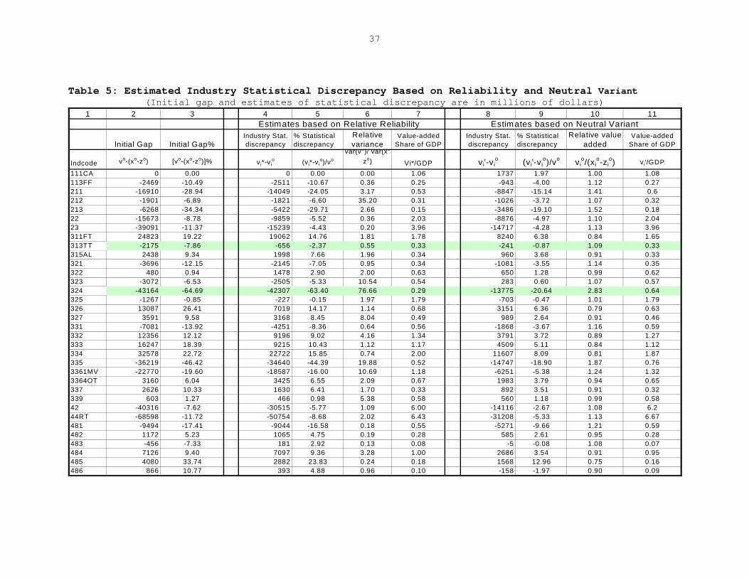
distributed to that industry. Table 5 shows how the aggregate

statistical discrepancy is distributed among the 65 industries,

based on the relative reliability or the neutral variant of the

initial estimates.

Table 5 is here

Column 2 in Table 5 shows the initial gap between value-

added estimates from input-output and GDP-by-industry accounts

for each industry, measured in millions of dollars, and column 3

shows the initial gaps in percentage terms. The middle panel

contains the distributional results based on the relative

reliability of initial estimates. Columns 4 and 5 tabulate the

estimated statistical discrepancy by industry measured in

millions of dollars and in percentages. Column 6 shows relative

variances of initial estimates of value-added by industry from

the GDP-by-industry account to that from the input-output account

measured as the residual between gross output and intermediate

inputs. Column 7 contains the shares of final estimates of

value-added to GDP by industry.

Distributional results based on neutral variants of the

initial estimates are tabulated in the right panel. Columns 8, 9

and 11 correspond to columns 4, 5, and 7 in the middle panel.

Column 10 shows value-added from the GDP-by-industry accounts

relative to that from the input-output accounts. In both cases,

the gaps in the initial estimates of value-added indicate the

total adjustments needed to remove the inconsistency.

22

However, the distribution of estimated statistical

discrepancy is determined differently in each case. Results

shown in the middle panel suggest that for an industry if the

initial estimate of value-added from the GDP-by-industry account

is much less reliable than value-added estimate from the input-

output accounts, then, the absolute statistical discrepancy

allocated to the GDP-by-industry account of that industry is

large. Consider, for example, the Petroleum and coal (NAICS 324)

and Textile industries (NAICS 313TT). For Petroleum and coal

industry, the initial gap in value-added is –43.164 billion

dollars or -64.69%, and the relative variance of value-added is

76.66. Consequently, the adjustment needed to remove the

inconsistency goes largely to value-added in the GDP-by-industry

account. For Textile industry, the initial gap is –2.175 billion

dollars or -7.86%, and relative variance of value-added is .55.

The adjustment needed to remove the inconsistency goes largely to

gross output and to intermediate inputs in the input-output

account.

However, the right panel shows that the relative values of

value-added and the industry shares of value-added to GDP jointly

determine the industry distribution of the statistical

discrepancy. Consider, for example, Real estate (NAICS 531) and

Rental and leasing (NAICS 532RL) industries. The industry’s

share of value-added to GDP is 11.07% for Real estate industry,

which is the largest share among all industries. The initial

value-added estimate from GDP-by-industry account is 94% of that

from the input-output account. Because the share of value-added

for industry 531 is substantially larger than for any other

industry, the statistical discrepancy allocated to that industry

is 36.44 billion dollars, the largest amount among all

industries. For Rental and leasing industry, the share of value-

added to total GDP is merely 1.2% and the initial estimate of

value-added from the GDP-by-industry account is 51% of that from

the input-output accounts. The statistical discrepancy allocated

23

to that industry is 25.93 million dollars or 36% of the initial

gap.

Figure 4 and Table 6 are here

Histograms in Figures 4a and 4b, along with summary

statistics in Table 6, provide some insight on how statistical

discrepancy is allocated across industries in the two cases.

Figure 4a shows that if reconciliation is based on relative

reliabilities of the initial estimates, the industry’s

statistical discrepancy centers on 3.94 billion dollars, whereas

Figure 4b shows that if reconciliation is based on neutral

variants of the initial estimates, the industry’s statistical

discrepancy centers on 2.62 billion dollars. Summary statistics

in Table 6 show that variation in the industry allocation of the

statistical discrepancy is much larger if relative reliabilities

are used to remove inconsistencies. This is expected because

reliability of the initial estimates varies greatly across

industries in the input-output and GDP-by-industry accounts. The

difference in the industry distribution of the statistical

discrepancy observed here reiterates the potential value of

incorporating information about the relative degrees of

uncertainty in the initial data in reconciling different sets of

accounts.

VI. Conclusion

In this study the GLS method has been used to successfully

remove inconsistencies between different 1997 accounts and to

reconcile the input-output and GDP-by-industry accounts with the

benchmark revised GDP. The contributions of this study are: 1)

it has shown that using relative reliabilities to remove

inconsistencies produces statistically meaningful balanced

estimates; 2) the reconciliation process has helped identify some

24

problems in the source data and in the estimation methods,

especially those used to estimate adjustments intended to correct

non-sampling errors in the source data; and 3) it has

demonstrated that using the GLS method to reconcile disaggregated

accounts is empirically feasible and computational efficient.

As for future research, we should continue to improve

reliability measures, especially reliability measures of the

adjustments made to correct non-sampling errors in the source

data. Expanded coverage of industries and data items in future

economic censuses by primary source data agencies, reducing

inconsistencies between initial data from different sources

through data sharing among federal statistical agencies, and

improving the methods used to estimate adjustments to source data

are a few ways to improve reliabilities of initial data.

This study should be considered the first step toward a

full integration between national and industry accounts. In the

current study, expenditure-based GDP is considered final and is

not adjusted. However, there is little evidence that there is no

uncertainty in the initial data used to estimate final

expenditures. A full reconciliation of national and industry

accounts could produce balanced estimates based on reliabilities

of all data items in national and industry accounts and could

estimate the statistical discrepancy by industry and by

expenditure categories. The theoretical framework is fully

developed and large memory computer capacity and software are

available to handle a full reconciliation of a large

disaggregated system of accounts. The challenge lies in the

effort to obtain estimates of the reliability of the final

expenditures.

References

Beaulieu, J.J. and E.J. Bartelsman (2004), “Integrating Expenditure and Income Data: What to do with the Statistical Discrepancy?” Unpublished paper, Board of Governor of the Federal Reserve System and Free University, Amsterdam.

25

Byron, R.P. (1978), “The Estimation of Large Social Account Matrices,” Journal of Royal Statistics, Series A, 141(3), 359-367. Dagum, E.B. and P. Cholette (2006), Benchmark, Temporal Distribution, and Reconciliation Methods for Time Series, Lecture Notes in Statistics, Vol. 186, Springer publisher, Berlin, Germany. Fixler, D. and B. Grimm (2005), “Reliability of the NIPA Estimates of U.S. Economic Activity,” Survey of Current Business, 85(2), 8-19. Lawson, A., B. Moyer, S. Okubo and M. Planting (2004), “Integrating Industry and National Economic Accounts: First Steps and Future Improvements,” presented at NBER-CIRW conference on Architecture for the National Accounts, Washington, DC. van der Ploeg, F. (1982a), “Reliability and the Adjustment of Sequences of Large Systems and Tables of National Accounting Matrices,” Journal of Royal Statistical Society, Series A, 145(2), 169-194. van der Ploeg, F. (1982b), “Generalized Least Squares Methods for Balancing Large Systems and Tables of National Accounts,” Review of Public Data Use. Stone, R., J.E. Meade and D.G. Champernowne (1942), “The Precision of National Income Estimates,” Review of Economic Studies, 9 (2), 111-125. Weale, M. (1992), “Estimation of Data Measured with Error and Subject to Linear Restrictions,” Journal of Applied Econometrics, Vol. 7(2), 167-174.

26

Appendix A

If the objective is to reconcile the GDP-by-expenditure,

the input-output and the GDP-by-industry accounts, the

reconciliation model described in Section III can be easily

modified. To generalize the problem, let I, K, F and D denote

the total number of industries, the total number of commodities,

the total number of value-added categories, and total number of

final expense categories.

The mathematical problem is then to minimize the

reliability-weighted sum of squares of adjustments of initial

estimates in all components of value-added, intermediate inputs,

and gross output data, and in all final expenditure categories,

over all industries and commodities, subject to accounting

constraints,

( A1)

Min S =i

20ifif

I

1i

F

1fik

20ik

K

1=k

I

1=iik

20ikik

K

1k

I

1i wv)v(v

wx

)x(x

wz)z(z ik −

++−

∑ ∑∑∑∑∑= =

−

==

+wm

)mm + we

)ee +

wy

)yy

k

20kk(K

1kk

20k(K

1kkd

20kdkd(D

1d

K

1=k

k −∑∑∑∑=

−

=

−

= ,

subject to

(A2) - = 0, ikK

1kx∑

=

F

1fifik

K

1=kvz ∑∑

=−

for i = 1, …, I,

(A3) - = 0, ki

I

1=ix∑ kkkd

D

1=dki

I

1=imeyz +−− ∑∑

27

for k = 1, …, K,

(A4) - = 0, ∑∑==

F

1fif

I

1iv )∑ ∑

= =+−

K

1k

D

1dkkkd mey(

and with initial conditions which satisfy

(A5) = Y∑∑==

F

1f

0if

I

1iv I0,

(A6) = Y)∑ ∑= =

−+K

1k

D

1d

0k

0k

0kd mey( E0.

Balanced estimates generate the final estimate of GDP.

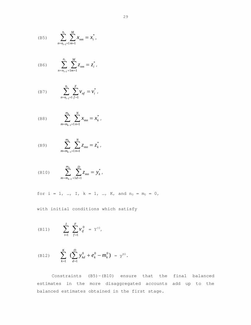
Appendix B

Account reconciliation can also be done in a hierarchical

manner. In the first stage of reconciliation, initial estimates

at a relatively aggregated level are reconciled. In the second

stage, the initial estimates at a more disaggregated level are

reconciled, and these reconciled estimates add up to the

previously reconciled aggregates.

Let , and , i = 1, …, I, denote the balanced

estimates of industry gross output, intermediate inputs, and

value-added from the first stage reconciliation. Let , and

, k = 1, …, K, be the corresponding balanced estimates of

commodity gross output, intermediate inputs, and final uses. Let

n = 1, …, N and m = 1, …, M denote the indexes for industries and

commodities at more disaggregated levels. Let n

*ix *

iz *iv

*kx *

kz

*ky

i be the number

of disaggregated industries in industry i where the total number

28

of disaggregated industries is = N. Let m∑=

I

iin

1k be the number of

disaggregated commodities in commodity group k where the total

number of disaggregated commodities is = M. Let f = 1, …,

F and d = 1, …, D be the index for value-add component and final

use categories. Then the second stage reconciliation model is

∑=

K

1kkm

(B1) Min S{x,z,v} =nm

20nm

M

1=m

N

1=nnm

20nmnm

M

1m

N

1n wz)z(z

wz

)x(xnm

−

==∑∑∑∑ +

−

+nf

nf

wvvv 20nf

F

1=f

N

1=n

)(

−∑∑ +

kd

kd

wyyy 20kd

D

1d

M

=1m

)

−∑∑=

(

+m

m

m wmm

we

20m

M

1m

20mm

M

1m

)m +

)e-(e

−∑∑==

(,

Subject to

(B2) - = 0, nmx∑=

M

1m

F

1f

M

1=m∑∑=

− nfnm vz

for n = 1, …, N,

(B3) - = 0, mnx∑N

=1nmm

F

=1dmn

N

=1n

z meymd +−−∑∑

for m = 1, …, M,

(B4) - = 0, ∑∑==

F

1f

N

1nnfv )∑ ∑

= =

+−M

1m

D

1dmm( meymd

29

(B5) , *

111

i

M

mnm

n

nnxx

i

i

=∑∑=+= −

(B6) , *

111

i

M

mnm

n

nnzz

i

i

=∑∑=+= −

(B7) , *

111

i

F

fnf

n

nnvv

i

i

=∑∑=+= −

(B8) , *

111

k

N

nmn

m

mmxx

k

k

=∑∑=+= −

(B9) , *

111

k

N

nmn

m

mmzz

k

k

=∑∑=+= −

(B10) , *

111

k

D

dmn

m

mmyz

k

k

=∑∑=+= −

for i = 1, …, I, k = 1, …, K, and n0 = m0 = 0,

with initial conditions which satisfy

(B11) = Y∑∑==

F

fif

I

iv

1

0

1

I0,

(B12) = y)( 00

1

0

1kk

D

dkd

K

kmey −+∑∑

==

E0.

Constraints (B5)–(B10) ensure that the final balanced

estimates in the more disaggregated accounts add up to the

balanced estimates obtained in the first stage.

30

Figure 1: Percentage Adjustments in Gross Output, Intermediate Inputs and Components of Value-added in Correction of Non-Sampling Errors in the 1997 Source Data

% Total Adjustment in Initial Gross Output

-40

-20

0

20

40

60

80

111C

A21

2 2331

5AL

323

326

332

335

337

44RT48

348

651

151

452

453

2RL

5415 56

262

2HO

713 81

GSLE

Industry

%A

dj(x

)

% Adjustment from Company to Establishment Datain GDP-by-Industry Account

-200

-150

-100

-50

0

50

100

150

200

250

300

350

111C

A21

2 2331

5AL

323

326

332

335

337

44RT48

348

651

151

452

453

2RL

5412

OP56

262

2HO

713 81

Industry

% C

o-Es

t Adj

ustm

ent

% Adjustment in Initial Intermediate Inputs

-60-40-20

020406080

100

111C

A21

2 2331

5AL

323

326

332

335

337

44RT48

348

651

151

452

453

2RL

5415 56

262

2HO

713 81

GSLE

Industry

%A

dj(z

)

% Category 3 Adjustments in Gross Operating SurplusIn GDP-by-industry Account

-100-50

050

100150200250300350400

111C

A 21

2 2331

5AL

323

326

332

335

337

44RT 48

348

651

151

452

453

2RL

5415 56

262

2HO

713 81

GSLE

Industry

%A

dj3(

GO

S)

31

Table 1: Initial and Balanced Estimates for 65 Industries (in millions of dollars)

1 2 3 4 5 6 7 8 9 10 11 12 13 Initial Estimates Balanced Estimates ( Relative Reliability) Balanced Estimates (Neutral Variant)

Gross Output

Intermediate Inputs

Value-added Intial Gap

Gross Output

Intermediate Inputs

Value-added

Industry Constraint

Gross Output

Intermediate Inputs

Value-added

Industry Constraint

Pubcode xi0 zi

0 vi0 (xi

0-(zi0+vi

0))% xi* zi* vi* xi*-zi*-vi* xi' zi' vi' xi'-zi'-vi'111CA 241952 153810 88142 0.00 241952 153810 88142 0 244496 154618 89878 0113FF 48627 27550 23546 -5.08 48302 27268 21035 0 49419 26816 22603 0211 91610 50096 58424 -18.46 94177 49802 44375 0 91695 42118 49577 0212 51919 26212 27608 -3.66 51920 26133 25787 0 52065 25483 26582 0213 25200 13217 18250 -24.87 25214 12386 12828 0 25447 10682 14765 022 289375 126557 178491 -5.42 292619 123986 168633 0 296658 127042 169616 023 679314 374546 343859 -5.75 683369 354748 328620 0 687476 358334 329142 0311FT 519348 365401 129125 4.78 519182 370996 148186 0 515517 378152 137364 0313TT 89388 63893 27670 -2.43 89410 62395 27014 0 90385 62957 27429 0315AL 77228 48697 26093 3.16 77295 49203 28092 0 76860 49806 27054 0321 88476 61742 30430 -4.18 88593 60307 28285 0 89579 60230 29350 0322 149062 97640 50943 0.32 149169 96748 52421 0 149786 98193 51593 0323 97586 53623 47035 -3.15 97963 53433 44530 0 100310 52992 47317 0324 174942 151379 66727 -24.67 175144 150724 24420 0 189264 136312 52953 0325 408567 260843 148991 -0.31 408670 259906 148764 0 407348 259060 148288 0326 157721 95088 49546 8.30 157205 100640 56565 0 153285 100588 52697 0327 85827 44737 37498 4.18 85632 44966 40666 0 84229 45742 38487 0331 168318 124548 50851 -4.21 168348 121747 46601 0 170290 121307 48983 0332 239045 124731 101959 5.17 238258 127104 111154 0 235036 129287 105749 0333 260246 155665 88334 6.24 257697 160148 97549 0 255916 163073 92843 0334 433139 257160 143401 7.52 432611 266488 166123 0 423578 268570 155008 0335 109172 67362 78029 -33.18 109352 65963 43389 0 118336 55055 63281 03361MV 417807 324381 116195 -5.45 417783 320175 97608 0 420387 310443 109944 03364OT 150342 94898 52284 2.10 151049 95340 55709 0 150616 96350 54267 0337 63529 35470 25433 4.13 63391 36328 27063 0 62828 36503 26325 0339 102268 54242 47424 0.59 102202 54312 47890 0 102286 54303 47983 042 754944 266354 528905 -5.34 762009 263619 498390 0 768585 253795 514790 044RT 830070 313587 585081 -8.26 835741 301413 534328 0 844738 290864 553874 0481 120232 75185 54541 -7.90 110042 64545 45497 0 117143 67873 49270 0482 42357 18746 22438 2.77 41765 18262 23503 0 41721 18698 23023 0483 24598 18839 6215 -1.85 24619 18223 6396 0 24951 18741 6210 0484 169107 86150 75832 4.21 169072 86143 82928 0 167624 89106 78518 0485 24717 8542 12094 16.51 24017 9040 14977 0 23326 9664 13662 0486 27527 18617 8044 3.15 27527 19089 8437 0 26723 18837 7886 0

32

Table 1: Initial and Balanced Estimates for 65 Industries (Continue) (in millions of dollars)

te: A table that contains NAICS code and tries is at the end of the papers

Initial Estimates Balanced Estimates ( Relative Reliability) Balanced Estimates (Neutral Variant)Gross Output

Intermediate Inputs

Value-added Intial Gap

Gross Output

Intermediate Inputs

Value-added

Industry Constraint

Gross Output

Intermediate Inputs

Value-added

Industry Constraint

Pubcode xi0 zi

0 vi0 (xi

0-(zi0+vi

0))% xi* zi* vi* xi*-zi*-vi* xi' zi' vi' xi'-zi'-vi'487OS 84777 34680 59189 -10.72 84777 34330 50448 0 88934 32605 56329 0493 27211 8317 19902 -3.71 27501 8303 19199 0 27530 8036 19494 0511 183378 71328 65295 25.50 176819 77240 99578 0 165737 84881 80856 0512 61496 35872 22783 4.62 61650 35828 25822 0 60835 36627 24208 0513 377161 178927 209913 -3.10 378116 178528 199588 0 381986 174054 207932 0514 47220 16953 18587 24.74 47219 19564 27655 0 42507 19636 22870 0521CI 418041 146014 249138 5.48 420582 151684 268898 0 416623 152049 264574 0523 199457 88051 130180 -9.41 199499 80634 118866 0 204458 82319 122139 0524 350988 168429 215462 -9.37 351079 158167 192912 0 358608 160764 197844 0525 53059 42899 9822 0.64 53179 43361 9819 0 53140 43450 9690 0531 1260014 318624 883180 4.62 1256714 338400 918314 0 1248366 328743 919623 0532RL 176438 31943 73375 40.31 164017 32017 132000 0 141976 42670 99306 05411 152096 41414 118401 -5.08 152459 41332 111126 0 154159 39159 115000 05412OP 489099 148023 306413 7.09 487683 148005 339678 0 478806 153175 325630 05415 101417 31646 86899 -16.89 102621 31203 71418 0 107868 27936 79932 055 241960 94294 145738 0.80 241786 93113 148673 0 240088 92621 147467 0561 305939 78047 197254 10.02 304907 78431 226476 0 295485 82814 212671 0562 41959 19204 20194 6.10 41956 19533 22423 0 41153 20042 21111 061 111493 48250 61209 1.83 111222 48285 62937 0 110705 48061 62644 0621 381139 116383 260386 1.15 381154 116277 264877 0 380766 115859 264907 0622HO 368320 164002 199284 1.37 368314 163737 204577 0 367392 164170 203222 0624 66930 28502 42972 -6.79 66944 28468 38476 0 67223 26373 40850 0711AS 55432 25987 34440 -9.01 55494 25851 29643 0 56837 24289 32548 0713 68571 23735 37443 10.78 68408 23811 44597 0 66356 25367 40989 0721 109988 34159 70517 4.83 109980 34143 75837 0 108985 34932 74053 0722 299834 150156 132759 5.64 297860 150816 147044 0 295287 154337 140951 081 347541 142648 184592 5.84 345855 142591 203264 0 338940 146481 192459 0GFE 74622 16864 58335 -0.77 74924 16798 58126 0 75134 16908 58225 0GFG 466570 176186 290870 -0.10 466570 175700 290870 0 466470 174086 292384 0GSLE 131232 71583 58053 1.22 131329 71809 59520 0 130992 72528 58464 0GSLG 950643 304840 645781 0.00 950643 304862 645781 0 953069 303411 649658 0

Sum 15217582 6917468 8257803 15202554.3 6898210 8304344 0 15184319 6879975 8304344 0

No description of the indus

33

Table 2: Initial and Balanced Estimates for 69 Commodities (In millions of dollars)

1 2 3 4 5 6 7 8 9 10 11 12 13 Initial Estimates Balanced Estimates (Relative Reliability) Balanced Estimates (Neutral Variant)

Gross Output

Intermediate Inputs Uses Final Uses Initial Gap

Gross Output

Intermediate Inputs Uses Final Uses

Comm Constraint

Gross Output

Intermediate Inputs Uses Final Uses

Comm Constraint

Com Code xk0 zk

0 yk0 (xk-zk-yk)% xk* zk* yk

0 xk*-zk*-yk0 xk' zk

0 yk' xk'-zk'-yk0

111CA 235666 193581 42084 0.20 235685 193601 42084 0 238388 196304 42084 0113FF 55668 55573 95 0.71 55750 55655 95 0 56131 56036 95 0211 84179 147515 -63336 0.33 86149 149485 -63336 0 83972 147308 -63336 0212 50908 46183 4726 0.32 50908 46182 4726 0 50993 46267 4726 0213 25220 2681 22539 -0.06 25235 2696 22539 0 25398 2858 22539 022 335214 182958 152256 0.01 338234 185978 152256 0 340426 188170 152256 023 763229 95129 668100 -0.01 765704 97605 668100 0 767622 99523 668100 0311FT 524786 206343 318443 -0.08 524237 205794 318443 0 522698 204255 318443 0313TT 86513 66187 20326 -0.38 86531 66205 20326 0 87455 67129 20326 0315AL 76142 17602 58541 -0.15 76203 17662 58541 0 75964 17424 58541 0321 88337 84760 3577 -0.08 88349 84772 3577 0 89332 85755 3577 0322 146453 132462 13991 0.07 146566 132575 13991 0 147165 133174 13991 0323 71052 67562 3490 0.07 71373 67883 3490 0 72470 68981 3490 0324 173626 117449 56177 -0.37 173745 117568 56177 0 185043 128865 56177 0325 414505 311243 103262 0.68 414089 310827 103262 0 415757 312495 103262 0326 155614 141008 14606 -0.26 155437 140832 14606 0 151616 137010 14606 0327 84489 84183 306 -0.09 84414 84108 306 0 83049 82743 306 0331 169789 189514 -19725 0.32 169785 189510 -19725 0 171619 191343 -19725 0332 232993 215503 17490 -0.38 232311 214821 17490 0 229577 212087 17490 0333 257474 88839 168635 0.06 256437 87802 168635 0 254101 85467 168635 0334 420874 242384 178490 0.40 420001 241511 178490 0 413539 235049 178490 0335 107526 75460 32066 -0.13 107695 75629 32066 0 115069 83003 32066 03361MV 411995 178164 233831 0.14 412154 178323 233831 0 414016 180185 233831 03364OT 148435 63250 85185 -1.53 149094 63909 85185 0 148853 63668 85185 0337 62588 13706 48882 0.44 62549 13667 48882 0 61954 13071 48882 0339 98545 39938 58607 0.08 98481 39874 58607 0 98567 39960 58607 042 736429 356396 380034 -0.03 744859 364826 380034 0 743952 363919 380034 044RT 750417 82944 667473 0.07 754616 87144 667473 0 753242 85770 667473 0481 124418 64416 60002 8.65 114560 54558 60002 0 120992 60990 60002 0482 38949 27836 11113 -0.49 38442 27330 11113 0 38566 27453 11113 0483 24634 6599 18034 -2.30 24655 6621 18034 0 25005 6970 18034 0484 171443 116817 54626 -0.61 170407 115781 54626 0 170495 115868 54626 0485 32076 15341 16734 0.20 31935 15201 16734 0 31231 14497 16734 0486 27284 26281 1003 0.22 27284 26281 1003 0 26488 25485 1003 0

34

Table 2: Initial and Balanced Estimates for 69 Commodities (Continue) (In millions of dollars)

Balanced Estimates (Relative Re Initial Estimates liability) Balanced Estimates (Neutral Variant)Gross Output

Intermediate Inputs Uses Final Uses Initial Gap

Gross Output

Intermediate Inputs Uses Final Uses

Comm Constraint

Gross Output

Intermediate Inputs Uses Final Uses

Comm Constraint

Code xk0 zk

0 yk0 (xk-zk-yk)% xk* zk* yk

0 xk*-zk*-yk0 xk' zk

0 yko xk'-zk'-yk

0

OS 83861 67676 16186 -6.65 83875 67689 16186 0 88136 71950 16186 029295 28388 906 0.03 29270 28363 906 0 29505 28599 906 0

11 122672 32465 90207 0.33 118673 28465 90207 0 118508 28301 90207 012 64848 40441 24407 -0.57 65006 40599 24407 0 64439 40032 24407 013 319608 172178 147431 -0.33 320588 173157 147431 0 321639 174208 147431 014 53954 47923 6032 -0.35 53954 47922 6032 0 50064 44032 6032 021CI 354596 204255 150341 0.17 352845 202504 150341 0 349556 199215 150341 023 203385 135307 68077 -0.06 203367 135290 68077 0 207210 139133 68077 024 351128 185752 165376 -0.98 351216 185840 165376 0 358249 192872 165376 025 59378 2608 56771 -0.26 59496 2725 56771 0 59346 2575 56771 031 1227089 384429 842660 0.00 1225686 383026 842660 0 1219163 376503 842660 032RL 246249 154850 91399 -0.02 239468 148069 91399 0 221342 129943 91399 0411 152745 96634 56111 -0.05 154038 97927 56111 0 154855 98744 56111 0412OP 607192 542196 64996 -0.86 603575 538579 64996 0 591865 526869 64996 0415 141476 43519 97957 -0.52 142253 44295 97957 0 143504 45547 97957 0

237689 215272 22417 0.00 237551 215134 22417 0 235686 213269 22417 061 309843 286064 23778 -0.07 307641 283863 23778 0 300323 276544 23778 062 46927 38189 8738 0.00 46925 38187 8738 0 46478 37740 8738 0

142495 21866 120629 0.15 142229 21599 120629 0 141957 21328 120629 021 396741 7106 389634 0.00 396755 7121 389634 0 396752 7117 389634 022HO 435235 4121 431114 0.00 435229 4116 431114 0 435182 4068 431114 024 67868 3253 64615 -0.02 67883 3268 64615 0 68050 3435 64615 011AS 52629 30072 22557 -0.58 52702 30145 22557 0 53712 31155 22557 013 84857 5411 79447 0.07 84796 5349 79447 0 84479 5032 79447 021 82707 31275 51433 0.10 82661 31229 51433 0 81915 30483 51433 022 356604 65285 291318 0.07 353329 62011 291318 0 353661 62343 291318 0

448282 154314 293968 -0.07 445169 151201 293968 0 446536 152568 293968 0FE 60927 52267 8660 -0.57 61229 52569 8660 0 61621 52961 8660 0FG 459378 0 459378 0.00 459378 0 459378 0 459378 0 459378 0SLE 43059 10464 32595 0.01 43055 10460 32595 0 43163 10568 32595 0SLG 760065 0 760065 0.00 760065 0 760065 0 760065 0 760065 0002 7622 82833 -75211 -2.12 0 75211 -75211 0 0 75211 -75211 0003 0 11036 -11036 0.00 7622 18658 -11036 0 7513 18549 -11036 0004 19711 -14 19725 -0.07 19725 0 19725 0 19725 0 19725 0

0otal 15217582 6913238 15221812 15201130 6896787 8304344 15184319 6879975 8304344 0

Com4874935555555555555555561666777781GGGGSSS

T

Note: yk represents final expenditures, exports, and imports.

35

Figure2: Histograms of % Adjustments Table 3: Statistics of % Adjustment(Reliability Weights) (Reliability Weights)

% Adjustments in Gross OutputMean -0.26

Max 2.80

Min -8.48

Median 0.00

St Dev 1.57

% Adjustments in Intermediate InputsMean -0.10

Max 15.40

Min -14.15

Median -0.12

St Dev 3.78

% Adjustments in Value Added EstimatesMean 1.46

Max 79.90

Min -63.40

Median 1.73

St Dev 19.41

% Deviation of Balance Gross Output from Initial Estimates

0

10

20

30

40

50

-8.48 -7.07 -5.66 -4.25 -2.84 -1.43 -0.02 1.39 MoreBin

Freq

uenc

y

% Deviation of Balanced Intermediate Inputs from Initial Estimates

0

10

20

30

40

50

-14.15 -10.46 -6.76 -3.07 0.63 4.32 8.01 11.71 MoreBin

Freq

uenc

y

% Deviation of Balanced VA from Initial Estimates

05

10152025303540

-63.40 -45.49 -27.58 -9.67 8.25 26.16 44.07 61.99 MoreBin

Freq

uenc

y

36

Figure 3: Histograms of % Adjustments Table 4: Statistics of % Adjustment(Neutral Variants) (Neutral Variants)

% Adjustments in Gross OutputMean -0.38

Max 8.39

Min -19.53

Median -0.02

St Dev 3.83

% Adjustments in Intermediate InputsMean -0.11

Max 33.58

Min -19.18

Median 0.10

St Dev 7.81

% Adjustments in Value Added EstimatesMean 0.76

Max 35.34

Min -20.64

Median 0.71

St Dev 8.88

% Difference between Balanced and Initial EstimatesIntermediate inputs

05

1015202530

-19.18 -12.58 -5.99 0.61 7.20 13.80 20.39 26.98 MoreBin

Freq

uenc

y

% Difference between Balanced and Initial Estimates Gross output

0

10

20

30

40

50

-19.53 -16.04 -12.55 -9.06 -5.57 -2.08 1.41 4.90 MoreBin

Freq

uenc

y

% Difference betweem Balance and Initial EstimatesValue-added

05

101520253035

-20.64 -13.65 -6.65 0.35 7.35 14.35 21.35 28.34 MoreBin

Freq

uenc

y

37

Table 5: Estimated Industry Statistical Discrepancy Based on Reliability and Neutral Variant (Initial gap and estimates of statistical discrepancy are in millions of dollars)

1 2 3 4 5 6 7 8 9 10 11 Estimates based on Relative Reliability Estimates based on Neutral Variant

Initial Gap Initial Gap%Industry Stat. discrepancy

% Statistical discrepancy

Relative variance

Value-added Share of GDP

Industry Stat. discrepancy

% Statistical discrepancy

Relative value-added

Value-added Share of GDP

Indcode vo-(xo-zo) [vo-(xo-zo)]% vi*-vio (vi*-vi

o)/vovar(vo)/ var(xo-

zo) Vi*/GDP vi'-vio (vi'-vi

o)/vo vio/(xi

o-zio) vi'/GDP

111CA 0 0.00 0 0.00 0.00 1.06 1737 1.97 1.00 1.08113FF -2469 -10.49 -2511 -10.67 0.36 0.25 -943 -4.00 1.12 0.27211 -16910 -28.94 -14049 -24.05 3.17 0.53 -8847 -15.14 1.41 0.6212 -1901 -6.89 -1821 -6.60 35.20 0.31 -1026 -3.72 1.07 0.32213 -6268 -34.34 -5422 -29.71 2.66 0.15 -3486 -19.10 1.52 0.1822 -15673 -8.78 -9859 -5.52 0.36 2.03 -8876 -4.97 1.10 2.0423 -39091 -11.37 -15239 -4.43 0.20 3.96 -14717 -4.28 1.13 3.96311FT 24823 19.22 19062 14.76 1.81 1.78 8240 6.38 0.84 1.65313TT -2175 -7.86 -656 -2.37 0.55 0.33 -241 -0.87 1.09 0.33315AL 2438 9.34 1998 7.66 1.96 0.34 960 3.68 0.91 0.33321 -3696 -12.15 -2145 -7.05 0.95 0.34 -1081 -3.55 1.14 0.35322 480 0.94 1478 2.90 2.00 0.63 650 1.28 0.99 0.62323 -3072 -6.53 -2505 -5.33 10.54 0.54 283 0.60 1.07 0.57324 -43164 -64.69 -42307 -63.40 76.66 0.29 -13775 -20.64 2.83 0.64325 -1267 -0.85 -227 -0.15 1.97 1.79 -703 -0.47 1.01 1.79326 13087 26.41 7019 14.17 1.14 0.68 3151 6.36 0.79 0.63327 3591 9.58 3168 8.45 8.04 0.49 989 2.64 0.91 0.46331 -7081 -13.92 -4251 -8.36 0.64 0.56 -1868 -3.67 1.16 0.59332 12356 12.12 9196 9.02 4.16 1.34 3791 3.72 0.89 1.27333 16247 18.39 9215 10.43 1.12 1.17 4509 5.11 0.84 1.12334 32578 22.72 22722 15.85 0.74 2.00 11607 8.09 0.81 1.87335 -36219 -46.42 -34640 -44.39 19.88 0.52 -14747 -18.90 1.87 0.763361MV -22770 -19.60 -18587 -16.00 10.69 1.18 -6251 -5.38 1.24 1.323364OT 3160 6.04 3425 6.55 2.09 0.67 1983 3.79 0.94 0.65337 2626 10.33 1630 6.41 1.70 0.33 892 3.51 0.91 0.32339 603 1.27 466 0.98 5.38 0.58 560 1.18 0.99 0.5842 -40316 -7.62 -30515 -5.77 1.09 6.00 -14116 -2.67 1.08 6.244RT -68598 -11.72 -50754 -8.68 2.02 6.43 -31208 -5.33 1.13 6.67481 -9494 -17.41 -9044 -16.58 0.18 0.55 -5271 -9.66 1.21 0.59482 1172 5.23 1065 4.75 0.19 0.28 585 2.61 0.95 0.28483 -456 -7.33 181 2.92 0.13 0.08 -5 -0.08 1.08 0.07484 7126 9.40 7097 9.36 3.28 1.00 2686 3.54 0.91 0.95485 4080 33.74 2882 23.83 0.24 0.18 1568 12.96 0.75 0.16486 866 10.77 393 4.88 0.96 0.10 -158 -1.97 0.90 0.09

38

Table 5: Estimated Industry Statistical Discrepancy Based on Reliability and Neutral Varia(Continue)

nt

Initial Gap Initial Gap%Indust tat Relative ue Indust tat Relative vary Stat. discrepancy

% S istical discrepancy variance

Val -added Share of GDP

ry Stat. discrepancy

% S istical discrepancy

lue-added

Value-added Share of GDP

Indcode vo-(xo-zo) [vo-(xo-zo)]% vi*-vio (vi*-vi

o)/vovar(vo)/ var(xo-

zo) Vi*/GDP vi'-vio (vi'-vi

o)/vo vio/(xi

o-zio) vi'/GDP

487OS -9092 -15.36 -8742 -14.77 37.60 0.61 -2860 -4.83 1.18 0.68493 -1008 -5.07 -703 -3.53 1.65 0.23 -408 -2.05 1.05 0.23511 46755 71.61 34283 52.51 0.84 1.20 15561 23.83 0.58 0.97512 2841 12.47 3039 13.34 4.57 0.31 1424 6.25 0.89 0.29513 -11679 -5.56 -10325 -4.92 457.31 2.40 -1982 -0.94 1.06 2.5514 11681 62.85 9069 48.79 3.30 0.33 4284 23.05 0.61 0.28521CI 22889 9.19 19760 7.93 1.31 3.24 15436 6.20 0.92 3.19523 -18774 -14.42 -11315 -8.69 1.34 1.43 -8041 -6.18 1.17 1.47524 -32903 -15.27 -22550 -10.47 0.35 2.32 -17617 -8.18 1.18 2.38525 338 3.44 -3 -0.03 0.00 0.12 -132 -1.34 0.97 0.12531 58210 6.59 35134 3.98 3.35 11.06 36443 4.13 0.94 11.07532RL 71120 96.93 58626 79.90 0.03 1.59 25932 35.34 0.51 1.25411 -7719 -6.52 -7275 -6.14 32.75 1.34 -3401 -2.87 1.07 1.385412OP 34663 11.31 33265 10.86 34.18 4.09 19217 6.27 0.90 3.925415 -17128 -19.71 -15482 -17.82 2.25 0.86 -6967 -8.02 1.25 0.9655 1928 1.32 2935 2.01 5.14 1.79 1729 1.19 0.99 1.78561 30638 15.53 29223 14.82 14.18 2.73 15418 7.82 0.87 2.56562 2561 12.68 2229 11.04 0.69 0.27 918 4.55 0.89 0.2561 2034 3.32 1728 2.82 0.33 0.76 1435 2.35 0.97 0.75621 4370 1.68 4491 1.73 339.05 3.19 4521 1.74 0.98 3.19622HO 5034 2.53 5293 2.66 90.25 2.46 3938 1.98 0.98 2.45624 -4545 -10.58 -4496 -10.46 7.59 0.46 -2122 -4.94 1.12 0.49711AS -4995 -14.50 -4798 -13.93 725.66 0.36 -1892 -5.49 1.17 0.39713 7393 19.74 7154 19.11 5.46 0.54 3546 9.47 0.84 0.49721 5312 7.53 5320 7.54 22.35 0.91 3537 5.02 0.93 0.89722 16919 12.74 14284 10.76 0.69 1.77 8191 6.17 0.89 1.781 20301 11.00 18672 10.12 13.58 2.45 7867 4.26 0.90 2.32GFE -577 -0.99 -209 -0.36 2.74 0.70 -110 -0.19 1.01 0.7GFG -486 0.00 0 0.00 0.00 3.50 1514 0.52 1.00 3.52GSLE 1596 2.75 1467 2.53 2.37 0.72 411 0.71 0.97 0.7GSLG 22 0.00 0 0.00 0.00 7.78 3877 0.60 1.00 7.82

Sum 46541 46541

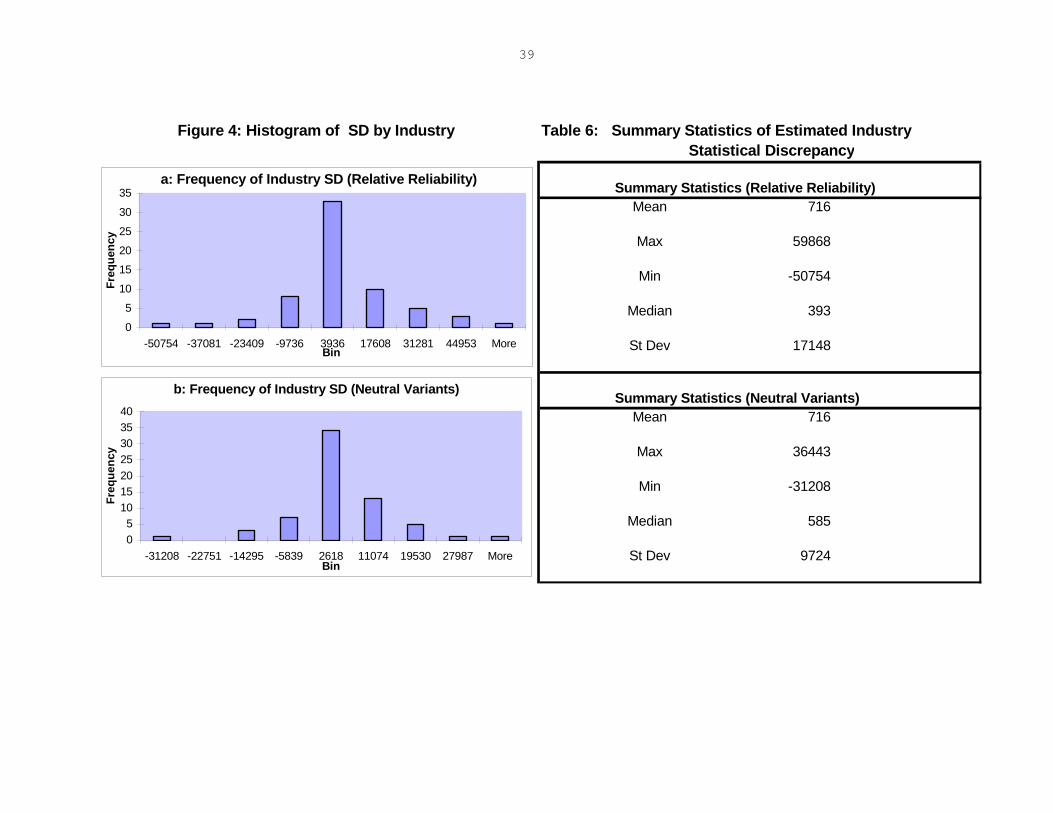
39

Figure 4: Histogram of SD by Industry Table 6: Summary Statistics of Estimated IndustryStatistical Discrepancy

Summary Statistics (Relative Reliability)Mean 716

Max 59868

Min -50754

Median 393

St Dev 17148

Summary Statistics (Neutral Variants)Mean 716

Max 36443

Min -31208

Median 585

St Dev 9724

a: Frequency of Industry SD (Relative Reliability)

0

5

10

15

20

25

30

35

-50754 -37081 -23409 -9736 3936 17608 31281 44953 MoreBin

Freq

uenc

y

b: Frequency of Industry SD (Neutral Variants)

05

10152025303540

-31208 -22751 -14295 -5839 2618 11074 19530 27987 MoreBin

Freq

uenc

y

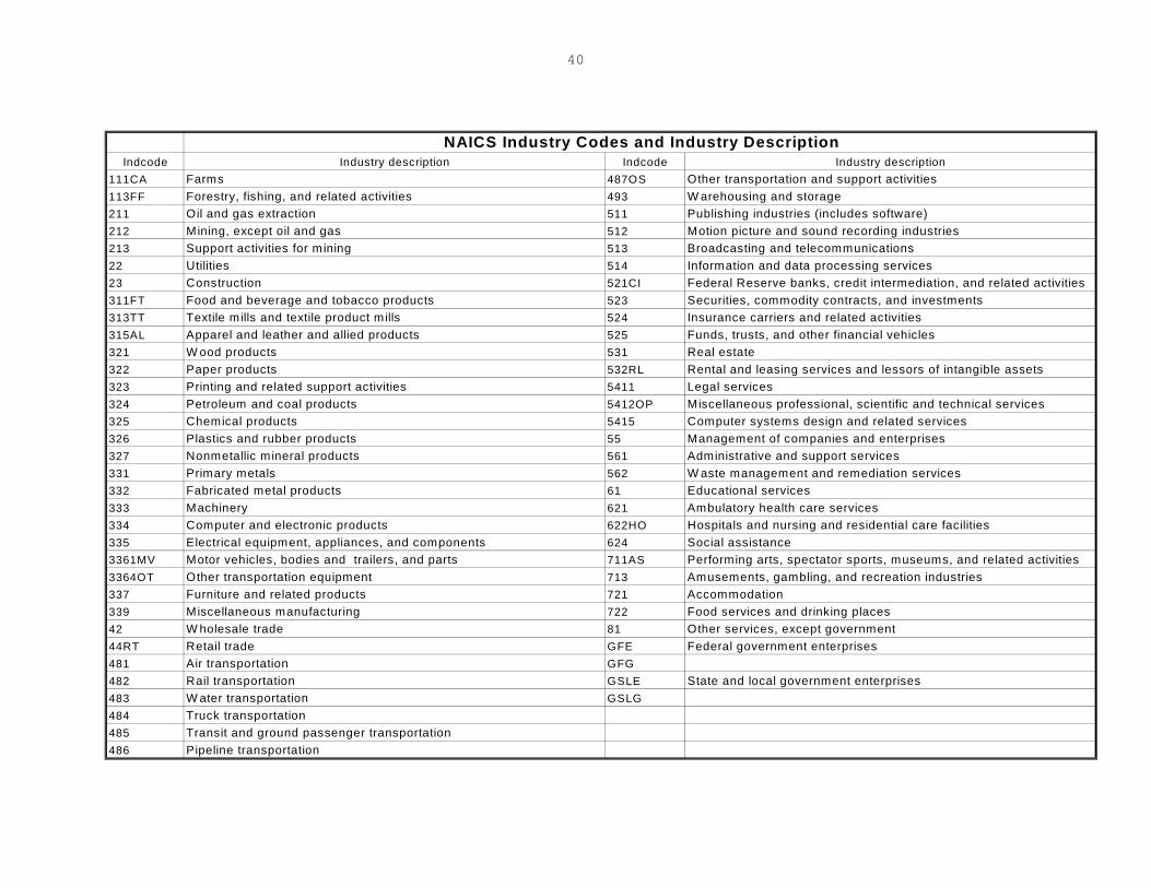
40

NAICS Industry Codes and Industry DescriptionIndcode Industry description Indcode Industry description

111CA Farms 487OS Other transportation and support activities113FF Forestry, fishing, and related activities 493 W arehousing and storage211 Oil and gas extraction 511 Publishing industries (includes software)212 Mining, except oil and gas 512 Motion picture and sound recording industries213 Support activities for mining 513 Broadcasting and telecommunications22 Utilities 514 Information and data processing services23 Construction 521CI Federal Reserve banks, credit intermediation, and related activities311FT Food and beverage and tobacco products 523 Securities, commodity contracts, and investments313TT Textile mills and textile product mills 524 Insurance carriers and related activities315AL Apparel and leather and allied products 525 Funds, trusts, and other financial vehicles321 W ood products 531 Real estate322 Paper products 532RL Rental and leasing services and lessors of intangible assets323 Printing and related support activities 5411 Legal services324 Petroleum and coal products 5412OP Miscellaneous professional, scientific and technical services325 Chemical products 5415 Computer systems design and related services326 Plastics and rubber products 55 Management of companies and enterprises327 Nonmetallic mineral products 561 Administrative and support services331 Primary metals 562 W aste management and remediation services332 Fabricated metal products 61 Educational services333 Machinery 621 Ambulatory health care services334 Computer and electronic products 622HO Hospitals and nursing and residential care facilities335 Electrical equipment, appliances, and components 624 Social assistance3361MV Motor vehicles, bodies and trailers, and parts 711AS Performing arts, spectator sports, museums, and related activities3364OT Other transportation equipment 713 Amusements, gambling, and recreation industries337 Furniture and related products 721 Accommodation339 Miscellaneous manufacturing 722 Food services and drinking places42 W holesale trade 81 Other services, except government44RT Retail trade GFE Federal government enterprises

81 Air transportation GFG 82 Rail transportation GSLE State and local government enterprises

483 W ater transportation GSLG 484 Truck transportation485 Transit and ground passenger transportation486 Pipeline transportation

44