8722 - World Bank Documents and Reports

8722WORLD BANK

COMPARATIVE STUDIES I

The Political Economy of Agricultural Pricing Policy

Trade, Exchange Rate,and Agricultural Pricing Policiesin Argentina

Adolfo Sturzeneggerwith the collaboration ofWylian Otreraand the assistance ofBeatriz Mosquera

FtLECEP

Pub

lic D

iscl

osur

e A

utho

rized

Pub

lic D

iscl

osur

e A

utho

rized

Pub

lic D

iscl

osur

e A

utho

rized

Pub

lic D

iscl

osur

e A

utho

rized

The Political Economy of Agricultural Pricing Policy

Trade, Exchange Rate,and Agricultural Pricing Policies

in Argentina

Adolfo Sturzeneggerwith the collaboration of

Wylian Otreraand the assistance of

Beatriz Mosquera

WORLD BANKCOMPARATIVE STUDIES

The World BankWashington, D.C.

Copyright © 1990The International Bank for Reconstructionand Development/THE WORLD BANK

1818 H Street, N.W.Washington, D.C. 20433

All rights reservedManufactured in the United States of AmericaFirst printing May 1990

World Bank Comparative Studies are undertaken to increase the Bank's capacity to offer soundand relevant policy recommendations to its member countries. Each series of studies, of which ThePolitical Economy of Agricultural Pricing Policy is one, comprises several empirical, multicountryreviews of key economic policies and their effects on the development of the countries in which theywere implemented. A synthesis report on each series will compare the findings of the studies ofindividual countries to identify common patterns in the relation between policy and outcome-thusto increase understanding of development and economic policy

The series The Political Economy of Agricultural Pricing Policy, under the direction of Anne0. Krueger, Maurice Schiff, and Alberto Valdes, was undertaken to examine the reasons underlyingpricing policy, to quantify the systematic and extensive intervention of developing countries in thepricing of agricultural commodities during 1960-85, and to understand the effects of suchintervention over time. Each of the eighteen country studies uses a common methodology tomeasure the effect of sectoral and economywide price intervention on agricultural incentives andfood prices, as well as their effects on output, consumption, trade, intersectoral transfers,government budgets, and income distribution. The political and economic forces behind priceintervention are analyzed, as are the efforts at reform of pricing policy and their consequences.

The findings, interpretations, and conclusions in this series are entirely those of the authors andshould not be attributed in any manner to the World Bank, to its affiliated organizations, or tomembers of its Board of Executive Directors or the countries they represent.

The material in this publication is copyrighted. Requests for permission to reproduce portions of itshould be sent to Director, Publications Department, at the address shown in the copyright noticeabove. The World Bank encourages dissemination of its work and will normally give permissionpromptly and, when the reproduction is for noncommercial purposes, without asking a fee.Permission to photocopy portions for classroom use is not required, though notification of such usehaving been made will be appreciated.

The complete backlist of World Bank publications is shown in the annual Index of Publications,which contains an alphabetical title list and indexes of subjects, authors, and countries and regions;it is of value principally to libraries and institutional purchasers. The latest edition is available freeof charge from Publications Sales Unit, Department F, The World Bank, 1818 H Street, N.W.,Washington, D.C. 20433, U.S.A., or from Publications, The World Bank, 66, avenue d'I6na, 75116Paris, France.

Adolfo Sturzenegger is an economist with the consulting firm Econometrica in Buenos Aires; WylianR. Otrera is an economist with the Fundaci6n Mediterranea, also in Buenos Aires; both areconsultants to the World Bank.

Library of Congress Cataloging-in-Publication Data

Sturzenegger, Adolfo, 1935-Trade, exchange rate, and agricultural pricing policies in

Argentina / Adolfo Sturzenegger, with the collaboration of Wyl1anOtrera and the assistance of Beatriz Mosquera.

p. cm. -- (The Political economy of agricultural pricingpolicy)Includes bibliographical references.ISBN 0-8213-1588-41. Agricultural prices--Argentina. 2. Export duties--Argentina.

3. Tariff--Argentina. 4. Foreign exchange administration--Argentina. 5. Argentina--Commercial policy. I. Otrera, Wyllan,1935- . II. Title. III. Series.HD1883.S78 1990338.1'3'0982--dc2O 90-36771

CIP

iii

Abstract

From the beginning of the twentieth century until the start ofWorld War II, Argentina was one of the world's leading exporters ofagricultural goods. During the 1930s, for example, there were years whenArgentina supplied more than 50 percent of all the world's exports of beef,just slightly less than 50 percent of all the world's exports of corn, andalmost 20 percent of all exported wheat.

By the early 1980s, Argentina was a country where agriculturestill played a dominant economic role. Between 1981 and 1985, for example,agriculture accounted for roughly 57 percent of the country's totalexports. In world terms, however, Argentina had lost much of itsimportance as a producer of raw foodstuffs. Its beef exports werenegligible, and its exports of corn and wheat accounted for substantiallyless than 10 percent of world trade in those commodities. The country'ssignificance as an agricultural producer for other countries rested mainlyon its substantial trade in soybeans and soybean products.

During the period covered by this study (1961 to 1985),Argentina's trade policy was designed to discriminate against most exportsvis-&-vis imports. This policy was carried out through export taxes on themain agricultural and agroindustrial products and through industrialprotection. In combination with other policies that produced realappreciation of the currency, the net effect was a serious weakening of theagricultural sector.

This study examines the impact of trade and exchange rate policieson the production of wheat, corn, sorghum, soybeans, sunflower seeds, andbeef. One of its principal findings is that direct price interventionsubstantially reduced producer prices for all six of these commoditiesthroughout the study period, and that industrial protection policies andovervaluation of the real exchange rate taxed agriculture even more thandirect interventions. In the meantime, moderate economic growth between1950 and 1974 turned to stagnation in the period 1975-85. Total GDP duringthis last period remained stationary, and GDP per capita fell. As is wellknown, these were also years in which Argentina's annual rate of inflationoften grew at an alarming pace.

Among other things, this study also reports that Argentina'sagricultural output and the related earnings of foreign exchange werestrongly and adversely affected by price intervention. It is estimated,for example, that the cumulative impact of such intervention reduced thecountry's foreign exchange earnings during the 1982-85 period by more thanUS$6 billion a year, on average.

The study concludes with an exploration of the political factorsunderlying the establishment of policies that had these negative effects onthe agricultural sector. The main conclusion here is that external eventssuch as the Great Depression and World War II had led to a fall in exportprices and to higher import prices, and that due to the change in therelative power of industrialists compared to landowners due to the externalevents over that period (1930-1945), policies were established in the postwar period to maintain the protection to import-substitutes and thetaxation of agriculture which had been provided in the part by externalevents. Export taxes on the main agricultural products were seen as a wayof keeping domestic food prices lower than they would have been otherwise,and of improving fiscal equilibrium by producing larger tax revenues.

j

v

Table of Contents

Page

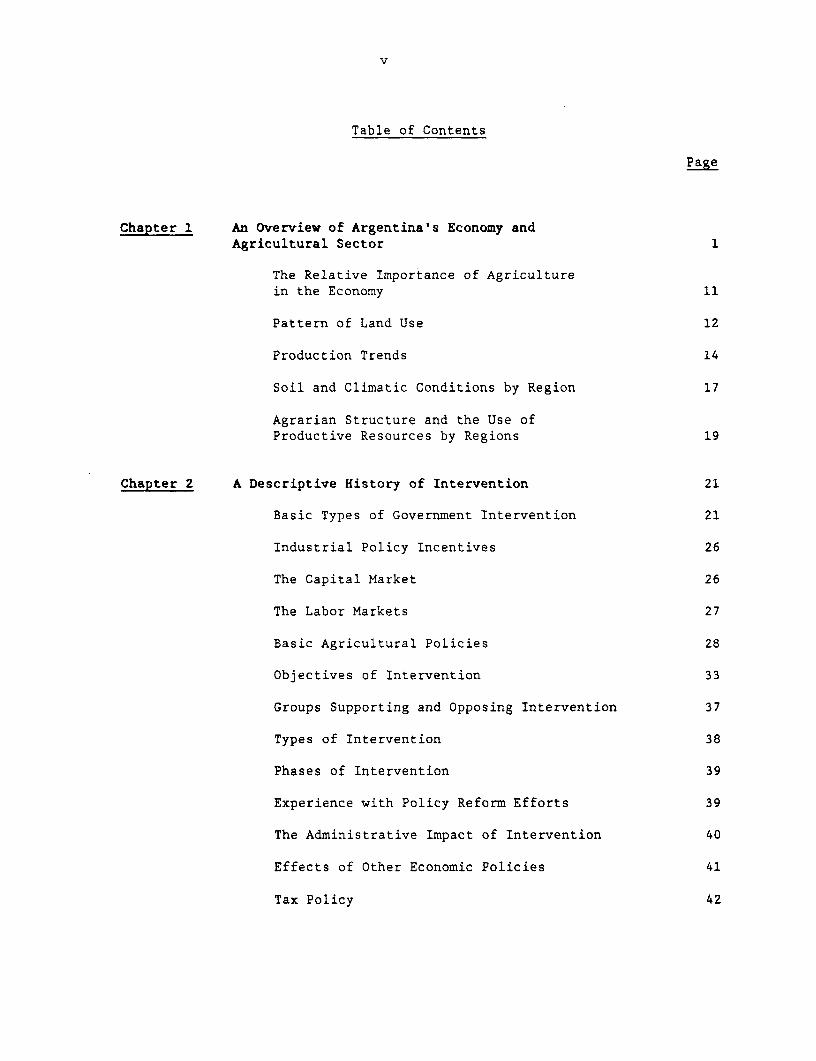
Chapter 1 An Overview of Argentina's Economy andAgricultural Sector 1

The Relative Importance of Agriculturein the Economy 11

Pattern of Land Use 12

Production Trends 14

Soil and Climatic Conditions by Region 17

Agrarian Structure and the Use ofProductive Resources by Regions 19

Chapter 2 A Descriptive History of Intervention 21

Basic Types of Government Intervention 21

Industrial Policy Incentives 26

The Capital Market 26

The Labor Markets 27

Basic Agricultural Policies 28

Objectives of Intervention 33

Groups Supporting and Opposing Intervention 37

Types of Intervention 38

Phases of Intervention 39

Experience with Policy Reform Efforts 39

The Administrative Impact of Intervention 40

Effects of Other Economic Policies 41

Tax Policy 42

vi

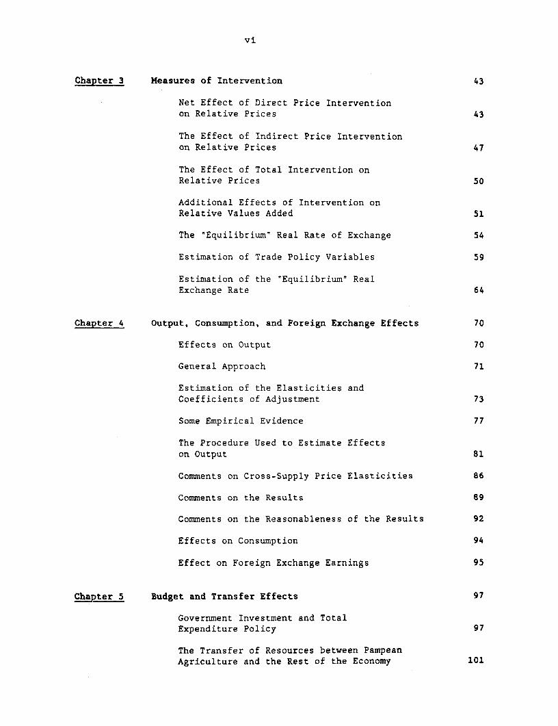
Chapter 3 Measures of Intervention 43

Net Effect of Direct Price Interventionon Relative Prices 43

The Effect of Indirect Price Interventionon Relative Prices 47

The Effect of Total Intervention onRelative Prices 50

Additional Effects of Intervention onRelative Values Added 51

The "Equilibrium" Real Rate of Exchange 54

Estimation of Trade Policy Variables 59

Estimation of the "Equilibrium" RealExchange Rate 64

Chapter 4 Output, Consumption, and Foreign Exchange Effects 70

Effects on Output 70

General Approach 71

Estimation of the Elasticities andCoefficients of Adjustment 73

Some Empirical Evidence 77

The Procedure Used to Estimate Effectson Output 81

Comments on Cross-Supply Price Elasticities 86

Comments on the Results 89

Comments on the Reasonableness of the Results 92

Effects on Consumption 94

Effect on Foreign Exchange Earnings 95

Chapter 5 Budget and Transfer Effects 97

Government Investment and TotalExpenditure Policy 97

The Transfer of Resources between PampeanAgriculture and the Rest of the Economy 101

vii

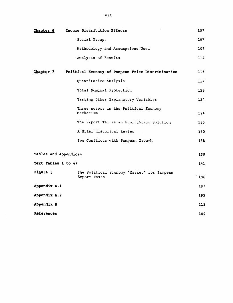
Chapter 6 Income Distribution Effects 107

Social Groups 107

Methodology and Assumptions Used 107

Analysis of Results 114

Chapter 7 Political Economy of Pampean Price Discrimination 115

Quantitative Analysis 117

Total Nominal Protection 123

Testing Other Explanatory Variables 124

Three Actors in the Political EconomyMechanism 124

The Export Tax as an Equilibrium Solution 133

A Brief Historical Review 135

Two Conflicts with Pampean Growth 138

Tables and Appendices 139

Text Tables 1 to 47 141

Figure 1 The Political Economy "Market" for PampeanExport Taxes 186

Appendix A.l 187

Appendix A.2 193

Appendix B 213

References 309

I

Chapter 1

AN OVERVIEW OF ARGENTINA'S ECONOMY AND AGRICULTURAL SECTOR

Argentina has a surface area of 2,797,000 square kilometers. Its

population was 28 million in 1980 (see Table 1), with a density of ten

inhabitants per square kilometer. The annual rate of population growth is

around 1.8 percent. The degree of urbanization is high--83 percent in

1980--and has been increasing constantly during recent decades. In its

largest urban area, Greater Buenos Aires, live more than one-third of the

total population. The labor force, as a percentage of total population,

was 38 percent in 1980. The share of the labor force employed in

agriculture was 13 percent for the same year, much like a developed

country. Most of the population is of European origin, predominantly

Spanish or Italian. The level of general education is high because of the

well-developed educational system. Skilled labor is sometimes cited as a

comparative advantage of the country.

Argentina is well endowed with agrarian resources. Arable land is

approximately 1,950,000 square kilometers, 70 percent of the surface.

Consequently, the proportion of arable land per person employed in

agriculture is high, 156 hectares (see Table 1). The most fertile and

productive land is located within a radius of 500 kilometers of Buenos

Aires. Well known as the Argentine pampas, these lands account for more

than 50 percent of total agricultural production, and for most of its three

main products: cereals, oilseeds, and cattle.

Because of the size of its population and its GDP per capita,

around US$2,300, Argentina can be considered a medium-sized economy (around

US$70 billion) with a medium-sized internal market (see Table 2). Thus,

normal proportions of international trade should be expected.

Characteristics tending to favor trade include the location of the pampas,

which are close to Argentina's ports, and a long coastline. On the other

hand, a wide range of climates, the long distances from the main

international supply and demand centers, and the physical limitations of

most of Argentina's best-located ports tend to limit trade.

Argentina began the second half of the last century at a very low

level of development. But important internal and external developments

during the last decades of the century significantly changed the situation.

Internally, the country attained political stability and the pampas became

a safe place to live and work. Significant reductions in overseas

transport costs and large increases in world demand for agricultural

products greatly improved Argentina's export prospects. These factors led

to a high positive rent for marginal pampean lands, and a type of "vent for

surplus" development scheme was set in motion to take advantage of the fact

(Di Tella and Zymelmann, 1967). Important inflows of European immigrants

and external capital, mainly invested in economic infrastructure (railways,

ports, electricity) contributed to high and sustained growth. Cultivated

land, exports, and national product increased at very high rates (Diaz-

Alejandro, 1975; Cavallo and Mundlak, 1982).

Agricultural and export-led growth in Argentina continued until

the world crisis of the 1930s, when the comparative advantage of

agriculture began to decline. Two principal factors were involved: First,

the external terms of trade worsened for agricultural products; and second,

because of population growth, land became a less abundant factor of

production. As exports decreased, internal demand replaced exports as the

leading growth factor (Ferrer, 1980). These 'spontaneous' changes during

- 3 -

the 1930s improved the relative conditions for industrial production. This

improvement also was encouraged by "policy induced" changes, such as a

moderate increase during the 1930s in tariffs on imports (Diaz-Alejandro,

1975) and external exchange restrictions imposed because of balance of

payments problems.

Relative international prices of Argentina's traditional exports

increased significantly after World War II. But policy-induced changes

became dominant, neutralizing the improvement in external terms of trade

through a discriminatory policy against internal agricultural prices. High

tariffs, and restrictions on imports, were imposed to protect the import-

competing sector from external competition, which had almost disappeared

during the war but reappeared in the postwar years. Agriculture stagnated,

and industrial import-substitution grew rapidly. Mainly because of strong

discrimination against agricultural prices, real wages increased in

relation to the price of exports. The scenario thus was set for the "stop-

go" pattern that has characterized the Argentine economy (Berlinski and

Schydlowsky, 1977) for a major portion of the last four decades.

During Argentina's 'go' phases, real GDP, real wages, real

consumption, industrial production, and imports have increased at rather

high rates. Because of strong import-substitution, most of the imports

have been intermediate industrial inputs and capital goods not produced

domestically. Exports, both traditional and nontraditional, have lagged

behind imports. This eventually creates a balance of payments crisis and

sets in motion a "stopf phase. The exchange rate is set higher to improve

the relative price of tradables, and then to stimulate an increase in

-4-

exports and a reduction in imports.1 But the price elasticities of all

tradables have been low in the short run. Thus, it has been necessary to

resort to reductions in domestic absorption to improve the external

balance. These have been obtained through monetary policy and through

restrictions on nominal wage increases. The impact of devaluation has been

inflationary, reducing domestic absorption and leading to recession.

Relative price changes and reductions in domestic demand eventually have

then led to positive trade balances. Net inflows of external capital also

have tended to improve because of the higher exchange rate. With the

correction of external accounts, the cycle starts again.

During the period under analysis, 1960-85, several attempts were

made to neutralize the stop-go pattern. The first, intended to promote

industrial exports, began in the early 1960s. It was assumed that

promoting industrial exports would increase the level of trade and would

change the structure of exports and imports, and that price elasticities of

tradables probably would be stronger. Import tax drawbacks, refunds of

domestic taxes, temporary admission of imported inputs, and other measures

were adopted. During the first half of the 1970s, large fiscal and

financial incentives for nontraditional exports were introduced (World

Bank, 1984). Some improvements in industrial exports were achieved,

especially during 1973-74 and 1977-80, but they were weak. Public sector

fiscal deficits led to restrictions on fiscal incentives, and it was very

difficult to neutralize the strong "antitrade bias" of commercial policy.

1/ A "high" exchange rate indicates a high value for foreign currencies.Thus, the international purchasing power of the domestic currencydecreases, the higher the exchange rate. This definition of a "high"exchange rate is used throughout the paper.

A second attempt was made during Kreiger Vasena's administration

(1967-69). A strongly compensated devaluation and a very active incomes

policy were implemented to avoid the combined inflation and recession that

had followed previous devaluations. The high rate of exchange improved

external short- and long-run capital flows.

A major attempt was made during the Martinez de Hoz administration

(1976-80) to achieve closer integration with external financial markets.

The rate of exchange was increased, a scheme of preannounced devaluations

was set, ceilings on internal interest rates were removed, and controls on

prices, markets, and capital movements were largely abolished. The

administration expected external capital inflows to close gaps in trade

balances, at least temporarily, giving time for the elasticities to work

and thus avoiding a resort to depressing internal activity levels. Second,

the administration attempted to reverse the inward-looking strategy by

reducing the "antitrade bias" and opening the economy. Export taxes were

cut, industrial exports were promoted, and a program of tariff reduction

was begun.

None of these attempts was very successful. During the two most

recent five-year periods, however, the typical stop-go pattern was somewhat

modified. The year 1978 was one of recession, but it was not a typical

slow year because there was no balance of payments problem; the main cause

of recession was a high internal interest rate. In 1980 there was a

visible reduction in the rate of growth because of significant

overvaluation. An important reason for the reduction was the depressive

impact on some industrial sectors of reduced tariffs and an overvalued

exchange rate. The years 1981 and 1982 were recessionary ones, with a

large reduction in gross domestic investment as the main factor. On the

other hand, during the last four years, problems in the external accounts

have reappeared. But these problems seem to be somewhat different from the

typical stop-go balance of payment crisis. They are long-run problems

associated with financial servicing of Argentina's large external debt.

Another way of viewing the general evolution of the Argentine

economy is from a long-run growth perspective. Between 1950 and 1974, per

capita real GDP increased at an average annual rate of around 2.3 percent.

Total real GDP increased almost 4 percent annually. Actually, this 4

percent was attained, on average, for the four decades between 1935 and

1974 (Elias, 1982). Surprisingly, during the decade 1975-85 the economy,

as measured by total GDP, was stagnant, and GDP per capita decreased

substantially.2

It is not the purpose of this study to try to explain the long-run

growth of the Argentine economy. But, in very general terms, it may be

said that the transition from growth to stagnation seems related to a

deterioration in productivity (defined in a very general sense, i.e.,

including changes in the proportion of resource utilization) in the use of

resources and not to stagnation in the level of resources. Let us define,

in the style of elementary growth models,

2/ Some opinions have been voiced in Argentina that with the three-digitinflation that took place in that period, the "black' or "informal'sector of the economy grew strongly, and that this sector cannot becompletely measured in social accounts. It is difficult to agree onthe quantitative significance of this factor. We will assume that GDPwas correctly measured.

-7-

GDPt = Kt St

A A A

GDP = K + 8

GDP = effective GDP

K = available reproducible physical capital

6 = effective average product-capital ratio.

These relations are identities, because 3 and 8 are computed

residually. Actually, the level of 9 depends on other growth factors that

work with physical capital to generate GDP. Those factors are quantity and

quality of human resources, technology, allocation and X-efficiency, and

proportion of utilization of productive capital.

In Table 3, annual rates of growth in GDP, capital, and

productivity by five-year periods for the period 1950-84 can be observed.

- 8 -

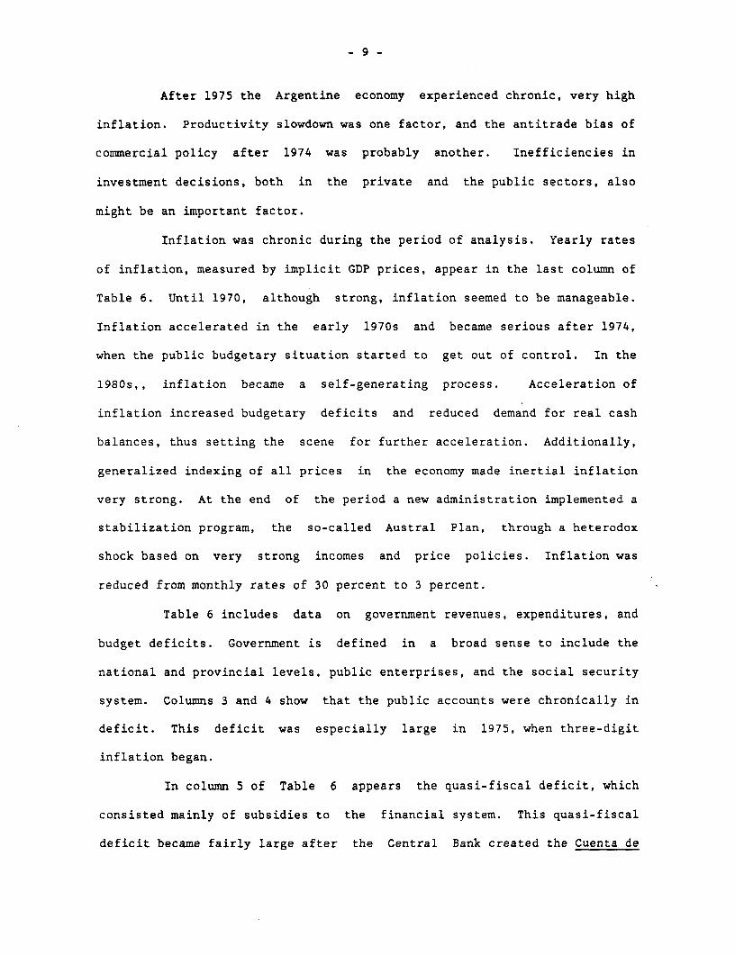
Table 3

GDP, Capital, and Productivity

Annual Rates of Growth, 1950-84 (percent)

Period GDP Captal Productivity

1950-55 3.2 2.4 0.8

1955-60 3.4 2.9 0.5

1960-65 4.6 3.3 1.3

1965-70 3.0 4.1 -1.1

1970-75 3.8 4.5 -0.7

1975-80 1.8 4.1 -2.3

1980-84 -1.6 2.2 -3.8

1970-84 1.2 3.7 -2.5

Note: Data for the period 1950-80 were taken from Elias (1982); data after

1980 is the author's estimation. It can be can be seen that during the.

first three periods up to 1965, the effective product capital/ratio was

increasing. After that, the situation reversed, especially after 1975.

During the period 1970-84, GDP increased at a much lower rate than capital.3

It seems clear that stagnation is much more related to decreases in the

productivity of resources than to lack of growth of resources.

3/ A stylized fact in growth experience is that 8 is approximatelyconstant in the long run (i.e., that rates of growth of GDP and capitalare more or less the same).

- 9 -

After 1975 the Argentine economy experienced chronic, very high

inflation. Productivity slowdown was one factor, and the antitrade bias of

commercial policy after 1974 was probably another. Inefficiencies in

investment decisions, both in the private and the public sectors, also

might be an important factor.

Inflation was chronic during the period of analysis. Yearly rates

of inflation, measured by implicit GDP prices, appear in the last column of

Table 6. Until 1970, although strong, inflation seemed to be manageable.

Inflation accelerated in the early 1970s and became serious after 1974,

when the public budgetary situation started to get out of control. In the

1980s,, inflation became a self-generating process. Acceleration of

inflation increased budgetary deficits and reduced demand for real cash

balances, thus setting the scene for further acceleration. Additionally,

generalized indexing of all prices in the economy made inertial inflation

very strong. At the end of the period a new administration implemented a

stabilization program, the so-called Austral Plan, through a heterodox

shock based on very strong incomes and price policies. Inflation was

reduced from monthly rates of 30 percent to 3 percent.

Table 6 includes data on government revenues, expenditures, and

budget deficits. Government is defined in a broad sense to include the

national and provincial levels, public enterprises, and the social security

system. Columns 3 and 4 show that the public accounts were chronically in

deficit. This deficit was especially large in 1975, when three-digit

inflation began.

In column 5 of Table 6 appears the quasi-fiscal deficit, which

consisted mainly of subsidies to the financial system. This quasi-fiscal

deficit became fairly large after the Central Bank created the Cuenta de

- 10 -

Regulaci6n Monetaria (Monetary Regulation Account) in 1977. Through this

account, commercial banks were charged a fee on their demand deposits, and

financial institutions were paid interest on the legal reserves required

against their term deposits. The quasi-fiscal deficit was extremely high

during the last years of the period, when large budget deficits financed by

monetary creation made it necessary to prevent private credit expansion.

This was done through increased legal reserve requirements. Also, because

of high inflation, demand deposits decreased to very low levels, and the

deficit of that regulatory account increased.

The share of government expenditures and revenues in GDP can also

be observed. Two facts appear--first, a high ratio between public

expenditures and GDP, and second, a strong increase in public expenditures

after 1972. The chronic deficit can also be observed. Only between 1967

and 1970 did the budget balance appear reasonable.

As noted above, state enterprises are included in the public

sector. That subsector accounts for approximately 10 percent of GDP and

includes large public service enterprises, such as railways, airlines,

postal services, and public utilities; large enterprises in the energy

production sector: military factories; and more than 100 smaller

enterprises. State enterprises have constituted one of the more serious

sources of deficit spending in the public sector, accounting for an average

2 percent GDP in 1968-71 and 5 percent of GDP in 1980-83 (World Bank,

1984).

The establishment of rates and prices for services and products

provided by the large state enterprises generally has been divorced from

their marginal economic costs. Such rates and prices have been fixed

mainly on account of budgetary needs or the need to support anti-

- 11 -

inflationary programs. Income redistribution objectives have also been

involved. It is presumed that these procedures have resulted in

significant allocative inefficiencies. Also, inefficiency is rather high

in state enterprises. The port of Buenos Aires, for example, has very high

operating costs.

The Relative Importance of Agriculture in the Economy

In the first two columns of Table 4, the share of the agricultural

sector in nominal and real GDP can be observed. No trend can be detected

when the share is measured in real terms; it amounted to approximately 15

percent. When the agricultural share is measured in nominal terms,

however, two characteristics can be observed. First, the nominal share has

much greater volatility than the real one; second, there is a downward

trend in the nominal share. The higher volatility of the nominal share

seems natural for a sector with a majority of tradable components that

experience very large external demand elasticities. The fact that the

nominal share shows a downward trend while the real one remained constant

is important.

It reflects the deterioration of agricultural relative prices

during the period of analysis. The lowest nominal share was obtained in

1980, mainly because of the strong overvaluation of the currency during

that year. It is also worthwhile to observe that despite lower relative

prices, real shares remained constant. As is explained below,

technological innovations such as hybrid seeds were introduced into the

sector, and yields were profitable despite low relative prices (i.e., the

innovations were "dominant" in the sense that they were more profitable for

any relevant price relation--see Sturzenegger, 1978). Also, subsidization

of some important agricultural inputs led to technological improvements and

production increases.

- 12 -

It can be observed in Table 4 that the share of agricultural

imports in total imports was very low and consisted mainly of tropical

products, such as coffee and bananas. In the same table the share of

agriculture in total exports can be observed. There was no significant

change in this share.

It can also be seen in the last column of Table 4 that the share

of agricultural exports in total agricultural output showed a positive

trend, mainly reflecting the appearance during later periods of new, highly

exportable products such as soybeans, and also a strong increase in the

production of seeds, an increase that can be exported to a great degree.

In Table 5 the structure of the value of agricultural production

and its changes (increases in soybeans and reductions in beef and wool)

during the period of analysis can be observed.

Pattern of Land Use

The total continental land area of Argentina is almost 280 million

hectares, with only about 50 million of them unusable. The use and

evolution of the other 230 million hectares are shown in Table 7a in

Appendix A.2.

Between the periods 1960-61 and 1982-83 the areas used for crops

and permanent pastures increased by 49 and 53 percent, respectively,

whereas the natural grassland area decreased. The area under forest and

bush remained almost unchanged.

The large areas covered by natural grasslands have a wide range of

grazing potential, from tundra and semi desert land that have extremely low

carrying capacities to pastures in the mid-to-northern regions that enjoy

favorable growing conditions and high carrying capacities. The latter are

being improved through techniques that promote the soil nitrogen content.

- 13 -

Agricultural land use has changed considerably over the years in

Argentina. There has been a large increase in the area devoted to oilseed

crops, a drastic reduction in forage crops, and a slow expansion in the

areas planted with cereal, industrial, fruit, and vegetable crops.

Between the periods 1960-64 and 1980-84 the area devoted to the

cultivation of oilseed crops expanded at a rate of 3 percent annually.

This was mainly because of increased soybean and sunflower plantings; areas

planted with linseed and peanuts have decreased.

Although forage crops accounted for 29 percent of the total area

planted in 1960-64, by 1980-84 the amount of farmland planted with forage

had fallen to about 8 percent.

The size of the area devoted to cereal crops has fluctuated around

16 million hectares, with a slight upward trend (0.5 percent annually)

during the past decades. The areas with industrial crops and vegetables

have increased more substantially, by 9 percent and 17 percent,

respectively. Vegetable crops expanded from about 440,000 hectares in

1960-64 to 550,000 hectares in 1980-84. With the exceptions of soybeans,

sunflowers, and grain sorghum, most cash crops showed little variation in

annual area planted.

The soybean area increased from an insignificant level in the

1960s and early 1970s to more than 2.2 million hectares during the period

1980-84. A high percentage of that area is double-cropped, with soybeans

as a summer crop following winter wheat.

Sunflower planting has increased by 65 percent from the period

1960-64 and now covers an area of 1.8 million hectares. Grain sorghum

planting rose from 1 million hectares in 1960-64 to almost 3 million

hectares in the period 1970-74 but fell back to 2.5 million for the most

recent period, 1980-84.

- 14 -

The area devoted to wheat has fluctuated between 4.3 and 7.4

million hectares, but has shown a generally upward trend amounting to 1.3

percent annually. Corn planting steadily increased from 1959-60 to

1970-71, reaching a peak of 4 million hectares in 1970-71 before declining

to about 3 million hectares by 1983-84.

The area devoted to barley and rye (used partially for livestock

grazing in winter) has decreased almost 2 million hectares during the

period analyzed. This reduction is explained by an exodus of cattle and

sheep from the main crop areas of the pampas to areas less suitable for

crops.

The area harvested for the five main grains (wheat, corn, grain

sorghum, soybean, and sunflower) has grown between 1960-64 and 1980-84 at a

higher annual rate than the area planted with those grains. The higher

area-harvested/area-planted relation is due to new technology that not only

has achieved higher crop yields per hectare but also has reduced losses due

to bad climatic conditions, mainly during dry seasons. A reduction in crop

planting with double purpose, as a consequence of relocating grazing

animals from the humid pampa to adjacent fringe areas, has also helped to

increase the harvested area.

The improvement in the area-harvested/area-planted ratio has

accounted for these increases in yields (Elena, 1985): corn, 27 percent;

wheat, 14 percent; grain sorghum, 47 percent; soybean, 12 percent; and

sunflower, 13 percent.

Production Trends

The volume of production of the agricultural sector increased 72

percent from the period 1962-63/1964-65 to the period 1982-83/1984-85.

- 15 -

The cereal and oilseed group enjoyed exceptional growth in that

period--150 percent (i.e., 4.7 percent annually). There are important

differences from crop to crop, however.

Wheat production grew 70 percent, from 6.1 million tons in the

period 1960-64 to an average 10.3 million tons during the period 1980-84.

Production reached 15 million tons in 1983 and 12.3 million in 1984.

Corn production increased at a rate of 3.5 percent annually

between 1960-64 and 1983-84, rising from 4.8 million tons annually to 9.5

million. The peak year was 1980-81, when production reached 12.9 million

tons.

The high growth rates for wheat and corn are explained mainly by

rapid increases in yields, and only to a much lesser extent by expansion of

the planted area. The exceptional advances in wheat production were made

possible in part through the use of early maturing wheat varieties obtained

from Mexican genetic material. Because of lack of fertilizers, the use of

hybrid corn has not become widespread.

The growth rates of soybeans, sunflower seeds, and grain sorghum

were particularly outstanding between 1960-64 and 1980-84. There was a

simultaneous increase in the area harvested and in average yields per

hectare. A large part of soybean production is double-cropped; that is, it

is cultivated on soil from which a winter crop of wheat has just been

harvested. The increased soybean production has been facilitated by the

introduction of the new, early-maturing wheat varieties that have enabled

farmers to plant a soybean crop early enough to reach maturity before the

end of the growing season. A large increase in sunflower yield was

achieved through the introduction of a new hybrid. Grain sorghum yields

also benefited from new planting material.

- 16 -

Worthy of special note with regard to the increased production of

cereals and oilseeds is that it is occurring without major increases in the

relatively low utilization of chemical fertilizer.

The cattle population reached a historic peak of about 59 million

head in the period 1975-79, almost nine million more than had existed only

a few years earlier.

From 1975-79 to 1980-84, however, herds declined almost as rapidly

as they had been built up. That reflected a long-term shift away from

livestock toward crop production. At the same time, crop production was

stimulated by a favorable price ratio of grain to beef.

Sheep herds continued their long-term decline in the pampa zone.

In the traditional sheep production zones of Patagonia, however, no

agricultural production alternatives exist, and the sheep population there

has remained stable.

The value of Argentina's agricultural products and by-products

averaged US$16.7 billion during the period 1980-84.4 Crops accounted for

half of that amount, the livestock sector for the other half.

Grains accounted for about one-quarter of the value of Argentina's

agricultural production from 1960 to 1984. Oilseed value almost doubled,

from 5 percent in the 1960s and 1970s to 10 percent in the 1980s. The

share of the other crop subsectors (fruit, vegetables, and industrial

crops) remained more or less stable for the whole period, about 2, 3, and 4

percent of the total value, respectively.

Beef production as a share of total farm production declined from

30 percent in the 1960s and 1970s to 25 percent in the 1980s, reflecting a

4/ This is value of production and not value added.

- 17 -

reduction in cattle prices. However, the share of the value of hides

increased from 5 percent in the period 1970-74 to 8 percent in the period

1980-84.

Soil and Climatic Conditions by Region

Data pertaining to the whole country reveal only part of the

agricultural production picture. In Argentina, agricultural production

takes place in either the pampean region or the rest of the country. The

pampas have different ecological characteristics (soil, rain, temperatures,

etc.), different agrarian structures and uses of factors of production, and

different production locations and availability of general infrastructure

and services. The region has specialized in products that constitute the

main source of foreign exchange and is also the main grower of food for the

Argentine population. More than 85 percent of the country's grains and

oilseeds, and about 90 percent of its livestock, come from this region.

Agricultural producers in the rest of the country have

concentrated mainly on the domestic market, providing some goods that are

part of the basic diet and others that are inputs for the industrial

sector. The rest are nonessential agricultural goods. More than 80

percent of the country's industrial crops and more than half of the

vegetables and fruits are produced outside the pampean region.

Argentina classifies its soils according to agricultural yield and

following the rules of the U.S. Soil Conservation Service. These

classifications include the production characteristics of soils and their

relationship to local climate (rain and temperatures). According to the

U.S. Soil Conservation Service, Classes I through IV are soils fit for

crops--that is, soils in which rotations of crops with different

intensities and different yields may be made. Soils in Classes I through

VIII are used for livestock raising.

- 18 -

More than 25 percent of Argentina's 230 million hectares (i.e.,

58.5 million) are soils included in Classes I to IV. Less than 10 percent

(21.8 million hectares) are class I and II soils, however. These are

concentrated in the pampean region, which contain 100 percent of the soils

in Class I and 75 percent of the soils in Class II.

Excellent ecological conditions in the pampean region have

permitted the use of efficient production systems. These are characterized

by the following features:

o Rotation of crops and livestock: The rotation of crops and

livestock increases fertility by incorporating nitrogen, one

of the most important nutrients for crops. Moreover, this

technique helps revive the physical condition of the soil

during the livestock period.

Soil structure is especially important for the pampean region,

where production is done under generally dry conditions.

Because rain distribution is so uneven during the cycle of

crops, the soil must serve as a receptacle so that water

accumulated during surplus periods can compensate for periods

of deficit. Soils that are physically well structured may

transfer a higher volume of water, decreasing the risk of crop

failure at times of drought.

o Double-Cropping: The absence of long periods of snow and cold

weather allows double-crop cultivation. This allows three

harvests in two years or permits growing of secondary crops:

soybeans on top of wheat or sunflowers on top of wheat. At

present, the cultivated surface has increased by nearly 2

million hectares in the same space occupied by that surface.

- 19 -

o Flexibility in production systems: The existence of Class I

and II soils permits a wide variety of production systems,

allowing shifts from wheat to forage crops and from these to

oilseeds, depending on the profitability of each crop.

Agrarian Structure and the Use of Productive Resources by Regions

Meaningful data on agrarian structure were derived by taking one

province as representative of the pampean region and three provinces as

representative of different subregions within the rest of the country. In

that way, land use can be broken down by farm size groups and system of

tenure according to potential soil fertility. Here, Buenos Aires is used

for the pampean region; Chaco, Tucuman, and Chubut stand for the rest of

the country.

Pampean region. Full data for the Province of Buenos Aires can be

seen in Tables 7.o and 7.p in Appendix A.2. In general, whereas the

percentage of total area in the classifications of 200 to 1,000 hectares

and 1,000 to 5,000 hectares expanded from 34.7 percent to 36 percent and

from 33.8 percent to 38 percent between 1960 and 1974, respectively, the

percentages of the classifications from 100 to 200 hectares and 5,000 or

more hectares declined during the same period.

Farms of 200 to 1,000 hectares now occupy a considerable portion

of total arable land, a shift brought about by mechanization. Farms with

more than 1,000 hectares usually have larger areas of natural grassland,

which are used primarily for livestock production.

The share of farmland in the hands of owner-operators increased

from 52 percent in 1960 to 76 percent in 1974, whereas the share of land in

the hands of tenants and sharecroppers remained at about 22 percent. The

share of land cultivated by other tenants--a category that includes

- 20 -

nonpaying tenants, fiscal land, and unspecified types of tenants--decreased

from 26 to 2 percent during that period.

The increase in the amount of land farmed by owner-operators is

partially explained by the emergence of "machine contractors," who are

mobile and who undertake to perform all farm tasks for a fee. Machinery

contract work is a well-established practice in Argentina's agriculture.

Even larger farmers who can afford to buy combine harvesters usually find

it cheaper to use machine contractors, who often get more than six months

of useful work each year from a single combine harvester. Significant

improvements in labor productivity have been achieved through

mechanization, and that has led to a reduction in the farm labor force.

At present, the typical farm of the pampean region is a family

farm, highly mechanized and operating on a size and scale larger than

before. The farm is commercially oriented, although it retains the

traditional family-farm capacity to adjust its supply of seasonal labor via

longer working hours and more extensive mechanization.

The agrarian structure in the rest of the country is heterogenous.

There are both large farms (latifundios) and very small farms (minifundios)

(see Tables 7.q to 7.v).

Owners of minifundios are precluded from choosing the most

profitable crops, most of which are perennials that must be grown within a

rigid system. The existence of the minifundio also leads to overintensive

use of land and precludes soil conservation. Furthermore, there is an

excessive supply of rural labor. This set of circumstances has led to

underemployment and low labor productivity. The use of capital, with some

exceptions, is low in relation to capital use in the pampean region, thus

indicating a lower level of adoption of technological innovation.

Chapter 2

A DESCRIPTIVE HISTORY OF INTERVENTION

Government intervention in Argentina's economy has been very

strong. Intervention in product and input markets had been so widespread

that it has been suggested that the Argentine private sector can be defined

as a capitalist sector without markets (Sturzenegger, 1984).

Here, a summary of policy intervention in relation to trade

regimes, industrial policy, and capital and labor markets is presented.

Next, a general description is given of basic agricultural policies.

Finally, other general aspects of intervention are treated.

Basic Types of Government Intervention

Protectionism. High protection against imports has been a

standard feature of postwar economic policy. The main instruments have

been tariffs, quantitative restrictions, official prices, preimport

deposits, preferential arrangements with some countries and regions, and

special import regimes.

Tariffs have been very high in Argentina. The average weighted

(by production) implicit nominal protection against importables was

estimated by Berlinski and Schydlowsky (1977) at 56 percent in 1969. This

implicit nominal protection has increased significantly during the last

five years. In 1969, effective protection against importables was

estimated as significantly higher than nominal protection.

Tariff protection has not been uniform across different goods. As

Berlinski and Schylowsky (1977) put it, "Tariffs were generally set higher

for consumption than for capital goods, higher for closer foreign

substitutes than for less close substitutes and higher also for products

- 22 -

with high degrees of fabrication, i.e., escalation was built in.'

Nevertheless, explicit tariff protection for many goods did not coincide

with implicit protection. For many goods, the latter was lower than the

explicit tariff for two reasons: first, legal tariffs often have been

prohibitive because tariff protection has existed long enough and at

sufficiently high levels to allow internal prices to fall below external

ones (i.e., water-in-the-tariff situations); second, special import regimes

have existed that have allowed some beneficiaries to import some products

with lower or no duties, making the average import tax effectively paid

lower than the legal tariff. On the other hand, many nontariff barriers

have existed--mainly import prohibitions or requirements for import

licenses. This made implicit tariffs higher than explicit tariffs.

Nontariff barriers have been important in capital, and in iron and

steel products.5 Tariffs on capital goods have usually been low so as to

promote internal investment. But it was not easy to obtain import licenses

when there was an internal supply of similar goods. On this account,

prices of capital goods were usually very different for different sectors,

depending on the existence of a competitive product produced domestically.

Official customs valuations supported many tariff positions. The

purpose of those valuations was sometimes to prevent underinvoicing and a

lower tariff payment. At other times, the official valuations prevented

overinvoicing of imports with low tariffs. The usual requirement of

advance deposits on many imports has further reinforced the system of

protection.

5/ This also has been true for consumption goods.

- 23 -

Argentina has had preferential arrangements (lower tariffs) with

some Latin American nations. These preferences did not necessarily imply

lower protection, however, because imports from such areas were generally

intramarginal ones, and the usually higher CIF prices of goods from those

areas compensated for tariff reduction (Berlinski and Schydlowsky, 1977).

Argentina's system of protection has had several characteristics.

First, protection against imports has been very high. Second, protection

has been implemented through a very complicated system. Third, these

complications have made explicit tariffs poor indicators of implicit

protection against importables. Fourth, most imports have not been close

substitutes for internal products because the implicit tariffs on competing

imports were very high, but explicit tariffs were probably close to

implicit tariffs in relation to noncompeting imports. Fifth, the economic

behavior of many of these importables, within certain ranges, was like that

of domestic goods because explicit protection (considering quantitative

restrictions as explicit) was higher than implicit protection.

Export Protection. Export protection has to be considered in

relation to two different groups of exports: traditional exports, which

include cereals, oilseeds, meats, and manufactured products derived from

agricultural primary products such as edible oils, leather goods, and

washed wool; and nontraditional exports, which are, in general, other

manufactured products of industrial and mineral origin.

As noted, protection against importables has been very high. This

has reduced the real rate of exchange and has served as a strong

disincentive for exports. In spite of this, Argentina has taxed

traditional exports highly, making those disincentives much stronger. The

level of discrimination (see chapter 3) against the more efficient export

- 24 -

sectors has been rather amazing. In addition to export taxation, there

have been export prohibitions on sunflower seeds and on hides that have

implicitly disprotected these primary products.

The situation is different for nontraditional exports. For

instance, in 1975 the effective exchange rate for nontraditional

manufactured exports was 106 percent higher than that for agricultural

exports (World Bank, 1984). Nontraditional exports have been promoted

mainly through fiscal, financial, and administrative incentives.

The main fiscal incentive has been tax reimbursements to

producers. In general, these reimbursements (reeembolsos) have been

implemented through a flat rate, depending on the degree of processing of

the export product. During the period of analysis, such rates usually

ranged between 5 and 30 percent. The criteria for the inclusion of

products and treatment have been rather vague. It was supposed that the

degree of processing was what should be promoted. Technological complexity

and "nontraditionality" of the product were good qualifying

characteristics. There usually have been special reimbursement schemes for

some special exports (for example, turnkey plants), and for products from

special regions (e.g., Patagonia). The reimbursements received by

exporters have been exempt from income tax.

The second main fiscal incentive was a drawback system. Exporters

received refunds on the import duties levied on the raw materials and

intermediate inputs used in the production and packing of export products.

In contrast to reimbursements, which were given only to promoted exports,

drawbacks have been granted to all categories of exports that required

imported inputs. "Over time, the drawback system came to protect domestic

suppliers of inputs to exports producers, since once a product had been

- 25 -

typified, there was no further check on whether the imports on which duties

were originally paid still in fact occurred, or whether they had since been

substituted by domestic production.' (Berlinski and Schydlowsky, 1977).

Financial incentives have come through the prefinancing and

financing of exports. The former provided preferential credit to encourage

the production of promoted export goods. The coverage and maturity of the

loans has varied according to the export product; capital goods have more

coverage and a longer maturity (one year) than consumer goods. The

principal was adjusted in line with the U.S. dollar exchange rate. The

annual real rate of interest was low.

The export financing scheme is intended to enable Argentina to

offer financing to its importers on conditions similar to those granted by

international competitors. Maturity extends to eight years for capital

goods, and coverage is around 70 percent. Loans are denominated in U.S.

dollars, and the annual rate of interest has been generally well below

world rates.

Temporary admission regimes for intermediate inputs to be used in

the production of goods exported within a certain period have been the main

administrative incentives for nontraditional exports.

It is worthwhile to note that despite the rather high level of

incentives in favor of nontraditional exports, the growth performance of

those exports has been rather weak. This shows the strength of the

antitrade bias imbedded in the high protection against importables. On the

other hand, a traditional export such as edible oil, which had negative

nominal protection, was able to grow at a very high rate. This was because

oilseeds, a very important input component of its cost, had stronger

nominal disprotection, thus giving edible oil a high positive effective

- 26 -

rate of protection and enabling it to perform much better than the promoted

nontraditional exports.

Industrial Policy Incentives

During recent decades, Argentina has had various legal regimes of

industrial promotion. These regimes have had both regional and sectoral

bases. Regionally, new manufacturing activities located in

"nonindustrialized" areas, generally outside of the provinces of Buenos

Aires, Santa Fe, and C6rdoba, have been promoted through different types of

incentives, such as national tax exemptions, duty-free imports of capital

goods, lower prices of goods and services provided by public enterprises,

and financial support. Sectorally, promotion regimes have existed for

mining, shipbuilding, paper, petrochemicals, and other manufacturing

activities. Sectoral incentives were similar to regional incentives,

although tax exemptions were sometimes replaced by tax deferments for

several years. Because of high inflation and the lack of interest or

inflationary adjustments to the deferment, these eventually had an

incentive effect similar to the exemptions.

The Capital Market

For most of the most recent decades, Argentine interest rates have

been administered and kept negative in real terms.

For the period of analysis, 1960-85, real deposit rates were

positive only in 1969, 1970, and 1981 (World Bank, 1984). With high

inflation and negative interest rates, financial deepening decreased

significantly in recent decades. M-1/GDP and M-2/GDP went down from 0.34

and 0.47 in 1950 to 0,04 and 0.11 in 1983. These figures show that the

Argentinian financial system has performed very poorly as a mobilizer of

funds compared to both less- and more-developed countries (World Bank,

1984).

- 27 -

The shallowness of the financial system, combined with large

public sector credit demands and negative real lending rates, made credit

to the private sector a commodity in very high demand. Private credit has

had to be administratively rationed and very probably is inefficiently

allocated. The many firms that did not have access to institutionally

subsidized credit had to resort to other sources of funds, such as self-

financing, trade credit, and informal credit, all of which had much higher

and usually positive real rates of interest.

The Labor Markets

The labor market in Argentina is far from being a free market.

The labor unions are very strong, and each production sector (iron and

steel, electricity, vehicles, paper, etc.) has a labor union that, in the

manner of a bilateral monopoly, negotiates a work and wage agreement that

applies to all workers in the sector. A main item in each agreement is

the basic wages for other categories or levels. At the same time, the

evolution of basic wages6 has generally been controlled by the government

(Nogues, 1982).

There is a large difference between the wage that the worker

receives and the amount paid by the employer. From the gross wage there

are deductions (for social security and for union dues). After gross

salaries are paid, employers have to make several other payments to the

government (for social security, the national housing fund, family

assignments, several wage taxes, etc.) and also to the labor unions. These

payments have amounted to around 40 percent of gross wages.

6/ Basic wages are more relevant for labor markets than minimum wages,which have generally been below basic wages.

- 28 -

Labor and employer payments to social security have been very

large, around 25 percent of gross wages. But there have been serious

differences in the efficiency of tax collection across sectors; the largest

degree of evasion is in the primary sector (Nogues, 1982). Another

characteristic of labor market intervention is that it has been stronger in

relation to nonskilled workers.

The substitution of labor for capital in the manufacturing sector

has probably been excessive, given Argentina's high wage costs and the

relatively lower costs for capital goods resulting from fiscal incentives

for investment in physical capital, an overvalued exchange rate, and low

relative tariffs on imports of capital goods. The substitution of skilled

workers for nonskilled ones in manufacturing also has been excessive.

Thus, there has been a very low rate of absorption of unskilled labor into

the formal manufacturing sector, and consequently there is a large informal

labor market, mainly in the construction, commerce, and personal service

sectors (see Nogues 1982).

Basic Agricultural Policies

This overview of government policies on agriculture concentrates

on pampean production--that is, cereals, oilseeds, and cattle. These

represent nearly 60 percent of agricultural production. Any analysis of

government policies associated with nonpampean products such as tobacco,

sugar cane, grapes, apples, and cotton would be very complex. Various

overlapping policies exist, including trade exchange, support prices,

production regulations, and fiscal subsidies. In consequence, the effects

of one policy are often neutralized by the effects of others.

Government intervention in pampean agriculture was very weak

before the 1930s. Intervention was almost exclusively relative to tax

- 29 -

revenue services. Because import tariffs were around 20 percent, an

indirect disprotection of pampean products resulted. Even storage

facilities in cities and ports were built by the private sectors, chiefly

rail and exporting companies.

The export-led pattern of growth waned during the Depression.

Agricultural exports decreased in the early 1930s, and farm income

decreased substantially. The government then decided to intervene in

agricultural markets to reduce the impact of the crisis on agricultural

income. Two central government agencies were created, the National Grain

Board (JNG) for cereal and oilseed production and the National Meat Board

(JNC) for meat and its derivative products. Basic prices for wheat, corn,

and flaxseed were fixed and supported by JNG purchases. The building of

new storage facilities was supported by special legislation.

After World War II, international trade began to expand at a high

rate, and agricultural prices rose substantially. This was probably a good

opportunity for Argentina to increase its exports, but government

intervention began to favor import sectors over export ones. There was

strong protection for domestic manufacturers and high taxation on

agricultural exports.

The standard explanation for these policies (see Diaz-Alejandro,

1975; Cavallo and Mundlak, 1982) may be summarized as follows: Political

and ideological factors associated with populism, nationalism, and

antiliberalism characterized the Peronist movement. The working class,

especially the urban working class, provided the main support for this

movement. Its main goal was to improve working-class living conditions by

maintaining low prices for food and by sustaining increases in demand for

urban labor through rapid industrialization. Large stocks of cereals and

- 30 -

of foreign reserves had accumulated during the war years. Additionally,

there probably was a pessimistic view concerning the long-run evolution of

the external agricultural terms of trade.

Reca (1980) provided a description of pampean price policies

applied by President Peron's government:

The price policy in effect from 1946 to 1955 was based on astate monopoly over both domestic and export markets combinedwith substantial differences between domestic and world pricesimplemented through export taxes and exchange ratedifferentials. The subsidization of domestic wheatconsumption was substantial. Farmgate prices were announcedbefore harvest time. Inflation brought about frequent upwardrevisions of prices, but these revisions were not able toprevent a steady decline in grain production due to inadequatematerial incentives.

This decline in grain production began to create balance of

payments problems, which were compounded by the deterioration of

agriculture's external terms of trade. There was some amelioration of the

policies against agriculture during the last half of the Peronist era and

the policies were changed substantially after 1955:

Another chapter of grain policy began at the end of 1955:prices of most of the crops already planted were increased by40 percent, in a clear attempt to boost farm income, andexport taxes were not used as heavily as in previous years.The state monopoly was discontinued except for wheat, andbeginning in 1957 official prices became minimal prices,farmers being free to dispose of their crops elsewhere if theypreferred (Reca, 1980).

During the 1960s and early 1970s, although price discrimination

against agriculture was lower than during the Peronist years, it remained

very high. This can be seen through the antitrade bias depicted in Table

A.l.b in Appendix A.1 and the disprotection rates computed in Chapter 3.

Other policy measures were tried to improve agricultural profitability

through better technologies and lower input prices. This line of action

- 31 -

was adopted for three main reasons: First, price elasticity pessimism

existed because a rather weak direct association between agricultural

prices and agricultural total production was found (this low response of

total production to prices, which is a short-run phenomenon, is treated in

Chapter 4). Second, anti-inflationary objectives made lower input prices a

preferred instrument. Third, higher agricultural prices implied lower real

wages.

At the end of the 1950s, technological research and extension

began, mainly through the creation of the National Institute of

Agricultural Technology (INTA). Also, the policy of subsidized credit for

agricultural production was expanded. Although this was very far from

offering full compensation for price discrimination, it had a significant

role in capitalization of the sector.

Fiscal policy, mainly through tax exemptions for agricultural

investment, also supported sectoral incentives and capitalization for

several years. These technological and input policies were important in

increasing pampean agricultural productivity during the 1960s and were even

more important in the 1970s.

During the period 1973-76, that of the second Peronist government,

there was a strong improvement in external agricultural terms of trade in

1973 and 1974, combined with increased price discrimination against

agriculture, mainly through high taxes on exports.

During the period 1976-80, as described below, there was an

attempt to change policies to achieve a significant reduction in price

discrimination against agriculture. However, overvaluation of the exchange

rate after 1978 prevented the achievement of more favorable relative prices

for agriculture. After 1980, agricultural price policies returned to the

previous pattern.

- 32 -

Price policies related to beef prices have been closely associated

with problems caused by the cattle cycle:

Beef prices have traditionally posed a special problem becauseof their wide variations and high incidence in the cost ofliving and consequently in the real wage. At times of soaringprices, maximum beef prices at the consumer level have beenusually imposed. Several attempts to help regulate meatprices at the producer level have been unsuccessful. Theimposition of meatless days in the big urban centers ofArgentina has proved to be the most effective measure todampen the increase in producer prices. Different such 'veda"schemes were used in 1964-65 and 1972-73 in times of high andincreasing prices. However, experience also shows that thisinstrument is a typical short-run tool. Difficulties in fullycontrolling the process of slaughter and distribution of meatcreate conditions, after some time, for the functioning of asophisticated black market. During periods of low beefprices, no direct government intervention in the market hastaken place. Only a timid and unsystematic use has been madeof anticyclical measures, mainly cheap credit and taxdeductions (Reca, 1980).

The discussion of basic agricultural policies may conclude with a

brief overview of the pattern of price intervention in the Argentine

economy, which is most relevant for pampean agriculture. During the period

of analysis, the typical scheme of price intervention directly or

indirectly relevant to the six pampean products included in this study was

the following: Mainly through commercial policy, there was strong

discrimination against exports vis-a-vis imports. This discrimination was

implemented through positive implicit tariffs that protected the import

sector. The discrimination was mainly against traditional exports

(agricultural and agroindustrial goods), because nontraditional exports

were partially aided in overcoming the effect of overvalued exchange rates

through the use of export subsidies. Among traditional exports,

agricultural products faced the strongest discrimination. This was because

agroindustrial exportables benefited from disprotection of their

- 33 -

agricultural inputs. Moreover, there were lower taxes on agroindustrial

exports than on agricultural exports. To compensate partially for reduced

agricultural relative prices, some support to the pampean sector was

implemented through the subsidization of some inputs to agriculture. The

three main instruments were credit at subsidized rates of interest, tax

exemptions for the purchase of machinery, and public financing for

agricultural research. These input policies received support because they

were viewed as a way of increasing production without incurring

agricultural price increases.

The relative prices of pampean agricultural products deteriorated

during World War II, mainly on account of exogenous or spontaneous factors.

After the war, deterioration continued as a result of policy intervention.

At the beginning of the period of analysis (1960) the typical scheme,

although somewhat less discriminatory against pampean production than it

was during the 1940s, had become institutionalized. It seems that it was

either not desired or not possible to dismantle the discriminatory

structure of relative sectoral incentives. As is shown in Chapter 3, such

discrimination seems to have been increasing during more recent years.

Following most devaluations or increases in the international prices of

agricultural exportables, export taxes have been increased. When the real

rate of exchange or international prices were decreasing, such taxes were

reduced (see CEPAL/FAO, 1983). There were some attempts to change the

pattern, particularly in the period 1976-80, but these reform efforts

failed.

Objectives of Intervention

The purpose of this section is to comment on the objectives of

price intervention that have usually been suggested in Argentina's case

(Diaz-Alejandro, 1975).

- 34 -

Objectives ascribed to price intervention that directly or

indirectly discriminate against pampean agriculture should seem consistent

with other policies, and with some facets of reality or presumptions about

it. Thus, objectives ascribed to agricultural price intervention should

seem consistent with the objectives of typical economic policies during the

period, such as price stability, full employment, support for

industrialization, and external balance, and to objectives concerning

personal, functional, and regional income distribution. They also must be

consistent with the facts concerning the Argentine economy during the

period of concern: a chronic deficit in fiscal balances and chronic and

accelerating inflation (see Table 6). Finally, they should be consistent

with some predominant visions or perceptions (some of them wrong) of

economic reality, such as weak responsiveness of agricultural production

(as a whole) to sectoral prices; perception of only partial equilibrium

effects; considering import substitution as always positive; emphasizing

balanced growth between sectors and regions regardless of comparative

advantages; and emphasizing self-sufficiency.

Below, we comment on each of ten objectives and include some

specifications related to Argentina in the period of analysis:

o Consumer welfare: This objective is distributional in nature

and is mainly associated with the distribution of personal

income. Its main purpose is to provide inexpensive food for a

relatively low-income population. It also is intended to

improve labor employment by means of a relative reduction in

the price of labor without reducing the welfare of the labor

force.

- 35 -

o Farm income: This objective is not relevant to the typical

scheme of intervention, which discriminates against farm

income.

o Government revenue: Because of chronic fiscal deficits in

Argentina and interventions that have consisted mainly of

export taxes and import tariffs, this is usually suggested as

an important objective.

o Foreign exchange: In relation to the discrimination against

pampean exports, this objective is not relevant. But

intervention has discriminated also in favor of importables,

and this has to be considered as a device for saving foreign

exchange. This study assumes very large--rather, infinite-

-external demand and supply elasticities for Argentine exports

and imports and that, therefore, the "optimal tariff"

consideration has to be ruled out.

O Self-sufficiency: This objective is not relevant to the

typical Argentine scheme of trade policy intervention. On the

other hand, if it is reinterpreted as self-sufficiency in as

many products as possible, then it would be very relevant for

intervention in Argentina.

o Price stability: At first glance, one can doubt the relevance

of this objective to price intervention. These interventions

could be viewed as "once and for all changes," important only

for comparative static adjustments in relative prices and

therefore without relevance to continued price instability.

But this seems a very simplistic view of inflation.

Introducing structural and inertial inflation and considering

- 36 -

demand and supply of money as partially endogenous variables

depending on the rate of inflation strongly support a

different view of price instability. This view sees changes

in the prices of wage goods as potentially quite important for

inflationary processes. In fact, this has been the standard

view in Argentina.

o Regional equity: The pampean agricultural region is

considered richer than the nonpampean one. Thus, the

objective of regional equity means that policy should favor

the nonpampean region. Export taxation was mainly on pampean

production, and therefore the regional equity objective may be

relevant for our case. Actually, it is very probable that the

whole typical scheme of intervention has had a negative effect

on the nonpampean agricultural region. Although nonpampean

export production has not been strongly taxed, and export

taxes on pampean products have made the equilibrium rate of

exchange higher, thus favoring such production, taxation on

imports has had an inverse impact on the rate of exchange,

which, as is estimated in Chapter 3, has been a predominant

effect. Also, if pampean products had not been so highly

discriminated against, they might have been cultivated in

nonpampean regions, leading to more production flexibility.

O Nutrition: As consumer welfare, this is mainly a

distributional objective, in this case associated with the

welfare of the very poor. In Argentina, nutritional standards

are relatively high. Therefore, this objective seems less

important than in other countries.

- 37 -

o Support for domestic industry: This objective is related to

extracting a surplus from agriculture to be used for

industrial development. It is also related to providing cheap

food for the urban sector and, in turn, to reducing the cost

of labor inputs for industry.

o Support of processing industry: All of the six products are

grown for domestic processing industries. Therefore, an

effective way of promoting these industries is to reduce the

prices of those inputs.

These are the objectives that are usually ascribed to intervention

in external trade prices. For reasons that will become clear, we have not

undertaken to assign weights to objectives.

Groups Supporting and Opposing Intervention

The treatment of groups supporting and opposing intervention is

brief here. It will be taken up in detail later, when we analyze the

dominant role played by some groups--mainly rural and industrial

entrepreneurs--in determining the characteristics of intervention.

The income distribution effects (Chapter 6) are the basis of the

following observations. Groups that gained from intervention were:

o Urban industries;

o Urban labor, both formal and informal (public employees

included);

o High-level members of the government, mainly on account of an

improvement in fiscal results;

o Politicians, in general, because of higher urban real wages.

- 38 -

Groups that lost were:

o Owners of pampean land, both large and small;

o Contractors, tenants, and sharecroppers;

o Rural labor (in the short-run);

o Small entrepreneurs in the service sectors of rural cities.

Types of intervention

Direct intervention in the prices of pampean agriculture products

was effected through export taxes, low effective exchange rates, and (of

minor importance) export prohibitions. The reasons for adopting these

means of direct intervention probably were their effectiveness in

satisfying the purpose of intervention and their lower administrative costs

in relation to alternative instruments, such as marketing boards.

The indirect intervention analyzed in this study was effected

through export taxes, export subsidies, tariffs, and quantitative

restrictions. It was also accomplished by equilibrating variations in the

real exchange rate associated with those restrictions on trade, and,

finally, by disequilibrium levels of the real rate of exchange associated

with nonsustainable levels of fiscal deficits and flows of foreign capital.

The reasons for intensive use of quantitative restrictions were periodic

requirements to obtain equilibrium in the balance of payments as well as

pressures from economic interest groups. The reasons for disequilibrium

levels in the exchange rate were unsustainable macroeconomic situations.

Price intervention was partially neutralized by credit policies,

tax deductions, and public investment in agricultural research and

extension. Credit and fiscal aspects are considered below;s public

investment aspects are discussed in Chapter 5.

- 39 -

Phases of Intervention

During the entire period analyzed in this study, the pattern of

intervention in relative prices has been uniform. There have been obvious

changes in the degree of intervention, but the general pattern persisted

from the beginning to the end of the period. The reasons for this

consistency are explained later.

Experience with Policy Reform Efforts

With the change of government in 1976, it became possible to think

about changing external trade policy. The main goal was to reopen the

economy through a realignment of internal relative prices in the direction

of a closer approximation to international prices. This purpose implied a

change in favor of agricultural vis-a-vis industrial prices.

The first steps occurred at the end of 1976, when drastic

reductions were made in export taxes on pampean production. On the import

side, there were reductions in tariffs and in quantitative restrictions,

although most analysts agree that during 1977 and 1978 the main result was

just an incomplete elimination of water-in-the-tariff situations. A

gradual but significant program of reduction in protection was approved

only at the end of 1978. The goal was to reach, after five years, tariff

protection levels equal to or less than 20 percent for all sectors. If all

of the objectives had been accomplished, the persistent pattern of

intervention against pampean agricultural prices would have changed

significantly.

During the years 1977 and 1978 (see Tables 9 to 12), there was a

significant reduction in the degree of intervention against pampean

agricultural production. But the goal of reforming pricing policies then

began to collapse. Although the degree of direct intervention continued to

- 40 -

decrease in subsequent years, indirect intervention began to increase and

led to a similar pattern in the degree of total intervention. The collapse

was so pronounced that the program ended in 1980-81 with the lowest

observed relative prices for the entire period, even though international

prices for goods produced in the pampean region were rather high.

The apparent reason for the failure of reform was extreme

overvaluation of the domestic currency, which occurred as a result of the

following: (1) drastic reductions in export taxes; (2) the rapid financial

opening of the economy together with a much slower commercial opening; (3)

expansionary fiscal policy; (4) a rather restrictive internal monetary

policy, which, when combined with the financial opening, generated a large

inflow of external capital that placed additional downward pressure on the

rate of exchange.

The Administrative Impact of Intervention

Decisions on intervening in agricultural prices were made at the

highest levels of government, specifically in the executive branch (the

president and cabinet). A surprisingly minor role was played by the

legislative branch, given that the policies consisted of taxes, subsidies,

and transfers of income and wealth between sectors. Before World War II,

external trade policy was decided mainly in Congress.

It is evident that there were important bureaucratic costs and

losses of productive resources (Krueger, 1974) associated with the

administration of quantitative restrictions (quotas, import licenses, etc.)

on imports, but those costs are rather far from the export sector.

Two administrative problems directly relevant to the export sector

were of some importance on occasion. One was the smuggling of products to

neighboring countries, mainly Brazil. The other was the underinvoicing

- 41 -

(subfacturaci6n) of exports. The incentives for both illegal procedures

were the desire to avoid the payment of export taxes and the desire to

obtain foreign exchange without having to exchange it at the official rate

of exchange, thus profiting from a higher price of black market rate of

exchange. Both problems could have had some importance in 1974, 1975, and

1982, when the gap between the official and unofficial rates of exchange

was large. Because the effects of intervention have been measured here by

observed prices and not official export taxes or official effective rates

of exchange, our measurements probably have captured some of the price

effects of those irregularities.

Effects of Other Economic Policies

The previous sections of this chapter have made it clear that the

system of price intervention played a dominant role in relative prices and

relative incentives for the pampean agricultural sector. However, we have

also stated that credit and fiscal policies had some effects on these

prices and incentives.

Credit Policy: Argentina has a highly developed farm credit

system in which the Banco de la Naci6n and the provincial banks play

central roles. According to data from the World Bank (1984) and from Reca

(1980), agricultural credits have tended to be around 25 percent of

agricultural value added.

Interest rate subsidies have been used primarily because of

inflation. Reca (1980), taking account of the differences between

inflation rates and nominal rates of interest, estimated that these

subsidies increased effective protection coefficients by 1.5 percent for

the period 1950-74.

- 42 -

Another study (Penna and Palazuelos, 1987) estimated the effect on

value added excluding wages of two different interest-rate situations.

Using the Banco de la Naci6n nominal interest rate for the agricultural

sector deflated by an agricultural price index, they compared this "real"

interest rate with a real interest rate equal to 0 (see Table 13 for

results).

These results, in general, clearly favor pampean production, since

Penna and Palazuelos used statistics on pampean cereals and oilseeds to

make their calculations. The percentage impact was significant only in

1971, 1972, 1975, and 1976. However, even for these years the percentage

appears small in relation to the impact on value added of trade and

exchange rate policies. Actually, as measured by Penna and Palazuelos the

percentage impact of credit policy on value added (inclusive of wages) is

lower than the effects shown in Table 13.

Tax Policy

Reca (1980) approximated the effects of differential taxation on

agriculture vis-a-vis the rest of the economy. He concluded that taxation

differentially favored agriculture but noted that the effective protection

coefficients would be only one percent higher. He added, however, that

there could be some underestimation of taxation effects in favor of

agriculture because his measurements did not include special tax deductions

and promotional schemes. Reca's measures reached only to 1974.

Nevertheless, it seems that fiscal treatment after that year did not change

in any major way.

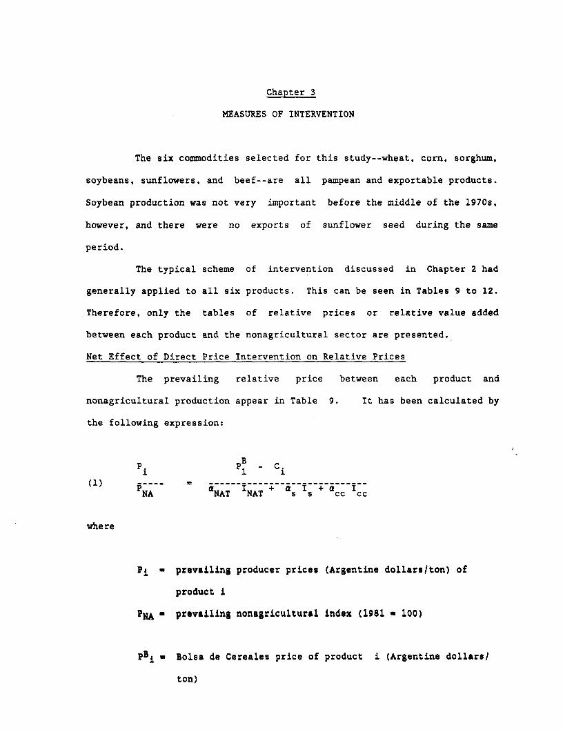
Chapter 3

MEASURES OF INTERVENTION

The six commodities selected for this study--wheat, corn, sorghum,

soybeans, sunflowers, and beef--are all pampean and exportable products.

Soybean production was not very important before the middle of the 1970s,

however, and there were no exports of sunflower seed during the same

period.

The typical scheme of intervention discussed in Chapter 2 had

generally applied to all six products. This can be seen in Tables 9 to 12.

Therefore, only the tables of relative prices or relative value added

between each product and the nonagricultural sector are presented.

Net Effect of Direct Price Intervention on Relative Prices

The prevailing relative price between each product and

nonagricultural production appear in Table 9. It has been calculated by

the following expression:

pB _ C

(1) P. P - C. ii ~ ~~~1 1

NA aNAT INAT Qs Is Qcc Icc

where

Pi - prevailing producer prices (Argentine dollars/ton) of

product i

PNA - prevailing nonagricultural index (1981 a 100)

pBi - Bolsa de Cereales price of product i (Argentine dollars/

ton)

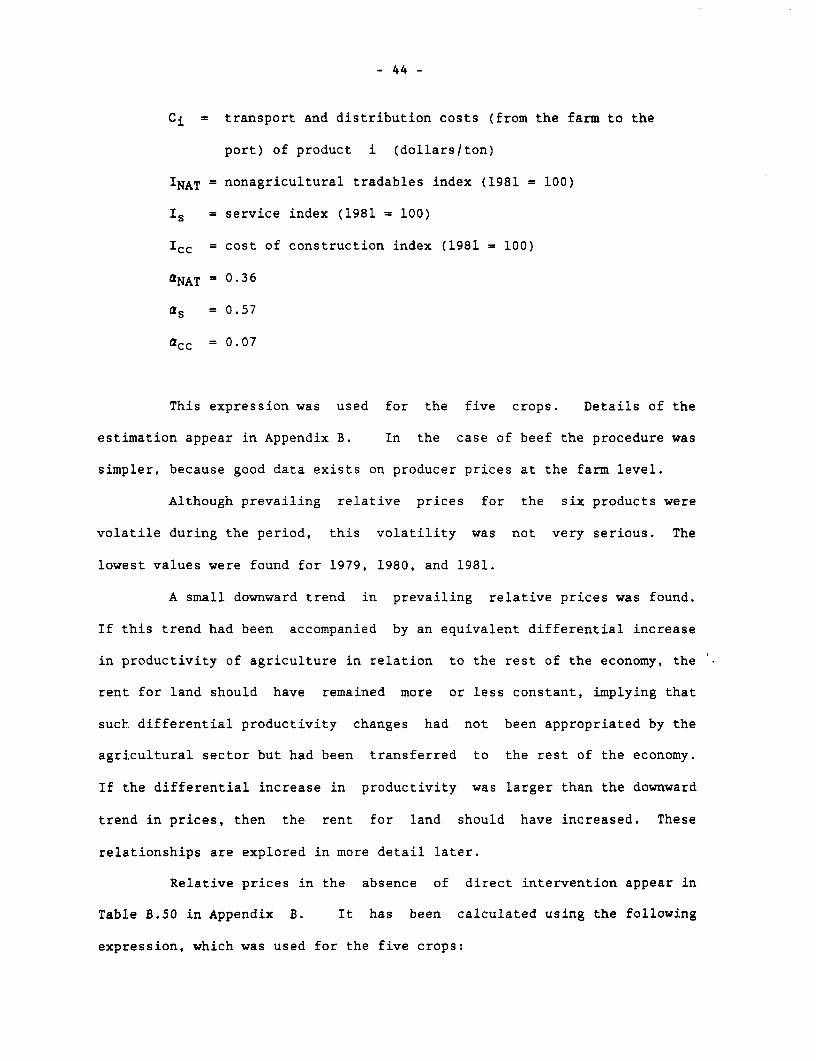
- 44 -

Ci= transport and distribution costs (from the farm to the

port) of product i (dollars/ton)

INAT = nonagricultural tradables index (1981 = 100)

Is = service index (1981 = 100)

Icc = cost of construction index (1981 = 100)

aNAT = 0.36

as = 0.57

acc 0.07

This expression was used for the five crops. Details of the

estimation appear in Appendix B. In the case of beef the procedure was

simpler, because good data exists on producer prices at the farm level.

Although prevailing relative prices for the six products were

volatile during the period, this volatility was not very serious. The

lowest values were found for 1979, 1980, and 1981.

A small downward trend in prevailing relative prices was found.

If this trend had been accompanied by an equivalent differential increase

in productivity of agriculture in relation to the rest of the economy, the

rent for land should have remained more or less constant, implying that

such differential productivity changes had not been appropriated by the

agricultural sector but had been transferred to the rest of the economy.

If the differential increase in productivity was larger than the downward

trend in prices, then the rent for land should have increased. These

relationships are explored in more detail later.

Relative prices in the absence of direct intervention appear in

Table B.50 in Appendix B. It has been calculated using the following

expression, which was used for the five crops:

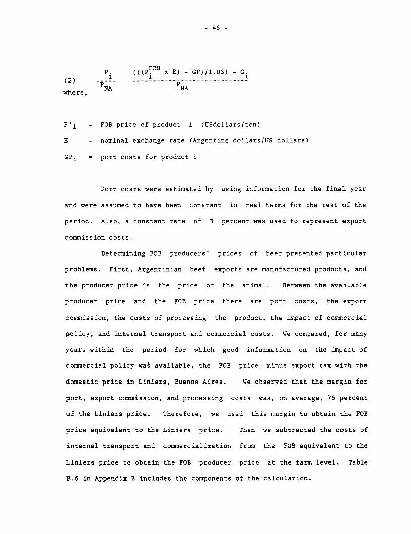
- 45 -

P. (((P B x E) - GP)/1.03) - C.(2) p ----_ ---_ ------------------ ____

PNA PNAwhere,

P'i = FOB price of product i (USdollars/ton)

E = nominal exchange rate (Argentine dollars/US dollars)

GPi = port costs for product i

Port costs were estimated by using information for the final year

and were assumed to have been constant in real terms for the rest of the

period. Also, a constant rate of 3 percent was used to represent export

commission costs.

Determining FOB producers' prices of beef presented particular

problems. First, Argentinian beef exports are manufactured products, and

the producer price is the price of the animal. Between the available

producer price and the FOB price there are port costs, the export

commission, the costs of processing the product, the impact of commercial

policy, and internal transport and commercial costs. We compared, for many

years within the period for which good information on the impact of

commercial policy was available, the FOB price minus export tax with the

domestic price in Liniers, Buenos Aires. We observed that the margin for

port, export commission, and processing costs was, on average, 75 percent

of the Liniers price. Therefore, we used this margin to obtain the FOB

price equivalent to the Liniers price. Then we subtracted the costs of

internal transport and commercialization from the FOB equivalent to the

Liniers price to obtain the FOB producer price at the farm level. Table

B.6 in Appendix B includes the components of the calculation.

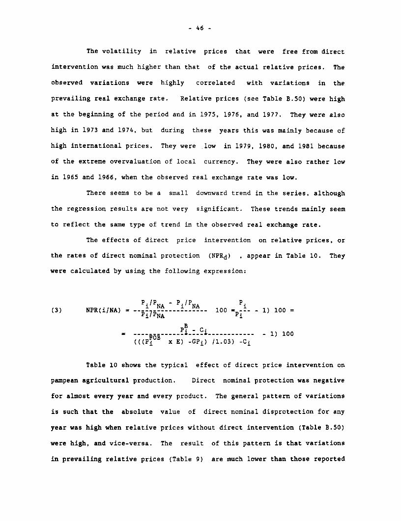
- 46 -

The volatility in relative prices that were free from direct

intervention was much higher than that of the actual relative prices. The

observed variations were highly correlated with variations in the

prevailing real exchange rate. Relative prices (see Table B.50) were high

at the beginning of the period and in 1975, 1976, and 1977. They were also

high in 1973 and 1974, but during these years this was mainly because of

high international prices. They were low in 1979, 1980, and 1981 because

of the extreme overvaluation of local currency. They were also rather low

in 1965 and 1966, when the observed real exchange rate was low.

There seems to be a small downward trend in the series, although

the regression results are not very significant. These trends mainly seem

to reflect the same type of trend in the observed real exchange rate.

The effects of direct price intervention on relative prices, or

the rates of direct nominal protection (NPRd) , appear in Table 10. They

were calculated by using the following expression:

piP NA 1i/ NA a.(3) NPR(i/NA) = __I7PNA_--------- 100 = - 1) 100 =

= ---- FOB----_PL--Ci ------------ _ 1) 100(((Pi11 x E) -GPi) /1.03) -Ci

Table 10 shows the typical effect of direct price intervention on

pampean agricultural production. Direct nominal protection was negative

for almost every year and every product. The general pattern of variations

is such that the absolute value of direct nominal disprotection for any

year was high when relative prices without direct intervention (Table B.50)

were high, and vice-versa. The result of this pattern is that variations

in prevailing relative prices (Table 9) are much lower than those reported

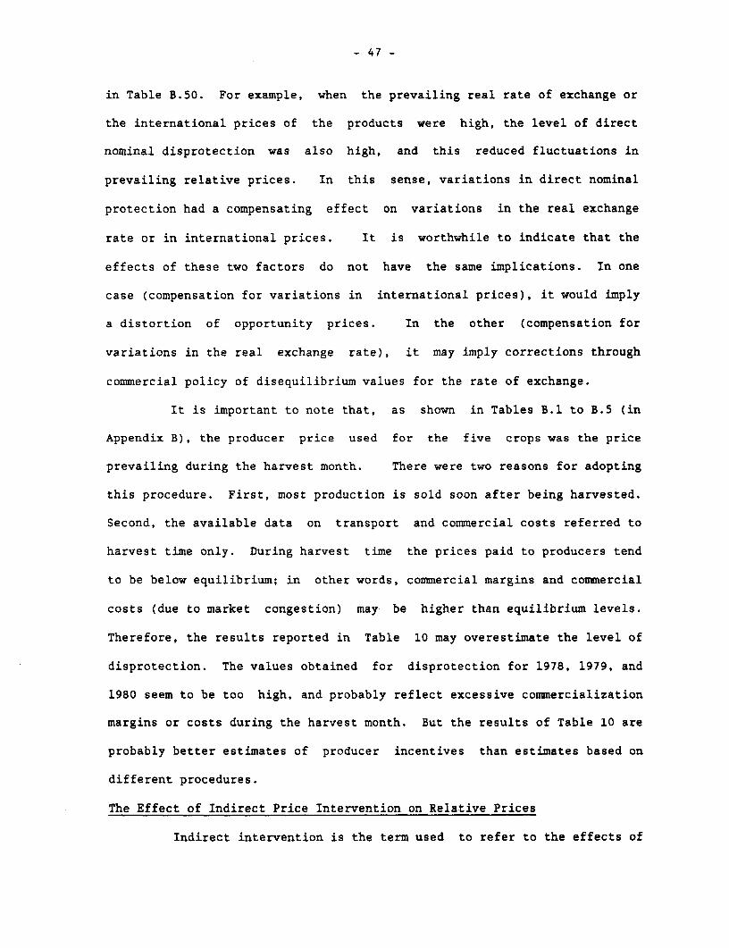
- 47 -

in Table B.50. For example, when the prevailing real rate of exchange or

the international prices of the products were high, the level of direct

nominal disprotection was also high, and this reduced fluctuations in

prevailing relative prices. In this sense, variations in direct nominal

protection had a compensating effect on variations in the real exchange

rate or in international prices. It is worthwhile to indicate that the

effects of these two factors do not have the same implications. In one

case (compensation for variations in international prices), it would imply

a distortion of opportunity prices. In the other (compensation for

variations in the real exchange rate), it may imply corrections through

commercial policy of disequilibrium values for the rate of exchange.

It is important to note that, as shown in Tables B.1 to B.5 (in

Appendix B), the producer price used for the five crops was the price

prevailing during the harvest month. There were two reasons for adopting

this procedure. First, most production is sold soon after being harvested.

Second, the available data on transport and commercial costs referred to

harvest time only. During harvest time the prices paid to producers tend

to be below equilibrium; in other words, commercial margins and commercial

costs (due to market congestion) may be higher than equilibrium levels.

Therefore, the results reported in Table 10 may overestimate the level of

disprotection. The values obtained for disprotection for 1978, 1979, and

1980 seem to be too high, and probably reflect excessive commercialization

margins or costs during the harvest month. But the results of Table 10 are

probably better estimates of producer incentives than estimates based on

different procedures.

The Effect of Indirect Price Intervention on Relative Prices

Indirect intervention is the term used to refer to the effects of

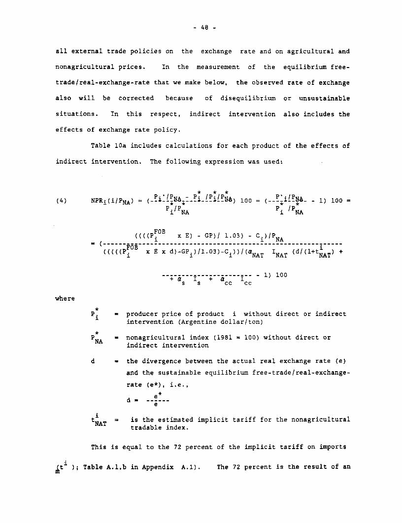
- 48 -

all external trade policies on the exchange rate and on agricultural and

nonagricultural prices. In the measurement of the equilibrium free-

trade/real-exchange-rate that we make below, the observed rate of exchange

also will be corrected because of disequilibrium or unsustainable

situations. In this respect, indirect intervention also includes the

effects of exchange rate policy.

Table lOa includes calculations for each product of the effects of

indirect intervention. The following expression was used:

(4) NPRi(i/PNA) = ( i i -:-i2-U4) 100 = - 1) 100 =

il NA i / NA

((((P. x E) - GP)/ 1.03) - C )/P2. i ~~~~~~NA

((-PFOB x E x d)-GP )/l.03)-C ))/(a I (d(l+ATl +1 1 1 NAT NATNA

----- I--- 1) 100+a I + a Is s cc cc

where

Pi = producer price of product i without direct or indirect2. intervention (Argentine dollar/ton)

pNA = nonagricultural index (1981 = 100) without direct orindirect intervention

d = the divergence between the actual real exchange rate (e)

and the sustainable equilibrium free-trade/real-exchange-

rate (e*), i.e.,

e*e

tNAT = is the estimated implicit tariff for the nonagriculturaltradable index.

This is equal to the 72 percent of the implicit tariff on imports

t); Table A.l,b in Appendix A.1). The 72 percent is the result of an

- 49-

assumption of a 0+ percent tariff for the beverage and food sectors. Then,

and considering the weights in the index of national wholesale

nonagricultural prices, we have

tN = x 28Z + tm x 72ZNAT ~~~m

As can be seen, the results of indirect intervention depend on the

relation between relative prices without direct intervention (Table B.50)

and relative prices without any intervention (Table B.51). Differences

between these two sets of relative prices come through d, which measures

the level of the equilibrium free-trade/real-exchange-rate in relation to

the observed real exchange rate, and though the relation between the level

of the equilibrium free trade nonagricultural price and the observed

nonagricultural price.

Table lOa shows the pattern of the effects of indirect

intervention. Although factor d has dual effect on the results--that is,

generating indirect disprotection through its effects on Pi* for each

product and generating indirect protection through its effects on the free

trade price of the tradable component of the nonagricultural sector

(INAT*)--the first factor is predominant. Thus, the indirect nominal rate

of protection on the products appears as negative.

The greatest impact of indirect intervention appears when the rate

of required devaluation is greatest (see Table A.l.c in Appendix A.1).

This rate is higher the more overvalued and out of equilibrium is the

prevailing real rate of exchange and when the implicit tariff on

importables (tim) is higher and the implicit tax on exportables (tix) is

lower. The greatest impact occurred in 1980 and 1981, when the currency

was extremely overvalued.

- 50 -

It is interesting to note that there are compensations between

direct and indirect effects. In general, when the level of the real

exchange rate is low (overvaluation of local currency), the direct effects

are low (in absolute values) and indirect effects are high. These

compensatory effects between direct and indirect intervention came about in

the following way. When the rate of exchange was low, export taxes on

agriculture were reduced: after a strong devaluation, those taxes were

increased.

Table B.51 shows relative prices without any intervention.

Because of the compensation effects just discussed, volatility in these

prices is lower than in Table B.50 (i.e., than those with only direct

intervention).

Effect of Total Intervention on Relative Prices

In Table 11 the effects of direct and indirect intervention are

computed--that is, the level of nominal (both direct and indirect)

protection. The following expression was used:

1i/ NA i /PNA piiNA(5) NPRT (i/NA) = …… 100 = (--; ---- 1) 100

i NA i NA

The typical results of intervention emerge very clearly: strong

negative nominal protection for the whole period and for all of the

products. Volatility is much lower than the volatility of direct nominal

protection because of the noted compensation effects between direct and

indirect intervention.

Negative trends appeared in the level of protection for grains,

and a positive trend showed in the case of beef. These trends are

explained in Chapter 7.

- 51 -

The relative prices of pampean products appear to have been

discriminated against by nearly 50 percent during the period 1960-85. In

other words, relative prices without any intervention would have been

nearly 100 percent higher than those that prevailed during the period.

Additional Effects of Intervention on Relative Values Added

Incentives for producers may change not only with changes in

producer prices but also with changes in input prices. Hence, it is

worthwhile to estimate effective protection rates and to compare the

relative values added in intervention and nonintervention situations.

We did not compute relative values added in relation to beef

production, both because intermediate inputs are not very important and

because the difficulties in computation seemed to be great. On the other

hand, we did compute values added for the five other crops because

intermediate inputs are significant and the computations were manageable.

We used three inputs; seeds, fuel, and a composite consisting of

fertilizers, herbicides, and insecticides. As can be seen in the tables of

Appendix B, the importance of these inputs has been increasing with time.

As a percentage of producers' prices they rose from less than 10 at the

beginning of the period to more than 20 during the final year.

To make these computations of rates of relative effective

protection simpler, we estimated only total effects (i.e., we did not make

any distinction between direct and indirect effects). As shown below, the

results for effective protection are very close to those for nominal

protection. This is mainly because the costs of the composite input were

small and there was a significant difference between nominal protection

rates for the product and this input. To compute the effects of

intervention on relative values added, we used the following expression for

each crop:

- 52 -

Y~i - Vi VAi

VANA VANA VAN(6) ERP (i/NA) =........_____NA____ 100 = (-1) 100 =

VA VA.1. 1

VANA VANA

*VA. VA N- Ai VAN- -- 1) 100

VAi VANA

where

VAi and VANA = prevailing (or distorted) values added of product

i and of the nonagricultural sector

VAi and VA=NA undistorted (without direct, indirect, and input

price intervention values added of product i and of

the nonagricultural sector

VAi values were obtained from detailed data computed by the

Secretary of Agriculture. These values appear in Appendix B, Tables B.26

to B.31. VAi* values were computed by using undistorted producer prices

for each crop (Table B.38 to B.43). In relation to the three inputs, it

was necessary to estimate undistorted prices. When the seed input was not

a hybrid it was considered to be a tradable input, and the nominal

protection for the seed was the same as for the product (i.e., direct and

indirect nominal protection was taken as computed from the relation between

prevailing producer prices and undistorted producer prices). When the seed

was a hybrid, it was considered as a domestic input, and nominal protection

was taken as zero. In relation to fuel, undistorted prices were computed

by multiplying U.S. prices by the nominal exchange rate adjusted by the

factor e*/e and adding 15 percent for transportation costs. Finally,

undistorted prices for the fertilizer/herbicide/insecticide input were

estimated by using the relations between prices in the United States,

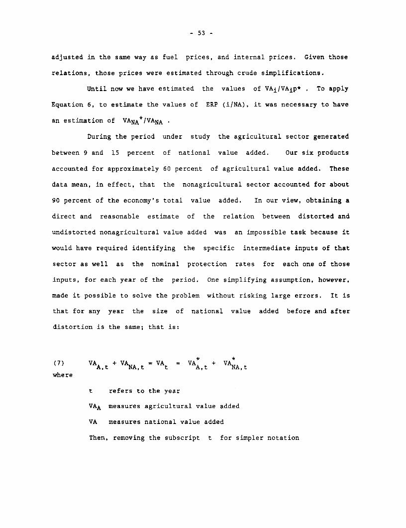
- 53 -

adjusted in the same way as fuel prices, and internal prices. Given those

relations, those prices were estimated through crude simplifications.

Until now we have estimated the values of VAi/VAip* . To apply

Equation 6, to estimate the values of ERP (i/NA), it was necessary to have

an estimation of VANA*/VANA -

During the period under study the agricultural sector generated

between 9 and 15 percent of national value added. Our six products

accounted for approximately 60 percent of agricultural value added. These

data mean, in effect, that the nonagricultural sector accounted for about

90 percent of the economy's total value added. In our view, obtaining a

direct and reasonable estimate of the relation between distorted and

undistorted nonagricultural value added was an impossible task because it

would have required identifying the specific intermediate inputs of that

sector as well as the nominal protection rates for each one of those

inputs, for each year of the period. One simplifying assumption, however,

made it possible to solve the problem without risking large errors. It is

that for any year the size of national value added before and after

distortion is the same; that is:

* *(7) VAA,t + VANAlt = VAt = VAA,t + VANA,t

where

t refers to the year

VAA measures agricultural value added

VA measures national value added

Then, removing the subscript t for simpler notation

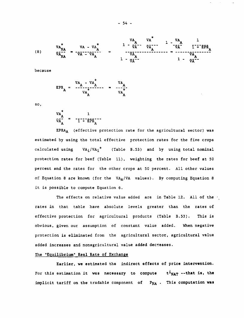
-54-

VA VA 1 VAA 1

VANA VA - VA VA VAA VA 1 + EPRA

(8) ---- --V ----V --- ------------------ -= -------------- ~VA.... VA-VA - VA VANA A A VA

VA V

because

VA - VA VAAEPRA= A

A ~~~*~-- = *__VA VAA A

so,

*VAA 1

A~~~VA. 1 l+EPRA

EPRAA (effective protection rate for the agricultural sector) was

estimated by using the total effective protection rates for the five crops

calculated using VAi/VAi* (Table B.53) and by using total nominal

protection rates for beef (Table 11), weighting the rates for beef at 50

percent and the rates for the other crops at 50 percent. All other values

of Equation 8 are known (for the VAA/VA values). By computing Equation 8

it is possible to compute Equation 6.

The effects on relative value added are in Table 12. All of the

rates in that table have absolute levels greater than the rates of

effective protection for agricultural products (Table B.53). This is

obvious, given our assumption of constant value added. When negative

protection is eliminated from the agricultural sector, agricultural value

added increases and nonagricultural value added decreases.

The "Equilibrium" Real Rate of Exchange

Earlier, we estimated the indirect effects of price intervention.

For this estimation it was necessary to compute tiNAT --that is, the

implicit tariff on the tradable component of PNA . This computation was

- 55 -

needed to estimate P*NA, --that is, the nonagricultural price excluding

any price intervention. To compute t*NAT , we needed t'm , --that is,

the implicit tariff on the import sector.

But another estimation was also needed: the estimation of

d = e*/e . The value of d was needed to move from the values of P i

(i.e., the values of the products without direct intervention), to the

values of P*i (i.e., the values without any intervention). Also, the

value of d was needed to make an additional adjustment to the tradable

component of PNA -

In this section we describe the procedures used in computing those

variables. First, we present the general approach. Second, we comment on

the estimation of the variables of external trade policy, basically the

estimation of the value of t, i and tmi for each (i.e., the implicit

taxes on exports and imports. Last, we comment on the estimation of the

values of e and e* .

For the required estimations we assume that the economy is divided

into an export sector, an import sector, and a domestic sector.

For Argentina, the first sector (exports) includes a large part of

the agricultural sector, some agroindustrial production (edible oil, meat,

leather, etc.), and other industrial production (some iron and steel

products, aluminum, some textiles, etc.).

The second sector (importables) includes most Argentinian

industrial production (textiles, chemicals, iron and steel, vehicles,

etc.). It is important to differentiate clearly between import products

and importables. Most imports do not compete with domestic production

because they are noncompeting intermediate and capital goods.

- 56 -

It is assumed here that the Argentinian economy is a price taker

in international markets and that the "law of one price" is applicable to

tradables. In the actual functioning of the economy it is important to

recognize that the law of one price is more applicable to exports than to

imports. Within the import-competing sector are domestic goods that are

protected through quantitative restrictions on imports or through explicit

tariffs that are higher than implicit tariffs7 (water-in-the-tariff case).

Therefore, these goods may behave like home goods. Nevertheless, because

we are computing relative prices in a free trade situation, it is

reasonable to assume that the law of one price will also be a fairly good

rule within the import-competing sector.

The price of a domestic good (Ph) will be one that equilibrates

internal supply and internal demand.

In Note 2 the algebraic structure of the models for export,

import-competing, and domestic goods is presented. It contains two

independent relative prices, PxIPh and Pm/Ph . In that note, a formula

(the last equation in the note) is derived for computing variations in the

real exchange rate (e) due to variations in international prices, in

terms of trade, in commercial policy, and in trade balances.

This method is based on the "elasticity approach" called by

Dornbusch (1975) the BRM approach. We apply a more accepted version of

that method, as proposed by Dornbusch, in which a third sector (the home

sector) appears explicitly, and a nominal variable (the price of the home

good) is supposed to be fixed. The three goods are mutual substitutes;8

7/ This is defined as the relation between internal and external prices,both expressed in the same currency.

8/ This seems reasonable given the level of aggregation.

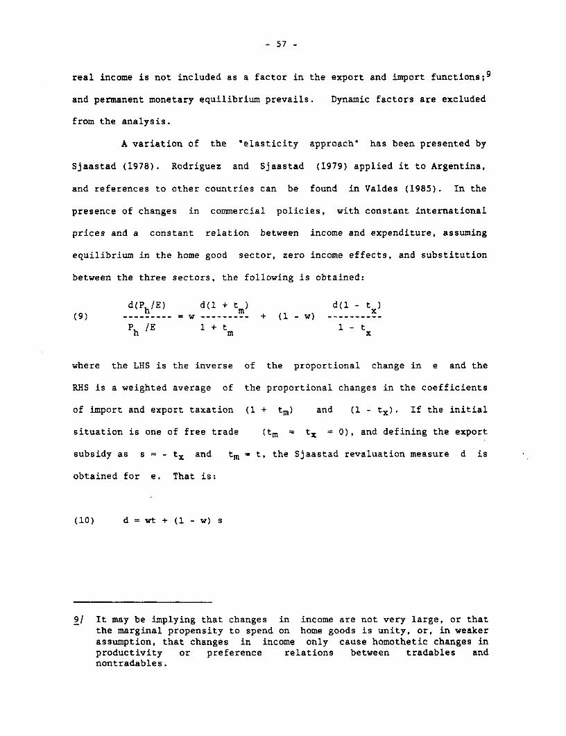
- 57 -

real income is not included as a factor in the export and import functions;9

and permanent monetary equilibrium prevails. Dynamic factors are excluded

from the analysis.

A variation of the "elasticity approach" has been presented by

Sjaastad (1978). Rodriguez and Sjaastad (1979) applied it to Argentina,

and references to other countries can be found in Valdes (1985). In the

presence of changes in commercial policies, with constant international

prices and a constant relation between income and expenditure, assuming

equilibrium in the home good sector, zero income effects, and substitution

between the three sectors, the following is obtained:

d(Ph/E) d(1 + t ) d(l - t)(9) --------- = w--------+ (1 - w)---

P /E 1 + t 1 - th ~~~m x

where the LHS is the inverse of the proportional change in e and the

RHS is a weighted average of the proportional changes in the coefficients

of import and export taxation (1 + tm) and (1 - tx). If the initial

situation is one of free trade (tm = tx = 0), and defining the export

subsidy as s = - tx and tm = t, the Sjaastad revaluation measure d is

obtained for e. That is:

(10) d = wt + (1 - w) s

9/ It may be implying that changes in income are not very large, or thatthe marginal propensity to spend on home goods is unity, or, in weakerassumption, that changes in income only cause homothetic changes inproductivity or preference relations between tradables andnontradables.

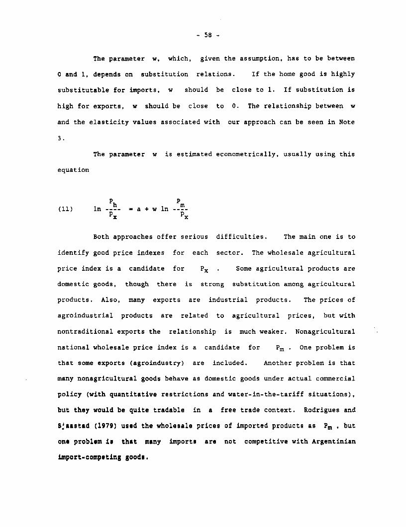
- 58 -

The parameter w, which, given the assumption, has to be between

0 and 1, depends on substitution relations. If the home good is highly

substitutable for imports, w should be close to 1. If substitution is

high for exports, w should be close to 0. The relationship between w

and the elasticity values associated with our approach can be seen in Note

3.

The parameter w is estimated econometrically, usually using this

equation

ph ~~~pm(:L1) ln ---- = a + w ln ----

P_ PY

Both approaches offer serious difficulties. The main one is to

identify good price indexes for each sector. The wholesale agricultural

price index is a candidate for Px . Some agricultural products are

domestic goods, though there is strong substitution among agricultural

products. Also, many exports are industrial products. The prices of

agroindustrial products are related to agricultural prices, but with

nontraditional exports the relationship is much weaker. Nonagricultural

national wholesale price index is a candidate for Pm . One problem is

that some exports (agroindustry) are included. Another problem is that

many nonagricultural goods behave as domestic goods under actual commercial

policy (with quantitative restrictions and water-in-the-tariff situations),

but they would be quite tradable in a free trade context. Rodrigues and

Sjaastad (1979) used the wholesale prices of imported products as Pm , but

one problem is that many imports are not competitive with Argentinian

import-competing goods.

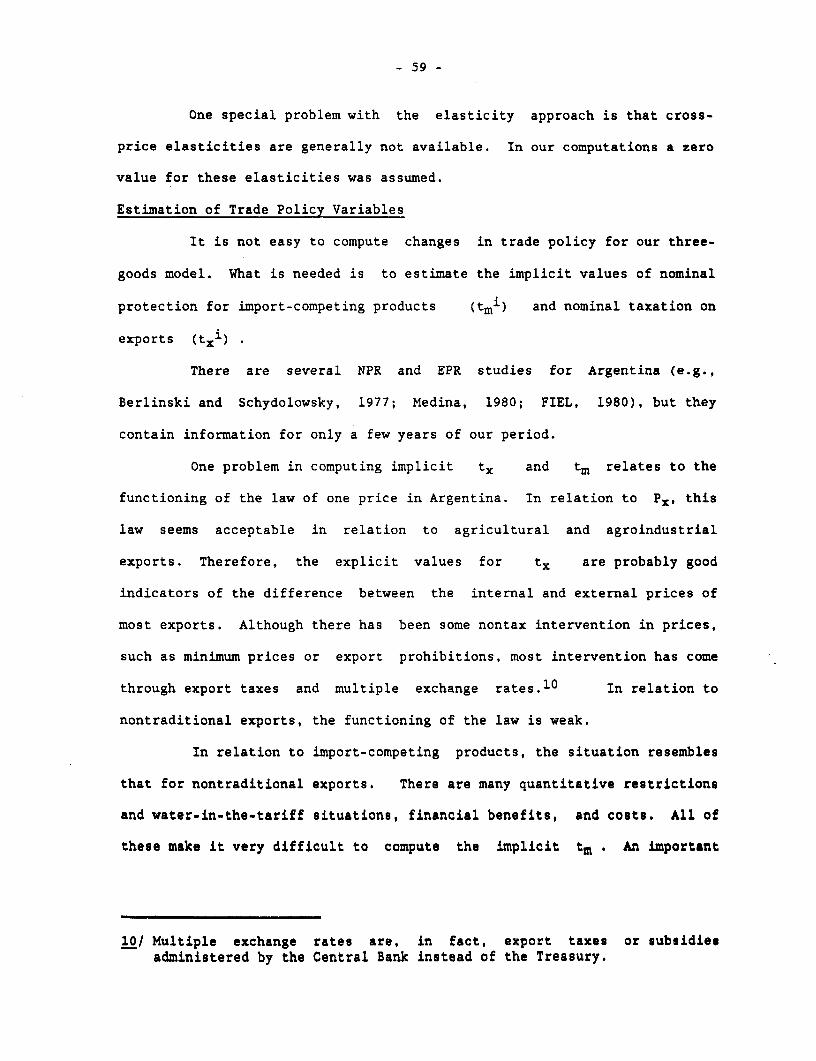
- 59 -

One special problem with the elasticity approach is that cross-

price elasticities are generally not available. In our computations a zero

value for these elasticities was assumed.

Estimation of Trade Policy Variables

It is not easy to compute changes in trade policy for our three-

goods model. What is needed is to estimate the implicit values of nominal

protection for import-competing products (tmi) and nominal taxation on

exports (txi) .

There are several NPR and EPR studies for Argentina (e.g.,

Berlinski and Schydolowsky, 1977; Medina, 1980; FIEL, 1980), but they

contain information for only a few years of our period.

One problem in computing implicit tx and tm relates to the

functioning of the law of one price in Argentina. In relation to Px, this

law seems acceptable in relation to agricultural and agroindustrial

exports. Therefore, the explicit values for tx are probably good

indicators of the difference between the internal and external prices of

most exports. Although there has been some nontax intervention in prices,

such as minimum prices or export prohibitions, most intervention has come

through export taxes and multiple exchange rates.10 In relation to

nontraditional exports, the functioning of the law is weak.

In relation to import-competing products, the situation resembles

that for nontraditional exports. There are many quantitative restrictions

and water-in-the-tariff situations, financial benefits, and costs. All of

these make it very difficult to compute the implicit tm . An important

10/ Multiple exchange rates are, in fact, export taxes or subsidiesadministered by the Central Bank instead of the Treasury.

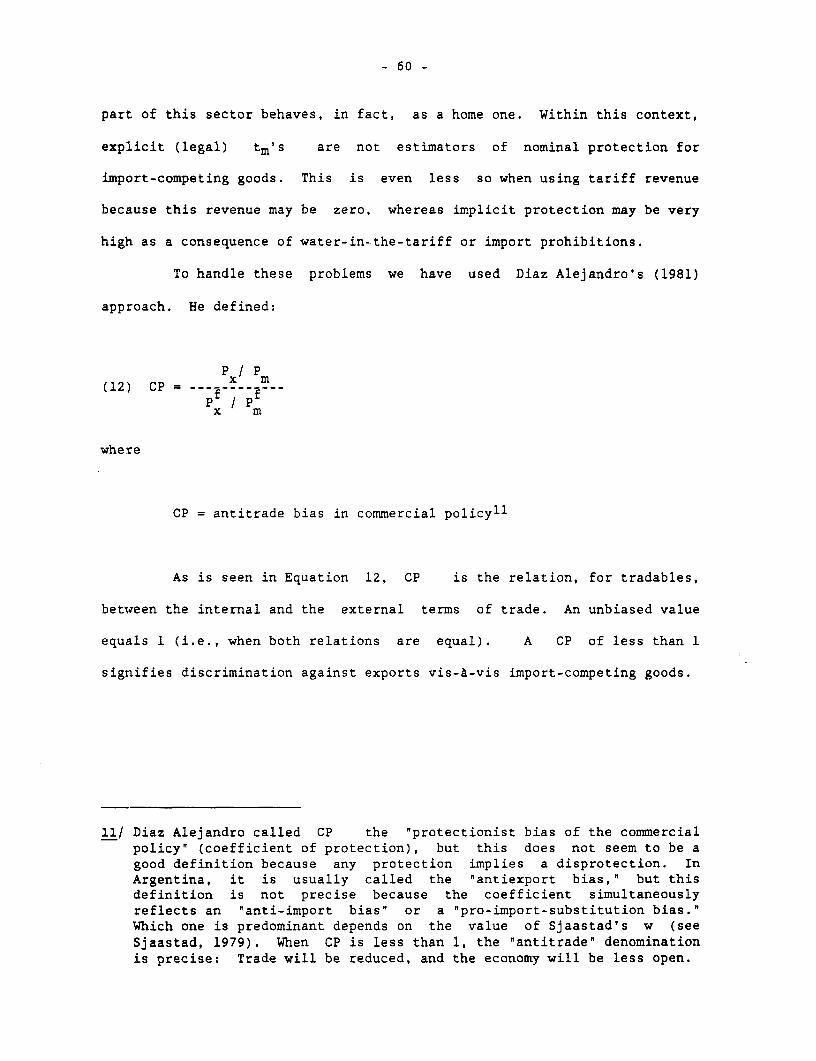
- 60 -

part of this sector behaves, in fact, as a home one. Within this context,

explicit (legal) tm's are not estimators of nominal protection for

import-competing goods. This is even less so when using tariff revenue

because this revenue may be zero, whereas implicit protection may be very

high as a consequence of water-in-the-tariff or import prohibitions.

To handle these problems we have used Diaz Alejandro's (1981)

approach. He defined:

px / m(12) CP = -____-x/-P

pf I fx m

where

CP = antitrade bias in commercial policyll

As is seen in Equation 12, CP is the relation, for tradables,

between the internal and the external terms of trade. An unbiased value

equals 1 (i.e., when both relations are equal). A CP of less than 1

signifies discrimination against exports vis-A-vis import-competing goods.

11/ Diaz Alejandro called CP the "protectionist bias of the commercialpolicy" (coefficient of protection), but this does not seem to be agood definition because any protection implies a disprotection. InArgentina, it is usually called the "antiexport bias," but thisdefinition is not precise because the coefficient simultaneouslyreflects an "anti-import bias" or a "pro-import-substitution bias."Which one is predominant depends on the value of Sjaastad's w (seeSjaastad, 1979). When CP is less than 1, the "antitrade" denominationis precise: Trade will be reduced, and the economy will be less open.

- 61 -

When CP is greater than 1 it means that commercial policy causes

an increase in "tradability," and it is correct to say that commercial

policy has, in this case, a "protrade bias." The bias in Argentina goes in

the other direction: CP is less than 1, and commercial policy has

decreased "tradability;" that is, it has an "antitrade bias.0

Having defined CP, we next must compute the implicit tx and tm.

Because Sectors x and m are considered tradables, it is defined that

(13) p = P E (1 - t)x x x

(14) P = Pf E (1 + tm m m

where ti means implicit export or import taxes. Therefore, using

Equations 12, 13, and 14, we obtain

(1 - t1 )

(15) CP = --------(1 + t1 )

m

Equation 15 is used to compute CP for any year for which the

values of t and t are available. The year 1969 was chosen becausex m

an estimation of tim exists.12

Then, using Equation 12 with base year 1969, the CPs for the

period are estimated.

In relation to exports the law of one price is accepted (with the

limitation commented on below) and then tix (the implicit export tax)

will be assumed equal to tx (the explicit tax). Then, tim for the

whole period is estimated by using for the other years

12/ The value for tix was computed using the explicit tx; se below.

- 62 -

I 1- tx(16) t CP - 1

m CP

Estimating CP using Equation 12 has difficulties similar to those

with Sjaastad's w. Diaz Alejandro used agricultural wholesale prices for

Pm , but, as we have said, imports and import-competing goods are not close

substitutes. He assumed CP = 1 for his base year, 1929.

We have used a weighted average of prices of agricultural and

agroindustrial products for Px . Such products account for 75 percent of

exports. It seems reasonable to exclude nontraditional exports. They are,

to a large extent, import-competing goods protected through tim (i.e.,

internal prices usually are higher than external ones). The level of

exports is weakly related to relative prices because the economic cycle is

a more important factor in determining the level of exports. For Pm we

used nonagricultural wholesale prices, excluding food and beverages. For

tix we used explicit taxes on traditional exports.

As tix we used explicit taxes on traditional exports.

As we stated, to estimate CP for the whole period it was necessary

to make an estimate of CP for some year, using Equation 15. Berlinski and

Schydlowsky (1977), in a detailed analysis of nominal and effective

protection, estimated an implicit tariff on imports of 56 percent for 1969.

The tx on traditional exports was 12 percent (see Table A.l.b). With

these values, using Equation 15, CP = 0.564. Diaz Alejandro (1981)

obtained CP = 0.658 for 1969. In one of his other studies ("Aranceles

Aduaneros: 1906-1940," in Diaz Alejandro, 1975), tm was equal to 17

percent in 1929 (explicit and implicit tm were probably very similar for

that year), and that was not consistent with CP = 1. That 17 percent

gives CP - 0.855 for 1929.13 With this new base value, Diaz Alejandro's

13/ the value of tx is assumed nil for 1929.

- 63 -

computations gave CP = 0.563 for 1969. This remarkable coincidence in his

results and ours for 1969 supports our estimation of tim, for the whole

period. Our estimated values for t. , tim . and CP can be seen in Table

A.l.b.

There are two interesting points in the results. First, the

'antitrade bias' of Argentine commercial policy seems to have been

increasing (i.e., the bias against an open economy is stronger now than 25

years ago). During the 1940s and early 1950s the economy experienced its

largest "antitrade bias.' During the 1960s and early 1970s the bias was

reduced, but it increased again and was particularly high during the last

five years of the period.

Second, the largest antitrade bias appeared in 1980 and 1981. The

1980 result is surprising, because the Martinez de Hoz administration's

main economic goal was to reopen the economy. Imports were very high at

the time. In general, 1980 has been considered a good example of

liberalization of the Argentinian economy. Therefore, a very high CP would

be expected. In our view, two factors explain the opposite result. First,

internal prices in some sectors were still too high in 1980 in relation to

competitive imports (i.e., equilibrium adjustments of internal prices to

the strong fall in e were not complete). And, second, with the decrease of

e , in other sectors where the law of one price was not functioning, the

effect of reduction in e was a reduction in 'water" and not in internal

prices (Cottani, 1985). That is, the implicit tariff behaved as an

endogenous variable; the operative commercial policy was dependent on

exchange rate policy14 or on fiscal and monetary policies (Cavallo,

1985).

14/ This can be seen by using Equation 14 for the pertinent sectors: As Egoes down, instead of Pm going down, tlm goes up.

- 64 -

It also can be observed that tim was very high in 1965 and 1966,

years in which the actual e was below "parity.' On the other hand, the

lowest levels for tim appeared in 1972 and 1963, where the actual e was

above "parity." This means that for a country such as Argentina, where the

law of one price functions much better for exports than for import-

competing goods, overvaluations of the currency eventually may cause

discrimination in favor of import-competing goods vis-a-vis exports (i.e.,

may tend to cause a closing of the economy).

Estimation of the 'Equilibrium" Real Exchange Rate

In this section we describe the procedure for estimating the value

of e* (the "equilibrium' real exchange rate). With this value and the

value of e (the observed real exchange rate), the value of d , which is

used to estimate the indirect effects of price intervention, is computed.

First, we must define "equilibrium." The equilibrium rate of

exchange should be the rate that generates a sustainable external trade

balance. This is the first reason why e* may be different from e . For

instance, if the sustainable trade balance is greater than what is

observed, then e* should probably be greater than e . We say "probably"

and not "necessarily,' since the actual relation between the observed e

and the observed trade balance may be not a stable equilibrium relation

because of short-run or temporary effects.

The equilibrium rate of exchange should also be a rate that

generates a sustainable trade balance within a context of free trade. This

is the second reason why e* may be different from e. In our three-final

goods approach, because they are mutual substitutes, if the level of tim

is very large relative to tiX 9 e* will probably be greater than e .

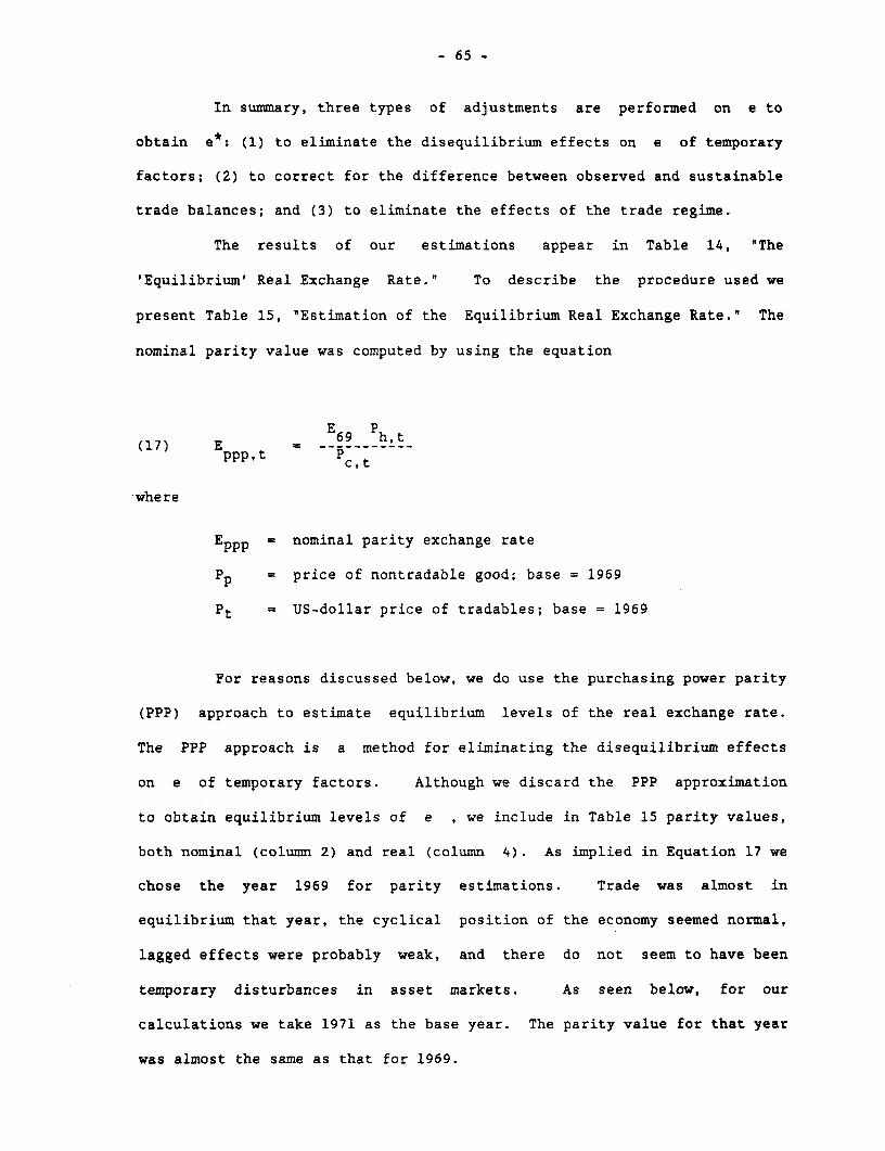
- 65 -

In summary, three types of adjustments are performed on e to

obtain e*: (1) to eliminate the disequilibrium effects on e of temporary

factors; (2) to correct for the difference between observed and sustainable

trade balances; and (3) to eliminate the effects of the trade regime.

The results of our estimations appear in Table 14, 'The

'Equilibrium' Real Exchange Rate." To describe the procedure used we

present Table 15, "Estimation of the Equilibrium Real Exchange Rate.' The

nominal parity value was computed by using the equation

E 69Ph(17) E - -69 h,tppp,t C,t

where

Eppp = nominal parity exchange rate

Pp = price of nontradable good; base = 1969

Pt = US-dollar price of tradables; base = 1969

For reasons discussed below, we do use the purchasing power parity

(PPP) approach to estimate equilibrium levels of the real exchange rate.

The PPP approach is a method for eliminating the disequilibrium effects

on e of temporary factors. Although we discard the PPP approximation

to obtain equilibrium levels of e , we include in Table 15 parity values,

both nominal (column 2) and real (column 4). As implied in Equation 17 we

chose the year 1969 for parity estimations. Trade was almost in

equilibrium that year, the cyclical position of the economy seemed normal,

lagged effects were probably weak, and there do not seem to have been

temporary disturbances in asset markets. As seen below, for our

calculations we take 1971 as the base year. The parity value for that year

was almost the same as that for 1969.

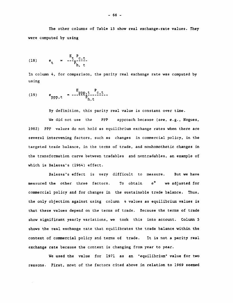
- 66 -

The other columns of Table 15 show real exchange-rate values. They

were computed by using

(8 tEt c,t(18) e ~ ------

h, t

In column 4, for comparison, the parity real exchange rate was computed by

using

(19) e --- -- c--- --ppp,t ph,t

By definition, this parity real value is constant over time.

We did not use the PPP approach because (see, e.g., Nogues,

1982) PPP values do not hold as equilibrium exchange rates when there are

several intervening factors, such as changes in commercial policy, in the

targeted trade balance, in the terms of trade, and nonhomothetic changes in

the transformation curve between tradables and nontradables, an example of

which is Balassa's (1964) effect.

Balassa's effect is very difficult to measure. But we have

measured the other three factors. To obtain e* we adjusted for

commercial policy and for changes in the sustainable trade balance. Thus,

the only objection against using column 4 values as equilibrium values is

that these values depend on the terms of trade. Because the terms of trade

show significant yearly variations, we took this into account. Column 5

shows the real exchange rate that equilibrates the trade balance within the

context of commercial policy and terms of trade. It is not a parity real

exchange rate because the context is changing from year to year.

We used the value for 1971 as an "equilibrium" value for two

reasons. First, most of the factors cited above in relation to 1969 seemed

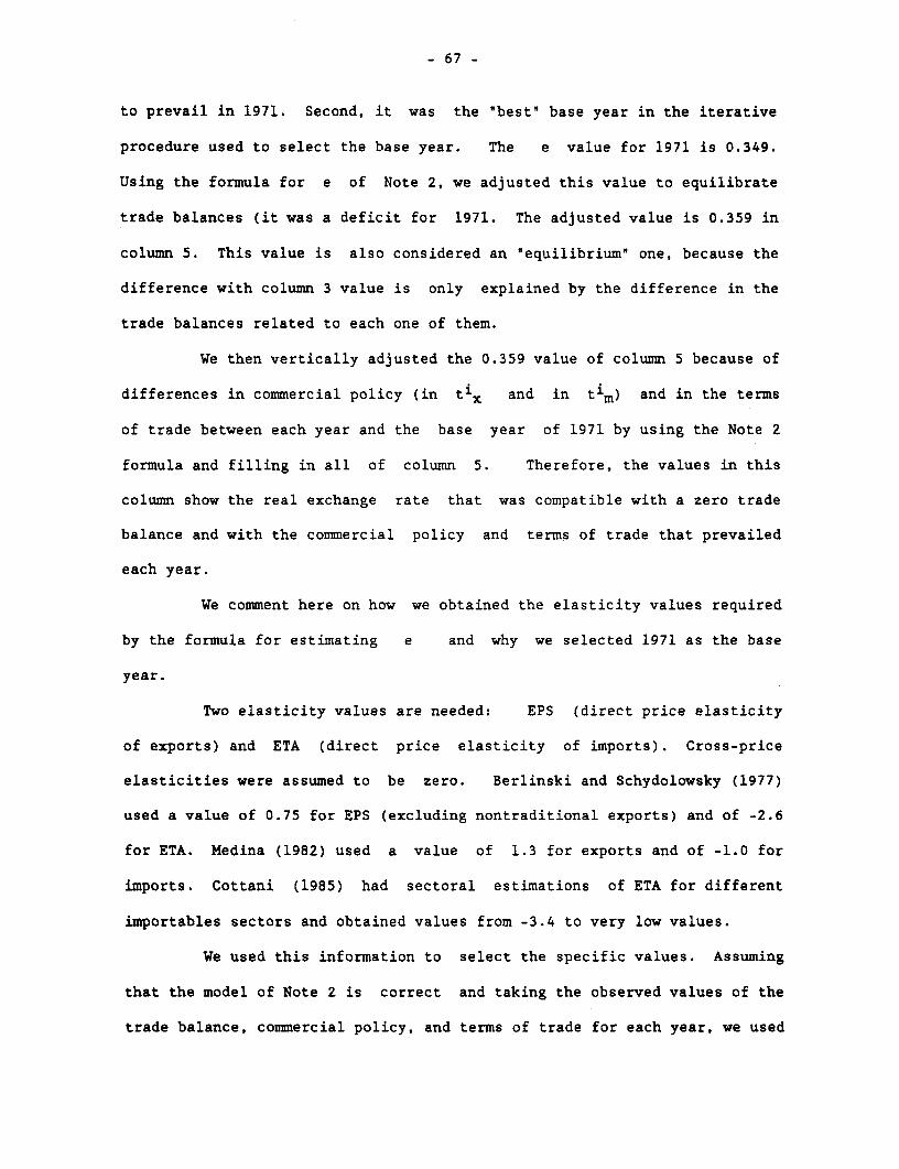
- 67 -

to prevail in 1971. Second, it was the 'best' base year in the iterative

procedure used to select the base year. The e value for 1971 is 0.349.

Using the formula for e of Note 2, we adjusted this value to equilibrate

trade balances (it was a deficit for 1971. The adjusted value is 0.359 in

column 5. This value is also considered an "equilibrium" one, because the

difference with column 3 value is only explained by the difference in the

trade balances related to each one of them.

We then vertically adjusted the 0.359 value of column 5 because of

differences in commercial policy (in ti, and in tim) and in the terms

of trade between each year and the base year of 1971 by using the Note 2

formula and filling in all of column 5. Therefore, the values in this

column show the real exchange rate that was compatible with a zero trade

balance and with the commercial policy and terms of trade that prevailed

each year.

We comment here on how we obtained the elasticity values required

by the formula for estimating e and why we selected 1971 as the base

year.

Two elasticity values are needed: EPS (direct price elasticity

of exports) and ETA (direct price elasticity of imports). Cross-price

elasticities were assumed to be zero. Berlinski and Schydolowsky (1977)

used a value of 0.75 for EPS (excluding nontraditional exports) and of -2.6

for ETA. Medina (1982) used a value of 1.3 for exports and of -1.0 for

imports. Cottani (1985) had sectoral estimations of ETA for different

importables sectors and obtained values from -3.4 to very low values.

We used this information to select the specific values. Assuming

that the model of Note 2 is correct and taking the observed values of the

trade balance, commercial policy, and terms of trade for each year, we used

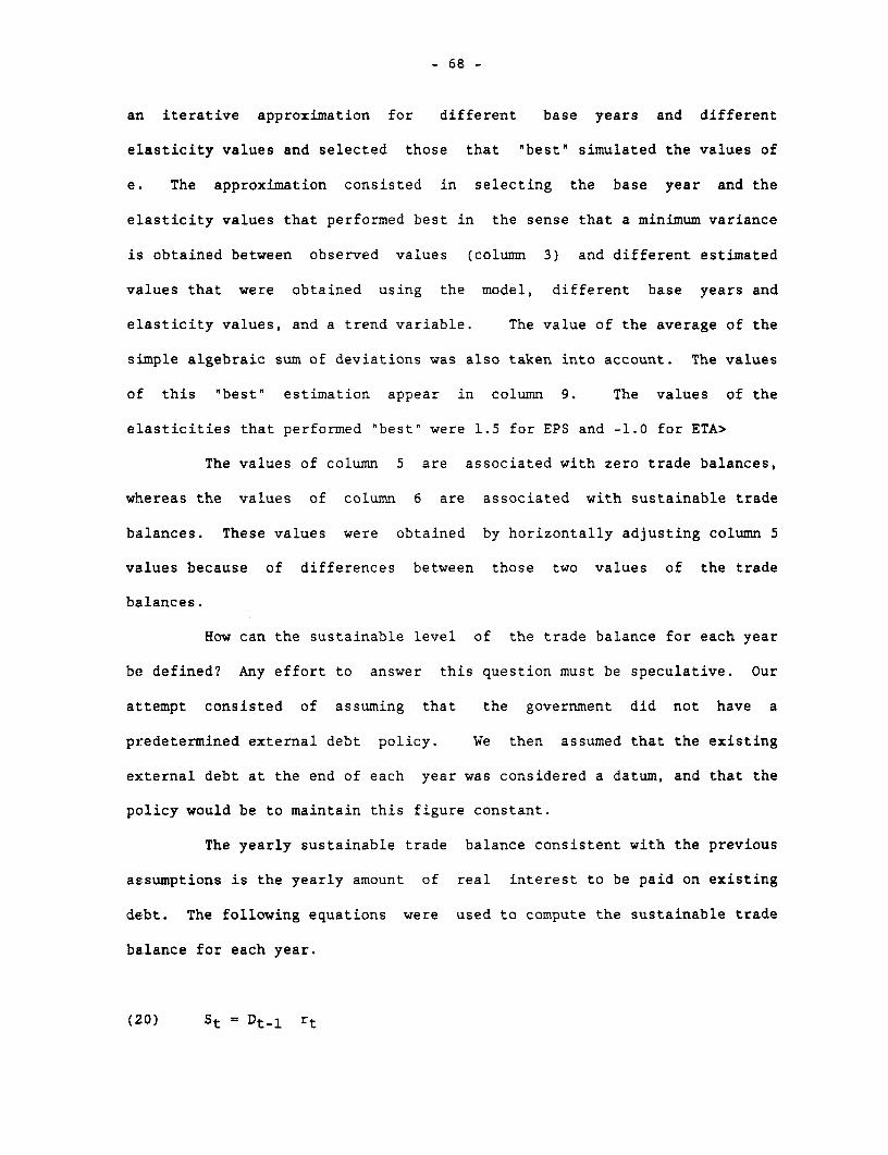
- 68 -

an iterative approximation for different base years and different

elasticity values and selected those that "best' simulated the values of

e. The approximation consisted in selecting the base year and the

elasticity values that performed best in the sense that a minimum variance

is obtained between observed values (column 3) and different estimated

values that were obtained using the model, different base years and

elasticity values, and a trend variable. The value of the average of the

simple algebraic sum of deviations was also taken into account. The values

of this "best" estimation appear in column 9. The values of the

elasticities that performed 'best" were 1.5 for EPS and -1.0 for ETA>

The values of column 5 are associated with zero trade balances,

whereas the values of column 6 are associated with sustainable trade

balances. These values were obtained by horizontally adjusting column 5

values because of differences between those two values of the trade

balances.

How can the sustainable level of the trade balance for each year

be defined? Any effort to answer this question must be speculative. Our

attempt consisted of assuming that the government did not have a

predetermined external debt policy. We then assumed that the existing

external debt at the end of each year was considered a datum, and that the

policy would be to maintain this figure constant.

The yearly sustainable trade balance consistent with the previous

assumptions is the yearly amount of real interest to be paid on existing

debt. The following equations were used to compute the sustainable trade

balance for each year.

(20) St = Dt-l rt

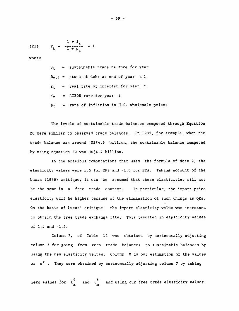
- 69 -

1 + 1

Pt(21) rt -l----- 1

where

St sustainable trade balance for year

Dt_ = stock of debt at end of year t-l

rt = real rate of interest for year t

it LIBOR rate for year t

Pt = rate of inflation in U.S. wholesale prices

The levels of sustainable trade balances computed through Equation

20 were similar to observed trade balances. In 1985, for example, when the

trade balance was around US$4.6 billion, the sustainable balance computed

by using Equation 20 was US$4.4 billion.

In the previous computations that used the formula of Note 2, the

elasticity values were 1.5 for EPS and -1.0 for ETA. Taking account of the

Lucas (1976) critique, it can be assumed that these elasticities will not

be the same in a free trade context. In particular, the import price

elasticity will be higher because of the elimination of such things as QRs.

On the basis of Lucas' critique, the import elasticity value was increased

to obtain the free trade exchange rate. This resulted in elasticity values

of 1.5 and -1.5.

Column 7, of Table 15 was obtained by horizontally adjusting

column 5 for going from zero trade balances to sustainable balances by

using the new elasticity values. Column 8 is our estimation of the values

of e* . They were obtained by horizontally adjusting column 7 by taking

zero values for t and tm and using our free trade elasticity values.x m

Chapter 4

OUTPUT, CONSUMPTION, AND FOREIGN EXCHANGE EFFECTS

In this chapter we compute the effects of intervention on: output

of the six products; the internal consumption of those products; and on

foreign exchange earnings.

Effects on Output

There are two main views on how to distinguish between the short-

run and long-run effects of price intervention. One view is that the

distinction should be based on the terms of trade between agriculture and

the rest of the economy (i.e., PA/PNA)* Long-run effects would be

associated with changes in the allocation of factors between agricultural

and nonagricultural sectors caused by changes in those terms of trade. It

is assumed that such reallocation occurs through movements of capital and

labor. Endogenous changes in technology' should also be included as long-

run effects (i.e., technical changes induced by relative price changes).

The effects of changes in the terms of trade between agriculture

and intermediate inputs--that is, in PA/PI --are considered short-run

effects, though most of PI 's prices are nonagricultural. Therefore, the

short-run effects of intervention on the output of each product would be a

function of their own price, the prices of other agricultural products, and

the prices of intermediate inputs. Long-run effects would be a function of

the relation between the price of each commodity and nonagricultural

prices.

It is also suggested that long-run effects would not be wholly

captured by conventional econometric determination of lon-run elasticities

and that additional computations may be needed through computation of

- 71 -

investment or migration functions, or ideally, through estimation of

dynamic general equilibrium models.

A second approach has been called "comparative-dynamics analysis"

because it traces the effects of policy over time. This approach has been

presented in a Nerlovian distributed lags framework. The lags are

attributed alternatively to adaptive expectations and adjustment costs.

The distinction between short-run and long-run effects here is based on the

passage of time and not on the distinction between effects with or without

reallocation of factors between sectors. Hence, short-run effects are

those taking place during the first period of time, and long-run effects

are those taking place later. However, a short-run effect takes place in

all periods (i.e., the effect of any price change for that period). The

long-run effect will be the effect related to previous price changes.

If it is assumed that intersectoral movements of production

factors will take more time than shifts within the agricultural sector

itself, the two approaches seem very similar. But this assumption is not

true under all circumstances. For instance, a positive change in PA/PNA

may cause a quicker response (e.g., using more labor to improve

cultivation) than a change in Pwheat/Pcorn because of the existence of a

program for seasonal rotation of crops.

We use this second approach, assuming a distributed lags time path

mainly resulting from adjustment costs. This approach is more suitable to

the information available.

General Approach

For the computation of output effects on each of the selected

products we used the following equation

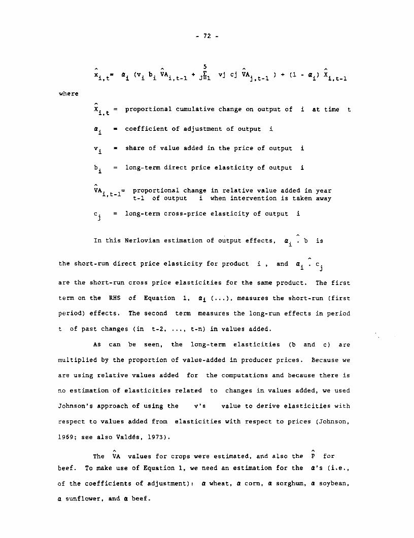
-72-

x = ai (vi bi VA it l + JEl vj cj VAj,t-l ) + (1 - a X

where

Xi.t = proportional cumulative change on output of i at time t

a. = coefficient of adjustment of output i

vi = share of value added in the price of output i

b. = long-term direct price elasticity of output i

VA = proportional change in relative value added in yeari,tl t-l of output i when intervention is taken away

c. = long-term cross-price elasticity of output i

In this Nerlovian estimation of output effects, a. . b is

the short-run direct price elasticity for product i , and a. . c.

are the short-run cross price elasticities for the same product. The first

term on the RHS of Equation 1, ai (...), measures the short-run (first

period) effects. The second term measures the long-run effects in period

t of past changes (in t-2, ... , t-n) in values added.

As can be seen, the long-term elasticities (b and c) are

multiplied by the proportion of value-added in producer prices. Because we

are using relative values added for the computations and because there is

no estimation of elasticities related to changes in values added, we used

Johnson's approach of using the v's value to derive elasticities with

respect to values added from elasticities with respect to prices (Johnson,

1969; see also Valdes, 1973).

The VA values for crops were estimated, and also the P for

beef. To make use of Equation 1, we need an estimation for the a's (i.e.,

of the coefficients of adjustment): a wheat, a corn, a sorghum, a soybean,

a sunflower, and a beef.

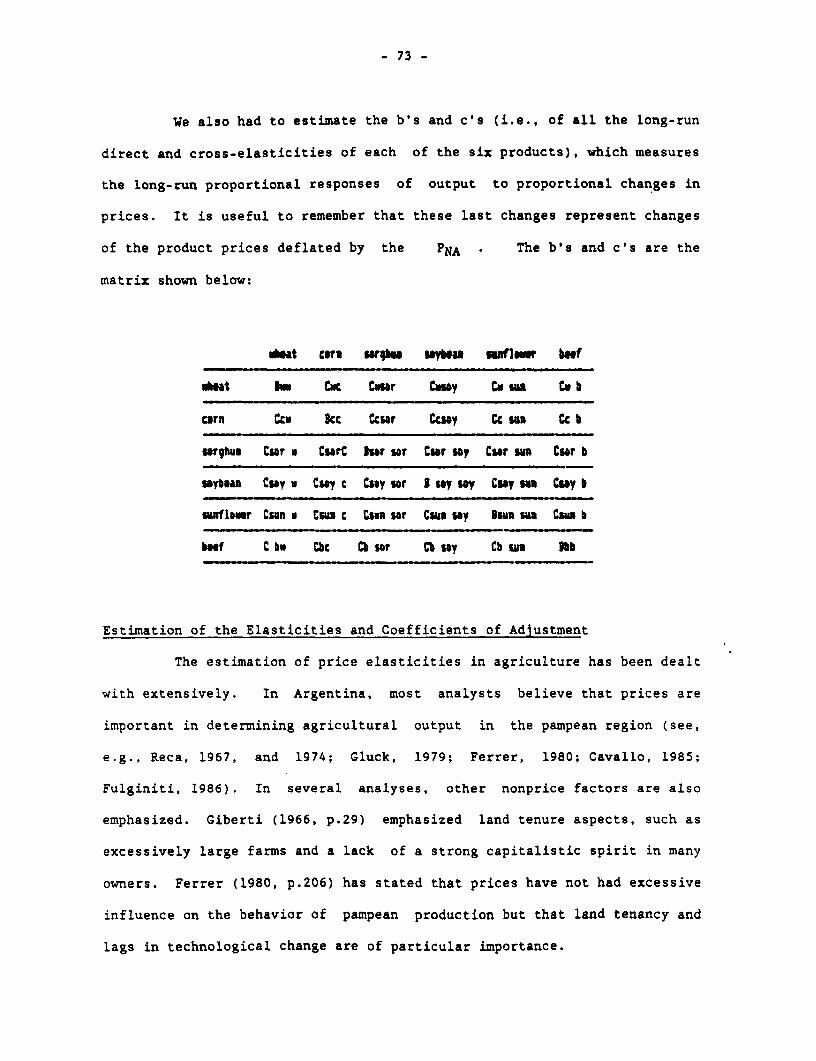
- 73 -

We also had to estimate the b's and c's (i.e., of all the long-run

direct and cross-elasticities of each of the six products), which measures

the long-run proportional responses of output to proportional changes in

prices. It is useful to remember that these last changes represent changes

of the product prices deflated by the PNA * The b's and c's are the

matrix shown below:

isat core Wro u"eba iWleur bf

Mat Om Cue Car Caoy CH so C b

corn Ccu kc Ccst Ccsy Cckse Cc b

ergias Cser a CerC lir sot Cur my Czr un Ci b

myboan Cas y Cas c Csy sor I toy y Csy ow CAy b

sunfdler Czan a Cm c Csu sr Cans say Duln Su Can b

buf Cbe Cbc Cbaso Cb say Cb an Dbb

Estimation of the Elasticities and Coefficients of Adjustment

The estimation of price elasticities in agriculture has been dealt

with extensively. In Argentina, most analysts believe that prices are

important in determining agricultural output in the pampean region (see,

e.g., Reca, 1967, and 1974; Gluck, 1979; Ferrer, 1980; Cavallo, 1985;

Fulginiti, 1986). In several analyses, other nonprice factors are also

emphasized. Giberti (1966, p.29) emphasized land tenure aspects, such as

excessively large farms and a lack of a strong capitalistic spirit in many

owners. Ferrer (1980, p.206) has stated that prices have not had excessive

influence on the behavior of pampean production but that land tenancy and

lags in technological change are of particular importance.

- 74 -

Econometric studies of pampean agriculture usually find that price

response at the product level is very strong--that is, when relative prices

change within the agricultural sector, there are significant changes in the

structure of agricultural production (see, e.g., Reca, 1974). These

results support the view of strongly capitalistic behavior within the

sector. There is clear evidence of such behavior. First, there were

changes in factor proportions between labor and machinery when a

significant change in relative prices between those two inputs occurred in

the 1950s. Moreover, there has been very rapid introduction in almost all

of the sectors of more profitable technologies.

It is important to point out, however, that econometric studies

have also found a much weaker price response for all pampean production

with respect to prices for the rest of the economy. That is, when pampean

prices increased in relation to PNA , output increased but not very

strongly, and when those prices decreased, output decreased but not much,

especially when short-run variations are taken into account.

These results suggest ordinarily some inconsistency. A producer

will react immediately, for example, when the relative price between

soybeans and corn changes in favor of the first, or he will rapidly change

the proportion of hired labor to machinery when the relative price of these

two inputs changes. On the other hand, output reacts weakly and slowly

when agricultural prices change in relation to the price of machinery or

labor, or to nonagricultural prices.

A consistent explanation for both results is provided by Glenn L.

Johnson, which may be called the "fixed assets explanation" (see Hathaway,

1963). The main idea here is that there is a difference between the

acquisition value of most inputs and their salvage value, which is what the

farm operator could get for the input if it were sold rather than used on

- 75 -

the farm. Therefore, many inputs, once acquired, became fixed assets once

they have been incorporated into production up to the point where marginal

returns equal acquisition value. They are not likely to be withdrawn from

use even if agriculture prices fall, causing a decrease in marginal return.

The only options left to the farmers are a low marginal return or

a lower salvage value, which will almost always be less than the

acquisition value.

The degree of asset fixity varies with the nature of the input and

with the reference point. That is, the input's value may be "fixed" for

the agricultural sector but not for an individual farm or a specific

agricultural product.

It is worthwhile to consider some examples. The acquisition value

of perennial fruit trees is the cost of planting and waiting for their

growth, whereas their salvage value will be zero, or even negative, for the

industry and the farm. Therefore, their value will be fixed in relation to

any reference point.

For an experienced farmer, acquisition value may be associated

with marginal return, whereas salvage value will be a marginal return out

of agriculture. Therefore, asset value will be fixed for the industry,

movable for the farm, and more movable between products. A tractor's asset

value will be fixed for the industry and the farm but will be very movable

at the level of the farm enterprise (i.e., between different farm products,

because the acquisition value will be the same as salvage value).

When acquisition values are more relevant than salvage values--for

instance, in a situation in which agricultural prices are increasing--the

farm (and the industry) will be near equilibrium. In the inverse

situation, the farm (and the industry) will be in disequilibrium, in the

sense that marginal and total returns on fixed inputs will be less than

- 76 -

long-run equilibrium values. In the long run, of course, only acquisition

values will be relevant since almost all inputs are movable. In the long

run, only equilibrium will prevail.

What happens in the case of rising agricultural prices? If the

sector is at disequilibrium (i.e., if marginal returns to fixed assets are

closer to salvage values than to acquisition values), output will respond

weakly to prices. If the sector is close to equilibrium, the response of

output to prices may be stronger. In this case, the degrees of stability

that the farm operator assigns to new prices will be important. If

stability seems low (and presumably it will be low when prices are

volatile), the response will be weak. Given the fixed nature of inputs,

optimization will only occur within a long-run horizon, and the returns

below equilibrium that will be experienced by fixed inputs during periods

of low agricultural prices will be taken into account. In any case,

relative price changes within the sector will cause strong supply

responses.

To summarize, we may say that there is clear evidence of strong

and extended capitalistic behavior in the pampean agricultural sector.

Cross-responses to relative prices within the sector are strong. The fixed

assets approach rationalizes the consistency of capitalistic behavior with

weak price responses for the whole pampean output in the short run and even

in the medium run. Fourth, the previous point does not imply that these

price responses will be nil, because there are several inputs that are

movable even in the short run, or are only weakly "fixed,, such as

fertilizer, agrochemicals, gas-oil, marginal land (with near-zero rent),

tractor hours, and hired labor. In equilibrium situations with reasonable

stability in prices, there will be normal supply responses to price

increases. Endogenous technological adjustments without fixed

- 77 -

characteristics may also support a normal supply response over the short

run.

Some Empirical Evidence

In this sector we review empirical evidence on the problem of

supply response of pampean production. Four types of empirical studies are

discussed:

1. Fulginiti's results, obtained through a multiple-equation

approach.

2. The results obtained by various authors who used single-

equation approaches.

3. The Cavallo-Mundlak results, obtained through a dynamic

general equilibrium approach.

4. Our results, obtained through a single-equation approach.

Fulginiti's (1986) study is a multiple-equation supply model

including our six products and linseed. The period covered is 1940-80.

Output supply functions and factor demand functions are based on the

necessary conditions for maximization of a profit function applying duality

theorems (Diewert, 1974). It is assumed that the functions for all outputs

and inputs are interrelated by common dependence on production

possibilities and the farm's objectives. In Table 16 appear all the direct

and cross-elasticities obtained by Fulginiti.

On the whole, the results are rather good, although many parameter

values are not significant. Several results are unsatisfactory however.

The values of the linseed column are unsatisfactory because they are too

high. It is stated, for example, that a decrease of 20 percent in the

price of linseed would increase production of wheat by 34 percent, which is

not reasonable.

- 78 -

Furthermore, the output results of Table 17 appear to be too

large. These results are mainly caused by the high levels of parameters

Ei,c, Ei,l, and Ei,o, and hence the very high value of Ei, PNA . With the

exception of soybeans, values for the Ei, PNA are around 2, which means

that a 10 percent decrease in the price of capital, labor, and other inputs

such that it should be implying an approximate equal decrease in PNA

(because this implication is the reason for our previous assumption), will

increase production 20 percent. This seems too high.

Gluck (1979) reviewed various single-equation studies on

agricultural supply. Most of these studies were done within a Nerlovian

structure. The more significant results are related to the entire

agricultural supply, to the entire pampean output, and to individual crops,

such as wheat and corn. Most of the studies cover periods prior to 1960,

although some extended to 1974.

Gluck found the following:

o Short- and long-run elasticities of total agricultural supply

were between 0.30 and 0.50, and between 0.60 and 0.85,

respectively. A coefficient of adjustment of around 0.60 is

implied by these results.

o Short-run elasticities for total crop supply (long-run

elasticities were not obtained) were a bit larger, between

0.40 and 0.50. Gluck explained that this was not because of a

difference in long-run elasticities between crops and

livestock production but because of slower reactions in

livestock output.

o The supply responses for wheat and corn are strong, especially

for corn; there were several long-run direct elasticities

greater than 3.

- 79 -

Cavallo (1985) estimated the supply response of total agricultural

output using Mundlak's dynamic general equilibrium approach, with explicit

modeling of sectoral resource allocation and endogenous productivity

changes. The study covered a period of more than 20 years, ending in the

first half of the 1970s. The results are presented in Table 18. It can be

observed that short-run output elasticity appears very low (0.08), whereas

long-run elasticity (for instance, after 10 years) had similar values to

those in the studies reviewed by Gluck (0.78), thus implying a much slower

adjustment process. Intersectoral labor movements are almost nil in

Cavallo and Mundlak, whereas they are strong in Fulginiti.

Using a single-equation approach, the present author made several

estimations using our own data for the period 1961-85 and for two

subperiods, 1961-74 and 1975-85, both at the product level and for all

crops together. A few statistically good results were obtained only for

the first subperiod--that is, significant responses to prices for corn and

for all crops combined. Results for the whole period, and especially for

the second subperiod, were not satisfactory either at the product or

overall levels. As a sample of our results we include in Table 19 three

regressions of price response for total crops with respect to Pcrops/PNA,

We assume that the following four factors account for our

unsatisfactory results.

First, we used simple econometrics. A multiple-equation approach

might have given better results.

Second, several explanatory variables were not included because of

time costs or difficulties in measurement. The trend variable does not

seem to have captured the effects of excluded variables, such as climate.

It is not easy to get a good measure of this variable for every pampean

subregion. The last decade has been a humid one, and that fact was

- 80 -

probably captured by the trend variable. However, the exclusion of a

variable for measuring yearly variations in climate during the second

subperiod may have been an important shortcoming.

The trend variable should have captured most of another factor,

namely exogenous technological change, but there probably has been some

discontinuity in such change that prevents full representation of it

through a trend variable.

Although exogenous technical change is a feasible explanation for

the consistency of output growth despite the negative trend in relative

prices, one could ask whether the technical change was really exogenous or

whether it is possible that it took place on account of lower prices or a

squeeze on agricultural rent. Nonexogeneity within a context of lower

prices would imply a lesser degree of capitalistic behavior in pampean

agriculture.

The fixed assets approach may offer another explanation for the

poor results. After 1974, relative prices became more volatile, and the

fixed assets approach suggests that output responded weakly to prices.

Greater volatility in relative prices may also mean that it became more

difficult to model the response of supply to price because it is difficult

to determine-how price expectations are created.

This review of the main empirical evidence on agricultural output

response to prices indicates that results that can be accepted with

confidence are lacking. We believe that deeper analyses are required.

Even with better analyses and good results on price elasticities, doubts

will remain on whether such elasticities will be the same with a different

set of policies.

_ 81 -

The Procedure Used to Estimate Effects on Output

Here, we describe the procedure used to estimate the effects of

intervention on output. Our procedure, though much less systematic and

complete, is similar to Fulginiti's. We assume rationality and

capitalistic behavior in the agricultural sector, and therefore the

existence of a variable profit function (Diewert 1974) that is maximized by

the "producer' (the agricultural sector). The variable profit function

(Diewert):

(2) X(P; V)

depends on the vector of variable quantity prices P and on the vector of

fixed inputs V. The vector P pertains to the prices of variable outputs

and variable inputs. Because of a lack of information, all variable inputs

are combined into one variable input. Its price is PNA In this sense,

Equation 2 is

W(Pw, Pc' Psor Psoy Psun' Pb PNA; V)

Outputs and inputs are called variable because of the existence of

the vector of fixed inputs, V , which is the fixed agronomical conditions

for agricultural production, such as soil conditions, rain fall, and

sunlight.

Note that i(P; V) can be increasing (in output prices) or

decreasing (in input prices) with respect to the components of vector P.

Diewert specifies several conditions for T(P;V). One is that it

is positive homogenous of degree one in P; that is, for every B > O ,

r(B P;V) = 8 i(P;V). We also assume that f(P;V) will be twice

- 82 -

differentiable with respect to variable quantity prices. Then, by

Hotelling's lemma (Diewert, p. 137), we have 67(P*; V*)/6pi = Xi (P*; V*).

Xi is the profit-maximizing amount of output i , or of input i if Xi

is less than 0 , given prices P* and fixed inputs V*).

Also, there will be the symmetrical result:

52 62f(3) 6T6T 6r767

Opi Opi Dpi Opi

6x. 6x.(3') 1 = ]

The homogeneity and the symmetrical results are then imposed as

restrictions on the elasticity matrix used later in estimating output

effects.

The homogeneity of degree zero of the supply functions xj means

that if all prices P* increase in the same proportion, output will remain

constant. In terms of price elasticities this implies that

E Ex. P. = 0 , for all j (i = wheat, corn, sorghum, soybean,i 3 sunflower, beef, and NA).

or, for our case

(4) Exjpw xjpc xjpsor xjpsoy xpjsun xjpb xjpNA °

for all j = wheat, corn, sorghum, soybean, sunflower, and beef.

The symmetrical condition imposes restrictions between cross-

elasticities. For instance, taking any two products j,

6Xw . pc 6Xc<.>pxExwpc = -pc Xw , and Excpw = 5- Xc

or

6Xw Xw 5Xc Xcspc = Exwpc. p and =Excpw _

-83 -

Now, using Equation 3'

6Xw 6Xc6_ _ = a_ _

we get

(5) E = E pcXcxwpc xcpw -- X-

The homogeneity condition (Equation 4) and the symmetrical

condition (Equation 5) constitute one of the three main elements used later

to obtain an elasticity matrix.

The most important elasticity values are ExjpNA for the six

products. These values, which measure how output of each of the products

responds to changes in relative prices between agriculture and

nonagriculture, are the most relevant for determining the output effects of

price intervention against agriculture, especially because the effects of

intervention have been very uniform across products. The main effect of

intervention has been to change relative prices between the agricultural

and nonagricultural sectors, and not between agricultural products.

The most acceptable empirical results for our purposes are those

reviewed by Gluck for all agricultural supply, and those of Cavallo and

Mundlak. In the first case, the long-run elasticity is between 0.60 and

0.85. In the second, if we consider the long run as ten years, the value

is 0.78.

Two points merit consideration here, however. First, those values

refer to all agriculture. Are we going to use the same value for each

product? Actually, we must do so, because there is no reasonable

alternative. Any errors are probably not very large, since our five plant

crops are very similar and there is no clear reason why beef should have a

different value. The second point is whether it is correct to use the

empirical results for all of agriculture for only one part of the sector

- 84 -

--that is, for the pampas. Those results measure changes in the

utilization of intermediate inputs, labor, capital, and marginal land (and

endogenous technical change) for the whole sector, whereas we are

discussing only a subsector. Therefore, movements of factors between

pampean and nonpampean agriculture are not considered. In other words, our

values should be larger than those obtained for the whole sector.1 We

decided to use a value of 0.75--that is, within the range given by the

empirical evidence for all of agriculture--partly because movements of

factors between pampean and nonpampean production are probably not very

extensive but mainly because it appears to be a reasonable value, as shown

by a feasibility analysis made later in this paper.

Previous studies also gave us some data on direct price

elasticities. In relation to wheat, statistically acceptable results (see

Gluck, 1979) estimate a long-run direct elasticity of land used for this

product of between 0.53 and 1.78. Because many other results are not

statistically significant, the true value is probably closer to the

smallest one. On the other hand, because we are estimating output effects,

the elasticity should be greater than those values. We decided to locate

the value of this elasticity between those two values. This was consistent

with the 0.75 value associated with variations in PNA and a crude

estimation of cross-elasticities for wheat based on agronomical relations.

In relation to corn, several acceptable results gave larger values

for elasticity of land used than for wheat. Taking account of these

results and the strong substitution relations that exist between corn and

the other products, we assigned corn a larger direct price long-run

elasticity than wheat.

1/ This may explain why Fulginiti's results are larger.

- 85 -

With regard to sorghum, soybean, and sunflowers, previous studies

are of almost no help. For sorghum and sunflowers, strong substitution

relations were assumed, and therefore direct price long-run elasticities

were assumed to be high. In the case of soybeans, a strong complementarity

relation with wheat suggested a much lower direct elasticity.

Previous studies also have permitted assigning an approximate

value for direct elasticity for beef. Cavallo and Mundlak estimated a

cross-price elasticity of -0.31 for using land cultivated with crops as a

function of the price of livestock. We used this estimation, together with

the 0.75 value, to determine a direct price elasticity for beef of 1.06.

On account of agronomical relations, a value of 0.31 was assigned to each

of the five plant crops.

The third element used for estimation of the elasticity matrix was

qualitative (mainly agronomical) relations of substitution and

complementarity between the six products. As pointed out above, those

relations were used for estimating approximate values for cross-

elasticities and, accompanied by the homogeneity and the symmetry

conditions and the 0.75 value, were also used to approximate some direct

elasticities.

The last parameters needed were coefficients of adjustment, one

for each of the six products. Again, the relevant empirical evidence is

that of Cavallo and Mundlak and that of Gluck referring to agriculture as

an aggregate. One would assume that the coefficients of adjustment are

larger at the level of individual products than at the aggregate level

because of cross-effects between products. However, there were two reasons

why we based our selection of coefficients by taking account of the

aggregate evidence. First, adequate information does not exist at the

product level. Second, intervention has tended to change prices between

- 86 -

sectors much more than to change prices within the agricultural sector.

Therefore, eliminating intervention will change relative prices among

agricultural products to some degree, but it will mainly change relative

prices between agriculture and nonagriculture. For this reason, the

aggregate results are probably the most relevant in discussing the

political economy of agricultural prices.

In Gluck's review the coefficient of adjustment is around 0.60.

In Cavallo and Mundlak the adjustment is much lower. We decided to use

0.50 for all five crops and 0.40 for beef because it is generally

recognized that production adjustment in beef is slower. These values,

together with the 0.75 value, imply short-run elasticities with respect to

PNA of 0.37 for the five crops and 0.30 for beef. The rather low values

of these short-run elasticities seem compatible with the fixed asset

approach, discussed above.

Comments on Cross-Supply Price Elasticities

Almost 22 million of Argentina's 58.5 million hectares of arable

land have soils in Classes I and II. These soils are deep, well drained,

and easily worked. They are apt to retain moisture and are well supplied

with nutritious elements. Erosion is minimal, and the mild climate

contributes to the production of several crops. Almost 80 percent of the

soils in Classes I and II are in the pampean region. There, conditions

permit the use of efficient production systems that are characterized by:

(1) flexible production that allow shifts from wheat to forage crops and

from forage crops to oilseeds, depending on the profitability of each crop;

(2) rotation between crops and livestock, which increases the fertility of

soils by incorporating nitrogen that revives the physical conditions of the

soil during the livestock period; and double-cropping, possible because

mild winters permit cultivation of soybeans or sunflowers after wheat, for

example.

- 87 -

These characteristics lead to different rates of crop substitution

and therefore to different own- and cross-elasticity among the various

commodities.

Cross-elasticity between livestock and crop. In the long run, because of

rotation of crops and livestock, there is some degree of complementarity

between them. Forages are only one of the products of pastures. Other

important aspects of pastures are enhanced nitrogen, better physical

condition, erosion control, and direct and indirect contributions to yields

of subsequent grain crops. Therefore, some land should be cultivated for

pasture even if a direct return is not realized. Returns may increase by

enlarging the forage area as long as legumes or grasses are complementary

to grains.

However, competition for land between various kinds of crops also

exists. The more pasture, the smaller the output of grains possible within

a given year, since the effect of rotation is only reflected in grain

yields over a period of years.

We think that on the whole, the substitution effect is larger than

the complementarity effect. As noted, Cavallo and Mundlak (1982) found a

long-run price elasticity of -0.31 for the response of area planted with

grains to the price ratio of livestock to crops.

Obviously, cross-elasticities between livestock and individual

crops are different, depending on the production characteristics of each

crop. Livestock and grain sorghum are complements because the stubble and

on occasion the grain are used in feeding livestock. Therefore, we can

expect some positive cross-elasticity between livestock and grain sorghum.

A system similar to grazing livestock on stubble of sorghum is

practiced for corn and wheat, but they are less important. It is estimated

- 88 -

that the complementarity effect between livestock and corn is more than

offset by the substitution effect and that therefore, the cross-elasticity

is negative.

Because there is no complementarity between the production of

livestock and the oilseed grains (sunflower and soybean), the negative

substitution effect prevails in the cross-elasticities.

Cross-elasticity between oilseed grains and cereals. The possibility of

planting soybeans or sunflowers after wheat has a significant influence on

the cross-elasticities between these products. It is estimated that a

significant proportion of Argentina's soybean area is double-cropped, with

soybeans as the summer crop following winter wheat. In this case, there is

complementarity (the improvement of fertility through the addition of

nitrogen by a legume) and supplementarity (the output of each product can

be increased without sacrifice in the other product) between both crops.

This is responsible for the positive cross-elasticity between soybeans and

wheat.

Soybeans are mainly competitive with sunflowers, corn, and

sorghum. The complementarity effect that soybeans (as a legume) could have

with those grains is more than offset by the substitution effect.

Therefore, the cross-elasticities are assumed to be zero or negative.

It is estimated that the cross-elasticity between sunflowers and

wheat is zero because a change in the price of wheat will change production

of sunflowers in the same direction for sunflowers planted after wheat.

However, for sunflowers planted in the winter or spring, a change in the

price of wheat will lead to a change in the production of sunflowers in the

opposite direction. We assumed that both effects mutually cancel out.

- 89 -

Because of the competition of sunflowers, sorghum, and corn, high

negative cross-elasticities were expected among these crops.

Comments on the Results

Tables 9 through 12 do not contain any information on the years

before 1960 because the computations of the effects of intervention began

in that year. It was assumed that the effects of intervention on relative

prices or values added prior to 1960 were the same as those of 1960. This

assumption is more satisfactory than to have assumed zero rates of nominal

and effective protection before 1960, since the general pattern of

intervention also prevailed before 1960.

Equation 1 computes proportional changes in production for each

year and product, changes that are applied to the volumes of observed

production shown in Table B.55.

Supply elasticities are shown in Table B.56, which has two

elasticity matrixes. The second one gives the elasticity values applied to

the period 1977-85. In this period, soybeans were a significant crop and

sunflowers can be considered a fully tradable product. For the period

1960-76, however, soybeans and sunflowers were considered to be purely

domestic products. As can be seen in the first matrix, the rows and

columns for soybeans and sunflowers have values of zero. Soybean

production was nonexistent during the period. For sunflowers we made the

simplified assumption that production would have remained constant without

intervention or (what is an equivalent assumption for a home good) that

there was completely inelastic demand. Eliminating intervention would have

shifted upwards (to the left) the supply curve of sunflower production,

while exports of sunflower seed oil would have decreased. We assume that

intervention would have prevented this through a reduction in export taxes

on edible oils.

- 90 - ,

As can be seen by comparing the two elasticity matrixes,

eliminating a competitive product reduces direct supply elasticity.

Eliminating a complementary product (soybeans) increases the direct supply

elasticity of wheat. The direct supply elasticity of beef does not change

because for both periods the two relevant "exogenous" pieces of information

were maintained (i.e., the -0.31 and the 0.75 values).

We continue by explaining how the two matrixes were filled in by

using the second period. The first thing to observe is the seventh column

of the matrix, with the same 0.75 value for the six rows. These values

estimate the long-run elasticity of agricultural products in relation to

changes in the terms of trade between agriculture and nonagriculture. We

can consider the 0.75 value as "exogenous" information for building the

matrix. We then have a square six-by-six matrix and need an estimation of

thirty-six values (all direct and cross-price elasticities for the six

products). On these thirty-six unknowns the following restrictions helped

fill up the matrix: Six on account of homogeneity of degree zero (see

Equation 4); fifteen on account of symmetry conditions (see Equation 5);

one on account of the equation, Ebw + Ebc + Ebsor + Ebsoy + Ebsun = -0.31;

Two on account of approximate values obtained from Gluck's review for

direct price elasticities for wheat and corn; and one on account of

assuming independence between wheat and sunflowers.

For the symmetry equations, the average value of production, one

for each product and each of the two periods, was used to compute the

coefficients that relate any two cross-elasticities.

A first step to fill in the matrix consisted in using some of the

above 25 restrictions. This step had quantitative support from previous

studies, and it is clear that it allowed the determination of the main

elasticity values as direct price elasticities for the three principal

- 91 -

products, wheat, corn, and beef (that of beef on account of the 0.75 and

-0.31 values and the homogeneity condition) and the long-run elasticity for

each product with relation to the nonagriculture price (the 0.75 values).

A second step consisted of distributing the -0.31 value between

the five crops, using qualitative complementarity and substitution

relations between each plant crop and beef production.

The final step consisted of a "calibrated" approximation of the

direct elasticities of sorghum, soybean, and sunflowers, and to the cross-

elasticities not yet obtained by using the homegeneity and symmetry

conditions, together with the qualitative agronomical relations of

complementarity and substitution between crops.

The first results appear in Table B.57, where values are shown for

the proportional short-run changes in output if direct intervention had not

existed. The largest change is for wheat in 1975. This occurred because

of a combination of strong direct discrimination against wheat with much

weaker discrimination against some of its substitute products, such as corn

and sorghum, during the previous year. There are several negative output

reactions that are explained through changes in relative prices between the

products and the values of cross-elasticities.

Table B.58 reports the cumulative changes related to direct

intervention. The largest proportional output effect appears for wheat in

1976 because of strong direct discrimination against this product in the

two previous years. The corresponding volumes of production in millions of

tons related to direct intervention are shown in Table B.59.

Tables 20 and 21 show the short-run and cumulative proportional

changes in output if total (direct and indirect) intervention had been

eliminated. The pattern of output effects that emerges from the last table

is very clear. Without intervention, all production would have

- 92 -

significantly increased. This indicates that all six products were

strongly discriminated against. Taking the simple average of proportional

output changes for each product for the whole period, increases of 57

percent for wheat, 40 percent for corn, 59 percent for sorghum, 38 percent

for soybean, 98 percent for sunflowers, and 57 percent for beef are

obtained. These values are not very far from the 0.75 value, indicating

that prices or values added by intervention were only slightly more than

half of those that would have prevailed without intervention. These

results clearly indicate that intervention has mainly discriminated between

agriculture and nonagriculture. Discrimination among agricultural products

themselves has been much weaker.

Table B.60 reports the levels of production in millions of tons

that would have been reached without any intervention. The largest value

for all crops is that of 1982, 69 million tons. The five largest values

for crops appear during the last five years. The largest value for beef is

for 1969, 5 million tons. It is important to remember that the results for

each year depend not only on the level of intervention for that year and

the previous years but also on the level of observed production for that

year.

Comments on the Reasonableness of the Results

The reasonableness of our results may be assessed by comparing

them with those in a detailed study (Oris de Roa, 1984) of the

possibilities for increasing crop production in Argentina.

The Oris de Roa study, for the five-year period 1977-81, included

a detailed estimate of the potential for crop production. This estimate

was based on an increase in the land used for crops and an increase in

yields. Both estimates should be considered rather conservative. The

possibility of using fertilizers was not considered. This decreases the

- 93 -

possibility of making more cultivable land available for crops. Without

fertilizers, rotation between crops and livestock is more necessary, and

crop land availability is reduced. For yields, not considering more

intensive use of fertilizers implies a conservative estimation of

possibilities. The increase in yields was mainly explained by greater use

of capital and agrochemicals, and by generalized use of the most efficient

techniques of production.

It is clear that a comparison of our results with those of Roa

(Table B.61) is satisfactory. When the results refer to the same period

(1977-81), we computed smaller output effects, but when the comparison is

with our final period, we have computed larger effects (14 percent larger).

This last comparison is perhaps more relevant than the first one because of

the nature of potential output of Oris de Roa's estimation.

Although differences appear for each product, they are explained

through specific changes in relative prices between the six products when

eliminating intervention and the values of the cross-elasticities that we

have used.

A second type of control is depicted in Table B.62. The level of

demand for hectares appears consistent with our results for crops for 1981-

85 and the yields estimated for each product by Oris de Roa, although this

demand should be reduced by approximately 3 million hectares because of

double-cropping of wheat and soybeans. Oris de Roa estimated an

availability of 20.6 million hectares. As we have noted, Class I and II

soils amount to 22 million hectares, and almost 30 million hectares have

actually been cultivated for many years. We conclude that in relation to

potential land availability, even for the largest hectares, our results

appear reasonable. On the other hand, results obtained using Fulginiti's

estimation would not pass this test.

- 94 -

Intersectoral movements of labor were not considered by Oris de

Roa. The estimations of Cavallo and Mundlak indicated that the price

elasticity of this input is close to zero in ten years and negative,

although very small, for the 20-year period. Therefore, this input does

not seem to be a limitation for agricultural production and is very

insensitive to price changes. Fulginiti's estimations lead to a different

result.

In relation to capital, Oris de Roa estimates that an increase of

35 percent in agricultural machinery would be needed. The computation made

by Cavallo and Mundlak gave a price elasticity for capital input of greater

than 1 for the ten-year period and greater than 2 for the 2-year period.

Given the price changes we have estimated and the values of the

elasticities, the availability of this input would be much greater than

Oris de Roa's requirement.

Effects on Consumption

There is little information concerning demand elasticities for

agricultural products. The most thorough analysis seems to be by De Janvry

and Muflez (1971). They present a matrix of direct and cross-price

elasticities for agricultural products at the wholesale level. Most of the

direct and cross-elasticities are negligible.

In constructing Table B.64 with demand elasticities we used one

direct elasticity from De Janvry and Nuflez (that of beef). We also

assigned some low values to direct elasticity for wheat (in their study it

is estimated at -0.015) and to direct and cross-elasticities for corn and

sorghum, mainly explained by competition between these two products as

inputs for meat production.

The computations are straightforward (see Table 22 and Tables B.63

to B.67).

- 95 -

Effect on Foreign Exchange Earnings

The effects of the elimination of intervention on foreign exchange

earnings are estimated in Table 23 and in Tables B.68 to B.79.

We estimated changes in the volume and value of exports of each

product when direct and total intervention are eliminated. Those changes

appear in Tables B.71 to B.76. The results in B.76 reflect the increases

in agricultural export values that would have taken place without

intervention. Taking the simple average for the whole period, the value of

export crops would have increased by 103 percent, those of beef by 395

percent, and the total for all products by 198 percent. The stronger

effect on beef exports is because much stronger consumption effects have

been computed for this product than for crops, and also because the

observed relation between exports and production is lower for beef than for

crops.

Next, we estimated the loss in foreign exchange because of the

intermediate inputs required to support the simulated increases in

agricultural output. All of these intermediate inputs were considered

tradables, and no distinction was made related to the alternatives of being

produced domestically or imported. Intermediate inputs were assumed to be

used only for crops, and therefore no estimation of beef production was

made.

Table B.79 shows the estimated net increases in foreign exchange

earnings. We deducted observed exports and the value of foreign exchange

needed to pay for the intermediate inputs required to increase output.

Taking the results for all products and computing a simple average yearly

value of foreign exchange earnings in constant 1985 U.S. dollars gives

$4,254 million. If we take the data for 1985, we see that foreign exchange

earnings of $5,400 million represents 64 percent of the observed value of

- 96 -

total exports, 142 percent of the observed value of total imports, and 167

percent of the observed value of exports of the six products.

Three qualifications should be noted in relation to these

estimations. The first relates to the estimated volume of exports.

Because seeds are an intermediate input, and because we estimated foreign

exchange requirements resulting from increased utilization of intermediate

inputs, the seeds appear to have been imported, whereas it would have been

more correct to reduce exports of some crops on account of additional

domestic seed utilization. In any case, the net gain in foreign exchange

earnings is correctly estimated.

The second qualification is that foreign exchange earnings are

overestimated because increases in nonagricultural imports because of the

removal of tariffs and quantitative restrictions were not computed. On the

other hand, industrial exports probably would have been greater because of

equilibrium devaluation of the currency.

The third qualification is that we assumed that intermediate input

use for additional production was the same that prevailed each year. This

is a strong assumption, given the significant estimated changes in relative

prices between products and intermediate inputs.

Chapter 5

BUDGET AND TRANSFER EFFECTS

The results of our computation of the direct effect on the

government budget of removing intervention in agricultural prices are found

in Table 24, where the loss of fiscal revenues resulting from the removal

of export taxes and subsidies and of import tariffs is shown in current

U.S. dollars. The results are also presented as a percentage of total tax

revenues.

Two main points can be observed in Table 24. First, export taxes

(mainly taxes on agricultural exports) became an increasingly important

source of revenues during the period under study. While such taxes

accounted for 6.6 percent of the government's fiscal resources in 1960-62,

they accounted for 13.0 percent in 1983-85.

Second, import taxes became less important. While they accounted

for 31.7 percent of the government's fiscal resources in 1960-62, they

accounted for only 7.1 percent in 1983-85. It is important to note that

this reduction does not indicate a reduction in direct protection for

import substitution. It only indicates a reduction in explicit protection;

implicit protection remained very high, primarily because of quantitative

restrictions.

Government Investment and Total Expenditure Policy

It was difficult to obtain reliable data on the proportion of

government investment which specifically supports pampean agricultural

development. Investments in roads, railways, and port facilities cannot be

easily disaggregated and assigned to specific economic activities. Public

investment in grain storage facilities and agricultural research and

- 98 -

extension can be traced more easily, but the volume of this investment is

probably much smaller than the specific portion of expenditures on roads,

railways, and port facilities that should be assigned to pampean

agriculture. Therefore, it would be risky to construct indexes of

government investment bias.

Given the data limitations, it would have also been incorrect to

try to obtain results on the evolution of such indexes because it is clear

that nonspecific public expenditures for agriculture have varied from year

to year. For example, at the end of the 1960s there were huge expenditures

for paved roads, most of which were very important for agricultural

production. When the existing stock of unpaved roads was significantly

reduced, expenditures on roads were reallocated to other purposes.

In fact, this example points to other limitations in the

calculation of biases in public expenditures when poor data exist. The

huge expenditures on rural paved roads at the end of the 1960s were

probably correct investment decisions, but when the stock of unpaved roads

was exhausted, such investment had to stop. That is not a "biased" or

incorrect change.

If there has been any bias in public investment policy, it is not

clear whether the bias has been for or against the pampean agricultural

sector. If the bias has been in favor of this sector, it was of minor

importance in neutralizing the strong discrimination that the sector

suffered through the commercial and exchange rate policies.

Provincial and local public investment is of minor importance for

the sector. Therefore, we will concentrate on the national level. Public

investment during our period has been very substantial in electricity, oil

production, communications, roads, and air transport. With the exception

of roads, investment in these sectors was not directly relevant to pampean

- 99 -

agrarian development. Rural electrification and rural telecommunications

are not very important in the pampas, while railways, which are an

important means of transport for crops and cattle, experienced negative

investment.

The only items where it is possible to observe investment clearly

in favor of pampean agriculture are port storage facilities and the

generation and transfer of agricultural technology. To measure the impact

of investment ir port facilities we used public budget data for the last

fourteen years of our period of analysis.

Investment expenditures are distributed among the following

categories:

- Soil

- Agriculture

- Energy

- Mining

-Industry

-Tourism

- Transport

- Communications

- Commerce and Storage

- Finance

We have measured the portions of investment in Soil and

Agriculture and that of Commerce and Storage related to agriculture.

Comparing this data with the total investment of the national

administration we have obtained the following table:

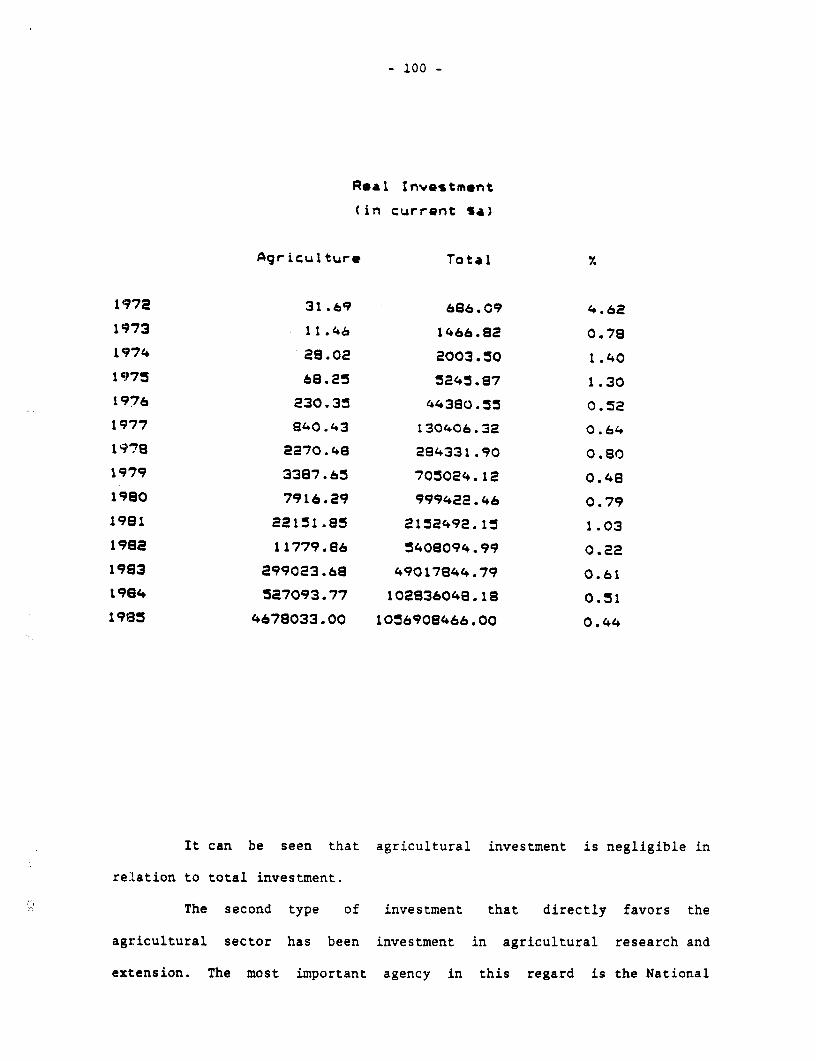
- 100 -

Real Ivestment

(in current Sa)

Agriculture Total r

1972 31.69 686.09 4.62

1973 11.46 1466.82 0.78

1974 28.02 2003.50 1.40

1975 68.25 5245.87 1.30

1976 230.35 44380.55 0.52

1977 e40.43 130406.32 0.'64

i978 2270.46 294331.90 0.80

1 979 33e7.65 705024.12 0.4e

19eo 7916.29 999422.46 0.79

1991 22151.65 2152492.15 1.03

1992 11779.66 5408094.99 0.22

i993 299023.68 49017844.79 0.61

19Q4 527093.77 102836046.i8 0.51

1995 4678033.00 1056908466.00 0.44

It can be seen that agricultural investment is negligible in

relation to total investment.

The second type of investment that directly favors the

agricultural sector has been investment in agricultural research and

extension. The most important agency in this regard is the National

- 101 -

Institute of Agricultural Technology (INTA), a semi-autonomous governmental

organization. INTA has a network of 40 experimental stations, including 13

centers in the major ecological zones of the country. Research findings

produced by these stations are disseminated by 230 extension agencies.

At the federal level, research and extension was financed by an

export tax of around 2 percent during most of the study period. Reca

(1980) estimated the impact of investment on agricultural research and

extension, and concluded: "As a first approximation it could be assumed

that all resources (Federal and State) channeled to research and extension

in agriculture increase the effective protection coefficients by a figure

close to 1 percent, clearly insufficient to compensate for the value taken

away from agriculture by price policies."

The Transfer of Resources between Pampean Agriculture and the

Rest of the Economy

The transfer of resources between pampean agriculture and the rest

of the economy is influenced by price-related and non-price-related

intervention. Here, we compute only the transfers related to price

intervention. As we say earlier, transfers occurring through government

investment have been very modest. On the other hand, it is obvious that

there have been transfers from pampean agriculture, but we do not know of

any study that has found any significant pro or anti-pampean agricultural

bias.

Another instrument for transferring resources between pampean

agriculture and the rest of the economy has been credit policy. As noted

earlier, credit policy has generally implied a transfer in favor of

agriculture, but the transfer has been of minor importance when compared

with the effects of price intervention.

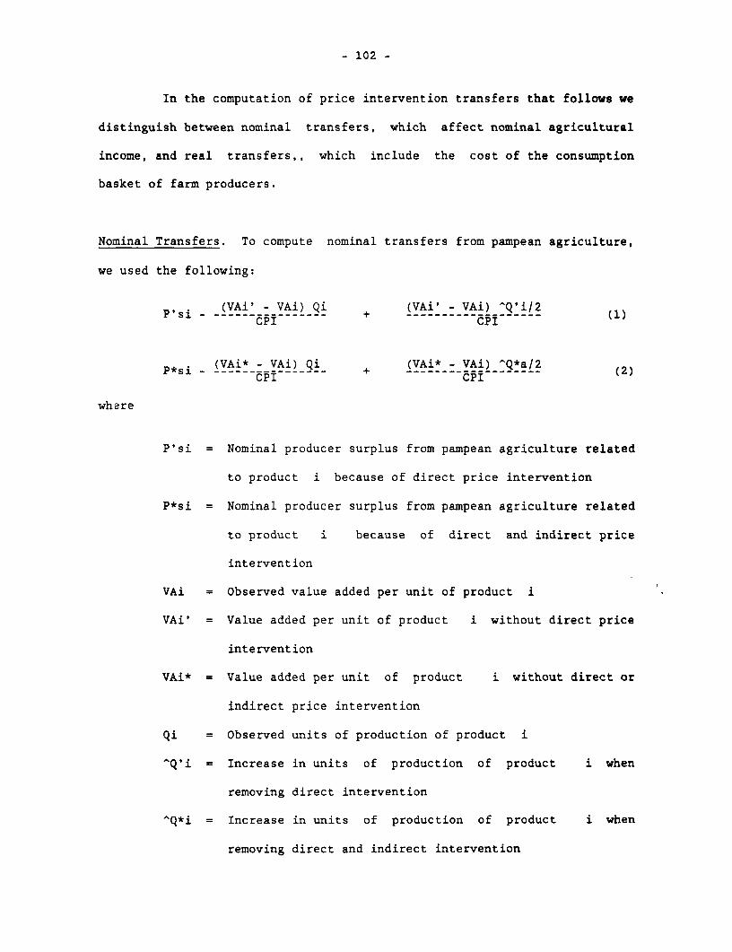
- 102 -

In the computation of price intervention transfers that follows we

distinguish between nominal transfers, which affect nominal agricultural

income, and real transfers,, which include the cost of the consumption

basket of farm producers.

Nominal Transfers. To compute nominal transfers from pampean agriculture,

we used the following:

P,si -(VAi' - VAi) Qi + (VAi' - VAi) ̂ Q'i|2PpI CPI

P*Si - (VAi* - VAi) Qi + (VAi* - VAi) ^Q*a/2 (2)sl ------CPI------- + --------CPI

where

P'si = Nominal producer surplus from pampean agriculture related

to product i because of direct price intervention

P*si = Nominal producer surplus from pampean agriculture related

to product i because of direct and indirect price

intervention

VAi = Observed value added per unit of product i

VAi' = Value added per unit of product i without direct price

intervention

VAi* = Value added per unit of product i without direct or

indirect price intervention

Qi = Observed units of production of product i

^Q'i = Increase in units of production of product i when

removing direct intervention

^Q*i = Increase in units of production of product i when

removing direct and indirect intervention

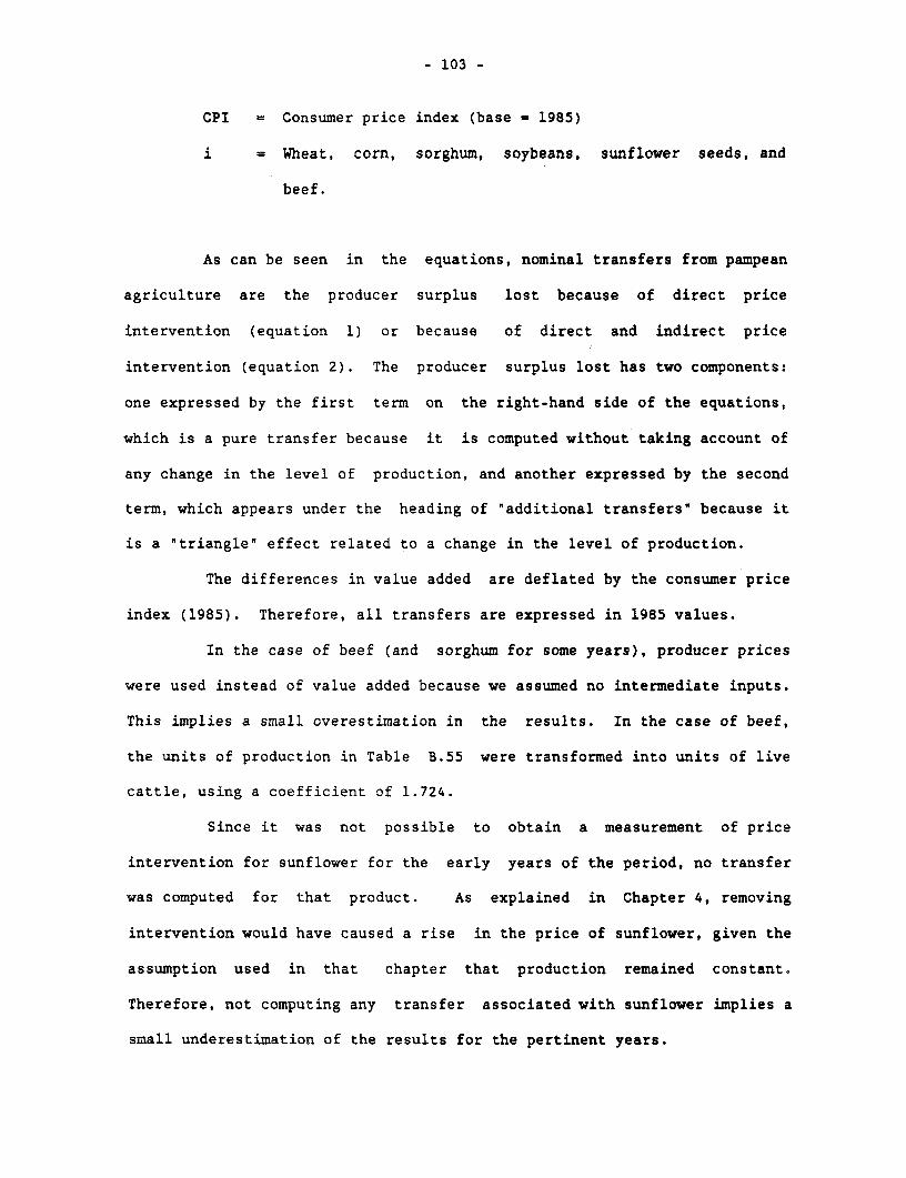
- 103 -

CPI = Consumer price index (base = 1985)

i = Wheat, corn, sorghum, soybeans, sunflower seeds, and

beef.

As can be seen in the equations, nominal transfers from pampean

agriculture are the producer surplus lost because of direct price

intervention (equation 1) or because of direct and indirect price

intervention (equation 2). The producer surplus lost has two components:

one expressed by the first term on the right-hand side of the equations,

which is a pure transfer because it is computed without taking account of

any change in the level of production, and another expressed by the second

term, which appears under the heading of "additional transfers" because it

is a ftriangle' effect related to a change in the level of production.

The differences in value added are deflated by the consumer price

index (1985). Therefore, all transfers are expressed in 1985 values.

In the case of beef (and sorghum for some years), producer prices

were used instead of value added because we assumed no intermediate inputs.

This implies a small overestimation in the results. In the case of beef,

the units of production in Table B.55 were transformed into units of live

cattle, using a coefficient of 1.724.

Since it was not possible to obtain a measurement of price

intervention for sunflower for the early years of the period, no transfer

was computed for that product. As explained in Chapter 4, removing

intervention would have caused a rise in the price of sunflower, given the

assumption used in that chapter that production remained constant.

Therefore, not computing any transfer associated with sunflower implies a

small underestimation of the results for the pertinent years.

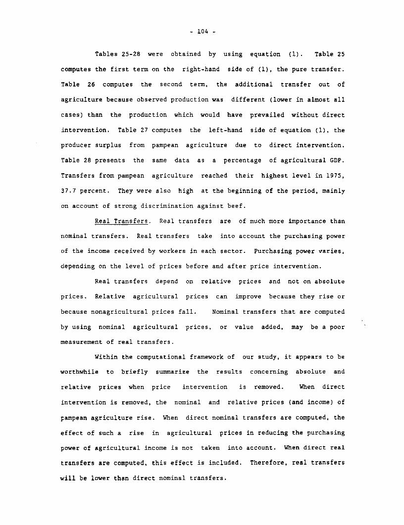
- 104 -

Tables 25-28 were obtained by using equation (1). Table 25

computes the first term on the right-hand side of (1), the pure transfer.

Table 26 computes the second term, the additional transfer out of

agriculture because observed production was different (lower in almost all

cases) than the production which would have prevailed without direct

intervention. Table 27 computes the left-hand side of equation (1), the

producer surplus from pampean agriculture due to direct intervention.

Table 28 presents the same data as a percentage of agricultural GDP.

Transfers from pampean agriculture reached their highest level in 1975,

37.7 percent. They were also high at the beginning of the period, mainly

on account of strong discrimination against beef.

Real Transfers. Real transfers are of much more importance than

nominal transfers. Real transfers take into account the purchasing power

of the income received by workers in each sector. Purchasing power varies,

depending on the level of prices before and after price intervention.

Real transfers depend on relative prices and not on absolute

prices. Relative agricultural prices can improve because they rise or

because nonagricultural prices fall. Nominal transfers that are computed

by using nominal agricultural prices, or value added, may be a poor

measurement of real transfers.

Within the computational framework of our study, it appears to be

worthwhile to briefly summarize the results concerning absolute and

relative prices when price intervention is removed. When direct

intervention is removed, the nominal and relative prices (and income) of

pampean agriculture rise. When direct nominal transfers are computed, the

effect of such a rise in agricultural prices in reducing the purchasing

power of agricultural income is not taken into account. When direct real

transfers are computed, this effect is included. Therefore, real transfers

will be lower than direct nominal transfers.

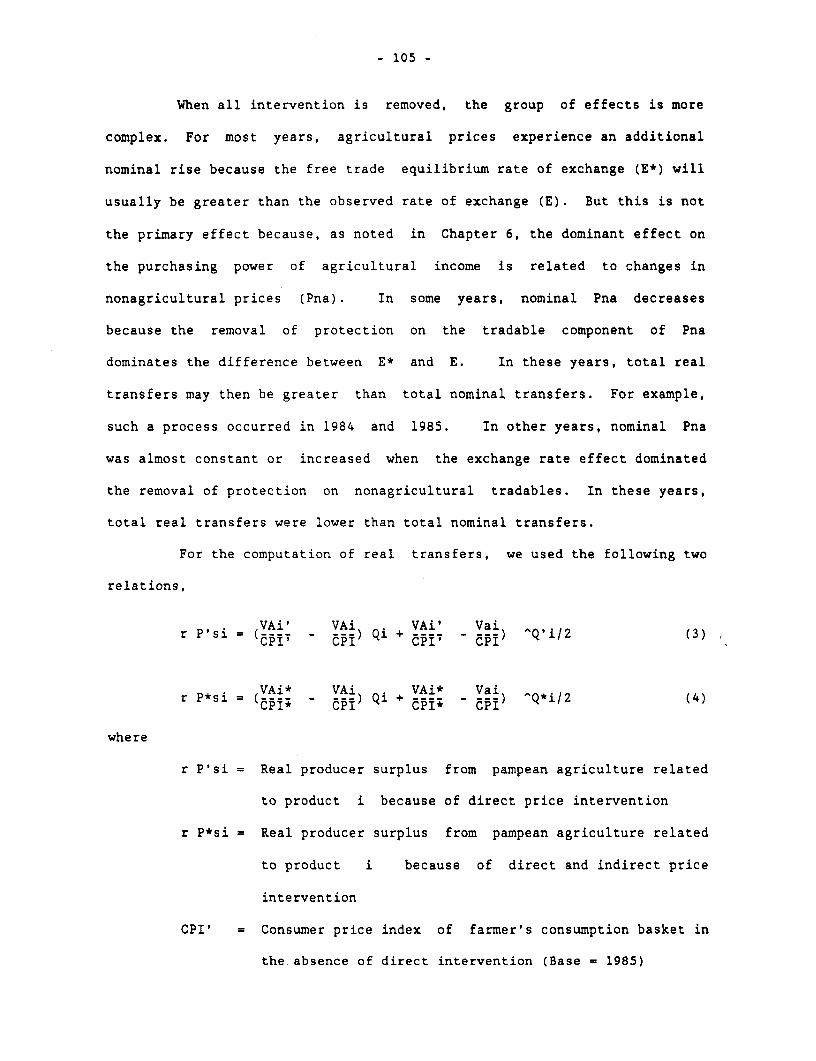
- 105 -

When all intervention is removed, the group of effects is more

complex. For most years, agricultural prices experience an additional

nominal rise because the free trade equilibrium rate of exchange (E*) will

usually be greater than the observed rate of exchange (E). But this is not

the primary effect because, as noted in Chapter 6, the dominant effect on

the purchasing power of agricultural income is related to changes in

nonagricultural prices (Pna). In some years, nominal Pna decreases

because the removal of protection on the tradable component of Pna

dominates the difference between E* and E. In these years, total real

transfers may then be greater than total nominal transfers. For example,

such a process occurred in 1984 and 1985. In other years, nominal Pna

was almost constant or increased when the exchange rate effect dominated

the removal of protection on nonagricultural tradables. In these years,

total real transfers were lower than total nominal transfers.

For the computation of real transfers, we used the following two

relations,

r P'si = YAi' VAi) Qi + VAi' - Vai (3)

VAi* VAi VAi Vai

r P*si = (Yi* VAI) Qi + Y-i* - VaI) ^Q*i/2 (4)

where

r P'si = Real producer surplus from pampean agriculture related

to product i because of direct price intervention

r P*si = Real producer surplus from pampean agriculture related

to product i because of direct and indirect price

intervention

CPI' = Consumer price index of farmer's consumption basket in

the absence of direct intervention (Base = 1985)

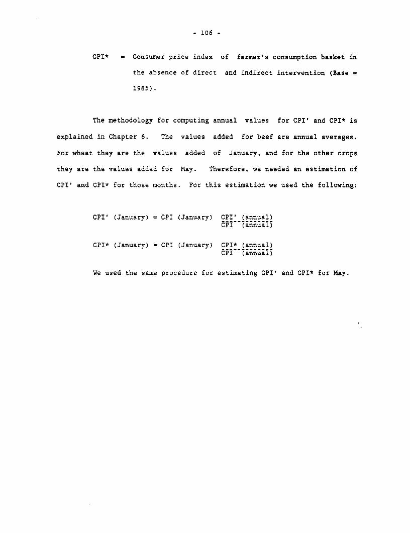
- 106 -

CPI* = Consumer price index of farmer's consumption basket in

the absence of direct and indirect intervention (Base -

1985).

The methodology for computing annual values for CPI' and CPI* is

explained in Chapter 6. The values added for beef are annual averages.

For wheat they are the values added of January, and for the other crops

they are the values added for May. Therefore, we needed an estimation of

CPI and CPI* for those months. For this estimation we used the following:

CPI' (January) = CPI (January) CPI' (annual)cPI (annual)

CPI* (January) = CPI (January) CPI* (annual)WPI (annual)

W.e used the same procedure for estimating CPI' and CPI* for May.

Chapter 6

INCOME DISTRIBUTION EFFECTS

Efforts to determine the distributional impacts of intervention

are seriously limited by a lack of necessary information. Occasionally,

the required data did not exist in any form. Under the circumstances, we

used a substantial number of assumptions in order to obtain a rough

estimation of the income effects of the commercial policies that were

followed.

Social Groups

We chose three large groups representative of society as whole.

Measurement of the effects on the incomes of these groups gives a good idea

about the effects of intervention on society. They are

The rural sector (owners, tenants, and labor); the

urban sector 1 (low and middle-income); and

urban sector 2 (high-income).

Methodology and Assumptions Used

The assumptions are the following:

1. Total real income does not change as a consequence of

intervention.

2. Rural income is only obtained from agricultural activity.

3. The urban sector does not receive any income from agricultural

activity.

4. The proportions of nominal urban income between the two urban

groups do not change.

Total real income is defined as:

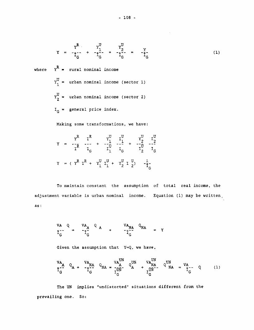
- 108 -

YR y

y =- + G (1)+G G G

Rwhere y = rural nominal income

= urban nominal income (sector 1)

y = urban nominal income (sector 2)2

IG= general price index.

Making some transformations, we have:

yR IR yU IU IU UR 1 1 2 I2

R + U + UTR IG 1 G 2 G

y (yR IR + yU I + yU I U 11 1 2 2 IG

To maintain constant the assumption of total real income, the

adjustment variable is urban nominal income. Equation (1) may be written,

as.

VA Q VAA Q A VANA QNAI-- - -I- ~+ -I--- y

G G G

Given the assumption that Y=Q, we have,

VA VA VA U UN VA UN UA QA + -NA QNA = A QA + -A- Q NA = VA__ (1)

IG IG I ~UN IUN G '~G GN

The UN implies "undistorted" situations different from the

prevailing one. So:

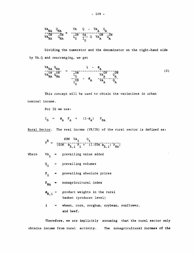
- 109 -

VA A QNA VA Q - VAA QA

VAUN QUN IUN VA_ UN UNVNA~ QNA IG i- VA

G

Dividing the numerator and the denominator on the right-hand side

by VA.Q and rearranging, we get

VNA QNA 1 - aA

UN UN UN UN UN(2VA-A -NA IG VAA QA

UN aA -----------IUN A VAA AG~~~~

This concept will be used to obtain the variations in urban

nominal income.

For IG we use:

I = aA PA + (1-A) PNA

Rural Sector. The real income (YR/IR) of the rural sector is defined as:

{R SUM VA. Qi

(SUM aR,i Pi + (1-SUM aR,i NA

Where VA. = prevailing value added.1

Qi = prevailing volumes

P. = prevailing absolute prices

P = nonagricultural index

aR,i product weights in the rural

basket (producer level)

i = wheat, corn, sorghum, soybean, sunflower,

and beef.

Therefore, we are implicitly assuming that the rural sector only

obtains income from rural activity. The nonagricultural incomes of the

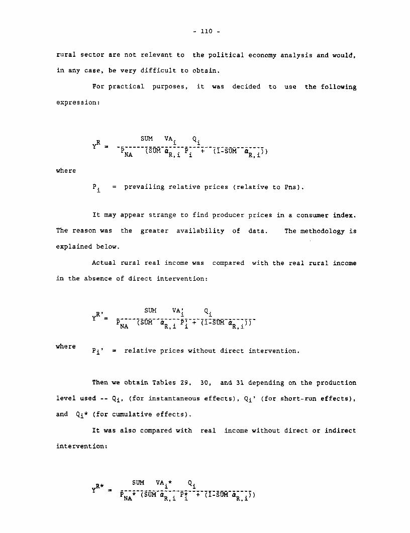
- 110 -

rural sector are not relevant to the political economy analysis and would,

in any case, be very difficult to obtain.

For practical purposes, it was decided to use the following

expression:

R SUM VAi Qiy = ------------------------- 1---------

NA (SUM a P + (1-SUM aR,))NA R,i iRi

where

P. = prevailing relative prices (relative to Pna).

It may appear strange to find producer prices in a consumer index.

The reason was the greater availability of data. The methodology is

explained below.

Actual rural real income was compared with the real rural income

in the absence of direct intervention:

SUM VA! Qiy = ----------------------- 1 ---------

P A (SUM a Pi + (1-S a'NA R,i I +R(-SU

where Pi' = relative prices without direct intervention.

Then we obtain Tables 29, 30, and 31 depending on the production

level used -- Qi. (for instantaneous effects), Qi' (for short-run effects),

and Qi* (for cumulative effects).

It was also compared with real income without direct or indirect

intervention:

YR* SUM VAi* Qi

PNA* (SUM aRi P + (1-SUM aRi))

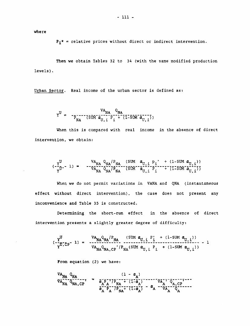
- 111 -

where

Pi* = relative prices without direct or indirect intervention.

Then we obtain Tables 32 to 34 (with the same modified production

levels).

Urban Sector. Real income of the urban sector is defined as:

PY(SUMUVA NA QNA

PNA (SUM AU,i Pi + (1-SUM aU,i))

When this is compared with real income in the absence of direct

intervention, we obtain:

YU V NA QNA/PNA (SUM aU i Pi' + (1-SUM aQ i))( YU 1) NA-QN7P (SUM A P + (1-SUM a ))Y NA NA NA UI I 134

When we do not permit variations in VANA and QNA (instantaneous

effect without direct intervention), the case does not present any

inconvenience and Table 35 is constructed.

Determining the short-run effect in the absence of direct

intervention presents a slightly greater degree of difficulty:

_U VNAQNA/PNA (SUM a Pi + (1-SUM aQ i))_ VN A/N ---- U,i__ i ------ U i -

Y ~~~VANAQNA 'IPNA(SUM a p. + (1-SUM a NA NA,CP / NA( U,i i ( aU,i

From equation (2) we have:

VANA QNA - a)

VAN =NA,CP QAPATNA + (l-aA) VAA' QA,CP'- A NA(IQA) -"A VAA A A A Q

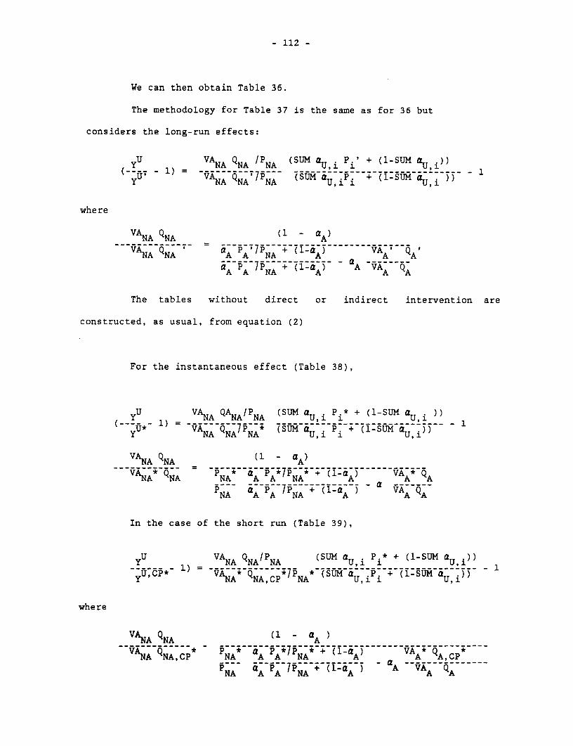
- 112 -

We can then obtain Table 36.

The methodology for Table 37 is the same as for 36 but

considers the long-run effects:

YU 1_ VANA QNA /PNA (SUM aUi Pi' + (1SUM QU,i))

(-YUT ) NA QNA 7 NA (SUM Qu iPi + (1-SUM Ui )

where

VANA QNA (1 - a )

VANA QNA a A PA 7PNA + (1laA) VA A' Q'

----- --- ------- - a --------AA / NA + (-a &) A VAA QA

The tables without direct or indirect intervention are

constructed, as usual, from equation (2)

For the instantaneous effect (Table 38),

YU *V1) A NA QA NAPNA (SUM aU i Pi* + (1-SUM a Ui)U* ~VAAQAANA, Y =--VANA QNA7PNA* (SUM aU. P. + (1-SUM aQU

VNA QNA (1 - QA)VA* * Q N A PAN PNA + (A) aA) VAA*QA

N-------- --NA ~AA NA (Ia AAQ

In the case of the short run (Table 39),

YU VANA QNA/ NA (SUM QU i Pi + (1-SUM QU.

U,Cp* VA * Q-*7- * (1SYU,CP* NA QNA,CP NA UM i + UM i

where

VANA QNA (1 - a )VANA ACP*~~~~~~~~V

ANA QNA,CP NA aA A NA + (l-A QA,CPp A-- 7N ) - A VAA QANA aAPA NA + (l"A A

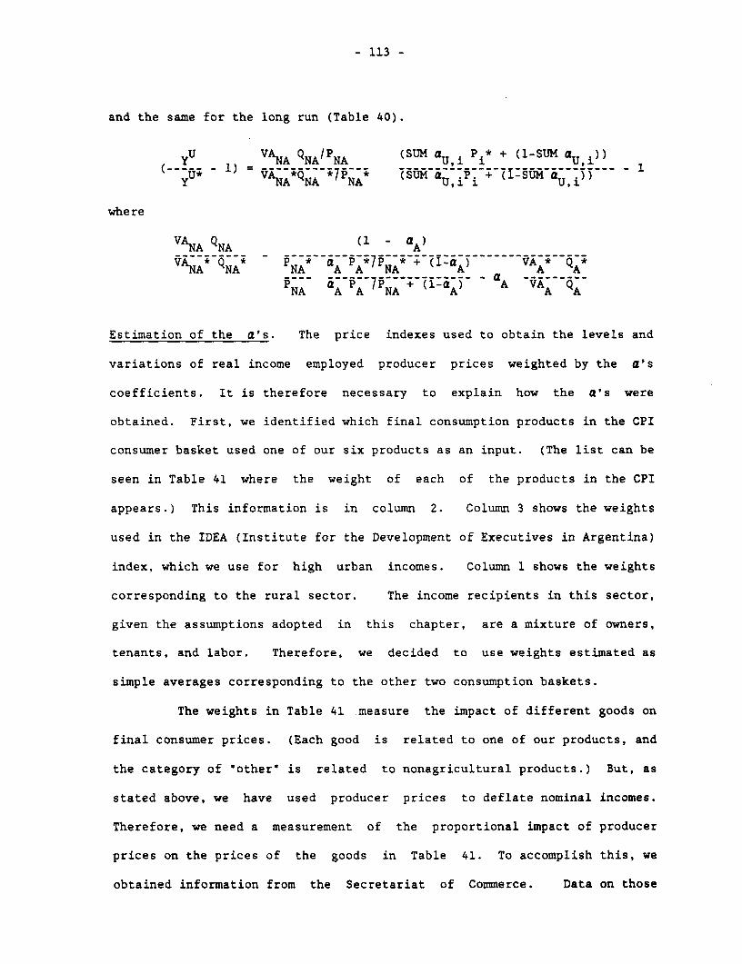
- 113 -

and the same for the long run (Table 40).

VA NA QNA/ NA (SUM aU i Pi* + (1-SUM aU,i))(-Y -1) = --- 1

YNAQNA 7NA (SUM-+ (-1-SUM- Ui)

where

VA NA QNA (1 - A)

VANA* QNA* -NA aA A NA + CiGA) VAA* QA*

NA NA PpA A A VAA QA

Estimation of the a's. The price indexes used to obtain the levels and

variations of real income employed producer prices weighted by the a's

coefficients. It is therefore necessary to explain how the a's were

obtained. First, we identified which final consumption products in the CPI

consumer basket used one of our six products as an input. (The list can be

seen in Table 41 where the weight of each of the products in the CPI

appears.) This information is in column 2. Column 3 shows the weights

used in the IDEA (Institute for the Development of Executives in Argentina)

index, which we use for high urban incomes. Column 1 shows the weights

corresponding to the rural sector. The income recipients in this sector,

given the assumptions adopted in this chapter, are a mixture of owners,

tenants, and labor. Therefore, we decided to use weights estimated as

simple averages corresponding to the other two consumption baskets.

The weights in Table 41 measure the impact of different goods on

final consumer prices. (Each good is related to one of our products, and

the category of "other" is related to nonagricultural products.) But, as

stated above, we have used producer prices to deflate nominal incomes.

Therefore, we need a measurement of the proportional impact of producer

prices on the prices of the goods in Table 41. To accomplish this, we

obtained information from the Secretariat of Commerce. Data on those

- 114 -

impacts is in Table 42. The a coefficients are the value of the Table 41

coefficients times those of Table 42.

Analysis of Results

Direct and indirect intervention both cause an income transfer

from the rural sector to the urban sector. As a consequence of direct

intervention, rural nominal income is reduced 30 to 60 percent (depending

on the time of adjustment). This nominal change is compensated for, in

part, by the consumption effect.

Total intervention adds more discrimination against rural nominal

income. In this case, the consumption effect generally amplifies the

result. The high participation of nonagricultural products in the

consumption basket contributes to this effect.

Urban nominal income is higher under intervention. The percentage

of variations are smaller than the rural variations because the weight of

the rural sector in total real income was only 13 percent during the

period. The impact of the consumption effect on the urban sector is

similar to that on the rural sector.

The results described were as expected. Substantial transfers

from rural to urban income took place that sometimes became higher as a

result of their effects on consumption baskets.

Chapter 7

POLITICAL ECONOMY OF PAMPEAN PRICE DISCRIMINATION

Twentieth-century pampean development is a remarkable case of

growth followed by stagnation. Pampean production grew consistently until

the early 1940s. In the first two decades of the century, when fertile

land was an almost free resource, production grew at a very high rate. In

the next two decades, when the land was already cultivated, it grew at a

more moderate, although significant, rate.

After World War II, sustained growth became sustained stagnation

until the 1970s. During the last 15 years there has again been significant

growth, mainly on account of significant technological advances.

In the prewar period (1909-1939), average yearly production of

cereals and oilseeds was 13.2 million tons, while in the postwar period

(1945-1976) it was only 16 million tons (Mir6 1982). This represents an

increase of only 21 percent. In the period 1960-64, wheat production was

equal to that of 1925-29, while corn production was 33 percent less (Diaz-

Alejandro, 1975).

Stagnation is particularly evident when export performance is

considered. In the prewar period, average annual exports of cereals and

oilseeds was 9.5 million tons, while in the postwar period they reached

only 7.3 million tons (Mir6, 1982).

Pampean growth in the initial decades of the century was due to

the existence of a high positive rent on the margin. Growth then

persisted, encouraged by good prices and technological advances.

- 116 -

The relative prices of pampean agricultural products deteriorated

severely during World War II, however. This decline persisted after the

war as a result of strong discrimination against the sector. In the 1970s,

however, technological advances were able to overcome an additional,

although small, deterioration in relative prices.

Exports of pampean products were low during World War II because

of shortages of ships and other transport facilities. Agricultural prices

fell. On the other hand, industrial prices increased substantially, due to

lack of import competition and increased industrial exports.

After the war the facilities for shipping were reestablished, and

the international prices of pampean products increased significantly. On

the other hand, flows of imports were also reestablished, and Argentina's

industrial exports declined. Without any policy intervention, pampean

agriculture would have become a booming sector, while industry would have

lagged behind because of spending and resource movement effects (see

Corden, 1984).

Those "Dutch disease' effects never took place. The government,

through a highly aggressive external commercial policy, avoided them. This

policy strongly discriminated against the relative prices of agriculture

while protecting industry.

The resource movement effect was into tradables, as in the Dutch

disease case, but in an inverse direction. In that case the movement is

into the nonintervention, booming sector. In the case of Argentina it was

into the nonintervention, lagging sector.

The spending effect in the Argentine case was lower than in a

Dutch disease situation because price discrimination against agricultural

production prevented some income increases. Also different from a typical

Dutch disease situation was that income increases in the booming sector

- 117 -

were taken away through price discrimination, and not through fiscal

instruments. As a result, extra expenses were incurred by the state, by

consumers, and by industrialists. In fact, such extra spending caused

problems that were similar to Dutch disease situations. Argentina became

the scene of an increase in public sector activities, a weakening of the

tax system, and a high level of private consumption. Later, the expansion

of public services and of private consumption proved to be a serious

problem because they were not easily sustainable when the industrial sector

weakened. They were also politically very difficult to cut back.

The postwar experience of policy intervention in Argentina proved

that trying to prevent Dutch disease effects through price and production

disincentives in a potentially booming sector may be very bad medicine.

Postwar growth was disappointing. The import substitution sector provided

the economy with some initial stimulation; since this was the booming

sector and exports were the lagging sector, the economy became very closed.

In 1987, Argentina's share of world trade was eight times smaller than it

was at the beginning of the century.

Quantitative Analysis

In this section we present regression results that provide

quantitative indicators of agricultural price intervention. They also

permit identification of the stabilizing role that direct price

intervention has played.

Observation of Tables 10 and 11 suggests that at least three facts

should be explained:

1. Short-run or annual variations in the rates of direct nominal

protection. The coefficients of variation are wheat, 0.31; corn, 0.25;

sorghum, 0.20; and beef, 0.20.

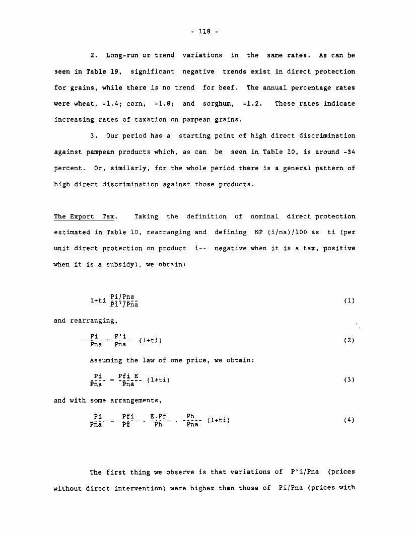
- 118 -

2. Long-run or trend variations in the same rates. As can be

seen in Table 19, significant negative trends exist in direct protection

for grains, while there is no trend for beef. The annual percentage rates

were wheat, -1.4; corn, -1.8; and sorghum, -1.2. These rates indicate

increasing rates of taxation on pampean grains.

3. Our period has a starting point of high direct discrimination

against pampean products which, as can be seen in Table 10, is around -34

percent. Or, similarly, for the whole period there is a general pattern of

high direct discrimination against those products.

The Export Tax. Taking the definition of nominal direct protection

estimated in Table 10, rearranging and defining NP (i/na)/100 as ti (per

unit direct protection on product i-- negative when it is a tax, positive

when it is a subsidy), we obtain:

l+ti Pi/Pna (1)

and rearranging,

Pi P'i__pia = --pn (l+ti) (2)

Assuming the law of one price, we obtain:

Pi PfinE (l+ti

and with some arrangements,

Pi Pfi E.Pf Ph- Pf_ ph Pna_ (l+ti) (4)

The first thing we observe is that variations of P'i/Pna (prices

without direct intervention) were higher than those of Pi/Pna (prices with

- 119 -

direct intervention--i.e., observed prices). The coefficients of

variations were wheat, 0.39 and -0.20; corn, 0.27 and 0.24; sorghum 0.27

and 0.23; beef, 0.27 and 0.23.

These findings suggest that taxes on agricultural exports would

have played a stabilizing role in actual pampean production. If so, a

negative correlation between P'i/Pna and (l+ti) should be found. For

example, if prices rise because a devaluation takes place, the coefficient

of direct protection (l+ti) will decrease, meaning a higher export tax.

In Table 43 we test the possibility of a stabilizing role. We use

equation (4), which separates P'i/Pna into three components: the world

price of the product in relation to the world prices of Argentine tradables

(PfifPf); the observed real rate of exchange (e-EPfIph); and the domestic

relationship between home goods and nonagricultural goods (Ph/Pna), which

depends on implicit tariffs and export taxes or subsidies on nonpampean

tradables and on e. We also use a trend variable to capture long-run

variations in direct protection. In the case of beef, a dummy variable is

included to signify periodic overreactions in the observed prices of beef

caused by what has been called the "cattle cycle."

The results are very satisfactory. It is important to observe the

stability of the coefficients of the relative world price of the product

and of the observed real exchange rate among products. Both variables are

also highly significant. The elasticity of direct protection with respect

to both of those variables is around -0.70.

In Table 44 we present additional regressions, again using

relative prices without direct intervention as the main explanatory

variable but now in its compact form as P'i/Pna. In part a of the table

the explained variable is again the level of the coefficient of direct

protection for any of the four products. In part b the explained

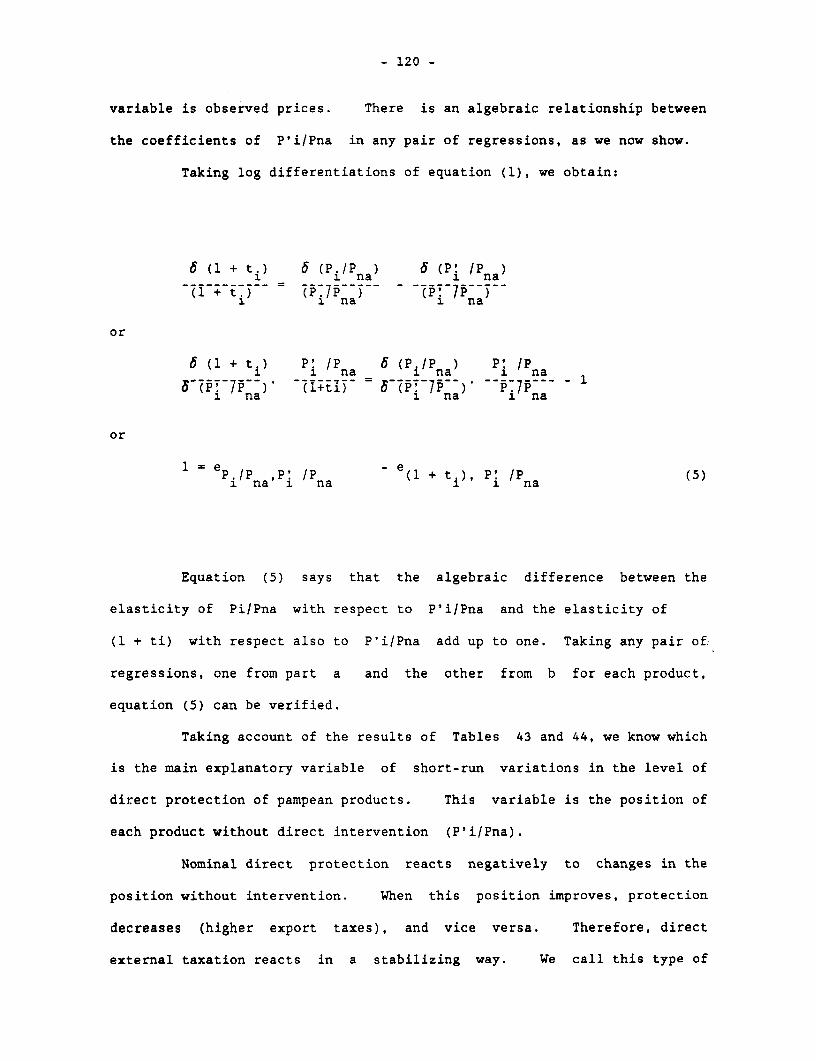
- 120 -

variable is observed prices. There is an algebraic relationship between

the coefficients of P'i/Pna in any pair of regressions, as we now show.

Taking log differentiations of equation (1), we obtain:

6 (1 + t) 6 (Pi/Pna) 6 (P /P

(1 + ti) 1(P/7 ( -Pna)1 1~~ na i na

or

6 (1 + ti) i IP 6 (PIP ) Pi /P1- I n i nna -I na

1 na i na 1na

or

1 = ep / P /P e e( + t.), P! /P(5i na' 1 na I 1 na (5)

Equation (5) says that the algebraic difference between the

elasticity of Pi/Pna with respect to P'i/Pna and the elasticity of

(1 + ti) with respect also to P'i/Pna add up to one. Taking any pair of,

regressions, one from part a and the other from b for each product,

equation (5) can be verified.

Taking account of the results of Tables 43 and 44, we know which

is the main explanatory variable of short-run variations in the level of

direct protection of pampean products. This variable is the position of

each product without direct intervention (P'i/Pna).

Nominal direct protection reacts negatively to changes in the

position without intervention. When this position improves, protection

decreases (higher export taxes), and vice versa. Therefore, direct

external taxation reacts in a stabilizing way. We call this type of

- 121 -

intervention the "conservative export tax." It tries to maintain the

status quo of preexisting relative prices. The neutralization of changes

in these prices is not complete in the short run between changes in

protection and changes in observed relative prices in the same direction of

the change in P'i/Pna. This point will be important in our explanation of

intervention.

We now try to explain long-run variations. This will provide

additional support for the notion of the stabilizing role played by export

taxes. It will also allow for a clearer specification of the nature of

such a role.

In observing Tables 43 and 44, we see that the trend variable is

significant, and its coefficient has negative signs for wheat, -1.4

percent, corn, -1.8 percent, and sorghum, -1.2 percent annually; there is

no trend for beef. To explain these results and, more generally, to

explain the long-run behavior of direct protection, we have to look at the

long-run behavior of observed relative prices and of estimated changes in

the productivity of variable-factors in pampean agriculture, all of which

can be observed in parts a and b of Table 45.

In Table 45, section a, it can be observed that relative prices

show significant negative trends for grains; wheat, -2 percent; corn, -2.7

percent; sorghum, -2.1 percent. In the case of beef, there is also a

negative (although not significant) trend of -1.2 percent. This evolution

in relative prices is associated with negative trends in direct nominal

protection and the fact that relative prices without direct intervention

(P'ilPan) also showed, although weakly, negative trends.

At first, these results lead to doubts about the existence of a

stabilizing long-run role for export taxes. While prices without

intervention showed negative trends, direct nominal protection also showed

- 122 -

negative price trends. Therefore, instead of playing a stabilizing role,

these taxes seem to have played a long-run magnifying role.

But when the results of subsection b of Table 45 are considered,

they provide a clearer specification of the characteristics of export taxes

and provide additional support for the stabilization hypothesis. The

results of subsection b indicate that there have been important increases

in the productivity of pampean inputs. The levels of production for each

product are regressed on three variables: relative prices lagged by one

period, harvested surface, and a trend variable. These regressions attempt

to estimate the long-run rate of variation in the productivity of inputs

independent of price changes. It can be seen that during our period of

analysis there were important increases in exogenous productivity in grain

production: wheat, 2 percent; corn, 3.5 percent; and sorghum, 2.3 percent.

These increases are somewhat stronger than the negative trend in prices,

mainly in corn. In the case of beef, no increase in productivity is

detected, while there is a negative trend in relative prices, although it

is not statistically significant.

We have indicated how intervention discriminated against the

agricultural sector after the war. The above results indicate that

intervention has taxed the most successful products the most. In the cases

of corn, large increases in productivity were followed by a significant

increase in taxation (at 1.8 percent annually; see Table 44). There was no

productivity increase in beef production, however, and no increase in

taxation.

The results tend to indicate that, in fact, export taxes tended to

conserve pampean agricultural income more than pampean agricultural prices

in the long run. In fact, it seems very plausible that relative pampean

agricultural income has declined because the positive differences between

- 123 -

increases in exogenous productivity and decreases in relative prices (nil

in wheat, 0.8 percent in corn, 0.2 percent in sorghum, and probably

negative in beef) were presumably lower than increases in productivity in

the economy as a whole.

Total Nominal Protection

Total nominal protection measures the effects of all intervention

in the trade of pampean products--that is, of direct nominal protection on

the products and of indirect protection on them resulting from direct

nominal protection on all other tradables, and from the real exchange rate

effects of all protection. Then, the only 'exogenous" changes that a

conservative total intervention scheme has to neutralize in order to

stabilize incomes are changes in world relative prices and in exogenous

productivity. Therefore, we include Table 46, which shows the results of

regressing the coefficients of total nominal protection for each product on

two explanatory variables: relative world prices and a trend.

It is worthwhile to observe again the conservative role of

intervention. Increases in the international relative prices of each

product are neutralized by decreases in the coefficients of protection.

The statistical significance of these results is somewhat lower

than those related to direct intervention, but the coefficients of

transmission of the conservative pattern are higher. The extreme case is

sorghum, for which any proportional change in world relative prices is

completely neutralized by a change in total protection.

It can also be seen how total protection neutralizes long-run

changes in productivity. Once again, in the case of corn, total taxation

increased at a rate of 2.1 percent annually, while there was no increase in

the total taxation for beef.

- 124 -

Testing Other Explanatory Variables

Although the previous regression results are very satisfactory, we

discuss here a second regression analysis. The results of this analysis,

shown in Table 47, are not satisfactory. None of the coefficients of the

explanatory variables are significant. The rate of inflation has the wrong

sign for wheat and beef; when inflation is high, direct taxation is

reduced. It is precisely in these two wage goods where a positive sign was

expected--that is, intervention to reduce prices through higher export

taxes. The deficit variables, on the other hand, have the right sign for

wheat, sorghum, and beef; export taxes increase when the deficit rises.

The results related to credit subsidies, although not significant, have the

right sign; export taxes are higher when there are credit subsidies. The

results on income redistribution--that is, with the dummy variable used to

represent two "populist" administrations (the governments of Illia and

Per6n)--are very poor. From Table 9, on prevailing relative prices, we can

see that pampean prices were, in general, higher during these two

administrations than in almost any other.

Three Actors in the Political Economy Mechanism

The Government. The "government' is primarily the executive

branch. Within this branch the functionaries mainly involved in trade

policy have been the president and his economic team: the economics

minister and the treasury, agriculture, domestic trade, industry, and

foreign trade secretaries. There has been a conflict between the interests

of the government and those of the agricultural sector. Within the

economic team this conflict pitted the agriculture secretary against the

economics minister and the treasury and domestic trade secretaries. There

have been two types of agriculture secretaries. One type was more

- 125 -

technically oriented and somewhat independent of sectoral pressures. The

other type served as a representative of sectoral interests. The first

type tried to design policies to reduce conflict. The second served as a

channel for the views of the agrarian lobby.

Nature of the Government. In standard welfare economics, private

firms acting in their self-interest provide goods and services that serve

the utility function of someone in society. Since the conditions for

Pareto optimality are not fully satisfied in any economy without state

intervention, the government's first role is to try to solve the problems

associated with externalities, monopolies, and the provision of public

goods. A second role for the government is associated with the duty of

redistributing income: the goal of maximizing a "social welfare (or public

interest) function" a la Bergson-Samuelson.

A new and more positive approach to government intervention in the

economy is obtaining growing support in contemporary economic theory. In

this approach, two of the three basic assumptions of standard economic

analysis are rejected.

First, in the case of modern pluralistic societies, it is not

assumed that private agents try to maximize their welfare only through the

production and exchange of useful goods and services. Among others, one

additional activity is lobbying, or "the use of resources to obtain

government regulations that enhance the incomes of members of some

particular group in the society by raising the prices of goods they sell,

or by lowering the prices of goods they purchase' (Wellisz and Findlay,

1986).

Also rejected is the idea that public representatives are

completely or primarily altruistic. Instead, government is seen to be

composed of different groups and individuals who seek to maximize their own

- 126 -

gains. Altruistic and public interest motivations are not completely

excluded, but they are given much less weight.

The traditional approach is considered to be appropriate for

normative analysis, but it is not considered to be appropriate for a

positive theory of government intervention. When the existence of pressure

groups and lobbying activities is acknowledged, the remaining assumption of

the standard approach--that decisionmakers have full autonomy--is also

rejected.

Under the new approach, many government interventions are viewed

as equilibrium solutions between the desires of different pressure groups

and the actions of the government in the pursuit of its own objectives.

Limited Autonomy. The limited autonomy of the national government

in Argentina is demonstrated, first, by the fact that regimes have been

very unstable during the period of analysis. No elected president remained

in power for an entire term, and during periods of nonconstitutional

government various groups within the armed forces constantly threatened to

change the leaders of the government. Economic teams were even more

unstable than presidents.

Second, there was a clear and permanent pattern of intervention

(the export tax) during the entire period. If autonomous governments are

assumed, it would appear to be difficult to compatibilize such a sustained

pattern with the existence of frequent change in political institutions.

On the other hand, the constant action of pressure groups has been

pointed out by many authors (see for example, Diaz-Alejandro, 1975, and

Imaz, 1964). This fact is consistent with the sustained pattern of

intervention, and it supports the assertion that the various governments

had only limited autonomy.

- 127 -

Third, agrarian interests have always succeeded in blocking the

introduction of land taxes at the national level, while industrial

interests have sucessfully argued for implicit types of protection that do

not require government revenues, such as quantitative restrictions,

tariffs, or negative protection on tradable inputs. These factors have

produced a tax collection system whose inefficiency clearly implies weak

governments.

A fourth argument in support of the assertion of weak government

is that it is not easy to find an objective for an assumed autonomous

government which, once accomplished by an omnipotent decisionmaker,

resulted in the type of external intervention observed.

Standard welfare economics assumes the existence of objectives

that ensure efficiency and an optimal distribution. In considering the

efficiency objective, it is not possible to explain the existence of

substantial taxation of some tradables and strong protection for others in

a small-country economy. Prohibitive tariffs and quantitative restrictions

have been the main reason for the lack of competition in the Argentinian

economy. It also does not explain the use of tariffs instead of subsidies

to protect industries in order to avoid efficiency costs for consumption;

nor does it explain the neglect of a more Pareto-efficient combination of

land taxes and less price discrimination against pampean products.

Finally, it does not explain short-run variations in direct protection.

One distributional objective must be clearly rejected. It was

assumed that price discrimination against pampean products was used to

improve the income of urban workers. There are two problems in accepting

this objective. First, reductions in export taxes are difficult to

explain. Second, the relative prices of pampean products were generally

higher the more populist the government.

- 128 -

One distributional objective that is compatible with an export tax

is that the government wants to stabilize the division of income between

the agricultural and urban sectors. The problem with this explanation is

that it is difficult to believe that an autonomous government would have

allowed reductions in export taxes only to stabilize pampean income when

such reductions conflicted with much more demanding objectives, such as

price stabilization and fiscal equilibrium. Rejecting a stabilization of

relative income objective also implies rejecting a similar hypothesis,

Corden's idea of the existence of a 'conservative social welfare function"

(Corden, 1978).

Objectives such as price stabilization, fiscal equilibrium, and

external accounts equilibrium were predominant during the period of

analysis. But the objectives of price stability and fiscal equilibrium do

not explain reductions in export taxes, which are both inflationary and

which increase the fiscal deficit. Inflation and fiscal deficits were

persistent problems during the period (see Table 5).

We have noted that shortages of foreign exchange were a recurring

problem during the period of analysis. It is possible to argue that, under

certain assumptions, an export tax will be used to resolve such shortages.

But the problem is that reductions in export taxes were perceived as

irrelevant, if not negative, in attempting to resolve foreign exchange

shortages. There were three arguments for this perception: first, that the

main variable for short-run corrections was the rate of exchange (actually,

export taxes were usually higher when shortages existed because the rate of

exchange was high); second, the short-run elasticity of pampean grain

production was low; and third, there were possible 'perverse' short-run

supply effects in the case of beef.

- 129 -

A search for political objectives produces the same results. For

instance, if the objective of maximizing votes is assumed, it is difficult

to reconcile this objective with the short- and long-run variations in

export taxes. Reducing inflation was usually the best way to obtain more

votes.

In the Triannual Plan for National Reconstruction and Liberation

it is found that agricultural prices 'should hold a stable relation with

non-agricultural prices, avoiding sudden income transfers between sectors

which affect industrial development and the level of welfare of the people"

(Mir6, 1982); and also that "price stability is a key objective of this

policy. Then it will be tried that internal prices get unlinked to

variations in world prices..."

The National Agricultural Program (PRONAGRO) (Secretaria de

Agricultura, 1985) states:

In this sense, a stabilization of agricultural prices will be

promoted through a flexible policy of export taxes in order to

regulate variations that the country, as a price taker, does not

control. The flexible use of export taxes means using them as an

instrument of incomes policy for the sector and avoiding their

utilization for only fiscal purposes.

It is very tempting to conclude that a clear explanation of the

export tax is the confluence of an autonomous decisionmaker and explicit

policies of agricultural price stabilization. We disagree with such a

conclusion. First, these policies were not permanent. For instance, they

were not explicitly recognized during the Martinez de Hoz (1976-80)

administration.

Second there was a chronic conflict between economic policymakers

and the agricultural sector. The policies described above were implemented

- 130 -

by the technically oriented agriculture secretaries to reduce such

conflict, but they were not the primary policies of the government. The

most important policies were general price stabilization and fiscal

equilibrium. Therefore, in the case of export tax reductions, the

hypothesis of an autonomous decisionmaker remains inconsistent with the

reductions.

Objectives. We postulated above that the Argentinian government

had only a limited degree of autonomy. This does not imply that its

objectives were not important in the design of price intervention.

Governments were central and permanent actors in the political economy

mechanism, and acted occasionally to oppose the rural lobby, and sometimes

with full autonomy when these pressure groups were not active.

In Argentina's case, there were three short-run problems: general

price stability, fiscal equilibrium, and resolving foreign exchange

shortages without resorting to highly recessionary policy instruments.

As noted above, export taxes were not considered to be very

relevant in the short run to accomplish the third objective. When we

interviewed former members of the National Meat Board, they referred to

several instances when they were not able to convince various ministers to

reduce export taxes on beef (or not to increase them). The ministers, with

respect to export taxes, were apparently more interested in price

stabilization or fiscal equilibrium than they were in beef exports.

Export taxes on pampean products appear to be an excellent

instrument to achieve greater price stability and fiscal equilibrium in the

short run. They reduce prices and increase fiscal revenues. They are

easily collected, and a reduction in the prices of wage goods implies a

reduction in public sector salaries. If Argentina had a well-developed tax

system, it would have been possible to reduce the deficit and to reduce

inflationary pressures (for instance, by increasing wage taxes).

- 131 -

Since export taxes are a good instrument for the accomplishment of

the objectives of decisionmakers, there has been a constant conflict

between governments, who always preferred high export taxes, and pampean

interests, who wanted low or nil export taxes.

Explicit policies of flexible export taxes were usually

complemented with the idea of implementing some form of national land tax.

In the PRONAGRO it was proposed to improve the price relation between

output and inputs for pampean products by reducing the prices of some

inputs, primarily agrochemicals and fertilizers.

These schemes did not work. The implementation of land taxes was

strongly resisted by the agrarian lobby as well as the treasury secretary,

who saw export taxes as a reliable fiscal resource. Reductions of input

prices faced severe fiscal restrictions.

The Agrarian Lobby. The rural sector was geographically dispersed

during the study period. It consisted of several hundred thousand farmers

located around the country. The literature on the economic theory of

regulation (Olson, 1965; Baldwin, 1982) indicates that it is not easy for a

group with these characteristics to sustain a high level of lobbying

activity. The first problem is that of free-riding, which is very

extensive in the case of export taxes. Another problem is that the benefit

for each member of the group from getting a favorable ruling is usually

very small. Third, it is difficult to coordinate and monitor a very large

group. Fourth, it may be very difficult for members of the group to

understand the costs and benefits of intervention.

Because of these characteristics, we assume the existence of

asymmetry in the rural lobby's degree of activity. When the position of

the group is "bad,' the problems of difficulties of perception, of lack of

incentives for members, and of monitoring and coordinating activities tend

- 132 -

to be less, and the level of lobbying becomes very high. When the position

of the group is better than its "parity" level, the level of lobbying

activity tends to be very low.

More specifically, we assume that the pampean lobby becomes more

active when facing significant reductions in its income or facing the

possibility of being taxed through direct taxes, such as taxes on land. It

becomes passive when prices and income are rising.

The Industrial Lobby. A second pressure group, the industrial

lobby, acts in two possible directions. It moves in one direction when the

sector tries to improve its prices relative to agricultural prices in order

to induce income redistribution from land to capital. Wage goods (mainly

wheat and beef) are, through industrial labor, inputs to industrial

production. Therefore, it should be beneficial to industry to reduce the

costs of such inputs. In any case, when the industrial lobby acted a la

Stolper-Samuelson, their interests were compatible with those of urban

labor.

Second, the industrial lobby has acted in a sector-specific

direction to obtain a sectoral redistribution of income. The rationale

behind this type of lobbying activity is the relative immobility between

entrepreneurship, capital, and labor. When labor is not perfectly mobile,

the industrialists' interests are compatible with the sector-specific labor

factor.

The four factors that activate the rural lobbying sector are much

less important to the industrial sector. Therefore, a low level of

asymmetry in the degree of activity of the industrial lobby is presumed.

It is clear that that pampean sector is in conflict with

industrial interests. Since pampean products are small country

exportables, they do not greatly benefit from the development of processing

- 133 -

industries, but the development of those industries is accelerated by low

pampean prices.

The import substitution industry, as well as exporters of

industrial products, also benefit from low pampean prices, mainly because

they imply lower prices for wage goods, and hence lower wage costs.

The only industrial sector that is interested in high pampean

prices, and therefore, in high pampean production is the sector that

provides production inputs, such as agricultural machines and

agrochemicals.

The Export Tax as an Equilibrium Solution

Figure 1 shows the equilibrium level of export taxes. The

absolute value of these taxes is represented in the horizontal axis. The

vertical axis shows the marginal 'benefits' and marginal 'costs' of export

taxes. The benefits went to the government and the industrialists, while

the 'costs" were imposed on pampean producers. Alternatively, such

benefits and costs may be viewed as the price intervention motivation of

the government and the lobbying level of the industrialists, on one side,

and the lobbying level of the agrarian sector, on the other.

The CA curve indicates, for agrarian interests, the marginal

"costs' or lobbying level of additional units of export taxes, given the

levels of relative prices without direct intervention (P'A/Pna) and of

exogenous productivity (Pr). Such 'costs' increase with higher export

taxes--very slowly with low taxation, and very rapidly with high taxation-

-because of the asymmetry in the activity levels of that lobby.

The BGI curve indicates the marginal benefits, or price

intervention motivation and/or lobbying activity levels, for the government

and/or industry of additional units of export taxes, given certain levels

of inflation and fiscal deficits. These benefits decrease very slowly

because of the weakness of the asymmetry effects.

- 134 -

Given the postulated shape of the curves, the equilibrium

solutions are located in the steep part of the curve CA. Because of this,

movements of the BGI curve do not significantly change the equilibrium

levels of export taxes, as is shown by the dotted BGI curve. BGI moves

when the rate of inflation or the fiscal deficit changes. Therefore,

export taxes are not very sensitive to changes in these two variables.

This is consistent with the poor results obtained when those two variables

were used to explain export taxes (Table 22).

On the other hand, movements of the curve CA will cause

significant changes in export taxes, as is shown by the dotted CA curve.

The curve CA moves when relative prices change without direct intervention

or because of exogenous productivity. It is clear that when two variables

increase, the CA curve will move to the right and the equilibrium level of

export taxes will increase. For instance, if P'/Pna is higher for the

same level of export taxes, observed prices (P/Pna) and observed pampean

income will be higher. This will reduce the "costs" of export taxes and

thus lead to less activity by the agrarian lobby. Both interpretations

imply a rightward shift in the CA curve.

This political economy hypothesis of direct price intervention is

consistent with the short- and long-run variations discussed earlier.

Nevertheless a third item remains to be explained. It is the high level of

price discrimination against the pampean sector during the entire period as

a result of intervention and the absence of a major trend in relative

prices without intervention.

We do not have enough information to explain the initial level of

price discrimination. Therefore, we will try to answer this question

through a brief historical review of external trade policy.

- 135 -

A Brief Historical Review

There was no direct discrimination against agricultural products

during the first three decades of this century. Indirect discrimination

against them came in the form of a tariff of approximately 20 percent on

imports (Diaz-Alejandro, 1975).

It is possible that the tariff, at least partially, originated

from pressure group activity. The industrial lobby was still weak, and the

agrarian lobby was much less asymmetric; it was basically a livestock

ranchers lobby run by a few large landowners (Imaz, 1964). Public goods

were obviously needed for agricultural development, and the rural sector

probably believed that financing them through the revenue raised by the

tariff was not the worst possible outcome.

During the 1930s, relative international prices changed in favor

of industrial products. Balance of payments problems appeared in Argentina

and were attacked (Macario, 1964) through the use of foreign exchange

restrictions, which in turn protected industry. In addition, tariffs were

slightly increased (Diaz-Alejandro, 1975). This set of factors, together

with internal changes in relative factor prices which also favored

industry, encouraged additional industrialization.

Intervention did not play a stabilizing role then because, in

spite of reduction in international relative agricultural prices,

intervention changed to favor industrial production. This does not seem to

be completely inconsistent with the pressure group mechanism. The rural

lobby, still basically a cattle lobby, was mainly worried about external

trade markets for beef. There was a possibility that England could meet

its demand for beef by importing it from British Commonwealth countries.

Such a possibility was eliminated when the Roca-Runciman treaty was signed.

- 136 -

During World War II, there were strong external impulses for

further industrialization. Industrial exports increased significantly

(Diaz-Alejandro, 1975), while logistical restrictions on imports led to a

very high level of de facto protection for import substitution sectors.

The scarcity of facilities to ship grains and beef out of the

country, and the virtual nonexistence of industrial imports, greatly

reduced the validity of the ntradablesn characterizations applied to the

primary and import substitution sectors. In this context, external trade

policy became a nonrelevant variable. In fact, during this period there

were strong adjustments in the relative prices of tradables. For example,

Cavallo and Mundlak (1982) computed a 9.2 percent annual decrease in

relative prices between agriculture and imported products during the five-

year period of the war. There were also significant changes in income

distribution, but all these changes had a de facto origin and were not a

result of changes in external trade policy.

When the war was over, the industrial sector needed internal

stimuli (Llach, 1984), as external stimuli for industrialization tended to

disappear. With the normalization of the world economy, world wide

industrial exports decreased and import flows were gradually reestablished.

Two things were decisive for sustaining (in fact, increasing)

production in Argentina. First, it was necessary to expand internal demand

in order to sell industrial products, since they could no longer be

exported. To stimulate demand it was necessary to increase real wages.

This required a transfer of the rural sector's increases in land rents that

would have taken place if high world agricultural prices had been

transmitted to domestic prices. The transfer from the pampas was carried

out through high direct price discrimination against pampean agricultural

products. Second, it was necessary to protect domestically produced import

- 137 -

substitutes from import goods. This was done through high tariffs and

quantitative restrictions on imports.

The external trade price intervention that took place during the

first years of President Per6n's government was a remarkable example of

intervention. Without any doubt, such a policy strongly favored immediate

industrial development, but it did not attain this through intervention in

relative prices. On the contrary, it was a policy that avoided major

changes in relative prices. In other words, without intervention, relative

prices would have changed dramatically in favor of the rural sector.

Despite a high level of price discrimination against pampean

products, internal agricultural prices increased significantly after the

war. This circumstance deactivated the agrarian lobby. It seems clear

that during the war years the agrarian interests either accepted lower

relative prices or were not able to successfully oppose them. After the

war, with pampean prices increasing, the agrarian lobby accepted the new

structure of relative prices which became the basis for the 'parity" levels

prevailing after the war.

The efforts of the industrial lobby to protect its interests were

supported by the government because of its interest in avoiding short-run

unemployment problems and in improving the welfare of urban workers who

comprised the popular base of the peronist movement. The story of the

following years is better known. The international prices of pampean

products began to decrease, triggering actions by the agrarian lobby.

Therefore, discrimination against these products gradually decreased. On

the other hand, new industrial sectors obtained intervention in their

favor. While these were cases where pressure groups were important actors,

price intervention was not conservative in nature.

- 138 -

In summary, external trade price intervention prior to the war

might have reflected the actions of rather autonomous decisionmakers. When

intervention was influenced by pressure group actions, it does not seem to

have been conservative. The war created a de facto relative price

situation that was strongly pro-industrialist and which agrarian interests

could not overcome. After the war the status quo persisted.

Two Conflicts with Pampean Growth

It was indicated earlier that pampean agricultural growth faced

two obstacles after the war. Both were incorrectly dealt with, and these

mistakes became the basis for the poor development performance of pampean

agriculture and the Argentine economy.

The first obstacle was the different views of the pampas and the

government. For growth, the pampas needed high prices. This implied high

incomes for owners of land. The government, however, needed resources to

finance high public expenditures, and the tax system was unable to provide

them. Therefore, the solution chosen was price discrimination against the

pampas to transfer land rents from the sector to the government. Fiscal

instruments, presumably, would have provided a much better resolution of

the problem.

The second obstacle was the conflicting interests of the pampas

and industry. High pampean prices implied low protection for industry.

This conflict was intense after the war. Its solution was again price

discrimination against the pampas, and was again, incorrect. These

incorrect policies stemmed from the conditions of external trade during the

war, which created a strong antitrade and pro-industrial structure in the

relative prices of tradables; the bias of pressure groups toward the status

quo, which meant support for already established import-competing

industries; and the existence of weak governments, which were not able to

resist industrial lobbying pressures.

Tables and Arnnendices

l

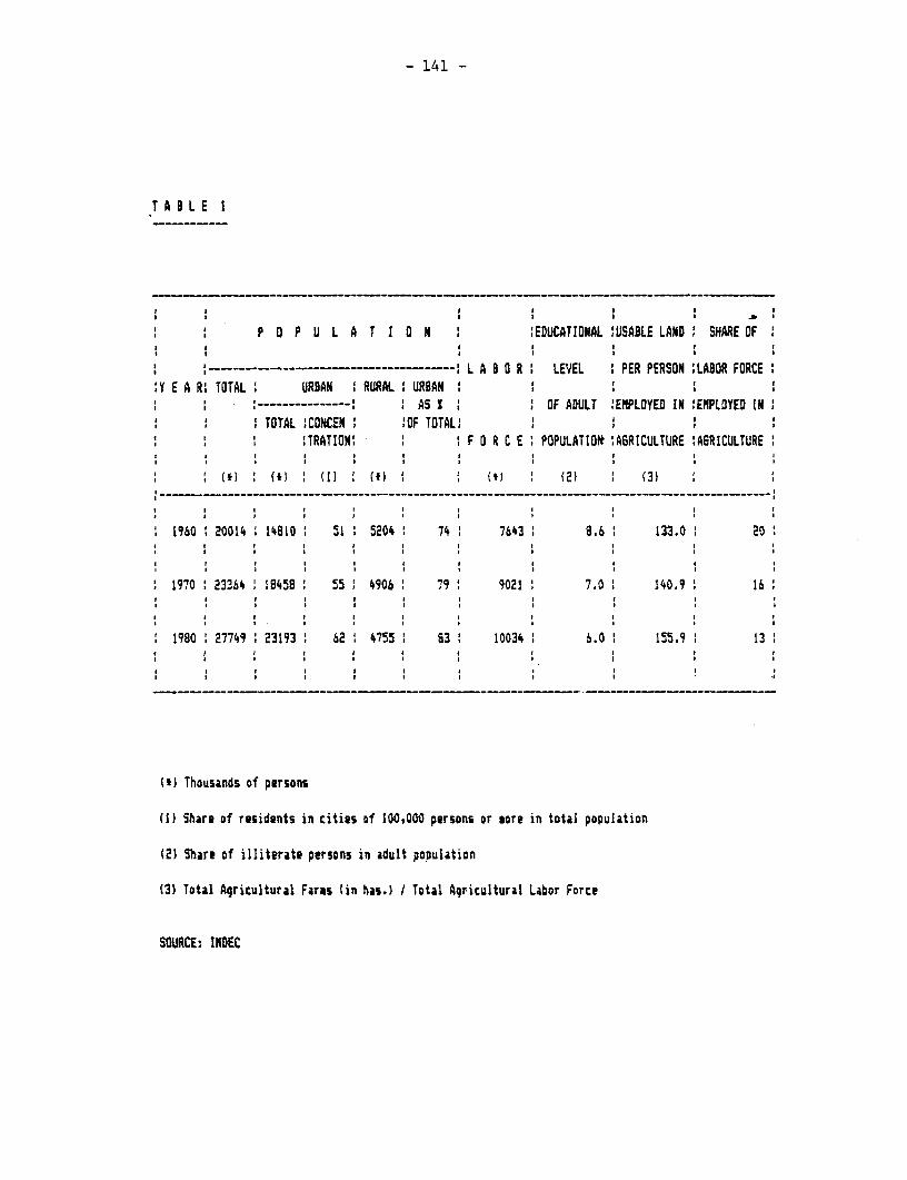
- 141 -

T A B L E 1

P 0 P U L A T I 0 N EDUCATIONAL USABLE LAND SHARE OF

-- - ---- -------- - -------- -- L A 3 0 R LEVEL PER PERSON LABOR FORCEYE AR: TOTAL URBAN RURAL URBAN

0t---------------: AS S OF ADULT :EMPLOYED IN !EMPLOYED INTOTAL CONCEN OF TOTAL,'

1TRATION i F 0 R C E POPULATIODt :A6RICULTURE !AGRICULTURE

W (I I I, I ' 2 I ((I ' (2) (3)

1960 20014 14810 51 5204 74 7643 I 8.6 1 133.0 20

1970 2336S 18458 55 4906 79 9021 7.0 140.9 16

1980 27749 23193 62 1 4755: 83 10034 6.0 155.9 13

(fl Thousands of persons

(1) Share of residents in cities of 100,000 persons or sore in total population

(2) Share of illiterate persons in adult population

(3) Total Agricultural Fares (in has.) I Total Agricultural Labor Force

SOURCE: INDEC

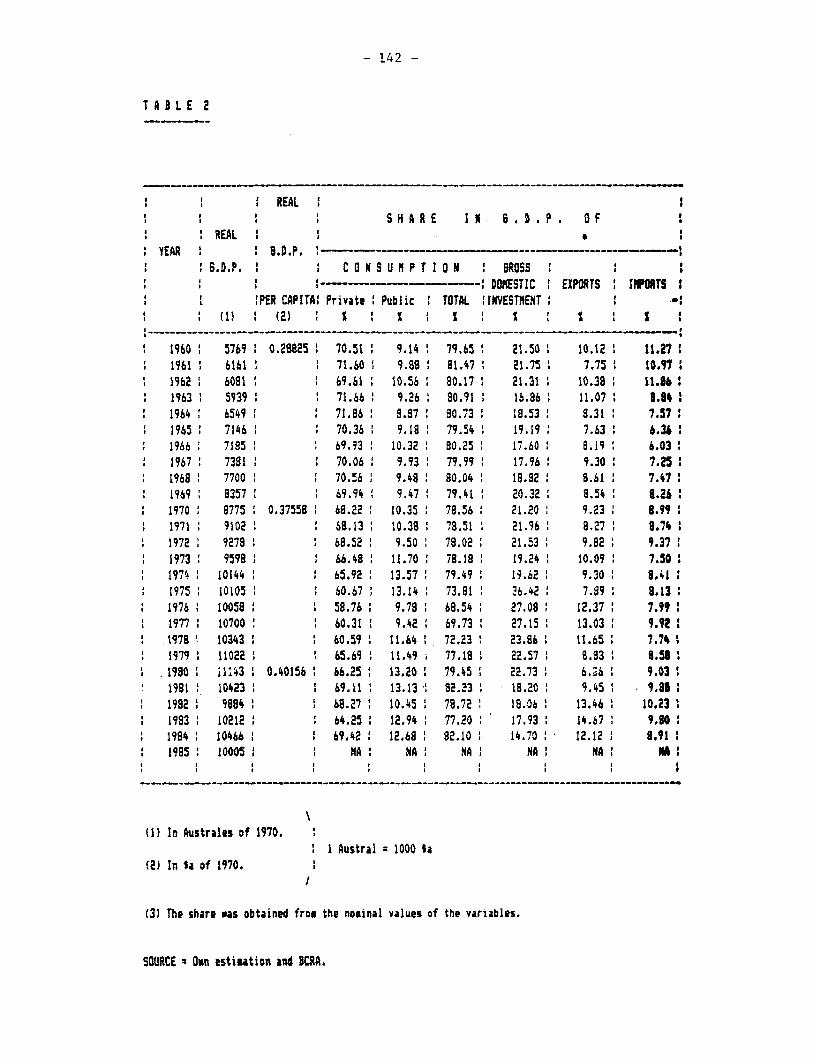
- 142 -

T A B L E 2

I REAL i

i : AR f I P . f:REAL *

YEAR 8 i .D.P. ---- ------ 1:6.D.P. : C O h S Pt I O N I ROSS

. '- - - -'-------- --- DOIESTIC EXPORTS INPORTS'PER CAPITA: Private Public TOTAL INvE ENT'I-

(ii ' (2) ' S ' X 1 S ' S

1960 : 5769 0.28825 70.51 9.14 79.65 21.50 10.12 11.271961 6161 71.60 9.88 81.47 21.75 7.75 10.971962 6081 69.61: 10.56 90.17 21.31 10.38 11.961963 5939 71.66 9.26 80.91M 16.86 11.07 : 8.34 1964 6549 71.86 8.87 80.73 18.53 9.31 7.571965 7146 70.36 9.19 79.54 19.19 7.63 6.3b1966 7185 69.93 10.32 80.25 17.60 8.i9 6.03:1967: 73981 70.06: 9.93 79.99 17.96 9.30: 7.25:196a 7700 70.56 9.48 1 80.04 18.82 8.61 7.471969 8357 69.94 9.47 79.41 20.32: 8.54 6.26:1970 8775 0.37558: 68.22 10.35 78.56 21.20 9.23 8.99:1971 91021 68.13 110.38: 78.51 21.96: 8.27 1 8.741972 9279 68.52 9.50 78.02 21.53 9.82 9.37:19731 9598 I 66.48: 11.70 1 78.182 19.24: 10.09 7.50197k1 10144 l 65.92 13.57 1 79.49 19.62 9.30 B8.1975 10105 : 60.67 : 13.14 73.81 26.42 : 7.99 : 8.131976: 10058 : 58.76 9.78 68.54 27.08 12.37 7.99:1977: 10700 60.31 1 9.42 69.73 27.15: 13.03 9.9Z:¶978 10343: 60.591 11.641 72.23: 23.86 11.65: 7.741979 1 11022 65.69 11.49 77.18: 22.57 9.83: 8.5:

.1980 11.13 0.40156 66.25: 13.20 79.45 22.73 6.Sh 9.031981: 10423 1: 69.11: 13.13I 82.23: 18.20 : 9.45 I 9.831982 1 9884 1 68.271 10.45 1 78.72 : 18.06: 13.46 1 10.23:1983 1 10212 : 64.251 12.94 77.20: 17.93 14.67 9.90:1984 10466: 1 69.42 1 12.68: 82.10 1 14.70 12.12 9.91985: 10005: 1 NA. NA: NA NA: NA: NA:

11) In Australes of 1970.1 Austral = 1000 la

(2) In $a of 1970.I

(3) rhe share oas obtained from the nosinal values of the variables.

SOURCE: Ogn estiuation and BCRA.

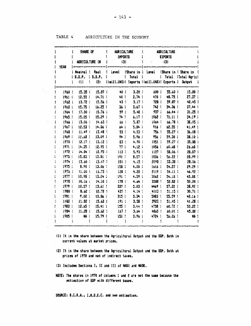
- 143 -

TABLE 4 AGRICULTURE IN THE ECONOMY

SHARE OF ARICULTURE AGRICULTUREI I I IMPORTS EXPORTS

AGRICULTURE IN I (3) (3)i YEAR I -

t Nocinal 5 Real I Level Share in 0 Level !Share in Share in IG.D.P. IG.D.P. I Total I I Total ITotal Agric(1) 1(2) !(mill.USS)I Ieports 1(eill. USS)! Exports Output

i 1960 15.35 15.97 40 3.20: 600 S5.60 1 15.90i 1961 1 12.55 1 14.71 1 40 2.74 470 48.75 1 27.37 11 1962 13.72 15.56 43 3.171 7281 59.87 1 42.45II 1963 15.75 16.25 I 36 1 3.67 1 742 1 54.36 1 37.44 1

1964: 17.30 15.76 59: 5.48I 937 66.441 31.25: 1965 15.05 15.29 74 6.17 1 1062 71.11 34.191966 13.06 14.63 66 5.87 1064 66.78 38.051967 12.53 14.86 64 5.94 916 1 62.55 i 41.49 119681 11.49 13.48: 53 4.53 756 1 55.27 36.08:1969 11.681 13.09 941 5.96 956 59.30: 38.10:1970 12.17 13.12 83 4.90 1051 . 59.271 35.9881971 14.35 12.95 77 4.12 1056 60.68 i 26.68 11972 14.84 12.93 113 5.93 1127 58.06 28.871973 15.83 13.81 i 191 8.57 1836 56.22 28.991974 13.60 13.47 151 4.15 2098 53.398 28.06

i 1975 8.90 13.06 158 1 4.00 1616 1 54.57 1 29.291976 11.00 13.73 129 4.22 2119: 54.11 46.921977 1 10.99 13.24 1 191 i 4.59 3062 54.18 45.881978 10.16 14.10 178 4.b4 3388 52.82 1 50.201979 10.57 13.61 337 5.03 449 57.22 38.9211980 8.62 12.721 437 4.14 41031 51.151 30.711

1 1981 1 9.02 . 13.86 1 3151 3.34 . 5083 : 55.59 1 42.161-82 11.821 15.631 191 3.58: 39231 51.45 41.29.1993 12.65 15.41 155. 3.44 4758 60.72 50.22

1 1984 11.29 1 15.62 167 i 3.64 865 1 60.01 45.3819951 MA 15.79 1511 3.96. 47241 56.26 MAII I : . , I

(1) It is the share between the Agricultural Output and the SDP. Both in

current values at market prices.

(2) It is the share between the Agricultural Output and the GDP. Both at

prices of 1970 and net of indirect taAes.

(3) Includes Sections 1, II and III of MADI and NADE.

NOTE: The shares in 1970 of columns I and 2 are not the sme because theestimation of GDP _ith different bases.

SOURCE: D.C.R.A., I.N.D.E.C. and own estisation.

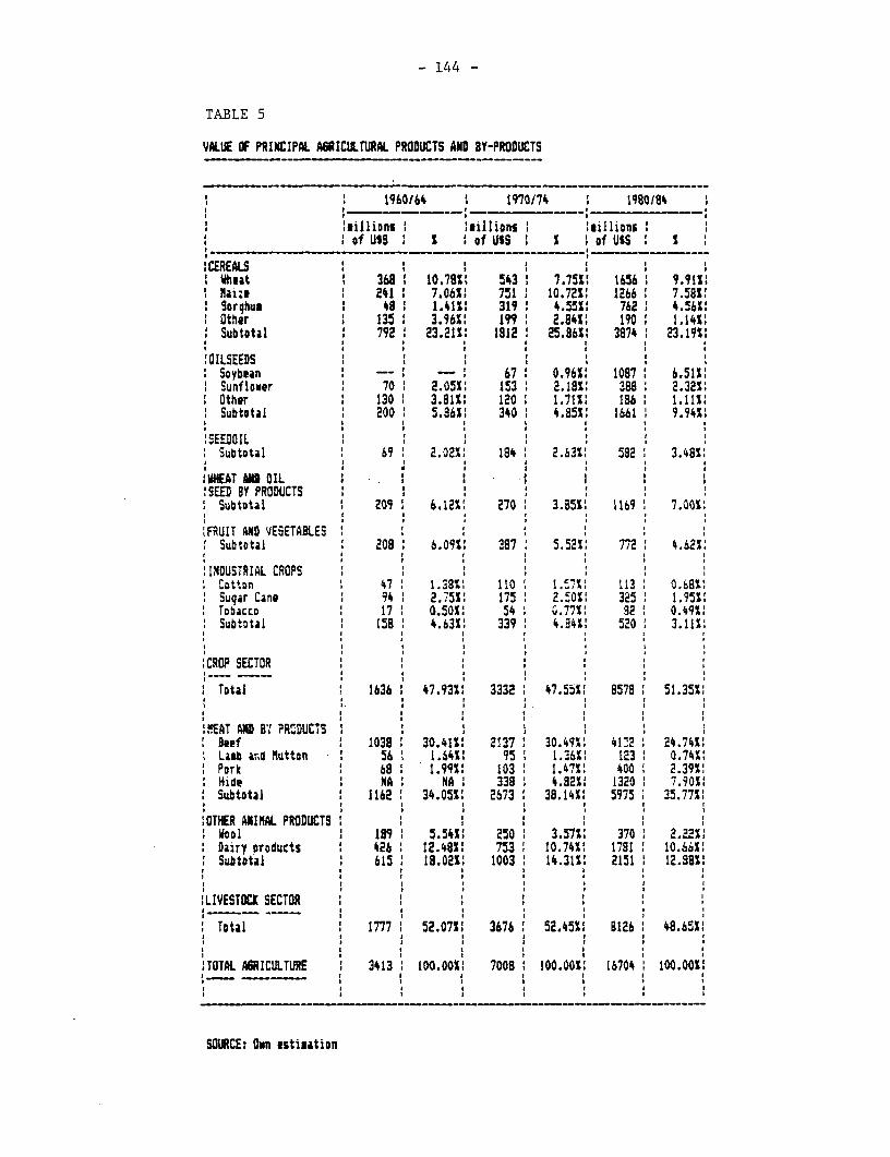
- 144 -

TABLE 5

VALUE Of PRINCIPAL A8AICULMURAL PRODUCTS AND BY-PRODUCTS

I ' 1960164 1970174 1980184

:Billions meillions I m4illionsO of UtS I S of USS S % of U$S % S

'CEREALSXhH~at 1 368 10.78S' 543 7.751' 1656 9.915l

1 Maize 2411 7.06%1 751 : 10.7211 1266 7.58S'Sorghum 48i 1.41%1 319 4.55%: 762 4.561:Other 135 1 3.96b: 1 9 2.84S' 190 1.14$'

' Subtotal ' 792 23.215: 1812 1 25.861: 3874 ' 23.19%:

'OILSEEDS, Soybean - - 67: 0.965: 1097 : 6.515:

Sunflower 70 1 2.051: 153 2.181: 388 2.321:* Other : 130 ' 3.81S1 120 1.711: 196: 1.11:

Subtotal 1 200 ' 5.861: 340 4.855: 1661 9.94X:

'SEEDOIL 'Subtotal 69 2.02X: 184 2.631: 582 3.48S:

,~~ ~ ~ ~~ , J . .

iWEAT A OIL I I : - .1!SEED BYf PRODUCTS ' e', ' Subtotal : 209 6.12%' 270 3.85%' 1169 ' 7.00S,

'FRUIT AND VESETABLES ' i 'Subtotal , 208 6.09S: 387 5.52%: 7722 4.i21:

:INDUSTRIAL CROPS 'CDtton 47 1.38S' 110 1.'7S 113 0.68Suqar Cane , 94, 2.751: 175 ' 2.50S' 325 1.951:TObacCD 17 ' .50%: 54 ' G.771: 82: 0.49%:Subtotal ' 158 ' 4.63X: 339 1 4.84A: 520 1 3.111X

'CROP SECTOR ' '

* Total 1636 ' 47.93%: 3332: 47.55%1 8578 51.35S1. . . I. . .

fMEAT AN B'. PRZDUCTS IB3ef 1 1039 1 30.41%: 2137 1 30.49%: 4122 : 24.741:Lamb ant Mutton 56' 1.64%: 95 1 1.36%$ 123 1 0.74%'Park ' 68 1.995: 103 1.471: 400 2.39%:H Kide : NA ' NA ' 338 . 4.825: 1320 ' 7.90S:Subtotal : 1162 ' 34.05%: 2673 ' 38.14S: 5975 35.77%:

IOTHER ANIMAL PRODUCTS:Wool 1891 5.541: 250 : 3.57S: 370 ' 2.225%Dairy products : 426 ' 12.48%1 753 ' 10.74%: 1781 ' 10.66%:Subtotal 615 :18.02: 1003 14.31%: 2151 12.88%:

:LIVESTOCK SECTOR , ':~~~~~~~~~ : I : I

Total 1 1777 52.07S1 3676 52.45%: 9126: 48.65%:

ITOTAL AGRICULTURE 1 3413 ' 100.00%1 7008 . 100.00%: 16704 1 100.00%:

SOURCE: Own estimation

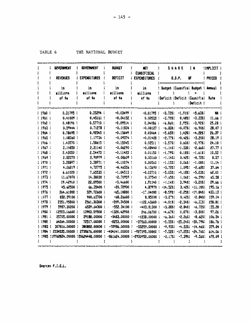
- 145 -

TABLE 6 THE NATIONAL BUDGET

WOVERNMENT GOVERNMENT RUDGET ET S HA R E IN UINPLICIT II . : a I CUASIFISCAL I ' t

REVENUES EXPENDITURES DEFICIT EXPENDITURES 6.D.P. OF PRICESa : : I a t I

in in t in in B Budget 'Cuasifis! Budget Anual illions Billions : *illions ; millions i : : + I

of $a of $a of la of Sa 'Oeficit 'Deficit lCuasifis: Rate: a a a a : l 'DeficitI _ _ _ _ _ _ _ _ _ _ _ _ _ _ _ _ _ _ _ _ _ _ _ _ ________

1960 0.31795 0.35294 -0.03499 -0.01795 -3.7211 -1.9I1% -5.63S: NA1961 0.41009 0.45161 : -0.04152 0.00533 -3.70S: 0.48S: -3.23S: 11.661962 0.48196 0.57710 -0.09514 0.04086 -6.86X1 2.951 -3.92S: 25.291963 0.59444 0.71278 -0.11834 -0.00127 -6.83S1 -0.071: -6.901: 28.071964 I 0. 78J65: 0.92345 * -0.13649 -50.0346 6 -5.tSSt 1.43' -4.2S: 26.37

a1965 1 1.08360 1.17734 -0.09374 -0.01429 -2.77X: -0.42St -3.201S 28.191966 1.43570 1.58615 i -0.15045 0.02511 -3.57S: 0.60S -2.971: 24.10 11967 2.14850 2.21140 -0.06290 -0.08440 -1.1411 -1.531: -2.6611 27.77 ?1968 2.43050 2.54473 -0.11423 0.01150 -1.79%1 0.1BS -1.61t: 10.531969 2.82370 2.909M9 -0.08609 0.03160 S -1.1411 0.42S -0.721S 8.571970 1 3.29897 3.38971 -0.10074 0.00560 -1.151 0.0611 -1.081: 11.14 11971 1 4.26219 4.72775 -0.46556 0.13690 -3.721: 1.095 -2.625: 37.6419721 6.61020 7.6533 -1.04513 1 -0.03710 -5.05%1 -1.181: -5.23X: 62.011973 11.67070 1 14.38030 : -2.70959 0.37540 -7.651: 1.06S: -6.591: 65.581974 19.429t0 I 22.89500 1 -3.46600 1 1.91140 -7.1.%1 3.94%: -3.20S: 29.661975 45.62500 1 66.35400 1 -20.72900 4 4.87970 -14.521: 3.42S1 -11.10: 195.161976 1 264.61800 : 329.72600 1 -65.10800 -17.04000 -8.59%1 -2.251: -11.841: 433.13i9771 32.39100 900.6b700 1 -68.26600 8.85000 -3.a71: 0.21: -2.841: 159.141978 2351.95800 : 256l.30300 -209.34500 -122.43600 -4.011: -2.341: -6.37:: 159.911979 5987.30200 1 6539.64300 : -552.34100 1 -403.83300 -3.8811 -2.841: -6.721: :55.201980 12353.16600 : 13903.59500 : -1320.42900 246.06700 1 -4.671: 0.87X: -3.80S) 97.261981 2 35705.00000 2918d.00000 1 -3483.00000 1 -1238.00000 -6.365: -2.261: -8.62%1 106.541982 b 64264.00000 72517.00000 : -8253.00000 -37563.00000 -5.551S -25.241: -30.7911 186.761983 1 307816.00000 1 380802.00000 1 -72986.00000 1 -33259.00000 -9.931: -4.531: -14.4611 379.04

119841 3334535.00000 : 2738676.00000 : -404141.00000 -927395.00000 -7.5211 -17.25X -24.76X: 614.0611985 119762824.00000 120624448.00000 I -961624.00000 1-2930952.00000 1 -Z.17S1 -7.391: -9.56E1 672.09

Source: F.I.E.L.

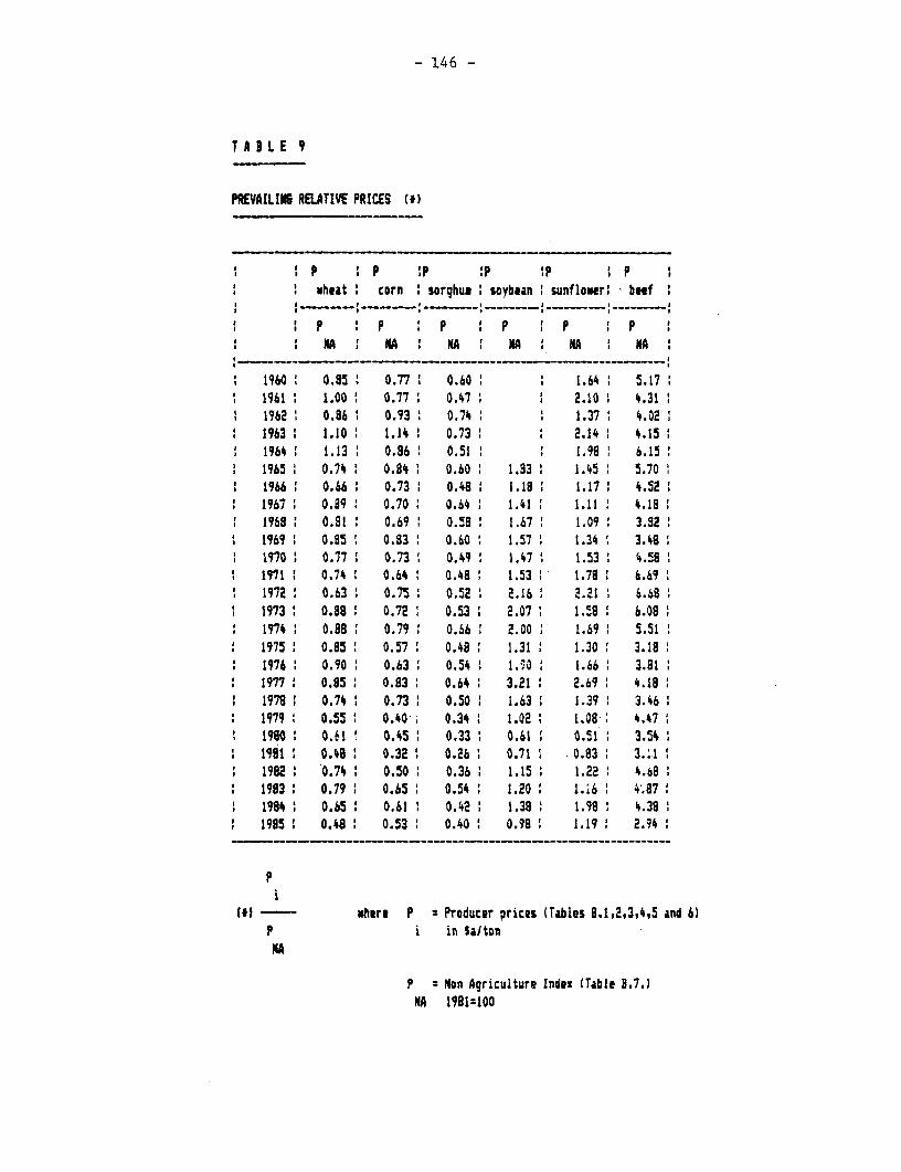
- 146 -

TA9LE 9

PREVAILING RELATIVE PRICES (J)

I ' P ' P ' p p ) P' wheat corn sorghue 1 soybean ' sunflower: beef

: : P :p :P I : p :p p* ' MA . INA: MA MA MA M IA

1960 0.15 0.77 0.60 I 1.64 5.171 1961 1.001 0.77 0.47 * 2.101 4.31

19621 0.86 : 0.93: 0.74 * 1.37: 4.02:1963: 1.10: 1.14: 0.73: 2.14' 4.151964: 1.13: 0.961 0.5 1.98 6.151965 0.74 0.84 0.60 1.83 1.45 5.70

1 1966 0.66 0.73 0.48 1.18 1.17 4.521967: 0.89: 0.70: 0.64: 1.41: 1.11: 4.181968: 0.91 0.69 0.58 1.67 1.09: 3.821969: 0.85: 0.83: 0.60: 1.57: 1.34 3.48

1 1970 0.77: 0.73: 0.49: 1.47: 1.53 4.5981971' 0.74: 0.64: 0.48: 1.53 1.78: 6.691972' 0.63: 0.75: 0.521 2.16 2.21 : 6.68

1 1973: 0.88' 0.72 0.53 2.07 : 1.58 6.081974 : 0.88 : 0.79: 0.66 : 2.00 : 1.69 5.511975 0.85 0.57 0.48 1.31 1.30 3.181976 0.90 0.63 0.54: 1.,O 1 1.66: 3.811977: 0.85: 0.83 0.64 . 3.21 : 2.69: 4.181979 1 0.74 : 0.73 0.50 1.63 1.39: 3.461979 : 0.55 1 0.40 ; 0.34 I 1.02 1 1.098 4.471900 0.61! 0.45: 0.33: 0.61 0.51: 3.54198 : 0.48 0.32: 0.26 0.711 .0.831 3.'11982 ' 0.74: 0.50 0.36 1.15: 1.22 4.681983 0.79: 0.65: 0.54: 1.20 1.i6 4.87:1984 : 0.65: 0.61 0.42 1.38: 1.99 4.38

: 1985: 0.48: 0.53 : 0.40: 0.98: 1.19 2.94

(M - where P : Producer prices (Tables 9.1,2,3,4, and 6)P i in Saton

P N Non Agriculture Index (Table 3.7.)NA 1991:100

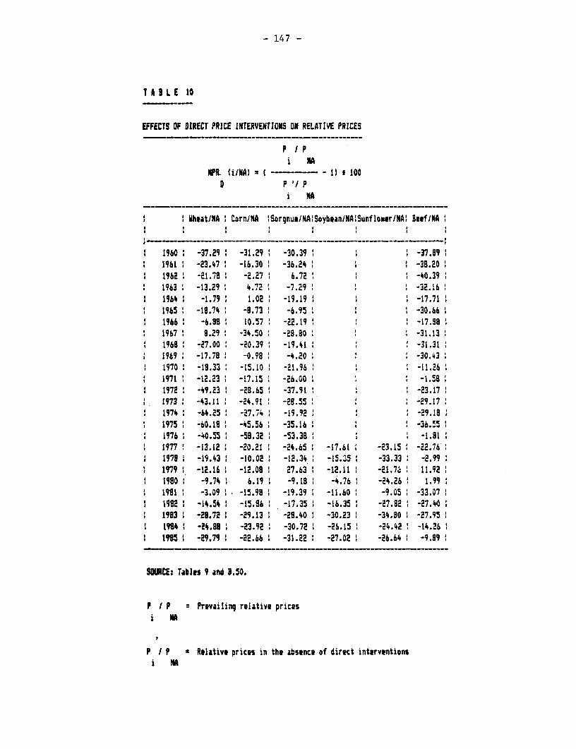
- 147 -

T A I L E 10

EFFECTS OF DIRECT PRICE INTERVENTIONS ON RELATIVE PRICES

P IPi NA

wFR WM"^ : I - - IJ t oD p I/ p

i NA

: heatiNA Corn/NA 'SorghumINA'SoybmanINA'Sunflomer/NA' Beef/NA

1 1960: -37.29 1 -31.29 ' -30.39 -37.89 11961 -23.47 -16.30 ' -36.24 ' : -38.20

1 1962 -21.78 -2.27 6.72 ' ' ' -40.391963 -13.29 4.7 '2 -7.29 -32.1'61964 -1.791 1.02 -19.19 1 , ' -17.711965 : -19.74 -8.73 -6.95 . ' ' -30.66 t1966b -6.38 ' 10.57 ' -22.19 ' -17.981967: 8.29 -34.50 -28.80 -31.13 '

1 1968 -27.00 ' -20.39 ' -19.41 ' ' -31.311969 , -17.789 -0.98 ' -4.20 . -30.431970 -19.33: -15.10: -21.96 I -11.261971 ' -12.23: -17.15 -26.00 1 : -1.58

1 1972 ' -49.23 ' -28.65 ' -37.91 ' ' -23.171973 -43.11 -24.91 ' -29.55 ' -29.17'1974: -64.25 -27.7w: -19.92 ' ' -29.191975 ' -60.18: -45.56 , -35.16 ' ' -36.5,1976: -40.55 -58.32: -53.38 ' : -1.81:1977 ' -13.12 : -20.21 ' -24.65 ' -17.61 , -23.15 ' -22.76

1 1978 -19.43 ' -10.02 1 -12.34 : -15.35 , -33.33 1 -2.991 1979 ' -12.16 1 -12.08 27.63 ' -12.11 ' -21.7a 1 11.921 1980 1 -9.74 1 6.19 1 -9.18 1 -4.76 ' -24.26 ' 1.991 1981 ' -3.09 1 -15.98 1 -19.39 1 -11.60 1 -9.05 -33.071 1982 ' -14.54 1 -15.96 1 -17.35 ' -16.35 , -27.82 : -27.40 ,I 1983 1 -28.72 ; -29.13 1 -28.40 1 -30.23 1 -34.80 1 -27.95 '1 1984 1 -24.88 1 -23.92 1 -30.72 1 -26.15 ' -24.42 1 -14.26 '

1985 1 -29.79 1 -22.66 ' -31.22 : -27.02 ' -26.64 1 -9.99

SOURCE: Tablcs 9 and 3.50.

P I P : Prevailing relative pricesiN

P I P : Relative prices in the absence of direct inttrventionsi NA

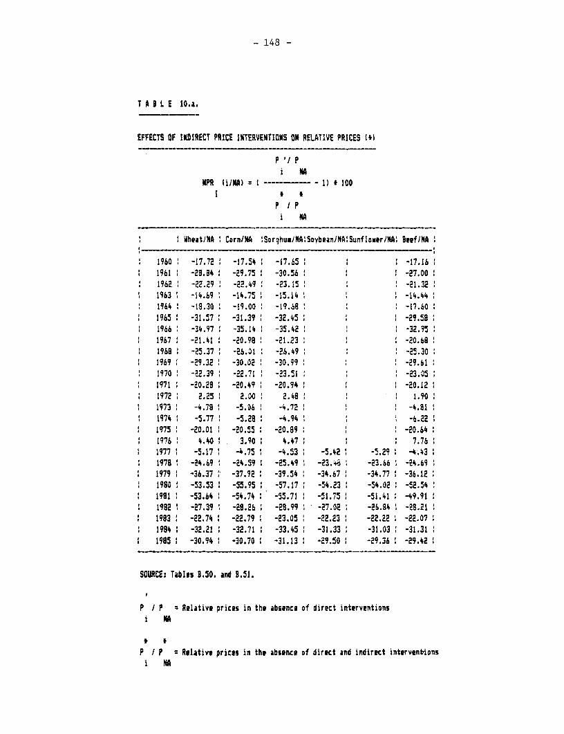
- 148 -

T A B L E 10.a.

EFFECTS OF INDIRECT PRICE INTERVENTIONS ON RELATIVE PRICES 1(0

P '1 Pi A

MMR iliA) I 1) f 100I I t

P lPi NA

6heatJNA Corn/NA Sorghu/ANA SoybeanlNA Sunflover/MA Beef/NA

1960 -17.72 -17.54 ' -17.65 ' -17.161961 -28.4 -29.75 -30.56 b -27.001962 -22.29 -22.49 -23.15 -21.321963 -14.69 -14.75 -15.14 * -14.441964 1 -18.30 -19.00 -19.68 -17.601965 1 -31.57 -31.39 1 -32.45 -29.581966 : -34.97 -35.14 1 -35.42 . -32.951967 -21.41 -20.98 -21.23 -20.681968 -25.37 -26.01 1 -26.49 1 : -25.301969 -29.32 -30.02 -30.99 -29.611970 -22.39 -22.71 1 -23.51 -23.051971 -20.28 -20.49 -20.94 -20.121972: 2.25' 2.00: 2.48: : 1.901973 -4.78 ' -5.06 1 -4.72 1 ' -4.811974 : -5.77 1 -5.28 1 -4.94 -6.221975 -20.01 -20.55 1 -20.89 : : -20.641976: 4.40 3.90 4.47 . : 7.761977 1 -5.17 -4.75 1 -4.53 : -5.42 1 -5.29 : -4.431978 I -24.69 1 -24.59 1 -25.49 1 -23.+4 -23.66 1 -24.691979 1 -36.37 -37.92 : -39.54 : -34.67 -34.77 : -36.121980 1 -53.53 i -55.95 ' -57.17 ' -54.23 : -54.02 1 -52.541981 -53.64 -54.74 ' -55.71 : -51.75 1 -51.41 -49.911982 -27.39 1 -28.26 1 -28.99 1 -27.02 : -26.84 i -28.211983 1 -22.74 i -22.79 1 -23.05 : -22.23 1 -22.22 : -22.071984 ' -32.21 1 -32.71 ' -33.45 : -31.33 -31.03 : -31.311995 -30.94 1 -30.70 1 -31.13 1 -29.50 1 -29.36 1 -29.42

SOURCE: Tables 8.50. and 8.51.

P / P : Relative prices in the absence of direct interventions

i H

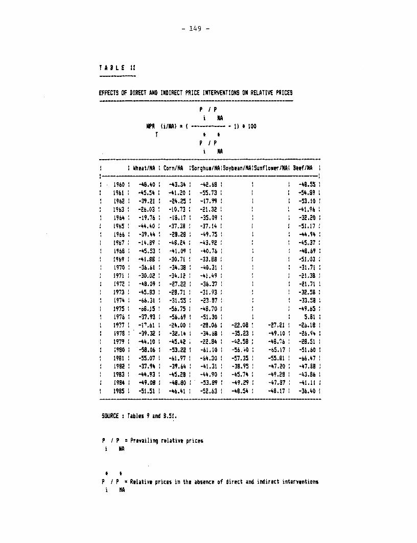
- 149 -

T A 8 L E 11

EFFECTS OF DIRECT AND IIIIRECT PRICE INTERVENTIONS ON RELATIVE PRICES

P fPi 14

IIPR liJ) 11) 100T

p pi a

Wheat]NA 'Corn/NA 'Sorghum/NA'SoybeaniNA'Sunflo.erNA' Beaf/hNA

1960 -48.40 -43.34 -42.68 -49.551961' -45.54 -41.20 -55.73 1 -54.891962 -39.21 : -24.25 1 -17.99 -53.101963 -26.03 1 -10.73 -21.32 -41.961964 -19.76 -18.17 -35.09 -32.201965 -44.40 -37.38 -37.14 -51.171966 -39.44 ' -29.29 -49.75 -44.941967 -14.89 -48.24 -43.92 -45.371968 -45.53 -41.09 -40.76 -48.691969 -41.88 -30.71 -33.88 -51.031970 -36.61 -34.38 -40.31 i -31.711971 -30.02 -34.12 -41.49 -21.381972 -48.09 -27.22 1 -36.37 . -21.711973 -45.93 -29.71 -31.93 -32.581974 -66.31 1 -31.55 -23.87 1 1 -33.581975 -o8.15 -56.75 -48.70 -49.651976 -37.93 1 -56.69 -51.30 5.811977 1 -l1.61 -24.00 -28.06 1 -22.08 -27.21 -2c.181978 -39.32 -3e.14 -34.68 1 -3S.23 1 -49.10 1 -2b.941979 -44.10 1 -45.42 . -22.94 : -42.589 -48.76 -29.511980 1 -58.06 1 -53.22 1 -61.10 1 -56.40 . -65.17 -51.60 11991 -55.07 1 -61.97 ' -64.30 1 -57.35 1 -55.81 1 -66.471982 -37.94 -39.64 -41.31 -38.95 -47.20 -47.881983 1 -44.93 ' -45.28 1 -44.90 1 -45.74 1 -49.29 1 -43.861984 I -49.08 -48.80 ' -53.89 -49.29 -47.87 -41.111995 1 -51.51 1 -46.41 -52.63 1 -48.54 -48.17 -36.40 1

SOURCE Tables 9 and 8.51.

P 1 P Prevailing relative pricesi NA

P / P Relative prices in the absence of direct and indirect interventionsi NA

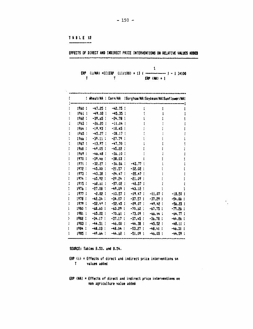
- 150 -

T A I L E 12

EFFECTS OF DIRECT AND INDIRECT PRICE INTERVENTIONS ON RELATIVE VALUES ADD

ERP (i/NA) s((ERP (il/lO0) + 1] - - J - I et1OoT T ERP (NA) * I

I I Oheat/NA I Corn/NA ISorghus/NAlSoybean/NA:Sunflower/NA

1960 -47.25 -42.751961: -49.02 1 -45.35 '1962 I -39.65 -24.781963 -26.20 -11.041964 -19.93 -18.451965 ' -45.27 -38.171966 -35.11 ' -27.79 11967 t -13.97 1 -47.70 119685 -49.05 -45.22 :1969 . -46.48 -36.101970 -39.46 1 -38.03 :1971 -32.27 -36.86 -43.77 1 11972 -45.00 -21.57 ' -32.02! 973 -43.38 ' -2i.47 ' -2a.47 ' 1974 -65.92 -29.24 -21.09 '1975 -68.61 -57.02 ' -48.57

1 1976 -27.08 ' -49.09 1 -43.12 '1977 -2.82 -13.57 -19.47: -11.07 -19.50 1979 -42.34 -34.07 1 -37,57 -37.29 -54.8b1979 1 -52.4$ -52.45 -29.07 -49.42 -56.2231980 1 -68.60: -63.29 -70.62 -67.75 1 -7?.261991 -65.22 1 -70.61 1 -73.09 -66.44 -64.771982 -34.17 -37.17 -37.45 -36.78 -44.86

1 1983 -44.51 -46.00 -44.38: -45.52 1 -48.111 1984 -48.03 1 -48.04 1 -53.271 -49.41 -46.31:: 1985 -49.64 : -44.62 ! -51.09 1 -46.03 -44.59 1

SOURCE: Tables 8.53. and 9.54.

ERP Qi) Effects of direct and indirect price interventions onT values added

ERP (NA) Effects of direct and indirect price interventions onnon agriculture value added

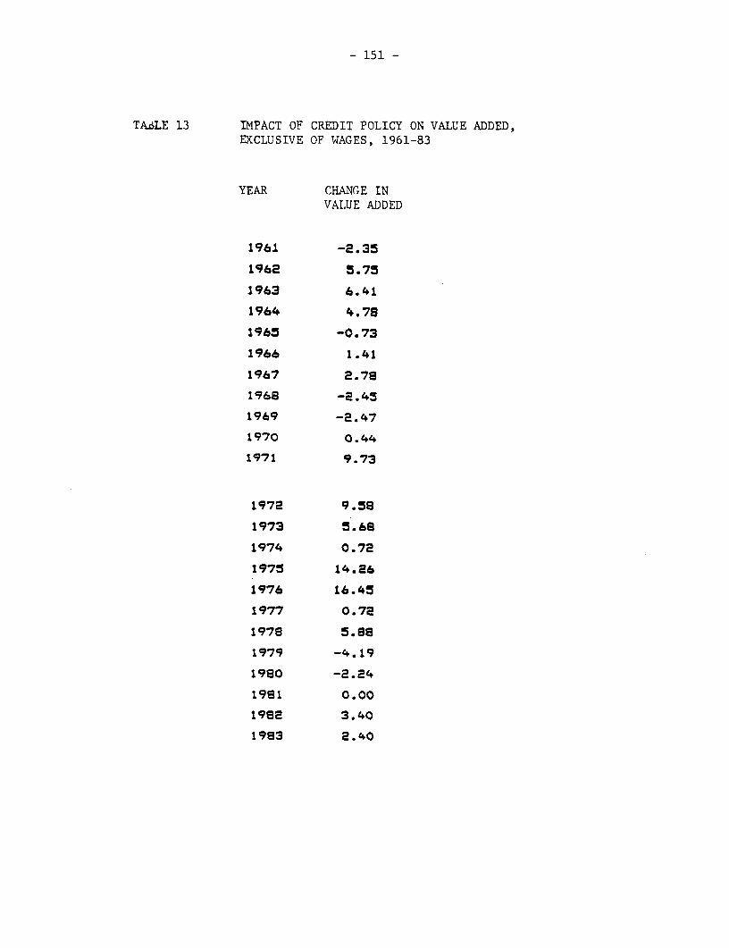
- 151 -

TAbLE 13 IMPACT OF CREDIT POLICY ON VALUE ADDED,EXCLUSIVE OF WAGES, 1961-83

YEAR CHANGE INVALUE ADDED

1961 -2.35

1962 5.75

1963 6.41

1964 4.78

1965 -0.73

1966 1.41

1967 2.78

1968 -2.45

1969 -2.47

1970 0.44

1971 9.73

1972 9.58

1973 5.68

1974 0.72

1975 14.26

1976 16.45

1977 0.72

1978 5.88

1979 -4.19

1980 -2.24

1981 0.00

1982 3.40

1983 2.40

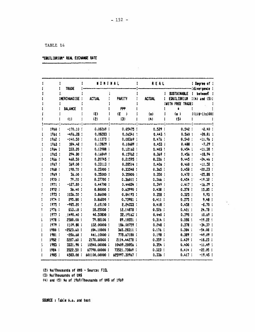
- 152 -

TABLE 14

'"EUILIBRIUM* REAL EXCHANSE RATE

I N : h O N IN A L R E A L DIOgru ofI TRADE Idiverq.uc

SUSTAINABLE I botsetd:MERCHANDISE I ACTUAL I PARITY ACTUAL I EQUILIBRIUM :4) and (5):

I I l IUITH FRE TRADE,I IALANCE It P P I

: 5I5 (£) 5 (E ) I (n) ( (I ) UlI/d-1)zIOO'I . 111 I (2) ' (3) : (O : IS) I I

1 1960 -170.10 0.08269 0.05475 0.5293 0.542 i -2.40': 1961 -496.28 1 0.08283 ' 0.06541 ' 0.443 t 0.560 -20.81 '

1962 -140.50 0.11373 0.08369 0.476 0.540 -11.961963 384.42 0.13829 0.106i9 0.4539 0.488 -7.291964 333.20 0.13988 0.12162 0.403 0.454 1 -11.38 11965 294.80 0.16849 0.15962 0.369: 0.456 -18.94

1 1966 468.50 0.20745 0.21595 0.336' 0.445 -24.461967 369.00 0.33113 0.28514 0.406 0.460 -11.581968 1 198.70 0.35000 0.33548 0.365 5 0.458: -20.23

1 1969 36.00' 0.35000 0.35000 0.350 0.472 1 -25.88:1 1970 ' 79.20 5 0.37700 5 0.36011 ' 0.366 ' 0.454 - -19.32: 1971 -127.80: 0.44700 ' 0.44834 5 0.349 5 0.417 ' -16.29 '

1972 36.40 5 0.80000 5 0.63990 5 0.438 1 0.378 15.85 S1 1973 5 1036.50 ' 0.86000 0.84193 0.358 ' 0.325 ' 9.93: 19?34 295.80 ' 0.86800 ! 0.73981 1 0.411 i 0.375 9.48 1 1975 1 -985.20 2.68100 5 2.24333 I 0.418 1 0.458 i -6.70 '

1976 5 63.10 ' 18.25000 . 12.14878 1 0.526 1 0.421 i 24.71 15 1977 1490.40 5 40.50800 32.19163: 0.440 0.398 . 10.69:: 1978 2580.00 ' 79.88100 1 89.10551 1 0.314 0.388: -19.22 :1 1979 1 1109.80 5 132.00000 186.00759 1 0.248 . 0.378 1 -34.371 1980 ' -2523.60 t 184.10000 ' 365.28311 ' 0.176 ' 0.384 1 -54.08 .1 19811 -296.60 441.10000 778.67180 0.198 5 0.389 -49.091 1982 ' 2287.60 2170.00000 2114.44278 0.359 i 0.439 5 -18.23 '1 1983 ' 3331.30 10540.00000 10109.28056 1 0.354 1 0.400 1 -11.49I 1984 : 3522.50 1 67790.00000 1 73521.73869 1 0.323 1 0.414 1 -22.05

1985 1 4583.00 1 601100.00000 5 625997.30967 1 0.336 0.417 5 -19.45:

(2) $a/Thousands of USS - Sourcv: FIEL(3) $a/Thousands of USS(4) and (5) $a of 1969/Thousands of USS of 1969

SWURCE : Table 6.a. and text

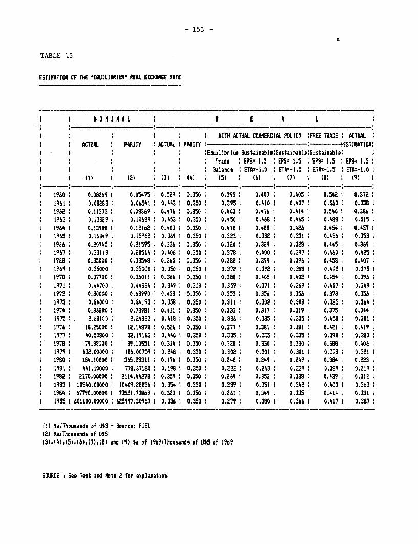
- 153 -

TABLE 15

ESTIMATION OF THE 'EOUILIJRIUI REAL EXCHA6£ RATE

N110X111AL R E A L.I . _ _ _t__ _ _ _ _ _.__ _ _ _ _

:1 ITH ACTUAL CIMCIAL POLICY 'FREE TRADE t ACTUALACTUAL PARITY ACTUAL PARITY --4ESTINATION:: S l ' . ~~~~~~~~~EquilibriualSustainable'Sustainibl.lSustainab}l ef

Trade IEPS 1.5 IEPS: 1.5 I EPS= 1.5 EPS: 1.5SI I I Balance ETA-1.0 I ETA-1.5 ETA-1.5 ETA-l.O0

l l (1) ' {(2) l(3) l(4) (5) () l 7 l (9) l(9): : __ __ __ __ _ -- |- ___ __ I _ _ _ _ _ _ _ __ I ____ _ _ _ _ _ _ _ I __ ____________ I

1960 0.08269 1 0.05475 1 0.529 1 0.350 0.395 0.407 l 0.405 i 0.542 0.3721961 0.08283 0.06541 ' 0.443 ' 0.350 0.395 0.410 l 0.407 0.560 0.3381962 0.11373 0.08369 ' 0.476 0.350 ' 0.403 1 0.416 ' 0.414 0.540 0.386 :1 l963 0.13B29 0.10689 0.453 0.350 0.450 0.468 0.465 0.488 0.5151 l964 : 0.13988 ' 0.12162 0.403 0.350 0.410 : 0.428 0.426 ' 0.454 0.4571965 0.16849 ' 0.15962 0.369 0.350 0.323 0.332 0.331 0.456 0.353 1

1 1966 0.20745 0.21595 0.336 1 0.350 1 0.320 1 0.329 0.328 0.445 1 0.369 '1967 0.33113 0.28514 0.406 0.350 0.378 1 0.400 0.397 0.460 0.4251968 0.35000 0.33548 ' 0.365 0.350 ' 0.382 0.399 0.396 ' 0.458 1 0.407 '1969 ' 0.35000 1 0.35000 0.350 0.350 1 0.372 : 0.392 1 0.388 0.472 1 0.3751970 : 0.37700 1 0.36011 0.366 0.350 1 0.398 0.405 i 0.402 ' 0.454 : 0.3961971 ' 0.44700 1 0.44834 1 0.349 1 0.350 0.359 0.371 1 0.369 1 0.417 1 0.349197? 0.80000 0.03990 ' 0.438 i 0.350 : 0.353 ' 0.356 1 0.356 , 0.378 , 0.356

: 1973 0 0.86000 : .83 ' 0.358 . 0.350 0.311 : 0.302 1 0.303 , 0.325 1 0.3641974 0.86800 0.73981 1 0.411 : 0.350 0.333 1 0.317 .319 0.375 1 0.3441975 1 2.681603 2.24333 i 0.418 1 0.350 1 0.336 0.335 0.335 ' 0.458 1 0.301 :

1 1776 1 19.25000 i 12.14878 0.526 1 0.350 1 0.377 1 0.381 0.381 ' 0.421 ' 0.4191977 1 40.50800 i 32.19163 1 0.440 : 0.350 1 0.335 1 0.'3 0.335 1 0.398 1 0.380 V1978 i 79.88100 1 89.10551 1 0.314 1 0.350 1 0.328 ' 0.330 1 0.330 ' 0.388 0.406

1 1979 1 132.00000 ' 186.00759 1 0.248 1 0.350 1 0.302 ' 0.301 1 0.301 1 0.378 1 0.321 11 1980 1 184.10000 1 365.28311 1 0.176 1 0.350 1 0.248 1 0.249 i 0.249 1 0.384 1 0.223 1: 1981 : 441.10000 1 778.67180 : 0.198 1 0.350 1 0.222 1 0.243 : 0.239 1 0.389 1 0.219 '1 1982 1 2170.00000 1 2114.44278 1 0.359 1 0.350 1 0.269 i 0.353 1 0.338 1 0.439 1 0.312I 1983 1 10540.00000 ! 10409.28056 : 0.354 : 0.350 1 0.289 1 0.351 ' 0.342 1 0.400 1 0.363 11 1984 67790.00000 1 73521.73869 1 0.323 1 0.350 1 0.261 : 0.349 1 0.335 0.414 1 0.331 :1 1985 : 601100.00000 : 625997.30967 : 0.336 1 0.350 1 0.279 1 0.380 1 0.366 : 0.417 1 0.387

(1) Si/Thousands of U$S - Source: FIEL(2) Si/Thousands of USSt3),14J,t5),1J),t7),18) and (9) 5a of 1969/Thousands of USS of 1969

SOURCE : See Text and Note 2 for explanation

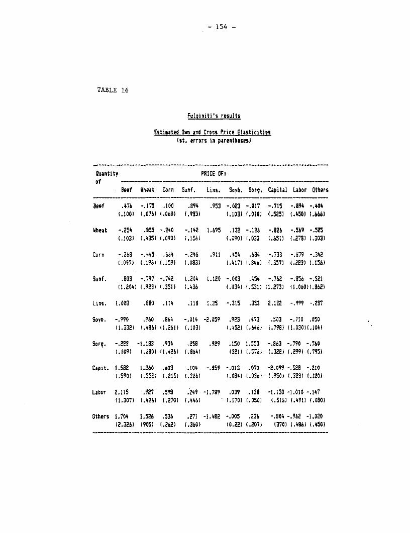
- 154 -

TABLE 16

FulQiniti's results

Estimated Own and Cross Price Elasticities1st. errors in parentheses)

Quantity PRICE OF:of

Beef Wheat Corn Sunf. Lins. Soyb. Sorg. Capital Labor Others

Beef .476 -.175 .100 .894 .953 -.023 -.017 -.715 -.894 -.404(.100) (.076) (.060) (.983) (.103) (.010) (.525) (.4501 (.666)

Wheat -.254 .855 -.240 -.142 1.695 .132 -.126 -.826 -.569 -.525(.1031 (.435) (.090) (.156) (.090) (.033 (.651) (.273) (.303)

CDrn -.2S8 -.445 .664 -.246 .911 .454 .6S4 -.733 -.679 -.342

(.097) (.196) (.159) (.083) (.417) (.846) (.357) (.223) (.156)

Sunf. .803 -.797 -.742 1.204 1.120 -.003 .454 -.762 -.856 -.521(1.204) (.923) (.351) (.436 (.034) (.531) (1.273) (1.060)(.862)

Lins. 1.008 .880 .l14 .118 1.25 -.315 .353 2.122 -.999 -.287

Sovb. -.990 .960 .864 -.014 -2.059 .923 .473 .'03 -.T10 .050(1.332) (.486) (1.261) (.103) (.4521 (.646) (.798) (1.030)(.104)

Sorg. -.229 -1.183 .934 .258 .929 .150 1.553 -.863 -.790 -.760(.109) (.690) (1.426) (.964) (321) (.5M6) (.322) (.299) (.795)

Capit. 1.582 1.260 .603 .104 -.959 -.013 .070 -2.099 -.523 -.210(.590) (.5521 (.215) (.326) (.084) (.036) (.950) (.329) (.120)

Labor 2.115 .927 .598 .249 -1.799 .039 .138 -1.130 -1.010 -.147(1.307) (.426) (.270) (.446) (.170) (.050) (.516) (.491) (.080)

Others 1.704 1.526 .536 .271 -1.482 -.005 .236 -.804 -.962 -1.020(2.326) (905) (.262) (.360) (0.22) (.207) (370) (.486) (.450)

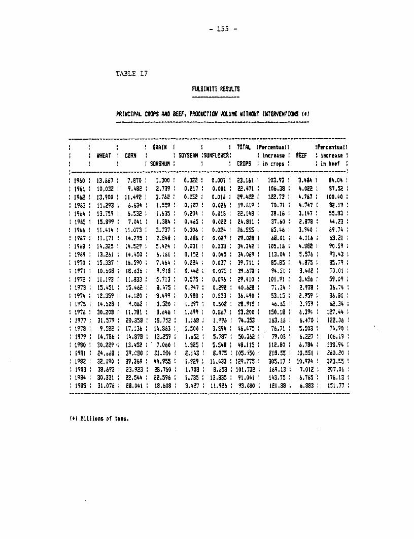
- 155 -

TABLE 17

FULSINITI RESULTS

PRINCIPAL CROPS AND BEEF, PRODUCTION VOLlUME VITHOUT INTERVENTIONS (II

GRAIN : TOTAL !Parcmntual: :Prcntual: WHEAT CORN t : SOYBEAN :SUNFLVER t increase EEF increase:

'SORGHUM 'CROPS in crops . in beef

1960 1 13.667 7.870 1.300 0.322 0.001 23.161 103.93 3.484 : 94.041961 ' 10.032 9 9.482 2.739 0.217 : O.00o 22.471 : 106.38 : 4.022 97.521962 13.900 11.492 3.762 0.252 0.016 29.422 122.73 4.767 100.401963 11.293 6.634 I. '59 0.107 0.026 19.619 70.71 : 4.747 82.191964 13.759 6.532 1.635 0.204 0.018 22.149 38.16 : 3.147 55.831965 15.899 7.041 1.384 0.465 0.022 2 24.311 37.60 : 2.878 : 44.231966 11.414 11.073 3.737 : 0.06 0.024 26.555 65.46 3.940 69.741967 : 11.71 14.295 2.348 : 0.686 : 0.027 : 29.029 68.01 4.116 6 63.211968 1 14.325 14.529 5.424 0.031 0.033 : 34.342 1 105.16 4.882 90.591969 13.261 14.450 6.161 0.152 0.045 34.069 113.04 5.576 93.431970 1 15.337 : 16.590 7.464 0.284 0.037 39.711 85.85 4.975 a85.79

1971 10.609 1: 8.636 9.918 0.442 0.075 39.678 94.51 3.402 70.011972 : 11.0.333 5.713 0.575 0.0 : 29.410: 101.91 3.46: 59.091973 15.451 15.462 8.475 0.947 : 0.292 4 40.621 7%.34 2.938 36.741974 12.359 1: .120 9.499 0.990 : 0.533 36.490 : 53.15 2.959 1 36.311 1 9 75 14.528 9.062 3.520 1.297 0.508 : 29.915 46.65 3.959 62.341976 : 30.208 11.781 8 9.646 1.699 0.367 1 53.200 150.118 1 6.394 127.441977 31.579 20.858 15.752 : 1.168 1.956 74.353 163.hS 6.470 : 122.061 l979 : 9.582 17.36 14.963 : 1.500 3.394 46.475 : 76.71 5.503 74.901 l979 : 14.786 14.878 13.25C 1. .O : 5.787 : 50.362 1 79.03 6.227 106.19 91930 : 0.229: 13.452 7.060 I 1.825 : S.548 1 48.115 : 112.80 1 6.784 1 138.94

: 1981 24.o68 39.'S0 31.038 t 2.143 t 8.975 105.:50 . 219.55 10.51 6 260.201982 32.090 39.369 44.955 : 1.929 11 1.433 :129.7715 t 305.17 1 10.924 323t.55

1 1983 38.693 23.923 : 28.760 : 1.703 8.653 101.732 1 l69.13 t 7.012 : 207.01:1994 : 30.331 22.544 22.596 1.735 13.835 91.041 1 43.75 6.765 176.131985 : 31.076 t 28.041 : 18.608 t 3.427 11.926 93.080 : 121.38 6.393 151.77

(I) Millions of tons.

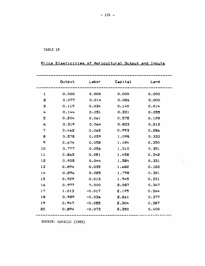
- 156 -

TABLE 18

Price Elasticities of Aaricultural Output and InDuts

Output Labor Capital Land

1 0.000 0.000 0.000 0.000

2 0.077 0.014 0.026 0.000

3 0.119 0.034 0.140 0.014

4 0.144 0.051 0.331 0.055

5 0.204 0.061 0.578 0.128

6 0.319 0.064 0.833 0.212

7 0.462 0.062 0.993 0.286

8 0.578 0.059 1.098 0.333

9 0.674 0.058 1.184 0.350

10 0.777 0.056 1.310 0.351

11 0.865 0.051 1.45e 0.342

12 0.905 0.044 1.584 0.331

13 0.894 0.035 1.682 0.322

14 0.896 0.025 1.798 0.321

15 0.929 0.013 1.945 0.331

16 0.977 0.000 2.087 0.347

17 1.013 -0.017 2.195 0.364

18 0.989 -0.036 2.261 0.377

19 0.947 -0.055 2.304 0.387

20 0.894 -0.073 2.350 0.400

SOURCE: CAVALLO (1985)

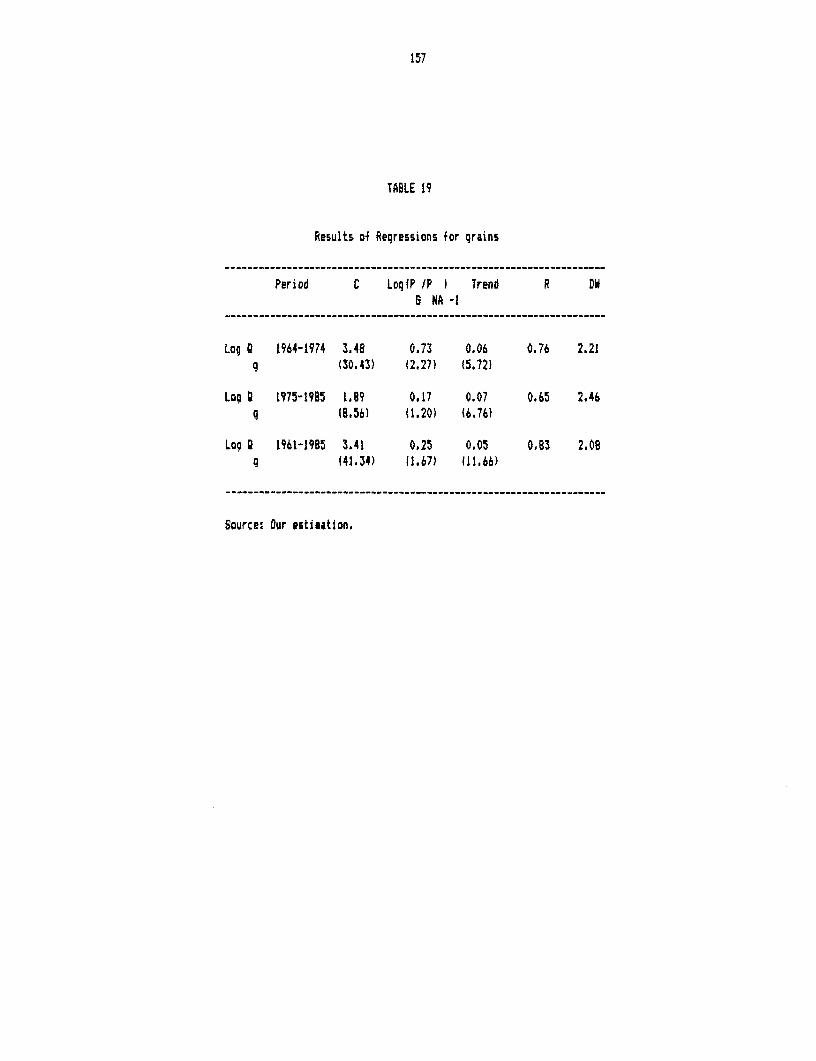
157

TABLE 19

Results of Rearessions for grains

Period C Log(P /P ) Trend R DW6 NA -1

Log 0 1964-1974 3.48 0.73 0.06 0.76 2.21q (30.43) (2.27) (5.72)

LoQ Q 1975-1985 1.99 0.17 0.07 0.65 2.46q (8.56) (1.20) (6.76)

Los 0 1961-1985 3.41 0.25 0.05 0.83 2.08q (41.34) (1.67) 111.66)

Source: Our estisation.

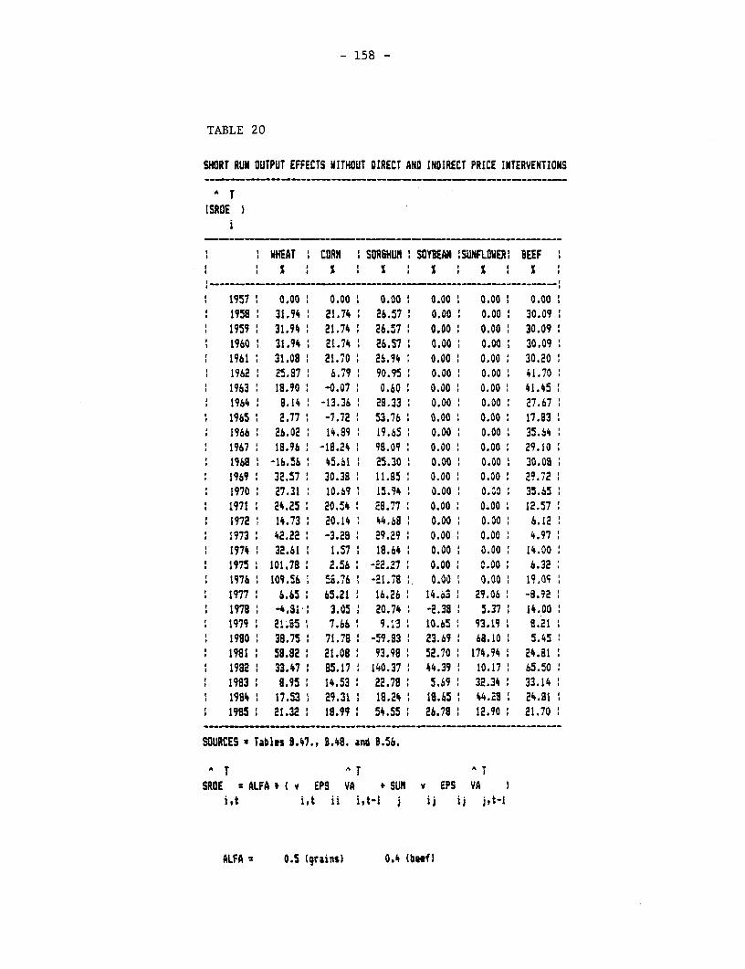
- 158 -

TABLE 20

SHORT RUN OUTPUT EFFECTS UITHOUT DIRECT AND INDIRECT PRICE INTERVENTIONS

ATISROE )

i

I WHEAT CORN SORHIUNI SOYBEAN SUNFLOWER! BEEF I

1957 0.00 1 0.00 0.00 t 0.00 1 0.00 0.00 :1958 131.94 121.74 126.57 0.00 0.00 :30.091959 1 31.94 ' 21.74 : 26.57 0.00 : 0.00 1 30.091960 31.94 21.74 I 26.57 0.00 0.00 30.091961: 31.09 21.70: 26.94 0.00 0.00 30.201962 25.57 6.79 90.95 0.00 0.00 41.701963: 19.90 -0.07: 0.60' 0.00' 0.00: 41.45'1964 8.14 -13.36 29.33 0.00 0.00 27.671965 ' 2.77 1 -7.72 ' 53.76 0.00 ' 0.00 17.931966 26.02 14.89 19.65 0.00 0.00 35.641967 19.96: -19.24 98.09' 0.00 0.00 29.101968 -16. S6, 45.61 1 25.30 0.00 0.001 30.08'1969 ' 32.57: 30.38 : 11.85 ' 0.00 0.00: 29.721970 27.31 ' 10.69 15.94 0.00' 0.Z0 35.65

1 1971' 24.25 20.54 28.77 0.00 0.00 1 12.571972 14.73: 20.141 44.698 0.00 0.00 6.12:1973 4 42.22 : -3.28 : 29.29 : 0.00 : 0.00 4 4.971974: 32.61 1.57 18.64 0.00 0.00: 14.001975 , 101.79 : 2.56 : -22.27 : 0.00 : 0.00 : 6.321976 t 109.56 5;.76 1 -21.78 0.0o : 0.00 : 19 051977 6.65 : 65.21 ' 16.26 14.63 : 29.06 ' -8.921978 -4831: 3.05 20.74 . -2.38 : 5.37: 14.001979 : 2E.l55 7.66 1 9.M ' 10.65 93.19 1 8.21 :1990 ' 39.75 : 71.78 : -59.83 ' 23.69 : 68.10 : 5.451991 5 59.82 21.09 93.98 52.70 174.94 24.81

1 1992 1 33.47 8 85.17 ' 140.37 , 44.39 : 10.17 6 65.501983: 9.95: 14.53: 22.79: 5.69 32.34: 33.14

1 1984 1 17.53: 29.31 1 19.24: 18.651 44.211 24.511 1985 1 21.32 ' 19.99 I 54.55 : 26.78 1 12.90 : 21.70

SOURCES a Tables 3.47., 1.i2. and 3.56.

A T AT AT

SROE : ALFA *( EPS VA + SUN v EPS VAiLt i0 t ii i,l 0. ij ij j,t-(

ALFA 0 .S (grains) 0.4 (beef)

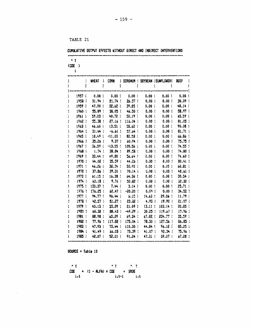
- 159 -

TABLE 21

CUMULATIVE OUTPUT EFFECTS WITHOUT DIRECT AND IH0IRECT INTERVENTIONS

AT

tC8E I

W HEAT CORN SORGHUM MYBEAN !SUNFLOWER BEEF. , I . . .

1957 0.00 0.00 0.00 0.00 i 0.00 o0.001958 31.94 : 21.74 26.57 0.00 0.00 30.091959 47.90 : 32.62 : 39.85 0o.oo 0.00 48.141960 : 55.89 38.05 46.50 I 0.00 0.00 58.971961 59.03 40.72 50.19 0.00 0.00 : 65.591962 55.38 27.16 116.04 0.00 0.00: 81.051963 : 46.60 13.51 i 58.62 0.00 0.00 190.081964 : 31.44 -6.61 : 57.64 0.00o 0.00 81.711965 18.49 -11.03 92.58 0.00 0.00 66.861966 : 35.26 : 9.37: 60.94 1 0.00 0.00: 7.751967 36.59 -13.55 129.56 o0.00 0.00 74.551968 1.74 38.84 89.58 0.00 0.00 74.801969 : 33.44 49.80 56.64 0.00 0.00o 74.601970 44.02 35.59 44.26 0.00 0.00 80.411971 1 46.26 38.24 50.90 0.00 0.00 60.811972 1 37.86 39.31 1 70.14 G.00 1 0.00 142.611973 : 61.15 16.38 : 64.36 0.00 0.00 : 30.541974 : 63.18 9.76 50.82 o 0.00 c.00 . 32.321975 : 133.37 : 7.44 1 3.14 o0.00 1 0.00 25.71i?76 : 176.25 1 62.47 -20.20 0.04 : 0.00 34.521977 94.77: 96.44 6.151 14.63 29.06 11.791978 42.57 51.27 . 23.82 4.93 19.90 21.07

1 1979 : 43.13 : 33.29 1 21.09 : 13.11 : 103.14 1 20.5 11980 60.32 1 88.43 -49.29 30.25 119.67 17.961981 1 88.98 : 65.29 : 69.34 67A.B : 234.77 35.591982 : 77.96 1 117.82 1 175.04 78.30 1 127.56 1 86.85

1 1983 1 47.93 1 73.44 : 110.30 1 44.84 1 96.12 1 95.251984 1 41.49 66.03 1 73.39 41.07 92.34 : 75.961985 1 42.07 1 52.01 1 91.24 47.31 : 59.07 67.28

-- -- - - - - - _- - - - --___--_-_

SOURCEz Table 13

AT AT A TCOE 2 (1 - ALFA) # COE + SROE

i.t i,t-l i.t

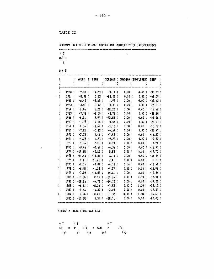
- 160 -

TABLE 22

CMNSUNPTIOM EFFECTS WITHWT DIRECT AND INDIRECT PRICE INTERVENTIONS

^T(CE

i

(in 1)

WHEAT 1 CORN ' SORSHU' SOYBEAN !SUNFLOUER! BEEF

1960 -9.38 ' -4.23 -3.11 0.00 0.00 -33.031961 -8.36 7.65 -23.03 0.00 0.00 1 -42.591962 -6.45 -3.62 1.93 0.00 0.00 1 -39.621963 -3.52 2.42 -5.38 0.00 0.00 -25.311964 -2.46 5.26 -12.26 0.00 0.00 -16.621965 -7.98 -3.10 -2.78 0.00 0.00 -36.681966 1 -6.51 ' 9.94 -22.82 0.00 0.00 -28.56'1967 -1.75 -7.64 0.55 ' 0.00 0.00 -29.071968 -8.36 -3.68 -3.15 : 0.00 0.00 -33.221969 -7.21 -0.33 -4.64 , 0.00 0.00 -36.471970 -5.78 0.41 -7.92 0.00 0.00 -16.251971 -4.29 1.23 -9.28 0.00 0.00 -9.521972 -9.26 2.08 -8.79 0.00 0.00 -9.711973 -8.46 -0.69 -4.34 0.00 0.00 -16.911974 ' -1(.68 -5.25 2.95 0.00 0.00 -17.tO0

1975 -21.40 -13.82 6.14 i' 0.00 0.00 -34.511976 -6.11 -11.66 2.41 . 0.00 0.00 1.;21977 1 -2.14 ' -0.09 -4.1a : 0.30 . 0.00 -12.41 .!s9 . -6.48 , -1.22 , -4.37 0.00 0.00 -12.911979 -7.89 -14.38 8 14.61 . 0.00 . j.00 -13.961J90 -13.34 . 2.q7 . -20.84 . 0.00 0.00 -37.311981 -12.26 -4.72 . -14.15 , 0.00 1 0.00 . -69.391992 -6.11 . -2.34 . -4.931 0.00 ' 0.00 -32.151993 -9.16 -4.39 -3.69 0.00 0.00 -27.341994 -9.64 -0.45 . -12.32 . 0.00 . 0.00 . -24.43 11985 : -10.62 1 0.57 1 -12.91 . 0.00 . 0.00 . -20.03 '

SOURCE Table 8.45. and 3.64.

AT AT AT

CE : P ETA + SUM P ETAi,t i,t i,i i,t i,

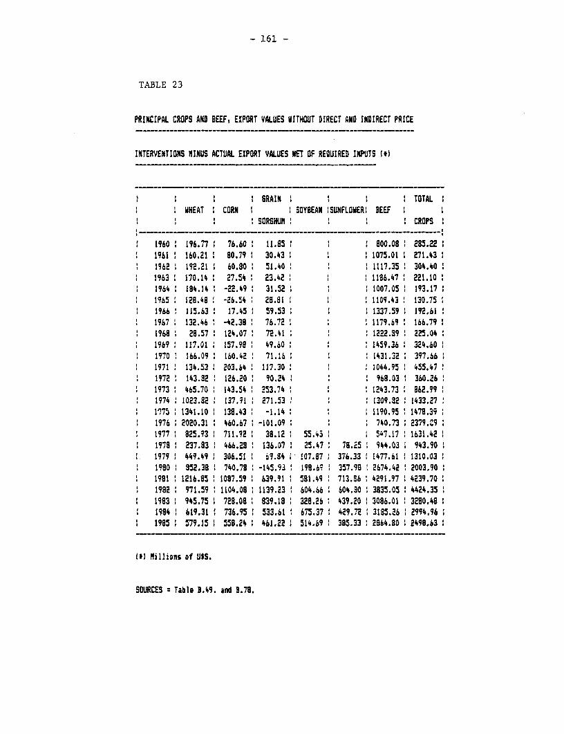
- 161 -

TABLE 23

PRINCIPAL CROPS AND BEEF, EXPnRT VALUES VITHOUT DIRECT AND INDIRECT PRICE

INTERVENTIONS MINUS ACTUAL EXPORT VALUES NET OF REOUIRED INPUTS (t)

GRAIN TOTALHEAT CORN ' , SOYBEAN :SUNFLOWER' BEEF

SORSHUM ' CROPS

1960 196.77 76.60 1 11.85 : 800.08 1 285.22 i1961 160.21 80.79 30.43 I 1 1075.01 1 271.43 I

I 1962 1 192.21 60.80 1 51.40 1 1117.35 1 304.401963 1 170.14 27.54 23.42 i 1186.47 : 221.10

1 1964 184.14 -22.49 31.52 1 1007.05 1 93.171965 128.48 -26.54 29.81 1 11109.43 130.75

I 1966 115.63 1 17.45 59.53 1 11337.59 1 192.611 1967 132.46 -42.38 76.72 I 1179.69 166.79

1968 28.57 124.07 7 72.41 1222.89 225.041969 1 117.01 157.98l 49.60 * 1459.36 324.60

1 1970 166.09 160.42 71.16 1431.32 397.661971 134.53 1 203.64 117.30 1 1044.95 455.471972 143.82 126.201 90.24 1 968.03 1 360.261973 1 465.70 143.54 1 253.74 1 1243.73 862.991974 1023.82 137.91 271.53 1 . . 1309.82 . 1433.27

1 11753 1341.10 1 138.43 -1.14 1 1190.95 1478.391976 2020.31 1 460.67 . -101.09 740.73 1 2379.291977 1 825.93 1 711.12 : 38.12 55.i; 1 1 5'7.17 1631.42

: 1979 237.93 466.29 1 136.07 25.47 78.5S 944.03 1 943.901979 449.49 306.51 60.84 1107.87 376.33 1 1477.61 1 1310.03

1 1980 1 952.38 740.78 -145.93 198.6: 1 357.98 2674.42 1 2003.901 1991 1 1216.85 1 1087.59 639.91 581.49 1 713.S6 1 4291.97 4239.701 1982 971.59 1104.08 1139.23 1 604.66 1 604.90 1 3835.05 4424.35: 1993 945.75 728.089 839.18 1 328.26 1 439.20 13096.01 13290.48 1

1984 1 619.31 : 736.95 . 533.61 : 675.37 t 429.72 1 3185.26 1 2994.96 :1995 1579.15 1 558.24 : 461.22 1 514.69 1 385.33 1 2864.80 12498.63 1

1f) Millions of USS.

SOURCES z Table 3.49. and 3.78.

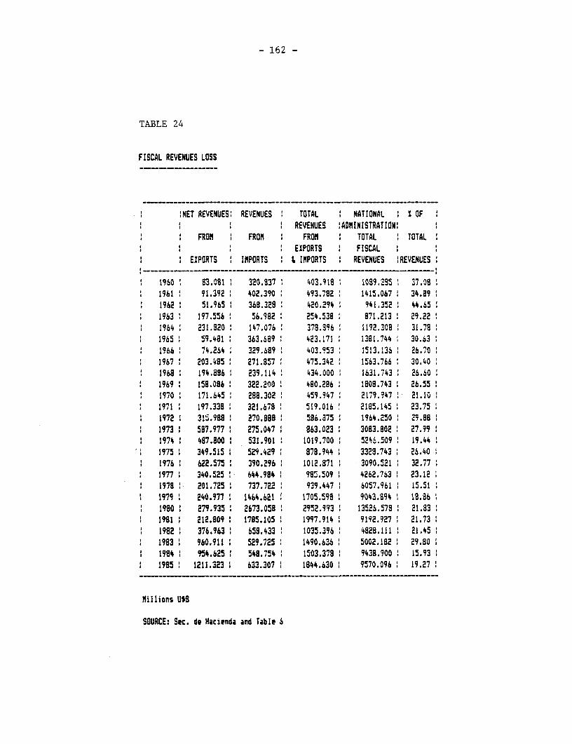
- 162 -

TABLE 24

FISCAL REVENUES LOSS

:NET REVENUES: REVENUES 1 TOTAL NATIONAL : I OFI REVENUES :ADMINISTRATION:

FROM I FROM I FROM I TOTAL TOTALI EXPORTS 1 FISCAL I

EXPORTS IMPORTS ' £ IMPORTS REVENUES !RE VENUES

1960 83.3081 320.837 403.918 109s.285 37.081961 1 91.392 402.390 493.782 1415.067 34.891962 51.965 368.328 420.294 941.352 44.651963 197.556 56.982 254.538 871.213 29.221 1964 231.920 147.076 378.996 1192.308 31.781965 59.4al8 363.689 423.171 1381.744 30.631966 1 74.264 329.689 403.953 1513.136 26.701967 203.485 271.857 475.342 1563.766 30.401968 194.886 239.114 434.000 1631.743 26.601969 158.086 1 322.200 480.286 1 1808.743 1 26.55

1 1970 1 171.645 285.302 459.947 2179.?47 1 21.101971 1 197.338 321.678 519.016 2185.145 23.751972 315.9885 270.888 586.A75 1964.250 T8.81973 597.977 1 275.047 8 863.023 3083.802 27.991974 487.800 531.901 1 1019.700 52k.509 19.441975 349.515 529.429 878.944 3329.743 26.40l1976 622.575 390.296 1012.871 3090.5121 32.771977 340.525 1 644.984 98:.509 4262.763 23.121978 201.725 ! 737.722L 939.447 6057.961 15.51

1 1979 1 240.977 1 1464.621 1705.598 9043.894 18.56B190 279.935 2673.058 2952.993 13526.578 21.8319I 212.909 I 1785.105 1997.914 9192.927 21.73

1 1982 I 376.963 6 658.433 1 1035.396 4828.111 21.451 1983 960.911 529.725 1490.636 i 5002.182 29.80: 1984 954.625 1 548.754 1503.378 I 9438.900 15.931 1985 1211.323 1 633.307 1844.630 9570.096 119.27

millions U1S

SOURCE: Sec. de Hacienda and Table 6

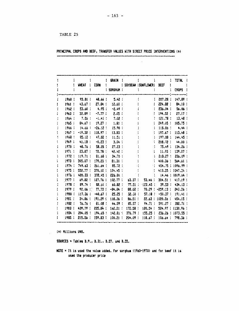
- 163 -

TABLE 25

PRINCIPAL CROPS AND BEEF, TRANSFER VALUES WITH OIRECT PRICE INTERVENTIONS011 )

SRAIN ' TOTAL 1I WHEAT ' CORN . t SOYBEAN :SUNFLOWER: BEEF

SORSHUMI CROPS '

1960 93.81 48.66 5.42 t 207.28 147.891961 43.67 27.84 112.60 224.88 84.101962 53.60 4.95 -2.49 236.04 56.061963 32.89 1 -7.77 2.05 194.52 27.171964 7.36 -1.41 7.02 121.78 13.481965 1 84.67 1 19.27 1.91 249.05 105.75

1 1966 14.66 ! -26.12 15.90 1 1 113.86 4.441967 1 -19.32 ' 119.97 13.33 ' ' 197.67 113.481968 85.12 1 47.321 11.51 1 1 197.898 144.451969 41.181 -0.231 3.04 ' 208.72' 44.00

i 1970 48.76 58.29' 27.23 1 ' 75.49 134.261971 ' 23.871 72.78 42.42 ' 1 11.93 139.0719721 119.71 1 91.68 1 34.70 ' 1 219.27 236.091973 305.07' 179.23 1 81.31 i 1 400.36 1 564.6119741 749.63 261.641 85.72 454.751 1096.991975 552.77 1 370.12 1 124.45 i 413.35 1047.241976 420.33 372.45 226.86 I 14.46 1019.64 11977 1 69.82 1 127.76 102.77 63.37 53.46 304.51 1 417.191978 1 89.74 1 82.S1 60.82 1 77.51 1 123.45 1 39.53 1 434.131979 92.06 77.73' -84.84 88.02 1 70.29 -259.a3 243.361980 117.36 -40.67' 25.25 32.30 57.18 -50.37 191.411981 34;.86 I 191.29§ 118.36 86.51 ' 22.63' 1020.56 1 454.151982 76.76 81.08 44.59 85.57 94.71 591.27 ' 382.711983 439.79 235.84 162.21 1 172.58 ' 120.54 524.97 1 1130.96

1 1994 204.05' 194.65 I 142.81 I 376.79 155.25 236.26 1073.55J1985 215.56 1 159.83 1 100.21 1 204.09 1 118.67 1 106.64 799.36

1t) Mlillions USS.

SOURCES Tables 9.9. 9.31., 9.37. and 9.55.

NOTE 2 It is used the value added. For sorghum (1960-1970) and for beef it isused the producer price

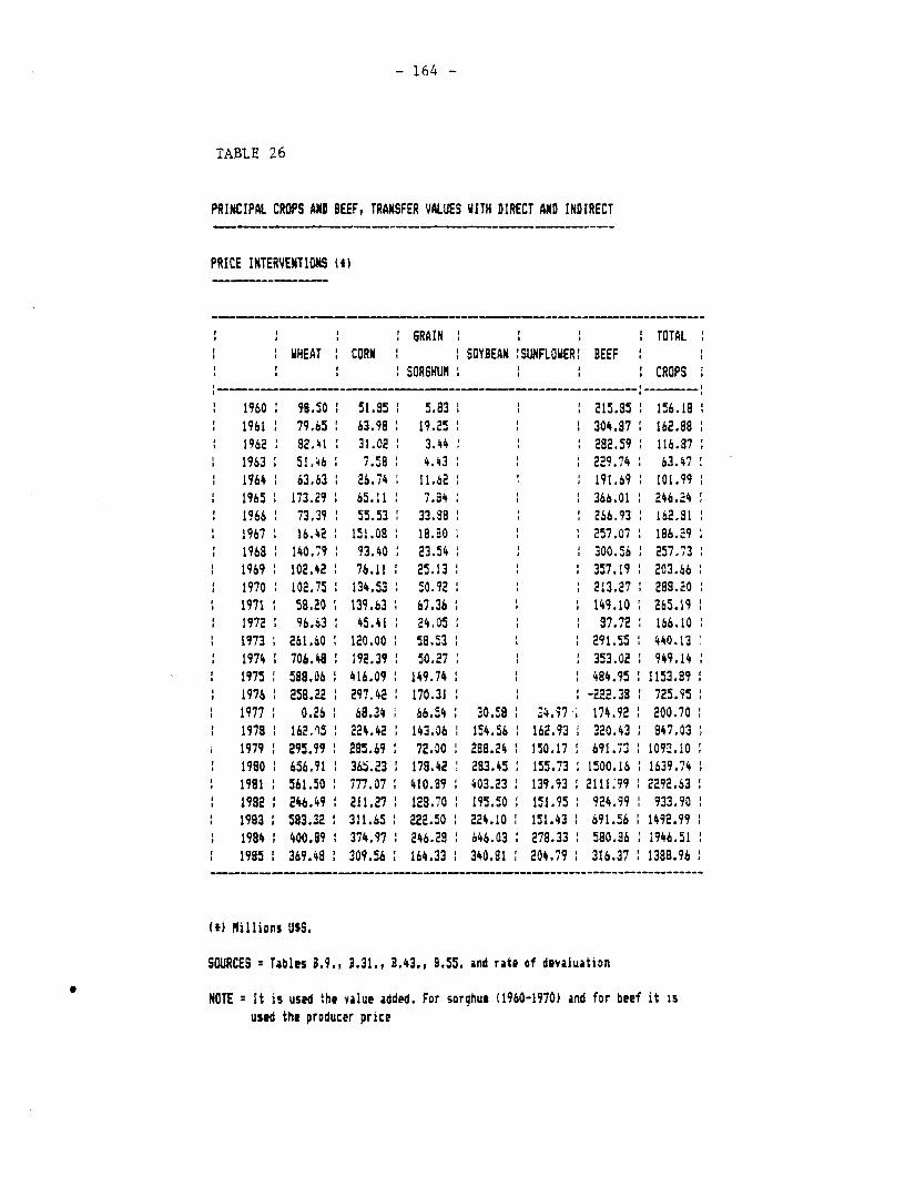
- 164 -

TABLE 26

PRINCIPAL CROPS AND BEEF, TRANSFER VALUES WITH DIRECT AND INDIRECT

PRICE INTERVENTIONS I1)

' GRAIN T ' tOTAL' WHEAT 1 CORN t 1 SOYBEAN 'SUNFLOWER' BEEF

:SORSHUh, CROPS

1960 98.50 51.95 5.83 215.85 156.181961 79.65 63.98 19.25 i 1 304.87 162.981962 82.41 31.02 3.44 : 282.59 116.871963 51.46 7.58 4.43 229.74 63.471964 63.63: 26.74 11.62 191.69 101.991965 173.29 65.11 7.84 366.01 246.241966 73.39 55.53 33.88 266.93 162.811967 16.42 151.08 18.80 i 1 257.07 186.291968 140.79 93.40 23.54 300.56 257.731969 102.42 76.11 ' 25.13 : 1 357.19 203.661970 M 102.75 : 134.53 ; 50.92 : : 213.27 ; 288.201971 58.20: 133.63: 67.36 1 1 149.10; 265.191972 : 96.63' 45.41 : 24.05 3 ; 87.72 166.101973 261.60 120.00 58.53 1 1 291.55 1 440.131974 706.48 192.39 50.27 ' 1 353.02 949.141975 588.06 416.09 149.74 ' ' 484.95 1153.891976 ' 258.22 1 297.42 : 170.31 1 ; 1 -222.38 1 725.951977 0.26 : 68.34 66.54 ; 30.58 ; ;4.97, 174.92 ; 200.701978 162A5 : 224.42 143.06 154.56 162.93M 320.43 847.031979 1 295.99 1 285.69 ' 72.00 1 288.24 150.17 ; 691.7 : 1092.101980 656.91 1 36g.23' 178.42 283.45 155.73 1500.16 1639.741981 1 561.50 ' 777.07 410.99 1 403.23 1 139.93 :2111.99 '2292.631982 246.49 211.27 128.70 195.50 151.95 924.99 933.901993 583.32 I 311.65 222.50, 224.10 151.43 691.56 : 1492.991984 1 400.39 374.97 246.28 646.03 278.33 580.86 1946.511995 1 369.48 1 309.56 : 164.33 ; 340.91 1 204.79 ; 316.37 : 1388.96

(I) Nillions U59,

SOURCES T Tables 0.9., B.31., B.43., 3.55. and rate of devaluation

NOTE = It is used 'the value added. For sorghue (1960-1970) and for beef it isused the producer price

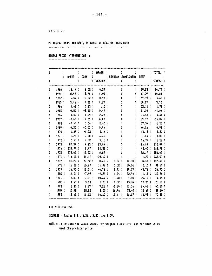
- 165 -

TABLE 27

PRINCIPAL CROPS AND BEEF, RESOURCE ALLOCATION COSTS WITH

DIRECT PRICE INTERVENTIONS 1t)

B GRAIN TOTAL: WHEAT CORN SOYBEAN !SUNFLOWER BEEF

SORSHUIS CRMPS

1960 18.14: 6.05 0.57 39.29 24.771961:1 9.972 3.71 1.45 :47.39 14.081962 6.57 -0.02: -0.90: 57.75 5.661963 3.06 0.36 0.291 54.19 3.701964 0.43 0.15 1.15 32.11 1.73

* 1965 0.80 -2.32 0.47 51.10 -1.041966 0.50 1.89 2.25 : 24.48 4.641967 -0.40 -19.15 4.47 33.97 -15.071968 -7.47 3.54 2.40 37.54 -1.531969 0.50 -0.01 0.44 40.06 0.921970 1.39 -1.33 3.14 : 15.18: 3.201971 1.29 0.08 6.66 1.64: 8.031972: 5.73 2.72 7.13: 16.97: 15.58

* 1973 87.34: 4.65 23.04 26.68 115.041974 : 239.74 : 8.47 20.51 . 42.40 268.721975 372.05 13.5Z X. : : 28.17: 386.4511976 314.08: 81.47 1 -28.47 : 1.20 367.071977 31.27 1 72.22 : 8.66 8.1E2 12.20 : 0.30 132.471978 19.66 26.67 10.09 5.52 20.05 2.10 B1.991979 14.97 : 11.71: -4.76 : 3.71: 29.07 -5.% 554.701980 16.71 : -7.49: -6.24 1.34: 22.94 1.16 27.26

* 1981 3.57 2.91 -10.67 2.00: 9.65 -25.18 7.461982 1.49: 3.13 3.93 0.z2: 13.84 50.36 22.91:1993 3.50 6.99 9.28 -1.24: 21.36: 64.42 40.201984 10.42 18.25 8.50 16.46 35.47 31.60: 89.101985 13.42 11.15 14.60 15.41 16.27 10.92 70.85

(*) Millions USS.

SOURCES = Tables 8.9., 9.31., 8.37. and B.59.

NOTE - It is used the value added. For sorghum (1960-1970) and for beef it isused the producer price

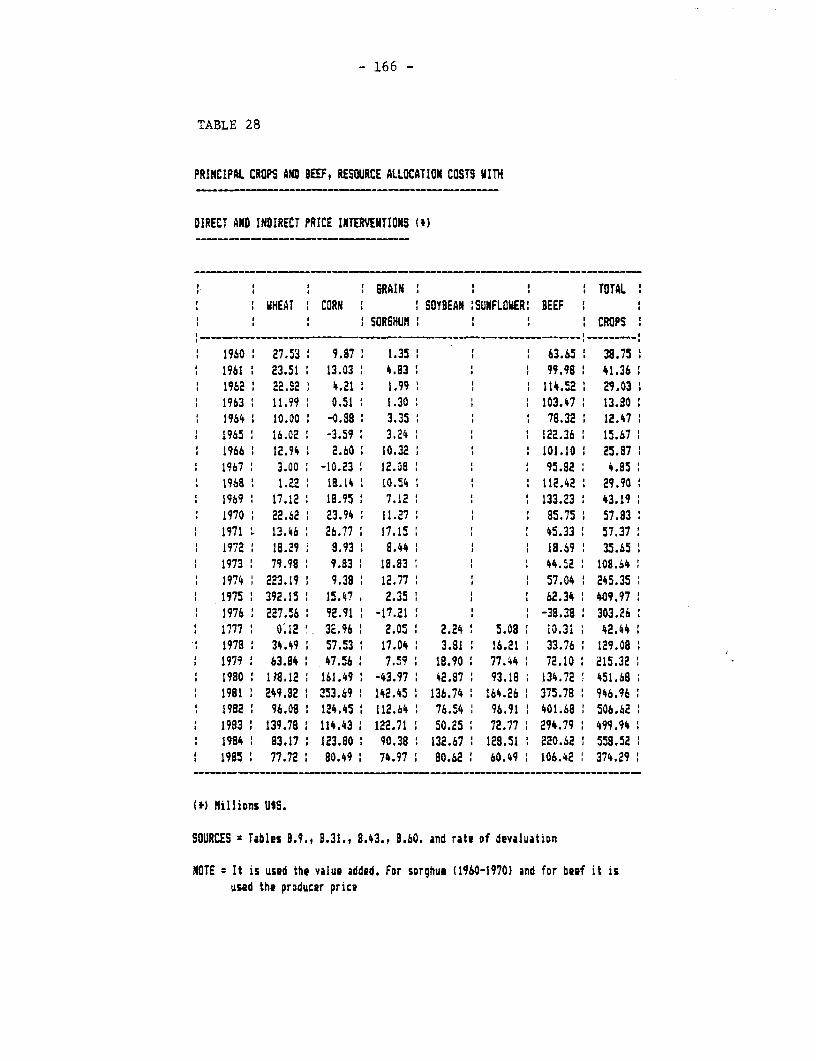
- 166 -

TABLE 28

PRINCIPAL CROPS AND BEEF, RESOURCE ALLOCATION COSTS HITH

DIRECT AND INDIRECT PRICE INTERVENTIONS (I)

; G ' ' &RAIN 1 TOTALWHEAT CORN ' SOYBEAN :SUNFLDWER! BEEF

SORSHUM I CROPS

1960 27.53 9.87 1.35 1 63.65 38.751961 23.51 13.03 4.83 1 99.98 41.361962 22.32 4.21 1.99 i 114.52 I 29.031963 11.99 0.51 1.30 : 103.47 13.801964 10.00 : -0.88: 3.35 : : 78.32 12.471965 : 16.02 -3.59 3.2s4 : 1 122.36 15.671966 12.94: 2.60 10.32 . 101.10 1 25.871967 : 3.00 -10.23 12.08 ' : : 95.82 : 4.851968 1.22 tB.14 : 10.54 112.42' 29.901969 : 17.12 1 18.95 7.12 ' : 133.23 43.191970 : 22.S2 : 23.94 , 11.27 : 95.75 57.831971 13.46 ' 26.77 : 17.15 : : 45.33 : 57.371972 1 18.29 8.93 1 8.44 : : 18.69 1 35.651973 1 79.98 9.83: 18.83 ' 44.A2 1 108.i41974 1 223.19 9.38 12.77 : : : 57.04 1 245.351975 : 392.15 : 15.47 2.35 1 1 62.34 409.971976 227.56 92.91 1 -17.21 : 1 -38.38 303.261777 ' O.12 3E.96 2.05 O 2.24 5.08 ' 10.311 42.441978 : 34.49 : 57.53 17.04 : 3.81 1 16.21 : 33.76 1 129.081979 ' 63.84 1 47.56 1 7.59 18.90 77.4 4 72.10 215.321980 1 i?8.12 : 161.49 ' -43.97 ' 42.87 : 93.18 , 134.72 451.681981 ' 249.92 1 253.6 1 142.45 : 136.74 164.26 1 375.78 : 946.961982 1 96.08 124.45 112.64 76.54 : 96.91 401.68 1 506.621983 1 139.78 1 114.43 122.71 50.25 : 72.77 : 294.79 1 499.941984 : 83.17 1 123.80 90.38 : 132.67 : 128.51 : 220.62 558.521985 : 77.72 80.49 1 74.97 80.62 : 60.49 : 106.42 374.29

(C) Millions UIS.

SOURCES Tables 3.9., 9.31., 8.43., 9.60. and rate of devaluation

NOTE It is used the value added. For sorghum (1960-1970) and for beef it isused the producer price

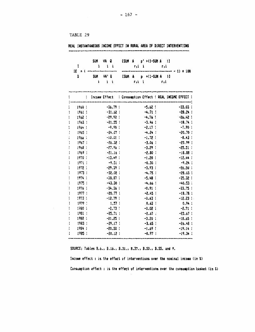
- 167 -

TABLE 29

REAL INSTAITAXEOUS INCOME EFFECT IN RURAL AREA OF DIRECT INTERVENTIONS

SUL VA Q [SUN A p' *(I-SUM A )]I ~~i i ir, iri

IE : I 1) t 1t-0 SUn VA', ESIU A p +(l-SUNa )A

i i i r,i i r,i

i 1 Incose Effect 1 Consumption Effect REAL INtOME EFFECT

1960 -36.79 -5.62 -33.031961 -31.S2 -4.71 -28.2419b2 -29.92 -4.76 -26.421963 -21.55 -3.A6 -18.741964 1 -9.90 -2.17 -7.901965 -24.07 -4.24 -20.701966 -10.01 -1.72 -8.431967 -26.32 -3.06 -23.991968 -27.96 -3.29 ' -25.511969 -21.16 -2.80 -18.881970 -13.49 -1.20 1 -12.441971 -9.51 -0.30 : -9.241972 1 -29.39 -3.93 i -26.501973 -32.02 -4.75 : -29.631974 -38.87 -5.48 t -35.321975 -43.30 t -4.66 -40.531976 -34.36 -0.91 -33.751977 -20.77 -2.45 . -18.'31973 -12.79 -0.63 -12.231979 1.57 . 0.63 0.94i980a -2.73 ! -0.02 -2.711981 -25.71 ' -2.57 -a3.671992 -21.25 , -3.20 -18.651993 -29.17 -3.65 -26.481984 -20.50 -1.69 -1q.141985 -20.12 -0.97 . -19.34

SOURCE: Tables 8.6., 8.16., 8.31., 3.37., 3.50., 3.55. and 9.

Income effect : is the effect of interventions over the nosinal income (in X)

Consumption effect : is the effect of interventions over the consueption basket (in I)

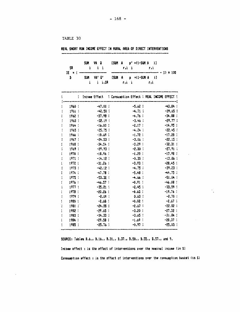
- 168 -

TABLE 30

REAL SHORT RUE IICDOE EFFECT IN RURAL AREA OF DIRECT INTERVENTIONS

SUN VA t [SUM A pI +(-SUN A )ASR i i i rTi i r,i

IE :1) 100D SUN VA, G ESUN A p +(l-SUNA A 1

i i i,SR r,i i r,i

1 Incose Effect Consumption Effect REAL INCOME EFFECT

1960 -47.00 -5.62 -43.841961 -42.50 -4.71 -39.651962 -37.98 -4.76 -34.881963 -32.19 -3.46 -29.771964 -16.80 -2.17 -14.951965 -25.75 -4.24 -22.451966 -18.69 -1.72 -17.281967 -24.53 -3.06 -22.151968 -34.54 -3.29 -32.311969 -29.93 -2.30 -27.911970 -18.96 -1.20 -17.981971 -14.12 -0.30 1 -13.861972 -31.26 -3.93 -28.451973 -42.12 -4.75 -39.231974 -47.78 -5.48 -44.751975 -53.32 -4.66 -51.041976 -46.57 -0.91 -46.0819777 -35.21 -2.45 i -33.591978 -20.26 1 -6.63 -19.76!979 -2.09 1 0.63 -2.701980 -2.68 : -0.02 -2.671981 -24.39 -2.67 1 -22.821992 -29.65 -3.20 -27.321983 -34.33 -3.65 1-31.841984 -29.58 -1.69 -28.371985 -25.76 -0.97 -25.03 i

SOURCE: Tables 3.6., 3.16., 3.31., 9.37., 3.50., 3.55., 3.57., and 9.

Income effect : is the effect of interventions over the nosinal incose (in Sl

Consumption effect : is the effect of interventions over the consumption basket (in 1)

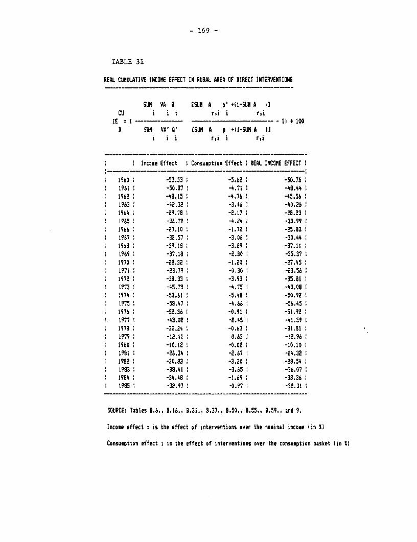
- 169 -

TABLE 31

REAL CUMULATIVE INCOME EFFECT IN RURAL AREA OF OIRECT INTERVENTIONS

SUN VA O ESUN A p' fl1-SUN A llCU i i i r,i i r,i

IE :(---1) f 100D SUN VA' Q' (SUN A p +(1-SUM A l1

i i i r,i i ri

I Income Effect 1 Consumption Effect REAL INCOME EFFECT

1960 -53.53 -5.62 -50.761961 -50.a7 -4.71 -48.441962 -48.15 -4.76 1 -45.561963 -42.32 -3.46 -40.2b1964 -29.78 1 -2.17 -28.23 I1965 -36.79 -4.24 -33.991966 -27.10 -1.72 1 -25.831967 -32.57 1 -3.06 -30.44196' -39.18 -3.29 -37.111969 -37.18 -2.80 -35.37 I

i 1970 1 -28.32 -1.20 ' -27.451971 : -23.79 ' -0.30 -23.S61972 1 -38.33 1 -3.93 1 -35.81 i1973 1 -45.79 1 -4.75 1 -43.081974 -53.61 -5.48 -50.921975 1 -58.47 1 -4.66 I -56.451976 ' -52.36 1 -0.91 1 -51.921977 -43.02 -2.45 -41.591978 -32.24 1 -0.63 1 -31.811979 1 -12.S1 0.63 1 -12.961960 1 -10.12 1 -0.02 : -10.101981 -26.34 : -2.67 1 -24.321982 1 -30.93 1 -3.20 1 -28.54

: 1983 1 -38.41 : -3.S5 1 -36.071984 1 -34.48 1 -1.69 : -33.361985 -32.97 1 -0.97 : -32.31

SOURCE: Tables 1.6., 3.16., 3.31., 3.37., 8.50., 3.55., B.59., and 9.

Income effect : is the effect of interventions over the nominal incose lin %)

Consueption effect : is the effect of interventions over the consumption basket (in %)

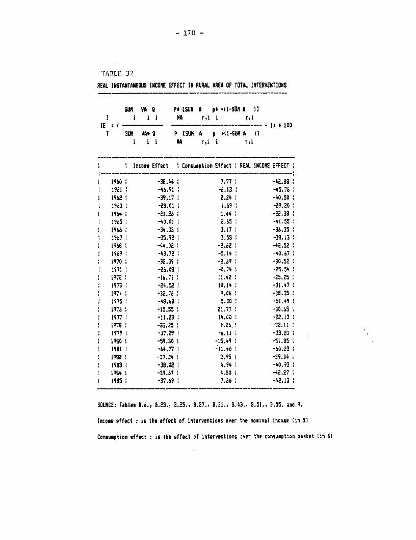
- 170 -

TABLE 32

REAL INSTANTANEOU IKOPE EFFECT IN RURAL AREA OF TOTAL INTERVENTIONS

SUn VA O Pt (SUN A pt +(-SUNA A ]I i i i #A r,i i r,i

IE 1 ( ----- 1)t100T SUn VA* 3 P ESUN A p +11-SUM A )

i i i KA r,i i r.i

Incomn Effect ' Consumption Effect : REAL INCOME EFFECT

1960 -39.44 1 7.77 -42.881961 -46.91 -2.13 t -45.761962 -39.17 2.24 -40.501963 -28.01 1.69 -29.201964 i -21.26 1 1.44 -22.381965 -40.01 2.i5 -41.551966 -34.33 3.17 -36.351967 -35.92 3.58 1 -33.131968 -44.02 -2.62 i -42.521969 -43.72 : -5.14 -40.671970 -32.39 -2.69 -30.521971 -26.08 -0.74 -25.541972 -16.71 11.42 -25.251973 -24.52 10.14 -31.471974 1 -32.76 1 9.06 ' -38.351975 -48.68 5.30 -51.491976 -15.55 21.77 -30.651977 -11.23 14.30 -22.131978 -31.25 1.26 -32.111979 -37.29 -6.11 -33.211980 , -59.30 ' -15.49 -51.851981 ' -64.77 -11.40 -60.231982 -37.24 2.95 -39.041983 1 -38.02 4.94 -40.931984 1 -39.67 : 4.50 1 -42.1985 -37.69 1 7.66 ' -42.13

SOURCE: Tables 3.6., 3.23., 3.25., 3.27., B.31., 3.43., 3.51., 3.55. and 9.

Income effect : is the effect of interventions over the nominal incone (in X)

Consueption effect : is the effect of interventions over the consueotion basket (in X)

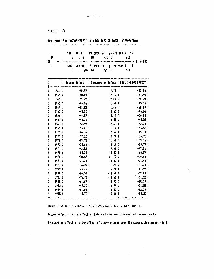
- 171 -

TABLE 33

REAL SHORT RUM INCONE EFFECT IN RURAL AREA OF TOTAL INTERVENTIONS

SUIM VA O P (SUII A p* +(-SUN A 4 3SR i i i A r,ii r,i

IE ( - t100T SUN VA* g P (SUN A p (Il-SUMA )A

i i i,SR MA r,i i r,i

I Income Effect Consumption Effect 1 REAL INCOME EFFECT 1

1960 -52.37 7.77 -55.80 :1961 -59.80 -2.13 -57.901962 -53.97 2.24 -54.98

1 1963 -44.24 1.69 -45.161964 -31.63 1.4 -32.601965 -45.25 2.65 -46.66

: 1966 -49.27 1 3.17 -50.831967 -43.26 3.58 -45.221968 -53.59 -2.62 -52.34

: 1969 : -56.86 ' -5.14 -54.521970 -46.76 -2.69 -45.291971 -37.22 -0.74 -36.761972 -25.75 11.42 -33.36

: 1973 -33.66 : 10.14 -39.77 '1974 -42.53 : 9.06 -47.31

* 1975 -58.28 5.80 -60.!'1976 -39.62 21.77 ' -49.60 1

: 1977 -21.1 1 14.00 -31.41 117B -3a.45. 1.26 -37.24 :1979 : -45.49 1 -6.11 -41.95 :

i 1990 -66.10 : -15.49 : -59.89 .i 1981 -74.77 -11.40 -71.52 '

1982 -61.67 2.95 , -62.77 11983 -49.50 , 4.94 -51.88 ,1984 -51.69 : 4.50 , -53.77 1

* 1995 ' -49.72 : 7.66 , -53.30

SOURCE: Tables 8.6., B.7., 3.23., 3.25., B.31.,3.43., 9.55. and 13.

Income effect : is the effect of interventions over the nominal income (in S)

Consumption effect : is the effect of interventions over the consueption basket (in S)

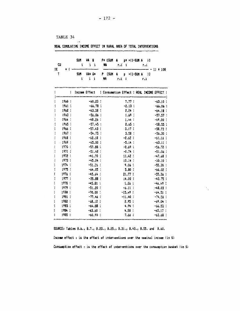
- 172 -

TABLE 34

REAL CUMULATIVE INCOME EFFECT IN RURAL AREA OF TOTAL INTERVENTIONS

SUN VA 0 Pt [SUN A pt +(1-SUM A J]CU i i i NA r,i i r,i

IE = C - ----- - 11)* 100T SUN VA* Ot P [SUN A p +(-SU0 A J1

i i i NA r,i i r,i

1 Income Effect Consueption Effect : REAL IbCOhE EFFECT

1960 1 -60.23 7.77 -63.101961 -66.78 1 -2.13 -66.061962 -63.38 2.24 -64.181963 -56.86 1.69 -57.571964 -48.26 1.44 -49.001965 -57.45 2.65 -58.551966 -57.43 3.17 -58.731967 -54.73 3.598 -56.301968 -62.18 -2.62 -61.161969 -65.00 -5.14 -63.111570 -57.88 -2.69 -56.721971 -S1.42 -0.74 -51.061972 -41.70 11.42 -47.681973 -45.04 10.:4 -iO.101974 -51.216 9.06 1 -55.301975 -64.05 5.S0 -66.021976 -45.64 21.77 -55.361977. -35.88 1 14.00 -43.751978 -45.81 1.26 -46.491979 1 -51.20 -6.11 -48.031580 -70.00 -15.49 -64.511981 -77.46 -11.40 -74.561982 : -68.12 2.95 -69.041983 -64.88 4.94 -66.531984 -63.60 4.50 -65.171985 -60.90 7.66 -63.68

SOURCE: Tables 8.6., 8.7., B.23., 3.25., 8.31., 8.43., 8.55. and 8.60.

Incose effect is the effect of interventions over the nosinal income (in 1

Consumption effect : is the effect of interventions over the consumption basket fin S

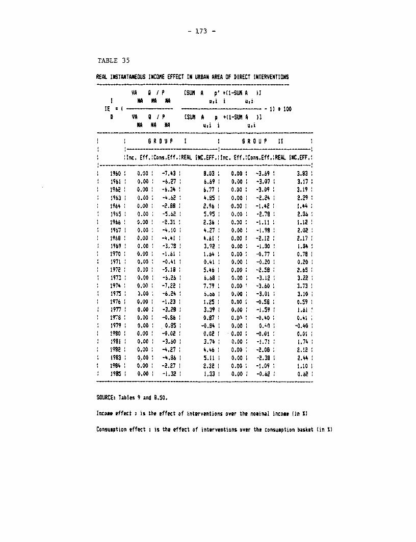
- 173 -

TABLE 35

REAL INSTANTAXEOUS INCOME EFFECT IN URBAN AREA OF DIRECT INTERVENTlINS

VA Q f P CSLU A pI +1-SUN A 11I NA NA uA i ui

IE : t -- oO VA 9 J P [SUL A p +(I-SUM A )1

NA NA NA u,i i u,i

a R O U P I 6 R O U P 11

Inc. Eff.2Cons.Eff.;REAL INC.EFF.:Inc. Eff.2Cons.Eff.!REAL ICH.EFF.

1960 0.00 -7.43 3.03 0.00 -3.69 3.931961 0.00 -6.27 6.69 0.00 -3.07 3.171962: 0.00 -6.34 6.77 0.00 -3.09 3.191963 0.00 -4.62 4.85 0.00 -2.24 2.291964 0.00 -2.88 2.96 0.00 -1.42 1.441965 0.00 -5.62 5.95 0.00 -2.78 2.861966 0.00 -2.31 2.36 0.00 -1.11 1.121967 0.00 -4.10 4.27 0.00 -1.98 2.021968 0.00 -4.41 4.61 0.00 -2.12 2.171969: 0.00 -3.78 3.92 0.00 -1.30 1.341970 0.00 -1.61 1.64 0.00 -0.77: 0.781971 0.00 -0.41i 0.41 0.00 -0.20 0.201972 0.00 -5.18 5.46 0.00 -2.8: 2.651971 7 0.00 -6.26 6.68 0.00 -3.12 3.221974 0.00 -7.22 7.79 o0.00 -3.60 1 3.731975 0.00 -6.24 6.66 0.00 -3.01 3.101976 0.00 -1.23 1.25 0.00 -0.58 0.59:1977 0.00: -3.298 3.39 0.00 -1.59 1.6119?8 0.00 * -0.86 . 0.87 : 0.OA -0.40 0.411979 0.00 : 0.85 -0.84 1 0.00 0.40 -0.40!980 0.00 -0.02 0.02 : 0.00: -0.01 0.011981 0.00: -3.60 3.74 0.00 -1.71 1.741982 0.001 -4.27 4.46 0.00 -2.08 2.121983 0.00: -4.86 5.11 0.00 1 -2.38 2.441984 : 0.00: -2.27 2.32; 0.00 -1.09 1.10:1985 0.00: -1.32 1.33 0.00 -0.62 0.62

SOURCE: Tables 9 and 8.50.

Income effect : is the effect of interventions over the nosinal incoee (in S)

Consumntion effect : is the effect of interventions over the consumption basket (in X)

- 174 -

TABLE 36

REAL SHORT RUN INCUE EFFECT IN URBAN AREA OF DIRECT INTERVENTIONS

VA O I P ISUN A p' *11-SUNA )ASR A A NA u,i i u,i

IE -I I) t 100

D VA A' IP [SUM A p +fl-SUM A )JNA MA,SR NA u,i i u,i

* ' & R a u P I 6R 0 U P ta __________ ________ _____

: lInc. Eff.lCons.Eff.;REAL INC.EFF.4Inc. Eff.lCons.Eff.;REAL INC.EFF.1

: 1960 5.50 -7.43 13.97 5.50 : -3.69 9.551961 3.67 -6.27 10.61 3.67 1 -3.07 1 6.96?1962' 1.99 -6.34 8.90 1.99: -3.09: 5.25

: 1963 2.48 -4.62 7.45 2.48 -2.24: 4.831964 -0.28 ' -2.89 1 2.68 -0.28 -1.42 1.1519651 -1.57 -5.62 4.29 -1.57 -2.783 1.2519661 0.97 -2.31 1 3.36b 0.97 -1.11 : 2.10

: 19671 -0.33 -4.10 3.93 -0.33: -1.981 1.6819681 2.49 -4.41 7.22 2.491 -2.12 1 4.71

a 1969 1.?9 -3.78 5.99 1.99 -1.90 3.86: 1970 1 1.55 -1.61 1 3.21 1.55 -0.77 2.34

1971 : 2.19 -0.41 2 2.S1 1 2.19 -0.20 2.3919721 0.97 1 -5.18 1 6.481 0.97 -2.58 3.641973 : 4.83 ' -6.26 ' 11.83 ' 4.83 -3.12 38.d1l197' : 6.39 : -7.22 14.68 6.39 1 -3.60 10.37

: 1975 1 7.05 ' -6.24 1 14.17 . 7.05 -3.01 10.37: 1976 1 9.941 -1.23' 11.31 ' 9.94 -0.58 10.58 l: 1977' 3.91 1 -3.29 1 7.43 , 3.91 -1.59 1 5.58

19791 2.47 ' -0.86 3.36 1 2.47 --0.40 1 2.89: 1979 1.091 0.95' 0.24 1.09 0.40: 0.69

1980 0.34 1 -O.a2 0.36 ' 0.34 1 -0.01 1 0.35a 1931 : 0.57 -3.60 ' 4.34 1 0.57: -1.71 ; 2.32a 1992 1.40 -4.27 5.93 1.40i -2.08 3.55a 1983 1 2.29 : -4.86 : 7.52 1 2.29 -2.38 4.78* 1918 1 3.44 : -2.27 ' 5.84 3.44 1 -1.09 1 4.598

: l?.85 : 3.30 ' -1.32 4.68 ' 3.30 ! -0.62 3.94

SOURCE: Tables 9, 19.b., B.50. and B.54.

Incone effect : is the effect of interventions over the nosinal incose (in X)

Cansuaption effect : is the effect of interventions over the consumption basket (in S)

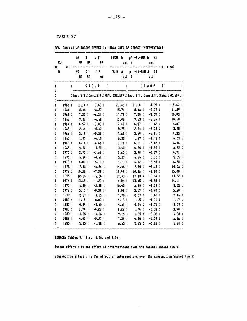
- 175 -

TABLE 37

REAL CUMULATIVE INCCOE EFFECT 1i URBAN AREA OF DIRECT INTERVENTIONS

VA Q /P [SUN A p' +(I-SUN A 11CU MNA NA u,i i u,i

IE t - - 1) t100a VA o' I P [SUN A p +(I-SUNA A 1

NA NA NA u,i i u,i

:6 R a U F I : 6 F a U P , ~ ~~~~ -_ _ _ _ _ _ -_ _ _ _ _ ----- ___ ------ -_ _ _ __-_,

i Inc. Eff.:Cons.Eff.:REAL INC.EFF.:lnc. Eff.!COns.Eff.,REAL IYC.EFF.

1960 11.14 -7.43 20.06 11.14 -3.69: 15.401961 8.46 -6.27 15.71 8.46 -3.07 : 11.391962 : 7.50 -6.34 : 14.78 7.50 : -3.09 : 10.931963 7.93 -4.62 : 13.06 7.83 : -2.24 10.301964 4.57 -2.998 7.67 : 4.57 -1.42 6.071965 2.64 -5.62 9.75 2.64 -2.78 5.581966 3.19 -2.31 5.63 3.19: -1.11 : 4.351967 1.97: -4.10 6.33: 1.97 -1.99: 4.031968 4.11 -4.41 8.91 4.11 -2.12: 6.361969 : 4.30 -3.78 98.40 4.30 -1.80 6.221970 3.90 -1.61 5.60 3.90 -0.77 4.711971 4.84 -0.41 5.27 4.94 -0.20 5.051972 4.02 -5.19 9.70 4.02 -2.58 6.7:1973 7.30 -6.26 14.46: 7.30 -3.12 10.761974 : 10.86 -7.22 19.49 10.86 -3.60 : 15.001975 10.10 -6.24 17.43 10.10 -3.01 13.521976 13.45 : -1.23 : 14.86 13.45: -0.58 : 14.111977 6.90 -.219 10.43 : 6.80 -1.59 8.:2

* 1978 5.7 -0.96: 6.08 5.17: -0.40: 5.601979 2.57: 0.85 1.70 2.57: 0.40 2.161980 : 1.15: -0.02 1.18 1.15: -0.011 1.171981 0.84 -3.60 4.61 0.84 -1.71 .591982: 1.74: -4.27 6.28: 1.74 -2.08 3.901983 : 3.95 -4.86 9.15 3.85 -2.38 : 6.381984 4.90 : -2.27: 7.34 4.90 -1.09 6.06:1985 1 5.25: -1.32 6.65: 5.25 : -0.62 : 5.90

SOURCE: Tables 9, 19.c., 3.50. and 3.54.

Incom, effect : is the effecttof interventions Dver the nominal income (in S)

Consumption effect : is the effect of interventions over the consumption basket (in Sl

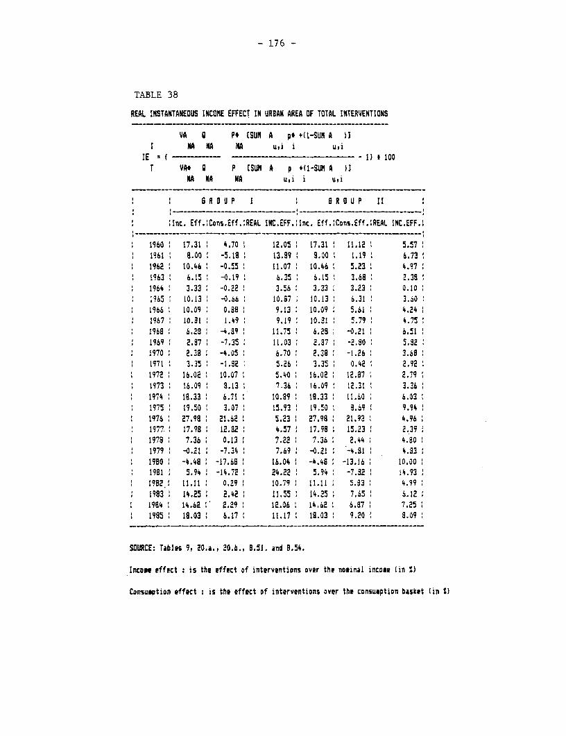
- 176 -

TABLE 38

REAL INSTANTANEOUS INCOME EFFECT IN URBAN AREA OF TOTAL INTERVENTIONS

VA Q Pt (SUN A pt (I-SUN A 11I NA NA NA u,i i u,i

IE I_____ __T VAt O P [SUN A p *(I-SUNA a

NA MA MA u,i i u,i

6 R 0 U P I 'R OU 3 II :

,Inc. Eff.!Cons.Eff.IREAL INC.EFF.:5nc. Eff.!Cons.Eff.:REAL INC.EFF.:

1960 17.31 4 4.70 12.05 17.31 11.12 5.571961 8.00 -5.18 13.39 8.00 1.19 6.731962 10.46 -0.55 11.07 10.46 5.23 4.971963 6.15 -0.19 6.35 6.15 3.68 2.381964: 3.33 -0.22: 3.56 3.33 3.23 :.101965 10.13 -0.66 10.87 10.13 : 6.31 : 3.601966' 10.09 0.88 9.13 10.09 5.61 4.241967 10.81 1.49 9.19 10.91 5.79 4.751968 6.298 -4.39 11.75 6.29 -0.21 6.511969 2.87 -7.35 11.03 2.37 -2.90 5.821970 2.38 -4.05 6.70 2.38 f -1.26 3.68i 1971 3.35: -1.82 5.26: 3.35 0.42 2.921972 : 16.02 ' 10.07 ' 5.40 16.02: 12.87 ' 2.791973 : 16.09 : 8.13 7.36 : 16.09 ' 12.31 ' 3.361974 18.33 6.71 10.89 19.33 11.60 6.031975 19.50 3.07 15.93 19.50: 8.69 9.941976 27.98 21.62 1 5.23 ' 27.S9 8 21.92 ' 4.961977.: 17.98 12.82 4.57 17.98 15.23: 2.391978 7.36 0.13 7.22 7.36: 2.44 4.801979 . -0.21 -7.34 7.69 -0.21 -4.31 4.83:1980 -4.48 : -17.68 16.04 1 -4.46.: -13.16 ' 10.001981 5.94 : -14.72 : 24.22 5.94 ' -7.92 : 14.931982 11.11 0.29: 10.79: 11.11: 5.83 4.99:19831 14.25: 2.421 11.55: 14.25: 7.65: 6.121964 14.62 2.29 : 12.06 14.62: 6.87 7.251995: 18.03' 6.17 11.171 18.03 9.20: 8.09

SOURCE: Tables 9, 20.a., 20.b., 8.51. and 8.54.

Income effect is the effect of interventions over the nosinal incose (in 1)

Consumption effect : is the effect of interventions over the consuaption basket (in S)

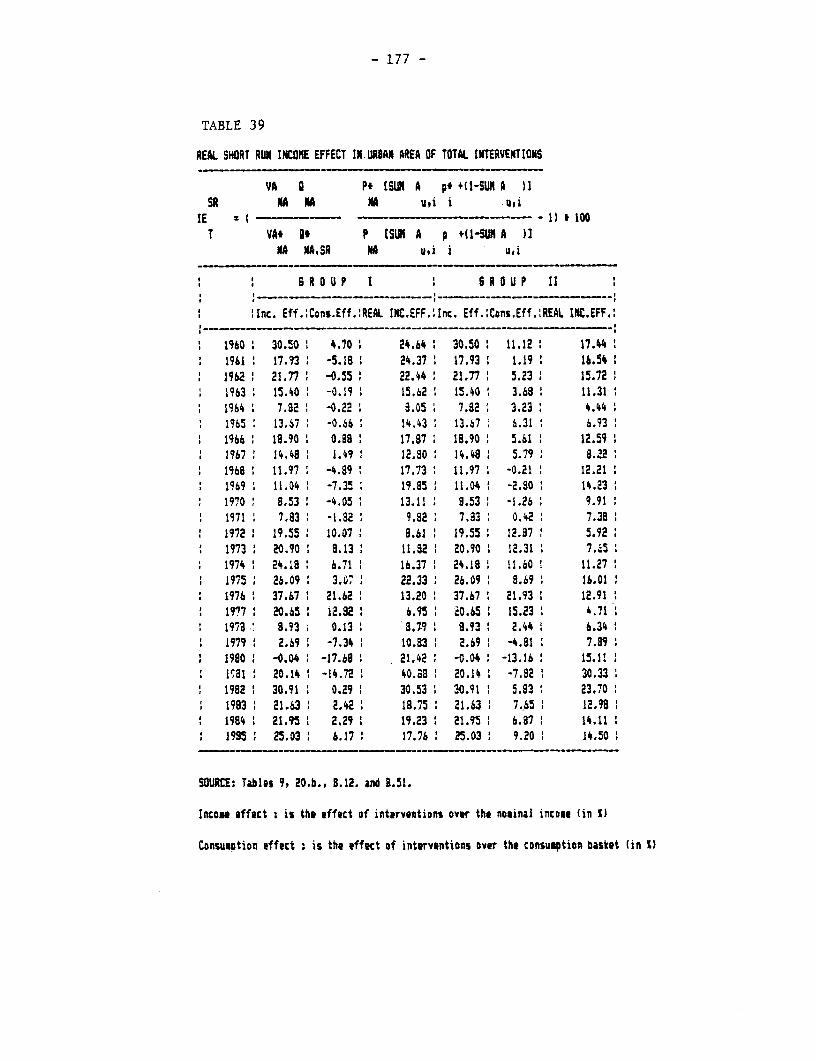
- 177 -

TABLE 39

REAL SHORT RUN INCONE EFFECT Ih URBAN AREA OF TOTAL INTERVENTIONS

VA O Pt tSUh A pt4(1-SUMA 11SR hAm NA u.ii iui

IE : - - - -1) 100T VAt of P ESUI A p 4(1-SUNA )]

NA NA,SR NA u.i i U,i

6 R O U P I 6 R O U P I1

5Inc. Eff.;Cons.Eff.IREAL INC.EFF.:Inc. Eff.5Cons.Eff.'REAL IKC.EFF.:

1960 30.50 4 4.70 24.64 ' 30.50 11.12 17.441961 17.93 -5.18: 24.37 ' 17.93 1.19 16.541962 ' 21.77 -0.55' 22.44 ' 21.77 5.23 15.721963 : 15.40 -0.19 15.62 15.40 : 3.68 : 11.311964 5 7.82 -0.22: 8.05: 7.82 3.23 4.441965 ' 13.67 -0.66 14.43 13.67 6.31 6.931966 18.90 0.88 17.87 : 18.90 5.61 : 12.591967: 14.48 1.49 12.80 14.48 5.79 8.221968 11.97 -4.89 17.73 11.97 -0.21 12.211969 : 11.04 -7.35 19.85 11.04 : -2.80 14.231970 8.53: -4.05 13.11 9.53 -1.26 9.911971 : 7.83 -1.32 9.92 ' 7.33 0.42 : 7.381972 19.55 : 10.07 8.61 : 19.55 ' 12.87 5.921973 : 20.90 8.13 11.82 : 20.90 12.31 7.651974 ' 24.18: 6.71 : 16.37: 2§.19: 11.60 1 11.271975 : 26.09 3.07 22.33 : 26.09 : 8.69 : 16.011976 5 37.67 5 21.62 : 13.20 : 37.67 : 21.93 12.9119'7 7 20.65: 12.32 6.935 '0.65: 15.23 : h.711978 8.93 0.13 a.7.9 8.93 : 2.44 6.341979 : 2.69 : -7.34: 10.83 : 2.69 5 -4.81 : 7.891980 -0.04 -17.68 21.42 -0.04: -13.16 15.1I1q81 5 20.14 ' -14.72 40.038 20.14 : -7.82 : 30.331982 5 30.91 : 0.29 ' 30.53 : 30.91 5 5.83 5 23.701993 21.63 : 2.42 18.75: 21.63 : 7.65 : 12.98:

: 1984 1 21.95 I 2.29 : 19.23 : 21.95 : 6.97 : 14.111995: 25.03 6.17 17.76 : 25.03 9.20 14.50

SOURCE: Tables 9, 20.b., B.12. and B.51.

Income effect : is the effect of interventions ovtr the nocinal incose (in Sl

Consusption effect : is the effect of interventions over the consumption basket (in Sl

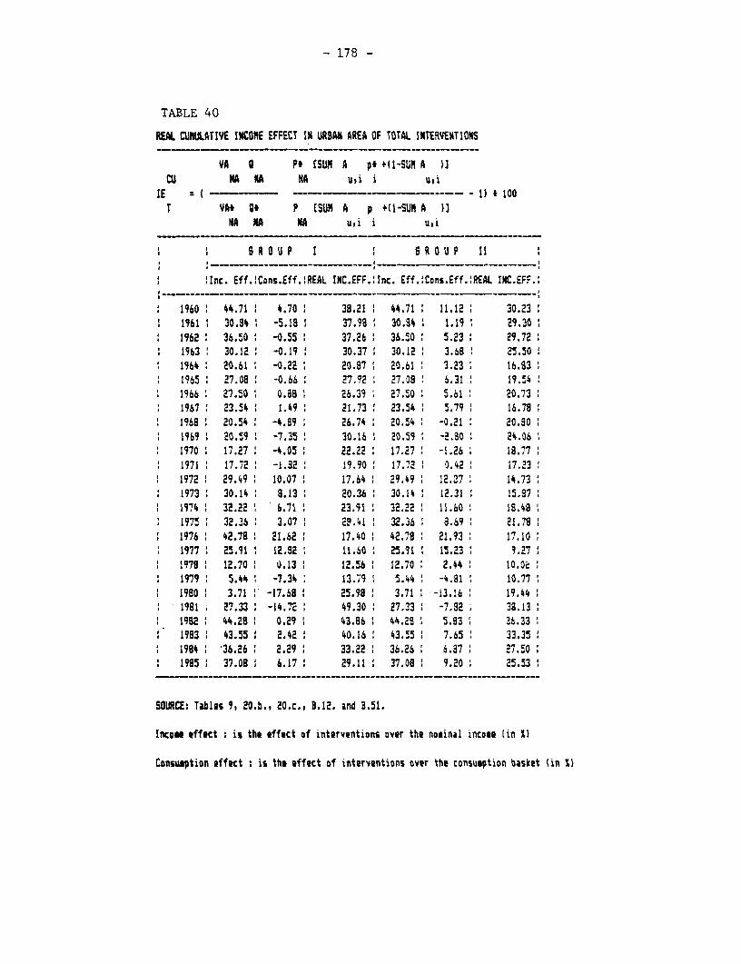
- 178 -

TABLE 40

REAL CUULATIVE INCOME EFFECT IN URDUM AREA OF TOTAL INTERVE%TIGOS

VA a Pt (SUN A pf +(I-SUM A UCU MA A NA u)i i u,i

IE : { - I~~~~~~~~~~~~~) t 100

T VA* Of P ESUM A p +(I-SUMA ANA N A u,i i u,i

a R O U P I R O U P 11

i !Inc. Eff.!Cons.Eff.:REAL INC.EFF.!Inc. Eff.'Cons.Eff.'REAL INC.EFF.'

1960 44.71 4.70 38.21 : 44.71 11.12 30.231961 30.341 -5.18 37.98 30.34 1.19 29.301962 36.50 -0.55 37.26 36.50 5.23 29.721963 30.12 -0.19 30.37 30.12 3.68 25.501964 20.61' -0.2 ' 20.87 20.61 1 3.23 ' 16.831965 ' 27.08: -0.66 27.92 27.08 6.31 19.541966 27.50 0.88 26.39 27.50 5.61 20.731967 23.54 1.49 21.73 23.54 5.79 16.781968 ' 20.54 ' -4.89 : 26.74 20.54 -0.21 20.801969 1 20.59 -7.35 30.16 : 20.59: -2.80 24.061970 17.27 ' -4.05 ' 22.22 : 17.27 -1.26 18.771971 17.72: -1.82 19.90: 17.72 O.42 17.231972 29.49 10.07 17.64 29.49 12.37 14.731973 30.14: 8.13 20.36 30.14 12.31: 15.971974 : 32.22 : 6.71 : 23.91 : 32.22 : 11.60 ' 18.481975: 32.36 3.07 ' 2 .41 ' 32.36 ' 8.69 : 21.,781976 42.78 21.62 17.40 : 42.78: 21.93 17.101977 ' 25.91 : 12.82 ' 11.60 : 25.91 15.23: 9.27?1979 : 12.70 0.13 : 12.56 ' 12.70 : 2.44 : l .Oc1979 : 5.44 : -7.34: 13.'i9 5.44 : -4.31 : 10.771980 : 3.71 : -17.68: 25.98: 3.71 : -13.16 : 19.441981 27.33 -14.72 49.30: 27.33 : -7.82 38.131982: 44.28 : 0.29 4 43.86 44.28 5.83 36.331983 43.55 2.42 : 40.16 : 43.55 : 7.65 : 33.351984: 36.26 2.29 : 33.22 : 36.26 : 6.87 : 27.501985 : 37.08: 6.17 : 29.11 : 37.08 : 9.20 : 25.53

SOURCE: Tables 9, 20.b., 20.c., 3.12. and 8.51.

Income effect : is the effect of interventions over the nominal income (in X)

Consumption effect : is the effect of interventions over the consueption basket (in )

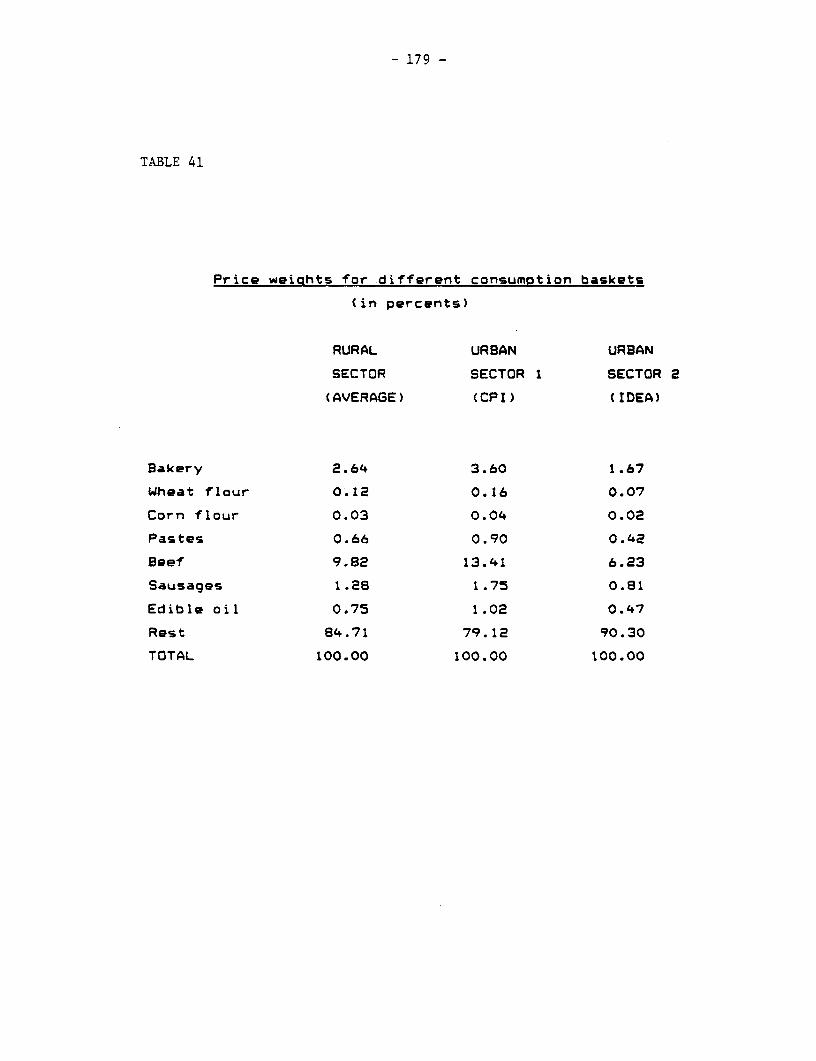
- 179 -

TABLE 41

Price weiahts for different consumotion baskets

(in percents)

RURAL URBAN URBAN

SECTOR SECTOR I SECTOR 2

(AVERAGE) (CPI) (IDEA)

Bakery 2.64 3.60 1.67

Wheat flour 0.12 0.16 0.07

Corn flour 0.03 0.04 0.02

Pastes 0.66 0.90 0.42

Beef 9.82 13.41 6.23

Sausages 1.28 1.75 0.81

Edible oil 0.75 1.02 0.47

Rest 84.71 79.12 90.30

TOTAL 100.00 100.00 100.00

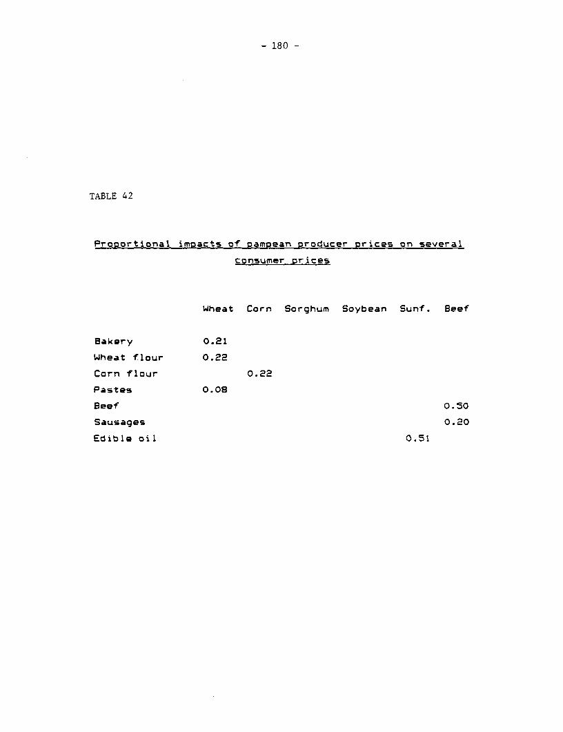
- 180 -

TABLE 42

Proportional imoacts of pam2ean producer Prices on several

consumer Prices

Wheat Corn Sorghum Soybean Sunf. Beef

Bakery 0.21

Wheat flour 0.22

Corn flour 0.22

Pastes 0.08

Beef 0.S0

Sausages 0.20

Edible oil 0.51

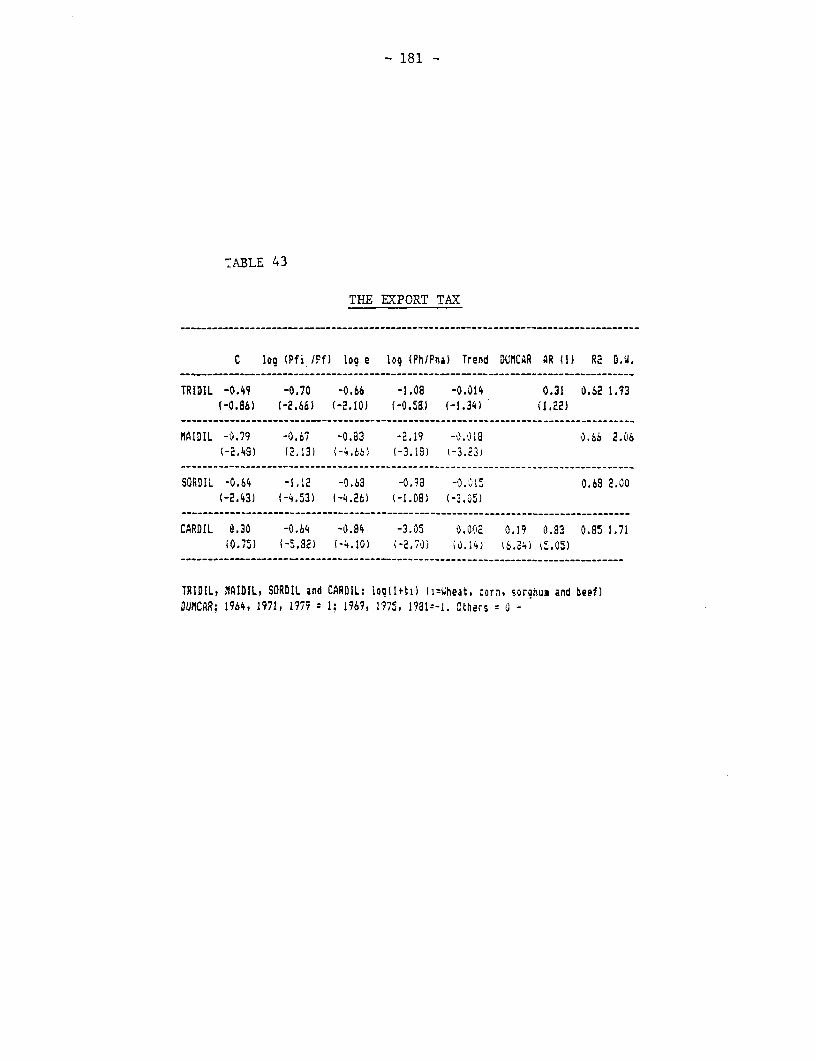
- 181 -

'ABLE 43

THE E:PORT TAX

C log (Pfi 1Pf) log e log (Ph/Pna) Trend DlulCAR AR il) R2 D.W.

TRIDIL -0.49 -0.70 -0.66 -1.08 -0.014 0.31 0.62 1.93(-0.861 (-2.66) (-2.10) (-0.481 (-1.34) (1.22)

MAIDIL -0.79 -0.67 -0.83 -2.19 -0.018 0.S6 2.00(-2.43) (2.13) (-4.'6) (-3.15) -3.23i

SORDIL -0.64 -1.12 -0.S3 -0.93 -O.O15 0.68 2.00(-2.43) (-4.53) (-4.26) (-1.08) (-3.05)

CARDIL 0.30 -0.64 -0.84 -3.05 0.002 0.19 0.83 0.85 1.71(0.75) (-5.82) (-4.10) (-2.70) (0.14) i6.24) (i5.05)

TRIDIL, MAIDIL, SORDIL and CARDIL: loq(l+t0) fi=heat, corn, sorchus and beef)DUflCAR; 1964, 1971, 1979 1; 1969, 1975, Oth1:-l. Cthers = -

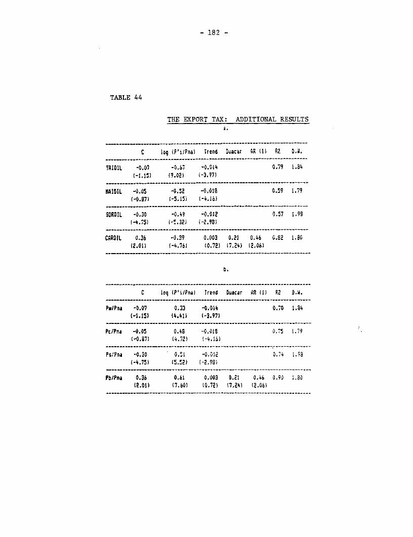
- 182 -

TABLE 44

THE EXPORT TAX: ADDITIONAL RESULTSS.

…--- ----- …-- - - - - - - - - - - - - -- - - - - - - - - - - - - - -

C log (P'iipna) Trend Duccar "R (1) R2 0.U.

TRIDIL -0.07 -O.S7 -0.014 0.79 1.84(-1.15) (9.02) (-3.97)

- - - - - - - - - - ------ … -…-- - - - - - - - -- - - - - - - - -

MAIDIL -0.05 -0.52 -0.018 0.59 1.79(-0.871 (-5.15) (-4.16)

SaRDIL -0.30 -0.4? -0.012 0.57 1.99(-4.75) (-5.32) (-2.98)

CrRDIL 0.36 -0.39 0.003 0.21 0.46 0.82 1.80(2.01) (-4.76) (0.72) (7.24) (2.06)

.

C log (P'iIPna) Trend Duacar A.9 (1) R2 0.;.

Pw/Pna -0.07 0.33 -0.014 0.70 1.84(-1.15) (4.41) (-3.97)

Pc/Pna -0.05 0.48 -0.018 0.75 1.79(-0.87) (4.72) (-4.16)

PsgPna -0.30 0.51 -0.012 0.74 i.;S(-4.75) (5.52) (-2.99)

PbJPna 0.36 0.61 0.003 0.21 0.46 0.90 i.80(2.01) (7.601 (0.72) (7.24) (2.06)

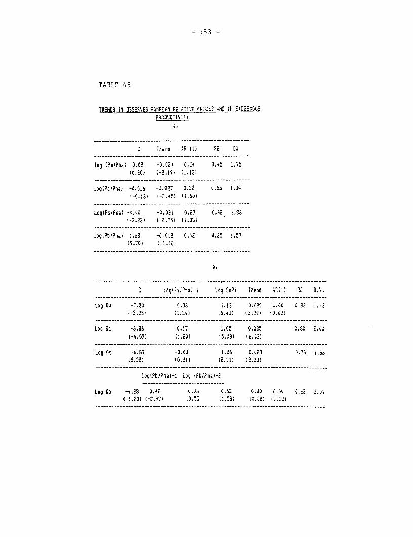
- 183 -

TABLE 45

TRENDS IN OBSERVED ?A1PEA.I RELATiVE PRICES ;ND INt EiGHE,15U'PRODUCTIVITY

a.

C Trend AR ll) P2 OW

log (?wiPlP) 0.02 -0.02e 0.24 0.45 1.75(0.20) (-3.19) (1.13)

loo(PtcPna) -0.016 -0.027 0.32 0.55 1.84(-0.13) i-3.45) (1.60)

Log(PsJPna) -0.40 -0.021 0.27 0.42 1.36(-3.23) (-2.75) (1.33]

loG(PbJPna) 1.63 -0.012 0.42 0.25 1.57(9.70) (-1.12)

b.

C loa(PiIPna)-l Lco iuPi Trend AR1) R2 0.'4.

Log Qw -7.80 0.36 1.13 0.020 v.v3 0.83 1.43(-5.25) (1.24) i6.40) (3.2) (0.02)

LDg gc -6.86 0.17 1.05 0.035 0.80 2.00(-4.07) (1.20] (5.03) (6.43)

Log Os -6.87 -0.03 1.O6 0.023 0.95 1.ib18.52) (0.21) (8.71) (2.23)

Iog(PbIPna)-1 Loq Pbi/Pna)-2

Log Ob -4.29 0.42 O .06 0.53 0.00 .4 0.v c 2.. 1(-1.20) (-2.97) (0.55 (1.58) (0.22) (.3.

-- - -- - - - - - - -- - -- - - -- - - -- - -- - - -- - - -- -- - - -- - - - _ - -

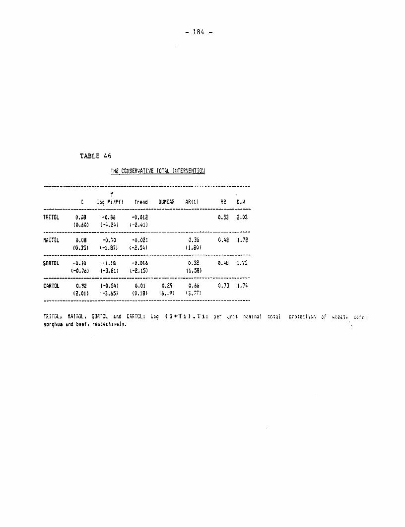
- 184 -

TABLE 46

THE CC,ISER'VATIVE TOTAL IJTERV!ENTiON

C ID9 PiIpf) Trend DUMCAR ARil) P2 D.W

TRITOL 0.08 -0.86 -0.012 0.53 2.03(0.60) (-4.2;) (-2.411

1ITCL 0.08 -0.70 -0.021 O.3S 0.42 1.72(0.35) (-1.871 (-2.54) (1.8O)

SORTOL -0.10 -1.18 -0.016 0.32 0.48 1.75(-0.76) (-3.81) (-2,15) (1.58)

CARTOL 0.92 (-0.54) 0.01 0.29 0.66 0.73 1.74(2.01) (-3.65i (0.18) f6.19) !3.,7)

TRITGL, )AITOL, SORTOL and CARTCL: Loc ( 1+Ti ) .Ti: ~er unit %,orlnal tctal crotect;r, Gt ea 'r

sorghum ind beef, resectively.

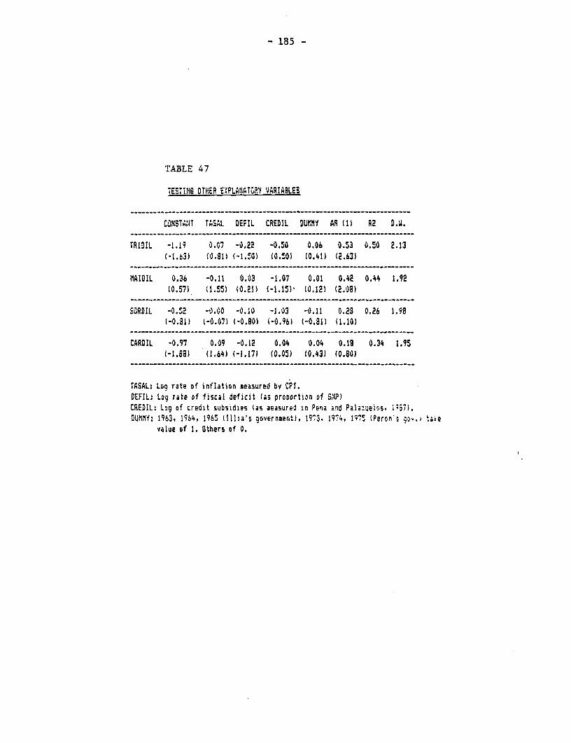
- 185 -

TABLE 47

TESTINS OTHER EXPLA!IATG?.Y VARIABLES

UNKSTANT TASAL DEFIL CREDIL DUr.Y AR 1i) R2 D.U.

TRIDIL -1.19 0.07 -0.22 -0.50 0.06 0.53 0.50 2.13(-1.b3) (0,81) (-1.50) (0.50) (0.41) (2.63)

flAIDIL 0.36 -0.11 0.03 -1.07 0.01 0.42 0.44 1.92(0.57] (1.55) ;0.21) (-1.15), (0.12) (2.08)

SORDIL -0.52 -0.00 -0.10 -1.03 -0.11 0.23 0.26 1.98(-0.81) (-0.07) (-0.80) (-0.96) (-0.81) (1.10)

CARDIL -0.97 0.09 -0.12 0.04 0.04 0.18 0.34 1.95(-1.89) (1.64) (-1.171 (0.05) (0.43) (0.80)

TASAL: Loo rate of inflation measured bv CPl.DEFIL: Log rate of fiscal deficit (as proportion of SN?P)CREDIL: Lg of credit subsidies (as aeasured in Pena and Pali:ueios. 1337).DUMi:Y: 1963, 1564, 1965 (illia's oovern3ent), 17S,. 19-r, 1$q' (Peron'- . taie

value of 1. Others of 0.

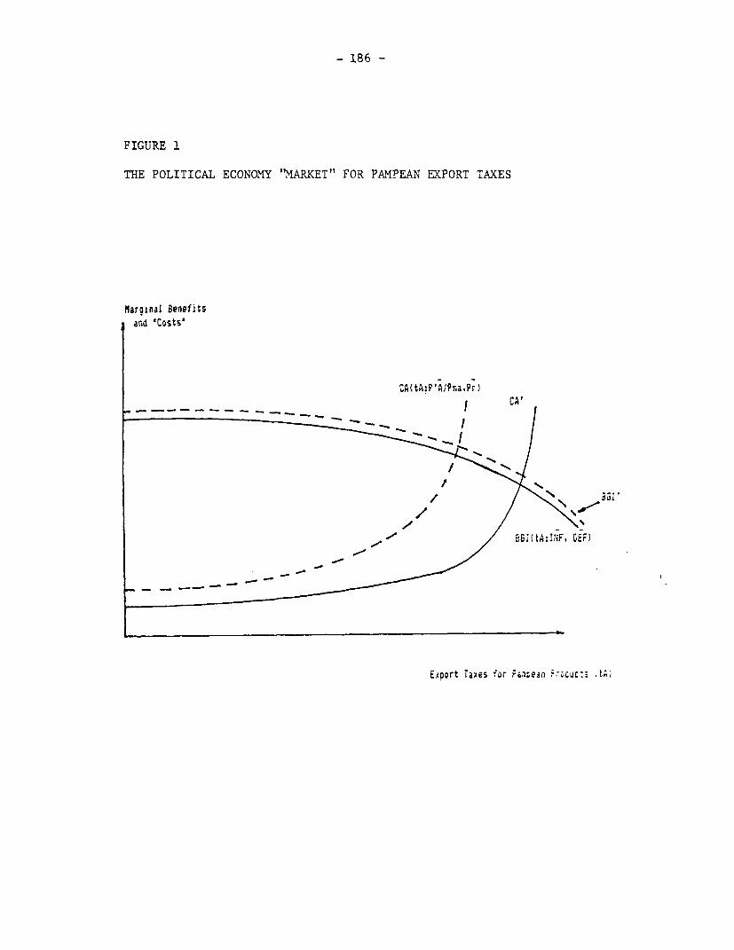
- 186 -

FIGURE 1

THE POLITICAL ECONOMY "MARKET" FOR PAMPEAN EXPORT TAXES

faroinal Benefitsand Costs'

CAI(tA,P'AIPna,Pr)_AD~rt Taxs f= F i uCA,

EADDrt Taxes fr Fur aein ;"ouc:z- itnil

A n P E N D I X A.1.

I

I

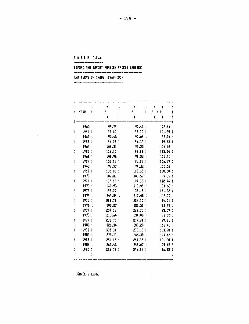
- 18 9 -

T A 8 L E A.1.a.

EXPORT AND IMPORT FOREIGN PRICES INDEXES

AND TERMS OF TRADE (Q969=100)

f f f :YEAR P P P I P

:f_t ___ __

1960 99.79 97.41 102.441961 97.00 95.20 101.891962 90.48 97.04 93.241963 94.29 94.35 99.931964 106.31 93.23 114.031965 106.10 93.81 . 113.10 t1966 I 106.96 96.23 111.151967 102.17 95.67 106.791968 99.57 94.32 105.571967 100.00 100.00 100.00 1970 107.87 108.57 1 99.361971 123.16 : 109.22 112.761972 ;4d.93: 113.091 124.62!1973 195.27 1138.18 141.321974 244.84 217.08 112. :1975 I 221.71 : 234.10 : 94.71 11976 : 203.27 : 228.51 88.961977 209.13 1 224.70 93.071978 213.64 1 234.00 : 91.301979 273.75 274.81 99.611980 326.34 1 280.20 116.461981 : 335.34 1 270.92 123.781982 278.77 266.38 1 104.65 11983 1 251.15 i 247.96 101.281984 265.43 242.07 109.65:1985 1 236.72 1 244.24 1 96.92

SOURCE: CEP4L

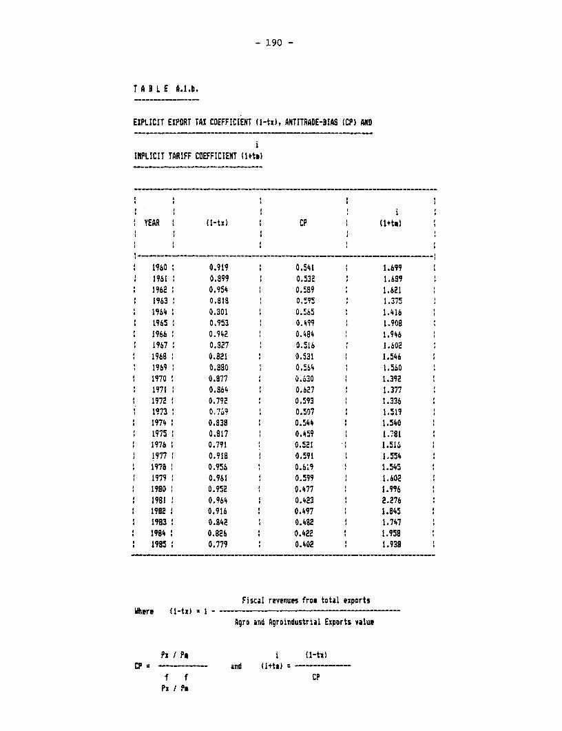
- 190 -

T A 3 L E A.1.b.

EXPLICIT EXPORT TAX COEFFICIENT (1-tx), ANTITRADE-BIAS tCP) AND

iINPLICIT TARIFF COEFFICIENT (I+te)

t : : :

* I t Ii

YEAR t (1-tx) CP I (+ta)

1960 0.919 0.541 : 1.6991961 t 0.899 ' 0.532 : 1.689: 1962 '0.954 0.589 1.6211963 ' 0.819 0 .595 1.3751964 0.801 OO 0.565 1.4161965 0.953 0.499 1.9081966 0.942 0.484 1.9461967 0.827 0.516 1.602

: 1968 0.821 t 0.531 : 1.5461969 0.880 i 0.564 ' 1.5601970 0.877 1 0.630 ' 1.3921971 . 0.864 ' 0.627 1.3771972 0.792 0.593 1.3361973 0.745 0.507 : 1.5191974 0.838 1 0.544 : 1.540

t 1975 t 0.817 0.459 t 1.?911976 , 0.791 ' 0.521 1 1.514

t 1977 1 0.918 1 0.591 1.5541978 ' 0.956 : 0.619 1.545

1 1979 : 0.961 0.599 1 1.6021980 ' 0.952 ' 0.477 ' 1.996

t 1981 0 0.964 : 0.423 2.276t 1982 : 0.916 0.497 t 1.845t 1983 : 0.842 1 0.482 1 1.7471 1984 0 0.826 t 0.422 1.958

1985 1 0.779 0.402 1.938

Fiscal revenues from total exportsWiere (1-tx) I - - ------

Agro and Agroildustrial Exports value

Px I Pe i (1-tx)CP w - - -- -and (1+ta) = -

f f CPPs I Ps

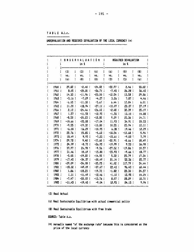
- 191 -

T A B L E A.l.c.

UNDERVALUATION AND REQUIRED DEVALUATION OF THE LOCAL CURRENCY (*M

U N D E R V A L U A T I O N REQUIRED DEVALUATIONin X in S

(3] (3) (6) (6) (8) (8)vs. vs. vs. vs. * vs. vs.(6) '(8) ( 3) (3) (6) 1

' 1960 29.82 -2.40 -24.82 -22.97 2.46 33.021961 8.05 ' -20.81 -26.71 -7.45 ' 26.298 1 36.451962 1 14.33 1 -11.96 1 -23.00 1 -12.54 1 13.58 29.861963 -3.16 -7.29 -4.27 3.26 7.87 4.46 i1964 -6.05 1 -11.38 1 -5.67 6.44 1 12.84 6.011965 1 11.20 -18.94 1 -27.11 ' -10.07 1 23.37 37.19196b 1 2.12i -24.46 -26.03 -2.08 1 32.39 ' 35.191967 1.57 -11.58 -12.95 1 -1.55 13.10 1 14.88

S1968 -8.50 -20.23 1 -12.82 9.291 25.36 14.711969 1 -10.66 1 -25.83 1 -17.04 1 11.93 1 34.91 20.531970 ' -9.55 ' -19.32 -10.80 1 10.55 1 23.94 1 12.111971 1 -6.00 1 -16.29 1 -10.95 1 6.38 1 19.46 1 12.291972 1 22.76 15.85 1 -5.63 1 -18.54 -13.68 ' 5.96 i

1 1973: 18.49 1 9.93 -7.23 -15.61 1 -9.03 7.79'974 29.72 1 9.48 1 -15.60 ' -22.911 -8.66 ' 18.49

1 1975 1 24.9R 1 -8.70 1 -26.95 -19.99 1 9.53 36.901976 ' 37.97 ' 24.78 1 -9.56 1 -27.52 -19.96 1 10.571977 31.46 10.69 -15.80 -23.93 -9.66 18 .77 11978 -5.05 -19.22 ' -14.92 ' 5.32 2 23.79 1 17.54 1

1 1979 1 -i7.45 1 -34.37' -20.49 1 21.14 1 52.36 1 25.771980 . -29.09 1 -54.08 -35.25 41.02 ' 117.79 ' 54.44

1 1981 ' -19.32 ' -49.09 1 -37.67 1 22.43 1 96.43 1 60.441992 1 1.86 1 -18.23 1 -19.72 1 -1.92 2 22.30 1 24.57 11983 ' 1.11 ; -11.49 ' -12.46 . -1.10 1 IZ.98 1 14.241984 1 -7.47 1 -22.05 ' -15.76 1 8.07 1 29.29 1 18.71 1

1 1985 1 -11.45 1 -19.45 1 -9.04 ' 12.93 1 24.15 ' 9.94 1

(3) Real Actual

(6) Real Sustainable Equilibrius with actual commercial policy

(8) Real Sustainable Equilibrius with free trade

SOURCE: Table 6.a.

(t) normally named 'of the exchange rate because this is considered as theprice of the local currency

A P P E N D I X A.2.

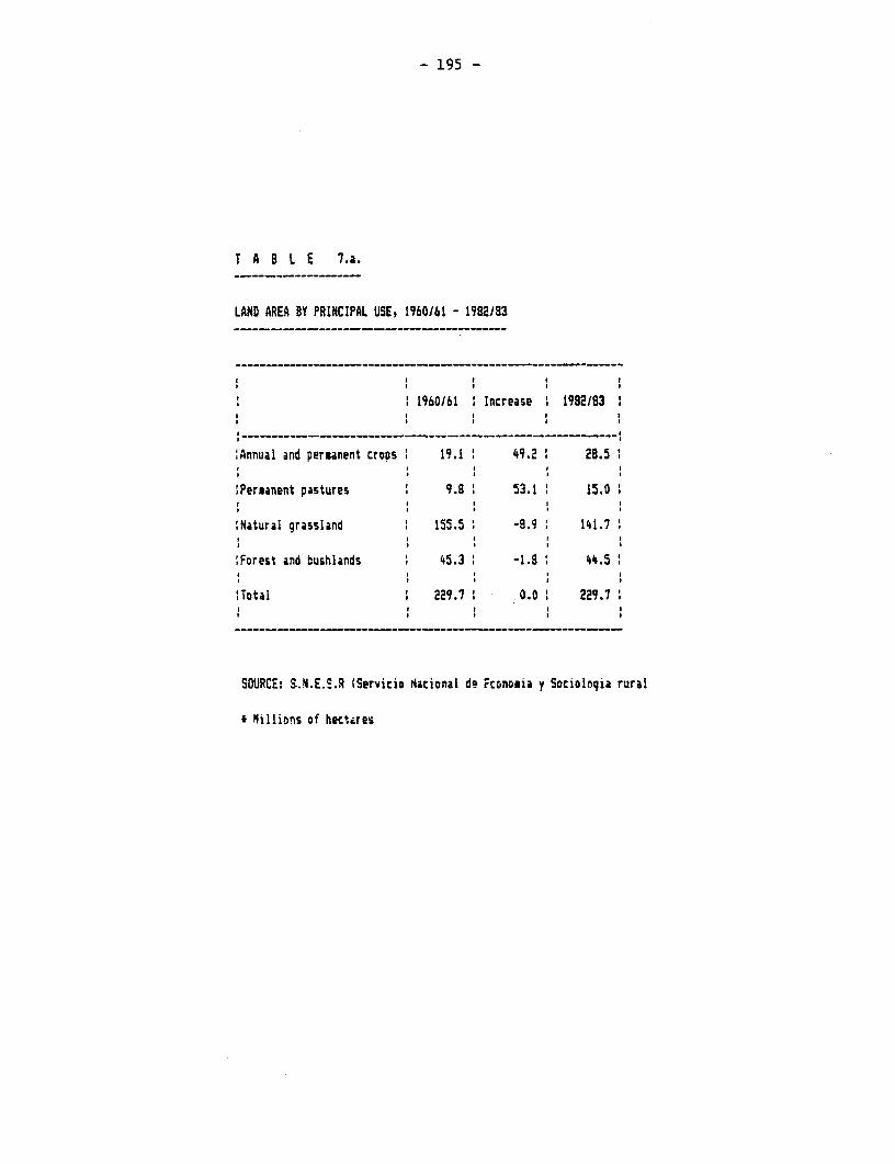
- 195 -

T A B L E 7.a

LAND AREA BY PRINCIPAL USE, 1960161 - 1982183

, , , I

1960161 Increase 1992183

Annual and peruanent crops 19.1 49.2 28.5

RPereanent pastures 9.8 53.1 15.0

Natural grassland 155.5 -8.9 141.7

:Forest and bushlands 45.3 -1.8 44.5

Total 229.7 0.0 229.7

SOURCE: S.N.E.S.R (Servicio Macional dq Fconoaia y Sociologia rural

* flillions of hec¶ires

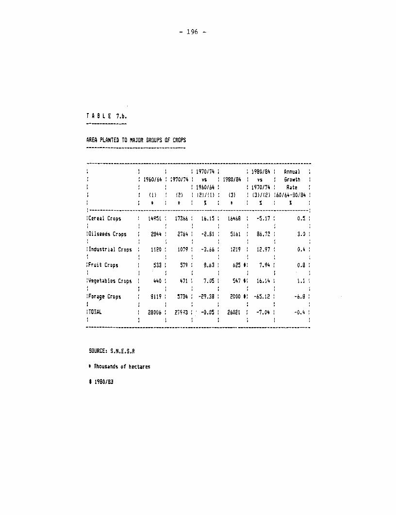
- 196 -

T A L E 7.b.

AREA PLANTED TO MAJOR GROUPS OF CROPS

[190174 1198018 Annual1960/64 1970/74 vs 1980184 Vs I Growth

1960/64 1970/74 Rate: (1) (2) (2)1(1) (3) (3)/(2) 60164-90/94

Cereal Croos 14951 17366 16.15 16468 -5.17 0.5

Oilseeds Crops 2844 2764 -2.81 5161 86.72 3.0

Industrial Crops 1120 1079 -3.66 1219 12.97 0.4

Fruit Crops . 533 579 a.63 625 1 7.94 1 0.8

Yegetables Crops 440 471 7.05 547 t 16.14 1.1

.Forage Crops 9119 5734 -29.38 2000 tI -65.12 -6.8

:TOTAL 28006 27773 -0.05 26021 -7.04 -0.4

SOURCE: S.N.E.S.R

t rhousands of hectares

# 1980/83

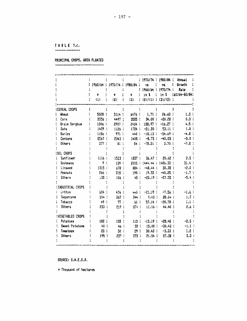
- 197 -

T A B L E 7.c.

PRINCIPAL CROPS, AREA PLANTED

1. 1. 1 1970/74 1980/84 : Annual1960/64 1970/74 1980194 vs vs 6 Growth I

a ,1960/64 1970/74 Rate t

* ' I * i ' t I in X in X 60164-30184(1) (2) (3) 1 (2)/(1) ( (3)/(2)

:CEREAL CROPS : I I I

Wheat 50281 5114 6476 1.71 26.63 1.3Corn 1 3356 4497 3595 34.00 -20.29 0.3Grain Sorghum 1006 2907 2434 188.97 1 -16.27 4.5Oats 1 1429 1126 1724 -21.20 53.11 1.0Barley 1186 971 440 1 -18.13 -54.69 -4.aCenteno 1 2567 2343 1 1405 1 -9.73 -40.03 -3.0Others 377 1l 84 -78.51 3.70 -7.2

:OIL CROPSSunflower 1116 1523 1837 36.47 20.62 2.5Soybeans 9 1 139 2205 1444.44 1486.33 31.4Linseed 1315 679 884 -48.44 30.38 -2.0Peanuts 266 319 190 19.55 1 -40.25 1 -1.7Others i38 106 45 -23.19 -57.55 -5.4

INDUSTRIAL CROPS 1C>tton 604 476 O0t -21.19 -7.56 -1.6Suqarcane 244 267 1 344 9 9.43 2S.54 1.7TobacoD 49 77 61 57.14 -20.78 1.1Others 1 233 9 2 31 11.161 44.40 2.6

VEGETABLES CROPSPotatoes 182 158 113 1 -13.19 -28.48 1 -2.3Sweet Potatoes 1 40 1 46 32 15.00 -30.43 -1.1TomatoRs 23 30 29 30.43 1 -3.33 1.21Others 195 237 373 21.54 57.38 3.3

SOURCE: S.N.E.S.R.

* Thousand of hectares

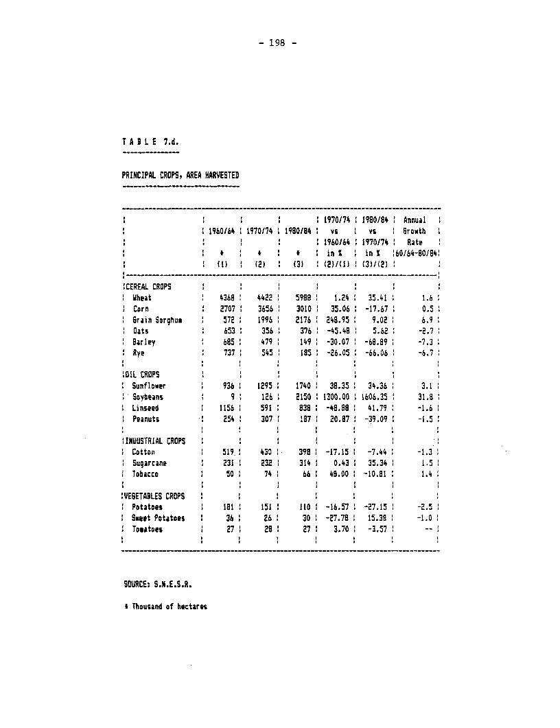
- 198 -

T A 8 L E 7.d.

PRINCIPAL CROPS, AREA HARVESTED

: 1970/74:u 1980/84 Annual1960(64 1 1970174 1980/84 ' S vs 6rowth

' 1 ) 1960/64 1970/74: Rate :: * ' * : * in X in : '60/64-80/84:

: {1) ' (2): (3): t 2)1(1) I MM/{) '

:CEREAL CROPS : Wheat 4368 4422 5989 1.24 35.41 1.6Corn 2707 3656 3010 35.06 -17.67 0.56rain Sorghus : 572 1996 2176 2 248.95 9.02 6.9Oats 653 356: 376 -45.48 5.62 -2.7Barley 685 479 149 -30.07 -68.89 -7.3

* Rye 737 545 185 -26.05 -66.06 : -6.7

MOlL CROPSSunflower 936 1295 1740 1 38.35 : 34.36 3.1Soybeans 9 126 2150 1300.00 1 1606.35 1 31.8

* Linseed 1156 591 838: -48.88 41.79 -1.6. Peanuts 254 ' 307: 187 20.87 -39.09 ' -1.5

:INDUSTRIAL CROPS : :Cotten : 519.: 430 1 398 : -17.15 1 -7.44 : -1.3Sugarcane 231 I 232 314 : 0.43 35.34 I 1.5

. Tobacco : 50 74 : 66 48.00: -10.81: 1.4

:VEGETABLES CROPS ' :: Potatoes 181 151 : 110 ' -16.57 1 -27.15 : -2.5a Sweet Potatoes i 36 ' 26: 30: -27.78 1 15.38 : -1.0a Tomatoes 271 28 1 27: 3.70 I -3.57 -

SBURCE: S.H.E.S.R.

I Thousand of hectares

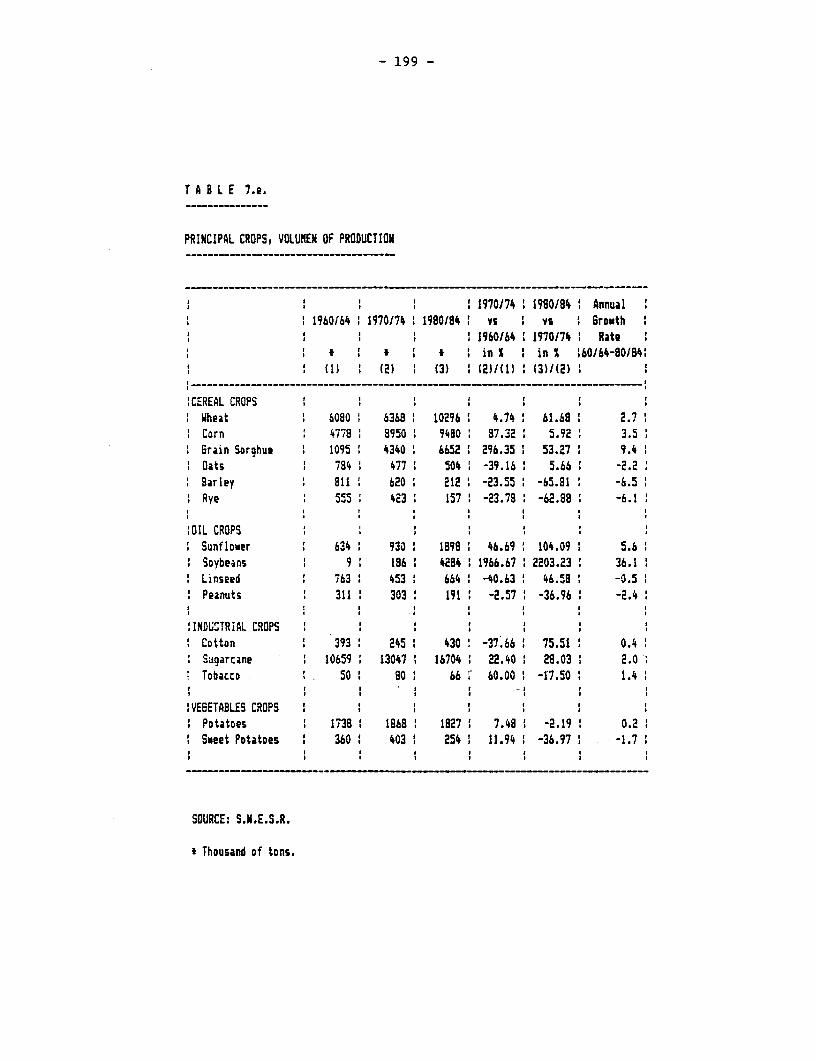
- 199 -

T A B L E 7.e.

PRINCIPAL CROPS, VOLUNEN OF PRODUCTION

' * 1970174 1950/84 Annual1960164 1970174 1980184 v vs Vs I Growth

1 1960/64 11970174 ! Ratet 4 t in X in S :60164-90134:(1) (2) 1 (3) 1 (MM1(1) (3)1(2)

CEREAL CROPS * t

Wheat 6080 6368 10296 4.74 61.68 2.7Corn 4778 8950 9480 87.32 5.92 3.5Grain Sorghum 1095 4340 6652 296.35 53.27 9.4Oats 784 477 504 -39.16 5.66 -2.2Barley a11 620 212 -23.55 1 -65.81 -6.5Rye 555 423 157 -23.78 -62.88 -6.1

OIL CROPS : ISunflower : 634 930 1898 46.69 104.09 5.6Soybeans 9 196 : 4284 1966.67 2203.23 1 36.1Linseed : 763 453 664 1 -40.63 1 46.58 1 -0.5Peanuts 311 303 191 -2.57 -36.96 -2.4

:INDUOTRIAL CROPS iI Cotton . 393 245 430 -37'.66 75.51 1 0.4Sugarcane 10659 13047 16704 22.40 28.03 2.0Tobacco 501 80 : 66 : 60.00 1 -17.50 1 1.4

VEBETABLES CROPS : :: Potatoes 1738 : 1868 1827 1 7.48 -2.19 0.2: Sweet Potatoes 360 4031 254 1 11.941 -36.971 -1.71

SOURCE: S.H.E.S.R.

* Thousand of tons.

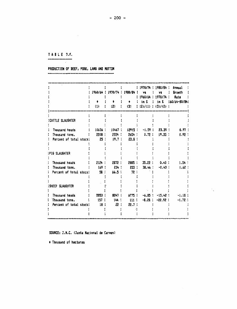
- 200 -

T A B L E 7.f.

PRODUCTION OF BEEF, PORK, LAMB AND MUTTON

* a a ' a 1970/74 1 1980/94 ! Annual 11 1960/64 1 1970/74 1990184 VS I Vs I 6roUth

: 1960/64 1 1970/74 ' Ratet 1 I t I t I in I 1 in S :60/64-80/84:' (1) 1 (2) ' (3 (2)/1() ' (3)/(2) 1

:CATTLE SLAUSHTER

I Thousand heads 1 10636 10467 12915 : -1.59 . 23.39 0.97Thousand tons. ' 2209 ' 2224 2654 ' 0.72 ' 19.33 0.92Percent of total stock: 25: 19.7 1 23.8 '

:PIS SLAUGHTER

Thousand heads I 2124 ' 2872 ' 2885 ' 35.22 ' 0.45 . 1.54I Thousand tons. 1 169 234 233 ' 38.46 ' -0.43 1.621 Percent of total stock! 591 66.5' 721

j ' ~ ~ ~ : : t : ::'SHEEF SLAUEHTER : : 1 1 :

I Thousand heads 2 Q853 1 82471 6C75 1 -6.85 -15.42 1 1.15'1 Thousand tons. 157 1 144 1 IIl I -8.25 ' -22.92 1 -1.?2.1 Percent of total stock: 19 E2 ' 22.7 i a a

a a a. a . a. a a

SOURCE: J.N.C. (3unta Nacional de Carnes)

t Thousand Df hectares

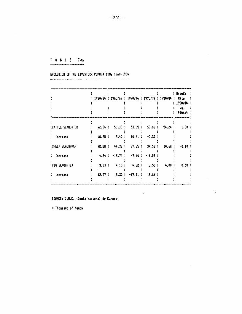
201 -

T A 8 L E 7.q.

EVOLUTION OF THE LIVESTOCK POPULATION, 1960-1984

1. 11 w I I S 6routh 11960(64 1965169 1970174 1 1975/79 '1980/84 ' Rate 1

a a a a : : ' 1990184:a ' a a a a a vs. a

I , a a 1 t : 1960(64 1

:CATTLE SLAUGHTER 42.34 50.33 53.05 58.68 54.264 1.20

Increase ' 18.88 ' 5.40 10.61 -7.57

:SHEEP SLAUSHTER 42.2a ' 44.32 37.35 ' 34.58 1 30.68 -2.10

' Increase 4.84 -15.74 -7.40 -11.29 '

'PIG SLAUGHTER 3.63 ' 4.10 - 4.32 1 3.55 1 4.00 ' 0.50

I Increase , 12.77 ' 5.30 1 -17.71 1 12.64 '

53URC8: J.H.C. (Junta iacional de Carnesi

t Thousand of heads

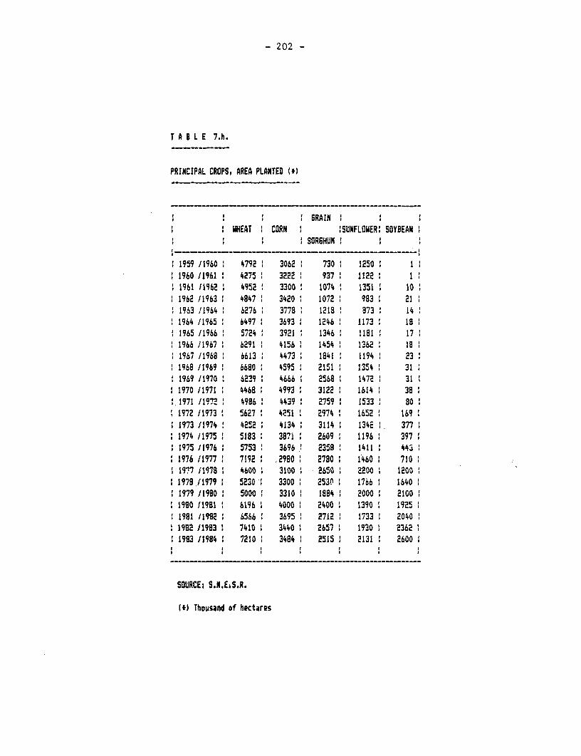
- 202 -

T A B L E 7.h.

PRINCIPAL CROPS, AREA PLANTED (U

G GRAIN WHEAT : CORN :SUNFLOWER: SOYBEAN

i : SOR6HUN

1959 /1960 4792 3062 730 1250 :1960 /1961 4275 3222 937 1122:1961 f1962 4952 3300 1074 1351 101962 11963 4847 3420 1072 983 211963 /1964 6276 3778 1218 873 141964 /1965 6497 3693 1246 1173 181965 /1966 5724 3921 1346 1181 17

I 1966 /1967 6291 4156 1454 1362 181967 11968 6613 4473 1841 1194 231968 /1969 6680 4595 2151 1354 311969 11970: 6239 46661 2568 1472 311970 /1971 4468 4993: 3122 1614 381971 /1972 4986 4439 2759 1533 801972 11973 5627 4Z51 E974 1652 1691973 /1974 4252 4134 3114 134E 3771974 /1975 5183 3871 2609 : 1196 3971975 /1976 5753 3696 2358 1411 4431976 /1977 : 7192 .2980 2790 1460 7101977 11978 4600 3100 2650 2200 12001978 /1979: 52a0: 3300 258n 1766 16401979 /1980 : 5000 : 3310 : 1884: 2000 C21001980 11981 S6196 4000: 2400 1390 19251981 /1982 6566: 3695 2712 1733 : 2040

:1982 /1983: 7410 : 3440 2657 1 1930 : 23621983 /1984 : 7210 3484 1 2515 : 2131 : 2600

SOURCE: S.N.E.S.R.

1*) Thousand of hectares

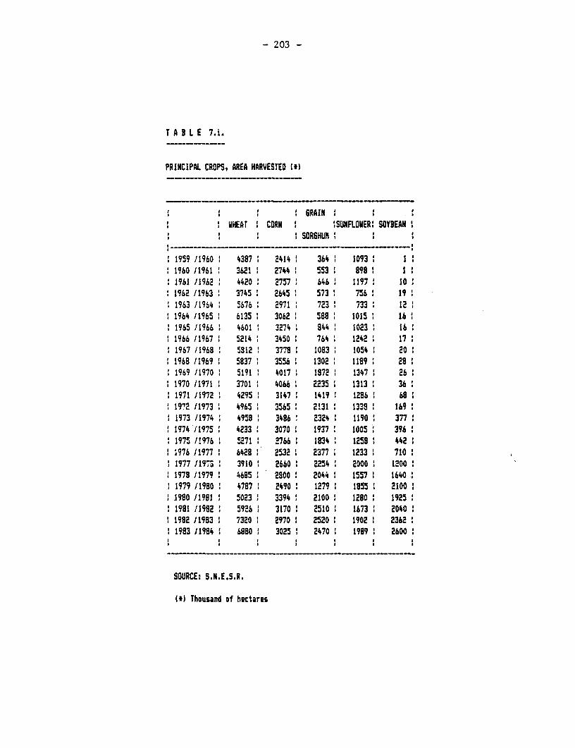
- 203 -

T A B L E 7.i.

PRINCIPAL CROPS, AREA HARVESTED ('1

GRAIN :WHEAT CORN :SUNFLOWER: SOYBEAN:

: I : SORGHUM :, ____-------------------------- _____ __ _ __ _ _

1959 11960 4387 2414 1 364: 1093 I11960 11961 3621 2744 1 553 999 I1961 11962 ' 4420 27571 646 11971 101962 /1963 3745 2645 5731 756 191963 /1964 5676 29711 7231 733 12

1 1964 11965 ' 6135 3062 ' 588 1015 ' 161965 /1966 1 4601 3274 844 ' 1023 161966 /1967 ' 5214 3450 764 12421 17:1967 11968 5812 ' 3778 10831 1054 ' 201968 11969 1 5837 ' 35561 1302 1189 2s11969 /1970 5191 ' 40171 1972 ' 1347 261970 /1971 ' 3701 ' 4066 1 2235 ' 1313 36 1971 /1972 4295 1 3147 1 1419 ' 1286 681972 11973 ' 4965 ' 3565 ' 2131 1338 I 1691973 /1974 4 4958 ' 3486 ' 2324 1190 3771974/1975 1 4233 1 3070 1937 1005 396 11975 /!976 1 5271 1 2766 1834 1 1258 4421976 /1977 6428 2532 1 2377 1 1233 1 710:1977 /1973 ' 3910 2660 2254 2000 1 12001978 11979 4695 1 2800 1 2044 1 1557 1640 I1979 /1980 4 4787 ' 2490 1 1279 1 1855 1 2100 1

11980 11981 1 5023 1 3394 1 2100 1 1280 1925 1:1981 /1982: 5926 1 3170 2510 1 1673 1 2040 I1 1982 /1983 1 7320 1 2970 1 2520 1 1902 : 2362 1

1983 /1984 6880 1 3025 2470 1999 2600I I I I I I I* I I I 3 a a

SOURCE: S.N.E.S.R.

(*) Thousand of hectares

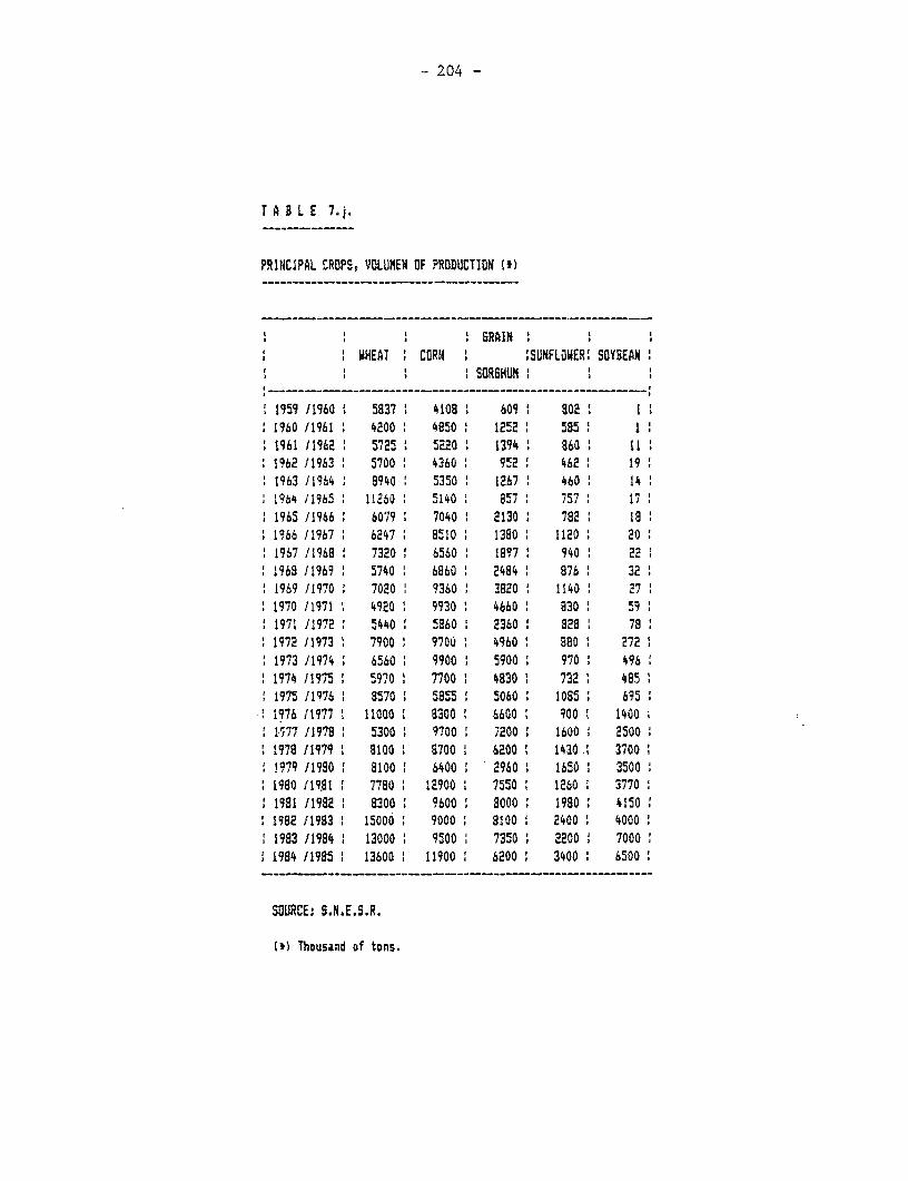
- 204 -

T A B L E 7.

PRINCIPAL CROPS, VOLUMEN OF PRODUCTION 1*)

t 6~~~~ ~ ~~~RAIN: VHEAT CORN 1 SUNFLOWERr SOYBEAN

ISORGHUtI

1959 /1960 t 5837 1 4108 1 609 1 802 I 1960 /1961 4200 4850 1252 585 s 11961 11962 5725 5220 1394 860 111962 11963 5700 4360 952 462 191963 /1964 8 8940 5350 1267 460 141964 /196b5 11260 5140 857 757 171965 11966 6079 1 7040 2130 782 la1966 /1967 6247 8510 . 1380 1120 201967 /1968 7320 6560 1897 940 221968 /1969 5740 6860 2484 1 876 321969 /1970 7020 9360 3820 1140 27

I 1970 11971 1 4920 9930 1 4660 1 830 59:: 1971 /1972 5440 5860 2360 828 781 1972 119731 7900 9700 4960 8801 272: 1973 /1974 . 6560 . 9900 1 5900 970 496I 1974 11975 5970 1 7700 4830 i 732 485 i1 1975 /1976 8570 5855 5060 1085 1 695

1976 11977 1 11000: 8300 6600 900 i 14001S77 J1979 5300 9700 7 ;200 1600 25001978 /1979 8100 8700 6200 14301 37001979 /1990 8100 1 6400 2960 1650 35001980 119,91 7780 12900 7550 1260 3770 I1981 11982 8300 9600 8000 1980 1 41501982 /1983 1 15000 9000 8100 1 2400 40001983 /1984 13000 9500 7350 1 22001 7000

1 1984 /1985 13600 11900 . 6200 3400 : 6500

SOURCE: S.l.E.S.R.

(t) Thousand of tons.

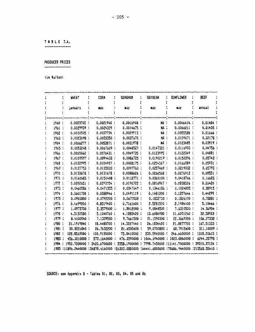
- 205 -

T A B L E 7.k.

PRODUCER PRICES

(in Salton)

WHEAT CORN SOR6HUM 1 SOYBEAN SUNFLOWER I BEEF

january say nay say may annual

-- - -- - - - -- -- -- - -- - -- - -- - -- - -- - I

1960 0.0023705 0.0021940 0.0016948 M NA 0.0046414.: 0.014841961 0.0029939 0.0024329 0.0014675 NA 0.0066211 0.014051962 0.0030505 1 0.0037734 0.0029913 NA 0.0055588 0.016661963 0.0053098 0.0058350 0.0037670 NA 0.0109671 0.021781964 0.0066277 1 0.0053871 1 0.0031978 NA 0.0123485 0.039191965 ' 0.0053248 1 0.0067609 0.0048527 1 0.0147321 0.0116903 0.047561966 0.0065062 0.0076431 0.0049735 0.0123995 1 0.0122349 0.048811967 0.0105597 0.0094433 0.0086725 0.0190219 0.0150396 0.057431968 0.0122995 0.0104907 0.0088175 1 0.0254367 0.0166539 0.059311969 0.0137753 0.0135833 0.0097763 0.0257469 0.0219032 0.05793

1 1970 1 0.0133678 0.0131678 0.0088626 0.0266568 0.0276912 O.Oe5511971 0.0160683 0.0151408 0.0112771 ' 0,0360100 0.0418766 0.166231972 0.0202651 ' 0.0263054 0.0196722 ' 0.0816967 0.0838'06 ' 0.264201973 0.0460586 0.0471335 0.0347647 0.1346186 1 0.1024805 : 0.389151974 0.0601700 0.0588946 0.0491119 0.1481200 0.125%646 1 0.442991975 0.0903800 0.0792200 0.0677500 0.1832r(': 0.1826100 4 0.788811976 0.4699200 0.8319400 0.7161600 t 2.5281500 2.1984100 5.104661977 1.8973700 ' 2.3579000 ' 1.8012000 9.0848500 7.6310500 14.369041978 4.5150580 5.1040760 4.1983420 13.6086980 11.6051260 32.589231979 8.4100540 7.1339580 9.7661500 21.1590300 22.3669200 1 106.273321980 21.1919840 18.4480700 ' 14.3227440 26.1834420 21.8877720 1 167.51333 '1981 : 30.8226840 26.7632200 21.6505600 1 59.0700800 1 68.7915600 ' 311.100091982 122.8512000 ' 100.9130000 73.8410000 233.5940000 246.6600000 ' 1318.20615

1 1983 456.3010000 : 573.1640000 476.3590000 1064.6940000 1023.0840000 . 6244.357951994 1950.7300000 : 3420.6700000 ' 2359.1900000 7798.7450000 :11141.7000000 i 39310.37134 '1985 :11896.2440000 134878.4160000 '26303.8880000 :64441.6800000 :78686.9440000 :213565.55410

SOURCE: see Appendix B - Tables 81, 82, 83, 84, 85 and 96

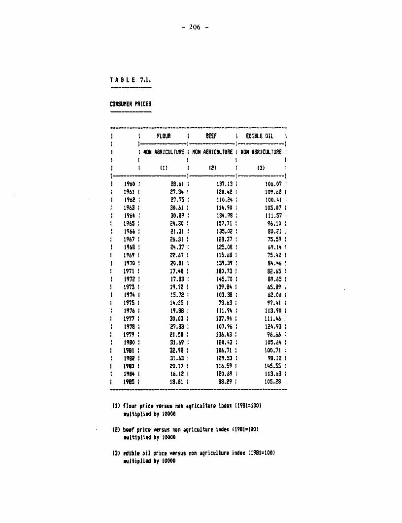
- 206 -

T A 8 L E 7.1.

CNIOMER PRICES

: I FLOUR BEEF : EDILE OIL

ENO AGRICULTURE NON AGRICULTURE NON A6RICULTURE

5 - (1) (3):_ _ _ _ _ __ _ _ _ _- _ _ _ _ _ I ____ _ _ _ _ _ _ _ _ _ _ _ _ __ _ _ _ _ _ _ _ _

1960 28.61 137.13 : 106.071961 27.34 I 120.42 109.62

: 1962 : 27.75 : 110.24 :100.4111963 : 30.61 : 114.90 105.071964 : 30.89 134.98 111.57

: 1965 : 24.30 1 157.71 : 96.101966 : 21.31 : 135.02 : 80.211967 26.31 : 128.37 75.59

: 1968 : 24.37 125.08 69.141969 : 22.67 : 115.68 : 75.42

1 1970 1 20.81 i 139.39 8 84.46 : 1971 : 17.48 : 190.73 : 82.651 1972 : 17.83 : 145.70 8 99.65

5 1973 19.72 139.84 65.891 1974 ! 5.72 : 103.38 : 62.005 1975 : 14.25 : 73.b3 97.41 :1 1976 : 19.88 111.94 : 113.90 1: 1977 : 30.03 : 137.94 : 111.46 I: 1978 . 27.83 : 107.96 : 124.93 1: 1979 : 21.58 : 136.43 : 96.66 :

1980 : 31.69 : 120.43 : 105.64 :1981 . 32.98 106.71 100.71 i

: 1982 : 31.63 1 129.53 : 98.12 :: 1983 : 20.17 : 116.59 145.55: 1984 : 16.12 : 120.69 1 113.63 :: 1995 : 18.81 88.29 : 105.28 :

(1) flour price versus non agriculture index 11981=100)multiplied by 10000

(2) beef price versus non agriculture index (1981=100)multiplied by 10000

(3) edible oil price versus non agriculture index (1981=100)wultiplied by 10000

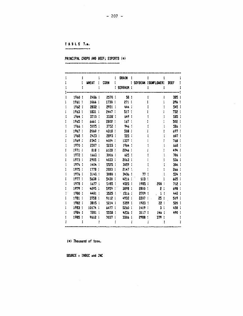
- 207 -

T A O L E 7.s.

PRINCIPAL CROPS AND BEEFi EXPORTS (It)

I : 6 I GRAIN I 1 1WHEAT I CORN : SOYBEAN 1SUNFLOWER: BEEF I

I SOR6HUIM

1960 24861 25701 58 s 385:1961 10661 17301 271 : 396:

1 1962 2832 2931 4441 , 545:1 1963: 1831: 2447 517 : 732

1964 3710 33381: 649 585: 19651 66611 2802 167 : 5021

1966 5055 3752 946 : 5861967 2060 4318 508 a 697

: 1968 2423 28931 523 : a 607:: 19691 2345 4024 13371 768: 1970 2307 5233 19641 : 6681

19711 818 6129 2246 i 494: 1972 1663 3006 625 706: 19731 2905 4033 2063 : : 536: 1974 14041 5525 3059 306:: 1975 1778 38331 2147 . : 266: 1976. 3143.1 3080 34361 771 1 5341: 19771 5638 54301 4216 613 : 6051

1978e 16271 5i95: 45231 1985 200 7121. 19791 42951 59591 38981 28101 21 698a: 19801 44811 35251 15161 27091 . 1 4431: 19811 37581 9112 49321 22071 25 519 1: 19821 3815 1 52141 53591 1923 22 5201 19831 10174 6477: 52601 14191 3 45011 19841 7281: 55581 4236: 31171 146 49011 1985 1 9612 7037 I 3306: 2989 8 379 .

(t) Thousand of tons.

SOURCE : INDEC and JNC

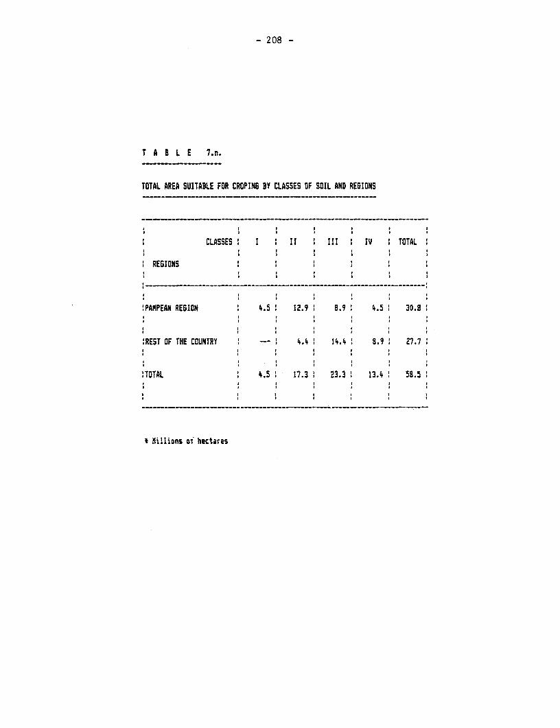
- 208 -

T A S L E 7.n.

TOTAL AREA SUITABLE FOR CROPINS BY CLASSES OF SOIL AND RESIONS

_ _ _ _ _ _ _ _ _ _ _ _ _ _____ __

CLASSES I :11 I1 1 IV ITOTAL :

1 REGIONS :

:PAMPEAN REGION : 4.5 12.9 9.9 4.5 30.8

:REST OF THE COUNTRY 4.4 14.4 8.9 27.7

'TOTAL ' 4.5 17.3 23.3 13.4 58.5

- 1illions of hectaris

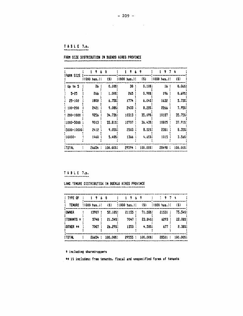
- 209 -

T A I L E 7.o.

FARM SIZE DISTRIBUTION IN BUENOS AIRES PROVINCE

i 1 9 6 O I 1 9 6 9 : 1 9 7 4!FARM SIZE 1 -- -- - -

11000 has.)' (1) .1000 has.)l (1) 1f000 has.)l IX 1

'Up to 5 1 26: 0.101: 30 0.101 16: 0.06X1

5-25 266 1.0011 265 0.90X1 196 0.6911

1 25-100 1800 6.751: 1774 6.04%: 1632 5.731:

100-200 i 2421 9.0981 2433 8.29X1 2266 7 7.95X1

200-1000 9256 34.73%1 10313 35.09%: 10197 35.75%1

:1000-5000 9013 33.81%1 10707 1 36.43X: 10805 37.91X:

i5000-10000l 2412 i 9.05Xi 2503 i 8.521X 2381 i 8.35Si

;10000- 1460 5.489X 1366 4.65X. 1015 3.56bX

ITOTAL 26654 i 100.00: 29394 100.00 28498 100.00:

T A B L E 7.p.

LAND TENURE DI0TRIBUTIOX IN BUENKS AIRES PROVINCE

ITYPE OF 1 9 6 0 1 1 9 6 9 :9 75 1

I TENURE :1000 has.: IS) '(000 has.): (X) 1(000 has.)' (X) 1

'OWNER 1 13907 1 52.198X 21155 71.58X: 21531 75.54X:

iTENANTS * i 5740 i 21.54Xi 7047 1 23.84Xi 6293 i 22.08Xi

OTHER * 1 7007 1 26.291: 1353 4.58X1 677 2.3819* * . . . . .

I ----- ~~~~~~~------ -… -- …------------…

ITOTAL 1 26654 1 100.00 29555 1 100.001: 28501 : 100.00

t including sharecroppers

tt it includes: free tenants, fiscal and unspecified forms Df tenants

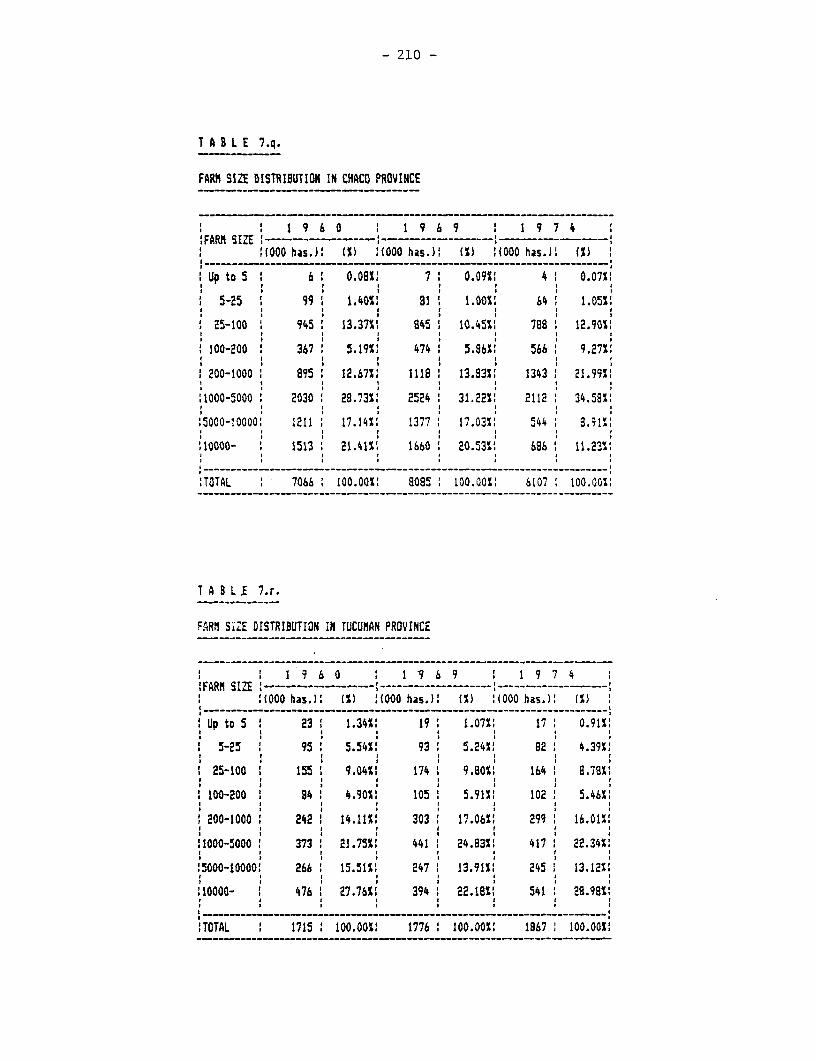
- 210 -

t A B L E 7.q.

FARM SIZE DISTRIBUTION IN CHACO PROVINCE

1 9 6 0 1 9 6 9 1 I 9 7 4,FARM SIZE ------------------ '----------------------

'(0OO has.): S) :(000 has.)! IX) U)OO has.): (1)

Up to 5 h6 0.08X: 7: 0.09%1 4 0.07X'

5-25 99 1.4011 81 1.0011 64 1.05%:

25-100 i 945 13.37%t 845 1 10.45%1 788 ' 12.90X'

100-200 1 367 5.19%: 474 5.86%: 566 9.27X'

:200-1000, 895 ' 12.67%: il1 ' 13.933X 1343 ' 21.99X'

o1000-5000 1 2030 ' 28.73X: 2524 31.22X' 2112 34.58%1

15000-100001 1211 17.14X' 1377 17.03%1 544 8.31%1

;10000- 1513 21.4311 1660 20.53S1 686 11.23%;

'TOTAL 7066 : 100.00X 8085 : 100.00 6107 t 100.00%1

T A B LE 7.r.

FARM SiZE DISTRIBUTION IN TUCUMAN PROVINCE

I 9 6 0 : 19 6 9 1 9 7 4'FARM SIZE -----------------------------------…-----------------

' h(000 has.): (' ) 1 (000 has.): (%) '(000 has.): ' 1X

1 Up to 5 ' 23 1.34X' 19 1.07X: 17 0.91X:

5-25 95. 5.54X1 93'. 5.24X. 82 4.39%1

' 25-100 155 I 9.04%': 174 9.80X'1 164 8.78X1

' 100-200 . 84 4.9011 105 . 5.9111 102 5.46X.

I200-1000 ' 242 . 14.11%: 303 1 17.06X: 299 16.01X.

.1000-5000 373 21.751: 441 : 24.831' 417 22.3411

:5000-10000: 266 15.51X. 247 13.911: 245 13.12X:

:10000- ' 476 27.76X' 394 . 22.18X. 541 1 28.98%:,, _______ i___ _ _ _ _ _ _ _ _ _____ _ _ .~_____

.TOTAL . 1715 1 100.00: 1776 . 100.001 1867 . 100.00S- - -- - ----- - -------- - ---- - - - -_ - -- - -______________-------

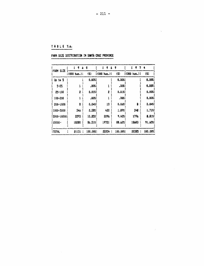
- 211 -

T A B L E 7.s.

FARM SIZE DISTRIBUTION IN SANTA CRUZ PROVINCE

9 6 0 1 9 6 9 1 9 7 4:FARM SIZE'--------:--------:------:l '1000 has.): (S) :(000 has.)X (X) :(OOO has.): IS :

Up to 5 : O.OOS: : O.OOX: 0.00:

:5-25 I: .00: 1 .001: :1 o.0s:

25-100 2 0.01S: 2 1 0.01S: : O.OOS:. . ~ ~ ~ ~ ~~. 1. .1 .

' 100-200 I I .0011 I ' .00: l O.OOt:

:200-1000 ' 8 I 0.041S 13 1 0.06S: 8 0.04%:

:1000-5000 . 546 : 2.581: 420 ' 1.89X' 348 1.71S:

'5000-100001 2293 10.85%1 2096 9.42X' 1796 8.8l11

110000- 1 18280 : 86.51X' 19721 1 88.62X: 18683 : 91.65X:

:TOTAL 1 21131 100.00: 22254 1 100.001 20385 : 100.0011

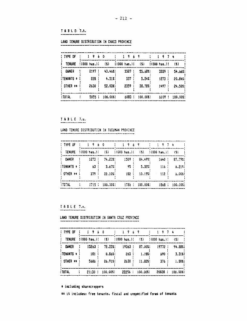
- 212 -

T A 8 L E. 7.t.

LAND TENURE DISTRIBUTION IN CHACO PROVINCE

:TYPE OF , I 9 6 0 1 9 6 9 : 1 9 7 4I I…~- - -- - - -- - ---- …--- - - -- ;- --- ---I ,

TENURE ,(OOO has.)! (X) U000 has.): (%) :(OOO has.), ( 1

,ONER I 2197: 43.4b11 3387 : 55.61 3339 1 54.665,

:TENANTS * , 228 , 4.51S, 337 5.54S, 1273 20.84X,* . I , . , I I

: OTHER tt 2630 52.03X: 2359 38.78%: 1497 24.50S:

,TOTAL , 5055, 100.00X 6083 100.00,X 6109 , 100.00:

T A B L E 7.u.

LAND TERURE DISTRIBUTION IN TUCUMAN PROVINCE

,TYPE OF , 1 9 6 0 1 9 6 9 1 9 7 4I …-…_ __ __ __ _ __ _,_

I TENURE 1(OOO has.fl (Xl !(000 has.)t (%) .(000 has.lt (%) '

OWNER 1 1273 7z'4.23%1 1509 84.495, 1640 87.79X:

;TENANTS t 63, 3.67X, 95 5.32S, 116 6.21%:

OTHER t* 1 379 ' 22.10, 182 , 10.19X 112 ' 6.00X,I I I I . .

'TOTAL , 1715 ' 100.00X 1789 100.00' . 1868 100.00X

T A B L E 7.v.

LAND TENURE DISTRIBUTION IN SANTA CRUZ PROVINCE

,TYPE OF I 1 9 6 0 1 9 6 9 1 I 9 7 4

I TENURE (OOO has.)X f1) 1(000 has.), (X) :(000 has.): (X)

: OWNER : 15263, 72.23X1 19363 1 87.00X, 19772 94.881X

,TENANTS * 1 181 1 0.86X, 263 1.18S: 690 3.31X:

I OTHER ** 1 5686 1 26.91X1 2630 11.8211 376, 1.80X,I I . . . .

-: - - - - - - - - - - - - - - - - - - -- -_- __ __ ------- __ _ __ ____

,TOTAL 1 21130 , 100.00: 22256 , 100.00X 20838 , 100.00X

t including sharecroppers

tt it includes: free tenants, fiscal and unspecified foras of tenants

A P P E N D I X B

I

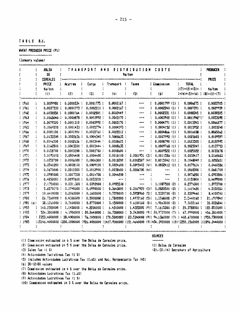
- 215 -

T A I L B.1.

WHEAT PRODUCER PRICE (Pi)

iJamiary values)

BOLSA 1 TRANSPORT AND9 DISTRI9UTI0N COSTS PROWC£1: * DE ' i;/ton ' :: 'CEREALES -------------------- ---------------------- PRICE

PRICE Acarreo I Cara Transport Taxes ' Comission : TOTALla/ton :aitonII) : s(2) (4) 15) (6)

_A- - - ---- - - - --- - -- - - - _-- - ----- - - -- -- ----- - - - - -- -- -- -- - -- - - -- -- -- -- - -- - - - -- -_ - -_- -- - -- - - -- -- -- -- -- -- -- -- -,

1960 0.0029980 0.0000534 0.0001775 . 0.0002167 -- 0.0001799 (1) 0.0006275 0.0023705161 1 0.0037330 . 0.0000773 0.0002211 ' 0.0002167 :0--- : .0002240 (w 0.0007391 0.00299391962 0.003850: 0.0000764 0.0002901 0.0002449 - - 0.0002331 (1) 0.0008345 0.00305051963 0.0065040. o 0.0000979 0.003992 0.0003170 --- 0.0003902 (1) 0.001194t' 0.0053099196 0.0079520 I 0.0001310 0.0003992 0.0003170 -- 0.0004771 (1) 0.0013243 0.006627719MS 0.0069200 0.0001433 0.0005774 0.0004593 --- 0.0004152 (u' 0.O0019s2 0.0053248

I 1966 0.0081100 0.000190 : 0.0003760 0.0005512 --- 0.0004866 (1) : 0.0016038 0.0065062 o1967 0.0133200 0.0002636 : 0.0004340 0.0008635 --- 0.0007ssz (1) 0.0023603 0.010t5971968 0.014650o 0.0002636 0.0003444 0.0008635 --- 0.0008710 (1) 0.0023505 0.012299r1969 0.0162800 0.0003200 0.0003444 0.000863 --- 0.0009768 (1) 0.0025047 0.01377531970 0.0158700 0.0003200 0.0003or00 0.0008600 ^- :.0009522 1ll 0.0025022 0.01336781971 0.0193100 0.0004400 0.000440O 0.0010100 0.000131 (3): 0.0011586 (11 0.0032417 0.01606a3197? 0.0250700 0.0006000 0.0006300 1 0.0013200 0.0002507 (4)1 0.0013042 (1) 0.0048049 : 0.0202l1973 I 0.0540200 0.00091,00 0.0009100 0.0024600 0.0005402 '4II 0.0032412 (1) 0.0079614 0.04605361974 0.0670000 0.0010300 0.0012900 0.0038400 0.0006700 M4) --- 0.0068300 0.06017001975 0.09aOOOO 0.0017300 W.0014700 0.0044200 --- . -- ' 0.0076200 0.09038001976 0.4850000 0.0097600 0.0053200 : 0.0150900 0.46h92001977 2.17?0000 0.03l30O 0.0392000 0.0M85500 --- 0.1087500 (2' 0.27?6300 1 1.99737001973 5.6570Co0 -0.0790000 0.0990000 0.3643000 0.3167920 f5W 0.2928500 (2) 1.141*20 4.5150,801979 1 10.6410000 0.2060000 I 0.1600000 0.7270000 0.5959960 5): 0.5320^00 (21 2.2309460 S 9.4 101401980 ' 26.736000 0.4300000 0.5000000 1.7800000 1. 49721 60, 151 1.3368000 at o 2 54s40160 21.19199401981 (6): 38.1260000 0.76000001 0.3770000 3.1500000 10.6100160 '8): 1.9063000 (2) 7.30331aa 30.32268401982 1 143.2300000 1 1.1450000 4.2200000: 6.4200o00: 1.4323000 19)1 7.1615000 12) 1 20.379aOOO 122.85120001953 524.3000000 1 4.19OOO 20.8640000 t 16.7300000 5.2430000 f911 20.9720000 !7) 67.9990000 456.30100001984 2353.4000000 39.4000000 76.1000000 170.5000000 23.5340000 19): 94.1360000 17) 402.6700000 1950.73000001985 115146.4000000 1300.o000000 :926.4000000 11417.9000000 !151.4640000 191454.3920000 110)!3250.1560000 111896.2440000

SOURCES11) COmmission estimated in 6 % over the Bolsa de Cereales ;rice. ------(2) Comnission estizated in 5 I over the Bolsa de Cereales price. (1J Bolsa de Cereales13) Sales Tax Ii S) R2),3),(4) Secretary of Aoriculture(4) Actividades lucrativas Tax (1 %)15) Includes Actividades Lucrativas Tax (1,6%) and Nac. a ropecuario Tax 14%)(6) 30-12-80 values17) Comuission estimated in 4 S over the Bolsa de Cereales rice.(8) Actividades Lucrativas Tax (1,6%)(9) Actividades Lucrativas Tax (1 %)110) Cosaission estiauted in 3 S over the Bolsa de Cereales price.

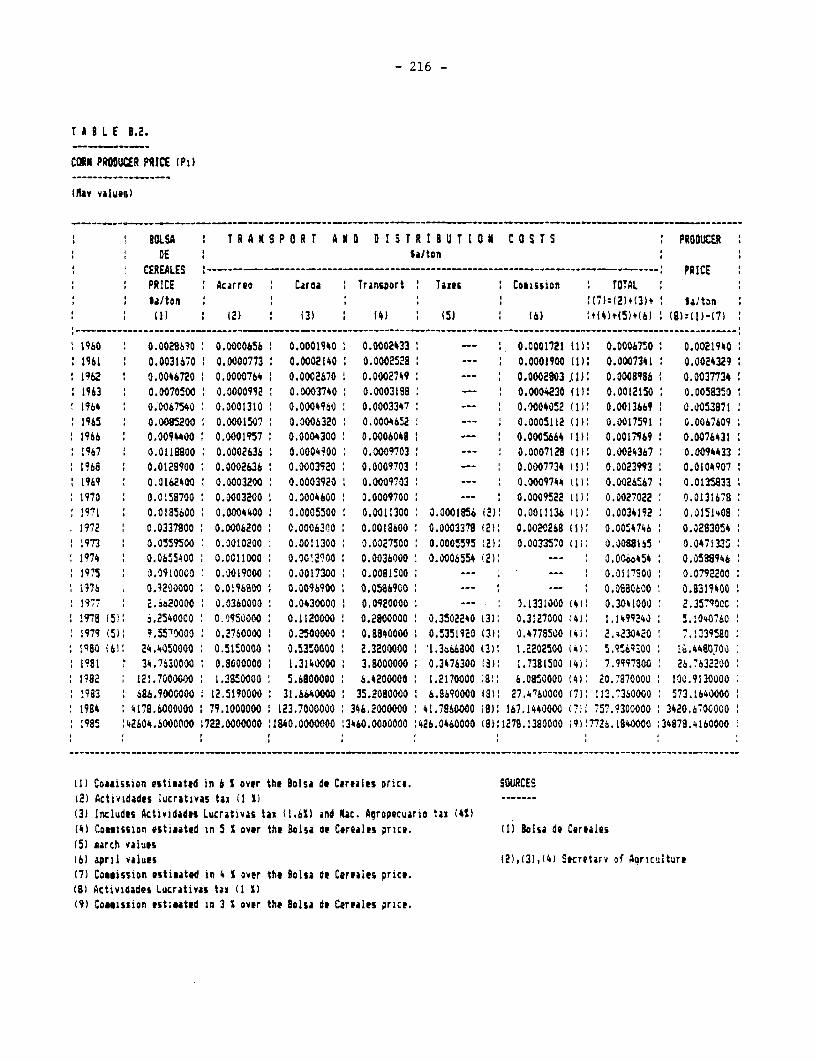
- 216 -

T A 3 L E B.2.

CORN PRODUCER PRICE (Pi)

(Eav values)

IOLSA r R A S P 0 R T A ND D I S T R I I U T I o N C o S T S PRODUCER* ~ 8 :Si/ton:

CEREALES -- ---- ---------- ----------- - --- -- --------- ------------ I PRICEPRICE Acarreo Ciroa Transport Taxes Cosission TOTALS alton :(71:2)t(3)t W^ton :(1) : 2) (3) (4) : (51 (6) s-

1960 0.0021600 0.0000656 0.0001940 0.0002433 -- 0.0001721 (W1 0.000h7v0 : 0.0021940

1961 0.0031670 0.0000773 : 0.0002140 0.0002528 --- 1 0.0001900 (I) 0.0007341 0.00243291?62 . 0.0046720 0.0000764 i 0.0002670 0.0002749 --- 0.0002903 .Jl8 0.0008996 0.00377341963 0.0070500 0.0000992 : 0.0003740 0.0003188 -- 0.0004230 (1: 0.0012150 0.00583'5 01964 0.067W40 0.0001310 1 0.0004960 0.0003347 --- 0.M004052 (): 0.0013669 0.00538711965 1 0.0085200 0.0001507 0.0006320 0.0004652 --- : 0.0005112 M! 0.0017591 * 0.00676091966 0.009400 0.0001957 0,0004300 0.0006048 1 -- 0.0005664 (1): 0.0017969 : 0.00764311967 0.0118900 0. O02636 0.0004100 0.0009703 --- 0.0007128 (II: 0.0024367 0.00944331:68 0.0129900 0.0002636 0.0003920 0.0009703 -- 0.0007734 II): 0.00239s3 0.0104907

1969 0.0162400 0.0003200 0.0003920 0.0009703 .0009744 (1): 0.0026567 0.0135331970 0.0!58700 : 0.0003200 1 0.0004600 0.0009700 : --- : 0.0009522 (.): 0.0027022 : 0.0131679:971 0.0la5600 0.0004400 0.0005500 0.0011300 0.0002956 2): 0.0081136 il 0.0034192 0.315140:

1 2972 0.0337800 0.0006200 0.0006300 0.0018600 0.0003378 (2)1 0.0020268 MII: 0.0054746 0.02830541973 0.0559500 0.3010200 0.0011300 0.0027500 0.0005595 t2): 0.0033570 (1w: 0.00981 0.04713351974 0.06'5500 0.0011000 1 0.1002.700 0.0036000 0.M006554 (2): --- : ,0C.6454 1 0.05999461975 , : ,0910000 0.00000 0.0017300 0.0091!00 0--- I .0117soo 0.07922001*71 0.9200000 0.01968M0 0.0096900 : .860 --- : -- : 0.0880600 0.831940019: 7 E6.620000 0.0360000 0.0430000 : 0.0920000 --- 0.1331000 (41: 0.3041000 2.35790CC1978 (5i: i.2540000 0.0)950000 0.1120000 0.2890000 0.3502240 (31: 0.3127000 (4: 1.1499240 : 5.040760.1979 (5): 9.55?0000 0.2'760000 0.2500000 0.8840000 0.5351920 (31: 0.4778500 14) 2.2304120 7.4J39580Iqao (61: 24,4050000 0.5150000 0.5350000 : 2.3M00000 : 1.3e66800 3)i 1.2202500 (14) 5.9!6w900 1 0'.0480700 :1991 34.7630000 : 0.8000000 1.3140000 3,8000000 0.3476300 (311 1.7381500 (4) 7.9997300 26.76322001982 121.7000000 1 1.3850000: 5.6B00000 1 6.4200000 1.2170000 isJ1 6.0850000 (4)1 20.7570000 100.91300001933 686.9000000 1 12.5190000 : 3.6640000 35.2080000 6.8690000 (S)i 27,4760000 (7): 112.7360000 573.16400001994 4178.6000000 79.1000000 123.7000000 346.2000000 :41.7860000 (S): 167.1440000 (I7: 757.9300000 3420.67000001985 :42604.6000000 :722.0000000 :19840.0000000 3460.0000000 :426.0460000 (98):1276.1390000 I987726.1940000 :34878.4160000

----------- - --- - - - - ---- - -- - -- - ---- - - -- -- -- -- -- -- -- -- -- -- -- - -- -- -- -- -- -- -- -- -- -- -- -- -- -- -- -- -- -- -- -- -- -- -- -- -

(1) Comaission estisated in 6 s over the BOlsa di Creales Drince. SOURCES(2) Actividades lucrativas tax It 1) -------(3) Includes Actividades Lucrativas tax 11.65) and Mac. AgrDOecuatio ta3 M45I(4) Conmission estisated in S s over the Balsa do Careales price. (1) Bolsa de Cerealis(5) march values(6) april values (2),i31i41 Secretary of Aoriculture(7) Cosmission estimated in 4 S over the Blsa de Cereiles price.(9) Actividades Lucrativas tax (i S)(9) Cossission est;eated in 3 S over the Balsa de Cereales price.

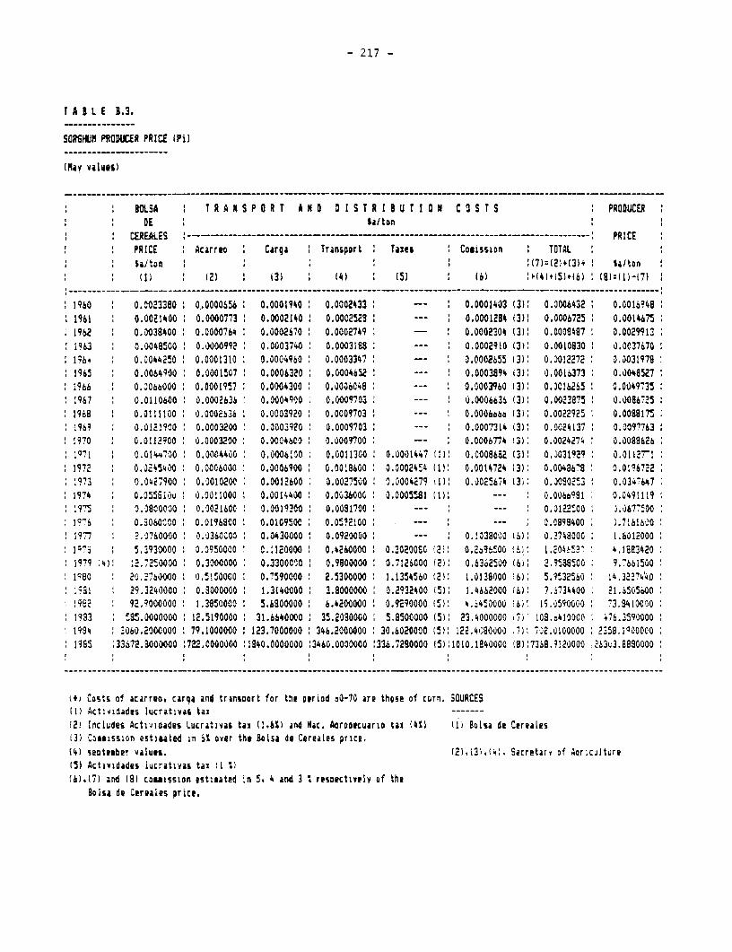
- 217 -

T A I L E B.3.

SORSI PRODUCER PRICE (Pi)

(May value;)

OLSA T R A S 5 P O R T A N D D I S T R I 8 U T I D N C 3 S TS PRODUCERDE Ia/ton

CEREALES -------------------------------------------- …-- ----- PRICEPRICE Acarrto Carga Transport Taxes Coaission TOTAL

at ' '(7)=12!tl3)t Saltonsl) ~~~(2) 03) (4) s5 l)+W*+(SJ+(b) (8)-e)-17)

------- - - - ----_ - _- -- ------ - --- -- -- -- ----- - -- -- -- ----- - -- ----- - - -- -- -- -- ----- - -- - - - -- ---- - ---- -- -- ------

1960 0.0023380 0.0000656 0.0001940 0.0002433 - 0.0001403 1311 0.0006432 0.0016948t 1961 0.0021400 0.0000773 0.0002140 0.0002528 --- 0.0001284 (3)8 0.0006725 0.00146751962 0.0038400 0.0000764 0.0002670 0.0002749 0.0002304 (3)8 0.000848 7 0.002191963 0.M48500 O.0000992 0.0003740 0.0003188 --- 0.0002910 i3): 0.0010830 0.0037670196o 0.00o4250 0.0001310 0.0004960 0.0003347 -- 0.0002655 (3): 0.0012272 0.30319791965 0.0064900 0.0001507 0.0006320 0.0004652 --- 0.0003894 3): 0.0016373 0.0048527!966 0.C0o000 0.0001957 0.0004300 0.0006048 --- : O.3003960 (3): 0.0C6265 0.00497351967 0.0110600 0.0002636 O.MO04900 0.0009703 --- u.0006636 (3): 0.0023675 0.00867251968 : 0.01100 : 0.0002S36 0.0003920 0.0009703 --- 0.0006o6a (3): 0.002292 : 0.00881751969 : 0.0121900 0.0003200 0.0003920 0.0009703 --- 0.0007314 3): 0.0024137 0.00977631970 0.0112900 : 0.0003200 0.0004600 : .oo009700 -- : 0.0006774 (3): 0.0024274 0.308662b

1 q71 0.014s700 0. 004400 0.0006100 0.0011300 0.0001447 i1n: 0.00086a2 (3)1 0.0031929 : 0.011211972 : 0. 02540v 0.0006000 : 0.0006900 0.0018600 : 0.0002454 (1 0.0014724 13)1 0.0048679 0.0196722973 0.0427900 0 0.2010200 0.0012600 0.0027500 : n.3004279 tl: 0.0025674 (31; 0.0 X0023 0.034-647

1974 I 0.055610v : 0.0011000 0.0014400 0.0036000 0.0005M81 (1) --- 0.0066991 0.04911191975 0.0800000 0.0021600 : 0.00 9200 0.0081700 --- --- 0.0122500: s, 677500

19`6 : 0.3060O30 0.0196800 0.010950C ; 0.0!?2!00 . --- : --- 0.0899400 ; .7161600

19-7 2.3760000 0.0J3600: 0.0430000 0.0920000 : 0.!038000 (6)1 0.2748000 1.6012000la's 5.3930000 0.3950000 C.:120000 0.4260000 0.30200SC ;28: 0.296S00 (i: 1.204sE:^ 4.19834201979 4 : 2. 72 500 : 0. 300000 0.33000C0 0.9900000 0.7126000 (2): 0.6362500 (6) .2.9538500 9.76615001980 20.7600O0 0.5!=0000 : 0.7590000 2.5300000 1.1354560 12): 1.0136000 6): 5.9s322560 14.32274X01931 : 29.3240000 0.3000000 1 1.3140000 3.8000000 0.2932400 15): 1.4662000 (S)8 7.6734400 21.SS05600962 : 92.9000000 1.3950000 5.6800000 6.4200000 0.92-90000 (5)! 4..*450000 l6,1 19.0590000 : 73. SAIO001933 5895.0000000 12.5190000 31.6640000 35.2080000 5.8500000 15k 23.4000000 i7) 108.o410000 476.35900001924 23060.2000000 79.1000000 123.7000000 346.2000000 30.6020000 (5s: 122.4t180000 71 702.0100000 2358.l9000O1985 ;33672.a000000 :722.0000000 1840.0000000 :3460.0000000 :336.7280000 15):1010.1840000 987368.?120000 263Q3.8890000

-------- - -_- ----- - _--__ - - ----- -- -- -------- - -- -- -- -- ------ - ---------------------------- -- -- --- - -- -----

(t) Costs of acarreo, caroa and trinsoort for the period o0-70 are those of corn. SOURCES(1) Actividades lucratvva; tax -------(2) Includes ActXidades Lucrativas tax (1.65i and Nac. Aoraotcuario tai (4S) (ii Bolsa de Cereales31) oaamission estimated in i% over the Bolsa de Cereales price.(4) seotember Values. (2),(31,(4, Secretary of Aariculture(5) Actovidades lucrativas tax 1 Il(6).17) and (9) coaission estimated in 5, 4 and 3 : resoectively of the

8aol de Cereales price.

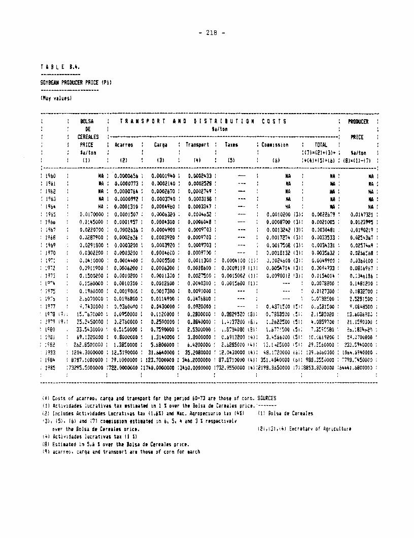
- 218 -

T A 3 L E 9.4.

SOYBEA PRODUCER PRICE (P1i

lnay vilues)

BOLSA T R A l S P O R T A 1 D O I S T R I I u T I N C os s PStTUCERDE Salton

: CEREALES :- --- --- -- ---- - ------ -------------------------- - - --------- I PICE :PRICE Acarroo : Carga Transport Tains Commission TOTALSalton : * . 7)(2)+(3)+ Saltonfl) : 2) : 3) (4 c)l) (5) ()t :+M l(5 ' M=MX1-M7

1960 NA 0.0000656 0.0001940 0.0002433 N- NA NA KA1961 N A 0.0000773 : 0.000210 : 0.0002528 --- : NA NA1962 : NA 0.0000764 0.0002670 0.0002749 NA I NAY1963 KA o.0000o s2 0.0003740 0.0003158 --- A : MA: tA1964 NA 0.0001310: 0.0004960 0.0003347 --- A NAh1915 0.0170000 0.0001507 : 0.0006320 0.0004o52 --- 0.0010200 i3): 0.0022679 3.0147321:196 0.0145000 0.0001957 0.0004300 : 0.0006048 --- 0.0008700 (31: 0.0021005 0.01239951967 0.0220700 0,00O2636 0.0004o0 0.0009:03 --- 0.0013242 (3). 0.0030481 O.01902191968 0.0287900 0.0002626 0.0003920 0.0009703 --- 0.0017274 (3): 0.0032533 0.0254367196 0.0291500 0.0003200 0.0003920 0.0009703 --- MOM (3 0.0034.3131 0.02574b91970 0.0302200 : 0.0003200 o.ooo*oo : 0.0009700 --- 170.0018132 f3): 0.003%632 0.02W68197: 0.04!0000 0.00C4400 0.0005500 0.0011300 0.0004100 (1)l J.024600 (3): 0.00499C0 0.03601001972 0.0911900 0,0006200 : 0.0006300 : 0.0018600 0.0009119 (1): 0.0054714 (31: 0.M004133 0.0816967973 0.1500200 : 0.0010200 0.0011330 0.002750: 0.0015002 iM: 0.0090012 31) 0.0154014 0.2346136

1??*4 , o.56oo000 0.0010300 : 0.0012600 0.0040300 : .00150600 (1): --- : 0.o0780 o 0.1481200

1975 0oo960000 0.00M1900C 0.0017300 0.0091000 0 --- : 1 .0127300 0.1932700: , la^S i 2.4070000 :0.019680 0.0114900 : 0.0476800 --- --- : ;.073OO 2.2S:00

1977 ;.7430000 0.0360ifO I 0.0430000 0.0920000 : I 0.4871!00 ;51 0..J!8I500 : .0648500197?9 * i; 15.'670000 10.095OOOO 0.1120000 0.2900000 : 0.3829520 C8): 0.78MO350 ); 2.1532020 13.4026?1G :

1979 (9; 25.2450000 : 0.2760000 : 0.2500000 0.8840000 1.-37200 8i; 1.2622500 5): 4.0859700 21.1!90300: 1980 33.543000' 0.51'0000 0.7590000 2.5300000 1 ..8?340.OO tln 1.6?7'00 75; ?.3'i55B0

1?El ' 69.1320000 0.8000000 1.3140000 3.8000000 C 0.6913200 (4): 3.W566000 151! 102-:0200 '59.700800:q82 262.85000GO 1.38S0000 5.S800000 : 6.4200000 2. 28ss00 (4): 1.1ia5OOO is): 29.2S60000 :a32.59400001933 1204.3000000 12.5190000 3.6640000 35.2080000 12.0430i000 ()1 48.1720000 i6ii :39.u630100 1064.6940000194 : 8787.1)00000 0 79.1000000 123.7000000 346.2000000 : 97.9710000 (4): 351.4340000 (6)1 983.32Z5o000 7793.74s00001985 :73295.5000000 "7M.0O000oo :174o.0000000 :3460.0000000 M732.9550000 (4):2198.3650000 (7) M53.8200000 :64441.SCOOO3

({) Costs of acarreo, caroa and transport for the pmriod 60-73 are those of corn. SOURCES11) Actividades lucrativas tax est;eated in I S over the Bolsa de Cereales price -------v21 Includes Actividades Lucrativis tax (1.61) and Mac. Aqropecuaroo tax (4) (11) Boisa de Cereales'3), i5), (6) and (71 comission estisated in 6, 5, 4 and 3 S respectively

over the Bolsa de Cereal.s orice. 2),i3),(4) Secretary of Agriculture14) Actividades lucrativas tao (1 1)8B) Estimated in 5,6 S over the lolsa de Cereales price.(1) acarrec, carqa and transoort are those of corn for march

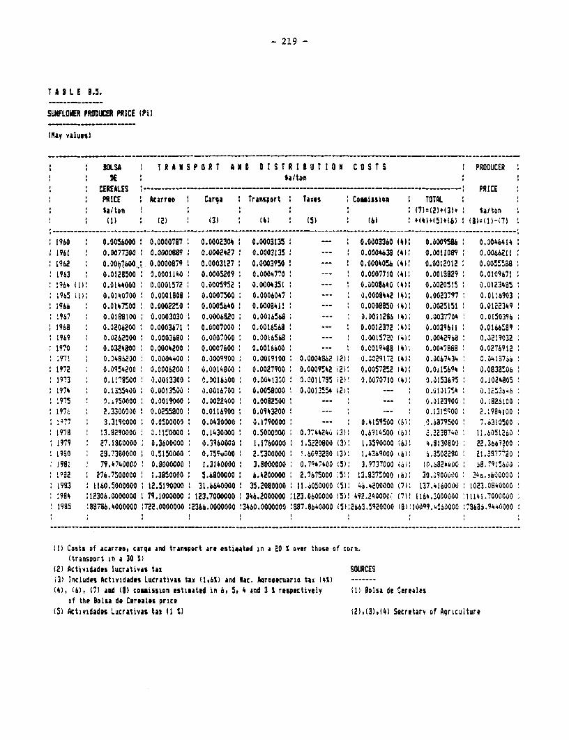
- 219 -

T A I L E 3.5.

SWUFLOWER PRODUCER PRICE (Pi)

ISA : T R A N S P O R T A ND D I S T R I B U T I ON C O TS PRODUCERDE ' ta/ton :

I ' ~~~CEREALES '----------- ------ --------------- - -' PRICEPRICE : Acarr.o : Carga TraiDsport Taies Comissioe. TOTAL

: ..$$/ton ' : : : h ' I7)=121+(31t Sa/ton

:(I1} : [2) ' {(3) '61 (5) (61 81I)(7) :

1960 0.0056000 0.0000787 0.000E304 0.0003135 0.0003360 (41: 0.0009586 0.00464141961 : 0.0077300 0.00 f9 0.0002427: 0.0003135 --- 0.0004638 (4): 0.00110 .9 0.00662111962 O.OO7.600,: 0.0000879 0.0003127 : 0.0003950 --- 0.000056 (4): 0.0012012: o.oos5sa81963 : 0.0128500 0.0001140 0.0005209: 0.00047?0 0.0007710 -41: 0.0018829 0.0109c711964 I1I: 0.0144000 0.0001572 0.0005952 0.0004351 . --- 0.3001640 (4) 0.0020515 3.01234851965 (I: 0.0140700 0.0001808 0.0007500 0.0006047 --- : 0.0008442 141: 0.0023797 0.01169031h6 I o.o017soo 0.000220 : 0.0005640: 0.0009411 0--- o .000os5o 4)1 0.0025151 0.0122349:967 0.0189100 0.0003030 . 0.0006820 0.0016568 --- 0.0011286 14): 0.0037704 0.01503961968 0.0203200 0.000367 1 0.0007000 0.0016568 --- 0.0012372 4H 0.0039611 0.0166!891969 0.0262000 0.0003680 : 0.0007000 0.0016568 --- 0.0015720 1411 0.0042968 0.02190321970 : 0.0324800 0.0004200 : 0.0007600 0.0016600 --- 0.0019488 141 0.00476a8 0.0276912IS?7! 0.o4s6200 o.ooo00 oo 0.0009900 1 0.0019100 0.0004862 (2): 0.3029172 141: 0.0067434 0.3J4137i1972 0.0954200 0.0006200 0.0014800 0.0027900 :0.0009542 k2(: 0.0057252 14): 0.0x15694 : 0.083L50619?3 0.1119500 .0.0013300 '.0016600 0.0041300 0.C011735 121 0.0070710 (41: 0.0153695 0.10248051974 0.1355430 0 0.00135S3 0.0016700 : 0.0058000 0.3012554 (2)i --- 0.i13l754 i 0.136461975 !.i50000 0.0019000 : 0.0022400 0.0082500 --- --- : .0123900 0.:82S!001975 2.3300000 0.0255800 0.0116900 0.0943200 --- --- : 0135oo 2.1984100.1q77 3.3190000 o.osooooo : 0.0430000 : .1790000 --- 0.4159500 (6): 0.a795500 7.63105001978 13.8290000 0.11!0000 0.1430000 0.5000000 0.774424~ i3)I 0.6914500 (6): 2.2238740 i1.60512631979 27.1800000 0.3600000 0.39 .0000 1.1760000 11.5220000 (32: 1.3590000 (6): 4.813080) 22.36692001990 : 29.7380000 3.5150000 0.759u00 1 2.5300000 !.603280 13): 1.4369000 tb)' i.3502280 21.3877'201981 79.4740000 0.8000000 1.3140000 1 3.8000000 0.7947400 t5): 3.9737000 (ii: !o..S624400 6.791SO6O1?92 276.7500000 1.3850000 : 5.6800000: 6.4200000 2.7675000 ~51! 13.827r000 t6: 30.390iI0 : 24t.36000001993 1160.5000000 112.5190000 31.6640000 35.2080000: i1.6sooeo0 5): 46.4.200000 (711 137..160000 1023.38400001984 :12306.0000000 :79.1000000 1 123.7000000 346.2000000 :123.0600000 (5): 492.2400001 (71: 1164.3000000 '11141.70000001995 :88786.4000000 :722.0000000 :2366.0000000 :3460.0000000 :887.8640000 (5):2663.1920000 (8)10099.4!S3000 :78686.9440000

* , . . , I

-- -- -- - -- - - -- - - -- ------ - -- -- - - - - ------------ - _- ---- - -----------------------------

(1) Costs of acarres carqa and transport are estiuted in a 20 S over those of corn.(transport in a 30 %)

(2) Actividdes lucrativas tax SOWRCES(3) Includes Actividades Lucrativas taz (It,6) and Mac. Acrocecuario tax (4$) -------(4), (6), (7) and (9) comaission estimated in 6J 5, 4 and 3 1 respectively (1) Balsa de Cereales

Df the Bolsa de Cerealns price(5) Actividades Lucrativas tax 11 S) (2),13).(4) Secretary of Acriculture

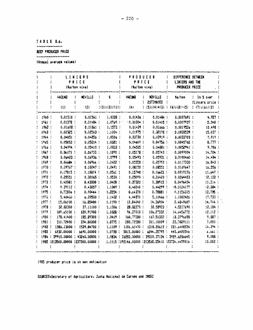
- 220 -

t A B t £ 8.6.

KUF PRODUCER PRICE

(Annual averaQi Values)

L I 1 I E R S : P R 0 0 U C E R DIFFERECE BETWEENP R ICE ' P R I C E LINIERS AND TE

(Si/ton viva) ' ia/ton viva) DPRODUCER PRICE

vAUNO ' OVILLO S VACDNO NOVIULL : Si/ton In S over' ' ' ' ' ESTIMATED :Liniers price .

(1) (2) ;(3):(2)/(I)I (4) (51):(4)13) (6):(2)-15) (7)1:16)(2)

1960 0.01510 0.01561 1.0338 0.01436 0.01484 0.00076st1 4.9271961 0.01371 0.01494 1.0769: 0.01304 : 0.01405 0.0007937 5.3481962 0.01609 0.01a61 1.1573 0.01439 0.01666 0.0019536 10.4981963 0.02325 . 0.02563 1.1024 0.01975 0.02178 : 0.0038539 15.0371964 0.04051 0.04256 1.0506 : 0.03730 0.03919 0.0033703 7.9191965 0.05052 0.05214 1.0321 0.04609 0.04756 0.0045762 8.7771966 0.04994 0.05410' 1.0833 0.04505 0.04881 0.0052941 9.7861167 : 0.06071 0.06733 1.1090 0.05178 0.05743 0.0099004 14.7041968 0.06423 0.06936 1l.07 1 0.05493 0.05931 0.01o0060 i 14.4941969 0.06684 0.06966 1.0422 1 0.055'B 0.05793 0.0117330 16.8431970 0.09767 0.10247 1.0491 0.08150 0.08551 0.0169647 16.5561771 0.17315 0.18814 1.0561 : 0.15740 0.16623 0.0219126 11.6471972 0.29551 0.30065 1.0530 0.25090 0.26420 0.0364453 12.1221973 0.42081 0.43880 1.0A28 . 0.37320 0.38915 : 0.0496454 11.3141974 0.39112 0.43057 1.1009 0.40240 0.44299 -0.0124177 -2.8841795 0.7:806 : 0.90444 4 1.2254 0.64370 0.78881 0.1156315 12.795* 1976 : 5.4040 ' 6.20500 ' 1. 12 : 4.44570 5.10466 1.1003426 1 7.7331977 11 15.06100 16.a5400 1.1190 12.34040 1 14.36904 2.4849607 14.7441978 32.32300 37.11100 : 1.1206 21.82370 32.58923 4.5217690 12.1841979 109.65100 120.91900 : 1.1028 96.37010 106.27332 14.6456772 12.1121990 : 17S.41400 185.89300 1 1.0419 160.7,73Bo 167.51333 18.3796658 9.871981 , 310.72400 334.80300 1.0775 : 288.72580 311..10009 23.7029111 7.0801982 ' 1386.13000 11539.84700 1.1109 1116.61470 1319.20615 221.6406534 14.3941993 6230.00000 1 6090.00000 1 1.0738 1 5815.00000 6244.35795 445.6420546 1 6.i611984 1 39910.00000 : 43240.00000 : 1.0834 1 36283.00000 39310.37134 1 3929.62>6645 9.0881985 :213500.00000 '237300.00000 : 1.1115 :192146.00000 !213565.55410 !23734.4459016 10.002

1985 producer price is an own estimation

SOURCESzSecretary Df Agriculture, Junta Macional de Carnes aind INOEC

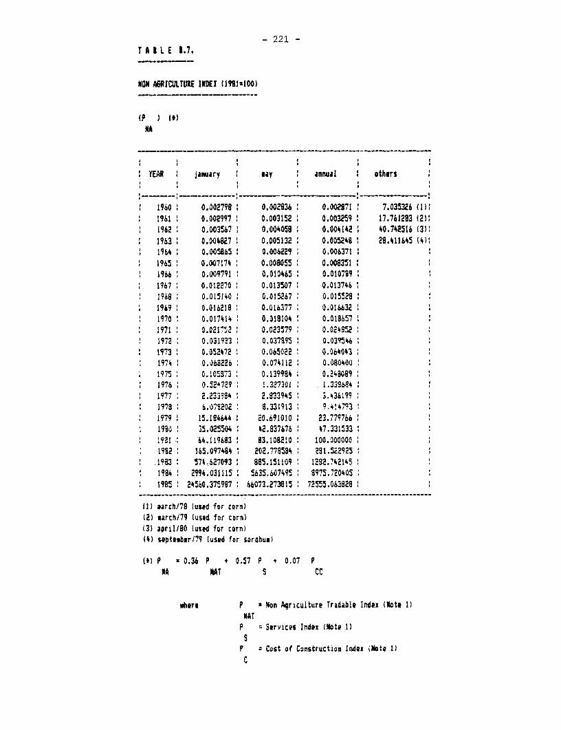
- 221 -

T A I L E 1.7.

NON AGRICULTURE INDEI (19811100)

NA

, * I

YEAS jaary ,ay annual 1 othersI I : I

1960 0.002798 0.0Q02834 0.002871 7.035326 (1:1961 1 0.002997 0.003152 0.003259 17.761213 (2111962 0.003567 0.004058 0.004142 40.74a516 (31:1963 0.00W827 0.005132 0.005248 29.411645 (S):1964 0.005865 0.006229 0.006371 '1965 0.007174 0.008055 O.0083511966 0.009791 0.010465 0.0107891967 0.012270 0.013507 0.01374419I8 0.015140 0.015267 0.015528 1949 ' 0.016218 0.016377 0.0166321970 0.017414 0.018104 0.0186571971 0.0217i2 0.023579 0.0248521972 0.031923 0.037895 ' 0.03?5461973 0.052472 t 0.065022 0.0640431974 0.068226 0.074112 0.0804001975 0.105873 0.139984 0.2480891976 0.52'729 1.32730I 1.3386841977 2.233?84 2.933945 3.4361991978 6,078202 8.331913 9 t'4t931979 15.184644 20.691010 23.77976619iO '35.025504 42.837676 ' 7.331533:931 : 64.119683 83.108210 100.000000 1982 : 165.097414 1 202.779S94 281.5229251963 : 574.627093 885.151109 1292.742145198i 1 2994.031115 5635.607495 8975.7204051985 : 24560.375997 66073.273e15 72555.068298

11) aarch/78 (used for corn)(2) earchJ79 (used for corn)(3) april/80 (used for corn)(4) s;etesbarl?9 [used for sorohus)

(1) P z 0.36 P + 0.57 P + 0.07 PNA NT S CC

whre P : Non Aqriculture Tradable Index (Mote 1)MAT

P Services Index lbote 1)s

P Cost of Construction Index ,Note 1)C

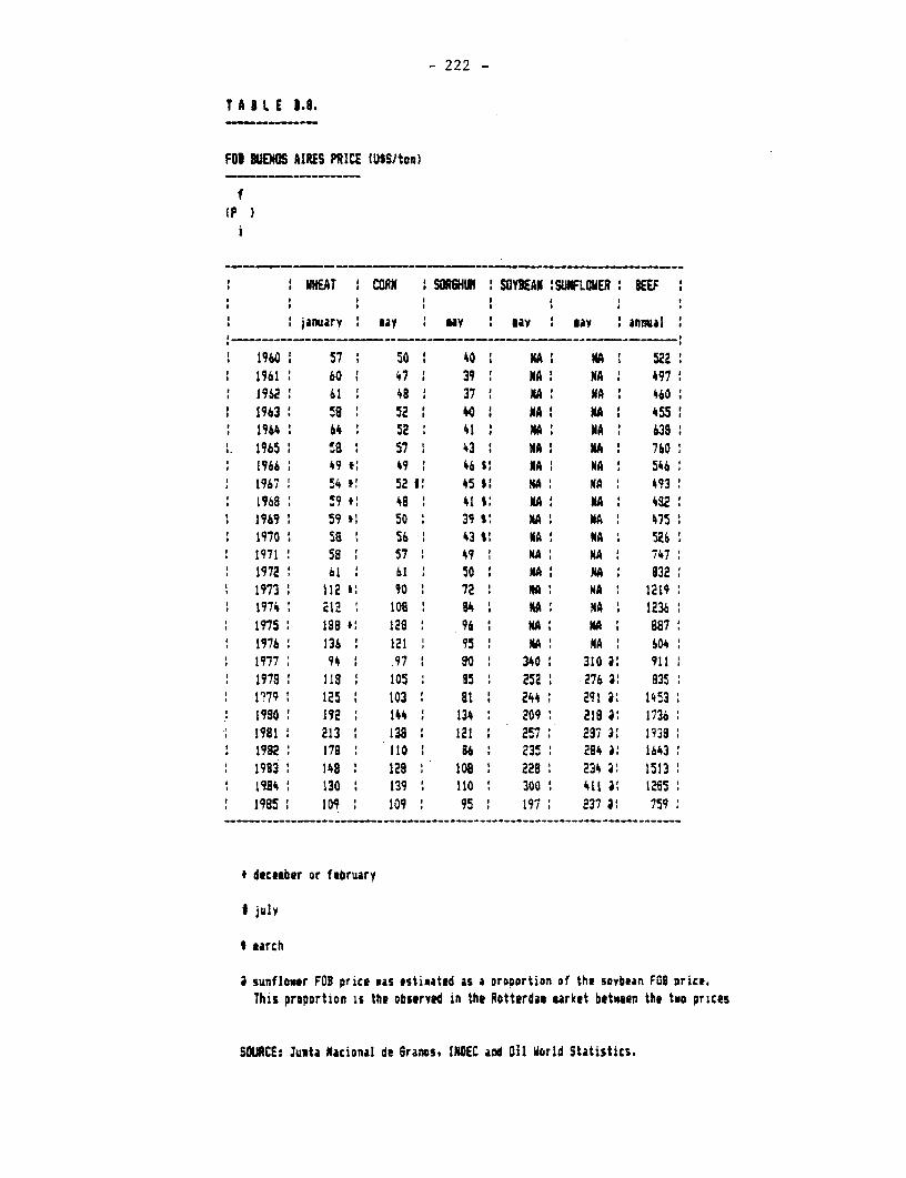
- 222 -

T A I L E M.6.

F0B BUEOS AIRES PRICE (USS/ton)

f(P

:HEAT CMRN SSLHII SYEAN SUIFLOWER KUEEF

january: ay : say say s : ay 'annual- --- -- - -

19601 57 50 40 KA MA 52:1961 60 47 39 MA MA 4971912' 61 48 37 I JA MA: 460:l 1963: 5 9 : 40 NA: A 45511964 : 64 1 52: 41 MA: MA 638

. 1965 s 1: 57' 43: MAt NA 760:: 1966 49 t' 49: 46 1 NA: MA: 546:

1967 ! 54 #1 52 1 45 1: MA MA 4931968: 59.t 48 41 1' KA: NA: 4821969: 59 50 39 * ' MA NA 1 495S1970: s58 56 43 S A NA I MA ' 526'1971' 58: 57: 49 KA MA J 747:19728: 61 ' 61 . 50: NA: MA 832I1973. 112 90 ' 72 ' A: MA ' 1219:1974: 212 1061 841 NAf NA 1236:1975: 188I* 128 : 96 MA N MA 1 887:

1 1976: 136: 121 1 9S 5 ' A' MAI 604:: 1977; 94 : .97 ' 8so 340: 310 i: 911:

1978' 119 ' oS: 85 252 276 3: 83SI1?791 125 : 103 1 81 ' 2441 l 291 : 14531950: 192: 1441 134: 209: 218 i: 173619811 213 138: 121: 257: 287 3: 1938:1982: 178 1 110: 86: 235: 284 i: 1643'1983: 148 128 108 :22 8 234 1513:

: 1984 i 130 : 139 110 1 30 4 i11ll 1265 5;1985 109 ' 109 ' 95 1 197 237 3! 759:

t decoeber or february

I july

t march

3 sunflower FOB price uas estimated as a Proportion of the soybean FOB price.This proportion is the observed in the Rotterdas market between the two prices

SOURCE: Justa Nacional de 6ranes, INDEC and Oil World Statistics.

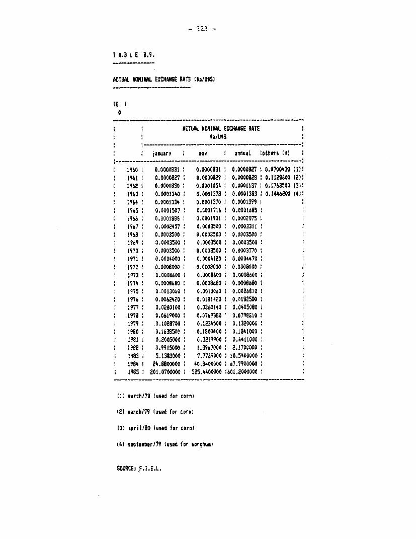
- 223 -

T A.B L E B.9.

ACTUAL NOIIAL EXCHANIE RATE $aIUSS)

(E )0

ACTUAL NOMINAL EXCHANE RATE

: : ;~~auuarv : ay annual bot1hers Ci)

I 1960 0.0000831: 0.0000931 0.0000827 0.0700430 (11)1961 : 0.0000827 0.0000829 0.0Q009o8s 0.1128600 12):1962 0.0000830 0.0001054 0.0001137 0.1763500 (3J21963 0.0001340 0.000 378 0.0001383 1 0.1446200 (411964 : 0.0001334 0.0001370 0.00013991965 0.0001507 : 0.0001716 0.00016851966 : 0.0001888 : 0.0001901 0.00020751967 0.0002457 0.0003500 0.00033111968 0.0003500 : 0.0003500 0.00035001969 : 0.0003500 0.0003500 0.00035001970 0.0003500 0.0003500 0.0003770

: 1971 0.0004000 0.0004120 0.0004470:: 1?72 O.OMO800 0.000800Q 0.000@Q000: 1973 0.0008600 0.0008000 : 0.000860001974 0.00068b0 : 0.0008680 0.00066801 975 0-0013060 : 0.0013060 : 0.00268101976 0.00 R iZO 0.0181420 0.nts2500 : 1977 0.0280100 0.0360140 : 0.0405080

: 1978 0.0619000 0 Q.0769380 0.07910::19t9 0.1029700 0.1234500 0.13200001990 : 0.1638500 0.1800400 0.18410001978 0.2005000 0.3219900 0.44110001 1982 0.9915000 1.3967000 : 2.1700000: 1983 5.1383000 7.7709000 .10.54000001984 I 24.8100000 40.8400000 : 67.7900000 :1985 : 201.07000O0 : 525.4400000 :601.2000000

C1) uarch/78 (used for corn)

(2) iuarchl79 (used for carn)

(3) april/80 (used for corn)

(4) s@ptueb@r/79 (used for sorqhum)

SOURCE: F.1.E.L.

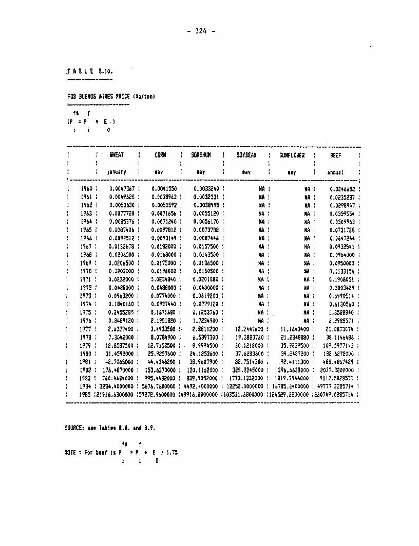
- 224 -

T I L E 3.10.

FOB BUENOS AIRES PRICE (Salton)

fS f(Pp - 7 £*

i 0

WHEAT I CORN 1SCRSHUH SOlYBEAN SUNFLOWER BEEF

: ' january ' ay : ly m ' say : ay N annual,~~~~~ ~~ ~ ~~~~~~~~ ~ ___ - __ -__- -- --

1960 I 0.0047367 : 0.0041550 1 0.0033240 NA NA 0.0246652I961 : 0.0049620 : 0.0038963 0.0032331 NA NA 1 0.02352371962 0.0050630 0.0050592 0.0038998 NA XA : 0.02989471963 0.0077720 0.0071656 0.0055120 N NA : NA 0.03595541964 0.0085376 0.0071240 0.0056170 NA NA 0.05099%31965 0.0087406 0.0097812 0.0073788 NA KA 0.0731,281966 0.0092512 0.0093149 0.0087446 A NA 0.064724Z1967 0.0132679 0.0192000 0.0157500 Nm NA 0.093241I1968 0.0206500 0.0168000 0.0143500 MA XA 0.09640001969 0.0206500 0.0175000 0.0136500 NA NA 0.09500001970 0.0203000 0.0196000 0.0150500 NA NA 0.11331541971 0.0232000 0.0234840 0.020180, NA KA 0.19080511972 0.0488000 0.0488000 : 0.0400000 NA MNA 0.38034291973 0.0963200 0.0774000 0.0619200. MA NA 0.59905141974 0.1840160 0.0937440 0.0729120 NI KA 0.61305601975 0.245529S 0.1671690 O.i253760 NA NA 1.35888401976 0.8489120 2.1951820 : 1.7234900 NA NA 6.29885711977 2.6329400 3.4933580 2.8811200 12.2447600 11,1643400 21.08730741978 7.3042000 8.0784900 . 6.5397300 19.3883760 21.2349880 38.11464861979 1 2.8587500 12.7153500 : 9.994500 30.1218000 35.9239500 109.59771431980 31.4592000 25.9257600 24.1253600 37.6283600 39.24c7200 182,627200O1981 42.7065000 44.4346200 : 38.9607900 82.7514300 92.4111300 488.48i142911982 176.4870000 153.6370000 120.1142000 328.2245000 396.i668000 2037.32000001993 1 760.4684000 1 995.4432000 : 839.9052000 1773.1332000 ' 1819.7946000 9112.582957119904 3234.400000 0 5676.7600000 1 4492.4000000 ' 12252.0000000 116795.2400000 1 49777.22857141985 :21116.6300000 157272.9600000 :49916.8000000 '103511.6800000 :124529.2800000 :260749.0295714

SOURCE: see Tables 1.9. and 3.9.

fS fNOTE For beef is P z P * E /1.75

i i 0

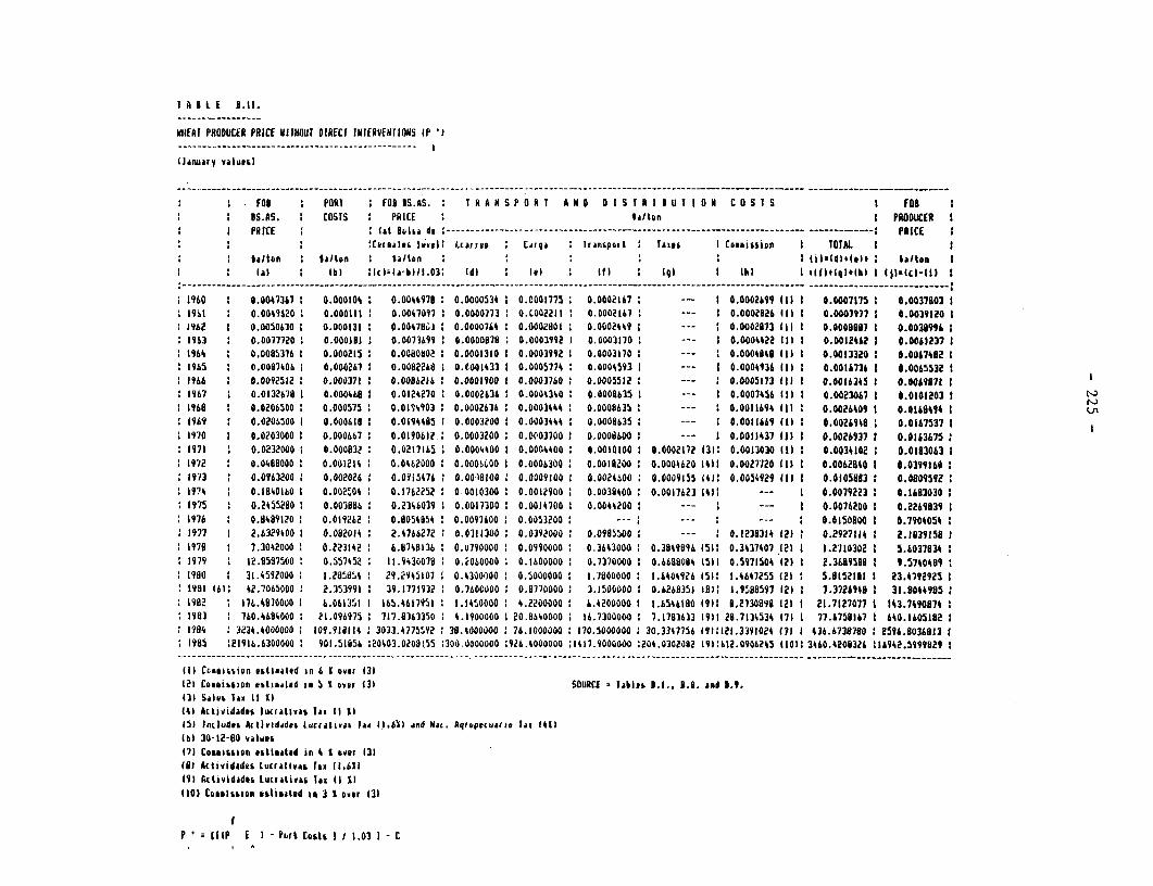
I A A 0 E 9.11.

iHEAI PRODUCER PRICE RIIIHOUT DIRECI INIERVEIIIIONS IP ')_~~~~ I

(Januaty valun I

I fOi : PORT : FOB IS.AS. T T R A N S P O T A D D I S T A I I U T I O 1 C O S I S I fOtBS.AS. COSTS : PRICE : laIIon I PRODUCER I

: I PR KE ( it 90 di :------------------------------------------------------------------------- ------- PRiCE I: :alls .lWRI: flEAFa^eg : CAF : If anipDil C 19 1 Cu.illiDn I TOTAL I I

: : Ia/lon : Ia/lon : $&Ialin I (ilsIdlalfl : Salton I; : lal :blb) Iclala-b011.03: Idl : If) 191 I hl ) *41)fMlf*Ihl I ills)tl-f il:

1960 : 0.0047367: 0.000104 0.0044970: 0.0000534 1 0.0001775 0.0002167 -- I 0.0002699 Ill I 0.0007175 1 0.0037803 119SI : 0.0009S20 0.000111 0.0047097 0.0000773: 0.L00221I: 0.00021M7 --- : 0.0002826 Ill 1 0.0007977 t 0.0039120 I1962 1 0.0050630 I 0.000131 0.00478u3: 0.0000764 0.0002801 0.000244S: 0.0002873 (11 1 0.0009o 97 1 0.0039"6 ::ISM3 0.0077720 I 0.000181 0.0073699 0.0000o 79 0.00039921 0.0003170 --- I 0.0004422 Ill1 0.oe00 I2 1 0.0061237 11164 : 0.0085376 1 0.000215 0.0010802 1 0.0001310 1 0.0003992 1 0.0003170: --- 1 0.0004849 Ill 1 0.0013320 1 0.007082 11965 I 0.0087406 0.000267: 0.00822h8: 0.0001433 1 0.0005774 0.0004593 I --- 1 0.0004936 IlIl 0.0016736 1 0.00655321966 I 0.0092512 1 0.000371 0.0086216 0.0001900 1 0.0003760 0.0005512 --- : 0.0005l73 Ill 1 0.0016345 1 0.0049871 11967 : 0.0132678 0.000468 1 0.0124270: 0.0002636 0.0004340 0.0008635 1 --- 0.0007456 MI 1 0.0023067 I 0.0100203 1

: 1960 1 0.0206500 1 0.000575: 0.01T4903 0.0002636 0.0003444 o0.00086b35 --- 0.0011694 Ill 0.0026409 1 0.0114,14 I:949 I 0.0206500 1 0.000418 0.0194485 0.0003200 0.0003444 0.0008635: --- : 0.001A649 Ill 1 0.0026948 0.0167537 11 1970 1 0.0203000 1 0.000667 0.01906)2C 0.0003200 0.0003700: 0.0008600 I--- 0.0011437 11) 1 0.0026937 1 0.0143675 :1:71 : 0.0232000 0.000832 0.0217165 0.0004^00 I 0.0004400 1 0.0010100 0.0002172 311: 0.0013030 41) 0.0034102 : 0.0183063 1

: 1972 : 0.048000a 0.001214 0.0462000 0.0006C00 I 0.0006300 0.00182001 0.0004620 1411 0.0027720 MII: 0.0062840 I 0.0399160:1973 : 0.0963200 1 0.002026 4 0.0574 C 0.0018100 0.0009100 1 0.0024600: 0.000955 (44: 0.0054929 Ill 1 0.0105883 e0.0o095a2

: 194 : 0.1840160 1 0.0025:04 0.1762252 0 0010300 0.0012900 : 0.0038400 0.0017623 14)1 --- : 0.0079223: 0.1683030I1975 : 0.2455290 0.003886 0.2346039 0.00173001 0.0014700 I 0.0044200: --- --- I 0.0076200 t 0.2269839 I1 176 : 0.84991201 0.0192621 0.8054854 C 0.0097600 0.0053200: --- : --- : --- 1 0.0150800 0 0.7904054:

: 1977 : 2.6329400 0.08201M4 2.4766272 0.0311300: 0o0392000: 0.0985500 --- 0.1238314 121 1 0.2927114 1 2.1939158 11979 : 7.3042000 0.223)42: 6.8748136 0.u790000 0.0990000 0.3643000 0.3849896 151: 0.3437407 12) 1 1.2710302: 5.6037834 T

: I979 1 12.8557500 0.557452 11.9430078 o.osooooC 0.1600000 0.7370000: 0.6680084 (51 0.5971504 12) 1 2.3689588 1 9.5740489 1: 1980 1 31.4592000 1.2a85*4: 29.29451071 0.4300000 C0.5000000 1.7800000 1.1404926 15): 1.4647255 (2) : 5.0152111 1 23.4792925 I

:19i 161: 42.7065000 2.353991 I 39.1771932 1 0.7600000 0.8770000 3.1500000 1 0.6268351 480) 1.98a8597 12) 1 7.3726948 1 31.8044985 1: (902 : 176.4970000 6.061351 1 165.4617951 1.1450000 4.2200000 6.4200000 : 1.6546180 M)I 8.2730898 121 1 21.7127077 1 143.7490874: I983 : 760.4684000 21.096975 717.8343350 4.1900000 1 20.8640000 16.7300000 7.1783633 MI1: 28.7134534 17) 1 77.6758167 640.1051112 I: 1304 : 3234.40000001 109.918114 3033.4775Y2e 30.4000000 : 76.1000000 170.5000000 30.3347756 (9:121.3391024 172 1 436.67387800 2596.8036813

1 I985 121916.6300000: 901.5(056 :20403.0208!55 :300 0ooooooo :926.4000000 :1417.9000000 :204.0302082 19:C612.0906245 (lll: 3460.208326 11694a2.5999829

111 Ccasmssion estimated in 6 1 over 431121 Cusaission 1itiadad an 5 I n.ver 43) SOURCE fabiti, 3.1.. 8.8. and 3.9.431 Si.es Tax (I )14) Actividadvn. lucFativas Tai II 1145) Includes Aci(viddd&s lutLraliav Tax 1..6'1) and WaM. Aqisptiuauia Iii 1411

46) 30-12-80 valuesM7) Cossistnon estimt( ed in 4 1 over 131IS1 Actividades tucrallivaii rx 11,611I49 Actividad&6 LIWcrtivAS lag I 11I

110) Comsission ensti.ated in 3 1 over 13)

P M - IP E I - Phrt Costs 1 1 1.03 1 - C

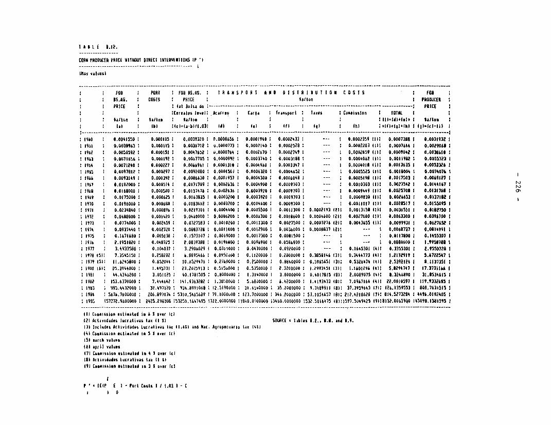
I A BLEf 3.12.

CORN PRODUtCER PRICE VII11OU1 DIRECt INIERVillIONS IP 'I

* 2 ~~~FOB FORT FOB IS.AS. T R A N SPORT AN9D 0 5I I ISIR II BUT 101 O T S FOB 20* 2 I~~~S.AS. 2 COS1S PRICE la/~ton I PRODUCER I

i PRICE li2(t olsa di ----------------------------------------- …-------… PRICE ICre litiIveI AEarimo 2 Caroa Tran6port Tae Caiiln OAL. I

2 2 lal 2 ~~~ ~ ~~(bi HcIzIA-blI.032 Udi 2 11Il 2 Il1 (I:vfgo j~c-a

I0 0.0041550 2 0.000105 0.0039320 20.0000656 0.0001940 0.0002433 -- 0.0002359 III: 0,0007388 I 0.003193222 1963 ~0.0030963 0.000115 2 0.0036712 U.0000773 0.0002140 0.0002529 - 0.000?203 (lIlt 0.0007644 2 0.0029063

1962 0.0050592 0.000151 0.004765e 0.0000764 0.0002670 0.0002749 *- 2 0.0002859 fill, 0.0009042 I 0.00396102 1963 0.007ilS165 0.000192 1, 0.0067705 I0.0000992 0.0003740 0.0003188 --- 0.0004062 I11- 0.0011982 2. 0.0055723 I;1954 0.00712402 0.000227 2 .00669612 0.0001310 0.0004960 0.0003347 2 - 0.0004018 (111 0.0013635 I 0.005332& 12 19615 2 0.0097012 : .000297 2 0.0092080 2 .00015Oi 0.0006320 2 0.0004652 2II- 0.0005525 lit., 0.0011004 2 0.0074074 1966 2 0.0093149 0.000392 2 0.0086630 20.0001957 2 0.0004300 2 0.0006049 1 - 0.0005190 (1112 0.00175503 I 0.0069(27 I219S7 2 0.0102000 2 0.000514 0.0171709 0.0002636 0.0004900 2 0.0009703 -- .000 (( .074 .0144147 I1969 0.0140000 21 0.0005800 0.0157476 20.0102636 2 0.0003920 I 0.0009703 2 - 0.0009449 Ill: 0.0025708 1 0.0131761 I2 1969 2 0.0175000 2 0.000625 I 0.0163835 2 0.0003?00 1 0.0003910 2 0.0009703 - 0.0009830 Ill.' 0.0026653 2 0.0137112 I1970 2 0.0196000 2 0.000600 0.01936112 0.0003200 2 0.0004600 2 0.0009700 2-- 2 0.0011017 (Ill 0.00?8517 I 0.0155095 I19711 0.0234840 2 0.000896 2 0.0219:301 20.0004400 2 0.0005500 1 0.0011300 0.0002193 ffl1 0.0013158 fill 0.0036551 1 0.0192750 I21972 2 0.04880000 0.001420 2 0.0460000 0.0006200 2 0.00011300 2' 0.0019600 20.0004600 (212 0.0027600 (1', 0.0063300 I 0.0396700 121973 2 0.0774000 2 0.002459 2 0.0727583 20.0010200 2 0.0011300 0.0027500 20.0007276 (2)2 0.0043655 Ill2 0.0099931 I 0.0627652 22 1974 2 ~0.0937440 2 0.002720 2 0.0983719 0.0011000 I 0.0012900 2 0.0036000 2 .0000837 (211, --- 2 00087I 00849 1

1975 2 0.1671690 2 0.005138 2 0.1573107 20.0019000 2 0.0017300 2 0.0091500 2 - - 2 0.0117800 2 0.1455307 I2 1936 2 .1951920 2 0.048725 2 .0839390 0.01968000 0.0096900 2 0.0596900 2 - 2-- 2 0.0880600 2 1.9958798 21977 2 3.§933580 2 0.104037 2 3.2906029 I 0.036'iOOO 0.0430000 2 0.0920000 2 - 0.1645301 1411 0.3355301 I 2.95507?9 I21917 1512 7.3545150 2 0.2502022 6.9095466 20.0950000 2 0.1120000 2 0.28000000 0.3859146 (3)2 0.3444773 (4112 1.2172919 2 5.4722547 121979 (512 11.614581002 0.65210442 10.6529476 O .2)600002 0.2500000 0.98400002 0.5965651 131: 0.5326474 (101 2.5392124 1 8111373511 21990 (141 25.3944000 2 1.495731 2 23.2025913 20.515100002 0.5350000 2 2.3200000 21.2993451 1312 1A1,01294 1412 5.8294747 I 17.3731164 I1991 2. 44.4345200 2 3.051125 2 40.1791505 20.8000000 2 1.3140000 2 3.80000000 0.4017815 18(2 ?.0099075 1412 0.3246890 I 31.853465 1219022 153.63700002 7.4446422 14L.934322 1 .30',0000 2 .6000000 2 .4200000 2 1.193633 1812 7.0967164 (tit 22.0010597 I 119.9332685 I21993 2 995.4432000 2. 32.4971?02 934.9991069 2 12.51300002 31.hS400002 35.2090000 9.3489911 (812 37.3959643 1712 12i.J3595531 2 808.7631515 21994 25676.7600000 2 206.897034 25310.5A65689 2 79.1000100 2123.7000000 2346.2000000 253.1054657 1912 ?12.4219629 Ill: 814.5273294 2 4496.0192405221995 2572.72.9600000 2 425.290309 25101679 722.0000000 2l840.0C500000 2*3460.0000000 2,532.5016475 18121597.5049%25 19128152.0065900 145098.1581595 2

III cfhwfisian estimated in 6 I over (c)(2I Aciividad*6 lucratjva. tax (I 11 SOURICE a liblms B.2., 3.9. ari4 1,9.(31 Includes Ackivididvi Lucrativao tax (11611 and Mac. Aqropec.iauio tax 4411141 Commiss ion estiated iR 51 I ver Id)(5I marhb valvosa(63 april valiaes171 Commnission estimated inl 4 I over (c)(9) Actividades l.ucrativas tat I 11 %

93CoemiLooon lfitimated in 3 1 over (cd

IP (lip E Part Costsi I1I1.03 I - C

i 0

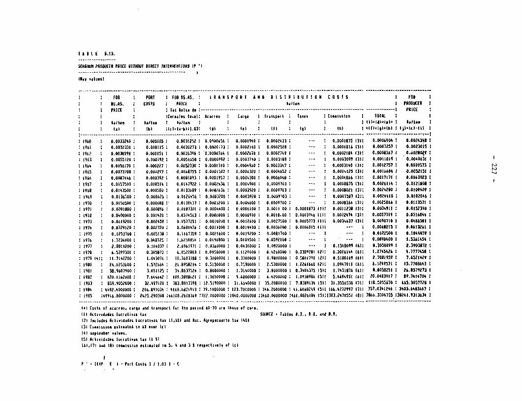
T A B L E 8.13.

SO0R613U PRODUCER PRICE WilTOUT DIRECI INFERVE(IIONS (P 'I_~~~ I

("AV vilues)

: ' FOB PORT FOB IS.AS. I R A N S P O R I A N D D S I R I U I I O N C o S I s I FOE : : .AS. : COSTS PRICE : Olaon : PRODUCER IPRICE (at olBa de :---------------------------------------P---------------------------------- ------------- I PRICE

: : : ICorealo level: Acarreao c: qa I Tronsport Txtes Cassis6lon I OITAL I: : $Saltou Salton : SAo,In : : I ll)lI Iu). I alton I: : 1a) (bi hlc) (a-b)iI.G3: id) (: lt (f) : (q (hi I *(fl*(gl4(hl I jli)c-(il :--------- -~~~-------------------- I ~-------- --~--I -~~-------------~-~-~------------ ----- ~---~--------------------~-------------------- ---- ~-----------*-------r-3960 : 0.0033240 : 0.000105 0.0031252: 0.0006,56 0.000(940 0.0002433 -- : 0.000(175 13): 0.0006904: 0.00243i8 I

1:W : 0.0032331: 0.000115 0.003C2713 0.0000 73 0.0002140 0.0002528: --- : 0.000(113l (3) 0.0001257 0.0023015 119: 2 0.0038999 i 0.000151 1 0.0036396: 0;0004764 1 0.0002670 0.0002749 I --- : 0.0002134 (311 0.0008367 e.4o28049

1963 : 0.0055120 1 O.OOOI92 0.0051650 0.00009O2 2 0.0003740 0.00031398 --- : 0.0003099 (3)l O.0O0ilo9 1 0.0040631 1

:197ab : 0.0056170 0.0002?7 o0.0052330 0.0001310 2 0.4000960 0.0003307: --- 0.0003140 131: 0.0012757 1 0.00395731:I65 : 0.0073788 0.0002-7 a0.00607S1 0.0001507: 0.0006320 0.0004652 --- 0.0004(25 (31: 0.0036604 1 0.0052(51 1

:9466 0.0087446 0.000392 0.0081093 I 0.0001957 0.0004300 0.0006048 2 --- 0o.ooo0 96 (31: 0.0017171 o0.0063923

: l%7 0 .0Tszso00 0.0005s^ 0.0147922: 0.OOO b36: 0.0009000 0.OOOS703: -- I .ooosa7s 131: 0.002611.: 0.012l1608 1

: 1967 : 0.01(5500: 0.0005o s 0.0134792 0.000.63:6 0.0003Y2 0.0009703 2 --- : 0.0008721 13)1 0.00242a1 0.0109809 I

1968 0.0131300 0.00065: 0.032689b 0.0003200 0.0003920 0.0009703 --- : 0.0007857 13)1 0.0024410 0.0102040

1970 : 0.0136500 0.000625: 0.0132437 0.0003200 0 o.ooo000 0 0.0009700 --- : 0.0008378 331.: 0.0025440 1 0.0113571

1971 0.0201890 2 0.o000896 o0.0187,1 0.0004400 0.0006300 1 0.003.00 0.00013873 1131 0.0011238 1331: 0.0034911 : 0.0152390 I

1 1972 : 0.0400000 0.001420: 0.0374563 200001000 0.0006900 1 0.001O,00 0.0003o46 (ll. 0.0022474 (311 0.0057711 1 0.0316844 :

19I73 0.0619200: 0.002.59: 0.0577391 0.0010200: 0.0012bOO0 0.0021t0o: 0,0005773 11H: 0.003s637 (31: 0.0090710 1 oo.0a8u531 1

: 1974 0.0729120 0 .0027202 0.0b847b6 2 0.003000 0 000100 0.0036000 0.0006835 11)l --- : 0.0068215 1 0.0613261 1

1975 0.1253760 0.005139: 0.1367359 10.OO1600 o0.0039200 1 0.0081700: --- t --- : 0.0322500 1 0.1044859 1

:1976 1 .7234900 0.0ia72s: 1.625Yd.i: 0.0IYb"OO: 0.0104500: 0.05,12lo: - I-0 0.08-7s*00 1 1.5361S54 :; 3977 : 2.0883200 0.104037 2.6961971 0.0360000 0.0430000 0.0920000: -- : 0.1334099 (61: 0.3058099 1 2.3903872I

: (970 6.5397300 0.305873: 6.0522883 0.0950000 o 0.3120000 0.4260000 0.3389281 (23: 0.3026144 (631 1.2745426 i 4.7777458

: I9 (4): 11.7142,100: 1.043011: 10.3603390: 0.3000000: 0.3300000: 0.98l00000: 0. S0179o (21. 0.51aol6s j61:. 2.30s0s95 7.02elles

:980 24.1253600 1.5726&4 21.8952314 1 0.5150000: 0.7590000: 2.5300000 1.2261660 12): 1.0947911 (631 6.1249571 15.7708643 1

1981 : 3a.9607900 3.0511252 34.1637524 0.d000000 1.3140000 3.8000000 1 0.348637 155: 1.7431876 16(1 8.0051251 I 26.8579273 1

: 1al : 20.116?000: 7.Wi6i2: 10138qobel: 1.3d50000; 5.bdOOOOO: 6.200000: 1.0938986 (Sit 5.4b6iS31 (61: 20.0s839'1: 89.3414704 1

(983 : 839.9052000 32.97120 1 783.89(3390 12.5190000: 31.6640000: 35.2000000 7.8381334 (5(: 31.3556536 373: 1B.d5855670 i 6s.3057728 s

: Is84 4492.4000000 2206.97034 i 4160,66bd13 79.1000000 123.70C000OO 346.2000000: 41.6068249 (5(l 166.4272997 1711 757.0341246 : 3JO3.6483667 :

13985 :4991ii8000000 2425.29030a 246108.2618369 :722 0000000 :1840.0000000 :3460.0000000 :461.0826184 151338]3.2478551 l8(: 7866.3304735 38241.9313634 :

(a) Costs of acarroo, carqA and trfrnport for the period 60-70 are those of Coro.111 Actividadeo lucrativac tax SOIUCE fabIes 8.3., B.8. a*d l.9.(21 Includ*6 Actividadoe tucrativari tax (11611 and Mac. Aqropecuario tie (4I1(3) CDomission tstisated In 61 over (cl(4I *epletaer values.(IS Actividades lucrativas ta (1 tl161.173 arnd (81 cosmlwon tstutated in 5, 4 arid 3 1 respoctivoly of tci

P ((IP E I - Port Costs I I 1.03 1 - C

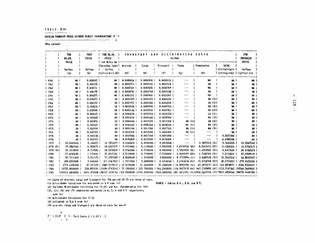
ITABL E 8.14.

SUIBEAM PRODUEER PRICE VIlIHONI DIRECI 1MlfRVEN110MS I? '

(Play values$

* hID 1~~to PONT :FOBIS.AS,1 I RAMS POR I AMO D BI STI 8IAUTIOIM CO0STIS , FOB I* R~~~~S.AS. I costs -PRICE . a t a' PRODUCER

I PRICE 1(at 801S.4dt --------------------------------------- …-- - PRICE :Cer#4l0i level: Acai'ren raol an6port Tae 'mis OTAL I

* Ia~~~1./tArl 1 tai/in I lit/on I ,IlllWd)*(uI. I tlo (Ai (bi :lcI;aA-bl;I.03: (d) : 1. : f' 191 I h0 o (fmomlnbi I).c-)

19o0 MA IA 0.000)05: NA I .00oo0so 0.0001940 0.00024331 -- IMA I MA I MAI196)1 MAI 0.0001151 MA 0.00007731 0.0002140: 0.0002521 MA- KA I M)mA1902 MA 0.000151 N A 0.00300764 0.0002670 0.0002741 I --- NA IMA I NA 1963 N A 0.000192 i A 0.00009921 0.00037401 0.0003188 I- NA IMA 1.NA I1964 MA: 0.000227 MA: 0.o01310 0.0004960 0.0003347 1 -- A NtA I MA I 1905 MA 0.000297 1 A 0.0001507 0.00006320 0.0004052 I - MA (3)1 M NA : .l"1900 N A 0.000392 NA 0.0001957 0.0004300 0.0000048 1 - A (3)1 MA I NA I '1907 1 MA i 0.0005)9 i A I 0.00Qh301b 0.0004900 I 0.0009703 )- NA 13)1. MA I MA I 0i19o NA 0 .ooosoo MA I0.0002636 0.0003920 1 0.0009703 : - INA (311 KA I NAII1909 : NA 0. 000025 1NA 0.0003200 0.0003920 0.0009703 t - ~ A (31: KA BAI1970 IMA 0.000000 MA 0.0003200 0.0004000 0.0009700 - I NA (3): NA N A1971 N A 0.000090 NAo I0.000§400 : 0.0005500 : 0.0011300 I MA (III NA 131: MA M A1972 MA 0.001420 1NA :0.0006200 0.0006300 : 0.0018600 1 NA (111 NA 1311' MA I NAI1973 1NA 0.002959 NA 0.Ooio0oo 0.0011300 1 0.0027500 MA III! NA 131: MA ! NA

Wk i N~~~A 0.002720 1 A 0.0010300 1 0.00126000 0.00%0300 NA 11W1 --- M A I NA 1975 N A: 0.005138: NA: 0.0019000: 0.0017300: 0.0091000: - I- 0.0127300 : NA:1970 MA : 0.040725 1NA 0.0196000 0.0114900 : 0.0478000 : -- -- 1 0.0700500 I MA1973 : 12.24976000 0.104037 11.7071097 0.03600000 0.0430000 0.09e000o --- I 0.5893555 IS)? 0.7603555 1 11.0207542 1978 19i1 19.30837600 0.305073 10.5207019 10.01150000 0.1120000 : 0.2000000 1 .0374953 181: O.I20351 Wi1 2.9508304 1&.0750715 (979 h9i1. 30.1210000 I 0.759500 1 28.5070039 : 0.27040000 0.2500000 0.0040000 : 1.5163922 1Wl 1.425350? Oil1 4.4317424 1 24.0752615 11900 37.0203000 1.572664: 35.00553101 0.5150000 0.7590000: 2.5300000 1.9003097 lOll 1.7502705 (S)i 7.5145062 1 27.4909439 1901 1 2.7514300 1 3.051125 77.3709J09 :0.80000000 1.3140000 : .80000000 0.7737899 191 3.8009960 (51 (0.556730 1, 60.8222007 I1902 : 320.2245000 1 7.444642 311.9367553 11.335,0000 1 .6800000 6 .4200000 :3.1143670 (411 15.5719370 (511 32.1712053 1 279.2055500 I1963 : 1773.1332000: 32.497120 :1689.9379417 12.5190000 31.6640000 35.2080000 IS10.993794 19) 07,5975177 1611 163.8878971 1 1520.0500447 1I1909 12?52.0000000 200.897039 :11694.2747243 79.1000000 1123.7000000 :346.2000000 :1114.9927972 (911 467.7709090 161: 1133.7137362 I1056O.5609881 190, :103511.08000000 2425.290308 191215 :40 22.0000000 :1740.0000000 :3W0.0000000 :981.4212591 l§4l1`949.2b]777k 171: 9847.6850340 188294.9400780I

(el Cosit of acarigo, carcla and tranoport for the poniod 60073 a(* thoit of coin.(II Aclividadol. 1ucrAtinA% IAn gLitmoAild in I I ~ver IC) SOURCE *TAbIiL 8.9.. 8.8. And 8.9.2I?In lnlde6 kctividades Lucrativao tan 11,61) and Mac. Agropecuarac tam 1401(31, 151, 101 and (7) romamlnlon estimated in 0, J, 4 ankd 3 1 'seopoctvely

over It)141 Aclividadrs IuErativas tax It 1I0)1 Estiatod Jn 5,0 1 overF (I191 an atort, cargA and tranopoit are thoss, cf corn for earth

N

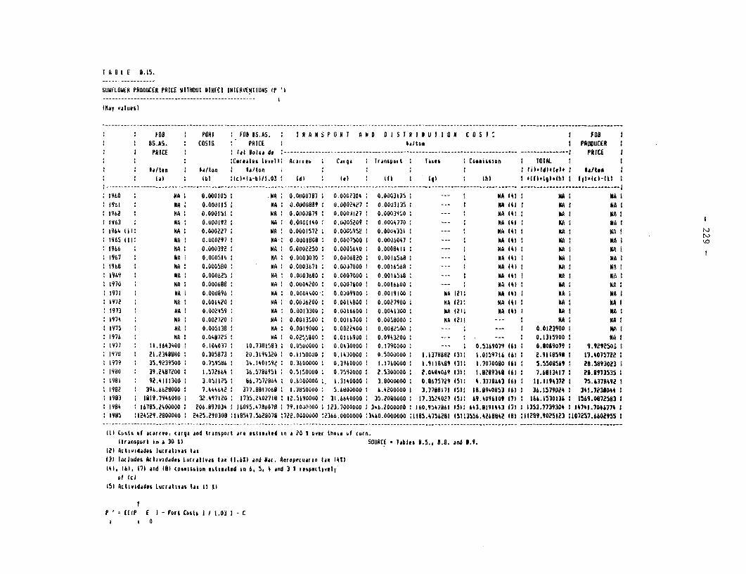
I A BIE 6.15.

SUNFELOWER PRODUCER PRICE W(ITHOUT DIRECTI (HEROEHi(oNs (P 11

(lmay valuesl

* 2 FOB P~~~ ~ ~~~~ORT FOB BS.AS. R A M POR 0 I A ID D I S IR I I U Il 01 LO S I FOR* 2 ~~~BS.AS. COSTS 2 PRICE I $Altoia PRODUCER I* ~~~~~PRICE fat plo(ode -------------------------------------- ------------……… PRICE I

* * , 2~~~~~~~~~~~~CoroaaLei level) Acarr,,. CJIQI frariopoit Taxes 2Caaoe I TOTAL 2I

* 2 taO (Dl 2Id(~~~~~~~~Ia-bl/I.03 (dO 2 0.) ((0~~~~~~tt I III 2. lb) I ff*(t(.(ql.(h I Il(-IEI-(il 21

(960 N A 0.000(05 H A 0.0000187 0.0002304 0.0003135 2 --- H. A (40 NA A 1. fist NA: 0.000115 i A 0.0000869 0.0002427 0.0003135 - I NA (41 N A I NA0I1962 I NA 0.000151 NAl 0.0000879 0.000.117 0.0003(510 N- A (41 NA I W

2 1963 2 BA ~~~~~0.00092% NA :0.0001140 2 0.0005209 0.0004770 -- :B 4 AB

964 (((2 HA ~~~~0.000227 NA i0.0001572 2 0.0005,952 0.0004350 - A(0I AB .(965 (II: NA 2 0.60002971 NV: 0.0001008 0.0002500 1 0.o005047 -- H (41 2 NA K A I(966 N A 2 0.000392 N A 20.0002250 2 0.0005640 0.0008411 N - A (40 i KA 8 KA I21967 N A 2 0.0005(42 KA 0.0003030 0.0006820 0.0016568 N- A (40 : NA2 NA I(968 NA 2 0.0005800N 0.0003671 0.0037000 I 0.0016560 N- A (40 NAI N A I21969 NA2 0.0006252 IA00060 .0702 00(58 - KA (40 2AI NAS A2

2 1970 N A I 0.0006B02 NA 0.0004200 0.0007400 0.00166002 N- A (4012 NA I NA21 971 N A 2 0.000896 NA 20.00040002 0.0009900 2 0.0019(00 2 NA (2)2 HA 141 N A I MA21 072 N A 2 0.001420 :NA 20.0036200 2 0.00(4600 2 .0027900 1 MA (2(2 NA 141 M A 2. NA I(913 N A 2 0.002459 M A 2.0.0013300 2 0.00(6600 2 0,004(300 K A (2(2 NA (4) 2 I I NA I21974 N A 2 0.002120 N A 20.00135,00 2 0.0016700 2 0.0058000 HA 1212 --- 2 H MA I2 975 N A 2 0.005(302 MA 0.00(90002 0,00224002 0.00025,00 2- -- 2 0.01239002 HA 21 976 N A 2 0.008725 MA 20.02t55800 2 0.0116900 2 0.0943200 2- - 2 0.13(5900 2 B I1 971 11(.16434000 0,10h037 1 0.738(5893 2 0.0500000 2 0.0430000 2 0(1790000 2-- 2 0.5369079 (61 0.8039079 2 .929250121978 2 2.23408602 0.3058732 20.3(043202 0.1(500002 0.14300002 0.5000000 1,(1379882 (3(2. 1.0(597(6 (612 2.(118591 1 17.407572222 (79 2 35.9239500 2 0.759586 2 34.l401594 0.3600000 2 0.3960000 2 .1760000 2 1.91(0489 (3(2 (.7070080 (60l 2 5.5508156 2 28.5893023 22 9600 39.2487200 1 .572664 2 36.5786951 20.5(50000 2 0.7590000 2I 2.5300000 2 2.0484069 (3(2 (.8289348 (6) 2 .68(3417 2 28.3973535 11 98) 92.4(10(00 2 3.0tiII25 2 6.7572064 2 0.6300000 2. 1.3140000 2 3.8000000 2 0.0675729 (5(2 4.3378&43 (61 1 1.1194372 I 75.637849? 2

2 (982 2 39h.6628000 2 7.4446422 377.0817068 1 .3850000 2 5A6800000 6.4200000 I 3.7708171 (5)2 18.0940853 (6) 2 3b.2579024 2 341.7238044 22 (963 21(19.79460002 32.497120 1 735.24027(10 12.5110000 31.66400002 35.2080000 1 7.35.2027 (5(2 69.4096(09l (70 I2 16.530134 1(569.0872583 I

1 9804 16785.2000000 2 206.8970342 16095.4786076 2 79.1000000 1 23.7000000 346.20000002 160.9547861 15)2 1,43.8191443 17) 1 353.77393D4 I 14741.7046774 I1 985 2(24529.28100000 2 2425.290308 2(08547.5628078 27?2.000000,0 22366.0000000 23460.0000000 2(115.4756281 (5(23556.4268642 (80 :11289.9025123 .107257.66029552

((0 Ca,ote of ocarreo, cafqa and trrainpo,t Are sitisated an &20 1 ever these o-f coira.((ranspoi,i in a 30 1) SOURCE *Tables 5.5., 18.8. and 3.8.

(20 ActavidadlL lucrat(vis tam13) Includes ALlavidad&o I-uarAI(vaD tam (1,61) and Nit. Aaaopepouarae (ax (4t)(40, (61, I7l alad (81 comoaciioaict eo(ated in 6, 5. 4 ankd 3 0 respectively

of Ic)(50 Actavidadnoi Lucrativas (ax II 00

P (lip I I - fort CostsI 111.03 1 - C

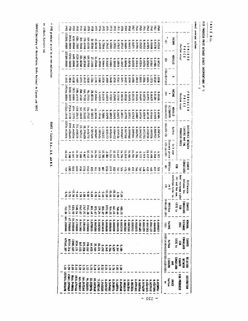
a, - - -~~~~~ - - - - --

0 - 4 4 -= - -C - --

0 - 4………4~~~~~~~~~~~~~~~ - - -- -- -- -

- .* I ~.tO. . . .= .c.c ..c . o . oo oo.t o- 0 .e4.- 4

- 4 ~ ~ ~ -- - -~ -' - - - a 40 - . - -0 0 4- 4 -v

an - -4 0 4 =- - -- - - --

- - 4 - 04 IC Cc~ cl 1 c c

ooOoeOeOoOtrrU--uI el a ~-e "I LAC0 II - = - I CCX -~~~~~~Cm --

- - 4* 4 4 -~~~~~-oc

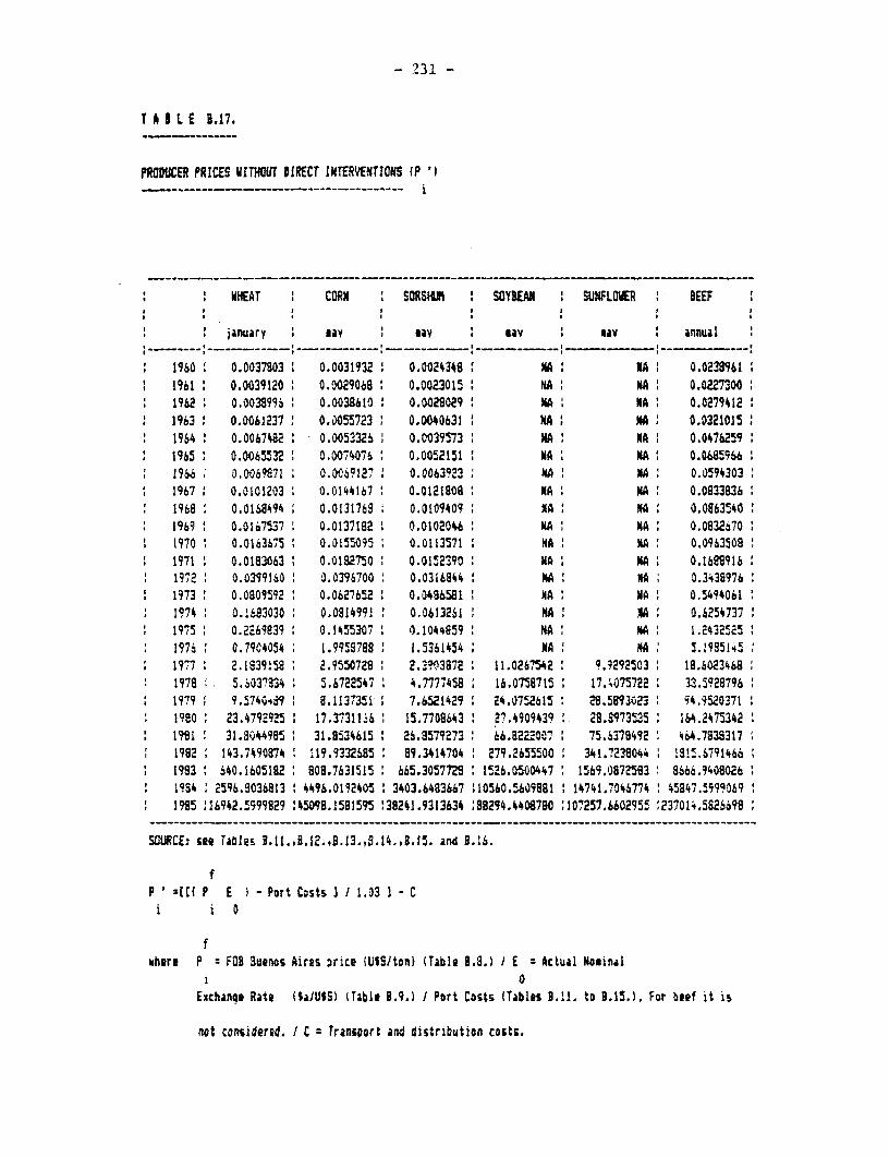
- 231 -

T A I L E 8.17.

PRODUCER PRICES wiTHOUT DIRECT INTERVENTIONS (P

WHEAT CORN SORSI SOYBEAN SUNFLOWER BEEF

' anuary sa' ' : ay lay annual

1960 0.0037803: 0.0031932 0.0024348 MA IA 0.02389611961 0.0039120 0.00 ^ 9068 0.0023015 NA MA 0.02273001962 0.0038996 0.0038610 0.0028029 NA NA ' 0.02794121963 0.0061237 0.0055723 0.0040b31 MA NA 0.03210151964 0.0067482 - 0.0053325 0.0039573 MA M NA 0.04762591965 0.0065532 0.007,076 0.0052151 NA MA 0.0M596619S6 0.0069871 0.0069127 0.0063923 MA MA 0.05943031967 0.0101203 0.0144167 0.0121808 NA MA 0.08338361968 0.0168494 0.0131768 0.0109409 NA NA 0.0863S401969 0.0167537 0.0137192 0.0102046 KA NA 0.08326701970 0.016375 0.0155095 0.0113571 : NA A 0.09635081971 0.0183063 0.0182750 0.0152390 N A I 0.168'9161972 0.03991So 0.0396700 0.0316844 NA *A : 0.34399761973 0.0809592 0.0627652 1 0.0486581 MA NA 0.54940611974 0.1683030 o.DS1499r 0.0613261 MA MA 0.62547371975 0.2269839: 0.1455307 0.1044859 NA NA 1.24325251976 0.7904054 1.9958788 1.5361454 NA I N 1.1985!451?77 2.1839158 2.9550729 2.3903872 11.0267542I 9.9292503 18.60234681978 5.6037934 5.6722547 4.7777458 1 16.07715 17.;075722 33.59287961979 1 .57409 : 8.11377351 7.652429 24.0752615 29.5893023 : 94.95203711980 23.4792925 ' 17.37311J6 A 15.7708643 ' 27.4909439 : 28.8973535 ' 164.247534219M1 1 31.8044985 ' 31.9534615 26.8579273 ' 66.8222007 : 75.6378492 464.78383171992 1 143.7490874 119.9332685 : 89.3414704 2 279.2655500 : 341.7238044 M135.67914661983 1 640.1605182 809.7631515 f6b5.3057729 11526. 0500447 1569.0872583: 866c.940802619S4 2596.8036813 : 4496.0192405 3403.6483667 '10560.5609881 : 14741.7046774 ' 45847.59990691985 '16942.5999829 :45098.1581595 :38241.9313634 :88294.4408780 '10'257.6602955 1237014.5826698

SOURCE: see Tables 3.11.,B.12..B.13.,B.14.,8.15. and 8.16.

fP' SfM P E )-Prt Costs 3 1.03 1 - C

ii 0

where P FOB aUeros Aires orice (USS/ton) (Table 9.8.) / E z Actual Nominali 0Exchanqe Rate tIaiUSS) (Table 3.9.) 1 Port Costs (Tables 9.11. to 8.15.). For beef it is

not considered. I C = Transport and distribution costs.

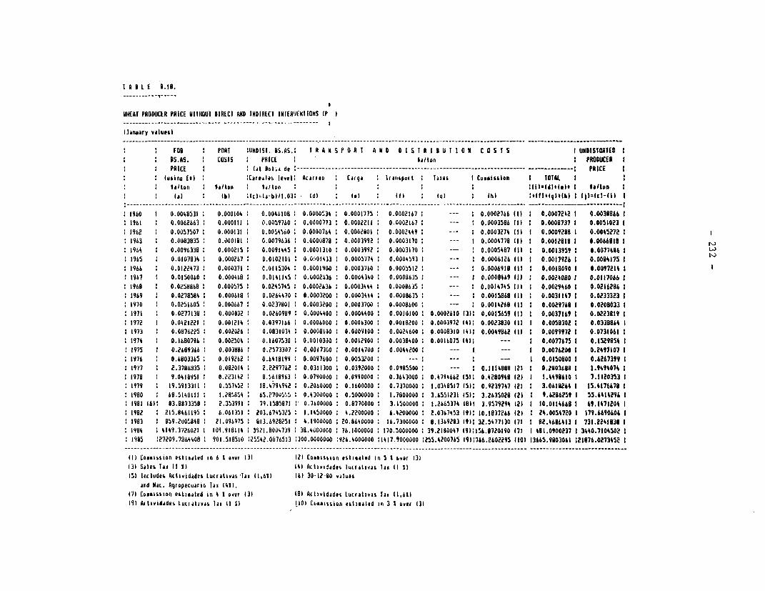
I A B E 1.18.

WHEAT PRODUCER PRICE WITHOUT DIRECT A)ID INDIRECT I1AIER1E9TIONS (P

lianuarY VAIueel

: : FOB PORT UNDISI. BS.AS.: T R A k S P 0 R T A h D 01ST R I I U T I 0 B C 0 S T s I UADISTORTED IMM SA5. COSIS P PAICE :I/lou : PRODUCER I

: : PRICE fat lol;a de :------------------------------------------------- - --------------------- -…------ : PRICE Itusino Eel: C*,eale ievel: Acart.o Caiga : raniport Taio IConicelon I TOTAL I:

laiton la/ton 11/ton laltlondltI. I talo* : l : {b) Ic)-l~-bl-/t.03: (d)l : 1. 1 : f) : I : hI 1*It)o11)*(hl 1 Il))hIc-(l)

…---.--- … - - … ----- I~~~~~~~~~~~~~~~~~~~~~~~~~~~-- --- ___ _ _ __ ____

1960 0.0048531 0.000104 : 0.0046108 0.0000534 0.0001775 0.0002147 : --- : 0.0002766 (Il: 0.0007242 1 0.0039846 11961 1 0.0062663 0.000111 0.0059740 0.0000771 0.0002211 0.0002167: --- : 0.0003596 (I) 0.0008737 1 0.0051023 t196: 0.0057507 0.000131 0.00oo41sao 0.00007oo : 0.0002801 0.0002i 1 --k : 0.0003274 (1I I 0.00092f8 1 0.00o527 : I19:3 : 0.0083835 0.000101 0.0079S36 10.0000878 0.0003992 0.0003170 --- 0.0004779 (I) : 0.0012811 1 0.006818 Ir:9L4 0.0096330 0.000215 0.0011%45 0.0001310: 0.00039912 0.0003170: -- : 0.0005487 (II : 0.0013959 I 0.0077446 I:1l965 : 0.01 i07834: 0.0006126 111 0.0017926 1 0.0094175 I196: 0.0122473 0.000371 e 0.0115304 0.0001900 0.0003760 0.0005512: --- 0.0006918 ttl 0.0018090 I 0.0097214 I:1Is47 : 0.0150000 0.0004681 0.0141145 0.(00263&: 0.0004340 0.000063s: --- I 0.0008669 tII) 0.0024090 t 0.011704 t196: 1 0.0250040 0.000575 0.0245745 0.0002636: 0.000344t 0.0000635 1 --- : 0.0014745 (1) 0.0029460 I 0.02162961969 : 0.0278584 0.000619 0.0244170 0.0003200 0.0034§4 0.0000835 --- 01.001506 )II 1 0.0031147 I 0.0233323 11970 0.0251605 0.000667 0.0237801 0.0003200 0.0003700: 0.0000.600 --- : 0.0014268 III 0.0029749 t 0.0208033 t1971 : 0.0277138 0.000032 0.0260999 0.0004400 0.0004400 0.0010100 0.0002410 13): 0.0015459 (I) 1 0.00371t9 I 0.0223819 t1 1972 1 0.0420221 0.001214 0.0397166 10.0006000 0.0006300: 0.0018200 0.0003972 (4): 0.0023930 (1 I 0.0058302 1 0.0338864 I

I 1973 0.0874225 0.002026 0.083103k: 0.0008100 0.0009100 0.0024400 0.0008310 14' 0.0049862 III : 0.0099972 1 0.0731061 1: 1974 : 0.1600796 0.002504: 0.1607530 0.0010300 0.0012S00 0.0038400 0.0016075 I4): --- : 0.0077675 1 0.1529954 t1975 : 0.2689344 0.003884: 0.2573307 0.00173C0O 0.0014700 0.004200 : --- I --- I 0.0076200 t 0.2497107 11976 : 0.6803365 0.01922 o0.6410199 0.0097600 0.0053200: --- : -- : --- 1 0.0150900 1 0.4247399 1

: 1917 7 2.3786535 0.082014 2.2297762 0.0311300 0.0392000: 0.0985500 -- : 0.1114888 121 : 0.2903688 1 1.9494074 1: 197 9.0418951 0.223142 1 0.561993 0.0790000: 0.0990000 0.3643000 0.4714662 (51: 0.4280949 12) I 1.4498610 1 7.1120353 11979 : 19.5913311 0.557452 10.4094942 0.20S0000 0.1600000 1 0.7370000: 1.0348517 (5): 0.9239747 121 : 3.0418264 I 15.4176478 I1900 6:1.5140111 1.28a a-54 65.270055 1J 0.4300000: 0.5000000: 1.78000000 3.6551231 1511 3.2635028 (2) I 9.6286259 I 55.6414294 I1981 1611 83.8873350 2.353991 79.1585871 0.7600000 0.8770000: 3.1500000 1.2665314 IO)t 3.9579294 121 : 10.0114668 I 69.1471204 t1902 : 215.8461195 1 6.061351 203.6745325 1.1450000 4.2200000 6.4200000 2.0367453 19): 10.1837266 121 : 24.0054720 1 179.4690606 I1 1903 859,20050840 21.090975 913.6928251 4.1900000 1 20.8640000 16.7300000 8.1t39203 191s1 32.5477130 7)1 1 92.4616413 1 731.2241838 I

: 1904 414:.3726021: 109.918114 3921.8004739 38.i00000o 74.1000000 1 70.5000000: 39.2180047 191:156.1720190 171 1481.0900237 I 3440.7104502 119: 5 :27209.7864408 901.518560 :25542.0076513 :300.0000000 :9?2.4000000 11417.1000000 :255.4200745 111:766.2602295 1101 I3665.9803061 121876.0273452I

1I) CDOOiSSion efitiatld in 6 I owe, 131 121 CoaIssilOn ,itlOAled In 5 I over 131(3) Salve TAh (I 1) 141 Actlvkd.doi iucallwai Tax 11 1)151 Includes AEtividades Iu(rativos lax 11,49) (6) 30-12-80 value&

ar,d Mac. Agropecuario liv 141).17) CoDsienjon estiated in 4 9 over 13) (0I Aclivldad.s Lucratlivs tax 11,41)19) Actlivdades Lu.Crlivds tax (I 11 1101 CLOaiSSojOn aillealed In 3 I over 131

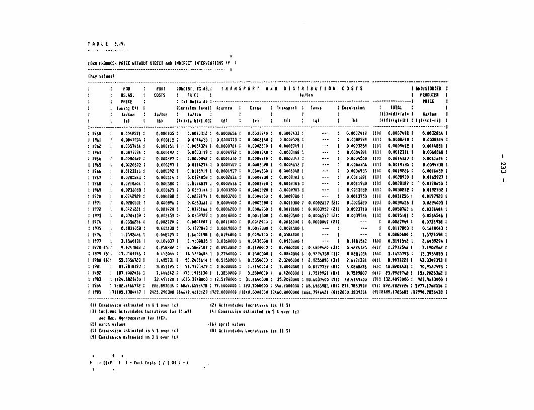
T A I L E 5.19.

CORN PRODUCER PRICE iITHOUl DIRECT aND INDIRECT INIERVENrIONS (P I- I

(hay vIlueti

: : fOFOB PORT :UNDISI. BS.AS.: f R A K 5 P O R I A O O I S r R I tl U I I O k C O S r S I UWDISTORIED: : BS.AS, : COSTS : PRICE Salton I PRODUCER I: : PRICE :C fat Blsa d ---------------------------------------------------------------------- -----------------…I PRICE I

: : lu qing Eel :CereAleS lvlV: ALarre : Carga : Iran lport Taxhes : Coasiein TOTAL I: : la/tar, : 0,/tan : Iala/t , : : : )=lduh. I lle. I: : (at : (bl Slc) 1a-6(II.03: 142 : Irl : Il (f (4) : (hi :I(fiegqlu(hI I (IslBci-li) I

1960 0.0042571 0.000105 0.0040312 0.00006o56 0.0001940 0.0002433: --- 0.0002429 Ill.1 0.0007448 1 0.00328?64 : 1961 : 0.0049204 0.000115 0.0046655 0o0000773 0.0002140 0.0002520 : --- : 0.00027ss (III 0.0008240: 0.003841 21962 0.00574M 1 0.000151: 0.0o0s4324 o0.0000o764 0.0002670 0.0002749 I --- 0.0003259 (1I: 0.00094%2 1 0.0044981 11963 0.0077294 o.ooo012: 0.00717 I0.0000092: 0,0003740: 0.0003188 : --- : 0.0004311 (1U: 0.0012311: 0.0060868 I1964 0.00803a7 0.000227 1 0.0075842 o0.0001310 0.00040o60 0.0003347 1 --- I 0.0004550 fill 0.0014167 1 0.0061674 I1 1965 0.0120672 0.000297 0.0114274 2 0.0001507 0.0006320 I 0.0004652 2 --- 0.0006856 1(ll 0.0019335 I 0.0094938 I1966 : 0.0123316 0.000392 0.0115919 I 0.0001957 0.0004300 0.000604i: --- : 0.0006955 (Ill 0.0019260 1 0.009665S 2:19S67 0.020 3: 0.0005(4 2 0.0194050 2 0.0002636 0.0004900 0.00097032 --- 2 0.0021692 ((22 0.ooe8s30 2 0.0265927 2196: 0.02(06o04 0.0005oo 0.0(9s839 0.0002b36 0.0003920: 0.0009703 --- : 0.0011930 1llt 0.0028189 1 0.0170650 1969 0.0236080 0.000625 0.0223144 10.0003200: 0.0003920 0.0009703 --- 0.001339 (111: 0.00302122 0.0192132 11 1970 : 0.0242929 0.000I8 1 0.0229174: 0.0003200: 0.0004600: 0.0009700: --- 2 0.0013750 101) 0.00312502 0.0197923 11971 : 0.025053 1 0.000896: 0.0263S6(1 0.0004400 0.000500 o 0.0011300 1 0.0002637 2MI 0.0015820 dIll 0.0039656 1 0.0224005 11972 : 0.0421221 0.001420 1 0.0395166 0.0006200 I 0.0006300 0.0018600 0 0.0003952 (222 0.0023710 (III 0.0058762 1 0.0336404 I1973 I 0.0704109: 0.002459 :- 0.0659727 0.0010200 0.0011300: 0.0027500 0.0006597 121: 0.0039504 1111 0.009561 1 0.0564546 11:74 0.0056254 0.002720 0.D504907 1 0.0011000 0.0012SOO: 0.0036000 0.00080I4 (21: --- : 0.0067SSS 0.o76sss::975 : 0.10310ss: 0.005138 0.1727843: 0.0019000 0.001730: 0.0001500 I --- I --- 1 0.0117800: 0.2610043:1 1976 1 1.7592664 0.040725 1 1.6607190 1 .019600 0.0096o 0 o : 0.056900 : --- I --- I 0.080600 : 1.5726598219177 : 3.1540131 1 0.104037: 2.L63035 2 0.0360000: 0.0430000: 0.0920000 1 --- I 0.1481542 141: 0.3191542 2 £.64392942

1 2978 (511 9.104(803 : 0.259282 1 8.5802507 1 0.0950000 0.1120000 : 0.2000000 2 0.4809420 (31: 0.4294125 14): 1.3973546 1 7.1908962 11979 251: 17.710974i 1 0.652044 16.5620686 0.2760000 0.2500000: 0.5840000 I 0.9274758 131: 0.8281034 1411 3.1655713 1 13.3964893 I1980 161: 55.3056723: 1.495731 52.2426614 o0.5(50000 0.5350000 2.3200000 : 2.9255s90 13(2 2.4121331 (42: 8.9077221 1 43.3349393 11981 8 : 7.2811397 3.0511252 81.7773192q 0.8000000 1.3140000: 3.8000000 0.8177739 (8(: 4.0888696 4(2 10.81206436 1 70.9567493 21982 : (87.9002434: 7.444642 175.1996130 1.385 0000 5.8D00000 I 6.42000001 1.751)996 18)2 5.7599807 14): 23.9969768 1 151.2026362:1983 1124.6823400 1 32.497220 1060.3740000 12.5190000 31.6640000 35.20a0000 10.6037400 fill 42.4149600 171: 132.4097000 127.16430002

: 1984 27282.6466772: 206.897034: 6069.6590478 79.1000000 123.7000000: 34i.2000000 68.6965985 (8(: 274.7863939 (72: 892.482924 977.1768554219: 5 271105.1304467: 2425.290308 :66679.4642123 1722.0000000 (840.0000000 13460.0000000 (666.7946421 (8222000.3839264 (92:8689.1785685 :57990.2856436 I

Ili CoDsession estimated in 6 1 ver Itl (21 Actlvidides lutraliwas tas It 11131 Includeo Actividades luoratiavs tat (1,6121 (4) COEM101),n StlkaAtd In 5 1 eVer (d

and Mac. Aqropecuario tax (42).(I march Walues (61 april values171 Coooission esti.ated in 4 I over cIt (8) Actividades Lucrativat tat It 11(92 Coeeiosrein estiated In 3 1 over (c)

I ,I

P f(UP C I - Prof Co0$ts I/ (.03 1 - C

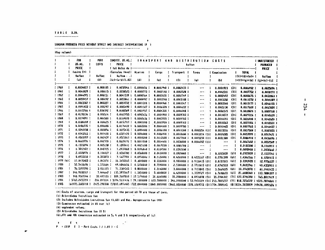
I A IE 8.20.

SOR6H1U11 PRODUCER PRICE IITHOUT DIRECT AND I(DINRECT (NTERVETIIIS IP

(Itay valu)sl

: : F01o a PORT ?UNDIST. BS.AS.: T R A N s P o R T A N D O I S t R I I UT I IO C O TS IUS DISTOREDTEO: I O-5.A5. : COSTS : PRICE : ,a/ton I PRODUCER I: I PRICE ( iat Sola de I---------------------------------------------- ------------------ --- -…-------: PRICE I: :l(using E*l: :Crealm level: Acarreo Car : Iranipout I Taiu: Coaeission I TOTAL I I

: : ton ta/ton I la/ton .: : : : Ii d.(eI* bi/tea: (al ( i lc)}-a-b)/I .021 d :) : 1W 1 if Ii i (hi :(fi*Ig$Ilhb I I 1(a(ci-(l)

19O0 0.0030057: 0.000105 0.0032004: 0.0000656 0.00019400 0.0002433 1 --- 0.0001923 f3il 0.0006952 1 0.002500 1I9S1 0.0000829 0.000115: 0.0030523 I 0.0000773 0.0002?100 0.0002520 1 -- : 0.0002311 (311 0.0007752 I 0.0030771 I19S2 0.0044295 0.000151 o 0.041539 0.00007644 0.0002610 0.0002749 --- 0.4000242 (31: 0.0008475 1 0.0032843 11943 0.0059457: 0.0001921 0.0ooo0099 2 0.000370 2 0.0003188 --- 0.0003352 13): 0.0011272 I 0.0004589 I19i 0 0.0063382 : 0.000227 0.00O9332 0.0001310 I 0.0004940o 0.000347 --- 1 0.0003560 131: 0.0013171 1 0.0044155 11915 : 0.0091033 0.000297: 0.0085498 0.0001507: 0.000O320 0.0004652: --- 0.0005130 (3): 0.0017409 1 0.0067689 I19b6 : 0.01(57646 1 0.000392 I 0.0(0858l9 0.0OOIS7: 0.0004300 : 0.000O4: --- : 0.000615 1(31 0.0018820 I 0.00os72a 119S7 : 0.0178134 : 0.000514: 0.0(41955 0.0002b3b: 0.0004900: 0.0009703 1 --- I 0.0010077 1311 0.0027314 I 0.01400639(968 : 0.0179891 : 0.0005o0 0.0169020 0.0002636 0.0003920 0.000S703 -*- I 0.0010141 131t 0.0026400 1 0.01426201919 : 0.0(80(09 0.000:25 0.017Z717 0.0003200 0.00039s0 0.0009703 : --- 0.0010343 (3)1 0.0027116 1 0.0145531 11970 2 0.0(54535 0.000 bO 0.0174422 0.0003200 00004boo0 0.0009700: --- : 0.00D0465 13)1 0.0027945 1 0.0144457 12971 0.0201158 1 0.000894 0.0225435: 0.0004400 0.000 100 0.0011300 0.0002254 (Ii: 0.0013524 (3): 0.0037580 0.0187155 1(972 : 0.0345243 0.001420: 2 0.0321420 0.0004000 I 0.0004900: O.0o0(600 1 0.0003214 11H 0.00(9285 131? 0.0053999 t 0.0267029 I973 : 0.053287: 0.002459 0.0523007 0.00(0200: 0.0021600 0.0027500: 0.0005230 (I): 0.003(380 13): 0.0084910 I 0.0036096 I(970 0.0:4b594b 0.002720 0.0620(71 0.00(2000 2 0.00(4000 0.0031000 I 0.0006202 (2: --- : 0.0047402 1 0.0552549 I1975 0.1373294 0.005138 0.1283411 0.0021600 0.0019200 0.0081700 -- : --- : 0.0122500 0.1160911 S974 : 1.3822422 0.008725 1.2937040 0.0(96buO 0.0(09500 0.0592100 1 --- - -0.089i000 1.20386601917 7 2.6028971: 0.104037: 2.0260780 0.0360000 0.0030000 0.0920000? --- : 0.1213039 fill 0.2923039 I 2.1337741 2197a 8.0955550 : 0.305073 7.627981 0.0950000 : 0.1120000: 0.4260000 0.4235167 (21: 0.3710399 fll 1.3460564 1 4.1281415 11979 14: 17.8475483: 1.043071 16.3150265S 0.30000002 0.3300000 0.9s00000 : 0.9136015 121? 0.8157513 Ib2' 3.33939201 12.9756337 1(900 52.5428491 1 .5726640 49.4846656 0.5150000 2 0.7590000: 2.53D00000 2.7711013 12I: 2.0742333 16) 9.0493746 1 40.4352911 1191 : 71.529720O: 3.05il25 71.334505 o0.9000000 : 1.3140000 3.8000000 0.7133805 151: 3.5669225 121: 10.1943070 1 61.1441435(902 146.90302b7: 7.444642 135.3972667: 12.3050000 I 5.6800000 6.4200000 1.3539271 (5)l 4.7498433 (b6 21.6088360 I 113.7184307 11903 298.9507244 32.0971202 989.7607810 12.5190000 31.1000002 35.2080000 8.0974078 (5(: 35.5904312 /711 123.8790390 2765.88(7419 (904 : 5763.2571(9 2 206.89703: 5394.513143b: 79.1000000 123.7000000: 341.2000000 1 53.95131( (51 2(.15.7805257 171: 810.7256572 I4575.7874864 I1905 :61972,.36371(0 2225.290308 s57012.6971485 :722.0000000 :14o0o.ooOooo :3060.0000000 s578.1269715 (5l11734.3109145 (l)i8334.5078859 :49478.1892424 1

(11 Costs of acarreo, carqa and traniport for the period 60-70 are these ot cotn.(11 Aclividades lucrativas tax(21 IcEludeL Actividadea Luiatjivs tat 11,411 and Mac. Aoropeuanio tas (41)131 Cousission estinated in 61 orve (cIl(41 septeeber values.(5) Actividades lutcraliva tax (I 1I(Ib1721 and (81 coossssion esaheaed in 5, S and 3 s tespoEtively of Icl

P tIIP E I - Port CbIts I / 1.03 1 - C

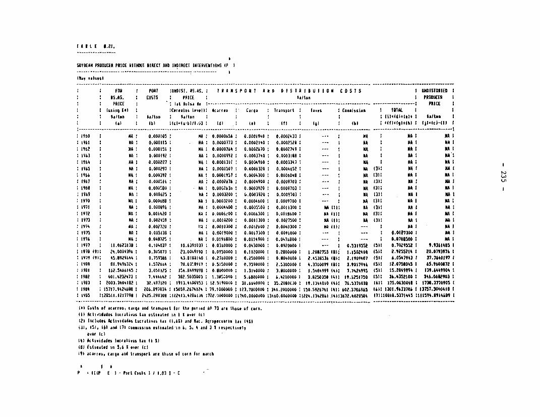
TI AIE. 1.21.

SOYBEAN PRODUCER PRICE VI19H1U0 DIRECT AND INDIRICT INIERYENIIONS IP I

* 1 ~~~~FOB I PORI :UNDIST. lS.AS. I TR A NSPORTI A ND DISI AI I U IOI0N CODS TS I UNDISTORTED I

* I ~~~~BS.AS. COSTS I PRICE W aton I PRODUCER I

* I ~~~~PRICE (iat Dolsa de - - - --- … …-----------……---------… ---------- ------ PRICE

* usinq El, :Cerealei level: karual) Citarl lfianoport I taxes Comamsiomio TOINA. II

lVion laftm W~taton fiic(i ull, I

* : hI~~~la l b) :hcIgha-bI/I.'j3 I (di (Iii(I I (I(I *fi(ola(Isi I 11WzCHI-II

i9i0 NA I 0.000105 M A I0.0000656 0 .oaott9 I 0.0002433 I--NA M A I MAI

196t NA: 0.0001151 MA 0.0000773 0.000?1401 0.0002528 -- IN M A I NA I

19t2 : N~ ~ ~~A 0.000151 NA: 0.0000764: 0.0002670: 0.00027491 K- A N A I KAI

1963 M A: 0.000192i KAI 0.00009921 0.0003740:t 0.0003199 I --- :NA N Al NA:

1964 M A I 0.000227 :N: 0.000131C, 0.0004960 1 0.0003347 K - A I NA: HA

1965 M A I 0.000297 M A I0.0001507 1 0.0006320 : 0.0004652 K - A (31: NA I NA I1966 MA (3I NA I NMA 0.00039? NA I 0.0001957 1 0.0004300 : 0.000604 1 - N 3: A A

1967 M A: 0.O00044 I1 NA:. 0.0002636: 0.00049001 0.0009703:- NA 13): MAl HAI

1968 M A I 0.000S80 M A I0.00C2636 : .0003920O 0.0009703 I - A 131: NAS HAI

1969 :NA: 0.00025: NA: 0.0003200: 6.0003920 1 0.0009703: N- A (31: MA I NA I

11970 1NA 1 0.000668 M A 0.0003200 1 0.0004600 1 0.0009700 1 --- :NA 1311. MAI NA:

1971 NA1 0.000896 MA I 0.00oo%00 0 .0005'.o 0.0011300 : N (II: MA 131:- NA I NA

1972 :NA 0.001420 M A I0.0006~OO 1 0.0006300 1 0.0019600 :NA III: NA (311 NA I MA I1973 K A: 0.0O21iji " A: u.0010200 1 0.0011300: 0.0027500 NA (Ill NA (3): NA I HASI

1974 M A 1 0.002720 Q 0.0010300 1 0.0012600 1 0.0040300 MAe:-- A I HA I

1975 M A: 0.005138 H A 0.0019000: 0.00173001 0.0091000: - - 0.0127300 1 HASI1976 M A: 0.048725 NA: 0.0196800: 0.0114900: 0.0476800: 8- - .0798500I MA I1977 1 11.0623138 1 0.104037 1 10.6391037 0.03s0000 0.0430000 1 0.09?0000 I --- S 0.531955a 1511 0.7029552 1 9.9361485 I

1979 191:, Zi.000939h o .305873 1 23.0049190 10.0950000 : .110000 : .2800000 I 1.2692755 9161. 1.1502460 ISIS 2.9255214 1 20.0793976 I

1979 19): 45.0929644 1 0.759586 43.910140 1k( 0.2760000 1 0.2500000 1 0.9940000 2.4539536 (911 2.1909407 (511 6.0547943 1 37.7640197 1

19900 91.9496324 1.572664 78.03'8917 0.5150000 0.7190000 2.5300000 1 4.3700099 1911 3.90179%L 1511 12.0758045 I 65.9600972 5

11991 1 162.500645 1 3.05I?S 15,4.8499898 V 9000000 1.3140000 3.9000000 1 1.5484999 141:. 7.7424995 1511- 15.204999% 1 139.64449904

1992 1 401.4232473 : 7.444642 1 382.5035003 :1.3115~010 S .6800000 4 .4200000 13.8250350 141.1 19.1251750 15I11 3&.4352100 1 346.06829031

1983 I2003.3404182 32.4971?0 11913.W40953 1 2.51900~00 31.6640000 135.2060C)0 19.1344010 141 76.5376038 1611 175.0630048 1 1738.3770905 I

11984 115717.14246881 206.997034 115059.26741?4 179.1000000 :123.7000000 1346.2000000 1150.5926741 (41:, 602.3706965 16)1 1301.9633706 11 13757.3040418 1

11985 1128511.1217799 ?k225.290309 :122AI3.4286l04 :722.')000000 :1740.0000000 :3460.0000000 :1224.1342961 .14113672.4028584 1711,10816.53714%5 159.149 I

III Cbits of acarrob, carga and transpoit for the poriod 60-73 are tIhose of corn.(ll Actividadvii Iuurativani tao estimaiLd in I I over IEI121 Includeao Actividades Lgcralovao, tax 11,6111 and Mac. Agropecuark. o 1a 411

(31, (51, 16 and I7) oamoogison esitiat,d in 6, 5, 4 and 3 1 repet"Wvilyover Ic)

141 kctvidades luacrativas tan II 1)(9) fstiaiald in 5,6 1 over (c)i'll IEarreni, targa and transport are tt,ios of coro for mArch

a f I P I(IP E I - Port Costs I / 1.03 1 - C

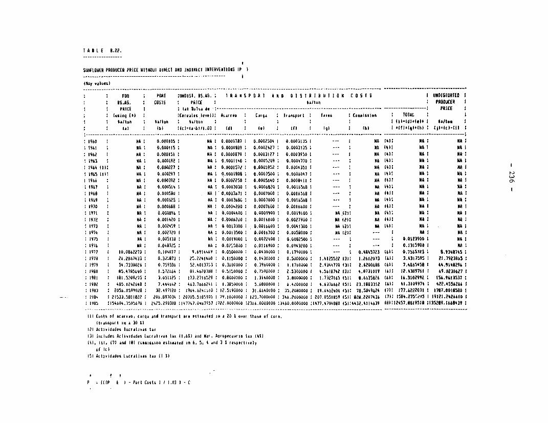
T AB6LE 8.22.

SUNiFLOWER PRODUCER PRICE HIIIHOUI DIRECT AND INDIRECI IN]IRVEN]IONS (P

(flay valuus)

* FOB POAT FOB BDISI. 8S.AS. I I A N S P 0 R 1 A N 0 DI S I R I 8 Ui I I 0 N C 0 5 T S I UNDISTORTED* 2 *~~~S.AS. 2 costs 2 PRICE I2 PRODUCER I

* PRICE 2 ta~~~~~~~~~~lt vLkia de --------------------------------------- -- -------- PRICE * 2(u6anq El) 2 Cerva(as levoll: Acarreo cArga f(rAnpoil fAl Coeamisi~on 2 TOTAL I

Saltoner,niI(-IM ) $A/ton* ~~~ ~~(a) (6) Icla-6.)1.03 (di8 (.) 2 (ft IqI (hi I *tift(q)*lhI : Ij)=c-M

1960 NA 2 0.000105 NA I 0.0000,717 0.000230k 2 0.0003145 -- 2NA (All NA 2NA IMI1 NA 0.000115 PA 20.0000009 0.0002427 0.0003135 1.--- 2. NA (k)2 NA I NA I1962 NA 2 0.000151 NA 0.0000879 0.0003127 0.0003950 1 --- I NA M:) NA 2NA, 1963 K NA 0.000i92kA 0.0010 DO005209 0.0004770 - NA (4)1 NA KA I1964 (I1: NA 0.000227 NA 20.000(572 0.0005952 0.0004351 2-- 2NA 14)1 NA K A I2 965 (1112 NA 0.0091 NA 1.0.00019009 0.0007500 I 0.0006047 K - A 1412 NA 2NA

2 (966 NA 0.000392 NA :0.00022550 0.0005640 0.0008411 2 - A (1 A2N 1967 K A 2 0.000514 2NA I2 0.0003030 2 0.0006820 2 0.0016568 - NA MI1 KA I IIA1968 2NA 2 0.0005800 NA I 0.0003671 0.0007000 2 0.0016568 1 --- 2NA 14(1 NA HIA I19T9 K A 0.000625 NA 0.0003680 2 0.0007000 2 0.00165602-- I NA 1412. NA I NA I.(970 2NA 2 0.0006602 NA 20.0004200: 0.0007600 0.00166002 -- NA M(( NA I NA I21971 2NA 2 0.000896 i NA 20.0004400 0.0009900 2 0.0019(002 NA 12)2 NA 141 NA2 NA I2 9)22 NA I 0.00(42 I WA 0.-0006200 2 0.0014800 2 0.0027900 NA (2): NA 14)2 NA 1NA21973 k A 2 0.00245,9 2NA 2 0013300 2 0.00(6600 2 0.0041300 V A 12)1 NA (4)2 NA 2NA1974 2NA 2 0.002720 I NA 20.0013500 2 0.0016700 2 0.00580000 NA (2)2 --- 1 A NA I1975 2NA 2 0.005(30 k A 20.0019000 2 0.0022400 2 0.00020 2-- . - 0.0123900 1 NA (976 2NA 0.040725j NA0 0.0255,000 o .0116900 2 0.0943200 2-- 0.13(5900 2 NA 1 977 I 10.0862273 2 0.104037 2 9.69(4469 20.0500000 2 0.0430000 2 0.1790000 2-- 0.4045723 (612! 0.7565723 I 8.934874521 910 26.20674332 0.305,8732 25.2241460 0.1(500002 0.14300002 0.50000o0 1,(4(25522 13)2 (.26(2073 (6) 3.437595 2 12.7923065 1 979 2 54.7330026 2 0.759536 2 52.40(3753 0.3600000 2 0.3960000 1 .1760000 2 29344770 (3(2 2.6200688 (Lit ?.486545B I 44.914929622 900 2 5.47115640 1 .57M64 810.4620388 0.5(5,0000 2 0.7590000 2 2.5300000 I 4.56(0742 (3(2 4.0731019 (6)2 12.4309761 1 69.0230627 I(981 1 (01.5209275 2 3.051125 1 73.27(6529 20.6000000 1 .3(40000 2 3.80000000 1.7327165 (5(2. 8.6635026 (612 16.3102912 2 (6.96(35372(902 2 485.1242648 2 7.~4o4262 463.7666241 1 (3050000 5.69000000 6.4200000 2 4.6376662 (5(2 23.1883312 (6)2 41.3109974 2 422.4556266 (903 2 2056.0599028 32.497(20 1 964.62§4~10 2 (.51900002 3(.66400002 35.2080000 1 9.6462406 (512 78.5849624 I7) 177.6222031 1787.0018580 11 . 904 212533.50(1122 2 206.0197034 2 0705.5105905 2 79.1000000 1 23.7000000 2346.2000000 2207.055(059 (5(2 020.2207436 (7) 1 514.275Oe5 1 19(21.24266(0 I2 905 2(54604.7505676 22425.290300 2(47747.0467957 2722.0000000 22360.0000000 23460.0000000 2(47.470400 m5(4432.4(4639 (0(212457.8819518 :135289.1668439 21

(II Costs of acarivD, c4rqa and 1rar-spurt are estiealed in a 20 1 over that. of coin.lIranspoft Ain 30 0)

12) Activida0dr, lucratavas tax13) ricElude, AdtiwidAdes Lucr4tavis tax (1.611 and Nd(. Anroptcuiarao ta, (41)14). 16), (7 and (0) coeasmion estiealed in 6, 5, 4 ind0 3 1 rei0ectmvely

of Id)(S Actividaden Lucrativas tax II 1)

a f

P i(IP I I - por[t Ccostc I1 I (.03 I - C

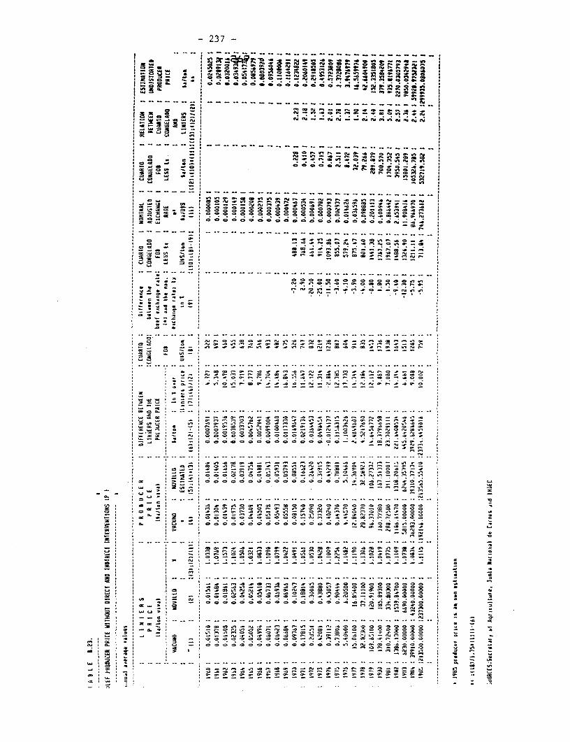
- 237 -

I -�a � O�-0��4.p�

OOa-I

I cmos a†.**� n4,44..cae,oo.. 0 ,I0.0O� -

tU.aa-ma4a... I

fla a- , 0* I

* �

- -4-I01.404 j I

La 0* .44 - Laas a.a

-4....-…aaOr-fl�%-4aU�.aC.ONflan a-I

0-a--an e..ne 505

* a. -I b-.4 -e I 00000fl*afl�.aaeo.�...

-a -�

* - a �I � O

0Cu�0r-,.a-a-��

� 8 0�tO.ta -c00O � a �

COo - t 00000000o0o0o0oooo000.�nj..c= Cua

a.

o fl C C fl .4 a- .t r- 0 0 .� a-. .

00 - a

aaaocfl 0-O.Ca4�r.r.o...4..4Coa oanaar-.aa-aa-4e.

a.aO .a faa

.- 00000000 oOOOoova., a* a.. naanon.4aoaaraa-,r.

* raau0v�aer¶s0..an�,,..C - 0. 4 - I 04 a-a - a,,,,

- C -- -a .4 Ca

.40 a- S - C a

.4-4- CC - -

* C .4 a As a.fltla0.0s 0. Or. oa�.-a-a -a-aa -On-.. a -- 41o.ra- 0 a.aOsr-a -OwOOaa--.

* .. .aaa WV- SO aa-e-a-� a., .4�a-a 0a.0-a-.--fOa�, .400

* a-.. 4004,r-a- .rs.4 .4oflJr..a- aa,Ja,Jaa-..4a0

0I -a

LaOS , -a--.4O-0¶a,a--00 e-.oa-ar. .4r-oaua--t-.40.4* .4 . - I a a-ar. 00.450CC.� -ta'4040 r-�ra.a oar. 40 -m - - -aLa-c, , In , -taafl..0C. a-. a Oem .4 -SC -C .4 .4r. .4 .. C., -00a - r-a-.o-oana.,a'sa Or-a 0.,.4.4r-ar- .4.400.4a

a 0 o�era.r 40a0-.fl--flafla..aO . -afl0aaaoaasoaa* - - 0000000-0004 S.rOo -

�oo *.. ILs , OoOOOOOOCOCOOOO..-.fl.4aAr..0.4...

* �.4 , - - 4 000000000000000 OAsOa 50

* I - I .. v¶-COa ma InC �-0 -C.a, Cat, SO* , Ca-ta a 0.flr--4-aOS sa-aaInr.aaaa-oa-o oaC�r-a�ao-0aa-

* Otaa-a-aO-aC.0.0- at, .4-ta c.40.r.4-ar�r-0 -ca-.-a . - -..- C�aafls S.C CC *0 .4-Cart CO .400- 00.00-atC a* �0- .0000000 00O0-a¶Jr--r--aC.1CCaIn�n.ac.amIn

am a 0..-a OOO0000000000000InsaCa.Ca-.-0e0In a La*� -:�a-- .mo… -C a

- .44.' 14440 -. COm 0

C. a LaC� a faa

* - CaaJCa 0 Ca , alt SanoarCanraaeooooooooooooooo .4

a a aa a a"0

r-r-a-,oOr-acIns0. a,a.ta-.r-.r r-..0aa-.00o a F 0 -� a a sa-asae-.C In-..tIn-r-OmCCsa.C IcCoraoa,4-C.s000 a

C. I-a - a 00000000O00O0000anJa�40a.4v-,a-,.aa. �a-4a-400-Ca.t a La0' a r 0 a - faa 00ILa a a a a 40.40 a 4.

* a .. a r�a-.u�aotaa�bO 0r-.rs�aata.r 0aaa.at-a-�0..r--r.0- a -OS a a - a O0-.-000-00000…O000� a- a - a-i.= .4

a, I S C

S a a a , - -a a a a -- a.0.rOa-IaO.4a-.eIn0r-S0000000000 a .4

- a a a a 40

.0.O,...ma-an.r.4OWaaOOeOCeOOOO a a -Laa I S = a 4050 Cua,a.rr-Oaa-JaOOoIn..aananCaooO a -Laa a .4 a….,In.a.IThCOOOananOOfl-4a.aOOOO a 4 -a a a a .4 -a 000000000 a-�a-a.reaa,aa- aOaOoOO a 3 .4- a a alt - a - CIA.a -Ca 010 - a 0

00

00

00

00000000

0.C.CO-0In.taOOO a -

a a 0... * o a -a-aa-aaa-,a-Caso a C .4- a a - a a a a. -

a arm a - -

a-.�C a a-a

CI at, - rCa .t - a-I s a-.. In - - a., *0I.4. -Va a -aa.Oaaa.rCanar.fl4O.a-afla-000 .40000000La a Ca - a a ,� 40m000.05�flr-0I0.0S0C..S #0000 a - -.4a - a .5 - a 0 a �a.-Cu.t.,-t�O-0--dar-,40C-��-O a0046C-fCaaOZO OO0

00000000-4flJea-I0-.C0aC.*Ca000 a - -

a C. a a a La - a 0000000000 000000.�CflI��IaV-00-a000 a C - -* a a a a S a -mOr.�0a.I -0 a aj atI aa Oa a 0 4 a �aaa-Ifla0., a C e. -

a La a 0 a a a -CIa I - 4a .I a . a a a C - a .4 - .4a fa 4a a a a Cu a = an

La a 0 a a...a....0 -.4 a 0 a a a 0 Ja-a -CV, .4,-. 0 aan�aaa-¶.ra.Cflr-0a,. arC ... flaa-a.a * 40 -

a V. a - a a .0-0-040-fl -0fl-fl.4 r-a-..r-.4r-!aaa-a�-. .a,aoan,,0.4 a a - a..O a a S a 000000000a0.000

00.O o-0.aaaaao-a a a ..

a a- a 0'………………a - --.2 a La a .4 a -

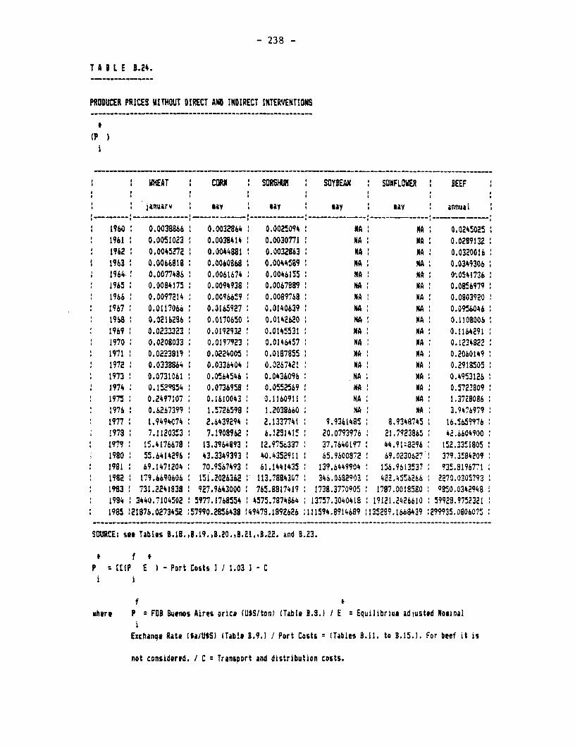
- 238 -

T A I L E 0.24.

PRODUCER PRICES VITHOUT DIRECT AND INDIRECT INTERVENTION

('P )

WHEAT . SORM SOYBEAN SUNFLOV' BEEF

' j1nuarlt ' *ae ' uy . uy ' us annual* __ _ _ _ _ , _ _ _ _ _ _ _ _ _ _ _ _ _ _ _ _ _ _

1960 0.0038866 0.0032864 0.002o 094 NAK A 0.02450251961 0.0051023 0.00384141. 0.0030771 NA NA 0.02891321962 0.0045272 0.0044881 0.0032863 NA NA 1 0.03200161963 0.0066818 0.0060868 0.0044589 NA NA 0.03493061964- 0.0077486 0.0061674 0.0046155 NA NA 0.05417361965 0.0084175 0.0094938 0.0067889 MA: NA 0.08569791966 0.0097214 0.0096bS9 0.0089768 NA NA 0.09039201967 0.0117066 0.0165927 0.0140639 NA MA 0.0904619$8 0.0216286 0.0170650 0.0142620 NA NA 0.11080061969 0.0233323 0.0192932: 0.0145531 NA NA. 0.11642911970 0.0208033 0.0197923 0.0146457 NA KA 0.12348221971 0.0223819 0.0224005 0.0187855 NA NA: 0.20601491972 0.0338864 0.0336404 0.0267421 NA NA 0.29195051973 0.0731061 0.0564546 0.0436096 NA NA 0.49531261974 0.1529854 0.0736958 0.05S2569 NA NA 0.57238091975 0.2497107 0.1610043 0.1160911 NA NA 1.37290861976 0.6267399 1.5726598 1.2038660 N A 3.94769791977 1.949t0741 2.6439294 2.1337741 9.9361485 8.9348745 16.56599761978 7.1120353 7.1908962 6.123141! 20.07939?6 21.7q23965 *c.66049001979 15.4176678 13.3964993 12.J75c337 37.7640197 44.91 3296 152.33518051980 55.6414296 43.3349393 40.4352911 : 65.9600972 69.0230627 379.3i942091981: 69.1471204 70.9567493 61.1*41435 139.6449904 156.9613537 935.91967711982 M 179.6690606 151.2026362 113.7884301 346.08203 1 422.4556266 . 270.0305793183 731.22419338 927.9643000 765.8917419 1738.3770905 1787.0018580 985.03429481984 3440.7104502 5977.1768554 4575.7874864 13757.3040418 19121.2426610 59929.97523211985 121876.0273452 :57990.2856438 149479.1992626 :111594.8914689 135289.1668439 1299935.0806075

SURCE: see Tables 8.18.J3.19.,B.20.,1.21.JB.22. and 8.23.

t f tP :1[ E ) -Port Costs I J 1.03 3 - C

i i

f I

*here P: FOB Buenos Aires price (USS/ton) (Table .8.) I E Equilibriua adjusted Nominal

Exchanqi Rate ISa/JUS) (Table 8.9.) J Port Costs (Tables 8.11. to B.15.1. For beef it is

not considered. I C Trinsport and distribution costs.

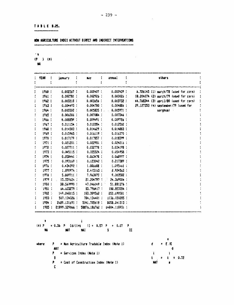
- 239 -

T A I L 1.25.

NON AGRICULTURE INDEX VITNOUT DIRECT AND INDIRECT INTERMITIOIIS

(p ) (t)

MA

YEAR ajanuary : ay nnual : others

--------- _- _-_- _-_---- --_-_-_- -- ----------

1960 0.002367 0.002407 0.002439 6.726145 (1) uarch178 [used for cDrn)1961 0.002791 0.002926 0.003026 18.204074 (2) uarch/79 fused for corn)1962 0.003218 0.003656 0.003732 44.768344 (3) april/90 (used for corn)1963 0.004493 0.004780 0.004886 29.127353 (4) upteeberl79 (used for1964 0.005502 0.005835 0.005971 sarghus)1965 0.006306 0.007084 0.0073461966 0.008859 0.009491 0.0097961967 0.011154 0.012294 0.0125021963: 0.014503 0.014629 0.01'+883:1969 0.015965 0.016119 0.0163701970 0.017179 0.017857 0.0113991971 0.021201 0.022981 0.0242161972 0.027711 1 0.032778 0.0341981973 0.045115 0.0S5524 0.0549581974: 0.058441 0.063472 0.0689971975 0.093169 0.123042 0.217389:1976 0.434392: 1.086688 L.0954611977 l 1.8774 2.415163 2.924563197s: 5.809711 7.963073 9. 0W3921979 15.5S52i 21.204787 ' 24.3690341980 39.56"990 47.046149 51.9813761981 64.633279 83.796417 100.9533541982 149.340115 183.389562 252.6905811993 1 507.134326 764.134401 1136.0502851984 2689.131691 5041.785619 BO58.8413131985 21899.329066 58876.186762 6 64804.118931

C iIt) p :0.36 P id/(l+t )] + 0.57 P + 0.07 P

NA NAT MT S Cc

where P Non Aqriculture Tradable Index (Note 1) d : E IEHAT 0

P = Services Index (Note I) i iS t : t t 0.72

P = Cost of Construction Index (Note 1) MAT aC

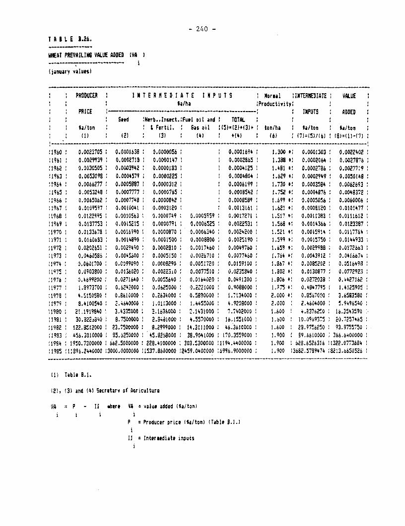
- 240 -

T A I 3 E 1.26.

WHEAT PREVAILING VALUE ADDED (VA

(ljaiarv valuesl

PRODUCER I N T E R N E D I A T E I N P U T S 4orual I INTERMEDIATE VALUESi: ta/ha !Productivity'

PRICE '-------------------------… IIPUTS ADDEDSaid 'Herb.,lnsect.;Futl oil and TOTAL.

Sa/ton ' F' rtil. G as oil US):(2)+(3)+ ton/ha ta/ton Salton(1) : (2) (3) : 4) ' (4) (6) : (7):(5)I(63 I (8)2(l1-(7)

!1960 0.0023705 0.0001638 : 0.0000056 0.0001694 1.300 t, 0.0001303 0.0022402:1961 0.0029939 0.0002718 0.0000147 0.0002865 1.388 t 0.0002064 0.0027876f1962 0.00X3505 OO.O3942 0.0000183 0.0004125 1 .481 t' 0.0002786 0.0027719fl963 0.0053098 0.0004579 0.0000225 : 0.0004804 1.629 Cl 0.0002949 0.0050148s1964 0.0066277 0.0005887 0.0000312 0.0006199 1.730 t 0.0003584 0.0062693:1965 : 0.0053248 0.0007777 0.0000765 0.0008542 1.752 C 0.0004876 : 0.004837211966 0.0065062 : 0.0007748 0.0000842 0.0008589 1.699 *1 0.0005056 : 0.0060006:1967 0.0109597 O.0010041 0.0003120 : 0.0013161 1.621 CI 0.0008120 0.01014771968 1 0.0122q95 0.0010563 0.0000749 1 0.0005959 0.0017271 1.517 CI 0.0011383 1 0.0111612~1969 1 0.0137753 1 0.0015215 0.0000791 0.0006525 0.0022531 1 1.568 t 0.0014366 0.0123387:1970 0: .0133673 0.0016990 0.0000870 0.0006340 : 0.0024200 1.521 tC 0.0015914 0.0117764:1971 : 0.01h0633 0.0014890 0.0001500 . 0.0008800 . 0.0025190 1.59 : t: 0.0015750 0.0144933:1972 : 0.0202651 0.0029490 : 0.0002910 0.0017460 0.0049760 1.659 t, 0.002?998 0.01726a3:1973 0.0460586 0.0045S0o 0.0005150 0.0026710 0.0077460 : 1.764 t 0.0043912 0.0416674:1974 0.001700 O .N99090 0.0008290 0.005i720 0.0159100 1 1.967 ' 0.0085202 0.05164931 975 0.0903900 0.0136020 0.00223i0 0.0077510 0.0235840 1 1.902 al 0.0130877 1 0.077292311976 0.4699200 0.0271640 0.0055640 0.0164020 0.0491300 1 .906 C: 0.0272038 0.4427162:1977 1.8973700 0.624.000 0.0625000 : 0.2221000 0.9088000 1 il5 t: 0.4847795 1.41259051197& 4.5150580 1 0.8610000 0.2634000 0.5890000 1.7134000 2.000 C 0.8567010 3.6583580t1979 8.4100540 2.4640OO0 1.0113000 1.4455000 4.9208000 2.000 .24604000 1.9496540:1980 21.1919840 3.4335000 2.1636000 2.1431000 7.7402000 I 1.600 4.237620 1 16.2435901981 30.322'a4O 8.7500000 2.4841000 1 4.5570000 16.1551000 1,600 10.0969375 Z0.7257465

:1982 122.3512000 23.7500000 8.2999000 1 14.3111000 46.3610000 1 .600 : 29.9756250 93.3755750:1983 456.3010000 85.625000 45.8268000 38.9041000 170.3559000 1.900 89.6610000 366.64000001994 1950.7300000 Wb2.5000000 :228.4100000 303.5300000 :1194.4400000 1.900 628.6526316 :1322.0773684:1985 81896.2440000 :3000.0000000 :1537.860000 !2459.0400000 :6996.9000000 1 1.900 :3682.5789474 1S213.6650526

~~~~- - - -- - -- _-- -- -- -- - -- - - - -- -- -- -- -- -- -_- -- - -- - -- -- -- - -- - ___----- - ----- - - - ---- - -- - ------

(1) Table 8.1.

(2i, (3) and (41 StEratary of Akriculture

VA P - I w Bhere VA value added (Saiton)i i i i

P = Producer orice (SaIton) (Tabia B.1.)

IIl zIntersediate inputs

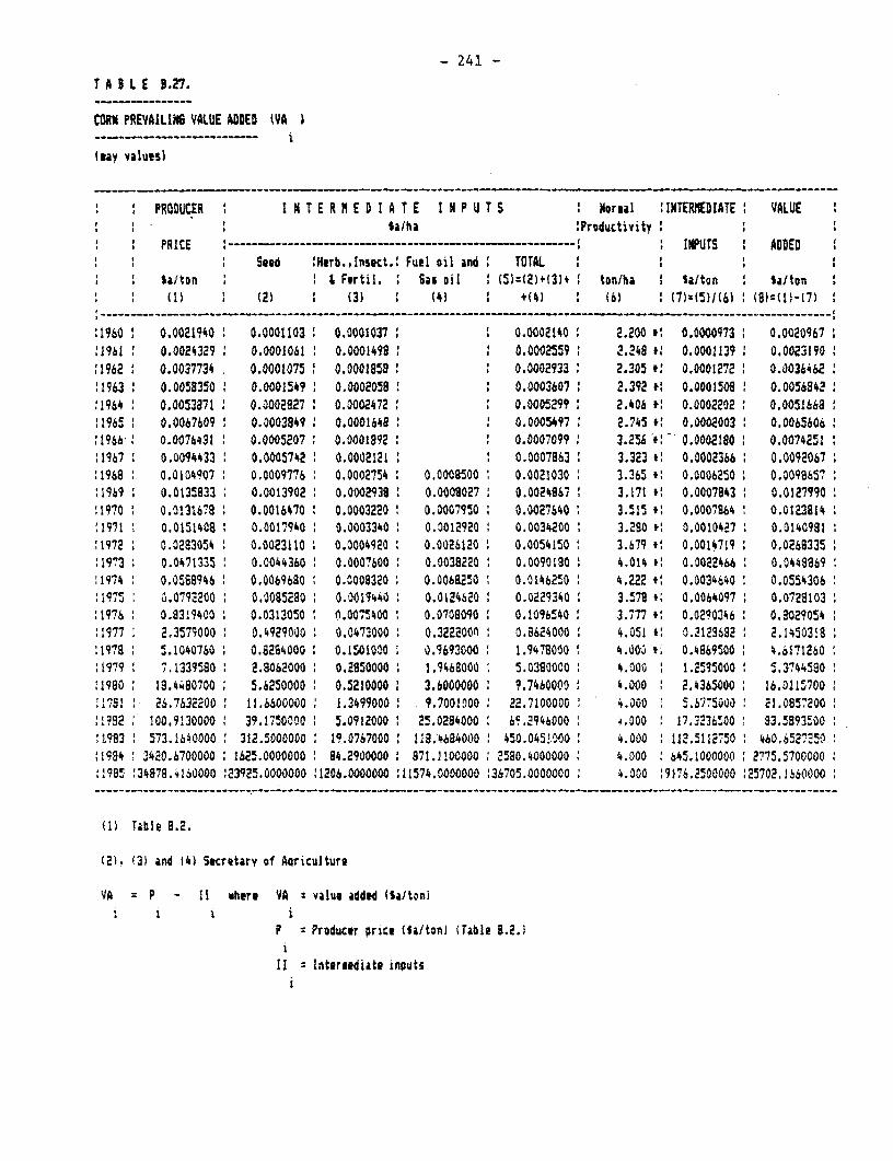
- 241 -

T A I L E 3.27.

CORN PREVAILING VALUE ADDED (VA

teay values)

PRODUCER I N T E R N E D I A T E I I P U T S : Moreal :INTERMEDIATEC VALUE-a/ha .:Productivity

PRICE : ----------------------------------- ----- ----- I IPUTS C ADDEDSeed 'Herb.,Insect.' Fuel oil and TOTAL C

' a/ton * & Fsrtil. Gas oil : (5):(2)+(31+4 ton/ha : Sa/ton S la/ton It C Cl) t (2) C (3) C (4) ' +(4) C (6) ' (7(5W6)1{ ' (8):(13-(7) '

:1960 C 0.0021940 C 0.0001103 C 0.0001037 C C 0.0002140 C 2.200 *C 0.0000973 . 0.0020967 11961 0.0024329 0.0001061 C 0.0001499 0.0002559 2.249 IC 0.0001139 C 0.0023190

f1962 C 0.0037734 0.0001075 C 0.0001858 C . 0.0002933 2.305 t: 0.0001272 C 0.00364621963 C 0.0058350 C 0.0001549 C 0.0002058 C : 0.0003607 C 2.392 #: 0.0001508 0.00569824:1964 C 0.0053871 C 0.0002827 C 0.0002472C 0.0005299 2.406 tC 0.0002202 C 0.0051668 C:1965 0.0067609 0.0003849 0.0001648 C 0.005497 C 2.745 cC 0.0002003 0.065606C1?66C 0.0076431: 0.0005207 C 0.0001892 : 0.0007099 C 3.256 t 0.0002180 C 0.0074251C1967 C 0.0094433 C 0.0005742 C 0.0002121 C 0.0007863 C 3.323 cC 0.0002366 C 0.00920671968 C 0.0104907 0.00091776 0.0002754 C 0.0008500 C 0.0021030 3.365 tt 0.0006250 0.0099657 .

C1969 0.0135933 t 0.0013902 0.0002938: 0.0008027 0.0024867 C 3.171 C 0.0007943 0.0127990:1910 0.0131678 C 0.0016470 0.0003220 C 0.0007950 C 0.0027640 3.515 IC 0.0007964 C 0.0123814 CC1971 C 0.0151408 C 0.0017940 C 0.0003340 C 0.0012920 0.0034200 C 3.290 ti 0.0010427 C 0.0140981 CC1972 C 0.0293054 C 0.0023110 C 0.0004920 C 0.0026120 C 0.0054150 C 3.679 *C 0.00147l9 C 0.0268335 CC 1973 0.0471335 C 0.0044360 0.0007600 0.0038220 C 0.0090180 C 4.014 C 0.0022466 0.0449869:1974 0.0588946 : 0.0069680 0.0008320 0.0068250 C 0.0146250 C 4.222 t: 0.0034640 C 0.0554306

:1975 0.0792200 0.0085280 0.0019440 C 0.0124620 C 0.0229340 C 3.579 IC 0.0064097 C 0.0729103C1976C 0.9319400 C 0.0313050 C 1.00=5400 C 0.0709090C 0.1096540 C 3.777 C 0.0290346 o.8029054C 1977 2.35719000 0.4929000 0.0473000 C 0.322200nC 0.8624000 4.051 IC 0-.123692 C 2.14503181978 5.1040760 0.8294000 C 0.1501000 0.9693000 C 1.9478000 C 4.-0W ti 0.4869500 C 4.6171260 C

t1979 C 7.1339580 2.8062000 C 0.2950000 C 1.9468000 5.0380000 C 4.00O 1.2595000 C 5.3744580 CC 1990 19.4480700 C 5.6250000 C 0.5210000 C 3.6000000 9.7460000 C '.000 2.4365000: 16.0115700 CC178 -1 26.7632200 11.6600000 1 1.3499000 C 9.7001000 22.7100000 C 4.000 5.6775M0 C 21.0857200 C:1992 100.9130000 39.1750000 5.0912000 25.0294000C 6S,946000 4.000 C 17.3236500 C 93.5893500C:1993 C 573.1640000 312.5000000 19.0767000C 118.46840O0 0 450.0451e00 C 4.000 C 112.5112750 C 460. 6527250:1984 C3420.6700000C 1625.0000000 94.2900000 871.1100000 2590.4000000 C 4.000 C 645.1000000 2775.5700000 C1985 C34878.4160000 C23925.0000000 :1206.0000000 11574.0000000 :36705.0000000 4.000 C9176.2500000 :25702 1660000-- -- -- -- -- -- - -- - _-- - -- - - -- - -- -- - -- - - _- -- _- - - - - -- - - -- -__-- -- -- - -- - - - -- -- -- - -- - -- -- -___- - ------- - - - - -------

(t) Table 8.2.

(2). (31 and (4) Secretary of Aariculture

VA P - 1I where VA value added (Salton)i i i i

P Producer price (Ia/ton) (Table B.2.t

11 - Intersediate inputs

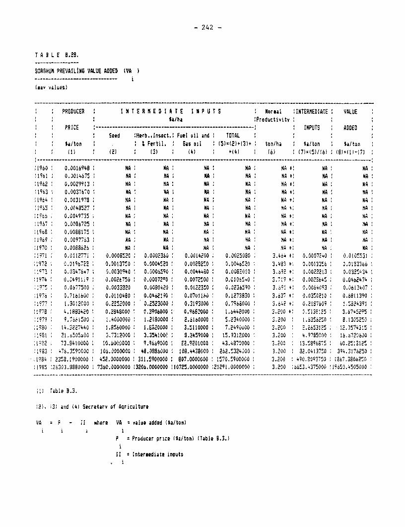
- 242 -

T A B L E B.28.

SORGHUM PREVAILING VALUE ADDED (VA

(mav values)

pRtDUCER I N T E R N E D I A T E I N P U T S Normal 'INTERMEDIATE VALUESa/h :Productivity I

PRICE '--------------------------- - ----- - ------------------- ' ' INPUTS ADDEDSeed :Herb.,Insect. Fuel oil and TOTAL

Saiton I & Fertil. 6as oil (5):(3)+(3)+ toniha la/ton Sa/ton(IJ ) (2) 1 11 '3) ) 4) 1 (6) (7)153)/'6) (8J:(l)-(7)

;1960 0.0016948 NA NA NA NA NA t' NA NA1961 0.0014675 NA NA KA NA NA *' NA NA1962 0.0029913 NA NA NA NA NA *1 NA NA1963 0.0037670 NA NA KA NA NA tl NA NA;1964 0.0031978 NA Nd NA : NA NA F NA 1 NA

1965 0.004852? YA NA NA NA NA ': MA YA

:Iq66 0.0049735 NA NA NA NA NA C MA NA'1967 0.0096725 MA MA MA NA NA t NMA: SA'1968 0.0088175 NA NA KA NA NA C KA MA:1969 0.0097763 NA MA N A : NA NA i: NA NA:1q70 0.008a626 NA MA NA MA NA F ,a NA1971 0.0112??1 0.0006520 0.0002360 0.0014200 0.0025080 3.464 i 0.0007240 0.010!5311972 0.0196722 0.00137S0 0.0004520 0.002B5Z0 1 0.0046520 3.483 * 0.00132!S 0.0183366:1972 0.334?647 0.0030940 0.0006590 0.0044480 0.0032)10 3.632 {' 0.0022213 0.03254341974 0.G491!iq 0.0026750 0.00072qO 0.0072500 0.010t540 3.719 il 0.0029645 0.0462474

0.0677500 0.0033920 0.0080420 0.0122350 1 0.0236590 3.671 C 0.0064093 0.061'407:1976 0.7161600 0.0110480 0.04a!90 0.07u1160 0.1273830 3.637 C 0.03'.0210 0.6811390:1977 1.3012000 0.2252000 0.2523000 ' 0.3193000 0.7968000 3.642 it 0.21957609 !.: '8439l:19,78 4.1883420 0.2948000 C.3906000 : 0.9682000 1.6442000 3.200 .1 G.J513l125 3.67452q51979 9.766l500 :.4000000 1.2180000 2.6160000 5.2340000 3.200 1.635i650 8 1305250;1930 14.3227440 1.6560000 : 1.8520000 . 3.5110000 . 7.249v000 3.200 2.265312 ' 12.3574315191 '21.a 505600 3.732000 3.354100C : 9.3459000 1 15.9312000 3.200 4.9?95030 16.??G6001722 73.341000v lO.i000000 9.96a9000 22.?201000 43.48a70000 3.200 5 13.599667S 60.2513125:1583 476.3590000 : 106.0000000 48.0S86000 108.4438000 2652.'394040 3.200 32.0413?53 394.3176250

-'?984 232.1'900000 452.0000000 311.5900000 807.0000C30 1570.'900000 3.200 490.oi37c50 : 1367.380c2'0:1985 :26303.8880000 7360.0000000 :3206.0000000 10725.0000000 :21291.0000000) : 3.200 :6653.4375000 :19650.4505000

(1) Table 8.3.

2). i31) and (4) Secretarv of Aqriculture

VA P - II where VA value added (Sa/ton)i i I 1

P Producer price (Iaiton) (Table 8.3.1i

II Intersediate inruts

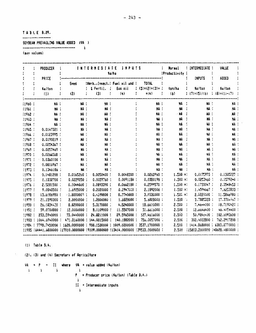
- 243 -

T A B L E R.29.

SOYBEAN PREVAILINS VALUE ADDED (VA…---- -- - - - …----- - -

(say values)

PRODUCER I N T E R A E D I A T E I N P U TNormal INTERMEDIATE VALUEI : Salha !Productivity

PRICE - - -- - - --- - ---------------- - INPUTS ADDEDSeed 'Herb.,Insect.l Fuel oil and 1 TOTAL

ia/ton . Fertil. Gas oil (5)=(2)+(3)+ ton/ha la/ton Sa/ton(1) (2) . ) : 4) . +l4 ,6) :7)/ ,b-

---------------------------- ------ - ------ - -- -- -- -- -- -- -- -- -- ---------------

11960 NA NA NA NAl NA NHA HAl11963 MA NN HA ' NA NA NA NA NA11962 NA NA MA NA NA MA NA'1963 NA NA HA. HAN NA NA NA1964 I HA NA NA NA NA NA N MA:1965 0.0147321 1 NA NA NA NA : NA t NA1966 0.0123995 HA HA. HA MA NA NA ,1967 0.0190219 MA MNA NA NA N HA MA

s1968 0.0254367 MA N A NA NA NA MA:1969 0.0257469 MA NA A M NA : NA MA1970 0.0266S68 NA NA NA NA MA NA:1971 0.0360100 NA MA 'A MA KA NA:19?2 0.0816967 NA A: ' KA ' NA NA:A NA1973 0.1346186 NA NA NA HA NA MA11974 0.1481200 0.0165260 : 0.0050400 0.0048300 0 0 . 0263?50 1.500 e: 0.017S973 0.130522711975 0.1332700 0.02,9250 0.00!97SO 0.0091130 0.0380190 1.500 tI 0.0223460 0.15792*01976 2.5281500 0.1044000 0 0.0893310 0.0662180 0.2599570 1.5100 C 0.1?33047 2.3548453:1977 9.0843500 1.6925000 0.2020000 0.2947VCC0 2.1992000 1.0 1o t 1.4594667 7.6253933:1978 13.see6980 : ;.800000I 0.430000 : 0.7740000 3.0330000 I. 5GC *: 2.0220000 11.5866990-197? 21.1590300 : 2.8000000 1.2000000 1.6829000 5.s828000 1.500 , 3.7385333 17?,37447:1990 : 26.!83i0 o 8.8200000 : S.3170000 ; 4.5240000 1: 1.6610000 2.500 7.46.4000 8.719c420!1921 59.0700800 12.0000000 1 8.1109000 : 11.5507000 31.616$000 2.500 12.646400 46.4OF4400:1982 233,5940000 7 73.0440000 24.8211000 29.5965000 1 127.4616000 : 2.500 50.984>40 ' 182.609s3600:!1993 1064.6940000 : 471.3160000 1 144.0015000 ' 140.1382000 75U.0057000 2.500 301,42.022o00 : 762.2917200:1984 7798.7450000 1620.0000000 :908.1500000 1009.0200000 : 3537.1700000 2.500 1414.3860000 :6383.8,70000:1985 ;4441.68000o0 :17010.0000000 :9109.0000000 '13414.0000000 :39533.0000000 2.500 ;15823.2000000 l4628.48;0000

(11) Table 3.4.

(2k (31 and (4) Secretarv of Aqriculture

VA = P - II where VA value added (ISa/ton)1 1 i i

P = Producer price (ia/ton) (Table 3.4.)i

II -InterBediate inputs

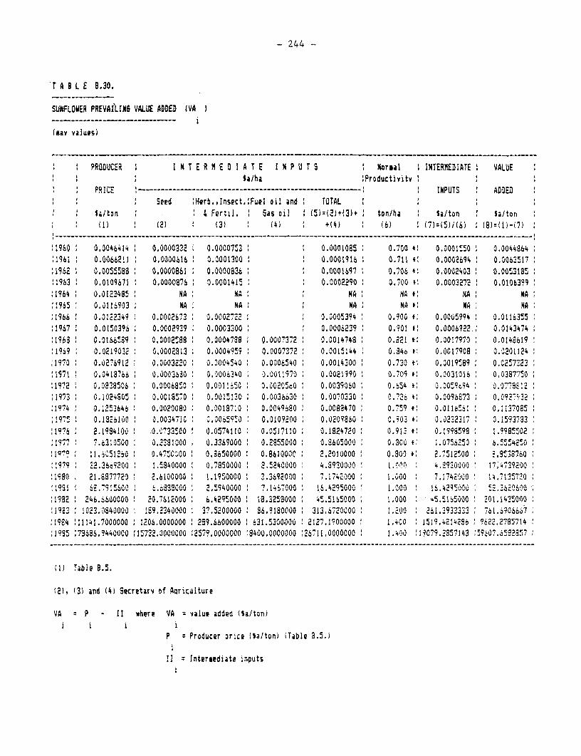
- 244 -

T A 8 L E 8.30.

SUNFLONER PREYAfLIMS VALUE ADDED (VA

(say vaIiaes)

PRODUCER I N T E R t E 0 1 A T E I N P U T S ' oral INTERMEDIATE' VALUE' ' Sa/ha :Productivity '

PRIE …-…--------------------------------------I--N iPUTS ADDED: ' a Seed ;Herb.,Insect.:Fuel oil and TOTAL I :I a a/ton & Fertil. Sas oil (5)=(12+(3)4 ton/ha ' a/ton ' a/ton

(1) 1 (2) (3A (4) +(4) (6) (7))=(1)7)6

!1960 0.0046414 0.0000332 0.0000753 0.0001085 0.700 '1 0.0001 50 0.00448641961 0.0066211 0.0000616 0.0001300 0.0001916 0.711 * 0.0002694 0.0063517:1962 0.0055588 0.0000861 0.0000836 0.000197 0.706 C 0.0002403 0.0053185:1963 0.0109671 ' 0.0000876 0.0001415 0.0002290 0.700 +1 0.0003272 0.01063A9:1964 0.01234s5 NA NN HA NAf : N,A 'A11965 0.01!6903 HA NA NA NA *1 NA MA;1966 0.0122349 0.0002673 0.0002722 0.0005394 0.900 * 0.0005994 0.0116255:1967 0.0150396 0.0002939 0.0003300 : 0.0006239 0.901 . : 0.0006922 . 0.0143474:1966 0.0166589 0.0002Kss 0.0004798 0.0007372 0.0014748 O.221 II 0.0017970 0.0148619196? 0.0219032 0.0002813 0.0004959 0.0007372 0.0015144 0.64o # 0.0017908 0,020112411930 0.0276912 0.0003220 0.0004540 : 0.0006540 0.0014300 0.720 t 0.3019589 0.0257323S1971 0.0418766 0.0003630 0.0006340 0.0011970 0.0021390 0.709 F 0.0031016 0,0397750

:1972 G0.093506 0.0006850 0.0011650 0.0020aO 1 0.0039060 i 0.654 t: 0.005%94 0.0778812;193 0.1024805 0.0013570 1 0,0015130 0.0036630 0.00?07330 0.726 i 0.0096873 0.0927-12:1974 0.1253646 0.0020080 0.0018710 0.0049680 0.0082470 0.7S? f' 0.0116!6: 0.1137085:1975 0.19.il00 ' 0.003471, 0.00659r0 ' 0.0109200 0.0209860 0.903 0 0.02-2317 0.1593?93:1976 ' 2.1984100 : . O.C733500 0.0574110 1 0.0517110 ' 0.1824720 0.912 f; 0.1998599 : 1.99855021327 7.6310500 0.^291000 0.3369000 0.2855000 o0.8605000 0.300C ;1 .0756250 : 6.55542501^9 11.951260 1 0.4 C800 0.3650000 ' 0.8610000 : 2.201)000 0.600 .1 2.7512500 1 .85X38760:t979 .2.3665200 : 1.5840000 0.7850000 2.5240000 4.8930000 I . oo 4.8930000 17>4739200

'1990 21.88777203 2.6100000 1.1?S0000: 3.36920O ? 7.42000 1.d00 7.1742000 14.I735720-,1S 68.79156o00 e 88800 GO: 2.6940000 1 7.1457000 1S.4295000 1.000 16.42500' 52.362'6$00I982 1 246.6600000 20.761E000 ' 6.S2S5000: 18.3258000 ' 45.5165000 1 1.000 ' 5.51l E000 2-01.1435000

:1933 . !023.0840000 199.2340000 1 37.5200000 8 86.9180000 313.6720000 I l .2dO 2 61.3933333 1 761.6906667:19s4 :11141.7000000 1206.0000000 299.6600000 631.5300000 : 2127.1?00000 1.400 1519.4214296 1 9622.2785714:1985 :736a6.?440000 :15732.0000000 :2579.0000000 '8400.0dCOOO '26711.0000000 1 1.400 '19079.2957143 159607,6592857

(1) Table B.5.

(2), 131 and (4) Secretary of Anriculture

VA P - 11 where VA z value added llaltDnii i i i

P = Producer price (Ialton) (Table 3.5.)I

I1 - Intersediate Inputs

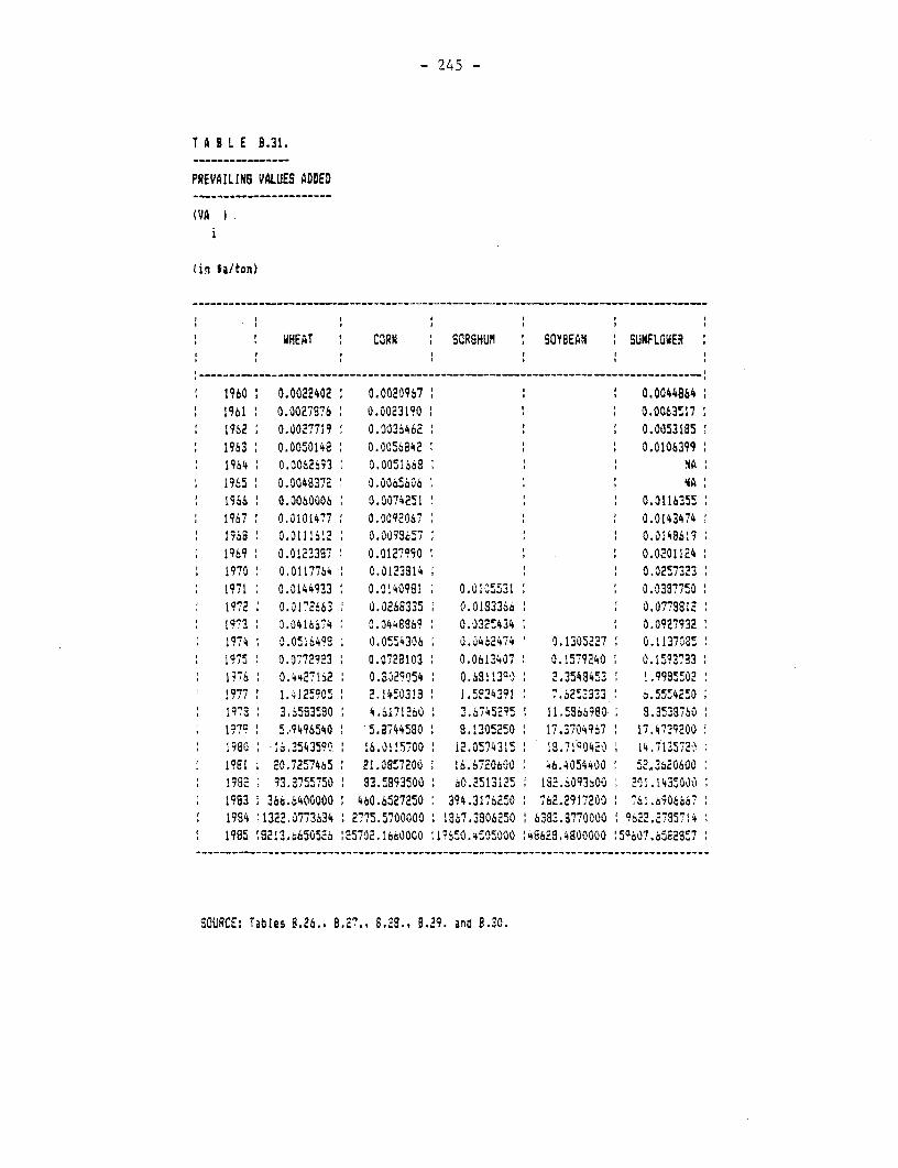
- 245 -

T A B L E B.31.

PREVAILING VALUES ADDED

(VAi

lin SaI'ton}

WHEAT CORN SORGHUM S0YBEaN SUNFLOWER

1960 W 0.0022402 0.0020967 . 0.00448641961 0.0027676 0.00231S0 0.0063S17* 1962 0.0027719 0.0036462 0.00531Es1963 0.0050148 0.0056642 0.01063991964 0.00626i3 0.0051668 NA1965 0.0048372 0.0065606 NA1966 0.0060006 0.0074251 0.01163551967 0.0(01477 0.00q2067 0.01434741968 0.0111,612 0,0093657 * 0.01486191969 0.0123387 0.0127990 0.0201124

i 1970 0.0117764 0.0123814 1 0.02573231971 0.0144933 0.0140981 0.010551t 0.038775019?2 0.0172663 0.0268335 0.0183366 0.07738121973 0.0416674 0.0448869 0.032!434 0.09279321974 0.0516498 0.0QS4306 0.0462474 0.1305227 0.11370G51975 0.0772923 0.0728103 0.0612407 0.1579240 0.15937831976 1 0.442?162 O.S029054 0.581139) 2.3548453 1.9985.5,0'977 : 1.41259!05 2.1450313 1.5?24391 7.62i2'333 6.55Z42c501973 1 3.6583580 4.61712360 !2.674523S 11.5366980s 8.35387601979 5.9496540 ' 5.a74458 0 8.1305250 17.3?70497 17.4739200198E :6.3543590?. 16.0115700 12.0574315 8.712c0420 14.71357201981 20.7257465 21.0857200 16.6720600 46.4054400 52 3-6206001982 93.2755750 83.5893500 60.sO513125 182.609360s0 201.14350001983 366.L400000 460.6527250 394.3176250 762.2917200 76 S.90O66671984 1322.0773634 l 2775.5700000 li1367.3306250 6383.8770000 96,22.21735714

1985 :8213,.650516: 25702. 1660000 I:SS05. q'000 1.8628.4800000 :5%07.65822E7

SOURCE: Tables 3.26.. 3.27., 8,28.. B.29. and B.30.

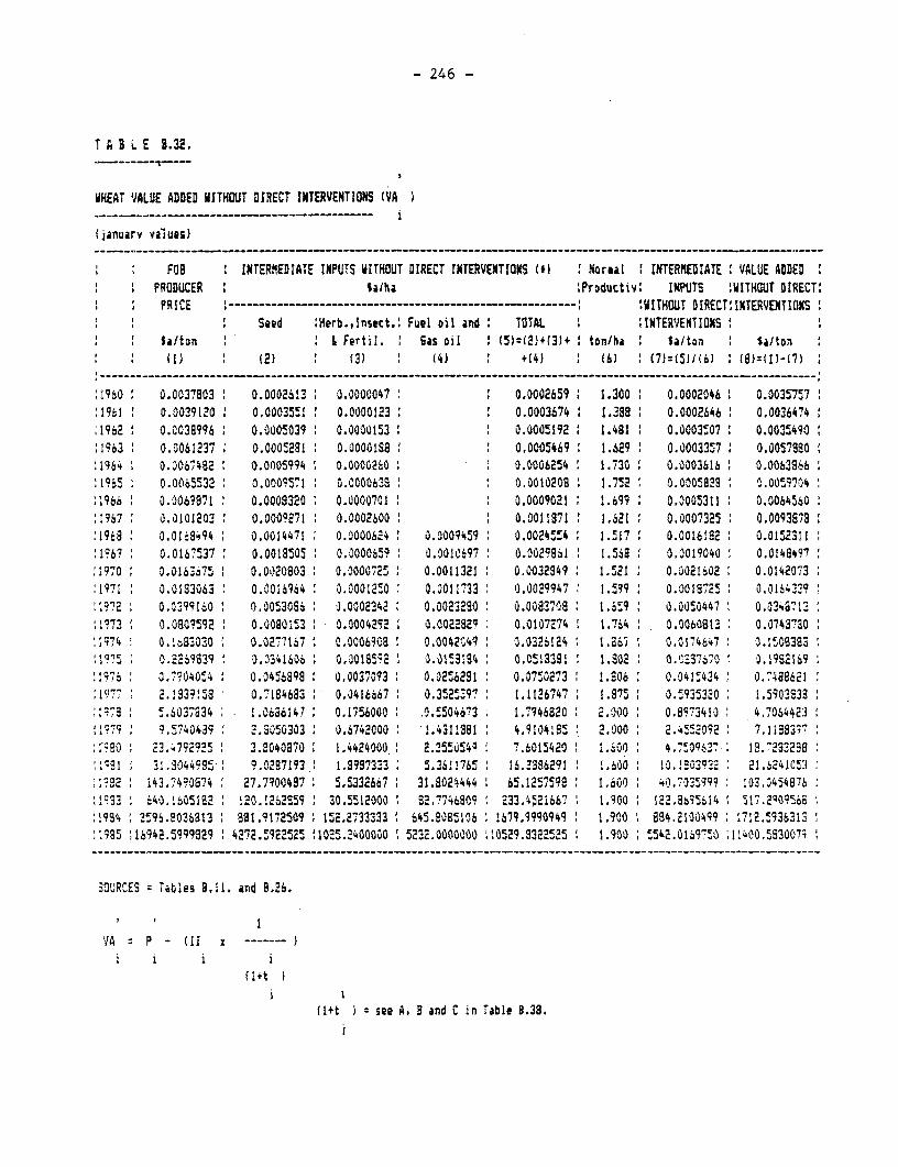
-246-

T A BLE S. 32.

WHEAT V/ALUE ADDED HITHOUT DIRECT INTERVENTIONS (VA

fianuary au;

FOS INTERMEDIATE INPUJTS 41T1iOUT DIRECT rNTERVENTIONS (1 Noraal ! INTERMEDIATE VALUE ADDEDPRODUCER a/F roductiv' I PUTS '.ITHOUT DIRECT:

*PRICE …--- ---- …-------- --------- - ---------- :ITHMUT DIRECT29TERVENTIONS

Seed :4erb.,Irsect.! Fuel oil and TOTAL ;INTERVENTIONS la/ton I Fertil. 6 as oil (5)=(23+(3)+ ton/ha Si/ton Si/aton(1) (2) 13) (4) : +(4) : (6) (71=1511(6) (8):(11-(7)

:1960 0.0037803 0.0002613 0.0000047 0.0002659 1 1.300 0.0002046 0.0035757:1961 0.00391,20 0.0003551 0.0000123 :1 0.0003674 1.388 0.0002646 0.0036474:1962 i 0.0038996 0.0005039 1 0.0030153 0.0005.192 1.481 1 0.000350O7 0.0035490:1963 0.0061,237 0.00045281 0.00001S8 0.0005469 1.629 1 0.0003357 0.0057880:1964 0.00674B2 0.0005994 0.0000260 10.0006254 1.730 0.0003616 0.00633966

: Ib 0.0065532 0.0009571 1 0.0000638 0.0010208 1.752 0.00058?3 O.0059?04:1966 0.0069871 0.0008320 0.0000701 0.0009021 !.699 0-0005311 1 0.00645601!967 0.0101203 1 0.0009271 0.0002600 0.0011871 1.6621 0.0007325 0.0093873196 0.0168494 0.0014471 0.00006124 0.0009459 0.00244554 1.517 0.0016182 0.0152311

!196? 0.0167537 0.0018505 0.0000659 0.0010697 0.002986I 1.563 0.0019040 0.0148497:19190 0.0163675 0.0020803 0.000072.5 0.00113211 0.0032349 1 .521 0.030216021 0.014207311971 0,0133063 0.0016964 0.0001250 0.0011`33 0.00219947 1.599 1 0.001872! 0.0164329~1972 0.0399160 0.005308i 0.0002342 0.00232290 0.0083708 t.i59 1 0.0050447 0.034a7li3~1173 0.0309592 0.0090153 0.0004292 0.002282q 0.01072674 1.764 00081 0.730

11974 0 .1, 310 0 0.027i 167 0.0006908 0.0042C41 0.0226124 1.367 0.017,4647 3.1,50838311975j 0.2269839 O. 0341606 0.00189592 i3.0153184 0.0513381 1 1.802 0.,0337670 0.1952169:1976 0.0790405.4 0.0456898 1 0,0037/093 0.02S62911 0.07'50273 11.806 1 0.0415434 0.7488621:I977 : 21.1833158 0.7184683 0.0416667 0.3525397 1 1.1121671471 1.875 0.59353120 1.5903338:1978 5.6037a34 1.0686147 0,1756000 1 .0.5504673 1.7746820 2.000 0.8973410 4.71064423:1979 ?.5740439 1 2.5050303 0.674,2000 1I.4311381 4.910418 12.000 2.4512 092 7.11883w'

&90 23.47929259 3.2040870 1.4424000 2.1355054; 7.6015420 1.6-00 4.750963? 13.7233298;''I 31.3044985i 9.0287193 1.89973133 5.3611765 16.2386291 1.600 10.19039321 21.624105,31932 : 143.7490874 27.71900487 1 5.5332667 31.8024444 65.1257598 1,1600 40.039 : 033547

:1993 i40.1605182 120.1262859 30.5512000I 32.7746809 21233.4521,667 1.900 1212.2675.614 5117.2qO9569:1984 :2596.9036313 881 .91712509 152.2733133 3 645.SX85106 11679.9990949 1.900 : 884.121004q9 :1712.!936313 2.9 35 :16942.53999829 42772.5922525. 11025-2400000 5232.0000000 :110529.33225215 1 1.900 : 5zi2.0169750O 111400.5830079 1

SOURCES Tables 3.11. and 3.216.

PA - (11… … …---

(1+t I

fl+t ):see A. B and C in Table 0.38.

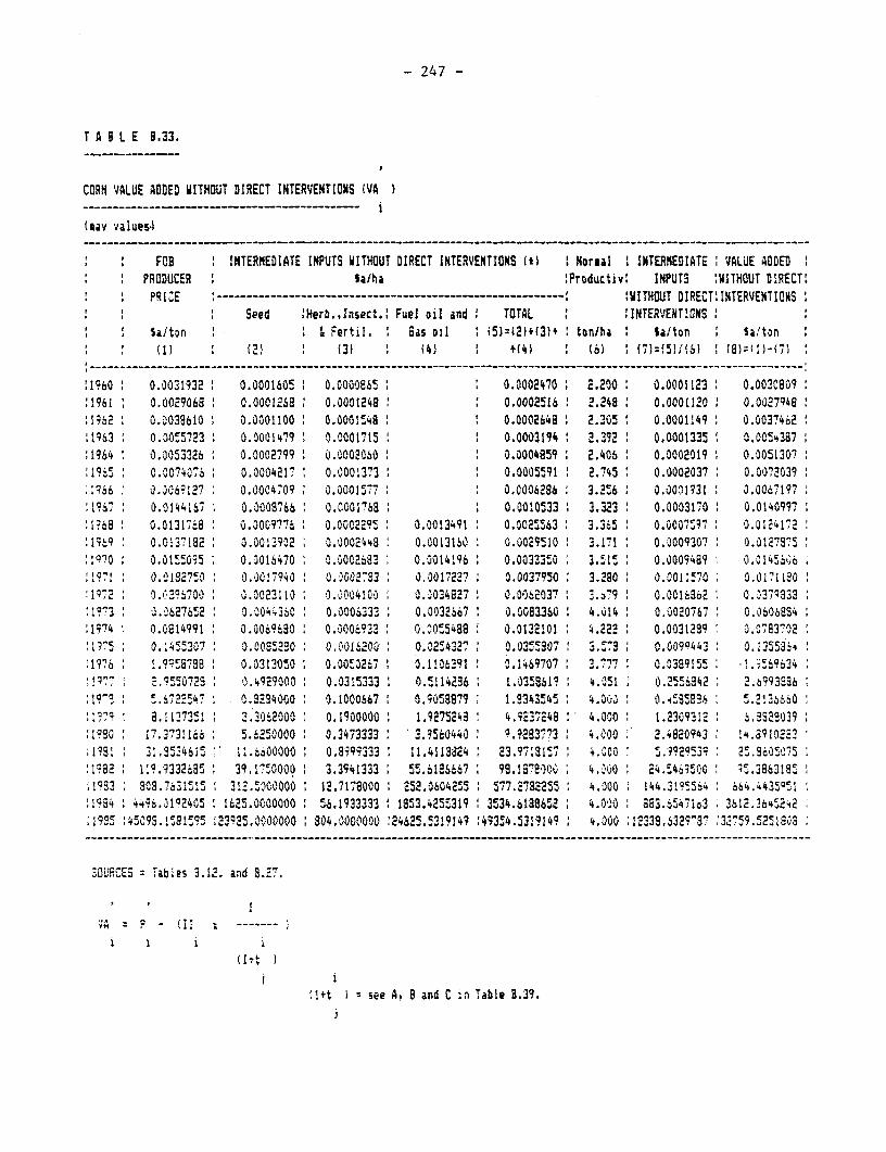
-247 -

T ABL E 8.33.

CORN VALUE ADDED 91THOUT DIRECT INTERVENTIONS (VA

(gay values.)

FOEB INTERMEDIATE INPUTS VITHOUT DIRECT INTERVENTIONS (I) Normal I INTERMEDIATE ; VALUE ADDED PRODUCER $alha :Productiv: INPUTS :WITHOUT DIRECT:PR I E………----------------------------- - -- UITHOUT DIREOTI INTERVENTIONS

Seed :Herb..Insect.; Fuel oil and TOTAL : INTERVENTIONS S.aiton &Fertil. Gas oil I(5):(214(31+ ton/ha I Salton S alton(1) (21(3) (41 4(41 (6) (15fS1 (8)=(11)-i7

:1960 0.0031932 0.0001605 0.0000865 0.0002470 2.200 0.0001123 0.0020909:1?61 0.0029068 0.0001268 0.0001248 0.0002!16 2.2048 0.0001120 0.00"27948:1962 1 0.0038610 0.0001100 0.0001548 0.0002648 2.305 0.0001149 0.0037,462!1963 0.30r55723 0.0001479 0.0001715 0.0003194 2.3?2 0.0001335 O .0054387:1964 0.3053226 1 0.0002799 0.0002,060 10.0004859 1 2.406 1 0.0002019 0.0051307:1965j 0.0074076 0.0004217 0.0001373 0.00055.91 2.745 0.0002037 0.007203919766 0.006?127 0.0004709 0.0001577 0.00062896 3.2!6 0.0001931 0.0067197:1967 0.0144167 0.30003766 1 0.0001768 0.0010533 3.323 0.0003170 0.0140997:1968 0.0131768 0.0009?776 0.00022195 : 0.0013491 0.00205563 3.36.5 0.0007S37 : 0.0124172:196L9 0.0137182 3.00133702 0.0002448 0.0013160 0.0029510 3.171 1 0.0009307 0.0127675:11970 : 0.0t5SosS 5 0.0016470 Av.00c2683 0.0014196 0.0033350 3.51l 1 0.0009489 0.0145J606:1971 0.0182-750 0.0017940 : 0.,002733 0.0017227 1 0.0037950 3.2680 1 0.0011570 0,01?11301lq7,2 0.1303%700 0.0023110 1 0.3004100 0.0034827 0.0062037 13.z79 0.0016862 0.03798333:1973 3.01627652 0.0044-360 0.0006333 0.30326S67 0.0083360 1 4.014 1 0.0020767 0.0b06834:19'74 0.01214991 0.00696190 1 0.0006922 0.005t5488 0.0132101 4.222 0.0031299 0.0783702:1975 0.:45.5307 : 0.008S290 0,0016200u 0.02!4327 0.03.c5507 3-r73 : 0.0090443 0.1355364~1976 i.9qSB798 0.03130t0 0.00t3267 0.1!063191 0.1469707 : 3.777 0.0389155 *.!.3569634

2!7`~.?550723 0.4929000 : 0.0315333 1 0.5114236 : 1.035861? 4.051 0.2556842 2.6993386:1 9:3 5z. 6.7225 -.4 7 0 0.34000 0.1000667 0.90589791 1.234T I 4.003~ 0AS852!E 5.2!3~660l1371 8.113735! 21. 3062000 0.1900000 1 1.9275248 4.iK-7248 4.000 1.2309312l 6.32819039;1930 17.37311646 5.i250000 0.3473333 3.9560440 !.292377Y3 4.000 2.4820943 14.39102231

151: 31 .35314615 '1:.4-o00o0oo 0.8599333 11.41138264 213 .97117 I 1 7 4.C'000 5J.s9295-39 25.S60E075!1q32 119.93132685 1 39,1750000 3.3941333 1 55.61096667 99. 18782000 4.000 24.S463to0 15 .3363l8St19383 8,08.76315115 312.5~.000000 12.7178000 '1 52.0604255 5577.127912255 1 4.000 144.31135564 :664.4435:951,:1134 4496.0l92405 116265.0000000 :56.1933333 13153.425S319 3534.6138652, 4.11i00 : 83.65471o3 36i2.3b65242:195c :45093.152:5f95 :23925.0000000 804.0000000 :246215.531914? :4935F4.5319149 4. 000 :121133.6329797 :32759.5251930

306'CES Tables 3.12. antd 9.27.

tl+t see A, B and C zn Table 3.39.

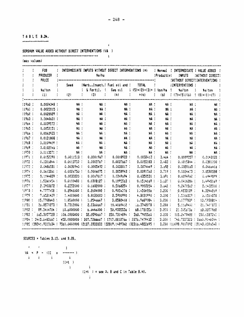
-248 -

T A 91 L! 9 .3k.

SORGHUM VALUE ADDED WITHOUT DIRECT INTERVENTIONS C VA

(say values)

FOB INTERMEDIATE INPUTS WITHOUT DIRECT INTERVENTIONS (I) Norsal INTERMEDIATE !VALUE ADDEDPRODUCER la/ha :Productiv: INPUTS WI1THOUT DIRECT:PRICE - --------------- WITHOUT OIRECT;INTERVENTIONS

Seed Herb.,Insect.: Fuel Dil and TOTAL :INTER' VENTIONS

!90 0.0024348 NA NA NA !NA M A NA : NAio6 .0o23o01 NA NA NA INA : NA 1NA NA

:062 0.0028029 1NA NA NA HA KA NA NA:16 .0040631 NA NA NA NA NA INA NA

;1964 0.0039573 NA NA NA :NA NA NA :A:1965: 0.00!21151 NA MA NA NA ~ NA NA: NA:1966 0.0063923 NA NA NA NA KA HA NA:1967: 0.01216108: NA: NA KA: NA NA: NA::1968 : 0.0109409: NA: NA: NA: NA: NA: NA:N:1969: 0.01020M46: NA: NA: NA: NA: NA: NA: KA:1970 0.0113571 NA NA NA :NA NA :NA NA:1971 0.01523290 : 0.0011513 0.000[967 0.0018933 0.0022413 : 3.4644 0.000935-7 0.0143032; I r2 0.01316844 : 0.0013750O 0.0003767 : 0.0037667 0.0055183 : 3.,83 : 0.J01,1844 m0.020000:1977 : 0.0486581 0.0030340 0.0005~496 : 0.0038017 : 0.0074449 3.692 : 0.0020165 : 0.0466416:!974 : 0.0613261 : 0.0026750 : 0.0006075 : 0.3058943 : 0.0091762 : 3.719 O .C024673 I.0588588:1975 0.1c044859 V 0.0033820 : 0.0067017 1 0.0249694 : 0.0350531 3-69I 0.00o49c 699:i197n : 1.53614S4 : 0.0110480 : 0.3308127 : 0.109SSW63 : 0.1t5141091 3a7I 0012 1.4945J169~1977 I 2.3903872 . 0-2252000 : 0.1682000 : 0.!068254 : .9002054 3,.42 0.23471 5-2 2-1432310

93 4.177'7458i oa2S4ooo0 0.12604000 : 0.90!42-06 l ;4!062%06 3 .2.0 C. 0.4!33!39 : 4.32442637.791 9 .4000000 : 0.81200,00 21 .5900990 : 4.30,2009 0 : 3.6200 62130

:1980 15.770%643 ! L8560000 1.2546667 : 3.B582418 6 b. Ib8908)a4 I 3.2100 2.1777s3q 1.30W191 6.257h270 1 3.71.1200G : 2.2360667 : 10.4069412 6.37420'73 2.200 5, 1:90 21.74CS 37192: 89.3414704 : 10.6000000 : 6.6446000 50. 933S5z"r6 : 68.1731SS6 : 3.300 : !2:.05673Z 30r76

:!9S3 665.3057725 106.0000000 32.0590667 : 2330.7314894 3 68.7905560 3.200 11.!03 50. Q52724; :1994 2426826 4c2.0000000 2 207.7266667 1717.0212766 : 2376.7473433 3 .Z0 74.7)i2: 1995z 28214.9321234 I 7360.0000000 :2137.3333333 :22S1?9248?362 :,31316.432,2695 : .200 110099.079 140352

SOURCES Tables 3.12. and 2.28.

VA p- (II ----

(41+t see A. B and C in Table 0.40.

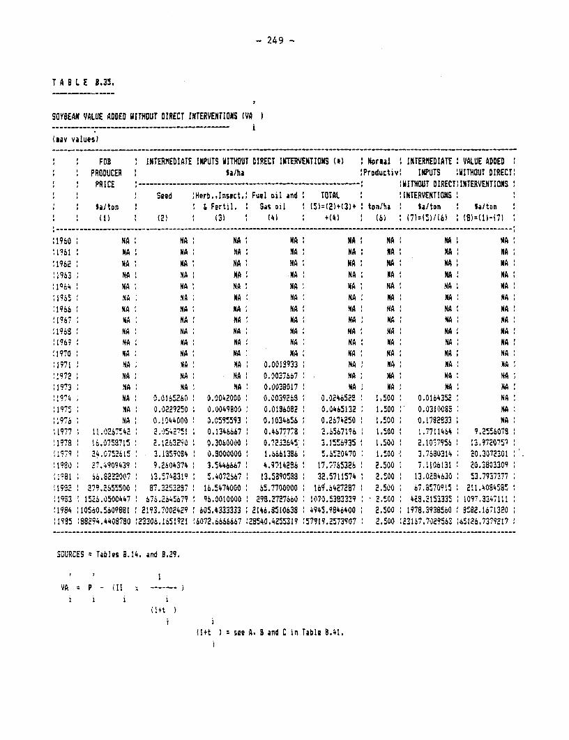
- 249 -

T A B L E 8.35.

SOYBEAN VALUE ADDED WITHOUT DIRECT INTERVENTIONS (VA--- - - - -- - ------- - ---- - - -- - - -

(oav values)~~~~~~~~~~~~- -- - -- - - - - -__- - - - - - - - - -_ _ __ _

FOR INTERMEDIATE INPUTS WITHOUT DIRECT INTERVENTIONS lt) Norval INTERNEDIATE VALUE ADDEDPRODUCER ! Ia/ha Productiv: INPUTS WlITHOUT DIRECTI

PRICE ---------- --------- IWITHOUT DIRECTNTERVENTIONS

Seed ;Herb.,Insect. fuel oil and TOTAL :INTERVENTIONSSalton I Fertil. Sas oil f(S)=1(213)+ ton/ha S la/ton Salton(I) (2) ;32 (4)41S ( 71 67 -

:1960 MA I NA NA NA MA MA NA MA:1861 MA NA : NA A NA ' NA I NA NA!1962 MA ' NaM NA Na NAI NA MA N NA1963 NA NA MA MA NA MA: NAI NAI:1064 fNA; NA: NA MA MA MA' NA' NA':1965 NA, 9A; MA: NA: NA: NA: KA: NA:1966 NaMA NA MA MA NA M HA NA: NA1967 NA NAH NA I Na HA NAt HAIS8 d'H d dI NA NAaAAlA11969 NA MAA Ma NA : Ma : NA : NA ::1969: MAt MA NA: NA ~ MA: NA NA MA:19?? :HNA NA M NA NA : NA : MA NA : NAJ1971 NdA MA NA: 0.0013933 NA: NA :NA MANa

:1972 : NA t A NA 0.003?6o7 HA: Na M NA: NA::1973 NA NA: NA 0.0038017: N MA :A m NA:1974 MNA: 0.0165260 . 0.0042000 0.00392i3 0.0246529 1.500 : 0.0164352 NA

19- , iNA: 0.0229250 0.0049800 0.0196092 0.0465132 : 1.500 : 0.0310088 NA?976 NA : 0.1034000 0.059S593 0.1034656: 0.2674250 1.500 0.1782833 M NA1977 11.0267542 2.d542751 0.1346667 0.4677778 : 2.i6567196 1.500 1.7711464 : 9.255607919-78 16.0758715 2 2.12932Y0 0.3060000 0.7?21645' 3.155935: 1.500: 2.10^7956 1;.97720751;9179 24,0752615 3.135i084 0.3000000 : 1.6i61386 : .i.1S0470 ; 1.50O 3.7680314 . 20.3072301

'1030 27.4909439 9.2604374 : 3.5446667 : 4.9714296 1 17,7765326 ' 2.500 ' 7.1106131 20.3803309'1991 , 6.822 2007 7 13.5748319 : 5.4072S67 ' 13.5890588 32.5711574 : 2.500 13.0284630 , 3.7937377

279.2655500 ' S?:.32532987: 1S.54740O0 6-S.1700000 ' 16q.427287 : 2.500 67.s570915 211.4084585:1583 ' 1526.0500447 : 67;.2645679 : 96.0010000 : 298.2772'7660 1070.5383339 : 2.500 : 4ES.2153335 1097.3347,111

!1984 '10560.5609881 , 2193.7002429 605.4333333 :2146.8510638 : 4945.9846400 : 2.500 1978.39385,0 :8!82.1671320

:1535 :88294.4408780 :23306.1651921 '6072.6666667 :2854.0.4255319 :57?19.2573907 : 2.500 :23167.7029563 45126.7319217

SOiURCES Tables 8.14. and 8.27.

VA P - (II … --

i 1 i 1(I+tt

tniil+t ) see A. B and C in table B.41.

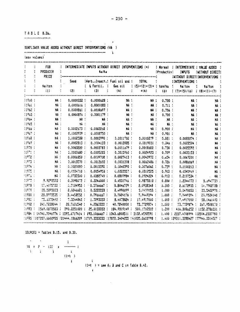
- 250 -

T A 8 L E £.36.

SUNFLOWER VALUE ADDED WITHOUT DIRECT INTERVENTIONS (VA )

FOB INTERMEDIATE INPUTS VITHOUT DIRECT INTERVENTIONS (I) Normal 1 INTERMEDIATE VALUE ADDEDPRODUCER :a/ha :Productiv: INPUTS :WITHOUT DIRECT:PRICE ---- ------- ……-------- -- -------- --- ------------- ---- :WITIWOUT DIRECT:INTERVENTIONS

. ' Seed !Herb.,Insect.: Fuel oil and TOTAL :INTERVENTIONStalto^n L ' t Fertil. 6as oil : (5)=(21+(3fl. ton/ha Salton I S/ton

(2) 13) (4) f+f) : ( : (7)=l5)/(6) ,(8)z l)-17)-------------------- ------------------------------------------------------------- …----------------…------------

'1?60 NA 0.0000332 : 0.0000628 NA NA 0.700 MA NAt I?VI IMNA : 0,0000616 t 0.0001083 NA NA 0.711: NA: A1962 NA 0-0000861 0.0000697 MA MA 0.706 NA MA

:1963 : NA 0.0000876 ' 0.0001179 NA N NA : 0.700 NA I NA:1964: NA: NAY NA A A NA' NA MA MA1965: M aY MA A NA: NA N,A NA MA:'1966 NA 0.0002i73 0.0002268 NA NA , 0.900 : NA: HA1i967 NA 0.0002939 0.0002750 1 NA I NA 0.901 N HA NA,1968 N A 0.00025s88 0.0003990 , 0.0011?02 0.0013279 0.921 0.0022274 NA:1969 NA 0.0002913 0.2004133 0.0012085 O.0019031 2.346 , 0.002250 : NMA:197,0 NA 0.0003220 1 0.0003783 1 0.0011679 : 0.00186E2 : 0.?30 1 0.0025r92 : NA

37', 'MNA C2.003680 : 0.0005293 0 -.0,1S960 1 0.0024923 : 0.709 : 0.0035153 NA!lq72 N ,A 0 O0OOOs6o : 0.00097A8 : 0.0027413 , 0.0043972 0.654 a.0067201 NA:!9"3 ;MNA : 0.0019570 0.001 603 1 0.0031208 1 0.0061486 : 0.726 : 0.0086069 M NA:1974 N mA ' 0.2'Oc00Ov0 1 0.001155X92 0.004O30 0 00076062 1 0.759 1 0.0100213 NA1975' 'MNA 0.2334110 : 0.0054953 C.022:257 0.0312542 : O.i93 : 0.03459si NA

NA : .07332500 0.0382740 1 0.0807994 0.1924224 0.?13 : 0.2107534 YA' 1?-7 : 9.9202503 1 0.3090ss2 1 0.2246000 0.4531746 0.9859813 0.800 : 1,2344773 S9. 097730.:1973 ' I7075722 0.7124952 I 0.5766667 I 0.046720 2.0939343 0 v.30O 2.6172935 ' i4.7?02T3821177 2S9.!33023 2.0246621 1.5233333 2.49900s9 5,Y!70053 1.000 5.0470053 23.5422970 ,:1930 : 29.S?73535 3.4454852 : 0.7366i667 : 3.7024176 7 7.?449394 1.000 1 7.9449394 B Ej.952414011931 75I6373492 ' 7.3f44243 1 1.7293333 1 8.4078824 1 17.4917000 1.000 : 174917000 5.1461493sa92 '341.723S044 2 29.626S540 : 4.2363333 1 40.7240000 : 73.77,2974 1 1.000 : 73.7,72974 2 267.9509170

:1?33 1569.0872533 1 290.2251020 : 25.3133333 184.9319149 500.17035021 1.200 416.308625g2 1152.2786331:1984 : 14741.7046774 1595.6717414 19 93.1066667 1343.6808511 1 3132.4S92c91 : 1.400 2237.4708994 :12504.2337780;1995 :107257.6602955 :21444.1366209 :1719.3333333 17872.3404255 :41035.3603798: 1.400 :29311.3298427 :77946.331452171

SOURCES Tables 3.15. and 2.30.

, IVA~~~~~( p ---- - -- I

I+t )

ll+t ) ;ee A. B and C in Table 3.42.

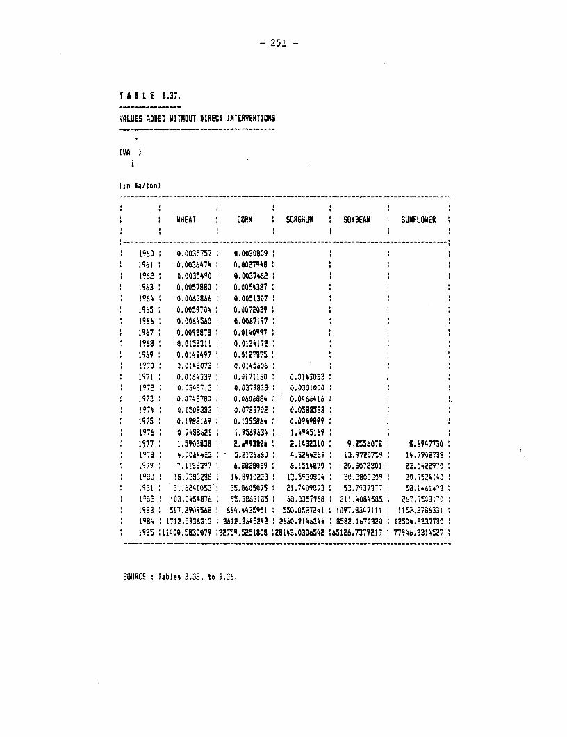
- 251 -

T A D L E B.37.

VALUES ADDED WiTHOUT DIRECT INTERVENTIOKS

(VA

WHEAT CORN ISORGHUM I SOYBEAN SUNFLOUER

1960 0.0035757 0.0030809 1961 0.0036474 0.00279*91962 0.0035490 o .0037&621963 0.0057880 0.00543871964 0.0063866 0.0051307

1fl,8 AAAC(211A I AAA?,A,a

1970 0.0142031 0.01241760

* 1971 0.016433? 0.0171!80 0.0143033* 1972 0.03487,13 0.0379338 0.0301000* 1973 0.37,48780 0.0606884 0.0466416* 1974 0.1508383 0.0783702 0.0!83598

1975 0.1982169 0.!35.5864 0.0949899* 1976 0 .748862!1 1.9569634 1.49451691977 1.5903838 2.6993886 2.1432310 9.2556078 8.694773019178 4.70644,23 5.2136o6O 4.324426- -i3.37203759 I 14.7902739

i 1979 1.11S8397 6.8828039 1 6.1S14870 20.3072301 23.5422,97A* 920 15.7233285 48902 13.5930S04 2.830 0 544* 1981 21.6241053'1 25.8605075 .1 21.7,409373 53.79373`7 58.14614?3* 1992 103.0454876 ?q5.39631a5 63.03571968 211.4084585 7b.?!08170

1983 517.2909568 1664.443!951 1 !50.0e587241 ! 097.83471111 II152,217163311984 1712.5936313 3612.3645242 ; 6640.9146344 8582.1671320 12504.2237"301995 !11400.5830079 :32759 .52SI808 :28143.0306542 165126.73.79217 1 77946.33145.27

SOURCE Tables 8.32. to 3.36.

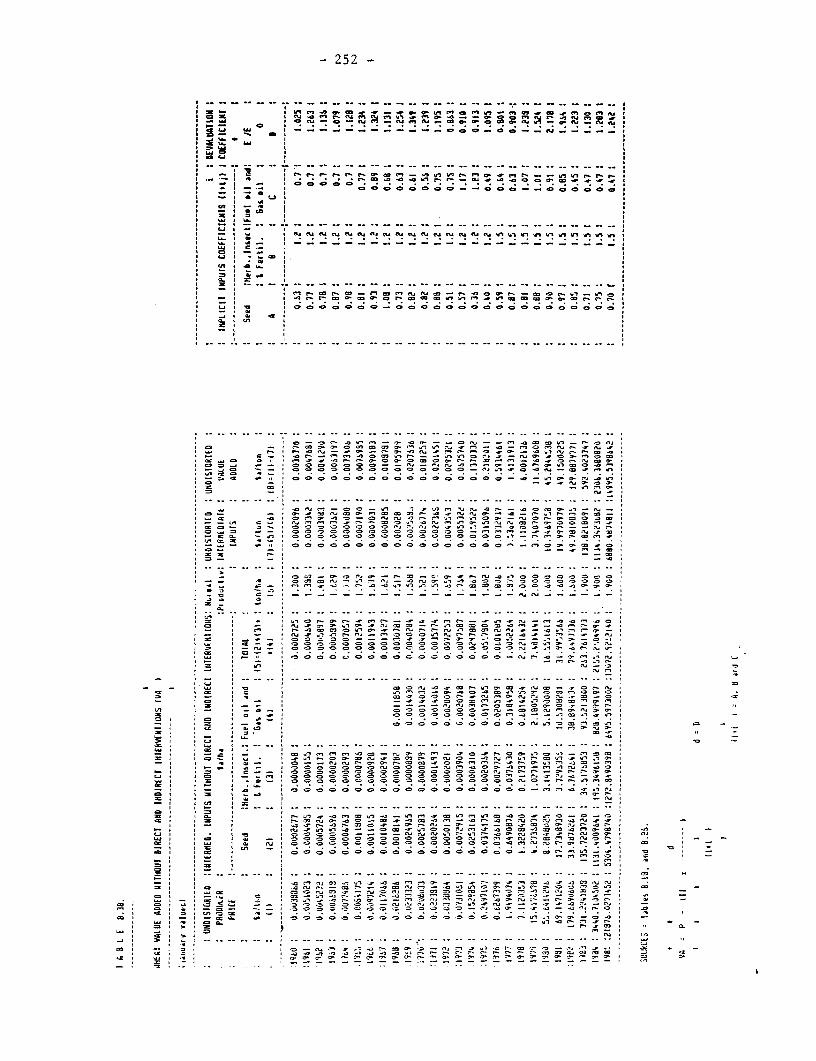
- 252 -

a aa - -a a

aM - 000.0o-a.,0Ia *..ja�a I

I U. SM I* �ajaa a* aI aLa a aa.----- aa - a C I � aa � � aa - I - 00000.a - a a 000O0000�0@0�0C00C0 aI - a toaa a * I a* ma -a -a SW aa a a a

a - a…………aa �J a - a- a a njC4fljUfljaUflaCUaaO.aa'afl.qu84njn��,n,n,aflv,n,v,a,r,

a a.aI '- I -- a…a

a La -� a.a a *na Ia ma a�a. aa a - Ia C aa �. ar aa a----aa a a � a

- a a .O7a.r- aOOo a n-n-r..aa.ea. a* -a La a-U I 0000 OC04-000000000000000000

a. Ian aa C S S

I 0-n-a-. -ag-ar--n- C0-�0n4 -- r-�o00�aa-oa..aC - a--Oat-n-C 00 oaIanwI a..jsa--a-a-a 0a-flata. 7a* a-- I 7- .On.a - 5. �C- 5.-fl n.j - C., a--a-% a -� - -0 &I n.j a-. aa. -aI - C - -at-- �a-0Ona--��aa-aflo7ho--a'an-.r0o.a-ooI OGO Ga I fl-P -r -ant-. a- n-On- 00 n-a--a-OS-Ca-a -a 00.0 .- '00000 00fl.J-t'J n.j0a,-n--Ca- a- 0-0a,

- a - - ' 0 0 0 0 0 0 0 0 0 0 0 0 0 0 - $a a -C 0 4 fl.I - - 541 01* aCaCO* � - aS a 000COO000000CO00C-SO0O-nj�C0

0 - - - 'an-an-2 = - a�� a-n-0 - I na-s.

* .4ttgej -00 -0-, C s0a aata 07.- .C0O5.fl -ala-

* La C Cl Ca-,- 00-0S'an.j0a- C.Ia.15000. -naor--O.CO-aZm II - -an C- alaa-sa-a-.rra.a- On-a, -ca-ar-fl -ananae- a- GOOr-, .PI

0 I 0-S-0

00000I'ananaala *flC -a-GaO .da---nar�.S C.� 0 -- I 00000000000000- flfla-.mt o-oaa.j *oa* - CO Ca, 0000000000000 000o.S�a-a-o.a-.Oa-.

* -La- - *a , CCOCCCOCO00000000n-a-On-n-=.OCX

I S 0o,�5-0n.jn-�S-.in�n-.rea.atJ.naS0eO00On-O-- '0010 �'��fla-n �0a12 n-wa C C On-a- 00000000- S - Cia-S r .Oa-. -a -. � fljaaCat--000o0 -40 COn.@

- . � C...…fl.jSlj* C C 0

C - -

= I C a-,0a-5.a--.�.aa.a-..�.r.s -� a--�.Sa-5.en.j-a--nCa-COI C I - S n.J P 5 0 CS 0.t flJ 00 a--v-a 0000- I 54' r--000a'5.-r(a.74t--a- nasa00IraatSa. -0&'-,fln- -

- a - a n.j-t�afla-�fla �a-O0 OattSaaa-r-.S- �.fla Cs-fla-as na.

= a - I 00.. =…0*. .laS. -0.5,S a a -. 00000000000000a..jaCI .a0C�.jafla�$0 SC �alaa- I �Sta� 5 0000000000000 OOOOOna .5.-,- .0S--a.O-

a a C�.L.a H - a S 00000000000000000S-a--007',flj ,

0 a n.j-az, 0

a a a a = a aCSala- 5.00-aOra.ran-OOa-000* � -0

C I - -.-. a.flafla 00-000-7-n-a- aan a - 0000000 naOOaC.0n400 I2 a a a - 0000000007 -�o--..-aov-a.ra-a a

- I I = I - S 000 OOa-3000

00aaa&,00a-COafl S a - --.4 a GaaS -a-an- n.j 4-a2. 4. a 0-Pa 55 -Laa a a - a a� a -c

- a a -� a - a OaflaI7Ce, -an0-CS.j0n-a'-'� .50..ra--On.ajIo -. )C0C a a a a . a . ci a-. 000 n.j *0 On ala. n-n.j 0ai n.jca a-at-. 00-tO wan-- a .. S 0-�fl.jna7--O-0a-�O0.S 0 Or-a- -- a-a-- OaaiSfl 00a,

a -- £ n - 5000 OOOOC'.j0O 0-n.j an .00 0aC00- a 0 a c�a 000000000000 COOII.jI12a-a--t--07-a-00 aLa a a C a - a-, a O0o000000000O0000S-¶�C'a0-I'a.O- JP a

0 a -na-a. a 0000000000000000075J0-t--a-flC'1O- a - a a 0000000000000000 C-ZO-a-m-o -a- a

74 a

Ca a S I a-n-a-XI a a as a - a alt, a =05 '0 aa, a a.. a a a-.aaC.a��on,aa1..3��fla ra.a-,4'CO.OOSaa-,0-O-O

a a C a , a--4ln.j0 .o0

-a0..0

= .,a-.O7-Ca- naS-alJa-.OaCj.a-.a- a -a - a a .o.t�a. -fla--Co .a-�0r-�a'a 5.-Oo- 00nJ7�Ca-

= a a a a n.j.,aOWa ... 00.0

00flJC.,..tCe.OOOCa-O0 a -.0 aLa a a . a 'a a a 0…n.j a-.. n.j wa a-- an a-- -o n- Ca.j a- -r -� a-. "a o a- t a-aSM a 0 as - ' 0 0 0 0 0 00000000051aa-a--Pnaa-fl0Ca.10t-- a . - -O a a L.a a as n.j a 0 0o0 0 0 0 0000000000flnjn.ja-0a-.r-a- a 0 a -- a a C am -...... 0 -o a a a a a 000000000000000 0o0�-SOr-C,a� a 0 -- a a .0 a a -a.,a-O a -

a a a a - - en a 'SO I a C a a - a-, a

= a a-a-C

- a a a Onan anan.r-ea..aa-a-n- .5-4-a-- n--ranO.0-t-aa O,nana ao , 'a a -on-sa-- - Oa-.,On.aaC- CCfl0 1 .�a-S.-aa-n-00a.wa a 0 -a Iw en 0n.jos.r-n.j-Za.aaa 00CC rn-a--an-a- -ann.a.aa.0Owa Pa -0 a - a -� C a-an.0a-.Pa-..0a-SOt-'0 a-C--a-a 0-4.7 -n--a-a a .0 -

a L.a a a C .jLaa .4 -fla- Sf5 - - a- Ca-a '� a- ala n-C oasaa-.�a--o.s -at a-. a as -0 Ca 0a COLa -- .0.00000-0 a..naa'.jatI'a ,a-n.j----a--e. .Oau.na a -S-IS Ca 4, 0 -- - a C00ZOOOOaZ Z0-.0ac)0-S�a..aO -� -0 --.. j 'Car-C a .0

a a. = ' afloat an.---S a= a a - a a0. - a 00O0C0O000O00.0C00-a-an.a00-a0�a2 a -

a sass a a., a -aslO a-. a- -r a-. - -a CS at a a * -a-. 0'01 a aS 0.

.0 a .s a a 0 F an - aa a a - a CIa aa a- a - a----aa - a .. a a Ci

01 - = a a 0 -��S-a ... a .0a--0 -� -ala an.a-.S.oa-.Caa-, -a.aCflr' a .4 -.4 a 4 a S a a, -a-a -a, .. j-a an-an-S a--a-a- 7-7-a-a- a-- a-- C� 0 Onn.j 000 .0 0

.4 a aJ.j a a a a,- n-ca-n- - C'. n--al--n-0 a�-n-n- ca- a-ca-a-n-n-n-on- a'.O a 0 a-a 0a - S a…a

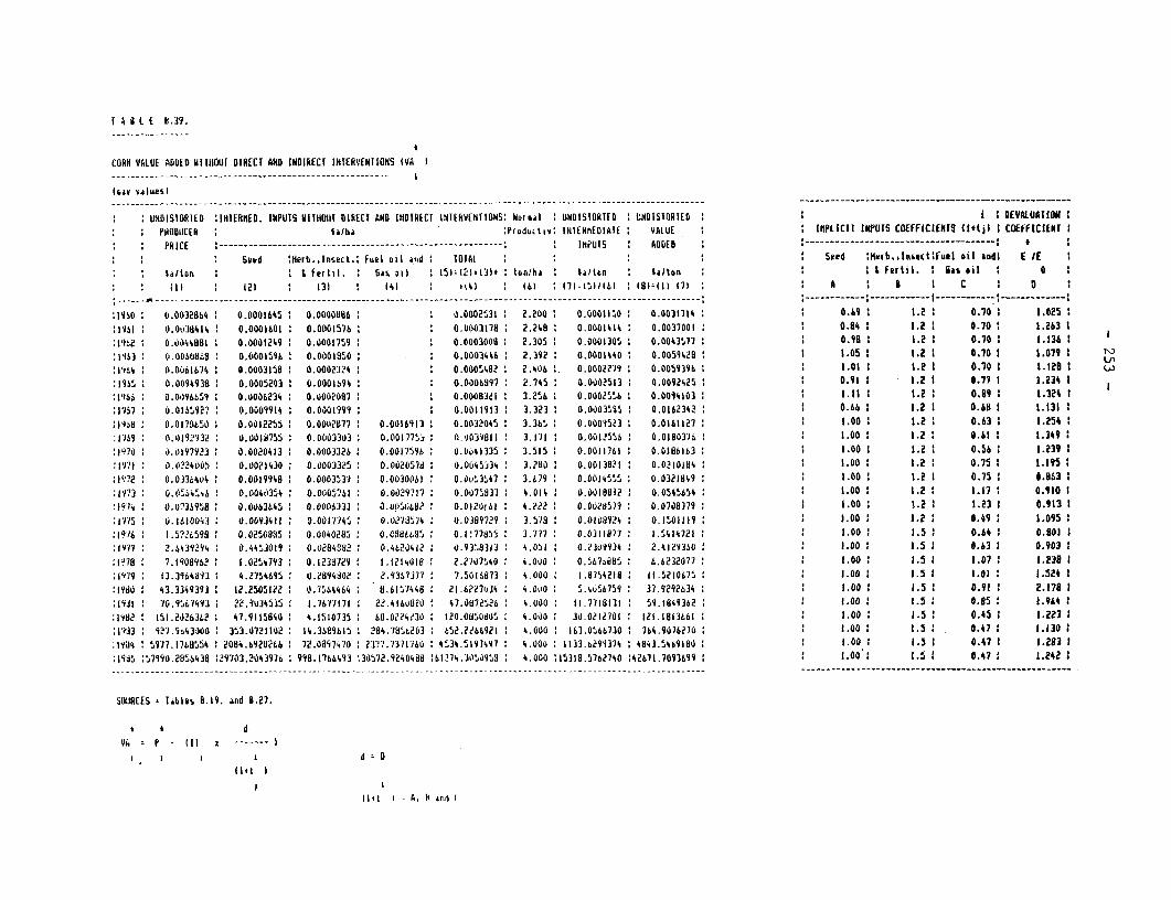
I A a L E k.39.

CORN VALUE ADDED WITHOUr DIRECT AND INoIRECt ITERvEINlloNS (VA I

it.aw value,)- - - - - - - - - - - -- - - - - - - - - - - - -

: : UNOISIORIED :INlERnED. INPUIS WIIHOUT DIRECT AND INDIIRECT IIEI4OENTIOWS4 k4orsaIl 'UNDIS4ORTED IDISIORIED I i REVALUATION 4

: : PaOOuCER : laha :Ptcducttv: IlNIE"RtED4AIE VALUE 4 : InPLICIT INPUTS COEFFICIENTS (I.t4 I COEFFICIENT I

PRICE ---------------------------------------------------------- : INPUTS ADDED -------------------------------------- I :

Seed Fur,I sett.4 fuel Dl alid (Al : : Seed ierb.,Insuct4Full oil and: E IE

: Rd/toO : : I fertil.: Gaas all : 5I4S.31' tooiha S aton : Salon : L fertil. I as oil : 0 :

: : 4 { 12 : 4:34 : 141 , 44) (64 : l7l~454I46l : 494~4l 13-74(,116 A f CI : C

1950 : 0.0032864 0.0001645 0.0000886 0.0002S31 : 2.200 0.0001150 0.0031714 0.69 : 1.2 0.70 I 1.025

4I95I : .6v384I4 0.0001601 0.0001676 0,(1031784 2.248 0.0001414 0.0037001 ' 0.84 4.2 0.70I 1.263 1

I1162 0.06144081 0.0001249 0.0001759 : 0.000300a: 2.305 0.000130.: 0.0043577: 0.99 I 1.2 I 0.70 : 1.136 1

44963: Q4s0.0060803 0.0004 0.00019S : 0.0003446 2,392 0.0001(440 0.0059428 : 1.05 I.2 0.70 1 1.079 1 :4 P.O4 .0(1667S4 0.0003158 0.0002324 0.0005.82 2.06b 0.0002279 0.0059396: 1.04I 1.2 1 0.70 1 4.121 1t L

41496 0.0094938 . 0.0005203 4 0.0004694, 0.0006997 2.745 0.0002513: 0.0092425 : 0.91 1 (.2 1 0.77 1 1.234 1 4:449S4 0.0096b59 0.0006234: 0.o0020W7 : 0.0008321 3.256 4 0.0002'6:6 0.0094103: 1.11 1 .2 I 0.81 4 1.324 441467 0.0105927: 0.0009914: 0.0007999 : 0.0011913 3.323 0.0003692: 0.0162344 o.L66 1.2: 0.68 I 1.131

)449A 0.01700:(4 0.0042255: 0.004,2?877 0.0046943 : 0.0032045 3.366 0,0009523 0.0161127 4 .00 1.2 i 0.63 1.254 :4709 0.0192732: 0.00407556 0.0003303 0.001775. I 0.7039811 3.171: 0.001556 4 0.019037% : i (.00 1.24 0.61 1.349 I:I47() .i.0197923 0.0020413 0.0003326 0.0047596 o.W41335 3.515: 0.0044764 0.0186163: 1.00 .2 0.56 1.239 I:4974 4 0.4224S105 0.0021430 0.0003325 0.0020570d 0.0645334: 3.20 4 0.0013024 0.02)10184: 1.80 1.2 0.75 : I.I95:1'!22 0.03640411 0.0019940: 0.0003531: 0.003006(: 0.4 to ' 3i7 3.079: 0 .0945 0.0324049 1.00 1.2 : 0.75 0.863:

:4973 0.05P4ii 4: 0.0040354 0.0005Sl 4 0.0029247 0.007-833: 4.014 4 0.0048082 0.0545654: 1.00 I 4.2 1 .17 0.910 II ?7; 0.023A9584s 0.0063645 4 006333 o0. 0050682 0.0120464 4.222: 0.00205)9 0.0708379 4i.00 1.2 1.23 1 0.913 1

:175: 4 .6l100q3 0.0093411: 0.0017746 0.0273074 0.0389729: 3 .5731 4 0.008924 4 0.1401119 : 1.004 1.2 : 0.49 14.095: I 4 :6 1.57059894 0.02s0osss: 0.00402s-: 0.088068 0.1!77?055 3.777 4 0.03111?77 1 .5414721 : 1.00 4.5 0.64 0.801 t:177 : e2.6439294 0.4453019 0.02840.82 0.462v412 : 0.933133 4.051 4 0.2307934: 2.4129360 4.00 4 1.5 t 0.63 t 0.903 t

:fo7 7.jq06sY,2 i.025i793 0.4238729: 1.4244010 2.7107,40: 4.000 0-56758854 6.6232077 : 1.00 4.5 I 1.07 t 1.238 t

("1,79 13.3q6473 4 4.27546954 0.2994SO24 2.1307377: 7.5016073 4 4.000 1.8754291 11.5210675 : 4.00 1.5 t 1.01 I 1.524 1

449d04 43.33i9393 I 2.2505422, 0.7504464 8.6'5/44946 24.6?271J34 4i.0v0 00 5.4u567S9 37.9292634 : 1.00 t 1.5 t 0.94I 2.178 t:19314 70.95C7493 ee.s43s3 s: 1.7677171: 22.4416020H 47.0872526 4.0400 4 11.77181314 4 9.4899362 1.00 : 14.5 O 0.85 1.964 I:19S2 451.20263W24 47.9144540 4.1510735: 68.0224?30 5 20.0s,00Pdo 4.000 30.02O2701 424.14136 i4 1.00 1.5 t 0.45 1.223 1

:1 33 927.5643M00 353.0721102 14.3695 7 .23 652.266`924: 4.000 1 463.05667304 764.9076270 : 1.00 4.54 0.47 4.430 t.IYU4: 5977.4768554: 2084.69292L6 4 72.08974704 23?7.7371760 4 3§.5l974q7 4.00 1133.6299374 4843.546180 :1.00 :1.5 I 0.47 t 1.283 t;19$ :7s990.28564308 :29703.2043976 : 998.4766493 :30572.9240498 :61474.30509.9 4.000 441348.5762740 :42671.7093699s 1.004 1.5 0.47 1.242 4

SlltRCES lables 8.49. and 8.27.

t *t d

'A. P - 1 ------ I

lilt 1

4~~~~1+ Ih8 n

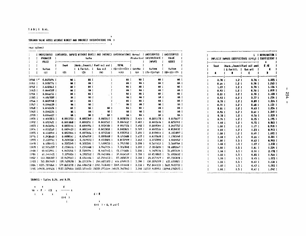
I A hI 8.40.

S0MEMOU VALUE 68CDE WiI TOU! DIRECT AND INDIRECT INTERVENIIONS (VA*

* INDISIORJED 21N1EP.lIED. INPIJIS UI[IHIJJ DIHECi AND INDIRECi INIEAV(NIONS: wel :. UNDISIORTID UNDISIORIED II DEVALUATION I* 2 PAOIUCER 2 iSha 2Pioductiv: INIERAMAIAE 2 VALUE 2IIIPLICIT INPUTS COEFFICIENTS li1tt. COEFFICIENT I* 2 PRICE ------- ------------------------ IePUIS ADDED ---------------- 1 ---- I*

* . ~~~~~ ~~~Seed :Merb.-Inlect.1 fuel *aI1 ar.d TOIAL I Seed Iffers.,iussect.FurI oil and: E /1 I* 2 IdUOA 2 2 & Feglal. 2 ~~~~~~~Ga asIl (51zQa.I3I. 2aih la/too Salton I F Prtil. 2Gas oil 0 1

M I 2 21 2. (31 2 41 a4 1 O lb)6 2 7('Wibl/6 2 l3l.lM-17) 2 A I C I 3 2

216 .02549412N NA 2. NA MA NA M A 20.70 21.2 It 0.70 1.025 M111 0.00330?71 MA 2NA 2 NA 2 NA 2NA K A 2 .114 I!2 2 0.70 21.113 12I'I162 0.6032063 M A M A 2NA 2 NA M A MA 2 1.07 I.2 1 0.70 2 .136 a1403 6 .0u44589l NA 2NA 2 NA NA NA 2NA 22 0.93 21.2 2 0.70 21.079 I

21064 2 0.0 ;6155 NA M A 2 NA M A M A 2NA 2 0.11 I 1.R 0.70 1 1.123 I 'I16 0 .0067899 M A 2NA i NA 2 NA NA M A 2 0.93 I.? 1 0.77 I .234 I 1219%4 0.0009Th8 M A M A M A M A 2NA NA 22 0.7111 I .2 10.89 :1.3234 I

2972 0.010069 M A " A M A 2 NA 2 NA 2NA 0 2 ai 1.2 1 0.63 1.131 MA9~ 2 .014WbO NA M A 2 NA 2NA NA 2NA " A : 0.81 Ile2 0.63 21.234 1tI9B0 0. 014V531 2NA IINA 2NA " A 2 NA 2NA 2NA 22 0.96 1.2 20.61 I 1.3492:19,0 21 0.0146457 M A 2NA 2NA 2NA M A M A 2NA 22 0.78 21.2 20.56 I 1.239 121971 2 .01378.15 0.0013753 2 0.0002349 2 0.002?617 0.0038720 2 3.hLk 0.0011178 2 0.0176677 22 0.74 21.12 0.75 21.195 1:1972 0.0627421 0.0011868 2 0.0003251 0.0032522 0.0047632 2 3.483 0.0013676 0.0253745 22 1.00 21.2 2. 0.75 20.863 I21973 6 .6i36096 2 0.0028146 2 0.0004996 2 0.0034594 2 0 0067726 2 3.6922 0.0018344 2 0.041775?2 1.00 I 1.2 21.17 2 .9104.:297,14 2 0.055125,69 2 0.0024433 2 0.0005549 2 0.005,3838 0.0083821 3.719 2 0.00/2236 2 0.053003?22 1.00 21.2 2 .23 2 .913 1:1M7 0.1160911 2 0.003?044 0.0073406 .0.0273500 2 0.0333950 2 3.691 2 0.0104014 0.105S8M 1.00 21.2 2 0.49 21.0952219476 2 .203WO0 0.00880541 2 0.0246939 2 0.0370008 0.1213'i88 3.637 2 0.0333620 1.1705040 22 1.00 21.5 2 0.64 20.1901221977 2 2.1337741 2 0.2034530 2 0.1519573 2 0.4573325 0.9132929 2 3.642 2 0.2232890 1.910480522 1.00 21.5 20.63 2 0.903 2:Wa8 6.1281415 2 .3525549 2 0.3?235,01 2 1.10233 2 1.7457/83 2 3.00 2 0.516116511 2 5.5669764 2 1.00 1 1.5 1 1.07 2 .239 I:14119 12.q`l56337 2 2.1330116 1.2371468 3.94o2?24 I 7.3103008 2 3.20f3 2.280630 ; 10.bMW64 2 .00 2 1.5 21 2.01 2 .5242lI;do2 40.4111.29ll 4.0421?46 2 2.7324q94 8.4027~45 I 151713604 2 3.?00 2 .1423236 I 35.6923634 I 1.00 I 1.5 20.91 I 2.178211931 2 61.1441'u35 7.3291051 2 4.392251?2 20.k4421006 32.16345069 2 3200 2 10.0510903 2 51.0930632 21.00 I 1.5 20.85 2. 1.9642

:193? 113.7304307 2 12.96395i3 2 .1264406 2 62.2`12,L53 2 8.3028572 Moo20 26,05714?9 87.7312878 22 1.00 2 1.5 20.45 2. 1.2232;1/33 27b5.8917419 2119.76205911 2 36.2?13194 2260.687023 2416.6709115 2 3200 2130.2096599 2635.6720821 22 1.00 2. 1.5 20.47 2 .t30 1

114 457-.73740t,4 2 77.8653?78 2 266.4900258 2 202.74AoL83 23049.1011618 2 3.200 2952.8M4131 23622.9§33733 22 1.00 21.5 20.47 21.283 :i'i1s !.97.622 9137.537i866 22653.5276433 :26330.2756544 :40121.3407ki3 3.200 HM207.9183991 236940.2702675 22 1.00, 21.5 2 0.47 1 1.2422

ST II( m1bles 8.?0. and 8.28.

d

I a & a~~~~~~~ d =

llt I zA. I st.a C

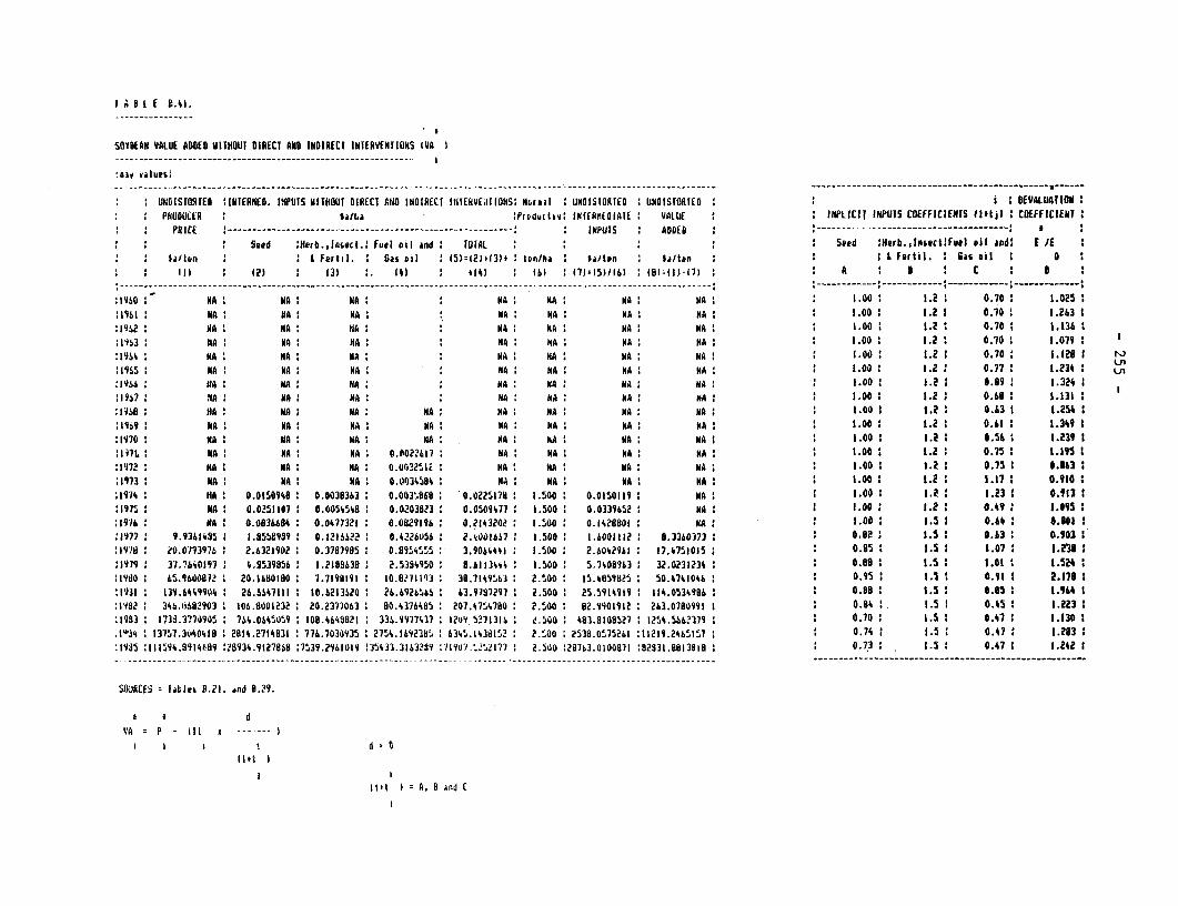
I A i. E 8.45.

SOyBEAN VALUE ADDED VlITHIOUT DIRECT AND INDIRECT INTERVENTIONS IVA

tell vaiuW~

* NwD(IsORIED IINTIERNED. INPUTS WITHOUT DIRECT MIDO INDIRECT IIIIERVEdtIONS: Notmaa : UNDISIORIED UNDISIORfIlD I 1 DEVALUATION* : PRODUCER WhIa :PrifutIIv: INIERtIEOIA1E : A : I IPLICIT INPUTS COEFFICIENTS lijt)I COEFFICIENT*PRICE ------------------------------- INPUiS ADDED ----- -------------- 1

seed I1Ierb.,Inisect.: fuel oil and i I I : Seed 'Norb.,Insect:FulI oil and', E IfED~~IIun I : & FeftIll. I B~~~as ea 502)I) en6 Oe Dlo L fortil. fias oil 10 IIII 1 I?) 1 (3) 1. (4) 1 ~~~4) ) 1 ):5)161 0 7~5l6 D1I1)-171 AB I £ 1 0

1960 MA NA MA MA MA MA MA1 1.00 1.2 I0.70 1.026:1962 N NA MA 1. NA NA NA MA 1.00 1.2 07 1 OO1.1361

:1965 : ~~~NA NA I A MA M A INA M A 1 1.00 1I.? 0.77 1 1.134U610 "A NA I NA M A : NA M A " A * 1.00 11.2 1 0.79 1.324

:l9S4 NA MA MA H A NA INA :NA 1 1.00 1.2 10.680 1.13) 1

Il9i9 NA IM MA NA "A NA MA NA , 1.001 1.2 0.77 1.2349 L:1970 1 A A NA NA NA NA NA NA . 1.00 1 I.2 0.569 1.3234

I1S MA MA: N .D~I A NA NA M A , 1.00 I 1.2 0.75 I .131:II97s OA IM NA 0.321 I NA MAM NA MA I NA , 1.00 1.2 0.75 0.363 119739 NA NA NA M .049 A NA NA MA NA 1.00 1I.e .1 0.9t103i 1:lq7 M N M IIA MA.104 .03331 003~~ .257 NA150 NA.0501 MA 1.00 11.2 I:.5 1.23 1093 111975 NA MA.05I0 NA.04581 0.~3 0.0 .050194NA NA150 NA.o365 MA I* 1.00 11.2 1 0.795 1.095 I

:191 1 A 1 .08668 I 00473251 0.8299MA NA1420 NA.0 .42811N 1.00 1.5 I 0.415 0.wa 3.1977 NA.9613 NA.5599 0.0012Stt6IZ NA0567: .0 MA.011 .3632:09 .5106 .0

I11 NA0739t M.3 A90 NA.3898 0.00489555I 396411 .0 .026 MA174NA NA NA 10.9 1.2 1.07 0 .2'38 :1979 1 7.4 A9 0 .01SO980 0 .20383638 : .05394950 1 8.6123447 1.500 005.708193 MA20313 * 08 1. 5 1I. 1.013 0.524 :197S NA900i 1 0.16021807 0.0098191 1 0.D020393 I 038.014776 i .500 05.0359925 MA0441 0.511. 5 I. 0.491 2.071 :1936 NA396490 0.08668471 1 0.04773621 0.126.9M6 0 6.921920 1 .500 1 2.914988 1 MA.0346 .0.8 1.5 0.85 1 .9601

: 1 98 1 346.068239'I tD63210022 : 0.23730793 1 80.84376485 3.907.47478 12.500 1 2.bO01912 17263.75809151 0.84 1.5 1 0.4 I 1.2 1,

:1983 :1730.3?70905 1 74.064'509 1108.46%3821 133S.9977437 112v9 5?7131S 1 tl)O 483.8108527 : 254k.5662337 6 .70 1.5 10.47 11.130 1; 1 I3 3757.3t,40418 :2814.271431 1776.7030935 1 754.1692365 634i.14381,2 ? .'~00 2538.05715261 :11211.2465,157 0.74 1.5 0.47 11.283

:1935 I11I594,9`1I4M9 2,8934.9127868 :,7539.2961019 135433.3163289 :107l9-.'~ 5.,277 I 2.500 :29763.0100871 :82931.8813189 0.713 :1.5 1 0.47 1 1.242 I…-- - - - - - - - - - - - -- - - - - - - - - - - - - - -- - - - - -…-- - - - - - -- - - - - - - - - - - - - - --- - - - - - - - - - -…--- - - - - - - - - - . . . .

SWJAME aTien 11.21. 4nd 8.29.

ft * 0~~~~~VA P M x - -----

I I 1 I 0.1~~~~~~~lt I= .9 ti

I ~~~~~~~~~~~~~~~~~~~~~~I

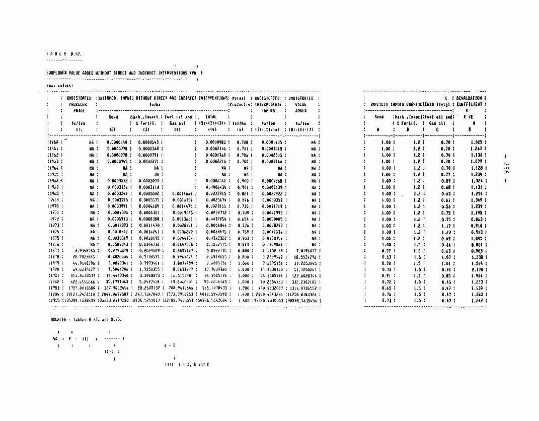
I A 8 L E 0.42.

SUNFLOWER VALUE ADDED WIWHOUI DIRECT AND ItDIRMEC INTFRVENI IONS -(VA

* .UNDISIS0TEO :INJERED. INPUTS AITNOUT DIRECI ANiD INDIRCEC INIMRENITONS: Nbriol 2 UNDISIORTED UNT1IONIOED 2 DBEVALUATION I* PROO0-CER Wh Produtie2 tiNI ERM DAlf VALUE I 1P2.ICII INPUTS COEFFICIENTS Iltj) 2 COEfFICIMIN . PRiICE ----------- ---------------------- ADDED ------ ---------------- I* ~~~~~ ~~~~~Seed MtIrb-1neEl.t.2 fuel t.0 uid J OIAL 21 * Seed 2Herb..Ins*cIlFu&I oil and: I JE* .i./I~~~~~~~~~~n I 1 Fertil. Gas~ (,II (52~1221(31 toolh la/on W aton * I fortht. I Bee si6t 0 * * Ii, ta~~~~~~(2 (31 (42 t(41 2 62 01(1'15I26 2 2DjhM-217 AI 2. C 3 1

:156tl ~~NA 2 0.0000340 2 0.0000643 2 0.0000983 0.700 0.0001405 NA 2 1.00 21.2 2 0.70 1.025 iMl6 NA I 0.0000198 2. 0.0001368 2. 0 .0001146 0.711 2 0.0003019 NA I2 1.00 1 .2 0.70 21.263 :1962 ~~NA 0.0000978 2 0.0000791 0.0001769 0.706 0.0002505 NA 1.00 I .2 0.70 1 1.13i2I93 NA 0.0000945 2 0.00012721 0.0002216 : 0,700 2 0.0003166 2NA 2 1.00 21.2 20.70 21.0792:196; ll~~A 11NA 2 22 NA NA 2NA NA 22 1.00 21.2 2 0.70 21.128 2LItI90.15 NA NA NA NA NA 2NA 2NA 2 .00 21.2 24 0.77 21.234 Ia:196L .4 NA 0.0003538 2 0.0003003 2 0.0006541 0.900 0.0001268 NA 22 1.00 21.2 2 0.89 21.324 2220 ,;, NA 0.0003324 2 0.0003120 I 0.0006434 0.901 2 0.0001238 h A 2 1.00 21.2 20.69 I 1.131221969 NA 2 0.0003244 2 0.0005002 2 0.0014669 0 .o02?915 08021 2 0.00219,22 2NA 22 1.00 1.2I.? 0.63 21.2542:lsi,iNA 0.0003795 2 0.0005575 MOW00634 0.0025674 2 0.846 0.0030359 2 NA 22 1.00 21.2 2 0.61 1.3492:1970 2NA 2 0.0003991 2 0.0004689 2 0.0014475 0.00231255 0.730 2 0.0031711 M A 2 1.00 24 1.2 20.56 21.2392:021I NA 2 0.0004396 2 0.0006311 2 0.0019065 0.0029772 : 0.709 2 0.0041992 2NA 2 1.00 21.2 20.75 2 .1952219072 M A 0.000S913 2 0.0000380 0.0023~662 0.00371954 0.654 2. 0.005,8005 2NA 21.00 21.2 0.75 20.863221I9?73 MA 0.0016893 2 0.0011470 0.0028431 2 0.0056644 2 0.726 2 0.0078297 NA 2 1.00 2 .2 1 .17 20.910222974 M A 0.0018341 0.0014241 2 0.0036092 0.0069415 0.759 2 0.00925,3i NA i 2 .00 21.2 2 .23 20.9132:1975 MA 2 0.0033009 2 0.0060190 0.024420. 0.12342322 2 0.903 0.03718254 2NA 22 1.00 2. 1.2 20.4? 1.0952:29?6 NA 2 0.0507043 2 0.0306736 2 .0647536 0.J!I;?115, 0.913 2 0.1bH9064 2 NA 22 1.00 1.5 20.64 20.801222: I 2?1 3.93407452 0.2398899 2 0.2039109 2 0.40941221 0.2292235 2 0.1100 2 .2252 .69 2 .81960772 0.77 I 1.5 20.63 1 0.9032220,!" 2 12.9192365 0.118200042 0.71305117 0.99612074 2.4199655 2 0.8002 3.23M969 1 0.5524296 2 .S7 1.5 1 .07 2 61.3 2:2979 44.91402196 3.0034134 0.7973462 3.8004409 .0.6 lO0vO2 1.60 1515 37.2253145 22 0.70 2 .5 1.01 21.524 Iq0 y6l.2J0627 7.5046206 8 .305 .063313?7 1 ?206 .000 1 1.3.23(160 S1.7200263 2 0.76 2 .5 20.92 2.178221" 15.J53 4.4462340 2 3.3960073 2 65592: 34.M18594 1.000 2 34.35052194 21222.6028344 I 0.91 1.5 20.95 2.9642:230 2 22 be I 35.2172133 2 5.24?22458 2 49.80~0331 2 01~46 .000 2 9O.2242M 332.2302203 22 0.122 1.5 20.45 21.2,23 2.:1?53 2 72.0061590 2 327.9052454 228.26031332 208.9W4274 565.2107433 1 .200 2470.9232027 2 390065 0.65 21.5 2 0.41 2 1.130 I21994 172122.242652 2t 2047.0795,81 2 47.7342048 2 2723.7198963 24028.59q4j598 2 .~00 2 00.2 L24 2 2 O5.0293326 22 0.76 21.5 20.47 21.283 1:295 22 35289. 168.39 226623.2417280 :2134.5751061 :22189.7473553 :5962520 2 .400 ;35390.4030o03 :ibm9.763343S 2 0.73 21.5 0.47 2 .242 2

SOURCES ld.Ies 8.2. od 8.30.

I I d

I 0

2152 I A, 015, C

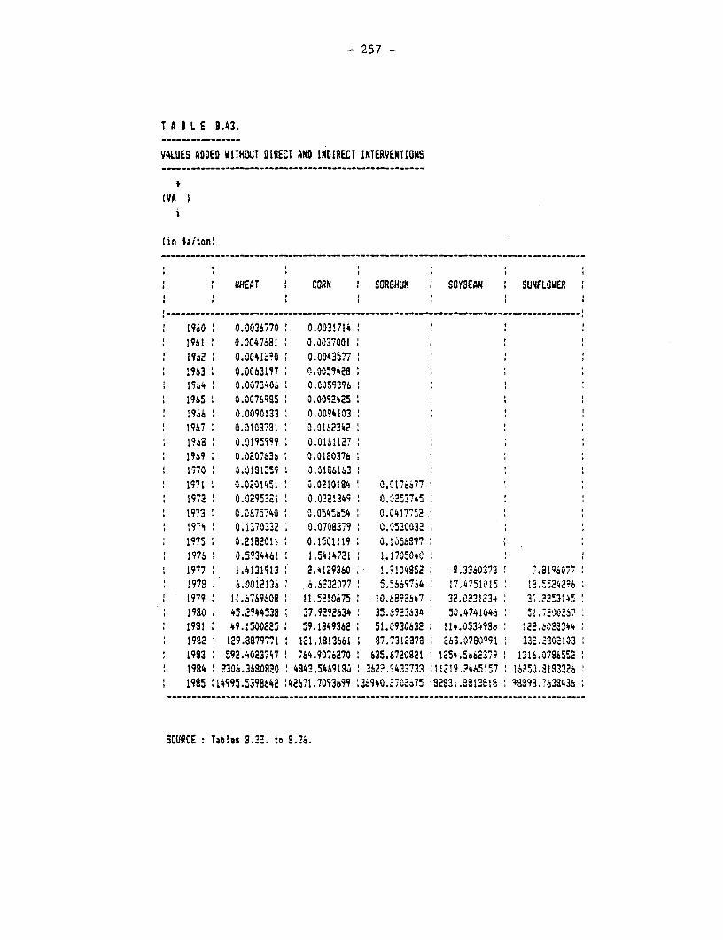
- 257 -

T A B L E 3.43.

VALUES ADDED WITHOUT DIRECT AND INDIRECT INTERVENTIONS

(VA i

(in $aIton)

WHEAT CORN SORSHUM SOYBEAN ' SUNFLOWE

1960 0.0036770 0.00317141961 0.0047681 0.003700I

* 1962 0.004,200 0.00435771963 0.0063197 0.00594281964 0.0073406 0.00593961965 0.0076995 0.0092425

t 1966 I 0.0090133 0.00941031967 0.0109787 0.01623421968 0.0195999 0.0161127

* 1969 0.0207636 0.0180376* 1570 ' .01312:5 30.0186163

197 1I 0.02.145;l 6.0210184 1 0.31766771972 0.0295321 0.021,849 0.02537451973 0.0675740 0 3.0545654 0.0417752llqis OQh 0.1370332 0.0708379 t 0.0520032

1975 0.2IB20o 0.1501119 0.14569771976 0.5934461 1.5414721 1.17050401977 1.4131913 2.4129360 !.7104852 9.2360373 7.31960771978 i.d012136 6.6232077 5.5669764 17.4751015 18.5 " 42961979 1: .67S9608 11.!210675 10.68924?: 32.0231234 3;.22!3145

* 1980 45.2944538 37.9292634 35.6?23634 50.4741046 5i.71-1.720067* 1991 49.15002 25 59.1849362 51.0930632 114.053499% 122.-022344

1992 129.8879771 121.1813661 87.7312a378 263.07S9991 332.23021031983 592.4023747 764.9076270 635.6720821 1254.956623179 131i.A0786s5r521 1984 2306.3680820 4941.5469193 3622.1433733 111219246515c7 1625e.31933261995 :14995.5398642 ,42671.7093699 ;36940.21702675 92531.881381E '8188.7638436s

SOURCE': Tables 3.32. tD 8.^6.

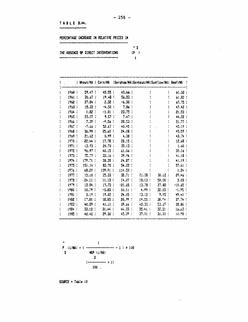
- 258 -T A 8 L E 1.44.

PERCENTASE INCREASE IM RELATIVE PRICES IN

^ D

THE ABSENCE OF DIRECT INTERVENTIONS (P

:Wheit/NA: Corn/NA SorohumJNA"SovbesniNA'Sunflau/WA: Beef/NA

1960 59.47 45.55 43.66 61.021961 30.07 19.48 56.33 61.3221962 27.84 2.32; -6.30 : 67.751i963 15.33: -4.5O 7.86 47.4219i4 1.32 -1.01 23.75' 21.531%15 23.07 9.57 7.47 44.221966 i 7.39 -9.56; 22..53 21.771976 -7.66: 52.67 40.45: 45.!91968 36.99 25.60 24.08 45.591%69 21.62: 0.99 4.38 1 43.741970, 22.44 t17.73 29.15 ' ' 12.681971 13.93 20.70 35.13 : 1.60:1972: 96.97: 40.15: 61.06 : : 30.16:1973 75.77. 33.16: 39.96 : 1.181974 179.71 33.38: 24.37 : 4'1.191975 151.14 83.70 ; 54.22 : ; 57.61176; 69.'3 ' 139.91 114-.0, : 1.9i41977 1 25.10 ; 25.33 32.71 : 21.8 :9 30.1 C| 29.4619'73 24.11 11.13: 14.07 2' .13: 50.00: 3.0219 9 ; 13.2§ : 13.73 -21.65 13.78 : 27.82 -10.651980 10.179; -s.a3 : io.ii : 4.99: 32.03 -l.9ASi 1i9 3.19; 19. 062 .4.05 13. 12 9.95 : 49.401982 17.01 . 18.85s 20.99 1 19 .55' 38.t4 : 37.741953 40.29; 41.11 39.66 43.33 53.37 32.80'1984 33.12: 31.44 : 44.33: 35.41 32.3! 16.631985 : 42.42 ; 29.30: 45.39 37.01 3 36.31 1: .98

A I

P HA) -……- - I 100D NRP (iiNA)

0--- …----- + 1)

100

SOURCE Table 10

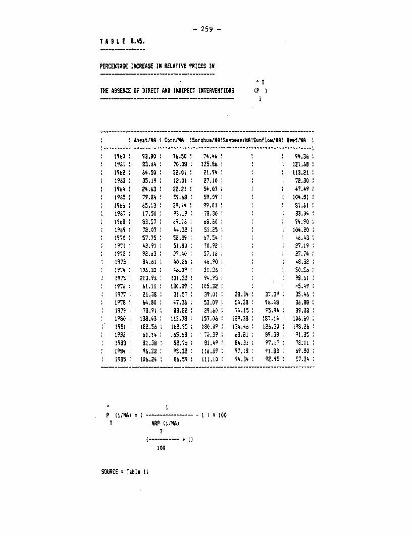
- 259 -

T A 3 L E 3.45.

PERCENTAGE INCREASE IN RELATIVE PRICES IN

A T

THE ABSENCE OF DIRECT AND INDIRECT INTERVENTIONS 1P- ----.---- …-------------

I ' Wheat/NA ! Corn/NA Sorqhua/NA:Sovbean/NA'Sunflou/NA: Beef/NA

1960 93.90 76.50 1 74.46 : 94.361961 93.64 70.08 115.86 ' 121.681962 64.50 32.01 : 21.94 113.211963 35.19: 12.01 27.10 : 72.30:1964 ' 24.63 ' 22.21 : 54.07 : 47.491965 79.84 ' 59.68 59.09 104.911966 65.13 39.44 99.01 '1.61:1967' 17.50 ' 3.19: 78.30 : 83.04:1968 83.'7 ' 9.6 6S..a: ' 94.90:1969 : 72.07 ' 4.32 ' 51.25 104.201970 : 57.75 , 52.39 , 67.!4 46.431971 42.91 51.90 70.92 ' , 27.191972: 92.i3: 37.40: 57.16 ; 27.74'1973: 94.61 40.26 ' 46.90 . : : 48.321974 : 196.33 : 46.09 : 31.36 50.i 1975 213.96S 131.22: 94.95 ' ' 99.6:9? 7: Sl.1l 1 30.89 105.32 '': -5.i9:1977 21.38 31.57 39,.1 29.34 : 3?.39 ' 35.4S1978 64.90 47.36 ' 53.09 : S4.3s ' 96.48 : 36.881979 7 3.91 ' 3 .-2 ' 29.60 I 74.15: S5.°4 39.331M8O ' 138.43 1 13.78 157.06 ' 129.38: 18?.14 , 106.601Sl ' 122.56 162.95 180.0 : 134.46 1 26.30 : 198.'21982 h S1.'4 65.68 : 70.39 6-s3.9' : 89.39 91.351983 : 81.58 92.76 ' 91.9 ' 94.31 : 9?7.1, 7;111984 9 96.3 ' 954.32 : 116-.9 : 97.19 : 91.93 : 9.820

1995: 106.24: 96.59 ' 11. i3 94.34: 92.95: ' 7.24

A I

P (i/NA) ----------------- - 1) 100T NRP (1iNA)

T----------- - t

100

SOURCE - Table It

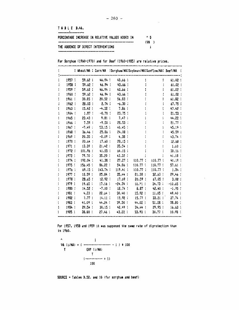
- 260

T A B L E 3.46.__ __ _____

PERCENTA6E INCREASE IN RELATIVE VALUES ADDED IN A D-_- --------------------- (VA

THE ABSENCE OF DIRECT INTERVENTIONS i

For Sorghus (1960-1970) and for Beef (1960-19851 are relative prices.

Wheat/NA : Corn/KA 'Sorghuu/NA'Soybean/NA'Sunflow/NAI Beef/NA19-- 59.624 --4-- - _ __ __ ,1957 59.62 I 46.94 43.66 1 61.021958 59.62 1 46.94 1 43.66 61.021959 59.62 4 6.94 43.66 '' 61.021960 59.62 46.94 43.66 61.021961 30.85: 20.52 56.83: 61.821962 28.03 ' 2.74 1 -6.30 1 67.751963 15.42 -4.32 7.86 47.421964 1.37 -0.70 23.75 21.531965 23.43 : 9.81 ' 7.47 ' 44.221966 7.59 -9.50 28.53 : : 21.771967 . -7.49 53.15 40.45 45.191968 : 36.46 1 25.86 : 24.08 : ' 45.591969 20.35 -0.09 ' 4.38 ' : 1 43.741970 20.64 17.60 29.15 : 12.681971 1 13.39 21.42 35.54 1 . 1.601972 101.96: 41.55 64.15 1 30.161973 79.70 35.20 43.32 : : 41.181974 . 192.04 I 41.38 1 27.27 1 110.77 ' 110.77 1 41.191975 1 156.45 : 86.22 : 54.86 : 110.77 : 110.77 : 57.611976 . 69.15 . 143.74 1 119.41 : 110.77 I 110.77 1 1.941977 12.59: 25.84 : 35.44 ' 21.38 32.63 29.461978 ' 28.65 : 12.92 1 17.69 ' 20.59 1 67.05 : 3.081979 : 19.6 ": 17.16 ' -24.34 : 16.01 1 34.73 : -10.651980 : 14.52 . -7.00 : 12.74 1 8.97 1 42.40 -1.951981 : 4.33 ' 22.S4 30.40 : 15.92 1 11.05 49.401982 .77 : !4.11: 12.92 : 15.77: 33.21: 37.741983 41.09 1 44.24 : 39.50 : 44.02 ' 51.28 : 38.301994 1 29.54 1 30.15 : 42.49 1 34.44 1 29.95 : 16.631985 : 38.80 : 27.46 : 43.22 1 33.93 1 30.77 : 10.98

For 1957, 1958 and 1959 it was supposed the same rate of diprotection thanin 1960.

AI

VA (iINA) ---- -1-------- - I J 100T ERP (i/NA)

100

SOURCE - Tables B.52. and 10 (for sorghum and beef)

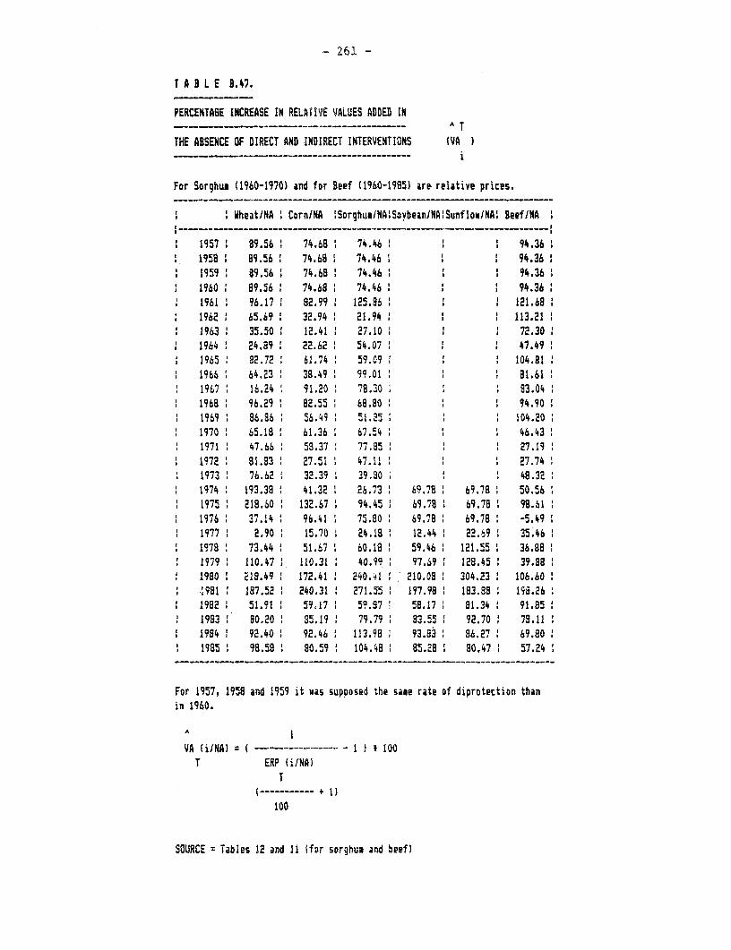
- 261 -

T A 8 L E 8.47.

PERCENTAGE INCREASE IN RELATIVE VALUES ADDED INA T

THE ABSENCE OF DIRECT AND INDIRECT INTERVENTIONS IYAi

For Sorghum (1960-1970) and for Beef (1960-1985) are relative prices.

Wheat]NA 1 Corn/NA lSorghuu/NAlSoybean/iNASunflow/NAI Beef/NA

1957 89.56 74.68 1 74.46 ' 94.3611 1958 89.56 74.68 1 74.46 1 i 1 94.36

1959 1 89.56 1 74.68 7 74.46 1 ' 94.36 11960 89.561 74.681 74.46 i t 94.361961 96.171 82.991 125.861 1 1 121.681962, 65.691 32.941 21.94 1 113.211963 35.50 12.41 27.10 1 1 72.30

1 1964 24.891 22.62 54.07 1 1 47.4919651 82.721 61.741 59.091 1 1 104.81

1 19661 64.231 38.491 99.011 81.61I1967 16.24' 91.201 78.30 83.041968 96.29 1 82.55 1 68.80 1 1 94.901969 86.86 56.49 1 51.251 i 1 104.20 i19701 65.18 61.361 67.54 1 1 46.431971 1 47.66 58.37 77.851 1 1 27.19

1 19721 81.831 27.511 47.111 1 1 27.7419731 76.62 1 32.39 1 39.80 1 * 48.32

1 1974 193.38 41.321 26.73 1 69.7a8 69.78 50.56 11975 ' 218.60 ' 132.67 1 94.45, 69.78 1 69.78 1 98.61

1 1976 ' 37.14 ' 96.41 1 75.80 6 69.78 1 69.78 1 -5.491977 1 2.90 1 15.70 24.18 12.44 22.69 35.46

1 1978 73.44 51.67 60.18' 59.46 121.55 1 36.88 11979 ' 110.47 1 110.31, 40.9 97.69 . 128.45 ' 39.881980 ' 218.49 1 172.41 240.41 ' 210.08 1 304.23 1 106.60,1.981 187.52 240.31 ' 271.55 197.98 183.88 1 J.2619821 51.911 59.171 59.97 58.171 81.34' 91.85

1 1983, 80.20 1 5.19 79.79 83.55 92.70' 78.111 1984 1 92.401 92.46 113.98 93.83a 86.27 69.801 1985 1 98.58 1 80.59 1 104.48 1 85.28 80.47 1 57.24

For 1957, 1958 and 1959 it was supposed the sase rate of diprotection thanin 1960.

A I

Va (ifA) I …1)100T ERP (i/NA)

TI …- -*1)

100

SOURCE = Tables 12 and 11 (fDr sorghus and beef)

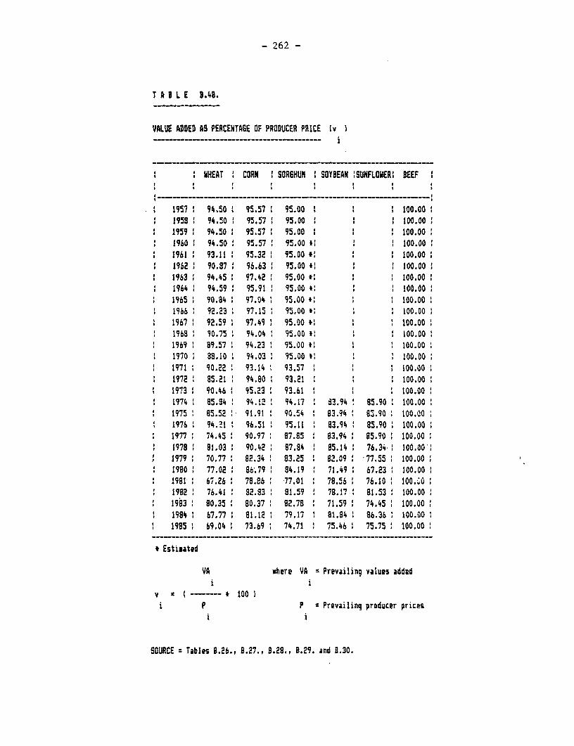
- 262 -

T A I L E 3.48.

VALUE ADDED AS PERCENTASE OF PRODUCER PRICE Iv

U 'HEAT CORN 1 SORGHUM I SOYBEAN 'SUNFOlVER' BEEF

1557 94.50 195.57 5 5.00 1 100.00' 1958 ' 94.50 ' 95.57 95.00 ' loo.oo

1959 94.50 ' 95.57 1 95.00 : ' 100.001960 94.50 95.57 95.00 1 100.00

1 1961 1 93.11 95.32 95.00 1' 100.001962 9 50.87 96.63 95.00 if 10oo.01963 94.45 97.42 95.00 *: 100.001964 94.59 95.91 1 95.00 * 100.001965 90.84 97.04 95.00 *1 100.001966 92.23 97.15 ' 95.00 *' 100.0019i7 1 92.59 1 97.49 95.00 *t 100.001968 90.75 ; 94.04 95.00 *: 100.001969 89.57 1 94.23 1 95.00 * 100.001970 88.10 94.03 95.00 9. t 100.001971 90.22 93.14 93.57 1 1 100.001972 85.21 94.80 93.21 : 100.001973 90.46 95.23: 93.61 ' 100.001974 85.84 94.12' 94.i7 : 93.94 a5.90 100.001975 85.52 91.91 90.54 83.94 8K.90 100.00

: 1976 94.?1: 96.51 1 95.11 ' 83.54 85.90 100.001977 74.45 90.97 87.85 1 83.94 85.90 100.001978 5 81.03 1 90.42 87.84 85.14 1 76.34i 100.00'

1 1979 70.77 82.34 83.25 82.09 177.55 100.001980 77.02 : 86.79 84.19 : 71.495 67.23 100.001981' 67.26 78.86 -77.01 78.56 76.10 100.iO01982 1 76.41 1 92.83 1 81.59 78.17 1 81.53 100.001983 80.35 80.37 1 82.78 1 71.59 74.45 100.00

1 1984 6 67.77 ' 81.12 : 79.17 1 81.84 ' 86.36 ' 100.00 '1985 1 69.04 1 73.69 1 74.71 ' 75.46 ' 75.75 1 100.00 :

* Estisated

VA where VA Prevailing values addedi i

v - -- # 1001i P P Prevailing producer prices

i i

SOURCE Tables B.26., B.27., 3.28., B.29. and B.30.

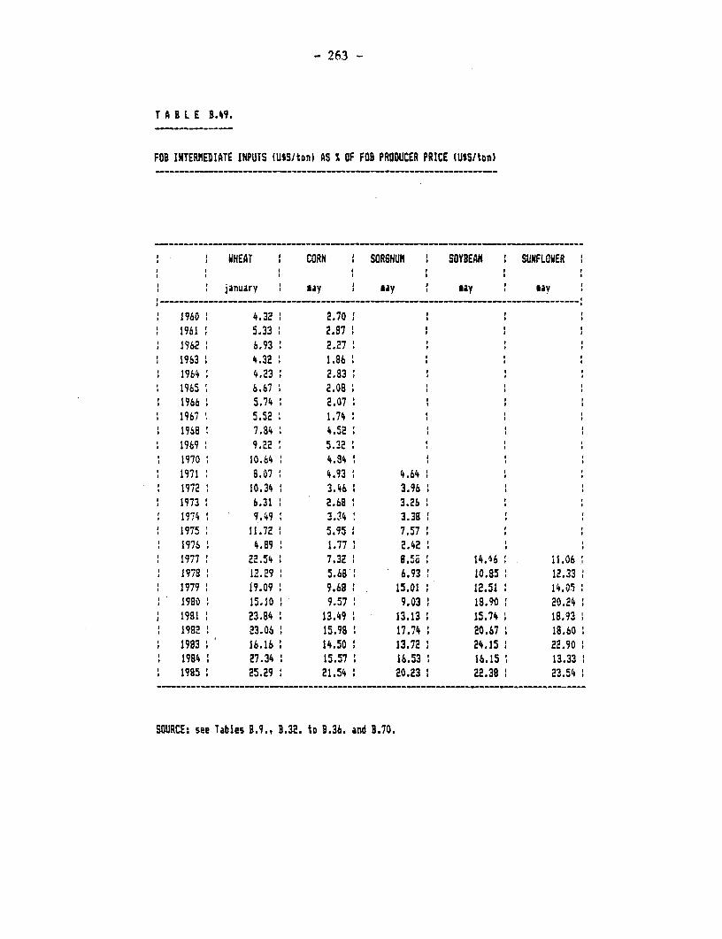
- 263 -

T A B L E B.49.

FOB INTERMEDIATE INPUTS (USSIton) AS s OF FOB PRODUCER PRICE (U$S/ton)

WHEAT CORN SORGHUM I SOYBEAN SUNFLOWER

january m may may may may

1960 4.32 ! 2.701961 5.33 2.57'1962' 6.93 2.271963' 4.32 1.961964 4.23 2.83:1965' 6.67; 2.081966b 5.74 2.071967 5.52 1.74 I

1968; 7.84 4.521969; 9.22; 5.321970; 10.64; 4.8411971; 8.071 4.93 4.6411972 10.34 3.46 3.961973: 6.31 2.68: 3.26:19?74 9.49 3.34 3.381975 11.72 5.95 7,57197L L.89 1.77: 2.2'1977 22.54 7.32 8.5' II4.46 i1.06 1978 12.29 5.68: 6.93 10.85 12.331979 19.09 9.68; 15.01 1 12.51 14.051980 15.10 9.57 9.03 18.90 20.241981 23.84 13.49 13.13 15.74 18.93 I1982 23.06 15.98 17.74 20.67 18.601983 16.16 14.50 13.72 24.15 22.901984 27.34 1 15.57: 16.53 16.151 13.331985 25.29 21.54 20.23 22.38 23.54

SOURCE: see Tables B.9., B.32. tD B.36. and 3.70.

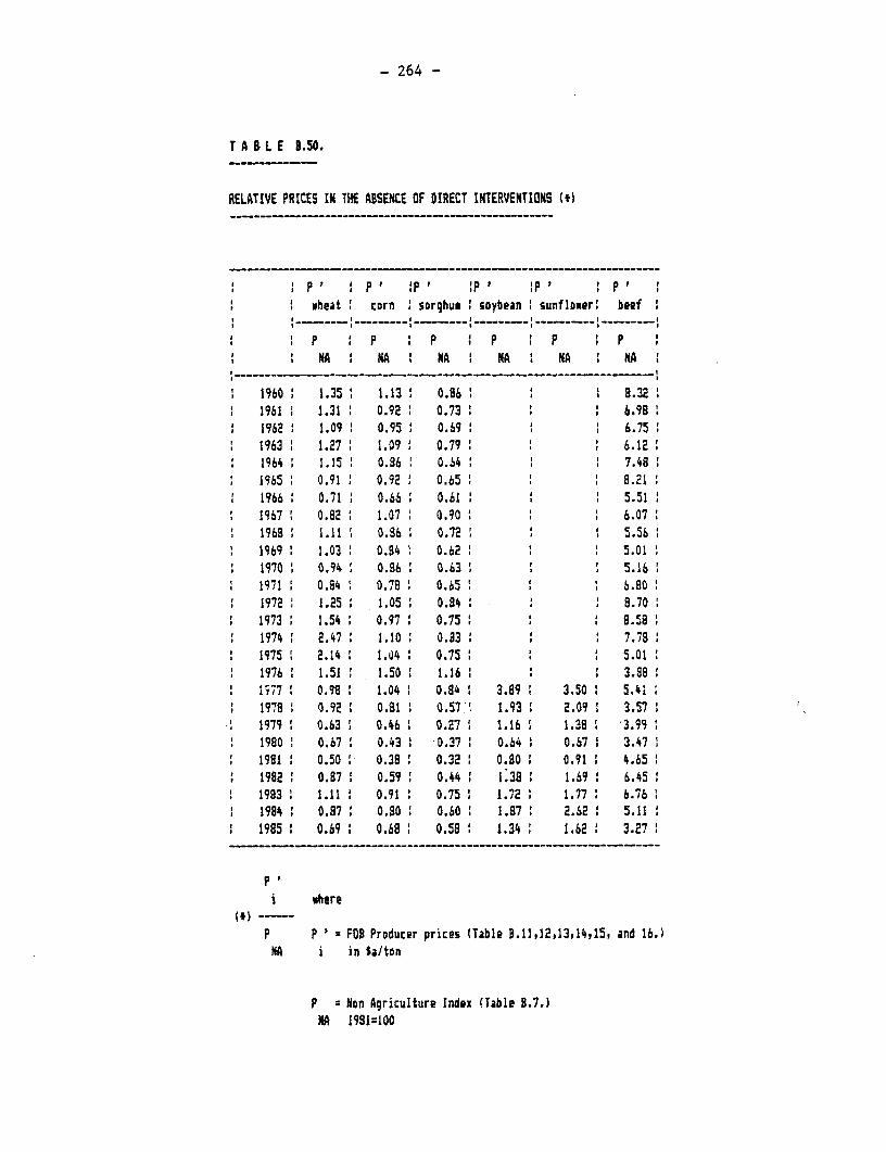
- 264 -

T A iL E 8.50.

RELATIVE PRICES IN THE ABSENCE OF DIRECT INTERVENTIONS (M)

I wheat corn 1 sorghus soybean sunflower: beef

P p p I p I p

MA NA NA I NA 'A NA

1960: 1.35 1.13 : 0.86 : : 8.321961 1.31 0.92 : 0.73 6.981962 : 1.09: 0.95 i 0.69 1 6.751963 1.27 1.09 0.79 : 6.121964 1.15 0.96 0.644 : 7.481965 0.91 0.92 0.65 8.2119661 0.71 0.66 0.61: 5.5151967 0.32: 1.07 o0.90 6.071968 1.11 0.86: 0.72 5.561969 1.03 : 0.94 0.b2 1 5.011970 : 0.94 ' 0.86 0.63 ' 5.161971 0.84 0.78: 0.65 : S.80:1972 1.25: 1.05 0.84 . 8.701973 1.54 0.97 : 0.75 : ' : 9.581974 2.47 1.10 0.93 ' 7.781975 2.14: 1.4 0.75: : 5.011976 1.51 1.50 1.16 : ' 3.981S;7 0 0.98 ' 1.04 ' 0.84 3.89 3.50 : 5.411978 0.52 0.81 : 0.57, 1.93 : 2.09 : 3.571979 : 0.63 0.46 0.27: 1.16 1.38 3.991980 0.67 0.43 1 '0.37 1 0.64 ' 0.67 : 3.471911 0.50 : 0.38 ' 0.32 ' 0.90 : 0.91 ' 4.651992: 0.87: 0.59 0.44: 1.38 1.69 6.451983 1.11: 0.91: 0.75 1.72 1.77 6.761984' 0.87 0.80: 0.60 1.871: 2.62 5.11:1985 0.69 0.b8: 0.58 : 1.34: 1.62 3.27

i where

P P ' = FOB Producer prices (Table 8.11,12,13,14,15, and 16.)NA i in Sa/ton

P Non Agriculture Index (Table 8.7.)NA 1981=100

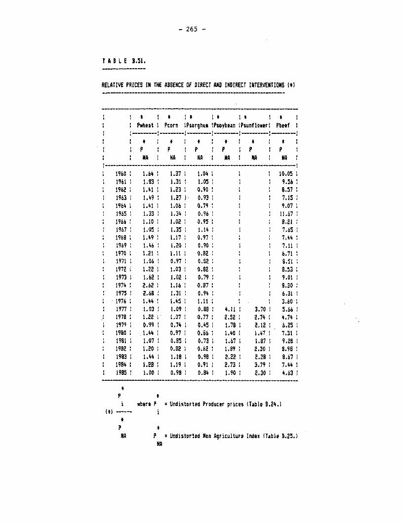
- 265 -

T A B L E B.51.

RELATIVE PRICES IN THE ABSENCE OF DIRECT AND INDIRECT INTERVENTIONS (*3

Pwheat Ptorn 'Psorghue !Psoybean !Psunflowert Pbeef

* I t I t I t I

'p P IP IP (P pNA NA I NA NA A I NA

--- ----- ---- …-------------- --------------

1960 1.64 1.37 1.04 10.0519611 1.831 1.31 1.05 * : 9.561962 1.41 1.231 0.901 8.571963 1 1.49 1.27 1- 0.93 1 I 7.15

1 1964 1 1.41 1.06 1 0.79: 1 9.07119651 1.331 1.341 0.961 1 ' 11.6719661 1.101 1.021 0.951 ' 1 8.211967 1 1.05 1 1.35 1 1.14 1 1 7.6519681 1.491 1.171 0.971 1 1 7.44119691 1.461 1.201 0.901 1 1 7.111

1 19701 1.211 1.111 0.821 1 6.711971 1 1.06 0.97 : 0.82 1 8.511972 1.22 1 1.031 0.821 1 8.5319731 1.621 1.021 0,79: 1 9.0119741 2.62' 1.16: 0.87: , ' 8.3019751 2.6B 8 1.31 0.94 ' ' 6.311976: 1.44 1.451 1.11 ' 3.601977 1.03 1 1.09 0.881 4.11: 3.70 5.661978 1 1.22 1 1.07 ' 0.77 1 2.52 1 2.74 : 4.74197q 1 0.99 0.741 0.451 1.78 2.12' 6.25

1 19801 1.44' 0.97 0.S6 1 1.401 1.471 7.311981: 1.07: 0.851 0.731 1.671 1.87 9.2811982 1 1.20: 0.822 0.62 1.89 2.301 8.981983 1.44 1 1.18 0.98 1 2.221 2.28' 8.6719841 1.281 1.19 0.91 1 2.73 1 3.79' 7.44

1 1985 1.00 1 0.981 0.84 1 1.90 . 2.30 4.63

P {i where P = Undistorted Producer prices (Table 8.24.)

P tNA P = Undistorted Non Agriculture Index (Table B.25.)

NA

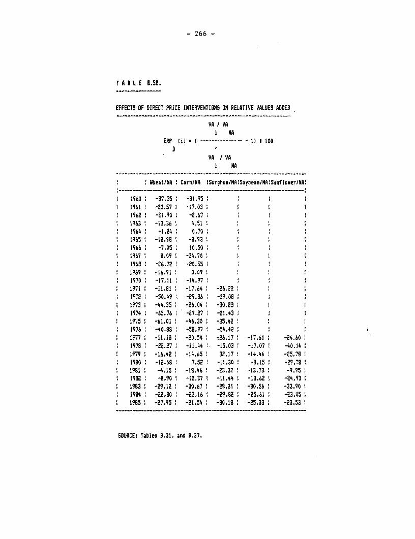
- 266 -

T A B L E B.52.

EFFECTS OF DIRECT PRICE INTERVENTIONS ON RELATIVE VALUES ADDED

VA l VAi NA

ERP li): f ------ - 1) * 100

VA l VAi MA

Wheat/NA : Corn/NA :Sorghuu/NA;Soybean/NA:Sunflower/NA:

1960 -37.35 1 -31.95 1961 -23.57 -17.031962 -21.90 -2.671963 -13.36 4.51

i 19641 -1.84: 0.70 I I

1965 -1B.98 -8.931966 -7.05 10.501967 8.09 -34.70l1968 -26.72 -20.551969 -16.91 0.0991970 -17.11 -14.971971 1 -i.81 -17.64 -26.22* 1972 -50.49 -29.36 -39.08* 1973 -44.35 -26.04 -30.231974 -65.76 -E9.27 -21.431i95 -61.01 -46.30 -35.421976 -40.8B -58.97 -54.421577 -11.18 I -20.54 -26.17 -1-7.61 -24.601978 -22.27 -11.44 -15.03 -17.07 -40.141979 -16.42 -14.65 32.17 -14.46 -25.791980 -12.68 7.52 -11.30 -8.15 -29.781981 -4.15 -18.46 -23.32 -13.73 -9.951982 -8.90 -12.37 -11.44 -13.62 -24.9319B3 1 -29.12 -30.67 -28.31 -30.56 -33.901984 1 -22.8O 1 -23.16 . -29.82 -25.61 -23.051985 -27.95 1 -21.54 -30.18 -25.33 1 -23.53

SOURCE: Tables 8.31. and 3.37.

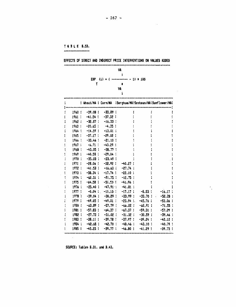
- 267 -

T A B L E B.53.

EFFECTS OF DIRECT AND INDIRECT PRICE INTERVENTIONS ON VALUES ADDED

VAi

ERP i) - ------ --- 1) * 100T *

i

Wheat/NA Corn/NA :Sorghua/NAISoybeaniNAlSunfloverINA'

1960 -39.08 9 -33.89 : : t 1961 -41.54 -37.32 :1962 1 -32.97 -16.331963 1 -20.65 -4.351964 -14.59 -13.011965 -37.17 -29.02 '1966 1 -33.46 1 -21.101967 -6.71 -43.291968 -43.05 -38.771969 -40.58 -29.041970 -35.03 : -33.49 '1971 1 -29.06 : -32.92 -40.271972 1 -41.53 1 -16.63 -27.741973 1 -38.34 -17.74 : -22.10 l

1974 t -62.31 1 -21.75 1 -12.751975 -64.59 I -51.50 : -41.96 11976 1 -B5.40 ' -47.91 ; -41.91 I1977 : -0.04 L -11.10 I -17.17 1 -8.53 : -16.1715?9 1 -39.04 1 -30.29 1 -33.99 : -33.70 1 -52.291979 -49.05 : -49.01 1 -23.94 ' -45.76 1 -53.061980 : -63.89 : -57.79 : -66.22 : -62.91 : -71.551991 : -57.93 -64.37 1 -67.37 1 -59.31 1 -57.29 11982 1 -27.73 : -31.02 1 -31.32 1 -30.59 : -39.461983 : -38.11 : -39.78 ' -37.97 ' -39.24 -42.12 :1984 1 -42.68 1 -42.70 . -48.46 1 -43.10 1 -40.79 :1985 : -45.23 ' -39.77 1 -46.90 1 -41.29 : -39.73 1

SOURCE: Tables 0.31. and 3.43.

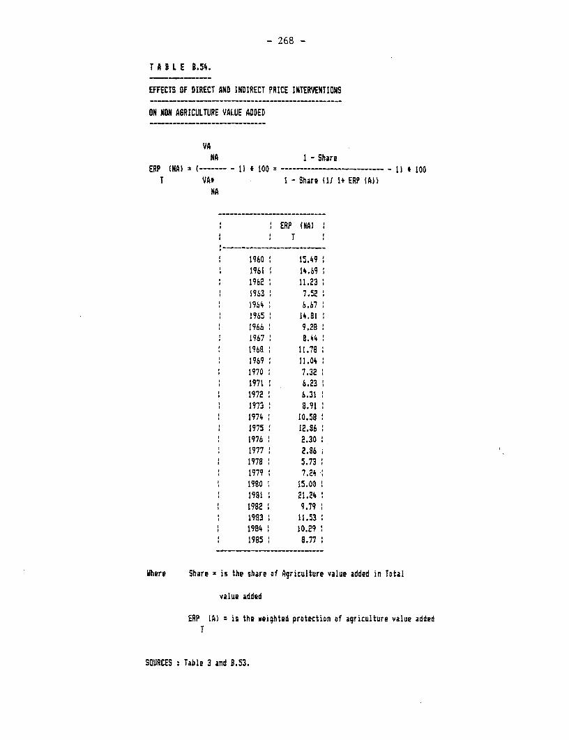
- 268 -

T A 8 L E 8.54.

EFFECTS OF DIRECT AND INDIRECT PRICE INTERVEENTIONS

ON NON ASRICULTURE VALUE ADDED

VANA I - Share

ERP (NA): -------- 1) 100 ------------------- 100T VA* I - Share (11 1 ER? (A))

NA

ERP (NA)T

1960 15.49* 1961 i' 14.69i 1962 11.23

1963 7.521964 ' 6.671965 14.811966 9."A1967 8.441968 11.781969 11.041970 7.321971 6.23

i' 1972 6.311973 8.91

i' 1974 i 10.581975 ' 12.861976 2.301977 2.36

'i 1978 i 5.731979 7.24 i1980 15.001981 21.241982 9.791983 ; 11.53

5 1984 i 10.29 '1985 i 8.77

Where Share = is the share of Agriculture value added in Total

value added

ERP (A) - is the weighted protection of agriculture value addedT

SOURCES Table 3 and 8.53.

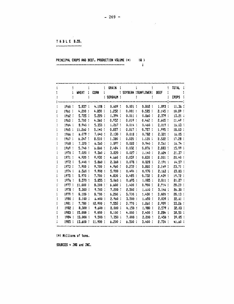
- 269 -

T A B L E B.55.

PRINCIPAL CROPS AND BEEF, PRODUCTION VOLUME (U) (Q

I6RAIN 1 1 TOTAL*WiHEAT 1 CORN 1 1 SOYBEAN !SUNFLOWER! BEEF

SORSHUM ' CROPS

1960 5.837 4.108 0.609 0.001 0.802 1 1.893 11.361961 4.200 4.850 1.252 0.001 0.585 2.145 10.391962 5.725 5.220 11.394 0.011 0.860 2.379 13.211963 5.700 4.360 0.952 0.019 0.462 2.605 11.491964 8.940 5.350 1.267 0.014 0.460 2.019 16.031965 11.260 5.140 0.857 0.017 0.757 1.995 18.031966 6.079 7.040 2.130 0.018 0.782 1 2.321 16.051967 6.247 8.510 1.380 0.020 1.120 2.522 17.291968 7.320 6.560 1.897 0.022 0.940 2.561 ' 16.741969 5.740 6.860 2.484 0.032 0.876 2.883 1 15.991970 1 7.020 9.360 3.820 0.027 1.140 2.624 :1.371971 4.920 9.930 4.660 0.059 0.830 2.001 20.401972 5.440 5.860 2.360 0.078 0.828 2.191 14.571973 7.900 9.700 4.960 0.272 0.880 2.149 23.711974 6.560 9.900 1 5.900 0.496 0.970 2.163 1 23.831975 1 5.970 1 7.700 ' 4.930 0.495 1 0.732 1 2.439 19.721976 8.570 5.855 1 5.060 0.695 1 1.085 2.811 21.271977 11.000 8.300 6.600 1.400 0.900 2.°14 28 .0

1 1978 5.300 1 9.700 7.200 1 2.500 1 1.69-O 3.146 ' 26.301979 1 8.100 9.700 6.200 3.700 1 1.430 1 3.0201 28.131980 1 8.100 6.400 I 2.960 3.500 1.650 2.939 1 22.611981 7.780 12.900 : 7.5561 3.770 1.260 2.929 33.26

1 1982 8 8.300 1 9.600 1 8.000 1 4.150 1.980 2.579 32.031983 1 15.000 1 9.000 8.100 4.000 1 2.400 1 2.294 1 38.501994 1 13.000 1 9.500 1 7.350 1 7.000 1 2.200 1 2.450 1 39.05 11985 1 13.600 ; 11.900 6.200 1 6.500 ! 3.400 1 2.734 ; 41.60 ;

(*) Millions of tons.

SOURCES -JNS and 3NC.

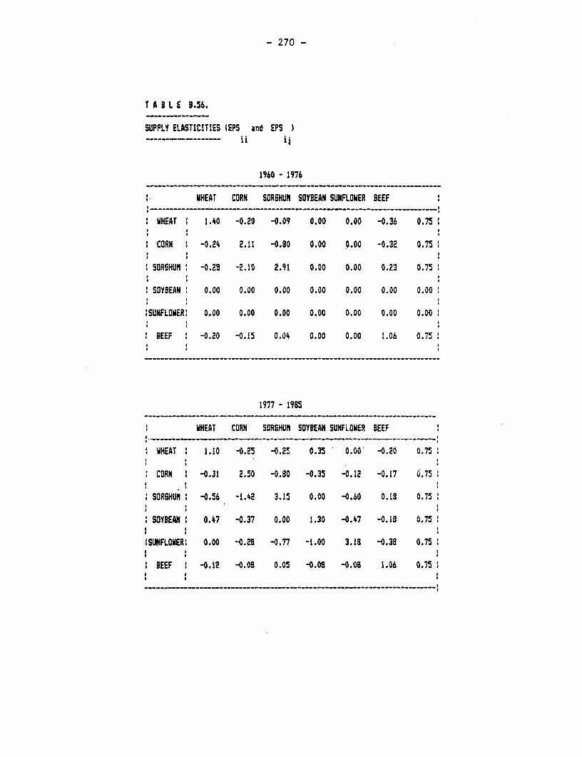
- 270 -

T A B L E 8.56.

SUPPLY ELASTICITIES )EPS and EPS…--- ------- ii

19-0 - 1976

I HHEAT CORN SOR6HUN SOYBEAN SUNFLOWER BEEF- - - - - - - - - - - - - - - - - - - - - - -WHEAT I 1.40 -0.20 -0.09 0.00 0.00 -0.36 0.75 '

CORN : -0.24 2.11 -0.80 0.00 0.00 -0.32 0.75

SORSHU( -0.23 -2.10 2.91 0.00 0.00 0.23 0.75: I

:SOYBEANR' 0.00 0.00 0.00 0.00 0.00 0.00 0.00 '

ISUNFLOWERI 0.00 0.00 0.00 0.00 0.00 0.00 0.00'

BEEF -0.20 -0.15 0.04 0.00 0.00 1.06 0.75

1977 - 1985

: WHEAT CORN SOR6HUM SOYBEAN SUNFLOWER BEEF

WHEAT ' 1.10 -0.25 -0.25 0.35 0.00 -0.20 0.75

CORN i -0.31 2.50 -0.80 -0.35 -0.12 -0.17 0.75, I

:SRSHUN -0.56 -1.42 3.15 0.00 -0.60 0.18 0.75

: SOYBEAN : 0.47 -0.37 0.00 1.30 -0.47 -0.18 0.75 .

!SUNFLOWERI 0.00 -0.28 -0.77 -1.00 3.18 -0.38 0.75 1

1 BEEF 1 -0.12 -0.08 0.05 -0.08 -0.08 1.06 0.75I . I

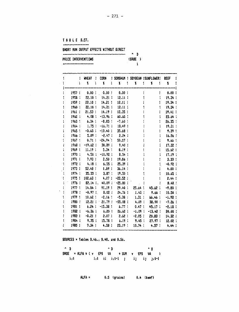
- 271 -

T A B L E 9.57.

SHORT RUN OUTPUT EFFECTS VITHOUT DIRECT

PRICE INTERVENTIONS (SRE )

IIHAT ' CORN SORSHUfl SOYBEAN 'SUNFLOWER' BEEF* I S I S I X ' I S A

1957 0.00: 0.001 0.00' : 0.001958 22.10 14.21 1 12.11 1 19.34

1 1959 22.10 14.21 1 12.11 19.341960 ' 22.10 14.21 12.11 1 19.341961 1 21.53 1 14.19 12.351 1 1 19.4119623 4.08 -13.96 60.65 1 23.641963 6.34 -8.83 -7.60 ' 1 26.35 11964 1.75 -16.71 18.49 ' 19.31

1 1965 ' -3.63 -13.40 35.68 I 9.391 1966 5.89: -2.471 2.241 ' 1 16.56

1967 0.71 -24.94 50.57 1 : 9.661 1968: -19.621 30.89 9.401 . 1 17.321 1969 1 11.19 : 5.34 1 8.19 ' ' 15.62I1 1970 : 4.50 1 -10.92 1 9.54 ' 17.19

1971 7.93 : 2.50: 19.86 1 ' 3.33I 19721 4.18 ' 6.55 1 25.39 1 1 1 -0.92

1973 : 5.48 1.59: 36.14 1 1 4.001974 35.33 3.87 19.501 1 1 10.651975 102.631 4.07 -22.52: : : 2.441976 1 82.14:. 40.091 -25.80 ' ' 8.4811977 1 14.84 91'.19 1 29.40 1 25.641 45.62 1 -9.80

1 1978: -0.971 9.021 24.76: 1.431 9.66: 10.501979 1 10.S2 1 -2.16 : -5.38 1.31 1 66.46 1 -1.92

1 19801 12.21 1 21.79 -55.08 4.09 38.90 : -7.261 1981 1 6.24 : -15.38 1 6.77 1 0.47 1 45.17 1 -2.181 1982 ' -6.36 1 6.20 : 26.62 1 -1.09 1 -13.42 ' 20.00

1983 1 -0.21 1 2.07 1 2.62 1 -2.05 20.83 14.321 1984 1 9.35 1 15.78 1 6.19 1 9.45 1 27.97 1 12.02 1

1985 7.34 1 4.58 1 23.19 1 10.74 1 4.57 1 4.44

SOURCES Tables 9.46., 9.48. and 8.56.

A D AD AD

SROE ALFA ( Y EPS VSA + SUN1 V EPS VAi,t i 0t ii i,t-l i ij i0 jit-l

ALFA O.S (grains) 0.4 (beef)

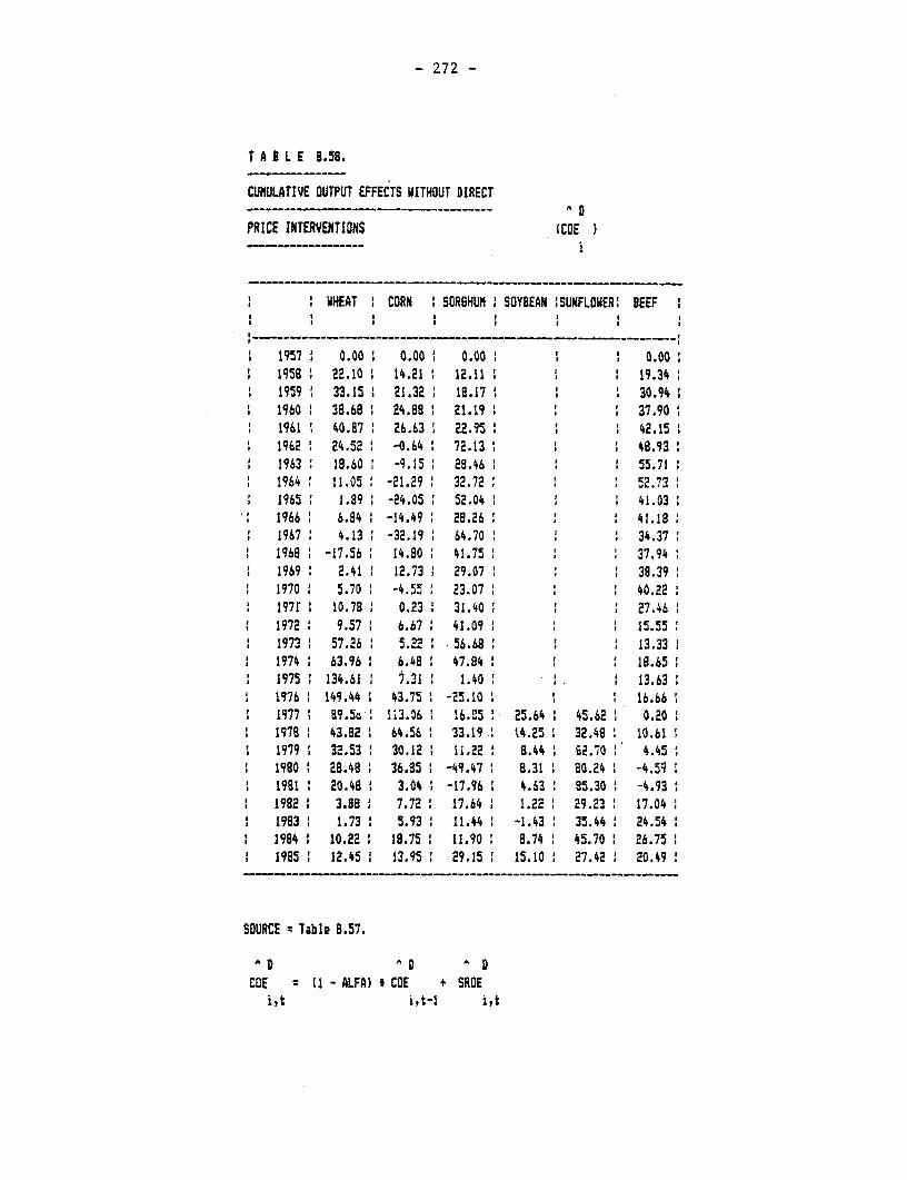
- 272 -

T A B L E S.58.

CUMULATIVE OUTPUT EFFECTS WITHOUT DIRECTA D

PRICE INTERVENTIONS (COE

' WHEAT : CORN ' SORGHUM SOYBEAN :SUNFLOWER! BEEF I. I I .

, _________ _ _ _ _ _ _ _ _ _ _ _ ,

1957 1 0.00 0.00 i 0.00 0.00o1958 22.10 14.21 12.11 19.34

t 1959 33.15 21.32 1 18.17 ' 30.941960 1 38.68 24.88 21.19 i : 37.90:1961 ; 40.87 26.63 22.95 ' 42.15'

t 1962 1 24.52 1 -0.64 72.13 : 48.93:1963: 18.60 -9.15 28.46 : 55.711964 11.05 -21.29: 32.72 : : 52.731965: 1.89: -24.05 52.04: 41.03:

*2 1966 1 6.84 1 -14.49 : 28.26 1 41.181967 4.13 -32.19: 64.70 1 1 34.371968 : -17.56 : 14.80 1 41.75 : I : 37.941969 1 2.41 1 12.73 ' 29.07 : : 39.391970 1 5.70 : -4.55 1 23.07 : 1 : 40.22197f 10.78 0.23 31.40: , 27.461972: 9.57 6.67 41.09 1 15.55 :

l 1973 : 57.26 1 5.22 .56.68 1 13.331974 1 63.96 : 6.48 ' 47.84 : 1 : 18.651975: 134.611 7.31 1 1.40 ' 13.63

1 1976: 149.44: 43.75 : -25.10: 1 16.66:1977 1 89.561 .13.06 : 16.&5 V 25.64 1 45.62 ' 0.20 1

1 1978 1 43.82 ' 64.56 : 33.19 . 14.25 1 32.48 1 10.61 11979 3 32.53 1 30.12 1 11.22 I 8.44 6 u2.70 : 4.45

1 1980 1 28.48 : 36.85 1 -49.47 1 8.31 1 80.24 1 -4.59 ,1 1981 : 20.48 ' 3.04 1 -17.96 1 4.63 1 85.30 1 -4.93: 1982 : 3.88 7.72 ' 17.64 1 1.22 : 29.23 ' 17.04 '1 1983 : 1.73 : 5.93 1 11.44 1 -1.43 35.44 24.5411 1984 1 10.22 18.75 1 11.90 8 8.74 1 45.70 1 26.75 11 1985 1 12.45 1 13.95 1 29.15 : 15.10 : 27.42 1 20.49 '

SOURCE Table B.57.

A D AD A D

COE 11 - ALFA) t CUE + SROEi,t i,t-l i.t

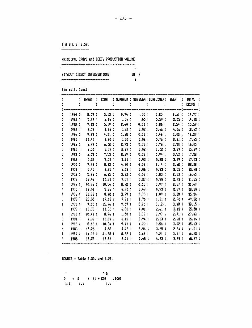
- 273 -

T A B L E 8.59.

PRINCIPAL CROPS AND BEEF, PRODUCTION VOLUME

WITHOUT DIRECT INTERVENTIONS (a

(in fill. tons)

WHEAT I CORN SORSHUM SOYBEAN 'SUNFLOWER' BEEF TOTALi CROPS

1960 ! 8.09 . 5.13 : 0.74 ! .00 i 0.80 2.61 : 14.771961 1 5.92 ' 6.14 ' 1.54 1 .00 . 0.59 3.05 14.1811962 7.13 5.19 2 2.40 0.01 1 0.86 3.54 15.591963' 6.76 3.96 1 1.22 ' 0.02 0.46 1 4.06 12.4319641 9.93' 4.21 1.68 1 0.01 0.461 3.08 16.29

1 1965 ' 11.47 ' 3.90 ' 1.30 . 0.02 1 0.76 1 2.81 1 17.451966 1 6.49 1 6.02 2.73 ' 0.02 0.78 3.28 16.05119671 6.50 5.771 2.27' 0.021 1.121 3.391 15.691968 1 6.03 7.53 1 2.69 0.02 0.94 1 3.53 17.221969 1 5.88 ' 7.73 1 3.21 ' 0.03 ' 0.88 1 3.99 : 17.7311970: 7.42 8.93 4.70' 0.031 1.14' 3.681 22.221971 5.45 1 9.95 1 6.12 0.06 0.83 1 2.551 22.421972 ' 5.96 1 6.25 1 3.33 0.08 1 0.83 t 2.53 ' 16.451973 1 12.42 1 10.21 1 7.77 1 0.27 0.88 ' 2.43 31.55 11974 110.76 10.54 8.72' 0.50 0.97 2.57' 31.491975 14.01 1 8.26 I 4.90 0.49 0.73 1 2.77' 28.38 11976 1 21.33' 8.42 3.79 1 0.701 1.09' 3.281 35.3611977 ; 20.85 17.68 ' 7.71 . 1.76 ' 1.31 1 2.92 . 49.32 1

1 1978 1 7.62 15.96 1 9.59 1 2.86 1 2.2 3.48 38.151979 10.73 11.32 6.90 4.01 1 2.61 1 3.151 35.581 1980 10.41 1 8.76 1 1.50 3.79 1 2.97 ' 2.71 27.43

1 1981 9 9.37 1 13.29 : 6.191 3.94 1 2.33 1 2.798 35.141 1982 1 8.621 10.34 9.41 4.201 2.556 3.021 35.131

19831 15.261 9.53 1 9.031 3.94 1 3.251 2.84: 41.01 11984 14.33 .11.28 8.22 7.61 1 3.21 1 3.11 1 44.65

1 1985 1 15.29 13.56 8.01 7.48 . 4.33 3.29 1 48.67

SOURCE Table 3.55. and 8.58.

I ^D

aQ ( t1 CDE J100)i,t i,t i,t

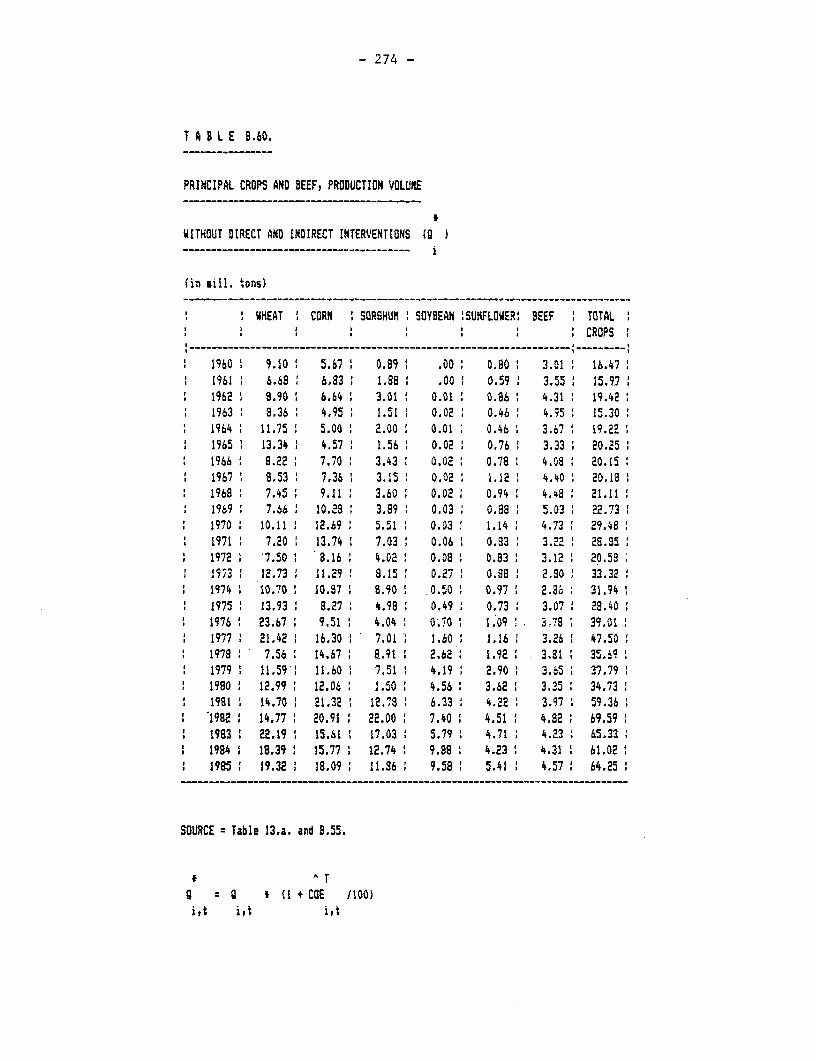
- 274 -

T A B L E B.60.

PRINCIPAL CROPS AND BEEF, PRODUCTION VOLUfE

WITHOUT DIRECT AND INDIRECT INTERVENTIONS (O

(in sill. tons)

WHEAT 1 CORN SORGHUM SOYBEAN :SUNFLOWER! BEEF TOTALI S I I I CROPS

-- -- - -- --- -- - - ---- -------- …-…--- - --- -- -- --

1960 9.10 5.67 ' 0.89 ' .00 : 0.90 : 3.01 16.47* 1961 6.68 6.83 1.88 1 .00 i 0.59 1 3.55 15.92

1962 8.90 6.64 3.01 0.01 0.86 4.31 19.421963 8.36 4.95 : 1.51 : 0.02 0.46 4.95 15.301964 11.75 5.00 2.00 0.01 0.46 : 3.67: 19.221965 13.34 4.57 1.56 0.02 0.76 3.33 20.251966 8 8.22 7.70 3.43 0.02 0.78 4.08 : 20.151967 : 8.53 7.36 : 3.15 0.02 1.12 : 4.40 20.181968 7.45 9.11: 3.60 0.02: 0.94 4.48 21.111969 : 7.66' 10.28 : 3.89 1 0.03 ' 0.88 ' 5.03 ' 22.731970 10.11 12.69 5.51: 0.03 1.14 4.73 29.481971 : 7.20 1 13.74 : 7.03 : 0.06 ' 0.83 ' 3.22 ' 28.851972 '7.50: 8.16 4.02 0.08: 0.83 3.12 I 20.581973 12.73 11.29! 8.15 0.27: 0.98 8 2.90: 33.321974 ' 10.70 : 10.97 ' 8.90 : .0.50 ' 0.97 2 2.86 31.941975 13.93 8 8.27: 4.98: 0.49: 0.73 3.07: 28.401976 23.67 9.51 4.04 0.70 1.09: 3?78: 39.011977 21.42 16.30 : 7.01 1.60 1.16 3.26 47.501978 : 7.56 14.67 ' 8.91 2 2.62: 1.92 . 3.81 1 35.091979 1 11.59:' 11.60 : 7.51 : 4.19 : 2.90 : 3.65 : 37.791980 ; 12.99 : 12.06 : 1.50 4.56 3.62: 3.35 : 34.731981 ' 14.70 1 21.32 1 12.78 : 6.33 : 4.22 1 3.97 : 59.36'1982 ' 14.77 20.91 2 22.00 7 7.40 ' 4.51 ' 4.82 ' 69.591983 : 22.19 ' 15.61 : 17.03 1 5.79 1 4.71 ' 4.23: 65.331984 1 18.39 ' 15.77 : 12.74 : 9.88 : 4.23 4.31 ' 61.021985 ' 19.32 . 18.09 : 11.96 ; 9.58 ' 5.41 1 4.57 : 64.25

SOURCE Table 13.a. and 8.55.

* AT

g = Q ' (I COE 1100)i,t i,t i,t

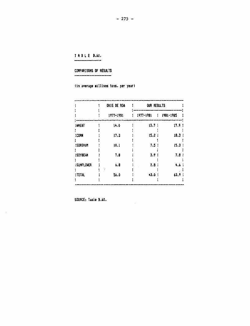
- 275 -

T A B L E 0.61.

COMPARISONS OF RESULTS

{in average sillions tons. per year)

t ORIS DE ROA 1 OUR RESULTS

I : 1977-1981 1 1977-1981 1 1981-1985! --------_---______-_------ - -----

,WHEAT : 14.0 1 13.7 17.9

CORN 17.3 1 15.2 18.3

.SORSHUN 10.1 7.5 1 15.3

:SOYBEAN I 7.8 3.9 1 7.8

ISUNFLOWER 1 6.8 2.8 4.6

,TOTAL i 56.0 43.0 63.9

SOURCE: Taale 9.60.

- 276 -

TABL 8.62.

PRINCIPAL CROPS, AREA W1THOUT INTERVENTIONS (U)

BRAINW WHEAT CORN SOYBEAN :SUNFLOWER: TOTAL

I I I I~~~~~ *ounullUnIUI I I

1981 6.321 4.462 2.835 1 2.986 2.781 19.3851982 6.350 4.375 4.890 , 3.492 2.970 22.0681963 9.540 3.266 3.778 ' 2.734 ' 3.103 22.4211934 7.908 3.300 2.826 4.660 2.789 21.4851995 8.307 3.785 2.630 4.519 3.565 22.905

(I) nillions of has.

SOURCE: Table B.60. and the fcllowinq yields:

Tons/has

Wheat 2.326Corn 4.779Sorqhua 4.509Soybean 2.119Sunflower 1.517

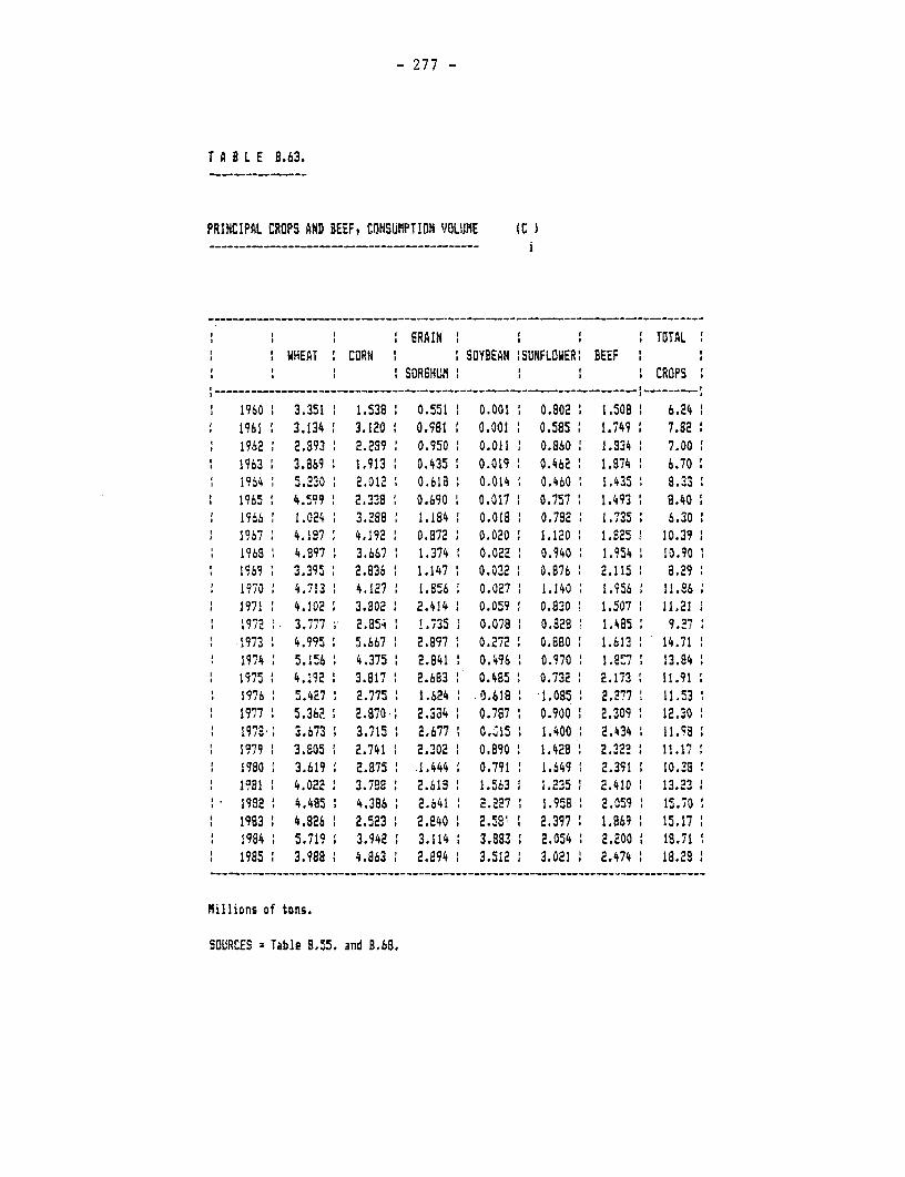
- 277 -

T A B L E 8.63.

PRINCIPAL CROPS AND BEEF, CONSU"PTION VOLUME (C-- - - -- - - -- - - -- ----- -- --

- -- -- - -- - - - - -- - - - -

GRAIN i ' '§ TOTAL 'WHEAT CORN SOYBEAN !SUNFLDWER BEEF

' SOR6HUM 1 i i CROPS

1960 3.351 1.538 0.551 0.001 . 0.802 1.508 6.241961 3.134 3.120 0.981 0.001 0.585 1.741 7.8219621 2.393 2.2z9 0.950 0.011 0.860 1.934 7.001963 3.869 1.913 0.435 0.019 0.462 1.874 6.701964 5.230 2.012 0.613 0.014 0.460 1.435 8.331965 4.599 2.338 0.690 0.017 0.757 1.493 8.401966 1.024 3.2388 1.184 0.018 0.792 1.735 6.301967 4.187 4.192 0.872 0.020 1.120 1.825 10.391968 4.897 3.667 1.374 0.022 0.940 1.954 10.901969 3.395 2.836 1.1471 0.032 0.876 2.115 8.291970 4.713 4.127 1.856 0.027 1.140 1.956 11.861971 4.102 3.802 2.414 0.059 0.830! 1.507 11.211972 3.777 2.854 1.735 0.078 0.828 1.485 9.271973 4.995 5.667 2.897 0.272 0.8B0 1.613 14.711974 5.156 4.375 1 2.841 0.496 1 0.970 : I.8V7 1 13.841975: 4.192 3.817 1 2.683 0.485 0.732 2.13 11.911976 5.427 2.775 1.624 0.618 1.085 2.277 11.531977 : 5.36? 2.870: 2.3a4 0.787 : 0.900 1 2.309 1 12.3019/7S 3.673 3.715 2.677 : 0.J15 1.400 1 2.434 1 11.981979 3.E05 2.741 2.302 0.890 1.428 2.322 : 11.171980 3.619 2.875 1.444 0.791 1.649 2.391 10.281091 : 4.022 3.7881 2.619 1.563. 1.235 2.410 13.231992 4.485 4.386 2.641 2.227 1.9589 2.059 15.701983: 4.826 2.523 2.840 I E.581 2.397 1.869 15.171984 5.719 3.942 3.114 1 3.883 2.054 2.200 1 18.71 1

* 1985 : 3.98e 4.863 2.894 1 3.512 3.021 2.474 1 18.28:

Millions of tons.

SOURCES = Table B.55. and 3.68.

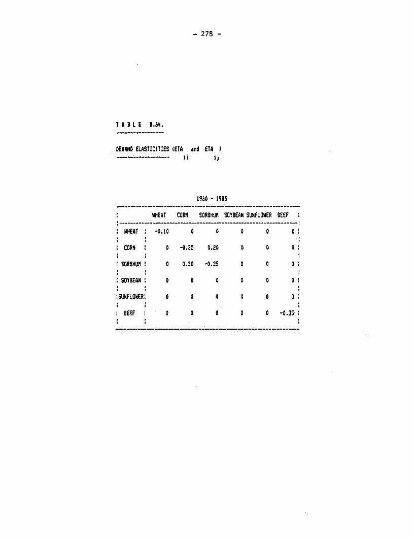
- 278 -

t A I L E B.6'4.

DEMAND ELASTICITIES (ETA and ETAii ij

1960 - 1985

WHEAT CORN SORGHUM SOYBEAN SUNFLOWER BEEF------------- ---------------- - ------------------------------- _

WHEAT 1 -0.10 0 0 0 0 0'

CORN 0 -0.25 0.20 0 0 0I I

SORSHUf 0 0.30 -0.35 0 0 0

l lISOYBEAN: 0 0 0 0 0 0 i

'SUNFLOWER' 0 0 0 0 0 0O

BEEF I 0 0 0 0 0 -0.35 .! !

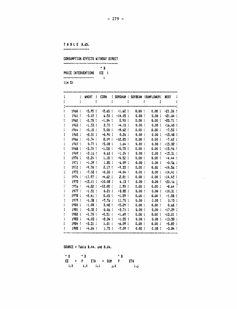
- 279 -

T A B L E D.65.

CONSUMPTION EFFECTS WITHOUT DIRECT

A D

PRICE INTERVENTIONS (CE

(in 1)

* WHEAT CORN SORGHUM SOYBEAN :SUNFLOWER: BEEF

1960 -5.95 . -2.65 1 -1.62 0.00 0.00 -21.361961 -3.07 6.50 1 -14.05 0.00 0.00 -21.641962 -2.79 -1.84 2.90 1 0.00 0.00 -23.711963 -1.53 2.70 -4.10 0.00 0.00 -16.601964 -0.18 5.00 -8.62 0.00 0.00 -7.531965 -2.31 -0.90 0.26 0.00 0.00 -15.481966 -0.74 8.09 -12.85 0.00 0.00 -7.621967 0.77 -5.08 1.64 0.00 0.00 -15.921968 -3.70 -1.58 -0.75 0.00 0.00 -15.961969 -2.16 0.63 -1.24 0.00 0.00 -15.311970 -2.24 1.18 -4.52 0.00 0.00 -4.441971 1 -1.39 1 1.85 -6.09 0.00 . 0.00 -0.56 :

1 1972 -9.70 2.17 -9.33 0.00 0.00; -10.56 11973 -7.58 -0.30 --4.04 0.00 0.00 -14.41 1974 -17.97 1 -4.62 2.81 0.00 0.00 : -14.421975 1 -15.11 : -10.08 6.13 1 0.00 0.00 -20.16l976 -6.822 -12.08 1.90 . 0.00 0.00 1 -0.641977 -1.51 1 0.21 . -3.85 0.00 0.00 -10.3119?8 -2.41 0.03 1 -1.59 0.u0 0.00 -1.08

1 1979 -1.381 -7.76 11.70l .0.001 0.00 1 3.731 1980 1 -1.08 3.48a -5.29 0.00 0.00 0.68

1981 1 -0.32 0.061 -2.71 0.00 1 0.00 -17.291 1982 . -1.70 1 -0.51 -1.69 1 0.00 . 0.00 -13.21 1

1983 1 -4.03 1 -2.34 . -1.55 . 0.00 . 0.00 -13.58 11984 1 -3.31 . 1.01 1 -6.091 0.00 1 0.00 -5.821985 : -4.24 1 1.75 : -7.09 1 0.00 0.00 . -3.84

SOURCE = Table 8.44. and 8.64.

AD AD

CE = P ETA + SUN P ETAi t i t i i j t i.j

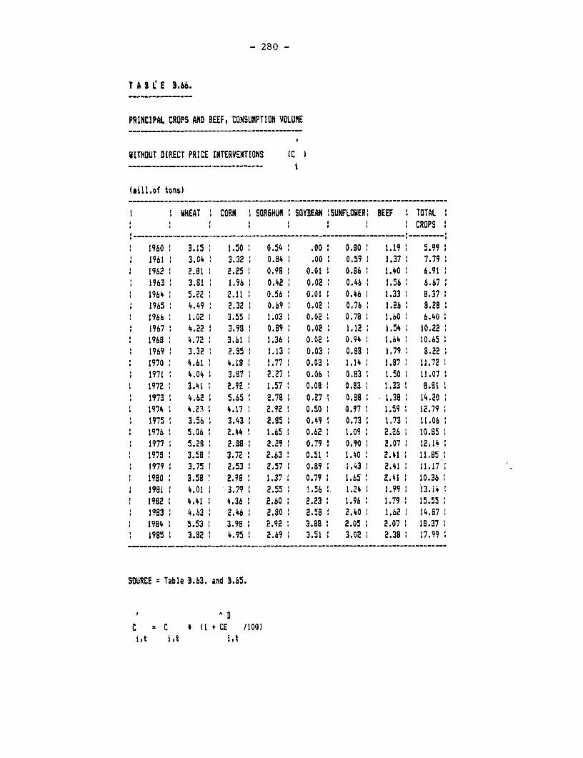
- 280 -

T A B L E B.66.

PRINCIPAL CROPS AND BEEF, tONSUMPTION VOLUME

LITHOUT DIRECT PRICE INTERVENTIONS (C______~~ -_-_--------- i

(Aill.of tons)

IWHEAT I CORN I SORGHUM SOYBEAN !SUNFLOWER: BEEF 1 TOTAL' i ' ' ' ' CROPS

1960 3.15 1.50 0.54 .00: 0.80 1 1.19 i 5.99* 1961 3.04 3.32' 0.84 .00 0.59 1.37 7.795 1962 2.81 1 2.25 0.98 0.01 0.86 1.40 6.91

1963 3.81 1.96 0.42 0.02 0.46 1.56 6.671964 5.22 1 2.11 0.56 0.01 ' 0.46 1 1.33 8.371965 4.49 2.32 0.69 0.02 0.76 1.26 8.28

* 1966 1.02 3.55 1.03 0.02 0.78 1.60 6.401967 4.22 3.98: 0.899 0.02 1.12: 1.54 10.221968 4.72 3.61 1.36 0.02 0.94 1.64 10.65

* 1969 3.32: 2.85 1.13 : 0.03: 0.88 1.79: 8.221970 4.61 4.18 1.77 : 0.03 1.14 1.87 11.721971 4.04 1 3.87 2.27 0.06 0.83 1.50 11.071972 1 3.41 2.92 1.57 0.08 ' 0.83: 1.33 8.8111973 4.62 1 5.65 2.78' 0.27 1 0.88 1.38 : 14.201974 4.23 4.17 : 2.92 0.50 0.97 1.59 : 12.7919751 3.56 3.43 2.85 0.49: 0.73: 1.73 11.061976 5.06 2.44: 1.65 0.62: 1.09 2.26 10.851977? 5.28 : 2.88 2.29 0.79 1 0.90 2.07: 12.1419791 3.58 1 3.72 : 2.63 0.51! 1.S 0 2.41 11.851979 3.75 2.53 2.57 0.89 1.43 2.41 1 11.171

* i980 3.58 2.98 1 1.37 1 0.79 1.65 1 2.41 1 10.361981 : 4.01 1 3.79 ' 2.55 ' '.56 1.24 1 1.99 1 i3.i41982: 4.41 4.36 2.60 2.23: 1.96: 1.79: 15.55

* 1983 : 4.63 2.46 2.80 ' 2.58 ' 2.40 ' 1.62 14.87I 1984 5.531 3.98 2.92 3.88 : 2.05 2.07 1 18.37* 1985 : 3.82 1 4.95 1 2.69 3.51 3.02 1 2.38 : 17.99

SOURCE Table 3.63. and 3.65.

I AD0

C C * (1 + CE /1001i,t i t i,t

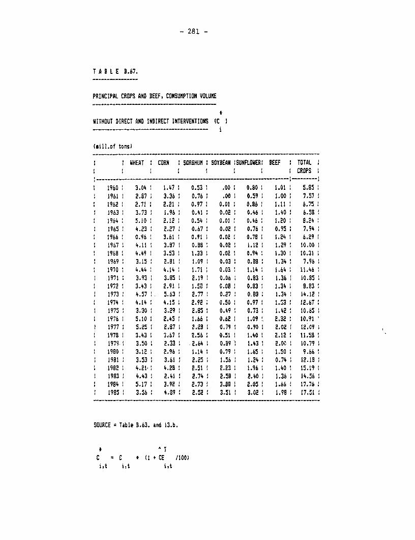
- 281 -

T A 8 L E B.67.

PRINCIPAL CROPS AND BEEF, CONSUMPTION VOLUME

WITHOUT DIRECT AND INDIRECT INTERVENTIONS (C

(sill.of tons)

WHEAT CORN ' SORSHUM SOYBEAN :SUNFLOUER: BEEF TOTAL: i ' :r ': 'CROPS

1 1960 3.04 1 1.47 0.53 .00 0.0 ' 1.01 5.851961 2.87 3.36 0.76 .00 0.59 1.00 7.571962 2.71 2.21 0 0.97: 0.01 0.86: 1.11 6.751963 3.73 1.96 0.41 0.02 0.46 1.40 ' 6.581964 5.10 2.122 0.54 0.01 0.46 1.20 8.241965 4.23 2.27 ' 0.67: 0.02 1 0.76 1 0.95 : 7.941966 0.96 3.61 0.91 O.OZ 0.79 1.24 6.291967 4.11: 3.87 0.88 0.02: 1.12: 1.29: 10.0019681 4.491 3.531 1.331 0.02 0.941 1.30 10.31

1 1969 3.15: 2.81: 1.09 0.03 : 0.88: 1.34 7.961970 4.44 4.14 1.71 0.03 1.14 1.64 11.4619711 3.93 1 3.85: 2.19: 0.06 1 0.83: 1.361 10.851972 1 3.43: 2.91.: 1.52; t.08 ' 0.83: 1.34 1 8.83

* 1973 4.57:. 5.63: 2.77 0.27 0.881 1.34 14.121974 4.14: 4.15 2.92 0.50: 0.97: 1.53 ' 12.6719751 3.30 1 3.29 : 2.85: 0.49 : 0.73 1.42 : 10.65

* 1976 5.10 : 2.45 1 1.66: 0.62 : 1.09' 2.32 1 10.91* 1977 5.25 2.87 2.28 0.79 1 .0.90 1 2.02 12.09i 1978 1 3.43 : 3,67 : 2.56 1 0.51 : 1.40: 2.12: 11.58:

1979' 3.50 : 2.33 ' 2.64 1 0.9: 1.43 I 2.00 1 10.79 119801 3.12 2.96 1.141 0.79 : 1.65 1.50: 9.66:

* 1981 3.53 3.61 : 2.25 1 1.56 1 1.24: 0.74 : 12.181 1982 1 4.21 : 4.28: 2.51 ( 2.23 : 1.96 1 1.40 : 15.19: 1983 4.43 1 2.41 2 2.74 1 2.58: 2.40: 1.36 1 14.56

1984: 5.17: 3.92 1 2.73 : 3.88 2.05 : 1.66 6 17.761985 : 3.56 : 4.89 2.52 3.51 : 3.02 1.98 ! 17.51

SOURCE Table 8.63. and 13.b.

* AT

C C (I + CE /100)i,t i,t i,t

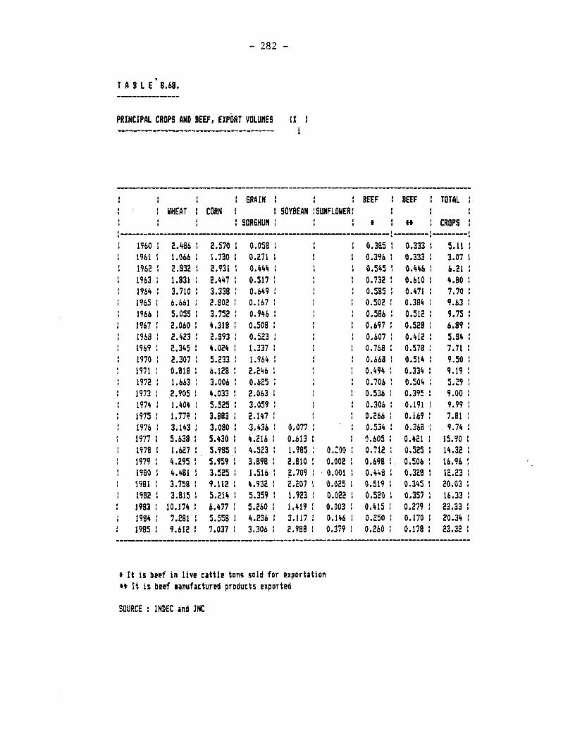
- 282 -

T A B L E B.69.

PRINCIPAL CROPS AND BEEF, EXPORT VOLUMES (IX---------- ------------

1 6RAIN BEEF BEEF : TOTAL:WHEAT I CORN SOYBEAN :SUNFLOWER:

:SORGHUM * : CROPS

1960 2.486 2.570 0.058 ' 0.385 0.333 5.111961 1.066 1.730 : 0.271 1 1 0.396 1 0.333 : 3.071962 : 2.932 1 2.931 1 0.444 ; 0.545 : 0.446 1 6.21

* 1963 1.831 1 2.447 1 0.517 1 0.732 1 0.610 1 4.80: 1964 t 3.710 ' 3.338 ' 0.649 : 1 0.535 I 0.471 1 7.70

1965 6.661 2.802 1 0.167 0.502 1 0.384 1 9.63* 1966 : 5.055 I 3.752 : 0.946 : 1 0.586 : 0.512 1 9.75

1967 : 2.060 1 4.318 1 0.508 1 : : 0.697 : 0.528 : 6.99a1968 2 .423 1 2.893 1 0.523 1 1 0.607 1 0.412 : 5.84

1969 2.345 1 4.024 1.337 ' ' 0.768 : 0.578 7.711970 1 2.307 1 5.233 1 1.964 1 : 1 0.668 1 0.514 1 9.501971 0.88 1 6.128 1 2.246 1 : 0.494 1 0.334 : 9.19 11972 1 1.663 3.006 1 0.625 ; 1 0.706 ' 0.504 1 5.291973 1 2.905 1 4.033 : 2.063 1 ' : 0.536 0.395 1 9.001974 ' 1.404 1 5.525 : 3.059 : 1 : 0.306 0.191 1 9.991975 1 1.772 1 3.883 1 2.147 1 ' 0.266 0.169 1 7.81

1 1976 1 3.143 : 3.080 1 3.436 1 0.077 1 : 0.534 : 0.368 I 9.741977 : 5.638 : 5.430 1 4.216 : 0.613 : 1 t.605 : 0.421 1 15.901978 1 1.627 ' 5.985 1 4.523 1 1.985 0.:00 0.712 0.525 1 14.321979 1 4.295 : 5.959 1 3.898 : 2.810 1 0.002 1 0.698 1. 0.506 ' 16.961980 1 4.481 1 3,525 1 1.516 1 2.709 1 0.001 1 0.448 1 0.328 1 12.23 11981 I 3.758 1 9.112 1 4.932 1 2.207 1 0.025 1 0.519 1 0.345 20.03

* 1982 1 3.815 1 5.214 1 5.359 : 1.923 1 0.022 1 0.520 1 0.357 16.331983 1 10.174 6.477 1 5.260 1 1.419 1 0.003 1 0.415 1 0.279 1 23.331984 1 7.281 : 5.558 : 4.236 : 3.117 : 0.146 1 0.250 1 0.170 1 20.341995 : 9.612 1 7.037 1 3.306 1 2.988 1 0.379 1 0.260 : 0.178 1 23.32

t It is beef in live cattle tons sold for exportation*t It is beef eanufactured prDducts expDrted

SOURCE : INDEC and JNC

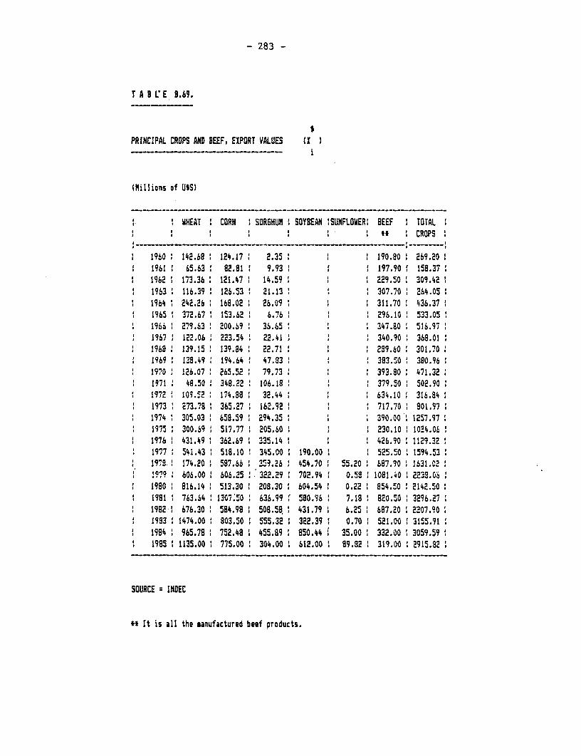
- 283 -

T A 9 L E 8.69.

PRINCIPAL CROPS AND BEEF, EXPORT VALUES (X

(Millions of USS)

WHEAT CORN SORGHUM N SOYBEAN :SUNFLOUER: BEEF TOTAL I: t CROPS I

1960 142.68 124.17 2.35 1 190.80 269.201961 1 65.63 82.81 9.?3 197.90 158.371962 1 173.36 121.47 1 14.59 1 229.50 1 309.421963 116.39 126.53 : 21.13 1 307.70 1 264.051964 242.26 168.02 1 26.09 , 311.70 436.371965 1 372.67 153.62 6.76 1 296.10 533.05

* 1966 279.63: 200.69 : 36.65 347.80 1 516.971967 122.06 223.54 22.41 340.90 368.011968 1 139.15 139.84 22.71 299.60 301.701969 1 138.49 1 194.64 47.83 1 383.50' 380.961970 1 126.07 265.52 79.73 1 393.80 471.321971 1 48.50 348.22 : 106.18 1 1 379.50 1 502.901972 109.52 174.88 32.44 1 1 634.10 316.841973 1 273.78 I 365.27 162.92 1 717.70 901.971974 1 305.03 1 658.59 1 294.35 1 ; 390.00 ' 1257.971975 1 300.69 517.77 ! 205.60 1 : : 230.10 1024.061976 1 431.49 1 362.69 1 335.14 1 1 426.90 11129.321977 1 541.43 1 518.10 345.00 1 190.00 1 525.50 1 1594.531973. 1 174.20 1 587.6S ' 359.2$6 454.70 1 55.20 1 687.90 1 1S31.02!979 1 606.00 1 606.25 1 322.29 1 702.94 0.58 :1081.40: 2238.61980 : 816.14 : 513.30 1 208.30 : 604.54 : 0.22 8 854.50 2142.50:1981 1 763.64 : 1307;50 ; 636.99 r 580.96 1 7.18 1 820.50 :3296.171982 1 676.30 1 584.99 1 508.59 1 431.79 6 b.25 1 687.20 :2207.90:1983 :1474.00 ! 803.50 ' 555.32 ' 322.39 0.70 1 521.00 13155.911994 1 965.78 1 752.48 1 455.89 1 850.44 35.00 1 332.00 :3059.591985 : 1135.00 1 775.00 : 304.00 6 612.00 1 89.82 1 319.00 :2915.a2:

SOURCE = INDEC

H It is all the manufactured beef products.

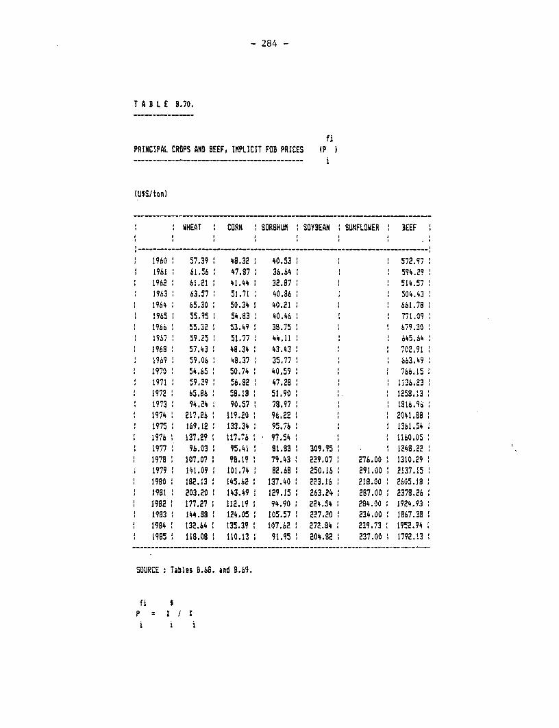
- 284 -

T A 8 L E 8.70.

fiPRINCIPAL CROPS AND BEEF, IMPLICIT FOB PRICES tP

…---------------~- ---------- -… i

(USSfton)

WHEAT CORN ' SORGHUM ' SOYBEAN t SUNFLOWER BEEF. .I . . ..

1960 57.39 48.32 40.53 ' 572.971961 61.56 47.87 36.64 594.291962 61.21 41.44 32.87 514.571963 63.57 51.71 40.86 504.431964 65.30 50.34 40.21 ' 661.781965 55.95 54.93 40.46 : 771.091966 55.32 53.49 38.75 9 679.301967 59.25 51.77 44.11 645.641968 57.43 48.34 43.43 702.911969 59.06 48.37 35.77 663.491970 54.65 50.74 40.59 1 766.151971 59.29 56.82 1 47.28 ' 1136.231972 65.86 58.181 51.90' 1258.131973 94.24 90.57' 78.97 1 1816.91974 2 Z17.26 1 119.20 1 96.22 1 ' 2041.881975 169.12 133.34 95.76 ' ' 1361.54i976 137.29 1117.76 97.541 1 1160.0519771 96.03 1 95.41 1 81.83 309.95 ; 1248.22

1 1978 107.071 98.19 79.43 229.07 1 276.00 1. 1310.291979 141.09 1 101.74 82.68 ' 250.16 ' 291.00 ) 2137.15

1 1980 112.13' 145.62' 137.40' 223.16 1 218.00 2605.181 1981 ' 203.20 1 143.49 1 129.15 ' 263.24 ) 2B7.00 1 2378.26

1982 1 177.27 1 112.19 1 94.90 ' 224.54 1 284.00 1 1924.931 1983 ' 144.88 ' 124.05 ' 105.57 ' 227.20 1 234.00 ' 1367.38

1984 1 132.64 1 135.39 1 107.62 1 272.84 : 239.73 1 1952.941985 ) 118.08 ) 110.13 1 91.95 ' 204.82 237.00 1 1792.13

SOURCE Tables 3.68. and B.69.

fi SP = XIJXi i i

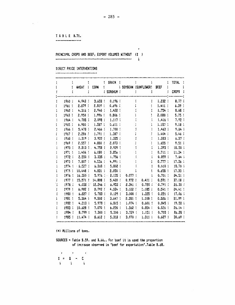
- 285 -

T A B L E B.71.

PRINCIPAL CROPS AND BEEF, EXPORT VOLUMES WITHOUT (X-------- … --- - ---- ------ …-------

DIRECT PRICE INTERVENTIONS

I GRAIN ' TOTALWHEAT CORN 1 SOYBEAN !SUNFLOWER! BEEF

SOR6HUN: ' : : CROPS

1960 4.943 3.633 0.196 ' 1.232 : 8.771961 2.879 2.919 0.696 1.411 1 6.39

1 1962 4.316 2.940 1.422 1 1.754 8.681 1963 2.950 1.996 0.806 i 2.080 5.751964 4.708 2.098 1.117 1.416 1 7.921965 6.980 1.587 0.611 I ?1.187 9.181966 5.478 2.466 1.700 1 1.463 1 9.641967 2.286 1.791 1.387 : 1.404 5.461968 1.319 1 3.922 1 1.325 : : 1 1.283 1 6.57

1 1969 2.557 4.880 2.073 : : 1.655 9.511970 1 2.313' 4.758 : 2.929 1.393 10.501971: 1.406 6.080: 3.856: : : 0.711 11.34

1 1972 2.550 1 3.335 1.756 , 1 0.859 ?.S7.41973: 7.807 1 4.5Z6 : 4.991 ' ' 0.777 : 17.361974 1 6.52? 1 6.368 ' 5.802: I 0.610 18.701971 '10.448 : 4.931 1 2.050 : : : 0.659 1 17.331976 : 16.320 : 5.976 : 2.135 1 0.077 : : 0.701 : 24.511977 ' 15.571 : 14.808 : 5.420 ' 0.972 ' 0.411 , 0.591 1 37.181978 4.058 12.246 : 6.955 , 2.341 , 0.720 : 0.791 : 26.301979: 6.982 1 8.792 1 4.324 : 3.122 1.135: 0.541 : 24.411980 1 6.827 ' 5.783 : 0.129 : 3.000 : 1.325 ' 0.221 ' 17.061981 5.364 : 9.502 ' 3.647 , 2.391 ' 1.100 0.526 , 21.99

1 1982 ' 4.213 5.979 ' 6.815 1 1.974 ' 0.601 1 0.845 : 19.58i 1983 : 10.628 1 7.070 1 6.230 : 1.362 ' 0.954 t 0.26 1 26.14

1994 8 8.799 : 7.300 1 5.300 1 3.729 : 1.151 : 0.703 ' 26.281 1985 ' 11.474 : 8.612 1 5.318 : 3.970 : 1.311 : 0.627 : 30.69

(4) Millions of tons.

SOURCES Table 0.59. and 8.66.. For beef it is used the proportionof increase observed in 'beef for exportation'.Table 8.68.

i i

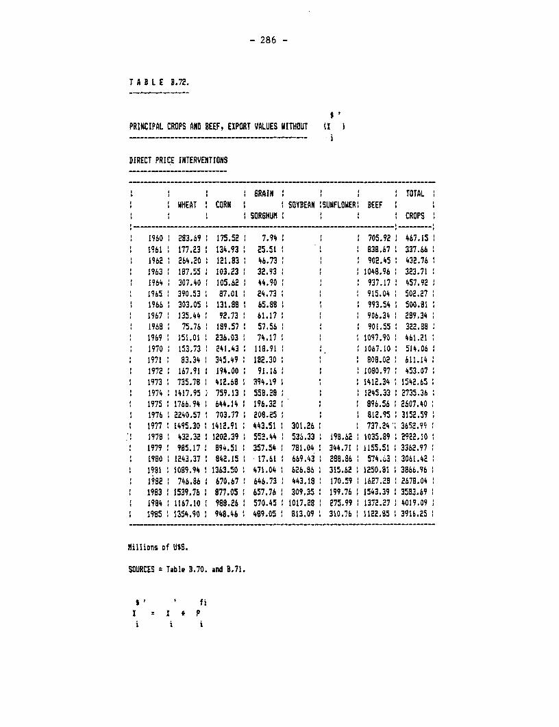
- 286 -

T A 8 L E B.72.

PRINCIPAL CROPS AND BEEF, EXPORT VALUES WITHOUT (I I

DIRECT PRICE INTERVENTIONS

' 1 IB6RAIN I TOTAL'WHEAT 1 CORN 1 1 SOYBEAN !SUNFLOWER: BEEF

SORSHUI I I CROPS

1960 293.69 175.52 7.94 ' , 705.92 467.151961 177.23 134.93 25.51 ' 838.67 337.661962 :264.20 1 121.83 1 46.73 1 902.45 1 432.761963 187.55 1 103.23 1 32.93 1048.96 323.711964 307.40 105.62 1 44.90 f 937.17 457.921965 390.53 87.01 24.73 915.04 502.271966 303.05 131.88 65.88 1 ' 993.54 500.81 '1967 135.44 92.73 61.17 1 ' 906.34 289.341968 75.76 189.57 57.56 901.55 322.881969 151.01 2 236.03 74.17 1097.90 461.211970 153.73 241.43 118.91 1 1 . 1067.10 514.061971 83.34 1 345.49 ' 182.30 ' ' 1 809.02 ' 611.141972 ' 167.91 ' 194.00 91.16 ' 1090.97 ' 453.071973 ' 735.78 412.68 .394.19 1412.34 1542.65 '1974 1 1417.95 759.13 ' 558.-8 ' ' 1245.33 ' 2735.36 '1975 . 1766,94 ' 644.14 ' 196.32 8 ' 896.56 :2607.401976 2240.57 ' 703.77 ' 208.25, 1 812.95 3152.59'1977 1495.30 '1412.91 443.51 ' 301.26 ' 737.24" 3652.95 '1978 '432.32 1 1202.39: 552.44 53S.33 i98.62 1 1035.89 '2522.10 '

* 1979 985.17 ' 894.51 ' 357.54 ' 781.04 ' 344.71 1 i155.51 '3362.97 '1980 1 1243.37 1 842.15 1 17.61 ' 669.43 ' 288.86 574.3 1 3061.42 '1981 1089.94 1 1363.50 471.04 1 626.96 . 315.62 ' 1250.81 13866.96 11982 1 746.86 1 670.67 1 646.73 1 443.18 1 170.59 1 1627.28 2679.041983 1 1539.76 ' 977.05 657.7b 1 309.35 ' 199.76 11543.39 3583.691984 11167.10 1 988.26 1 570.45 1 1017.28 1 275.99 1 1372.27 1 4019.091985 1 1354.90 1 948.46 1 469.05 1 813.09 1 310.76 1 1122.85 1 3916.25

NilliDns of USS.

SOURCES Table B.70. and 3.71.

I I I fiX I1 t Pi i i

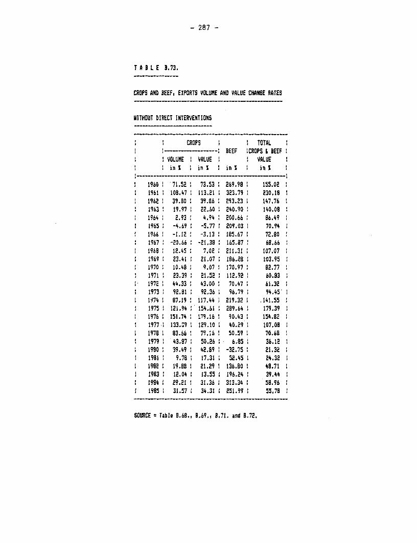
- 287 -

T A a L E B.73.

CROPS AND BEEF, EXPORTS VOLUME AND VALUE CHANSE RATES

WITHOUT DIRECT INTERVENTIONS

CROPS I TOTAL i- - ---- ------- : 9BEEF !CROPS L BEEF

t VOLUME VALUE : I YALUE: in S 1 in S in X I in S

1960 71.52 73.53 269.98 155.021 1961 108.47 113.21 323.79 230,18 :

1962 39.80 39.86 293.23 147.761963 19.97 22.60 240.90 140.081964 2.93 4.94 200.66 86.491 1965 -4.69 -5.77 209.03 70.941966 -1.12 -3.13 185.67 72.801967 -20.66 -21.38 165.87 68.661968 12.45 7.02 211.31 107.071969 23.41 21.07 186.28 103.951970 10.48 9.07 170.97 82.771971 23.39 21.52 1 112.92 1 60.83 1972 1 44.33 43.00 70.47 61.321973 92.81 92.36 96.79 : 94.45 :

: lq74 87.19 117.44; 219.32 .141.55 11975 121.94 154.61 289.64 179.39 1

1 1976 151.74 179.16: 90.43 154.82:19771 133.09 1 129.10 1 40.29 107.081978 1 83.66 1 79.6 50.59 70.681979 43.97 50.26 6.95 1 36.12 :

1 1980 39.49 42.99 1 -32.75 21.32 :1 1981 1 9.78 17.31 I 52.45 1 24.32 :

1 1982 19.98 21.29 1 136.80 1 48.7111 1983 12.04 13.55 1 196.24 1 39.44 11 1984 29.21 1 31.36 313.34 58.96 1: 1985 31.57 1 34.31 1 251.99 1 55.78 1

SOURCE = Table B.68., B.69., 8.71. and 8.72.

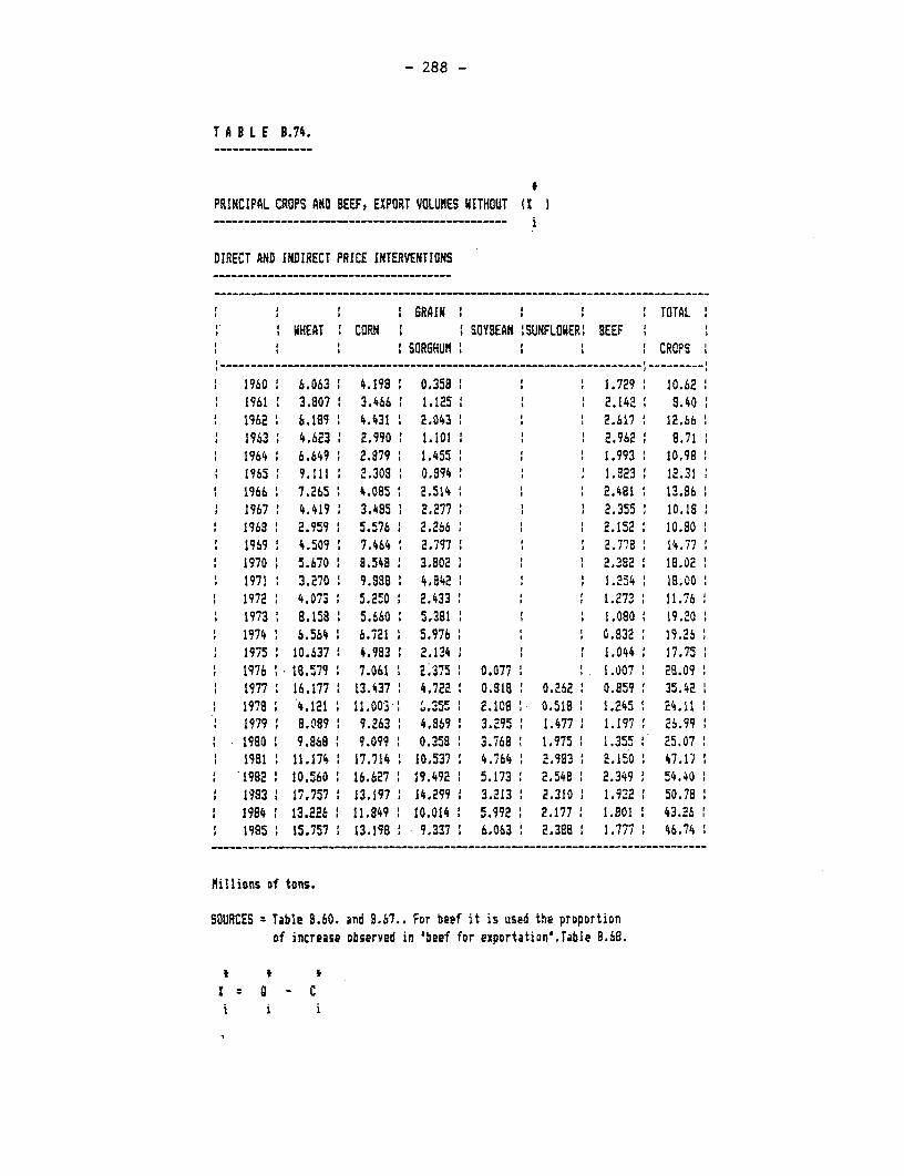
- 288 -

T A B L E 9.74.

PRINCIPAL CROPS AND BEEF, EXPORT VOLUMES WITHOUT tI

DIRECT AND INDIRECT PRICE INTERVENTIONS-----------------------------------

G 'RAIN ' ' ' 5 TOTALWHEAT 5 CORN 5 SOYBEAN !SUNFLOWER BEEF

5SOR6HUM! 5 5 CROPS

1960 ' 6.063 ' 4.199 0.359 5 1.729 10.621961: 3.807 3.466 1.125 2.142 8.4019621 6.189 4.431 2.043 ' 2.617 12.b61963 4.623: 2.990 . 1.101 ' 2.962 9.711964: 6.649 2.979 1.455 1.993 10.981965 9.111: 2.309 0.994 : 1.923 12.311966 1 7.265 4.085 2.514 1 1 2.481 13.36

1 1967 4.419 3.485' 2.277 ' ' 2.355' 10.11968 ' 2.959 ' 5.576 2.266 : 1 2.152 10.90

1969: 4.509 5 7.464: 2.797 ' 1 2.778 14.771970 5.670 8.548 3.802: : : 2.382 8.021971 . 3.270: 9.888 4.942 ' ' 1.254: 18.001972: 4.073: 5.250: 2.433: 1.273: 11.761973 : 8.158 5.660: 5,381 : ' 1.090: 19.201974 : 6.564 5 6.721 ' 5.976 5 0.832 ' 19.261975: 10.637: 4.993: 2.134: : ' 1.044: 17.751976 : 18.579 ' 7.061 ' 2.375 ' 0.077 ' 1 1.007 2 29.09

1 1977 1 16.177 13.437 ' 4.722 0.918 0.262 0.959' 35.421978 4.121' 11.003: '.35'r 2.1081 0.518 1 1.245 I 24.111979 9.089 ' 9.263 4.969 ' 3.295.: 1.477 . 1.197 26.991980 ' 9.868 ' 9.099 ' 0.358 ' 3.768 : 1.975' i.355 1 25.071981 ' 11.174 1 17.714 10.537 4.764 2.9933 2.150: 47.171982 2 10.560 2 16.627 1 19.492 ' 5.173 : 2.548 ' 2.349 : 54.401983 2 17.757 2 13.197 1 14.299 2 3.213' 2.310 : 1.932 50.781994 13.2262 11.849 : 10.014 5.992 2.177' 1.901 43.261985 : 15.757 1 13.198 - 9.337 6.063 2.388: 1.777 46.74

Millions of tons.

SOURCES Table B.60. and 9.67.. For beef it is used the proportionof increase observed in 'beef for exportation'.Table B.68.

X = 0 - Ci i i

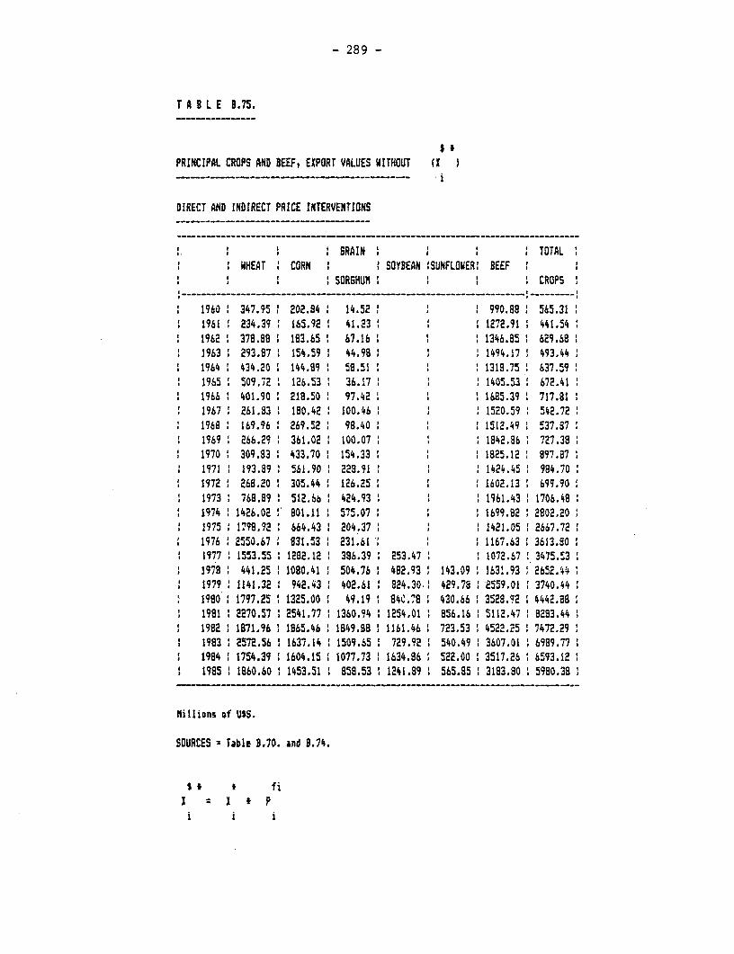
- 289 -

T A 8 L E B.75.

PRINCIPAL CROPS AND BEEF, EXPORT VALUES WITHOUT (I

DIRECT AND INDIRECT PRICE INTERVENTIONS

i i B 6RAIN TOTALWHEAT : CORN SOYBEAN :SUNFLOWER: BEEF

SOR6HUN ; CROPS

1960 1 347.95 1 202.84 14.52 1 990.88 565.311961 234.39 165.92 41.23 1 1272.91 441.541962 378.88 183.65 67.16 1346.85 629.681963 293.87 ; 154.59 44.98 : 1494.17 493.441964 434.20 144.89 59.51 1318.75 637.59 I1965 509.72 126.53 36.17 1405.53 672.411966 1 401.90 218.50 97.42 1685.39 717.811967 261.83 180.42 100.46 1520.59 542.721968 169.96 269.52 98.40 1512.49 537.871969 266.29 361.02 100.07 * 1842.86 727.391970 309.83 433.70 154.33 7 1825.12 897.871971 193.89 561.90 229.91 : 1424.45 984.701972 268.20 1 305.44 126.25 : 1602.13 699.90

1 1973 768.89 : 512.66 I 424.93 1 1961.43 1706.481974 1426.02 1 801.11 I 575.07 * : 1699.82 2802.201975 1798.92 1 664.43 204.37 1 * 1 1421.05 2667.721976 2550.67 8 831.53 231.61 1 1167.63 3613.801977 1553.55 1 1282.12 1 386.39 253.47 1072.67 3475.531978 1 441.25 1080.41 I 504.76 482.93 : 143.09 1631.93 2652.441979 1141.32 i 942.43 402.61 824.30.: 429.78 2559.01 3740.441990 :1797.25 :1325.00 49.19 1 84C.78 4 430.66 :3528.92 4442.88

1 1981 :2270.57: 2541.77 1360.94 1254.01 856.16 :5112.47 8283.441982 1871.96 :1865.46 1849.88 1161.46 723.53 1 4522.25 7472.291983 2572.56 1637.14 1509.65 1 729.92 540.49 :3607.01 6989.77 11984 : 1754.39 1604.15 1077.73 1634.86: 522.00 1 3517.26 :6593.121985 : 1860.60 :1453.51 858.53 1241.89 565.85 3183.80 5980.38

NilliDns of USS.

SOURCES = Table 9.70. and 9.74.

* t t fiI X t p

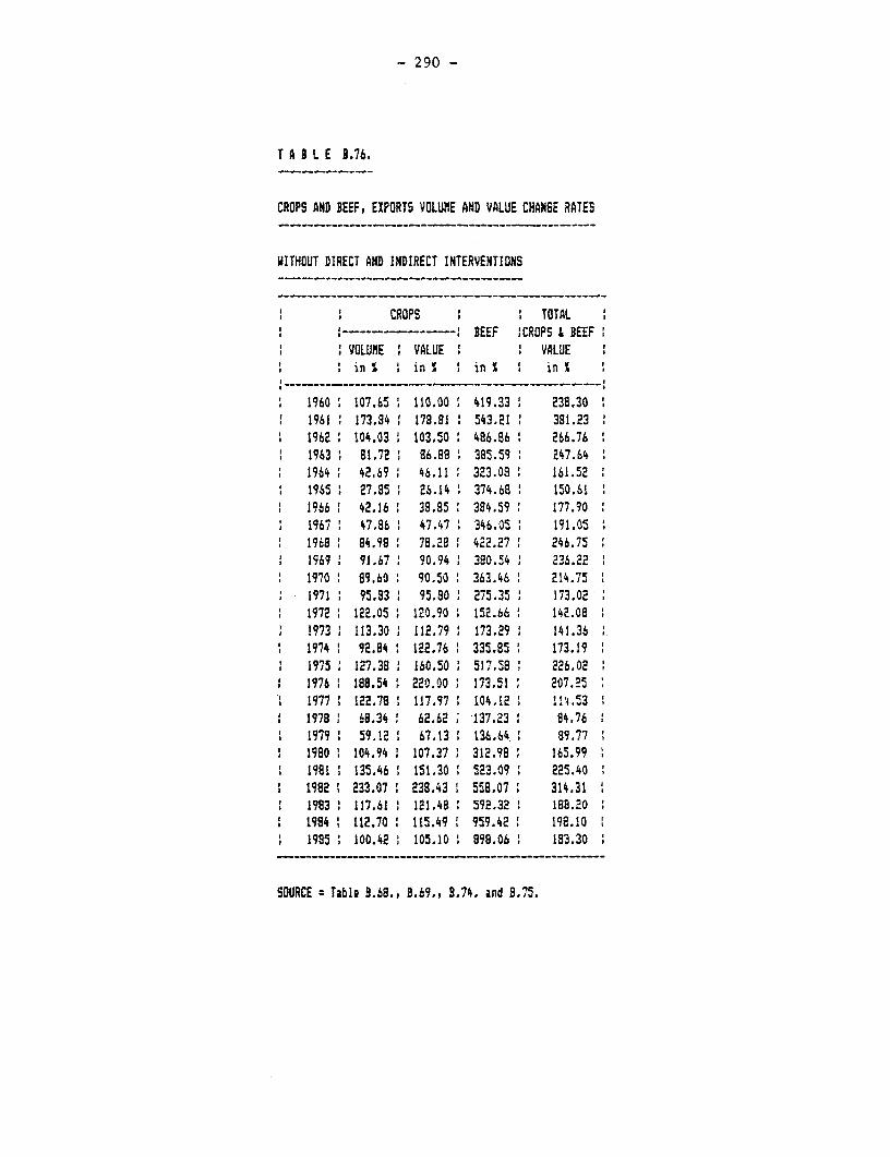
- 290 -

T A 3 L E 3.76.

CROPS AND BEEF, EXPORTS VOLUME AND YALUE CHANGE RATES

WITHOUT DIRECT AND INDIRECT INTERVENTIONS

CROPS TOTAL---- B--------- -- BEEF ICROPS & BEEFVOLUME : VALUE VALUEin S I i in X 1 in %

1960 i 107.65 110.00 419.33 238.301961 1 173.84 178.81 1 543.21 I 381.231962 104.03 103.50 486.86 1 266.761963 81.72 86.88 385.59 247.641964 42.69 46.11 323.08 161.521965 27.85 26.14 374.68 150.611966 42.16 38.85 384.59 177.901967 47.86 47.47 346.05 191.051968 94.98 79.28 ' 422.27 246.751969 91.67 90.94 380.54 236.221970 t 89.60 90.50 363.46 214.751971 95.83 95.80 275.35 173.021972 122.05 120.90 152.66 142.081973 113.30 112.79 173.29 141.361974 92.84 122.76 1 335.85 173.19

1 1i75 127.38 160.50 ' 517.58 226.021976 ' 188.54 220.00 ' 173.51 207.25

1 1977 1 122.78 1 117.97 104.12 1!4.531 1978 ' 68.34 ' 62.62 137.23 ' 94.761 1979 , 59.12 1 67.13 , 136.64 89.77

1980 1 104.94 . 107.37 312.98 1 165.991 1981 ' 135.46 ' 151.30 ' 523.09 : 225.40

1982 233.07 238.43 ' 558.07 314.311983 117.61 ' 121.48 ' 592.32 188.201984 ' 112.70 1 115.49 ' 959.42 198.10

1 1985 100.42 1 105.10 1 898.06 1 183.30

SOURCE = Table 9.68., 3.69., 3.74. and 3.75.

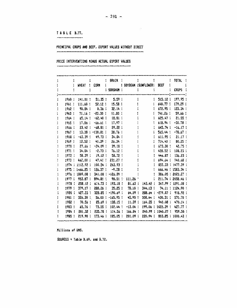
- 291 -

T A B L E B.77.

PRINCIPAL CROPS AND BEEF, EXPORT VALUES WITHOUT DIRECT

PRICE INTERVENTIONS MINUS ACTUAL EXPORT VALUES

- -- _- --- -- -- --- -- -- --- -- - -- - - - - _-_-- - - -- -

GRAIN : TOTAL: WHEAT : CORN I SOYBEAN !SUNFLOWER: BEEF :

: : * ISORGHUM : CROPS

1960 : 141.01 51.35 : 5.59 : : 515.12 197.95S1961 1 111.60 52.12 15.58 640.77 179.29 11962 : 90.84 : 0.36 : 32.14 1 : 672.95 123.341963 71.16 -23.30 11.80 : 741.26 59.661964 65.14 : -62.40 18.811 625.47 21.551965 17.86 -66.61 1 17.97 618.94 -30.78

1 1966 1 23.42 1 -68.81 1 29.22 645.74 -16.171967 1 13.38 : -130.81 38.76 1 : 565.44 : -78.67 1I1968 -63.39: 49.73 34.84 : 611.95 21.171969 12.52 41.39 26.34 714.40 80.25

1 1970 27.66 -24.09 39.18 673.30 42.7511971 34.84 -2.73 1 76.12 428.52 1108.231972 58.39 19.12 1 58.72 : 446.87 1 136.231973 462.00 47.41 ' 231.27 : 694.64 740.681974 1112.92 100.54 263.93 : 855.33 1477.391975 1466.25 126.37 1 -9.28 : : 666.46 1583.341976 1809.08 341.08 -126.89 1 : 386.05 2023.27

I 1977 953.87 1894.81 99.51 1 111.26 1 211.74 2058.461978 258,12 : 64.73 193.18 1 81.63 143.42 : 347.99 1291.081979 379.17 : 288.26 35.25 : 78.10 344.13 : 74.11 1124.90 11980 427.23 328.85 1 -190.69 64.39 288.64 1 -279.87 918.921981 326.30 : 56.00 -165.95 45.90 : 308.44 430.31 570.70

f 1982 70.56 : 85.69 138.15 : 11.39 1 164.35 9 940.08 470.14 11983 65.76 73.55 102.44 : -13.04 1 199.06 1022.39 1 427.77 ;

1 1984 1 201.32 1 235.78 114.56 : 166.84 240.99 1040.27 959.50 11 1985 : 219.90 : 173.46 1 195.05 201.09 220.94 803.85 1000.43 1

Millions of USS.

SOURCES 2 Table B.69. and B.72.

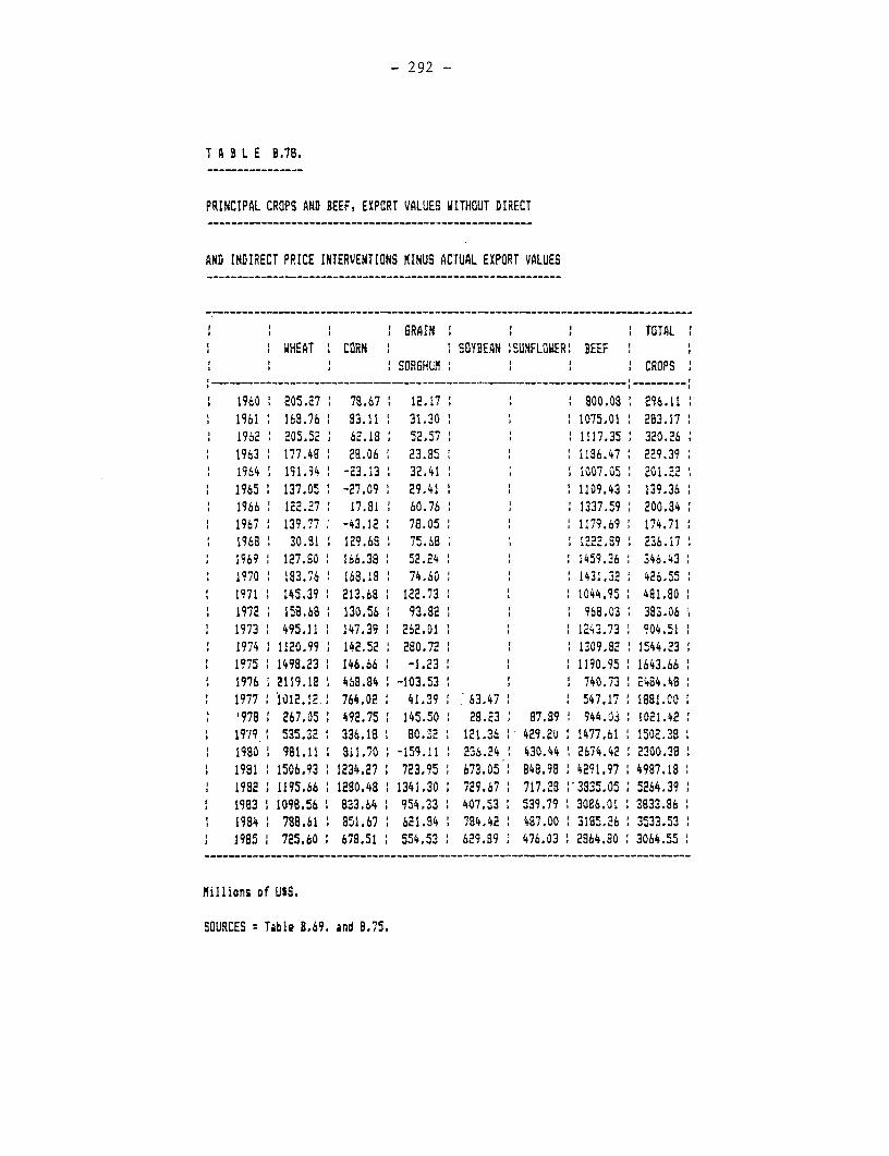
- 292 -

T A B L E 8.7S.

PRINCIPAL CROPS AND BEEF, EXPORT VALUES WITHOUT DIRECT

AND INDIRECT PRICE INTERVENTIONS MINUS ACTUAL EXPORT VALUES

GRAIN I TOTALWHEAT CORN ' SOYBEAN 'SUNFLOWER: BEEF

SORGHUM i CROPS

19.60 205.27 78.67 12.7 800.018 296.111961 168.76 8 93.11 31.30 i 1075.01 293.17 I1962 205.52 62.18 52.57 1117.35 320.2661963 177.48 28.06 23.85 1186.47 229.391964 191.94 -23.13 : 32.41 1007.05 201.221965 137.05 -27.09' 29.41 i 1 1109.43: 139.361966 122.27 17.81 60.76 1337.59 200.8419677 139.77 -43.12 78.05 1179.69 174.711968 30.81 129.68 75.68 12.22.89 236.171969 127.80 166.38 52.24 1 1459.26 346.431970 183.76 168.18 74.60 1431.32 426.551971 ' 145.39 213.68 1 122.73 1 ' ' 1044.95 461.80'1972 158.68 130.56 93.82 1 ' 968.03: 383.061973 495.11 ' 147.39 262.01 ' ' : 1213.73 904.51 '1974 ' 1120.99 ' 142.52 280.72 ' ' ' 1309.82 2 1544.2231975 1498.23 146.66 ' -1.23 ' ' 1190.95 1643.661976 2119.18 1 468.84 -103.53 ' 1 740.73 : 2484.481977 1012.12.: 764.02 1 41.39 ' 63.47 : 547.17 11881.0C0'978 267.05 : 492.75 145.50 ' 28.23 ' 97.89 944.03 1021.42:1979 1 535.32 1 336.18 ' 80.'2 ' 121.36 429.20 ' 1477.61 ' 1502.381980 ' 981.11 ' 311.70 I -159.11 ' 236.24 ' 430.44 ' 2674.42 :2300.381981 1506.93 1234.27 723.95 ' 673.05 848.98 4291.97 4987.18:1992 :1195.66 ' 1280.48 :1341.30 : 729.67 1 717.28 ; 3835.05 5264.39 '1983 1098.56 ' 833.64 ' 954.33 ' 407.53 ' 539.79 3086.01: 3633.86 '1934 788.61 1 851.67 1 621.84 ' 784.42 ' 487.00 :3185.26: 3533.531985 725.60 678.51 554.53 ; 629.89 9 476.03 '2864.80 3064.55

Millions of USS.

SOURCES = Table B.69. and 8.75.

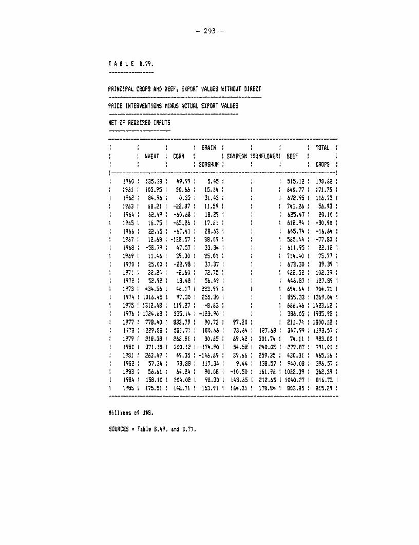
- 293 -

T A I L E B.79.

PRINCIPAL CROPS AND BEEF, EXPORT VALUES WITHOUT DIRECT

PRICE INTERVENTIONS MINUS ACTUAL EXPORT VALUES

NET OF REQUIRED INPUTS

'f RAIN ITTALWHEAT CORN SOYBEAN 'SUNFLOWER' BEEF '

: :. :SDRSHIJI1 U : C CROPS ., _ _ _ _ _ _ _ _ _ _ _ _ _ _______ __ I__ __ _ _

1960 135.18 1 49.99 5.45 , 515.12 1 190.62 ,1961 105.95 1 50.66 15.14 640.77 171.75 11962 84.96 0.35 31.43 672.95 116.7319631 68.21 1 -22.87 11.59 741.26 56.931964 1 62.49 -60.68 18.29 1 625.47 20.101965 16.75 -65.26 17.61 618.94 -30.901966 22.15 -67.41 28.63 i 1 645.74 -16.641967 12.68 -129.57 38.09 i i 565.44 -77.801968 -58.79 47.57 33.34 i 1 611.95 22.12t 1969 11.46 39.30 25.01 t 1 714.40 75.77

1 1970 25.00 -22.98 37.37 673.30 39.391 1971 32.24 1 -2.60 72.75 429.52 102.391972 52.92 18.48 56.49 1 446.7 1 127.89 :

1 1973 1 434.56 1 46.17 1 223.97 1 1 694.64 1 704.711 1974l 1016.45 97.30 255.30 1 1 855.33 1 1369.041 1975 1312.48 119.27 -8.63 1 1 666.46 1423.12'

1976 1124.68 1 335.14 1 -123.90 1 : 386.05 1 1935.92 11 1977 778.40 833.79 1 90.73 1 97.20 f 211.74 :1800.12 :

1; I 22 29.98 58:.71 , 180.66 1 73.64 1 127.68 347.99 1193.57 11 1979 318.38 262.El1 30.65 69.42 301.74 74.11' 983.00

1980 ' 371.18 300.12 1-174.90 , 54.58 1 240.05 : -279.87 1 791.011981 1 263.49 1 49.35 1 -146.69 1 39.66 1 259.35 , 430.31 1 465.16 1

1 1982 1 57.34 1 73.88 1 117.34 1 9.44 138.57 1 940.08 ! 396.57 11983 : 56.61 : 64.24 1 90.08 1 -10.50 161.96 1 1022.39 1 362.39 1

1 1984 1 158.10 1 204.02 . 98.30 1 143.65 1 212.65 1 1040.27 816.73 11 1985 ; 175.51 ; 142.71 1 153.91 1 164.31 1 178.84 1 803.85 1 815.29 1-- -- -- -- - -- - - - - - - -- - - -- -- -- -- -- - - -_-- - - -- -- -- -- -- ---------------

Millions of USS.

SOURCES : Table 3.49. and 8.77.

- 294 -

NOTE 1

Construction of Price Indexes

A) CONSUMER PRICE INDEX (Base 1974 = 1.00) (1960-1985)

A.1. Food and Beverages (1960-1985)

The period 1974-1985 corresponds to the indexes of this

entry. They have been made by INDEC (Instituto Nacional de

Estadistica y Censos).

A reestimation of the period 1960-1973 had to be made due

to a change in the composition of the basket and in the 1974

base. INDEC only made the junction of the series for the

"General Level".

In general, INDEC combined the series by using a

coefficient based on a comparison for one month of the indexes

with different bases and/or baskets. A more accirate metnod

derived from the result of the regression for the period that

overlapped for both series has been taken into account in order

to estimate a coefficient th.t may express the relation bstwe6n

both baskets. In this case, the data for the period Jan./1974 to

may./1977 (i9 observations) was taken into account for both se-

ries (Basis 60 = 100 and Basis 74 = 100).

The coefficient resulting therefrom allowed the estimation

of the period 1960-1973 with a base of 1974 = 100 using as an

independent variable the data of the series 60 for this period

as an independent variable.

In such manner the series 1960-1985 (base 1974 = 100) with

monthly data was obtained. Quarterly and annual indexes were

obtained for all of the series by arithmetical averages.

(Coefficient = 0.0003598).

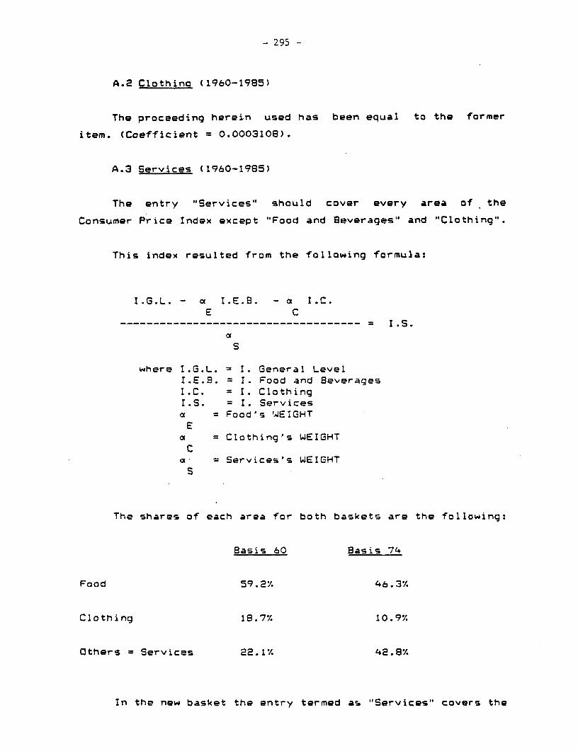
- 295 -

A.2 Clothing (1960-1985)

The proceeding herein used has been equal to the former

item. (Coefficient = 0.0003108).

A.3 Services (1960-1985)

The entry "Services" should cover every area of the

Consumer Price Index except "Food and Beverages" and "Clothing".

This index resulted from the following formula:

.G.L. - aI.E.B. - I.C.E C

_________I__---------------------- I.S.as

where I.G.L. I. General LevelI.E.S. = 1. Food and BeveragesI.C. = I. ClothingI.S. = I. Servicesa = Food's WEIGHTE

a = Clothing's WEIGHTC

a = Services's WEIGHTS

The shares of each area for both baskets are the following:

Basis 60 Basis 74

Food 59.2% 46.3%

Clothing 1B.7% 10.9%

Others = Services 22.1% 42.8%

In the new basket the entry termed as "Services" covers the

- 296 -

following items:

- Living, Fuel and Electricity

- Medical Care

- Transport and Communications

- Home Appliances and Functioning

- Entertainment

- Property and Services of various types

The monthly data for all the period (1960-1985) was

obtained by using the formula mentioned and the base=1974 basket

weights.

A.4 General Level

The series of consumer price indexes "General Level" (Sasis

1974 = 100) was proportioned by INDEC.

3) WHOLESALE

a.1 General Series

The following indexes resulted out of the combination made

by INDEC (base 198S = 100)

- General Level

- Total National

- Agricultural National

- Non-Agricultural National

- Imported

- Total Non-agricultural

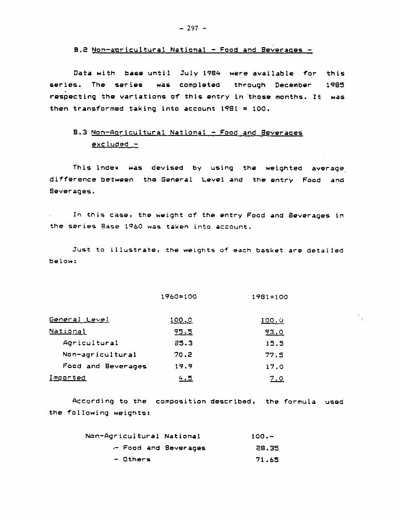
- 297 -

B.2 Non-amricultural National - Food and 8everages -

Data with base unti-l July 1924 were available for this

series. The series was completed through December 19S5

respecting the variations of this entry in 'those months. It was

then transformed taking into account 1981 = 100.

2.3 Non-Agricultural National - Food and Beverages

excluded -

This index was devised by using the weighted average

difference between the General Level and the entry Food and

Beverages.

In this case, the weight of the entry Food and Beverages in

the series Base 1960 was taken into account.

Just to illustrate, the weights of each basket are detailed

below:

1960=100 1981=100

General Level 100.0 100.I

National 95.5 93.0

Agricultural 25.3 15.5

Non-agricultural 70.2 77.5

Food and Beverages 19.9 17.0

Imported 4.5 7.0

According to the composition described, the formula used

the following weights:

Non-Agricultural National 100.-

Food and Beverages 2S.35

- Others 71.65

- 298 -

C) CONSTRUCTION COST

The series with base 1960 was available and this was

transformed with a coefficient that respects the junction made

by the INDEC as from 1970 with the new basis 1980 = 100.

D) EXPORTABLES

In order to detect the evolution of the domestic prices of

exportables, the National Agricultural Index is usually used.

However, exports consist of three entries:

- Agricultural

- Agroindustrial

- Non-traditional

Since the annual export taxes (in %) have been calculated

in the form of percentage resulting from the levy and the

exports of the two former entries, the index of exportables

shiould take only those two entries into account.

On the contrary, non t-aditional exports generally exhibit

unusual behaviour in which the domestic price is higher than the

FOB export price, even though this is not justified by the size

of the export subsidy granted. This is explained by the

protection duty which is received.

In this way and according to the composition of the

wholesale basket, the index of exportables was made in the

following manner:

Exportables= (Agricultural Nat. x Agric. Nat.'s weight) +

(Non-agric. Nat.'s - Food and 8ev. - x Food and 3ev.'s

weight)

- 299 -

Where,

Weiahts

Agricultural National 47.7% (15.5/32.5)

Non-agricult. Nat.-Food and Bev.- 52.3% (17.-/32.5)

Exportables 100.-X. (32.5/32.5)

E) IMPORTABLES

In order to make this index the Non-agricultural National

Index - Food and Beverages excluded - and the Imported goods

index have been used with the following weights:

Non-Agricultural Nat.

(Food and Bev.excluded) 90.-r. (60.5/67.5)

Imported 10.-% ( 7.-/67.5)

Importables 100.-x. (67.5/67.5)

F) TRADABLFS

According to the former items, it can be inferred that the

Wholesale General Level Index has been taken as the one which is

representative of tradables products with the following

composition:

Wholesale = Tradables 100.-X.

Agricultural National 15.5%

Non-Agricult.Nat. - Food and Bev.- 17--

Exportables 32.5%

Non-Agric. Nat. - Food and Bev. exc. - 60.5%

Imported 7.-J

Imoortables 67.5%

This weight does not contradict the actual shares in the

- 300 -

composition of the Gross Domestic Product (G.D.P.):

G.D.P. 100.-/,

- Agricultural

- Industrial 31 .- %.

- Food and Bev. (e.-'.)

- Others (23.-%)

- Construction 6.-.

- Services 50.-%

G) NON TRADABLE

In order to derive this index, the Construction Cost Index

(item C) and the entry "Services" of the Consumer Price Index

(item A.3) have been taken into account according to the

following weights in the G.D.P.:

- Non-Tradables 100.-?. (56.-/56.-)

Construction Cost 11.-% ( 6.-/56.-)

"Services" 89.-'. (50.-/56.-)

H) TRADA8LES

The Tradables Index is a weighted average of the foreign-f ~f

price indexes, P and P . The weights are those of exports andx ~mimports for each year.

I) NON AGRICULTURE

In order to derive this index the following weights of the

G.D.P. have been used:

Non-agricultural 100.-?.

- Non-agric. National 36.-% (31.-/87.-)

- Services 57.-?. (50.-/87.-)

- Construction Cost 7.-% t 6.-/87.-)

- 301 -

NOTE 2

The equilibrius equation is:

f f f fE PI gx + E Pe Ca + Ph th = E Px Cx + E Pe Cm + Ph Ch + S E

where E : noeinal exchange rate

fPx : foreign price of exportables

fPa = foreign price of iaoDrtables

Ph - dosestic price of non tradables

a - ;rodduction

C cccnsuaotion

Defining

X-g Cx exoorts

Ca- g imports

We have

f fE Pi I E Pn h : Ph (Ch - Ohl + S E

where I X (Px/Ph i Pm-Ph)

N - IPxlPh Pa/Ph)

Qh :agh IPx/Ph ; PmlPh)

Ch= Ch (PI/Ph ; Pa/Ph)

So, the equilibrius in the earket of non tradable goods isplies:

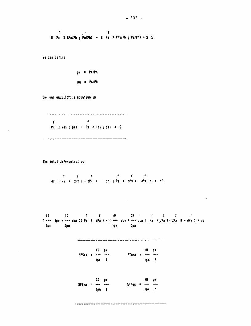
- 302 -

f fE Pi I (PI/Ph; iPuIh) - E Pm I thPPh; PuJPh)S SE

we can dofine

px a PsIPh

So, our equilibrius equation is

f fPI S (pi ; om) - PI n (px ; pI) S

The total diferential is

f f f f f fil I Ps + dP ) + dPxS- !M 1e t dPx I - dP 2 : dS

f f f f f f--- dox + --dpa H Pi t dPxsI -- dpw --- d;m 3 Pi t dPa )z dPa 1 - dP XI dS

31 px Ps paEPSxx --- -* ETAm -…

)px ) )ps A

)1 Ps )1 pIEPSxa * - -- ETAx. -- -

3pm I ipx x

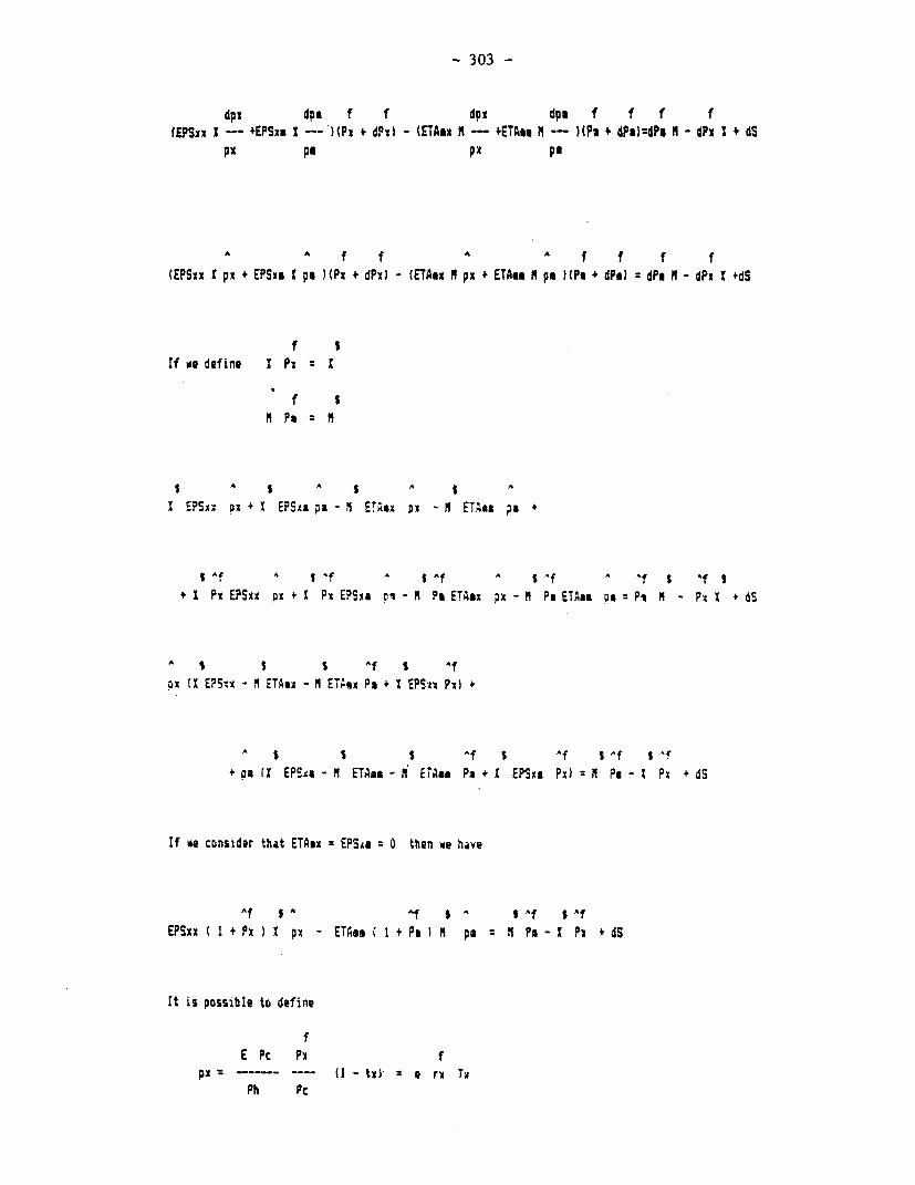
- 303 -

dpi dpa f f dpi dp f f f f(EPSxx -- 4EPSxm I-- )(Px * Ox) - (ETAux N -- *ETAhm N -- )(Pt * dP:dP N11 - POx I dS

pi eP px pe

A A f f A A f f f f

(EPSxx I px + EPSxs Ipe )(PM + dPx) - (ETAnx N px + ETAe. N ps )(Pe * dPe) dPi N - dPi S +dS

f SIf we define I Px I

f I

A A5 A 5A

X EPSXX px+X EPSXaSp-a ETI .x oX -f ETA&& ps +

I If A^IIf S I IIf A S If ̂ A -f ^ If I

4 I Pi EPSxx px+I PiEPSXs e N- Ps ETAx pX -M Po ETAss Ps: P1 - PX I + dS

A 5 5 5 Af S Af

pi EPMx I 1 ETA*% - N ETr.x Pa + I EPS:x Pi) +

' S 5 S ^f S Af SIf S -

+ p. (I EPSxa- N ETAme - ETAa. Pa + X EPSxa Px) = N PS - Px P dS

If we cDnsider that ETAax EPSAI - 0 then we have

Af *A If $ ^ 5Af gAf

EPSxx ( I + Pi) I px - ETAa( + Pe ) N pa P - I Pi + dS

It is possible to define

fE Pc Pi f

pi- (I - tx) z e ri TxPh Pc

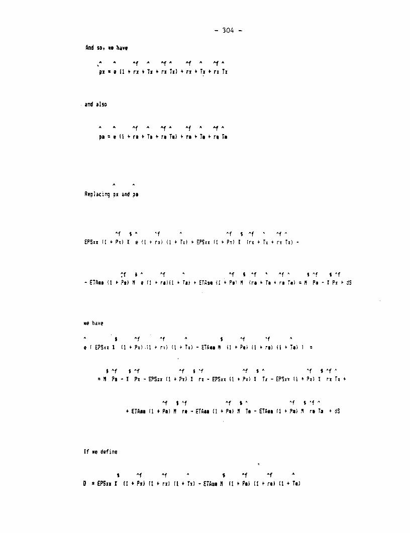
- 304 -

And so, to have

A A Af A sf A Af A Af A

px - (I t rx t Tx + rx Tx) t rx + Tx * rx Tx

and also

A Af A f A Af A Af A

pa=e (1 + ra * Ta + ra Ta) + ra * To 4 ra To

Replacing px and pi

'S f 'S A Af S ^f A If^

EPSsx (1 t Ps) I e (I + rx) (I + Tx) + E?Six (I t Psl I (rv + Tx rx Tx) -

Af ) A Af A Af S f f AfS Af Sf

- ETAsa i I Pg) N e (I *+ ei) t I + T ErT (I + ps I. (re r. t ra 7m) z A Ps - I Px 4 dS

we have

A I Af Af A , Af 'f A

e I EPSti I (i t Ps) .l + rw) (I 4 Tx) - ETAe N il t Pxi) H t ra) H + T4) ):

A f S Af Af s If Af A ^f Sf

M Ps - X Px - EPSxx (1 + Pt) I rx - EPSxx il t PY) X Tx - EPSxr il t Pi) I ri Tx t

IIf S 'f A A Af $ If A

t ETAPa fl + Pa) I re - ETA#a (I t Pa) M ta - ETAee (1 + Ps) N ro Ta + dS

If we define

5 Af Af S f Af A

D: EPSsx I (I PO) (1 + rx) (+ Tx) - Tdaam . (I 1 Pt ) (I + ra) (1 + Ts)

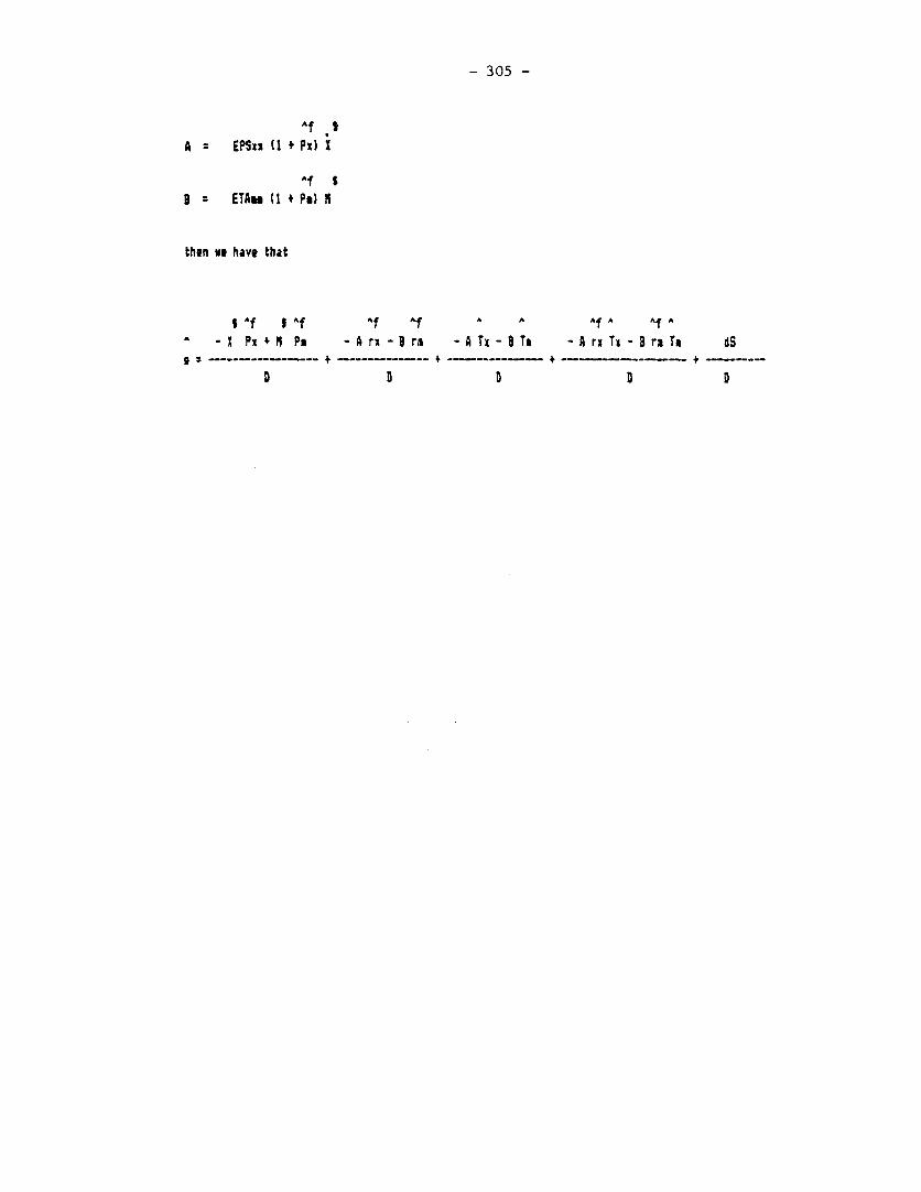
- 305 -

Af ,

A : EPSxx (I + Px A

A 5

a ETAme t + Pn) a

then we have that

* Af 5 Af Af Af A A Af A Af A

-X Px + P -A rx - 8 ra -ATx-BT - A rx Tx - 3 ra T dS

:---- - -- +--------+------- + +

D D D D

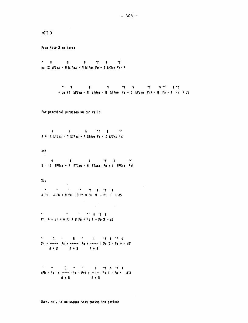
- 306 -

NOTE 3

FrDs Note 2 me have:

A 5 I 5 Af S Af

px UI EPSxx - M ETAex -1 ETAdx Pe + I EPSsx Px) +

A $ I I Af S Af $'f S f

+ ps IX EPSxa - A ETAu - A ETA. P + I EPSxe Px) A Pa - I Px + dS

For practical purooses we can call:

s s s .4f s "f

: =X ESnx -n ETAax - N ETAnx Po+ I EPSxX Px)

and

* S s ^f Af

a: (I EPSx- N ETAoe - M ETAre °n + I EPSxa Px)

So,

A* .* I If s Af S

Pit - A Ph + 9 Pe - 9 Ph - PI 1 -Px I + ds

A A If A .f I

Ph (A + 3 A Px + Ps + P I - Pm - dS

A A 3 ' A I Af I If i

Pi Po ----- iPPx X - P - dS)A i 3 A + a A + 9

1 A 3 A A I f A f S S

(Ph - Px) (P - PxO + --- Px I - Pe - dSlA+8 A+3

Then. only if ve assuse that durinc the period:

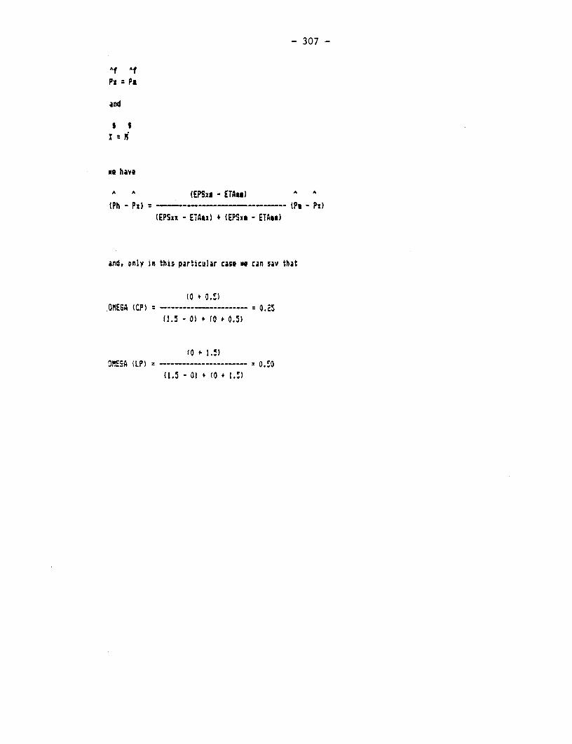
- 307 -

Af Af

and

2'S

we have

A A (EPSXs - ETAu) A A

(Ph - Pfl -(Ps - Psl)(EPSxx - ETAesl + (EPSxm - ETAse)

and, only in this particular case go can say that

(O t 0.S),OMEGA ICP) - ------ - - -----~~- --:0° 25

(1.5 - 0) + (O + 0.5)

(0 t 1.!)OSSA ILP): -------- ----- - ---.5) O

(1.5 - Oi t (0 t I.,.)

- 309 -

REFERENCES

BALASSA, B., The purchasing-power parity doctrine: A

reappraisal, Journal of Political Economy 72. 1964.

BALDWIN, Robert E., The Political Economy of Proteccionism, en

Jagdish Bhagwati: Import Competition and Response, The

University of Chicago Press, 1982.

BECKER, Gary S., A Theory of Competition among pressure groups

for political influence, en The Quarterly Journal of Economics.

Vol. 98, Agosto 1983, No 3.

BERLINSKI, J. and SCHYDLOWSKY, D.M., Incentives for

Industrialization in Argentina, IBRD, 1977

BROCK, William A. and MAGGEE, Stephen P., The economics of

Special Interest Politics: the case of the tariff. American

Economic Review, Vol. 68, No2., 1968.

BUCHANAN, J. and TULLOCK, G., El cAlculo del consenso, Madrid,

Espasa-Calpe. 1964.

CAVALLO,D.F. and MUNDLAK, Y., Agriculture and Econom;c Growth in

an open Economy: The case of Argentina, IFPRI, Research Report,

Na 36, 1982

CAVALLO, D.F., Exchanqe rate overvaluation and agriculture (The

case of Araaentina), Background paper for WDR 86, First Draft,

1985.

CEPAL/FAO, La Politica Aqropecuaria y la Economia Argentina,

1955-1980, RLAT 3/2, 1983 (Documento preparado por L. Cuccia).

CORDEN, W.M., Politica comercial v Bienestar Econ6mico, Ice Ed.,

Madrid, 1978.