6281 Synchronous Generators GB 20070912

1

The Impact of Synchronous Generators Excitation Supply on Protection and Relays

Gabriel Benmouyal, Schweitzer Engineering Laboratories, Inc.

Abstract—Synchronous generators have two types of opera-tional limits: thermal and stability. These limits are commonly defined in the P-Q plane and, consequently, the point of opera-tion of a generator should not lie beyond any of these limits. The functions that prevent the generator from infringing into the forbidden zones are known as limiters and are normally embed-ded in the generator Automatic Voltage Regulator (AVR). The combination of these limiters and the nature of the AVR itself will have an impact on some generator protective functions like the loss-of-field (LOF) or out-of-step protection. The purpose of this paper is not to review generators’ protection principles, be-cause this has been done extensively elsewhere, but rather to revisit the basic physical and engineering principles behind the interaction between a synchronous generator AVR and its asso-ciated limiters and some of the generator protective functions. We review the technology of the limiters embedded in a genera-tor AVR. In LOF coordination studies, the steady-state stability limit (SSSL) used most often has been traditionally based on a generator-system with a constant-voltage excitation (or manual SSSL). In this paper, we discuss the impact of the excitation sys-tem with an AVR or a power system stabilizer (PSS) on the gen-erator stability limits. A new numerical technique is introduced to determine the stability limits of a generator-system where the excitation supply could be regulated using either an AVR or an AVR supplemented by a PSS.

I. GENERATOR THERMAL AND STEADY-STATE STABILITY LIMITS

There are three types of thermal limits ([1]–[4]) in a gen-erator: the armature current limit that is directly related to the generator rated power, the field current limit, and the end core limit. The steady-state stability limit is a direct consequence of the power transfer equation between a generator and the net-work that it is supplying. These different limits are reviewed in the next section.

A. Generator Thermal Operational Limits In Fig. 1, the three types of thermal limits found on a gen-

erator are represented. Assuming that the power is measured in per-unit (p. u.) values, a half-circle with unit radius repre-sents the generator theoretical maximum capability (GTMC). This limit is caused by the armature current ohmic losses and corresponds simply to the generator MVA rating.

The end-core limit is a consequence of the end-turn leakage flux existing in the end region of a generator. The end-turn leakage flux enters and leaves in a direction perpendicular to the stator lamination. Eddy currents will then flow in the lamination and will be the cause of localized heating in the end region. In overexcited mode, the field current is high and as a consequence the retaining ring will get saturated so that the end flux leakage will be small. In the underexcited mode,

the field current will be reduced and the flux caused by the armature current will add up to the flux produced by the field current. This will exacerbate the end-region heating and will severely limit the generator output. The end-core limit de-pends upon the turbine construction and geometry. The limita-tion could be particularly severe for gas turbines, yet could be nonexistent for hydro units as shown in Fig. 1; steam units would have a limiting characteristic in the middle [1].

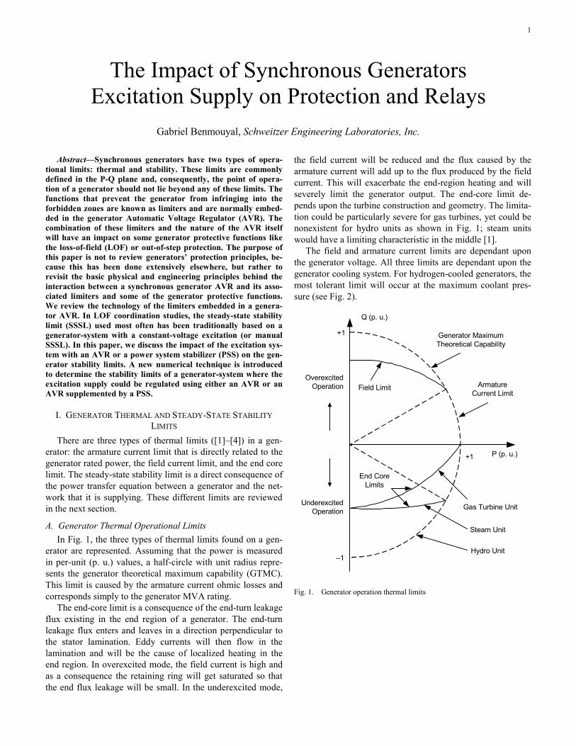
The field and armature current limits are dependant upon the generator voltage. All three limits are dependant upon the generator cooling system. For hydrogen-cooled generators, the most tolerant limit will occur at the maximum coolant pres-sure (see Fig. 2).

Q (p. u.)

P (p. u.)

Generator MaximumTheoretical Capability

+1

+1

–1

Field Limit

End Core Limits

Steam Unit

Gas Turbine Unit

Hydro Unit

ArmatureCurrent Limit

OverexcitedOperation

UnderexcitedOperation

Fig. 1. Generator operation thermal limits

2

P (MW)

0

50

100

150

200

250

50

100

150

200

Q (

MV

AR

)

50 100 150 200 250 300 350

300

LeadingPowerFactor

LaggingPowerFactor

H Pressure3.0 kg/cm2

2.0 kg/cm2

2

0.90

0.95

Fig. 2. Capability curve at nominal voltage of a 312 MW, 347 MVA, 20 kV, 0.9 PF, 3600 rpm, 60 Hz, hydrogen-cooled steam-turbine generator

B. Classic Steady-State Stability Limit of Round Rotor Gen-erator

The steady-state stability limit of a generator determines the region in the P-Q plane where the generator operation will be stable in a normal mode of operation. Normal mode of op-eration is defined here as a mode where only small and minor disturbances are occurring on the network, as opposed to ma-jor disturbances such as faults, significant addition of load, or loss of generation. The steady-state stability limit is used by protection engineers in some coordination studies and for the adjustment of the under-excitation limiter (UEL) function in the AVR [1, 5].

Eq

Xd,Xq

Et Es

Xe

Fig. 3. Elementary generator-system

The manual SSSL is derived for a generator-system corre-sponding to Fig. 3, where the generator supplies its load to an infinite bus through a line with impedance Xe. The generator excitation is assumed to be supplied with a constant voltage. The power transfer equation for a salient-pole machine is pro-vided in steady state by the conventional formula:

δ++

−+δ

+= 2sin

)XX()XX(2XX

EsinXX

EEP

eqed

qd2s

ed

sq (1)

In this last equation, the angle δ is the angle between the generator internal voltage Eq and the infinite bus voltage Es. It is a well-established principle that the generator stability limit is reached when the derivative of the real power P with respect to the angle δ becomes equal to zero.

02cos)XX()XX(

XXEcos

XXEE

tP

eqed

qd2s

ed

sq =δ++

−+δ

+=

δδ (2)

Trying to solve (2) will lead to non-linear equations, and there is no algebraic equation for the SSSL. The problem can be simplified, however, by considering a round-rotor machine, for which Xd equals Xq equals the synchronous reactance Xs so that the power transfer equation becomes:

δ+

= sinXX

EEP

es

sq (3)

In this case, the stability limit is reached when the angle δ reaches the value of 90°. A circle with a center and radius, as shown in Fig. 4, provides the stability limit under manual op-eration in the P-Q plane [1].

Q (p. u.)

P (p. u.)

⎟⎟⎠

⎞⎜⎜⎝

⎛−=

de

2t

X1

X1

2EjCenter

⎟⎟⎠

⎞⎜⎜⎝

⎛+=

de

2t

X1

X1

2ERadius

Fig. 4. Manual SSSL circle for generator system with constant excitation

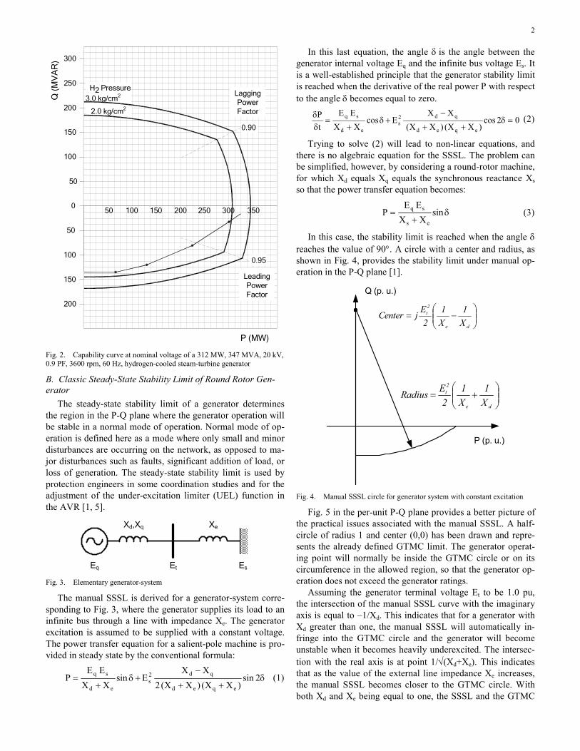
Fig. 5 in the per-unit P-Q plane provides a better picture of the practical issues associated with the manual SSSL. A half-circle of radius 1 and center (0,0) has been drawn and repre-sents the already defined GTMC limit. The generator operat-ing point will normally be inside the GTMC circle or on its circumference in the allowed region, so that the generator op-eration does not exceed the generator ratings.

Assuming the generator terminal voltage Et to be 1.0 pu, the intersection of the manual SSSL curve with the imaginary axis is equal to –1/Xd. This indicates that for a generator with Xd greater than one, the manual SSSL will automatically in-fringe into the GTMC circle and the generator will become unstable when it becomes heavily underexcited. The intersec-tion with the real axis is at point 1/√(Xd+Xe). This indicates that as the value of the external line impedance Xe increases, the manual SSSL becomes closer to the GTMC circle. With both Xd and Xe being equal to one, the SSSL and the GTMC

3

circle coincide. There are high values of Xe for which the gen-erator could not supply its rated power without becoming un-stable: the manual SSSL infringes inside the GTMC limit.

-1.5

-1

-0.5

0

0.5

1

1.5

0 0.5 1 1.5 2 2.5 3

Per U

nit Q

Per Unit P

Xd=1.4

Xe=0.2

Xd=0.8

Xe=0.2

Xd=1.0

Xe=1.0

Xd=1.4

Xe=0.9

GTMC Et=1.0

Fig. 5. Manual SSSL with respect to the GTMC circle

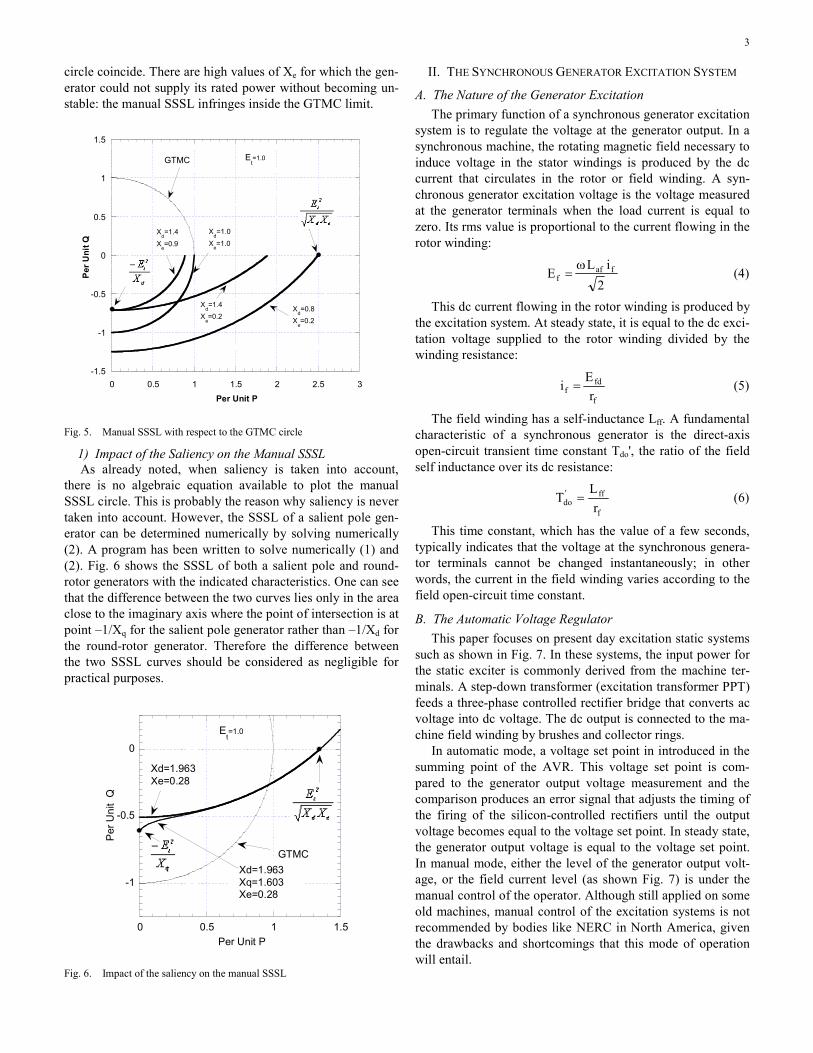
1) Impact of the Saliency on the Manual SSSL As already noted, when saliency is taken into account,

there is no algebraic equation available to plot the manual SSSL circle. This is probably the reason why saliency is never taken into account. However, the SSSL of a salient pole gen-erator can be determined numerically by solving numerically (2). A program has been written to solve numerically (1) and (2). Fig. 6 shows the SSSL of both a salient pole and round-rotor generators with the indicated characteristics. One can see that the difference between the two curves lies only in the area close to the imaginary axis where the point of intersection is at point –1/Xq for the salient pole generator rather than –1/Xd for the round-rotor generator. Therefore the difference between the two SSSL curves should be considered as negligible for practical purposes.

-1

-0.5

0

0 0.5 1 1.5

Per

Uni

t Q

Per Unit P

Xd=1.963Xe=0.28

Xd=1.963Xq=1.603Xe=0.28

GTMC

Et=1.0

Fig. 6. Impact of the saliency on the manual SSSL

II. THE SYNCHRONOUS GENERATOR EXCITATION SYSTEM

A. The Nature of the Generator Excitation The primary function of a synchronous generator excitation

system is to regulate the voltage at the generator output. In a synchronous machine, the rotating magnetic field necessary to induce voltage in the stator windings is produced by the dc current that circulates in the rotor or field winding. A syn-chronous generator excitation voltage is the voltage measured at the generator terminals when the load current is equal to zero. Its rms value is proportional to the current flowing in the rotor winding:

2

iLE faff

ω= (4)

This dc current flowing in the rotor winding is produced by the excitation system. At steady state, it is equal to the dc exci-tation voltage supplied to the rotor winding divided by the winding resistance:

f

fdf r

Ei = (5)

The field winding has a self-inductance Lff. A fundamental characteristic of a synchronous generator is the direct-axis open-circuit transient time constant Tdo', the ratio of the field self inductance over its dc resistance:

f

ff'do r

LT = (6)

This time constant, which has the value of a few seconds, typically indicates that the voltage at the synchronous genera-tor terminals cannot be changed instantaneously; in other words, the current in the field winding varies according to the field open-circuit time constant.

B. The Automatic Voltage Regulator This paper focuses on present day excitation static systems

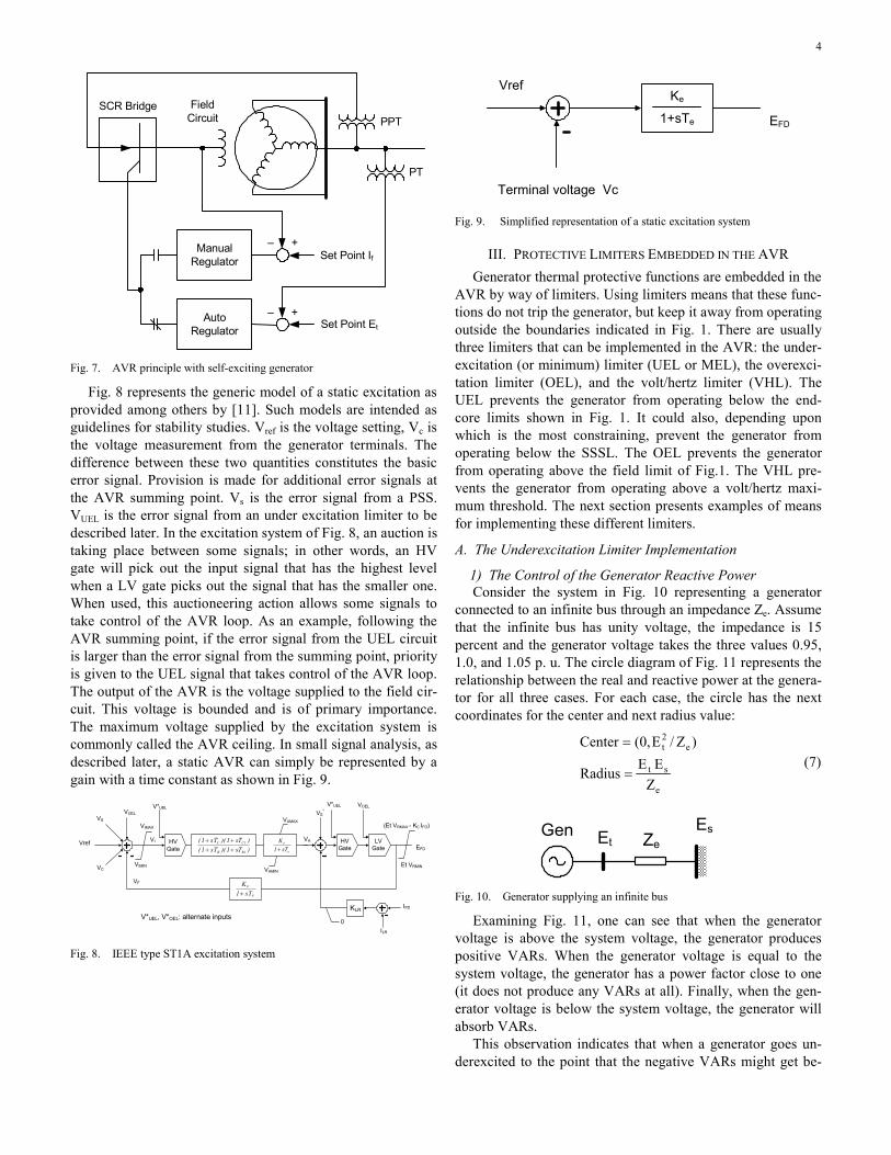
such as shown in Fig. 7. In these systems, the input power for the static exciter is commonly derived from the machine ter-minals. A step-down transformer (excitation transformer PPT) feeds a three-phase controlled rectifier bridge that converts ac voltage into dc voltage. The dc output is connected to the ma-chine field winding by brushes and collector rings.

In automatic mode, a voltage set point in introduced in the summing point of the AVR. This voltage set point is com-pared to the generator output voltage measurement and the comparison produces an error signal that adjusts the timing of the firing of the silicon-controlled rectifiers until the output voltage becomes equal to the voltage set point. In steady state, the generator output voltage is equal to the voltage set point. In manual mode, either the level of the generator output volt-age, or the field current level (as shown Fig. 7) is under the manual control of the operator. Although still applied on some old machines, manual control of the excitation systems is not recommended by bodies like NERC in North America, given the drawbacks and shortcomings that this mode of operation will entail.

4

Manual Regulator

AutoRegulator

SCR Bridge

Set Point Et

Set Point If

PPT

PT

FieldCircuit

+–

+–

Fig. 7. AVR principle with self-exciting generator

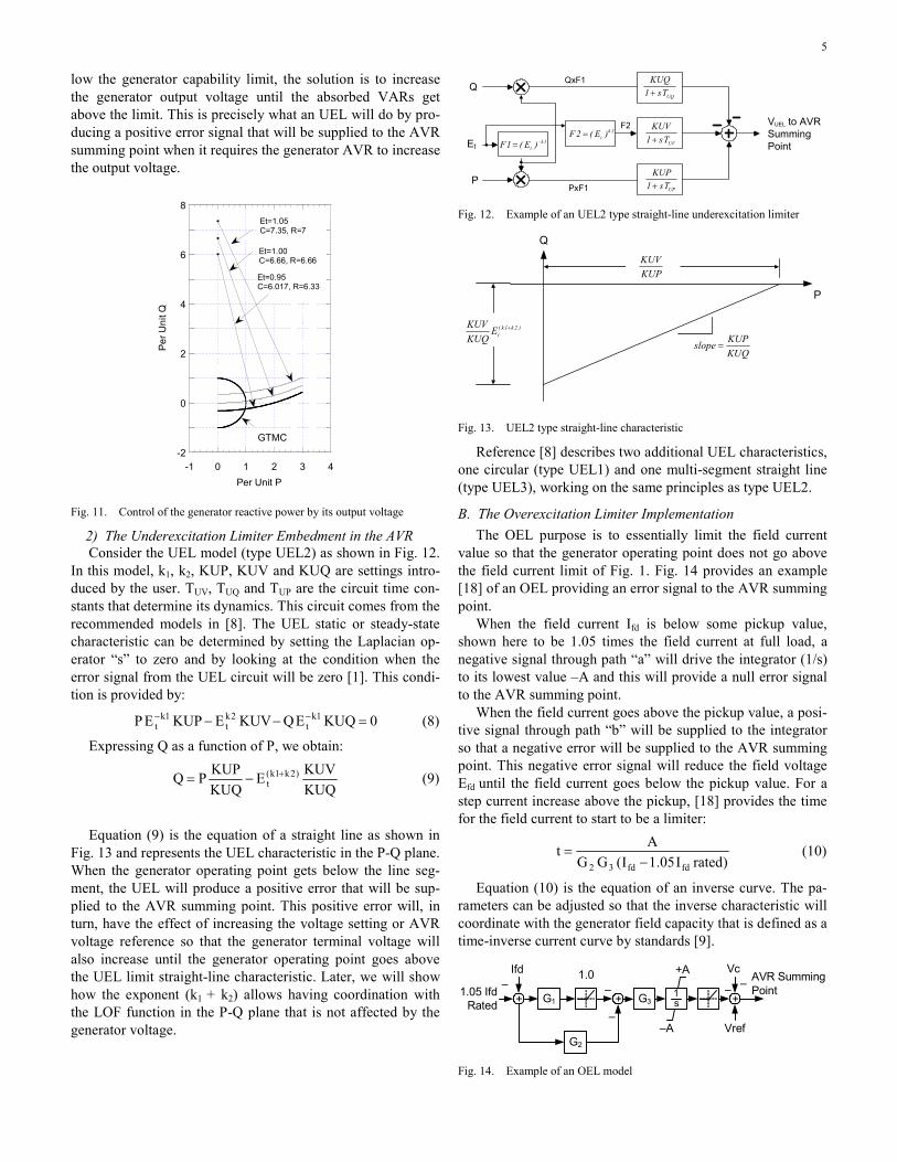
Fig. 8 represents the generic model of a static excitation as provided among others by [11]. Such models are intended as guidelines for stability studies. Vref is the voltage setting, Vc is the voltage measurement from the generator terminals. The difference between these two quantities constitutes the basic error signal. Provision is made for additional error signals at the AVR summing point. Vs is the error signal from a PSS. VUEL is the error signal from an under excitation limiter to be described later. In the excitation system of Fig. 8, an auction is taking place between some signals; in other words, an HV gate will pick out the input signal that has the highest level when a LV gate picks out the signal that has the smaller one. When used, this auctioneering action allows some signals to take control of the AVR loop. As an example, following the AVR summing point, if the error signal from the UEL circuit is larger than the error signal from the summing point, priority is given to the UEL signal that takes control of the AVR loop. The output of the AVR is the voltage supplied to the field cir-cuit. This voltage is bounded and is of primary importance. The maximum voltage supplied by the excitation system is commonly called the AVR ceiling. In small signal analysis, as described later, a static AVR can simply be represented by a gain with a time constant as shown in Fig. 9.

Vref)sT1)(Ts1()sT1)(Ts1(

1BB

1CC

++++

F

F

Ts1K+

VF

VUELVS

VC

HVGate

HVGate

LVGate

V*UEL

VI

VIMAX

VIMIN

VA

VAMIN

VAMAX

V*UEL VOEL

VS*

EFD

Et VRMIN

(Et VRMAX - KC IFD)

KLR

0

IFD

ILR

V*UEL, V*OEL: alternate inputs

e

e

sT1K+

Fig. 8. IEEE type ST1A excitation system

Vref

EFD

Terminal voltage Vc

Ke

1+sTe

Fig. 9. Simplified representation of a static excitation system

III. PROTECTIVE LIMITERS EMBEDDED IN THE AVR Generator thermal protective functions are embedded in the

AVR by way of limiters. Using limiters means that these func-tions do not trip the generator, but keep it away from operating outside the boundaries indicated in Fig. 1. There are usually three limiters that can be implemented in the AVR: the under- excitation (or minimum) limiter (UEL or MEL), the overexci-tation limiter (OEL), and the volt/hertz limiter (VHL). The UEL prevents the generator from operating below the end-core limits shown in Fig. 1. It could also, depending upon which is the most constraining, prevent the generator from operating below the SSSL. The OEL prevents the generator from operating above the field limit of Fig.1. The VHL pre-vents the generator from operating above a volt/hertz maxi-mum threshold. The next section presents examples of means for implementing these different limiters.

A. The Underexcitation Limiter Implementation

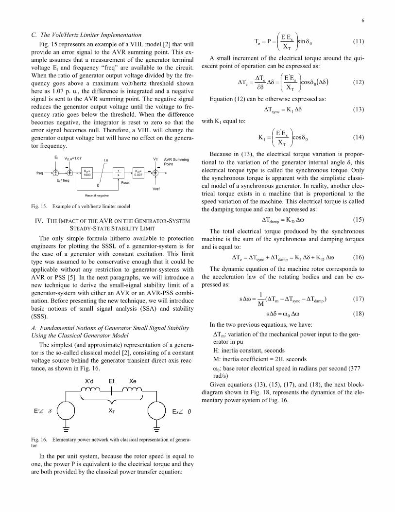
1) The Control of the Generator Reactive Power Consider the system in Fig. 10 representing a generator

connected to an infinite bus through an impedance Ze. Assume that the infinite bus has unity voltage, the impedance is 15 percent and the generator voltage takes the three values 0.95, 1.0, and 1.05 p. u. The circle diagram of Fig. 11 represents the relationship between the real and reactive power at the genera-tor for all three cases. For each case, the circle has the next coordinates for the center and next radius value:

e

st

e2t

ZEERadius

)Z/E,0(Center

=

= (7)

Et ZeEsGen

Fig. 10. Generator supplying an infinite bus

Examining Fig. 11, one can see that when the generator voltage is above the system voltage, the generator produces positive VARs. When the generator voltage is equal to the system voltage, the generator has a power factor close to one (it does not produce any VARs at all). Finally, when the gen-erator voltage is below the system voltage, the generator will absorb VARs.

This observation indicates that when a generator goes un-derexcited to the point that the negative VARs might get be-

5

low the generator capability limit, the solution is to increase the generator output voltage until the absorbed VARs get above the limit. This is precisely what an UEL will do by pro-ducing a positive error signal that will be supplied to the AVR summing point when it requires the generator AVR to increase the output voltage.

-2

0

2

4

6

8

-1 0 1 2 3 4

Per U

nit Q

Per Unit P

Et=1.05C=7.35, R=7

Et=1.00C=6.66, R=6.66

Et=0.95C=6.017, R=6.33

GTMC

Fig. 11. Control of the generator reactive power by its output voltage

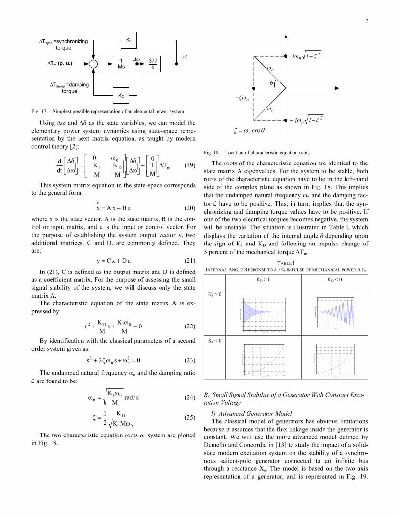
2) The Underexcitation Limiter Embedment in the AVR Consider the UEL model (type UEL2) as shown in Fig. 12.

In this model, k1, k2, KUP, KUV and KUQ are settings intro-duced by the user. TUV, TUQ and TUP are the circuit time con-stants that determine its dynamics. This circuit comes from the recommended models in [8]. The UEL static or steady-state characteristic can be determined by setting the Laplacian op-erator “s” to zero and by looking at the condition when the error signal from the UEL circuit will be zero [1]. This condi-tion is provided by:

0KUQEQKUVEKUPEP 1kt

2kt

1kt =−− −− (8)

Expressing Q as a function of P, we obtain:

KUQKUVE

KUQKUPPQ )2k1k(

t+−= (9)

Equation (9) is the equation of a straight line as shown in

Fig. 13 and represents the UEL characteristic in the P-Q plane. When the generator operating point gets below the line seg-ment, the UEL will produce a positive error that will be sup-plied to the AVR summing point. This positive error will, in turn, have the effect of increasing the voltage setting or AVR voltage reference so that the generator terminal voltage will also increase until the generator operating point goes above the UEL limit straight-line characteristic. Later, we will show how the exponent (k1 + k2) allows having coordination with the LOF function in the P-Q plane that is not affected by the generator voltage.

UVTs1KUV+

UQTs1KUQ+

UPTs1KUP+

2kt )E(2F =

1kt )E(1F −=

VUEL to AVR Summing Point

Q

P

QxF1

PxF1

F2

Et

Fig. 12. Example of an UEL2 type straight-line underexcitation limiter

Q

P

KUPKUV

KUQKUPslope =

)2k1k(tE

KUQKUV +

Fig. 13. UEL2 type straight-line characteristic

Reference [8] describes two additional UEL characteristics, one circular (type UEL1) and one multi-segment straight line (type UEL3), working on the same principles as type UEL2.

B. The Overexcitation Limiter Implementation The OEL purpose is to essentially limit the field current

value so that the generator operating point does not go above the field current limit of Fig. 1. Fig. 14 provides an example [18] of an OEL providing an error signal to the AVR summing point.

When the field current Ifd is below some pickup value, shown here to be 1.05 times the field current at full load, a negative signal through path “a” will drive the integrator (1/s) to its lowest value –A and this will provide a null error signal to the AVR summing point.

When the field current goes above the pickup value, a posi-tive signal through path “b” will be supplied to the integrator so that a negative error will be supplied to the AVR summing point. This negative error signal will reduce the field voltage Efd until the field current goes below the pickup value. For a step current increase above the pickup, [18] provides the time for the field current to start to be a limiter:

)ratedI05.1I(GG

Atfdfd32 −

= (10)

Equation (10) is the equation of an inverse curve. The pa-rameters can be adjusted so that the inverse characteristic will coordinate with the generator field capacity that is defined as a time-inverse current curve by standards [9].

1.0

Vref

VcAVR SummingPoint1.05 Ifd

Rated

Ifd +A

–A

+–

+–

–

– –G1

G2

G31s +

Fig. 14. Example of an OEL model

6

C. The Volt/Hertz Limiter Implementation Fig. 15 represents an example of a VHL model [2] that will

provide an error signal to the AVR summing point. This ex-ample assumes that a measurement of the generator terminal voltage Et and frequency “freq” are available to the circuit. When the ratio of generator output voltage divided by the fre-quency goes above a maximum volt/hertz threshold shown here as 1.07 p. u., the difference is integrated and a negative signal is sent to the AVR summing point. The negative signal reduces the generator output voltage until the voltage to fre-quency ratio goes below the threshold. When the difference becomes negative, the integrator is reset to zero so that the error signal becomes null. Therefore, a VHL will change the generator output voltage but will have no effect on the genera-tor frequency.

Kz1=1000

1s

Kz2=0.007

1.0

0Vref

Vc AVR SummingPoint

Et

freq

Et / freq

VZLM=1.07

Reset if negative

Reset

Fig. 15. Example of a volt/hertz limiter model

IV. THE IMPACT OF THE AVR ON THE GENERATOR-SYSTEM STEADY-STATE STABILITY LIMIT

The only simple formula hitherto available to protection engineers for plotting the SSSL of a generator-system is for the case of a generator with constant excitation. This limit type was assumed to be conservative enough that it could be applicable without any restriction to generator-systems with AVR or PSS [5]. In the next paragraphs, we will introduce a new technique to derive the small-signal stability limit of a generator-system with either an AVR or an AVR-PSS combi-nation. Before presenting the new technique, we will introduce basic notions of small signal analysis (SSA) and stability (SSS).

A. Fundamental Notions of Generator Small Signal Stability Using the Classical Generator Model

The simplest (and approximate) representation of a genera-tor is the so-called classical model [2], consisting of a constant voltage source behind the generator transient direct axis reac-tance, as shown in Fig. 16.

E'∠ δ

Et

Es∠ 0

X’d Xe

XT

Fig. 16. Elementary power network with classical representation of genera-tor

In the per unit system, because the rotor speed is equal to one, the power P is equivalent to the electrical torque and they are both provided by the classical power transfer equation:

0T

s'

e sinX

EEPT δ⎟⎟⎠

⎞⎜⎜⎝

⎛== (11)

A small increment of the electrical torque around the qui-escent point of operation can be expressed as:

( )δΔδ⎟⎟⎠

⎞⎜⎜⎝

⎛=δΔ

δ∂Δ

=Δ 0T

s'

ee cos

XEETT (12)

Equation (12) can be otherwise expressed as: δΔ=Δ 1sync KT (13)

with K1 equal to:

0T

s'

1 cosX

EEK δ⎟⎟⎠

⎞⎜⎜⎝

⎛= (14)

Because in (13), the electrical torque variation is propor-tional to the variation of the generator internal angle δ, this electrical torque type is called the synchronous torque. Only the synchronous torque is apparent with the simplistic classi-cal model of a synchronous generator. In reality, another elec-trical torque exists in a machine that is proportional to the speed variation of the machine. This electrical torque is called the damping torque and can be expressed as: ωΔ=Δ Ddamp KT (15)

The total electrical torque produced by the synchronous machine is the sum of the synchronous and damping torques and is equal to: ωΔ+δΔ=Δ+Δ=Δ D1dampsynce KKTTT (16)

The dynamic equation of the machine rotor corresponds to the acceleration law of the rotating bodies and can be ex-pressed as:

)TTT(M1s dampsyncm Δ−Δ−Δ=ωΔ (17)

ωΔω=δΔ 0s (18)

In the two previous equations, we have: ΔTm: variation of the mechanical power input to the gen-erator in pu H: inertia constant, seconds M: inertia coefficient = 2H, seconds ω0: base rotor electrical speed in radians per second (377 rad/s)

Given equations (13), (15), (17), and (18), the next block-diagram shown in Fig. 18, represents the dynamics of the ele-mentary power system of Fig. 16.

7

K1

377s

1MsΔTm (p. u.)

ωΔ δΔ

KD

ΔTsync =synchronizing torque

ΔTdamp =damping torque

Fig. 17. Simplest possible representation of an elemental power system

Using Δω and Δδ as the state variables, we can model the elementary power system dynamics using state-space repre-sentation by the next matrix equation, as taught by modern control theory [2]:

mD1

0T

M10

MK

MK0

dtd

Δ⎥⎥⎦

⎤

⎢⎢⎣

⎡+⎥

⎦

⎤⎢⎣

⎡ωΔδΔ

⎥⎥

⎦

⎤

⎢⎢

⎣

⎡

−−

ω=⎥

⎦

⎤⎢⎣

⎡ωΔδΔ

(19)

This system matrix equation in the state-space corresponds to the general form:

uBxAxo

+= (20)

where x is the state vector, A is the state matrix, B is the con-trol or input matrix, and u is the input or control vector. For the purpose of establishing the system output vector y, two additional matrices, C and D, are commonly defined. They are: uDxCy += (21)

In (21), C is defined as the output matrix and D is defined as a coefficient matrix. For the purpose of assessing the small signal stability of the system, we will discuss only the state matrix A.

The characteristic equation of the state matrix A is ex-pressed by:

0M

KsM

Ks 01D2 =ω

++ (22)

By identification with the classical parameters of a second order system given as:

0s2s 2nn

2 =ω+ωζ+ (23)

The undamped natural frequency ωn and the damping ratio ζ are found to be:

s/radM

K 01n

ω=ω (24)

01

D

MKK

21

ω=ζ (25)

The two characteristic equation roots or system are plotted in Fig. 18.

nω

2n 1j ζω −

2n 1j ζω −−

nζω−

nω

θωζ cosn=

θ

Fig. 18. Location of characteristic equation roots

The roots of the characteristic equation are identical to the state matrix A eigenvalues. For the system to be stable, both roots of the characteristic equation have to lie in the left-hand side of the complex plane as shown in Fig. 18. This implies that the undamped natural frequency ωn and the damping fac-tor ζ have to be positive. This, in turn, implies that the syn-chronizing and damping torque values have to be positive. If one of the two electrical torques becomes negative, the system will be unstable. The situation is illustrated in Table I, which displays the variation of the internal angle δ depending upon the sign of K1 and KD and following an impulse change of 5 percent of the mechanical torque ΔTm.

TABLE I INTERNAL ANGLE RESPONSE TO A 5% IMPULSE OF MECHANICAL POWER ΔTM

KD > 0 KD < 0

K1 > 0

0 5 10 15 20 25 30 35-0.8

-0.6

-0.4

-0.2

0

0.2

0.4

0.6

Time (s)

Var

iatio

n o

f th

e R

oto

r A

ngle

0 5 10 15

-5

-4

-3

-2

-1

0

1

2

3

4

5

Time (s)

Var

iati

on o

f th

e R

oto

r A

ngle

K1 < 0

0 0.05 0.1 0.15 0.2 0.250

0.5

1

1.5

2

2.5

3

3.5

4

4.5

Time (s)

Var

iatio

n of

the

Rot

or A

ngle

0 0.05 0.1 0.15 0.2 0.250

0.5

1

1.5

2

2.5

3

3.5

4

4.5

5

Time (s)

Var

iatio

n of

the

Rot

or A

ngle

B. Small Signal Stability of a Generator With Constant Exci-tation Voltage

1) Advanced Generator Model The classical model of generators has obvious limitations

because it assumes that the flux linkage inside the generator is constant. We will use the more advanced model defined by Demello and Concordia in [13] to study the impact of a solid-state modern excitation system on the stability of a synchro-nous salient-pole generator connected to an infinite bus through a reactance Xe. The model is based on the two-axis representation of a generator, and is represented in Fig. 19.

8

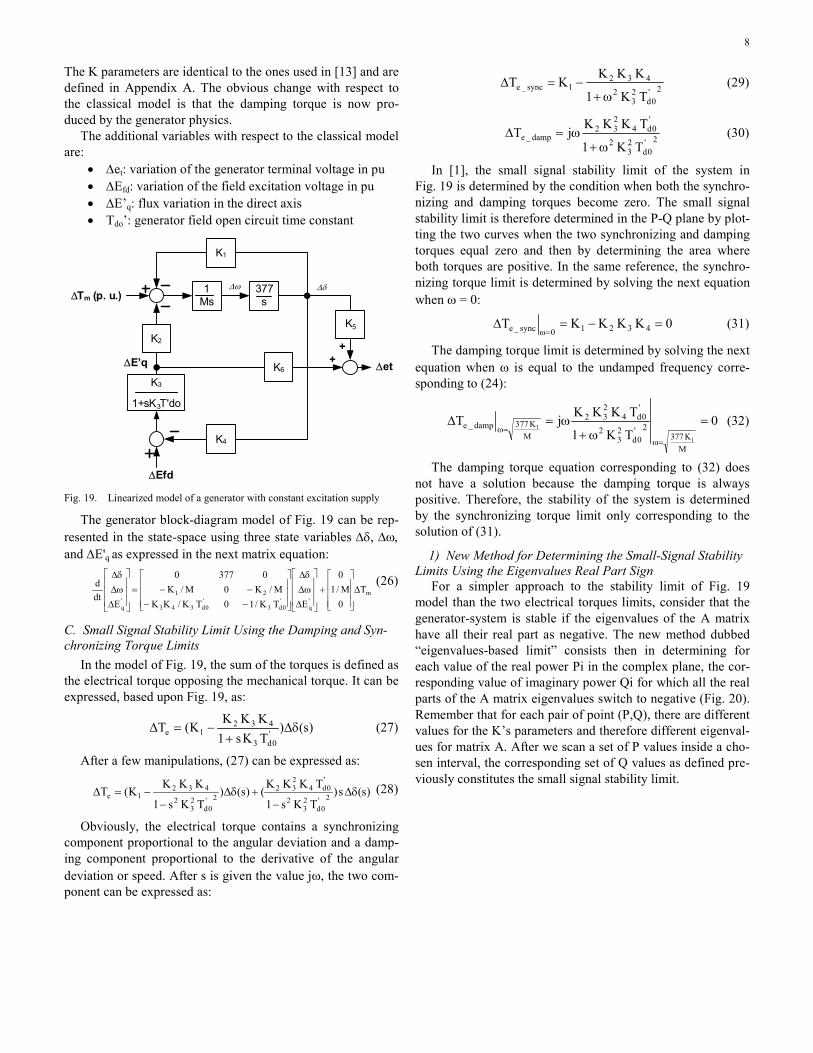
The K parameters are identical to the ones used in [13] and are defined in Appendix A. The obvious change with respect to the classical model is that the damping torque is now pro-duced by the generator physics.

The additional variables with respect to the classical model are:

• Δet: variation of the generator terminal voltage in pu • ΔEfd: variation of the field excitation voltage in pu • ΔE’q: flux variation in the direct axis • Tdo’: generator field open circuit time constant

K1

K2

377s

1Ms

K5

K6

K4

1+sK3T'do

K3

ΔTm (p. u.)

ΔEfd

Δet

δΔωΔ

ΔE’q ++

Fig. 19. Linearized model of a generator with constant excitation supply

The generator block-diagram model of Fig. 19 can be rep-resented in the state-space using three state variables Δδ, Δω, and ΔE'q as expressed in the next matrix equation:

m

'q

'0d3

'0d343

21'q

T0M/1

0

ETK/10TK/KKM/K0M/K

03770

Edtd

Δ⎥⎥⎥

⎦

⎤

⎢⎢⎢

⎣

⎡+

⎥⎥⎥

⎦

⎤

⎢⎢⎢

⎣

⎡

ΔωΔδΔ

⎥⎥⎥

⎦

⎤

⎢⎢⎢

⎣

⎡

−−−−=

⎥⎥⎥

⎦

⎤

⎢⎢⎢

⎣

⎡

ΔωΔδΔ (26)

C. Small Signal Stability Limit Using the Damping and Syn-chronizing Torque Limits

In the model of Fig. 19, the sum of the torques is defined as the electrical torque opposing the mechanical torque. It can be expressed, based upon Fig. 19, as:

)s()TKs1KKKK(T '

0d3

4321e δΔ

+−=Δ (27)

After a few manipulations, (27) can be expressed as:

)s(s)TKs1

TKKK()s()

TKs1

KKKK(T 2'

0d23

2

'0d4

232

2'0d

23

2432

1e δΔ−

+δΔ−

−=Δ (28)

Obviously, the electrical torque contains a synchronizing component proportional to the angular deviation and a damp-ing component proportional to the derivative of the angular deviation or speed. After s is given the value jω, the two com-ponent can be expressed as:

2'0d

23

2432

1sync_eTK1

KKKKT

ω+−=Δ (29)

2'0d

23

2

'0d4

232

damp_eTK1

TKKKjT

ω+ω=Δ (30)

In [1], the small signal stability limit of the system in Fig. 19 is determined by the condition when both the synchro-nizing and damping torques become zero. The small signal stability limit is therefore determined in the P-Q plane by plot-ting the two curves when the two synchronizing and damping torques equal zero and then by determining the area where both torques are positive. In the same reference, the synchro-nizing torque limit is determined by solving the next equation when ω = 0:

0KKKKT 43210sync_e =−=Δ=ω

(31)

The damping torque limit is determined by solving the next equation when ω is equal to the undamped frequency corre-sponding to (24):

0TK1

TKKKjT

MK377

2'0d

23

2

'0d4

232

MK377damp_e

1

1=

ω+ω=Δ

=ω=ω

(32)

The damping torque equation corresponding to (32) does not have a solution because the damping torque is always positive. Therefore, the stability of the system is determined by the synchronizing torque limit only corresponding to the solution of (31).

1) New Method for Determining the Small-Signal Stability Limits Using the Eigenvalues Real Part Sign

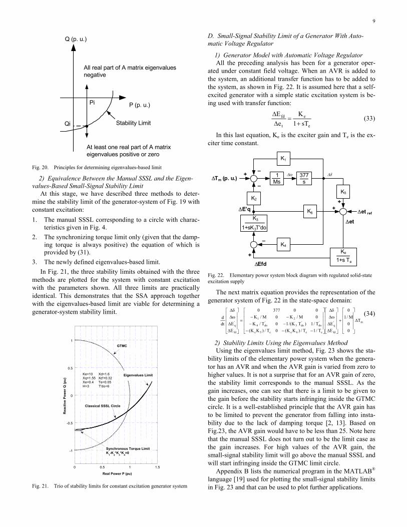
For a simpler approach to the stability limit of Fig. 19 model than the two electrical torques limits, consider that the generator-system is stable if the eigenvalues of the A matrix have all their real part as negative. The new method dubbed “eigenvalues-based limit” consists then in determining for each value of the real power Pi in the complex plane, the cor-responding value of imaginary power Qi for which all the real parts of the A matrix eigenvalues switch to negative (Fig. 20). Remember that for each pair of point (P,Q), there are different values for the K’s parameters and therefore different eigenval-ues for matrix A. After we scan a set of P values inside a cho-sen interval, the corresponding set of Q values as defined pre-viously constitutes the small signal stability limit.

9

P (p. u.)

Q (p. u.)

All real part of A matrix eigenvalues negative

At least one real part of A matrix eigenvalues positive or zero

Stability LimitQi

Pi

Fig. 20. Principles for determining eigenvalues-based limit

2) Equivalence Between the Manual SSSL and the Eigen-values-Based Small-Signal Stability Limit

At this stage, we have described three methods to deter-mine the stability limit of the generator-system of Fig. 19 with constant excitation: 1. The manual SSSL corresponding to a circle with charac-

teristics given in Fig. 4. 2. The synchronizing torque limit only (given that the damp-

ing torque is always positive) the equation of which is provided by (31).

3. The newly defined eigenvalues-based limit. In Fig. 21, the three stability limits obtained with the three

methods are plotted for the system with constant excitation with the parameters shown. All three limits are practically identical. This demonstrates that the SSA approach together with the eigenvalues-based limit are viable for determining a generator-system stability limit.

-1

-0.5

0

0.5

1

0 0.5 1 1.5

Rea

ctiv

e Po

wer

Q (p

u)

Real Power P (pu)

Ke=10 Xd=1.6Xq=1.55 Xd'=0.32Xe=0.4 Te=0.05H=3 T'do=6

Eigenvalues Limit

Classical SSSL Circle

Synchronous Torque LimitK

1-K

2*K

3*K

4=0

GTMC

Fig. 21. Trio of stability limits for constant excitation generator system

D. Small-Signal Stability Limit of a Generator With Auto-matic Voltage Regulator

1) Generator Model with Automatic Voltage Regulator All the preceding analysis has been for a generator oper-

ated under constant field voltage. When an AVR is added to the system, an additional transfer function has to be added to the system, as shown in Fig. 22. It is assumed here that a self-excited generator with a simple static excitation system is be-ing used with transfer function:

e

e

t

fd

sT1K

eE

+=

ΔΔ

(33)

In this last equation, Ke is the exciter gain and Te is the ex-citer time constant.

K1

K2

377s

1Ms

K5

K6

K4

1+sK3T'do

K3

ΔTm (p. u.)

ΔEfd

Δet ref

Ke

1+s Te

Δet

ωΔ δΔ

ΔE’q ++

+

+

–

–

–

Fig. 22. Elementary power system block diagram with regulated solid-state excitation supply

The next matrix equation provides the representation of the generator system of Fig. 22 in the state-space domain:

m

fd

'q

e

'do

e6e

'do3

2

e5e

'do4

1

fd

'q

T

00M/1

0

EE

T/1T/100

T/)KK()TK/(1

M/K0

000

377

T/)KK(T/KM/K

0

EEdt

dΔ

⎥⎥⎥⎥

⎦

⎤

⎢⎢⎢⎢

⎣

⎡

+

⎥⎥⎥⎥

⎦

⎤

⎢⎢⎢⎢

⎣

⎡

ΔΔ

ωΔδΔ

⎥⎥⎥⎥

⎦

⎤

⎢⎢⎢⎢

⎣

⎡

−−−

−

−−−

=

⎥⎥⎥⎥

⎦

⎤

⎢⎢⎢⎢

⎣

⎡

ΔΔ

ωΔδΔ (34)

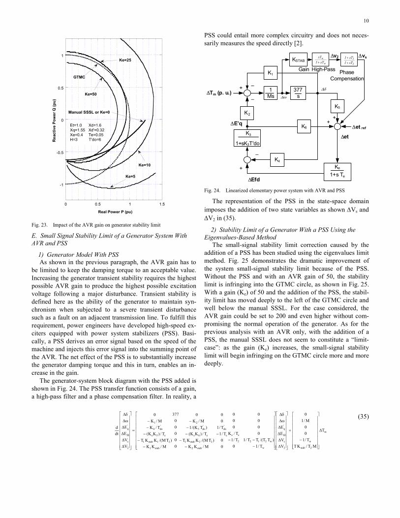
2) Stability Limits Using the Eigenvalues Method Using the eigenvalues limit method, Fig. 23 shows the sta-

bility limits of the elementary power system when the genera-tor has an AVR and when the AVR gain is varied from zero to higher values. It is not a surprise that for an AVR gain of zero, the stability limit corresponds to the manual SSSL. As the gain increases, one can see that there is a limit to be given to the gain before the stability starts infringing inside the GTMC circle. It is a well-established principle that the AVR gain has to be limited to prevent the generator from falling into insta-bility due to the lack of damping torque [2, 13]. Based on Fig.23, the AVR gain would have to be less than 25. Note here that the manual SSSL does not turn out to be the limit case as the gain increases. For high values of the AVR gain, the small-signal stability limit will go above the manual SSSL and will start infringing inside the GTMC limit circle.

Appendix B lists the numerical program in the MATLAB® language [19] used for plotting the small-signal stability limits in Fig. 23 and that can be used to plot further applications.

10

-1

-0.5

0

0.5

1

0 0.5 1 1.5

Rea

ctiv

e Po

wer

Q (p

u)

Real Power P (pu)

GTMC

Et=1.0 Xd=1.6Xq=1.55 Xd'=0.32Xe=0.4 Te=0.05H=3 T'do=6

Manual SSSL or Ke=0

Ke=5

Ke=10

Ke=50

Ke=25

Fig. 23. Impact of the AVR gain on generator stability limit

E. Small Signal Stability Limit of a Generator System With AVR and PSS

1) Generator Model With PSS As shown in the previous paragraph, the AVR gain has to

be limited to keep the damping torque to an acceptable value. Increasing the generator transient stability requires the highest possible AVR gain to produce the highest possible excitation voltage following a major disturbance. Transient stability is defined here as the ability of the generator to maintain syn-chronism when subjected to a severe transient disturbance such as a fault on an adjacent transmission line. To fulfill this requirement, power engineers have developed high-speed ex-citers equipped with power system stabilizers (PSS). Basi-cally, a PSS derives an error signal based on the speed of the machine and injects this error signal into the summing point of the AVR. The net effect of the PSS is to substantially increase the generator damping torque and this in turn, enables an in-crease in the gain.

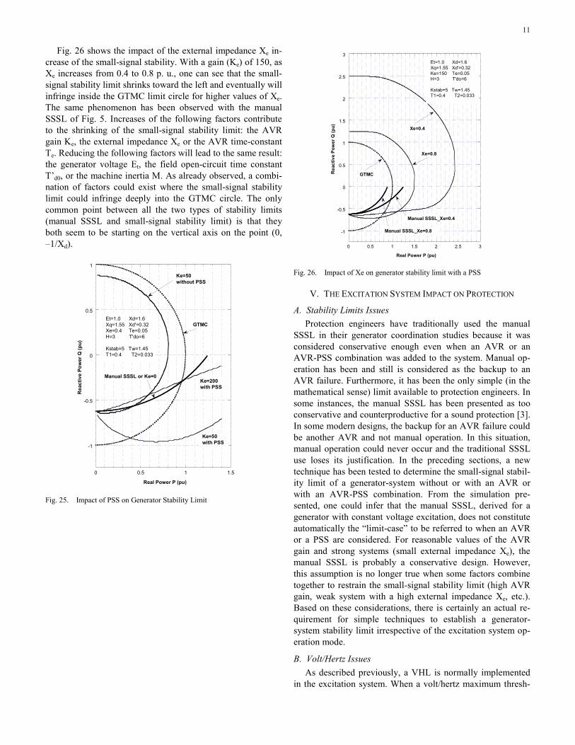
The generator-system block diagram with the PSS added is shown in Fig. 24. The PSS transfer function consists of a gain, a high-pass filter and a phase compensation filter. In reality, a

PSS could entail more complex circuitry and does not neces-sarily measures the speed directly [2].

+

K1

K2

377s

1Ms

K5

K6

K4

1+sK3T'do

K3

ΔTm (p. u.)

ΔEfd

Δet ref

Ke

1+s Te

Δet

ωΔ

δΔ

KSTABw

wsT1

sT+ 2

1sT1sT1

++

Gain High-Pass PhaseCompensation

ΔE’q

ΔvsΔv2

+

++

–

–

–

Fig. 24. Linearized elementary power system with AVR and PSS

The representation of the PSS in the state-space domain imposes the addition of two state variables as shown ΔVs and ΔV2 in (35).

2) Stability Limit of a Generator With a PSS Using the Eigenvalues-Based Method

The small-signal stability limit correction caused by the addition of a PSS has been studied using the eigenvalues limit method. Fig. 25 demonstrates the dramatic improvement of the system small-signal stability limit because of the PSS. Without the PSS and with an AVR gain of 50, the stability limit is infringing into the GTMC circle, as shown in Fig. 25. With a gain (Ke) of 50 and the addition of the PSS, the stabil-ity limit has moved deeply to the left of the GTMC circle and well below the manual SSSL. For the case considered, the AVR gain could be set to 200 and even higher without com-promising the normal operation of the generator. As for the previous analysis with an AVR only, with the addition of a PSS, the manual SSSL does not seem to constitute a “limit-case”: as the gain (Ke) increases, the small-signal stability limit will begin infringing on the GTMC circle more and more deeply.

m

2stab

w

2

s

fd

'q

w

w2122

eee

'do

stab2

22stab1

e6e

'do3

2

stab1

21stab1

e5e

'do4

1

2

s

fd

'q T

MT/KTT/1

00M/10

VVEE

T/10)TT/(TT/1T/1

0T/K000000

00

T/1T/100

M/KK)TM/(KKT

T/)KK()TK/(1

M/K0

00000

377

M/KK)TM/(KKT

T/)KK(T/KM/K

0

VVEE

dtd

Δ

⎥⎥⎥⎥⎥⎥⎥⎥

⎦

⎤

⎢⎢⎢⎢⎢⎢⎢⎢

⎣

⎡

−

+

⎥⎥⎥⎥⎥⎥⎥⎥

⎦

⎤

⎢⎢⎢⎢⎢⎢⎢⎢

⎣

⎡

ΔΔΔΔ

ωΔδΔ

⎥⎥⎥⎥⎥⎥⎥⎥

⎦

⎤

⎢⎢⎢⎢⎢⎢⎢⎢

⎣

⎡

−−−

−

−−

−−

−

−−

−−−

=

⎥⎥⎥⎥⎥⎥⎥⎥

⎦

⎤

⎢⎢⎢⎢⎢⎢⎢⎢

⎣

⎡

ΔΔΔΔ

ωΔδΔ (35)

11

Fig. 26 shows the impact of the external impedance Xe in-crease of the small-signal stability. With a gain (Ke) of 150, as Xe increases from 0.4 to 0.8 p. u., one can see that the small-signal stability limit shrinks toward the left and eventually will infringe inside the GTMC limit circle for higher values of Xe. The same phenomenon has been observed with the manual SSSL of Fig. 5. Increases of the following factors contribute to the shrinking of the small-signal stability limit: the AVR gain Ke, the external impedance Xe or the AVR time-constant Te. Reducing the following factors will lead to the same result: the generator voltage Et, the field open-circuit time constant T’d0, or the machine inertia M. As already observed, a combi-nation of factors could exist where the small-signal stability limit could infringe deeply into the GTMC circle. The only common point between all the two types of stability limits (manual SSSL and small-signal stability limit) is that they both seem to be starting on the vertical axis on the point (0, –1/Xd).

-1

-0.5

0

0.5

1

0 0.5 1 1.5

Rea

ctiv

e Po

wer

Q (p

u)

Real Power P (pu)

Et=1.0 Xd=1.6Xq=1.55 Xd'=0.32Xe=0.4 Te=0.05H=3 T'do=6

Kstab=5 Tw=1.45T1=0.4 T2=0.033

Ke=50without PSS

Ke=200with PSS

Ke=50with PSS

Manual SSSL or Ke=0

GTMC

Fig. 25. Impact of PSS on Generator Stability Limit

-1

-0.5

0

0.5

1

1.5

2

2.5

3

0 0.5 1 1.5 2 2.5 3

Rea

ctiv

e Po

wer

Q (p

u)

Real Power P (pu)

Et=1.0 Xd=1.6Xq=1.55 Xd'=0.32Ke=150 Te=0.05H=3 T'do=6

Kstab=5 Tw=1.45T1=0.4 T2=0.033

Manual SSSL_Xe=0.4

Xe=0.4

Xe=0.8

GTMC

Manual SSSL_Xe=0.8

Fig. 26. Impact of Xe on generator stability limit with a PSS

V. THE EXCITATION SYSTEM IMPACT ON PROTECTION

A. Stability Limits Issues Protection engineers have traditionally used the manual

SSSL in their generator coordination studies because it was considered conservative enough even when an AVR or an AVR-PSS combination was added to the system. Manual op-eration has been and still is considered as the backup to an AVR failure. Furthermore, it has been the only simple (in the mathematical sense) limit available to protection engineers. In some instances, the manual SSSL has been presented as too conservative and counterproductive for a sound protection [3]. In some modern designs, the backup for an AVR failure could be another AVR and not manual operation. In this situation, manual operation could never occur and the traditional SSSL use loses its justification. In the preceding sections, a new technique has been tested to determine the small-signal stabil-ity limit of a generator-system without or with an AVR or with an AVR-PSS combination. From the simulation pre-sented, one could infer that the manual SSSL, derived for a generator with constant voltage excitation, does not constitute automatically the “limit-case” to be referred to when an AVR or a PSS are considered. For reasonable values of the AVR gain and strong systems (small external impedance Xe), the manual SSSL is probably a conservative design. However, this assumption is no longer true when some factors combine together to restrain the small-signal stability limit (high AVR gain, weak system with a high external impedance Xe, etc.). Based on these considerations, there is certainly an actual re-quirement for simple techniques to establish a generator-system stability limit irrespective of the excitation system op-eration mode.

B. Volt/Hertz Issues As described previously, a VHL is normally implemented

in the excitation system. When a volt/hertz maximum thresh-

12

old is exceeded, this volt/hertz limiter will send a negative error signal to the AVR summation point until the generator voltage at the terminals goes back to an acceptable voltage level. The VHL does not preclude the implementation of volt/hertz protection on the generator and the step-up trans-former. On the contrary, this back-up protection is desirable and recommended [5]. Bear in mind that the error signal originating from the VHL can come into conflict with the er-ror signal from the UEL in some particular situations. As an example, in an islanding situation or during light load with a high level of charging current, the generator could be driven into an underexcited state so that the UEL will send a positive error signal to the AVR summing point. This signal will in-crease the generator output voltage until the generator moves out of the forbidden underexcited zone. In doing so, the volt-age could go to a level high enough that the volt/hertz thresh-old will be exceeded and the VHL will start sending a nega-tive error signal to lower the voltage. The outcome of this con-flicting situation could be an unstable oscillation in the gen-erator output voltage.

C. Overvoltage Issues The primary contribution of an AVR is to keep constant the

generator output voltage under a normal mode of operation. Overvoltage could occur on a transient basis during network disturbances, however. At rated frequency, the volt-hertz pro-tection constitutes a de-facto overvoltage protection; this is probably the reason why generator overvoltage protection is not widely used in North America. A classical situation exists where overvoltage could develop without being accompanied by overfluxing: the islanding of a hydro unit or its load rejec-tion is normally followed by a voltage build up together with an acceleration of the machine. The only protection then against machine dielectric stress is a conventional definite-time delay or inverse-time overvoltage protection.

D. Loss-of-Field Protection Issues The main issue with the loss-of-field (LOF) protection is to

ensure that when the generator goes into the underexcited re-gion, an infringement into the LOF characteristics will not occur, with the possible consequence of the generator tripping. Two types of coordination should be considered here: static (or steady state) and dynamic coordination. Steady-state coor-dination corresponds to the situation where there are no dis-turbances on the network. Dynamic coordination corresponds to the situation where there is a disturbance and when the UEL circuit might allow the generator operating point to infringe into the forbidden underexcited region on a transient or tem-porary basis.

1) Steady-state Coordination This is accomplished by coordinating the LOF characteris-

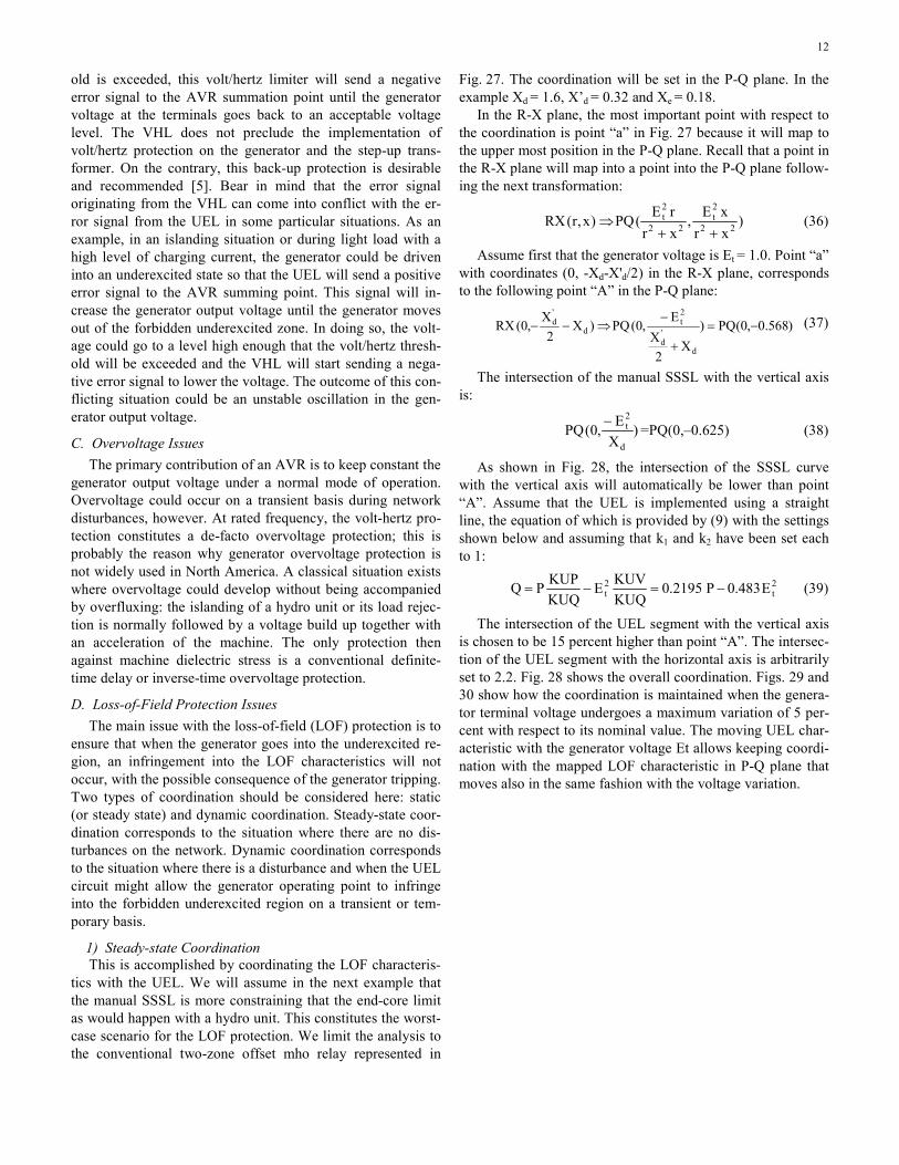
tics with the UEL. We will assume in the next example that the manual SSSL is more constraining that the end-core limit as would happen with a hydro unit. This constitutes the worst-case scenario for the LOF protection. We limit the analysis to the conventional two-zone offset mho relay represented in

Fig. 27. The coordination will be set in the P-Q plane. In the example Xd = 1.6, X’d = 0.32 and Xe = 0.18.

In the R-X plane, the most important point with respect to the coordination is point “a” in Fig. 27 because it will map to the upper most position in the P-Q plane. Recall that a point in the R-X plane will map into a point into the P-Q plane follow-ing the next transformation:

)xrxE,

xrrE(PQ)x,r(RX 22

2t

22

2t

++⇒ (36)

Assume first that the generator voltage is Et = 1.0. Point “a” with coordinates (0, -Xd-X'd/2) in the R-X plane, corresponds to the following point “A” in the P-Q plane:

)568.0,0(PQ)X

2X

E,0(PQ)X2

X,0(RX

d

'd

2t

d

'd −=

+

−⇒−− (37)

The intersection of the manual SSSL with the vertical axis is:

)XE,0(PQ

d

2t− =PQ(0,–0.625) (38)

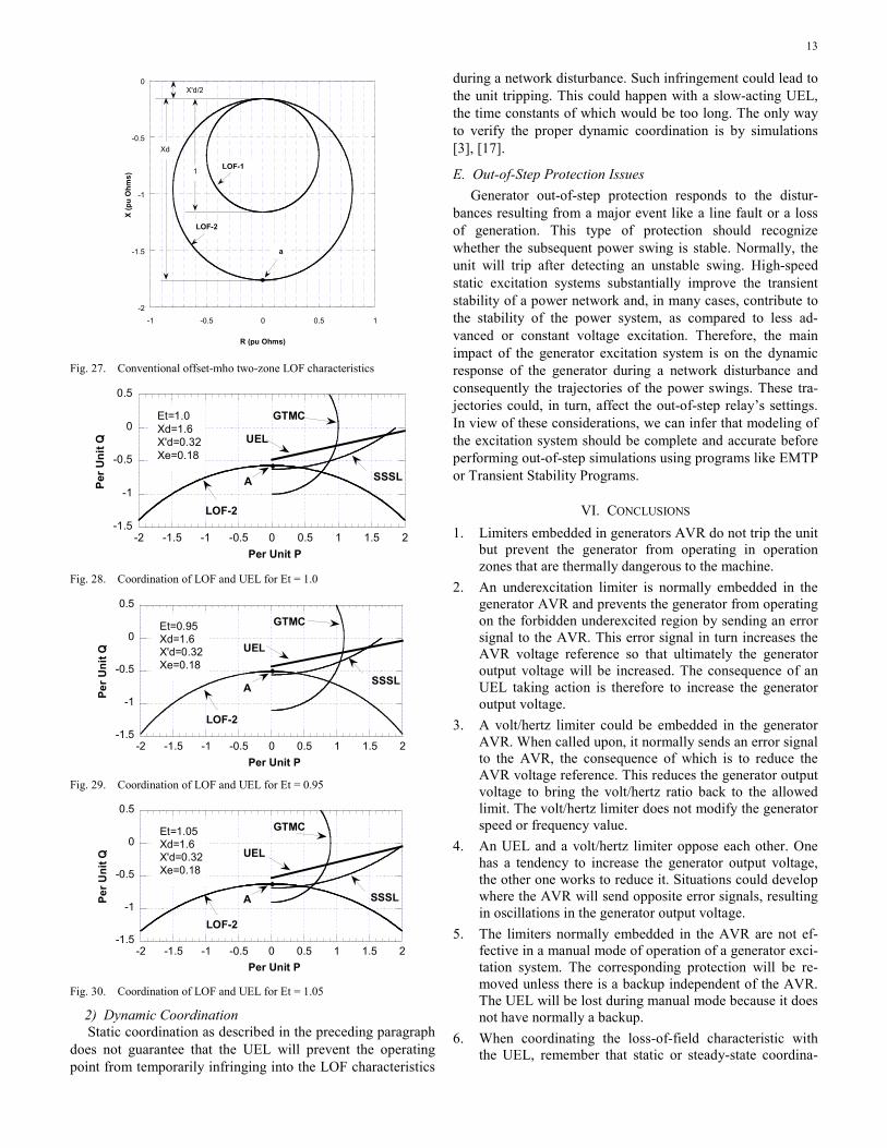
As shown in Fig. 28, the intersection of the SSSL curve with the vertical axis will automatically be lower than point “A”. Assume that the UEL is implemented using a straight line, the equation of which is provided by (9) with the settings shown below and assuming that k1 and k2 have been set each to 1:

2t

2t E483.0P2195.0

KUQKUVE

KUQKUPPQ −=−= (39)

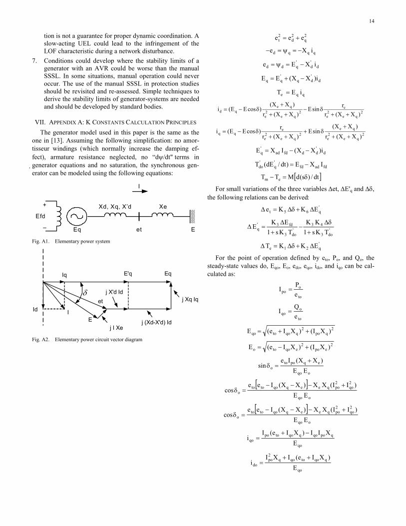
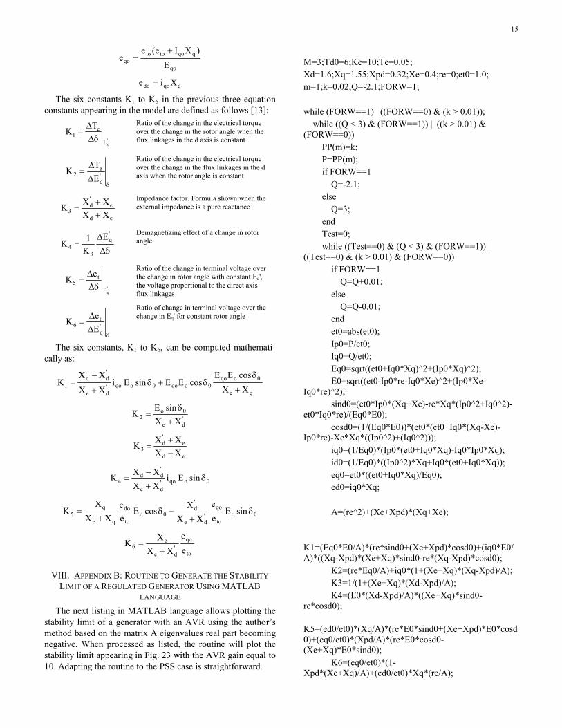
The intersection of the UEL segment with the vertical axis is chosen to be 15 percent higher than point “A”. The intersec-tion of the UEL segment with the horizontal axis is arbitrarily set to 2.2. Fig. 28 shows the overall coordination. Figs. 29 and 30 show how the coordination is maintained when the genera-tor terminal voltage undergoes a maximum variation of 5 per-cent with respect to its nominal value. The moving UEL char-acteristic with the generator voltage Et allows keeping coordi-nation with the mapped LOF characteristic in P-Q plane that moves also in the same fashion with the voltage variation.

13

-2

-1.5

-1

-0.5

0

-1 -0.5 0 0.5 1

X (p

u O

hms)

R (pu Ohms)

Xd

1

X'd/2

a

LOF-1

LOF-2

Fig. 27. Conventional offset-mho two-zone LOF characteristics

-1.5

-1

-0.5

0

0.5

-2 -1.5 -1 -0.5 0 0.5 1 1.5 2

Per U

nit Q

Per Unit P

GTMC

SSSL

UEL

Et=1.0Xd=1.6X'd=0.32Xe=0.18

LOF-2

A

Fig. 28. Coordination of LOF and UEL for Et = 1.0

-1.5

-1

-0.5

0

0.5

-2 -1.5 -1 -0.5 0 0.5 1 1.5 2

Per U

nit Q

Per Unit P

GTMC

SSSL

UEL

Et=0.95Xd=1.6X'd=0.32Xe=0.18

LOF-2

A

Fig. 29. Coordination of LOF and UEL for Et = 0.95

-1.5

-1

-0.5

0

0.5

-2 -1.5 -1 -0.5 0 0.5 1 1.5 2

Per U

nit Q

Per Unit P

GTMC

SSSL

UEL

Et=1.05Xd=1.6X'd=0.32Xe=0.18

LOF-2

A

Fig. 30. Coordination of LOF and UEL for Et = 1.05

2) Dynamic Coordination Static coordination as described in the preceding paragraph

does not guarantee that the UEL will prevent the operating point from temporarily infringing into the LOF characteristics

during a network disturbance. Such infringement could lead to the unit tripping. This could happen with a slow-acting UEL, the time constants of which would be too long. The only way to verify the proper dynamic coordination is by simulations [3], [17].

E. Out-of-Step Protection Issues Generator out-of-step protection responds to the distur-

bances resulting from a major event like a line fault or a loss of generation. This type of protection should recognize whether the subsequent power swing is stable. Normally, the unit will trip after detecting an unstable swing. High-speed static excitation systems substantially improve the transient stability of a power network and, in many cases, contribute to the stability of the power system, as compared to less ad-vanced or constant voltage excitation. Therefore, the main impact of the generator excitation system is on the dynamic response of the generator during a network disturbance and consequently the trajectories of the power swings. These tra-jectories could, in turn, affect the out-of-step relay’s settings. In view of these considerations, we can infer that modeling of the excitation system should be complete and accurate before performing out-of-step simulations using programs like EMTP or Transient Stability Programs.

VI. CONCLUSIONS 1. Limiters embedded in generators AVR do not trip the unit

but prevent the generator from operating in operation zones that are thermally dangerous to the machine.

2. An underexcitation limiter is normally embedded in the generator AVR and prevents the generator from operating on the forbidden underexcited region by sending an error signal to the AVR. This error signal in turn increases the AVR voltage reference so that ultimately the generator output voltage will be increased. The consequence of an UEL taking action is therefore to increase the generator output voltage.

3. A volt/hertz limiter could be embedded in the generator AVR. When called upon, it normally sends an error signal to the AVR, the consequence of which is to reduce the AVR voltage reference. This reduces the generator output voltage to bring the volt/hertz ratio back to the allowed limit. The volt/hertz limiter does not modify the generator speed or frequency value.

4. An UEL and a volt/hertz limiter oppose each other. One has a tendency to increase the generator output voltage, the other one works to reduce it. Situations could develop where the AVR will send opposite error signals, resulting in oscillations in the generator output voltage.

5. The limiters normally embedded in the AVR are not ef-fective in a manual mode of operation of a generator exci-tation system. The corresponding protection will be re-moved unless there is a backup independent of the AVR. The UEL will be lost during manual mode because it does not have normally a backup.

6. When coordinating the loss-of-field characteristic with the UEL, remember that static or steady-state coordina-

14

tion is not a guarantee for proper dynamic coordination. A slow-acting UEL could lead to the infringement of the LOF characteristic during a network disturbance.

7. Conditions could develop where the stability limits of a generator with an AVR could be worse than the manual SSSL. In some situations, manual operation could never occur. The use of the manual SSSL in protection studies should be revisited and re-assessed. Simple techniques to derive the stability limits of generator-systems are needed and should be developed by standard bodies.

VII. APPENDIX A: K CONSTANTS CALCULATION PRINCIPLES The generator model used in this paper is the same as the

one in [13]. Assuming the following simplification: no amor-tisseur windings (which normally increase the damping ef-fect), armature resistance neglected, no “dψ/dt" terms in generator equations and no saturation, the synchronous gen-erator can be modeled using the following equations:

+ Xd, Xq, X’d Xe

Eq E

I

– et

Efd

Fig. A1. Elementary power system

IId

Iq E'q Eq

j X'd Id

j (Xd-X'd) Id

j Xq Iqet

Ej I Xe

δ

Fig. A2. Elementary power circuit vector diagram

2q

2d

2t eee +=

qqqd iXe −=ψ=−

d'd

'qdd iXEe −=ψ=

d'dq

'qq i)XX(EE −+=

qqe iET =

2

qe2e

e2

qe2e

qeqd )XX(r

rsinE)XX(r

)XX()cosEE(i

++δ−

++

+δ−=

2

qe2e

qe2

qe2e

eqq )XX(r

)XX(sinE

)XX(rr

)cosEE(i++

+δ+

++δ−=

d'ddfdad

'q i)XX(IXE −−=

fdadfd'q

'do IXE)dt/dE(T −=

[ ]dt/)s(dMTT em δ=−

For small variations of the three variables Δet, ΔE'q and Δδ, the following relations can be derived:

'q65t EKKe Δ+δΔ=Δ

'do3

43'do3

fd3'q TKs1

KKTKs1

EKE

+δΔ

−+

Δ=Δ

'q21e EKKT Δ+δΔ=Δ

For the point of operation defined by eto, Po, and Qo, the steady-state values do, Eqo, Eo, edo, eqo, ido, and iqo can be cal-culated as:

to

opo e

PI =

to

oqo e

QI =

2qpo

2qqotoqo )XI()XIe(E ++=

2epo

2eqotoo )XI()XIe(E +−=

oqo

eqpotoo EE

)XX(Iesin

+=δ

[ ]

oqo

2qo

2poqeeqqototo

o EE)II(XX)XX(Iee

cos+−−−

=δ

[ ]

oqo

2qo

2poqeeqqototo

o EE)II(XX)XX(Iee

cos+−−−

=δ

qo

qpoqoqqotopoqo E

XII)XIe(Ii

−+=

qo

qqotoqoq2po

do E)XIe(IXI

i++

=

15

qo

qqototoqo E

)XIe(ee

+=

qqodo Xie =

The six constants K1 to K6 in the previous three equation constants appearing in the model are defined as follows [13]:

'qE

e1

TKδΔ

Δ=

Ratio of the change in the electrical torque over the change in the rotor angle when the flux linkages in the d axis is constant

δΔΔ

= 'q

e2 E

TK

Ratio of the change in the electrical torque over the change in the flux linkages in the d axis when the rotor angle is constant

ed

e'd

3 XXXXK

++

= Impedance factor. Formula shown when the external impedance is a pure reactance

δΔ

Δ=

'q

34

EK1K

Demagnetizing effect of a change in rotor angle

'qE

t5

eKδΔ

Δ=

Ratio of the change in terminal voltage over the change in rotor angle with constant Eq', the voltage proportional to the direct axis flux linkages

δΔΔ

= 'q

t6 E

eK

Ratio of change in terminal voltage over the change in Eq' for constant rotor angle

The six constants, K1 to K6, can be computed mathemati-cally as:

qe

0oqo0oqo0oqo'

de

'dq

1 XXcosEE

cosEEsinEiXXXX

K+

δδ+δ

+

−=

'de

0o2 XX

sinEK

+δ

=

ed

e'd

3 XXXXK

−+

=

0oqo'de

'dd

4 sinEiXXXXK δ

+−

=

0oto

qo'de

'd

0oto

do

qe

q5 sinE

ee

XXXcosE

ee

XXX

K δ+

−δ+

=

to

qo'de

e6 e

eXX

XK

+=

VIII. APPENDIX B: ROUTINE TO GENERATE THE STABILITY LIMIT OF A REGULATED GENERATOR USING MATLAB

LANGUAGE The next listing in MATLAB language allows plotting the

stability limit of a generator with an AVR using the author’s method based on the matrix A eigenvalues real part becoming negative. When processed as listed, the routine will plot the stability limit appearing in Fig. 23 with the AVR gain equal to 10. Adapting the routine to the PSS case is straightforward.

M=3;Td0=6;Ke=10;Te=0.05; Xd=1.6;Xq=1.55;Xpd=0.32;Xe=0.4;re=0;et0=1.0; m=1;k=0.02;Q=-2.1;FORW=1; while (FORW==1) | ((FORW==0) & (k > 0.01)); while ((Q < 3) & (FORW==1)) | ((k > 0.01) & (FORW==0)) PP(m)=k; P=PP(m); if FORW==1 Q=-2.1; else Q=3; end Test=0; while ((Test==0) & (Q < 3) & (FORW==1)) | ((Test==0) & (k > 0.01) & (FORW==0)) if FORW==1 Q=Q+0.01; else Q=Q-0.01; end et0=abs(et0); Ip0=P/et0; Iq0=Q/et0; Eq0=sqrt((et0+Iq0*Xq)^2+(Ip0*Xq)^2); E0=sqrt((et0-Ip0*re-Iq0*Xe)^2+(Ip0*Xe-Iq0*re)^2); sind0=(et0*Ip0*(Xq+Xe)-re*Xq*(Ip0^2+Iq0^2)-et0*Iq0*re)/(Eq0*E0); cosd0=(1/(Eq0*E0))*(et0*(et0+Iq0*(Xq-Xe)-Ip0*re)-Xe*Xq*((Ip0^2)+(Iq0^2))); iq0=(1/Eq0)*(Ip0*(et0+Iq0*Xq)-Iq0*Ip0*Xq); id0=(1/Eq0)*((Ip0^2)*Xq+Iq0*(et0+Iq0*Xq)); eq0=et0*((et0+Iq0*Xq)/Eq0); ed0=iq0*Xq; A=(re^2)+(Xe+Xpd)*(Xq+Xe); K1=(Eq0*E0/A)*(re*sind0+(Xe+Xpd)*cosd0)+(iq0*E0/A)*((Xq-Xpd)*(Xe+Xq)*sind0-re*(Xq-Xpd)*cosd0); K2=(re*Eq0/A)+iq0*(1+(Xe+Xq)*(Xq-Xpd)/A); K3=1/(1+(Xe+Xq)*(Xd-Xpd)/A); K4=(E0*(Xd-Xpd)/A)*((Xe+Xq)*sind0-re*cosd0); K5=(ed0/et0)*(Xq/A)*(re*E0*sind0+(Xe+Xpd)*E0*cosd0)+(eq0/et0)*(Xpd/A)*(re*E0*cosd0-(Xe+Xq)*E0*sind0); K6=(eq0/et0)*(1-Xpd*(Xe+Xq)/A)+(ed0/et0)*Xq*(re/A);

16

A3=[0 377 0 0;-K1/M 0 -K2/M 0;-K4/Td0 0 -1/(K3*Td0) 1/(Td0); -(Ke*K5)/Te 0 -Ke*K6/Te -1/Te]; H3=eig(A3); x1=real(H3(1,1)); x2=real(H3(2,1)); x3=real(H3(3,1)); x4=real(H3(4,1)); Test= (x1 < 0) & (x2 < 0) & (x3 < 0) & (x4 < 0); end if FORW==1 & Q > 2.8 m=m-2; k=k-0.02; else QQ(m)=Q; end m=m+1; if FORW==1 k=k+0.01; else k=k-0.01; end end FORW=0; end plot(PP,QQ) grid

IX. REFERENCES [1] D. Reimert, Protective Relaying for Power Generation Systems, Boca

Raton: CRC Press, 2006. [2] P. Kundur, Power System Stability and Control, New York: McGraw-

Hill, 1994. [3] J. R. Ribero, “Minimum Excitation Limiter Effects on Generator Re-

sponse to System Disturbances,” IEEE Transactions on Energy Conver-sion, Vol. 6, No. 1, March 1991.

[4] S. S. Choy and X. M. Xia, “Under excitation limiter and its role in pre-venting excessive synchronous generator stator end-core heating,” IEEE Trans. Power Syst., vol. 15, no. 1, pp. 95−101, February 2000.

[5] Working Group J5 of Power System Relaying Committee, Charles J. Mozina, Chairman, “Coordination of Generator Protection with Genera-tor Excitation Control and Generator Capability”, IEEE PES General Meeting, June 2007, Tampa, Fl.

[6] S. B. Farnham and R. W. Swarthout, “Field excitation in relation to machine and system operation,” AIEE Trans., vol. 72, pt. III, no. 9, pp. 1215−1223, Dec. 1953.

[7] IEEE Power Engineering Society, IEEE Tutorial on the Protection of Synchronous Generators, 95 TP 102.

[8] Guide for AC Generator Protection, IEEE Standard C37.102/D7−200X, April 2006.

[9] Requirements for Cylindrical Rotor Synchronous Generators, 1989. ANSI Std. C50.13−1989.

[10] Standard for Requirements for Salient-Pole Synchronous Generators and Generator/Motors for Hydraulic Turbine Applications, 1982. ANSI Std. C50.12−1982.

[11] IEEE Recommended Practice for Excitation System Models for Power system Stability Studies, IEEE standard 421.5-1992.

[12] IEEE Task Force on Excitation Limiters, “Underexcitation Limiter Model for Power System Stability studies”, IEEE Trans. On Energy Conversion, Vol. 10, No. 3, September 1995.

[13] F. P. DeMello and C. Concordia, “Concepts of synchronous machine stability as affected by excitation control,” IEEE Trans. Power App. Syst., vol. PAS−88, No. 4, pp. 316−329, April 1969.

[14] C. K. Seetharaman, S. P. Verma, and A. M. El-Serafi, “Operation of synchronous generators in the asynchronous mode,” IEEE Trans. Power App. Syst., vol. PAS−93, pp. 928−939, 1974.

[15] C. R. Mason, “A new loss of excitation relay for synchronous genera-tors,” AIEE Trans., vol. 68, pt. II, pp. 1240−1245, 1949.

[16] J. Berdy, “Loss-of excitation protection for modern synchronous genera-tors,” General Electric Co. Document GER-3183.

[17] R. Sandoval, A. Guzmán, H. J. Altuve, “Dynamic simulations help improve generator protection,” 33rd Annual Western Protective Relay Conference, Spokane, WA, October 17-19, 2006.

[18] Carson W. Taylor, Power System Voltage Stability, McGraw Hill Inter-national editions 1994.

[19] The MathWorks, MATLAB The language of Technical Computing, Using MATLB, Version 6, November 2000.

X. BIOGRAPHY Gabriel Benmouyal, P.E., received his B.A.Sc. in Electrical Engineering and his M.A.Sc. in Control Engineering from Ecole Polytechnique, Université de Montréal, Canada, in 1968 and 1970, respectively. In 1969, he joined Hydro-Québec as an Instrumentation and Control Specialist. He worked on different projects in the field of substation control systems and dispatching centers. In 1978, he joined IREQ, where his main field of activity has been the applica-tion of microprocessors and digital techniques for substation and generating-station control and protection systems. In 1997, he joined Schweitzer Engi-neering Laboratories, Inc. in the position of Principal Research Engineer. He is a registered professional engineer in the Province of Québec, is an IEEE Senior Member, and has served on the Power System Relaying Committee since May 1989. He holds over six patents and is the author or co-author of several papers in the field of signal processing and power networks protection and control.

© 2007 by Schweitzer Engineering Laboratories, Inc. All rights reserved.

20070912 • TP6281-01