4/21/2012 NY - KJP 585 2009 1 Operations Management Topic 6 – Forecasting UiTM Shah Alam Lecturer: Pn. Noriah Yusoff T1-A16-6C

Welcome message from author
This document is posted to help you gain knowledge. Please leave a comment to let me know what you think about it! Share it to your friends and learn new things together.
Transcript
8/4/2019 6.0-Topic 6_ Forecasting
http://slidepdf.com/reader/full/60-topic-6-forecasting 1/39
4/21/2012 NY - KJP 585 2009 1
Operations Management
Topic 6 – Forecasting
UiTM Shah Alam Lecturer: Pn. Noriah Yusoff T1-A16-6C

8/4/2019 6.0-Topic 6_ Forecasting
http://slidepdf.com/reader/full/60-topic-6-forecasting 2/39
4/21/2012 NY - KJP 585 2009 2
What is Forecasting?
Process of predicting afuture event
Underlying basis of all business decisions Production
Inventory
Personnel
Facilities
Hmm…. you
gonna get an A forthis subject
8/4/2019 6.0-Topic 6_ Forecasting
http://slidepdf.com/reader/full/60-topic-6-forecasting 3/39
4/21/2012 NY - KJP 585 2009 3
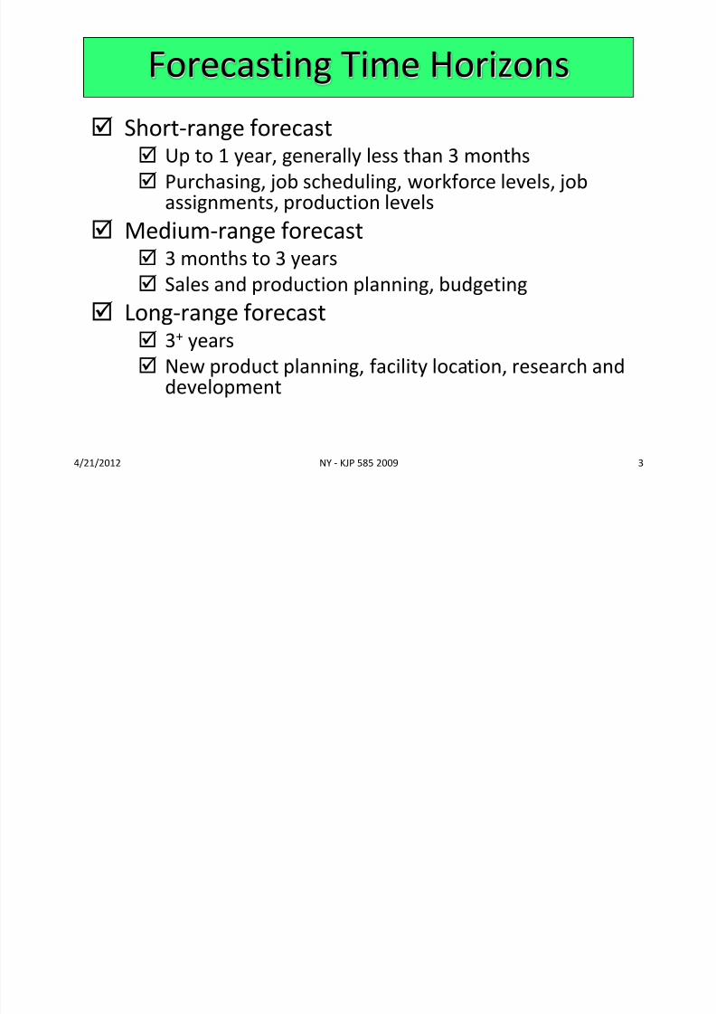
Short-range forecast Up to 1 year, generally less than 3 months
Purchasing, job scheduling, workforce levels, jobassignments, production levels
Medium-range forecast 3 months to 3 years
Sales and production planning, budgeting
Long-range forecast
3+ years New product planning, facility location, research and
development
Forecasting Time Horizons
8/4/2019 6.0-Topic 6_ Forecasting
http://slidepdf.com/reader/full/60-topic-6-forecasting 4/39
4/21/2012 NY - KJP 585 2009 4
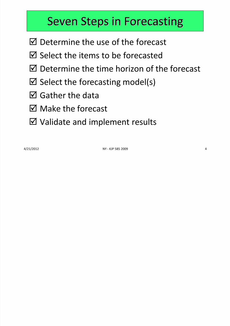
Seven Steps in Forecasting
Determine the use of the forecast
Select the items to be forecasted
Determine the time horizon of the forecast
Select the forecasting model(s)
Gather the data
Make the forecast Validate and implement results
8/4/2019 6.0-Topic 6_ Forecasting
http://slidepdf.com/reader/full/60-topic-6-forecasting 5/39
4/21/2012 NY - KJP 585 2009 5
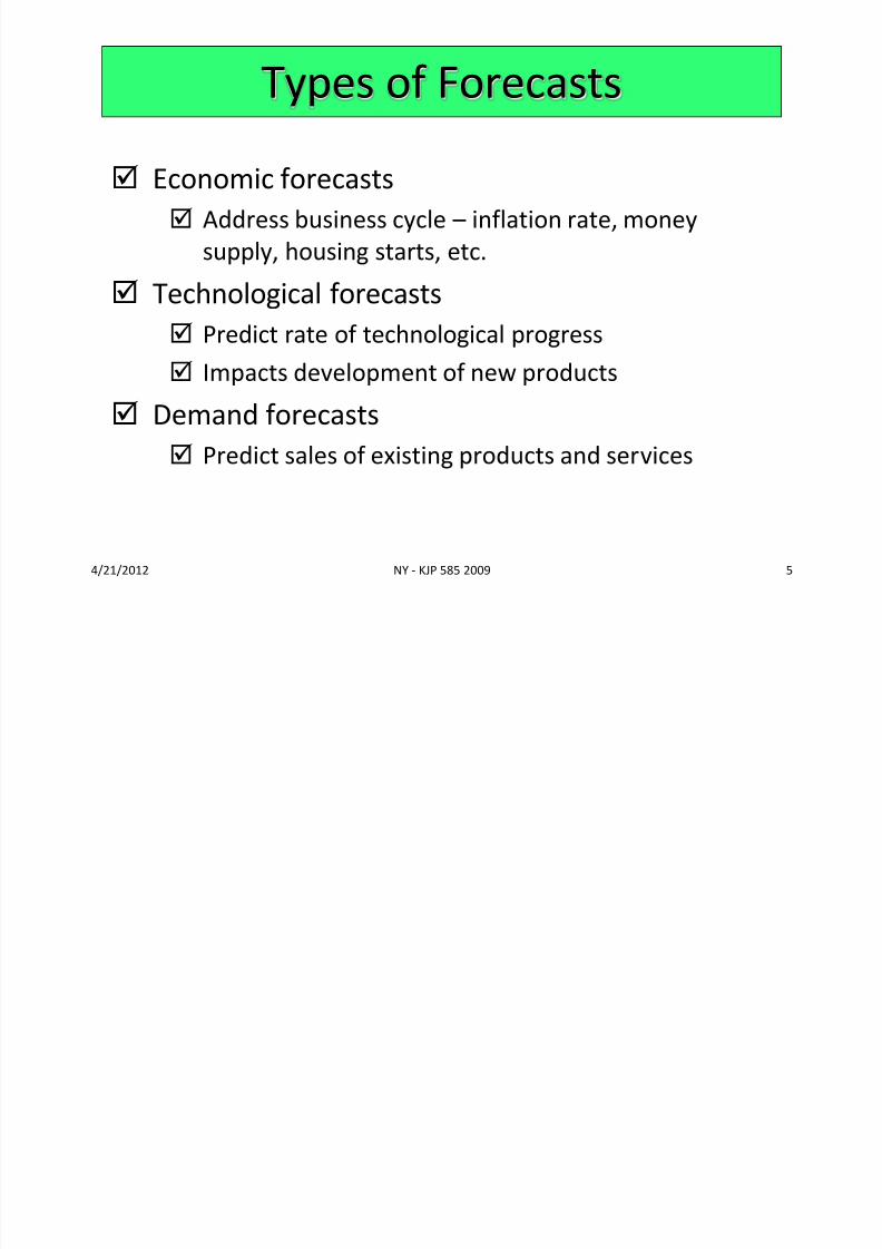
Types of Forecasts
Economic forecasts
Address business cycle – inflation rate, money
supply, housing starts, etc.
Technological forecasts
Predict rate of technological progress
Impacts development of new products
Demand forecasts Predict sales of existing products and services

8/4/2019 6.0-Topic 6_ Forecasting
http://slidepdf.com/reader/full/60-topic-6-forecasting 6/39
4/21/2012 NY - KJP 585 2009 6
Strategic Importance of
Forecasting
Human Resources – Hiring, training, laying off
workers Capacity – Capacity shortages can result in
undependable delivery, loss of customers,loss of market share
Supply Chain Management – Good supplierrelations and price advantages

8/4/2019 6.0-Topic 6_ Forecasting
http://slidepdf.com/reader/full/60-topic-6-forecasting 7/39
4/21/2012 NY - KJP 585 2009 7
The Realities!
Forecasts are seldom perfect
Most techniques assume an underlying stability in the system
Product family and aggregated forecasts are more accurate than individual product forecasts
8/4/2019 6.0-Topic 6_ Forecasting
http://slidepdf.com/reader/full/60-topic-6-forecasting 8/39
4/21/2012 NY - KJP 585 2009 8
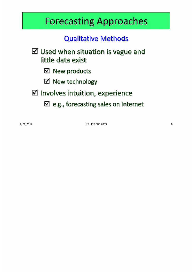
Forecasting Approaches
Used when situation is vague and
little data exist New products
New technology
Involves intuition, experience
e.g., forecasting sales on Internet
Qualitative Methods

8/4/2019 6.0-Topic 6_ Forecasting
http://slidepdf.com/reader/full/60-topic-6-forecasting 9/39
4/21/2012 NY - KJP 585 2009 9
Forecasting Approaches
Used when situation is ‘stable’ and
historical data exist Existing products
Current technology
Involves mathematical techniques
e.g., forecasting sales of color televisions
Quantitative Methods
8/4/2019 6.0-Topic 6_ Forecasting
http://slidepdf.com/reader/full/60-topic-6-forecasting 10/39
4/21/2012 NY - KJP 585 2009 10
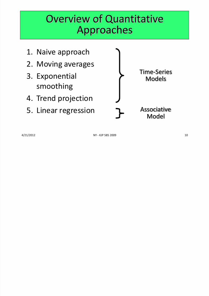
Overview of Quantitative
Approaches1. Naive approach
2. Moving averages3. Exponential
smoothing
4. Trend projection5. Linear regression
Time-SeriesModels
AssociativeModel
8/4/2019 6.0-Topic 6_ Forecasting
http://slidepdf.com/reader/full/60-topic-6-forecasting 11/39
4/21/2012 NY - KJP 585 2009 11
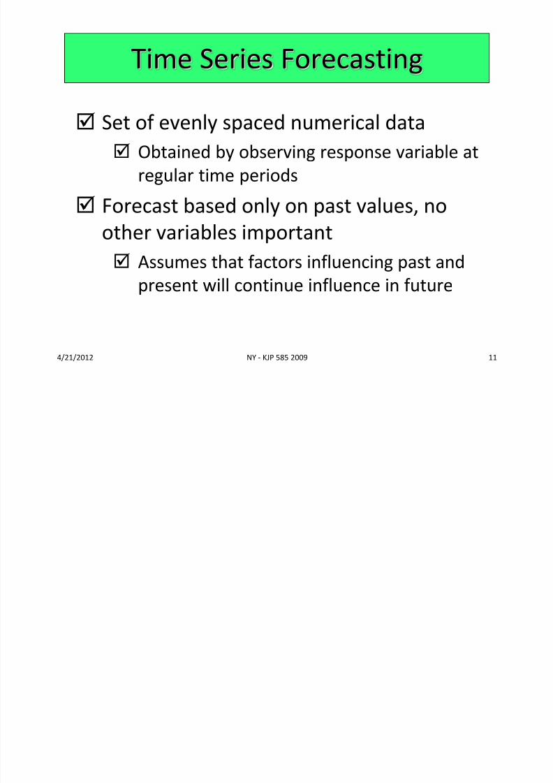
Set of evenly spaced numerical data
Obtained by observing response variable at
regular time periods
Forecast based only on past values, no
other variables important
Assumes that factors influencing past andpresent will continue influence in future
Time Series Forecasting

8/4/2019 6.0-Topic 6_ Forecasting
http://slidepdf.com/reader/full/60-topic-6-forecasting 12/39
4/21/2012 NY - KJP 585 2009 12
Components of Demand
D e m a
n d f o r p r o d u c t o r
s e r v i c e
| | | |
1 2 3 4
Year
Average demand
over four years
Seasonal peaks
Trendcomponent
Actualdemand
Randomvariation
Figure 4.1
8/4/2019 6.0-Topic 6_ Forecasting
http://slidepdf.com/reader/full/60-topic-6-forecasting 13/39
4/21/2012 NY - KJP 585 2009 13
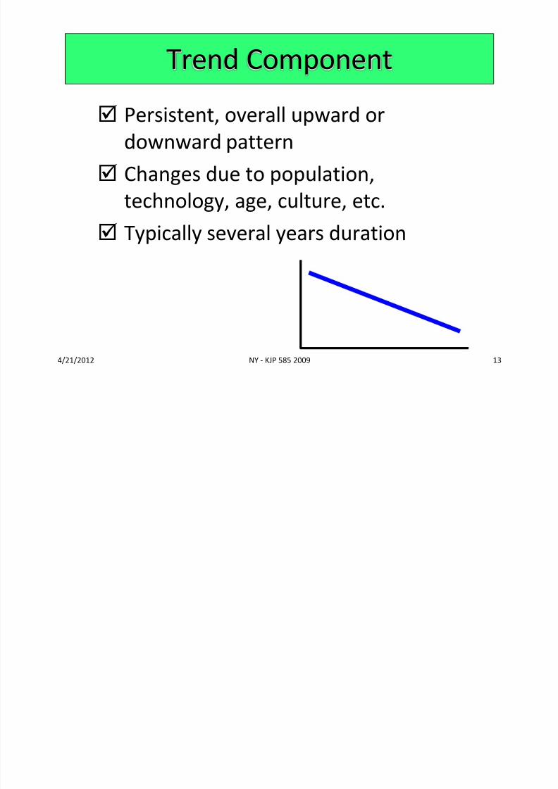
Persistent, overall upward or
downward pattern
Changes due to population,technology, age, culture, etc.
Typically several years duration
Trend Component
8/4/2019 6.0-Topic 6_ Forecasting
http://slidepdf.com/reader/full/60-topic-6-forecasting 14/39
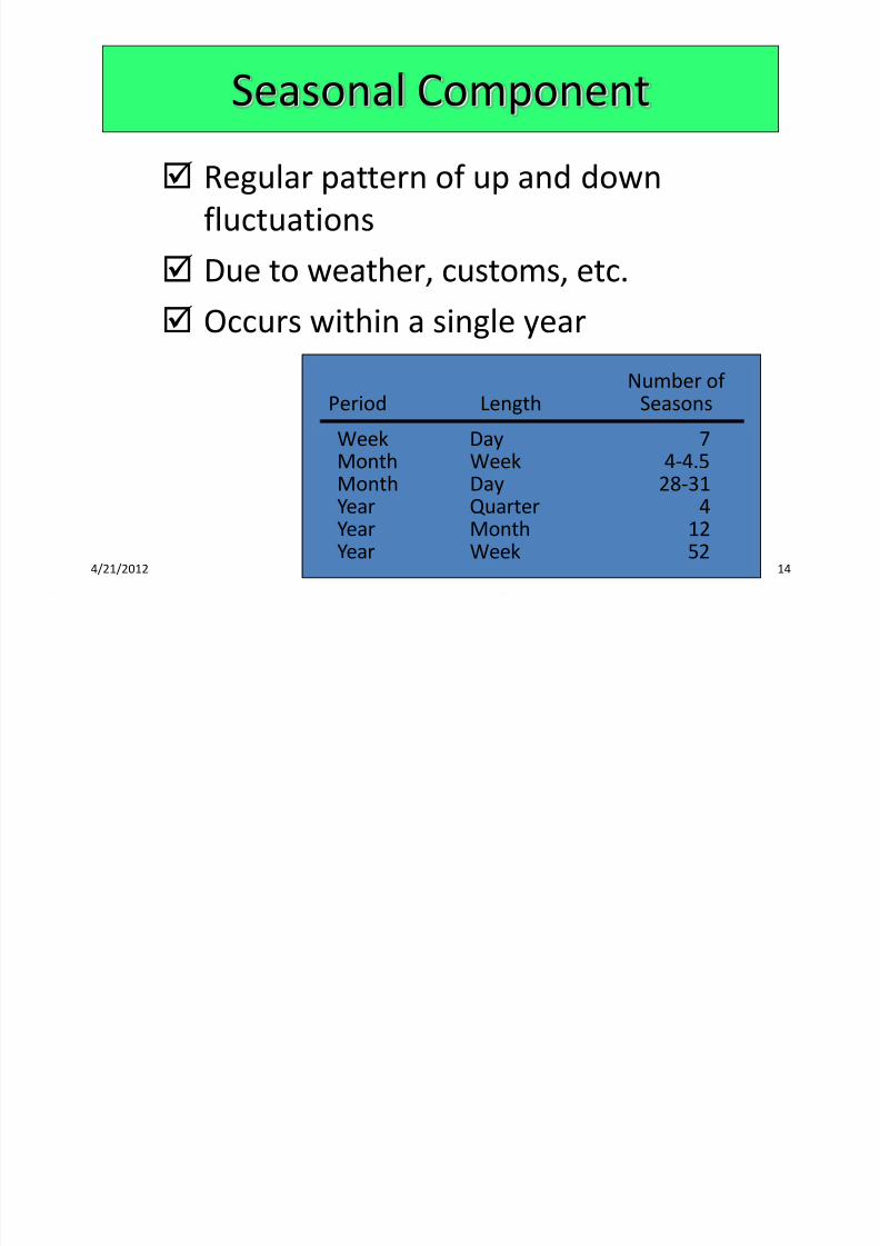
4/21/2012 NY - KJP 585 2009 14
Regular pattern of up and down
fluctuations
Due to weather, customs, etc. Occurs within a single year
Seasonal Component
Number of Period Length Seasons
Week Day 7Month Week 4-4.5Month Day 28-31Year Quarter 4Year Month 12
Year Week 52
8/4/2019 6.0-Topic 6_ Forecasting
http://slidepdf.com/reader/full/60-topic-6-forecasting 15/39
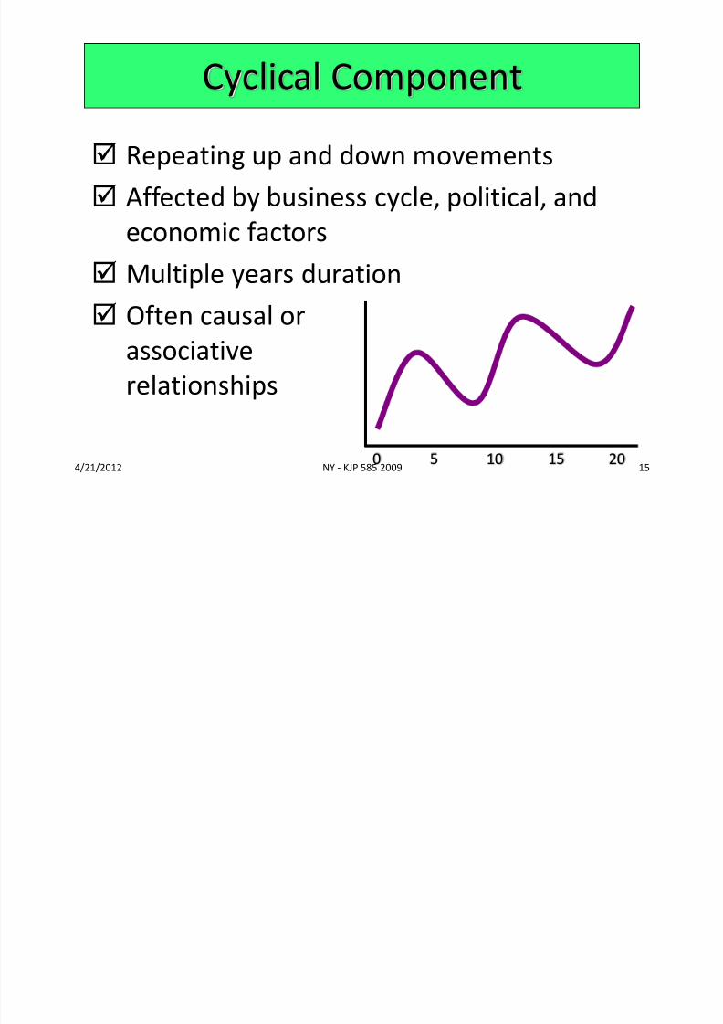
4/21/2012 NY - KJP 585 2009 15
Repeating up and down movements
Affected by business cycle, political, and
economic factors Multiple years duration
Often causal or
associativerelationships
Cyclical Component
0 5 10 15 20
8/4/2019 6.0-Topic 6_ Forecasting
http://slidepdf.com/reader/full/60-topic-6-forecasting 16/39
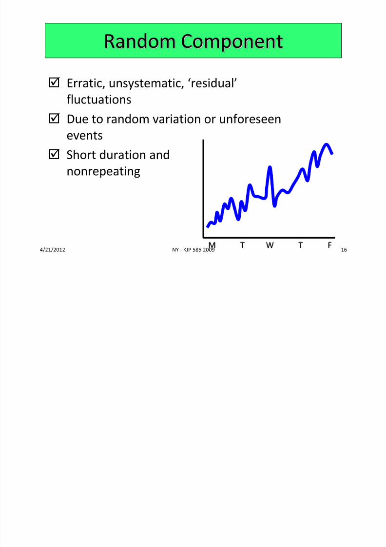
4/21/2012 NY - KJP 585 2009 16
Erratic, unsystematic, ‘residual’
fluctuations
Due to random variation or unforeseenevents
Short duration and
nonrepeating
Random Component
M T W T F
8/4/2019 6.0-Topic 6_ Forecasting
http://slidepdf.com/reader/full/60-topic-6-forecasting 17/39
4/21/2012 NY - KJP 585 2009 17
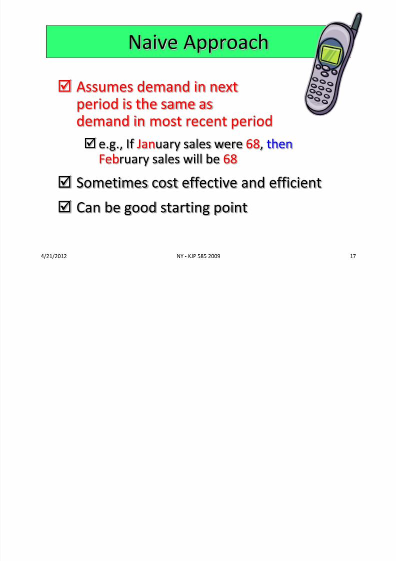
Naive Approach
Assumes demand in nextperiod is the same as
demand in most recent period e.g., If January sales were 68, then
February sales will be 68
Sometimes cost effective and efficient
Can be good starting point

8/4/2019 6.0-Topic 6_ Forecasting
http://slidepdf.com/reader/full/60-topic-6-forecasting 18/39
4/21/2012 NY - KJP 585 2009 18
Moving average
Weighted moving average
Exponential smoothing
Techniques for Averaging
8/4/2019 6.0-Topic 6_ Forecasting
http://slidepdf.com/reader/full/60-topic-6-forecasting 19/39
4/21/2012 NY - KJP 585 2009 19
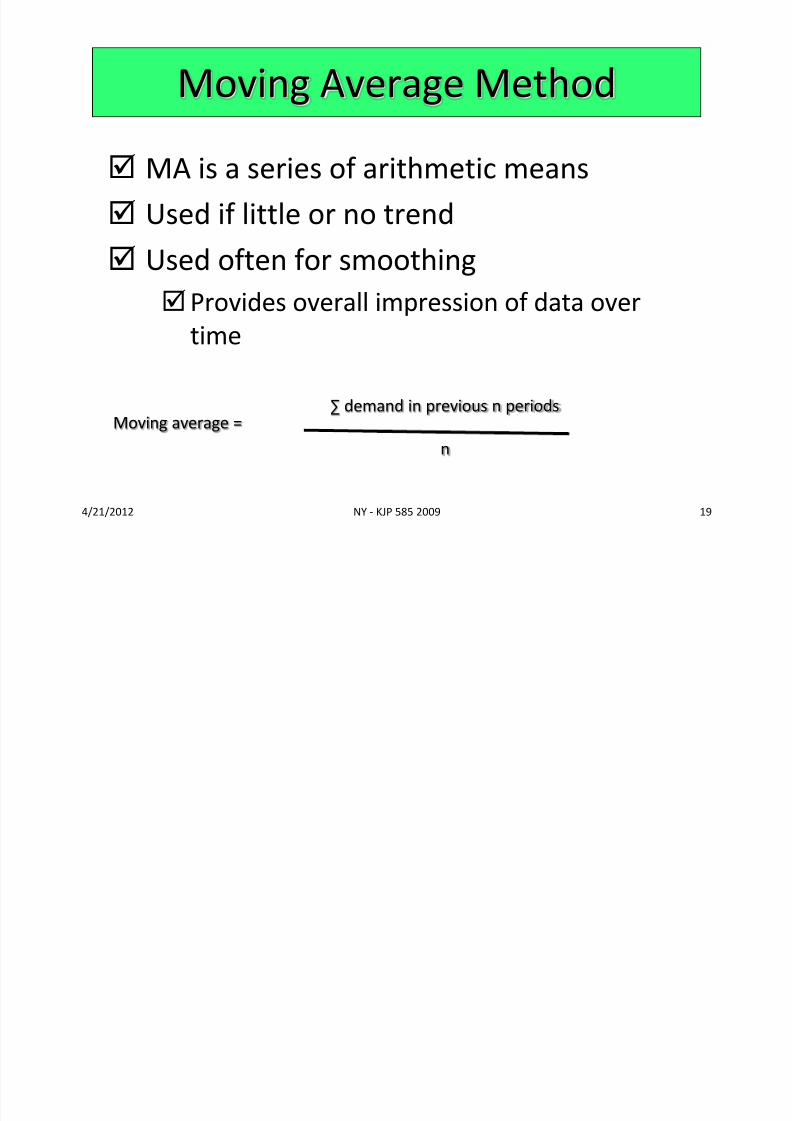
MA is a series of arithmetic means
Used if little or no trend
Used often for smoothingProvides overall impression of data over
time
Moving Average Method
Moving average =∑ demand in previous n periods
n
8/4/2019 6.0-Topic 6_ Forecasting
http://slidepdf.com/reader/full/60-topic-6-forecasting 20/39
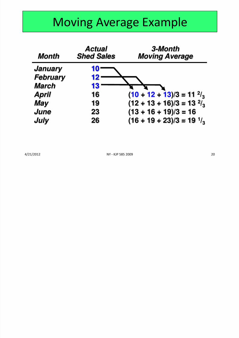
4/21/2012 NY - KJP 585 2009 20
January 10
February 12 March 13 April 16May 19
June 23July 26
Actual 3-Month Month Shed Sales Moving Average
(12 + 13 + 16)/3 = 13 2/3
(13 + 16 + 19)/3 = 16(16 + 19 + 23)/3 = 19 1/3
Moving Average Example
10
12 13
(10 + 12 + 13)/3 = 11 2/3
8/4/2019 6.0-Topic 6_ Forecasting
http://slidepdf.com/reader/full/60-topic-6-forecasting 21/39
4/21/2012 NY - KJP 585 2009 21
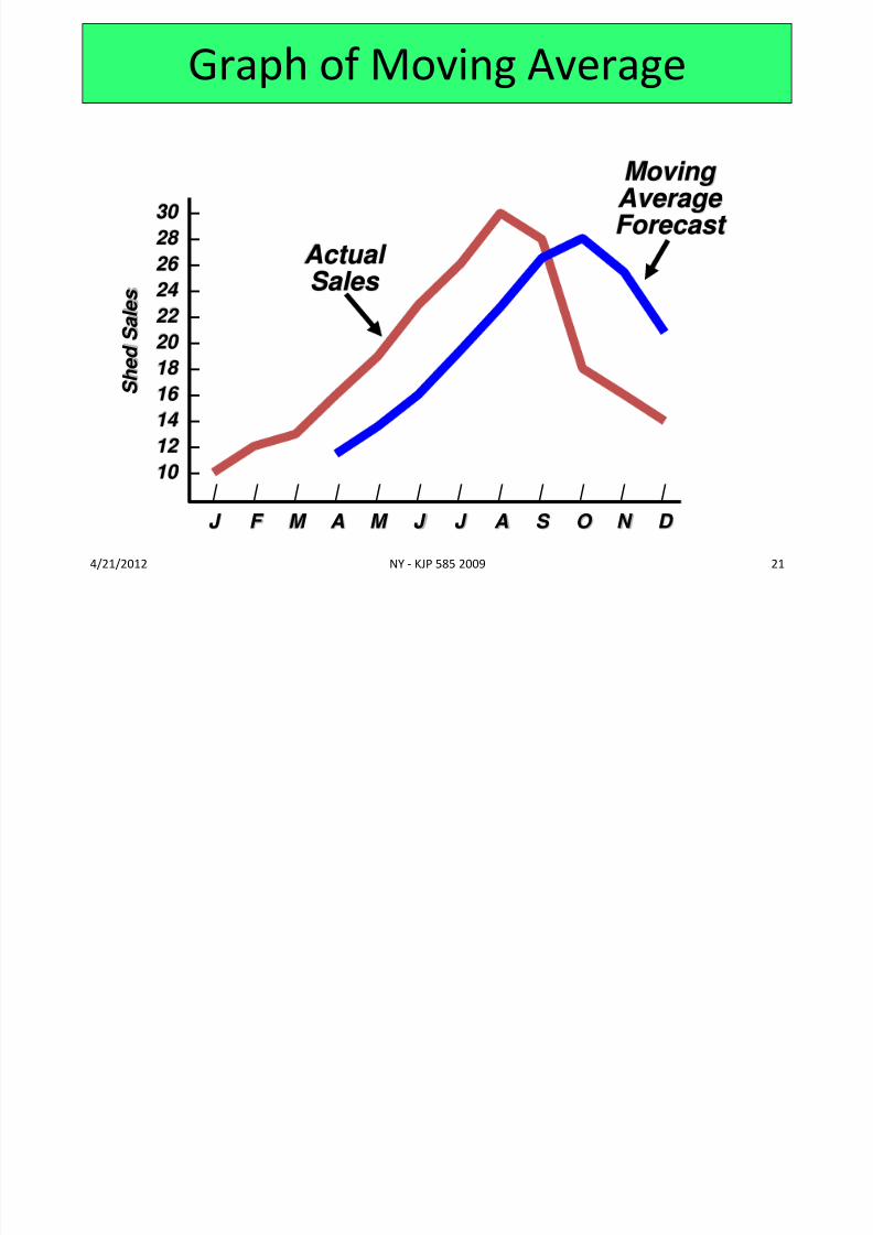
Graph of Moving Average
| | | | | | | | | | | |
J F M A M J J A S O N D
S h e d S a l e s
30 –
28 –
26 –
24 –
22 –
20 –
18 –
16 –
14 – 12 –
10 –
Actual
Sales
Moving Average Forecast
8/4/2019 6.0-Topic 6_ Forecasting
http://slidepdf.com/reader/full/60-topic-6-forecasting 22/39
4/21/2012 NY - KJP 585 2009 22
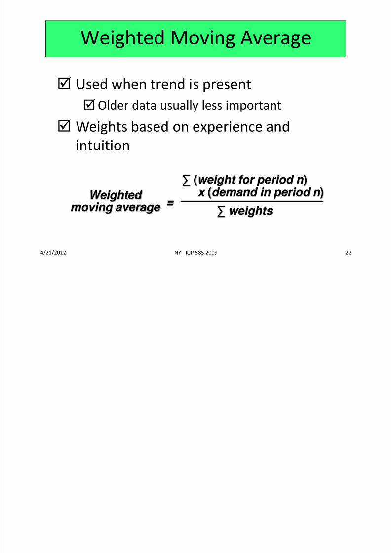
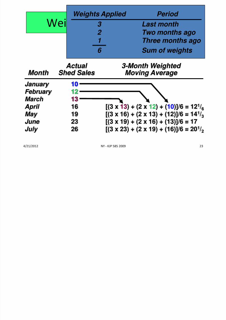
Used when trend is present
Older data usually less important
Weights based on experience andintuition
Weighted Moving Average
Weighted moving average =
∑ (weight for period n ) x (demand in period n )
∑ weights
8/4/2019 6.0-Topic 6_ Forecasting
http://slidepdf.com/reader/full/60-topic-6-forecasting 23/39
4/21/2012 NY - KJP 585 2009 23
January 10 February 12 March 13
April 16May 19June 23July 26
Actual 3-Month Weighted
Month Shed Sales Moving Average
[(3 x 16) + (2 x 13) + (12)]/6 = 141/3 [(3 x 19) + (2 x 16) + (13)]/6 = 17[(3 x 23) + (2 x 19) + (16)]/6 = 201/2
Weighted Moving Average
10 12 13
[(3 x 13) + (2 x 12) + (10)]/6 = 121
/6
Weights Applied Period
3 Last month 2 Two months ago 1 Three months ago
6 Sum of weights
8/4/2019 6.0-Topic 6_ Forecasting
http://slidepdf.com/reader/full/60-topic-6-forecasting 24/39
4/21/2012 NY - KJP 585 2009 24
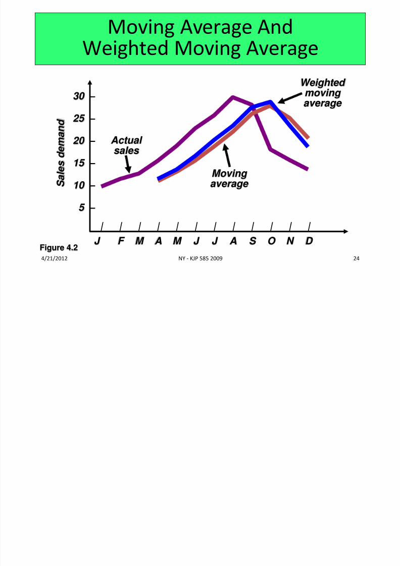
Moving Average AndWeighted Moving Average
30 –
25 –
20 –
15 –
10 –
5 –
S a l e s d e m a n
d
| | | | | | | | | | | |
J F M A M J J A S O N D
Actual sales
Moving average
Weighted moving average
Figure 4.2
8/4/2019 6.0-Topic 6_ Forecasting
http://slidepdf.com/reader/full/60-topic-6-forecasting 25/39
4/21/2012 NY - KJP 585 2009 25
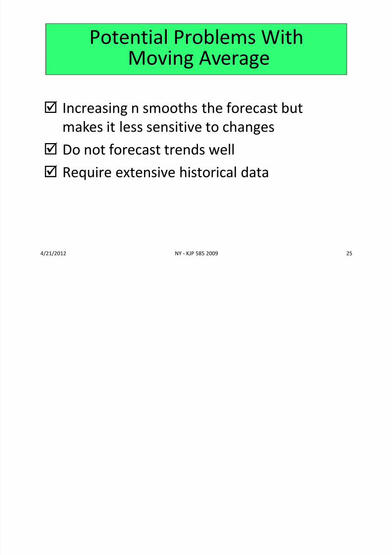
Increasing n smooths the forecast but
makes it less sensitive to changes Do not forecast trends well
Require extensive historical data
Potential Problems With
Moving Average
8/4/2019 6.0-Topic 6_ Forecasting
http://slidepdf.com/reader/full/60-topic-6-forecasting 26/39
4/21/2012 NY - KJP 585 2009 26
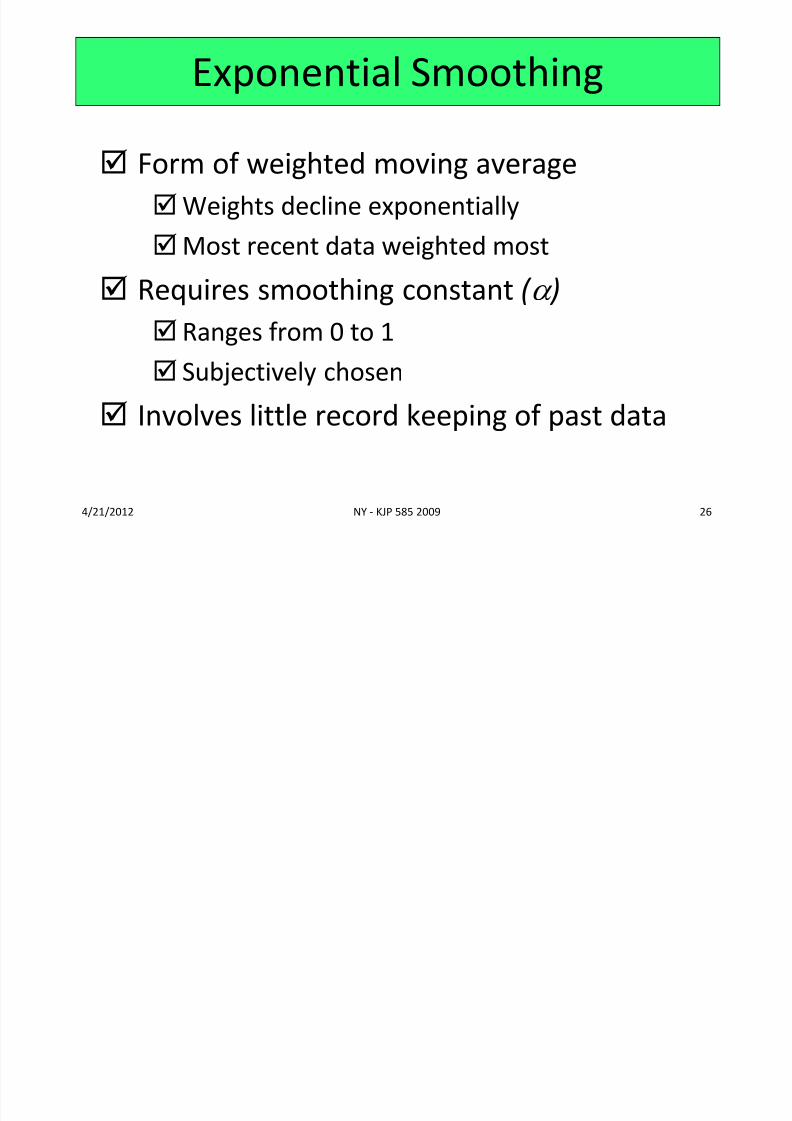
Form of weighted moving average
Weights decline exponentially
Most recent data weighted most
Requires smoothing constant ( )
Ranges from 0 to 1
Subjectively chosen Involves little record keeping of past data
Exponential Smoothing
8/4/2019 6.0-Topic 6_ Forecasting
http://slidepdf.com/reader/full/60-topic-6-forecasting 27/39
4/21/2012 NY - KJP 585 2009 27
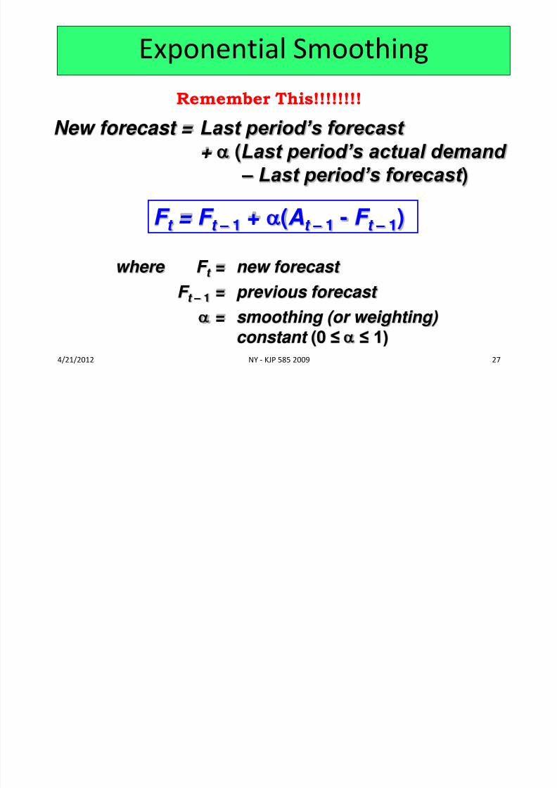
Exponential Smoothing
New forecast = Last period’s forecast + (Last period’s actual demand
– Last period’s forecast )
F t = F t – 1 + (At – 1 - F t – 1)
where F t = new forecast F t – 1 = previous forecast
= smoothing (or weighting) constant (0 ≤ ≤ 1)
Remember This!!!!!!!!
8/4/2019 6.0-Topic 6_ Forecasting
http://slidepdf.com/reader/full/60-topic-6-forecasting 28/39
4/21/2012 NY - KJP 585 2009 28
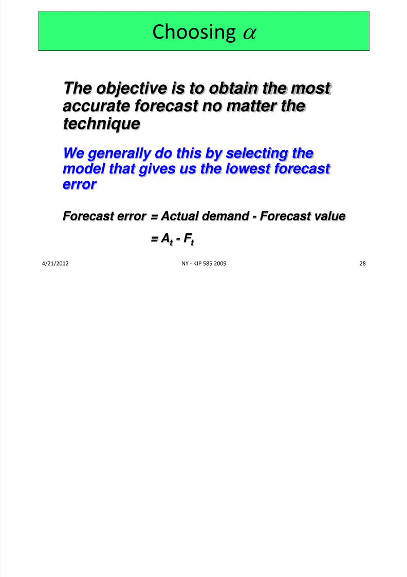
Choosing
The objective is to obtain the most accurate forecast no matter the
technique We generally do this by selecting the model that gives us the lowest forecast error
Forecast error = Actual demand - Forecast value
= At - F t
8/4/2019 6.0-Topic 6_ Forecasting
http://slidepdf.com/reader/full/60-topic-6-forecasting 29/39
4/21/2012 NY - KJP 585 2009 29
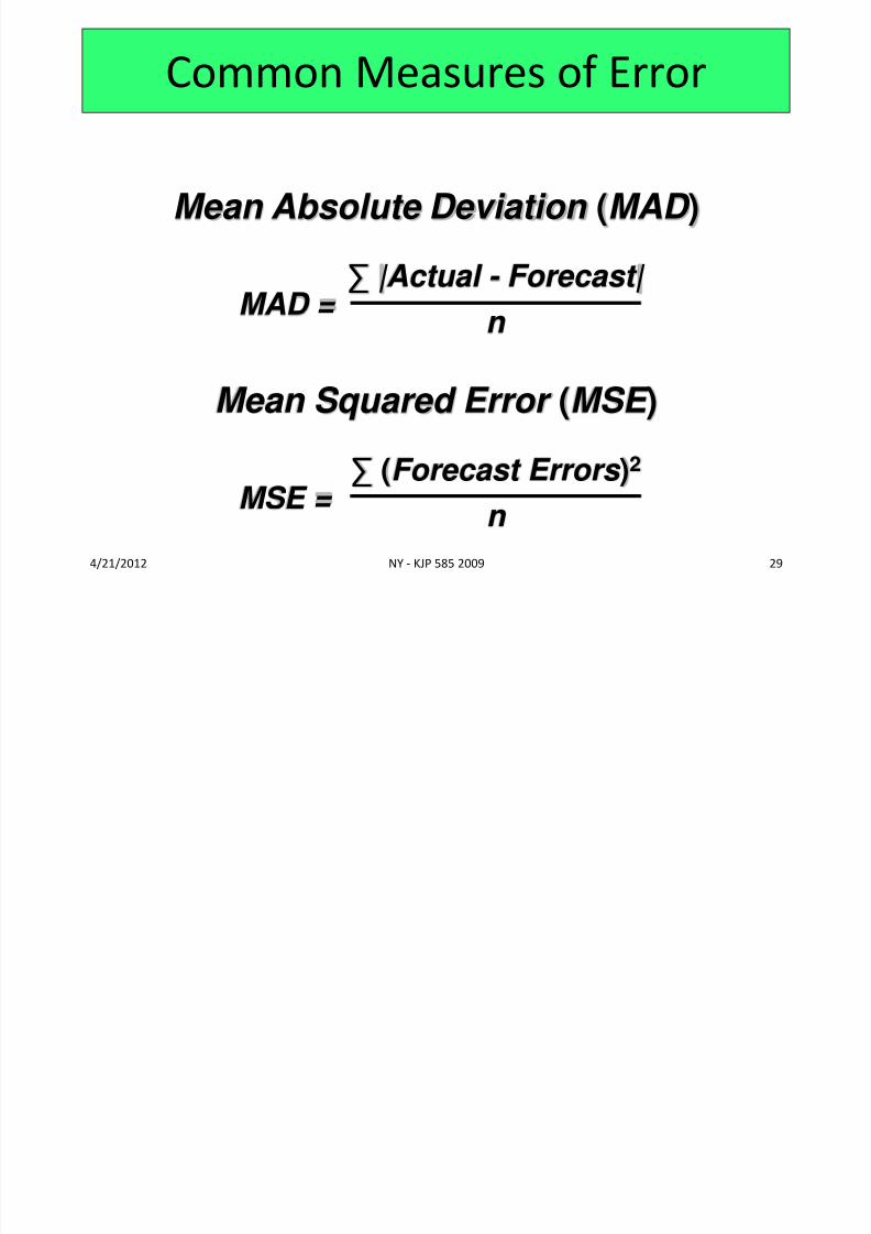
Common Measures of Error
Mean Absolute Deviation (MAD )
MAD = ∑ |Actual - Forecast| n
Mean Squared Error (MSE )
MSE = ∑ (Forecast Errors )2
n
8/4/2019 6.0-Topic 6_ Forecasting
http://slidepdf.com/reader/full/60-topic-6-forecasting 30/39
4/21/2012 NY - KJP 585 2009 30
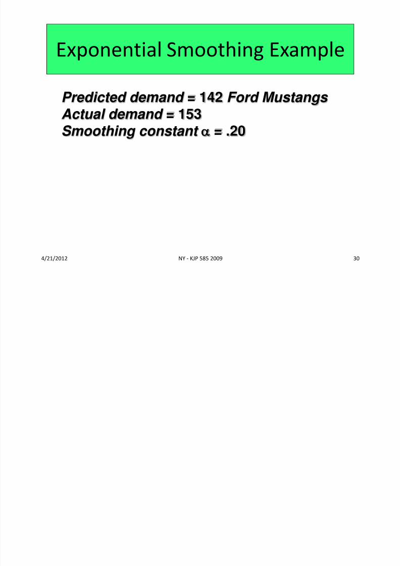
Exponential Smoothing Example
Predicted demand = 142 Ford Mustangs Actual demand = 153
Smoothing constant = .20
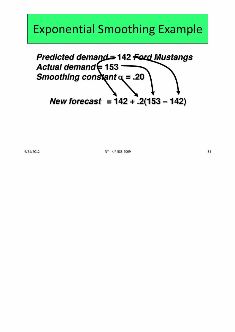
8/4/2019 6.0-Topic 6_ Forecasting
http://slidepdf.com/reader/full/60-topic-6-forecasting 31/39
4/21/2012 NY - KJP 585 2009 31
Exponential Smoothing Example
Predicted demand = 142 Ford Mustangs Actual demand = 153
Smoothing constant = .20
New forecast = 142 + .2(153 – 142)
8/4/2019 6.0-Topic 6_ Forecasting
http://slidepdf.com/reader/full/60-topic-6-forecasting 32/39
4/21/2012 NY - KJP 585 2009 32
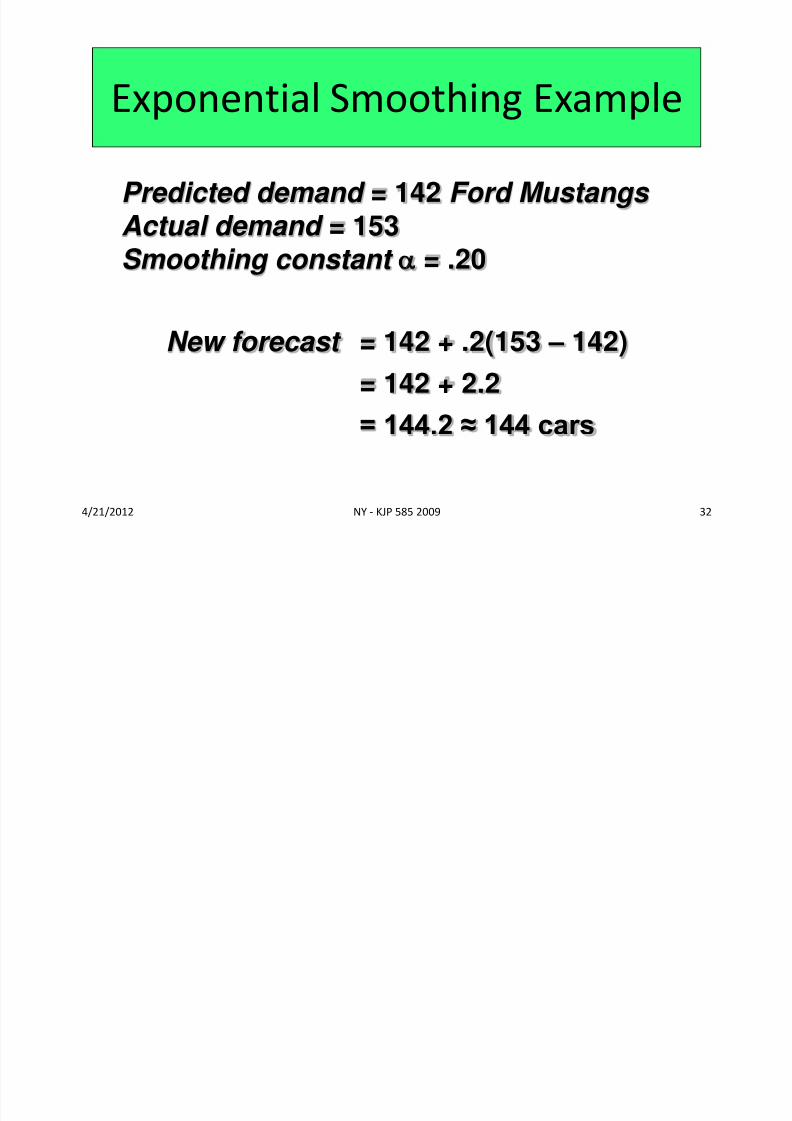
Exponential Smoothing Example
Predicted demand = 142 Ford Mustangs Actual demand = 153
Smoothing constant = .20
New forecast = 142 + .2(153 – 142)
= 142 + 2.2= 144.2 ≈ 144 cars
8/4/2019 6.0-Topic 6_ Forecasting
http://slidepdf.com/reader/full/60-topic-6-forecasting 33/39
4/21/2012 NY - KJP 585 2009 33
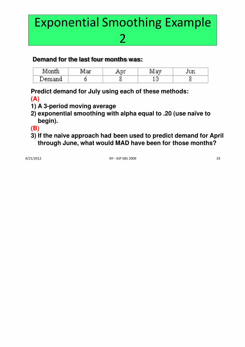
Exponential Smoothing Example
2Demand for the last four months was:
Predict demand for July using each of these methods:(A)1) A 3-period moving average2) exponential smoothing with alpha equal to .20 (use naïve to
begin).(B)3) If the naive approach had been used to predict demand for April
through June, what would MAD have been for those months?
8/4/2019 6.0-Topic 6_ Forecasting
http://slidepdf.com/reader/full/60-topic-6-forecasting 34/39
4/21/2012 NY - KJP 585 2009 34
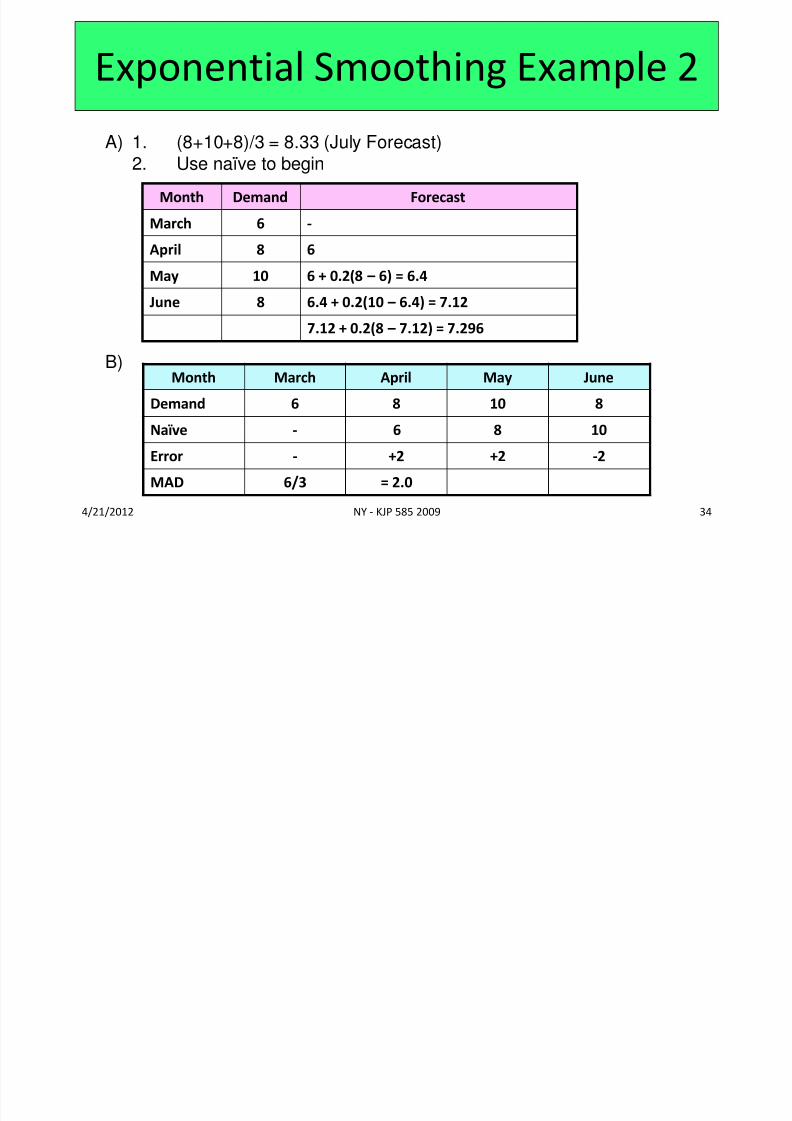
Exponential Smoothing Example 2
Month Demand Forecast
March 6 -
April 8 6May 10 6 + 0.2(8 – 6) = 6.4
June 8 6.4 + 0.2(10 – 6.4) = 7.12
7.12 + 0.2(8 – 7.12) = 7.296
A) 1. (8+10+8)/3 = 8.33 (July Forecast)2. Use naïve to begin
B)
Month March April May JuneDemand 6 8 10 8
Naïve - 6 8 10
Error - +2 +2 -2
MAD 6/3 = 2.0
8/4/2019 6.0-Topic 6_ Forecasting
http://slidepdf.com/reader/full/60-topic-6-forecasting 35/39
4/21/2012 NY - KJP 585 2009 35
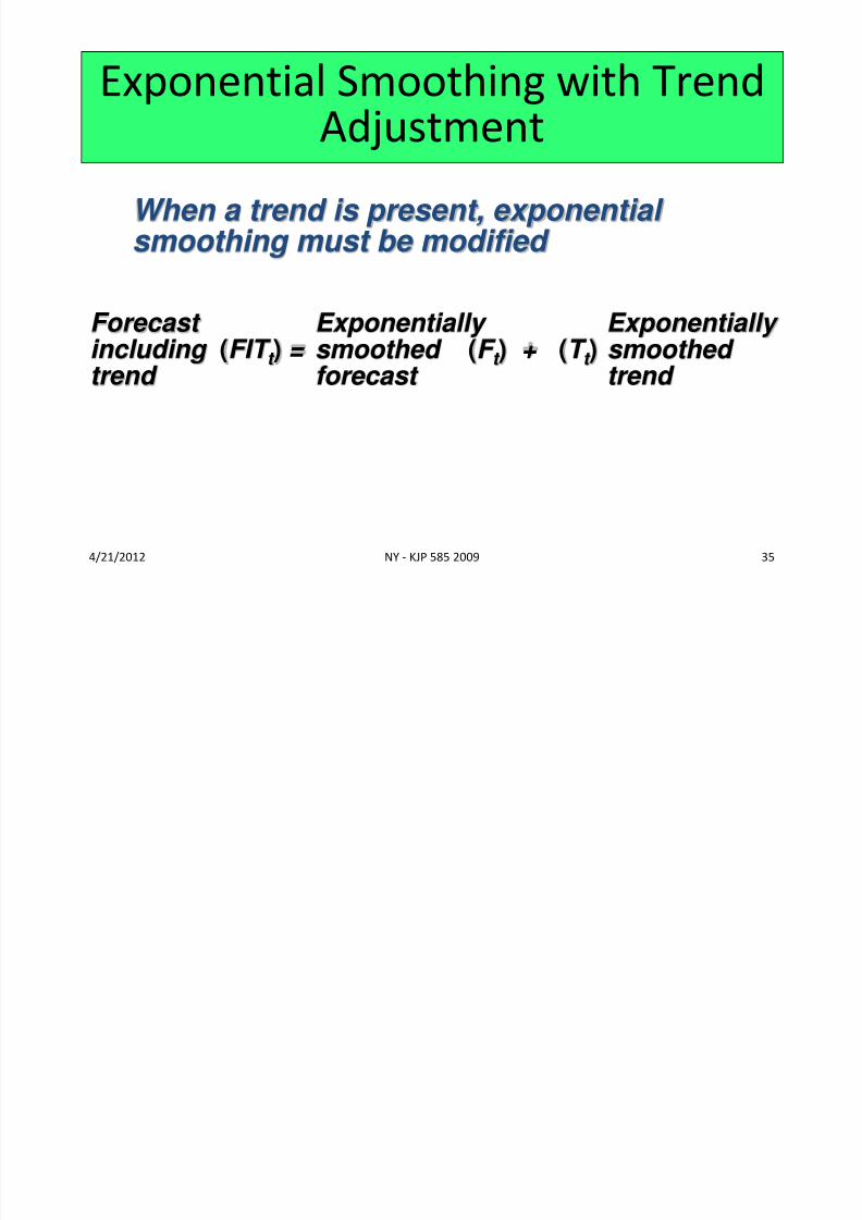
Exponential Smoothing with Trend
AdjustmentWhen a trend is present, exponential smoothing must be modified
Forecast including (FIT t ) = trend
Exponentially Exponentially smoothed (F t ) + (T t ) smoothed forecast trend
8/4/2019 6.0-Topic 6_ Forecasting
http://slidepdf.com/reader/full/60-topic-6-forecasting 36/39
4/21/2012 NY - KJP 585 2009 36
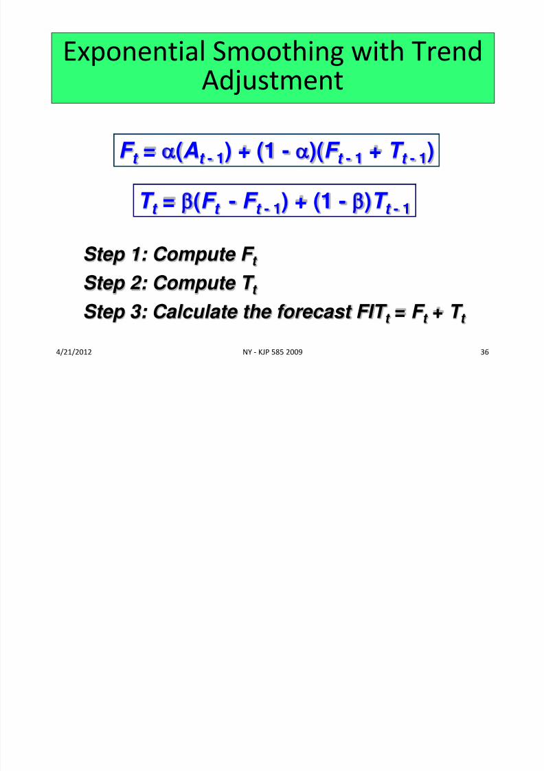
Exponential Smoothing with Trend
Adjustment
F t = (At - 1) + (1 - )(F t - 1 + T t - 1)
T t = b(F t - F t - 1) + (1 - b)T t - 1
Step 1: Compute F t Step 2: Compute T t
Step 3: Calculate the forecast FIT t = F t + T t

8/4/2019 6.0-Topic 6_ Forecasting
http://slidepdf.com/reader/full/60-topic-6-forecasting 37/39
4/21/2012 NY - KJP 585 2009 37
Moving Average
Weekly sales of ten-grain bread at the local organic food market are in the
table below. Based on this data, forecast week 9 using a five-week moving
average.
Other Examples
Week 1 2 3 4 5 6 7 8
Sales 415 389 420 382 410 432 405 421
(382+410+432+405+421)/5 = 410.0
8/4/2019 6.0-Topic 6_ Forecasting
http://slidepdf.com/reader/full/60-topic-6-forecasting 38/39
4/21/2012 NY - KJP 585 2009 38
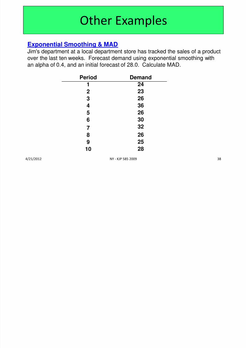
Exponential Smoothing & MAD Jim's department at a local department store has tracked the sales of a productover the last ten weeks. Forecast demand using exponential smoothing withan alpha of 0.4, and an initial forecast of 28.0. Calculate MAD.
Other Examples
Period Demand1 24
2 23
3 26
4 36
5 26
6 30
7 32
8 26
9 25
10 28
8/4/2019 6.0-Topic 6_ Forecasting
http://slidepdf.com/reader/full/60-topic-6-forecasting 39/39
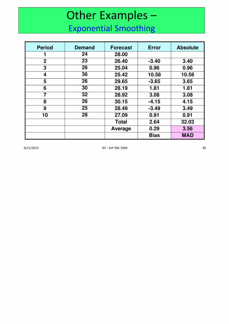
4/21/2012 NY KJP 585 2009 39
Period Demand Forecast Error Absolute
1 24 28.00
2 23 26.40 -3.40 3.40
3 26 25.04 0.96 0.96
4 36 25.42 10.58 10.58 5 26 29.65 -3.65 3.65
6 30 28.19 1.81 1.81
7 32 28.92 3.08 3.08
8 26 30.15 -4.15 4.15
9 25 28.49 -3.49 3.49 10 28 27.09 0.91 0.91
Total 2.64 32.03
Average 0.29 3.56
Bias MAD
Other Examples – Exponential Smoothing
Related Documents