University of Tennessee, Knoxville Trace: Tennessee Research and Creative Exchange University of Tennessee Honors esis Projects University of Tennessee Honors Program Spring 5-2002 Video-tracking PongBot Frederick Bachman Kuhlman University of Tennessee - Knoxville Follow this and additional works at: hps://trace.tennessee.edu/utk_chanhonoproj is is brought to you for free and open access by the University of Tennessee Honors Program at Trace: Tennessee Research and Creative Exchange. It has been accepted for inclusion in University of Tennessee Honors esis Projects by an authorized administrator of Trace: Tennessee Research and Creative Exchange. For more information, please contact [email protected]. Recommended Citation Kuhlman, Frederick Bachman, "Video-tracking PongBot" (2002). University of Tennessee Honors esis Projects. hps://trace.tennessee.edu/utk_chanhonoproj/565

Welcome message from author
This document is posted to help you gain knowledge. Please leave a comment to let me know what you think about it! Share it to your friends and learn new things together.
Transcript

University of Tennessee, KnoxvilleTrace: Tennessee Research and Creative
Exchange
University of Tennessee Honors Thesis Projects University of Tennessee Honors Program
Spring 5-2002
Video-tracking PongBotFrederick Bachman KuhlmanUniversity of Tennessee - Knoxville
Follow this and additional works at: https://trace.tennessee.edu/utk_chanhonoproj
This is brought to you for free and open access by the University of Tennessee Honors Program at Trace: Tennessee Research and Creative Exchange. Ithas been accepted for inclusion in University of Tennessee Honors Thesis Projects by an authorized administrator of Trace: Tennessee Research andCreative Exchange. For more information, please contact [email protected].
Recommended CitationKuhlman, Frederick Bachman, "Video-tracking PongBot" (2002). University of Tennessee Honors Thesis Projects.https://trace.tennessee.edu/utk_chanhonoproj/565

'--
'-
'--
"-
'--
'--
'-
'--
'----
'--
'--
'--
Video-Tracking PongBot Rick Kuhlman
Senior Honors Thesis May 2002
80120
Slider
Sawhorse stand
Authors and Contributors:
Rick Kuhlman Joe Peek
Mark Hale Joe Rowland
Gabriel Chereches Jeremy Jackson Travis Farner
I
BaH Bearing Unit

"-
---
UNIVERSITY HONORS PROGRAM
SENIOR PROJECT - APPROV AL
Name:_F~(e..::..::::d~e~{_-,('-=-~t~_1~-I'=~==-1}_';"":')"':"':""\LLVV"I:....!.'c..:::::.!..!v'\~ __________ _
College: EIIl.7 i 1\ e-t r, /I); Department: _---'-E_t=-....>:E-"--______ _
Faculty Mentor: 1:\ \:)",,-11\-1\ "f N e vl E I,) I t-7
PROJECT TITLE: V '\ cLw - tv", e-\L\ !\ J: Pba B 04:
I have reviewed this completed senior honors thesis with this student and certify that it is a project commensurate with honors level undergraduate research in this field.
Signed: <11 ;<: ~b , Faculty Mentor
Date: S/II;L':l... Comments (Optional):

Report Outline
1-Introduction
2-System Linking Diagram
3-lmage Processing 3.1- Video Acquisition
3.1.1- Hardware Component. 3.1.2- Software Component
3.2- Software Implementation 3.2.1- Initialization 3.2.2- Capture of Video into X and Y Spike Arrays 3.2.3- Two Ball Detection 3.2.4- One Ball Prediction 3.2.5- Two Ball Tracking 3.2.6- Video to Motor Position Scaling 3.2.7- Move Motor 3.2.8- Closing Steps 3.2.9- Problems and Additions
4-Frame and Motor
5- Paddle 5.1- Design Considerations and Various Paddle Designs
5.1.1- The Solenoid Design 5.1.2- The Pitching Design 5.1.3- The Rotating Design 5.1.4- The C02 Design
5.2- Final Paddle Design Analysis and Implementation
6- Competition Results and Conclusions
2

'--
1- Introduction
The project was to build a robot for the IEEE SECon hardware competition held in
Columbia, South Carolina. The robot was to play PONG against other robots on a 4'x 8'
table (see Fig.I). The purpose of the game is to catch a ball in the paddle zone and volley it
back to the opposite side of the playfield to try to pass the opponent's robot and put the ball
in the scoring bin. Throughout the course of the match, the robot must operate
autonomously.
Fig.l Playing area.
An Everfocus ET100AE camera and a 6 mm lens from Global Technologies capture
the image of the playfield on the table. The camera mounts approximately 88" above the
table. The SECon 2002 competition rules suggest mounting the camera 80" above the table
in order to view just the playfield, which is 5' by 3 '9".
The image is taken at a rate of around 30 frames per second, which is then routed through a
Radio Shack three-output AV Distribution Amplifier (Cat. #15-1103). The video signal
format coming from the camera is standard black and white NTSC. Each frame in the video
signal consists of 640 by 480 pixels, each with a value from 0 to 255 (black to white). One
output is sent to a monitor while the other two outputs are sent to each team through a
1OMHz, 750 isolation buffer.
3

A National Instruments image acquisition board captures the image on our side and
generates an array of pixel values for use in LabVIEW, which finds the position of the ball
by using an image-processing algorithm using the same table setup and equipment as is
recommended on the SECon 2002 web page. A detailed overview of how Lab VIEW is
implemented for this problem will be discussed in section 3. Lab VIEW then sends a position
signal to the motor through the Com port on the computer, which moves the paddle in front
of the ball. The driving mechanism for this assembly is a 3400 series SmartMotor from
Animatics. The framing system and motor details are discussed in detail in section 4. The
paddle is a simple paddle wheel design and is further highlighted in section 5 of the paper. A
diagram of the complete system is shown in section 2 below.
4

2- System Linking Diagram
Camera
NTSCVideo Signal
'If
Image AQuisition Board
Captured Frames
It
Image Processing Algorithm l\abVIEWj
Ball Position
, Animalics motor
Turns the gear and pulley ,V system
Gear and pulley system connected to the frame
Paddle guided b ythe pulley system
"",, paddle guided by the gear and pulley system
5

3- Image Processing
3.1- Video Acquisition
3.1.1- Hardware Component.
For this project, we are required to use a standard NTSC black and white video
signal. The camera from which this signal originates is pointed at the playing area. Buried
in this signal is the information we need to find the location of the ball on the table. The first
obstacle in this project is to somehow process this signal into a usable format so that we can
isolate the position of the ball. Although a homemade circuit of some kind can accomplish
this sort of acquisition, we are not interested in reinventing the wheel. We found that we can
be much more productive by using an existing piece of hardware that is meant specifically
for video acquisition. The National Instruments IMAQ 1408 PCI Image acquisition board
became the most attractive hardware choice. First, it can capture the signal into a PC, which
greatly expands options for processing as opposed to using an FPGA or microcontroller.
Second, it can easily interface with National Instruments' mainstream graphical
programming language, which is a great software environment tailored to automation and
control. Third, both the hardware and software were donated which made the choice feasible
financially. Below are the specifications for the IMAQ board.
• Four video inputs for standard and nonstandard sources
• Monochrome and Still Color acquisition '--' • Onboard pixel decimation
'-- • Onboard programmable region of interest
• Variable scan rate (5 to 20 MHz)
• Four external trigger/digital 110 lines
2
This piece of hardware can be configured in many ways. We are mostly concerned
with the configuration that gives the greatest speed. For this application, we are not
interested in viewing the data on a TV screen, our only interest is to find the white ball on the
black background. With this luxury, we are able to use two configuration steps within the
IMAQ card itself that greatly enhance the speed of the system by compromising the
viewability of the actual data. First, we change the acquisition from frames to fields. To
explain this step one needs to know just a little about video signals and particularly NTSC.
Display devices for video signals like Televisions are separated into horizontal lines which
are all filled in from top to bottom 30 times a second. Each time they are filled, it is called a
frame of data and these frames happen so fast that our eyes and brains meld them together
which creates the illusion of smooth movements on a television screen. To get all of the lines
filled up 30 times a second there are actually two sweeps that occur from top to bottom on
the screen. First, every other line is filled in and then the remaining lines are filled. When
only every other line is filled it is called a field, and fields are captured 60 times per second,
thus two fields make a complete frame. Looking at the size of the ball compared to the
overall camera view, one can see that it is not necessary to have every single line of data to
fmd where the ball is. Therefore, we can use fields rather than frames to fmd the ball and we
can achieve this acquisition twice as fast as standard frame acquisition.
The second configuration change we make to the acquisition board is to scale the
image. Again, one is not concerned with viewing the image. Furthermore, despite the field
acquisition rather than frame, the ball is still relatively large (about 16 pixels in diameter).
The overall image can be to scales by , and still maintain enough data to easily locate the
ball. This makes the image pixel dimensions go from 640X480 to 160X120. Although we
3
still were capturing our data 60 times a second, we made the image much easier for the
computer to process by reducing the total number of pixels by 16 times.
At this point in the system we have a computer-based image acquisition system that
will capture fields 60 times a second, and the total image area is scaled by Y4 for speed of
software processing.
3.1.2- Software Component
In the most general sense, the robot tracks a ball rolling around on a black table and
positions a paddle in front of the ball in order to send it back to the opposing side. To
achieve this goal, the software does two main things. First, it "grabs" the frame, which
comes out as a pixel array to find the location of the ball. Second, it sends an instruction to
the motor to move to a certain position in order to intercept that ball. This simple process
happens for every frame of acquired data. Therefore, the processing and motor instruction is
being executed every 1/60th of a second. This is how the motor ends up tracking the ball in
apparent real-time. Unfortunately, when one begins to work on the processing of the image
to send the correct position to the motor the project becomes non-trivial very quickly. The
simple two-step process requires many smaller steps in order to function correctly. Perhaps
the best way to show the Software design is by illustration. A general flow diagram for the
whole software application is shown below, and later in the Software Implementation
section, there will be flow diagrams that are more detailed and explanations of the Lab VIEW
code used to implement each step.
4

Simple Flow Diagram:
r-----I~ Capture video into X and Y spike graphs
Video to motor position scaling
5
3.2- Software Implementation
As aforementioned the programming environment our robot uses for control is National
Instruments Lab VIEW with the additional Vision Utilities Toolbox. This environment
interfaces easily with the IMAQ 1408, and it takes a lot of work out of the low-level image
acquisition. It is also a graphical programming language. Instead of lines of code, the
program is controlled by pictures, which can be "wired" together. Everything that can be
implemented in C can be done in Lab VIEW with added benefits including ease of
programming and visualization. However, the real beauty of this language is that there is no
such thing as a syntax error. When one is spending time in other languages trying to figure
out exactly how to write a certain line of code, we are working on our algorithms and
functions. As one will see, LabVIEW code not only serves as the program controller, but it
is so easy to follow that it can be used as a flow diagram as well, even for people who have
never used LabVIEW before. To illustrate the software implementation in detail, each part
of the "simple flow diagram" from the preceding figure is going to be broken down into a
more detailed flow diagram, and the Lab VIEW coding for that part will be explained. Below
is the Front panel of the final program.
6

'_.
3.2.1- Initialization
Paddle startup: Using LabVIEW and a serial controllable power supply (Agilent E3631A)
we are able to automate the power delivered to the paddle. Which means that we can set the
voltage delivered to the paddle motor directly from the front panel of the main program.
This is very helpful because it speeds the setup time drastically by being able to configure
everything straight from the computer conveniently rather than having to turn the power
7
'--
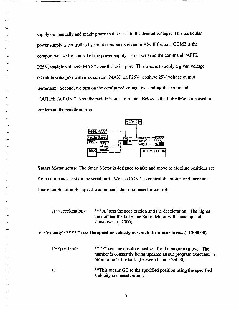
supply on manually and making sure that it is set to the desired voltage. This particular
power supply is controlled by serial commands given in ASCII format. COM2 is the
comport we use for control of the power supply. First, we send the command "APPL
P25V,<paddle voltage>,MAX" over the serial port. This means to apply a given voltage
«paddle voltage» with max current (MAX) on P25V (positive 25V voltage output
terminals). Second, we turn on the configured voltage by sending the command
"OUTP:STAT ON." Now the paddle begins to rotate. Below is the LabVIEW code used to
implement the paddle startup.
Smart Motor setup: The Smart Motor is designed to take and move to absolute positions set
from commands sent on the serial port. We use COMI to control the motor, and there are
four main Smart motor specific commands the robot uses for control:
A =<acceleration> ** "A" sets the acceleration and the deceleration. The higher the number the faster the Smart Motor will speed up and slowdown. (~2000)
V=<velocity> ** "V" sets the speed or velocity at which the motor turns. (-1200000)
P=<position>
G
** "P" sets the absolute position for the motor to move. The number is constantly being updated as our program executes, in order to track the ball. (between 0 and ~23000)
* * This means GO to the specified position using the specified Velocity and acceleration.
8

The initialization is a series of two functions that initialize the Smart Motor to all of
its correct settings. The ftrst function is "limit test" which tells the Smart Motor to move the
paddle the full length of table and back to home position. During this limit test, group
members can make sure that both the home position and the farthest position are correct. If
they are not, we can easily change the limits and rerun the program to check the limits again.
The Second function called "INIT" is used to set the velocity and acceleration and to
initialize the Smart Motor to home position.
Command outlines for both initialization functions:
Limit test:
P=<limit> A=lQOO V=1000000 G
i IN IT i INIT:
A=<acceleration> V=<velocity> P=O G
**<limit> is the number of steps to the far position (app. 23000) * * acceleration is low to avoid overshoot when checking the limits * * Velocity is set low also for the same reason. * * executes the limit test.
**usually set to 1900 * * usually set to 1100000 * * initializes the motor to its home position (0) **makes the motor actually move to the home position
Frame Acquisition setup: There are two ways to grabs frames from the camera. First, is the
single "snapshot" and second is the buffered output. We chose the buffered way because it
drastically increased the speed of the frame-grabbing. In fact, when we ftrst setup this
software to take "snapshots" every time it needed image data the system was limited to 20.41
frames per second. However, when we switch over to the more complicated buffered
technique we are able to get near a true 60 fps system. The process for initializing the
9

--
buffered acquisition uses existing lMAQ functions. First, create an image. Then you must
initialize the acquisition, create the buffer list, initialize the buffer itself, and start the
acquisition. After the acquisition, you use the copy from buffer function in order to get the
data. Below the Lab VIEW code responsible for initializing the acquisition, grab frames at
60fps, and close the session.
1" inliaUze IMAQ board stores the data in
system memory
T ill start acquistion
3.2.2- Capture of Video into X and Y Spike Arrays
10
acquire from system memory
W
Left
cortnuous whUeloop
session

'-..-.
. -.......
Capture a frame: For every iteration of the continuous tracking loop, the first step is
to acquire the image from the buffer. This buffer resides in system memory and is being
filled continuously in the background of our software. Using the IMAQ copy utility, the
program retrieves the most recent data from the buffer. This data is then converted to an 8-
bit pixel array, which represents the current frame ofinfonnation. The array's dimensions
are 120X160, and it is filled with numbers ranging from 0 to 255. Each array element
corresponds to a pixel, and the number of this element corresponds to the amount of
"whiteness" the particular pixel has. A zero is totally black, a 255 is totally white, and a
number between is some shade of gray. Because the table is designed such that the
background is black and the ball is white, the pixels corresponding to the ball are high
numbers while the background is low.
Threshold: To find the exact position of the ball, the software first uses a function
called threshold, which changes every pixel above a certain threshold to a one and the rest of
the pixels to zeros. After this function is executed, the data consists of a 120X 160 array that
is almost entirely full of zeros except there is a small group of ones where the ball is located.
The threshold we use ranges from about 190 to 230 depending on the lighting conditions .
For example, we can set the threshold to 220. This means that every pixel above 220
changes to a 1 and the rest change to O. A small-scale example is shown below.
11

Picture array before threshold (unction:
23 22 ~1 23 22 21 23 22 21 23 17 22 23 17 22 23 17 22_ 23 17 23 19 20 23 19 20 23 19 20 23 23 ~ :.11 23 22 21 23 22 21 23 11 22 23 17 22 23 11 22 23 11 23 19 20 23 19 20 23 19 20 23 23 22 21 23 22 21 23 22 21 23 17 22 23 17 22 23 17 22 23 I, 23 19 20 23 19 20 23 19 20 243 23 22 21 23 2:.1 ill 23 22 21 245 11 22 23 1] ~ ~ 17 22 23 I~ 23 19 20 23 19 20 23 19 20 2.j 23 22 21 23 22 21 23 22 21 23 11 22 23 11 22 23 11 22 23 II 23 19 20 23 19 20 23 19 20 23
Threshold (unction in Lab VIEW:
binary Thresholdl
Picture array after threshold (unction:
0 0 0 0 0 0 0 0 0 0 0 0 0 0 0 0 0 0 0 0 0 0 0 0 _0 0 0 0 0 0 0 0 0 0 0 0 _0 0 0 0
_0 _0 0 0 0 0 0 0 0 0 0 0 0 _0 0 0 0 0 0 0 0 0 U 0 0 0 _0 _0 0 0" 0 _0 0 0 0 0 0 0 0 ~ 0 _U _0 0 0 0 0 0 o ~ 1 0 0 0 U U U 0 0 o • 1 0 0 0 _0 0 0 U 0 0 ~ 0 0 0 0 0 _0 _U 0 0 u 0 0 0 0 0 0 0 _U 0 0 0 0 0 0 0 0 0 U U U 0 0 0 0 0 0 0 0 0 0
22 21 22 23 19 20 22 21 22 23 19 20 iJ.. 21
249 :r.. 255 245 255 244 24lS 2~ ~ _w
22 :.11 2] ~3 19 20
0 0 0 0 0 0 0 0 0 0 0 0
0 1 ~ 1 1 1 1 1 QI'
-u 0 0 0 0 0 0
12
23 22 21 17 22 23 23 19 20 23 22 21 17 22 3 23 19 ., I""'"
.. 23 ~ 1
.~ 22 23 i'23 19 20 23 22 21 17 22 23 23 19 _20 23 22 21 17 22 )3 23 19 20
0 0 0 0 0 0 0 -~ 0 0 0 0 0 0 0 0 0 t,;I"" ~ ~ 0
~ 0 0 0 0 0 0 u 0 0 0 0 0 0 0 0 0 0 0 0 0 0 0 0
..""
The pixies above the 220 threshold indicate the location of the ball.
After the threshold function the program can easily find the ball

Table side check: When this robot is being used, it can be setup at either end of the
table. The camera stays in the same place with the same orientation. This means, if one
were to look at the video feed from the camera the robot can be on the right side or the left.
The problem is if the ball is detected traveling from right to left on the video, it can be
traveling toward the robot or away from the robot. Therefore, there must be a way of telling
the program which side of the table the robot is on so that it can be programming to
accommodate the change. To overcome this issue, ftrst the whole program was written to
accommodate the robot being on the right side. Then for the left side conftguration the video
signal is rotated 180 degrees and fed into the program for the right side. Therefore, it
appeared to the software that the robot was always on the right side, and there were no major
changes to the software to change the side. A simple switch on the front panel to tell the
program to keep the real image for the right or rotate the image for the left is all that is
needed. The Lab VIEW code to implement the rotate is show below:
True
Robot on right side: •....... ?
Robot on left side: ratrnl 1:0.;; f
Find X and Y spike
array: The image array is now
13
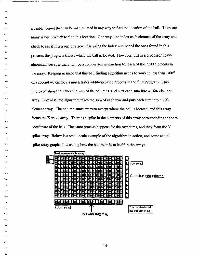
a usable format that can be manipulated in any way to find the location of the ball. There are
many ways in which to find this location. One way is to index each element of the array and
check to see if it is a one or a zero. By using the index number of the ones found in this
process, the program knows where the ball is located. However, this is a processor heavy
algorithm, because there will be a comparison instruction for each of the 7200 elements in
the array. Keeping in mind that this ball finding algorithm needs to work in less than 1/60th
ofa second we employ a much faster addition-based process in the final program. This
improved algorithm takes the sum of the columns, and puts each sum into a 160- element
array. Likewise, the algorithm takes the sum of each row and puts each sum into a 120-
element array. The column sums are zero except where the ball is located, and this array
forms the X spike array. There is a spike in the elements of this array corresponding to the x-
coordinate of the ball. The same process happens for the row sums, and they form the Y
spike array. Below is a small-scale example of the algorithm in action, and some actual
spike-array graphs, illustrating how the ball manifests itself in the arrays.
ISmail scale example array!
IIStl nb h h h
I~ 0 0 00 0 0 kl 1 kl klkl klo kl 0 kl klo kl kl 1 1 1 n b no b b b bb b b 1 1 1 1 1 0 klo kl b b 0 D 111 111 b bb b 0 D DO D bb 1 1 1 b b b bb b D kl b b b b b b b b b nn n klo D DO D klD b b kl kl h D b b b b kl D DD b Db D Db D Db D
IkllJl:ll:llJlJlJ 11111111., kl;k 13111J IJIJIJIJIJ IJIJII
~olumn sums! /
max value index = 13
14
fow sums!
( hlax value index = 4!
The coodinates of the ball are: (13,4)
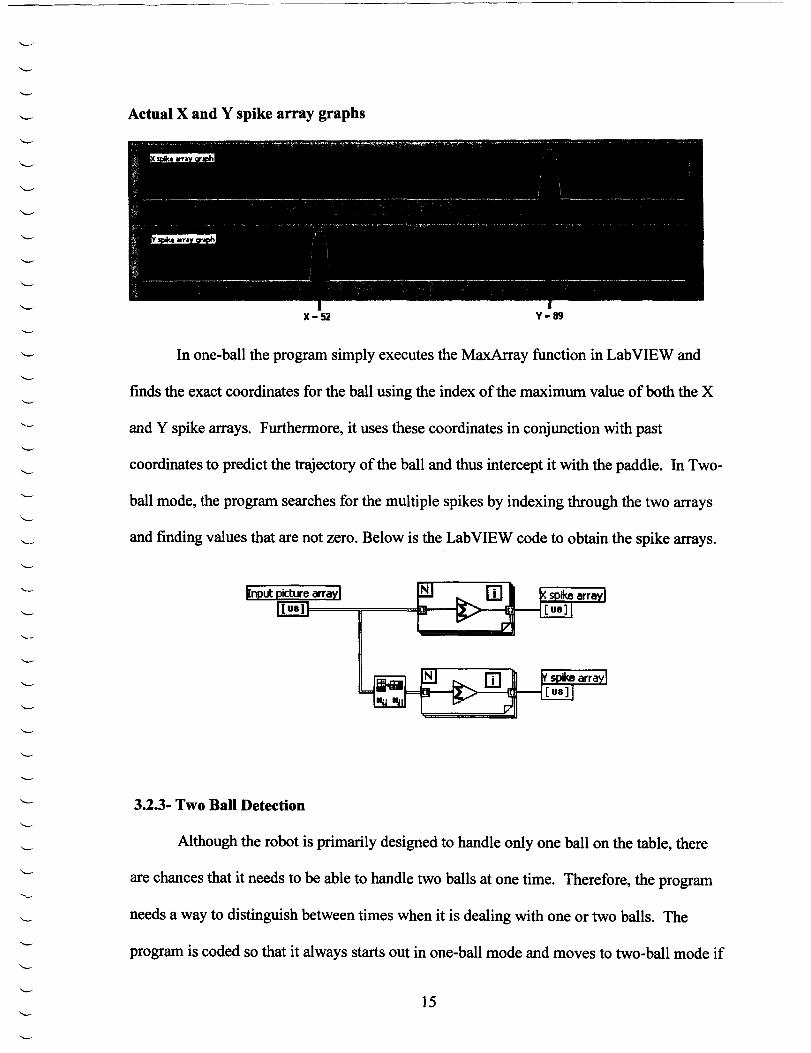
Actual X and Y spike array graphs
X-52 Y-89
In one-ball the program simply executes the MaxArray function in Lab VIEW and
finds the exact coordinates for the ball using the index of the maximum value of both the X
and Y spike arrays. Furthermore, it uses these coordinates in conjunction with past
coordinates to predict the trajectory of the ball and thus intercept it with the paddle. In Two
ball mode, the program searches for the multiple spikes by indexing through the two arrays
and finding values that are not zero. Below is the Lab VIEW code to obtain the spike arrays.
3.2.3- Two Ball Detection
Although the robot is primarily designed to handle only one ball on the table, there
are chances that it needs to be able to handle two balls at one time. Therefore, the program
needs a way to distinguish between times when it is dealing with one or two balls. The
program is coded so that it always starts out in one-ball mode and moves to two-ball mode if
15

necessary. The simplest way we found to detect when two balls are present is to perform a
simple addition. Much like the original ball-locating algorithm, we can have checked each
pixel for a "one", but an addition-based algorithm is multiple times faster. We experimented
and took note that when one ball was on the table the addition of all the white pixels ranges
from approximately 15 to 30, and when two balls were on the table it ranges from
approximately 25 to 55. Therefore, by implementing a simple threshold test we can roughly
determine if two balls were on the table at the same time despite the small overlap. By
setting this threshold to 28, we are able to have one part of the program running when the
sum is less than 28 and another part, the two-ball algorithm, when it is greater than 28.
However, with this simple check the program sometimes slips into the wrong mode due to
the small overlap in sums. For example, with one ball on the table there is a small amount of
time when the threshold rises above the magic number 28. This is mainly due to the crest in
the middle of the table. At the top of the crest, the ball is closer to the camera and thus looks
bigger to the camera. This makes the sum of the white pixels increase above 28 momentarily
causing the program to go into 2-ball mode for a few frames. Sometimes, during the
switching between modes, the ball manages to pass our paddle because of the confusion.
Below is a graph of the sum of white pixels with one ball and two balls as they are rolled
across the table versus the frame number. Notice how there is a slight bit of crossover with a
stagnant threshold value of 28. One ball crosses over in the middle while two-ball crosses
over at the edges.
16

To fix this problem we implement a more stringent check in order for the program to
change modes. This new design still implements the threshold technique, but with a one
change. Instead of changing the mode right when the sum rises above the threshold, the
mode changes when the sum rises above the threshold 40 frames in a row. Notice on the
graphs above how the one-ball curve never stays above the threshold for more than few
frames and the two-ball curve it never goes below the threshold for more than a few frames.
Furthermore, when it is in the correct mode it stays in the correct area for well over forty
frames. This new design makes sure that indeed another ball has been put onto the table and
it is not just a small spike of "whiteness" above the threshold.
3.2.4- One Ball Prediction
To this point the program has located the current x and y coordinates of the ball on a
screen that is 120X160. The next step is to take these coordinates and find out where the ball
is going to cross the into the paddle zone in order to relocate our paddle to that position and
send the ball back to the opponent.
17
Our first thought was to simply track the ball the whole time. In other words, simply
uses the current x coordinate as the paddle position. If the ball goes from one side of the table
to the other, the paddle follows it the whole time. Therefore, when it arrives at the paddle
zone the paddle is there to catch it. This simple algorithm works flawlessly with slow
traveling balls. However, when we increase the ball speed during testing, the paddle could
not keep up and sometimes would let the ball go by. We realized that we needed to predict
where the ball was going to be. Instead of the paddle correcting itself across the whole length
of the table, it would correct itself in a small area of prediction. Therefore, it is much less
likely to let a ball go past.
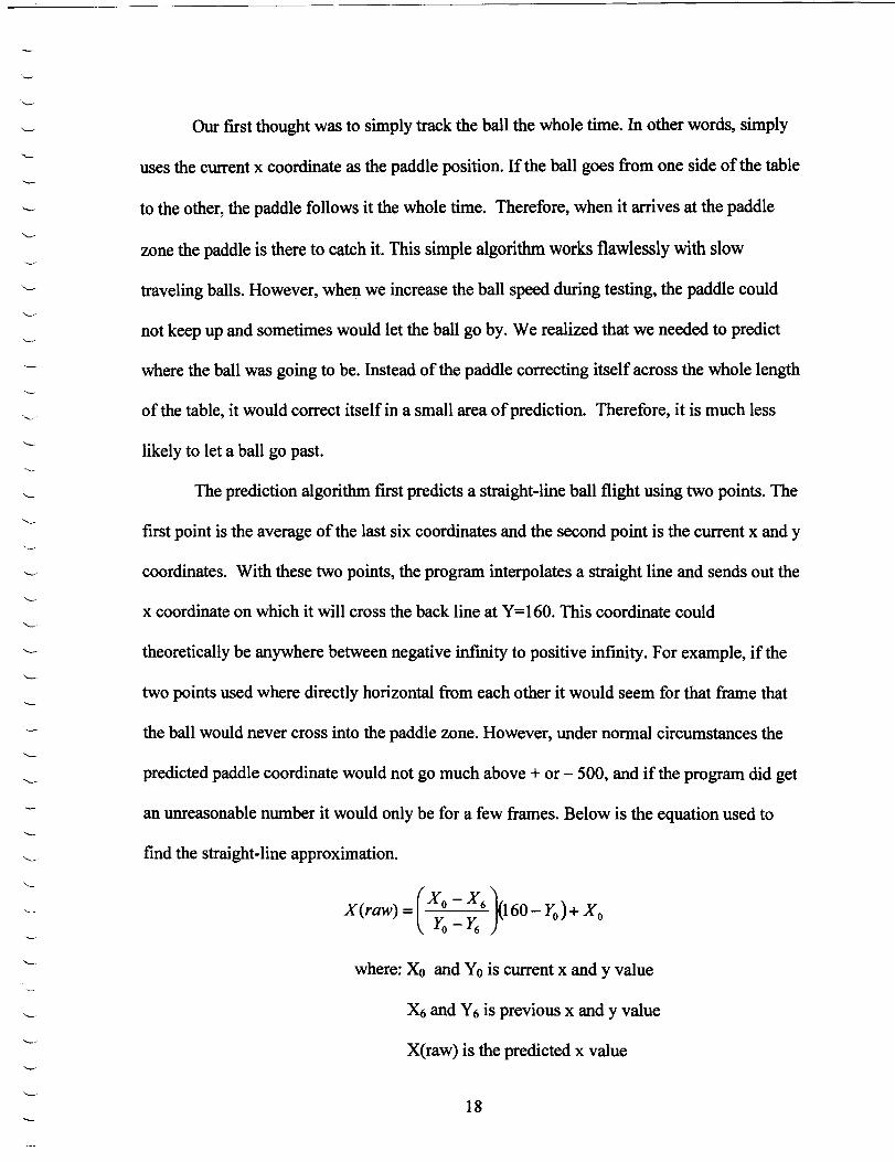
The prediction algorithm first predicts a straight-line ball flight using two points. The
first point is the average of the last six coordinates and the second point is the current x and y
coordinates. With these two points, the program interpolates a straight line and sends out the
x coordinate on which it will cross the back line at Y=160. This coordinate could
theoretically be anywhere between negative infinity to positive infinity. For example, if the
two points used where directly horizontal from each other it would seem for that frame that
the ball would never cross into the paddle zone. However, under normal circumstances the
predicted paddle coordinate would not go much above + or - 500, and if the program did get
an unreasonable number it would only be for a few frames. Below is the equation used to
find the straight-line approximation.
X(raw) = 0 6 (160- Yo)+ Xo (X -X) Yo -~
where: Xo and Yo is current x and y value
Xt; and Y 6 is previous x and y value
X(raw) is the predicted x value
18

Now the program has a raw crossing point. However, this crossing point does not take into
account that there are walls on the table. The next step in the program is bouncing
compensation. The area is 120X160 and we are dealing with just an x value so our paddle
will reside somewhere between 0 and 120. Therefore, using the raw data and programming
the location of the walls at 0 and 120, we mirror the data across the walls until the raw data
reside somewhere between 0 and 120. This is the coordinate we want our paddle to be when
the ball comes into the paddle zone. Below is an example of how the prediction works with
one wall bounce.
y=O
y=160
x=120 x=O
19
predicted position without bounce compens8i:ion

'---
'--
Below is the Lab VIEW code used to predict the ball flight line and bouncing compensation:
---0 --[Q]
3.2.5- Two ball Tracking
The basic premise of the two-ball algorithm is to track the ball that is closest to the
paddle AND coming toward the paddle. In theory, this will always works unless the balls are
both coming toward the paddle and crossing the line at the same time. In this case, any two
ball algorithm fails, because the paddle obviously cannot be two places at the same time in
order to get both balls. Furthermore, since the paddle does have a non-zero movement time
from one position to another, even if the balls crossed the line at approximately the same
time and they were spread more than 4 inches apart the paddle can not get to them fast
enough. However, under normal condition barring the impossible shot, the "closest and
coming" concept works very well. Below is a flow diagram of two-ball mode, and how we
implemented "closest and coming"
20

Search for first Y-spike
Index picture array
Max indexed array
3.2.6- Video to Motor Position Scaling
No
Yes
Look for second spike
Index picture array with old spike
The algorithm finds the position of the ball in terms of the 120X160 area of the
frame; however, the actual positions of the motor are much different. In fact, it takes the
motor 23000 steps to get across the table. Therefore, it is necessary to have a conversion
between the number between 0 and 120 corresponding to the frame to a number between 0
and 23000 that corresponds to the motor. Obviously, these two values are proportional and
the proportionality factor is equal to the number of steps for the motor divided by the number
of steps for the frame. 23000/120 = 1916.6. Therefore multiplying the frame coordinate by
this factor tells the correct position to the motor.
After testing a straight proportionality, it was evident that something was needed at
the edges of the table. If the ball was all the way against the wall close to home position the
coordinate sent to the motor was zero. However, if the ball moved one pixel over the motor
21

moved over also. The ideal situation at the edges would be that the motor would not move
until the ball moved at least a distance equal to half the paddle away from the side wall
before the paddle started to move away. Therefore, before the position is sent to the
multiplier it is scaled by the following equation to make it "stick" to the wall when the ball is
between the middle of the paddle and the side wall.
60-Xbal/ Xmotor = Xbal/ - (STM)----
60-STM
Where: STM is the number of steps to middle of paddle (-13.66)
Xball is the calculated x position before "stick" scaling
Xmotor is the final position sent to the multiplier for the motor
Below is a graphical example of "stick" scaling.
motor coordinates
bllli poslion coordinates
x=O
distance from side of '>---paddle to middle
22

3.2.7- Move Motor
The move-motor function takes the absolute position for the motor and sends the
correct messages to the SmartMotor via the serial port. This function also uses a hardcoded
max limit so that it never sends position that is greater than 23000 or less than 0 in order to
guard against the motor making contact or even damaging the walls of the table. This
function uses the P=<position> function and the G (go) function described in the
initialization section of this paper.
~ ~ Move Motor (immediately)
3.2.8- Closing Steps
After the program is finished running and the user presses the stop button on the front
panel, there are a few closing steps that occur. First, the velocity and acceleration are set low
and the motor is moves back to the home position. Next, the IMAQ session is closed using
IMAQ close. Third, the session with the SmartMotor closes. Lastly, the power to the paddle
is switched off. Below is the Lab VIEW code that executes each of these closing steps.
23

3.2.9- Problems and Additions
Sweet spot compensation: Dubbed the sweet spot, there was one shot that can fool
our paddle nearly every time. A hard 45-degree bounce off the side % of the way down the
table can usually fly by the paddle. The problem was that the paddle overshoots the
predicted position of the ball and by the time it had gotten back to where it was supposed to
be, the ball was already past. Furthermore, this was a software overshoot and not a problem
in the motor feedback system. For some reason, the program was actually sending inaccurate
positions. We believe it was due to the data being a little rough at the front end, and the error
propagated through the program getting worse through every step. Below is a graph of the
absolute position versus frame number with the over shoot shown.
To fix this problem spot we hard-coded this special case into the program. When it
sees the ball was going to bounce of the wall anywhere near the "sweet spot", the paddle
stops tracking and waits at a certain location that we experimentally found to be close to
where most of these shots go. At the last second the paddle tracks to the exact location and
hits the ball every time. The sweet spot was no longer an issue. Below are graphs of the
overshoot problems before and after the "sweet spot" compensation.
24

Fisbeye Compensation: Referred to as the fisheye, the areas at the four comers of
camera view were blurred and curved such that the ball went out of the camera view in these
areas even though it was still on the playing field. This was a very simple fix even though
many of the teams at the conference did not compensation for this problem. If the ball
traveled out of the camera view then the paddle sits at the location it was sent to the last time
it saw the ball. Therefore, even though the ball left the camera view the paddle was sitting
waiting on it. After it hit the ball back into the view, the program continued normally.
Middle return system: Since the robot did not know where the opposing team was
going to hit the ball we knew that we stood the best chance of return if we returned to the
middle of the paddle zone before the opposing team sent the ball back across the table. To
achieve this we simply tested to see if the ball was moving away from us and it was past the
middle of the table. Therefore, after we hit it over the crest it returns to the middle, and waits
to track the ball when it starts coming toward the paddle again.
Failsafe proximity tracking: Although rarely, glitches do sometimes occur in the
program. They are due to bad data being sometimes sent to the prediction algorithm. Rarely
the paddle would glitch for a second, and let the ball past. To fix this problem the program
looks for any white spots within five pixels of the paddle zone and if there is even one the
paddle tracks it instead of using the prediction data. This protects against the ball being right
in front of the paddle zone when it glitches, letting the ball past.
Slow ball tracking: When the ball is moving very slowly on the table the prediction
algorithm is very jittery because the difference between the previous ball coordinates and the
current are small. Under these conditions, the straight-line approximation changes greatly
from frame to frame, because the points are not well spread in order to get a nice line of
25

approximation. To fix this problem, the program checks the difference between the points. If
the difference is below a threshold of 3, which means it is moving slowly, then it straight
tracks the ball. By turning off the prediction it stabilizes the paddle when the ball is moving
slowly.
Run-time Diagnostics: Another part of the initialization procedure for the camera is
a diagnostic step. This small part of the initialization procedure that takes one snap of the
table and displays the data results on a graph. By looking at this graph, we can immediately
tell if there is an unwanted white mark on the table or if the lighting is such that we need to
change the range of the threshold function discussed later. This is very useful when trying to
diagnose problems with our prediction due to cleanliness of the playing area, and lighting
conditions. In addition, the program has runtime diagnostics that have LED's on the front
panel that signify what part of the program was running at the time. Some of the lights
include a working light, a two-ball indicator, and some lights that show where in the two-ball
algorithm the program lays.
4.0 Frame and Motor
The rule sheet states that the game table will be forty-five inches across and that three
feet of additional space will be available for the robot frame on each side of the table. There
is also three feet behind the table to place any items for the robot. At no time during the
competition can your robot or frame extend outside of this boundary zone.
Once the allowable robot area was established, the first step in the design process is to
find a low friction rail system to attach the paddle to for motion across the table. We found a
compact rail system made by the company Rollon. These units have a very strong and
26

durable rail with an internal slide running on a ball bearing system. The rail itself has
mounting holes every two inches (Fig. 4.1) that not only allows for mounting of the rail, but
also allows additional units to be connected to it. The overall rail length purchased was
seventy-three inches. As Fig. 4.1 depicts, the slider is not flush to the rail, but hangs one
quarter of an inch lower.
Slider
T-housing
~ Compact Rail
Figure 4.1
The slider runs on a low friction ball bearing unit. The ball bearing unit is encased in
a "t-housing" (Fig. 4.1). The "t-housing" hugs the bearing so that slippage does not occur,
but it hugs enough so that when the driving unit stops, the slider will also stop, or in other
words, it has an internal braking unit. The slider is what connects the paddle to the rail
system. Two mount holes that are symmetric from end to end on the slider secure the paddle.
The next step is to setup the drive unit frame to move the slide and paddle. A timing
belt driven system will be the best suited for this application. The timing belt is more precise
with start and stop points, pending on the number of teeth on the pulley itself (i.e. more teeth,
less slippage). With a drive motor on one end, a single shaft with a ball bearing unit attached
to the other end will complete the loop (Fig. 4.2).
27

'- .
'--
Top View
(:D
Side View Pulley
Servo Motor
Figure 4.2
This design seemed to be more than adequate, but some problems were encountered
when trying to implement it. The problem is that the horizontal load and torque is going to
be too great for the motor shaft to handle for an extended period. Under this configuration,
the motor can be damaged and rendered useless. The solution is to uncouple all of the
stresses away from the motor. This is accomplished by lengthening the shaft with a half-inch
wide, stainless steel, chrome plated shaft roughly six inches long. Using a coupler from
Lovejoy, the three-eighths inch motor shaft connects to the half-inch diameter extension. A
housing unit was designed to accommodate the new shaft length so that the motor can still be
mounted to the frame. A ball bearing unit decouples the resulting motor shaft from any
excessive horizontal torque (Fig. 4.3).
28

0 C upler
Motor 3/8 ~ 112 I
Housing unit
Ball Bearing
Motor 3/8
Figure 4.3
The next part of the frame assembly is to find a support bar for the compact rail
system and the motor. The Rollon bar was initially going to support the motor alone, but the
housing unit added too much height to the motor. The rail also flexes in the center slightly so
a sturdier member is needed. The solution is to use some industrial railing called 80/20 to
mount on top of the rail which will stop any flexing in the compact rail system and also
provide an easier way to mount the motor (Fig. 4.4).
Side View 80/20
Figure 4.4 Rail
The 80/20 bar is centrally grooved on all four sides so that connections can be made
to it at any point using a "t-nut" which slides into the groove. Since the timing belt cannot be
29
'-
"-
"-
'-
"-
'-.--
.~
inside the rail and attach to the slider, the timing belt must be offset and attach to the slider
from the side. Therefore, the motor must be offset as well. Due to the weight of the motor,
the frame can become unbalanced if it is not secured properly. A highly compressed and
hardened aluminum alloy sheet supports the offset motor.
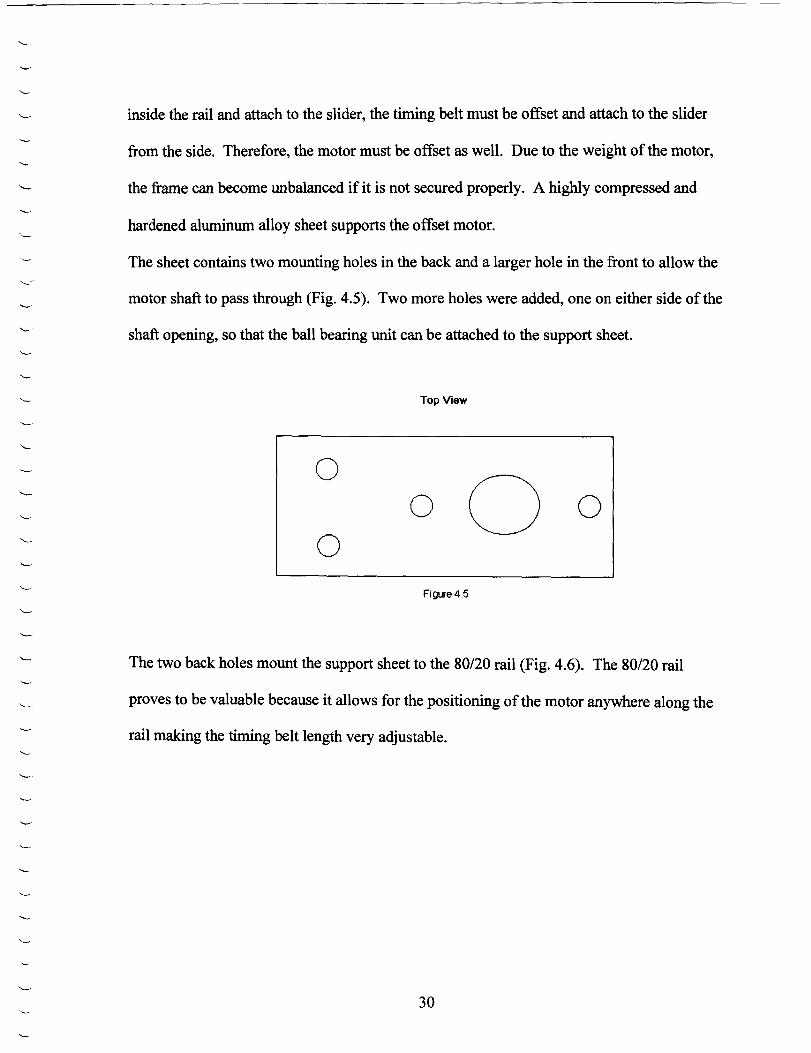
The sheet contains two mounting holes in the back and a larger hole in the front to allow the
motor shaft to pass through (Fig. 4.5). Two more holes were added, one on either side of the
shaft opening, so that the ball bearing unit can be attached to the support sheet.
Top View
0
0 o o o
Figure 4.5
The two back holes mount the support sheet to the 80/20 rail (Fig. 4.6). The 80/20 rail
proves to be valuable because it allows for the positioning of the motor anywhere along the
rail making the timing belt length very adjustable.
30

Top View
0 0
0 < Timing Belt > 0 0 0
• 0 0 0 o~ Figure 4.6
Once the main body of the frame is built, it is attached to the support stands using
more 80/20 railing. The support stands are nothing more than just metal sawhorses but are
utilized because of their ability to adjust vertically. The ftnal frame arrangement is shown in
Fig. 4.7. The pulleys and timing belt are attached to the slider on the backside of this frame
using a locking plate mechanism.
Front View
Ball Bearing unt 80120
'"- -
"-
"- Slider
"-
Paddle
Sawhorse Stand
"-
Figure 4.7
The motor in this design is a 3440 series Smart Motor from Animatics. This series
motor is a brushless D.C. servo motor with a built in 1,000 line encoder. Important
speciftcations for the motor are contained in Table 1.
31

Ta e : otor ~eCI lcatlons hI 1 M S ·fi .
Peak Torque (oz-in) 625 (N-m) 4.41
Continuous Torque (oz-in) 210
(N-m) 1.48
Voltage Constant (VlkRPM) 12.9
No Load Speed (RPM) 3609
Torque Constant (oz-in/amp) 17.4 (N-m/amp) 0.123
Rotor Inertia (oz-in-secJ\2) 0.025
Weight (Ibs) 5.5 (kg) 2.5
Nominal Continuous Power (hp) 0.34 (kW) 0.26
The motor is much more accurate than what is utilized for this project. There are a
total of 23,000 step positions for the motor across the 45" table giving us a possible
resolution of2e-3 in/step. The camera however only outputted a 480x640 array image. This
array is then sized down by a factor of four to increase processing speed allowing for 120
possible steps across the width of the table. This reduced our resolution by a factor of 200
down to 375e-3 inlstep and this still proved to be more than enough accuracy to position an
8" paddle in front of a 2" ball.
Most of the speed loss of the motor came from trying to move the slider of the
compact rail system. Our initial presumptions were that the Rollon system that we were
ordering would be close to frictionless but that did not turn out to be the case. Over time, the
bearing system did loosen up allowing for less torque on the motor. The paddle itself is
around 6 lbs and the motor can still move it from one side of the table to the other in about v..
second.
32

The commands to move the motor are simple. The motor needs a position,
acceleration, and a velocity in order to carry out a command. The acceleration and velocity
are set once during the initialization of the motor and then saved internal to the motor
allowing for a quicker processing time of the variable positions.
The acceleration and velocity data used for our runs is 1900 and 11500000
respectively, however; this is not the actual acceleration and velocity of the motor. For the
SM34XX series motor there is a factor of 15.82 and 64424 that is multiplied by your desired
acceleration and velocity respectively, to set the 'A' and 'V' values used by the motor. The
actual acceleration of the motor is 120 rev/sec2 and the velocity is 180 rev/sec.
The position data sent to the motor is based on a factor of 4000 pos/rev for the
SM34XX series. An absolute position scheme is used to save in processing time. The
SmartMotor has 4000 increments for one complete revolution of the shaft. Added to this
shaft are two, 2-Y2 pulleys used to move the paddle across the table so each revolution of the
motor sends the paddle a distance of approximately 7 % inches. Realizing that the table is
only 45" across, the motor only needs to complete 5 Y2 revolutions to completely cover the
surface area of the table.
5- Paddle
5.1- Design Considerations and Various Paddle Designs
After much discussion, two paddle designs were chosen. The paddle designs
considered were either event driven paddle or a continuous motion paddle. Several designs
for each paddle type were considered and two teams were formed. One would focus on a
33

solenoid event driven paddle and the other team would focus on a continuous pitching style
machine.
S.l.t- The Solenoid Design
1 1 T o~
The main idea of the solenoid paddle is a hinged piece of metal with a solenoid
behind it. The upper metal piece contains a sensor that allows the paddle to know when the
ball is in the striking zone. Suspended from the upper horizontal metal piece is hinged the
swinging piece of metal that acts as the striking mechanism. Directly behind the striking
piece of metal is the solenoid itself. The solenoid activates by the sensor in such a way that it
will activate any time the ball is within the striking zone. The striking zone is located
directly under the sensor. When activated the solenoid fires into the hinged piece of metal
which in turn strikes the ball. The whole structure mounts with metal framing.
The complexity of the solenoid paddle is higher than other designs. The paddle
contains a sensor that adds an extra element of electronics to the paddle. The timing of the
paddle needs to be highly accurate in order to strike the ball at the exact moment that it is in
the striking zone. The mechanical complexity of the paddle is simple with only the metal
structure supporting the solenoid and the hinged metal striking element.
34
'-
The accuracy of the paddle is not as good as other possible designs. The accuracy
depends on a solid hit each time the ball is in the striking zone. Any variation in the strike, as
in the case of a slow incoming ball or a fast one can result in a miss hit. The accuracy also
depends on the speed and strength of the solenoid firing as well as the accuracy of the sensor
in detecting the ball. The accuracy for the paddle is one of the design's weaker points.
The stability of the solenoid paddle design is good. The simplicity of the mechanical
aspects allows for a strong paddle. High acceleration does not affect the effectiveness of the
paddle. A strong point of the paddle is the paddle's stability.
The variability of the paddle is limited in the shots it can produce. The speed of the
returned ball does not vary on its own. It only changes with the varied velocity of an
incoming ball. The variation of shots is limited as well. The paddle gives a mirrored effect
with each returning ball.
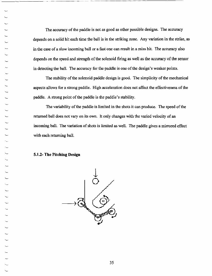
5.1.2- The Pitching Design
1 o
35
The pitching design is made with the idea of shooting a ball from spinning wheels.
The paddle has a funnel face and uses spinning wheels to accelerate the ball through a
rounded track. Next two additional wheels are used to return the ball. The frame is metal
and metal tracks are used to direct the ball. Four wheels are used and two small dc motors to
actuate the wheels. One wheel is directly at the back of the funnel, which pushes the ball to
the next wheel at the bottom of the direction track. This wheel directs the ball to the flring
wheels located on the right of the paddle.
The pitching design is a complex paddle. The paddle requires two separate DC
motors as well as a gearing system to spin the wheels. The shape of the paddle is complex
and needs to be precise in order for the wheels to fire the ball correctly. The speed of the
wheels needs to be constant and calibrated correctly in order to direct and shoot the ball
correctly.
The accuracy of the pitching design is good. It uses continual motion to return the
ball therefore, no sensors are needed. The accuracy depends on the reliability of the directing
wheels. The only inaccuracy is if the ball did not make it to the directing wheels. The funnel
design does not always bring the ball to the correct location. It is possible the ball could be
stuck within the funnel.
The pitching design is an instable paddle. Due to its complexity, high changes in
acceleration can affect the speed and calibration of the DC motors. The mechanical elements
can provide instability as well. Both the electrical as well as the gearing system is delicate
under fast movement.
The variability of the pitching design is limited. The speed of each shot is the same
and each return is a bank shot of the right rail. The only variability is within the location of
36

'-
the paddle when the ball is fired. The different location produces a different bank off the
right rail. Based on the location of the paddle the shot is either a deeper bank or shallower
one.
5.1.3- The Rotating Design
! o
The rotating paddle is designed with a vertical DC motor located in the center of the
paddle. The motor is attached to a gear on top. The gear attaches to the paddle face with a
metal bar. The paddle face is connected to a slider that uses ball bearings for movement.
The rotation of the gear forces the paddle face back and forth on the slider. The paddle face
is thin metal and the structure of the paddle is metal as well.
The rotating paddle design is an overly complex paddle design. The mechanical
structure is difficult to implement correctly. The paddle requires high speeds from the DC
motor. The metal bar must be connected to both the gear and the paddle face in a way that
allows smooth motion but a strong connection as well. The motor must be directly mounted
in the center of the paddle, but in a way that does not impede the motion of the gear. The
37

electrical part of the paddle is simple with only the DC motor, but the mechanics must be
suited for a torque that the motor can handle.
The rotating paddle design is not an accurate design. The movement of the paddle
face is limited by the mechanics of the gearing system. This limitation comes from too small
movement from the gear. This lack of movement only moves the paddle face 'h to % of an
inch back and forth. This amount of movement is not enough to strike the ball in an
acceptable manner each time. From testing, the ball is struck correctly about 1/5 of the time.
The paddle uses continual motion that is beneficial but has stability limited accuracy.
The stability of the rotating paddle design is not good. The mechanics are too
difficult to implement in order for the paddle to work correctly. The main problem lies in the
connection of the gear with the attachment bar to the paddle face. The bar's connection with
the gear as well as the connection with the paddle face is highly unstable at high speeds. It
detaches from either the gear or the paddle face after limited running time.
The variability of the rotating paddle is limited. The power depends on the received shot and
the angle of the shot is a direct reflection of the shot received. It did however have capability
for texture that allows a more varied shot.
38

'--
5.1.4- The C02 Design
\ ....
! o /
The C02 design was based on the idea of returning the ball using C02 compressed
gas. The paddle is a funnel design. The base of the funnel is a tube that contains a sensor.
The sensor is connected to a solenoid that fires into the back of a C02 cartridge. The C02
cartridge releases a burst of compressed air firing the ball much the same as used with a paint
ball gun. The funnel design is made from metal as well as the structure supporting the
solenoid, C02 cartridge, and the rubber tube from which the ball is fired.
The C02 paddle design is complex. The paddle sensor needs to be accurate for the
timing of firing the solenoid. The solenoid must fire in a means that activates the C02
cartridge correctly each time. The C02 cartridge must release the correct amount of gas in
order to "burst" the ball from the tube. The funnel design must allow the ball to come to rest
within the tube each time in order for the shot to work correctly.
39

The accuracy of the C02 paddle is low. There are a number of actions that must be
perfect in order for the paddle to fire correctly. The complexity of the paddle lowers the
probability of an accurate hit each time.
The stability of the paddle is good. Everything is mounted on a metal structure and
there are not intricate details that weaken the design. The paddle is able to handle high
accelerations and quick stops.
The C02 paddle design is not a variable paddle design for ball returns. The speed of
each shot is the same and each return is a bank shot of the right rail. The only variability is
within the location of the paddle when the ball fired. The different location produces a
different bank off the right rail. Based on the location of the paddle the shot is either a
deeper bank or shallower one.
5.2- Final Paddle Design Analysis and Implementation
The final paddle design resembles a paddle wheel seen on paddleboats. This design
eliminates the use of a sensor to detect when the ball was in close proximity of the paddle.
The motor used to generate the spin of the paddle is a DC motor. The paddle system was
rigorously tested for flaws. One flaw that was found that could jeopardize the robot's ability
to return the ball to the opposite side of the table was that when the ball approached the
paddle there was a slight possibility that the ball could completely pass under the paddle.
This occurs when the ball approaches the paddle at a time in which both faces of the paddle
are parallel with the surface of the table. Changing the two faced paddle to a four faced
paddle decreased the probability of a miss. The final paddle is made of an 8-inch horizontal
and 6-inch vertical metal plate that is to rotate constantly around the horizontal axis (Refer to
figure below). On one of the vertical sides, the metal plate is cut in such a way that a round
40

'---'
'-
'-..-
'-
'-
'"-
'-
DC motor about 2.5 inches long and 1.5 inches in diameter fits horizontally along the center
of the plate. A copper cylindrical tube about 0.4 inches in diameter is cut along its length
allowing the metal plate to slide in between. The copper tube is then fit along the horizontal
axis of the plate leaving about 1 inch of tube at both ends. Using bolts and lock nuts, the
copper tube is secured together with the plate. A gear that fits inside the copper tube is
placed on the shaft of the DC motor and then by inserting the gear inside the copper tube the
motor is secured to the metal plate.
6 inches rs Metal Plate ~
A screw is used to hold the motor shaft, the gear, and the copper tube together. At the other
side of the plate, a ball bearing was fit inside the copper tube, allowing the plate to rotate
with minimum friction (Refer to figure below). Two additional metal plates each measuring
8 inches horizontally and 3 inches vertically are placed along the axis of either side of the
41

main plate. At this point if looking from the side of the paddle four equal size perpendicular
plates and the round base of the DC motor are seen.
An aluminum flat bar about 18 inches long and 1.5 inches wide is bend at 90 degrees angles
at both ends leaving the middle part about 9.5 inches long. The paddle is attached to the bar
by screwing the DC motor to one side and attaching the center of the ball bearing to a shaft
secured to the other side of the bar. Strong metal comer brackets are secured to each comer
of the frame to ensure more stability. The flat bar is attached to the main frame of the robot
and placed about 1 inch above the table.
The spin of the paddle is controlled manually depending on the amount of DC voltage
transmitted to the De motor. The paddle hits the ball and the traveling speed of the ball
across the table depends on the speed by which the paddle spins. After numerous tests, the
range between 4.5 DeV to 5.5 Dev is the most accurate for the ball to end up in the scoring
42

',-
bin at the opposite side of the table. The four metal plates of the paddle are flat and when the
ball is hit, most of the time it travels in a strait line. To compensate for the strait shoots small
pieces of metal of different shapes are attached to two of the plates. This gives the paddle a
chance to hit random shoot where the ball can travel at different angles.
A backup paddle is built very similar in appearance with the final paddle. A shaft of 0.5 inch
in diameter is used for the axes of the metal plates. Two plates 8 x 8 inches are pressed
against each other with the shaft in between them and secured using screws and lock nuts. A
DC motor is attached to the end of the shaft and then two additional metal plates are placed
perpendicular along the axes of the main plates. One side of a flat bar similar to the bar used
to support the final paddle is secured to the base of a DC motor The other side of the flat bar
is drilled to let the axis shaft fit through and rotate with minimum friction.
6- Competition Results and Conclusions
The V.T. robot was able to compete with any of the other robots at the hardware
competition. We scrimmaged against two of the best robots at the competition (Georgia
Tech and Tennessee Tech) and did very well against them. The robot operated properly and
won the first two matches (one being a forfeit) at the competition table, but the third and
fourth match we lost because of a bad signal from the competition hosts. We placed 9th
overall out of28 robots. We believe the results of the competition do not accurately reflect
the abilities of the robots, since some robots (including ours) had a problem with the
competition setup. The robot performed well on the competition practice tables, which
should have had the same signal conditions sourced to the robots as the competition table
43

(according to the competition hosts). The competition table had a monitor and an
oscilloscope connected to the camera as well as the opposing robot. The competition hosts
used isolation buffers and video amplifiers to isolate the other equipment from the video
signal fed to the robot, but there was a problem in their signal processing. We only had 5
minutes to set up the robot before the match began, so we did not have much time to analyze
the problem. The National Instruments lMAQ software showed us a video window of the
NTSC signal being fed to the robot. It showed numerous horizontal line flickers before
losing synchronization and locking up. It appears that the monitor, oscilloscope, and other
robot were not properly isolated from our signal. Other robots using frame grabbers also had
problems. We have not been able to reproduce this problem, and we verified that the robot
was working fine on the competition table after the competition was over.
If we had a chance to redo the competition, the signal acquisition aspect of our design
is the only major change we would make. An extra video amplifier or buffer may have
solved our problem. When our robot was receiving a good signal, it performed better than
any other robots at the competition. We would most likely have made it to the final match if
it were not for the signal acquisition problem.
References
SECon 2002 Hardware Competition web page: http://www.ee.sc.eduJorgs/Secon2002/Rules/
National Instruments web page: IMAQ 1408 specifications at http://www.ni.com
44
Related Documents