4.1 Slides for Parallel Programming Techniques & Applications Using Networked Workstations & Parallel Computers 2nd ed., by B. Wilkinson & M. Allen, @

4.1Slides for Parallel Programming Techniques & Applications Using Networked Workstations & Parallel Computers 2nd ed., by B. Wilkinson & M. Allen,

@ 2004 Pearson Education Inc. All rights reserved.

Chapter 4Partitioning

and Divide-and-Conquer Strategies

• Two fundamental techniques in parallel programming- Partitioning- Divide-and-conquer

• Typical problems solved with these techniques



Partitioning/Divide and Conquer Examples

Many possibilities.

• Operations on sequences of number such as simply adding them together

• Several sorting algorithms can often be partitioned or constructed in a recursive fashion

• Numerical integration

• N-body problem



Partitioning

• Dividing the problem into parts.• Basis for all parallel programming, in one form or another.• Domain decomposition - partitioning applied to the

program data.• Dividing the data and operating upon the divided data

concurrently.• Functional decomposition - partitioning applied to the

functions of a program.• Dividing the program into independent functions and

executing the functions concurrently.• Domain decomposition forms the foundation of most

parallel algorithms



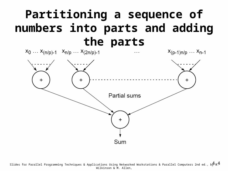
Partitioning a sequence of numbers into parts and adding the parts



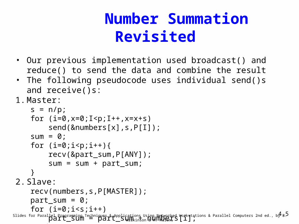
Number Summation Revisited• Our previous implementation used broadcast() and reduce() to send

the data and combine the result• The following pseudocode uses individual send()s and receive()s:1. Master:

s = n/p;for (i=0,x=0;I<p;I++,x=x+s) send(&numbers[x],s,P[I]);sum = 0;for (i=0;i<p;i++){ recv(&part_sum,P[ANY]); sum = sum + part_sum;}

2. Slave:recv(numbers,s,P[MASTER]);part_sum = 0;for (i=0;i<s;i++) part_sum = part_sum + numbers[i];send(&part_sum, P[MASTER]);



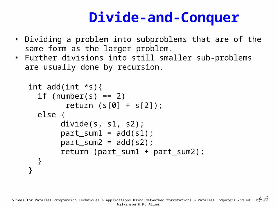
Divide-and-Conquer• Dividing a problem into subproblems that are of the same form as the

larger problem.• Further divisions into still smaller sub-problems are usually done by

recursion.

int add(int *s){ if (number(s) == 2) return (s[0] + s[2]); else { divide(s, s1, s2); part_sum1 = add(s1); part_sum2 = add(s2); return (part_sum1 + part_sum2); }}



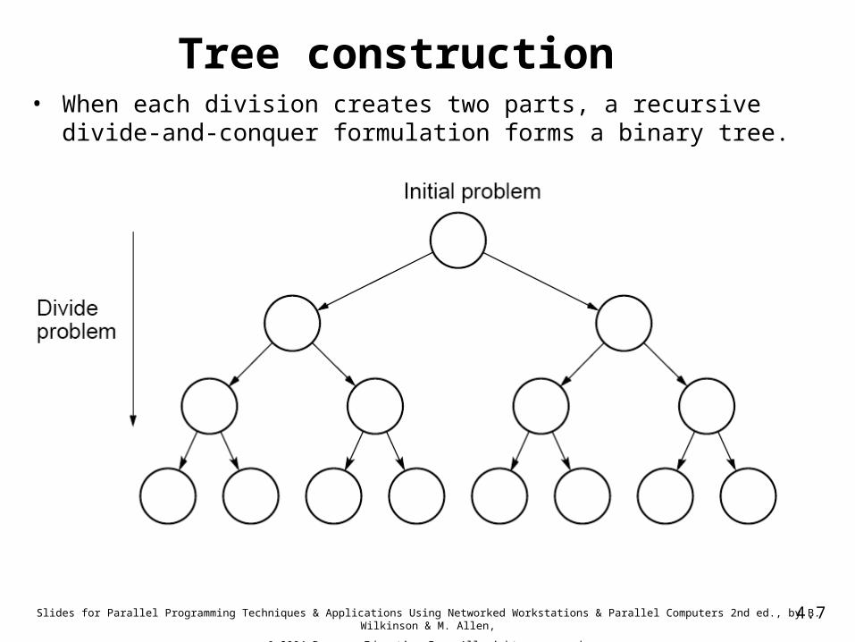
Tree construction• When each division creates two parts, a recursive divide-and-conquer

formulation forms a binary tree.



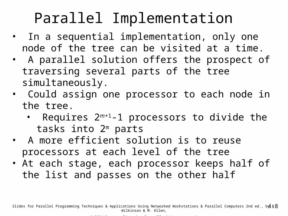
Parallel Implementation• In a sequential implementation, only one node of the tree

can be visited at a time.• A parallel solution offers the prospect of traversing several

parts of the tree simultaneously.• Could assign one processor to each node in the tree.

• Requires 2m+1-1 processors to divide the tasks into 2m parts

• A more efficient solution is to reuse processors at each level of the tree

• At each stage, each processor keeps half of the list and passes on the other half



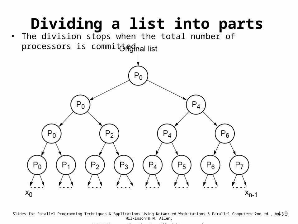
Dividing a list into parts• The division stops when the total number of processors is committed.



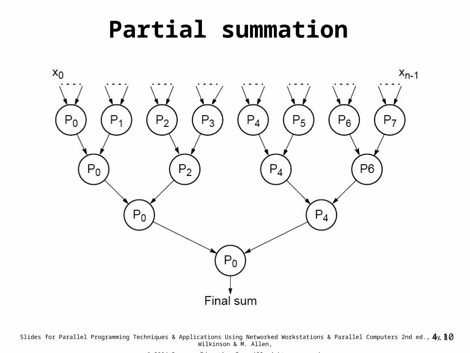
Partial summation



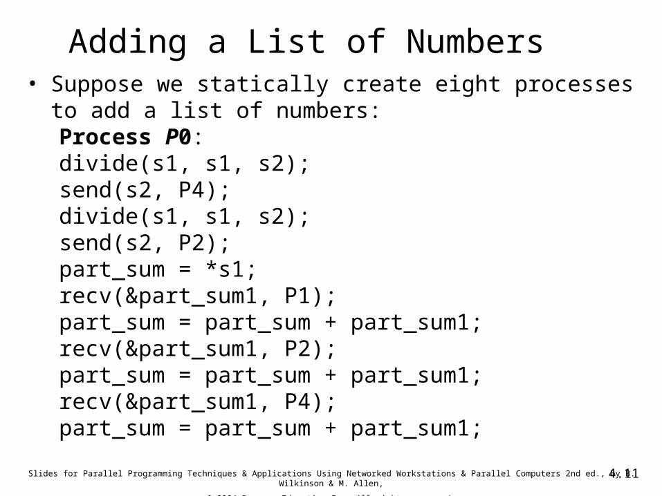
Adding a List of Numbers• Suppose we statically create eight processes to add a list of

numbers:Process P0:divide(s1, s1, s2);send(s2, P4);divide(s1, s1, s2);send(s2, P2);part_sum = *s1;recv(&part_sum1, P1);part_sum = part_sum + part_sum1;recv(&part_sum1, P2);part_sum = part_sum + part_sum1;recv(&part_sum1, P4);part_sum = part_sum + part_sum1;



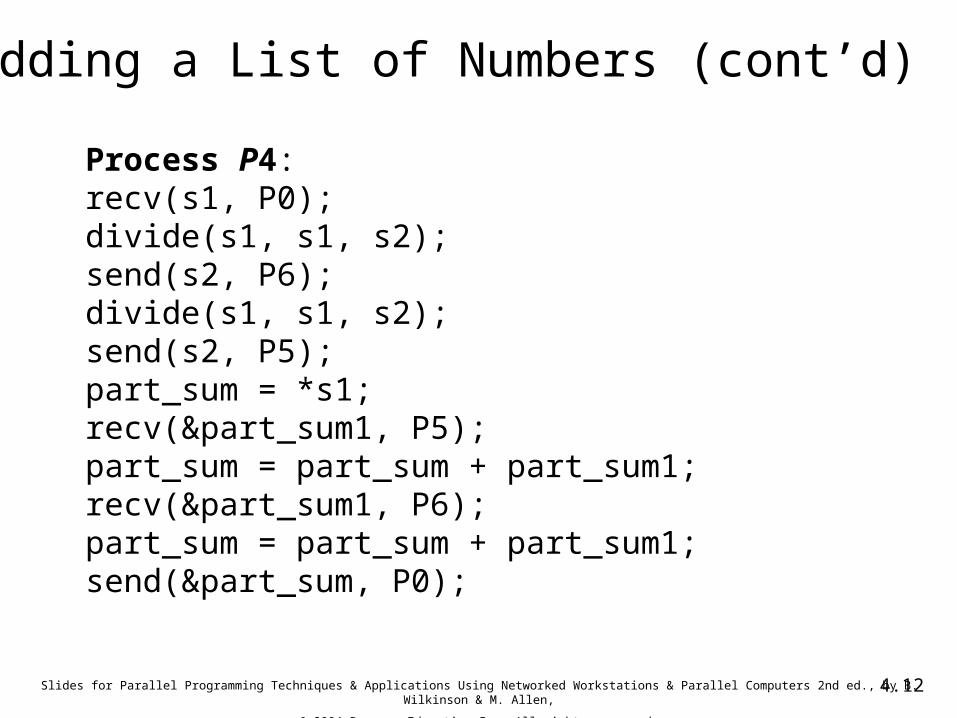
Adding a List of Numbers (cont’d)

Process P4:recv(s1, P0);divide(s1, s1, s2);send(s2, P6);divide(s1, s1, s2);send(s2, P5);part_sum = *s1;recv(&part_sum1, P5);part_sum = part_sum + part_sum1;recv(&part_sum1, P6);part_sum = part_sum + part_sum1;send(&part_sum, P0);



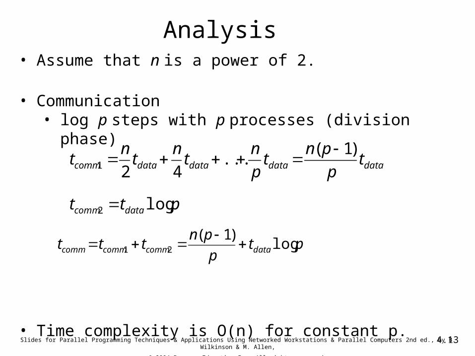
Analysis• Assume that n is a power of 2.

• Communication• log p steps with p processes (division phase)

• Time complexity is O(n) for constant p.

datadatadatadatacomm tp

pntp

ntn

tn

t)1(

...421

ptt datacomm log2

ptp

pnttt datacommcommcomm log

)1(21



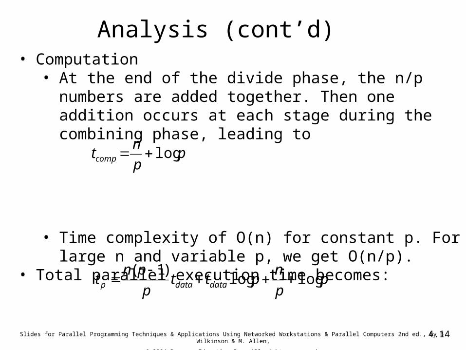
Analysis (cont’d)• Computation

• At the end of the divide phase, the n/p numbers are added together. Then one addition occurs at each stage during the combining phase, leading to

• Time complexity of O(n) for constant p. For large n and variable p, we get O(n/p).

• Total parallel execution time becomes:

pp

ntcomp log

pp

nptt

p

pnt datadatap loglog

)1(



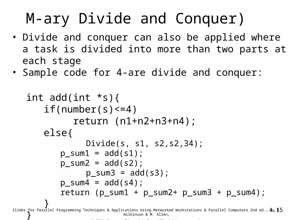
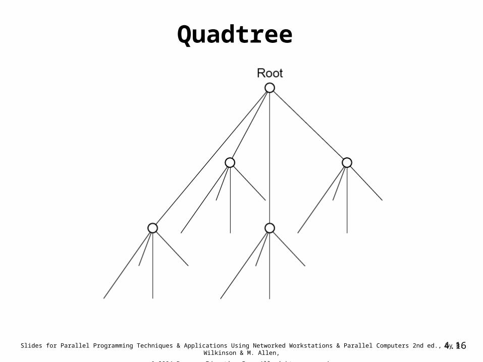
M-ary Divide and Conquer)• Divide and conquer can also be applied where a task is

divided into more than two parts at each stage• Sample code for 4-are divide and conquer:

int add(int *s){ if(number(s)<=4) return (n1+n2+n3+n4); else{ Divide(s, s1, s2,s2,34); p_sum1 = add(s1); p_sum2 = add(s2);

p_sum3 = add(s3); p_sum4 = add(s4); return (p_sum1 + p_sum2+ p_sum3 + p_sum4); }}



Quadtree



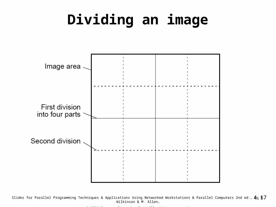
Dividing an image



Example 1: Sorting Using Bucket Sort

• Most sequential sorting algorithms are based on comparing and exchanging pairs of numbers

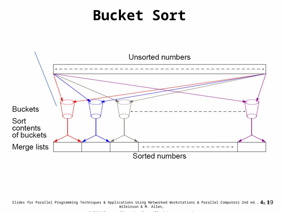
• Bucket sort is not based on compare and exchange, but is naturally a partitioning method

• Works well only if the numbers to be sorted are uniformly distributed across a known interval

• If all the numbers in the interval 0 to a-1– Divide numbers into m regions 0 to a/m-1, a/m to 2a/m-1,…– One “bucket” is assigned to hold numbers that fall a region



Bucket Sort



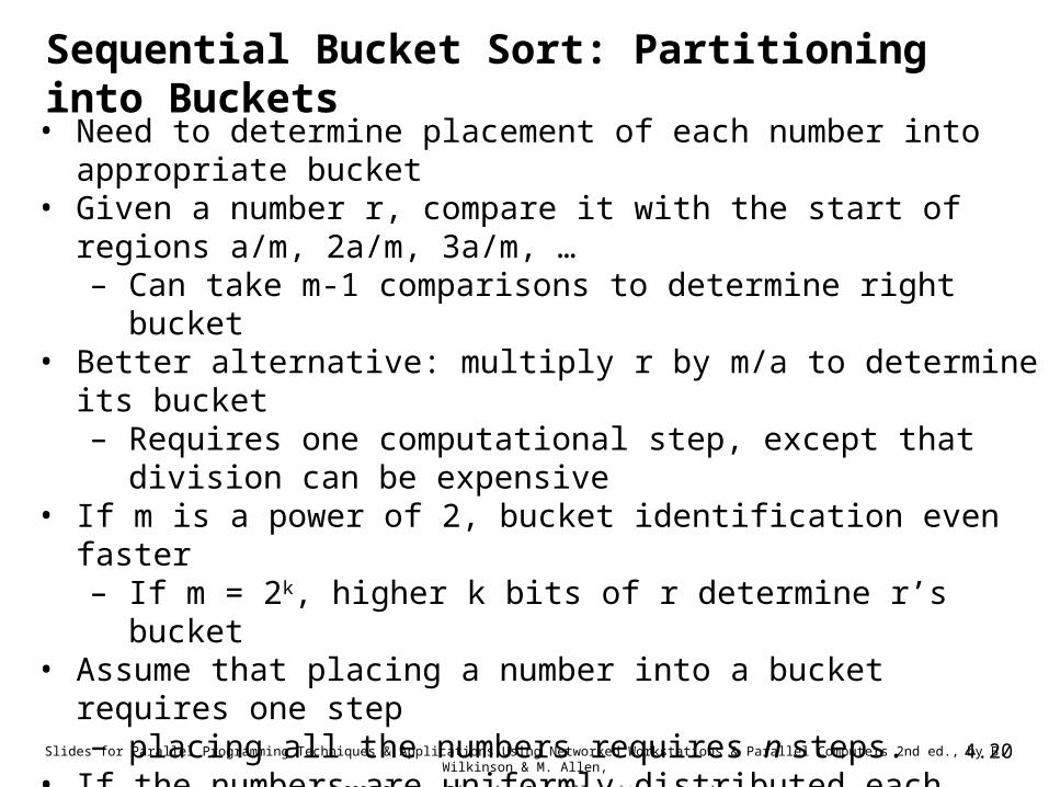
Sequential Bucket Sort: Partitioning into Buckets

• Need to determine placement of each number into appropriate bucket

• Given a number r, compare it with the start of regions a/m, 2a/m, 3a/m, …– Can take m-1 comparisons to determine right bucket

• Better alternative: multiply r by m/a to determine its bucket– Requires one computational step, except that division can be

expensive• If m is a power of 2, bucket identification even faster

– If m = 2k, higher k bits of r determine r’s bucket• Assume that placing a number into a bucket requires one step

– placing all the numbers requires n steps.• If the numbers are uniformly distributed each bucket will contain

n/m numbers



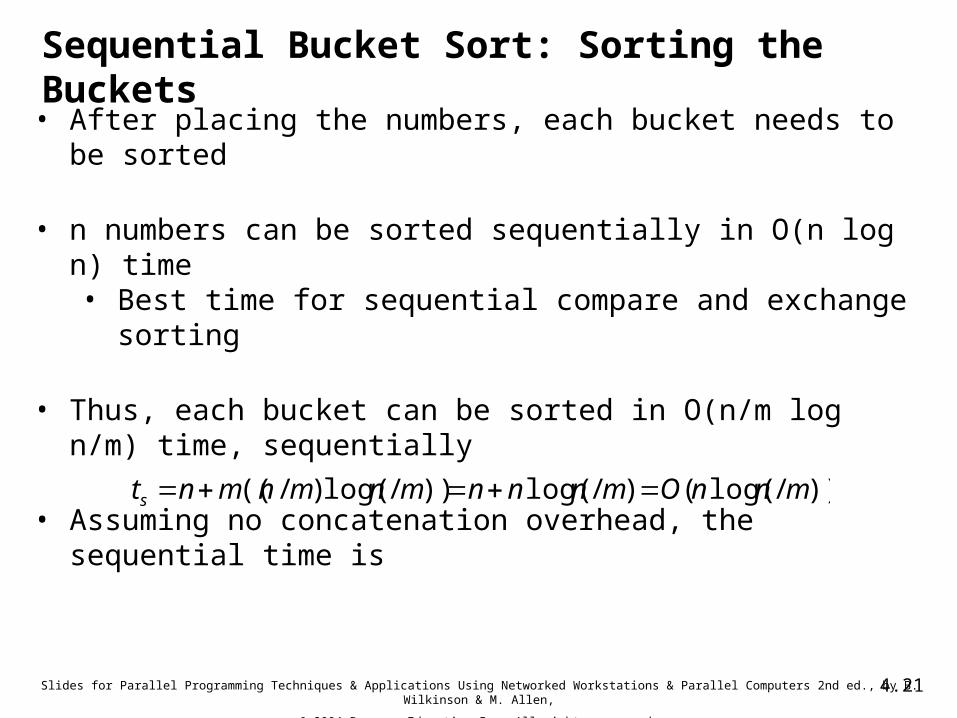
Sequential Bucket Sort: Sorting the Buckets

• After placing the numbers, each bucket needs to be sorted

• n numbers can be sorted sequentially in O(n log n) time• Best time for sequential compare and exchange sorting

• Thus, each bucket can be sorted in O(n/m log n/m) time, sequentially

• Assuming no concatenation overhead, the sequential time is

))/log(()/log())/log()/(( mnnOmnnnmnmnmnts



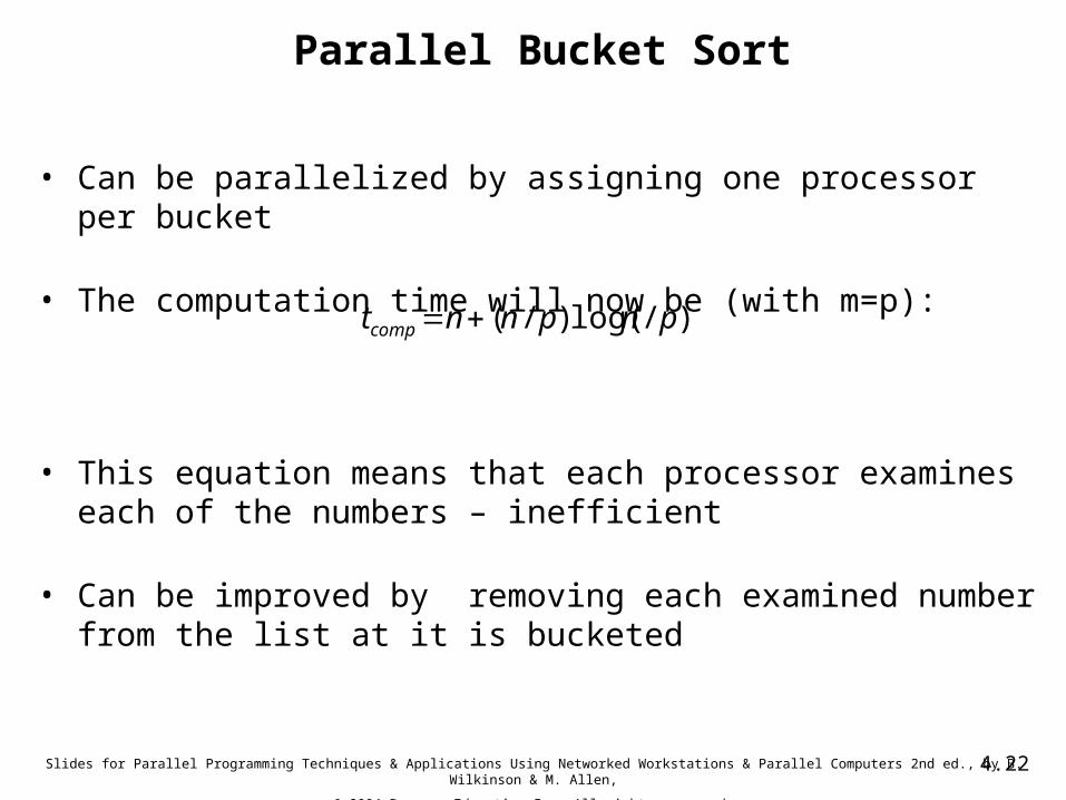
Parallel Bucket Sort

• Can be parallelized by assigning one processor per bucket

• The computation time will now be (with m=p):

• This equation means that each processor examines each of the numbers – inefficient

• Can be improved by removing each examined number from the list at it is bucketed

)/log()/( pnpnntcomp



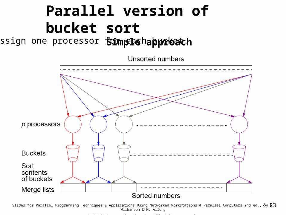
Parallel version of bucket sortSimple approach

Assign one processor for each bucket.



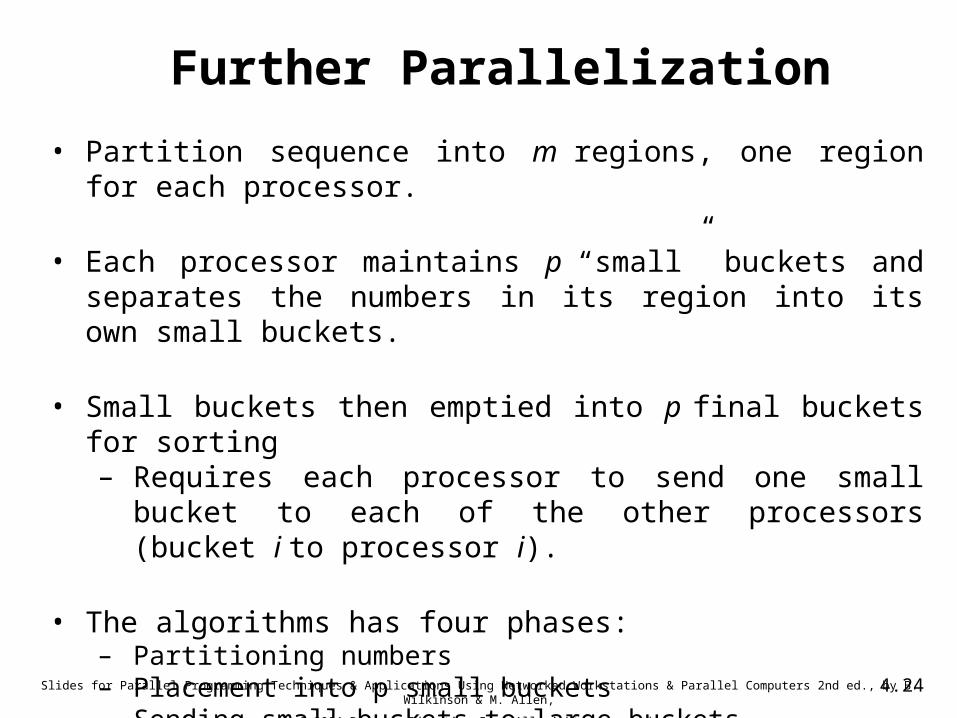
Further Parallelization

• Partition sequence into m regions, one region for each processor.

• Each processor maintains p “small” buckets and separates the numbers in its region into its own small buckets.

• Small buckets then emptied into p final buckets for sorting– Requires each processor to send one small bucket to each

of the other processors (bucket i to processor i).

• The algorithms has four phases:– Partitioning numbers– Placement into p small buckets– Sending small buckets to large buckets– Sorting large buckets



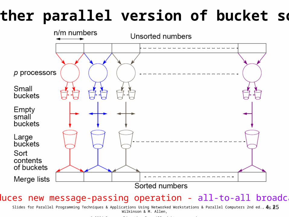
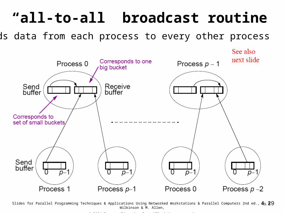
Another parallel version of bucket sort

Introduces new message-passing operation - all-to-all broadcast.



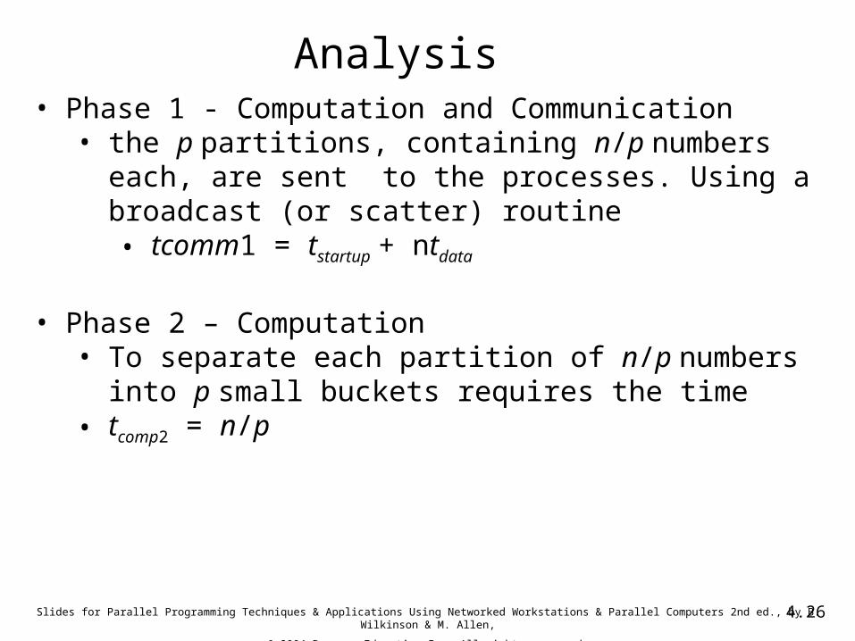
Analysis• Phase 1 - Computation and Communication

• the p partitions, containing n/p numbers each, are sent to the processes. Using a broadcast (or scatter) routine• tcomm1 = tstartup + ntdata

• Phase 2 – Computation• To separate each partition of n/p numbers into p small

buckets requires the time• tcomp2 = n/p



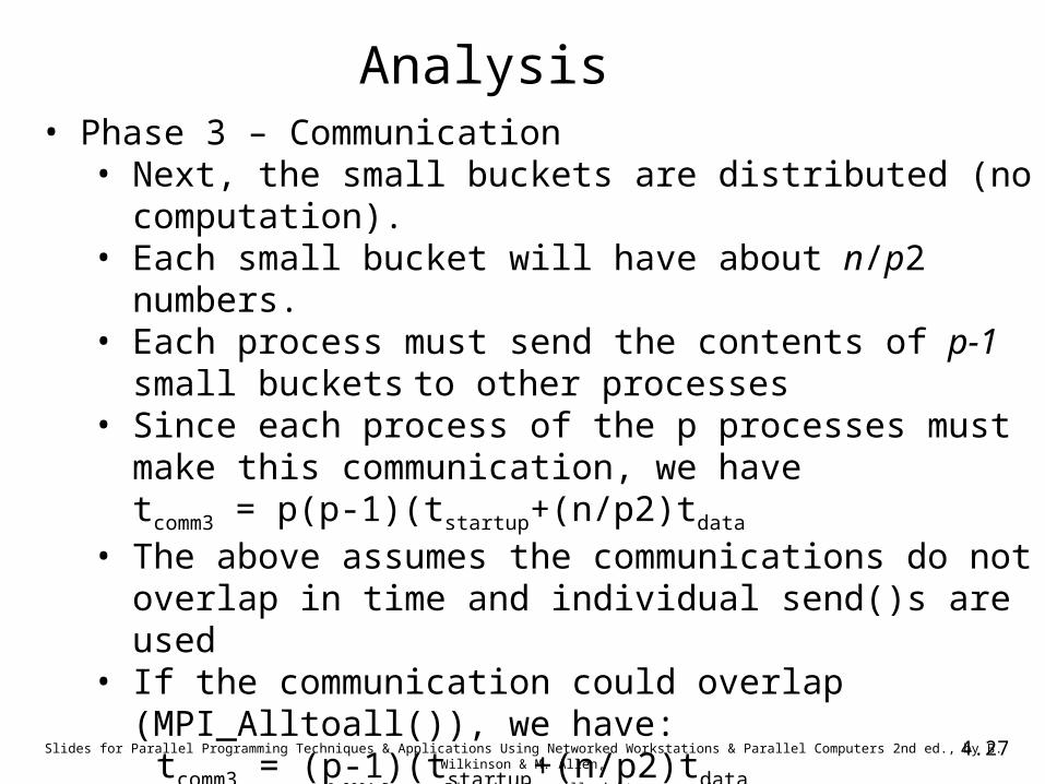
Analysis• Phase 3 – Communication

• Next, the small buckets are distributed (no computation).• Each small bucket will have about n/p2 numbers.• Each process must send the contents of p-1 small

buckets to other processes• Since each process of the p processes must make this

communication, we havetcomm3 = p(p-1)(tstartup+(n/p2)tdata

• The above assumes the communications do not overlap in time and individual send()s are used

• If the communication could overlap (MPI_Alltoall()), we have:

tcomm3 = (p-1)(tstartup+(n/p2)tdata



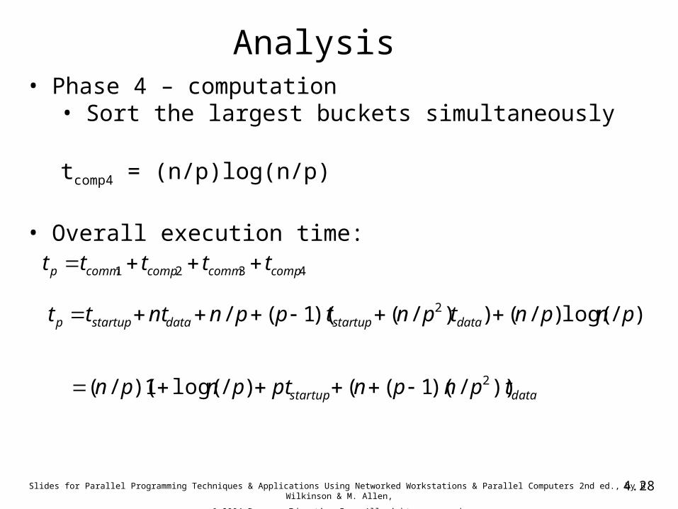
Analysis• Phase 4 – computation

• Sort the largest buckets simultaneously

tcomp4 = (n/p)log(n/p)

• Overall execution time:

4321 compcommcompcommp ttttt

)/log()/())/()(1(/ 2 pnpntpntppnnttt datastartupdatastartupp

datastartup tpnpnptpnpn ))/)(1(()/log(1)(/( 2



“all-to-all” broadcast routineSends data from each process to every other process



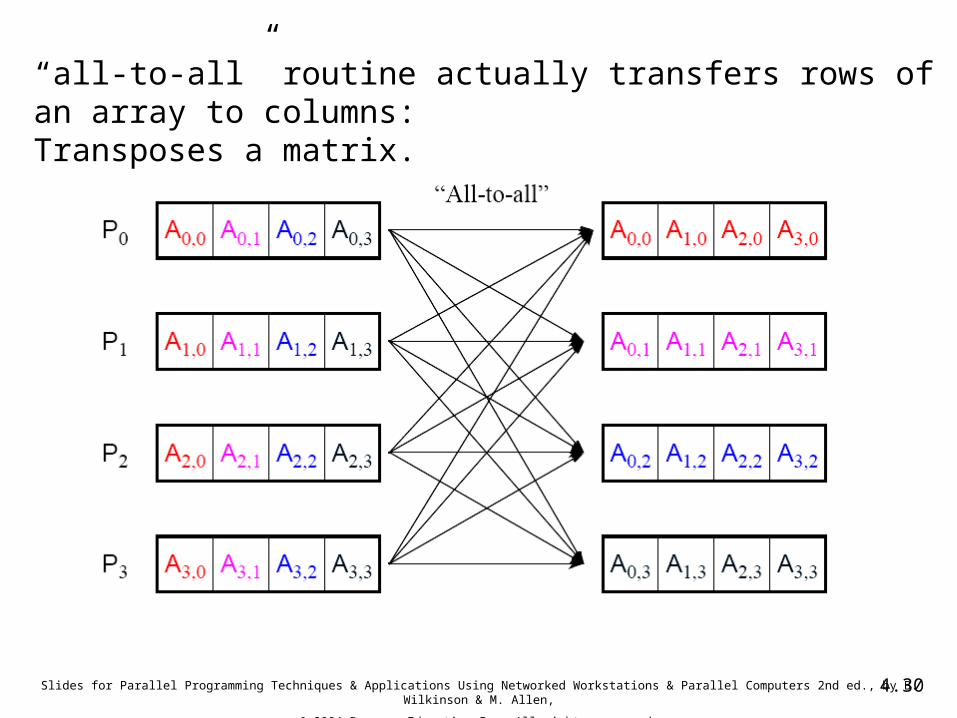
“all-to-all” routine actually transfers rows of an array to columns:Transposes a matrix.



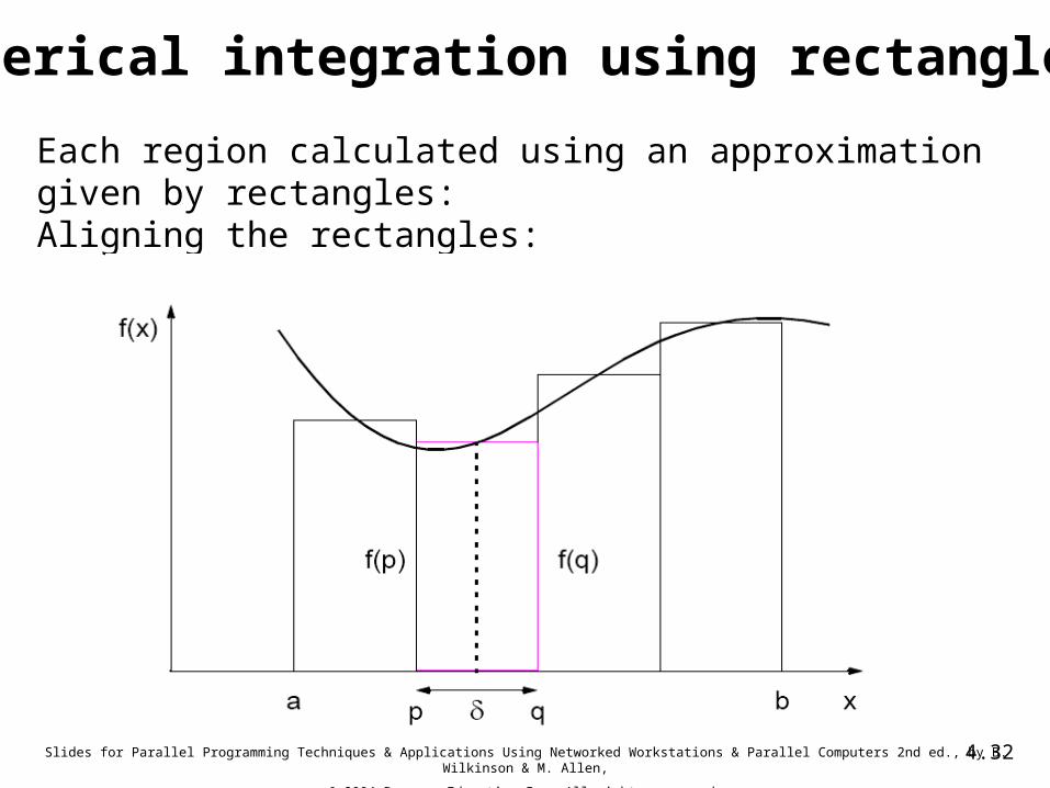
Example 2: Numerical integration

• In many areas of mathematics and science it is necessary to calculate the area bounded by y = f(x), the axis, and the lines x = a, and x = b.

• The area can be calculated using definite integrals• Can be difficult or impossible sometimes

• Typically, approximations methods are used to calculate such area• Trapezoidal rule• Simpson rule• Adaptive quadrature methods

• Area approximated by partitioning the interval [a, b] into n equal pieces and inscribing a rectangle above each sub-interval thus obtained



Numerical integration using rectangles.

Each region calculated using an approximation given by rectangles:Aligning the rectangles:



Trapezoidal Rule:Static Assignment

• One process is assigned statically to compute each region, before the computation begins

• As before an SPMD programming model is used• Each calculation has same form

• With p processors to compute the area between x=a and x=b, each process will handle a region of size• (b-a)/p

• Each process will compute its area in the manner shown by the code overleaf



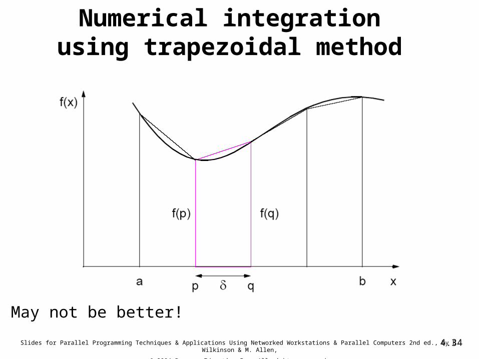
Numerical integration using trapezoidal method

May not be better!



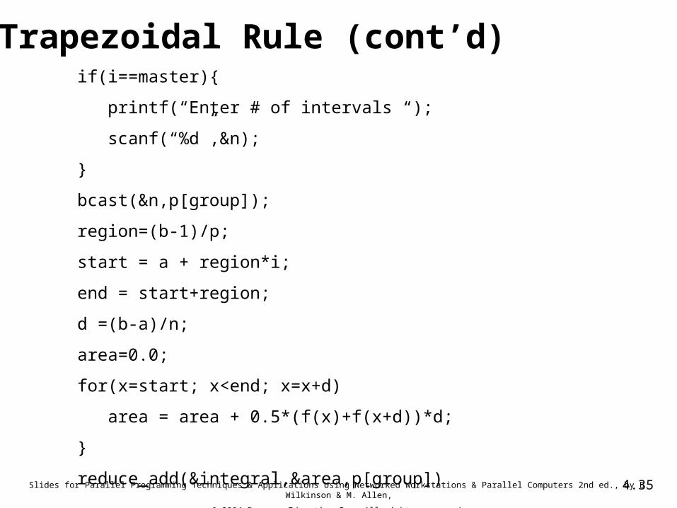
Trapezoidal Rule (cont’d)if(i==master){

printf(“Enter # of intervals “);

scanf(“%d”,&n);

}

bcast(&n,p[group]);

region=(b-1)/p;

start = a + region*i;

end = start+region;

d =(b-a)/n;

area=0.0;

for(x=start; x<end; x=x+d)

area = area + 0.5*(f(x)+f(x+d))*d;

}

reduce_add(&integral,&area,p[group])



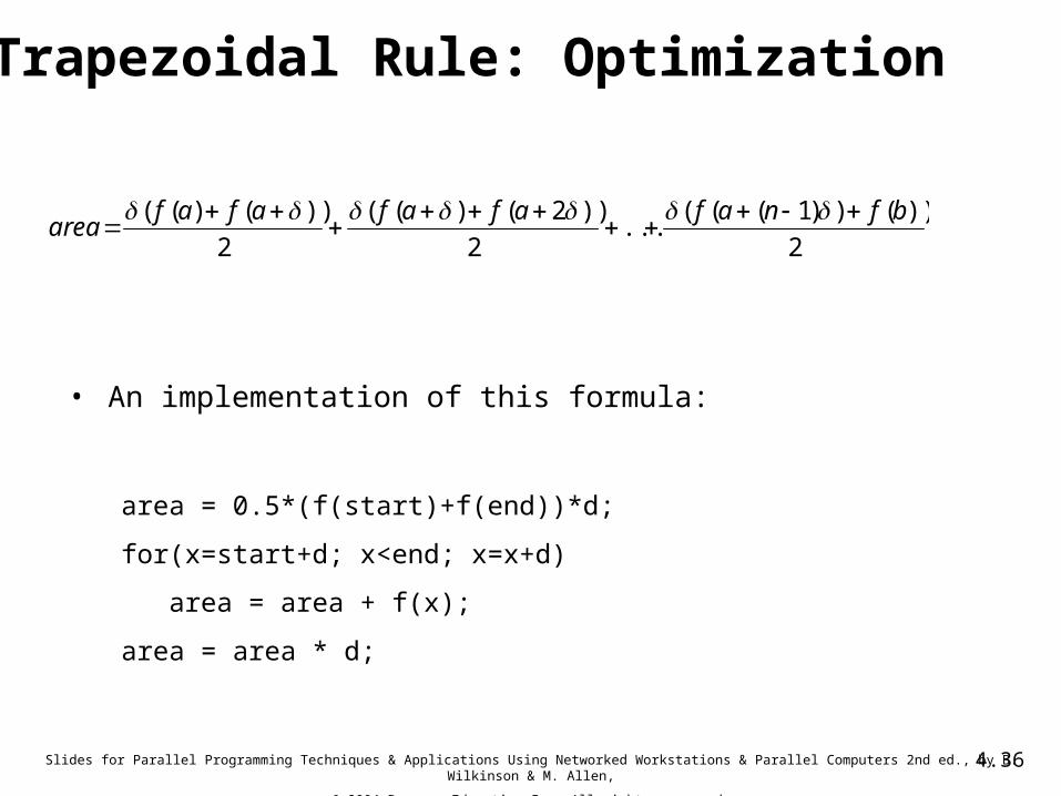
Trapezoidal Rule: Optimization

• An implementation of this formula:

area = 0.5*(f(start)+f(end))*d;

for(x=start+d; x<end; x=x+d)

area = area + f(x);

area = area * d;

2

))())1(((...

2

))2()((

2

))()(( bfnafafafafafarea



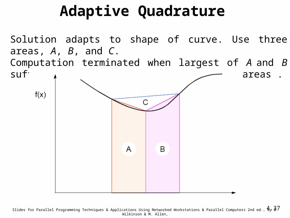
Adaptive Quadrature

Solution adapts to shape of curve. Use three areas, A, B, and C.Computation terminated when largest of A and B sufficiently close to sum of remain two areas .

4.1 Slides for Parallel Programming Techniques & Applications Using Networked Workstations & Parallel Computers 2nd ed., by B. Wilkinson & M. Allen, @

Documents

parallel algorithms

pearson education

fundamental techniques

parts slide

program data

divided data

independent functions

number summation