3623-Seismic anisotropy beneath Ruapehu Volcano

S&G 3623

I. -

REi·

154 G

1 · 3 4 13

1

1Final Report to the Earthquake Commission

on Project No. 01/459

"Can changes in seismic anisotropy be used to predict volcanic eruptions?"

Martha K. Savage and Alexander Gerst

10 October 2003

1

LAYMAN'S ABSTRACT

We tested the interpretation of Miller and Savage (2000) that observed changes in shearwaveforms between events recorded on portable seismographic stations surrounding Mt.Ruapehu in 1994 and 1998 were caused by stress changes due to the 1995-1996 eruption.The simplest interpretation was that stress changed, but because the stations were in

different locations for the two deployments, there remained the possibility that thedifferences could be caused by unusual path variations between the earthquake sources(at 5-100 km depth) and the stations operating in 1994 and 1998.

To test the interpretation, in 2002 we reoccupied six sites that showed apparent variationsin waveforms from 1994 to 1998. Recordings of local earthquakes were used to measurethe fast direction of seismic anisotropy at those stations. Selected events were also

reanalysed from the 1994 and 1998 deployments. We found that the orientation ofcrustal anisotropy changed by 80 degrees in association with the 1995/96 eruption of Mt.Ruapehu volcano, New Zealand. This change occurred with a confidence level of morethan 99.9%, and affects an area with a radius of at least 5 km around the summit. It

provides the basis for a new monitoring technique and possibly for future mid-termeruption forecasting at volcanoes.

TECHNICAL ABSTRACT

To test the theory of Miller and Savage (2001) that seismic anisotropy around Mt.Ruapehu Volcano changed after the 1995/96 phreatomagmatic eruption, for this project

we reoccupied sites in 2002 that had previously been occupied in 1994 and 1998. Usingall three sets of data, the fast anisotropic direction was measured by a semi-automatic

algorithm, using the method of shear wave splitting. Prior to the eruption, a strong trend

for the fast anisotropic direction was found to be around NW-SE, which is approximatelyperpendicular to the regional compressive stress direction. This deployment was followedby a moderate phreatomagmatic eruption in 1995/96, which ejected material with anoverall volume of around 0.02--0.05 km3. Splitting results from a deployment after theeruption (1998) suggested that the fast anisotropic direction for deep earthquakes (>55km) has changed by around 80 degrees, becoming parallel to the regional stress field.Shallow earthquakes (<35 km) also show this behaviour, but with more scatter of the fastdirections. The 2002 deployment covered the exact station locations of both the 1994 and

the 1998 deployments and indicates further changes. Fast directions of deep eventsremain rotated by 80 degrees compared to the pre-eruption direction, whereas arealignment of the shallow events towards the pre-eruption direction is observed.

The interpretation is that, prior to the eruption, a pressurised magma dike systemoverprinted tile regional stress field, generating a local stress field and therefore altering

the fast anisotropic direction via preferred crack alignment. Numerical modellingsuggests that the stress drop during the eruption was sufficient to change the local stressdirection back to the regional trend, which was then observed in the 1998 experiment. Arefilling and pressurising magma dike system is responsible for the newly observedrealignment of the fast directions for the shallow events, but is not yet strong enough torotate the deeper events with their longer delay times and lower frequencies.

These effects provide a new method for volcano monitoring at Mt. Ruapehu and possiblyat other volcanoes. They might, after further work, serve as a tool for eruption forecastingat Mt. Ruapehu or elsewhere. It is therefore proposed that changes in anisotropy aroundother volcanoes be investigated.

Publications relating to this project:

Masters' thesis:

Gerst, A. Temporal changes in seismic anisotropy as a new eruption forecasting tool?,184 pp., Mar. 2003

Abstracts:

Gerst, A. and M. K. Savage, Testing Proposed Changes in Seismic Anisotropy at Mt.Ruapehu Volcano in New Zealand , Eos, Trans. AGU, 83 (22) West. Pac. Geophys.Meet. Suppl., Abstract SE31C-03, 2002.

Savage, M. K., Audoine, E. L., Gerst, A. and Hofmann, S., Seismic anisotropy beneaththe North Island, New Zealand, abstract in: Proceedings of the 10th Internationalsymposium on deep seismic profiling of the contintents and their margins (SEISMIX),Taupo, New Zealand, p. 118, 2003.

Gerst, A. and Savage, M. K.,Temporal changes in seismic anisotropy after an eruption atMt. Ruapehu volcano, New Zealand-a new monitoring technique, abstract given atEGS - AGU - EUG Joint Assembly, Nice, France, Geophysical Research Abstracts,Volume 5, abstract number EAE03-A-04782,2003.

Gerst, A. and Savage, M., Seismic anisotropy as an eruption forecasting tool?, presentedat the Cities on Volcanoes Workshop 3 held in Hilo, Hawaii on 14-18 July, 2003.

Other presentations:

Gerst, A., Changes in seismic anisotropy-a new monitoring technique? Given at theRoyal Society New Zealand student prize night, 3 October, 2002. Mr. Gerst shared theBeanland-Thornley prize for the best presentation of the evening.

TEMPORAL CHANGES IN SEISMIC

ANISOTROPY AS A NEW ERUPTION

FORECASTING TOOL?

by

Alexander Gerst

A thesis submitted to Victoria University of Wellingtonfor the degree of

Master of Science

in Geophysics

Institute of Geophysics, School of Earth SciencesVictoria University of Wellington

Te Whare Wananga o te Upoko o te Ila a MguiWellington, New Zealand

March 2003

1 ii

1

1

1

1

1

1

1

1

1

1

1

1

1

FRONTISPIECE

..

V

NOTHING IN LIFE IS TO BE FEARED.IT IS ONLY TO BE UNDERSTOOD.

Marie Curie

iii

1

iV

1

1

1

1

1

1

1

1

1

1

1

1

ABSTRACT

The orientation of crustal anisotropy changed by -80 degrees in association with the 1995/96

eruption of Mt. Ruapehu volcano, New Zealand. This change occurred with a confidence level

of more than 99.9%, and affects an area with a radius of at least 5 km around the summit. It

provides the basis for a new monitoring technique and possibly for future mid-term eruption

forecasting at volcanoes.

Three deployments of seismometers were conducted on Mt. Ruapehu in 1994, 1998 and

2002. The fast anisotropic direction was measured by a semi-automatic algorithm, using the

method of shear wave splitting. Prior to the eruption, a strong trend for the fast anisotropic

direction was found to be around NW-SE, which is approximately perpendicular to the re-

gional main stress direction. This deployment was followed by a moderate phreatomagmatic

eruption in 1995/96, which ejected material with an overall volume of around 0.02-0.05

km3. Splitting results from a deployment after the eruption (1998) suggested that the fast

anisotropic direction for deep earthquakes (>55 km) has changed by around 80 degrees, be-

coming parallel to the regional stress field. Shallow earthquakes (<35 km) also show this

behaviour, but with more scatter of the fast directions. Another deployment (2002) covered

the exact station locations of both the 1994 and the 1998 deployments and indicates fur-

ther changes. Fast directions of deep events remain rotated by 80 degrees compared to the

pre-eruption direction, whereas a realignment of the shallow events towards the pre-eruption

direction is observed.

The interpretation is that prior to the eruption, a pressurised magma dike system over-

printed the regional stress field, generating a local stress field and therefore altering the fast

anisotropic direction via preferred crack alignment. Numerical modelling suggests that the

stress drop during the eruption was sufficient to change the local stress direction back to the

regional trend, which was then observed in the 1998 experiment. A refilling and pressurising

magma dike system is responsible for the newly observed realignment of the fast directions

for the shallow events, but is not yet strong enough to rotate the deeper events with their

longer delay times and lower frequencies. These effects provide a new method for volcano

monitoring at Mt. Ruapehu and possibly at other volcanoes on Earth. They might, after

further work, serve as a tool for eruption forecasting at Mt. Ruapehu or elsewhere. It is

therefore proposed that changes in anisotropy around other volcanoes be investigated.

V

1 Vi

1

1

1

1

1

1

1

1

1

1

ACKNOWLEDGEMENTS

This thesis is not only the result of a year of field work, data processing, reading and writing,

but it is also the result of the knowledge and the help of others. It is entirely impossible

to name all the people that contributed to the success of this study, yet I will attempt to

mention the most important ones.

First of all I thank my parents, Hans-Dieter and Brigitte Gerst, for the support I have

always got from them, without any form of doubt or question.

I thank my advisors Martha Savage and Friedemann Wenzel for all their support, useful

advice and ideas. Thanks also to Martha for always having an open door for me and for the

help with the field work. Thanks to John Gamble for teaching me everything about volcanoes

and about never forgetting the fun side of things. Thanks to Ralph Wahrlich, for helping me

with uncountable computer problems and for always staying nice and friendly in the heat of

things. Thanks to Tim Stern for all the scientific advice and the awesome snowboard ride

from the top of Mt. Ruapehu.

My field work was made possible by the invaluable help of Sonja Hofmann, Mike Hagerty,

Martha Savage, Dennis Gerst, Frederik Gerst, Mathieu Duclos, Frederique Jeandron, Tony

Hurst and Geoff Kilgour. I can not thank you enough for voluntarily helping me to carry truck

batteries up and down Mt. Ruapehu, and to still keep smiling. The field work was logistically

supported by Harry Keys and the Department of Conservation (DOC) with friendly support

and permissions to access the national park.

Thanks to Ken Gledhill, Mike Hagerty, Euan Smith, Kevin Furlong, Tony Hurst, John

Townend and John Gamble for the help and many useful discussions. Thanks also to

Matthew D. Hall, Andrew Orme, John Townend, Stephanie Simmonds, Kevin Furlong,

Michelle Salmon and Tim Stern for reviewing my manuscripts.

Thanks to Matthew D. Hall and Andrew Orme for being very good friends and flatmates,

and for the introduction into the Kiwi lifestyle. Thanks also to John & Sue Hall for an

incredibly warm welcome and an unforgettable Kiwi Christmas.

Thanks to Iain & Glenna Matcham for bringing me to New Zealand, for a Scottish wed-

ding, and for making me wear a kilt. Thanks to Andy, Anna, Audrey, Brett, Etienne, Katie,

Kevin, Kitty, Kunal, Marda, Mark, Martin, Mathieu, Matt, Michelle, Ralph, Sandra, Sonja,

Vii

Viii ACKNOWLEDGEMENTS

Stefan, Susanne, Vicky and Wanda for great BBQs, climbing evenings, snowboarding trips,

drinks, pavlovas, pool games and parties.

Thanks to Jiirgen Neuberg, Graham Stuart and David Frances from Leeds University for

collecting and providing the 1994 and 1998 data, together with Tony Hurst (IGNS), Peter

MeGinty, and Bernice Hicks (VUW). Thanks to Vicky Miller for important help with her

data. Thanks to the Heads of School, Euan Smith and Phil Morisson for administrative help,

to the librarian Jill Ruthven, to the owners of Lahar Farm for the permission to access their

land, and to IGNS for letting their volcano observatory become my second home. Thanks to

Dee, Marie, Marita and Morna for being helpful and always friendly school administrators.

Thanks to all my friends at home in Germany for keeping in touch over one and a half

years. A special thanks to Gabi for never giving up calling me.

Thanks to Brett, Stefan and Mark for numerous jumps out of perfectly good aeroplanes,

and to my parachute for keeping me alive in every respect. Thanks to Andy Nybla(le and

Doug Wiens for taking me down to Antarctica, and to Kevin Furlong for setting my trip in

motion.

Thanks to Karen Williams, W.H. Freeman publishers, Etienne Audoine, Vicky Miller and

John Gamble for the friendly permissions to print some of their figures or photos. Thanks to

Shinji Toda for the useful help with his Coulomb software

Thank you all very much, I couldn't have done it without you!

A special thanks goes to Sonja Hofmann for an infinite amount of smiles and patience. And

yet there is no way of thanking enough for not even hesitating a second to climb Mt. Ruapehu

with me in a winter blizzard at -10°C, only to dig out a data disk under one metre of solid

ice.

This study was funded by the New Zealand Earthquake Commission (EQC) and by a

scholarship of the German Academic Exchange Service (DAAD). The majority of maps in

this thesis were produced using the free Generic Mapping Tools (GMT; Wessel and Smith,

2001). The seismic processing was done using the Seismic Analysis Code (SAC 2000; Tapley

et al., 1990). Figures describing the data dependencies were mainly generated with the

MATLAB software, and numeric models were calculated with the Coulomb program. The

typesetting of this thesis was done with I#Iy, which proved to be an outstandingly helpful

software for this purpose, and is freely available.

The photograph in the Frontispiece was printed with the friendly permission of John

Gamble, and shows the initial explosion of the 1996 eruption.

CONTENTS

Frontispiece iii

Abstract v

Acknowledgements Vii

Table Of Contents ix

List Of Figures Xiii

List Of Tables xvi

Chapters

1 Introduction 1

1.1 Motivation of this work

1.1.1 Why the 2002 deployment is critically important for this study .... 2

1.1.2 The need for eruption forecasting tools.................. 4

1.2 Regional tectonic settings ............................. 5

1.2.1 The Central Volcanic Region and the Taupo Volcanic Zone ...... 7

1.3 The local tectonic setting of Mt. Ruapehu volcano ...............10

1.3.1 Eruption style and volcanic hazards at Mt. Ruapehu .......... 12

1.3.2 The 1995 / 1996 eruption sequence .................... 13

1.3.3 Velocity model............. ..................14

2 Seismic anisotropy 17

2.1 Theoretical background ..............................17

2.1.1 Hexagonal anisotropy ...........................20

2.1.2 Systems of anisotropy with a lower order of symmetry ......... 23

2.1.3 The cause of mantle anisotropy ...................... 24

2.1.4 Effect on the waveforms ..........................26

2.1.5 Delay times and percent anisotropy....... ............26

1X

x CONTENTS

2.1.6 Multiple layers of anisotropy ....................... 27

2.1.7 The shear wave window .......................... 28

2.2 Observations ....................................29

2.2.1 Seismic anisotropy in the vicinity of volcanoes .............. 29

2.2.2 Discoveries of temporal changes in seismic anisotropy ......... 32

3 Method 35

3.1 Data processing ................................... 35

3.2 How to measure shear wave splitting .......................36

3.2.1 Reprocessing of 1994 and 1998 data ................... 37

3.2.2 The Silver & Chan algorithm ....................... 38

423.2.3 NULL measurements............................

3.2.4 Cycle Skipping ............................... 44

3.3 The slope corrected shear wave angle ....................... 49

3.4 Mean value and error analysis ...........................52

3.4.1 Obtaining the mean value of splitting measurements .......... 52

3.4.2 Why angles have to be doubled ......................53

3.4.3 Calculating standard deviation and errors : The Von Mises Statistics . 53

3.4.4 The difference between standard deviation and standard error ..... 57

4 Data acquisition 59

4.1 The CHARM experiment....... ......................59

4.1.1 Setup ....................................60

4.1.2 Relation to previous deployments... ..................61

4.1.3 Equipment ............... ..................63

4.1.4 Logistics ...................................63

4.2 Information about previous deployments at Mt. Ruapehu ........... 64

4.2.1 The 1994 deployment....... ....................64

4.2.2 The 1998 deployment... ........................65

5 Results 69

5.1 General results of the deployments . .......................69

5.2 Raypaths and source locations ..........................84

5.3 Examination for dependencies on different parameters ............. 92

CONTENTS xi

6 Discussion 101

6.1 Authenticity of the changes in anisotropy .................... 101

6.2 The source region of the anisotropy ........................ 103

6.3 The model ...................................... 105

6.3.1 How can a dike change the fast direction? ................ 108

6.3.2 Further observations that agree with this model. ............ 112

6.3.3 Observations that require further refinement of the model. ....... 115

6.3.4 Numerical modelling ............................ 117

6.3.5 Could the fast direction have changed by exactly 90° ?......... 121

6.4 Alternative models ................................. 123

6.5 Seismicity associated with the changes in anisotropy .............. 125

7 Summary & conclusions 129

7.1 Implications ..................................... 132

7.2 Answered questions ................................. 132

7.3 Testable predictions ................................ 133

7.4 The suitability of FWVZ as a long term monitoring station .......... 134

7.5 Unanswered questions and future recommendations ............... 135

Appendices

A Mathematical appendix 137

A. 1 Calculating the Christoffel matrix for the isotropic case . . . . . . . . . . . . 137

B Data properties 139

B.1 Splitting results without multiple frequency filters ............... 139

B.2 Instrument recording times......... ................... 142

B.3 Data quality control ................................ 143

B.3.1 Check for rotated components ....................... 143

B.3.2 Sun compass test for correct orientation ................. 144

C List of all measurements 145

D Data processing software 165

D.1 Description of routines used ............................ 165

D.2 List of newly developed programs for future users ................ 168

D.2.1 UNIX shell, NAWK and C++ programs ................. 168

D.2.2 SAC macros.................... ........... . . 169

1

xii CONTENTS

References and indices

References 170

1Index 183

1

1

1

1

1

l

1

1

1

1

1

1

1

1

1

1

1

FIGURES

1.1 The Ring Of Fire: An overview over continental plate margins ........ 5

1.2 Bathymetric image of New Zealand ........................ 6

1.3 Sketch of a cross cut through the CVR ...................... 7

1.4 Map of the CVR and the TVZ .......................... 8

1.5 Photograph of Mt. Ruapehu ... .........................10

1.6 Map of New Zealand volcanoes ..........................10

1.7 Lava formations and vents in the Tongariro Volcanic Centre .......... 11

1.8 A cross cut through the North Island of New Zealand ............. 12

1.9 The 1996 eruption from the town of Ohakune .................. 13

1.10 Map of five year seismicity around New Zealand ................ 15

2.1 Illustration of possible wave polarisations .................... 20 -

2.2 Illustration of shear wave splitting ........................ 22 -

2.3 Shear wave splitting in the presence of two layers of anisotropy........ 28 -

3.1 Data processing flow chart....... ...................... 35 -

3.2 How to un-split an S-wave .... .........................39

3.3 The NULL phenomenon .............................. 43 -

3.4 Example for an A-quality measurement ..................... 45 -

3.5 Example for an A-quality measurement ..................... 46 -

3.6 Example for an AB-quality measurement..... ............... 46 -

3.7 Example for a B-quality measurement ...................... 47

3.8 Example for a C-quality measurement...................... 47

3.9 Example for a NULL measurement ........................ 48

3.10 Example for cycle skipping........ .................... 48 -

3.11 The slope corrected shear wave window..................... 49

3.12 Incidence angle on a slope... .......................... 49 -

3.13 Geometry of incoming rays at a slope ...................... 50 -

3.14 Effect of doubling the angles ............................ 53 -

3.15 Validity of the Von Mises Distribution ...................... 54

X111

FIGURES

4.1 Digital elevation model of Mt. Ruapehu with the CHARM stations ...... 59

4.2 Field picture of LTUR2 station.... ......................62

4.3 Map with station locations ............................ 66

4.4 3D perspective view of all available earthquake sources ............. 67

5.1 Overview of the splitting results: Combined results as histograms ....... 74

5.2 Map of individual splitting results, 1994 .....................75

5.3 Map of individual splitting results, 1998 .....................77

5.4 Map of individual splitting results, CHARM 2002 ................79

5.5 Overview of the splitting results: Individual station histograms ........ 80

5.6 Shallow events from 1998 and 2002 with special data selection criteria .... 81

5.7 Map of NULL measurements, 1998 ........................82

5.8 Map of NULL measurements, CHARM 2002 ...................83

5.9 Raypaths of the 1994 and 1998 measurements .................. 85

5.10 Raypaths of the 2002 measurements .......................86

5.11 Vertical cross section of the 1994 results .....................87

5.12 3D perspective view of the 2002 measurements .................88

5.13 Vertical cross section of the 1998 results... ..................89

5.14 3D perspective view of the used earthquakes ................... 90

5.15 Vertical cross section of the 2002 results...... ...............91

5.16 Fast directions vs. depth.... ..........................93

5.17 Frequency vs. depth ................................94

5.18 Delay time vs. frequency . . ............................95

5.19 Delay time vs. period .............. .................96

5.20 Delay time vs. depth ................................97

5.21 Fast direction vs. frequency ............................98

5.22 Delay time vs. hypocentral distance .99

5.23 Fast direction vs. back azimuth.......... ................ 100

5.24 Delay time vs. time (2002) ............................ 100

5.25 Delay time vs. time (1994) ............. ............... 100

6.1 Illustration of dikes and sills in a volcanic system . ............... 106

6.2 Anisotropy model for 1994, 1998 and 2002 .................... 107

6.3 Model of crustal crack orientation before and after the 1995/96 eruption ... 108

6.4 Initial polarisations of 2002 events ........................ 114

6.5 Stress changes caused by an opening dike .................... 118

6.6 Grid displacement of the numeric dike model .................. 119

6.7 Shallow seismicity rate (ML 5 0) at Mt. Ruapehu between 1988 and 2002 . . 127

1

FIGURES xv

6.8 Seismicity rate (ML 22)at Mt. Ruapehu between 1988 and 2002 ...... 127

1

1

B.1 Splitting measurements with only one measurement per event ......... 140

B.2 Individual station histograms with only one measurement per event ...... 141

B.3 Recording times of the CHARM instruments .................. 142

B.4 Estimating back azimuth from first motion ................... 143

D.1 Data processing flow chart... ..................... ..... 165

1

1

l

1

1

1

I

1

1

1

1

xvi

1

1

1

1

1

1

1

1

1

TABLES

3.1 Earthquake selection criteria ........................... 36

3.2 Numbers of available and selected events ..................... 37

3.3 Quality mark definitions .............................. 38

3.4 Slope angles for recording stations......... ...............51

4.1 Station locations and equipment of the CHARM project ............ 60

4.2 Station locations and equipment of the 1994 deployment ............ 65

4.3 Station locations and equipment of the 1998 deployment ............ 65

5.1 Results of individual stations and deployments ................. 71

5.2 Special results of the 1998 and 2002 shallow data ................ 73

B.1 Sun compass test for rotated components .................... 144

C.1 List of individual measurements, 1994 deployment ................ 146

C.2 List of individual measurements, 1998 deployment ................ 149

C.3 List of individual measurements, 2002 deployment ................ 153

D.1 Earthquake selection criteria....... ................. . . . 166

xvii

xviii TABLES

1

1

1

1

1

1

1

1

1

1

1

CHAPTER 1

INTRODUCTION

This chapter will give an overview of the motivation for this project and its objectives. It will

illustrate previous work in this field and show the relation of this work to volcanic hazard

assessment on Mt. Ruapehu and other volcanoes in the world. An introduction to the regional

tectonic setting of New Zealand and the local setting of Mt. Ruapehu volcano will also be

given.

1.1 Motivation of this work

The aim of this study is to investigate possible changes in seismic velocities and stress in the

earth's crust, which might be associated with an eruption sequence at Mt. Ruapehu volcano,

New Zealand. Such changes - if they are recurring - might serve as an indicator for imminent

eruptions at the mountain and therefore as an eruption forecasting tool.

It is known that volcanic eruptions are almost always preceded by magma movements in

the feeder system of the volcano. Such movements involve high pressures and great masses,

and are therefore likely to influence the stress state of the crust in the immediate vicinity of

the volcano. This stress state is the main subject of this investigation. Geophysical methods

are used for this task, of which the most important one is the method of shear wave splitting.

Shear wave splitting occurs in the earth, and is the acoustical analogue to the optical

phenomenon of birefringence. This means that a shear wave travelling in an anisotropic

medium (like the crust) will split into a fast and a slow S-wave, with these waves polarised

perpendicular to each other. The polarisation direction of the first shear wave* is measured

at the surface, and can be used as a tool to obtain information about the in-situ state of

stress in the earth's crust by measuring its velocity anisotropy.

The first indications for a temporal change in setsmic velocity anisotropyt were observed

by Miller and Savage (2001), when analysing shear wave splitting data from two seismometer

* from this point on called the fast directiontfrom this point on referred to as anisotropy

1

2 INTRODUCTION

deployments at Mt. Ruapehu, the first carried out in 1994 and the second in 1998. Temporal

changes were suggested as the most likely, but not the unique explanation for observed

phenomena, and concerns about effects from heterogeneities, frequency, and back azimuth

dependencies could not be rejected (See Section 1.1.1). The lack of compelling evidence

directly lead to this project, which was designed to clarify the matter and to critically assess

the results from the two deployments. In order to do so, a third seismometer deployment was

carried out in 2002, covering station locations from both previous deployments. The results

of the project and a comprehensive interpretation of all three deployments will be presented

in this thesis, together with an overview of the theories and techniques that were applied.

The main objectives of this study can be expressed in the form of the following six

questions:

1. Did the direction of seismic anisotropy change between 1994 and 1998?

2. Where did this change in anisotropy occur?

3. Can it be associated with a volcanic eruption at Mt. Ruapehu?

4. Will such a change happen again?

5. What are the processes that lead to such a change?

6. Will this behaviour lead to a usable method for forecasting volcanic eruptions?

7. What should be done in the future - both at Mt Ruapehu and on other volcanoes on

Earth?

This thesis will attempt to provide a satisfying answer to each one of these questions.

1.1.1 Why the 2002 deployment is critically important for this study

When comparing the data from the 1994 and the 1998 deployments, the most striking feature

is a systematic difference in the average polarisation of the fast S-waves (Miller and Savage,

2001), indicating differences in the anisotropic medium. Since the two deployments covered

approximately the same regions (within 10 km of Mt. Ruapehu), and since a major volcanic

eruption occurred between the two deployments, a temporal change of anisotropy seems to

be a valid explanation for the differences. However, there are several scenarios that could

account for a systematic difference in the observed fast directions without the necessity for

assuming a temporal change.

• Station locations from the two deployments in 1994 and 1998 were different by a mini-

mum of 1 km, and a maximum of >10 km. Furthermore, the 1998 deployment consisted

MOTIVATION OF THIS WORK 3

of only three stations. With the given frequencies of around 1-3 Hz, and surface S-wave

speeds of around 1.3 km/s, it must be assumed that the stations all sample different re-

gions of the shallow crust (i.e. the raypaths, and the affected zones around the raypaths

do not overlap). Therefore, lateral heterogeneities in the anisotropic medium (as can

be expected in the vicinity of complex structures such as volcanoes) can lead to system-

atic differences in the measured fast directions between the stations and thus also to

apparent differences between the two deployments. This effect is observed in a number

of studies, where stations as close together as 200 m yielded average fast directions as

different as 45° without a temporal change (e.g. Munson and Thurber, 1993; Munson

et al., 1995; Savage et al., 1989; Gledhill, 1991b; Booth et al., 1985; Chen, 1987). This

is a major concern that has to be proven wrong before a temporal change in anisotropy

can be assumed.

• The frequency filters that were used for filtering the seismic traces before the measure-

ment was obtained showed systematic differences between the two deployments. This

was the result of different noise properties of the two datasets, which caused different

filters to yield different signal to noise ratios (i.e. the 1994 events were mainly filtered

with 1-7 Hz, whereas the 1998 events were mainly filtered with 1-3 Hz). Since there

are reported cases of frequency dependent anisotropy (e.g. Marson-Pidgeon and Savage,

1997; Audoine, 2002), choosing systematically different frequency filters can lead to sys-

tematically different fast directions. To address this problem, Miller (2000) attempted

to re-filter the 1994 events with the same filter as the 1998 events, but scattering of the

now very noisy measurements, and an insufficient number of measurements led to an

ambiguous result. Therefore the question about the effects of frequency filtering has to

be investigated.

• Effects of back azimuth dependence, and dependence on the initial polarisation of the

S-wave have not been investigated. Babuska and Cara (1991), Silver and Savage (1994),

and Saltzer et al. (2000) show that in the case of an inclined system of anisotropy, or

in the presence of more than one layers of anisotropy, a complex dependency of the

fast direction on the back azimuth or the initial polarisation emerges. These systematic

variations of the fast direction can lead to an apparent change in anisotropy if systematic

differences in the back azimuth or in the initial polarisations existed during the two

deployments.

These examples show that from the data obtained in 1994 and 1998, the question of whether

the anisotropy has changed can not be answered conclusively. Yet the answer to this question

is critical for assessing the value of the method in regard to forecasting future eruptions

at Mt. Ruapehu. In order to do so, a third deployment was planned to investigate all

mentioned effects in combination with the data from 1994 and 1998. This thesis will describe

4 INTRODUCTION

the implementation and the results of a third deployment, and will attempt to provide a

comprehensive interpretation of all data that were obtained in 1994, 1998, and 2002.

1.1.2 The need for eruption forecasting tools

Mt. Ruapehu is a potentially dangerous volcano on the North Island of New Zealand. Erup-

tions at Mt. Ruapehu have led to the loss of life in the past, and every year thousands of

skiers and snowboarders are at risk while performing winter sports on the volcano. Fur-

thermore, important parts of New Zealand's infrastructure and industry are vulnerable to

eruptions at Mt. Ruapehu (an overview over volcanic hazards at Mt. Ruapehu will be given

in Section 1.3.1).

Eight years after the 1945 eruption at Mt. Ruapehu, on Christmas Eve 1953, the wall

of a refilling Crater Lake suddenly collapsed and generated a large lahar (i.e. a volcanic

mudflow), which surged down the Whangaehu valley in the southwest of the mountain. This

lahar destroyed the Tangiwai railway bridge 38 km downstream, shortly before the Auckland-

Wellington express train arrived at the bridge. The train was derailed and partially dragged

into the lahar, causing the loss of 151 lives. This lahar was not immediately preceded by an

eruption, but is nevertheless a consequence of the 1945 eruption at Mt. Ruapehu (Healy,

1954).

Several eruptions at Mt. Ruapehu have occurred with little or no warning in the past

(e.g. such as increased seismicity or gas emissions), with more than 50 small eruptions

occurring during the last 50 years (Latter, 1986), all of which were possibly life threatening to

persons within a certain radius of the Crater Lake. Even though there are many sophisticated

methods that help to forecast volcanic eruptions, the ability to reliably predict them is not

yet sufficient.

This problem applies to most volcanoes on Earth. It is estimated that about 10% of the

world's population lives in the close proximity of an active volcano (Peterson, 1986) and is

therefore threatened by volcanic eruptions. Several hundred thousand people have been killed

by volcanic eruptions in the last few centuries, one of the most recent being the eruption of

Nevado del Ruiz (Colombia) in 1985, which killed more than 22,000 people in a debris flow

(e.g. Fisher et al., 1997). Eighteen hundred years ago, an eruption at Lake Taupo, New

Zealand ejected around 100 km' of hot volcanic ash and rocks within hours and annihilated

every form of life within several hundred kilometres from the volcano in a matter of minutes.

Ash and gas discharge rates of up to 40 km3 per second have been suggested for this eruption

(Dade and Huppert, 1996). Fortunately, this last scenario took place at a time when New

Zealand was not inhabited by humans, but similar eruptions are likely to occur again within

geologic timescales (e.g. several thousand years), in an area that is now densely populated

by humans.

REGIONAL TECTONIC SETTINGS 5

It is obvious from the reasons above that a thorough understanding of the mechanisms in

the interior of volcanoes is necessary, which might eventually lead to a more reliable way of

predicting volcanic eruptions and therefore to saving lives.

1.2 Regional tectonic settings

Eurasian Plate

-0

P .lava TI

r'-r?417* I- (02, Eurastan,Elate", North AmericA Plate , Ay,1 h,1 b f

Neutian Trinch )01 U\SUU>t <1 *03 % r1 20 - RANG[ U';.M"Ring of Fire " A san 77"t r-A-6-

Lists,VA-71"-7 • :ZZ

7 Arabian ]LI danpar-i . 1 Plate 'IL<iHawaiian "Hol Spot' Cocos Plate - "

\62 id-77'Elatz,1,622(-a Soutly * ) 4. <£ Plate % Amejpan , 5 African Plate

.ido-Autratig27are .,10 '9- Pacific Plate

PlAte

¥UL. .>t Antarctic Plate

IZUSGS .Top,1 USGS,DVO, 1997, Muled frorn riN¥, Meaer, and W*t 1987, -,d Ha,r,Tfut 1976

Figure 1.1 New Zealand and The Ring Of Fire: An overview of continental plate margins. Red

dots mark the places where active volcanoes exits. The New Zealand volcanoes are part of a band of active

volcanoes, which encircles the pacific plate and is called the Ring Of Fire. (Source: USGS)

New Zealand lies at the boundary between the Pacific and the Australian plate (See

Figure 1.1). On the North Island, this plate boundary zone is dominated by the subduction

of the oceanic crust of the Pacific plate beneath the continental crust of the Australian

plate (See Figure 1.2). Subduction is oblique under the North Island of New Zealand, and

obliqueness increases towards the south, eventually turning into a transpressional boundary

with a major strike slip component within the South Island of New Zealand. Movement

in this region occurs as reverse-dextral movement on the Alpine Fault system (Figure 1.2).

Subduction rates vary from about 50 mm per year (Walcott, 1978; Anderson and Webb,

1994) in the north, to around 37 mm strike slip component in the centre of the South Island

(DeMets et al., 1990). Further south, the subduction zone switches polarity, and the oceanic

crust of the Australian plate is being subducted beneath the Pacific plate (Cole, 1990).

An arc-trench system (called the Taupo-Hikurangi arc-trench system) extends from the

Hikurangi trough on the east side of the system to the Taupo Volcanic Zone in the centre of

the North Island (Figure 1.2).

6 INTRODUCTION

n

I

I

tti_

I

¥5

l f

Australian Plate

Mt Ruapehu CVR 47mm

£3

t.

f 41mm

PpeeY

'Mmm

Pacific Plate

*V

f

<k

Figure 1.2 Living on an active continental boundary: Bathymetric image ofNew Zealand. Kindlysupplied by the National Institute for Water and Atmospheric Research (NIWA). The map key shows a tectonicinterpretation with data from DeMets et al. (1990).

,«,41 » 31 > 9%

REGIONAL TECTONIC SETTINGS 7

1.2.1 The Central Volcanic Region and the Taupo Volcanic Zone

The Central Volcanic Region (CVR; Figure 1.4) is a wedge-shaped basin of predominantly

Quaternary rhyolitic and andesitic volcanism (Cole, 1990), and represents the continental

continuation of an otherwise oceanic back-

arc spreading zone (Havre Trough). It is4- CVR +dominated by normal faulting and exten-

sional structures, and is defined by a distinct15 crust .-Iextension <low in gravity and seismic velocities (Stern, 30

1985). Due to the subduction of dense andkm depth

old oceanic lithosphere under the North Is-

land, the stress between the two plates is rel-

atively low and the subducting plate is rolling

back towards the east (Figure 1.3; Stern, 1987;

Smith et al., 1989). This causes extension in

the CVR and results in thinning of the con-

tinental lithosphere, accompanied by the in-

trusion of hot mantle material from below.

1 i

Figure 1.3 Sketch of a cross cut through

the CVR. The subducting pacific plate is slowly

rolling back, causing crustal extension behind the

arc system in the Central Volcanic Region (CVR).

Source: Hofmann (2002).

Crustal thicknesses as little as 15 km (Stern

and Davey, 1985) are observed, which are confirmed by a recent study (the NIGHT project;

Stratford and Stern, 2002).

The Taupo Volcanic Zone (TVZ) is the youngest and easternmost part of the CVR and

describes the portion that is currently volcanically active (<2 Ma). It is approximately 300

km long (200 km on land), up to 60 km wide, and can be divided into a young (mostly < 200

ka), predominantly andesitic volcanic front (or arc) in the east and a predominantly rhyolitic

basin in the western part (Figure 1.4). The common eastern boundary of the CVR and

the TVZ is the present volcanic front, of which Mt. Ruapehu is the southernmost volcano.

This volcanic front was constantly migrating south-eastwards in the past, and does so at the

present day (e.g. Calhaem, 1973; Stern et al., 1987). At the same time, it is rotating clockwise

due to the oblique subduction of the Pacific plate, which is consistent with the rotation of

sediments in the eastern part of the North Island (Walcott, 1984; Wright and Walcott, 1986).

Different opinions exist about the correct name of the basin to the west of the arc (See

Cole, 1990). The term "back-arc basin" seems most appropriate due to the fact that the

TVZ is located behind the arc of an active trench system, and has a subduction related

origin (Taylor and Karner, 1983). However, some argue that back-arc basins usually refer

to oceanic crust instead of continental crust (as in the TVZ), and that the term "marginal

basin" therefore seems more appropriate. Others suggest a "rifted arc" (i.e. an arc that is

disrupted by rifting; Wilson et al., 1995). This study will use the term "back-arc basin",

8 INTRODUCTION

17612 771E

MayorO Island

/ Whit

TVZ

Island

D/ BAY

+ TaurangaPLENTY,/ lk

7-iAwbkatanc _0-/ Sq¥ 38°S -

Kawerau

Ro orua/Matahana

/ Basin

< 47gakinoOhaaki

Ngatamariki . 0 yBroadlandsRotokawa /

Lf -AnTaupo ,

riro

'Rolles Peak

Lhara

©4:02- 39'S 47 39°S -

gauruhoe%<t. Ruapehu9

Ohakune

9

HAWKE BAY

Napil50 km \

175°E l 76°E 17!71E

1 I . Wanganui A

Figure 1.4 Map of the CVR and the TVZ. The orange region marks the Central Volcanic Region(CVR); the blue region marks the young part of the Taupo Volcanic Zone (TVZ), which is also the volcanicfront (or arc). The red and the blue zone together represent the whole TVZ (adapted from Miller (2000) andWilson et al. (1995))

following the former definition.

There are different estimates of the extension rate in the TVZ, ranging from 3 to 18

mm per year, depending on the method of measurement and the location within the CVR

(overview in Villamor and Berryman, 2001). From the average spreading rate and the widthof the zone, an approximate start time of the spreading is 4 Ma before present. Magnetic

anomaly data from the Havre Trough suggests a start around 3 Ma ago (Malhoff et al.,

1982), and is therefore roughly consistent with the other results. Andesitic volcanic activityin the TVZ can be traced back to at least 2 Ma (e.g. Wilson et al., 1995). Present strainrates, derived by GPS measurements, are around 0.15 x 106/yr to 0.2 x 106/yr, with an

REGIONAL TECTONIC SETTINGS 9

extensional azimuth of 120° to 130° (e.g. Darby and Meertens, 1995; Cole et al., 1995). This

extensional strain direction is oriented perpendicular to the dominant normal faults in the

zone, and suggests a regional maximum horizontal principal stress direction of around 30° to

40° (NNE-SSW to NE-SW). Such a maximum horizontal stress direction is also consistent

with regional anisotropy studies (Audoine, 2002).

The TVZ consists of mainly rhyolitic volcanic deposits, reaching to depths of at least 2 to

3 km (e.g. Stern, 1987; Cole, 1990), according to borehole and seismic data. Suggested bulk

volumes of these deposits range around 20,000 km'' of which more than 15,000 kma (%85%)

are rhyolitic deposits (with typically 70-77% SiO2). Andesites are an order of magnitude

less abundant (=15%), and basalt and dacite only have suggested volumes of around 100

knP (.1%) each (e.g. Gamble et al., 1993; Wilson et al., 1995). These volumes can only be

minimum values, since the thickness of the deposits is not exactly known. Eight rhyolitic

caldera centres have so far been identified in the central segment of the TVZ, with ages up to

1.6 Ma (Wilson et al., 1995). This central TVZ is the most frequently active and productive

silicic volcanic system on Earth, erupting rhyolite at an average rate of around 0.3 m3/s

(Houghton et al., 1995). Several single eruptions ejected material with volumes well in excess

of 1000 kmE Magmas are generated in the mantle wedge below the TVZ by the interaction

of H20 released from a dehydrating subducting slab, which leads to partial melting in the

mantle (anatexis). The magmas are initially largely basaltic and undergo a complex process

of partial melting, fractional recrystallisation, crustal assimilation, and magma mixing (e.g.

Gamble et al., 1993; Wilson et al., 1995). This leads to a wide variety of compositions of the

erupted material. It is remarkable that no rhyolitic volcanism occurs in the north and the

south part of the central TVZ; these areas are dominated by andesitic volcanism (e.g. White

Island, Tongariro, or Ruapehu). The most recent voluminous eruptions in the TVZ originated

from Lake Taupo in 186 A.D. (.100 km3 ejected material), and from Mt. Tarawera in 1886

(ss2 km) ejected material).

The total heat output of the TVZ is suggested to be at least 4200 MW, which can be

expressed as an equivalent heat flow of 700-800 mW/m2 if the area of convective transferof heat is assumed to be 5000-6000 km2 (Stern, 1987; Bibby et al., 1995). This heat flow is

13 times greater than the continental norm and is one of the highest reported in a back-arc

basin (Cole et al., 1995).

To the west and east of the TVZ, the upper crust consists of pre-volcanic greywacke

sediments. These might be continuous under the TVZ, but the heat flux requires that the

entire sub-volcanic crust is replaced by intermediate to silicic intrusions if the heat flow is

due to cooling crustal magmatic intrusions. (e.g. Stern, 1985, 1987). Explosion seismology

studies in the TVZ report low surface velocities (<2 km/s) and crustal wave speeds of 3.0-6.1

km/s, overlying a layer of 7.4-7.5 km/s at a depth of around 15 km (Stern and Davey, 1985).

10 INTRODUCTION

Figure 1.5 Mt. Ruapehu in the setting sun (2002)

1.3 The local tectonic setting of Mt. Ruapehu volcano

Major Volcanoes ofNew Zealand

South Pacific

Ocean

4

NORTH ISLAND White Island

Rotorua *.T.uAnr>Okataina 4 fMaroal Gliborni,/

Now Pll,mo), 9 'TaupoM k Topgariro

Egmonth- RuapeAW'rre , pul,-on Nonh

NEW ZEALAND,Wi WELLINGTON

T- 7k

Thsman

Sea

Aucklwl

Mt. Ruapehu lies in the Tongariro Volcanic Centre at

the southern boundary of the TVZ (Figures 1.4 and

1.6), and is the largest active andesite-dacite volcano

on the onshore part of the TVZ with an estimated cone

volume of around 110 km'' (Hackett and Houghton,

1989). It is also the highest mountain on the North Is-

land of New Zealand, with an elevation of 2797 m above

sea level, forming an eroded active strato-volcano with

an almost permanent snow cap.

Greymouth 4

> The Tongariro Volcanic Centre consists of several¢SOUTH ISLAND .*Chmtch.ch active volcanoes, which are located on a NNE-SSW

striking line: Mt. Ruapehu, Mt. Ngauruhoe and Mt.South Pacihe

Ocean Tongariro (see Figure 1.7). This volcanic vent align-1-

' Stewl,1 Island ment is very likely caused by the regional stress pat-0 150 300 km

0 150 300 mi tern (e.g. Nakamura, 1977), with an inferred maximum

1.USGS 4,6,50,;10,1.-°'- horizontal stress direction of around NNE-SSW. This

direction also coincides with the orientation of several

Figure 1.6 Map of New Zealand exposed volcanic dike structures in the Tongariro Vol-volcanoes. (Source: USGS)

canic Centre (e.g. Pinnacle Ridge and Meads Wall

Cff Ounedin

ire-111. /

THE LOCAL TECTONIC SETTING OF MT. RUAPEHU VOLCANO 11

%'NOU-WNG-O illVOLCANIC CENTER

ke Taua

Lake Rolairm

CM O Tok-uToo:-,ro8-ke I

39' 00' S

Lake

Rotopounamu

ke

1

X

Ming

Ohakunc

b National Park

39' 13' S

Tama

Lakes

KEY TO LAVAS OF

TONGARIRO & RUAPEHU

Young lavas (<2(KI)

Lavas from NonhCrater (ca. 10ka?)

CZE] Older lavas ofTongariro (>20ka)

iakune

0 0 10km

k 1.0 .ELI

O1

Rangataua

Craters xX

Whakapapa Fm (<15ka)

- Mangawhero Fm (15-556)

Wahianoa Fm0 15-1606)

Te Herenga Fm(180-250ka)

X Main (<50 ka) vents I Mesozoic Greywacke - Argillite

Faults Tertiary Sediments

Figure 1.7 Lava formations and vents in the Tongariro Volcanic Centre. Note the strong NNE-SSWalignment of faults and vents (from Cole (1990) and Miller (2000), with corrected dates from Gamble et al.

(2003)).

Dyke on Mt. Ruapehu; John Gamble, pers. comm.). The area is dominated by typi-

cally NNE-SSW trending faults, which are suggested to be caused by magmatic intrusion

into shallow (<10 km) crustal reservoirs and overlying dike injection, again aligned with the

stress field (Cole, 1990).

The depth of the subducted plate under Mt. Ruapehu is around 100 km (see Figure 1.8),

and is marked by a narrow region of intensive seismicity, known as the Wadati-BenioN zone

(see Figure 1.10 and Chapter 4, Figure 4.4; Anderson and Webb, 1994; Reyners and Stuart,

2002).

Stratigraphy on and around Mt. Ruapehu consists of four major formations. They are

12 INTRODUCTION

Hikurangi EASTWEST Taranaki Central Volcanic Region Kaimanawa

( Mt. Egmont) Mt. Ruapehu Range Trench

25 Im

75 km

180 km

Indian·Austral,anPacific Plate

Figure 1.8 A cross cut through the North Island. Interpretation of the plate kinematics under the

North Island of New Zealand. Kindly supplied by Karen Williams (Artist unknown; Williams, 2001)

(from oldest to youngest) Te Herenga (250-180 ka), Wahianoa (160-115 ka), Mangawhero

(55-15 ka), and Whakapapa (<15 ka), which are dated by radiometric methods (Haokett and

Houghton, 1989; Gamble et al., 2003). Even though the oldest of these formation reaches

back only 250 ka, there is petrologic evidence for volcanic activity at Mt. Ruapehu as early

as 340 ka (e.g. Gamble et al., 2003). The average flux of erupted material at Mt Ruapehu is

0.6 km3/ka (-0.02 m,3/s), but periods with more than 1 km:3/ka existed.

Pyroclastic rocks and lavas from Mt. Ruapehu are porphyritic basaltic andesites. Phe-

nocrysts are dominated by plagioclase, clinopyroxene, orthopyroxene and Fe-Ti oxides (Gam-

ble et al., 2003). SiO2 contents vary over a wide range between around 53% and 67%.

1.3.1 Eruption style and volcanic hazards at Mt. Ruapehu

Over the last several thousand years, volcanic activity at Mt. Ruapehu has mainly been

concentrated in a vent system beneath the Crater Lake (Gamble et al., 2003). This Crater

Lake is filled with around 107 ma of acid water, with varying pH values sometimes lower than

pH 1 (e.g. Nairn and Scott, 1996). Therefore, the most recent activity at Mt. Ruapehu has

mainly been phreatomagmatic, but several other eruption styles (or the evidence for them)

were observed in the past (e.g. extrusion of lava flows, strombolian and sub-plinian eruptions,

lava dome extrusion and disruption, sector collapse, collapse of the Crater Lake wall, Hank

vent eruptions; Houghton et al., 1987).

Hazards from Mt. Ruapehu exist mainly in the form of lahars, which have a consistency

similar to wet concrete, and reach speeds of up to 100 km/h with flow rates exceeding 2000

THE LOCAL TECTONIC SETTING OF MT. RUAPEHU VOLCANO 13

bt

-J.

Figure 1.9 The 1996 eruption from the town of Ohakune in 15 km distance. (Photo: John Gamble)

m3/s (Manville et al., 1998). These lahars have destroyed ski field facilities, hydroelectric

power canals, power lines, roads, and rail bridges during various eruptions of the last cen-

tury Deposits suggest that lahars reach distances of up to 160 km from Mt. Ruapehu (e.g.

Houghton et al., 1987). Especially vulnerable to lahars are people in the crater area and on

the ski fields. Lahars are estimated to take approximately 90 s to reach the upper Whakapapa

ski field, therefore leaving only little time for evasive actions (Sherburn and Bryan, 1999).

Every year, around 500,000 people visit the mountain to perform winter sports or other out-

door activities (Houghton et al., 1987), with peak times of far more than 10,000 people per

day (Nairn and Scott, 1996).

A second hazard is the ashfall that is associated with an eruption cloud. In the recent

history, ashfalls at Mt. Ruapehu resulted in drinking water contamination, crop damage,

widespread fish loss, collapse of buildings, and the closure of roads and international airports

(Houghton et al., 1987; Johnston et al., 2000). Further sources of hazards on Mt. Ruapehu

are ballistic block fall, sector collapse and lava flows.

1.3.2 The 1995 / 1996 eruption sequence

The largest historical eruption of Mt. Ruapehu took place between September 1995 and

August 1996 (Johnston et al., 2000), following a series of phreatomagmatic explosions in an

14 INTRODUCTION

increasingly warming Crater Lake. The first eruptions took place in the Crater Lake, gener-

ating major lahars down the Hanks of the volcano and through the ski fields (a photograph

of the 1996 eruption is shown in the Frontispiece). After the lake water was ejected, the

eruptions grew drier and more sustained. Acidic ash was deposited up to 250 km from the

mountain (Johnston et al., 2000) by a 12 km high volcanic plume (e.g. Bryan and Sherburn,

1999).

Peak times of the eruption sequence were 18-25 September 1995, 7-14 October 1995, and

17-18 June 1996. The eruptions were largely accompanied by 1-2 Hz volcanic tremor and

occasional volcanic earthquakes (Nairn and Scott, 1996). Since the initial lahar generating

explosions took place with no warning, thousands of skiers had been on the Whakapapa ski

field on the day of the eruption, and therefore partially in the pathways of the lahars. It has

to be assumed that the main circumstance leading to the lack of casualties at this eruption

was that it took place in the early evening, shortly after the ski fields closed for the day. A

group of tourists had visited the crater lake one hour before the eruption, and fortunately was

already far enough away when the eruption started (Ruapehu Alpine Lifts Ltd., pers. comm.).

Buildings and facilities on the ski field were destroyed, as well as electricity transmission lines.

The minimum estimate for the economic damage caused by the 1995/1996 eruption sequence

lies around NZ$130,000,000 (New Zealand dollars).

Estimates for the erupted volume lie between 0.02 km3 and 0.05 km3 (e.g. Bryan and

Sherburn, 1999; Nairn and Scott, 1996), and the recurrence time for this type of eruption at

Mt. Ruapehu is estimated to be 25 years (e.g. Gamble et al., 2003).

1.3.3 Velocity model

The data processing in this study is largely independent of the velocity model for the crust

under Mt. Ruapehu. However, for the calculation of the shear wave window (for explanation

see Section 2.1.7) a near-surface wave speed is necessary. Also, for the calculation of the per-

cent anisotropy (see Section 2.1.5), an average shear wave speed between source and receiver

is necessary. These calculations were based on the following velocity models.

A model determined from seismic refraction profiles and earthquake seismology (Latter,

1981) consists of the following layers (from top to bottom): a low-velocity, laharic or pyro-

elastic surface material with Vp gs 1.4 km/s (Vs = 1.0 km/s), sometimes capped by andesite

lava flows. This material is underlain by sub-horizontal Tertiary sediments at around sea level

with Vp = 2.35 km/s (Vs = 1.4 km/s). Below the sediments, a horizontal layer of around 0.65

km thickness is inferred, interpreted as weathered greywacke with Vp - 3.8 km/s (Vs . 2.2

km/s). The lowest layer is interpreted as schistose greywacke, starting at a depth of around

1 km below sea level with Vp = 5.1 km/s (Vs = 2.9 km/s), and grading down into an average

wave speed of Vp - 5.4 km/s (Vs - 3.12 km/s). A Vp/Vs-ratio of 1.73 has been assumed

throughout. This model is refined by Hurst (1998), who obtain best results for determining

shallow earthquake hypocentres when assuming surface layer wave speeds of Vp = 2.0 * 0.2

km/s down to a depth of 2 km beneath Crater Lake (i.e. approximately 0.5 km above sea

level).

In this study, a surface layer velocity of Vs = 1.6 km/s was assumed for the calculation

of the shear wave window, which is higher than in all suggested models, and which therefore

yields the most conservative shear wave window (i.e. selects the data with the highest quality).

For larger depths, Latter's model can be extended by the velocity model reported by

Hayes (2002), who relocated earthquakes from the Waiouru earthquake swarm (some 20 km

southeast of Mt. Ruapehu). However, in this study, Hayes' model was only used to obtain

a rough estimate for the average S-wave speed of waves travelling through the uppermost 10

km of the crust (=2.5 km/s).

-35'

AUSTRALIAN PLATE

New Zealand Seismicity

0 15 30 50 100 200 400 600

Depth (km)

. 6·

-45'

PACIFIC PLATE

170' 175 . 180'

Figure 1.10 Five year seismicity around New Zealand. The strong correlation of earthquake locationswith depth depicts the subducting Pacific plate under the North Island. Auther south, the system transforms

to lateral movement on the Alpine Fault, and eventually switches polarity south of New Zealand. (Source:

IGNS)

15

1 16

1

1

1

1

1

1

1

1

1

1

1

1

1

1

1

1

CHAPTER 2

SEISMIC ANISOTROPY

This chapter will concentrate on the theory of anisotropy and its mathematical background.

It will explain the basic derivations of formulae and their relation to observed phenomena.

2.1 Theoretical background

The aim of this section is to show the theory and the mathematical derivations that lead to

understanding body wave behaviour in anisotropic media. Starting from the most general

equation in seismology, it will explain why S-wave splitting occurs, and how to calculate the

wave velocities in an anisotropic medium. The derivations in this chapter generally follow

the approach from Crampin (1984) and Babuska and Cara (1991), with slight modifications.

The start of the derivation will be the three dimensional elastodynamic equation of mo-

tion for a continuous, homogeneous medium. For small displacements € compared with the

wavelength, it describes Newton's law of force balance and can be written as:

02UP-30

1- - 80 ijami

(2.1)

for i,j = 1,2,3, where ui are the components of the displacement vector €, and p is the density

of the medium. Please note that the Einstein summation convention is used throughout this

chapter. aij are the components of the second-order stress tensor, which is related to the

most general law for linear elasticity, Hooke's law:

aij = cijkl Ekl (2.2)

forij, k, l = 1,2,3, where cij/el represents the fourth-order tensor of elastic moduli and defines

the material properties of the medium. In the most general form, it has 34 - 81 terms. Eki

17

18 SEISMIC ANISOTROPY

are the components of the second-order strain tensor in the medium and are defined by

Ekl1 C aul2 (3*

+auk jDIL )

(2.3)

Both stress and strain tensors are symmetric, i.e. aij = aj: and Eki = Elk. This leads to

Cijkl = Cjikl and Cij/el = Culk, which reduces the number of independent coefficients in cijki to36. Thermodynamic assumptions further reduce the number to 21 coefficients (Cijkl = Cklij)·

This means that the most general form of anisotropic elastic medium can be described by 21

independent parameters (Lay and Wallace, 1995; Aki and Richards, 1980).

Inserting Equations 2.3 and 2.2 in Equation 2.1 produces

a2uiP-T

02ulcijkl azjazk ' (2.4)

which represents the wave equation in an anisotropic medium. The displacement vector € of

a plane wave travelling in this medium can be expressed as:

14 = aifIt- (2.5)RmTm C

for i, m = 1,2,3; where at is the vector amplitude of the wave in direction i (polarisation

direction), c is the phase velocity and nm are the components of the normal vector n pointing

into the propagation direction of the wave. f (t - 22-la) is an arbitrary wavelet function at

time t and position f (with the components xm)· The derivatives of € in time and space can

be expressed as:

a2Ui-3i2

02ul8:jazk

a: r t _ 7*mam ) (2.6)C )

nj nk // f n,71=7721 (2.7).al f (t -e C )

Inserting these derivatives into Equation 2.4 leads directly to:

1

pai == -;iC.

Cijkinjnkal, (2.8)

which can be written as:

Clijklnjnk 2al -cai 0 (2.9)

ai can also be written as Sital, where dil is the Kronecker delta function. This allows Equation

THEORETICAL BACKGROUND 19

2.9 to be simplified to:

774£ - (26:l) at = 0 (2.10)

with:

Cij kinjnkmil = (2.11)

mil are the components of the so called Christo#el Tensor M, and are dependent on a

certain propagation direction n (Babuska and Cara, 1991). It describes the propagation

velocities of waves with a common propagation direction but various polarisation directions

a, as will be explained below.

Equation 2.10 can be considered a classic eigenvalue problem:

(2.12)

Solutions exist for det(M - c21) = 0, which represents a polynomial of degree 3. 1 is the

identity matrix.

Every polarisation vector 6 that satisfies Equation 2.12 is an eigenvector of M. In general

there are three vectors satisfying this equation, which are mutually orthogonal to each other

due to the symmetry of the Christoffel matrix. c is the eigenvalue for the i-th eigenvector

(i = 1,2,3), and represents the squared phase velocity for a polarisation direction parallel to

this vector. *

An implication of this is that a body wave that is polarised in the direction of one of

the three eigenvectors does not experience a polarisation change while travelling. These

three "stable" body waves are commonly called quasi-P, quasi-Sl and quasi-S2. They are

travelling with different velocities and are not "real" P or S-waves because their polarisation

directions are not strictly parallel or perpendicular to the propagation direction. The reason

for this is that the propagation direction does not generally coincide with an eigenvector of

M. However, depending on the anisotropic parameters of the medium, they are often close

to each other. For most rocks, the particle motion is less than 10° away from being parallel

or perpendicular to the propagation direction (Savage, 1999; Babu@ka and Cara, 1991).

As a simplification, these quasi-waves are from now on referred to as P, Sl and S2, of

which the two last are also often called fast S-wave and slow S-wave.

A wave entering the anisotropic medium with an arbitrary polarisation vector a can be

described as a superposition of the three eigenvectors and their respective body waves. Since

* Note that phase and group velocity are generally not strictly parallel to each other in an anisotropicmedium, even though they are almost parallel for weak anisotropy (<15%). The energy of a seismic wavealways travels with the group velocity.

20 SEISMIC ANISOTROPY

they are travelling with different velocities, the wave will inevitably split up into the three

waves ( P, St and 92), each one travelling at its own speed. This is the acoustical analogue

to the optical phenomenon of birefringence, and is sometimes also called shear wave double

refraction.

2.1.1 Hexagonal anisotropy

The equations above describe the most general system of anisotropy possible, without any

symmetries involved. However, in the case of anisotropy in the earth's crust, the system

often has symmetries that reduce the number of independent coefficients in the elasticity

tensor. One very common anisotropic system is the system of hexagonal anisotropy (radial

anisotropy). It naturally occurs in ice, as well as in layered media, and is described by five

independent coefficients, as well as by its orientation. An example of this would be a stack

of alternating layers of fast and slow material. The system has a vertical axis of symmetry,

therefore an S-wave travelling vertically (parallel to a-axis) has a speed independent of its

polarisation, i.e. it will not split.

However, a wave travelling perpendicular to the axis of symmetry will have an S-velocity

dependent on its polarisation direction (See Figure 2.1). Intuitively, it seems logical that an

X3 S-wave with a polarisation vector perpen-A propagation direction dicular to the plane of fast and slow lay-X2

ers (92) will be travelling with a velocity

¥ that lies somewhere in between the fast and

slow velocities of the layers. Yet an S-wave./

with a polarisation vector in this plane (Sl)Figure 2.1 Illustration ofpossible wave polari-

can travel mainly in fast layers without be-sations with a given propagation direction. The

material consists of a stack of alternating fast and ing severely influenced by the slow layers,

slow velocity layers, yielding hexagonal anisotropy. therefore it is faster (S-wave anisotropy).The axis of symmetry in this picture is the 23 - axis;

the propagation direction (oci) is perpendicular to it. The behaviour of P-waves is similar: a

There are three possible plane waves travelling along P-wave that is polarised and therefore alsoZi; all three have different velocities. (after Babuika

and Cara (1991)) travelling along the axis of symmetry has

to cross both fast and slow layers. Thus

it has a slower velocity than a P-wave that is travelling exclusively in a fast layer (P-wave

anisotropy).

Returning to the case of general anisotropy, the fourth-order tensor cijki can be conve-

niently expressed as 6-by-6 matrix Cij, where Ce = ckimn with i = k = l if k = l, and

i - 9-k-lif k#l, and j =m=n if m=n, and j = 9 -m -nif m # n (Babugka and

4»42* 3 4 '

-/...3@im¥&**8

,# f.: "3 10/*2 Nil

-'Uid«j*6**tft N?ty- *¢ Afzt? t1th )Ibh\ **94 XX88 TO> 1-vq 94'-Air-

Af .Al- A-.7 rejo.r 53

91,00,«t. 10<--

2-0 f f /0 5-

Seismic Anisotropy Beneath RuapehuVolcano: A Possible Eruption

Forecasting Tool

Alexander Gerst and Martha K. Savage

26 November 2004, Volume 306, pp. 1543-1547

Copyright © 2004 by the American Association for the Advancement of Science

St 6 36 11 Ad : 6 f oc/4 s'33, 3414

Seismic Anisotropy Beneath

Ruapehu Volcano: A Possible

Eruption Forecasting ToolAlexander Gerstl,2*t and Martha K. Savagel

The orientation of crustal seismic anisotropy changed at least twice by up to80° because of volcanic eruptions at Ruapehu Volcano, New Zealand. Thesechanges provide the basis for a new monitoring technique and possibly for

future midterm eruption forecasting at volcanoes. The fast anisotropic di-rection was measured during three seismometer deployments in 1994, 1998,and 2002, providing an in situ measurement of the stress in the crust underthe volcano. The stress direction changed because of an eruption in 1995-1996. Our 2002 measurements revealed a partial return to the pre-eruptionstress state. These changes were probably caused by repeated filling and de-pressurizing of a magmatic dike system.

REPORTS

the potential to provide a new tool formidterm eruption forecasts (months to years).

Mount Ruapehu is the largest andesite-dacite volcano in New Zealand. Eruptions

have caused the loss of life and property andare likely to recur in the near future. In 1995

and 1996, the largest historical eruption of

Ruapehu took place with little warning,ejecting a volume of material of about 0.05

km; producing a 12-km-high volcanicplume, sending major lahars down the flanks(3,4), and producing economic damage ofabout US$50 million (5). Major eruptionsalso occurred in 1945, 1969, 1975, 1981, and1988, many with little or no warning.

Volcanic eruptions are almost alwayspreceded by magma movements in the feeder

i Institute of Geophysics, School of Earth Sciences,

About 10% of the world's population live nearan active volcano and are therefore threatened

by volcanic eruptions (1). More tools are

needed to fill in the gap between short-term

eruption forecasting (days to weeks) and long-

term forecasting (several years) to provideinformation about the future onset of an

eruption and the current state of the volcano

within an eruption cycle (2). The method of

shear-wave splitting analysis at volcanoes has

Victoria University of Wellington, New Zealand.zUniversity of Karlsruhe, Germany.

*Present address: Institute of Geophysics, Universityof Hamburg, Bundesstrasse 55, 20146 Hamburg,Germany.tTo whom correspondence should be addressed.E-mail: [email protected]

www.sciencemag.org SCIENCE VOL 306 26 NOVEMBER 2004 1543

REPORTS

system of the volcano. Such movements

involve high pressures and great masses, and

are therefore likely to influence the stress stateof the crust around the volcano. Stresses in the

crust influence the alignment of fluid-filled

microcracks and pore space (which we will

from now on loosely refer to as "cracks") and

therefore cause seismic anisotropy (6-9).

Seismic anisotropy is the analog to optical bi-

refringence and leads to a direction-dependentspeed of earthquake waves. This anisotropy

influences wave propagation in the ernst,

leading to the splitting of a near-vertically

traveling S-wave from a local or distant

earthquake into two nearly perpendicularcomponents with different velocities. The

polarization direction of the faster S-wave at

the surface (also called the "fast direction," or

*) is commonly observed subparallel to the

crack alignment and the direction of maxi-

mum principal horizontal stress a„ (7,10,11)Observations of * and the delay time (60between the fast and slow wavelets provide

the direction and relative strength of c„ in thecrust (12, D. In contrast to other stress-

monitoring methods, such as earthquakesource mechanism inversions, which deter-

mine stress at earthquake depths, the tech-

nique of analyzing anisotropy determines the

average stress state in a region around the ray

path. Complex fluctuations of the stress field

are averaged out, and an in situ measurement

of the stress state of the crust is possible, with

the probed area mainly controlled by thereceiver location. Also, studies that monitor

stress changes by the use of source mecha-

nisms often use migrating earthquake swarms,

which means they have systematically chang-

ing source conditions, making it difficult to

distinguish a heterogeneous stress field from a

temporal stress change.

Three deployments of seismometers re-

cording local earthquakes were conducted at

Ruapehu in 1994, 1998, and 2002. An earlier

study (13) examined data from the seismom-

eters deployed in 1994 and 1998 and reported

indications for a temporal change in anisotropy

between the two deployments. However,

doubts remained whether a change really

occurred, because the station locations of thesetwo deployments were several (-1 to 10)kilometers apart, which in other studies pro-

duced major differences in the measured fast

directions without a temporal change in anisot-

ropy (in an extreme case, up to 45° difference at

stations as closely spaced as 200 m) (10, 14-

16). In addition, frequency and back azimutheffects could not be excluded. Therefore, we

deployed instruments in 2002, covering all butone previously occupied station location, todetermine whether the measured changes are of

a temporal nature rather than a misinterpreta-tion of heterogeneities.

We examined waveforms of local and

regional earthquakes [magnitude (M) 2 to

5.5] from depths between 5 and 250 km and

at distances as far away as 150 km from

Ruapehu. These earthquakes mainly have atectonic origin and were therefore not nec-

essarily caused by the volcanic system, but

their waves traveled through it ( l D. Afterthe splitting measurements were obtained by

a semiautomatic algorithm (/ 7), the splittingparameters were divided into those from

shallow events (crustal, depth <35 km), anddeep events (mantle, depth >55 km), basedon similar splitting parameters within the twosubsets (18) (Table 1). We reprocessed data

from the earlier study (13) with advanced

processing techniques, leading to a higher

number of measurements (17, 19).

m total

V' 1:.*AM'

4¢44. 7*1?4 t

5

99?111,d#$/5/Ji2/1,"i,PRips/litere)

r -7 1"1"'Al t 1 '**1?lhE.r™ C 1 /

TOTAL

175°25' 175°: 175° 35' 175° 40'

-39° 20'

*08 1*inll,210&851&41ikiWSWHIW "tal 1 11

f*4*Ar.,1 4-%44406

175° 25' 175° 30 175° 35' 175° 40' 175° 25 175° 30' 175° 35' 175° 40'

Fig. 1. Station histograms of the fast direction. (A to C) Shallowearthquakes (<35 km); (D to F) deep earthquakes (>55 km) (18). Thehistograms visualize the number of measurements in every 15° anglesegment of the fast direction for each station. In each histogram, theunderlying gray area shows the standard deviation of the fast directions,the center bar shows the mean fast direction, the two outer bars show

the standard deviation of the mean fast direction (standard error). Thenumbers in the corner of the histograms show the number of measure-

1544 26 NOVEMBER 2004 VOL 306

ments. The histogram in the upper right corner of each subset is acomposite for all the stations. Filled stars show the station locations thatwere occupied at the respective deployments; open stars show stationsfrom other deployments for orientation. In (B), the white arrow showsthe direction of GH, as deduced from geodetic measurements (20). Notethe 80° change of fast directions between the deep events of 1994 (D)and 1998 (E), and the two -40° changes in the shallow fast directionsbetween 1994 (A), 1998 (B), and 2002 (C).

SCIENCE www.sciencemag.org

The combined data show a change in

anisotropy between 1994 and 1998, when the

mean * from deep earthquakes (*deep)changed by 80° (Table 1 and Figs. 1 and 2)

( / 7), rotating from a perpendicular to a

parallel alignment relative to the regional G„[roughly north-northeast to south-southwest

(NNE-SSW)] (20). This change was mea-

sured after the largest historical eruption in1995-1996. The mean * from shallow earth-

quakes (*shallow ) changed by 42° between the

1994 and 1998 measurements (Fig. 2 and

Table 1). The 99.9% confidence regions for

the average <Ddeep are -55° to -31° in 1994,and I 3° to 62° in 1998. The hypothesis that

80 44% '60 320

Depth [km]

Fig. 2. Fast directions versus depth in a densityplot. Filled circles represent high-quality mea-surements; open circles represent medium-quality measurements. Every measurement ofhigh quality has an error bar and a weightfunction attached. The weight is 1 at the pointof the measurement and decays exponentiallywhen moving away in depth or * direction.The underlying map is the sum of al[ weightfunctions; its contours indicate the density ofthe measurements. Note the different fast

directions during the three deployments. In1994 (A) and 1998 (B), the deep events yieldapproximately the same average fast directionsas the shallow events in the respectivedeployment. In 2002 (C), however, the deepevents show a different average fast directionfrom the shallow ones. [This figure is alsoprovided in color in (17).1)

0

20

40

80

*EEEMEEL=

E

-60 -

9 j f I

no change occurred must be rejected at the99.9% confidence level. With a confidence

level of at least 95%, the change of *deep

(1994 to 1998) was between 58° and 102°.

Another major change occurred in theshallow events between 1998 and 2002: The

ct.4,„w of the 2002 data set is different fromthe *

.hallow of the 1998 data set by 43°, again

with a high statistical significance (>99.9%).This change almost completely reversed the

change of *.hallowthat occurred between 1994

and 1998 (Fig. 2). Therefore, the *shallowin

2002 is similar to the one in 1994 (before the

eruption) and is perpendicular to the regional

c„. The change is visible at all stations (21)

In contrast, the * remained almost con-deep

slant between 1998 and 2002 (Figs. 1 and 2).Both * and *

deep are independentshallow

of ray paths, source regions, frequencies,

focal mechanisms, and initial polarizations

( / 7). Furthermore, none of these parametersshowed relevant variations between the de-

ployments; hence, they cannot be the cause

for the measured changes in anisotropy,

Thus, the observed changes reflect a tempo-

ral change in the anisotropic medium andcannot be accounted for by other effects. In

contrast to the changes in *, we were not

able to distinguish statistically significant

changes in the delay times (22)Now that the occurrence of a temporal

change in * is established, the question of itscause arises. The alignment of *

deepon the

North Island is controlled by mantle anisotro-

py above a subduction zone (23). The deepevents at Ruapehu acquired their first splitting

in the mantle. No known processes could

change the fast direction over a large (>300

by 300 km) region of the mantle over theobserved time scales (4 years). Thus, we must

assume that during the three deployments, the

fast direction of anisotropy beneath the crust

did not change but was constant and subpar-

allel to the commonly observed NNE-SSW-

aligned * (23). In 1994, when a *deepdeep

different from NNE-SSW was observed, the

fast direction must have been altered while

passing through the upper ernst. Therefore, atleast two independent layers of anisotropy are

present: one in the mantle, and a temporally

Table 1. Shallow events have a source dept'lof <(18). + is the circular mean fast direction; 1* is 1(se), whereas ** is the circular standard deviatiordelay time and the standard deviationmeasurements. Multiply standard error by 1.96, ;interval for mean. Delay times, because of their la

Year/subset + (0) dE{D (0)

1994 shallow -28.3 3.9

1994 deep -42.8 3.6

1998 shallow 13.4 5.8

1998 deep 37.4 7.5

2002 shallow -30.0 2.4

2002 deep 19.2 2.7

REPORTS

variable region in the upper et-ust, which we

refer to as the "anomalous region."

Shallow (<35 km) earthquakes in 2002have 6t between 0.05 and 0.2 s, which do

not increase with depth (19)· This behavior

implies that the anomalous region must becloser to the stations than are the closest

earthquakes, with path lengths slightly less

than 10 km. Assuming that the whole path lies

in the anisotropic medium, and assuming an

average S-wave speed of 2.5 km/s and a & of

0.2 s, we calculate at least 5% anisotropy. As

a result of strong velocity gradients (17) that

lead to very steep incoming ray paths, and at

the typical frequencies in this study (-4 Hz),

stations separated by more than 300 m will

sample different regions of the shallow crust.Because all stations in the network show the

changes, these changes must have occurred

in a region that is at least as large as thestation network (-100 kmb. Therefore, the

anomalous region has a minimum size of

about 10 by 10 km.

The only plausible mechanism for rapid

temporal changes in anisotropy (i.e., within 4

years) is a stress change in the medium (11)

The obvious source for stress changes is

volcanic activity at Ruapehu. Under the

given stress conditions (61' »CH> ch;where Qi, and c F are the minimum horizontaland the vertical principal stress) of the back-

arc spreading zone in which Ruapehu is

situated, the expected shape of a magma

intrusion in the shallow crust is a hydraulic

extension fracture: one or multiple vertical

dikes aligned with a„ (24)We propose that magma intruded under

Ruapehu into a shallow (<10 km) magma

chamber, which has the form of a single dike

or a swarm of subparallel dikes, aligned

perpendicular to the inferred minimum princi-

pal stress and therefore parallel to a„ (-NNE-SSW) (Fig. 3). The length of the dike system

is unknown, but considering that all stations in

the network (-10 by 10 km) are showing

changes in the crust beneath them, we expectit to extend at least 5 km in either direction

from the summit. This model is consistent

with a study (25) that reported anomalously

high S-wave attenuation under the summit of

km; deep events have a source depth of >55 kmcircular standard error of the mean fast direction

the fast directions (so) dt and t are the mean"No." shows the respective number of

;, or 3.29 to get 95%, 99%, or 99.9% confidencevariance, were not interpreted.

14) C.) 6t (s) tot (s) NO.

23.3 0.108 0.060 36

22.3 0.231 0.129 37

33.0 0.113 0.058 39

28.9 0.118 0.063 16

26.2 0.107 0.053 123

28.6 0.272 0.175 117

of the delay times

www.sciencemag.org SCIENCE VOL 306 26 NOVEMBER 2004 1545

REPORTS

Ruapehu at depths from 2 to at least 1 () km

and proposed the presence of three dike-

shaped intrusions of partially molten rock

aligned with the regional c„. On Ruapehuand in the surrounding region, several old

exposed dikes are mapped, with lengths up toseveral kilometers and thicknesses of several

meters (26). The majority of them aligned

NNE-SSW, parallel to G„ (27) and subparallelto the alignment of faults and volcanic vents

in the region, therefore supporting our model.

A dike in the crust exerts pressure on the

surrounding rock, generating a local stress field

that is superimposed on the regional stress

field. The stresses of such an elongated

structure are mainly oriented perpendicular to

the strike axis (-a„) and are therefore parallelto a;, (24) (Fig. 3). When the pressure in thedike system is high enough, the generated

stress field locally reorients the principal

stresses as well as the local "crack" alignment

Fig. 3. (A to C) Stress and anisotropy model. Ina pressurized dike (here representative of asystem) created a local stress field with a„ Carrow) oriented perpendicular to the region:(white arrow). Within the reach of this local 1field, fluid-filled microcracks and pore space effecly realigned (as indicated by bars), following thecH. In 1998, after the eruption, when the dike sywas depressurized, a„ (and with it the crack iment) partially returned to the regional trend. In ,the dike system is refilling, and the stress field ianomalous region is dominated by the dike againalignment of cracks is not yet as strong as in 196the anisotropy in the anomalous region is not senough to affect fast directions from deep eventSchematic cross section along the dashed line iI* * (crustal), and the dike alignmenmantle' regional

perpendicular to the plane of the paper, whereas(anomalous region) is within the plane. The thiclof the anomalous region (<10 km) is exaggeratedrespect to the depth of the deepest earthqi(-250 km). Before entering the anomalous rfwaves have acquired the splitting parameterseither * or *

mantle regional·

(i.e., fluid-filled microcracks and aligned pore

space) (12), effectively swapping c„ and 9, inthe anomalous region. We suggest that, before

the eruption, the dike system was highlypressurized by new magma arriving from adeeper reservoir, rotating G„ and the crackalignment (and therefore *) in the anomalousregion (28), and eventually exceeding thestrength of the rock and triggering an erup-

tion. In this region, the direction of a„ and *became nearly perpendicular to the dike. Thetime scale for these changes in anisotropy, asa result of fluid movement between cracks

under applied differential stress, is dependenton the rock permeabilities but is on the orderof several minutes or less for even low

permeabilities of 10-9 to 10-6 Darcy, assum-

ing a differential stress of 10 MPa (29). Weemphasize that the cracks, which are a com-

mon phenomenon in Earth's ernst (8), are notdirectly caused by volcanic processes but act

1994, A 1,-= U.3.- 1.224©**7.4.. _ iv•'I-5dike

black 19 10

11 CH;tress

ilive-

local. ty / L

'Stern 1

3lign2002,n the

i. The)4, so

trongs. (D)1 (8)it are

IDtocat

kness

with

Jakes

Bion,from

39.10

194 -/

39 15' C

19 20·

D 1994 Ct-1998 2002anomalous

(uppene IJZz /1\shallow erl

®® regional \U,-/*onal cristal anisotropy

®®

\ Inant. mantle

deep eventanlaotropy

39' 20 km

19' 15

42

39 20

0 5 '

/ 'dike

as an indicator for stresses in the crust, as

described by the anisotropic poroelasticity

(APE) theory (29).

We suggest that the anomalous region

was large (>5% anisotropy distributed over a

region at least 10 km wide with a maximum

depth of 10 km) in 1994 as a result of a

highly pressurized dike system. The eruption

in 1995-1996 caused the pressure in the

system to drop, consequently leading to a

decreased size or a disappearance of the

anomalous region in 1998 (Fig. 3). In 2002,

the dike system began to repressurize,

leading to a reappearance of the anomalous

region. The direction of the measured *

followed the stress changes and therefore

showed an almost 90° change between 1994

and 1998 (Figs. 1 and 3). The repressuriza-

tion of the magma chamber is reflected in

the changes of **,„,w between 1998 and2002. The observation that the * in 2002

deepdoes not show any changes may be due to

insufficient pressure in the dike system

leading to weaker anisotropy or a smaller

anomalous region than in 1994, which

cannot be detected with the longer wave-

lengths of the deeper waves. Deep events in

our study generally have lower frequencies

than shallow events, and have already

acquired shear-wave splitting with long

delay times (>0.2 s) in the mantle (/9, 23).

They are therefore not as easy to resplit in

the upper crust as the shallow events and will

only show this behavior when the anisotropy

in the upper layer is strong enough. If this is

the case, the *deep would be expected torealign to a state similar to that in 1994 if the

pressures in the dike system also increase to

a state similar to that before the eruption.

Such a situation might indicate the onset of

another eruption. Additional support for such

behavior, and for the decoupling of the

splitting in the mantle and crust, is provided

by synthetic seismograms through models

with two anisotropic layers ( / 7) and by the

measured initial polarizations (17)

An alternative way for explaining the

changes in anisotropy is a mechanism called

90° flip ( 9, 3()), which is a mathematical

prediction of the APE theory (29). It sug-

gests that highly overpressured pore fluid

could lead to a fast S-wave with a polariza-

tion direction perpendicular to c„, that is,changing the observed * by 90° without a

change in the stress direction. However,possible observations of the phenomenon(30-32) cannot clearly be distinguished

from conventional explanations such as

fault-controlled anisotropy ( /4, 33). To ex-

plain our data with such a mechanism, a pore

fluid substantially larger than the hydrostatic

pressure is required to be sustained over an

area spanning at least the whole stationnetwork (>100 kmz). Even though high fluid

pressures can be common directly in or above

1546 26 NOVEMBER 2004 VOL 306 SCIENCE www.sciencemag.org

volcanic systems, it is unlikely that such apressure is sustained over such a large areainside the brittle volcanic deposits surround-ing Ruapehu. However, because our datacannot rule out this possibility, we considerit a potential explanation. Both explanationsinvolve the magma system of Ruapehu inconnection with an eruption as a source forthe changes in anisotropy, and the deducedassumptions about eruption forecasting aresimilar for both mechanisms.

We conducted a three-dimensional numer-

ical stress calculation (17) to check quantita-tively whether our proposed dike model canexplain the required stress changes. Resultsshow that stress changes inflicted by theproposed dike system can be strong enoughto influence anisotropy. Other studies alsofi nd temporal and spatial variations in stressaround active volcanoes. which suggests thatfavorable stress conditions may be common atother volcanoes. At Spurr Volcano, thedirection of cy„, as determined by focalmechanism analysis, changed by 90° (34) as

a result of an inflating magma dike before theeruption. At Unzen Volcano (35), CH is

spatially rotated by 90°, which indicates alocal stress field with dimensions similar to

those in our study, produced by pressurizedvolcanic gas or magma. At Vesuvius volcano,splitting parameters determined from a localearthquake swarm (36) show a slight increasein & and minor variations of * before the

time of the largest earthquake (M3.6) of theswarm, interpreted as a stress-change causedby the earthquake. All these findings and theirinterpretations are consistent with our pro-posed model. Because the observations fromMt. Spun· show a 90° rotation of the stressdirection, they do not provide evidence for the90°-flip model (30), which involves a rotationof * but not of the stress direction.

If the anisotropy changes recur beforeand after eruptions, they could be used formidterm forecasting of eruptions. Once thetime intervals between changes and eruption,or the existence of a certain "stress thresh-

old" before an eruption, have been estab-lished by further monitoring, predictions canbe made for the onset of new eruptions.Achievable warning times could be monthsto a few years in advance, therefore possiblyfilling a gap in the available forecastingmethods. Additionally, the changes between1998 and 2002 suggest that the techniquecan be used to monitor real-time stress

changes in and around magma chambers thatare more subtle than those caused by a largeeruption. For other areas in geophysics, theevidence presented in this paper suggeststhat renewed attempts at using anisotropy forstress monitoring associated with other ac-tivities, such as reservoir loading, mining, oreven natural changes associated with earth-quake activity, could be fruitful.

References and Notes

1. D. W. Peterson, Studies in Geophysics: Active Tecton-ics (Nationat Academy Press, Washington, DC, 1986),pp. 2311-2346.

2. D. Dzurisin, Rev. Geophys. 41,1 (2003).3. C. Bryan, S. Sherburn, j. Volcanol. Geotherm. Res. 90,1

(1999).4. M. Nakagawa, K. Wada, T. Thordarson, C. P. Wood, J· A.

Gamble, Bull. Vokanol. 61,15 (1999).5. D. Johnston, D. Paton, B. Houghton, V. Neat[, K. Ronan,

Bull. Geot. Soc. Am. 112, 720 (2000).6. A. Nur, G. Simmons, j. Geophys. Rei 74,6667 (1969).7. S. Crampin, D. C. Booth, Geophys. J. R. Astron. Soc.

87, 75 098518. V. Babuska, M. Cara, Seismic Anisotropy in the Earth

(Kluwer Acad., Norwell Mass., 1991).9. S. Crampin, S. Chastin, Geophys. 1 int. 155,221 (2003).

10. M. K. Savage, X. Shih, R. Meyer, R, Astec Tectono-

physks 165, 279 (1989).11. M. K. Savage, Rev. Geophys. 37,65 (1999).12. Below a depth of a few hundred meters, the min-

imum stress is typically horizontal and thereforecauses cracks with a vertical crack plane (37). Thissystem yields a hexagona[ or orthorhombic symme-try system with a horizontal symmetry axis. The fastdirection is commonly observed parallel to a„.

13. V. Mi[[er, M. Savage, Science 293, 2231 (2001).14. K. Gledhill, j Geophys. Res. 96, 21,503 (1991).15. C. Munson, C Thurber, Y. Li. P. Okubo, 1 Geophys.

Rei 100,20,367 (1995).16. T.-C. Chen, Geophys. 1. R. Astron. Soc. 91,287 (1987).17. Materials and methods are available as supporting

material on Science Online.

18. There are few earlhquakes between 35 km and 55km in depth in the region, leading to only twomeasurements. A complete tist of all individualmeasurements of all deployments is available (19)

19. A. Gerst, thesis, Victoria University of Wellington,New Zealand (2003).

20. D. Darby, C. Meertens, J. Geophys. Res. 100,8221 (1995).21. At the Far West T-Bar station (FWYZ), which usually

shows strong scatter, this trend is visible when eventsat frequencies higher than 3.5 Hz are excluded (19)

22. Throughout this study, scatter of the delay times wasmore than 10 times higher than scatter of the fastdirections. Further, the average delay times dependon the observed frequencies and depths, and thus onprocessing techniques (e.g., frequency filters) andearthquake magnitudes.

23. E. Audoine, M. Savage, K. Gledhill, j. Geophys. Res, inpress.

24. T. Parsons, G. A. Thompson, Science 253, 1399 (1991).

REPORTS

25. h M. Latter, J. Volcanot. Geotherm. Res. 10, 125

(1981).26. W. R. Hackett, thesis, Victoria University of Welling-

ton, New Zealand (1985).27. I. A. Nairn, T. Kobayashi, M. Nakagawa, J. Volcanol.

Geotherm. Rei 86,19 (1998).28. Cracks that are aligned perpendicular to the new GH

were forced to close, with their pore fluid migratinginto cracks that are aligned parallel to the new cH(which were previously closed). Effectively, thealignment of the cracks adjusted to the new stressfield and became parallel to the new a„.

29. S. V. Zatsepin, S. Crampin, Geophys J. Int. 129,477(1997).

30. S. Crampin, T. Volti, S. Chastin, A. Gudmundsson,R. Stefansson, Geophys. j. /nt. 151, Fl (2002).

31. Y. Liu, S. Crampin, I. Main, Geophys. J. Int. 130,771

(1997).32. E. Angerer, S. Crampin, X. Y. Li, T. L. Davis, Geophys.

j. /nt. 149, 267 (2001).33. J. C. Zinke, M. D. Zoback, 8ull. Seismol. Soc. Am. 90,

1305 (2000).34. D. Roman, S. Moran, J. Power, K. Cashman, Bull.

Seismot Soc. Am. (2004).35. K. Umakoshi, H. Shimizu, N. Matsuwo, j. Volcanot.

Geotherm. Res. 112, 117 (2001).36. E. D. Pezzo, F. Bianco, S. Petrosino, G. Saccorotti, Bum

Seismot. Soc. Am. 94,439 (2004).37. S. Crampin, Geophys. 1. int. 118,428 (1994).38. We thank Earthquake Commission, Marsden, Founda-

tion for Research Science and Technology, DeutschesAkademisches Austausch Dienst (German AcademicExchange Service), and Planet Earth fund for fundingthis study. Thanks to J. Neuberg and G. Stuart fromLeeds University for data and to Institute of Geologicaland Nuclear Sciences for providing instruments andresources. We also thank S. Hofmann, K. Gledhill L

Hurst, M. Hagerty, J. Gamble, J. Townend, E. Smith, T.Stem, V. Miller, and F. Wenzel for invaluable help.Thanks to S. Toda and J. Park for help with theirsoftware. Maps were generated with Generic Map-ping Tools by Wesse[ and Smith. Thanks to H. Keysand Department of Conservation for field support.

Supporting Online Materialwww.sciencemag.org/cgi/content/full/306/5701/1543/DC1

Materials and Methods

Figs. Sl to S7Tables Sl and S2

References

30 July 2004; accepted 14 October 2004

www.sciencemag.org SCIENCE VOL 306 26 NOVEMBER 2004 1547

THEORETICAL BACKGROUND 21

Cara, 1991):

/ C1111 C1122 C1133 C1123 Clll3 C1112

C2211 C2222 C2233 C2223 C2213 C2212

C3311 C3322 C3333 C3323 C3313 C3312(Cij) = (2.13)

C2311 C2322 C2333 C2323 C2313 C2312

C1311 C1322 C1333 C1323 C1313 C1312

( C1211 C1222 C1233 C1223 C1213 C1212

In the case of hexagonal anisotropy, (Cij) has five independent coefficients A, C, F, L, N which

are called Love's coefficients (Love, 1927):

/A A-2N F000\

A-2N AF000

(Cij)FFC000

(2.14)000L00

0000L0

(00000N)

This means that there are at least five measurements necessary to determine the coefficients

in a laboratory experiment. In this case, the axis of symmetry is the 1;3-axis.

If, for example, the direction of propagation is the zi-axis, the Christoffel tensor reduces

to:

CA O 0\

(mij) =M=1 0 N 0 (2.15)9

(0 0 L,

with a system of eigenvectors that are parallel to the coordinate axes Z 1, Z2, T3 · The respective

eigenvalues can be read from the diagonal components: they are c? = A/p, 4 - N/pand

d = L/p. In the case of horizontal layering or crack induced anisotropy, A>N>L. A

wave with a polarisation parallel to the zi-axis (and therefore also parallel to the propagation

direction in this case) will travel with a velocity of cl - afb (P-wave). The wave with a

polarisation direction parallel to Z2 will be the fast S-wave with a velocity of c2 - vNli.

Finally, the wave with a polarisation direction parallel to Z3 (and therefore parallel to the axis

of symmetry in this case) will be the slow S-wave, and travels with a velocity of 03 = vL/p

(see also Figure 2.1). Note that there are also hexagonal symmetry systems with A>L>

22 SEISMIC ANISOTROPY

N, where the fast S-wave is polarised parallel to the axis of symmetry:

Vp = cl = V/Alp

141 - Q = JN1---b (2.16)

142 = c3 - VL/p

with A>N>L.

In the case of a propagation direction parallel to the axis of symmetry (=3), two of the three

eigenvalues are degenerate, i.e. cf,2 = L/p. This means that all waves with a polarisationvector in the Il, r2-plane travel at the same speed, and at the speed of the axis of symmetry

- in this case, slow. As a result of this, Sl = '92 and no shear wave splitting occurs.

An example for using this theory to derive the parameters in the isotropic case is shown

in Appendix A.1.

Another system with equivalent properties is a medium that is homogeneous and isotropic

by itself, but with cracks aligned in a certain direction. Figure 2.2 shows such a system, the

only difference from the case above (and to Figure 2.1) being that the axis of symmetry is now

horizontal (perpendicular to theFirst S-Wave is

crack planes). Since cracks are either . . ---1------' polarized in *Delay Time & I - fast Direction

fluid or air-filled, they slow down aslow direction,

minimal horizontalwave that has to cross them. Thus /2 - ... , stress-- 7.- /1 /

the principle is the same as above: a 0.09 'reittllo eGo o / O l" 1 x/(horizontal) P-wave that travels per- Anisotropic Medium °O'0 0,0 5 0 01 -f0.00 o ; git ij-1.1pendicular to the crack planes, and 0 0'/ 'O t''ll fast direction,

2 0 y. r 0 1 / maximal horizontal

O stress

therefore along the axis of symme-

try, has to cross many cracks. A Isotropic Medium «T PolarisationP-wave that is travelling along the

cracks never has to cross one and is

therefore faster. The same behaviour Figure 2.2 Illustration of shear wave splitting. The

is valid for S-waves: an (in this case undisturbed S-wave enters the anisotropic medium from be-

vertical) S-wave with a polarisationlow. The component that is oriented in the slow direction

starts travelling slower than the component in the fast di-vector parallel to the crack planes rection and therefore lags behind it. After sumcient time

can travel faster than an S-wave with travelling in the anisotropic medium, the two wavelets can

a polarisation vector perpendicular even be completely separated, The axis of symmetry is hor-

izontal and parallel to the slow direction.to the crack planes. These polarisa-

tion directions are from now on called the fast direction and the slow direction. The slow

direction is parallel to the axis of symmetry, and therefore perpendicular to the crack planes.

The fast direction lies in the crack planes. Note that a medium with randomly oriented

cracks does not yield this form of anisotropy. The effective anisotropy of a medium is also

THEORETICAL BACKGROUND 23

strongly dependent on the wavelength in relation to the size of the features that are causing

the anisotropy. Therefore a medium which shows anisotropy at long wavelengths may merely

behave heterogeneously at short wavelengths (Crampin et al., 1984a).

The model above is assumed to be representing the mechanism of anisotropy in the upper

10 to 15 km of the earth's crust. The preferred alignment of otherwise randomly oriented

dry or fluid filled cracks, microcracks, or aligned pore space is caused by a predominant main

stress direction in the crust (e.g. Crampin and Booth, 1985; Savage et al., 1989). Cracks

with a plane that is perpendicular to the maximum principal stress direction can be forced

to close, while cracks with a plane perpendicular to the minimum principal stress direction

widen upt (see Figure 2.2). This behaviour is confirmed by experiments by Nur and Simmons

(1969) on igneous rocks. The stresses required for this process are one or two orders of

magnitude less than the stresses that are needed to actually generate and to enlarge cracks

in a medium (Crampin et al., 1990). Therefore it is very sensitive to even minor stress

changes in the anisotropic body and reflects these changes almost instantaneously. This

phenomenon is called extensive-dilatancy anisotropy (EDA, Crampin et al., 1984b; Crampin,

1987; Babugka and Cara, 1991) and exists in the upper 10 to 15 km in the crust. At greater

depths, corresponding to pressures of 200 - 300 MPa, the anisotropy largely disappears due

to closure of all cracks (e.g. Kern, 1990). Note that below a few hundred metres in depth

the minimum stress is typically horizontal and is therefore causing EDA cracks with vertical

crack planes, aligned in the direction of the maximum horizontal stress (Crampin, 1994).

As a result of this phenomenon, the measured crustal fast direction becomes

an indicator for the present maximum horizontal stress direction in the crust.

Yet it has to be noted that there are also other mechanisms that lead to a preferred

crack alignment and therefore to anisotropy. These are (Crampin and Lovell, 1991): [a]

alignment of stress-induced cracks in the close vicinity of active fault zones, [b] preferential

mineral alignment, and [c] alignment of cracks by past tectonic regimes (lithologic anisotropy).

However, none of these processes take place in the timescales that are the focus of this study

(less than 10 years). They therefore only play a marginal role in the explanation of the

observed changes in shear wave splitting.

2.1.2 Systems of anisotropy with a lower order of symmetry

The two hexagonal models above both describe possible scenarios in the crust. Thus there

are cases where both systems exist at the same time, e.g. a horizontally layered medium that

tThis process represents a systematic change in the aspect ratio of pre-existing cracks. An important partof the concept is that the orientations of the cracks themselves do not change during the process. However,the overall alignment of the cracks does change, since only the ones with a certain orientation remain open.Therefore this process will be referred to from now on as "crack alignment" for convenience

24 SEISMIC ANISOTROPY

has a preferred crack orientation. This is basically a linear superposition of two hexagonal

systems, one with a vertical axis of symmetry and the other one with a horizontal axis of

symmetry The resulting anisotropic system is called orthorhombic (e.g. Crampin and Lovell,

1991), and is described by nine independent elastic coefficients (Crampin, 1984). Due to

this lower order of symmetry, the wave behaviour is generally more complicated than in

a hexagonal system. However, when the wave is travelling vertically or near-vertically, the

system behaves similarly to a hexagonal system with a horizontal axis of symmetry. Therefore

they can not be distinguished from each other in this case. This is not very surprising if one

considers the fact that a vertically travelling S-wave will not split in a hexagonal system

with a vertical axis of symmetry (as mentioned above). Therefore only the system with the

horizontal axis of symmetry influences the wave.

An example of a mineral that naturally has an orthorhombic anisotropic system is olivine,

which occurs mainly in the earth's mantle.

2.1.3 The cause of mantle anisotropy

In contrast to highly fractured rocks in the earth's crust, the earth's mantle does not contain

many cracks or fractures. Therefore the source of mantle anisotropy has to be different from

the source of crustal anisotropy.

In the ductile environment of the mantle, crystalline anisotropy is the main mechanism

for anisotropic behaviour (Crampin et al., 1984a; Silver and Chan, 1991). This phenomenon

occurs when individual anisotropic crystals in a crystalline solid have preferred orientations

over a large volume (lattice-preferred orientation, or LPO). In the mantle, these crystals are

olivine and possibly orthopyroxene crystals, which have pronounced anisotropic properties

(Crampin et al., 1984a). Today it is widely accepted that the crystals are oriented by at least

two processes. One is a deformation process called dislocation creep, which is the motion

of crystalline dislocations within grains, and causes a preferred mineral orientation if the

stresses are high enough (e.g. Nicolas and Christensen, 1987). The other process is called

dynamic recrystallisation, and represents the dissolving of unfavourably aligned crystals under

pressure, and their subsequent recrystallisation in a more favourable alignment. This process

enhances the effects of the dislocation creep.

At high temperatures (>900°) and for large strain (>150%) by progressive simple shear,

olivine s-axes align within the foliation plane and nearly parallel to the lineation direction

and the direction of ductile shear. These conditions often occur in the mantle (e.g. Vinnik

et al., 1992) and are associated with plate movements and convection currents (Crampin

et al., 1984a). Olivine has an intrinsic orthorhombic anisotropic symmetry system. However,

since mostly only the a-axes are aligned, and the b and c axes are more or less random, the

effective anisotropic system is often hexagonal. There are many variations of this behaviour

THEORETICAL BACKGROUND 25

and complicated dependencies on parameters like strain, temperature and grain size exist.

Recent studies report of further complications for H2O saturated mantle materials (Jung and

Karato, 2001). In summary however, it appears to be valid for most cases (Savage, 1999),

that:

• the fast direction * is parallel to the a-axis orientations of olivine;

• the fast direction * is subparallel to the horizontal flow direction, or the extension

direction;

• for simple shear and large strains, the maximum extension is approximately parallel to

shear (Silver and Chan, 1991).

Since only crack induced anisotropy can be considered a direct indicator of present stress,

mantle anisotropy can not only express present stress or strain, but also "frozen" anisotropy

from the last important period of coherent internal deformation (Silver and Chan, 1991).

Therefore the common conception is that in a non-active region, anisotropy indicates a paleo

strain direction, while in active regions it reflects the present strain.

Anisotropic behaviour of the mantle was observed at depths down to 650 km (e.g. Main-

price and Silver, 1993; Wookey et al., 2002), and in the D" layer above the core-mantle

boundary with up to 3% anisotropy (Kendall and Silver, 1996). The lower mantle seems to

be largely isotropic (Kaneshima and Silver, 1992).

Anisotropy in subduction zones shows an even more complicated behaviour than in the

rest of the mantle. Fast polarisations of ScS waves have been reported perpendicular to the

trench in Japan, South America or Tonga (e.g. Bowman and Ando, 1987; Fischer and Wiens,

1996), while other subduction zones often yield trench-parallel polarisation directions (e.g

Silver and Chan, 1991; Audoine, 2002). Observations range from * being parallel to the

strike of the trench, to being subparallel to back-arc extension directions, to being parallel to

convergence direction, to being parallel to strikes of major shear systems. See Savage (1999)

for a comprehensive overview and discussion.

Currently, there are at least two accepted mechanisms that lead to the observed behaviour.

One possibility is a two dimensional corner flow of material parallel to the relative plate

motion (i.e. the mantle material is dragged along the subducting plate), which yields fast

directions parallel to the convergence direction and therefore perpendicular to the trench.

Another model suggests that the subducting plate, rather than entraining the asthenosphere,

may act as a barrier to astenospheric flow in some cases. Such a barrier would channel the

flow parallel to the slab, especially at subduction zones where the slab is retreating, or rolling

back (see Figure 1.3). Therefore fast directions are expected to be parallel to the trench in

this case.

26 SEISMIC ANISOTROPY

This behaviour is also seen in New Zealand, where trench-parallel fast directions are

observed both above and below the slab (e.g. Marson, 1997; Audoine, 2002). Measurements

from deep events under Mt. Ruapehu are therefore expected to show a similar, trench parallel

fast direction. This, however, only applies if the waves are not further influenced by additional

crustal anisotropy along their path.

Typical values for percent anisotropy (for definition see 2.1.5) in subduction zones are

between 0.5% and 2% for the mantle above and below the slab, and up to 5% in the slab

(e.g. Savage, 1999). Delay times as high as 4 s are observed (Russo and Silver, 1994).

2.1.4 Effect on the waveforms

A property of S-waves in an isotropic medium is their linearly polarised particle motion,

i.e. a particle on the raypath vibrates only in one direction. When an S-wave with an

arbitrary polarisation direction enters an anisotropic medium travelling in a direction other

than the axis of symmetry, the wave splits into the two waves Sl and S2, with perpendicular

polarisations, one travelling faster than the other. This leads to a time shift at between the

two wavelets and causes the particle motion to change. When the lag is small in comparison

with the period of the wave, then the particle motion changes from being linear to being

elliptical. The only exceptions to this are S-waves that are entering the anisotropic medium

with a polarisation direction parallel to either the fast or the slow direction. These waves

will not split since they only have a component in one of the two directions.

Vinnik et al. (1989) show with a simple geometrical relation that when the S-wave is

split by a fraction of the wavelength (dt « T), the component perpendicular to the initial

polarisation represents the derivative of the component parallel to the initial polarisation.

When a wave travels for a sufficient time in the anisotropic medium, the two wavelets

will eventually separate completely (as is the case in Figure 2.2). The two S-waves Sl and S2

have linear particle motions, which are pointing in the fast and slow direction, respectively.

This causes the particle motion at a position along the raypath to assume a cruciform shape.

An example of this will be shown in Chapter 3, Figure 3.5.

2.1.5 Delay times and percent anisotropy

The delay time 6t between the split waves results from the two S-wave speeds and the length

of the path in the anisotropic medium:

/1 1jat=LI--- (2.17)C Vkl VS2 )

THEORETICAL BACKGROUND 27

where Vsi and 162 represent the two quasi-shear wave speeds for the given propagation

direction; and L is the length of the anisotropic path traversed. From these two wave speeds,

a percent anisotropy can be defined (e.g. Savage, 1999):

ks = 200141 - 1/k2

Vsl + 142'(2.18)

which, in the case of simple hexagonal anisotropy with a propagation perpendicular to the

axis of symmetry, can also be derived from the two Love parameters N and L (Bat)uaka and

Cara, 1991; Savage, 1999):

200 6/Ng -1)ks = (2.19)VWIL+1

For 141 - 142 « VS, Equations 2.17 and 2.18 can be combined to:

dt

ks =- 14 · 100, (2.20)T,

where Vs is the average S-wave speed for the given propagation direction.

This anisotropy is not equal to the so called intrinsic anisotropy, which describes the

percent difference between the fastest and the slowest wave speed in a medium. ks depends

on the propagation direction of the wave and has therefore often a lower value than the

intrinsic anisotropy

For typical crustal anisotropy, average delay times range from 0.05 to 0.2 s. However,

some studies report delay times as high as 0.5 s recorded at stations above fault lines (Savage

et al., 1990). Mantle delay times are much higher than crustal ones, and are reported to be

as high as 4 s (Russo and Silver, 1994)

2.1.6 Multiple layers of anisotropy

When a shear wave passes through two anisotropic layers with arbitrary fast directions on

its way to the receiver, the observed splitting parameters depend strongly on the thickness

and percent anisotropy of the layers, and on the wavelength.

If the anisotropy is strong enough, a wave entering the lower layer will completely split

while passing through it. The two split wavelets then enter the upper layer, which has a

different fast direction than the lower one. Therefore, both wavelets split up again in the fast

and slow direction of the upper layer. The first wavelet arriving at the receiver will thus be

polarised in the fast direction of the upper layer, and the splitting measurement will show

this as the fast direction. The splitting measurement is therefore not influenced by the lower

layer (see Figure 2.3).

28 SEISMIC ANISOTROPY

0-06t2 AisooptLayerTWO

01 - .%32X-/ Anisotropic

Layer One

6tl

Figure 2.3 Shear wave splitting in the presence

of two layers of anisotropy with different *. When

the wave enters the lower layer, it splits in two wavelets,

polarised in the fast and the slow direction of the lower

layer. Upon entering the upper layer, both wavelets

split again, being now polarised in the fast and slow

direction of the upper layer. In this figure, the delay

times 64 and 6t2 of both layers are large enough to

completely separate the wavelets. A splitting measure-

ment at the surface will then only show the parameters

of the upper layer (from Audoine, 2002).

However, when the layers are sufficiently thin, or the anisotropy too weak, then the

wavelets can not separate completely, and a complicated waveform results. This waveform

could be misinterpreted if the presence of more than one layer is not known, but often a mea-

surement can not even be obtained due to bad quality and non-matching waveforms. Silver

and Savage (1994) show that if measurements are obtained, a characteristic 71-/2-periodicity

of the measured fast directions as a function of initial polarisation results. This pattern can

help to identify two (or more) layers of anisotropy

2.1.7 The shear wave window

When shear wave splitting is measured, in most cases the receivers are located at or close

to the earth's surface. However, the particle motion on the earth's surface does not always

represent the particle motion of an incoming S-wave along its path. Due to interaction of the

incoming wave with the surface, the measured particle motion gets distorted and can adopt

an elliptical wave form even if travelling in an isotropic medium. This leads to apparent shear

wave splitting with an apparent fast direction pointing into the direction of the incoming wave,

or the back azimuth. However, Nuttli (1961) showed that the distortion is only significantly

strong if the incidence angle of the S-wave is larger than the critical Sv to P conversion angle

at the free surface:

ic = arcsin(US

'Up) vs, up : near surface S and P-wave velocities (2.21)

Assuming a normal *-ratio of around 16/5 (i.e. a Poisson's ratio of 0.25), the critical shearwave angle is close to 35°, i.e. near-vertical incidence (Babuska and Cara, 1991).

Crampin and Lovell (1991) point out that there are also sub-surface shear wave windows

at internal interfaces. These are defined by various critical angles of Sl, 82, Pl and P2 conver-

sions. The properties of the incident shear wave are preserved in the innermost window, and

OBSERVATIONS 29

complications get stronger beyond each window. However, in most cases these disturbances

at sub-surface windows are likely to be negligible (Crampin and Lovell, 1991).

Due to this phenomenon, measurements of shear wave splitting with an incidence angle

larger than 35° at the surface should not be included in the results. This can be especially

difficult in an area with large differences in topography, since the slope angle around the

station has to be included in this calculation (see Section 3.3).

A theoretical study from Neuberg and Pointer (2000) reinforces the notion that waveforms

from very shallow incidence angles generate elliptical particle motion even without the pres-

ence of anisotropy, especially when recording extremely shallow (<1 km) local earthquakes in

the vicinity of strong topography like volcanoes. This is also confirmed in a study by Hagerty

and Benites (2003), who recorded long period seismic events beneath Mt. Tongariro volcano,

New Zealand.

One characteristic of measurements that were obtained from rays with a large deviation

from vertical is a 7r-periodicity of the fast directions in the back azimuth (e.g. Crampin and

Booth, 1985). In case of a single, but dipping layer of anisotropy (i.e. an inclined axis of

symmetry), fast directions will be obtained that show a characteristic 27r-periodicity, even if

only near-vertical raypaths are selected (Silver and Savage, 1994).

2.2 Observations

At the present day, crustal anisotropy is observed in many locations around the world. There

are far too many studies to be mentioned here. Savage (1999) gives a comprehensive overview

on the topic of seismic anisotropy and the present state of observations. An even more detailed

discussion of crustal anisotropy is given by Crampin (1994).

Since the purpose of this study is to investigate possible changes in anisotropy at Mt.

Ruapehu volcano, it will focus on mainly two areas in the field of seismic anisotropy:

1. Anisotropy in the vicinity of volcanic systems; and

2. Investigations of temporal changes in anisotropy elsewhere in the world.

These two areas will be discussed in the following sections.

2.2.1 Seismic anisotropy in the vicinity of volcanoes

Several surveys have been conducted in recent years to determine anisotropy around volcanic

systems. Savage et al. (1989) analysed shear wave data from a seismometer deployment on

the South fiank of Kilauea Volcano and the East Rift Zone, Hawaii, and from a deployment in

30 SEISMIC ANISOTROPY

the Phlegraean Fields, Italy. Strong S-wave splitting was observed in Hawaii, and an average

fast direction was found to be parallel to the regional maximum horizontal stress direction,

with a minimum velocity anisotropy of about 5%. However, large variations (. 50°) of fast

directions were found at stations that had a separation of only 6 km. The conclusion was

drawn that local, near-site stress conditions affect the measured fast directions. The dataset

from the Phlegraean Fields caldera, Italy, shows similar behaviour. Average fast directions

were found to be only 9° different from the maximum compressive stress direction, derived

from fault-plane solutions. Here, a minimum of 7% velocity anisotropy in the upper 4 km

of the crust was observed with only a small amount of pervasive anisotropy. The measured

delay times were about 0.2 s.

Booth et al. (1992) examined data from 84 shear wave records obtained at the seismometer

station AIN at Kaoiki, Hawaii. Shear wave splitting was found with delay times around 0.19

s, and a fast direction that is consistent with anisotropy being caused by cracks aligned

approximately perpendicular to the direction of the least principal stress. The data was

also examined for a temporal change in anisotropy associated with the magnitude M=6.6

mainshock in the Kaoiki Region, which occurred in November 1983. However, no evidence

for such a change was found.

Munson and Thurber (1993) and later Munson et al. (1995) analysed data from five

different seismometer arrays that were deployed in southern Hawaii. Velocity anisotropy

exceeding 10% was found to be contained in the upper 3 to 8 km of the crust, which resulted

in delay times between 0.1 and 0.2 s. A search for temporal changes in anisotropy associated

with the 1983 Kaoiki main shock (ML=6.6) was unsuccessful. The recording time lasted from

eight months before to one year after the earthquake, and the observed fast directions were

generally consistent with independent information on stress orientation. Remarkably, several

closely spaced stations showed a 45° difference in the fast directions over a distance as small

as 200 metres. This emphasises the importance of consistent station locations down to a scale

of a few metres when searching for temporal variations.

Bianco et al. (1999) investigated the 1995/96 seismic crises at Mt. Vesuvius volcano, Italy

and found fast directions parallel to the main fault system of the volcano. Crack alignment

due to stress can not clearly be distinguished from structure related alignment, therefore the

mechanism for the crack alignment remains unknown in this case. Comparison of the data

with results from previous studies yielded no temporal change in anisotropy.

A study by Lees and Wu (1999) uses P-wave anisotropy to investigate stress and crack

distribution in three dimensions at Coso geothermal field in California. Velocity anisotropy

of up to 8% was found in very shallow parts of the crust (0.5 - 1 km depth) with a horizontal

fast direction. The measured fast directions coincide with the principal stress direction, which

was obtained in an independent study using earthquake focal mechanisms.

OBSERVATIONS 31

All of the above mentioned studies find a strong anisotropic behaviour of the crust and

mostly a strong correlation between the fast directions and the maximum horizontal coin-

pressive stress direction (0-H), which was always derived by independent methods. Thus, the

presence of extensive dilatancy anisotropy (EDA, Crampin et al., 1984b), was suggested for

these cases. As mentioned above, this theory predicts a fast direction parallel to the maxi-

mum horizontal stress direction due to preferred closure of cracks that are perpendicular to

this direction, causing hexagonal anisotropy. Not only volcano related studies, but also the

majority of general crustal shear wave studies report similar behaviour. However, it should

be pointed out that there are also studies that report polarisation directions not being aligned

with aH. Savage et al. (1990) investigated shear wave splitting in the Long Valley Caldera,

California, and found a fast direction that is parallel to both the strike of the fault and CH·

Therefore the two cases can not be distinguished. However, at a station above the Hilton

creek fault, a pattern of fast directions varying with the azimuth suggests an inclined axis

of symmetry and matches the dip of the fault zone. Therefore fault controlled anisotropy

seems more likely than EDA in this case. Gledhill (1991a) postulates that both EDA and

near-surface structural anisotropy in the form of oriented fractures in the direct vicinity of

an active fault system in New Zealand contribute to the measured fast directions. Zhang and

Schwartz (1994) report similar behaviour at the Loma Prieta segment of the San Andreas

Fault system.

Newer studies also confirm EDA as being the general source of crustal anisotropy, while

structure controlled anisotropy seems to be present in the close vicinity of fault zones, where

stresses often exceed the strength of the rock (e.g. Zinke and Zoback, 2000; Evans et al.,

1995).

Several studies (e.g. Booth et al., 1992; Munson et al., 1995; Savage et al., 1990; Bianco

et al., 1999) searched for temporal changes in anisotropy around volcanoes, associated with

earthquakes or volcanic eruptions. However, to the knowledge of the author, apart from the

changes reported from Mt. Ruapehu, no evidence for such a temporal change at a volcano

has been found to the present day. The paper by Miller and Savage (2001), which motivated

this study, includes data from the 1994 and 1998 deployments, and reports indications for

a temporal change in anisotropy between 1994 and 1998. However, the station locations of

these two deployments were several kilometres apart, which in many other studies produced

major changes in the measured fast directions without a temporal change (as shown above,

e.g. Savage et al., 1989; Gledhill, 1991a; Munson et al., 1995; Booth et al., 1985; Chen, 1987).

Therefore no proof for a temporal change in anisotropy has yet been reported.

.....................

32 SEISMIC ANISOTROPY

2.2.2 Discoveries of temporal changes in seismic anisotropy

Shortly after the theory of extensive dilatancy anisotropy (EDA) emerged, there were sug-

gestions that measuring this anisotropy could be used to detect and forecast temporal stress

changes that are associated with earthquakes (e.g. Crampin et al., 1984a). Many studies in-

vestigated possible changes, until in 1988 the first discovery of temporal changes in anisotropy

was claimed $.

Peacock et al. (1988) observed normalised delay times § of 186 local earthquakes in the

Anza Seismic Gap, Southern California, increasing by 0.003 s per km path length over a

period of three years after 1986. Delay times were manually determined, i.e. the time between

the onset of the fast S-wave and the onset of elliptical particle motion was measured. The

interpretation was that extensive dilatancy anisotropy (EDA) is responsible for the changes

in delay time by reacting to a changing stress field associated with the San Jacinto fault. The

observed fast directions were stable, and oriented parallel to the maximum stress direction,

which was determined via source mechanisms. Crampin et al. (1990) later claimed to observe

a change in delay times at the same stations near the time of the North Palm Springs

earthquake (ML = 5.6) of July 8, 1986.

However, Aster et al. (1990) processed the same dataset as Peacock et al. (1988) and

Crampin et al. (1990) with an automatic algorithm, and could not confirm any temporal

changes. Considerable scatter of delay times between 0 s and 0.2 s was reported. The

conclusion was drawn that the results from the earlier studies are invalid. Crampin et al.

(1991) later defended their studies and showed that the automatic algorithm, used by Aster

et al. (1990), is not appropriate to automatically pick S-wave arrivals. It was shown that

the algorithm often picks wrong windows with no identifiable S-wave features and therefore

leads to large scatter in the measured delay times. This was replied to by Aster et al. (1991),

who showed that manual picks from Crampin et al. (1990) were also wrong in several cases.

It was further claimed that analysis of waves from nearly identical earthquake sources limits

possible temporal changes to a fraction of those reported by Crampin et al. (1990).

The above discussion showed that measuring anisotropy solely by determining the time

of linear particle motion after the first S-wave arrival is a disputable technique, even though

temporal changes were observed. It has to be noted that there is a more advanced, semi-

automatic method of determining delay times and polarisation directions available now, which

was used in this study (see Section 3.2.2).

Earlier, Booth et al. (1985) investigated shear wave splitting of the Turkish Dilatancy

Projects (TDP) near the North Anatolian Fault, and found mostly consistent fast directions

tfirst claims actually came from Gupta (1973), who analysed moderate-sized earthquakes in Nevada, butthese claims were later shown to be unsupported by the presented evidence (e.g. Ryall and Savage, 1974)

Normalised delay times are the measured delay times, divided by the length of the traversed path

OBSERVATIONS 33

which were attributed to EDA. However, fast directions from one station were different by

60° from fast directions of a station that was deployed one year later in a distance of only 1.2

km. The possibility of a temporal change was suggested, but Chen (1987) later proved by

reoccupying both sites that there were no temporal changes, but there was a spatially rapid

change in fast direction. This example further emphasises the need for consistent station

locations when investigating temporal changes in anisotropy.

Temporal changes have also been reported by Booth et al. (1990), occurring during an

earthquake swarm in Arkansas. The polarisations of the fast shear waves correlated with

the regional stress field, and the delay times between split shear waves appeared to increase

before, and to decrease at or after each earthquake. This behaviour was attributed to stress

changes before and after each main shock, changing the aspect ratios of EDA cracks in the

medium.

Liu et al. (1997) investigated shear wave splitting in Parkfield, Central California, and

found evidence for temporal changes in delay times, associated with a ML = 4 earthquake.

Fast directions were observed being parallel to ali, with the exception of one station that

was situated directly on the San Andreas Fault. At this station, fast directions were observed

parallel to the strike of the fault zone. At two stations, the normalised time delays seem to

increase before, and abruptly decrease near the time of the earthquake by about 2 ms/km.

However, the statistical significance of this temporal change is only 68%, which means that

there is a one in three chance of being wrong. The largest total delay time in this dataset

was 80 ms, corresponding to about 2% to 3% anisotropy in the uppermost 8 to 14 km of the

crust.

An example of the possibilities arising from temporal changes in anisotropy is reported

by Crampin et al. (1999). At 10 November 1998, rising normalised delay times over a period

of three months at two stations in Iceland, approaching a level of 10 ms/km (which was

considered a critical level from previous observations), led to an earthquake forecast with a

specific time-magnitude window. This forecast predicted an earthquake between the time of

the forecast and three months later, with a magnitude varying from ML 2 5 (if it happened

soon) to ML 2 6 (if it happened three months later). Three days later, a ML = 5 earthquake

occurred close to one of the two stations. This example of a successfully "stress-forecast"

earthquake emphasises the possibilities of anisotropy as a new tool in seismology. However,

expectations should not be raised too high, since at the present time, almost ideal conditions

have to be given for such a forecast (see Crampin et al., 1999).

Evidence for man-made temporal changes in anisotropy is reported by Bokelmann and

Harjes (2000). Shear wave splitting at the German Continental Deep Drilling Program (KTB)

borehole was observed under particularly well-controlled conditions during a hydraulic frac-

turing experiment. Within 12 hours of the start of the injection of fluid at 9 km depth, the

difference between the fast and the slow wave speed decreased by 2%, and then assumed a

steady state. This behaviour was explained by the presence of EDA cracks that respond to

stress release due to induced seismicity during the injection experiment.

A very recent study by Tadokoro and Ando (2002) is one of the rare cases where temporal

changes in the fast directions were observed. A station network on the Nojima fault zone,

Japan, deployed after the 1995 Hyogo-ken Nanbu earthquake, was used to measure anisotropic

parameters. Fast directions during a period of 9-12 months after the main shock were observed

being parallel to aH, with the exception of one station directly on the fault, which yielded

fault strike-parallel fast directions. Measurements of this station during a second period (33

to 45 months after the main shock) showed that fast directions had changed by 68°, being

now parallel to OW and to the fast directions of the other stations. Rapid fault healing within

33 months after the earthquake was suggested as mechanism for the change, closing fault

controlled (i.e. fault parallel) cracks and allowing stress controlled EDA cracks (parallel to

aH) to open. It has to be noted that the crucial station was moved by 130 metres between the

two deployment periods, but it was argued that this spatial distance of less than a wavelength

can not be responsible for an apparent temporal change.

All studies mentioned above report a change in anisotropic parameters, either in delay

time, or in polarisation directions. Several further ones are listed in Crampin and Zatsepin

(1997). The presence of EDA is widely accepted and explains most of the observations......................34

CHAPTER 3

METHOD

This chapter will describe the method that is used to process the data and to obtain infor-

mation about physical parameters beneath the ground. Detailed information will be given

about the algorithm that is used to determine the fast direction and delay time for each

measurement. Also, theories and methods for the error evaluation of the results will be

explained.

3.1 Data processing

A detailed overview of the data col-

lection will be given in Chapter 4.

This section will concentrate on the

data processing methods.

Connect the data cartridge

to the PC via SCSI port.

| Trim the ringbuffer

Rename the dincto,y: \USER\

(eg 0177d218LHUT21

| FTP the raw data onto network |

Data preparation Make two copies of the rawdata. (Tape and CD)

Once the data disk had been re- 11 Execute Sumnnrize 1

trieved from the field, the data was I1 1 1

Execute extractall | Execute extractiocal |Execute extractsurnmy.pl| Move the".gaps" filesloaded onto the computer system and L-7 FIJ from soh to some

other directory

Execute evrmlocal processed with several different pro- 111 1 Execute month Igrams. Detailed information about Use selectseed or Use selectsced or

viewseed to view viewseed to view 1 Exccute graph:aps Ithe seed files the seed files

the software routines can be found 1 1Make two tape Make two tape

in Appendix D. The aim of this first copies of the copies of the

global directory local directory

processing step was to generate files

in SEED format, of which each one Figure 3.1 Data processing now chart For a detailed de-scription see Appendix D

contains all recordings of only one

earthquake. For extracting these events from the raw data, earthquake catalogue data were

used, provided by the Institute of Geological and Nuclear Sciences, New Zealand (IGNS).

The earthquake locations were determined using CUSP (Caltech-USGS Seismic Processor).

35

36 METHOD

Data selection

After extracting every event into a sepa- Block Distance Magnitudes

rate file, the events were divided into different Blockl < 1.5 ° 2.0 - 2.9

Block2 S30 3.0 - 3.4"blocks", depending on their distance from the

Block3+ 55° > 3.5

receivers, and their magnitude (see Table 3.1).Table 3.1

Of the numerous event-files, the ones had to beEarthquake selection criteria

selected that were suitable for S-wave splitting Distance is measured radially from

measurements. The events were manually di- Mt. Ruapehu

vided into mainly three categories: very-nice, us-

able and not-usable. The following aspects were considered for the categorisation:

1. Signal to Noise ratio of traces (usually larger than -3).

2. Clarity of S-wave onset.

3. No "leakage" of S-wave energy from the horizontal components onto the vertical coin-

ponent (sign for converted phases or shallow incidence angle).

4. No sinusoidal wavelets, since they are vulnerable to cycle skipping (see Section 3.2.4).

These criteria had to be satisfied for at least one station per event. Since the priority in this

project was a very high data quality, only events in the category "very_nice" were included

in further processing.

Out of a total number of 830 events in blocks 1, 2 and 3+ , 142 were selected in this

category and therefore used for S-wave splitting measurements (see Table 3.2). Every one of

these events is recorded by a maximum of seven stations and therefore yield the possibility

of seven measurements. However, sometimes only one or two stations per event had a usable

waveform, which further reduced the number of measurements. In the 2002 experiment (see

Chapter 4), a total of 424 measurements were obtained, including A, AB, B and C marks, as

well as NULL measurements of all qualities.

3.2 How to measure shear wave splitting

The last section described how the raw data were prepared and selected for the shear wave

splitting measurements. How these measurements were obtained will be described in this

section. It will concentrate on software and methods, so that all processes call be reproduced.

After selecting the data, the SEED files were converted into the SAC file format. The

data were not corrected for instrument response, since Giiralp CMG-40T seismometers were

used, which have a sufficiently flat response curve between 0.033 Hz and 50 Hz (i.e. 0.02 s

HOW TO MEASURE SHEAR WAVE SPLITTING 37

Block # available # selected eventsevents ("very_nice")

Blockl 206 47

Block2 202 32

Block3+ 422 63

Total 830 142

Table 3.2

Numbers of available and selected events in the CHARM 2002 experiment. Note that

defining the blocks is only a very basic method to counter the energy loss of increasingly

distant earthquakes by selecting increasing magnitudes. Thus it is not surprising that the ratio

of available vs. selected events fluctuates for different blocks.

to 30 s period). Phase corrections are also not necessary, since only the relative times are

important for this study.

Before the splitting measurements were obtained, every recording of an event was filtered

with different frequency filters in the range of 0.1 to 10 Hz, and the effect on the wavelet was

observed. Usually, the filter generating the clearest wavelet and the highest Signal to Noise

ratio was chosen for the splitting measurement. If two filters resulted in significantly different

wavelet shapes, then both were chosen for a splitting measurement. Typical frequency filters

were butterworth bandpass filters from 0.1 to 1 Hz, 0.5 to 3 Hz, or 1 to 7 Hz. These filter

values also proved to be suitable in other crustal anisotropy studies (Audoine, 2002). See

Appendix D for more details on the programs.

Following the selection of appropriate frequency filters, the shear wave splitting mea-

surement was carried out by a SAC macro. After the right window for the measurement is

manually picked (i.e. encompassing both S-waves) and the splitting values are obtained, the

program offers the possibility to view the corrected waveforms and to give a quality mark

for the measurement. Further, the user picks the start and end time of the main wavelet,

which leads to a calculation of the main frequency of this measurement. All output of the

program was written to a so called measurement JiM, which exists for every station and con-

tains information about every measurement that was obtained at this station. A list of all

measurement files is given in Appendix C. For a detailed description of the algorithm which

is used for the shear wave splitting, see Section 3.2.2.

The quality marks that are given to every measurement range from A to C and NULLA

to NULLC. A definition of the marks is given in Table 3.3.

3.2.1 Reprocessing of 1994 and 1998 data

The datasets from 1994 and 1998 have been processed for shear wave splitting before (Miller

and Savage, 2001). However, no record was kept of the frequency filters and main frequencies

38 METHOD

Mark Definition Exannple

A Excellent Figure 3.4 (p. 45)AB Very Good, with small flaw Figure 3.6 (p. 46)B Good, but flaws present Figure 3.7 (p. 47)C Acceptable, but ambiguous Figure 3.8 (p. 47)NULL<A/AB/B/C> NULL measurement with mark Figure 3.9 (p. 48)

Table 3.3

Quality mark definitions

of the events. Also, only a small range of filters was used and not all available data was

processed. In order to obtain a comparable database for all three deployments, the crucial

parts of the datasets were reprocessed with the newly developed software. These were the

1994 deep measurements (>55 km) and the 1998 shallow measurements (<35 km).

For the 1994 deep dataset, all events from the old processing were reprocessed. These

were events with a magnitude ML > 3 within a distance of 1° from Mt. Ruapehu. For the

1998 shallow dataset, all events from the old processing were reprocessed plus all events with

a magnitude At > 3 within a distance of 1.5°. Events with an unknown depth (e.g. depth

stated as zero) were excluded.

For the rest of the old data, the measurement files were converted into the new format so

all results could be processed and interpreted. These data have been filtered with bandpass

filters from 1 to 3 Hz or 1 to 7 Hz, which is in the range of the filters used in the new

processing. Thus the possibility of a systematic difference in filtering can be excluded. A list

of all measurement files from the 1994, 1998 and 2002 datasets is given in Appendix C.

3.2.2 The Silver & Chan algorithm

The kernel of the splitting measurement macro is an algorithm developed by Silver and Chan

(1991). It is implemented in a program that was originally written by Paul Silver and then

extended several times. The general idea is to un-split the S-wave with its elliptical particle

motion to produce a linearly polarised S-wave. The algorithm calculates an eigenvalue of a

waveform based matrix and tries to minimise it. The parameters (*, dt) that lead to the

smallest eigenvalue are considered the true parameters of the splitting measurement. This

algorithm will now be described in detail.

HOW TO MEASURE SHEAR WAVE SPLITTING 39

d)

... Slow slow initii

%. comp. comp. npol.

fast initial

comp. pol.

a) b)

A E comf

fast

N comp. comp.

-90°

Figure 3.2 How to un-split an S-wave

a) A split S-wave. Components and hodogram (display of the particle motion) are oriented in N-E

directions. The seismogram seems complicated, and the particle motion is elliptical.

b) Components and hodogram are now oriented in the fast and slow directions, respectively. The two

waveforms match, but are separated by 6t.

c) The fast component is shifted back by 6t so the waveforms jit on top of each other. This causes the

particle motion to become linear again. The S-wave is now un-split.

d) The components and the hodogram are now rotated into the direction of the initial polarisation. All

energy is contained on this component, no energy is contained on the other component.

Un-splitting the S-wave

The approach for estimating the parameters * and 6t is based on trying to un-split the

S-wave so that the original isotropic waveform will be restored. The assumption is made that

the S-wave has a small angle of incidence (i.e. a vertical raypath). Therefore the polarisation

plane is known to be horizontal (the polarisation vector a is contained in that plane and has

an azimuth of a towards North).

i) It is helpful to look at the following case first: Assume that the parameters *, Ot

and the original polarisation are known. In which case the un-splitting of the wave is trivial.

The way to do this is to rotate the North and East components of the wave into the direction

of * and perpendicular to *. The wave is now in the coordinate system of the fast and slow

direction (see Figure 3.2 b). In this coordinate system, the waveforms of the fast and the

slow direction should be the same, the only difference being that the waveform of the slow

direction lags behind the fast one by Jt. Now the wave can simply be un-split by shifting the

fast component backwards by Jt (or alternatively shifting the slow component forward by dt

- this is equivalent since only relative times are important). Then the wave is no longer split,

but still rotated in the direction of the fast and slow components (3.2 c). A simple rotation

into the direction of the initial polarisation will finally produce the familiar shape of a linear

S-wave seismogram: All energy will be on the component of the initial polarisation, the other

component will contain no energy (3.2 d).

40 METHOD

ii) Now assume that the parameters * and St of a wave are known, but the initial

polarisation is unknown. The procedure is similar to i), up to the point where the un-split

wave is rotated into its initial polarisation. Since it is not known, a method has to be found

to determine its direction. A well known property of an S-wave in an isotropic medium is its

linearity, i.e. the particles only vibrate in one direction. If the particle motion was drawn in

a plot, an observer could easily pick the initial polarisation by just looking at the plot and

judging the direction of the particle motion (3.2 c). However, this might not be so easy if

noise is present.

This is where the Eigenvalues Xi of the covariance matriz of the horizontal components

provide valuable information. The components of the horizontal covariance matrix (Silver

and Chan, 1991) are:

•-00

cij(, Ot) = ui(t) uj (t - Ot) dt i,j = 1,2 (3.1)J -00

where ui (t) is the particle motion vector at the time t. dt = 0 in this case, since the delay

time is corrected already while un-splitting the wave. cij is therefore the cross-correlation of

component i with component j.

This 2x2 matrix is a mathematical property of the waveform, yet it also has a simple

meaning: Equation 3.1 shows that the diagonal components of this matrix represent an

autocorrelation, i.e. a kind of integral over one component of the particle motion. Thus

they can be imagined as a measure of the relative surface spanned by one component of the

particle motion. As a result of this, the matrix assumes a singular shape when rotated into

the polarisation-direction of the wave: The component c11 is maximal, since it represents

the particle movement into this direction. The other components are zero since there is no

movement in the direction perpendicular to the polarisation direction (Fig. 3.2 d). This

rotation represents a rotation of the matrix into the system of its eigenvectors, which then

automatically assumes a diagonal shape (in this case even singular), with its eigenvalues as

diagonal components. Therefore it is easier to just calculate the eigenvalues of the matrix,

instead of trying every possible rotation. The larger eigenvalue (Al) has an eigenvector that

points into the direction of the initial polarisation, the other eigenvalue (A2) is zero.

This effect is used by the algorithm: It simply calculates the eigenvalues and their re-

spective eigenvectors and therefore determines the polarisation of a wave. Note that in the

presence of noise or elliptical particle motion, the smaller eigenvalue can never become equal

to zero. Thus the size of the small eigenvalue is a measure for the linearity of the waveform,

and the larger eigenvalue has an eigenvector that points in the direction of the polarisation,

even if noise is present.

HOW TO MEASURE SHEAR WAVE SPLITTING 41

iii) Now assume that none of the parameters *, dt or the original polarisation are

known. This means that the wave can not be un-split as in i) and ii). Yet it is possible

to assume an arbitrary, (and probably wrong) pair of *-64 and to un-split the S-wave with

them. Then the algorithm described in ii) will calculate the eigenvalues, but none of them

will be close to zero, since the alleged un-splitting of the S-wave did not produce a linear

particle motion.

However, it is possible to try every potential pair of * and dt in a grid search, and map

the resulting smaller eigenvalue X2 in a 2D plot. It can then be assumed that the *-dt pair

that produces the smallest eigenvalue is the best one, since it produced the most singular

covariance matrix and therefore the most linear waveform. Silver and Chan (1991) show

that minimising X2 is equivalent to maximising Xi or Al/A2, due to invariance of the trace

(Al + x2) of the matrix with respect to changes in dt and *.

For *, a range -90° to 90° is searched in steps of 1°. For 81, a range of 0 s to 2.0 s with an

increment of 0.01 s is searched. This leads to a total of 36,000 eigenvalue calculations, which

can be computed in a fraction of a second. The pair *-dt with the smallest X2 eigenvalue is

automatically chosen as the solution, and the resulting waveforms are displayed for judgement

by the experimenter. An example of this plot is shown in Figure 3.4 (page 45).

Criteria for the quality of a measurement are:

• Contour plot: Existence of one clear maximum (Figure 3.4 (12)).

• Contour plot: Small size of the 95% confidence area (closest contour in plot).

• Linearity of corrected particle motion (11).

• Matching waveforms of corrected wavelet (9).

• Stability of the solution with regard to changes of the manually picked window.

• Removal of energy on the component perpendicular to the initial polarisation (7).

• No "correction" (=removal) of noise on this component (7).

• Width of window: Is the whole wavelet included (1 - 9)?

• No sinusoidal waveform (to avoid cycle skipping; see Section 3.2.4).

• High Signal to Noise ratio (1), (2).

• Clarity of S-wave onset and wavelet.

• No S-wave signature on the vertical component (3).

The referenced numbers are shown in Figure 3.4 on page 45. Several measurement examples

with different qualities are shown in Figures 3.4 to 3.9..

42 METHOD

Note that the fast and the slow wavelet do not always match each other perfectly, i.e.

they display slightly different waveforms. The reason for this is that they have different

polarisations and thus respond differently to the structure between source and receiver (e.g.

Liu et al., 1997). This is also one of the reasons why attempts to fully automate the splitting

measurement algorithm were only partially successful in the past (e.g. Crampin et al., 1991,

see Section 2.2.2).

3.2.3 NULL measurements

NULL measurements are obtained if one of the following conditions is true:

1. The medium is isotropic (Ot = 0)

2. The initial polarisation of the wave is parallel to the fast anisotropic direction

(a =** 180°)

3. The initial polarisation of the wave is parallel to the slow anisotropic direction

(a =** 900)

In this case the S-wave will not split and it therefore retains its near linear particle motion.

This has two effects on the behaviour of the algorithm, and is expressed as a prominent U-

shaped pattern in the contour plot (Figure 3.9):

1. All * values in the grid search that belong to a pair with 6t = 0 will lead to a minimal

eigenvalue X2 since the particle motion is already linear without shifting the wavelet.

2. For dt values in the grid search that correspond to *=a* 90°,the eigenvalue will also

be minimal. This happens because the component that is shifted during the un-splitting

contains no energy (perpendicular to a). Thus it has no effect on the waveform and

the particle motion will stay linear even for an arbitrary dt.

As a result of this, the meaning of a NULL measurement is ambiguous in the three above

mentioned cases (dt =0,a=*:1: 180° or a=** 90°). However, when a large number

of NULL measurements are obtained with similar directions, the first case can be excluded

(See Chapter 5, Figure 5.8). Yet a 90° ambiguity in the fast direction always remains.

Another consequence for the behaviour of the algorithm is that the position of the minimum

is determined by noise and can not be trusted. Under the assumption that anisotropy is

present, the solution for * has to be manually picked as being one of the two "bars" of the

U. In this project, the positive value was chosen for consistency reasons. The value for dt is

insignificant and should not be used for any interpretation.

HOW TO MEASURE SHEAR WAVE SPLITTING 43

80-

20-

0

901 : 21 1.8 8

6

Figure 3.3 The NULL phenomenon

top: 2002, all valid splitting measurements

The plot shows the fast direction * vs. initial polarisation a.If interpreted by itself, the plot seems to reveal a prominent

dependency of® on the initial polarisation. However, the reason6- for this is that NULL measurements are not included in theliLL - plot. This is common practise since NULLs are ambiguous in

* and are therefore being separated from valid measurements

4 for argumentation reasons. The size of the dots represent the-80 -60 -40 -20 0 20 40 00 80 quality of the measurement.

Incoming Polarisation Diredon [Degrees]

80

60

LL

/. centre: 2002, all NULL measurementsIn this plot, only NULL measurements are shown. Since their

g. fast direction is ambiguous by 90°, both directions are plotted for- each NULL. It is clear that the NULLs gather on straight lines

- where * =a:E 90°, which is only a visualisation of the dejinition•: of a NULL measurement. Potentially valid measurements from

. the area close to the lines are interpreted as NULLs if the noiselevel is higher than the signal on the transverse component (ie.

£ the component 90° to a). They are therefore also missing in theplot above. The width of this area is thus directly linked to the

. : S/N level of the data.-80 -60 -40 -20 0 20 40 60 80

Incoming Polarisation Direction [Degrees]

bottom: 2002, NULLs and valid measurements.

This plot shows NULLs as well as splitting measurements.

They are plotted in the same colour to emphasise that there

is no existing dependency of the parameters in this plot. Theclustering of events on the right merely shows a predominantpolarisation of earthquakes in this direction.

ii

20'...1.82000

3888LL

11 8 8S2 -60 40 1 °6 '20 40 60 '80

Incoming Polarlsation Direction [Degrees]

NULL measurements can be a source for data misinterpretation in shear wave studies.

They will therefore be examined closer: For the reasons explained above it is obvious that

a situation, where the initial polarisation a of a wave is close to (or perpendicular to) the

fast direction *, will lead to a NULL measurement. One property of NULL measurements is

that they are ambiguous in * and therefore experimenters tend to separate them from valid

measurements. This means that NULLs are often left out of plots that serve to investigate a

relationship between different parameters. If a plot is made for * vs. initial polarisation a, the

missing NULLs lead to a characteristic pattern of blank spots, even though the relationship

between * and a might be random. This plot is illustrated in Figure 3.3. Two zones of blank

spots stretch over the plot, each with a gradient of 1, encompassing the line where * = a. All

measurements in that zone are interpreted as NULLs because their particle motion is already

very linear and can not be further linearised. In other words, they do not seem to have any

energy on the component perpendicular to the initial polarisation. In theory, this zone of

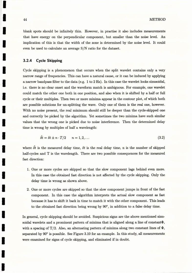
44 METHOD

blank spots should be infinitely thin. However, in practise it also includes measurements

that have energy on the perpendicular component, but smaller than the noise level. An

implication of this is that the width of the zone is determined by the noise level. It could

even be used to calculate an average S/N ratio for the dataset.

3.2.4 Cycle Skipping

Cycle skipping is a phenomenon that occurs when the split wavelet contains only a very

narrow range of frequencies. This can have a natural cause, or it can be induced by applying

a narrow bandpass filter to the data (e.g. 1 to 2 Hz). In this case the wavelet looks sinusoidal,

i.e. there is no clear onset and the waveform match is ambiguous. For example, one wavelet

could match the other one both in one position, and also when it is shifted by a half or full

cycle or their multiples. Then two or more minima appear in the contour plot, of which both

are possible solutions for un-splitting the wave. Only one of them is the real one, however.

With no noise present, the real minimum should still be deeper than the cycle-skipped one

and correctly be picked by the algorithm. Yet sometimes the two minima have such similar

values that the wrong one is picked due to noise interference. Then the determined delay

time is wrong by multiples of half a wavelength:

Ot=ot=En· 772 n=l,2,... (3.2)

where A is the measured delay time, dt is the real delay time, n is the number of skipped

half-cycles and T is the wavelength. There are two possible consequences for the measured

fast direction:

1. One or more cycles are skipped so that the slow component lags behind even more.

In this case the obtained fast direction is not affected by the cycle skipping. Only the

delay time is wrong as shown above.

2. One or more cycles are skipped so that the slow component jumps in front of the fast

component. In this case the algorithm interprets the actual slow component as fast

because it has to shift it back in time to match it with the other component. This leads

to the obtained fast direction being wrong by 90°, in addition to a false delay time.

In general, cycle skipping should be avoided. Suspicious signs are the above mentioned sinu-

soidal wavelets and a prominent pattern of minima that is aligned along a line of constant*,

with a spacing of T/2. Also, an alternating pattern of minima along two constant lines of *,

separated by 90° is possible. See Figure 3.10 for an example. In this study, all measurements

were examined for signs of cycle skipping, and eliminated if in doubt.

HOW TO MEASURE SHEAR WAVE SPLITTING 45

4- S TUR2 Q

2- A JAN M (0161 20021 12:01:5730 A

I r

TUR2 Q

2- A A - 16 (016). 2002

I A/\N UUrt:,411 1/ f

V

TUR2 8HZ

21 -1 16 0161 2002A A 2:02:59.7 30 -

2 +11 F

. 1 1 . 1 1 1 1 1 1 '6'''6'11 .

@

.I 10+4

Tule R 62.0

JAN 16 (016), 2002h>brnm39!1012 T -28.0

JAN 1,4 (0161 2002

1 A //498»Vr v. V

TUR2 R 62.0

JAN 16 (016), 2002

TUR2 T -28.0JAN 16 (0161 2002

-*h AA»/\ 17023:1FV- V

Seconds Seconds

Event:2002.016 Sla:TUR2 Dist:0.5 Az: 147.4 Baz:327.2 -38.930N 175.21 OE 224.2km

02016 JAN 16 TUR2 angle 3.000000e+01+/-3.500000e+00 log 3.000000e-01+/-1.875000e-02pol. oz 6.195059e+01 dl 2.000000e+01 df/somp 1.16959le-01 File: 2002.016.12.02.TUR2.0.2-2 Filter: 0.2-2 Hz

4 °3<=--m 4 KY °-°rn1%03- , tv'}.l, 1 - -0.5-

11 lili

57.0 57.5 58.0 58.5 57.0 57.'

Seconds Sec

1- 43 @n2 2-

--

-2- 2 -01111111 1 1 1 1 1 1 1- X -1 1 1 1 0 1 1 1

-2 024 -2 024 0.0 0.5 1.5 2.0

X 10+4 X 10+4 LogwFast relative amplitude Fost relative amplitude

Figure 3.4 Example for an A-quality measurement. This measurement was recorded at station TURO2

(=TUR2). Information about the obtained parameters can be found in the header of the lower picture.

* = 31°, 6t = 0.3 sec, initial polarisation a = 62°.

(1) Original seismogram, rotated into direction of back azimuth.

(2) Original seismogram, rotated 90° to back azimuth.

(3) Original seismograIn, vertical component.

(4) Original seismogram, rotated into direction of initial polarisation.

(5) Original seismogram, rotated 90° to initial polarisation.

(6) Corrected seismogram, rotated into direction of initial polarisation.

(7) Corrected seismogram, rotated 9(P to initial polarisation.

(8) Original seismogram, fast and slow components in overlay wave form plot.

(9) Corrected seismogram, fast and slow components in overlay wave form plot.

(10) Original waveform, hodogram (horizontal particle motion). Axes are the fast and slow directions.

(11) Corrected waveform, hodogram (horizontal particle motion).

(12) Contour plot (* vs, 60, solution is marked as a star. Innermost contour outlines the 95% con/idenceregion.

The criteria for judging the quality of a measurement are shown at the end of Section 3.2.2.

3 58.0 58.5onds ift0@

46 METHOD

I L+010 Q

- 12( 321 2002

1+ ILHOIC QA 2. A -12 0321 2002-'.t -rfV\20,9%0,1.A

i..

1 U-1012 De

-J 12 (132), 2002A.gA»W\.9,9,2,1

1-V

0..

m¥ 12 11 -

UN T -44A . . a w. 12 un). 2092

4- Ul R 416

1-

UN T -44IMY 12 (1321 zoe

In r ---

6·,6 6·,6Seconds Seconds

Event:2002.132 Sic:LH0R2 Dist:0.4 Az:180.2 Boz:0.2 -38.940N 1 75.440E 1 80.9km

02132 MAY 12 LHOR2 ongle -1.300000e+01 +/-4.000000e+00 log 2.500000e-01 +/- 1.250000e-02pol. oz 4.36228&+01 df 3.200000e+01 df/somp 2.091503e-01 File: 2002.132.04.15.LHOR2 Filter: None applied

ii,•1'Al"'' |. 1 1.fl'. 11.1,1.1An . I30. lili - 0.3-

- 1 b l 4 1 Loc X -i°-°n'i, PA Tnj v -i E.-- . , -87' 22..,6 1.3 SOL A8,0 87.5 6,0 885

Seconds4-

0 4 ' 01 i.b ' il '* 10+4 , 10+4

Fast relative amplitude Fast relative amplitude Log (s)

Figure 3.5 Example for an A-quality measurement (unfiltered). Note the cruciform of theuncorrected particle motion (left). The reason for this is the almost complete separation of the fast and

slow wavelets

LHU12 0 LI*12 R 27.5A w U (143). 2002 A . i AA .•Y 23 0431 20021 . ··4 \Ivtvvrm'*4C 7.14Avi v Whll V !.11 -2-.1 U«02 1 -625

4 •A Ult!2 R 273

b. In1 - A AA .5 231•31 2002

UU!2 Se i. . 0Wv\NVV Vyvmpk | 1<)· 2002 U«02 1 -62.5

:C A A /89L?!(1431 2002

--47*-VVYJV'I'.wlili. .h'11 J.1 1,4.1.....0..1. ><i. 1 4 1 1 6 . 1 1 L., 1 1 4 . 1 . 6 . 1 1 . 1 . 2

Seconds Seconds

Event:2002.143 Slo:LHUT2 Dist:0.3 Az:334.3 Boz:154.4 -39.510N 1 75.720E 19.9km

02143 MAY 23 LHUT2 angle -4.000000e+01 +/- 7.500000e+00 log 5.000000e-02+/-1.250000e-02pol. oz 2.753156e+01 df 3.6000000+01 df/somp 3.272727e-01 File: 2002.143.11.19.LHUT2.0.5-3 Filter: 0.5-3 Hz

Al -gA

Seconds Seconds

3 01 b

(sa@Jb@P) 41nuug '* 10+4 * 10+4

Fast relative amplitude Fost relative amplitude

Figure 3.6 Example for an AB-quality measurement. Reason: Stretched contours around the

solution. This is a sign of uncertainty in *-direction

HOW TO MEASURE SHEAR WAVE SPLITTING 47

X 10+3

10110 0 ,01,12 R 22.2

M. 110.Ut-, . A ..dvMA4*YUJAMJ t A 1.W 01 QW. 2002

' V,V V A 1 . £ 1 -67.8

Fl /1211 2002 VW-vw,ANY. f

RAA W\ AA /k PK WJAAg2„ V, V -4-11\4"V v·v,em:»---LOU*2 @12 . V,WY 01 (121). 2002

I .A. LOUO. 1 -67.8

-v./-PVV«00,mp0- 1-

1,1 r .

.. 14 1.....6Seconds Secods

Event:2002.121 Slo:LQUA2 Dist:0.2 Az:92.4 Boz:272.2 -39.21 ON 1 75.220[ 6.7km

02121 MAY 01 LQUA2 ongle -2.100000e+01+/-7.000000e+00 loq 1.000000e-01+/-1.250000e-02pol. az 2.217668e+01 dI 3.100000e+01 df/somp 1.834320e-01 File: 2002.121.10.34.LQUA2.1-3 Filter: 1-3 Hz

1 1 1 1 . 1 111 -. 1 ' 1 ' 1 ' "1 ./ 1 ' 1 ' 1 11 01 11- 11 -. f\-1 0.5- A --

1 1 - 45-

*U 44.5 43.0 435 46.0 44.0 ' 44.5 ' 43.0 ' 43.3 46.0 Jr - |Seconds Seconds -

S0-

00

X 10•3 Log (s)Fost relotive omplitude Asr'relative omplitude

Figure 3.7 Example for a B-quality measurement. Reason: Waveform fit not perfect; transverseenergy not completely minimised (right plot, lowest trace); existence of a second minimum in contour

plot.

LOUO 0

1 A A AA At 5(31.UN), -

- DAIVI/VVMVV'V

-1 IN,1 2002

.VV' V .V X 10+3

-w..=/LaRalLOW T-1 316

--/MAA,AArm#*,82vpvvA I lote R 4 6

v -I. v VL . Lot#2 T-MU

11- Aa _ . *91,41211 2002

-11;14.4·4'·4·4·LA,6'* '6'4'4'6'44'/Seconds Seconds

Event:2002.121 Sla:LQUA2 Dist:0.2 Az:92.4 Baz:272.2 -39.210N 1 75.220[ 6.7km

02121 MAY 01 LQUA2 anole -2.400000,+01 +/-6.500000e+00 log 2.625000e-01+/-1.25000 le-02pol. oz -6.855922e+01 df 3.100000e+01 di/somp 1.937500e-01 File: 2002.121.10.34.l-QUA2.0.5-3 Filter: 0.5-3 Hz

1.0 .lilli 11 - 1 .

2 0.5_

vir. Cgj 11806- &I l- -0.5- .

2 - ' V i -1-6-U '45 '46 '45.3 46.0 U.5 450 453 460 -8 - - M

-1.0 '1•1•1 1

-p 1 1

-4 0

Cal

J 10+3 Log (s)Ast*'relative amplitude Fast relative omplitude

Figure 3.8 Example for a C-quality measurement. Same measurement as Fig. 3.7 with a di/Terentfilter. Reason for mark: Bad waveform fit, no linear particle motion, transverse energy not minimised.

Probably cycle skipped (compare 6t to Fig. 3.7). Note that C-marked measurements are not used;

They are only kept for reference.

Seconds

48 METHOD

- 05 (156), 20021*2 0

- - AAW\,A,vAr'AA?1131!5,AI

-6

11*02 Q

Z:Rt (g), 2002· · A/\4\WWVVVV,VW

/+ I F

U102 &12. 05 (156),2002

Seconds

t · MMA *48#0491 11•02 0 4&5

. V,. 1 1,26

14- m ,

.1,

07772 66'6 6'.6Seconds

Event:2002.156 Sta:TUR02 Dist:0.3 Az:34.2 Boz:214.0 -39.590N 1 75.280[ 72.5km

02156 JUN 05 TUR02 ongle -4.700000e+01 +/-2.000000e+00 log 4.875000e-01 +/-1.250000e-01pol. oz 4.852565e+01 df 3.300000e+01 di/somp 2.142857e-01 File: 2002.156.00.27.TUR02.2-6 Filter: 2-6 Hz

1.0

=: 0.5- 05

0.0

1·0 20 ' 63 5 '..0 '.J A.O 20 ' ds ' .JSeconds

4

2-

0-

-2-apnp.dwo @Al}DIal mots64.5

Seconds 1

J 10+4 Log (s)tost relative omplitude AO"relative amplitude

Figure 3.9 Example for a NULL measurement (A-quality). Note the lack of energy on thetransverse initial polarisation component (top right). Waveform is linear before and after correction.

Contour plot has U-shape. dt is determined by noise and can not be trusted (see overlaying waveforms).

* has to be set manually to the direction of one of the U-bars (Here 42°)

AA

-WiA/VviVVvwl

--6&4Aial

IMY 09 '129' 2002

»'.f\4.-«AI ,

X 14'614,4 4 ' A ' 6 ' 6 ' 6 ' 6Seconds

X 10+5 ..8ING R 104

--*V+*\AFW1 6 6 . LJ ."i ' 1

Event:2002.129 Sto:TUKI2 Dist:1.6 Az:202.7 Boz:23.2 -37.810N 176.400E 174.8km

02129 MAY 09 TUKI2 ongle 2.600000e+01+/-1.150000e+01 log 5.625000e-01+/-1.875000e-01Pol. az 6.040326e+01 df 3.000000e+01 di/somp 8.670520e-02 File: 2002.129.19.24.TUK:2.1-3 Filter: 1-3 Hz

'1'141·1

0.5- 0

Seconds

Z

& -1 -21 1 01 1 21-

qlitude .,Rel*e nplitude Seconds

2-

0

Azimuth (decrees)4 IIi i*A, A A,/9

0.0 0,5 1.0 1.5 2.0

X 10+5 * to+3 Log (s)Fast relative amplitude Fost relotive amplitude

Figure 3.10 Example for cycle skipping. Note the sinusoidal wavelet and the prominent patternof minima in the contour plot. They are aligned along a line of constant * = 25°, with a spacing of half

a wavelength. However, the probably correct minimum was chosen by the algorithm in this case.

THE SLOPE CORRECTED SHEAR WAVE ANGLE 49

3.3 The slope corrected shear wave angle

Section 2.1.7 described why it is necessary to

select events with a steep angle of incidence

at the receiving station. This is especially

difficult when the stations are positioned on

the slope of a mountain, as was the case dur-

709106,0,)d ing all deployments at Mt. Ruapehu. The/ normal . j window

/ shear wavA Aslope-angle 6 varied from 2.3° at LHOR to

/ window L..

14.0° at LHUT (see Table 3.4). The deter-

mination of this slope angle is also not triv-

ial. Based on the length of the scale, this

angle is highly variable at any given station.

For example, when the steepness of the sur-

face close to a station is measured, the result

could be 90° if the station is placed at the

base of a cliff face. On the other hand, if

the whole mountain is considered, the angle

would certainly be very shallow when it is

calculated only by the height and the width of the base of the mountain. The answer to

this question is choosing the right length of scale. Thus it is important to know the main

wavelength of the incoming waves. With an assumed surface S-wave velocity of around 1.3 -

1.6 km/s (Latter, 1981) and main frequencies of around 1 Hz and lower, a scale length of 2

km was chosen.

Station_/

/ n/70°

Figure 3.11 The slope corrected shear

wave window. Note that a wave coming from

the left side of the blue window would strike the

surface at the station at a very shallow angie,

which would cause strong distortion of the mea-

sured wavelet. This can be avoided by defining

a slope corrected shear wave window (red) which

only allows events that strike the surface at an

angle of max. 35°.

For Table 3.4, the direction of the steep-

est gradient was determined and then the

altitude difference between a point 1 km

downslope and 1 km upslope of the station

along that direction was measured on a map.

The resulting slope angle allows the exper-

imenter to calculate the incidence angle at

the slope surface. However, the incidence

angle on an assumed horizontal surface has

to be calculated first. This is done by using

the ray parameter for the event. It is given

by the IASPEI earth model (Kennett, 1991),

which is assumed to be a valid model under

the low velocity layers of the volcanic edifice.

VV

Station /

A station

tslope

horiz

Figure 3.12 Incidence angle on a slope. Forthe same incoming wave, the incidence angle at a

station on the slope can be substantially different

from that of a station on a horizontal surface.

To calculate the incidence angle at an assumed

50 METHOD

horizontal surface, the following formula was used (Lay and Wallace, 1995):

thoriz = arcsm 1 -C Rj

(3.3)

where

ihoriz : incidence angle on a horizontal surface [°l

P: ray parameter (slowness) Is/rad]

US : S-wave velocity at or near the surface [km/s]

R: Earths radius (6371 km)

4t

1 L ' slope

_slope-f

X3-

h / x2:(North)67 7 1

I .%

I x (East)a gradient azimuth

/lon, (North)

I X1 (East)B = baz-180°

Figure 3.13 Geometry of incoming rays at a slope. n is the normal vector on the slope surfaceat the station; F is the unit vector of the incoming ray, pointing in propagation direction. 8 is the

slope angle, a is the azimuth of the steepest downslope gradient. The ray azimuth B represents the

back azimuth - 180% ihortz is the horizontal incidence angle.

The incidence angle at the slope is determined by calculating the angle between fi and F.

The incidence angle at the slope surface can be obtained by calculating the angle between

an incoming ray F and the normal vector on the slope n. Both vectors have the length 1 and

are defined by:

< Tz sin(ihoriz) Sill B / nx ( sin 6 sin a

F = ry = sin (ihoriz) cos B i n = ny -sin 6 cos a ,

< 7'z COS(ihoriz) nz 3 < cos 6 j

where B is the back azimuth minus 180°; 8 is the slope angle and a is the azimuth of the

steepest downslope gradient (see Figure 3.13). The incidence angle is then defined by the

THE SLOPE CORRECTED SHEAR WAVE ANGLE 51

Station Azimuth of steepest Altitude difference Resultingname gradient (downslope) a within 2 km slope angle 8

FWVZ 340° 500 m 14.0°

LHOR2 255° 80 m 2.3°

LHUT2 340° 500 m 14.0°

LQUA2 0° 220 m 6.3°

LTUR2 240° 300 m 8.5°

TUKI2 90° 320 m 9.1°

TUK2 80° 160 m 4.6°

TURO2 240° 300 m 8.5°

Table 3.4

Slope angles for recording stations.

angle between n and F, which in a cartesian coordinate system is defined by:

/ n.r \

tslope = arccos I ; 161=li =1 (3.4)C 'Al. 1 11 ,= arccos sin(ihoriz) sin #sinosina +

+ sin(ihoriz) cos #sin 6 cos a + cos(ihoriz) cos 6)= arccos cos(ihoriz) cos 6 + sin(ihoriz) sin 6sin#sina + cosdcosa= arccos cos(ihoriz) cos 6 + sin(ihoriz) sin 8 cos09 - a) .

which can be expressed as:

tslope = arccos cos(ihoriz) cos 6 - sin(ihoriz) sin 6 cos(baz - a) . (3.5)

This formula was used to calculate the incidence angle at the slope surface, where

islope : incidence angle on the slope surface [°] (= corrected arrival angle)

Liz : incidence angle on a horizontal surface [°]

6 : slope angle [°]

a: azimuth of the steepest downslope gradient [°]

baz: back azimuth of the event [°].

Once this value was calculated, only events with an 2slope incidence angle smaller than

35° were selected for the further visualisation and interpretation of the data. A program has

been developed to automatically calculate the normal and corrected S-wave incidence angles

from a measurement file (See Appendix D.2 for more details).

52 METHOD

3.4 Mean value and error analysis

In this study, most of the data consists of measurements of the fast anisotropic direction,

which can be classified as directional data. When handling directional data, a normal error

statistic can not be used for two reasons:

1. The range of directional data is wrapped and has a maximum of 360°. In a normal

statistic, the maximum possible range is [-00...+ 00].

2. Splitting data has a bimodal distribution. This means that a fast direction of 1° is

at the same time also 181°. Thus, every measurement is ambiguous by 180°, which

constrains the effective maximum possible range of data to only 180°.

Mardia (1972) and Davis (1986) describe methods for handling this special type of data,

which will be presented in the following sections.

3.4.1 Obtaining the mean value of splitting measurements

In order to obtain the mean value of all splitting measurements, every measurement is treated

as a normalised vector with the direction *i (i = 1,...,n), which represents the measured

fast direction. All vectors are added up and the length of the resultant vector is divided by

the number of measurements (n). Equation 3.6 shows how the individual vectors are added

up. The factor l (l = 2) represents the fact that the distribution is bimodal, and will be

explained in Section 3.4.2.

< ir - Ell cos(l *i) f Eli sin(l *i)(3.6)

The direction of this resultant vector R represents the mean direction * of all measurements,

and its length is related to the variance. Equation 3.7 shows how it is obtained:

= arctan (Xr/Yr) / ln in

= arctan ( 1 y. cos(l *i) / lE sin(l *i) ) / l (3.7)i=1 i:==1

(adapted from Davis (1986)), again, l=2 (see Section 3.4.2).

MEAN VALUE AND ERROR ANALYSIS

3.4.2 Why angles have to be doubled

Since splitting data has a bimodal distribution (i.e. 18(

vectors would lead to the wrong result. For example, t,

represent the same fast direction,a)

but adding them up will result

in a vector with zero length and

an undefined direction. A way

of avoiding this is to double the

angles of all measurements before

the vectors are added up (Krum-

bein, 1939), hence the factor

l = 2 in the sine and cosine of b)

Equation 3.6 and 3.7. This, of course, will lead to an average di- <rection that is also multiplied by the factor two. Thus, the mean

direction of the resultant vector

has to be divided by this factor in

Equation 3.7 (Davis, 1986). See

Figure 3.14 for an example. In

the case of a higher order of multi-

directional data, the factor l also <rises. For example, if the direc-

tions of NULL measurements are added up (which have a *90° am-

biguity), then l would be four.

3.4.3 Calculating standard deviation and errors :

53

)° ambiguity), simply adding up all

wo measurements of -90° and +90°

Figure 3.14 Effect of dou-

bling the angles:

a) A set of six directional mea-

surements was plotted (-100°,

-105°, 90°, -107°, 68° and 60°)

and the resulting vector It calcu-

lated (red arrow). The resultant

mean direction is -82.r and very

short in length (0.225). Obviously

it does not represent the trend in

the data. b) The same set of data was plotted now with doubled angles (-200°,-210°,180°,...). The pop-

/ ulation is no longer bimodal andthe resultant vector shows the real

trend (142.4°) of the doubled an-

gles. Its length is nearly one

(0.972), which indicates a strong

trend in the data.

c) The data set is plotted with

original angles, and the resultant

vector is plotted now with half theangle obtained in b). The true

mean direction of the dataset istherefore#=71.7.

The Von Mises Statistics

C)

For the evaluation of the data quality, it is important to obtain information about the errors

and deviations of the dataset. Every statistic uses certain assumptions about the probability

model of the data involved, and a special kind of distribution has to be used for directional

data. The Von Mises distribution is a circular analog to the normal distribution (Mardia,

1972) and will be used as a basis for the following calculations. It is defined by the two pa-

rameters * (mean direction) and K, which is called the concentration parameter. Figure 3.15

shows the distribution of the 2002 deep events with the expected Von Mises and Normal

distributions. It is shown that a Von Mises distribution fits well to the data in this study. Its

54

35

30

VM kappa' 1.2- Von Mises distr

- Normal disk0 25 - / VAI kappa ' 0.8G

020

E1215 -

9310

-60 -40 -20 0 20 40 60 80

Fast Direction relative to mean value [Degrees]

VM kappa * 1.2- Von Mises distr

- VM kappa * 0.8- Normal distr

E

10-

858

-60 -40 -20 0 20 40 60 80Fast Direction relative to mean value [Degrees]

·.L-

-80

15-

0

-80

METHOD

Figure 3.15 Validity of the Von Mises Distri-bution

top: 2002, deep events. Number of observed mea-

surements vs. the fast direction (relative to the meanfast direction). The blue curve represents a normaldistribution, the red curve a Von Mises distribution.

Considering the fact that the dataset consists of data

from several different stations that sample different

regions of the crust, a broad distribution can be

expected. This also means that the centre columnwill be smaller than the theoretical value for a Von

Mises distribution. The red curve is only determined

by the concentration parameter of the distribution(A) and the total number of measurements. Notethat the curve was not jitted to the data. Yet it

predicts the probabilities surprisingly well. For theother two curves, K was manually altered to display

the dependency on this parameter. In this example,only measurements of A and AB quality are included.The red dots on the curve represent the standarderror interval and show how well constrained the

mean value is. The black dots represent the standard

deviation and show how spread the data is. It is clearthat a Von Mises distribution is a valid assumptionfor the data.

bottom: 2002, deep events recorded at TURO2.This plot shows that the Von Mises distribution is also

a valid assumption for data that is recorded at onlyone station.

probability density function is given by Mardia (1972):

1ex cOS(*: -3)

27rIo (K) 0 < *: 5274 K> 0, 0 5 *<27r, (3.8)

where Io(/c) is the modified Bessel function of the first kind and order zero:

Io(,c) = ---1- 1 K)2r (3.9)r=0 r82 2

* is the mean direction; A is the concentration parameter and a direct function of R; it will

be described in a paragraph later in this section.

Standard deviation

The above calculated resultant vector R also carries information about the spread of the

data.

The longer R is (with a maximum of 1), the more homogeneous is the data. If all

measurements point in the same direction, then the length of the vector will be one. If the

measurements are randomly dispersed in all directions, then the resultant vector will be of

MEAN VALUE AND ERROR ANALYSIS 55

almost zero length. Mardia (1972) provides a more quantitative formula for this. First, the

length of R has to be calculated:

R = IRI

= q X3 + Y,2 21n 1n= \ (- E cos(l *i)) + (- I sin(l *i) (3.10)( n i=1

From this value, the so called circular variance So can be derived:

So = 1-R. (3.11)

Since R lies in the Range [0,1], the following formula of a wrapped normal distribution is

valid (Mardia, 1972):

1,2-2

1 -So = e-r °0, (3.12)

with the circular standard deviation so. Thus

so = -2 ln(1 - So) l (3.13)

The circular standard deviation describes the width of an interval around the mean value, in

which a random measurement will fall with a 68% probability. However, before this value can

be trusted, it has to be shown that the sample of measurements is not uniformly distributed.

Test for Non-Randomness (Rayleigh's Test)

In order to use error statistics on a sample of data, it has to be proven that the data is

not random (uniformly distributed). This can be achieved by applying Rayleigh's test, which

assumes that the measurements are sampled from a Von Mises distribution. This test is very

simple, and only the number of measurements n and the calculation of R is needed. For every

value n, there is a critical value for non-randomness at a certain level of significance. Tables

for this are provided in Mardia (1972) and Davis (1986). Since the value of R rises with the

uniformity of the data, it has to be larger than the critical value specified by the number of

measurements. Also the level of significance has to be specified, which gives the likeliness

of the test being wrong. For example, the dataset described in Figure 3.14 has a value of

R = 0.972, n = 6. Assuming that the observer wants to be 99% sure that this dataset is not

random, he or she would look up the critical R-value for n=6 and a significance level of

1% (= 100% - 99%). This value is 0.825, which is exceeded by the R-value of the dataset

56 METHOD

(0.972). This means that the observer can be at least 99% sure that the data in this example

is not random.

Concentration parameter

Another parameter that can be derived from 11 is the concentration parameter x. It behaves

similarly to R, i.e. it is zero for random data, and its value rises with the homogeneity of

the data. However, its maximum value approaches infinity for homogeneous data, i.e. when

all measurements are pointing into the same direction (R = 1 in this case). The relationship

between R and x is not trivial, as it is described by two Bessel functions:

120£) = Ii(K)/Io(,c). (3.14)

Mardia (1972) provides charts, tables and also several approximations for this relation. For

example, an approximation for R > 0.8 is given by:

- 2(1 - R) - (1 - 12)2 - (1 - 12)3 (3.15)

A program called kappa was developed which combines different approximation methods to

provide an accurate estimation for 412).

Standard error

With a given dataset, a mean direction can be calculated as described above. The standard

deviation of the measurements describes how spread the data are around this mean value.

However, it does not give any information about how accurate this mean value represents the

true fast direction. This information is given by the standard deviation of the mean, which

is also called the standard error. Assuming that a true fast direction in the ground exists,

the standard error can be derived from Equation 3.8. The exact derivation will not be shown

here, as it is of considerable length, and is also shown in Mardia (1972). A key part of it is

the relation of the expected value E{cos((Dz - *)} = R, which eventually leads to:

1Se = i-7;JE '

l=2 (3.16)

where

Se :

n:

R:

K(R) :

standard error [rad]

number of measurements

resultant vector length

concentration parameter

MEAN VALUE AND ERROR ANALYSIS 57

With this parameter known, it can be expected that the true mean of the population is

contained in the interval

* i drase (3.17)

where Za is a factor that specifies the level of significance. E.g. 48% = 1 and 45% = 1.96.

For the dataset in Figure 3.14, the standard error calculates to se = 3.0. This means that the

probability is 95% that the true mean value is contained in the interval 71.2° * 1.96 · 3.0° (i.e.

from 65.32° to 77.08°). These values can also serve to test whether two sets of samples are

drawn from the same population. In other words: is the set of measurements from one station

sampling the same region of anisotropy as the measurements from the next station? With a

specified standard error value, the answer is easily obtained: if the standard error intervals of

the two stations do not overlap, then it can be excluded with the specified significance that

the measurements of the two stations represent the same region of anisotropy. For a more

quantitative evaluation of this, an F-Test statistic can be computed (Davis, 1986). During

this study, software was developed which calculates the above mentioned error parameters

(std. deviation, std. error, 12, n, *,...) for a given measurement file (see Appendix D.2 for

more details).

3.4.4 The difference between standard deviation and standard error

When a physical property is measured a certain number of times (e.g. 10), then the mea-

surements will suffer from the same statistical error sources as every measurement, i.e. the

results will form a gaussian, bell shaped curve around the true value. Out of this shape, a

standard deviation interval for the measurements can be estimated, which means that the

random chance for the next measurement falling into this interval is 68%. The mean value of

the measurements is an estimate of the true value (assuming that no systematic errors were

made), but due to only 10 measurements it will have a limited accuracy. This accuracy is

given by the standard deviation of the mean value, which is also called the standard error. It

means that there is a 68% probability for the true value being contained in the standard error

interval around the mean value. For a normal distribution this is the standard deviation of

the measurements divided by the square root of the number of measurements. So in this case

the standard deviation of the mean value is 4-1-6 (- 3.2) times smaller than the standarddeviation of the measurements.

SO

Se = .a (3.18)

This means that if not only 10 measurements, but 10,000 measurements were obtained, the

standard deviation of the mean value is 410,000 (= 100) times smaller than the standard

1

58

deviation of the measurements. Thus the error interval for the mean value becomes sub-

stantially smaller. Yet the measurements will still form the same gaussian curve around the

mean value as before. The width of the curve and therefore the standard deviation of the

measurements will be the same as with only 10 measurements, since the error sources have

not changed.

1

1

1

1

1

1

1

1

1

1

1

1

1

1

1

1

CHAPTER 4

DATA ACQUISITION

This chapter provides information about the data collection during the CHARM 2002 ex-

periment and the instrument deployments from 1994 and 1998. Details about sensors and

recording equipment will be given, as well as about logistical aspects.

4.1 The CHARM experiment

CHARM (CHanges of Anisotropy at Ruapehu Mountain)

Figure 4.1 Real scale digital elevation model of Mt. Ruapehu with the CHARM stationsshown in red

59

60 DATA ACQUISITION

Station Latitude Longitude Alt. Serial # Sensor SENSOR #

FWVZ -39.2564° 175.5518° 2000 m Q-980306 CMG-40T T4605

LHOR2 -39.3391° 175.4382° 1022 m ORION 251 CMG-40T T4788

LHUT2 -39.2542° 175.5606° 2066 m ORION 253 CMG-40T T4C49

LQUA2 -39.2216° 175.5403° 1364 m ORION 252 CMG-40T T41076

LTUR2 -39.3156° 175.5153° 1483 m ORION 162 CMG-40T T4431

TUKI2 -39.2795° 175.6097° 1746 m ORION 177 CMG-40T T4432

TUK2 -39.2725° 175.6458° 1525 m ORION 177 CMG-40T T4432

TURO2 -39.3122° 175.5241° 1571 m ORION 178 CMG-40T T4430

TUR2 -39.3125° 175.5235° 1565 m ORION 178 CMG-40T T4430

Table 4.1

Station locations and equipment of the CHARM project. Note that all station

coordinates are given in the international lat/long geodetic system (Hayford 49).

4.1.1 Setup

In order to obtain the data for this experiment, six NANOMETRICS ORION digital seismo-

graph recorders were deployed on Mt. Ruapehu in January 2002, with GURALP CMG-40T

three component broadband sensors connected (see Figures 4.1-4.3). The power supply con-

sisted of a 70 Watt solar panel and three to four 60 Amp-h batteries per station. Where

possible, the sensors were placed on rock, protected by a plastic easing and several layers

of insulation. The plastic case was then buried under a pile of rocks (TUKI2, TURO2).

Where this was not possible, the sensors were placed in a pit in the ground, sitting on a

concrete pad, protected by several layers of insulation and a plastic easing. These were then

covered with at least 20 cm of soil as additional noise protection (LQUA2, LHUT2, LTUR2,

LHOR2). A seventh station (FWVZ, the station formerly known as FWTB) is now perma-

nently installed in the Whakapapa ski field area at the "Far West T-Bar" and is run by the

Institute of Geological and Nuclear Sciences as part of the Eruption Detection System and

the GEONET program (Sherburn and Bryan, 1999). It uses a QUANTERRA Q730-4G-CW

data recorder, which is a 4 channel 24-bit diskless unit, running with a sampling rate of 40

Hz. The sensor is a Guralp CMG-40T three component, broadband seismometer which is

enclosed in a concrete and polystyrene vault. The data from this station is telemetered via

spread-spectrum radio to the Chateau Mountain Observatory and then sent via VSAT to

IGNS at Gracefield and Wairakei. See Table 4.1 for exact station locations. Note that there

are nine stations described in Table 4.1. The additional two stations were TUR2 and TUK2,

which were deployed for one month and then relocated to TURO2 and TUKI2.

The CHARM stations were recording from January 2002 to July 2002 (for a detailed time

chart, see Appendix B.2, figure B.3) with a sampling rate of 80 Hz. The data was stored on

THE CHARM EXPERIMENT 61

2 GByte hard drives, which were swapped while servicing the stations every six weeks. A

total number of 830 events in the proximity of Mt. Ruapehu were recorded (see Table 3.1 for

selection criteria). The hypocentres of all available events, recorded by the IGNS/GEONET

network during the time of the three deployments are shown in Figure 4.4.

The sensor orientation was adjusted with a magnetic compass, and then checked with a

sun azimuth compass to detect possibly wrong declinations caused by magnetised volcanic

rock. All but one of the obtained errors for the north components are under 6°, which is about

the accuracy threshold for this method (for the individual values, see appendix table B.1).

Pictures of the sensors in the ground together with a compass were taken to allow later veri-

fication of the correct sensor orientation. Also, a huddle test with all sensors and instruments

was carried out prior to the deployment in order to ensure a correct sensor response and

component orientation.

The recording units of the three VUW owned stations were placed in a lockable aluminium

box and anchored to the ground. Attached to the boxes were the poles for the solar panels

and GPS antennae (see Figure 4.2). The three IGNS owned instruments had a lighter setup

which enabled them to be carried to more remote locations. The recording units were placed

in an open A-frame construction, to which the solar panel and the GPS antenna was attached.

4.1.2 Relation to previous deployments

The aim of the CHARM project was to investigate the exact nature of the changes in

anisotropy directions. Since the idea was to eliminate the possibilities of lateral inhomo-

geneities and site effects as cause of misinterpretation, it would have been ideal to reoccupy

all the sites of the previous two deployments (1994 and 1998). However, availability of record-

ing instruments and financial considerations restricted the number of CHARM stations to

six, plus one now permanent station at the Far West T-Bar location (FWVZ). Since it is

important to compare the results of the previous deployments to the current state, the most

practical solution was to reoccupy the sites that delivered the most results. The name con-

vention was chosen so that a reoccupied site would get the same name as before, with the

number "2" added at the end. Only the former FWTB station is now called FWVZ as part

of the GEONET programme.

Of the 1994 deployment, which originally had more than the five stations that are shown

in the maps, only those live stations delivered usable shear wave splitting measurements. Two

other stations were situated in the summit and crater area of Mt. Ruapehu, but the ambient

noise level and the scattering of waves in the volcanic structure prevented any reasonable

measurements. These two stations were not reoccupied in the CHARM deployment. Another

1994 station, at the Pukeonake scoria cone (LPUK), was also not reoccupied. Only six deep

and one of the shallow events resulted in a usable splitting measurement. However, those six

62 DATA ACQUISITION

iMFAf-.2

t

Figure 4.2 Field picture of LTUR2 station

deep measurements lie within the trend of the others and do not show any surprising results,

thus they are not very significant to the overall result. The other four stations of the 1994

deployment were reoccupied in the same spots (+/- 3 m) as before. At the stations LTUR

and LHOR the sensors were probably even placed in the same pits as before.

All three stations of the 1998 deployment were reoccupied. At TURO2 and TUKI2 the

sensors are placed on the same concrete platforms as during the previous deployments. Both

concrete platforms sit directly on andesite rock. The third station, FWVZ is now placed on

a concrete basement in a hut at the Far West T-Bar lift on Whakapapa ski field. Its relation

to the old spot is not exactly known but is very likely not more than 10 metres away from

the old spot.

The stations TUK2 and TUR2 were previously not occupied by broadband 3D instru-

ments. They were only installed for one month, and were then relocated to TUKI2 and

TURO2, respectively. The reason for this was that at the time of the deployment they were

mistakenly installed at previous short-period sites. The distance between TUK2 and TUKI2

is 3.2 km, whereas the distance between TUR2 and TURO2 is only 50 m. Due to the close

proximity of TUR2 and TURO2, which is negligible compared to the wavelength of the sig-

nal, the results of TUR2 were included in the results of TURO2 during the data processing.

THE CHARM EXPERIMENT 63

However, the results of the two stations were compared before and combining them showed

no significant differences in * or 6t.

4.1.3 Equipment

The recording instruments were Canadian built NANOMETRICS ORION recorders (see

table 4.1 for serial numbers) with the following recording parameters:

Model: ORION-3S

Channel sensitivity: - 800 nv/Bit

Sample rate: 80 Hz

DC Filter: none applied

Recording mode: continuous

GPS duty cycle: 5 out of every 60 minutes

Disk capacity: 2 GigaByte

The sensor parameters were the following:

Sensor Model:

No. of components:

Velocity Output:

Guralp CMG-40T

3

VUW Sensors (T4431, T4432, T4433): - 2 x 1600 V/m/s

Norm factor at 1 Hz:

Poles:

Zeros:

IGNS Sensors (T4788, T41076, T4O49): -2x 400 V/In/s

VUW: -0.314

IGNS: -0.346

VUW: -23.56 · 10-3 * *23.56 · 10-3 Hz; -50 Hz

IGNS: -11.78· 10-3 £ i11.78· 10-3 Hz; -48.4 Hz

VUW: 0 Hz; 0Hz; 159 Hz

IGNS: 0 Hz; 0Hz; 140 Hz

4.1.4 Logistics

Since many of the sites are located in remote areas, the stations had to be portable. The

IGNS owned A-frame constructions were especially suitable for these areas. Access to the

LHUT2 site was only possible by foot, since it is situated in the Whakapapa ski field. The

altitude difference between the closest possible road and the station is 750 m, but a chairlift

could be used during good weather to transport equipment to a point 1 km away from the

station and about 100 m lower in altitude. Special backpacks for carrying the 100 Amp-h

truck batteries were used and are highly recommended for future deployments. This site is

situated on a ridge and was covered with about 1.5 m of snow and solid ice in the winter.

64 DATA ACQUISITION

Abnormal weather conditions delayed the removal of the instrument for about 6 months into

the summer of 2002/2003.

Several other sites required access via roads that are only usable by four wheel driven

vehicles. TUKI2 is situated in the Tukino ski field, which is only accessible in low snow

conditions during the autumn and winter months. 4WD and snow chains are required.

LHOR2 is situated on a forest clearing close to the Makotuku river, which has to be

crossed by foot in order to access the station. After heavy rain and during the spring time

the river becomes unpassable, so the station is not accessible during this time. Also, the road

to the site crosses the private property of a farm and permission to enter the property had

to be obtained.

The stations LQUA2, LTUR2 and TUKI2 are all in the vicinity of roads, so the equipment

had to be carried for only a few hundred metres. In these cases, the heavier and sturdier

VUW stations were used, which provide a better protection against theft and vandalism with

their lockable aluminium box.

Since all the stations are located in the Tongariro National Park, a permit from the New

Zealand Department of Conservation (DOC) to install the stations in the field was obtained

prior to the deployment. This permit specified the exact location, setup and deployment time

for each station.

Two field teams of two to three people each were involved in the installation and the

removal of the stations. Six - weekly service runs were usually carried out by a team of two,

sometimes by a single person. The base for all operations was the IGNS volcano observatory

hut in Whakapapa village.

4.2 Information about previous deployments at Mt. Ruapehu

4.2.1 The 1994 deployment

The deployment in 1994 was conducted by Leeds University, the University of Memphis and

the New Zealand Institute of Geological and Nuclear Sciences (IGNS). 14 broadband 3D

seismographs were installed around the Tongariro National Park and Mt. Ruapehu between

28 January and 13 March 1994 (Hurst, 1998). The recorders were 9 Lennartz MARS-88

dataloggers and 5 REFTEK systems, provided by Jer-Ming Chiu from the IRIS PASSCAL

pool. All stations were equipped with Guralp CMG3 sensors. The REFTEK sets were

stationed further away from the mountain but did not produce valuable data in most of the

cases (Hurst, pers. comm.). Also, the stations located close to the summit and crater lake

on Mt. Ruapehu did not produce valuable S-wave splitting measurements (Miller, 2000).

INFORMATION ABOUT PREVIOUS DEPLOYMENTS AT MT. RUAPEHU 65

The data that was used is shown inStation Latitude Longitude Alt.

Chapter 5, the station locations are de-LHOR -39.3391° 175.4382° 1022 m

scribed in Table 4.2 and plotted in Fig-LHUT -39.2542° 175.5606° 2066 m

ure 4.3. During the time of this de-LQUA -39.2216° 175.5403° 1364 m

ployment, a total number of 272 earth-LTUR -39.3156° 175.5153° 1483 m

quakes were recorded by the IGNS net-LPUK -39.1408° 175.5526° 1010 m

work, and their locations determined us-

ing CUSP (Caltech-USGS Seismic Pro- Table 4.2

cessor) (Maunder, 1999). These earth- Station locations and equipment of the

quakes produced 99 splitting measure- 1994 deployment.

ments (note that most earthquakes pro-

duce measurements at more than one station).

4.2.2 The 1998 deployment

This deployment was also conductedStation Latitude Longitude Alt.

by Leeds University (Neuberg et al.,FWVZ -39.2564° 175.5518° 2000 m

pers. comm.) between February andTUKI2 -39.2795° 175.6097° 1746 m

July 1998. Three Lennartz MARS-88TURO2 -39.3122° 175.5241° 1571 m

dataloggers were installed with Giiralp

CMG3 3D broadband seismometers at Table 4.3

station locations specified in Table 4.3. Station locations and equipment of the

A map with station locations is shown 1998 deployment.

in Figure 4.3. During the time of this

deployment, a total number of 997 earthquakes were recorded and located by the IGNS

network, which produced 126 splitting measurements.

To confirm a correct sensor orientation for the 1994 and 1998 deployments, the coin-

ponents of each sensor were individually checked by comparing the first motion of arriving

P-waves with the expected first motion for a certain back azimuth of the incoming wave

(results shown in Miller, 2000, Appendix A). In all cases the observed first motion matched

the expected one. Thus it is ruled out that the sensor orientations were substantially wrong,

or that internal components of the sensors had a switched polarity. For an illustration of this

method, see Appendix B.3.1.

66 DATA ACQUISITION

175° 20' 175° 30' 175° 40'

-1 Z..1|FliM i.jli M. IL--'.-....M- -39° 00'

@-BIZiIZZ station v:...i:"Zkk1,1,4 P

M 0 1994 & 2002 Station 4' ,#*..2,;21• . & .

0 Other le>Iii*i,).. h '0 - Fault lines AL h*t.-'-h- i.. 'rt

.'. I - Rivers P.*/tra=ty > r .'. .tl ,

4- 7,>49 2 L. D *

arpar ..:e,A, -39° 10'I-

k

Wha {h

:61.1 lot' A,Il; *3Ati>-1

FWVZ/FWTB t• LHUT/2 TUK2 (2002 only)

*1

./24F*'

een- 1-

-39° 20'

LTUR/2 .-a.

/ 4A ' TURO/2

' 'b.& LHOR/2,

. ....aL. I

1 -39° 20'

-4- 3/Ohakune

km

0 5 10

'tl'*3>/-22452

Cal

-7 272/

*24».Cal39° 30' ' -·,---dil- -39° 30'

175° 20' 175° 30' 175° 40'

Figure 4.3 Station locations of all deployments. Circular outlines show stations that were deployedin 1998 and 2002. Diamond shaped outlines show stations that were deployed in 1994 and 2002. The station

LPUK was only deployed in 1994, the station TUK2 recorded only in 2002. Note the predominant NE-SW

alignment of fault lines (mostly normal faults; shown in red)

Depth (km)0

-25

-50

-75

-100

-125

-150

17€ ,40*

-200

-225

-250

t

0

g

-50

' o.v-v E,»44.-9-R -4 -4 -- 1 -0 , -:4be

5$?f» --*24*4,

- - *E t

t

.f

40-

-4

.33@lid#:44{>I? p -f' *«&¢ij5452: ...¢*24002941;<-*,4/%2494 -

Figure 4.4 A 3D perspective view of the North Island with all earthquakes sources that were available in the three deployments. Coloured dots are plotted at thehypocentres of all earthquakes. The colours indicate the depth of the hypocentre. It is clearly visible that the deep earthquakes follow the shape of the subducting

pacific plate under the North Island (left). All station locations and their projections are marked by yellow cubes. The depth of this model is 250 km and is not

vertically exaggerated. For a figure with all EQ that were actually used in the data processing, see Figure 5.14 on page 90.

1 1

l

1

INFORMATION ABOUT PREVIOUS DEPLOYMENTS AT MT. RUAPEHU67

68

1

1

1

1

1

1

1

1

1

1

1

1

CHAPTER 5

RESULTS

This chapter will report the results of the three deployments at Mt. Ruapehu. In the first

part, an overview of all measurements will be given in the form of maps and tables. In the

second part, detailed investigations for dependencies on different parameters will be carried

out.

5.1 General results of the deployments

The aim of this project is to investigate changes in the fast directions between the three

deployments at Mt. Ruapehu. In order to achieve an unambiguous result, a high data

quality is necessary. Therefore only results with the highest quality marks are included in

the following results. Generally, the obtained splitting parameters are divided into shallow

(i.e. crustal) events with a depth < 35 km, and deep events (originating from the subducting

slab) with a depth > 55 km. It was found that events in these "subsets" show similar splitting

parameters and are therefore often treated as a group*. In several cases, however, the results

from different stations behave differently, and the stations have to be distinguished. There

are very few earthquakes between 35 km and 55 km depth, and their behaviour is somewhat

in between the shallow and the deep earthquakes. These few events are not included in the

map results, but are shown in all figures of Section 5.3.

Only events within a slope corrected shear wave window of 35° to the normal vector at

the slope were included. For obtaining a high data quality, a surface S-wave speed of 1.6

km/s was assumed. This is a significantly higher speed than was proposed for the surface

material at Mt. Ruapehu (Section 1.3.3), therefore the shear wave window criterion is more

conservative than with a lower surface S-wave speed (Section 2.1.7). The difference in the

results between using a slope corrected shear wave window and a conventional shear wave

window was found to be minor in this study. The results were also stable with respect to

changing the width of the window in either direction.

* These groups of shallow and deep earthquakes of the different deployments are from now on referred toas shallow and deep subsets.

69

70 RESULTS

Since the data quality in the 2002 deployment was very high, measurements of A, AB and

B quality are included in the results. The data quality in 1998 was not as high as in 2002, and

B-quality events are often ambiguous. Therefore, only A and AB quality events are included

in both shallow and deep subsets. In 1994, shallow events were not reprocessed, and the

same events as in the previous study (Miller, 2000) were included. These had qualities of A

and AB. Deep events from 1994 were reprocessed, and a high data quality was found, which

allowed the inclusion of A, AB and B quality events. Generally, it was found that including

C quality events increases the scatter in the data, but does not affect the overall trends.

Different frequency filters were applied to the data in order to maximise the signal to

noise ratio, and the most successful filter was chosen for the measurement. In some cases,

two separate frequency filters (i.e. 0.1-1 Hz and 3-10 Hz) that were applied to the same

event on a certain station resulted in significantly different wavelet shapes, which both led to

valid measurements. In these cases both measurements were included in the results, which

effectively means that the event acquires a double weight. The reason for this practice is

that when different fast directions were obtained, none of them should be favoured over the

other. When the two fast directions are similar despite their different waveform, then it can

be assumed that the measured fast direction has a low error and is not influenced by noise.

In this case, a double weight enhances the data quality Therefore it can be argued that this

practice is the most objective way of handling different frequency filters. However, one might

also argue that introducing weighted data is not objective by itself. Therefore, Appendix B

shows the same data as presented in this chapter, but with only one measurement per station

and event included (similar to Figures 5.2 to 5.4, and 5.5). The chosen measurement was

always the one with the highest quality; in the case of two measurements with the same quality

the choice was randomly made by the computer. It is clear that no significant differences to

the data with multiple filters are present.

Table 5.1 shows the results, grouped for different stations. Shallow and deep events are

shown separately, and a summary for all stations of each deployment is also included. The

measured splitting parameters are:

1. Mean fast direction (*).

2. Standard error se of the mean fast direction (**).

3. Standard deviation so of the fast directions (**).

4. Mean delay time (dt).

5. Standard deviation of the delay times (=bot).

6. Mean wavelet main frequency (7).

7. Standard deviation of the main frequencies (*f)

8. Number of contributing measurements (#)

GENERAL RESULTS OF THE DEPLOYMENTS 71

Year/Station/Depth 0 [°] =E¥ [°] =E * [°] U [s] *6t (s) 7 [Hz] *f [Hz] #94 ALL shallow -28.3 3.9 23.3 0.108 0.060 N/A N/A 3694 ALL deep -42.8 3.6 22.3 0.231 0.129 2.48 0.86 37

98 ALL shallow 13.4 5.8 33.0 0.113 0.058 3.82 1.40 39

98 ALL deep 37.4 7.5 28.9 0.118 0.063 N/A N/A 1602 ALL shallow -30.0 2.4 26.2 0.107 0.053 4.10 1.91 123

02 ALL deep 19.2 2.7 28.6 0.272 0.175 2.44 1.33 117

94 LHOR shallow -14.5 11.4 29.1 0.076 0.048 N/A N/A 794 LHOR deep -41.0 3.4 14.0 0.258 0.121 2.69 0.76 17

94 LHUT shallow -40.6 10.7 27.7 0.076 0.026 N/A N/A 7

94 LHUT deep -74.9 13.5 23.6 0.213 0.080 2.05 0.21 3

94 LPUK shallow 8.0 N/A N/A 0.080 N/A N/A N/A 194 LPUK deep -48.1 8.1 20.0 0.175 0.127 2.01 0.54 6

94 LQUA shallow -35.1 6.2 17.9 0.109 0.041 N/A N/A 894 LQUA deep -11.1 19.1 34.0 0.315 0.133 2.17 1.12 4

94 LTUR shallow -27.1 3.9 14.3 0.143 0.070 N/A N/A 1394 LTUR deep -42.4 6.3 17.0 0.174 0.120 2.70 1.02 7

98 FWTB shallow -7.1 12.1 37.5 0.117 0.065 3.59 1.27 14

98 FWTB deep 38.0 17.6 34.6 0.094 0.020 N/A N/A 598 TUKI shallow 42.2 15.8 26.9 0.133 0.021 2.06 0.55 3

98 TUKI deep 46.4 9.8 24.1 0.117 0.060 N/A N/A 698 TURO shallow 17.8 5.5 25.5 0.107 0.056 4.21 1.33 22

98 TURO deep 26.0 10.9 24.3 0.144 0.083 N/A N/A 502 FWVZ shallow -8.3 10.2 29.4 0.090 0.030 3.35 1.16 9

02 FWVZ deep 39.5 8.7 29.1 0.305 0.182 2.12 0.55 12

02 LHOR2 shallow -14.1 5.4 26.3 0.150 0.042 3.91 1.80 24

02 LHOR2 deep -5.3 6.8 28.7 0.224 0.104 2.94 1.42 19

02 LHUT2 shallow -45.4 3.0 16.9 0.075 0.038 5.27 1.57 31

02 LHUT2 deep 37.8 9.2 33.9 0.240 0.209 3.03 1.27 17

02 LQUA2 shallow -24.9 4.0 17.8 0.110 0.030 3.29 1.26 19

02 LQUA2 deep 24.5 3.2 11.2 0.367 0.152 1.36 0.71 12

02 LTUR2 shallow -17.9 3.7 12.3 0.122 0.054 2.83 0.27 11

02 LTUR2 deep 7.4 5.8 25.6 0.252 0.077 2.24 0.95 20

02 TUK2 shallow 10.0 13.8 19.8 0.140 0.030 1.97 0.95 2

02 TUK2 deep -8.5 5.3 7.5 0.200 0.060 1.59 0.24 2

02 TUKI2 shallow -73.1 7.7 23.2 0.112 0.080 4.16 3.31 9

02 TUKI2 deep 33.4 6.0 20.1 0.392 0.243 2.15 1.10 11

02 TURO2 shallow -31.1 3.3 14.0 0.095 0.057 4.58 1.78 18

02 TURO2 deep 18.7 3.7 18.3 0.237 0.181 2.69 1.69 24

Table 5.1

Results of individual stations and deployments. Shallow events have a source depth of <

35 km, deep events have a source depth of > 55 km. * is the mean fast direction; :E* is the

standard error of the mean fast direction (se), whereas &* is the standard deviation of the fast

directions (so). 6t and Nt are the mean delay time and the standard deviation of the delay

times. 7 and =Ef are the mean frequency of the wavelet and the standard deviation of the

frequencies. # shows the respective number of measurements. Note that the datasets

1994-shallow and 1998-deep were not reprocessed, so no frequency measurements were obtainedfor these datasets.

72 RESULTS

A list of all individual measurements with A, AB, B and C marks of all three deployments

is given in Appendix C.

When considering only the total results of the different subsets (Table 5.1, top part), it is

clear that the fast directions vary substantially between the three deployments (Figure 5.1). In

1994, both shallow and deep events show fast directions strongly aligned in NW-SE direction.

In 1998, shallow events show considerable scatter, with a mean fast direction of about NNE-

SSW. The fast directions of the deep 1998 events are much more aligned, and point in a

NE-SW direction, which is 80° from the deep 1994 fast directions (however, station locations

in 1994 and 1998 were different). In the 2002 dataset, shallow and deep events yield different

fast directions. The deep 2002 events have a fast direction that is aligned in a NNE-SSW

direction, similar to the 1998 deep results. The shallow 2002 events however, have a mean

fast direction that is aligned in a NNW-SSE direction, similar to the 1994 shallow events.

The station locations in 2002 include both 1994 and 1998 stations.

Figures 5.2 to 5.4 show the individual splitting measurements plotted as bars in a map,

where the direction of the bar points in the fast direction of this measurement, and its length

is in scale with the delay time. For visual reasons, the splitting bars were plotted where a

straight line between source and receiver intersects 5 km depth (for shallow events) and 10

km depth (for deep events). In all three deployments, the strong alignment of fast directions

is visible, with the exception of the 1998 shallow fast directions, that seem to align in two

distinct directions and also show scatter. In the 2002 results (Figure 5.4), stations that were

previously installed in 1994 do not yield significantly different results from stations that were

installed in 1998 (e.g. TURO2 and LTUR2).

The behaviour of fast directions from different stations was also investigated, and a

station-histogram was plotted for each station (Figure 5.5, see also large foldout at end

of thesis). In 1994, fast directions of all stations are subparallel, although some stations rep-

resent merely one to three measurements. In the shallow 1994 subset, station LHOR yields

fast directions that are slightly more oriented towards North than the others.

In 1998, the FWTB station is mainly responsible for the large scatter in the shallow data.

Figure 5.6 b shows this subset again, but only events with a main frequency under 3.5 Hz

were included. Also, a set with low frequency events inside a 30° shear wave window is shown

(Figure 5.6 c). This causes the fast directions to show a stronger alignment in a NNE-SSW

direction (see also Table 5.2). The deep 1998 events do not show as much scatter as the

shallow events, possibly because the incidence angles of the deep events are generally steeper,

and therefore further inside the shear wave window.

In the 2002 deep subset, most stations yield subparallel fast directions, with the exception

of LHOR2 and TUK2. These two stations show mean fast directions that are oriented slightly

more towards North than the others (similar to the behaviour of LHOR in the shallow 1994

GENERAL RESULTS OF THE DEPLOYMENTS 73

Year/Station/Depth * [°] :biti [°] ** [°] U [s] =Edt (s) 7 [Hz] *f [Hz] #98 ALL shallow 13.4 5.8 33.0 0.113 0.058 3.82 1.40 39

98 ALL shallow L 13.4 6.6 27.6 0.125 0.057 2.56 0.57 18

98 ALL shallow LN 20.8 6.0 23.2 0.114 0.053 2.47 0.56 15

02 ALL shallow -30.0 2.4 26.2 0.107 0.053 4.10 1.91 123

02 ALL shallow L -26.5 3.5 26.7 0.123 0.053 2.60 0.55 61

98 FWTB shallow -7.1 12.1 37.5 0.117 0.065 3.59 1.27 14

98 FWTB shallow L 7.4 7.9 21.3 0.153 0.059 2.50 0.53 7

98 FWTB shallow LN 17.8 5.5 12.3 0.150 0.068 2.38 0.56 5

02 FWVZ shallow -8.3 10.2 29.4 0.090 0.030 3.35 1.16 9

02 FWVZ shallow L -26.6 11.8 26.2 0.110 0.024 2.49 0.54 5

Table 5.2

Special results of the 1998 and 2002 shallow data. For the 1998 and 2002 shallow results, only events

with main frequencies lower than 3.5 Hz were included (marked as L). In addition to this, the 1998

shallow events are shown with only events inside a narrow (30°) shear wave window and with frequencies

lower than 3.5 Hz included (marked as LN). A significant change in the fast directions is visible, especially

at FWTB/FWVZ. However, choosing a narrow shear wave angle in 2002 had no significant effect on the

fast directions (not shown). Generally, all other subsets and stations did not show any significant changes

with respect to changing the selection criteria (not shown).

data). Again, there is a strong consistency of fast directions between stations that had also

been installed in 1994 and stations that had also been installed in 1998.

1994 1998 2002

(a) 1994 shallow Eruption (b) 1998 shallow (c) 2002 shallow

(d) 1994 deep (e) 1998 deep (f) 2002 deep

Figure 5.1 Overview of the splitting results: Combined results. The fast direction of the shallow events is aligned NNW-SSE in 1994 (a), scatters in 1998

(b), and is realigned in 2002 (c). The fast direction of the deep events in 1994 (d) shows the same orientation as the fast direction of the shallow 1994 events; in 1998

(e) it is different by almost 90° from the 1994 deep fast direction. The orientation of deep fast directions in 2002 (f) is only slightly different from the orientation

measured in 1998.

snai:ow I

UCCP 1

74

RESULTS

GENERAL RESULTS OF THE DEPLOYMENTS 75

175° 10'

39° 00' -/I

*' l-PUK station·*' OUA .i'.,4*LHUT station*LTUR stationLHOR station- 0.05 sec splitting

' - 0.1 sec splitting

175° 20' 175° 30' 175° 40'

-390 00'total

f /

h

7 - r..'. Mt Ngauruhoe f-39° 10' Natiols:rk

WhaKapap:

V..

C L iF V *

-39° 20'

Xlut)hakune

-39° 10'

Lt"peho summit-39° 20'

1994 shallokm

iwaiouru0 5. 10 1

-39° 30 -- r - -39° 30'\

390 001 --.m\-e.r„ r.

-39° 00'

*LPUK station 1 -=1

LHUT station

LTUR station

LHOR station 37

0.05 sec splitting -

5 - 0.1 Sec splittingNgauruloe L

-39° 10' Na I Park -39° 10

Wha

4401summit-39° 20' Horopito -39° 20

hakune

1994 deep t-Yrkm

0 5 10

175° 10'

Waiouru

175° 40'

-39°30' C ./. -39° 30'

Figure 5.2 Map of individual splitting results, 1994. Top: shallow earthquakes, bottom: deep earth-

quakes. The splitting bars are scaled in length to their delay time and are plotted at a point where a straight

line between source and receiver intersects 5 km (shallow) and 10 km (deep) depth. The histogram in the

corner shows the total distribution of measurements for each plot, as well as the total number of measurements.

Note the strong NNW-SSE alignment of fast directions for both shallow and deep events.

175° 20' 175° 30'

76 RESULTS

Changes between 1994 and 2002

From Figure 5.5, it is clear that the stations LQUA, LHUT, LTUR and LHOR in the 1994

shallow subset show subparallel fast directions to the respective stations in the 2002 shallow

dataset (LQUA2, LHUT2, LTUR2 and LHOR2). However, the fast directions of the deep

events in 1994 are significantly different from the fast directions of the deep 2002 events at

the corresponding stations. Station LQUA shows a 36° change, LHUT changes by around

70°, although only 3 and 4 measurements respectively were obtained in 1994, which means

that these values do not have a high statistical significance. Station LTUR changed by 50°,

station LHOR only by 35°. These two stations have 7 and 17 measurements respectively in

1994, and the numbers are therefore more significant.

In total, the fast direction of the 2002 deep subset is different from the fast direction of

the 1994 deep subset by 62°. The 99.9% confidence intervals of the mean fast directions of

these two subsets do not overlap (49*9% = 3.29, i.e. the 99.9% confidence interval is an

interval around * with a width of *3.29 · se). Therefore, the hypothesis that the two subsets

have the same fast direction can be rejected with a statistical significance of more than 99.9%

(e.g. Davis, 1986).

The shallow fast directions changed by only 1.7° between 1994 and 2002. This change is

not statistically significant (< 50%).

Changes between 1998 and 2002

All three stations that recorded deep events in 1998 show subparallel fast directions to

the deep 2002 events, i.e. the standard error bars overlap. Shallow events, however, have

different fast directions. Station TUKI changed by 65°, and station TURO changed by

49°. Station FWVZ, which is located at the same place as FWTB in 1998, shows strong

scatter in the 2002 shallow data. However, this scatter only seems to be present at high

frequencies, and disappears when only measurements with a main frequency under 3.5 Hz

are included (Figure 5.6 a and Table 5.2). Without these special selection criteria, the fast

directions of the shallow events at FWTB/FWVZ are scattered, and no significant change

between 1998 and 2002 call be seen. When selecting only frequencies below 3.5 Hz, then the

fast directions from 1998 and 2002 at this station are different by 34°. In addition to this,

the fast directions of FWVZ in 2002 then become subparallel to the fast directions at the

station LHUT2 at a distance of 1 km. At frequencies under 3.5 Hz, the Fresnel zones of rays

travelling to FWVZ and LHUT2 overlap, therefore similar results are expected. However,

at frequencies higher than 3.5 Hz, an assumed local heterogeneity under the FWVZ station

alters the results significantly No other subsets and stations show any significant changes

when specifying these or other selection criteria, so it can be considered a local effect at the

station FWTB/FWVZ.

GENERAL RESULTS OF THE DEPLOYMENTS 77

175° 10' 175° 20' 175° 30' 175° 40'

-39° 00' I- -39° 00'total

·*FWTB station

·*· RUK( station _ <•* TURO station- 0.05 sec splitting

- 0.1 sec splitting 39jr

l*

Dapa

MChal-JD' tv Natioqal Var'L.1 \

9 13-39° 20' HoropitoLA

ine

turuhoe -39° 10'

-39° 20'

V

1/Ohali

1998 sliallo#--r-\,/.\--hkm

0 Waiouru0 5 10

-39°30' =r' -V, \ ..1 / 1 -39°30'

39° 00' /I -Ill.i

*FWTB station·*TUKI station* URO statio,1- 0.05 sec splitting

- 0.1 sec splitting

-- -39°00' total

1

16

1€kldkuruhae f

t

-jy lu L Natiorpar Whal,papa ,

Z £\254ehu summit1 T

-39° 20' Horopito / -39° 20'

hakune1. J

1998 deep t--frkm r

1 1 If Waiouru0 5 10

-39° 30' - - , 2,4 --- 1.......... -39°30'

175° 10' 175° 20' 175° 30' 175° 40'

Figure 5.3 Map of individual splitting results, 1998. Top: shallow earthquakes, bottom: deep earth-quakes. For a description of the annotation scheme, see Figure 5.2.

The alignment of the deep events is now NE-SW, while the shallow events show a more random pattern with

a slight tendency to NE-SW.

78 RESULTS

In summary, the fast direction of the 2002 shallow subset is different from the fast direction

of the 1998 shallow subset by 43.4°. The statistical significance (as explained above) is larger

than 99.9%. When choosing frequencies under 3.5 Hz, the difference is 39.9° with the same

confidence level.

The deep fast directions changed by 18.2° between 1998 and 2002 with a confidence level

of gs go%.

Changes between 1994 and 1998

Assuming that station, frequency, and back azimuthal effects are not responsible for the

difference in the fast directions, the shallow fast direction changed by 41.7° between 1994 and

1998, with a confidence level of >99.9%.

The deep fast directions changed by 80° between 1994 and 1998, with a confidence level of

>99.9%. When choosing a specific statistical significance, the error boundaries of this change

can be given. For example, with a confidence of at least 95%, this change of fast direction

was between 58° and 102°.

NULL measurements

NULL measurements were obtained in 2002 and in the reprocessed datasets, i.e. the 1994

deep events and the 1998 shallow events. Records from NULL measurements from the old

processing are not available. Figures 5.7 and 5.8 show these NULL measurements from 1998

and 2002. Since a fast direction that is obtained by a NULL measurement is ambiguous by

90°, not only one, but two bars are plotted for each measurement, pointing in perpendicular

directions and resembling a cross (see Section 3.2.3). A strong alignment of these crosses in

NE-SW/NW-SE direction can be seen both in 1998 and 2002.

GENERAL RESULTS OF THE DEPLOYMENTS 79

175° 10' 175° 20' 175° 30'

39° 00' . c- BE#* r

175° 40'

-39° 00'

- total

LHUT2 station* F WVZ station*TUK2 station* I UKI2 station•* i l.IRC)2 station*LTUR2 stationPl HORP station

123

- 0.05 sec splitting <«2. M¢dauruhoe-39° 10' - 0.1 sec splitting Natiorid Park / U ) -39° 10'

Whtpapa ,

' summit

-39°20' Horop -39° 20'

1/6hakune

km p

-Waiouru11'f i'-3/0 5 10-39° 30' - '417 - -39° 30'

39° 00' /I

*lillia' .t,tp.nr

-39° 00'

- total

ior

ri wvz station

r ! Ul<2 stationior

p i I JAC)2 station

3 * LTUR2 stationIOR

- 0.05 sec splitting

- 0.1 sec splitting-97 'U

-39° 20'-,12

Hor

17

oe

Natio al Park -39°10

W

SU

ito -39° 20

hakune

2002 dtep Mkm F

1 1 1, lili

O 5 10 7 1. VI:7 ----»ouru-39° 30' r ./4 i |I . -39°30'

175° 10' 175° 20' 175° 30' 175° 40'

Figure 5.4 Map of individual splitting results, CHARM 2002. Top: shallow earthquakes, bottom:

deep earthquakes. For a description of the annotation scheme, see Figure 5.2.

Note that the alignment of the deep events is similar to 1998, and the alignment of the shallow events is

NNW-SSE again (similar to 1994), The figures are plotted in a way that the changes become obvious

when flipping through the last two pages in quick succession

175' 25' 175- 30' 17535

9.-.

19#4#hy#*LPUK station 0 - u•.,21*.. 4LHUT station ,

39'10 ·lLTUR station

*LHOR station L_,/"39' 15' * 175'40' 175' 25' 175' 30 175'35 1775°40

*FWTB statio· 29#84!i#11*·- .».5- total

*TUKI statio*TIJao s.&·

./. .4.

I I.

i.1 \272 -*74 »

. 10'

- '15'

175' 25' 175' 30 175'35' 175' 40

2902*,12*11OW » /\ €%14 total»4. - i %5i»,m* ,

*LHUT2 station·*·FWVZ station*TUK2 statio·*TUKI2 static:-

. *-LROs q ,·*LTUR2 station*LHOR2 station1// 1

00

rit.1 44 4.0411

{% ift ? 12

m 3 .20'

) .24

3

k

0

-

I 11 5 74) -'12'-6-- :*J--41a .

€L'

km

0 5

. ·*LPUK station

*LHUT station-39' 10' *LTUR station

*LHOR station

1ipd-j +.

* i..

;19'4499 I - '* 20¢12·AeeC 0;1- €91I tots*FWTB statior I ... .**TUKI stat·r · LHUT2 station

*=wvz stationl•* ·_1<2 s a· 0*-UK<12 s·

- ·*LTUR2 stationLHOR2 station

-: ' 15'

'10

'15

'9117

-39' 15' < '9 laim[** 1 1//

1 . 649-.+ -te:'le:,21,5.:wr..3621# Wil:IN90%'ll/4."il./9/Ir lar/Mit. · /4411 :t·W

./ -12?3 1

km1

44 - &122,I.iiagi*,:;Ffifil46-1*,

39' 20'

.17

d) 175' 25'

0

175 30 175°35'

4

3 0 20'

5° 35' 175' 40' i) 175' 25'175' 30' 175'35' 17540' 175' 25' 175° 30' 17 175° 40'

Figure 5.5 Overview of the splitting results. The histograms visualise the number of measurements in every 15° angle segment of the fast direction for each station. In each

histogram, the underlying grey area shows the standard deviation of the fast directions, the red bar shows the mean fast direction, the blue bar shows the standard deviation of the

mean fast direction (= std. error). The numbers in the corner of the histograms show the number of measurements that were taken into account. This figure is printed as a large

fold out map on the last page of this thesis for better reference.

1 1 1

RESULTS

GENERAL RESULTS OF THE DEPLOYMENTS 81

177525' 175' 30'

:777-:20dguih'GE·* 1 HUT2 station .*l WVZ station

175' 35' 175* 40

r Figure 5.6 Shallow events from 1998 and 2002total

with special data selection criteria

-39*10

101<12 stalion

*LTUR2 station*1 HOR2 station

-39' 15'

km

a) 2002 shallow, frequencies <3.5 Hz:

In this plot, only events with a main frequency (the

frequency of the split wavelet) under 3.5 Hz were in-

cluded. This strongly alters the mean direction of the

FWVZ station, which is then similar to the other sta-

tions, and especially to the LHUT2 station at a dis-

tance of only 1 km. None of the other stations show

significant changes. Selecting events from a narrower

shear wave window does not significantly affect the re-

suits (not shown).

175'25' 175' 30' 175' 35' 175' 40

- b) 1998 shallow, frequencies <3.5 Hz:total

*l WIB stalion .1998 S.,110*th/\»f, & This plot shows the shallow 1998 data, with the same*1131(1·11.lion .r* lilinslalion 7 7 44 -132,im-NU selection criteria as a). It is visible that after select-

| ing only events with a frequency under 3.5 Hz, the--t 1 - • aviv remaining events show a stronger NE-SW trend. This

.4,0' I' - egect isstrongest at FWTB, withafastdirection nowsimilar to the 1998 deep events (see Figure 5.5 or fold-

out map).

-39 10'

-39' 15'

.*%-4 .n:=i

·.1-44% "9P

-39' 20

-R-y >a

175-25

km

175' 30 175' 35 175° 40'

total

V 99124

' c) 1998 shallow, narrow S-wave window:. ·* rwT B slation This plot shows the shallow 1998 data again, but only* r I JKI station

* 1 lip , 1," events with frequencies <3.5 Hz in a narrow shear-39' 10'

wave window were selected, i.e. with an angle of inci-

4 1 ! (jenee < 30°. In comparison with b), an even stronger1 alignment of the FWTB fast directions into NE-SW

direction is visible.

-39' 15

. f'

4 /4'

#4444*1tk.. - 9 - I .1

*02 4 a- ,# / // 21<

48,4 - 4 27 -:21 .4X,·.

44 b€24!4>%;f km-39° 20'1

O.- h. 5

82 RESULTS

-39' 00

175 10 175 20' 175'30

-39' 00'Figure 5.7 Map of obtained

*tv'/luq.latu),1 NULL measurements for the

* 1 l)KI stal,on* 111110 Matton shallow 1998 measurements. The

-- NULL measurement bars are oriented in (and perpendic-

ular to) the direction of the initial1 1 ru '

Mf-Noaunihoe polarisation. Therefore they repre-) -39' 10

sent a fast direction which is ambigu-- /7

2 1ous by 90°. The bars are plotted

at a point where a straight line be-

tween source and receiver intersects

5 km (shallow) and 10 km (deep)

depth. The histogram in the cor-

' - - ner shows the total distribution ofNULL measurements for each plot. If

1998 hallo there were no common fast direction

present, the histogram would be ex--39° 30'

pected to show a random pattern of

directions. However, the clear align-

ment suggests that a relatively uni-

form fast direction is present in the

area around the stations.

1

175 40

total

-39' 10' L NaMm .papa

,un¥NI

-39' 20' -39'20

0 5 10-39° 30

une

Waiouru

GENERAL RESULTS OF THE DEPLOYMENTS 83

1775'10 175' 20 175' 30

-39' 00

*LHUT2 stalion11-wvz slation

-39' 10'

175'40

- -39' 00'Figure 5.8 Map of obtained

NULL measurements, CHARM

2002. Top: shallow earthquakes, I 1 'K2 stalli)/

'* 1 " JK'2 slat,on bottom: deep earthquakes. The bars*1(11 102 st,,1,11, 1*LTUR2 alation are oriented in (and perpendicular to)*1 HOR2 stalion

••- NULL memrement 274 - ,-, KNoau..e r the direction of the initial polarisa-Natiorial Park A 1 41 ' 1 .39- 10'

\ ewhAapapa tion. Therefore they represent a fast

1 -£ 1 direction which is ambiguous by 90°.The bars are plotted at a point where

a straight line between source and re-

, ceiver intersects 5 km (shallow) and

10 km (deep) depth. The histogram

. in the corner shows the total distribu-

2002 shallo#-«««tion of NULL measurements for each

plot. If there were no common fast di-

rection present, the histogram would-39' 30

be expected to show a random pat-- -39' 00'

C tern. However, the clear alignment*LHUT2 station*FWVZ stalion suggests that a relatively uniform fast* I LIK2 station*TUK12 slalion direction is present in the area around* 1 I j,302.fallon•11l TI ]AI elat-,n the stations.

1

-39' 20 -39' 20

km

0 5 10-39'30'

-39' 00'Lrv- .. r -- total

-39' 10'

HOF

- NULL measurement

Natlorial Park

33

1 -390 10fhakwapa -

Horopil

»bhakune

17530'

2 h

mmit

0 -39*201 I

-39' 20

2002 deep h<«lon

0 5 10-39' 30 -39 30

175'10 175' 20'

Waiouru5' 40

84 RESULTS

5.2 Raypaths and source locations

When examining the 2D map of the earthquake epicentres (Figures 5.9 and 5.10), it is clear

that largely the source regions for shallow and deep earthquakes do not overlap. They are

therefore not only separated by their depth, but also by their back azimuth. Yet in all three

deployments, all shallow earthquakes originate in the same source regions. The same is valid

for the deep earthquakes, thus there is no systematic shift between the source regions of the

different deployments.

The 3D perspective view (Figure 5.12) shows that the deep events exclusively follow the

shape of the subducting slab, while the shallow events originate in the crust around Mt.

Ruapehu. Splitting bars are printed at the earthquake hypocentres for visualisation reasons,

but the splitting may occur anywhere along the path from the source to the receiver.

When plotted in a 2D vertical cross section (Figures 5.11 to 5.15), the changes between

the three deployments become very clear. Two cross sections are shown for each deployment,

one perpendicular to the subducting slab, and one parallel to it. Splitting bars in 1994 show

a uniform fast direction, which changes by almost 90° in 1998. 2002 shows a mixture of both

(shallow events as in 1994 and deep events as in 1998). The figures are plotted in a way so

the changes can be visualised by turning the pages forth and back in quick succession.

A 3D plot of all events that were used in the three deployments shows the source regions

of each deployment (Figure 5.14). Different coloured dots represent earthquake hypocen-

tres from different deployments. It is clear that the respective source regions of the three

deployments coincide, as the dots are well mixed up and show no systematic differences.

RAYPATHS AND SOURCE LOCATIONS 85

174° 175° 177°176

39°

11

-40

1994Jaypathskm

-38°

D

t.3454 h

-39°

-40° 1 -40°

1998jaypathskm

174' 175° 176° 177°

Figure 5.9 This map of the North Island shows the raypaths and epicentres of the 1994 (top) and1998 (bottom) measurements. Green bars show the shallow earthquakes (<35 km), and red bars show the

deep earthquakes (>55 km). Null measurements are shown as black crosses. The source regions for shallow and

deep events are largely separated. However, the splitting bars in this figure are only printed at the epicentre

for visual reasons - this is not where the splitting of the wave actually occurred. Under the stations, the rays

arrive on a steep raypath and therefore all rays sample this region.

86

174° 175° 176° 177°

-38°

r

RESULTS

ypathskm

177°

Figure 5.10 This map of the North Island shows the raypaths and epicentres of the 2002 mea-

surements. Green bars show the shallow earthquakes (<35 km), and red bars show the deep earthquakes

¢>55 km). Null measurements are shown as black crosses. The source regions for shallow and deep events are

largely separated. However, the splitting bars in this figure are only printed at the epicentre for visual reasons

- this is not where the splitting of the wave actually occurred. Under the stations, the rays arrive on a steep

raypath and therefore all rays sample this region. The lack of usable shallow earthquakes from the North can

be attributed to strong attenuation in the Taupo Volcanic Zone.

RAYPATHS AND SOURCE LOCATIONS 87

Figure 5.11Vertical cross section of the

1994 results. The trace of the

cross section is shown in the

overview map. A-A' represents

a cut perpendicular to the sub-

ducting slab. It is clear that

the deep events follow the shape

of the slab under the North Is-

land. 8-B' cuts the slab along

its strike.

A (ki

50 -100 -501

iK

1994 dataI 0.1 sec

splitting withN-S fast

direction

0.4 sec

splitting withE-W fast

direction

A'Note that the orientations of the

1 150splitting bars do not lie in the

0-cross section plane; they merely

indicate the horizontal fast di-

rection as in a map projection,

i.e. a vertical bar means a N-

S oriented fast direction (un-

like in Figure 5.12, where they2 -100 -

are shown in perspective view). 6The length of the bars is pro- €

portional to the measured de- tE -150 -lay time. This and the following

two figures are printed in a way

that the changes can be visu-

alised by turning the pages forth

and back in quick succession.

n)

50 100

-50 -

-200 -

-250

B (km) B

-150 -100 -50 0 50 100 15(

Also note that the splitting bars

are only plotted at the hypocen-

tre for visual reasons. This 10-

cation is probably not where the 0 --I;---

fast directions were acquired.

1 1-

-50 -

f -100 - 3€€ 4101

0 -150 -

-200 -

4-250 1 1 1 1

Depth (km)

r0 C!

-25

-50

- -75

- -100

- -125

- -150

- -175

lan

CHARM stations / Mt. Ruapehu

EQ hypocenter projections

0.1 sec splitting time- 0.2 sec splitting time

Vit x .-- 57

-50

F .joo

-200

L--VV

- -225/ /1

-250

D

0

00

00

e¤ 0 0

00

0

0

0

0

00 C>

0

00 l

Aer

Depth (km)-100

-150

-200

#' 00

0

0

0 0 74

%

0

0 0

00

0

00

C

0 0

0

Figure 5.12 This map of the North Island shows the measurements of the 2002 deployment plotted at the earthquake hypocentres for visualisation purposes.

The colours of the perspective splitting bars indicate the depth of the hypocentre. Underlying grey shadows represent their vertical projections. The dots on the walls

are projections of the hypocentres. The depth of this model is 250 km and is not vertically exaggerated. Note that the deep events clearly follow the shape of the

subducting slab (projections on the left wall), while the shallow ones originate from the crust around Mt. Ruapehu. The splitting bars are also shown in perspective

view, they are therefore not exactly to scale.

88

RESULTS

RAYPATHS AND SOURCE LOCATIONS

Figure 5.13Vertical cross section of the

1998 results. For the complete

figure caption, see Figure 5.11.

0 j. 100

A (ki

50 -100 -50

1998 dataI 0.1 sec

splitting with

N-S fast

direction

0.4 sec

splitting with

E-W fast

direction

50 100

0-

-50 -

.1 -100 -

-

€CL

3 -150 -

-200 -

1

-100 -

-

€C

-150 -

¢

(km)

-50 0

1

-250 ·i, i·i

B

-150 -100 50

/l

1

-200 -

-250 1 1 1

1

1

1 M V;

1

1

1

1

1

O CHARM stations / Mt. Ruapehu 1994 usable events

O 1998 usabte events

0 Liu_ usable eve:it.

• all available EQf.9 r

0

g

-50

-150

3-1-4**Eze>.=-21404-9.0,94- -

I »17.42441 ---.-0 .

- 0 -213 -

I.

It

-400

44-7!Ill-0'Iia"/'4*1+2-=Er£6,1-'IME,- AILTE =lRIa

21, 4 238*1-41/- 6132:91:203•'23- - 9- /9,2/Ar - -

:if? /*ti :kti :.-

20

Figure 5.14 A 3D perspective view of earthquakes that were used in the three deployments. Coloured dots are plotted at the hypocentres of all earthquakesused in the analysis. The colours indicate in which deployment they were used. The grey dots are the hypocentres of all available earthquakes. The Egure shows that

the source regions of the different deployments coincide and that no systematic differences in the used EQ source locations are present. The depth of this model is250 km and is not vertically exaggerated. For a figure with all available EQ only, see page 67.

40

90

RESULTS

RAYPATHS AND SOURCE LOCATIONS

Figure 5.15Vertical cross section of the

2002 results. For the complete

figure caption, see Figure 5.11.

L

2002 dataI 0.1 secA 4 splitting with

N-S fast

direction

5 ' 100 2Qt

0.4 sec

splitting with

B j A'E-W fast

direction

B

100 15(

A (km)

-150 -100 -50 0 50 100 150

0-

-50 -

-100 -

44 1(unt) 41(ia1 -130 -

-200 -

r-250

B (km)

-150 -100 -50 0 50

-50 -

.- -100 -

-

1 X3 -150 - -

-200 -

-250 1

92 RESULTS

5.3 Examination for dependencies on different parameters

Dependency on depth and frequency

When plotting the observed fast directions versus the depth of the earthquakes, it is clear

that in 1994 there is a mostly constant fast direction for all depths (Figure 5.16 top). In 1998,

this is also the case, but with slightly more scatter in the shallow fast directions (Figure 5.16

centre). However, in 2002, most of the shallow events show a fast direction that is different

from the majority of the deep events (Figure 5.16 bottom).

A plot of the observed main frequencies of the wavelet versus the depth also reveals a

prominent depth dependence of the frequencies (Figure 5.17). Shallow earthquakes have

frequencies mainly in the range from 2 to 6 Hz (some of them up to 9 Hz), while deep

earthquakes only range from 1 to 3 Hz. This can be explained by the fact that for deep

earthquakes, only strong ones have enough energy to be observed at the surface. Strong

earthquakes naturally have lower frequencies due to a longer rise time in the fracture process

(Lay and Wallace, 1995). In addition, while travelling through the ductile mantle above the

slab, high frequencies get attenuated more strongly than low frequencies (Aki and Richards,

1980).

A strong dependence of the observed delay times on the depth is also observed (Fig-

ure 5.18). It is clear that frequencies and delay times of shallow and deep earthquakes appear

in two distinctive bands. The shallow earthquakes (with their frequencies of mainly 2 to 6 Hz,

see above) yield delay times of around 0.1 s to 0.2 s, while deep earthquakes (with frequencies

around 1 to 3 Hz) yield delay times of around 0.3 s. Some low-frequency deep events show

delay times as high as 0.9 s. Another feature of this plot is a distinct cutoff at the top of

the samples, where the delay time is larger than the wavelet period. This probably reflects

the tendency of the algorithm to interpret wavelets with a very large splitting time as NULL

measurements, since the slow wavelet may not be included in the processing window, or it

may be obscured by noise (see also Figure 5.19).

When plotting the delay times vs depth (Figure 5.20), it becomes clear that even the

shallowest A or AB quality earthquakes (with depths around 6 km) show delay times of up

to 0.2 s. This value seems to be constant for all shallow earthquakes, with only occasional B

quality events having delay times larger than 0.2 s. Delay times of deep events also seem to

be constant with depth, mainly ranging around 0.3 s, but with a second band of delay times

of around 0.1 s.

The dependency of the fast directions on the frequency seems to be random for all shallow

events (the 1998 and 2002 shallow events are plotted in Figure 5.21). However, the deep events

in 2002 show an interesting correlation: for frequencies under 2 Hz, the fast direction seems

to be constant at around 10° to 30°. For frequencies above 2 Hz, the fast directions become

EXAMINATION FOR DEPENDENCIES ON DIFFERENT PARAMETERS 93

Fast Direction vs. Depth (1994)

0 0

-40-

-60- 0 0

0

-80

0 50 100 150 900 250

Figure 5.16

Fast directions vs. depth in

a density plot.

Large black dots represent

A quality measurements, the

slightly smaller black dots are

AB quality. Outlined dots

represent B-quality measure-

ments. Every measurement

of A and AB quality has an

error bar, and is the centre

of a weight function. This

Depth [km]

Fast Direction vs. Depth (1998)

0

20- i

-60-

0 50 100 150 200 250

Fast Direction [Degr

weight is 1 at the point of

the measurement, and decays

exponentially when moving

away from the measurement in

either depth- or Phi-direction.

The underlying colour map is

the representation of the sum of

all weight functions, its colour

therefore indicates the density

of the measurements.

Depth [km]

Fast Direction vs. Depth (2002)

Note the different fast di-

rections during the three

deployments. Also note that in

1994 (top) and 1998 (centre),

the deep events yield approxi-

mately the same fast directions

as the shallow events in the

respective deployment. In 2002

(bottom) however, the deepevents show a different fast

direction from the shallow ones.

i.1

1 0 *' 2 *I I *OU

I T

*O

0

-60- A 0 0

-80-

0 50 100 150 200 250

[gaa-IMar,1 unilnalin lm@JDepth [km]

80

94 RESULTS

Frequency vs. Depth (2002)10

8

0. 0

0 .

i-

Frequency [Hz]

)0 1500 200 250

Depth [km]

Figure 5.17 Main frequency of the measurements vs. depth (2002 data). The density map wasgenerated in the same way as in Fig. 5.16, although a di/Terent colour map was used. Note that the measured

frequencies of the wavelets strongly decrease with the depth of the source. The different sized black dots

represent A and AB quality measurements, the outlined dots represent B quality measurements.

increasingly scattered, and show a broad range of fast directions. The stations were plotted in

different colours, so the behaviour of individual stations could be investigated. Most stations

seem to follow the general trend, even though a slight frequency dependence of the shallow

2002 FWVZ measurements can be seen (Figure 5.21 centre; purple dots). This observation is

consistent with the observation made earlier that the FWTB/FWVZ station yields different

fast directions at high frequencies (see Figure 5.6) to the ones at low frequencies.

In general, it can be noted that delay times strongly depend on the observed frequencies

and depths (and therefore also on frequency filters and earthquake magnitudes). Since the

shallow 1994 events and the deep 1998 events were not reprocessed, it is deceptive to compare

delay times from these subsets. Yet for the rest of the dataset, the average delay times of

shallow events range around 0.1 s, and the average delay times of the deep events range

around 0.25 s (Table 5.1). An exception to this is the deep 1998 subset with an average delay

time of 0.12 s. This low average reflects the fact that no low frequency filters were used in the

50 1C

EXAMINATION FOR DEPENDENCIES ON DIFFERENT PARAMETERS 95

Delay Time vs. Frequency (2002)

• Z< 35 km

• 35<Z<55 km

0 Z>55 km

0.8 -

0.4 -

0.2 -

00

10 10

Delay Time

1

Main Frequency [Hz]

Figure 5.18 Delay time vs. main frequency of the measurements (2002 data). Green dots representshallow measurements, red dots represent deep measurements. The size of the dots refers to the quality, where

large means A, medium size means AB, and small means B quality. Error bars were drawn at all A and

AB measurements, but are often hidden behind the dots. Note the difference in frequencies and delay times

between the shallow and deep events. The distinct cutojT at the top of the samples is likely to be an artefact

of the algorithm, since measurements with a delay time of more than one period may have been interpreted

as NULL measurements (See Figure 5.19). The shallow events (green dots) do not show any frequency

dependence.

old processing, which tends to allow measurements of low frequency events that yield long

delay times. Also, a narrow processing window was used in the old processing, so events with

very long delay times were probably interpreted as NULL measurements.

The frequency contents of the reprocessed shallow subsets (1998 & 2002) match, as do

the frequency contents of the reprocessed deep subsets (1994 & 2002). Therefore the datasets

that show differences in the fast direction do not show differences in the frequency content.

Dependency on hypocentral distance

Figure 5.22 shows delay times with respect to the hypocentral distance of the earthquake.

It is clear that the delay times of the shallow events do not increase with depth in 1994 and

2002, which suggests a local source of shallow anisotropy (i.e. closer to the stations than the

closest earthquakes). In 1998, however, the delay times of the shallow events seem to increase

with depth, and reach up to 0.3 s. This suggests a more regional source of shallow anisotropy

in this case.

Delay Time vs. Period (2002)

E

0

1

0.9 -

0.8 -

0.7 -

0.6 -

0.5 -

0.4 -

0.3 -

0.2 -

0.1 -

00 0.5 1

Z < 35 km

35<Z<55 km

Z > 50 km

1.5 2

Main Period [s]

Figure 5.19 Delay time vs. main period of the measurements (2002 data). The annotation schemeis similar to Figure 5.18. Only a few measurements yield delay times that are longer than one period (upper

line). Generally, the algorithm tends to interpret these as NULL measurements. In addition, the algorithm

detects only a few delay times under 1/10 of a period (lower line). These are mainly NULL measurements,

and ambiguities are large (due to noise interference).

Dependency on back azimuth and initial polarisation

A plot of the fast directions versus the back azimuth reveals no obvious relation. It was

shown above that shallow and deep events have different back azimuths respectively. Since

they also yield different fast directions, this plot shows different areas occupied by shallow

and deep events. However, no 271-- or 7r-variation is observed, as may be expected in the case

of an inclined axis of symmetry, or with large deviations from vertical incidence, for example

(see Section 2.1.7).

Also, a plot of the observed fast direction versus the initial polarisation reveals no relation,

as already shown in Section 3.2.3, Figure 3.3.

Dependency on time

Apart from the already mentioned variations of the splitting parameters between the de-

ployments, all but one of the parameters showed no obvious variation during the time of

the individual deployments. These plots are not all shown, only Figure 5.24 is given as an

example. However, in one case there is weak evidence for a temporal change during the time

of a deployment: Figure 5.25 shows the variation of delay times of the shallow 1994 events

over the time of the deployment. The delay times seem to slightly increase towards the end

of the deployment, but it could also represent a random variation.

96

Delay Time vs. Depth (2002)1

0

0.8

£0.6

0.40

0

0

0.2-

0

0

0-

0 50 100 150 200 250

Delay time ec]

Depth [km]

Figure 5.20 Delay time vs. depth (2002 data). Note that the shallow events (<35 km) have delaytimes of up to 0.2 s. The delay times of the deep events mainly lie around 0.3 s, with a second cluster just

under 0.1 s. They do not correlate with depth. The density map was generated in the same way as in Fig. 5.16.

97

Fast Direction vs. Frequency (1998 shallow)

80-

60-

40-

20-

0

20-

40-

60-

I FWTB

I TUKI80-

0 TURO

010

Figure 5.21

- Fast direction vs. frequency.

In these plots, the colour of the

dots represent the station at. which the measurement was ob-

tained. Large dots represent A

quality measurements, medium

sized dots are AB-quality,

small dots represent B-quality

- measurements. Error bars

were drawn at all A and AB

measurements.

1 For the 1998 shallow (top)10

Main Frequency [Hz] and the 2002 shallow (centre)

measurements, there seems

Fast Direction vs. Frequency (2002 shallow) to be no overall correlation

between the measured fast

directions and the frequencies.

- However, the 2002 deep mea-

surements (bottom) show a

strong alignment of the fast

- directions (around 10° to 30° )

at frequencies under 2 Hz, but

; show signincant scatter above 2

Hz.

LQUA2

LHUT2

FWVZ

TUK2

TUKI2

TUR02

LTUR2

LHOR2

10

*

4-

010

Note also that the 2002

shallow FWVZ fast directions

seem to align towards NE-SW

with increasing frequencies

(centre plot, purple dots).

Main Frequency [Hz]

Fast Direction vs. Frequency (2002 deep)

40- I

20-

0

20-

LQUA2 **.LHUT2 ..FWVZ

TUK2 ..t4

..

100 101Main Frequency [Hz]

Fast Direction [Degrees]

Fast Direction [Degrees]

Fast Direction [Degrees]

1

1

1

1

1

1

1

1

00

1

1

1

CD

1

C)

00

00

0

N

N

0)

00

0

0

0

0

0

0

0

0

0

0

0

0

0

0

........

........

98

Delay Time vs. Hypocentral Distance (2002) Delay Time vs. Hypocentral Distance (1994)1...i.. 1

0 Z<35 km 0 Z < 35 km

• 35<Z<55km 0 35<Z<55 km

0 Z>50 km 0 Z >50 km

0.8 - U.¤ -

0

wn6- -0.6-

E

O.2 -64., 0.2 -

%

.4

F

0 50 100 150 200 250 300 350 0 50 100 150 200 250 300 350

Hypocentral Distance [km] Hypocentral Distance [km]

Delay Time vs. Hypocentral Distance (2002 shallow) Delay Time vs. Hypocentral Distance (1998 shallow)0.5 i , 0.5

0.4 -

0.3 -

2'0.2 -0

8 1-QUA2

• LHUT2

0 FWVZ

* TUK2

I TUK12

• TURO2

0 LTUR2

I LHOR2

* FATB

• TUKI

e TURO

0.4 -

-

- 20.3.

0.2 -

0.1 -

0

aul!1 Xeleae

0.1 -

00 50 100 150 0 50 100 150

Hypocentral distance [km] Hypocentral distance [km]

Figure 5.22 Delay time vs. hypocentral distance.

The two figures on the top show the 2002 delay times (top left) and the 1994 delay times (top right) as a

function of the earthquake hypocentre distance. The colours of the dots indicate the depth, where green dots

have a source depth <35 km, and red dots have a source depth of >55 km. The dot size refers to the quality

(similar to Fig. 5.18). Note that in both deployments (1994, 2002), the delay times of the shallow events donot increase with the distance.

The two bottom figures show the 2002 shallow delay times (bottom left) and the 1998 shallow delay times

(bottom right). In these cases the colours indicate the recording station. Note that the 2002 shallow delay

times do not correlate with the distance, whereas the 1998 shallow delay times seem to increase with the

distance.

99

F-t Dlrictton vs. Back Azimuth (1994) F-t Dir,ction vs. Back Azimuth (1901) F-t DIrectlon vi. Back Allmuth (2002)

80

00· 888

88830

80.

80...

80

T 1 401 20- -2 -2E o ; 1 c E1-20... 0 7 + t :14 .

1-40.

-80- ' ---

t.

300 3500 50 100 150 200 250 300 350 0 50 100 150 200 250 300 350 0 50 100 150 200 260

Back Azimuth IDegr-] Back Azimuth [Deg/-1 Back Azimulh [Degr•-]

Figure 5.23 Fast direction vs. back azimuth. This jigure shows the variation of the fast directions

of the 1994 (left), 1998 (centre) and 2002 (right) measurements with the back azimuth. In the case of aninclined axis of symmetry, a typical 27r-variation of the fast directions can be expected (see Section 2.1.7)

Note that there is a systematic difference in the back azimuth of shallow (green dots) and deep events (red

dots) due to different source locations. Since shallow and deep events also have different fast directions, an

apparent correlation between * and back azimuth emerges. However, this is not a true dependence on the

back azimuth, and no systematic variation is visible otherwise. The annotation scheme in this figure is similar

to Fig. 5.18.

Delay Time vs. Time (2002 shallow)

0.2 -

£0.15-

2

0.05 -

0

I LQUA2

0 LHUT2

0 FWVZ

0 TUK2

I TUK12

05 TURO2

0 LTUR2

0 LHOR2

Figure 5.24 Delay time vs. time. This jigure showsthe variation of the delay times of the shallow events dur-

ing the 2002 deployment. No variation of the delay times

over the period of the deployment can be found in 2002.

This also applies for the variation of the other parame-

ters (6t,. .), and the results of the 1998 deployment (not

shown).

0 50 100 150

Days after 2002, day 16

Delay Time vs. Time (1994 shallow)

0.35 -

0.3 -

0.25 -

0.2-

0.15-

0.1 -

0.05 - +t00

' • LPUK- e LQUA

0 LHUT

I LTUR

- • LHOR

0

EF

0)0

10

,1

20 30 40

Figure 5.25 Delay time vs. time. This jigureshows the variation of the delay times of the shallow

events during the 1994 deployment. The colours of the

dots represent the recording station. Over the period of

45 days, there seems to be a slight increase in delay times

towards the end. However, due to the lack of data it is

not claimed that this trend is statistically significant.

The variation of the fast directions over the time of the

1994 deployment was also investigated, but yields no

visible trend (not shown).Days after 1994, day 28

100

CHAPTER 6

DISCUSSION

This chapter aims to provide a logical explanation for the phenomena that were described

in the last chapter. Questions about the authenticity of the changes in anisotropy will be

addressed, as well as about the source of the anisotropy. A model will be proposed to

explain the mechanism of the changes, and a numerical implementation of this model will be

presented.

6.1 Authenticity of the changes in anisotropy

The first question that needs to be answered is whether the differences in anisotropy were

truly due to temporal changes, or whether they are effects of differences in station locations,

frequency effects, or effects of back azimuth and polarisation dependence. These questions

will be addressed in the following.

Station effects

In order to test for station effects, the 2002 deployment consisted of stations that were

either previously deployed in 1994, or previously deployed in 1998. If the different stations in

1994 and 1998, combined with lateral heterogeneities in anisotropy were responsible for the

observed change in fast directions, they would be expected to also yield substantially different

results from each other in 2002. However, Figures 5.2 to 5.5 show that these stations yield

similar fast directions. At the stations FWVZ and LHUT2, which are around 1 km apart,

the difference in the average fast direction of deep events is only 1.7° in 2002. Shallow events

at FWVZ show strong scatter at high frequencies; the average of measurements under 3.5

Hz differs by 18.8° from the average of fast directions measured at LHUT2. However, only 5

measurements contribute to the average at FWVZ, and the uncertainty of this value is larger

than 10°.

A further example is the station pair TURO2-LTUR2. These two stations are 1 km apart,

and show average fast directions that are different by only 13.2° for shallow events, with a

101

102 DISCUSSION

standard error of 3.3° and 3.7° respectively, and standard deviations of 14.0° and 12.3°. The

average fast directions of deep events are different by -11.3° with standard errors of 3.7° and

5.8° respectively, and standard deviations of 18.3° and 25.6°.

The difference of the average fast directions measured at this station pair between 1994

and 1998 was 44.9° for shallow events, and 68.4° for deep events. The 2002 data shows that

in 2002, the hypothesis that the average fast directions of the two stations differ by these

amounts can be rejected with a confidence level of more than 99.9%. Therefore it has to be

assumed that the differences in the average fast direction at the two stations can not account

for a difference of 44.9° and 68.4° respectively. Thus the difference in station locations (and

therefore the difference in the shallow part of the ray path) can not be responsible for the

observed changes in anisotropy.

Frequency effects

Figure 5.20 shows that the observed delay times are dependent on the depth of the source.

Since the observed frequencies also depend on the depth (Figure 5.17), a frequency depen-

dence of the delay times is observed (Figure 5.18). When considering only the shallow events,

no frequency dependence of delay times is present.

Even more importantly, Figure 5.21 shows that the fast directions of the individual subsets

do not show a correlation with the frequency. Only the deep 2002 fast directions show an

increase of scatter above 2 Hz, as do the shallow fast directions at station FWVZ above

3.5 Hz. This scatter at high frequencies can be interpreted as a slight form of frequency

dependence, but not as a systematic change of fast directions, depending on the frequency.

Therefore, a systematic difference in frequencies between the deployments would not cause a

difference in the measured fast directions.

In addition to this, Figure 5.21 and Table 5.1 show that the average frequency content of

the wavelets did not change significantly between the deployments (=2.5 Hz for deep events

of the different deployments, and =4Hz for shallow events). Therefore, frequency effects can

not account for the observed changes in anisotropy. However, note that shallow and deep

events behave fundamentally differently in 2002, which is partially related to their different

frequency content, and will be explained in Section 6.3.1.

Back azimuth, polarisation, source and path effects

Figure 5.23 shows that shallow and deep events have largely different back azimuths. Since

shallow and deep events also yield different fast directions in 2002, an apparent dependence on

the back azimuth emerges. This behaviour can not be distinguished from a real dependence

on the back azimuth when only 2002 events are considered. However, the plots with the

THE SOURCE REGION OF THE ANISOTROPY 103

1994 and 1998 events show that a similar fast direction is measured for all back azimuths.

Therefore a back azimuth dependence can be excluded.

This study did not investigate the focal mechanisms of the earthquake sources. However,

other studies show that focal mechanisms in the CVR, TVZ (e.g. Cole et al., 1995), and in the

vicinity of Mt. Ruapehu (Hurst and McGinty, 1999) show a wide variety of focal mechanisms.

Therefore it is not likely that the focal mechanisms of earthquakes (and with them the initial

S-wave polarisations) show a systematic change between 1994, 1998 and 2002. Furthermore,

in Section 3.2.3 (Figure 3.3), it was shown that the fast directions do not depend on the

initial polarisations of the waves. Therefore the measured fast directions are not affected,

even in the unlikely case of a systematic difference in focal mechanisms.

Figure 5.14 shows that the source regions of the three deployments do not show any

systematic differences, as can also be seen in the cross section plots (Figure 5.11 to 5.15).

This means that there are no systematic differences in the ray paths between source and

receiver. Therefore back azimuth, polarisation, source and path effects did not cause the fast

direction to change.

Summary

Neither station, frequency, back azimuth, polarisation, source nor path effects can explain

the observed changes in the fast direction between the three deployments. Therefore it must

be assumed that the changes reflect a temporal change in the anisotropic medium somewhere

on the path of the incoming waves.

6.2 The source region of the anisotropy

Since the authenticity of the changes in fast direction is now established, the question arises

of where the shear wave splitting originates, and what processes can change the behaviour of

the anisotropic medium. The first question will be answered in this section.

Several studies on the North Island showed that shear wave splitting of deep events

(e.g. teleseismic events or events from the subducting slab) is mostly influenced by mantle

anisotropy (e.g. Audoine, 2002; Marson, 1997; Marson-Pidgeon et al., 1999). In the case of

the deep events at Mt. Ruapehu, this shear wave splitting is acquired on the path through

the mantle wedge above the subducting slab. Since there are no known processes that could

change the fast direction over a large region of the mantle in the time scales involved (i.e. in

less than a few years), an explanation is needed that invokes only a small region in the crust.

This implies that at depths greater than the crustal thickness, the polarisation of the fast

S-waves has not changed during the three deployments, but was constant and subparallel to

the common deep fast direction that is observed over the central and southern part of the

104 DISCUSSION

North Island (around NNE-SSW; Audoine, 2002). This is consistent with the data in this

study. Therefore, in the cases where a fast direction different to NNE-SSW was observed

for deep events, the fast direction must have been altered while passing through the crust.

A further implication of this is that at least two independent layers of anisotropy must be

present: one in the above mentioned mantle wedge, and a hitherto unspecified region in the

crust.

This region will be the subject of the next part of the discussion. Figures 5.20 and

5.22 show that shallow earthquakes have delay times between 0.05 and 0.2 s, which are not

increasing with depth or hypocentral distance. The only exception are the shallow 1998

events, which will be discussed later. This behaviour implies that the anisotropic body in

1994 and 2002 must be closer to the stations than the closest earthquakes, otherwise an

increasing delay time with depth or distance would be expected. The path length of the

closest earthquakes is just under 10 km, with delay times of up to 0.2 s. Assuming that

the whole path lies in the anisotropic medium, and assuming an average S-wave speed of 2.5

km/s, Equation 2.20 gives a percent anisotropy of about 5% for delay times of 0.2 s. This

can only be a rough estimate, because the error of each individual earthquake depth might

be as large as several km, and therefore the hypocentral distance is not well known for events

close to Mt. Ruapehu. Also, errors in the measured delay times (in the order of 0.05 s for

individual measurements; Table 5.1) lead to uncertainties in the percent anisotropy. However,

since many of the closest events show a path length of 10 km (none of them is closer) and

delay times of up to 0.2 s, these values are assumed to be good estimates for the correct

values.

The initially almost horizontal raypaths of incoming waves from shallow earthquakes

strongly curve upwards in the volcanic system due to a strong velocity contrast. This implies

that the depth region that is common to all observed raypaths must be very shallow, possibly

significantly less than 10 km. In case of a shallower source region, the percent anisotropy

must be accordingly higher.

With typical frequencies of around 4 Hz and S-wave speeds of around 2.3 km/s in the

upper 5 km of the crust, the Fresnel zones* of the incoming rays have radii of only about

300 metres. An implication of this is that stations with a distance of more than 300 metres

sample different regions of the shallow crust, since the Fresnel zones of the raypaths do not

overlap. This means that the changes in the fast directions must have occurred in a region

that is at least as wide as the area spanned by the stations measuring the changes. At Mt.

Ruapehu, this area is around 100 km2 (e.g. Figure 4.3). From the data that is available

in this study, the maximum size of the affected area can not be constrained with a high

statistical significance. However, there are indications that suggest that the stations LHOR2

*The Fresnel zone is the area around a ray that is assumed to influence its behaviour. Its radius is half awavelength.

THE MODEL 105

and TUK2 are close to the edge of the affected area in 2002. This will be discussed in more

detail at the end of Section 6.3.2.

Figure 5.22 shows that in 1998, the delay times of shallow events show indications for

an increase with the hypocentral distance. Some events show up to 0.3 s delay time with a

hypocentral distance of around 80 km. This suggests that the shear wave splitting in 1998

was not acquired while travelling through a narrow local region of strong anisotropy, but

rather while travelling through a wide region of pervasive anisotropy.

Summary

There must be at least two regions of anisotropy, one in the mantle wedge above the

subducting slab ("lower layer"), and another in the shallow crust (<10 km), directly beneath

Mt. Ruapehu ("upper layer"). Changes in anisotropy originate from the upper layer, and

influence the fast directions from deep earthquake waves travelling through the upper layer.

This layer yields a minimum of 5% anisotropy in 1994 and 2002, while a locally less strong

but more pervasive anisotropy is observed in 1998.

6.3 The model

"All models are wrong - but some models are useful"

George E. P. Boz

As shown above, a model is needed that can explain the presence of a shallow anisotropic

body beneath Mt. Ruapehu, that changes its fast direction in a maximum time scale of a few

years. Apart from earthquakes, the only processes known to generate changing conditions in

the earth within these time scales involve either liquids, or gas (e.g. volcanic activity, drainage

of a reservoir, hydraulic fracturing, etc.). These processes only act locally, and not over great

distances. Therefore, in addition to a rapidly changing "anisotropy source" process, a way of

transporting the change of conditions has to be found. A process capable of acting fast and

over great distances in the earth is a changing stress field.

Latter (1981) finds evidence of bodies of partially molten rock under Mt. Ruapehu by

means of S-wave attenuation. Anomalously high attenuation was found under Ruapehu

Crater Lake in depths between 2 and at least 10 km under the surface of the lake. The pres-

ence of three principal intrusions is proposed, which are steeply dipping structures, aligned

with the regional stress field (NNE-SSW to NE-SW) and the main axis of volcanic vents.

Petrologic evidence suggests that these intrusions are about 70% molten. Under the given

stress conditions (av » aH > ah), they strongly resemble the expected shape of a magma

intrusion in the shallow crust, which is basically a hydraulic fracture: one or multiple vol-

canic dikes, aligned with the principal horizontal stress direction. Many studies report dikes

106 DISCUSSION

Stock lava flow Ash falls andVOICan,L 11CLK W,U,

Pluton

Batholith

Figure 6.1 Illustration of dikes

and sills in a general volcanic sys-

tem. In the case of Mt. Ruapehu,

vertical stresses are much higher than

horizontal stresses, so magma pockets

are expected to assume the shape of

dikes rather than silk. Also, the region

around Mt. Ruapehu is dominated by

a maximum horizontal stress direction

of around NNE-SSW, so a strong sub-

parallel alignment of dikes is expected

in this direction (unlike in the jigure

here). Source: Press and Siever (2000)

of similar sizes and alignment, one of the most recent of which is presented by Gudmundsson

(2002). Regional magma dike swarms are found in Iceland with dike lengths between 4 to 22

km and an average thickness of around 10 metres. The average length is 8 km. These dikes

are extension fractures (mode I cracks), and are oriented perpendicular to the minimum coin-

pressive principal stress; their strike is therefore parallel to the maximum horizontal stress

direction. Several exposed dikes and faults are mapped in the Tongariro Volcanic Centre,

with a NNE-SSW alignment, parallel to the inferred maximum horizontal stress direction

(See Section 1.3 and Figure 1.7).

Following these observation, a magma intrusion in the form of a dike or a swarm of par-

allel dikes under Mt. Ruapehu is proposed, aligned perpendicular to the inferred minimum

principal stress, and therefore parallel to the maximum horizontal stress aH (approximately

NNE-SSW). The length of the dike system is unknown, but is at least 5 km in either direction

from Crater Lake, considering the results from Latter (1981). The thickness is also undeter-

mined, but is assumed no more than a few hundred metres, following suggestions made by

Gudmundsson (2002).

Such an intrusion of volume in the crust exerts pressure on the surrounding rock, therefore

generating a local stress field which is superimposed on the regional stress field. The stresses

of this elongated structure will mainly be oriented perpendicular to the strike axis and are

therefore parallel to the regional minimum principal stress (See Figure 6.2).

It is suggested that prior to an eruption, the dike system is pressurised by uprising magma

from a deeper reservoir, with this pressure eventually triggering an eruption at the volcano.

THE MODEL 107

175' 25' 175' 30 175' 35' 175' 40'

'. * LPUK station :1'0 - r>z., ·BA,614*£ QUA ·,1.1.. . · 4.* LHUT station

-39' 10' * L TUR sfation I. '2·* LHOR station „ .4 . ' C.:1 *5==:.,Il':

- 4.

4*0= 4.£ M'fft *7471--<*'fr i- D.

-39' 15' C V,Flimi,,461 .*ia, j-0.2--*REI

9 b A l-39' 20' km

Figure 6.2 Anisotropy model

for 1994, 1998 and 2002

In 1994 (top), a pressurised system of

subparallel dikes (visualised as only

one dike) creates a local stress field

with a main horizontal stress direc-

tion aligned between WNW-ENE and

NW-SE (red arrows). Within the

anomalous region in the reach of this

local stress field, EDA cracks realign

by changing their aspect ratios, i. e.

cracks that are perpendicular to the

new aH close (blue bars), while the

ones parallel to the new GH open up

(yellow bars)

-1-

In 1998 (centre), after the eruption,

:1¥==RE4¢3=1 the dike system is depressurised andJr I UKI stalin ...'.- I.- . .¥ -

*;,Ut'(1 .t .11 . A / 1*ATTY .5.4?4/'66k r . the main horizontal stress direction39' 10' -..+Mr

- - -34 ' in the anomajous region partially re-MJI,8 \ turns back to the regional trend (be-

tween NNE-SSW and NE-SW). EDA

cracks therefore also partially realign

in NE-SW direction, but a large part

assumes a random alignment (black

bars). The anisotropy in the anoma-

lous region is more heterogeneous

than in 1994.

-39' 15'

-39' 20' km

- . J In 2002 (bottom), the dike system is. *LOU,42 St,9/,1 , 2002NI2 rejilling, and the stress field in the LHUT2 slation

* FWVZ Station ./»21·39'10' * ' jK2 statof, .. anomalous region is dominated by the* TUK]2 statior dike again. However, the alignment

· * mRO; gmt•. LTUR2 station of EDA cracks is not yet as strong as·*/ HO/?2.sfului;

in 1994, so the overall strength of the.

anisotropy in the anomalous region isf. not strong enough to ajTect fast direc-

:1* tions from low frequency, deep events.-39' 15'

-39' 20'

175' 25' 175' 30' 175'35'

km

---1

175' 40

Note that the true length of the dike

is unknown; this jigure only shows

the dike with its minimum length,

therefore stress effects from the tips of

the dike were not included (See Fig-

ure 6.5).

.r

108 DISCUSSION

Pre-eruption Post-cruption

) 0 0 00 £2_ lot oc c

0O 0.P

0 007.1. 000 11 0,0 0

ovo / /: 0

Ov„/n„„4 dik» 1 ---/--1

tP- F-

Figure 6.3 Model of crustal crack orientation before and after the 1995/96 eruption. Before theeruption (left), a system of magma dikes pressurised the surrounding rock and closes cracks that were oriented

parallel to the dike. After the eruption, the pressure went back to normal and cracks in all directions could

open up again, preferably the ones parallel to the regional stress direction (NE-SW).

6.3.1 How can a dike change the fast direction?

It was shown that there are no systematic variations of the fast direction with frequency,

back azimuth, polarisation, or hypocentre location. The most plausible explanation for the

observed temporal changes in shear wave splitting is stress-induced changes to EDA crack

geometry (e.g. Peacock et al., 1988; Crampin et al., 1990; Savage, 1999). Below a depth

of a few hundred metres, the minimum stress is typically horizontal and therefore causes

EDA cracks with vertical crack planes (Crampin, 1994). This system yields a hexagonal or

orthorhombic symmetry system with a horizontal symmetry axis (See Section 2.1.1). The

fast direction is commonly observed parallel to aH ·

These EDA cracks are widely observed fluid filled inclusions in the crust. They are not

necessarily connected to volcanic processes in any way, and only act as indicator for stresses

in the crust. It is assumed that the proposed dike system itself due to its restricted thickness

does not influence the incoming S-waves as much as the EDA cracks. Thus, it is important

to separate these two processes: the dike system as source of the stress field, and the EDA

cracks as source of the anisotropy.

Changes in the stress field, triggered by pressurisation of the proposed dike system, could

alter the effective maximum horizontal stress direction and therefore the polarisation direction

of the leading S-wave (See Figure 6.3). This process will now be described in detail:

It is assumed that prior to the eruption (i.e. in 1994), a recently pressurised magma dike

system generated a local stress field beneath Mt. Ruapehu. This local stress field would have

THE MODEL 109

been superimposed on the regional stress field, and therefore added to the regional stress.

As typical hydraulic fractures, dikes mainly pressurise the surrounding crust perpendicular

to their strike. When the pressures in the dike system are high enough, this stress direction

then becomes the maximum horizontal stress direction in a certain region around the dike.

This region is from now on referred to as anomalous region (See Figure 6.2). If such a

region existed around Mt. Ruapehu before the eruption, then the direction of CH within

this region would be expected to be subparallel to the direction that was previously the

minimum horizontal stress direction 01 (NW-SE), i.e. the maximum and the minimum stress

directions would be basically swapped. The EDA cracks in the region would react to these

changing stress conditions, and cracks that were open perpendicular to the new aH would be

forced to close, with their pore fluid migrating into cracks that were previously closed (and

which are now able to open due to being oriented perpendicular to the new minimum stress

direction). Effectively, the alignment of the cracks would be expected to adjust to the new

stress field, and to orient parallel to the new aH· Zatsepin and Crampin (1997) show that the

time scale for these changes is dependent on the rock permeabilities. Estimates for applied

differential stresses of 10 MPa range from seconds to several minutes, assuming reasonable

rock permeabilities of 10-9 to 10-6 Darcy (Zatsepin and Crampin, 1997).

Such a change in the alignment of EDA cracks would be expected to cause a near 90°

change in fast directions obtained within the anomalous region - which is observed in the

data. Below it is described in detail how the model explains the observed measurements.

Influence on the shallow measurements

Events that originate in the crust have a polarisation direction that is dependent on their

focal mechanism, and a wide variety of these can be expected. On their way to the receiver,

the waves travel through the mostly isotropic lower crust, until they enter a region of EDA

cracks at a depth of approximately 15 km. With no anomalous stress field present, the S-

waves split, with a fast direction that is expected to be parallel to the regional stress field (in

this case around NE-SW or NNE-SSW).

However, prior to the eruption (1994), subparallel fast directions from shallow events were

strongly oriented in -NW-SE direction (see Figure 5.1 and the supplementary plot). This

observation is consistent with the model, as the dike was pressurised prior to the eruption,

causing the fast direction within the anomalous region to change to NW-SE. The earthquake

waves that crossed this region on the way to the receivers would have acquired shear wave

splitting with a NW-SE fast direction.

In 1995 and 1996, a phreatomagmatic eruption sequence occurred at the main crater of

Mt. Ruapehu, which ejected material with an overall volume of around 0.02 kma to 0.05

km:3 (e.g. Bryan and Sherburn, 1999; Nakagawa et al., 1999; Nairn and Scott, 1996). This

110 DISCUSSION

might have lowered the pressure in the proposed dike system enough to let the majority of

the EDA cracks partially change back to their inferred original alignment: approximately

parallel to the regional crustal aH (around NE-SW, but with significant scatter; see Audoine,

2002). In this case, earthquake waves that travelled through this region after the eruption

would have been expected to acquire the regional fast direction. This is consistent with

the observed shallow fast directions in 1998 (mainly NE-SW, with strong scatter). It is

not known to what degree the EDA cracks realigned to their original orientation after the

eruption. However, the increased scatter and several different alignment directions in the

1998 shallow dataset suggest that only some of the cracks realigned, while some of them

were possibly still under the influence of an only partly depressurised dike system, or a very

heterogeneous stress field around Mt. Ruapehu. Furthermore, the observation of increasing

delay times with an increasing hypocentral distance of the 1998 shallow events suggests that

the splitting parameters were acquired over a large part of the path, rather than only in the

inferred anomalous region (See Figure 5.22 and Section 6.2)

In 2002, fast directions of shallow events are found to be aligned NW-SE and NNW-

SSE, similar (within 2°) to the fast direction observed prior to the eruption (1994). This

can be explained by a currently refilling dike system that is re-pressurising the surrounding

crust. Such a re-pressurisation would cause the EDA cracks in the anomalous region to

align perpendicular to the dike again, and therefore to generate fast directions in a NW-SE

direction.

Influence on the deep measurements

Generally, the behaviour of the deep events is more complicated in this study, since the

deep events have already acquired a NE-SW fast direction from the mantle anisotropy by the

time they enter the inferred anomalous region beneath Mt. Ruapehu. Therefore they behave

similar to a two layer problem. As shown in Section 2.1.6, the faster S-wave entering the

upper anisotropic medium might simply split again into a new fast and slow S-wave, oriented

parallel and perpendicular to the fast direction of the upper layer (Silver and Savage, 1994).

In this case, the fast direction of the lower layer is lost, and only the fast direction of the

upper layer is measured at the surface.

Generally, there are two conditions that have to be fulfilled in order to re-split the S-wave

upon entering the upper layer:

1. The wavelength of the incoming wave has to be sufficiently small to be affected by the

upper layer. This means it should not be longer than the thickness of the layer. In

the case of a longer wavelength, the upper layer is simply "overlooked". Therefore, low

frequency waves tend to show the parameters (dt,*) of the (thicker) lower layer, and

high frequency waves show the parameters of the upper layer. Also, since low frequency

THE MODEL 111

waves have a longer wavelet period, their fast and slow wavelets are not as separated

(in relation to the period) as those of high frequency waves with the same delay time.

This means that for high frequency waves, the fast wavelet entering the upper layer

is more likely to be "cleared" from the slow wavelet and can therefore more easily be

re-split without complicating the waveform.

2. The anisotropy in the upper layer has to be strong enough to split the entering wave

by a sufficient amount. Figure 5.19 showed that delay times under 1/10 of a period can

not be detected by the algorithm. Therefore, waves with a period longer than 10 · dt

will yield either no splitting parameters, or the ones from the lower layer. When the

strength of the anisotropy in the upper layer rises beyond a certain point (e.g. by dike

pressurisation), then waves that previously showed the parameters of the lower layer

will suddenly show the parameters of the upper layer.

Figures 5.17, 5.18 and 5.20 show that deep events generally have lower frequencies (i.e.

longer periods and wavelengths) than shallow events. They also yield longer delay times due

to a long path in the anisotropic mantle wedge.

In 1994, prior to the eruption, fast directions from the deep events were strongly aligned

NW-SE (similar to the shallow events in this deployment; see Figure 5.5, or foldout map).

This can be explained by a highly pressurised dike system before the eruption, causing EDA

cracks in the anomalous region to strongly align NW-SE. The resulting anisotropy would

have been high enough to re-split waves from deep earthquakes that entered the anomalous

region (condition 2), and would have caused the fast directions to be observed in a NW-SE

direction.

In 1998, after the eruption, the fast directions of the deep events were aligned NE-SW to

NNE-SSW. This is consistent with a depressurised dike system after the eruption, causing

EDA cracks to show more or less random directions, with a tendency towards the regional a

(NNE-SSW). The resulting anisotropy would have been significantly less strong than with

highly aligned EDA cracks. Thus, condition 2 would have not been fulfilled, and the incoming

deep waves would have not been re-split. The measured parameters of the deep events were

therefore the ones from the lower layer: a fast direction around NE-SW, resulting from the

mantle anisotropy (long delay times would also be expected, but since the 1998 deep subset

was not reprocessed, long delay times were not recognised by the algorithm).

In 2002, deep events yielded fast directions aligned NNE-SSW, together with large delay

times (up to 0.8 s and more). Even though this alignment is similar to the deep fast directions

in 1998, it is still consistent with the model of a refilling and repressurising dike system (as

inferred from the realigning 2002 shallow events), where the resulting realignment of EDA

cracks is not yet strong enough to re-split the deep events. The situation for the 2002 deep

112 DISCUSSION

events is assumed to be similar to the 1998 deep events, where the splitting parameters from

the lower layer are measured at the surface: a fast direction around NE-SW and longer delay

times than those from shallow events. However, the slight difference of 18° between 1998 and

2002 might be an indicator of the onset of re-splitting of the deep events in 2002. When the

inferred pressurisation of the dike continues in the future to a similar stage as that before the

eruption (1994), then the reorientation of measured fast directions from deep events would

be expected (similar to 1994). This might be an important indicator for the current pressure

in the dike system.

A simple test for this hypothesis is plotting all initial polarisations of deep events on a

map. Since the polarisation of the wave before entering the upper layer is the fast direction

of the lower layer, this direction should be automatically calculated by the algorithm as

initial polarisation of the split wave. Figure 6.4 shows such a plot. Initial polarisations of all

deep events show a strong alignment in the NE-SW direction, which coincides with the fast

direction of the mantle anisotropy (lower layer), as expected.

6.3.2 Further observations that agree with this model.

In addition to the observations described above, there are further observations that agree

with the model:

• In the 2002 deep subset, the majority of events are aligned NE-SW and show long

delay times. This is consistent with the deep events being aligned by the mantle wedge.

However, not all measurements are aligned in this direction (Figure 5.4 bottom, eg.

stations LHOR2 and TURO2). These few measurements, aligned more towards NW-

SE, have shorter delay times (around 0.1 s) than the NE-SW aligned measurements,

and might represent deep events that were re-split in the upper layer by the same

process that split the 2002 shallow events (repressurising dike). However, due to the

small number of these events, normal scatter can not be excluded as an alternative

explanation.

• In 1998, a large variety of delay times is observed in the deep subset (Figure 5.3 bottom).

This is consistent with the dike system being depressurised, causing none of the deep

events to re-split. Very long delay times were not detected in this subset, since it was

not reprocessed.

• In 1994, all deep events with short delay times are aligned NW-SE; they are re-split.

However, three events (aligned NE-SW) do not seem to be re-split„ all of which have

delay times longer than 0.2 s (Figure 5.2, bottom). This is consistent with the pres-

surised dike system in 1994 being strong enough to re-split the shorter period deep

THE MODEL 113

waves, but nevertheless not being strong enough to re-split waves with long periods

and long delay times. However, this effect could also be attributed to scatter as an

alternative explanation.

• The reason for the absence of delay times >0.4 s (which are usually yielded by low

frequency waves) in the 1994 deep subset can be explained by their partial re-splitting

in the strongly anisotropic upper layer. This would cause their waveforms to become

complicated since they can not be re-split completely due to their long period. Therefore

no valid measurements from these events would be obtained.

In addition to these observations, there are indications of a constraint on the size of the

affected area. Figure 5.5 shows that in 2002, the overall fast directions of shallow events are

significantly different from the fast directions of deep events. However, the stations LHOR2

and TUK2 do not show such strong differences between shallow and deep events. At station

LHOR2, 24 and 19 measurements were obtained from shallow and deep events respectively.

Shallow and deep fast directions at this station are different by only 8.8°, with the standard

error intervals overlapping each other. At station TUK2, only 2 measurements each were

obtained from shallow and deep events respectively, therefore the results are statistically not

as significant as the results from LHOR2. Shallow and deep fast directions at this station are

different by 18.5°, also with their standard error intervals overlapping each other.

It was argued above that the overall NW-SE alignment of the 2002 shallow events, and the

difference between shallow and deep events, is caused by the realignment of EDA cracks in

the anomalous region around the dike system. Only stations LHOR2 and LTUK2, which are

the ones furthest away from the proposed dike system (Figure 6.2), show different behaviour.

These two stations (at a distance of >5 km from the dike axis) show neither a NW-SE

alignment, nor different fast directions between shallow and deep events due to being outside

the reach of the anomalous region in 2002. This would constrain the size of the anomalous

region in 2002 to within approximately 5 km from the dike. Station LHOR2 might also be

too far south to be affected by the dike system.

It is not clear to what amount the size of the anomalous region is increasing with the

pressure of the dike system, and whether LHOR2 was inside the anomalous region in 1994.

Figure 5.5 shows that for the 1994 deep events, fast directions from LHOR2 were strongly

aligned in NW-SE direction, indicating that LHOR2 was inside the anomalous region. How-

ever, the shallow fast directions at LHOR2 in 1994 show a more northerly direction than fast

directions from shallow events at other stations, indicating that LHOR2 might be close to

the edge of the anomalous region.

Even though these observations and their above interpretation are consistent with the

model, the possibility exists that they are merely the result of hitherto undiscovered station

-39· 00·

175 10

LHUT2 station

FWVZ slalion

C K<2 stalin

i UK]2 station

622 stat,op

LTUR2 station

LHOR2 station

175' 20 175'30 175-40 175' 10

-3900

*LHUT2 station*FWVZ station* ,!12 lation UKI2 station

Te slatior

LTUR2 statk:rl5 LHOR2 slater

175' 20' 175- 30

Ir-

175' 40' 175' 10 175' 20'

-39* 00total

*LHUT2 station*FWVZ station

21<2 slation

JKI2 station

/-2 statior

175* 30 175'40

77.total

f '-' 7.- - 4,3 Noaurt.,0/-39' 10'

L

f

*LTUH2 station » r7Bh / - *1 HOR2 slaton170\« h A --h ...

' fi ry<.,4 1*un.,hoe67'69 *un,hoe f

It, sunmil

Mkune

1994 shallo6Ar¥itia[Eotarisations

a)10 - 0 3 10 - h I m.-.j

-39' 30'

-39' 00'

km

0

LHUT2 station

iNVZ station

-39' 10' Natiofial Paft /\ - 39- 10

-39' 20 Horopno * -39 20

klne

1998 shallo risations

b) km

Waiouru0 5 10

-39*30' -39'30

Waiol

2002 shallor,rinittat powisationslun

r +42 st#oCUK12 stationI IR/9 4+2

*LTUR2 sta

-39' 10

-39' 20'

-39'00

aL

t.

total

HUT2 station

WVZ station

·Q sta:;en

UKI2 stabon

LTUR2 stallor

AC'.2 statio·

** 1

1--

-39' 00' -

*LHUT2 station

* . 1<2 stator'WVZ stalin

UKI2 station

. - Rl.*LTUR2 station

- •1LHOA2 gabon

f -r - total I

1 lit-Doe CL 7 - 7L

Horopito

39'19

39'20 A- 9

1- 'FlHo.AL-* 7 4

-39' 10

-39' 20'

10

175' 20'

ktrle

a tions j/j-

10 -Waiou,u

IA

175' 20' 175* 30' 175· 40

f'W

Nat I Park

initi,rl¥1rls@tions3

16Wl'Ol

175 20 175' 30' 175' 40

1994 deep tions 2002 deep,1998 dee,

1

km

rWaiouru 0-39' 30'

1 75'40 175' 10'

d) 6 / 0 oth-39· 30· -39 30'

175*10 175'30 175'10

Figure 6.4 Initial polarisations of 1994 (left), 1998 (centre) and 2002 events (right). In 1994 and 2002, both shallow (top) and deep (bottom) events show

a strong alignment of initial polarisations in NNE-SSW to NE-SW directions (see histograms in the maps). Consistent initial polarisations emphasise the quality of

the obtained fast directions, since initial polarisations are a subsequent byproduct of the splitting algorithm (e.g. it is unlikely that one obtains the correct initial

polarisation when the fast direction is wrong). It is remarkable that the initial polarisations of the deep 1994 events show this alignment. It shows that the majority

of earthquake waves have a NNE-SSW alignment when entering the upper layer of anisotropy. This indicates that waves leaving the lower layer (mantle wedge) have

constant fast directions. In 1998, initial polarisations are scattered, possibly due to the depressurised dike (see explanation at the end of Section 6.3.3).

1 1

114

DISCUSSION

THE MODEL 115

effects at LHOR2, combined with the lack of a significant number of measurements at TUK2.

Thus, even though indications exist, it must be stated that the available data yields no

compelling constraint on the maximum size of the anomalous region.

6.3.3 Observations that require further refinement of the model.

The model, as hitherto described, explains all observed phenomena that were mentioned up

to this point. For the time prior to the eruption, it consists of two layers of anisotropy with

different fast directions that are separated by an isotropic (or weakly anisotropic) region (i.e.

the lower crust between the anisotropic mantle wedge and the upper layer). The interfaces

of these layers were not described above, but have been assumed to be abrupt. It was shown

that all events (shallow and deep) originate from below the upper layer, i.e. the shallow

earthquakes (10 km <Z<35 km) in the crust, and the deep earthquakes (Z >55 km) in

the subducting slab, below the anisotropic mantle wedge.

In this case there are three possibilities for the behaviour of the deep events:

1. The wave period is short enough to "see" the upper layer and to acquire the splitting

parameters of the upper layer.

2. The wave period is long enough not to "

splitting parameters of the lower layer.

see" the upper layer and to therefore keep the

3. A situation in between 1. and 2., where the waveform becomes complicated and either

no valid measurement can be obtained, or, less likely, polarisation-dependent splitting

parameters can be observed (see Section 2.1.6).

A logical consequence of this is that in case 1, all measurements from shallow and deep

events are expected to show approximately the same delay times. However, even though case

1 applies to the majority of the 1994 deep events, they show longer delay times than the 1994

shallow eventst, and also longer delay times than the 2002 shallow events. This behaviour is

not explained by the above mentioned model.

It is therefore proposed that the layer boundary between the upper layer and the isotropic

part is not an abrupt change in the anisotropic medium, it rather is a smooth change over

several kilometres of distance: from a fast direction parallel to the regional stress direction

(NE-SW) below the dike system (e.g. at around 10 to 15 km depth) to a fast direction that is

t It was argued before that the delay times of the 1994 shallow and deep subsets should not be compareddue to the fact that the 1994 shallow events were not reprocessed, However, the 1994 deep events not onlyshow longer delay times than the 1994 shallow events, but also show longer average delay times than the 2002shallow events, which were newly processed, and are assumed to be similar to the 1994 shallow events. Thisphenomenon can not be explained with a strict 2 layer model.

116 DISCUSSION

determined by the dike system closer to the surface (NW-SE in 1994 and 2002, and NE-SW

with scatter in 1998).

Saltzer et al. (2000) show that in this case, waves that enter the upper layer when the

dike system is pressurised do not simply re-split into the new fast and slow direction, but

can under certain circumstances smoothly rotate into the new fast direction. The delay time,

which was acquired in the lower layer, is partly preserved while travelling through the upper

layer. In this case, the measured parameters at the surface are the fast direction of mainly

the upper part Of the upper layer (determined by the dike system) and a delay time that is

influenced by both layerst.

Thus, long delay times of realigned deep events are not contradictory to the extended

model. The theory, which was backed up by numerical tests, also predicts that waves with

increasingly lower frequencies sample regions from an increasing depth (Saltzer et al., 2000).

This provides a further possible explanation for the observation that the fast directions of

the low frequency deep events in 2002 show a better alignment in NNE-SSW direction than

the high frequency deep events, which show more scatter (Figure 5.21).

Similar examples of frequency dependent behaviour of shear wave splitting were observed

by Marson-Pidgeon and Savage (1997), with a theoretical framework developed by Silver and

Savage (1994), and Rumpker and Silver (1998).

A further argument for the need of the extended model (instead of only two sharply defined

anisotropic layers) is the consistent initial polarisation that is observed in the shallow events

of the 1994 and the 2002 deployment (Figure 6.4). In the case of a sharply defined upper

layer, the deep events would be expected to show the fast direction of the lower layer as initial

polarisation (as observed), whereas the shallow events should show their source polarisation,

determined by the focal mechanism. These polarisations should show a much wider variation

than observed in 1994 and 2002. Such consistent initial polarisations in NE-SW direction

can be explained by a fast direction parallel to the regional stress (NE-SW) at the base of

the upper layer, which was then rotated into NW-SE by the dike system. This is consistent

with the "rotation" theory. In 1998, the shallow initial polarisations are more or less random,

which might reflect the fact that they travelled through only one layer of anisotropy. In this

case the initial polarisations are expected to represent the source polarisations (determined by

the focal mechanisms), which show a wide variety of possible polarisations. This is consistent

with the fast directions not having been rotated due to a de-pressurised dike system.

In summary, it can be stated that the basic model needed refinement in order to accom-

modate the observations described in this section. All observations can be explained when

allowing a smooth change of fast direction in the upper layer.

; Considering the smooth change between the layers, it would be more appropriate to refer to them asregions instead of layers. Nevertheless, the term will be used for convenience

THE MODEL 117

6.3.4 Numerical modelling

In order to test whether an opening dike could affect the stress field in the crust sufficiently

to change the fast direction, a numerical model was used to calculate the expected stress

changes in the surrounding crust. It is assumed that all stress related effects in the crust

are linear, i.e. the stress field of the injected dike can be added to the regional stress field

to calculate the total stress field. Therefore, opening up a dike by a certain amount in a

previously undisturbed elastic half space is equivalent to widening an existing dike by the

same amount.

In order to change the fast direction, the condition that the total stress in the direction

perpendicular to the dike (x-direction) exceeds the regional maximum horizontal stress aH

parallel to the dike (y-direction) has to be fulfilled: ax,dike > aH,regional - ah,regional · Inother words, the dike has to be strong enough to overcome the difference between the two

horizontal stresses, and therefore to locally swap ab with aH· Since the exact dimensions of

the dike system are unknown, this analysis will concentrate on the solution well between the

tips of the dike (e.g. a region -5 km <y<5 kmin Figure 6.5), where the stress field call be

presumed to vary only in the x-direction and the y-component of the dike stress field can be

neglected.

The software that was used to calculate the stress changes is Coulomb 2.3, and was

developed by Toda et al. (1998). It implements the elastic dislocation formulae of Okada

(1992) and the boundary element formulae of Crouch and Starfield (1983). All calculations

are made in a half space with uniform elastic properties, namely a Young's modulus of 40

GPa and a Poisson's ratio of 0.25.

Oka<la's dislocation formulae are used to calculate the 3D displacement field of a shear

or a tensile fault in a homogeneous elastic half space. They are based on the formulae for

a displacement field caused by a single (point) dislocation in the half space (displacement

Green's function). Since the medium is elastic, the solution for a single dislocation can be

integrated over the area of the modelled "fault" (in the case of a dike, the fault is purely

tensile). The solutions of this integral are Okada's dislocation formulae, and represent the

complete dislocation field produced by the fault (or dike) in the half space. They can also be

expressed as a stress field, derived from the elastic parameters of the medium. Such a stress

field is shown in Figure 6.5.

It is assumed that the erupted volume during the 1995/96 eruptions at least equals the

volume of material that was injected into the dike system shortly before the eruption, and is

therefore responsible for the modelled stress changes. Estimates of the total erupted volume

are approximately 0.05 km3 or less (e.g. Bryan and Sherburn, 1999; Nakagawa et al., 1999;

Nairn and Scott, 1996). With the assumptions that were made about the dimensions of the

118 DISCUSSION

Stress changes caused by an opening dike (map view)15

10-

5-

1

-5 -

-10 -

-15

-30 -20 -10 0 10 20 30

x [km]

-20 -10 0 1(-30 20 31

change of stress component perpendicular to the dike [bar]

Figure 6.5 Stress changes caused by an opening dike. This numerical model shows the changes of the

stress component perpendicular to the opening dike (on). The dimensions of the dike are 15 km in lengths

6 km in height (2 - 8 km depth), and it has a thickness of 1 m (the amount of opening). The plane that is

shown here is horizontal and lies in the centre of the dike at a depth of 5 km. All edges of the dike are linearly

tapered, so that an overall volume of.0.05 km3 is injected into the elastic half space. The parameters of the

elastic medium are: Poisson's ratio: 0.25; Young's modulus: 40 GPa. The contours show the stress change in

bar (kg/cn]2j, where 10 bar 2 1 MPa. Note that stress changes of 10 bar (1 MPa) reach as far as 10 km away

from the dike axis. Changes in the order of >50 bar can be expected within 3 km of the dike.

dike system, the following single dike is assumed to be representative of the dike system under

Mt. Ruapehu: a vertical "crack" with a length of 15 km and a height of 6 km, ranging from

2 to 8 km depth. The amount of opening in the dike is 1 metre in the centre. This amount

of opening is linearly tapered at the edges of the dike, where no opening is assumed. The

total injected volume is approximately 0.05 km3. Figure 6.5 shows the resulting changes in

the x-component of the stress field, which is perpendicular to the dike and therefore exhibits

the strongest changes. The figure represents a horizontal plane at 5 km depth. Figure 6.6

shows the displacement of the grid cells, where every cell has a base length of 200 m.

The model presented here is different from the one initially proposed by Miller and Savage

(2001) for several reasons:

THE MODEL 119

Figure 6.6 Grid displacement by the numeric

dike model. Every cell in the grid is 200 m by 200

m m area. The plane shown here lies at 5 km depth,

which is the centre of the dike. The length of the

3.5 km (horizontally) and 1.5 km (vertically) of all

edges of the dike, the amount of opening is linearly

- The complete model is 30 km by 60 km in size, and

3- tapered to zero. In this Agure, the amount of opening

is exaggerated by a factor of 3000 for visual reasons.1 11

1 IN consists of a total of 45000 grid cells.

ii.

1-----

1 - , I.

'41,"i.£3031iligil....... 1. ....................illia,in,• .I--7-VMIUNUMM

Ille : Mnwatit-.'AQ'#F:,RmiUHA:::f. : .:411:411&'it::'ghnvj#Re!51:1:1:::50.1:1:li::&7:4,7.•:-,347:4:1:40:1::i:N::iir:

mlmlimmag22#jmlilifii,s1:4!!ilimitillibligrbilinil,Ill,I!:ft:f:!:E:j:2;...........1...1

..................=.i....E'......................ME:

mill i ii i lim*tttli i iii 11 immm

1. A dike-shaped magma chamber is assumed, instead of a spherical magma chamber,

which does not conform to the expected shape in the local stress regime. Also, assuming

a spherical pressure source leads to an unrealistic decay of the stress in the near field

(1/R21 where R is the radius from the source). The stress decay of a dike (on the

symmetry axis perpendicular to the strike) is significantly weaker than this in the near

field (e.g. if the distance is smaller than the length of the dike).

2. The stress in the magma chamber and in the rock around it is not determined by the

compressibility of magma in a static magma chamber, but rather by the compressibil-

ity of the elastic medium surrounding a (quasi-statically) expanding magma chamber

(dike). The latter model must be considered more realistic since injecting magma into a

chamber will inevitably lead to an expansion of the chamber. The pressures determined

from the former model are unrealistically high. That is, the resulting 280 MPa pres-

sure (Miller and Savage, 2001) at 5 km depth is almost twice as high as the lithostatic

pressure, and would lead to an immediate rupture of the crust above and around the

chamber.

The dike model reveals that even with an injected volume of only 0.05 km'' a 10 bar (1

MPa) change in the stress field§ can be expected up to 10 km away from the dike axis. Stress

Note that this stress change relates to the total stress field of the dike. It is not the Coulomb stress field,

120 DISCUSSION

changes mainly take place between the tips of the dike (in this case -7.5 km <y< 7.5 km).

Considering that the whole station network is affected by changes in the fast direction (see

Section 6.2), the length of such a dike system under Mt. Ruapehu would be expected to be

at least 10-15 km.

Temporal changes in the fast direction were observed as far as 5 km from the inferred

dike axis. At this distance, the stress change predicted by the model is approximately 30

bar (3 MPa), and even exceeds 80 bar (8 MPa) in the immediate vicinity of the dike. This

means that for the dike to induce a 90° change of the maximum horizontal stress direction

up to 5 km from the dike axis, the two horizontal stresses aH and ah would have to lie within

30 bar (3 MPa) of each other at this location. However, the true dimensions and expansion

parameters of the dike are unknown, and the values presented here can only be viewed as

preliminary estimates of the true values. Generally, pronounced alignment of EDA cracks

can be expected at differential stresses as low as 0.1 MPa (Crampin, 1998) and as much as

300 MPa, when all cracks begin to close (Hrouda et al., 1993). However, this upper limit is

far higher than the lithostatic pressure at 5 km depth and seems therefore too large to be

reached at this depth in a normal faulting regime like the TVZ.

The magnitudes of the horizontal stresses in this region are not known. However, in a

normal faulting regime, the maximum stress is vertical, and can be estimated by av = Pgz,where p is the average density of the rock, g is the gravitational acceleration, and z is the

target depth. Townend and Zoback (2000) point out that the brittle crust appears to be

in a state of failure equilibrium according to the Coulomb frictional failure criterium. This

means, that if the fluid pressure of the regime is known, the least horizontal stress ah can be

estimated using

Ch = av - pgzlX - 1)(1 - F)\F (6.1)

(Zoback and Townend, 2001); where

'2

(6.2)

p is the friction coefficient (= 0.75); A is the ratio of the fluid pressure to the lithostatic load

(vertical stress), i.e. A = P!/Sv· Using an average density of 2700 kg/nr' and a hydrostatic

fluid pressure (A = 0.37), av and ah are found to be 130 and 70 MPa, respectively, at

a depth of 5 km. If the fluid pressure is slightly higher than hydrostatic (X = 0.5), the

resulting a is approximately 80 MPa. Due to extensive fracturing and the permeable nature

of volcanic sediments, the brittle crust around Mt. Ruapehu is presumed to be an open

hydraulic system. Therefore, the hydrostatic fluid pressure is probably the more realistic

which describes changes on assumed "receiver" faults with predefined orientations and friction coefficients,and which is used to investigate possible earthquake triggering on the receiver faults.

THE MODEL 121

case. Unfortunately, the maximum horizontal stress aH is not as easy to estimate as the

other two stresses. Plausible estimates range from aH being the average of av and a, to a

situation in which aH and ah are very close together. The latter case represents conditions

consistent with the hypothesis of dike inflicted changes in anisotropy better than the former

case, since the numerical model predicts stress changes of around 3 MPa in a few kilometres

distance from the dike. In might also be assumed that the dike system had exerted pressure

on the surrounding crust prior to the injection that led to the 1995/96 eruptions, since much

of the injected magma remains in the crust and is not ejected. Therefore, a "pre-loaded"

stress field in NW-SE direction may have existed in which ah was already close to aH before

the 1995/96 injection. The above-mentioned stress changes would then merely be the final

amount that is necessary to change the main horizontal stress directions.

Evidence for a small difference between ah and aH in the area comes from the shallow

measurements made in 1998. If the difference between the two horizontal principal stress

directions were large, then a much stronger alignment would be expected. Further evidence

for the difference between ah and CH being in the range of stresses caused by a volcanic system

comes from frequent observations of radiating dikes emerging from the centre of volcanoes

(see also Figure 6.1). In this case, the pressure of the magma intrusion, together with the

load of the volcanic edifice creates a local stress regime in which aH Points radially towards

the main magma intrusion. Furthermore, Takada (1994) argued that polygenetic' volcanoeslike Mt. Ruapehu are indicators of a small differential stress in the crust. However, the

best way of obtaining quantitative stress and fluid pressure values in the crust is via careful

earthquake focal mechanism analysis. Such an analysis has not yet been carried out in the

region subject to this thesis.

Overall, it must be concluded that this model represents only a first attempt to model

the complex behaviour of dike intrusion at Mt. Ruapehu. Many different combinations of

injected volume, dike dimensions and opening amounts are plausible, all of which affect the

changes in the stress field. Further modelling is thus necessary, but lies beyond the scope

of this study. However, these preliminary results suggest that under certain circumstances,

the stress changes inflicted by an opening dike in the crust can be large enough to affect the

effective stress field in the vicinity, and to therefore change the alignment of EDA cracks.

6.3.5 Could the fast direction have changed by exactly 90° ?

When interpreting changes in the fast direction, the question arises whether the measured

temporal changes (of the order of a maximum of 80°) in reality represent changes of 90°,

masked by scattering or measurement uncertainties.

'Polygenetic volcanoes are volcanoes that repeatedly erupt from the same vent over periods of 104 to 105years. Monogenetic volcanoes erupt only once over a short period of time.

122 DISCUSSION

If - as a working hypothesis - the fast direction changed by exactly 90° between 1994

and 1998, then, according to the model, the fast directions of the upper and the lower layer

must have been different by exactly 90°. In a situation where two layers lie on top of each

other with perpendicular fast directions, the fast direction of the upper layer is equal to the

slow direction of the lower layer. In this case, a wave entering the upper layer from below

will alreaily have its S-wave polarised in the new fast and slow direction - with the only

difference being that the new slow S-wave enters the upper layer first, since it was the fast

S-wave of the lower layer. Then the delay time of the wave from the lower layer will simply

be reduced while travelling through the upper layer (Crampin and Lovell, 1991). The degree

of this reduction depends on the thickness and grade of anisotropy in the two layers. When

the upper layer yields a smaller delay time than the lower one (e.g. if it is thinner or only

weakly anisotropic), then the delay time that was acquired in the lower layer will be reduced,

and the polarisation of the first S-wave still shows the fast direction of the lower layer. If the

upper layer yields a larger delay time than the lower one, then the delay time of the wave will

get reversed, and the first S-wave polarisation shows the fast direction of the upper layer. If

both layers yield the same delay time, then the two layers will exactly cancel each other out

and no splitting is observed.

It could be argued that exactly this happened in 1994, when the dike system was pres-

surised and the upper layer had a fast direction in NW-SE direction. The anisotropy of the

upper layer then must have been strong enough to completely reverse the delay time of the

lower layer (with a fast direction of NE-SW), and then to imprint its own delay time (with a

fast direction of NW-SE). However, such a strong anisotropy in the upper layer should have

caused extremely long delay times in shallow events, which were not influenced by the strong

mantle anisotropy and therefore did not have to be reversed. Also, the delay times of the

deep events would then be expected to be smaller than the delay times of the shallow events.

These phenomena were not observed. Even though the 1994 shallow subset was not repro-

cessed and therefore very long delay times were not detectable, it still shows very consistent

delay times around 0.1 s with a standard deviation of only 0.06 s (Table 5.1). This can only

be explained by assuming that the upper layer in 1994 yielded an average delay time of 0.1

s, which is not enough to reverse the long delay times of the deep events.

Therefore the hypothesis that the fast directions of the two layers are different by exactly

90° has to be rejected if one assumes this simple model. Yet it could be argued that due

to the proposed smooth "rotation" of the fast direction in the upper layer (as explained in

Section 6.3.3), an exact 90° change is possible without reversing the delay times of the lower

layer. In this case, the experimenter at the surface would not observe longer delay times for

the shallow events than for the deep events. Thus the hypothesis that the fast directions

of the two layers are different by exactly 90° can not easily be rejected on the basis of the

ALTERNATIVE MODELS 123

extended model.

However, when comparing the measured average fast directions (Table 5.1), it is clear

that none of the stations changed by exactly 90°. The average deep fast direction changed by

80.2° between 1994 and 1998; the hypothesis that this change was 90° can be rejected with

a confidence level of around 90%. The average shallow fast direction changed by only 41.7°

between 1994 and 1998; in this case it can be rejected with a confidence level of more than

99.9% that the change was in reality 90°.

The observed maximum change of 80.2° might be an indication for the regional fast

direction in the mantle wedge being different from the regional fast direction in the crust by

a small amount (e.g. in the order of 10° to 20°). In this case the maximum horizontal stress

direction caused by the pressurising dike (which is perpendicular to the regional aH in the

crust, and therefore also perpendicular to the regional fast direction in the crust) is slightly

different from being perpendicular to the fast direction in the mantle. Therefore the observed

changes in the fast direction are also slightly different from 90° in this case.

In summary, it can be stated that the observations do not allow a change by exactly 90°

if the simple two layer model is assumed. If the refined model is assumed (Section 6.3.3),

it is possible that the fast directions changed by exactly 90° but very unlikely according to

the standard error intervals of the changes. The reason for the deviation from 90° might be

a slight difference (e.g. 10°-20°) between the regional fast direction in the mantle and the

regional fast direction in the crust.

6.4 Alternative models

Even though the dike model explains the observations very well, alternative models must

be considered. Such models would need to explain the temporal changes in anisotropy,

observed over short time periods, and the different behaviour of fast directions dependent on

the earthquake depth. One possible scenario that explains some of the observations will be

presented in this section.

Crampin et al. (1996), and Zatsepin and Crampin (1997) show that the theory of extensive

dilatancy anisotropy (EDA) predicts a situation where the behaviour of waves travelling

through a medium with aligned cracks is substantially different from the behaviour that was

described so far. For high values of the excess pore pressure (i.e. the pore pressure in excess

of the undisturbed equilibrium) in a cracked medium, it is predicted that the speed of a wave

that is polarised perpendicular to the cracks becomes faster than the speed of the one that

is polarised parallel to the cracks. This means that the leading (faster) split shear wave in

near-vertical directions is polarised perpendicular to the maximum horizontal stress direction

- which is the opposite behaviour to the normal case. It is also predicted that all vertical

124 DISCUSSION

cracks are open in this case. This means that the pore (fluid) pressure has to be higher than

the maximum horizontal compressive stress, which is assumed to be close to the vertical stress

(and therefore lithostatic in a normal faulting regime) when the fluid pressures are high (see

Equation 6.1). Thus a fluid pressure close to the lithostatic pressure is required to trigger

the described behaviour.

However, these theoretical predictions are backed up by only a few observations, and to the

knowledge of the author, no plausible physical explanation of the phenomenon has yet been

given. Angerer, Crampin, Li, and Davis (2001) investigated anisotropy during overpressured

fluid-injection experiments in a hydrocarbon reservoir, and report of 90° changes in the fast

directions related to the injection. These changes are interpreted as the described 90°-flips

due to anomalous pore pressure. Crampin et al. (2002), in a project that was designed to

search for 90°-fips, measured fast directions at several seismic stations in Iceland, and find

three stations above a fault zone with fast directions perpendicular to the regional trend. It

is claimed that 90° Hips due to high pore pressure in the fault zone are responsible for this

effect. However, the alignment of fast directions at these stations is approximately parallel to

the strike of the fault zone, which is in good agreement with observations of fault controlled

anisotropy made elsewhere (e.g. Zinke and Zoback, 2000; Zhang and Schwartz, 1994). It is

not explained why a 90°-flip should be assumed when conventional theories can explain the

phenomenon (see Section 2.2.1).

In the case of Mt. Ruapehu, it can be argued that prior to the eruption, the pore fluid

pressure in the surrounding rock (i.e. at least the area covered by the stations) increased

drastically and caused the described 90° flip of the fast direction. This would then lead to

fast directions that are oriented perpendicular to the normal fast direction (i.e. at normal

pore fluid pressures). From this point on, the implications of this model are similar to the

implications of the above described dike model, i.e. the influence on the shallow and deep

measurements would be approximately the same.

The model requires a large area (>100 km2) being affected by an almost lithostatic pore

fluid pressure, and a mechanism to generate and maintain this pore fluid pressure over time

scales in the order of months and years. It has to be considered that the crust in the affected

region mostly consists of brittle volcanic sediments, underlain by some form of weathered and

schistose greywacke at depths around two to three km (e.g. Latter, 1981). In such an open

hydraulic system, the sustenance of an almost lithostatic pore pressure over such a large area

is unlikely, and can not be explained by merely high pressurised feeder dikes, as suggested by

Crampin et al. (2002) when interpreting Miller and Savage (2001).

Another implication of this model is that an observed change in fast directions should be

very close to, or exactly 90°. However, it was shown above that with a confidence level of

more than 90%, the fast directions at Mt. Ruapehu did not change by exactly 90°, but by

SEISMICITY ASSOCIATED WITH THE CHANGES IN ANISOTROPY 125

around 80°and less.

In summary, the explanation for the temporal changes in the fast direction based on

Crampin et al. (1996, 2002) seems unlikely. However, both this and the first model for the

temporal changes in anisotropy have their source in the volcanic activity at Mt Ruapehu, and

are related to the eruptions of 1995/96, therefore their differences do not affect the conclusions

drawn from the first model.

6.5 Seismicity associated with the changes in anisotropy

Considering that between the deployments in 1994, 1998 and 2002, the parameters of the

Earth's crust changed significantly over a wide areall, the question arises whether these

changes were accompanied by an increased seismicity in the area. Figures 6.7 and 6.8 show

the shallow crustal seismicity from 1988 to 2002 within a radius of 20 km around Mt. Ru-

apehu. Figure 6.7 shows the number of events with M120 in a depth shallower than 10 km

per month. Figure 6.8 shows all earthquakes with ML22 in a depth of up to 25 km. The

event data was supplied by the Institute of Geological and Nuclear Sciences in New Zealand.

Small earthquakes show a slight increase in seismicity shortly before the 1994 deployment,

then a peak of activity between the eruptions of 1995 and 1996 and a further dominant peak

of activity in the early months of 1997 is observed. During the time after the eruptions, the

level of activity remained on a relatively low level. It is not clear whether the slight onset

of activity in late 1993 and early 1994 is a real phenomenon or whether it is associated with

the subsequent improvement of earthquake monitoring capabilities in the area.

The larger earthquakes (ML22) show two small peaks of activity in 1989 and 1992 respec-

tively, which are followed by a small increase of activity in 1994 and a distinctive peak several

months before the 1995 eruption. Hurst and MeGinty (1999) attributes this peak of activity

to earthquake swarms some 15 to 20 km to the west of Mt. Ruapehu, with several large

events up to a magnitude of ML = 4.8. These earthquake swarms are followed by high ac-

tivity during the time of the eruptions, and another dominant peak in late 1997, only several

months before the 1998 deployment. It is remarkable that the two peaks of activity in 1997

for small and large earthquakes do not coincide but lie several months apart. Following the

peak in late 1997, the number of large earthquakes decreased during 1998 and was followed

by a last minor peak in 2001.

Since volcanic eruptions are almost always accompanied by seismic activity, it is not

surprising to find increased seismicity between the deployments of 1994 and 1998. However,

" the area spanned by the recording stations, over which the changes in the fast directions were observed,is larger than 100 km2

there is no evidence that the increased seismicity is directly connected to the change in the

anisotropic parameters. Since it is not clear if the onset of seismicity in late 1993 and early

1994 is a real phenomenon or an artefact of improved earthquake monitoring, it can not

be attributed to a pressurising dike or a change in fast direction. In addition to this, no

information is available as to when the dike was pressurised before 1994. There is a medium

sized peak of activity of larger events in 2002, which could possibly be accompanying a

movement of magma into the dike system and therefore a pressurisation. However, such an

assumption can only be speculative.

From the evidence presented here, it is not clear whether changes in anisotropy or a dike

pressurisation coincide with an increased seismicity. Furthermore, Bryan and Sherburn (1999)

report a lack of deep volcano-tectonic earthquakes during the 1995/96 eruption period, so

that these call be excluded as indicators or precursors of stress changes in the dike. However,

the question whether changes in seismic anisotropy are accompanied by increase seismicity

can only be answered to its full extent by further and constant monitoring of seismicity and

anisotropy at Mt. Ruapehu.

126

Crustal earthquakes within 20 km of Mt. Ruapehu (1988 to 2002)

1400 - 0 Events per month Seismometer deploymentsI Eruptions

1200- _ -

.c M >= 0 Depth < 10 km 1000-E

E c c

k 0 0

E E 22 800- R 0

8 0a --0 -a

E 600-g -

2 - p2 400 -

200-

0 1 1 9-- 1

89 90 91 92 93 94 95 96 97 98 99 00 01 02

Year

88

Figure 6.7 Shallow crustal seismicity rate (ML E 0) within 20 km of A/It. Ruapehu between 1988

and 2002. Included are events with magnitudes 2 0 and a depth shallower than 10 km. The height of the

bars indicates the number of earthquakes observed per month. Red bars mark the times of the eruptions in

1995 and 1996, green bars mark the times of the three deployments. An increased seismic activity is observed

mainly during the eruptions and up to a year afterwards, with a dominant peak in the early months of 1997.

Crustal earthquakes within 20 km of Mt. Ruapehu (1988 to 2002)

6 Events per month .70 - I seismometer deployments

I Eruptions

60-

M > 2 Depth < 25 kmC 1 1

OE 50 -

0

0

40-

2 30 - 3. g 8-2E

2 20 -1

.

10-

88 89

4,1 111111Ii-

n I -Ill#lillilll -1. .n.h 11111111UllIlimh 11 11

n#n n 46) 44d IWIIhI 111 IllIl [ IllIlllIlllIllill11111190 91 92 93 94 95 96 97 98 99 00 01 02

Year

Figure 6.8 Crustal seismicity rate (ML 2 2) within 20 km of Mt. Ruapehu between 1988 and2002. Included are events with magnitudes 2 2 and depths up to 25 km. The annotation scheme is similar to

Fig. 6.7. Peaks of activity can be observed not only during and after the eruptions, but also several months

before. No obvious correlation between the seismic activity and the changes in anisotropy can be observed.

127

128

1

1

1

1

1

1

1

I

1

1

1

1

1

CHAPTER 7

SUMMARY & CONCLUSIONS

The aim of this study was to investigate near 90° changes of seismic anisotropy beneath Mt.

Ruapehu volcano, associated with a volcanic eruption in 1995/96. Three broadband seismic

deployments were carried out on Mt. Ruapehu in 1994, 1998, and 2002, and polarisations of

the leading shear wave from earthquakes up to a depth of 250 km were measured. The fast

directions show a consistent alignment in all deployments, but differences between shallow

crustal events (with a depth < 35 km) and deeper events from the subducted slab (with a

depth > 55 km) are observed.

Before the eruption (in 1994), fast directions of both shallow and deep events were aligned

approximately NW-SE, close to perpendicular to the direction of inferred maximum horizontal

principal stress (aH) in the region. This orientation is also perpendicular to the average

regional fast direction of shear waves, reported in a national study from nearby stations in

the centre of the North Island. After the eruption (in 1998), the alignment of fast directions

from shallow events is more scattered, with an overall trend of NNE-SSW, which is parallel

to the direction of aH. The fast directions of shear waves from deep events in 1998 show a

strong alignment of NNE-SSW, also parallel to the inferred direction of aH· Measurements

of shear wave splitting from the most recent deployment (2002) yield different fast directions

for shallow and deep events. Fast directions from deep events in 2002 are aligned NNE-SSW,

similar to the deep events from 1998. Shallow events in 2002 show an alignment of NNW-SSE

to NW-SE, and are therefore similar to 1994 (before the eruption).

The station locations in the 1994 and the 1998 deployment were different by at least 1

km, up to around 10 km; the station locations in 2002 covered all but one previously occupied

station locations from both 1994 and 1998.

It was investigated whether the difference in station locations before and after the erup-

tion, combined with lateral heterogeneities in the anisotropic medium could have caused the

differences in the measured fast direction, and thus caused an apparent temporal change. The

data was also tested for the influence of parameters like frequency, source location, ray path,

back azimuth and initial polarisation. It was shown that none of these parameters are likely

129

130 SUMMARY & CONCLUSIONS

to explain the observed changes. Also, differences in the station locations can be excluded as

the source for the observed differences in fast directions.

It must therefore be concluded that the differences in the fast direction between 1994 and

1998 represent temporal changes, and that the anisotropic system further changed between

1998 and 2002.

The magnitude of these temporal changes is different for shallow and deep events, with the

deep events changing by an average of 80° between 1994 and 1998, and the shallow events

changing by around 42°. The hypothesis that these changes did not occur, and that the

differences in the fast directions are only due to measurement uncertainties, can be rejected

with a confidence level of more than 99.9%. Between 1998 and 2002, the shallow events show

a change in the average fast direction by 43°. This change is also significant with more than

99.9% confidence level. The deep fast directions between 1998 and 2002 changed by only 18°,

with a confidence level of approximately 90%.

Analogous to a wide range of studies elsewhere, the anisotropy in the shallow crust beneath

Mt. Ruapehu is most likely caused by stress induced, preferred alignment of fluid filled cracks,

microcracks, and pore space (extensive dilatancy anisotropy, EDA).

The measured delay times are not as consistent as the fast directions, and show a signifi-

cant amount of scatter. Shallow events have average delay times of around 0.1 s, with some

events showing up to 0.2 s. Deep events have long paths in the anisotropic mantle wedge,

and therefore show much larger delay times, with an average of around 0.25 s and extreme

cases of up to 0.8 s.

We proposed that the changes in anisotropy were a result of changes in the crustal stress

field, caused by a (pre-eruption) pressurised and subsequently (post-eruption) depressurised

magmatic dike or dike system under Mt. Ruapehu. This model explains all observed phe-

nomena, and is consistent with the results from other geophysical and geological studies in

the Mt. Ruapehu region and in other volcanic areas on Earth. The alignment of the dike is

NNE-SSW, parallel to the regional stress field, and consistent with the alignment of mapped

surface faults and dikes in the area. It coincides with a body of low-velocities and high S-wave

attenuation, reported in a geophysical study (Latter, 1981). The proposed length of the dike

(system) is at least 10 km to 15 km, with a height of around 6 km to 10 km, but reaching no

deeper than 10 km depth.

Prior to the eruption, such a dike system would generate a local stress field with a new

(local) aH perpendicular to both the old (regional) aH and the dike axis. It is inferred that

these local stress conditions in 1994 led to a strongly (around 5%) anisotropic region beneath

the volcano with a fast direction of NW-SE, which was imprinted on shallow and deep events

that were travelling through the region.

We propose that, after the eruption, which ejected material with an overall volume of

0.02-0.05 kmt the dike system was depressurised, therefore causing the local stress field

to relax and to return to the regional trend, around NNE-SSW, but with significant scatter.

Fast directions of shallow events therefore showed considerable scatter in 1998, with an overall

trend around NNE-SSW. Deep events in 1998, which have longer periods than the shallow

events, yielded splitting parameters which we propose were acquired while travelling through

the anisotropic mantle wedge above the subducted slab. These were long delay times (>0.2

s), and fast directions around NNE-SSW to NE-SW, which coincide with the regional fast

directions in the crust.

The realignment of the shallow events in 2002 suggests that the dike system is refilling,

therefore repressurising the crust, and causing a stress field similar to 1994. This causes the

shallow events to acquire fast directions similar to 1994 (within 2°), around NW-SE. The

fast directions of the deep events do not realign to NW-SE in 2002, still mainly showing the

splitting parameters acquired in the mantle wedge, and suggesting that the pressure in the

dike system is not (yet?) as high as in 1994 (long-period events, which are mainly deep events

that have already experienced shear wave splitting on their path through the mantle wedge,

do not acquire this new fast direction as easily as the shorter-period shallow events).

The maximum depth of the region affected by the temporal changes is 10 km, and the

minimum affected area is around 100 km2, spanned by the station network. There is weak

evidence that suggests that in 2002, the affected area is not much larger than the area spanned

by the network, limiting the observed changes to around 5 km within the dike axis. However,

this assumption might be subject to review in future experiments at Mt. Ruapehu.

Numerical modelling shows that a dike of the proposed dimensions, forced to expand by

an injection of around 0.05 km:3 magma, causes stress changes in the crust in the order of 3

to 5 MPa or more at distances up to 5 km from the dike. Stress changes in the order of 0.1

MPa can be expected several tens of kilometres away from the volcano. Such stresses, which

are only approximate values due to a strong dependency on the amount of injected material

and the size of the dike, are well capable of altering the direction of aH when the differential

horizontal stress in the region is small (i.e. in the order of the stress changes caused by the

dike), as expected in this region.

An alternative model for the mechanism of the changes in anisotropy was considered. In

this model, a wide zone of overpressured pore fluid causes the change in anisotropy, rather

than a change in the direction of aH· Theoretical models show that above such a zone, the

measured fast directions can flip by 90°. However, this model is unlikely for several reasons,

one of them being that it requires the sustenance of a near-lithostatic pore fluid pressure over

an area of approximately 100 km2 in heavily fractured shallow volcanic sediments, which is

unlikely.

131

132 SUMMARY & CONCLUSIONS

7.1 Implications

If the cause for the newly aligned fast directions of the shallow events in 2002 is a refilling dike

system, then the question immediately arises whether this process will lead to an eruption

in the near future. It can be assumed that a refilling dike system will almost certainly lead

to an eruption eventually. However, it is not known how early before an eruption the fast

directions of the shallow earthquakes change, nor if the fast directions of the deep events

always change before an eruption. Therefore there is no minimum or maximum constraint

on the time to the eruption. This question can only be answered by continued monitoring of

the fast directions over at least a full eruption cycle.

7.2 Answered questions

In the introduction of this thesis, several questions were raised about the changes in anisotropy

and their relation to Mt. Ruapehu. With the data presented in this study, many of these

questions can now be answered.

Did the direction of seismic anisotropy change between 1994 and 1998?

The shallow crustal seismic anisotropy at Mt. Ruapehu changed between 1994 and 1998.

This change was most significant in the deep subsets, where the average fast direction changed

by about 80°. Furthermore, it was shown that the fast direction of the shallow events changed

again between 1998 and 2002, possibly indicating a refilling dike system under Mt. Ruapehu.

Where did this change in anisotropy occur?

Even though the overall trend of the fast directions is similar at almost all of the stations

in 2002, there are significant differences between the different stations that can only be

explained by local differences in the anisotropic medium. This and further arguments about

the raypaths of shallow events and the delay time versus distance relationship lead to the

conclusion that the change in anisotropy happened in a shallow region of the crust ( < 10 km

depth), which is at least as wide as the area spanned by the stations in the 2002 deployment,

but possibly not much larger.

Can it be associated with a volcanic eruption at Mt. Ruapehu?

Even though there is no final proof that the changes in anisotropy are related to the erup-

tions of 1995 and 1996, it is the most likely explanation. Generally, processes in the earth's

crust are slow and cover geologic time periods. The only known processes that significantly

TESTABLE PREDICTIONS 133

change their surroundings in time periods of less than a few years are earthquakes and vol-

canic eruptions. Since no major earthquakes were observed between the three deployments,

it must be assumed that the changes in anisotropy are of volcanic origin.

Will such a change happen again?

From the evidence presented here, it is inferred that the anisotropy is already in the process

of changing, possibly towards a state that is similar to 1994, 1-2 years before the eruption

sequence in 1995/96.

What are the processes that led to such a change?

A plausible mechanism for causing the observed changes in anisotropy is the pressurisation

of the surrounding crust by a volcanic dike system under Mt. Ruapehu prior to an eruption.

This change in the stress field changes the preferred alignment of fluid filled cracks, microc-

racks and pore space in the crust and therefore leads to a changing polarisation of the leading

S-wave travelling through the upper crust.

Will this behaviour lead to a usable method for forecasting volcanic eruptions?

Unfortunately, this question can only be answered in part. While it was shown that changes

in anisotropy occurred in association with an eruption sequence at Mt. Ruapehu, it is not

clear whether this pattern will repeat before future eruptions.

It can be speculated that future eruptions are accompanied by changes in anisotropy. In

this case, the method presented here has the capability of predicting eruptions in the mid

term. This means that the forecasting period is a matter of months or years, but certainly

not days or weeks. However, this question can only be answered by future monitoring of

anisotropy at Mt. Ruapehu.

Another question is the efficacy of this method on other volcanoes. Since volcanoes exist

in different kinds of stress regimes, it is possible that these changes can be observed at

certain volcanoes in similar tectonic regimes to the one at Mt. Ruapehu. However, it is also

possible that the observed phenomenon is unique to Mt. Ruapehu. This question can only

be answered by monitoring anisotropy on other volcanoes in New Zealand and elsewhere.

7.3 Testable predictions

The described model predicts several phenomena that might be observed at Mt. Ruapehu

in the future. While it is not claimed that these phenomena will occur, the possibility is

provided to test the model and to readjust it, if necessary. Some of these predictions are:

134 SUMMARY & CONCLUSIONS

• In the case of a refilling and repressurising dike system, the fast directions of the deep

events should eventually realign towards NW-SE. The events that are aligned in this

direction are expected not to show very long delay times (i.e. <0.3 s). However, no

information is available whether this behaviour can be observed before every eruption

cycle, or how long before an eruption the changes will take place.

• Even if the majority of the deep events realign, there should always be events with long

enough periods (low frequencies) that can not be re-split by the upper layer. These

events then yield either no valid measurement, or the fast direction and delay time of

the lower layer (NE-SW, dt>0.3 s). However, some of these events might partially get

re-split in a strongly anisotropic upper layer, so that their waveforms might become

complicated and no splitting measurement can be obtained.

• During or after a future eruption at Mt. Ruapehu in the order of the 1995/96 eruption,

the fast directions of shallow events would be expected to realign towards NNE-SSW,

accompanied by a large amount of scatter. The deep events would be also expected to

change towards NNE-SSW.

7.4 The suitability of FWVZ as a long term monitoring station

The station FWVZ (formerly FWTB) is a permanent three component, broadband seismo-

graph station that is installed at the Far West T-bar in the Whakapapa ski field on Mt.

Ruapehu. It is part of the Eruption Detection System (EDS) and the GEONET programme.

Such a permanently installed station provides a first step towards continuous monitoring of

seismic anisotropy at Mt. Ruapehu. It is therefore proposed that a continuous processing

system is established, which allows measurement of the fast direction of incoming waves at

FWVZ in near real-time*. This might provide valuable data for the further refinement of

the model and mechanism of the changes in anisotropy, and therefore towards a better un-

derstanding of the processes inside Mt. Ruapehu. Furthermore, in the case that a strong

realignment of fast directions from deep events towards NW-SE is observed, an alert for a

possibly increased risk of a volcanic eruption can be given.

However, when using FWVZ as a monitoring station, it must be considered that this sta-

tion yields the most scattered results of all stations, combined with anomalous station effects

above wavelet frequencies of 3.5 Hz. These effects might mask the changes in anisotropy,

rendering the warning system less reliable. It must therefore be concluded that in order to

improve and develop this new monitoring method, the installation of further 3D broadband

stations on Mt. Ruapehu is required.

*The presently used algorithm is semi-automatic, i.e. it needs to be controlled by a human. The author isnot aware of a fully automatic algorithm that obtains reliable splitting measurements at the present time.

UNANSWERED QUESTIONS AND FUTURE RECOMMENDATIONS 135

7.5 Unanswered questions and future recommendations

Among the many answers that can be derived from the data in this study, there are also

several unanswered questions that could not be addressed with the available data. Some

other questions go beyond the scope of this study, and have to be answered by scientists

working on other volcanoes. The most important of these questions are:

1. How soon before and after an eruption do these changes take place?

2. What is the horizontal extent of the region that is affected by the changes in the fast

direction?

3. Is the observed behaviour between 1994 and 2002 a representative cycle in a repetitive

pattern?

4. Is this process unique to Mt. Ruapehu, or can it be observed at other volcanoes

elsewhere in the world?

These questions directly lead to the necessity of future studies on Mt. Ruapehu and on

other volcanoes.

What should be done in the future - at Mt Ruapehu and on other volcanoes?

In order to obtain information about the repetitive pattern of changes in anisotropy, about

the reliability of this method as eruption forecasting tool, and about the spatial extent of

these changes, further monitoring is certainly necessary at Mt. Ruapehu.

Such further monitoring would require the long term installation of several three com-

ponent, broadband seismograph stations at different distances and azimuths from the main

eruptive vent, Crater Lake. An efficient configuration would be the alignment of stations on

three radial lines outward from Crater Lake, with stations installed every three kilometres

up to a distance of at least 20 kilometres. Such a network could also be implemented in the

existing Eruption Detection System (EDS). At least one eruptive cycle should be covered by

the installation, so the behaviour of the changes near the time of the eruption can be inves-

tigated. This configuration would allow investigation of the spatial extent of the anomalous

area as a function of time. Ideally, the investigation should be combined with other stress

monitoring methods like earthquake source mechanism studies and deformation measurement

via the global positioning system (GPS), strain- and tilt-meters.

Such an experiment, combined with further modelling, might establish a relation between

the size of the affected area and the pressure in the dike system. This would provide an

indirect way of measuring the pressures inside a volcano, and therefore provide a direct

handle on the processes that lead to volcanic eruptions.

136

1

1

1

1

1

1

1

1

1

1

1

1

APPENDIX A

MATHEMATICAL APPENDIX

A.1 Calculating the Christoffel matrix for the isotropic case

In Section 2.1, it was shown how to derive the Christoffel matrix and the respective wave

velocities for an arbitrary anisotropic medium. Since the isotropic case is only a special kind

of general anisotropy, it will now be used as an example for calculating the wave velocities.

The start of the derivation shall be the elastic tensor in the isotropic case (Babudka and

Cara, 1991; Lay and Wallace, 1995, p.49):

Cijkl = X6ij·41 + /1(6ik6jl + 6it6jk), (A.1)

or:

(Cij ) =

/ A+2p A A 0 0 0 \

A A+2p X000

A A A+2F 000: (A.2)000#00

0 0 0 0 p 0

100000#7

where A and p are the two Lam@ parameters. These are the only two independent parameters

in the isotropic case. 6:j is the Kronecker delta function, i.e. dij = 1 for i=j, otherwise 6:j = 0.

Note that the Einstein summation convention is used throughout this example.

From Equation 2.11 follows:

mit = Adijoklnjnk + /1(Jikti + 6:lojk)njnk, (A.3)

where 74 are the components of the propagation direction vector n. If n is parallel to the

Zi-axis [6 = (1,0,0)71], then the term njnk is always zero, unless j=k=1. This, however,means that all terms for mit vanish, unless i = l. Therefore only diagonal elements remain

137

in (mil)· In these diagonal elements (i = l), only terms with j=k=1 (see above) remain.

As a result of this, mil reduces to:

mil = M = 1 A+2/1 0 0 )0 0 . (AA)

0 0 p'

This is the Christoffel tensor in the isotropic case under the condition that the propagation

direction n is parallel to the zi-axis. However, since isotropic conditions apply, the coordinate

system @1, 12, 13) can always be chosen so that this condition is true. Therefore, the first

eigenvector is always the propagation direction itself and (A.4) represents a general solution.

The eigenvalues of this diagonalised matrix can be read from the diagonal components.

It is obvious that ci and d are degenerate. They correspond to a set of eigenvectors in the

Z2 - 3;3 plane and therefore represent a polarisation in the Z2 - T:3 plane.

d = (A + 2,4/p2

C2,3 - Bl p(A.5)

Therefore Vs = 1/sl = 142, and no S-wave splitting occurs:

I/h = ci = v/*22p (A.6)

14 = £2,3 4

The wave speeds thus obtained are the well known S- and P-wave speeds in an isotropic

medium.

138

1

1

1

1APPENDIX B

1 DATA PROPERTIES

1B.1 Splitting results without multiple frequency filters

(see next pages)

1

1

1

1

1

1

1

1

1

1

1

1139

175* 10 175° 20' 175° 30' 175° 40'

39°00 · -

R «.»» r ,-- totalLPUK station*1lLHUT stabon*LTUR stationLHOR station

0.05 800 *Imng

- 01 sec apming .2*'\'71**unihoe

175' 10 1756 20 175° 30 175' 40 175¤ 10 175* 20' 175' 30 1756 40'

- - -3900' -39'00 '--39.00· -39.00 , 14, 4»A»·. r - total K 4,-'. r I total* _ lil rlFWTS stalionLHUT2 station*-ulo station*=wVZ station·*-'.JAO statior * - <2 sla€top <0.05 sec splitt•,g*TUKI2 station

-- 0.1 sec *ing I

*LTUR2 staUon* .532 stabf 6 AA- LHOR2 stallon i i

0.05 sec splitting

-39 10' -39° 10 -39* 10' -39 10 - 0.1 sec splitting

-39* 00

6. f ffy1 Park

Pa

h ,\hakune

h

4 «th f39° 10 Norial ea X

/ - i InaTpapa '

-39 20»3

ne

Horopito

< -39· to

18urnrnit

-39° 20 -396 20. -39° 20rb L

yhakune

-39° 20' -39 20

fl , 2002 .4£ 1994 Snal,01« -\ --1 , A / Ll 1998 shallot*«r\ --- / A -.

km U) km km

M Waluru0 10 0 5 10 2 0 5 10

-39' 30' - I. -3930 -3930' . v -39'30' -39*30 .

-39'00· '.- .,. _ - . - -39• 00' -39* 00' ' P .-,.,- T - total*LPUK station *- 2/1 slalion

7LHUT station

-:i'TB station

*1 IRO Sta f If)n C*LTUR gtation 0.05 -c splitting

1l HOA -ion - 0.1 ...litting

- 0.05 sec splimin9 1 »4- 0.1 sec 'pktting

-39* 00· -39* 00'

*unlige f - ' 11 *unmoe I - 01 8.c lptting

- 0-05 -(c spliting

-39*19 1 -39' 10' -39°10' 1 -39'10' -39' 10L.-,

1 deep l

Na PIM<

Wha

surn.

Horopito

une

.\2 >:·iti i

*LHUTZ Station*=WV' station

..2 stan<r

/ LKI' station-02./lion

LTUR2 station1LHOR2 slator

Na 1 Palk

Wha Pa

T

Horopito

hakune

-- 1 5?

01Aummit

-39'20' -39'20' -39°20' -39 3Y -39' 20 ,Ae .

15 f 13 4

L

*Waiounl

175*20 175* 30

d) 8206 e)0 5 10

Walouru

tl-39 30

-39 00total

Na PaR -39'10

0 -39* 20

3

una

Waiouru

-39' X

175* 20' Ely 30 175° 40

'Pr A.--1.< h

1992 --c - - : 2 1998 d#ep E- L-1 - 2002 deep 1A .rj

9 *Wa»ul ° 7 10-39 30 - .39 30' .39 30' · -39 30' -39 300

175 10 175* 20 175' 30 175' 40 175° 10' 75° 40 175° 100

Figure B.1 Splitting measurements with only one measurement per event and station. This figure is a reprint of Figures 5.2 to 5.4, with the difference

that only one measurement was included per station for every earthquake (i. e. no multiple measurements from one event with different filters). When comparing the

two methods, it is clear that the difference between them is only minor and does not signijicantly affect the results.

1 1 1

140

DATA PROPERTIES

175' 25 175' 30' 175-25 175- 30 175- 35' 175- 40' 175'25 175 30175' 35' 175' 40'

total

-39'10-39' 10' 191=E ,/4\1» 1 *JStat01 :71 i E-dfil *.WVZ station X L

1994 sh·*·:WTB statio 1998_,IG,k_« tota * .-2 LE 0 2002,*\PUKIWn --

71 *TUKI station »1LHUT2 station

*LTUR2 station·* LHOA2 station

.

/7 0/7

-3915

11

1

175' 35 175' 40'

total

-3915' f --\.1

0

km -39' 20'

5

- b)

39'15' /

-39' 20

a)1

*,PUK statn 199448,¢r- UN*L·*LHUT station

-39' 10 7LTUR stationLHOR station lei

total

-39'10'

1998-d*-11/

3NT E static f·

7UKI stalion

km -39'20

0 5

C)

total

-39' 15

-39'200 / 7

d) 175* 25

7

n

vht'LHUT2 station*FWVZ station

39' 10' * JK2 station

* i UK12 station

-.902 stal,0LTUR2 station*L+092 S·,1 Or

39'15- 17540' 17525 175 40

39' 15

) 2/*4*

b

0

175' 35'

0

30' 175' 35'

6..Ly' -1. ...r km :zo· J

175'25

km

0

175' 30 175- 35'175' 175' 40

Figure B.2 Individual station histograms with only one measurement per event and station. This figure is a reprint of Figure 5.5, with the dijTerence being thatonly one measurement was included per station for every earthquake, similar to Figure B.1 (i.e. no multiple measurements from one event with different filters). When

comparing the histograms between the two methods, it is clear that the dijTerences are only minor and do not significantly affect the results.

175 30

SPLITTING RESULTS WITHOUT MULTIPLE FREQUENCY FILTERS141

142 DATA PROPERTIES

B.2 Instrument recording times

LQUA2

LTUR2

LHUTZ

LHORZ

TUKE 1 1

TURZ-

020101 020105 020110 020115 020120 020125 020130

Date (yymmdd)

LQUA,1

LTURE

LHUTZ

LHOR2

i.,2 | | 1 "1 H I 11 1

TUKe lili

TURI

TUROZ

020201 020205 020210 020215 020220 02025

Date Oymmdd)

LQUA1LTURLHulfLHOR

1 Ukli1 1 1 1 lili

TURG020301 020305 020310 020315 020320 020325 020330

LQU4

LHU 1 k

Date (yymmdd)

LH04 |1 ...2 1 1 111 1

1 UMUk 11

020401 020405 020410 020415 020420 020423 020430

Date (yyinindd)

LQU4Ll uLHU,k. 1 lili

LHORTU-11 lili 1 1

TUROF 11

020501 020505 020510 020515 020520 020525 020530

Date (yymn*ld)

LQL.14LTURLHUTLHORTbruTURU

Ill I Il I I I H I I HN H H I

111 1 1 1 1 1 1 .1.11 11 1.11

I H H-WHIHHIN H H H 1·-4 IN m 1--1 H k-l i I

11..11.1. 1 1 11 1-1 1 ..11.111,111 NIHHHI

020610 020615 020620 020625 020630020601 020605

LQUA--0-t H 141 H HH 111

LTUR 1 ILHU7LHORki IN .Ill H I

TUKI| 111 . N

TURO|| | 1

020701 020705

Date (yymmcid)

H---IH 1-+-Nt--11--1

HH„ H I H ,-1 1

H H-1 H H H H I

H Hil H k-1 H k--4IIH M

H MH HI H H 1'',''',,,,'',',',,1111I

020710 020715 020720 020725 020730

Date (yymmdd)

Figure B.3 Recording times of the CHARM instruments. Each row represents a month, starting with January

2000. A horizontal bar is drawn at times when the respective station was recording, terminated by vertical bars at the

start and stop times. The long gap in January at the station LHOR2 is due to a disk failure. In the winter months

(June/July), all the stations had frequent down times due to few daylight hours and snow cover on the solar panels

DATA QUALITY CONTROL 143

B.3 Data quality control

B.3.1 Check for rotated components

Estimating Backazimuth from First Motion

- = Up

- component

-component

Vertical = 4-

N

E

Figure B.4 Check for rotated compo-

nents by comparing the estimated back

azimuth with the real one. When the es-

timated back azimuth of an event does not

match its real one, then at least one compo-

nent of this sensor is likely to be rotated.

1 -1-

W

V V

S

Vertical = - =Down

N

1 i.W E

S

40 ++

++ 4+

Sun azimuth to Sun Azimuth Error of N

Station assumed true N [°] date (UT) time (UT) date (NZ) time (NZ) rel. UTC Lat [°] Lon r] to true N r] comp. T]

LQUA2 -27.0 = 333.0 8-Jan-02 1:10:00 8-Jan-02 14:10:00 +13 -39.2216 175.5403 326.8 -6.2

TUR2 -329.0 = 31.0 10-Jan-02 23:54:30 11-Jan-02 12:54:30 +13 -39.3125 175.5235 23.1 -7.9

LTUR2 -342.5 = 17.5 16-Jul-02 23:28:45 17-Jul-02 11:28:45 +12 -39.3156 175.5153 14.6 -2.9

TURO2 -359.0 = 1.0 17-Jul-02 0:35:00 17-Jul-02 12:35:00 +12 -39.3122 175.5241 357.1 -3.9

close to TUKI2 -52.7 = 307.3 18-Jul-02 4:13:30 18-Jul-02 16:13:30 +12 -39.273 175.646 307.1 -0.2

LHUT2 -286 = 74.0 10-Jan-03 22:03:45 11-Jan-03 11:03:45 +13 -39.2542 175.5606 70.6 -3.4

LHUT2 -302 = 58.0 10-Jan-03 22:53:45 11-Jan-03 11:53:45 +13 -39.2542 175.5606 55.1 -2.9

LHUT2 -29.0 = 331.0 14-Sep-02 1:46:00 14-Sep-02 13:46:00 +12 -39.2542 175.5606 328.1 -2.9

LHUT2 -30.0 = 330.0 14-Sep-02 1:50:00 14-Sep-02 13:50:00 +12 -39.2542 175.5606 326.8 -3.2

LHOR2 -102.5 = 257.5 4-Jan-03 5:40:00 4-Jan-03 18:40:00 +13 -39.3391 175.4382 258.1 0.6

LHOR2 -103.5 = 256.5 4-Jan-03 5:46:00 4-Jan-03 18:46:00 +13 -39.3391 175.4382 257.3 0.8

LHOR2 -103.5 = 256.5 4-Jan-03 5:48:30 4-Jan-03 18:48:30 +13 -39.3391 175.4382 256.9 0.4

Table B.1

Sun compass test for rotated components. Calculated with NOAA Sun Position Calculator:http://www. srrb. noaa.gov/highlights/sunrise/azel. html

checked with the US. Naval Observatory Sun Azimuth Tables:

http://aa. usno.navy.mil/data/docs/AltAz.htmlPlease note that this is only a coarse test method for the correct orientation of the sensors. The sun compass is veryhard to adjust, so that the uncertainty on this method has about the same range as the obtained results (5 to 10°).

144

B.3.2 Sun compass test for correct orientation

APPENDIX C

LIST OF ALL MEASUREMENTS

This Appendix contains a full list of all measurements that were obtained in 1994, 1998 and

2002. The following parameters are listed in the tables: *

Event ID A seven-digit number that identifies the earthquake source

time, and consists of: <year><Julian day><hour><minute>

Station Name of recording Station.

Fast direction [°].=b * 68% confidence interval (error) of the fast direction [°].

U Delay time Is].*Ot 68% confidence interval (error) of the delay time [s].

Baz Back azimuth of earthquake source [°].

Pol Initial polarisation of wavelet [°].

RayP Ray parameter [s/°].

Edepth Earthquake depth [km].

Edist Earthquake distance [°].Elat Earthquake latitude [°].Elon Earthquake longitude [°].Filter Applied frequency bandpass filter values [lIz].

Freq Main frequency of the wavelet [Hz].

Quality Quality mark of the measurement; Tag of NULL measurements.

Incid Slope-corrected incidence angle at the station [°]

(Assumes 1.6 km/s surface S-velocity).

*Note that the shallow events from 1994 and the deep events from 1998 were not reprocessed. Thus theirfrequencies were not measured, and the respective field shows "N/A". All of these measurements have qualitymarks of either A or AB, and the respective field in the table shows "A-AB". Measurements with B- and C-quality from these two groups are not included, since only good quality measurements (A, AB) were taken overfrom the old processing. B- and C- quality measurements in the old processing were both rated as ambiguousand therefore not usable (Miller, 2000), i.e. the definition for "B-quality" was different in the old processing.

145

Table C.1: List of individual measurements, 1994 deployment

Event ID Station * ° =1:* ° dt s =i:61(s) Baz °] Pol ° RayP s/° Edepth km Edist ° Elat ° Elon ° Filter Hz Freq[Hz Quality Incid °

19940360458 LHOR -37 4 0.34 0.01 334 23 6.0 208.0 0.46 -38.92 175.18 0.5-3 2.11 A 5.8

19940360458 LHOR -43 2 0.34 0.02 334 24 6.0 208.0 0.46 -38.92 175.18 2-6 3.60 A 5.8

19940360458 LHOR -44 2 0.34 0.01 334 27 6.0 208.0 0.46 -38.92 175.18 4-100 4.19 C 5.8

19940362324 LHOR 13 6 0.05 0.01 278 70 27.7 28.0 0.48 -39.27 174.82 N/A N/A A-AB 25.6

19940381540 LHOR -51 10 0.08 0.01 39 16 13.7 118.0 0.66 -38.82 175.97 2-6 4.17 B 9.6

19940381540 LHOR -62 5 0.08 0.02 39 5 13.7 118.0 0.66 -38.82 175.97 1-3 2.90 A 9.6

19940390255 LHOR -32 8 0.05 0.03 126 41 24.4 23.0 0.24 -39.48 175.69 N/A N/A A-AB 19.2

19940402050 LHOR 46 6 0.05 0.01 116 78 26.7 19.0 0.23 -39.44 175.71 N/A N/A A-AB 20.9

19940421323 LHOR -34 4 0.18 0.02 26 78 12.5 141.0 0.71 -38.70 175.84 2-6 3.82 B 9.0

19940421323 LHOR 0 4 0.32 0.01 26 62 12.5 141.0 0.71 -38.70 175.84 1-3 2.80 B 9.0

19940461652 LHOR -10 15 0.05 0.02 2 57 32.5 9.0 0.43 -38.91 175.46 N/A N/A A-AB 27.3

19940470141 LHOR -13 22 0.03 0.04 123 46 28.9 14.0 0.26 -39.48 175.72 N/A N/A A-AB 23.1

19940470456 LHOR -40 6 0.56 0.02 33 14 16.2 138.0 1.03 -38.48 176.16 1-3 1.72 AB 11.9

19940500737 LHOR -34 4 0.24 0.02 268 25 0.6 104.0 0.02 -39.34 175.41 0.2-2 1.93 A 2.8

19940500737 LHOR -35 2 0.24 0.01 268 28 0.6 104.0 0.02 -39.34 175.41 2-6 3.43 A 2.8

19940500737 LHOR -35 6 0.24 0.01 268 26 0.6 104.0 0.02 -39.34 175.41 1-3 2.66 A 2.8

19940511320 LHOR -48 3 0.14 0.01 280 20 25.9 27.0 0.35 -39.28 174.99 N/A N/A A-AB 24.0

19940600050 LHOR -73 9 0.29 0.02 20 60 11.8 124.0 0.57 -38.80 175.69 1-3 1.82 B 8.7

19940620658 LHOR -12 7 0.37 0.02 214 40 29.5 21.0 0.56 -39.80 175.03 1-3 2.39 C 26.9

19940620658 LHOR -12 7 0.37 0.02 214 40 29.5 21.0 0.56 -39.80 175.03 1-3 2.39 C 26.9

19940651249 LHOR -37 22 0.35 0.24 339 28 6.5 165.0 0.39 -38.97 175.26 2-6 3.40 C 6.1

19940691450 LHOR -37 8 0.05 0.01 82 13 21.9 55.0 0.66 -39.24 176.28 4-100 9.20 C 16.1

19940691450 LHOR -45 10 0.10 0.02 82 1 21.9 55.0 0.66 -39.24 176.28 1-3 2.74 AB 16.1

19940691450 LHOR -48 10 0.10 0.02 82 0 21.9 55.0 0.66 -39.24 176.28 0.2-2 2.31 A 16.1

19940692342 LHOR -26 4 0.16 0.02 20 37 24.1 13.0 0.14 -39.21 175.50 N/A N/A A-AB 19.1

19940710826 LHOR -39 4 0.34 0.01 328 21 5.9 212.0 0.47 -38.94 175.12 0.5-3 1.71 A 6.0

19940710826 LHOR -42 4 0.34 0.02 328 20 5.9 212.0 0.47 -38.94 175.12 2-6 3.03 A 6.0

19940711319 LHOR -37 12 0.30 0.08 36 22 14.5 119.0 0.73 -38.75 175.99 2-6 3.23 B 10.4

19940711319 LHOR -37 7 0.30 0.02 36 18 14.5 119.0 0.73 -38.75 175.99 1-3 1.81 A 10.4

19940362324 LHUT -44 8 0.08 0.01 268 -7 28.8 28.0 0.57 -39.27 174.82 N/A N/A A-AB 31.6

19940390558 LHUT -58 22 0.08 0.07 264 -27 28.6 25.0 0.46 -39.30 174.97 N/A N/A A-AB 30.7

19940421323 LHUT 54 4 0.34 0.02 22 -53 10.8 141.0 0.59 -38.70 175.84 1-3 1.71 C 21.5

19940451058 LHUT -10 10 0.05 0.02 159 20 22.7 25.0 0.22 -39.46 175.66 N/A N/A A-AB 5.1

19940471421 LHUT -50 4 0.05 0.01 293 -13 25.6 28.0 0.35 -39.12 175.15 N/A N/A A-AB 32.7

continued on next page...

146

LIST OF ALL MEASUREMENTS

Event ID Station * ° =i=* °] 8t s =£8t(s) Baz ° Pol ° RayP s/° Edepth km E(list ° Elat ° Elon ° Filter Hz Freq Hz Quality Incid °

19940500737 LHUT -68 10 0.16 0.02 234 75 4.0 104.0 0.14 -39.34 175.41 2-6 4.84 C 13.5

19940500737 LHUT 71 4 0.27 0.02 234 -35 4.0 104.0 0.14 -39.34 175.41 1-3 1.93 B 13.5

19940530525 LHUT -33 18 0.05 0.02 0 -65 31.4 6.0 0.16 -39.09 175.56 N/A N/A A-AB 40.3

19940531146 LHUT 76 6 0.06 0.01 169 38 21.2 27.0 0.21 -39.46 175.61 N/A N/A A-AB 4.5

19940600050 LHUT 90 6 0.35 0.10 13 -21 9.9 124.0 0.46 -38.80 175.69 1-3 2.92 C 21.3

19940600305 LHUT -23 5 0.08 0.01 284 45 20.9 13.0 0.10 -39.23 175.44 N/A N/A A-AB 27.8

19940620658 LHUT -30 6 0.13 0.01 217 -68 29.5 21.0 0.68 -39.80 175.03 4-100 4.82 AB 20.9

19940620658 LHUT -30 6 0.13 0.01 217 -68 29.5 21.0 0.68 -39.80 175.03 4-100 4.82 AB 20.9

19940681950 LHUT 0 12 0.18 0.57 42 -8 15.5 99.0 0.65 -38.77 176.12 2-6 3.96 NULLB 23.0

19940691450 LHUT -60 9 0.10 0.01 89 -7 20.7 55.0 0.56 -39.24 176.28 1-3 1.88 A 18.2

19940691450 LHUT -62 9 0.27 0.02 89 66 20.7 55.0 0.56 -39.24 176.28 2-6 2.34 B 18.2

19940691450 LHUT -66 22 0.08 0.10 89 -8 20.7 55.0 0.56 -39.24 176.28 0.2-2 1.28 C 18.2

19940360458 LPUK -42 18 0.08 0.02 307 -20 4.7 208.0 0.36 -38.92 175.18 2-6 2.87 B 3.9

19940360458 LPUK -9 5 0.18 0.02 307 15 4.7 208.0 0.36 -38.92 175.18 1-3 1.56 AB 3.9

19940361516 LPUK 8 6 0.08 0.01 207 75 24.7 28.0 1.16 -40.18 174.87 N/A N/A A-AB 20.8

19940381540 LPUK -43 6 0.10 0.02 46 -62 10.2 118.0 0.46 -38.82 175.97 2-6 2.45 B 8.4

19940381540 LPUK -53 5 0.13 0.02 46 -75 10.2 118.0 0.46 -38.82 175.97 1-3 1.70 A 8.4

19940421323 LPUK -73 15 0.11 0.02 27 -33 9.3 141.0 0.49 -38.70 175.84 1-3 1.32 AB 7.7

19940600050 LPUK -61 4 0.45 0.02 18 -40 7.9 124.0 0.36 -38.80 175.69 1-3 2.17 B 6.5

19940362324 LQUA -42 4 0.08 0.02 265 -23 28.8 28.0 0.56 -39.27 174.82 N/A N/A A-AB 24.7

19940381236 LQUA -27 5 0.11 0.01 260 19 27.4 27.0 0.44 -39.30 174.98 N/A N/A A-AB 22.9

19940390558 LQUA -12 4 0.11 0.01 260 42 28.5 25.0 0.45 -39.30 174.97 N/A N/A A-AB 23.9

19940451227 LQUA -55 3 0.10 0.01 296 17 28.6 8.0 0.14 -39.16 175.38 N/A N/A A-AB 27.6

19940470456 LQUA -40 19 0.13 0.22 33 14 14.8 138.0 0.88 -38.48 176.16 1-3 2.02 C 17.9

19940471421 LQUA -3 8 0.06 0.02 288 -50 24.9 28.0 0.32 -39.12 175.15 N/A N/A A-AB 23.7

19940500737 LQUA 26 22 0.11 1.02 221 -9 4.3 104.0 0.16 -39.34 175.41 4-100 4.32 NULLB 4.3

19940600050 LQUA -39 18 0.40 0.18 16 21 9.4 124.0 0.44 -38.80 175.69 1-3 1.44 B 13.9

19940600305 LQUA -47 6 0.10 0.01 264 -4 18.9 13.0 0.08 -39.23 175.44 N/A N/A A-AB 16.3

19940620658 LQUA -38 4 0.21 0.08 214 77 29.5 21.0 0.70 -39.80 175.03 2-6 2.63 AB 20.2

19940620658 LQUA -38 4 0.21 0.08 214 77 29.5 21.0 0.70 -39.80 175.03 2-6 2.63 AB 20.2

19940620658 LQUA -50 7 0.38 0.55 214 23 29.5 21.0 0.70 -39.80 175.03 1-3 1.76 C 20.2

19940620658 LQUA -50 7 0.38 0.55 214 23 29.5 21.0 0.70 -39.80 175.03 1-3 1.76 C 20.2

19940651809 LQUA 35 3 0.46 0.01 54 -77 19.0 73.0 0.66 -38.83 176.22 1-3 1.23 B 20.2

19940691450 LQUA -36 8 0.11 0.01 92 4 20.9 55.0 0.57 -39.24 176.28 0.5-3 1.97 A 18.4

19940691450 LQUA 7 6 0.29 0.02 92 -48 20.9 55.0 0.57 -39.24 176.28 4-100 4.06 B 18.4

19940692342 LQUA -51 8 0.10 0.01 291 -15 11.4 13.0 0.03 -39.21 175.50 N/A N/A A-AB 13.1

19940321115 LTUR 6 5 0.05 0.02 130 26 24.7 21.0 1.23 -40.18 176.32 N/A N/A A-AB 19.5

19940362324 LTUR -45 4 0.14 0.01 275 14 28.7 28.0 0.54 -39.27 174.82 N/A N/A A-AB 31.7

continued on next page... 1,PI

Event ID Station * ° ** ° dt s =1=6t(s) Baz ° Pol ° RayP s/° Edepth km Edist ° Elat ° Elon ° Filter Hz Freq Hz Quality Incid19940381236 LTUR -32 3 0.13 0.01 272 30 27.1 27.0 0.42 -39.30 174.98 N/A N/A A-AB 30.5

19940381540 LTUR -15 8 0.29 0.01 36 -54 12.9 118.0 0.61 -38.82 175.97 2-6 4.62 B 4.5

19940381540 LTUR -8 4 0.29 0.01 36 -60 12.9 118.0 0.61 -38.82 175.97 1-3 1.82 C 4.5

19940390558 LTUR -36 3 0.13 0.01 272 24 27.9 25.0 0.42 -39.30 174.97 N/A N/A A-AB 31.2

19940451227 LTUR -35 4 0.18 0.01 326 27 30.9 8.0 0.19 -39.16 175.38 N/A N/A A-AB 28.2

19940470456 LTUR -33 18 0.10 0.02 31 21 15.7 138.0 0.97 -38.48 176.16 1-3 1.78 B 6.9

19940470456 LTUR -70 13 0.11 0.01 31 -21 15.7 138.0 0.97 -38.48 176.16 2-6 4.07 C 6.9

19940471421 LTUR -9 4 0.06 0.01 304 48 25.6 28.0 0.34 -39.12 175.15 N/A N/A A-AB 26.4

19940500737 LTUR -43 6 0.26 0.02 253 62 2.4 104.0 0.09 -39.34 175.41 2-6 2.78 C 10.4

19940500737 LTUR -62 7 0.11 0.10 253 10 2.4 104.0 0.09 -39.34 175.41 0.5-3 2.37 B 10.4

19940511320 LTUR -40 4 0.13 0.01 275 15 27.0 27.0 0.41 -39.28 174.99 N/A N/A A-AB 30.2

19940531146 LTUR -42 6 0.16 0.01 153 8 17.6 27.0 0.16 -39.46 175.61 N/A N/A A-AB 17.3

19940540442 LTUR -32 6 0.13 0.01 273 24 28.5 24.0 0.42 -39.29 174.97 N/A N/A A-AB 31.7

19940600050 LTUR -28 8 0.40 0.02 15 35 11.1 124.0 0.53 -38.80 175.69 1-3 1.65 AB 6.8

19940620658 LTUR -16 9 0.35 0.07 218 45 29.5 21.0 0.61 -39.80 175.03 1-3 2.26 AB 33.1

19940620658 LTUR -16 9 0.35 0.07 218 45 29.5 21.0 0.61 -39.80 175.03 1-3 2.26 AB 33.1

19940642346 LTUR -13 11 0.10 0.01 132 32 29.5 14.0 0.28 -39.50 175.78 N/A N/A A-AB 23.8

19940651809 LTUR -55 20 0.03 0.02 49 -9 19.9 73.0 0.73 -38.83 176.22 1-3 2.14 AB 8.4

19940681950 LTUR -41 9 0.10 0.01 41 5 16.5 99.0 0.72 -38.77 176.12 0.5-3 2.55 B 6.3

19940691911 LTUR -27 6 0.14 0.01 272 32 28.9 26.0 0.55 -39.29 174.81 N/A N/A A-AB 32.1

19940701435 LTUR -25 4 0.16 0.01 73 23 11.6 8.0 0.02 -39.31 175.54 N/A N/A A-AB 2.3

19940710826 LTUR -61 4 0.19 0.02 320 6 6.1 212.0 0.49 -38.94 175.12 2-6 3.82 B 10.6

Table C.1: List of individual measurements, 1994 deployment

148

LIST OF ALL MEASUREMENTS

0

Table C.2: List of individual measurements, 1998 deployment

Event ID Station *[°] :1:*[°] dt s *6€s) Baz[° Pol[° RayP[s/° Edepth[km Edist[° Elat[° Elon[° Filter Hz Freq[Hz Quality Incid[°19980361212 FWTB 31 6 0.14 0.01 266 -16 24.5 30.0 0.33 -39.28 175.13 1-3 2.44 AB 27.8

19980520510 FWTB -49 8 0.03 0.01 310 66 18.1 13.0 0.07 -39.21 175.48 2-6 5.20 C 28.1

19980531508 FWTB -2 11 0.06 0.02 249 58 27.2 10.0 0.15 -39.31 175.37 0.3-2 2.06 B 26.5

19980540756 FWTB -61 18 0.06 0.02 123 2 25.8 16.0 0.17 -39.35 175.74 2-6 4.31 C 13.4

19980562202 FWTB -29 4 0.19 0.02 328 21 24.6 13.0 0.15 -39.13 175.45 0.5-3 3.09 A 34.5

19980562202 FWTB -33 4 0.19 0.01 328 18 24.6 13.0 0.15 -39.13 175.45 2-6 5.04 AB 34.5

19980611150 FWTB -54 22 0.06 0.05 114 7 25.6 15.0 0.16 -39.32 175.74 1-3 3.31 C 15.4

19980611150 FWTB -80 22 0.08 0.02 114 -26 25.6 15.0 0.16 -39.32 175.74 2-6 4.09 B 15.4

19980611505 FWTB -38 8 0.05 0.01 283 90 26.1 18.0 0.20 -39.21 175.30 1-3 3.54 A 31.8

19980670552 FWTB 55 6 0.08 0.01 254 14 11.5 209.0 0.98 -39.52 174.33 N/A N/A A-AB 17.4

19980680255 FWTB -29 6 0.10 0.02 224 -65 21.9 93.0 1.35 -40.23 174.33 N/A N/A A-AB 17.4

19980731032 FWTB -81 16 0.08 0.02 110 -25 25.4 15.0 0.16 -39.31 175.74 1-3 3.12 C 16.3

19980731032 FWTB 88 14 0.08 0.01 110 -41 25.4 15.0 0.16 -39.31 175.74 2-6 6.77 B 16.3

19980731048 FWTB -64 4 0.06 0.01 113 0 25.4 16.0 0.17 -39.32 175.75 2-6 5.38 B 15.5

19980802203 FWTB -51 4 0.32 0.02 251 57 28.8 28.0 0.58 -39.44 174.84 1-3 2.28 B 28.2

19980820651 FWTB -55 22 0.14 0.08 297 48 22.2 14.0 0.12 -39.20 175.41 2-6 5.17 C 30.4

19980831502 FWTB -17 12 0.06 0.01 277 -78 26.2 18.0 0.21 -39.23 175.29 1-3 2.83 B 31.0

19980831502 FWTB -45 22 0.05 0.06 277 84 26.2 18.0 0.21 -39.23 175.29 2-6 4.17 C 31.0

19980860245 FWTB 15 2 0.06 0.01 272 77 27.4 27.0 0.44 -39.24 174.99 1-3 3.30 AB 31.1

19980860245 FWTB 42 4 0.05 0.01 272 -79 27.4 27.0 0.44 -39.24 174.99 2-6 4.36 AB 31.1

19980860610 FWTB -55 11 0.05 0.01 295 85 26.9 9.0 0.13 -39.20 175.40 0.5-3 4.40 AB 34.1

19980861055 FWTB -40 4 0.11 0.01 263 25 29.8 19.0 0.39 -39.30 175.05 1-3 4.17 AB 31.4

19981430951 FWTB 70 4 0.08 0.02 298 51 3.0 131.0 0.14 -39.19 175.39 N/A N/A A-AB 15.9

19981471844 FWTB -13 3 0.13 0.01 284 -70 29.5 22.0 0.73 -39.07 174.64 0.5-3 2.51 AB 34.8

19981562222 FWTB -49 21 0.05 0.06 118 13 24.9 16.0 0.16 -39.33 175.73 1-3 3.56 C 14.0

19981562222 FWTB -66 10 0.06 0.02 118 -1 24.9 16.0 0.16 -39.33 175.73 2-6 5.94 C 14.0

19981751045 FWTB 22 8 0.14 0.02 259 -16 29.1 22.0 0.44 -39.34 175.00 0.2-2 2.38 AB 30.1

19981751045 FWTB 24 7 0.14 0.02 259 -12 29.1 22.0 0.44 -39.34 175.00 0.1-1 2.21 A 30.1

19981860033 FWTB 60 4 0.48 0.41 267 51 26.3 30.0 0.41 -39.28 175.02 1-3 2.81 NULLAB 29.4

19982041621 FWTB 33 6 0.06 0.01 298 -73 26.7 10.0 0.14 -39.19 175.39 2-6 5.38 AB 34.2

19982061711 FWTB 23 7 0.08 0.01 82 58 17.9 81.0 0.66 -39.16 176.39 N/A N/A A-AB 18.1

19982072027 FWTB 31 6 0.13 0.02 328 1 6.4 192.0 0.46 -38.87 175.24 N/A N/A A-AB 19.2

19982090347 FWTB -56 2 0.06 0.01 142 17 29.7 11.0 0.22 -39.43 175.73 2-6 5.89 AB 12.7

19982090347 FWTB -57 7 0.06 0.02 142 16 29.7 11.0 0.22 -39.43 175.73 0.5-3 5.07 C 12.7

continued on next page... 6PI

Event ID Station * ° :1:* °] 6t s :1:6t(s) Baz ° Pol ° RayP s/° Edepth km Edist ° Elat ° Elon ° Filter Hz Freq Hz Quality Incid

19982122228 FWTB -5 6 0.27 0.01 122 -49 29.0 30.0 0.76 -39.66 176.38 1-3 1.55 AB 16.0

19980562202 TUKI -5 6 0.08 0.01 320 24 27.1 13.0 0.19 -39.13 175.45 2-6 4.49 C 18.4

19980562202 TUKI 8 8 0.08 0.02 320 37 27.1 13.0 0.19 -39.13 175.45 0.5-3 2.45 B 18.4

19980591316 TUKI 40 22 0.08 1.03 129 43 29.5 22.0 1.06 -39.94 176.68 1-3 1.95 NULLB 32.7

19980611150 TUKI 50 3 0.08 0.01 112 -16 20.8 15.0 0.11 -39.32 175.74 2-6 5.83 C 26.1

19980612142 TUKI 34 8 0.18 0.02 283 5 29.4 21.0 0.46 -39.17 175.03 0.5-2 1.71 C 16.3

19980612142 TUKI 82 14 0.06 0.02 283 37 29.4 21.0 0.46 -39.17 175.03 1-3 2.29 B 16.3

19980620131 TUKI 54 8 0.13 0.03 285 28 29.3 24.0 0.67 -39.10 174.78 0.5-2 1.49 A 16.3

19980620131 TUKI 60 4 0.11 0.02 285 35 29.3 24.0 0.67 -39.10 174.78 1-3 1.87 A 16.3

19980670552 TUKI 78 6 0.08 0.01 256 50 11.8 209.0 1.02 -39.52 174.33 N/A N/A A-AB 2.4

19980760734 TUKI 76 6 0.19 0.01 130 -45 29.5 21.0 1.04 -39.95 176.64 2-6 4.02 B 32.6

19980811134 TUKI 88 16 0.08 0.06 161 34 23.1 21.0 0.19 -39.46 175.69 2-6 4.81 C 23.9

19980860245 TUKI 3 8 0.16 0.02 275 -45 28.0 27.0 0.48 -39.24 174.99 1-3 2.81 AB 14.7

19980862111 TUKI 67 19 0.08 0.02 180 31 27.2 26.0 0.40 -39.68 175.61 1-3 2.67 C 24.7

19981020851 TUKI 36 22 0.06 0.04 293 56 18.0 17.0 0.10 -39.24 175.49 1-3 2.27 C 7.5

19981131534 TUKI 48 22 0.26 1.02 262 33 23.9 14.0 0.15 -39.30 175.42 0.5-3 1.98 NULLAB 11.2

19981271247 TUKI -23 6 0.16 0.02 281 86 29.3 22.0 0.48 -39.19 175.00 0.5-3 2.06 C 16.1

19981281809 TUKI 29 4 0.13 0.02 39 4 9.0 84.0 0.27 -39.07 175.83 N/A N/A A-AB 14.9

19981291122 TUKI -59 4 0.24 0.02 127 14 24.7 29.0 0.89 -39.82 176.53 1-3 2.97 B 28.6

19981291122 TUKI -83 6 0.08 0.01 127 46 24.7 29.0 0.89 -39.82 176.53 2-6 4.05 C 28.6

19981310648 TUKI -5 8 0.26 0.02 276 -61 29.6 20.0 0.64 -39.21 174.79 2-6 4.08 C 16.2

19981310648 TUKI 53 7 0.22 0.58 276 76 29.6 20.0 0.64 -39.21 174.79 1-3 2.21 NULLAB 16.2

19981310759 TUKI 4 12 0.24 0.02 275 -53 29.5 21.0 0.63 -39.22 174.80 2-6 2.95 C 16.1

19981431320 TUKI 62 2 0.14 0.02 92 -36 11.1 65.0 0.26 -39.29 175.94 4-100 6.17 NULLA 18.3

19981431320 TUKI 64 2 0.16 0.01 92 -33 11.1 65.0 0.26 -39.29 175.94 2-6 5.14 NULLA 18.3

19981550612 TUKI 46 22 0.06 0.07 220 -75 6.1 81.0 0.17 -39.41 175.47 N/A N/A A-AB 7.0

19981562222 TUKI 86 22 0.10 0.10 118 30 19.5 16.0 0.11 -39.33 175.73 2-6 5.77 B 24.7

19981650941 TUKI 70 21 0.08 0.02 212 -76 19.8 67.0 0.65 -39.83 175.17 N/A N/A A-AB 14.0

19981812010 TUKI 9 3 0.11 0.02 11 29 10.2 189.0 0.76 -38.53 175.80 N/A N/A A-AB 13.5

19982031628 TUKI 44 2 0.24 0.01 62 -72 21.0 59.0 0.64 -38.98 176.33 N/A N/A A-AB 26.0

19980781045 TURO 23 22 0.03 0.81 93 21 26.6 16.0 0.19 -39.32 175.77 la 2.79 NULLB 16.0

19980802203 TURO -29 6 0.32 0.01 256 -84 28.7 28.0 0.55 -39.44 174.84 1-3 2.91 B 32.6

19980810239 TURO 45 22 0.45 1.21 349 58 28.8 23.0 0.43 -38.89 175.42 1-3 2.97 NULLAB 23.1

19980810239 TURO 5 10 0.16 0.02 349 -33 28.8 23.0 0.43 -38.89 175.42 2-6 4.80 B 23.1

19980820651 TURO -5 13 0.08 0.02 322 34 23.5 14.0 0.14 -39.20 175.41 1-3 2.56 B 22.5

19980820651 TURO -8 10 0.10 0.01 322 32 23.5 14.0 0.14 -39.20 175.41 2-6 5.29 B 22.5

19980831502 TURO -37 6 0.08 0.01 294 82 26.0 18.0 0.20 -39.23 175.29 1-3 3.83 C 27.8

19980831502 TURO -55 2 0.06 0.01 294 56 26.0 18.0 0.20 -39.23 175.29 2-6 5.72 C 27.8

continued on next page...

150

LIST OF ALL MEASUREMENTS

0

Event ID Station * ° ** ° dt s *6€s) Baz ° Pol ° RayP s/° Edepth km Edist ° Elat ° Elon ° Filter Hz Freq[Hz Quality Incid °

19980860245 TURO -4 12 0.08 0.02 280 45 27.1 27.0 0.42 -39.24 174.99 1-3 2.96 AB 29.9

19980860610 TURO -15 6 0.05 0.01 319 34 28.0 9.0 0.15 -39.20 175.40 1-3 3.72 AB 26.6

19980860610 TURO -18 6 0.06 0.01 319 40 28.0 9.0 0.15 -39.20 175.40 2-6 5.23 B 26.6

19980861055 TURO -26 4 0.22 0.01 272 -75 29.5 19.0 0.37 -39.30 175.05 0.5-3 3.40 AB 32.6

19980862111 TURO 58 9 0.08 0.02 170 33 26.8 26.0 0.37 -39.68 175.61 1-3 3.82 B 26.7

19980900705 TURO -14 14 0.27 0.11 259 -58 27.6 29.0 0.51 -39.41 174.88 1-3 2.62 B 31.6

19980900840 TURO -63 10 0.14 0.05 301 5 25.9 16.0 0.18 -39.22 175.33 2-6 6.39 C 27.0

19980901411 TURO 5 4 0.08 0.01 341 31 26.4 13.0 0.18 -39.14 175.45 2-6 5.24 B 22.2

19980960629 TURO -1 4 0.16 0.01 315 43 26.4 26.0 0.36 -39.06 175.20 2-6 5.52 A 25.8

19980960629 TURO -6 9 0.16 0.01 315 35 26.4 26.0 0.36 -39.06 175.20 1-3 4.22 A 25.8

19981011853 TURO 17 10 0.16 0.01 249 58 29.1 22.0 0.44 -39.47 174.99 1-3 4.61 B 33.2

19981011853 TURO 24 5 0.26 0.01 249 -27 29.1 22.0 0.44 -39.47 174.99 2-6 5.28 AB 33.2

19981020851 TURO -20 12 0.05 0.01 340 13 14.5 17.0 0.08 -39.24 175.49 1-3 5.27 C 13.4

19981020851 TURO 39 6 0.06 0.01 340 -84 14.5 17.0 0.08 -39.24 175.49 4-100 7.48 B 13.4

19981040032 TURO 38 16 0.10 0.38 114 28 31.5 9.0 0.24 -39.41 175.81 1-3 3.49 NULLAB 22.9

19981071927 TURO -52 10 0.08 0.02 119 14 29.5 23.0 0.90 -39.74 176.55 2-6 4.01 C 21.9

19981112103 TURO 34 12 0.06 0.01 292 81 27.5 29.0 0.49 -39.13 174.94 2-6 5.17 AB 29.3

19981112103 TURO 79 9 0.05 0.02 292 -37 27.5 29.0 0.49 -39.13 174.94 4-100 7.28 C 29.3

19981131534 TURO 53 3 0.11 0.01 278 -56 18.5 14.0 0.08 -39.30 175.42 0.2-2 1.92 A 22.7

19981131534 TURO 56 4 0.11 0.01 278 -48 18.5 14.0 0.08 -39.30 175.42 1-3 3.79 AB 22.7

19981131553 TURO 13 8 0.11 0.02 285 48 19.3 13.0 0.08 -39.29 175.42 2-6 5.17 B 22.9

19981131553 TURO 48 5 0.11 0.02 285 -63 19.3 13.0 0.08 -39.29 175.42 1-3 2.69 AB 22.9

19981161730 TURO -6 8 0.06 0.01 292 32 24.3 26.0 0.27 -39.21 175.20 1-3 2.36 A 26.5

19981161730 TURO 2 5 0.06 0.01 292 46 24.3 26.0 0.27 -39.21 175.20 2-6 5.57 A 26.5

19981172018 TURO -18 7 0.08 0.02 141 50 21.6 27.0 0.22 -39.48 175.70 0.2-2 2.65 C 18.7

19981172018 TURO 28 10 0.06 0.02 141 -89 21.6 27.0 0.22 -39.48 175.70 2-6 4.16 AB 18.7

19981172018 TURO 7 9 0.06 0.01 141 55 21.6 27.0 0.22 -39.48 175.70 0.5-3 2.98 AB 18.7

19981172030 TURO -1 3 0.06 0.01 132 61 22.1 28.0 0.24 -39.47 175.75 1-3 3.29 A 17.8

19981172030 TURO 39 10 0.05 0.02 132 -79 22.1 28.0 0.24 -39.47 175.75 2-6 4.69 A 17.8

19981191336 TURO 37 14 0.16 0.02 207 -24 23.1 71.0 1.22 -40.40 174.81 N/A N/A A-AB 26.9

19981211113 TURO -8 13 0.29 0.07 317 -62 28.4 21.0 0.33 -39.07 175.24 1-3 2.93 B 27.2

19981211113 TURO -9 6 0.29 0.01 317 -64 28.4 21.0 0.33 -39.07 175.24 2-6 5.06 B 27.2

19981271247 TURO -3 6 0.13 0.08 286 67 29.0 22.0 0.42 -39.19 175.00 0.5-3 3.00 C 31.1

19981271247 TURO -6 4 0.16 0.01 286 61 29.0 22.0 0.42 -39.19 175.00 4-100 6.40 AB 31.1

19981271247 TURO 8 2 0.16 0.06 286 83 29.0 22.0 0.42 -39.19 175.00 2-6 4.88 B 31.1

19981290124 TURO -17 8 0.21 0.01 274 -57 29.5 22.0 0.58 -39.27 174.78 2-6 5.55 C 32.5

19981290124 TURO 19 22 0.14 0.56 274 12 29.5 22.0 0.58 -39.27 174.78 4-100 7.65 NULLB 32.5

19981291122 TURO 34 2 0.54 0.10 123 28 24.7 29.0 0.93 -39.82 176.53 1-3 2.92 NULLA 18.5

continued on next page... IGI

Event ID Station * ° :E* ° 6t s =Edt(s) Baz ° Pol ° RayP s/° Edepth km Edist ° Elat ° Elon ° Filter Hz Freq Hz Quality Incid

19981411433 TURO 49 4 0.14 0.01 352 4 11.0 216.0 0.96 -38.36 175.36 N/A N/A A-AB 9.819981430951 TURO 35 2 0.29 0.02 319 78 3.5 131.0 0.16 -39.19 175.39 N/A N/A A-AB 9.5

19981641910 TURO 59 18 0.02 0.06 201 61 29.5 22.0 0.74 -40.00 175.18 +100 5.90 NULLC 32.1

19981641910 TURO 60 2 0.11 0.01 201 77 29.5 22.0 0.74 -40.00 175.18 2-6 5.01 NULLA 32.119981641910 TURO 72 22 0.11 0.70 201 88 29.5 22.0 0.74 -40.00 175.18 1-3 2.71 NULLAB 32.1

19981650941 TURO 14 14 0.05 0.02 208 -36 19.0 6L0 0.58 -39.83 175.17 N/A N/A A-AB 23.5

19981731421 TURO 4 10 0.03 0.02 148 70 22.9 23.0 0.21 -39.49 175.67 1-3 3.40 B 20.7

19981860033 TURO 18 6 0.10 0.01 274 74 26.0 30.0 0.39 -39.28 175.02 2-6 4.24 A 29.4

19981892134 TURO -19 6 0.08 0.01 59 37 7.1 85.0 0.21 -39.20 175.76 N/A N/A A-AB 2.6

19981962106 TURO 26 5 0.08 0.01 12 63 20.4 13.0 0.09 -39.22 175.55 1-3 2.80 A 13.0

19981962106 TURO 26 8 0.08 0.01 12 62 20.4 13.0 0.09 -39.22 175.55 2-6 5.84 AB 13.0

19981971848 TURO 59 6 0.16 0.01 148 24 23.6 22.0 0.21 -39.49 175.67 2-6 4.74 AB 21.3

19982011310 TURO 44 5 0.11 0.01 286 -6 27.1 26.0 0.39 -39.20 175.04 4-100 6.94 A 29.5

Table C.2: List of individual measurements, 1998 deployment

152

LIST OF ALL MEASUREMENTS

0

Table C.3: List of individual measurements, 2002 deployment

Event ID Station *[° rE*[° 6t s =1=6*s) Baz[° Pol[° RayP[s/° Edepth[km Edist ° Elat[° Elon ° Filter[Hz Freq[Hz Quality Incid °

20020730214 FWVZ -64 14 0.08 0.03 250 -88 14.0 142.8 0.85 -39.54 174.52 2-4 3.81 C 18.1

20020771811 FWVZ 13 5 0.05 0.01 143 40 25.4 14.4 0.18 -39.40 175.69 1-3 4.70 C 9.0

20020771811 FWVZ 9 5 0.15 0.01 143 -22 25.4 14.4 0.18 -39.40 175.69 2-6 6.16 C 9.0

20020771840 FWVZ 11 4 0.05 0.01 145 36 26.5 12.5 0.17 -39.40 175.68 0.5-3 4.94 B 9.6

20020771939 FWVZ 14 6 0.15 0.01 140 -22 27.0 15.9 0.20 -39.41 175.72 2-6 6.44 C 10.8

20020791111 FWVZ -20 16 0.05 0.01 293 -60 25.5 7.6 0.09 -39.22 175.44 0.5-3 3.68 B 32.6

20020810622 FWVZ -65 8 0.15 0.01 263 -16 27.3 33.0 0.56 -39.32 174.83 0.5-3 2.49 AB 29.4

20021072114 FWVZ 48 3 0.73 0.03 54 -65 17.5 81.9 0.64 -38.88 176.22 0.1-1 0.84 AB 22.7

20021092051 FWVZ -78 10 0.25 0.01 160 67 31.4 10.3 0.27 -39.51 175.67 2-6 6.54 C 12.9

20021101137 FWVZ 49 4 0.95 0.16 32 59 20.2 247.4 3.25 -36.46 177.66 0.5-3 1.68 NULLB 27.7

20021211034 FWVZ 5 3 0.08 0.01 280 63 32.4 6.7 0.26 -39.21 175.22 1-3 4.32 AB 36.7

20021291925 FWVZ 43 22 0.50 0.41 25 31 17.8 174.8 1.59 -37.81 176.40 2-6 2.83 NULLB 26.6

20021302308 FWVZ 9 2 0.08 0.01 275 70 32.3 7.7 0.27 -39.23 175.20 1-3 4.15 AB 35.7

20021320156 FWVZ 10 3 0.08 0.01 274 80 29.4 12.0 0.23 -39.24 175.25 1-3 2.41 C 33.1

20021320156 FWVZ 20 4 0.08 0.01 274 88 29.4 12.0 0.23 -39.24 175.25 2-6 5.42 B 33.1

20021320415 FWVZ 43 7 0.33 0.01 345 78 4.9 180.9 0.33 -38.94 175.44 0.2-2 2.18 AB 18.0

20021320415 FWVZ 55 12 0.30 0.02 345 88 4.9 180.9 0.33 -38.94 175.44 0.5-3 2.69 B 18.0

20021331816 FWVZ 24 4 0.08 0.01 217 -8 22.1 9.1 0.08 -39.32 175.49 0.5-3 3.61 AB 15.9

20021331816 FWVZ 52 9 0.05 0.01 217 16 22.1 9.1 0.08 -39.32 175.49 2-6 4.48 C 15.9

20021380320 FWVZ 53 6 0.30 0.01 14 -72 6.2 115.0 0.25 -39.01 175.63 0.5-3 2.79 A 18.5

20021380320 FWVZ 54 7 0.30 0.01 14 -75 6.2 115.0 0.25 -39.01 175.63 0.2-2 2.48 AB 18.5

20021431119 FWVZ 2 7 0.08 0.01 153 50 27.8 19.9 0.28 -39.51 175.72 1-3 3.21 B 9.8

20021461304 FWVZ 45 4 0.28 0.01 16 -18 3.3 98.6 0.11 -39.15 175.59 0.5-3 2.02 A 16.3

20021461304 FWVZ 62 6 0.25 0.01 16 6 3.3 98.6 0.11 -39.15 175.59 2-6 2.58 A 16.3

20021520644 FWVZ 17 3 0.35 0.11 257 -68 27.4 21.3 0.30 -39.32 175.18 1-3 2.84 NULLAB 28.3

20021521457 FWVZ -13 5 0.12 0.01 307 14 28.3 10.4 0.18 -39.15 175.37 1-3 5.01 AB 36.5

20021521457 FWVZ -29 15 0.05 0.05 307 -46 28.3 10.4 0.18 -39.15 175.37 2-6 6.07 C 36.5

20021521911 FWVZ -1 2 0.10 0.01 267 58 32.5 12.0 0.56 -39.28 174.83 1-3 2.63 AB 34.5

20021560027 FWVZ 72 3 0.25 0.01 212 -43 14.0 72.5 0.39 -39.59 175.28 1-3 2.12 A 11.4

20021561837 FWVZ -11 2 0.12 0.01 221 -38 23.7 66.3 1.33 -40.26 174.41 0.8-2 1.93 AB 17.8

20021561837 FWVZ -14 6 0.15 0.01 221 -43 23.7 66.3 1.33 -40.26 174.41 0.5-3 2.13 B 17.8

20021600118 FWVZ 1 4 0.12 0.01 267 74 21.1 8.1 0.06 -39.26 175.47 1-3 2.32 C 25.4

20021641137 FWVZ -35 5 0.10 0.03 282 12 29.6 16.6 0.76 -39.10 174.60 0.1-1 1.53 A 34.6

20021641137 FWVZ -37 9 0.12 0.01 282 11 29.6 16.6 0.76 -39.10 174.60 0.2-2 2.61 AB 34.6

continued on next page... EGI

Event ID Station * ° d=* ° 6t s :i:81(s) Baz ° Pol ° RayP s/° Edepth km Edist ° Elat ° Elon ° Filter Hz Freq Hz Quality Incid

20021782057 FWVZ 12 18 0.05 0.01 57 63 15.4 82.9 0.53 -38.97 176.12 1-3 2.38 AB 20.9

20021950322 FWVZ 6 6 0.60 0.01 334 -49 9.0 207.8 0.73 -38.60 175.14 1-3 1.25 AB 21.4

20020540947 LHOR2 5 5 0.25 0.01 301 55 25.9 14.4 0.19 -39.24 175.23 2-3 2.80 B 23.5

20020551137 LHOR2 4 5 0.24 0.01 40 63 24.7 5.0 1.63 -38.07 176.76 2-6 5.09 C 19.0

20020580325 LHOR2 22 6 0.09 0.01 311 -25 18.3 30.1 0.19 -39.21 175.25 1-3 3.73 AB 16.7

20020710606 LHOR2 -15 5 0.25 0.01 264 31 7.0 194.1 0.51 -39.39 174.78 1-3 3.11 AB 8.1

20020730214 LHOR2 -52 10 0.15 0.05 254 -10 12.7 142.8 0.74 -39.54 174.52 2-100 4.53 AB 12.8

20020771840 LHOR2 -23 20 0.06 0.02 109 40 27.7 12.5 0.20 -39.40 175.68 0.5-3 2.34 C 21.6

20020771840 LHOR2 -46 16 0.09 0.03 109 18 27.7 12.5 0.20 -39.40 175.68 0.5-1.5 1.53 B 21.6

20020771912 LHOR2 -39 10 0.09 0.02 91 28 27.1 15.7 0.20 -39.34 175.70 1-3 2.47 C 20.7

20020791111 LHOR2 -21 5 0.15 0.01 1 22 27.5 7.6 0.12 -39.22 175.44 0.2-2 3.26 A 22.8

20020791111 LHOR2 -9 4 0.16 0.01 1 38 27.5 7.6 0.12 -39.22 175.44 1-7 6.60 A 22.8

20020830214 LHOR2 -9 6 0.31 0.02 37 54 13.0 124.6 0.66 -38.81 175.94 0.2-2 1.67 AB 9.1

20020830518 LHOR2 -18 13 0.10 0.01 322 -54 26.0 12.1 0.16 -39.21 175.31 N/A 7.58 B 22.9

20020830518 LHOR2 -25 8 0.10 0.01 322 -68 26.0 12.1 0.16 -39.21 175.31 1-10 7.29 AB 22.9

20020961020 LHOR2 -25 8 0.33 0.01 16 20 5.1 166.2 0.31 -39.04 175.55 2-7 2.87 B 3.6

20020961020 LHOR2 -27 5 0.31 0.01 16 18 5.1 166.2 0.31 -39.04 175.55 1.4-3 2.40 AB 3.6

20020980052 LHOR2 -10 4 0.11 0.01 291 -34 22.2 30.6 0.27 -39.24 175.11 0.5-3 4.85 C 20.5

20020980052 LHOR2 -12 5 0.11 0.01 291 -34 22.2 30.6 0.27 -39.24 175.11 1-3 5.22 B 20.5

20020981048 LHOR2 84 22 0.08 0.05 139 -68 29.6 12.0 1.13 -40.18 176.41 2-6 3.66 C 24.3

20021020444 LHOR2 -9 5 0.21 0.01 270 -72 32.6 12.0 0.64 -39.33 174.61 1-3 3.01 AB 30.2

20021101137 LHOR2 35 22 0.06 0.30 32 30 20.4 247.4 3.37 -36.46 177.66 0.5-3 1.86 NULLAB 15.5

20021130013 LHOR2 8 20 0.03 0.01 56 47 24.2 77.5 2.37 -37.97 177.91 1.5-7 4.69 B 18.2

20021170309 LHOR2 34 10 0.21 0.06 225 23 21.6 90.3 1.22 -40.19 174.30 0.1-1 0.96 NULLB 20.1

20021170309 LHOR2 50 22 1.16 1.58 225 68 21.6 90.3 1.22 -40.19 174.30 0.5-3 2.69 NULLC 20.1

20021211034 LHOR2 20 14 0.09 0.05 307 50 32.1 6.7 0.21 -39.21 175.22 1-7 6.97 C 29.0

20021211034 LHOR2 27 7 0.19 0.01 307 4 32.1 6.7 0.21 -39.21 175.22 0.5-3 2.12 C 29.0

20021240504 LHOR2 -64 6 0.12 0.02 154 -14 24.7 24.0 1.30 -40.50 176.19 1-3 1.31 AB 20.5

20021240504 LHOR2 -65 16 0.09 0.01 154 -23 24.7 24.0 1.30 -40.50 176.19 1-7 5.53 B 20.5

20021240504 LHOR2 -71 8 0.14 0.02 154 -23 24.7 24.0 1.30 -40.50 176.19 0.5-2 1.46 A 20.5

20021251706 LHOR2 -6 18 0.10 0.02 118 53 21.3 62.9 0.73 -39.68 176.27 0.5-3 2.27 C 16.2

20021302308 LHOR2 78 6 0.05 0.01 300 20 31.6 7.7 0.21 -39.23 175.20 1-7 5.51 C 28.7

20021311639 LHOR2 -7 7 0.36 0.02 1 49 8.6 205.6 0.69 -38.65 175.46 0.5-3 2.82 C 6.8

20021311639 LHOR2 3 7 0.35 0.11 1 67 8.6 205.6 0.69 -38.65 175.46 1-3 2.68 C 6.8

20021320415 LHOR2 -18 3 0.25 0.01 0 35 5.9 180.9 0.40 -38.94 175.44 4-100 3.36 B 4.8

20021320415 LHOR2 -9 2 0.25 0.01 0 49 5.9 180.9 0.40 -38.94 175.44 1-3 2.43 A 4.8

20021320415 LHOR2 -9 5 0.26 0.02 0 50 5.9 180.9 0.40 -38.94 175.44 0.1-1 1.17 A 4.8

20021331816 LHOR2 -6 10 0.28 0.04 67 44 16.7 9.1 0.04 -39.32 175.49 1-7 5.08 C 11.6

continued on next page...

154

LIST OF ALL MEASUREMENTS

0

Event ID Station * ° :E* ° 6t s =128t(s) Baz ° Pol ° RayP s/° Edepth km Edist ° Elat ° Elon ° Filter Hz Freq Hz Quality Incid °

20021331816 LHOR2 -7 4 0.16 0.01 67 -58 16.7 9.1 0.04 -39.32 175.49 1-3 3.51 AB 11.6

20021331816 LHOR2 0 8 0.16 0.01 67 -47 16.7 9.1 0.04 -39.32 175.49 0.2-2 3.27 B 11.6

20021380320 LHOR2 0 5 0.30 0.01 25 58 8.5 115.0 0.36 -39.01 175.63 0.1-1 1.28 A 5.8

20021380320 LHOR2 6 3 0.31 0.01 25 64 8.5 115.0 0.36 -39.01 175.63 0.2-2 1.58 A 5.8

20021380320 LHOR2 6 8 0.15 0.01 25 -56 8.5 115.0 0.36 -39.01 175.63 4-100 3.62 C 5.8

20021380320 LHOR2 7 3 0.33 0.01 25 65 8.5 115.0 0.36 -39.01 175.63 1-3 2.51 B 5.8

20021510328 LHOR2 -53 6 0.12 0.01 148 0 23.6 66.6 1.34 -40.47 176.38 1-3 2.52 B 19.3

20021512336 LHOR2 39 9 0.15 0.01 68 0 17.4 92.7 0.74 -39.06 176.32 0.5-3 2.38 B 12.2

20021520644 LHOR2 -12 5 0.16 0.01 275 48 23.6 21.3 0.20 -39.32 175.18 1-3 3.19 B 22.0

20021520644 LHOR2 -8 2 0.17 0.01 275 58 23.6 21.3 0.20 -39.32 175.18 2-6 5.98 AB 22.0

20021521457 LHOR2 11 8 0.16 0.01 344 58 29.1 10.4 0.19 -39.15 175.37 0.8-3 2.57 B 24.9

20021521911 LHOR2 11 2 0.19 0.01 277 79 32.4 12.0 0.48 -39.28 174.83 1.5-4 2.96 AB 29.9

20021551105 LHOR2 72 14 0.06 0.01 112 -73 22.8 66.5 1.03 -39.71 176.68 2-6 4.32 AB 17.4

20021560027 LHOR2 -12 6 0.09 0.01 206 -70 10.8 72.5 0.28 -39.59 175.28 1-3 2.51 AB 10.6

20021560027 LHOR2 45 10 0.08 0.01 206 8 10.8 72.5 0.28 -39.59 175.28 4-100 7.34 AB 10.6

20021560027 LHOR2 54 22 0.08 0.01 206 24 10.8 72.5 0.28 -39.59 175.28 2-6 4.83 C 10.6

20021561837 LHOR2 39 22 0.09 0.05 220 -62 23.4 66.3 1.22 -40.26 174.41 1-3 1.96 NULLB 21.6

20021600118 LHOR2 -10 6 0.17 0.01 18 42 23.4 8.1 0.08 -39.26 175.47 2-6 5.55 AB 18.5

20021600118 LHOR2 -4 4 0.17 0.01 18 43 23.4 8.1 0.08 -39.26 175.47 1-3 2.27 A 18.5

20021641137 LHOR2 -13 6 0.19 0.01 290 39 32.5 16.6 0.69 -39.10 174.60 1-3 2.37 B 29.8

20021641137 LHOR2 -14 8 0.19 0.01 290 45 32.5 16.6 0.69 -39.10 174.60 4-100 5.39 C 29.8

20021641137 LHOR2 -20 5 0.17 0.01 290 26 32.5 16.6 0.69 -39.10 174.60 0.2-2 2.54 A 29.8

20021641137 LHOR2 -7 4 0.19 0.01 290 52 32.5 16.6 0.69 -39.10 174.60 2-6 5.18 A 29.8

20021770025 LHOR2 -87 13 0.09 0.07 14 -47 24.7 12.0 1.47 -37.91 175.90 4-100 5.11 AB 19.8

20021950322 LHOR2 0 7 0.34 0.02 342 49 9.5 207.8 0.77 -38.60 175.14 1-3 2.41 A 8.3

20021950322 LHOR2 16 8 0.34 0.01 342 62 9.5 207.8 0.77 -38.60 175.14 2-6 2.73 B 8.3

20020150921 LHUT2 54 7 0.28 0.01 277 88 5.9 216.5 0.48 -39.19 174.95 1-3 2.83 AB 16.8

20020161202 LHUT2 32 11 0.10 0.01 320 -13 5.0 224.2 0.42 -38.93 175.21 4-100 4.50 B 17.9

20020161202 LHUT2 39 22 0.53 0.81 320 42 5.0 224.2 0.42 -38.93 175.21 0.2-2 1.25 NULLAB 17.9

20020161202 LHUT2 39 10 0.10 0.01 320 3 5.0 224.2 0.42 -38.93 175.21 1-10 3.19 AB 17.9

20020161202 LHUT2 43 3 0.80 0.04 320 33 5.0 224.2 0.42 -38.93 175.21 0.1-1 0.66 NULLAB 17.9

20020180109 LHUT2 1 22 0.08 0.21 243 19 13.5 196.1 1.14 -39.76 174.24 0.5-3 2.78 C 16.8

20020180109 LHUT2 20 22 0.05 0.28 243 22 13.5 196.1 1.14 -39.76 174.24 1-2 2.29 NULLB 16.8

20020200048 LHUT2 -60 7 0.08 0.01 250 -15 26.3 12.1 0.17 -39.31 175.36 0.3-3 4.83 AB 26.1

20020221745 LHUT2 -29 2 0.06 0.01 150 42 27.3 16.3 0.22 -39.44 175.70 1-7 6.24 AB 9.6

20020221745 LHUT2 -40 6 0.06 0.01 150 28 27.3 16.3 0.22 -39.44 175.70 0.5-3 5.59 AB 9.6

20020230636 LHUT2 78 5 0.84 0.03 194 -63 24.4 49.2 1.18 -40.40 175.20 0.1-1 0.81 CWEIRD 11.8

20020230636 LHUT2 81 3 0.82 0.01 194 -56 24.4 49.2 1.18 -40.40 175.20 0.5-1 0.85 CWEIRD 11.8

continued on next page... GGI

Event ID Station * ° :I:* ° dt s *8t(s) Baz ° Pol ° Rayf' s/° Edepth km Edist ° Elat ° Elon ° Filter Hz Freq Hz Quality Incid

20020250314 LHUT2 -27 22 0.04 0.05 43 37 15.2 87.2 0.55 -38.85 176.04 0.5-3 2.44 B 22.7

20020250314 LHUT2 -39 7 0.06 0.03 43 34 15.2 87.2 0.55 -38.85 176.04 1-3 2.67 B 22.7

20020250314 LHUT2 29 22 0.26 1.12 43 21 15.2 87.2 0.55 -38.85 176.04 0.1-1 1.00 NULLAB 22.7

20020250314 LHUT2 35 10 0.08 0.08 43 57 15.2 87.2 0.55 -38.85 176.04 4-100 5.36 C 22.7

20020250314 LHUT2 36 22 0.08 0.84 43 34 15.2 87.2 0.55 -38.85 176.04 0.2-2 1.09 NULLA 22.7

20020301730 LHUT2 22 5 0.09 0.01 261 82 31.5 16.5 0.45 -39.32 174.99 0.5-3 4.35 C 32.4

20020390120 LHUT2 -35 4 0.08 0.01 277 21 28.8 26.1 0.51 -39.19 174.91 1-7 5.65 B 33.1

20020390120 LHUT2 -67 6 0.09 0.01 277 -5 28.8 26.1 0.51 -39.19 174.91 1-3 3.64 B 33.1

20020411851 LHUT2 -25 1 0.06 0.01 152 49 22.8 14.1 0.13 -39.37 175.64 4-100 7.22 A 5.6

20020411851 LHUT2 -36 2 0.06 0.01 152 34 22.8 14.1 0.13 -39.37 175.64 1-7 5.98 A 5.6

20020411851 LHUT2 -40 4 0.06 0.01 152 29 22.8 14.1 0.13 -39.37 175.64 0.2-2 5.19 AB 5.6

20020500534 LHUT2 -42 2 0.09 0.01 291 24 28.8 22.2 0.40 -39.11 175.08 1-7 4.84 A 35.2

20020500534 LHUT2 -44 2 0.08 0.01 291 20 28.8 22.2 0.40 -39.11 175.08 1-3 3.24 A 35.2

20020530147 LHUT2 -46 8 0.06 0.02 304 19 31.5 8.7 0.24 -39.12 175.31 1-3 3.06 B 39.1

20020530147 LHUT2 -78 4 0.09 0.01 304 -13 31.5 8.7 0.24 -39.12 175.31 4-100 9.60 B 39.1

20020580325 LHUT2 -56 2 0.26 0.01 280 46 21.2 30.1 0.25 -39.21 175.25 1-3 4.58 C 27.5

20020580325 LHUT2 -68 4 0.09 0.01 280 58 21.2 30.1 0.25 -39.21 175.25 4-100 8.28 A 27.5

20020710606 LHUT2 56 8 0.28 0.02 257 -82 8.4 194.1 0.62 -39.39 174.78 1-3 2.47 AB 16.3

20020730214 LHUT2 -88 4 0.05 0.01 250 -23 14.1 142.8 0.86 -39.54 174.52 2-10 5.70 AB 18.2

20020771811 LHUT2 -42 6 0.06 0.01 146 27 25.3 14.4 0.18 -39.40 175.69 0.7-3 5.28 A 8.4

20020771811 LHUT2 -50 4 0.08 0.01 146 12 25.3 14.4 0.18 -39.40 175.69 1-7 6.76 AB 8.4

20020771840 LHUT2 -25 4 0.06 0.01 148 48 26.2 12.5 0.17 -39.40 175.68 N/A 5.95 AB 8.9

20020771840 LHUT2 -39 2 0.06 0.01 148 29 26.2 12.5 0.17 -39.40 175.68 0.5-3 5.55 A 8.9

20020771912 LHUT2 -41 2 0.06 0.01 129 27 23.7 15.7 0.14 -39.34 175.70 1-3 5.58 A 10.6

20020771912 LHUT2 -47 5 0.08 0.01 129 17 23.7 15.7 0.14 -39.34 175.70 1-7 6.16 A 10.6

20020771939 LHUT2 -28 4 0.06 0.01 142 44 26.9 15.9 0.20 -39.41 175.72 4-100 7.66 B 10.4

20020771939 LHUT2 -46 4 0.06 0.01 142 22 26.9 15.9 0.20 -39.41 175.72 1-5 5.62 AB 10.4

20020791111 LHUT2 -10 6 0.21 0.01 289 13 26.0 7.6 0.10 -39.22 175.44 1-3 4.93 C 32.6

20020791111 LHUT2 -59 10 0.03 0.01 289 -1 26.0 7.6 0.10 -39.22 175.44 1-7 5.63 B 32.6

20020810622 LHUT2 -48 4 0.23 0.01 263 21 27.3 33.0 0.57 -39.32 174.83 0.5-3 5.29 B 29.4

20020830518 LHUT2 -38 4 0.17 0.01 282 75 28.0 12.1 0.20 -39.21 175.31 1-7 4.94 B 33.2

20020961020 LHUT2 33 8 0.51 0.02 358 0 3.6 166.2 0.21 -39.04 175.55 1.4-3 2.70 C 16.8

20020970004 LHUT2 -42 20 0.05 0.02 268 -15 32.4 6.5 0.26 -39.26 175.22 0.5-3 2.83 AB 34.6

20020971717 LHUT2 -56 4 0.06 0.01 270 16 32.1 12.0 0.37 -39.25 175.08 0.8-3 5.06 B 34.7

20020980052 LHUT2 26 2 0.05 0.01 272 -86 24.9 30.6 0.35 -39.24 175.11 1-7 6.19 C 29.1

20020981220 LHUT2 80 9 0.08 0.01 113 -49 23.8 62.2 1.28 -39.74 177.09 0.5-3 2.48 AB 14.5

20021001827 LHUT2 -80 22 0.05 0.01 143 -42 32.3 11.2 0.40 -39.57 175.87 2-6 4.72 B 14.8

20021001827 LHUT2 83 17 0.08 0.02 143 -63 32.3 11.2 0.40 -39.57 175.87 1-3 2.74 B 14.8

continued on next page...

156

LIST OF ALL MEASUREMENTS

0

Event ID Station * ° rE* ° 81; s :E8€s) Baz ° Pol ° RayP s/° Edepth km] Edist[° Elat °} Elon °] Filter Hz Freq Hz Quality Incid °

20021072114 LHUT2 33 7 0.70 0.03 54 -86 17.4 81.9 0.63 -38.88 176.22 0.2-2 1.57 B 22.7

20021072114 LHUT2 41 6 0.68 0.03 54 -81 17.4 81.9 0.63 -38.88 176.22 0.1-1 1.31 B 22.7

20021072114 LHUT2 43 16 0.70 0.14 54 -81 17.4 81.9 0.63 -38.88 176.22 1-7 1.96 C 22.7

20021092051 LHUT2 -59 22 0.10 0.09 162 7 31.4 10.3 0.27 -39.51 175.67 1-3 2.38 B 12.9

20021101137 LHUT2 22 4 0.84 0.02 31 44 20.2 247.4 3.25 -36.46 177.66 0.2-2 1.53 C 27.9

20021101137 LHUT2 22 4 0.84 0.16 31 44 20.2 247.4 3.25 -36.46 177.66 0.5-3 1.73 C 27.9

20021211034 LHUT2 -40 6 0.09 0.01 279 11 32.4 6.7 0.27 -39.21 175.22 1-7 7.41 C 36.5

20021211034 LHUT2 -45 10 0.08 0.01 279 6 32.4 6.7 0.27 -39.21 175.22 0.2-2 3.53 AB 36.5

20021211034 LHUT2 -47 4 0.08 0.01 279 5 32.4 6.7 0.27 -39.21 175.22 1-3 4.44 A 36.5

20021211034 LHUT2 -48 5 0.10 0.01 279 3 32.4 6.7 0.27 -39.21 175.22 4-100 11.15 AB 36.5

20021240504 LHUT2 79 18 0.12 0.03 159 -58 24.7 24.0 1.34 -40.50 176.19 0.2-2 1.21 C 6.8

20021251706 LHUT2 31 7 0.10 0.01 128 76 21.0 62.9 0.70 -39.68 176.27 0.5-3 2.34 A 9.3

20021262050 LHUT2 -71 3 0.05 0.01 235 0 15.7 131.9 0.92 -39.78 174.59 4-100 6.10 B 16.4

20021262050 LHUT2 24 6 0.10 0.01 235 56 15.7 131.9 0.92 -39.78 174.59 1-2 2.14 A 16.4

20021291925 LHUT2 20 22 1.70 1.26 25 15 17.8 174.8 1.58 -37.81 176.40 0.1-1 1.39 NULLA 26.6

20021291925 LHUT2 23 22 1.62 1.81 25 19 17.8 174.8 1.58 -37.81 176.40 1-7 1.88 NULLA 26.6

20021291925 LHUT2 23 3 0.30 0.71 25 32 17.8 174.8 1.58 -37.81 176.40 N/A 1.91 NULLA 26.6

20021302308 LHUT2 -42 8 0.09 0.04 274 7 32.3 7.7 0.28 -39.23 175.20 1-7 6.50 AB 35.6

20021302308 LHUT2 -46 6 0.08 0.01 274 4 32.3 7.7 0.28 -39.23 175.20 0.5-3 4.56 A 35.6

20021302308 LHUT2 -47 6 0.08 0.01 274 3 32.3 7.7 0.28 -39.23 175.20 0.2-2 2.99 C 35.6

20021302308 LHUT2 -50 7 0.10 0.01 274 -6 32.3 7.7 0.28 -39.23 175.20 4-100 9.62 AB 35.6

20021310608 LHUT2 22 5 0.11 0.06 236 45 17.1 201.8 1.73 -40.20 173.68 1-7 4.75 NULLAB 17.3

20021311639 LHUT2 21 10 0.38 0.02 353 58 7.7 205.6 0.61 -38.65 175.46 1-3 2.66 B 20.2

20021320156 LHUT2 -43 8 0.08 0.01 273 4 29.6 12.0 0.24 -39.24 175.25 1-3 3.31 A 33.1

20021320156 LHUT2 -44 6 0.10 0.01 273 2 29.6 12.0 0.24 -39.24 175.25 4-100 8.96 A 33.1

20021320156 LHUT2 -47 7 0.09 0.01 273 1 29.6 12.0 0.24 -39.24 175.25 1-7 5.82 C 33.1

20021320156 LHUT2 -50 12 0.08 0.01 273 -3 29.6 12.0 0.24 -39.24 175.25 0.2-2 2.88 AB 33.1

20021320415 LHUT2 23 22 0.10 0.93 343 19 4.9 180.9 0.33 -38.94 175.44 0.2-2 2.19 NULLA 18.0

20021320415 LHUT2 33 8 0.49 0.10 343 6 4.9 180.9 0.33 -38.94 175.44 1-3 2.45 0 18.0

20021320415 LHUT2 39 6 0.49 0.01 343 5 4.9 180.9 0.33 -38.94 175.44 1-7 2.91 AB 18.0

20021331816 LHUT2 28 22 0.16 0.49 219 31 23.0 9.1 0.09 -39.32 175.49 1-7 6.72 NULLA 16.9

20021331816 LHUT2 32 6 0.34 0.34 219 24 23.0 9.1 0.09 -39.32 175.49 4-100 8.07 NULLAB 16.9

20021341356 LHUT2 35 3 0.34 0.04 207 51 24.7 41.8 2.40 -41.38 174.10 4-100 5.14 NULLB 15.1

20021380320 LHUT2 10 10 0.38 0.82 13 -5 6.1 115.0 0.25 -39.01 175.63 0.5-1 1.48 NULLAB 18.4

20021431119 LHUT2 -1 8 0.03 0.01 154 49 27.8 19.9 0.29 -39.51 175.72 1-7 5.78 B 9.8

20021431119 LHUT2 -40 8 0.05 0.01 154 27 27.8 19.9 0.29 -39.51 175.72 0.5-3 3.90 AB 9.8

20021431119 LHUT2 -48 6 0.06 0.01 154 21 27.8 19.9 0.29 -39.51 175.72 1-3 3.69 AB 9.8

20021461304 LHUT2 19 8 0.30 0.01 13 -33 3.1 98.6 0.10 -39.15 175.59 1-7 3.84 AB 16.2

continued on next page... LGI

Event ID Station * ° ** ° 8t s =k:8t(s) Baz ° Pol ° RayP s/° Edepth km Edist ° Elat ° Elon ° Filter Hz Freq Hz Quality Incid

20021461304 LHUT2 25 5 0.29 0.01 13 -32 3.1 98.6 0.10 -39.15 175.59 0.5-3 2.44 A 16.2

20020150921 LQUA2 52 18 0.11 0.03 274 -67 5.7 216.5 0.46 -39.19 174.95 1-3 1.51 C 8.1

20020161202 LQUA2 11 5 0.21 0.02 318 66 4.6 224.2 0.39 -38.93 175.21 0.4-1 0.77 A 9.5

20020180109 LQUA2 18 18 0.57 0.14 241 -37 13.5 196.1 1.14 -39.76 174.24 1-3 1.93 C 9.8

20020221745 LQUA2 -4 6 0.09 0.01 151 38 28.3 16.3 0.25 -39.44 175.70 1-3 2.53 B 18.8

20020230636 LQUA2 14 6 1.48 1.34 192 -82 24.4 49.2 1.21 -40.40 175.20 0-0.5 0.65 NULLB 14.4

20020231642 LQUA2 -37 4 0.17 0.02 152 38 28.2 20.7 0.32 -39.50 175.73 1-3 2.43 AB 18.6

20020250314 LQUA2 29 10 0.55 0.06 47 -27 15.0 87.2 0.54 -38.85 176.04 0.2-2 0.78 AB 17.4

20020250314 LQUA2 31 8 0.49 0.06 47 -27 15.0 87.2 0.54 -38.85 176.04 0.1-1 0.74 A 17.4

20020281737 LQUA2 -29 4 0.16 0.02 169 51 27.9 16.2 0.23 -39.45 175.60 1-3 2.42 AB 17.5

20020301730 LQUA2 -27 10 0.25 0.03 257 -89 31.4 16.5 0.44 -39.32 174.99 0.1-1 2.22 C 26.1

20020360844 LQUA2 11 8 0.17 0.02 233 47 18.8 179.2 1.84 -40.31 173.61 0.7-2 1.38 AB 12.9

20020390120 LQUA2 -1 10 0.14 0.01 273 41 28.7 26.1 0.49 -39.19 174.91 1-3 4.46 C 25.5

20020390120 LQUA2 9 6 0.14 0.01 273 52 28.7 26.1 0.49 -39.19 174.91 1-7 5.21 B 25.5

20020410319 LQUA2 66 22 0.15 1.02 138 50 24.9 13.7 0.16 -39.34 175.68 1-3 2.26 NULLB 16.8

20020411851 LQUA2 -3 14 0.08 0.01 153 29 25.0 14.1 0.17 -39.37 175.64 1-7 4.81 C 15.7

20020411851 LQUA2 2 6 0.09 0.01 153 36 25.0 14.1 0.17 -39.37 175.64 0.5-3 2.29 AB 15.7

20020500534 LQUA2 -24 15 0.11 0.01 287 28 28.5 22.2 0.37 -39.11 175.08 1-4 3.80 B 26.7

20020530147 LQUA2 -34 6 0.11 0.01 299 12 30.8 8.7 0.20 -39.12 175.31 1-3 3.17 A 29.8

20020671226 LQUA2 62 8 0.47 0.03 232 -62 20.9 114.0 1.47 -40.11 174.03 0.2-2 1.98 C 14.5

20020771840 LQUA2 3 12 0.09 0.01 149 39 28.1 12.5 0.21 -39.40 175.68 0.5-3 3.46 A 18.7

20020771912 LQUA2 -32 14 0.06 0.01 134 15 25.9 15.7 0.17 -39.34 175.70 1-3 2.27 AB 18.1

20020791111 LQUA2 -22 13 0.12 0.02 270 30 23.7 7.6 0.08 -39.22 175.44 0.5-2 2.31 AB 20.9

20020791111 LQUA2 -45 15 0.10 0.01 270 -4 23.7 7.6 0.08 -39.22 175.44 1-7 4.32 AB 20.9

20020830518 LQUA2 19 22 0.08 0.07 273 -63 27.1 12.1 0.18 -39.21 175.31 0.4-2 2.89 NULLB 24.0

20020980052 LQUA2 -27 6 0.05 0.01 266 32 24.5 30.6 0.33 -39.24 175.11 1-3 3.98 B 21.1

20020980052 LQUA2 -33 9 0.05 0.01 266 33 24.5 30.6 0.33 -39.24 175.11 0.5-3 4.28 C 21.1

20021010800 LQUA2 10 22 0.17 1.08 149 5 24.7 35.7 1.40 -40.41 176.49 0.4-1 0.88 NULLAB 15.7

20021072114 LQUA2 31 6 0.70 0.30 58 -42 17.3 81.9 0.63 -38.88 176.22 0.2-2 1.02 0 18.5

20021072114 LQUA2 34 11 0.74 0.31 58 -70 17.3 81.9 0.63 -38.88 176.22 0.1-1 0.87 B 18.5

20021072114 LQUA2 40 5 0.26 0.02 58 -27 17.3 81.9 0.63 -38.88 176.22 1-7 3.01 B 18.5

20021072114 LQUA2 40 8 0.25 0.03 58 -27 17.3 81.9 0.63 -38.88 176.22 1-3 1.81 C 18.5

20021211034 LQUA2 -21 7 0.10 0.01 272 22 32.3 6.7 0.25 -39.21 175.22 1-3 3.06 B 28.6

20021211034 LQUA2 -24 6 0.26 0.01 272 -68 32.3 6.7 0.25 -39.21 175.22 0.5-3 2.33 C 28.6

20021211034 LQUA2 -27 8 0.11 0.01 272 16 32.3 6.7 0.25 -39.21 175.22 1-7 3.86 AB 28.6

20021240504 LQUA2 -70 8 0.15 0.02 159 -21 24.7 24.0 1.37 -40.50 176.19 0.5-3 1.30 A 15.1

20021302308 LQUA2 -22 6 0.10 0.01 268 14 32.2 7.7 0.26 -39.23 175.20 0.5-3 3.53 AB 28.0

20021302308 LQUA2 -24 10 0.11 0.01 268 19 32.2 7.7 0.26 -39.23 175.20 1-7 4.12 C 28.0

continued on next page...

158

LIST OF ALL MEASUREMENTS

0

Event ID Station * ° =I=* °] dt s *8€s) Baz ° Pol ° RayP s/° Edepth km Edist ° Elat ° Elon ° Filter Hz Freq[Hz Quality Incid °

20021311639 LQUA2 18 8 0.38 0.02 354 68 7.3 205.6 0.57 -38.65 175.46 1-7 2.30 B 12.3

20021311639 LQUA2 27 8 0.35 0.02 354 78 7.3 205.6 0.57 -38.65 175.46 1-3 2.04 C 12.3

20021320156 LQUA2 -31 13 0.10 0.01 265 7 29.1 12.0 0.23 -39.24 175.25 1-7 4.03 C 25.0

20021320415 LQUA2 14 7 0.29 0.03 344 68 4.4 180.9 0.29 -38.94 175.44 0.5-3 1.25 A 9.8

20021320415 LQUA2 17 5 0.29 0.02 344 70 4.4 180.9 0.29 -38.94 175.44 0.2-2 0.90 A 9.8

20021380320 LQUA2 38 5 0.34 0.03 18 -81 5.4 115.0 0.22 -39.01 175.63 0.3-1 0.88 A 10.6

20021380320 LQUA2 38 6 0.34 0.03 18 -88 5.4 115.0 0.22 -39.01 175.63 0.2-2 1.20 AB 10.6

20021461304 LQUA2 4 22 0.54 1.15 29 87 2.4 98.6 0.08 -39.15 175.59 2-6 2.59 NULLB 8.1

20021461304 LQUA2 5 3 0.34 0.34 29 -79 2.4 98.6 0.08 -39.15 175.59 1-3 2.27 NULLAB 8.1

20021520644 LQUA2 -27 6 0.14 0.01 250 29 27.5 21.3 0.30 -39.32 175.18 2-6 7.07 A 21.9

20021521911 LQUA2 -26 6 0.11 0.01 264 15 32.5 12.0 0.56 -39.28 174.83 1-3 2.36 AB 27.9

20021600118 LQUA2 24 22 0.01 0.02 234 22 21.7 8.1 0.07 -39.26 175.47 1-3 3.08 NULLAB 15.3

20021641137 LQUA2 -42 9 0.09 0.01 279 2 29.6 16.6 0.74 -39.10 174.60 0.5-3 3.07 A 26.9

20021950322 LQUA2 13 6 0.34 0.02 333 66 8.6 207.8 0.69 -38.60 175.14 1-3 2.18 AB 13.0

20020150921 LTUR2 37 22 0.09 0.11 286 16 5.6 216.5 0.46 -39.19 174.95 0.5-3 2.80 C 12.2

20020150921 LTUR2 45 21 0.08 0.02 286 24 5.6 216.5 0.46 -39.19 174.95 1-7 2.99 C 12.2

20020161202 LTUR2 20 4 0.29 0.01 328 46 5.4 224.2 0.45 -38.93 175.21 0.5-3 2.43 A 9.7

20020161202 LTUR2 21 6 0.29 0.02 328 44 5.4 224.2 0.45 -38.93 175.21 1-7 2.95 AB 9.7

20020161202 LTUR2 22 2 0.29 0.01 328 52 5.4 224.2 0.45 -38.93 175.21 0.2-2 1.91 A 9.7

20020180108 LTUR2 -83 5 0.11 0.01 245 -16 13.0 196.1 1.08 -39.76 174.24 1-3 2.89 C 19.3

20020221745 LTUR2 27 4 0.05 0.01 131 50 26.4 16.3 0.19 -39.44 175.70 0.5-3 3.26 C 21.1

20020231642 LTUR2 -11 4 0.11 0.01 138 51 26.5 20.7 0.25 -39.50 175.73 1-3 3.24 C 22.2

20020250314 LTUR2 -10 7 0.25 0.03 42 -71 16.4 87.2 0.62 -38.85 176.04 0.2-2 1.17 B 6.1

20020250314 LTUR2 2 7 0.26 0.07 42 -65 16.4 87.2 0.62 -38.85 176.04 0.1-1 0.49 B 6.1

20020301730 LTUR2 -21 6 0.08 0.01 269 16 30.9 16.5 0.41 -39.32 174.99 0.5-3 3.01 AB 34.1

20020301730 LTUR2 -35 9 0.09 0.01 269 13 30.9 16.5 0.41 -39.32 174.99 1-7 2.69 B 34.1

20020301730 LTUR2 -38 9 0.06 0.01 269 12 30.9 16.5 0.41 -39.32 174.99 0.2-2 2.48 AB 34.1

20020301917 LTUR2 -15 6 0.09 0.01 270 23 26.9 26.2 0.38 -39.31 175.02 0.5-3 2.86 C 30.4

20020390120 LTUR2 -4 4 0.14 0.01 285 62 28.6 26.1 0.49 -39.19 174.91 1-3 2.78 AB 30.9

20020411851 LTUR2 26 6 0.05 0.01 120 46 21.2 14.1 0.11 -39.37 175.64 0.2-2 3.09 C 15.3

20020411851 LTUR2 27 6 0.05 0.01 120 49 21.2 14.1 0.11 -39.37 175.64 0.5-3 2.66 C 15.3

20020521025 LTUR2 -18 3 0.31 0.01 230 -88 10.2 86.0 0.32 -39.52 175.20 1-3 2.60 AB 16.9

20020522041 LTUR2 55 8 0.10 0.02 187 75 32.8 5.0 0.35 -39.66 175.46 0.3-3 2.38 NULLB 33.9

20020531312 LTUR2 -28 22 0.03 0.23 84 6 32.6 12.0 0.65 -39.24 176.35 1-3 4.00 C 20.5

20020540947 LTUR2 -31 6 0.23 0.02 288 78 27.8 14.4 0.23 -39.24 175.23 1-3 2.93 C 29.9

20020580325 LTUR2 -1 6 0.06 0.01 297 17 20.5 30.1 0.23 -39.21 175.25 1-7 6.61 C 22.9

20020710606 LTUR2 -40 4 0.11 0.01 262 23 7.8 194.1 0.58 -39.39 174.78 1-7 3.59 B 14.7

20020710606 LTUR2 -46 4 0.11 0.01 262 16 7.8 194.1 0.58 -39.39 174.78 0.5-3 2.92 A 14.7

continued on next page... 69I

Event ID Station * ° :1:* ° 6t s :Edt(s) Baz ° Pol ° RayP s/° Edepth km Edist ° Elat ° Elon ° Filter Hz Freq Hz Quality Incid

20020771811 LTUR2 25 8 0.05 0.01 123 49 24.3 14.4 0.16 -39.40 175.69 1-3 3.26 C 18.2

20020771840 LTUR2 28 12 0.05 0.01 124 50 25.1 12.5 0.15 -39.40 175.68 0.5-3 4.12 C 19.0

20020791111 LTUR2 4 22 0.38 0.74 328 13 27.0 7.6 0.11 -39.22 175.44 1-7 5.28 NULLB 24.6

20020830214 LTUR2 8 9 0.25 0.04 33 39 12.2 124.6 0.60 -38.81 175.94 0.5-1 0.97 A 4.6

20020830518 LTUR2 4 4 0.11 0.01 303 -17 27.5 12.1 0.19 -39.21 175.31 0.5-3 2.63 B 28.2

20020871712 LTUR2 -56 20 0.16 0.05 126 14 23.8 63.0 1.30 -40.07 176.89 0.6-2 1.94 C 18.2

20020922122 LTUR2 -37 6 0.16 0.14 162 40 32.6 8.3 0.42 -39.71 175.68 0.5-3 3.29 C 30.8

20020970004 LTUR2 71 22 0.82 1.12 283 -11 32.3 6.5 0.24 -39.26 175.22 1-3 2.79 NULLAB 34.4

20020971717 LTUR2 -20 6 0.15 0.01 281 39 31.8 12.0 0.34 -39.25 175.08 1-3 2.88 AB 34.0

20020980052 LTUR2 -26 8 0.06 0.01 283 12 24.1 30.6 0.32 -39.24 175.11 0.5-3 3.49 B 27.1

20021010800 LTUR2 25 12 0.21 0.04 146 -33 24.7 35.7 1.33 -40.41 176.49 0.4-1 0.97 B 21.9

20021020444 LTUR2 -40 11 0.19 0.01 268 20 32.7 12.0 0.70 -39.33 174.61 1-3 2.24 B 35.8

20021141142 LTUR2 -67 3 0.10 0.01 144 9 27.7 12.0 0.19 -39.47 175.66 1-3 3.04 C 24.0

20021211034 LTUR2 -17 6 0.23 0.02 294 -83 32.3 6.7 0.25 -39.21 175.22 0.5-2 2.88 B 33.4

20021262050 LTUR2 -31 6 0.15 0.01 237 34 15.0 131.9 0.85 -39.78 174.59 1-2 2.03 AB 21.0

20021291925 LTUR2 -50 6 0.34 0.03 25 68 18.1 174.8 1.65 -37.81 176.40 0.5-3 1.82 C 9.5

20021291925 LTUR2 22 22 0.38 0.40 25 -16 18.1 174.8 1.65 -37.81 176.40 0.1-1 0.64 C 9.5

20021320415 LTUR2 20 16 0.28 0.12 351 45 5.7 180.9 0.38 -38.94 175.44 1-7 2.64 C 8.1

20021320415 LTUR2 22 4 0.29 0.01 351 55 5.7 180.9 0.38 -38.94 175.44 0.2-2 2.13 A 8.1

20021320415 LTUR2 22 8 0.28 0.02 351 51 5.7 180.9 0.38 -38.94 175.44 0.5-3 2.48 B 8.1

20021320415 LTUR2 25 3 0.29 0.01 351 63 5.7 180.9 0.38 -38.94 175.44 0.1-1 1.83 A 8.1

20021331816 LTUR2 -21 9 0.21 0.01 253 28 11.1 9.1 0.02 -39.32 175.49 0.5-3 2.54 B 17.6

20021380320 LTUR2 26 5 0.31 0.02 16 64 7.6 115.0 0.32 -39.01 175.63 0.1-1 1.31 A 5.9

20021380320 LTUR2 39 4 0.33 0.01 16 86 7.6 115.0 0.32 -39.01 175.63 0.2-2 2.11 B 5.9

20021380320 LTUR2 45 4 0.33 0.01 16 -83 7.6 115.0 0.32 -39.01 175.63 1-3 2.51 A 5.9

20021461304 LTUR2 12 3 0.23 0.02 20 -62 5.1 98.6 0.18 -39.15 175.59 0.5-3 1.56 AB 5.9

20021461304 LTUR2 3 4 0.19 0.32 20 80 5.1 98.6 0.18 -39.15 175.59 1-7 2.26 NULLAB 5.9

20021520644 LTUR2 -14 3 0.11 0.01 269 52 26.2 21.3 0.26 -39.32 175.18 1-3 3.02 AB 29.9

20021521457 LTUR2 -5 2 0.10 0.01 326 20 29.3 10.4 0.20 -39.15 175.37 1-3 2.70 AB 26.8

20021521911 LTUR2 -6 8 0.15 0.01 274 48 32.5 12.0 0.53 -39.28 174.83 1-3 2.85 C 35.2

20021521911 LTUR2 41 22 0.26 0.38 274 -42 32.5 12.0 0.53 -39.28 174.83 2-6 3.82 NULLAB 35.2

20021531944 LTUR2 13 10 0.05 0.01 83 62 32.1 12.0 0.37 -39.27 175.98 1-3 2.48 C 19.9

20021551105 LTUR2 -44 22 0.09 0.09 114 12 22.6 66.5 0.99 -39.71 176.68 0.5-3 2.01 C 15.5

20021560027 LTUR2 -25 3 0.06 0.01 213 37 12.2 72.5 0.33 -39.59 175.28 2-6 4.84 AB 18.1

20021561837 LTUR2 2 9 0.30 0.09 222 52 23.5 66.3 1.27 -40.26 174.41 0.5-3 2.08 A 28.0

20021561837 LTUR2 7 8 0.30 0.01 222 58 23.5 66.3 1.27 -40.26 174.41 1-3 2.98 A 28.0

20020150921 TUK2 35 20 0.14 0.04 278 8 6.7 216.5 0.55 -39.19 174.95 0.8-3 1.82 C 1.8

20020161202 TUK2 -1 6 0.26 0.03 315 -34 5.7 224.2 0.48 -38.93 175.21 0.2-2 1.83 AB 4.3

continued on next page...

160

LIST OF ALL MEASUREMENTS

0

Event ID Station *[° =Et °] 8t s =E8t(s) Baz ° Pol © RayP s/° Edepth km] Edist ° Elat ° Elon ° Filter Hz Freq Hz Quality Incid °

20020180109 TUK2 -73 11 0.10 0.02 245 53 13.9 196.1 1.19 -39.76 174.24 1-3 2.65 C 7.2

20020250314 TUK2 21 4 0.99 0.08 36 -82 14.7 87.2 0.52 -38.85 176.04 0.1-1 0.88 NULLC 15.8

20020301730 TUK2 29 5 0.17 0.03 264 -32 32.2 16.5 0.51 -39.32 174.99 0.1-1 1.02 AB 23.0

20020360844 TUK2 -16 5 0.14 0.01 236 -77 19.0 179.2 1.88 -40.31 173.61 1-3 1.35 AB 11.8

20020390120 TUK2 -9 6 0.11 0.01 278 -72 29.0 26.1 0.58 -39.19 174.91 1-3 2.92 B 20.3

20020521025 TUKI2 -10 12 0.19 0.01 233 -59 12.2 86.0 0.40 -39.52 175.20 1-3 2.29 C 6.1

20020531312 TUKI2 62 12 0.08 0.01 86 7 32.5 12.0 0.58 -39.24 176.35 0.7-5 4.38 B 37.0

20020531312 TUKI2 73 8 0.06 0.01 86 20 32.5 12.0 0.58 -39.24 176.35 1-3 3.98 AB 37.0

20020531312 TUKI2 76 17 0.08 0.06 86 28 32.5 12.0 0.58 -39.24 176.35 0.5-3 4.15 C 37.0

20020771811 TUKI2 -37 10 0.20 0.08 153 -87 22.9 14.4 0.14 -39.40 175.69 1-3 3.98 C 24.7

20020771840 TUKI2 42 22 0.12 0.45 156 -43 23.7 12.5 0.13 -39.40 175.68 N/A 5.98 NULLA 25.0

20020771912 TUKI2 43 4 0.03 0.01 132 -39 18.1 15.7 0.09 -39.34 175.70 4-100 13.09 NULLA 22.7

20020771939 TUKI2 -58 12 0.01 0.01 147 -44 25.0 15.9 0.16 -39.41 175.72 4-100 12.74 B 27.1

20020791111 TUKI2 3 22 0.25 0.81 294 -73 29.3 7.6 0.14 -39.22 175.44 0.6-2 2.02 NULLAB 17.0

20020791111 TUKI2 8 22 0.04 0.46 294 -85 29.3 7.6 0.14 -39.22 175.44 1-3 3.63 NULLA 17.0

20020810622 TUKI2 85 11 0.06 0.01 266 41 27.6 33.0 0.61 -39.32 174.83 1-7 5.55 C 14.3

20020830214 TUKI2 52 22 0.03 0.79 29 51 11.1 124.6 0.53 -38.81 175.94 0.5-3 3.34 NULLA 15.7

20020830214 TUKI2 67 8 0.04 0.02 29 52 11.1 124.6 0.53 -38.81 175.94 4-100 4.67 B 15.7

20020830518 TUKI2 -41 10 0.20 0.01 286 22 29.5 12.1 0.24 -39.21 175.31 1-3 1.87 C 16.6

20020871712 TUKI2 41 22 0.76 1.24 129 34 23.7 63.0 1.27 -40.07 176.89 0.7-2 1.15 NULLB 27.6

20020971717 TUKI2 10 8 0.23 0.02 274 -13 32.3 12.0 0.41 -39.25 175.08 2-3 2.61 C 18.6

20020971717 TUKI2 15 8 0.25 0.03 274 -10 32.3 12.0 0.41 -39.25 175.08 1-3 2.35 C 18.6

20020980052 TUKI2 -14 8 0.10 0.02 275 -72 25.8 30.6 0.39 -39.24 175.11 1-3 2.90 AB 12.8

20020981220 TUKI2 34 6 0.39 0.03 112 53 23.7 62.2 1.23 -39.74 177.09 0.6-2 1.66 B 28.6

20021001827 TUKI2 84 10 0.08 0.01 145 49 32.2 11.2 0.35 -39.57 175.87 1-7 5.73 B 33.6

20021001827 TUKI2 84 8 0.06 0.01 145 46 32.2 11.2 0.35 -39.57 175.87 1-3 2.78 C 33.6

20021020444 TUKI2 -58 4 0.10 0.02 266 48 32.7 12.0 0.78 -39.33 174.61 1-3 3.18 AB 19.0

20021072114 TUKI2 -4 16 0.05 0.02 50 48 17.1 81.9 0.62 -38.88 176.22 1-7 2.27 B 22.0

20021072114 TUKI2 13 8 0.86 0.30 50 78 17.1 81.9 0.62 -38.88 176.22 0.1-1 0.86 B 22.0

20021072114 TUKI2 41 22 0.04 0.03 50 40 17.1 81.9 0.62 -38.88 176.22 0.5-3 2.33 NULLAB 22.0

20021072114 TUKI2 48 22 0.04 0.05 50 50 17.1 81.9 0.62 -38.88 176.22 1-3 2.34 NULLB 22.0

20021072114 TUKI2 7 8 0.36 0.03 50 -55 17.1 81.9 0.62 -38.88 176.22 0.2-2 1.30 0 22.0

20021092051 TUKI2 -88 8 0.06 0.02 169 34 30.6 10.3 0.24 -39.51 175.67 1-3 2.00 AB 29.2

20021151528 TUKI2 34 22 1.11 1.33 66 27 17.3 72.8 0.55 -39.05 176.25 0.2-2 1.77 NULLAB 23.0

20021151528 TUKI2 38 22 0.23 0.71 66 47 17.3 72.8 0.55 -39.05 176.25 0,5-3 2.13 NULLA 23.0

20021170309 TUKI2 16 22 0.33 0.36 228 -81 22.1 90.3 1.36 -40.19 174.30 0.1-1 1.26 C 13.2

20021240504 TUKI2 -59 22 0.05 0.11 160 -81 24.7 24.0 1.30 -40.50 176.19 1-7 4.71 C 25.3

20021240504 TUKI2 -62 7 0.30 0.03 160 -4 24.7 24.0 1.30 -40.50 176.19 0.1-1 1.38 B 25.3

continued on next page... I9I

Event ID Station * ° £* ° dt s :Edt(s) Baz ° Pol ° RayP s/° Edepth km Edist ° Elat ° Elon ° Filter Hz Freq Hz Quality Incid

20021251706 TUKI2 88 7 0.08 0.01 128 43 20.5 62.9 0.65 -39.68 176.27 0.5-3 2.02 C 24.9

20021291925 TUKI2 12 22 0.61 0.42 23 44 17.8 174.8 1.59 -37.81 176.40 0.1-1 1.21 C 20.2

20021291925 TUKI2 18 6 0.59 0.19 23 53 17.8 174.8 1.59 -37.81 176.40 0.2-2 1.27 AB 20.2

20021291925 TUKI2 26 12 0.56 0.19 23 60 17.8 174.8 1.59 -37.81 176.40 1-3 1.36 B 20.2

20021311639 TUKI2 34 4 0.20 0.01 349 1 8.1 205.6 0.64 -38.65 175.46 1-3 3.31 AB 10.2

20021320415 TUKI2 61 10 0.16 0.02 339 25 5.4 180.9 0.36 -38.94 175.44 1-3 2.38 C 8.6

20021320415 TUKI2 61 6 0.15 0.02 339 20 5.4 180.9 0.36 -38.94 175.44 0.5-3 2.39 AB 8.6

20021340332 TUKI2 36 22 1.83 1.92 225 40 19.8 82.3 0.84 -39.87 174.84 0.8-2 1.69 NULLAB 11.9

20021380320 TUKI2 27 5 0.47 0.04 3 52 6.5 115.0 0.27 -39.01 175.63 0.2-1 0.90 B 10.8

20021431119 TUKI2 37 4 0.11 0.03 160 -32 26.9 19.9 0.25 -39.51 175.72 4-100 12.32 NULLAB 27.2

20021461304 TUKI2 -5 8 0.14 0.02 353 -61 3.8 98.6 0.13 -39.15 175.59 0.5-3 1.46 C 9.3

20021520644 TUKI2 -16 16 0.16 0.17 263 -82 28.4 21.3 0.34 -39.32 175.18 1.2-2.4 2.09 C 15.1

20021600118 TUKI2 -84 6 0.09 0.01 279 62 26.3 8.1 0.11 -39.26 175.47 1-3 2.26 A 13.3

20021600118 TUKI2 89 19 0.08 0.01 279 51 26.3 8.1 0.11 -39.26 175.47 2-6 4.94 B 13.3

20021761403 TUKI2 -76 6 0.19 0.01 291 -48 5.4 33.0 0.05 -39.26 175.55 1-3 2.34 B 5.2

20021782057 TUKI2 45 6 0.50 0.01 52 70 14.9 82.9 0.50 -38.97 176.12 0.2-2 2.03 B 20.3

20021782057 TUKI2 46 8 0.50 0.08 52 71 14.9 82.9 0.50 -38.97 176.12 1-3 2.97 B 20.3

20020150921 TUR2 -59 22 0.11 0.12 285 53 5.7 216.5 0.46 -39.19 174.95 1-7 3.58 C 12.3

20020150921 TUR2 31 22 0.08 0.07 285 7 5.7 216.5 0.46 -39.19 174.95 0.8-3 2.63 C 12.3

20020150921 TUR2 31 22 0.08 0.07 285 7 5.7 216.5 0.46 -39.19 174.95 0.8-3 2.70 B 12.3

20020161202 TUR2 27 3 0.29 0.01 327 56 5.4 224.2 0.45 -38.93 175.21 0.5-3 1.72 A 9.8

20020161202 TUR2 29 8 0.31 0.04 327 62 5.4 224.2 0.45 -38.93 175.21 0.1-1 1.09 A 9.8

20020161202 TUR2 30 4 0.30 0.02 327 62 5.4 224.2 0.45 -38.93 175.21 0.2-2 1.69 A 9.8

20020180108 TUR2 4 8 0.06 0.01 245 29 13.1 196.1 1.09 -39.76 174.24 1-7 4.21 A 19.3

20020180108 TUR2 4 9 0.06 0.01 245 29 13.1 196.1 1.09 -39.76 174.24 0.8-5 3.76 A 19.3

20020180108 TUR2 6 6 0.06 0.01 245 34 13.1 196.1 1.09 -39.76 174.24 +100 4.89 A 19.3

20020200048 TUR2 -26 6 0.16 0.01 270 -56 23.8 12.1 0.13 -39.31 175.36 1-7 6.77 B 27.7

20020200048 TUR2 -32 6 0.16 0.01 270 -60 23.8 12.1 0.13 -39.31 175.36 1-3 4.71 B 27.7

20020250314 TUR2 33 22 0.31 0.58 41 42 16.3 87.2 0.61 -38.85 176.04 0.2-2 2.30 NULLB 6.2

20020250314 TUR2 39 22 0.12 0.52 41 26 16.3 87.2 0.61 -38.85 176.04 0.5-3 2.63 NULLB 6.2

20020250314 TUR2 42 22 0.04 0.06 41 45 16.3 87.2 0.61 -38.85 176.04 1-3 2.93 NULLB 6.2

20020301730 TUR2 -45 4 0.06 0.01 269 18 31.0 16.5 0.41 -39.32 174.99 0.5-3 2.70 AB 34.2

20020301730 TUR2 -48 8 0.08 0.01 269 13 31.0 16.5 0.41 -39.32 174.99 1-7 3.09 AB 34.2

20020301730 TUR2 -68 8 0.08 0.03 269 6 31.0 16.5 0.41 -39.32 174.99 0.1-1 2.10 C 34.2

20020301917 TUR2 -39 3 0.06 0.01 270 18 27.0 26.2 0.39 -39.31 175.02 1-3 2.68 AB 30.5

20020390120 TUR2 9 13 0.08 0.02 284 62 28.7 26.1 0.49 -39.19 174.91 1-3 2.70 C 31.0

20020411851 TUR2 44 2 0.31 0.01 123 66 20.9 14.1 0.11 -39.37 175.64 0.5-3 3.24 C 15.5

20020500534 TUR2 -11 10 0.08 0.01 300 36 28.8 22.2 0.40 -39.11 175.08 1-7 5.84 C 29.6

continued on next page...

162

LIST OF ALL MEASUREMENTS

0

Event ID Station * ° ** ° 8tt s =£8€s) Baz ° Pol ° RayP s/° Edepth km Edist ° Elat ° Elon ° Filter Hz Freq Hz Quality Incid °

20020521025 TURO2 0 10 0.09 0.02 230 54 10.4 86.0 0.33 -39.52 175.20 1-3 2.14 A 17.0

20020521025 TURO2 10 8 0.10 0.01 230 64 10.4 86.0 0.33 -39.52 175.20 2-6 4.21 A 17.0

20020521025 TURO2 17 8 0.10 0.01 230 73 10.4 86.0 0.33 -39.52 175.20 4-100 7.33 AB 17.0

20020522041 TURO2 52 22 0.24 0.48 188 67 32.8 5.0 0.35 -39.66 175.46 0.3-2 2.25 NULLAB 34.0

20020531312 TURO2 18 22 0.01 0.26 84 18 32.6 12.0 0.64 -39.24 176.35 0.5-5 4.83 NULLAB 20.5

20020540947 TURO2 40 2 0.23 0.02 287 47 28.0 14.4 0.24 -39.24 175.23 1-3 3.29 NULLAB 30.2

20020580325 TURO2 -27 6 0.04 0.01 295 13 20.7 30.1 0.24 -39.21 175.25 1-3 4.17 A 23.2

20020580325 TURO2 -55 4 0.01 0.01 295 -13 20.7 30.1 0.24 -39.21 175.25 4-100 8.44 AB 23.2

20020671226 TURO2 -68 8 0.25 0.06 235 1 20.7 114.0 1.40 -40.11 174.03 0-0.6 1.27 C 25.8

20020671226 TURO2 28 6 0.69 0.22 235 43 20.7 114.0 1.40 -40.11 174.03 0.1-1 1.29 NULLB 25.8

20020771811 TURO2 40 18 0.04 0.74 125 43 24.1 14.4 0.16 -39.40 175.69 1.5-4.5 4.18 NULLAB 18.3

20020771912 TURO2 40 2 0.35 0.11 102 34 23.7 15.7 0.14 -39.34 175.70 1-3 3.13 NULLAB 14.7

20020811252 TURO2 -49 11 0.05 0.01 247 11 14.6 172.4 1.11 -39.73 174.20 2-100 3.63 AB 20.6

20020830214 TURO2 14 6 0.28 0.03 33 39 12.1 124.6 0.60 -38.81 175.94 0.2-1 0.91 A 4.6

20020830518 TURO2 -20 18 0.04 0.04 301 11 27.5 12.1 0.19 -39.21 175.31 1-7 7.17 B 28.4

20020830518 TURO2 -24 14 0.04 0.01 301 8 27.5 12.1 0.19 -39.21 175.31 +100 6.90 B 28.4

20020830518 TURO2 0 22 0.10 0.34 301 -7 27.5 12.1 0.19 -39.21 175.31 0.5-3 3.43 NULLAB 28.4

20020961020 TURO2 33 7 0.29 0.02 4 80 4.5 166.2 0.27 -39.04 175.55 1.4-3 2.60 AB 7.1

20020971717 TURO2 74 15 0.01 0.01 280 -15 31.9 12.0 0.35 -39.25 175.08 1-7 4.93 NULLC 34.2

20020980052 TURO2 -57 4 0.21 0.02 282 45 24.3 30.6 0.33 -39.24 175.11 1-3 3.61 B 27.4

20020980052 TURO2 29 10 0.21 0.06 282 46 24.3 30.6 0.33 -39.24 175.11 0.5-3 3.68 NULLB 27.4

20020981220 TURO2 39 12 0.20 0.02 110 77 23.8 62.2 1.28 -39.74 177.09 0.7-2.2 2.19 C 15.9

20021010800 TURO2 33 22 0.11 0.14 146 -24 24.7 35.7 1.33 -40.41 176.49 0.1-1 1.00 B 21.9

20021020444 TURO2 -8 6 0.19 0.01 268 42 32.7 12.0 0.71 -39.33 174.61 1-3 3.24 B 35.8

20021072114 TURO2 24 2 0.94 0.03 52 -82 18.2 81.9 0.69 -38.88 176.22 0.1-1 0.93 A 6.9

20021101137 TURO2 30 8 0.10 0.02 31 58 20.3 247.4 3.31 -36.46 177.66 1-7 3.19 AB 10.4

20021151528 TURO2 14 22 0.23 0.76 65 34 18.5 72.8 0.62 -39.05 176.25 0.5-3 2.25 NULLAB 7.0

20021291925 TURO2 57 14 0.53 0.06 25 4 18.1 174.8 1.65 -37.81 176.40 0.1-1 0.61 C 9.5

20021320156 TURO2 -27 11 0.16 0.06 288 -62 29.0 12.0 0.22 -39.24 175.25 1-7 4.89 C 31.0

20021320415 TURO2 17 9 0.29 0.02 350 44 5.6 180.9 0.38 -38.94 175.44 1-3 2.14 B 8.2

20021320415 TURO2 20 4 0.30 0.01 350 51 5.6 180.9 0.38 -38.94 175.44 0.2-2 1.67 A 8.2

20021320415 TURO2 23 6 0.31 0.03 350 56 5.6 180.9 0.38 -38.94 175.44 0.1-1 1.07 A 8.2

20021320415 TURO2 4 6 0.31 0.03 350 25 5.6 180.9 0.38 -38.94 175.44 1-7 2.18 C 8.2

20021331816 TURO2 -26 7 0.21 0.01 250 17 13.3 9.1 0.03 -39.32 175.49 0.5-3 2.57 C 19.5

20021331816 TURO2 -45 14 0.12 0.05 250 82 13.3 9.1 0.03 -39.32 175.49 1-7 5.16 B 19.5

20021380320 TURO2 28 9 0.29 0.04 15 67 7.5 115.0 0.31 -39.01 175.63 0.2-1 0.93 A 6.0

20021380320 TURO2 32 5 0.33 0.01 15 75 7.5 115.0 0.31 -39.01 175.63 0.2-2 1.86 A 6.0

20021380320 TURO2 45 4 0.35 0.01 15 -81 7.5 115.0 0.31 -39.01 175.63 1-3 2.07 AB 6.0

continued on next page... £9I

Event ID Station * ° d:* ° 6t s zi:6t(s) Baz ° Pol ° RayP s/° Edepth km Edist ° Elat ° Elon ° Filter Hz Freq Hz Quality Incid

20021380320 TURO2 47 8 0.34 0.02 15 -89 7.5 115.0 0.31 -39.01 175.63 1-7 2.32 C 6.0

20021431119 TURO2 47 4 0.08 0.02 143 53 27.0 19.9 0.25 -39.51 175.72 1-3 2.91 NULLAB 23.3

20021461304 TURO2 72 4 0.28 0.01 18 30 4.9 98.6 0.17 -39.15 175.59 1-3 2.04 C 6.1

20021512249 TURO2 15 20 0.08 0.02 241 -15 15.8 150.0 1.07 -39.82 174.30 1-3 2.92 C 21.6

20021512340 TURO2 -16 5 0.16 0.01 286 -57 32.6 12.0 0.64 -39.13 174.73 2-6 4.85 AB 34.4

20021512340 TURO2 -22 8 0.17 0.01 286 -68 32.6 12.0 0.64 -39.13 174.73 1-3 2.99 AB 34.4

20021520644 TURO2 -33 22 0.12 0.08 268 22 26.6 21.3 0.27 -39.32 175.18 2-6 5.46 B 30.3

20021520644 TURO2 -34 9 0.12 0.01 268 30 26.6 21.3 0.27 -39.32 175.18 1-3 2.82 B 30.3

20021521457 TURO2 -16 6 0.06 0.01 323 18 29.3 10.4 0.20 -39.15 175.37 1-3 2.46 B 27.2

20021521457 TURO2 -24 10 0.08 0.06 323 12 29.3 10.4 0.20 -39.15 175.37 2-6 6.45 C 27.2

20021551105 TURO2 39 10 0.19 0.03 114 73 22.6 66.5 0.98 -39.71 176.68 0.4-2 1.02 B 15.5

20021560027 TURO2 42 2 0.49 0.12 214 48 12.5 72.5 0.34 -39.59 175.28 2-6 4.90 NULLA 18.4

20021560027 TURO2 42 22 0.49 0.69 214 48 12.5 72.5 0.34 -39.59 175.28 4-100 4.98 NULLA 18.4

20021561837 TURO2 -11 6 0.26 0.01 222 41 23.5 66.3 1.28 -40.26 174.41 4-100 6.28 B 28.0

20021561837 TURO2 -5 6 0.26 0.01 222 39 23.5 66.3 1.28 -40.26 174.41 1-3 2.48 AB 28.0

20021600118 TURO2 -10 8 0.05 0.01 320 30 21.4 8.1 0.07 -39.26 175.47 2-6 5.49 AB 21.1

20021600118 TURO2 -14 4 0.05 0.01 320 25 21.4 8.1 0.07 -39.26 175.47 0.5-3 2.93 A 21.1

Table C.3: List of individual measurements, 2002 deployment

1

164

LIST OF ALL MEASUREMENTS

0

APPENDIX D

DATA PROCESSING SOFTWARE

D.1 Description of routines used

Data preparation

Once the data disk has been re- Connect the data cartridge

to the PC via SCSI port.

trieved from the field, it is connected I| Trim the ringbuffer4

via SCSI port to a lab PC. Several |Rename the directory: \USER\

(eg 0177d2181-HUT2)

programs of the ORION processing package are then used to further pro- | FTP the raw data onto network

Make two copies of the rawcess the data, which will be describeddata. (Tape and CD)

in the following (see also Figure D.1). | Execute Summarize I

First, the program RBTRIM is used 1 1 1 1| Execute extractall | | Execute extracdocal | | Execute extractsunmnary.pl | Move the ".gaps" files

to trim down the size of the 2GB- L--1 FIJ from soh to soli

other dir/ctoly Execum cvrmlocal I

ringbuffer files to the actual data r'--' L | Execute month |Use selectseed or Use selectseed or

size. The name of the :\USER di- viewseed to view view·seed to view Execute graphgaps

the seed files the seed files

rectory is then changed to a name | IMake two tape Make two tape

copies of the copies of theconsisting of the following charac- global directofy local directory

ters: O< ORION-number>D<DISK-

number><Station-name>. It is then Figure D.1 Data processing Now chart

copied to the SOLARIS file system via ftp. The files of all stations are pooled in a so called

elperiment directory. Two backup copies of the raw data are made after this. Response

files for the sensors are then generated with the program Mkresponse, or modified from the

previous download. As a next step, the program summarize is called to extract the state of

health (SOH) information and the station locations, which are placed in the experiment di-

rectory. The first step to extracting the data is the execution of the program extractall, which

extracts the whole data set and places it (in 24 hour blocks) to files encoded in the SEED

data format. These are not actually needed for the processing and are thus only written to

tape for archival storage. To extract only local events that were triggered by the internal

ORION triggers, a program called extructlocal can be run. These are also not used in this

165

166 DATA PROCESSING SOFTWARE

project due to sufficient local earthquake catalogue data provided by IGNS.

Earthquake catalogue data was downloadedBlock Distance Magnitudes

from the GEONET web site and converted in a Blockl < 1.5 ° 2.0 - 2.9

format that could be used by the ORION soft- Block2 530 3.0 - 3.4

Block3+ 55° > 3.5ware. From this catalogue, special events were

Block4 < 18 ° 4.5 - 4.7

then selected with the program weed. The events Block5 < 30 ° 4.8 - 4.9

Block9 < 100 ° 5.0 - 5.9were divided into several blocks, depending on -

Blockl0 5 180° 6.0 - 6.9

their distance from the receivers, and their mag- Blockll S 180 ° 27.0nitude (see Table D.1). After the selection of the

Table D.1blocks, summary-files were created and then used

Earthquake selection criteria

to cut out the data with the program extractsum- Distance is measured radially from

mary.pl. Each of the events was placed in a single Mt. Ruapehu

file and copied to a directory called global/, with

subdirectories for each block. Every event file contains the data of all instruments that were

recording during the time of the earthquake. The data format follows the SEED convention.

Two backup copies were then made on tape. In this project, only local earthquakes were

used, which means only blocks 1 to 3+ were needed for the further processing.

Data selection

After extracting all events to separate files, the ones that are usable for shear wave splitting

measurements had to be selected (for selection criteria see Section 3.1). A UNIX shell program

called vs was developed by the author for this selection, based on the PASSCAL viewing

software PQL (See Appendix D.2), which allows the application of different frequency filters.

After selecting the data, the SEED files are converted into the SAC file format. This means

that for every recording station in a SEED event file, a triple set of files representing the three

components (North, East and West) is extracted. During this process, event information (EQ

source coordinates, source time, depth, magnitude,...) is written to the SAC file headers.

A SAC macro program called localhead-alex was adapted for this task. The data was not

corrected for instrument response, since the Giiralp CMG-40T seismometer has a sufficiently

flat response curve (see Section 3.2).

In order to view and test different frequency filters on the event file, a SAC macro called

showjilt was developed. It applies different frequency filters to the data and also calculates

a spectrum of the Signal-to-Noise ratio. This allows the experimenter to judge at which

frequencies the signal is higher than the noise and to therefore choose the right filter values.

After selecting a filter, the event can be saved to a new filename which has the filter frequencies

appended (e.g. 2002.025.03.14.LTUR2.0.1-1.E means the trace starts at the Julian day 25 in

2002 at 3:14 am, is recorded by LTUR2 and has a bandpass filter from 0.1 to 1 Hz). Also,

DESCRIPTION OF ROUTINES USED 167

the filter values are written to the headers of the files. The lower bandpass value is written

to the variable "KUSERO", the upper one is "KUSER1". A standard Butterworth filter was

used for the bandpass (see Appendix D.2 for more details on the programs).

Splitting measurements

After the frequency filters are selected, the shear wave splitting measurement is carried

out by a the SAC macro split-local-alez (or sa). All output of this program is written to

a so called measurement jile, which exists for every station and contains information about

every measurement that was obtained at this station. Measurement files have the name

" ". The program was adapted for this project in order to also allow frequencyextension .amea

measurements on the wavelet. After the right window for the measurement is chosen and

the splitting values are obtained, the program offers the possibility to view the corrected

waveforms and to give a quality mark for the measurement. Further, the user can pick the

start and end time of the main wavelet, which leads to a calculation of the main frequency of

this measurement. All values are then saved in the measurement file for this station. A list

of all measurement files is given in Appendix C. For a detailed description of the algorithm

which is used for the shear wave splitting, see Section 3.2.2.

The following parameters are included in the measurement files:

Event ID Station name * [0] Delta (=E) * [°]

Delay time (dt) [s] Delta (*) dt [s] Eigenvalue ratio Back azimuth [°]

Initial polarisation [°] Ray parameter [s/°] Max. variation # degrees of freedom

NDF fae Inversion mode EQ depth [km] EQ distance [°]

EQ latitude [°] EQ longitude [°] Low filter value [Hz] High filter value [Hz]

Main frequency [Hz] Quality mark Filename

The quality marks that are given to every measurement range from A to C and NULLA

to NULLC. A definition of the marks is given in Table 3.3. After all measurement files

are created or updated, a MAKE program (usually named Makejile), located in the results

directory is called. It serves as coordinator for all measurements and was written during the

data processing for this project. Its purposes are to:

• collect all available measurement files (.amea) from all subdirectories (which represent

different downloads of data) and save them into a general measurement file for each

station.

• select data from specified criteria (e.g. mark, frequency, incidence angle, back azimuth,

station) and bring them into a format that is readable by GMT scripts (for visualisa-

tion).

168 DATA PROCESSING SOFTWARE

• project coordinates of measurements to the specified position in the plots (e.g. where

a straight line between earthquake and station intersects a depth of 10 km).

• run the meanerr program to calculate statistical data like *, delay time U, standard

error, standard deviation, number of measurements, average frequency, and standard

deviation of the frequencies. The output is written to the file CHARMstatistics.

After this Makefile is executed, the data is ready to be either plotted on maps or interpreted

with mathematical software.

D.2 List of newly developed programs for future users

Several programs were developed during the completion of this thesis. Future users are

welcome to change and adapt them to their purposes. This list is meant to give a brief

overview over the purpose of each program. Details for the use of the program can be

obtained by either just typing the name of the program, or by documentation in the source

code. The programs are located on the VUW file system, but can also be requested from the

author ([email protected]).

D.2.1 UNIX shell, NAWK and C++ programs

Located on wellman.geo.vuw.ac.nz under /opt/software/users/bin/

(or alternatively under -agerst/bin/)

Makejile........... for selecting data and generating GMT input files

add_station-location adds the station location (lat/long) to every line of the .amea file

(further stations can be added)

arrivaLangle...... adds the conventional incidence angle of every measurement for a

certain surface S-wave speed to an .amea file

corr_arrivaLangle.. a program to calculate the normal and corrected S-wave incidence

angles from a measurement file (.amea).

date£julian........ transforms date into Julian day

distance........... calculates the distance (in km or °) between two points

intliEwgs.......... transforms coordinates from international lat/long into WGS84

jul2date........... transforms Julian days into date

kappa ............. calculates the Von Mises concentration parameter from a given

resultant vector length

meanerr........... calculates several different statistical properties of an .amea file

LIST OF NEWLY DEVELOPED PROGRAMS FOR FUTURE USERS 169

nz2int ............... transforms NZ map grid into international lat/long

project-event-locations projects event locations to points where the straight raypath

intersects a certain depth

project-nulls......... projects NULL measurements

single-select.......... allows only one measurement per event and station (e.g. no

multiple frequency filters)

VS................... bulk-views SEED files and allows to visualise different frequency

filters

All programs should be well commented, or even have a little help-page (just type the program

name without parameters).

D.2.2 SAC macros

Located on wellman.geo.vuw.ac.nz under /opt/software/users/SAC/

(or alternatively under -agerst/SAC/)

Makejile................

create_list..............

prepare-local-head-macro

locaLhead_alez..........

showjilt................

sa......................

shortname..............

me,ye-sgfs..............

printsgf.

showslf................

for preparation of SEED files and generating SAC files

creates a list of all event files in the current directory

prepares the SAC input files for the splitting program

extended and adapted from locaLhead macro. It prepares the

SAC input files for the splitting program sa

views single SEED files and allows to select the final frequency

filter as output for the splitting program sa

This program measures the shear wave splitting (extended from

Serdhar split macro and Rick Aster's macro)

shortens the name of the SAC output files

prints three SGF graphics files on one page (written by Katrina

Marson-Pidgeon)

sends a number of SGF graphic files (SAC output) to the printer