2014 Han Phillips Sul X-Differencing and Dynamic Panel Model Estimation

Econometric Theory, 30, 2014, 201–251.doi:10.1017/S0266466613000170

X-DIFFERENCING AND DYNAMICPANEL MODEL ESTIMATION

CHIROK HANKorea University

PETER C. B. PHILLIPSYale University

University of AucklandUniversity of Southampton and

Singapore Management University

DONGGYU SULUniversity of Texas at Dallas

This paper introduces a new estimation method for dynamic panel models with fixedeffects and AR(p) idiosyncratic errors. The proposed estimator uses a novel formof systematic differencing, called X-differencing, that eliminates fixed effects andretains information and signal strength in cases where there is a root at or nearunity. The resulting “panel fully aggregated” estimator (PFAE) is obtained by pooledleast squares on the system of X-differenced equations. The method is simple toimplement, consistent for all parameter values, including unit root cases, and hasstrong asymptotic and finite sample performance characteristics that dominate otherprocedures, such as bias corrected least squares, generalized method of moments(GMM), and system GMM methods. The asymptotic theory holds as long as thecross section (n) or time series (T ) sample size is large, regardless of the n/T ratio,which makes the approach appealing for practical work. In the time series AR(1)case (n = 1), the FAE estimator has a limit distribution with smaller bias and vari-ance than the maximum likelihood estimator (MLE) when the autoregressive coeffi-cient is at or near unity and the same limit distribution as the MLE in the stationarycase, so the advantages of the approach continue to hold for fixed and even small n.Some simulation results are reported, giving comparisons with other dynamic panelestimation methods.

1. INTRODUCTION

There is now a vast empirical literature on dynamic panel regressions coveringa wide arena of data sets and applications that extend beyond economics across

Helpful comments on the original version were received from Jun Yu and two referees. Aspects of this researchwere presented in seminars at Kyoto University and University College London in April and May, 2009. Phillipsgratefully acknowledges support from a Kelly Fellowship and the NSF under Grant Nos. SES 06-47086 and SES09-56687. Han acknowledges support by SSK-Grant funded by the Korean Government (NRF-2010-330-B00060).Address correspondence to Chirok Han, Department of Economics, Korea University, Anam-dong Seongbuk-gu,Seoul, 136–701, Korea; e-mail: [email protected].

c© Cambridge University Press 2013 201

202 CHIROK HAN ET AL.

the social sciences. Much of the appeal of panel data stems from its potential toaddress general socioeconomic issues involving decision making over time, sothat dynamics play an important role in model formulation and estimation. To theextent that there is commonality in dynamic behavior across individuals, it is nat-ural to expect that pooling cross section data will be advantageous in regression.However, since Nickell (1981) pointed to the incidental-parameter-induced biaseffects in pooled least squares regression, there has been an ongoing search forimproved statistical procedures.

Prominent among these alternative methods is generalized method of moments(GMM) estimation, which is now the most common approach in practical em-pirical work with dynamic panel regression. The popularity of GMM is mani-fest in the extensive citation of articles such as Arellano and Bond (1991), whichdeveloped a general GMM approach to dynamic panel estimation. GMM is conve-nient to implement in empirical research, and its widespread availability in pack-aged software enhances the usability of this methodology. On the other hand,it is now well understood that the original first-difference instrumental variable(IV) (Anderson and Hsiao, 1981, 1982) and more general GMM approaches tothe estimation of autoregressive parameters in dynamic panels often suffer fromproblems of inefficiency and substantial bias, especially when there is weak in-strumentation, as in the commonly occurring case of persistent or near unit rootdynamics. Solutions to the weak instrument problem have followed several direc-tions. One approach focuses on the levels equation, where there is no loss of sig-nal in the unit root case, combined with the use of differenced lagged variables asinstruments under the assumption that the fixed effects are uncorrelated with theidiosyncratic errors, as developed by Arellano and Bover (1995) and Blundell andBond (1998). Another approach corrects for the bias of least squares estimatorsbased on parametric assumptions, leading to improved estimation procedures. Forexample, Kiviet (1995) proposed a bias correction that is based on Nickell’s(1981) bias calculations for the panel AR(1); and Hahn and Kuersteiner (2002)modified the pooled least squares (LSDV) method to remove bias up to orderO

(T −1

), where T is the time dimension. Other recent work suggests alterna-

tive methods of bias-free parametric estimation. For instance, Hsiao, Pesaran, andTahmiscioglu (2002) and Kruiniger (2008) propose the use of quasi-maximumlikelihood on differenced data under some parametric assumptions on the dis-tribution of the idiosyncratic errors, which appears to reduce bias without mak-ing an explicit bias correction. Han and Phillips (2010) suggest a simple leastsquares procedure applied to a difference-transformed panel model that effec-tively reduces bias in the panel AR(1) case and leads to an asymptotic theory thatis continuous as the autoregressive coefficient passes through unity. While the firstapproach makes moment assumptions on the unobservable individual effects, theother approaches effectively make parametric assumptions on the idiosyncraticerror process.

The methods developed in the present paper belong to the second categoryabove, but they introduce a novel technique of systematic differencing, which

X-DIFFERENCING AND DYNAMIC PANEL MODEL ESTIMATION 203

we call “X-differencing,” that eliminates fixed effects while retaining informationand signal strength in cases of practical importance where there is an autore-gressive root at or near unity. The resulting “panel fully aggregated” estimator(PFAE) is obtained by applying least squares regression to the full system ofX-differenced equations. The method is simple to implement, is asymptoticallyfree from bias for all parameter values, and in the unit root case has higher asymp-totic efficiency than bias-corrected LSDV estimation, thereby retaining signalstrength and resolving many of the difficulties associated with weak instrumen-tation and dynamic panel regression bias. In the stationary case, both PFAE andthe bias-corrected LSDV estimator are large-T efficient. The general model con-sidered here is a linear dynamic panel model with AR(p) idiosyncratic errors andexogenous variables, so the framework is well suited to a wide range of modelsused in applied work.

Unlike the Hahn and Kuersteiner (2002) bias corrected LSDV estimator, thePFAE method does not require large T for consistency. The PFAE procedure alsosupersedes the Han and Phillips (2010) least squares method by generalizing itto AR(p) models and by considerably improving its efficiency both in stationaryand unit root cases. Since the PFAE is a least squares estimator, there is no de-pendence on distributional assumptions besides time series stationarity, and noneof the computational burden and potential singularities that exist in numericalprocedures such as first-difference MLE (see Han and Phillips, 2013). Moreover,since X-differencing eliminates fixed effects, the asymptotic distribution of thePFAE estimator does not depend on the distribution of the individual effects,whereas GMM in levels (Arellano and Bover, 1995) and system GMM (Blundelland Bond, 1998) are both known to suffer from this problem (Hayakawa, 2007).Furthermore, because the autoregressive coefficients are consistently estimated,it is straightforward to implement parametric panel generalized least squares(GLS) estimation in a second-stage regression (e.g., generalizing Bhargava,Franzini, and Narendranathan, 1982, to panel AR(p) models). Finally, note thatX-differencing removes fixed effects and at the attains same time strong identifi-cation by making use of moment conditions implied by the AR(p) error structureand the stationarity of the differenced data. Thus, the procedure requires that fixedeffects be additive in the model and that the processes be temporally stationary.

The current paper relates to a companion work by the authors (Han, Phillips,and Sul, 2011; HPS hereafter), which introduced the “time-reversal” technologyused here to design the X-differencing transformations that eliminate fixed effectsand correct for autoregressive estimation bias. Using this methodology, the com-panion paper developed a new “fully aggregated” estimator (FAE) specifically forthe time series AR(1) model. That paper focused on the process of information ag-gregation in X-differenced equation systems to enhance efficiency in time seriesregression and to retain asymptotic normality for inference purposes, while thecurrent paper emphasizes bias removal and efficiency improvement in the panelcontext. The present paper also extends the HPS technology to AR(p) panel re-gressions and to models with exogenous variables.


The remainder of the paper is organized as follows: Section 2 provides thekey motivating ideas and some heuristics that explain the X-differencing processand how the new estimation method works in the simple panel AR(1) model.Section 3 extends the methodology to the panel AR(p) model, develops theX-differenced equation system, verifies orthogonality, and discusses implemen-tation of the PFAE procedure. Section 4 presents the limit theory of the PFAEand provides comparisons with other methods such as bias-corrected LSDV andfirst-difference MLE (FDMLE). This section also discusses issues of lag lengthselection in the context of dynamic panels with unknown lag length. Section 5reports some simulation results that compare the finite sample performance ofthe new procedure with existing estimators. Section 6 concludes. Some moregeneral limit theory, proofs, and supporting technical material are given in theAppendixes.

2. KEY IDEAS AND X-DIFFERENCING

We start by developing some key ideas and provide intuition for the new procedureusing the simple panel AR(1) model with fixed effects

yit = ai +uit , with uit = ρuit−1 +εi t , t = 1, . . . ,T ; i = 1, . . . ,n, (1)

where the innovations εi t are independent and identically distributed (i.i.d.)(0,σ 2

)over i and t. The model can be written in alternative form as

yit = αi +ρyit−1 + εi t , αi = ai (1−ρ), (2)

which corresponds to the conventional dynamic panel AR(1) model yit = αi +ρyit−1 + εi t when |ρ| < 1. When ρ = 1, the individual effects are eliminated bydifferencing and both (1) and (2) reduce to �yit = εi t . The AR(1) specificationis used only for expository purposes and is replaced by AR(p) dynamics in therest of the paper, where we also relax the conditions on the innovations εi t . Initialconditions are set in the infinite past in the stable case |ρ| < 1 and at t = 0 withsome Op (1) initialization when ρ = 1, although various other settings, while notour concern here, are possible and can be treated as in Phillips and Magdalinos(2009).1 Observe that there is no restriction on ρ in (1), whereas in (2) ρ is effec-tively restricted to the region −1 < ρ ≤ 1 because for ρ > 1, αi = ai (1−ρ) �= 0, inwhich case the system has a deterministic explosive component in contrast to (1).This implicit restriction in (2) is not commonly recognized in the literature but,as mentioned later in the paper, it is important in comparing different estimationprocedures where some may be restricted in terms of their support but not others.

No distributional assumptions are placed on the individual effects αi . So themodel corresponds to a fixed effects environment where the incidental parametersneed to be estimated or eliminated. Various approaches have been developed inthe literature, including the within-group (regression) transformation, first dif-ferencing, recursive mean adjustment, forward filtering, and long-differencing.


However, all of these methods lead to final estimating equations for ρ in whichthe transformed (dynamic) regressor is correlated with the transformed error. Inthe simple time series case, where the intercept is fitted in least squares regres-sion leading to a demeaning transformation, the effects of bias in the estimationof ρ have long been known to be exacerbated by demeaning (e.g., Orcutt andWinokur, 1969) and in the panel case these bias effects persist asymptoticallyas n → ∞ for T fixed (Nickell, 1981). Accordingly, various estimation methodshave been proposed to address the difficulty, such as instrumental variable andGMM methods, direct bias correction methods, and the various transformationand quasi-likelihood methods discussed in the Introduction.

The essence of the technique introduced in the present paper is a novel dif-ferencing procedure that successfully eliminates the individual effects (like con-ventional differencing) while at the same time making the regressor and the erroruncorrelated after the transformation (which other methods fail to do). A key ad-vantage is that the new approach does not suffer from the weak identificationand instrumentation problems that bedevil IV/GMM methods based on first dif-ferenced (or forward filtered) equations when the dynamics are persistent. Thisfailure of GMM in unit root and near unit root cases produces some undesirableperformance characteristics in the GMM estimator and poor approximation by theusual asymptotic theory.2 At the same time, because the αi are eliminated, the newmethod is unaffected by the relative variance ratio between the individual effectsαi and the idiosyncratic errors εi t , which, if large, makes the system GMM esti-mator (Blundell and Bond, 1998) perform poorly (see Hayakawa, 2008). Hence,we expect that the new procedure should offer substantial gains over both GMMand system GMM methods, while still having the advantage of easy computation.

The new procedure begins by combining (2) with the implied forward-lookingregression equation

yis = αi +ρyis+1 + ε∗is, with ε∗

is = εis −ρ(yis+1 − yis−1), (3)

and where the “future” variable is on the right-hand side, as opposed to the orig-inal “backward looking” equation (2). Importantly in both the backward- and theforward-looking equations, the regressors are uncorrelated with the correspondingregression errors. That is, Eyit−1εi t = 0 in (2) and

Eyis+1ε∗is = Eyis+1εis −ρE

[yis+1 (yis+1 − yis−1)

] = ρσ 2ε −ρσ 2

ε = 0 (4)

in (3), under the following conditions: (i) Eαiεi t = 0 for all t (a condition thatis not actually required in our subsequent development because the αi are elimi-nated; see equation (6) below); (ii) εi t is white noise over t ; and (iii) |ρ| < 1. Theproof of (4) is given in Appendix A. If ρ = 1, then the last equality of (4) is nottrue, but this restriction is removed in the final transformation (see (7) below). Theorthogonality (4) is a critical element in the development of the new estimationprocedure involving systematic differencing.


Importantly, the orthogonality (4) still holds if we replace s +1 with any t > s,i.e., Eyitε

∗is = 0 for any t > s. The implication is that the original backward-

looking regressor yit−1 is uncorrelated with the forward-looking regression errorsε∗

is as long as t −1 > s. That is, under the conditions that Eαiεi t = 0, εi t is whitenoise over t , and |ρ| < 1, we have

Eyit−1ε∗is = −ρE

[yit−1 (yis+1 − yis−1)

]+Eyit−1εis = 0 for any t > s +1. (5)

Again, the condition that |ρ| < 1 is not required in the final transformation stepshown below in (7).

Results (4) and (5) can be used to eliminate the fixed effects. By simply sub-tracting (3) from (2), we get the new regression equation

yit − yis = ρ (yit−1 − yis+1)+ (εi t − ε∗

is

), (6)

where the regressor yit−1 − yis+1 is uncorrelated with the error εi t −ε∗is as long as

s < t −1 for all −1 < ρ ≤ 1. Note that we now allow for the unit root case ρ = 1,and this relaxation is justified in Lemma 1 below. Thus, for model (2), if εi t iswhite noise over t , then the key orthogonality condition

E(yit−1 − yis+1)(εi t − ε∗

is

) = 0 for all s < t −1 and −1 < ρ ≤ 1 (7)

holds for model (6), thereby validating the use of pooled least squares regressiontechniques.

We call the data transformation involved in setting up the regression equation(6) “X-differencing.” Observe that the dependent variable yit − yis is X = t − sdifferenced, whereas the regressor yit−1 − yis+1 is X = t − s −2 differenced. So,the regression equation is structured with variable differencing: The differencingvaries in a systematic and critical way between the dependent variable and theregressor. Further, we want to allow for the differencing rate X itself to change,so X is a variable. Hence, the terminology X-differencing. Figure 1 shows howX-differencing combines observations (using cross rather than parallel combina-tions) to eliminate fixed effects in comparison with other methods.

The simple X-differencing transformation that leads to (6) eliminates thenuisance parameters αi , just like ordinary differencing, but it has the additionaladvantage that the regression equation satisfies a fundamental orthogonality con-dition: There is no correlation between the regressor and the error in (6). As aresult, X-differencing is very different from existing differencing methods thathave been used in the literature. In one way it is fundamentally simpler becauseof the appealing orthogonality property satisfied by (6). In another way it is morecomplete because the differencing rate X is variable, so that it is possible to thinkof (6) as a system of equations over s < t − 1, each equation of which carriesuseful information about the autoregressive coefficient ρ.

It is interesting to compare (6) with other differencing transformations thathave been used in the literature. First, it is different from long differencing


FIGURE 1. Illustration of X-differencing. X-differencing combines short and long differ-encing, preserves orthogonoality, and retains all relvant information, unlike other differ-encing methods such as first differencing and long differencing.

(Hahn, Hausman, and Kuersteiner, 2007), which transforms equation (2) toyit − yi2 = ρ(yit−1 − yi1)+ (εi t − εi2), whereas our method (when s = 1) yieldsyit − yi1 = ρ(yit−1 − yi2)+(εi t −ε∗

i1), so the positions of yi1 and yi2 are switched,the equation error is different, and our approach allows s to vary. Second,X-differencing (when s = t − 3) is also distinguished from simple first-differencing, which gives the equation yit − yit−1 = ρ(yit−1 − yit−2) +(εi t − εi t−1). In our model, we replace yit−1 on the left-hand side with yit−3, theequation error is different, and again we allow for higher-order differences. Also,X-differencing is quite different from forward orthogonal deviations (Arellanoand Bover, 1995). While forward orthogonal deviations preserve serial orthogo-nality in the transformed errors, X-differencing maintains orthogonality betweenthe transformed regressors and the corresponding errors.

Third, when s = t − 3, the transformed equation (6) in our model can be writ-ten as

�yit +�yit−1 +�yit−2 = ρ�yit−1 + (εi t − ε∗i t−3), (8)

where �yit = yit − yit−1. This equation can usefully be compared with the AR(1)bias-correction transformation model

2�yit +�yit−1 = ρ�yit−1 + errori t (9)

that was used in Phillips and Han (2008) and Han and Phillips (2010). In thenew X-differencing approach, the present method replaces the term 2�yit inmodel (9) with �yit +�yit−2. This “temporal balancing” around the lagged dif-ference �yit−1 is a subtle but important breakthrough that leads to the variableX-differencing generalization of (9) and, as we shall see, leads to considerableefficiency gains and further allows for convenient generalization from AR(1) toAR(p) models.


Importantly, any s values such that s < t − 1 satisfy (7) under the stated reg-ularity, so that the new regression equation (6) is valid across all these values.To make full use of all this information, we propose to stack the regressionequations (6) for all possible s values. But we exclude s = t − 2, because in thiscase the corresponding regressor in (6) is zeroed out. Thus, we propose to useequation (6) for s = 1,2, . . . , t −3. The resulting stacked and pooled least squaresestimator has the simple form

ρ = ∑ni=1 ∑T

t=4 ∑t−3s=1(yit−1 − yis+1)(yit − yis)

∑ni=1 ∑T

t=4 ∑t−3s=1(yit−1 − yis+1)2

and is the PFAE of ρ in the panel AR(1) model (2). In the time series case wheren = 1, ρ reduces to the FAE estimator introduced in HPS (2011).

In view of (7), there is, in fact, exact uncorrelatedness between the regressor anderror in (6), which turns out to be important in producing good location propertiesof the PFAE estimator. As shown in the simulations reported later (see Table 1),the estimator ρ has virtually no bias for 0 ≤ ρ ≤ 1. In the limit, consistency holds

TABLE 1. Simulation for panel AR(1), 1000, replications, n = 100, yit =ai (1−ρ)+ρyit−1 + εi t , ai ∼ N (2,σ 2

a ), εi t ∼ i id N (0,1)

Bias

σa = 1 σa = 3

GMM1 GMM2 GMM1 GMM2ρ T LSDV HK∗ DIF SYS DIF SYS PFAE

4 −0.3333 −0.1111 −0.0051 0.0101 −0.0048 0.0573 −0.00080.0 10 −0.1105 −0.0116 −0.0128 0.0022 −0.0152 0.0487 0.0008

20 −0.0533 −0.0035 −0.0121 0.0012 −0.0127 0.0577 −0.00074 −0.4539 −0.1719 −0.0137 0.0037 −0.0216 0.0595 0.0006

0.3 10 −0.1504 −0.0226 −0.0210 −0.0006 −0.0273 0.0407 −0.000420 −0.0709 −0.0062 −0.0179 −0.0064 −0.0195 0.0402 −0.0011

4 −0.5371 −0.2161 −0.0221 −0.0059 −0.0522 0.0395 0.00130.5 10 −0.1818 −0.0353 −0.0279 −0.0037 −0.0412 0.0309 −0.0012

20 −0.0840 −0.0095 −0.0230 −0.0122 −0.0267 0.0230 −0.00134 −0.6223 −0.2631 −0.0371 −0.0169 −0.1296 0.0034 0.0011

0.7 10 −0.2206 −0.0562 −0.0374 −0.0099 −0.0677 0.0145 −0.001920 −0.1003 −0.0161 −0.0296 −0.0202 −0.0399 0.0007 −0.0012

4 −0.7095 −0.3126 −0.1023 −0.0325 −0.2763 −0.0295 −0.00010.9 10 −0.2715 −0.0905 −0.0691 −0.0215 −0.1265 −0.0170 −0.0026

20 −0.1271 −0.0338 −0.0444 −0.0323 −0.0707 −0.0321 −0.00094 −0.7539 −0.3386 −0.8929 −0.0151 −0.8906 −0.0154 −0.0014

1.0 10 −0.3027 −0.1141 −0.4283 −0.0123 −0.4273 −0.0122 −0.002820 −0.1507 −0.0533 −0.2199 −0.0327 −0.2202 −0.0318 −0.0014

Table continues on overleaf


TABLE 1. continued

Variance×103

σa = 1 σa = 3


4 3.269 5.812 16.016 10.258 33.820 22.485 10.5360.0 10 1.159 1.431 2.278 2.103 2.500 3.430 1.503

20 0.497 0.550 0.722 0.827 0.768 1.494 0.5574 3.984 7.083 26.429 12.681 74.392 23.779 13.710

0.3 10 1.213 1.498 2.825 2.364 3.401 3.267 1.59320 0.492 0.545 0.769 0.867 0.857 1.242 0.551

4 4.450 7.912 37.652 13.884 124.390 22.584 15.9190.5 10 1.174 1.450 3.124 2.485 4.300 3.250 1.545

20 0.460 0.510 0.752 0.885 0.900 1.123 0.5124 4.875 8.666 56.160 15.235 209.942 21.632 18.156

0.7 10 1.084 1.338 3.410 2.414 5.934 3.270 1.44220 0.401 0.445 0.705 0.763 0.977 0.984 0.439

4 5.239 9.314 174.002 19.408 405.666 22.419 20.4250.9 10 0.973 1.201 4.940 2.261 10.11 2.712 1.367

20 0.315 0.350 0.797 0.691 1.345 0.882 0.3454 5.377 9.560 635.802 14.933 649.873 18.269 21.542

1.0 10 0.921 1.138 30.54 0.769 30.37 0.760 1.36920 0.252 0.279 4.177 0.681 4.214 0.682 0.273

* HK = LSDV× T/(T −1)+1/(T −1)

provided the total number of observations tends to infinity—irrespective of then/T ratio—indicating that the estimator will be useful in short and long panels,as well as narrow and wide panels, making it appealing in both microeconometricand macroeconometric data sets. This result, together with the asymptotic distri-bution theory and associated tools for inference, will be developed in the follow-ing sections in the context of the general AR(p) panel model.

3. THE PANEL AR(P) MODEL WITH FIXED EFFECTS

This section extends the above ideas on X-differencing and fully aggregated esti-mation to the general case of a dynamic panel AR(p) model. Our primary concernis the estimation of the common autoregressive parameters {ρj : j = 1, . . . , p} inthe following panel model with fixed effects and autoregressive errors,

yit = ai +uit , ρ (L)uit = εi t , t = 1, . . . ,T ; i = 1, . . . ,n, (10)

ρ (L) = 1−ρ1L −·· ·−ρp L p, (11)


where εi t is, for each i , a martingale difference sequence (mds) under the naturalfiltration with Eεi t = 0, and Eε2

i t = σ 2i . As in the AR(1) case, we have the equiv-

alent specification (at least in the stationary and unit root cases, cf. the discussionfollowing (2) above)

yit = αi +ρ1 yit−1 +·· ·+ρp yit−p + εi t , αi = ai (1−ρ1 −·· ·−ρp). (12)

We maintain the assumption that uit has at most one unit root. When uit isI (1), the long-run AR coefficient is ρlr = ∑p

j=1 ρj = 1, and we write ρ (L) =(1− L)ρ∗ (L) where the roots of ρ∗ (L) = 0 are outside the unit circle. In thisevent, αi = 0 in (12) and there is no drift in the process. Initial conditions foruit may be set in the infinite past in the stationary case. In the unit root case,we can write �uit = 1

ρ∗(L) εi t := u∗i t and set the initial conditions for the station-

ary AR(p − 1) process u∗i t in the infinite past. Since our estimation procedure

relies only on X-differenced data, it is not necessary to be explicit about initialconditions for uit . In fact, our results will hold for distant and infinitely distantinitializations (where ui0 can be Op

(√T κT

)for some κT that may tend to infin-

ity with T ) as well as Op (1) initializations (see Phillips and Magdalinos, 2009,for discussion of these initial conditions).

Following the same motivation as in the AR(1) case, to construct theX-differenced equation system we rewrite (12) in forward-looking format as

yis = αi +ρ1 yis+1 +·· ·+ρp yis+p + ε∗is,

where ε∗is = εis − ∑p

j=1 ρj (yis+ j − yis− j ). Then, by subtracting this equationfrom the original backward-looking equation (12), we construct the X-differencedequation system

yit − yis = ρ1(yit−1 − yis+1)+·· ·+ρp(yit−p − yis+p)+ (εi t − ε∗is), (13)

just as in the AR(1) case. The system may also be written as

uit −uis = ρ1(uit−1 −uis+1)+·· ·+ρp(uit−p −uis+p)+ (εi t − ε∗is)

and is free of fixed effects.Observe that the variables appearing in (13) involve X = t − s −2k differences

for k = 0, . . . , p. The regressors in (13) are all uncorrelated with the regressionerror in the equation, as shown in Lemma 1 below. Importantly, this orthogonalitycondition holds for the full system of equations given in (13)—that is, for allt − s ≥ p +1.

LEMMA 1. E(yit−k − yis+k)(εi t − ε∗is) = 0 for all s ≤ t − p − 1, for all

k = 1, . . . , p.


In stacking the system (13) for estimation purposes, we use all possible s valuesup to s = t − p − 1. To put the estimator in a concise form, let Zi t,s =(yit−1, yit−2, . . . , yit−p)

′ − (yis+1, yis+2, . . . , yis+p)′, yi t,s = yit − yis , εi t,s =

εi t − ε∗is, and ρ= (ρ1, . . . ,ρp)

′. Then, (13) can be expressed as

yi t,s = ρ′ Zi t,s + εi t,s . (14)

The PFAE for ρ is simply the least squares estimator based on the stacked (over s)and pooled (over i and t) system (14), viz.,

ρ=(

n

∑i=1

T

∑t=p+2

t−p−1

∑s=1

Zi t,s Z ′i t,s

)−1 n

∑i=1

T

∑t=p+2

t−p−1

∑s=1

Zi t,s yi t,s . (15)

The degrees of freedom condition T ≥ p +3 is required for the existence of ρ, sothat one more time series observation is needed than for other estimators such asLSDV and GMM. Note that a single (t,s) such that t −2p ≤ s ≤ t − p −1 leadsto regressor singularity in (14), making it appear as if T ≥ 2p + 2 is required.But the regressor matrix stacked over all possible t and s has full column rank aslong as T ≥ p +3. For example, for p = 2 and T = p +3 = 5, we have the threeequations

yi4 − yi1 = ρ1(yi3 − yi2)+ρ2(yi2 − yi3)+ (εi4 − ε∗i1),



for which the regressors and the errors are uncorrelated. The two regressors ofeach of these equations are linearly dependent, but they jointly identify ρ1 andρ2 when stacked. (We can verify this for stationary yit and integrated yit sepa-rately.) In general, the denominator of (15) is nonsingular as long as T ≥ p+3 andn(T − p −2) ≥ p.

The double summation in (15) for each i indicates that the computational bur-den increases at an O(T 2) rate, as is the case for the conventional GMM estima-tors. But we can use the identity (A.7) in the Appendix to reduce computation toan O(T ) rate of increase.

This PFAE may be expressed as

ρ=(

T −1

∑�=p+1

n

∑i=1

T

∑t=�+1

Zit,t−�Z′it,t−�

)−1 T −1

∑�=p+1

n

∑i=1

T

∑t=�+1

Zit,t−� yit,t−�. (16)

The effect of aggregating � is fully discussed in HPS (2011) in the time seriescontext, where it is shown that there is a trade-off between uniform asymptoticGaussianity and efficiency/rate of convergence. When panel data are available,on the other hand, asymptotic normality is driven by the power of cross-sectional


variation and so it is unnecessary to partially aggregate the lags unless n is smalland all possible lags are employed.

The orthogonality condition in Lemma 1 holds if εi t is white noise for each i .However, the development of an asymptotic theory for ρ requires stronger regular-ity conditions that validate laws of large numbers (LLNs), central limit theorems(CLTs), and functional CLTs as n and T pass to infinity. Our theory includes bothfixed T and fixed n cases. For these developments, we assume the following.

Condition A. (i) εi t = σiε◦i t with infi σi > 0 and supi σi < ∞, where ε◦

i t isi.i.d across i with E[(ε◦

i t )4+δ] ≤ M for all t and some M < ∞ and δ > 0; (ii)

ε◦i t is a stationary and ergodic martingale difference sequence (mds) over t for all

i such that E(ε◦i t |ε◦

i t−1,ε◦i t−2, . . .) = 0, E(ε◦

i t |ε◦i t+1,ε

◦i t+2, . . .) = 0, and with unit

conditional variances

E(ε◦2i t |ε◦

i t−1,ε◦i t−2, . . .) = E(ε◦2

i t |ε◦i t+1,ε

◦i t+2, . . .) = 1 a.s. ;

(iii) n−1 ∑ni=1 σ 2

i and n−1 ∑ni=1 σ 4

i converge to finite limits as n → ∞.

Remark 1. We allow cross section heterogeneity in (i) by considering a scaledversion εi t = σiε

◦i t of an mds random sequence (ε◦

i t ) for each t . This assump-tion is not crucial, but it simplifies the analysis considerably. Generalization tononidentically distributed (across i) innovations is possible but involves furthertechnicalities, including some explicit conditions for third and fourth momentsand the Lindeberg condition.

Remark 2. Condition (ii) is a bidirectional mds condition and corresponds toa conventional white noise assumption. This condition is weaker than requiringindependence in ε◦

i t over t , but is stronger than a unidirectional mds condition.

Remark 3. Higher-order serial dependence (over t) may be allowed as long asCondition A(ii) is satisfied. If T is fixed and n is large, no conditions on the serialdependence of εi t are required other than Eεi t = 0, Eε2

i t = σ 2i , and Eεi tεis = 0

for all t and s �= t .

Remark 4. Condition A(iii) seems quite weak, although it is not implied byCondition A(i). When A(iii) holds, the average moments converge to finite posi-tive limits in view of Condition A(i).

When T is fixed and n → ∞, we require the following regularity for the stan-dardized error sequence εi t/σi so we may establish standard asymptotics for thePFAE.

Condition B. For any given T , (i) E(η◦iT η◦′

iT ) is nonsingular, where

η◦iT =

T

∑t=p+2

t−p−1

∑s=1

Zi t,s εi t,s/σ2i

and Zi t,s and εi t,s are defined in (14); (ii) n−1 ∑ni=1(η

◦iT η◦′

iT −Eη◦iT η◦′

iT ) →p 0.


Remark 5. In developing a CLT for the numerator of a centered form of (15),only Condition A is required. Condition B(i) is relevant for establishing the stan-dard normal limit given in Theorem 2 below. Condition B(ii) is useful for theestimation of the variance-covariance matrix of the limit distribution. When εi t isindependent and possibly heterogeneous across i , a sufficient condition for B(ii)is given in Phillips and Solo (1992, Thm. 2.3).

When T → ∞, the temporal dependence structure matters and affects the limittheory and rates of convergence. In the general AR(p) model with a unit root,there is an asymptotic singularity in the sample moment matrix because of thestronger signal in the data in the unit root direction, just as in the time series case(Park and Phillips, 1988). Singularities are treated by rotating the regressor spaceand reparameterization as detailed in Appendix A.

4. ASYMPTOTIC THEORY

This section develops an asymptotic theory for the PFAE ρ. Technical derivationsand a general theory are given in Appendix A. To make the results of the papermore accessible, only the main findings that are useful for empirical research arereported here. We start with the notation

ViT = 1

T

T

∑t=p+2

t−p−1

∑s=1

Zi t,s Z ′i t,s and ηiT = 1

T

T

∑t=p+2

t−p−1

∑s=1

Zi t,s εi t,s, (17)

so that ρ= ρ+ (∑n

i=1 ViT)−1 ∑n

i=1 ηiT .Because EηiT = 0 for all T by Lemma 1, we can expect the panel estima-

tor ρ to be consistent and asymptotically normal under regularity conditions thatensure suitable behavior for the sample components (∑n

i=1 ViT ,∑ni=1 ηiT ) of ρ.

In particular, if yit is stationary, then consistency and asymptotic normalitywill hold, provided the total number of observations in the regression is large,i.e., if N = n(T − p − 2) → ∞. So, no condition on the behavior of the ration/T is required in the limit theory. If yit is persistent (so that the long-run ARcoefficient ρlr := ∑p

j=1 ρj is unity) and T is finite, then large-n asymptotics areagain standard because any special behavior in the components (e.g., nonstandardconvergence rates and limit behavior associated with nonstationarity) occurs onlywhen T → ∞. Next, if yit is persistent and T → ∞, the estimator ρ is consistentand still asymptotically normal when n → ∞, again irrespective of the n/T ratio.In this case, the corresponding estimate of the long-run AR coefficient ρlr (which,because of persistence, is ρlr = 1) has a faster convergence rate Op(n1/2T ) stem-ming from the stronger signal in the nonstationary component of the data, therebyproducing a singularity in the joint asymptotic normal distribution of ρ with onecomponent (in the direction ρlr = ∑p

j=1 ρj ) converging faster to its normal distri-bution than the other components. When n is fixed and T → ∞ in the persistentcase, then the limit distribution of ρ is again singular normal (when p > 1), but


there is a faster rate of convergence in the direction ρlr and the limit distribution isnonstandard in that direction. The latter result is related to the limit theory of thetime series FAE estimator given in HPS (2011) for the special case where n = 1.

Theorem 5 in Appendix A provides a complete statement for interested readersof this limit theory, covering the general panel AR(p) case in a uniform way forlarge T and n, as well as both fixed T and fixed n cases. The remainder of thissection focuses on practical aspects of this limit theory and the usability of thePFAE in applied works.

For inference and practical implementation, Theorem 2 below presents a fea-sible version of the main part of Theorem 5 in Appendix A that holds uniformlyfor all ρ values including both stationary and unit root cases. For convenience,we use the model (1) formulation in which yit = ai +uit , where uit is an AR(p)process as defined in (10).

THEOREM 2. Suppose uit is AR(p) as defined in (10). Under Condition A,

BnT

(n

∑i=1

ViT

)(ρ−ρ) ⇒ N (0, Ip), (18)

for any BnT such that BnT (∑ni=1 ηiT η′

iT )B ′nT = Ip, where ViT and ηiT are defined

in (17). The convergence (18) holds as nT → ∞ if ρlr := ∑pj=1 ρj < 1, and as

n → ∞, in all cases (that is, for any T , either finite or increasing to infinity,no matter how fast). The limit distribution of ρ when n is fixed, T → ∞, andρlr = 1 is partly normal and partly nonstandard. It is given in Theorem 5(d) inAppendix A.

Remark 6. Note that cross section heterogeneity is permitted in Theorem 2under Condition A. The matrices ∑n

i=1 ViT and ∑ni=1 ηiT η′

iT in the theorem aredesigned to be heteroskedasticity robust so that (18) provides a central limittheorem suitable for implementation upon estimation of ∑n

i=1 ηiT η′iT as discussed

below. The asymptotic form of the standardization matrix BnT in (18) is given in(A.24) in Appendix A and shows explicitly the convergence rates in terms ofn and T as well as the transformation matrix involved in arranging directions offaster and slower convergence when there is a unit root in the system.

Remark 7. For statistical testing, it is necessary to replace ηiT by a feasiblestatistic. In view of (17) and the consistency of ρ, we can use the residuals

ηiT =T

∑t=p+2

t−p−1

∑s=1

Zi t,s(yi t,s − Z ′i t,s ρ) (19)

in place of ηiT . The asymptotic covariance matrix estimate[∑i ViT ]−1 ∑i ηiT η′

iT [∑i ViT ]−1 may then be used in inference. Simulationsshow that this choice works well when n is large. If n is not so large, inferencesbased on this method still show reasonable performance and may be improvedby modification of the limit distribution of the associated (scalar) test statistics


to a Student t distribution with n − 1 degrees of freedom as proposed in Hansen(2007) if the random variables are i.i.d. across i .

Remark 8. For practical work, it may be useful to provide estimates of theremaining (nondynamic) parameters in the model (10). Consistent estimation ofthe autoregressive coefficients in (10) enables estimation of the fixed effects, thevariance of the fixed effects, and that of the random innovations in a standard way.For example, the transformed fixed effects αi := ai (1 −ρlr ) can be estimated bythe individual sample mean, αi , of the residuals ei t := yit −∑p

j=1 ρj yi t−1, and therandom idiosyncratic innovations εi t can be estimated by the quantity ei t − αi .The average variances of αi and εi t can then be estimated by the sample variancesof αi (across i) and ei t −αi (across i and t after the degrees of freedom correction),respectively. Asymptotics for these additional estimates follow in a standard wayfrom the usual limit theory for sample moments and the consistency of the fittedautoregressive coefficients.

We now provide some further discussion of efficiency. At present there is nogeneral theory of asymptotic efficiency for panel data models that applies formulti-index asymptotics and possible nonstationarity. The usual Hajek-Le Camrepresentation theory (Hajek, 1972; Le Cam, 1972) holds for locally asymp-totically normal (LAN) families and regular estimators in the context of singleindex and

√n asymptotics. Panel LAN asymptotics were developed for the sta-

tionary Gaussian AR(1) case by Hahn and Kuersteiner (2002) allowing for fixedeffects under certain rate conditions on n and T passing to infinity. But their resultdoes not apply when there is a unit root in the system. Any such further exten-sion of existing optimality theory would require that n → ∞ because for fixed n(and in particular n = 1) the likelihood does not belong to the LAN familybut is of the locally asymptotically Brownian functional family (Phillips, 1989;Jeganathan, 1995), for which there is no present theory of optimal estimation orasymptotic efficiency. Moreover, it is now known from the results of HPS (2011)that improvements in both bias and variance over the MLE and bias-correctedMLE are possible in local neighborhoods of unity in the time series case (n = 1).

For the purpose of the present study, we undertake a more limited investiga-tion of efficiency and consider the simple panel AR(1) model (1) with Gaussianerrors. Normality is not needed for the limit theory but only for the discussion ofoptimality in the stationary case (cf. Hahn and Kuersteiner, 2002). For this model,the following result holds and sheds light on the relative efficiency properties ofthe PFAE procedure, including both the stationary and unit root cases, in relationto the MLE.

THEOREM 3. Suppose that εi t = uit − ρuit−1 is iid N(0,σ 2

)for some

ρ ∈ (−1,1]. Then

(nT )1/2 (ρ −ρ

) ⇒ N (0,1−ρ2), as T → ∞ if |ρ| < 1, (20)

n1/2T(ρ −1

) ⇒ N (0,9), as n,T → ∞ if ρ = 1. (21)


Remark 11. Asymptotics for the stationary case (20) hold as T → ∞ regard-less of the cross-sectional dimension n. We further note that asymptotic normal-ity does not require large T . However, the form of the asymptotic variance givenin (20) does require T → ∞. In this case, LAN asymptotics apply as T → ∞and the variance attains the Cramer Rao bound, which is the same as in thestationary time series (n = 1) case. So, when |ρ| < 1, the PFAE is asymptoti-cally efficient as T → ∞. This result corresponds to the finding in Hahn andKuersteiner (2002, Thm. 3) that when |ρ| < 1, the bias-corrected MLE attainsthe (semiparametric) efficiency bound for the estimation of the common au-toregressive coefficient in the presence of fixed effects under the rate condition0 < limn,T →∞ n

T < ∞.

Remark 12. Hahn and Kuersteiner (2002, Thm. 4) show that when ρ = 1and n,T → ∞, the (bias-corrected) LSDV estimator ρlsdv is asymptotically dis-tributed as

n1/2T

(ρlsdv −1+ 3

T +1

)⇒ N

(0,

51

5

). (22)

Thus, the PFAE estimator has smaller asymptotic variance than the bias-correctedLSDV estimator, and the PFAE requires no bias correction. Observe that theLSDV estimator is the Gaussian MLE corrected for its asymptotic bias. So, theimprovement of the PFAE over the bias-corrected LSDV estimator at ρ = 1 isanalogous to the improvement of the FAE estimator over the MLE in the timeseries unit root case shown in HPS (2011). In that case, correcting for the bias byre-centering the MLE estimator about its mean does not reduce variation, whereasHPS (2011) show that the FAE estimator reduces both the asymptotic bias and thevariance of the MLE not only at ρ = 1 but also in the vicinity of unity, while hav-ing the same limit theory in the stationary case. The limit result (21) reveals thatthe improvement of the FAE over the (levels) MLE at unity in the time series casecarries over to the panel case where n → ∞.

Remark 13. The improvement of the PFAE over the bias-corrected LSDVestimator might be considered counterintuitive because differencing is usuallyregarded as inferior in terms of efficiency to levels estimation and the use of awithin-group transformation to eliminate individual effects (unless GLS or max-imum likelihood is applied to the differenced data). However, the considerableadvantage of the PFAE technique is that it removes individual effects by sys-tematic X-differencing; in addition, because long differences are included in thestacked system estimation, any strong signal information in the data is retained byvirtue of the full aggregation that is built into the estimator. The result is improvedestimation in terms of both bias and efficiency over regression-based demeaningof the levels data and bias correction in ML estimation.

Remark 14. Similarly, for the AR(p) panel model, when uit is stationary, thePFAE is approximately equivalent to the bias-corrected LSDV estimator. In this


case, bias rapidly disappears as the total sample size increases. When uit has aunit root, the PFAE has substantially smaller bias and an efficiency gain comparedwith the LSDV estimator.

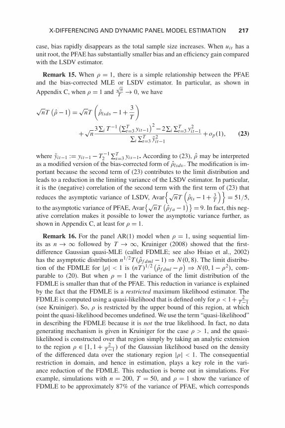
Remark 15. When ρ = 1, there is a simple relationship between the PFAEand the bias-corrected MLE or LSDV estimator. In particular, as shown in

Appendix C, when ρ = 1 and√

nT → 0, we have

√nT

(ρ −1

) = √nT

(ρlsdv −1+ 3

T

)

+√n

3∑i T −1(∑T

t=3 yit−1)2 −2∑i ∑T

t=3 y2i t−1

∑i ∑Tt=3 y2

i t−1

+op(1), (23)

where yi t−1 := yit−1 − T −12 ∑T

s=3 yis−1. According to (23), ρ may be interpretedas a modified version of the bias-corrected form of ρlsdv . The modification is im-portant because the second term of (23) contributes to the limit distribution andleads to a reduction in the limiting variance of the LSDV estimator. In particular,it is the (negative) correlation of the second term with the first term of (23) that

reduces the asymptotic variance of LSDV, Avar{√

nT(ρls −1+ 3

T

)}= 51/5,

to the asymptotic variance of PFAE, Avar{√

nT(ρ f a −1

)} = 9. In fact, this neg-ative correlation makes it possible to lower the asymptotic variance further, asshown in Appendix C, at least for ρ = 1.

Remark 16. For the panel AR(1) model when ρ = 1, using sequential lim-its as n → ∞ followed by T → ∞, Kruiniger (2008) showed that the first-difference Gaussian quasi-MLE (called FDMLE; see also Hsiao et al., 2002)has the asymptotic distribution n1/2T (ρ f dml − 1) ⇒ N (0,8). The limit distribu-tion of the FDMLE for |ρ| < 1 is (nT )1/2

(ρ f dml −ρ

) ⇒ N (0,1 − ρ2), com-parable to (20). But when ρ = 1 the variance of the limit distribution of theFDMLE is smaller than that of the PFAE. This reduction in variance is explainedby the fact that the FDMLE is a restricted maximum likelihood estimator. TheFDMLE is computed using a quasi-likelihood that is defined only for ρ < 1+ 2

T −1(see Kruiniger). So, ρ is restricted by the upper bound of this region, at whichpoint the quasi-likelihood becomes undefined. We use the term “quasi-likelihood”in describing the FDMLE because it is not the true likelihood. In fact, no datagenerating mechanism is given in Kruiniger for the case ρ > 1, and the quasi-likelihood is constructed over that region simply by taking an analytic extensionto the region ρ ∈ [1,1 + 2

T −1 ) of the Gaussian likelihood based on the densityof the differenced data over the stationary region |ρ| < 1. The consequentialrestriction in domain, and hence in estimation, plays a key role in the vari-ance reduction of the FDMLE. This reduction is borne out in simulations. Forexample, simulations with n = 200, T = 50, and ρ = 1 show the variance ofFDMLE to be approximately 87% of the variance of PFAE, which corresponds


well with the limit theory variance ratio of 8/9 � 88.9%. Also, in view of thesingularity in the quasi-likelihood at the upper limit of the domain of definition,numerical maximization of the log-likelihood frequently encounters convergencedifficulties in the computation of the FDMLE. Numerical optimization can failif ρ � 1 and n is not large. For example, in simulations with n = 10, T = 50,and ρ = 1, we found that a total 32 out of 1,000 iterations failed to convergeto a local optimizer. These restricted domain and convergence issues associ-ated with the FDMLE procedure are discussed more fully in separate work(Han and Phillips, 2013).

Remark 17. Asymptotics for the FDMLE procedure are developed inKruiniger (2008) only for the panel AR(1) model, and computation is much moredifficult in the case of the panel AR(p) model. These limitations make it desir-able to have asimple unrestricted estimator like PFAE with good finite sampleand asymptotic properties that can be easily implemented in general panel AR(p)models.

Remark 18. In the unit root case with ρ = 1, the limit distribution (21) holdsfor both n,T → ∞, but no condition is required on the n/T ratio. For n = 1, weknow from the results in HPS (2011) that the (time series) MLE based on levelsis not efficient, and that remains true even when we bias correct the MLE. In fact,as shown in HPS (2011), the FAE is superior to the MLE in the whole vicinityof unity when n = 1. So, we can at least conclude that the PFAE is superior tothe MLE for n = 1. We expect but do not prove that this conclusion holds for allfixed n.

The limit theory for the (restricted domain) FDMLE estimator at ρ = 1indicates that there may be scope for improving estimation efficiency at ρ = 1and possibly in the immediate neighborhood of unity. This issue is complex and,as indicated earlier, there is currently no general optimal estimation theory thatcan be applied to study this problem. In Appendix C we prove that a small mod-ification to the PFAE procedure can indeed reduce variance for the case ρ = 1.The modification is of some independent interest because it makes use of therelationship (23) between PFAE and the bias-corrected LSDV estimator of Hahnand Kuersteiner (2002). In particular, in the simple panel AR(1) model (1), themodified estimator is obtained by taking the linear combination for some scalarweight γ ,

ρ+ = γρ + (1−γ )(ρlsdv + 3T ) = ρ − (1−γ )(ρ − ρlsdv − 3

T ), (24)

so that the centered and scaled estimator has the form

n1/2T (ρ+ −1) = n1/2T (ρlsdv −1+ 3T )+n1/2T γ (ρ − ρlsdv − 3

T ). (25)

The PFAE corresponds to γ = 1. In this case, the (negative) correlation of thesecond term with the first term of (25) reduces the asymptotic variance of


n1/2T (ρlsdv − 1 + 3/T ), which is 51/5, down to the asymptotic variance ofn1/2T (ρ −1), which is 9, as discussed in Remark 15 above. The variance can belowered further by choosing an optimal γ . According to the calculations shown inAppendix C, γ = 5/8 gives n1/2T (ρ+ −1) ⇒ N (0,8.325), which is the minimalvariance attainable by adjusting γ in the relationship (25).

The modified estimator ρ+ can also be understood as a GMM estimator basedon the two moment conditions Eg1i (ρ) = 0 and Eg2i (ρ) → 0 at ρ = 1, whereg1i (ρ) identifies ρ and g2i (ρ) identifies ρlsdv + 3

T , i.e.,

g1i (ρ) = 1

T 32

T

∑t=4

t−3

∑s=1

(yit−1 − ys+1)[(yit − yis)−ρ(yit−1 − yis+1)

],

g2i (ρ) = 1

T 22

T

∑t=3

yi t−1

[yi t −

(ρ − 3

T

)yi t−1

],

with yi t−1 = yit−1 − T −12 ∑T

s=3 yis−1, yi t = yit − T −12 ∑T

s=3 yis , and T2 = T − 2.Note that the first observations are ignored in g2i (ρ) for algebraic simplicity, andtheir effect is asymptotically negligible when T → ∞. In view of the identity (seeHPS, 2011)

1

T2

T

∑t=4

t−3

∑s=1

(yit−1 − yis+1)2 =

T

∑t=3

y2i t−1,

any weighted GMM estimator can be expressed in the form γ ρ+(1−γ )(ρls + 3T )

for some γ , thereby leading back to the original formulation (24).The modified PFAE ρ+ with γ = 5/8 attains an efficiency level of 8/8.325 =

0.96096 (i.e., 96% efficiency) relative to the restricted FDMLE. However, thisargument cannot be used for general ρ values, because ρlsdv + 3

T does not correctthe bias if |ρ| < 1 unless n/T → 0. This is evident from the fact that

√nT

(ρlsdv + 3

T −ρ)

= √nT

(ρhk −ρ

)+√

nT

T +1

(2+ 3

T− ρhk

),

where ρhk is the bias-corrected estimator proposed by Hahn and Kuersteiner(2002, p. 1645) for the stationary case, i.e., ρhk = T +1

T ρlsdv + 1T such that

(nT )1/2(ρhk −ρ) ⇒ N (0,1−ρ2) when |ρ| < 1 and limn/T ∈ (0,∞). Of course,when n/T → 0 we also have

√nT (ρlsdv + 3

T −ρ) = √nT (ρlsdv −ρ)+ op (1) ,

so in this event the bias is small because T → ∞ so fast.To close this section, we now discuss some remaining practical issues involved

in modeling and the use of X-differencing. First, practical applications often callfor data determination of the lag length in the autoregression. Consistent panel in-formation criteria may be constructed or a general-to-specific modeling algorithmcan be used for this purpose. One such possibility is considered in HPS (2010).See also Lee (2010b).


Next, the moment conditions used in (7) require that �uit is stationary over t.So, when the innovations are temporally heteroskedastic or there are nonstation-ary initial conditions, the PFAE may be inconsistent. For example, for the panelAR(1) with T = 4, from (A.7) in Appendix A we find that

plimn→∞

ρ = ρ − (1/2)ρ(1−ρ)[σ 22 − (1−ρ2)ω2

1]

plimn−1 ∑ni=1 ∑T

t=3 y2i t−1

,

where yi t−1 = yit−1 −T −12 ∑T

s=3 yis−1 as before. Thus, if ρ is moderate (� 12 ) and

temporal heteroskedasticity is so severe that σ 22 − (1 − ρ2)ω2

1 is huge, then thePFAE may be more biased than the LSDV estimator.

Finally, extension to models with explanatory variables is straightforward ifthey appear as in yit = αi + β ′ Xit + uit with uit = ∑p

j=1 ρj uit− j + εi t . Forthis model the persistence parameters ρj can be identified by X-differencingfor given β, while the slope parameter β satisfies the usual orthogonality con-ditions if E[Xisuit ] = 0 for relevant s and t . A two-step procedure can thenbe used, effectively generalizing Bhargava et al.’s (1982) feasible GLS proce-dure to the panel AR(p) if Xit is strictly exogenous. On the other hand, it isunclear if and how we can derive moment conditions for the dynamic modelyit = αi + β ′ Xit + ∑p

j=1 ρj yi t− j + εi t . This important topic is left for futureresearch.

5. SIMULATIONS

This section reports simulations that shed light on the finite sample propertiesof our procedures in relation to existing methods of dynamic panel estimation.In particular, we compare the PFAE procedure with existing estimators such asArellano and Bond’s (1991) difference GMM estimator and Blundell and Bond’s(1998) system GMM estimator for a panel AR(2) model. (The FDMLE methodis not included because of computational difficulties with this procedure and thefact that it is a restricted estimator, as discussed earlier.) We then consider pan-els with nonstationary initial conditions to examine the effect of departures fromstationarity.

I. Comparison of bias and efficiency: AR(1)We first compare the properties of the PFAE with the LSDV estimator (whichis inconsistent), Hahn and Kuersteiner’s (2002) bias-corrected LSDV estimator(HK), the one-step first-difference GMM (GMM1/DIF), and the two-step systemGMM (GMM2/SYS), for the panel AR(1) model. The model is yit = ai + uit ,uit = ρuit−1 + εi t , where εi t is i.i.d. standard normal variables and ai is alsonormal with E(ai ) arbitrarily set to 2. When generating the data, the processesare initialized at t = −100 such that ui,−100 := 0, and then observations for t ≤ 0are discarded. The normal variates are generated using the rnormal function ofStata. The difference GMM and the system GMM are estimated by the “xtabond”and the “xtdpdsys” commands of Stata, respectively, and the PFAE is obtained


by direct calculation using formula (16). We consider n = 100 and T = 4,10,20,where T = 4 is the smallest time dimension that allows for the X-differencingestimation, while the other estimators (LSDV, HK, GMM estimators) are alsocalculable for T = 3.

Table 1 reports the simulated means of the estimators from 1,000 replications.The LSDV estimator is obviously biased downward, as per Nickell (1981). The(small sample) biases of the first-difference and system GMM estimators dependon the distribution of αi . On the other hand, PFAE shows very little bias for allparameter values and is considerably superior to HK (2002).

Table 1 also presents simulated variances of the estimators. When T is small(T = 4 and T = 10), PFAE is less efficient than the bias-corrected LSDV estima-tor (HK, 2002), but when T is larger (T = 20) and ρ is large (ρ = 0.7, 0.9, and 1 inour simulation), PFAE is as efficient or more efficient than HK. The inefficiency ofPFAE relative to HK for T = 4 is due to the smaller degrees of freedom of PFAE,but it is also notable that the MSE is considerably smaller for PFAE for all ρ andfor all T , including T = 4. With larger T values, PFAE attains the asymptotic vari-ance (nT )−1(1−ρ2), as does the HK estimator. For T = 20, we notice that PFAEappears less efficient than LSDV at ρ = 1, which looks contrary to the asymptoticfindings that n1/2T (ρlsdv − 3/T ) ⇒ N (0,51/5) and n1/2T (ρ f a − 1) ⇒ N (0,9)with ρlsdv and ρ f a , respectively, denoting the LSDV and PFAE estimators. Thisoutcome occurs because T = 20 is not large enough for the asymptotics to be ac-curate enough for the distinction to manifest. For ρ = 1, the asymptotic varianceof ρ f a is 9/n(T − 2)2, which is approximately 0.277 × 10−3 with n = 100 andT = 20. This theoretical value is close to the simulated variance 0.273 × 10−3.As T increases further, so that T 2/(T − 2)2 is close to 1 and the asymptotics forthe PFAE are sufficiently accurate, we expect the higher asymptotic efficiency ofPFAE relative to LSDV to become evident in simulations. Table 2 reveals that thisexpected improvement occurs for T ≥ 80 for all values of n.

The performance of the GMM estimators differs as sd(ai ) changes. ComparingPFAE and GMM, PFAE performs uniformly better than the GMM estimators in

TABLE 2. 103×Variance of LSDV and PFAE for AR(1) with ρ = 1, 10,000 repli-cations, yit = yit−1 + εi t , εi t ∼ i id N (0,1)

n = 50 n = 100 n = 200

T LSDV PFAE LSDV PFAE LSDV PFAE

20 0.4910 0.5526 0.2448 0.2769 0.1231 0.139240 0.1246 0.1252 0.0638 0.0643 0.0310 0.031980 0.0328 0.0305 0.0159 0.0153 0.0078 0.0073160 0.0080 0.0074 0.0040 0.0036 0.0020 0.0018

Note: The LSDV estimator is unbiased for 1 − 3/T . The slight disparity between Tables 1 and 2 for n = 100 andT = 20 is ascribed to the fact that Stata is used for one table and Gauss for the other, the generated samples aredifferent, and the replication numbers are different.


our simulations except for ρ = 1 with T = 10. It is, however, worth noting that theGMM estimators are based on moment conditions different from those used byPFAE and LSDV, and that the performance of the GMM estimators also dependson the initial cross-sectional variance of the idiosyncratic errors.

It would also be worth comparing the performance of the PFAE and the indirectinference (II) procedure (Gourieroux, Phillips, and Yu, 2010). Some comparisonsin the time series case were undertaken in HPS (2011)—both estimators havenegligible bias, but II has smaller variance in the unit root case. For the panelmodel, interested readers are referred to Gourieroux et al.’s Table 2, though cau-tion is needed in this comparison because the sizes of T do not exactly match thoseused here and the generated samples are different. Looking at these results in thepanel case, it appears that both II and PFAE have negligible bias and II has smallervariance. A full comparison between the two procedures is not yet possible,because the limit theory for panel II is not yet available in unit root and near unitroot cases. This limit theory has only recently been obtained for the time seriesmodel (Phillips, 2012), and the panel extension is left for a subsequent contri-bution. Similarly, extensions to mildly explosive cases (Phillips and Magdalinos,2007) are left to future work.

II. Comparison of bias and efficiency: AR(2)We next consider an AR(2) dynamic panel model (i.e., yit = ai + uit , uit =ρ1uit−1 + ρ2uit−2 + εi t ). Except for uit being AR(2), all other settings are thesame as in the previous simulation. We set ρ2 = −0.2, and ρ1 = 0.2,0.5,0.7,0.9,1.1, and 1.2. The panels are stationary when ρ1 < 1.2 and are integrated whenρ1 = 1.2.

Table 3 reports the simulated means and variances of the estimates of ρ1. Hahn

TABLE 3. Simulation for ρ1 from AR(2), 1000 replications, n = 100, yit =ai (1 − ρ1 − ρ2) + ρ1 yit−1 + ρ2 yit−2 + εi t , ρ2 = −0.2, ai ∼ N (2,σ 2

a ), εi t ∼i id N (0,1)

Bias

σa = 1 σa = 3

GMM1 GMM2 GMM1 GMM2ρ1 T LSDV HK DIF SYS DIF SYS PFAE

5 −0.3929 −0.1994 −0.0358 0.0082 −0.0676 0.1559 −0.00150.2 10 −0.1135 −0.0255 −0.0199 0.0033 −0.0241 0.0976 0.0000

20 −0.0476 −0.0056 −0.0126 −0.0002 −0.0133 0.0825 −0.00075 −0.4552 −0.2452 −0.0407 −0.0067 −0.0969 0.0865 −0.0012

0.5 10 −0.1252 −0.0369 −0.0238 −0.0020 −0.0316 0.0601 −0.001020 −0.0500 −0.0080 −0.0147 −0.0081 −0.0161 0.0428 −0.0009



TABLE 3. continued

Bias

σa = 1 σa = 3


5 −0.5102 −0.2843 −0.0446 −0.0149 −0.1251 0.0411 −0.00120.7 10 −0.1404 −0.0515 −0.0275 −0.0057 −0.0413 0.0380 −0.0015

20 −0.0531 −0.0110 −0.0171 −0.0125 −0.0199 0.0193 −0.00105 −0.5813 −0.3340 −0.0531 −0.0201 −0.1637 0.0025 −0.0006

0.9 10 −0.1704 −0.0800 −0.0348 −0.0105 −0.0626 0.0136 −0.001720 −0.0599 −0.0178 −0.0211 −0.0172 −0.0280 −0.0020 −0.0011

5 −0.6764 −0.3997 −0.1172 −0.0252 −0.2525 −0.0237 0.00021.1 10 −0.2362 −0.1407 −0.0676 −0.0188 −0.1166 −0.0162 −0.0021

20 −0.0853 −0.0425 −0.0355 −0.0250 −0.0533 −0.0271 −0.00125 −0.7371 −0.4414 −0.8647 −0.0139 −0.8791 −0.0137 −0.0002

1.2 10 −0.2990 −0.1978 −0.4500 −0.0075 −0.4494 −0.0075 −0.002320 −0.1341 −0.0896 −0.2215 −0.0233 −0.2217 −0.0226 −0.0016

Variance×103

σa = 1 σa = 3


5 4.435 6.960 22.874 10.249 50.301 27.440 8.7260.2 10 1.481 1.489 2.537 2.095 2.897 4.858 1.444

20 0.546 0.540 0.707 0.751 0.738 1.504 0.5175 4.856 7.516 28.359 9.722 73.099 19.188 8.645

0.5 10 1.576 1.519 2.675 2.149 3.314 3.319 1.40120 0.562 0.545 0.712 0.758 0.762 1.024 0.516

5 5.059 7.742 34.362 9.411 98.816 15.715 8.1580.7 10 1.648 1.554 2.854 2.195 3.980 2.909 1.362

20 0.576 0.551 0.716 0.712 0.793 0.863 0.5175 5.161 7.878 46.882 9.156 134.727 13.798 7.753

0.9 10 1.729 1.613 3.223 2.208 5.551 2.751 1.34120 0.600 0.567 0.735 0.711 0.879 0.818 0.521

5 5.149 8.026 112.019 10.432 189.902 13.019 7.8731.1 10 1.777 1.648 5.189 2.260 9.172 2.583 1.396

20 0.650 0.611 0.922 0.779 1.256 0.880 0.5425 5.135 7.968 418.209 8.470 406.491 8.496 8.053

1.2 10 1.713 1.585 32.59 1.818 32.43 1.827 1.47920 0.672 0.632 4.488 0.914 4.530 0.906 0.569

and Kuersteiner’s (2002) estimator is evaluated by applying their Theorem 2to the AR(1) representation of AR(2) rather than their AR(1) correction for-mula, as bias correction based on the misspecified model can exacerbate the bias(Lee, 2010a). The LSDV estimator is again biased downward, and the PFAE ex-hibits very low finite sample bias. The GMM estimator performance depends on


the variance of ai . Again, LSDV, HK (2002), and PFAE are free from the effectsof the ai , while the two GMM estimators are not. The PFAE performs well in allconsidered cases. As remarked in the discussion of the AR(1) simulations, it isnoteworthy that the accuracy of the GMM estimators depends on the variance ofthe initial idiosyncratic errors as well.

III. InferenceWe next investigate the properties of the estimated variance Q−1

Z QV Q−1Z of the

PFAE, where

Q Z =n

∑i=1

T

∑t=p+2

t−p−1

∑s=1

Zi t,s Z ′i t,s and QV =

n

∑i=1

ViT V ′iT ,

with Zi t,s defined right after Lemma 1 and ViT found in (19).Because all the statistics are free from individual effects, we can eliminate ai

from the data generation process. We focus on the panel AR(1) model yit =ρyit−1 + εi t , where εi t ∼ N

(0,σ 2

)with σ 2 = 1. We test (i) H0 : ρ = 0 and

(ii) H0 : ρ = 1. We present test sizes for the null hypothesis that the ρ param-eter is the same as the true parameter used in the data generation. Gauss was usedfor the simulations. We use the tn−1 critical values in testing, as recommended byHansen (2007).

Table 4 reports the empirical sizes from a simulation of 5,000 replications. Ex-cept for a slight over-rejection in small samples with high ρ, size performanceis reasonably good. The simulated powers for the null hypotheses H0 : ρ = 0(left) and H0 : ρ = 1 (right) are presented in Table 5. This part of the simu-lation is intended to be illustrative, as its main purpose is to exhibit generalperformance characteristics of inference with the PFAE procedure. Thoroughcomparisons with other estimators would require a more systematic simulationstudy.

IV. Departures from stationarityFinally, we examine the performance of the PFAE when the stationarity assump-tion is violated. As the example of an AR(1) with T = 4 shows at the endof the previous section, the bias of the PFAE can be made arbitrarily large bycorrespondingly large heterogeneity in the error variances. Various other depar-tures from stationarity are possible, and in this section we consider the case ofnonstationary initial conditions, leaving other departures to separate research.Specifically, the data are generated by yit = ai + uit , uit = ρuit−1 + εi t withεi t ∼ i id N (0,σ 2) as in part I above, but this time we set ui0 ≡ 0 (instead ofui,−100 ≡ 0). We deliberately use this model to make the individual means invari-ant over time.

Table 6 reports simulation results for LSDV, HK (2002), difference GMM, sys-tem GMM, and PFAE. The results are similar to part I, and for this specific datagenerating process (DGP), nonstationarity of uit does not introduce serious bias


TABLE 4. Simulated sizes for AR(1), 5000 replications

ρ, H0 : ρ = truth vs H1 : ρ �= truth

n T 0.0 0.3 0.5 0.7 0.9 1.0

25 10 0.0658 0.0652 0.0656 0.0672 0.0754 0.077025 20 0.0592 0.0628 0.0640 0.0650 0.0666 0.072625 40 0.0534 0.0534 0.0552 0.0572 0.0606 0.071050 10 0.0582 0.0590 0.0642 0.0638 0.0652 0.063050 20 0.0454 0.0468 0.0496 0.0530 0.0566 0.062850 40 0.0530 0.0504 0.0522 0.0540 0.0576 0.0618

100 10 0.0538 0.0520 0.0534 0.0512 0.0540 0.0522100 20 0.0506 0.0532 0.0546 0.0534 0.0514 0.0614100 40 0.0486 0.0510 0.0502 0.0558 0.0562 0.0610200 10 0.0480 0.0498 0.0550 0.0558 0.0530 0.0556200 20 0.0482 0.0502 0.0464 0.0504 0.0518 0.0522200 40 0.0470 0.0498 0.0508 0.0466 0.0512 0.0514

TABLE 5. Simulated power for H0 : ρ = 0,1 for AR(1) model, 5000 replications

ρ, H0 : ρ = 0 vs H1 : ρ �= 0 ρ, H0 : ρ = 1 vs H1 : ρ �= 1

n T 0.000 0.025 0.050 0.075 0.925 0.950 0.975 1.000

25 10 0.0658 0.0742 0.1126 0.1768 0.2234 0.1440 0.0968 0.077025 20 0.0592 0.0874 0.1814 0.3380 0.6018 0.3340 0.1456 0.072625 40 0.0534 0.1214 0.3308 0.6156 0.9898 0.8466 0.3726 0.071050 10 0.0582 0.0790 0.1560 0.2748 0.3274 0.1794 0.0892 0.063050 20 0.0454 0.1134 0.3046 0.5822 0.8866 0.5760 0.2076 0.062850 40 0.0530 0.1796 0.5562 0.8888 1.0000 0.9916 0.5972 0.0618

100 10 0.0538 0.1006 0.2490 0.4826 0.5594 0.2964 0.1204 0.0522100 20 0.0506 0.1838 0.5400 0.8734 0.9948 0.8598 0.3478 0.0614100 40 0.0486 0.3320 0.8642 0.9932 1.0000 1.0000 0.8886 0.0610200 10 0.0480 0.1478 0.4510 0.7910 0.8384 0.4952 0.1688 0.0556200 20 0.0482 0.3108 0.8306 0.9916 1.0000 0.9936 0.5866 0.0522200 40 0.0470 0.5724 0.9866 1.0000 1.0000 1.0000 0.9964 0.0514

to PFAE, but we still observe slightly more bias for moderate ρ values comparedwith part I. If the mean of yit changes over t or if heteroskedasticity is wilder,then the X-difference estimators may be more biased than GMM estimators thatdo not depend on the stationarity of yit (or �yit ).


TABLE 6. Simulation for nonstationary initial conditions, 1000 replications,n = 100, yit = ai + uit , uit = ρuit−1 + εi t , ui0 ≡ 0, ai ∼ N (2,σ 2

a ), εi t ∼iid N (0,1)

Bias

σa = 1 σa = 3


4 −0.3343 −0.1124 −0.0098 0.0078 −0.0161 0.0488 −0.00260.0 10 −0.1118 −0.0132 −0.0124 0.0024 −0.0138 0.0510 −0.0008

20 −0.0525 −0.0027 −0.0117 0.0016 −0.0125 0.0574 0.00014 −0.4668 −0.1891 −0.0180 0.0013 −0.0370 0.0483 −0.0146

0.3 10 −0.1536 −0.0262 −0.0206 −0.0006 −0.0248 0.0429 −0.005320 −0.0704 −0.0057 −0.0173 −0.0059 −0.0191 0.0401 −0.0018

4 −0.5730 −0.2640 −0.0289 −0.0086 −0.0690 0.0206 −0.04950.5 10 −0.1900 −0.0445 −0.0291 −0.0045 −0.0371 0.0317 −0.0187

20 −0.0847 −0.0102 −0.0223 −0.0117 −0.0255 0.0226 −0.00774 −0.6808 −0.3411 −0.0636 −0.0083 −0.1703 −0.0122 −0.0919

0.7 10 −0.2418 −0.0798 −0.0465 −0.0115 −0.0601 0.0125 −0.046220 −0.1047 −0.0208 −0.0298 −0.0191 −0.0350 0.0011 −0.0210

4 −0.7496 −0.3661 −0.5086 −0.0013 −0.6422 −0.0102 −0.07120.9 10 −0.3057 −0.1286 −0.1553 −0.0170 −0.1798 −0.0123 −0.0596

20 −0.1447 −0.0523 −0.0639 −0.0359 −0.0706 −0.0293 −0.03954 −0.7509 −0.3345 −0.8673 0.0006 −0.8833 −0.0031 0.0012

1.0 10 −0.3026 −0.1140 −0.4405 −0.0131 −0.4376 −0.0133 −0.001920 −0.1508 −0.0535 −0.2235 −0.0452 −0.2227 −0.0441 −0.0005

Variance×103

σa = 1 σa = 3


4 3.216 5.718 14.163 9.564 29.605 20.622 9.9410.0 10 1.127 1.403 2.052 1.925 2.295 3.317 1.480

20 0.524 0.581 0.730 0.832 0.772 1.642 0.5864 4.017 7.141 24.831 12.427 63.064 22.796 12.381

0.3 10 1.225 1.513 2.671 2.252 3.181 3.193 1.59620 0.527 0.584 0.818 0.939 0.895 1.400 0.590

4 4.501 8.001 42.910 12.484 106.775 20.574 13.7480.5 10 1.216 1.502 3.171 2.424 4.018 3.132 1.543

20 0.488 0.541 0.831 0.932 0.941 1.245 0.5374 4.871 8.659 125.308 9.721 231.386 16.084 15.377

0.7 10 1.155 1.436 4.117 2.253 5.398 2.889 1.42320 0.417 0.462 0.826 0.854 0.963 1.005 0.442



TABLE 6. continued

Variance×103

σa = 1 σa = 3


4 5.152 9.159 628.131 5.326 796.382 7.974 18.1290.9 10 1.038 1.281 11.234 1.447 13.137 1.672 1.335

20 0.319 0.354 1.246 0.938 1.357 0.900 0.3174 5.240 9.316 677.739 3.828 811.331 4.656 20.125

1.0 10 0.926 1.143 28.754 0.737 28.130 0.766 1.33620 0.239 0.265 4.142 0.739 3.989 0.771 0.268

* HK = LSDV× T/(T −1)+1/(T −1)

6. CONCLUSION

The estimation method introduced in this paper for linear dynamic panel modelsuses a new differencing procedure called X-differencing to eliminate fixed effectsand a simple technique of stacked and pooled least squares on the full system ofX-differenced equations. The method is therefore straightforward to implementin practical work. It is also free from bias for all parameter values and avoidsweak instrumentation problems in unit root and near unit root cases. The asymp-totic theory shows gains in efficiency in the unit root case over bias-correctedmaximum likelihood and equivalent efficiency in the stationary case, but the newmethod has no need for bias correction. The asymptotics also apply irrespectiveof the n/T ratio as n,T → ∞. These advantages make the new estimation proce-dure attractive for empirical research, especially in cases of data persistence anddispersed individual effects where other methods can perform poorly.

The findings of the present paper point the way to further research. First, thereis a need for a theory of optimal estimation in panel models that allows for rootsin the vicinity of unity and dual index asymptotics. While there is, as yet, nooptimal estimation theory in time series autoregression that includes the unit rootcase, the process of cross section averaging in panel estimation leads to importantsimplifications in the limit theory that make such an optimality theory feasible. Inparticular, the limit theory belongs to an asymptotically normal (as distinct from anonstandard distribution) family when n → ∞. But the limit distribution can alsobe degenerate with a singularity in the covariance structure and a change in theconvergence rate when there is an autoregressive unit root. These features of thelimit theory and their impact on optimality in estimation deserve detailed study.As indicated earlier, there is also scope for further work on model selection indynamic panels, including an extensive numerical study of sequential testing rulesand a further analysis of the asymptotic behavior of various information criteria.


Second, consistent estimation of panel autoregressions using X-differencingand PFAE methods is useful in the estimation of more general panel models withadditional regressors. For example, in parametric models with exogenous regres-sors and AR(p) errors such as yit = ai +β ′xit +uit , with uit = ∑p

j=1 ρj uit− j +εi t ,we can consistently estimate ρ = (ρ1, . . . ,ρp)

′ using PFAE and residuals based ona preliminary consistent estimate of β. Then, a parametric feasible GLS estimatecan be conducted as a natural extension of Bhargava et al.’s (1982) treatment ofthe AR(1). Such stepwise estimation of β and ρ may be iterated until conver-gence, combining moment conditions for β based on assumed exogeneity of xit

and the moment conditions implied by Lemma 1 using yit −β ′xit for given β.Finally, as noted above, the consistency of X-difference estimators relies on

the stationarity of uit (or �uit if uit is integrated) over t . As a result, whenthe variance of the innovations varies over time or there are nonstationary initialconditions, the X-difference estimators may not be consistent. While important,these issues introduce new complications that have not been addressed properlyunder the fixed effects environment. Full exploration of them is left for futureresearch.

NOTES

1. Stationary initialization in the infinite past for |ρ| < 1 is also assumed in levels GMM (Arellanoand Bover, 1995; Blundell and Bond, 1998) and is more restrictive than error serial uncorrelatedness,which is assumed by Anderson and Hsiao (1981, 1982) and Arellano and Bond (1991). Hahn (1999)discusses how assumptions about initial conditions may affect efficiency.

2. For instance, the finite sample variance of the first-difference GMM estimator in the stationarycase increases rather than decreases as ρ increases (see Alvarez and Arellano, 2003; Hayakawa, 2008)in contrast to the prediction of asymptotic theory.

REFERENCES

Ahn, S.C. & P. Schmidt (1995) Efficient estimation of models for dynamic panel data. Journal ofEconometrics 68, 5–27.

Alvarez, J. & M. Arellano (2003) The time series and cross-section asymptotics of dynamic panel dataestimators. Econometrica 71(4), 1121–1159.

Anderson, T.W. & C. Hsiao (1981) Estimation of dynamic models with error components. Journal ofAmerican Statistical Association 76, 598–606.

Anderson, T.W. & C. Hsiao (1982) Formulation and estimation of dynamic models using panel data.Journal of Economics 18, 47–82.

Arellano, M. (1987) Computing robust standard errors for within-groups estimators. Oxford Bulletinof Economics and Statistics 19, 431–434.

Arellano, M. & S. Bond (1991) Some tests of specification for panel data: Monte Carlo evidence andan application to employment equations. Review of Economic Studies 58, 277–297.

Arellano, M. & O. Bover (1995) Another look at the instrumental variable estimation of error-components models. Journal of Econometrics 68, 29–51.

Bauer, P., B.M. Potscher, & P. Hackl (1988) Model selection by multiple test procedures. Statistics 19,39–44.

Bertrand, M., E. Duflo, & S. Mullainathan (2004) How much should we trust differences-in-differences estimates? Quarterly Journal of Economics 249–275.


Bhargava, A., L. Franzini, & W. Narendranathan (1982) Serial correlation and the fixed effects model.Review of Economic Studies 49(4), 533–549.

Blundell, R. & S. Bond (1998) Initial conditions and moment restrictions in dynamic panel datamodels. Journal of Econometrics 87, 115–143.

Davidson, J. (1994) Stochastic Limit Theory. Oxford University Press.Gourieroux, C., P.C.B. Phillips, & J. Yu (2010) Indirect inference for dynamic panel models. Journal

of Econometrics 157, 68–77.Hahn, J. (1999) How informative is the initial condition in the dynamic panel model with fixed effects?

Journal of Econometrics 93, 309–326.Hahn, J., J. Hausman, & G. Kuersteiner (2007) Long difference instrumental variables estimation for

dynamic panel models with fixed effects. Journal of Econometrics 140(2), 574–617.Hahn, J. & G. Kuersteiner (2002) Asymptotically unbiased inference for a dynamic panel model with

fixed effects when both N and T are large. Econometrica 70(4), 1639–1657.Hajek, J. (1972) Local asymptotic minimax and admissibility in estimation. In L.M. Lecam,

J. Neyman, & E.L. Scott (eds.), Proceedings of Sixth Berkeley Symposium in Mathematical Statis-tics and Probability Vol. 1, 175–194.

Han, C. & P.C.B. Phillips (2006) GMM with many moment conditions. Econometrica 74, 147–192.Han, C. & P.C.B. Phillips (2010) GMM estimation for dynamic panels with fixed effects and strong

instruments at unity. Econometric Theory 26, 119–151.Han, C., P.C.B. Phillips, & D. Sul (2010) X-Differencing and Dynamic Panel Model Estimation.

Cowles Foundation Discussion Papers 1747, Yale University.Han, C., P.C.B. Phillips, & D. Sul (2011) Uniform asymptotic normality in stationary and unit root

autoregression. Econometric Theory 27(6), 1117–1151.Han, C. & P.C.B. Phillips (2013) First Difference MLE and Dynamic Panel Estimation. Journal of

Econometrics, 175, 35–45.Hansen, C.B. (2007) Asymptotic properties of a robust variance matrix estimator for panel data

when T is large. Journal of Econometrics 141, 597–620.Hayakawa, K. (2007) A Simple Efficient Instrumental Variable Estimator in Panel AR(p) Models.

Hi-Stat Discussion Paper Series d07-213, Institute of Economic Research, Hitotsubashi University.Hsiao, C., M.H. Pesaran, & A.K. Tahmiscioglu (2002) Maximum likelihood estimation of fixed effects

dynamic panel data models covering short time periods. Journal of Econometrics 109, 107–150.Imbs, J., H. Mumtaz, M.O. Ravn, & H. Rey (2005) PPP strikes back: Aggregation and the real

exchange rate. Quarterly Journal of Economics120, 1–43.Jeganathan, P. (1995) Some aspects of asymptotic theory with applications to time series models.

Econometric Theory 11, 818–867.Keane, M., & D. Runkle (1992) On the estimation of panel-data models with serial-correlation when

instruments are not strictly exogenous. Journal of Business & Economic Statistics 10(1), 1–9.Kezdi, G. (2002) Robust Standard Error Estimation in Fixed-Effects Panel Models. Working Paper,

University of Michigan.Kiefer, N.M. (1980) Estimation of fixed effect models for time series of cross section with arbitrary

intertemporal covariance. Journal of Econometrics 14, 195–202.Kiviet, J.F. (1995) On bias, inconsistency, and efficiency of various estimators in dynamic panel data

models. Journal of Econometrics 68, 53–78.Kruiniger, H. (2008) Maximum likelihood estimation and inference methods for the covariance

stationary panel AR(1)/unit root model. Journal of Econometrics 144, 447–464.LeCam, L. (1972) Limits of experiments. In L.M. LeCam, J. Neyman, & E.L. Scott (eds.), Proceedings

of the Sixth Berkeley Symposium in Mathematical Statistics and Probability, vol. 1, 245–261.Lee, Y. (2010a) Bias in Dynamic Panel Models under Time Series Misspecification. Unpublished

manuscript, University of Michigan.Lee, Y. (2010b) Model Selection in the Presence of Incidental Parameters. Unpublished manuscript,

University of Michigan.


Nickell, S. (1981) Biases in dynamic models with fixed effects. Econometrica 49, 1417–1426.Orcutt, G.H. & H.S. Winokur (1969) First order autoregression: Inference, estimation and prediction.

Econometrica 37, 1–14.Park, J.Y. & P.C.B. Phillips (1988) Statistical inference in regressions with integrated processes: Part 2.

Econometric Theory 5, 95–131.Phillips, P.C.B. (1987) Time series regression with a unit root. Econometrica 55, 277–301.Phillips, P.C.B. (1989) Partially identified econometric models. Econometric Theory 5, 181–240.Phillips, P.C.B. (2012) Folklore theorems, implicit maps, and indirect inference. Econometrica 80,

425–454.Phillips, P.C.B. & C. Han (2008) Gaussian inference in AR(1) time series with or without unit root.

Econometric Theory 24, 631–650.Phillips, P.C.B. & T. Magdalinos (2007) Limit theory for moderate deviations from a unit root. Journal

of Econometrics 136, 115–130.Phillips, P.C.B. & T. Magdalinos (2009) Unit root and cointegrating limit theory when initialization is

in the infinite past. Econometric Theory 25, 1682–1715.Phillips, P.C.B. & H.R. Moon (1999) Linear regression limit theory for nonstationary panel data.

Econometrica 67(5), 1057–1111.Phillips, P.C.B. & W. Ploberger (1994) Posterior odds for testing for a unit root with data-based model

selection. Econometric Theory 10, 774–808.Phillips, P.C.B. & V. Solo (1992) Asymptotics for linear processes. Annals of Statistics 20(2),

971–1001.Potscher, B.M. (1983) Order estimation in ARMA-models by Lagrangian multiplier tests. Annals of

Statistics 11, 872–885.Qian, H. & P. Schmidt (2003) Partial GLS regression. Economics Letters 79, 385–392.White, H. (1980) A heteroskedasticity-consistent covariance matrix and a direct test for heteroskedas-

ticity. Econometrica 48, 817–838.Wooldridge, J.M. (2002) Econometric Analysis of Cross Section and Panel Data. MIT Press.

APPENDIX A: Technical Results and Proofs

Proof of (4). Because ε∗is = yis −αi −ρ1 yis+1, we have

Eyis+1ε∗is = Eyis+1 yis −Eyis+1αi −ρ1Ey2

is+1.

Replacing the first yis+1 on the right-hand side with αi +ρ1 yis + εis+1, we get

Eyis+1ε∗is = Eyisαi +ρ1Ey2

is −Eyis+1αi −ρ1Ey2is+1.

Because Eyitαi is the same for all t and Ey2is = Ey2

is+1, we have Eyis+1ε∗is = 0. n

Proof of (7). It is simpler to work with uit = yit − ai , where uit = ρ1uit−1 + εi t . Weshall show that A := E(uit−1 −uis+1)(εi t − ε∗

is) = 0. For s +1 < t , we have

A = E(uit−1 −uis+1)εi t −E(uit−1 −uis+1)(uis −ρ1uis+1)

= −E(uit−1 −uis+1)(uis −ρ1uis+1)

= −Euit−1uis +ρ1Euit−1uis+1 +Euisuis+1 −ρ1Eu2is+1

= −ρ1Euit−2uis +ρ1Euit−1uis+1 +ρ1Eu2is −ρ1Eu2

is+1,


where the last equality is derived by expanding uit−1 = ρ1uit−2 + εi t−1 and uis+1 =ρ1uis + εis+1. When |ρ1| < 1, uit is stationary, so A is obviously zero. If ρ1 = 1, thenEuit uis = Eu2

is for s ≤ t , so when s ≤ t −2, we have

A = −ρ1Eu2is +ρ1Eu2

is+1 +ρ1Eu2is −ρ1Eu2

is+1 = 0

as claimed. n

We prove Lemma 1 using uit = yit −ai . Note that uit = ∑pj=1 ρj ui t− j + εi t where εi t

is white noise(

0,σ 2i

). We also have ε∗

is = uis − ∑pj=1 ρj uis+ j . We first establish the

following general lemma.

LEMMA 4. Let uit be a panel AR(p) process such that �muit is stationary AR(p −m)for some nonnegative integer m ≤ p, where � := 1 − L . Then, for all t and s such thatt > s, Eε∗

is−m�muit = 0.

Proof. First, consider the case where uit is covariance stationary AR(p), i.e., m = 0. Letγj = Euit uit− j /σ

2i . Let ρ(L) = 1−ρ1L −·· ·−ρp L p . We have

Euitε∗is = Euit

(uis −

p

∑j=1

ρj uis+ j

)= σ 2

i

(γt−s −

p

∑j=1

ρj γt−s− j

)= 0

by the Yule-Walker equations when t > s as claimed. Now, for general m ≤ p, wehave ρ(L) = (1 − L)mρ∗(L), where ρ∗(L) = 1 −ρ∗

1 L −·· ·−ρ∗p−m L p−m and the roots

of ρ∗(L) = 0 are outside the unit circle. First note that ε∗is = ρ

(L−1)

uis , so using

(1− L−1)muis−m = (−1)m(1− L)muis and � := 1− L , we have

ε∗is−m = ρ∗(

L−1)(1− L−1)muis−m = (−1)mρ∗(

L−1)�muis =: ε∗

is .

That is, ρ∗(L−1)

uis = (−1)m ε∗is , where uis = �muis . Furthermore, ui t is station-

ary AR(p − m) by assumption, and by the result for the stationary case, we haveE(−1)m ε∗

is ui t = 0 for all s < t . The result follows by writing ε∗is = ε∗

is−m and ui t =�muit . n

Lemma 1 is now straightforward.

Proof of Lemma 1. Because uit − uis = yit − yis for all s and t , we shall prove thatE(uit−k −uis+k)(εi t −ε∗

is) = 0 for all s < t − p. Because E(uit−k −uis+k)εi t = 0 for alls ≤ t − p − 1 and 1 ≤ k ≤ p, it suffices to show that E(uit−k − uis+k)ε∗

is = 0 for such sand k. If uit is stationary AR(p), then this holds because of Lemma 4 with m = 0. If uit isI (1) and �uit is stationary AR(p −1), we have Eε∗

is�uir = 0 for all r ≥ s +2 by Lemma4. But,

yit−k − yis+k = uit−k −uis+k =t−k

∑r=s+k+1

�uir −s+k

∑r=t−k+1

�uir ,

where r ≥ s + k + 1 implies r ≥ s + 2 (because k ≥ 1) and r ≥ t − k + 1 implies r ≥t − p +1 ≥ s +2 (because k ≤ p and t ≥ s + p +1). In both cases, Eε∗

is�uir = 0 and theresult follows. n


Next, we prove Theorem 2.We first introduce some useful notation and transformations that facilitate analysis of

the unit root case.Let ViT = 1

T ∑Tt=p+2 ∑t−p−1

s=1 Zi t,s Z ′i t,s and ηiT = 1

T ∑Tt=p+2 ∑t−p−1

s=1 Zi t,s εi t,s ,

where Zi t,s and εi t,s are defined in (14). Define the p × p transformation matrix F and itsinverse F−1 as

F =

⎡⎢⎢⎢⎢⎢⎣1 −1 0 · · · 00 1 −1 · · · 00 0 1 · · · 0...

......

...0 0 0 · · · 1

⎤⎥⎥⎥⎥⎥⎦ , F−1 =

⎡⎢⎢⎢⎢⎢⎣1 1 1 · · · 10 1 1 · · · 10 0 1 · · · 1...

......

...0 0 0 · · · 1

⎤⎥⎥⎥⎥⎥⎦ . (A.1)

Note that F ′z = (z1, z2 − z1, . . . , zp − zp−1)′ for any z = (z1, . . . , zp)′, and F−1ρ =(∑p

j=1ρj , ∑pj=2ρj , . . . ,ρp)′ for any ρ= (ρ1, . . . ,ρp)′. These transformation matrices are

needed for the unit root case. Also, let

DT ={

T 1/2 I if uit ∼ I (0),

diag(T,T 1/2, . . . ,T 1/2) if uit ∼ I (1) and �uit ∼ I (0).(A.2)

For a uniform development of the asymptotic theory, we derive the limit distribution ofthe standardized and centered quantity n1/2 DT F−1(ρ−ρ) in what follows. Note that

n1/2 DT F−1(ρ−ρ) = A−1nT bnT , (A.3)

where

AnT = 1

n

n

∑i=1

D−1T F ′ViT F D−1

T and bnT = 1√n

n

∑i=1

D−1T F ′ηiT . (A.4)

Let CnT = n−1 ∑ni=1 D−1

T F ′ηiT η′iT F D−1

T .

THEOREM 5. If uit is stationary AR(p) or if uit ∼ I (1) and �uit−1 is stationaryAR(p −1), then under Conditions A and B(i), the following results hold:

(a) If n → ∞ and T is fixed,

n1/2 DT F−1(ρ−ρ) ⇒ N (0, A−1T CT A−1

T ),

where AT := limn→∞EAnT = plimn→∞ AnT and CT := limn→∞ECnT =plimn→∞ CnT .

(b) If n,T → ∞ jointly

n1/2 DT F−1(ρ−ρ) ⇒ N (0, A−1C A−1),

where A = limT →∞ AT = limn,T →∞EAnT , and C = limT →∞ CT =limn,T →∞ECnT .


(c) If T → ∞ and n ≥ 1 is fixed, and if uit is stationary AR(p),

n1/2 D−1T F ′(ρ−ρ)⇒N

(0,λ2

n(F ′�F)−1), � = σ−2

i E(Xit−1 X ′i t−1),

where Xit−1 = (uit−1, . . . ,uit−p)′, and λ2n = ∑n

i=1 σ 4i /(∑n

i=1 σ 2i )2.

(d) If T → ∞ and n ≥ 1 is fixed, and if uit ∼ I (1) and �uit−1 is stationary AR(p−1),

n1/2 DT F−1(ρ−ρ) ⇒[√

n(π ′ρ)∑ni=1 σ 2

i Ybi

∑ni=1 σ 2

i Yai, Z ′

n

]′,

with

Yai =∫ 1

0Wi (r)2dr −

[∫ 1

0Wi (r)dr

]2,

Ybi =∫ 1

0Wi (r)dWi (r)−

∫ 1

0Wi (r)[1− Wi (r)]dr,

where Wi (·) are independent standard Brownian motions, Zn ∼ N (0,λ2n�−1),

� is the variance-covariance matrix of (�uit−1, . . . ,�uit−p+1)′, and Wi (·) andZn are independent.

The proof of (a) is straightforward and is given first. Let E(σ ki ) := limn→∞ n−1

∑ni=1 σ k

i .

Proof of Theorem 5(a). We consider the numerator and denominator of (A.3) sepa-rately.

(i) Denominator: Note that EV ◦iT := EViT /σ 2

i is identical for all i . Also, EV ◦iT is finite

due to the uniformly finite fourth moment assumption for εi t/σi . So,

1

n

n

∑i=1

EViT =(

1

n

n

∑i=1

σ 2i

)EV ◦

1T → E(σ 2i )EV ◦

1T := AoT , (A.5)

where E(σ 2i ) := limn→∞ n−1 ∑n

i=1 σ 2i and D−1

T F ′ AoT F D−1

T = AT . The uniform bound-

edness of Eε4i t implies that E[ViT ( j,k)2] is bounded uniformly over all i for all j and k,

where ViT ( j,k) is the ( j,k) element of ViT , so

var

[1

n

n

∑i=1

ViT ( j,k)

]≤ 1

n2

n

∑i=1

E[ViT ( j,k)2] = O(n−1).

Thus, the denominator converges to the right-hand side of (A.5) in mean and therefore inprobability. The equivalence of AT and plimn→∞ AnT is also implied straightforwardly.

(ii) Numerator: We have EηiT = 0 by Lemma 1. Condition A implies the convergenceof n−1 ∑n

i=1EηiT η′iT . The Lindeberg condition holds, since σ−2

i ηiT is i.i.d. and σ 2i

is bounded under the uniform finite fourth-moment condition. Thus, n−1/2 ∑ni=1 ηiT ⇒

N (0,CoT ), where Co

T := limn→∞ n−1 ∑ni=1EηiT η′

iT and CT = D−1T F ′Co

T F D−1T . The

result for bnT follows immediately. That CT = plimn→∞ CnT is implied by ConditionB(ii). n


The remaining parts of Theorem 5 involve T → ∞, and we proceed by approxi-mating the components of ρ− ρ by simpler terms. Let Xit−1 = (uit−1, . . . ,uit−p)′,Xi = (Xi0, . . . , XiT −1)′, and εi = (εi1, . . . ,εiT )′. Let M1 = IT − T −11T 1′

T , where 1T isa T -vector with unit elements. Let F and DT be defined by (A.1) and (A.2), respectively.Let � = diag(1,2, . . . , p). Also, let

ψ( j,k)iT = 1

T

T

∑t=p+2

t−p−1

∑s=1

(uit− j −uis+ j )(uit−k −uis+k), j,k = 0,1, . . . , p,

so ρ = (∑ni=1 �den

iT )−1 ∑ni=1 �num

iT , where

�deniT =

⎡⎢⎢⎣ψ

(1,1)iT · · · ψ

(1,p)iT

......

ψ(p,1)iT · · · ψ

(p,p)iT

⎤⎥⎥⎦ and �numiT =

⎡⎢⎢⎣ψ

(1,0)iT...

ψ(p,0)iT

⎤⎥⎥⎦ . (A.6)

(Thus, we have ViT = �deniT and ηiT = �num

iT −�deniT ρ.) Let Tm = T − m for notational

brevity. We first approximate ψ( j,k)iT as shown in the result

ψ( j,k)iT = Tj+k

T

T

∑t= j+k+1

uit− j ui t−k − 1

T

T

∑s= j+k+1

uis− j

T

∑t= j+k+1

uit−k + R( j,k)1,iT ,

= Tj+k

T

T

∑t=1


T

T

∑s=1

uis− j

T

∑t=1

uit−k + R( j,k)1,iT + R( j,k)

2,iT + R( j,k)3,iT ,

(A.7)

where

R( j,k)1,iT = 1

2T

T

∑t= j+k+1

(uit− j −uit−k)2 − 1

2T

[T

∑t= j+k+1

(uit− j −uit−k)

]2

− 1

T

p− j−k

∑�=1

T

∑t= j+k+1+�

(uit− j −uit−k−�)(uit−k −uit− j−�), j + k < p +1,

(A.8)

R( j,k)1,iT =− 1

2T

T

∑t= j+k+1

(uit− j −uit−k)2 − 1

2T

[T

∑t= j+k+1

(uit− j −uit−k)

]2

+ 1

T

j+k−p−1

∑�=1

T

∑t= j+k+1−�

(uit− j −uit−k+�)(uit−k −uit− j+�), j + k ≥ p +1,

R( j,k)2,iT =− Tj+k

T

j+k

∑t=1


T

j+k

∑s=1

uis− j

j+k

∑t=1

uit−k , (A.9)

R( j,k)3,iT = 1

T

T

∑t=1

uit− j

j+k

∑s=1

uis−k +j+k

∑s=1

uis− j1

T

T

∑t=1

uit−k . (A.10)


Proof of (A.7). Let j ≤ k. Let r = k − j . We derive the first line of (A.7) for given jand r . Let f r

ts = (uit −uis)(uit−r −uis+r ), omitting the i subscript. We have

T ψ( j, j+r)iT =

T

∑t=p+2

t−p−1

∑s=1

f rt− j,s+ j =

T − j

∑t=p+2− j

t−p+ j−1

∑s=1

f rt,s+ j =

T − j

∑t=p+2− j

t−p+2 j+r−1

∑s= j+r+1

f rt,s−r

=T + j+r−p−1

∑s= j+r+1

T − j

∑t=s+p−2 j−r+1

f rt,s−r =

T + j+r−p−1

∑t= j+r+1

T − j

∑s=t+p−2 j−r+1

f rt,s−r .

The second and third identities above are obtained by letting t ′ = t − j and s′ = s + j + r,respectively, and then removing the dashes. The first identity of the second line is obtainedby rearranging terms, and the last identity is obtained by swapping t and s and then notingf rs,t−r = f r

t,s−r . The right hand side on the first line and the right hand side term on thesecond line together yield

2T ψ( j, j+r)iT =

T − j

∑t=p+2− j

t−p+2 j+r−1

∑s= j+r+1

f rt,s−r +

T + j+r−p−1

∑t= j+r+1

T − j

∑s=t+p−2 j−r+1

f rt,s−r .

We have

(p +1)− (2 j + r) = (p +2− j)− ( j + r +1)

= (T − j)− (T + j + r − p −1)

= 12 [(t + p −2 j − r +1)− (t − p +2 j + r −1)].

Hence, for 2 j + r < p +1, we have

2T ψ( j, j+r)iT =

T − j

∑t= j+r+1

T − j

∑s= j+r+1

f rt,s−r −

T − j

∑t= j+r+1

f rt,t−r −2

p−2 j−r

∑�=1

T − j

∑t= j+r+1+�

f rt,t−�−r ;

and for 2 j + r ≥ p +1,

2T ψ( j, j+r)iT =

T − j

∑t= j+r+1

T − j

∑s= j+r+1

f rt,s−r +

T − j

∑t= j+r+1

f rt,t−r +2

2 j+r−p−1

∑�=1

T − j

∑t= j+r+1−�

f rt,t+�−r .

Note that f rt,t−�−r = f r

t−�,t−r and f rt,t+�−r = f r

t+�,t−r . Recover k = j + r and let

m = j + k. Transforming by t ′ = t + j and s′ = s + j, then removing the dashes fromt ′ and s′, we get

2T ψ( j,k)iT =

T

∑t=m+1

T

∑s=m+1

f rt− j,s−k −

T

∑t=m+1

f rt− j,t−k −2

p−m

∑�=1

T

∑t=m+1+�

f rt− j,t−k−�, m < p+1,

and

2T ψ( j,k)iT =

T

∑t=m+1

T

∑s=m+1

f rt− j,s−k +

T

∑t=m+1

f rt− j,t−k +2

m−p−1

∑�=1

T

∑t=m+1−�

f rt− j,t−k+�, m ≥ p+1.


Because r = k − j , we have

f rt− j,s−k = (uit− j −uis−k)(uit−k −uis− j )

= uit− j ui t−k +uis− j uis−k −uit− j uis− j −uit−kuis−k ,

f rt− j,t−k = (uit− j −uit−k)(uit−k −uit− j ) = −(uit− j −uit−k)2,

f rt− j,t−k−� = (uit− j −uit−k−�)(uit−k −uit− j−�).

Thus, when m < p +1,

2T ψ( j,k)iT = 2Tm

T

∑t=m+1

uit− j ui t−k −(

T

∑t=m+1

uit− j

)2

−(

T

∑t=m+1

uit−k

)2

+T

∑t=m+1

(uit− j −uit−k)2

−2p−m

∑�=1

T

∑t=m+1+�

(uit− j −uit−k−�)(uit−k −uit− j−�).

Result (A.7) is obtained by subtracting and adding 2(∑Tt=m+1 uit− j )(∑T

t=m+1 uit−k) andthen dividing through by 2T in this case. The identity holds for j > k as well, because

ψ( j,k)iT = ψ

(k, j)iT . The case with m ≥ p +1 is similarly handled. Finally, the second line of

(A.7) is derived by means of the identity ∑Tt= j+k+1 at = ∑T

t=1 at −∑ j+kt=1 at . n

All the R( j,k)h,iT terms in (A.7) turn out to be negligible compared with the other terms

when considering either time series or panel asymptotics with large T . More precisely, thedenominator AnT and numerator bnT in (A.4) above may be approximated as shown in thefollowing lemma, where the approximation holds both for stationary and integrated uit .

LEMMA 6. Under Condition A, we have

AnT = 1

n

n

∑i=1

D−1T F ′X ′

i M1 Xi F D−1T + ξ A

nT , (A.11)

and

bnT = 1√n

n

∑i=1

D−1T F ′(ζi −Eζi )+ ξb

nT , (A.12)

where ζi = X ′i M1εi + T −1 X ′

i Xi �ρ, and AnT and bnT are defined in (A.4), for some ξ AnT

and ξbnT such that

limT →∞sup

nE‖ξ A

nT ‖ = 0 and limT →∞sup

nE

[ξb

nT ξb′nT

]= 0, (A.13)

as given in (A.16) and (A.17) below.


Proof. Let

Rdenh,iT =

⎡⎢⎢⎣R(1,1)

h,iT · · · R(1,p)h,iT

......

R(p,1)h,iT · · · R(p,p)

h,iT

⎤⎥⎥⎦ and Rnumh,iT =

⎡⎢⎢⎣R(1,0)

h,iT...

R(p,0)h,iT

⎤⎥⎥⎦ , (A.14)

where R( j,k)h,iT are defined in (A.7).

(i) Denominator: For (A.11), the second line of (A.7) implies

ViT = �deniT = X ′

i M1 Xi − T −1(π1′p +1pπ ′)� X ′

i Xi +3

∑h=1

Rdenh,iT , (A.15)

where π = (1, . . . , p)′ and � stands for the Hadamard (element-wise) product. Becauseπ1′

p � X ′i Xi = �X ′

i Xi and 1pπ ′ � X ′i Xi = X ′

i Xi � with � = diag(π), we have

ξ AnT = − 1

nT

n

∑i=1

D−1T F ′(�X ′

i Xi + X ′i Xi �)F D−1

T +3

∑h=1

1

n

n

∑i=1

D−1T F ′ Rden

h,iT F D−1T .

(A.16)

The expectation of the absolute value of the first term is O(T −1)

, which can be obtained by

writing D−1T F ′�X ′

i Xi F D−1T as D−1

T F ′�F ′−1 DT · D−1T F ′X ′

i Xi F D−1T and noting that

n−1 ∑ni=1 D−1

T F ′X ′i Xi F D−1

T has a uniformly bounded first moment. We can also show

that E‖σ−2i D′

T F ′ Rdenh,iT F D−1

T ‖ → 0 as T → ∞ for all h by Lemma 9 in Appendix B.Thus, (A.11) and the first part of (A.13) follow.

(ii) Numerator: For (A.12) and the second part of (A.13), we use (A.6) and the second lineof (A.7) again, giving

�numiT = X ′

i M1ui − T −1π � X ′i ui +

3

∑h=1

Rnumh,iT ,

where ui = (ui1, . . . ,uiT )′. This last expression and (A.15) imply that

ηiT := �numiT −�den

iT ρ= X ′i M1εi − T −1π � X ′

i ui + T −1[(π1′p +1pπ ′)� X ′

i Xi ]ρ

+3

∑h=1

(Rnumh,iT − Rden

h,iTρ).

Since 1pπ ′ � X ′i Xi = X ′

i Xi �, we have ζiT = X ′i M1εi + T −1(1pπ ′ � X ′

i Xi )ρ. Usingπ � X ′

i ui = �X ′i ui and π1′

p � X ′i Xi = �X ′

i Xi , it follows that

ξbnT = − 1

n1/2T

n

∑i=1

D−1T F ′�X ′

i εi +3

∑h=1

1√n

n

∑i=1

D−1T F ′(R∗

h,iT −ER∗h,iT ), (A.17)

where R∗h,iT = Rnum

h,iT − Rdenh,iTρ. (Note that subtracting means is valid because EηiT = 0.)

Lemma 10 shows that the variance-covariance matrix of the last term on the right-hand sideis o(1), and the first term is −T −1 · D−1

T F ′�F−1′DT ·n−1/2 ∑ni=1 D−1

T F ′X ′i εi , where the

second moment of σ−2i D−1

T F ′X ′i εi is bounded. The result follows. n


With these results in hand, the proof of Theorem 5(c) for the stationary case with largeT and small n is now straightforward.

Proof of Theorem 5(c). In this case, note that n is fixed, T → ∞, uit is stationary(over t), and DT = T 1/2 Ip . Under Condition A, we have T −1 X ′

i M1 Xi = T −1 X ′i Xi +

op(1) →p σ 2i � for each i, where � = σ−2

i E(Xit−1 X ′i t−1) is independent of i in view of

Condition A(i). From this result and (A.11), we have

plimT →∞

AnT =(

1

n

n

∑i=1

σ 2i

)F ′�F

(see Phillips and Solo, 1992, Thm. 3.16). Also, T −1/2 X ′i M1εi = T −1/2 X ′

i εi + op(1) ⇒N (0,σ 4

i �), which together with (A.12) implies that

bnT ⇒ N

(0,

[1

n

n

∑i=1

σ 4i

]F ′�F

).

The result follows immediately. n

In the unit root case with large T , we use the standardization matrix DT =diag(T,T 1/2, . . . ,T 1/2) and coordinate transformation

F ′Xit−1 = (uit−1,−�uit−1, . . . ,−�uit−p+1)′. (A.18)

The denominator can be handled using (A.11). For the numerator, we have

bnT = 1√n

n

∑i=1

(ϕiT −EϕiT )+ ξcnT , where E[‖ξc

nT ‖2] = o(1), (A.19)

and ϕiT = (ϕ1,iT ,ϕ2,iT , . . . ,ϕp,iT )′ with

ϕ1,iT = ρ∗(1)−1

T

T

∑t=1

vi t−1εi t − ρ∗(1)−1

T 2

T

∑t=1

vi t−1

T

∑t=1

εi t + ρ∗(1)−1

T 2

T

∑t=1

v2i t−1, (A.20)

ϕj,iT = 1√T

T

∑t=1

�uit− j+1εi t , j = 2, . . . , p, (A.21)

due to Lemma 11. The large T asymptotics (for small n or large n) are obtained by evalu-ating n−1/2 ∑n

i=1 ϕiT because Eϕ1,iT → 0 as T → ∞.

Proof of Theorem 5(d). Note that ui0 := 0 without loss of generality because theestimator is expressed in terms of differences. Otherwise, we could simply replace uitwith uit −ui0.

(i) Denominator: The first diagonal element of D−1T F ′X ′

i M1 Xi F D−1T is

1

T 2

T

∑t=1

[uit−1 − 1

T

T

∑s=1

uis−1

]2

⇒ σ 2i

ρ∗(1)2

∫ 1

0Wi (r)2dr,

Wi (r) := Wi (r)−∫ 1

0Wi (r)dr,


where the Wi (r) are independent standard Brownian motions. (See Phillips, 1987,Thm. 3.1, or use the BN decomposition in (B.2) below.) The other elements of the firstrow (and the first column) are −T 3/2 ∑T

t=1 uit−1�uit− j for j = 1, . . . , p − 1, which

are Op(T −1/2) and thus converge to zero as T → ∞. The remaining elements of the

D−1T F ′X ′

i M1 Xi F D−1T matrix correspond to the stationary series {−�uit− j }j=1,...,p−1,

and this matrix converges in probability to σ 2i �, where � is the variance-covariance matrix

of σ−1i (�uit−1, . . . ,�uit−p+1)′. We therefore have

D−1T F ′X ′

i M1 Xi F D−1T ⇒ σ 2

i diag{(π ′ρ)−2Yai , �

}, Yai =

∫ 1

0Wi (r)2dr, (A.22)

for each i , where the coefficient (π ′ρ)−2 appears in the limit because of Lemma 7 below.

(ii) Numerator: Due to (A.20) and Lemma 7, we have

ϕ1,iT ⇒ σ 2i

ρ∗(1)

[∫ 1

0Wi (r)dWi (r)− Wi (1)

∫ 1

0Wi (r)dr +

∫ 1

0Wi (r)2dr

]:= σ 2

i Ybi

ρ∗(1),

which is also the weak limit of the first element of D−1T F ′ζiT . From (A.19) and (A.21),

the vector of the second to last elements of D−1T F ′ζiT , denoted by d2,iT (a notation used

only in this proof), is

d2,iT = T −1/2�X ′i εi + Op(T −1/2) ⇒ σ 2

i Z2i , Z2i ∼ N (0,�),

where �Xi denotes the first p −1 columns of �Xi , � = E�Xi t−1�X ′i t−1, and �Xi t−1

denotes the first p−1 elements of �Xit−1. Thus, D−1T F ′ζiT ⇒ [σ 2

i (π ′ρ)−1Ybi ,σ2i Z ′

2i ]′.Finally, to see the relationship between the limits of ϕ1,iT and d2,iT , we note that the

sample random function corresponding to Wi (r) is T −1/2 ∑[T r ]t=1 εi t and the j th element of

d2,iT is −T −1/2 ∑Tt=1 �uit− j εi t . The joint Gaussianity of (ϕ1,iT ,d ′

2,iT )′ is straightfor-ward, and the covariance between ϕ1,iT and d2,iT is zero under the bidirectional martin-gale difference assumption. So Ybi and Z2i are independent.

Combining these results with (A.22) and (A.12), and noting that EYbi = 0, EZ2i = 0,we get the stated result. n

Next, we prove the panel limit theory where n → ∞. Here the LLN and CLT are estab-lished using variation across i .

Proof of Theorem 5(b). Let E(σ 2i ) := limn→∞ n−1 ∑n

i=1 σ 2i as before and E(σ 4

i ) :=limn→∞ n−1 ∑n

i=1 σ 4i . (i) Stationary case: We have DT = T 1/2 I . For the denominator,

we have Eu2i = σ 2

i O(T −1)

, where ui = T −1 ∑Tt=1 uit , thus

1

nT

n

∑i=1

X ′i M1 Xi = 1

nT

n

∑i=1

X ′i Xi + Op

(T −1) →p E(σ 2

i )�.

For the numerator, by the martingale CLT we have

1√nT

n

∑i=1

(ζiT −Eζi t ) = 1√nT

n

∑i=1

X ′i εi +op(1) ⇒ N

(0,E(σ 4

i )�).

The result follows straightforwardly as n,T → ∞.


(ii) Integrated case: We work with the rotated variables. For the denominator, let A∗nT ( j,k)

be the ( j,k) element of A∗nT := n−1 ∑n

i=1 D−1T F ′X ′

i M1 Xi F D−1T , which is the leading

term of AnT in (A.11). Then,

A∗nT (1,1) = 1

nT 2

n

∑i=1

T

∑t=1

u2i t−1 − 1

nT 3

n

∑i=1

[T

∑t=1

uit−1

]2

→pE(σ 2

i )

6ρ∗(1)2 ,

because limn,T →∞E[A∗nT (1,1)] = ρ∗(1)−2

E(σ 2i )/6 and its variance is O(n−1) by

Lemma 8 below. So A∗nT (1,1) →p ρ∗(1)−2/6. This is also the probability limit of the

(1,1) element of AnT by Lemma 6.The remaining elements in the first row (and the first column) of the denominator matrixare

AnT (1, j) = 1

nT 3/2

n

∑i=1

T

∑t=1

uit−1�uit− j+1, j = 2, . . . , p,

whose first moment is O(T −1/2) by Lemma 8(iii) and second moment isO(n−1T −1) by Lemma 8(vii). So, AnT (1, j) →p 0 for all j = 2, . . . , p, which islimn,T →∞E

[AnT (1, j)

]. Finally, for j ≥ 2, k ≥ 2,

AnT ( j,k) = 1

nT

n

∑i=1

T

∑t=1

�uit− j+1�uit−k+1 →p E(σ 2i )ω| j−k|,

which is limn,T →∞EAnT ( j,k), by evaluating the mean and the variance again. So,AnT →p limn,T →∞EAnT , where the limit is taken as n,T → ∞.For the numerator, we use (A.19), (A.20) and (A.21). Lemma 12 shows that the varianceof the first element of bnT converges, and its limit is the same as the variance of the corre-sponding weak limit obtained in Theorem 5(d). The variance of the remaining terms of bnTand the covariances are also straightforwardly shown to converge to the limit variance andcovariance of the corresponding weak limits in Theorem 5(d). Convergence of the varianceand the boundedness of σ 2

i imply the Lindeberg condition

1

n

n

∑i=1

E

[(λ′diT )21{(λ′diT )2 > T c}

]→ 0 ∀ c > 0, diT = D−1

T F ′ηiT , (A.23)

for all p ×1 vectors λ, which ensures the CLT for bnT .These arguments justify joint limits as n,T → ∞, as discussed in Phillips and Moon’s

(1999) general treatment of panel asymptotics. n

Proof of Theorem 2. Theorem 5(a)–(c) implies that

n1/2 DT F−1(ρ−ρ) ⇒ N(

0,plim A−1nT CnT A−1

nT

),

where

AnT = 1

n

n

∑i=1

D−1T F ′ViT F D−1

T , CnT = 1

n

n

∑i=1

D−1T F ′ηiT η′

iT F D−1T ,


and the probability limits are taken as n(T − p −2) → ∞ when uit ∼ I (0), or as n → ∞(and for any T sequence) when uit ∼ I (1). Thus,

n1/2 AnT DT F−1(ρ−ρ) = n−1/2 D−1T F ′Q Z (ρ−ρ) ⇒ N (0,plimCnT ),

where Q Z := ∑ni=1 ViT . For any GnT such that GnT CnT G′

nT = I , i.e., such that

n−1GnT D−1T F ′Qη F D−1

T G′nT = I, where Qη =

n

∑i=1

ηiT η′iT ,

we have

n−1/2GnT D−1T F ′Q Z (ρ−ρ) ⇒ N (0, I ).

(Here we used the Lyapunov condition A(i) and the high level condition B(ii). See Phillipsand Solo, 1992, for the convergence of CnT .) The result follows by letting

BnT := n−1/2GnT D−1T F ′. (A.24)

n

Proof of Theorem 3. The first result is immediate from Corollary 4(i) of HPS (2011).The second result follows from the direct evaluation of the mean of the denominator andthe variance of the expression in the numerator of Corollary 4(ii) of HPS (2011). n

APPENDIX B: Supplementary Lemmas

This section gathers together some technical lemmas. Since σ−1i εi t is i.i.d., the σi are

uniformly bounded, and the quantities n−1 ∑n1 σ 2

i and n−1 ∑n1 σ 4

i are convergent, the het-eroskedasticity may be ignored in the calculations given here. Hence, instead of introduc-ing new notation for the standardized quantities σ−1

i ui t , σ−1i Xi , σ−2

i ViT , we simply let

σ 2i := 1 ∀i, (B.1)

so that the component random variables are i.i.d. across i . We also maintain ConditionsA and B throughout and assume that ui0 := 0 without loss of generality if uit ∼ I (1);otherwise, we could simply replace all the uit in the proofs with uit −ui0. This translationis justified by that fact that the PFAE is expressed in terms of differences.

We frequently use the following BN decomposition (Phillips and Solo, 1992, Lem. 2.1;Phillips and Moon, 1999, Lem. 2): Let G(L) = ∑∞

0 gj L j . Then

G(L) = G(1)− (1− L)G(L),

where G(L) = ∑∞0 gj L j , gj = ∑∞

j+1 gk . In the AR(p) case, G(L) = ρ(L)−1, where

ρ(L) := 1−ρ1L −·· ·−ρp L p , so ∑∞1 jk |gj |k < ∞ for any k ≥ 1, thus ∑∞

0 |gj |k < ∞ forany k ≥ 1 and |G(1)| < ∞ (Phillips and Solo, 1992). Therefore,

uit ={

ρ(1)−1εi t + εi t−1 − εi t if uit ∼ I (0),

ρ∗(1)−1 ∑ts=1 εis + εi0 − εi t if uit ∼ I (1),

(B.2)


where ρ∗(L) = ρ(L)/(1− L), and

T

∑t=1

uit−1 = ρ∗(1)−1T −1

∑t=1

(T − t)εi t + T εi0 −T

∑t=1

εi t−1 if uit ∼ I (1). (B.3)

Note that εi t for the stationary case has a different meaning than the same notation forthe I (1) case. This duplicated usage of one notation will not cause any confusion becausethese terms do not appear together.

For ρ∗(1), the following is true.

LEMMA 7. If 1′pρ = 1, ρ∗(1) = π ′ρ, where ρ∗(L) = ρ(L)/(1−L) and π = (1, . . . , p)′.

Proof. When 1′pρ = 1, we have ρ(L) = (1 − L)ρ∗(L). So ρ′(L) = −ρ∗(L) +

(1 − L)ρ∗′(L), implying that ρ∗(1) = −ρ′(1) = ∑pj=1 jρj = π ′ρ because ρ(L) =

1−∑pj=1 ρj L j . n

Some results for the unit root case are provided next. These are useful in analyzing termswhen uit ∼ I (1).

LEMMA 8. Under (B.1), if ui0 = 0 and uit ∼ I (1), then

(i) T −2 ∑Tt=1Eu2

i t−1 → (1/2)ρ∗(1)−2;

(ii) T −3E[(∑T

t=1 uit−1)2] → (1/3)ρ∗(1)−2;

(iii) E(∑Tt=1 uit−1�uit− j ) = O(T ) for all j ;

(iv) T −1Eu2

iT → ρ∗(1)−2;

(v) Eu4iT = O(T 2);

(vi) E[(∑Tt=1 u2

t−1)2] = O(T 4);

(vii) E[(∑Tt=1 ut−1�ut− j )

2] = O(T 2) for all j .

Proof.

(i) From (B.2), we have

1

T 2

T

∑t=1

Eu2i t−1 = ρ∗(1)−2

T 2

T

∑t=1

(t −1)2 + O(T −1) → 1

2ρ∗(1)−2.

(ii) From (B.3), we have

1

T 3E

⎡⎣(T

∑t=1

uit−1

)2⎤⎦ = ρ∗(1)−2

T 3

T −1

∑t=1

(T − t)2 + O(T −1) → 1

3ρ∗(1)−2.

(iii) We have uit−1 = ∑t−1s=1 �uis , so

E(uit−1�uit− j ) =t−1

∑s=1

E(�uis�uit− j ) =t−1

∑s=1

ω|t− j−s| ≤∞∑

k=0|ωk | < ∞,

where ωk =E�uit�uit−k . So T −1 ∑Tt=1Euit−1�uit− j ≤ T −1 ∑T

t=1 ∑∞0 |ωk | =

∑∞0 |ωk | < ∞ for all T .


(iv) and (v): By (B.3), uiT = ρ∗(1)−1 ∑T1 εi t + εi0 − εiT . So

T −1Eu2

iT = ρ∗(1)−2

TE

⎡⎣(T

∑t=1

εi t

)2⎤⎦+o(1) = ρ∗(1)−2 +o(1) → ρ∗(1)−2,

and

u4iT ≤ 8ρ∗(1)−4

(T

∑t=1

εi t

)4

+8(εi0 − εiT )4,

implying that T −2E(u4

i t ) = O(1).

(vi) We have(T

∑t=1

u2i t−1

)2

=T

∑t=1

u4i t−1 +2

T

∑t=2

t−1

∑s=1

u2is−1u2

i t−1.

And Eu4i t−1 ≤ Mt2 for some uniformly finite constant M . Thus, the expectation

of the above displayed equation is O(T 3)+ O(T 4). (For the second term, use theCauchy-Schwarz inequality.)

(vii) We have(T

∑t=1

uit−1�uit− j

)2

=T

∑t=1

u2i t−1(�uit− j )

2 +2 ∑s<t

ui t−1uis−1�uit− j �uis− j .

But E[u2i t−1(�uit− j )

2] ≤ Mt for some finite M , and the result follows. (For thesecond term, use the Cauchy-Schwarz inequality.) n

Now we show that the remainder terms Rdenh,iT in the denominator are negligible under

large T asymptotics (whether n is large or small).

LEMMA 9. Under (B.1), limT →∞E‖D−1T F ′ Rden

h,iT F D−1T ‖ = 0 for h = 1,2,3, where

F and DT are defined in (A.1) and (A.2) and Rdenh,iT are defined in (A.14).

Proof. We will show that E|R( j,k)h,iT | = O(1) for h = 1,2 and E|R( j,k)

3,iT | = O(T 1/2) at

most for all j,k = 1, . . . , p, where R( j,k)h,iT are defined in (A.8)–(A.10).

(i) h = 1: Let the three components of R( j,k)1,iT be denoted by R( j,k)

1a,iT , R( j,k)1b,iT , and R( j,k)

1c,iT ,

so R( j,k)1,iT = R( j,k)

1a,iT + R( j,k)1b,iT + R( j,k)

1c,iT as written in (A.8). For R( j,k)1a,iT , j ≤ k, we have

T

∑t= j+k+1

(uit− j −uit−k) =T

∑t= j+k+1

k− j−1

∑r=0

�uit− j−r =k− j−1

∑r=0

(uiT − j−r −uik−r ),

so

0 ≤ R( j,k)1a,iT = 1

2T

[k− j−1

∑r=0

(uiT − j−r −uik−r )

]2

≤ k − j

2T

k− j−1

∑r=0

(uiT − j−r −uik−r )2.


Taking expectations and averaging across i yields

0 ≤ ER( j,k)1a,iT ≤ k − j

2

k− j−1

∑r=0

E

[T −1(uiT − j−r −uik−r )2

]= O(1)

at most by Lemma 8(iv). For R( j,k)1b,iT and R( j,k)

1c,iT , consider

diT,� := 1

T

T

∑t= j+k+1

θ( j,k)i t,� , θ

( j,k)i t,� := (uit− j −uit−k+�)(uit−k −uit− j+�). (B.4)

(The diT,� notation is used only in this part of the proof.) Because of the inequality

1

T

T

∑t=1

E|Xt Yt | ≤ 1

T

T

∑t=1

(EX2t EY 2

t )1/2 ≤[

1

T

T

∑t=1

EX2t · 1

T

T

∑t=1

EY 2t

]1/2

,

we have(E|diT,�|

)2 ≤ 1

T

T

∑t=1

E

[(uit− j −uit−k−�)

2]· 1

T

T

∑t=1

E

[(uit− j −uit−k−�)

2]

= O(1).

Because this bound holds for any �, we have E|R( j,k)1b,iT | = O(1) and E|R( j,k)

1c,iT | = O(1).

(ii) h = 2: This case is clear because t runs from 1 to j + k.

(iii) h = 3: We first show that E|T −1 ∑Tt=1 uit− j uik | = O(T 1/2) for given j and k, which

is true because

E

∣∣∣∣∣ 1

T

T

∑t=1

uit− j uik

∣∣∣∣∣ ≤ 1

T

T

∑t=1

(Eu2i t− j )

1/2(Eu2ik)

1/2 ≤[

1

T

T

∑t=1Eu2

i t− j

]1/2

(Eu2ik)

1/2 = O(T 1/2),

where we used the fact that T −1 ∑Tt=1Eu2

i t− j is O(1) if uit ∼ I (0) and O(T ) if

uit ∼ I (1) by Lemma 8(i). The result follows because n−1 ∑ni=1 D−1

T F ′E[Rden

3,iT ]F D−1T =

D−1T F ′O(T 1/2)F D−1

T = O(T −1/2), where D−1T = O(T −1/2). n

We derive similar results for the numerator. Here, the remainder terms disappear in L2.

LEMMA 10. limT →∞E

[∥∥∥D−1T F ′ (Rnum

h,iT − Rdenh,iTρ

)∥∥∥2]

= 0 ∀h.

Proof. For h = 1,2, we will get E

[(R( j,k)

h,iT −ER( j,k)h,iT

)2]

≤ ER( j,k)h,iT

2 = O(1) because

then E

[D−1

T F ′ (Rnumh,iT − Rden

h,iTρ)(

Rnumh,iT − Rden

h,iTρ)′

F D−1T

]= O(D−2

T ) = O(T −1)

.

For h = 3, we will establish a sharper boundary for the rotated and rescaled remainder

D−1T F

[Rnum

3,iT − Rden3,iTρ

].

(i) h = 1: Again, note that R( j,k)1,iT = R( j,k)

1a,iT + R( j,k)1b,iT + R( j,k)

1c,iT as in the proof of Lemma

9. For R( j,k)1a,iT , we have

ER( j,k)1a,iT

2 ≤ (k − j)3

4

k− j−1

∑r=0

E

[T −2(uiT − j−r −uik−r )4

]= O(1), (B.5)


by Lemma 8(v). For R( j,k)1b,iT , we have

ER( j,k)1b,iT

2 = 1

4T 2

T

∑t=1E

[(uit− j −uit−k)

2]+ 1

4T 2

T

∑s<tE

[(uit− j −uit−k)

2(uis− j −uis−k)2],

which is O(1) for given j and k (small) because uit− j −uit−k is a finite sum of stationaryterms for given j and k irrespective of the existence of the unit root, so its fourth moments

are uniformly (over t) bounded. R( j,k)1c,iT is similarly handled.

(ii) h = 2: This case is straightforward because j + k is fixed and small.(iii) h = 3: We have

Rden3,iT = Xi 1′

p � Gi + (Xi 1′p � Gi )

′ and Rnum3,iT = Xi � vi + vi ui ,

where Gi is the p × p matrix whose ( j,k) element is ∑ j+ks=1 uis−k , vi is the p × 1 vector

whose j th element is ∑ jt=1 uit , vi is the p × 1 vector whose j th element is ∑ j

t=1 uit− j ,and � is the Hadamard product. Because vi ( j) + vi (k) = ui1−k + ui2−k + ·· · + ui j =∑ j+k

t=1 uit−k = Gi ( j,k), where vi ( j) is the j th element of vi , vi (k) is the kth element ofvi , and Gi ( j,k) is the ( j,k) element of Gi , we have Gi = vi 1′ +1v ′

i . So

Rnum3,iT − Rden

3,iTρ= Xi � vi − (Xi 1′p � Gi )ρ+ vi ui − (1p X ′

i � G′i )ρ

= Xi � vi − (Xi 1′p � vi 1′

p)ρ− (Xi 1′p �1p v ′

i )ρ+ vi ui

− (1p X ′i �1p v ′

i )ρ− (1p X ′i � vi 1′

p)ρ

= (Xi � vi )(1−1′ρ)− Xi v′iρ+ vi (ui − X ′

iρ)−1p(Xi � vi )′ρ,

where we use the relation ab′ � cd ′ = (a � c)(b � d)′ for column vectors a, b, c, and d.Because ui − X ′

iρ = εi , vi = F−1′Xi0, and F ′1 = e1, where e1 is the first column of Ip ,we have

D−1T F ′(Rnum

3,iT − Rden3,iTρ) = D−1

T F ′(Xi � vi )(1−1′ρ)− D−1T F ′ Xi v

′iρ

+D−1T Xi0εi − D−1

T e1(Xi � vi )′ρ. (B.6)

If uit ∼ I (0), then all the terms in (B.6) are easy to handle: The variances disappear asT → ∞ because the variances of Xi and εi disappear at an O

(T −1)

rate. Now, let uit ∼I (1). The first term of (B.6) is null because 1′ρ= 1. For the second term of (B.6), we have

D−1T F ′ Xi v

′iρ= D−1

T F ′ Xi X ′i0 F−1ρ,

where D−1T F ′ Xi = (T −1 ∑t ui t−1,−T −1/2 ∑t �uit−1, . . . ,−T −1/2 ∑t �uit−p+1)′. So

the (1,k) element of D−1T F ′ Xi X ′

i0 is T −2 ∑t ui t−1ui1−k and satisfies

E

[1

T 2

T

∑t=1

(uit−1ui1−k −Euit−1ui1−k)

]2

≤ 1

T 4E

⎡⎣(T

∑t=1

uit−1ui1−k

)2⎤⎦ = O

(T −1)

,

(B.7)

where the last order can be obtained using (B.3). The ( j,k) elements of D−1T F ′ Xi X ′

i0 forj > 1 are easily handled because they involve only differences (which are stationary) and


initial values. The variance of the third term on the right-hand side of (B.6) is O(T −2)

.The last term of (B.6) contains only one nonzero element, which is the first element equalto T −1(Xi � vi )

′ρ. Its variance is O(T −1)

, as shown in (B.7). n

Next, we approximate D−1T F ′ζi when uit ∼ I (1). The first element of D−1

T F ′ζi

is T −1 ∑Tt=1 uit−1εi t − T −2

(∑T

1 uit−1

)(∑T

1 εi t

)+ ∑p

j=1 T −2 ∑Tt=1 uit−1uit− j jρj . Of

these terms, the uit− j terms in the last term can be replaced by uit−1 in the sense that

p

∑j=1

1

T 2

T

∑t=1

uit−1uit− j jρj = 1

T 2

T

∑t=1

u2i t−1

p

∑j=1

jρj +op(1),

where the last op(1) term is negligible in the L2 sense, and all the uit−1 terms can be

replaced with the leading term of (B.2), i.e., with ρ∗(1)−1 ∑t−1s=1 εis . Also, the vector of the

second to last elements of D−1T F ′ζi is approximated by −T −1/2[�uit−1, . . . ,�uit−p+1]′

because the remaining terms are negligible in the L2 sense, as shown later. Thus, we havethe following result.

LEMMA 11. Let uit ∼ I (1). Then D−1T F ′ζi = ϕiT + δiT with ϕiT = (ϕ1,iT ,ϕ′

2,iT )′,where

ϕ1,iT = 1

ρ∗(1)

[1

T

T

∑t=1

vi t−1εi t − 1

T 2

(T

∑t=1

vi t−1

)(T

∑t=1

εi t

)+ 1

T 2

T

∑t=1

v2i t−1

],

ϕ2,iT = − 1√T

T

∑t=1

[�uit−1, . . . ,�uit−p+1

]′εi t ,

vi t = ∑t1 εis , and limT →∞EδiT δ′

iT = 0.

Proof. Let

ϕ1,iT = 1

T

T

∑t=1

uit−1εi t − 1

T 2

(T

∑t=1

uit−1

)(T

∑t=1

εi t

)+

p

∑j=1

1

T 2

T

∑t=1

u2i t−1 jρj ,

and ϕiT = (ϕ1,iT ,ϕ′2,iT )′. We first show that D−1

T F ′ζi = ϕiT + δiT , where EδiT δ′iT =

o(1). Let δ1,iT be the first element of δiT and δ2,iT the remaining elements, so that δiT =(δ1,iT ,δ′

2,iT )′. Then

δ1,iT =p

∑j=1

1

T 2

T

∑t=1

uit−1(uit− j −uit−1) jρj .

Because uit− j −uit−1 = −∑ j−1k=1 �uit−k , we have

δ1,iT =p

∑j=1

j−1

∑k=1

[1

T 2

T

∑t=1

uit−1�uit−k

]jρj :=

p

∑j=1

j−1

∑k=1

diT (k) jρj .

(This diT (k) notation is used only in this proof.) But,

E

[diT (k)2

]= 1

T 4

T

∑t=1

E

[u2

i t−1(�uit−k)2]+ 2

T 4

T

∑t=2

t−1

∑s=1

E

[uit−1uis−1�uit−k�uis−k

].


Using the BN decomposition (B.2), we can approximate uit−1 by ρ∗(1)−1 ∑t−1s=1 εis and

�uit by ρ∗(1)εi t . Then the first term on the right-hand side of the last expression isO

(T −2)

, and the second term is also O(T −2)

. Because δ1,iT is a finite sum of diT (k),

we have shown that Eδ21,iT = o(1). Next, we have

δ2,iT = − 1

T 3/2

[T

∑t=1

�Xi t−1

]T

∑t=1

εi t + 1

T 3/2

T

∑t=1

�Xi t−1 X ′i t−1�ρ,

where �Xi t−1 is the first p − 1 elements of �Xit−1. Because �Xit−1 is stationary, thevariance of the first term of δ2,iT is O

(T −1)

, and the second term also has an O(T −1)

variance-covariance matrix, which can be shown using (B.2). The covariance also disap-pears due to Holder’s inequality.

So far, we have approximated D−1T F ′ζiT with ϕiT (in the L2 sense). Now we show that

ϕiT − ϕiT → 0 in L2. This part can be done using (B.2) and Lemma 7. More precisely,because ∑p

1 jρj = ρ∗(1) by Lemma 7, we have

d1,iT := ϕ1,iT −ϕ1,iT = 1

T

T

∑t=1

(εi t−2 − εi t−1)εi t − 1

T 2

T

∑t=1

(εi0 − εi t−1) ·T

∑t=1

εi t

+ 1

T 2

T

∑t=1

[ρ∗(1)uit−1 +

t−1

∑s=1

εis

](εi0 − εi t−1).

The second moments of the first and second terms are O(T −1)

, and for the last term, we

again apply (B.2) and show that its second moment is O(T −1)

. n

LEMMA 12. If uit ∼ I (1), under (B.1), Eϕ1,iT → 0 and Eϕ21,iT → (1/4)ρ∗(1)−2.

Proof. Let vi t = ∑s1 εis , vi = T −1 ∑T

1 vi t−1, and εi = T −1 ∑T1 εi t . Then

ϕ1,iT = 1

ρ∗(1)

[1

T

T

∑t=1

vi t−1εi t − vi εi + 1

T 2

T

∑t=1

v2i t−1

]

(a notation used only in this proof). Using ∑Tt=1 vi t−1 = ∑T −1

t=1 (T − t)εi t , we have

Eϕ1,iT → 1

ρ∗(1)

[0− 1

2+ 1

2

]= 0.

For the second moment, we have

E

[ρ∗(1)2ϕ2

1,iT

]= 1

T 2

T

∑t=1

Ev2i t−1ε2

i t +Ev2i ε2

i + 1

T 4E

⎡⎣(T

∑t=1

v2i t−1

)2⎤⎦

− 2

TE

[vi εi

T

∑t=1

vi t−1εi t

]+ 2

T 3E

[T

∑t=1

vi t−1εi t

T

∑t=1

v2i t−1

]

− 2

T 2E

[vi εi

T

∑t=1

v2i t−1

]= H1 + H2 + H3 + H4 + H5 + H6.


First, H1 → 1/2 because Ev2i t−1 = t −1. For H2, we have vi = T −1 ∑T −1

t=1 (T − t)εi t , so

(T

∑t=1

vi t−1

)2

=T

∑t=1

(T − t)2ε2i t +2

T

∑t=2

t−1

∑s=1

(T − t)(T − s)εi tεis ,(T

∑t=1

εi t

)2

=T

∑t=1

ε2i t +2

T

∑t=2

t−1

∑s=1

εi tεis .

Thus,

H2 →∫ 1

0

∫ r

0

[(1− r)2 + (1− s)2

]ds dr +4

∫ 1

0

∫ r

0(1− r)(1− s)ds dr = 5

6.

For the rest, note that

T

∑t=1

vi t−1εi t =T

∑t=2

t−1

∑s=1

εisεi t , (B.8)

T

∑t=1

vi t−1 ·T

∑t=1

εi t =T

∑t=1

(T − t)ε2i t +

T

∑t=2

t−1

∑s=1

(2T − t − s)εisεi t , (B.9)

T

∑t=1

v2i t−1 =

T

∑t=1

(T − t)ε2i t +2

T

∑t=2

t−1

∑s=1

(T − t)εisεi t , (B.10)

where (B.8) is obvious, (B.9) uses ∑Tt=1 vi t−1 = ∑T

t=1(T − t)εi t , and (B.10) is obtained

by rearranging the terms after expanding v2i t−1 to ∑t−1

s=1 ε2is +2∑t−1

s=2 ∑s−1r=1 εir εis . Now, for

H3, from (B.10), we have

H3 → 2∫ 1

0

∫ r

0(1− r)(1− s)ds dr +4

∫ 1

0

∫ r

0(1− r)2ds dr = 1

4+ 1

3= 7

12.

Using (B.8) and (B.9), we have

H4 = − 2

T 3

T

∑t=2

t−1

∑s=1

(2T − t − s) → −2∫ 1

0

∫ r

0(2− r − s)ds dr = −1.

From (B.8) and (B.10), we have

H5 = 4

T 3

T

∑t=2

t−1

∑s=1

(T − t) = 4

T 3

T

∑t=2

(t −1)(T − t) → 4∫ 1

0r(1− r)dr = 2

3.

Finally, from (B.9) and (B.10), we have

H6 → −4∫ 1

0

∫ r

0(1− r)(1− s)ds dr −4

∫ 1

0

∫ r

0(2− r − s)(1− r)ds dr = −4

3.

So E[ρ∗(1)2ϕ21,iT ] = 1

2 + 56 + 7

12 −1+ 23 − 4

3 = 14 , which implies the result. n


APPENDIX C: Unit Root Asymptoticsfor a Modified PFAE

Proof of (23). Theorem 3 of HPS (2011) gives a representation of the FAE estimatorin terms of the pooled OLS estimator. This relationship in the panel context gives therelationship between the PFAE estimator ρ and the LSDV estimator ρlsdv ,

ρ = ρlsdv + ∑i T −12 ∑T

t=3 y2i t−1

∑i ∑Tt=3 y2

i t−1

+∑i

{yi1 yi2 − T −1

2 (yi1 + yi2)∑Tt=3 yit−1

}∑i ∑T

t=3 y2i t−1

,

where yi t−1 = yit−1 − T −12 ∑T

s=3 yis−1, T2 = T −2, and where

ρlsdv −ρ = ∑i ∑Tt=3 yt−1ui t

∑i ∑Tt=3 y2

i t−1

,

with ui t := uit − T −12 ∑T

s=3 uis . It follows that when ρ = 1 and√

nT → 0,

√nT

(ρ −1

)= √

nT(ρlsdv −1

)+√

nT

T2

∑i ∑Tt=3 y2

i t−1

∑i ∑Tt=3 y2

i t−1

+√

nT ∑i

{yi1 yi2 − T −1

2 (yi1 + yi2)∑Tt=3 yit−1

}∑i ∑T

t=3 y2i t−1

= √nT

(ρlsdv −1+ 1

T

∑i ∑Tt=3 y2

i t−1

∑i ∑Tt=3 y2

i t−1

)+ Op

(√n

T

)

= √nT

(ρlsdv −1+ 1

T

3∑i ∑Tt=3 y2

i t−1 + (∑i ∑T

t=3 y2i t−1 −3∑i ∑T

t=3 y2i t−1

)∑i ∑T

t=3 y2i t−1

)+op (1)

= √nT

(ρlsdv −1+ 3

T

)+√

n∑i ∑T

t=3 y2i t−1 −3∑i ∑T

t=3 y2i t−1

∑i ∑Tt=3 y2

i t−1

+op (1)

= √nT

(ρlsdv −1+ 3

T

)+√

n3∑i T −1

2

(∑T

t=3 yit−1)2 −2∑i ∑T

t=3 y2i t−1

∑i ∑Tt=3 y2

i t−1

+op (1) ,

giving the stated relationship between the two estimators ρ and ρlsdv . n

We now proceed to derive asymptotics for the modified PFAE given by (24) asn,T → ∞ when ρ = 1. Note that we can set ui0 := 0 without loss of generality whenρ = 1. Let Q = n−1T −2 ∑n

i=1 ∑Tt=3 u2

i t−1 where ui t−1 := uit−1 − T −12 ∑T

t=3 uis−1. Thefirst identity of (25) implies that

n1/2T (ρ+ −1) = n1/2T (ρlsdv −1+ 3T )+n1/2T γ (ρ − ρlsdv − 3

T ) = G +γ H , (C.1)


where

G = Q−1 · 1

n1/2T

n

∑i=1

T

∑t=3

ui t−1

[εi t + 3

Tuit−1

],

εi t := εi t − T −22 ∑T

s=3 εis , and

H = Q−1 · 1

n1/2T

n

∑i=1

[1

T2

T

∑t=3

u2i t−1 +ui1ui2 − ui1 +ui2

T2

T

∑t=3

uit−1 − 3

T

T

∑t=3

u2i t−1

].

(For the expression for H , see HPS, 2011, Thm. 3.)It is straightforward to show that Q →p σ 2/6. Next, Hahn and Kuersteiner (2002) show

that EG = 0 and the asymptotic variance of QG is 51σ 4/180. So the asymptotic varianceof G is 51/5.

For the variance of H , we note that

Q H = 1

n1/2T

n

∑i=1

[1

T2

T

∑t=3

u2i t−1 − 3

T

T

∑t=3

u2i t−1

]+ Op(T −1/2)

= σ 2

n1/2

n

∑i=1

(ξi −Eξi )+op(1), ξi = −2∫ 1

0Wi (r)2dr +3

[∫ 1

0Wi (r)dr

]2,

where Wi (r) are i.i.d. standard Wiener processes. Note that Eξi = 0, and we need to cal-culate the variance of ξi , Eξ2

i . First,

Eξ2i = 4E

[∫ 1

0Wi (r)2dr

]2−12E

[∫ 1

0Wi (r)2dr

(∫ 1

0Wi (s)ds

)2]

+ 9E

[∫ 1

0EWi (r)dr

]4. (C.2)

For the first term of (C.2), we have

E

[∫ 1

0Wi (r)2dr

]2

= 2∫ 1

0

∫ r

0EWi (r)2Wi (s)

2dsdr, Wi (r) = Wi (s)+ [Wi (r)− Wi (s)],

= 2∫ 1

0

∫ r

0

(EWi (s)

4 +E[Wi (r)− Wi (s)]2Wi (s)

2)

dsdr

= 2∫ 1

0

∫ r

0

[3s2 + (r − s)s

]dsdr = 7

12,

by direct calculation, where the second identity holds because E[Wi (r)− Wi (s)]Wi (r)3 =0. For the second term of (C.2), after long and tedious algebra, we have

E

[∫ 1

0Wi (r)2dr

(∫ 1

0Wi (s)ds

)2]

= 13

30.

For the third term of (C.2), we note that∫ 1

0 Wi (r)dr ∼ N (0,1/3), so that

E

[∫ 1

0Wi (r)dr

]4= 1

9E

[N (0,1)4

]= 1

9×3 = 1

3.


Thus, the asymptotic variance of Q H is σ 4 times

4× 7

12−12× 13

30+9× 1

3= 24

180,

implying that the asymptotic variance of H is 24/5.To recapitulate, what we have obtained so far is Avar(G) = 51/5, and Avar(H) = 24/5.

We also have Avar(n1/2T (ρ f a −1)

) = 9 by Theorem 3, and

n1/2T (ρ f a −1) = G + H .

Thus,

Avar(n1/2T (ρ f a −1)

) = Avar(G)+Avar(H)+2Acov(G, H),

or 9 = 51/5+24/5+2Acov(G, H), implying that Acov(G, H) = −3.It therefore follows from (C.1) that

Avar(

n1/2T (ρ+ −1))

= Avar(G)−2γ Acov(G, H)+γ 2 Avar(H)

= 51

5−6γ + 24

5γ 2.

This asymptotic variance is minimized at γ = 5/8, where the minimum variance attainedis 51/5−6×5/8+ (24/5)× (5/8)2 = 333/40 = 8.325.

2014 Han Phillips Sul X-Differencing and Dynamic Panel Model Estimation

Documents