2011 Gravitational Waves and Experimental Gravity

Welcome message from author
This document is posted to help you gain knowledge. Please leave a comment to let me know what you think about it! Share it to your friends and learn new things together.
Transcript
2011
Gravitational Waves and
Experimental Gravity
Sponsored by . CNRS (Centre National de la Recherche Scientifique) . CEA (Commissariat à l'Énergie Atomique) . IN2P3 (Institut National de Physique Nucléaire et de Physique des Particules) . CNES (Centre National d’Etudes Spatiales) . ESA (European Space Agency) . Observatoire de Paris . GPhyS (Gravitation et Physique Fondamentale dans l’Espace)
XLVIth Rencontres de Moriond and GPhyS Colloquium
La Thuile, Aosta Valley, Italy – March 20-27, 2011
2011 Gravitational Waves and Experimental Gravity © Thê Gioi Publishers, 2011 All rights reserved. This book, or parts thereof, may not be reproduced in any form or by any means, electronic or mechanical, including photocopying, recording or any information storage and retrieval system now known or to be invented, without written permission from the publisher.
Proceedings of the XLVIth RENCONTRES DE MORIOND And GPhyS Colloquium
Gravitational Waves and Experimental Gravity
La Thuile, Aosta Valley Italy March 20-27, 2011
2011
Gravitational Waves and
Experimental Gravity
edited by
Etienne Augé,
Jacques Dumarchez
and
Jean Trân Thanh Vân
The XLVIth Rencontres de Moriond and GPhyS Colloquium
2011 Gravitational Waves and Experimental Gravity
was organized by : Etienne Augé (IN2P3, Paris) Jacques Dumarchez (LPNHE, Paris) with the active collaboration of : M.-Ch. Angonin (Observatoire de Paris) R. Ansari (LAL, Orsay) M.-A. Bizouard (LAL, Orsay) L. Blanchet (IAP, Paris) M. Cruise (Univ of Birmingham) Y. Giraud-Héraud (APC, Paris) S. Hoedl (University of Washington, Seattle) Ch. Magneville (IRFU/SPP, Saclay) E. Rasel (Hannover Institute of Quantum Optics) S. Reynaud (LKB, Paris) F. Ricci (Univ Roma I) R. Schnabel (AEI, Hannover) J.-Y. Vinet (OCA, Nice) P. Wolf (Observatoire de Paris)
2011 RENCONTRES DE MORIOND
The XLVIth Rencontres de Moriond were held in La Thuile, Valle d’Aosta, Italy.
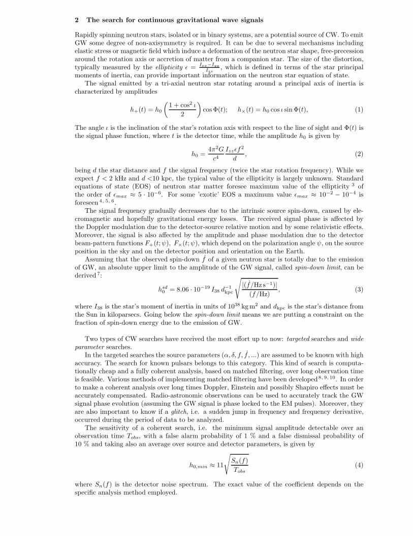
The first meeting took place at Moriond in the French Alps in 1966. There, experimentalas well as theoretical physicists not only shared their scientific preoccupations, but alsothe household chores. The participants in the first meeting were mainly french physicistsinterested in electromagnetic interactions. In subsequent years, a session on high energystrong interactions was added.
The main purpose of these meetings is to discuss recent developments in contemporaryphysics and also to promote effective collaboration between experimentalists and theo-rists in the field of elementary particle physics. By bringing together a relatively smallnumber of participants, the meeting helps develop better human relations as well as morethorough and detailed discussion of the contributions.
Our wish to develop and to experiment with new channels of communication and dialogue,which was the driving force behind the original Moriond meetings, led us to organize aparallel meeting of biologists on Cell Differentiation (1980) and to create the MoriondAstrophysics Meeting (1981). In the same spirit, we started a new series on CondensedMatter physics in January 1994. Meetings between biologists, astrophysicists, condensedmatter physicists and high energy physicists are organized to study how the progress inone field can lead to new developments in the others. We trust that these conferences andlively discussions will lead to new analytical methods and new mathematical languages.
The XLVIth Rencontres de Moriond in 2011 comprised four physics sessions:
• March 13 - 20: “Electroweak Interactions and Unified Theories”
• March 13 - 20: “Quantum Mesoscopic Physics”
• March 20 - 27: “QCD and High Energy Hadronic Interactions”
• March 20 - 27: “Gravitational Waves and Experimental Gravity”
We thank the organizers of the XLVIth Rencontres de Moriond:
• A. Abada, J. Conrad, S. Davidson, P. Fayet, J.-M. Frere, P. Hernandez, L. Iconomidou-Fayard, P. Janot, M. Knecht, J. P. Lees, S. Loucatos, F. Montanet, L. Okun, J.Orloff, A. Pich, S. Pokorski, D. Wood for the “Electroweak Interactions and UnifiedTheories” session,
• D. Averin, C. Beenakker, Y. Blanter, K. Ennslin, Jie Gao, L. Glazman, C. Glattli,Y. Imry, Young Kuk, T. Martin, G. Montambaux, V. Pellegrini, M. Sanquer, S.Tarucha for the “Quantum Mesoscopic Physics” session,
• E. Auge, E. Berger, S. Bethke, A. Capella, A. Czarnecki, D. Denegri, N. Glover, B.Klima, M. Krawczyk, L. McLerran, B. Pietrzyk, L. Schoeffel, Chung-I Tan, J. TranThanh Van, U. Wiedemann for the “QCD and High Energy Hadronic Interactions”session,
• M.-Ch. Angonin, R. Ansari, M.-A. Bizouard, L. Blanchet, M. Cruise, J. Dumarchez,Y. Giraud-Heraud, S. Hoedl, Ch. Magneville, E. Rasel, S. Reynaud, F. Ricci, R.Schnabel, J.-Y. Vinet, P. Wolf for the “Gravitational Waves and Experimental Grav-ity” session, joint with the GPhyS Colloquium
and the conference secretariat and technical staff:
V. de Sa-Varanda and C. Bareille, I. Cossin, G. Dreneau, D. Fligiel, S. Hurtado, N. Ribet,S. Vydelingum.
We are also grateful to Andrea Righetto, Gioacchino Romani, Erik Agostini, PatriziaRago, Matteo Tuzzi and the Planibel Hotel staff who contributed through their hospi-tality and cooperation to the well-being of the participants, enabling them to work in arelaxed atmosphere.
The Rencontres were sponsored by the Centre National de la Recherche Scientifique, theInstitut National de Physique Nucleaire et de Physique des Particules (IN2P3-CNRS),the Fondation NanoSciences, the Commissariat a l’Energie Atomique (DSM and IRFU),the Centre National d’Etudes Spatiales, the European Space Agency, the Fonds de laRecherche Scientifique (FRS-FNRS), the Belgium Science Policy and the National Sci-ence Foundation. We would like to express our thanks for their encouraging support.
It is our sincere hope that a fruitful exchange and an efficient collaboration between thephysicists and the astrophysicists will arise from these Rencontres as from previous ones.
E. Auge, J. Dumarchez and J. Tran Thanh Van
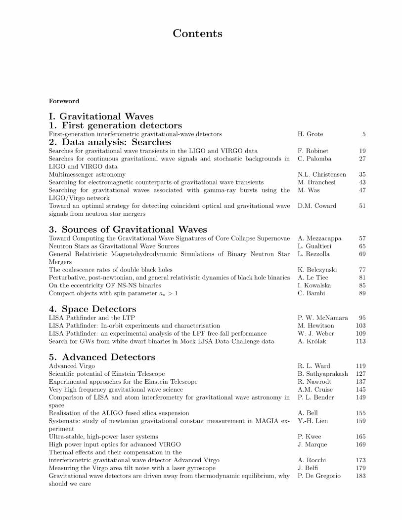
Contents
Foreword
I. Gravitational Waves1. First generation detectorsFirst-generation interferometric gravitational-wave detectors H. Grote 5
2. Data analysis: SearchesSearches for gravitational wave transients in the LIGO and VIRGO data F. Robinet 19Searches for continuous gravitational wave signals and stochastic backgrounds inLIGO and VIRGO data
C. Palomba 27
Multimessenger astronomy N.L. Christensen 35Searching for electromagnetic counterparts of gravitational wave transients M. Branchesi 43Searching for gravitational waves associated with gamma-ray bursts using theLIGO/Virgo network
M. Was 47
Toward an optimal strategy for detecting coincident optical and gravitational wavesignals from neutron star mergers
D.M. Coward 51
3. Sources of Gravitational WavesToward Computing the Gravitational Wave Signatures of Core Collapse Supernovae A. Mezzacappa 57Neutron Stars as Gravitational Wave Sources L. Gualtieri 65General Relativistic Magnetohydrodynamic Simulations of Binary Neutron StarMergers
L. Rezzolla 69
The coalescence rates of double black holes K. Belczynski 77Perturbative, post-newtonian, and general relativistic dynamics of black hole binaries A. Le Tiec 81On the eccentricity OF NS-NS binaries I. Kowalska 85Compact objects with spin parameter a∗ > 1 C. Bambi 89
4. Space DetectorsLISA Pathfinder and the LTP P. W. McNamara 95LISA Pathfinder: In-orbit experiments and characterisation M. Hewitson 103LISA Pathfinder: an experimental analysis of the LPF free-fall performance W. J. Weber 109Search for GWs from white dwarf binaries in Mock LISA Data Challenge data A. Krolak 113
5. Advanced DetectorsAdvanced Virgo R. L. Ward 119Scientific potential of Einstein Telescope B. Sathyaprakash 127Experimental approaches for the Einstein Telescope R. Nawrodt 137Very high frequency gravitational wave science A.M. Cruise 145Comparison of LISA and atom interferometry for gravitational wave astronomy inspace
P. L. Bender 149
Realisation of the ALIGO fused silica suspension A. Bell 155Systematic study of newtonian gravitational constant measurement in MAGIA ex-periment
Y.-H. Lien 159
Ultra-stable, high-power laser systems P. Kwee 165High power input optics for advanced VIRGO J. Marque 169Thermal effects and their compensation in theinterferometric gravitational wave detector Advanced Virgo A. Rocchi 173Measuring the Virgo area tilt noise with a laser gyroscope J. Belfi 179Gravitational wave detectors are driven away from thermodynamic equilibrium, whyshould we care
P. De Gregorio 183
II. Experimental Gravity6. Short Range GravityGravitation at short distances : theory I. Antoniadis 191Casimir and short-range gravity tests S. Reynaud 199Testing the inverse square law of gravitation at short range with a superconductingtorsion balance
E.C. Chalkley 207
Short range tests with neutrons at ILL V. Nesvizhevsky 211Gravity Spectroscopy T. Jenke 221Forca-G: A trapped atom interferometer for the measurement of short range forces B. Pelle 227
7. Tests of relativity in the solar systemPlanetary ephemerides and gravity tests in the solar system A. Fienga 233Tests of gravity at the solar system scale M.-T. Jaekel 241OSS (Outer Solar System) Mission B. Christophe 249On the anomalous increase of the lunar eccentricity L. Iorio 255Radioscience simulations in General Relativity and in alternative theories of gravity A. Hees 259GAME - Gravitation Astrometric Measurement Experiment M. Gai 263A relativistic and autonomous navigation satellite system P. Delva 267Optical clock and drag-free requirements for a Shapiro time-delay mission P. Bender 271
8. Long range gravityProbing the dark energy nature with type Ia supernovae : cosmological constraintsfrom the Supernova Legacy Survey first 3-years
D. Hardin 279
Is Dark Energy needed? A. Blanchard 287Testing MOND in the Solar System L. Blanchet 295Testing dark matter with GAIA O. Bienayme 303Beyond Einstein: cosmological tests of model independent modified gravity D.B. Thomas 309
9. Weak equivalence principleEquivalence Principle Torsion Pendulum Experiments T. A. Wagner 315Among space fundamental physics missions, MICROSCOPE, a simple challenging freefall test
P. Touboul 319
Atom interferometry and the Einstein equivalence principle P. Wolf 327Significance of the Compton frequency in atom interferometry M. A. Hohensee 333Observability of short-range gravitation with the experiment FORCA-G S. Pelisson 337Major challenges of a high precision test of the equivalence principle in space A.M. Nobili 341
10. Lorentz invariance and CPTLorentz symmetry, the SME, and gravitational experiments J. D. Tasson 349Electromagnetic cavity tests of lorentz invariance on earth and in space A. Peters 357
11. ClocksThe ACES mission: fundamental physics tests with cold atom clocks in space L. Cacciapuoti 365
12. PulsarsGravitational wave detection through pulsar timing arrays D. J. Champion 377
13. Other TopicsMeasuring g with a beam of antihydrogen (AEgIS) C.Canali 387GBAR - Gravitational Behavior of Antihydrogen at Rest P. Dupre 391Evidence for time-varying nuclear decay dates: experimental results and their impli-cations for new physics
E. Fischbach 397
Analysis of experiments exhibiting time-varying nuclear decay rates: systematic effectsor new physics?
J.H. Jenkins 403
14. PostersEinstein Equivalence Principle and Bose–Einstein condensates A. Camacho 411MICROSCOPE instrument servo-loops and digitization A. Levy 413Electrostatic accelerometer with bias rejection for deep space gravitation tests B. Lenoir 415Lorentz invariant phenomenology of quantum gravity: Main ideas behind the model Y. Bonder 417Towards an ultra-stable optical sapphire cavity system for testing Lorentz invariance M. Nagel 419The search for primordial gravitational waves with Spider: a balloon-borne cmbpolarimeter
C. Clark 421
Strong lensing system and dark energy models B. Malec 423Constraints on a model with extra dimensions for the black hole at the galactic center A.F. Zakharov 425Cosmological and solar-system constraints on tensor-scalar theory with chameleoneffect
A. Hees 427
The STAR Mission: SpaceTime Asymmetry Research T. Schuldt 439On the maximum mass of differentially rotating neutron stars A. Snopek 431Measurement of slow gravitational perturbations with gravitational wave interferom-eters
V.N.Rudenko 433
Spikes in Gravitational Wave Radiation from Quickly Rotating Galactic Centers A. A. Sadoyan 437Kick Processes in the Merger of Two Black Holes I. Damiao Soares 439Cosmology models and graviton counting in a detector A. Beckwith 441Transverse, traceless, plane fronted, monochromatic plane waves in conformal gravityhave zero-energy
M. Paranjape 443
Gravitational wave recoil in nonsymmetric Robinson-Trautman spacetimes A. Saa 445Modification of atomic states in a vertical optical trap near a surface R. Messina 447Torsion pendulum with 2 DoF for the study of residual couplings between the TMand the GRS: approaching thermal noise limited sensitivity
L. Marconi 451
List of participants 453


I.Gravitational Waves

1.First generation detectors

FIRST-GENERATION INTERFEROMETRIC GRAVITATIONAL-WAVE
DETECTORS
H. GROTE∗, D. H. REITZE+
∗MPI for Grav. Physics (AEI), and Leibniz University Hannover, 38 Callinstr.,30167 Hannover, Germany
E-mail: [email protected]
+Physics Department, University of Florida,Gainesville, FL 32611, USAE-mail: [email protected]
In this proceeding, we review some of the basic working principles and building blocks oflaser-interferometric gravitational-wave detectors on the ground. We look at similarities anddifferences between the instruments called GEO, LIGO, TAMA, and Virgo, which are currently(or have been) operating over roughly one decade, and we highlight some astrophysical resultsto date.
1 Introduction
The first searches for gravitational waves began in earnest 50 years ago with the experiments ofJoseph Weber using resonant mass detectors (‘Weber Bars’). 1 Weber’s pioneering efforts wereultimately judged as unsuccessful regarding the detection of gravitational waves, but from thosebeginnings interest in gravitational wave detection has grown enormously. For some decadesafter, a number of resonant mass detectors were built and operated around the globe withsensitivities far greater than those at Weber’s time. Some resonant bars are still in operation,but even their enhanced sensitivities today are lower and restricted to a much smaller bandwidththan those of the current laser interferometers.
Over the past decade, km-class ground-based interferometers have been operating in theUnited States, Italy and Germany, as well as a 300m arm length interferometer in Japan.Upgrades are underway to second generation configurations with far greater sensitivities. Withfurther astrophysics ‘reach’, these detectors will usher in the era of gravitational wave astronomywith the expectation of tens or possibly hundreds of events per year based on current rateestimates. 2 (See also the contributions about Advanced detectors in this volume.)
Section 2 of this paper presents a brief introduction to ground-based gravitational waveinterferometry, detector architecture, and methods used to minimize the influence of externalperturbations. Section 3 surveys the currently operational (or operational until late 2010) in-terferometers, with a particular view on some unique features of the individual instruments.Finally we give a brief review of the most significant observational results to date in Section 4.Parts of this paper have been published as proceeding of the 12th Marcel Grossmann meeting. 3
Laser
ModeCleanerCavity
FI
Beamsplitter
PowerRecyclingMirror
ModeMatchingTelescope
Input TestMass Mirror
InputTestMassMirror
End TestMass Mirror
EndTestMassMirror
Detection PhotodiodeAlignment Sensing Photodiodes;
Length and AlignmentSensing Photodiodes
Length and AlignmentSensing Photodiodes
Electro-opticModulator
SignalRecyclingMirror
FI
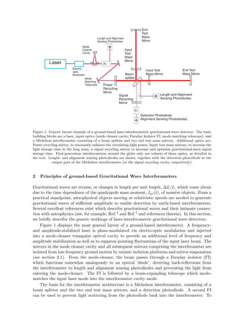
Figure 1: Generic layout example of a ground-based laser-interferometric gravitational-wave detector. The basicbuilding blocks are a laser, input optics (mode cleaner cavity, Faraday Isolator FI, mode matching telescope), anda Michelson interferometer consisting of a beam splitter and two end test mass mirrors. Additional optics are:Power recycling mirror, to resonantly enhance the circulating light power, Input test mass mirrors, to increase thelight storage time in the long arms, a signal recycling mirror to increase and optimize gravitational-wave signalstorage time. First-generation interferometers around the globe only use subsets of these optics, as detailed inthe text. Length- and alignment sensing photodiodes are shown, together with the detection photodiode at the
output port of the Michelson interferometer (or the signal recycling cavity, respectively).
2 Principles of ground-based Gravitational Wave Interferometers
Gravitational waves are strains, or changes in length per unit length, ∆L/L, which come aboutdue to the time dependence of the quadrupole mass moment, Iµν(t), of massive objects. From apractical standpoint, astrophysical objects moving at relativistic speeds are needed to generategravitational waves of sufficient amplitude to enable detection by earth-based interferometers.Several excellent references exist which describe gravitational waves and their intimate connec-tion with astrophysics (see, for example, Ref.4 and Ref.5 and references therein). In this section,we briefly describe the generic workings of laser-interferometric gravitational wave detectors.
Figure 1 displays the most general layout of a ground-based interferometer. A frequency-and amplitude-stabilized laser is phase-modulated via electro-optic modulation and injectedinto a mode-cleaner triangular optical cavity to provide an additional level of frequency andamplitude stabilization as well as to suppress pointing fluctuations of the input laser beam. Themirrors in the mode cleaner cavity and all subsequent mirrors comprising the interferometer areisolated from low-frequency ground motion by seismic isolation platforms and mirror suspensions(see section 2.1). From the mode-cleaner, the beam passes through a Faraday isolator (FI)which functions somewhat analogously to an optical ‘diode’, diverting back-reflections fromthe interferometer to length and alignment sensing photodiodes and preventing the light fromentering the mode-cleaner. The FI is followed by a beam-expanding telescope which mode-matches the input laser mode into the interferometer cavity mode.
The basis for the interferometer architecture is a Michelson interferometer, consisting of abeam splitter and the two end test mass mirrors, and a detection photodiode. A second FIcan be used to prevent light scattering from the photodiode back into the interferometer. To
minimize noise associated with amplitude fluctuations of the laser, the interferometer differen-tial path length is set to interfere carrier light destructively at the detection photodiode suchthat the quiescent state is nearly dark. A passing gravitational wave differentially modulatesthe round-trip travel time of the light in the arms at the gravitational wave frequency whichin turn modulates the light intensity at the detection photodiode. In effect, the interferometertransduces the dynamic metric perturbation imposed by the passing gravitational wave to pho-tocurrent in the detection photodiode. The magnitude of photocurrent depends not only on theamplitude, but also on the direction and polarization of the passing gravitational wave.
Beyond the simple Michelson configuration, the sensitivity of the interferometer can be fur-ther increased in three ways. By adding input test mass mirrors into each arm, Fabry-Perotcavities are formed, effectively increasing the light storage time in the arms (or, in an alterna-tive view, amplifying the phase shift for a given amount of displacement). Second, since therecombined laser light at the beam splitter interferes constructively toward the laser, it canbe coherently recirculated back into the interferometer by a ‘power-recycling’ mirror located inbetween the mode-matching telescope and the beam splitter. Finally, the gravitational signalitself can be recycled by placing a ‘signal-recycling’ mirror between the beam splitter and thedetection photodiode to recirculate the light modulated by the gravitational wave into the in-terferometer, further increasing the light storage time and thus the depth of modulation by thegravitational wave. The signal-recycling mirror also allows for tuning of the response curve ofthe interferometer. By shifting the signal-recycling mirror a fraction of a wavelength from res-onant recirculation (‘tuned’ operation), specific frequencies of the light are resonantly recycledat the expense of others (‘detuned’ operation), allowing for enhanced sensitivities over specificfrequency ranges of interest.
Current interferometers are designed to be sensitive in the frequency range from approxi-mately 10-50Hz out to a few kHz. Fundamental noises limiting interferometer sensitivity dependon the specifics of the interferometer design, and different interferometers have approached thetask of minimizing interferometer noise in different ways. However, the limiting sensitivity en-velope for all ground-based detectors roughly breaks down as follows: seismic ground motion atlow frequencies, thermal noise due to the Brownian motion of the mirror suspension wires andmirror coatings in the mid-frequency bands, and shot noise at high frequencies. In addition,technical noise sources from length and alignment sensing and control systems can also limitinterferometer performance, in particular at the low-frequency end. To minimize phase noisefrom light scattering off molecules, the components of the interferometer and the input optics(mode-cleaner, FI, and telescope) are located in an ultrahigh vacuum system. Light scatteringoff mirrors however, which can be reflected by seismically ’noisy’ components and then beingre-directed to interfere with the main interferometer beams, can also contribute to excess noise.
2.1 Seismic isolation and suspensions
A typical ambient horizontal ground motion on the surface of the earth is about 10−10m/√Hz
at 50Hz. Depending on the choice of sensitive frequency band, the test mass mirrors ofgravitational-wave interferometers have to be quieter by roughly 10 orders of magnitude atthese frequencies, motivating sophisticated seismic isolation systems.
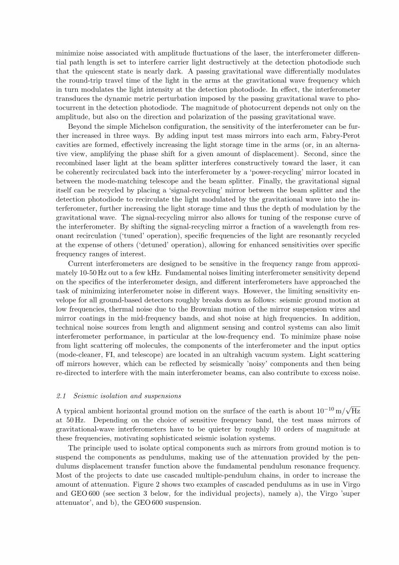
The principle used to isolate optical components such as mirrors from ground motion is tosuspend the components as pendulums, making use of the attenuation provided by the pen-dulums displacement transfer function above the fundamental pendulum resonance frequency.Most of the projects to date use cascaded multiple-pendulum chains, in order to increase theamount of attenuation. Figure 2 shows two examples of cascaded pendulums as in use in Virgoand GEO600 (see section 3 below, for the individual projects), namely a), the Virgo ’superattenuator’, and b), the GEO600 suspension.
Figure 2: a) The Virgo ’super attenuator’ consists of multiple pendulum stages connected by single suspensionwires. Vertical isolation is provided by the ’mechanical filter’ stages, which act as pendulum masses, but alsohold the subsequent suspension wire by blade-springs. b) The GEO600 suspension consists of 3 pendulum stages(including the test-mass mirror). The upper two stages provide vertical isolation by steel springs holding thesuspension wires. Both suspension types a) and b) use fused silica fibres to suspend the test mass mirror from
the penultimate, or intermediate mass.
A Virgo super-attenuator 6 consists of multiple pendulum stages, which are connected toeach other by single suspension wires. In addition to the inherent horizontal isolation of thependulums, the intermediate pendulum masses, denoted as mechanical filters, provide verticalisolation by a magnetic anti-spring mechanism. The penultimate mass holds the test-massmirror on 4 suspension slings, such that angular control can be applied to the mirror from thepenultimate mass. In addition to this, angular and longitudinal control forces can be appliedto the mirror by a reaction mass (not shown in Figure 2), suspended around the test mass.Coils are attached to the reaction mass, applying forces to magnets glued onto the test mass.The mechanical filter at the top of the suspension chain is supported by an inverted pendulum,completing the supreme low-frequency passive isolation of the super-attenuator. Active feedbackcontrol using position- and inertia sensors is required to keep the inverted pendulum at itsoperating point. The GEO suspension is much more compact in total dimensions, and makesuse of three cascaded pendulum stages. Vertical isolation is provided by blade springs, holdingthe suspension wires of the first and second pendulum stage. For two of the main test massesGEO uses two similar pendulum chains closely located to each other, as shown in Figure 2. Thesecond pendulum chain serves as a reaction ’platform’ from which forces can be applied to thetest-mass chain without using force actuators referenced to the much larger ground motion.
2.2 Control
While suspended optics are supremely quiet in the measurement band of interest (i.e. above10-50Hz) the motion of the suspended optics is resonantly enhanced on the eigenmodes of thesuspensions, typically around 0.5 to a few Hz. Therefore, different techniques are employedto reduce motion amplitudes of these modes. In many cases, actual mirror motion is measuredlocally by shadow-sensors, CCD images, or optical lever configurations. Feedback is then appliedby coil/magnet actuators to damp the motion of pendulum components. This type of dampingcan be applied at different levels of the suspension chain, preferably on one of the upper massesto reduce re-introduced displacement noise in the measurement band.
To achieve the sensitivities required for gravitational wave detection, all of the interferometermirrors must be held to absolute positions of a picometer or less in the presence of severalsources of displacement noise. Global length sensing and control systems keep the cavities lockedon resonance, using sophisticated variants of the Pound-Drever-Hall cavity locking technique.Phase modulation by the electro-optic modulator (see Figure 1) produces radio-frequency (RF)sidebands on the laser light which serve as references (local oscillators) for sensing length changesin the various length degrees of freedom. In addition, the alignment of the mirrors must bemaintained to a few nanoradians using a sensing and control system based on a spatial analogof Pound-Drever-Hall locking.
Hundreds of control loops are thus necessary to keep the interferometer at its nominaloperating point. The procedure of bringing the interferometer to this highly-controlled stateis non-trivial, and all of the projects have spent many months to years to arrive at reliablyreproducible locking sequences, which have become highly automated in most cases.
3 First generation Detectors around the Globe
At the present time, there are five gravitational wave observatories — two LIGO sites in theUS, the Virgo and GEO600 sites in Europe, and the TAMA300 observatory in Japan (seeFigure 3). These observatories have been in operation for the past decade, and constitute thefirst generation of large-scale interferometers. In this sense the term ’first generation’ refers to thetime at which these instruments have been built and are operating. However, as we will see below,some of the instruments employ techniques which are technically more advanced than others.These techniques are commonly described as ’second generation’ or ’advanced’ techniques, withthe anticipation that they will be widely implemented in the detector generations planned toreplace the existing ones. On these planned upgrades (see other papers in this volume) theinfrastructures including buildings, vacuum systems etc. will be re-used, but substantial partsof the interferometer will be replaced with new systems.
3.1 LIGO
LIGO consists of two separately located facilities in the United States, one in Hanford, Wash-ington and one in Livingston, Louisiana. The LIGO Hanford Observatory used to house twointerferometers, a 4–km arm length interferometer and a 2–km arm length interferometer. TheLIGO Livingston Observatory houses a single 4–km long interferometer. The 2–km interferom-eter in Hanford was taken out of operation in summer 2009, and the two 4–km interferometerswere taken out of operation in October 2010, to make way for the Advanced LIGO project (seearticle on Advanced LIGO in this volume). Here we report on the LIGO interferometers up toOctober 2010, referred to as Initial and Enhanced LIGO.
The three initial LIGO interferometers were identical in configuration, employing Fabry-Perot arm cavities and power-recycling (but not signal recycling). The seismic isolation systemof initial LIGO consisted of passive pre-isolation stacks, using alternating layers of metal and
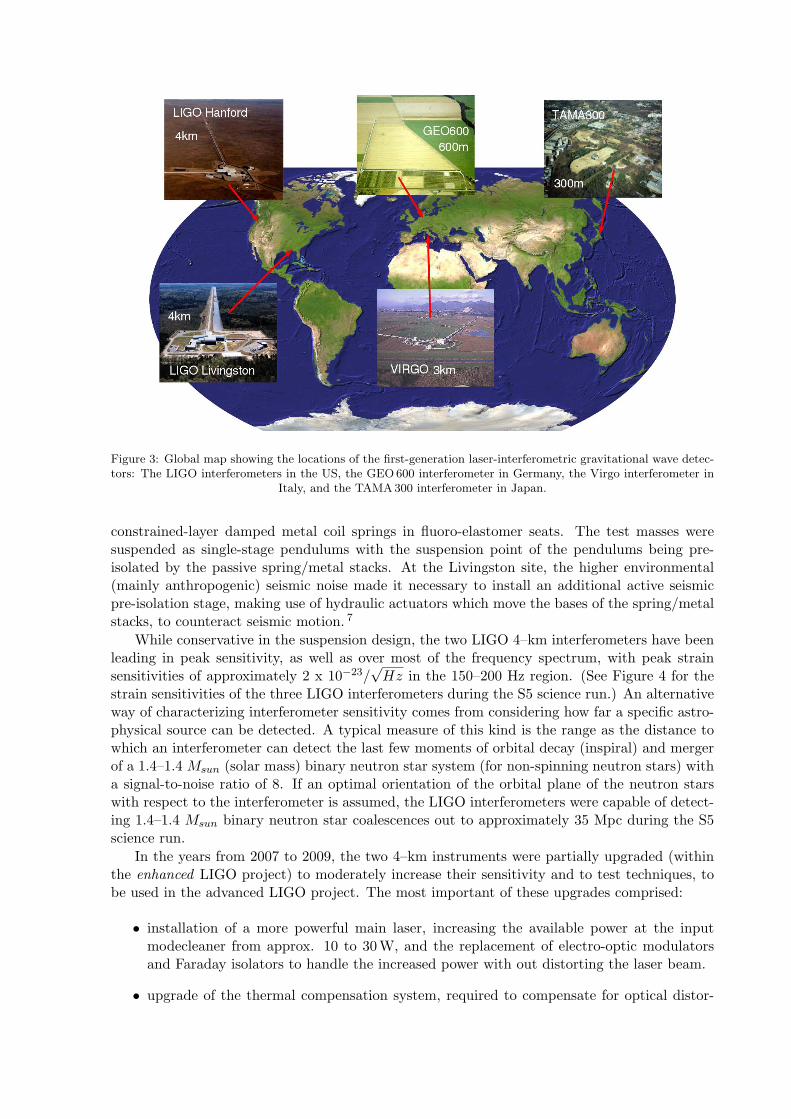
Figure 3: Global map showing the locations of the first-generation laser-interferometric gravitational wave detec-tors: The LIGO interferometers in the US, the GEO600 interferometer in Germany, the Virgo interferometer in
Italy, and the TAMA300 interferometer in Japan.
constrained-layer damped metal coil springs in fluoro-elastomer seats. The test masses weresuspended as single-stage pendulums with the suspension point of the pendulums being pre-isolated by the passive spring/metal stacks. At the Livingston site, the higher environmental(mainly anthropogenic) seismic noise made it necessary to install an additional active seismicpre-isolation stage, making use of hydraulic actuators which move the bases of the spring/metalstacks, to counteract seismic motion. 7
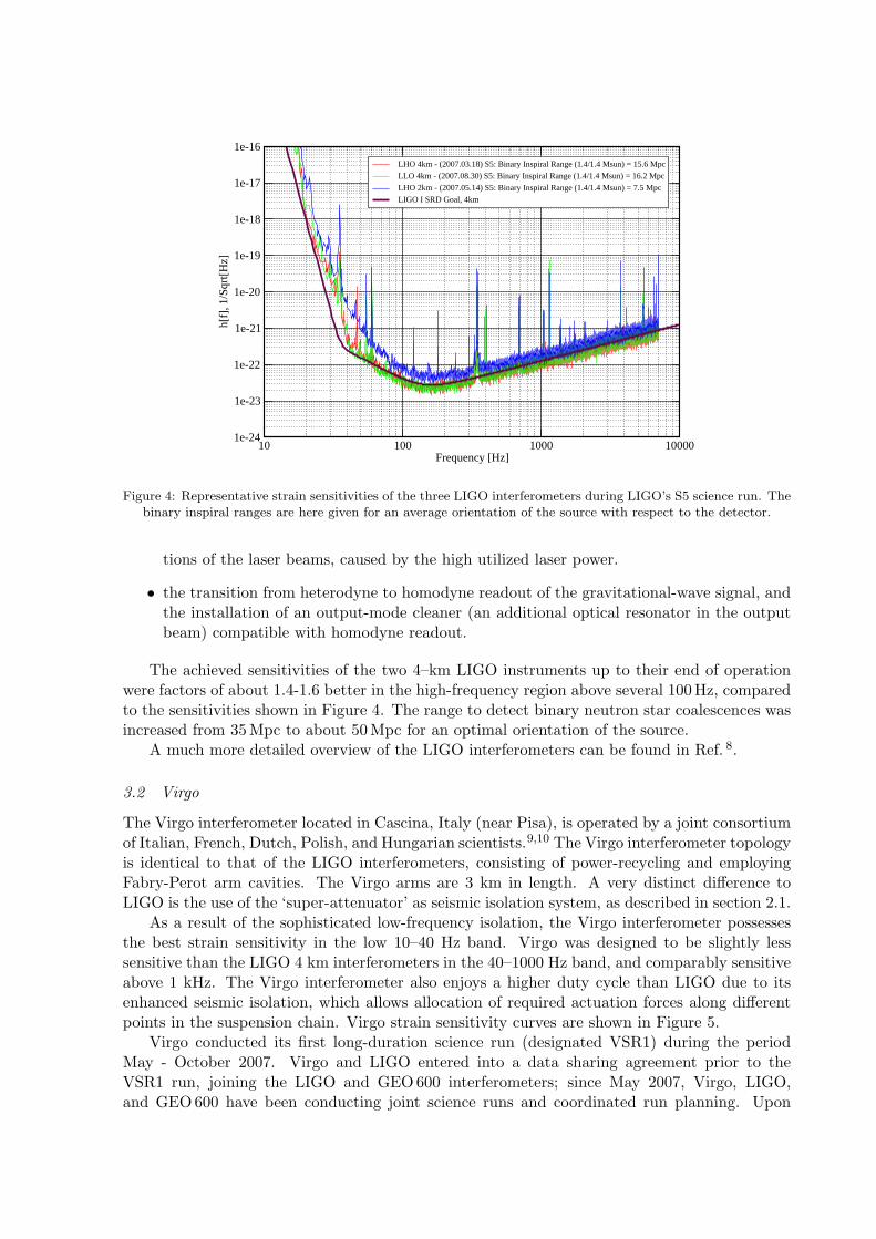
While conservative in the suspension design, the two LIGO 4–km interferometers have beenleading in peak sensitivity, as well as over most of the frequency spectrum, with peak strainsensitivities of approximately 2 x 10⁻²³/
√Hz in the 150–200 Hz region. (See Figure 4 for the
strain sensitivities of the three LIGO interferometers during the S5 science run.) An alternativeway of characterizing interferometer sensitivity comes from considering how far a specific astro-physical source can be detected. A typical measure of this kind is the range as the distance towhich an interferometer can detect the last few moments of orbital decay (inspiral) and mergerof a 1.4–1.4 Msun (solar mass) binary neutron star system (for non-spinning neutron stars) witha signal-to-noise ratio of 8. If an optimal orientation of the orbital plane of the neutron starswith respect to the interferometer is assumed, the LIGO interferometers were capable of detect-ing 1.4–1.4 Msun binary neutron star coalescences out to approximately 35 Mpc during the S5science run.
In the years from 2007 to 2009, the two 4–km instruments were partially upgraded (withinthe enhanced LIGO project) to moderately increase their sensitivity and to test techniques, tobe used in the advanced LIGO project. The most important of these upgrades comprised:
• installation of a more powerful main laser, increasing the available power at the inputmodecleaner from approx. 10 to 30W, and the replacement of electro-optic modulatorsand Faraday isolators to handle the increased power with out distorting the laser beam.
• upgrade of the thermal compensation system, required to compensate for optical distor-
10 100 1000 10000Frequency [Hz]
1e-24
1e-23
1e-22
1e-21
1e-20
1e-19
1e-18
1e-17
1e-16
h[f]
, 1/S
qrt[
Hz]
LHO 4km - (2007.03.18) S5: Binary Inspiral Range (1.4/1.4 Msun) = 15.6 Mpc
LLO 4km - (2007.08.30) S5: Binary Inspiral Range (1.4/1.4 Msun) = 16.2 Mpc
LHO 2km - (2007.05.14) S5: Binary Inspiral Range (1.4/1.4 Msun) = 7.5 Mpc
LIGO I SRD Goal, 4km
Figure 4: Representative strain sensitivities of the three LIGO interferometers during LIGO’s S5 science run. Thebinary inspiral ranges are here given for an average orientation of the source with respect to the detector.
tions of the laser beams, caused by the high utilized laser power.
• the transition from heterodyne to homodyne readout of the gravitational-wave signal, andthe installation of an output-mode cleaner (an additional optical resonator in the outputbeam) compatible with homodyne readout.
The achieved sensitivities of the two 4–km LIGO instruments up to their end of operationwere factors of about 1.4-1.6 better in the high-frequency region above several 100Hz, comparedto the sensitivities shown in Figure 4. The range to detect binary neutron star coalescences wasincreased from 35Mpc to about 50Mpc for an optimal orientation of the source.
A much more detailed overview of the LIGO interferometers can be found in Ref. 8.
3.2 Virgo
The Virgo interferometer located in Cascina, Italy (near Pisa), is operated by a joint consortiumof Italian, French, Dutch, Polish, and Hungarian scientists.9,10 The Virgo interferometer topologyis identical to that of the LIGO interferometers, consisting of power-recycling and employingFabry-Perot arm cavities. The Virgo arms are 3 km in length. A very distinct difference toLIGO is the use of the ‘super-attenuator’ as seismic isolation system, as described in section 2.1.
As a result of the sophisticated low-frequency isolation, the Virgo interferometer possessesthe best strain sensitivity in the low 10–40 Hz band. Virgo was designed to be slightly lesssensitive than the LIGO 4 km interferometers in the 40–1000 Hz band, and comparably sensitiveabove 1 kHz. The Virgo interferometer also enjoys a higher duty cycle than LIGO due to itsenhanced seismic isolation, which allows allocation of required actuation forces along differentpoints in the suspension chain. Virgo strain sensitivity curves are shown in Figure 5.
Virgo conducted its first long-duration science run (designated VSR1) during the periodMay - October 2007. Virgo and LIGO entered into a data sharing agreement prior to theVSR1 run, joining the LIGO and GEO600 interferometers; since May 2007, Virgo, LIGO,and GEO600 have been conducting joint science runs and coordinated run planning. Upon
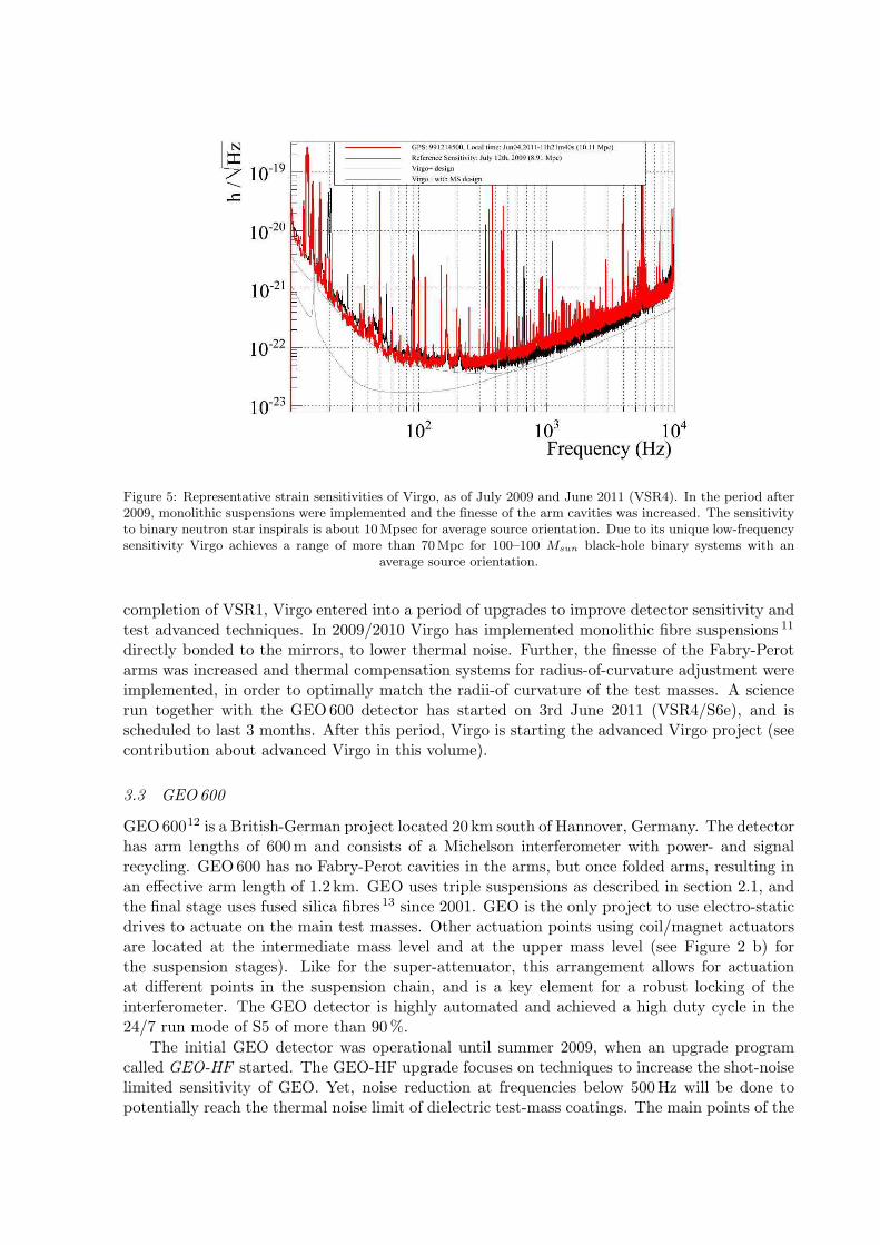
Figure 5: Representative strain sensitivities of Virgo, as of July 2009 and June 2011 (VSR4). In the period after2009, monolithic suspensions were implemented and the finesse of the arm cavities was increased. The sensitivityto binary neutron star inspirals is about 10Mpsec for average source orientation. Due to its unique low-frequencysensitivity Virgo achieves a range of more than 70Mpc for 100–100 Msun black-hole binary systems with an
average source orientation.
completion of VSR1, Virgo entered into a period of upgrades to improve detector sensitivity andtest advanced techniques. In 2009/2010 Virgo has implemented monolithic fibre suspensions 11
directly bonded to the mirrors, to lower thermal noise. Further, the finesse of the Fabry-Perotarms was increased and thermal compensation systems for radius-of-curvature adjustment wereimplemented, in order to optimally match the radii-of curvature of the test masses. A sciencerun together with the GEO600 detector has started on 3rd June 2011 (VSR4/S6e), and isscheduled to last 3 months. After this period, Virgo is starting the advanced Virgo project (seecontribution about advanced Virgo in this volume).
3.3 GEO600
GEO60012 is a British-German project located 20 km south of Hannover, Germany. The detectorhas arm lengths of 600m and consists of a Michelson interferometer with power- and signalrecycling. GEO600 has no Fabry-Perot cavities in the arms, but once folded arms, resulting inan effective arm length of 1.2 km. GEO uses triple suspensions as described in section 2.1, andthe final stage uses fused silica fibres 13 since 2001. GEO is the only project to use electro-staticdrives to actuate on the main test masses. Other actuation points using coil/magnet actuatorsare located at the intermediate mass level and at the upper mass level (see Figure 2 b) forthe suspension stages). Like for the super-attenuator, this arrangement allows for actuationat different points in the suspension chain, and is a key element for a robust locking of theinterferometer. The GEO detector is highly automated and achieved a high duty cycle in the24/7 run mode of S5 of more than 90%.
The initial GEO detector was operational until summer 2009, when an upgrade programcalled GEO-HF started. The GEO-HF upgrade focuses on techniques to increase the shot-noiselimited sensitivity of GEO. Yet, noise reduction at frequencies below 500Hz will be done topotentially reach the thermal noise limit of dielectric test-mass coatings. The main points of the
102
103
10−22
10−21
10−20
10−19
10−18
Str
ain
[1/ s
qrt(
Hz)
]
Frequency (Hz)
June 2006 (S5)June 2011 (S6e)
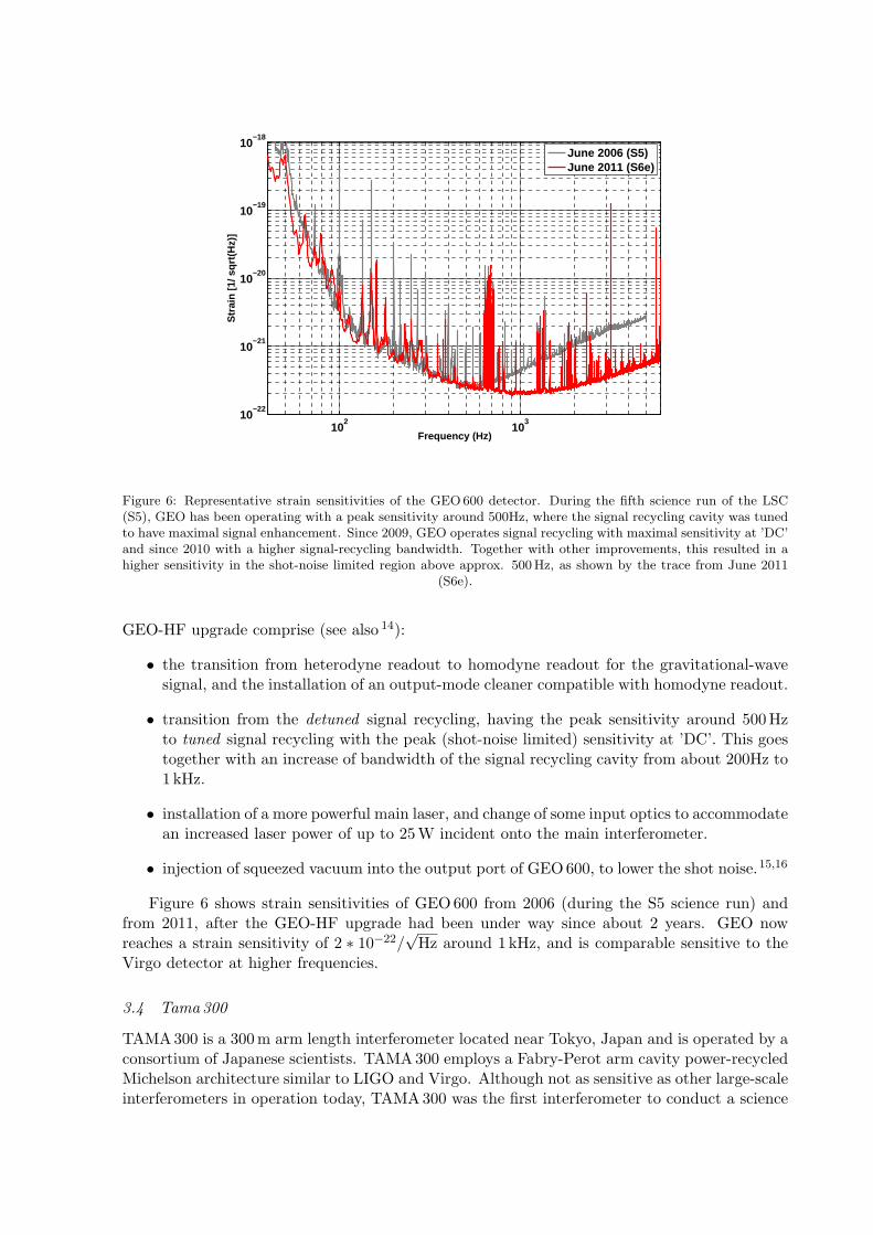
Figure 6: Representative strain sensitivities of the GEO600 detector. During the fifth science run of the LSC(S5), GEO has been operating with a peak sensitivity around 500Hz, where the signal recycling cavity was tunedto have maximal signal enhancement. Since 2009, GEO operates signal recycling with maximal sensitivity at ’DC’and since 2010 with a higher signal-recycling bandwidth. Together with other improvements, this resulted in ahigher sensitivity in the shot-noise limited region above approx. 500Hz, as shown by the trace from June 2011
(S6e).
GEO-HF upgrade comprise (see also 14):
• the transition from heterodyne readout to homodyne readout for the gravitational-wavesignal, and the installation of an output-mode cleaner compatible with homodyne readout.
• transition from the detuned signal recycling, having the peak sensitivity around 500Hzto tuned signal recycling with the peak (shot-noise limited) sensitivity at ’DC’. This goestogether with an increase of bandwidth of the signal recycling cavity from about 200Hz to1 kHz.
• installation of a more powerful main laser, and change of some input optics to accommodatean increased laser power of up to 25W incident onto the main interferometer.
• injection of squeezed vacuum into the output port of GEO600, to lower the shot noise.15,16
Figure 6 shows strain sensitivities of GEO600 from 2006 (during the S5 science run) andfrom 2011, after the GEO-HF upgrade had been under way since about 2 years. GEO nowreaches a strain sensitivity of 2 ∗ 10−22/
√Hz around 1 kHz, and is comparable sensitive to the
Virgo detector at higher frequencies.
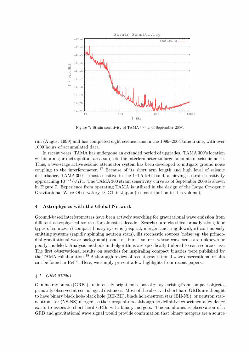
3.4 Tama 300
TAMA300 is a 300m arm length interferometer located near Tokyo, Japan and is operated by aconsortium of Japanese scientists. TAMA300 employs a Fabry-Perot arm cavity power-recycledMichelson architecture similar to LIGO and Virgo. Although not as sensitive as other large-scaleinterferometers in operation today, TAMA300 was the first interferometer to conduct a science
1e-21
1e-20
1e-19
1e-18
1e-17
1e-16
1e-15
1e-14
1e-13
1e-12
10 100 1000 10000
1 / sqrt(Hz)
f (Hz)
Strain Sensitivity
2008-09-18
Figure 7: Strain sensitivity of TAMA300 as of September 2008.
run (August 1999) and has completed eight science runs in the 1999–2004 time frame, with over1000 hours of accumulated data.
In recent years, TAMA has undergone an extended period of upgrades. TAMA300’s locationwithin a major metropolitan area subjects the interferometer to large amounts of seismic noise.Thus, a two-stage active seismic attenuator system has been developed to mitigate ground noisecoupling to the interferometer. 17 Because of its short arm length and high level of seismicdisturbance, TAMA300 is most sensitive in the 1–1.5 kHz band, achieving a strain sensitivityapproaching 10−21/
√Hz. The TAMA300 strain sensitivity curve as of September 2008 is shown
in Figure 7. Experience from operating TAMA is utilized in the design of the Large CryogenicGravitational-Wave Observatory LCGT in Japan (see contribution in this volume).
4 Astrophysics with the Global Network
Ground-based interferometers have been actively searching for gravitational wave emission fromdifferent astrophysical sources for almost a decade. Searches are classified broadly along fourtypes of sources: i) compact binary systems (inspiral, merger, and ring-down), ii) continuouslyemitting systems (rapidly spinning neutron stars), iii) stochastic sources (noise, eg, the primor-dial gravitational wave background), and iv) ‘burst’ sources whose waveforms are unknown orpoorly modeled. Analysis methods and algorithms are specifically tailored to each source class.The first observational results on searches for inspiraling compact binaries were published bythe TAMA collaboration.18 A thorough review of recent gravitational wave observational resultscan be found in Ref. 8. Here, we simply present a few highlights from recent papers.
4.1 GRB 070201
Gamma ray bursts (GRBs) are intensely bright emissions of γ-rays arising from compact objects,primarily observed at cosmological distances. Most of the observed short hard GRBs are thoughtto have binary black hole-black hole (BH-BH), black hole-neutron star (BH-NS), or neutron star-neutron star (NS-NS) mergers as their progenitors, although no definitive experimental evidenceexists to associate short hard GRBs with binary mergers. The simultaneous observation of aGRB and gravitational wave signal would provide confirmation that binary mergers are a source
of GRBs.
GRB 070201 was an exceptionally short hard GRB observed in the x-ray spectrum by satel-lites in the Interplanetary Network (IPN). The error box had significant overlap with the M31(Andromeda) galaxy (located 730 kpc from the Milky Way galaxy), thus making it a prime can-didate for gravitational wave searches. Data from the LIGO Hanford detectors were analyzed ina 180 s time window around GRB 070201 using both template-based searches for binary mergersand burst search algorithms. 19 No signal was found, and LIGO was able to exclude a compactbinary BH-NS, NS-NS merger progenitor of GRB 070201 located in M31 at > 99% and 90%confidence levels, respectively. The analysis did not rule out a soft gamma repeater (SGR) inM31, but was able to place a limit on energy conversion to gravitational wave of less than 4 x10⁻⁴ Msun.
4.2 Beating the Spindown Limit on the Crab Pulsar
Spinning neutron stars can emit gravitational waves if they possess ellipticities arising fromcrustal deformations, internal hydrodynamic modes, or free precession (‘wobble’). Ground-based gravitational wave detectors are potentially sensitive to gravitational wave emissions fromneutron stars in our galaxy. The Crab pulsar (PSRB0531+21, PSRJ0534+2200), located 2kpc distant, is a particularly appealing candidate for gravitational wave emission because itis relatively young and rapidly slowing in rotation (‘spinning down’). While the predominantenergy dissipation mechanisms are magnetic dipole radiation or charged particle emission in thepulsar’s magnetosphere, the measured braking index of the Crab pulsar suggests that neitherdipole radiation or particle ejection can account for the rotational braking.
Using a subset of data from LIGO’s S5 science run, the LIGO Scientific Collaborationsearched for gravitational wave emission from the Crab pulsar during a nine month durationduring which no pulsar timing jumps occurred. 20 No gravitational waves were observed, and thedata was used to set upper limits on the strain h = 3.35× 10⁻²⁵ and ellipticity ǫ = 1.79× 10⁻⁴.The limit on strain is significant in that it implies no more than 5.5% of the energy emitted bythe Crab pulsar is in the form of gravitational waves. An updated analysis by the LIGO andVirgo collaborations using a more extensive data set have reduce the upper limit on radiatedgravitational wave energy to approximately 2%. 21
4.3 The Primordial Gravitational Wave Background
A stochastic gravitational wave background could arise from an incoherent superposition of pointsource emitters or from the remnant gravitational wave emission from the Big Bang. Electro-magnetic observations of the cosmic microwave background have provided the best knowledge sofar of the early universe, however they are limited to probe the universe after the recombinationera when the universe became transparent to electromagnetic radiation. Searches for primordialgravitational waves are thus particularly significant from a cosmological standpoint since theydirectly probe the universe at its earliest epoch.
Recent results by the LIGO Scientific and Virgo Collaborations have placed the most strin-gent direct observational limit on a stochastic gravitational wave background from the primordialuniverse. By cross-correlating data from the LIGO Livingston and Hanford 4–km interferome-ters during the S5 science run, an upper limit of Ω0,GW < 6.9 × 10⁻⁶ on the energy density ofstochastic gravitational waves (normalized to the closure energy density of the universe) assum-ing the gravitational wave background is confined within the 50–150 Hz frequency band. 22 Thislimit is the best experimental limit in the LIGO frequency band, beating the limit inferred fromthe Big Bang Nucleosynthesis by almost a factor of 2.
Acknowledgments
The authors gratefully acknowledge support from the Science and Technology Facilities Council(STFC), the University of Glasgow in the UK, the Bundesministerium fur Bildung und Forschung(BMBF) and the state of Lower Saxony in Germany. We further gratefully acknowledge thesupport of the US National Science Foundation through grants PHY-0855313 and PHY-0757968.We also thank Francesco Fidecaro, David Shoemaker, Giovanni Losurdo, and Daisuke Tatsumifor very useful discussions and for supplying material for this article.
References
1. J. Weber, Phys. Rev. 117, 306 (1960).2. J. Abadie, et al., arXiv:1003.2480 (submitted).3. D. Reitze, WSPC proceedings MG12, (2010)4. P. Saulson, Fundamentals of Interferometric Gravitational Wave Detectors, 1st edn.
(World Scientific Publishing, Hackensack, NJ, 1994).5. M. Maggiore, Gravitational Waves: Volume 1: Theory and Experiments, 1st edn. (Oxford
University Press, Oxford, UK, 2007).6. G. Ballardin, et al., Rev. Sci. Instrum. 72, 3643 (2001).7. http://etd.lsu.edu/docs/available/etd-01212009-101352/unrestricted/Wen diss.pdf8. B. Abbott, et al. (LIGO Science Collaboration), Rep. Prog. Phys. 72, 076901 (2009).9. T Accadia and B L Swinkels (for the Virgo Collaboration), Class. Quantum Grav. 27,
084002 (2010).10. Information about Virgo can be found at www.virgo.infn.it.11. M Lorenzini (on behalf of the Virgo Collaboration), Class. Quantum Grav. 27, 084021
(2010).12. H Grote (for the LIGO Scientific Collaboration), Class. Quantum Grav. 27, 084003
(2010).13. M. V. Plissi, C. I. Torrie, M. E. Husman, N. A. Robertson, K. A. Strain, H. Ward, H.
Luck, and J. Hough, Rev. Sci. Instrum. 71, 2539 (2000).14. H Luck, et al., J. Phys.: Conf. Ser. 228, 012012 (2010).15. H Vahlbruch, Alexander Khalaidovski, Nico Lastzka, Christian Graf, Karsten Danzmann,
and Roman Schnabel, Class. Quantum Grav. 27, 084027 (2010).16. R Schnabel, N Mavalvala, D E McClelland, P K Lam, Nat. Commun. 1:121 doi:
10.1038/ncomms1122 (2010).17. R Takahashi, K Arai, D Tatsumi, M Fukushima, T Yamazaki, M-K Fujimoto, K Agatsuma,
Y Arase, N Nakagawa, A Takamori, K Tsubono, R DeSalvo, A Bertolini, S Marka, and VSannibale (TAMA Collaboration), Class. Quantum Grav. 25, 114036 (2008).
18. H. Tagoshi, et al., (TAMA Collaboration) Phys. Rev. D 63, 062001 (2001).19. B. Abbott, et al. (LIGO Science Collaboration), Astrophys. J. 681, 1419 (2008).20. B. Abbott, et al. (LIGO Science Collaboration), Astrophys. J. Lett. 683, L45 (2008).21. B. Abbott, et al. (LIGO Science Collaboration), Astrophys. J. 713, 671-685 (2010).22. B. Abbott, et al. (LIGO Science Collaboration), Nature 460, 990 (2009).
2.Data analysis: Searches

SEARCHES FOR GRAVITATIONAL WAVE TRANSIENTS IN THE LIGO
AND VIRGO DATA
F. ROBINET, for the LIGO Scientific Collaboration and the Virgo CollaborationLAL, Univ. Paris-Sud, CNRS/IN2P3, Orsay, France.
In 2011, the Virgo gravitational wave (GW) detector will definitively end its science programfollowing the shut-down of the LIGO detectors the year before. The years to come will bedevoted to the development and installation of second generation detectors. It is the opportunetime to review what has been learned from the GW searches in the kilometric interferometersdata. Since 2007, data have been collected by the LIGO and Virgo detectors. Analyses havebeen developed and performed jointly by the two collaborations. Though no detection hasbeen made so far, meaningful upper limits have been set on the astrophysics of the sourcesand on the rate of GW events. This paper will focus on the transient GW searches performedover the last 3 years. This includes the GW produced by compact binary systems, supernovaecore collapse, pulsar glitches or cosmic string cusps. The analyses which have been specificallydeveloped for that purpose will be presented along with the most recent results.
1 Introduction
Gravitational waves (GW) were predicted by Albert Einstein 1 with his theory of general rela-tivity. It shows that an asymmetric, compact and relativistic object will radiate gravitationally.The waves propagate with a celerity c and their amplitude is given by the dimensionless strain hwhich can be projected over two polarizations h+ and h
×. The existence of GW was indirectly
confirmed through observations on the binary pulsar PSR 1913+16 discovered in 1974. Thisbinary system has been followed-up over more than 30 years and the orbit decay can be fullyexplained by the energy loss due to the gravitational wave emission 2. The great challenge ofthis century is to be able to detect gravitational waves directly by measuring the space-timedeformation induced by the wave. The Virgo 3 and the two LIGO 4 interferometric detectors aredesigned to achieve this goal. Thanks to kilometric arms, Fabry-Perot cavities, sophisticatedseismic isolation, a high laser power and the use of power-recycling techniques, the LIGO andVirgo detectors were able to reach their design sensitivity which is to measure h below 10−21 overa wide frequency band, from tens to thousands of Hz (and below 10−22 at a few hundreds Hz).Such sensitivity over a large range of frequencies offers the possibility to detect gravitationalwaves originating from various astrophysical sources which will be described in Section 2.
The searches for GW in LIGO-Virgo were historically divided into four analysis groups. Thephysics of these groups does not really match the type of GW sources but rather the expectedsignals. This has the advantage to develop efficient searches adapted to the signal seen in thedetector. The CBC group is specifically searching for signals resulting from the last instantsof the coalescence and the merging of compact binary systems of two neutron stars, two blackholes or one of each. The expected signal is well-modeled, especially the inspiral part, so thatthe searches are designed to be very selective. On the contrary, the burst group performs
more generic searches for any type of sub-second signals. This unmodeled approach offers arobustness to the analyses and remains open to the unexpected. Doing so, the burst groupcovers a large variety of GW sources for which the expected signals are poorly known. Thisincludes the asymmetric core bounce of supernovae, the merging of compact objects, the star-quakes of neutron stars or the oscillating loops of cosmic strings. This paper will focus on thework performed within the CBC and the burst group and present the searches for short-durationGW signals. C. Palomba will describe the searches for continuous signals and for a stochasticbackground of GW5. Section 3 will detail the different aspects of a multi-detector GW transientsearch while Section 4 will highlight some of the latest results of the analyses.
Very early on, the Virgo and LIGO collaborations chose to share their data and to performanalyses in common in order to maximize the chance of detection. Indeed, having severaldetectors in operation presents many advantages such as performing coincidences, reconstructingthe source location, having a better sky coverage or estimating the background for analyses. Thisclose collaboration started in 2007 with the Virgo first science run VSR1 (2007) and LIGO S5(2005-2007) run and continued until recently with the following science runs VSR2 (2009), VSR3(2010) and S6 (2009-2010). In October 2010, the LIGO detectors shut-down to install the secondgeneration of detectors which should resume science in 2015. Virgo will perform one more sciencerun, VSR4, during the summer jointly with the GEO 600 6 detector in Germany. After that,Virgo will start the preparation for the next phase with Advanced Virgo.
As the first generation of interferometers is about to take an end, the analyses performed sofar were not able to claim a detection. However it was possible to set astrophysically relevantupper limits and this paper will present some of them. Moreover the pioneering work performedto build efficient analyses pipelines will be a great strength for the Advanced detector era andthe first steps of gravitational wave astronomy.
2 Sources, signals and searches
2.1 The coalescence of binary objects
The coalescence of stellar compact binary systems is often seen as the most promising candidatefor a first detection. Indeed, such objects have been extensively studied and the expectedwaveform is rather well-modeled. The inspiral phase, up to the last stable circular orbit, canbe reliably described with a post-Newtonian approximation 7. The signal is expected to sweepupwards in frequency and to cross the detector bandwidth for a short period of time (from afew ms to tens of s). This is followed by the merger of the two bodies whose waveform can bederived from numerical relativity 8 even though this part of the waveform is the least knownof the evolution of the binary. Finally, the resulting black hole is excited and loses part of itsenergy by radiating gravitationally. Black hole pertubation theory is well able to predict theringdown waveform 9 and the signal is expected to be in the detector sensitive band for masseslarger than 100 M
⊙.
The search for coalescence signals, led by the CBC group, takes two free parameters intoaccount: the masses of the two binary components. The low-mass search covers a total massrange between 2 and 35 M
⊙where most of the energy is contained in the inspiral phase. As a
complement, the high-mass search probes the 25-100 M⊙total mass region where the signal-to-
noise ratio is significant mostly during the merger and ringdown phase. A ringdown-only searchis also performed for very high-mass systems (75-750 M
⊙) in which case it is possible to use the
spin as an additional parameter. The merger and the ringdown signals are also included in theburst searches. The robust nature of the burst analyses offers a nice complement to the CBCsearches, especially for the merger phase for which the waveform is less reliable.
Astrophysical rates for compact binary coalescence are still uncertain since they are based
on a few assumptions like the population of observed double pulsars in our galaxy. A plausiblerate for the coalescence of two neutron stars could be somewhere between 0.01 to 10 Myr−1
Mpc−3. These numbers offers a chance for a detection which could span between 2× 10⁻⁴ and0.2 events per year 10 with the initial detector sensitivities.
2.2 Supernovae core collapse
The core bounce of supernovae could also be an interesting source of GW bursts. In this case,the GW production is a complex interplay of general relativity, nuclear and particle physics.Recent studies 11 show that various emission mechanisms could come into play. The coherentmotion of the collapsing and bouncing core during the proto-neutron star formation could beasymmetric enough to produce GW. Then the prompt convective motion behind the hydro-dynamic shock in the central part of the star due to non-axisymmetric rotational instabilitiescould also trigger some GW radiation. Recent 2- or 3-dimensional simulations 11 are able toextract complex waveforms but they are extremely parameter-dependent and not robust enoughto be used directly in a GW search. In this case again, the burst’s unmodeled searches arewell-suited. Some studies are in progress to decompose the supernova signatures over a basis ofmain components which could be then searched in the data 12.
2.3 Isolated neutron stars
Instabilities of isolated neutron stars can also produce GW bursts which could be detected byearth-based interferometers. The invoked mechanism corresponds to the excitation of quasi-normal mode oscillations which couple to GW emission. This excitation could occur as a conse-quence of flaring activity in soft-gamma repeaters (SGR) resulting from intense magnetic fields13. Another possibility comes from the merging of a binary system of two neutron stars. Inthat case a massive neutron star can be formed. Often excited, it could radiate gravitationalwaves. Fractures or star-quakes of the neutrons star crust are other possible scenarios for thequasi-normal mode oscillations of the star. F-modes oscillations are the preferred mechanism toproduce GW in case of neutron stars. Hence, ringdown waveforms are often used in the searcheswith a high frequency (from 500 Hz to 3 kHz) and a short damping time (from 50 ms to 500ms).
2.4 Cosmic strings
The hypothetic existence of cosmic strings 14 could be proven by looking for a signature in theGW spectrum. Indeed, gravitational radiation is the main mechanism for the cosmic stringnetwork to lose its energy. When intersecting with each other, strings can form loops whichoscillate and produce some cuspy features with a strong Lorentz boost. Cosmic string cusps aretherefore a powerful source of GW. Gravitational waveforms are very well predicted 15 and thismotivates a dedicated search in the LIGO/Virgo data. In case of no detection, it is possible toset constraints on the string tension which is the main parameter to describe the cosmic stringnetwork.
2.5 External triggers
GW emission often results from violent events in the universe. Therefore, these events could alsobe seen through other channels like electro-magnetism or neutrino emission. The coincidence of aGW event with another type of trigger could critically increase the confidence into the veracity ofthe event. Moreover the knowledge of the position and/or the time of the event can considerablyenhance the sensitivity of the searches. For instance, a gamma-ray burst (GRB) trigger could be
an indication that either a binary system merged or a hyper-massive star collapsed. Dedicatedanalyses over GRB triggers are performed and are presented by M. Was in these proceedings 16.
3 How to extract a GW signal
3.1 Trigger production
As discussed above, many LIGO/Virgo GW searches benefit from the knowledge of the expectedwaveform. In this case, match-filtering techniques can be used to produce the GW triggers. Onefirst needs to define a template bank where the reference waveforms are covering the parameterspace (the component masses for the CBC searches, for example). The distance from onetemplate to the next must be small enough to insure a negligible loss of efficiency but largeenough to limit the total number of templates and the computational cost. Then each templateis slid over the detector gravitational wave strain hdet(t) and the match between the two iscomputed as a function of time. If this match exceeds a given threshold then a trigger isproduced and a signal-to-noise ratio (SNR) is defined.
Most of the burst searches cannot rely on a modeled waveform. The main procedure is toperform a time-frequency analysis. It consists in tiling the time-frequency plane and in lookingfor an excess of energy in clusters of pixels. Again, a threshold on the energy is set to definetriggers.
With an ideal detector, if no GW event is present in the detection strain, the distributionof the SNR should follow a Gaussian statistic. Then a GW event could be detected if its SNRis much larger than the noise SNR distribution. In reality the noise of the detector displays anon Gaussian behavior and the tail of the distribution is composed by many detector artefactscalled glitches. Therefore, using only a single detector output, a genuine GW event cannot bedisentangled from the noise. When performing a multi-detector analysis, it is possible to set incoincidence different parameters of the search like the time of the trigger or any discriminativevariables describing the event. This significantly reduces the tail of the background. However theremaining distribution of events is still not Gaussian and the accidental background distributionneeds to be evaluated to quantify confidence of a given event.
3.2 Background estimation
There is a reliable way to evaluate the accidental background distribution when performing amulti-detector analysis. It consists in time-sliding the data of one detector with respect to theother and looking at the time-coincident triggers which cannot contain any real signal. Thisgives a fair estimation for the background provided that the time shift is larger than the durationof the expected signals and that the noise is locally stationary. With the resulting distributionone can set a detection threshold corresponding to a fixed false alarm rate.
3.3 Data quality
After having performed coincidences between detectors, the background tail is still the mainlimiting factor for the searches. It is crucial to understand the origin of the glitches to removethem safely and to be able to lower the detection threshold as much as possible. The dataquality groups in Virgo 17 and LIGO 18 play a major role in the analysis. They study thecouplings between the detection channel and the auxiliary channels to define efficient vetoesto reduce the number of glitches in the tails. Interferometers are sensitive instruments to theenvironment so it is imperative to monitor disturbances of different natures: acoustic, magnetic,mechanical etc. Then selective vetoes based on environmental channels are produced to increasethe sensitivity of the searches.
3.4 Upper limits
Until now, no GW detection has been made. However upper limits can be obtained provided thatthe efficiency of the search is known. To achieve this, analyses pipelines are run on the detectordata streams where fake signals have been injected. The number of recovered injections providesthe efficiency of the search. In case of template searches, the modeled waveforms are injectedto cover the parameter space. Then upper limits can be given as a function of the physicalparameters. For unmodeled searches generic waveforms are injected with varying parameters.For instance, for the burst all-sky analyses, sine-Gaussian, Gaussian, ringdowns and cosmicstring cusps signals are injected. Because of the unmodeled nature of the search, the upperlimits are given on the rate as a function of the GW amplitude for a specific set of waveforms.
4 Selection of results
4.1 Limits on the rate of binary coalescence
The first search for gravitational waves from compact binary coalescence with the coincidenceof the LIGO and Virgo data was performed on S5 and VSR1 data19. It covers the low-massregion (from 2 to 35 M
⊙). No detection resulted from this search and upper limits on the rate
of compact binary coalescence were estimated. If the spin is neglected and assuming a mass of1.35 ± 0.04 M
⊙for the neutron star and 5.0 ± 1.0 M
⊙for the black hole, the upper limits at
90% confidence level are:
RBNS
90%= 8.7× 10⁻³yr−1L−1
10, (1)
RBHNS
90%= 2.2× 10⁻³yr−1L−1
10, (2)
RBBH
90%= 4.4 × 10⁻⁴yr−1L−1
10, (3)
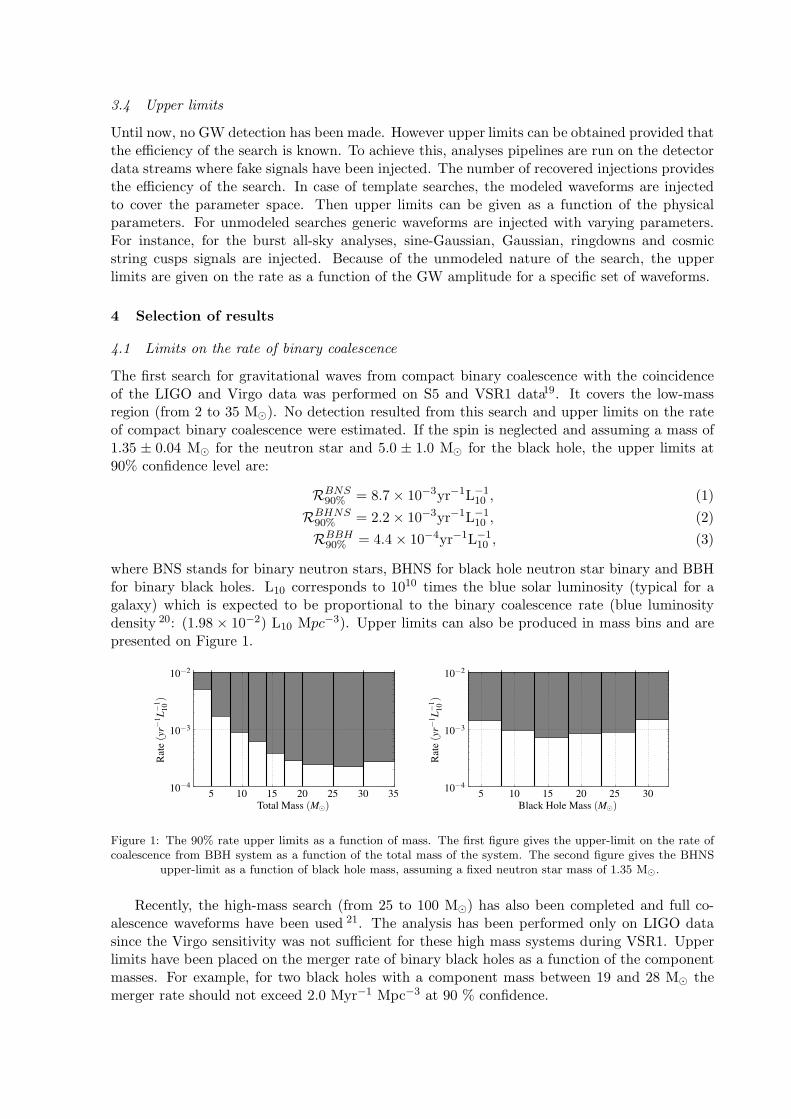
where BNS stands for binary neutron stars, BHNS for black hole neutron star binary and BBHfor binary black holes. L10 corresponds to 1010 times the blue solar luminosity (typical for agalaxy) which is expected to be proportional to the binary coalescence rate (blue luminositydensity 20: (1.98 × 10⁻²) L10 Mpc−3). Upper limits can also be produced in mass bins and arepresented on Figure 1.
Figure 1: The 90% rate upper limits as a function of mass. The first figure gives the upper-limit on the rate ofcoalescence from BBH system as a function of the total mass of the system. The second figure gives the BHNS
upper-limit as a function of black hole mass, assuming a fixed neutron star mass of 1.35 M⊙.
Recently, the high-mass search (from 25 to 100 M⊙) has also been completed and full co-
alescence waveforms have been used 21. The analysis has been performed only on LIGO datasince the Virgo sensitivity was not sufficient for these high mass systems during VSR1. Upperlimits have been placed on the merger rate of binary black holes as a function of the componentmasses. For example, for two black holes with a component mass between 19 and 28 M
⊙the
merger rate should not exceed 2.0 Myr−1 Mpc−3 at 90 % confidence.
4.2 All-sky burst search
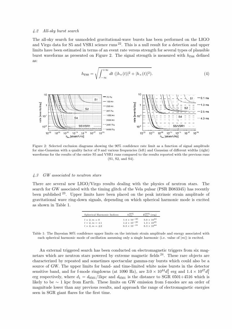
The all-sky search for unmodeled gravitational-wave bursts has been performed on the LIGOand Virgo data for S5 and VSR1 science runs 22. This is a null result for a detection and upperlimits have been estimated in terms of an event rate versus strength for several types of plausibleburst waveforms as presented on Figure 2. The signal strength is measured with hrss definedas:
hrss =
√
∫
+∞
−∞
dt (|h+(t)|2 + |h×(t)|2). (4)
Figure 2: Selected exclusion diagrams showing the 90% confidence rate limit as a function of signal amplitudefor sine-Gaussian with a quality factor of 9 and various frequencies (left) and Gaussian of different widths (right)waveforms for the results of the entire S5 and VSR1 runs compared to the results reported with the previous runs
(S1, S2, and S4).
4.3 GW associated to neutron stars
There are several new LIGO/Virgo results dealing with the physics of neutron stars. Thesearch for GW associated with the timing glitch of the Vela pulsar (PSR B083345) has recentlybeen published 23. Upper limits have been placed on the peak intrinsic strain amplitude ofgravitational wave ring-down signals, depending on which spherical harmonic mode is excitedas shown in Table 1.
Spherical Harmonic Indices h90%
2mE90%
2m(erg)
l = 2, m = 0 1.4 × 10⁻²⁰ 5.0 × 1044
l = 2, m = ±1 1.2 × 10⁻²⁰ 1.3 × 1045
l = 2, m = ±2 6.3 × 10⁻²¹ 6.3 × 1044
Table 1: The Bayesian 90% confidence upper limits on the intrinsic strain amplitude and energy associated witheach spherical harmonic mode of oscillation assuming only a single harmonic (i.e. value of |m|) is excited.
An external triggered search has been conducted on electromagnetic triggers from six mag-netars which are neutron stars powered by extreme magnetic fields 24. These rare objects arecharacterized by repeated and sometimes spectacular gamma-ray bursts which could also be asource of GW. The upper limits for band- and time-limited white noise bursts in the detectorsensitive band, and for f-mode ringdowns (at 1090 Hz), are 3.0 × 1044d21 erg and 1.4 × 1047d21erg respectively, where d1 = d0501/1kpc and d0501 is the distance to SGR 0501+4516 which islikely to be ∼ 1 kpc from Earth. These limits on GW emission from f-modes are an order ofmagnitude lower than any previous results, and approach the range of electromagnetic energiesseen in SGR giant flares for the first time.
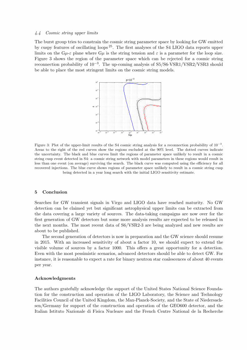
4.4 Cosmic string upper limits
The burst group tries to constrain the cosmic string parameter space by looking for GW emittedby cuspy features of oscillating loops 25. The first analyses of the S4 LIGO data reports upperlimits on the Gµ-ε plane where Gµ is the string tension and ε is a parameter for the loop size.Figure 3 shows the region of the parameter space which can be rejected for a cosmic stringreconnection probability of 10−3. The up-coming analysis of S5/S6-VSR1/VSR2/VSR3 shouldbe able to place the most stringent limits on the cosmic string models.
10−12
10−11
10−10
10−9
10−8
10−7
10−6
10−5
10−4
10−12
10−10
10−8
10−6
10−4
10−2
100
Gµ
ε
p=10−3
Figure 3: Plot of the upper-limit results of the S4 cosmic string analysis for a reconnection probability of 10−3.Areas to the right of the red curves show the regions excluded at the 90% level. The dotted curves indicatethe uncertainty. The black and blue curves limit the regions of parameter space unlikely to result in a cosmicstring cusp event detected in S4: a cosmic string network with model parameters in these regions would result inless than one event (on average) surviving the search. The black curve was computed using the efficiency for allrecovered injections. The blue curve shows regions of parameter space unlikely to result in a cosmic string cusp
being detected in a year long search with the initial LIGO sensitivity estimate.
5 Conclusion
Searches for GW transient signals in Virgo and LIGO data have reached maturity. No GWdetection can be claimed yet but significant astrophysical upper limits can be extracted fromthe data covering a large variety of sources. The data-taking campaigns are now over for thefirst generation of GW detectors but some more analysis results are expected to be released inthe next months. The most recent data of S6/VSR2-3 are being analyzed and new results areabout to be published.
The second generation of detectors is now in preparation and the GW science should resumein 2015. With an increased sensitivity of about a factor 10, we should expect to extend thevisible volume of sources by a factor 1000. This offers a great opportunity for a detection.Even with the most pessimistic scenarios, advanced detectors should be able to detect GW. Forinstance, it is reasonable to expect a rate for binary neutron star coalescences of about 40 eventsper year.
Acknowledgments
The authors gratefully acknowledge the support of the United States National Science Founda-tion for the construction and operation of the LIGO Laboratory, the Science and TechnologyFacilities Council of the United Kingdom, the Max-Planck-Society, and the State of Niedersach-sen/Germany for support of the construction and operation of the GEO600 detector, and theItalian Istituto Nazionale di Fisica Nucleare and the French Centre National de la Recherche

Scientifique for the construction and operation of the Virgo detector. The authors also grate-fully acknowledge the support of the research by these agencies and by the Australian ResearchCouncil, the International Science Linkages program of the Commonwealth of Australia, theCouncil of Scientific and Industrial Research of India, the Istituto Nazionale di Fisica Nucleareof Italy, the Spanish Ministerio de Educacion y Ciencia, the Conselleria d’Economia Hisendai Innovacio of the Govern de les Illes Balears, the Foundation for Fundamental Research onMatter supported by the Netherlands Organisation for Scientific Research, the Polish Ministryof Science and Higher Education, the FOCUS Programme of Foundation for Polish Science, theRoyal Society, the Scottish Funding Council, the Scottish Universities Physics Alliance, TheNational Aeronautics and Space Administration, the Carnegie Trust, the Leverhulme Trust,the David and Lucile Packard Foundation, the Research Corporation, and the Alfred P. SloanFoundation.
References
1. A. Einstein, Preuss. Akad. Wiss. Berlin, Sitzungsberichte der physikalisch-mathematischen Klasse, 688 (1916).
2. J. Taylor and J. Weisberg., Astrophys. J. 345, 434 (1989).3. F. Acernese et al (Virgo Collaboration), Class. Quant. Grav. 25, 114045 (2008).4. B. P. Abbott et al (LIGO Scientific Collaboration), Rep. Prog. Phys. 72, 076901 (2009).5. C. Palomba (LIGO Scientific Collaboration and the Virgo Collaboration), submit. to these
proceedings.6. H. Grote (the LIGO Scientific Collaboration), Class. Quant. Grav. 25, 114043 (2008).7. L. Blanchet, Living Rev. Rel. 9, 3 (2006).8. Frans Pretorius, Phys. Rev. Lett. 95, 121101 (2005).9. E. Berti et al, Phys. Rev. D 73, 064030 (2006).
10. J. Abadie et al (LIGO Scientific Collaboration and the Virgo Collaboration), Class. Quant.Grav. 27, 173001 (2010).
11. C. D. Ott, Class. Quant. Grav. 26, 063001 (2009).12. C. Rover et al, Phys. Rev. D 80, 102004 (2009).13. R. C. Duncan and C. Thompson, Astrophys. J. 392, L9 (1992).14. A. Vilenkin and E. Shellard, Cambridge University Press (2000).15. T. Damour and A. Vilenkin, Phys. Rev. Lett. 85, 3761 (2000).16. M. Was (LIGO Scientific Collaboration and the Virgo Collaboration), submit. to these
proceedings.17. F. Robinet (LIGO Scientific Collaboration and the Virgo Collaboration), Class. Quant.
Grav. 27, 194012 (2010)18. N. Christensen (LIGO Scientific Collaboration and the Virgo Collaboration), Class.
Quant. Grav. 27, 194010 (2010)19. J. Abadie et al (LIGO Scientific Collaboration and the Virgo Collaboration), Phys. Rev.
D 82, 102001 (2010)20. R. K. Kopparapu et al, Astrophys. J. 675, 1459 (2008)21. J. Abadie et al (LIGO Scientific Collaboration and the Virgo Collaboration), to appear in
Phys. Rev. D, arXiv:1102.3781.22. J. Abadie et al (LIGO Scientific Collaboration and the Virgo Collaboration), Phys. Rev.
D 81, 102001 (2010).23. J. Abadie et al (the LIGO Scientific Collaboration), Phys. Rev. D 83, 042001 (2011).24. J. Abadie et al (LIGO Scientific Collaboration and the Virgo Collaboration), to appear in
ApJ Lett, arXiv:1011.4079.25. B. Abbott et al (the LIGO Scientific Collaboration), Phys. Rev. D 80, 062002 (2009).
SEARCHES FOR CONTINUOUS GRAVITATIONAL WAVE SIGNALS AND
STOCHASTIC BACKGROUNDS IN LIGO AND VIRGO DATA
C. PALOMBA for the LIGO Scientific Collaboration and the Virgo Collaboration
Istituto Nazionale di Fisica Nucleare, sezione di Roma, I-00185 Roma, Italy
Abstract
We present results from searches of recent LIGO and Virgo data for continuous gravitationalwave signals (CW) from spinning neutron stars and for a stochastic gravitational wave background(SGWB).
The first part of the talk is devoted to CW analysis with a focus on two types of searches. Inthe targeted search of known neutron stars a precise knowledge of the star parameters is used toapply optimal filtering methods. In the absence of a signal detection, in a few cases, an upperlimit on strain amplitude can be set that beats the spindown limit derived from attributing spin-down energy loss to the emission of gravitational waves. In contrast, blind all-sky searches arenot directed at specific sources, but rather explore as large a portion of the parameter space aspossible. Fully coherent methods cannot be used for these kind of searches which pose a non trivialcomputational challenge.
The second part of the talk is focused on SGWB searches. A stochastic background of grav-itational waves is expected to be produced by the superposition of many incoherent sources ofcosmological or astrophysical origin. Given the random nature of this kind of signal, it is notpossible to distinguish it from noise using a single detector. A typical data analysis strategy relieson cross-correlating the data from a pair or several pairs of detectors, which allows discriminatingthe searched signal from instrumental noise.
Expected sensitivities and prospects for detection from the next generation of interferometersare also discussed for both kind of sources.
1 Introduction
The most recent results obtained in the search of CW and SGWB have used data from LIGO S5 1
and Virgo VSR2 2 runs. S5 run involved all three LIGO detectors, Hanford 4km (H1), Hanford2km (H2) and Livingston 4km (L1), and took place from November 2005 to September 2007 withan average single-interferometer duty cycle of 73.6%, an average two-site coincident duty cycle of59.4% and an average triple-interferometer duty cycle of 52.5%. Virgo (V1) VSR2 run took placefrom July 2009 to January 2010 with a duty cycle of 80.4%. At low frequency, say below 70 Hz,VSR2 sensitivity was better than S5. At intermediate frequency, between 70 Hz and 500 Hz, S5sensitivity was better than VSR2. At frequency above about 500 Hz the sensitivity of the two runswere very similar.
In 2010 two more scientific runs, LIGO S6 and Virgo VSR3, took place. The data are beinganalyzed and some interesting results have already been obtained, but are still under internalreview, so we will not discuss them here.
A generic gravitational wave (GW) signal is described by a tensor metric perturbation h(t) =h+(t) e+ + h×(t) e×, where e+ and e× are the two basis polarization tensors. The form of the twoamplitudes depends on the specific kind of signal.
2 The search for continuous gravitational wave signals
Rapidly spinning neutron stars, isolated or in binary systems, are a potential source of CW. To emitGW some degree of non-axisymmetry is required. It can be due to several mechanisms includingelastic stress or magnetic field which induce a deformation of the neutron star shape, free-precessionaround the rotation axis or accretion of matter from a companion star. The size of the distortion,typically measured by the ellipticity ǫ =
Ixx−Iyy
Izz, which is defined in terms of the star principal
moments of inertia, can provide important information on the neutron star equation of state.The signal emitted by a tri-axial neutron star rotating around a principal axis of inertia is
characterized by amplitudes
h+(t) = h0
(
1 + cos2 ι
2
)
cosΦ(t); h×(t) = h0 cos ι sin Φ(t), (1)
The angle ι is the inclination of the star’s rotation axis with respect to the line of sight and Φ(t) isthe signal phase function, where t is the detector time, while the amplitude h0 is given by
h0 =4π2
G
c4
Izzǫf2
d, (2)
being d the star distance and f the signal frequency (twice the star rotation frequency). While weexpect f < 2 kHz and d <10 kpc, the typical value of the ellipticity is largely unknown. Standardequations of state (EOS) of neutron star matter foresee maximum value of the ellipticity 3 ofthe order of ǫmax ≈ 5 · 10−6. For some ’exotic’ EOS a maximum value ǫmax ≈ 10−2
− 10−4 isforeseen 4, 5, 6.
The signal frequency gradually decreases due to the intrinsic source spin-down, caused by ele-cromagnetic and hopefully gravitational energy losses. The received signal phase is affected bythe Doppler modulation due to the detector-source relative motion and by some relativistic effects.Moreover, the signal is also affected by the amplitude and phase modulation due to the detectorbeam-pattern functions F+(t;ψ), F×(t;ψ), which depend on the polarization angle ψ, on the sourceposition in the sky and on the detector position and orientation on the Earth.
Assuming that the observed spin-down f of a given neutron star is totally due to the emissionof GW, an absolute upper limit to the amplitude of the GW signal, called spin-down limit, can bederived 7:
hsd0 = 8.06 · 10−19
I38 d−1kpc
√
|(f /Hz s−1)|
(f/Hz), (3)
where I38 is the star’s moment of inertia in units of 1038 kgm2 and dkpc is the star’s distance fromthe Sun in kiloparsecs. Going below the spin-down limit means we are putting a constraint on thefraction of spin-down energy due to the emission of GW.
Two types of CW searches have received the most effort up to now: targeted searches and wide
parameter searches.In the targeted searches the source parameters (α, δ, f, f , ...) are assumed to be known with high
accuracy. The search for known pulsars belongs to this category. This kind of search is computa-tionally cheap and a fully coherent analysis, based on matched filtering, over long observation timeis feasible. Various methods of implementing matched filtering have been developed8, 9, 10. In orderto make a coherent analysis over long times Doppler, Einstein and possibly Shapiro effects must beaccurately compensated. Radio-astronomic observations can be used to accurately track the GWsignal phase evolution (assuming the GW signal is phase locked to the EM pulses). Moreover, theyare also important to know if a glitch, i.e. a sudden jump in frequency and frequency derivative,occurred during the period of data to be analyzed.
The sensitivity of a coherent search, i.e. the minimum signal amplitude detectable over anobservation time Tobs, with a false alarm probability of 1 % and a false dismissal probability of10 % and taking also an average over source and detector parameters, is given by
h0,min ≈ 11
√
Sn(f)
Tobs(4)
where Sn(f) is the detector noise spectrum. The exact value of the coefficient depends on thespecific analysis method employed.
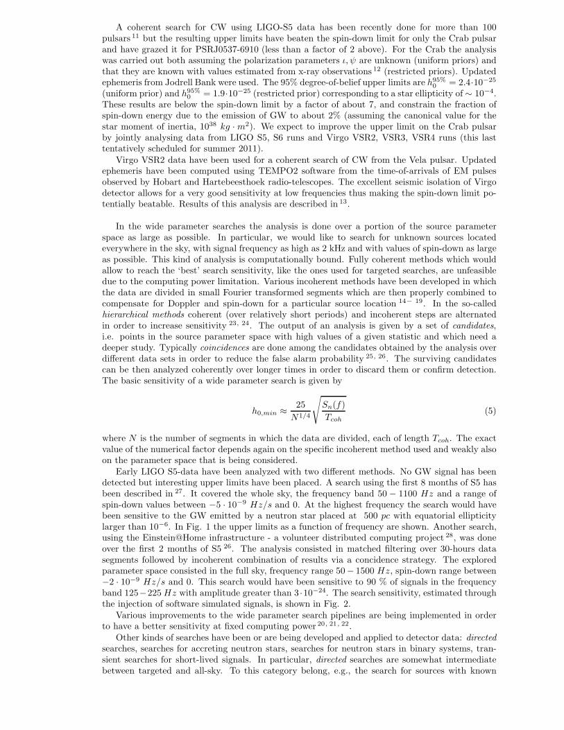
A coherent search for CW using LIGO-S5 data has been recently done for more than 100pulsars 11 but the resulting upper limits have beaten the spin-down limit for only the Crab pulsarand have grazed it for PSRJ0537-6910 (less than a factor of 2 above). For the Crab the analysiswas carried out both assuming the polarization parameters ι, ψ are unknown (uniform priors) andthat they are known with values estimated from x-ray observations 12 (restricted priors). Updatedephemeris from Jodrell Bank were used. The 95% degree-of-belief upper limits are h95%
0 = 2.4·10−25
(uniform prior) and h95%0 = 1.9·10−25 (restricted prior) corresponding to a star ellipticity of ∼ 10−4.
These results are below the spin-down limit by a factor of about 7, and constrain the fraction ofspin-down energy due to the emission of GW to about 2% (assuming the canonical value for thestar moment of inertia, 1038
kg ·m2). We expect to improve the upper limit on the Crab pulsar
by jointly analysing data from LIGO S5, S6 runs and Virgo VSR2, VSR3, VSR4 runs (this lasttentatively scheduled for summer 2011).
Virgo VSR2 data have been used for a coherent search of CW from the Vela pulsar. Updatedephemeris have been computed using TEMPO2 software from the time-of-arrivals of EM pulsesobserved by Hobart and Hartebeesthoek radio-telescopes. The excellent seismic isolation of Virgodetector allows for a very good sensitivity at low frequencies thus making the spin-down limit po-tentially beatable. Results of this analysis are described in 13.
In the wide parameter searches the analysis is done over a portion of the source parameterspace as large as possible. In particular, we would like to search for unknown sources locatedeverywhere in the sky, with signal frequency as high as 2 kHz and with values of spin-down as largeas possible. This kind of analysis is computationally bound. Fully coherent methods which wouldallow to reach the ‘best’ search sensitivity, like the ones used for targeted searches, are unfeasibledue to the computing power limitation. Various incoherent methods have been developed in whichthe data are divided in small Fourier transformed segments which are then properly combined tocompensate for Doppler and spin-down for a particular source location 14− 19. In the so-calledhierarchical methods coherent (over relatively short periods) and incoherent steps are alternatedin order to increase sensitivity 23, 24. The output of an analysis is given by a set of candidates,i.e. points in the source parameter space with high values of a given statistic and which need adeeper study. Typically coincidences are done among the candidates obtained by the analysis overdifferent data sets in order to reduce the false alarm probability 25, 26. The surviving candidatescan be then analyzed coherently over longer times in order to discard them or confirm detection.The basic sensitivity of a wide parameter search is given by
h0,min ≈
25
N1/4
√
Sn(f)
Tcoh(5)
where N is the number of segments in which the data are divided, each of length Tcoh. The exactvalue of the numerical factor depends again on the specific incoherent method used and weakly alsoon the parameter space that is being considered.
Early LIGO S5-data have been analyzed with two different methods. No GW signal has beendetected but interesting upper limits have been placed. A search using the first 8 months of S5 hasbeen described in 27. It covered the whole sky, the frequency band 50 − 1100 Hz and a range ofspin-down values between −5 · 10−9
Hz/s and 0. At the highest frequency the search would havebeen sensitive to the GW emitted by a neutron star placed at 500 pc with equatorial ellipticitylarger than 10−6. In Fig. 1 the upper limits as a function of frequency are shown. Another search,using the Einstein@Home infrastructure - a volunteer distributed computing project 28, was doneover the first 2 months of S5 26. The analysis consisted in matched filtering over 30-hours datasegments followed by incoherent combination of results via a concidence strategy. The exploredparameter space consisted in the full sky, frequency range 50− 1500 Hz, spin-down range between−2 · 10−9
Hz/s and 0. This search would have been sensitive to 90 % of signals in the frequencyband 125−225Hz with amplitude greater than 3 ·10−24. The search sensitivity, estimated throughthe injection of software simulated signals, is shown in Fig. 2.
Various improvements to the wide parameter search pipelines are being implemented in orderto have a better sensitivity at fixed computing power 20, 21, 22.
Other kinds of searches have been or are being developed and applied to detector data: directed
searches, searches for accreting neutron stars, searches for neutron stars in binary systems, tran-sient searches for short-lived signals. In particular, directed searches are somewhat intermediatebetween targeted and all-sky. To this category belong, e.g., the search for sources with known
f [Hz]
Equatorial declination band
Intermediate declination band
Polar declination band
0h
Figure 1: Minimum (H1 or L1) 95% confidence level upper limits on signal amplitude for equatorial, intermediate andpolar declination bands. Lower curves corresponds to best neutron star orientation, upper curves to worst neutron star
orientation. Figure adapted from PRL 27.
102
103
10−24
10−23
10−22
f [Hz]
h0
10%50%90%
Figure 2: Estimated sensitivity of the Einstein@Home search for early LIGO S5 data. The three curves show the sourceamplitude h0 at which 10% (bottom), 50% (middle), 90% (top) of the simulated sources would be confidently detected.
Figure adapted from PRD 26.
position but unknown frequency (like the compact objects in supernova remnants) and the searchover relatively small sky area (like the galactic center or globular clusters). An interesting upperlimit has been obtained in the analysis of ∼ 12 days of S5 data searching for GW signals from thesupernova remnant Cassiopeia A 29. The source position is known and a coherent search over thefrequency range 100 − 300 Hz and a wide range of spin-down values has been done establishing a95% confidence upper limit below the indirect limit based on energy conservation and age of theremnant. This search established also the first upper limit on r-modes amplitude.
With Advanced LIGO and Virgo detectors the spin-down limit on GW emission from knownpulsars will be beatable for tens of objects and in few cases the minimum detectable ellipticity willbe below 10−5 and down to 10−8, a range of values which is sustainable also by standard neutronstar EOS. Concerning all-sky searches, nearby gravitars (say, a few hundreds of parsecs away) wouldbe detectable for ellipticity larger than a few units in 10−8. Objects with ellipticity of the order of10−6 would be detectable up to the Galactic center (see, e.g., Fig. 41 of 19 after up-scaling by afactor of about 10 the distance associated to red curves).
3 The search for stochastic gravitational wave backgrounds
Typically, two kinds of stochastic gravitational wave backgrounds (SGWB) are considered. Cos-mological backgrounds, due to processes taking place in the very early stages of Universe evolution,like amplification of vacuum fluctuations, phase transition, cosmic string cusps. These kinds ofbackgrounds are expected to be stationary, gaussian, unpolarized and, in a first approximation,isotropic. Astrophysical backgrounds, due to the superposition of many unresolved sources, sincethe beginning of stellar activity, like core collapse to supernovae or the final stages of compactbinary mergers. The assumption of isotropy would not hold, if of galactic origin, and an astrophys-ical background could also be not gaussian, if the number of contributing sources is not very large.Detection of a background of cosmological origin may allow us to probe time scales and energy notaccessible with conventional astronomy or accelerators. Even in case of non-detection importantconstraints to model parameters can be established. An astrophysical background, interesting in itsown right, could in fact be a foreground obscuring the cosmological background in some frequencyband. See references in the review papers by Maggiore 30 and Regimbau 31 for a more detaileddescription of various possible sources of SGWB.
A SGWB is usually characterized by the dimensionless parameter
ΩGW (f) =1
ρc
dρgw
dlnf(6)
where ρgw is the gravitational wave densitiy, f is the frequency in the observer frame and ρc =3H2
0
8πGis the critical energy density to close the Universe (H0 is the Hubble constant). It is also useful,in particular to make easier the comparison with detector sensitivity, to express the background interms of the signal energy spectral density
Sh(f) =3H2
0
4π2ΩGW (f) (7)
In Fig.3 theoretical predictions (for given model parameters, see figure caption) of various SGWBof cosmological origin and observational bounds are shown.
The signal would appear as excess noise in a single detector. In principle, to conclude thata SGWB is really present one should exclude that the excess noise is not due to some source ofnoise not taken into account. The difficulty in doing this is also increased by the fact that thesignal-to-noise ratio does not increase with the observation time, differently from what happensin the search for continuous signals. On the other hand, the signal would show up as a coherentstochastic process between two or more detectors. Then, a typical analysis strategy consists incross-correlating the data from multiple detectors. By indicating with s1(t), s2(t) the data streamsfrom two detectors, the cross-correlation is
Y =
∫ +Tobs/2
−Tobs/2
dt
∫ +Tobs/2
−Tobs/2
dt′
s1(t)s2(t′)Q(t− t
′) (8)

where Q(t − t′) is a filter function chosen to maximize the signal-to-noise ratio. In the frequency
domain the optimal filter function takes the form
Q(f) ∝Γ(f)Ωgw(f)
f3S1(f)S2(f)(9)
where S1, S2 are the power spectral noise density of the two detectors and Γ(f) is the overlapreduction function which takes into account the fact that the two detectors can see a differentsignal because they are at a different location or because they have a different angular sensitivity.In particular, if the separation between the two detectors is much larger than the signal reducedwavelength, the correlation is strongly suppressed. On the other hand, if the distance among twodetectors is very small, or if they are co-located, the identification of coherent disturbances is nota trivial task. The sensitivity of a pair of detectors is usually given in terms of the minimumdetectable amplitude for a flat spectrum 32:
Ωmin ≈
34
H20
√
Tobs
[∫
∞
0
Γ2(f)
f6S1(f)S2(f)df
]
−1/2
(10)
where a false alarm rate of 1% and a false dismissal rate of 10% have been considered.The full-S5 data set from LIGO detectors has been analyzed to search for a SGWB cross-
correlating data from the detector pairs H1-L1 and H2-L1 33. The effective observation time was∼ 293 days. The analysis was focused on the frequency band 41 − 170 Hz, which includes about99% of the instrumental sensitivity. A bayesian 95% degree of belief upper limit has been set,taking the S4 posterior as a prior:
Ωgw(f) < 6.9 · 10−6 (11)
Models to explain the element abundance observation constrain total energy at the time of the Big-Bang nucleosynthesis to
∫
Ωgw(f)d(ln f) < 1.5 · 10−5. Allocating all the energy to the analyzedfrequency band implies an upper bound of 1.1 · 10−5. Then the limit of Eq. 11 beats the indirectlimits provided by Big-bang nucleosynthesis and cosmic microwave background, see Fig.3. Thisresult constrains also models of cosmic super-strings, in which the gravitational background is dueto the superposition of many cusp burst signals 34, excluding regions in the Gµ− ǫ plane, as shownin Fig.4.
The analysis of data from the pair H1-H2 is also underway. From one hand having two co-locateddetectors would give a sensitivity improvement of about one order of magnitude. On the other,the presence of correlations between the two data streams reduces the gain. A big effort is beingdone in order to identify all the environmental contributions to the H1-H2 cross-correlation. Alsothe search for non-isotropic backgrounds is being considered, and an analysis method optimized forthis kind of signal, called radiometer analysis 35, has already produced results for S4 and is beingapplied to S5 data.
Advanced detectors should push the upper limit a couple of orders of magnitude below the cur-rent limit thus further constraining the parameter space of various models of cosmological SGWB,see Fig.3. In particular, for cosmic super-string models they could exclude regions of Gµ > 10−11
and ǫ > 10−10. They should be also able to put constraints on Pre-Big-Bang models by excludingregions in the f1 − µ plane.
4 Conclusions
The search for continuous gravitational wave signals and stochastic gravitational wave backgroundsin LIGO and Virgo data has already produced several upper limits of astrophysical interest, altoughno detection. New results will come soon by analyzing most recent data and using improved analysispipelines. The development of more sensitive and robust methods will follow in the next years inorder to be ready for the advanced detectors era.
Acknowledgments
The authors gratefully acknowledge the support of the United States National Science Foundationfor the construction and operation of the LIGO Laboratory, the Science and Technology FacilitiesCouncil of the United Kingdom, the Max-Planck-Society, and the State of Niedersachsen/Germanyfor support of the construction and operation of the GEO600 detector, and the Italian Istituto
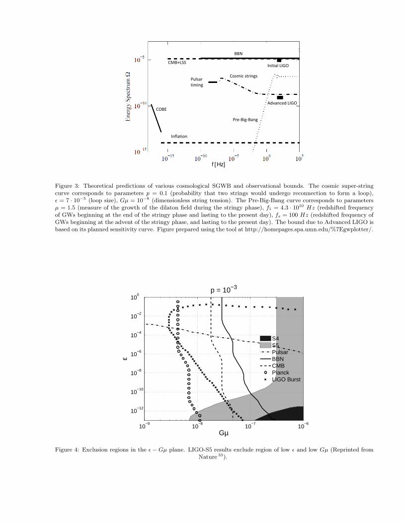
][Hzf
BBN
CMB+LSS
COBE
Inflation
Pulsar
timing
Cosmic strings
Pre-Big-Bang
Initial LIGO
Advanced LIGO
Figure 3: Theoretical predictions of various cosmological SGWB and observational bounds. The cosmic super-stringcurve corresponds to parameters p = 0.1 (probability that two strings would undergo reconnection to form a loop),ǫ = 7 · 10−5 (loop size), Gµ = 10−8 (dimensionless string tension). The Pre-Big-Bang curve corresponds to parametersµ = 1.5 (measure of the growth of the dilaton field during the stringy phase), f1 = 4.3 · 1010 Hz (redshifted frequencyof GWs beginning at the end of the stringy phase and lasting to the present day), fs = 100 Hz (redshifted frequency ofGWs beginning at the advent of the stringy phase, and lasting to the present day). The bound due to Advanced LIGO isbased on its planned sensitivity curve. Figure prepared using the tool at http://homepages.spa.umn.edu/%7Egwplotter/.
10−9
10−8
10−7
10−6
10−12
10−10
10−8
10−6
10−4
10−2
100
Gµ
ε
p = 10−3
S4S5PulsarBBNCMBPlanckLIGO Burst
Figure 4: Exclusion regions in the ǫ − Gµ plane. LIGO-S5 results exclude region of low ǫ and low Gµ (Reprinted fromNature 33).
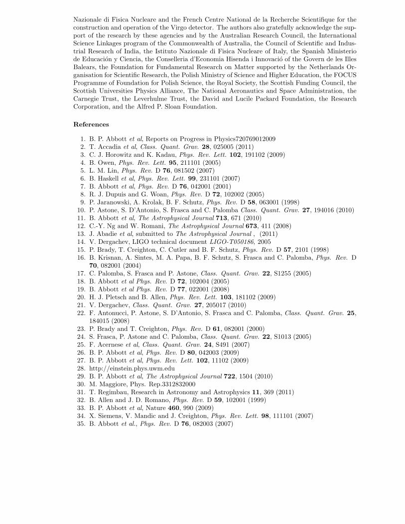
Nazionale di Fisica Nucleare and the French Centre National de la Recherche Scientifique for theconstruction and operation of the Virgo detector. The authors also gratefully acknowledge the sup-port of the research by these agencies and by the Australian Research Council, the InternationalScience Linkages program of the Commonwealth of Australia, the Council of Scientific and Indus-trial Research of India, the Istituto Nazionale di Fisica Nucleare of Italy, the Spanish Ministeriode Educacion y Ciencia, the Conselleria d’Economia Hisenda i Innovacio of the Govern de les IllesBalears, the Foundation for Fundamental Research on Matter supported by the Netherlands Or-ganisation for Scientific Research, the Polish Ministry of Science and Higher Education, the FOCUSProgramme of Foundation for Polish Science, the Royal Society, the Scottish Funding Council, theScottish Universities Physics Alliance, The National Aeronautics and Space Administration, theCarnegie Trust, the Leverhulme Trust, the David and Lucile Packard Foundation, the ResearchCorporation, and the Alfred P. Sloan Foundation.
References
1. B. P. Abbott et al, Reports on Progress in Physics7207690120092. T. Accadia et al, Class. Quant. Grav. 28, 025005 (2011)3. C. J. Horowitz and K. Kadau, Phys. Rev. Lett. 102, 191102 (2009)4. B. Owen, Phys. Rev. Lett. 95, 211101 (2005)5. L. M. Lin, Phys. Rev. D 76, 081502 (2007)6. B. Haskell et al, Phys. Rev. Lett. 99, 231101 (2007)7. B. Abbott et al, Phys. Rev. D 76, 042001 (2001)8. R. J. Dupuis and G. Woan, Phys. Rev. D 72, 102002 (2005)9. P. Jaranowski, A. Krolak, B. F. Schutz, Phys. Rev. D 58, 063001 (1998)
10. P. Astone, S. D’Antonio, S. Frasca and C. Palomba Class. Quant. Grav. 27, 194016 (2010)11. B. Abbott et al, The Astrophysical Journal 713, 671 (2010)12. C.-Y. Ng and W. Romani, The Astrophysical Journal 673, 411 (2008)13. J. Abadie et al, submitted to The Astrophysical Journal , (2011)14. V. Dergachev, LIGO technical document LIGO-T050186, 200515. P. Brady, T. Creighton, C. Cutler and B. F. Schutz, Phys. Rev. D 57, 2101 (1998)16. B. Krisnan, A. Sintes, M. A. Papa, B. F. Schutz, S. Frasca and C. Palomba, Phys. Rev. D
70, 082001 (2004)17. C. Palomba, S. Frasca and P. Astone, Class. Quant. Grav. 22, S1255 (2005)18. B. Abbott et al Phys. Rev. D 72, 102004 (2005)19. B. Abbott et al Phys. Rev. D 77, 022001 (2008)20. H. J. Pletsch and B. Allen, Phys. Rev. Lett. 103, 181102 (2009)21. V. Dergachev, Class. Quant. Grav. 27, 205017 (2010)22. F. Antonucci, P. Astone, S. D’Antonio, S. Frasca and C. Palomba, Class. Quant. Grav. 25,
184015 (2008)23. P. Brady and T. Creighton, Phys. Rev. D 61, 082001 (2000)24. S. Frasca, P. Astone and C. Palomba, Class. Quant. Grav. 22, S1013 (2005)25. F. Acernese et al, Class. Quant. Grav. 24, S491 (2007)26. B. P. Abbott et al, Phys. Rev. D 80, 042003 (2009)27. B. P. Abbott et al, Phys. Rev. Lett. 102, 11102 (2009)28. http://einstein.phys.uwm.edu29. B. P. Abbott et al, The Astrophysical Journal 722, 1504 (2010)30. M. Maggiore, Phys. Rep.331283200031. T. Regimbau, Research in Astronomy and Astrophysics 11, 369 (2011)32. B. Allen and J. D. Romano, Phys. Rev. D 59, 102001 (1999)33. B. P. Abbott et al, Nature 460, 990 (2009)34. X. Siemens, V. Mandic and J. Creighton, Phys. Rev. Lett. 98, 111101 (2007)35. B. Abbott et al., Phys. Rev. D 76, 082003 (2007)
MULTIMESSENGER ASTRONOMY
N.L. CHRISTENSENa
for the LIGO Scientific Collaboration and the Virgo CollaborationPhysics and Astronomy, Carleton College,
Northfield, Minnesota 55057, USA
Multimessenger astronomy incorporating gravitational radiation is a new and exciting fieldthat will potentially provide significant results and exciting challenges in the near future.With advanced interferometric gravitational wave detectors (LCGT, LIGO, Virgo) we willhave the opportunity to investigate sources of gravitational waves that are also expected to beobservable through other messengers, such as electromagnetic (γ-rays, x-rays, optical, radio)and/or neutrino emission. The LIGO-Virgo interferometer network has already been usedfor multimessenger searches for gravitational radiation that have produced insights on cosmicevents. The simultaneous observation of electromagnetic and/or neutrino emission could beimportant evidence in the first direct detection of gravitational radiation. Knowledge of eventtime, source sky location, and the expected frequency range of the signal enhances our abilityto search for the gravitational radiation signatures with an amplitude closer to the noise floorof the detector. Presented here is a summary of the status of LIGO-Virgo multimessengerdetection efforts, along with a discussion of questions that might be resolved using the datafrom advanced or third generation gravitational wave detector networks.
1 Introduction
The era of gravitational wave (GW) astronomy has begun. The LIGO 1 and Virgo 2 GWinterferometric detectors have demonstrated their ability to operate at or near their initialdesign sensitivities. LIGO’s sixth scientific run, S6, and Virgo’s third scientific run, VSR3, wererecently completed; GEO 600 3 also acquired data during this period. The LIGO ScientificCollaboration (LSC) and the Virgo Collaboration have been working together in their effort todetect binary inspiral 4, 5, burst 6,7, continuous wave 8,9, and stochastic background 10 signals, aswell as GWs associated with electromagnetic (EM) events (such as a γ-ray burst, GRB) 11,12.In 2014, a new generation of detectors, with an even better ability to observe the universe,
will come on-line; advanced LIGO (aLIGO) 16 and advanced Virgo (AdV) 17 will work towardachieving a factor of 10 better sensitivity than the initial detectors. The Large-scale CryogenicGravitational wave Telescope (LCGT) is expected to also come on-line around 2015 18. A trulyglobal network of advanced detectors will be simultaneously operating in the second half of thisdecade. The initial ground based laser interferometers were sensitive to GWs in the frequencyband from 20 Hz (for Virgo, 40 Hz for LIGO) up to 8 kHz, while the lower frequency for theadvanced detectors should drop to 10 Hz.
The existence of GWs was predicted by Einstein 13, and confirmed through observationson the binary pulsar PSR 1913+16. This binary system was discovered in 1974 by Taylor andHulse14, and subsequent observations by Taylor and Weisberg15 have shown that the decay of theorbit matches perfectly with what is predicted via energy loss by GW emission. GW detectors,like LIGO and Virgo, hope to observe GWs produced by astrophysical sources. The observationof these GWs will provide information about the astrophysical event. LIGO, Virgo, and otherdetectors will not be just GW detectors, they will also be the new generation of astronomicalobservatories. It is possible that some sources of GWs may not emit EM radiation; for example,imagine the oscillations of a newly formed black hole. Other sources, like a supernova, will likelyemit both EM radiation and GWs, and the observation of the GWs in coincidence with EMobservations could give new insight about the source. EM observations of the universe are donewith radiation having frequencies above 10 MHz. On the other hand, GW observations will befrom frequencies below 10 kHz; this should provide very different information about the universe.Since GWs are weakly interacting, any waves produced will traverse the universe without beingscattered or absorbed; this gives another unique opportunity for scientists to see new phenomenain our universe. In this article we discuss how LIGO and Virgo are searching for GW signalsin coincidence with EM events. This is an example of multimessenger astronomy. Searchesare conducted for GWs at times of observed EM events (the external trigger strategy) 11,12.Since GW data from LIGO and Virgo is non-stationary 19,20, finding a GW signal candidatein coincidence with an EM transient will increase confidence that the signal is astrophysicallyproduced, and not a spurious noise event.
LIGO and Virgo have developed another strategy for finding GW events in association withEM transients. During a period of joint data collection directional information was sent to EMobservatories soon after outlier events were observed in the LIGO-Virgo data; these initial teststook place from Dec 17 2009 to Jan 8 2010, and Sep 4 to Oct 20 2010. When interesting GWtriggers were generated, numerous EM observatories have been notified within 30 minutes aspart of an EM follow-up effort 21.
There are a number of possible sources for an EM signal accompanying a GW. Long GRBsare likely associated with massive star collapse 22, producing γ-rays then subsequent x-ray andoptical afterglows. A double neutron star (NS) or NS/blackhole merger could be the source ofshort GRBs 23 (with prompt γ-rays and maybe weak, isotropic afterglows). Other interestingphenomena include soft gamma repeater (SGR) flares; these are highly magnetized (1015G)neutron stars that emit γ-ray flares sporadically 29.
In addition, many astrophysical events will produce detectable high and low energy neutrinos;neutrino events will be another important multimessenger area. LIGO and Virgo are currentlyworking with IceCube 24,25 and ANTARES 26,27 in the search for GW signals at the time theseneutrino observatories register events. It is suspected that high energy neutrinos could beemitted from long GRBs 22, short GRBs 23, low-luminosity GRBs 28, or even choked GRBs 30.Core collapse supernovae have prompt low energy neutrino emission (along with delayed opticalsignals). In the future, with the advanced detectors, it will be fruitful to search for GWs incoincidence with low energy neutrinos from supernovae 31.
Multimessenger observations could help to address and perhaps resolve a number of openquestions in astrophysics 32. For example:
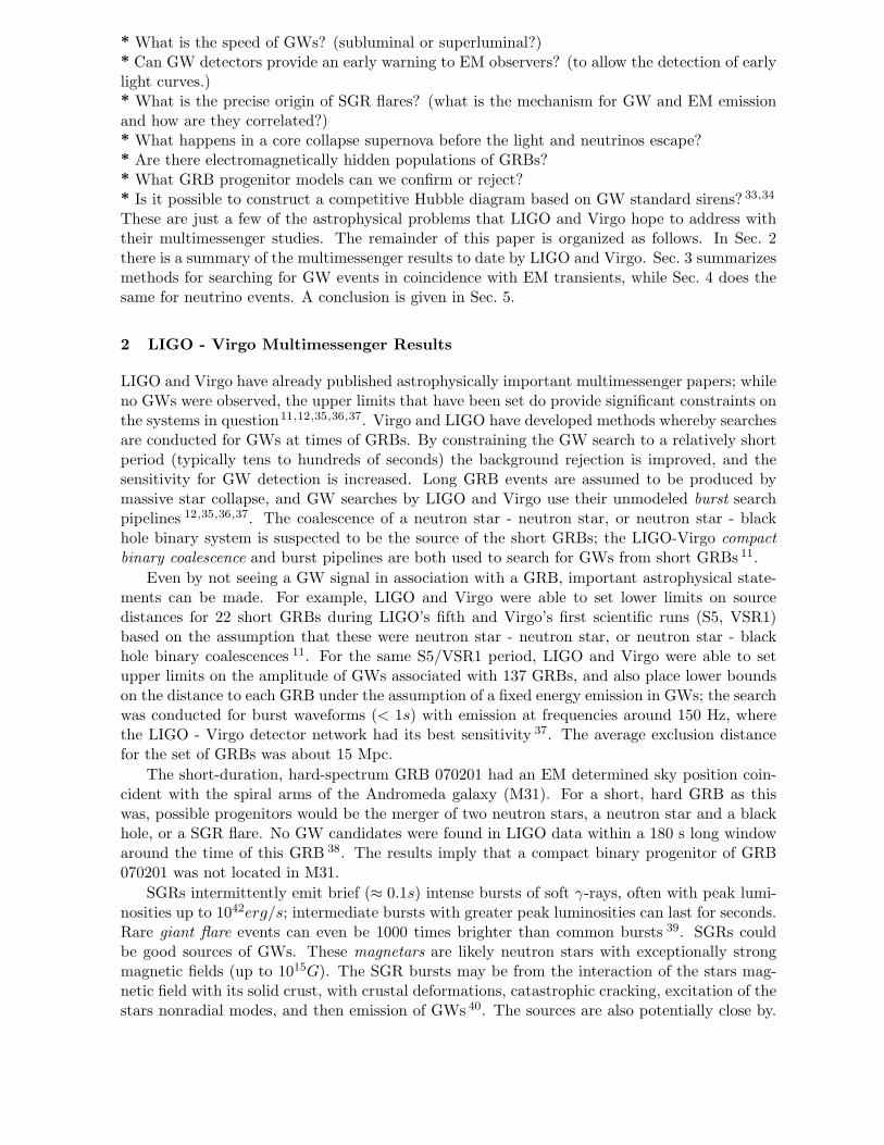
* What is the speed of GWs? (subluminal or superluminal?)* Can GW detectors provide an early warning to EM observers? (to allow the detection of earlylight curves.)* What is the precise origin of SGR flares? (what is the mechanism for GW and EM emissionand how are they correlated?)* What happens in a core collapse supernova before the light and neutrinos escape?* Are there electromagnetically hidden populations of GRBs?* What GRB progenitor models can we confirm or reject?* Is it possible to construct a competitive Hubble diagram based on GW standard sirens? 33,34
These are just a few of the astrophysical problems that LIGO and Virgo hope to address withtheir multimessenger studies. The remainder of this paper is organized as follows. In Sec. 2there is a summary of the multimessenger results to date by LIGO and Virgo. Sec. 3 summarizesmethods for searching for GW events in coincidence with EM transients, while Sec. 4 does thesame for neutrino events. A conclusion is given in Sec. 5.
2 LIGO - Virgo Multimessenger Results
LIGO and Virgo have already published astrophysically important multimessenger papers; whileno GWs were observed, the upper limits that have been set do provide significant constraints onthe systems in question11,12,35,36,37. Virgo and LIGO have developed methods whereby searchesare conducted for GWs at times of GRBs. By constraining the GW search to a relatively shortperiod (typically tens to hundreds of seconds) the background rejection is improved, and thesensitivity for GW detection is increased. Long GRB events are assumed to be produced bymassive star collapse, and GW searches by LIGO and Virgo use their unmodeled burst searchpipelines 12,35,36,37. The coalescence of a neutron star - neutron star, or neutron star - blackhole binary system is suspected to be the source of the short GRBs; the LIGO-Virgo compact
binary coalescence and burst pipelines are both used to search for GWs from short GRBs 11.
Even by not seeing a GW signal in association with a GRB, important astrophysical state-ments can be made. For example, LIGO and Virgo were able to set lower limits on sourcedistances for 22 short GRBs during LIGO’s fifth and Virgo’s first scientific runs (S5, VSR1)based on the assumption that these were neutron star - neutron star, or neutron star - blackhole binary coalescences 11. For the same S5/VSR1 period, LIGO and Virgo were able to setupper limits on the amplitude of GWs associated with 137 GRBs, and also place lower boundson the distance to each GRB under the assumption of a fixed energy emission in GWs; the searchwas conducted for burst waveforms (< 1s) with emission at frequencies around 150 Hz, wherethe LIGO - Virgo detector network had its best sensitivity 37. The average exclusion distancefor the set of GRBs was about 15 Mpc.
The short-duration, hard-spectrum GRB 070201 had an EM determined sky position coin-cident with the spiral arms of the Andromeda galaxy (M31). For a short, hard GRB as thiswas, possible progenitors would be the merger of two neutron stars, a neutron star and a blackhole, or a SGR flare. No GW candidates were found in LIGO data within a 180 s long windowaround the time of this GRB 38. The results imply that a compact binary progenitor of GRB070201 was not located in M31.
SGRs intermittently emit brief (≈ 0.1s) intense bursts of soft γ-rays, often with peak lumi-nosities up to 1042erg/s; intermediate bursts with greater peak luminosities can last for seconds.Rare giant flare events can even be 1000 times brighter than common bursts 39. SGRs couldbe good sources of GWs. These magnetars are likely neutron stars with exceptionally strongmagnetic fields (up to 1015G). The SGR bursts may be from the interaction of the stars mag-netic field with its solid crust, with crustal deformations, catastrophic cracking, excitation of thestars nonradial modes, and then emission of GWs 40. The sources are also potentially close by.
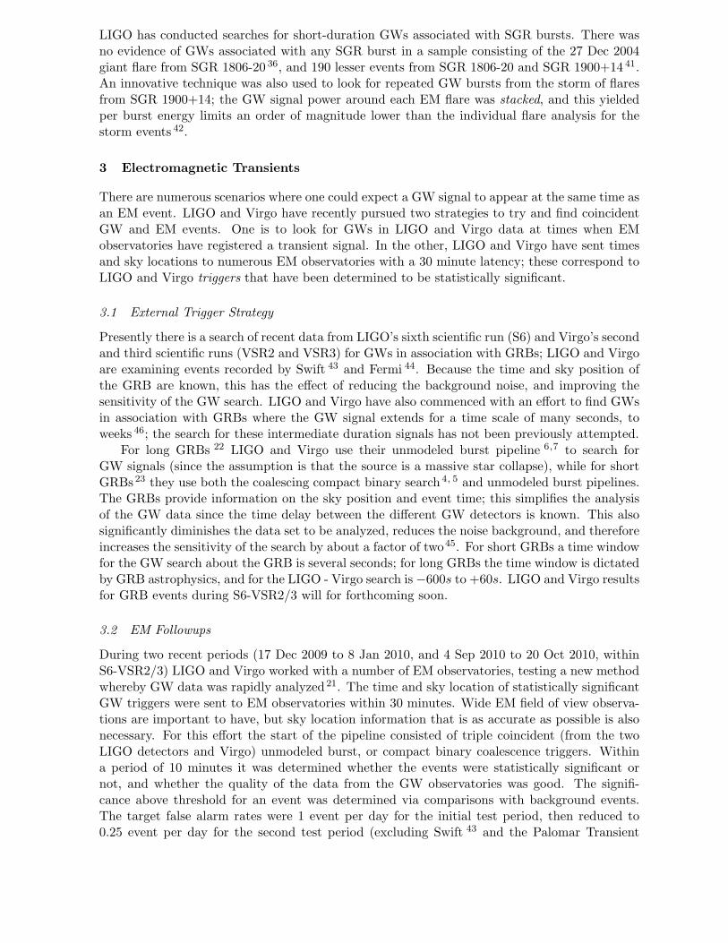
LIGO has conducted searches for short-duration GWs associated with SGR bursts. There wasno evidence of GWs associated with any SGR burst in a sample consisting of the 27 Dec 2004giant flare from SGR 1806-20 36, and 190 lesser events from SGR 1806-20 and SGR 1900+14 41.An innovative technique was also used to look for repeated GW bursts from the storm of flaresfrom SGR 1900+14; the GW signal power around each EM flare was stacked, and this yieldedper burst energy limits an order of magnitude lower than the individual flare analysis for thestorm events 42.
3 Electromagnetic Transients
There are numerous scenarios where one could expect a GW signal to appear at the same time asan EM event. LIGO and Virgo have recently pursued two strategies to try and find coincidentGW and EM events. One is to look for GWs in LIGO and Virgo data at times when EMobservatories have registered a transient signal. In the other, LIGO and Virgo have sent timesand sky locations to numerous EM observatories with a 30 minute latency; these correspond toLIGO and Virgo triggers that have been determined to be statistically significant.
3.1 External Trigger Strategy
Presently there is a search of recent data from LIGO’s sixth scientific run (S6) and Virgo’s secondand third scientific runs (VSR2 and VSR3) for GWs in association with GRBs; LIGO and Virgoare examining events recorded by Swift 43 and Fermi 44. Because the time and sky position ofthe GRB are known, this has the effect of reducing the background noise, and improving thesensitivity of the GW search. LIGO and Virgo have also commenced with an effort to find GWsin association with GRBs where the GW signal extends for a time scale of many seconds, toweeks 46; the search for these intermediate duration signals has not been previously attempted.
For long GRBs 22 LIGO and Virgo use their unmodeled burst pipeline 6,7 to search forGW signals (since the assumption is that the source is a massive star collapse), while for shortGRBs 23 they use both the coalescing compact binary search 4, 5 and unmodeled burst pipelines.The GRBs provide information on the sky position and event time; this simplifies the analysisof the GW data since the time delay between the different GW detectors is known. This alsosignificantly diminishes the data set to be analyzed, reduces the noise background, and thereforeincreases the sensitivity of the search by about a factor of two45. For short GRBs a time windowfor the GW search about the GRB is several seconds; for long GRBs the time window is dictatedby GRB astrophysics, and for the LIGO - Virgo search is −600s to +60s. LIGO and Virgo resultsfor GRB events during S6-VSR2/3 will for forthcoming soon.
3.2 EM Followups
During two recent periods (17 Dec 2009 to 8 Jan 2010, and 4 Sep 2010 to 20 Oct 2010, withinS6-VSR2/3) LIGO and Virgo worked with a number of EM observatories, testing a new methodwhereby GW data was rapidly analyzed 21. The time and sky location of statistically significantGW triggers were sent to EM observatories within 30 minutes. Wide EM field of view observa-tions are important to have, but sky location information that is as accurate as possible is alsonecessary. For this effort the start of the pipeline consisted of triple coincident (from the twoLIGO detectors and Virgo) unmodeled burst, or compact binary coalescence triggers. Withina period of 10 minutes it was determined whether the events were statistically significant ornot, and whether the quality of the data from the GW observatories was good. The signifi-cance above threshold for an event was determined via comparisons with background events.The target false alarm rates were 1 event per day for the initial test period, then reduced to0.25 event per day for the second test period (excluding Swift 43 and the Palomar Transient
Factory 47, where the rate was 0.1 event per day). Information on known globular cluster andgalaxy locations were then used to further restrict the likely sky position of the potential source;only sources out to a distance of 50 Mpc were considered to be possible. Within 30 minutes ofthe initial registration of the potential GW event, the significant triggers were manually vettedby on-call scientific experts, and scientific monitors in the the observatory control rooms. If apotential GW trigger passed all of the tests the direction information was then sent to vari-ous EM observatories, including a number of optical observatories: The Liverpool telescope 48,the Palomar Transient Factory 47, Pi of the Sky 53, QUEST 59, ROTSE III 54, SkyMapper 55,TAROT 56, and the Zadko Telescope 57. Trigger information was also sent to the Swift X-rayobservatory 43,58, and the radio network LOFAR 49. Part of the research work from LIGO andVirgo has also involved the development of image analysis procedures able to identify the EMcounterparts. In the initial S6-VSR2/3 test period there were 8 potential GW events wherethe information was passed onto the EM observatories, and observations were attempted for4 of them; for the second test period there were 6 potential GW events, and 4 of them hadEM observations attempted. The full results from this EM follow-up effort will be published inthe near future. This EM follow-up effort during S6-VSR2/3 was a successful milestone, and apositive step toward the advanced detector era where the chances of GW detections will be veryenhanced, and these rapid EM observations, when coupled with the GW data, could provideimportant astrophysical information on the sources.
Long and short GRB afterglows peak a few minutes after the prompt EM/GW emission50,51,and it is critical to have EM observations as soon as possible after the GW trigger validation.Kilo-novae model afterglows peak about a day after the GW emission 52, so EM observations aday after the GW trigger would be an important validation for these type of events. In orderto discriminate between the possible EM counterpart (to the GW source) from contaminatingtransients repeated observations over several nights are necessary to study the light curve.
4 Neutrinos
Many of the energetic astrophysical events that could produce GWs are also expected to emitneutrinos. LIGO and Virgo are currently investigating methods to use observations of high andlow energy neutrinos to aid in the effort to observe GWs.
4.1 High Energy Neutrinos
High energy neutrinos (HENs) are predicted to be emitted in astrophysical events that alsoproduce significant amounts of GWs, and by using the time and sky location of observed HENsthe ability to confidently identify GWs will be improved. HENs should be emitted in long GRBs;in the prompt and afterglow phases, HENs (105
− 1010 GeV ) are expected to be produced byaccelerated protons in relativistic shocks 22. HENs can also be emitted during binary mergersinvolving neutron stars 23. HENs and GWs could both come from low luminosity GRBs; thesewould be associated with an energetic population of core-collapse supernovae 28. There is aclass of events where GWs and HENs might be observed in the absence of a GRB observation,namely with choked GRBs; these could plausibly come from baryon-rich jets. Because theenvironment could be optically thick, the choked GRB events may be hidden from conventionalEM astronomy, and HENs and GWs will be the only messengers to reveal their properties 30.
LIGO and Virgo are presently working with IceCube24,25 and ANTARES26,27 to see if thereare HEN events in coincidence with GW signals in LIGO (S5 and S6) and Virgo (VSR1, VSR2and VSR3) data. The HEN event time, sky position, and reconstructed energy informationenhance the sensitivity of the GW search. During S5 and VSR1 IceCube had 22 of its strings inoperation, while ANTARES had 5 strings. IceCube reached its full complement of 86 strings near
the time of the end of S6 and VSR3, while ANTARES reached 12 strings. IceCube can providea neutrino trigger sky location to about 1 degree squared accuracy; then by using catalogs ofgalaxy positions, including distance, the trigger information from the LIGO and Virgo datacan provide a joint test statistic, and reduced false alarm rate. For example, there would be afalse alarm rate of about 1 in 435 years for a one-second coincidence time window and spatialcoincidence p-value threshold of 1% 60,61. The size of the time window to be used about theneutrino trigger is a critical parameter in the search, and will need to be larger than 1 s; takinginto account the physical processes that could result in neutrino, γ-ray, and GW emission, itwas determined that a conservative ±500s time window would be appropriate 62. The results ofthis research effort be published soon.
A potential problem for a neutrino - GW search occurs with long GRBs, where HENs fromrelativistic shocks might be emitted between a few hours (internal shocks 28) to a few days(external shocks 22) after the GW emission caused by core bounce 60. For these events a largertime window will be necessary (days) which will increase the false alarm rate. Better sky positionaccuracy, either through an improved neutrino detector or an expanded GW detector network(for example with the coming network of advanced detectors), would help to address this issue.
4.2 Low Energy Neutrinos
Low energy neutrinos (LENs) will be an important multimessenger partner to GWs for corecollapse supernovae (CCSN). LIGO and Virgo are developing search methods involving LENs,especially for the advanced detector era. A range of 3 to 5 Mpc is admittedly at the edge ofdetectability for aLIGO and Super-K 63; at this distance the supernovae rate becomes about1/year 64. A weak coincident signal in both GWs and LENs may be convincing, especially ifthere were also an optical signal. For a galactic supernova, the neutrino signal will be large,and LIGO and Virgo would do a standard external trigger search (GRB search) with a tightcoincidence window. A CCSN produces 10-20 MeV neutrinos (all flavors) over a few 10s ofseconds. It is expected that all three neutrino flavors would be created; GWs and neutrinoswould be emitted promptly in the CCSN, while EM radiation could be delayed. The neutrinoand GW information would truly provide a probe of the physics of the core collapse 65. Theonset of the signal could probably be determined to better than 1 s. Detectors, such as Super-K 63, would detect of order 104 neutrinos for a CCSN at the galactic center. The optical (EM)signature of a CCSN could be obscured; for example, SN 2008iz in M82 was missed via opticalobservations 66. With just EM information the exact time of the core collapse bounce could beuncertain to many hours. A tight coincidence window provided by neutrino observations couldbe used to establish a correlation with GWs. In the advanced GW detector era the sensitivityrange of GW and neutrino detectors will be similar, and it is a research goal of LIGO and Virgothat LEN information will be used in association with data from the advanced GW detectors.
5 Conclusions
There is an active effort by LIGO and Virgo to find GWs in coincidence with EM or neutrinocounterparts. Numerous studies have already been conducted using LIGO and Virgo data fromthe initial generation of detectors, and more results will be forthcoming soon. AdV17, aLIGO16,and GEO-HF (an upgraded GEO, with improved high frequency response)3,67 should be on-linein 2014 and start trying to achieve their enhanced sensitivities. LCGT 18 could be operating in2015. A global network of advanced detectors will be simultaneously observing in the secondhalf of this decade, and multimessenger techniques using EM and neutrino event informationwill improve the probability for detecting GWs. By using GW, EM and neutrino observationsall together there will be a tremendous opportunity to decipher the astrophysics pertaining to
many different types of cataclysmic events in the universe.
Acknowledgments
This document has been assigned LIGO Document Number P-1100053. The work was fundedby NSF Grant PHY-0854790. The authors gratefully acknowledge the support of the UnitedStates National Science Foundation for the construction and operation of the LIGO Laboratory,the Science and Technology Facilities Council of the United Kingdom, the Max-Planck-Society,and the State of Niedersachsen/Germany for support of the construction and operation of theGEO600 detector, and the Italian Istituto Nazionale di Fisica Nucleare and the French CentreNational de la Recherche Scientifique for the construction and operation of the Virgo detec-tor. The authors also gratefully acknowledge the support of the research by these agenciesand by the Australian Research Council, the Council of Scientific and Industrial Research ofIndia, the Istituto Nazionale di Fisica Nucleare of Italy, the Spanish Ministerio de Educacion yCiencia, the Conselleria d’Economia Hisenda i Innovacio of the Govern de les Illes Balears, theFoundation for Fundamental Research on Matter supported by the Netherlands Organisationfor Scientific Research, the Polish Ministry of Science and Higher Education, the FOCUS Pro-gramme of Foundation for Polish Science, the Royal Society, the Scottish Funding Council, theScottish Universities Physics Alliance, The National Aeronautics and Space Administration, theCarnegie Trust, the Leverhulme Trust, the David and Lucile Packard Foundation, the ResearchCorporation, and the Alfred P. Sloan Foundation.
References
1. B. Abbott et al (LIGO Scientific Collaboration), Rep. Prog. Phys. 72, 076901 (2009).2. F. Acernese et al (Virgo Collaboration), Class. Quantum Grav. 25, 114045 (2009).3. H. Grote (LIGO Scientific Collaboration), Class. Quantum Grav. 25, 114043 (2008).4. B. Abbott et al (LIGO Scientific Collaboration), Phys. Rev. D 80, 047101 (2009).5. F. Acernese et al (Virgo Collaboration) Class. Quantum Grav. 24, 5767 (2007).6. B. Abbott et al (LIGO Scientific Collaboration), Phys. Rev. D 80, 102001 (2009).7. F. Acernese et al (Virgo Collaboration), Class. Quantum Grav. 26, 085009 (2009).8. B. Abbott et al (LIGO Scientific Collaboration and the Virgo Collaboration), ApJ 713,
671 (2010).9. F. Acernese et al (Virgo Collaboration), Class. Quantum Grav. 26, 204002 (2009).
10. B. Abbott et al (LIGO Scientific Collaboration and the Virgo Collaboration), Nature 460,990 (2009).
11. J. Abadie et al (LIGO Scientific Collaboration and the Virgo Collaboration), ApJ 715,1453 (2010).
12. F. Acernese et al (Virgo Collaboration), Class. Quantum Grav. 25, 225001 (2008).13. A. Einstein, Preuss. Akad. Wiss. Berlin, Sitzungsberichte der physikalisch-
mathematischen Klasse, 688 (1916).14. R. Hulse and J. Taylor, ApJ 195, L51 (1975).15. J. Taylor and J. Weisberg, ApJ 345, 434 (1989).16. G.M. Harry (LIGO Scientific Collaboration), Class. Quantum Grav. 27, 084006 (2010).17. https://wwwcascina.virgo.infn.it/advirgo/docs.html18. K. Kuroda and the LCGT Collaboration, Class. Quantum Grav. 27, 084004 (2010).19. N. Christensen (LIGO Scientific Collaboration and the Virgo Collaboration), Class. Quan-
tum Grav. 27, 194010 (2010).20. F. Robinet (LIGO Scientific Collaboration and the Virgo Collaboration), Class. Quantum
Grav. 27, 194012 (2010).
21. J. Kanner et al, Class. Quantum Grav. 25, 184034 (2008).22. E. Waxman and J.N. Bahcall, ApJ 541, 707 (2000).23. E. Nakar, Phys. Rep. 442, 166 (2007).24. R. Abbasi et al (IceCube Collaboration), Phys. Rev. D 83, 012001 (2011).25. F. Halzen and J.P. Rodrigues, Class. Quantum Grav. 27, 194003 (2010).26. J.A. Aguilar et al, Phys. Lett. B 696, 16 (2011).27. T. Pradier (Antares Collaboration), Class. Quantum Grav. 27, 194004 (2010).28. N. Guptaa and B. Zhang, Astropart. Phys. 27, 386 (2007).29. K. Ioka, MNRAS 327, 639 (2001).30. S. Horiuchi and Shin’ichiro Ando, Phys. Rev. D 77, 063007 (2008).31. C.D. Ott, Adam Burrows, Luc Dessart and Eli Livne, ApJ 685, 1069 (2008).32. S. Marka (LIGO Scientific Collaboration and the Virgo Collaboration), J. Phys. Conf.
Ser. 243, 012001 (2010).33. B.S. Sathyaprakash et al, Class. Quantum Grav. 27, 215006 (2010).34. S. Nissanke et al, ApJ 725, 496 (2010).35. B. Abbott et al (LIGO Scientific Collaboration), Phys. Rev. D 72, 042002 (2005).36. B. Abbott et al (LIGO Scientific Collaboration), Phys. Rev. D 77, 062004 (2008).37. B. Abbott et al (LIGO Scientific Collaboration and the Virgo Collaboration), ApJ 715,
1438 (2010).38. B. Abbott et al (LIGO Scientific Collaboration), ApJ 681, 1419 (2008).39. D.M. Palmer et al, Nature 434, 1107 (2005).40. J.E. Horvath, Mod. Phys. Lett. A 20, 2799 (2005).41. B. Abbott et al (LIGO Scientific Collaboration), Phys. Rev. Lett. 101, 211102 (2008).42. B. Abbott et al (LIGO Scientific Collaboration), ApJ 701, L68 (2009).43. http://swift.gsfc.nasa.gov/docs/swift/swiftsc.html44. http://fermi.gsfc.nasa.gov/45. M. Was, PhD thesis, Universite Paris Sud, Document LAL-11-119 (2011).46. E. Thrane et al, Phys. Rev. D 83, 083004 (2011).47. A. Rau et al, Publ. Astron. Soc. Pac. 121, 1334 (2009).48. I.A. Steele et al, Proceedings of the SPIE 5489, 679 (2004).49. H.D. Falcke et al, Proceedings of the International Astronomical Union 2, 386 (2007).50. D.A. Kann et al, arXiv:0804.1959v2 (2008).51. D.A. Kann et al, ApJ 720, 1513 (2010).52. B. D. Metzger et al MNRAS 406, 2650 (2010).53. K. Malek et al, Proceedings of the SPIE 7502, 75020D (2009).54. C.W. Akerlof et al, Publ. Astron. Soc. Pac. 115, 132 (2003).55. S. C. Keller et al, Publ. Astron. Soc. of Australia 24, 1 (2007).56. A. Klotz et al, AJ 137, 4100 (2009).57. D.M. Coward et al, Publ. Astron. Soc. of Australia 27, 331 (2010).58. N. Gehrels et al, New Journal of Physics 9, 37 (2007).59. C. Baltay et al, Publ. Astron. Soc. Pac. 119, 1278 (2007).60. Y. Aso et al, Class. Quantum Grav. 25, 114039 (2008).61. E. Chassande-Mottin (LIGO Scientific Collaboration and the Virgo Collaboration) J. Phys.
Conf. Ser. 243, 012002 (2010).62. B. Baret et al, Astropart. Phys. 35, 1 (2011).63. M. Ikeda et al, ApJ 669, 519 (2007).64. S. Ando et al, Phys. Rev. Lett. 95, 171101 (2005).65. C.D. Ott et al, ApJ 685, 1069 (2008).66. A. Brunthaler et al, Astronomy and Astrophysics 499, L17 (2009).67. B. Willke et al, Class. Quantum Grav. 23, S207 (2006).
SEARCHING FOR ELECTROMAGNETIC COUNTERPARTS OF
GRAVITATIONAL WAVE TRANSIENTS
M. BRANCHESIon behalf of the LIGO Scientific Collaboration and the Virgo CollaborationDiSBeF, Universita degli Studi di Urbino “Carlo Bo”, 61029 Urbino, Italy
INFN, Sezione di Firenze, 50019 Sesto Fiorentino, Italy
A. KLOTZUniversite de Toulouse, Institut de Recherche en Astrophysique et Planetologie
9 Avenue Colonel Roche, 31028 Toulouse Cedex 4 France
M. LAAS-BOUREZICRAR / School of Physics, University of Western Australia,
Crawley WA 6009, Australia
A pioneering electromagnetic (EM) observation follow-up program of candidate gravitationalwave (GW) triggers has been performed, Dec 17 2009 to Jan 8 2010 and Sep 4 to Oct 202010, during the recent LIGO/Virgo run. The follow-up program involved ground-based andspace EM facilities observing the sky at optical, X-ray and radio wavelengths. The jointGW/EM observation study requires the development of specific image analysis proceduresable to discriminate the possible EM counterpart of GW trigger from background events. Thepaper shows an overview of the EM follow-up program and the developing image analysisprocedures as they are applied to data collected with TAROT and Zadko.
1 Introduction
The LIGO1 and Virgo2 detectors aim at the first direct detection of gravitational waves from veryenergetic astrophysical events. The most promising sources are mergers of neutron stars (NS)and/or stellar mass black holes (BH) and the core collapse of massive stars. More exotic sourcesinclude cosmic string cusps. It is likely that a fraction of the large energy reservoir associated tothose sources be converted into electromagnetic radiation. This possibility is a feature of severalastrophysical scenarios. For instance, Gamma-Ray Bursts (GRBs) are thought to be associatedwith the coalescence of NS-NS or NS-BH binaries or the collapse of very massive stars (see 3 andreferences therein). Another scenario associated with compact object mergers is the prediction 4
of an isotropic EM emission from supernova-like transients powered by the radioactive decay ofheavy elements produced in merger ejecta (this is referred to as the kilonova model). There aremodels that predict that cusps produce electromagnetic radiation 5.
In this respect, multi-messenger GW and EM astronomy is a very promising field of re-search. An electromagnetic counterpart discovered through a follow-up of a gravitational wavecandidate event would considerably increase the confidence in the astrophysical origin of theevent. The detection of an EM counterpart would give the precise localization and possibly leadto the identification of the host galaxy and redshift. Furthermore, EM and GW observations
provide complementary insights into the progenitor and environment physics. In the long termcombined measurements of the luminosity distance through GW radiation and redshifts throughEM observations may allow a new way of estimating some cosmological parameters.
2 Enabling EM Follow-up of Candidate GW Events
2.1 Selection of Candidate GW Events
A first program of EM follow-up to GW candidates took place (Dec 17 2009 to Jan 8 2010and Sep 4 to Oct 20 2010) during the last LIGO/Virgo observation periods, thanks to thedevelopment of a low-latency GW data analysis pipeline that uses real time gravitational wavetriggers to obtain prompt EM observations to search for the EM counterparts.
One of the challenges of successfully obtaining “target of opportunity” EM observationsis to identify the GW candidates quickly: the data from the three operating detectors (thetwo LIGOs and Virgo) must be transferred and analyzed in near-real time. As soon as the databecome available, three search algorithms (Omega Pipeline, coherent Wave Burst both describedin 6,7 and Multi Band Template Analysis 8) run over the data. For each generated trigger, thedirection of arrival of the wave (and hence potential sky position of the source) is estimatedusing a method based on differences in arrival time at each detector. The event candidatesare collected in the Gravitational-wave candidate event database (GraCEDb). Two softwarepackages LUMIN and GEM select statistically significant triggers and determine the telescopepointing positions. This process typically takes ∼10 minutes. It is followed by a manual eventvalidation. A team of trained experts is on duty and their role is to rapidly coordinate withscientists at the GW detectors to evaluate the detector performances. If no problem is foundthe alert is sent to telescopes. The entire process is typically completed within 30 minutes. Thetriggers selected as GW candidates for EM follow-up are the ones detected in triple coincidencesand with a power above a threshold estimated from the distribution of background events. Afull description of the GW trigger selection and the entire EM follow-up process will be detailedin 9.
2.2 Sky Pointing strategy
The uncertainty in the source direction reconstruction scales inversely with the signal-to-noiseratio 10. GW events near the detection threshold are localized into regions of tens of squaredegrees. Generally, the error regions have a non-trivial geometrical shape, often formed ofseveral disconnected patches. Follow-up EM-telescopes with a wide Field Of View (FOV) arethus required. However, the majority of those telescopes have a FOV which is much smaller thanthe GW angular error box. Additional priors are necessary to improve the location accuracyand increase the chance that the actual source be in the selected FOV. The observable Universeis limited to an horizon of 50 Mpc, taking into account the detector sensitivity to the signalscoming from NS binaries 11. The observation of the whole GW error box is not required 12, butit can be restricted to the regions occupied by Globular Clusters and Galaxies within 50 Mpc,listed in the Gravitational Wave Galaxy Catalog 13. Tens of thousands of galaxies are includedwithin this horizon and the GW observable sources are more likely to be extragalactic.
To determine the telescope pointing position, the probability sky map based on GW datais “weighted” taking into account the mass and the distance of nearby galaxies 14 and globularclusters. It is assumed that the probability of a given galaxy being the host of the actual sourcei) is directly proportional to the galaxy’s mass (the blue luminosity is used as proxy for the massand thus for the number of stars) and, ii) is inversely proportional to the distance.
2.3 Follow-up EM Observatories and Observation Strategy
The follow-up program involved ground-based and space EM facilities: the Liverpool Telescope,the Palomar Transient Factory (PTF), Pi of the Sky, QUEST, ROTSE III, SkyMapper, TAROTand the Zadko Telescope observing the sky in the optical band, the Swift satellite with X-ray andUV/Optical telescopes and the radio interferometer LOFAR. The observing strategy employedby each telescope will be described in 9.
The cadence of EM observations is guided by the expected EM counterpart. The opticalafterglow of an on-axis GRB peaks few minutes after the EM/GW prompt emission. Thekilonova model predicts an optical ligth curve that peaks a day after the GW event, due to thetime that the out flowing material takes to become optically thin. The agreement with the EMfacilities allowed observations as soon as possible, the day after the GW event and, repeatedobservations over longer time-lag to follow the transient light curve dimming.
During the recent winter and summer LIGO/Virgo runs a total of 14 alerts have been sentout to the telescopes and 8 of them led to images being taken.
3 Optical Transient Search in the Wide-Field Telescope Observations
Once the follow-up observations are completed, the collected set of images needs to be analyzed todecide the presence or not of an optical transient of interest. The analysis method is conceptuallysimilar to one used to study a GRB afterglow with a main difference: the arc minute localizationof the current generation gamma-ray observatories allows a significant reduction of the searcharea with respect to the GW observations.
Searching for optical transients in a large sky area requires the development and use of specificimage analysis procedures able to discriminate the EM counterpart from background/contaminantevents. Several analysis pipelines are being developed and tested by groups within the LIGOScientific Collaboration and the Virgo Collaboration in partnership with astronomers.
This section describes one of the considered approaches based on the cross-correlation ofobject catalogs obtained from each image. The resulting pipeline has been designed and testedwith the images collected by the two TAROT and the Zadko telescopes.
TAROT 15 are two robotic 25 cm telescopes with a FOV of 3.5 square degrees located inCalern (France) and in La Silla (Chile). In case of a GW alert, TAROT followed a nominalobservation schedule including six consecutive images with 180 second exposures during thefirst night and same for the three following nights. An exposure of 180 seconds corresponds toa red limiting magnitude of 17.5 under ideal conditions. Zadko 16 is a 1 meter telescope with aFOV of 0.17 square degrees located in Gingin (Western Australia). For each GW trigger, Zadkofollowed a nominal observation schedule including a mosaic of five fields with six consecutiveimages during the first night and same for the three following nights. A 120 sec exposurecorresponds to a red limiting magnitude of 20.5 under ideal conditions.
The main steps of the fully automated analysis pipeline are as follows:1) extraction of the catalog of objects visible in the images using SExtractor 17;2) removal of “known objects” listed in USNO-A2.0 or USNO-B star catalogs that are completedown to a fainter magnitude than the collected images by using a positional cross-correlationtool match 18;3) trace objects in common to several image catalogs by using a cross-positional check. Thisresults in a light curve for each traced object;4) rejection of “rapid contaminating transients” (like cosmic rays, asteroids or noise): the pres-ence is required in at least four consecutive images;5) rejection of “background transients”: the objects are selected in the image regions associatedwith the galaxies within 50 Mpc. A circular region with a diameter equal to 4 times the major
axis galaxy size is used. This is to take into account the possible offset between the host galaxycenter and the optical transients (observed up to tens of kpc for GRBs);6) rejection of “contaminating events” like galaxies, variable stars or false transients by analyz-ing the light curves. The code selects the objects that show a luminosity dimming with time.Assuming that the dimming is described by a single power-law L ∝ t
−β, corresponding to alinear variation in terms of magnitude equal to m = 2.5β log10(t) + C, a “slope index” 2.5β isdefined and evaluated for each objects. The expected “slope index” for GRB afterglows andkilonova-like light curves is around 2.5-3. In practice, a conservative cut is applied by selectingas the possible EM counterparts the objects with the “slope index” larger than 0.5. This valuehas been checked using Monte Carlo simulations.
The preliminary results on the pipeline sensitivity indicate for a survey red limiting magni-tude of 15.5 that the majority of GRB afterglows can be detected further away the GW horizondistance of 50 Mpc, while the kilonova objects can be detected up to a distance of 15 Mpc.These results are obtained by repeatedly running the pipeline over sets of TAROT and Zadkoimages where fake on-axis GRB and kilonova optical transients were injected.
Estimates of the rate of false detections may be deduced from the occurence of detectedoptical transients that would be unrelated to the GW event and observed by chance in the field.The contaminant transients that are able to pass the light-curve cut include some rapid variableCepheid stars and Active Galactic Nuclei.
4 Concluding remarks
The present paper reports on the first EM follow-up program to GW candidates performed bythe LIGO/Virgo collaborations together with partner observatories. This follow-up program isa milestone toward the advanced detector era. With a ten-fold improvement of sensitivity19, thenumber of detectable sources increases by a factor of 103. It is likely that advanced detectorswill make the first direct detection of GWs. The observation of an EM counterpart may be acrucial ingredient in deciding the astrophysical nature of the first event.
References
1. B. P. Abbott et al., Reports on Progress in Physics 72, 076901 (2009)2. F. Acernese et al., Classical and Quantum Gravity 25, 184001 (2008)3. J. Abadie et al., Astrophys. J 715, 1438 (2010)4. B. D. Metzger et al., MNRAS 406, 2650 (2010)5. T. Vachaspati, Phys. Rev. Lett. 101, 141301 (2008)6. J. Abadie et al., Phys. Rev. D 81, 102001 (2010)7. A. C. Searle et al, Classical and Quantum Gravity 26, 155017 (2009)8. D. Buskulic for the LVC, Classical and Quantum Gravity 27, 194013 (2010)9. The LSC and Virgo Collaboration, “Implementation and testing of the first prompt search
for electromagnetic counterparts to gravitational wave transients” (in preparation).10. S. Fairhurst, Classical and Quantum Gravity 28, 105021 (2011)11. J. Abadie et al., arxiv:1003.248112. J. Kanner et al., Classical and Quantum Gravity 25, 184034 (2008)13. D. J. White, E. J. Daw & V. S. Dhillon, Classical and Quantum Gravity 28, 085016 (2011)14. L. K. Nuttall & P. J. Sutton, Phys. Rev. D 82, 102002 (2010)15. A. Klotz et al., PASP 120, 1298 (2008)16. D. M. Coward et al.,PASA 27, 331 (2010)17. E. Bertin & S. Arnouts, Astronomy & Astrophysics Supplement 117, 393 (1996)18. M. Richmond http://spiff.rit.edu/match
19. J. Abadie et al., Classical and Quantum Gravity 27, 173001 (2010)
Searching for gravitational waves associated with gamma-ray bursts using theLIGO/Virgo network
M. Was, for the LIGO Scientific Collaboration and the Virgo Collaboration
LAL, Univ Paris-Sud, CNRS/IN2P3, Orsay, France.
Gamma-ray bursts are among the most violent events observed in the universe; their progen-itors could also emit copious amounts of gravitational waves. We discuss the astrophysicalmotivations and prospects of searching for gravitational waves associated with gamma raybursts in data collected in 2009-2010 by the LIGO and Virgo network of gravitational wavedetectors.
Gamma-ray bursts (GRBs) are among the most violent events observed in the universe. Theenergy released by the progenitors into γ-rays is estimated to be of the order of 10−3 Mc2, andthis energy is released in a matter of seconds. The duration of the γ-ray emission is characterizedby T90, the time length over which the 5th to 95th percentile of the total photon count in the∼ 15 − 300 keV energy range is collected by a γ-ray satellite. The distribution of the durationhas a bimodal structure, and GRBs are observationally classified by their duration into shortGRBs (T90 < 2 s) and long GRBs (T90 > 2 s). However, one should note that there is no clearcut separation between the two families at the 2 s duration threshold 1.
The most popular model for explaining GRBs is the beamed emission by a relativistic jet.For long GRBs the progenitor is thought to be the core collapse of a massive rapidly spinningstar, which in extreme cases might form a black hole or a magnetar and launch the relativisticjet along the rotation axis. For short GRBs the central engine which launches the jet is thoughtto be the coalescence of a neutron star with either another neutron star or a black hole. In bothcases the central engine could emit copious amounts of gravitational waves.
When analyzing data from gravitational wave detectors such as LIGO 2 and Virgo 3 a crucialquestion for improving the search is what are the expectations on the sought signal. In particularfor the case of searching for gravitational waves emitted by GRB progenitors, the questions toanswer are what are the expected signal time of arrival with regard to the GRB, and whatwaveform and polarization of the potential gravitational wave is expected. We look at these twoquestions in the next sections.
1 Gravitational wave emission and polarization
In this section we discuss the expectations one should have for the gravitational waves potentiallyassociated with a GRB observation. We separate the discussion for the case of the compactbinary coalescence model (short GRBs) and the extreme stellar collapse model (long GRBs).
1.1 Compact binary coalescence
The gravitational waves emitted by the inspiral of a neutron star and another compact objectis well understood, and precise waveforms can be derived using the post-newtonian expansionformalism 4. The gravitational wave emission at the time of the merger and afterwards is notwell known, among others due to the uncertainty in the neutron star equation of state. Howeverfor current gravitational wave detectors only the inspiral part is of importance, as the mergerand post-merger GW emission is at higher frequencies resulting in a much smaller signal to noiseratio. The inspiral gravitational wave signal enters the sensitive band of current detectors atmost 50 s before the merger.
A GRB observation means that the opening angle θj of the relativistic jet includes theobserver, hence the rotation axis of the binary has an inclination angle that is smaller than θj .The opening angle for short GRBs is estimated to be typically 5,6 θj ∼ 10 − 50. For orbitalinclination angles smaller than 60 the emitted gravitational waves are approximately circularlypolarized, with an amplitude discrepancy between the “plus” and “cross” polarizations of atmost 20%.
1.2 Extreme stellar collapse
The collapse of a star is notoriously difficult to model or simulate, moreover the GRB progenitorsmodels corresponds to extreme cases of stellar collapse with very rapid rotation, which requiresfull 3D modelling. Hence the gravitational wave emission for long GRBs is poorly known.
Many possible emission channels have been proposed. A first family comes from numericalsimulations of the stellar collapse, which are by necessity simplified in some aspects (micro-physics, number of dimensions, ...). These numerical simulation predict gravitational emission 7
of at most ∼ 10−8 Mc2, which if compared to the most sensitive point in the current detectorsspectrum correspond to a detection range 8 of ∼ 10 kpc. Hence these models are not relevantfor the detection of gravitational waves from extra-galactic progenitors.
A second class of models come from analytical estimation of extreme scenarios. These modelspredict an energy radiated in gravitational waves of up to 10−2 Mc2 and correspond to variousrotational instability scenarios. For (proto)-neutron star central engines these could be barmode instabilities 9, or fragmentation of the neutron star 10. For central engines consisting ofa black hole with dense accretion disk the instabilities could involve disk fragmentation 11 ordisk precession 12. A common aspect of these extreme models is that emission is coming froma rotating quadrupole mass moment. Given that for long GRBs the typical jet opening anglesare estimated 6,13 to be θj ∼ 5 − 10, the gravitational emission associated with long GRBs inthese models is expected to be circularly polarized.
2 Gravitational wave - GRB coincidence
The expected time of arrival between gravitational waves and GRBs is also crucial. Obtaininga small coincidence window while keeping all the plausible emission scenarios allows to reducethe background without losing any sensitivity, when searching for gravitational waves associatedwith a GRB.
2.1 Compact binary coalescence
For the compact binary coalescence a central engine composed of a black hole surrounded bya dense disk should be formed on a viscous time scale and launch a jet in less than 1 s afterthe merger 14. In the standard fireball internal shock model 1 the expected delay between thejet launch and the γ-ray emission is of the order of the GRB variability time scale, which is
shorter than the duration ≤ 2 s of the short GRB. Hence the merger time should be within[−3 − T90, 0] s of the GRB trigger time, and the inspiral gravitational wave emission spreadwithin [−53 − T90, 0] s of the GRB trigger time.
2.2 Extreme stellar collapse
For the stellar collapse scenario several models have been proposed for the central engine andhave not been ruled out by observations 15: type I and type II collapsars 16 and the millisecondmagnetar model 17. Each of these models has difficulties with explaining some of the observedGRB properties and the actual picture of GRB progenitors remains unclear. In particular thepredictions on the timing of the different parts of the GRB progenitor emissions are not precise,we will mention here only the most extreme contribution that would cause a large time delaybetween the time of arrival of GWs and γ-rays.
The type II collapsar model has the largest time span with a two step central engine 16. Thestar collapses first to a proto neutron star, which forms a black hole through fall back accretionup to 100 s later. Gravitational wave and γ-ray emission might be produced at either of thesetwo stages. The propagation of the jet through the stellar envelope at sub-relativistic speed maytake as long as 100 s. After break-out the jet accelerates to relativistic speed. In the standardfireball model with internal shocks the γ-ray emission is delayed by the GRB variability timescale compared to the jet break-out, that is at most 100 s later. In the Poynting flux dominatedjet of the electromagnetic model 18, the GRB is emitted with a similar delay. In total, in themost extreme cases the gravitational wave emission may happen up to several hundred secondsbefore the GRB trigger, and at the latest throughout the γ-ray emission.
3 Analysis
This astrophysical models discussion has consequences on how gravitational wave data analysisis performed. For the compact binary coalescence model of short GRBs the waveform is wellknown, hence a template based search is performed for binary systems of total mass between 2and 40 M. For gravitational wave candidates the recovered merger time should coincide witha short GRB trigger time within a [−5, 1] s window to account for the astrophysical delay anddetection timing uncertainty. Such a search has been performed previously using LIGO-Virgodata from 2005-2007 19, and is currently being finalized for the 2009-2010 data set. On the2005-2007 data set a typical exclusion distance of ∼ 7 Mpc for neutron star - black hole systemwas obtained 19. This exclusion was performed without assuming any orientation for the binarysystem, but that assumption will be used for the 2009-2010 data set. Overall an improvementof a factor ∼ 2 in the exclusion distance is expected for this new data set.
For the extreme stellar collapse models, the only reliable astrophysical input is that a de-tectable gravitational wave should be circularly polarized. This polarization constraint is nowused with a coincidence window of [−600,max(60, T90)] s to search for gravitational waves asso-ciated with both long and short GRBs. The results of the analysis of the 2009-2010 data setare currently being finalized. For the previous data set, the circular polarization assumptionwas not used and a shorter coincidence window was used 20. Expanding the coincidence windowallows to fully include all possible gravitational wave emission models, whereas using the cir-cular polarization assumption one can constructs powerful noise rejection tests. For circularlypolarized signals at the optimal frequency the lack of detection in the 2005-2007 data put atypical exclusion distance of ∼ 12 Mpc assuming that an energy of 10−2 Mc2 is carried by thegravitational wave 20. For the latest data set a slight improvement in these exclusion distancesis expected, unless a gravitational wave is found.
The two approaches (template vs. unmodelled) are complementary as one is tailored for one
particular well understood model for which it is more sensitive, whereas the second is broadscope and includes most available models of joint gravitational wave and GRB emission.
Acknowledgments
The authors gratefully acknowledge the support of the United States National Science Founda-tion for the construction and operation of the LIGO Laboratory, the Science and TechnologyFacilities Council of the United Kingdom, the Max-Planck-Society, and the State of Niedersach-sen/Germany for support of the construction and operation of the GEO600 detector, and theItalian Istituto Nazionale di Fisica Nucleare and the French Centre National de la RechercheScientifique for the construction and operation of the Virgo detector. The authors also grate-fully acknowledge the support of the research by these agencies and by the Australian ResearchCouncil, the International Science Linkages program of the Commonwealth of Australia, theCouncil of Scientific and Industrial Research of India, the Istituto Nazionale di Fisica Nucleareof Italy, the Spanish Ministerio de Educacion y Ciencia, the Conselleria d’Economia Hisendai Innovacio of the Govern de les Illes Balears, the Foundation for Fundamental Research onMatter supported by the Netherlands Organisation for Scientific Research, the Polish Ministryof Science and Higher Education, the FOCUS Programme of Foundation for Polish Science, theRoyal Society, the Scottish Funding Council, the Scottish Universities Physics Alliance, TheNational Aeronautics and Space Administration, the Carnegie Trust, the Leverhulme Trust,the David and Lucile Packard Foundation, the Research Corporation, and the Alfred P. SloanFoundation.
References
1. G. Vedrenne and J.-L. Atteia. Gamma-Ray Bursts. Springer (2009).2. B. P. Abbott et al. Rep. Prog. Phys. 72, 076901 (2009).3. F. Acernese et al. Class. Quantum Grav. 25, 184001 (2008).4. L. Blanchet. Living Rev. Relativity 9, 4 (2006).5. Gao. Y. and Dai. Z. Res. Astron. Astrophys. 10, 142 (2010).6. A. Goldstein et al. arxiv:1101.2458 (2011).7. C. D. Ott. Class. Quantum Grav. 26(6), 063001 (2009).8. J. Abadie et al. Phys. Rev. D 81, 102001 (2010).9. M. Shibata, K. Shigeyuki, and E. Yoshiharu. Mon. Not. R. Astron. Soc. 343, 619 (2003).
10. M. B. Davies, A. King, S. Rosswog, and G. Wynn. Astrophys. J. Lett. 579, L63 (2002).11. A. L. Prio and E. Pfahl. Astrophys. J. 658, 1173 (2007).12. G. E. Romero, M. M. Reynoso, and H. R. Christiansen. Astron. Astrophys. 524, A4
(2010).13. J. L. Racusin et al. Astrophys. J. 698, 43 (2009).14. E. Rantsiou, S. Kobayashi, P. Laguna, and F. A. Rasio. Astrophys. J. 680, 1326 (2008).15. S. E. Woosley and J. S. Bloom. Annu. Rev. Astron. Astrophys. 44, 507 (2006).16. A. I. MacFadyen, S. E. Woosley, and A. Heger. Astrophys. J. 550, 410 (2001).17. B. D. Metzger et al. Mon. Not. R. Astron. Soc. 413, 2031 (2011).18. M. Lyutikov. New J. Phys. 8, 119 (2006).19. B. P. Abbott et al. Astrophys. J 715, 1453 (2010).20. B. P. Abbott et al. Astrophys. J. 715, 1438 (2010).
Toward an optimal strategy for detecting coincident optical and gravitational wavesignals from neutron star mergers
D.M. Coward and E.J. Howell
School of Physics, University of Western Australia,Crawley WA 6009, Australia
A pan-spectral approach to gravitational wave detection is one of the most prioritized goals inthe gravitational wave community. Observations of an optical source coincident with gravita-tional wave emission detected from a binary neutron star merger will improve the confidence ofdetection, provide host galaxy localisation, and test models for the progenitors of short gammaray bursts. We employ optical observations of three short gamma ray bursts, GRB050724,GRB050709, GRB051221, to estimate the detection rate of a coordinated optical and grav-itational wave search for neutron star mergers. We use the sensitivity limits of two robotictelescopes, TAROT (m=18) and Zadko (m=21) that have participated in the optical follow-upof LIGO/Virgo triggers in 2010. For a broad distribution of short gamma ray burst beamingangles the optimal strategy for identifying the optical emissions is a combination of rapid re-sponse triggered searches followed by deep imaging at late times if an afterglow is not detectedwithin several days of the trigger.
1 Introduction
The search for gravitational waves is entering a new era. Combining an optical search withcoincident gravitational wave (GW) observatory data is one of the most prioritized search tech-niques in the gravitational wave community. It allows gravitational wave candidates that are tooweak to claim detection based on gravitational wave data alone to be associated with an opticalsignal that could provide strong confirmation. In principle a joint electromagnetic-gravitationalwave search for binary neutron star mergers (NS-NS) reduces the gravitational wave amplitudedetection threshold by a factor of about 1.5.
One expected EM counterpart of a NS-NS merger is a short gamma ray burst (SGRB). Thefavoured model for SGRBs is a compact object merger triggering an a burst of collimated γ-rays2 powered by accretion onto the newly formed compact object. The outflow is eventually decel-erated by interaction with interstellar matter to produce a fading x-ray and optical afterglow.After Γ decreases to Γ ∼ θ−1
j , where θj is the jet opening half angle, the radiation beam is widerthan the outflow, so the afterglow becomes observable from angles greater than θj.
Because the coalescing binary NSs are expected to radiate GWs in the sensitivity band ofAdvanced LIGO/Virgo, coincident GW-EM observations of SGRBs will determine if the engine isa NS-NS or NS-BH binary merger. Furthermore, the rates of EM and coincident GW detectionscould constrain the distribution of jet collimation angles of SGRBs, crucial for understandingenergetics. This is possible because the binary inclination angle to the line of sight is a GWobservablea. A direct consequence of collimation is that the rate of (both long and short) GRBafterglows should be higher than those observed as prompt bursts (see Coward et al. (2011) 1
for a more detailed description of this effect on coincidence detection rates).
1.1 SGRB observations
In order to constrain the detection rate, we require localisation (including redshift), beamingangles and the optical flux values for our sample of bursts. We use three SGRBs that haveestimates for these parameters: namely GRB 050709, GRB 050724, and GRB 051221A.
GRB 050709: From comparison of X-ray and optical data, a jet break is present in the opticalat about 10 days after the burst 3. On the other hand, 4 claimed that the light curves were notdisplaying such a break. We note however that they excluded one optical data point within theirfit, arguing it was coincident with a late X-ray flare. However, the data point they excluded was9.8 days after the burst, compared to 16 days for the X-ray flare. We assume the explanationof Fox et al. (2005), noting that the detection of the jet-break is supported by only one datapoint.GRB 050724: From radio and near infrared data, 5,6 claimed evidence of a jet break about 1day after the burst. The X-ray light curve is consistent with no jet break up to 22 days afterthe event.GRB 051221A: The detection of the jet break was observed in X-ray only 7. A jet-break isclearly visible in the light curve at about 5 days post-burst.
2 Coincident detection rates
To estimate the optical flux of a SGRB as the EM counterpart of a NS-NS coalescence, we usethe plausible estimates of 8 for the Advanced LIGO/Virgo sensitivity distances and detectionrates of NS-NS coalescences. Taking a rate density of NS-NS coalescences ∼ 10−6 Mpc−3yr−1
and DH = 445 Mpc, they find Ds ≈ 200 Mpc and a detection rate Rdet ∼ 40 yr−1 . This ratecould potentially be increased by considering the improved signal to noise ratio for a coincidentGW and optical search. The estimated increase in signal to noise ratio is about 1.5, assuminga narrow coincidence window, but the optical afterglows may not be imaged until hours afterthe GW trigger. Nonetheless, the afterglows should be relatively bright at the distances weare considering so it is possible that light curves could be extracted and extrapolated to earliertimes. Hence, we assume the sensitivity distance increases by a factor of 1.5, to 300 Mpc, sothat Rdet ∼ 135 yr−1.
Table 1 shows the derived parameters, including θoj using the observed jet break timesandextrapolated R-band magnitudes at 1 hr post burst at 300 Mpc. We point out that theoptical data used in the references to derive the beaming angle and break times is uncertain,and we do not account for optical bumps and flares that can be significant, especially at earlytimes. Nonetheless, it is clear from Table 1 that if one of the well localised SGRBs occurred
aIn practice, for sources not associated with host galaxies, the inclination angle has a strong degeneracy withdistance, particularly for angles less than 45o.
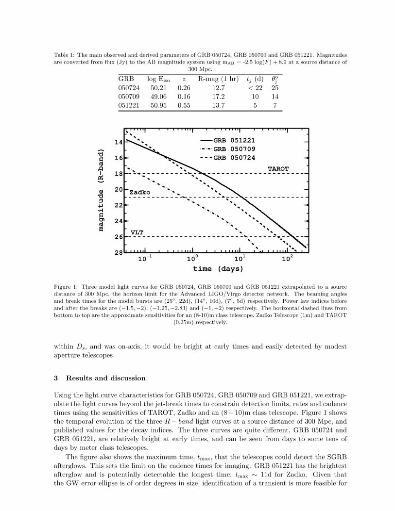
Table 1: The main observed and derived parameters of GRB 050724, GRB 050709 and GRB 051221. Magnitudesare converted from flux (Jy) to the AB magnitude system using mAB = -2.5 log(F ) + 8.9 at a source distance of
300 Mpc.
GRB log Eiso z R-mag (1 hr) tj (d) θoj050724 50.21 0.26 12.7 < 22 25050709 49.06 0.16 17.2 10 14051221 50.95 0.55 13.7 5 7
10−1
100
101
102
14
16
18
20
22
24
26
28
magnitude (R−band)
time (days)
GRB 051221
GRB 050709
GRB 050724
TAROT
Zadko
VLT
Figure 1: Three model light curves for GRB 050724, GRB 050709 and GRB 051221 extrapolated to a sourcedistance of 300 Mpc, the horizon limit for the Advanced LIGO/Virgo detector network. The beaming anglesand break times for the model bursts are (25o, 22d), (14o, 10d), (7o, 5d) respectively. Power law indices beforeand after the breaks are (−1.5,−2), (−1.25,−2.83) and (−1,−2) respectively. The horizontal dashed lines frombottom to top are the approximate sensitivities for an (8-10)m class telescope, Zadko Telescope (1m) and TAROT
(0.25m) respectively.
within Ds, and was on-axis, it would be bright at early times and easily detected by modestaperture telescopes.
3 Results and discussion
Using the light curve characteristics for GRB 050724, GRB 050709 and GRB 051221, we extrap-olate the light curves beyond the jet-break times to constrain detection limits, rates and cadencetimes using the sensitivities of TAROT, Zadko and an (8−10)m class telescope. Figure 1 showsthe temporal evolution of the three R− band light curves at a source distance of 300 Mpc, andpublished values for the decay indices. The three curves are quite different, GRB 050724 andGRB 051221, are relatively bright at early times, and can be seen from days to some tens ofdays by meter class telescopes.
The figure also shows the maximum time, tmax, that the telescopes could detect the SGRBafterglows. This sets the limit on the cadence times for imaging. GRB 051221 has the brightestafterglow and is potentially detectable the longest time; tmax ∼ 11d for Zadko. Given thatthe GW error ellipse is of order degrees in size, identification of a transient is more feasible for
this afterglow type. Unfortunately, they occur at a rate of 1 yr−1, and given optical selectioneffects may be missed altogether. GRB 050724 like events, occurring at an optimistic rate of 13yr−1, would be detectable up to 5d by Zadko. This would allow time for surveying degree sizefields and multiple telescopes at different longitudes to perform follow-up imaging. Coward etal. (2011)1, extends this work to show that SGRB afterglows could be observed off-axis at latetimes by telescopes sensitive to m = 21 − 26.
The first attempts for a triggered search of the optical counterparts of NS-NS coalescencesusing GW detectors are just commencing. There are many uncertainties and issues that will needcareful consideration for these types of searches. Firstly, our results show that the coincidentdetection rate depends critically on the beaming angle distribution. For nearly isotropic opticalemission, similar to GRB 050724, the coincident rates are very promising and will improve theconfidence of the GW detection and provide much needed localisation.
Another important issue for the joint searches is the large errors in the GW source local-isation, which can extend to some tens of degrees. To address this, the GW triggered searchstrategy may use the estimated horizon distance of the detector network to reduce the number ofpotential host galaxies, as opposed to a ‘blind’ error box that extends to cosmological distances.Another problem that manifests with large coincidence error boxes is the increasing chance ofdetecting false coincident optical transients. False coincident sources may include supernovae,flare stars, variable active galactic nuclei and even Earth orbiting space debris. Fortunately,some of these sources can be excluded in the analysis because of the sensitivity distance of GWsearches and the expectation that the strongest GW sources will be associated with cataloguedhost galaxies.
The science pay-off for joint optical and GW observations is enormous and provides moti-vation to address the issues discussed here in more detail. Now is the time to determine theoptimal strategies for optical follow-up in readiness for the more sensitive GW searches in thefollowing years. To accomplish this will require a more comprehensive understanding of opticalselection effects, the false alarm rate expected from SGRBs within the error ellipses of GWnetworks, and techniques to improve the localisation of the host galaxy.
Acknowledgments
D. M. Coward is supported by an Australian Research Council Future Fellowship. He thanks theorganisers of the 2011 Rencontres de Moriond for providing a rich and stimulating environment.
References
1. D.M. Coward et al, MNRAS , Accepted 2011 April 22 (arXiv:1104.5552)2. D. Eichler et al, Nature 340, 126 (1989)3. Fox et al, Nature 437, 845 (2005)4. Watson et al, Astronomy and Astrophysics 454, L123 (2006)5. A. Panaitescu, MNRAS 367, L42 (2006)6. E. Berger et al.Nature 438, 988 (2005)7. A.M., Soderberg et al, ApJ 650, 261 (2006)8. J. Abadie et al, Classical and Quantum Gravity 27, 173001 (2010)
3.Sources of Gravitational Waves

Toward Computing the Gravitational Wave Signaturesof Core Collapse Supernovae
Anthony Mezzacappa1,2, Konstantin N Yakunin3, Pedro Marronetti3, Stephen W Bruenn3,Ching-Tsai Lee2, M Austin Chertkow2, W Raphael Hix1,2, John M Blondin4,
Eric J Lentz1,2, O E Bronson Messer51 Physics Division, Oak Ridge National Laboratory, Oak Ridge, TN 37831-6354
2 Department of Physics and Astronomy, University of Tennessee, Knoxville, TN 37996-1200
3 Physics Department, Florida Atlantic University, Boca Raton, FL 33431-0991
4 Department of Physics, North Carolina State University, Raleigh, NC 27695-8202
5 National Center for Computational Sciences, Oak Ridge National Laboratory,Oak Ridge, TN 37831-6161
We present the gravitational wave signatures of three non-parameterized core collapse super-nova explosion models for 12, 15, and 25 M non-rotating progenitors. The signatures exhibitfour distinct stages. The third stage, induced by mass accretion onto the proto-neutron starowing to neutrino-driven convection and the SASI, dominates. The total gravitational waveenergy emitted rises quickly as the SASI develops at ∼ 200 ms after bounce in all three mod-els and levels off as explosion develops and the convection- and SASI-induced mass accretionpowering the explosions and gravitational wave emission decreases. We decompose the grav-itational wave signatures spectrally and show that the signal is within AdvLIGO’s bandpassfor a Galactic event. The fundamental limitation of the current models and their associ-ated predictions is the restriction to axisymmetry. Counterpart three-dimensional models areforthecoming.
1 Introduction
Recent advances in multidimensional core collapse supernova modeling and the promise of agravitational wave detection by AdvLIGO 1 for a Galactic event engender an optimism thatcore collapse supernovae will be much better understood in the near future, that more detailedpredictions of their gravitational wave emission will therefore be possible in that time frame,and that, consequently, a Galactic core collapse supernova event will both be identifiable ingravitational waves and used to probe the extreme environments present at the center of suchexplosions.
Colgate and White2 were the first to propose that core collapse supernovae could be neutrinodriven and performed the first numerical simulations of these events. More recently, the discov-ery by Wilson 3 of the delayed revival of the core collapse supernova shock wave by neutrinoheating provided the framework for contemporary core collapse supernova theory—the majorityof models performed in the last two decades are centered around this phenomenon (for a review,see Mezzacappa 4 and Janka et al. 5).
Core collapse supernovae are spatially three-dimensional events involving turbulent magne-tohydrodynamics in interaction with an intense flux of neutrinos and antineutrinos emanating
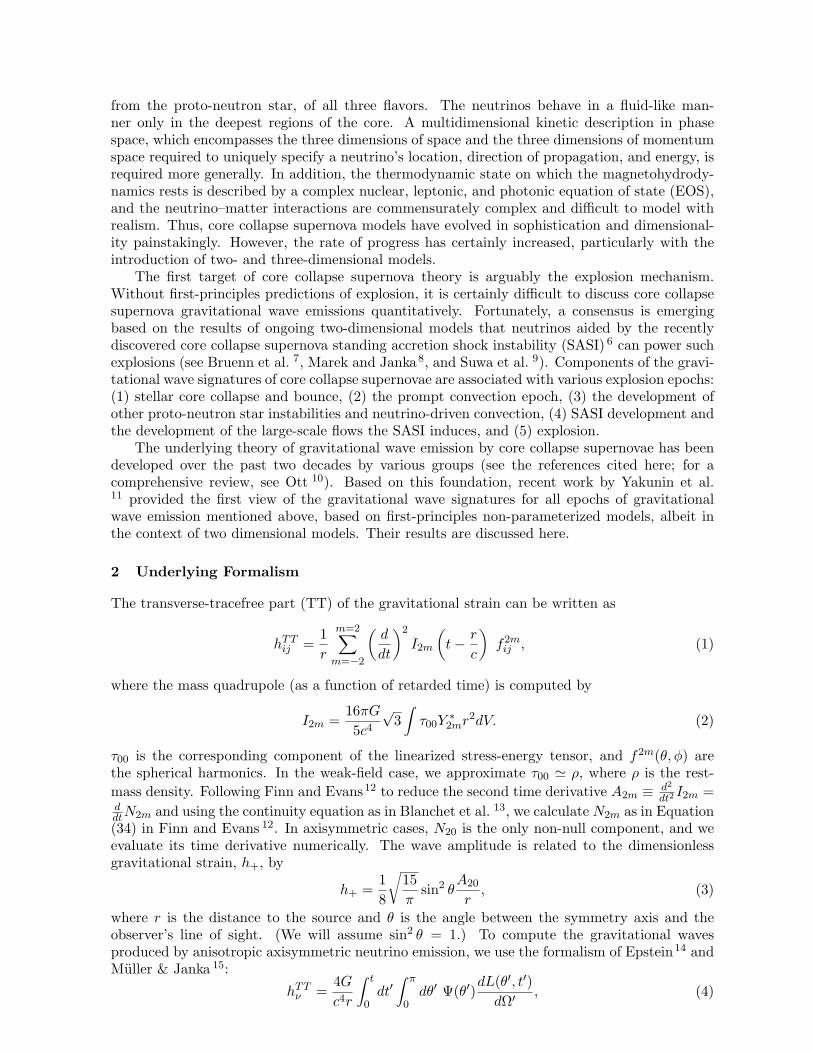
from the proto-neutron star, of all three flavors. The neutrinos behave in a fluid-like man-ner only in the deepest regions of the core. A multidimensional kinetic description in phasespace, which encompasses the three dimensions of space and the three dimensions of momentumspace required to uniquely specify a neutrino’s location, direction of propagation, and energy, isrequired more generally. In addition, the thermodynamic state on which the magnetohydrody-namics rests is described by a complex nuclear, leptonic, and photonic equation of state (EOS),and the neutrino–matter interactions are commensurately complex and difficult to model withrealism. Thus, core collapse supernova models have evolved in sophistication and dimensional-ity painstakingly. However, the rate of progress has certainly increased, particularly with theintroduction of two- and three-dimensional models.
The first target of core collapse supernova theory is arguably the explosion mechanism.Without first-principles predictions of explosion, it is certainly difficult to discuss core collapsesupernova gravitational wave emissions quantitatively. Fortunately, a consensus is emergingbased on the results of ongoing two-dimensional models that neutrinos aided by the recentlydiscovered core collapse supernova standing accretion shock instability (SASI) 6 can power suchexplosions (see Bruenn et al. 7, Marek and Janka8, and Suwa et al. 9). Components of the gravi-tational wave signatures of core collapse supernovae are associated with various explosion epochs:(1) stellar core collapse and bounce, (2) the prompt convection epoch, (3) the development ofother proto-neutron star instabilities and neutrino-driven convection, (4) SASI development andthe development of the large-scale flows the SASI induces, and (5) explosion.
The underlying theory of gravitational wave emission by core collapse supernovae has beendeveloped over the past two decades by various groups (see the references cited here; for acomprehensive review, see Ott 10). Based on this foundation, recent work by Yakunin et al.11 provided the first view of the gravitational wave signatures for all epochs of gravitationalwave emission mentioned above, based on first-principles non-parameterized models, albeit inthe context of two dimensional models. Their results are discussed here.
2 Underlying Formalism
The transverse-tracefree part (TT) of the gravitational strain can be written as
hTTij =1r
m=2∑m=−2
(d
dt
)2
I2m
(t− r
c
)f2mij , (1)
where the mass quadrupole (as a function of retarded time) is computed by
I2m =16πG5c4√
3∫τ00Y
∗2mr
2dV. (2)
τ00 is the corresponding component of the linearized stress-energy tensor, and f2m(θ, φ) arethe spherical harmonics. In the weak-field case, we approximate τ00 ' ρ, where ρ is the rest-mass density. Following Finn and Evans12 to reduce the second time derivative A2m ≡ d2
dt2I2m =
ddtN2m and using the continuity equation as in Blanchet et al. 13, we calculate N2m as in Equation(34) in Finn and Evans 12. In axisymmetric cases, N20 is the only non-null component, and weevaluate its time derivative numerically. The wave amplitude is related to the dimensionlessgravitational strain, h+, by
h+ =18
√15π
sin2 θA20
r, (3)
where r is the distance to the source and θ is the angle between the symmetry axis and theobserver’s line of sight. (We will assume sin2 θ = 1.) To compute the gravitational wavesproduced by anisotropic axisymmetric neutrino emission, we use the formalism of Epstein14 andMuller & Janka 15:
hTTν =4Gc4r
∫ t
0dt′∫ π
0dθ′ Ψ(θ′)
dL(θ′, t′)dΩ′
, (4)
with Ψ(θ) given in Kotake et al. 16. The direction-dependent differential neutrino luminosity,dL/dΩ, is calculated at the outermost radial grid zone. In order to determine the detectabilityof the gravitational waves, we calculate the characteristic gravitational wave strain for a givenfrequency f using 17
hc (f) =1r
√2π2
G
c3dEGW (f)
df
dEGW (f)df
=c3
G
(2πf)2
16π
∣∣∣A20 (f)∣∣∣2 , (5)
withdEGW (f)
df=c3
G
(2πf)2
16π
∣∣∣A20 (f)∣∣∣2 , (6)
where dEGW (f) /df is the gravitational-wave energy spectrum and A20 (f) is the Fourier trans-form of A20 (t).
3 Our Code
CHIMERA contains five primary modules: hydrodynamics, neutrino transport, self-gravity, anuclear equation of state, and a nuclear reaction network (see Bruenn et al. 7 for details).The hydrodynamics is evolved via a Godunov finite-volume scheme—specifically, a Lagrangianremap implementation of the piecewise parabolic method 18. Neutrino transport along ourradial rays is computed by means of multigroup flux-limited diffusion (in the “ray-by-ray-plus”approximation 19), with a flux limiter that has been tuned to reproduce Boltzmann transportresults to within a few percent20. A spectral Poisson solver is used to determine the gravitationalfield21, with general relativistic corrections to the spherical component22. The Lattimer–Swesty(LS) EOS 23 is used for matter in NSE above 1.7 × 10⁸ g/cm3. (The runs documented hereassumed a bulk compressibility of 180 MeV.) Below this density, matter in NSE is describedby 4 species (neutrons, protons, helium, and a representative heavy nucleus) in a correctedand improved version of the Cooperstein EOS 24, extended to regions where the composition isdetermined externally by a reaction network. Continuity with the LS-EOS is achieved by useof a common electron–positron EOS (a revised and extended version of that in Cooperstein 24)and establishment of a common zero for the mass energy. For regions not in NSE, an EOS witha nuclear component consisting of 14 α-particle nuclei from 4He to 60Zn, protons, neutrons, andan iron-like nucleus is used. An electron–positron EOS with arbitrary degeneracy and degree ofrelativity spans the entire density–temperature regime of interest. The nuclear composition inthe non-NSE regions of these models is evolved by the thermonuclear reaction network of Hixand Thielemann 25. Finally, a complete weak interaction set is used in the neutrino transportevolution, including neutrino–antineutrino pair emission from nucleon–nucleon bremsstrahlungand angle and energy exchange from scattering on electrons and nucleons (see Bruenn et al. 7
for a complete list).The history of field variables for a given parcel of material, crucial for nucleosynthesis, is lost
for Eulerian hydrodynamics schemes, such as the one deployed in CHIMERA. To compensatefor this, and to allow post-processed nuclear network computations, the tracer (or test) particlemethod 26 has been implemented. The tracer particles are equally distributed on the sphericalgrid (40 particles/row x 125 rows) at the pre-collapse phase and follow the flow in the courseof the Eulerian simulation, recording their temperature and density history by interpolatingthe corresponding quantities from the underlying Eulerian grid 26. Each particle is assigned aconstant mass (1/5000 of the progenitor mass) and the gravitational wave signal it produces iscalculated taking the quadrupole integral. Comparing the gravitational wave signal correspond-ing to a given group of tracers with the signal produced by the bulk matter motion allows us toidentify what part of the fluid generates a specific gravitational wave feature.
Figure 1: Left: Entropy distribution at 244 ms after bounce in our 15 M model. A large, low-entropy (blue-green) accretion funnel at an angle quasi-orthognal to the symmetry axis and high-entropy (yellow-orange-red)outflows below the shock, along the symmetry axis, are evident. Right: Shock radius as a function of time forthree regions: the north pole (solid blue), the equatorial plane (dotted black), and the south pole (dashed red).
4 Gravitational Wave Predictions
We performed three axisymmetric two-dimensional core collapse supernova simulations, begin-ning with 12, 15, and 25 M non-rotating progenitors 27. Successful explosions were obtainedin all three cases. (Details are provided in Bruenn et al. 7.)
A clear gravitational wave signature, in four parts (left column of Figure 2), emerges: (1) Aprompt signal, which is an initial and relatively weak signal that starts at bounce and ends atbetween 50 and 75 ms post-bounce. ( 2) A quiescent stage that immediately follows the promptsignal and ends somewhere between 125 ms and 175 ms after bounce. (3) A strong signal, whichfollows the quiescent stage and is the most energetic part of the gravitational wave signal. Thisstage ends somewhere between 350 ms and 450 ms after bounce. (4) A tail, which starts beforethe end of the strong signal at about 300 ms after bounce and consists of a slow increase in rh+.
Computations of the gravitational waveforms covering the first three of four phases (priorto explosion) based on non-parameterized models have also been reported by Marek et al. 28,and waveforms covering all four phases and based on parameterized explosions were reportedby Murphy et al. 29.
The prompt signal arises from two phenomena: Prompt convection inside the proto-neutronstar generates a high-frequency signal that is superimposed on a lower-frequency component.The low-frequency signal from 20 ms to 60 ms after bounce originates at the shock radius, whichis at ∼100 km at this time and well outside the proto-neutron star. The separation of these twocomponents is clearly seen in the inset of Figure 3.
The quiescent stage corresponds to the period after prompt convection has ceased and beforeneutrino-driven convection and the SASI have developed. It is followed by a strong signal. Thestrong signal arises from neutrino-driven-convection- and SASI-induced funnels impinging onthe proto-neutron star surface (see Figure 1) and has two components (also described in Mareket al. 28): The low-frequency component arises from the modulations in the shock radius asthe SASI develops and evolves. The high-frequency component is generated when the neutrino-driven-convection- and SASI-induced accretion flows strike the proto-neutron star. The shockmodulations affect the kinetic energy of the accretion flows and, consequently, the amplitude ofthe gravitational waves generated when these flows hit the surface. Hence the high-frequencymodulations are beneath a low-frequency envelope.
All of our gravitational wave signals end with a slowly increasing tail, which reflects the grav-itational memory associated with accelerations at the prolate outgoing shock (see also Murphyet al. 29).
Looking at hchar (Figure 2 right), the peak at ∼ 700 − 800 Hz is associated with the high-frequency component of rh+, which in turn is associated with the accretion downflows hitting
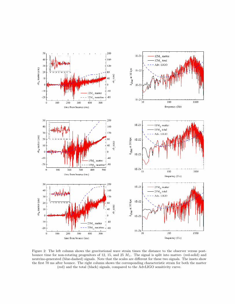
Figure 2: The left column shows the gravitational wave strain times the distance to the observer versus post-bounce time for non-rotating progenitors of 12, 15, and 25 M. The signal is split into matter- (red-solid) andneutrino-generated (blue-dashed) signals. Note that the scales are different for these two signals. The insets showthe first 70 ms after bounce. The right column shows the corresponding characteristic strain for both the matter
(red) and the total (black) signals, compared to the AdvLIGO sensitivity curve.
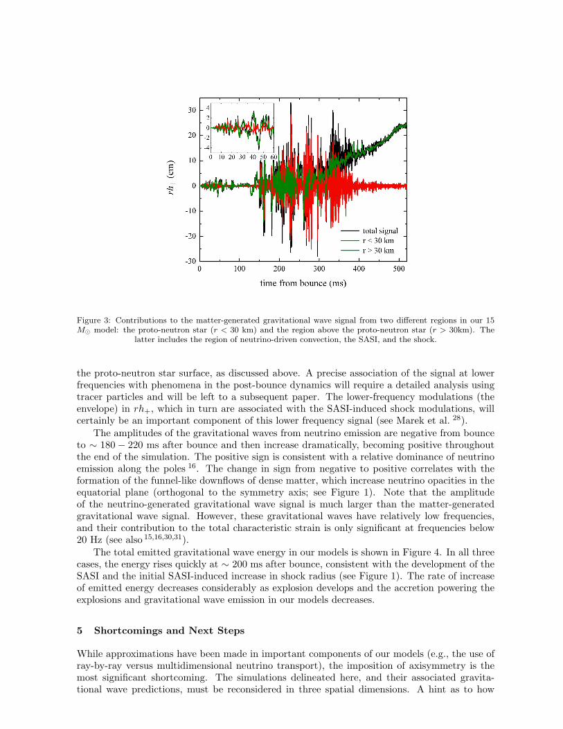
Figure 3: Contributions to the matter-generated gravitational wave signal from two different regions in our 15M model: the proto-neutron star (r < 30 km) and the region above the proto-neutron star (r > 30km). The
latter includes the region of neutrino-driven convection, the SASI, and the shock.
the proto-neutron star surface, as discussed above. A precise association of the signal at lowerfrequencies with phenomena in the post-bounce dynamics will require a detailed analysis usingtracer particles and will be left to a subsequent paper. The lower-frequency modulations (theenvelope) in rh+, which in turn are associated with the SASI-induced shock modulations, willcertainly be an important component of this lower frequency signal (see Marek et al. 28).
The amplitudes of the gravitational waves from neutrino emission are negative from bounceto ∼ 180 − 220 ms after bounce and then increase dramatically, becoming positive throughoutthe end of the simulation. The positive sign is consistent with a relative dominance of neutrinoemission along the poles 16. The change in sign from negative to positive correlates with theformation of the funnel-like downflows of dense matter, which increase neutrino opacities in theequatorial plane (orthogonal to the symmetry axis; see Figure 1). Note that the amplitudeof the neutrino-generated gravitational wave signal is much larger than the matter-generatedgravitational wave signal. However, these gravitational waves have relatively low frequencies,and their contribution to the total characteristic strain is only significant at frequencies below20 Hz (see also 15,16,30,31).
The total emitted gravitational wave energy in our models is shown in Figure 4. In all threecases, the energy rises quickly at ∼ 200 ms after bounce, consistent with the development of theSASI and the initial SASI-induced increase in shock radius (see Figure 1). The rate of increaseof emitted energy decreases considerably as explosion develops and the accretion powering theexplosions and gravitational wave emission in our models decreases.
5 Shortcomings and Next Steps
While approximations have been made in important components of our models (e.g., the use ofray-by-ray versus multidimensional neutrino transport), the imposition of axisymmetry is themost significant shortcoming. The simulations delineated here, and their associated gravita-tional wave predictions, must be reconsidered in three spatial dimensions. A hint as to how
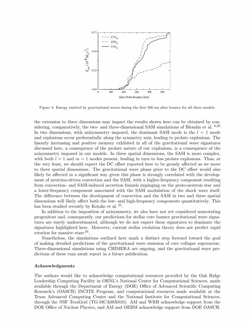
Figure 4: Energy emitted by gravitational waves during the first 500 ms after bounce for all three models.
the extension to three dimensions may impact the results shown here can be obtained by con-sidering, comparatively, the two- and three-dimensional SASI simulations of Blondin et al. 6,32
In two dimensions, with axisymmetry imposed, the dominant SASI mode is the l = 1 modeand explosions occur preferentially along the symmetry axis, leading to prolate explosions. Thelinearly increasing and positive memory exhibited in all of the gravitational wave signaturesdiscussed here, a consequence of the prolate nature of our explosions, is a consequence of theaxisymmetry imposed in our models. In three spatial dimensions, the SASI is more complex,with both l = 1 and m = 1 modes present, leading in turn to less prolate explosions. Thus, atthe very least, we should expect the DC offset reported here to be grossly affected as we moveto three spatial dimensions. The gravitational wave phase prior to the DC offset would alsolikely be affected in a significant way given this phase is strongly correlated with the develop-ment of neutrino-driven convection and the SASI, with a higher-frequency component resultingfrom convection- and SASI-induced accretion funnels impinging on the proto-neutron star anda lower-frequency component associated with the SASI modulation of the shock wave itself.The difference between the development of convection and the SASI in two and three spatialdimensions will likely affect both the low- and high-frequency components quantitatively. Thishas been studied recently by Kotake et al. 31.
In addition to the imposition of axisymmetry, we also have not yet considered nonrotatingprogenitors and, consequently, our predictions for stellar core bounce gravitational wave signa-tures are surely underestimated, although we do not expect these signatures to dominate thesignatures highlighted here. Moreover, current stellar evolution theory does not predict rapidrotation for massive stars 33.
Nonetheless, the simulations outlined here mark a distinct step forward toward the goalof making detailed predictions of the gravitational wave emission of core collapse supernovae.Three-dimensional simulations using CHIMERA are ongoing, and the gravitational wave pre-dictions of these runs await report in a future publication.
Acknowledgments
The authors would like to acknowledge computational resources provided by the Oak RidgeLeadership Computing Facility in ORNL’s National Center for Computational Sciences, madeavailable through the Department of Energy (DOE) Office of Advanced Scientific ComputingResearch’s (OASCR) INCITE Program, and computational resources made available at theTexas Advanced Computing Center and the National Institute for Computational Sciences,through the NSF TeraGrid (TG-MCA08X010). AM and WRH acknowledge support from theDOE Office of Nuclear Physics, and AM and OEBM acknowledge support from DOE OASCR.
AM, OEBM, PM, SWB, and WRH acknowledge support from NASA ATFP (07-ATFP07-0011).PM acknowledges support from NSF-PHYS-0855315, and PM and SWB acknowledge supportfrom NSF-OCI-0749204.
References
1. http://www.ligo.caltech.edu/advLIGO2. Colgate, S A and White, R H 1966 Astrophys. J. 143 6263. Wilson J R 1985, in Numerical Astrophysics, eds. Centrella, J M, LeBlanc, J M, and
Bowers, R L, Jones and Bartlett, Boston, 4224. Mezzacappa A 2005 Ann. Rev. Nucl. Part. Sci. 55 4675. Janka H-T, Langanke, K, Marek, A, Martinez-Pinedo G, and Muller B 2007 Phys. Rep.
442 386. Blondin J M, Mezzacappa A, and DeMarino C 2003 Astrophys. J. 584 9717. Bruenn S W, Mezzacappa A, Hix W R, Blondin J M, Marronetti P, Messer O E B, Dirk
C and Yoshida S 2009 Journ. Phys. Conf. Ser. 180 0120188. Marek A and Janka, H-T 2009 Astrophys. J. 694 6649. Suwa Y, Kotake, K, Takiwaki, T, Whitehouse, S C, Liebendorfer, M, and Sato K 2010
PASJ 62 L4910. Ott C 2009 Class. Quant. Grav. 26 06300111. Yakunin K N, Marronetti P, Mezzacappa A, Bruenn S W, Lee C-T, Chertkow M A, Hix
W R, Blondin J M, Lentz E J, Messer O E B, and Yoshida S 2010 Class. Quant. Grav.27 194005
12. Finn L S and Evans C R 1990 Astrophys. J. 351 58813. Blanchet L, Damour T, and Schaefer G 1990 MNRAS 242 28914. Epstein R 1978 Astrophys. J. 223 103715. Muller E and Janka H-T 1997 Astron. Astrophys. 317 14016. Kotake K, Ohnishi N, and Yamada S 2007 Astrophys. J. 655 40617. Flanagan E and E Hughes S A 1998 Phys. Rev. D 57 456618. Colella P and Woodward P R 1984 Journ. Comp. Phys. 54 17419. Buras R, Rampp M, Janka H T, and Kifonidis K 2006 Astron. Astrophys. 447 104920. Liebendorfer M, Messer O E B, Mezzacappa A, Bruenn S W, Cardall C, and Thielemann
F-K 2004 Astrophys. J. Suppl. Ser. 150 26321. Muller E and Steinmetz M 1995 Comp. Phys. Comm. 89 4522. Marek A, Dimmelmeier H, Janka H-T, Muller E, and Buras R 2006 Astron. Astrophys.
445 27323. Lattimer J M and Swesty F D 1991 Nucl. Phys. A 535 33124. Cooperstein J 1985 Nucl. Phys. A 438 72225. Hix W R and Thielemann F-K 1999 Astrophys. J. 511 86226. Lee C-T 2008 The Applications of the Tracer Particle Method to Multi-Dimensional Su-
pernova Simulations PhD Thesis The University of Tennessee Knoxville TN USA27. Woosley S E and Heger A 2007 Phys. Rep. 442 26928. Marek A, Janka H-T, and E. Muller 2009 Astron. Astrophys. 496 47529. Murphy J, Ott C, and Burrows A 2009 Astrophys. J. 707 117330. Burrows A and Hayes J 1996 Phys. Rev. Lett. 76 35231. Kotake K, Iwakami W, Ohnishi N, and Yamada S 2009 Astrophys. J. 697 13332. Blondin J and Mezzacappa A 2007 Nature 445 5833. Heger A, Fryer C L, Woosley S E, Langer N, and Hartmann D H 2003 Astrophys. J. 591
288
Neutron Stars as Gravitational Wave Sources
Leonardo GualtieriDipartimento di Fisica, “Sapienza” Universita di Roma
& Sezione INFN Roma1, P.A. Moro 5, 00185 Roma, Italy
Neutron stars, among the most extreme objects in the universe, are very promising sourcesfor the gravitational wave detectors of the present and next generation. On the other hand,gravitational waves can give us unvaluable information on neutron stars, since we do notknow the behaviour of matter in their inner core. Detection of the gravitational emissionfrom neutron stars could teach us something about the nature of hadronic interactions. Idiscuss some neutron star processes associated to gravitational wave emission, looking at bothaspects: whether the neutron star can produce detectable gravitational waves, and whether agravitational wave detection could tell us something about the neutron star equation of state.
1 Introduction
Neutron stars (NSs) can be considered as the “ground state” of matter: they are the mostcompact self-graviting stellar objects in nature. Several quantities reach extreme values in NSs:
• The density can reach, at the center, ρ ∼ 1015 g/cm3, larger than nuclear density.
• The surface gravitational potential, of the order of GM/R ∼ (0.1 − 0.3)c2; therefore,general relativity has to be included to model a NS.
• The rotation rate reaches (in the fastest spinning NSs) ν ∼ 700 Hz.
• The magnetic field strength reaches (in “magnetars”, i.e. strongly magnetized NSs) B ∼
1015 G on the surface, and probably even larger values in the interior.
• The electromagnetic luminosity can reach, in violent events like giant flares, peaks as largeas Lγ ∼ 1047 erg/s.
All these features make NSs very promising sources of gravitational waves (GWs). Since mostprocesses involving NSs have characteristic frequencies ranging from some tens of Hz to somekHz, they are relevant sources for ground based interferometers (LIGO, VIRGO)a, which aresensitive in this range of frequency, in their advanced configurations.
On the other hand, GWs can give us unvaluable information on NSs. We probably knowhow matter is organized in the crust of a NS (and maybe in the outer core, too), but ourunderstanding of their inner core, where matter reaches supranuclear densities, is very poor.Indeed, in these conditions hadron interactions play a crucial role; neglecting such interactionsand considering neutron Fermi pressure only, one would find a NS maximum mass of ∼ 0.7M⊙,
ahttp://www.virgo.infn.it ; http://www.ligo.caltech.edu
in contrast with the observations of M ∼ (1.2 − 2.0)M⊙. Our lack of knowledge on the NSequation of state (EOS) in the inner core reflects our ignorance on the non-perturbative regimeof quantum cromo-dynamics. We do not even know the particle content of the core: Hadrons?Hyperons? Meson condensates? Deconfined quark matter?
Unfortnuately, supranuclear densities cannot be reproduced in the laboratory, and electro-magnetic signals do not carry direct information about the physics of NS inner cores; our onlyhope to have observative data on this extreme regime relies on GWs, which are mainly generatedwhere the star is most dense, and are nearly unaffected by interaction with interstellar matterand energy. For instance, knowing the radius of NSs we would learn a lot about its EOS, butit is very difficult to get a “clean” observation of a NS radius in the electromagnetic spectrum;detection of gravitational waves from NS oscillations, instead, would allow us to estimate theradius, and then to set constraints on the NS EOS (see Sec. 2).
I will discuss some processees involving NS as GWs sources, trying to answer to the followingquestions: Can detectable GWs be produced? Would a GW detection tell us something aboutthe EOS of NSs? The answer to both questions is potentially affirmative for NS oscillations(discussed in Sec. 2) and coalescences of NS binary systems (discussed in Sec. 3). I will notdiscuss, instead, NS deformations: even though they are a promising source of GWs, it wouldbe very difficult to infer information on the NS EOS from the gravitational signal they produce.
2 Gravitational wave asteroseismology
When a neutron star is perturbed, it oscillates and (if the oscillations are non-radial and non-dipolar) it emits gravitational waves. The perturbation can be due to a variety of differentprocesses, like glitches, accreting matter or, when the NS is born, the shock originating fromthe gravitational collapse. These oscillations occur with characteristic frequencies and dampingtimes, which do not depend on the nature of the exciting perturbation, but only on the structureof the NS; they are called quasi-normal modes (QNMs).
Similarly to normal modes of Newtonian stars, QNMs are classified in terms of the mainrestoring force which brings a displaced element of matter back to equilibrium; we have g-modesif the main restoring force is buoyancy, p-modes if it is pressure; the fundamental mode (f -mode) has an intermediate character between g-modes and p-modes. Typically, NS g-modeshave frequencies of some hundreds of Hz; the f -mode of 1 − 2 kHz; and p-modes of a few kHz.Furthermore, there are pure space-time modes, the w-modes, with higher frequencies; r-modes,associated with the stellar rotation; and other classes of modes associated to the magnetic fieldand to the elastic properties of the crust.
The detection of the GWs emitted by an oscillating star will allow us to measure the fre-quencies and damping times of the QNMs, which carry the imprint of the NS EOS. The study ofthe structure of NSs through the observation of their proper oscillations by gravitational wavedetectors, is named gravitational wave asteroseismology.
The case of cold, old NSs has been studied in a series of articles in the last decade 1, whichhave been focussing onto the g, f, p modes of spherically symmetric stars. It was found thata GW detection from a pulsating star would allow to: (i) infer the value of the NS radius,which would strongly constrain the EOS; (ii) discriminate between different possible EOS; (iii)establish whether the emitting source is a NS or a quark star, constraining, in the latter case,the quark star EOS. More recently different kinds of oscillations have been modeled, includingmore and more physics in the game: the star rotation 2, magnetic fields and elastic propertiesof the crust 3, superfluidity 4.
Oscillations of hot, young proto-neutron stars (PNSs) are a very interesting source of GWs.Indeed, they are likely to be strongly excited by the processes associated to the gravitationalcollapse, and they can give information not only on the PNS EOS, but also on the thermo-
dynamical properties, and on the neutrino dynamics, of the PNS. They have been studied in5,6. In these works, the first minute after the core bounce is considered, and the evolution istreated as a sequence of quasi-stationary configurations. In5 the thermodynamical variables andthe lepton fraction are determined by solving Boltzmann’s equation, and the EOS is obtainedwithin the mean field approximation 7. In 6, instead, a microscopic EOS is employed, obtainedwithin the Brueckner-Hartree-Fock nuclear many-body approach 8; Boltzmann’s equation is notsolved: different entropy and lepton fraction profiles are considered, in order to understand howthe QNMs depend on the thermodynamical and composition variables.
By comparing the QNMs of old, cold NS 1 with that of hot, young PNS 5,6, one finds that:
• In cold, old NSs the f -mode has the shortest damping time (νf ∼ 1 s); thus, it is expected tobe the best candidate for QNM detection by gravitational interferometers. Since νf ∼ 1−2kHz, it falls in the detector bandwidth (∼ 100− ∼ 1000 Hz) only marginally. The p- andg-modes are unnlikely to be detected, since p-modes have higher frequencies, and g-modes,when present, have very large gravitational damping times, and are then damped by otherdissipative mechanisms, like viscosity and heat transport.
• The frequency of the g-mode in a hot, young PNS carries information on the entropyprofile of the star: higher frequencies correspond to larger entropy gradients.
• In hot, young PNSs the f -mode has lower frequency (which is better for GW detection)than in older and colder NSs, but its damping time is larger (which is worst for GWdetection). It is not clear which of the two effects prevails.
• In the first seconds of the PNS life, g-mode excitation is a promising source of GWs. Indeed,its damping time is comparable with the damping time of the f -mode. These dampingtimes, of the order of seconds, are smaller than the dissipation timescale associated tonon-gravitational processes (like viscosity, heat transport, neutrino diffusion, etc.). Moregenerally, when the PNS is very hot the lowest order g- f - and p-modes cluster, acquiringsimilar frequencies and damping times.
In order to make solid statements about the QNMs of PNS, further studies are required, toinclude in the model the cooling of the star and its rotation. We remark that including rotationshould yield lower values of the frequencies and the damping times of the QNMs 2, i.e. a morelikely detection of the GW signal.
3 Gravitational waves from neutron stars in binaries
The coalescence of binary systems with neutron stars (NS-NS and black hole (BH)-NS binaries)is one of the most promising GW sources for advanced LIGO/VIRGO. Recent studies haveshown that the gravitational signal from these processes can carry the imprint of the NS EOS.
In the latest stage of a BH-NS coalescence, the neutron star is disrupted by the BH tidalfield. If this occurs when the NS has not yet reached the innermost circular orbit about the BH,it forms an accretion torus; otherwise, it directly plunges in the BH horizon. In the former case,the gravitational signal is characterized by a cut-off frequency νc, corresponding to the stellardisruption 9,10. The presence of this cut-off, and its value, strongly depends on the NS EOS; itsobservation would give us valuable information about the behaviour of matter in the NS core.
This problem has been studied both in the framework of numerical relativity (numericalintegration of Einstein’s equations coupled with hydrodynamical equations) 11 and using semi-analytical approaches 10,12. As shown in 10, if we know the mass and angular momentum of theblack hole, and measure the cut-off frequency νc, it would be possible to estimate the NS radiuswith an error of few percent, thus discriminating between different possible equations of state.
In NS-NS binaries, the signature of the EOS is expected to be even stronger. As shownin 13, even in the early inspiral phase the stars are significantly affected by tidal deformation.The post-Newtonian analysis of 13 shows that it is possible to extract from the GW signal thetidal deformability λ, which measures the stellar quadrupole deformation in response to theperturbing tidal field of the companion. This parameter strongly depends on the features of theNS EOS. The dependence of the merger phase on the EOS has been studied in 14, using thetechniques of numerical relativity; the outcome of the merger (a black hole, or a hypermassiveneutron star) crucially depends on the equation of state of the coalescing NSs.
The detection of GWs from NSs will then be of utmost importance, not only to understandthe behaviour of astronomical objects, but also to have a deeper insight on the behaviour ofmatter at supranuclear densities, shedding light on the nature of hadronic interactions.
Acknowledgements
I thank V. Ferrari for useful suggestions. This work was supported by CompStar, a ResearchNetworking Programme of the European Science Foundation.
References
1. N. Andersson, K.D. Kokkotas, Mon. Not. Roy. Astron. Soc. 299, 1059 (1998); K.D.Kokkotas, T.A. Apostolatos, N. Andersson, Mon. Not. Roy. Astron. Soc. 320, 307(2001); O. Benhar, V. Ferrari, L. Gualtieri, Phys. Rev. D 70, 124015 (2004); O. Benhar,V. Ferrari, L. Gualtieri, S. Marassi, Gen. Rel. Grav. 39, 1323 (2007).
2. H. Dimmelmeier, N. Stergioulas, J.A. Font, Mon. Not. Roy. Astron. Soc. 368, 1609(2006); A. Passamonti, A. Stavridis, K.D. Kokkotas, Phys. Rev. D 77, 024029 (2008);E. Gaertig, K.D. Kokkotas, Phys. Rev. D 78, 064003 (2008); ibid. 80, 064026 (2009);ibid. 83, 064031 (2011); A. Passamonti, B. Haskell, N. Andersson, D.I. Jones, I. Hawke,Mon. Not. Roy. Astron. Soc. 394, 730 (2009); B. Zink, O. Korobkin, E. Schnetter, N.Stergioulas, Phys. Rev. D 81, 084055 (2010).
3. H. Sotani, K.D. Kokkotas, N. Stergoiulas, Mon. Not. Roy. Astron. Soc. 385, L5 (2008);A. Colaiuda, H. Beyer, K.D. Kokkotas, Mon. Not. Roy. Astron. Soc. 396, 1441 (2009);A. Colaiuda, K.D. Kokkotas, Mon. Not. Roy. Astron. Soc. (2011), DOI: 10.1111/j.1365-2966.2011.18602.x; M. Gabler, P. Cerda Duran, J.A. Font, E. Muller, N. Stergioulas Mon.
Not. Roy. Astron. Soc. 410, L37 (2011).4. N. Andersson, K. Glampedakis, L. Samuelsson, Mon. Not. Roy. Astron. Soc. 396, 894
(2009); N. Andersson, B. Haskell, N. Andersson, Mon. Not. Roy. Astron. Soc. 396, 951(2009); A. Passamonti, N. Andersson, Mon. Not. Roy. Astron. Soc. 413, 47 (2011).
5. V. Ferrari, G. Miniutti, J.A. Pons, Mon. Not. Roy. Astron. Soc. 342, 629 (2003).6. G.F. Burgio, V. Ferrari, L. Gualtieri, H.-J. Schultze, in preparation.7. J.A. Pons, S. Reddy, M. Prakash, J.M. Lattimer, J.A. Miralles, Astrophys. J. 513, 780
(1999).8. G.F. Burgio, H.-J. Schultze, Astron. & Astrophys. 518, A17 (2010).9. M. Vallisneri, Phys. Rev. Lett. 84, 3519 (2000).
10. V. Ferrari, L. Gualtieri, F. Pannarale, Phys. Rev. D 81, 064026 (2010).11. M. Shibata, K. Kyutoku, T. Yamamoto, K. Taniguchi, Phys. Rev. D 79, 044030 (2009);
Z.B. Etienne, Y.T. Liu, S.L. Shapiro, T.W. Baumgarte, Phys. Rev. D 79, 044024 (2009).12. F. Pannarale, A. Tonita, L. Rezzolla, Astrophys. J. 727, 1 (2011); V. Ferrari, L. Gualtieri,
A. Maselli, in preparation.13. T. Hinderer, B.D. Lackey, R.N. Lang, J.S. Read Phys. Rev. D 81, 123016 (2010).14. K. Hotokezaka, K. Kyutoku, H. Okawa, M. Shibata, K. Kiuki, arXiv:1105.4370.
General Relativistic Magnetohydrodynamic Simulations of Binary Neutron StarMergers
Bruno GiacomazzoDepartment of Astronomy, University of Maryland, College Park, Maryland, USA
Gravitational Astrophysics Laboratory, NASA Goddard Space Flight Center, Greenbelt, Maryland, USA
Luciano RezzollaMax-Planck-Institut fur Gravitationsphysik, Albert-Einstein-Institut, Potsdam Germany
Department of Physics and Astronomy, Louisiana State University, Baton Rouge, Louisiana, USA
Luca BaiottiInstitute of Laser Engineering, Osaka University, Osaka, Japan
We report on our recent general-relativistic simulations of magnetized, equal-mass neutron-star binaries and on the role that realistic magnetic fields may have in the evolution of thesesystems. In particular, we study the evolution of the magnetic fields and show that they caninfluence the survival of the hypermassive neutron star produced at the merger by acceleratingits collapse to a black hole. We also show how the magnetic field can be amplified and thatthis can lead to the production of the relativistic jets observed in short gamma-ray bursts.
1 Introduction
The numerical investigation in full general relativity (GR) of the merger of binary neutron stars(BNSs) has produced a series of new and interesting results in the last years. 1 Thanks to severalnumerical improvements, it has been indeed possible to start to investigate the full dynamics ofthese systems including the formation of tori around rapidly rotating black holes (BHs) 2,3,4,5
which could not be modeled via Newtonian simulations. This progress has allowed the beginningof an accurate investigation of whether BNS mergers could indeed be behind the central engineof short γ-ray bursts (GRBs). 6,7,8 Fully GR simulations have shown that the end result of BNSmergers is the formation of a rapidly spinning BH surrounded by a hot torus. Driven by neutrinoprocesses and magnetic fields, such a compact system may be capable of launching a relativisticfireball with an energy of ∼ 1048 erg on a timescale of 0.1− 1 s. 9 Moreover, BNSs are also oneof the most powerful sources of gravitational waves (GWs) that will be detected in the nextfew years by advanced LIGO and advanced Virgo. 10 GR simulations of BNSs have then startedto provide accurate templates that can be used to infer properties of the NSs composing thebinaries, such as the equation of state (EOS) of NSs, once their GWs will be detected. 11 Herewe review some of the main results we published recently 5,8 and that describe the merger ofmagnetized equal-mass BNSs. We will show how magnetic fields can affect the dynamics ofthese systems and their role in powering short GRBs.
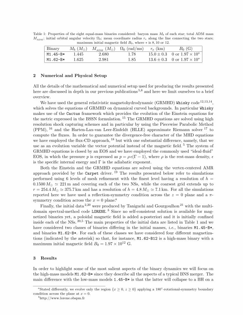
Table 1: Properties of the eight equal-mass binaries considered: baryon mass Mb of each star; total ADM massMADM ; initial orbital angular velocity Ω0; mean coordinate radius re along the line connecting the two stars;
maximum initial magnetic field B0, where ∗ is 8, 10 or 12.
Binary Mb (M) MADM (M) Ω0 (rad/ms) re (km) B0 (G)M1.45-B* 1.445 2.680 1.78 15.0± 0.3 0 or 1.97× 10∗
M1.62-B* 1.625 2.981 1.85 13.6± 0.3 0 or 1.97× 10∗
2 Numerical and Physical Setup
All the details of the mathematical and numerical setup used for producing the results presentedhere are discussed in depth in our previous publications 5,8 and here we limit ourselves to a briefoverview.
We have used the general relativistic magnetohydrodynamic (GRMHD) Whisky code12,13,14,which solves the equations of GRMHD on dynamical curved backgrounds. In particular Whiskymakes use of the Cactus framework which provides the evolution of the Einstein equations forthe metric expressed in the BSSN formulation. 15 The GRMHD equations are solved using highresolution shock capturing schemes and in particular by using the Piecewise Parabolic Method(PPM), 16 and the Harten-Lax-van Leer-Einfeldt (HLLE) approximate Riemann solver 17 tocompute the fluxes. In order to guarantee the divergence-free character of the MHD equationswe have employed the flux-CD approach, 18 but with one substantial difference, namely, that weuse as an evolution variable the vector potential instead of the magnetic field. 5 The system ofGRMHD equations is closed by an EOS and we have employed the commonly used “ideal-fluid”EOS, in which the pressure p is expressed as p = ρ ε(Γ− 1), where ρ is the rest-mass density, εis the specific internal energy and Γ is the adiabatic exponent.
Both the Einstein and the GRMHD equations are solved using the vertex-centered AMRapproach provided by the Carpet driver. 19 The results presented below refer to simulationsperformed using 6 levels of mesh refinement with the finest level having a resolution of h =0.1500 M ' 221 m and covering each of the two NSs, while the coarsest grid extends up tor = 254.4 M ' 375.7 km and has a resolution of h = 4.8 M ' 7.1 km. For all the simulationsreported here we have used a reflection-symmetry condition across the z = 0 plane and a π-symmetry condition across the x = 0 plane.a
Finally, the initial data 2,20 were produced by Taniguchi and Gourgoulhon 21 with the multi-domain spectral-method code LORENE. b Since no self-consistent solution is available for mag-netized binaries yet, a poloidal magnetic field is added a-posteriori and it is initially confinedinside each of the NSs. 20,5 The main properties of the initial data are listed in Table 1 and wehave considered two classes of binaries differing in the initial masses, i.e., binaries M1.45-B*,and binaries M1.62-B*. For each of these classes we have considered four different magnetiza-tions (indicated by the asterisk) so that, for instance, M1.62-B12 is a high-mass binary with amaximum initial magnetic field B0 = 1.97× 10¹² G.
3 Results
In order to highlight some of the most salient aspects of the binary dynamics we will focus onthe high-mass models M1.62-B* since they describe all the aspects of a typical BNS merger. Themain difference with the low-mass models 1.45-B* is that the latter will collapse to a BH on a
aStated differently, we evolve only the region x ≥ 0, z ≥ 0 applying a 180-rotational-symmetry boundarycondition across the plane at x = 0.
bhttp://www.lorene.obspm.fr
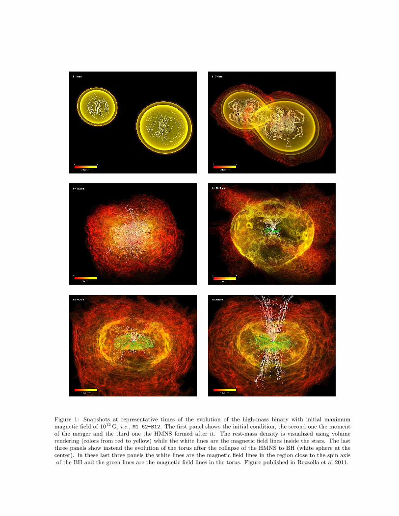
Figure 1: Snapshots at representative times of the evolution of the high-mass binary with initial maximummagnetic field of 1012 G, i.e., M1.62-B12. The first panel shows the initial condition, the second one the momentof the merger and the third one the HMNS formed after it. The rest-mass density is visualized using volumerendering (colors from red to yellow) while the white lines are the magnetic field lines inside the stars. The lastthree panels show instead the evolution of the torus after the collapse of the HMNS to BH (white sphere at thecenter). In these last three panels the white lines are the magnetic field lines in the region close to the spin axisof the BH and the green lines are the magnetic field lines in the torus. Figure published in Rezzolla et al 2011.
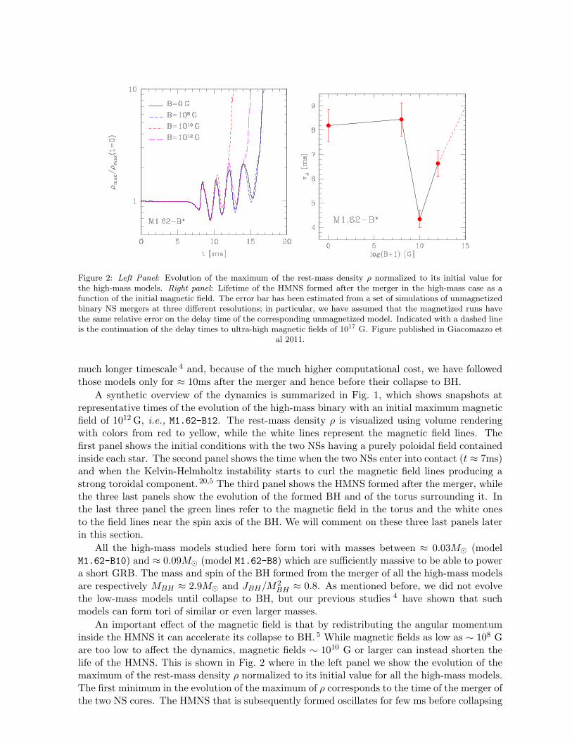
Figure 2: Left Panel: Evolution of the maximum of the rest-mass density ρ normalized to its initial value forthe high-mass models. Right panel: Lifetime of the HMNS formed after the merger in the high-mass case as afunction of the initial magnetic field. The error bar has been estimated from a set of simulations of unmagnetizedbinary NS mergers at three different resolutions; in particular, we have assumed that the magnetized runs havethe same relative error on the delay time of the corresponding unmagnetized model. Indicated with a dashed lineis the continuation of the delay times to ultra-high magnetic fields of 1017 G. Figure published in Giacomazzo et
al 2011.
much longer timescale 4 and, because of the much higher computational cost, we have followedthose models only for ≈ 10ms after the merger and hence before their collapse to BH.
A synthetic overview of the dynamics is summarized in Fig. 1, which shows snapshots atrepresentative times of the evolution of the high-mass binary with an initial maximum magneticfield of 1012 G, i.e., M1.62-B12. The rest-mass density ρ is visualized using volume renderingwith colors from red to yellow, while the white lines represent the magnetic field lines. Thefirst panel shows the initial conditions with the two NSs having a purely poloidal field containedinside each star. The second panel shows the time when the two NSs enter into contact (t ≈ 7ms)and when the Kelvin-Helmholtz instability starts to curl the magnetic field lines producing astrong toroidal component. 20,5 The third panel shows the HMNS formed after the merger, whilethe three last panels show the evolution of the formed BH and of the torus surrounding it. Inthe last three panel the green lines refer to the magnetic field in the torus and the white onesto the field lines near the spin axis of the BH. We will comment on these three last panels laterin this section.
All the high-mass models studied here form tori with masses between ≈ 0.03M (modelM1.62-B10) and ≈ 0.09M (model M1.62-B8) which are sufficiently massive to be able to powera short GRB. The mass and spin of the BH formed from the merger of all the high-mass modelsare respectively MBH ≈ 2.9M and JBH/M2
BH ≈ 0.8. As mentioned before, we did not evolvethe low-mass models until collapse to BH, but our previous studies 4 have shown that suchmodels can form tori of similar or even larger masses.
An important effect of the magnetic field is that by redistributing the angular momentuminside the HMNS it can accelerate its collapse to BH. 5 While magnetic fields as low as ∼ 108 Gare too low to affect the dynamics, magnetic fields ∼ 1010 G or larger can instead shorten thelife of the HMNS. This is shown in Fig. 2 where in the left panel we show the evolution of themaximum of the rest-mass density ρ normalized to its initial value for all the high-mass models.The first minimum in the evolution of the maximum of ρ corresponds to the time of the merger ofthe two NS cores. The HMNS that is subsequently formed oscillates for few ms before collapsing
Figure 3: Left panel: Evolution of the maximum of the temperature T (top) and of the maximum of the Lorentzfactor (bottom). The two vertical dotted and dashed lines represent respectively the time of the merger and ofthe collapse to BH. Right panel: Evolution of the maximum of the magnetic field in its poloidal (red solid line)and toroidal (blue dashed line) components. The bottom panel shows the maximum local fluid energy indicatingthat an unbound outflow (i.e., Eloc > 1) develops and is sustained after BH formation. All the panels refer to the
high-mass model M1.62-B12. Figure published in Rezzolla et al 2011.
to a BH which happens when the maximum of ρ grows exponentially. As one can see from thisfigure the evolution of ρ in the case with a magnetic field ∼ 108 G (blue dot-dashed line) isalmost identical to the unmagnetized case (solid black line). The models with higher values ofthe magnetic field instead collapse much earlier (magenta long-dashed line, model M1.62-B12and red short-dashed line, model M1.62-B10). In the right panel of Fig. 2 we plot instead thelifetime of the HMNS formed after the merger of the high-mass models as a function of the initialmagnetic field. The fact that this curve exhibits a minimum should not come as a surprise. Assaid before low magnetic fields do not change the lifetime τd and so the curve is expected tobe flat for low magnetic fields, i.e., smaller than ∼ 108 G. Stronger magnetic fields, i.e., largerthan ∼ 1016 G, will instead increase the total pressure in the HMNS and extend its lifetime. 20
Intermediate field values instead do not sufficiently contribute to the the total pressure in theHMNS, but are still sufficient to redistribute its angular momentum and accelerate its collapseto BH. From this figure it is also clear that if we were able to determine the lifetime of theHMNS (by measuring for example the delay between the merger and the collapse to BH in theGW signal), we would then be able to infer approximatively the strength of the magnetic field.
3.1 Jet formation
By continuing the evolution of the high-mass model M1.62-B12 far beyond BH formation wewere also able to show for the first time that BNS mergers can generate the jet-like structuresthat are behind the emission of short GRBs. 8 In particular the last three panels of Fig. 1 showthe evolution of the rest-mass density and magnetic field lines in the torus and around the BHformed after the collapse of the HMNS. In these panels the white lines are the magnetic fieldlines in the region close to the spin axis of the BH and the green lines are the magnetic fieldlines in the torus. It is evident that after the formation of the BH, the magnetic field lineschange from the “chaotic” structure they had in the HMNS (third panel in Fig. 1) to a moreordered structure with a mainly toroidal field in the torus (green lines) and a mainly poloidalfield along the spin-axis of the BH (white lines). It has been already shown in the past that sucha configuration can launch the relativistic jets that are thought to be behind the short GRBs, 22
but it is the first time that it has been shown that such configuration is the natural result of the
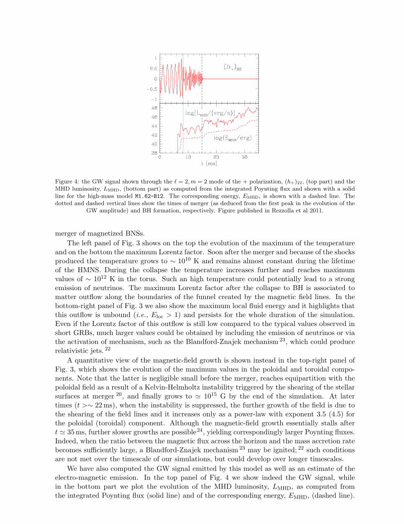
Figure 4: the GW signal shown through the ` = 2, m = 2 mode of the + polarization, (h+)22, (top part) and theMHD luminosity, LMHD, (bottom part) as computed from the integrated Poynting flux and shown with a solidline for the high-mass model M1.62-B12. The corresponding energy, EMHD, is shown with a dashed line. Thedotted and dashed vertical lines show the times of merger (as deduced from the first peak in the evolution of the
GW amplitude) and BH formation, respectively. Figure published in Rezzolla et al 2011.
merger of magnetized BNSs.The left panel of Fig. 3 shows on the top the evolution of the maximum of the temperature
and on the bottom the maximum Lorentz factor. Soon after the merger and because of the shocksproduced the temperature grows to ∼ 1010 K and remains almost constant during the lifetimeof the HMNS. During the collapse the temperature increases further and reaches maximumvalues of ∼ 1012 K in the torus. Such an high temperature could potentially lead to a strongemission of neutrinos. The maximum Lorentz factor after the collapse to BH is associated tomatter outflow along the boundaries of the funnel created by the magnetic field lines. In thebottom-right panel of Fig. 3 we also show the maximum local fluid energy and it highlights thatthis outflow is unbound (i.e., Eloc > 1) and persists for the whole duration of the simulation.Even if the Lorentz factor of this outflow is still low compared to the typical values observed inshort GRBs, much larger values could be obtained by including the emission of neutrinos or viathe activation of mechanism, such as the Blandford-Znajek mechanism 23, which could producerelativistic jets. 22
A quantitative view of the magnetic-field growth is shown instead in the top-right panel ofFig. 3, which shows the evolution of the maximum values in the poloidal and toroidal compo-nents. Note that the latter is negligible small before the merger, reaches equipartition with thepoloidal field as a result of a Kelvin-Helmholtz instability triggered by the shearing of the stellarsurfaces at merger 20, and finally grows to ' 1015 G by the end of the simulation. At latertimes (t >∼ 22 ms), when the instability is suppressed, the further growth of the field is due tothe shearing of the field lines and it increases only as a power-law with exponent 3.5 (4.5) forthe poloidal (toroidal) component. Although the magnetic-field growth essentially stalls aftert ' 35 ms, further slower growths are possible24, yielding correspondingly larger Poynting fluxes.Indeed, when the ratio between the magnetic flux across the horizon and the mass accretion ratebecomes sufficiently large, a Blandford-Znajek mechanism 23 may be ignited; 22 such conditionsare not met over the timescale of our simulations, but could develop over longer timescales.
We have also computed the GW signal emitted by this model as well as an estimate of theelectro-magnetic emission. In the top panel of Fig. 4 we show indeed the GW signal, whilein the bottom part we plot the evolution of the MHD luminosity, LMHD, as computed fromthe integrated Poynting flux (solid line) and of the corresponding energy, EMHD, (dashed line).
Clearly, the MHD emission starts only at the time of merger, it is almost constant and equalto ≈ 1044 erg/s during the life of the HMNS, and increases exponentially after BH formation,when the GW signal essentially shuts off. Assuming that the quasi-stationary MHD luminosity is∼ 4×1048 erg/s, the total MHD energy released during the lifetime of the torus is ∼ 1.2×1048 erg,which, if considering that our jet structure has an opening half-angle of ∼ 30, suggests a lowerlimit to the isotropic equivalent energy in the outflow of ∼ 9× 1048 erg. While this is at the lowend of the observed distribution of gamma-ray energies for short GRBs, larger MHD luminositiesare expected either through the additional growth of the magnetic field via the on-going windingof the field lines in the disk (the simulation covers only one tenth of taccr), or when magneticreconnection (which cannot take place within our ideal-MHD approach), is also accounted for.Even if we did not follow the entire evolution of the torus, by measuring its accretion rates weestimated that its lifetime would be ≈ 0.3 seconds and consequently in good agreement with theduration of short GRBs.
4 Conclusions
We have reported on some of the main results obtained from the first general relativistic simula-tions of magnetized BNSs with astrophysically realistic magnetic fields.5,8 We have shown for thefirst time how the magnetic fields can impact the evolution of the HMNS formed after the mergerand that fields equal or larger than ∼ 1010 G accelerate its collapse to BH. We have shown thatall the systems that collapse to BH form tori sufficiently massive to power short GRBs and thatthe magnetic field structure around the BH has those characteristics that are necessary in orderto launch relativistic jets. A detailed analysis of our results has also shown a good agreementwith observations, even if the introduction of more physical ingredients (e.g., neutrino emissionand more realistic EOS) will be required in order to increase the accuracy of this model.
Acknowledgments
We thank the developers of Lorene for providing us with initial data and those of Cactus andCarpet for the numerical infrastructures used by Whisky. Useful input from M. A. Aloy, J. Gra-not, I. Hinder, C. Kouveliotou, J. Read, C. Reisswig, E. Schnetter, A. Tonita, A. Vicere, andS. Yoshida is also acknowledged. We also thank M. Koppitz for assisting us in the productionof Fig. 1. The computations were performed on the Damiana Cluster at the AEI, on Queen-Bee through LONI (www.loni.org), and at the Texas Advanced Computing Center throughTERAGRID Allocation No. TG-MCA02N014. This work was supported in part by the DFGGrant SFB/Transregio 7, by “CompStar”, a Research Networking Programme of the EuropeanScience Foundation, by the JSPS Grant-in-Aid for Scientific Research (19-07803), by the MEXTGrant-in-Aid for Young Scientists (22740163) and by NASA Grant No. NNX09AI75G.
References
1. Matthew D. Duez. Numerical relativity confronts compact neutron star binaries: a reviewand status report. Class. Quantum Grav., 27:114002, 2010.
2. L. Baiotti, B. Giacomazzo, and L. Rezzolla. Accurate evolutions of inspiralling neutron-star binaries: Prompt and delayed collapse to a black hole. Phys. Rev. D, 78:084033,2008.
3. K. Kiuchi, Y. Sekiguchi, M. Shibata, and K. Taniguchi. Exploring Binary-Neutron-Star-Merger Scenario of Short-Gamma-Ray Bursts by Gravitational-Wave Observation. Phys.Rev. Lett., 104:141101, 2010.
4. L. Rezzolla, L. Baiotti, B. Giacomazzo, D. Link, and J. A. Font. Accurate evolutionsof unequal-mass neutron-star binaries: properties of the torus and short GRB engines.Class. Quantum Grav., 27:114105, 2010.
5. Bruno Giacomazzo, Luciano Rezzolla, and Luca Baiotti. Accurate evolutions of inspi-ralling and magnetized neutron stars: Equal-mass binaries. Phys. Rev. D, 83:044014,2011.
6. R. Narayan, B. Paczynski, and Tsvi Piran. Gamma-ray bursts as the death throes ofmassive binary stars. Astrophys. J., 395:L83, 1992.
7. B. Zhang and P. Meszaros. Int. J. Mod. Phys. A, 19:2385, 2004.8. L. Rezzolla, B. Giacomazzo, L. Baiotti, J. Granot, C. Kouveliotou, and M. A. Aloy. The
missing link: Merging neutron stars naturally produce jet-like structures and can powershort Gamma-Ray Bursts. Astrophys. Journ. Lett., 732:L6, 2011.
9. Tsvi Piran. The physics of gamma-ray bursts. Rev. Mod. Phys., 76:1143–1210, 2004.10. K. Belczynski, R. E. Taam, V. Kalogera, F. Rasio, and T. Bulik. On the Rarity of Double
Black Hole Binaries: Consequences for Gravitational Wave Detection. Astrophys. J.,662:504, 2007.
11. J. S. Read, C. Markakis, M. Shibata, K. Uryu, J. D. E. Creighton, and J. L. Friedman.Measuring the neutron star equation of state with gravitational wave observations. Phys.Rev. D, 79:124033, 2009.
12. Luca Baiotti, Ian Hawke, Pedro Montero, and Luciano Rezzolla. A new three-dimensionalgeneral-relativistic hydrodynamics code. In R. Capuzzo-Dolcetta, editor, ComputationalAstrophysics in Italy: Methods and Tools, volume 1, page 210, Trieste, 2003. MSAIt.
13. Luca Baiotti, Ian Hawke, Pedro J. Montero, Frank Loffler, Luciano Rezzolla, NikolaosStergioulas, Jose A. Font, and Ed Seidel. Three-dimensional relativistic simulations ofrotating neutron star collapse to a Kerr black hole. Phys. Rev. D, 71:024035, 2005.
14. Bruno Giacomazzo and Luciano Rezzolla. WhiskyMHD: a new numerical code for generalrelativistic magnetohydrodynamics. Class. Quantum Grav., 24:S235, 2007.
15. Denis Pollney, Christian Reisswig, Luciano Rezzolla, Bela Szilagyi, Marcus Ansorg, BarretDeris, Peter Diener, Ernst Nils Dorband, Michael Koppitz, Alessandro Nagar, and ErikSchnetter. Recoil velocities from equal-mass binary black-hole mergers: a systematicinvestigation of spin-orbit aligned configurations. Phys. Rev. D, 76:124002, 2007.
16. P. Colella and P. R. Woodward. J. Comput. Phys., 54:174, 1984.17. A. Harten, P. D. Lax, and B. van Leer. SIAM Rev., 25:35, 1983.18. G. Toth. The div b=0 constraint in shock-capturing magnetohydrodynamics codes. J.
Comput. Phys., 161:605–652, 2000.19. Erik Schnetter, Scott H. Hawley, and Ian Hawke. Evolutions in 3D numerical relativity
using fixed mesh refinement. Class. Quantum Grav., 21:1465–1488, 2004.20. B. Giacomazzo, L. Rezzolla, and L. Baiotti. Can magnetic fields be detected during the
inspiral of binary neutron stars? Mon. Not. R. Astron. Soc., 399:L164–L168, 2009.21. K. Taniguchi and E. Gourgoulhon. Phys. Rev. D, 66:104019, 2002.22. S. S. Komissarov and M. V. Barkov. Activation of the Blandford-Znajek mechanism in
collapsing stars. Mon. Not. R. Astron. Soc., 397:1153–1168, 2009.23. R. D. Blandford and R. L. Znajek. Electromagnetic extraction of energy from Kerr black
holes. Mon. Not. R. Astron. Soc., 179:433–456, 1977.24. M. Obergaulinger, P. Cerda-Duran, E. Muller, and M. A. Aloy. Semi-global simulations
of the magneto-rotational instability in core collapse supernovae. Astronomy and Astro-physics, 498:241–271, 2009.
THE COALESCENCE RATES OF DOUBLE BLACK HOLES
BELCZYNSKI K.1,2, BULIK, T.1, DOMINIK., M.1, PRESTWICH, A.3
1 Astronomical Observatory, University of Warsaw, Al. Ujazdowskie 4, 00-478 Warsaw, Poland2 Center for Gravitational Wave Astronomy, University of Texas at Brownsville, Brownsville, TX
78520, USA3 Harvard-Smithsonian Center for Astrophysics, Cambridge, MA 02138, USA
We present the summary of the recent investigations of double black hole binaries in context oftheir formation and merger rates. In particular we discuss the spectrum of black hole masses,the formation scenarios in the local Universe and the estimates of detection rates for gravita-tional radiation detectors like LIGO and VIRGO. Our study is based on observed propertiesof known Galactic and extra-galactic stellar mass black holes and evolutionary predictions.We argue that the binary black holes are the most promising source of gravitational radiation.
1 Population Synthesis Coalescence Rates
We employ the StarTrack population synthesis code (Belczynski et al. 2002, 2008) to performseveral Monte Carlo simulations of binary evolution with a range of metallicity. We base thecalculations on recent results from the Sloan Digital Sky Survey observations (Panter et al.2008) indicating (∼ 300, 000 galaxies) that recent star formation (within the last 1 billion years)is bimodal: half the stars form from gas with high amounts of metals (solar metallicity), andthe other half form with small contribution of elements heavier than Helium (∼ 10−30% solar).Additionally, we use the recent estimates of mass loss rates producing much heavier stellar blackholes than previously expected (∼ 30 − 80 M⊙; Belczynski et al. 2010a). The results of thesecalculations were presented for the first time by Belczynski et al. (2010b). We have evolveda population of 2 million massive binary stars, and investigated the formation of close doublecompact objects: double neutron stars (NS-NS), double black hole binaries (BH-BH), and mixedsystems (BH-NS). Our modeling utilizes updated stellar and binary physics, including resultsfrom supernova simulations (Fryer & Kalogera 2001) and compact object formation (Timmes etal. 1996), incorporating elaborate mechanisms for treating stellar interactions like mass transferepisodes and tidal synchronization and circularization. We put special emphasis on the commonenvelope evolution phase, which is crucial for close double compact object formation as theattendant mass transfer allows for efficient hardening of the binary. This orbital contraction canbe sufficiently efficient to cause the individual stars in the binary to coalesce and form a singlehighly rotating object, thereby aborting further binary evolution and preventing the formationof a double compact object. Due to significant radial expansion, stars crossing the Hertzsprunggap (HG) very frequently initiate a common envelope phase. HG stars do not have a clearentropy jump at the core-envelope transition (Ivanova & Taam 2004); if such a star overflowsits Roche lobe and initiates a common envelope phase, the inspiral is expected to lead to acoalescence (Taam & Sandquist 2000). In particular, it has been estimated that for a solar
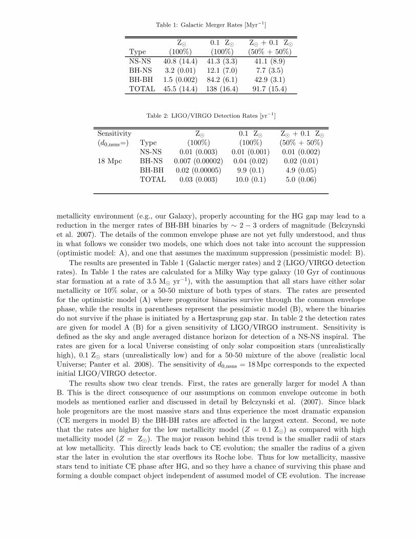
Table 1: Galactic Merger Rates [Myr−1]
Z⊙ 0.1 Z⊙ Z⊙ + 0.1 Z⊙
Type (100%) (100%) (50% + 50%)
NS-NS 40.8 (14.4) 41.3 (3.3) 41.1 (8.9)BH-NS 3.2 (0.01) 12.1 (7.0) 7.7 (3.5)BH-BH 1.5 (0.002) 84.2 (6.1) 42.9 (3.1)TOTAL 45.5 (14.4) 138 (16.4) 91.7 (15.4)
Table 2: LIGO/VIRGO Detection Rates [yr−1]
Sensitivity Z⊙ 0.1 Z⊙ Z⊙ + 0.1 Z⊙
(d0,nsns=) Type (100%) (100%) (50% + 50%)NS-NS 0.01 (0.003) 0.01 (0.001) 0.01 (0.002)
18 Mpc BH-NS 0.007 (0.00002) 0.04 (0.02) 0.02 (0.01)BH-BH 0.02 (0.00005) 9.9 (0.1) 4.9 (0.05)TOTAL 0.03 (0.003) 10.0 (0.1) 5.0 (0.06)
metallicity environment (e.g., our Galaxy), properly accounting for the HG gap may lead to areduction in the merger rates of BH-BH binaries by ∼ 2 − 3 orders of magnitude (Belczynskiet al. 2007). The details of the common envelope phase are not yet fully understood, and thusin what follows we consider two models, one which does not take into account the suppression(optimistic model: A), and one that assumes the maximum suppression (pessimistic model: B).
The results are presented in Table 1 (Galactic merger rates) and 2 (LIGO/VIRGO detectionrates). In Table 1 the rates are calculated for a Milky Way type galaxy (10 Gyr of continuousstar formation at a rate of 3.5 M⊙ yr−1), with the assumption that all stars have either solarmetallicity or 10% solar, or a 50-50 mixture of both types of stars. The rates are presentedfor the optimistic model (A) where progenitor binaries survive through the common envelopephase, while the results in parentheses represent the pessimistic model (B), where the binariesdo not survive if the phase is initiated by a Hertzsprung gap star. In table 2 the detection ratesare given for model A (B) for a given sensitivity of LIGO/VIRGO instrument. Sensitivity isdefined as the sky and angle averaged distance horizon for detection of a NS-NS inspiral. Therates are given for a local Universe consisting of only solar composition stars (unrealisticallyhigh), 0.1 Z⊙ stars (unrealistically low) and for a 50-50 mixture of the above (realistic localUniverse; Panter et al. 2008). The sensitivity of d0,nsns = 18Mpc corresponds to the expectedinitial LIGO/VIRGO detector.
The results show two clear trends. First, the rates are generally larger for model A thanB. This is the direct consequence of our assumptions on common envelope outcome in bothmodels as mentioned earlier and discussed in detail by Belczynski et al. (2007). Since blackhole progenitors are the most massive stars and thus experience the most dramatic expansion(CE mergers in model B) the BH-BH rates are affected in the largest extent. Second, we notethat the rates are higher for the low metallicity model (Z = 0.1 Z⊙) as compared with highmetallicity model (Z = Z⊙). The major reason behind this trend is the smaller radii of starsat low metallicity. This directly leads back to CE evolution; the smaller the radius of a givenstar the later in evolution the star overflows its Roche lobe. Thus for low metallicity, massivestars tend to initiate CE phase after HG, and so they have a chance of surviving this phase andforming a double compact object independent of assumed model of CE evolution. The increase
of rates with decreasing metallicity is additionally connected with the fact that low metallicitystars experience low wind mass loss and thus form more massive compact objects. This leadsto a shorter merger times and higher merger rates.
Had the initial configuration of LIGO/VIRGO instruments reached its design sensitivity ofd0,nsns18 Mpc for its entire lifetime (averaged horizon for NS-NS merger) we would be able toexclude model A from our considerations. This model generates about 5 BH-BH inspirals peryear within this horizon (of course the actual horizon for BH-BH detection was accordinglyextended with the increased mass of each BH-BH merger). So far there was no report ofdetection in LIGO/VIRGO data so one would be tempted to exclude this model from furtherconsiderations. However, the time averged sensitivity of the last LIGO/VIRGO run (S5, themost recently relesed) has reached only about d0,nsns ≈ 9 Mpc. Therefore, the rates should bedecreased by factor (18/9)3 = 8 and the expected detection rate for BH-BH binaries would dropbelow 1 yr−1 and consequently model A cannot be yet excluded.
2 Empirical Coalescence Rates
The optical followup of X-ray sources revealed the nature of several X-ray binaries in the galaxiesin the Local Group. Two objects: IC10 X-1 and NGC300 X-1 are of particular interest. Theidentification of optical counterparts and their spectroscopy allowed to estimate the propertiesof these two binaries. Both host massive black holes on a tight orbit with WR stars. Both residein low metallicity environments (Crowther et al. 2007, Crowther et al. 2010, Prestwich et al.2007, Silverman and Filipenko 2008). In the future the accretion in these binaries will continueand the WR stars will loose mass through stellar winds. The typical lifetime of the WR stars insuch systems is from 100 to 300 kyrs. After that time the WR stars will explode as supernovaeleading to formation of a BH, or a NS in the case of extremely large mass loss. The systemswill most likely survive the explosions and remain bound since the current orbital velocities areabove 500km s−1. Both systems will end up as binary black holes in a few hundred thousandyears.
Given the estimate of the future evolution of the two binaries: IC10 X-1 and NGC300 X-1,we estimate the formation rate of such binaries.The estimated merger time is smaller than theHubble time. Therefore assuming that the star formation rate was constant the merger rate of thebinary black holes formed from such systems will be the same as their formation rate. For eachsystem we estimate the volume in which it is detectable. This is determined by the possibilityof measuring the radial velocity curve, which can be done up to the distance of r ≈ 2Mpc,thus Vobs = 4πr
3/3. Each binary was detected only because of its X-ray radiation, thus the
observability is proportional to the X-ray active phase. The formation rate of each binary canbe approximated as: R = (Vobstobs)
−1. A detailed statistical analysis is presented in Bulik,Belczynski and Prestwich (2010). We present the probability distributions of the formation andmerger rates of the binary black holes corresponding to each binary IC10 X-1 and NGC300 X-1in Figure 1. The thick line in Figure 1 represents the probability density of the sum of the tworates. This calculation implies a merger rate density of R = 0.36+0.50
−0.26Mpc−3Myr−1. For thetime averaged the sensitivity range of LIGO and VIRGO to binary black holes coalescence of≈ 100Mpc, this implies the expected detection rate around one per year. This is in a strikingagreement with the population synthesis results.
3 Conclusions
Both theoretical simulations and empirical estimate indicate that detection rates of BH-BHbinaries are significantly higher than other double compact objects (NS-NS and BH-NS). Thepopulation synthesis predictions for our realistic model of local Universe with a mixture of high
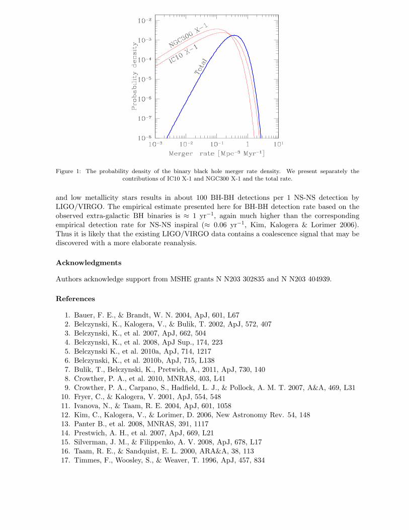
Figure 1: The probability density of the binary black hole merger rate density. We present separately thecontributions of IC10 X-1 and NGC300 X-1 and the total rate.
and low metallicity stars results in about 100 BH-BH detections per 1 NS-NS detection byLIGO/VIRGO. The empirical estimate presented here for BH-BH detection rate based on theobserved extra-galactic BH binaries is ≈ 1 yr−1, again much higher than the correspondingempirical detection rate for NS-NS inspiral (≈ 0.06 yr−1, Kim, Kalogera & Lorimer 2006).Thus it is likely that the existing LIGO/VIRGO data contains a coalescence signal that may bediscovered with a more elaborate reanalysis.
Acknowledgments
Authors acknowledge support from MSHE grants N N203 302835 and N N203 404939.
References
1. Bauer, F. E., & Brandt, W. N. 2004, ApJ, 601, L672. Belczynski, K., Kalogera, V., & Bulik, T. 2002, ApJ, 572, 4073. Belczynski, K., et al. 2007, ApJ, 662, 5044. Belczynski, K., et al. 2008, ApJ Sup., 174, 2235. Belczynski K., et al. 2010a, ApJ, 714, 12176. Belczynski, K., et al. 2010b, ApJ, 715, L1387. Bulik, T., Belczynski, K., Pretwich, A., 2011, ApJ, 730, 1408. Crowther, P. A., et al. 2010, MNRAS, 403, L419. Crowther, P. A., Carpano, S., Hadfield, L. J., & Pollock, A. M. T. 2007, A&A, 469, L31
10. Fryer, C., & Kalogera, V. 2001, ApJ, 554, 54811. Ivanova, N., & Taam, R. E. 2004, ApJ, 601, 105812. Kim, C., Kalogera, V., & Lorimer, D. 2006, New Astronomy Rev. 54, 14813. Panter B., et al. 2008, MNRAS, 391, 111714. Prestwich, A. H., et al. 2007, ApJ, 669, L2115. Silverman, J. M., & Filippenko, A. V. 2008, ApJ, 678, L1716. Taam, R. E., & Sandquist, E. L. 2000, ARA&A, 38, 11317. Timmes, F., Woosley, S., & Weaver, T. 1996, ApJ, 457, 834
PERTURBATIVE, POST-NEWTONIAN, AND GENERAL RELATIVISTICDYNAMICS OF BLACK HOLE BINARIES
A. LE TIECMaryland Center for Fundamental Physics & Joint Space-Science Institute,
Department of Physics, University of Maryland, College Park, MD 20742, USA
The orbital motion of inspiralling and coalescing black hole binaries can be investigated usinga variety of approximation schemes and numerical methods within general relativity: post-Newtonian expansions, black hole perturbation theory, numerical relativity, and the effective-one-body formalism. We review two recent comparisons of the predictions from these varioustechniques. Both comparisons rely on the calculation of a coordinate invariant relation, inthe case of non-spinning binary black holes on quasi-circular orbits. All methods are shownto agree very well in their common domain of validity.
1 Introduction
The detection and analysis of the gravitational radiation from black hole binaries by the ground-based LIGO/Virgo observatories, and future space-based antennas, requires very accurate theo-retical predictions for use as gravitational wave templates. The orbital motion of such compactbinary systems can be analyzed using multiple approximation schemes and numerical meth-ods in general relativity: post-Newtonian (PN) expansions, black hole perturbation theory, theeffective-one-body (EOB) formalism, and numerical relativity (NR). It is crucial to compare thepredictions from these various techniques for several reasons: such comparisons (i) provide inde-pendent consistency checks of the validity of the various calculations, (ii) they help to delineatethe respective domains of validity of each method, and (iii) they can inform the development ofa universal semi-analytical model of the binary dynamics and gravitational wave emission. Inthis paper, we shall summarize the main results of two such recent comparisons, both related tothe local orbital dynamics of non-spinning black hole binaries on quasi-circular orbits.
2 Redshift Observable
Our first comparison is concerned with the relativistic motion of compact binary systems withinblack hole perturbation theory and the PN approximation. Consider two non-spinning blackholes with masses m1 and m2, moving on an exactly circular orbit with angular frequency Ωϕ.The dissipative effects associated with the emission of gravitational radiation are neglected,which is formalized by assuming the existence of a helical Killing vector (HKV) field kα. The4-velocity uα1 of the “particle” m1 is necessarily tangent to the HKV evaluated at that location;hence uα1 = U kα1 . The scalar U is a constant of the motion associated with the helical symmetry.It also measures the gravitational redshift of light rays emitted from m1, and received at largedistance, along the helical symmetry axis perpendicular to the orbital plane;1 we shall henceforth
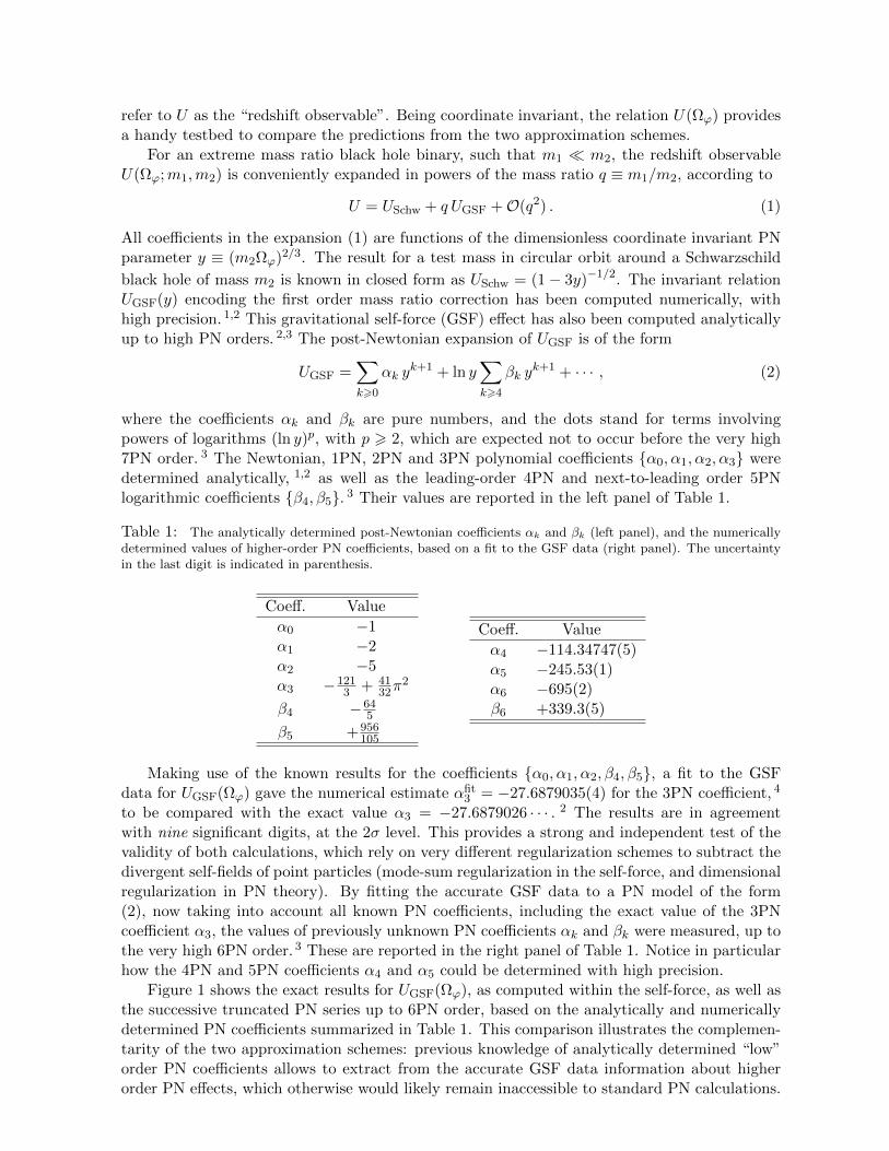
refer to U as the “redshift observable”. Being coordinate invariant, the relation U(Ωϕ) providesa handy testbed to compare the predictions from the two approximation schemes.
For an extreme mass ratio black hole binary, such that m1 m2, the redshift observableU(Ωϕ;m1,m2) is conveniently expanded in powers of the mass ratio q ≡ m1/m2, according to
U = USchw + q UGSF +O(q2) . (1)
All coefficients in the expansion (1) are functions of the dimensionless coordinate invariant PNparameter y ≡ (m2Ωϕ)2/3. The result for a test mass in circular orbit around a Schwarzschild
black hole of mass m2 is known in closed form as USchw = (1− 3y)−1/2. The invariant relationUGSF(y) encoding the first order mass ratio correction has been computed numerically, withhigh precision. 1,2 This gravitational self-force (GSF) effect has also been computed analyticallyup to high PN orders. 2,3 The post-Newtonian expansion of UGSF is of the form
UGSF =∑k>0
αk yk+1 + ln y
∑k>4
βk yk+1 + · · · , (2)
where the coefficients αk and βk are pure numbers, and the dots stand for terms involvingpowers of logarithms (ln y)p, with p > 2, which are expected not to occur before the very high7PN order. 3 The Newtonian, 1PN, 2PN and 3PN polynomial coefficients α0, α1, α2, α3 weredetermined analytically, 1,2 as well as the leading-order 4PN and next-to-leading order 5PNlogarithmic coefficients β4, β5. 3 Their values are reported in the left panel of Table 1.
Table 1: The analytically determined post-Newtonian coefficients αk and βk (left panel), and the numericallydetermined values of higher-order PN coefficients, based on a fit to the GSF data (right panel). The uncertaintyin the last digit is indicated in parenthesis.
Coeff. Value
α0 −1α1 −2α2 −5α3 −121
3 + 4132π
2
β4 −645
β5 +956105
Coeff. Value
α4 −114.34747(5)α5 −245.53(1)α6 −695(2)β6 +339.3(5)
Making use of the known results for the coefficients α0, α1, α2, β4, β5, a fit to the GSFdata for UGSF(Ωϕ) gave the numerical estimate αfit
3 = −27.6879035(4) for the 3PN coefficient, 4
to be compared with the exact value α3 = −27.6879026 · · · . 2 The results are in agreementwith nine significant digits, at the 2σ level. This provides a strong and independent test of thevalidity of both calculations, which rely on very different regularization schemes to subtract thedivergent self-fields of point particles (mode-sum regularization in the self-force, and dimensionalregularization in PN theory). By fitting the accurate GSF data to a PN model of the form(2), now taking into account all known PN coefficients, including the exact value of the 3PNcoefficient α3, the values of previously unknown PN coefficients αk and βk were measured, up tothe very high 6PN order. 3 These are reported in the right panel of Table 1. Notice in particularhow the 4PN and 5PN coefficients α4 and α5 could be determined with high precision.
Figure 1 shows the exact results for UGSF(Ωϕ), as computed within the self-force, as well asthe successive truncated PN series up to 6PN order, based on the analytically and numericallydetermined PN coefficients summarized in Table 1. This comparison illustrates the complemen-tarity of the two approximation schemes: previous knowledge of analytically determined “low”order PN coefficients allows to extract from the accurate GSF data information about higherorder PN effects, which otherwise would likely remain inaccessible to standard PN calculations.
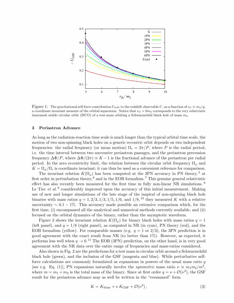
0.1
0.2
0.3
0.4
0.5
5 6 7 8 9 10
−UGSF
rΩ / m2
N1PN2PN3PN4PN5PN6PNExact
Figure 1: The gravitational self-force contribution UGSF to the redshift observable U , as a function of rΩ ≡ m2/y,a coordinate invariant measure of the orbital separation. Notice that rΩ = 6m2 corresponds to the very relativisticinnermost stable circular orbit (ISCO) of a test-mass orbiting a Schwarzschild black hole of mass m2.
3 Periastron Advance
As long as the radiation-reaction time scale is much longer than the typical orbital time scale, themotion of two non-spinning black holes on a generic eccentric orbit depends on two independentfrequencies: the radial frequency (or mean motion) Ωr = 2π/P , where P is the radial period,i.e. the time interval between two successive periastron passages, and the periastron precessionfrequency ∆Φ/P , where ∆Φ/(2π) ≡ K − 1 is the fractional advance of the periastron per radialperiod. In the zero eccentricity limit, the relation between the circular orbit frequency Ωϕ andK = Ωϕ/Ωr is coordinate invariant; it can thus be used as a convenient reference for comparison.
The invariant relation K(Ωϕ) has been computed at the 3PN accuracy in PN theory, 5 atfirst order in perturbation theory,6 and in the EOB formalism.7 This genuine general relativisticeffect has also recently been measured for the first time in fully non-linear NR simulations. 8
Le Tiec et al. 9 considerably improved upon the accuracy of this initial measurement. Makinguse of new and longer simulations of the late stage of the inspiral of non-spinning black holebinaries with mass ratios q = 1, 2/3, 1/3, 1/5, 1/6, and 1/8, 10 they measured K with a relativeuncertainty ∼ 0.1 − 1%. This accuracy made possible an extensive comparison which, for thefirst time, (i) encompassed all the analytical and numerical methods currently available, and (ii)focused on the orbital dynamics of the binary, rather than the asymptotic waveform.
Figure 2 shows the invariant relation K(Ωϕ) for binary black holes with mass ratios q = 1(left panel), and q = 1/8 (right panel), as computed in NR (in cyan), PN theory (red), and theEOB formalism (yellow). For comparable masses (e.g. q = 1 or 2/3), the 3PN prediction is ingood agreement with the exact result from NR (to better than 1%). However, as expected, itperforms less well when q → 0. 11 The EOB (3PN) prediction, on the other hand, is in very goodagreement with the NR data over the entire range of frequencies and mass-ratios considered.
Also shown in Fig. 2 are the predictions for a test mass in circular orbit around a Schwarzschildblack hole (green), and the inclusion of the GSF (magenta and blue). While perturbative self-force calculations are commonly formulated as expansions in powers of the usual mass ratio q[see e.g. Eq. (1)], PN expansions naturally involve the symmetric mass ratio ν ≡ m1m2/m
2,where m = m1 +m2 is the total mass of the binary. Since at first order q = ν+O(ν2), the GSFresult for the periastron advance may as well be written in the “resummed” form
K = KSchw + ν KGSF +O(ν2) , (3)
1.2
1.3
1.4
1.5
1.6
K
NR
Schw
GSFq
GSFνEOB
3PN
-0.01
0
0.01
0.015 0.02 0.025 0.03
K/K
NR−
1
mΩϕ
1.3
1.4
1.5
1.6
1.7NR
Schw
GSFq
GSFνEOB
3PN
-0.01
0
0.01
0.021 0.024 0.027 0.03 0.033
mΩϕ
q = 1 q = 1/8
Figure 2: The periastron advance K = 1 + ∆Φ/(2π), as a function of the circular orbit frequency Ωϕ, for blackhole binaries with mass ratios 1 : 1 (left panel) and 1 : 8 (right panel). Notice that in the later case, ∆Φ reacheshalf an orbit per radial period for mΩϕ ∼ 0.03, corresponding to an orbital separation r ∼ 10m.
where all coefficients are functions of the dimensionless invariant PN parameter x ≡ (mΩϕ)2/3.
The GSF correction KGSF to the test-particle result KSchw = (1− 6x)−1/2 has recently beencomputed numerically. 6 Although the GSFq prediction [obtained by replacing ν → q in Eq. (3)]agrees with the exact result within a relative difference of magnitude ∼ q2, as expected, the GSFνprediction (3) agrees remarkably well with the NR data for all mass ratios. This surprising resultsuggests that GSF calculations may very well find application in a broader range of physicalproblems than originally envisaged, including the modelling of intermediate mass ratio inspirals,a plausible source of gravitational waves for Advanced LIGO/Virgo.
Acknowledgments
The results summarized in this paper were obtained in collaboration with L. Barack, L. Blanchet,A. Buonanno, S. Detweiler, A.H. Mroue, H.P. Pfeiffer, N. Sago, A. Taracchini, and B.F. Whiting.The author acknowledges support from NSF Grant PHY-0903631, and from the Maryland Centerfor Fundamental Physics. He is grateful to the organizing committee of the 46th Rencontres deMoriond & GPhyS Colloquium for their kind invitation, and for providing financial support.
References
1. S. Detweiler, Phys. Rev. D 77, 124026 (2008).2. L. Blanchet, S. Detweiler, A. Le Tiec, and B.F. Whiting, Phys. Rev. D 81, 064004 (2010).3. L. Blanchet, S. Detweiler, A. Le Tiec, and B.F. Whiting, Phys. Rev. D 81, 084033 (2010).4. L. Blanchet, S. Detweiler, A. Le Tiec, and B.F. Whiting, in Mass and Motion in General
Relativity, eds. L. Blanchet, A. Spallicci, B. Whiting (Springer, 2011).5. T. Damour, P. Jaranowski, and G. Schafer, Phys. Rev. D 62, 044024 (2000).6. L. Barack, T. Damour, and N. Sago, Phys. Rev. D 82, 084036 (2010).7. T. Damour, Phys. Rev. D 81, 024017 (2010).8. A.H. Mroue, H.P. Pfeiffer, L.E. Kidder, S.A. Teukolsky, Phys. Rev. D 82, 124016 (2010).9. A. Le Tiec et al., submitted for publication (2011), arXiv:1106:3278 [gr-qc].
10. A.H. Mroue et al., in preparation.11. L. Blanchet, Phys. Rev. D 65, 124009 (2002).
ON THE ECCENTRICITY OF NS-NS BINARIES.
I. KOWALSKA1, T. BULIK1, K. BELCZYNSKI1,2, M. DOMINIK 1, D. GONDEK-ROSINSKA 3
1Astronomical Observatory, University of Warsaw, Al Ujazdowskie 4, 00-478 Warsaw, Poland2Dept. of Physics and Astronomy, University of Texas, Brownsville, TX 78520, USA
3Institute of Astronomy, University of Zielona Gora, ul. Lubuska 2, 65-265 Zielona Gora, Poland
The current gravitational wave detectors have reached their operational sensitivity and arenearing detection of compact object binaries. In the coming years, we expect that the Ad-vanced LIGO/VIRGO will start taking data. We discuss the eccentricity distribution of doubleneutron stars during they inspiral phase. We analyze the expected distributions of eccentric-ities at the frequency that is characteristic for Advanced Virgo and LIGO detectors. We usethe StarTrack binary population code to investigate the properties of the population of com-pact binaries in formation. We evolve their orbits until the point that they enter a detectorsensitivity window and analyze the eccentricity distribution at that time. Within the rangeof considered models, we found that a fraction of between 0.2% and 2% NS-NS binaries willhave an eccentricity above 0.01 for the Advanced LIGO/VIRGO detectors.
1 Motivation
Binary neutron stars are among the most promising candidates for gravitational wave sources.During the inspiral phase bounding energy is carried away from the system by gravitationalwaves. Separation between components and eccentricity of the orbit are decreasing very rapidly.The evolution of the orbit of compact object binary under the influence of gravitational radia-tion had been calculated by Peters 1,2. Last stable orbits are very well circularized. In currentdetectors such as Virgo 3 and LIGO 4, only those last orbits before coalescence are within sensi-tivity band. Therefore, eccentricity is negligible and there is no need to include it during dataanalysis. Situation will change when the second generation detectors will appear. Sensitivitywindow for Advanced Virgo and LIGO detectors will be expanded towards lower frequencies.Observing earlier stages of inspiral evolution will be possible. In that regime, eccentricity couldplay important role. Brown et al. 5 shown, that searching for eccentric binary using circulartemplate may lead to serious lost of efficiency. It is very important to check how many eccentricbinaries is expected within advanced detectors sensitivity band.
2 Initial parameters
So far we have very few observations of binary compact objects. All of them are double neutronstars observed in radio band (at least one of the components is seen as a pulsar). That sampleis not representative, because of selection effects. Therefore, we created synthetic sample ofdouble compact objects using StarTrack code 6. It perform a suite of Monte Carlo simulationsof the stellar evolution of stars in environments of two typical metallicities: Z = Z⊙ = 0.02 andZ = 10% Z⊙ = 0.002 7 (denoted by Z and z, respectivley). We place special emphasis on the
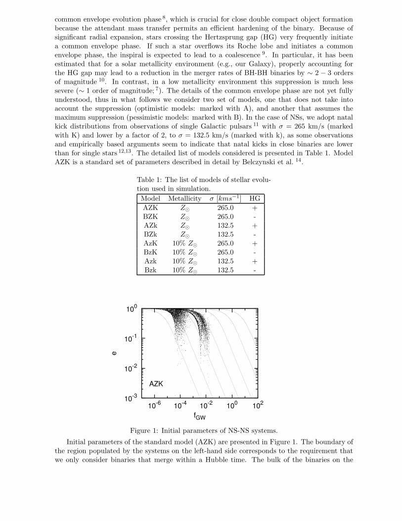
common envelope evolution phase 8, which is crucial for close double compact object formationbecause the attendant mass transfer permits an efficient hardening of the binary. Because ofsignificant radial expansion, stars crossing the Hertzsprung gap (HG) very frequently initiatea common envelope phase. If such a star overflows its Roche lobe and initiates a commonenvelope phase, the inspiral is expected to lead to a coalescence 9. In particular, it has beenestimated that for a solar metallicity environment (e.g., our Galaxy), properly accounting forthe HG gap may lead to a reduction in the merger rates of BH-BH binaries by ∼ 2 − 3 ordersof magnitude 10. In contrast, in a low metallicity environment this suppression is much lesssevere (∼ 1 order of magnitude; 7). The details of the common envelope phase are not yet fullyunderstood, thus in what follows we consider two set of models, one that does not take intoaccount the suppression (optimistic models: marked with A), and another that assumes themaximum suppression (pessimistic models: marked with B). In the case of NSs, we adopt natalkick distributions from observations of single Galactic pulsars 11 with σ = 265 km/s (markedwith K) and lower by a factor of 2, to σ = 132.5 km/s (marked with k), as some observationsand empirically based arguments seem to indicate that natal kicks in close binaries are lowerthan for single stars 12,13. The detailed list of models considered is presented in Table 1. ModelAZK is a standard set of parameters described in detail by Belczynski et al. 14.
Table 1: The list of models of stellar evolu-tion used in simulation.
Model Metallicity σ [kms−1] HG
AZK Z⊙ 265.0 +BZK Z⊙ 265.0 -AZk Z⊙ 132.5 +BZk Z⊙ 132.5 -AzK 10% Z⊙ 265.0 +BzK 10% Z⊙ 265.0 -Azk 10% Z⊙ 132.5 +Bzk 10% Z⊙ 132.5 -
10-3
10-2
10-1
100
10-6
10-4
10-2
100
102
e
fGW
AZK
Figure 1: Initial parameters of NS-NS systems.
Initial parameters of the standard model (AZK) are presented in Figure 1. The boundary ofthe region populated by the systems on the left-hand side corresponds to the requirement thatwe only consider binaries that merge within a Hubble time. The bulk of the binaries on the
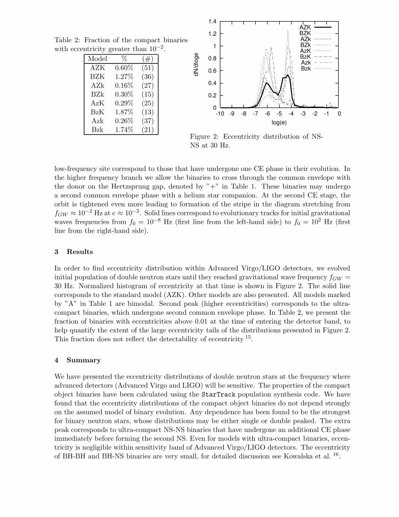
Table 2: Fraction of the compact binarieswith eccentricity greater than 10−2.
Model % (#)
AZK 0.60% (51)BZK 1.27% (36)AZk 0.16% (27)BZk 0.30% (15)AzK 0.29% (25)BzK 1.87% (13)Azk 0.26% (37)Bzk 1.74% (21)
0
0.2
0.4
0.6
0.8
1
1.2
1.4
-10 -9 -8 -7 -6 -5 -4 -3 -2 -1 0
dN
/dlo
ge
log(e)
AZKBZKAZkBZkAzKBzKAzkBzk
Figure 2: Eccentricity distribution of NS-NS at 30 Hz.
low-frequency site correspond to those that have undergone one CE phase in their evolution. Inthe higher frequency branch we allow the binaries to cross through the common envelope withthe donor on the Hertzsprung gap, denoted by ”+” in Table 1. These binaries may undergoa second common envelope phase with a helium star companion. At the second CE stage, theorbit is tightened even more leading to formation of the stripe in the diagram stretching fromfGW ≈ 10−2 Hz at e ≈ 10−2. Solid lines correspond to evolutionary tracks for initial gravitationalwaves frequencies from f0 = 10−8 Hz (first line from the left-hand side) to f0 = 102 Hz (firstline from the right-hand side).
3 Results
In order to find eccentricity distribution within Advanced Virgo/LIGO detectors, we evolvedinitial population of double neutron stars until they reached gravitational wave frequency fGW =30 Hz. Normalized histogram of eccentricity at that time is shown in Figure 2. The solid linecorresponds to the standard model (AZK). Other models are also presented. All models markedby ”A” in Table 1 are bimodal. Second peak (higher eccentricities) corresponds to the ultra-compact binaries, which undergone second common envelope phase. In Table 2, we present thefraction of binaries with eccentricities above 0.01 at the time of entering the detector band, tohelp quantify the extent of the large eccentricity tails of the distributions presented in Figure 2.This fraction does not reflect the detectability of eccentricity 15.
4 Summary
We have presented the eccentricity distributions of double neutron stars at the frequency whereadvanced detectors (Advanced Virgo and LIGO) will be sensitive. The properties of the compactobject binaries have been calculated using the StarTrack population synthesis code. We havefound that the eccentricity distributions of the compact object binaries do not depend stronglyon the assumed model of binary evolution. Any dependence has been found to be the strongestfor binary neutron stars, whose distributions may be either single or double peaked. The extrapeak corresponds to ultra-compact NS-NS binaries that have undergone an additional CE phaseimmediately before forming the second NS. Even for models with ultra-compact binaries, eccen-tricity is negligible within sensitivity band of Advanced Virgo/LIGO detectors. The eccentricityof BH-BH and BH-NS binaries are very small, for detailed discussion see Kowalska et al. 16.
Acknowledgments
This work was supported by the FOCUS 4/2007 Program of Foundation for Polish Science, thePolish grants N N203 511238, N N203 387237, DPN/N176/VIRGO/2009, N N203 302835, NN203 404939 and by CompStar a Research Networking Programme of the European ScienceFoundation.
References
1. P. C. Peters and J. Mathews, Phys. Rev. 131, 435 (1963).2. P. C. Peters, Phys. Rev. 136, 1224 (1964).3. A. D. A. M. Spallicci et al, Class. Quantum Grav 22, 461 (2005).4. J. R. Smith and LIGO Scientific Collaboration, Class. Quantum Grav 26, 114013 (2009).5. D. A. Brown and P. J. Zimmerman , Phys. Rev. D 81, 024007 (2010).6. K. Belczynski et al, ApJ 174, 223 (2008).7. K. Belczynski et al, ApJ 715, L138 (2010).8. R. F. Webbink, ApJ 277, 355 (1984).9. R. E. Taam and E. L. Sandquist Ann. Rev. A&A 38, 113 (2000).
10. K. Belczynski et al, ApJ 662, 504 (2007).11. G. Hobbs et al, MNRAS 360, 974 (2005).12. L. Dessart et al, ApJ 644, 1063 (2006).13. F. S. Kitaura et al, A&A 450, 345 (2006).14. K. Belczynski et al, ApJ 572, 407 (2002).15. K. J. Shapiro and N. J. Cornish, ArXiv e-prints, 2010.16. I. Kowalska et al, A&A 527, A70 (2011).
COMPACT OBJECTS WITH SPIN PARAMETER a∗ > 1
COSIMO BAMBIInstitute for the Physics and Mathematics of the Universe, The University of Tokyo
Kashiwa, Chiba 277-8583, Japan
In 4-dimensional General Relativity, black holes are described by the Kerr solution and arecompletely specified by their mass M and by their spin angular momentum J . A fundamentallimit for a black hole in General Relativity is the Kerr bound |a∗| ≤ 1, where a∗ = J/M2
is the spin parameter. Future experiments will be able to probe the geometry around theseobjects and test the Kerr black hole hypothesis. Interestingly, if these objects are not blackholes, the accretion process may spin them up to a∗ > 1.
1 Introduction
Today we believe that the final product of the gravitational collapse is a black hole (BH). In4-dimensional General Relativity, BHs are described by the Kerr solution and are completelyspecified by two parameters: the mass, M , and the spin angular momentum, J . A fundamentallimit for a BH in General Relativity is the Kerr bound |a∗| ≤ 1, where a∗ = J/M2 is the spinparameter. For |a∗| > 1, the Kerr solution does not describe a BH, but a naked singularity,which is forbidden by the weak cosmic censorship conjecture 1.
From the observational side, we have at least two classes of astrophysical BH candidates 2:stellar-mass bodies in X-ray binary systems (M ∼ 5 − 20 Solar masses) and super-massivebodies in galactic nuclei (M ∼ 105 − 1010 Solar masses). The existence of a third class ofobjects, intermediate-mass BH candidates (M ∼ 102 − 104 Solar masses), is still controversial,because there are not yet reliable dynamical measurements of their masses. All these objects arecommonly interpreted as BHs because they cannot be explained otherwise without introducingnew physics. The stellar-mass objects in X-ray binary systems are too heavy to be neutronor quark stars. At least some of the super-massive objects in galactic nuclei are too massive,compact, and old to be clusters of non-luminous bodies.
2 Testing the Kerr Black Hole Hypothesis
In Newtonian gravity, the potential of the gravitational field, Φ, is determined by the massdensity of the matter, ρ, according to the Poisson’s equation, ∇2Φ = 4πGNρ. In the exteriorregion, Φ can be written as
Φ(r, θ, ϕ) = −GN
∑lm
MlmYlm(θ, ϕ)
rl+1, (1)
where the coefficients Mlm are the multipole moments of the gravitational field and Yml are theLaplace’s spherical harmonics.
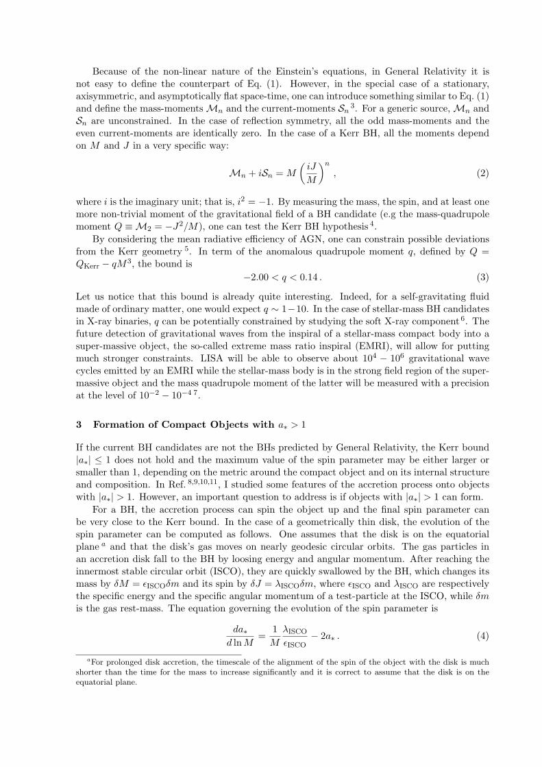
Because of the non-linear nature of the Einstein’s equations, in General Relativity it isnot easy to define the counterpart of Eq. (1). However, in the special case of a stationary,axisymmetric, and asymptotically flat space-time, one can introduce something similar to Eq. (1)and define the mass-moments Mn and the current-moments Sn
3. For a generic source, Mn andSn are unconstrained. In the case of reflection symmetry, all the odd mass-moments and theeven current-moments are identically zero. In the case of a Kerr BH, all the moments dependon M and J in a very specific way:
Mn + iSn = M
(iJ
M
)n
, (2)
where i is the imaginary unit; that is, i2 = −1. By measuring the mass, the spin, and at least onemore non-trivial moment of the gravitational field of a BH candidate (e.g the mass-quadrupolemoment Q ≡ M2 = −J2/M), one can test the Kerr BH hypothesis 4.
By considering the mean radiative efficiency of AGN, one can constrain possible deviationsfrom the Kerr geometry 5. In term of the anomalous quadrupole moment q, defined by Q =QKerr − qM3, the bound is
−2.00 < q < 0.14 . (3)
Let us notice that this bound is already quite interesting. Indeed, for a self-gravitating fluidmade of ordinary matter, one would expect q ∼ 1−10. In the case of stellar-mass BH candidatesin X-ray binaries, q can be potentially constrained by studying the soft X-ray component 6. Thefuture detection of gravitational waves from the inspiral of a stellar-mass compact body into asuper-massive object, the so-called extreme mass ratio inspiral (EMRI), will allow for puttingmuch stronger constraints. LISA will be able to observe about 104 − 106 gravitational wavecycles emitted by an EMRI while the stellar-mass body is in the strong field region of the super-massive object and the mass quadrupole moment of the latter will be measured with a precisionat the level of 10−2 − 10−4 7.
3 Formation of Compact Objects with a∗ > 1
If the current BH candidates are not the BHs predicted by General Relativity, the Kerr bound|a∗| ≤ 1 does not hold and the maximum value of the spin parameter may be either larger orsmaller than 1, depending on the metric around the compact object and on its internal structureand composition. In Ref. 8,9,10,11, I studied some features of the accretion process onto objectswith |a∗| > 1. However, an important question to address is if objects with |a∗| > 1 can form.
For a BH, the accretion process can spin the object up and the final spin parameter canbe very close to the Kerr bound. In the case of a geometrically thin disk, the evolution of thespin parameter can be computed as follows. One assumes that the disk is on the equatorialplane a and that the disk’s gas moves on nearly geodesic circular orbits. The gas particles inan accretion disk fall to the BH by loosing energy and angular momentum. After reaching theinnermost stable circular orbit (ISCO), they are quickly swallowed by the BH, which changes itsmass by δM = ϵISCOδm and its spin by δJ = λISCOδm, where ϵISCO and λISCO are respectivelythe specific energy and the specific angular momentum of a test-particle at the ISCO, while δmis the gas rest-mass. The equation governing the evolution of the spin parameter is
da∗d lnM
=1
M
λISCO
ϵISCO− 2a∗ . (4)
aFor prolonged disk accretion, the timescale of the alignment of the spin of the object with the disk is muchshorter than the time for the mass to increase significantly and it is correct to assume that the disk is on theequatorial plane.
An initially non-rotating BH reaches the equilibrium aeq∗ = 1 after increasing its mass by a factor√6 ≈ 2.4 12. Including the effect of the radiation emitted by the disk and captured by the BH,
one finds aeq∗ ≈ 0.998 13, because radiation with angular momentum opposite to the BH spin haslarger capture cross section.
As ϵISCO and λISCO depend on the metric of the space-time, if the compact object is nota BH, the value of the equilibrium spin parameter aeq∗ may be different. The evolution of thespin parameter of a compact object with mass M , spin angular momentum J , and non-Kerrquadrupole moment Q was studied in14,15. In15, I considered an extension of the Manko-Novikov-Sanabria Gomez (MMS) solution 16,17, which is a stationary, axisymmetric, and asymptoticallyflat exact solution of the Einstein-Maxwell’s equations. In Fig. 1, I show the evolution ofthe spin parameter a∗ for different values of the anomalous quadrupole moment q, defined byQ = −(1 + q)J2/M . For q > 0, the compact object is more oblate than a BH; for q < 0, theobject is more prolate; for q = 0, one recovers exactly the Kerr metric. In Fig. 1 there aretwo curves for every value of q because, for a given quadrupole moment Q, the MMS metricmay have no solutions or more than one solution. In other words, two curves with the same qrepresent the evolution of the spin parameter of two compact objects with the same mass, spin,and mass-quadrupole moment, but different values of the higher order moments.
As shown in Fig. 1, objects more oblate than a BH (q > 0) have an equilibrium spinparameter larger than 1. For objects more prolate than a BH (q < 0), the situation is morecomplicated, and aeq∗ may be either larger or smaller than 1. The origin of this fact is that forq < 0 the radius of the ISCO may be determined by the vertical instability of the orbits, whilefor q ≥ 0 (which includes Kerr BHs) it is always determined by the radial instability.
Lastly, let us notice that Fig. 1 shows how, “in principle”, the accreting gas can spin acompact object with non-Kerr quadrupole moment up. It may happen that the compact objectbecomes unstable before reaching its natural equilibrium spin parameter. This depends on theinternal structure and composition of the object. For example, neutron stars cannot rotatefaster than about ∼ 1 kHz, or a∗ ∼ 0.7. If the accretion process spins a neutron star up aboveits critical value, the latter becomes unstable and spins down by emitting gravitational waves.If the same thing happens to the super-massive BH candidates in galactic nuclei, they may bean unexpected source of gravitational waves for experiments like LISA.
4 Conclusions
The future gravitational wave detector LISA will be able to check if the super-massive objectsat the center of most galaxies are the BHs predicted by General Relativity. A fundamentallimit for a BH in General Relativity is the Kerr bound |a∗| ≤ 1, which is the condition forthe existence of the event horizon. If the current BH candidates are not the BHs predicted byGeneral Relativity, the Kerr bound does not hold and the maximum value of the spin parametermay be either larger or smaller than 1. Here I showed that compact objects with |a∗| > 1 mayform if they have a thin disk of accretion.
Acknowledgments
This work was supported by World Premier International Research Center Initiative (WPIInitiative), MEXT, Japan, and by the JSPS Grant-in-Aid for Young Scientists (B) No. 22740147.
References
1. R. Penrose, Riv. Nuovo Cim. Numero Speciale 1, 252 (1969).2. R. Narayan, New J. Phys. 7, 199 (2005).
0
0.2
0.4
0.6
0.8
1
1.2
1.4
1.6
1 2 3 4 5 6 7 8 9 10
a *
M/M0
q~ = 0.0 (Kerr)q~ = 0.1 (MMS1)q~ = 0.1 (MMS2)q~ = 1.0 (MMS1)q~ = 1.0 (MMS2)
0
0.2
0.4
0.6
0.8
1
1.2
1.4
1.6
1 2 3 4 5 6 7 8 9 10
a *
M/M0
q~ = 0.0 (Kerr)q~ = -0.1 (MMS1)q~ = -0.1 (MMS2)q~ = -1.0 (MMS1)q~ = -1.0 (MMS2)
Figure 1: Evolution of the spin parameter a∗ for an initially non-rotating object as a function of M/M0, whereM0 is the mass at a∗ = 0.
3. R. Hansen, J. Math. Phys. 15, 46 (1974).4. F. D. Ryan, Phys. Rev. D 52, 5707 (1995).5. C. Bambi, arXiv:1102.0616 [gr-qc].6. C. Bambi and E. Barausse, Astrophys. J. 731, 121 (2011).7. L. Barack and C. Cutler, Phys. Rev. D 75, 042003 (2007).8. C. Bambi, et al., Phys. Rev. D 80, 104023 (2009).9. C. Bambi, T. Harada, R. Takahashi and N. Yoshida, Phys. Rev. D 81, 104004 (2010).
10. C. Bambi and N. Yoshida, Phys. Rev. D 82, 064002 (2010).11. C. Bambi and N. Yoshida, Phys. Rev. D 82, 124037 (2010).12. J. M. Bardeen, Nature 226, 64 (1970).13. K. S. Thorne, Astrophys. J. 191, 507 (1974).14. C. Bambi, arXiv:1101.1364 [gr-qc].15. C. Bambi, arXiv:1103.5135 [gr-qc].16. V. S. Manko, E. W. Mielke and J. D. Sanabria-Gomez, Phys. Rev. D 61, 081501 (2000).17. V. S. Manko, J. D. Sanabria-Gomez and O. V. Manko, Phys. Rev. D 62, 044048 (2000).
4.Space Detectors

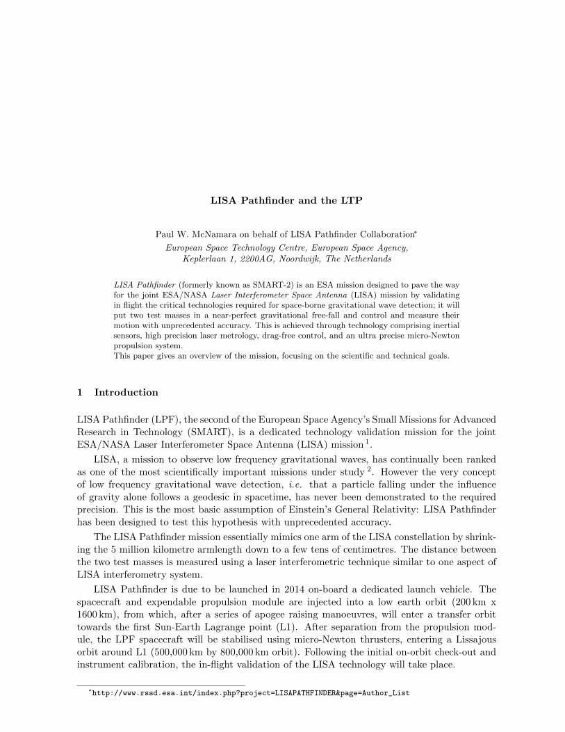
LISA Pathfinder and the LTP
Paul W. McNamara on behalf of LISA Pathfinder Collaboration∗
European Space Technology Centre, European Space Agency,Keplerlaan 1, 2200AG, Noordwijk, The Netherlands
LISA Pathfinder (formerly known as SMART-2) is an ESA mission designed to pave the wayfor the joint ESA/NASA Laser Interferometer Space Antenna (LISA) mission by validatingin flight the critical technologies required for space-borne gravitational wave detection; it willput two test masses in a near-perfect gravitational free-fall and control and measure theirmotion with unprecedented accuracy. This is achieved through technology comprising inertialsensors, high precision laser metrology, drag-free control, and an ultra precise micro-Newtonpropulsion system.This paper gives an overview of the mission, focusing on the scientific and technical goals.
1 Introduction
LISA Pathfinder (LPF), the second of the European Space Agency’s Small Missions for AdvancedResearch in Technology (SMART), is a dedicated technology validation mission for the jointESA/NASA Laser Interferometer Space Antenna (LISA) mission 1.
LISA, a mission to observe low frequency gravitational waves, has continually been rankedas one of the most scientifically important missions under study 2. However the very conceptof low frequency gravitational wave detection, i.e. that a particle falling under the influenceof gravity alone follows a geodesic in spacetime, has never been demonstrated to the requiredprecision. This is the most basic assumption of Einstein’s General Relativity: LISA Pathfinderhas been designed to test this hypothesis with unprecedented accuracy.
The LISA Pathfinder mission essentially mimics one arm of the LISA constellation by shrink-ing the 5 million kilometre armlength down to a few tens of centimetres. The distance betweenthe two test masses is measured using a laser interferometric technique similar to one aspect ofLISA interferometry system.
LISA Pathfinder is due to be launched in 2014 on-board a dedicated launch vehicle. Thespacecraft and expendable propulsion module are injected into a low earth orbit (200 km x1600 km), from which, after a series of apogee raising manoeuvres, will enter a transfer orbittowards the first Sun-Earth Lagrange point (L1). After separation from the propulsion mod-ule, the LPF spacecraft will be stabilised using micro-Newton thrusters, entering a Lissajousorbit around L1 (500,000 km by 800,000 km orbit). Following the initial on-orbit check-out andinstrument calibration, the in-flight validation of the LISA technology will take place.
∗http://www.rssd.esa.int/index.php?project=LISAPATHFINDER&page=Author_List
2 LISA Pathfinder Mission Concept
LISA Pathfinder will test in a space experiment that free falling bodies do follow geodesics inspacetime by more than two orders of magnitude better than any past, present, or plannedmission (with the exception of LISA itself). The concept that a particle falling under theinfluence of gravity alone follows a geodesic in space-time is at the very foundation of GeneralRelativity (GR).
In GR, gravity is not considered as an external force: instead gravity is the source of space-time curvature. Therefore, in a universe devolved of mass (a flat spacetime) free-falling testmasses will move in straight lines with uniform velocity (Newton’s 1st Law). In the real (asdescribed by General Relativity) Universe, the presence of mass, hence gravity/curvature, mod-ifies Newton’s 1st Law to state that in the absence of any external force, test masses move alonggeodesics.
All experiments aimed at directly measuring curvature caused by celestial bodies, or to testsubtle effects of GR, e.g., frame-dragging, detection of gravitational waves, or to probe its veryfoundation - the Equivalence Principle, invariably search for violation of geodesic motion.
The difficulty of achieving high purity geodesic motion is that any parasitic forces competewith spacetime geometry to set masses into motion, perturbing them away from their geodesiclines. As gravity is by far the weakest of all fundamental interactions, achieving the requiredextremely low level of non-gravitational acceleration requires the understanding, reduction andcontrol of the disturbances produced by a wide range of physical phenomena.
LISA Pathfinder’s experiment concept is to improve the uncertainty in the proof of geodesicmotion. This is achieved by tracking, using pico-meter resolution laser interferometry, two test-masses nominally in free-fall, and by showing that their relative parasitic acceleration, at fre-quencies around 1 mHz, is at least two orders of magnitude smaller than anything demonstratedor planned so far. The LISA Pathfinder spacecraft as an inertial platform, free of spurious accel-erations, will be the best laboratory ever created for Fundamental Physics experiments, wherethe conditions hypothesised by Einstein will be realised in the real world.
LISA Pathfinder is both a mission in General Relativity and in Precision Metrology, pushingthese disciplines several orders of magnitude beyond their current state of the art. In doing soit opens new ground for an entire class of new missions in General Relativity, in FundamentalPhysics at large, and in Earth Observation. The high resolution optical readout of test-massmotion allows test-mass to test-mass tracking even when they are located in different spacecraft,at large distance and in interplanetary space, e.g. LISA, or at short distance in low Earth orbit,like in future geodesy missions.
It must be stated that the true objective of LISA Pathfinder is not to develop hardware, butto confirm the overall physical model of the forces that act on a test mass in interplanetary space.To fulfill this program, the mission is not going to just make a measurement of acceleration butwill implement a full menu of measurements: at the end of this set of measurements, the residualacceleration noise model will be verified down to painstaking detail.
3 Mission Goals
The mission goals of LISA Pathfinder can be split into three categories, covering the performanceof the inertial sensor, the performance of the laser interferometer, and the demonstration of theflight readiness of the technologies critical for a successful LISA mission. The mission goals canbe summarised as follows (for a full description of the mission goals, the reader is directed to 3):
• demonstrate that a test mass can be put in a pure gravitational free-fall within approximatelyone order of magnitude of the LISA requirement. The one order of magnitude applies also
to the measurement bandwidth. Therefore, the differential acceleration noise requirementof LISA Pathfinder is stated quantitively as:
∆a ≤ 3× 10⁻¹⁴
[1 +
(f
3 mHz
)2]
ms−2/√
Hz (1)
over the frequency bandwidth, f , of 1 - 30 mHz. This is the top-level science requirementof the mission.
• demonstrate laser interferometry with free-falling mirrors (test masses of the LISA TechnologyPackage) with a displacement sensitivity equal to the LISA requirements. Therefore, theflight test is considered successful if the laser metrology resolution is demonstrated towithin:
∆x ≤ 9× 10⁻¹²
[1 +
(3 mHz
f
)2]
m/√
Hz (2)
over a frequency bandwidth of 1 - 30 mHz with a dynamic range on the order of one mil-limetre.
• assess the lifetime and reliability of the micro-Newton thrusters, lasers and optics in a spaceenvironment.
4 The LISA Technology Package
Unlike traditional observatory or planetary missions, the payload in LISA Pathfinder cannotbe considered as a discrete piece of hardware carried by the spacecraft. Instead, during scienceoperations, the payload and the spacecraft act as a single unit: the attitude control of the space-craft is driven by the payload. LISA Pathfinder will carry two payloads; the LISA TechnologyPackage (LTP), and the Disturbance Reduction System (DRS). The LISA Technology Packageis provided by a consortium of European national space agencies (France, Germany, Italy, Spain,Switzerland, The Netherlands, and the United Kingdom) and ESA, while the DRS is providedby NASA. Only the LTP will be described here.
The LTP consists of two major subsystems; the Inertial Sensor Subsystem, and the OpticalMetrology Subsystem. Both subsystems are described in further detail in the following sections.
4.1 Inertial Sensor Subsystem
The Inertial Sensor Subsystem (ISS) is at the heart of the LISA Pathfinder mission; the devel-opment and on-orbit testing of this subsystem are the main reasons for ESA implementing themission. The ISS of LISA Pathfinder is the ISS of LISA - the relaxation in the requirementsof LPF comes from the relaxation in the environmental conditions of the LPF spacecraft ascompared to LISA.
The inertial sensor subsystem comprises the test masses and all systems interacting directlywith the test masses, i.e. the electrode housing, front-end electronics, vacuum system, chargemanagement, and caging mechanism. This section will describe each of these subsystems inturn.
The test masses consist of a 1.96 kg cube of Gold:Platinum mono-phasic alloy of dimension46 mm on a side. The alloy is formed from 73% gold and 27% platinum, chosen as this alloy hasan extremely low magnetic susceptibility (χm ≈ 10−5) and high density ≈ 2× 10⁴ kgm−3. Thecombination of both greatly reduces the effect of external forces on the test mass.
The test masses’ position is readout by two means: high resolution laser interferometry,and electrostatic (capacitive) sensing. The former only senses the test mass position along the
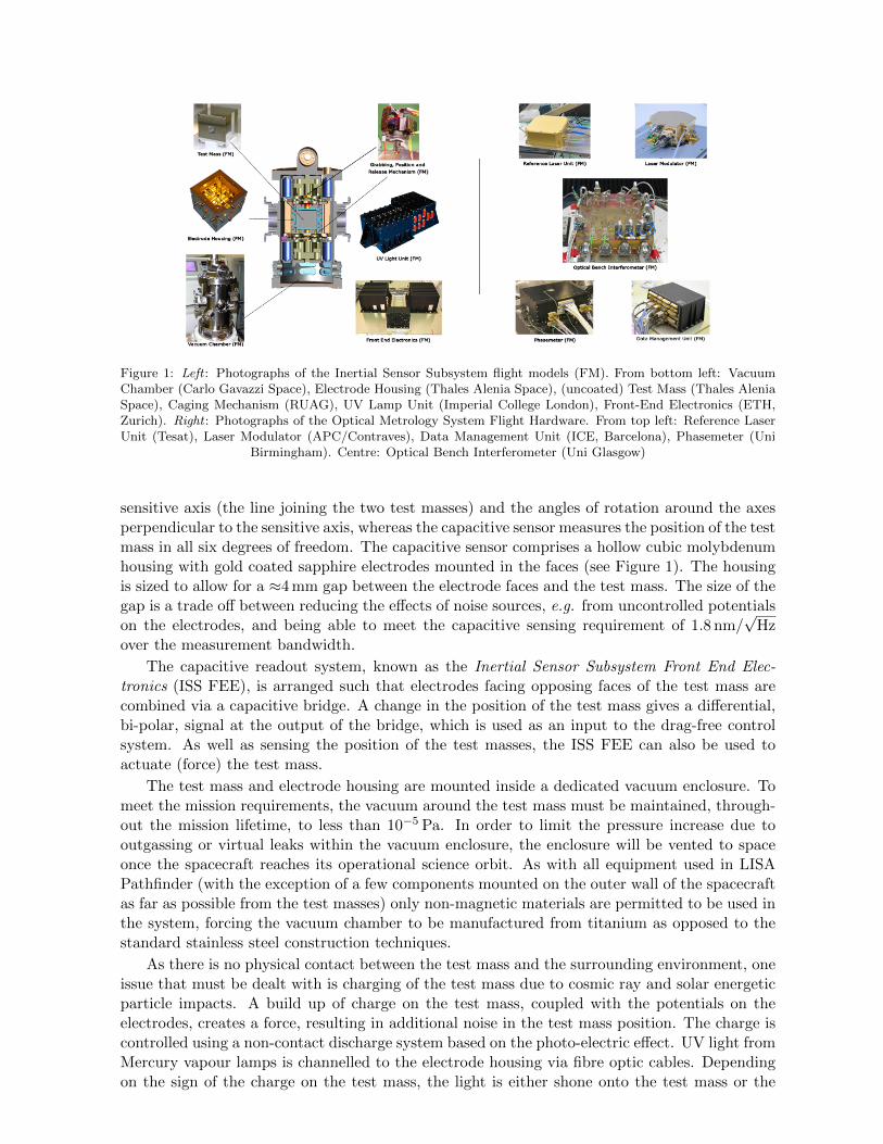
Figure 1: Left : Photographs of the Inertial Sensor Subsystem flight models (FM). From bottom left: VacuumChamber (Carlo Gavazzi Space), Electrode Housing (Thales Alenia Space), (uncoated) Test Mass (Thales AleniaSpace), Caging Mechanism (RUAG), UV Lamp Unit (Imperial College London), Front-End Electronics (ETH,Zurich). Right : Photographs of the Optical Metrology System Flight Hardware. From top left: Reference LaserUnit (Tesat), Laser Modulator (APC/Contraves), Data Management Unit (ICE, Barcelona), Phasemeter (Uni
Birmingham). Centre: Optical Bench Interferometer (Uni Glasgow)
sensitive axis (the line joining the two test masses) and the angles of rotation around the axesperpendicular to the sensitive axis, whereas the capacitive sensor measures the position of the testmass in all six degrees of freedom. The capacitive sensor comprises a hollow cubic molybdenumhousing with gold coated sapphire electrodes mounted in the faces (see Figure 1). The housingis sized to allow for a ≈4 mm gap between the electrode faces and the test mass. The size of thegap is a trade off between reducing the effects of noise sources, e.g. from uncontrolled potentialson the electrodes, and being able to meet the capacitive sensing requirement of 1.8 nm/
√Hz
over the measurement bandwidth.
The capacitive readout system, known as the Inertial Sensor Subsystem Front End Elec-tronics (ISS FEE), is arranged such that electrodes facing opposing faces of the test mass arecombined via a capacitive bridge. A change in the position of the test mass gives a differential,bi-polar, signal at the output of the bridge, which is used as an input to the drag-free controlsystem. As well as sensing the position of the test masses, the ISS FEE can also be used toactuate (force) the test mass.
The test mass and electrode housing are mounted inside a dedicated vacuum enclosure. Tomeet the mission requirements, the vacuum around the test mass must be maintained, through-out the mission lifetime, to less than 10−5 Pa. In order to limit the pressure increase due tooutgassing or virtual leaks within the vacuum enclosure, the enclosure will be vented to spaceonce the spacecraft reaches its operational science orbit. As with all equipment used in LISAPathfinder (with the exception of a few components mounted on the outer wall of the spacecraftas far as possible from the test masses) only non-magnetic materials are permitted to be used inthe system, forcing the vacuum chamber to be manufactured from titanium as opposed to thestandard stainless steel construction techniques.
As there is no physical contact between the test mass and the surrounding environment, oneissue that must be dealt with is charging of the test mass due to cosmic ray and solar energeticparticle impacts. A build up of charge on the test mass, coupled with the potentials on theelectrodes, creates a force, resulting in additional noise in the test mass position. The charge iscontrolled using a non-contact discharge system based on the photo-electric effect. UV light fromMercury vapour lamps is channelled to the electrode housing via fibre optic cables. Dependingon the sign of the charge on the test mass, the light is either shone onto the test mass or the
electrode housing, thereby extracting electrons from either surface, providing bi-polar chargemanagement.
A further challenge which is unique to space flight hardware is the need for a launch-lockdevice to prevent hardware being damaged during the extreme vibration conditions experiencedduring launch. In LISA Pathfinder, this is especially true for the test masses - the most sensitivepart of the experiment must survive a random load of ≈ 50 grms, requiring a holding force of≈1200 N, while not damaging the gold coated surface of the cube. In addition to the launch loadrequirement, when on-orbit, the device must release the test mass within an error box of 200µm,with a velocity of less than 5µms−1. These requirements are met by the Caging MechanismAssembly. This device consists of three actuators: a first stage launch lock mechanism providingthe 1200 N preload; a second stage positioning actuator, which is used to break the adhesionof the launch lock and position the test mass to the desired location; and finally, the releaseactuator, a small diameter pin which is used to break the adhesion of the positioning plungerand release the mass with the required accuracy.
Several other challenges must also be solved in order to meet the requirements of the LTP.These include: balancing of the differential gravitational force and gradient at the test masspositions - achieved by mounting compensation masses inside, and external to, the vacuumenclosure; creating a thermally quiet environment around the test mass - a temperature sta-bility of 10−5 K/
√Hz over the measurement bandwidth; associated with the thermal stability
requirement is the need to have thermometers with a resolution better than 10−5 K/√
Hz; andas mentioned earlier, no magnetic materials can be used - this makes the design of several of thesubsystem units especially difficult (e.g. vacuum chamber, mounting brackets, bolts, etc).
4.2 Optical Metrology Subsystem
The Optical Metrology Subsystem (OMS) is the high resolution laser interferometric readoutof the test masses’ positions. The OMS comprises several subsystems, namely; the referencelaser unit, the laser modulator, the optical bench interferometer, the phasemeter, and the datamanagement unit (Figure 1).
The Reference Laser Unit (RLU) comprises a 40 mW Nd:YAG non-planar ring oscillator4 ofthe same design commonly used in metrology labs around the world. This laser design is idealfor space applications due to its small size, high electrical to optical efficiency and inherent lownoise operation. The challenges for space applications come from the need for a robust designwhich can survive both the launch loads and thermal environment, as well as having a sufficientlifetime to guarantee the life of the mission. All of these challenges have been overcome andsimilar lasers are now flying in space on optical communication satellites5. The RLU is baselinedas the master oscillator in the LISA laser system.
The RLU output is fibre coupled using single-mode, polarisation-maintaining (sm/pm) fibre.The fibre couples the light to the subsequent component in the optical chain, the Laser Modulator(LM). The LM consists of a beam splitter, two acousto-optic modulators, and optical pathlengthactuators. The light from the laser is split into two paths, each path is passed through anacousto-optic modulator. One modulator is driven at 80 MHz, while the other is driven at80 MHz + 1.2 kHz, thereby creating two beams with a frequency difference of 1.2 kHz. Thebeams are then passed through the optical pathlength difference (OPD) actuator which consistsof a fibre optic cable wrapped around a cylindrical piezo-electric transducer. The OPD is usedto stabilise the optical pathlength of the fibre optic cables leading to the optical bench. After theOPD, the beams are transmitted, again via sm/pm fibre, to the Optical Bench Interferometer(OBI).
The main function of the OBI is to direct the beams to the relevant positions in 3-dimensionalspace, without adding any significant noise to the measurement path. The primary optical bench
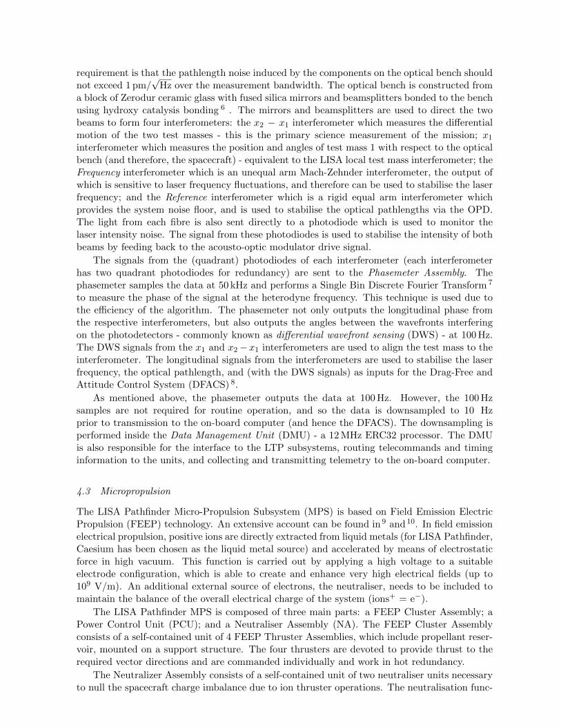
requirement is that the pathlength noise induced by the components on the optical bench shouldnot exceed 1 pm/
√Hz over the measurement bandwidth. The optical bench is constructed from
a block of Zerodur ceramic glass with fused silica mirrors and beamsplitters bonded to the benchusing hydroxy catalysis bonding 6 . The mirrors and beamsplitters are used to direct the twobeams to form four interferometers: the x2 − x1 interferometer which measures the differentialmotion of the two test masses - this is the primary science measurement of the mission; x1interferometer which measures the position and angles of test mass 1 with respect to the opticalbench (and therefore, the spacecraft) - equivalent to the LISA local test mass interferometer; theFrequency interferometer which is an unequal arm Mach-Zehnder interferometer, the output ofwhich is sensitive to laser frequency fluctuations, and therefore can be used to stabilise the laserfrequency; and the Reference interferometer which is a rigid equal arm interferometer whichprovides the system noise floor, and is used to stabilise the optical pathlengths via the OPD.The light from each fibre is also sent directly to a photodiode which is used to monitor thelaser intensity noise. The signal from these photodiodes is used to stabilise the intensity of bothbeams by feeding back to the acousto-optic modulator drive signal.
The signals from the (quadrant) photodiodes of each interferometer (each interferometerhas two quadrant photodiodes for redundancy) are sent to the Phasemeter Assembly. Thephasemeter samples the data at 50 kHz and performs a Single Bin Discrete Fourier Transform 7
to measure the phase of the signal at the heterodyne frequency. This technique is used due tothe efficiency of the algorithm. The phasemeter not only outputs the longitudinal phase fromthe respective interferometers, but also outputs the angles between the wavefronts interferingon the photodetectors - commonly known as differential wavefront sensing (DWS) - at 100 Hz.The DWS signals from the x1 and x2−x1 interferometers are used to align the test mass to theinterferometer. The longitudinal signals from the interferometers are used to stabilise the laserfrequency, the optical pathlength, and (with the DWS signals) as inputs for the Drag-Free andAttitude Control System (DFACS) 8.
As mentioned above, the phasemeter outputs the data at 100 Hz. However, the 100 Hzsamples are not required for routine operation, and so the data is downsampled to 10 Hzprior to transmission to the on-board computer (and hence the DFACS). The downsampling isperformed inside the Data Management Unit (DMU) - a 12 MHz ERC32 processor. The DMUis also responsible for the interface to the LTP subsystems, routing telecommands and timinginformation to the units, and collecting and transmitting telemetry to the on-board computer.
4.3 Micropropulsion
The LISA Pathfinder Micro-Propulsion Subsystem (MPS) is based on Field Emission ElectricPropulsion (FEEP) technology. An extensive account can be found in 9 and 10. In field emissionelectrical propulsion, positive ions are directly extracted from liquid metals (for LISA Pathfinder,Caesium has been chosen as the liquid metal source) and accelerated by means of electrostaticforce in high vacuum. This function is carried out by applying a high voltage to a suitableelectrode configuration, which is able to create and enhance very high electrical fields (up to109 V/m). An additional external source of electrons, the neutraliser, needs to be included tomaintain the balance of the overall electrical charge of the system (ions+ = e−).
The LISA Pathfinder MPS is composed of three main parts: a FEEP Cluster Assembly; aPower Control Unit (PCU); and a Neutraliser Assembly (NA). The FEEP Cluster Assemblyconsists of a self-contained unit of 4 FEEP Thruster Assemblies, which include propellant reser-voir, mounted on a support structure. The four thrusters are devoted to provide thrust to therequired vector directions and are commanded individually and work in hot redundancy.
The Neutralizer Assembly consists of a self-contained unit of two neutraliser units necessaryto null the spacecraft charge imbalance due to ion thruster operations. The neutralisation func-
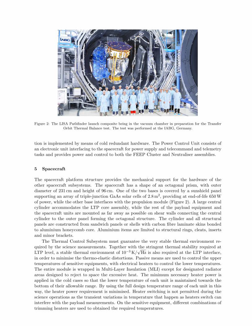
Figure 2: The LISA Pathfinder launch composite being in the vacuum chamber in preparation for the TransferOrbit Thermal Balance test. The test was performed at the IABG, Germany.
tion is implemented by means of cold redundant hardware. The Power Control Unit consists ofan electronic unit interfacing to the spacecraft for power supply and telecommand and telemetrytasks and provides power and control to both the FEEP Cluster and Neutraliser assemblies.
5 Spacecraft
The spacecraft platform structure provides the mechanical support for the hardware of theother spacecraft subsystems. The spacecraft has a shape of an octagonal prism, with outerdiameter of 231 cm and height of 96 cm. One of the two bases is covered by a sunshield panelsupporting an array of triple-junction GaAs solar cells of 2.8 m2, providing at end-of-life 650 Wof power, while the other base interfaces with the propulsion module (Figure 2). A large centralcylinder accommodates the LTP core assembly, while the rest of the payload equipment andthe spacecraft units are mounted as far away as possible on shear walls connecting the centralcylinder to the outer panel forming the octagonal structure. The cylinder and all structuralpanels are constructed from sandwich panels or shells with carbon fibre laminate skins bondedto aluminium honeycomb core. Aluminium items are limited to structural rings, cleats, insertsand minor brackets.
The Thermal Control Subsystem must guarantee the very stable thermal environment re-quired by the science measurements. Together with the stringent thermal stability required atLTP level, a stable thermal environment of 10−3 K/
√Hz is also required at the LTP interface,
in order to minimise the thermo-elastic distortions. Passive means are used to control the uppertemperatures of sensitive equipments, with electrical heaters to control the lower temperatures.The entire module is wrapped in Multi-Layer Insulation (MLI) except for designated radiatorareas designed to reject to space the excessive heat. The minimum necessary heater power isapplied in the cold cases so that the lower temperature of each unit is maintained towards thebottom of their allowable range. By using the full design temperature range of each unit in thisway, the heater power requirement is minimised. Heater switching is not permitted during thescience operations as the transient variations in temperature that happen as heaters switch caninterfere with the payload measurements. On the sensitive equipment, different combinations oftrimming heaters are used to obtained the required temperatures.
6 Conclusions
Throughout the history of the LISA mission, the science return has never been in doubt - LISAwill observe the Universe in a way which has never been possible before. This has captured theimagination of the science community, but at the same time has cast doubt on the probabilitythat such a mission can be realised. Together, this prompted the European Space Agency toadopt the LISA Pathfinder mission - the science return of LISA easily justifies the technologydevelopment mission.
The final return of LISA Pathfinder is not only related to the development of the criticaltechnologies for LISA - in the process of implementing the mission, the industrial experiencerequired to build a mission like LPF (and LISA) has also been acquired, as has the knowledgeof the ground segment required by a LISA-like mission.
In conclusion, LISA Pathfinder is on track to demonstrate the first in-flight test of lowfrequency gravitational wave detection metrology. Launch is scheduled for 2014, with firstresults available to the science community approximately three months thereafter.
Acknowledgments
The authors would like to thank the entire LISA Pathfinder team for their continued work inmaking the mission possible. The LISA Pathfinder mission is funded through the EuropeanSpace Agency, while the LTP is funded by ESA, France, Germany, Italy, The Netherlands,Spain, Switzerland, and the United Kingdom.
References
1. Jennrich, O., et al., LISA - Unveiling a hidden Universe, ESA/SRE(2011)3 unpublished(2011)
2. National Academy of Sciences, New Worlds, New Horizons in Astronomy and Astro-physics, Report of the National Research Council’s Decadal survey of Astronomy andAstrophysics (2010)
3. Vitale, S., et al., Science Requirements and Top-Level Architecture Definition for the LISATechnology Package (LTP) on board LISA Pathfinder (SMART-2), ESA Ref: LTPA-UTN-ScRD-Iss3-Rev1 (2005)
4. Kane, T.J., and Byer, R.L., Monolithic, unidirectional single-mode Nd:YAG ring laser,Optics Letters, 10, 2, 65-67 (1985)
5. Lange, R, et al., BPSK Laser communication terminals to be verified in space, MILCOM2004 - IEEE Military Communications Conference (2004)
6. Middleton, K., et al.,Prototype optical bench instrument in the interferometer for the LISA-Pathfinder space mission, Optical Engineering, 45 (2006)
7. Heinzel, G, et al., Interferometry for the LISA Technology Package, LTP: an update,Journal of Physics Conference Series, 32, 132 (2006)
8. Fichter, W., et al., Drag-Free Control Design with Cubic Test Masses, In ”Lasers, Clocks,and Drag-Free Control”, Astrophysics and Space Science Library, Vol. 349, Dittus, H.J.;Lammerzahl, C.;Turyshev, S. (Eds.), December 2007, Springer, ISBN: 978-3-540-34376-9
9. Nicolini, D., LISA Pathfinder Field Emission Thruster System Development Program, 30th
International Electric Propulsion Conference, IEPC-2007-363, Florence, (2007)10. Ceruti, L., and Nicolini, D., Power Processing Control Units for FEEP Micro-Propulsion
Subsystems, International Astronautic Congress, Glasgow, (2008)
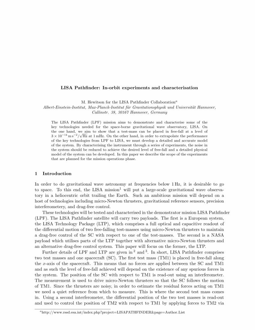
LISA Pathfinder: In-orbit experiments and characterisation
M. Hewitson for the LISA Pathfinder Collaborationa
Albert-Einstein-Institut, Max-Planck-Institut fur Gravitationsphysik und Universitat Hannover,Callinstr. 38, 30167 Hannover, Germany
The LISA Pathfinder (LPF) mission aims to demonstrate and characterise some of thekey technologies needed for the space-borne gravitational wave observatory, LISA. Onthe one hand, we aim to show that a test-mass can be placed in free-fall at a level of3× 10−14 m s−2/
√Hz at 1 mHz. On the other hand, in order to extrapolate the performance
of the key technologies from LPF to LISA, we must develop a detailed and accurate modelof the system. By characterising the instrument through a series of experiments, the noise inthe system should be reduced to achieve the desired level of free-fall and a detailed physicalmodel of the system can be developed. In this paper we describe the scope of the experimentsthat are planned for the mission operations phase.
1 Introduction
In order to do gravitational wave astronomy at frequencies below 1 Hz, it is desirable to goto space. To this end, the LISA mission1 will put a large-scale gravitational wave observa-tory in a heliocentric orbit trailing the Earth. Such an ambitious mission will depend on ahost of technologies including micro-Newton thrusters, gravitational reference sensors, precisioninterferometery, and drag-free control.
These technologies will be tested and characterised in the demonstrator mission LISA Pathfinder(LPF). The LISA Pathfinder satellite will carry two payloads. The first is a European system,the LISA Technology Package (LTP), which comprises a full optical and capacitive readout ofthe differential motion of two free-falling test-masses using micro-Newton thrusters to maintaina drag-free control of the SC with respect to one of the test-masses. The second is a NASApayload which utilises parts of the LTP together with alternative micro-Newton thrusters andan alternative drag-free control system. This paper will focus on the former, the LTP.
Further details of LPF and LTP are given in 2 and 3. In short, LISA Pathfinder comprisestwo test masses and one spacecraft (SC). The first test mass (TM1) is placed in free-fall alongthe x-axis of the spacecraft. This means that no forces are applied between the SC and TM1and as such the level of free-fall achieved will depend on the existence of any spurious forces inthe system. The position of the SC with respect to TM1 is read-out using an interferometer.The measurement is used to drive micro-Newton thrusters so that the SC follows the motionof TM1. Since the thrusters are noisy, in order to estimate the residual forces acting on TM1we need a quiet reference from which to measure. This is where the second test mass comesin. Using a second interferometer, the differential position of the two test masses is read-outand used to control the position of TM2 with respect to TM1 by applying forces to TM2 via
ahttp://www.rssd.esa.int/index.php?project=LISAPATHFINDER&page=Author List
an electrostatic actuator. The bandwidth of this so-called suspension control is 1 mHz and thedrag-free control has a band-width of around 100 mHz. A schematic of this control system isshown in Figure 1.
drag-freetest-mass
Hdf
Hsus
o1
o12
TM1 TM2
x-axis
Fibre injectors
Figure 1: A schematic of the two x-axis control loops on LPF. The SC surrounds two test masses. The first testmass is in free fall and the SC is made to follow it by using the interferometric readout shown to control the forceapplied to SC by the thrusters. The second test mass is electrostatically suspended and made to follow TM1
using the differential interferometer measurement.
2 Characterisation of LPF
Characterisation of LPF has two aims. The first is to optimise the system so that the quietestpossible free-fall of TM1 can be achieved. The second is to develop a detailed physical modelof the system so that the performance of the different subsystems can be extrapolated to givean expected performance for LISA. Both of these aims require various physical parametersof the system to be estimated. For example, the precise behaviour of x-axis control loopsdescribed above will depend critically on any residual couplings in the system, such as thespring-like stiffness couplings between the TMs and the SC arising from the voltages appliedin the electrostatic actuation scheme and imperfections in the gravitational balancing of thespacecraft as a whole. Such couplings, as well as actuator gains and system delays will need tobe measured through a series of experiments. The typical way to identify such system parametersis to stimulate the system in such a way that the observed response depends on the parameter(s)of interest.
Measuring physical parameters of the system is only the first step in building a noise modelof the entire system. Two other components are needed to complete the picture: estimates ormodels of any noise sources which may couple to the sensitive differential position measurement,and models or measurements of the transfer functions that describe the coupling of these noisesources to the observations. For some sources of noise we have various environmental and systemmonitors which will provide a wealth of data. For other noise sources, we will need to rely onground measurements and/or models. The various couplings of the system will need to bemodelled. Typically these models will be parametric and the determination of the parametervalues will be done through dedicated experiments. In this way we aim to build up a full noisemodel of the system which should, when complete, explain the observed level of differentialacceleration of the two TMs.
Clearly, the process of optimising the system to achieve the purest free-fall and of developingthe physical model are fully entwined. The system model can be used to develop a noise budgetfor the differential measurement which in turn will identify the limiting noise sources whichare disturbing the free-fall. Once identified, these noise sources have to be mitigated, either bysuppressing the noise source (through optimisation of the responsible subsystem), or by reducing
the coupling to the differential test mass motion. The design of the various experiments thatwill be carried out during the mission operations phase is critical to the success of this plan.As each experiment is performed, the data must be retrieved and analysed so that subsequentexperiments can be optimised and performed in the optimal order.
3 Data flow and data analysis
As mentioned above, data from each experiment will be analysed as soon as it becomes available.It is expected that we will have contact with the SC for a few hours each day. As such, theexperiments will be carried out in an automated fashion and the data for the experimentscarried out on day N will be retrieved on day N + 1. The analysis of the data for day N mustbe completed before the end of day N + 1 so that the turn-around time for reconfiguring themission time-line (and as such, the up-coming experiments) can be minimised.
In order to allow the mission scientists to analyse the data coming from the experiments, arobust and flexible data analysis infrastructure (The LISA Technology Package Data AnalysisToolbox) has been developed4. As well as providing a wealth of standard data analysis tools ex-pected to be required for instrument characterisation, the toolbox will also contain LTP-specifichigh-level routines and algorithms to allow routine data analysis tasks common to multiple ex-periments to be performed in an efficient way. In addition, the data analysis procedures forall planned experiments will be developed and tested in advance under the LTPDA framework.One of the main features of this data analysis toolbox is the ability to inspect analysis resultsand to determine precisely what processing has been done to the original data. This is achievedusing an object-oriented system where the result of any particular analysis is an object whichcomprises, not only the numerical results, but also a full history tree of the steps taken to arriveat that result. The reason for implementing such a scheme is to ensure that the results obtainedduring LPF can still be understood and reconstructed during the time of LISA, which will takeplace perhaps 1 decade after LPF.
4 System Identification and Modelling
Many of the experiments that will be carried out on LPF will be system identification experi-ments. Typically, by means of stimulating the system and observing the response, parameters ofa system model can be determined. If the models are sufficiently detailed, these parameters willusually be closely, if not directly, related to actual physical parameters of the system. Figure 2shows a schematic of a model of the x-axis dynamics of the system. Here we see the two controlloops described earlier in this paper. The parameters of the system are shown in red. They are:
S21 The cross-talk of the interferometer due to the imperfect common-mode rejection arisingfrom the geometry of the system. This parameter forms a coupling which allows the noiseof the drag-free loop (essentially the thruster noise) to leak in to the sensitive differen-tial measurement. This coupling is flat in frequency and its effect can be subtracted indata processing due to the fact that we have a very precise (pm resolution) measurementof the thruster noise via the first interferometer channel (o1). In order to subtract thecontribution, however, we need to determine/measure the coupling coefficient.
D1 and D2 The delay on the execution of commanded guidance signals on the drag-free andsuspension loops respectively. These arise from the finite processing power available on-board the satellite. Depending on what else the main computer is doing, the commandto start a signal injection may not be executed at exactly the requested time. As such wehave some uncertainty as to when any stimulus is applied, and this needs to be identifiedfor each experiment.
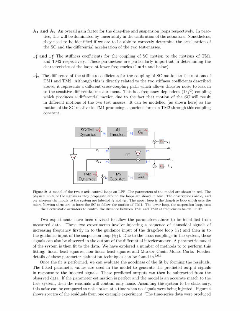
A1 and A2 An overall gain factor for the drag-free and suspension loops respectively. In prac-tice, this will be dominated by uncertainty in the calibration of the actuators. Nonetheless,they need to be identified if we are to be able to correctly determine the acceleration ofthe SC and the differential acceleration of the two test-masses.
ω21 and ω2
2 The stiffness coefficients for the coupling of SC motion to the motions of TM1and TM2 respectively. These parameters are particularly important in determining thecharacteristics of the loops at lower frequencies (1 mHz and below).
ω212 The difference of the stiffness coefficients for the coupling of SC motion to the motions of
TM1 and TM2. Although this is directly related to the two stiffness coefficients describedabove, it represents a different cross-coupling path which allows thruster noise to leak into the sensitive differential measurement. This is a frequency dependent (1/f2) couplingwhich produces a differential motion due to the fact that motion of the SC will resultin different motions of the two test masses. It can be modelled (as shown here) as themotion of the SC relative to TM1 producing a spurious force on TM2 through this couplingconstant.
Figure 2: A model of the two x-axis control loops on LPF. The parameters of the model are shown in red. Thephysical units of the signals as they propagate around the loops are shown in blue. The observations are o1 ando12 whereas the inputs to the system are labelled i1 and i12. The upper loop is the drag-free loop which uses themicro-Newton thrusters to force the SC to follow the motion of TM1. The lower loop, the suspension loop, uses
the electrostatic actuators to control the distance between TM1 and TM2 at frequencies below 1 mHz.
Two experiments have been devised to allow the parameters above to be identified frommeasured data. These two experiments involve injecting a sequence of sinusoidal signals ofincreasing frequency firstly in to the guidance input of the drag-free loop (i1) and then in tothe guidance input of the suspension loop (i12). Due to the cross-couplings in the system, thesesignals can also be observed in the output of the differential interferometer. A parametric modelof the system is then fit to the data. We have explored a number of methods to to perform thisfitting: linear least-squares, non-linear least-squares and Markov Chain Monte Carlo. Furtherdetails of these parameter estimation techniques can be found in 5,6,4.
Once the fit is performed, we can evaluate the goodness of the fit by forming the residuals.The fitted parameter values are used in the model to generate the predicted output signalsin response to the injected signals. These predicted outputs can then be subtracted from theobserved data. If the parameter estimation is perfect and the model is an accurate match to thetrue system, then the residuals will contain only noise. Assuming the system to be stationary,this noise can be compared to noise taken at a time when no signals were being injected. Figure 4shows spectra of the residuals from one example experiment. The time-series data were produced
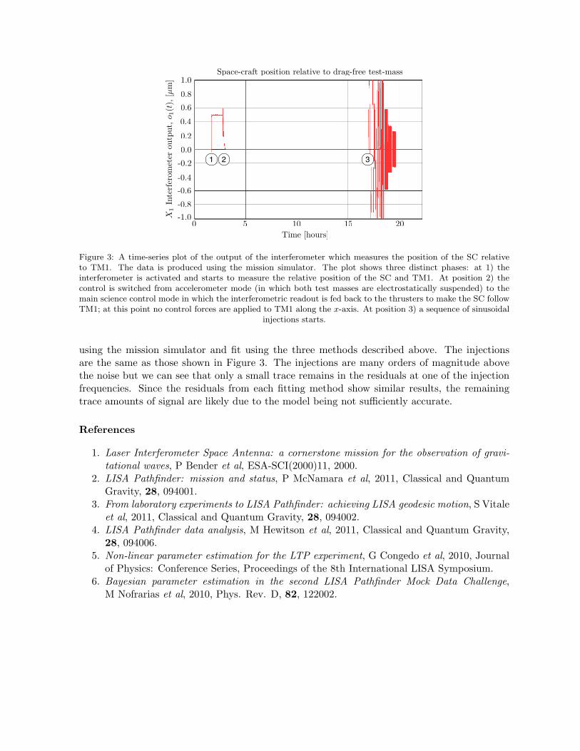
0 5 10 15 20-1.0
-0.8
-0.6
-0.2
-0.4
0.0
0.2
0.4
0.6
0.8
1.0
Time [hours]
X1
Inte
rfer
omet
erou
tput,
o1(t
),[µ
m]
Space-craft position relative to drag-free test-mass
1 2 3
Figure 3: A time-series plot of the output of the interferometer which measures the position of the SC relativeto TM1. The data is produced using the mission simulator. The plot shows three distinct phases: at 1) theinterferometer is activated and starts to measure the relative position of the SC and TM1. At position 2) thecontrol is switched from accelerometer mode (in which both test masses are electrostatically suspended) to themain science control mode in which the interferometric readout is fed back to the thrusters to make the SC followTM1; at this point no control forces are applied to TM1 along the x-axis. At position 3) a sequence of sinusoidal
injections starts.
using the mission simulator and fit using the three methods described above. The injectionsare the same as those shown in Figure 3. The injections are many orders of magnitude abovethe noise but we can see that only a small trace remains in the residuals at one of the injectionfrequencies. Since the residuals from each fitting method show similar results, the remainingtrace amounts of signal are likely due to the model being not sufficiently accurate.
References
1. Laser Interferometer Space Antenna: a cornerstone mission for the observation of gravi-tational waves, P Bender et al, ESA-SCI(2000)11, 2000.
2. LISA Pathfinder: mission and status, P McNamara et al, 2011, Classical and QuantumGravity, 28, 094001.
3. From laboratory experiments to LISA Pathfinder: achieving LISA geodesic motion, S Vitaleet al, 2011, Classical and Quantum Gravity, 28, 094002.
4. LISA Pathfinder data analysis, M Hewitson et al, 2011, Classical and Quantum Gravity,28, 094006.
5. Non-linear parameter estimation for the LTP experiment, G Congedo et al, 2010, Journalof Physics: Conference Series, Proceedings of the 8th International LISA Symposium.
6. Bayesian parameter estimation in the second LISA Pathfinder Mock Data Challenge,M Nofrarias et al, 2010, Phys. Rev. D, 82, 122002.
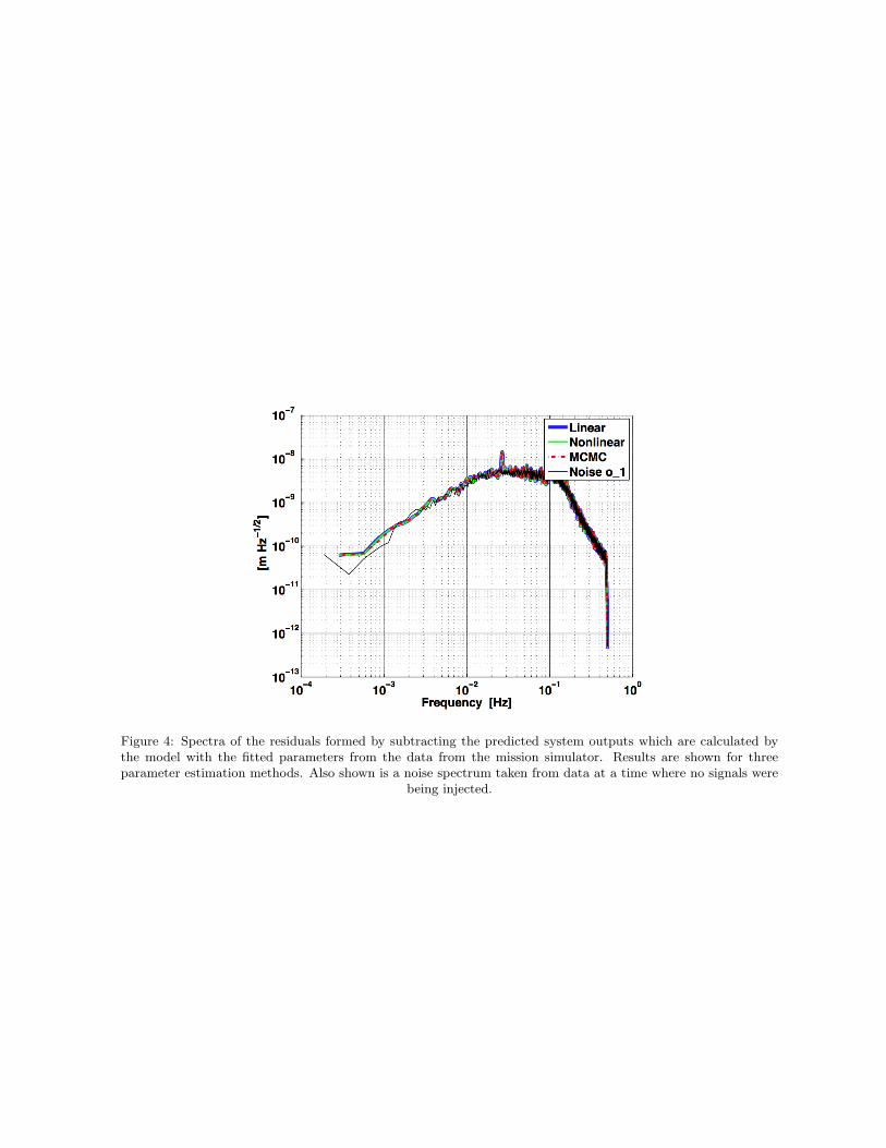
Figure 4: Spectra of the residuals formed by subtracting the predicted system outputs which are calculated bythe model with the fitted parameters from the data from the mission simulator. Results are shown for threeparameter estimation methods. Also shown is a noise spectrum taken from data at a time where no signals were
being injected.
LISA Pathfinder: an experimental analysis of the LPF free-fall performance
William J. Weber on behalf of the LISA Pathfinder Collaboration a
Dipartimento di Fisica and INFN, Universita di Trento,
Via Sommarive 14, 38123 Povo, Trento, Italy
The LISA gravitational wave observatory requires free-falling test masses that serve as refer-ences of geodesic motion to within a residual stray acceleration of 3 fm/s2 /
√
Hz at frequenciesabove 0.1 mHz. The LISA Pathfinder (LPF) mission is dedicated to demonstrating the tech-nology of free-falling test masses at a level close to the LISA goal. This article addresses theexperimentally-based performance analysis for the LPF measurement of differential test massacceleration noise, including a discussion of the applicability of the LPF results to the LISAmission.
1 Introduction
The primary science objective of the LISA Pathfinder (LPF) mission is demonstrating by directmeasurement that two geodesic reference test masses (TM) can be placed in perfect free-fall towithin a residual differential acceleration noise of 30 fm/s2 /
√Hz at frequencies down to 1 mHz1.
Using the same TM, gravitational sensor (GRS), and local interferometer metrology hardwareas for the proposed gravitational wave mission LISA, LPF is a testbed for most of the neededperformance aboard LISA, where the target sensitivity requires free-falling test masses at thelevel of 3 fm/s2 /
√Hz acceleration relative to an inertial system at 0.1 mHz.
In the main LPF acceleration noise measurement2, an optical interferometer measures therelative acceleration of two free-falling TM. One TM is used as a “drag-free” reference to controlthe translation and attitude of the satellite, and the other (TM2) is electrostatically forced tomaintain constant separation from the first TM. The measurement and subsequent analysis aredesigned to measure the stray forces acting on the TM in conditions as close as possible to thoserelevant to the LISA TM. The TM2 electrostatic suspension introduces additional force noise.This suspension is not needed for LISA – it is necessitated here by the LPF single spacecraftconfiguration – and as such the mission also foresees a dedicated free-fall “drift mode” test 3
where the electrostatic suspension is turned off for the sensitive X axis, to allow measurementof TM acceleration noise in the absence of electrostatic actuation, as is most relevant for LISA.
Preparation for LPF hinges on an analysis of all sources of TM acceleration noise and metrol-ogy noise, but also on an aggressive laboratory campaign for directly measuring the performancewith prototype flight hardware. This short paper summarizes the noise budget for the LPF mea-surement of stray TM acceleration, and its application to the performance for LISA. A detailedanalysis of the LISA Pathfinder noise performance and the experimental background for thepredictions for the various noise sources can be found in Ref. 4.
aFull author list available at http://www.rssd.esa.int/index.php?project=LISAPATHFINDER&page=Author List
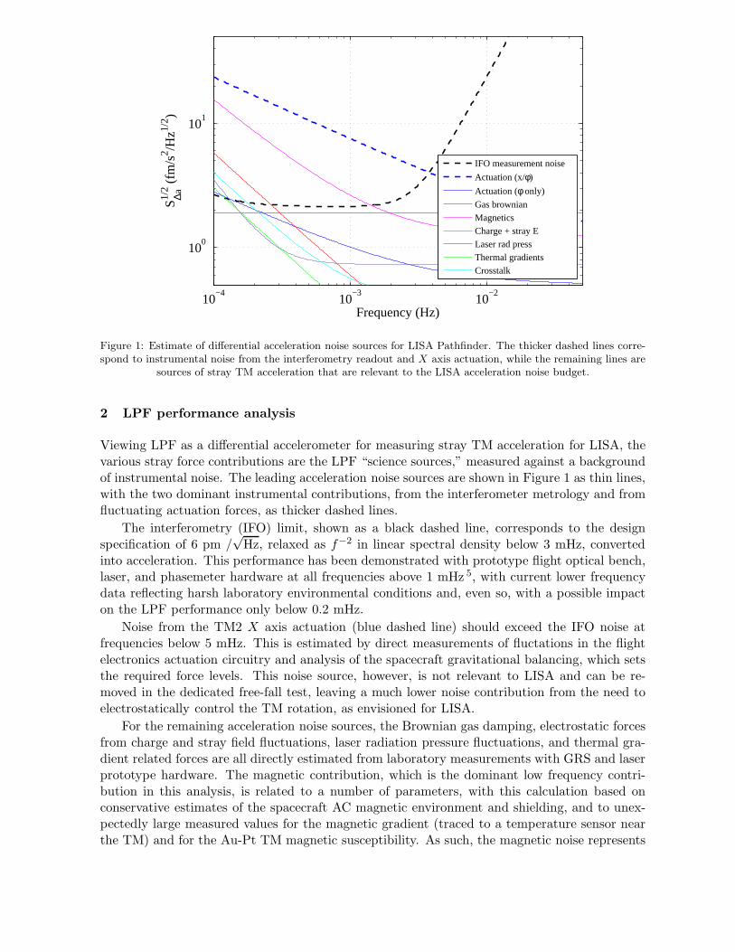
10−4
10−3
10−2
100
101
Frequency (Hz)
S ∆a1/2 (
fm/s
2 /Hz1/
2 )
IFO measurement noise
Actuation (x/φ)
Actuation (φ only)
Gas brownian
Magnetics
Charge + stray E
Laser rad press
Thermal gradients
Crosstalk
Figure 1: Estimate of differential acceleration noise sources for LISA Pathfinder. The thicker dashed lines corre-spond to instrumental noise from the interferometry readout and X axis actuation, while the remaining lines are
sources of stray TM acceleration that are relevant to the LISA acceleration noise budget.
2 LPF performance analysis
Viewing LPF as a differential accelerometer for measuring stray TM acceleration for LISA, thevarious stray force contributions are the LPF “science sources,” measured against a backgroundof instrumental noise. The leading acceleration noise sources are shown in Figure 1 as thin lines,with the two dominant instrumental contributions, from the interferometer metrology and fromfluctuating actuation forces, as thicker dashed lines.
The interferometry (IFO) limit, shown as a black dashed line, corresponds to the designspecification of 6 pm /
√Hz, relaxed as f−2 in linear spectral density below 3 mHz, converted
into acceleration. This performance has been demonstrated with prototype flight optical bench,laser, and phasemeter hardware at all frequencies above 1 mHz 5, with current lower frequencydata reflecting harsh laboratory environmental conditions and, even so, with a possible impacton the LPF performance only below 0.2 mHz.
Noise from the TM2 X axis actuation (blue dashed line) should exceed the IFO noise atfrequencies below 5 mHz. This is estimated by direct measurements of fluctations in the flightelectronics actuation circuitry and analysis of the spacecraft gravitational balancing, which setsthe required force levels. This noise source, however, is not relevant to LISA and can be re-moved in the dedicated free-fall test, leaving a much lower noise contribution from the need toelectrostatically control the TM rotation, as envisioned for LISA.
For the remaining acceleration noise sources, the Brownian gas damping, electrostatic forcesfrom charge and stray field fluctuations, laser radiation pressure fluctuations, and thermal gra-dient related forces are all directly estimated from laboratory measurements with GRS and laserprototype hardware. The magnetic contribution, which is the dominant low frequency contri-bution in this analysis, is related to a number of parameters, with this calculation based onconservative estimates of the spacecraft AC magnetic environment and shielding, and to unex-pectedly large measured values for the magnetic gradient (traced to a temperature sensor nearthe TM) and for the Au-Pt TM magnetic susceptibility. As such, the magnetic noise represents
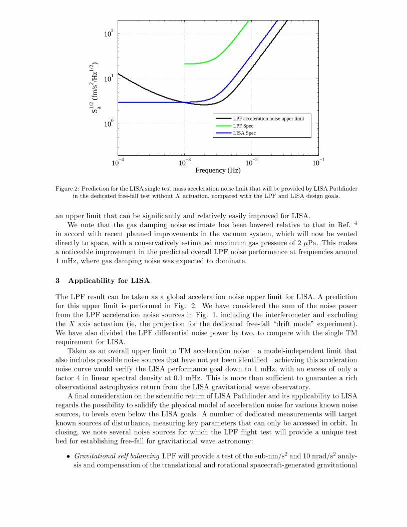
10−4
10−3
10−2
10−1
100
101
102
S a1/2 (
fm/s
2 /Hz1/
2 )
Frequency (Hz)
LPF acceleration noise upper limit
LPF Spec
LISA Spec
Figure 2: Prediction for the LISA single test mass acceleration noise limit that will be provided by LISA Pathfinderin the dedicated free-fall test without X actuation, compared with the LPF and LISA design goals.
an upper limit that can be significantly and relatively easily improved for LISA.We note that the gas damping noise estimate has been lowered relative to that in Ref. 4
in accord with recent planned improvements in the vacuum system, which will now be venteddirectly to space, with a conservatively estimated maximum gas pressure of 2 µPa. This makesa noticeable improvement in the predicted overall LPF noise performance at frequencies around1 mHz, where gas damping noise was expected to dominate.
3 Applicability for LISA
The LPF result can be taken as a global acceleration noise upper limit for LISA. A predictionfor this upper limit is performed in Fig. 2. We have considered the sum of the noise powerfrom the LPF acceleration noise sources in Fig. 1, including the interferometer and excludingthe X axis actuation (ie, the projection for the dedicated free-fall “drift mode” experiment).We have also divided the LPF differential noise power by two, to compare with the single TMrequirement for LISA.
Taken as an overall upper limit to TM acceleration noise – a model-independent limit thatalso includes possible noise sources that have not yet been identified – achieving this accelerationnoise curve would verify the LISA performance goal down to 1 mHz, with an excess of only afactor 4 in linear spectral density at 0.1 mHz. This is more than sufficient to guarantee a richobservational astrophysics return from the LISA gravitational wave observatory.
A final consideration on the scientific return of LISA Pathfinder and its applicability to LISAregards the possibility to solidify the physical model of acceleration noise for various known noisesources, to levels even below the LISA goals. A number of dedicated measurements will targetknown sources of disturbance, measuring key parameters that can only be accessed in orbit. Inclosing, we note several noise sources for which the LPF flight test will provide a unique testbed for establishing free-fall for gravitational wave astronomy:
• Gravitational self balancing LPF will provide a test of the sub-nm/s2 and 10 nrad/s2 analy-sis and compensation of the translational and rotational spacecraft-generated gravitational
accelerations that is required, to limit actuation-related noise, for both LPF and LISA.This information will be obtained from the DC levels of actuation needed in flight, forthree translational and six rotational degrees of freedom, and will be the first verificationof the detailed design and analysis of the LPF spacecraft self-gravity.
• Test mass charging and charge fluctuations LPF will measure TM charging from cosmicray and solar particles, both the deterministic charging and, in dedicated long term highprecision measurements, the low frequency stochastic fluctuations relevant for producinglow frequency force noise in the presence of a steady stray electrostatic field. Also, LPFwill test both the TM discharge system and techniques for measuring and compensatingstray fields.
• Spacecraft thermal environment With an array of thermometers, LPF will monitor thethermal environment around the TM at the 10 µK resolution6. In addition to use inpossible correlations with force noise – through the thermal gradient coupling with theradiometric, radiation pressure and outgassing effects – the measurements will allow a realverification of the thermal model for a LISA-like satellite across the LISA band. A similarcharacterization should be possible for the magnetic environment and fluctuations onboardthe satellite7.
References
1. M Armani et al, Class. Quantum Grav. 26, 094001 (2009).2. D Bortoluzzi et al, Class. Quantum Grav. 21, S573 (2004).3. A Grynagier et al, Class. Quantum Grav. 26, 094007 (2009).4. F Antonucci et al, Class. Quantum Grav. 28, 094002 (2011).5. F Antonucci et al, Class. Quantum Grav. 28, 094003 (2011).6. P Canizares et al, Class. Quantum Grav. 28, 094004 (2011).7. M Diaz-Aguilo, E Garcıa-Berro and A Lobo, Class. Quantum Grav. 27, 035005 (2010).
Search for GWs from white dwarf binaries in Mock LISA Data Challenge data
S. BabakAlbert Einstein Institute, Golm, Am Muchlenberg 1, D-14476 Golm bei Potsdam, Germany
A. B lautInstitute of Theoretical Physics, University of Wroc law, Pl.Maxa Borna 9, Pl-50-204 Wroc law, Poland
A. KrolakInstitute of Mathematics, Polish Academy of Sciences, Warsaw, Poland
Methods and results of the analysis of the simulated data of the proposed gravitational wavedetector LISA for the case of white dwarf binaries are presented. The simulated data areproduced by the Mock LISA Data Challenge project. Our method is based on maximumlikelihood method and uses the popular F-statistic that is applied in the analysis of groundgravitational wave detector data. We show that the LISA detector has the potential do identifyover ten thousand of white dwarf binary systems in our Galaxy.
1 Introduction
LISA is a laser interferometric detector of gravitational waves in the orbit around the Sun trailingthe Earth by 20 degrees. LISA was planned to be launched in the next decade as a joint ESAand NASA project. The bandwidth of the LISA detector is from 0.1 mHz to 100 mHz. In thisband LISA could observe gravitational radiation originating from compact white dwarf binaries,coalescence of massive black hole binaries, inspirals of stelar mass compact stars into massiveblack holes and gravitational wave stochastic background from the early Universe.
The Mock LISA Data Challenges (MLDC) were initiated by the LISA International ScienceTeam (LIST) at the end of 2005. A taskforce exists which decides on the severity of the challenge,the types and number of sources etc. and also conducts the analysis of entries at the end ofeach challenge. A challenge data set is regularly issued with a deadline ranging from six totwelve months. These challenges are open to everyone within the GW community, and allowthe community to simulate a realistic data analysis effort where the number of input sourcesand parameters are relatively unknown.
We shall present data analysis methods to detect signals and estimate parameters for whitedwarf binaries in MLDC data sets. This is a particularly challenging task because the numberof such signals so large that the signals interfere and the problem of signal resolution arises.
2 Gravitational waves from compact white dwarf binaries
In the LISA frequency band we expect around 6 × 10⁷ compact white dwarf binaries. Theexpected number of binaries below 3 mHz is so large that they are not individually resolvable(except for the brightest ones) and form a stochastic background which dominates over the
instrumental noise above 0.1 mHz. It is expected that above 3mHz all the statistically significantwhite dwarf binary signals are resolvable.
There are two major types of white dwarf binaries:(i) Detached, separated white-dwarf/white-dwarf binaries whose evolution is driven by radi-
ation reaction. They are the end points of many binary evolution scenarios. The gravitationalwave carry information about the mass of the binary and the distance.
(ii) Interacting binaries. Those are close systems with a significant tidal interaction and/orwith the Roche lobe overflow. In those systems the gravitational radiation reaction competesagainst mass transfer and the orbital period can either increase or decrease.
3 Detection gravitational waves signals from compact binaries and estimation oftheir parameters
The response of the LISA detector to a gravitational wave (GW) signal from a binary system isgiven by a linear combination of the four time-dependent functions h(k)(t).
s(t) =4∑
k=1
a(k)h(k)(t), (1)
where a(k) are 4 constant amplitudes. The functions h(k)(t) are periodic functions of gravitationalwave frequency ω with complicated amplitude and phase modulations3,5. The phase modulationfunction ϕ(t) is given by
ϕ(t) = ωt +1
2ωt2 + (ω + ωt)R cosβ cos(Ωt + ηo − λ), (2)
where β is the ecliptic latitude of the source, λ is the ecliptic longitude of the source, Ω =2π/1year, ηo is the position of the constellation on the orbit around the Sun at time t = 0,and R is 1 astronomical unit. The parameter ω is the frequency drift which may occur eitherdue to the gravitational radiation reaction or as a result of the tidal interaction between thecomponents of the binary system. In the case of a detached binary system evolving only due tothe gravitational radiation reaction the frequency drift ω is approximately given by 3
ω =48
5
(Mc
2
)5/3
ω11/3, (3)
where Mc = m3/51 m
3/52 /(m1 + m2)
1/5 is the chirp mass (m1 and m2 are the individual massesof the components of the binary).
In order to detect the signal s(t) above in LISA data x we apply the maximum likelihoodmethod in the form of F-statistic1,3,2. The F-statistic is the reduced form of maximum likelihoodfunction where amplitude parameters a(k) are eliminated:
F = ToSo
4∑l=1
4∑k=1
(M−1)(l)(k)N (l)N (k), (4)
where
M (l)(k) = ⟨h(k) h(l)⟩, (5)
N (l) = ⟨xh(l)⟩. (6)
To is the observation time and So is the spectral density of noise at frequency ω. The time-averaging operator ⟨·⟩ is defined by
⟨g⟩ :=1
To
∫ To
0g(t) dt. (7)
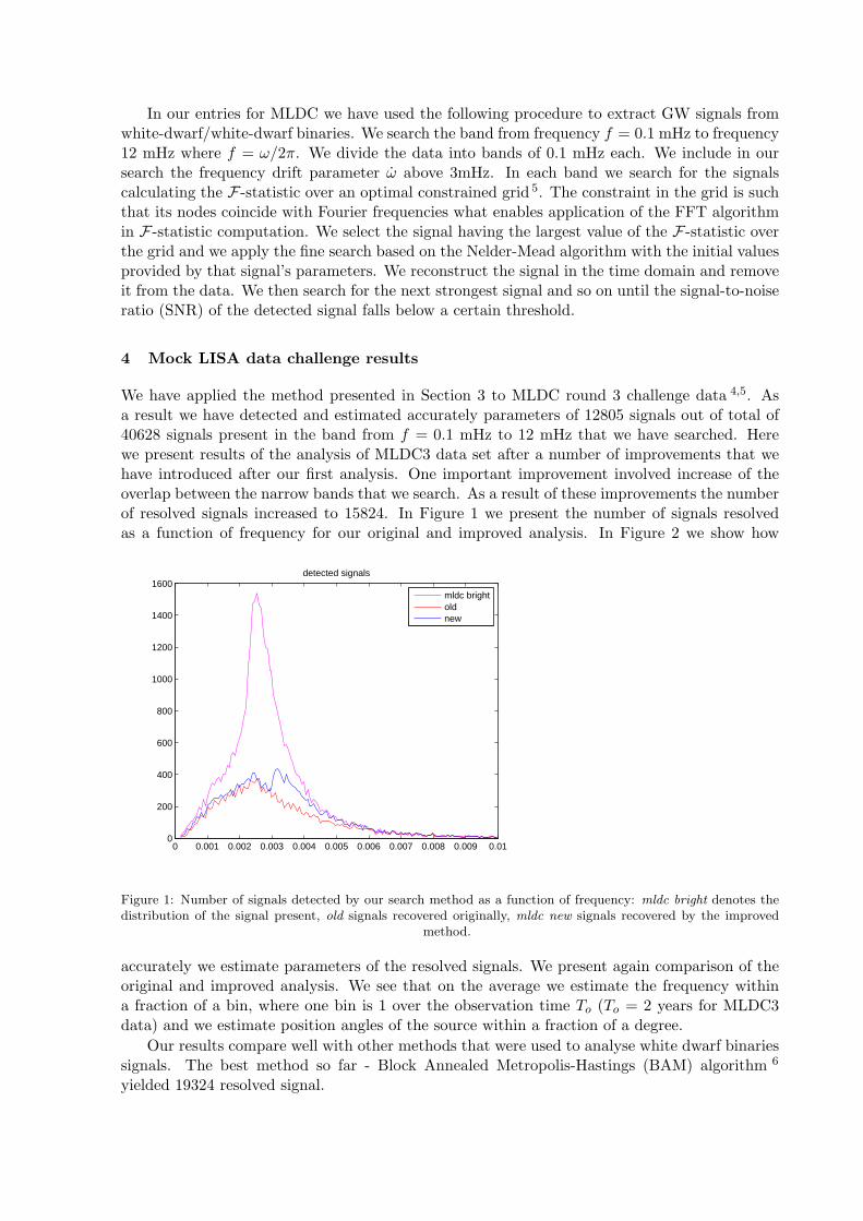
In our entries for MLDC we have used the following procedure to extract GW signals fromwhite-dwarf/white-dwarf binaries. We search the band from frequency f = 0.1 mHz to frequency12 mHz where f = ω/2π. We divide the data into bands of 0.1 mHz each. We include in oursearch the frequency drift parameter ω above 3mHz. In each band we search for the signalscalculating the F-statistic over an optimal constrained grid 5. The constraint in the grid is suchthat its nodes coincide with Fourier frequencies what enables application of the FFT algorithmin F-statistic computation. We select the signal having the largest value of the F-statistic overthe grid and we apply the fine search based on the Nelder-Mead algorithm with the initial valuesprovided by that signal’s parameters. We reconstruct the signal in the time domain and removeit from the data. We then search for the next strongest signal and so on until the signal-to-noiseratio (SNR) of the detected signal falls below a certain threshold.
4 Mock LISA data challenge results
We have applied the method presented in Section 3 to MLDC round 3 challenge data 4,5. Asa result we have detected and estimated accurately parameters of 12805 signals out of total of40628 signals present in the band from f = 0.1 mHz to 12 mHz that we have searched. Herewe present results of the analysis of MLDC3 data set after a number of improvements that wehave introduced after our first analysis. One important improvement involved increase of theoverlap between the narrow bands that we search. As a result of these improvements the numberof resolved signals increased to 15824. In Figure 1 we present the number of signals resolvedas a function of frequency for our original and improved analysis. In Figure 2 we show how
0 0.001 0.002 0.003 0.004 0.005 0.006 0.007 0.008 0.009 0.010
200
400
600
800
1000
1200
1400
1600detected signals
mldc brightoldnew
Figure 1: Number of signals detected by our search method as a function of frequency: mldc bright denotes thedistribution of the signal present, old signals recovered originally, mldc new signals recovered by the improved
method.
accurately we estimate parameters of the resolved signals. We present again comparison of theoriginal and improved analysis. We see that on the average we estimate the frequency withina fraction of a bin, where one bin is 1 over the observation time To (To = 2 years for MLDC3data) and we estimate position angles of the source within a fraction of a degree.
Our results compare well with other methods that were used to analyse white dwarf binariessignals. The best method so far - Block Annealed Metropolis-Hastings (BAM) algorithm 6
yielded 19324 resolved signal.
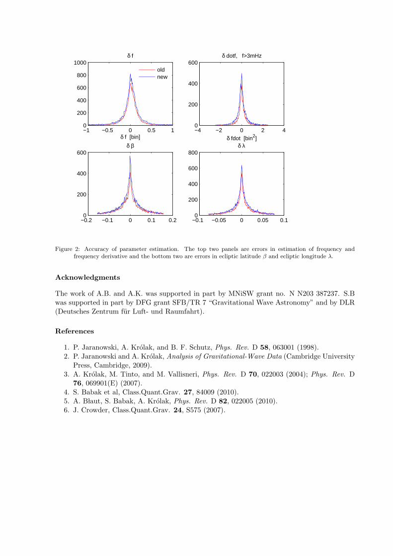
−1 −0.5 0 0.5 10
200
400
600
800
1000
δ f [bin]
δ f
oldnew
−4 −2 0 2 40
200
400
600
δ fdot [bin2]
δ dotf, f>3mHz
−0.2 −0.1 0 0.1 0.20
200
400
600
δ β
−0.1 −0.05 0 0.05 0.10
200
400
600
800
δ λ
Figure 2: Accuracy of parameter estimation. The top two panels are errors in estimation of frequency andfrequency derivative and the bottom two are errors in ecliptic latitude β and ecliptic longitude λ.
Acknowledgments
The work of A.B. and A.K. was supported in part by MNiSW grant no. N N203 387237. S.Bwas supported in part by DFG grant SFB/TR 7 “Gravitational Wave Astronomy” and by DLR(Deutsches Zentrum fur Luft- und Raumfahrt).
References
1. P. Jaranowski, A. Krolak, and B. F. Schutz, Phys. Rev. D 58, 063001 (1998).2. P. Jaranowski and A. Krolak, Analysis of Gravitational-Wave Data (Cambridge University
Press, Cambridge, 2009).3. A. Krolak, M. Tinto, and M. Vallisneri, Phys. Rev. D 70, 022003 (2004); Phys. Rev. D
76, 069901(E) (2007).4. S. Babak et al, Class.Quant.Grav. 27, 84009 (2010).5. A. B laut, S. Babak, A. Krolak, Phys. Rev. D 82, 022005 (2010).6. J. Crowder, Class.Quant.Grav. 24, S575 (2007).

5.Advanced Detectors

Advanced Virgo
T. Accadia1, F. Acernese2ac, P. Astone3a, G. Ballardin4, F. Barone2ac, M. Barsuglia5, A. Basti6ab,Th. S. Bauer7a, M. Bebronne1, M. Bejger8c, M.G. Beker7a, A. Belletoile1, M. Bitossi6a,
M. A. Bizouard9a, M. Blom7a, F. Bondu10b, L. Bonelli6ab, R. Bonnand11, V. Boschi6a, L. Bosi12a, B.Bouhou5, S. Braccini6a, C. Bradaschia6a, M. Branchesi13ab, T. Briant14, A. Brillet10a, V. Brisson9a,
T. Bulik8b, H. J. Bulten7ab, D. Buskulic1, C. Buy5, G. Cagnoli13a, E. Calloni2ab, B. Canuel4,F. Carbognani4, F. Cavalier9a, R. Cavalieri4, G. Cella6a, E. Cesarini13b, O. Chaibi10a,
E. Chassande-Mottin5, A. Chincarini15, A. Chiummo4, F. Cleva10a, E. Coccia16ab, P.-F. Cohadon14,C. N. Colacino6ab, J. Colas4, A. Colla3ab, M. Colombini3b, A. Conte3ab, J.-P. Coulon10a, E. Cuoco4,
S. D’Antonio16a, V. Dattilo4, M. Davier9a, R. Day4, R. De Rosa2ab, G. Debreczeni17, W. Del Pozzo7a,M. del Prete18b, L. Di Fiore2a, A. Di Lieto6ab, M. Di Paolo Emilio16ac, A. Di Virgilio6a, A. Dietz1,M. Drago18ab, G. Endroczi17, V. Fafone16ab, I. Ferrante6ab, F. Fidecaro6ab, I. Fiori4, R. Flaminio11,
L. A. Forte2a, J.-D. Fournier10a, J. Franc11, S. Frasca3ab, F. Frasconi6a, M. Galimberti11,L. Gammaitoni12ab, F. Garufi2ab, M. E. Gaspar17, G. Gemme15, E. Genin4, A. Gennai6a, A. Giazotto6a,
R. Gouaty1, M. Granata5, C. Greverie10a, G. M. Guidi13ab, J.-F. Hayau10b, A. Heidmann14,H. Heitmann10, P. Hello9a, P. Jaranowski8d, I. Kowalska8b, A. Krolak8ae, N. Leroy9a, N. Letendre1,
T. G. F. Li7a, N. Liguori18ab, M. Lorenzini13a, V. Loriette9b, G. Losurdo13a, E. Majorana3a,I. Maksimovic9b, N. Man10a, M. Mantovani6ac, F. Marchesoni12a, F. Marion1, J. Marque4,
F. Martelli13ab, A. Masserot1, C. Michel11, L. Milano2ab, Y. Minenkov16a, M. Mohan4, N. Morgado11,A. Morgia16ab, B. Mours1, L. Naticchioni3ab, F. Nocera4, G. Pagliaroli16ac, L. Palladino16ac,
C. Palomba3a, F. Paoletti6a,4, M. Parisi2ab, A. Pasqualetti4, R. Passaquieti6ab, D. Passuello6a,G. Persichetti2ab, F. Piergiovanni13ab, M. Pietka8d, L. Pinard11, R. Poggiani6ab, M. Prato15,
G. A. Prodi18ab, M. Punturo12a, P. Puppo3a, D. S. Rabeling7ab, I. Racz17, P. Rapagnani3ab, V. Re16ab,T. Regimbau10a, F. Ricci3ab, F. Robinet9a, A. Rocchi16a, L. Rolland1, R. Romano2ac, D. Rosinska8cf ,
P. Ruggi4, B. Sassolas11, D. Sentenac4, L. Sperandio16ab, R. Sturani13ab, B. Swinkels4, M. Tacca4,L. Taffarello18c, A. Toncelli6ab, M. Tonelli6ab, O. Torre6ac, E. Tournefier1, F. Travasso12ab,
G. Vajente6ab, J. F. J. van den Brand7ab, C. Van Den Broeck7a, S. van der Putten7a, M. Vasuth17,M. Vavoulidis9a, G. Vedovato18c, D. Verkindt1, F. Vetrano13ab, A. Vicere13ab, J.-Y. Vinet10a,
S. Vitale7a, H. Vocca12a, R. L. Ward5, M. Was9a, K. Yamamoto18bd, M. Yvert1, A. Zadrozny8e,J.-P. Zendri18c
1Laboratoire d’Annecy-le-Vieux de Physique des Particules (LAPP), Universite de Savoie,CNRS/IN2P3, F-74941 Annecy-Le-Vieux, France
2INFN, Sezione di Napoli a; Universita di Napoli ’Federico II’b Complesso Universitario di MonteS.Angelo, I-80126 Napoli; Universita di Salerno, Fisciano, I-84084 Salernoc, Italy
3INFN, Sezione di Romaa; Universita ’La Sapienza’b, I-00185 Roma, Italy
4European Gravitational Observatory (EGO), I-56021 Cascina (PI), Italy
5Laboratoire AstroParticule et Cosmologie (APC) Universite Paris Diderot, CNRS: IN2P3, CEA:DSM/IRFU, Observatoire de Paris, 10 rue A.Domon et L.Duquet, 75013 Paris - France
6INFN, Sezione di Pisaa; Universita di Pisab; I-56127 Pisa; Universita di Siena, I-53100 Sienac, Italy
7Nikhef, Science Park, Amsterdam, the Netherlandsa; VU University Amsterdam, De Boelelaan 1081,1081 HV Amsterdam, the Netherlandsb
8IM-PAN 00-956 Warsawa; Astronomical Observatory Warsaw University 00-478 Warsawb;CAMK-PAN 00-716 Warsawc; Bia lystok University 15-424 Bia lystokd; IPJ 05-400 Swierk-Otwocke;
Institute of Astronomy 65-265 Zielona Goraf , Poland
9LAL, Universite Paris-Sud, IN2P3/CNRS, F-91898 Orsaya; ESPCI, CNRS, F-75005 Parisb, France
10Universite Nice-Sophia-Antipolis, CNRS, Observatoire de la Cote d’Azur, F-06304 Nicea; Institut dePhysique de Rennes, CNRS, Universite de Rennes 1, 35042 Rennesb, France
11Laboratoire des Materiaux Avances (LMA), IN2P3/CNRS, F-69622 Villeurbanne, Lyon, France
12INFN, Sezione di Perugiaa; Universita di Perugiab, I-06123 Perugia,Italy
13INFN, Sezione di Firenze, I-50019 Sesto Fiorentinoa; Universita degli Studi di Urbino ’Carlo Bo’,I-61029 Urbinob, Italy
14Laboratoire Kastler Brossel, ENS, CNRS, UPMC, Universite Pierre et Marie Curie, 4 Place Jussieu,F-75005 Paris, France
15INFN, Sezione di Genova; I-16146 Genova, Italy
16INFN, Sezione di Roma Tor Vergataa; Universita di Roma Tor Vergata, I-00133 Romab; Universitadell’Aquila, I-67100 L’Aquilac, Italy
17RMKI, H-1121 Budapest, Konkoly Thege Miklos ut 29-33, Hungary
18INFN, Gruppo Collegato di Trentoa and Universita di Trentob, I-38050 Povo, Trento, Italy; INFN,Sezione di Padovac and Universita di Padovad, I-35131 Padova, Italy
The Virgo interferometer, a detector for gravitational waves located near Pisa in Italy, will soonbe upgraded to become the next-generation detector Advanced Virgo. Advanced Virgo willbe approximately ten times more sensitive than Virgo, with a design strain sensitivity betterthan 10−23/
√Hz near 100 Hz. This is expected to enable regular detections of gravitational
waves and to yield significant astrophysical results. Many of the components of the detectorwill be changed for this upgrade. These changes include new core optics, a more powerful lasersystem, the signal-recycling technique, the use of homodyne detection at the output port, andan improvement of the vacuum system. The existing seismic isolation system in Virgo will bere-used. Advanced Virgo will form part of a global network of advanced gravitational wavedetectors along with Advanced LIGO, GEO HF, and LCGT.
1 Introduction
Interferometric gravitational wave (GW) detectors of the first generation (Virgo1, LIGO2, GEO6003)have successfully completed their first long-duration data taking runs and are installing signif-icant upgrades. Advanced Virgo is the project to upgrade the Virgo detector to a secondgeneration instrument. Even though it will be hosted in the same infrastructures as Virgo, theAdvanced Virgo sensitivity will be better by one order of magnitude over most of the detectionband, and thus will increase by a factor of 1000 the accessible volume of the Universe whencompared to initial Virgo. This paper provides a brief overview of the challenges that must beovercome to achieve this sensitivity increase, and the solutions designed to meet those challenges.
The Advanced Virgo detector will be based on the same basic principles of the Virgo detector,an electromagnetically coupled broadband gravitational wave antenna based on a Michelsoninterferometer with Fabry-Perot cavities in the arms (cf. figure 1). The seismic isolation system
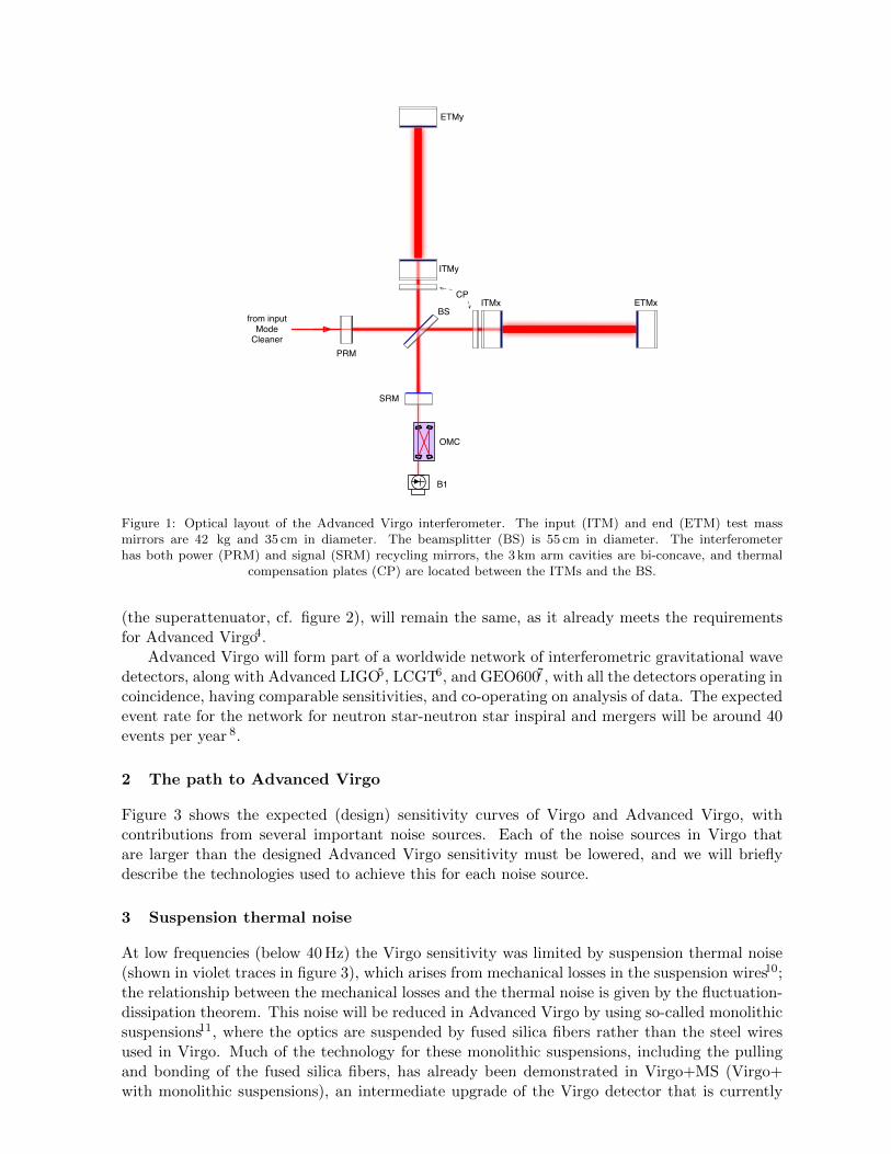
ITMy
ETMy
from input Mode
Cleaner
BSITMx ETMx
CP
PRM
SRM
B1
OMC
Figure 1: Optical layout of the Advanced Virgo interferometer. The input (ITM) and end (ETM) test massmirrors are 42 kg and 35 cm in diameter. The beamsplitter (BS) is 55 cm in diameter. The interferometerhas both power (PRM) and signal (SRM) recycling mirrors, the 3 km arm cavities are bi-concave, and thermal
compensation plates (CP) are located between the ITMs and the BS.
(the superattenuator, cf. figure 2), will remain the same, as it already meets the requirementsfor Advanced Virgo4.
Advanced Virgo will form part of a worldwide network of interferometric gravitational wavedetectors, along with Advanced LIGO5, LCGT6, and GEO6007, with all the detectors operating incoincidence, having comparable sensitivities, and co-operating on analysis of data. The expectedevent rate for the network for neutron star-neutron star inspiral and mergers will be around 40events per year 8.
2 The path to Advanced Virgo
Figure 3 shows the expected (design) sensitivity curves of Virgo and Advanced Virgo, withcontributions from several important noise sources. Each of the noise sources in Virgo thatare larger than the designed Advanced Virgo sensitivity must be lowered, and we will brieflydescribe the technologies used to achieve this for each noise source.
3 Suspension thermal noise
At low frequencies (below 40 Hz) the Virgo sensitivity was limited by suspension thermal noise(shown in violet traces in figure 3), which arises from mechanical losses in the suspension wires10;the relationship between the mechanical losses and the thermal noise is given by the fluctuation-dissipation theorem. This noise will be reduced in Advanced Virgo by using so-called monolithicsuspensions11, where the optics are suspended by fused silica fibers rather than the steel wiresused in Virgo. Much of the technology for these monolithic suspensions, including the pullingand bonding of the fused silica fibers, has already been demonstrated in Virgo+MS (Virgo+with monolithic suspensions), an intermediate upgrade of the Virgo detector that is currently
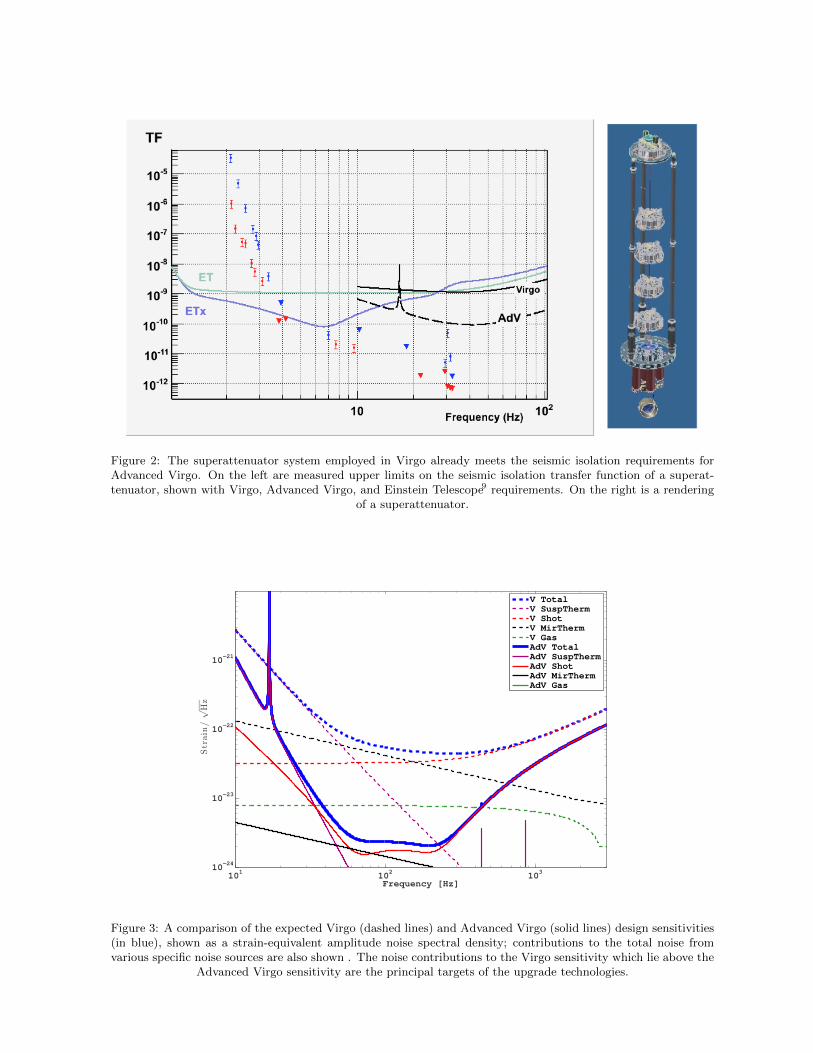
Figure 2: The superattenuator system employed in Virgo already meets the seismic isolation requirements forAdvanced Virgo. On the left are measured upper limits on the seismic isolation transfer function of a superat-tenuator, shown with Virgo, Advanced Virgo, and Einstein Telescope9 requirements. On the right is a rendering
of a superattenuator.
101
102
103
10−24
10−23
10−22
10−21
Frequency [Hz]
Strain/√Hz
V TotalV SuspThermV ShotV MirThermV GasAdV TotalAdV SuspThermAdV ShotAdV MirThermAdV Gas
Figure 3: A comparison of the expected Virgo (dashed lines) and Advanced Virgo (solid lines) design sensitivities(in blue), shown as a strain-equivalent amplitude noise spectral density; contributions to the total noise fromvarious specific noise sources are also shown . The noise contributions to the Virgo sensitivity which lie above the
Advanced Virgo sensitivity are the principal targets of the upgrade technologies.
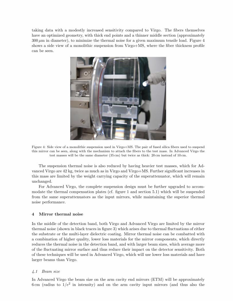
taking data with a modestly increased sensitivity compared to Virgo. The fibers themselveshave an optimized geometry, with thick end points and a thinner middle section (approximately300µm in diameter), to minimize the thermal noise for a given maximum tensile load. Figure 4shows a side view of a monolithic suspension from Virgo+MS, where the fiber thickness profilecan be seen.
Figure 4: Side view of a monolithic suspension used in Virgo+MS. The pair of fused silica fibers used to suspendthis mirror can be seen, along with the mechanism to attach the fibers to the test mass. In Advanced Virgo the
test masses will be the same diameter (35 cm) but twice as thick: 20 cm instead of 10 cm.
The suspension thermal noise is also reduced by having heavier test masses, which for Ad-vanced Virgo are 42 kg, twice as much as in Virgo and Virgo+MS. Further significant increases inthis mass are limited by the weight carrying capacity of the superattenuator, which will remainunchanged.
For Advanced Virgo, the complete suspension design must be further upgraded to accom-modate the thermal compensation plates (cf. figure 1 and section 5.1) which will be suspendedfrom the same superattenuators as the input mirrors, while maintaining the superior thermalnoise performance.
4 Mirror thermal noise
In the middle of the detection band, both Virgo and Advanced Virgo are limited by the mirrorthermal noise (shown in black traces in figure 3) which arises due to thermal fluctuations of eitherthe substrate or the multi-layer dielectric coating. Mirror thermal noise can be combatted witha combination of higher quality, lower loss materials for the mirror components, which directlyreduces the thermal noise in the detection band, and with larger beam sizes, which average moreof the fluctuating mirror surface and thus reduce their impact on the detector sensitivity. Bothof these techniques will be used in Advanced Virgo, which will use lower loss materials and havelarger beams than Virgo.
4.1 Beam size
In Advanced Virgo the beam size on the arm cavity end mirrors (ETM) will be approximately6 cm (radius to 1/e2 in intensity) and on the arm cavity input mirrors (and thus also the
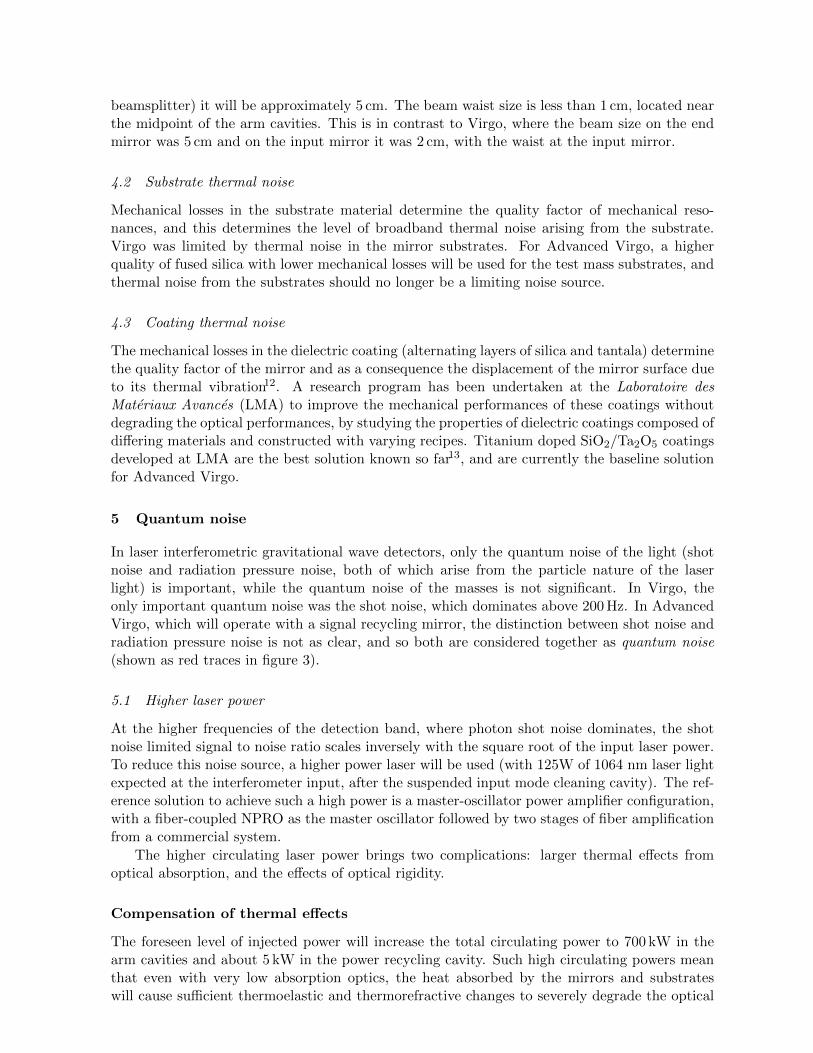
beamsplitter) it will be approximately 5 cm. The beam waist size is less than 1 cm, located nearthe midpoint of the arm cavities. This is in contrast to Virgo, where the beam size on the endmirror was 5 cm and on the input mirror it was 2 cm, with the waist at the input mirror.
4.2 Substrate thermal noise
Mechanical losses in the substrate material determine the quality factor of mechanical reso-nances, and this determines the level of broadband thermal noise arising from the substrate.Virgo was limited by thermal noise in the mirror substrates. For Advanced Virgo, a higherquality of fused silica with lower mechanical losses will be used for the test mass substrates, andthermal noise from the substrates should no longer be a limiting noise source.
4.3 Coating thermal noise
The mechanical losses in the dielectric coating (alternating layers of silica and tantala) determinethe quality factor of the mirror and as a consequence the displacement of the mirror surface dueto its thermal vibration12. A research program has been undertaken at the Laboratoire desMateriaux Avances (LMA) to improve the mechanical performances of these coatings withoutdegrading the optical performances, by studying the properties of dielectric coatings composed ofdiffering materials and constructed with varying recipes. Titanium doped SiO2/Ta2O5 coatingsdeveloped at LMA are the best solution known so far13, and are currently the baseline solutionfor Advanced Virgo.
5 Quantum noise
In laser interferometric gravitational wave detectors, only the quantum noise of the light (shotnoise and radiation pressure noise, both of which arise from the particle nature of the laserlight) is important, while the quantum noise of the masses is not significant. In Virgo, theonly important quantum noise was the shot noise, which dominates above 200 Hz. In AdvancedVirgo, which will operate with a signal recycling mirror, the distinction between shot noise andradiation pressure noise is not as clear, and so both are considered together as quantum noise(shown as red traces in figure 3).
5.1 Higher laser power
At the higher frequencies of the detection band, where photon shot noise dominates, the shotnoise limited signal to noise ratio scales inversely with the square root of the input laser power.To reduce this noise source, a higher power laser will be used (with 125W of 1064 nm laser lightexpected at the interferometer input, after the suspended input mode cleaning cavity). The ref-erence solution to achieve such a high power is a master-oscillator power amplifier configuration,with a fiber-coupled NPRO as the master oscillator followed by two stages of fiber amplificationfrom a commercial system.
The higher circulating laser power brings two complications: larger thermal effects fromoptical absorption, and the effects of optical rigidity.
Compensation of thermal effects
The foreseen level of injected power will increase the total circulating power to 700 kW in thearm cavities and about 5 kW in the power recycling cavity. Such high circulating powers meanthat even with very low absorption optics, the heat absorbed by the mirrors and substrateswill cause sufficient thermoelastic and thermorefractive changes to severely degrade the optical
performance of the interferometer. For this reason a thermal compensation system is necessary;this system illuminates the compensation plates (cf. figure 1) with a 10µm laser projector witha pattern complementary to that of the heat deposited by the main laser beam. As 10µm lightis strongly absorbed by fused silica, much less power (about 15 W) is needed in this systemthan for the main laser light. In addition to this projector + compensation plate system, whichcompensates for thermorefractive effects in the mirror substrates, annular heating elementswill surround the test masses to adjust the radii of curvature of these mirrors to counteractthermoelastic deformation of the mirror surfaces caused by absorption in the mirror coatings.
Optical rigidity
The high circulating power means that the dynamics of the interferometer mirrors, particularlyin the arm cavities, are modified by the light fields due to radiation pressure. This results inopto-mechanical resonances (i.e., optical springs) in the differential length degree of freedom 14,which is the one sensitive to gravitational waves, and in the angular degrees of freedom15. Suchopto-mechanical resonances are in general dynamically unstable, but appropriately designedcontrol systems can quench these instabilities.
5.2 Signal recycling
The use of the signal recycling technique permits a certain amount of flexibility in shapingthe spectrum of quantum noise; this allows optimization of the sensitivity in the presence ofother noise sources 14. The sensitivity plotted in figure 3 has been optimized for neutron starbinary inspirals, in the presence of suspension and mirror thermal noise. Small changes in theparameters of the signal recycling cavity (such as a small change in the reflectivity of the signalrecycling mirror or even a microscopic, sub-wavelength adjustment of the signal recycling mirrorposition) can modify the quantum noise, to maximize the sensitivity to another source (e.g., aparticular millisecond pulsar, or stellar mass black hole binaries).
5.3 DC readout
In place of the optical heterodyne technique used in Virgo, Advanced Virgo will use opticalhomodyne detection in the form of the technique known as DC readout. This technique involvesa slight detuning of the differential arm degree of freedom (the one which is also sensitive togravitational waves) slightly from destructive interference to allow a small amount of light toleak out the detection port to serve as a local oscillator. Because this light has been storedin the interferometer, it has been passively filtered by the so-called coupled-cavity pole16. Thispassive optical filtering, combined with the laser pre-stabilization system, means this light is avery low noise optical local oscillator in the detection band. Furthermore, optical homodynedetection has a lower level of shot noise than optical heterodyne detection17. To implement DCreadout an output mode cleaner (OMC in figure 1) is placed after the interferometer and beforethe photodetector (B1 in figure 1).
5.4 Optical losses
The surface quality of the test mass substrates is an important factor in the optical performance(i.e., the optical losses) of the interferometer, which can impact the quantum noise limitedsensitivity. To achieve an appropriately low level of surface figure error, a corrective coatingprocess has been developed at LMA. This process is expected to suppress surface figure errorswith spatial scale larger than 50 m−1, which have a large effect on the optical performance ofkm-scale cavities with large beam sizes. The apparatus for this corrective coating has been
constructed, and the first tests of this process on large scale mirrors (i.e., the 35 cm diameter ofthe Advanced Virgo substrates) will take place soon.
6 Residual gas noise
Residual gas in the 3 km beam tubes can induce phase fluctuations in the laser light circulatingin the Fabry-Perot arm cavities, resulting in noise in the interferometer output (the green tracesin figure 3). The current Virgo vacuum system operates at a residual pressure of about 10−7
mbar; this level must be reduced to about 10−9 mbar to meet the Advanced Virgo requirements.This will be done by performing a vacuum bake-out of the beam tubes and installing cryotrapsat each end of each beam tube. The cryotraps will allow regular intervention into the vacuumsystem at the mirror locations without spoiling the level of vacuum in the beam tubes throughwater migration.
7 Conclusions
Achieving a factor of 10 sensitivity improvement over Virgo requires pushing the limits of technol-ogy on several frontiers. The maturing Advanced Virgo design will meet these limits. Expectedto be online in 2015, Advanced Virgo will be a crucial part of the network of next generationgravitational wave detectors that will usher in the era of gravitational wave astronomy.
Acknowledgments
Advanced Virgo is a joint project of the Centre National de la Recherche Scientifique (CNRS)and the Istituto Nazionale di Fisica Nucleare (INFN).
References
1. F. Acernese et al., Class. Quant. Grav. 25, 184001 (2008)2. B. Abbott, et al., Rep. Prog. Phys. 72, 076901 (2009)3. H Grote and the LIGO Scientific Collaboration, Class. Quant. Grav. 27, 084003 (2010)4. F. Acernese et al., Astropart. Phys., 33, 182 (2010)5. G. Harry and the LIGO Scientific Collaboration Class. Quant. Grav. 27, 084007 (2010)6. K. Kuroda (on behalf of the LCGT Collaboration), Class. Quant. Grav. 27, 084004
(2010)7. B. Willke et al., Class. Quant. Grav. 23, S207 (2006)8. J. Abadie et al., Class. Quant. Grav. 27, 173001 (2010)9. M. Punturo et al., Class. Quant. Grav. 27, 194002 (2010)
10. P.R. Saulson. Phys. Rev. D 42, 2437 (1990)11. M. Lorenzini and the Virgo Collaboration, Class. Quant. Grav. 27, 084021 (2010)12. G.M. Harry, et al., Appl. Opt., 45, 1569 (2006)13. C.Comtet et al., Proceedings of the 42nd Rencontres de Moriond, (2007)14. A. Buonanno and Y. Chen, Phys. Rev. D 64, 042006 (2001)15. J.A. Sidles and D.Sigg. Physics Letters A, 354, 167 172, (2006).16. J.B. Camp, et al., J. Opt. Soc. Am. A, 17 12 (2000)17. A.Buonanno, Y.Chen, and N.Mavalvala. Phys. Rev. D 67, 122005 (2003)
SCIENTIFIC POTENTIAL OF EINSTEIN TELESCOPE
B Sathyaprakash18, M Abernathy3, F Acernese4,5, P Amaro-Seoane33,46, N Andersson7, K Arun8,F Barone4,5, B Barr3, M Barsuglia9, M Beker45, N Beveridge3, S Birindelli11, S Bose12, L Bosi1,
S Braccini13, C Bradaschia13, T Bulik14, E Calloni4,15, G Cella13, E Chassande Mottin9, S Chelkowski16,A Chincarini17, J Clark18, E Coccia19,20, C Colacino13, J Colas2, A Cumming3, L Cunningham3,E Cuoco2, S Danilishin21, K Danzmann6, R De Salvo23, T Dent18, R De Rosa4,15, L Di Fiore4,15,
A Di Virgilio13, M Doets10, V Fafone19,20, P Falferi24, R Flaminio25, J Franc25, F Frasconi13, A Freise16,D Friedrich6, P Fulda16, J Gair26, G Gemme17, E Genin2, A Gennai16, A Giazotto2,13, K Glampedakis27,C Graf6 M Granata9, H Grote6, G Guidi28,29, A Gurkovsky21, G Hammond3, M Hannam18, J Harms23,
D Heinert32, M Hendry3, I Heng3, E Hennes45, S Hild3, J Hough4, S Husa44, S Huttner3, G Jones18,F Khalili21, K Kokeyama16, K Kokkotas27, B Krishnan6, T.G.F. Li45, M Lorenzini28, H Luck6,
E Majorana34, I Mandel16,35, V Mandic31, M Mantovani13, I Martin3, C Michel25, Y Minenkov19,20,N Morgado25, S Mosca4,15, B Mours37, H Muller–Ebhardt6, P Murray3, R Nawrodt3,32, J Nelson3,
R Oshaughnessy38, C D Ott39, C Palomba34, A Paoli2, G Parguez2, A Pasqualetti2, R Passaquieti13,40,D Passuello13, L Pinard25, W Plastino42, R Poggiani13,40, P Popolizio2, M Prato17, M Punturo1,2,
P Puppo34, D Rabeling10,45, I Racz47, P Rapagnani34,41, J Read36, T Regimbau11, H Rehbein6, S Reid3,L Rezzolla33, F Ricci34,41, F Richard2, A Rocchi19, S Rowan3, A Rudiger6, L Santamarıa23, B Sassolas25,
R Schnabel6, C Schwarz32, P Seidel32, A Sintes44, K Somiya39, F Speirits3, K Strain3, S Strigin21,P Sutton18, S Tarabrin6, A Thuring6, J van den Brand10,45, M van Veggel3, C van den Broeck45,
A Vecchio16, J Veitch18, F Vetrano28,29, A Vicere28,29, S Vyatchanin21, B Willke6, G Woan3,K Yamamoto30
1 INFN, Sezione di Perugia, I-6123 Perugia, Italy2 European Gravitational Observatory (EGO), I-56021 Cascina (Pi), Italy
3 SUPA, School of Physics and Astronomy, The University of Glasgow, Glasgow, G12 8QQ, UK4 INFN, Sezione di Napoli, Italy
5 Universita di Salerno, Fisciano, I-84084 Salerno, Italy6 Max–Planck–Institut fur Gravitationsphysik and Leibniz Universitat Hannover, D-30167 Hannover,
Germany7 University of Southampton, Southampton SO17 1BJ, UK
8 LAL, Universite Paris-Sud, IN2P3/CNRS, F-91898 Orsay, France9 AstroParticule et Cosmologie (APC), CNRS; Observatoire de Paris, Universite Denis Diderot, Paris
VII, France10 VU University Amsterdam, De Boelelaan 1081, 1081 HV, Amsterdam, The Netherlands
11 Universite Nice ‘Sophia–Antipolis’, CNRS, Observatoire de la Cote d’Azur, F-06304 Nice, France12 Washington State University, Pullman, WA 99164, USA
13 INFN, Sezione di Pisa, Italy14 Astronomical Observatory, University of warsaw, Al Ujazdowskie 4, 00-478 Warsaw, Poland
15 Universita di Napoli ‘Federico II’, Complesso Universitario di Monte S. Angelo, I-80126 Napoli, Italy16 University of Birmingham, Birmingham, B15 2TT, UK
17 INFN, Sezione di Genova, I-16146 Genova, Italy
18 Cardiff University, Cardiff, CF24 3AA, UK19 INFN, Sezione di Roma Tor Vergata I-00133 Roma, Italy20 Universita di Roma Tor Vergata, I-00133, Roma, Italy
21 Moscow State University, Moscow, 119992, Russia22 INFN, Laboratori Nazionali del Gran Sasso, Assergi l’Aquila, Italy
23 LIGO, California Institute of Technology, Pasadena, CA 91125, USA24 INFN, Gruppo Collegato di Trento, Sezione di Padova; Istituto di Fotonica e Nanotecnologie,
CNR-Fondazione Bruno Kessler, I-38123 Povo, Trento, Italy25 Laboratoire des Materiaux Avances (LMA), IN2P3/CNRS, F-69622 Villeurbanne, Lyon, France26 Institute of Astronomy, University of Cambridge, Madingley Road, Cambridge, CB3 0HA, UK27 Theoretical Astrophysics (TAT) Eberhard-Karls-Universitat Tubingen, Auf der Morgenstelle 10,
D-72076 Tubingen, Germany28 INFN, Sezione di Firenze, I-50019 Sesto Fiorentino, Italy
29 Universita degli Studi di Urbino ‘Carlo Bo’, I-61029 Urbino, Italy30 INFN, sezione di Padova, via Marzolo 8, 35131 Padova, Italy
31 University of Minnesota, Minneapolis, MN 55455, USA32 Friedrich–Schiller–Universitat Jena PF, D-07737 Jena, Germany
33 Max Planck Institute for Gravitational Physics (Albert Einstein Institute) Am Muhlenberg 1, D-14476Potsdam, Germany
34 INFN, Sezione di Roma 1, I-00185 Roma, Italy35 NSF Astronomy and Astrophysics Postdoctoral Fellow, MIT Kavli Institute, Cambridge, MA 02139
36 University of Mississippi, University, MS 38677, USA37 LAPP-IN2P3/CNRS, Universite de Savoie, F-74941 Annecy-le-Vieux, France
38 The Pennsylvania State University, University Park, PA 16802, USA39 Caltech–CaRT, Pasadena, CA 91125, USA
40 Universita di Pisa, I-56127 Pisa, Italy41 Universita ‘La Sapienza’, I-00185 Roma, Italy
42 INFN, Sezione di Roma Tre and Universita di Roma Tre, Dipartimento di Fisica, I-00146 Roma,Italy
43 Universita degli Studi di Firenze, I-50121, Firenze, Italy44 Departament de Fisica, Universitat de les Illes Balears, Cra. Valldemossa Km. 7.5, E-07122 Palma
de Mallorca, Spain45 Nikhef, Science Park 105, 1098 XG Amsterdam, The Netherlands
46 Institut de Ciencies de l’Espai (CSIC-IEEC), Campus UAB, Torre C-5, parells, 2na planta,ES-08193, Bellaterra, Barcelona, Spain
46 KFKI Research Institute for Particle and Nuclear Physics, Budapest, Hungary
Abstract
Einstein gravitational-wave Telescope (ET) is a design study funded by the EuropeanCommission to explore the technological challenges of and scientific benefits from building athird generation gravitational wave detector. The three-year study, which concluded earlierthis year, has formulated the conceptual design of an observatory that can support the im-plementation of new technology for the next two to three decades. The goal of this talk isto introduce the audience to the overall aims and objectives of the project and to enumer-ate ET’s potential to influence our understanding of fundamental physics, astrophysics andcosmology.
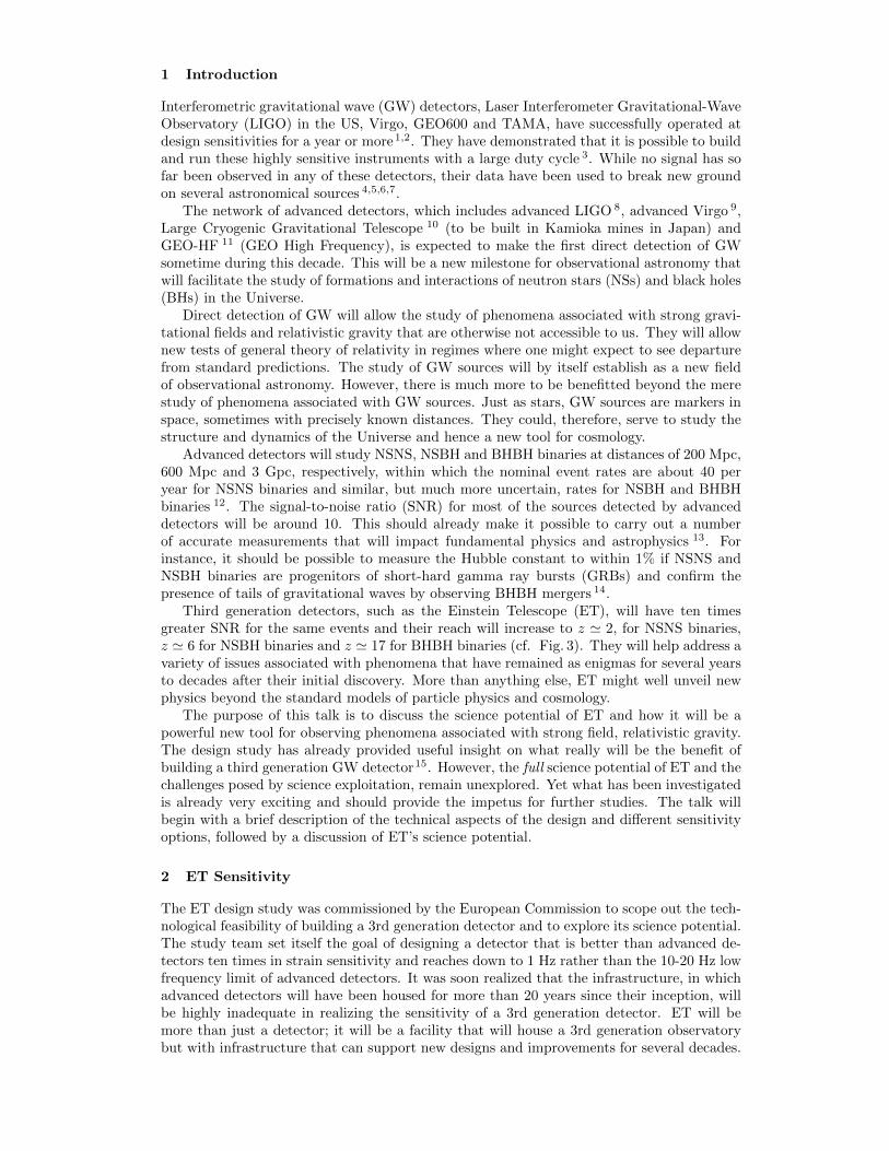
1 Introduction
Interferometric gravitational wave (GW) detectors, Laser Interferometer Gravitational-WaveObservatory (LIGO) in the US, Virgo, GEO600 and TAMA, have successfully operated atdesign sensitivities for a year or more1,2. They have demonstrated that it is possible to buildand run these highly sensitive instruments with a large duty cycle 3. While no signal has sofar been observed in any of these detectors, their data have been used to break new groundon several astronomical sources 4,5,6,7.
The network of advanced detectors, which includes advanced LIGO 8, advanced Virgo 9,Large Cryogenic Gravitational Telescope 10 (to be built in Kamioka mines in Japan) andGEO-HF 11 (GEO High Frequency), is expected to make the first direct detection of GWsometime during this decade. This will be a new milestone for observational astronomy thatwill facilitate the study of formations and interactions of neutron stars (NSs) and black holes(BHs) in the Universe.
Direct detection of GW will allow the study of phenomena associated with strong gravi-tational fields and relativistic gravity that are otherwise not accessible to us. They will allownew tests of general theory of relativity in regimes where one might expect to see departurefrom standard predictions. The study of GW sources will by itself establish as a new fieldof observational astronomy. However, there is much more to be benefitted beyond the merestudy of phenomena associated with GW sources. Just as stars, GW sources are markers inspace, sometimes with precisely known distances. They could, therefore, serve to study thestructure and dynamics of the Universe and hence a new tool for cosmology.
Advanced detectors will study NSNS, NSBH and BHBH binaries at distances of 200 Mpc,600 Mpc and 3 Gpc, respectively, within which the nominal event rates are about 40 peryear for NSNS binaries and similar, but much more uncertain, rates for NSBH and BHBHbinaries 12. The signal-to-noise ratio (SNR) for most of the sources detected by advanceddetectors will be around 10. This should already make it possible to carry out a numberof accurate measurements that will impact fundamental physics and astrophysics 13. Forinstance, it should be possible to measure the Hubble constant to within 1% if NSNS andNSBH binaries are progenitors of short-hard gamma ray bursts (GRBs) and confirm thepresence of tails of gravitational waves by observing BHBH mergers 14.
Third generation detectors, such as the Einstein Telescope (ET), will have ten timesgreater SNR for the same events and their reach will increase to z ' 2, for NSNS binaries,z ' 6 for NSBH binaries and z ' 17 for BHBH binaries (cf. Fig. 3). They will help address avariety of issues associated with phenomena that have remained as enigmas for several yearsto decades after their initial discovery. More than anything else, ET might well unveil newphysics beyond the standard models of particle physics and cosmology.
The purpose of this talk is to discuss the science potential of ET and how it will be apowerful new tool for observing phenomena associated with strong field, relativistic gravity.The design study has already provided useful insight on what really will be the benefit ofbuilding a third generation GW detector15. However, the full science potential of ET and thechallenges posed by science exploitation, remain unexplored. Yet what has been investigatedis already very exciting and should provide the impetus for further studies. The talk willbegin with a brief description of the technical aspects of the design and different sensitivityoptions, followed by a discussion of ET’s science potential.
2 ET Sensitivity
The ET design study was commissioned by the European Commission to scope out the tech-nological feasibility of building a 3rd generation detector and to explore its science potential.The study team set itself the goal of designing a detector that is better than advanced de-tectors ten times in strain sensitivity and reaches down to 1 Hz rather than the 10-20 Hz lowfrequency limit of advanced detectors. It was soon realized that the infrastructure, in whichadvanced detectors will have been housed for more than 20 years since their inception, willbe highly inadequate in realizing the sensitivity of a 3rd generation detector. ET will bemore than just a detector; it will be a facility that will house a 3rd generation observatorybut with infrastructure that can support new designs and improvements for several decades.
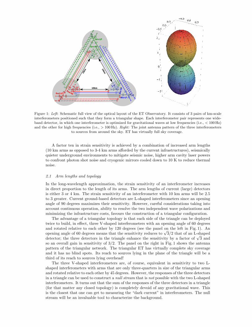
Out
In
Out
In
Out
In
Out
In
Out
In
Out
In
Red-LF
Red-HF Blu-H
F
Grn-LF
Blu-LF
Grn-HF
10km
10km
10km
Figure 1: Left: Schematic full view of the optical layout of the ET Observatory. It consists of 3 pairs of km-scaleinterferometers positioned such that they form a triangular shape. Each interferometer pair represents one wide-band detector, in which one interferometer is optimized for gravitational waves at low frequencies (i.e., < 100 Hz)and the other for high frequencies (i.e., > 100 Hz). Right: The joint antenna pattern of the three interferometers
to sources from around the sky. ET has virtually full sky coverage.
A factor ten in strain sensitivity is achieved by a combination of increased arm lengths(10 km arms as opposed to 3-4 km arms afforded by the current infrastructures), seismicallyquieter underground environments to mitigate seismic noise, higher arm cavity laser powersto confront photon shot noise and cryogenic mirrors cooled down to 10 K to reduce thermalnoise.
2.1 Arm lengths and topology
In the long-wavelength approximation, the strain sensitivity of an interferometer increasesin direct proportion to the length of its arms. The arm lengths of current (large) detectorsis either 3 or 4 km. The strain sensitivity of an interferometer with 10 km arms will be 2.5to 3 greater. Current ground-based detectors are L-shaped interferometers since an openingangle of 90 degrees maximizes their sensitivity. However, careful considerations taking intoaccount continuous operation, ability to resolve the two independent wave polarizations andminimizing the infrastructure costs, favours the construction of a triangular configuration.
The advantage of a triangular topology is that each side of the triangle can be deployedtwice to build, in effect, three V-shaped interferometers with an opening angle of 60 degreesand rotated relative to each other by 120 degrees (see the panel on the left in Fig. 1). Anopening angle of 60 degrees means that the sensitivity reduces to
√3/2 that of an L-shaped
detector; the three detectors in the triangle enhance the sensitivity by a factor of√
3 andso an overall gain in sensitivity of 3/2. The panel on the right in Fig. 1 shows the antennapattern of the triangular network. The triangular ET has virtually complete sky coverageand it has no blind spots. Its reach to sources lying in the plane of the triangle will be athird of its reach to sources lying overhead!
The three V-shaped interferometers are, of course, equivalent in sensitivity to two L-shaped interferometers with arms that are only three-quarters in size of the triangular armsand rotated relative to each other by 45 degrees. However, the responses of the three detectorsin a triangle can be used to construct a null stream that is not possible with the two L-shapedinterferometers. It turns out that the sum of the responses of the three detectors in a triangle(for that matter any closed topology) is completely devoid of any gravitational wave. Thisis the closest that one can get to measuring the “dark current” in interferometers. The nullstream will be an invaluable tool to characterize the background.
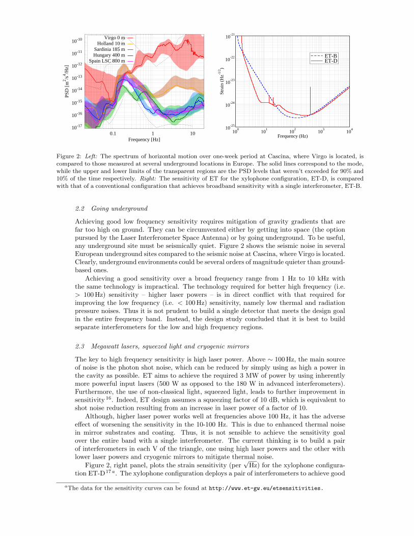
10-17
10-16
10-15
10-14
10-13
10-12
10-11
10-10
0.1 1 10
PSD
[m2 /s
4 /Hz]
Frequency [Hz]
Virgo 0 mHolland 10 m
Sardinia 185 mHungary 400 m
Spain LSC 800 m
100 101 102 103 104
Frequency (Hz)
10-25
10-24
10-23
10-22
10-21
Stra
in (H
z-1/2
)
ET-BET-D
Figure 2: Left: The spectrum of horizontal motion over one-week period at Cascina, where Virgo is located, iscompared to those measured at several underground locations in Europe. The solid lines correspond to the mode,while the upper and lower limits of the transparent regions are the PSD levels that weren’t exceeded for 90% and10% of the time respectively. Right: The sensitivity of ET for the xylophone configuration, ET-D, is comparedwith that of a conventional configuration that achieves broadband sensitivity with a single interferometer, ET-B.
2.2 Going underground
Achieving good low frequency sensitivity requires mitigation of gravity gradients that arefar too high on ground. They can be circumvented either by getting into space (the optionpursued by the Laser Interferometer Space Antenna) or by going underground. To be useful,any underground site must be seismically quiet. Figure 2 shows the seismic noise in severalEuropean underground sites compared to the seismic noise at Cascina, where Virgo is located.Clearly, underground environments could be several orders of magnitude quieter than ground-based ones.
Achieving a good sensitivity over a broad frequency range from 1 Hz to 10 kHz withthe same technology is impractical. The technology required for better high frequency (i.e.> 100 Hz) sensitivity – higher laser powers – is in direct conflict with that required forimproving the low frequency (i.e. < 100 Hz) sensitivity, namely low thermal and radiationpressure noises. Thus it is not prudent to build a single detector that meets the design goalin the entire frequency band. Instead, the design study concluded that it is best to buildseparate interferometers for the low and high frequency regions.
2.3 Megawatt lasers, squeezed light and cryogenic mirrors
The key to high frequency sensitivity is high laser power. Above ∼ 100 Hz, the main sourceof noise is the photon shot noise, which can be reduced by simply using as high a power inthe cavity as possible. ET aims to achieve the required 3 MW of power by using inherentlymore powerful input lasers (500 W as opposed to the 180 W in advanced interferometers).Furthermore, the use of non-classical light, squeezed light, leads to further improvement insensitivity 16. Indeed, ET design assumes a squeezing factor of 10 dB, which is equivalent toshot noise reduction resulting from an increase in laser power of a factor of 10.
Although, higher laser power works well at frequencies above 100 Hz, it has the adverseeffect of worsening the sensitivity in the 10-100 Hz. This is due to enhanced thermal noisein mirror substrates and coating. Thus, it is not sensible to achieve the sensitivity goalover the entire band with a single interferometer. The current thinking is to build a pairof interferometers in each V of the triangle, one using high laser powers and the other withlower laser powers and cryogenic mirrors to mitigate thermal noise.
Figure 2, right panel, plots the strain sensitivity (per√
Hz) for the xylophone configura-tion ET-D17 a. The xylophone configuration deploys a pair of interferometers to achieve good
aThe data for the sensitivity curves can be found at http://www.et-gw.eu/etsensitivities.
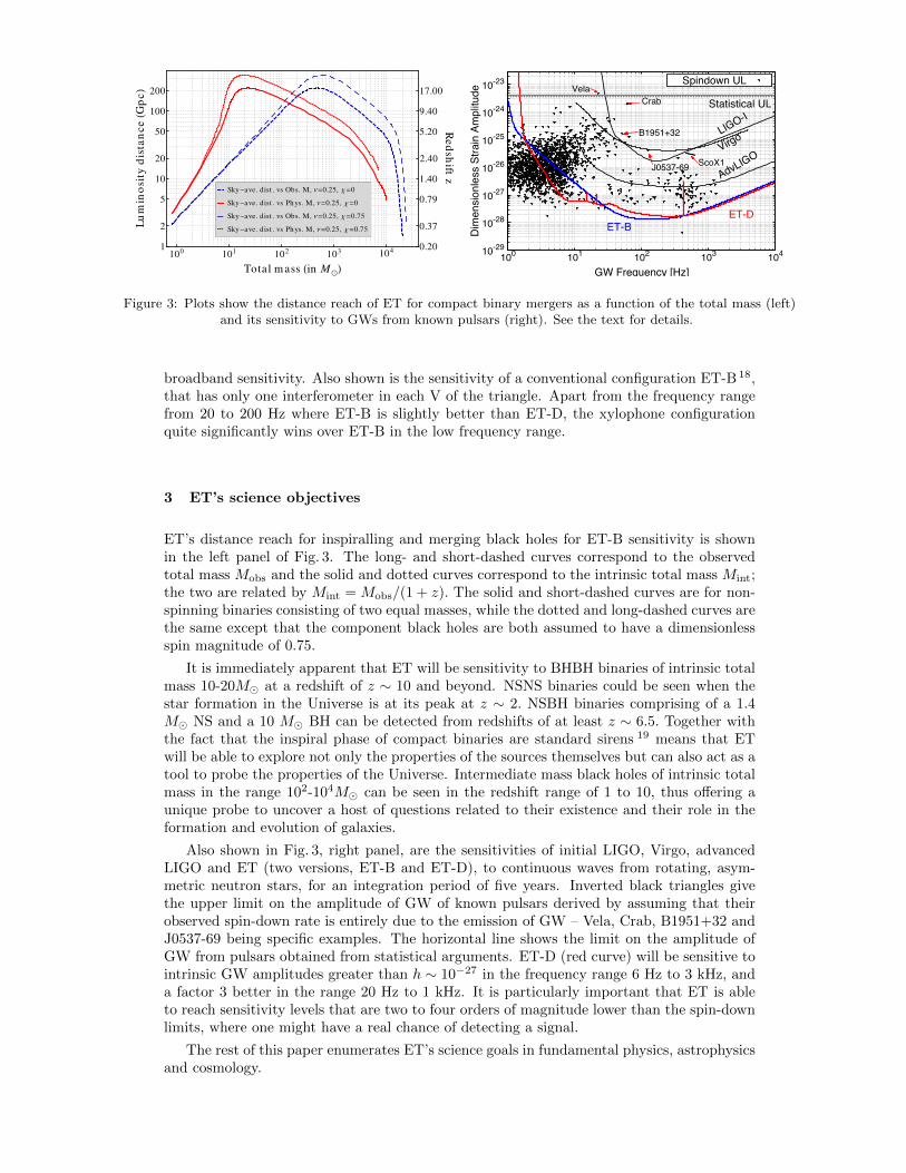
100 101 102 103 1041
2
5
10
20
50
100
200
0.20
0.37
0.79
1.40
2.40
5.20
9.40
17.00
Total mass !in M!"
Luminosity
distance!G
pc"
Redsh
iftz
Sky!ave. dist . vs Phys. M, "#0.25, $#0.75
Sky!ave. dist . vs Obs. M, "#0.25, $#0.75
Sky!ave. dist . vs Phys. M, "#0.25, $#0
Sky!ave. dist . vs Obs. M, "#0.25, $#0
10-29
10-28
10-27
10-26
10-25
10-24
10-23
100 101 102 103 104
Dim
ensi
onle
ss S
train
Am
plitu
de
GW Frequency [Hz]
LIGO-I
Virgo
AdvLIGO
ET-BET-D
Crab
J0537-69
B1951+32
ScoX1
VelaStatistical UL
Spindown UL
Figure 3: Plots show the distance reach of ET for compact binary mergers as a function of the total mass (left)and its sensitivity to GWs from known pulsars (right). See the text for details.
broadband sensitivity. Also shown is the sensitivity of a conventional configuration ET-B 18,that has only one interferometer in each V of the triangle. Apart from the frequency rangefrom 20 to 200 Hz where ET-B is slightly better than ET-D, the xylophone configurationquite significantly wins over ET-B in the low frequency range.
3 ET’s science objectives
ET’s distance reach for inspiralling and merging black holes for ET-B sensitivity is shownin the left panel of Fig. 3. The long- and short-dashed curves correspond to the observedtotal mass Mobs and the solid and dotted curves correspond to the intrinsic total mass Mint;the two are related by Mint = Mobs/(1 + z). The solid and short-dashed curves are for non-spinning binaries consisting of two equal masses, while the dotted and long-dashed curves arethe same except that the component black holes are both assumed to have a dimensionlessspin magnitude of 0.75.
It is immediately apparent that ET will be sensitivity to BHBH binaries of intrinsic totalmass 10-20M at a redshift of z ∼ 10 and beyond. NSNS binaries could be seen when thestar formation in the Universe is at its peak at z ∼ 2. NSBH binaries comprising of a 1.4M NS and a 10 M BH can be detected from redshifts of at least z ∼ 6.5. Together withthe fact that the inspiral phase of compact binaries are standard sirens 19 means that ETwill be able to explore not only the properties of the sources themselves but can also act as atool to probe the properties of the Universe. Intermediate mass black holes of intrinsic totalmass in the range 102-104M can be seen in the redshift range of 1 to 10, thus offering aunique probe to uncover a host of questions related to their existence and their role in theformation and evolution of galaxies.
Also shown in Fig. 3, right panel, are the sensitivities of initial LIGO, Virgo, advancedLIGO and ET (two versions, ET-B and ET-D), to continuous waves from rotating, asym-metric neutron stars, for an integration period of five years. Inverted black triangles givethe upper limit on the amplitude of GW of known pulsars derived by assuming that theirobserved spin-down rate is entirely due to the emission of GW – Vela, Crab, B1951+32 andJ0537-69 being specific examples. The horizontal line shows the limit on the amplitude ofGW from pulsars obtained from statistical arguments. ET-D (red curve) will be sensitive tointrinsic GW amplitudes greater than h ∼ 10−27 in the frequency range 6 Hz to 3 kHz, anda factor 3 better in the range 20 Hz to 1 kHz. It is particularly important that ET is ableto reach sensitivity levels that are two to four orders of magnitude lower than the spin-downlimits, where one might have a real chance of detecting a signal.
The rest of this paper enumerates ET’s science goals in fundamental physics, astrophysicsand cosmology.
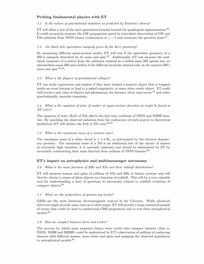
Probing fundamental physics with ET
3.1 Is the nature of gravitational radiation as predicted by Einstein’s theory?
ET will allow a test of the wave generation formula beyond the quadrupole approximation20.It could accurately measure the GW propagation speed by coincident observation of GW andEM radiation from NSNS binary coalescences at z ∼ 2 and constrain the graviton mass 21.
3.2 Are black hole spacetimes uniquely given by the Kerr geometry?
By measuring different quasi-normal modes, ET will test if the spacetime geometry of aBH is uniquely described by its mass and spin 22. Additionally, ET can measure the mul-tipole moments of a source from the radiation emitted as a stellar-mass BH spirals into anintermediate-mass BH and confirm if the different moments depend only on the massive BH’smass and spin 23,24.
3.3 What is the physics of gravitational collapse?
ET can study supernovae and explore if they leave behind a massive object that is trappedinside an event horizon or lead to a naked singularity, or some other exotic object. ET couldwell reveal a new class of objects and phenomena, for instance silent supernovae 25 and othergravitationally unstable transients.
3.4 What is the equation of state of matter at supra-nuclear densities as might be found inNS cores?
The equation of state (EoS) of NSs affects the late-time evolution of NSNS and NSBH bina-ries. By matching the observed radiation from the coalescence of such sources to theoreticalpredictions ET will deduce the EoS of NS cores 26,27.
3.5 What is the maximum mass of a neutron star?
The maximum mass of a white dwarf is ' 1.4M as determined by the electron degener-acy pressure. The maximum mass of a NS is an additional test of the nature of matterat extremely high densities; it is currently unknown and should be determined by ET byaccurately constructing their mass function from millions of NSNS binaries 28.
ET’s impact on astrophysics and multimessenger astronomy
3.6 What is the mass function of BHs and NSs and their redshift distribution?
ET will measure masses and spins of millions of NSs and BHs in binary systems and willthereby obtain a census of these objects as a function of redshift. This will be a very valuabletool for understanding a host of questions in astronomy related to redshift evolution ofcompact objects 29.
3.7 What are the progenitors of gamma-ray bursts?
GRBs are the most luminous electromagnetic sources in the Universe. While advanceddetectors might provide some clues as to their origin, ET will provide a large statistical sampleof events that could be used to understand GRB progenitors and to test their astrophysicalmodels 28.
3.8 How do compact binaries form and evolve?
The process by which main sequence binary stars evolve into compact binaries (that is,NSNS, NSBH and BHBH) could be understood by ET’s observation of millions of coalescingbinaries with different masses, mass ratios and spins and mapping the observed populationto astrophysical models 30.
3.9 What is the physical mechanism behind supernovae and how asymmetric is the gravita-tional collapse that ensues?
Supernovae are complex processes whose modelling requires many different inputs, includingrelativistic magneto-hydrodynamics, general relativity and nuclear and particle physics 31.ET’s observation of supernovae in coincidence with the detection of neutrinos could providethe data necessary to constrain models and help understand the process by which starscollapse to form NSs and BHs.
3.10 Do relativistic instabilities occur in young NSs and if so what is their role in theevolution of NSs?
Non-linearities of general relativity could cause instabilities in NSs that lead to paramet-ric amplification of GWs. ET’s observations of the formation of NSs can explore if suchinstabilities occur in young NSs and how that might affect their spin frequencies 27.
3.11 Why are spin frequencies of NSs in low-mass X-ray binaries bounded?
ET will verify if gravitational radiation back-reaction torque is responsible for the observedupper limit on NS spin frequencies in low-mass X-ray binaries 32.
3.12 What is the nature of the NS crust and its interaction with the core?
ET should detect NS ellipticities that are few × 10−10 (for sources within a distance of1 kpc) or larger depending on their spin frequency and their distance from earth. Suchobservations can be used to deduce the property of NS crusts. ET might also detect GWsthat are expected to be emitted when pulsars glitch and magnetars flare and thereby helpunderstand crust-core interaction that is believed to transfer angular momentum from thecore to crust 33.
3.13 What is the population of GW sources at high redshifts?
A large population of point sources would produce a confusion background that would bedetectable by ET if the energy density of the background is large enough. Detection ofconfusion backgrounds can be used to understand the nature and population of GW sourcesin the Universe.
ET as a new cosmological tool
3.14 What are the luminosity distances of cosmological sources?
Compact binaries are an astronomer’s ideal standard candles or, more appropriately, sirens.Gravitational wave observations can alone determine both the apparent and absolute lumi-nosity of a source and hence deduce their luminosity distance. With ET, these self-calibratingstandard sirens can be used to calibrate the cosmic distance ladder 34.
3.15 What is the EoS of dark energy and how does it vary with redshift?
ET could observe thousands of coalescing NSNS and NSBH systems in coincidence withoptical or gamma-ray observations and hence measure both the luminosity distance andredshift. ET will, therefore, facilitate precision measurement of the dark energy EoS and itsvariation with redshift 35.
3.16 How did the black holes at galactic nuclei form and evolve?
ET can verify if seeds of galaxy formation were intermediate BHs of hundreds to thousandsof solar masses and map their merger history up to redshifts of z ∼ 5–15 depending on thetotal mass and mass ratio of progenitor binaries 36,24,37.
3.17 What were the physical conditions in the primeval Universe and what phase transitionsoccurred in its early history?
Stochastic GW backgrounds could be produced by quantum processes in the primordialUniverse or during phase transitions in its early history. ET will be sensitive to backgrounddensities ρGW ∼ 10−12 ρc, where ρc is the critical density of the Universe 38.
4 Conclusions
This decade will see the construction and operation of second generation interferometricdetectors, pulsar timing arrays and results from the Planck space mission. There is littledoubt that we are at the verge of a new era in astronomy that will witness the opening ofthe gravitational window for observing the Universe. I hope this talk has convinced you thatthe field promises to have a huge potential and that ET can not only help solve some of theenigmas in astronomy and cosmology but push the frontiers of science into new avenues.
References
1. B. Abbott et al. (LIGO Scientific Collaboration). LIGO: the Laser InterferometerGravitational-Wave Observatory. Reports on Progress in Physics, 72(7):076901, 2009.
2. T. Accadia et al. Commissioning status of the Virgo interferometer. Class. QuantumGrav., 27, 2010.
3. H. Grote for the LIGO Scientific Collaboration. The status of GEO 600. Classical andQuantum Gravity, 25(11):114043 (9pp), 2008.
4. B. Abbott et al. Beating the spin-down limit on gravitational wave emission from thecrab pulsar. The Astrophysical Journal Letters, 683(1):L45, 2008.
5. B.P. Abbott et al. An Upper Limit on the Stochastic Gravitational-Wave Backgroundof Cosmological Origin. Nature, 460:990, 2009.
6. B. Abbott et al. (LIGO Scientific Collaboration) and K. Hurley. Implications for theOrigin of GRB 070201 from LIGO Observations. Astrophys. J., 681:1419–1430, 2008.
7. J. Abadie et al. Search for gravitational-wave inspiral signals associated with shortgamma-ray bursts during ligo’s fifth and virgo’s first science run. The AstrophysicalJournal, 715(2):1453, 2010.
8. David Shoemaker for the Advanced LIGO Team. Advanced ligo reference design. 2009.9. The VIRGO Collaboration. Advanced Virgo baseline design. Virgo Technical Report
VIR-0027A-09, 2009.10. Large-scale cryogenic gravitational-wave telescope project.11. B. Willke et al. The GEO-HF project. Class. Quantum Grav., 23:S207–S214, 2006.12. J. Abadie, B. P. Abbott, R. Abbott, M. Abernathy, T. Accadia, F. Acernese, C. Adams,
R. Adhikari, P. Ajith, B. Allen, and et al. TOPICAL REVIEW: Predictions for therates of compact binary coalescences observable by ground-based gravitational-wavedetectors. Classical and Quantum Gravity, 27(17):173001–+, September 2010.
13. B.S. Sathyaprakash and Bernard F. Schutz. Physics, astrophysics and cosmology withgravitational waves. Living Reviews in Relativity, 12(2), 2009.
14. L. Blanchet and B.S. Sathyaprakash. Detecting the tail effect in gravitational waveexperiments. Phys. Rev. Lett., 74:1067–1070, 1995.
15. M Abernathy et al. Einstein gravitational wave Telescope: Conceptual Design Study.available from European Gravitational Observatory, document number ET-0106A-10,2011.
16. K. McKenzie et al. Squeezing in the audio gravitational-wave detection band. Phys.Rev. Lett., 93(16):161105, Oct 2004.
17. S. Hild, M. Abernathy, F. Acernese, P. Amaro-Seoane, N. Andersson, et al. SensitivityStudies for Third-Generation Gravitational Wave Observatories. Class.Quant.Grav.,28:094013, 2011.
18. Stefan Hild, Simon Chelkowski, and Andreas Freise. Pushing towards the ET sensitivityusing ‘conventional’ technology. arXiv:0810.0604v2 [gr-qc], 2008.
19. B F Schutz. Determining the Hubble constant from gravitational wave observations.Nature (London), 323:310, 1986.
20. C.K. Mishra, K.G. Arun, B.R. Iyer, and B.S. Sathyaprakash. Parameterized testsof post-newtonian theory using advanced ligo and einstein telescope. Phys. Rev. D,82:064010, 2010.
21. K. G. Arun and Clifford M. Will. Bounding the mass of the graviton with gravitationalwaves: Effect of higher harmonics in gravitational waveform templates. Class. Quant.Grav., 26:155002, 2009.
22. I. Kamaretsos, M. Hannam, S. Husa, and B.S. Sathyaprakash. Black-hole hair loss:learning about binary progenitors from ringdown signal. 2011.
23. E.A. Huerta and J.R. Gair. Phys. Rev. D, 83:044020, 2011.24. Pau Amaro-Seoane and Lucia Santamaria. Detection of IMBHs with ground-based
gravitational wave observatories: A biography of a binary of black holes, from birth todeath. Astrophys. J., 722:1197–1206, 2010.
25. S. E. Woosley and E. Baron. The collapse of white dwarfs to neutron stars. Astro-phys. J., 391:228–235, May 1992.
26. Jocelyn S. Read et al. Measuring the neutron star equation of state with gravitationalwave observations. Phys. Rev., D79:124033, 2009.
27. N. Andersson, V. Ferrari, D. I. Jones, K. D. Kokkotas, B. Krishnan, J. S. Read, L. Rez-zolla, and B. Zink. Gravitational waves from neutron stars: promises and challenges.General Relativity and Gravitation, 43:409–436, February 2011.
28. B.S. Sathyaprakash and C. Van Den Broeck. Astrophysics with einstein telescope.2011.
29. C. Van Den Broeck and A.S. Sengupta. Binary black hole spectroscopy. Class.Quantum Grav., 24:1089–1114, 2007.
30. K. Belczynski, V. Kalogera, and T. Bulik. A comprehensive study of binary com-pact objects as gravitational wave sources: Evolutionary channels, rates, and physicalproperties. Astrophys. J., 572:407–431, 2002.
31. Christian D. Ott. Probing the Core-Collapse Supernova Mechanism with GravitationalWaves. Class.Quant.Grav., 26:204015, 2009.
32. L. Bildsten. Gravitational radiation and rotation of accreting neutron stars. Astrophys.J. Lett., 501:L89, 1998.
33. M. Ruderman. Crust-breaking by neutron superfluids and the vela pulsar glitches.Astrophys. J., 203:213–222, 1976.
34. B.S. Sathyaprakash, B.F. Schutz, and C. Van Den Broeck. Cosmography with theEinstein Telescope. Class.Quant.Grav., 27:215006, 2010.
35. W. Zhao, C. Van Den Broeck, D. Baskaran, and T.G.F. Li. Determination of DarkEnergy by the Einstein Telescope: Comparing with CMB, BAO and SNIa Observations.Phys.Rev., D83:023005, 2011.
36. A. Sesana, J. Gair, I. Mandel, and A. Vecchio. Observing Gravitational Waves fromthe First Generation of Black Holes. Astrophys. J. Lett., 698:L129–L132, 2009.
37. Jonathan R. Gair, Ilya Mandel, M.Coleman Miller, and Marta Volonteri. Exploring in-termediate and massive black-hole binaries with the Einstein Telescope. Gen.Rel.Grav.,43:485–518, 2011.
38. T. Regimbau, C. Robinson, B. Sathyaprakash, C. Van Den Broeck, D. Meacher, C.Rodriguez, T. Dent, S. Giampanis, T.G.F. Li, and W.Del Pozzo. A Mock DataChallenge for the Proposed Einstein GW Telescope. 2011.
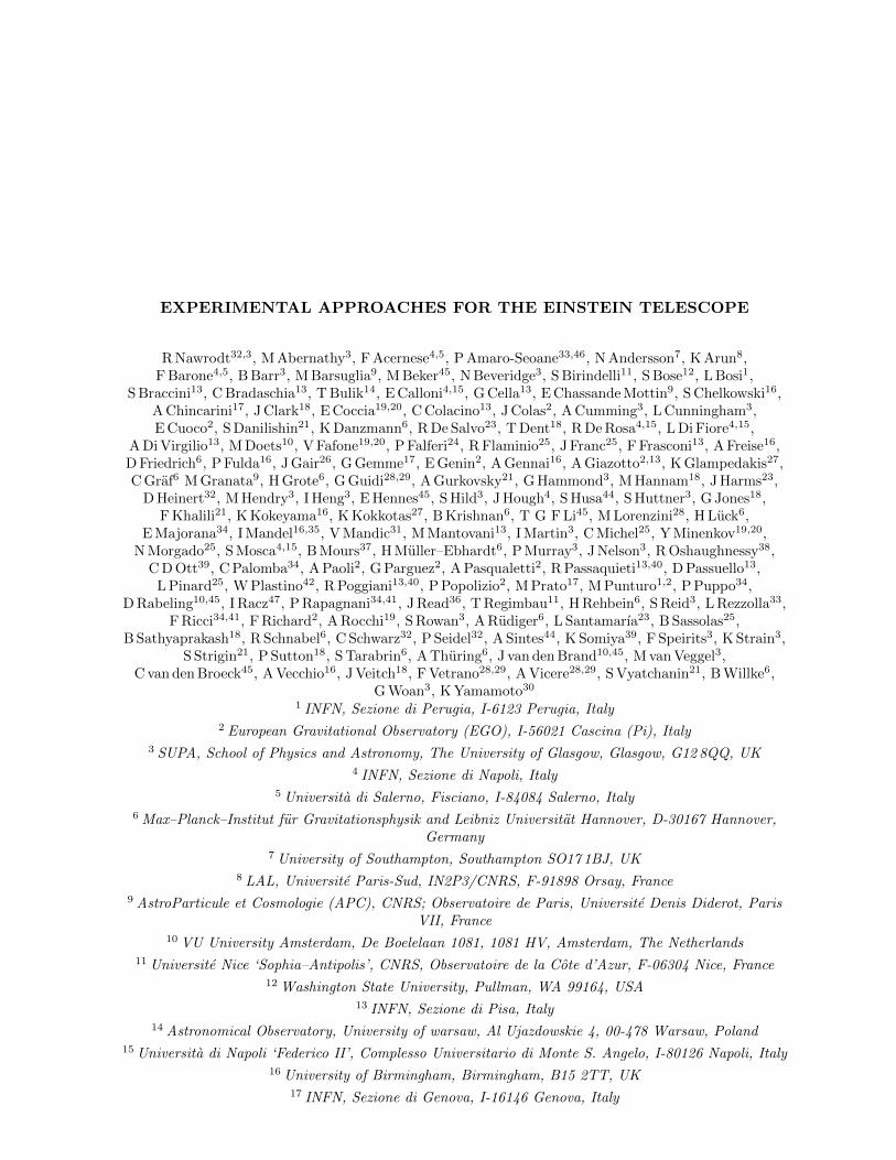
EXPERIMENTAL APPROACHES FOR THE EINSTEIN TELESCOPE
R Nawrodt32,3, M Abernathy3, F Acernese4,5, P Amaro-Seoane33,46, N Andersson7, K Arun8,F Barone4,5, B Barr3, M Barsuglia9, M Beker45, N Beveridge3, S Birindelli11, S Bose12, L Bosi1,
S Braccini13, C Bradaschia13, T Bulik14, E Calloni4,15, G Cella13, E Chassande Mottin9, S Chelkowski16,A Chincarini17, J Clark18, E Coccia19,20, C Colacino13, J Colas2, A Cumming3, L Cunningham3,E Cuoco2, S Danilishin21, K Danzmann6, R De Salvo23, T Dent18, R De Rosa4,15, L Di Fiore4,15,
A Di Virgilio13, M Doets10, V Fafone19,20, P Falferi24, R Flaminio25, J Franc25, F Frasconi13, A Freise16,D Friedrich6, P Fulda16, J Gair26, G Gemme17, E Genin2, A Gennai16, A Giazotto2,13, K Glampedakis27,C Graf6 M Granata9, H Grote6, G Guidi28,29, A Gurkovsky21, G Hammond3, M Hannam18, J Harms23,
D Heinert32, M Hendry3, I Heng3, E Hennes45, S Hild3, J Hough4, S Husa44, S Huttner3, G Jones18,F Khalili21, K Kokeyama16, K Kokkotas27, B Krishnan6, T G F Li45, M Lorenzini28, H Luck6,
E Majorana34, I Mandel16,35, V Mandic31, M Mantovani13, I Martin3, C Michel25, Y Minenkov19,20,N Morgado25, S Mosca4,15, B Mours37, H Muller–Ebhardt6, P Murray3, J Nelson3, R Oshaughnessy38,
C D Ott39, C Palomba34, A Paoli2, G Parguez2, A Pasqualetti2, R Passaquieti13,40, D Passuello13,L Pinard25, W Plastino42, R Poggiani13,40, P Popolizio2, M Prato17, M Punturo1,2, P Puppo34,
D Rabeling10,45, I Racz47, P Rapagnani34,41, J Read36, T Regimbau11, H Rehbein6, S Reid3, L Rezzolla33,F Ricci34,41, F Richard2, A Rocchi19, S Rowan3, A Rudiger6, L Santamarıa23, B Sassolas25,
B Sathyaprakash18, R Schnabel6, C Schwarz32, P Seidel32, A Sintes44, K Somiya39, F Speirits3, K Strain3,S Strigin21, P Sutton18, S Tarabrin6, A Thuring6, J van den Brand10,45, M van Veggel3,
C van den Broeck45, A Vecchio16, J Veitch18, F Vetrano28,29, A Vicere28,29, S Vyatchanin21, B Willke6,G Woan3, K Yamamoto30
1 INFN, Sezione di Perugia, I-6123 Perugia, Italy2 European Gravitational Observatory (EGO), I-56021 Cascina (Pi), Italy
3 SUPA, School of Physics and Astronomy, The University of Glasgow, Glasgow, G12 8QQ, UK4 INFN, Sezione di Napoli, Italy
5 Universita di Salerno, Fisciano, I-84084 Salerno, Italy6 Max–Planck–Institut fur Gravitationsphysik and Leibniz Universitat Hannover, D-30167 Hannover,
Germany7 University of Southampton, Southampton SO17 1BJ, UK
8 LAL, Universite Paris-Sud, IN2P3/CNRS, F-91898 Orsay, France9 AstroParticule et Cosmologie (APC), CNRS; Observatoire de Paris, Universite Denis Diderot, Paris
VII, France10 VU University Amsterdam, De Boelelaan 1081, 1081 HV, Amsterdam, The Netherlands
11 Universite Nice ‘Sophia–Antipolis’, CNRS, Observatoire de la Cote d’Azur, F-06304 Nice, France12 Washington State University, Pullman, WA 99164, USA
13 INFN, Sezione di Pisa, Italy14 Astronomical Observatory, University of warsaw, Al Ujazdowskie 4, 00-478 Warsaw, Poland
15 Universita di Napoli ‘Federico II’, Complesso Universitario di Monte S. Angelo, I-80126 Napoli, Italy16 University of Birmingham, Birmingham, B15 2TT, UK
17 INFN, Sezione di Genova, I-16146 Genova, Italy
18 Cardiff University, Cardiff, CF24 3AA, UK19 INFN, Sezione di Roma Tor Vergata I-00133 Roma, Italy20 Universita di Roma Tor Vergata, I-00133, Roma, Italy
21 Moscow State University, Moscow, 119992, Russia22 INFN, Laboratori Nazionali del Gran Sasso, Assergi l’Aquila, Italy
23 LIGO, California Institute of Technology, Pasadena, CA 91125, USA24 INFN, Gruppo Collegato di Trento, Sezione di Padova; Istituto di Fotonica e Nanotecnologie,
CNR-Fondazione Bruno Kessler, I-38123 Povo, Trento, Italy25 Laboratoire des Materiaux Avances (LMA), IN2P3/CNRS, F-69622 Villeurbanne, Lyon, France26 Institute of Astronomy, University of Cambridge, Madingley Road, Cambridge, CB3 0HA, UK27 Theoretical Astrophysics (TAT) Eberhard-Karls-Universitat Tubingen, Auf der Morgenstelle 10,
D-72076 Tubingen, Germany28 INFN, Sezione di Firenze, I-50019 Sesto Fiorentino, Italy
29 Universita degli Studi di Urbino ‘Carlo Bo’, I-61029 Urbino, Italy30 INFN, sezione di Padova, via Marzolo 8, 35131 Padova, Italy
31 University of Minnesota, Minneapolis, MN 55455, USA32 Friedrich–Schiller–Universitat Jena PF, D-07737 Jena, Germany
33 Max Planck Institute for Gravitational Physics (Albert Einstein Institute) Am Muhlenberg 1, D-14476Potsdam, Germany
34 INFN, Sezione di Roma 1, I-00185 Roma, Italy35 NSF Astronomy and Astrophysics Postdoctoral Fellow, MIT Kavli Institute, Cambridge, MA 02139
36 University of Mississippi, University, MS 38677, USA37 LAPP-IN2P3/CNRS, Universite de Savoie, F-74941 Annecy-le-Vieux, France
38 The Pennsylvania State University, University Park, PA 16802, USA39 Caltech–CaRT, Pasadena, CA 91125, USA
40 Universita di Pisa, I-56127 Pisa, Italy41 Universita ‘La Sapienza’, I-00185 Roma, Italy
42 INFN, Sezione di Roma Tre and Universita di Roma Tre, Dipartimento di Fisica, I-00146 Roma,Italy
43 Universita degli Studi di Firenze, I-50121, Firenze, Italy44 Departament de Fisica, Universitat de les Illes Balears, Cra. Valldemossa Km. 7.5, E-07122 Palma
de Mallorca, Spain45 Nikhef, Science Park 105, 1098 XG Amsterdam, The Netherlands
46 Institut de Ciencies de l’Espai (CSIC-IEEC), Campus UAB, Torre C-5, parells, 2na planta,ES-08193, Bellaterra, Barcelona, Spain
46 KFKI Research Institute for Particle and Nuclear Physics, Budapest, Hungary
Interferometric gravitational wave detectors currently under operation have reached their de-sign sensitivities and will by upgraded to their second generation having ten times more sen-sitivity. It is expected that these instruments will detect gravitational waves directly for thefirst time and thus opening the era of gravitational wave astronomy. The Einstein Telescopedesign study - funded by the European Commission - investigates the technical and scientificchallenges for a third generation of gravitational wave detectors that will have a 100 timesbetter sensitivity compared to the first generation. This contribution summarises selectedexperimental approaches for the Einstein Telescope and will discuss challenges for the futureresearch within this vital field of precision measurements.
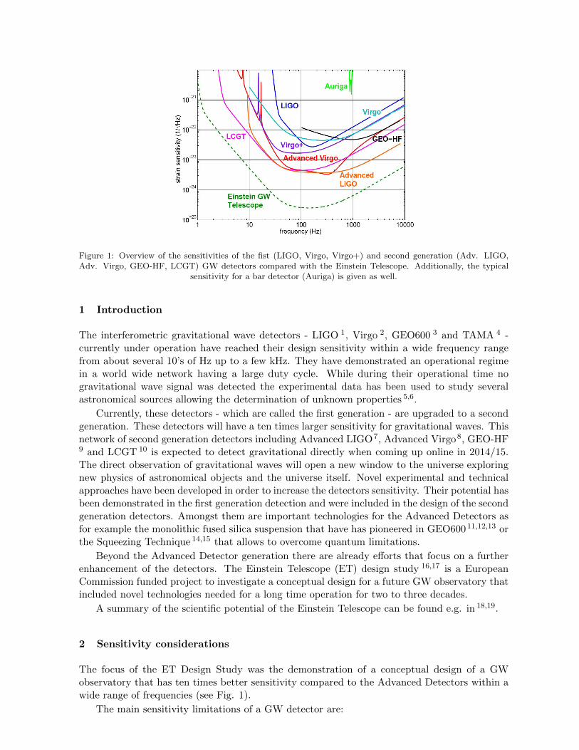
Figure 1: Overview of the sensitivities of the fist (LIGO, Virgo, Virgo+) and second generation (Adv. LIGO,Adv. Virgo, GEO-HF, LCGT) GW detectors compared with the Einstein Telescope. Additionally, the typical
sensitivity for a bar detector (Auriga) is given as well.
1 Introduction
The interferometric gravitational wave detectors - LIGO 1, Virgo 2, GEO600 3 and TAMA 4 -currently under operation have reached their design sensitivity within a wide frequency rangefrom about several 10’s of Hz up to a few kHz. They have demonstrated an operational regimein a world wide network having a large duty cycle. While during their operational time nogravitational wave signal was detected the experimental data has been used to study severalastronomical sources allowing the determination of unknown properties 5,6.
Currently, these detectors - which are called the first generation - are upgraded to a secondgeneration. These detectors will have a ten times larger sensitivity for gravitational waves. Thisnetwork of second generation detectors including Advanced LIGO7, Advanced Virgo8, GEO-HF9 and LCGT 10 is expected to detect gravitational directly when coming up online in 2014/15.The direct observation of gravitational waves will open a new window to the universe exploringnew physics of astronomical objects and the universe itself. Novel experimental and technicalapproaches have been developed in order to increase the detectors sensitivity. Their potential hasbeen demonstrated in the first generation detection and were included in the design of the secondgeneration detectors. Amongst them are important technologies for the Advanced Detectors asfor example the monolithic fused silica suspension that have has pioneered in GEO600 11,12,13 orthe Squeezing Technique 14,15 that allows to overcome quantum limitations.
Beyond the Advanced Detector generation there are already efforts that focus on a furtherenhancement of the detectors. The Einstein Telescope (ET) design study 16,17 is a EuropeanCommission funded project to investigate a conceptual design for a future GW observatory thatincluded novel technologies needed for a long time operation for two to three decades.
A summary of the scientific potential of the Einstein Telescope can be found e.g. in 18,19.
2 Sensitivity considerations
The focus of the ET Design Study was the demonstration of a conceptual design of a GWobservatory that has ten times better sensitivity compared to the Advanced Detectors within awide range of frequencies (see Fig. 1).
The main sensitivity limitations of a GW detector are:
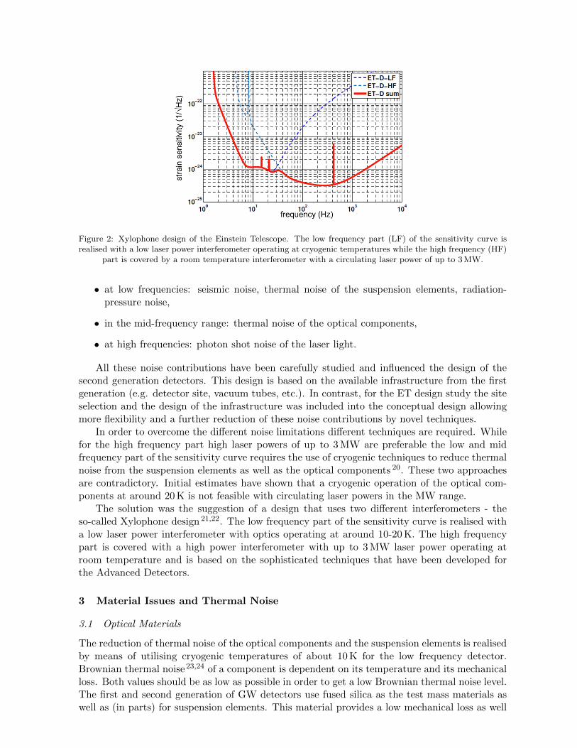
Figure 2: Xylophone design of the Einstein Telescope. The low frequency part (LF) of the sensitivity curve isrealised with a low laser power interferometer operating at cryogenic temperatures while the high frequency (HF)
part is covered by a room temperature interferometer with a circulating laser power of up to 3 MW.
• at low frequencies: seismic noise, thermal noise of the suspension elements, radiation-pressure noise,
• in the mid-frequency range: thermal noise of the optical components,
• at high frequencies: photon shot noise of the laser light.
All these noise contributions have been carefully studied and influenced the design of thesecond generation detectors. This design is based on the available infrastructure from the firstgeneration (e.g. detector site, vacuum tubes, etc.). In contrast, for the ET design study the siteselection and the design of the infrastructure was included into the conceptual design allowingmore flexibility and a further reduction of these noise contributions by novel techniques.
In order to overcome the different noise limitations different techniques are required. Whilefor the high frequency part high laser powers of up to 3 MW are preferable the low and midfrequency part of the sensitivity curve requires the use of cryogenic techniques to reduce thermalnoise from the suspension elements as well as the optical components 20. These two approachesare contradictory. Initial estimates have shown that a cryogenic operation of the optical com-ponents at around 20 K is not feasible with circulating laser powers in the MW range.
The solution was the suggestion of a design that uses two different interferometers - theso-called Xylophone design 21,22. The low frequency part of the sensitivity curve is realised witha low laser power interferometer with optics operating at around 10-20 K. The high frequencypart is covered with a high power interferometer with up to 3 MW laser power operating atroom temperature and is based on the sophisticated techniques that have been developed forthe Advanced Detectors.
3 Material Issues and Thermal Noise
3.1 Optical Materials
The reduction of thermal noise of the optical components and the suspension elements is realisedby means of utilising cryogenic temperatures of about 10 K for the low frequency detector.Brownian thermal noise 23,24 of a component is dependent on its temperature and its mechanicalloss. Both values should be as low as possible in order to get a low Brownian thermal noise level.The first and second generation of GW detectors use fused silica as the test mass materials aswell as (in parts) for suspension elements. This material provides a low mechanical loss as well
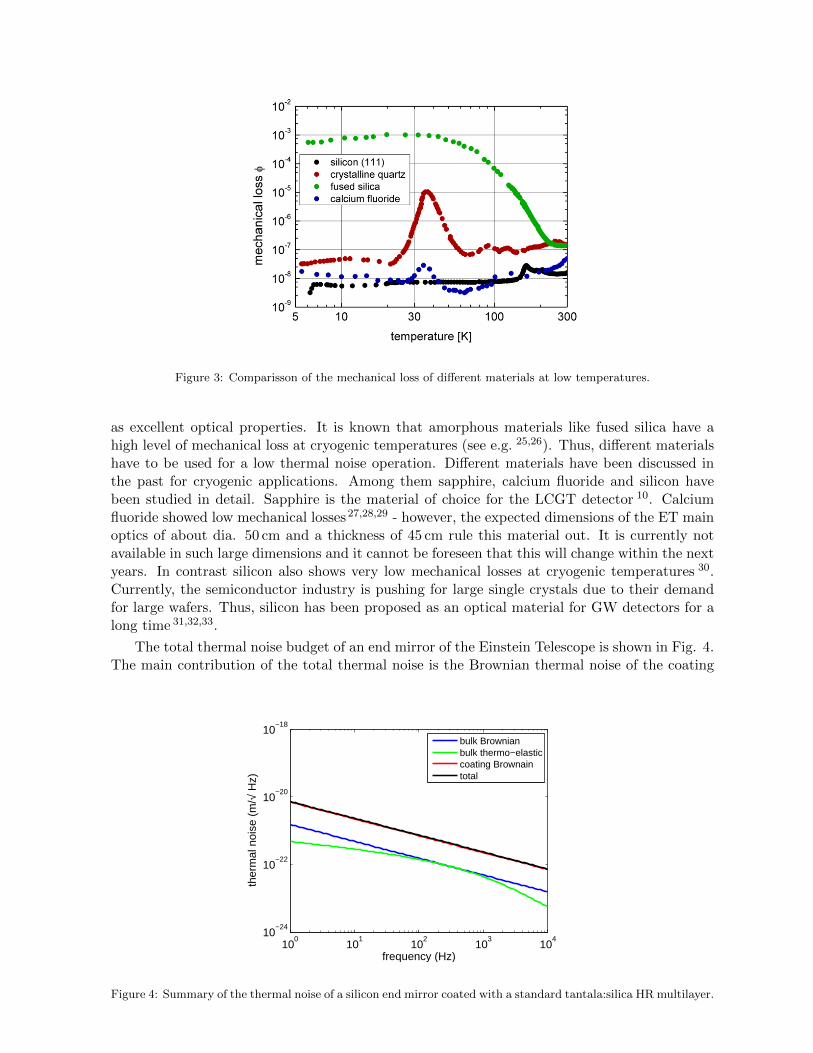
Figure 3: Comparisson of the mechanical loss of different materials at low temperatures.
as excellent optical properties. It is known that amorphous materials like fused silica have ahigh level of mechanical loss at cryogenic temperatures (see e.g. 25,26). Thus, different materialshave to be used for a low thermal noise operation. Different materials have been discussed inthe past for cryogenic applications. Among them sapphire, calcium fluoride and silicon havebeen studied in detail. Sapphire is the material of choice for the LCGT detector 10. Calciumfluoride showed low mechanical losses27,28,29 - however, the expected dimensions of the ET mainoptics of about dia. 50 cm and a thickness of 45 cm rule this material out. It is currently notavailable in such large dimensions and it cannot be foreseen that this will change within the nextyears. In contrast silicon also shows very low mechanical losses at cryogenic temperatures 30.Currently, the semiconductor industry is pushing for large single crystals due to their demandfor large wafers. Thus, silicon has been proposed as an optical material for GW detectors for along time 31,32,33.
The total thermal noise budget of an end mirror of the Einstein Telescope is shown in Fig. 4.The main contribution of the total thermal noise is the Brownian thermal noise of the coating
100
101
102
103
104
10−24
10−22
10−20
10−18
frequency (Hz)
ther
mal
noi
se (
m/√
Hz)
bulk Brownianbulk thermo−elasticcoating Brownaintotal
Figure 4: Summary of the thermal noise of a silicon end mirror coated with a standard tantala:silica HR multilayer.
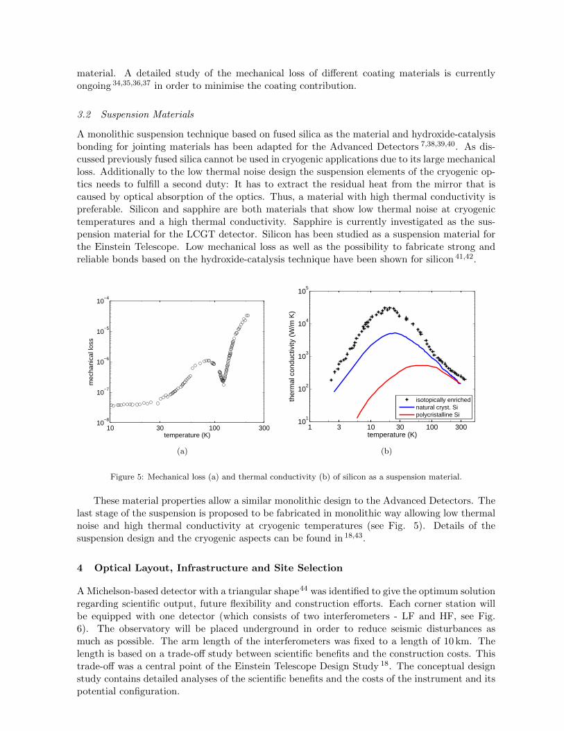
material. A detailed study of the mechanical loss of different coating materials is currentlyongoing 34,35,36,37 in order to minimise the coating contribution.
3.2 Suspension Materials
A monolithic suspension technique based on fused silica as the material and hydroxide-catalysisbonding for jointing materials has been adapted for the Advanced Detectors 7,38,39,40. As dis-cussed previously fused silica cannot be used in cryogenic applications due to its large mechanicalloss. Additionally to the low thermal noise design the suspension elements of the cryogenic op-tics needs to fulfill a second duty: It has to extract the residual heat from the mirror that iscaused by optical absorption of the optics. Thus, a material with high thermal conductivity ispreferable. Silicon and sapphire are both materials that show low thermal noise at cryogenictemperatures and a high thermal conductivity. Sapphire is currently investigated as the sus-pension material for the LCGT detector. Silicon has been studied as a suspension material forthe Einstein Telescope. Low mechanical loss as well as the possibility to fabricate strong andreliable bonds based on the hydroxide-catalysis technique have been shown for silicon 41,42.
10 30 100 30010
−8
10−7
10−6
10−5
10−4
temperature (K)
mec
hani
cal l
oss
(a)
1 3 10 30 100 30010
1
102
103
104
105
temperature (K)
ther
mal
con
duct
ivity
(W
/m K
)
isotopically enrichednatural cryst. Sipolycristalline Si
(b)
Figure 5: Mechanical loss (a) and thermal conductivity (b) of silicon as a suspension material.
These material properties allow a similar monolithic design to the Advanced Detectors. Thelast stage of the suspension is proposed to be fabricated in monolithic way allowing low thermalnoise and high thermal conductivity at cryogenic temperatures (see Fig. 5). Details of thesuspension design and the cryogenic aspects can be found in 18,43.
4 Optical Layout, Infrastructure and Site Selection
A Michelson-based detector with a triangular shape44 was identified to give the optimum solutionregarding scientific output, future flexibility and construction efforts. Each corner station willbe equipped with one detector (which consists of two interferometers - LF and HF, see Fig.6). The observatory will be placed underground in order to reduce seismic disturbances asmuch as possible. The arm length of the interferometers was fixed to a length of 10 km. Thelength is based on a trade-off study between scientific benefits and the construction costs. Thistrade-off was a central point of the Einstein Telescope Design Study 18. The conceptual designstudy contains detailed analyses of the scientific benefits and the costs of the instrument and itspotential configuration.
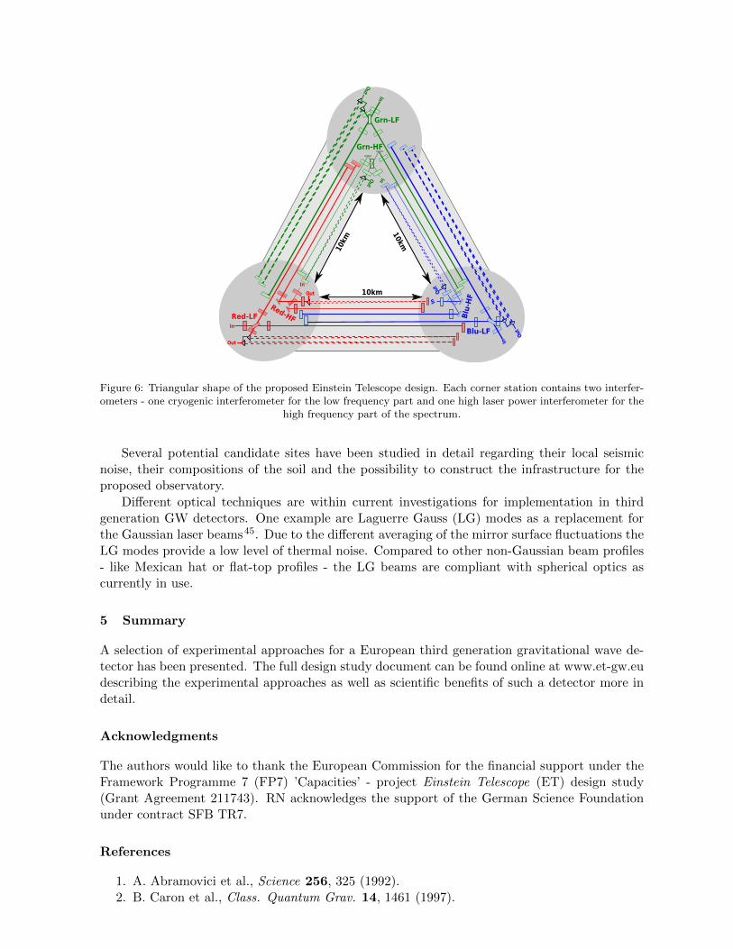
Figure 6: Triangular shape of the proposed Einstein Telescope design. Each corner station contains two interfer-ometers - one cryogenic interferometer for the low frequency part and one high laser power interferometer for the
high frequency part of the spectrum.
Several potential candidate sites have been studied in detail regarding their local seismicnoise, their compositions of the soil and the possibility to construct the infrastructure for theproposed observatory.
Different optical techniques are within current investigations for implementation in thirdgeneration GW detectors. One example are Laguerre Gauss (LG) modes as a replacement forthe Gaussian laser beams45. Due to the different averaging of the mirror surface fluctuations theLG modes provide a low level of thermal noise. Compared to other non-Gaussian beam profiles- like Mexican hat or flat-top profiles - the LG beams are compliant with spherical optics ascurrently in use.
5 Summary
A selection of experimental approaches for a European third generation gravitational wave de-tector has been presented. The full design study document can be found online at www.et-gw.eudescribing the experimental approaches as well as scientific benefits of such a detector more indetail.
Acknowledgments
The authors would like to thank the European Commission for the financial support under theFramework Programme 7 (FP7) ’Capacities’ - project Einstein Telescope (ET) design study(Grant Agreement 211743). RN acknowledges the support of the German Science Foundationunder contract SFB TR7.
References
1. A. Abramovici et al., Science 256, 325 (1992).2. B. Caron et al., Class. Quantum Grav. 14, 1461 (1997).
3. H. Luck and the GEO600 Team, Class. Quantum Grav. 14, 1471 (1997).4. K. Kawabe and the TAMA collaboration, Class. Quantum Grav. 14, 1477 (1997).5. B. Abbott et al., The Astrophysical Journal Letters 683, L45 (2008).6. B. Abbott et al., Nature 460, 990 (2009).7. G. M. Harry and the LIGO Scientific Collaboration, Class. Quantum Grav. 27, 084006
(2010).8. F. Acernese et al., Class. Quantum Grav. 25, 114045 (2008).9. B. Willke et al., Class. Quantum Grav. 23, S207 (2006).
10. K. Kuroda et al., Class. Quantum Grav. 27, 084004 (2010).11. S. Traeger, B. Willke, K. Danzmann, Phys. Lett. A 225, 39 (1997).12. B. W. Barr et al., Class. Quantum Grav. 19, 1655 (2002).13. J. R. Smith et al., Class. Quantum Grav. 21, S1091 (2004).14. C. M. Caves, Phys. Rev. D 23, 1693 (1981).15. R. Schnabel, Nature Physics 4, 440 (2008).16. M. Punturo et al., Class. Quantum Grav. 27, 084007 (2010).17. M. Punturo et al., Class. Quantum Grav. 27, 194002 (2010).18. Einstein Telescope Design Study, available at www.et-gw.eu.19. B. Sathyaprakash et al., Moriond Proceedings 2011.20. S. Hild, S. Chelkowski, A. Freise, arXiv:0810.0604v2 (2008).21. S. Hild, S. Chelkowski, A. Freise, J. Franc, N. Morgado, R. Flaminio, R. DeSalvo, Class.
Quantum Grav. 27, 015003 (2010).22. S. Hild et al., Class. Quantum Grav. 28, 094013 (2011).23. P. R. Saulson, Phys. Rev. D 42, 2437 (1990).24. R. Nawrodt, S. Rowan, J. Hough, M. Punturo, F. Ricci, J.-Y. Vinet, General Relativity
and Gravitation 43, 593 (2010).25. R. E. Strakna, Phys. Rev. 123, 2020 (1961).26. H. J. McSkimin, J. Appl. Phys. 24, 988 (1953).27. P. Amico et al., Class. Quantum Grav. 19, 1663 (2002).28. R. Nawrodt et al., Eur. Phys. J. Appl. Phys. 38, 53 (2007).29. C. Schwarz et al., physica status solidi a DOI: 10.1002/pssa.201127331.30. D. F. McGuigan, C. C. Lam, R. Q. Gram, A. W. Hoffman, D. H. Douglass, H. W. Gutche,
J. Low. Temp. Phys. 30, 621 (1978).31. W. Winkler, K. Danzmann, A. Rudinger, R. Schilling, Phys. Rev. A 44, 7022 (1991).32. S. Rowan et al., Proc. SPIE 4856, (2003).33. S. Rowan, J. Hough, D. R. M. Crooks, Phys. Lett. A 347, 25 (2005).34. I. W. Martin et al., Class. Quantum Grav. 26, 155012 (2009).35. I. W. Martin et al., Class. Qauntum Grav. 27, 225020 (2010).36. R. Flaminio, J. Franc, C. Michel, N. Morgado, L. Pinard, B. Sassolas, Class. Quantum
Grav. 27, 084030 (2010).37. R. Bassiri, K. B. Borisenko, D. J. H. Cockayne, J. Hough, I. MacLaren, S. Rowan, Appl.
Phys. Lett. 98, 031904 (2011).38. S. Rowan, S. M. Twyford, J. Hough, D.-H. Gwo, Phys. Lett. A 246, 471 (1998).39. A. Cumming et al., Class. Quantum Grav. 26, 215012 (2009).40. M. Lorenzini et al., Class. Quantum Grav. 27, 084021 (2010).41. A. A. van Veggel et al., Class. Quantum Grav. 26, 175007 (2009).42. N. L. Beveridge et al., Class. Quantum Grav. 28, 085014 (2011).43. P. Puppo, F. Ricci, General Relativity and Gravitation 43, 657 (2011).44. A. Freise, S. Chelkowski, S. Hild, W. Del Pozzo, A. Perreca, A. Vecchio, Class. Quantum
Grav. 26, 085012 (2009).45. P. Fulda, K. Kokeyama, S. Chelkowski, A. Freise, Phys. Rev. D 82, 012002 (2010).
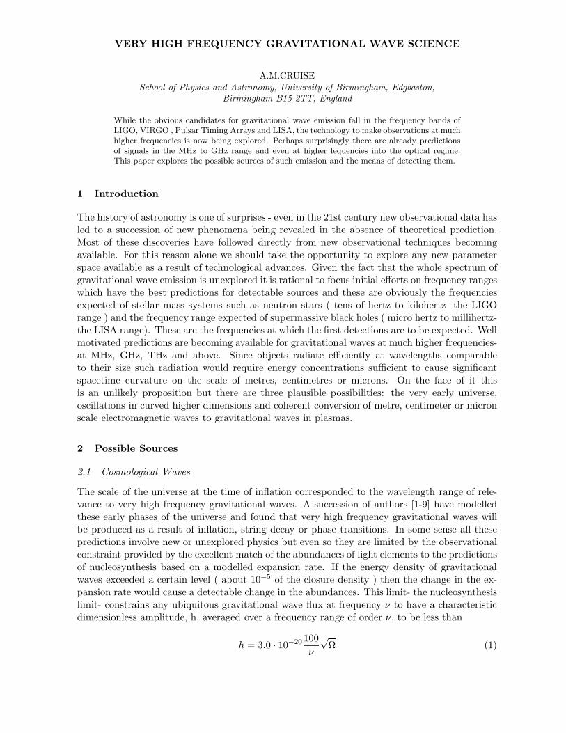
VERY HIGH FREQUENCY GRAVITATIONAL WAVE SCIENCE
A.M.CRUISE
School of Physics and Astronomy, University of Birmingham, Edgbaston,
Birmingham B15 2TT, England
While the obvious candidates for gravitational wave emission fall in the frequency bands ofLIGO, VIRGO , Pulsar Timing Arrays and LISA, the technology to make observations at muchhigher frequencies is now being explored. Perhaps surprisingly there are already predictionsof signals in the MHz to GHz range and even at higher fequencies into the optical regime.This paper explores the possible sources of such emission and the means of detecting them.
1 Introduction
The history of astronomy is one of surprises - even in the 21st century new observational data hasled to a succession of new phenomena being revealed in the absence of theoretical prediction.Most of these discoveries have followed directly from new observational techniques becomingavailable. For this reason alone we should take the opportunity to explore any new parameterspace available as a result of technological advances. Given the fact that the whole spectrum ofgravitational wave emission is unexplored it is rational to focus initial efforts on frequency rangeswhich have the best predictions for detectable sources and these are obviously the frequenciesexpected of stellar mass systems such as neutron stars ( tens of hertz to kilohertz- the LIGOrange ) and the frequency range expected of supermassive black holes ( micro hertz to millihertz-the LISA range). These are the frequencies at which the first detections are to be expected. Wellmotivated predictions are becoming available for gravitational waves at much higher frequencies-at MHz, GHz, THz and above. Since objects radiate efficiently at wavelengths comparableto their size such radiation would require energy concentrations sufficient to cause significantspacetime curvature on the scale of metres, centimetres or microns. On the face of it thisis an unlikely proposition but there are three plausible possibilities: the very early universe,oscillations in curved higher dimensions and coherent conversion of metre, centimeter or micronscale electromagnetic waves to gravitational waves in plasmas.
2 Possible Sources
2.1 Cosmological Waves
The scale of the universe at the time of inflation corresponded to the wavelength range of rele-vance to very high frequency gravitational waves. A succession of authors [1-9] have modelledthese early phases of the universe and found that very high frequency gravitational waves willbe produced as a result of inflation, string decay or phase transitions. In some sense all thesepredictions involve new or unexplored physics but even so they are limited by the observationalconstraint provided by the excellent match of the abundances of light elements to the predictionsof nucleosynthesis based on a modelled expansion rate. If the energy density of gravitationalwaves exceeded a certain level ( about 10−5 of the closure density ) then the change in the ex-pansion rate would cause a detectable change in the abundances. This limit- the nucleosynthesislimit- constrains any ubiquitous gravitational wave flux at frequency ν to have a characteristicdimensionless amplitude, h, averaged over a frequency range of order ν, to be less than
h = 3.0 · 10−20100
ν
√
Ω (1)
For frequencies in the range 1 GHz to 1015 Hz, this gives an upper limit on dimensionlessamplitudes of between 10−30 and 10−35 - extremely challenging signals to detect.
2.2 Higher Dimensional Gravity
The well known problem of incorporating gravity into a quantum field theory has led to seriousinvestigation of the properties of higher dimensional spaces, prompted in part by the Kaluza-Klein calculations linking electromagnetism and gravitation. Considering the observable fourdimensional manifold as a brane embedded in a higher dimensional space, models of black holeson the brane have been developed requiring two branes for reasons of stability. Stellar mass sizedcompact objects falling into such a black hole generate the expected gravitational waves in thebrane at the (low) frequencies related to the orbital motion as in four dimensional gravity. Anadditional feature found by Seahra and Clarkson [10-11] is the stimulation of gravitational modesin the fifth dimension, the dimension separating the two branes. The amplitudes predicted fromsuch an interaction at our galactic centre are large- dimensionless amplitudes of 10−18 , againaveraged over a bandwidth of order the observed frequency. Such amplitudes are within therange of possible detectors currently being commissioned at GHz and optical frequencies. Whilethere is no doubt that such a source mechanism is highly speculative in the absence of firmevidence that we do inhabit a five dimensional universe, the ability to probe the existence ofpossible extra dimensions is a rare experimetal opportunity worth exploring.
2.3 Plasma conversion of intense electromagnetic waves to gravitation modes
Servin and Brodin [12] have shown that the presence of a magnetised plasma can improvethe coupling between electromagnetic and gravitational wave modes. For plasmas magnetisedby a static field parallel to an intense incoming electromagnetic wave an instability developesin which the generation of gravitational waves is theoretically limited by the available freeenergy of the plasma. In extreme astrophysical situations-AGN jets, SS433, GRB’s, for example,this could represent a substantial source of gravitational wave energy at the frequency of theelectromagnetic wave. Higher frequencies are more effective, well above the plasma and hybridfrequency, because the phase velocity of the electromagnetic wave will be closer to that of thegravitational wave allowing phase coherence over larger pathlengths. Observations at radioor optical frequencies can already identify sources with suitable geometry and electromagneticstimulus.
Perhaps surprisingly then, there are possible mechanisms for generating gravitational wavesat very high frequencies despite the most obvious sources being at very much longer wavelengths.The important issue is whether there are detectors at these high frequencies of sufficient sensitiv-ity. An interesting parallel may be noticed with the 1960’s when the only X-Ray source detectedin the universe was thermal X-Ray emission from the Sun, an emission process which, if placedat the distance of the nearest local stars, would have been undetectable. However, simple spaceinstruments easily detected the unpredicted X-Rays from local neutron stars (Sco-X1) and blackholes (Cyg-X1) because they were radiating via a different mechanism.
3 Possible Detectors
The sophistication and sensitivity of laser interferometers is remarkable and these instruments, on the ground or in space, seem likely to achieve the first detections. Such instruments can beconfigured to work at very high frequency as Akutsu and Kawamura [13-14] have shown, withsensitivities in averaged dimensionless amplitude of order 10−17 being achieved at 100 MHz.However, the minimum detectable signal of an interferometer increases as ν
1/2 with the operat-ing frequency ν and this may preclude such instruments from being competitive at the higher
frequencies, essentially due to the photon statistics from current lasers being inadequate at suchhigh frequencies. A more direct method of detecting very high frequency gravitational waves isto use a static electromagnetic field to convert the gravitational wave to an electromagnetic waveat the same frequency and travelling in the same direction, a process described by Gershenstein[15-18] and many others. Provided the generated electromagnetic wave has the same phasevelocity as the incoming gravitational wave over a path length of N wavelengths, the powerconverted to an electromagnetic wave is given by
P =π
2B
2N
2h
2c
2µ0
(2)
where B is the perpendicular, static magnetic field, h is the dimensionless amplitude of thegravitational wave, µ0 is the permeability of free space and c is the velocity of light. Onceconverted to an electromagnetic wave, the signal can be detected by the normal range of electro-magnetic detectors, depending on the frequency. One interesting feature of such a detector is thefact that the full range of electromagnetic technology becomes available to improve sensitivity,wavelength resolution or angular response and techniques such as aperture synthesis are nowbeing explored by a collaboration between groups at the University of Birmingham and JodrellBank.
4 Current Status
The prototype detector at the University of Birmingham operates at two frequency ranges, 14GHz and 3.1014
−1015 Hz using the same magnetic field volume which is approximately one metrelong and a few square centimetres cross section. The sensitivity is very strongly constrained tothe long axis of the magnetic field volume and therefore the detector is constructed on anequatorial mount which permits continuous pointing at selected astronomical objects. A secondprototype is being constructed with a similar geometry to carry out an all-sky scan over aperiod of six months. The graph below shows the current and future expected sensitivity ofsuch detectors at microwave and optical frequencies in comparison to predicted gravitationalwave signals. As equation 2 indicates the converted signal power is proportional to the squareof the magnetic field and current facilities can provide fields between 0.2T and 40T. Highersensitivity would come from higher magnetic fields but there is no immediate prospect of verysubstantial increases in this parameter. Sensitivity improvements are likely with the use ofcryogenic front end amplifiers to reduce thermal noise, correlating co-located detectors whichexperience the same signal but uncorrelated thermal noise and building detectors with a largercollecting area. These steps are planned in the form of a two element interferometer to be basedat Jodrell Bank.
Acknowledgments
The author is grateful for support from the Science and Technology Facilities Council in theUK.
Statement
The work presented here has no connection with publications by the HFGW group in the USand China.
104
106
108
1010
1012
1014
1016
10−40
10−35
10−30
10−25
10−20
10−15
10−10
Frequency, Hz
Dim
ensi
onle
ss A
mpl
itude
KK Modes: GalacticCentre: Shadow Brane
KK Modes: GalacticCentre: Visible Brane
Cosmological Models
Nuleosynthesis Limit
B
A
C
D
Figure 1: Possible source dimensionless amplitudes, averaged over bandwidths of the same order as the observingfrequency. Detector sensitivities: A: Current 14 GHz system, B: Current optical system, C: Planned cryogenic
detector at 5GHz, D: Planned two element interferometer based on C
References
1. Grischuk L P JETP Letts23 293, 19762. Giovannini M Phys Rev D60 123511, 19993. Gasperini M and Veneziano G CERN-TH 2002-104, 20024. Garcia-Bellido and Feguira Class Quantum Grav 22 s155, 20005. Easther R, Giblin J T and Lim E A, Phys Rev Letts99 221301, 20076. Caprini C, Durrer R, Konstandin T and Servant G Phys Rev D 79, 083519, 20097. Copeland E J, Mulryne D J ,Nunes N J and Shaeri, M Phys Rev D 79, 023508, 20098. Caldwell R R, Battye R A and Shellard E P S Phys Rev D54 7146, 19969. Leblond l,Shlaer B and Siemens X Phys Rev D79,123519, 200910. Seahra S S, Clarkson C and Maartens R Phys Rev Letts94 121302, 200511. Clarkson C and Seahra S S Class Quantum Grav24 F33, 200712. Servin M and Brodin G Phys Rev D68, 044017, 200313. Akutsu T, Kawamura S, Nishizawa A, Arai K, Yamamoto K, Tatsumi D, Nagano S,
Nishida E, Chiba T, Takahashi N, Sugiyama N, Fukushima M, Yamazaki T and FujimotoM-K Phys Rev Letts101, 101101, 2008
14. Nishizawa A, Kawamura S, Akutsu T, Arai K, Yamamoto K, Tatsumi D, Nishida E,Sakagami M-a, Chiba T, Takahashi R, and Sugiyama N Phys Rev D77, 022002, 2008
15. Gertsenshtein M E Sov Phys JETP14 No 1, 84, 196216. Lupanov G A Sov Phys JETP25 No 1 76, 196717. Boccaletti D, De Sabbata V, Fortini P and Gualdi Nuovo Cimento70 B No 2, 129, 197018. De Logi W K and Mickelson A R Phys Rev D16 No 10, 2915, 1977
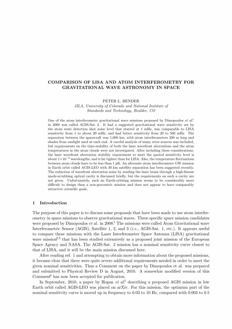
COMPARISON OF LISA AND ATOM INTERFEROMETRY FOR
GRAVITATIONAL WAVE ASTRONOMY IN SPACE
PETER L. BENDER
JILA, University of Colorado and National Institute ofStandards and Technology, Boulder, CO
One of the atom interferometer gravitational wave missions proposed by Dimopoulos et al.1
in 2008 was called AGIS-Sat. 2. It had a suggested gravitational wave sensitivity set bythe atom state detection shot noise level that started at 1 mHz, was comparable to LISAsensitivity from 1 to about 20 mHz, and had better sensitivity from 20 to 500 mHz. Theseparation between the spacecraft was 1,000 km, with atom interferometers 200 m long andshades from sunlight used at each end. A careful analysis of many error sources was included,but requirements on the time-stability of both the laser wavefront aberrations and the atomtemperatures in the atom clouds were not investigated. After including these considerations,the laser wavefront aberration stability requirement to meet the quoted sensitivity level isabout 1×10⁻⁸ wavelengths, and is far tighter than for LISA. Also, the temperature fluctuationsbetween atom clouds have to be less than 1 pK. An alternate atom interferometer GW missionin Earth orbit called AGIS-LEO with 30 km satellite separation has been suggested recently.The reduction of wavefront aberration noise by sending the laser beam through a high-finessemode-scrubbing optical cavity is discussed briefly, but the requirements on such a cavity arenot given. Unfortunately, such an Earth-orbiting mission seems to be considerably moredifficult to design than a non-geocentric mission and does not appear to have comparablyattractive scientific goals.
1 Introduction
The purpose of this paper is to discuss some proposals that have been made to use atom interfer-ometry in space missions to observe gravitational waves. Three specific space mission candidateswere proposed by Dimopoulos et al. in 2008.1 The missions were called Atom Gravitational waveInterferometric Sensor (AGIS), Satellite 1, 2, and 3 (i.e., AGIS-Sat. 1, etc.). It appears usefulto compare these missions with the Laser Interferometer Space Antenna (LISA) gravitationalwave mission2,3 that has been studied extensively as a proposed joint mission of the EuropeanSpace Agency and NASA. The AGIS-Sat. 2 mission has a nominal sensitivity curve closest tothat of LISA, and it will be the main mission discussed here.
After reading ref. 1 and attempting to obtain more information about the proposed missions,it became clear that there were quite severe additional requirements needed in order to meet thegiven nominal sensitivities. Thus a Comment on the paper by Dimopoulos et al. was preparedand submitted to Physical Review D in August, 2010. A somewhat modified version of thisComment4 has now been accepted for publication.
In September, 2010, a paper by Hogan et al.5 describing a proposed AGIS mission in lowEarth orbit called AGIS-LEO was placed on arXiv. For this mission, the optimum part of thenominal sensitivity curve is moved up in frequency to 0.03 to 10 Hz, compared with 0.003 to 0.5
Hz for AGIS-Sat. 2, and the sensitivity is about a factor 20 worse. The main orbit geometryconsidered was a leader-follower configuration on a circular orbit at nearly constant altitude.
The proposed AGIS-Sat. 2 mission and the requirements to meet its sensitivity goals will bedescribed in Section 2. This will be followed by a discussion of the proposed AGIS-LEO missionin Section 3. Then, a brief comparison with the requirements of LISA will be given in Section4.
2 AGIS-Sat. 2 Mission
In ref. 1, each of the three space missions proposed was assumed to make use of short sequencesof laser pulses at three different times separated by times T to carry out the atom interferometry.Satellites at each end of a path of length L would prepare atom clouds with temperatures of100 pK and send them out at a rate of one per second along the path. Pulsed laser beams fromone end would provide the light pulses for the atom interferometry, and a continuous laser beamfrom the other end would provide the phase reference needed to permit correlation of the resultsobtained by the atom interferometers at the two ends.
The proposals for AGIS-Sat. 2 and AGIS-Sat. 3 assumed times T between the three pulsesequences of 100 s, atom interferometer path lengths of 100 to 200 m at each end, and a differenceof 200 to 400 photon momenta between momenta transferred to the two split parts of the atomwavefunctions by the first of the short laser pulse sequences. However, a factor 10 larger valuefor the distance L between satellites was assumed for AGIS-Sat. 3, and a factor 10 better phasesensitivity for detecting differences in the atom populations in two ground-state sublevels at theend of each atom interferometer, leading to about a factor 50 better nominal gravitational wavesensitivity than for AGIS-Sat. 2.
In ref. 4, the proposal for AGIS-Sat. 3 was considered. However, ref. 1 says that AGIS-Sat.3 “is an aggressive possibility that might be realizable in the future.” Since the sensitivity forAGIS-Sat. 2 is comparable with that for LISA from about 1 to 20 mHz, and since AGIS-Sat. 3appears to be much more difficult to implement, attention will be focused on the AGIS-Sat. 2proposal in this paper. For AGIS-Sat. 1, the nominal gravitational wave sensitivity is a factorof roughly 20 worse than for AGIS-Sat. 2 down to about 0.03 Hz, and much worse at lowerfrequencies. Whether there is a science justification for such a mission appears to be uncertain.
It is stated clearly in ref. 1 that the nominal gravitational wave sensitivities given are onlythose due to the statistical uncertainties in atom sublevel populations determined at the endsof the atom interferometers. A large number of other error sources are considered, but noneare estimated to exceed the statistical uncertainties. However, two additional error sources thatwere not considered are the subject of ref. 4. The first of these is laser wavefront aberrationvariations over periods of 1 to 200 s. For a number of error sources considered in ref. 1, thereis a strong cancellation of the errors because they are closely the same for the atoms in the twoatom interferometers. For example, the effect of laser phase noise at fairly low frequencies isreduced because the travel time between the two interferometers separated by 1000 km is only0.003 s. However, this is not true for laser wavefront aberrations.
The expected size of the atom clouds is considerably less than the suggested telescope diam-eter of roughly 1 m for AGIS-Sat. 2. And there will be a substantial reduction in the amplitudeof the wavefront aberrations over the 1000 km path length. An estimate similar to that madein ref. 4 based on primary spherical aberrations indicates that such aberration variations wouldneed to be kept down to 1x10⁻⁸ wavelengths in order to keep the gravitational wave noise fromthis source down to that from the statistical atom state sensing noise.
The second additional error source is fluctuations from cloud to cloud in the atom cloudtemperatures. For 0.001 wavelength of dc primary spherical aberration in the initially transmit-ted laser beam, fluctuations of only 1 pK in the atom cloud temperature from cloud to cloud
would substantially increase the gravitational wave noise level.
3 AGIS-LEO proposal
The proposal in ref. 5 for a mission called AGIS-LEO was quite different. To reduce some of theeffects of being in Earth orbit, the baseline length between the satellites was reduced to 30 kmand the time interval T between the different short sets of laser pulses applied to the atoms wasreduced to 4 s. In addition, the use of five short sets of pulses instead of three and operationat 1,000 km altitude are assumed. The disturbing effects are mainly gradients in the Earth’sgravity field and the Coriolis force.
Although the suggested gravitational wave sensitivity for AGIS-LEO is about a factor 20worse than for AGIS-Sat. 2, the requirement on the laser wavelength aberration fluctuationsis slightly tighter because of the satellite separation being only 30 km. The use of a high-finesse mode-scrubbing cavity is discussed, but no estimate of the possible level of wavefrontaberration noise from a suitable laser is given, and corresponding requirements on the filtercavity performance are not considered. The conceptual design shown for a single AGIS-LEOtelescope is a 30 cm diameter off-axis Gregorian system, and 1 W of laser power is assumed.
The possible use of a pinhole spatial filter at the real intermediate focus of the telescope toeliminate wavefront errors from all optics and lasers before the primary mirror is mentioned.However, in view of the suggested laser beam waist size of 10 cm and the 30 cm telescopediameter, careful apodization of the beam from the telescope appears to be needed in order toreduce the amplitude of near-field diffraction ripples, which would affect the atom clouds in thenear interferometer differently than those in the far interferometer.
For the laser wavefront aberration noise, some information is available on the fluctuations inwavefront tilt6 from a set of 8 lasers similar to those that might be used in the Advanced LIGOprogram. These lasers had roughly 2 W of output power, and similar ones may be used as themaster lasers in the laser amplifier or injection-lock configurations needed to get the requiredhigh input power for Advanced LIGO. The relative pointing fluctuations for the lasers weremeasured at frequencies down to 1 Hz, and were much higher at that frequency than at 3 Hz.
In the AGIS-LEO proposal, a possible alternative interferometer laser beam geometry isdiscussed. In this approach, the atom optics laser beams can be made to first propagate betweentwo satellite stations along a path that is displaced from the atoms before being redirected tointeract with the atoms. As a consequence, the first propagation segment would serve as aspatial filter, allowing high frequency wavefront noise to diffract out of the beam. It is suggestedthat “If needed, this alternative beam geometry could be used in conjunction with a mode-scrubbing cavity.” However, for the longer wavelength wavefront aberrations such as variationsin wavefront curvature, it appears that a substantial reduction in aberration amplitude wouldalso lead to a significant reduction in the laser power.
Because of the reduction in the time T between short sequences of laser pulses for AGIS-LEO,the tight requirement on the temperature differences between the atom clouds in the two atominterferometers is removed. However, this requirement is replaced by a very tight requirementon the fluctuations in mean radial velocity for the clouds of 10 nm/s. This requirement comesfrom item 12 in Table IV of ref. 5, and involves the Earth’s gravity gradient and the satelliteorbital frequency, plus a factor T
4. It is stated that such requirements could be relaxed by amoderate reduction in T , but there would be some reduction in the measurement bandwidthalso.
In Fig. 4 of ref. 5, signal strength curves are shown for four types of gravitational wavesources. One of these is white dwarf binaries at 10 kpc distance. However, such binaries wouldonly be detectable by AGIS-LEO at frequencies above about 0.03 Hz, and it is not clear thatthere are likely to be any white dwarf binaries currently in the galaxy at frequencies higher than
this. The other types of sources shown are inspirals of one solar mass black holes into 103 or105 solar mass black holes at distances of up to 10 Mpc, but the expected rates for such eventsis very low. Thus it does not appear that there is a substantial scientific case for such a missionbased on gravitational wave detection.
A secondary objective for AGIS-LEO that is mentioned in ref. 5 is the determination of timevariations in the Earth’s gravity field. The GRACE satellite mission currently is monitoring suchvariations, but is near the end of its life. The next mission after GRACE probably will still flyat roughly 500 km altitude, but later missions with fairly simple drag-free systems are expectedto fly at about 300 km altitude. This is because of the importance of monitoring time variationsin the higher harmonics of the Earth’s field, and thus of obtaining higher spatial resolution.The 1,000 km altitude for AGIS-LEO would be a substantial limitation, since for degree 100harmonics the attenuation of the signal at that altitude would be a factor 20,000 higher than at300 km altitude.
4 Comparison of the LISA and AGIS-Sat. 2 Missions
A major difference between the LISA and AGIS-Sat. 2 missions is in the degree of complexity.For LISA, one of the two main mechanical requirements is to be able to clamp the test massesduring launch, and then release them reliably later. The other, because of LISA needing tohave at least two interferometer arms, is to be able to change the angle between the two op-tical assemblies sending beams along the arms smoothly over about a degree range during theyear. These are quite standard engineering design requirements. For laser interferometry, therequirement of about 2 × 10⁻⁵ wavelength/
√Hz accuracy in measuring distance changes down
to about 1 mHz does not come close to the state of the art at all, and the only challenge is toaccomplish this reliably over the whole mission lifetime with fairly simple hardware.
For AGIS-Sat. 2, even without the additional requirements discussed earlier, there are manymore and more challenging requirements. For example, 108 atom clouds have to be preparedand cooled to 100 pK temperature at a rate of one cloud per second. The clouds then haveto be moved 30 m or more from the satellite, placed along the axis of the laser beams, andsent off accurately along the desired path. The velocities have to be different for the differentclouds in order to permit them to be interrogated separately. And the population ratios of theatom ground-state sublevels have to be determined to 1 × 10⁻⁴ accuracy up to more than 100m from the spacecraft. No sketch of what a satellite capable of accomplishing this might looklike appears to have been presented so far in descriptions of the proposed mission.
There also appears to be a problem with the 200 atom clouds assumed to be simultaneouslyin each interferometer. If sequences of Bragg and/or Raman pulses are used to apply 100 unitsof photon momentum to each part of the atom wavefunction, with 1 W of laser power and 1m diameter telescopes, and the stimulated Rabi frequency is 100 Hz, the spontaneous emissionrate for the atoms appears to be too high. The possibility of operating about 10 concurrentinterferometers is stated in Section V A 3 of ref. 5, but it isn’t clear that 200 clouds can behandled simultaneously for the set of parameters assumed for AGIS-Sat. 2, unless there hasbeen an error in understanding the calculations.
For the additional requirement on reducing laser wavefront aberration noise, it is not clear ifthe impact on the design of the satellites would be substantial. In principle, a fairly small filtercavity could do what is needed if the aberration noise level of roughly 1 W lasers is low. Otheraberrations besides wavefront tilt that may be important are variations in wavefront curvatureand beam center displacements. The laser power would only be a consideration if the finesseneeded is fairly high.
The wavefront aberration noise requirement for AGIS-Sat. 2 is much tighter than for LISAbecause of the far shorter baseline between satellites. For the statistical limit on sensitivity
from the atom sublevel measurements, the very short de Broglie wavelength of the atoms is therelevant length scale. However, when laser beams between spacecraft are used to provide thereference for gravitational wave sensing, the laser wavelength becomes an important scale forsystematic measurement limitations. Even for possible LISA satellite separations as short as1× 106 km, the AGIS-Sat. 2 baseline is a factor 1,000 shorter, and the sensitivity to wavefrontaberration noise would be increased by this factor
For the requirement on the atom cloud temperature variations, it seems difficult to see asolution other than reducing the time T substantially or developing methods for extremely pre-cise control of cloud temperatures. In Section IV B 5 of ref. 5, it is suggested that “Spatiallyresolved detection of the atom cloud can help mitigate the wavefront requirements that resultfrom spatially averaging.” However, even with an extra requirement for measurement of the atomspatial distribution, this wouldn’t help with determining fluctuations in the atom cloud temper-ature, since such measurements would be made only at the time of atom sublevel populationdetermination.
In the Introduction to ref. 1, it is stated that the use of atom interferometry “leads to anatural reduction in many systematic backgrounds, allowing such an experiment to reach sensi-tivities comparable to and perhaps better than LISA’s with reduced engineering requirements.”But, in fact, nothing in that paper or in ref. 5 supports that claim.
References
1. Dimopoulos, S., et al., Phys. Rev. D 78, 122002 (2008).2. Danzmann, K., & Ruediger, A., Class. & Quantum Grav. 20, S1 (2003).3. Bender, P. L., in: S. A. Klioner, P. K. Seidelmann, & M. H. Soffel, (eds.), Proc. IAU Symp
261, Relativity in Fundamental Astronomy, (Cambridge) 240-248 (2010).4. Comment: Atomic gravitational wave interferometric sensor, Phys. Rev. D. (accepted),
(2011).5. Hogan, J. M., et al., An atomic gravitational wave interferometric sensor in low Earth
orbit (AGIS-LEO), arXiv:1009.2702v1, 14 Sep (2010).6. Kwee, P., & Willke, B., Applied Optics 47, 6022 (2008).

REALISATION OF THE ALIGO FUSED SILICA SUSPENSION
A. S. BELL1, A. V. CUMMING1, G. D. HAMMOND1, A. HEPTONSTALL2, W. CUNNINGHAM1, A.A. VAN VEGGEL1, R. JONES1, K. A. STRAIN1, J. HOUGH1, S. ROWAN1
1SUPA, Institute for Gravitational Research, School of Physics and Astronomy, University of Glasgow,Glasgow G12 8QQ, Scotland
2LIGO Laboratory, California Institute of Technology, Pasadena, California 91125, USA
The planned upgrade for the LIGO gravitational wave detectors (Advanced LIGO) has beenunderway for a number of years. One of the most significant aspects of this upgrade is the useof all-fused-silica pendulums to reduce thermal noise. The test mass mirrors, made from fusedsilica, will each be suspended using four fused silica fibres from a fused silica isolation mass.The fibres are welded in place using a CO2 laser. We describe the realisation of a workingprototype suspension at the LIGO Advanced Systems Test Interferometer (LASTI) facility.
1 Introduction
The suspension design for the Advanced LIGO (aLIGO) interferometers is based on that usedin the UK-German GE600 gravitational wave detector 1, but adapted to the requirements ofaLIGO 2. As shown in Figure 1, it consists of four masses, the upper two of which are madefrom steel and suspended by wires from maraging steel blade springs 3. The lower two stages ofthe suspension consist of synthetic fused silica pieces which are 340 mm in diameter, 200 mmthick and each has a mass of 40 kg. The test mass is suspended by 4 fused silica fibres from thepenultimate mass. The fibres are welded at both ends to silica attachment points (known asears) that are hydroxide-catalysis bonded to the masses4. One can minimise thermoelastic noisecaused by temperature fluctuations close to the bending point, by choosing the fibre dimensionsin that region such that there is a cancellation between the noise terms originating from thethermal expansion coefficient and the combination of applied stress with the change in Young’smodulus with temperature 5.
2 Fibre production
The silica fibres are drawn from 3 mm diameter fused silica stock using a laser heating method6.A copy of the original Glasgow designed machine was constructed at the LASTI facility at MIT
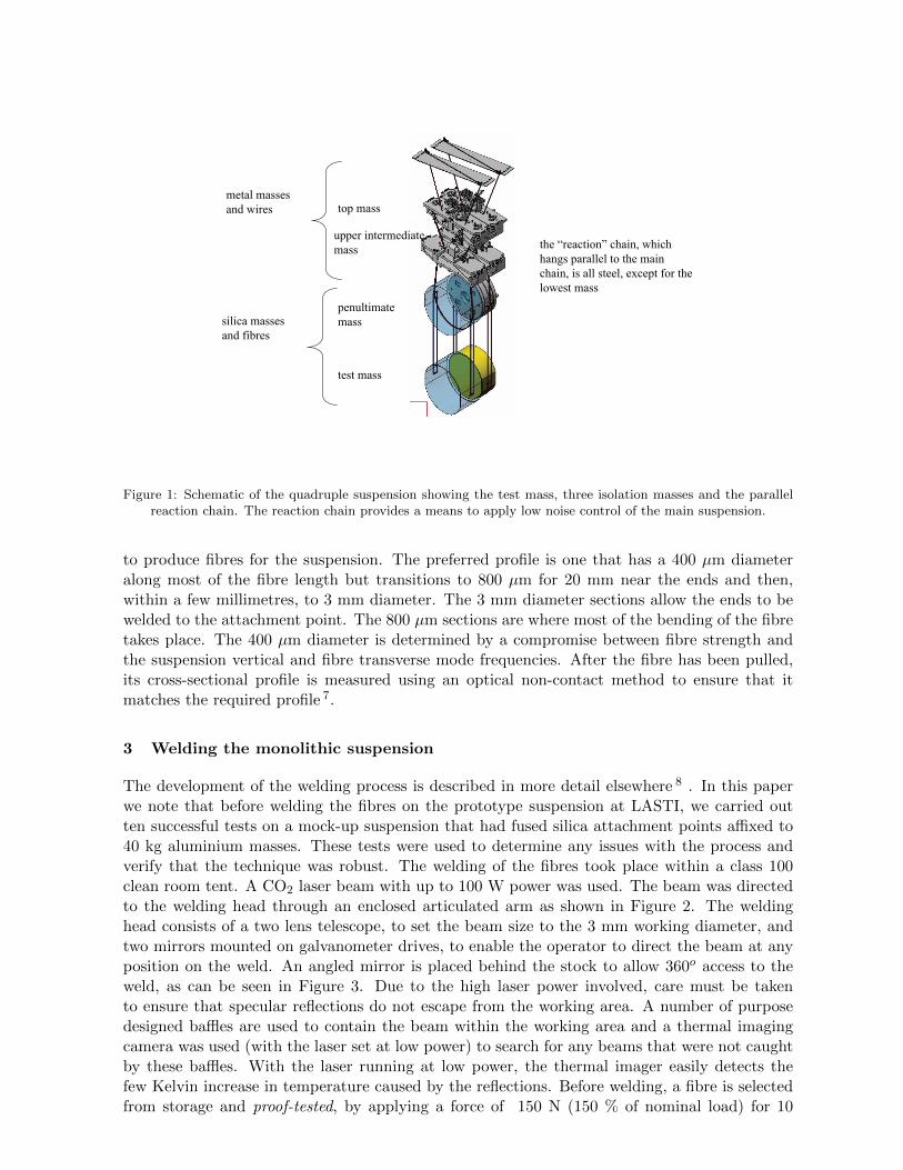
silica masses and fibres
metal masses and wires
the “reaction” chain, which hangs parallel to the main chain, is all steel, except for the lowest mass
penultimate mass
test mass
upper intermediate mass
top mass
Figure 1: Schematic of the quadruple suspension showing the test mass, three isolation masses and the parallelreaction chain. The reaction chain provides a means to apply low noise control of the main suspension.
to produce fibres for the suspension. The preferred profile is one that has a 400 µm diameteralong most of the fibre length but transitions to 800 µm for 20 mm near the ends and then,within a few millimetres, to 3 mm diameter. The 3 mm diameter sections allow the ends to bewelded to the attachment point. The 800 µm sections are where most of the bending of the fibretakes place. The 400 µm diameter is determined by a compromise between fibre strength andthe suspension vertical and fibre transverse mode frequencies. After the fibre has been pulled,its cross-sectional profile is measured using an optical non-contact method to ensure that itmatches the required profile 7.
3 Welding the monolithic suspension
The development of the welding process is described in more detail elsewhere 8 . In this paperwe note that before welding the fibres on the prototype suspension at LASTI, we carried outten successful tests on a mock-up suspension that had fused silica attachment points affixed to40 kg aluminium masses. These tests were used to determine any issues with the process andverify that the technique was robust. The welding of the fibres took place within a class 100clean room tent. A CO2 laser beam with up to 100 W power was used. The beam was directedto the welding head through an enclosed articulated arm as shown in Figure 2. The weldinghead consists of a two lens telescope, to set the beam size to the 3 mm working diameter, andtwo mirrors mounted on galvanometer drives, to enable the operator to direct the beam at anyposition on the weld. An angled mirror is placed behind the stock to allow 360o access to theweld, as can be seen in Figure 3. Due to the high laser power involved, care must be takento ensure that specular reflections do not escape from the working area. A number of purposedesigned baffles are used to contain the beam within the working area and a thermal imagingcamera was used (with the laser set at low power) to search for any beams that were not caughtby these baffles. With the laser running at low power, the thermal imager easily detects thefew Kelvin increase in temperature caused by the reflections. Before welding, a fibre is selectedfrom storage and proof-tested, by applying a force of 150 N (150 % of nominal load) for 10
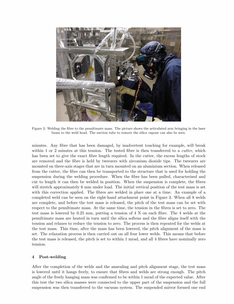
Figure 2: Welding the fibre to the penultimate mass. The picture shows the articulated arm bringing in the laserbeam to the weld head. The suction tube to remove the silica vapour can also be seen.
minutes. Any fibre that has been damaged, by inadvertent touching for example, will breakwithin 1 or 2 minutes at this tension. The tested fibre is then transferred to a cutter, whichhas been set to give the exact fibre length required. In the cutter, the excess lengths of stockare removed and the fibre is held by tweezers with zirconium dioxide tips. The tweezers aremounted on three-axis stages that are in turn mounted on an aluminium section. When releasedfrom the cutter, the fibre can then be transported to the structure that is used for holding thesuspension during the welding procedure. When the fibre has been pulled, characterised andcut to length it can then be welded in position. When the suspension is complete, the fibreswill stretch approximately 6 mm under load. The initial vertical position of the test mass is setwith this correction applied. The fibres are welded in place one at a time. An example of acompleted weld can be seen on the right-hand attachment point in Figure 3. When all 8 weldsare complete, and before the test mass is released, the pitch of the test mass can be set withrespect to the penultimate mass. At the same time, the tension in the fibres is set to zero. Thetest mass is lowered by 0.25 mm, putting a tension of 4 N on each fibre. The 4 welds at thepenultimate mass are heated in turn until the silica softens and the fibre aligns itself with thetension and relaxes to reduce the tension to zero. The process is then repeated for the welds atthe test mass. This time, after the mass has been lowered, the pitch alignment of the mass isset. The relaxation process is then carried out on all four lower welds. This means that beforethe test mass is released, the pitch is set to within 1 mrad, and all 4 fibres have nominally zerotension.
4 Post-welding
After the completion of the welds and the annealing and pitch alignment stage, the test massis lowered until it hangs freely, to ensure that fibres and welds are strong enough. The pitchangle of the freely hanging mass was confirmed to be within 1 mrad of the expected value. Afterthis test the two silica masses were connected to the upper part of the suspension and the fullsuspension was then transferred to the vacuum system. The suspended mirror formed one end
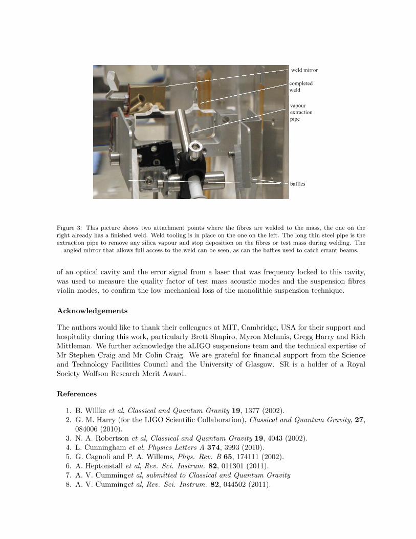
weld mirror
vapour extraction pipe
baffles
completed weld
Figure 3: This picture shows two attachment points where the fibres are welded to the mass, the one on theright already has a finished weld. Weld tooling is in place on the one on the left. The long thin steel pipe is theextraction pipe to remove any silica vapour and stop deposition on the fibres or test mass during welding. The
angled mirror that allows full access to the weld can be seen, as can the baffles used to catch errant beams.
of an optical cavity and the error signal from a laser that was frequency locked to this cavity,was used to measure the quality factor of test mass acoustic modes and the suspension fibresviolin modes, to confirm the low mechanical loss of the monolithic suspension technique.
Acknowledgements
The authors would like to thank their colleagues at MIT, Cambridge, USA for their support andhospitality during this work, particularly Brett Shapiro, Myron McInnis, Gregg Harry and RichMittleman. We further acknowledge the aLIGO suspensions team and the technical expertise ofMr Stephen Craig and Mr Colin Craig. We are grateful for financial support from the Scienceand Technology Facilities Council and the University of Glasgow. SR is a holder of a RoyalSociety Wolfson Research Merit Award.
References
1. B. Willke et al, Classical and Quantum Gravity 19, 1377 (2002).2. G. M. Harry (for the LIGO Scientific Collaboration), Classical and Quantum Gravity, 27,
084006 (2010).3. N. A. Robertson et al, Classical and Quantum Gravity 19, 4043 (2002).4. L. Cunningham et al, Physics Letters A 374, 3993 (2010).5. G. Cagnoli and P. A. Willems, Phys. Rev. B 65, 174111 (2002).6. A. Heptonstall et al, Rev. Sci. Instrum. 82, 011301 (2011).7. A. V. Cumminget al, submitted to Classical and Quantum Gravity8. A. V. Cumminget al, Rev. Sci. Instrum. 82, 044502 (2011).
SYSTEMATIC STUDY OF NEWTONIAN GRAVITATIONAL CONSTANTMEASUREMENT IN MAGIA EXPERIMENT
Y.-H. LIEN, G. ROSI, F. SORRENTINO, M. PREVEDELLI a, L. CACCIAPUOTI b, Q. BODART,and G. M. TINO
Dipartimento di Fisica e Astronomia and LENS, Universita di Firenze, INFN Sezione di Firenze, viaSansone 1, I-50019 Sesto Fiorentino (FI), Italy
The MAGIA experiment using atom interferometry to determine Newtonian gravitationalconstant G and the relevant study on systematic issues are presented. The G constant wasexperimentally determined by measuring the additional gravity gradient created by tungstenalloy cylinders with atom interferometer based gradiometer. The gradiometer comprised twolaser-cooled rubidium clouds which were launched in a fountain configuration and then simul-taneously interrogated by a Raman-pulse interferometry sequence. The system has recentlybeen upgraded to improve the signal-to-noise ratio. Besides, the long-term stability andsystematic issues of the gravity gradiometer are evaluated for pushing the G measurementprecision toward the 100 ppm level.
1 Introduction
The Newtonian gravitational constant G plays a key role in the fields of gravitation, cosmol-ogy, geophysics and astrophysics. Nevertheless, it is still the least precisely known among thefundamental constants. The Committee on Data for Science and Technology (CODATA) ac-knowledges the value of G with relative uncertainty 100 ppm in 2006 by evaluating eight differentmeasurements obtained in the past few years 1. These measurements with two more new ad-ditions 2,3 are shown in Fig. 1. Although the measurement of G has improved considerablysince 1998 4 and the most precise measurements of G even assigned uncertainties lower than50 ppm 2,5,6,7,8, most available values are still in poor agreement with the scattering of severalstandard deviations, especially, the latest JILA measurement 3 shows almost 300 ppm discrep-ancy to CODATA 2006 recommendation. With a few exceptions 8,9,10, most experiments wereperformed using conceptually similar schemes based on suspended macroscopic masses as probesand torsion balances or pendulums as detectors. From this point of view, the implementationof conceptually different experiments definitely help to identify hidden systematic effects andhence improve the confidence in the final result.
Quantum sensors based on atom interferometry 11 underwent a rapid development duringthe last decade, and different schemes were demonstrated and implemented. Many applicationscan be seen in precise measurements of gravity acceleration 12,13, Earths gravity gradient 14,15
and rotations 16,17. Currently, experiments based on atom interferometry are in progress totest Einsteins Equivalence Principle 18,19 and to measure the Newtonian gravitational constant
aPermeant address: Dipartimento di Fisica dellUniversita di Bologna, Via Irnerio 46, I-40126, Bologna, ItalybPermeant address: Research and Scientific Support Department, European Space Agency, Keplerlaan 1, 2201
AZ Noordwijk, The Netherlands
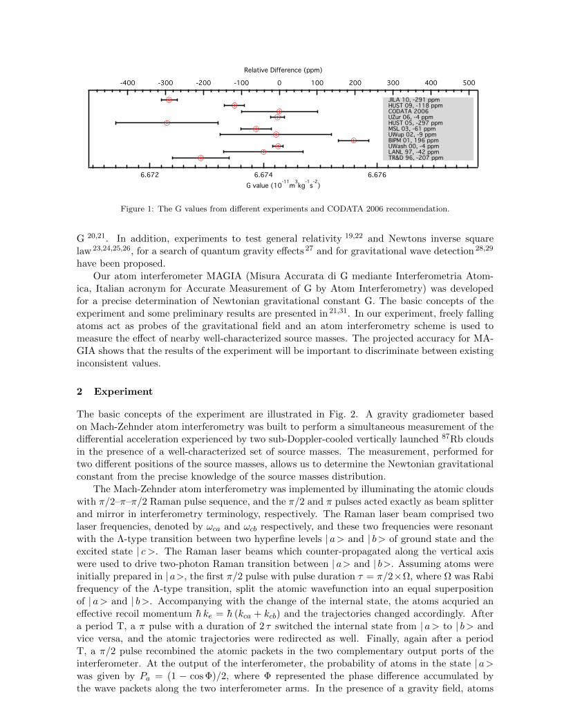
6.6766.6746.672G value (10-11m3kg-1s-2)
5004003002001000-100-200-300-400
Relative Difference (ppm)
JILA 10, -291 ppmHUST 09, -118 ppmCODATA 2006UZur 06, -4 ppmHUST 05, -297 ppmMSL 03, -61 ppmUWup 02, -9 ppmBIPM 01, 196 ppmUWash 00, -4 ppmLANL 97, -42 ppmTR&D 96, -207 ppm
Figure 1: The G values from different experiments and CODATA 2006 recommendation.
G 20,21. In addition, experiments to test general relativity 19,22 and Newtons inverse squarelaw 23,24,25,26, for a search of quantum gravity effects 27 and for gravitational wave detection 28,29
have been proposed.
Our atom interferometer MAGIA (Misura Accurata di G mediante Interferometria Atom-ica, Italian acronym for Accurate Measurement of G by Atom Interferometry) was developedfor a precise determination of Newtonian gravitational constant G. The basic concepts of theexperiment and some preliminary results are presented in 21,31. In our experiment, freely fallingatoms act as probes of the gravitational field and an atom interferometry scheme is used tomeasure the effect of nearby well-characterized source masses. The projected accuracy for MA-GIA shows that the results of the experiment will be important to discriminate between existinginconsistent values.
2 Experiment
The basic concepts of the experiment are illustrated in Fig. 2. A gravity gradiometer basedon Mach-Zehnder atom interferometry was built to perform a simultaneous measurement of thedifferential acceleration experienced by two sub-Doppler-cooled vertically launched 87Rb cloudsin the presence of a well-characterized set of source masses. The measurement, performed fortwo different positions of the source masses, allows us to determine the Newtonian gravitationalconstant from the precise knowledge of the source masses distribution.
The Mach-Zehnder atom interferometry was implemented by illuminating the atomic cloudswith π/2–π–π/2 Raman pulse sequence, and the π/2 and π pulses acted exactly as beam splitterand mirror in interferometry terminology, respectively. The Raman laser beam comprised twolaser frequencies, denoted by ωca and ωcb respectively, and these two frequencies were resonantwith the Λ-type transition between two hyperfine levels | a> and | b> of ground state and theexcited state | c >. The Raman laser beams which counter-propagated along the vertical axiswere used to drive two-photon Raman transition between | a> and | b>. Assuming atoms wereinitially prepared in | a>, the first π/2 pulse with pulse duration τ = π/2×Ω, where Ω was Rabifrequency of the Λ-type transition, split the atomic wavefunction into an equal superpositionof | a> and | b>. Accompanying with the change of the internal state, the atoms acquried aneffective recoil momentum h ke = h (kca + kcb) and the trajectories changed accordingly. Aftera period T, a π pulse with a duration of 2 τ switched the internal state from | a> to | b> andvice versa, and the atomic trajectories were redirected as well. Finally, again after a periodT, a π/2 pulse recombined the atomic packets in the two complementary output ports of theinterferometer. At the output of the interferometer, the probability of atoms in the state | a>was given by Pa = (1 − cos Φ)/2, where Φ represented the phase difference accumulated bythe wave packets along the two interferometer arms. In the presence of a gravity field, atoms
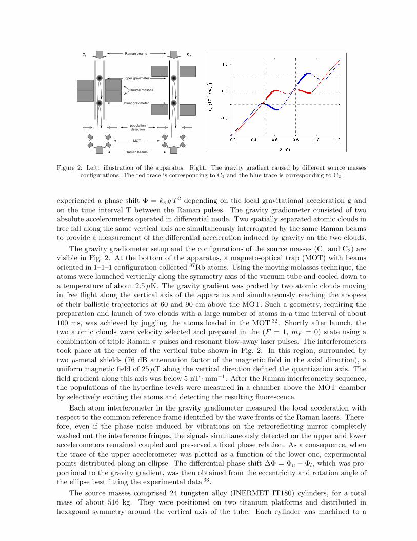
4
upper gravimeter
lower gravimeter
Raman beamsC1 C2
source masses
Raman beams
MOT
population
detection
Figure 1. Scheme of the MAGIA experiment.87
Rb atoms, trapped and cooled
in a MOT, are launched upwards in a vertical vacuum tube with a moving
optical molasses scheme, producing an atomic fountain. Near the apogees of the
atomic trajectories, a measurement of their vertical acceleration is performed by
a Raman interferometry scheme. External source masses are positioned in two
different configurations (C1 and C2) and the induced phase shift is measured as
a function of mass positions.
3. Experimental apparatus
Figure 1 shows a schematic diagram of the MAGIA experiment. The gravity gradiometer setup
and the configurations of the source masses (C1 and C2) are visible. At the bottom of the
apparatus, a magneto-optical trap (MOT) with beams oriented in a 1–1–1 configuration collects87
Rb atoms. Using the moving molasses technique, the sample is launched vertically along
the symmetry axis of the vacuum tube and cooled down to a temperature of about 2.5 µK.
The gravity gradient is probed by two atomic clouds moving in free flight along the vertical
axis of the apparatus and simultaneously reaching the apogees of their ballistic trajectories at
60 and 90 cm above the MOT. Such a geometry, requiring the preparation and launch of two
samples with a large number of atoms in a time interval of about 100 ms, is achieved by juggling
the atoms loaded in the MOT [43]. Shortly after launch, the two atomic samples are velocity
selected and prepared in the (F = 1, mF = 0) state using a combination of a Raman π pulse
and resonant blow-away laser pulses. The interferometers take place at the center of the vertical
tube shown in figure 1. In this region, surrounded by two µ-metal shields (76 dB attenuation
factor of the magnetic field in the axial direction), a uniform magnetic field of 25 µT along
the vertical direction defines the quantization axis. The field gradient along this axis is lower
than 5 nT mm−1
. After the Raman interferometry sequence, the population of the ground state
is measured in a chamber placed just above the MOT by selectively exciting the atoms on the
F = 1, 2 hyperfine levels and detecting the resulting fluorescence.
New Journal of Physics 12 (2010) 095009 (http://www.njp.org/)
Figure 2: Left: illustration of the apparatus. Right: The gravity gradient caused by different source massesconfigurations. The red trace is corresponding to C1 and the blue trace is corresponding to C2.
experienced a phase shift Φ = ke g T2 depending on the local gravitational acceleration g and
on the time interval T between the Raman pulses. The gravity gradiometer consisted of twoabsolute accelerometers operated in differential mode. Two spatially separated atomic clouds infree fall along the same vertical axis are simultaneously interrogated by the same Raman beamsto provide a measurement of the differential acceleration induced by gravity on the two clouds.
The gravity gradiometer setup and the configurations of the source masses (C1 and C2) arevisible in Fig. 2. At the bottom of the apparatus, a magneto-optical trap (MOT) with beamsoriented in 1–1–1 configuration collected 87Rb atoms. Using the moving molasses technique, theatoms were launched vertically along the symmetry axis of the vacuum tube and cooled down toa temperature of about 2.5µK. The gravity gradient was probed by two atomic clouds movingin free flight along the vertical axis of the apparatus and simultaneously reaching the apogeesof their ballistic trajectories at 60 and 90 cm above the MOT. Such a geometry, requiring thepreparation and launch of two clouds with a large number of atoms in a time interval of about100 ms, was achieved by juggling the atoms loaded in the MOT 32. Shortly after launch, thetwo atomic clouds were velocity selected and prepared in the (F = 1, mF = 0) state using acombination of triple Raman π pulses and resonant blow-away laser pulses. The interferometerstook place at the center of the vertical tube shown in Fig. 2. In this region, surrounded bytwo µ-metal shields (76 dB attenuation factor of the magnetic field in the axial direction), auniform magnetic field of 25µT along the vertical direction defined the quantization axis. Thefield gradient along this axis was below 5 nT ·mm−1. After the Raman interferometry sequence,the populations of the hyperfine levels were measured in a chamber above the MOT chamberby selectively exciting the atoms and detecting the resulting fluorescence.
Each atom interferometer in the gravity gradiometer measured the local acceleration withrespect to the common reference frame identified by the wave fronts of the Raman lasers. There-fore, even if the phase noise induced by vibrations on the retroreflecting mirror completelywashed out the interference fringes, the signals simultaneously detected on the upper and loweraccelerometers remained coupled and preserved a fixed phase relation. As a consequence, whenthe trace of the upper accelerometer was plotted as a function of the lower one, experimentalpoints distributed along an ellipse. The differential phase shift ∆Φ = Φu − Φl, which was pro-portional to the gravity gradient, was then obtained from the eccentricity and rotation angle ofthe ellipse best fitting the experimental data 33.
The source masses comprised 24 tungsten alloy (INERMET IT180) cylinders, for a totalmass of about 516 kg. They were positioned on two titanium platforms and distributed inhexagonal symmetry around the vertical axis of the tube. Each cylinder was machined to a
0.3 0.4 0.5 0.6 0.7 0.80.3
0.4
0.5
0.6
0.7
0.8
OriginalShield
0.70
0.65
0.60
0.55
0.50
0.45
0.40
uppe
r clo
ud
0.700.650.600.550.500.450.40lower cloud
7% unbalanced -7% unbalanced power balanced
Figure 3: The left on: ellipses with different shielding conditions. The red trace: several layers of shields. Theblack trace: no soft iron shield.
diameter of 100 mm and a height of 150 mm after a hot isostatic pressing treatment applied tocompress the material and reduce density inhomogeneities. The two platforms could be preciselytranslated along the vertical direction by four step motors, with a resolution of 2 µm providedby an optical encoder; the positioning precision had been tested with a laser tracker 31.
Although the differential measurement can suppress many sources of noises and drifts, thisscheme is still prone to the biases synchronized with the movements of source masses, for ex-ample, the trajectory variation induced by eddy current in the mass translation platforms. Theeddy current is generated by the magnetic field switching for different phases of the experiment,i.e., switching from MOT phase to atomic fountain phase and its magnitude is dependent onthe distance between the platforms and MOT coils. Therefore, the transient magnetic fieldgenerated by eddy current in MOT chamber is higher when the platforms, especially the lowerplatform, are approaching to the MOT chamber. The variation of transient magnetic fieldchanges the launching verticality of atomic fountain and turns out an extra phase shift inducedby Coriolis effect. To suppress this effect, several layers of soft iron shields were installed andthe transient field observed on the bottom surface of the lower platform received more than 10dB attenuation. The ellipses with different shielding conditions are shown in the left part ofFig. 3. The change of phase angle was more than 10 mrad in C2 configuration and could not bediscriminate in C1 configuration. Besides the shielding, we also explored the possible phase shiftcaused by power unbalancing between 1–1–1 MOT cooling laser beams. The results are shownin the right part of Fig. 3. The ellipse shifted its position as power unbalancing ratio changedfrom −7% to +7% but the differences between the phase angles of these ellipses were within thefitting errors, i.e., 1.2 mrad or 700 ppm. We even intentionally varied the unbalancing ratio to20% and no significant change was perceived in that test. The characterization of source masseshas been done and the contribution to final uncertainty is given in Table 1.
3 Conclusion
The basic concepts of MAGIA experiment and some of systematic issues are covered in thispaper. The experiment received many improvements in these two years, and hence both thesignal-to-noise ratio and long term stability have been significantly improved. With the inte-gration time of three weeks, the precision is expected to reach the final goal of 100 ppm. Theinvestigation of various systematic shifts are ongoing at present and the whole experiment wouldbe ready for final measurement in the near future.
present uncertainty ∆G/G× 10−4
Int. Cyl. rad. position 99.90 mm 10 µm 0.22Ext. Cyl. rad. position 173.00 mm 10 µm 0.05Hu-Hl (C1) 215.00 mm 10 µm 0.38Hu-Hl (C2) 449.85 mm 10 µm 0.3mass of cylinder 21486 g 10 mg 0.01Density homogeneity 18249 kg·m−3 24 kg·m−3 0.2mass of platform 24930 g 60 g 0.8
1.97
Table 1: The characterization of source masses and the contribution to the error budget of G measurement.
References
1. P. J. Mohr, B. N. Taylor, and D. B. Newell, Rev. Mod. Phys. 80, 633 (2008).2. J. Luo, Q. Liu, L.-C. Tu, C.-G. Shao, L.-X. Liu, S.-Q. Yang, Q. Li, and Y.-T. Zhang, Phys.
Rev. Lett. 102, 240801 (2009).3. H. V. Parks and J. E. Faller, Phys. Rev. Lett. 105, 110801 (2010).4. P. J. Mohr and B. N. Taylor, Rev. Mod. Phys. 72, 351 (2000).5. J. H. Gundlach and S. M. Merkowitz, Phys. Rev. Lett. 85, 2869 (2000).6. T. J. Quinn, C. C. Speake, S. J. Richman, R. S. Davis, and A. Picard, Phys. Rev. Lett.
87, 111101 (2001).7. T. R. Armstrong and M. P. Fitzgerald, Phys. Rev. Lett. 91, 201101 (2003).8. S. Schlamminger, E. Holzschuh, W. Kundig, F. Nolting, R. E. Pixley, J. Schurr, and
U. Straumann, Phys. Rev. D 74, 082001 (2006).9. J. P. Schwarz, D. S. Robertson, T. M. Niebauer, J. E. Faller, Science 282, 2230 (1998).
10. U. Kleinevoß, H. Meyer, A. Schumacher, and S. Hartmann, Meas. Sci. Tech. 10, 492(1999).
11. A. D. Cronin, J. Schmiedmayer, and D. E. Pritchard, Rev. Mod. Phys. 81, 1051 (2009).12. H. Muller, S.-W. Chiow, S. Herrmann, S. Chu, and K.-Y. Chung, Phys. Rev. Lett. 100,
031101 (2008).13. J. Le Gouet, T. E. Mehlstaubler, J. Kim, S. Merlet, A. Clairon, A. Landragin, and F. P. Dos
Santos, Appl. Phys. B: Lasers Opt. 92, 133 (2008).14. J. M. McGuirk, G. T. Foster, J. B. Fixler, M. J. Snadden, and M. A. Kasevich, Phys. Rev.
A 65, 033608 (2002).15. A. Bertoldi, G. Lamporesi, L. Cacciapuoti, M. de Angelis, M. Fattori, T. Petelski, A. Pe-
ters, M. Prevedelli, J. Stuhler, and G. M. Tino, Eur. Phys. J. D 40, 271 (2006).16. B. Canuel et al., Phys. Rev. Lett. 97, 010402 (2006).17. A. Gauguet, B. Canuel, T. Leveque, W. Chaibi, and A. Landragin, Phys. Rev. A 80,
063604 (2009).18. S. Fray, C. A. Diez, T. W. Hansch, and M. Weitz, Phys. Rev. Lett. 93, 240404 (2004).19. S. Dimopoulos, P. W. Graham, J. M. Hogan, and M. A. Kasevich, Phys. Rev. D 78,
042003 (2008).20. J. B. Fixler, G. T. Foster, J. M. McGuirk, and M. A. Kasevich, Science 315, 74 (2007).21. G. Lamporesi, A. Bertoldi, L. Cacciapuoti, M. Prevedelli, and G. M. Tino, Phys. Rev.
Lett. 100, 050801 (2008).22. H. Muller, A. Peters, and S. Chu, Nature 463, 926 (2010).23. G. M. Tino, Nucl. Phys. B: Proc. Suppl. 113, 289 (2002).24. G. Ferrari, N. Poli, F. Sorrentino, and G. M. Tino, Phys. Rev. Lett. 97, 060402 (2006).25. P. Wolf, P. Lemonde, A. Lambrecht, S. Bize, A. Landragin, and A. Clairon, Phys. Rev.
A 75, 063608 (2007).26. A. Alberti, G. Ferrari, V. V. Ivanov, M. L. Chiofalo, and G. M. Tino, New J. Phys. 12,
065037 (2010).27. G. Amelino-Camelia, C. Lammerzahl, F. Mercati, and G. M. Tino, Phys. Rev. Lett. 103,
171302 (2009).28. G. M. Tino and F. Vetrano, Class. Quantum Grav. 24, 2167 (2007).29. S. Dimopoulos, P. W. Graham, J. M. Hogan, M. A. Kasevich, and S. Rajendran, Phys.
Lett. B 678, 37 (2009).30. M. Fattori, G. Lamporesi, T. Petelski, J. Stuhler, and G. M. Tino, Phys. Lett. A 318,
184 (2003).31. G. Lamporesi, A. Bertoldi, A. Cecchetti, B. Duhlach, M. Fattori, A. Malengo, S. Pettor-
ruso, M. Prevedelli, and G. M. Tino, Rev. Sci. Instrum. 78, 075109 (2007).32. R. Legere and K. Gibble, Phys. Rev. Lett. 81, 5780 (1998).33. G. T. Foster, J. B. Fixler, J. M. McGuirk, and M. A. Kasevich, Opt. Lett. 27, 951 (2002).
ULTRA-STABLE, HIGH-POWER LASER SYSTEMS
P. KWEEMax-Planck-Institut fur Gravitationsphysik (Albert-Einstein-Institut),
Callinstr. 38, 30167 Hannover, Germany
Laser systems with a high output power and a comprehensive stabilization of most laser beamparameters are required for ground-based interferometric gravitational wave detectors. Thelaser system of the second generation gravitational wave detector Advanced LIGO is reviewedand a brief overview about laser development for the third generation is given.
1 Introduction
Interferometric, ground-based gravitational wave detectors (GWDs) are expected to measurethe tiny differential length variations caused by gravitational waves emitted by astrophysicalsources. The second generation of these kilometer-long baseline Michelson interferometers arecurrently installed and have a design strain sensitivity of 10−23
. . . 10−24 Hz−1/2. They requirelaser systems with high output power and at the same time with very good stability concerningall laser beam parameters.
A high output power is required to reach a high signal-to-quantum-noise ratio, since quantumnoise in the gravitational wave readout is reduced at high frequencies with increasing circulatinglaser power in the interferometer. In addition to quantum noise technical laser noise couples tothe gravitational wave channel. Thus on the one hand the coupling needs to be reduced e.g. byoptical design or by exploiting symmetries; and on the other hand laser noise has to be reducedby different active and passive stabilization schemes.
This article reviews the laser output power scaling and laser stabilization techniques usedin the laser system of the second generation detector Advanced LIGO1 (aLIGO). Furthermore abrief overview about current laser development for third generation detectors is given.
2 Advanced LIGO pre-stabilized laser system
Advanced LIGO requires a reliable, continuous-wave, single-frequency laser system with anoutput power of 165 W in a TEM00 mode at a wavelength of 1064 nm. Laser beam parameterssuch as power, frequency, or pointing have to be ultra-stable requiring an elaborate stabilizationscheme2. Furthermore modulation inputs for controlling the beam power and frequency have tobe provided.
The laser was developed by Laser Zentrum Hannover e.V. (LZH) and consists of three stages(see Fig. 1). The first stage, the master laser, is a commercial non-planar ring-oscillator3 (NPRO)from Innolight. This solid-state laser uses a Nd:YAG crystal as laser medium and resonator atthe same time. The laser is pumped by laser diodes at 808 nm and delivers an output power of2 W. Due to its monolithic resonator the laser has an exceptional intrinsic frequency stability.
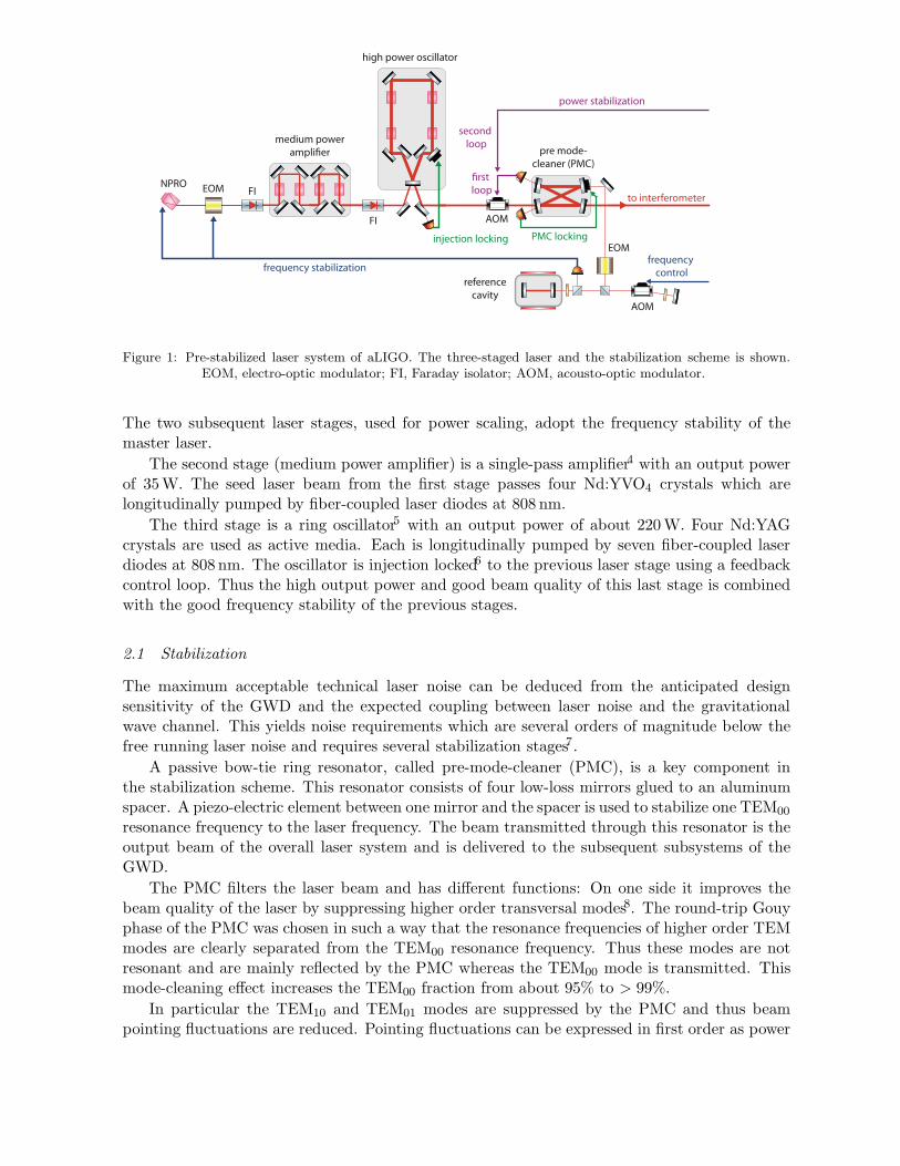
NPRO
high power oscillator
medium power
ampli!er pre mode-
cleaner (PMC)
frequency stabilization
power stabilization
frequency
control
injection locking PMC locking
reference
cavity
EOM FI
FI
EOM
AOM
to interferometer
!rst
loop
second
loop
AOM
Figure 1: Pre-stabilized laser system of aLIGO. The three-staged laser and the stabilization scheme is shown.EOM, electro-optic modulator; FI, Faraday isolator; AOM, acousto-optic modulator.
The two subsequent laser stages, used for power scaling, adopt the frequency stability of themaster laser.
The second stage (medium power amplifier) is a single-pass amplifier4 with an output powerof 35 W. The seed laser beam from the first stage passes four Nd:YVO4 crystals which arelongitudinally pumped by fiber-coupled laser diodes at 808 nm.
The third stage is a ring oscillator5 with an output power of about 220 W. Four Nd:YAGcrystals are used as active media. Each is longitudinally pumped by seven fiber-coupled laserdiodes at 808 nm. The oscillator is injection locked6 to the previous laser stage using a feedbackcontrol loop. Thus the high output power and good beam quality of this last stage is combinedwith the good frequency stability of the previous stages.
2.1 Stabilization
The maximum acceptable technical laser noise can be deduced from the anticipated designsensitivity of the GWD and the expected coupling between laser noise and the gravitationalwave channel. This yields noise requirements which are several orders of magnitude below thefree running laser noise and requires several stabilization stages7.
A passive bow-tie ring resonator, called pre-mode-cleaner (PMC), is a key component inthe stabilization scheme. This resonator consists of four low-loss mirrors glued to an aluminumspacer. A piezo-electric element between one mirror and the spacer is used to stabilize one TEM00
resonance frequency to the laser frequency. The beam transmitted through this resonator is theoutput beam of the overall laser system and is delivered to the subsequent subsystems of theGWD.
The PMC filters the laser beam and has different functions: On one side it improves thebeam quality of the laser by suppressing higher order transversal modes8. The round-trip Gouyphase of the PMC was chosen in such a way that the resonance frequencies of higher order TEMmodes are clearly separated from the TEM00 resonance frequency. Thus these modes are notresonant and are mainly reflected by the PMC whereas the TEM00 mode is transmitted. Thismode-cleaning effect increases the TEM00 fraction from about 95% to > 99%.
In particular the TEM10 and TEM01 modes are suppressed by the PMC and thus beampointing fluctuations are reduced. Pointing fluctuations can be expressed in first order as power
fluctuations of the TEM10 and TEM01 modes. The PMC reduces the field amplitude of thesemodes and thus the pointing fluctuations by a factor of about 60.
Finally the PMC reduces technical power fluctuations at radio frequencies. A good powerstability between 9 MHz and 100 MHz is important since phase modulated light injected into theinterferometer is used to sense several degrees of freedom of the interferometer which need tobe controlled. The PMC has a bandwidth of about 600 kHz and acts in first order as a low-passfilter for power fluctuations with a -3 dB corner frequency at this frequency.
Beside these passive stabilization effects of the PMC active stabilizations are necessary toreduce power and frequency noise in the detection band of the GWD from about 10 Hz to 10 kHz.The PMC reduces power fluctuations significantly only above 600 kHz. In the detection band agood power stability is required since fluctuations couple via radiation pressure imbalance andthe dark-fringe offset to the gravitational wave channel. The beam power at a pick-off port ofthe PMC is measured with a low-noise photodetector. An electronic feedback controller and anacousto-optical modulator (AOM) as power actuator upstream of the PMC are used to stabilizethe laser power. This first power stabilization loop reduces the relative power fluctuations byabout three orders of magnitude to the 10−8 Hz−1/2 level.
A second power stabilization loop with a photodetector directly upstream of the interfer-ometer is used to reach the required power stability in the interferometer. This stabilizationis developed at the moment and a precursor experiment9 demonstrated already the necessaryhigh-sensitivity photodetector.
Finally a good frequency stability is required for the lock acquisition of the interferometerand to reduce frequency noise coupling into the gravitational wave channel via asymmetries inthe interferometer arms. The interferometer has to be operated at a specific operation point toreach its design sensitivity requiring an elaborate lock acquisition. A linear rigid-spacer referenceresonator is used in the laser system for a frequency pre-stabilization. The Pound-Drever-Hallsensing scheme and a compound frequency actuator is used to stabilize the frequency up to aFourier frequency of about 500 kHz10. The compound actuator consists of the NPRO crystaltemperature control, the piezo-electric element attached to the NPRO crystal, and the broad-band electro-optic modulator (EOM) between NPRO and amplifier as phase corrector.
To be able to control the laser frequency while it is stabilized to the reference resonator afrequency shifting AOM in a double-pass configuration is used in front of the reference resonator.By controlling the AOM driving frequency the laser system frequency can be shifted by about1 MHz with a bandwidth of about 100 kHz.
3 Third generation laser systems
The laser systems for the second generation GWDs are installed at the moment. Meanwhilethe development for the third generation has started already. Since only rough third generationconceptual designs11 exist at the moment different development directions are conceivable: High-frequency GWDs or all-reflective GWDs might require high-power laser systems at the kW level.Cryogenic interferometers with silicon test masses might require a different laser wavelength at1550 nm since silicon has a low absorption coefficient at this wavelength. Laser systems with adifferent beam profile, such as Lag33 mode or flat-top profiles, might be required to reduce theinfluence of thermal noise of the test masses due to a more homogenous intensity distribution.
The LZH, e.g., develops a 1 kW 1064 nm TEM00 laser at the moment12. For this the powerof an NPRO master laser is scaled to the kW level by a combination of photonic crystal fiberamplifier, coherent beam combining and/or subsequent Nd:YAG amplifier. Furthermore a 100 W1550 nm TEM00 laser is currently developed. The concept is to amplify a distributed feedback(DFB) fiber master laser with an erbium fiber amplifier13,14,15. In general fiber lasers andamplifiers made a substantial progress in recent years. They stand out due to their efficiency,
compactness, and high intrinsic beam quality compared to the solid-state lasers and amplifierswhich are used at the moment in GWDs. Though long-term tests need to be performed todemonstrate if they are as reliable as solid-state lasers are today.
During the development of the laser stabilization for aLIGO the power and pointing stabi-lization turned out to be the most critical ones. The achieved power stability in the detectionband is limited by the sensitivity of the power sensor. The precursor experiment9 demonstratedjust the sensitivity required for aLIGO. In case third generation detectors require an even bet-ter power stability completely different stabilization schemes such as the optical ac couplingtechnique16 might be necessary. Until now beam pointing fluctuations were reduced only by thepassive filtering effect of the PMC fulfilling just the requirements of aLIGO. If a better pointingstability will be required in the future additional active stabilization schemes or cascaded PMCsmight be necessary.
4 Conclusion
Multi-stage laser systems combined with active and passive stabilizations deliver ultra-stable,high-power laser beams for second generation GWDs. The development, in particular of thelaser system for aLIGO, has almost finished and these laser systems are currently installed atthe observatory sites. One aLIGO laser system is comprehensively characterized at the momentto verify the required performance.
Meanwhile the development of lasers for third generation GWDs has started following differ-ent strategies. Probably most stabilization techniques applied in second generation laser systemscan be adapted for the third generation, whereas the power and pointing stabilization will bethe most challenging aspects.
Acknowledgments
The author thanks Benno Willke, Peter Weßels, and Albrecht Rudiger for their helpful commentsduring the preparation of this article.
References
1. P. Fritschel, Proc. SPIE 4856, 282 (2003).2. B. Willke, Laser & Photonics Reviews 4, 780–794 (2010).3. I. Freitag et al, SPIE 2379, 335–342 (1995).4. M. Frede et al, Opt. Express 15, 459–465 (2007).5. L. Winkelmann et al, App. Phys. B 102, 529–538 (2011).6. A.D. Farinas et al, J. Opt. Soc. Am. B 12, 328–334 (1995).7. P. Kwee, Laser Characterization and Stabilization for Precision Interferometry, Ph.D.
thesis, Universitat Hannover (2010).8. A. Rudiger et al, Opt. Acta 28, 641–658 (1981).9. P. Kwee et al, Opt. Lett. 34, 2912–2914 (2009).
10. F. Bondu et al, Opt. Lett. 21, 582–584 (1996).11. Einstein Telescope design study, http://www.et-gw.eu/.12. M. Karow et al, CLEO Europe , CJ7.4 (2011).13. V. Kuhn et al, Opt. Express 17, 18304–18311 (2009).14. V. Kuhn et al, IEEE Phot. Tech. Lett. 23, 432–434 (2011).15. V. Kuhn et al, CLEO Europe , CJ7.5 (2011).16. P. Kwee et al, App. Phys. B 102, 515–522 (2011).
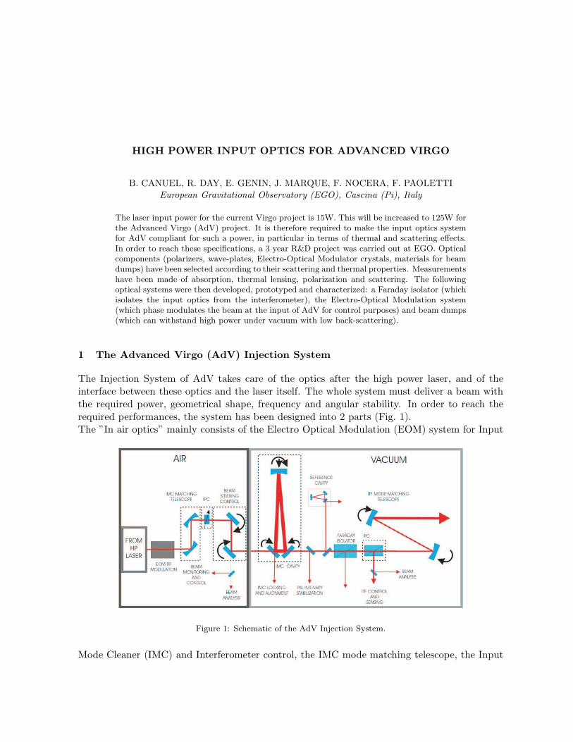
HIGH POWER INPUT OPTICS FOR ADVANCED VIRGO
B. CANUEL, R. DAY, E. GENIN, J. MARQUE, F. NOCERA, F. PAOLETTI
European Gravitational Observatory (EGO), Cascina (Pi), Italy
The laser input power for the current Virgo project is 15W. This will be increased to 125W forthe Advanced Virgo (AdV) project. It is therefore required to make the input optics systemfor AdV compliant for such a power, in particular in terms of thermal and scattering effects.In order to reach these specifications, a 3 year R&D project was carried out at EGO. Opticalcomponents (polarizers, wave-plates, Electro-Optical Modulator crystals, materials for beamdumps) have been selected according to their scattering and thermal properties. Measurementshave been made of absorption, thermal lensing, polarization and scattering. The followingoptical systems were then developed, prototyped and characterized: a Faraday isolator (whichisolates the input optics from the interferometer), the Electro-Optical Modulation system(which phase modulates the beam at the input of AdV for control purposes) and beam dumps(which can withstand high power under vacuum with low back-scattering).
1 The Advanced Virgo (AdV) Injection System
The Injection System of AdV takes care of the optics after the high power laser, and of theinterface between these optics and the laser itself. The whole system must deliver a beam withthe required power, geometrical shape, frequency and angular stability. In order to reach therequired performances, the system has been designed into 2 parts (Fig. 1).The ”In air optics” mainly consists of the Electro Optical Modulation (EOM) system for Input
Figure 1: Schematic of the AdV Injection System.
Mode Cleaner (IMC) and Interferometer control, the IMC mode matching telescope, the Input
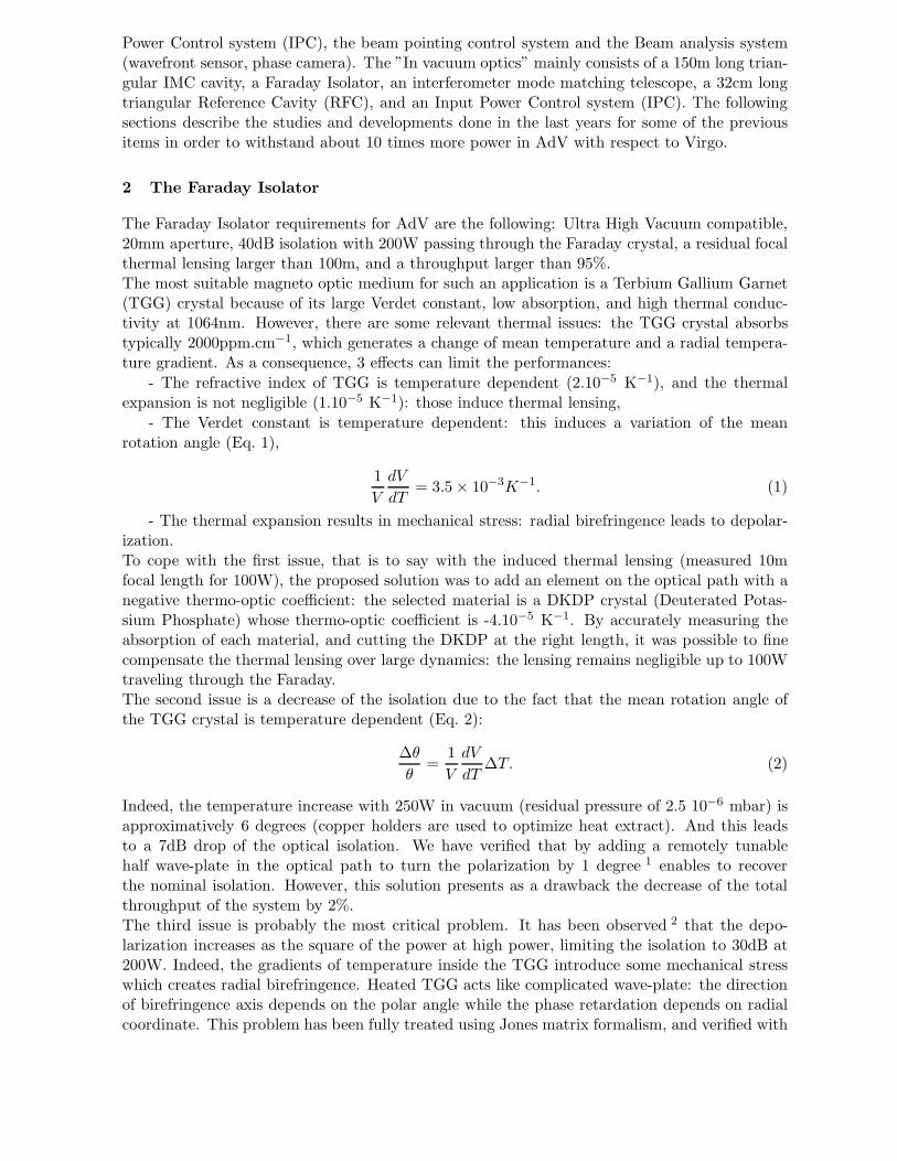
Power Control system (IPC), the beam pointing control system and the Beam analysis system(wavefront sensor, phase camera). The ”In vacuum optics” mainly consists of a 150m long trian-gular IMC cavity, a Faraday Isolator, an interferometer mode matching telescope, a 32cm longtriangular Reference Cavity (RFC), and an Input Power Control system (IPC). The followingsections describe the studies and developments done in the last years for some of the previousitems in order to withstand about 10 times more power in AdV with respect to Virgo.
2 The Faraday Isolator
The Faraday Isolator requirements for AdV are the following: Ultra High Vacuum compatible,20mm aperture, 40dB isolation with 200W passing through the Faraday crystal, a residual focalthermal lensing larger than 100m, and a throughput larger than 95%.The most suitable magneto optic medium for such an application is a Terbium Gallium Garnet(TGG) crystal because of its large Verdet constant, low absorption, and high thermal conduc-tivity at 1064nm. However, there are some relevant thermal issues: the TGG crystal absorbstypically 2000ppm.cm−1, which generates a change of mean temperature and a radial tempera-ture gradient. As a consequence, 3 effects can limit the performances:
- The refractive index of TGG is temperature dependent (2.10−5 K−1), and the thermalexpansion is not negligible (1.10−5 K−1): those induce thermal lensing,
- The Verdet constant is temperature dependent: this induces a variation of the meanrotation angle (Eq. 1),
1
V
dV
dT= 3.5 × 10⁻³
K−1
. (1)
- The thermal expansion results in mechanical stress: radial birefringence leads to depolar-ization.To cope with the first issue, that is to say with the induced thermal lensing (measured 10mfocal length for 100W), the proposed solution was to add an element on the optical path with anegative thermo-optic coefficient: the selected material is a DKDP crystal (Deuterated Potas-sium Phosphate) whose thermo-optic coefficient is -4.10−5 K−1. By accurately measuring theabsorption of each material, and cutting the DKDP at the right length, it was possible to finecompensate the thermal lensing over large dynamics: the lensing remains negligible up to 100Wtraveling through the Faraday.The second issue is a decrease of the isolation due to the fact that the mean rotation angle ofthe TGG crystal is temperature dependent (Eq. 2):
∆θ
θ=
1
V
dV
dT∆T. (2)
Indeed, the temperature increase with 250W in vacuum (residual pressure of 2.5 10−6 mbar) isapproximatively 6 degrees (copper holders are used to optimize heat extract). And this leadsto a 7dB drop of the optical isolation. We have verified that by adding a remotely tunablehalf wave-plate in the optical path to turn the polarization by 1 degree 1 enables to recoverthe nominal isolation. However, this solution presents as a drawback the decrease of the totalthroughput of the system by 2%.The third issue is probably the most critical problem. It has been observed 2 that the depo-larization increases as the square of the power at high power, limiting the isolation to 30dB at200W. Indeed, the gradients of temperature inside the TGG introduce some mechanical stresswhich creates radial birefringence. Heated TGG acts like complicated wave-plate: the directionof birefringence axis depends on the polar angle while the phase retardation depends on radialcoordinate. This problem has been fully treated using Jones matrix formalism, and verified with
optical measurements of the amplitude and phase of the field 3. The ”depolarization” effect canbe briefly summarized as follows: there is a self conversion of Spin to Orbital Angular Momen-tum which explains the non common orbital phase dependence of the beam. A solution hasbeen proposed to this issue using a specific optical configuration for the Faraday 4: the designconsists of 2 TGG crystals, each rotating the polarization by 22.5 degrees and separated by a67.5 degrees reciprocal polarization rotator. In this way, the second TGG converts back into thegaussian mode the light that was ”depolarized” by the first TGG. The complete design includingthe DKDP, the remote controlled half wave-plate and the 2 TGG crystals configuration is shownin Fig. 2. We have measured in this configuration the isolation for different powers (Fig. 2). Theisolation is 50 dB at low power and 38dB for 240W.
Figure 2: Optical setup of the Faraday isolator for Advanced Virgo and Faraday isolation performance withrespect to power traveling through it.
3 The Electro Optical Modulation System
The Electro Optical Modulation System of AdV is required to phase modulate the input beamat 2 frequencies: typically 10 and 65 MHz. First, we have selected the best material in termof thermal effects: an RTP crystal from Raicol (absorption of 45 ppm.cm−1). The system hasbeen designed with a unique crystal with 2 sections of modulation to get the highest modulationindex with the lowest possible RF power. Using a Scanning Fabry Perot, we have measured thefollowing modulation depth for 0.5W RF power: 0.16 at 10MHz and 0.12 at 65MHz.
4 Beam Dumps
By experience, it is crucial to design better beam dumps for AdV, in term of damage thresholdand back-scattering. The first step has been to make a comparative study of 3 materials:black absorbing glass (KG5), Silicon (Si) and Silicon Carbide (SiC). All these materials arewell absorbing at 1064nm but have different thermal conduction: 1W.m−1.K−1 for KG5, 150W.m−1.K−1 for Si, and 490 W.m−1.K−1 for SiC. As a consequence, they have different damagethreshold that have been measured in air: 25 W.cm−2 for KG5, 6 kW.cm−2 for Si, and 30kW.cm−2 for SiC. The SiC material has been selected then. Super-polished plates of SiC (withTotal Integrated Scattering of the order of 10ppm) are under development.Another related issue has been studied: how to extract the heat from beam dumps into vacuum?A possible solution is to radiate the heat towards the vacuum tank wall. We have developed 2kinds of mounts having a high emissivity for the beam dumps: sanded copper and pre-bakedstainless steel. The emissivity of these mounts has been optimized up to 70%.
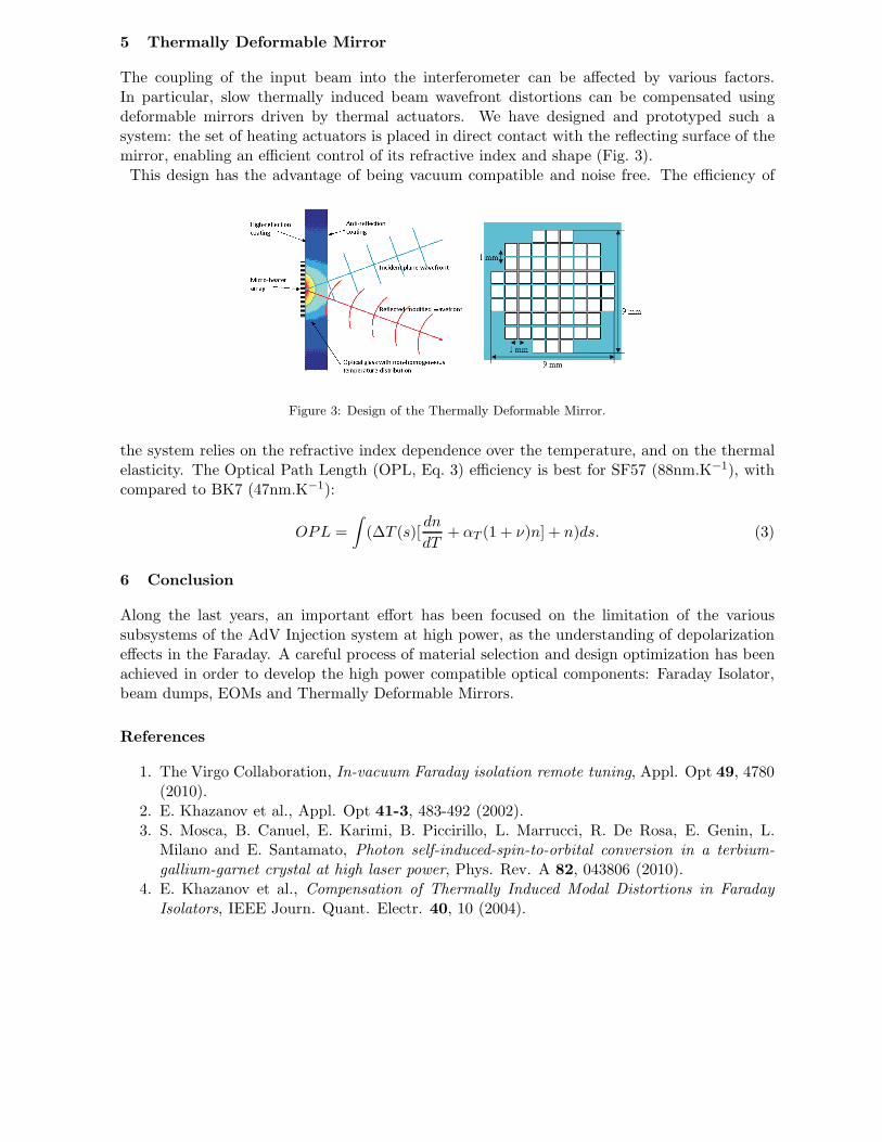
5 Thermally Deformable Mirror
The coupling of the input beam into the interferometer can be affected by various factors.In particular, slow thermally induced beam wavefront distortions can be compensated usingdeformable mirrors driven by thermal actuators. We have designed and prototyped such asystem: the set of heating actuators is placed in direct contact with the reflecting surface of themirror, enabling an efficient control of its refractive index and shape (Fig. 3).This design has the advantage of being vacuum compatible and noise free. The efficiency of
Figure 3: Design of the Thermally Deformable Mirror.
the system relies on the refractive index dependence over the temperature, and on the thermalelasticity. The Optical Path Length (OPL, Eq. 3) efficiency is best for SF57 (88nm.K−1), withcompared to BK7 (47nm.K−1):
OPL =
∫
(∆T (s)[dn
dT+ αT (1 + ν)n] + n)ds. (3)
6 Conclusion
Along the last years, an important effort has been focused on the limitation of the varioussubsystems of the AdV Injection system at high power, as the understanding of depolarizationeffects in the Faraday. A careful process of material selection and design optimization has beenachieved in order to develop the high power compatible optical components: Faraday Isolator,beam dumps, EOMs and Thermally Deformable Mirrors.
References
1. The Virgo Collaboration, In-vacuum Faraday isolation remote tuning, Appl. Opt 49, 4780(2010).
2. E. Khazanov et al., Appl. Opt 41-3, 483-492 (2002).3. S. Mosca, B. Canuel, E. Karimi, B. Piccirillo, L. Marrucci, R. De Rosa, E. Genin, L.
Milano and E. Santamato, Photon self-induced-spin-to-orbital conversion in a terbium-
gallium-garnet crystal at high laser power, Phys. Rev. A 82, 043806 (2010).4. E. Khazanov et al., Compensation of Thermally Induced Modal Distortions in Faraday
Isolators, IEEE Journ. Quant. Electr. 40, 10 (2004).
Thermal effects and their compensation in the
interferometric gravitational wave detector Advanced Virgo
A. Rocchi1, E. Coccia1,2, M. Di Paolo Emilio1, V. Fafone1,2,V. Malvezzi1, Y. Minenkov1, L. Sperandio1,2
1INFN Sezione di Roma Tor Vergata, I-00133 Rome, Italy2University of Rome Tor Vergata and INFN, I-00133 Rome, Italy
Thermal lensing due to the absorption of the laser beam in core optics of gravitational waveinterferometers can represent a strong limitation to their operation and sensitivity. This effecthas already been observed in the present detectors. Thermal compensation systems, basedon CO2 laser projectors, have been installed in Virgo and LIGO, to heat the peripheral ofthe input test masses to reduce the lensing effect. In second generation detectors, thermallensing will become more relevant, due to the much higher circulating power. In this paper,the concept of the compensation system for Advanced Virgo is described.
1 Introduction
The largest currently operating interferometric Gravitational Wave (GW) detectors Virgo 1 andLIGO 2 are power-recycled Michelson interferometers with Fabry-Perot cavities in the arms.They have operated at the initial design sensitivity, completing several observational runs. Up-grades of these detectors are planned on short term time-scale: the second generation detectorsAdvanced Virgo3 and Advanced LIGO 4 are now in the construction phase and will see a signifi-cant improvement of their sensitivity of about a factor of ten over the whole detection bandwidth,increasing by a factor of a thousand the volume of the observable Universe.
The second generation instruments will be characterized by a very high circulating power(from 20 kW in the initial interferometers to 700 kW in the advanced detectors), necessaryto keep the shot noise at the level required by their high sensitivity. In an interferometric GWdetector, the amount of allowable circulating power is limited by the non-zero optical absorptionin the substrate and coatings of the test masses and the beam splitter, which will affect boththe controllability and the sensitivity of the instrument 5 6.
In the test mass, the optical power is predominantly absorbed by the high reflectivity coatingand converted into heat, producing a gradient of temperature inside the substrate. Two differenteffects originate from the heating of the test mass:
• non-uniform optical path length distortions (thermo-optic effect, also termed thermal lens-ing) mainly due to the temperature dependency of the index of refraction;
• change of the profile of the high reflective surface, due to thermal expansion (thermo-elasticdeformation) in both input and end test masses.
In presence of thermal lensing, which changes the power recycling cavity (PRC) mode,the input laser no longer matches the PRC cavity and the coupling coefficient between the
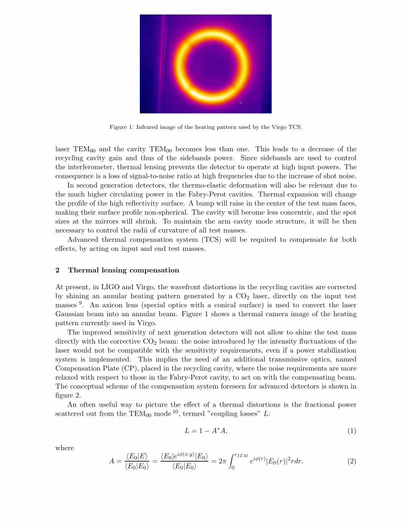
Figure 1: Infrared image of the heating pattern used by the Virgo TCS.
laser TEM00 and the cavity TEM00 becomes less than one. This leads to a decrease of therecycling cavity gain and thus of the sidebands power. Since sidebands are used to controlthe interferometer, thermal lensing prevents the detector to operate at high input powers. Theconsequence is a loss of signal-to-noise ratio at high frequencies due to the increase of shot noise.
In second generation detectors, the thermo-elastic deformation will also be relevant due tothe much higher circulating power in the Fabry-Perot cavities. Thermal expansion will changethe profile of the high reflectivity surface. A bump will raise in the center of the test mass faces,making their surface profile non-spherical. The cavity will become less concentric, and the spotsizes at the mirrors will shrink. To maintain the arm cavity mode structure, it will be thennecessary to control the radii of curvature of all test masses.
Advanced thermal compensation system (TCS) will be required to compensate for botheffects, by acting on input and end test masses.
2 Thermal lensing compensation
At present, in LIGO and Virgo, the wavefront distortions in the recycling cavities are correctedby shining an annular heating pattern generated by a CO2 laser, directly on the input testmasses 9. An axicon lens (special optics with a conical surface) is used to convert the laserGaussian beam into an annular beam. Figure 1 shows a thermal camera image of the heatingpattern currently used in Virgo.
The improved sensitivity of next generation detectors will not allow to shine the test massdirectly with the corrective CO2 beam: the noise introduced by the intensity fluctuations of thelaser would not be compatible with the sensitivity requirements, even if a power stabilizationsystem is implemented. This implies the need of an additional transmissive optics, namedCompensation Plate (CP), placed in the recycling cavity, where the noise requirements are morerelaxed with respect to those in the Fabry-Perot cavity, to act on with the compensating beam.The conceptual scheme of the compensation system foreseen for advanced detectors is shown infigure 2.
An often useful way to picture the effect of a thermal distortions is the fractional powerscattered out from the TEM00 mode 10, termed ”coupling losses” L:
L = 1 − A∗A, (1)
where
A =〈E0|E〉
〈E0|E0〉
=〈E0|e
iφ(x,y)|E0〉
〈E0|E0〉
= 2π
∫ rITM
0
eiφ(r)
|E0(r)|2rdr. (2)
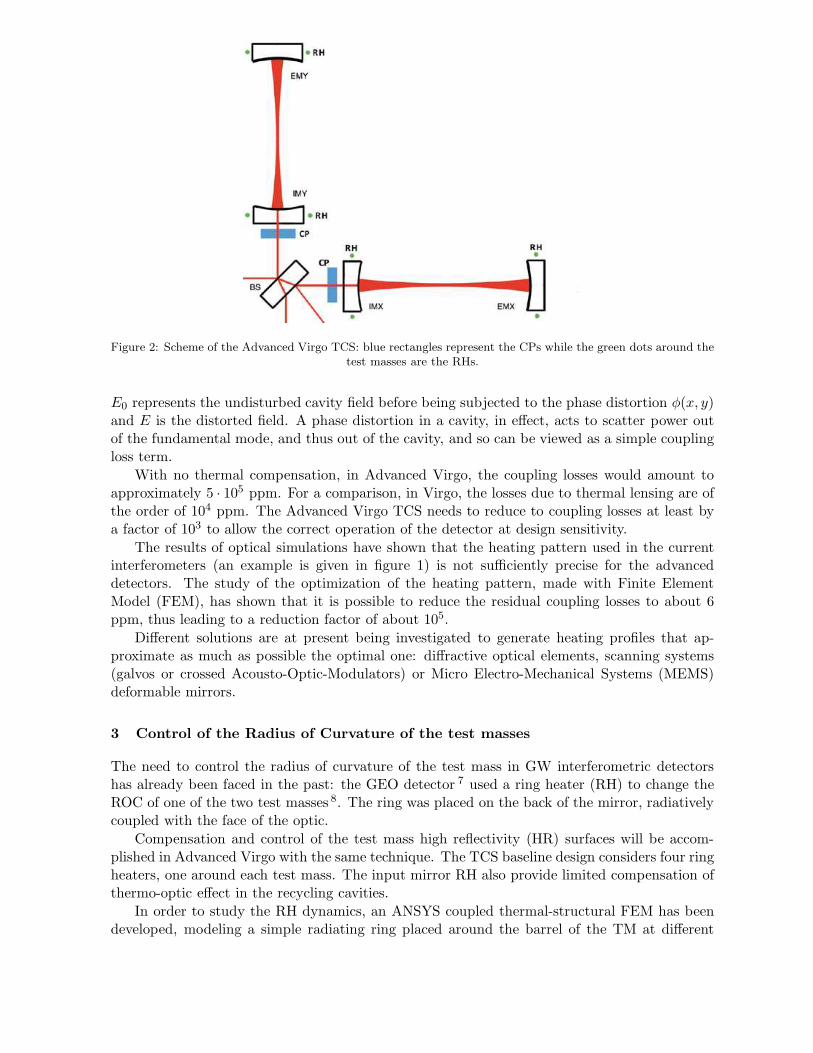
Figure 2: Scheme of the Advanced Virgo TCS: blue rectangles represent the CPs while the green dots around thetest masses are the RHs.
E0 represents the undisturbed cavity field before being subjected to the phase distortion φ(x, y)and E is the distorted field. A phase distortion in a cavity, in effect, acts to scatter power outof the fundamental mode, and thus out of the cavity, and so can be viewed as a simple couplingloss term.
With no thermal compensation, in Advanced Virgo, the coupling losses would amount toapproximately 5 · 105 ppm. For a comparison, in Virgo, the losses due to thermal lensing are ofthe order of 104 ppm. The Advanced Virgo TCS needs to reduce to coupling losses at least bya factor of 103 to allow the correct operation of the detector at design sensitivity.
The results of optical simulations have shown that the heating pattern used in the currentinterferometers (an example is given in figure 1) is not sufficiently precise for the advanceddetectors. The study of the optimization of the heating pattern, made with Finite ElementModel (FEM), has shown that it is possible to reduce the residual coupling losses to about 6ppm, thus leading to a reduction factor of about 105.
Different solutions are at present being investigated to generate heating profiles that ap-proximate as much as possible the optimal one: diffractive optical elements, scanning systems(galvos or crossed Acousto-Optic-Modulators) or Micro Electro-Mechanical Systems (MEMS)deformable mirrors.
3 Control of the Radius of Curvature of the test masses
The need to control the radius of curvature of the test mass in GW interferometric detectorshas already been faced in the past: the GEO detector 7 used a ring heater (RH) to change theROC of one of the two test masses 8. The ring was placed on the back of the mirror, radiativelycoupled with the face of the optic.
Compensation and control of the test mass high reflectivity (HR) surfaces will be accom-plished in Advanced Virgo with the same technique. The TCS baseline design considers four ringheaters, one around each test mass. The input mirror RH also provide limited compensation ofthermo-optic effect in the recycling cavities.
In order to study the RH dynamics, an ANSYS coupled thermal-structural FEM has beendeveloped, modeling a simple radiating ring placed around the barrel of the TM at different
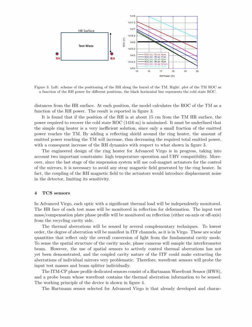
Figure 3: Left: scheme of the positioning of the RH along the barrel of the TM. Right: plot of the TM ROC asa function of the RH power for different positions, the black horizontal line represents the cold state ROC.
distances from the HR surface. At each position, the model calculates the ROC of the TM as afunction of the RH power. The result is reported in figure 3.
It is found that if the position of the RH is at about 15 cm from the TM HR surface, thepower required to recover the cold state ROC (1416 m) is minimized. It must be underlined thatthe simple ring heater is a very inefficient solution, since only a small fraction of the emittedpower reaches the TM. By adding a reflecting shield around the ring heater, the amount ofemitted power reaching the TM will increase, thus decreasing the required total emitted power,with a consequent increase of the RH dynamics with respect to what shown in figure 3.
The engineered design of the ring heater for Advanced Virgo is in progress, taking intoaccount two important constraints: high temperature operation and UHV compatibility. More-over, since the last stage of the suspension system will use coil-magnet actuators for the controlof the mirrors, it is necessary to avoid any stray magnetic field generated by the ring heater. Infact, the coupling of the RH magnetic field to the actuators would introduce displacement noisein the detector, limiting its sensitivity.
4 TCS sensors
In Advanced Virgo, each optic with a significant thermal load will be independently monitored.The HR face of each test mass will be monitored in reflection for deformation. The input testmass/compensation plate phase profile will be monitored on reflection (either on-axis or off-axis)from the recycling cavity side.
The thermal aberrations will be sensed by several complementary techniques. To lowestorder, the degree of aberration will be manifest in ITF channels, as it is in Virgo. These are scalarquantities that reflect only the overall conversion of light from the fundamental cavity mode.To sense the spatial structure of the cavity mode, phase cameras will sample the interferometerbeam. However, the use of spatial sensors to actively control thermal aberrations has notyet been demonstrated, and the coupled cavity nature of the ITF could make extracting theaberrations of individual mirrors very problematic. Therefore, wavefront sensors will probe theinput test masses and beam splitter individually.
The ITM-CP phase profile dedicated sensors consist of a Hartmann Wavefront Sensor (HWS),and a probe beam whose wavefront contains the thermal aberration information to be sensed.The working principle of the device is shown in figure 4.
The Hartmann sensor selected for Advanced Virgo is that already developed and charac-
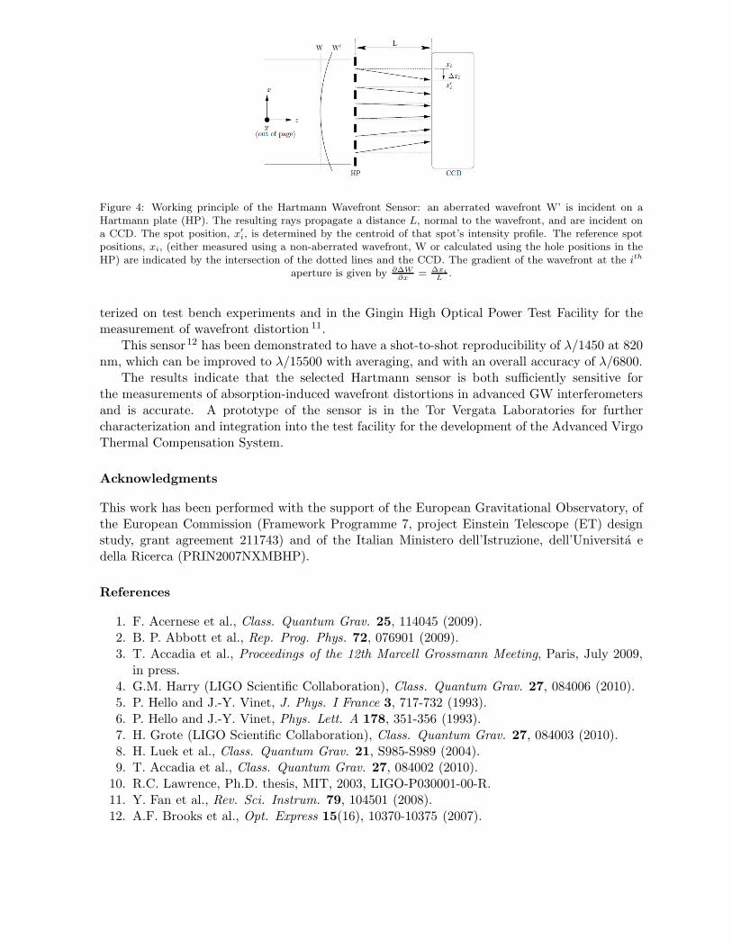
Figure 4: Working principle of the Hartmann Wavefront Sensor: an aberrated wavefront W’ is incident on aHartmann plate (HP). The resulting rays propagate a distance L, normal to the wavefront, and are incident ona CCD. The spot position, x′
i, is determined by the centroid of that spot’s intensity profile. The reference spot
positions, xi, (either measured using a non-aberrated wavefront, W or calculated using the hole positions in theHP) are indicated by the intersection of the dotted lines and the CCD. The gradient of the wavefront at the ith
aperture is given by ∂∆W
∂x= ∆xi
L.
terized on test bench experiments and in the Gingin High Optical Power Test Facility for themeasurement of wavefront distortion 11.
This sensor12 has been demonstrated to have a shot-to-shot reproducibility of λ/1450 at 820nm, which can be improved to λ/15500 with averaging, and with an overall accuracy of λ/6800.
The results indicate that the selected Hartmann sensor is both sufficiently sensitive forthe measurements of absorption-induced wavefront distortions in advanced GW interferometersand is accurate. A prototype of the sensor is in the Tor Vergata Laboratories for furthercharacterization and integration into the test facility for the development of the Advanced VirgoThermal Compensation System.
Acknowledgments
This work has been performed with the support of the European Gravitational Observatory, ofthe European Commission (Framework Programme 7, project Einstein Telescope (ET) designstudy, grant agreement 211743) and of the Italian Ministero dell’Istruzione, dell’Universita edella Ricerca (PRIN2007NXMBHP).
References
1. F. Acernese et al., Class. Quantum Grav. 25, 114045 (2009).2. B. P. Abbott et al., Rep. Prog. Phys. 72, 076901 (2009).3. T. Accadia et al., Proceedings of the 12th Marcell Grossmann Meeting, Paris, July 2009,
in press.4. G.M. Harry (LIGO Scientific Collaboration), Class. Quantum Grav. 27, 084006 (2010).5. P. Hello and J.-Y. Vinet, J. Phys. I France 3, 717-732 (1993).6. P. Hello and J.-Y. Vinet, Phys. Lett. A 178, 351-356 (1993).7. H. Grote (LIGO Scientific Collaboration), Class. Quantum Grav. 27, 084003 (2010).8. H. Luek et al., Class. Quantum Grav. 21, S985-S989 (2004).9. T. Accadia et al., Class. Quantum Grav. 27, 084002 (2010).
10. R.C. Lawrence, Ph.D. thesis, MIT, 2003, LIGO-P030001-00-R.11. Y. Fan et al., Rev. Sci. Instrum. 79, 104501 (2008).12. A.F. Brooks et al., Opt. Express 15(16), 10370-10375 (2007).

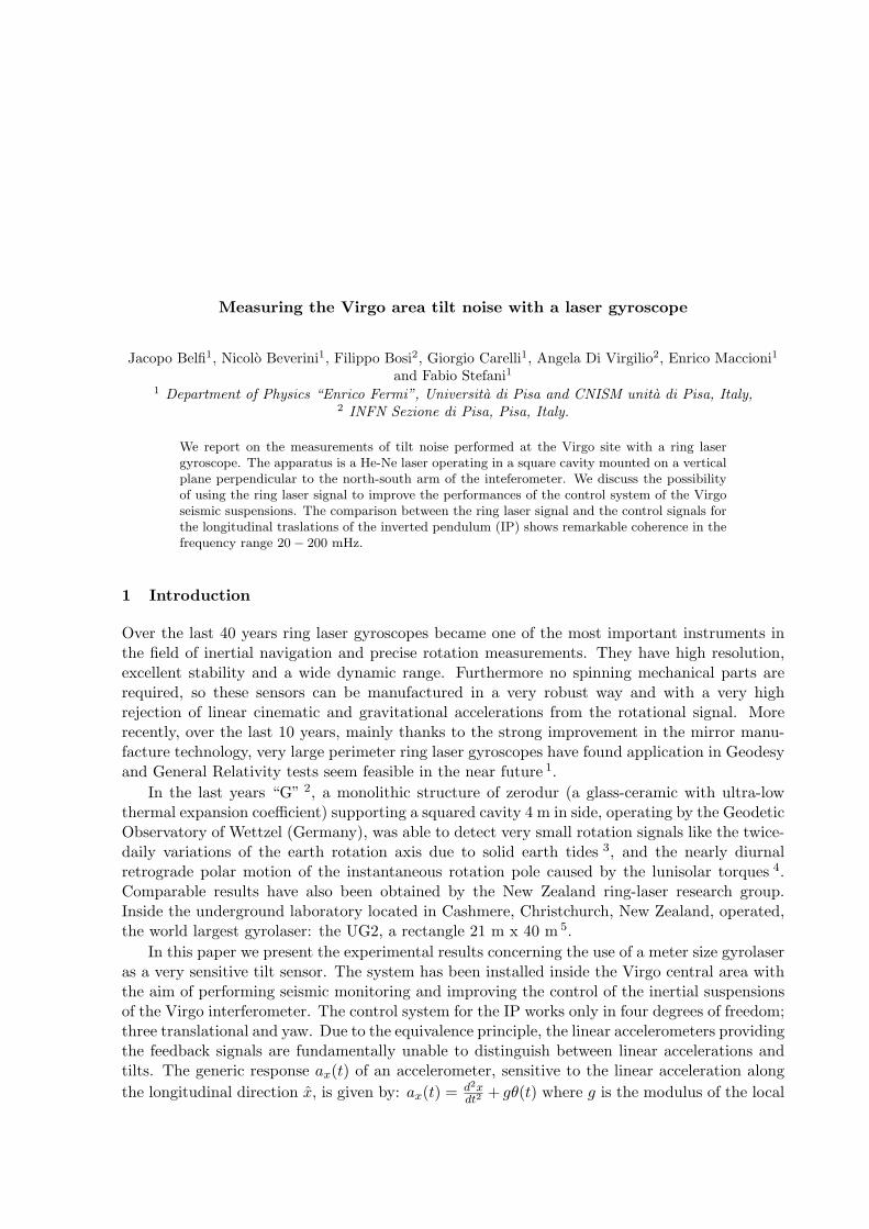
Measuring the Virgo area tilt noise with a laser gyroscope
Jacopo Belfi1, Nicolo Beverini1, Filippo Bosi2, Giorgio Carelli1, Angela Di Virgilio2, Enrico Maccioni1
and Fabio Stefani1
1 Department of Physics “Enrico Fermi”, Universita di Pisa and CNISM unita di Pisa, Italy,2 INFN Sezione di Pisa, Pisa, Italy.
We report on the measurements of tilt noise performed at the Virgo site with a ring lasergyroscope. The apparatus is a He-Ne laser operating in a square cavity mounted on a verticalplane perpendicular to the north-south arm of the inteferometer. We discuss the possibilityof using the ring laser signal to improve the performances of the control system of the Virgoseismic suspensions. The comparison between the ring laser signal and the control signals forthe longitudinal traslations of the inverted pendulum (IP) shows remarkable coherence in thefrequency range 20− 200 mHz.
1 Introduction
Over the last 40 years ring laser gyroscopes became one of the most important instruments inthe field of inertial navigation and precise rotation measurements. They have high resolution,excellent stability and a wide dynamic range. Furthermore no spinning mechanical parts arerequired, so these sensors can be manufactured in a very robust way and with a very highrejection of linear cinematic and gravitational accelerations from the rotational signal. Morerecently, over the last 10 years, mainly thanks to the strong improvement in the mirror manu-facture technology, very large perimeter ring laser gyroscopes have found application in Geodesyand General Relativity tests seem feasible in the near future 1.
In the last years “G” 2, a monolithic structure of zerodur (a glass-ceramic with ultra-lowthermal expansion coefficient) supporting a squared cavity 4 m in side, operating by the GeodeticObservatory of Wettzel (Germany), was able to detect very small rotation signals like the twice-daily variations of the earth rotation axis due to solid earth tides 3, and the nearly diurnalretrograde polar motion of the instantaneous rotation pole caused by the lunisolar torques 4.Comparable results have also been obtained by the New Zealand ring-laser research group.Inside the underground laboratory located in Cashmere, Christchurch, New Zealand, operated,the world largest gyrolaser: the UG2, a rectangle 21 m x 40 m 5.
In this paper we present the experimental results concerning the use of a meter size gyrolaseras a very sensitive tilt sensor. The system has been installed inside the Virgo central area withthe aim of performing seismic monitoring and improving the control of the inertial suspensionsof the Virgo interferometer. The control system for the IP works only in four degrees of freedom;three translational and yaw. Due to the equivalence principle, the linear accelerometers providingthe feedback signals are fundamentally unable to distinguish between linear accelerations andtilts. The generic response ax(t) of an accelerometer, sensitive to the linear acceleration along
the longitudinal direction x, is given by: ax(t) = d2xdt2
+ gθ(t) where g is the modulus of the local
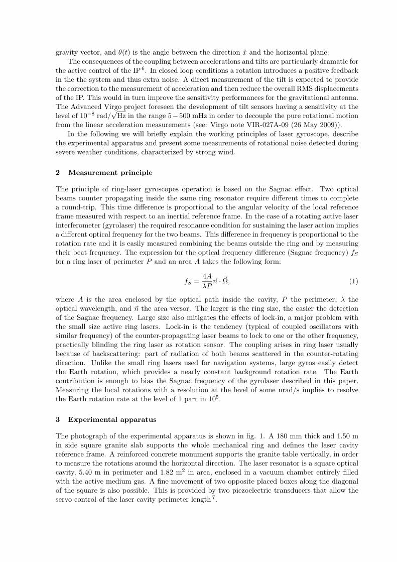
gravity vector, and θ(t) is the angle between the direction x and the horizontal plane.
The consequences of the coupling between accelerations and tilts are particularly dramatic forthe active control of the IP 6. In closed loop conditions a rotation introduces a positive feedbackin the the system and thus extra noise. A direct measurement of the tilt is expected to providethe correction to the measurement of acceleration and then reduce the overall RMS displacementsof the IP. This would in turn improve the sensitivity performances for the gravitational antenna.The Advanced Virgo project foreseen the development of tilt sensors having a sensitivity at thelevel of 10−8 rad/
√Hz in the range 5−500 mHz in order to decouple the pure rotational motion
from the linear acceleration measurements (see: Virgo note VIR-027A-09 (26 May 2009)).
In the following we will briefly explain the working principles of laser gyroscope, describethe experimental apparatus and present some measurements of rotational noise detected duringsevere weather conditions, characterized by strong wind.
2 Measurement principle
The principle of ring-laser gyroscopes operation is based on the Sagnac effect. Two opticalbeams counter propagating inside the same ring resonator require different times to completea round-trip. This time difference is proportional to the angular velocity of the local referenceframe measured with respect to an inertial reference frame. In the case of a rotating active laserinterferometer (gyrolaser) the required resonance condition for sustaining the laser action impliesa different optical frequency for the two beams. This difference in frequency is proportional to therotation rate and it is easily measured combining the beams outside the ring and by measuringtheir beat frequency. The expression for the optical frequency difference (Sagnac frequency) fSfor a ring laser of perimeter P and an area A takes the following form:
fS =4A
λP~n · ~Ω, (1)
where A is the area enclosed by the optical path inside the cavity, P the perimeter, λ theoptical wavelength, and ~n the area versor. The larger is the ring size, the easier the detectionof the Sagnac frequency. Large size also mitigates the effects of lock-in, a major problem withthe small size active ring lasers. Lock-in is the tendency (typical of coupled oscillators withsimilar frequency) of the counter-propagating laser beams to lock to one or the other frequency,practically blinding the ring laser as rotation sensor. The coupling arises in ring laser usuallybecause of backscattering: part of radiation of both beams scattered in the counter-rotatingdirection. Unlike the small ring lasers used for navigation systems, large gyros easily detectthe Earth rotation, which provides a nearly constant background rotation rate. The Earthcontribution is enough to bias the Sagnac frequency of the gyrolaser described in this paper.Measuring the local rotations with a resolution at the level of some nrad/s implies to resolvethe Earth rotation rate at the level of 1 part in 105.
3 Experimental apparatus
The photograph of the experimental apparatus is shown in fig. 1. A 180 mm thick and 1.50 min side square granite slab supports the whole mechanical ring and defines the laser cavityreference frame. A reinforced concrete monument supports the granite table vertically, in orderto measure the rotations around the horizontal direction. The laser resonator is a square opticalcavity, 5.40 m in perimeter and 1.82 m2 in area, enclosed in a vacuum chamber entirely filledwith the active medium gas. A fine movement of two opposite placed boxes along the diagonalof the square is also possible. This is provided by two piezoelectric transducers that allow theservo control of the laser cavity perimeter length 7.
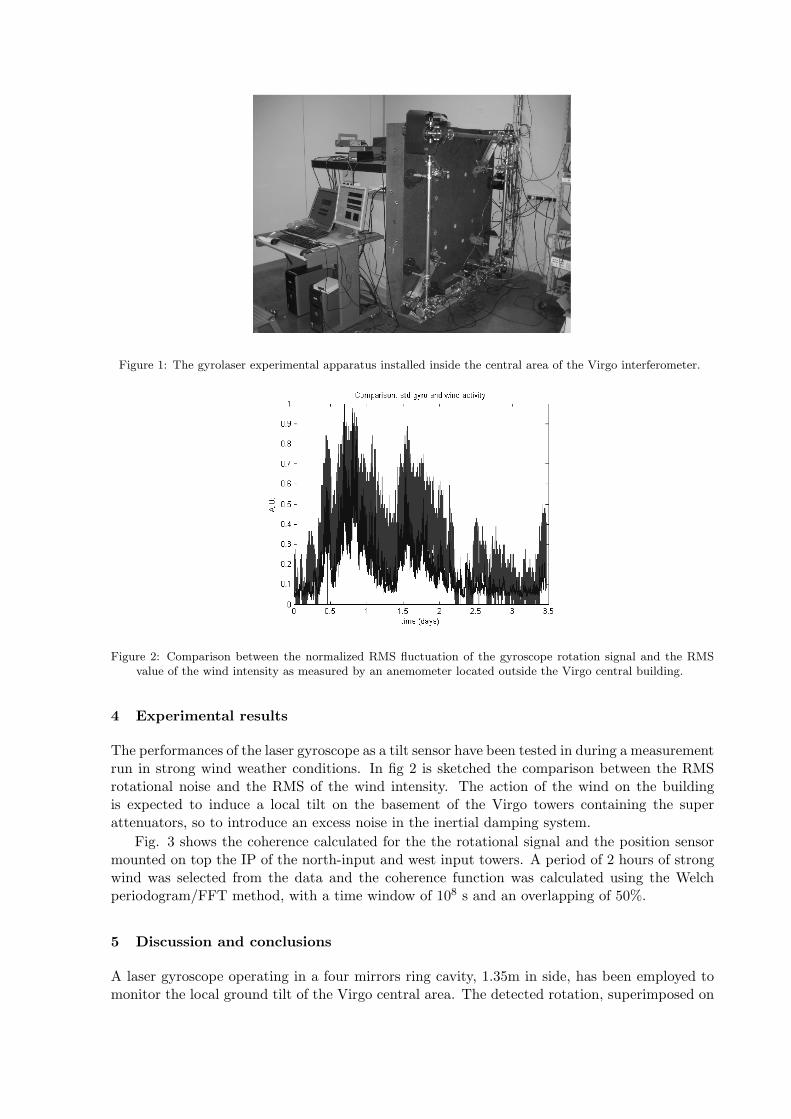
Figure 1: The gyrolaser experimental apparatus installed inside the central area of the Virgo interferometer.
Figure 2: Comparison between the normalized RMS fluctuation of the gyroscope rotation signal and the RMSvalue of the wind intensity as measured by an anemometer located outside the Virgo central building.
4 Experimental results
The performances of the laser gyroscope as a tilt sensor have been tested in during a measurementrun in strong wind weather conditions. In fig 2 is sketched the comparison between the RMSrotational noise and the RMS of the wind intensity. The action of the wind on the buildingis expected to induce a local tilt on the basement of the Virgo towers containing the superattenuators, so to introduce an excess noise in the inertial damping system.
Fig. 3 shows the coherence calculated for the the rotational signal and the position sensormounted on top the IP of the north-input and west input towers. A period of 2 hours of strongwind was selected from the data and the coherence function was calculated using the Welchperiodogram/FFT method, with a time window of 108 s and an overlapping of 50%.
5 Discussion and conclusions
A laser gyroscope operating in a four mirrors ring cavity, 1.35m in side, has been employed tomonitor the local ground tilt of the Virgo central area. The detected rotation, superimposed on
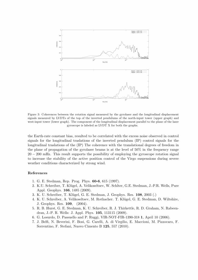
0
0.2
0.4
0.6
0.8
1
10-3 10-2 10-1
Coh
eren
ce
freq. (Hz)
Sagnac - LVDT-X WISagnac - LVDT-Z WI
0
0.2
0.4
0.6
0.8
1
10-3 10-2 10-1
Coh
eren
ce
freq. (Hz)
Sagnac - LVDT-X NISagnac - LVDT-Z NI
Figure 3: Coherences between the rotation signal measured by the gyrolaser and the longitudinal displacementsignals measured by LVDTs of the top of the inverted pendulums of the north-input tower (upper graph) andwest-input tower (lower graph). The component of the longitudinal displacement parallel to the plane of the laser
gyroscope is labeled as LVDT X for both the graphs.
the Earth-rate constant bias, resulted to be correlated with the excess noise observed in controlsignals for the longitudinal traslations of the inverted pendulum (IP) control signals for thelongitudinal traslations of the (IP) The coherence with the translational degrees of freedom inthe plane of propagation of the gyrolaser beams is at the level of 50% in the frequency range20 − 200 mHz. This result supports the possibility of employing the gyroscope rotation signalto increase the stability of the active position control of the Virgo suspensions during severeweather conditions characterized by strong wind.
References
1. G. E. Stedman, Rep. Prog. Phys. 60-6, 615 (1997).2. K.U. Schreiber, T. Klugel, A. Velikoseltsev, W. Schlter, G.E. Stedman, J.-P.R. Wells, Pure
Appl. Geophys. 166, 1485 (2009).3. K. U. Schreiber, T. Klugel, G. E. Stedman, J. Geophys. Res. 108, 2003 (.)4. K. U. Schreiber, A. Velikoseltsev, M. Rothacher. T. Klugel, G. E. Stedman, D. Wiltshire,
J. Geophys. Res. 109, (2004).5. R. B. Hurst, G. E. Stedman, K. U. Schreiber, R. J. Thirkettle, R. D. Graham, N. Rabeen-
dran, J.-P. R. Wells: J. Appl. Phys. 105, 113115 (2009).6. G. Losurdo, D. Passuello and P. Ruggi, VIR-NOT-FIR-1390-318 1, April 10 (2006).7. J. Belfi, N. Beverini, F. Bosi, G. Carelli, A. di Virgilio, E. Maccioni, M. Pizzocaro, F.
Sorrentino, F. Stefani, Nuovo Cimento B 125, 557 (2010).
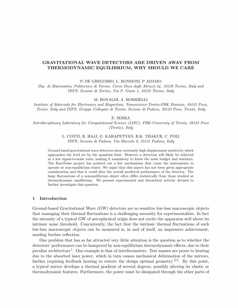
GRAVITATIONAL WAVE DETECTORS ARE DRIVEN AWAY FROM
THERMODYNAMIC EQUILIBRIUM, WHY SHOULD WE CARE
P. DE GREGORIO, L. RONDONI, P ADAMO
Dip. di Matematica, Politecnico di Torino, Corso Duca degli Abruzzi 24, 10129 Torino, Italy and
INFN, Sezione di Torino, Via P. Giura 1, 10125 Torino, Italy
M. BONALDI, A. BORRIELLI
Institute of Materials for Electronics and Magnetism, Nanoscience-Trento-FBK Division, 38123 Povo,
Trento, Italy and INFN, Gruppo Collegato di Trento, Sezione di Padova, 38123 Povo, Trento, Italy
E. SERRA
Interdisciplinary Laboratory for Computational Science (LISC), FBK-University of Trento, 38123 Povo
(Trento), Italy
L. CONTI, R. HAJJ, G. KARAPETYAN, R.K. THAKUR, C. POLI
INFN, Sezione di Padova, Via Marzolo 8, 35131 Padova, Italy
Ground based gravitational wave detectors show extremely high displacement sensitivity whichapproaches the level set by the quantum limit. However a detection will likely be achievedat a low signal-to-noise ratio, making it mandatory to know the noise budget and statistics.The RareNoise project has pointed out a few mechanisms that cause the instruments tooperate at non-equilibrium states. We argue that this aspect has not been given appropriateconsideration and that it could alter the overall predicted performance of the detector. Thelarge fluctuations of a nonequilibrium object often differ statistically from those studied atthermodynamic equilibrium. We present experimental and theoretical activity devised tofurther investigate this question.
1 Introduction
Ground-based Gravitational Wave (GW) detectors are so sensitive low-loss macroscopic objectsthat managing their thermal fluctuations is a challenging necessity for experimentalists. In factthe intensity of a typical GW of astrophysical origin does not excite the apparatus well above itsintrinsic noise threshold. Concurrently, the fact that the intrinsic thermal fluctuations of suchlow-loss macroscopic objects can be measured is, in and of itself, an impressive achievement,needing further reflection.
One problem that has so far attracted very little attention is the question as to whether thedetectors’ performance can be hampered by non-equilibrium thermodynamic effects, due to theirpeculiar architecture1. One example is that of interferometers. Test masses are prone to heatingdue to the absorbed laser power, which in turn causes mechanical deformation of the mirrors,further requiring feedback heating to restore the design optimal geometry 2,3. By this point,a typical mirror develops a thermal gradient of several degrees, possibly altering its elastic orthermodynamic features. Furthermore, the power must be dissipated through the other parts of
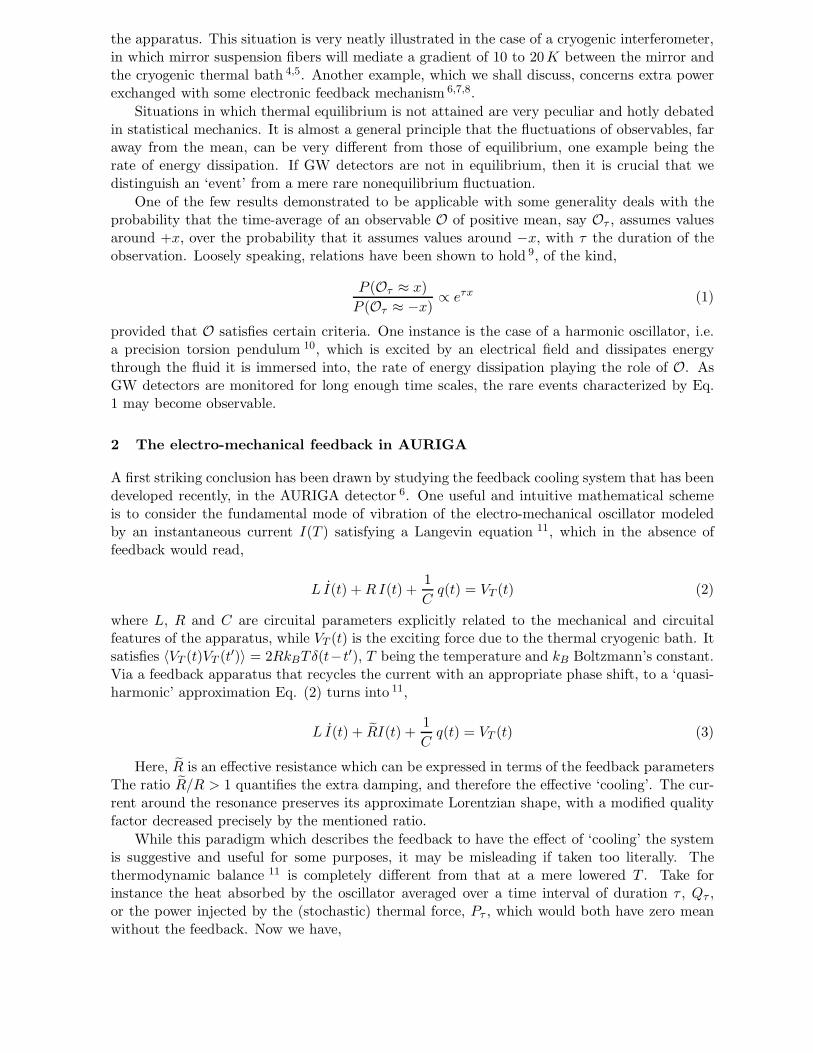
the apparatus. This situation is very neatly illustrated in the case of a cryogenic interferometer,in which mirror suspension fibers will mediate a gradient of 10 to 20K between the mirror andthe cryogenic thermal bath 4,5. Another example, which we shall discuss, concerns extra powerexchanged with some electronic feedback mechanism 6,7,8.
Situations in which thermal equilibrium is not attained are very peculiar and hotly debatedin statistical mechanics. It is almost a general principle that the fluctuations of observables, faraway from the mean, can be very different from those of equilibrium, one example being therate of energy dissipation. If GW detectors are not in equilibrium, then it is crucial that wedistinguish an ‘event’ from a mere rare nonequilibrium fluctuation.
One of the few results demonstrated to be applicable with some generality deals with theprobability that the time-average of an observable O of positive mean, say Oτ , assumes valuesaround +x, over the probability that it assumes values around −x, with τ the duration of theobservation. Loosely speaking, relations have been shown to hold 9, of the kind,
P (Oτ ≈ x)
P (Oτ ≈ −x)∝ e
τx (1)
provided that O satisfies certain criteria. One instance is the case of a harmonic oscillator, i.e.a precision torsion pendulum 10, which is excited by an electrical field and dissipates energythrough the fluid it is immersed into, the rate of energy dissipation playing the role of O. AsGW detectors are monitored for long enough time scales, the rare events characterized by Eq.1 may become observable.
2 The electro-mechanical feedback in AURIGA
A first striking conclusion has been drawn by studying the feedback cooling system that has beendeveloped recently, in the AURIGA detector 6. One useful and intuitive mathematical schemeis to consider the fundamental mode of vibration of the electro-mechanical oscillator modeledby an instantaneous current I(T ) satisfying a Langevin equation 11, which in the absence offeedback would read,
L I(t) + R I(t) +1
Cq(t) = VT (t) (2)
where L, R and C are circuital parameters explicitly related to the mechanical and circuitalfeatures of the apparatus, while VT (t) is the exciting force due to the thermal cryogenic bath. Itsatisfies 〈VT (t)VT (t′)〉 = 2RkBTδ(t−t
′), T being the temperature and kB Boltzmann’s constant.Via a feedback apparatus that recycles the current with an appropriate phase shift, to a ‘quasi-harmonic’ approximation Eq. (2) turns into 11,
L I(t) + ˜RI(t) +1
Cq(t) = VT (t) (3)
Here, ˜R is an effective resistance which can be expressed in terms of the feedback parametersThe ratio ˜R/R > 1 quantifies the extra damping, and therefore the effective ‘cooling’. The cur-rent around the resonance preserves its approximate Lorentzian shape, with a modified qualityfactor decreased precisely by the mentioned ratio.
While this paradigm which describes the feedback to have the effect of ‘cooling’ the systemis suggestive and useful for some purposes, it may be misleading if taken too literally. Thethermodynamic balance 11 is completely different from that at a mere lowered T . Take forinstance the heat absorbed by the oscillator averaged over a time interval of duration τ , Qτ ,or the power injected by the (stochastic) thermal force, Pτ , which would both have zero meanwithout the feedback. Now we have,
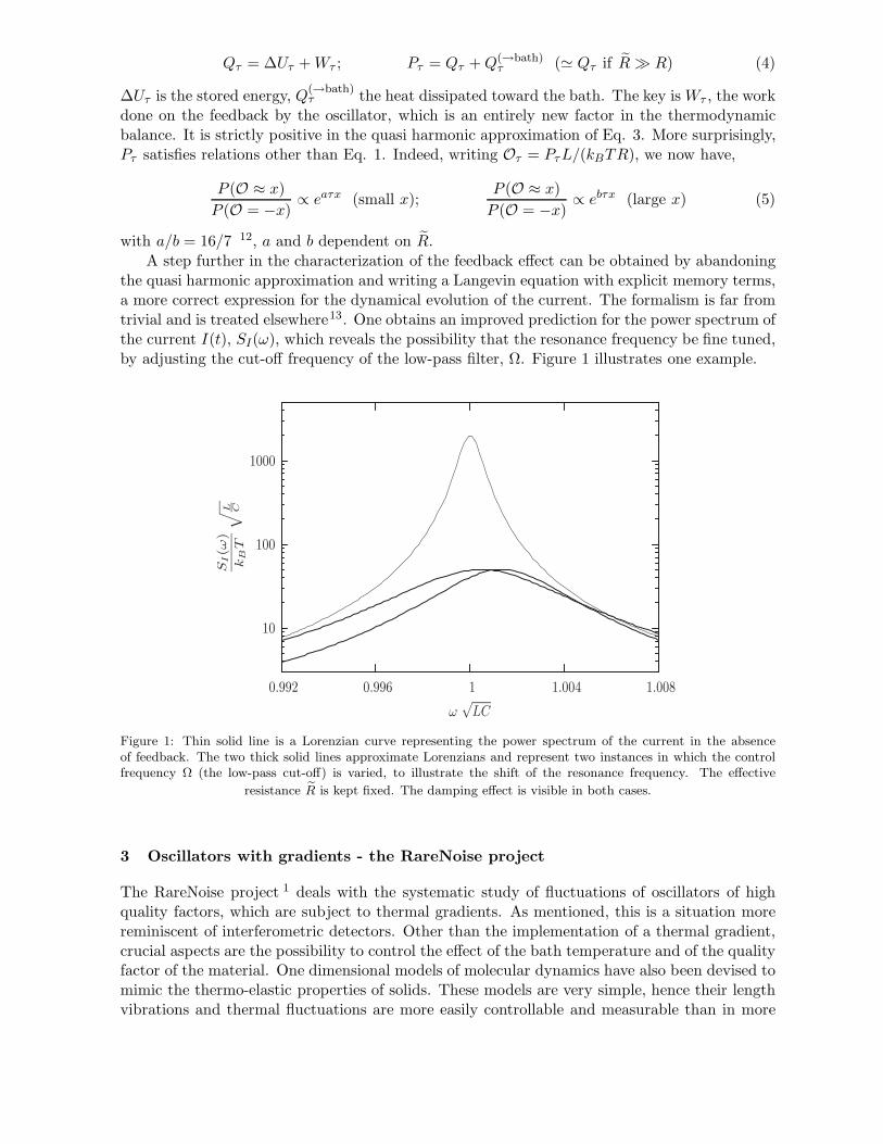
Qτ = ∆Uτ + Wτ ; Pτ = Qτ + Q(→bath)
τ (≃ Qτ if ˜
R ≫ R) (4)
∆Uτ is the stored energy, Q(→bath)
τ the heat dissipated toward the bath. The key is Wτ , the workdone on the feedback by the oscillator, which is an entirely new factor in the thermodynamicbalance. It is strictly positive in the quasi harmonic approximation of Eq. 3. More surprisingly,Pτ satisfies relations other than Eq. 1. Indeed, writing Oτ = PτL/(kBTR), we now have,
P (O ≈ x)
P (O = −x)∝ e
aτx (small x);P (O ≈ x)
P (O = −x)∝ e
bτx (large x) (5)
with a/b = 16/7 12, a and b dependent on ˜
R.
A step further in the characterization of the feedback effect can be obtained by abandoningthe quasi harmonic approximation and writing a Langevin equation with explicit memory terms,a more correct expression for the dynamical evolution of the current. The formalism is far fromtrivial and is treated elsewhere13. One obtains an improved prediction for the power spectrum ofthe current I(t), SI(ω), which reveals the possibility that the resonance frequency be fine tuned,by adjusting the cut-off frequency of the low-pass filter, Ω. Figure 1 illustrates one example.
10
100
1000
0.992 0.996 1 1.004 1.008
SI(ω
)
kB
T
√
L C
ω
√
LC
Figure 1: Thin solid line is a Lorenzian curve representing the power spectrum of the current in the absenceof feedback. The two thick solid lines approximate Lorenzians and represent two instances in which the controlfrequency Ω (the low-pass cut-off) is varied, to illustrate the shift of the resonance frequency. The effective
resistance ˜R is kept fixed. The damping effect is visible in both cases.
3 Oscillators with gradients - the RareNoise project
The RareNoise project 1 deals with the systematic study of fluctuations of oscillators of highquality factors, which are subject to thermal gradients. As mentioned, this is a situation morereminiscent of interferometric detectors. Other than the implementation of a thermal gradient,crucial aspects are the possibility to control the effect of the bath temperature and of the qualityfactor of the material. One dimensional models of molecular dynamics have also been devised tomimic the thermo-elastic properties of solids. These models are very simple, hence their lengthvibrations and thermal fluctuations are more easily controllable and measurable than in more
realistic, but more complicated, models. Indeed, they provide qualitative agreement with realsolids, for example the behavior of their elastic constant E with temperature, see Figure 2 Moreadvanced, 3 dimensional models of molecular dynamics are also being developed. Together withthe ongoing experiment, they will provide the groundwork for advancing our knowledge in bothGW detectors, and general nonequilibrium problems.
0.6
0.7
0.8
0.9
1
1.1
0 0.01 0.02 0.03 0.04 0.05
E/
E0
T [a.u.]
Figure 2: Elastic constants E for classical MD simulations of one-dimensional models with two different interatomicpotentials, referred to the extrapolated constant at zero temperature (harmonic oscillators).
Acknowledgments
The research leading to these results has received funding from the European Research Councilunder the European Community’s Seventh Framework Programme (FP7/2007-2013) / ERCgrant agreement n 202680. The EC is not liable for any use that can be made on the informationcontained herein.
References
1. L. Conti, M. Bonaldi and L. Rondoni, Class. Quantum Grav. 27, 084032 (2010)2. P. Hello, Eur. Phys. J. D 15, 373 (2001)3. T. Accadia, F. Acernese, F. Antonucci et al, Class. Quantum Grav. 28, 114002 (2011)4. T. Tomaru, T. Suzuki, T. Uchiyama et al, Phys. Lett. A 301, 215 (2002)5. F. Basti, F. Frasconi, M. Granata et al, Journal of Physics: Conference Series 228, 012030
(2010)6. A. Vinante, M. Bignotto, M. Bonaldi et al, Phys. Rev. Lett. 101, 033601 (2008)7. B.Abbott, New J. Phys. 11, 073032 (2009)8. T. Corbitt, C. Wipf, T. Bodiya et al, Phys. Rev. Lett. 99, 160801 (2007)9. L. Rondoni and C. Mejia-Monasterio, Nonlinearity 20, R1 (2007), and references therein.
10. S. Ciliberto, S. Joubaud and A. Petrosyan, J. Stat. Mech. 12, P12003 (2010)11. M. Bonaldi, L. Conti, P. De Gregorio et al, Phys. Rev. Lett. 103, 010601 (2009)12. J. Farago, J. Stat. Phys. 107, 781 (2002)13. P. De Gregorio, L. Rondoni, M. Bonaldi and L. Conti, J. Stat. Mech. , P10016 (2009)

II.Experimental Gravity


6.Short Range Gravity

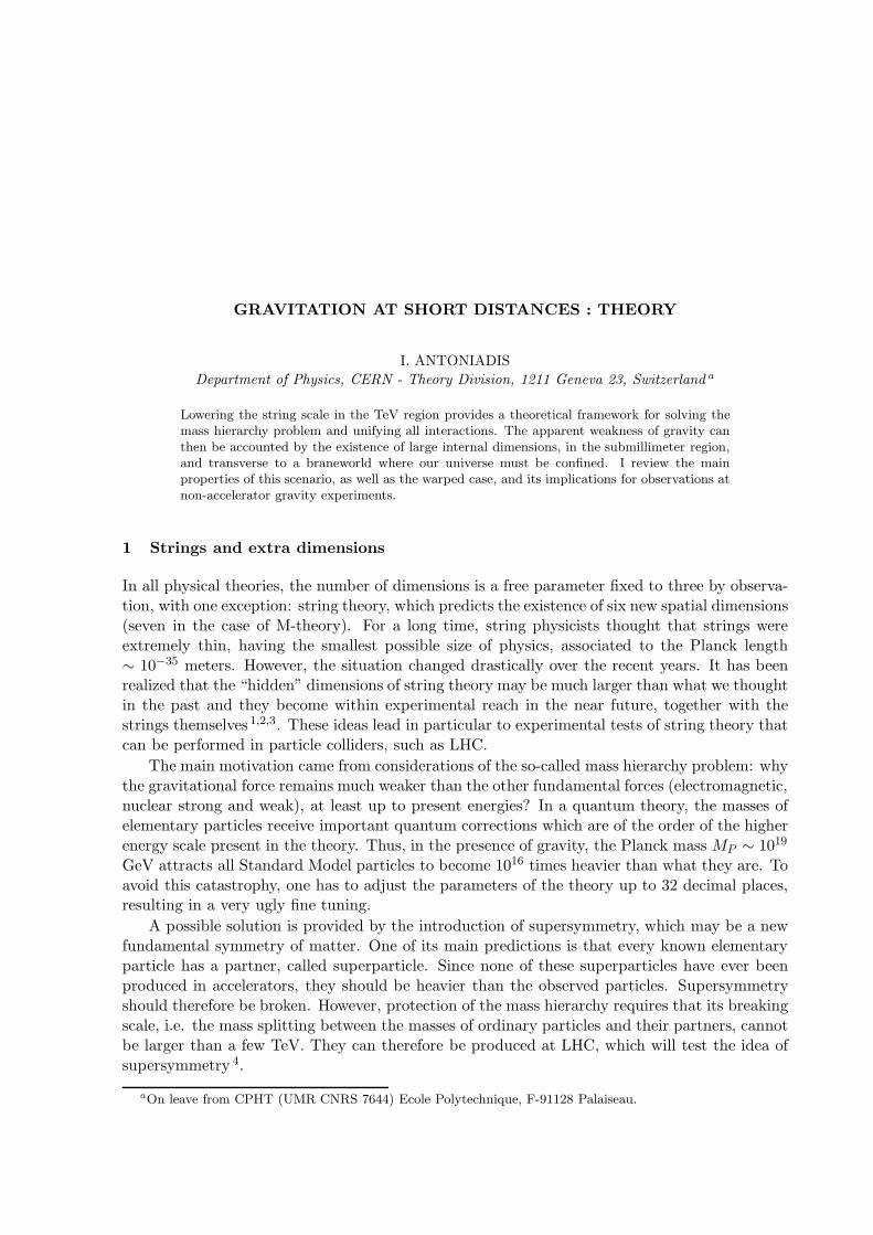
GRAVITATION AT SHORT DISTANCES : THEORY
I. ANTONIADIS
Department of Physics, CERN - Theory Division, 1211 Geneva 23, Switzerland a
Lowering the string scale in the TeV region provides a theoretical framework for solving themass hierarchy problem and unifying all interactions. The apparent weakness of gravity canthen be accounted by the existence of large internal dimensions, in the submillimeter region,and transverse to a braneworld where our universe must be confined. I review the mainproperties of this scenario, as well as the warped case, and its implications for observations atnon-accelerator gravity experiments.
1 Strings and extra dimensions
In all physical theories, the number of dimensions is a free parameter fixed to three by observa-tion, with one exception: string theory, which predicts the existence of six new spatial dimensions(seven in the case of M-theory). For a long time, string physicists thought that strings wereextremely thin, having the smallest possible size of physics, associated to the Planck length∼ 10−35 meters. However, the situation changed drastically over the recent years. It has beenrealized that the “hidden” dimensions of string theory may be much larger than what we thoughtin the past and they become within experimental reach in the near future, together with thestrings themselves 1,2,3. These ideas lead in particular to experimental tests of string theory thatcan be performed in particle colliders, such as LHC.
The main motivation came from considerations of the so-called mass hierarchy problem: whythe gravitational force remains much weaker than the other fundamental forces (electromagnetic,nuclear strong and weak), at least up to present energies? In a quantum theory, the masses ofelementary particles receive important quantum corrections which are of the order of the higherenergy scale present in the theory. Thus, in the presence of gravity, the Planck mass MP ∼ 1019
GeV attracts all Standard Model particles to become 1016 times heavier than what they are. Toavoid this catastrophy, one has to adjust the parameters of the theory up to 32 decimal places,resulting in a very ugly fine tuning.
A possible solution is provided by the introduction of supersymmetry, which may be a newfundamental symmetry of matter. One of its main predictions is that every known elementaryparticle has a partner, called superparticle. Since none of these superparticles have ever beenproduced in accelerators, they should be heavier than the observed particles. Supersymmetryshould therefore be broken. However, protection of the mass hierarchy requires that its breakingscale, i.e. the mass splitting between the masses of ordinary particles and their partners, cannotbe larger than a few TeV. They can therefore be produced at LHC, which will test the idea ofsupersymmetry 4.
aOn leave from CPHT (UMR CNRS 7644) Ecole Polytechnique, F-91128 Palaiseau.
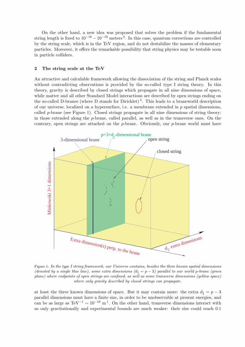
On the other hand, a new idea was proposed that solves the problem if the fundamentalstring length is fixed to 10−18
− 10−19 meters 3. In this case, quantum corrections are controlledby the string scale, which is in the TeV region, and do not destabilize the masses of elementaryparticles. Moreover, it offers the remarkable possibility that string physics may be testable soonin particle colliders.
2 The string scale at the TeV
An attractive and calculable framework allowing the dissociation of the string and Planck scaleswithout contradicting observations is provided by the so-called type I string theory. In thistheory, gravity is described by closed strings which propagate in all nine dimensions of space,while matter and all other Standard Model interactions are described by open strings ending onthe so-called D-branes (where D stands for Dirichlet) 5. This leads to a braneworld descriptionof our universe, localized on a hypersurface, i.e. a membrane extended in p spatial dimensions,called p-brane (see Figure 1). Closed strings propagate in all nine dimensions of string theory:in those extended along the p-brane, called parallel, as well as in the transverse ones. On thecontrary, open strings are attached on the p-brane. Obviously, our p-brane world must have
open string
closed string
Extra dimension(s) perp. to the brane
Min
kow
ski 3
+1
dim
ensi
ons
d extra dimensions
||
p=3+d -dimensional brane// 3-dimensional brane
Figure 1: In the type I string framework, our Universe contains, besides the three known spatial dimensions
(denoted by a single blue line), some extra dimensions (d‖
= p − 3) parallel to our world p-brane (green
plane) where endpoints of open strings are confined, as well as some transverse dimensions (yellow space)
where only gravity described by closed strings can propagate.
at least the three known dimensions of space. But it may contain more: the extra d‖ = p − 3parallel dimensions must have a finite size, in order to be unobservable at present energies, andcan be as large as TeV−1
∼ 10−18 m 1. On the other hand, transverse dimensions interact withus only gravitationally and experimental bounds are much weaker: their size could reach 0.1
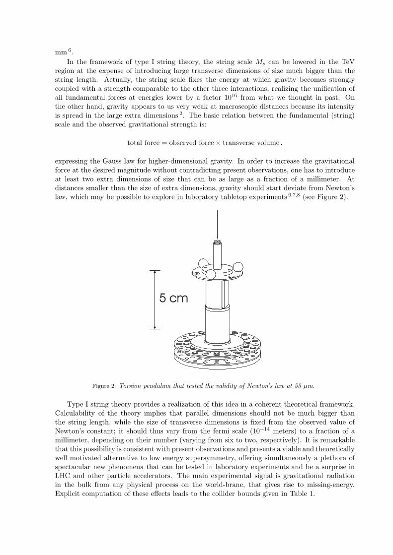
mm 6.
In the framework of type I string theory, the string scale Ms can be lowered in the TeVregion at the expense of introducing large transverse dimensions of size much bigger than thestring length. Actually, the string scale fixes the energy at which gravity becomes stronglycoupled with a strength comparable to the other three interactions, realizing the unification ofall fundamental forces at energies lower by a factor 1016 from what we thought in past. Onthe other hand, gravity appears to us very weak at macroscopic distances because its intensityis spread in the large extra dimensions 2. The basic relation between the fundamental (string)scale and the observed gravitational strength is:
total force = observed force × transverse volume ,
expressing the Gauss law for higher-dimensional gravity. In order to increase the gravitationalforce at the desired magnitude without contradicting present observations, one has to introduceat least two extra dimensions of size that can be as large as a fraction of a millimeter. Atdistances smaller than the size of extra dimensions, gravity should start deviate from Newton’slaw, which may be possible to explore in laboratory tabletop experiments 6,7,8 (see Figure 2).
Figure 2: Torsion pendulum that tested the validity of Newton’s law at 55 µm.
Type I string theory provides a realization of this idea in a coherent theoretical framework.Calculability of the theory implies that parallel dimensions should not be much bigger thanthe string length, while the size of transverse dimensions is fixed from the observed value ofNewton’s constant; it should thus vary from the fermi scale (10−14 meters) to a fraction of amillimeter, depending on their number (varying from six to two, respectively). It is remarkablethat this possibility is consistent with present observations and presents a viable and theoreticallywell motivated alternative to low energy supersymmetry, offering simultaneously a plethora ofspectacular new phenomena that can be tested in laboratory experiments and be a surprise inLHC and other particle accelerators. The main experimental signal is gravitational radiationin the bulk from any physical process on the world-brane, that gives rise to missing-energy.Explicit computation of these effects leads to the collider bounds given in Table 1.
Table 1: Collider bounds on the size of gravitational extra dimensions R⊥ in mm.
Experiment n = 2 n = 4 n = 6
LEP 2 5 × 10⁻¹ 2 × 10⁻⁸ 7 × 10⁻¹¹
Tevatron 5 × 10⁻¹ 10−8 4 × 10⁻¹¹
LHC 4 × 10⁻³ 6 × 10⁻¹⁰ 3 × 10⁻¹²
3 Short range forces
There are three categories of predictions in “table-top” experiments that measure gravity atshort distances:(i) Deviations from the Newton’s law 1/r2 behavior to 1/r2+n, which can be observable forn = 2 large transverse dimensions of sub-millimeter size. This case is particularly attractive ontheoretical grounds because of the logarithmic sensitivity of Standard Model couplings on thesize of transverse space 9, that allows to determine the hierarchy 10.(ii) New scalar forces in the sub-millimeter range, related to the mechanism of supersymmetrybreaking, and mediated by light scalar fields ϕ with masses:
mϕ ≃
m2susy
MP≃ 10−4
− 10−6 eV , (1)
for a supersymmetry breaking scale msusy ≃ 1 − 10 TeV. They correspond to Compton wave-lengths of 1 mm to 10 µm. msusy can be either the compactification scale of parallel dimensions1/R‖ if supersymmetry is broken by compactification 11, or the string scale if it is broken “max-imally” on our world-brane 2,3. A universal attractive scalar force is mediated by the radionmodulus ϕ ≡ MP lnR, with R the radius of the longitudinal (R‖) or transverse (R⊥) dimen-sion(s). In the former case, the result (1) follows from the behavior of the vacuum energy densityΛ ∼ 1/R4
‖for large R‖ (up to logarithmic corrections). In the latter, supersymmetry is broken
primarily on the brane, and thus its transmission to the bulk is gravitationally suppressed, lead-ing to (1). For n = 2, there may be an enhancement factor of the radion mass by ln R⊥Ms ≃ 30decreasing its wavelength by an order of magnitude 10.
The coupling of the radius modulus to matter relative to gravity can be easily computedand is given by:
√
αϕ =1
M
∂M
∂ϕ; αϕ =
∂ lnΛQCD
∂ ln R≃
13
for R‖
2nn+2
= 1 − 1.5 for R⊥
(2)
where M denotes a generic physical mass. In the longitudinal case, the coupling arises dom-inantly through the radius dependence of the QCD gauge coupling 11, while in the case oftransverse dimension, it can be deduced from the rescaling of the metric which changes thestring to the Einstein frame and depends slightly on the bulk dimensionality (α = 1 − 1.5 forn = 2 − 6) 10. Such a force can be tested in microgravity experiments and should be contrastedwith the change of Newton’s law due the presence of extra dimensions that is observable onlyfor n = 26,7. The resulting bounds for the higher dimensional gravity scale M∗, from an analysisof the radion effects, are 12:
M∗>∼
6TeV (for R⊥) . (3)
In principle there can be other light moduli which couple with even larger strengths. Forexample the dilaton, whose vacuum expectation value determines the string coupling, if it doesnot acquire large mass from some dynamical mechanism, can lead to a force of strength 2000times bigger than gravity 13.(iii) Non universal repulsive forces much stronger than gravity, mediated by possible abelian
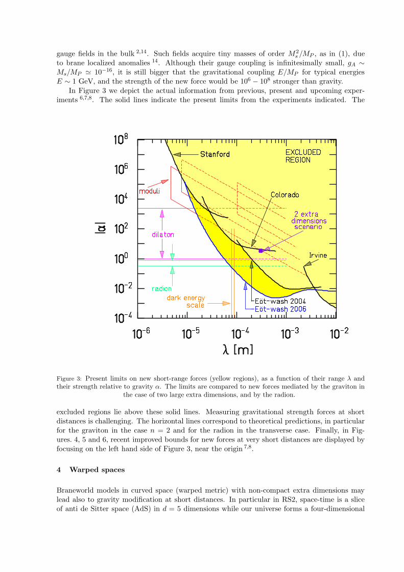
gauge fields in the bulk 2,14. Such fields acquire tiny masses of order M2s /MP , as in (1), due
to brane localized anomalies 14. Although their gauge coupling is infinitesimally small, gA ∼
Ms/MP ≃ 10−16, it is still bigger that the gravitational coupling E/MP for typical energiesE ∼ 1 GeV, and the strength of the new force would be 106
− 108 stronger than gravity.
In Figure 3 we depict the actual information from previous, present and upcoming exper-iments 6,7,8. The solid lines indicate the present limits from the experiments indicated. The
Figure 3: Present limits on new short-range forces (yellow regions), as a function of their range λ andtheir strength relative to gravity α. The limits are compared to new forces mediated by the graviton in
the case of two large extra dimensions, and by the radion.
excluded regions lie above these solid lines. Measuring gravitational strength forces at shortdistances is challenging. The horizontal lines correspond to theoretical predictions, in particularfor the graviton in the case n = 2 and for the radion in the transverse case. Finally, in Fig-ures. 4, 5 and 6, recent improved bounds for new forces at very short distances are displayed byfocusing on the left hand side of Figure 3, near the origin 7,8.
4 Warped spaces
Braneworld models in curved space (warped metric) with non-compact extra dimensions maylead also to gravity modification at short distances. In particular in RS2, space-time is a sliceof anti de Sitter space (AdS) in d = 5 dimensions while our universe forms a four-dimensional
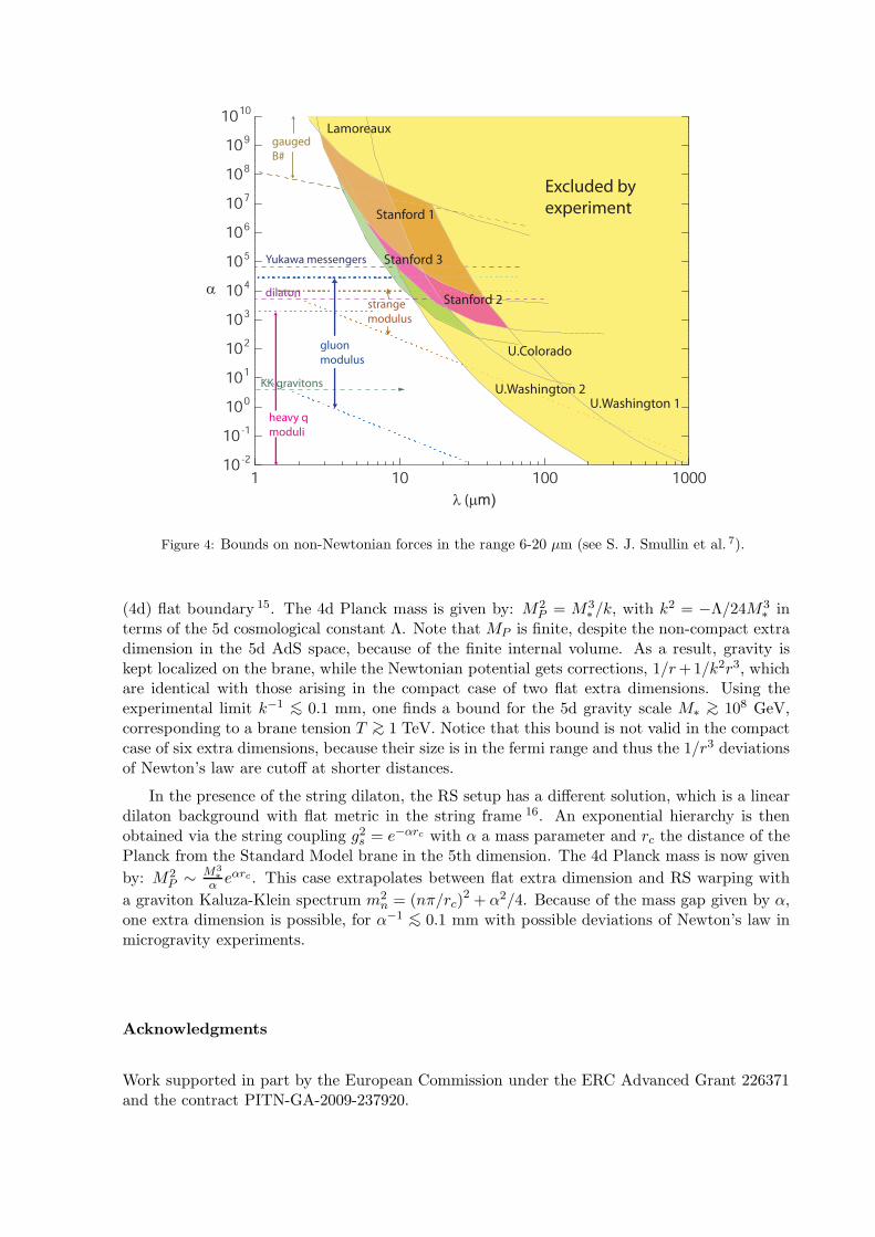
1 10 100 100010
-2
10-1
100
101
102
103
104
105
106
107
108
109
1010
Excluded by
experiment
Lamoreaux
U.Colorado
Stanford 2
Stanford 1
U.Washington 2
gauged
B#
Yukawa messengers
dilaton
KK gravitons
strange
modulus
gluon
modulus
heavy q
moduli
Stanford 3
α
λ (µm)
U.Washington 1
Figure 4: Bounds on non-Newtonian forces in the range 6-20 µm (see S. J. Smullin et al. 7).
(4d) flat boundary 15. The 4d Planck mass is given by: M2P = M3
∗ /k, with k2 = −Λ/24M3∗ in
terms of the 5d cosmological constant Λ. Note that MP is finite, despite the non-compact extradimension in the 5d AdS space, because of the finite internal volume. As a result, gravity iskept localized on the brane, while the Newtonian potential gets corrections, 1/r +1/k2r3, whichare identical with those arising in the compact case of two flat extra dimensions. Using theexperimental limit k−1 <
∼0.1 mm, one finds a bound for the 5d gravity scale M∗
>∼
108 GeV,corresponding to a brane tension T >
∼1 TeV. Notice that this bound is not valid in the compact
case of six extra dimensions, because their size is in the fermi range and thus the 1/r3 deviationsof Newton’s law are cutoff at shorter distances.
In the presence of the string dilaton, the RS setup has a different solution, which is a lineardilaton background with flat metric in the string frame 16. An exponential hierarchy is thenobtained via the string coupling g2
s = e−αrc with α a mass parameter and rc the distance of thePlanck from the Standard Model brane in the 5th dimension. The 4d Planck mass is now given
by: M2P ∼
M3∗
αeαrc . This case extrapolates between flat extra dimension and RS warping with
a graviton Kaluza-Klein spectrum m2n = (nπ/rc)
2 + α2/4. Because of the mass gap given by α,one extra dimension is possible, for α−1 <
∼ 0.1 mm with possible deviations of Newton’s law inmicrogravity experiments.
Acknowledgments
Work supported in part by the European Commission under the ERC Advanced Grant 226371and the contract PITN-GA-2009-237920.
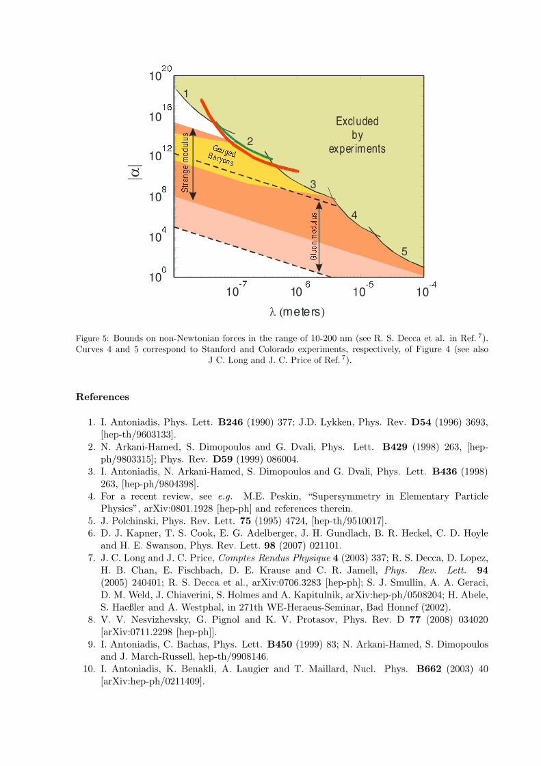
Figure 5: Bounds on non-Newtonian forces in the range of 10-200 nm (see R. S. Decca et al. in Ref. 7).Curves 4 and 5 correspond to Stanford and Colorado experiments, respectively, of Figure 4 (see also
J C. Long and J. C. Price of Ref. 7).
References
1. I. Antoniadis, Phys. Lett. B246 (1990) 377; J.D. Lykken, Phys. Rev. D54 (1996) 3693,[hep-th/9603133].
2. N. Arkani-Hamed, S. Dimopoulos and G. Dvali, Phys. Lett. B429 (1998) 263, [hep-ph/9803315]; Phys. Rev. D59 (1999) 086004.
3. I. Antoniadis, N. Arkani-Hamed, S. Dimopoulos and G. Dvali, Phys. Lett. B436 (1998)263, [hep-ph/9804398].
4. For a recent review, see e.g. M.E. Peskin, “Supersymmetry in Elementary ParticlePhysics”, arXiv:0801.1928 [hep-ph] and references therein.
5. J. Polchinski, Phys. Rev. Lett. 75 (1995) 4724, [hep-th/9510017].6. D. J. Kapner, T. S. Cook, E. G. Adelberger, J. H. Gundlach, B. R. Heckel, C. D. Hoyle
and H. E. Swanson, Phys. Rev. Lett. 98 (2007) 021101.7. J. C. Long and J. C. Price, Comptes Rendus Physique 4 (2003) 337; R. S. Decca, D. Lopez,
H. B. Chan, E. Fischbach, D. E. Krause and C. R. Jamell, Phys. Rev. Lett. 94
(2005) 240401; R. S. Decca et al., arXiv:0706.3283 [hep-ph]; S. J. Smullin, A. A. Geraci,D. M. Weld, J. Chiaverini, S. Holmes and A. Kapitulnik, arXiv:hep-ph/0508204; H. Abele,S. Haeßler and A. Westphal, in 271th WE-Heraeus-Seminar, Bad Honnef (2002).
8. V. V. Nesvizhevsky, G. Pignol and K. V. Protasov, Phys. Rev. D 77 (2008) 034020[arXiv:0711.2298 [hep-ph]].
9. I. Antoniadis, C. Bachas, Phys. Lett. B450 (1999) 83; N. Arkani-Hamed, S. Dimopoulosand J. March-Russell, hep-th/9908146.
10. I. Antoniadis, K. Benakli, A. Laugier and T. Maillard, Nucl. Phys. B662 (2003) 40[arXiv:hep-ph/0211409].
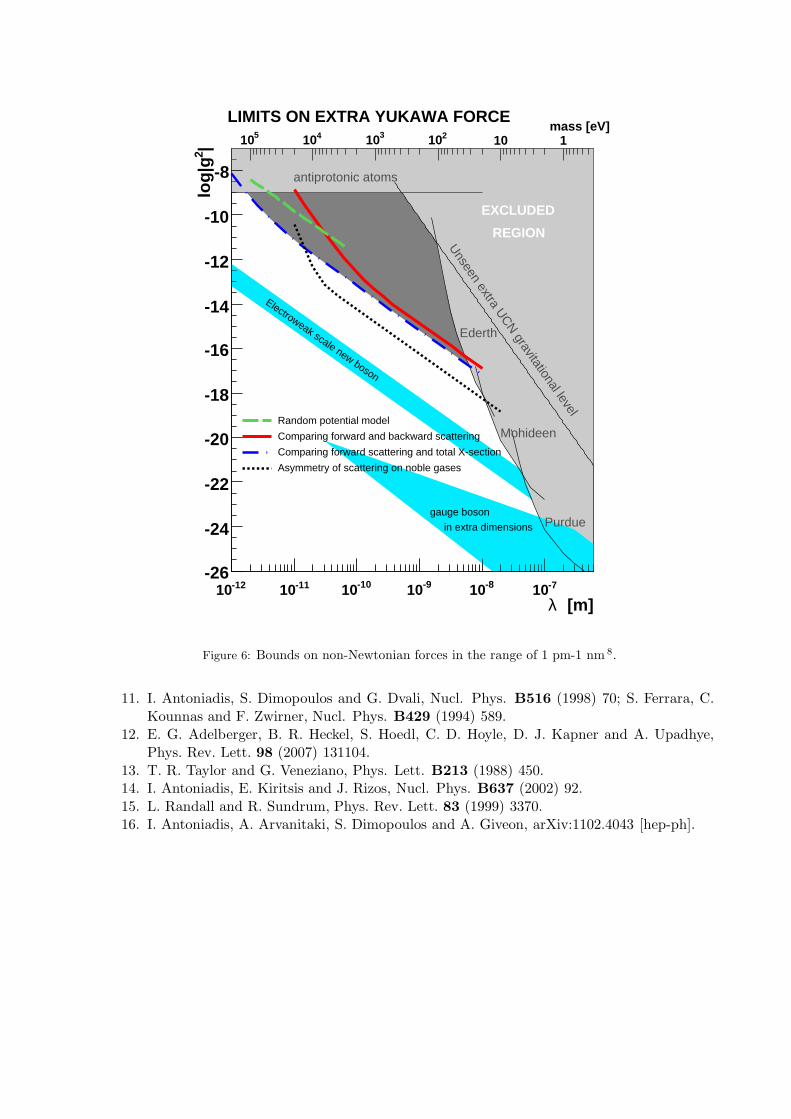
[m]λ-1210 -1110 -1010 -910 -810 -710
|2lo
g|g
-26
-24
-22
-20
-18
-16
-14
-12
-10
-8
Random potential model
Comparing forward and backward scattering
Comparing forward scattering and total X-section
Asymmetry of scattering on noble gases
EXCLUDED
REGION
antiprotonic atoms
Ederth
Mohideen
Purdue
Unseen extra U
CN
gravitational level
gauge boson
in extra dimensions
Electroweak scale new boson
LIMITS ON EXTRA YUKAWA FORCE mass [eV]
110210310410510
Figure 6: Bounds on non-Newtonian forces in the range of 1 pm-1 nm 8.
11. I. Antoniadis, S. Dimopoulos and G. Dvali, Nucl. Phys. B516 (1998) 70; S. Ferrara, C.Kounnas and F. Zwirner, Nucl. Phys. B429 (1994) 589.
12. E. G. Adelberger, B. R. Heckel, S. Hoedl, C. D. Hoyle, D. J. Kapner and A. Upadhye,Phys. Rev. Lett. 98 (2007) 131104.
13. T. R. Taylor and G. Veneziano, Phys. Lett. B213 (1988) 450.14. I. Antoniadis, E. Kiritsis and J. Rizos, Nucl. Phys. B637 (2002) 92.15. L. Randall and R. Sundrum, Phys. Rev. Lett. 83 (1999) 3370.16. I. Antoniadis, A. Arvanitaki, S. Dimopoulos and A. Giveon, arXiv:1102.4043 [hep-ph].
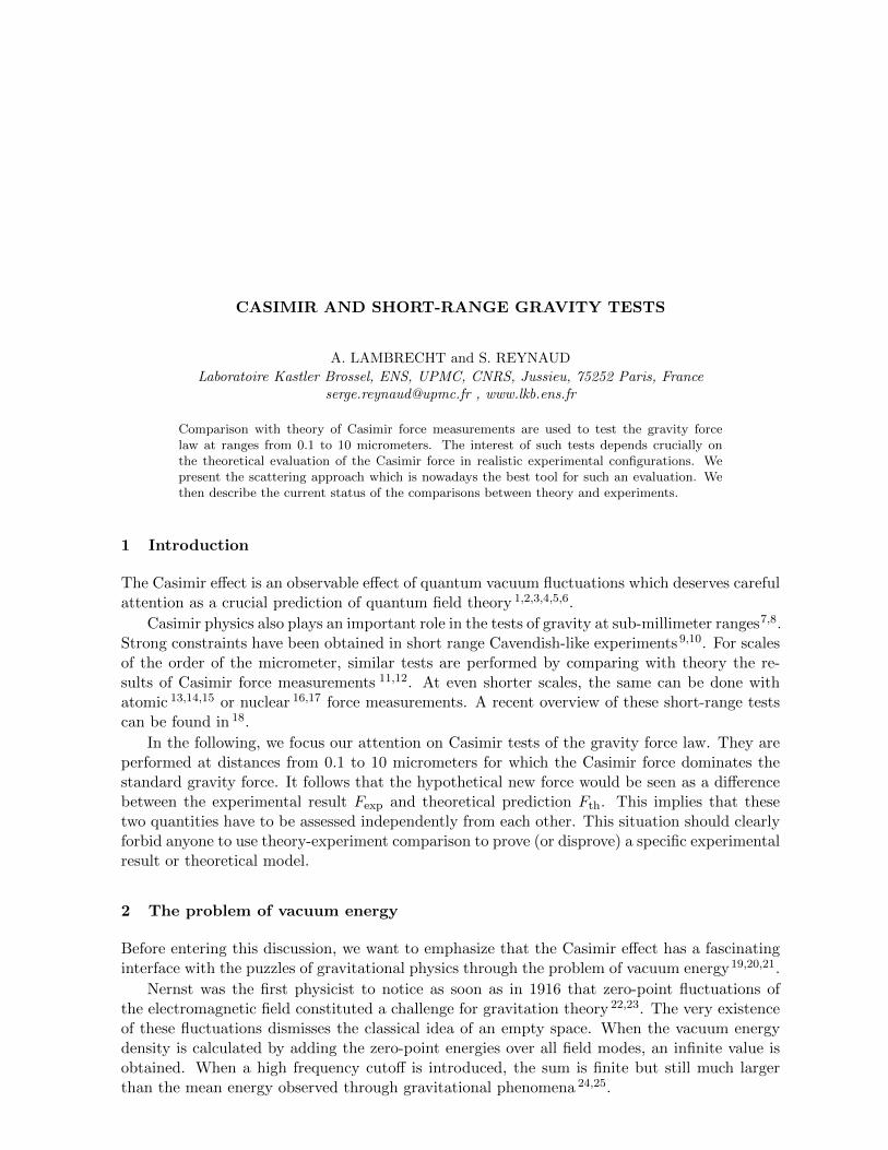
CASIMIR AND SHORT-RANGE GRAVITY TESTS
A. LAMBRECHT and S. REYNAUD
Laboratoire Kastler Brossel, ENS, UPMC, CNRS, Jussieu, 75252 Paris, [email protected] , www.lkb.ens.fr
Comparison with theory of Casimir force measurements are used to test the gravity forcelaw at ranges from 0.1 to 10 micrometers. The interest of such tests depends crucially onthe theoretical evaluation of the Casimir force in realistic experimental configurations. Wepresent the scattering approach which is nowadays the best tool for such an evaluation. Wethen describe the current status of the comparisons between theory and experiments.
1 Introduction
The Casimir effect is an observable effect of quantum vacuum fluctuations which deserves carefulattention as a crucial prediction of quantum field theory 1,2,3,4,5,6.
Casimir physics also plays an important role in the tests of gravity at sub-millimeter ranges7,8.Strong constraints have been obtained in short range Cavendish-like experiments 9,10. For scalesof the order of the micrometer, similar tests are performed by comparing with theory the re-sults of Casimir force measurements 11,12. At even shorter scales, the same can be done withatomic 13,14,15 or nuclear 16,17 force measurements. A recent overview of these short-range testscan be found in 18.
In the following, we focus our attention on Casimir tests of the gravity force law. They areperformed at distances from 0.1 to 10 micrometers for which the Casimir force dominates thestandard gravity force. It follows that the hypothetical new force would be seen as a differencebetween the experimental result Fexp and theoretical prediction Fth. This implies that thesetwo quantities have to be assessed independently from each other. This situation should clearlyforbid anyone to use theory-experiment comparison to prove (or disprove) a specific experimentalresult or theoretical model.
2 The problem of vacuum energy
Before entering this discussion, we want to emphasize that the Casimir effect has a fascinatinginterface with the puzzles of gravitational physics through the problem of vacuum energy19,20,21.
Nernst was the first physicist to notice as soon as in 1916 that zero-point fluctuations ofthe electromagnetic field constituted a challenge for gravitation theory 22,23. The very existenceof these fluctuations dismisses the classical idea of an empty space. When the vacuum energydensity is calculated by adding the zero-point energies over all field modes, an infinite value isobtained. When a high frequency cutoff is introduced, the sum is finite but still much largerthan the mean energy observed through gravitational phenomena 24,25.
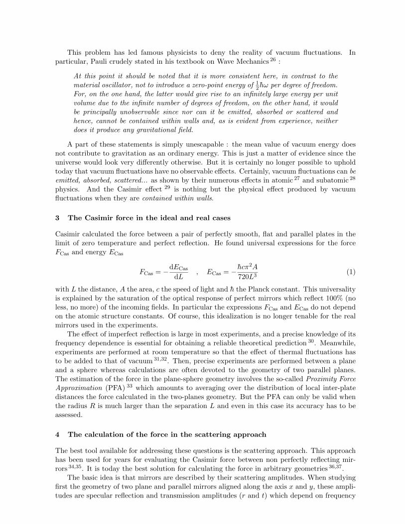
This problem has led famous physicists to deny the reality of vacuum fluctuations. Inparticular, Pauli crudely stated in his textbook on Wave Mechanics 26 :
At this point it should be noted that it is more consistent here, in contrast to thematerial oscillator, not to introduce a zero-point energy of 1
2 hω per degree of freedom.For, on the one hand, the latter would give rise to an infinitely large energy per unitvolume due to the infinite number of degrees of freedom, on the other hand, it wouldbe principally unobservable since nor can it be emitted, absorbed or scattered andhence, cannot be contained within walls and, as is evident from experience, neitherdoes it produce any gravitational field.
A part of these statements is simply unescapable : the mean value of vacuum energy doesnot contribute to gravitation as an ordinary energy. This is just a matter of evidence since theuniverse would look very differently otherwise. But it is certainly no longer possible to upholdtoday that vacuum fluctuations have no observable effects. Certainly, vacuum fluctuations can beemitted, absorbed, scattered... as shown by their numerous effects in atomic 27 and subatomic 28
physics. And the Casimir effect 29 is nothing but the physical effect produced by vacuumfluctuations when they are contained within walls.
3 The Casimir force in the ideal and real cases
Casimir calculated the force between a pair of perfectly smooth, flat and parallel plates in thelimit of zero temperature and perfect reflection. He found universal expressions for the forceFCas and energy ECas
FCas = −dECas
dL, ECas = − hcπ
2A
720L3(1)
with L the distance, A the area, c the speed of light and h the Planck constant. This universalityis explained by the saturation of the optical response of perfect mirrors which reflect 100% (noless, no more) of the incoming fields. In particular the expressions FCas and ECas do not dependon the atomic structure constants. Of course, this idealization is no longer tenable for the realmirrors used in the experiments.
The effect of imperfect reflection is large in most experiments, and a precise knowledge of itsfrequency dependence is essential for obtaining a reliable theoretical prediction 30. Meanwhile,experiments are performed at room temperature so that the effect of thermal fluctuations hasto be added to that of vacuum 31,32. Then, precise experiments are performed between a planeand a sphere whereas calculations are often devoted to the geometry of two parallel planes.The estimation of the force in the plane-sphere geometry involves the so-called Proximity ForceApproximation (PFA) 33 which amounts to averaging over the distribution of local inter-platedistances the force calculated in the two-planes geometry. But the PFA can only be valid whenthe radius R is much larger than the separation L and even in this case its accuracy has to beassessed.
4 The calculation of the force in the scattering approach
The best tool available for addressing these questions is the scattering approach. This approachhas been used for years for evaluating the Casimir force between non perfectly reflecting mir-rors 34,35. It is today the best solution for calculating the force in arbitrary geometries 36,37.
The basic idea is that mirrors are described by their scattering amplitudes. When studyingfirst the geometry of two plane and parallel mirrors aligned along the axis x and y, these ampli-tudes are specular reflection and transmission amplitudes (r and t) which depend on frequency
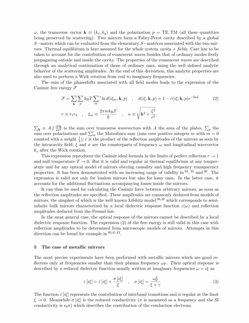
ω, the transverse vector k ≡ (kx, ky) and the polarization p = TE,TM (all these quantitiesbeing preserved by scattering). Two mirrors form a Fabry-Perot cavity described by a globalS−matrix which can be evaluated from the elementary S−matrices associated with the two mir-rors. Thermal equilibrium is here assumed for the whole system cavity + fields. Care has to betaken to account for the contribution of evanescent waves besides that of ordinary modes freelypropagating outside and inside the cavity. The properties of the evanescent waves are describedthrough an analytical continuation of those of ordinary ones, using the well defined analyticbehavior of the scattering amplitudes. At the end of this derivation, this analytic properties arealso used to perform a Wick rotation from real to imaginary frequencies.
The sum of the phaseshifts associated with all field modes leads to the expression of theCasimir free energy F
F =∑k
∑p
kBT∑m
′ ln d(iξm,k, p) , d(iξ,k, p) = 1− r(iξ,k, p)e−2κL (2)
r ≡ r1r2 , ξm ≡2πmkBT
h, κ ≡
√k2 +
ξ2
c2
∑k ≡ A
∫ d2k4π2 is the sum over transverse wavevectors with A the area of the plates,
∑p the
sum over polarizations and∑′m the Matsubara sum (sum over positive integers m with m = 0
counted with a weight 12); r is the product of the reflection amplitudes of the mirrors as seen by
the intracavity field; ξ and κ are the counterparts of frequency ω and longitudinal wavevectorkz after the Wick rotation.
This expression reproduces the Casimir ideal formula in the limits of perfect reflection r → 1and null temperature T → 0. But it is valid and regular at thermal equilibrium at any temper-ature and for any optical model of mirrors obeying causality and high frequency transparencyproperties. It has been demonstrated with an increasing range of validity in 34, 35 and 36. Theexpression is valid not only for lossless mirrors but also for lossy ones. In the latter case, itaccounts for the additional fluctuations accompanying losses inside the mirrors.
It can thus be used for calculating the Casimir force between arbitrary mirrors, as soon asthe reflection amplitudes are specified. These amplitudes are commonly deduced from models ofmirrors, the simplest of which is the well known Lifshitz model 38,39 which corresponds to semi-infinite bulk mirrors characterized by a local dielectric response function ε(ω) and reflectionamplitudes deduced from the Fresnel law.
In the most general case, the optical response of the mirrors cannot be described by a localdielectric response function. The expression (2) of the free energy is still valid in this case withreflection amplitudes to be determined from microscopic models of mirrors. Attempts in thisdirection can be found for example in 40,41,42.
5 The case of metallic mirrors
The most precise experiments have been performed with metallic mirrors which are good re-flectors only at frequencies smaller than their plasma frequency ωP. Their optical response isdescribed by a reduced dielectric function usually written at imaginary frequencies ω = iξ as
ε [iξ] = ε [iξ] +σ [iξ]
ξ, σ [iξ] =
ω2P
ξ + γ(3)
The function ε [iξ] represents the contribution of interband transitions and is regular at the limitξ → 0. Meanwhile σ [iξ] is the reduced conductivity (σ is measured as a frequency and the SIconductivity is ε0σ) which describes the contribution of the conduction electrons.
A simplified description corresponds to the lossless limit γ → 0 often called the plasmamodel. As γ is much smaller than ωP for a metal such as Gold, this simple model captures themain effect of imperfect reflection. However it cannot be considered as an accurate descriptionsince a much better fit of tabulated optical data is obtained 30 with a non null value of γ.Furthermore, the Drude model γ 6= 0 meets the important property of ordinary metals whichhave a finite static conductivity
σ0 =ω2P
γ(4)
This has to be contrasted to the lossless limit which corresponds to an infinite value for σ0.When taking into account the imperfect reflection of the metallic mirrors, one finds that the
Casimir force is reduced with respect to the ideal Casimir expression at all distances for a nulltemperature 30. This reduction is conveniently represented as a factor
ηF =F
FCas, F = −∂F
∂L(5)
where F is the real force and FCas the ideal expression. For the plasma model, there is only onelength scale, tha plasma wavelength λP = 2πc/ωP in the problem (136nm for Gold). The idealCasimir formula is recovered (ηF → 1) at large distances L λP , as expected from the factthat metallic mirrors tend to be perfect reflectors at low frequencies ω ωP . At short distancesin contrast, a significant reduction of the force is obtained (ηF 1), which scales as L/λP , as aconsequence of the fact that metallic mirrors are poor reflectors at high frequencies ω ωP . Inother words, there is a change in the power law for the variation of the force with distance. Thischange can be understood as the result of the Coulomb interaction of surface plasmons living atthe two matter-vacuum interfaces 43,44.
As experiments are performed at room temperature, the effect of thermal fluctuations hasto be added to that of vacuum fields 45. Significant thermal corrections appear at distances Llarger than a critical distance determined by the thermal wavelength λT (a few micrometers atroom temperature). Bostrom and Sernelius were the first to remark that the small non zerovalue of γ had a significant effect on the force at non null temperatures 46. In particular, thereis a large difference at large distances between the expectations calculated for γ = 0 and γ 6= 0,their ratio reaching a factor 2 when L λT . It is also worth emphasizing that the contributionof thermal fluctuations to the force is opposite to that of vacuum fluctuations for intermediateranges L ∼ λT .
This situation has led to a blossoming of contradictory papers (see references in 47,48,49). Aswe will see below, the contradiction is also deeply connected to the comparison between theoryand experiments.
6 The non-specular scattering formula
We now present a more general scattering formula allowing one to calculate the Casimir forcebetween stationary objects with arbitrary geometries. The main generalization with respect tothe already discussed cases is that the scattering matrix S is now a larger matrix accountingfor non-specular reflection and mixing different wavevectors and polarizations while preservingfrequency. Of course, the non-specular scattering formula is the generic one while specularreflection can only be an idealization.
The Casimir free energy can be written as a generalization of equation (2)
F = kBT∑m
′Tr lnD(iξm) (6)
D = 1−R1 exp−KLR2 exp−KL
The symbol Tr refers to a trace over the modes at a given frequency. The matrix D is thedenominator containing all the resonance properties of the cavity formed by the two objects 1and 2 here written for imaginary frequencies. It is expressed in terms of the matrices R1 andR2 which represent reflection on the two objects 1 and 2 and of propagation factors exp−KL.Note that the matrices D, R1 and R2, which were diagonal on the basis of plane waves whenthey described specular scattering, are no longer diagonal in the general case of non specularscattering. The propagation factors remain diagonal in this basis with their diagonal valueswritten as in (2). Clearly the expression (6) does not depend on the choice of a specific basis.But it may be written in specific basis fitting the geometry under study.
The multiple scattering formalism has been used in the past years by different groups usingdifferent notations (see as examples50,51,52) and numerous applications have been considered. Inparticular, the case of corrugated plates or gratings has been extensively studied 53,54,55,56 andit has given rise to interesting comparisons with experiments 57,58,59. Note also that calculationshave been devoted to the study of atoms in the vicinity of corrugated plates 60,61,62.
7 The plane-sphere geometry beyond PFA
Recently, it has also become possible to use the general scattering formula to obtain explicitevaluations of the Casimir force in the plane-sphere geometry. Such calculations have firstbeen performed for perfectly reflecting mirrors 63. They have then been done for the morerealistic case of metallic mirrors described by a plasma model dielectric function 64. Even morerecently, calculations were made which treat simultaneously plane-sphere geometry and non zerotemperature, with dissipation taken into account 65.
In these calculations, the reflection matrices are written in terms of Fresnel amplitudes forplane waves on the plane mirror and of Mie amplitudes for spherical waves on the sphericalmirror. The scattering formula is then obtained by writing also transformation formulas fromthe plane waves basis to the spherical waves basis and conversely. The energy takes the formof an exact multipolar formula labeled by a multipolar index `. When doing the numerics,the expansion is truncated at some maximum value `max, which degrades the accuracy of theresulting estimation for very large spheres x ≡ L/R < xmin with xmin proportional to `−1max.
The results of these calculations may be compared to the experimental study of PFA in theplane-sphere geometry 66. In this experiment, the force gradient is measured for various radii ofthe sphere and the results are used to obtain a constraint |βG| < 0.4 on the slope at origin βGof the function ρG(x)
ρG =G
GPFA= 1 + βGx+O(x2) , x ≡ L
R(7)
The slope obtained by interpolating at low values of x our theoretical evaluation of ρG revealsa striking difference between the cases of perfect and plasma mirrors. The slope βperfG obtainedfor perfect mirrors is larger than that βGold
G obtained for gold mirrors by a factor larger than 2
βperfG ∼ −0.48 , βGoldG ∼ −0.21 (8)
As a result, βGoldG is compatible with the experimental bound whereas βperfG is not 64.
The effect of temperature is also correlated with the plane-sphere geometry. The first calcu-lations accounting simultaneously for plane-sphere geometry, temperature and dissipation havebeen published very recently 65 and they show several striking features. The factor of 2 betweenthe long distance forces in Drude and plasma models is reduced to a factor below 3/2 in theplane-sphere geometry. Then, PFA underestimates the Casimir force within the Drude modelat short distances, while it overestimates it at all distances for the perfect reflector and plasma
model. If the latter feature were conserved for the experimental parameter region R/L (> 102),the actual values of the Casimir force calculated within plasma and Drude model could turnout to be closer than what PFA suggests. This would affect the discussion of the next section,which is still based on calculations using PFA.
8 Discussion of experiments
We end up this review by discussing the status of comparisons between Casimir experimentsand theory. We emphasize that, after years of improvement in experiments and theory, we haveto face a lasting discrepancies in their comparison.
On one side, the Purdue and Riverside experiments 67,68,69 appear to favor predictions ob-tained with γ = 0 rather than those corresponding to the expected γ 6= 0 (see Fig.1 in 68). Thisresult stands in contradiction to the fact that Gold has a finite conductivity. Note that theseexperiments are done at distances smaller than 0.75µm where the thermal contribution is small,so that accuracy is a critical issue here.
On the other side, a new experiment at Yale 70 has been able to measure the force at largerdistances (0.7µm-7µm) where the thermal contribution is larger and the difference between thepredictions at γ = 0 and γ 6= 0 significant. The results favor the expected Drude model (γ 6= 0),but only after subtraction of a large contribution of the patch effect.
It is worth emphasizing that the results of the new experiment see a significant thermalcontribution and fit the expected model. Of course, they have to be confirmed by furtherstudies 71. In particular, the electrostatic patch effect remains a source of concern in Casimirexperiments 72,73. It is not measured independently in any of the experiments discussed above.This means that the Casimir effect, which is now verified in several experiments, is however nottested at the 1% level, as has been sometimes claimed. This also entails that the tests of gravityat the micrometer range have still room available for improvement.
Acknowledgments
The authors thank A. Canaguier-Durand, A. Gerardin, R. Guerout, J. Lussange, R.O. Behunin,I. Cavero-Pelaez, D. Dalvit, C. Genet, G.L. Ingold, F. Intravaia, M.-T. Jaekel, P.A. Maia Neto,V.V. Nesvizhevsky for contributions to the work reviewed in this paper, and the ESF ResearchNetworking Programme CASIMIR (www.casimirnetwork. com) for providing excellent oppor-tunities for discussions on the Casimir effect and related topics.
References
1. P.W. Milonni, The quantum vacuum (Academic, 1994).2. S.K. Lamoreaux, Resource Letter in Am. J. Phys. 67 850 (1999).3. M. Bordag, U. Mohideen and V.M. Mostepanenko, Phys. Rep. 353 1 (2001).4. K.A. Milton, J. Phys. A 20 4628 (2005).5. R.G. Barrera and S. Reynaud eds., Focus on Casimir Forces, New J. Phys. 8 (2006).6. D. Dalvit et al eds., Casimir physics, Lecture Notes in Physics 834 (Springer, 2011)7. E. Fischbach and C. Talmadge, The Search for Non Newtonian Gravity (AIP
Press/Springer Verlag, 1998).8. E.G. Adelberger, B.R. Heckel and A.E. Nelson, Ann. Rev. Nucl. Part. Sci. 53 77 (2003).9. D.J. Kapner, T.S. Cook, E.G. Adelberger et al, Phys. Rev. Lett. 98 021101 (2007).
10. E.G. Adelberger et al, in this book.11. A. Lambrecht and S. Reynaud, Poincare Seminar on Vacuum Energy and Renormalization
1 107 (2002) [arXiv:quant-ph/0302073] and references therein.
12. R. Onofrio, New J. Phys. 8 237 (2006).13. P. Wolf, P. Lemonde, A. Lambrecht et al, Phys. Rev. A 75 063608 (2007).14. S. Lepoutre et al, EPL 88 20002 (2009).15. B. Pelle et al, in this book.16. V.V. Nesvizhevsky et al, Phys. Rev. D 77 034020 (2008).17. V.V. Nesvizhevsky et al, in this book.18. I. Antoniadis, S. Baessler, M. Buchner, V.V. Fedorov, S. Hoedl, V.V. Nesvizhevsky, G.
Pignol, K.V. Protasov, S. Reynaud and Yu. Sobolev, Compt. Rend. Acad. Sci. (2011).19. C. Genet, A. Lambrecht and S. Reynaud, in On the Nature of Dark Energy eds. U. Brax,
J. Martin, J.P. Uzan, 121 (Frontier Group, 2002) [arXiv:quant-ph/0210173].20. M.-T. Jaekel and S. Reynaud, in Mass and Motion in General Relativity, eds L. Blanchet,
A. Spallicci and B. Whiting 491 (2011) [arXiv:0812.3936] and references therein.21. M.-T. Jaekel et al, in this book.22. W. Nernst, Verh. Deutsch. Phys. Ges. 18 83 (1916).23. P.F. Browne, Apeiron 2 72 (1995).24. S. Weinberg, Rev. Mod. Phys. 61 1 (1989).25. R.J. Adler, B. Casey and O.C. Jacob, Am. J. Phys. 63 620 (1995).26. W. Pauli, Die Allgemeinen Prinzipien der Wellenmechanik, in Handbuch der Physik 24
1 (1933); translation reproduced from Enz C.P., in Enz C.P. andMehra J. eds, PhysicalReality andMathematical Description (Reidel, 1974) p.124.
27. C. Cohen-Tannoudji, J. Dupont-Roc and G. Grynberg, Atom-Photon Interactions (Wiley,1992).
28. C. Itzykson and J.-B. Zuber, Quantum Field Theory (McGraw Hill, 1985).29. H.B.G. Casimir, Proc. K. Ned. Akad. Wet. 51 793 (1948).30. A. Lambrecht and S. Reynaud, Euro. Phys. J. D 8 309 (2000).31. J. Mehra, Physica 37 145 (1967).32. J. Schwinger, L.L. de Raad and K.A. Milton, Ann. Phys. 115 1 (1978).33. B.V. Deriagin, I.I. Abrikosova and E.M. Lifshitz, Quart. Rev. 10 295 (1968).34. M.T. Jaekel and S. Reynaud, J. Physique I 1 1395 (1991) [arXiv:quant-ph/0101067].35. C. Genet, A. Lambrecht and S. Reynaud, Phys. Rev. A 67 043811 (2003).36. A. Lambrecht, P.A. Maia Neto and S. Reynaud, New J. Phys. 8 243 (2006).37. A. Lambrecht, A. Canaguier-Durand, R. Guerout, and S. Reynaud, in 6 [arXiv:1006.2959].38. E.M Lifshitz, Sov. Phys. JETP 2 73 (1956).39. I.E. Dzyaloshinskii, E.M. Lifshitz and L.P. Pitaevskii, Sov. Phys. Uspekhi 4 153 (1961).40. L.P. Pitaevskii, Phys. Rev. Lett. 101 163202 (2008); Phys. Rev. Lett. 102 189302 (2009);
B. Geyer et al, Phys. Rev. Lett. 102 189301 (2009).41. D.A.R. Dalvit and S.K. Lamoreaux, Phys. Rev. Lett. 101 163203 (2008); Phys. Rev.
Lett. 102 189304 (2009); R.S. Decca et al, Phys. Rev. Lett. 102 189303 (2009).42. V.B. Svetovoy, Phys. Rev. Lett. 101 163603 (2008); Phys. Rev. Lett. 102 219903 (E)
(2009).43. C. Genet, F. Intravaia, A. Lambrecht, and S. Reynaud, Ann. Found. L. de Broglie 29 311
(2004).44. F. Intravaia and A. Lambrecht, Phys. Rev. Lett. 94 110404 (2005).45. C. Genet, A. Lambrecht and S. Reynaud, Phys. Rev. A 62 012110 (2000) and references
therein.46. M. Bostrom and Bo E. Sernelius, Phys. Rev. Lett. 84 4757 (2000).47. S. Reynaud, A. Lambrecht and C. Genet, in Quantum Field Theory Under the Influence of
External Conditions, ed. K.A.Milton (Rinton Press, 2004) p.36 [arXiv:quant-ph/0312224].48. I. Brevik, S.A. Ellingsen and K. Milton, New J. Phys. 8 236 (2006).49. G.-L. Ingold, A. Lambrecht and S. Reynaud, Phys. Rev. E 80 041113 (2009).
50. T. Emig, J. Stat. Mech.: Theory Exp. P04007 (2008).51. O. Kenneth and I. Klich, Phys. Rev. B 78 014103 (2008).52. K.A. Milton and J. Wagner, J. Phys. A 41 155402 (2008).53. R.B. Rodrigues, P.A. Maia Neto, A. Lambrecht and S. Reynaud, Phys. Rev. Lett. 96
100402 (2006); Phys. Rev. Lett. 98 068902 (2007).54. R.B. Rodrigues, P.A. Maia Neto, A. Lambrecht and S. Reynaud, Phys. Rev. A 75 062108
(2007).55. R.B. Rodrigues, P.A. Maia Neto, A. Lambrecht and S. Reynaud, EPL 76 822 (2006).56. A. Lambrecht and V.N. Marachevsky, Phys. Rev. Lett. 101 160403 (2008); A. Lambrecht,
Nature 454 836 (2008).57. H.B. Chan, Y. Bao, J. Zou et al, Phys. Rev. Lett. 101 030401 (2008).58. H.C. Chiu, G.L. Klimchitskaya, V.N. Marachevsky et al, Phys. Rev. B 80 121402 (2009).59. Y. Bao, R. Gurout, J. Lussange et al, Phys. Rev. Lett. 105 250402 (2010).60. D.A.R. Dalvit, P.A. Maia Neto, A. Lambrecht and S. Reynaud, Phys. Rev. Lett. 100
040405 (2008).61. R. Messina, D.A.R. Dalvit, P.A. Maia Neto, A. Lambrecht and S. Reynaud, Phys. Rev.
A 80 022119 (2009).62. A.M. Contreras-Reyes, R. Gurout, P.A. Maia Neto, D.A.R. Dalvit, A. Lambrecht and S.
Reynaud, Phys. Rev. A 82 052517 (2010).63. P.A. Maia Neto, A. Lambrecht and S. Reynaud, Phys. Rev. A 78 012115 (2008).64. A. Canaguier-Durand, P.A. Maia Neto, I. Cavero-Pelaez, A. Lambrecht and S. Reynaud,
Phys. Rev. Lett. 102 230404 (2009).65. A. Canaguier-Durand, P.A. Maia Neto, A. Lambrecht and S. Reynaud, Phys. Rev. Lett.
104 040403 (2010).66. D.E. Krause, R.S. Decca, D. Lopez and E. Fischbach, Phys. Rev. Lett. 98 050403 (2007).67. R.S. Decca, D. Lopez, E. Fischbach et al, Annals Phys. 318 37 (2005).68. R.S. Decca, D. Lopez, E. Fischbach et al, Phys. Rev. D 75 077101 (2007).69. G.L. Klimchitskaya, U. Mohideen and V.M. Mostepanenko, Rev. Mod. Phys. 81 1827
(2009).70. A.O. Sushkov, W.J. Kim, D.A.R. Dalvit and S.K. Lamoreaux, Nature Physics 7 230
(2011).71. K. Milton, Nature Physics 7 190 (2011).72. C.C. Speake and C. Trenkel, Phys. Rev. Lett. 90 160403 (2003).73. W.J. Kim, A.O. Sushkov, D.A.R. Dalvit and S.K. Lamoreaux, Phys. Rev. A 81 022505
(2010).
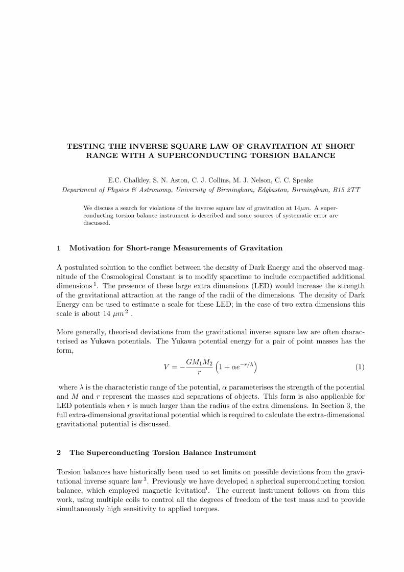
TESTING THE INVERSE SQUARE LAW OF GRAVITATION AT SHORTRANGE WITH A SUPERCONDUCTING TORSION BALANCE
E.C. Chalkley, S. N. Aston, C. J. Collins, M. J. Nelson, C. C. SpeakeDepartment of Physics & Astronomy, University of Birmingham, Edgbaston, Birmingham, B15 2TT
We discuss a search for violations of the inverse square law of gravitation at 14µm. A super-conducting torsion balance instrument is described and some sources of systematic error arediscussed.
1 Motivation for Short-range Measurements of Gravitation
A postulated solution to the conflict between the density of Dark Energy and the observed mag-nitude of the Cosmological Constant is to modify spacetime to include compactified additionaldimensions 1. The presence of these large extra dimensions (LED) would increase the strengthof the gravitational attraction at the range of the radii of the dimensions. The density of DarkEnergy can be used to estimate a scale for these LED; in the case of two extra dimensions thisscale is about 14 µm 2 .
More generally, theorised deviations from the gravitational inverse square law are often charac-terised as Yukawa potentials. The Yukawa potential energy for a pair of point masses has theform,
V = −GM1M2
r
(1 + αe−r/λ
)(1)
where λ is the characteristic range of the potential, α parameterises the strength of the potentialand M and r represent the masses and separations of objects. This form is also applicable forLED potentials when r is much larger than the radius of the extra dimensions. In Section 3, thefull extra-dimensional gravitational potential which is required to calculate the extra-dimensionalgravitational potential is discussed.
2 The Superconducting Torsion Balance Instrument
Torsion balances have historically been used to set limits on possible deviations from the gravi-tational inverse square law 3. Previously we have developed a spherical superconducting torsionbalance, which employed magnetic levitation4. The current instrument follows on from thiswork, using multiple coils to control all the degrees of freedom of the test mass and to providesimultaneously high sensitivity to applied torques.
2.1 A Magnetically Levitated Bearing
A novel element in the instrument is the use of a superconducting levitating bearing to replacethe fibre supporting the test mass. The levitation system consists of a bearing structure (seeFigure 1) which supports twelve coils which produce lift and transverse stiffness. The levitationsystem is currently being tested using coils handwound from lead wire into milled aluminiumsubstrates. The final coils used in the experiment are to be manufactured photolithographicallyby our collaborators at Heriot-Watt University.
Figure 1: Left: A silica prototype of the float structure that will be levitated, bearing one test mass on the topcircular face Right: The levitating bearing, showing hand-wound lead servo and levitation coils.
The levitated structure or ‘float’ which forms the free element in the torsion balance fits overthe top of the bearing with a test mass forming the upper surface of the disc. A silica prototypefloat has been constructed for testing (Figure 1) but the final version used in the experimentwill be an all-copper assembly.
2.2 Experimental Test Masses
The gravitational sources and test masses in the instrument are two identical discs, one placedon the levitated float structure (the test disc) and one controlled by the micropositioning system(the source disc). The discs bear identical patterns of 2048 radial stripes, alternating betweenAu and Cu organised into 16 sectors of alternating pattern phase. These materials were chosenbecause of their large density contrast and their well-matched thermal contraction at 4 K. Thetechnology for depositing these metals is also very well known, and good results for producingthe experimental surfaces to a high level of flatness can be expected.
3 Torques from Newtonian Gravity and the LED Signal
The gravitational potential of an object of mass M in a spacetime with 2 extra dimensions isgiven by,
V4+2 = − G4+2M
(r2 +∑∞
n=1(ξ1 − 2πRn)2 +∑∞
m=1(ξ2 − 2πRm)2)3/2, (2)
where r is the Euclidean distance given by√
x2 + y2 + z2 and the components of the higherdimensional distance are (x, y, z, ξ1, ξ2), G4+2 is the higher-dimensional gravitational constantand n and m are integers representing the number of revolutions around the extra dimensions5. By numerically integrating this potential for the case of 4 + 2 dimensions it was calculatedthat with a 15 µm spacing, the LED extra torque would be 3.49× 10⁻¹⁷ Nm. The pitch of thealternating Au/Cu pattern was set at 90 µm after examining the trade-off between sensitivityto the LED torque at a spacing of 15 µm and sensitivity to torques due to a Yukawa potentialwith λ = 14 µm, as shown in Figure 2.
0 0.05 0.1 0.15 0.2 0.25 0.30
1
2
3
4
5
6
7x 10
−17
Test Mass Pattern Pitch (mm)
Tor
que
(Nm
)
Newtonian Gravity2 Large Extra Dimensions, R=14µmYukawa potential with α = 1,λ = 14µm
Test mass patternpitch set at 90 µm
Figure 2: The calculated strength of the forces on the superconducting torsion balance at a separation of 15 µmdue to LED gravity, a Yukawa potential with α = 1 and λ = 14 µm and 4D Newtonian gravity as a function of
pattern pitch.
4 Analysis of Spurious Forces
The torque on the superconducting torsion balance may contain non-gravitational componentsthat are ideally eliminated from the readout. These excess torques are caused by the couplingof electrostatic, magnetic, Casimir and other forces to aspects of the test masses.
The experimental surfaces of the test mass are to be constructed to be optically flat at roomtemperature, with no correlation between the surface roughness and the underlying pattern. At4 K, the slightly different thermal contractions mean that the Au stripes will stand 0.2 nm higherthan the Cu stripes. This modulation of the gap between the experimental surfaces couples tothe forces which vary with the local gap size so that a torque may exist to align the Au stripeson both surfaces. This interaction of the modulation of the gap results in a transverse Casimirforce per unit length per stripe pair, which is given by,
FCas = −π3hcA2C
60g5v0
sin(
2πδ
p
)Nm−1, (3)
where AC is the amplitude of the thermal corrugations, p is the pitch of the spoke pattern,δ represents the shift parameter of the test mass patterns with respect to one another, and gv0
is the vacuum distance between the surfaces of the test masses, which is the separation . Usingthe values gv0 = 13 µm, AC = 0.2 nm and p = 90 µm , the value of FCas is 1.76× 10⁻²¹ Nm−1.At this spacing size, and assuming that the corrugations of the test mass at 4 K are no largerthan would be expected from thermal contraction mismatches, the transverse Casimir force isnegligible.
Electrostatic forces are likely to contribute significantly and in the same manner as the Casimirforce, by producing a torque that seeks to align the raised corrugations on both experimentalsurfaces. The electrostatic force per unit length per spoke pair is given by,
FElec = −ε02
∆V 2A2C
g3v0
2π sin(
2πδ
p
)Nm−1, (4)
where all symbols retain their earlier definitions and ∆V is the potential difference betweenthe two masses. With ∆V set at a value of 0.01 V and the same gap and corrugation parametersas used above, the force FM = −4.12 × 10⁻¹⁸ Nm−1 - an order of magnitude smaller than theLED signal torque.
The torque on the test masses per unit length per stripe pair caused by the contact poten-tial between the Au and Cu stripes is,
Fcpd = −pε02
∆V 2cpd
sinh(
2πgv0
p
)(
2π
p
)2
sin(
2πδ
p
)Nm−1, (5)
where ∆Vcpd is the voltage difference due to contact potentials. Without mitigation, Vcpd
between Au and Cu can be of the order of 0.5 V. In this experiment, the experimental surfacesare to be covered in a micron-thick layer of Au, effectively masking the difference in contactpotentials. The maximum allowed value of the residual contact potential is 5 µV .
The force per unit length per spoke pair due to the differences in diamagnetic polarisationof the Au and Cu stripes in test masses in a constant magnetic field is given by,
FM =p
µ0(∆χB)2e−2π(gv0/p sinh2
(2πt
p
)sin
(2πδ
p
)Nm−1, (6)
where ∆χ is the difference between the magnetic susceptibilities of the test mass materials,and t is the thickness of the test mass stripes. For Au-Cu, ∆χ is −1× 10⁻⁵ and the maximumallowed residual magnetic field is around 1 Gauss. The experimental chamber contains µ-metaland niobium shielding to ensure the residual field remains significantly lower than 1 Gauss.
5 Conclusions
This experiment is currently in the construction and commissioning stages. If the instrumentperforms to design sensitivity at a spacing of 15 µm, it will be possible to provide a limit on thesize of Large Extra Dimensions for the case of 2 extra dimensions at the length scale suggestedby the known density of Dark Energy. Sources of torque noise from spurious forces acting on thetest masses are quantifiable and aspects of experimental design have been designed to mitigatethem.
Acknowledgments
This project is funded by STFC. We would also like to acknowledge the support of the Univer-sity of Birmingham and our technical staff, and our collaborators at EUminafab, Heriot-WattUniversity and the National Physical Laboratory UK.
References
1. N. Arkani-Hamed et al Phys. Lett. B42926319982. P. Callin, C. P. Burgess, Nucl. Phys. B75260 20063. D. J. Kapner et alPhys. Rev. Lett.9802110120074. G. H. Hammond et al Phys. Rev. Lett.98 08110120075. A. Kehagias, K. Sfetsos, Phys. Lett. B47239 2000
SHORT RANGE TESTS WITH NEUTRONS AT ILL
V.V. NESVIZHEVSKY, on behalf of the GRANIT collaboration
Institut Laue-Langevin, 6 rue Jules Horowitz, Grenoble, France, F-38042
The present report is based on a talk given at the Recontres de Moriond and GPhyS
Colloquium “Gravitational Waves and Experimental Gravity” in La Thuile in 2011, and on the analysis of neutron constraints for short range forces to be published soon in ref. (1). It overviews advances in neutron experiments constraining short-range interactions. All measurements have been performed at the high-flux reactor of the Institut Laue-Langevin in Grenoble. We compare the best neutron constraints with those following from all most precise alternative methods and discus prospects for their further improvements.
The existence of other fundamental interactions in nature, mediated by new bosons, has been
extensively discussed, given their possibility in many extensions of the standard model of particle
physics (2), (3), (4), (5), (6), (7), (8). Theories with large extra spatial dimensions provide strong
motivation to search for such forces. If a boson is allowed to travel in large extra compactified
dimensions, with a strong coupling constant in the bulk, it behaves in our 4D world as a very
weakly coupled new boson, the coupling being diluted in the extra dimensions. The light dark
matter hypothesis also argues in favor of the existence of new short range interactions. New bosons,
for example, are predicted by most of the grand unified theories embedding the standard model,
with the coupling constant of ~0.1. These strongly coupled bosons have to be heavier than ~1 TeV
if they were not to conflict with present observations; heavier bosons will be searched for at the
LHC. Lighter bosons could mediate a finite range interaction between two fermions: ! ! =
!!!!!!
!"ℏ!!!!
!!, where ! ! is the interaction potential, ! is the coupling constant, !! and !! are
the charges of the fermions under the new interaction, and the range of this Yukawa-like potential
! = ℏ/!" is inversely proportional to the boson mass !. We consider the interactions of neutrons
with nuclei of atomic number !, thus the charge of the atom under the new interaction is equal
!! = !, and the neutron charge is equal to unity !! = !. The presence of light bosons would be
shown by deviations from the gravitational inverse square law.
The characteristic range of extra interactions as well as their strength varies largely in
various theories. Therefore a phenomenological approach is chosen: searches for extra Yukawa-
type forces are pursued over a very broad range !. Nevertheless, in many cases one could point out
promising distances. In theories with two large extra spatial dimensions, the characteristic range is
~!"!! !; in theories with three large extra dimensions it is ~!"!! !. Other numbers of extra
spatial dimensions are ruled out by experiments or correspond to too small effects to be observed
with known methods. In all mentioned interesting cases the ranges are accessible for neutron
experiments: !"!!" − !"!! !; the optimum condition is usually met if !~!!, where !! is the
neutron wavelength. Concerning the strength of extra interactions, one should compare the
constraints resulting from precision neutron experiments with those using all alternative methods.
Searches for short-range modifications of gravity are most sensitive at distances > !"!! ! (9),
(10). Searches for extra forces on top of the van der Waals or Casimir-Polder or (vdW/CP) forces
give the best constraints in the nanometer range !: !"!!(!) − !"!! ! (11), (12). Exotic atoms
constrain the sub-picometer domain: < !"!!" ! (13). Even shorter distances are probed in high-
energy accelerator experiments. Neutron constraints are most sensitive in the intermediate range of
!: !"!!" − !"!! !. In the range of !: !"!!(!) − !"!! ! neutron experiments could provide
complementary information as well, and higher sensitivity in limited cases.
An attractive feature of neutrons is smallness of false effects due to their electric neutrality.
On the other hand, neutron experiments are strongly limited by the available statistics; this
drawback might be overcome with new low-energy neutron sources. The current constraints for
spin-independent short-range interactions as well as perspectives for their improvement using
neutron experiments are shown in Fig. 1. The range of distances in this figure covers the range of
interest for neutron experiments plus that for the best alternative methods on its lower and upper
boundaries. In this plot, we give the limits for !! as defined above, and for ! in another
parameterization of spin-independent short-range interactions, where ! is normalized to the strength
of gravity: ! ! = !"!!!!!
!!!!. Here !! and !! are masses of the fermions that interact.
Neglecting the small difference between the neutron mass !! and the proton mass !! we can
translate: !! = !"#!!!
ℏ!!.
The neutron constraints are derived:
1) From studies of neutron gravitational quantum states (14), (15), (16), (17), (18), based on
data published in refs. (19), (20), (21)) (line 5 in Fig. 1). This first experiment has proven existence
of the phenomenon itself. Much more precise measurements seem to be feasible concerning both
eventual systematic effects and statistical sensitivity (22), (23). First improvements might be
expected in near future in flow-through-type experiments (24), (25), (26); thus the sensitivity of
(25) to new short-range interactions is discussed in (27), and is shown as line 9 in Fig. 1. In a
second step we aim at large increase in sensitivity profiting from long storage of UCN in
gravitational quantum states in the closed trap in the GRANIT spectrometer (line 10 in Fig. 1);
2) From the data on neutron whispering gallery effect (28), (29), (30) (line 6 in Fig. 1). This
very first measurement provided already the absolute accuracy of measuring energy differences of
quantum states significantly better than 10-3, however, proper analysis of eventual systematic effects
has not yet been done. We present therefore a conservative estimation for the short-range-forces
constraints based on the given accuracy that could be guaranteed on the present stage of our
analysis, and will continue working on further improvements (line 11 in Fig. 1, (31));
3) From neutron scattering on nuclei (13)) (line 7 in Fig. 1). The idea of this method was
proposed in ref. (32). Preliminary estimation of an even stronger constraint from neutron scattering
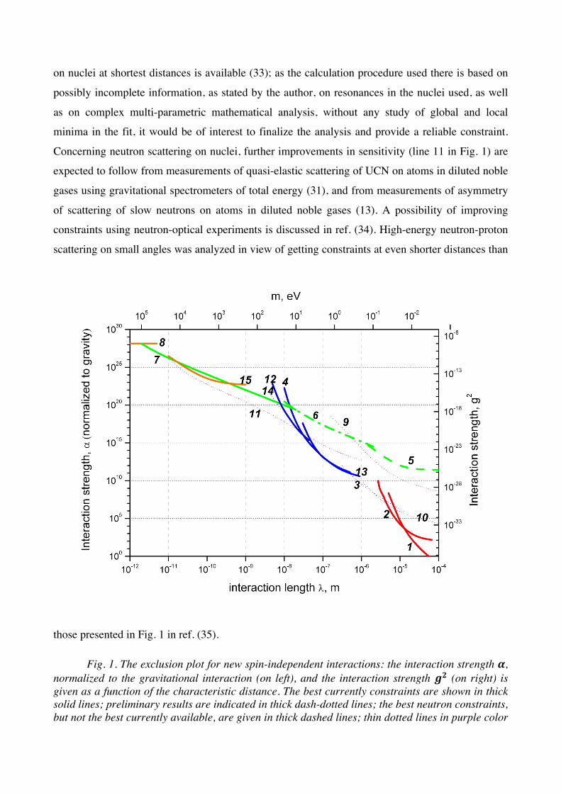
on nuclei at shortest distances is available (33); as the calculation procedure used there is based on
possibly incomplete information, as stated by the author, on resonances in the nuclei used, as well
as on complex multi-parametric mathematical analysis, without any study of global and local
minima in the fit, it would be of interest to finalize the analysis and provide a reliable constraint.
Concerning neutron scattering on nuclei, further improvements in sensitivity (line 11 in Fig. 1) are
expected to follow from measurements of quasi-elastic scattering of UCN on atoms in diluted noble
gases using gravitational spectrometers of total energy (31), and from measurements of asymmetry
of scattering of slow neutrons on atoms in diluted noble gases (13). A possibility of improving
constraints using neutron-optical experiments is discussed in ref. (34). High-energy neutron-proton
scattering on small angles was analyzed in view of getting constraints at even shorter distances than
those presented in Fig. 1 in ref. (35).
Fig. 1. The exclusion plot for new spin-independent interactions: the interaction strength !, normalized to the gravitational interaction (on left), and the interaction strength !! (on right) is given as a function of the characteristic distance. The best currently constraints are shown in thick solid lines; preliminary results are indicated in thick dash-dotted lines; the best neutron constraints, but not the best currently available, are given in thick dashed lines; thin dotted lines in purple color
correspond to projected sensitivity in various neutron experiments. Red color is reserved for measurements of gravity at short distances; blue-color constrains result from precision measurements of Casimir interactions; all constraints originated from neutron experiments are shown in green; constraint from measurements of exotic atoms is indicated in orange. Constraints “1” and “2” are obtained from measurements of short-range gravity in the torsion-balance (9) and the cantilever (10) experiment respectively. Constraints “4”, “12” and “13” follow from measurements of extra forces on top of Casimir and van der Waals interactions in refs. (12), (36), in reanalysis presented in ref. (11) of the experiment (37), and in ref. (38) respectively. We do not show the limit “3” from ref. (11), based on an experiment by Lamoreaux (39), as well as the limit “14” from ref. (40), based on an experiment by Ederth (41), as solid constraints; ref. (42) shows that correlations between fitted parameters deteriorate the sensitivity; furthermore a new systematical uncertainty was found (43) in the original experiment (39). Constrain “5” follows from measurements of neutron gravitational quantum states (14). Constrain “6” is derived from the data on neutron whispering gallery effect (these proceedings). Constrain “7” follows from neutron scattering on nuclei (13)). Constrain “8” is obtained from analysis of precision measurements of exotic atoms (13). Constrain “15” is obtained using searches for low-mass bosons from the Sun in a high-purity germanium detector (44). Lines “9”, “10”, “11” correspond to our estimations of eventual improvements in neutron constraints following from measurements of gravitational quantum states in a flow-through mode, in storage mode using the GRANIT spectrometer, from quasi-elastic scattering of UCN at diluted noble gases and from neutron whispering gallery effect respectively.
Many experiments look for spin-dependent short-range forces. Additional spin-dependent
interaction could be caused by new, light, pseudoscalar bosons such as the Axion. The Axion was
originally proposed in refs. (45), (46), (47), (48) as a solution to the strong CP problem, caused by
the smallness of the neutron electric dipole moment. The Axion would have profound consequences
in cosmology and astrophysics (49), and the non-observation of these effects limits the Axion to
have a mass in between 10 µeV and 10 meV. The general form of the potential caused by the
exchange of a pseudoscalar, axion-like, boson between a polarized spin-1/2 particle and another
unpolarized particle of the same kind is (50): ! ! = !!!!!!ℏ! !
!"!!!!!! ∙ !
!!"+ !
!!!"# −!/! .
Here, !!!!!! is the product of the relevant coupling coefficient between particle 1 (unpolarized) and
2 (polarized), and gives the strength of the potential. !! and !! are the mass and the spin of the
polarized particle, ! is the distance between the particles, and ! = ℏ/!" is the Yukawa range of
the new interaction. The Yukawa range is used as a free parameter in the analysis, as the mass ! of
the new exchange boson is not known a priori.
Most experiments look for new forces between electrons. More recently, much progress was
made in searches for new forces between nucleons. Comparisons between the coupling strengths for
electrons and nucleons require a particular model of the new interaction. Fig. 2 shows the exclusion
for new interactions between nucleons. The range for the ! values shown here is given by optimum
sensitivity of neutron and polarized 3He experiments.
Fig. 2. Searches for short-range nucleon spin-dependent interactions. Each line is excluding the region to the top. The limit from (55) (1, black solid line) was achieved by comparing the precession frequencies of atomic magnetometers made from either 199Hg or Cs atoms in presence of a 475 kg source mass made from lead. The sensitivity of the experiment with polarized 3He, described in these proceedings by Yuri Sobolev, is indicated in (2, thin dotted blue line). The limit from ref. (56) (3, blue solid line) was derived from the spin relaxation rate in polarized 3He cells; after subtraction of known causes of relaxation, the new interaction would constitute an extra relaxation channel. An even more constraining limit from experiments on storage of polarized 3He has been proposed (57) but the validity of the method used is being questioned (58). The limit in ref. (59) (4, thin green dash-dotted line) was derived from the study of gravitationally bound states of ultracold neutrons; the publication (59) triggered in significant extend the whole experimental program on spin-dependent short-range nucleon-nucleon interaction presented in the present proceedings. The limit from ref. (60) (5, thick green dashed line, proposed in (61)) was derived from comparison of the precession frequencies of ultracold neutrons in chambers in a vertical magnetic field, where the chamber bottom plate is made from a more dense material than top plate and vice versa. A force as in eq. (2) changes the precession frequency with a sign which depends on the position of the denser plate. The limit from ref. (62) (6, thick green solid line, criticized in ref. (63)) was derived from the fact that a new short-range spin-dependent force would cause spin relaxation of ultracold neutrons in vicinity of a reflecting surface; limits on the depolarization probability were turned into limits on new forces of that kind. The transmission of an unpolarized sample through a horizontal slit with an absorber at the top would look differently from the
measurement if a sufficiently strong new interaction given by eq. (2) would modify the wave functions of the gravitational bound states in dependence of their spin, as in a Stern-Gerlach experiment. We add projected sensitivities of different stages of the study of gravitationally bound quantum states: Assuming that an accuracy of 10-3 can be reached in the determination of the energy difference between ground state and second excited state in the flow-through experiment, we would be exploring some new territory in the exclusion plot at the range of a few micrometers (7, thin purple dotted line). The ultimate goal of GRANIT is to measure energy difference between quantum states of stored ultracold neutrons. Assuming an accuracy of 10-6, which is achieved if the precision is just the natural line-width of the transition, and assuming this line width is limited only by the neutron beta decay lifetime, we get the second project limit (8, thin purple dotted line). In ref. (64), a more optimistic scenario where a precision better than the size of the natural line width with the help of a Ramsey technique is discussed. An analogous method based on spin precession in a setup measuring neutron EDM and not requiring gravitational quantum states of neutrons is proposed in ref. (65).
Conclusion
The neutron methods considered in this report include asymmetric and quasi-elastic neutron
scattering on atoms of diluted noble gases, as well as centrifugal and gravitational quantum states of
neutrons near surface. Neutron constraints are competitive in the distance range of 10-11-10-7 m,
significant further improvements could be expected here in near future. Intense efforts are
continuing to improve constraints for short-range forces at larger distances up to 10-5 m, with the
goal to approach the currently best methods.
We appreciate financial support of Agence National de Recherche.
1. Antoniadis, I. et al. Compt. Rend. Acad. sciences. 2011 (accepted).
2. Antoniadis, I. Phys. Lett. B. 246 (1990) 377.
3. Lykken, J.D. Phys. Rev. D. 54 (1996) R3693.
4. Arkani-‐Hamed, N. et al. Phys. Lett. B. 429 (1998) 263.
5. Antoniadis, I. et al. Phys. Lett. B. 436 (1998) 257.
6. Rubakov, V.A. et al. Phys. Lett. B. 125 (1983) 136, 139.
7. Visser, M. Phys. Lett. B. 159 (1985) 22.
8. Frank, A. et al. Phys. Lett. B. 582 (2004) 15.
9. Kapner, D.L., et al. Phys. Rev. Lett. 98 (2007) 021101.
10. Geraci, A.A., et al. Phys. Rev. D. 78 (2008) 022002.
11. Bordag, M., et al. Phys. Rep. 353 (2001) 1.
12. Decca, R.S., et al. Phys. Rev. Lett. 94 (2005) 240401.
13. Nesvizhevsky, V.V., et al. Phys. Rev. D. 77 (2008) 034020.
14. Abele, H., et al. Lect. Notes Phys. 631 (2003) 355.
15. Nesvizhevsky, V.V., Protasov, K.V. Class. Quant. Grav. 21 (2004) 4557.
16. Zimmer, O., Kaiser, N. Class. Quant. Grav. 23 (2006) 6077.
17. Nesvizhevsky, V.V., Protasov, K.V. Class. Quant. Grav. 23 (2006) 6081.
18. Westphal, A. et al. arXiv:hep-‐ph/0703108.
19. Nesvizhevsky, V.V. et al. Nature. 415 (2002) 297.
20. Nesvizhevsky, V.V. et al. Phys. Rev. D. 67 (2003) 102002.
21. Nesvizhevsky, V.V. et al. Europ. Phys. J. C . 40 (2005) 479.
22. Baessler, S., Beau, M. et al. Compt. Rend. Acad. Sciences. 2011 (accepted).
23. Baessler, S., Gagarski, A.M. et al. Compt. Rend. Acad. Sciences. 2011 (accepted).
24. Sanuki, T., et al. NIM A. 600 (2009) 657.
25. Kreuz, M. et al. NIM A. 611 (2009) 326.
26. Jenke, T. et al. NIM A. 611 (2009) 318.
27. Pignol, G. PhD Thesis. Grenoble : University Joseph Fourier, 2009.
28. Nesvizhevsky, V.V. et al. Phys. Rev. A. 78 (2008) 033616.
29. Nesvizhevsky, V.V., et al. Nature Phys. 6 (2010) 114.
30. Nesvizhevsky, V.V. et al. New J. Phys. 12 (2010) 113050.
31. Nesvizhevsky, V.V. et al. Compt. Rend. Acad. Sciences. 2011 (accepted).
32. Leeb, H. et al. Phys. Rev. Let. 68 (1992) 1472.
33. Pokotilovsky, Yu.N. Phys. At. Nucl. 69 (2006) 924.
34. Gudkov, V. et al. Phys. Rev. C. 83 (2011) 025501.
35. Kamyshkov, Y. et al. Phys. Rev. D. 78 (2008) 114029.
36. Decca, R.S. et al. Europ. Phys. J. C. 51 (2007) 963.
37. Mohideen, U. et al. Phys. Lett. A. 132 (1988) 313.
38. Fischbach, E. et al. Phys. Rev. Lett. 94 (2005) 240401.
39. Lamoreaux, S.K. et al. Phys. Rev. Lett. 78 (1997) 5.
40. Mostepanenko, V.M., and Novello, M. Phys. Rev. D. 63 (2001) 115003.
41. Ederth, T. Phys. Rev. A. 62 (2000) 062104.
42. Long, J. et al. Nucl. Phys. B. 539 (1999) 23.
43. Lamoreaux, S.K. Phys. Rev. A. 82 (2010) 024102.
44. Horvat, R. et al. Phys. Lett. B. 699 (2011) 21.
45. Peccei, R.D. et al. Phys. Rev. Lett. 38 (1977) 1440.
46. Peccei, R.D. et al. Phys. Rev. D. 16 (1977) 1791.
47. Weinberg, S. Phys. Rev. Lett. 40 (1978) 223.
48. Wilczek, F. Phys. Rev. Lett. 40 (1978) 279.
49. Kuster, M. et al. Lect. Not. Phys. 741 (2008) 1.
50. Moody, J.E., Wilczek, F. Phys. Rev. D. 30 (1984) 130.
51. Adelberger, E. et al. Prog. Part. Nucl. Phys. 62 (2009) 102.
52. Hoedl, S.A. et al. Phys. Rev. Lett. 106 (2011) 041801.
53. Hammond, G.D. et al. Phys. Rev. Lett. 98 (2007) 081101.
54. Ni, W.-‐T. et al. Phys. Rev. Lett. 82 (1999) 2440.
55. Youdin, A.N. et al. Phys. Rev. Lett. 77 (1996) 2171.
56. Petukhov, A.K. et al. Phys. Rev. Lett. 105 (2010) 170401.
57. Fu, C.B. et al. Phys. Rev. D. 83 (2011) 031504.
58. Petoukhov, A.K. et al. arXiv:1103.1770.
59. Baessler, S. et al. Phys. Rev. D. 75 (2007) 075006.
60. Serebrov, A.P. et al. JETP Lett. 91 (2010) 6.
61. Zimmer, O. et al. Phys. Lett. B. 685 (2010) 38.
62. Serebrov, A.P. et al. Phys. Lett. B. 680 (2009) 423.
63. Ignatovich, V.K. et al. Europ. Phys. J. C. 64 (2009) 19.
64. Abele, H. et al. Phys. Rev. D. 81 (2010) 065019.
65. Zimmer, O. Phys. Lett. B. 685 (2010) 38.

Gravity Spectroscopy
Tobias Jenke1 , Peter Geltenbort2 , Hartmut Lemmel1,2 , Hartmut Abele1,3,4,a
1Atominstitut, Technische Universitat Wien, Stadionallee 2, 1020 Vienna, Austria
2Institut Laue-Langevin, 6 Rue Horowitz, 38042 Grenoble Cedex 9, France
3E18, Physikdepartment, Technische Universitat Munchen, 85748 Garching, Germany
4Physikalisches Institut, Universitat Heidelberg, Philosophenweg 12, 69120 Heidelberg, Germany
We demonstrate that - for the first time - the method of Rabi spectroscopy usually used in atomoptics can now be applied to quantum states in the gravity potential of the Earth togetherwith a mechanical or magnetic coupling1. This technique allows a precise measurement ofquantum mechanical phase shifts of a Schrodinger wave packet bouncing off a hard surfacein the Earth’s gravitational field. The idea behind this method is that phase shifts in gravitypotentials can now be related to frequency measurements with unprecedented accuracy.The experiment addresses some of the unresolved questions of modern science: the nature ofthe fundamental forces and underlying symmetries, the nature of gravitation at very smalldistances, and the nature of cosmological mass and the energy density of the universe.
1 Introduction
Gravity experiments at short distances might provide an answer for the ”big questions” aboutspace, time, and a unification of all forces, where space-time may not be restricted to four dimen-sions. Hypothetical extra-dimensions, curled up to cylinders or tori with a small compactificationradius would lead to deviations from Newton’s gravitational law at very small distances2. Theseideas triggered gravity experiments of different kinds, which in the past ten years have validatedNewton’s gravitational law down to about 50 µm3–7. The basic problem in searching for newphysics at small distances is that the size of the objects under study needs to be reduced, too,which is accompanied by a reduction in signal intensity.Our test of the law of gravity at small distances is based on quantum objects8 using a newresonance spectroscopy technique. This method allows precise measurement9 of quantum stateswith neutrons in the gravity potential of the earth with a Schrodinger wave packet bouncingoff a hard horizontal surface. The concept is related to Rabi’s magnetic resonance techniquefor measurements of nuclear magnetic moments10. The sensitivity is extremely high, because aquantum mechanical phase shift is converted into a frequency measurement. The sensitivity ofresonance methods reached so far11 is 6.8× 10⁻²² eV, or one Bohr rotation every six days.
aCorrespondence should be addressed to: [email protected]
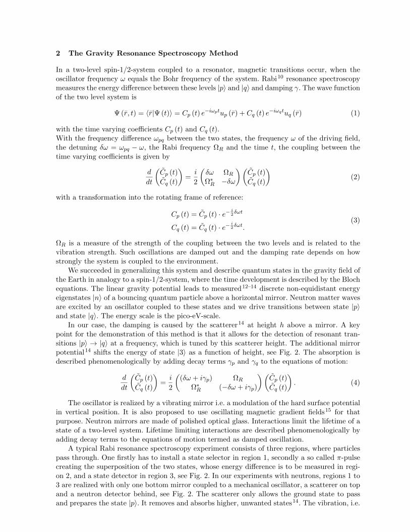
2 The Gravity Resonance Spectroscopy Method
In a two-level spin-1/2-system coupled to a resonator, magnetic transitions occur, when theoscillator frequency ω equals the Bohr frequency of the system. Rabi10 resonance spectroscopymeasures the energy difference between these levels |p〉 and |q〉 and damping γ. The wave functionof the two level system is
Ψ (r, t) = 〈r|Ψ (t)〉 = Cp (t) e−iωptup (r) + Cq (t) e−iωqtuq (r) (1)
with the time varying coefficients Cp (t) and Cq (t).With the frequency difference ωpq between the two states, the frequency ω of the driving field,the detuning δω = ωpq − ω, the Rabi frequency ΩR and the time t, the coupling between thetime varying coefficients is given by
d
dt
(Cp (t)
Cq (t)
)=i
2
(δω ΩR
Ω∗R −δω
)(Cp (t)
Cq (t)
)(2)
with a transformation into the rotating frame of reference:
Cp (t) = Cp (t) · e−i2δωt
Cq (t) = Cq (t) · e−i2δωt.
(3)
ΩR is a measure of the strength of the coupling between the two levels and is related to thevibration strength. Such oscillations are damped out and the damping rate depends on howstrongly the system is coupled to the environment.
We succeeded in generalizing this system and describe quantum states in the gravity field ofthe Earth in analogy to a spin-1/2-system, where the time development is described by the Blochequations. The linear gravity potential leads to measured12–14 discrete non-equidistant energyeigenstates |n〉 of a bouncing quantum particle above a horizontal mirror. Neutron matter wavesare excited by an oscillator coupled to these states and we drive transitions between state |p〉and state |q〉. The energy scale is the pico-eV-scale.
In our case, the damping is caused by the scatterer14 at height h above a mirror. A keypoint for the demonstration of this method is that it allows for the detection of resonant tran-sitions |p〉 → |q〉 at a frequency, which is tuned by this scatterer height. The additional mirrorpotential14 shifts the energy of state |3〉 as a function of height, see Fig. 2. The absorption isdescribed phenomenologically by adding decay terms γp and γq to the equations of motion:
d
dt
(Cp (t)
Cq (t)
)=i
2
((δω + iγp) ΩR
Ω∗R (−δω + iγp)
)(Cp (t)
Cq (t)
). (4)
The oscillator is realized by a vibrating mirror i.e. a modulation of the hard surface potentialin vertical position. It is also proposed to use oscillating magnetic gradient fields15 for thatpurpose. Neutron mirrors are made of polished optical glass. Interactions limit the lifetime of astate of a two-level system. Lifetime limiting interactions are described phenomenologically byadding decay terms to the equations of motion termed as damped oscillation.
A typical Rabi resonance spectroscopy experiment consists of three regions, where particlespass through. One firstly has to install a state selector in region 1, secondly a so called π-pulsecreating the superposition of the two states, whose energy difference is to be measured in regi-on 2, and a state detector in region 3, see Fig. 2. In our experiments with neutrons, regions 1 to3 are realized with only one bottom mirror coupled to a mechanical oscillator, a scatterer on topand a neutron detector behind, see Fig. 2. The scatterer only allows the ground state to passand prepares the state |p〉. It removes and absorbs higher, unwanted states14. The vibration, i.e.
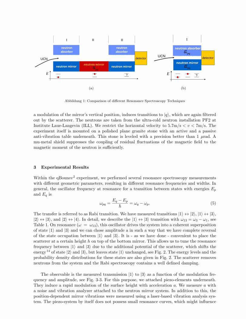
neutron mirror
neutron
absorber
neutron mirror
UCN detector
pqω
neutron
absorber
neutron mirror
I II II
E ?
(a)
neutron absorber
neutron mirror
UCN detector
pqω
ω
I
neutron mirror
pqωE ?
(b)
Abbildung 1: Comparison of different Resonance Spectroscopy Techniques
a modulation of the mirror’s vertical position, induces transitions to |q〉, which are again filteredout by the scatterer. The neutrons are taken from the ultra-cold neutron installation PF2 atInstitute Laue-Langevin (ILL). We restrict the horizontal velocity to 5.7m/s < v < 7m/s. Theexperiment itself is mounted on a polished plane granite stone with an active and a passiveanti-vibration table underneath. This stone is leveled with a precision better than 1 µrad. Amu-metal shield suppresses the coupling of residual fluctuations of the magnetic field to themagnetic moment of the neutron is sufficiently.
3 Experimental Results
Within the qBounce2 experiment, we performed several resonance spectroscopy measurementswith different geometric parameters, resulting in different resonance frequencies and widths. Ingeneral, the oscillator frequency at resonance for a transition between states with energies Epand Eq is
ωpq =Eq − Ep
h= ωq − ωp. (5)
The transfer is referred to as Rabi transition. We have measured transitions |1〉 ↔ |2〉, |1〉 ↔ |3〉,|2〉 ↔ |3〉, and |2〉 ↔ |4〉. In detail, we describe the |1〉 ↔ |3〉 transition with ω13 = ω3 − ω1, seeTable 1. On resonance (ω = ω13), this oscillator drives the system into a coherent superpositionof state |1〉 and |3〉 and we can chose amplitude a in such a way that we have complete reversalof the state occupation between |1〉 and |3〉. It is - as we have done - convenient to place thescatterer at a certain height h on top of the bottom mirror. This allows us to tune the resonancefrequency between |1〉 and |3〉 due to the additional potential of the scatterer, which shifts theenergy14 of state |2〉 and |3〉, but leaves state |1〉 unchanged, see Fig. 2. The energy levels and theprobability density distributions for these states are also given in Fig. 2. The scatterer removesneutrons from the system and the Rabi spectroscopy contains a well defined damping.
The observable is the measured transmission |1〉 to |3〉 as a function of the modulation fre-quency and amplitude, see Fig. 3-3. For this purpose, we attached piezo-elements underneath.They induce a rapid modulation of the surface height with acceleration a. We measure a witha noise and vibration analyzer attached to the neutron mirror system. In addition to this, theposition-dependent mirror vibrations were measured using a laser-based vibration analysis sys-tem. The piezo-system by itself does not possess small resonance curves, which might influence
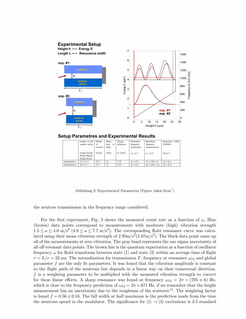
0 5 10 15 20 25 30
0
1
2
3
4
5
6
7
0
200
400
600
800
1000
1200
1400
1600
Height h @µmDE
nerg
yE
@peV
D
Freq
uenc
yHE
ê2π
L@H
zD
Length of the neutron mirror Length L[cm]x Width W[cm]x Height H[cm]
Height of scatterer h [µm]
Mean time of flight t [ms]
Energy difference E13 [peV]
Resonance frequency (prediction) ω13 [s-1]
Resonance frequency (measurement) ω13 [s-1]
Resonance width (FWHM) ∆ω [s-1]
Experiment 1 15 x 3 x 3 25.5 23 2.78 2π × 671 2π × (705 ± 6) 2π × 41.2 Experiment 2 10 x 3 x 3 27.1 15 2.55 2π × 615 2π × (592 ± 11) 2π × 61.6
neutronmirror
scatterer
1h
1
L
neutronmirror
scatterer
2h
2
L
Experimental Setup
Setup Parametres and Experimental Results
Height h Energy ELength L Resonance width
exp. #1:
exp. #2:
exp. #1exp. #2
Abbildung 2: Experimental Parameters (Figure taken from1)
the neutron transmission in the frequency range considered.
For the first experiment, Fig. 3 shows the measured count rate as a function of ω. Blue(brown) data points correspond to measurements with moderate (high) vibration strength1.5 ≤ a ≤ 4.0 m/s2 (4.9 ≤ a ≤ 7.7 m/s2). The corresponding Rabi resonance curve was calcu-lated using their mean vibration strength of 2.95m/s2(5.87m/s2). The black data point sums upall of the measurements at zero vibration. The gray band represents the one sigma uncertainty ofall off-resonant data points. The brown line is the quantum expectation as a function of oscillatorfrequency ω for Rabi transitions between state |1〉 and state |3〉 within an average time of flightτ = L/v = 23 ms. The normalization for transmission T , frequency at resonance ω13 and globalparameter f are the only fit parameters. It was found that the vibration amplitude is constantto the flight path of the neutrons but depends in a linear way on their transversal direction.f is a weighting parameter to be multiplied with the measured vibration strength to correctfor these linear effects. A sharp resonance was found at frequency ω13 = 2π × (705 ± 6) Hz,which is close to the frequency prediction of ω13 = 2π× 671 Hz, if we remember that the heightmeasurement has an uncertainty due to the roughness of the scatterer14. The weighting factoris found f = 0.56± 0.16. The full width at half maximum is the prediction made from the timethe neutrons spend in the modulator. The significance for |1〉 → |3〉 excitations is 3.5 standard
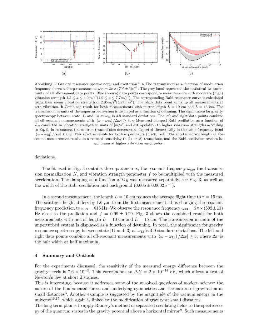
6
8
10
12
14
16
0 200 400 600 800 1000
Tra
nsm
issio
n [10
−3 s
−1]
ω/2π [Hz]
moderate vibration strengthhigh vibration strength
(a)
0.5
0.6
0.7
0.8
0.9
1
1.1
1.2
−3 −2 −1 0 1 2 3
Rela
tive T
ransm
issio
n
(ω − ω13)/ ∆ω
(b)
0.2
0.4
0.6
0.8
1
0 5 10 15 20 25
Re
lative
Tra
nsm
issio
n
Vibration Strength a [m/s²]
Measurement 1Measurement 2
(c)
Abbildung 3: Gravity resonance spectroscopy and excitation1: a The transmission as a function of modulationfrequency shows a sharp resonance at ω13 = 2π× (705± 6)s−1. The grey band represents the statistical 1σ uncer-tainty of all off-resonant data points. Blue (brown) data points correspond to measurements with moderate (high)vibration strength 1.5 ≤ a ≤ 4.0m/s2(4.9 ≤ a ≤ 7.7m/s2). The corresponding Rabi resonance curve is calculatedusing their mean vibration strength of 2.95m/s2(5.87m/s2). The black data point sums up all measurements atzero vibration. b Combined result for both measurements with mirror length L = 10 cm and L = 15 cm. Thetransmission in units of the unperturbed system is displayed as a function of detuning. The significance for gravityspectroscopy between state |1〉 and |3〉 at ω13 is 4.9 standard deviations. The left and right data points combineall off-resonant measurements with |(ω − ω13) /∆ω| ≥ 3. c Measured damped Rabi oscillation as a function ofΩR converted in vibration strength in units of [m/s2] and extrapolation to higher vibration strengths accordingto Eq. 9. In resonance, the neutron transmission decreases as expected theoretically in the same frequency band|(ω − ω13) /∆ω| ≤ 0.6. This effect is visible for both experiments (black, red). The shorter mirror length in thesecond measurement results in a reduced sensitivity to |1〉 ↔ |3〉 transitions, and the Rabi oscillation reaches its
minimum at higher vibration amplitudes.
deviations.
The fit used in Fig. 3 contains three parameters, the resonant frequency ωpq, the transmis-sion normalization N , and vibration strength parameter f to be multiplied with the measuredacceleration. The damping as a function of ΩR was measured separately, see Fig. 3, as well asthe width of the Rabi oscillation and background (0.005± 0.0002 s−1).
In a second measurement, the length L = 10 cm reduces the average flight time to τ = 15 ms.The scatterer height differs by 1.6 µm from the first measurement, thus changing the resonantfrequency prediction to ω13 = 615 Hz. We observe the resonance frequency ω13 = 2π×(592±11)Hz close to the prediction and f = 0.99 ± 0.29. Fig. 3 shows the combined result for bothmeasurements with mirror length L = 10 cm and L = 15 cm. The transmission in units of theunperturbed system is displayed as a function of detuning. In total, the significance for gravityresonance spectroscopy between state |1〉 and |3〉 at ω13 is 4.9 standard deviations. The left andright data points combine all off-resonant measurements with |(ω − ω13) /∆ω| ≥ 3, where ∆ν isthe half width at half maximum.
4 Summary and Outlook
For the experiments discussed, the sensitivity of the measured energy difference between thegravity levels is 7.6 × 10⁻³. This corresponds to ∆E = 2 × 10⁻¹⁴ eV, which allows a test ofNewton’s law at short distances.This is interesting, because it addresses some of the unsolved questions of modern science: thenature of the fundamental forces and underlying symmetries and the nature of gravitation atsmall distances3. Another example is suggested by the magnitude of the vacuum energy in theuniverse16,17, which again is linked to the modification of gravity at small distances.The long term plan is to apply Ramsey’s method of separated oscillating fields to the spectrosco-py of the quantum states in the gravity potential above a horizontal mirror9. Such measurements
with ultra-cold neutrons will offer a sensitivity to Newton’s law or hypothetical short-rangedinteractions that is about 21 orders of magnitude below the energy scale of electromagnetism.
Acknowledgments
We gratefully acknowledge support from the Austrian Science Fund (FWF) under Contract No. I529-N20 and
the German Research Foundation (DFG) within the Priority Programme (SPP) 1491”Precision experiments
in particle and astrophysics with cold and ultracold neutrons“, the DFG Excellence Initiative”Origin of the
Universe“, and DFG support under Contract No. Ab128/2-1.
References
[1] Jenke et al., Nature Physics 7, 468 (2011).[2] Arkani-Hamed, N., Dimopolos, S. & Dvali, G., Phys. Rev. D59, 086004 (1999).[3] Fischbach E. & Talmadge C. L. The search for non-Newtonian gravity. Springer-Verlag New York (1999).[4] Adelberger, E. G., Heckel B. R. & Nelson, A. E., Ann. Rev. Part. Sci. 53 77 (2003).[5] Long J. C. et al., Nature 421, 922 (2003).[6] Geraci, A. A. et al., Phys. Rev. D72, 022002 (2008).[7] Abele, H., Prog. Part. Nucl. Phys., 60, 1 (2008).[8] Abele, H. et al., Nucl. Phys. A827, 593c (2009).[9] Abele, H. et al., Phys. Rev. D81, 065019 (2010).[10] Rabi I. I. et al., Phys. Rev. 55, 526 (1939).[11] Baker, C. A. et al., Phys. Rev. Lett. 97, 131801 (2006).[12] Nesvizhevsky, V. V. et al., Nature 415, 299 (2002).[13] Nesvizhevsky, V. V. et al., C40, 479 (2005).[14] Westphal, A. et al., Eur. Phys. J C51, 367 (2007).[15] Kreuz, M. et al., arXiv:physics.ins-det 0902.0156.[16] Callin, P. & Burgess, C. P., Nucl.Phys. B752 60-79 (2006).[17] Sundrum, R., J. High Energy Phys. 07, 001 (1999).
Forca-G: A trapped atom interferometer for the measurement of short range forces
B. PELLE, G. TACKMANN, Q. BEAUFILS, X. WANG, A. HILICO and F. PEREIRA DOS SANTOSS. PELISSON, R. MESSINA, M.-C. ANGONIN and P. WOLF
LNE-SYRTE, Observatoire de Paris, LNE, CNRS, UPMC, 61 avenue de l’Observatoire,75014 Paris, France
The aim of the Forca-G project 1 lies into the study of short range atom-surface interactions.Using cold 87Rb atoms trapped into a 1D-optical lattice close to the reflecting surface, anatomic interferometer involving a coherent superposition between atomic states at differentdistances from the mirror can be realized. This would allow a precise measurement of thepotential experienced by the atoms. In the range of 1-20 µm, the atom-surface interaction isdominated by QED potential (Casimir-Polder or Van der Waals). Besides, a precise measure-ment of this interaction would also allow a test of Newton’s law at short distance. In a firststep, we have demonstrated the efficienty of our atomic interferometer in a regime far fromthe surface with a measurement of the Bloch frequency.
Introduction
Measurement of short range (< 1 mm) forces is one of the challenge of modern experimentalphysics. The use of cold atoms for the measurement of atom-surface forces 2 can be a promisingalternative to microelectromechanical systems and torsion balance which probe surface-surfaceforces. 3 In particular, good control of the experimental parameters and coherence propertiesmake the use of trapped cold atoms an interesting candidate to compete in precision withmechanical systems.
1 Principle of the experiment
In this first step, our system is composed of 87Rb atoms trapped in a vertical 1D-optical latticefar from the reflecting mirror.
The internal atomic structure is approximated by a two-level system, with two long lived
states, |g〉 =∣∣∣52S1/2, F = 1,mF = 0
⟩and |e〉 =
∣∣∣52S1/2, F = 2,mF = 0⟩
, the ground and excited
hyperfine levels separated in energy by hνHFS (see Fig. 1).In a vertical geometry, the atoms confined in the periodic potential experience a linear
acceleration due to Earth’s gravity, which is described by the following external Hamiltonian: 4
Hext =h2k2
2ma+Ul2
(1− cos (2klz)) +magz (1)
where h is the Planck’s constant, k the atomic momentum, ma the atomic mass, Ul the latticedepth, kl the optical lattice wavevector, z the vertical position and g the gravity.
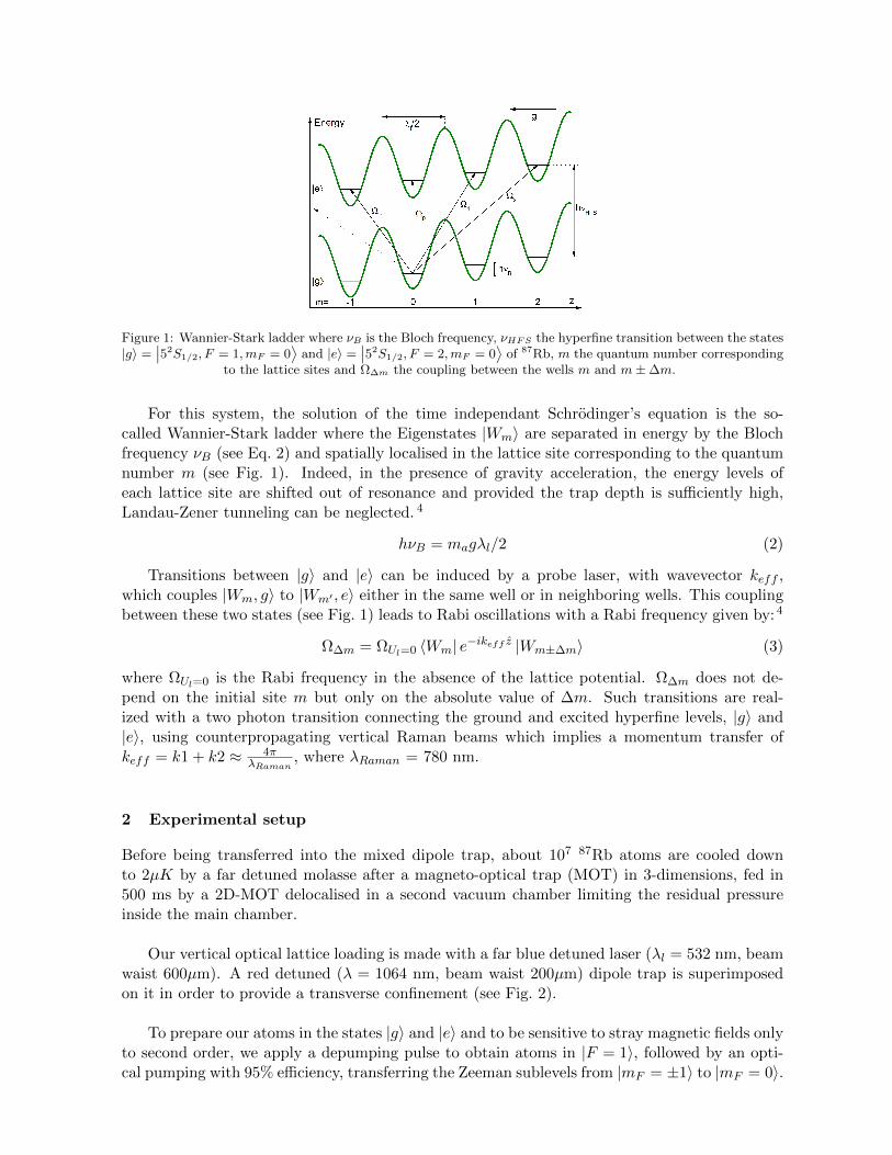
Figure 1: Wannier-Stark ladder where νB is the Bloch frequency, νHFS the hyperfine transition between the states|g〉 =
∣∣52S1/2, F = 1,mF = 0⟩
and |e〉 =∣∣52S1/2, F = 2,mF = 0
⟩of 87Rb, m the quantum number corresponding
to the lattice sites and Ω∆m the coupling between the wells m and m±∆m.
For this system, the solution of the time independant Schrodinger’s equation is the so-called Wannier-Stark ladder where the Eigenstates |Wm〉 are separated in energy by the Blochfrequency νB (see Eq. 2) and spatially localised in the lattice site corresponding to the quantumnumber m (see Fig. 1). Indeed, in the presence of gravity acceleration, the energy levels ofeach lattice site are shifted out of resonance and provided the trap depth is sufficiently high,Landau-Zener tunneling can be neglected. 4
hνB = magλl/2 (2)
Transitions between |g〉 and |e〉 can be induced by a probe laser, with wavevector keff ,which couples |Wm, g〉 to |Wm′ , e〉 either in the same well or in neighboring wells. This couplingbetween these two states (see Fig. 1) leads to Rabi oscillations with a Rabi frequency given by: 4
Ω∆m = ΩUl=0 〈Wm| e−ikeff z |Wm±∆m〉 (3)
where ΩUl=0 is the Rabi frequency in the absence of the lattice potential. Ω∆m does not de-pend on the initial site m but only on the absolute value of ∆m. Such transitions are real-ized with a two photon transition connecting the ground and excited hyperfine levels, |g〉 and|e〉, using counterpropagating vertical Raman beams which implies a momentum transfer ofkeff = k1 + k2 ≈ 4π
λRaman, where λRaman = 780 nm.
2 Experimental setup
Before being transferred into the mixed dipole trap, about 107 87Rb atoms are cooled downto 2µK by a far detuned molasse after a magneto-optical trap (MOT) in 3-dimensions, fed in500 ms by a 2D-MOT delocalised in a second vacuum chamber limiting the residual pressureinside the main chamber.
Our vertical optical lattice loading is made with a far blue detuned laser (λl = 532 nm, beamwaist 600µm). A red detuned (λ = 1064 nm, beam waist 200µm) dipole trap is superimposedon it in order to provide a transverse confinement (see Fig. 2).
To prepare our atoms in the states |g〉 and |e〉 and to be sensitive to stray magnetic fields onlyto second order, we apply a depumping pulse to obtain atoms in |F = 1〉, followed by an opti-cal pumping with 95% efficiency, transferring the Zeeman sublevels from |mF = ±1〉 to |mF = 0〉.
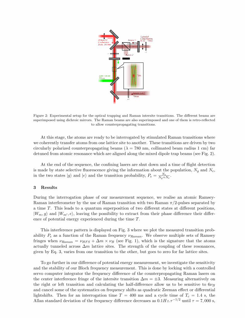
Figure 2: Experimental setup for the optical trapping and Raman intersite transitions. The different beams aresuperimposed using dichroic mirrors. The Raman beams are also superimposed and one of them is retro-reflected
to allow counterpropagating transitions.
At this stage, the atoms are ready to be interrogated by stimulated Raman transitions wherewe coherently transfer atoms from one lattice site to another. These transitions are driven by twocircularly polarized counterpropagating beams (λ = 780 nm, collimated beam radius 1 cm) fardetuned from atomic resonance which are aligned along the mixed dipole trap beams (see Fig. 2).
At the end of the sequence, the confining lasers are shut down and a time of flight detectionis made by state selective fluorescence giving the information about the population, Ng and Ne,in the two states |g〉 and |e〉 and the transition probability, Pe = Ne
Ng+Ne.
3 Results
During the interrogation phase of our measurement sequence, we realise an atomic Ramsey-Raman interferometer by the use of Raman transition with two Raman π/2-pulses separated bya time T . This leads to a quantum superposition of two different states at different positions,|Wm, g〉 and |Wm′ , e〉, leaving the possibility to extract from their phase difference their differ-ence of potential energy experienced during the time T .
This interference pattern is displayed on Fig. 3 where we plot the measured transition prob-ability Pe as a function of the Raman frequency νRaman. We observe multiple sets of Ramseyfringes when νRaman = νHFS + ∆m × νB (see Fig. 1), which is the signature that the atomsactually tunneled across ∆m lattice sites. The strength of the coupling of these resonances,given by Eq. 3, varies from one transition to the other, but goes to zero for far lattice sites.
To go further in our difference of potential energy measurement, we investigate the sensitivityand the stability of our Bloch frequency measurement. This is done by locking with a controlledservo computer integrator the frequency difference of the counterpropagating Raman lasers onthe center interference fringe of the intersite transition ∆m = ±3. Measuring alternatively onthe right or left transition and calculating the half-difference allow us to be sensitive to 6νBand cancel some of the systematics on frequency shifts as quadratic Zeeman effect or differentiallightshifts. Then for an interrogation time T = 400 ms and a cycle time of Tc = 1.4 s, theAllan standard deviation of the frequency difference decreases as 0.1Hz.τ−1/2 until τ = 7, 000 s,
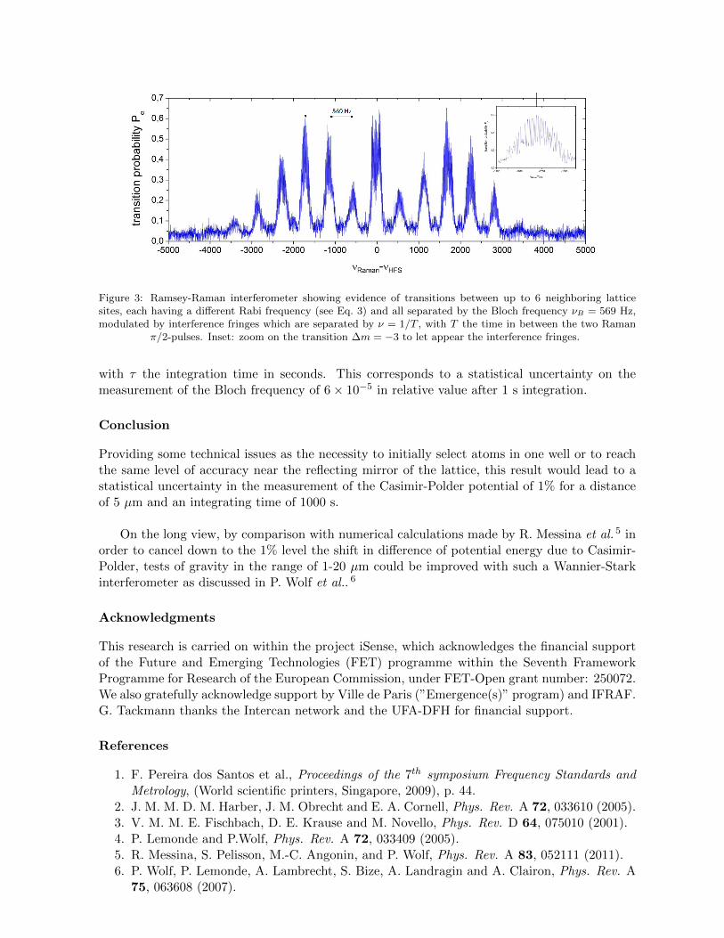
Figure 3: Ramsey-Raman interferometer showing evidence of transitions between up to 6 neighboring latticesites, each having a different Rabi frequency (see Eq. 3) and all separated by the Bloch frequency νB = 569 Hz,modulated by interference fringes which are separated by ν = 1/T , with T the time in between the two Raman
π/2-pulses. Inset: zoom on the transition ∆m = −3 to let appear the interference fringes.
with τ the integration time in seconds. This corresponds to a statistical uncertainty on themeasurement of the Bloch frequency of 6× 10⁻⁵ in relative value after 1 s integration.
Conclusion
Providing some technical issues as the necessity to initially select atoms in one well or to reachthe same level of accuracy near the reflecting mirror of the lattice, this result would lead to astatistical uncertainty in the measurement of the Casimir-Polder potential of 1% for a distanceof 5 µm and an integrating time of 1000 s.
On the long view, by comparison with numerical calculations made by R. Messina et al. 5 inorder to cancel down to the 1% level the shift in difference of potential energy due to Casimir-Polder, tests of gravity in the range of 1-20 µm could be improved with such a Wannier-Starkinterferometer as discussed in P. Wolf et al.. 6
Acknowledgments
This research is carried on within the project iSense, which acknowledges the financial supportof the Future and Emerging Technologies (FET) programme within the Seventh FrameworkProgramme for Research of the European Commission, under FET-Open grant number: 250072.We also gratefully acknowledge support by Ville de Paris (”Emergence(s)” program) and IFRAF.G. Tackmann thanks the Intercan network and the UFA-DFH for financial support.
References
1. F. Pereira dos Santos et al., Proceedings of the 7th symposium Frequency Standards andMetrology, (World scientific printers, Singapore, 2009), p. 44.
2. J. M. M. D. M. Harber, J. M. Obrecht and E. A. Cornell, Phys. Rev. A 72, 033610 (2005).3. V. M. M. E. Fischbach, D. E. Krause and M. Novello, Phys. Rev. D 64, 075010 (2001).4. P. Lemonde and P.Wolf, Phys. Rev. A 72, 033409 (2005).5. R. Messina, S. Pelisson, M.-C. Angonin, and P. Wolf, Phys. Rev. A 83, 052111 (2011).6. P. Wolf, P. Lemonde, A. Lambrecht, S. Bize, A. Landragin and A. Clairon, Phys. Rev. A
75, 063608 (2007).
7.Tests of relativity
in the solar system

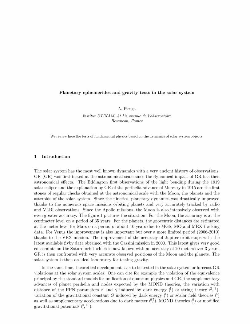
Planetary ephemerides and gravity tests in the solar system
A. Fienga
Institut UTINAM, 41 bis avenue de l’observatoireBesancon, France
We review here the tests of fundamental physics based on the dynamics of solar system objects.
1 Introduction
The solar system has the most well known dynamics with a very ancient history of observations.GR (GR) was first tested at the astronomical scale since the dynamical impact of GR has thenastronomical effects. The Eddington first observations of the light bending during the 1919solar eclipse and the explanation by GR of the perihelia advance of Mercury in 1915 are the firststones of regular checks obtained at the astronomical scale with the Moon, the planets and theasteroids of the solar system. Since the nineties, planetary dynamics was drastically improvedthanks to the numerous space missions orbiting planets and very accurately tracked by radioand VLBI observations. Since the Apollo missions, the Moon is also intensively observed witheven greater accuracy. The figure 1 pictures the situation. For the Moon, the accuracy is at thecentimeter level on a period of 35 years. For the planets, the geocentric distances are estimatedat the meter level for Mars on a period of about 10 years due to MGS, MO and MEX trackingdata. For Venus the improvement is also important but over a more limited period (2006-2010)thanks to the VEX mission. The improvement of the accuracy of Jupiter orbit stops with thelatest available flyby data obtained with the Cassini mission in 2000. This latest gives very goodconstraints on the Saturn orbit which is now known with an accuracy of 20 meters over 3 years.GR is then confronted with very accurate observed positions of the Moon and the planets. Thesolar system is then an ideal laboratory for testing gravity.
In the same time, theoretical developments ask to be tested in the solar system or forecast GRviolations at the solar system scales. One can cite for example the violation of the equivalenceprincipal by the standard models for unification of quantum physics and GR, the supplementaryadvances of planet perihelia and nodes expected by the MOND theories, the variation withdistance of the PPN parameters β and γ induced by dark energy (1) or string theory (2, 3),variation of the gravitational constant G induced by dark energy (4) or scalar field theories (5)as well as supplementary accelerations due to dark matter (6,7), MOND theories (8) or modifiedgravitational potentials (9, 10).
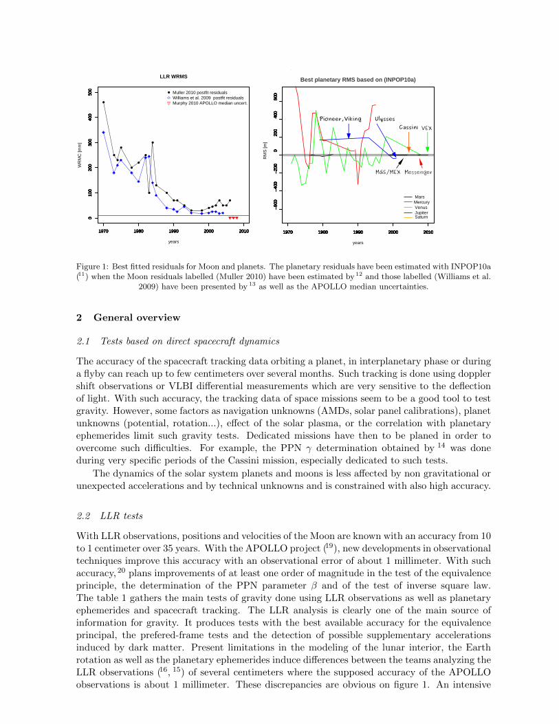
1970 1980 1990 2000 2010
010
020
030
040
050
0
LLR WRMS
years
WR
MC
[mm
]
1970 1980 1990 2000 2010
010
020
030
040
050
0
1970 1980 1990 2000 2010
010
020
030
040
050
0
1970 1980 1990 2000 2010
010
020
030
040
050
0
1970 1980 1990 2000 2010
010
020
030
040
050
0
1970 1980 1990 2000 2010
010
020
030
040
050
0 Muller 2010 postfit residuals
Williams et al. 2009 postfit residualsMurphy 2010 APOLLO median uncert.
1970 1980 1990 2000 2010
−600
−400
−200
020
040
060
0
years
RM
S [m
]
1970 1980 1990 2000 2010
−600
−400
−200
020
040
060
0
1970 1980 1990 2000 2010
−600
−400
−200
020
040
060
0
1970 1980 1990 2000 2010
−600
−400
−200
020
040
060
0
1970 1980 1990 2000 2010
−600
−400
−200
020
040
060
0
1970 1980 1990 2000 2010
−600
−400
−200
020
040
060
0
1970 1980 1990 2000 2010
−600
−400
−200
020
040
060
0
1970 1980 1990 2000 2010
−600
−400
−200
020
040
060
0
1970 1980 1990 2000 2010
−600
−400
−200
020
040
060
0
MGS/MEX Messenger
VEXPioneer,Viking Ulysses
Cassini
Best planetary RMS based on (INPOP10a)
MarsMercuryVenusJupiterSaturn
Figure 1: Best fitted residuals for Moon and planets. The planetary residuals have been estimated with INPOP10a(11) when the Moon residuals labelled (Muller 2010) have been estimated by 12 and those labelled (Williams et al.
2009) have been presented by 13 as well as the APOLLO median uncertainties.
2 General overview
2.1 Tests based on direct spacecraft dynamics
The accuracy of the spacecraft tracking data orbiting a planet, in interplanetary phase or duringa flyby can reach up to few centimeters over several months. Such tracking is done using dopplershift observations or VLBI differential measurements which are very sensitive to the deflectionof light. With such accuracy, the tracking data of space missions seem to be a good tool to testgravity. However, some factors as navigation unknowns (AMDs, solar panel calibrations), planetunknowns (potential, rotation...), effect of the solar plasma, or the correlation with planetaryephemerides limit such gravity tests. Dedicated missions have then to be planed in order toovercome such difficulties. For example, the PPN γ determination obtained by 14 was doneduring very specific periods of the Cassini mission, especially dedicated to such tests.
The dynamics of the solar system planets and moons is less affected by non gravitational orunexpected accelerations and by technical unknowns and is constrained with also high accuracy.
2.2 LLR tests
With LLR observations, positions and velocities of the Moon are known with an accuracy from 10to 1 centimeter over 35 years. With the APOLLO project (19), new developments in observationaltechniques improve this accuracy with an observational error of about 1 millimeter. With suchaccuracy, 20 plans improvements of at least one order of magnitude in the test of the equivalenceprinciple, the determination of the PPN parameter β and of the test of inverse square law.The table 1 gathers the main tests of gravity done using LLR observations as well as planetaryephemerides and spacecraft tracking. The LLR analysis is clearly one of the main source ofinformation for gravity. It produces tests with the best available accuracy for the equivalenceprincipal, the prefered-frame tests and the detection of possible supplementary accelerationsinduced by dark matter. Present limitations in the modeling of the lunar interior, the Earthrotation as well as the planetary ephemerides induce differences between the teams analyzing theLLR observations (16, 15) of several centimeters where the supposed accuracy of the APOLLOobservations is about 1 millimeter. These discrepancies are obvious on figure 1. An intensive
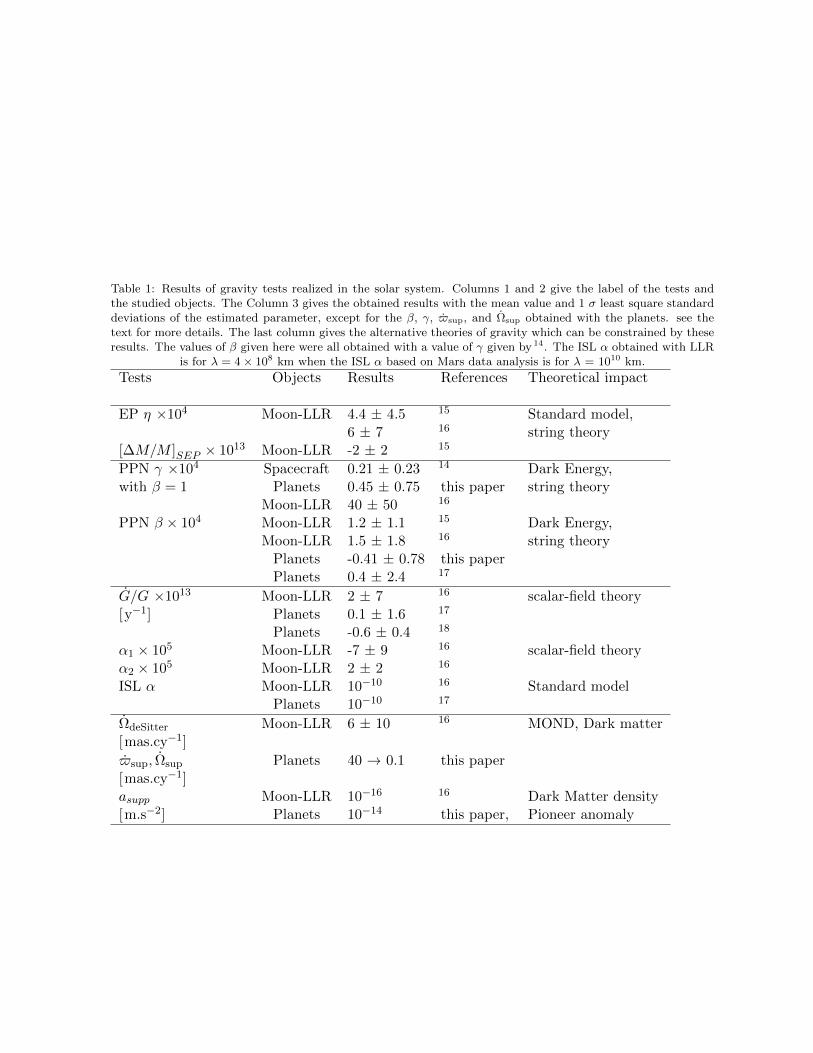
Table 1: Results of gravity tests realized in the solar system. Columns 1 and 2 give the label of the tests andthe studied objects. The Column 3 gives the obtained results with the mean value and 1 σ least square standarddeviations of the estimated parameter, except for the β, γ, $sup, and Ωsup obtained with the planets. see thetext for more details. The last column gives the alternative theories of gravity which can be constrained by theseresults. The values of β given here were all obtained with a value of γ given by 14. The ISL α obtained with LLR
is for λ = 4 × 10⁸ km when the ISL α based on Mars data analysis is for λ = 1010 km.
Tests Objects Results References Theoretical impact
EP η ×104 Moon-LLR 4.4 ± 4.5 15 Standard model,6 ± 7 16 string theory
[∆M/M ]SEP × 1013 Moon-LLR -2 ± 2 15
PPN γ ×104 Spacecraft 0.21 ± 0.23 14 Dark Energy,with β = 1 Planets 0.45 ± 0.75 this paper string theory
Moon-LLR 40 ± 50 16
PPN β × 104 Moon-LLR 1.2 ± 1.1 15 Dark Energy,Moon-LLR 1.5 ± 1.8 16 string theory
Planets -0.41 ± 0.78 this paperPlanets 0.4 ± 2.4 17
G/G ×1013 Moon-LLR 2 ± 7 16 scalar-field theory[y−1] Planets 0.1 ± 1.6 17
Planets -0.6 ± 0.4 18
α1 × 10⁵ Moon-LLR -7 ± 9 16 scalar-field theoryα2 × 10⁵ Moon-LLR 2 ± 2 16
ISL α Moon-LLR 10−10 16 Standard modelPlanets 10−10 17
ΩdeSitter Moon-LLR 6 ± 10 16 MOND, Dark matter[mas.cy−1]
$sup, Ωsup Planets 40 → 0.1 this paper[mas.cy−1]asupp Moon-LLR 10−16 16 Dark Matter density[m.s−2] Planets 10−14 this paper, Pioneer anomaly
work of comparisons and improvement of the Moon dynamics is now in progress.
2.3 Tests based on planetary ephemerides
As already discussed in section 1, the tracking observations of spacecrafts orbiting or flying byplanets became very accurate in the nineties. The Mars data are crucial for the adjustmentof the planetary ephemerides due to their high accuracy (about few meters on the Earth-Marsdistances), their number (about 30 % of the complete data set) and their long time span (from1998 to 2010). This makes the planetary ephemerides very depend on this type of data andalso very sensitive to the Mars orbit modeling and to the perturbations of the asteroids. Ontable 1 are found the tests done with planetary ephemerides. The dynamics of the planets givevery competitive estimations of β and γ PPN parameters as well as variations with time of thegravitational constant. Supplementary acceptable advances in the nodes and perihelia of planetsare also constrained with the observations used in the adjustment of the planetary ephemerides.Tests of possible Pioneer-like accelerations on outer planet orbits have also been tested withhigh accuracy. The limitations of the gravity tests obtained with planetary ephemerides aremainly linked with the overweight of the Mars datasets and with the perturbations of theasteroids. As demonstrated in 16, there is a strong correlation on the geocentric Mars distancesbetween the sun oblatness, the PPN parameter β and the mass of the asteroid ring used toaverage the perturbations of small asteroids on planet orbits. The decorrelation between thePPN parameters, the sun oblateness and the asteroid perturbations is then better obtainedwhen the global adjustement of all the planet orbits is done simultaneously. Furthermore, thedecorrelation between the β and γ parameters are only possible if the two following equationsare solved together in the fitting procedure.
∆$ =2π(2γ − β + 2)GM
a(1− e2)c2+
3πJ2R2
a2(1− e2)2and ∆t = (1 + γ)GMln
l0 + l1 + t
l0 + l1 − t,
where ∆$ is the advance of perihelia of the perturbed planet induced by GR (first term)and the oblateness of the sun J2 (second term with R2
, the sun radius). In the first equation,a,e are the semi-major axis and the eccentricity of the perturded planet and GM is the massof the sun. In the second equation, ∆t is the Shapiro delay, the supplementary delay inducedby the deflection of the light path by the sun.
3 Results and discussions
3.1 Equivalence principal
A detailed description of the method used to test the equivalence principal in using LLR obser-vations is given in 15. The test is an estimation of the gravitational mass to inertial mass ratioof the Moon and of the Earth. In GR, this ratio is equal to 1. However in PPN formalism, itcan be formulated as
MG/MI = 1 + η[(U
Mc2)]
where U is the body’s gravitational self-energy, M is the mass of the body, c the speed of lightand η a PPN parameter equal to 0 in GR. In the equation of the geocentric motion of the Moon,15 have introduced the differences in accelerations induced by MG/MI 6= 1 for the Moon andof the Earth. By comparisons to the LLR observations, it becomes possible to estimate theacceptable MG/MI ratio by direct least square fit of the numerically integrated acceleration orof the analytical estimations based on 21. The results presented in table 1 are the one obtainedby 15 combined with the laboratory estimations of the weak equivalence principal obtained by22.
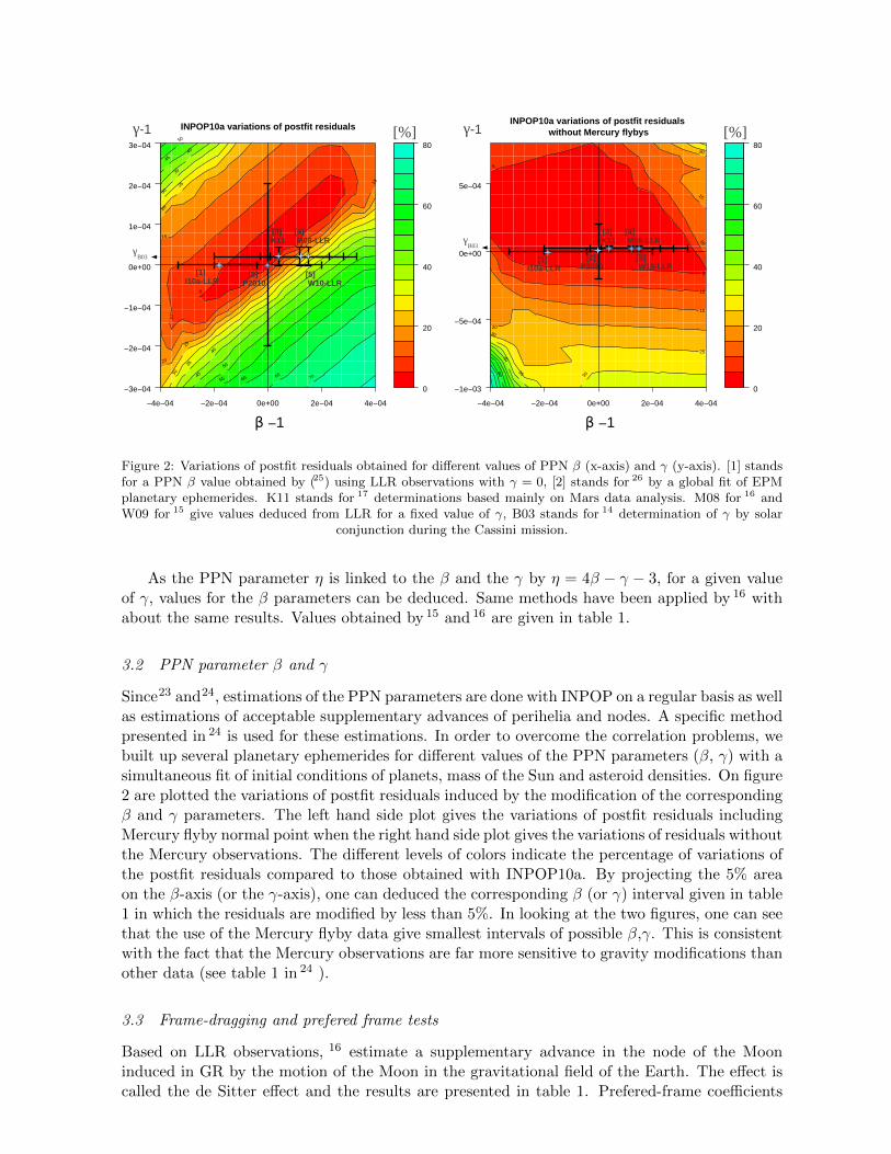
0
20
40
60
80
−4e 04− −2e 04− 0e+00 2e 04− 4e 04−
−3e 04−
−2e 04−
−1e 04−
0e+00
1e 04−
2e 04−
3e 04−
5
10
15
15
20
20
25
25
30
30
35
35
40
40
45
45
50
50
55
60 65
70
INPOP10a variations of postfit residualsγ-1
β 1−
[%]
[1] I10a-LLR
γB03
[2] P2010
[3] K11
[4] M08-LLR
[5] W10-LLR
[3] K11
0
20
40
60
80
−4e 04− −2e 04− 0e+00 2e 04− 4e 04−
−1e 03−
−5e 04−
0e+00
5e 04−
5
5
10
10
15
15
20
20
25
30
30
35
40
60
INPOP10a variations of postfit residuals without Mercury flybysγ-1
β 1−
[%]
[1] I10a-LLR
[3] K11
[5] W10-LLR
[4] M08-LLRγ
B03
[2] P2010
Figure 2: Variations of postfit residuals obtained for different values of PPN β (x-axis) and γ (y-axis). [1] standsfor a PPN β value obtained by (25) using LLR observations with γ = 0, [2] stands for 26 by a global fit of EPMplanetary ephemerides. K11 stands for 17 determinations based mainly on Mars data analysis. M08 for 16 andW09 for 15 give values deduced from LLR for a fixed value of γ, B03 stands for 14 determination of γ by solar
conjunction during the Cassini mission.
As the PPN parameter η is linked to the β and the γ by η = 4β − γ − 3, for a given valueof γ, values for the β parameters can be deduced. Same methods have been applied by 16 withabout the same results. Values obtained by 15 and 16 are given in table 1.
3.2 PPN parameter β and γ
Since23 and24, estimations of the PPN parameters are done with INPOP on a regular basis as wellas estimations of acceptable supplementary advances of perihelia and nodes. A specific methodpresented in 24 is used for these estimations. In order to overcome the correlation problems, webuilt up several planetary ephemerides for different values of the PPN parameters (β, γ) with asimultaneous fit of initial conditions of planets, mass of the Sun and asteroid densities. On figure2 are plotted the variations of postfit residuals induced by the modification of the correspondingβ and γ parameters. The left hand side plot gives the variations of postfit residuals includingMercury flyby normal point when the right hand side plot gives the variations of residuals withoutthe Mercury observations. The different levels of colors indicate the percentage of variations ofthe postfit residuals compared to those obtained with INPOP10a. By projecting the 5% areaon the β-axis (or the γ-axis), one can deduced the corresponding β (or γ) interval given in table1 in which the residuals are modified by less than 5%. In looking at the two figures, one can seethat the use of the Mercury flyby data give smallest intervals of possible β,γ. This is consistentwith the fact that the Mercury observations are far more sensitive to gravity modifications thanother data (see table 1 in 24 ).
3.3 Frame-dragging and prefered frame tests
Based on LLR observations, 16 estimate a supplementary advance in the node of the Mooninduced in GR by the motion of the Moon in the gravitational field of the Earth. The effect iscalled the de Sitter effect and the results are presented in table 1. Prefered-frame coefficients
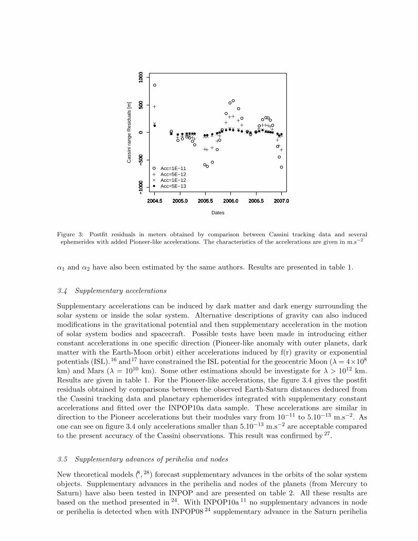
2004.5 2005.0 2005.5 2006.0 2006.5 2007.0
−10
00−
500
050
010
00
Dates
Cas
sini
ran
ge R
esid
uals
[m]
2004.5 2005.0 2005.5 2006.0 2006.5 2007.0
−10
00−
500
050
010
00
2004.5 2005.0 2005.5 2006.0 2006.5 2007.0
−10
00−
500
050
010
00
2004.5 2005.0 2005.5 2006.0 2006.5 2007.0
−10
00−
500
050
010
00
Acc=1E−11Acc=5E−12Acc=1E−12Acc=5E−13
Figure 3: Postfit residuals in meters obtained by comparison between Cassini tracking data and severalephemerides with added Pioneer-like accelerations. The characteristics of the accelerations are given in m.s−2
α1 and α2 have also been estimated by the same authors. Results are presented in table 1.
3.4 Supplementary accelerations
Supplementary accelerations can be induced by dark matter and dark energy surrounding thesolar system or inside the solar system. Alternative descriptions of gravity can also inducedmodifications in the gravitational potential and then supplementary acceleration in the motionof solar system bodies and spacecraft. Possible tests have been made in introducing eitherconstant accelerations in one specific direction (Pioneer-like anomaly with outer planets, darkmatter with the Earth-Moon orbit) either accelerations induced by f(r) gravity or exponentialpotentials (ISL).16 and17 have constrained the ISL potential for the geocentric Moon (λ = 4×10⁸
km) and Mars (λ = 1010 km). Some other estimations should be investigate for λ > 1012 km.Results are given in table 1. For the Pioneer-like accelerations, the figure 3.4 gives the postfitresiduals obtained by comparisons between the observed Earth-Saturn distances deduced fromthe Cassini tracking data and planetary ephemerides integrated with supplementary constantaccelerations and fitted over the INPOP10a data sample. These accelerations are similar indirection to the Pioneer accelerations but their modules vary from 10−11 to 5.10−13 m.s−2. Asone can see on figure 3.4 only accelerations smaller than 5.10−13 m.s−2 are acceptable comparedto the present accuracy of the Cassini observations. This result was confirmed by 27.
3.5 Supplementary advances of perihelia and nodes
New theoretical models (8, 28) forecast supplementary advances in the orbits of the solar systemobjects. Supplementary advances in the perihelia and nodes of the planets (from Mercury toSaturn) have also been tested in INPOP and are presented on table 2. All these results arebased on the method presented in 24. With INPOP10a 11 no supplementary advances in nodeor perihelia is detected when with INPOP08 24 supplementary advance in the Saturn perihelia
Table 2: Values of parameters obtained in the fit of INPOP08 24 and INPOP10a 11 to observations. The supple-mentary advances of perihelia and nodes are estimated in INPOP10a and INPOP08 as the interval in which the
differences of postfit residuals from INPOP10a are below 5%. P09 stands for (26) and P10 for (18).
INPOP08 INPOP10a P09 P10
$sup
mas.cy−1
Mercury -10 ± 30 0.4 ± 0.6 -3.6 ± 5 -4 ± 5Venus -4 ± 6 0.2 ± 1.5 -0.4 ± 0.5EMB 0.0 ± 0.2 -0.2 ± 0.9 -0.2 ± 0.4Mars 0.4 ± 0.6 -0.04 ± 0.15 0.1 ± 0.5Jupiter 142 ± 156 -41 ± 42Saturn -10 ± 8 0.15± 0.65 -6 ± 2 -10 ± 15
Ωsup
mas.cy−1
Mercury 1.4 ± 1.8Venus 200 ± 100 0.2 ± 1.5EMB 0.0 ± 10.0 0.0 ± 0.9Mars 0.0 ± 2 -0.05 ± 0.13Jupiter -200 ± 100 -40 ± 42Saturn -200 ± 100 -0.1 ± 0.4
was possible. Such variations can be explained by the improvement of INPOP10a outer planetorbits compared to INPOP08.
4 Conclusions
With the present gravity tests done in the solar system, GR is confirmed at the 10−4 accuracy forPPN parameter β and the equivalence principal and at 10−5 for PPN γ. No supplementary ad-vances of perihelia and nodes are detected at the present accuracy of the planetary ephemerides.Variations of the gravitational constant are not expected above 10−13 yr−1 and stringent limitsfor the ISL tests are given for the inner solar system. Messenger tracking data would bringimportant informations for PPN parameter determinations and ISL tests should be done in theouter solar system.
5 REFERENCES
1. J.-M. Alimi and A. Fuzfa. The Abnormally Weighting Energy Hypothesis: The origin of thecosmic acceleration. In J.-M. Alimi & A. Fuozfa, editor, American Institute of Physics ConferenceSeries, volume 1241 of American Institute of Physics Conference Series, pages 690–699, June 2010.
2. T. Damour. Testing the equivalence principle: why and how? Classical and Quantum Gravity,13:A33–A41, November 1996.
3. S. Kalyana Rama. Some cosmological consequences of non-trivial ppn parameters beta and gamma.Phys. Rev., 373(B):282–288, Apr 1996.
4. P. J. Steinhardt and D. Wesley. Dark energy, inflation, and extra dimensions. , 79(10):104026–+,May 2009.
5. J.-P. Uzan. Tests of Gravity on Astrophysical Scales and Variation of the Constants. AnnalesHenri Poincare, 4:347–369, December 2003.
6. H. Arakida. Influence of dark matter on light propagation in solar system. Advances in SpaceResearch, 45:1007–1014, April 2010.
7. K. L. Nordtvedt. Cosmic acceleration of Earth and the Moon by dark matter. , 437:529–531,December 1994.
8. L. Blanchet and J. Novak. External field effect of modified Newtonian dynamics in the Solarsystem. , 412:2530–2542, April 2011.
9. A. de Felice and S. Tsujikawa. f(R) Theories. Living Reviews in Relativity, 13:3–+, June 2010.10. S. G. Turyshev and V. T. Toth. The Pioneer Anomaly. Living Reviews in Relativity, 13:4–+,
September 2010.11. A. Fienga, J. Laskar, H. Manche, P. Kuchynka, G. Desvignes, . Gastineau, M, and andThereau G.
Cognard, I. The planetary ephemerides inpop10a and its applications in fundamental physics.Celestial Mechanics and Dynamical Astronomy, 2011.
12. J Muller. LLR by Hannover team. In ISSI meeting, 2010.13. T Murphy. APOLLO news. In MIT LLR workshop, 2010.14. B. Bertotti, L. Iess, and P. Tortora. A test of general relativity using radio links with the Cassini
spacecraft. , 425:374–376, September 2003.15. J.G. Williams, S.G. Turychev, and D.H. Boggs. LLR tests of the equivalence principle with the
Earth and Moon. ArXiv e-prints, January 2009.16. J. Muller, M. Soffel, and S. A. Klioner. Geodesy and relativity. Journal of Geodesy, 82:133–145,
March 2008.17. A. S. Konopliv, S. W. Asmar, W. M. Folkner, O. Karatekin, D. C. Nunes, S. E. Smrekar, C. F.
Yoder, and M. T. Zuber. Mars high resolution gravity fields from MRO, Mars seasonal gravity,and other dynamical parameters. , 211:401–428, January 2011.
18. E. V. Pitjeva. EPM Ephemerides. In Journees Systemes de Reference Spatio-temporels 2010,Journees Systemes de references, November 2010.
19. T. W. Murphy, E. G. Adelberger, J. B. R. Battat, L. N. Carey, C. D. Hoyle, P. Leblanc, E. L.Michelsen, K. Nordtvedt, A. E. Orin, J. D. Strasburg, C. W. Stubbs, H. E. Swanson, andE. Williams. The Apache Point Observatory Lunar Laser-ranging Operation: Instrument De-scription and First Detections. , 120:20–37, January 2008.
20. S. M. Merkowitz. Tests of Gravity Using Lunar Laser Ranging. Living Reviews in Relativity,13:7–+, November 2010.
21. K. Nordtvedt. Testing Relativity with Laser Ranging to the Moon. Physical Review, 170:1186–1187, June 1968.
22. E. G. Adelberger. New tests of Einstein’s equivalence principle and Newton’s inverse-square law.Classical and Quantum Gravity, 18:2397–2405, July 2001.
23. A. Fienga, and Laskar J. Manche, H., and M. Gastineau. Inpop06: a new numerical planetaryephemeris. , 477:315–327, 2008.
24. A. Fienga, J. Laskar, P. Kuchynka, C. Le Poncin-Lafitte, H. Manche, and M. Gastineau. Grav-ity tests with INPOP planetary ephemerides. American Astronomical Society, IAU Symposium#261. Relativity in Fundamental Astronomy: Dynamics, Reference Frames, and Data Analysis27 April - 1 May 2009 Virginia Beach, VA, USA, #6.02; Bulletin of the American AstronomicalSociety, Vol. 41, p.881, 261:602–+, May 2010.
25. H. Manche, A. Fienga, J. Laskar, M. Gastineau, S. Bouquillon, G. Francou, and P. Kuchynka. LLRresiduals of the latest INPOP solution and constraints on post-Newtonian parameters. In JourneesSystemes de Reference Spatio-temporels 2010, Journees Systemes de references, November 2010.
26. E. V. Pitjeva. EPM Ephemerides and Relativity. American Astronomical Society, IAU Symposium#261. Relativity in Fundamental Astronomy: Dynamics, Reference Frames, and Data Analysis 27April - 1 May 2009 Virginia Beach, VA, USA, #6.03; Bulletin of the American AstronomicalSociety, Vol. 41, p.881, 261:603–+, May 2009.
27. W. M. Folkner. Relativistic aspects of the JPL planetary ephemeris. In S. A. Klioner, P. K. Sei-delmann, & M. H. Soffel, editor, IAU Symposium, volume 261 of IAU Symposium, pages 155–158,January 2010.
28. J.-M. Frere, F.-S. Ling, and G. Vertongen. Bound on the dark matter density in the Solar Systemfrom planetary motions. , 77(8):083005–+, April 2008.
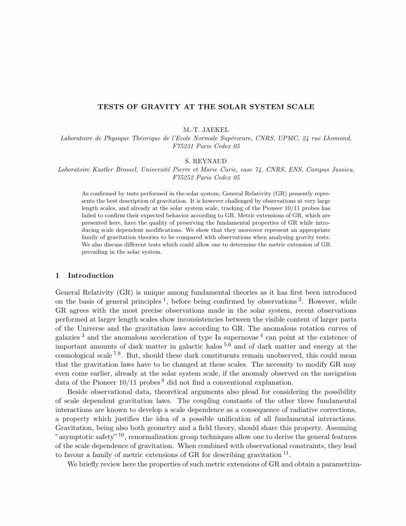
TESTS OF GRAVITY AT THE SOLAR SYSTEM SCALE
M.-T. JAEKEL
Laboratoire de Physique Theorique de l’Ecole Normale Superieure, CNRS, UPMC, 24 rue Lhomond,
F75231 Paris Cedex 05
S. REYNAUD
Laboratoire Kastler Brossel, Universite Pierre et Marie Curie, case 74, CNRS, ENS, Campus Jussieu,
F75252 Paris Cedex 05
As confirmed by tests performed in the solar system, General Relativity (GR) presently repre-sents the best description of gravitation. It is however challenged by observations at very largelength scales, and already at the solar system scale, tracking of the Pioneer 10/11 probes hasfailed to confirm their expected behavior according to GR. Metric extensions of GR, which arepresented here, have the quality of preserving the fundamental properties of GR while intro-ducing scale dependent modifications. We show that they moreover represent an appropriatefamily of gravitation theories to be compared with observations when analysing gravity tests.We also discuss different tests which could allow one to determine the metric extension of GRprevailing in the solar system.
1 Introduction
General Relativity (GR) is unique among fundamental theories as it has first been introducedon the basis of general principles 1, before being confirmed by observations 2. However, whileGR agrees with the most precise observations made in the solar system, recent observationsperformed at larger length scales show inconsistencies between the visible content of larger partsof the Universe and the gravitation laws according to GR. The anomalous rotation curves ofgalaxies 3 and the anomalous acceleration of type Ia supernovae 4 can point at the existence ofimportant amounts of dark matter in galactic halos 5,6 and of dark matter and energy at thecosmological scale 7,8. But, should these dark constituents remain unobserved, this could meanthat the gravitation laws have to be changed at these scales. The necessity to modify GR mayeven come earlier, already at the solar system scale, if the anomaly observed on the navigationdata of the Pioneer 10/11 probes 9 did not find a conventional explanation.
Beside observational data, theoretical arguments also plead for considering the possibilityof scale dependent gravitation laws. The coupling constants of the other three fundamentalinteractions are known to develop a scale dependence as a consequence of radiative corrections,a property which justifies the idea of a possible unification of all fundamental interactions.Gravitation, being also both geometry and a field theory, should share this property. Assuming”asymptotic safety”10, renormalization group techniques allow one to derive the general featuresof the scale dependence of gravitation. When combined with observational constraints, they leadto favour a family of metric extensions of GR for describing gravitation 11.
We briefly review here the properties of such metric extensions of GR and obtain a parametriza-
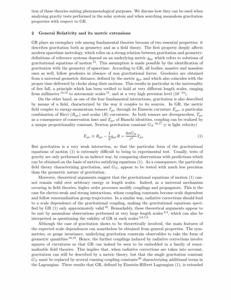
tion of these theories suiting phenomenological purposes. We discuss how they can be used whenanalysing gravity tests performed in the solar system and when searching anomalous gravitationproperties with respect to GR.
2 General Relativity and its metric extensions
GR plays an exemplary role among fundamental theories because of two essential properties: itdescribes gravitation both as geometry and as a field theory. The first property deeply affectsmodern spacetime metrology, which relies on a strong relation between gravitation and geometry:definitions of reference systems depend on an underlying metric gµν which refers to solutions ofgravitational equations of motion 12. This assumption is made possible by the identification ofgravitation with the geometry of spacetime. According to GR, all bodies, massive and masslessones as well, follow geodesics in absence of non gravitational forces. Geodesics are obtainedfrom a universal geometric distance, defined by the metric gµν and which also coincides with theproper time delivered by clocks along their motions. This results in particular in the universalityof free fall, a principle which has been verified to hold at very different length scales, rangingfrom millimeter 13,14 to astronomic scales 15, and at a very high precision level (10−13).
On the other hand, as one of the four fundamental interactions, gravitation is also describedby means of a field, characterized by the way it couples to its sources. In GR, the metricfield couples to energy-momentum tensors Tµν through its Einstein curvature Eµν , a particularcombination of Ricci (Rµν) and scalar (R) curvatures. As both tensors are divergenceless, Tµν
as a consequence of conservation laws and Eµν of Bianchi identities, coupling can be realized bya unique proportionality constant, Newton gravitation constant GN
16,17 (c is light velocity)
Eµν ≡ Rµν −
1
2gµνR =
8πGN
c4Tµν (1)
But gravitation is a very weak interaction, so that the particular form of the gravitationalequations of motion (1) is extremely difficult to bring to experimental test. Usually, tests ofgravity are only performed in an indirect way, by comparing observations with predictions whichcan be obtained on the basis of metrics satisfying equations (1). As a consequence, the particularfield theory characterizing gravitation, and GN , appear to be tested with much less precisionthan the geometric nature of gravitation.
Moreover, theoretical arguments suggest that the gravitational equations of motion (1) can-not remain valid over arbitrary energy or length scales. Indeed, as a universal mechanismoccuring in field theories, higher order processes modify couplings and propagators. This is thecase for electro-weak and strong interactions, whose coupling constants become scale dependentand follow renormalization group trajectories. In a similar way, radiative corrections should leadto a scale dependence of the gravitational coupling, making the gravitational equations speci-fied by GR (1) only approximately valid 10. Remarkably, these theoretical arguments appear tobe met by anomalous observations performed at very large length scales 3,4, which can also beinterpreted as questioning the validity of GR at such scales 5,6,7,8.
Although the case of gravitation shows to be theoretically involved, the main features ofthe expected scale dependences can nonetheless be obtained from general properties. The sym-metries, or gauge invariance, underlying gravitation constrain observables to take the form ofgeometric quantities 18,19. Hence, the further couplings induced by radiative corrections involvesquares of curvatures so that GR can indeed be seen to be embedded in a family of renor-malizable field theories. This implies that, when radiative corrections are taken into account,gravitation can still be described by a metric theory, but that the single gravitation constantGN must be replaced by several running coupling constants 20 characterizing additional terms inthe Lagrangian. There results that GR, defined by Einstein-Hilbert Lagrangian (1), is extended
to a theory which is both non local, as a result of radiative corrections, and non linear, due totheir geometric nature. It leads to gravitational equations of motion which can be put under ageneral form, with a susceptibility replacing Newton gravitation constant 21
Eµν = χµν(T ) =8πGN
c4Tµν + δχµν(T ) (2)
The resulting equations appear to be difficult to solve due to a particular mixing realized betweennon linearity and non locality.
As another general property, radiative corrections can be seen to essentially differ in twosectors corresponding to couplings to massless or massive fields 20,21: in the former case, trace-less energy-momentum tensors couple to Weyl curvature only, while in the latter case couplingsbetween energy-momentum traces and the scalar curvature also occur. GR should then be ex-tended to metric theories which are characterized by two sectors, of different conformal weights,with corresponding running coupling constants G
(0) and G(1) which generalize Newton gravita-
tion constant GN . The relations between coupling constants can be given simple expressionsin a linearized approximation (using a representation of fields in terms of momentum k andintroducing the corresponding projectors π on trace and traceless parts)22,23
Eµν = E(0)
µν + E(1)
µν , πµν ≡ ηµν −
kµkν
k2
E(0)
µν = π0
µπ0
ν −
πµνπ00
3
8πG(0)
c4T00, E
(1)
µν =πµνπ
00
3
8πG(1)
c4T00
G(0) = GN + δG
(0), G
(1) = GN + δG(1) (3)
Although the two running coupling constants remain close to GN , non locality and non linearitycombine in an intricate way and do not allow a decomposition as simple as (3) to hold beyondthe linearized approximation. Alternatively, one can look for non linear but local theories whichapproximate the previous metric extensions of GR. It is remarkable that, due to the presenceof two sectors, such approximations can be obtained which involve higher order field derivativesand nonetheless correspond to theories with stable ground states 24.
To the theoretical difficulties implied by non locality combined with non linearity, somecompensation can be found in direct observations. Indeed, the latter show that gravitationshould remain very close to GR over a large range of scales. They moreover show that departuresfrom GR can happen not only at large energy scales, as expected if gravitation should unify withother fundamental interactions, but also at large length scales 3,4. Gravitation tests performedup to now make it legitimate to consider the effective gravitation theory at ordinary macroscopiclength scales to be a perturbation of GR 2. Solutions of the generalized equations (2) shouldthen correspond to perturbations of the solutions of GR equations of motion (1). Equivalently,equations (2) may be seen as providing metrics which remain close to those determined by GRand just differ from the latter by curvature anomalies 25
E = [E]GR
+ δE, [E]GR
= 0 where T ≡ 0
δE = δE(0) + δE
(1) (4)
Metric extensions of GR are thus characterized by two independent components of Einsteincurvature tensor δE
(0) and δE(1), reflecting the two different running coupling constants G
(0)
and G(1) modifying GN (as seen in the linear approximation (3)). When solving the gravitation
equations of motion (2), the two independent Einstein curvature components are replaced by twogauge-invariant potentials ΦN and ΦP (for a point-like source, using Schwarzschild coordinates)
δE0
0 ≡ 2u4(ΦN − δΦP )′′, δErr ≡ 2u3Φ′
P u ≡
1
r, ()′ ≡ ∂u (5)
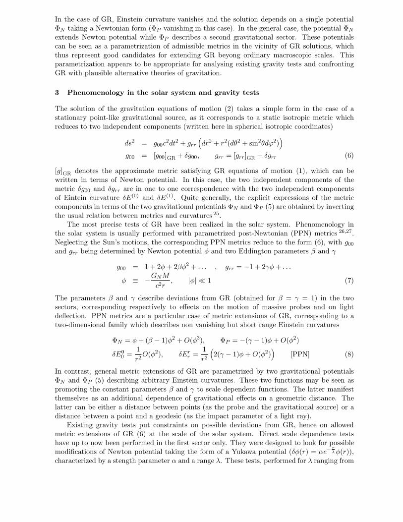
In the case of GR, Einstein curvature vanishes and the solution depends on a single potentialΦN taking a Newtonian form (ΦP vanishing in this case). In the general case, the potential ΦN
extends Newton potential while ΦP describes a second gravitational sector. These potentialscan be seen as a parametrization of admissible metrics in the vicinity of GR solutions, whichthus represent good candidates for extending GR beyong ordinary macroscopic scales. Thisparametrization appears to be appropriate for analysing existing gravity tests and confrontingGR with plausible alternative theories of gravitation.
3 Phenomenology in the solar system and gravity tests
The solution of the gravitation equations of motion (2) takes a simple form in the case of astationary point-like gravitational source, as it corresponds to a static isotropic metric whichreduces to two independent components (written here in spherical isotropic coordinates)
ds2 = g00c
2dt
2 + grr
(
dr2 + r
2(dθ2 + sin2
θdϕ2)
)
g00 = [g00]GR+ δg00, grr = [grr]GR
+ δgrr (6)
[g]GR
denotes the approximate metric satisfying GR equations of motion (1), which can bewritten in terms of Newton potential. In this case, the two independent components of themetric δg00 and δgrr are in one to one correspondence with the two independent componentsof Eintein curvature δE
(0) and δE(1). Quite generally, the explicit expressions of the metric
components in terms of the two gravitational potentials ΦN and ΦP (5) are obtained by invertingthe usual relation between metrics and curvatures 25.
The most precise tests of GR have been realized in the solar system. Phenomenology inthe solar system is usually performed with parametrized post-Newtonian (PPN) metrics 26,27.Neglecting the Sun’s motions, the corresponding PPN metrics reduce to the form (6), with g00
and grr being determined by Newton potential φ and two Eddington parameters β and γ
g00 = 1 + 2φ + 2βφ2 + . . . , grr = −1 + 2γφ + . . .
φ ≡ −
GNM
c2r
, |φ| ≪ 1 (7)
The parameters β and γ describe deviations from GR (obtained for β = γ = 1) in the twosectors, corresponding respectively to effects on the motion of massive probes and on lightdeflection. PPN metrics are a particular case of metric extensions of GR, corresponding to atwo-dimensional family which describes non vanishing but short range Einstein curvatures
ΦN = φ + (β − 1)φ2 + O(φ3), ΦP = −(γ − 1)φ + O(φ2)
δE0
0 =1
r2O(φ2), δE
rr =
1
r2
(
2(γ − 1)φ + O(φ2))
[PPN] (8)
In contrast, general metric extensions of GR are parametrized by two gravitational potentialsΦN and ΦP (5) describing arbitrary Einstein curvatures. These two functions may be seen aspromoting the constant parameters β and γ to scale dependent functions. The latter manifestthemselves as an additional dependence of gravitational effects on a geometric distance. Thelatter can be either a distance between points (as the probe and the gravitational source) or adistance between a point and a geodesic (as the impact parameter of a light ray).
Existing gravity tests put constraints on possible deviations from GR, hence on allowedmetric extensions of GR (6) at the scale of the solar system. Direct scale dependence testshave up to now been performed in the first sector only. They were designed to look for possiblemodifications of Newton potential taking the form of a Yukawa potential (δφ(r) = αe
−r
λ φ(r)),characterized by a stength parameter α and a range λ. These tests, performed for λ ranging from
the submillimeter range, using dedicated experiments28,29, to the range of planetary orbits, usingprobe navigation data and planetray ephemerides28,30, show that the strength α of a Yukawa-likeperturbation must remain rather small at all these scales, so that the form of the gravitationalpotential in the first sector is rather strongly constrained to remain Newtonian. However,constraints become much less stringent below the submillimeter range, where Casimir forcesbecome important 29, and at scales of the order of the outer solar system, where observationsused to determine ephemerides become less precise. They moreover only concern the first sector.
The increasing set of observations performed in the solar system has progressively reducedthe allowed deviations from GR for the two PPN parameters β and γ. Presently, the bestconstraint on the value of γ is given by the measurement of the Shapiro time delay, inducedby the gravitational field of the Sun on the radio link which was used to follow the Cassiniprobe during its travel to Saturn 31. GR prediction for the variation of the deflection angle, nearoccultation by the Sun, has been confirmed, constraining γ to be close to 1 with a precision of2.5 × 10−5. A similar bound is provided by VLBI measurements of light deflection 2. One mayremark that such a precision is obtained when assuming that the parameter γ remains constant.As the deflection angle decreases with the impact parameter of the ray, the precision on themeasurement of the deflection angle is mainly due to small impact parameters. As a result, thecorresponding constraints should be sensitively less stringent when confronted to general metricextensions of GR, which allow γ to depend on the impact parameter of the ray.
The value of γ being assumed, the parameter β can be obained either by means of a directmeasurement, such as Lunar Laser Ranging15, measuring the Sun polarization effect on the Moonorbit around the Earth, or by means of big fits, using all data made available by probe navigationand astrometry measurements, to determine planet ephemerides 32,33,34. Both methods lead tosimilar constraints on β, fixing the latter to remain close to 1, up to deviations less than 10−4.Let us remark that these determinations are performed at the scale of the Moon orbit in one case,and at a scale of several astronomic units (AU) in the other case. They can also be consideredas independent estimations of β being performed at different length scales.
Available data for gravitation at large length scales in the solar system are rather few.Hence, the navigation data of the Pioneer 10/11 probes, during their travel in the outer partof the solar system, provide an important consistency check for models of gravitation in thesolar system. Remarkably, the analysis of Doppler data has failed to confirm the predictionsmade according to GR. Comparison of observed with predicted values resulted in residualswhich did not vanish but could be interpreted as exhibiting the presence of an anomalousacceleration aP = (0.87±0.13) nm s−2, directed towards the Sun or the Earth, and approximatelyconstant over distances ranging from 20AU to 70AU 9. Many attempts have been made to finda conventional explanation to the Pioneer anomaly as a systematic effect either related to theprobe itself, allowed by a loss of energy from power generators on board, or to the environmentof the probe, due to the presence of dust or gravitating matter in the outer solar system 35.These have been followed by sustained efforts for recovering further data and performing newanalyses covering the whole Pioner 10/11 missions 36. Up to now, these attempts have remainedunsuccessful in explaining the totality of the Pioneer anomaly.
Furthermore, a recent study, confirming the secular part of the Pioneer anomaly, has alsoanalysed the modulations apparent in the Doppler data, showing that their frequencies cor-respond to the Earth’s motions, and that the Doppler residuals can be further reduced byintroducing simple modulations of the radio links 37. Modulated anomalies cannot be producedby a conventional explanation of the secular part but require a further mechanism (trajectorymismodeling, solar plasma effects, ...) to be accounted for. On the other hand, simple modelsmodifying the metric are able to reproduce both types of anomalies. These features leave thepossibility of a common gravitational origin of the Pioneer anomalies, pointing at a deficiencyof GR occuring at length scales of the order of the solar system size.
4 Tests of metric extensions of GR
Besides being favoured by theoretical arguments, metric extensions of GR also provide an appro-priate tool for analysing gravity tests performed in the solar system. Most precise tests realizedat or beyond the AU scale strongly rely on Doppler ranging, hence on an appropriate modelingof electromagnetic links and the trajectories of massive bodies. Metric extensions of GR providea general and simple expression for the time delay function T (x1,x2) which describes the linksused to follow a massive probe (xa ≡ ra(sin θa cos ϕa, sin θa sin ϕa, cos θa) with a = 2, 1 respec-tively denoting the coordinates of the probe and a station on Earth, T (x1,x2) is written herefor a static istropic metric (6)) 38
cT (r1, r2, φ) ≡
∫ r2
r1
−grr
g00(r)dr
√
−grr
g00(r) − ρ2
r2
, φ =
∫ r2
r1
ρdr/r2
√
−grr
g00(r) − ρ2
r2
cos φ ≡ cos θ1 cos θ2 + sin θ1 sin θ2 cos (ϕ2 − ϕ1) (9)
φ is the relative angle, when seen from the gravitational source, of the two points x1 and x2 andρ the impact parameter of the light ray joining these points. The two-point function T (x1,x2)describes the time taken by a light-like signal to propagate from position x1 to position x2 (thusgiving a parametrization of lightcones). The time delay function can be seen to be parametrizedby metric components (9), hence by the two gravitation potentials (ΦN ,ΦP ). Doppler signals areobtained by taking the time derivative of T (x1,x2), and evaluating the latter on the trajectoriesof the probe and the Earth station. As geodesics must be determined according to the samemetric extension of GR, the two potentials also enter the expressions of the trajectories 25.
Comparison between metric extensions and GR predictions can be performed explicitly andanalysing the former within the framework of GR leads to deviations which take the form ofPioneer-like anomalies (δa = δasec + δaann denotes the time derivative of Doppler signals 9)
δasec ≃ −
c2
2∂r(δg00) + [r2]GR
δ(g00grr)
2− δg00
−
c2
2∂
2
r [g00]GRδr2
δaann ≃
d
dt
[
dφ
dt
]
GR
δρ
(10)
The gravitational potentials in the two sectors contribute to both the secular part δasec andthe modulated part δaann of the anomaly. These furthermore depend on the probe and Earthmotions, which are obtained from the equations for geodesics and initial conditions. Hence,Pioneer-like anomalies appear as a prediction of metric extensions of GR. These moreover pre-dict strong correlations between secular and modulated anomalies, which can be considered assignatures to be looked for in observations 23,38.
Besides directly, through a precise analysis of probe navigation data, the two gravitationalpotentials may also be expected to be determined as part of a big fit of all navigation andastrometric data, such as those used to obtain the ephemerides of planets and some of theircharacteristic constants. In such an approach, the two potentials play the same role as Eddingtonparameters β and γ
32,33,34, with the additional feature of allowing significant dependences onlength scales of the order of the solar system size 25. The results of Doppler and rangingobservations should then be taken into account by using the time delay function (9) and thegeodesics, depending on the two gravitational potentials (ΦN ,ΦP ) which define a general metricextension of GR. Clearly, the need to recall to numerical methods entails that the neighborhooddefined by the two potentials, in their general form, is too large to be totally scanned by a fit.Hence, it appears crucial to design simplified models which depend on a small number of realparameters but still preserve the scale dependences which are most likely to be observed 39.
Metric extensions of GR also predict effects which can be expected to be exhibited by futureexperiments benefiting from a high increase in precision measurement. The time delay function(9) results in a particular scale dependence of the gravitational deflection of light which canbe equivalently represented as an additional dependence of the deflection angle ω, or else ofEddington parameter γ, on the impact parameter of the light ray (M denotes the mass of thegravitational source, r its distance to the observer, χ the apparent relative angle between thelight source and the gravitational source) 23
ω(χ) ≃GNM
c2r
1 + γ(χ)
tanχ2
The two gravitational potentials characterizing metric extensions combine to induce a modifi-cation of the deflection angle which, in contrast to GR, contains a part which increases withthe impact parameter. Such deviations should then become more noticeable for measurementsperformed with a high precision and at small deflection angles. In a near future, GAIA willperform a survey of our neighborhood in our galaxy and will follow with a very good accuracyan extremely large number of astrometric objects40,6. This will include in particular a very largenumber of light deflection observations performed at small deflection angles, or at large angulardistances from the Sun
δω < 40µas, ω ∼ 4mas, χ ∈ [45, 135]
As a consequence, GAIA data will improve the accuracy for the observed mean value of γ (betterthan 2 × 10⁻⁶) and will make it possibe to map the dependence of γ on χ over its whole rangeof variation. Such a mapping could put into evidence small deviations from GR and moreoverallow to determine and fit their particular dependence.
A definite answer to the question of modifying the gravitation theory at the solar systemscale would be provided by missions embarking dedicated means for directly measuring theeffects of gravity. A first example is OSS mission 41 which, beside ranging facilities, will alsopossess a high precision accelerometer, thus allowing to distinguish the effects of gravitationfrom other forces affecting the probe and hence to determine unambiguously whether the probefollows a geodesic, and whether the latter corresponds to GR. Another mission, SAGAS 42, aimsat reaching the outer part of the solar system with, beside an accelerometer, an atomic clock onboard. Using the combined information obtained, with a very high precision, from the opticallinks and the clock on board, one would be able to reconstruct the gravitational potentials inthe two sectors, and thus to exactly determine the gravitation theory prevailing at the largestscales which can be reached by artificial probes.
5 Conclusion
When generalized under the form of a metric extension, GR remains a successful theory ofgravitation within the whole solar system. Minimal modifications allow one to account for allgravity tests performed up to the solar system scale and to confirm the position of GR as thebasis of gravitation theory. They moreover correspond to scale dependences of the gravitationalcoupling, thus bringing gravitation closer to the other fundamental interactions.
From a phenomenological point of view, metric extensions of GR appear as a convenienttool for testing gravity within the solar system. They may also provide a natural answer to thepresence of anomalies when observations are analysed by confrontation with GR. The actualtheory of gravitation can be approached by looking for such anomalies occuring in residuals ofdirect ranging data or big fits. It may also be determined by future high precision observations(GAIA) or dedicated missions in the solar system (OSS, SAGAS).
References
1. A. Einstein, Annalen der Physik 49, 769 (1916).2. C.M. Will, Living Rev. Rel. 9, 3 (2005).3. S.S. McGaugh, Phys. Rev. Lett. 106, 121303 (2011).4. S. Perlmutter et al , Astrophys. J. 517, 565 (1999).5. G. Gentile et al., Mon. Not. R. Astron. Soc. 351, 903 (2004).6. see O. Bienayme in this volume.7. L.D. Ferramacho, A. Blanchard and Y. Zolnierowski, Preprint arXiv:0807.4608.8. see A. Blanchard in this volume.9. J.D. Anderson et al , Astrophys. J. 459, 365 (1996); Phys. Rev. Lett. 81, 2858 (1998);
Phys. Rev. D 65, 082004 (2002).10. S. Weinberg, ”Ultraviolet divergences in quantum theories of gravitation”, in S.W. Hawk-
ing and W. Israel eds., General Relativity, An Einstein Centenary Survey, (CambridgeU.P., Cambridge, U.K., 1979).
11. M.-T. Jaekel and S. Reynaud, Proc. Gravitational waves and experimental gravity
XLIIemes Rencontres de Moriond, J. Dumarchez, J. Tran Thanh Van eds., (The Gioi,Hanoi, 2007) 271.
12. M. Soffel et al., Astron. J. 126, 2687 (2003).13. E.G. Adelberger et al., Part. Nucl. Phys. 62, 102 (2009).14. see E.G. Adelberger in this volume.15. J.G. Williams, S.G. Turyshev and D.H. Boggs, Phys. Rev. Lett. 93, 261101 (2004).16. A. Einstein, Sitz. Preuss. Akad. Wiss. Berlin 844, (1915).17. D. Hilbert, Nach. Ges. Wiss. Gottingen 395, (1915).18. A.D. Sakharov, Doklady Akad. Nauk SSSR 177, 70 (1967) [Sov. Phys. Doklady 12, 1040].19. G. t’Hooft and M. Veltman, Ann. Inst. H. Poincare A 20, 69 (1974).20. E.S. Fradkin and A.A. Tseytlin, Nucl. Phys. B 201, 469 (1982).21. M.-T. Jaekel and S. Reynaud, Annalen der Physik 4, 68 (1995).22. M.-T. Jaekel and S. Reynaud, Mod. Phys. Lett. A 20, 1047 (2005).23. M.-T. Jaekel and S. Reynaud, Class. Quantum Grav. 22, 2135 (2005).24. J.P. Bruneton and G. Esposito-Farese, Phys. Rev. D 76, 124012 (2007).25. M.-T. Jaekel and S. Reynaud, Class. Quantum Grav. 23, 777 (2006).26. C.M. Will and K. Nordtvedt, Astrophys. J. 177, 757 (1972).27. K. Nordtvedt and C.M. Will, Astrophys. J. 177, 775 (1972).28. E. Fischbach and C. Talmadge, The Search for Non Newtonian Gravity (Springer Verlag,
Berlin, 1998); see E. Fischbach in this volume.29. see S. Reynaud in this volume.30. S. Reynaud and M.-T. Jaekel, Int. J. Mod. Phys. A 20, 2294 (2005).31. B. Bertotti, L. Iess and P. Tortora, Nature 425, 374 (2003).32. W.M. Folkner, Proc. IAU Symposium 261, 155 (2010).33. E.V. Pitjeva, Proc. IAU Symposium 261, 170 (2010).34. A. Fienga et al., Proc. IAU Symposium 261, 159 (2010); see A. Fienga in this volume.35. M.M. Nieto and J.D. Anderson, Contemp. Phys. 48, 41 (2007).36. S.G. Turyshev and Toth, Living Rev. Rel. 13, 4 (2010).37. A. Levy et al., Adv. Space Res. 43, 1538 (2009).38. M.-T. Jaekel and S. Reynaud, Class. Quantum Grav. 23, 7561 (2006).39. see A. Hees in this volume.40. M.A.C. Perryman et al., Astron. Astrophys. 369, 339 (2001).41. B. Christophe et al., Exp. Astron. 23, 529 (2009); see B. Christophe in this volume.42. P. Wolf et al., Exp. Astron. 23, 651 (2009).
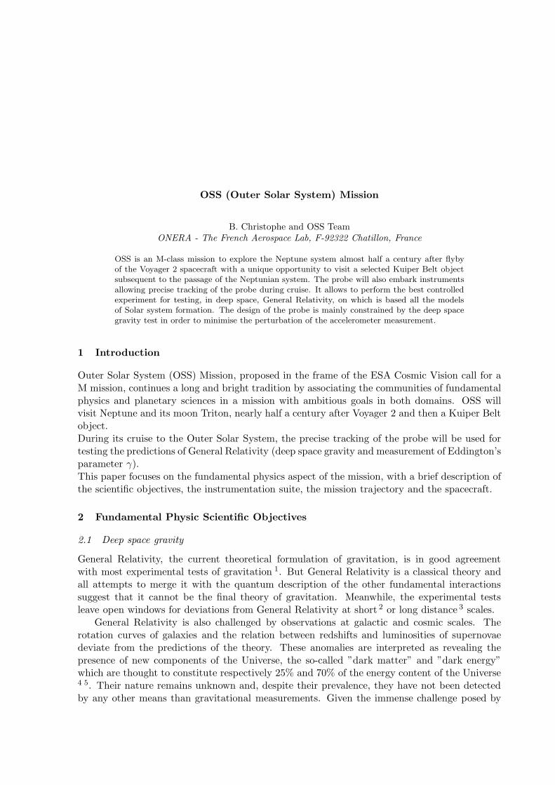
OSS (Outer Solar System) Mission
B. Christophe and OSS TeamONERA - The French Aerospace Lab, F-92322 Chatillon, France
OSS is an M-class mission to explore the Neptune system almost half a century after flybyof the Voyager 2 spacecraft with a unique opportunity to visit a selected Kuiper Belt objectsubsequent to the passage of the Neptunian system. The probe will also embark instrumentsallowing precise tracking of the probe during cruise. It allows to perform the best controlledexperiment for testing, in deep space, General Relativity, on which is based all the modelsof Solar system formation. The design of the probe is mainly constrained by the deep spacegravity test in order to minimise the perturbation of the accelerometer measurement.
1 Introduction
Outer Solar System (OSS) Mission, proposed in the frame of the ESA Cosmic Vision call for aM mission, continues a long and bright tradition by associating the communities of fundamentalphysics and planetary sciences in a mission with ambitious goals in both domains. OSS willvisit Neptune and its moon Triton, nearly half a century after Voyager 2 and then a Kuiper Beltobject.During its cruise to the Outer Solar System, the precise tracking of the probe will be used fortesting the predictions of General Relativity (deep space gravity and measurement of Eddington’sparameter γ).This paper focuses on the fundamental physics aspect of the mission, with a brief description ofthe scientific objectives, the instrumentation suite, the mission trajectory and the spacecraft.
2 Fundamental Physic Scientific Objectives
2.1 Deep space gravity
General Relativity, the current theoretical formulation of gravitation, is in good agreementwith most experimental tests of gravitation 1. But General Relativity is a classical theory andall attempts to merge it with the quantum description of the other fundamental interactionssuggest that it cannot be the final theory of gravitation. Meanwhile, the experimental testsleave open windows for deviations from General Relativity at short 2 or long distance 3 scales.
General Relativity is also challenged by observations at galactic and cosmic scales. Therotation curves of galaxies and the relation between redshifts and luminosities of supernovaedeviate from the predictions of the theory. These anomalies are interpreted as revealing thepresence of new components of the Universe, the so-called ”dark matter” and ”dark energy”which are thought to constitute respectively 25% and 70% of the energy content of the Universe4 5. Their nature remains unknown and, despite their prevalence, they have not been detectedby any other means than gravitational measurements. Given the immense challenge posed by
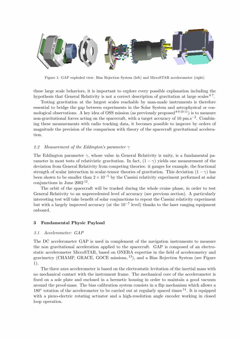
Figure 1: GAP exploded view: Bias Rejection System (left) and MicroSTAR accelerometer (right)
these large scale behaviors, it is important to explore every possible explanation including thehypothesis that General Relativity is not a correct description of gravitation at large scales 6 7.
Testing gravitation at the largest scales reachable by man-made instruments is thereforeessential to bridge the gap between experiments in the Solar System and astrophysical or cos-mological observations. A key idea of OSS mission (as previously proposed8 9 10 11) is to measurenon-gravitational forces acting on the spacecraft, with a target accuracy of 10 pm.s−2. Combin-ing these measurements with radio tracking data, it becomes possible to improve by orders ofmagnitude the precision of the comparison with theory of the spacecraft gravitational accelera-tion.
2.2 Measurement of the Eddington’s parameter γ
The Eddington parameter γ, whose value in General Relativity is unity, is a fundamental pa-rameter in most tests of relativistic gravitation. In fact, (1 − γ) yields one measurement of thedeviation from General Relativity from competing theories: it gauges for example, the fractionalstrength of scalar interaction in scalar-tensor theories of gravitation. This deviation (1− γ) hasbeen shown to be smaller than 2× 10⁻⁵ by the Cassini relativity experiment performed at solarconjunctions in June 2002 12.
The orbit of the spacecraft will be tracked during the whole cruise phase, in order to testGeneral Relativity to an unprecedented level of accuracy (see previous section). A particularlyinteresting test will take benefit of solar conjunctions to repeat the Cassini relativity experimentbut with a largely improved accuracy (at the 10−7 level) thanks to the laser ranging equipmentonboard.
3 Fundamental Physic Payload
3.1 Accelerometer: GAP
The DC accelerometer GAP is used in complement of the navigation instruments to measurethe non gravitational acceleration applied to the spacecraft. GAP is composed of an electro-static accelerometer MicroSTAR, based on ONERA expertise in the field of accelerometry andgravimetry (CHAMP, GRACE, GOCE missions, 13), and a Bias Rejection System (see Figure1).
The three axes accelerometer is based on the electrostatic levitation of the inertial mass withno mechanical contact with the instrument frame. The mechanical core of the accelerometer isfixed on a sole plate and enclosed in a hermetic housing in order to maintain a good vacuumaround the proof-mass. The bias calibration system consists in a flip mechanism which allows a180 rotation of the accelerometer to be carried out at regularly spaced times 14. It is equippedwith a piezo-electric rotating actuator and a high-resolution angle encoder working in closedloop operation.
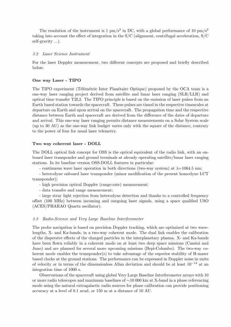
The resolution of the instrument is 1 pm/s2 in DC, with a global performance of 10 pm/s2
taking into account the effect of integration in the S/C (alignment, centrifugal acceleration, S/Cself-gravity ...).
3.2 Laser Science Instrument
For the laser Doppler measurement, two different concepts are proposed and briefly describedbelow.
One way Laser - TIPO
The TIPO experiment (Telemetrie Inter Planetaire Optique) proposed by the OCA team is aone-way laser ranging project derived from satellite and lunar laser ranging (SLR/LLR) andoptical time transfer T2L2. The TIPO principle is based on the emission of laser pulses from anEarth based station towards the spacecraft. These pulses are timed in the respective timescales atdeparture on Earth and upon arrival on the spacecraft. The propagation time and the respectivedistance between Earth and spacecraft are derived from the difference of the dates of departureand arrival. This one-way laser ranging permits distance measurements on a Solar System scale(up to 30 AU) as the one-way link budget varies only with the square of the distance, contraryto the power of four for usual laser telemetry.
Two way coherent laser - DOLL
The DOLL optical link concept for OSS is the optical equivalent of the radio link, with an on-board laser transponder and ground terminals at already operating satellite/lunar laser rangingstations. In its baseline version OSS-DOLL features in particular:
- continuous wave laser operation in both directions (two-way system) at λ=1064.5 nm;
- heterodyne onboard laser transponder (minor modification of the present homodyne LCTtransponder);
- high precision optical Doppler (range-rate) measurement;
- data transfer and range measurement;
- large stray light rejection from heterodyne detection and thanks to a controlled frequencyoffset (100 MHz) between incoming and outgoing laser signals, using a space qualified USO(ACES/PHARAO Quartz oscillator).
3.3 Radio-Science and Very Large Baseline Interferometer
The probe navigation is based on precision Doppler tracking, which are optimized at two wave-lengths, X- and Ka-bands, in a two-way coherent mode. The dual link enables the calibrationof the dispersive effects of the charged particles in the interplanetary plasma. X- and Ka-bandshave been flown reliably in a coherent mode on at least two deep space missions (Cassini andJuno) and are planned for several more upcoming missions (Bepi-Colombo). The two-way co-herent mode enables the transponder(s) to take advantage of the superior stability of H-maserbased clocks at the ground stations. The performance can be expressed in Doppler noise in unitsof velocity or in terms of the dimensionless Allan deviation and should be at least 10−14 at anintegration time of 1000 s.
Observations of the spacecraft using global Very Large Baseline Interferometer arrays with 10or more radio telescopes and maximum baselines of ∼10 000 km at X-band in a phase referencingmode using the natural extragalactic radio sources for phase calibration can provide positioningaccuracy at a level of 0.1 nrad, or 150 m at a distance of 10 AU.
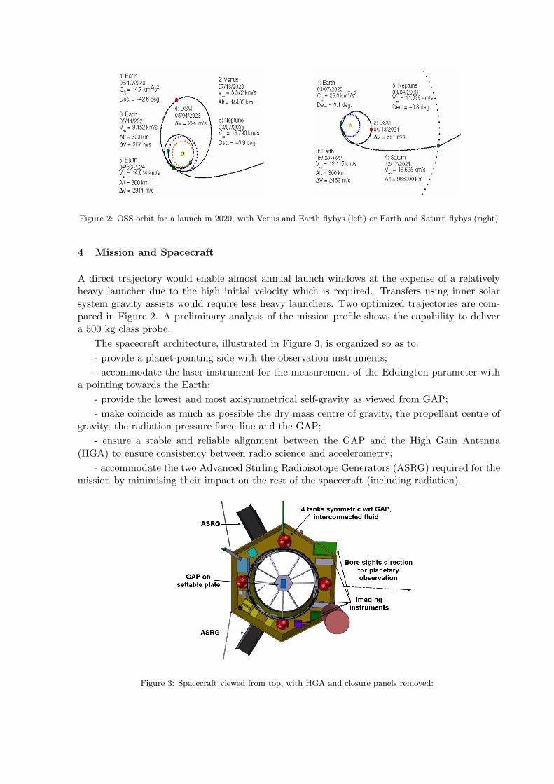
Figure 2: OSS orbit for a launch in 2020, with Venus and Earth flybys (left) or Earth and Saturn flybys (right)
4 Mission and Spacecraft
A direct trajectory would enable almost annual launch windows at the expense of a relativelyheavy launcher due to the high initial velocity which is required. Transfers using inner solarsystem gravity assists would require less heavy launchers. Two optimized trajectories are com-pared in Figure 2. A preliminary analysis of the mission profile shows the capability to delivera 500 kg class probe.
The spacecraft architecture, illustrated in Figure 3, is organized so as to:
- provide a planet-pointing side with the observation instruments;
- accommodate the laser instrument for the measurement of the Eddington parameter witha pointing towards the Earth;
- provide the lowest and most axisymmetrical self-gravity as viewed from GAP;
- make coincide as much as possible the dry mass centre of gravity, the propellant centre ofgravity, the radiation pressure force line and the GAP;
- ensure a stable and reliable alignment between the GAP and the High Gain Antenna(HGA) to ensure consistency between radio science and accelerometry;
- accommodate the two Advanced Stirling Radioisotope Generators (ASRG) required for themission by minimising their impact on the rest of the spacecraft (including radiation).
Figure 3: Spacecraft viewed from top, with HGA and closure panels removed:
Acknowledgments
OSS Team is composed by: B. Christophe, B. Foulon, B. Lenoir, A. Levy, C. Robert, P. Touboul(ONERA - The French Aerospace Lab, France), L.J. Spilker, J.D. Anderson, S.W. Asmar, G. Or-ton, K.R. Reh, T.R. Spilker (JPL/NASA, USA), N. Andre (CESR, France), D. Banfield (CornellUniversity, USA), J. Helbert, H. Hussmann, N. Schmitz, F. Sohl, K. Stephan (DLR/Institute ofPlanetary Research, Germany), H. Dittus (DLR/Institute of Space System, Germany), P. Brown(Imperial College London, UK), R. Srama (IRS, University of Stuttgart and MPIK, Heidelberg,Germany), F. Francisco, P.J.S. Gil, J. Paramos (Instituto Superior Tecnico, Portugal), S.V. Pro-grebenko (JIVE, Joint Institute for VLBI in Europe, The Netherlands), A. Barucci, B. Cecconi,L. Lamy (LESIA, Observatoire de Paris, CNRS, Meudon, France), J.-M. Courty, B. Lamine,S. Reynaud (LKB, CNRS, Paris, France), W. Grundy (Lowel Observatory, USA), E. Samain(Observatoire de la Cote d’Azur, GeoAzur, France), C. Hansen (PSI, USA), R. Bingham (RAL,UK), P. Wolf (SYRTE, Observatoire de Paris-Meudon, France), J. Poncy (Thales Alenia Space,Cannes, France), K.H. Glassmeier (Technical University of Braunschweig, Germany), O. Berto-lami (Universidade do Porto, Portugal), J. Saur (Universitat zu Koln, Germany), J. Aurnou,R. Helled, K.M. Sayanagi (University of California, USA), F. Postberg (University of Heidel-berg, Germany), L.N. Fletcher (University of Oxford, UK), C. Lammerzahl, H. Selig (ZARM,University of Bremen, Germany).
This proposal was supported by CNES (France) through a phase 0 study managed by E.Hinglais and S. Leon-Hirtz.
References
1. Will C.M., Living Reviews in Relativity 9, 3 (2006)2. Adelberger E., et al, Annual Review of Nuclear and Particle Science 53, 77 (2003)3. Reynaud, S. and Jaekel, M.-T., International Journal of Modern Physics A 20, 2294 (2005)4. Copeland E., Sami M., Tsujikawas S., Int J Mod Phys D 15, 1753 (2006)5. Frieman J.A., et al, Annual Review of Astronomy and Astrophysics 46, 385 (2008)6. Aguirre A., Burgess C., Friedland A., Nolte D., Class Quantum Grav 18, R223 (2001)7. Nojiri S., Odintsov S., Int. J. of Geometric Methods in Modern Physics 4, 115 (2007)8. Dittus H., Turyshev S., Lammerzahl C. et al, ESA Special Publications 588, 3 (2005)9. Johann U., Dittus H., Lammerzahl C. in Lasers, Clocks and Drag-Free Control: Explo-
ration of Relativistic Gravity in Space, ed. H. Dittus, C. Lammerzahl, and S.G. Turyshev(Astrophysics and Space Science Library, vol 349, pp 577, 2008)
10. Christophe B., Andersen P.H., Anderson J.D. et al, Exp. Astronomy 23, 529 (2009)11. Wolf P., Borde C.J., Clairon A. et al, Exp Astronomy 23, 651 (2009)12. Bertotti B., Iess L., Tortora P., Nature 425, 374 (2003)13. Touboul P., Willemenot E., Foulon B., Josselin V. Joint Meeting of the International
Gravity Commission and the International Geoid Commission No2, Bollettino di GeofisicaTeorica ed Applicata 40, 321 (1999)
14. Lenoir B., Levy A., Foulon B., Christophe B., Lamine B., Reynaud S., ArXiv e-printsarXiv:1011.6263 [physics.ins-det], Submitted to Advances in Space Resarch, (2010)

ON THE ANOMALOUS INCREASE OF THE LUNAR ECCENTRICITY
L. IORIOMinistero dell’Istruzione, dell’Universita e della Ricerca (M.I.U.R.)
Viale Unita di Italia 68, 70125, Bari (BA), Italy.
Possible explanations of the recently reported anomalous increase of the eccentricity of thelunar orbit are sought in terms of classical Newtonian mechanics, general relativity, and long-range modifications of gravity.
Anderson and Nieto, in a recent review1 of some astrometric anomalies detected in thesolar system by some independent groups, mentioned also an anomalous secular increase of theeccentricity e of the orbit of the Moon
emeas = (9± 3)× 10−12 yr−1 (1)
based on an analysis of a long LLR data record spanning 38.7 yr performed by Williams andBoggs2 with the dynamical force models of the DE421 ephemerides3,4 including all the knownrelevant Newtonian and Einsteinian effects. Notice that Eq. 1 is statistically significant at a3σ−level. The first account5 of this effect appeared in 2001 by Williams et al., who gave anextensive discussion of the state-of-the-art in modeling the tidal dissipation in both the Earthand the Moon. Later, Williams and Dickey6, relying upon the 2001 study5, released an anomalouseccentricity rate as large as emeas = (1.6± 0.5)× 10−11 yr−1. Anderson and Nieto1 commentedthat Eq. 1 is not compatible with present, standard knowledge of the dissipative processes in theinteriors of both the Earth and Moon, which were, actually, modeled by Williams and Boggs2.
Naive, dimensional evaluations of the effect caused on e by an additional anomalous accel-eration A can be made by noticing that
e ' A
na, (2)
withna = 1.0× 10³ m s−1 = 3.2× 10¹⁰ m yr−1 (3)
for the geocentric orbit of the Moon, whose mass is denoted as m. In it, a is the orbitalsemimajor axis, while n .=
√µ/a3 is the Keplerian mean motion in which µ
.= GM(1 + m/M)is the gravitational parameter of the Earth-Moon system: G is the Newtonian constant ofgravitation and M is the mass of the Earth. It turns out that an extra-acceleration as large as
A ' 3× 10⁻¹⁶ m s−2 = 0.3 m yr−2 (4)
would satisfy Eq. 1. In fact, a mere order-of-magnitude analysis based on Eq. 2 would beinadequate to infer meaningful conclusions: finding simply that this or that dynamical effect
induces an extra-acceleration of the right order of magnitude may be highly misleading. Indeed,exact calculations of the secular variation of e caused by such putative promising candidateextra-accelerations A must be performed with standard perturbative techniques in order tocheck if they, actually, cause an averaged non-zero change of the eccentricity. Moreover, it maywell happen, in principle, that the resulting analytical expression for 〈e〉 retains multiplicativefactors 1/ej , j = 1, 2, 3, ... or ej , j = 1, 2, 3... which would notably alter the size of the foundnon-zero secular change of the eccentricity with respect to the expected values according toEq. 2.
It is well known that a variety of theoretical paradigms7,8 allow for Yukawa-like deviations9
from the usual Newtonian inverse-square law of gravitation. The Yukawa-type correction to theNewtonian gravitational potential UN = −µ/r, where µ .= GM is the gravitational parameterof the central body which acts as source of the supposedly modified gravitational field, is
UY = −αµ∞r
exp(− r
λ
), (5)
in which µ∞ is the gravitational parameter evaluated at distances r much larger than the scalelength λ. In order to compute the long-term effects of Eq. 5 on the eccentricity of a test particleit is convenient to adopt the Lagrange perturbative scheme10. In such a framework, the equationfor the long-term variation of e is10⟨
de
dt
⟩=
1na2
(1− e2
e
)(1√
1− e2∂R∂ω− ∂R∂M
), (6)
where ω is the argument of pericenter, M is the mean anomaly of the test particle, and Rdenotes the average of the perturbing potential over one orbital revolution. In the case of aYukawa-type perturbation, Eq. 5 yields
〈UY〉 = −αµ∞ exp
(−a
λ
)a
I0
(aeλ
), (7)
where I0(x) is the modified Bessel function of the first kind Iq(x) for q = 0. An inspectionof Eq. 6 and Eq. 7 immediately tells us that there is no secular variation of e caused by ananomalous Yukawa-type perturbation.
The size of the general relativistic Lense-Thirring11 acceleration experienced by the Moonbecause of the Earth’s angular momentum12 S = 5.86× 1033 kg m2 s−1 is just
ALT '2vGSc2a3
= 1.6× 10⁻¹⁶ m s−2 = 0.16 m yr−2, (8)
i.e. close to Eq. 4. On the other hand, it is well known that the Lense-Thirring effect does notcause long-term variations of the eccentricity. Indeed, the integrated shift of e from an initialepoch corresponding to f0 to a generic time corresponding to f is13
∆e = −2GS cos I′(cos f − cos f0)
c2na3√
1− e2, (9)
in which I′
is the inclination of the Moon’s orbit with respect to the Earth’s equator and f isthe true anomaly. From Eq. 9 it straightforwardly follows that after one orbital revolution, i.e.for f → f0 + 2π, the long-term gravitomagnetic shift of e vanishes.
A promising candidate for explaining the anomalous increase of the lunar eccentricity is,at least in principle, a trans-Plutonian massive body X of planetary size located in the remoteperipheries of the solar system. Indeed, the perturbation induced by it would, actually, cause a
non-vanishing long-term variation of e. Moreover, since it depends on the spatial position of Xin the sky and on its tidal parameter
KX.=GmX
d3X
, (10)
where mX and dX are the mass and the distance of X, respectively, it may happen that a suitablecombination of them is able to reproduce Eq. 1. Let us recall that, in general, the perturbingpotential felt by a test particle orbiting a central body due to a very distant, pointlike mass canbe cast into the following quadrupolar form
UX =KX
2
[r2 − 3
(~r · l)2], (11)
where l = lx, ly, lz is a unit vector directed towards X determining its position in the sky. InEq. 11 ~r = x, y, z is the geocentric position vector of the perturbed particle, which, in thepresent case, is the Moon. Iorio14 has recently shown that the average of Eq. 11 over one orbitalrevolution of the particle is
〈UX〉 =KXa
2
32U(e, I,Ω, ω; l
), (12)
where U(e, I,Ω, ω; l
)is a complicated function of its arguments14: Ω is the longitude of the
ascending node and I is the inclination of the lunar orbit to the ecliptic. In the integrationyielding Eq. 12 l was kept fixed over one orbital revolution of the Moon, as it is reasonable giventhe assumed large distance of X with respect to it. Eq. 6, applied to Eq. 12, straightforwardlyyields
〈e〉 =15KXe
√1− e2
16nE(I,Ω, ω; l
). (13)
Also E(I,Ω, ω; l
)is an involved function of the orientation of the lunar orbit in space and of the
position of X in the sky14. Actually, the expectations concerning X are doomed to fade away.Indeed, apart from the modulation introduced by the presence of the time-varying I, ω and Ω inEq. 13, the values for the tidal parameter which would allow to obtain Eq. 1 are too large for allthe conceivable positions βX, λX of X in the sky. This can easily be checked by keeping ω andΩ fixed at their J2000.0 values as a first approximation. Indeed, Iorio14 showed that the physicaland orbital features of X postulated by two recent plausible theoretical scenarios15,16 for X wouldinduce long-term variations of the lunar eccentricity much smaller than Eq. 1. Conversely, itturns out that a tidal parameter as large as
KX = 4.46× 10⁻²⁴ s−2 (14)
would yield the result of Eq. 1. Actually, Eq. 14 is totally unacceptable since it corresponds todistances of X as absurdly small as dX = 30 au for a terrestrial body, and dX = 200 au for aJovian mass.
An empirical explanation of Eq. 1 can be found by assuming that, in addition to the usualNewtonian inverse-square law for the gravitational acceleration imparted to a test particle by acentral body orbited by it, there is also a small radial extra-acceleration of the form
A = kH0vr. (15)
In it k is a positive numerical parameter of the order of unity to be determined from theobservations, H0 = (73.8 ± 2.4) km s−1 Mpc−1 = (7.47 ± 0.24) × 10−11 yr−1 is the Hubbleparameter at the present epoch17, defined in terms of the time-varying cosmological scaling factor
S(t) as H0.= S/S
∣∣∣0, and vr is the component of the velocity vector ~v of the test particle’s proper
motion about the central body along the common radial direction. Indeed, a straightforwardapplication of the Gauss perturbative equation for e to Eq. 15 yields
〈e〉 = kH0
(1− e2
) (1−√
1− e2)
e. (16)
Since eMoon = 0.0647, Eq. 16 can reproduce Eq. 1 for 2.5 . k . 5. Here we do not intend tospeculate too much about possible viable physical mechanisms yielding the extra-accelerationof Eq. 15. It might be argued that, reasoning within a cosmological framework, the Hubblelaw may give Eq. 15 for k = 1 if the proper motion of the particle about the central mass istaken into account in addition to its purely cosmological recession which, instead, yields thewell-known local extra-acceleration of tidal type Acosmol = −q0H2
0r, where q0 is the decelerationparameter at the present epoch.
Acknowledgments
I gratefully acknowledge the financial support by the MORIOND scientific committee
References
1. J. D. Anderson and M. M. Nieto in Relativity in Fundamental Astronomy: Dynamics,Reference Frames, and Data Analysis, Proceedings IAU Symposium No. 261, ed. S. A.Klioner, P. K. Seidelmann and M. H. Soffel (Cambridge University Press, Cambridge,2010), pp. 189-197.
2. J. G. Williams and D. H. Boggs in Proceedings of the 16th International Workshop onLaser Ranging, ed. S Schilliak, pp. 101-120.
3. W. M. Folkner, J. G. Williams and D. H. Boggs JPL IOM 343R-08-003 (2008).4. J. G. Williams, D. H. Boggs and W. M. Folkner JPL IOM 335-JW,DB,WF-20080314-001
(2008).5. J. G. Williams, D. H. Boggs, C. F. Yoder, J. T. Ratcliff and J. O. Dickey , J. Geophys.
Res. 106, 27933 (2001).6. J. G. Williams and J. O. Dickey in Proceedings of the 13th International Workshop on Laser
Ranging, NASA/CP-2003-212248, ed. R. Noomen, S. Klosko, C. Noll, M. Pearlman, pp.75-86.
7. E. G. Adelberger, B. R. Heckel and A. E. Nelson, Ann. Rev. Nucl. Part. Sci. 53, 77(2003).
8. O. Bertolami and J. Paramos, Phys. Rev. D 71, 023521 (2005).9. C. P. Burgess and J. Cloutier, Phys. Rev. D 38, 2944 (1988).
10. B. Bertotti, P. Farinella and D. Vokrouhlicky Physics of the Solar System, (Kluwer Aca-demic Press, Dordrecht, 2003).
11. J. Lense and H. Thirring, Phys. Z. 19, 156 (1918)12. D. D. McCarthy and G. Petit, IERS Technical Note No. 32. IERS Conventions (2003).
12. (Verlag des Bundesamtes fur Kartographie und Geodasie, Frankfurt am Main, 2003).13. M. H. Soffel, Relativity in Astrometry, Celestial Mechanics and Geodesy, (Springer, Berlin,
1989).14. L. Iorio, Mon. Not. Roy. Astron. Soc. doi:10.1111/j.1365-2966.2011.18777.x (2011).15. P. S. Lykawka and T. Mukai, Astron. J. 135, 1161 (2008).16. J. J. Matese and D. P. Whitmire, Icarus 211, 926 (2011).17. A. G. Riess, L. Macri, S. Casertano, H. Lampeit, H. C. Ferguson, A. V. Filippenko, S. W.
Jha, W. Li, R. Chornock and J. M. Silverman, Astrophys. J. 730, 119 (2011).
Radioscience simulations in General Relativity and in alternative theories ofgravity
A. Hees1,2, P. Wolf2, B. Lamine3, S. Reynaud3, M.T. Jaekel4, C. Le Poncin-Lafitte2, V. Lainey5, A.Fuzfa6, V. Dehant1
1 Royal Observatory of Belgium, Avenue Circulaire 3, 1180 Bruxelles, Belgium, [email protected] LNE-SYRTE, Observatoire de Paris, CNRS, UPMC, France3 Laboratoire Kastler Brossel, UPMC, Campus Jussieu, France4 Laboratoire de Physique Theorique de l’ENS, Paris, France
5 IMCCE, Observatoire de Paris, France6 naXys, University of Namur (FUNDP), Belgium
In this communication, we focus on the possibility to test GR with radioscience experiments.We present a new software that in a first step simulates the Range/Doppler signals directlyfrom the space time metric (thus in GR and in alternative theories of gravity). In a secondstep, a least-squares fit of the involved parameters is performed in GR. This software allows oneto get the order of magnitude and the signature of the modifications induced by an alternativetheory of gravity on radioscience signals. As examples, we present some simulations for theCassini mission in Post-Einsteinian gravity and with the MOND External Field Effect.
1 Introduction
There is still a great interest in testing General Relativity (theoretical motivations such as quan-tification of gravity, unification with other interactions. . . ). Within the solar system, the grav-itational observations are always related with radioscience measurements (Range and Doppler)or with angular measurements (position of body in the sky, VLBI). In this communication, wepresent a new tool that performs simulations of radioscience experiments in General Relativityand in alternative metric theories of gravitation. The developed software simulates Range andDoppler signals directly from the space time metric (and from the initial conditions of the bod-ies considered). The aim of this tool is to provide orders of magnitude and signatures for thevariations of the Range/Doppler induced by alternative theories of gravity. In order to comparesignals in different theories, a least-squares fit of the different parameters involved in the problem(mainly the initial conditions) is performed. In this communication, we present the principlesof the software and results of simulations of the Cassini probe mission during its cruise fromJupiter to Saturn with Post-Einsteinian modifications of gravity (PEG) 1,2 or with an externalfield effect due to a MONDian modification of gravity 3.
2 Description of the software
Our software directly generates Doppler/Range signal from the metric considered in a fully-relativistic way. This includes the integration of the equations of motion in a given coordinatetime, the computation of the time transfer of light and the clock behavior.
The equations of motion are derived from the metric and the geodesic equations integratedwith respect to coordinate time 4.
The connection between the coordinate and proper time of clocks is obtained by integratingthe equation of proper time 4
dτ
dt=√g00 − 2g0ivi − gijvivj (1)
where gµν is the space-time metric, vi is the velocity of the clock and τ its proper time.Finally, the time transfer is also determined directly from the metric using Synge World’s
function formalism 5. Within this formalism, one does not need to integrate the photon tra-jectory in order to get the time transfer or the frequency shift (in the linear approximation).Instead, those quantities are expressed as integrals of functions defined from the metric (andtheir derivatives) along the photon Minkowski path. For example the coordinate propagationtime can be expressed as 5
T (xie(te), xir(tr), tr) =
Rerc
+Rerc
∫ 1
0f(zα(µ))dµ (2)
with
f = −h00 − 2N ierh0i −N i
erNjerhij , hµν = gµν − ηµν , N i
er =xir − xieRer
, (3)
xie, te are the position and time of the emitter (computed iteratively assuming flat space time),xir, tr are the position and time of the receptor and Rer =
∥∥xie(te) − xir(tr)∥∥. The integral in (2)
is performed over a Minkowski path between emitter and receptor (zα(µ) is a straight line). Asimilar expression is used for the frequency shift.
In order to investigate the observable signatures of an alternative theory of gravity in theRange and Doppler data we perform a least-squares fit in GR on the different parameters (initialconditions and masses of the bodies) and search for identifiable signatures in the residuals. Thefit of initial conditions is necessary in order to avoid effects due to the choice of coordinates. Asa matter of fact, this fit is always done in practice, which means that a reasonable analysis ofthe signal produced by an alternative theory has to be done after the fit.
3 Simulations of Cassini mission
As an example, we simulate the two-way range and Doppler signals to the Cassini spacecraftfrom June 2002 during 3 years (when the probe was between Jupiter and Saturn). To simplifythe situation we only consider the Sun, the Earth and Cassini spacecraft.
3.1 Post-Einsteinian Gravity (PEG)
The first alternative metric theory considered is Post-Einsteinian Gravity (PEG) 1,2. From aphenomenological point of view this theory consists in including two potentials ΦN (r) and ΦP (r)to the metric. Here we concentrate on the sector ΦP (r). We consider a series expansion. Thatis to say we suppose the spatial part of the metric to be modified as follows
gij = [gij ]GR − 2δij
(χ1r + χ2r
2 + δγGM
c2r
)(4)
where r is a radial isotropic coordinate, M is the sun mass, c the velocity of light and G thegravitational constant. The parameter δγ is related to the post-newtonian parameter δγ = γ−1.
Different simulations were performed with different values of the three PEG parameters.For example, Figure 1 represents the Range and Doppler differences between a simulation in a
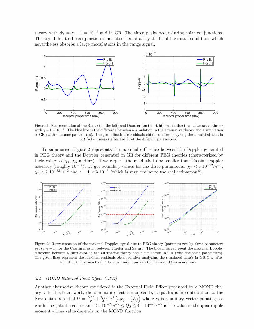
theory with δγ = γ − 1 = 10−5 and in GR. The three peaks occur during solar conjunctions.The signal due to the conjunction is not absorbed at all by the fit of the initial conditions whichnevertheless absorbs a large modulations in the range signal.
0 200 400 600 800 1000−1
−0.5
0
0.5
1
1.5
Range (
m)
Receptor proper time (day)
Pre fit
Post fit
0 200 400 600 800 1000−4
−3
−2
−1
0
1
2
3
4x 10
−15
Dopple
r
Receptor proper time (day)
Pre fit
Post fit
Figure 1: Representation of the Range (on the left) and Doppler (on the right) signals due to an alternative theorywith γ− 1 = 10−5. The blue line is the difference between a simulation in the alternative theory and a simulationin GR (with the same parameters). The green line is the residuals obtained after analyzing the simulated data in
GR (which means after the fit of the different parameters).
To summarize, Figure 2 represents the maximal difference between the Doppler generatedin PEG theory and the Doppler generated in GR for different PEG theories (characterized bytheir values of χ1, χ2 and δγ). If we request the residuals to be smaller than Cassini Doppleraccuracy (roughly 10−14), we get boundary values for the three parameters: χ1 < 5 10−22m−1,χ2 < 2 10−33m−2 and γ − 1 < 3 10−5 (which is very similar to the real estimation 6).
10−26
10−24
10−22
10−20
10−18
10−16
10−15
10−14
10−13
10−12
10−11
10−10
10−9
χ1 (m
−1)
Max D
opple
r D
iffe
rence
Pre fit
Post Fit
10−38
10−36
10−34
10−32
10−30
10−16
10−15
10−14
10−13
10−12
10−11
10−10
χ2 (m
−2)
Max D
opple
r D
iffe
rence
Pre fit
Post Fit
10−6
10−5
10−4
10−3
10−16
10−15
10−14
10−13
10−12
γ −1
Max D
opple
r D
iffe
rence
Pre fit
Post Fit
Figure 2: Representation of the maximal Doppler signal due to PEG theory (parametrized by three parametersχ1, χ2, γ − 1) for the Cassini mission between Jupiter and Saturn. The blue lines represent the maximal Dopplerdifference between a simulation in the alternative theory and a simulation in GR (with the same parameters).The green lines represent the maximal residuals obtained after analyzing the simulated data’s in GR (i.e. after
the fit of the parameters). The read lines represent the assumed Cassini accuracy.
3.2 MOND External Field Effect (EFE)
Another alternative theory considered is the External Field Effect produced by a MOND the-ory 3. In this framework, the dominant effect is modeled by a quadrupolar contribution to the
Newtonian potential U = GMr + Q2
2 xixj
(eiej − 1
3δij)
where ei is a unitary vector pointing to-
wards the galactic center and 2.1 10−27s−2 ≤ Q2 ≤ 4.1 10−26s−2 is the value of the quadrupolemoment whose value depends on the MOND function.
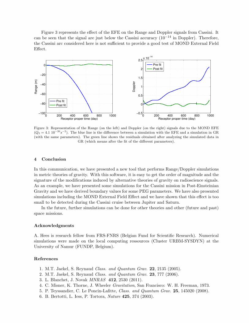
Figure 3 represents the effect of the EFE on the Range and Doppler signals from Cassini. Itcan be seen that the signal are just below the Cassini accuracy (10−14 in Doppler). Therefore,the Cassini arc considered here is not sufficient to provide a good test of MOND External FieldEffect.
0 200 400 600 800 1000−100
−80
−60
−40
−20
0
Range (
m)
Receptor proper time (day)
Pre fit
Post fit
0 200 400 600 800 1000−0.5
0
0.5
1
1.5
2
2.5x 10
−14
Dopple
r
Receptor proper time (day)
Pre fit
Post fit
Figure 3: Representation of the Range (on the left) and Doppler (on the right) signals due to the MOND EFE(Q2 = 4.1 10−26s−2). The blue line is the difference between a simulation with the EFE and a simulation in GR(with the same parameters). The green line shows the residuals obtained after analyzing the simulated data in
GR (which means after the fit of the different parameters).
4 Conclusion
In this communication, we have presented a new tool that performs Range/Doppler simulationsin metric theories of gravity. With this software, it is easy to get the order of magnitude and thesignature of the modifications induced by alternative theories of gravity on radioscience signals.As an example, we have presented some simulations for the Cassini mission in Post-EinsteinianGravity and we have derived boundary values for some PEG parameters. We have also presentedsimulations including the MOND External Field Effect and we have shown that this effect is toosmall to be detected during the Cassini cruise between Jupiter and Saturn.
In the future, further simulations can be done for other theories and other (future and past)space missions.
Acknowledgments
A. Hees is research fellow from FRS-FNRS (Belgian Fund for Scientific Research). Numericalsimulations were made on the local computing ressources (Cluster URBM-SYSDYN) at theUniversity of Namur (FUNDP, Belgium).
References
1. M.T. Jaekel, S. Reynaud Class. and Quantum Grav. 22, 2135 (2005).2. M.T. Jaekel, S. Reynaud Class. and Quantum Grav. 23, 777 (2006).3. L. Blanchet, J. Novak MNRAS 412, 2530 (2011).4. C. Misner, K. Thorne, J. Wheeler Gravitation, San Francisco: W. H. Freeman, 1973.5. P. Teyssandier, C. Le Poncin-Lafitte, Class. and Quantum Grav. 25, 145020 (2008).6. B. Bertotti, L. Iess, P. Tortora, Nature 425, 374 (2003).
GAME - Gravitation Astrometric Measurement Experiment
M. GAI
INAF - Astronomical Observatory of Torino, 20 V. Osservatorio
10025 Pino Torinese (TO), Italy
The Gravitation Astrometric Measurement Experiment (GAME) is a mission concept basedon astronomical techniques (astrometry and coronagraphy) for Fundamental Physics mea-surements, namely the γ and β parameters of the Parameterized Post-Newtonian formulationof gravitation theories extending the General Relativity. The mission concept, measurementapproach and instrument design are briefly described.
1 Introduction
The experiment of Dyson, Eddington and Davidson, whose concept is sketched in the left panelof Fig. 1, gave the first confirmation of Einstein’s General Relativity theory by observation ofknown stellar fields during the May 29th, 1919 eclipse. It measured the apparent positions of afew stars, within a few degrees from the solar limb during the eclipse, compared to their unper-turbed relative positions. The arc variation is interpreted in terms of light deflection, providingan estimate of the γ parameter with precision ∼ 10%, i.e. to a 10−1 accuracy estimation ofthe PPN γ parameter. Measurements of light deflection from the ground are affected by severalshortcomings, as short eclipse duration, high background flux from the solar corona, atmosphericdisturbances and the limited number of bright sources in the field, thus limiting the achievableperformance independently from foreseeable technological improvements. The current best esti-mate of γ, from the Cassini experiment, is in the 10−5 range 1. The β parameter was estimatedthrough accurate orbit determination of Solar System bodies 2 which put to evidence the effectof perihelion shift excess, extending the historical case of Mercury.
The main scientific goal of GAME is the estimation of key parameters of the ParametrizedPost-Newtonian formalism, commonly used to test the metric theories of gravity in the weak-fieldregime of the Solar System. The focus is on Eddington’s parameters, γ, to a few 10−8, and β, to afew 10−6. The possibility of testing gravity theories to this accuracy has significant implicationsfor our understanding of several physical and astrophysical issues at a very fundamental level.GAME can also provide crucial information on several other issues of Solar system (in particularNear Earth Object orbit determination), extra-solar planetary systems, stellar astrophysics andhigh angular resolution monitoring of the Corona and circumsolar environment.
2 Science goal: estimation of the PPN γ parameter
The Parametrised Post-Newtonian (PPN) formalism 3 was introduced to classify the metrictheories of gravity at their Post-Newtonian level through a set of parameters. The γ parameter
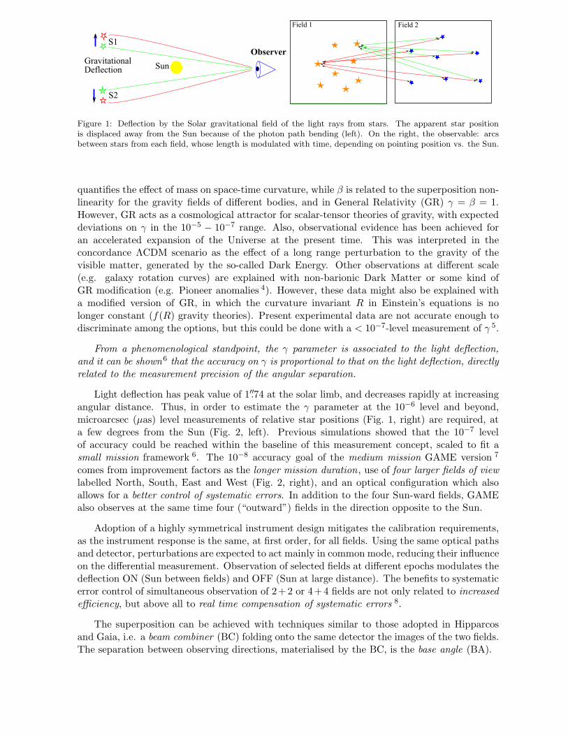
Figure 1: Deflection by the Solar gravitational field of the light rays from stars. The apparent star positionis displaced away from the Sun because of the photon path bending (left). On the right, the observable: arcsbetween stars from each field, whose length is modulated with time, depending on pointing position vs. the Sun.
quantifies the effect of mass on space-time curvature, while β is related to the superposition non-linearity for the gravity fields of different bodies, and in General Relativity (GR) γ = β = 1.However, GR acts as a cosmological attractor for scalar-tensor theories of gravity, with expecteddeviations on γ in the 10−5 − 10−7 range. Also, observational evidence has been achieved foran accelerated expansion of the Universe at the present time. This was interpreted in theconcordance ΛCDM scenario as the effect of a long range perturbation to the gravity of thevisible matter, generated by the so-called Dark Energy. Other observations at different scale(e.g. galaxy rotation curves) are explained with non-barionic Dark Matter or some kind ofGR modification (e.g. Pioneer anomalies 4). However, these data might also be explained witha modified version of GR, in which the curvature invariant R in Einstein’s equations is nolonger constant (f(R) gravity theories). Present experimental data are not accurate enough todiscriminate among the options, but this could be done with a < 10−7-level measurement of γ 5.
From a phenomenological standpoint, the γ parameter is associated to the light deflection,
and it can be shown6 that the accuracy on γ is proportional to that on the light deflection, directly
related to the measurement precision of the angular separation.
Light deflection has peak value of 1′′.74 at the solar limb, and decreases rapidly at increasingangular distance. Thus, in order to estimate the γ parameter at the 10−6 level and beyond,microarcsec (µas) level measurements of relative star positions (Fig. 1, right) are required, ata few degrees from the Sun (Fig. 2, left). Previous simulations showed that the 10−7 levelof accuracy could be reached within the baseline of this measurement concept, scaled to fit asmall mission framework 6. The 10−8 accuracy goal of the medium mission GAME version 7
comes from improvement factors as the longer mission duration, use of four larger fields of view
labelled North, South, East and West (Fig. 2, right), and an optical configuration which alsoallows for a better control of systematic errors. In addition to the four Sun-ward fields, GAMEalso observes at the same time four (“outward”) fields in the direction opposite to the Sun.
Adoption of a highly symmetrical instrument design mitigates the calibration requirements,as the instrument response is the same, at first order, for all fields. Using the same optical pathsand detector, perturbations are expected to act mainly in common mode, reducing their influenceon the differential measurement. Observation of selected fields at different epochs modulates thedeflection ON (Sun between fields) and OFF (Sun at large distance). The benefits to systematicerror control of simultaneous observation of 2+2 or 4+4 fields are not only related to increased
efficiency, but above all to real time compensation of systematic errors 8.
The superposition can be achieved with techniques similar to those adopted in Hipparcosand Gaia, i.e. a beam combiner (BC) folding onto the same detector the images of the two fields.The separation between observing directions, materialised by the BC, is the base angle (BA).
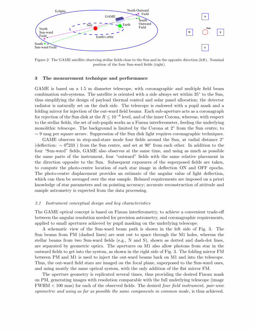
Figure 2: The GAME satellite observing stellar fields close to the Sun and in the opposite direction (left). Nominalposition of the four Sun-ward fields (right).
3 The measurement technique and performance
GAME is based on a 1.5 m diameter telescope, with coronagraphic and multiple field beamcombination sub-systems. The satellite is oriented with a side always set within 35 to the Sun,thus simplifying the design of payload thermal control and solar panel allocation; the detectorradiator is naturally set on the dark side. The telescope is endowed with a pupil mask and afolding mirror for injection of the out-ward field beams. Each sub-aperture acts as a coronagraphfor rejection of the Sun disk at the R ≤ 10−8 level, and of the inner Corona, whereas, with respectto the stellar fields, the set of sub-pupils works as a Fizeau interferometer, feeding the underlyingmonolithic telescope. The background is limited by the Corona at 2 from the Sun centre, to∼ 9 mag per square arcsec. Suppression of the Sun disk light requires coronagraphic techniques.
GAME observes in step-and-stare mode four fields around the Sun, at radial distance 2
(deflection: ∼ 0′′.233 ) from the Sun centre, and set at 90 from each other. In addition to thefour “Sun-ward” fields, GAME also observes at the same time, and using as much as possiblethe same parts of the instrument, four “outward” fields with the same relative placement inthe direction opposite to the Sun. Subsequent exposures of the superposed fields are taken,to compute the photo-centre location of each star image in deflection ON and OFF epochs.The photo-centre displacement provides an estimate of the angular value of light deflection,which can then be averaged over the star sample. Relaxed requirements are imposed on a prioriknowledge of star parameters and on pointing accuracy; accurate reconstruction of attitude andsample astrometry is expected from the data processing.
3.1 Instrument conceptual design and key characteristics
The GAME optical concept is based on Fizeau interferometry, to achieve a convenient trade-offbetween the angular resolution needed for precision astrometry, and coronagraphic requirements,applied to small apertures achieved by pupil masking on the underlying telescope.
A schematic view of the Sun-ward beam path is shown in the left side of Fig. 3. TheSun beams from PM (dashed lines) are sent out to space through the M1 holes, whereas thestellar beams from two Sun-ward fields (e.g., N and S), shown as dotted and dash-dot lines,are separated by geometric optics. The apertures on M1 also allow photons from star in theoutward fields to get into the system, as shown in the right side of Fig. 3. The folding mirror FMbetween PM and M1 is used to inject the out-ward beams back on M1 and into the telescope.Thus, the out-ward field stars are imaged on the focal plane, superposed to the Sun-ward ones,and using mostly the same optical system, with the only addition of the flat mirror FM.
The aperture geometry is replicated several times, thus providing the desired Fizeau maskon PM, generating images with resolution comparable with the full underlying telescope (imageFWHM < 100 mas) for each of the observed fields. The desired four field instrument, pair-wise
symmetric and using as far as possible the same components in common mode, is thus achieved.
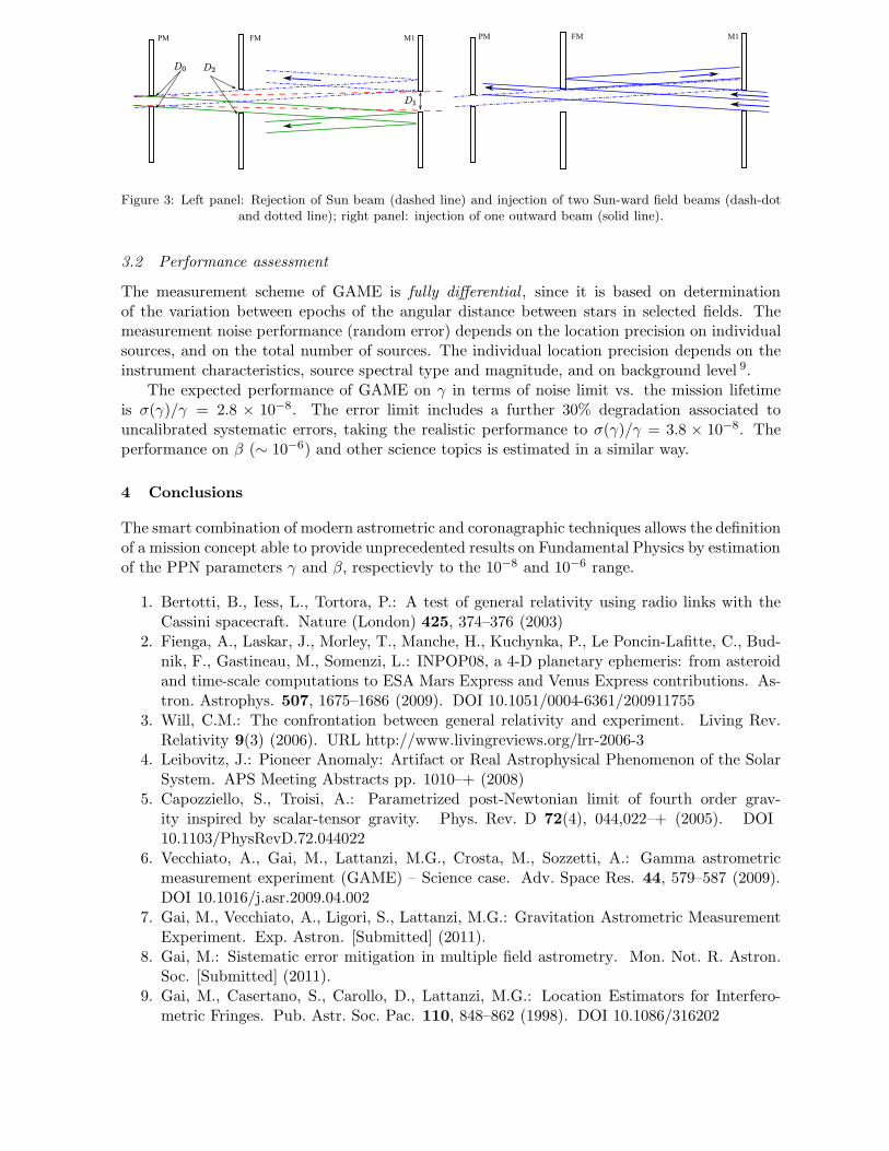
Figure 3: Left panel: Rejection of Sun beam (dashed line) and injection of two Sun-ward field beams (dash-dotand dotted line); right panel: injection of one outward beam (solid line).
3.2 Performance assessment
The measurement scheme of GAME is fully differential , since it is based on determinationof the variation between epochs of the angular distance between stars in selected fields. Themeasurement noise performance (random error) depends on the location precision on individualsources, and on the total number of sources. The individual location precision depends on theinstrument characteristics, source spectral type and magnitude, and on background level 9.
The expected performance of GAME on γ in terms of noise limit vs. the mission lifetimeis σ(γ)/γ = 2.8 × 10⁻⁸. The error limit includes a further 30% degradation associated touncalibrated systematic errors, taking the realistic performance to σ(γ)/γ = 3.8 × 10⁻⁸. Theperformance on β (∼ 10−6) and other science topics is estimated in a similar way.
4 Conclusions
The smart combination of modern astrometric and coronagraphic techniques allows the definitionof a mission concept able to provide unprecedented results on Fundamental Physics by estimationof the PPN parameters γ and β, respectievly to the 10−8 and 10−6 range.
1. Bertotti, B., Iess, L., Tortora, P.: A test of general relativity using radio links with theCassini spacecraft. Nature (London) 425, 374–376 (2003)
2. Fienga, A., Laskar, J., Morley, T., Manche, H., Kuchynka, P., Le Poncin-Lafitte, C., Bud-nik, F., Gastineau, M., Somenzi, L.: INPOP08, a 4-D planetary ephemeris: from asteroidand time-scale computations to ESA Mars Express and Venus Express contributions. As-tron. Astrophys. 507, 1675–1686 (2009). DOI 10.1051/0004-6361/200911755
3. Will, C.M.: The confrontation between general relativity and experiment. Living Rev.Relativity 9(3) (2006). URL http://www.livingreviews.org/lrr-2006-3
4. Leibovitz, J.: Pioneer Anomaly: Artifact or Real Astrophysical Phenomenon of the SolarSystem. APS Meeting Abstracts pp. 1010–+ (2008)
5. Capozziello, S., Troisi, A.: Parametrized post-Newtonian limit of fourth order grav-ity inspired by scalar-tensor gravity. Phys. Rev. D 72(4), 044,022–+ (2005). DOI10.1103/PhysRevD.72.044022
6. Vecchiato, A., Gai, M., Lattanzi, M.G., Crosta, M., Sozzetti, A.: Gamma astrometricmeasurement experiment (GAME) – Science case. Adv. Space Res. 44, 579–587 (2009).DOI 10.1016/j.asr.2009.04.002
7. Gai, M., Vecchiato, A., Ligori, S., Lattanzi, M.G.: Gravitation Astrometric MeasurementExperiment. Exp. Astron. [Submitted] (2011).
8. Gai, M.: Sistematic error mitigation in multiple field astrometry. Mon. Not. R. Astron.Soc. [Submitted] (2011).
9. Gai, M., Casertano, S., Carollo, D., Lattanzi, M.G.: Location Estimators for Interfero-metric Fringes. Pub. Astr. Soc. Pac. 110, 848–862 (1998). DOI 10.1086/316202
A RELATIVISTIC AND AUTONOMOUS NAVIGATION SATELLITE SYSTEM
P. DELVA
SYRTE, Observatoire de Paris, CNRS and UPMC,61 avenue de l’Observatoire, F-75014 Paris, France
A. CADEZ, U. KOSTIC
Department of Physics, University of LjubljanaJadranska 19, 1000 Ljubljana, Slovenia
S. CARLONI
ESA Advanced Concepts Team, ESTEC, DG-PIKeplerlaan 1, 2201 AZ Noordwijk, The Netherlands
A relativistic positioning system has been proposed by Bartolome Coll in 2002. Since then,several group developed this topic with different approaches. I will present a work done incollaboration with Ljubljana University and the ESA Advanced Concepts Team. We developeda concept, Autonomous Basis of Coordinates, in order to take advantage of the full autonomyof a satellite constellation for navigation and positioning, by means of satellite inter-links. Iwill present the advantages of this new paradigm and a number of potential application forreference systems, geophysics and relativistic gravitation.
1 Relativistic Positioning Systems (RPS)
The first proposal for a relativistic positioning system is SYPOR (“Systeme de PositionnementRelativiste”), proposed by Bartolome Coll in 2002 1. It is an alternative to the scheme of usualpositioning systems. The idea is to give the constellation of satellites the possibility to constituteby itself a primary and autonomous positioning system, without any a priori realization of aterrestrial reference frame.
The relativistic positioning system is defined with the introduction of emission coordinates,which contain dynamical information of the satellite constellation. They have been reintroducedrecently by several articles 2,3,4,5. The definition of these coordinates is rather simple, but theyare a very powerful tool in general relativity. Let us define four particles a = 1, 2, 3, 4 coupled togeneral relativity. Along their worldlines Ca, one defines four one-parameter families of futurenull cones Na(τa) which are parametrized by proper time. The intersection of four future nullcones Na(τa) from four worldlines Ca defines an event with emission coordinates (τ1, τ2, τ3, τ4).Then, a user receiving four electromagnetic signals broadcasting the proper time of four satellitesknows its position in this particular coordinate system.
RPS have been studied with different approaches these last years6,7,8,9,10,11,12,13,14,15,16,17,18,19,20,21.The purpose of this proceeding is to present an approach developed by a collaboration betweenthe Advanced Concepts Team of the European Space Agency, the department of physics ofLjubljana University and SYRTE/Paris Observatory/UPMC.
2 From emission to global coordinates
A GNSS is a system of satellites emitting precise timing signals for the purpose of providing alocal coordinate basis in space-time. In order to determine his space-time position with respectto this basis, an observer must receive four proper times emitted by four different satellites, andbe able to calculate the local coordinates of the four satellites as a function of their emissioncoordinates.
We studied the use of emission coordinates theoretically and in practical scenarii by numer-ical simulations 16,20,21. We provided mathematical tools to translate emission coordinates intospace-time coordinates of the observer. A local Schwarzschild coordinate system was introducedas an idealized prototype of space-time in the vicinity of the Earth. The problem of connectingthe local Schwarzschild frame to the global inertial frame is well understood in the framework ofclassical non-relativistic gravitational perturbation theory, but remains to be done in a generalrelativistic framework.
Analytic solutions for light-like and time-like geodesics were obtained in order to implementtwo algorithms: (i) an algorithm that calculates emission coordinates corresponding to the localSchwarzschild coordinates of a user, and (ii) the “reverse” algorithm that calculates space-timecoordinates of a user from its emission coordinates. In a first approach, we assumed that orbitalparameters of satellites are known. We have shown that the use of a fully relativistic code inGNSS offers a very promising alternative to the use of post-Newtonian approximations, andpresents no technical obstacle.
The effects of non-gravitational perturbations have been studied. We have shown that theonly yardstick of a GNSS is the clock, which provides absolute position both in space and timeto any accuracy and stability allowed by noise and clock drifts. Clock drifts, adding up aftersome time, would result in considerable error in absolute position in space if the the clocks werenot controlled. In current positioning scheme, correcting the clocks needs a constant monitoringof the satellites via Earth telemetry and the precise realization of a terrestrial reference frame.However, we realized that a GNSS constellation is also a very precise clock of its own, sinceorbital periods of its satellites are accurate constants of motion. Therefore, we proposed touse the dynamical information given by mutual timing between satellites to improve the longterm phase stability of onboard clocks, as well as to improve the precision of constants ofmotion of the constellation. This proposal led us to define the concept of Autonomous Basisof Coordinates (ABC). Within such a scheme, we have shown that it is possible to correct theclocks to a level considerably surpassing the classical scheme, which is limited in accuracy bystochastic components of Earth dynamics.
3 Autonomous Basis of Coordinates (ABC)
In a GNSS constellation with more than four satellites, more than four emission coordinatesare received by an observer: the positioning problem is over-determined. In order for the localbasis to be self consistent, all combinations of emission coordinates, received at any event inspace-time, must give the same four local coordinates for this event. The main constraint onself-consistency of a GNSS system comes from the precision of constants of motion. In order toadress this problem, the concept of Autonomous Basis of Coordinates (ABC) is introduced inCadez et al. 20. We propose that the constants of motion be determined and checked internallyby the GNSS system in such a way that each satellite checks its own position as any otherobserver with respect to all the other satellites: in addition to emitting its proper time, eachsatellite also receives other satellite’s emission coordinates and makes its information availableto the central GNSS control 22,23.
The ABC concept aims to describe in a coherent frame both the dynamics of non-interacting
test bodies transmitting emission coordinates and the propagation of electromagnetic wavesproviding those coordinates. It uses the fact that both light and test bodies trajectories aregeodesics that can be derived from the same Hamiltonian. It provides a means to translatedynamical information into the conventional representation based on local frames. Dynamicalinformation, expressed in terms of emission coordinates, gives direct information about theRiemannian structure of space-time, and thus allows the construction of a local frame withcoordinates and metric that provides a precise definition of equations of motion. We call thereference system and coordinates built via the ABC concept the ABC reference system and theABC coordinates.
Let us use the nomenclature introduced by J. Kovalevsky and I. Mueller 24 to describe theABC reference system:
Concept: the ABC coordinate system is built such that dynamics is consistent; dynamics isgiven by a Hamiltonian, that both describe space-time geometry and non-gravitational forces.
Physical structure: the reference system is physically materialized by a constellation of satel-lites in Earth orbit and inter-satellite links. Light and satellite geodesics create a physicalspace-time web that probe the space-time geometry.
Modelling: the model characterizes a particular choice of the Hamiltonian. We have studiedthree particular Hamiltonians 20: Minkowski, Kepler and Schwarzschild. The ultimate goal isto obtain a Hamiltionian containing a complete description of all known gravitational and non-gravitational perturbations. This is the purpose of the Slovenian PECS/ESA project: “Rela-tivistic global navigation system” a.
Realization: A realization of the reference system needs the implementation on future GNSSconstellation of inter-satellite links, which is now under study 22,23. We have done a simula-tion 16,20,21 for some specific idealized space-time geometries and have discovered some genericproperties of ABC systems, as robustness of recovering constants of motion with respect to noisein the data, consistency of description with redundant number of satellites, the possibility touse the constellation as a clock with long term stability and the possibility to use perturbationtheory to refine the Hamiltonian toward a better long term dynamical prediction. For example,we have shown an internal consistency of Galileo satellites positions at the millimetre level afteronly four orbits (∼ 36 hours) with 200 data points (one point every 10 mn). The accuracyof constants of motion is expected to increase with time, when more data will become avail-able to evaluate smaller and smaller discrepancies between dynamic prediction and dynamicobservations provided by exchange of emission coordinates between satellites.
4 Applications in geophysics and relativistic gravimetry
Dynamics of bodies and light in a given space-time is unique to the geometry of this space-time. Therefore, geometry can in principle be determined on the basis of dynamical informationand vice versa, dynamics can be predicted with an accuracy limited, in principle, only by theaccuracy of geometric information. Thus the GNSS with inter-satellite links is a new type ofgravimeter, we call it Riemannian gravimeter, that creates a space-time web with light andsatellite geodesics that “scan” the space-time geometry around Earth.
The accuracy of an ABC reference system, realized with Galileo satellites, would increasewith the accuracy of geometric information derived from dynamics. However, the relation of suchan ABC reference system to a celestial reference system is not trivial, since the ABC referencesystem is gauged with the local geometry of the part of space-time where satellites move, whilesignals from distant quasars travel long distances accross the universe and are affected by theintervening curvature of spacetime. Thus, the relation between the ABC reference frame and a
ahttp://www.esa.int/SPECIALS/PECS/index.html
celestial reference frame could, in principle, reveal important new information about the way inwhich the local geometry is integrated into the global arena of space-time. A discrepancy betweenthe two frames could also reveal a violation of the equivalence principle, if non-gravitationalperturbations as solar pressure can be modelled or measured accurately.
The possibility to define an extremely precise ABC reference frame is also very interestingfor geophysics. A sub-millimetre level of accuracy of satellite positions would eventualy allowcomparable position accuracy on Earth surface, at least statistically, by properly averagingpositions obtained by ground based GNSS receivers. Below millimetre level of accuracy, theshape of Earth and absolute positions of markers on the ground would certainly elucidate manyimportant phenomena about our planet Earth. For example, a much deeper understanding ofinterior structure of the Earth could be reached by studying Earth and ocean tides. Continentaldrift would be measured with a precision, that could possibly be sufficient to model changingstrain and stress in the Earth crust and eventually lead to earthquake prediction. Gravitationalpotential differences and driving ocean currents could also be detected, allowing us to studyocean dynamics at the same level of precision as todays meteorology understands dynamics ofatmosphere.
References
1. B. Coll, in N. Capitaine and M. Stavinschi, eds., Journees 2002 - systemes de referencespatio-temporels. Astrometry from ground and from space, Bucharest, 25 - 28 September2002 14, 34 (2003).
2. B. Coll and J. A. Morales, Journal of Mathematical Physics 32, 9 2450 (1991).3. C. Rovelli, Phys. Rev. D 65, 4 044017 (2002).4. M. Blagojevic et al., Phys. Rev. D 65, 4 044018 (2002).5. M. Lachieze-Rey, Class. Quantum Grav. 23, 10 3531 (2006).6. T. B. Bahder, Am. J. Phys. 69 315 (2001).7. B. Coll and A. Tarantola, poster at JSR 2003, “Astrometry, Geodynamics and Solar
System Dynamics: from milliarcseconds to microarcseconds”, St. Petersburg, September22 - 25, 2003 (2003), URL http://syrte.obspm.fr/~coll/.
8. B. Coll et al., Phys. Rev. D 73, 8 084017 (2006).9. B. Coll et al., Phys. Rev. D 74, 10 104003 (2006).
10. J.-F. Pascual-Sanchez, Ann. Phys. (Leipzig) 16 258 (2007).11. M. L. Ruggiero and A. Tartaglia, Int. J. Mod. Phys. D 17 311 (2008).12. D. Bini et al., Class. Quantum Grav. 25, 20 205011 (2008).13. A. Tarantola et al., ArXiv e-prints (2009).14. B. Coll et al., Phys. Rev. D 80, 6 064038 (2009).15. A. Tartaglia, Acta Astronautica 67 539 (2010).16. A. Cadez et al., Mapping the Spacetime Metric with a Global Navigation Satellite System
- Final Report, Tech. rep., Advanced Concepts Team, European Space Agency (2010).17. B. Coll et al., Classical and Quantum Gravity 27, 6 065013 (2010).18. B. Coll et al., Phys. Rev. D 82, 8 084038 (2010).19. A. Tartaglia et al., Advances in Space Research 47 645 (2011).20. A. Cadez et al., Mapping the Spacetime Metric with a Global Navigation Satellite System
- Extension of study: Recovering of orbital constants using inter-satellites links, Tech.rep., Advanced Concepts Team, European Space Agency (2011).
21. P. Delva et al., Advances in Space Research 47 370 (2011).22. I. Rodrıguez-Perez et al., Advances in Space Research 47 197 (2011).23. L. Arona et al., GNSSPLUS, Final Report. GNSSPLUS-DMS-TEC-FIR01-11-E-R (2006).24. J. Kovalevsky et al., eds., Reference frames in astronomy and geophysics, 154 (1989).
OPTICAL CLOCK AND DRAG-FREE REQUIREMENTS
FOR A SHAPIRO TIME-DELAY MISSION
N. ASHBY1 & P. BENDER2
1 University of Colorado, Boulder, CO2JILA, University of Colorado, Boulder, CO
In the next decade or two, extremely accurate tests of general relativity under extreme con-
ditions are expected from gravitational wave observations of binary black hole mergers with a
wide range of mass ratios. In addition, major improvements are planned in both strong and
weak equivalence principle tests; clock measurements based on the ACES program on the ISS;
more accurate light-bending measurements; and other new types of tests. However, whether
these tests are all consistent with general relativity or not, it still appears desirable to pro-
ceed with a much improved measurement of the Shapiro time delay. A suggested approach1
is based on using a high-quality optical clock in a drag-free spacecraft near the sun-earth L1
point and a smaller drag-free transponder spacecraft in a two-year period solar orbit. Laser
phase travel-time measurements would be made between the two spacecraft over a period of 10
or 20 days around the time when the line of sight passes through the Sun. The requirements
on the optical clock stability and on the drag-free systems will be discussed. The accuracy
achievable for the time-delay appears to be better than 1 part in 100 million.
1 Introduction
The first suggestion to measure the gravitational time delay for electromagnetic waves passingnear the sun was made by Irwin I. Shapiro in 1964.2 The extra gravitational time delay fortwo-way measurements of light propagating from Earth to a spacecraft passing behind the Suncan be more than 200 microseconds. In the Parametrized Post-Newtonian (PPN) formulation ofgravitational theory, the main contribution to the time delay is proportional to (1 + γ), whereγ is a measure of the curvature of space. In General Relativity (GR), γ = 1.
In view of the well-known lack of a theory that connects GR with quantum theory, im-provement of high-accuracy tests of the predictions of GR should be the object of research inthe coming decade. Many alternatives to GR involve additional scalar fields. Studies of theevolution of scalar fields in the matter-dominated era of the universe indicate that the universe’sexpansion tends to drive the scalar fields toward a state in which the scalar-tensor theory is onlyslightly different from GR. Some scalar-tensor extensions of GR3,4 predict deviations from theGR value of γ in the range from 10−5 to 10−8. Improved information about γ would provideimportant insight into the evolution of the universe and directly limit the range of applicabilituyof alternative gravitational theories.
Recently, a measurement of γ with accuracy ±2.3 × 10⁻⁵ was made during the Cassinimission.5 Further improvements in the accuracy for γ to roughly 10−6 are expected from twomissions of the European Space Agency (ESA): the GAIA astrometric mission, which will mea-sure the gravitational deflection of light rays by the sun, and the Bepi Colombo mission to
Mercury, which will make improved measurements of the solar time delay. We describe here amission1,6,7 that can reach an accuracy of about 1× 10⁻⁸ for determining γ.
2 Mission orbits and predicted time delay
For the proposed mission, one spacecraft (S1) containing a highly stable optical clock would beplaced in an orbit near the L1 point, about 1.5 million km from the Earth in the direction ofthe Sun. The second spacecraft (S2) would have a 2 year period orbit in the ecliptic plane, withan eccentricity of 0.37. S2 would pass through superior solar conjunction about 1, 3, and 5 yearsafter launch and would be near aphelion at those times. Both spacecraft would have drag-freesystems to nearly eliminate the effects of spurious non-gravitational forces. A measurement of γto a level of 1×10⁻⁸ would be carried out by observing the time delay of laser signals exchangedbetween the two spacecraft when the line of sight passes near the Sun’s limb. Atmosphericeffects would be absent and continuous observation would be possible. With S2 near aphelion,the range rate would be low, and the orbit determination problem would be much reduced.
The crucial measurements of time delay occur within a few days of superior conjunctionand are primarily characterized by a logarithmic dependence on the distance of closest approachof the light to the mass source. The predicted gravitational time delay due to a non-rotatingmass source, expressed in terms of the radii rA, rB of the endpoints of the photon path, and theelongation angle Φ between the radius vectors from the source to the endpoints, is 8
c∆tdelay = µ(1 + γ) log
(
rA + rB + rAB
rA + rB − rAB
)
−µ2(1 + γ)2rAB
rArB(1 + cos Φ)+
µ2rAB(8− 4β + 8γ + 3ǫ)
4rArB sinΦ(1)
where µ = GM⊙/c2, and rAB is the geometric distance between the endpoints in isotropic
coordinates and β and ǫ are PPN parameters measuring the nonlinearity of the time-time andspace-space components of the metric tensor. In GR, (8 − 4β + 8γ + 3ǫ)/4 = 15/4. The timedelay in Eq. (1) is expressed in terms of observable quantities, and does not involve the unknownimpact parameter or distance of closest approach. The non-linear terms are a few nanosecondsso they are significant, but do not have to be estimated with great accuracy. The contributionsto time delay due to the solar quadrupole moment are small and can be estimated with sufficientaccuracy that they will not contribute significantly to the error budget.
The measurements will be made by transmitting a laser beam with roughly 40 GHz sidebandson it from from S1 to S2, and comparing with a similar beam generated on S2 and sent backto S1. From the phase differences of the sideband beat notes, the round-trip delay time can beobtained. With 20 cm diameter telescopes, and given the one-way travel time of about 1600s, the received signal would be roughly 1000 counts/s for 1 W of transmitted power. This is aweak signal, but it is strong enough so that the chances of a cycle slip should be very small. Ifwe consider the round-trip delay times ∆tdelay to be the observable, then the change in delayfrom 0.75 days to 4 days on either side of conjunction is about 64 microseconds.
3 Signal-to-Noise Analysis
We can estimate the lowest possible uncertainty that could be attained in this experiment onthe basis of the optimal Wiener filter, which takes advantage of the known time signature ofthe signal and includes the expected clock noise.1,7,9 For this case, uncertainties in the variousorbit parameters for the two spacecraft are ignored, and the travel time between the spacecraftis assumed to be constant except for changes in the gravitational time delay. The time signatureof γ∗ = (1 + γ)/2 is taken to be represented by the logarithmic function
g(t) = −B(log |Rt| −M) (2)
where M is the mean value of log |Rt| over the time periods −t2 to −t1 and t1 to t2 (a short timeinterval during occultation is excluded), and for the proposed experiment B = 0.97 × 8µ/c =3.82× 10⁻⁵ s. The rate at which the line of sight to the distant spacecraft passes across the sunis R = 1.9 solar radii per day.
Let g(f) be the Fourier transform of g(t) over the time of the measurements. Then thesignal-to-noise ratio may be found 1,7,9 in terms of an integral over all frequencies of |g(f)|2.An important consequence of the logarithmic form of the time delay, Eq. (2), is that if thenoise has a constant spectral density, only about 2.5% of the signal-to-noise ratio comes fromfrequencies below 1 microHz, where the acceleration and clock noise are expected to increase.Just integrating down to 1 microHz, we find an uncertainty less than 1× 10⁻⁹ for γ. Almost allof the power in |g(f)|2 is at frequencies between 1 and 8 microHz, so it is clear that the noiseat these low frequencies will provide the main limitation on the results.
Actually, all of the in-plane parameters for the orbits of the two spacecraft have to besolved for, as well as γ. Our model for this includes uncorrelated 0.02 picosecond uncertaintiesfor measurements of the round-trip travel time over 3-hr periods. This is in addition to ourassumed white clock frequency noise of 5 × 10⁻¹⁵/
√Hz down to at least 1 microHz. Spurious
acceleration noise is not included in this model, but its effect has been estimated to be smallwith our assumptions about its spectrum. The resulting uncertainty in γ is less than 1× 10⁻⁸.
So far, we have assumed that time-delay measurements are only made over a total period of8 days around solar conjunction. This was done in order to make sure that spurious accelerationnoise at frequencies below 1 microHz would have little effect. However, simulations for longerobserving times are desirable, with full allowance for spurious acceleration noise at the lowestfrequencies, as well as for the orbit determination part of the problem. The longer observationperiod may help to improve the determination of orbit parameters as well as γ.
4 Spacecraft S1 clock
The major requirement for the mission is to fly an optical clock on S1 that has very highstability over a period of at least 8 days around superior conjunction. The nominal design goalfor the mission is to achieve a fractional frequency noise power spectral density amplitude of5 × 10−15/
√Hz from 1 Hz down to at least 1 microHz. (This is nearly equivalent to an Allan
deviation of 5× 10⁻¹⁵/√τ for times from 1 s up to 106 s.)
As an example of the desired performance, a spectral amplitude of about 2×10⁻¹⁵/√Hz has
been achieved in the laboratory down to 1 mHz for the 267 nm transition in sympathetically-cooled Al+ ions in a magnetic trap.10 Other leading candidates for optical clocks in space arecooled Sr88 atoms11,12 and Yb171 atoms13,14 in optical latices. However, substantial developmentis needed to show that such optical clocks can be designed for use in space and can be spacequalified.
5 Drag-free system
The required performance builds on that planned for the LISA mission. For frequencies down to10−4 Hz for LISA, the requirement on the acceleration power spectral density amplitude is lessthan 3×10⁻¹⁵m/s2/
√Hz. However, the performance is expected to degrade at lower frequencies.
The main challenge for achieving good performance at low frequencies is minimizing thermalchanges, and particularly thermal gradient changes, near the freely floating test mass in thedrag-free system. On LISA this is done almost completely by passive thermal isolation. For atime delay mission, a fairly slow active temperature control system would be used at frequenciesbelow 10−4 Hz. Changes in solar heat input over the 8 days around conjunction would be quite
small for S2, because conjunction occurs near aphelion. The required drag-free performance isroughly 1× 10⁻¹³m/s2/
√Hz down to 1 microHz.
In fact, much of the desired freedom from spurious accelerations needed for LISA has beendemonstrated in the laboratory with torsion pendulum measurements.15 But, more important,the overall performance of the drag-free system will be demonstrated in the LISA PathfinderMission, which is scheduled for launch by ESA in 2014.16,17
6 Other scientific benefits from the mission
Additional effects such as those arising from non-linear terms in the 00-component of the metrictensor, parameterized by β, as well as other time delay effects originating in the sun’s rotation,can also be measured. The clock at the L1 point will experience frequency shifts from the earth’spotential, solar tidal effects, and second-order Doppler shifts. Relative to a reference on earth’ssurface, the fractional frequency shift is about +6.9 × 10⁻¹⁰, and is almost all gravitational.Comparing the clock at L1 with a similar clock on earth’s geoid will give accuracies of a fewparts per million in a few hours, which is orders of magnitude more accurate than the Vessot-Levine 1976 Gravity Probe A result. This result is comparable to that expected from theupcoming ACES mission.18
7 Postscript
After the Moriond Meeting we learned about proposals19,20 for a mission called ASTROD I,with improved measurement of the gravitational time delay as one of its main objectives. In theproposed mission, the time delay measurements would be made between a drag-free spacecraftin a solar orbit with a semi-major axis of about 0.6 AU and laser ranging stations on the Earth.The projected accuracy for determining the PPN parameter gamma is 3× 10⁻⁸.
In these papers the drag-free requirement is given explicitly only over the frequency rangefrom 0.0001 to 0.1 Hz, and is 3× 10⁻¹⁴ m/s2/
√Hz at 0.0001 Hz. And the only clock frequency
stability requirements given are 1 × 10⁻¹⁴ for the clock in the satellite by comparison withground clocks and 6× 10⁻¹⁴ stability in the round-trip travel time of roughly 1700 s. However,to reach the accuracy goal given for gamma appears to require low levels of spurious accelerationnoise and clock noise down to about 1 microHz or lower. Thus it seems possible that quite lowspurious acceleration and clock noise levels at low frequencies actually were implemented in thesimulations on which the ASTROD I accuracy goals are based.
References
1. Ashby, N. et al., in: S. A. Klioner, P. K. Seidelmann, & M. H. Soffel, (eds.), Proc. IAUSymp 261, Relativity in Fundamental Astronomy, (Cambridge) 414-419 (2010).
2. Shapiro, I. I., Phys. Rev. Letts. 13, 789-91 (1964).3. Damour, T., & Nordtvedt, K., Phys. Rev. D48, 3436 (1993).4. Damour, T., & Esposito-Farese, G., Phys. Rev. D54, 5541 (1996).5. Bertotti, B., Iess, L., & Tortora, P., Nature, 425, 374 (2003).6. Bender, P., et al., in: Quantum to Cosmos III Workshop, Warrenton, VA, July 6-10 (2008).7. Ashby, N., & Bender, P., 2008, in: H. Dittus, C. Laemmerzahl, & S. Turyshev, (eds.),
Lasers, Clocks, and Drag-Free Control, Bremen, Germany, June 2005 Astrophysics andSpace Science Library 349, (Springer) 219-230, (2008).
8. Ashby, N., & Bertotti, B., Accurate light-time correction due to a gravitating mass, Class.& Quantum Grav. 26(9), 094001 (2009)
9. Thorne, K. S., Ch. 9 in: S. W. Hawking and W. Israel, (eds.) 300 Years of Gravitation(Cambridge University Press) 330-459 (1987).
10. Chou, C. W., et al., Phys. Rev. Letts. 104,070802 (2010).11. Swallows, M. D., et al., Science 331, 1043-1046 (2011).12. Ludlow, A. D., et al., Science 319, 1805 (2008).13. Lemke, N. et al., Phys. Rev. Letts. 103, 063001 (2009).14. Jiang, Y.Y., et al., Nature Photonics 5, 158 (2011). :L15. Carbone, L., et al., Phys. Rev. D75(4), 042001 (2007).16. Antonucci, F., et al., Class. & Quantum Grav. 28, 094001 (2011).17. Antonucci, F., et al., Class. & Quantum Grav. 28, 094002 (2011).18. R. Much et al., Status of the ACES mission Proc. EFTF Conf. Besancon, 20-24 April,
199-204 (2009).19. Appourchaux, T., et al., Exp. Astron. 23, 491-527 (2009).20. Braxmaier, C., et al., arXiv:1104.0060 (2011).

8.Long range gravity

Probing the dark energy nature with type Ia supernovae : cosmologicalconstraints from the Supernova Legacy Survey first 3-years
D. Hardin(on behalf of the SNLS experiment)
LPNHE, Universite Pierre et Marie Curie, Universite Paris Diderot, CNRS-IN2P3, 4 place Jussieu,75252 Paris Cedex 05, France
We present the recent cosmology results from the Supernova Legacy Survey (SNLS). Com-plementing the 242 high redshift type Ia supernovae sample from the first 3 years of theSupernova Legacy Survey with other mostly nearby supernovae samples, we measure a darkenergy equation of state parameter w parameter consistent with a cosmological constant. Thesytematic uncertainties we fully take into account are approximately equal to the statisticaluncertainties. Combining the supernovae data with WMAP7 CMB and SDSS BAO measure-ments, we obtain a most precise measurement of the dark energy equation of state w = −1.068with a precision of 0.08.
1 Introduction
The first evidence for the universe expansion acceleration was provided at the very end of lastcentury 1,2a. By using a few dozens of type Ia supernovae as standardized candles, discoveredand monitored with CCDs camera on 4-m class telescope, the Supernova Cosmology Projectand the High Z Team found that the universe expansion had stop decelerating 5 Gyr ago.
Since then, other cosmological probes — the cosmic microwave background (CMB) tem-perature fluctuations, the baryon acoustic oscillations (BAO) imprinted in the galaxies spatialdistribution, weak gravitational lensing mapping dark matter clustering etc. — have providednew evidence for the presence of a dark energy component opposing gravity and accounting for75% of the total universe energy density. The physical origin of cosmic acceleration remainsthough a deep mystery.
In the last decade, new generation supernova surveys have brought improvements in thequantity and the homogeneity of the supernova sample. The supernovae evidence for accelerationhas been strengthed. Combining the different cosmological probes, it is now possible to adress thequestion of the dark energy nature, by measuring its equation of state parameter : w = pX/ρX .
With the substantial increase up to ∼ 1000 SNeIa distance measurements and the consequentreduction of statistical errors, sytematics errors have become the limiting factor and as such thekey issue.
The Supernovae Legacy Survey is a 5 year program which goal is to measure the dark energyequation equation of state w in combination with other measurements to better than 0.10, payingspecial attention to include and limit thoroughly any systematics effects.
aSee e.g. (Frieman, 2009)3 for a review.
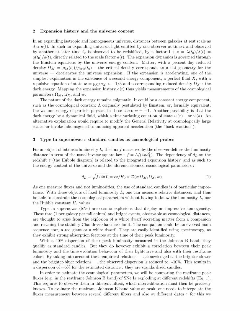
2 Expansion history and the universe content
In an expanding isotropic and homogeneous universe, distances between galaxies at rest scale asd ∝ a(t). In such an expanding universe, light emitted by one observer at time t and observedby another at later time t0 is observed to be redshifted, by a factor 1 + z = λ(t0)/λ(t) =a(t0)/a(t), directly related to the scale factor a(t). The expansion dynamics is governed throughthe Einstein equations by the universe energy content. Matter, with a present day reduceddensity ΩM = ρM (t0)/ρcrit(t0) – the critical density corresponds to a flat geometry for theuniverse — decelerates the universe expansion. If the expansion is accelerating, one of thesimplest explanation is the existence of a second energy component, a perfect fluid X, with arepulsive equation of state w = pX/ρX < −1/3 and a corresponding reduced density ΩX : thedark energy. Mapping the expansion history a(t) thus yields measurements of the cosmologicalparameters ΩM , ΩX , and w.
The nature of the dark energy remains enigmatic. It could be a constant energy component,such as the cosmological constant Λ originally postulated by Einstein, or, formally equivalent,the vacuum energy of particle physics, in these cases w = −1. Another possibility is that thedark energy be a dynamical fluid, whith a time variating equation of state w(z) – or w(a). Analternative explanation would require to modify the General Relativity at cosmologically largescales, or invoke inhomogeneities inducing apparent acceleration (the “back-reaction”).
3 Type Ia supernovae : standard candles as cosmological probes
For an object of intrinsic luminosity L, the flux f measured by the observer defines the luminositydistance in term of the usual inverse square law : f = L/(4πd2L). The dependency of dL on theredshift z (the Hubble diagram) is related to the integrated expansion history, and as such tothe energy content of the universe and the aforementionned cosmological parameters :
dL ≡√f/4πL = cz/H0 ×D(z; ΩM ,ΩX , w) (1)
As one measure fluxes and not luminosities, the use of standard candles is of particular impor-tance. With these objects of fixed luminosity L, one can measure relative distances. and thusbe able to constrain the cosmological parameters without having to know the luminosity L, northe Hubble constant H0 values.
Type Ia supernovae (SNe) are cosmic explosions that display an impressive homogeneity.These rare (1 per galaxy per millenium) and bright events, observable at cosmological distances,are thought to arise from the explosion of a white dwarf accreting matter from a companionand reaching the stability Chandrasekhar mass limit. The companion could be an evolved mainsequence star, a red giant or a white dwarf. They are easily identified using spectroscopy, asthey exhibit strong absorption features at the time of their peak luminosity.
With a 40% dispersion of their peak luminosity measured in the Johnson B band, theyqualify as standard candles. But they do however exhibit a correlation bewteen their peakluminosity and the time evolution behaviour of their lightcurve and also with their restframecolors. By taking into account these empirical relations — acknowledged as the brighter-slowerand the brighter-bluer relations —, the observed dispersion is reduced to ∼10%. This results ina dispersion of ∼5% for the estimated distance : they are standardized candles.
In order to estimate the cosmological parameters, we will be comparing the restframe peakfluxes (e.g. in the restframe Johnson B band) of SNe Ia exploding at different redshifts (Eq. 1).This requires to observe them in different filters, which intercalibration must then be preciselyknown. To evaluate the restframe Johnson B band value at peak, one needs to interpolate thefluxes measurement between several different filters and also at different dates : for this we
use a time dependent spectrophometric model of the SN Ia emission, φ(λ, t), that we constructempirically using spectrophometric data of nearby and distant SNe Ia.
The relationship between distance d, flux f and luminosity L translates simply in the loga-rithmic scales of the magnitudes, involving the corresponding quantities of distance modulus µ,apparent magnitude m and absolute magnitude M :
µ = m?B −M, M = MB − α× shape + β × color (2)
For each SN are estimated the three quantities m?B, corresponding to the peak B flux, the shape
of its lightcurve, and its color at peak. The absolute magnitude of the SN is parametrized sothat MB (fully degenerated with H0
b) corresponds to the luminosity of the (shape=0, color=0)standard SN Ia, and α and β empirically account for the linear corrections corresponding respec-tively to the brighter-slower and the brighter-bluer relations. The cosmological parameters areevaluated through a χ2 fit where µ is compared to its predicted value µcosmo(z; ~θ), ~θ beeing theparameters describing the cosmological model. MB, α and β are fitted on the Hubble diagramalong with the cosmological parameters.
4 The Supernova Legacy Survey
The Supernova Legacy Survey experimental setup and strategy have been designed so as toobtain sufficient quality data and to meet the necessary requirements to control the systematics.
Using the 1 square degree imager Megacam4 mounted on the 3.6-m Canadian-France-HawaiTelescope at Mauna Kea (Hawaii), we obtain a survey deep enough to reduce the Malmquistbias that affects all flux limited surveys6.
Both supernovae discovery and photometry are carried out with one instrument. We canthus devoid all the necessary time to the thorough understanding and the calibration of theinstrument5.
SNLS is a rolling search i.e. we repeat observations of the same 4 fields, enabling the follow-up of the already discovered SN and the detection of newly exploded SN at the same time. It isthus possible to go back in our image data base to recover early, pre-discovery SN photometry.This strategy permits to obtain well sampled lightcurve so as to measure precisely of m?
B andthe lightcurve shape.
The four g r i z filters make it possible to measure the B restframe flux from z=0.1 to z=1.,and also estimate precisely the restframe U-B and B-V colors of the SNe.
By observing 40 nights a year during 5 years (the survey ended in August, 2008), we obtained∼ 450 SNe Ia. All were spectroscopically identified on 10-m class telescopes7,9,10,11, which allowsto limit the non Ia contamination of the sample.
Finally, deep SN-free images stacks were built, to estimate the SNe host galaxy colors,enabling to caracterize the SN environment.
5 SNLS-3 years data Analysis
The constraints and systematic uncertainties from the SNLS-3 data are fully detailed in Conleyet al.12. We present here the SN sample, and some of the different steps involved in the dataanalysis.
SNLS is mainly a European and Canadian project : all the analysis steps were performed withindependent pipelines on each side of the atlantic ocean. Calibration, the spectro-photometricmodel have been improved since the SNLS-1 year results. We also reckon with the host galaxynature influence.
bWe fix H0 = 70 km/s/Mpc.
Finally, when estimating the cosmological parameters, we fully take into account the sytem-atics uncertainties as well as the statistical ones by incorporating them in the covariance matrixthat enter the χ2 minimization procedure. Publishing this full covariance matrix makes it pos-sible to other authors to exploit the SN data without loss of information.
5.1 The supernovae sample
To obtain precise cosmological measurement requires a long enough lever-arm in redshift in theHubble diagram (Eq. 1). We must then add to the SNLS sample complementary supernovaesample coming from external surveys.
The supernovae sample consists of 472 SNe Ia : 123 nearby supernovae, 93 at intermediateredshift form the Sloan Digitized Sky Survey (SDSS) supernovae search, 242 from SNLS and 14Hubble Space Telescope (HST) supernovae.
The nearby sample at z ∼ 0 are gathered from various sources, mainly the Calan/Tololo13, theCfAI-II-III14 and the CSP15 searches. The photometry of one third of this sample is expressedin the Landolt system, to which the Megacam magnitude system must be tied : this cross-calibration requirement induces the main systematic effect in this analysis.
At z > 1, ground observations are difficult, and the HST sample of 14 SNe Ia at z=0.7-1.4complements the high redshift part of the Hubble diagram.
Finally, we add 146 SNe Ia at intermediate redshift z < 0.4 from the SDSS SupernovaSurvey. This component of the SDSS-II survey carried out repeat imaging of a 300 square degreesouthern equatorial stripe using a dedicated 2.5-meter telescope in drifts scan mode at ApachePoint Observatory, New Mexico. They discovered and measured about 500 spectroscopicallyconfirmed SNe Ia. The SDSS filter system has been thouroughly studied and is very similar tothe Megacam system : as a consequence the intercalibration is not as problematic as with thenearby sample.
5.2 Calibration
The calibration procedure of the SNLS data achieved an accuracy of a 1% precision5. It consistsin two steps : the observations are first standardized onto some magnitude system, using acatalog of standard stars of known magnitudes. Then the standard system magnitudes areconverted into absolute fluxes : for this we rely on a reference star, of known magnitudesand spectral energy density (SED). Both SNLS and SDSS survey selected a red reference starmeasured by the HST CALSPEC16 calibration program.
To achieve the required precision, the spatial non-uniformities of the imager were mappedusing dithered observation of dense stellar fields. Because part of the external low-z SNe sampleis calibrated against the Landolt UBVRI system, the Megacam griz system has to be anchoredto the Landolt system. The uncertainties in the Landolt magnitudes of our reference star BD17 4708 are the largest single identified sytematic uncertainty in our current analysis.
5.3 The spectro-photometric model : SALT2 & SIFTO
To obtain for each SN the peak restframe B band magnitude and its lightcurve shape and color,we make use of two independent lightcurve fitters, SIFTO17 and SALT218. The SALT2 modelfor the rest-frame flux parametrization may be written as :
φ(λ, t) = X0 × [M0(λ, t) +X1 ×M1(λ, t)] exp(C CL(λ))
M0 is the mean spectrum and the corresponding parameter X0 is the flux normalisation. M1
describes the main variability of the SNe Ia and happens to naturally reproduce a brighter-slower
relation : X1 is thus equivallent to a lightcurve shape parameter. C corresponds by constructionto a color, and the color law CL encodes the corresponding variation of the model.
M0, M1 and CL are computed using a training sample of nearby and SNLS SNe Ia lightcurvesand spectra. The SNe distances are not used, which makes it possible to use nearby as well asdistant SNe for the training. As the U band data from nearby SNe turned out to be problematic,we used u’ measurement of nearby data when available, and we especially rely on distant SNe goptical data, which sample the UV restframe at a redshift of z ∼ 0.4.
No assumption were made on the color law CL wavelength dependency nor its cause —wether it be due to intrinsic SNe Ia variation or to the reddening by dust somewhere along theline of sight : in the intergalactic medium, the host galaxy or a dust shell around the SN. Asthere is no a-priori knowledge of the dust properties, or its putative evolution with environmentand/or redshift, no prior was set on the distribution of the SNe Ia C (color) parameter.
The color law is mathematically equivalent to an extinction law, but it does differ in theUV part from the dust extinction law as measured in the Milky Way Galaxy19, and also theselective ratio corresponding to β ∼ 2.5−3 in Eq. 2 is smaller than the MW value RB ∼ 4. Thisdifferences can be interpreted either as an unusual extinction occuring in the SN environnement,or an intrinsic color variation dominating the extinction effects.
In a nutshell, we make no assumption and let the SNe Ia data decide : on the range of theircolor value, on the selective ratio β value, and on the color law CL wavelength dependency.
SIFTO model consists of a SED sequence, which is time dilated by a stretch factor dependingon the wavelentgh. It does not contain an explicit color variation law but a linear color relationtailing the color=B-V to the U-B color, and the lightcurve shape.
Comparing the two fitters results permits to evaluate the uncertainties associated with thedifferent choices involved in their design. As they perform equally well, we use the average ofthe two, and propagate the differences as systematic uncertainties.
5.4 Host galaxy nature influence
To address the question whether MB, α and β in Eq. 2 are universal parameters, and whetherthere is any dependence on the SN environnement, we undertook a photometric study of the SNhost galaxies. Their ugriz fluxes were measured on deep stacked images free of SN light, andsupplementary data from the WIRDS survey20 in the IR part was added. The photometric dataare fitted by templates spectral energy densities, using the redshift information from the SN :this permits to derive the restframe colors of the galaxy, and its intrinsic luminosity. Using SEDscomputed with the population synthesis model PEGASE.221, one can recover the caracteristicsof the synthetic model galaxy, such as its present star formation rate (SFR), and its stellar masscontent.
The host galaxies properties are known22,23 to correlate with the SNe shape parameter :SNe Ia in red/high SFR/ low mass/faint galaxies are slower, and as a consequence, brighter.This could result from different evolutionary pathes leading to the explosion of the parent whitedwarf24,25.
Although in massive galaxies the mean SN Ia is fainter, it has been recently brought toevidence26,27,28 that the standard (shape=0, color=0) SN Ia is in fact there slightly brighter, ata 4−σ significance : this is a subtle effect - 0.08 mag, or 8% - smaller than the shape or colorcorrections.
We take this dependency into account by splitting the sample at M = 1010M between lowand high mass galaxies, and using two different MB values for each sub-sample. This leads toa significative improvement in the cosmological fits (at a ∼ 4σ level) and also to a shift in themeasured cosmology : for a flat universe, ΩM value is shifted by an amount comparable to thestatistical precision.
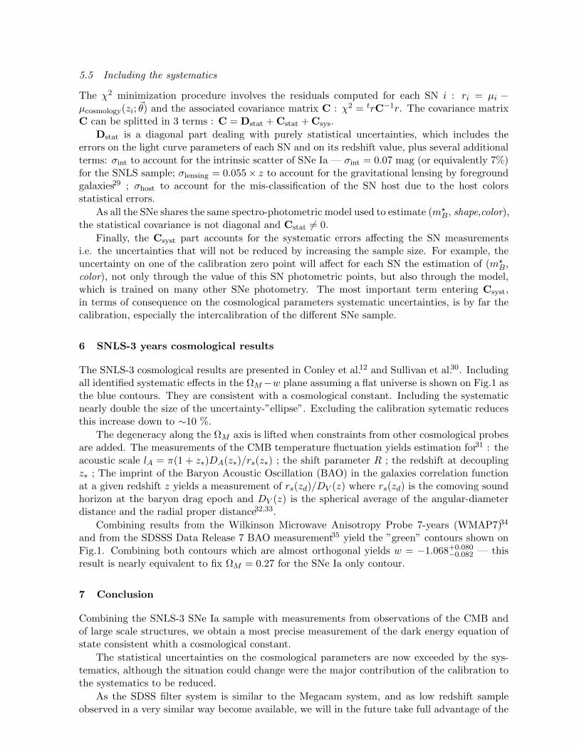
5.5 Including the systematics
The χ2 minimization procedure involves the residuals computed for each SN i : ri = µi −µcosmology(zi; ~θ) and the associated covariance matrix C : χ2 = trC−1r. The covariance matrixC can be splitted in 3 terms : C = Dstat + Cstat + Csys.
Dstat is a diagonal part dealing with purely statistical uncertainties, which includes theerrors on the light curve parameters of each SN and on its redshift value, plus several additionalterms: σint to account for the intrinsic scatter of SNe Ia — σint = 0.07 mag (or equivalently 7%)for the SNLS sample; σlensing = 0.055× z to account for the gravitational lensing by foregroundgalaxies29 ; σhost to account for the mis-classification of the SN host due to the host colorsstatistical errors.
As all the SNe shares the same spectro-photometric model used to estimate (m?B, shape,color),
the statistical covariance is not diagonal and Cstat 6= 0.
Finally, the Csyst part accounts for the systematic errors affecting the SN measurementsi.e. the uncertainties that will not be reduced by increasing the sample size. For example, theuncertainty on one of the calibration zero point will affect for each SN the estimation of (m?
B,color), not only through the value of this SN photometric points, but also through the model,which is trained on many other SNe photometry. The most important term entering Csyst,in terms of consequence on the cosmological parameters systematic uncertainties, is by far thecalibration, especially the intercalibration of the different SNe sample.
6 SNLS-3 years cosmological results
The SNLS-3 cosmological results are presented in Conley et al.12 and Sullivan et al.30. Includingall identified systematic effects in the ΩM−w plane assuming a flat universe is shown on Fig.1 asthe blue contours. They are consistent with a cosmological constant. Including the systematicnearly double the size of the uncertainty-”ellipse”. Excluding the calibration sytematic reducesthis increase down to ∼10 %.
The degeneracy along the ΩM axis is lifted when constraints from other cosmological probesare added. The measurements of the CMB temperature fluctuation yields estimation for31 : theacoustic scale lA = π(1 + z∗)DA(z∗)/rs(z∗) ; the shift parameter R ; the redshift at decouplingz∗ ; The imprint of the Baryon Acoustic Oscillation (BAO) in the galaxies correlation functionat a given redshift z yields a measurement of rs(zd)/DV (z) where rs(zd) is the comoving soundhorizon at the baryon drag epoch and DV (z) is the spherical average of the angular-diameterdistance and the radial proper distance32,33.
Combining results from the Wilkinson Microwave Anisotropy Probe 7-years (WMAP7)34
and from the SDSSS Data Release 7 BAO measurement35 yield the ”green” contours shown onFig.1. Combining both contours which are almost orthogonal yields w = −1.068+0.080
−0.082 — thisresult is nearly equivalent to fix ΩM = 0.27 for the SNe Ia only contour.
7 Conclusion
Combining the SNLS-3 SNe Ia sample with measurements from observations of the CMB andof large scale structures, we obtain a most precise measurement of the dark energy equation ofstate consistent whith a cosmological constant.
The statistical uncertainties on the cosmological parameters are now exceeded by the sys-tematics, although the situation could change were the major contribution of the calibration tothe systematics to be reduced.
As the SDSS filter system is similar to the Megacam system, and as low redshift sampleobserved in a very similar way become available, we will in the future take full advantage of the
0.0 0.1 0.2 0.3 0.4 0.5Ωm
−2.0
−1.5
−1.0
−0.5
w
99.7%
95.4%
68.3
%
SNLS3
BAO+WMAP7
With all systematics
Figure 1: Confidence contours in the plane ΩM − w obtained when fitting with the SNe Ia -only fit (in blue).A flat cosmology is assumed. Taking into account the systematics nearly double the size of the contour. Thedegeneracy along the ΩM axis is lifted when adding the SDSS BAO and WMAP7 CMB constraints (in green).
inter-calibration improvements possibilities.
In the near future, the SkyMapper36 project will provide nearby SNe Ia at z ∼ 0.05 discoveredand observed with a similar technique than SNLS. Next generation surveys either ground-basedsuch as the Large Synodic Survey Telescope (LSST) project or space-born such as the WideField Infrared Survey Telescope (WFIRST) or the EUCLID mission could bring thousands ofdistant SNe Ia up to z ∼ 1.5. Providing an adapted strategy , they could adress the question ofa time variating equation of state for the dark energy, w(a) = w0 + (1− a)wa
37.
References
1. A. G. Riess et al., Astronomical Journal 116, 1009 (1998)2. S. Perlmutter et al., Astrophysical Journal 517, 565 (1999)3. J. Frieman, “Lectures on Dark Energy and Cosmic Acceleration”, arXiv:0904.18324. O. Boulade et al., Instrument Design and Performance for Optical/Infrared Ground-based
Telescopes, ed M.Iye & A.F.M. Moorwood, Proc SPIE, 4841, 725. N. Regnault et al., Astronomy and Astrophysics 506, 999 (2009)6. C. Perrett et al., Astronomical Journal 140, 518 (2010)7. D.A. Howell, et al., Astrophysical Journal 634, 1190 (2005)8. T.J. Bronder, et al., Astronomy and Astrophysics 477, 717 (2008)9. R.S. Ellis, et al., Astrophysical Journal 674, 51 (2008)
10. C. Balland et al., Astrophysical Journal 507, 85 (2009)11. E. Walker et al., Monthly Notices of the Royal Atronomical Society 410, 1262 (2011)12. A. Conley et al., The Astrophysical Journal Supplement 192, 1 (2011)13. M. Hamuy et al., Astronomical Journal 112, 2408 (1996)14. M. Hicken et al., Astrophysical Journal 700, 331 (2009)15. C. Contreras et al., Astronomical Journal 139, 519 (2010)16. Bohlin, R.C. Astronomical Journal 111, 1743 (1996)17. A. Conley et al., Astronomical Journal 681, 482 (2008)18. J. Guy et al., Astronomy and Astrophysics 466, 11 (2007)19. J.A. Cardelli et al., Astrophysical Journal 345, 245 (1989)20. R. Bielby et al., in preparation21. D. Le Borgne et al., Astronomy and Astrophysics 386, 446 (2002)
22. M. Hamuy et al., Astronomical Journal 120, 1479 (2000)23. M. Sullivan et al., Astrophysical Journal 648, 868 (2006)24. E. Scannapieco et al., Astronomical Journal 629, L85 (2005)25. F. Manucci et al., Monthly Notices of the Royal Atronomical Society 370, 773 (2006)26. P.L. Kelly et al., Astrophysical Journal 715, 743 (2010)27. H. Lampeitl et al., Astrophysical Journal 722, 766 (2010)28. M. Sullivan et al., Monthly Notices of the Royal Atronomical Society 406, 782 (2010)29. M. Jonsson et al., Monthly Notices of the Royal Atronomical Society 405, 535 (2010)30. M. Sullivan et al., submitted31. E. Komatsu et al., The Astrophysical Journal Supplement 180, 330 (2009)32. D. Eisentein et al., Astrophysical Journal 633, 560 (2005)33. C. Blake et al., arXiv:1105.286234. E. Komatsu et al., The Astrophysical Journal Supplement 192, 18 (2011)35. W.J. Percival et al., Monthly Notices of the Royal Atronomical Society 401, 2148 (2010)36. S.C. Keller et al., Publications of the Astronomical Society of Australia 24, 1 (2007).37. P. Astier et al., Astronomy and Astrophysics 525, 7 (2011)
IS DARK ENERGY NEEDED?
A. BLANCHARD
Universite de Toulouse; UPS-OMP; IRAP; ; 14, avenue Edouard Belin
F-31400 Toulouse, France
Evidence for an accelerated expansion of the universe as it has been revealed ten years ago bythe Hubble diagram of distant type Ia supernovae represents the lattest revolution of moderncosmology with profound impact for fundamental physics. The construction of a scientficmodel of the universe is probably one of the most fascinating success of XXth century sci-ence. During its construction, there has been regular debates regarding whether the wholeconstruction being scientific. Indeed, existing evidence for the big bang picture, includingits modern version the Λ CDM picture, comes from astrophysical observations. It is there-fore interesting and essantial to critically examine the present situation of the astrophysicalobservations and the possible limitation in their interpretation. In this paper, the main var-ious observational probes at the fundation of the standard view are presented as well as thestandard framework to interpret them with special attention to the complex astrophysics andtheoretical hypotheses that may limit robust interpretation. It is concluded that, even whenscrutinized with sceptical eyes, the evidence for a homogenous accelerated universe, governedby standard Friedman-Lemaıtre equations, is robust. Therefore the standard Λ CDM picturehas to be regarded as the most successful scientific representation of the universe by now,possibly being the only one clearly consistent with the whole family of observations relevantto cosmology. The fact that this model could in principle be easily falsified makes it a verygood scientific theory. Understanding the origin of acceleration is probably one of the mostchallenging problem of fundamental physics.
1 Introduction
The determination of cosmological parameters has been one of the most important objectivesof cosmologists after the discovery of the expansion of the universe by Hubble. It is importanto provide a precise framework but also in the perspective to test the model. This problematichas become specially important after the theory of inflation which predicted the universe to beflat, something which was first interpret as a prediction for Ωm = 1. Although Peebles16 earlynoticed that the actual prediction of inflation was Ωm + ΩΛ = 1, little attention was paid tothe cosmological constant until the detection of small scale fluctuation in the microwave sky13.Indeed these measurements were in agreement with a flat universe and inconsistent with opencosmological models with Ωm ∼ 0.3. However the evidence for acceleration as obtained from theHubble diagram of distant supernovae has been the observational evidence that has lead to arapid change of paradigm. Since that time the improvment in the accuracy on the estimationsof cosmological parameters has been dramatic. This paper is a shortened version of a recentreview published by the author 5.
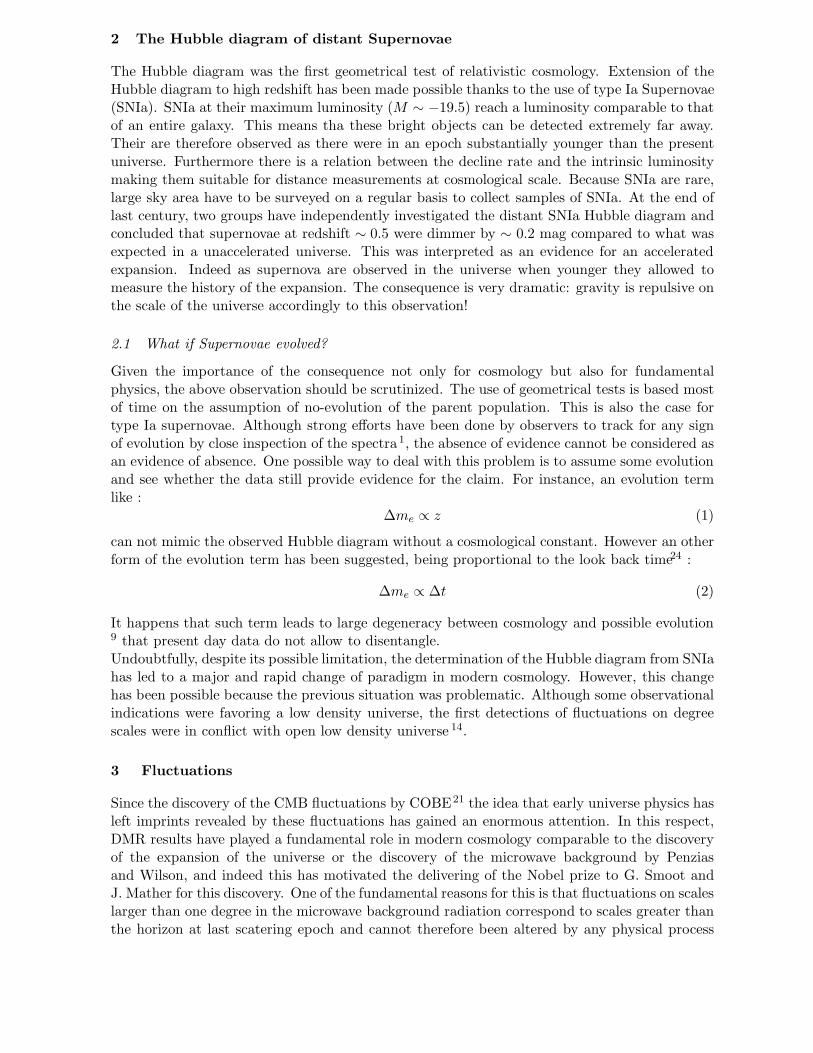
2 The Hubble diagram of distant Supernovae
The Hubble diagram was the first geometrical test of relativistic cosmology. Extension of theHubble diagram to high redshift has been made possible thanks to the use of type Ia Supernovae(SNIa). SNIa at their maximum luminosity (M ∼ −19.5) reach a luminosity comparable to thatof an entire galaxy. This means tha these bright objects can be detected extremely far away.Their are therefore observed as there were in an epoch substantially younger than the presentuniverse. Furthermore there is a relation between the decline rate and the intrinsic luminositymaking them suitable for distance measurements at cosmological scale. Because SNIa are rare,large sky area have to be surveyed on a regular basis to collect samples of SNIa. At the end oflast century, two groups have independently investigated the distant SNIa Hubble diagram andconcluded that supernovae at redshift ∼ 0.5 were dimmer by ∼ 0.2 mag compared to what wasexpected in a unaccelerated universe. This was interpreted as an evidence for an acceleratedexpansion. Indeed as supernova are observed in the universe when younger they allowed tomeasure the history of the expansion. The consequence is very dramatic: gravity is repulsive onthe scale of the universe accordingly to this observation!
2.1 What if Supernovae evolved?
Given the importance of the consequence not only for cosmology but also for fundamentalphysics, the above observation should be scrutinized. The use of geometrical tests is based mostof time on the assumption of no-evolution of the parent population. This is also the case fortype Ia supernovae. Although strong efforts have been done by observers to track for any signof evolution by close inspection of the spectra1, the absence of evidence cannot be considered asan evidence of absence. One possible way to deal with this problem is to assume some evolutionand see whether the data still provide evidence for the claim. For instance, an evolution termlike :
∆me ∝ z (1)
can not mimic the observed Hubble diagram without a cosmological constant. However an otherform of the evolution term has been suggested, being proportional to the look back time24 :
∆me ∝ ∆t (2)
It happens that such term leads to large degeneracy between cosmology and possible evolution9 that present day data do not allow to disentangle.Undoubtfully, despite its possible limitation, the determination of the Hubble diagram from SNIahas led to a major and rapid change of paradigm in modern cosmology. However, this changehas been possible because the previous situation was problematic. Although some observationalindications were favoring a low density universe, the first detections of fluctuations on degreescales were in conflict with open low density universe 14.
3 Fluctuations
Since the discovery of the CMB fluctuations by COBE21 the idea that early universe physics hasleft imprints revealed by these fluctuations has gained an enormous attention. In this respect,DMR results have played a fundamental role in modern cosmology comparable to the discoveryof the expansion of the universe or the discovery of the microwave background by Penziasand Wilson, and indeed this has motivated the delivering of the Nobel prize to G. Smoot andJ. Mather for this discovery. One of the fundamental reasons for this is that fluctuations on scaleslarger than one degree in the microwave background radiation correspond to scales greater thanthe horizon at last scatering epoch and cannot therefore been altered by any physical process
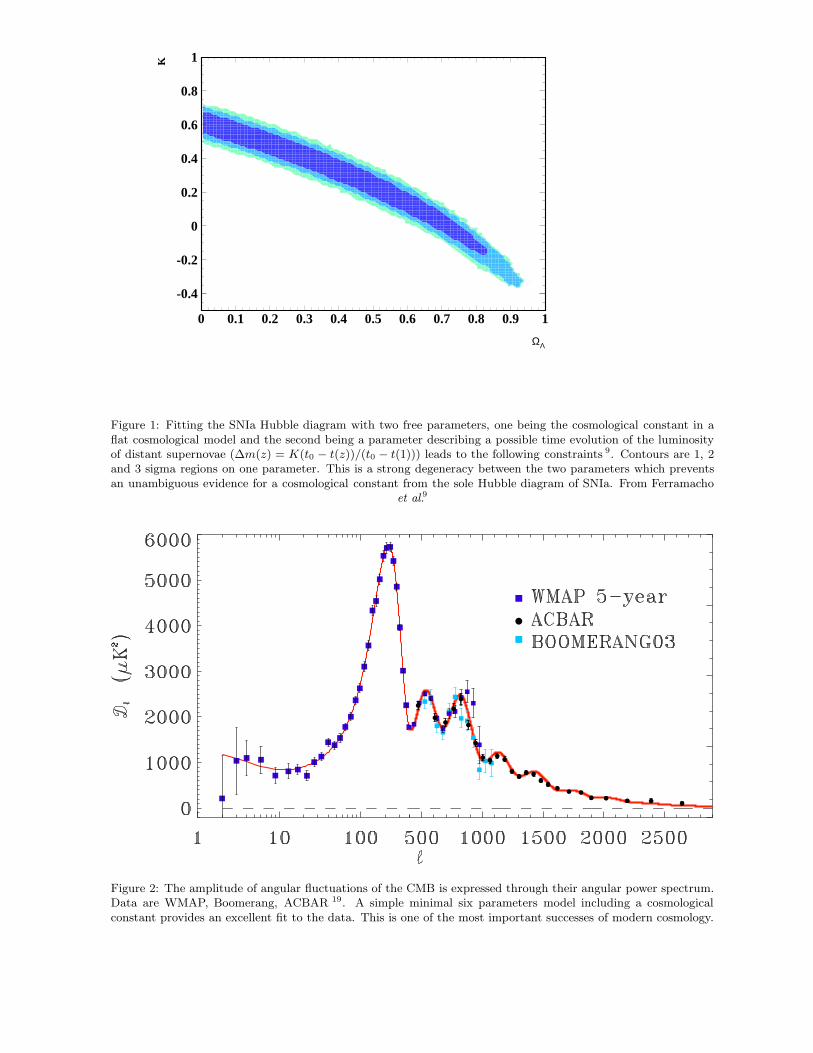
-0.4
-0.2
0
0.2
0.4
0.6
0.8
1
0 0.1 0.2 0.3 0.4 0.5 0.6 0.7 0.8 0.9 1
ΩΛ
K
Figure 1: Fitting the SNIa Hubble diagram with two free parameters, one being the cosmological constant in aflat cosmological model and the second being a parameter describing a possible time evolution of the luminosityof distant supernovae (∆m(z) = K(t0 − t(z))/(t0 − t(1))) leads to the following constraints 9. Contours are 1, 2and 3 sigma regions on one parameter. This is a strong degeneracy between the two parameters which preventsan unambiguous evidence for a cosmological constant from the sole Hubble diagram of SNIa. From Ferramacho
et al.9
Figure 2: The amplitude of angular fluctuations of the CMB is expressed through their angular power spectrum.Data are WMAP, Boomerang, ACBAR 19. A simple minimal six parameters model including a cosmologicalconstant provides an excellent fit to the data. This is one of the most important successes of modern cosmology.
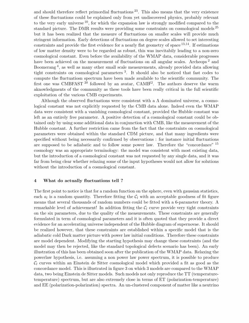
and should therefore reflect primordial fluctuations 23. This also means that the very existenceof these fluctuations could be explained only from yet undiscovered physics, probably relevantto the very early universe 10, for which the expansion law is strongly modified compared to thestandard picture. The DMR results were providing some constraints on cosmological models 25
but it has been realized that the measure of fluctuations on smaller scales will provide muchstringent information. Early detections of fluctuations on degree scales allowed to set interestingconstraints and provide the first evidence for a nearly flat geometry of space 13,14. If estimationsof low matter density were to be regarded as robust, this was inevitabily leading to a non-zerocosmological constant. Even before the availability of the WMAP data, considerable progresseshave been achieved on the measurement of fluctuations on all angular scales. Archeops 2 andBoomerang 4, as well as many other small scale measurements, already provided data allowingtight constraints on cosmological parameters 3. It should also be noticed that fast codes tocompute the fluctuatiosn spectrum have been made available to the scientific community. Thefirst one was CMBFAST 20 followed by an avatar, CAMB12. The authors deserve the warmaknowledgments of the community as these tools have been really critical in the full scientificexploitation of the various CMB experiments.
Although the observed fluctuations were consistent with a Λ dominated universe, a cosmo-logical constant was not explicitly requested by the CMB data alone. Indeed even the WMAPdata were consistent with a vanishing cosmological constant, provided the Hubble constant wasleft as an entirely free parameter. A positive detection of a cosmological constant could be ob-tained only by using some additional data in conjunction with CMB, like the measurement of theHubble constant. A further restriction came from the fact that the constraints on cosmologicalparameters were obtained within the standard CDM picture, and that many ingredients werespecified without being necessarily confirmed by observations : for instance initial fluctuationsare supposed to be adiabatic and to follow some power law. Therefore the “concordance” 15
cosmology was an appropriate terminology: the model was consistent with most existing data,but the introduction of a cosmological constant was not requested by any single data, and it wasfar from being clear whether relaxing some of the input hypotheses would not allow for solutionswithout the introduction of a cosmological constant.
4 What do actually fluctuations tell ?
The first point to notice is that for a random function on the sphere, even with gaussian statistics,each al is a random quantity. Therefore fitting the Cl with an acceptable goodness of fit figuremeans that several thousands of random numbers could be fitted with a 6-parameter theory. Aremarkable level of achievement! In addition fitting the Cl curve provide very tight constraintson the six parameters, due to the quality of the measurements. These constraints are generallyformulated in term of cosmological parameters and it is often quoted that they provide a directevidence for an accelerating universe independent of the Hubble diagram of supernovae. It shouldbe realized however, that these constraints are established within a specific model that is theadiabatic cold Dark matter picture with power law initial conditions. Therefore these constraintsare model dependent. Modifying the starting hypothesis may change these constraints (and themodel may then be rejected, like the standard topological defects scenario has been). An earlyillustration of this has been obtained soon after the publication of the WMAP data. Relaxing thepowerlaw hypothesis, i.e. assuming a non power law power spectrum, it is possible to produceCl curves within an Einstein de Sitter cosmological model which provided a fit as good as theconcordance model. This is illustrated in figure 3 on which 3 models are compared to the WMAPdata, two being Einstein de Sitter models. Such models not only reproduce the TT (temperature-temperature) spectrum, but are also extremely close in terms of ET (polarization-temperature)and EE (polarization-polarization) spectra. An un-clustered component of matter like a neutrino
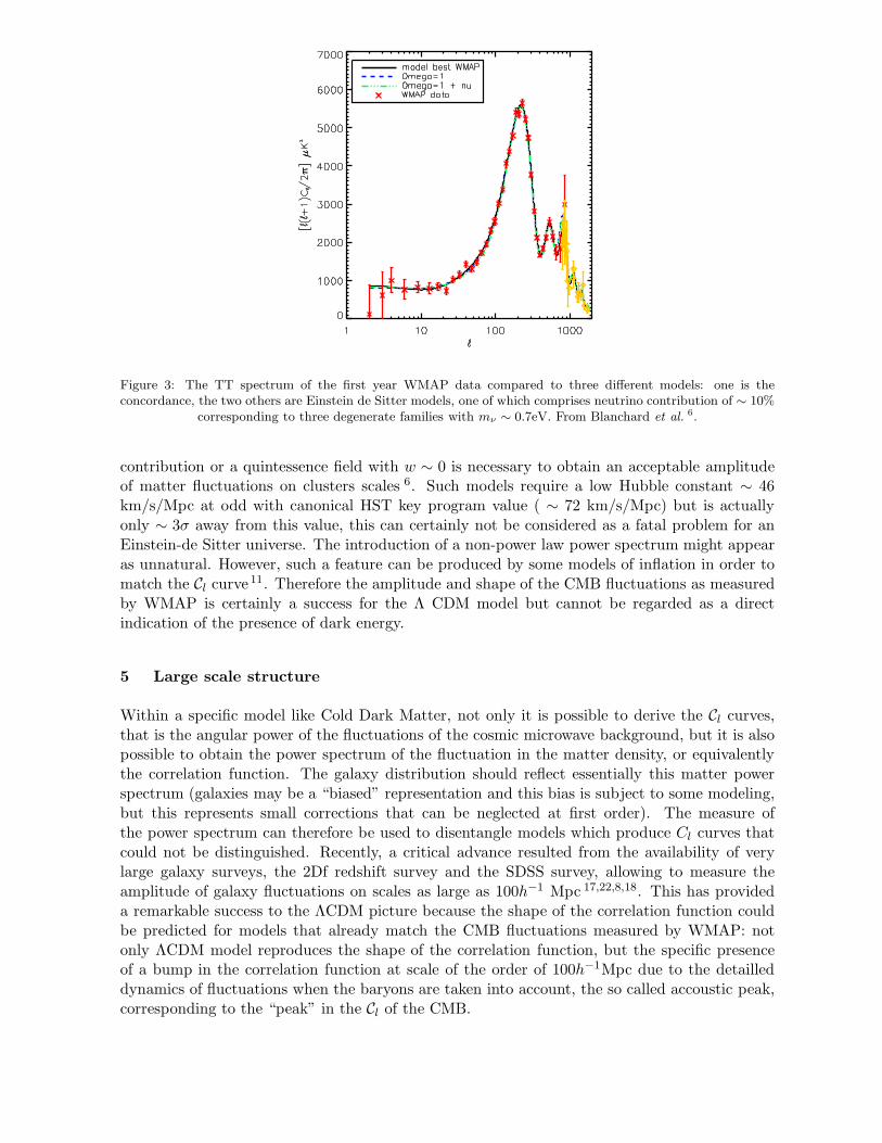
Figure 3: The TT spectrum of the first year WMAP data compared to three different models: one is theconcordance, the two others are Einstein de Sitter models, one of which comprises neutrino contribution of ∼ 10%
corresponding to three degenerate families with mν ∼ 0.7eV. From Blanchard et al.6.
contribution or a quintessence field with w ∼ 0 is necessary to obtain an acceptable amplitudeof matter fluctuations on clusters scales 6. Such models require a low Hubble constant ∼ 46km/s/Mpc at odd with canonical HST key program value ( ∼ 72 km/s/Mpc) but is actuallyonly ∼ 3σ away from this value, this can certainly not be considered as a fatal problem for anEinstein-de Sitter universe. The introduction of a non-power law power spectrum might appearas unnatural. However, such a feature can be produced by some models of inflation in order tomatch the Cl curve 11. Therefore the amplitude and shape of the CMB fluctuations as measuredby WMAP is certainly a success for the Λ CDM model but cannot be regarded as a directindication of the presence of dark energy.
5 Large scale structure
Within a specific model like Cold Dark Matter, not only it is possible to derive the Cl curves,that is the angular power of the fluctuations of the cosmic microwave background, but it is alsopossible to obtain the power spectrum of the fluctuation in the matter density, or equivalentlythe correlation function. The galaxy distribution should reflect essentially this matter powerspectrum (galaxies may be a “biased” representation and this bias is subject to some modeling,but this represents small corrections that can be neglected at first order). The measure ofthe power spectrum can therefore be used to disentangle models which produce Cl curves thatcould not be distinguished. Recently, a critical advance resulted from the availability of verylarge galaxy surveys, the 2Df redshift survey and the SDSS survey, allowing to measure theamplitude of galaxy fluctuations on scales as large as 100h−1 Mpc 17,22,8,18. This has provideda remarkable success to the ΛCDM picture because the shape of the correlation function couldbe predicted for models that already match the CMB fluctuations measured by WMAP: notonly ΛCDM model reproduces the shape of the correlation function, but the specific presenceof a bump in the correlation function at scale of the order of 100h−1Mpc due to the detailleddynamics of fluctuations when the baryons are taken into account, the so called accoustic peak,corresponding to the “peak” in the Cl of the CMB.
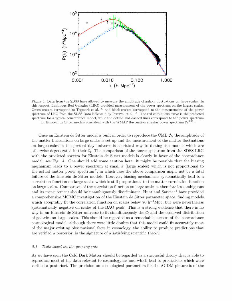
Figure 4: Data from the SDSS have allowed to measure the amplitude of galaxy fluctuations on large scales. Inthis respect, Luminous Red Galaxies (LRG) provided measurement of the power spectrum on the largest scales.Green crosses correspond to Tegmark et al. 22 and black crosses correspond to the measurements of the powerspectrum of LRG from the SDSS Data Release 5 by Percival et al. 18. The red continuous curve is the predictedspectrum for a typical concordance model, while the dotted and dashed lines correspond to the power spectrum
for Einstein de Sitter models consistent with the WMAP fluctuation angular power spectrum Cl
6,11.
Once an Einstein de Sitter model is built in order to reproduce the CMB Cl, the amplitude ofthe matter fluctuations on large scales is set up and the measurement of the matter fluctuationson large scales in the present day universe is a critical way to distinguish models which areotherwise degenerated in their Cl. The comparison of the power spectrum from the SDSS LRGwith the predicted spectra for Einstein de Sitter models is clearly in favor of the concordancemodel, see Fig. 4. One should add some caution here: it might be possible that the biasingmechanism leads to a power spectrum at small k (large scales) which is not proportional tothe actual matter power spectrum 7, in which case the above comparison might not be a fatalfailure of the Einstein de Sitter models. However, biasing mechanisms systematically lead to acorrelation function on large scales which is still proportional to the matter correlation functionon large scales. Comparison of the correlation function on large scales is therefore less ambiguousand its measurement should be unambiguously discriminant. Hunt and Sarkar 11 have provideda comprehensive MCMC investigation of the Einstein de Sitter parameter space, finding modelswhich acceptably fit the correlation function on scales below 70 h−1Mpc, but were neverthelesssystematically negative on scales of the BAO peak. This is a strong evidence that there is noway in an Einstein de Sitter universe to fit simultaneously the Cl and the observed distributionof galaxies on large scales. This should be regarded as a remarkable success of the concordancecosmological model: although there were little doubts that this model could fit accurately mostof the major existing observational facts in cosmology, the ability to produce predictions thatare verified a posteriori is the signature of a satisfying scientific theory.
5.1 Tests based on the growing rate
As we have seen the Cold Dark Matter should be regarded as a successful theory that is able toreproduce most of the data relevant to cosmologyhas and which lead to predictions which wereverified a posteriori. The precision on cosmological parameters for the ΛCDM picture is of the
Parameter Vanilla Vanilla + Ωk Vanilla + w Vanilla + Ωk + w
Ωbh2 0.0227 ± 0.0005 0.0227 ± 0.0006 0.0228 ± 0.0006 0.0227 ± 0.0005
Ωch2 0.112 ± 0.003 0.109 ± 0.005 0.109 ± 0.005 0.109 ± 0.005
θ 1.042 ± 0.003 1.042 ± 0.003 1.042 ± 0.003 1.042 ± 0.003τ 0.085 ± 0.017 0.088 ± 0.017 0.087 ± 0.017 0.088 ± 0.017ns 0.963 ± 0.012 0.964 ± 0.013 0.967 ± 0.014 0.964 ± 0.014Ωk 0 −0.005 ± 0.007 0 −0.005 ± 0.0121w −1 −1 −0.965 ± 0.056 −1.003 ± 0.102
Ωλ 0.738 ± 0.015 0.735 ± 0.016 0.739 ± 0.014 0.733 ± 0.020Age 13.7 ± 0.1 13.9 ± 0.4 13.7 ± 0.1 13.9 ± 0.6ΩM 0.262 ± 0.015 0.270 ± 0.019 0.261 ± 0.020 0.272 ± 0.029σ8 0.806 ± 0.023 0.791 ± 0.030 0.816 ± 0.014 0.788 ± 0.042zre 10.9 ± 1.4 11.0 ± 1.5 11.0 ± 1.5 11.0 ± 1.4h 0.716 ± 0.014 0.699 ± 0.028 0.713 ± 0.015 0.698 ± 0.037
Table 1: Summary of the mean values and 68% confidence intervals for the cosmological parameters of the ΛCDMmodel constrained from CMB, SNIa and BAO for different models (θ is the ratio of sound horizon to angulardiameter distance). These constraints are quite tight, most of them are below 5%, and are stable when additional
degrees of freedom are added to the model (w, Ωk), adapted from 9.
order of 5% at most, with accuracy close to 1% in some cases. Of course this doesn’t mean it isthe “right” theory; science does not provide “right” theories but only theories that reproduce allexisting data and which are able to lead to predictions that can lead to its invalidation. This isthe principle that to be scientific a statement has to be falsifiable accordingly to Kark Popper.
It is therefore the only possible path to continue to increase the accuracy of existing mea-surements and to develop new ways to test the theory. There is a way to test cosmologicalmodels which is fundamentally different from geometrical tests: it is based on the growing rateof fluctuations under their own gravity. In principle the abundance of clusters and weak lensingmeasurements are both sensitive to this growing rate. I do not think that they have by nowreach a level of precision that makes them useful, but it is certainly a way on which efforts willconcentrated in the future, in particular thanks to space mission like EUCLID or WFIRST.Measurements of this growing rate would allow to test whether predictions of general relativityat the scale of the universe are verified or if we have to turn to alternatives.
6 Conclusions
The Copernician model of the world was the first revolution of a series in the constructionof modern cosmology, and the discovery of the accelerated expansion being the latest in date.Theoretical considerations have always been a source of remarkable observational investigationsand Cosmology has always benefited from the confrontation of models with observations. Sincethe thirties, the big bang picture, the modern version of Lemaıtre’s primeval atom has beenremarkably successful, based on simple assumptions and physical laws that have been validatedby accurate experimental results. Although alternative theories have been developed, thesealternative were based on hypothetical unknown physics advocated to interpret cosmologicalobservations. None of these alternative theories has produced significant predictions differingfrom the standard view that would have been comforted a posteriori. Rather new observations inagreement with predictions of the big bang picture necessitated deep revision of the unorthodoxviews, at the cost of rather ad hoc assumptions added to fit the new observations. The situationhas evolved when the standard picture has necessitated the introduction of new ingredients,
first dark matter and more recently dark energy. The very nature of these new ingredients,which are supposed to dominate the mean density of the universe has not been established bydirect laboratory experiments, nor by astronomical observations, and this situation may sometime lead to the question whether cosmologists have not introduced new aethers. We had theopportunity to see that the situation is not so bad. The introduction of -cold- non-baryonicdark matter has led to specific predictions, the amplitude and shape of the fluctuations of thecosmological background on various angular scales, which were verified with high accuracy. Thepresence of dark energy has lead to a specific prediction, the shape of the matter power spectrumon large scales, which has been verified a posteriori. Although the inclusion of a cosmologicalconstant was concomitant to general relativity, the actual origin of dark energy remains totallyunknown and the presence of dark energy in the present day universe represents probably themost fundamental and unexpected new element in modern physics.
References
1. Balland, C., et al., A&A, 507, 85 (2009)2. Benoıt, A., et al., A&A, 399, L19 (2003).3. Benoıt, A., et al., A&A, 399, L25 (2003).4. de Bernardis, P., et al., Nature, 404, 955 (2000).5. Blanchard, A., A&A Rev., 18, 595 (2010).6. Blanchard, A., Douspis, M., Rowan-Robinson, M., & Sarkar, S., A&A, 412, 35 (2003).7. Durrer, R., Gabrielli, A., Joyce, M., & Sylos Labini, F., ApJL, 585, L1 (2003).8. Eisenstein, D. J., et al., ApJ, 633, 560 (2005).9. Ferramacho, L. D., Blanchard, A., & Zolnierowski, Y., A&A, 499, 21 (2009).
10. Guth, A. H., Phys. Rev. D, 23, 347 (1981).11. Hunt, P., & Sarkar, S., Phys. Rev. D, 76, 123504 (2007).12. Lewis, A., Challinor, A., & Lasenby, A., http://camb.info/, ApJ, 538, 473 (2000).13. Lineweaver, C. H., Barbosa, D., Blanchard, A., & Bartlett, J. G., A&A, 322, 365 (1997).14. Lineweaver, C. H., & Barbosa, D., ApJ, 496, 624 (1998).15. Ostriker, J. P., & Steinhardt, P. J., Nature, 377, 600 (1995).16. Peebles, P. J. E. 1984, ApJ, 284, 43917. Percival, W. J., et al., MNRAS, 327, 1297 (2001).18. Percival, W. J., et al., ApJ, 657, 645 (2007).19. Reichardt, C. L., et al., ApJ, 694, 1200 (2009).20. Seljak, U., & Zaldarriaga, M. ApJ, 469, 437 (1996).21. Smoot, G. F., et al., ApJL, 396, L1 (1992).22. Tegmark, M., et al., Phys. Rev. D, 74, 123507 (2006).23. Weinberg, S., Gravitation and Cosmology, ISBN 0-471-92567-5. Wiley-VCH (1972).24. Wright, E. L., arXiv:astro-ph/0201196 (2002).25. Wright, E. L., et al., ApJL, 396, L13 (1992).
Testing MOND in the Solar System
Luc BLANCHETGRεCO, Institut d’Astrophysique de Paris, CNRS,
Universite Pierre et Marie Curie, 98bis boulevard Arago, 75014 Paris, France
Jerome NOVAKLaboratoire Univers et Theories, Observatoire de Paris, CNRS,
Universite Denis Diderot, 5 place Jules Janssen, 92190 Meudon, France
The Modified Newtonian Dynamics (MOND) generically predicts a violation of the strongversion of the equivalence principle. As a result the gravitational dynamics of a systemdepends on the external gravitational field in which the system is embedded. This so-calledexternal field effect is shown to imply the existence of an anomalous quadrupolar correction,along the direction of the external galactic field, in the gravitational potential felt by planets inthe Solar System. We compute this effect by a numerical integration of the MOND equationin the presence of an external field, and deduce the secular precession of the perihelion ofplanets induced by this effect. We find that the precession effect is rather large for outergaseous planets, and in the case of Saturn is comparable to, and in some cases marginallyexcluded by published residuals of precession permitted by the best planetary ephemerides.
1 The external field effect with MOND
The Modified Newtonian Dynamics (MOND) has been proposed 1 as an alternative to the darkmatter paradigm 2. At the non-relativistic level, the best formulation of MOND is the modifiedPoisson equation 3,
∇ ·
[
µ
(
g
a0
)
∇U
]
= −4πGρ , (1)
where ρ is the density of ordinary (baryonic) matter, U is the gravitational potential, g = ∇Uis the gravitational field and g = |g| its ordinary Euclidean norm. The modification of thePoisson equation is encoded in the MOND function µ(y) of the single argument y ≡ g/a0, wherea0 = 1.2 × 10⁻¹⁰ m/s2 denotes the MOND constant acceleration scale. The MOND functioninterpolates between the MOND regime corresponding to weak gravitational fields y = g/a0 ≪ 1,for which it behaves as µ(y) = y + o(y), and the Newtonian strong-field regime y ≫ 1, where µreduces to 1 so that we recover the usual Newtonian gravity.
An important consequence of the non-linearity of Eq. (1) in the MOND regime, is thatthe gravitational dynamics of a system is influenced (besides the well-known tidal force) bythe external gravitational environment in which the system is embedded. This is known asthe external field effect (EFE), which has non-trivial implications for non-isolated gravitatingsystems. The EFE was conjectured to explain the dynamics of open star clusters in our galaxy1,since they do not show evidence of dark matter despite the involved weak internal accelerations(i.e. below a0). The EFE effect shows that the dynamics of these systems should actually be
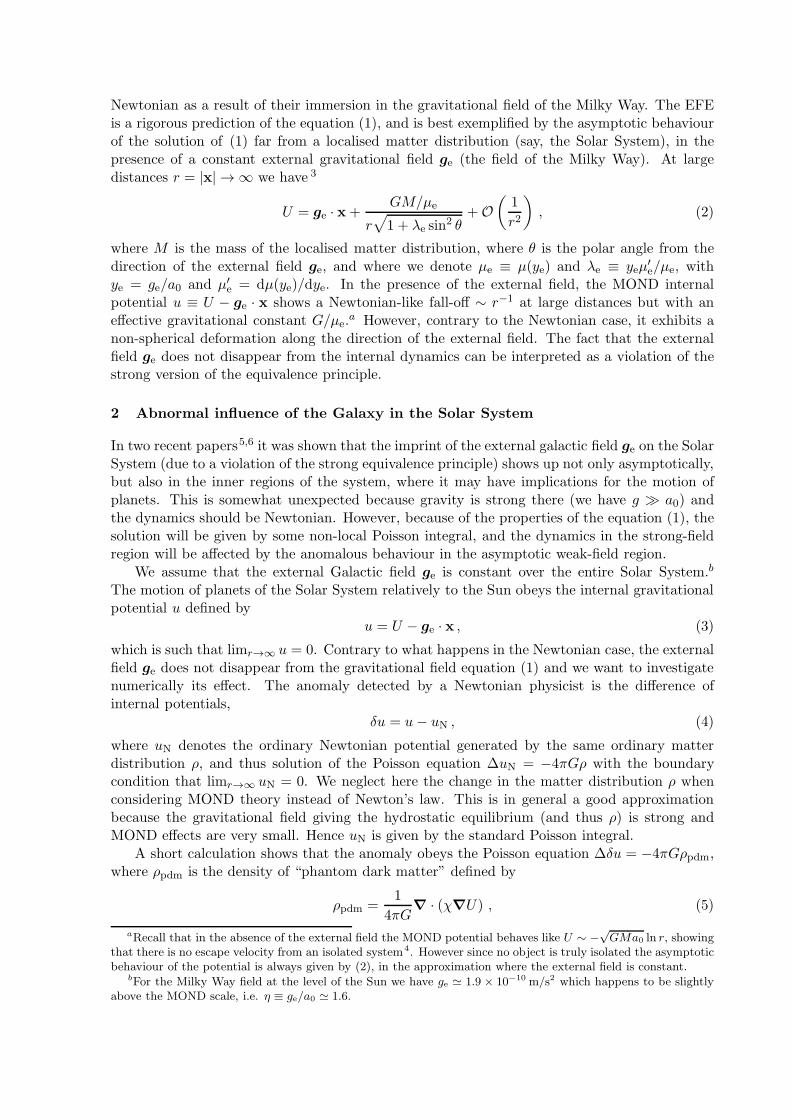
Newtonian as a result of their immersion in the gravitational field of the Milky Way. The EFEis a rigorous prediction of the equation (1), and is best exemplified by the asymptotic behaviourof the solution of (1) far from a localised matter distribution (say, the Solar System), in thepresence of a constant external gravitational field ge (the field of the Milky Way). At largedistances r = |x| → ∞ we have 3
U = ge · x+GM/µe
r√
1 + λe sin2 θ
+O
(
1
r2
)
, (2)
where M is the mass of the localised matter distribution, where θ is the polar angle from thedirection of the external field ge, and where we denote µe ≡ µ(ye) and λe ≡ yeµ
′
e/µe, withye = ge/a0 and µ′
e = dµ(ye)/dye. In the presence of the external field, the MOND internalpotential u ≡ U − ge · x shows a Newtonian-like fall-off ∼ r−1 at large distances but with aneffective gravitational constant G/µe.
a However, contrary to the Newtonian case, it exhibits anon-spherical deformation along the direction of the external field. The fact that the externalfield ge does not disappear from the internal dynamics can be interpreted as a violation of thestrong version of the equivalence principle.
2 Abnormal influence of the Galaxy in the Solar System
In two recent papers5,6 it was shown that the imprint of the external galactic field ge on the SolarSystem (due to a violation of the strong equivalence principle) shows up not only asymptotically,but also in the inner regions of the system, where it may have implications for the motion ofplanets. This is somewhat unexpected because gravity is strong there (we have g ≫ a0) andthe dynamics should be Newtonian. However, because of the properties of the equation (1), thesolution will be given by some non-local Poisson integral, and the dynamics in the strong-fieldregion will be affected by the anomalous behaviour in the asymptotic weak-field region.
We assume that the external Galactic field ge is constant over the entire Solar System.b
The motion of planets of the Solar System relatively to the Sun obeys the internal gravitationalpotential u defined by
u = U − ge · x , (3)
which is such that limr→∞u = 0. Contrary to what happens in the Newtonian case, the external
field ge does not disappear from the gravitational field equation (1) and we want to investigatenumerically its effect. The anomaly detected by a Newtonian physicist is the difference ofinternal potentials,
δu = u− uN , (4)
where uN denotes the ordinary Newtonian potential generated by the same ordinary matterdistribution ρ, and thus solution of the Poisson equation ∆uN = −4πGρ with the boundarycondition that limr→∞
uN = 0. We neglect here the change in the matter distribution ρ whenconsidering MOND theory instead of Newton’s law. This is in general a good approximationbecause the gravitational field giving the hydrostatic equilibrium (and thus ρ) is strong andMOND effects are very small. Hence uN is given by the standard Poisson integral.
A short calculation shows that the anomaly obeys the Poisson equation ∆δu = −4πGρpdm,where ρpdm is the density of “phantom dark matter” defined by
ρpdm =1
4πG∇ · (χ∇U) , (5)
aRecall that in the absence of the external field the MOND potential behaves like U ∼ −
√
GMa0 ln r, showingthat there is no escape velocity from an isolated system4. However since no object is truly isolated the asymptoticbehaviour of the potential is always given by (2), in the approximation where the external field is constant.
bFor the Milky Way field at the level of the Sun we have ge ≃ 1.9 × 10⁻¹⁰ m/s2 which happens to be slightlyabove the MOND scale, i.e. η ≡ ge/a0 ≃ 1.6.
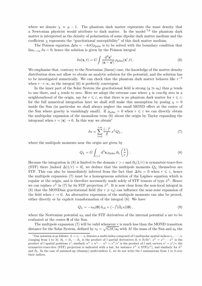
where we denote χ ≡ µ − 1. The phantom dark matter represents the mass density thata Newtonian physicist would attribute to dark matter. In the model 7,8 the phantom darkmatter is interpreted as the density of polarisation of some dipolar dark matter medium and thecoefficient χ represents the “gravitational susceptibility” of this dark matter medium.
The Poisson equation ∆δu = −4πGρpdm is to be solved with the boundary condition thatlimr→∞
δu = 0; hence the solution is given by the Poisson integral
δu(x, t) = G
∫
d3x′
|x− x′|ρpdm(x
′, t) . (6)
We emphasise that, contrary to the Newtonian (linear) case, the knowledge of the matter densitydistribution does not allow to obtain an analytic solution for the potential, and the solution hasto be investigated numerically. We can check that the phantom dark matter behaves like r−3
when r → ∞, so the integral (6) is perfectly convergent.In the inner part of the Solar System the gravitational field is strong (g ≫ a0) thus µ tends
to one there, and χ tends to zero. Here we adopt the extreme case where χ is exactly zero in aneighbourhood of the origin, say for r 6 ε, so that there is no phantom dark matter for r 6 ε;for the full numerical integration later we shall still make this assumption by posing χ = 0inside the Sun (in particular we shall always neglect the small MOND effect at the centre ofthe Sun where gravity is vanishingly small). If ρpdm = 0 when r 6 ε we can directly obtainthe multipolar expansion of the anomalous term (6) about the origin by Taylor expanding theintegrand when r = |x| → 0. In this way we obtainc
δu =+∞
∑
l=0
(−)l
l!xLQL , (7)
where the multipole moments near the origin are given by
QL = G
∫
r>ε
d3x ρpdm ∂L
(
1
r
)
. (8)
Because the integration in (8) is limited to the domain r > ε and ∂L(1/r) is symmetric-trace-free(STF) there [indeed ∆(1/r) = 0], we deduce that the multipole moments QL themselves areSTF. This can also be immediately inferred from the fact that ∆δu = 0 when r 6 ε, hencethe multipole expansion (7) must be a homogeneous solution of the Laplace equation which isregular at the origin, and is therefore necessarily made solely of STF tensors of type xL. Hencewe can replace xL in (7) by its STF projection xL. It is now clear from the non-local integral in(8) that the MONDian gravitational field (for r > r0) can influence the near-zone expansion ofthe field when r → 0. An alternative expression of the multipole moments can also be proved,either directly or by explicit transformation of the integral (8). We have
QL = −uN(0) δl,0 + (−)l(∂Lu)(0) , (9)
where the Newtonian potential uN and the STF derivatives of the internal potential u are to beevaluated at the centre 0 of the Sun.
The multipole expansion (7) will be valid whenever r is much less than the MOND transitiondistance for the Solar System, defined by r0 =
√
GM/a0 with M the mass of the Sun and a0 the
cOur notation is as follows: L = i1 · · · il denotes a multi-index composed of l multipolar spatial indices i1, · · · , il(ranging from 1 to 3); ∂L = ∂i1
· · · ∂ilis the product of l partial derivatives ∂i ≡ ∂/∂xi; xL = xi1
· · ·xil is the
product of l spatial positions xi; similarly nL = ni1· · ·ni
l = xL/rl is the product of l unit vectors ni = xi/r; thesymmetric-trace-free (STF) projection is indicated with a hat, for instance xL
≡ STF[xL], and similarly for nL
and ∂L. In the case of summed-up (dummy) multi-indices L, we do not write the l summations from 1 to 3 overtheir indices.
Figure 1: Left panel: profile of Q2(r) in the Solar System, for a standard choice of function µ1(y) [see Eq. (13a)],a0 = 1.2× 10⁻¹⁰m.s−2 and ge = 1.9× 10⁻¹⁰ m.s−2. The MOND transition radius is shown by a dash-dotted lineat r0 ≃ 7100 AU. Right panel: zoom of the central region (r 6 50 AU), where the quadrupole is almost constant.
MOND acceleration scale. This radius corresponds to the transition region where the Newtonianacceleration becomes of the order of the MOND acceleration a0 and therefore, MOND effectsbecome dominant. We have r0 ≃ 7100AU so the results (7)–(9) hold in a large volume aroundthe Sun including all the planets (recall that Neptune’s orbit is at 30AU).
3 Results for the induced quadrupole moment in the Solar System
So far we have elucidated the structure of the multipole expansion of the anomaly δu near theorigin. Next we resort to a numerical integration of the non-linear MOND equation (1) in orderto obtain quantitative values for the multipole moments.d
The Sun being assumed to be spherically symmetric, since all the multipole moments areinduced by the presence of the external field ge in the preferred direction e, the situation isaxisymmetric and all the moments QL will have their axis pointing in that direction e. Thuswe can define some multipole coefficients Ql by posing QL = Ql e
L, where eL denotes the STFpart of the product of l unit vectors eL = ei1 · · · eil . The multipole expansion (7) reads then as
δu(r, θ) =+∞
∑
l=0
(−)l
(2l − 1)!!rl Ql(r)Pl(cos θ) , (10)
where Pl(z) is the usual Legendre polynomial and θ is the angle away from the Galactic di-rection e. Although from the previous considerations the multipole coefficients Ql should beapproximately constant within the MOND transition radius r0, here we compute them directlyfrom the numerical solution of (1) and shall obtain their dependence on r. With our definitionthe quadrupolar piece in the internal field is given by
δu2 =1
2r2Q2(r)
(
cos2 θ −1
3
)
. (11)
The radial dependence of the anomaly (11) is ∝ r2 and can thus be separated from a quadrupolardeformation due to the Sun’s oblateness which decreases like ∝ r−3.
As a first result, we show in Fig. 1 the profile of the quadrupole induced by the MOND theorythrough the function Q2(r) defined in Eq. (11). We find that this quadrupole is decreasing from
dOur numerical scheme is based on the very efficient integrator of elliptic equations lorene, available fromthe website http://www.lorene.obspm.fr.
Table 1: Numerical values of the quadrupole Q2 together with the associated dimensionless quantity q2 definedby Eq. (12). All values are given near the Sun. We use different choices of the function µ(y) defined in Eqs. (13).
MOND function µ1(y) µ2(y) µ20(y) µexp(y) µTeVeS(y)
Q2 [s−2] 3.8 × 10⁻²⁶ 2.2× 10⁻²⁶ 2.1× 10⁻²⁷ 3.0 × 10⁻²⁶ 4.1× 10⁻²⁶
q2 0.33 0.19 1.8× 10⁻² 0.26 0.36
the Sun’s neighbourhood to zero, on a typical scale of 10000 astronomical units (AU). However,we check numerically that Q2(r) is almost constant in a large sphere surrounding the Solarsystem, as it has a relative variation lower than 10−4 within 30 AU (see the zoomed region inFig. 1). We shall therefore refer to the quadrupole as a simple number, noted Q2(0) or simplyQ2, when evaluating its influence on the orbits of Solar-system planets.
On dimensional analysis we expect that the quadrupole coefficient Q2 should scale with theMOND acceleration a0 like
Q2 =a0r0
q2(η) , (12)
where r0 =√
GM/a0 is the MOND transition radius and where the dimensionless coefficientq2 depends on the ratio η = ge/a0 between the external field and a0, and on the choice of theinterpolating function µ. Our numerical results for the quadrupole are given in Table 1, fordifferent coupling functions µ(y).e Here we consider various cases widely used in the literature:
µn(y) =y
n
√1 + yn
, (13a)
µexp(y) = 1− e−y , (13b)
µTeVeS(y) =
√1 + 4y − 1
√1 + 4y + 1
. (13c)
The function µ1 has been shown to yield good fits of galactic rotation curves 9; However becauseof its slow transition to the Newtonian regime it is a priori incompatible with Solar Systemobservations. The function µ2 is generally called the “standard” choice and was used in fits 10.We include also the function µexp having an exponentially fast transition to the Newtonianregime. The fourth choice µTeVeS is motivated by the TeVeS theory 11. One should note thatnone of these functions derives from a fundamental physical principle.
We have used several functions of type µn, as defined in Eq. (13a). One can notice thatthe value of Q2 decreases with n, that is with a faster transition from the weak-field regimewhere µ(y) ∼ y, to the strong field regime where µ(y) ∼ 1. We have been unable to determinenumerically a possible limit for Q2 as n goes to infinity.
4 Effect on the dynamics of the Solar System planets
We investigate the consequence for the dynamics of inner planets of the Solar System of thepresence of an abnormal quadrupole moment Q2 oriented toward the direction e of the galacticcentre. Recall that the domain of validity of this anomaly is expected to enclose all the inner SolarSystem (for distances r . r0 ≈ 7100 AU), with the quadrupole coefficient being constant up tosay 50 AU (see Fig. 1). As we have seen, the anomaly induces a perturbation on the Newtoniangravitational potential, namely u = uN + δu, where uN = GM/r and the perturbation functionR ≡ δu is given for the quadrupole moment by Eq. (11).
eNote that the quadrupole coefficient Q2 is found to be always positive which corresponds to a prolate elon-gation along the quadrupolar axis.
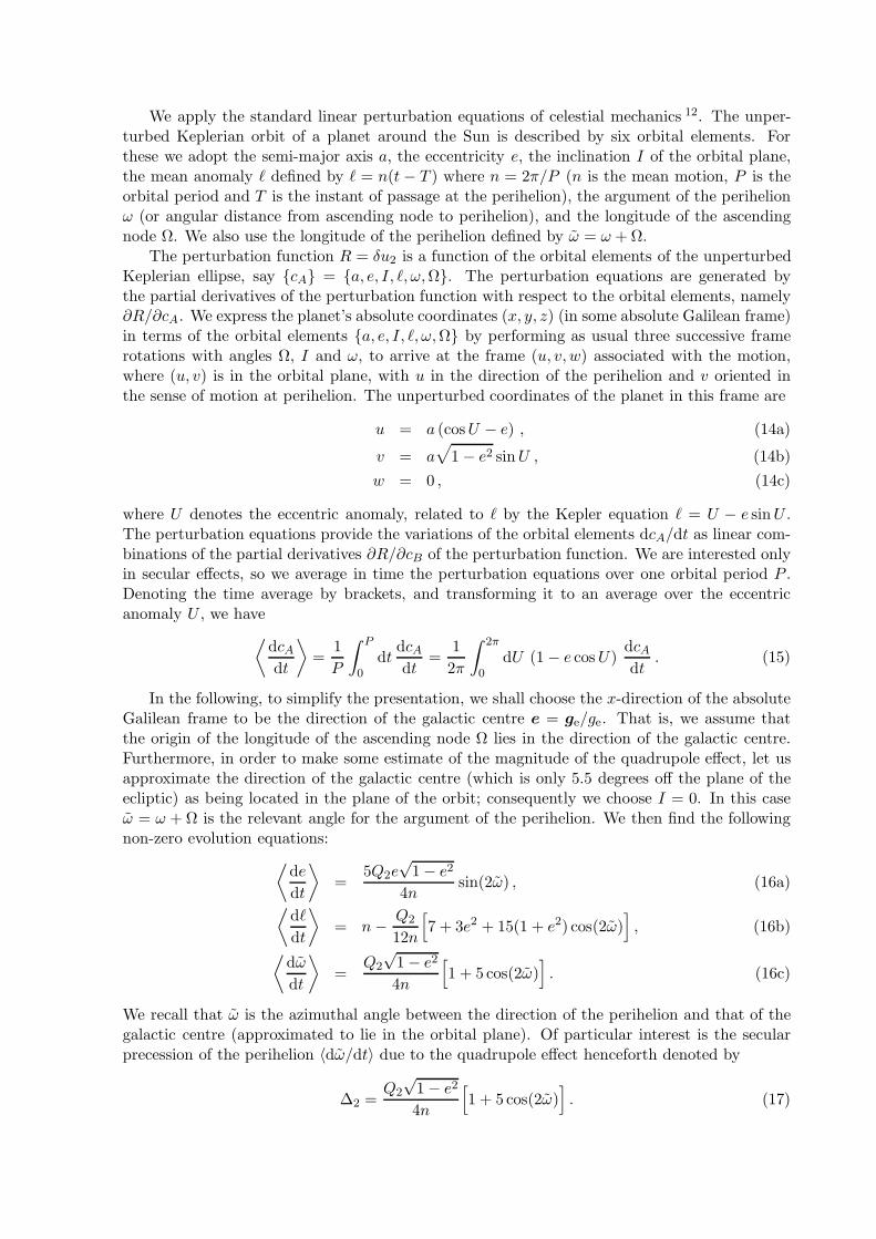
We apply the standard linear perturbation equations of celestial mechanics 12. The unper-turbed Keplerian orbit of a planet around the Sun is described by six orbital elements. Forthese we adopt the semi-major axis a, the eccentricity e, the inclination I of the orbital plane,the mean anomaly ℓ defined by ℓ = n(t− T ) where n = 2π/P (n is the mean motion, P is theorbital period and T is the instant of passage at the perihelion), the argument of the perihelionω (or angular distance from ascending node to perihelion), and the longitude of the ascendingnode Ω. We also use the longitude of the perihelion defined by ω = ω +Ω.
The perturbation function R = δu2 is a function of the orbital elements of the unperturbedKeplerian ellipse, say cA = a, e, I, ℓ, ω,Ω. The perturbation equations are generated bythe partial derivatives of the perturbation function with respect to the orbital elements, namely∂R/∂cA. We express the planet’s absolute coordinates (x, y, z) (in some absolute Galilean frame)in terms of the orbital elements a, e, I, ℓ, ω,Ω by performing as usual three successive framerotations with angles Ω, I and ω, to arrive at the frame (u, v, w) associated with the motion,where (u, v) is in the orbital plane, with u in the direction of the perihelion and v oriented inthe sense of motion at perihelion. The unperturbed coordinates of the planet in this frame are
u = a (cosU − e) , (14a)
v = a√
1− e2 sinU , (14b)
w = 0 , (14c)
where U denotes the eccentric anomaly, related to ℓ by the Kepler equation ℓ = U − e sinU .The perturbation equations provide the variations of the orbital elements dcA/dt as linear com-binations of the partial derivatives ∂R/∂cB of the perturbation function. We are interested onlyin secular effects, so we average in time the perturbation equations over one orbital period P .Denoting the time average by brackets, and transforming it to an average over the eccentricanomaly U , we have
⟨
dcAdt
⟩
=1
P
∫ P
0
dtdcAdt
=1
2π
∫ 2π
0
dU (1− e cosU)dcAdt
. (15)
In the following, to simplify the presentation, we shall choose the x-direction of the absoluteGalilean frame to be the direction of the galactic centre e = ge/ge. That is, we assume thatthe origin of the longitude of the ascending node Ω lies in the direction of the galactic centre.Furthermore, in order to make some estimate of the magnitude of the quadrupole effect, let usapproximate the direction of the galactic centre (which is only 5.5 degrees off the plane of theecliptic) as being located in the plane of the orbit; consequently we choose I = 0. In this caseω = ω +Ω is the relevant angle for the argument of the perihelion. We then find the followingnon-zero evolution equations:
⟨
de
dt
⟩
=5Q2e
√1− e2
4nsin(2ω) , (16a)
⟨
dℓ
dt
⟩
= n−Q2
12n
[
7 + 3e2 + 15(1 + e2) cos(2ω)]
, (16b)
⟨
dω
dt
⟩
=Q2
√1− e2
4n
[
1 + 5 cos(2ω)]
. (16c)
We recall that ω is the azimuthal angle between the direction of the perihelion and that of thegalactic centre (approximated to lie in the orbital plane). Of particular interest is the secularprecession of the perihelion 〈dω/dt〉 due to the quadrupole effect henceforth denoted by
∆2 =Q2
√1− e2
4n
[
1 + 5 cos(2ω)]
. (17)
Table 2: Results for the precession rates of planets ∆2 due to the quadrupole coefficient Q2. We use the values forQ2 for various MOND functions as computed in Table 1. Published postfit residuals of orbital precession (after
taking into account the relativistic precession). All results are given in milli-arc-seconds per century.
Quadrupolar precession rate ∆2 in mas/cyMOND function Mercury Venus Earth Mars Jupiter Saturn Uranus Neptune
µ1(y) 0.04 0.02 0.16 −0.16 −1.12 5.39 −10.14 7.93µ2(y) 0.02 0.01 0.09 −0.09 −0.65 3.12 −5.87 4.59µ20(y) 2× 10⁻³ 10−3 9× 10⁻³ −9× 10⁻³ −0.06 0.3 −0.56 0.44µexp(y) 0.03 0.02 0.13 −0.13 −0.88 4.25 −8.01 6.26µTeVeS(y) 0.05 0.02 0.17 −0.17 −1.21 5.81 −10.94 8.56
Postfit residuals for ∆ = 〈dω/dt〉 in mas/cyOrigin Mercury Venus Earth Mars Jupiter Saturn Uranus NeptunePitjeva 13 −3.6± 5 −0.4± 0.5 −0.2± 0.4 0.1± 0.5 - −6± 2 - -
Fienga et al. 14 −10± 30 −4± 6 0± 0.016 0± 0.2 142± 156 −10± 8 0± 2 · 104 0± 2 · 104
Fienga et al. 15 0.4± 0.6 0.2± 1.5 −0.2± 0.9 −0.04± 0.15 −41± 42 0.15± 0.65 - -
The precession is non-spherical, in the sense that it depends on the orientation of the orbitrelative to the galactic centre through its dependence upon the perihelion’s longitude ω. Theeffect scales with the inverse of the orbital frequency n = 2π/P and therefore becomes moreimportant for outer planets like Saturn than for inner planets like Mercury. This is in agreementwith the fact that the quadrupole effect we are considering increases with the distance to theSun (but of course will fall down when r becomes appreciably comparable to r0, see Fig. 1).
Our numerical values for the quadrupole anomalous precession ∆2 are reported in Table 2.As we see the quadrupolar precession ∆2 is in the range of the milli-arc-second per centurywhich is not negligible. In particular it becomes interestingly large for the outer gaseous planetsof the Solar System, essentially Saturn, Uranus and Neptune. The dependence on the choice ofthe MOND function µ is noticeable only for functions µn(y) defined by (13a) with large valuesof n, where the effect decreases by a factor ∼ 10 between n = 2 and n = 20.
We then compare in Table 2 our results to the best published postfit residuals for any pos-sible supplementary precession of planetary orbits (after the relativistic precession has beenduly taken into account), which have been obtained from global fits of the Solar System dynam-ics13,14,15. In particular the postfit residuals obtained by the INPOP planetary ephemerides14,15
use information from the combination of very accurate tracking data of spacecrafts orbiting dif-ferent planets. We find that the values for ∆2 are smaller or much smaller than the publishedresiduals except for the planets Mars and Saturn. Very interestingly, our values are smaller orgrossly within the range of the postfit residuals for these planets. In the case of Saturn notably,the constraints seem already to exclude most of our obtained values for ∆2, except for MONDfunctions of the type µn and given by (13a) with rather large values of n.
However let us note that the INPOP ephemerides are used to detect the presence of aneventual abnormal precession, not to adjust precisely the value of that precession 14,15. On theother hand the postfit residuals are obtained by adding by hands an excess of precession forthe planets and looking for the tolerance of the data on this excess 14,15. But in order to reallytest the anomalous quadrupolar precession rate ∆2, one should consistently work in a MONDpicture, i.e. consider also the other effects predicted by this theory, like the precession of thenodes, the variation of the eccentricity and the inclination, and so on — see Eqs. (16). Thenone should perform a global fit of all these effects to the data; it is likely that in this way thequantitative conclusions would be different.
Finally let us cautiously remark that MOND and more sophisticated theories such as TeVeS11,which are intended to describe the weak field regime of gravity (below a0), may not be extrap-olated without modification to the strong field of the Solar System. For instance it has been
argued9 that a MOND interpolating function µ which performs well at fitting the rotation curvesof galaxies is given by µ1 defined by (13a). However this function has a rather slow transition tothe Newtonian regime, given by µ1 ∼ 1 − y−1 when y = g/a0 → ∞, which is already excludedby Solar System observations. Indeed such slow fall-off −y−1 predicts a constant supplementaryacceleration directed toward the Sun δgN = a0 (i.e. a “Pioneer” effect), which is ruled out be-cause not seen from the motion of planets. Thus it could be that the transition between MONDand the Newtonian regime is more complicated than what is modelled by Eq. (1). This is alsotrue for the dipolar dark matter model 7,8 which may only give an effective description valid inthe weak field limit and cannot be extrapolated as it stands to the Solar System. While lookingat MOND-like effects in the Solar System we should keep the previous proviso in mind. Thepotential conflict we find here with the Solar System dynamics (notably with the constraints onthe orbital precession of Saturn 14,15) may not necessarily invalidate those theories if they arenot “fundamental” theories but rather “phenomenological” models only pertinent in a certainregime.
In any case, further studies are to be done if one wants to obtain more stringent conclusionsabout constraints imposed by Solar-system observations onto MOND-like theories. More preciseobservations could give valuable informations about an eventual EFE due to the MOND theoryand restrict the number of possible MOND functions that are compatible with the observations.More generally the influence of the Galactic field on the Solar-system dynamics through a possi-ble violation of the strong version of the equivalence principle (of which the EFE is a by-productin the case of MOND) is worth to be investigated.
1. M. Milgrom. Astrophys. J., 270:365, 1983; ibid. 270:371, 1983; ibid. 270:384, 1983.2. R.H. Sanders and S. McGaugh. Ann. Rev. Astron. Astrophys., 40:263, 2002.3. J.D. Bekenstein and M. Milgrom. Astrophys. J., 286:7, 1984.4. B. Famaey, J.-P. Bruneton, and H. Zhao. Escaping from modified newtonian dynamics.
Mon. Not. Roy. Astron. Soc., 377:L79, 2007.5. M. Milgrom. Mond effects in the inner solar system. Mon. Not. Roy. Astron. Soc.,
399:474, 2009.6. L. Blanchet and J. Novak. External field effect of modified newtonian dynamics in the
solar system. Mon. Not. Roy. Astron. Soc., 412:2530, 2011.7. L. Blanchet and A. Le Tiec. Model of dark matter and dark energy based on gravitational
polarization. Phys. Rev. D, 78:024031, 2008.8. L. Blanchet and A. Le Tiec. Dipolar dark matter and dark energy. Phys. Rev. D,
80:023524, 2009.9. B. Famaey and J. Binney. Mon. Not. Roy. Astron. Soc., 363:603, 2005.
10. K. Begeman, A. Broeils, and R. Sanders. Mon. Not. Roy. Astron. Soc., 249:523, 1991.11. J.D. Bekenstein. Phys. Rev. D, 70:083509, 2004.12. D. Brouwer and G.M. Clemence. Methods of celestial mechanics. Academic Press, New
York, 1961.13. E.V. Pitjeva. Astron. Lett., 31:340, 2005.14. A. Fienga, J. Laskar, P. Kuchynka, C. Leponcin-Laffite, H. Manche, and M. Gastineau.
Gravity tests with inpop planetary ephemerides. 2009. In Relativity in FundamentalAstronomy: Dynamics, Reference Frames, and Data Analysis, edited by S. Klioner et al,Cambridge University Press, p. 159.
15. A. Fienga, H. Manche, P. Kuchynka, J. Laskar, and M. Gastineau. Planetary and lu-nar ephemerides, inpop10a. 2010. The documentation of INPOP10A is available atwww.imcce.fr/inpop.
TESTING DARK MATTER WITH GAIA
O. BIENAYME
Strasbourg Observatory, 11 rue de l’universite,67000 Strasbourg, France
With the advent of Gaia, it will be possible to design tests of gravity on the scale of the Galaxy.Accurate measurements of positions and velocities of few hundred millions stars will allow todetail the stellar kinematics and Galactic dynamics, to draw the gravitational potential andto recover the 3D distribution of dark matter. Gaia data will allow to test modified gravityinterpretations on a galactic scale, like MOND that makes very specific predictions allowingto differentiate it from a spheroidal halo of dark matter.
1 Introduction
The Gaia satellite will survey the sky with three instruments. It will realize a nearly all skyphotometric survey within visible bands, an astrometric survey that will measures positions,parallaxes and proper motions, and a radial velocity survey.
The combination of data from these surveys will allow to determine the 3D positions and3D velocities of large sample of stars over a significant volume of the Galaxy. This will allowto recover the gravitational potential over this volume of the Galaxy. Gaia will also perform anaccurate determination of the distribution of visible mass. From these determinations, it willbe possible for the first time to map precisely the unseen mass within our Galaxy. Hipparcoshad constrained the amount of dark matter in the solar neigbourhood, Gaia will do it for asignificant fraction of the volume of our Galaxy.
Tests of the relativity within the solar system will be performed with Gaia. Hestroffer etal (2009) showed that observations of asteroids with Gaia allow a joint determination of thesolar quadrupole J2 and the PPN parameter β, a possible variation of the gravitational constant(dG/dt)/G, and deviation from Newtonian law. A detailed list of tests (Mignard & Klioner2009) includes a measure of γ from light deflection with a precision of 2×10⁻⁶, test of the LocalLorentz Invariance, detection of possible gravitational wave flux.
In this presentation, we propose a new test of the gravity on galactic scales: modification ofthe newtonian dynamics have been proposed to explain flat rotation curve of galaxies withoutneed of dark matter. MOND is such a phenomenological ’theory’ that implies flat rotation curveat large radius for galaxies, it also implies predictions on the kinematics of stars and on the 3Dshape of the gravitational potential. We may expect that any modifications of the relativity toexplain rotation curves in galaxy should also imply other observable properties identifiable withGaia observations.
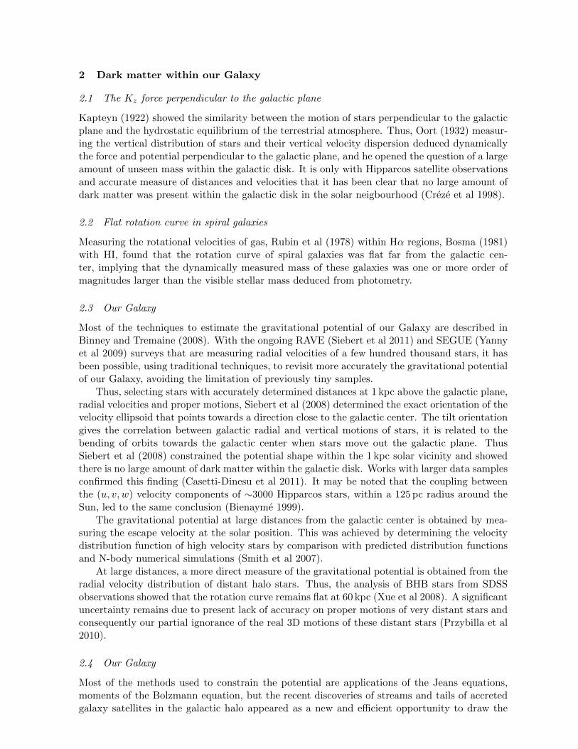
2 Dark matter within our Galaxy
2.1 The Kz force perpendicular to the galactic plane
Kapteyn (1922) showed the similarity between the motion of stars perpendicular to the galacticplane and the hydrostatic equilibrium of the terrestrial atmosphere. Thus, Oort (1932) measur-ing the vertical distribution of stars and their vertical velocity dispersion deduced dynamicallythe force and potential perpendicular to the galactic plane, and he opened the question of a largeamount of unseen mass within the galactic disk. It is only with Hipparcos satellite observationsand accurate measure of distances and velocities that it has been clear that no large amount ofdark matter was present within the galactic disk in the solar neigbourhood (Creze et al 1998).
2.2 Flat rotation curve in spiral galaxies
Measuring the rotational velocities of gas, Rubin et al (1978) within Hα regions, Bosma (1981)with HI, found that the rotation curve of spiral galaxies was flat far from the galactic cen-ter, implying that the dynamically measured mass of these galaxies was one or more order ofmagnitudes larger than the visible stellar mass deduced from photometry.
2.3 Our Galaxy
Most of the techniques to estimate the gravitational potential of our Galaxy are described inBinney and Tremaine (2008). With the ongoing RAVE (Siebert et al 2011) and SEGUE (Yannyet al 2009) surveys that are measuring radial velocities of a few hundred thousand stars, it hasbeen possible, using traditional techniques, to revisit more accurately the gravitational potentialof our Galaxy, avoiding the limitation of previously tiny samples.
Thus, selecting stars with accurately determined distances at 1 kpc above the galactic plane,radial velocities and proper motions, Siebert et al (2008) determined the exact orientation of thevelocity ellipsoid that points towards a direction close to the galactic center. The tilt orientationgives the correlation between galactic radial and vertical motions of stars, it is related to thebending of orbits towards the galactic center when stars move out the galactic plane. ThusSiebert et al (2008) constrained the potential shape within the 1 kpc solar vicinity and showedthere is no large amount of dark matter within the galactic disk. Works with larger data samplesconfirmed this finding (Casetti-Dinesu et al 2011). It may be noted that the coupling betweenthe (u, v, w) velocity components of ∼3000 Hipparcos stars, within a 125 pc radius around theSun, led to the same conclusion (Bienayme 1999).
The gravitational potential at large distances from the galactic center is obtained by mea-suring the escape velocity at the solar position. This was achieved by determining the velocitydistribution function of high velocity stars by comparison with predicted distribution functionsand N-body numerical simulations (Smith et al 2007).
At large distances, a more direct measure of the gravitational potential is obtained from theradial velocity distribution of distant halo stars. Thus, the analysis of BHB stars from SDSSobservations showed that the rotation curve remains flat at 60 kpc (Xue et al 2008). A significantuncertainty remains due to present lack of accuracy on proper motions of very distant stars andconsequently our partial ignorance of the real 3D motions of these distant stars (Przybilla et al2010).
2.4 Our Galaxy
Most of the methods used to constrain the potential are applications of the Jeans equations,moments of the Bolzmann equation, but the recent discoveries of streams and tails of accretedgalaxy satellites in the galactic halo appeared as a new and efficient opportunity to draw the
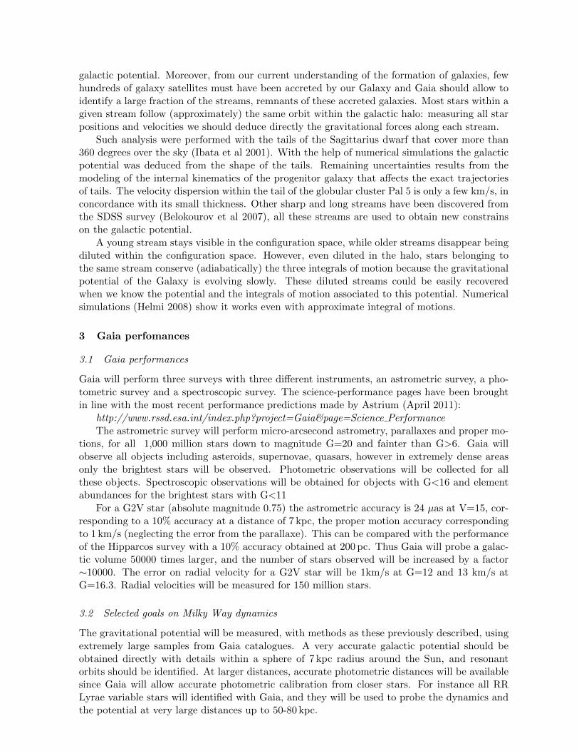
galactic potential. Moreover, from our current understanding of the formation of galaxies, fewhundreds of galaxy satellites must have been accreted by our Galaxy and Gaia should allow toidentify a large fraction of the streams, remnants of these accreted galaxies. Most stars within agiven stream follow (approximately) the same orbit within the galactic halo: measuring all starpositions and velocities we should deduce directly the gravitational forces along each stream.
Such analysis were performed with the tails of the Sagittarius dwarf that cover more than360 degrees over the sky (Ibata et al 2001). With the help of numerical simulations the galacticpotential was deduced from the shape of the tails. Remaining uncertainties results from themodeling of the internal kinematics of the progenitor galaxy that affects the exact trajectoriesof tails. The velocity dispersion within the tail of the globular cluster Pal 5 is only a few km/s, inconcordance with its small thickness. Other sharp and long streams have been discovered fromthe SDSS survey (Belokourov et al 2007), all these streams are used to obtain new constrainson the galactic potential.
A young stream stays visible in the configuration space, while older streams disappear beingdiluted within the configuration space. However, even diluted in the halo, stars belonging tothe same stream conserve (adiabatically) the three integrals of motion because the gravitationalpotential of the Galaxy is evolving slowly. These diluted streams could be easily recoveredwhen we know the potential and the integrals of motion associated to this potential. Numericalsimulations (Helmi 2008) show it works even with approximate integral of motions.
3 Gaia perfomances
3.1 Gaia performances
Gaia will perform three surveys with three different instruments, an astrometric survey, a pho-tometric survey and a spectroscopic survey. The science-performance pages have been broughtin line with the most recent performance predictions made by Astrium (April 2011):
http://www.rssd.esa.int/index.php?project=Gaia&page=Science Performance
The astrometric survey will perform micro-arcsecond astrometry, parallaxes and proper mo-tions, for all 1,000 million stars down to magnitude G=20 and fainter than G>6. Gaia willobserve all objects including asteroids, supernovae, quasars, however in extremely dense areasonly the brightest stars will be observed. Photometric observations will be collected for allthese objects. Spectroscopic observations will be obtained for objects with G<16 and elementabundances for the brightest stars with G<11
For a G2V star (absolute magnitude 0.75) the astrometric accuracy is 24 µas at V=15, cor-responding to a 10% accuracy at a distance of 7 kpc, the proper motion accuracy correspondingto 1 km/s (neglecting the error from the parallaxe). This can be compared with the performanceof the Hipparcos survey with a 10% accuracy obtained at 200 pc. Thus Gaia will probe a galac-tic volume 50000 times larger, and the number of stars observed will be increased by a factor∼10000. The error on radial velocity for a G2V star will be 1km/s at G=12 and 13 km/s atG=16.3. Radial velocities will be measured for 150 million stars.
3.2 Selected goals on Milky Way dynamics
The gravitational potential will be measured, with methods as these previously described, usingextremely large samples from Gaia catalogues. A very accurate galactic potential should beobtained directly with details within a sphere of 7 kpc radius around the Sun, and resonantorbits should be identified. At larger distances, accurate photometric distances will be availablesince Gaia will allow accurate photometric calibration from closer stars. For instance all RRLyrae variable stars will identified with Gaia, and they will be used to probe the dynamics andthe potential at very large distances up to 50-80 kpc.
Gaia will also allow an accurate determination of the faint end of the stellar luminosityfunction and will measure the dominant contribution of low mass stars to the mass budget ofthe different galactic stellar components. This is a central question since the difference betweenthe galactic mass determined from the dynamics and the stellar one, will give the invisible massor dark matter distribution.
Other results will be obtained concerning the internal dynamics of the stellar disk and itsgravitational potential by the observation and measure of the disk warp and flare as well as theirrotation and vertical oscillations.
To measure the gravitational potential, the identification of streams will offer a new andpromising perspective. The accretion events remain visible during a very long time in thephase space. While after many billion years, the spatial distribution of an accreted satellitesor disrupted globular cluster will be uniform within the inner halo, the distribution of thecorresponding stars stays clumpy in the velocity space, and are even easier to identify withinthe 3D integrals of motion space. If most of the inner halo is formed from such accretion events,a few hundreds streams or clumps will be visible in the phase space.
When a stream is identified, the galactic force is accurately constrained in the surroundingposition of every star of that stream. Thus potentially a very fine description of the potentialshould be achievable at the position of many halo stars, more accurately than any other techniqueand it will allow an accurate identification of a dark disk, of a dark thick disk, the descriptionof their shape, thickness, triaxiallity... if they exists.
How much clumpy is the dark halo is an open question. Depending on the size of clumps, itwill modify and disperse the orbits of streams. This will certainly complicate the analysis andidentification of streams, but, as far as we know, not much work has yet explored this questionin details.
4 Testing gravity with Gaia
A currently debated question is whether the missing mass problem is due to the existence ofdark matter or to a modification of the gravitational law on galaxy scales. Here, following thework of Bienayme et al (2009), we show how large-scale spectroscopic and astrometric surveysin general, and Gaia in particular, could help answer this question.
4.1 Cold Dark Matter or Modified Newtonian Dynamics?
The concordance cosmological model based on the existence of Cold Dark Matter is successful onlarge scales. However, the predictions of the model are in contrast with a number of observationalfacts on galaxy scales. Some well known issues are (i) the predicted overabundance of satellitegalaxies; (ii) the prediction of cuspy dark matter halos, whereas observations point toward darkhalos with a central constant density core; (iii) the problems to form large enough baryonicdisks due to their predicted low angular momentum within simulations. In addition galaxiesfollow tight scaling relations that involve an acceleration a0 = 10−10 m.s−2, for instance theuniversality of the dark and baryonic surface densities of galaxies within one scale-length of thedark halo (Gentile et al 2009). Below this gravitational acceleration, the enclosed dark massstarts to dominate over baryons in galaxies, and this acceleration scale also fixes the slope andzero-point of the Tully-Fisher and Faber-Jackson relations.
Milgrom (1983) postulated that for gravitational accelerations below a0, the true gravita-tional attraction is modified and MOND, the modified gravity interpretation (Bekenstein &Milgrom 1984), makes very specific predictions allowing to differentiate it from a spherical haloof dark matter. Here, we outline these predictions, that Gaia and other large-scale surveys couldhelp to test.
4.2 How Gaia can help
We build these predictions with the MOND Milky Way model of Wu et al (2008). This model isbased on one of the most realistic possible baryonic mass models of the Milky Way, the Besanconmodel (Robin et al 2003). Once the MOND gravitational potential of the model is known, onecan apply the Newtonian Poisson equation to it, in order to find back the density distributionthat would have yielded this potential within Newtonian dynamics. In this context, as shown inBienayme et al (2009), MOND predicts a disk of phantom dark matter allowing to differentiateit from a Newtonian model with a dark halo. (i) By measuring the force perpendicular to theGalactic plane: at the solar radius, MOND predicts a 60 percent enhancement of the dynamicalsurface density at 1.1 kpc compared to the baryonic surface density, a value not excluded bycurrent data. The enhancement would become more apparent at large galactic radii where thestellar disk mass density becomes negligible. (ii) By determining dynamically the scale length ofthe disk mass density distribution. This scale length is a factor 1.25 larger than the scale lengthof the visible stellar disk if MOND applies. Such test could be applied with existing RAVE data(Zwitter et al 2008), but the accuracy of available proper motions still limits the possibility toexplore the gravitational forces too far from the solar neighbourhood. (iii) By measuring thevelocity ellipsoid tilt angle within the meridional galactic plane. This tilt is different within thetwo dynamics in the inner part of the Galactic disk. However the tilt of about 6 degrees atz=1 kpc at the solar radius is in agreement with the recent determination of 7.3 ± 1.8 degreesobtained by Siebert et al (2008). The difference between MOND and a Newtonian model witha spherical halo becomes significant at z=2 kpc.
Such easy and quick tests of gravity could be applied with the first releases of future Gaiadata. Let us however note that these predictions are extremely dependent on the baryoniccontent of the model, so that testing gravity at the scale of the Galaxy heavily relies on starcounts, stellar population synthesis, census of the gaseous content (including molecular gas),and inhomogeneities in the baryonic distribution (clusters, gas clouds).
Acknowledgments
We thank Benoıt Famaey, HongSheng Zhao, Xufen Wu, and Dominique Aubert for their con-tribution to Bienayme et al (2009).
References
1. D. Hestroffer, S. Mouret et al, Proceedings IAU 261, 325 (2009).2. F. Mignard, S.A. Klioner, Proceedings IAU 261, 306 (2009).3. J.C. Kapteyn, ApJ 55, 302 (1922).4. J.H. Oort, BAN 6, 249 (1932).5. M. Creze, E. Chereul, O. Bienayme, C. Pichon, A&A 329, 920 (1998).6. V. C. Rubin, W.K. Ford, N. Thonnard et al, ApJ 225, L107 (1978).7. A. Bosma, ApJ 86, 1825 (1981).8. J. Binney, S. Tremaine, Galactic Dynamics , Princeton University Press (2008).9. A. Siebert et al, ApJ , in press (2011).
10. B. Yanny et al, AJ 137, 4377 (2009).11. A. Siebert et al, MNRAS 391, 793 (2008).12. D.J. Casetti-Dinescu et al, ApJ 728, 7 (2011).13. O. Bienayme, A&A 341, 86 (1999).14. M. Smith et al, MNRAS 379, 755 (2007).15. X.X. Xue et al, ApJ 684, 1143 (2008).
16. N. Przybilla et al, ApJ 718, 37 (2010).17. R. Ibata et al, ApJ 551, 294 (2001).18. V. Belokurov et al, ApJ 658, 337 (2007).19. A. Helmi, ARAA 15, 145 (2008).20. O. Bienayme et al, A&A 500, 801 (2009).21. L.C. Gentile et al, Nature 461, 627 (2009).22. M. Milgrom et al, ApJ 270, 365 (1983).23. J. Bekenstein, M. Milgrom, ApJ 286, 7 (1984)24. X. Wu et al, MNRAS 386, 2199 (2008).25. A.C. Robin et al, A&A 409, 523 (2003).26. T. Zwitter et al, AJ 136, 421 (2008).
BEYOND EINSTEIN: COSMOLOGICAL TESTS OF MODEL INDEPENDENT
MODIFIED GRAVITY
D.B. THOMAS AND C.R. CONTALDITheoretical Physics, Blackett Laboratory, Imperial College, London, England SW7 2AZ
Model-independent parametrisations of modified gravity have attracted a lot of attention overthe past few years; numerous combinations of experiments and observables have been sug-gested to constrain these parameterisations, and future surveys look very promising. GalaxyClusters have been mentioned, but not looked at as extensively in the literature as some otherprobes. Here we look at adding Galaxy Clusters into the mix of observables and examinewhether they could improve the constraints on the modified gravity parameters. In partic-ular, we forecast the constraints from combining the Planck CMB spectrum and SZ clustercatalogue and a DES-like Weak Lensing survey. We’ve found that adding cluster countsimproves the constraints obtained from combining CMB and WL data.
1 Introduction
Einstein’s General Relativity (GR) is one of the principal ingredients of modern cosmology.Nonetheless, it is our job as physicists to continue to test even the fundamental pillars of cos-mology in order to refine, improve and further justify our model of the universe. Testing GRoutside of the solar system can be quite challenging, particularly as the effects of a differenttheory of gravity could be degenerate with different possible constituents of the universe. Thisis the case with the current cosmological observations that suggest the presence of dark matterand dark energy. As well as explaining these observations, there are also fundamental physicsreasons for considering different theories of gravity: GR is inconsistent with quantum mechanicsand the search for ”Quantum Gravity” is one of the holy grails of modern physics.Here, we are interested in testing deviations from GR in a model independent way. There areseveral advantages to a model independent approach; some alternatives to GR do exist butthere is no complete theory of, for example, quantum gravity to draw on. Also, amongst themany options there are no ”stand-out” candidates that are universally considered to be strongalternatives. If a model independent approach suggests that the data is inconsistent with con-cordance cosmology and GR, it will be relatively unambiguous and therefore a strong motivatorto develop alternative theories, as well as possibly giving us a clue as to the nature of thesetheories.There are studies in the literature on the constraining power of current data 1,2 and the gen-eral conclusion is that the concordance cosomology is consistent with all of the current data,although the data isn’t strongly constraining. Work has also gone into forecasting future ex-periments 3,4 and again there is a fair degree of consensus here, namely that future surveys willgreatly improve prospects. In this work we will examine the constraints that can be put onmodel independent modified gravity using the combination of Cosmic Microwave Backgroundanisotropies (CMB) cross-correlated with weak lensing surveys and galaxy cluster counts.
2 Modified Gravity
Our potentials are defined in a flat FRW metric in the Newtonian gauge by g00 = −1 −
2Ψ(~x, t) , g0i = 0 , gij = a2δij(1 − 2Φ(~x, t)) . Ψ is the Newtonian potential and is responsiblefor the acceleration of massive particles. Φ is the curvature potential, which contributes to theacceleration of relativistic particles only.Several sets of modified gravity parameters (MGPs) have been proposed, see5 for one of the firstpapers and 6 for a partial translation table between the different parameterisations In this workwe will use two MGPs, η and µ, following7 and implemented in the code MGCAMB, to describedepartures from GR. The first, η, is the ratio of the two metric potentials, η = Ψ/Φ. This willbe approximately unity in GR unless any of the particle species has large anisotropic stress.The second, µ, is a modification of the poisson equation, and is essentially a time and spacedependent Newton’s constant. Fourier expanding the spatial dependence with wavenumbers kand assuming isotropy, the modification of the Possion equation is as follows
k2Ψ(a, k) = −4πGa2µ(a, k)ρ(a)∆(a, k) , (1)
where, a is the FRW scale factor, G is Newton’s constant, ρ is the background density of colddark matter and ∆ is the gauge invariant density contrast.We will assume that GR is valid up to a specified redshift zmg = 30. Beyond this, we assumethat the MGPs transition to a constant value that is different to the GR value. The backgroundexpansion history is already constrained to be close to that of a ΛCDM model, we will thereforeassume that the modified gravity mimics the expansion history of a standard ΛCDM setup.
3 Observables
3.1 Cluster Counts
Galaxy clusters are some of the largest collapsed structures in the universe. According tothe standard ΛCDM cosmology, they typically consist of hot gas bound in a large cold darkmatter halo. They are a useful cosmological probe as their size corresponds to scales near thelinear to non–linear transition in the underlying dark matter power spectrum. This has severalconsequences: they probe the tail of the matter perturbation spectrum and are therefore asensitive probe of growth. In addition, galaxy cluster counts can be predicted accurately fromthe linear theory matter power spectrum, using semi-analytic formulae or ones calibrated fromN-body simulations.Our theoretical predictions for the number of clusters in redshift bins will be compared topredicted SZ catalogues for a number of future observational stages. The SZ effect 8 is a nearlyredshift independent tracer of clusters that is due to the rescattering of CMB photons by hotintracluster gas. The observational limits on SZ observations are, in principle, determined simplyby resolution and sky coverage.
3.2 CMB
With the release of Planck satellite 9 results only a few years away we are entering an erawhere observations of the CMB total intensiy spectrum will have reached the sample variancelimit throughout scales where primary effects dominate the signal. The sensitivity to MGPsin the CMB spectrum is restricted to the largest scales and the main signal that will arise onthese scales is the ISW effect. This is sourced as the Universe transitions into a dark energydominated model and the potential starts to decay. The effect can be described by the integralof the time-deritvative of the sum of metric potentials along the line of sight.
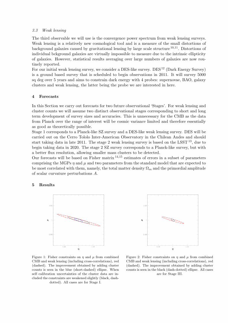
3.3 Weak lensing
The third observable we will use is the convergence power spectrum from weak lensing surveys.Weak lensing is a relatively new cosmological tool and is a measure of the small distortions ofbackground galaxies caused by gravitational lensing by large scale structure 10,11. Distortions ofindividual bckground galaxies are virtually impossible to measure due to the intrinsic ellipticityof galaxies. However, statistical results averaging over large numbers of galaxies are now rou-tinely reported.For our initial weak lensing survey, we consider a DES-like survey. DES12 (Dark Energy Survey)is a ground based survey that is scheduled to begin observations in 2011. It will survey 5000sq deg over 5 years and aims to constrain dark energy with 4 probes: supernovae, BAO, galaxyclusters and weak lensing, the latter being the probe we are interested in here.
4 Forecasts
In this Section we carry out forecasts for two future observational ‘Stages’. For weak lensing andcluster counts we will assume two distinct observational stages corresponding to short and longterm development of survey sizes and accuracies. This is unnecessary for the CMB as the datafrom Planck over the range of interest will be cosmic variance limited and therefore essentiallyas good as theoretically possible.Stage 1 corresponds to a Planck-like SZ survey and a DES-like weak lensing survey. DES will becarried out on the Cerro Tololo Inter-American Observatory in the Chilean Andes and shouldstart taking data in late 2011. The stage 2 weak lensing survey is based on the LSST 13, due tobegin taking data in 2020. The stage 2 SZ survey corresponds to a Planck-like survey, but witha better flux resolution, allowing smaller mass clusters to be detected.Our forecasts will be based on Fisher matrix 14,15 estimates of errors in a subset of parameterscomprising the MGPs η and µ and two parameters from the standard model that are expected tobe most correlated with them, namely, the total matter density Ωm and the primordial amplitudeof scalar curvature perturbations A.
5 Results
Figure 1: Fisher constraints on η and µ from combinedCMB and weak lensing (including cross-correlations), red(dashed). The improvement obtained by adding clustercounts is seen in the blue (short-dashed) ellipse. Whenself–calibration uncertainties of the cluster data are in-cluded the constraints are weakened slightly (black, dash-
dotted). All cases are for Stage I.
Figure 2: Fisher constraints on η and µ from combinedCMB and weak lensing (including cross-correlations), red(dashed). The improvement obtained by adding clustercounts is seen in the black (dash-dotted) ellipse. All cases
are for Stage III.
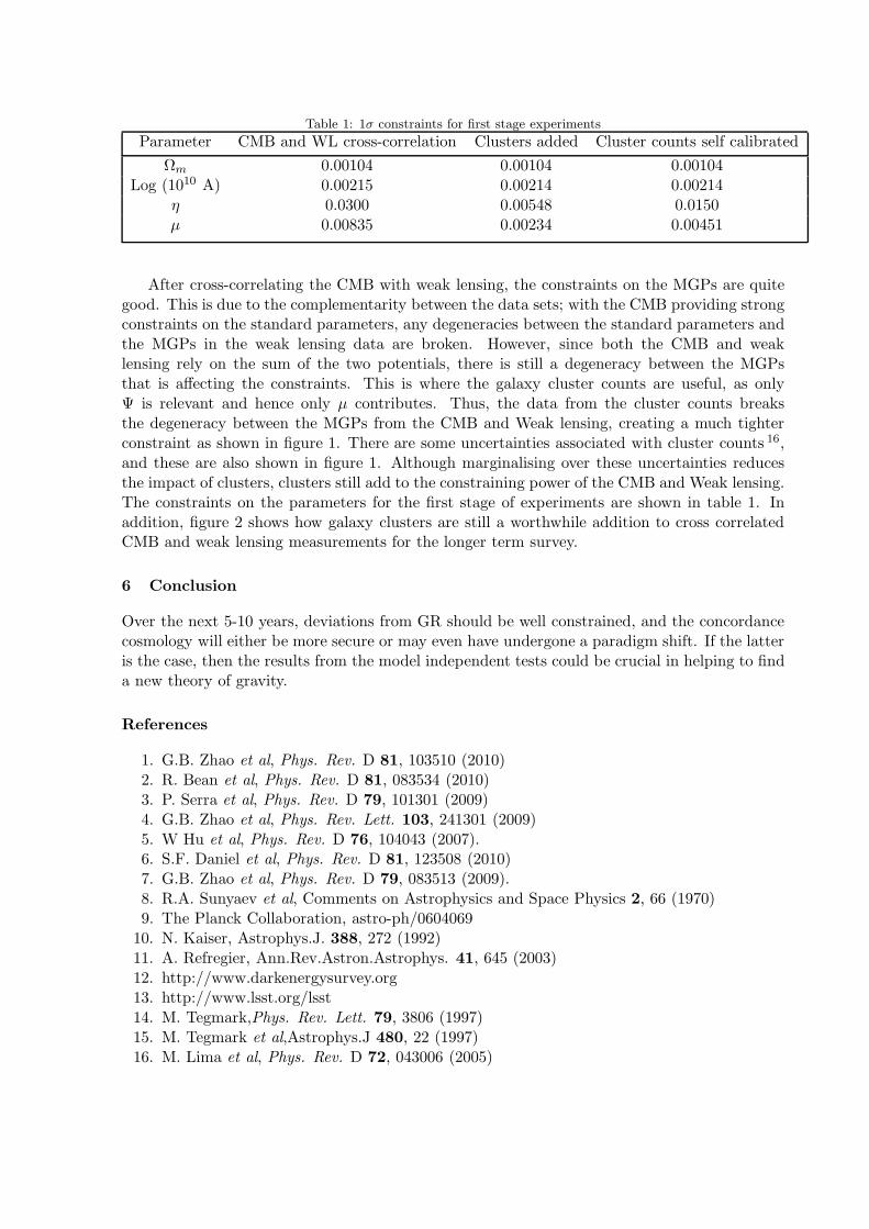
Table 1: 1σ constraints for first stage experiments
Parameter CMB and WL cross-correlation Clusters added Cluster counts self calibrated
Ωm 0.00104 0.00104 0.00104Log (1010 A) 0.00215 0.00214 0.00214
η 0.0300 0.00548 0.0150µ 0.00835 0.00234 0.00451
After cross-correlating the CMB with weak lensing, the constraints on the MGPs are quitegood. This is due to the complementarity between the data sets; with the CMB providing strongconstraints on the standard parameters, any degeneracies between the standard parameters andthe MGPs in the weak lensing data are broken. However, since both the CMB and weaklensing rely on the sum of the two potentials, there is still a degeneracy between the MGPsthat is affecting the constraints. This is where the galaxy cluster counts are useful, as onlyΨ is relevant and hence only µ contributes. Thus, the data from the cluster counts breaksthe degeneracy between the MGPs from the CMB and Weak lensing, creating a much tighterconstraint as shown in figure 1. There are some uncertainties associated with cluster counts 16,and these are also shown in figure 1. Although marginalising over these uncertainties reducesthe impact of clusters, clusters still add to the constraining power of the CMB and Weak lensing.The constraints on the parameters for the first stage of experiments are shown in table 1. Inaddition, figure 2 shows how galaxy clusters are still a worthwhile addition to cross correlatedCMB and weak lensing measurements for the longer term survey.
6 Conclusion
Over the next 5-10 years, deviations from GR should be well constrained, and the concordancecosmology will either be more secure or may even have undergone a paradigm shift. If the latteris the case, then the results from the model independent tests could be crucial in helping to finda new theory of gravity.
References
1. G.B. Zhao et al, Phys. Rev. D 81, 103510 (2010)2. R. Bean et al, Phys. Rev. D 81, 083534 (2010)3. P. Serra et al, Phys. Rev. D 79, 101301 (2009)4. G.B. Zhao et al, Phys. Rev. Lett. 103, 241301 (2009)5. W Hu et al, Phys. Rev. D 76, 104043 (2007).6. S.F. Daniel et al, Phys. Rev. D 81, 123508 (2010)7. G.B. Zhao et al, Phys. Rev. D 79, 083513 (2009).8. R.A. Sunyaev et al, Comments on Astrophysics and Space Physics 2, 66 (1970)9. The Planck Collaboration, astro-ph/0604069
10. N. Kaiser, Astrophys.J. 388, 272 (1992)11. A. Refregier, Ann.Rev.Astron.Astrophys. 41, 645 (2003)12. http://www.darkenergysurvey.org13. http://www.lsst.org/lsst14. M. Tegmark,Phys. Rev. Lett. 79, 3806 (1997)15. M. Tegmark et al,Astrophys.J 480, 22 (1997)16. M. Lima et al, Phys. Rev. D 72, 043006 (2005)
9.Weak equivalence principle

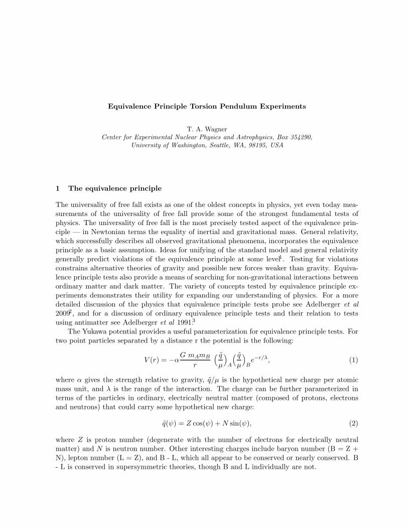
Equivalence Principle Torsion Pendulum Experiments
T. A. WagnerCenter for Experimental Nuclear Physics and Astrophysics, Box 354290,
University of Washington, Seattle, WA, 98195, USA
1 The equivalence principle
The universality of free fall exists as one of the oldest concepts in physics, yet even today mea-surements of the universality of free fall provide some of the strongest fundamental tests ofphysics. The universality of free fall is the most precisely tested aspect of the equivalence prin-ciple — in Newtonian terms the equality of inertial and gravitational mass. General relativity,which successfully describes all observed gravitational phenomena, incorporates the equivalenceprinciple as a basic assumption. Ideas for unifying of the standard model and general relativitygenerally predict violations of the equivalence principle at some level1. Testing for violationsconstrains alternative theories of gravity and possible new forces weaker than gravity. Equiva-lence principle tests also provide a means of searching for non-gravitational interactions betweenordinary matter and dark matter. The variety of concepts tested by equivalence principle ex-periments demonstrates their utility for expanding our understanding of physics. For a moredetailed discussion of the physics that equivalence principle tests probe see Adelberger et al
20092, and for a discussion of ordinary equivalence principle tests and their relation to testsusing antimatter see Adelberger et al 1991.3
The Yukawa potential provides a useful parameterization for equivalence principle tests. Fortwo point particles separated by a distance r the potential is the following:
V (r) = −αG mAmB
r
(
q
µ
)
A
(
q
µ
)
Be−r/λ
, (1)
where α gives the strength relative to gravity, q/µ is the hypothetical new charge per atomicmass unit, and λ is the range of the interaction. The charge can be further parameterized interms of the particles in ordinary, electrically neutral matter (composed of protons, electronsand neutrons) that could carry some hypothetical new charge:
q(ψ) = Z cos(ψ) +N sin(ψ), (2)
where Z is proton number (degenerate with the number of electrons for electrically neutralmatter) and N is neutron number. Other interesting charges include baryon number (B = Z +N), lepton number (L = Z), and B - L, which all appear to be conserved or nearly conserved. B- L is conserved in supersymmetric theories, though B and L individually are not.
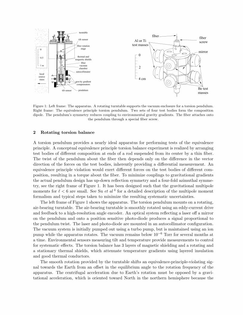
Figure 1: Left frame: The apparatus. A rotating turntable supports the vacuum enclosure for a torsion pendulum.Right frame: The equivalence principle torsion pendulum. Two sets of four test bodies form the compositiondipole. The pendulum’s symmetry reduces coupling to environmental gravity gradients. The fiber attaches onto
the pendulum through a special fiber screw.
2 Rotating torsion balance
A torsion pendulum provides a nearly ideal apparatus for performing tests of the equivalenceprinciple. A conceptual equivalence principle torsion balance experiment is realized by arrangingtest bodies of different composition at ends of a rod suspended from its center by a thin fiber.The twist of the pendulum about the fiber then depends only on the difference in the vectordirection of the forces on the test bodies, inherently providing a differential measurement. Anequivalence principle violation would exert different forces on the test bodies of different com-position, resulting in a torque about the fiber. To minimize couplings to gravitational gradientsthe actual pendulum design has up-down reflection symmetry and a four-fold azimuthal symme-try, see the right frame of Figure 1. It has been designed such that the gravitational multipolemoments for ℓ < 6 are small. See Su et al 4 for a detailed description of the multipole momentformalism and typical steps taken to minimize the resulting systematic uncertainties.
The left frame of Figure 1 shows the apparatus. The torsion pendulum mounts on a rotating,air-bearing turntable. The air-bearing turntable is smoothly rotated using an eddy-current driveand feedback to a high-resolution angle encoder. An optical system reflecting a laser off a mirroron the pendulum and onto a position sensitive photo-diode produces a signal proportional tothe pendulum twist. The laser and photo-diode are mounted in an autocollimator configuration.The vacuum system is initially pumped out using a turbo pump, but is maintained using an ionpump while the apparatus rotates. The vacuum remains below 10−6 Torr for several months ata time. Environmental sensors measuring tilt and temperature provide measurements to controlfor systematic effects. The torsion balance has 3 layers of magnetic shielding and a rotating anda stationary thermal shields, which attenuate temperature gradients using layered insulationand good thermal conductors.
The smooth rotation provided by the turntable shifts an equivalence-principle-violating sig-nal towards the Earth from an offset in the equilibrium angle to the rotation frequency of theapparatus. The centrifugal acceleration due to Earth’s rotation must be opposed by a gravi-tational acceleration, which is oriented toward North in the northern hemisphere because the
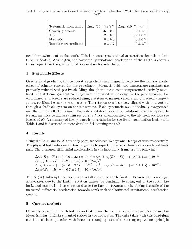
Table 1: 1-σ systematic uncertainties and associated corrections for North and West differential acceleration usingBe-Ti.
Systematic uncertainty ∆aN (10−15m/s
2) ∆aW (10−15m/s
2)
Gravity gradients 1.6 ± 0.2 0.3 ± 1.7Tilt 1.2 ± 0.6 −0.2 ± 0.7Magnetic 0 ± 0.3 0 ± 0.3Temperature gradients 0 ± 1.7 0 ± 1.7
pendulum swings out to the south. This horizontal gravitational acceleration depends on lati-tude. In Seattle, Washington, the horizontal gravitational acceleration of the Earth is about 3times larger than the gravitational acceleration towards the Sun.
3 Systematic Effects
Gravitational gradients, tilt, temperature gradients and magnetic fields are the four systematiceffects of primary concern for this experiment. Magnetic fields and temperature gradients areprimarily reduced with passive shielding, though the mean room temperature is actively stabi-lized. Gravitational gradient couplings were minimized in the design of the pendulum and theenvironmental gradients are reduced using a system of masses, called gravity gradient compen-sators, positioned close to the apparatus. The rotation axis is actively aligned with local verticalthrough a feedback system on the tilt sensors. Each systematic was individually exaggeratedand the induced effect measured. For a detailed description of gravitational gradient systemat-ics and methods to address them see Su et al.4 For an explanation of the tilt feedback loop seeHeckel et al.5 A summary of the systematic uncertainties for the Be-Ti combination is shown inTable 1 and is discussed in more detail in Schlamminger et al.6
4 Results
Using the Be-Ti and Be-Al test body pairs, we collected 75 days and 96 days of data, respectively.The physical test bodies were interchanged with respect to the pendulum once for each test bodypair. The measured differential accelerations in the laboratory frame are the following:
∆aN (Be− T i) = (+0.6 ± 3.1) × 10−15m/s
2⇒ η⊕(Be− T i) = (+0.3 ± 1.8) × 10−13
∆aW (Be− T i) = (−2.5 ± 3.5) × 10−15m/s
2
∆aN (Be−Al) = (−2.6 ± 2.5) × 10−15m/s
2⇒ η⊕(Be−Al) = (−1.5 ± 1.5) × 10−13
∆aW (Be−Al) = (+0.7 ± 2.5) × 10−15m/s
2.
The N (W) subscript corresponds to results towards north (west). Because the centrifugalacceleration due to the Earth’s rotation causes the pendulum to swing out to the south, thehorizontal gravitational acceleration due to the Earth is towards north. Taking the ratio of themeasured differential acceleration towards north with the horizontal gravitational accelerationgives η⊕.
5 Current projects
Currently, a pendulum with test bodies that mimic the composition of the Earth’s core and theMoon (similar to Earth’s mantle) resides in the apparatus. The data taken with this pendulumcan be used in conjunction with lunar laser ranging tests of the strong equivalence principle
to set limits on how gravitational binding energy obeys the equivalence principle. Using theseresults and results stemming from the more precise lunar laser ranging capability of the APOLLOcollaboration, an order of magnitude improvement over existing limits of ηgrav ≈ 1×10⁻³ shouldbe possible.7,8
Seasonal changes in gravitational gradients produce one of the largest systematic uncertain-ties for this apparatus. The Eot-Wash group is currently examining different approaches forcontinual monitoring of these gravitational gradients. Some possible approaches include dedi-cated gradiometer torsion pendulums and using vertically displaced tilt sensors to monitor thelowest order (Q21) gravitational gradients.
Acknowledgments
This work was funded by a grants from the NSF grant Nos. PHY0355012, PHY0653863, byNASA grant No. NNC04GB03G, and by DOE funding for the CENPA laboratory. I wouldlike to thank Eric Adelberger, Jens Gundlach, Blayne Heckel, Tom Butler, Ki-Young Choi,Stephen Merkowitz, Stephan Schlamminger, Ulrich Schmidt, Hank Simons, Chris Spitzer andErik Swanson for their contributions.
References
1. Thibault Damour. Testing the equivalence principle: why and how? Class. Quantum
Grav., 13:A33–A44, 1996.2. E. G. Adelberger, J. H. Gundlach, B. R. Heckel, S. Hoedl, and S. Schlamminger. Torsion
balance experiments: A low-energy frontier of particle physics. Prog. Part. Nuc. Phys.,62:102–134, 2009.
3. E. G. Adelberger, B. R. Heckel, C. W. Stubbs, and Y. Su. Does antimatter fall with thesame acceleration as ordinary matter? Phys. Rev. Lett., 66:850–853, 1991.
4. Y. Su, B. R. Heckel, E. G. Adelberger, J. H. Gundlach, M. Harris, G. L. Smith, andH. E. Swanson. New tests of the universality of free fall. Phys. Rev. D, 50:3614–3636,September 1994.
5. B. R. Heckel, E. G. Adelberger, C. E. Cramer, T. S. Cook, S. Schlamminger, andU. Schmidt. Preferred-frame and cp-violation tests with polarized electrons. Phys.
Rev. D, 78(9):092006, 2008.6. S. Schlamminger, K.-Y. Choi, T. A. Wagner, J. H. Gundlach, and E. G. Adelberger.
Test of the equivalence principle using a rotating torsion balance. Phys. Rev. Lett.,100(4):041101, 2008.
7. J. G. Williams, S. G. Turyshev, and D. H. Boggs. Progress in Lunar Laser Ranging Testsof Relativistic Gravity. Phys. Rev. Lett., 93:261101, 2004.
8. S. Baeßler, B. R. Heckel, E. G. Adelberger, J. H. Gundlach, U. Schmidt, and H. E. Swanson.Improved test of the equivalence principle for gravitational self-energy. Phys. Rev. Lett.,83:3585, 1999.
AMONG SPACE FUNDAMENTAL PHYSICS MISSIONS, MICROSCOPE, A SIMPLE CHALLENGING FREE FALL TEST
P. TOUBOUL1, R. CHHUN1, D. BOULANGER1, M.RODRIGUES1, G.METRIS2
1Onera, The French Aerospace Lab, Chemin de la Hunière, 91761 Palaiseau Cedex, France 2Observatoire de la Côte d’Azur, GeoAzur, Grasse, France.
Several space tests of gravity laws have already been performed but the MICROSCOPE mission is the first one to be fully dedicated to the test of the Equivalence Principle. The dedicated payload is now under qualification and the rather large micro satellite will be produced by Cnes for a launch at beginning of 2015. Each of the two differential accelerometers of the experimental device includes a pair of test-masses whose 720 km altitude orbital motions are constrained along the same purely gravitational trajectory. Evidence of an EP violation is provided by the comparison of the electrostatic configurations needed to maintain the two masses composed of different materials motionless relative to each other. Not only the servo-loop electronics must exhibit very weak level of noise but the geometrical and electrical configuration of the instruments must be very well optimised, accurate, cleaned and steady. Although the accelerometers are saturated on ground by normal gravity, they can be tested on board a free fall capsule in drop tower. These tests complete the fine verification of all mechanical and electrical functions. In addition, the present in flight results of the GOCE mission accelerometers are deeply analysed. Because the sensors of the gravity gradiometer exploits the same technologies, they provide confirmation of the MICROSCOPE instrument models used to extrapolate the in orbit performance and then estimate the expected mission accuracy.
1. The MICROSCOPE space mission One century after Einstein 1‘s paper on special relativity, initiating his elaboration of the new formulation of gravitational interactions, space remains the favorite environment to perform deep experimental investigation on Gravitation. After the Pound and Rebka 2 experiments in 1959, demonstrating frequency red shift with γ rays emission, R. Vessot 3 has performed in 1976 the comparison of two clocks at different gravity potential taking advantage of the parabolic trajectory of a rocket, up to an altitude of ten thousand kilometers. With this Gravity Probe A mission, redshift of 4.10-10 was measured with clock frequency stability of 10-14. The ACES (Atomic Clock Ensemble in Space) payload will be accommodated in 2014 on board the International Space Station and will include Hydrogen Maser and the cold atom PHARAO clock with a fine microwave link in order to perform, among other metrological objectives like C isotropy, time dilatation or time distribution, the comparison with ground clocks with an expected accuracy better than 10-16 [L. Cacciapuoti 4]. The three ton Gravity Probe B satellite was launched in April 2004 for 18 month operating mission. The drag free satellite mainly carries four dedicated cryogenic gyros in a very steady configuration, aligned with an inertially pointed telescope, in order to perform the accurate measurement of both the geodetic and the frame dragging effect along the Earth polar circular orbit at an altitude of 642 km. With a specific data processing, developed to correct the limitation of the gyros, induced by unforeseen electrical anisotropic charging of their spherical rotor and cage, the expected -6606.1 milliarcsecond/year N-S geodetic drift was measured with 0.3 % accuracy
(-6601.8+/-18.3 mas/yr) and the -39.2 mas/yr frame dragging drift with 20 % accuracy (-37.2+/-7.2 mas/yr) [C.W.F. Everitt 5]. These results agree with the previously measured Lense-Thirring effect on satellite orbital plane, previously performed with the LAGEOS 2 satellite. Eleven years of fine laser tracking of the 5620 km altitude orbit have been revisited taking advantage of the more accurate Earth gravity field model obtained from the GRACE space mission data. 10 % uncertainty on the measured effect was then evaluated by I. Ciufolini 6. The Parameterized Post-Newtonian (PPN) formalism is often considered to interpret the space tests of general relativity and γ and β are presently respectively limited to the following ranges:
- γ-1 = 2.1 +/- 2.3 10-5, as computed by B.Bertotti et al. 7 from the Cassini spacecraft navigation during its cruise from Jupiter to Saturn with the solar conjunction between Earth and Satellite,
- β-1= 1.2 +/- 1.1 10-4, as deduced by J.G. Williams et al. 8 from the accurate measurements by lunar laser ranging, of the relative motions of the Earth and Moon in Solar gravity field.
Other space tests of gravity are now proposed. Among them, the Outer Solar System mission proposed by B. Christophe et al. 9 envisages long range gravity test by finely tracking the gravitational motion of an interplanetary spacecraft carrying an electrostatic ultra-sensitive accelerometer to permanently survey any deviation from geodesic motion. The SAGAS mission, proposed by P. Wolf et al. 10 is much more ambitious considering a large satellite, able to cross the solar system with an optical atomic clock on board, cold atom interferometers as accelerometers and gyrometers, laser links for the satellite motion tracking with many major objectives like the test of universal redshift, the test of Lorentz invariance, PPN test, large scale gravity, variation of cosmologic constant… For what concerns the MICROSCOPE mission, it is fully dedicated to the test of the Equivalence Principle (EP). It has been selected by Cnes in 2004, the instrument is now under qualification and the satellite production should start this year for a launch of the satellite in 2015. The accurate test of the universality of free fall represents today much more than the verification of this well known property. The violation of the universality of free fall leads to the violation of the Equivalence Principle (EP), fundamental basis of the Einstein General Relativity. Einstein, himself, considered this symmetry as enacted by the experience. Today, most attempts of Grand Unification like String theory and M-theory allow the violation of this principle, introducing in particular scalar fields 11, while the experimental investigation of quantum gravity does appear directly very weakly accessible. The test of the Equivalence Principle is thus not only the test of general relativity but also the search for new experimental results as the necessary support for new theories: as expressed by T. Damour 12, EP test appears much more relevant by about a factor 106 than γ accurate determination when comparing presently obtained γ and EP test accuracy. In addition, Super symmetry might be confirmed by the CERN LHC near future results with new particles to be taken into account. The test of the universality of free fall with ultimate accuracy is then an important challenge and has also to be considered regarding dark matter query. Present laboratory tests, performed by the Eötwash group 13 reached a few 10-13 accuracy: the dedicated torsion pendulum exploits the 1m long, 20 µm diameter tungsten fibre, exhibiting a Q factor of about 5000. It is surrounded with 800 kg of lead designed to compensate the local gravity gradients. Much care is also taken to reject the vibrating environment and the thermal effects. The data can be integrated over periods as long as 3 months.
MICROSCOPE space experiment has been designed and the payload and the satellite specified to obtain at least two orders of magnitude better, i.e. 10-15 accuracy. Other missions are also proposed by A. Nobili 14 or T. Sumner 15 to perform this test with outstanding accuracy of 10-17 or 10-18. But not only the instruments demand new long developments but such missions require quite 10 times heavier satellites with much demanding performance for attitude controls and drag free motions as well as for the experiment environment controls. 2. The MICROSCOPE experiment The MICROSCOPE satellite is rather small, 270 kg in its definitive definition, with its new cold gas propulsion system, leading to major constraints on the dedicated scientific payload available mass, volume and power, respectively, 35 kg, 40 cm3 and 40 W, leading to a non cryogenic experiment, with
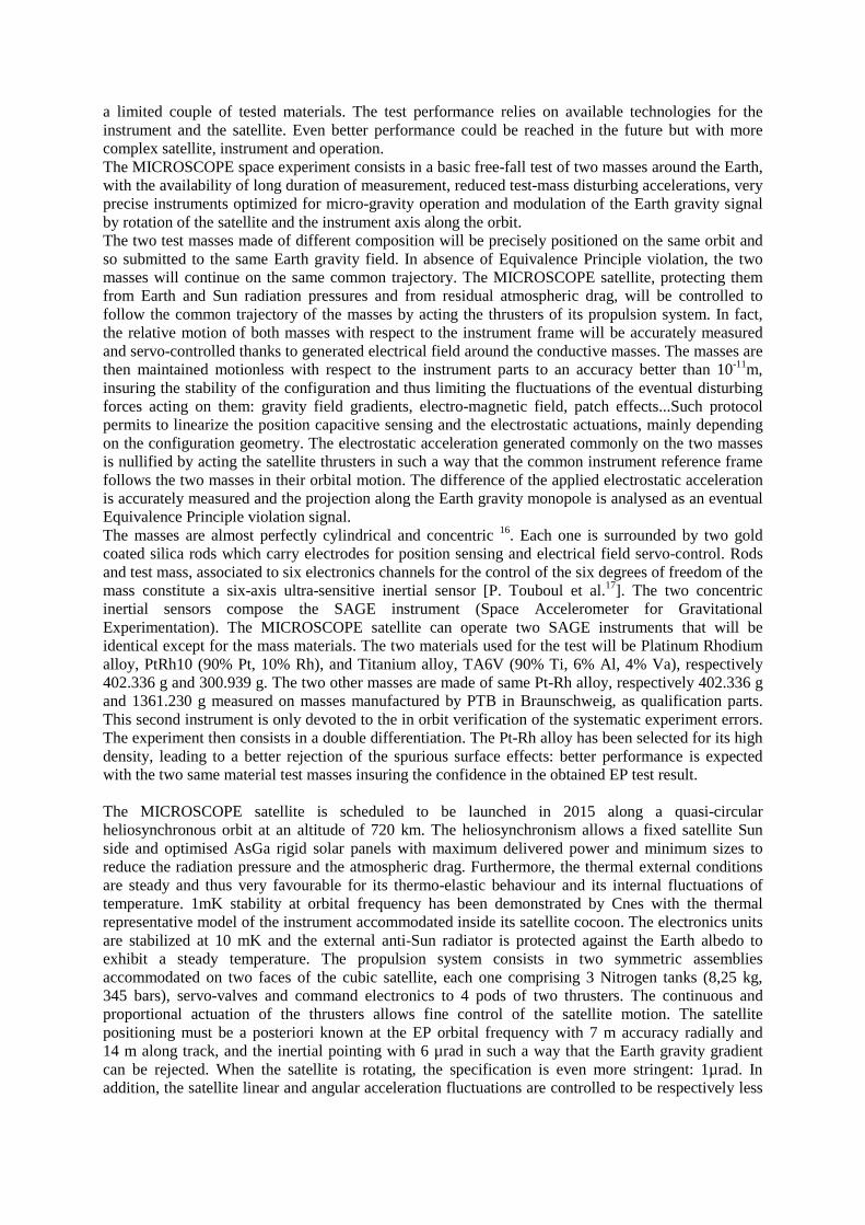
a limited couple of tested materials. The test performance relies on available technologies for the instrument and the satellite. Even better performance could be reached in the future but with more complex satellite, instrument and operation. The MICROSCOPE space experiment consists in a basic free-fall test of two masses around the Earth, with the availability of long duration of measurement, reduced test-mass disturbing accelerations, very precise instruments optimized for micro-gravity operation and modulation of the Earth gravity signal by rotation of the satellite and the instrument axis along the orbit. The two test masses made of different composition will be precisely positioned on the same orbit and so submitted to the same Earth gravity field. In absence of Equivalence Principle violation, the two masses will continue on the same common trajectory. The MICROSCOPE satellite, protecting them from Earth and Sun radiation pressures and from residual atmospheric drag, will be controlled to follow the common trajectory of the masses by acting the thrusters of its propulsion system. In fact, the relative motion of both masses with respect to the instrument frame will be accurately measured and servo-controlled thanks to generated electrical field around the conductive masses. The masses are then maintained motionless with respect to the instrument parts to an accuracy better than 10-11m, insuring the stability of the configuration and thus limiting the fluctuations of the eventual disturbing forces acting on them: gravity field gradients, electro-magnetic field, patch effects...Such protocol permits to linearize the position capacitive sensing and the electrostatic actuations, mainly depending on the configuration geometry. The electrostatic acceleration generated commonly on the two masses is nullified by acting the satellite thrusters in such a way that the common instrument reference frame follows the two masses in their orbital motion. The difference of the applied electrostatic acceleration is accurately measured and the projection along the Earth gravity monopole is analysed as an eventual Equivalence Principle violation signal. The masses are almost perfectly cylindrical and concentric 16. Each one is surrounded by two gold coated silica rods which carry electrodes for position sensing and electrical field servo-control. Rods and test mass, associated to six electronics channels for the control of the six degrees of freedom of the mass constitute a six-axis ultra-sensitive inertial sensor [P. Touboul et al.17]. The two concentric inertial sensors compose the SAGE instrument (Space Accelerometer for Gravitational Experimentation). The MICROSCOPE satellite can operate two SAGE instruments that will be identical except for the mass materials. The two materials used for the test will be Platinum Rhodium alloy, PtRh10 (90% Pt, 10% Rh), and Titanium alloy, TA6V (90% Ti, 6% Al, 4% Va), respectively 402.336 g and 300.939 g. The two other masses are made of same Pt-Rh alloy, respectively 402.336 g and 1361.230 g measured on masses manufactured by PTB in Braunschweig, as qualification parts. This second instrument is only devoted to the in orbit verification of the systematic experiment errors. The experiment then consists in a double differentiation. The Pt-Rh alloy has been selected for its high density, leading to a better rejection of the spurious surface effects: better performance is expected with the two same material test masses insuring the confidence in the obtained EP test result. The MICROSCOPE satellite is scheduled to be launched in 2015 along a quasi-circular heliosynchronous orbit at an altitude of 720 km. The heliosynchronism allows a fixed satellite Sun side and optimised AsGa rigid solar panels with maximum delivered power and minimum sizes to reduce the radiation pressure and the atmospheric drag. Furthermore, the thermal external conditions are steady and thus very favourable for its thermo-elastic behaviour and its internal fluctuations of temperature. 1mK stability at orbital frequency has been demonstrated by Cnes with the thermal representative model of the instrument accommodated inside its satellite cocoon. The electronics units are stabilized at 10 mK and the external anti-Sun radiator is protected against the Earth albedo to exhibit a steady temperature. The propulsion system consists in two symmetric assemblies accommodated on two faces of the cubic satellite, each one comprising 3 Nitrogen tanks (8,25 kg, 345 bars), servo-valves and command electronics to 4 pods of two thrusters. The continuous and proportional actuation of the thrusters allows fine control of the satellite motion. The satellite positioning must be a posteriori known at the EP orbital frequency with 7 m accuracy radially and 14 m along track, and the inertial pointing with 6 µrad in such a way that the Earth gravity gradient can be rejected. When the satellite is rotating, the specification is even more stringent: 1µrad. In addition, the satellite linear and angular acceleration fluctuations are controlled to be respectively less
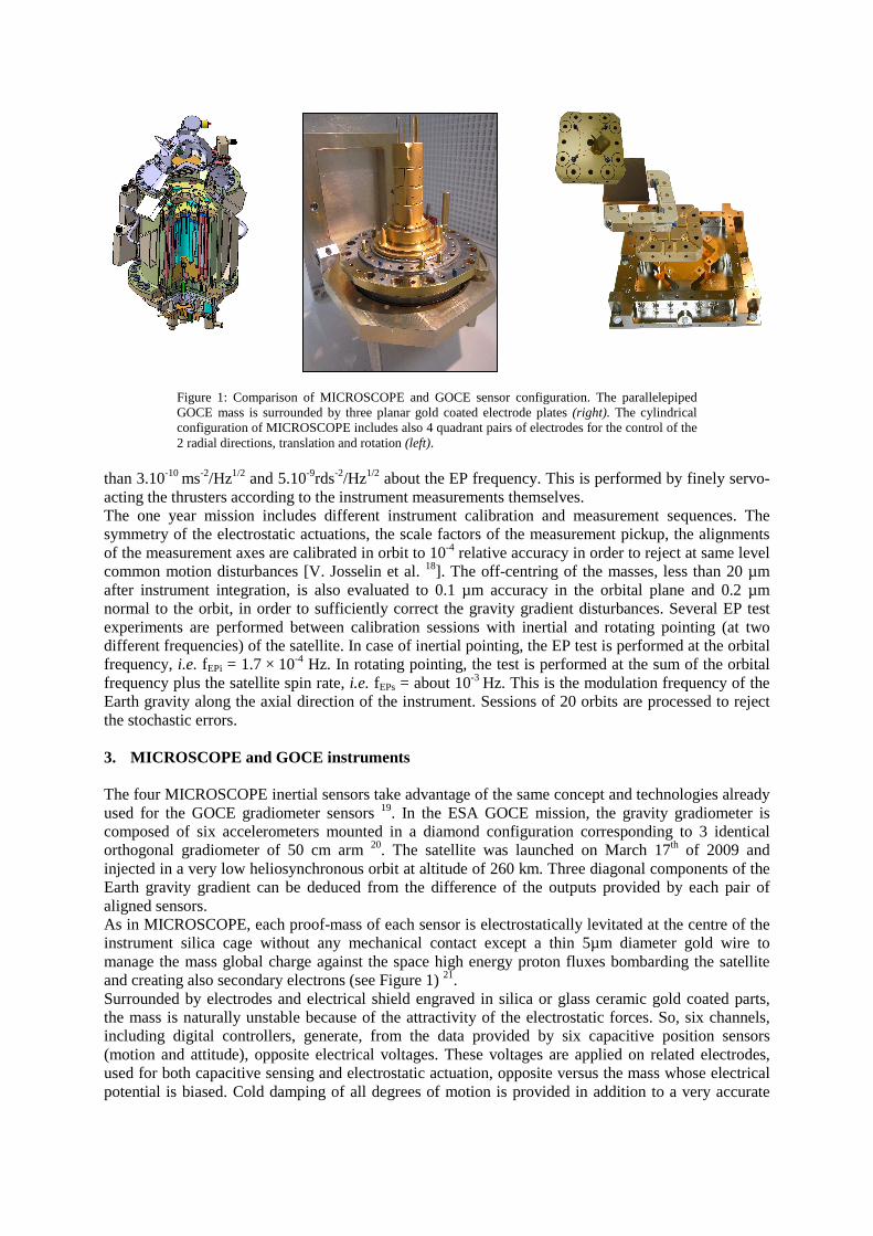
Figure 1: Comparison of MICROSCOPE and GOCE sensor configuration. The parallelepiped GOCE mass is surrounded by three planar gold coated electrode plates (right). The cylindrical configuration of MICROSCOPE includes also 4 quadrant pairs of electrodes for the control of the 2 radial directions, translation and rotation (left).
than 3.10-10 ms-2/Hz1/2 and 5.10-9rds-2/Hz1/2 about the EP frequency. This is performed by finely servo-acting the thrusters according to the instrument measurements themselves. The one year mission includes different instrument calibration and measurement sequences. The symmetry of the electrostatic actuations, the scale factors of the measurement pickup, the alignments of the measurement axes are calibrated in orbit to 10-4 relative accuracy in order to reject at same level common motion disturbances [V. Josselin et al. 18]. The off-centring of the masses, less than 20 µm after instrument integration, is also evaluated to 0.1 µm accuracy in the orbital plane and 0.2 µm normal to the orbit, in order to sufficiently correct the gravity gradient disturbances. Several EP test experiments are performed between calibration sessions with inertial and rotating pointing (at two different frequencies) of the satellite. In case of inertial pointing, the EP test is performed at the orbital frequency, i.e. fEPi = 1.7 × 10⁻⁴ Hz. In rotating pointing, the test is performed at the sum of the orbital frequency plus the satellite spin rate, i.e. fEPs = about 10-3 Hz. This is the modulation frequency of the Earth gravity along the axial direction of the instrument. Sessions of 20 orbits are processed to reject the stochastic errors.
3. MICROSCOPE and GOCE instruments The four MICROSCOPE inertial sensors take advantage of the same concept and technologies already used for the GOCE gradiometer sensors 19. In the ESA GOCE mission, the gravity gradiometer is composed of six accelerometers mounted in a diamond configuration corresponding to 3 identical orthogonal gradiometer of 50 cm arm 20. The satellite was launched on March 17th of 2009 and injected in a very low heliosynchronous orbit at altitude of 260 km. Three diagonal components of the Earth gravity gradient can be deduced from the difference of the outputs provided by each pair of aligned sensors. As in MICROSCOPE, each proof-mass of each sensor is electrostatically levitated at the centre of the instrument silica cage without any mechanical contact except a thin 5µm diameter gold wire to manage the mass global charge against the space high energy proton fluxes bombarding the satellite and creating also secondary electrons (see Figure 1) 21. Surrounded by electrodes and electrical shield engraved in silica or glass ceramic gold coated parts, the mass is naturally unstable because of the attractivity of the electrostatic forces. So, six channels, including digital controllers, generate, from the data provided by six capacitive position sensors (motion and attitude), opposite electrical voltages. These voltages are applied on related electrodes, used for both capacitive sensing and electrostatic actuation, opposite versus the mass whose electrical potential is biased. Cold damping of all degrees of motion is provided in addition to a very accurate
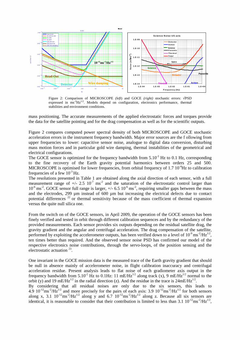
1 105−× 1 10
4−× 1 103−× 0.01 0.1 1 10
1 10 14−×
1 1013−×
1 1012−×
1 1011−×
1 1010−×
1 10 9−×requirementSU-EPI/SU-RFISU-EPESU-RFEEPE DetectorEPE Read-OutEPE Wire damping
X SCI
Hz
m/s
^2/H
z^1/
2
S cience N o ise U S axis
1.E-14
1.E-13
1.E-12
1.E-11
1.E-10
1.E-09
1 .E-04 1.E-03 1.E-02 1.E-01 1.E+00
F re q u e n cy (Hz)
No
ise
(m
/s2 /Hz1
/2)
De te ctor
Action
M e a sure
P a ra sitic
The rm a l
Tota l
Detector
Thermal
Science
Parasitic
Action
Specs
Science
S cience N o ise U S axis
1.E-14
1.E-13
1.E-12
1.E-11
1.E-10
1.E-09
1 .E-04 1.E-03 1.E-02 1.E-01 1.E+00
F re q u e n cy (Hz)
No
ise
(m
/s2 /Hz1
/2)
De te ctor
Action
M e a sure
P a ra sitic
The rm a l
Tota l
Detector
Thermal
Science
Parasitic
Action
Specs
Science
Figure 2: Comparison of MICROSCOPE (left) and GOCE (right) stochastic errors: √PSD expressed in ms-2Hz1/2. Models depend on configuration, electronics performance, thermal stabilities and environment conditions.
mass positioning. The accurate measurements of the applied electrostatic forces and torques provide the data for the satellite pointing and for the drag compensation as well as for the scientific outputs. Figure 2 compares computed power spectral density of both MICROSCOPE and GOCE stochastic acceleration errors in the instrument frequency bandwidth. Major error sources are the f ollowing from upper frequencies to lower: capacitive sensor noise, analogue to digital data conversion, disturbing mass motion forces and in particular gold wire damping, thermal instabilities of the geometrical and electrical configurations. The GOCE sensor is optimized for the frequency bandwidth from 5.10-3 Hz to 0.1 Hz, corresponding to the fine recovery of the Earth gravity potential harmonics between orders 25 and 500. MICROSCOPE is optimised for lower frequencies, from orbital frequency of 1.7 10-4Hz to calibration frequencies of a few 10-3 Hz. The resolutions presented in Table 1 are obtained along the axial direction of each sensor, with a full measurement range of +/- 2.5 10-7 ms-2 and the saturation of the electrostatic control larger than 10-6 ms-2. GOCE sensor full range is larger, +/- 6.5 10-6 ms-2, requiring smaller gaps between the mass and the electrodes, 299 µm instead of 600 µm but increasing the electrical defects due to contact potential differences 22 or thermal sensitivity because of the mass coefficient of thermal expansion versus the quite null silica one. From the switch on of the GOCE sensors, in April 2009, the operation of the GOCE sensors has been finely verified and tested in orbit through different calibration sequences and by the redundancy of the provided measurements. Each sensor provides six outputs depending on the residual satellite drag, the gravity gradient and the angular and centrifugal acceleration. The drag compensation of the satellite, performed by exploiting the accelerometer outputs, has been verified down to a level of 10-9 ms-2/Hz1/2, ten times better than required. And the observed sensor noise PSD has confirmed our model of the respective electronics noise contributions, through the servo-loops, of the position sensing and the electrostatic actuation 23. One invariant in the GOCE mission data is the measured trace of the Earth gravity gradient that should be null in absence mainly of accelerometer noise, in flight calibration inaccuracy and centrifugal acceleration residue. Present analysis leads to flat noise of each gradiometer axis output in the frequency bandwidth from 5.10-2 Hz to 0.1Hz: 11 mE/Hz1/2 along track (x), 9 mE/Hz1/2 normal to the orbit (y) and 19 mE/Hz1/2 in the radial direction (z). And the residue in the trace is 24mE/Hz1/2. By considering that all residual noises are only due to the six sensors, this leads to 4.9 10-12ms-2/Hz1/2 and more precisely for the pairs of each axis: 3.9 10-12ms-2/Hz1/2 for both sensors along x, 3.1 10-12ms-2/Hz1/2 along y and 6.7 10-12ms-2/Hz1/2 along z. Because all six sensors are identical, it is reasonable to consider that their contribution is limited to less than 3.1 10-12ms-2/Hz1/2,
Detector Wire damping
Read-Out
10-12ms-2/Hz1/2
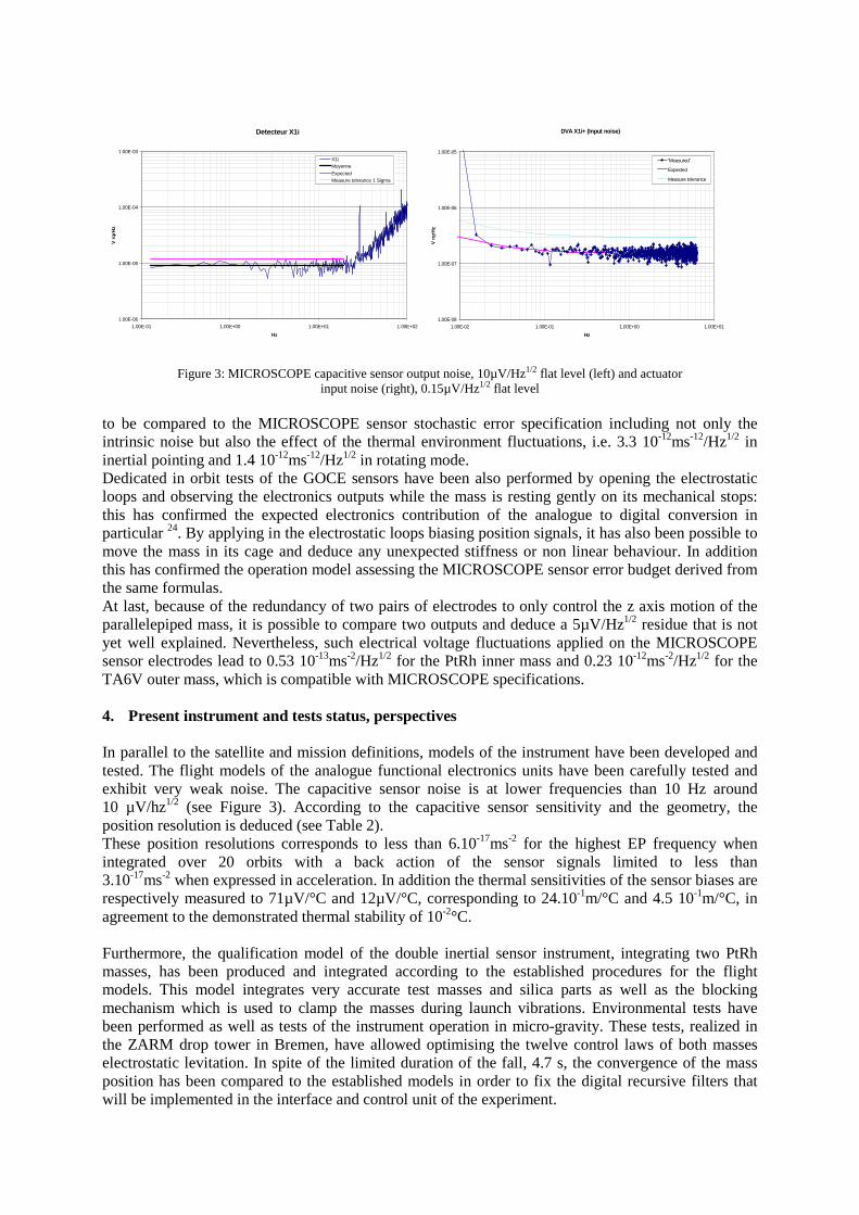
Figure 3: MICROSCOPE capacitive sensor output noise, 10µV/Hz1/2 flat level (left) and actuator input noise (right), 0.15µV/Hz1/2 flat level
to be compared to the MICROSCOPE sensor stochastic error specification including not only the intrinsic noise but also the effect of the thermal environment fluctuations, i.e. 3.3 10-12ms-12/Hz1/2 in inertial pointing and 1.4 10-12ms-12/Hz1/2 in rotating mode. Dedicated in orbit tests of the GOCE sensors have been also performed by opening the electrostatic loops and observing the electronics outputs while the mass is resting gently on its mechanical stops: this has confirmed the expected electronics contribution of the analogue to digital conversion in particular 24. By applying in the electrostatic loops biasing position signals, it has also been possible to move the mass in its cage and deduce any unexpected stiffness or non linear behaviour. In addition this has confirmed the operation model assessing the MICROSCOPE sensor error budget derived from the same formulas. At last, because of the redundancy of two pairs of electrodes to only control the z axis motion of the parallelepiped mass, it is possible to compare two outputs and deduce a 5µV/Hz1/2 residue that is not yet well explained. Nevertheless, such electrical voltage fluctuations applied on the MICROSCOPE sensor electrodes lead to 0.53 10-13ms-2/Hz1/2 for the PtRh inner mass and 0.23 10-12ms-2/Hz1/2 for the TA6V outer mass, which is compatible with MICROSCOPE specifications. 4. Present instrument and tests status, perspectives In parallel to the satellite and mission definitions, models of the instrument have been developed and tested. The flight models of the analogue functional electronics units have been carefully tested and exhibit very weak noise. The capacitive sensor noise is at lower frequencies than 10 Hz around 10 µV/hz1/2 (see Figure 3). According to the capacitive sensor sensitivity and the geometry, the position resolution is deduced (see Table 2). These position resolutions corresponds to less than 6.10-17ms-2 for the highest EP frequency when integrated over 20 orbits with a back action of the sensor signals limited to less than 3.10-17ms-2 when expressed in acceleration. In addition the thermal sensitivities of the sensor biases are respectively measured to 71µV/°C and 12µV/°C, corresponding to 24.10-1m/°C and 4.5 10-1m/°C, in agreement to the demonstrated thermal stability of 10-2°C. Furthermore, the qualification model of the double inertial sensor instrument, integrating two PtRh masses, has been produced and integrated according to the established procedures for the flight models. This model integrates very accurate test masses and silica parts as well as the blocking mechanism which is used to clamp the masses during launch vibrations. Environmental tests have been performed as well as tests of the instrument operation in micro-gravity. These tests, realized in the ZARM drop tower in Bremen, have allowed optimising the twelve control laws of both masses electrostatic levitation. In spite of the limited duration of the fall, 4.7 s, the convergence of the mass position has been compared to the established models in order to fix the digital recursive filters that will be implemented in the interface and control unit of the experiment.
Detecteur X1i
1.00E-06
1.00E-05
1.00E-04
1.00E-03
1.00E-01 1.00E+00 1.00E+01 1.00E+02
Hz
V r
qrH
z
X1iMoyenne
ExpectedMeasure tolerance 1 Sigma
DVA X1i+ (Input noise)
1.00E-08
1.00E-07
1.00E-06
1.00E-05
1.00E-02 1.00E-01 1.00E+00 1.00E+01
Hz
V r
qrH
z
'Measured'
Expected
Measure tolerance
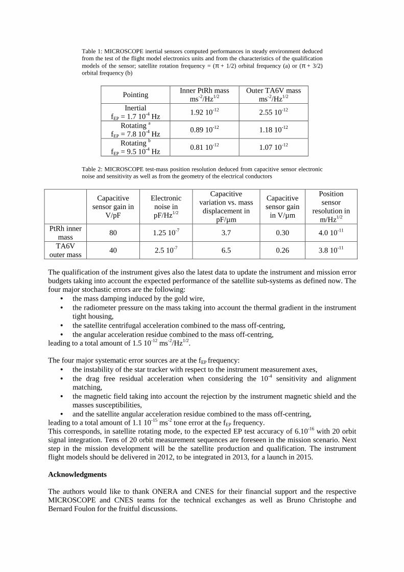
Table 1: MICROSCOPE inertial sensors computed performances in steady environment deduced from the test of the flight model electronics units and from the characteristics of the qualification models of the sensor; satellite rotation frequency = (π + 1/2) orbital frequency (a) or (π + 3/2) orbital frequency (b)
Pointing Inner PtRh mass
ms-2/Hz1/2 Outer TA6V mass
ms-2/Hz1/2 Inertial
fEP = 1.7 10-4 Hz 1.92 10-12 2.55 10-12
Rotating a fEP = 7.8 10-4 Hz
0.89 10-12 1.18 10-12
Rotating b fEP = 9.5 10-4 Hz
0.81 10-12 1.07 10-12
Table 2: MICROSCOPE test-mass position resolution deduced from capacitive sensor electronic noise and sensitivity as well as from the geometry of the electrical conductors
Capacitive
sensor gain in V/pF
Electronic noise in pF/Hz1/2
Capacitive variation vs. mass displacement in
pF/µm
Capacitive sensor gain
in V/µm
Position sensor
resolution in m/Hz1/2
PtRh inner mass
80 1.25 10-7 3.7 0.30 4.0 10-11
TA6V outer mass
40 2.5 10-7 6.5 0.26 3.8 10-11
The qualification of the instrument gives also the latest data to update the instrument and mission error budgets taking into account the expected performance of the satellite sub-systems as defined now. The four major stochastic errors are the following:
• the mass damping induced by the gold wire, • the radiometer pressure on the mass taking into account the thermal gradient in the instrument
tight housing, • the satellite centrifugal acceleration combined to the mass off-centring, • the angular acceleration residue combined to the mass off-centring,
leading to a total amount of 1.5 10-12 ms-2/Hz1/2. The four major systematic error sources are at the fEP frequency:
• the instability of the star tracker with respect to the instrument measurement axes, • the drag free residual acceleration when considering the 10-4 sensitivity and alignment
matching, • the magnetic field taking into account the rejection by the instrument magnetic shield and the
masses susceptibilities, • and the satellite angular acceleration residue combined to the mass off-centring,
leading to a total amount of 1.1 10-15 ms-2 tone error at the fEP frequency. This corresponds, in satellite rotating mode, to the expected EP test accuracy of 6.10-16 with 20 orbit signal integration. Tens of 20 orbit measurement sequences are foreseen in the mission scenario. Next step in the mission development will be the satellite production and qualification. The instrument flight models should be delivered in 2012, to be integrated in 2013, for a launch in 2015. Acknowledgments The authors would like to thank ONERA and CNES for their financial support and the respective MICROSCOPE and CNES teams for the technical exchanges as well as Bruno Christophe and Bernard Foulon for the fruitful discussions.
References
1. A. Einstein, Annalen der Physik, 17 (1905) 2. R.V. Pound and G.A. Rebka Phys. Rev. Lett., 3, 439–441 (1959) 3. R.F.C. Vessot et al., Phys. Rev. Lett., 45, 2081-2084 (1980) 4. L. Cacciapuoti and C. Salomon, EPJ, 172, 57 (2009) 5. C.W.F. Everitt et al, Phys. Rev. Lett., 106, 221101, (2011) 6. I. Ciufolini and E.C. Pavlis, NATURE, 431, 7011, 958-960 (2004) 7. B. Bertotti, L. Iess, P. Tortora, Nature, 425, 374-376 (2003) 8. J.G. Williams, S.G. Turyshev, D.H. Boggs, Phys. Rev. Lett., 93, 261101 (2004) 9. B. Christophe et al, Exp. Astron., 23, 529-547 (2009) 10. P. Wolf et al, Exp. Astron., 23, 651-687 (2009) 11. T. Damour and M. Lilley, arXiv:0802.4169v1 [hep-th] (2008) 12. T. Damour and J.F. Donoghue, arXiv:1007.2792v2 [gr-qc] (2010) 13. S. Schlamminger et al, Phys. Rev. Lett., 100, 041101 (2008) 14. A.M. Nobili et al, Adv. Space Res., 25, 6, 1231-1235 (2000) 15. T. Sumner et al, Adv. Space Res., 39, 254-258, (2007) 16. R. Chhun et al., IAU symposium proceedings, 261, 402-408 (2009) 17. P. Touboul, ISSI Space Science Series, 34, Springer (2010) 18. V. Josselin et al, Space Sciences Review, 151, 25-38 (2010) 19. P. Touboul et al., Aerospace Science and Technology, 8, 5, 431-441 (2004) 20. J.P. Marque et al, IAC-08-B1.3.7 (2010) 21. P. Touboul et al., Acta Astronautica, 45, 10, 605-617 (1999) 22. C.C. Speake, Class. Quantum Grav., 13, A291-A297 (1996) 23. P. Touboul et al, Series Proceedings IAG Symposia, 136, Sneeuw Ed. (2011) 24. B. Christophe et al., SF2A Meeting Proceedings, 113 (2010)
Atom interferometry and the Einstein equivalence principle
Peter WOLF 1, Luc BLANCHET 2, Christian J. BORDE 1,3,Serge REYNAUD 4, Christophe SALOMON 5, Clande COHEN-TANNOUDJI 5
1LNE-SYRTE, Observatoire de Paris, CNRS, UPMC, France2GRECO, Institut d’Astrophysique de Paris, CNRS, UPMC, France
3Laboratoire de Physique des Lasers, Universite Paris 13, CNRS, France4Laboratoire Kastler Brossel, CNRS, ENS, UPMC, France
5Laboratoire Kastler Brossel et College de France, CNRS, ENS, UPMC, France
The computation of the phase shift in a symmetric atom interferometer in the presence of agravitational field is reviewed. The difference of action-phase integrals between the two pathsof the interferometer is zero for any Lagrangian which is at most quadratic in position andvelocity. We emphasize that in a large class of theories of gravity the atom interferometerpermits a test of the weak version of the equivalence principle (or universality of free fall) bycomparing the acceleration of atoms with that of ordinary bodies, but is insensitive to thataspect of the equivalence principle known as the gravitational redshift or universality of clockrates.
The Einstein equivalence principle is at the basis of our understanding of modern theories ofgravity1. The weak version of the equivalence principle, also called universality of free fall (UFF),has been verified with high precision using torsion balances2,3,4 and the Lunar laser ranging5.Atom interferometry experiments have also yielded an important test of the UFF at the level7× 10−9, by comparing the acceleration of atoms with that of ordinary bodies6,12,7.
The gravitational redshift of universality of clock rates (UCR) is the least tested aspect of theequivalence principle. It is currently known with 10−4 accuracy8 and should be tested at the level10−6 in future space experiments with clocks9. In this contribution we report arguments10,11
showing that a recent claim12 that atom interferometry experiments have actually already testedthe UCR at the level 7×10⁻⁹ (thereby improving the validity of the redshift by several orders ofmagnitude, even with respect to future space experiments9), is fundamentally incorrect. Morerecently, our arguments have received support from several independent analyses13,14.
In conventional clock experiments8,9, the measurement of the gravitational redshift uses twoclocks A and B located at different heights in a gravitational field, and operating at the fre-quency ω of an atomic transition. The two measured frequencies ωA and ωB are continuouslycompared through the exchange of electromagnetic signals. These measurements rely on atomicspectroscopy (Cæsium clocks, hydrogen masers, optical clocks, etc.) or nuclear spectroscopy(like in the Pound-Rebka experiment15). The two clocks are put in devices (experimental set-ups, rockets, satellites, etc.) that are classical and whose trajectories can be measured by radioor laser ranging. The atomic transition of A and B used as a frequency standard is describedquantum mechanically but the motion of A and B in space can be described classically. Themotion of the two clocks can thus be precisely measured and the contribution of the special rel-ativistic term (i.e. the Doppler effect) can be evaluated and subtracted from the total frequency
shift to get a test of the gravitational redshift.
In the proposal12 the atoms in an atom interferometer are considered as “clocks” tickingat the Compton frequency ωC = mc2/~ associated with their rest mass, and propagating alongtwo “classical” arms of the interferometer. However we dispute this interpretation10,11: (i) Anatom is not a “Compton clock”, since it does not deliver a physical signal at the Comptonfrequency11,13. (ii) In an atom interferometer, we are using an interference between two possiblepaths followed by the same atom, which is described quantum mechanically. Contrary to clockexperiments the motion of atoms is not monitored. It is deduced from the theory by using thesame evolution equations which allow one to evaluate the phase shift. Thus the two classicalpaths in the interferometer cannot be determined by a measurement. In an interferometer,where a single atom can propagate along two different paths, trying to measure the path whichis followed by the atom destroys the interference signal (wave-particle complementarity). (iii)Using the theory in a consistent manner, the contribution to the phase shift which depends onthe mass of the atom (and therefore on its Compton frequency), and includes a contributionfrom the gravitational redshift, is in fact exactly zero17,21,18.
The Cæsium (or some alkali) atoms are optically cooled and launched in a vertical fountaingeometry. They are prepared in a hyperfine ground state g. A sequence of vertical laser pulsesresonant with a g → g′ hyperfine transition is applied to the atoms during their ballistic (i.e.free fall) flight. In the actual experiments the atoms undergo a two-photon Raman transitionwhere the two Raman laser beams are counter-propagating. This results in a recoil velocity ofthe atoms, with the effective wave vector k transferred to the atoms being the sum of the wavevectors of the counter-propagating lasers16,17,18. A first pulse at time t = 0 splits the atomsinto a coherent superposition of hyperfine states gg′ with the photon recoil velocity yielding aspatial separation of the two wave packets. A time interval T later the two wave packets areredirected toward each other by a second laser pulse thereby exchanging the internal states gand g′. Finally a time interval T ′ later the atomic beams recombine and a third pulse is applied.After this pulse the interference pattern in the ground and excited states is measured.
The calculation of the phase shift ∆ϕ of the atomic interferometer in the presence of agravitational field proceeds in several steps16,22,17. The first contribution to the phase shiftcomes from the free propagation of the atoms in the two paths. Since atom interferometersare close to the classical regime, a path integral approach is very appropriate as it reduces toa calculation of integrals along classical paths for a Lagrangian which is at most quadratic inposition z and velocity z, i.e. is of the general type17
L [z, z] = a(t) z2 + b(t) zz + c(t) z2 + d(t) z + e(t) z + f(t) , (1)
where a(t), b(t), c(t), d(t), e(t) and f(t) denote some arbitrary functions of time t. The phaseshift due to the free propagation of the atoms is given by the classical action
Scl(zT , T ; z0, 0) =
∫ T
0dt L [zcl(t), zcl(t)] , (2)
where the integral extends over the classical path zcl(t) obeying the Lagrange equations, withboundary conditions zcl(0) = z0 and zcl(T ) = zT . Thus the phase difference due to the freepropagation of the atoms in the interferometer is equal to the difference of classical actions inthe two paths,
∆ϕS ≡∆Scl~
=1
~
∮dt L [zcl, zcl] , (3)
where we use the notation∮
dτ to mean the difference of integrals between the two paths of theinterferometer, assumed to form a close contour.
Theorem16,22,17,18,19,20,21,11. For any quadratic Lagrangian of the form (1) the difference ofclassical actions in the interferometer, and therefore the phase shift due to the free propagationof the atoms, reduces to the contribution of the change of internal states g and g′, thusa
∆Scl = Egg′(T − T ′) , (4)
where the internal energy change is denoted by Egg′ ≡ Eg′ − Eg. (In particular, when theinterferometer is symmetric, which will be the case for a closed Mach-Zehnder geometry, andfor T = T ′, we get exactly ∆Scl = 0.)
One calculates the classical trajectories of the wave packets in the two arms using the equa-tions of motion of massive test bodies deduced from the classical Lagrangian and the knownboundary conditions (position and momenta) of the wave packets. In the case of the generalquadratic Lagrangian (1) the equations of motion read
d
dt
[2a(t)z
]=[2c(t)− b(t)
]z + e(t)− d(t) . (5)
Then, one calculates the difference in the classical action integrals along the two paths. Denotingby z1(t) and z3(t) the classical trajectories between the laser interactions in the upper path, andby z2(t) and z4(t) the trajectories in the lower path, we have
∆Scl =
∫ T
0
(L[z1, z1]− L[z2, z2]
)dt+
∫ T+T ′
T
(L[z3, z3]− L[z4, z4]
)dt+ Egg′(T − T ′) , (6)
where the integrals are carried out along the classical paths calculated in the first step. We havetaken into account the changes in energy Egg′ between the hyperfine ground states g and g′ ofthe atoms in each path. These energies will cancel out from the two paths provided that T ′ isequal to T , which will be true for a Lagrangian in which we neglect gravity gradients18.
We now show that the two action integrals in (6) cancel each other in the case of thequadratic Lagrangian (1). This follows from the fact that the difference between the LagrangiansL[z1(t), z1(t)] and L[z2(t), z2(t)], which are evaluated at the same time t but on two differenttrajectories z1(t) and z2(t), is a total time-derivative when the Lagrangians are “on-shell”, i.e.when the two trajectories z1(t) and z2(t) satisfy the equations of motion (5). To prove this weconsider the difference of Lagrangians L1 − L2 ≡ L[z1, z1]− L[z2, z2] on the two paths, namely
L1 − L2 = a (z21 − z22) + b (z1z1 − z2z2) + c (z21 − z22) + d (z1 − z2) + e (z1 − z2) . (7)
We re-express the first contribution a(z21 − z22) thanks to an integration by parts as a(z21 − z22) =ddt [a(z1−z2)(z1+ z2)]−(z1−z2) d
dt [a(z1+ z2)]. The second term is then simplified by means of thesum of the equations of motion (5) written for z = z1 and z = z2. In addition we also integrateby parts the second and fourth contributions in (7) as b(z1z1−z2z2) = d
dt [12b(z
21−z22)]− 1
2 b(z21−z22)
and d(z1 − z2) = ddt [d(z1 − z2)]− d(z1 − z2). Summing up the results we obtain
L1 − L2 =d
dt
[(z1 − z2)
(a (z1 + z2) +
1
2b (z1 + z2) + d
)]. (8)
Since the difference of Lagrangians is a total time derivative the difference of action functionalsin (6) can be immediately integrated. Using the continuity conditions at the interaction pointswith the lasers (9), which are
z1(0) = z2(0) , (9a)
z1(T ) = z3(T ) , (9b)
z2(T ) = z4(T ) , (9c)
z3(T + T ′) = z4(T + T ′) , (9d)
aRigorously, in this equation the time interval should be a proper time interval.
and are appropriate to a closed-path interferometer which closes up at time T + T ′, we obtain
∆Scl = a(T )[z1(T )− z2(T )
][z1(T ) + z2(T )− z3(T )− z4(T )
]+ Egg′(T − T ′) . (10)
Next we apply the boundary conditions in velocities which are determined by the recoils inducedfrom the interactions with the lasers. We see that once we have imposed the closure of the twopaths of the interferometer, only the recoils due to the second pulse at the intermediate time Tare needed for this calculation. These are given by
z1(T )− z3(T ) = +~km, (11a)
z2(T )− z4(T ) = −~km, (11b)
where k is the effective wave vector transferred by the lasers to the atoms. This readily showsthat the first term in (10) is zero for any quadratic Lagrangian hence ∆Scl = Egg′(T − T ′).
Finally, one calculates the contribution to the phase shift due to the light phases of the lasers.These are obtained using the paths calculated previously and the equations of light propagation,with the light acting as a “ruler” that measures the motion of the atoms. The phase differencefrom light interactions ∆ϕ` is a sum of terms given by the phases φ of the laser light as seen bythe atom, i.e. φ(z, t) = kz−ωt−φ0 where k, ω and φ0 are the wave vector, frequency and initialphase of the laser in the frame of the laboratory, and evaluated at all the interaction points withthe lasers16,18. Finally the total phase shift measured in the atom interferometer is
∆ϕ = ωgg′(T − T ′) + ∆ϕ` , (12)
and depends only on the internal states g and g′ through ωgg′ = Egg′/~, and the light phaseswhich measure the free fall trajectories of the atoms. At the Newtonian approximation in auniform gravitational field g, the interferometer is symmetric, T ′ = T , and one finds16
∆ϕ = ∆ϕ` = k g T 2 . (13)
This clearly shows that the atom interferometer is a gravimeter (or accelerometer): It measuresthe acceleration g of atoms with respect to the experimental platform which holds the optical andlaser elements. With k and T known from auxiliary measurements, one deduces the componentof g along the direction of k. If the whole instrument was put into a freely falling laboratory,the measured signal ∆ϕ would vanish.
The result for the final phase shift (12) or (13) is valid whenever the result (4) holds, i.e. in alltheories of gravity defined by a single (quadratic) Lagrangian and consistent with the principleof least action. In such theories the Feynman path integral formulation of quantum mechanicsremains valid, and a coherent analysis of atom interferometry experiments is possible. Mostalternative theories commonly considered belong to this class which encompasses a large numberof models and frameworks1. It includes for example most non-metric theories, some modelsmotivated by string theory23 and brane scenarios, some general parameterized frameworks suchas the energy conservation formalism24,25, the THεµ formalism26, and the Lorentz violatingstandard model extension (SME)27,28. In all such theories the action-phase shift of the atominterferometer is zero (in particular the Compton frequency of the atom is irrelevant). Becausethere is no way to disentangle the gravitational redshift from the Doppler shift, we concludethat the recent proposal12 is invalidated.
References
1. C. M. Will, Theory and experiment in gravitational physics (Cambridge University Press,1993).
2. P. Roll, R. Krotkov, and R. Dicke, Ann. Phys. (N.Y.) 26, 442 (1964).3. V. Braginsky and V. Panov, Sov. Phys. JETP 34, 463 (1972).4. S. Schlamminger, K.-Y. Choi, T. Wagner, J. Gundlach, and E. Adelberger, Phys. Rev.
Lett. 100, 041101 (2008).5. J. Williams, S. Turyshev, and D. Boggs, Phys. Rev. Lett. 93, 261101 (2004).6. A. Peters, K. Chung, and S. Chu, Nature 400, 849 (1999).7. S. Merlet, Q. Bodart, N. Malossi, A. Landragin, and F. Pereira Dos Santos, Metrologia
47, L9 (2010).8. R. Vessot and M. Levine, Gen. Rel. and Grav. 10, 181 (1979).9. L. Cacciapuoti and C. Salomon, Eur. Phys. J. Spec. Top. 127, 57 (2009).
10. P. Wolf, L. Blanchet, Ch.J. Borde, S. Reynaud, C. Salomon, and C. Cohen-Tannoudji,Nature 467, E1 (2010), arXiv:1009.0602 [gr-qc].
11. P. Wolf, L. Blanchet, Ch.J. Borde, S. Reynaud, C. Salomon, and C. Cohen-Tannoudji,Class. Quant. Grav. 28, 145017 (2011), arXiv:1009.2485 [gr-qc].
12. H. Muller, A. Peters, and S. Chu, Nature 463, 926 (2010).13. S. Sinha and J. Samuel, Class. Quant. Grav. 28, 145018 (2011), arXiv:1102.2587 [gr-qc].14. D. Giulini (2011), arXiv:1105.0749 [gr-qc].15. R. Pound and G. Rebka, Phys. Rev. Lett. 4, 337 (1960).16. Ch.J. Borde, Phys. Lett. A 140, 10 (1989).17. P. Storey and C. Cohen-Tannoudji, J. Phys. II France 4, 1999 (1994).18. P. Wolf and P. Tourrenc, Phys. Lett. A 251, 241 (1999).19. Ch. Antoine and Ch.J. Borde, Phys. Lett. A 306, 277 (2003).20. Ch. Antoine and Ch.J. Borde, J. Opt. B 5, S199 (2003).21. Ch.J. Borde, Eur. Phys. J. Spec. Top. 163, 315 (2008).22. M. Kasevich and S. Chu, Phys. Rev. Lett. 67, 181 (1991).23. T. Damour and A. Polyakov, Nucl. Phys. B 423, 532 (1994).24. K. Nordtvedt, Phys. Rev. D 11, 245 (1975).25. M. Haugan, Ann. Phys. (N.Y.) 118, 156 (1979).26. A. Lightman and D. Lee, Phys. Rev. D 8, 364 (1973).27. Q. Bailey and V. Kostelecky, Phys. Rev. D 74, 045001 (2006).28. V. Kostelecky and J. Tasson (2010), arXiv:1006.4106.

Significance of the Compton frequency in atom interferometry
Michael A. Hohensee and Holger Muller
Department of Physics, University of California, Berkeley, CA 94706, USA
The recent realization that atom interferometers (AIs) can be used to test the gravitationalredshift tests has proven to be controversial in some quarters. Here, we address the issuesraised against the interpretation of AIs as redshift tests, reaffirming the fact that Muller etal. [Nature 463, 926 (2010)] indeed report a gravitational redshift test.
1 Overview
A variety of arguments have been raised [2-4] against the interpretation of atom interferometers(AIs) as clock comparisons which test the gravitational redshift [1]. To this end, non-relativisticderivations of the AI phase have been offered as evidence that the Compton frequency, mc2/h,is both unphysical and irrelevant to AI tests of the Einstein Equivalence Principle (EEP) [2,3].As we demonstrate below, non-relativistic treatments of the problem obscure the fact that inthe fully relativistic theory, matter-waves do indeed oscillate at the Compton frequency, withrelevance to tests of the gravitational redshift.
Other objections focus upon the failings of possible alternative theories of gravity in whichcritics do consider AIs to be redshift tests [2,3]. AIs are, it is claimed, more properly understoodas tests of the weak equivalence principle (WEP) in any consistent theoretical framework [2,3].We address these objections in more detail elsewhere [5]. For these proceedings, however, we willsimply note that in all theories consistent with an action principle and energy conservation, anyexperiment which constrains violations of WEP also constrains anomalies in the gravitationalredshift, and vice versa, as originally hypothesized by Schiff [6], and covered in detail by [7-9],as well as more recent reviews of the subject [2,3]. The inconsistencies arising from the analysisof AIs in the context of a theory that decouples the gravitational redshift from WEP [2] resultfrom that very decoupling, and are not specific to any particular experiment.
Critics have also asserted [2,3] that the precision attained by torsion-balance tests of WEPis such that AI-based redshift tests can only be effectively used to constrain theories that donot conserve energy. This is ironic, given that in 1975 Nordtvedt [7] made the same observationregarding the general utility of any clock experiment in the face of the torsion-balance constraintsof the day. The assertion is also incorrect, in light of the subsequent 1977 study by Ni [10].a
As noted above, non-relativistic treatments of matter-waves obscure the features of theexperiment in the relativistic theory. Specifically, the non-relativistic Hamiltonian describing
aIn Ni’s theory [10], the EEP can be violated without generating signals in experiments in which the testmasses are restrained from moving freely, as happens in torsion balance (i.e. “WEP 1”) experiments. So far as iscurrently known, however, the EEP cannot be violated without generating signals in experiments involving freelyfalling masses (“WEP 2” tests), AIs, or other clock tests.
the semiclassical evolution of a particle of mass m in a gravitational potential U takes the form
H = mc2 +mU(~x) +p2
2m, (1)
where ~x is the particle’s position, and ~p is its momentum. As the Compton frequency term isconstant, the dynamics and accumulated phase of the particle are equivalently modeled by
H = mU(~x) +p2
2m, (2)
which some have argued demonstrates that the Compton frequency plays no role [2,3]. Thisanalysis hides the fact that in the fully relativistic theory, matter-waves do indeed oscillate atthe Compton frequency [11], with important consequences for tests of the EEP. In what follows,we present a discussion of the significance of the Compton frequency in matter-wave tests ofthe gravitational redshift, prefaced with a general review of how clock frequencies appear in thederivation of experimental observables in any clock comparison test. We find that the Comptonfrequency of matter-waves appears in the same way as does the oscillation frequency of moreconventional clocks, and demonstrate that the direct measurement of the clock frequencies isnot required to test the gravitational redshift, just as it was unnecessary for the original Pound-Rebka [12] test. We close with a gedankenexperiment which further illustrates this equivalence.
2 Significance of the Clock Frequency to Gravitational Redshift Rests
All clock comparison tests of the gravitational redshift measure the difference in the phaseaccumulated by two or more clocks that follow different paths through spacetime. In the simplestcase, all paths originate at a point A and end at a point B. The total phase accumulated byclock i between points A and B is given by
ϕ(i) = ω(i)
∫ B
Adτ(i) = ω(i)
∫ B
A
√−gµνdxµ(i)dxν(i), (3)
where ω(i) is the proper oscillation frequency of the ith clock, and xµ(i) denotes the path it takesfrom A to B. To leading order, this reduces to
ϕ(i) = ω(i)
∫ B
A
(1 +
U(~x(i)(t))
c2−x 2(i)
2c2
)dt. (4)
The calculated value of ϕ(i) its not itself a physical observable under any circumstances, for anykind of clock. All physical phase measurements yield the relative phase between two systems.Thus the physical observable in any clock comparison test is the difference ∆ϕij = ϕ(i) − ϕ(j)
between two clocks. If the clocks have the same proper frequency ω(i) = ω(j) = ω0, this becomes
∆ϕij = ω0
∫ B
A
(U(~x(i)(t))− U(~x(j)(t))
c2−x 2(i) − x 2
(j)
2c2
)dt. (5)
The first term in the integrand has the form ∆U/c2, and represents the gravitational redshift,while the second term accounts for the phase shift due to time dilation.
Note that we can also obtain Eq. (5) by replacing ϕ(i) and ϕ(j) with the relative phases ∆ϕi∞and ∆ϕj∞ that each clock accumulates relative to a fictional oscillator (∞) lying at rest, faraway from sources of the gravitational potential. Our freedom to designate any oscillator, real ornotional, as a reference for the purposes of calculation corresponds to our freedom to add totalderivatives to our particle Lagrangian, or equivalently, to choose the zero of our energy scalewhen transforming Eq. (1) to Eq. (2) without changing the physics. Such transformations cansave time in carrying out derivations, but serve to obscure the fundamental oscillation frequencyof the clock. The quantities ∆ϕi∞ are no more physically observable than are the ϕ(i), and sucha substitution has no impact on the observable phase ∆ϕij accumulated by clocks of any kind.
3 Significance of the Compton Frequency to Gravitational Redshift Tests
If we compare Eq. (5) with the phase accumulated by matter-waves propagating along the samepaths in the semiclassical limit, we obtain the same result; the phase accumulated by the ithmatter-wave is simply the integrated action S(i)/h. From the form of the standard generalrelativistic action for a particle of mass m, the phase is given by [13]
ϕ(i) =S(i)h
=mc2
h
∫ B
Adτ(i), (6)
where mc2/h is the matter-waves’ Compton frequency, ωC . See also [2,14] for a derivation ofEq. (6) using the Feynman path integral formalism, and of the equivalent Schrodinger represen-tation. As has been pointed out [2,3], the phase ϕ(i) is no more physically observable for matterwaves than for any other clock. The relative phase ∆ϕij , however, is observable. At present, theonly practical way to measure the relative phase of two matter-wave oscillators is by interferingcoherent superpositions of matter-waves with one another. Thus ω(i) = ω(j) = ωC , and we findthat the relative phase is given by Eq. (5) with ω0 replaced by the Compton frequency.
Although the leading order phase shift ωC∫dt is inaccessible to us,b this is of no importance
for tests of the gravitational redshift, since the Compton frequency also multiplies the redshiftand time dilation terms. It is for this reason that AI tests of the gravitational redshift areso competitive with tests involving conventional clocks, despite the fact that they measure therelative phase with far less precision, operate for far shorter periods of time, and involve clocksseparated by much smaller potential differences.
We have shown elsewhere that the specific AI configuration reported in [1] is entirely equiv-alent to an experiment in which conventional clocks follow the same paths, exchanging signalswith a stationary reference clock at discrete intervals [15]. That the matter-waves’ Comptonfrequency does not necessarily play a role in the derivation of the redshift signal [2,3] has nobearing on whether the Mach-Zehnder AI constitutes a redshift test. If it did, one could aseasily argue that the Pound-Rebka experiment [11] is not a redshift test. There, the redshiftof a 14.4 keV Mossbauer transition was determined from the velocity v = ∆U/c at which anidentical oscillator must move to compensate for it via the first order Doppler effect. The actualtransition frequency of the 14.4 keV transition drops out of the expression for the velocity, andis not measurable by nor necessary to carry out a test of the redshift.
4 A Concrete Example
The general situation may be clarified by considering a gedankenexperiment [16], Fig. 1: twohalves of a matter-wave are held at the extrema of a gravitational potential, where the localacceleration of free fall is zero. Though the net force acting upon the matter-waves is zero,implying a vanishing gravimeter (i.e. WEP) signal, they would still accumulate a relative phaseϕ at a rate of dϕ/dt = ωC∆U/c2, as would any pair of similarly positioned clocks ticking with aproper frequency ωC . This follows from derivations in part 3, or from the Schrodinger equation.
5 Conclusion
Atom interferometers are in every important respect equivalent to other clock tests of generalrelativity, and their ability to provide competitive limits on violations of EEP stems directlyfrom the fact that the intrinsic oscillation frequency of a matter-wave is the Compton frequency,
bIn the absence, that is, of a way to coherently convert atoms into microwaves and back again [2], which wouldallow us to compare the accumulated matter-wave phase directly to that of a conventional clock. Note that ω0tis never observable in direct measurements of the relative phase between separated yet identical clocks.
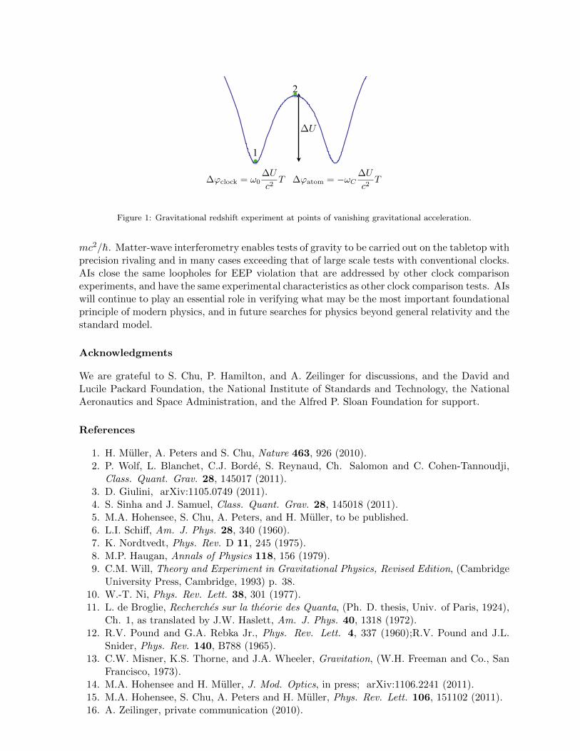
Do Matter-Waves Act Like Clocks?
Place clocks at different Lagrange points in a potential
∆U
1
2
δϕClock = ω0
dτ2 −
dτ1
δϕAtom =
S2 − S1
= −mc2
dτ2 −
dτ1
δϕClock = ω0∆U
c2T δϕAtom = −ωC
∆U
c2T
7Thursday, March 24, 2011
!!clock = "0!U
c2T !!atom = !"C
!U
c2T
Figure 1: Gravitational redshift experiment at points of vanishing gravitational acceleration.
mc2/h. Matter-wave interferometry enables tests of gravity to be carried out on the tabletop withprecision rivaling and in many cases exceeding that of large scale tests with conventional clocks.AIs close the same loopholes for EEP violation that are addressed by other clock comparisonexperiments, and have the same experimental characteristics as other clock comparison tests. AIswill continue to play an essential role in verifying what may be the most important foundationalprinciple of modern physics, and in future searches for physics beyond general relativity and thestandard model.
Acknowledgments
We are grateful to S. Chu, P. Hamilton, and A. Zeilinger for discussions, and the David andLucile Packard Foundation, the National Institute of Standards and Technology, the NationalAeronautics and Space Administration, and the Alfred P. Sloan Foundation for support.
References
1. H. Muller, A. Peters and S. Chu, Nature 463, 926 (2010).2. P. Wolf, L. Blanchet, C.J. Borde, S. Reynaud, Ch. Salomon and C. Cohen-Tannoudji,
Class. Quant. Grav. 28, 145017 (2011).3. D. Giulini, arXiv:1105.0749 (2011).4. S. Sinha and J. Samuel, Class. Quant. Grav. 28, 145018 (2011).5. M.A. Hohensee, S. Chu, A. Peters, and H. Muller, to be published.6. L.I. Schiff, Am. J. Phys. 28, 340 (1960).7. K. Nordtvedt, Phys. Rev. D 11, 245 (1975).8. M.P. Haugan, Annals of Physics 118, 156 (1979).9. C.M. Will, Theory and Experiment in Gravitational Physics, Revised Edition, (Cambridge
University Press, Cambridge, 1993) p. 38.10. W.-T. Ni, Phys. Rev. Lett. 38, 301 (1977).11. L. de Broglie, Recherches sur la theorie des Quanta, (Ph. D. thesis, Univ. of Paris, 1924),
Ch. 1, as translated by J.W. Haslett, Am. J. Phys. 40, 1318 (1972).12. R.V. Pound and G.A. Rebka Jr., Phys. Rev. Lett. 4, 337 (1960);R.V. Pound and J.L.
Snider, Phys. Rev. 140, B788 (1965).13. C.W. Misner, K.S. Thorne, and J.A. Wheeler, Gravitation, (W.H. Freeman and Co., San
Francisco, 1973).14. M.A. Hohensee and H. Muller, J. Mod. Optics, in press; arXiv:1106.2241 (2011).15. M.A. Hohensee, S. Chu, A. Peters and H. Muller, Phys. Rev. Lett. 106, 151102 (2011).16. A. Zeilinger, private communication (2010).
Observability of short-range gravitation with the experiment FORCA-G
S. Pelisson, R. Messina, M.-C. Angonin, P. Wolf
LNE-SYRTE, Observatoire de Paris, CNRS UMR8630, UPMC61 avenue de l’Observatoire, 75014 Paris, France
In this work, the states of an atom vertically trapped in front of a macroscopic surface arediscussed. This calculation is performed in the context of the recently proposed atomic-interferometry experiment FORCA-G, which aims at measuring the Casimir-Polder atom-surface interaction and, at the same time, setting constraints on hypothetical deviations fromNewtonian gravity described by a number of unification theories. The observability of thesedeviations is here quantitatively investigated.
1 Introduction
Several theories beyond the standard model predict a deviation from Newton’s laws of gravity atvery short (say micron or submicron) distance. To explore this range of distance, atomic inter-ferometry can be very efficient, the main reason being the high precision frequency measurementthat can be obtained with this technique. In this context, the experiment FORCA-G (FORce deCAsimir et Gravitation a courte distance) is being developed at SYRTE-Observatoire de Paris1,2. The purpose of this experiment is to study the short-range interaction between a Rubidiumatom and a surface, i.e. investigating at the same time the possible deviation from Newton’s lawsand the Casimir-Polder interaction resulting from the coupling of the atom with the fluctuatingelectromagnetic field 3. These goals will be achieved thanks to atomic-interferometry techniquescombined with a trapping potential which allows a precise knowledge of the distance betweenthe atom and the surface. The trapping potential is realized by a vertical optical standing waveproduced by the reflection of a laser beam on a surface. The vertical configuration inducesan additional linear potential due to Earth’s gravity: this deviation from a purely periodicalpotential produces a localization of the atomic wavepacket, corresponding to the transition fromBloch to Wannier-Stark states, well known in solid state physics 4. The main advantages ofFORCA-G are thus the refined control of the atomic position as well as the high precision ofinterferometric measurements, as demonstrated in the first experimental results2. In this paper,we will theoretically discuss the possibility of observing experimentally a possible deviation fromNewton’s laws at short distance. In the first section, we will present the so-called Wannier-Starkstates and their modification in presence of a surface, then we will study the constraints thatFORCA-G could impose on a Yukawa-type gravitational deviation. We will not describe herethe states in presence of Casimir-Polder effect which are the main subject of another paper (byMessina et al.) in the same volume.
2 Wannier-Stark states
2.1 Physical system
Let us consider a two-level atom trapped in an optical standing wave in proximity of a surface.In our configuration, the standing wave has a vertical orientation so that the Earth’s gravitationfield acting on the atom must be also taken into account. The complete Hamiltonian of thesystem is given by
H = H0 +Hint = Hf +Hat +HWS +Hint
Hf =∑p
∫ +∞
0dkz
∫d2k ~ω a†p(k, kz)ap(k, kz)
Hat = ~ω0|e〉〈e|
HWS =p2
2m+mgz +
U
2(1− cos(2klz)
)
Hint = −µ · E(r).
(1)
This Hamiltonian is written as a sum of a term H0 describing the atomic and field degrees offreedom and Hint which represents the interaction between the atom and the field, written inthis case in the multipolar coupling scheme. Here, Hat represents the internal hamiltonian of theatom having two levels |g〉 (ground) and |e〉 (excited) separated by an energy E = ~ω0. WhileHat
represents the internal degrees of freedom of the system, the term HWS accounts for the externalatomic dynamics. As a consequence, it contains the kinetic energy depending on the atomic massm, the trapping potential due to the optical standing wave of depth U and the linear term dueto the Earth’s gravity. Finally, Hf is the free Hamiltonian of the quantum electromagnetic field,written as usual as a function of a set of creation and annihilation operators. Here, we havetreated only the z-dependent terms of the Hamiltonian since the two other degrees of freedomx and y are decoupled from the longitudinal problem.
2.2 States in proximity of the surface
The first step to describe the short-range interaction between the atom and the surface is tocalculate the atomic states in the optical trap. In solid states physics, there is a similar classof states known as Wannier-Stark states which are metastable states of an infinite acceleratedperiodic potential 4. In our case, the presence of the surface has two effects on the states ofthe atom. On one hand, it imposes a boundary condition at z = 0, breaking in this waythe translational symmetry of the system. On the other hand, the quantum electrodynamicalinteraction between the atom and the surface must be taken into account. This last effect istreated in detail in 5 and will not be described here.
To work out the modified Wannier-Stark states numerically, we have used a finite differencemethod. The first step of our method is to consider a box 0 < z < zf and to impose that all thewavefunctions vanish at the borders. As for z = 0 this is a real physical condition (due to thepresence of the surface), whereas the condition at z = zf is purely numerical. As a consequence,we have to choose a box sufficiently large so that the eigenfunctions of interest decay to zerowell before zf . The next step is the discretization of our interval [0, zf ] using a set of N+2 meshpoints zi with z0 = 0, z1, . . . , zN+1 = zf (giving δz = zf
N+1 for equally spaced mesh points).Using this method, the problem is now reduced to an eigenvalues problem of a tridiagonal
matrix. To calculate the eigenvalues of such a matrix, an efficient algorithm is described in 6.
3 The search for a new gravitational force
Once the states in the lattice are well described, we can start the search for a new gravitationalinteraction at short distance. This investigation is based on indications from numerous unifica-tion theories and models, that gravity may be modified at short distance. These modificationscan be described by an additional Yukawa-type potential to the standard Newtonian potential.The complete gravitational potential between two point-like particles is then written under theform
V (z) =GMm
z
(1 + αYe
− zλY
)(2)
whereG is the gravitational constant, m andM the masses of the two particles. In this expressionαY and λY are two parameters introduced to characterize respectively the relative strength ofthe corrective potential and its typical range. The experiments aimed at testing the existenceof such a deviation set constraints on the allowed values of the parameters αY and λY.
In the experiment FORCA-G, the only relevant contribution of a possible deviation fromgravitation is the one due to the interaction between our atom and the surface. At the sametime, the Newtonian part of the atom-surface interaction is completely negligible with respectto the Earth-atom term already taken into account in the Wannier-Stark Hamiltonian (1) andwith respect to the expected experimental uncertainties. As a consequence, the correction weare looking for is obtained by integrating the Yukawa part of eq. (2) over the volume occupiedby the surface. Describing the mirror as a cylinder (the atom being on the direction of its axis)and recalling that we are looking for deviations having length scale λY in the µm range weobtain, after a straightforward calculation,
HY = 2παYGρSmλ2Ye− 2zλY (3)
ρS being the density of the surface. As the Yukawa contribution is due to the surface, we needan experimental configuration where the Casimir-Polder contribution is negligible with respectto the gravitational interaction. In fact, the experiment is planned to have two different configu-rations. The first one is a measurement at short distance where we compare the results obtainedusing two different isotopes of Rubidium (85Rb and 87Rb) in order to make the energy differencesbetween wells almost independent on the Casimir-Polder interaction1. As a consequence, in thisscheme, we need to calculate the energy difference between the 87Rb and 85Rb both in the caseof Wannier-Stark states and Yukawa states. The energy difference is noted
DEn =(E85n − E87
n
)− (E(Y )85n −E(Y )87
n
)(4)
where En is the energy of state n in the absence of a Yukawa term in the total Hamiltonian, andE
(Y )n is the energy of the same state in the presence of a Yukawa term of form 3. A Yukawa-
type deviation from gravity’s laws will be detectable if this difference is within the experimentalsensitivity, i.e. 10−4Hz. The second scheme is a measurement at larger distance, in a regionwhere the Casimir-Polder interaction can be theoretically modelled at a degree of precisioncomparable to the experimental sensitivity. This region extends approximatively between 10µmand 20µm.
In the far regime scheme we have calculated, for an atom of 87Rb, the Yukawa correction onthe well n = 40 and n = 70 (which correspond respectively to a distance of 10µm and 20µm) fordifferent values of λY and for each of them we have found our limiting value of αY by looking fora correction up to 10−4 Hz, coinciding with the experimental sensitivity estimated in 1. We haveperformed the same calculation for the near regime discussed above by evaluating the energydifference DE6 − DE4 between the wells n = 4 and n = 6 and evaluating the minimum αY
allowed that induces a shift of 10−4Hz. The resulting experimental constraints on the Yukawa-type correction is shown on the figure 1, originally taken from 7. The three superposed curves
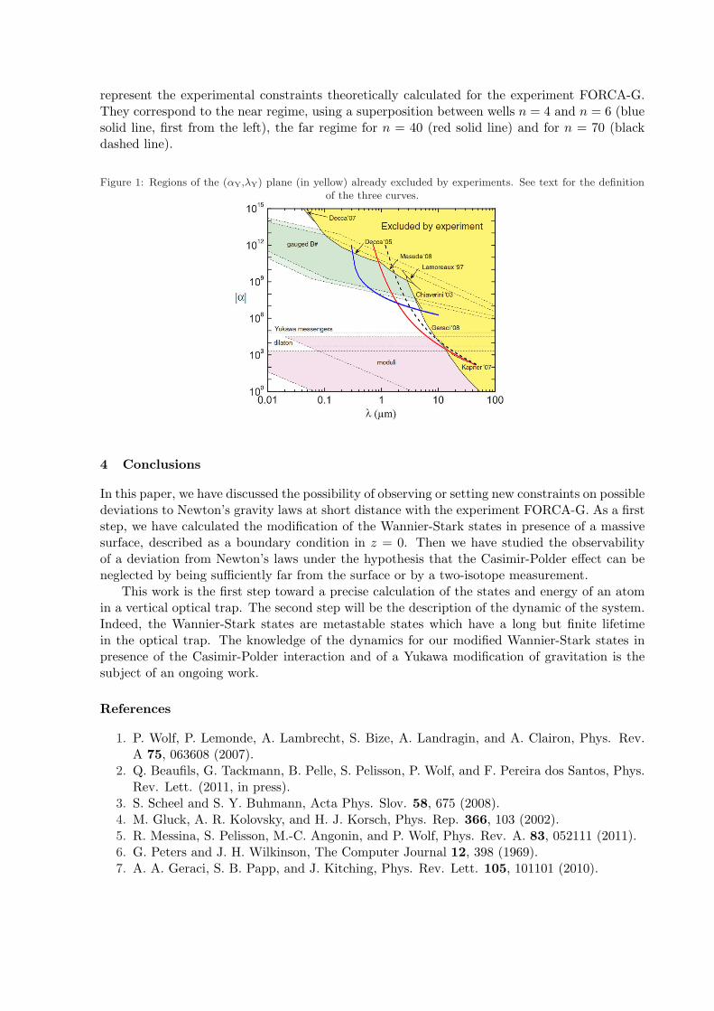
represent the experimental constraints theoretically calculated for the experiment FORCA-G.They correspond to the near regime, using a superposition between wells n = 4 and n = 6 (bluesolid line, first from the left), the far regime for n = 40 (red solid line) and for n = 70 (blackdashed line).
Figure 1: Regions of the (αY,λY) plane (in yellow) already excluded by experiments. See text for the definitionof the three curves.
4 Conclusions
In this paper, we have discussed the possibility of observing or setting new constraints on possibledeviations to Newton’s gravity laws at short distance with the experiment FORCA-G. As a firststep, we have calculated the modification of the Wannier-Stark states in presence of a massivesurface, described as a boundary condition in z = 0. Then we have studied the observabilityof a deviation from Newton’s laws under the hypothesis that the Casimir-Polder effect can beneglected by being sufficiently far from the surface or by a two-isotope measurement.
This work is the first step toward a precise calculation of the states and energy of an atomin a vertical optical trap. The second step will be the description of the dynamic of the system.Indeed, the Wannier-Stark states are metastable states which have a long but finite lifetimein the optical trap. The knowledge of the dynamics for our modified Wannier-Stark states inpresence of the Casimir-Polder interaction and of a Yukawa modification of gravitation is thesubject of an ongoing work.
References
1. P. Wolf, P. Lemonde, A. Lambrecht, S. Bize, A. Landragin, and A. Clairon, Phys. Rev.A 75, 063608 (2007).
2. Q. Beaufils, G. Tackmann, B. Pelle, S. Pelisson, P. Wolf, and F. Pereira dos Santos, Phys.Rev. Lett. (2011, in press).
3. S. Scheel and S. Y. Buhmann, Acta Phys. Slov. 58, 675 (2008).4. M. Gluck, A. R. Kolovsky, and H. J. Korsch, Phys. Rep. 366, 103 (2002).5. R. Messina, S. Pelisson, M.-C. Angonin, and P. Wolf, Phys. Rev. A. 83, 052111 (2011).6. G. Peters and J. H. Wilkinson, The Computer Journal 12, 398 (1969).7. A. A. Geraci, S. B. Papp, and J. Kitching, Phys. Rev. Lett. 105, 101101 (2010).
MAJOR CHALLENGES OF A HIGH PRECISION TEST OF THEEQUIVALENCE PRINCIPLE IN SPACE
A.M. NOBILIDepartment of Physics “E. Fermi”, University of Pisa, Largo B. Pontecorvo 3, 56127 Pisa, Italy
R. PEGNAINFN-Istituto Nazionale di Fisica Nucleare, Sezione di Pisa, Largo B. Pontecorvo 3, 56127 Pisa, Italy
G. CATASTINI, A. ANSELMIThales Alenia Space Italia, Strada Antica di Collegno 253, 10146 Torino, Italy
A. DE MICHELEDepartment of Physics “E. Fermi”, University of Pisa, Largo B. Pontecorvo 3, 56127 Pisa, Italy
D.M. LUCCHESIIstituto di Fisica dello Spazio Interplanetario, Istituto Nazionale di Astrofisica, IFSI/INAF, Via del
Fosso del Cavaliere 100, 00133 Roma, Italy
A violation of the Equivalence Principle would prove the existence of a new, composition-dependent physical interaction and make for a scientific revolution. Performing the test insidea spacecraft orbiting the Earth at low altitude can potentially improve the best ground resultsby 4 orders of magnitude, but the experiment faces several major challenges. We discuss themand show how one conceptual experiment and mission design can make the most challengingissues mostly go away.
1 Why testing the Equivalence Principle?
The Equivalence Principle (EP) is the founding pillar of General Relativity and one of themost fundamental principles of Physics. Among all tests of General Relativity, both in weakand strong field, EP tests are the only ones which test the theory for composition dependence.Evidence of an EP violation would not simply call for another metric theory of gravity slightlydifferent from GR; it would prove the existence of a new composition dependent force of Nature.This fact singles out EP tests as of extreme importance and calls for pushing the sensitivity toits limits whenever the experimental possibility for an improvement arises.
2 Why in space?
The Equivalence Principle is tested by measuring the differential acceleration ∆a of two proofmasses of different composition freely falling in the gravitational field of a source body (like theEarth or the Sun) with an acceleration a (the driving signal) and is quantified by the Eotvosparameter: η = ∆a/a. If EP holds η must be zero. Experimental evidence of η = 0 wouldshow a violation and prove the existence of a new composition-dependent force of Nature: the
smaller the measured value of η, the higher the sensitivity of the test. Therefore, for a givenexperimental capability to detect a differential acceleration ∆a, a strong driving signal a is crucialto measure a smaller value of the parameter η = ∆a/a which quantifies the level of testing of theEquivalence Principle. To date the best EP tests have been performed by the Eot-Wash groupwith slowly rotating torsion balances finding no violation to ηEot−Wash = 10−13 (Schlammingeret al. 1, Adelberger et al. 2). Torsion balances are sensitive in the horizontal plane, hence theytest only the small horizontal component of the free fall acceleration of the proof masses towardsthe Earth or the Sun. Despite the much smaller driving signal they have won over Galileo-likemass dropping tests by several orders of magnitude. This is due to the very high sensitivity ofthe torsion balance, to its inherent differential nature and to the possibility to rotate it so as toto modulate the signal at higher frequency.
Flying a space version of the torsion balance, a differential accelerometer inside a spacecraftorbiting the Earth at low altitude would provide almost 3 orders of magnitude higher sensitivityjust because of the stronger driving acceleration from the Earth. Absence of weight and the factof running the experiment inside an isolated “lab” (the spacecraft) are additional plus. Highsensitivity to very small forces requires the proof masses to be arranged with very small elasticconstants; in absence of weight 100 kg mass requires the same suspension spring needed to hold1 mg on ground, so space is ideal for weak coupling. In an isolated lab local terrain noise anddisturbances from nearby masses are greatly reduced.
3 Key requirements and major error sources
In order to exploit these advantages and to aim at much a higher precision test than on groundthe space experiment must fulfill two key requirements: i) the centers of mass of the test bodiesmust be well centered on one another, in order to reduce classical tidal differential effects asthe bodies orbit around the Earth (the general choice is to have 2 hollow cylinders one insidethe other and to find ways of centering their centers of mass on one another); ii) the apparatusshould rotate, in order to modulate the signal at a frequency different from (and higher than)the orbital one.
Random error sources –which decrease as the square root of the integration time– are readout noise and thermal noise.
The major challenging systematic errors can be restricted to 4: 1) the radiometer effect; 2)the effect of electric charges patches on the surfaces of the test bodies; 3) the effect of drag dueto residual air along the orbit of the satellite; 4) the different coupling of the quadrupole andmultipole mass moments of the test bodies with the monopole of the Earth.
Finally it comes the greatest challenge of all: should the mission succeed and achieve itstarget sensitivity, how to ensure that the effect measured at the expected frequency and phaseof an EP violation in the field of the Earth is really the signal of a violation of the EquivalencePrinciple, hence the proof of the existence of a new force, and not just a very small, unmodeledclassical disturbance?
4 A winning idea
One way to fulfill the requirements and reduce the challenging disturbances is by pushing everysingle mission element to the extreme limits of what is currently feasible. While this may bepossible, it is costly and risky. Our experience shows that a much better strategy is to design amission which —by exploiting the cylindrical symmetry of the experiment (the test masses aretwo cylinders one inside the other) and the 2 degrees of freedom of the problem (i.e. the 2-bodyproblem of each test body orbiting around the Earth)— can make the challenging issues mostlygo away.
“Galileo Galilei” (GG) satellite experiment, which aims at testing the EP to 10−17 (Nobili etal. 3), has been designed as a rotating torsion balance modified for flight such that both the keyrequirements listed above are passively fulfilled: a) The test cylinders, together with the wholespacecraft surrounding them (of cylindrical symmetry too) spin around the symmetry axis; b)The test cylinders are weakly coupled to each other in the plane perpendicular to it, where theycan detect the differential effect of an EP violation signal from the Earth in the orbital planearound it.
Thus, the satellite can be passively stabilized by one axis rotation (e.g. at 1 Hz) whileat the same time modulating the signal. In this design the proof masses form a rotating 2-D harmonic oscillator characterized by weak coupling and fast rotation (above the naturalcoupling frequency), which ensures auto-centering of their centers of mass by physics laws, noactive centering being required. This is possible only if the test cylinders are weakly coupled inboth directions of the plane and spin around the symmetry axis. In one dimension only –e.g. bymaking the symmetry axis the sensitive one and rotating around an axis perpendicular to it– itis impossible to spin fast and achieve auto-centering.
We can show how from this choice the most relevant error sources listed in Sec. 3 are largelyreduced or even eliminated. More importantly, we can also show how very stringent null checkscan be performed so as to establish beyond question whether the measured effect is an EPviolation or not.
Let us first put things in perspective by comparing the sensitivity to be achieved by anexperiment in space aiming at testing EP to 10−17 with the sensitivity achieved by rotatingtorsion balanced in their best EP tests to 10−13. Quite remarkably, they have been able to sensedifferential accelerations as small as 10−16g, which yields ηEot−Wash = 10−13 due to the smalldriving signal. In space, for GG to meet its target ηGG = 10−17 in the field of the Earth, itmust reach a sensitivity to differential accelerations of 10−17g, i.e. only one order of magnitudebetter than slowly rotating torsion balances. This is the main advantage of space: a one orderof magnitude improvement in sensitivity yields a 4 order of magnitude improvement in testingthe Equivalence Principle.
GG originally relied on a capacitance read-out sensor. In collaboration with JPL it hasnow been replaced by a JPL-developed laser interferometry gauge which is ideal for rejectingcommon mode effects (laser metrology is linear, hence large common mode motions do not giverise to false signals when two measurements are subtracted), allows a gap several times largerthan cap sensors (thus reducing many error sources) and has an extremely low noise (well below1pm/
√Hz). Read-out noise is not a limitation.
Once all systematic errors are reduced below the signal, thermal noise is the ultimate limita-tion and sets the length of the integration time required for it to become smaller than the signal.It is known that when a low frequency signal is modulated at higher frequency by rotating anoscillator of high mechanical quality surrounded by low pressure residual gas, thermal noise isreduced, as it has been measured by rotating torsion balances which are operated at thermalnoise level (Adelberger et al. 2). GG can spin well above the natural frequency without the sig-nal being attenuated, so the modulation frequency is much higher and thermal noise is reducedaccordingly (Pegna et al. 4). As a result, the integration time required to reduce thermal noisebelow the target signal is very short and a few orbits are sufficient to identify its size, frequencyand phase. In 1 day the satellite makes about 15 orbits around the Earth and this is the typicaltimespan for GG to make a measurement at the 10−17 target level. This fact has far reachingconsequences (see next Section) and it is unique to GG. By comparison, a proposed EP testwith cold atoms requires an integration time of 3 months despite a target 1 order of magnitudeworse than GG (Ertmer et al. 5).
Consider now the first systematic disturbance of our list, the radiometer effect, a well knownkiller of EP experiments in space. Inside the spacecraft there is a residual gas pressure, and
it is exposed to infrared radiation from the Earth, which gives rise to temperature gradientsalong the symmetry axis of the test cylinder. Since the cylinders have different composition,hence different density, there will be a differential acceleration. This is the radiometer effect.Then, if the cylinders axis is the sensitive axis for detecting an EP violation in the field ofthe Earth, a radiometer differential acceleration originated by the Earth (through its infraredradiation) would mimic the signal and be undistinguishable from it. The only way out wouldbe to make absolutely sure that the radiometer effect is smaller than the signal by sufficientlyreducing the residual pressure and/or the fractional temperature gradients along the axis. InGG the test masses are sensitive in the plane perpendicular to the symmetry axis and rapidlyspinning around it; any temperature gradient in this plane driven by the Earth would give riseto a radiometer effect competing with signal, but only in the presence of azimuthal temperatureasymmetries, which are greatly reduced by the rotation, making the main radiometer effect notan issue (Nobili et al. 6, 7). An indirect effect from radiometer along the symmetry/spin axisremains to be taken care of, but it is a minor effect.
Were not for this choice, the radiometer effect would make an EP test to 10−17 utterlyimpossible unless one could manage to perform it in cryogenic conditions, at supefluid Hetemperature at which extremely low pressures (< 10−14torr) can be achieved as in GP-B (Everittet al. 8). Thus, the GG experiment design makes the difference between a room temperatureand a cryogenic mission.
The next systematic error in the list of Sec. 3 is due to the so called electric patch effects.In spite of being equipotential the surface of a conductor is known to have residual patches ofelectric charges which have low frequency variations, including a component at the frequency ofthe signal. This is the case also if the test bodies are electrically grounded as in GG by theirmechanical suspensions. The GP-B mission of NASA has in fact been limited by this singleeffect (Everitt et al. 8). The patch effect decreases as the gap between the surfaces of the testmasses squared. in GG a method has been devised to measure the direct effect of electric patcheson the test masses and make sure that it is small enough. The method has been successfullydemonstrated in the laboratory prototype and can be used also in space as check. However,this is no longer needed because the laser interferometry gauge allows a gap several times largerthan originally planned with capacitance sensors, thus getting rid of the patch effect.
The residual atmosphere at the satellite altitude along its orbit around the Earth acts onthe external surface of the spacecraft giving rise to an acceleration of its center of mass; anymass weakly suspended inside the spacecraft will feel an inertial acceleration exactly equal andopposite to the acceleration of the spacecraft. Were the test cylinders suspended exactly thesame, the effect of this inertial acceleration would also be the same on both of them, and thereforeit would not compete with the differential acceleration due to an EP violation. Air drag has acomponent at the frequency and phase of the signal which –though in common mode– is largerthan the signal by several orders of magnitude. Since it is common mode, it is passible to dealwith it in 2 ways: by active drag compensation (so as to reduce the inertial common modeacceleration on the test masses) and by common mode rejection, that is by the capability of thetest masses and of their read out sensor to reject the effects of accelerations which are commonmode in nature. By sharing the burden between drag free control and common mode rejectionit is possible not to put an extremely tight requirement on either of them
The test cylinders have non zero multipole mass moments, which are also not the same forthe two bodies (they are made of different materials, have different mass distribution and size)and therefore couple differently with the monopole mass moment of the Earth. This resultsin a differential acceleration (the dominant contribution coming from the quadrupole moment)always pointing to the center of mass of the Earth exactly like the differential acceleration due toan EP violation. The effect is deterministic (it is derived unambiguously in celestial mechanicsfrom the orbital parameters) and is proportional to the quadrupole mass moments of the test
masses. It is made smaller than the signal by manufacturing them with small enough quadrupolemoments so that the differential effect is adequately small.
We show in Sec. 5 how the GG design is crucial in checking competing systematic effects likethese in order to establish if the measured effect is due to an EP violation or not.
5 Null checks of the effect measured by a single differential accelerometer
The signature of an EP violation signal for the GG differential accelerometer orbiting around theEarth is perfectly known. We know how it should vary along each orbit and during the mission—as the orbital plane precesses about the North celestial pole at about 1 degree per day dueto the quadrupole mass moment of the Earth (a sunsynchronous orbit at about 630 km altitudehas finally been selected for GG) while the spin axis of the satellite is fixed in space (due toits very high spin energy, at about 1 Hz spin rate). The geometrical configuration between thesensitive plane of the test cylinders (perpendicular to the spin/symmetry axis) and the plane ofthe signal (the orbital plane of the satellite) varies in a known way. During 80 days, in a totallypassive deterministic way, the angle between the two planes varies from −40o to +40o, thusmaking the EP violation signal also vary in a perfectly known way (only the sign and amplitudeof it are obviously not known). Since GG can make a full measurement to the required targetlevel of 10−17 in 1 day, in a timespan of 80 days it will perform 80 such measurement, allowingus to map the variation of the measured effect with the changing geometry. As shown in Sec. 4,this is possible in GG thanks to the high frequency modulation of the signal and consequentlyreduced thermal noise and integration time.
It can be easily demonstrated that none of the systematic effects listed in Sec. 3 has the samedependence on such geometry as the signal. In a single 1 day measurement they have the samefrequency –and in some cases even the same phase– as the violation signal, but over many daysdays of data they can all be distinguished from the signal without ambiguity. This is possiblealso for systematic effects whose frequency is not exactly the same as the frequency of the signabut close to it (e.g. some tidal effects) and are therefore worth a careful check.
These are very powerful null checks which allow us to establish beyond question whether atthe orbital frequency there is a non zero signal due to a violation of the Equivalence Principleand the existence of a new, composition dependent force of Nature. Any other research groupcan independently analyze the mission data by standard methods of celestial mechanics andspace geodesy.
GG null checks are carried out by off line data analysis. They do not require any additionalaccelerometer, such as a “zero check accelerometer” with equal composition test bodies (theEP violation signal should be detected only by the accelerometer with test masses of differentcomposition while classical disturbances would affect both) or even several more accelerometerswith an appropriate choice of different material for a cyclic check. In addition to increasing thecomplexity and cost of the mission, different accelerometers onboard the spacecraft designed toreach the same sensitivity do not ensure the same performance, because the satellite has onlyone center of mass and that is where disturbances on the test masses are minimized. Moreover,there are subtle systematic errors –such as the radiometer– which do not produce a differentialeffect on test bodies of the same composition if they have the same density, and could thereforebe mistaken for an EP violation (they would affect the accelerometer with test masses of differentcomposition and not the zero check one, just as the violation signal; Nobili et al. 7)
Acknowledgments
GG and the lab prototype are supported by the Italian Space Agency (ASI) and by INFN
References
1. S. Schlamminger, K.-Y. Choi, T.A. Wagner, J.H. Gundlach, E.G. Adelberger, Phys. Rev.Lett. 100 (2008) 041101
2. E.G. Adelberger, J.H. Gundlach, B.R. Heckel, S. Hoedl, S. Schlamminger, Progress inParticle and Nuclear Physics 62 (2009) 102
3. A.M. Nobili et al., Phys. Lett. A 318 (2003) 1724. R. Pegna, A.M. Nobili, M. Shao, S.G. Turyshev, G.L. Comandi, G. Catastini, A. Anselmi,
A. De Michele, submitted (2011)5. W. Ertmer et al., Exp. Atron. 23 (2009) 6116. A.M. Nobili, D. Bramanti, G. Comandi, R. Toncelli, E. Polacco, G. Catastini, Phys. Rev.
D 63 (2001) 101101-17. A.M. Nobili, D. Bramanti, G.L. Comandi, R. Toncelli, E. Polacco, New Astronomy 7
(2002) 5218. C.W.F. Everitt et al., Phys. Rev. Lett. 106 (2011) 21101-1

10.Lorentz invariance and CPT

LORENTZ SYMMETRY, THE SME, AND GRAVITATIONAL EXPERIMENTS
JAY D. TASSONDepartment of Physics, Whitman College
Walla Walla, WA 99362, USAE-mail: [email protected]
This proceedings contribution summarizes the implications of recent SME-based investigationsof Lorentz violation for gravitational experiments.
1 Introduction
General Relativity along with the Standard Model of particle physics provide a remarkabledescription of known physics. Lorentz symmetry is a foundational principle of each, and thusshould be well tested experimentally. It is also likely that General Relativity and the StandardModel are limits of a more fundamental theory that provides consistent predictions at thePlanck scale. Tests of Lorentz symmetry provide a technically feasible means of searchingfor potential suppressed signals from the Planck scale in existing experiments and observations.1
The gravitational Standard-Model Extension (SME) provides a comprehensive test frameworkfor searching for such potential signals across all areas of known physics.2,3
In spite of both the many high-sensitivity investigations of Lorentz symmetry 4 performedin the context of the SME in Minkowski spacetime,3 the scope of which continues to deepen andbroaden,4,5,6 and the many investigations of metric theories of gravity performed in the context ofthe Parametrized Post-Newtonian (PPN) formalism,7 there remain numerous potential Lorentz-violating deviations from General Relativity that have not yet been sought observationally andexperimentally. Some of these violations would lead to qualitatively new types of signals.
Lorentz-violating effects in gravitational experiments can originate from two basic places:the pure-gravity action and gravitational couplings in the other sectors of the theory. Whilesome distinct theoretical issues are associated with each origin, and some of the associatedexperimental signatures are quite different, the relevant effects can be observed in many of thesame classes of experiments. The pure-gravity sector was the subject of Ref. 8, and Sec. 2summarizes some of the key theoretical issues associated with that work. Section 3 provides asimilar summary of theoretical issues associated with matter-gravity couplings, which were thesubject of Ref. 9. Experiments relevant for investigations of Lorentz violation originating fromboth sectors are then considered in Sec. 4.
2 Lorentz violation in pure gravity
Investigations of Lorentz violation performed in the context of the minimal SME in Minkowskispacetime are extended to include the post-Newtonian implications of Lorentz violation in the
pure-gravity sector in Ref. 8, and several associated theoretical and phenomenological investi-gations have expanded aspects of that work.10,11 The action for the minimal pure gravity sectortakes the form 2
S =12κ
∫d4xe(R− uR+ sµνRTµν + tκλµνCκλµν), (1)
where Cκλµν is the Weyl tensor, RTµν is the traceless Ricci tensor, and e is the vierbein determi-nant. The first term here is the standard Einstein-Hilbert term. The relevant Lorentz-violatingsignals in the post-Newtonian analysis to follow stem from the third term involving the coef-ficient field sµν . The second term is not Lorentz violating, and the fourth term provides nocontributions in the post-Newtonian analysis.
It has been shown that in the present context of Riemannian spacetime, consistent Lorentzsymmetry breaking must be spontaneous,2 though use of more general geometries may admitexplicit breaking.12 A number of implications stemming directly from spontaneous symmetrybreaking can also be considered;13,14,15 however, a detailed discussion of these issues is beyondthe scope of the present discussion.
As a result of the specialization to spontaneous symmetry breaking in the present context, aprimary theoretical issue addressed in Ref. 8 is establishing a procedure for correctly accountingfor the fluctuations in the coefficient fields, including the massless Nambu-Goldstone modesof Lorentz-symmetry breaking.13 This challenge is met in a general way, without specializingto a specific model of spontaneous symmetry breaking, under a few mild assumptions. Uponaddressing this issue, the leading-order Lorentz-violating contributions to the linearized fieldequations are obtained and can be expressed in terms of the metric fluctuation hµν and thevacuum value sµν associated with the coefficient field sµν . The post-Newtonian metric is obtainedfrom these equations. With a suitable gauge choice 8 the metric takes the form
g00 = −1 + 2U + 3s00U + sjkU jk − 4s0jV j +O(4), (2)g0j = −s0jU − s0kU jk − 7
2(1 + 128s
00)V j + 34sjkV k − 1
2(1 + 154 s
00)W j
+54sjkW k + 9
4sklXklj − 15
8 sklXjkl − 3
8sklY klj , (3)
gjk = δjk + (2− s00)δjkU + (slmδjk − sjlδmk − sklδjm + 2s00δjlδkm)U lm, (4)
where U , U jk, V j , W j , Xklj , and Y klj are potentials formed from appropriate integrals over thesource body. The explicit form of the potentials is provided in Ref. 8.
The above metric is then compared and contrasted with the PPN metric. The basic ideais that the pure-gravity sector of the minimal SME provides an expansion about the action ofGeneral Relativity, while the PPN provides an expansion about the metric. Perhaps surprisingly,an overlap of only one parameter is found between the 20 coefficients in the minimal pure-gravitysector of the SME and the 10 parameters of the PPN formalism. This implies that leadingcorrections to General Relativity at the level of the action do not match those typically studiedin an expansion about the metric. Note also that the focus of the SME is on Lorentz violationthroughout physics, while the focus of the PPN is on deviations from General Relativity, whichmay or may not be Lorentz violating. Thus the minimal pure-gravity sector of the SME andthe PPN formalism provide complementary approaches to studying deviations from GeneralRelativity.
Finally, Ref. 8 introduces bumblebee models16 that provide specific examples of complete the-ories with spontaneous symmetry breaking that fit into the post-Newtonian results establishedin the general context of the SME.
3 Lorentz violation in matter-gravity couplings
Though many high-sensitivity investigations of Lorentz violation 4 have been performed in thecontext of the fermion sector of the minimal SME in Minkowski spacetime,3 there remains
a number of coefficients for Lorentz violation in that sector that have not been investigatedexperimentally. A methodology for obtaining sensitivities to some of these open parameters byconsidering gravitational couplings in the fermions sector of the SME is provided by Ref. 9.The set of coefficients aµ for baryons and charged leptons, which are unobservable in principlein Minkowski spacetime, is of particular interest. Due to gravitational countershading,17 thesecoefficients could be large relative to existing matter-sector sensitivities.
Prior to developing the necessary results for experimental analysis, the theoretical portionof Ref. 9 addresses a number of useful conceptual points. One such point is consideration ofthe circumstances under which relevant types of Lorentz violation are observable in principle.Though the aµ coefficient can be removed from the single fermion theory in Minkowski spacetimevia a spinor redefinition, it is highlighted that it cannot typically be removed in the presence ofgravity.2 This results in the gravitational countershading pointed out in Ref. 17.
A coordinate choice that can be used to fix the sector of the theory that defines isotropy isalso discussed, and the role of the gravitational sector in this context is established. Ultimately,the photon sector is chosen to have ηµν as the background metric, though no generality is lost,and other choices can be recovered.
The treatment of the fluctuations in the coefficient fields established for the gravitationalsector is adapted to the context of matter-gravity couplings. Two notions of perturbative orderare introduced to treat the fluctuations perturbatively under the assumptions that gravitationaland Lorentz-violating corrections are small. One notion of perturbative order, denoted O(m,n),tracks the orders in Lorentz violation and in gravity. Here the first entry represents the orderin the coefficients for Lorentz violation, and the second entry represents the order in the metricfluctuation hµν . A secondary notion of perturbative order, which tracks the post-Newtonianorder, is denoted PNO(p). The O(1,1) contributions are of primary interest in Ref. 9, since thegoal of that work is to investigate dominant Lorentz-violating implications in matter-gravitycouplings.
To proceed toward the analysis of relevant experiments, the results necessary for working ata number of energy levels are developed from the full field-theoretic action of the gravitationallycoupled fermion sector of the SME, which takes the form
Sψ =∫d4x(1
2 ieeµaψΓa
↔Dµ ψ − eψMψ). (5)
where
Γa ≡ γa − cµνeνaeµbγb − dµνeνaeµbγ5γ
b
−eµeµa − ifµeµaγ5 − 12gλµνe
νaeλbeµcσbc (6)
andM ≡ m+ aµe
µaγ
a + bµeµaγ5γ
a + 12Hµνe
µaeνbσab, (7)
where aµ, bµ, cµν , dµν , eµ, fµ, gλµν , Hµν are coefficient fields for Lorentz violation.Starting from Eq. 5, the relativistic quantum mechanics in the presence of gravitational
fluctuations and Lorentz violation is established after investigating two methods of identify-ing an appropriate hamiltonian. The explicit form of the relativistic hamiltonian involving allcoefficients for Lorentz violation in the minimal fermion sector is provided.
The standard Foldy-Wouthuysen procedure is then employed to obtain the nonrelativisticquantum Hamiltonian. At this stage, attention is specialized to the study of spin-independentLorentz-violating effects, which are governed by the coefficient fields (aeff)µ, cµν and the metricfluctuation hµν . Though interesting effects may exist in couplings involving spin, gravity, andLorentz violation, the pursuit of spin-independent effects maintains a reasonable scope focusedon the least well-constrained coefficients including the countershaded aµ coefficients.
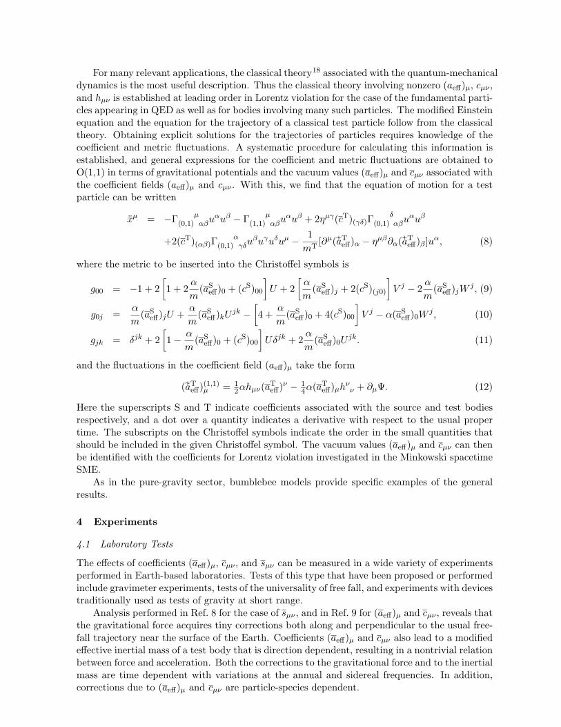
For many relevant applications, the classical theory18 associated with the quantum-mechanicaldynamics is the most useful description. Thus the classical theory involving nonzero (aeff)µ, cµν ,and hµν is established at leading order in Lorentz violation for the case of the fundamental parti-cles appearing in QED as well as for bodies involving many such particles. The modified Einsteinequation and the equation for the trajectory of a classical test particle follow from the classicaltheory. Obtaining explicit solutions for the trajectories of particles requires knowledge of thecoefficient and metric fluctuations. A systematic procedure for calculating this information isestablished, and general expressions for the coefficient and metric fluctuations are obtained toO(1,1) in terms of gravitational potentials and the vacuum values (aeff)µ and cµν associated withthe coefficient fields (aeff)µ and cµν . With this, we find that the equation of motion for a testparticle can be written
xµ = −Γ µ(0,1) αβu
αuβ − Γ µ(1,1) αβu
αuβ + 2ηµγ(cT)(γδ)Γδ
(0,1) αβuαuβ
+2(cT)(αβ)Γα
(0,1) γδuβuγuδuµ − 1
mT[∂µ( 7aT
eff)α − ηµβ∂α( 7aTeff)β]uα, (8)
where the metric to be inserted into the Christoffel symbols is
g00 = −1 + 2[1 + 2
α
m(aS
eff)0 + (cS)00]U + 2
[α
m(aS
eff)j + 2(cS)(j0)]V j − 2
α
m(aS
eff)jW j , (9)
g0j =α
m(aS
eff)jU +α
m(aS
eff)kU jk −[4 +
α
m(aS
eff)0 + 4(cS)00]V j − α(aS
eff)0W j , (10)
gjk = δjk + 2[1− α
m(aS
eff)0 + (cS)00]Uδjk + 2
α
m(aS
eff)0U jk. (11)
and the fluctuations in the coefficient field (aeff)µ take the form
( 7aTeff)(1,1)µ = 1
2αhµν(aTeff)ν − 1
4α(aTeff)µhνν + ∂µΨ. (12)
Here the superscripts S and T indicate coefficients associated with the source and test bodiesrespectively, and a dot over a quantity indicates a derivative with respect to the usual propertime. The subscripts on the Christoffel symbols indicate the order in the small quantities thatshould be included in the given Christoffel symbol. The vacuum values (aeff)µ and cµν can thenbe identified with the coefficients for Lorentz violation investigated in the Minkowski spacetimeSME.
As in the pure-gravity sector, bumblebee models provide specific examples of the generalresults.
4 Experiments
4.1 Laboratory Tests
The effects of coefficients (aeff)µ, cµν , and sµν can be measured in a wide variety of experimentsperformed in Earth-based laboratories. Tests of this type that have been proposed or performedinclude gravimeter experiments, tests of the universality of free fall, and experiments with devicestraditionally used as tests of gravity at short range.
Analysis performed in Ref. 8 for the case of sµν , and in Ref. 9 for (aeff)µ and cµν , reveals thatthe gravitational force acquires tiny corrections both along and perpendicular to the usual free-fall trajectory near the surface of the Earth. Coefficients (aeff)µ and cµν also lead to a modifiedeffective inertial mass of a test body that is direction dependent, resulting in a nontrivial relationbetween force and acceleration. Both the corrections to the gravitational force and to the inertialmass are time dependent with variations at the annual and sidereal frequencies. In addition,corrections due to (aeff)µ and cµν are particle-species dependent.
Based on the above discussion, laboratory tests using Earth as a source fall into 4 classes.Free-fall gravimeter tests monitor the acceleration of free particles over time, while force-comparison gravimeter tests monitor the gravitation force on a body over time. Both typesof gravimeter tests are sensitive to (aeff)µ, cµν , and sµν coefficients. The relative accelerationof, or relative force on a pair of test bodies can also be monitored constituting free-fall andforce-comparison Weak Equivalence Principle (WEP) tests respectively. Sensitivities to (aeff)µand cµν can be achieved in WEP tests. Relevant devices presently used for the above types oftests include experiments with falling corner cubes,19 atom interferometers,20,21,22 superconduct-ing levitation,23 tossed masses,24 balloon drops,25 drop towers,26 sounding rockets,27 and torsionpendula.28 Refs. 8 and 9 provide specific predictions and estimated sensitivities for the abovetests including a frequency decomposition of the relevant signal to which experimental datacould be fit. Note that the effective WEP violation with periodic time dependence consideredhere is a qualitatively different signal that would likely have been missed in past WEP tests. Oneexperiment of this type has already been performed using an atom-interferometer as a free-fallgravimeter.21
Variations of the above laboratory tests involving the gravitational couplings of charged par-ticles, antimatter, and second- and third-generation particles are also studied in Ref. 9. Thoughthey are very challenging experimentally, these tests can yield sensitivities to Lorentz and CPTviolation that are otherwise difficult or impossible to achieve. Charged-particle interferometry,29
ballistic tests with charged particles,30 gravitational experiments with antihydrogen,31 and sig-nals in muonium free fall 32 are considered. Some features of antihydrogen tests are illustratedwith simple toy-models limits of the SME.
Though less sensitive at present to the range-independent SME effects presently under dis-cussion, systems in which both the source mass and the test mass are contained within the lab,such as those devices traditionally used as tests of gravity at short range, can also be considered.A search for sµν has been performed using a cantilever system 33 and a search for (aeff)µ usinga torsion-strip balance 34 have been performed using this approach. A proposal to measure sµνusing a torsion pendulum with an asymmetric mass distribution also exists.8
4.2 Satellite-Based Tests
Space-based experiments can offer unique advantages in testing gravitational physics 35 and insearching for Lorentz violation.36 The WEP tests considered above are an example of a class oftests for which significant sensitivity improvements might be possible in space, due to the longfree-fall times that may be attainable on a drag-free spacecraft. There are several proposalsfor such missions in the advanced stages of development, including the Micro-Satellite a traıneeCompensee pour l’Observation du Principe d’Equivalence (MicroSCOPE),37 the Satellite Test ofthe Equivalence Principle (STEP),38 and the Galileo Galilei (GG) mission.39 A WEP experimentwith reach similar to that of STEP has also been suggested for the Grand Unification and GravityExplorer (GaUGE) mission.40
Monitoring the relative motion of test bodies of different composition as they obit the Earthinside of the spacecraft is the basic idea underlying these missions. Nonzero coefficients forLorentz violation (aweff)µ and (cw)µν , would result in material dependent orbits. Ref. 9 providesthe differential acceleration of the test masses, decomposed by frequency, that are relevant forfitting data for each of the above proposed tests, and achievable sensitivities are estimated.As in the lab-based tests, the SME signals would be distinguised from other sources of WEPviolation by the characteristic time dependences of the signals. A ground-based version of theGG experiment, Galileo Galilei on the Ground (GGG),39 which is presently taking data, couldalso obtain sensitivities to Lorentz violation.
Another test with sensitivity to Lorentz violation that was made possible using a space-based
platform is the gyroscope experiment, Gravity Probe B (GPB).41 The geodetic or de Sitterprecession about an axis perpendicular to the orbit and the gravitomagnetic frame-draggingor Lens-Thirring precession about the spin axis of the Earth are the primary conventionalrelativistic effects for a gyroscope in orbit around the Earth. An analysis of such a system inthe presence of sµν was performed in Ref. 8. It was found that additional Lorentz-violatingprecessions result, including a precession about an axis perpendicular to both the angular-momentum axis of the orbit and Earth’s spin axis. A similar investigation considering theeffects of (aeff)µ and cµν is possible based on the theoretical work in Ref. 9, but it remains anopen problem at present.
4.3 Orbital Tests
The search for anomalous effects on orbits provides a natural way of testing gravitational physics.References 8 and 9 consider tests which search for such effects via laser ranging to the Moonand other bodies, perihelion precession measurements, and binary-pulsar observations.
Lunar laser ranging provides extraordinarily sensitive orbital measurements.42 Based on thedetained proposal to search for the effects of pure-gravity sector coefficient sµν provided by Ref.8, some of the best existing constrains on several components of that coefficient have been placedusing lunar laser ranging data.43 A similar proposal to search of (aeff)µ and cµν effects on thelunar orbit is made in Ref. 9. Ranging to other satellites in different orientations or of differentcomposition could yield additional independent sensitivities.
Measurements of the precession of the perihelion of orbiting bodies 44 are also consideredfor the case of (aeff)µ and cµν coefficients 9 as well as sµν coefficients.8 Based on the establishedadvance of the perihelion for Mercury and for the Earth, constraints on combinations of (aeff)µ,cµν , and sµν are placed. These constrains provide the best current sensitivity to (aeff)J , thoughit comes as a part of a complicated combination of coefficients.
Binary-pulsar observations complement the above solar-system tests by providing orbits ofsignificantly different orientations.45 Reference 8 contains detailed predictions for the effects ofsµν on binary-pulsar systems. The effects of (aeff)µ and cµν on such systems could also beinvestigated, but detailed observational predictions remain to be made.
4.4 Photon and Clock Tests
A final class of tests involves the interaction of photons with gravity as well as effects on theclocks typically associated with such tests. References 11 and 9 consider signals arising inmeasurements of the time delay, gravitational Doppler shift, and gravitational redshift, alongwith comparisons of the behaviors of photons and massive bodies for Lorentz violation in thepure gravity sector and matter sector respectively. Null redshift tests are also considered inRef. 9 resulting in expected sensitivity to (aeff)µ and cµν coefficients. Implications for a varietyof existing and proposed experiments and space missions are considered.46 An analysis of avariety of clocks has been performed and sensitivities to (aeff)µ and cµν coefficients have beenachieved.22 Note that these results and proposals are in addition to the Minkowski spacetimeclock experiments which have been performed on the ground 4 and could be improved in space.36
5 Summary
Existing sensitivities from the experiments and observations summarized above can be foundin Data Tables for Lorentz and CPT Violation.4 Expected sensitivities based on the proposalssummarized above are collected in Table 6 of Ref. 8 and Tables XIV and XV of Ref. 9. Thesesensitivities reveal excellent prospects for using gravitational experiments to seek Lorentz vio-lation. Of particular interest are the opportunities to measure the countershaded coefficients
(aeff)µ since these coefficients typically cannot be detected in nongravitational searches.17 Thusthe tests of Lorentz symmetry proposed in Refs. 8 and 9 offer promising opportunities to searchfor signals of new physics, potentially originating at the Planck scale. The effects can be soughtin existing, planned, or feasible experiments and in some cases provide experimental signaturesthat are qualitatively different from those sought to date.
References
1. V.A. Kostelecky and S. Samuel, Phys. Rev. D 39, 683 (1989); V.A. Kostelecky and R.Potting, Nucl. Phys. B 359, 545 (1991).
2. V.A. Kostelecky, Phys. Rev. D 69, 105009 (2004).3. D. Colladay and V.A. Kostelecky, Phys. Rev. D 55, 6760 (1997); Phys. Rev. D 58, 116002
(1998).4. Data Tables for Lorentz and CPT Violation, 2010 edition, V.A. Kostelecky and N. Russell,
Rev. Mod. Phys. 83, 11 (2011), arXiv:0801.0287v4.5. V.A. Kostelecky and M. Mewes, Phys. Rev. D 80, 015020 (2009).6. A. Peters, these proceedings; W. Terrano, these proceedings; M. Romalis, these proceed-
ings; M. Tobar, these proceedings; M. Nagel, these proceedings.7. C.M. Will, Theory and Experiment in Gravitational Physics, Cambridge University Press,
Cambridge, 1993.8. Q.G. Bailey and V.A. Kostelecky, Phys. Rev. D 74, 045001 (2006).9. V.A. Kostelecky and J.D. Tasson, Phys. Rev. D 83, 016013 (2011).
10. Q.G. Bailey, Phys. Rev. D 82, 065012 (2010); B. Altschul, Q.G. Bailey, and V.A. Kost-elecky, Phys. Rev. D 81, 065028 (2010); M.D. Seifert, Phys. Rev. D 79, 124012 (2009).
11. Q.G. Bailey, Phys. Rev. D 80, 044004 (2009).12. V.A. Kostelecky, arXiv:1104.5488.13. R. Bluhm and V.A. Kostelecky, Phys. Rev. D 71 065008 (2005); R. Bluhm et al., Phys.
Rev. D 77, 065020 (2008).14. V.A. Kostelecky and R. Potting, Gen. Rel. Grav. 37, 1675 (2005); Phys. Rev. D 79, 065018
(2009).15. Y. Bonder, these proceedings.16. V.A. Kostelecky and S. Samuel, Phys. Rev. Lett. 63, 224 (1989); Phys. Rev. D 40, 1886
(1989).17. V.A. Kostelecky and J.D. Tasson, Phys. Rev. Lett. 102, 010402 (2009).18. V.A. Kostelecky and N. Russell, Phys. Lett. B 693, 443 (2010).19. I. Marson and J.E. Faller, J. Phys. E 19, 22 (1986); K. Kuroda and N. Mio, Phys. Rev. D
42, 3903 (1990); T.M. Niebauer, M.P. McHugh, and J.E. Faller, Phys. Rev. Lett. 59, 609(1987).
20. A. Peters, K.Y. Chung, and S. Chu, Nature 400, 849 (1999); J.M. McGuirk et al., Phys.Rev. A 65, 033608 (2002); N. Yu et al., Appl. Phys. B 84, 647 (2006); B. Canuel et al.,Phys. Rev. Lett. 97, 010402 (2006); H. Kaiser et al., Physica B 385-386, 1384 (2006); S.Fray et al., Phys. Rev. Lett. 93, 240404 (2004). S. Dimopoulos et al., Phys. Rev. D 78,042003 (2008); M. Kasevich, these proceedings; E. Rasel, these proceedings; Y.-H. Lien,these proceedings.
21. K.-Y. Chung et al., Phys. Rev. D 80, 016002 (2009); H. Muller et al., Phys. Rev. Lett.100, 031101 (2008).
22. M. Hohensee et al., Phys. Rev. Lett. 106 151102 (2011); M. Hohensee, these proceedings.23. R.J. Warburton and J.M. Goodkind, Astrophys. J. 208, 881 (1976); S. Shiomi,
arXiv:0902.4081; L. Carbone et al., in T. Damour, R.T. Jantzen, and R. Ruffini, eds.,Proceedings of the Twelfth Marcel Grossmann Meeting on General Relativity, World Sci-
entific, Singapore, 2010.24. R.D. Reasenberg, in V.A. Kostelecky, ed., CPT and Lorentz Symmetry II, World Scientific,
Singapore, 2005.25. V. Iafolla et al., Class. Quantum Grav. 17, 2327 (2000).26. H. Dittus and C. Mehls, Class. Quantum Grav. 18, 2417 (2001).27. R.D. Reasenberg and J.D. Phillips, Class. Q. Grav. 27, 095005 (2010).28. Y. Su et al., Phys. Rev. D 50, 3614 (1994); S. Schlamminger et al., Phys. Rev. Lett. 100,
041101 (2008); T. Wagner, these proceedings.29. F. Hasselbach and M. Nicklaus, Phys. Rev. A 48, 143 (1993); B. Neyenhuis, D. Christensen,
and D.S. Durfee, Phys. Rev. Lett. 99, 200401 (2007).30. F.S. Witteborn and W.M. Fairbank, Phys. Rev. Lett. 19, 1049 (1967).31. G. Gabrielse, Hyperfine Int. 44, 349 (1988); N. Beverini et al., Hyperfine Int. 44, 357
(1988); R. Poggiani, Hyperfine Int. 76, 371 (1993); T.J. Phillips, Hyperfine Int. 109,357 (1997); AGE Collaboration, A.D. Cronin et al., Letter of Intent: Antimatter GravityExperiment (AGE) at Fermilab, February 2009; D. Kaplan, arXiv:1007.4956; J. Walz andT.W. Hansch, Gen. Rel. Grav. 36, 561 (2004); P. Perez et al., Letter of Intent to theCERN-SPSC, November 2007; F.M. Huber, E.W. Messerschmid, and G.A. Smith, Class.Quantum Grav. 18, 2457 (2001); AEGIS Collaboration, A. Kellerbauer et al., Nucl. Instr.Meth. B 266, 351 (2008); C. Canali, these proceedings; P. Dupre, these proceedings.
32. K. Kirch, arXiv:physics/0702143; B. Lesche, Gen. Rel. Grav. 21, 623 (1989).33. J. Long, these proceedings.34. C. Speake, these proceedings.35. For reviews of space-based tests of relativity see, for example C. Lammerzahl, C.W.F.
Everitt, and F.W. Hehl, eds., Gyros, Clocks, Interferometers . . . : Testing RelativisticGravity in Space, Springer, Berlin, 2001.
36. R. Bluhm et al., Phys. Rev. Lett. 88, 090801 (2002); Phys. Rev. D 68, 125008 (2003).37. P. Touboul, M. Rodrigues, G. Metris, and B. Tatry, Comptes Rendus de l’Academie des
Sciences, Series IV, 2, 1271 (2001); P. Touboul, these proceedings; A. Levy, these proceed-ings.
38. T.J. Sumner et al., Adv. Space Res. 39, 254 (2007).39. A.M. Nobili et al., Exp. Astron. 23, 689 (2009); A.M. Nobili, these proceedings.40. G. Amelino-Camelia et al., Exp. Astron. 23, 549 (2009).41. C.W.F. Everitt et al., arXiv:1105.3456.42. J.G. Williams, S.G. Turyshev, and H.D. Boggs, Phys. Rev. Lett. 93, 261101 (2004); T.W.
Murphy et al., Pub. Astron. Soc. Pac. 120, 20 (2008).43. J.B.R. Battat, J.F. Chandler, and C.W. Stubbs, Phys. Rev. Lett. 99, 241103 (2007).44. C.M. Will, Living Rev. Rel. 4, 4 (2001).45. I.H. Stairs, Living Rev. Rel. 6, 5 (2003); these proceedings.46. B. Bertotti, L. Iess, and P. Tortora, Nature 425, 374 (2003); T. Appourchaux et al., Exp.
Astron. 23, 491 (2009); L. Iess and S. Asmar, Int. J. Mod. Phys. D 16, 2117 (2007); P.Wolf et al., Exp. Astron. 23, 651 (2009); B. Christophe et al., Exper. Astron. 23, 529(2009); S.G. Turyshev et al., Int. J. Mod. Phys. D 18, 1025 (2009); S.B. Lambert and C.Le Poncin-Lafitte, Astron. Astrophys. 499, 331 (2009); R. Byer, Space-Time AsymmetryResearch, Stanford University proposal, January 2008; L. Cacciapuoti and C. Salomon,Eur. Phys. J. Spec. Top. 172, 57 (2009); S.G. Turyshev and M. Shao, Int. J. Mod. Phys.D 16, 2191 (2007); S.C. Unwin et al., Pub. Astron. Soc. Pacific 120, 38 (2008); M. Gai,these proceedings; P.L. Bender, these proceedings; S. Bize, these proceedings; P. Lemonde,these proceedings; L. Cacciapuoti, these proceedings; T. Schuldt these proceedings.
ELECTROMAGNETIC CAVITY TESTS OF LORENTZ INVARIANCE ONEARTH AND IN SPACE
M. NAGEL, K. MOHLE, K. DORINGSHOFF, E.V. KOVALCHUCK, and A. PETERSHumboldt-Universitat zu Berlin, Institut fur Physik, Newtonstr. 15,
12489 Berlin, Germany
We present a Michelson-Morley type experiment for testing the isotropy of the speed of lightin vacuum and matter. The experiment compares the resonance frequency of an activelyrotated monolithic optical cryogenic sapphire resonator against the resonance frequency of astationary evacuated optical cavity made of ultra-low-expansion glass. The results yield anupper limit for the anisotropy of the speed of light in matter (sapphire) of ∆c/c < 1 × 10⁻¹⁶,limited by the frequency stability of the sapphire resonator.
1 Introduction
Testing the isotropy of the speed of light serves as a sensitive test of special relativity and Lorentzinvariance. The classic experiment to test the isotropy of the speed of light uses a Michelsoninterferometer and was first performed by A.A. Michelson more than hundred years ago. Hewas later joined by E.W. Morley and they published a 10−9 null-result in 1887,1 which surprisedthe scientific community at that time. Modern such type of experiments use electromagneticresonators to probe for Lorentz invariance violations and are generally based on comparing theresonance frequencies of two similar orthogonal resonators while either actively rotating the setupor relying solely on Earth’s rotation.2,3,4,6,5,7,8,9 The basic principle of a modern Michelson-Morleytype experiment is to search for orientation dependent relative changes of the eigenfrequenciesδν/ν0 of the employed electromagnetic resonators which might be caused by Lorentz invarianceviolation.
In case of a linear resonator a relative frequency change is most generally described byδν/ν0 = δc/c0 − δL/L0 − δn/n0, where δc/c0 denotes a relative change in the speed of lightin vacuum along the optical path, δL/L0 denotes a relative change in the length of the opticalpath, and δn/n0 denotes a relative change in the index of refraction along the optical path.All three effects can occur in the case of spontaneous Lorentz symmetry breaking.10,11,12 Themagnitude of the different types of Lorentz violations depend on the composition of the materialthe resonator is made of. Comparing the eigenfrequencies of two similar resonators made ofthe same material – as has been done in almost all previous reported modern Michelson-Morleyexperiments – makes it impossible to distinguish between the different types of Lorentz violationand due to the substraction of the different types an overall Lorentz violating signal could beeven suppressed or canceled. However, the material dependency makes it possible to distinguishbetween the different types of Lorentz violations by using dissimilar electromagnetic resonators.
In the past, we have combined results of an experiment performed in our laboratory in Berlin,Germany, consisting of linear optical resonators made of fused-silica with mirrors made of BK7
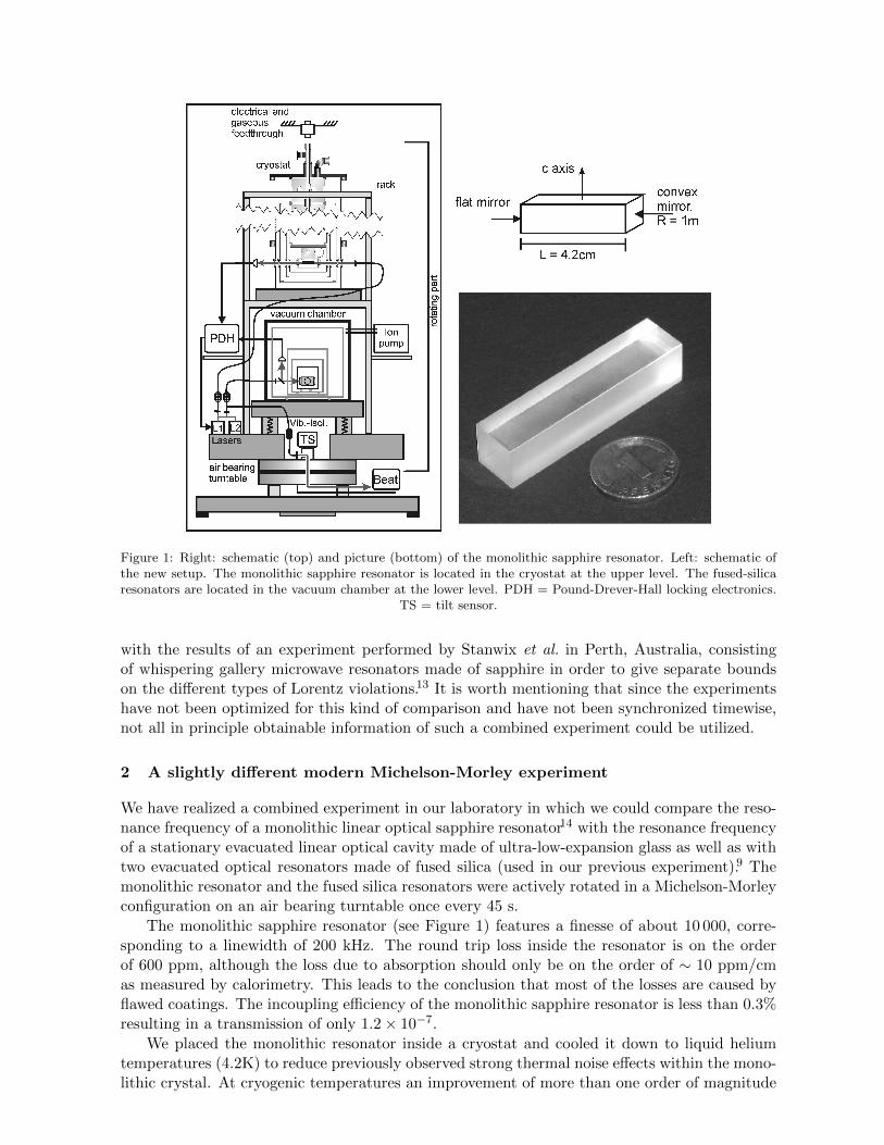
Figure 1: Right: schematic (top) and picture (bottom) of the monolithic sapphire resonator. Left: schematic ofthe new setup. The monolithic sapphire resonator is located in the cryostat at the upper level. The fused-silicaresonators are located in the vacuum chamber at the lower level. PDH = Pound-Drever-Hall locking electronics.
TS = tilt sensor.
with the results of an experiment performed by Stanwix et al. in Perth, Australia, consistingof whispering gallery microwave resonators made of sapphire in order to give separate boundson the different types of Lorentz violations.13 It is worth mentioning that since the experimentshave not been optimized for this kind of comparison and have not been synchronized timewise,not all in principle obtainable information of such a combined experiment could be utilized.
2 A slightly different modern Michelson-Morley experiment
We have realized a combined experiment in our laboratory in which we could compare the reso-nance frequency of a monolithic linear optical sapphire resonator14 with the resonance frequencyof a stationary evacuated linear optical cavity made of ultra-low-expansion glass as well as withtwo evacuated optical resonators made of fused silica (used in our previous experiment).9 Themonolithic resonator and the fused silica resonators were actively rotated in a Michelson-Morleyconfiguration on an air bearing turntable once every 45 s.
The monolithic sapphire resonator (see Figure 1) features a finesse of about 10 000, corre-sponding to a linewidth of 200 kHz. The round trip loss inside the resonator is on the orderof 600 ppm, although the loss due to absorption should only be on the order of ∼ 10 ppm/cmas measured by calorimetry. This leads to the conclusion that most of the losses are caused byflawed coatings. The incoupling efficiency of the monolithic sapphire resonator is less than 0.3%resulting in a transmission of only 1.2 × 10⁻⁷.
We placed the monolithic resonator inside a cryostat and cooled it down to liquid heliumtemperatures (4.2K) to reduce previously observed strong thermal noise effects within the mono-lithic crystal. At cryogenic temperatures an improvement of more than one order of magnitude
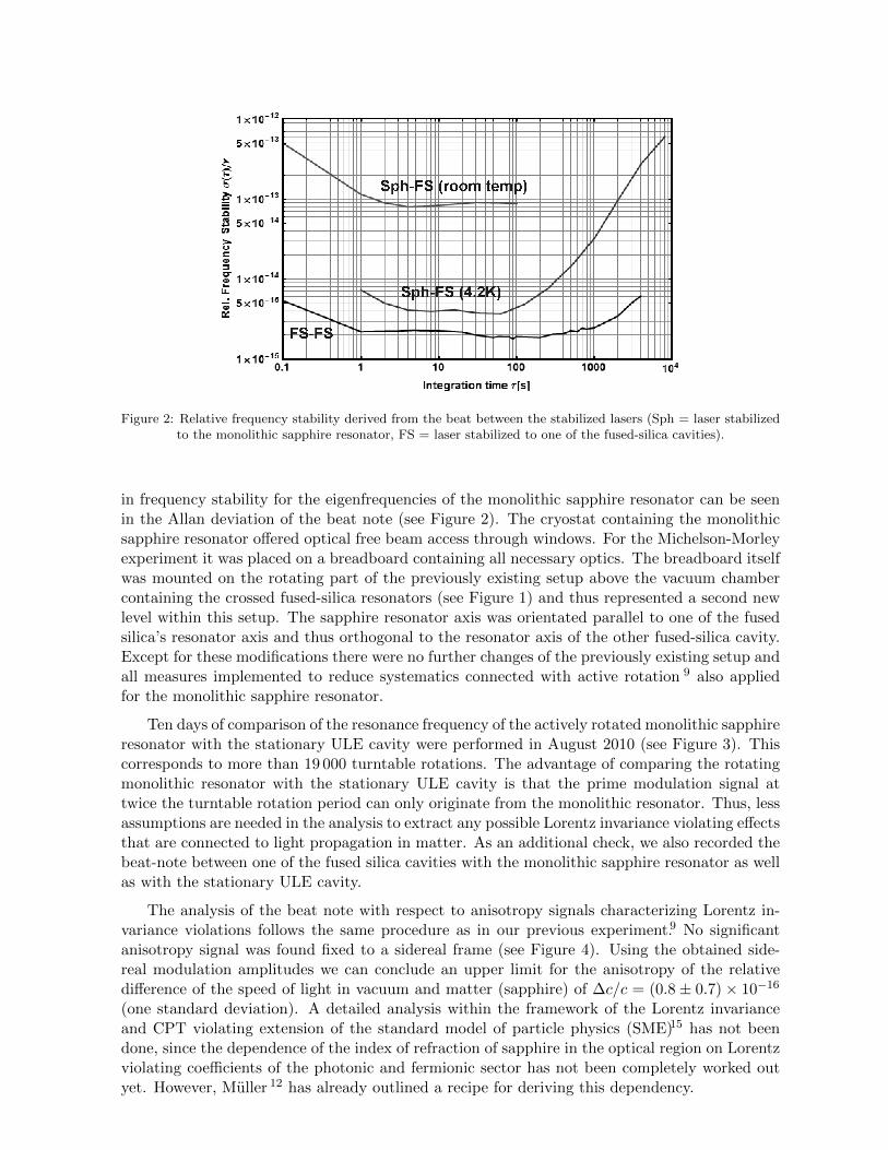
Figure 2: Relative frequency stability derived from the beat between the stabilized lasers (Sph = laser stabilizedto the monolithic sapphire resonator, FS = laser stabilized to one of the fused-silica cavities).
in frequency stability for the eigenfrequencies of the monolithic sapphire resonator can be seenin the Allan deviation of the beat note (see Figure 2). The cryostat containing the monolithicsapphire resonator offered optical free beam access through windows. For the Michelson-Morleyexperiment it was placed on a breadboard containing all necessary optics. The breadboard itselfwas mounted on the rotating part of the previously existing setup above the vacuum chambercontaining the crossed fused-silica resonators (see Figure 1) and thus represented a second newlevel within this setup. The sapphire resonator axis was orientated parallel to one of the fusedsilica’s resonator axis and thus orthogonal to the resonator axis of the other fused-silica cavity.Except for these modifications there were no further changes of the previously existing setup andall measures implemented to reduce systematics connected with active rotation 9 also appliedfor the monolithic sapphire resonator.
Ten days of comparison of the resonance frequency of the actively rotated monolithic sapphireresonator with the stationary ULE cavity were performed in August 2010 (see Figure 3). Thiscorresponds to more than 19 000 turntable rotations. The advantage of comparing the rotatingmonolithic resonator with the stationary ULE cavity is that the prime modulation signal attwice the turntable rotation period can only originate from the monolithic resonator. Thus, lessassumptions are needed in the analysis to extract any possible Lorentz invariance violating effectsthat are connected to light propagation in matter. As an additional check, we also recorded thebeat-note between one of the fused silica cavities with the monolithic sapphire resonator as wellas with the stationary ULE cavity.
The analysis of the beat note with respect to anisotropy signals characterizing Lorentz in-variance violations follows the same procedure as in our previous experiment.9 No significantanisotropy signal was found fixed to a sidereal frame (see Figure 4). Using the obtained side-real modulation amplitudes we can conclude an upper limit for the anisotropy of the relativedifference of the speed of light in vacuum and matter (sapphire) of ∆c/c = (0.8 ± 0.7) × 10−16
(one standard deviation). A detailed analysis within the framework of the Lorentz invarianceand CPT violating extension of the standard model of particle physics (SME)15 has not beendone, since the dependence of the index of refraction of sapphire in the optical region on Lorentzviolating coefficients of the photonic and fermionic sector has not been completely worked outyet. However, Muller 12 has already outlined a recipe for deriving this dependency.
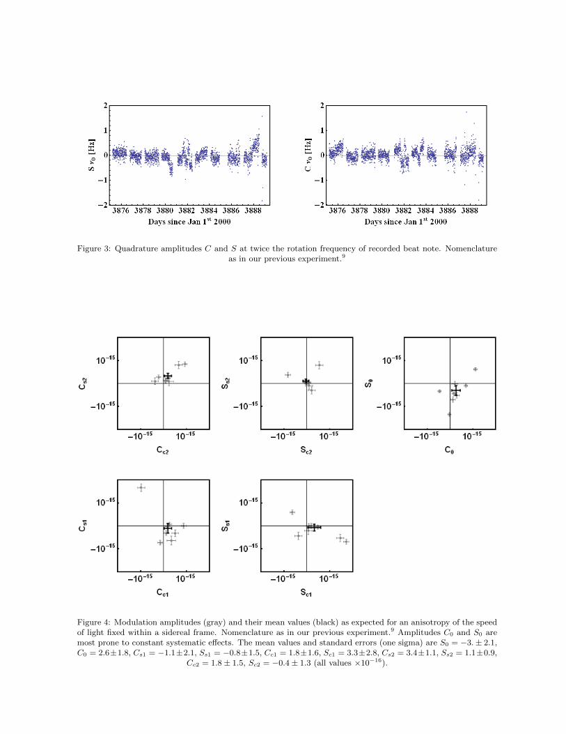
Figure 3: Quadrature amplitudes C and S at twice the rotation frequency of recorded beat note. Nomenclatureas in our previous experiment.9
Figure 4: Modulation amplitudes (gray) and their mean values (black) as expected for an anisotropy of the speedof light fixed within a sidereal frame. Nomenclature as in our previous experiment.9 Amplitudes C0 and S0 aremost prone to constant systematic effects. The mean values and standard errors (one sigma) are S0 = −3.± 2.1,C0 = 2.6±1.8, Cs1 = −1.1±2.1, Ss1 = −0.8±1.5, Cc1 = 1.8±1.6, Sc1 = 3.3±2.8, Cs2 = 3.4±1.1, Ss2 = 1.1±0.9,
Cc2 = 1.8 ± 1.5, Sc2 = −0.4 ± 1.3 (all values ×10−16).
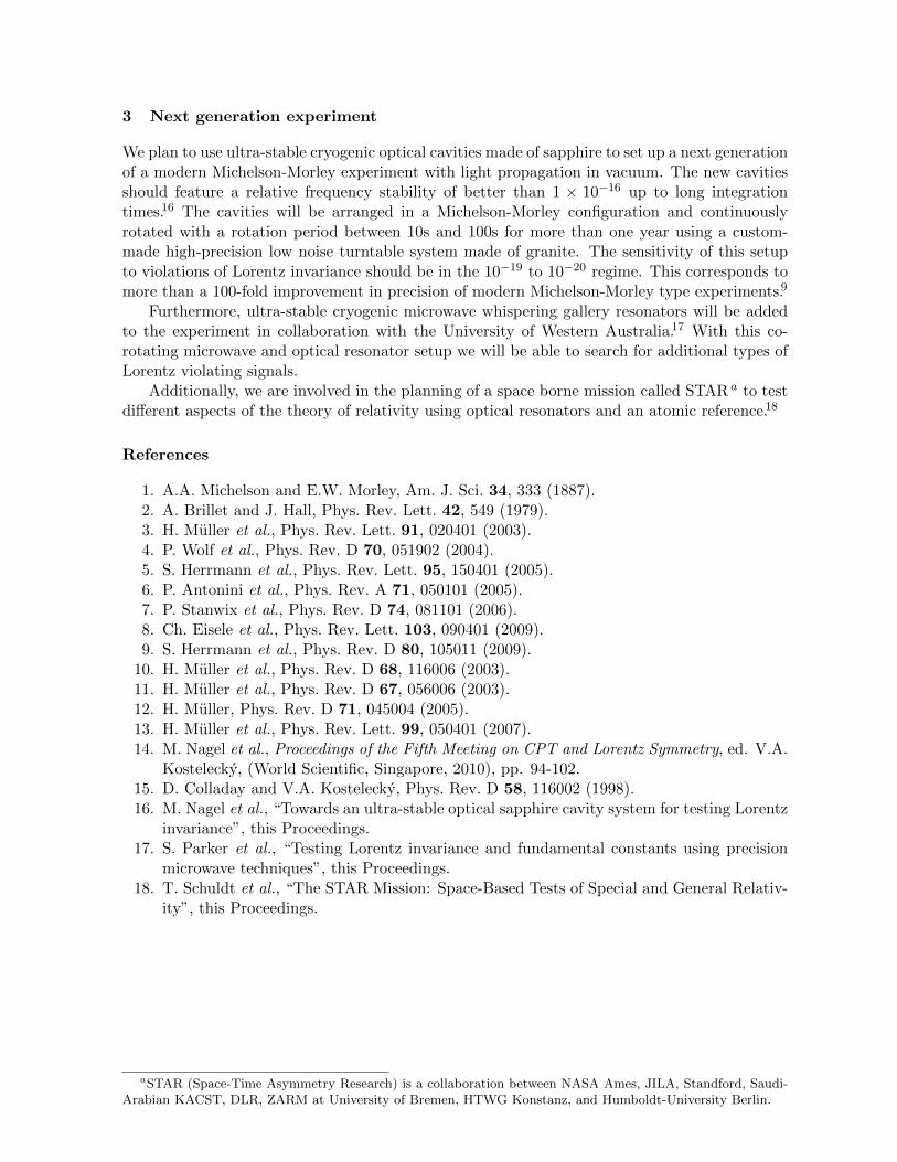
3 Next generation experiment
We plan to use ultra-stable cryogenic optical cavities made of sapphire to set up a next generationof a modern Michelson-Morley experiment with light propagation in vacuum. The new cavitiesshould feature a relative frequency stability of better than 1 × 10⁻¹⁶ up to long integrationtimes.16 The cavities will be arranged in a Michelson-Morley configuration and continuouslyrotated with a rotation period between 10s and 100s for more than one year using a custom-made high-precision low noise turntable system made of granite. The sensitivity of this setupto violations of Lorentz invariance should be in the 10−19 to 10−20 regime. This corresponds tomore than a 100-fold improvement in precision of modern Michelson-Morley type experiments.9
Furthermore, ultra-stable cryogenic microwave whispering gallery resonators will be addedto the experiment in collaboration with the University of Western Australia.17 With this co-rotating microwave and optical resonator setup we will be able to search for additional types ofLorentz violating signals.
Additionally, we are involved in the planning of a space borne mission called STAR a to testdifferent aspects of the theory of relativity using optical resonators and an atomic reference.18
References
1. A.A. Michelson and E.W. Morley, Am. J. Sci. 34, 333 (1887).2. A. Brillet and J. Hall, Phys. Rev. Lett. 42, 549 (1979).3. H. Muller et al., Phys. Rev. Lett. 91, 020401 (2003).4. P. Wolf et al., Phys. Rev. D 70, 051902 (2004).5. S. Herrmann et al., Phys. Rev. Lett. 95, 150401 (2005).6. P. Antonini et al., Phys. Rev. A 71, 050101 (2005).7. P. Stanwix et al., Phys. Rev. D 74, 081101 (2006).8. Ch. Eisele et al., Phys. Rev. Lett. 103, 090401 (2009).9. S. Herrmann et al., Phys. Rev. D 80, 105011 (2009).
10. H. Muller et al., Phys. Rev. D 68, 116006 (2003).11. H. Muller et al., Phys. Rev. D 67, 056006 (2003).12. H. Muller, Phys. Rev. D 71, 045004 (2005).13. H. Muller et al., Phys. Rev. Lett. 99, 050401 (2007).14. M. Nagel et al., Proceedings of the Fifth Meeting on CPT and Lorentz Symmetry, ed. V.A.
Kostelecky, (World Scientific, Singapore, 2010), pp. 94-102.15. D. Colladay and V.A. Kostelecky, Phys. Rev. D 58, 116002 (1998).16. M. Nagel et al., “Towards an ultra-stable optical sapphire cavity system for testing Lorentz
invariance”, this Proceedings.17. S. Parker et al., “Testing Lorentz invariance and fundamental constants using precision
microwave techniques”, this Proceedings.18. T. Schuldt et al., “The STAR Mission: Space-Based Tests of Special and General Relativ-
ity”, this Proceedings.
aSTAR (Space-Time Asymmetry Research) is a collaboration between NASA Ames, JILA, Standford, Saudi-Arabian KACST, DLR, ZARM at University of Bremen, HTWG Konstanz, and Humboldt-University Berlin.


11.Clocks

THE ACES MISSION: FUNDAMENTAL PHYSICS TESTS WITH COLDATOM CLOCKS IN SPACE
LUIGI CACCIAPUOTI
European Space Agency, Research and Scientific Support Department,Keplerlaan 1, P.O.Box 299, 2200 AG Noordwijk ZH The Netherlands
CHRISTOPHE SALOMON
Laboratoire Kastler Brossel, CNRS, UPMC, ENS24, rue Lhomond, 75005 Paris, France
High-performance clocks and links in space are key instruments to probe space-time properties.As such, they can be used to test Einstein’s theory of general relativity to high accuracy.Operated on-board the International Space Station, ACES will distribute a clock signal withfractional frequency instability and inaccuracy of 1 · 10−16. Space-to-ground and ground-to-ground comparisons of atomic frequency standards will be used to test Einstein’s theory ofgeneral relativity including a precision measurement of the gravitational red-shift, a search fortime variations of fundamental constants, and tests of the Standard Model Extension. Thispaper presents the ACES mission concept and discussed its development status.
1 Introduction
Atomic Clock Ensemble in Space (ACES) is a fundamental physics mission of the EuropeanSpace Agency based on a new generation of clocks to be operated in the microgravity envi-ronment of the International Space Station (ISS). ACES is a distributed system designed todisseminate a high stability and accuracy clock signal 1,2. It consists of a payload generatingan atomic frequency reference in space and a network of ground terminals connected to high-performance clocks on ground. Transported on the ISS by the Japanese transfer vehicle HTV,the ACES payload will be installed at the external payload facility of the Columbus module (seeFig. 1). The ACES payload accommodates two atomic clocks: PHARAO (acronym of “Projetd’Horloge Atomique par Refroidissement d’Atomes en Orbit”), a primary frequency standardbased on samples of laser cooled cesium atoms and SHM (acronym of “Space H-Maser”), anactive hydrogen maser for space applications. The performances of the two clocks are combinedto generate an on-board timescale with the short-term stability of SHM and the long-term sta-bility and accuracy of the PHARAO clock. The on-board comparison of PHARAO and SHMand the distribution of the ACES clock signal are ensured by the Frequency Comparison andDistribution Package (FCDP), while all data handling processes are controlled by the eXternalPayLoad Computer (XPLC). The ACES clocks are compared to clocks on the ground usingboth a microwave link (MWL) and an optical link (ELT). A GNSS receiver connected to theon-board time scale provides orbit determination of the ACES clocks.ACES will be ready for launch in 2014, for a planned mission duration of 18 months. During the
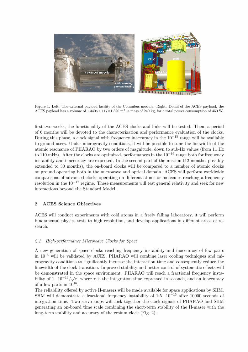
Figure 1: Left: The external payload facility of the Columbus module. Right: Detail of the ACES payload; theACES payload has a volume of 1.340×1.117×1.320 m3, a mass of 240 kg, for a total power consumption of 450 W.
first two weeks, the functionality of the ACES clocks and links will be tested. Then, a periodof 6 months will be devoted to the characterization and performance evaluation of the clocks.During this phase, a clock signal with frequency inaccuracy in the 10−15 range will be availableto ground users. Under microgravity conditions, it will be possible to tune the linewidth of theatomic resonance of PHARAO by two orders of magnitude, down to sub-Hz values (from 11 Hzto 110 mHz). After the clocks are optimized, performances in the 10−16 range both for frequencyinstability and inaccuracy are expected. In the second part of the mission (12 months, possiblyextended to 30 months), the on-board clocks will be compared to a number of atomic clockson ground operating both in the microwave and optical domain. ACES will perform worldwidecomparisons of advanced clocks operating on different atoms or molecules reaching a frequencyresolution in the 10−17 regime. These measurements will test general relativity and seek for newinteractions beyond the Standard Model.
2 ACES Science Objectives
ACES will conduct experiments with cold atoms in a freely falling laboratory, it will performfundamental physics tests to high resolution, and develop applications in different areas of re-search.
2.1 High-performance Microwave Clocks for Space
A new generation of space clocks reaching frequency instability and inaccuracy of few partsin 1016 will be validated by ACES. PHARAO will combine laser cooling techniques and mi-crogravity conditions to significantly increase the interaction time and consequently reduce thelinewidth of the clock transition. Improved stability and better control of systematic effects willbe demonstrated in the space environment. PHARAO will reach a fractional frequency insta-bility of 1 · 10−13/
√τ , where τ is the integration time expressed in seconds, and an inaccuracy
of a few parts in 1016.The reliability offered by active H-masers will be made available for space applications by SHM.SHM will demonstrate a fractional frequency instability of 1.5 · 10−15 after 10000 seconds ofintegration time. Two servo-loops will lock together the clock signals of PHARAO and SHMgenerating an on-board time scale combining the short-term stability of the H-maser with thelong-term stability and accuracy of the cesium clock (Fig. 2).
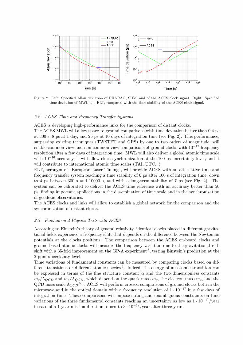
Figure 2: Left: Specified Allan deviation of PHARAO, SHM, and of the ACES clock signal. Right: Specifiedtime deviation of MWL and ELT, compared with the time stability of the ACES clock signal.
2.2 ACES Time and Frequency Transfer Systems
ACES is developing high-performance links for the comparison of distant clocks.The ACES MWL will allow space-to-ground comparisons with time deviation better than 0.4 psat 300 s, 8 ps at 1 day, and 25 ps at 10 days of integration time (see Fig. 2). This performance,surpassing existing techniques (TWSTFT and GPS) by one to two orders of magnitude, willenable common view and non-common view comparisons of ground clocks with 10−17 frequencyresolution after a few days of integration time. MWL will also deliver a global atomic time scalewith 10−16 accuracy, it will allow clock synchronization at the 100 ps uncertainty level, and itwill contribute to international atomic time scales (TAI, UTC...).ELT, acronym of “European Laser Timing”, will provide ACES with an alternative time andfrequency transfer system reaching a time stability of 6 ps after 100 s of integration time, downto 4 ps between 300 s and 10000 s, and with a long-term stability of 7 ps (see Fig. 2). Thesystem can be calibrated to deliver the ACES time reference with an accuracy better than 50ps, finding important applications in the dissemination of time scale and in the synchronizationof geodetic observatories.The ACES clocks and links will allow to establish a global network for the comparison and thesynchronization of distant clocks.
2.3 Fundamental Physics Tests with ACES
According to Einstein’s theory of general relativity, identical clocks placed in different gravita-tional fields experience a frequency shift that depends on the difference between the Newtonianpotentials at the clocks positions. The comparison between the ACES on-board clocks andground-based atomic clocks will measure the frequency variation due to the gravitational red-shift with a 35-fold improvement on the GP-A experiment 3, testing Einstein’s prediction at the2 ppm uncertainty level.Time variations of fundamental constants can be measured by comparing clocks based on dif-ferent transitions or different atomic species 4. Indeed, the energy of an atomic transition canbe expressed in terms of the fine structure constant α and the two dimensionless constantsmq/ΛQCD and me/ΛQCD, which depend on the quark mass mq, the electron mass me, and theQCD mass scale ΛQCD
5,6. ACES will perform crossed comparisons of ground clocks both in themicrowave and in the optical domain with a frequency resolution of 1 · 10−17 in a few days ofintegration time. These comparisons will impose strong and unambiguous constraints on timevariations of the three fundamental constants reaching an uncertainty as low as 1 · 10−17/yearin case of a 1-year mission duration, down to 3 · 10−18/year after three years.
The foundations of special relativity lie on the hypothesis of Local Lorentz Invariance (LLI).According to this principle, the outcome of any local test experiment is independent of thevelocity of the freely falling apparatus. In 1997, LLI tests based on the measurement of theround-trip speed of light have been performed by comparing clocks on-board GPS satellites toground hydrogen masers7. In such experiments, LLI violations would appear as variations of thespeed of light c with the direction and the relative velocity of the clocks. ACES will perform asimilar experiment by measuring relative variations of the speed of light at the 10−10 uncertaintylevel.
2.4 Applications
ACES will also demonstrate a new geodesy technique to map the Earth gravitational potential.This technique uses a precision measurement of the Einstein’s gravitational red-shift betweentwo clocks to determine the corresponding difference in the local gravitational potentials. Thepossibility of performing comparisons of ground clocks at the 10−17 frequency uncertainty levelwill allow ACES to resolve geopotential differences down to 10 cm on the geoid height.A dedicated GNSS receiver on-board the ACES payload will ensure orbit determination, im-portant for comparing clocks and for performing fundamental physics tests. In addition, thereceiver will be connected to the ACES clock signal, opening the possibility to use the GNSSnetwork for clock comparisons and remote sensing applications (radio-occultation and reflec-tometry experiments).The simultaneous operation of the optical (ELT) and microwave (MWL) links will provide atest bench for their mutual characterization. Optical versus dual-frequency microwave measure-ments will also provide useful data for the study of atmospheric propagation delays and for theconstruction of atmosphere mapping functions at the three different wavelengths. In addition,the ACES links will provide absolute range measurements, both in the microwave and in theoptical domain.
3 ACES Status
All ACES instruments and subsystems have now reached a high technology maturity, demon-strated by the engineering models, now delivered or in final assembly, and by the ongoingactivities on the flight hardware. The system tests on the ACES Engineering Model (EM)workbench (see Sec. 3.3) have represented a major milestone in the ACES development cycle.Their successful completion has indeed closed the EM phase with the performance verificationof the ACES clock signal and it has confirmed the adequacy of the ACES design, releasing themanufacturing for the flight hardware. ACES Flight Model (FM) activities are expected to becompleted in 2013.
3.1 The PHARAO Clock
PHARAO is a cesium clock based on laser cooled atoms developed by LNE-SYRTE, LKB, andCNES. Its concept is very similar to ground based atomic fountains, but with a major dif-ference: PHARAO will be operated under microgravity conditions. Atoms, launched in freeflight along the PHARAO tube, cross a resonant cavity where they interact twice with a mi-crowave field tuned on the transition between the two hyperfine levels of the cesium ground state(9.192631770 GHz, from the SI definition of the second). In a microgravity environment, thevelocity of the atoms along the ballistic trajectories is constant and can be continuously changedover almost two orders of magnitude (5 to 500 cm/s), allowing the detection of atomic signalswith sub-Hz linewidth.The engineering model of the PHARAO clock has been completed and tested. Cesium atoms
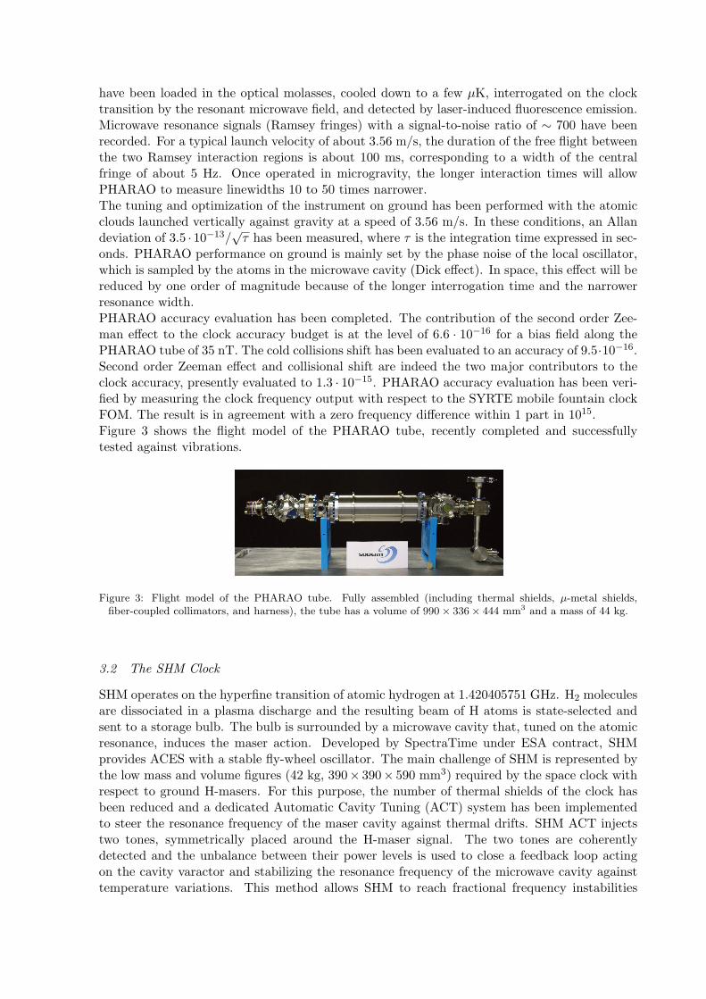
have been loaded in the optical molasses, cooled down to a few µK, interrogated on the clocktransition by the resonant microwave field, and detected by laser-induced fluorescence emission.Microwave resonance signals (Ramsey fringes) with a signal-to-noise ratio of ∼ 700 have beenrecorded. For a typical launch velocity of about 3.56 m/s, the duration of the free flight betweenthe two Ramsey interaction regions is about 100 ms, corresponding to a width of the centralfringe of about 5 Hz. Once operated in microgravity, the longer interaction times will allowPHARAO to measure linewidths 10 to 50 times narrower.The tuning and optimization of the instrument on ground has been performed with the atomicclouds launched vertically against gravity at a speed of 3.56 m/s. In these conditions, an Allandeviation of 3.5 · 10−13/
√τ has been measured, where τ is the integration time expressed in sec-
onds. PHARAO performance on ground is mainly set by the phase noise of the local oscillator,which is sampled by the atoms in the microwave cavity (Dick effect). In space, this effect will bereduced by one order of magnitude because of the longer interrogation time and the narrowerresonance width.PHARAO accuracy evaluation has been completed. The contribution of the second order Zee-man effect to the clock accuracy budget is at the level of 6.6 · 10−16 for a bias field along thePHARAO tube of 35 nT. The cold collisions shift has been evaluated to an accuracy of 9.5·10−16.Second order Zeeman effect and collisional shift are indeed the two major contributors to theclock accuracy, presently evaluated to 1.3 · 10−15. PHARAO accuracy evaluation has been veri-fied by measuring the clock frequency output with respect to the SYRTE mobile fountain clockFOM. The result is in agreement with a zero frequency difference within 1 part in 1015.Figure 3 shows the flight model of the PHARAO tube, recently completed and successfullytested against vibrations.
Figure 3: Flight model of the PHARAO tube. Fully assembled (including thermal shields, µ-metal shields,fiber-coupled collimators, and harness), the tube has a volume of 990× 336× 444 mm3 and a mass of 44 kg.
3.2 The SHM Clock
SHM operates on the hyperfine transition of atomic hydrogen at 1.420405751 GHz. H2 moleculesare dissociated in a plasma discharge and the resulting beam of H atoms is state-selected andsent to a storage bulb. The bulb is surrounded by a microwave cavity that, tuned on the atomicresonance, induces the maser action. Developed by SpectraTime under ESA contract, SHMprovides ACES with a stable fly-wheel oscillator. The main challenge of SHM is represented bythe low mass and volume figures (42 kg, 390× 390× 590 mm3) required by the space clock withrespect to ground H-masers. For this purpose, the number of thermal shields of the clock hasbeen reduced and a dedicated Automatic Cavity Tuning (ACT) system has been implementedto steer the resonance frequency of the maser cavity against thermal drifts. SHM ACT injectstwo tones, symmetrically placed around the H-maser signal. The two tones are coherentlydetected and the unbalance between their power levels is used to close a feedback loop actingon the cavity varactor and stabilizing the resonance frequency of the microwave cavity againsttemperature variations. This method allows SHM to reach fractional frequency instabilities
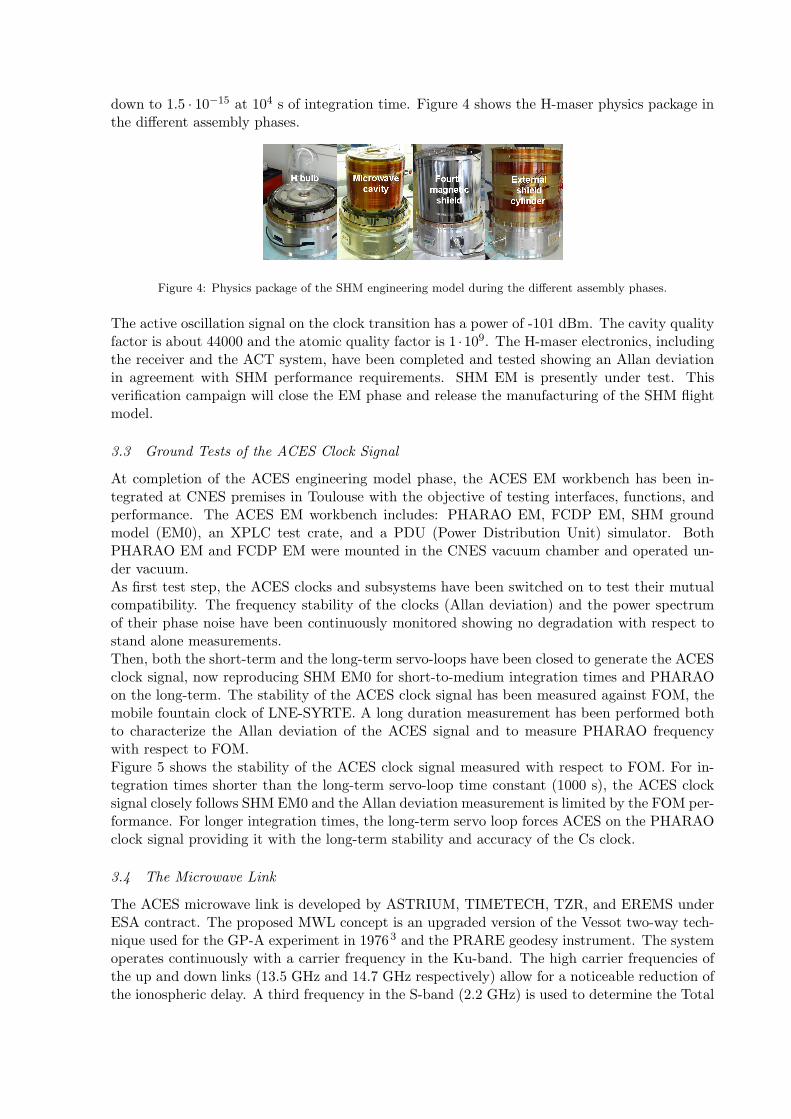
down to 1.5 · 10−15 at 104 s of integration time. Figure 4 shows the H-maser physics package inthe different assembly phases.
Figure 4: Physics package of the SHM engineering model during the different assembly phases.
The active oscillation signal on the clock transition has a power of -101 dBm. The cavity qualityfactor is about 44000 and the atomic quality factor is 1 ·109. The H-maser electronics, includingthe receiver and the ACT system, have been completed and tested showing an Allan deviationin agreement with SHM performance requirements. SHM EM is presently under test. Thisverification campaign will close the EM phase and release the manufacturing of the SHM flightmodel.
3.3 Ground Tests of the ACES Clock Signal
At completion of the ACES engineering model phase, the ACES EM workbench has been in-tegrated at CNES premises in Toulouse with the objective of testing interfaces, functions, andperformance. The ACES EM workbench includes: PHARAO EM, FCDP EM, SHM groundmodel (EM0), an XPLC test crate, and a PDU (Power Distribution Unit) simulator. BothPHARAO EM and FCDP EM were mounted in the CNES vacuum chamber and operated un-der vacuum.As first test step, the ACES clocks and subsystems have been switched on to test their mutualcompatibility. The frequency stability of the clocks (Allan deviation) and the power spectrumof their phase noise have been continuously monitored showing no degradation with respect tostand alone measurements.Then, both the short-term and the long-term servo-loops have been closed to generate the ACESclock signal, now reproducing SHM EM0 for short-to-medium integration times and PHARAOon the long-term. The stability of the ACES clock signal has been measured against FOM, themobile fountain clock of LNE-SYRTE. A long duration measurement has been performed bothto characterize the Allan deviation of the ACES signal and to measure PHARAO frequencywith respect to FOM.Figure 5 shows the stability of the ACES clock signal measured with respect to FOM. For in-tegration times shorter than the long-term servo-loop time constant (1000 s), the ACES clocksignal closely follows SHM EM0 and the Allan deviation measurement is limited by the FOM per-formance. For longer integration times, the long-term servo loop forces ACES on the PHARAOclock signal providing it with the long-term stability and accuracy of the Cs clock.
3.4 The Microwave Link
The ACES microwave link is developed by ASTRIUM, TIMETECH, TZR, and EREMS underESA contract. The proposed MWL concept is an upgraded version of the Vessot two-way tech-nique used for the GP-A experiment in 1976 3 and the PRARE geodesy instrument. The systemoperates continuously with a carrier frequency in the Ku-band. The high carrier frequencies ofthe up and down links (13.5 GHz and 14.7 GHz respectively) allow for a noticeable reduction ofthe ionospheric delay. A third frequency in the S-band (2.2 GHz) is used to determine the Total
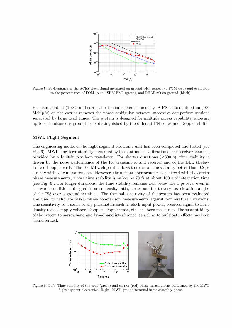
100 101 102 103 10410-16
10-15
10-14
10-13
10-12
Alla
n de
viat
ion
Time (s)
PHARAO on ground SHM EM0 FOM ACES
Figure 5: Performance of the ACES clock signal measured on ground with respect to FOM (red) and comparedto the performance of FOM (blue), SHM EM0 (green), and PHARAO on ground (black).
Electron Content (TEC) and correct for the ionosphere time delay. A PN-code modulation (100Mchip/s) on the carrier removes the phase ambiguity between successive comparison sessionsseparated by large dead times. The system is designed for multiple access capability, allowingup to 4 simultaneous ground users distinguished by the different PN-codes and Doppler shifts.
MWL Flight Segment
The engineering model of the flight segment electronic unit has been completed and tested (seeFig. 6). MWL long-term stability is ensured by the continuous calibration of the receiver channelsprovided by a built-in test-loop translator. For shorter durations (<300 s), time stability isdriven by the noise performance of the Ku transmitter and receiver and of the DLL (Delay-Locked Loop) boards. The 100 MHz chip rate allows to reach a time stability better than 0.2 psalready with code measurements. However, the ultimate performance is achieved with the carrierphase measurements, whose time stability is as low as 70 fs at about 100 s of integration time(see Fig. 6). For longer durations, the time stability remains well below the 1 ps level even inthe worst conditions of signal-to-noise density ratio, corresponding to very low elevation anglesof the ISS over a ground terminal. The thermal sensitivity of the system has been evaluatedand used to calibrate MWL phase comparison measurements against temperature variations.The sensitivity to a series of key parameters such as clock input power, received signal-to-noisedensity ratios, supply voltage, Doppler, Doppler rate, etc. has been measured. The susceptibilityof the system to narrowband and broadband interference, as well as to multipath effects has beencharacterized.
Figure 6: Left: Time stability of the code (green) and carrier (red) phase measurement performed by the MWLflight segment electronics. Right: MWL ground terminal in its assembly phase.
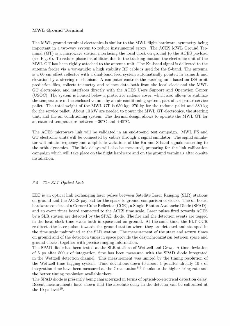
MWL Ground Terminal
The MWL ground terminal electronics is similar to the MWL flight hardware, symmetry beingimportant in a two-way system to reduce instrumental errors. The ACES MWL Ground Ter-minal (GT) is a microwave station interfacing the local clock on ground to the ACES payload(see Fig. 6). To reduce phase instabilities due to the tracking motion, the electronic unit of theMWL GT has been rigidly attached to the antenna unit. The Ku-band signal is delivered to theantenna feeder via a waveguide; a high stability RF cable is used for the S-band. The antennais a 60 cm offset reflector with a dual-band feed system automatically pointed in azimuth andelevation by a steering mechanism. A computer controls the steering unit based on ISS orbitprediction files, collects telemetry and science data both from the local clock and the MWLGT electronics, and interfaces directly with the ACES Users Support and Operation Center(USOC). The system is housed below a protective radome cover, which also allows to stabilizethe temperature of the enclosed volume by an air conditioning system, part of a separate servicepallet. The total weight of the MWL GT is 650 kg: 270 kg for the radome pallet and 380 kgfor the service pallet. About 10 kW are needed to power the MWL GT electronics, the steeringunit, and the air conditioning system. The thermal design allows to operate the MWL GT foran external temperature between −30C and +45C.
The ACES microwave link will be validated in an end-to-end test campaign. MWL FS andGT electronic units will be connected by cables through a signal simulator. The signal simula-tor will mimic frequency and amplitude variations of the Ku and S-band signals according tothe orbit dynamics. The link delays will also be measured, preparing for the link calibrationcampaign which will take place on the flight hardware and on the ground terminals after on-siteinstallation.
3.5 The ELT Optical Link
ELT is an optical link exchanging laser pulses between Satellite Laser Ranging (SLR) stationson ground and the ACES payload for the space-to-ground comparison of clocks. The on-boardhardware consists of a Corner Cube Reflector (CCR), a Single-Photon Avalanche Diode (SPAD),and an event timer board connected to the ACES time scale. Laser pulses fired towards ACESby a SLR station are detected by the SPAD diode. The fire and the detection events are taggedin the local clock time scales both in space and on ground. At the same time, the ELT CCRre-directs the laser pulses towards the ground station where they are detected and stamped inthe time scale maintained at the SLR station. The measurement of the start and return timeson ground and of the detection times in space provide the desynchronization between space andground clocks, together with precise ranging information.The SPAD diode has been tested at the SLR stations of Wettzell and Graz . A time deviationof 5 ps after 500 s of integration time has been measured with the SPAD diode integratedin the Wettzell detection channel. This measurement was limited by the timing resolution ofthe Wettzell time tagging system. Time deviations down to about 1 ps after already 10 s ofintegration time have been measured at the Graz station 8,9 thanks to the higher firing rate andthe better timing resolution available there.The SPAD diode is presently being characterized in terms of optical-to-electrical detection delay.Recent measurements have shown that the absolute delay in the detector can be calibrated atthe 10 ps level 10.
Acknowledgments
The authors express their warm thanks for their valuable contribution to the ACES scienceteam, to the ACES project team at ESA, ASTRIUM, and TimeTech, to the PHARAO team atLNE-SYRTE and CNES, to the SHM team at SpectraTime. This paper has been written onbehalf of the many scientists and engineers contributing to the mission development.
References
1. C. Salomon et al, C. R. Acad. Sci. Paris t.2 Series IV, 1313 (2002).2. L. Cacciapuoti and C. Salomon, Eur. Phys. J. Special Topics 172, 57 (2009).3. R.F.C. Vessot et al, Phys. Rev. Lett. 45, 2081 (1980).4. T. Fortier et al, Phys. Rev. Lett. 98, 070801 (2007).5. V.V. Flambaum et al, Phys. Rev. D 69, 115006 (2004).6. V.V. Flambaum et al, Phys. Rev. C 73, 055501 (2006).7. P. Wolf and G. Petit, Phys. Rev. A 56, 4405 (1997).8. U. Schreiber et al, IEEE Trans 57, 728 (2009).9. I. Prochazka et al, in Proc of 2010 European Time and Frequency Forum (2010).
10. I. Prochazka et al, Metrologia 48, L13 (2011).


12.Pulsars

GRAVITATIONAL WAVE DETECTION THROUGH PULSAR TIMING
ARRAYS
DAVID J. CHAMPIONMax-Planck-Institut fur Radioastronomie, Auf dem Hugel 69, 53121 Bonn, Germany
Pulsar timing arrays are the only means to detect very low frequency nanohertz gravitationalwaves (GWs). GWs in this part of the spectrum are expected to be generated by binarysuper-massive black-hole (SMBH) systems which are a consequence of the merger of galaxies.Individual nearby strong emitters can be detected, allowing the GW and parameters of theSMBH system to be determined. A stochastic background of GWs from weaker, more distantbut more numerous sources, is also expected. This will provide a measure of the galacticmerger rate which is important for our understanding of galaxy evolution. GW detectionvia pulsar timing provides science complementary to the space- and ground- based detectors,observing similar sources at different mass ranges and stages of evolution.
1 Introduction to Pulsar Timing
Pulsars are extraordinary tools for astronomy, condensed matter physics, electromagnetism and,in particular, testing general relativity. They are rapidly rotating neutron star remnants ofmassive stars. Their strong magnetic fields focus streams of electromagnetic radiation from thepoles which sweep like the beam of a lighthouse as the neutron star rotates. If these beamsintersect the line-of-sight of an observer, a pulse of emission is detected.
1.1 Pulsars
Pulsars are born in the explosive death of a high-mass star, a supernova. As the outer layers ofthe star are blown off, the core collapses and extreme pressure forms a neutron star with a massof ∼1.4 M
⊙within a diameter of only ∼20 km. During the collapse the angular momentum is
conserved causing the star to spin up to rotation periods of tens of milliseconds. The magneticflux is also conserved, meaning that the neutron star inherits a surface magnetic field of typically1012 G.
As the pulsar ages it slows down due to energy lost in magnetic dipole radiation. Eventuallythe neutron star rotates so slowly that emission from the poles becomes unstable and ceases.However if the pulsar is in a binary system (not disrupted by the supernova that created theneutron star) then the pulsar may undergo ‘recycling’. As the companion star evolves it swells,eventually overfilling its Roche lobe. At this point the outer layers of the star feel a strongergravitational pull from the neutron star than from the companion and material streams ontothe neutron star. The conservation of angular momentum spins the pulsar up to periods of onlya few milliseconds. The accretion of matter also suppresses the magnetic field, reducing thespin-down of the pulsar. These millisecond pulsars (MSPs) are the most stable branch of thepulsar family.
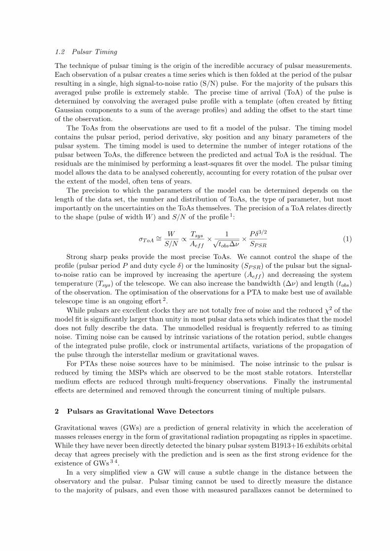
1.2 Pulsar Timing
The technique of pulsar timing is the origin of the incredible accuracy of pulsar measurements.Each observation of a pulsar creates a time series which is then folded at the period of the pulsarresulting in a single, high signal-to-noise ratio (S/N) pulse. For the majority of the pulsars thisaveraged pulse profile is extremely stable. The precise time of arrival (ToA) of the pulse isdetermined by convolving the averaged pulse profile with a template (often created by fittingGaussian components to a sum of the average profiles) and adding the offset to the start timeof the observation.
The ToAs from the observations are used to fit a model of the pulsar. The timing modelcontains the pulsar period, period derivative, sky position and any binary parameters of thepulsar system. The timing model is used to determine the number of integer rotations of thepulsar between ToAs, the difference between the predicted and actual ToA is the residual. Theresiduals are the minimised by performing a least-squares fit over the model. The pulsar timingmodel allows the data to be analysed coherently, accounting for every rotation of the pulsar overthe extent of the model, often tens of years.
The precision to which the parameters of the model can be determined depends on thelength of the data set, the number and distribution of ToAs, the type of parameter, but mostimportantly on the uncertainties on the ToAs themselves. The precision of a ToA relates directlyto the shape (pulse of width W ) and S/N of the profile 1:
σToA∼=
W
S/N∝
Tsys
Aeff
×1
√tobs∆ν
×Pδ3/2
SPSR
(1)
Strong sharp peaks provide the most precise ToAs. We cannot control the shape of theprofile (pulsar period P and duty cycle δ) or the luminosity (SPSR) of the pulsar but the signal-to-noise ratio can be improved by increasing the aperture (Aeff ) and decreasing the systemtemperature (Tsys) of the telescope. We can also increase the bandwidth (∆ν) and length (tobs)of the observation. The optimisation of the observations for a PTA to make best use of availabletelescope time is an ongoing effort 2.
While pulsars are excellent clocks they are not totally free of noise and the reduced χ2 of themodel fit is significantly larger than unity in most pulsar data sets which indicates that the modeldoes not fully describe the data. The unmodelled residual is frequently referred to as timingnoise. Timing noise can be caused by intrinsic variations of the rotation period, subtle changesof the integrated pulse profile, clock or instrumental artifacts, variations of the propagation ofthe pulse through the interstellar medium or gravitational waves.
For PTAs these noise sources have to be minimised. The noise intrinsic to the pulsar isreduced by timing the MSPs which are observed to be the most stable rotators. Interstellarmedium effects are reduced through multi-frequency observations. Finally the instrumentaleffects are determined and removed through the concurrent timing of multiple pulsars.
2 Pulsars as Gravitational Wave Detectors
Gravitational waves (GWs) are a prediction of general relativity in which the acceleration ofmasses releases energy in the form of gravitational radiation propagating as ripples in spacetime.While they have never been directly detected the binary pulsar system B1913+16 exhibits orbitaldecay that agrees precisely with the prediction and is seen as the first strong evidence for theexistence of GWs 3 4.
In a very simplified view a GW will cause a subtle change in the distance between theobservatory and the pulsar. Pulsar timing cannot be used to directly measure the distanceto the majority of pulsars, and even those with measured parallaxes cannot be determined to
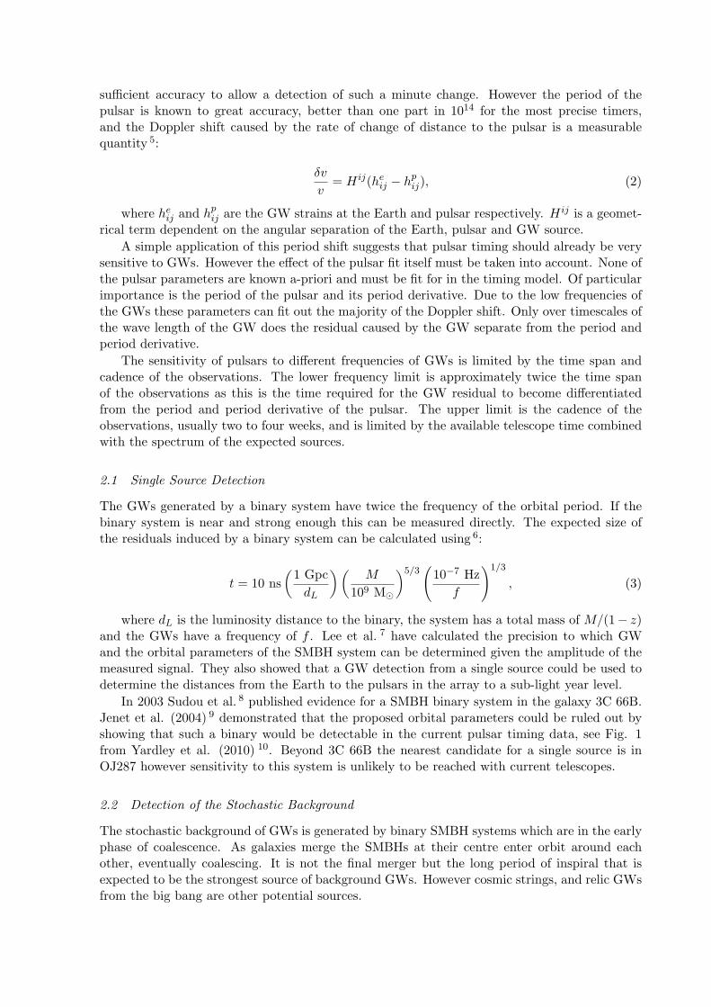
sufficient accuracy to allow a detection of such a minute change. However the period of thepulsar is known to great accuracy, better than one part in 1014 for the most precise timers,and the Doppler shift caused by the rate of change of distance to the pulsar is a measurablequantity 5:
δv
v= H ij(heij − hpij), (2)
where heij and hpij are the GW strains at the Earth and pulsar respectively. H ij is a geomet-rical term dependent on the angular separation of the Earth, pulsar and GW source.
A simple application of this period shift suggests that pulsar timing should already be verysensitive to GWs. However the effect of the pulsar fit itself must be taken into account. None ofthe pulsar parameters are known a-priori and must be fit for in the timing model. Of particularimportance is the period of the pulsar and its period derivative. Due to the low frequencies ofthe GWs these parameters can fit out the majority of the Doppler shift. Only over timescales ofthe wave length of the GW does the residual caused by the GW separate from the period andperiod derivative.
The sensitivity of pulsars to different frequencies of GWs is limited by the time span andcadence of the observations. The lower frequency limit is approximately twice the time spanof the observations as this is the time required for the GW residual to become differentiatedfrom the period and period derivative of the pulsar. The upper limit is the cadence of theobservations, usually two to four weeks, and is limited by the available telescope time combinedwith the spectrum of the expected sources.
2.1 Single Source Detection
The GWs generated by a binary system have twice the frequency of the orbital period. If thebinary system is near and strong enough this can be measured directly. The expected size ofthe residuals induced by a binary system can be calculated using 6:
t = 10 ns
(
1 Gpc
dL
)(
M
109 M⊙
)5/3(
10−7 Hz
f
)1/3
, (3)
where dL is the luminosity distance to the binary, the system has a total mass of M/(1− z)and the GWs have a frequency of f . Lee et al. 7 have calculated the precision to which GWand the orbital parameters of the SMBH system can be determined given the amplitude of themeasured signal. They also showed that a GW detection from a single source could be used todetermine the distances from the Earth to the pulsars in the array to a sub-light year level.
In 2003 Sudou et al. 8 published evidence for a SMBH binary system in the galaxy 3C 66B.Jenet et al. (2004) 9 demonstrated that the proposed orbital parameters could be ruled out byshowing that such a binary would be detectable in the current pulsar timing data, see Fig. 1from Yardley et al. (2010) 10. Beyond 3C 66B the nearest candidate for a single source is inOJ287 however sensitivity to this system is unlikely to be reached with current telescopes.
2.2 Detection of the Stochastic Background
The stochastic background of GWs is generated by binary SMBH systems which are in the earlyphase of coalescence. As galaxies merge the SMBHs at their centre enter orbit around eachother, eventually coalescing. It is not the final merger but the long period of inspiral that isexpected to be the strongest source of background GWs. However cosmic strings, and relic GWsfrom the big bang are other potential sources.
Figure 1: The sky-averaged sensitivity of pulsar timing arrays using current telescopes and the SKA to singlesources as a function of the source GW frequency. Figure from Yardley et al. 2009.
To detect the stochastic background a different technique is used. The residuals of each pairof pulsars are correlated and plotted against the angular separation of the pair. Due to thequadrupolar nature of the GWs, pulsars close to each other on the sky would be expected tobe highly correlated while those separated by 90 would be anti-correlated. As the separationincreases to 180 the degree of correlation also increases. The resulting curve is usually referredto as the Hellings and Downs curve. An example of a such a correlation is shown in Fig. 2 fromHobbs et al 2009 11.
3 Comparison with other Detection Efforts
The frequency range in which PTAs are sensitive and the expected sources are complementaryto the up-coming ground- and space- based detectors. The SMBHs seen in PTA data will be atan earlier evolutionary phase to those observed with the space-based Laser Interferometer SpaceAntenna (LISA): as the SMBHs in the binary coalesce, the frequency of the orbit increasesmoving into the LISA band. Observations of a coalescence in the LISA band could trigger adeep search of the archival PTA data (now that the position of the system is known) for thepre-ring-down system 12. Indeed any simultaneous observations would provide a full descriptionof the system including the elusive distance measurement 13. Finally all three types of detectorsare looking at black hole systems from stellar masses through to super-massive.
4 Current Pulsar Timing Array Projects
There are three large PTAs currently in operation. The Parkes Pulsar Timing Array 14 is thelongest running with more than 5 years of development and is based on data from the Parkes 64-m telescope in Australia. The European Pulsar Timing Array15 uses the 100-m Effelsberg, 100-m(equivalent) Nancay, 76-m Lovell, and (when completed) the 64-m Sardinia telescopes in addition
Figure 2: An example Hellings and Downs plot. The degree of correlation of pairs of pulsar residuals against theangular separation of the pulsar pair. The solid line is the fitted Hellings and Downs curve. Figure from Hobbs
et al. 2009.
to the Westerbork Sythesis Radio Telescope array. The North American Nanohertz Observatoryfor Gravitational Waves 6 uses the 100-m Green Bank and 305-m Arecibo telescopes, the largestsingle dish telescopes in the world. The three arrays work together as the International PulsarTiming Array to facilitate the sharing of data, techniques and personnel 16.
4.1 Large European Array for Pulsars
To make best use of the five large telescopes in use by the European Pulsar Timing Array aproject is underway to coherently combine baseband data to form the Large European Arrayfor Pulsar (LEAP) 15,17, a telescope with an equivalent collecting to a dish 200 m in diameter(approximately the same as the illuminated area of Arecibo). LEAP will be able to reach a widerange of declinations and should provide up to an order of magnitude improvement in timingfor pulsars outside the Arecibo range.
4.2 Pulsar Surveys
The global PTA effort would be greatly aided by the discovery of more precisely timed pulsars.This is important for providing more pulsar pairs for correlation and for the overall sensitivityof the arrays. There are several large scale ongoing surveys which are partially motivated byPTA science. The High Time Resolution Universe survey is a full sky survey covering bothhemispheres. The southern sky is covered by the Parkes telescope using a 13 beam receiverwhile the northern sky is covered by the Effelsberg telescope using a 7 beam receiver. The hightime and frequency resolution of the survey means that over eight times more galactic volumeis being searched than by previous surveys. The Arecibo sky is being search using a 7 beamreceiver and, thanks to the incomparable gain, this will be the deepest blind search for pulsars.The LOw Frequency ARray (LOFAR) will perform a search for pulsars at very low frequency.While this will not probe deep in the Galaxy it should provide an excellent census of the local
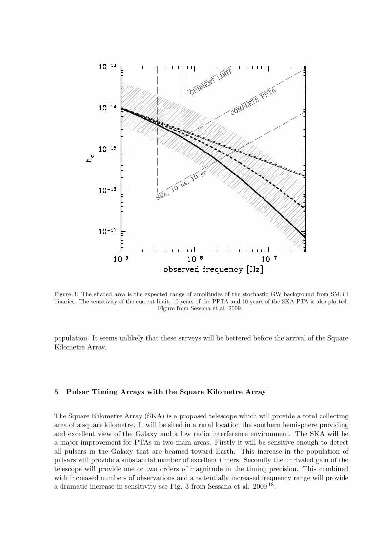
Figure 3: The shaded area is the expected range of amplitudes of the stochastic GW background from SMBHbinaries. The sensitivity of the current limit, 10 years of the PPTA and 10 years of the SKA-PTA is also plotted.
Figure from Sessana et al. 2009.
population. It seems unlikely that these surveys will be bettered before the arrival of the SquareKilometre Array.
5 Pulsar Timing Arrays with the Square Kilometre Array
The Square Kilometre Array (SKA) is a proposed telescope which will provide a total collectingarea of a square kilometre. It will be sited in a rural location the southern hemisphere providingand excellent view of the Galaxy and a low radio interference environment. The SKA will bea major improvement for PTAs in two main areas. Firstly it will be sensitive enough to detectall pulsars in the Galaxy that are beamed toward Earth. This increase in the population ofpulsars will provide a substantial number of excellent timers. Secondly the unrivaled gain of thetelescope will provide one or two orders of magnitude in the timing precision. This combinedwith increased numbers of observations and a potentially increased frequency range will providea dramatic increase in sensitivity see Fig. 3 from Sessana et al. 2009 18.
6 Conclusions
PTAs offer the only means to detect the very low frequency nHz range of GWs. This is partic-ularly important to measure SMBH coalescence rates and understand galaxy evolution in theearly universe. In combination with other space- and ground- based GW detectors a compre-hensive view of black holes in different mass ranges and evolutionary stages can be achieved.With the sensitivity of the SKA and the newly found pulsars it will provide, will allow for GWastronomy. Additionally the properties of the GWs wiill can be compared with predictions ofgeneral relativity and of alternate theories of gravity. With current PTAs a detection is possibleand vital research required for the SKA will be done. A future with the SKA-PTA, LISA andground-based detectors observing concurrently would certainly usher in a new era for astronomy.
References
1. Lorimer, D. R., & Kramer, M. 2005, Handbook of pulsar astronomy, by D.R. Lorimer andM. Kramer. Cambridge observing handbooks for research astronomers, Vol. 4. Cambridge,UK: Cambridge University Press, 2004
2. K.J. Lee et al., In prep.3. Hulse, R. A., & Taylor, J. H. 1975, ApJL, 195, L514. Taylor, J. H., & Weisberg, J. M. 1982, ApJ, 253, 9085. Hellings, R. W., & Downs, G. S. 1983, ApJL, 265, L396. Jenet, F., et al. 2009, arXiv:0909.10587. Lee, K. J., Wex, N., Kramer, M., Stappers, B. W., Bassa, C. G., Janssen, G. H., Karup-
pusamy, R., & Smits, R. 2011, MNRAS, 6288. Sudou, H., Iguchi, S., Murata, Y., & Taniguchi, Y. 2003, Science, 300, 12639. Jenet, F. A., Lommen, A., Larson, S. L., & Wen, L. 2004, ApJ, 606, 799
10. Yardley, D. R. B., et al. 2010, MNRAS, 407, 66911. Hobbs, G., et al. 2009, MNRAS, 394, 194512. Pitkin, M., Clark, J., Hendry, M. A., Heng, I. S., Messenger, C., Toher, J., & Woan, G.
2008, Journal of Physics Conference Series, 122, 01200413. Gopukumar et al. In prep.14. Verbiest, J. P. W., et al. 2010, Classical and Quantum Gravity, 27, 08401515. Ferdman, R. D., et al. 2010, Classical and Quantum Gravity, 27, 0840116. Hobbs, G., et al. 2010, Classical and Quantum Gravity, 27, 08401317. http://www.leap.eu.org18. Sesana, A., Vecchio, A., & Volonteri, M. 2009, MNRAS, 394, 2255


13.Other Topics

Measuring g with a beam of antihydrogen (AEgIS)
C.CANALI a
Istituto Nazionale di Fisica Nucleare and Department of Physics, University of Genoa, via Dodecaneso33, 16146 Genova, Italy
The gravitational interaction between matter and antimatter has never been tested experi-mentally. According to some attempts to unify gravity with the other forces, the possibilitythat g(p) 6= g(p) cannot be excluded 1. The AEGIS experiment 2 intends to measure forthe first time the gravitational acceleration of antimatter using cold antihydrogen atoms.Antihydrogen atoms will be obtained trough a charge exchange process between Rydbergpositronium atoms and antiprotons. Once H are accelerated to form a horizontal beam, theytravel through a Moire deflectometer, able to measure the vertical displacement of atoms dueto gravity. Knowing the velocity of the antiatoms from the time of flight measurement andthe length of the flight path allows to estimate the gravity acceleration g for antihydrogen.With this setup an initial precision on the measure of g of 1% is expected.
1 Introduction
In recent years few experiments at CERN have demonstrated the feasibility of producing largeamounts of antiatoms at low temperature 4, 5, 6. This result opens a very interesting scenario ofstudies on fundamental symmetries between matter and antimatter such as the CPT invariance(through high precision spectroscopy) and direct measurements of the validity of the equivalenceprinciple for antimatter (through ballistic experiments).
A precise test of CPT could arise from measurements on gross structure, fine structure, Lambshifts and hyperfine structures in antihydrogen to be compared with analougue measurementsdone on hydrogen. The CPT theory predicts that all these properties are identical for matter andantimatter systems. This kind of measurements, in principle, could reach a very high precision:a comparison of the 1S-2S frequency for hydrogen 7 and antihydrogen with a precision of 10−15
or higher will be the most accurate CPT tests for baryons regardless of any theoretical model.
While CPT test based on antihydrogen spectroscopy could give very precise results, at thesame time antihydrogen can be used to perform for the first time a direct measurement of gravityon an antimatter system.
Such a kind of measurement could be in principle performed using charged particles (forexample positrons), but a huge experimental trouble arises because the gravitational force ismuch weaker than the Coulomb force, and is virtually impossible to reduce electric fields to anegligible level (an electric field of only 6 ·10−11V/m gives to a positron an acceleration equal tothat of gravity). This make H a simple (and neutral) system with which WEP can be directlytested.
The primary scientific goal of the AEGIS experiment is the direct measurement of the Earth
aon behalf of AEGIS collaboration
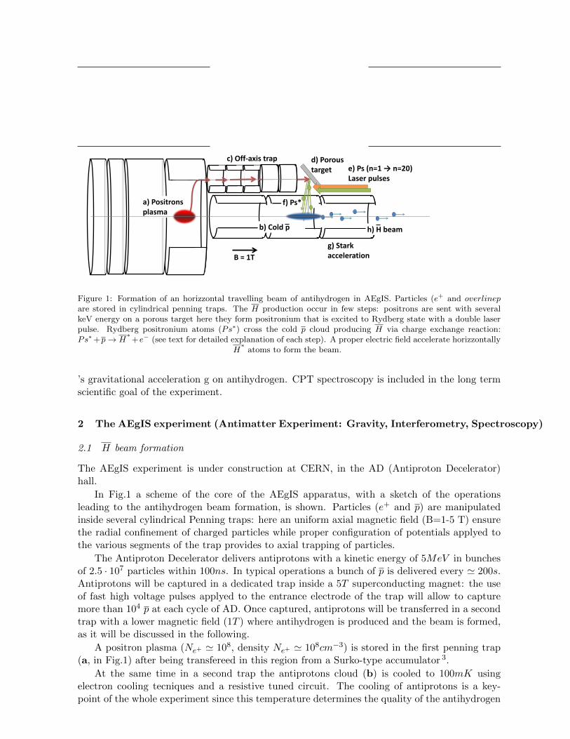
d) Porous target
f) Ps*
e) Ps (n=1 → n=20)Laser pulses
g) Stark acceleration
a) Positrons plasma
c) Off-axis trap
h) H beamb) Cold p
B = 1T
Figure 1: Formation of an horizzontal travelling beam of antihydrogen in AEgIS. Particles (e+ and overlinepare stored in cylindrical penning traps. The H production occur in few steps: positrons are sent with severalkeV energy on a porous target here they form positronium that is excited to Rydberg state with a double laserpulse. Rydberg positronium atoms (Ps∗) cross the cold p cloud producing H via charge exchange reaction:Ps∗ +p→ H
∗+e− (see text for detailed explanation of each step). A proper electric field accelerate horizzontally
H∗
atoms to form the beam.
’s gravitational acceleration g on antihydrogen. CPT spectroscopy is included in the long termscientific goal of the experiment.
2 The AEgIS experiment (Antimatter Experiment: Gravity, Interferometry, Spectroscopy)
2.1 H beam formation
The AEgIS experiment is under construction at CERN, in the AD (Antiproton Decelerator)hall.
In Fig.1 a scheme of the core of the AEgIS apparatus, with a sketch of the operationsleading to the antihydrogen beam formation, is shown. Particles (e+ and p) are manipulatedinside several cylindrical Penning traps: here an uniform axial magnetic field (B=1-5 T) ensurethe radial confinement of charged particles while proper configuration of potentials applyed tothe various segments of the trap provides to axial trapping of particles.
The Antiproton Decelerator delivers antiprotons with a kinetic energy of 5MeV in bunchesof 2.5 · 107 particles within 100ns. In typical operations a bunch of p is delivered every ' 200s.Antiprotons will be captured in a dedicated trap inside a 5T superconducting magnet: the useof fast high voltage pulses applyed to the entrance electrode of the trap will allow to capturemore than 104 p at each cycle of AD. Once captured, antiprotons will be transferred in a secondtrap with a lower magnetic field (1T ) where antihydrogen is produced and the beam is formed,as it will be discussed in the following.
A positron plasma (Ne+ ' 108, density Ne+ ' 108cm−3) is stored in the first penning trap(a, in Fig.1) after being transfereed in this region from a Surko-type accumulator 3.
At the same time in a second trap the antiprotons cloud (b) is cooled to 100mK usingelectron cooling tecniques and a resistive tuned circuit. The cooling of antiprotons is a key-point of the whole experiment since this temperature determines the quality of the antihydrogen
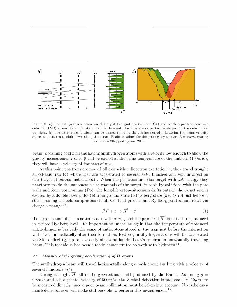
Figure 2: a) The antihydrogen beam travel trought two gratings (G1 and G2) and reach a position sensitivedetector (PSD) where the annihilation point is detected. An interference pattern is shaped on the detector onthe right. b) The interference pattern can be binned (modulo the grating period). Lowering the beam velocitycauses the pattern to shift down along the z-axis. Realistic values for the gratings system are L = 40cm, grating
period a = 80µ, grating size 20cm.
beam: obtaining cold p means having antihydrogen atoms with a velocity low enough to allow thegravity measurement: once p will be cooled at the same temperature of the ambient (100mK),they will have a velocity of few tens of m/s.
At this point positrons are moved off axis with a diocotron excitation 11, they travel troughtan off-axis trap (c) where they are accelerated to several keV , bunched and sent in directionof a target of porous material (d) . When the positrons hits this target with keV energy theypenetrate inside the nanometric-size channels of the target, it cools by collisions with the porewalls and form positronium (Ps): the long-life ortopositronium drifts outside the target and isexcited by a double laser pulse (e) from ground state to Rydberg state (nPs > 20) just before itstart crossing the cold antiprotons cloud. Cold antiprotons and Rydberg positronium react viacharge exchange 13:
Ps∗ + p→ H∗
+ e− (1)
the cross section of this reaction scales with ∝ n4Ps and the produced H∗
is in its turn producedin excited Rydberg level. It’s important to underline again that the temperature of producedantihydrogen is basically the same of antiprotons stored in the trap just before the interactionwith Ps∗. Immediatelly after their formation, Rydberg antihydrogen atoms will be acceleratedvia Stark effect (g) up to a velocity of several hundreds m/s to form an horizontally travellingbeam. This tecqnique has been already demonstrated to work with hydrogen 14.
2.2 Measure of the gravity acceleration g of H atoms
The antihydrogen beam will travel horizzontally along a path about 1m long with a velocity ofseveral hundreds m/s.
During its flight H fall in the gravitational field produced by the Earth. Assuming g =9.8m/s and a horizzontal velocity of 500m/s, the vertical deflection is too small (' 10µm) tobe measured directly since a poor beam collimation must be taken into account. Nevertheless amoire deflectometer will make still possible to perform this measurement 12.
The device (Fig.2.a), sligtly modified respect to standard moire deflectometers, consists oftwo gratings (G1 and G2) and a position sensitive detector (PSD) separated by a distanceL ' 40cm. Both gratings have a size of 20x20cm2 and a period of ' 80µm. The PSD is asilicon microstrip detector with an active area of about 20x20cm2, and a resolution of about10µm working at cryogenic temperatures.
Since the width of the slits is much larger than the De Broglie wavelength of the antihydrogen,diffraction can be neglected and all effects will be purely classically, so the PSD just records ashadow pattern corresponding to the positions of antiatom annihilations. The velocity of thebeam can be tuned changing the parameters of the Stark acceleration, so it is possible to measurethe vertical deflection of the shadow path for several values of velocities. The precise velocity ofH can be desumed from the time of flight measurement.
The position of anthydrogen will be detected reconstructing the annihilation point of eachantiatom on the position sensitive detector. The detected positions of annihilations can bebinned modulo the grating period as plotted in Fig.2.b. Here it’s shown from Montecarlo resultshow the verical shift of the shadow pattern increase with lower horizzontal velocity of the beam,assuming g = 9.8m/s.
The use of this method allow to measure the gravity acceleration g of antihydrogen witha precision of 1% detecting 105 antihydrogen atoms: it will be the first direct measurement ofgravity acceleration on an antimatter system.
3 Conclusion
Antihydrogen will be used in next years to investigate CPT validity and equivalence principle.Related to this latter topic, AEgIS will use antiprotons delivered from AD (the antiprotondecelerator at CERN) to produce an horizzontal beam of antihydrogen to measure the gravityacceleration g of antiatoms. The initial precision on the measured g is expected to be 1%, andlong and medium terms goals intends to improve noticeably this precision.
1. E. Fischbach, C.L. Talmadge The search for non Newtonian Gravity Springer (1999)2. AEgIS proposal http://doc.cern.ch/archive/electronic/cern/preprints/spsc/public/spsc-
2007-017.pdf3. T. J. Murphy and C. M. Surko, Phys. Lett. B 46, 5696 (1992).4. ATHENA Coll. Nature 419, 2002 (456)5. http://hussle.harvard.edu/ atrap/6. http://alpha.web.cern.ch/alpha/7. M. Niering et al., Phys. Rev. Lett. 84, 2000 (5496)8. C Jarlskog in CP Violation, ed. C Jarlskog (World Scientific, Singapore, 1988).9. J.D. Bjorken and I. Dunietz, Phys. Rev. D 36, 2109 (1987).
10. C.D. Buchanan et al, Phys. Rev. D 45, 4088 (1992).11. J. R. Danielson, T. R. Weber, and C. M. Surko Physics Of Plasmas 13, 123502 (2006)12. M. K. Oberthaler et al., Physical Review A 54, 3165 (1996).13. M. L. Wall, C. S. Norton, and F. Robicheaux Physical Review A 72, 052702 (2005)14. E. Vliegen and F. Merkt, J. Phys. B: At. Mol. Opt. Phys. 39, L241 (2006)
GBAR
Gravitational Behavior of Antihydrogen at Rest
P. DupreCEA Saclay, service de physique des particules
Gif-sur-Yvette, France
The GBAR experiment aims to test the Equivalence Principle with antimatter by measuringthe time of flight of ultra-cold antihydrogen atoms H in free fall. Antihydrogen atoms at∼20 µK are provided by sympathetic cooling of antihydrogen ions H+ with laser cooled Be+
ions. H+ ions are produced via two successive reactions using antiprotons and positroniums.The synthesis of H+ is obtained by the injection of a pulse of 107 slow antiprotons from theAD at CERN in a dense cloud of positronium. This target of positronium is created witha positron-to-positronium converter and requires an intense source of slow positrons, a few108 per second. Such a source based on a small electron accelerator is under construction atSaclay. A few 1010 positrons are accumulated in a Penning-Malmberg trap from which theyare ejected towards the e+/Ps converter to produce the target. The overall scheme of theexperiment is described along with the estimated efficiency of each step.
1 Introduction
The aim of the GBAR project is to perform the first test of the Weak Equivalence Principle(WEP) with antimatter. The Einstein Equivalence Principle is at the heart of general relativity.It has been tested with a very high precision with matter, but no conclusive direct test withantimatter is available. This is a basic scientific question, the interest of which is enhanced bythe unknown origin of the acceleration of the expansion of the universe and by the hypotheticalpresence of dominant quantities of dark matter: these observations suggest that our understand-ing of gravitation may be incomplete. Extensions of gravitation theory can lead to differencesin behavior between matter and antimatter 1.
Direct tests have been attempted with positrons 2 and antiprotons 3, but they turned out tobe too difficult to reduce electromagnetic effects sufficiently. It seems also out of present reachto perform gravity experiments with antineutrons 4 or positronium 5. The antihydrogen atom isthe next simplest candidate system. Indirect tests of the Equivalence Principle for antimatterhave been obtained by comparing the properties of particles and their antiparticles (such as p-p6
and K0-K07) or by arguing about the virtual content of the nuclei of ordinary matter. However,
all these tests rely upon disputable theoretical hypotheses - refer for example to the review 8 onexperimental and theoretical arguments.
2 Principle of the GBAR experiment
The GBAR experiment will measure the time of flight of ultra-cold antihydrogen atoms in freefall. The principle of GBAR has been described in a Letter of Intent to CERN9. The original way
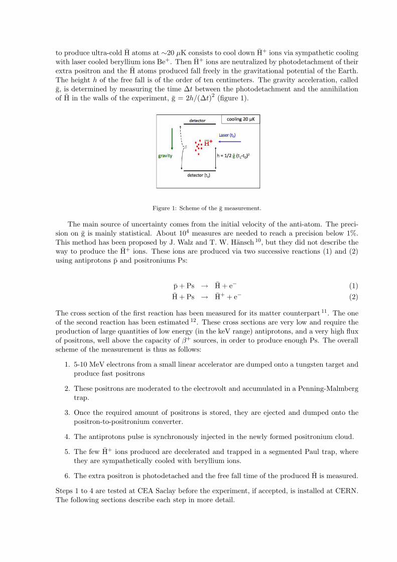
to produce ultra-cold H atoms at ∼20 µK consists to cool down H+ ions via sympathetic coolingwith laser cooled beryllium ions Be+. Then H+ ions are neutralized by photodetachment of theirextra positron and the H atoms produced fall freely in the gravitational potential of the Earth.The height h of the free fall is of the order of ten centimeters. The gravity acceleration, calledg, is determined by measuring the time ∆t between the photodetachment and the annihilationof H in the walls of the experiment, g = 2h/(∆t)2 (figure 1).
Figure 1: Scheme of the g measurement.
The main source of uncertainty comes from the initial velocity of the anti-atom. The preci-sion on g is mainly statistical. About 104 measures are needed to reach a precision below 1%.This method has been proposed by J. Walz and T. W. Hansch 10, but they did not describe theway to produce the H+ ions. These ions are produced via two successive reactions (1) and (2)using antiprotons p and positroniums Ps:
p + Ps → H + e− (1)
H + Ps → H+ + e− (2)
The cross section of the first reaction has been measured for its matter counterpart 11. The oneof the second reaction has been estimated 12. These cross sections are very low and require theproduction of large quantities of low energy (in the keV range) antiprotons, and a very high fluxof positrons, well above the capacity of β+ sources, in order to produce enough Ps. The overallscheme of the measurement is thus as follows:
1. 5-10 MeV electrons from a small linear accelerator are dumped onto a tungsten target andproduce fast positrons
2. These positrons are moderated to the electrovolt and accumulated in a Penning-Malmbergtrap.
3. Once the required amount of positrons is stored, they are ejected and dumped onto thepositron-to-positronium converter.
4. The antiprotons pulse is synchronously injected in the newly formed positronium cloud.
5. The few H+ ions produced are decelerated and trapped in a segmented Paul trap, wherethey are sympathetically cooled with beryllium ions.
6. The extra positron is photodetached and the free fall time of the produced H is measured.
Steps 1 to 4 are tested at CEA Saclay before the experiment, if accepted, is installed at CERN.The following sections describe each step in more detail.
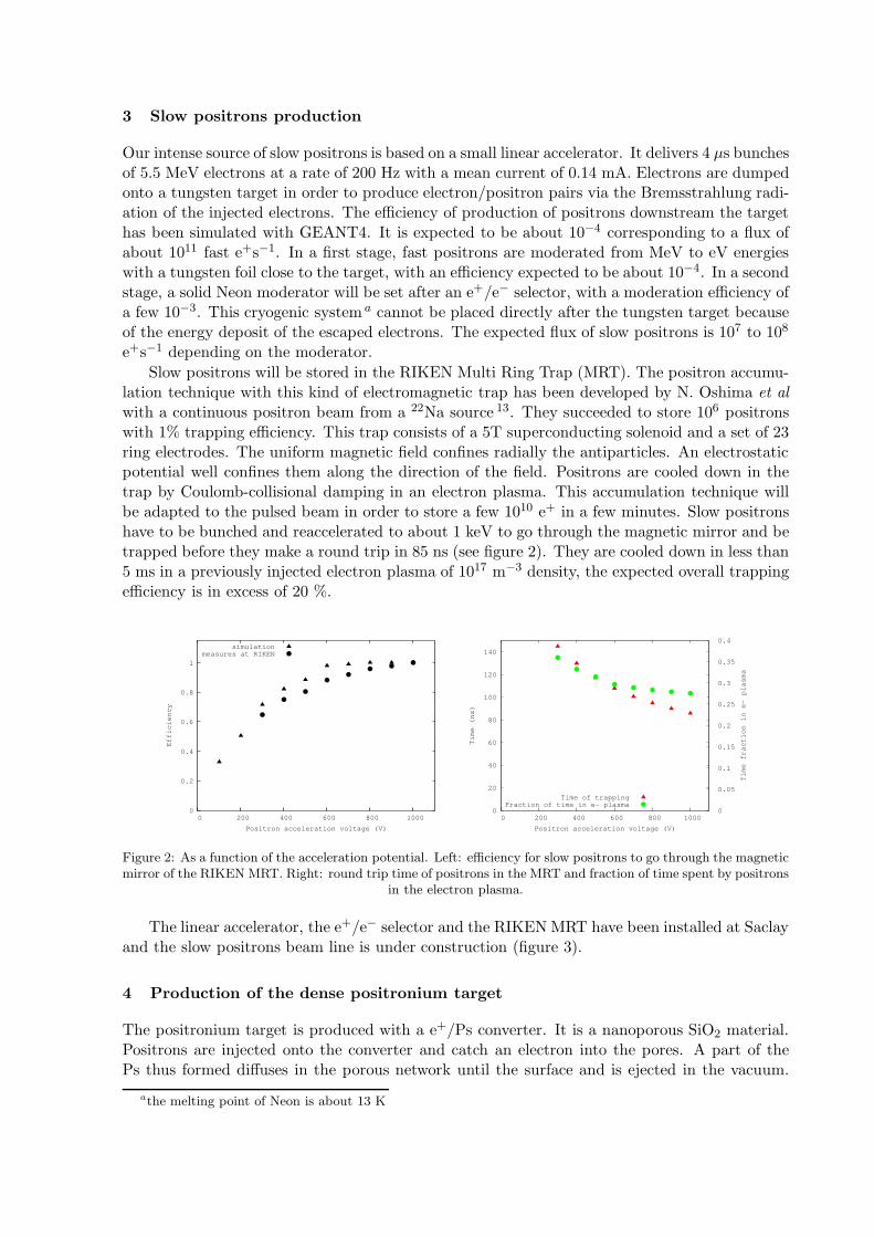
3 Slow positrons production
Our intense source of slow positrons is based on a small linear accelerator. It delivers 4 µs bunchesof 5.5 MeV electrons at a rate of 200 Hz with a mean current of 0.14 mA. Electrons are dumpedonto a tungsten target in order to produce electron/positron pairs via the Bremsstrahlung radi-ation of the injected electrons. The efficiency of production of positrons downstream the targethas been simulated with GEANT4. It is expected to be about 10−4 corresponding to a flux ofabout 1011 fast e+s−1. In a first stage, fast positrons are moderated from MeV to eV energieswith a tungsten foil close to the target, with an efficiency expected to be about 10−4. In a secondstage, a solid Neon moderator will be set after an e+/e− selector, with a moderation efficiency ofa few 10−3. This cryogenic system a cannot be placed directly after the tungsten target becauseof the energy deposit of the escaped electrons. The expected flux of slow positrons is 107 to 108
e+s−1 depending on the moderator.
Slow positrons will be stored in the RIKEN Multi Ring Trap (MRT). The positron accumu-lation technique with this kind of electromagnetic trap has been developed by N. Oshima et al
with a continuous positron beam from a 22Na source 13. They succeeded to store 106 positronswith 1% trapping efficiency. This trap consists of a 5T superconducting solenoid and a set of 23ring electrodes. The uniform magnetic field confines radially the antiparticles. An electrostaticpotential well confines them along the direction of the field. Positrons are cooled down in thetrap by Coulomb-collisional damping in an electron plasma. This accumulation technique willbe adapted to the pulsed beam in order to store a few 1010 e+ in a few minutes. Slow positronshave to be bunched and reaccelerated to about 1 keV to go through the magnetic mirror and betrapped before they make a round trip in 85 ns (see figure 2). They are cooled down in less than5 ms in a previously injected electron plasma of 1017 m−3 density, the expected overall trappingefficiency is in excess of 20 %.
0
0.2
0.4
0.6
0.8
1
0 200 400 600 800 1000
Efficiency
Positron acceleration voltage (V)
simulationmeasures at RIKEN
0
20
40
60
80
100
120
140
0 200 400 600 800 1000 0
0.05
0.1
0.15
0.2
0.25
0.3
0.35
0.4
Time (ns)
Time fraction in e- plasma
Positron acceleration voltage (V)
Time of trappingFraction of time in e- plasma
Figure 2: As a function of the acceleration potential. Left: efficiency for slow positrons to go through the magneticmirror of the RIKEN MRT. Right: round trip time of positrons in the MRT and fraction of time spent by positrons
in the electron plasma.
The linear accelerator, the e+/e− selector and the RIKEN MRT have been installed at Saclayand the slow positrons beam line is under construction (figure 3).
4 Production of the dense positronium target
The positronium target is produced with a e+/Ps converter. It is a nanoporous SiO2 material.Positrons are injected onto the converter and catch an electron into the pores. A part of thePs thus formed diffuses in the porous network until the surface and is ejected in the vacuum.
athe melting point of Neon is about 13 K
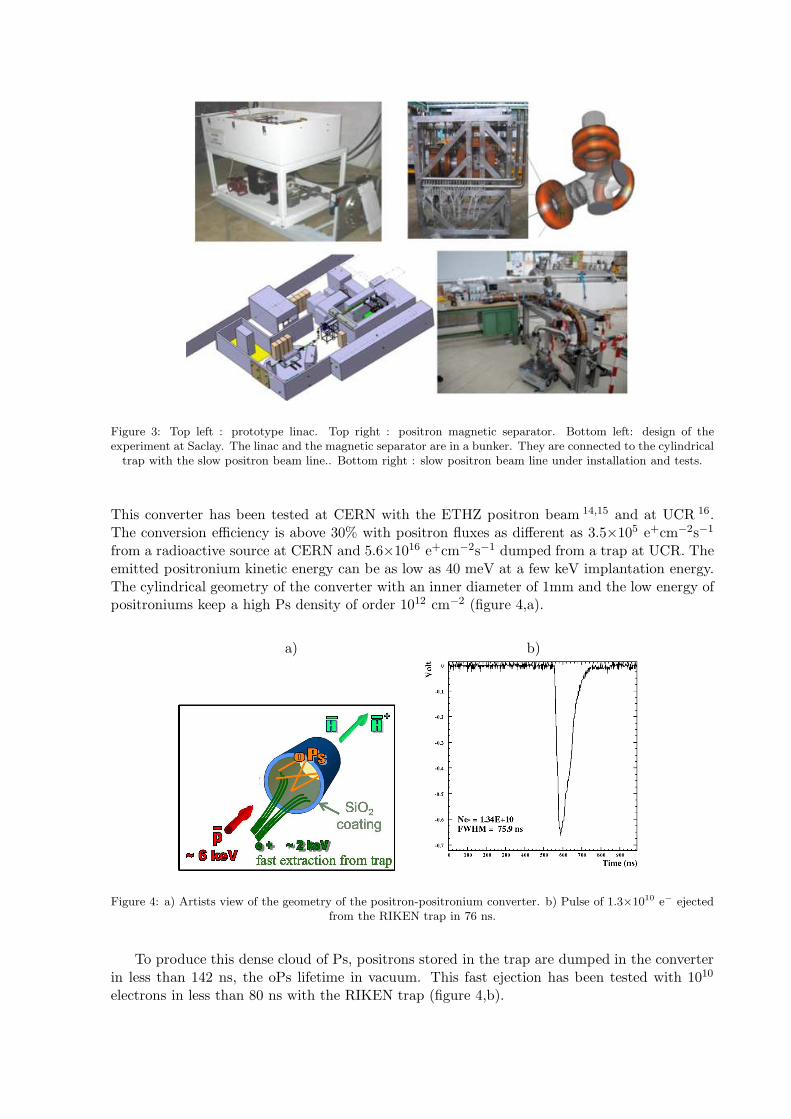
Figure 3: Top left : prototype linac. Top right : positron magnetic separator. Bottom left: design of theexperiment at Saclay. The linac and the magnetic separator are in a bunker. They are connected to the cylindrical
trap with the slow positron beam line.. Bottom right : slow positron beam line under installation and tests.
This converter has been tested at CERN with the ETHZ positron beam 14,15 and at UCR 16.The conversion efficiency is above 30% with positron fluxes as different as 3.5×10⁵ e+cm−2s−1
from a radioactive source at CERN and 5.6×10¹⁶ e+cm−2s−1 dumped from a trap at UCR. Theemitted positronium kinetic energy can be as low as 40 meV at a few keV implantation energy.The cylindrical geometry of the converter with an inner diameter of 1mm and the low energy ofpositroniums keep a high Ps density of order 1012 cm−2 (figure 4,a).
a) b)
Figure 4: a) Artists view of the geometry of the positron-positronium converter. b) Pulse of 1.3×10¹⁰ e− ejectedfrom the RIKEN trap in 76 ns.
To produce this dense cloud of Ps, positrons stored in the trap are dumped in the converterin less than 142 ns, the oPs lifetime in vacuum. This fast ejection has been tested with 1010
electrons in less than 80 ns with the RIKEN trap (figure 4,b).
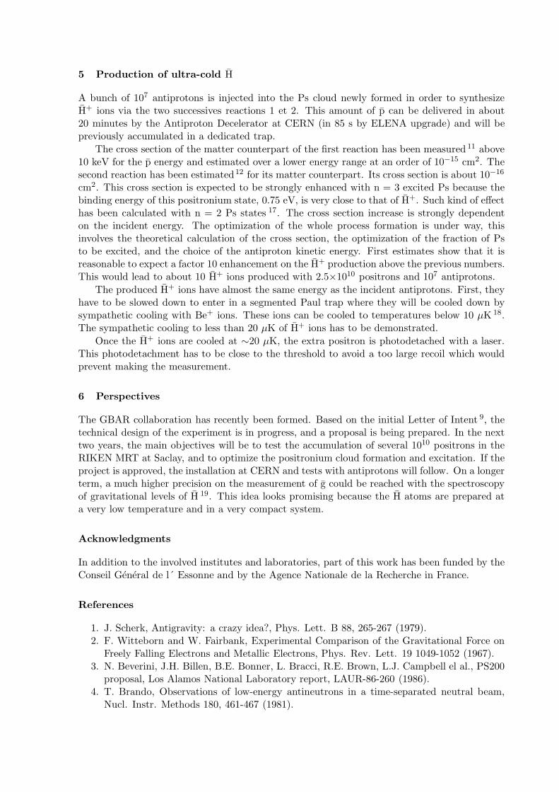
5 Production of ultra-cold H
A bunch of 107 antiprotons is injected into the Ps cloud newly formed in order to synthesizeH+ ions via the two successives reactions 1 et 2. This amount of p can be delivered in about20 minutes by the Antiproton Decelerator at CERN (in 85 s by ELENA upgrade) and will bepreviously accumulated in a dedicated trap.
The cross section of the matter counterpart of the first reaction has been measured 11 above10 keV for the p energy and estimated over a lower energy range at an order of 10−15 cm2. Thesecond reaction has been estimated12 for its matter counterpart. Its cross section is about 10−16
cm2. This cross section is expected to be strongly enhanced with n = 3 excited Ps because thebinding energy of this positronium state, 0.75 eV, is very close to that of H+. Such kind of effecthas been calculated with n = 2 Ps states 17. The cross section increase is strongly dependenton the incident energy. The optimization of the whole process formation is under way, thisinvolves the theoretical calculation of the cross section, the optimization of the fraction of Psto be excited, and the choice of the antiproton kinetic energy. First estimates show that it isreasonable to expect a factor 10 enhancement on the H+ production above the previous numbers.This would lead to about 10 H+ ions produced with 2.5×10¹⁰ positrons and 107 antiprotons.
The produced H+ ions have almost the same energy as the incident antiprotons. First, theyhave to be slowed down to enter in a segmented Paul trap where they will be cooled down bysympathetic cooling with Be+ ions. These ions can be cooled to temperatures below 10 µK 18.The sympathetic cooling to less than 20 µK of H+ ions has to be demonstrated.
Once the H+ ions are cooled at ∼20 µK, the extra positron is photodetached with a laser.This photodetachment has to be close to the threshold to avoid a too large recoil which wouldprevent making the measurement.
6 Perspectives
The GBAR collaboration has recently been formed. Based on the initial Letter of Intent 9, thetechnical design of the experiment is in progress, and a proposal is being prepared. In the nexttwo years, the main objectives will be to test the accumulation of several 1010 positrons in theRIKEN MRT at Saclay, and to optimize the positronium cloud formation and excitation. If theproject is approved, the installation at CERN and tests with antiprotons will follow. On a longerterm, a much higher precision on the measurement of g could be reached with the spectroscopyof gravitational levels of H 19. This idea looks promising because the H atoms are prepared ata very low temperature and in a very compact system.
Acknowledgments
In addition to the involved institutes and laboratories, part of this work has been funded by theConseil General de l´ Essonne and by the Agence Nationale de la Recherche in France.
References
1. J. Scherk, Antigravity: a crazy idea?, Phys. Lett. B 88, 265-267 (1979).2. F. Witteborn and W. Fairbank, Experimental Comparison of the Gravitational Force on
Freely Falling Electrons and Metallic Electrons, Phys. Rev. Lett. 19 1049-1052 (1967).3. N. Beverini, J.H. Billen, B.E. Bonner, L. Bracci, R.E. Brown, L.J. Campbell el al., PS200
proposal, Los Alamos National Laboratory report, LAUR-86-260 (1986).4. T. Brando, Observations of low-energy antineutrons in a time-separated neutral beam,
Nucl. Instr. Methods 180, 461-467 (1981).
5. A.P. Mills, Positronium molecule formation, Bose - Einstein condensation and stimulatedannihilation, Nucl. Instr. Methods in Physics Research B 192, 107116 (2002).
6. G. Gabrielse et al., Precision Mass Spectroscopy of the Antiproton and Proton UsingSimultaneously Trapped Particles, Phys. Rev. Lett. 82, 3198-3201 (1999).
7. CP LEAR collaboration, Tests of the Equivalence Principle with neutral kaons, Phys.Lett. B 452, 425-433 (1999).
8. M.M. Nieto and T. Goldman, The Arguments Against Antigravity and the GravitationalAcceleration of Antimatter, Phys. Rep. 205, 221-281 (1991).
9. P. Perez et al. A new path to measure antimatter free fall., CERN-SPSC-2007-038. De-cember 2007.
10. J. Walz and T. Hansch, A Proposal to Measure Antimatter Gravity Using Ultracold An-tihydrogen Atoms, General Relativity and Gravitation 36, 561-570 (2004).
11. J.P. Merrison et al., Hydrogen Formation by Proton Impact on Positronium, Phys. Rev.Lett. 78, 2728-2731 (1997).
12. H.R.J.Walters and C. Starrett, Positron and positronium scattering, Phys. Stat. Sol. C,3429-3436 (2007).
13. N. Oshima et al., New Scheme for Positron Accumulation in Ultrahigh Vacuum, Phys.Rev. Lett. 93, 195001 (2004).
14. L. Liszkay et al., Positronium reemission yield from mesostructured silica films, Appl.Phys. Lett. 92, 063114 (2008).
15. P. Crivelli et al., Measurement of the ortho-positronium confinement energy in mesoporousthin films, Phys. Rev. A 81, 052703 (2010).
16. D. B. Cassidy et al., Positronium cooling in porous silica measured via Doppler spec-troscopy, Phys. Rev. A 81, 012715 (2010).
17. S. Roy and C. Sinha, Formation of negative hydrogen ion in positronium-hydrogen colli-sions, Eur. Phys. J. D 47, 327-334 (2008).
18. M.D. Barrett et al., Sympathetic cooling of 9B+ and 24Mg+ for quantum logic, Phys. Rev.A 68, 042302 (2003).
19. A.Yu. Voronin, P. Froelich, and V.V. Nesvizhevsky, Gravitational quantum states ofAntihydrogen, Phys. Rev. A 83, 032903 (2011).
EVIDENCE FOR TIME-VARYING NUCLEAR DECAY DATES:
EXPERIMENTAL RESULTS AND THEIR IMPLICATIONS FOR NEW
PHYSICS
E. FISCHBACHDepartment of Physics, Purdue University, 525 Northwestern Ave,
West Lafayette, Indiana, 47907 USA
J.H. JENKINSSchool of Nuclear Engineering, Purdue University, West Lafayette, Indiana 47907 USA
P.A. STURROCKCenter for Space Science and Astrophysics, Stanford University, Stanford, California 94305 USA
Unexplained annual variations in nuclear decay rates have been reported in recent years bya number of groups. We show that data from these experiments exhibit not only variationsin time related to Earth-Sun distance, but also periodicities attributable to solar rotation.Additionally, anomalous decay rates coincident in time with a series of solar flares in December2006 also point to a solar influence on nuclear decay rates. This influence could arise fromsome flavor of solar neutrinos, or through some other objects we call “neutrellos” which behavein some ways like neutrinos. The indication that neutrinos or neutrellos must interact weaklyin the Sun implies that we may be able to use data on time-varying nuclear decay rates toprobe the interior of the Sun, a technique which we may call“helioradiology”.
1 Introduction
The widely held view that nuclear decay rates, along with nuclear masses, are fundamentalconstants of nature has been challenged recently by reports from various groups of periodicvariations in nuclear decay rates.1,2,3,4,5,6,7,8 Following the discovery of natural radioactivity byBecquerel in 1896 an intense effort was mounted to determine whether nuclear decay rateswere in fact constant. By 1930 Rutherford, Chadwick, and Ellis concluded that“the rate oftransformation of an element has been found to be a constant under all conditions.9 Subsequentwork by many groups has supported this conclusion, except for decays proceeding by electroncapture. In such decays the decay rate depends on the overlap of the electron wavefunction andthe nucleus, and this can be slightly modified by subjecting the decaying nucleus to extremepressure, or by modifying its chemical environment.10,11,12,13,14,15,16
Notwithstanding the impressive body of evidence supporting the conventional view that thedecay rate λ = ln2/T1/2 of an unstable isotope is an intrinsic property of that isotope, thereare growing indications of small (O
(
10−3)
) time-dependent variations in the decay rates ofsome nuclei. In Sec. 2 we summarize the existing experimental evidence for these variations,along with the arguments against some claims that the variations are simply the results of localenvironmental influences on the detector systems. What emerges from these considerations is a
picture in which the observed time-dependent variations are in fact occurring in the decay processitself, in response to time-dependent solar perturbations. Although a detailed mechanism is notyet available to explain how the Sun influences radioactive decays, previous work3 along withthe discussion in Sec. 3 below, provide a general framework for a future theory.
2 Experimental Results
In this section we summarize the experimental evidence for a solar influence on nuclear decayprocesses. A more detailed discussion of the various experiments can be found in the accom-panying paper by Jenkins et al.17 The interest of our group in time-dependent nuclear decayrates began with our attempt to understand an annually-varying periodic signal in the decayrate of 32Si reported by Alburger, et al.18 in a 4-year experiment at the Brookhaven NationalLaboratory (BNL). A subsequent examination of the literature revealed a ∼15-year experimentat the Physikalisch-Technische Bundesanstalt (PTB) in Germany in which data from 226Ra ex-hibited a similar annual variation.19 Coincidentally, these two experiments overlapped in timefor approximately two years, and the data from these experiments during this period were quitesimilar in both amplitude and phase.2,3 Further exploration of the literature has uncovered otherexperiments in which periodic effects in various decays were reported. These include the resultsof Falkenberg20, Parkhomov21,22, Baurov et al.23, Ellis24, and Shnoll et al.25,26.
The observation of periodic effects in what had been previously been thought of as randomdecay data motivated a series of experiments by our group at Purdue, chiefly focused on theelectron capture process: e− +54 Mn → νe +54 Cr + γ (834.8 keV). Our apparatus was operatingduring a series of solar flares in November and December of 2006. On 13 December 2006 amajor solar flare erupted at 02:37 UT (21:37 EST 12 December) which coincided with a ∼ 7σdrop in the measured 54Mn counting rate.1 A smaller flare with a large coronal mass ejection on17 December 2006 also coincided with a decrease in the 54Mn counting rate. Subsequently, anexamination of data acquired during December 2008 revealed a correlation between a change inthe measured 54Mn count rate and a solar storm on the far side of the Sun.
The correlations between observed changes in measured 54Mn count rates and solar flaresare significant for several reasons:
1. They now reinforce the inference, drawn from the annual periodicities in the BNL and PTBdata, that these periodicities arise from the annual variation of the Earth-Sun distance R
due to the ellipticity of the Earth’s orbit.
2. Since the flares erupt and subside over fairly short time-scales (typically minutes to hours),any apparent correlation between decay data and solar activity cannot plausibly be at-tributed to environmental effects on the detector systems in question due to a local changein temperature, pressure, humidity, etc.27
3. Finally, in all the cases we have observed, there is a precursor signal in which the 54Mncount rate begins to change ∼1 day before the solar event. This observation raises thepossibility of establishing an “early-warning” system for potentially dangerous impendingsolar storms, whose damaging effects on astronauts; communications, navigation, defenseand other satellites; and power grids and other electronic infrastructure could thus beprevented.1
The observation in decay data of time-dependent influences attributable to the Sun (eitherfrom a change in 1/R2 or via a solar flare), raises the question of whether other time-dependentsignals could be present in decay data associated, for instance, with solar rotation. This couldhappen if the sources of whatever influences were affecting decay rates were not distributedhomogeneously throughout the Sun, for which there were earlier indications.28 Further analysis
of the BNL, PTB, and Parkhomov data sets has indeed revealed evidence of a ∼32 d periodicity,which can be interpreted as evidence for an East-West asymmetry in the Sun, perhaps associatedwith a slowly rotating solar core.29 Additionally, the BNL and PTB data sets also revealedevidence of a ∼173 d periodicity, similar to the Rieger periodicity, which arises from retrogradewaves in a rotating fluid.7 Finally, recent work by our group has shown that the apparent phase-shift of the maximum count rate noted in BNL, PTB, and other data sets from what wouldbe expected from the variation in 1/R2 alone could be attributed to a North-South asymmetryin the Sun.8 While this observation does not directly deal with solar rotation, it does supportthe assumption that there are asymmetries in the Sun whose presence can be detected viaperiodicities in decay data. In this way decay data may allow us to probe the interior of theSun via a new technique which we may refer to as “helioradiology”.
3 Towards a Mechanism: Neutrinos and Neutrellos
Although the evidence for a solar influence on nuclear decay rates is quite compelling, what islacking is a mechanism through which this influence can be transmitted. Elsewhere3 we explorein detail a mechanism based on an interaction between solar neutrinos and decaying nuclei. Herewe broaden that discussion to address the question of whether nuclear decay rates are affectedby the Sun through some generic particles which we call “neutrellos”, which may or may not bethe same as neutrinos. In what follows we describe some of the properties that we would likeneutrellos to possess in order to account for existing data.
1. The solar flare of 13 December 2006 at 02:37UT was coincident in time with a localminimum (dip) in the 54Mn counting rate.1 Since this dip occurred at 21:37 EST in ourlaboratory, this suggests that neutrellos must be capable of passing unimpeded throughthe Earth at essentially the speed of light.
2. Although the solar flare was of short duration and occurred without warning, the decayrate of 54Mn began to decrease much earlier, approximately 40 hours before the flare. This“precursor signal” suggests that neutrellos originated from a region below the surface ofthe Sun and reached us before the actual flare because the Sun is effectively transparentto neutrellos, but not to photons.
3. As the Sun rotated, the region on the surface of the Sun from which the 13 December 2006flare originated, region 930, dropped over the West Limb of the Sun on 17 December andhence was no longer visible via X-rays. Nevertheless, a significant drop in the 54Mn countrate was detected on 22 December, suggesting that neutrellos were reaching the Earthfrom the far side of the Sun by passing through the Sun. This again implies that the Sunis transparent to neutrellos, at least to some degree.
4. Our 54Mn experiment also detected a solar event on 16 December 2008 which coincidedwith a storm on the far side of the Sun. This reinforces the assumption that the Sun isrelatively transparent to neutrellos.
5. The phase of the annual variation in decay rates seen in a number of experiments is shiftedfrom what would be expected from the annual variation of 1/R2, where R is the Earth-Sundistance.2,3 However, we have shown recently8 that if there is a North-South asymmetry inthe emission of neutrellos from the Sun, then the resulting contribution to the annual phasecould explain the observed data. Interestingly, evidence for a North-South asymmetry wasobserved in data from the Homestake solar neutrino experiment.?
6. As noted previously, there is evidence that nuclear decay data are modulated not only bythe variation of 1/R2 and the presence of a North-South asymmetry in the Sun, but alsoby the rotational motion of the Sun. Evidence for rotational modulation is based on thepresence in the decay data of periodicities of ∼ 32 d and ∼ 173 d, the latter being analogousto the well-known Rieger periodicity. Since similar evidence for rotational modulation hasbeen noted previously in data from the Homestake and GALLEX neutrino experiments28,this suggests that our hypothetical neutrellos may actually be neutrinos.
7. The ∼ 32 d rotational modulation mentioned above points to a source where the rotationrate is slower than that of the radiative and convection zones in the Sun. The fact that weobserve a solar influence from a source below the radiative zone indicates that the putativeneutrellos experience only slight (or no) scattering or absorption in travelling the outerlayers of the Sun.
8. The very existence of a signal in nuclear decay data for rotational modulation by theSun implies that neutrello production by the Sun is anisotropic. If neutrellos were in factneutrinos, then the rotational modulation could arise from the resonant spin flavor pre-cession (RSFP)30 effect induced by a strong magnetic field deep in the solar interior. Thismechanism, which assumes that neutrinos have a non-zero transition magnetic moment,is supported by existing neutrino data from Super-Kamiokande.28
Although the preceding considerations are compatible with the inference that neutrellos arein fact neutrinos, there is at least one major difference: to account quantitatively for existingexperimental data the interaction strength of neutrellos with decaying nuclei must be signifi-cantly greater than the strength of the known interactions of neutrinos with protons, neutrons,electrons, or with other neutrinos as described by the standard electroweak model. As an ex-ample, to produce a fractional peak-to-trough variation in tritium of order 10−3 (which is thenominal value suggested by the BNL, PTB, and Falkenberg data) requires an input of energy∆E ≈ 5eV . Although this is small on the scale of the O(1MeV ) energies carried by incomingsolar neutrinos, a value of ∆E this large is more characteristic of an electromagnetic interac-tion than a weak interaction. This can be seen in another way by picturing solar neutrinos orneutrellos affecting nuclear decays by transferring a momentum ∆p ≈ ∆E/c via a scatteringprocess with an effective cross section σ,
σ ≡
1
φ
(∆N/N)
∆t. (1)
Here φ is the presumed flux (or change in flux) of solar neutrinos or neutrellos responsible forinducing a fractional change ∆N/N in the number of decays over a time interval ∆t. Evidentlythe smallest estimate of σ will result from the largest assumed value for φ for which we adopt theknown solar flux φ = 6×10¹⁰
cm−2
s−1. Using the flare data of Jenkins and Fischbach1 we estimate
(∆N/N) /∆t ≈ 2.6×10⁻¹¹s−1 per atom, and hence σ ≈ 4.3×10⁻²²
cm2. By way of comparison,
the Thomson cross section for photon scattering of electrons is σT =(
8πr2o/3
)
= 6.6×10⁻²⁵cm
2,where ro = 2.82 × 10⁻¹³
cm is the classical electron radius.
The implication of the above calculations, that neutrinos could influence decaying nucleithrough an interaction of electromagnetic strength, is likely incompatible with existing data onνs − e, νs − p, and νs − n interactions (νs = solar neutrino), but could be compatible with apossible νs – νe interaction coupling a generic solar neutrino to an emitted νe from beta decayor electron capture. On the other hand, a much broader range of possibilities is available fornutrello couplings, and these may be accessible experimentally through appropriate “fifth force”experiments.31 Additional constraints on a possible influence of νe on radioactive decay followfrom an elegant reactor experiment by de Meijer et al.32
4 Discussion and Outlook
From the discussion in the previous sections several conclusions emerge: There is by now over-whelming evidence of anomalous and unexpected time-dependent features present in the countrates of various nuclei. Although some early criticism claimed that these features were merely ex-perimental artifacts arising form the response of the detection systems to local seasonal changesin temperature, pressure, humidity, etc.,33 it now appears that the observed effects are intrin-sic to the decay process itself. This follows from the detailed analysis of Jenkins, Mundy andFischbach27 of the detector systems used in the BNL, PTB and Purdue experiments, and alsofrom observation in multiple data sets of time-dependent features for which there is no known“environmental” cause.17
Although the preceding discussion, along with the analysis in Section 2, suggests that thedecay process is being influenced in some way by the Sun, there is at yet no detailed mechanismto explain how this influence comes about. Our discussion of neutrinos and neutrellos is anattempt to frame a future theory by outlining some of the specific characteristics that it shouldpossess, given the limited experimental data currently available.
Evidently, more experimental data on a variety of different isotopes are needed before we canrealistically expect to understand how the Sun influences radioactive decays. To start with, it isclear that there should be no expectation that time-dependent effects will show up in all decays,or that they should be detected at the same level when they are present. This follows by notingthat the same details of nuclear structure that are responsible for the wide range of half-lives,from fractions of a second to tens of billions of years, will likely produce a range of responsesto any solar influence. Moreover, if the Sun is in fact the source of the time-dependent effectsobserved in nuclear decays, its influence cannot be assumed to be constant in time. The wellknown ∼ 11 year solar cycle is but one example of a time-dependent solar feature whose affectswould not be constant, or even periodic, over the duration of a typical laboratory experiment.For this reason, experiments on the same isotopes carried out at different times may not exhibitthe same features. It is thus likely that “helioradiology” will be an important tool in studyingthe Sun, while at the same time creating new methods for studying neutrino (or neutrello)physics.
Acknowledgments
The work of PAS was supported in part by the NSF through Grant AST-06072572, and that ofEF was supported in part by U.S. DOE contract No. DE-AC02-76ER071428.
References
1. J.H. Jenkins and E. Fischbach, Astropart. Phys. 31, 407 (2009)2. J.H. Jenkins et al, Astropart. Phys. 32, 42 (2009)3. E. Fischbach et al, Space Sci. Rev. 145, 285 (2009)4. P.A. Sturrock et al, Astropart. Phys. 34, 121 (2010)5. Javorsek II et al, Astropart. Phys. 34, 173 (2010)6. P.A. Sturrock et al, Sol. Phys. 267, 251 (2010)7. P.A. Sturrock, E. Fischbach and J.H. Jenkins, Sol. Phys. In Press, (2011)8. P.A. Sturrock et al, ApJ In Press, (2011)9. E. Rutherford, J. Chadwick and C.D. Ellis, Radiations from radioactive substances, (Cam-
bridge University Press, Cambridge, 1930).10. G.T. Emery, Annual Rev. of Nucl. Sci. 22, 165 (1972)11. P.K. Hopke, Jour. Chem. Ed. 51, 517 (1974)
12. H.P. Hahn, Radiochimica Acta 23, 15 (1976)13. K.P. Dostal, M. Nagel and D. Pabst, Zeitschrift fur Naturforschung A 23A, 345 (1977)14. E.B. Norman et al, Phys. Lett. B 519, 15 (2001)15. T.H. Ohtsuki, Phys. Rev. Lett. 93, 11 (2004)16. B.F. Limata et al, Eur. Phys. J. A 28, 251 (2006)17. J.H. Jenkins, E. Fischbach, P.A. Sturrock and D.W. Mundy, Moriond 2011 Proceedings ,
(2011)18. D.E. Alburger, G. Harbottle and E. Norton, Ear. and Planet. Sci. Lett. 78, 168 (1986)19. H. Siegert, H. Schrader and U. Schotzig, Appl. Rad. and Isot. 49, 1397 (1998)20. E.D. Falkenberg, Aperion 8, 14 (2001)21. A.G. Parkhomov, Intl. J. Pure Appl. Phys. 1, 119 (2005)22. A.G. Parkhomov, arXiv:1004.1761v1 [physics.gen-ph] , (2010)23. Y.A. Baurov et al, Phys. Atomic Nuclei 70, 1825 (2007)24. K.J. Ellis, Phys. Med. Biol. 35, 1079 (1990)25. S.E. Shnoll et al, Physics-Uspekhi 41, 1025 (1998)26. S.E. Shnoll et al, Biophysics 43, 864 (1998)27. J.H. Jenkins, D.W. Mundy, and E. Fischbach, Nucl. Instrum. Methods A 620, 332 (2010)28. P.A. Sturrock, ApJ Lett. 688, L53 (2008)29. P.A. Sturrock, Solar Physics 254, 227 (2009)30. E.K. Akhmedov, Phys. Lett. B 257, 163 (1991)31. E. Fischbach and C.L. Talmadge, The Search for Non-Newtonian Gravity, (Springer, Ney
York, 1999).32. R.J. de Meijer, M. Blaauw and F.D. Smit, 69, 320 (2011)33. T.M. Semkow et al, Phys. Lett. B 675, 415 (2009)
ANALYSIS OF EXPERIMENTS EXHIBITING TIME-VARYING NUCLEAR
DECAY RATES: SYSTEMATIC EFFECTS OR NEW PHYSICS?
J.H. JENKINS
School of Nuclear Engineering, Purdue University,
400 Central Dr., West Lafayette, Indiana 47907 USA
E. FISCHBACH
Department of Physics, Purdue University, West Lafayette, Indiana, 47907 USA
P.A. STURROCK
Center for Space Science and Astrophysics, Stanford University, Stanford, California 94305 USA
D.W. MUNDY
Department of Radiation Oncology Physics, Mayo Clinic, Rochester, Minnesota 55905 USA
Since the 1930s, and with very few exceptions, it has been assumed that the process of radioac-tive decay is a random process, unaffected by the environment in which the decaying nucleusresides. There have been instances within the past few decades, however, where changes inthe chemical environment or physical environment brought about small changes in the decayrates. But even in light of these instances, decaying nuclei that were undisturbed or un-“pressured” were thought to behave in the expected random way, subject to the normal decayprobabilities which are specific to each nuclide. Moreover, any “non-random” behavior wasassumed automatically to be the fault of the detection systems, the environment surroundingthe detectors, or changes in the background radiation to which the detector was exposed.Recently, however, evidence has emerged from a variety of sources, including measurementstaken by independent groups at Brookhaven National Laboratory, Physikalisch-TechnischeBundesanstalt, and Purdue University, that indicate there may in fact be an influence thatis altering nuclear decay rates, albeit at levels on the order of 10−3. In this paper, we willdiscuss some of these results, and examine the evidence pointing to the conclusion that theintrinsic decay process is being affected by a solar influence.
1 Introduction
It has long been a universal belief that radioactive decay is a random process, one that is almostcompletely insensitive to external influences. There have been a few special cases in recent timeswhere minor changes in decay rates have been measured due to artificially produced changes inthe physical environment of the decaying nuclides1,2,3,4,5,6,7, but on the whole the assumption hasbeen that radioactive decays follow the standard exponential decay law which is based on thesedecays being a random process. In recent years, however, a few independent groups have identi-fied some interesting behaviors in measured nuclear decay rates that did not arise from a changein the physical or chemical environment of the decaying nuclei.8,9,10,11,12,13,14,15 In these results,there appears to be some structure in what should be randomly distributed data points. Morerecently, however, Recent work by our group16,17,18,19,20,21,22,23 has gone further and detailed the
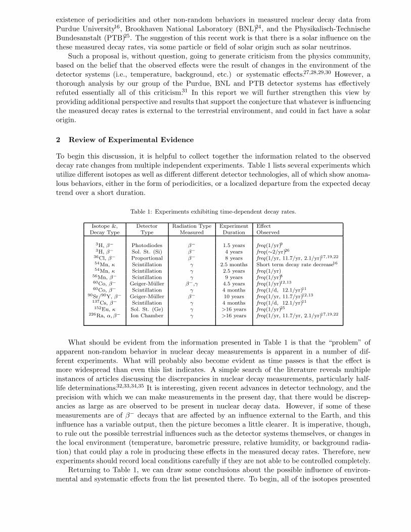
existence of periodicities and other non-random behaviors in measured nuclear decay data fromPurdue University16, Brookhaven National Laboratory (BNL)24, and the Physikalisch-TechnischeBundesanstalt (PTB)25. The suggestion of this recent work is that there is a solar influence on thethese measured decay rates, via some particle or field of solar origin such as solar neutrinos.
Such a proposal is, without question, going to generate criticism from the physics community,based on the belief that the observed effects were the result of changes in the environment of thedetector systems (i.e., temperature, background, etc.) or systematic effects.27,28,29,30 However, athorough analysis by our group of the Purdue, BNL and PTB detector systems has effectivelyrefuted essentially all of this criticism.31 In this report we will further strengthen this view byproviding additional perspective and results that support the conjecture that whatever is influencingthe measured decay rates is external to the terrestrial environment, and could in fact have a solarorigin.
2 Review of Experimental Evidence
To begin this discussion, it is helpful to collect together the information related to the observeddecay rate changes from multiple independent experiments. Table 1 lists several experiments whichutilize different isotopes as well as different different detector technologies, all of which show anoma-lous behaviors, either in the form of periodicities, or a localized departure from the expected decaytrend over a short duration.
Table 1: Experiments exhibiting time-dependent decay rates.
Isotope &, Detector Radiation Type Experiment Effect
Decay Type Type Measured Duration Observed
3H, β− Photodiodes β− 1.5 years freq(1/yr)9
3H, β− Sol. St. (Si) β− 4 years freq(∼2/yr)26
36Cl, β− Proportional β− 8 years freq(1/yr, 11.7/yr, 2.1/yr)17,19,22
54Mn, κ Scintillation γ 2.5 months Short term decay rate decrease
16
54Mn, κ Scintillation γ 2.5 years freq(1/yr)
56Mn, β− Scintillation γ 9 years freq(1/yr)8
60Co, β− Geiger-Muller β−,γ 4.5 years freq(1/yr)12,13
60Co, β− Scintillation γ 4 months freq(1/d, 12.1/yr)11
90Sr/
90Y, β−
Geiger-Muller β−
10 years freq(1/yr, 11.7/yr)12,13
137Cs, β−
Scintillation γ 4 months freq(1/d, 12.1/yr)11
152Eu, κ Sol. St. (Ge) γ >16 years freq(1/yr)25
226Ra, α, β− Ion Chamber γ >16 years freq(1/yr, 11.7/yr, 2.1/yr)17,19,22
What should be evident from the information presented in Table 1 is that the “problem” ofapparent non-random behavior in nuclear decay measurements is apparent in a number of dif-ferent experiments. What will probably also become evident as time passes is that the effect ismore widespread than even this list indicates. A simple search of the literature reveals multipleinstances of articles discussing the discrepancies in nuclear decay measurements, particularly half-life determinations.32,33,34,35 It is interesting, given recent advances in detector technology, and theprecision with which we can make measurements in the present day, that there would be discrep-ancies as large as are observed to be present in nuclear decay data. However, if some of thesemeasurements are of β
− decays that are affected by an influence external to the Earth, and thisinfluence has a variable output, then the picture becomes a little clearer. It is imperative, though,to rule out the possible terrestrial influences such as the detector systems themselves, or changes inthe local environment (temperature, barometric pressure, relative humidity, or background radia-tion) that could play a role in producing these effects in the measured decay rates. Therefore, newexperiments should record local conditions carefully if they are not able to be controlled completely.
Returning to Table 1, we can draw some conclusions about the possible influence of environ-mental and systematic effects from the list presented there. To begin, all of the isotopes presented
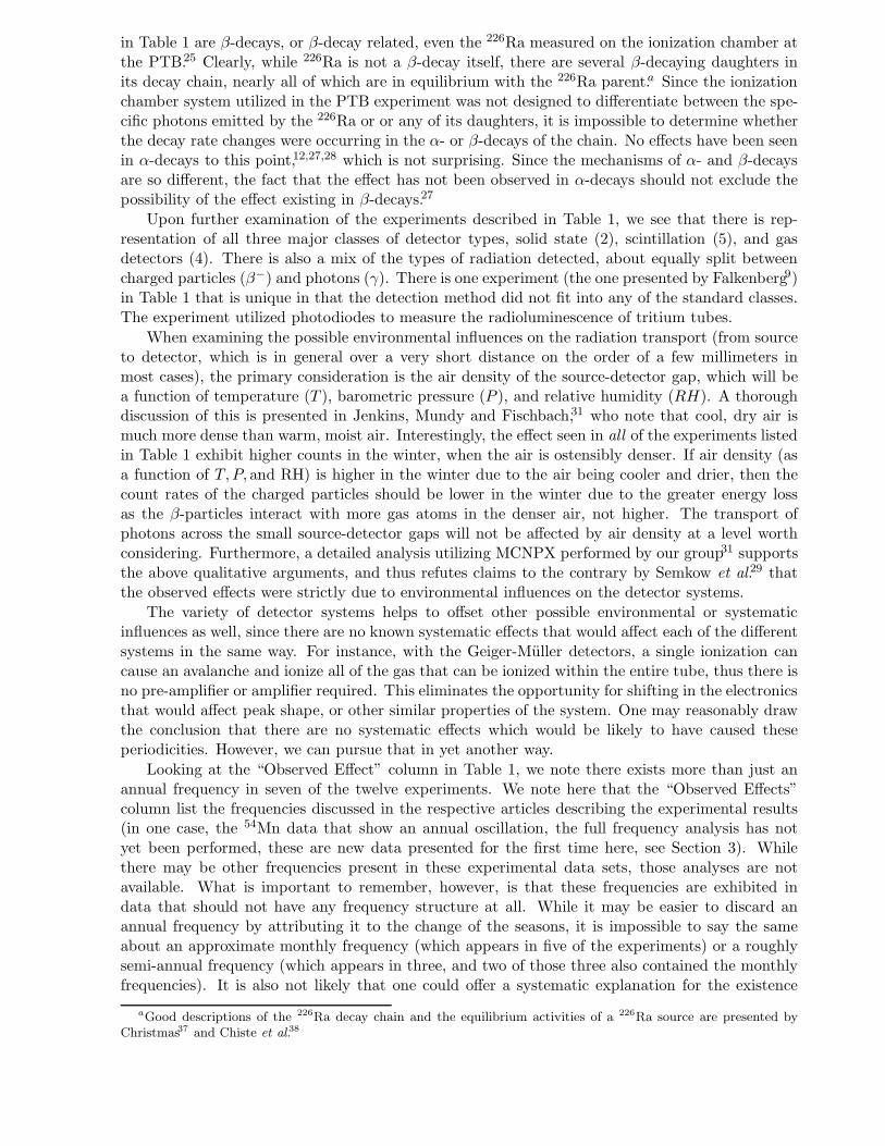
in Table 1 are β-decays, or β-decay related, even the 226Ra measured on the ionization chamber atthe PTB.25 Clearly, while 226Ra is not a β-decay itself, there are several β-decaying daughters inits decay chain, nearly all of which are in equilibrium with the 226Ra parent.a Since the ionizationchamber system utilized in the PTB experiment was not designed to differentiate between the spe-cific photons emitted by the 226Ra or or any of its daughters, it is impossible to determine whetherthe decay rate changes were occurring in the α- or β-decays of the chain. No effects have been seenin α-decays to this point,12,27,28 which is not surprising. Since the mechanisms of α- and β-decaysare so different, the fact that the effect has not been observed in α-decays should not exclude thepossibility of the effect existing in β-decays.27
Upon further examination of the experiments described in Table 1, we see that there is rep-resentation of all three major classes of detector types, solid state (2), scintillation (5), and gasdetectors (4). There is also a mix of the types of radiation detected, about equally split betweencharged particles (β−) and photons (γ). There is one experiment (the one presented by Falkenberg9)in Table 1 that is unique in that the detection method did not fit into any of the standard classes.The experiment utilized photodiodes to measure the radioluminescence of tritium tubes.
When examining the possible environmental influences on the radiation transport (from sourceto detector, which is in general over a very short distance on the order of a few millimeters inmost cases), the primary consideration is the air density of the source-detector gap, which will bea function of temperature (T ), barometric pressure (P ), and relative humidity (RH). A thoroughdiscussion of this is presented in Jenkins, Mundy and Fischbach,31 who note that cool, dry air ismuch more dense than warm, moist air. Interestingly, the effect seen in all of the experiments listedin Table 1 exhibit higher counts in the winter, when the air is ostensibly denser. If air density (asa function of T, P, and RH) is higher in the winter due to the air being cooler and drier, then thecount rates of the charged particles should be lower in the winter due to the greater energy lossas the β-particles interact with more gas atoms in the denser air, not higher. The transport ofphotons across the small source-detector gaps will not be affected by air density at a level worthconsidering. Furthermore, a detailed analysis utilizing MCNPX performed by our group31 supportsthe above qualitative arguments, and thus refutes claims to the contrary by Semkow et al.29 thatthe observed effects were strictly due to environmental influences on the detector systems.
The variety of detector systems helps to offset other possible environmental or systematicinfluences as well, since there are no known systematic effects that would affect each of the differentsystems in the same way. For instance, with the Geiger-Muller detectors, a single ionization cancause an avalanche and ionize all of the gas that can be ionized within the entire tube, thus there isno pre-amplifier or amplifier required. This eliminates the opportunity for shifting in the electronicsthat would affect peak shape, or other similar properties of the system. One may reasonably drawthe conclusion that there are no systematic effects which would be likely to have caused theseperiodicities. However, we can pursue that in yet another way.
Looking at the “Observed Effect” column in Table 1, we note there exists more than just anannual frequency in seven of the twelve experiments. We note here that the “Observed Effects”column list the frequencies discussed in the respective articles describing the experimental results(in one case, the 54Mn data that show an annual oscillation, the full frequency analysis has notyet been performed, these are new data presented for the first time here, see Section 3). Whilethere may be other frequencies present in these experimental data sets, those analyses are notavailable. What is important to remember, however, is that these frequencies are exhibited indata that should not have any frequency structure at all. While it may be easier to discard anannual frequency by attributing it to the change of the seasons, it is impossible to say the sameabout an approximate monthly frequency (which appears in five of the experiments) or a roughlysemi-annual frequency (which appears in three, and two of those three also contained the monthlyfrequencies). It is also not likely that one could offer a systematic explanation for the existence
aGood descriptions of the 226Ra decay chain and the equilibrium activities of a 226Ra source are presented byChristmas37 and Chiste et al.
38
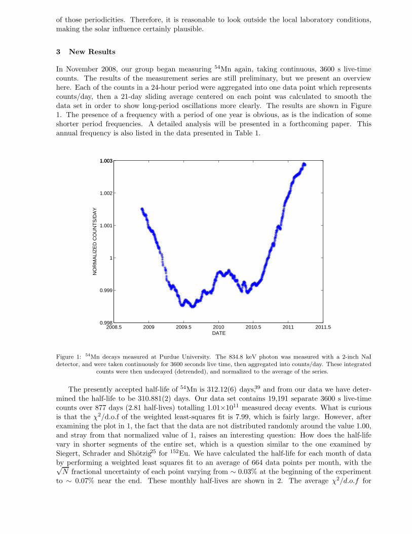
of those periodicities. Therefore, it is reasonable to look outside the local laboratory conditions,making the solar influence certainly plausible.
3 New Results
In November 2008, our group began measuring 54Mn again, taking continuous, 3600 s live-timecounts. The results of the measurement series are still preliminary, but we present an overviewhere. Each of the counts in a 24-hour period were aggregated into one data point which representscounts/day, then a 21-day sliding average centered on each point was calculated to smooth thedata set in order to show long-period oscillations more clearly. The results are shown in Figure1. The presence of a frequency with a period of one year is obvious, as is the indication of someshorter period frequencies. A detailed analysis will be presented in a forthcoming paper. Thisannual frequency is also listed in the data presented in Table 1.
2008.5 2009 2009.5 2010 2010.5 2011 2011.50.998
0.999
1
1.001
1.002
1.0031.003
DATE
NO
RM
ALI
ZE
D C
OU
NT
S/D
AY
Figure 1: 54Mn decays measured at Purdue University. The 834.8 keV photon was measured with a 2-inch NaIdetector, and were taken continuously for 3600 seconds live time, then aggregated into counts/day. These integrated
counts were then undecayed (detrended), and normalized to the average of the series.
The presently accepted half-life of 54Mn is 312.12(6) days,39 and from our data we have deter-mined the half-life to be 310.881(2) days. Our data set contains 19,191 separate 3600 s live-timecounts over 877 days (2.81 half-lives) totalling 1.01×10¹¹ measured decay events. What is curiousis that the χ
2/d.o.f of the weighted least-squares fit is 7.99, which is fairly large. However, afterexamining the plot in 1, the fact that the data are not distributed randomly around the value 1.00,and stray from that normalized value of 1, raises an interesting question: How does the half-lifevary in shorter segments of the entire set, which is a question similar to the one examined bySiegert, Schrader and Shotzig25 for 152Eu. We have calculated the half-life for each month of databy performing a weighted least squares fit to an average of 664 data points per month, with the√
N fractional uncertainty of each point varying from ∼ 0.03% at the beginning of the experimentto ∼ 0.07% near the end. These monthly half-lives are shown in 2. The average χ
2/d.o.f for
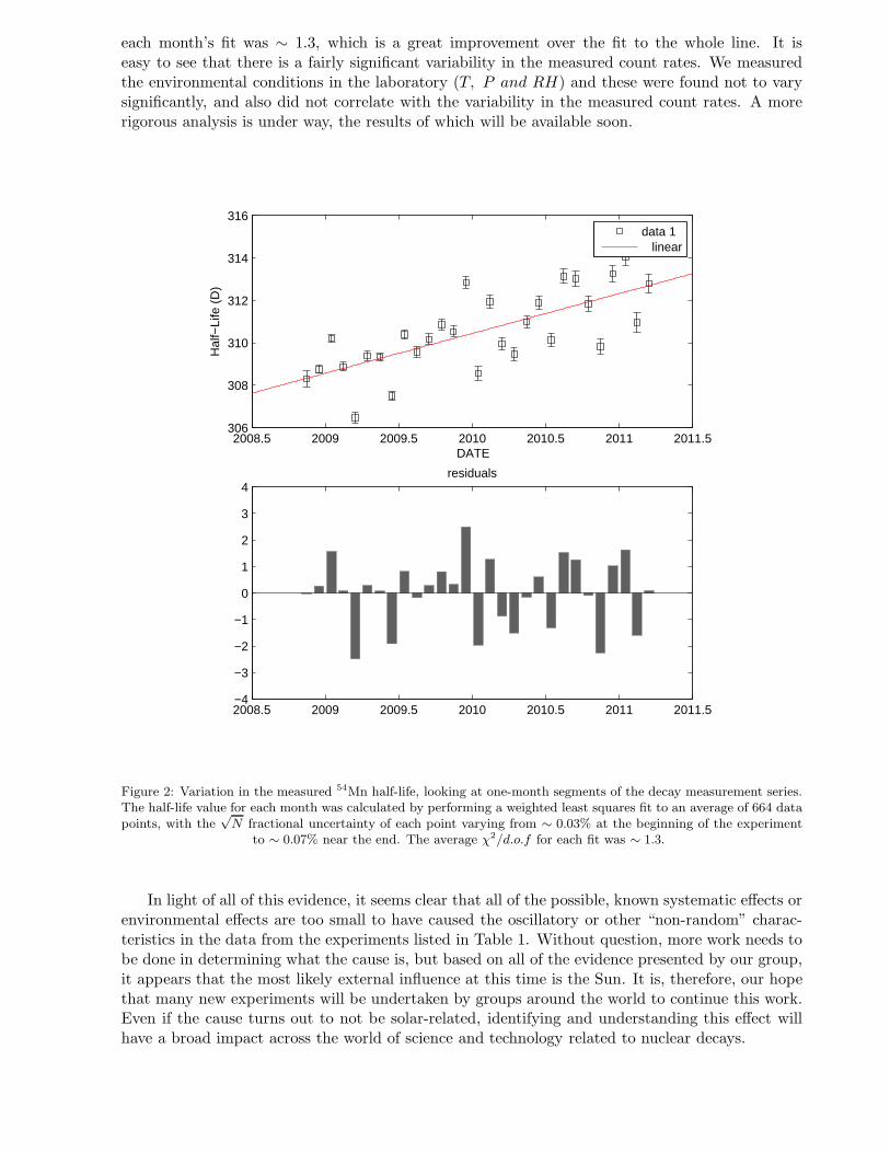
each month’s fit was ∼ 1.3, which is a great improvement over the fit to the whole line. It iseasy to see that there is a fairly significant variability in the measured count rates. We measuredthe environmental conditions in the laboratory (T, P and RH) and these were found not to varysignificantly, and also did not correlate with the variability in the measured count rates. A morerigorous analysis is under way, the results of which will be available soon.
2008.5 2009 2009.5 2010 2010.5 2011 2011.5−4
−3
−2
−1
0
1
2
3
4residuals
2008.5 2009 2009.5 2010 2010.5 2011 2011.5306
308
310
312
314
316
DATE
Hal
f−Li
fe (
D)
data 1 linear
Figure 2: Variation in the measured 54Mn half-life, looking at one-month segments of the decay measurement series.The half-life value for each month was calculated by performing a weighted least squares fit to an average of 664 datapoints, with the
√
N fractional uncertainty of each point varying from ∼ 0.03% at the beginning of the experimentto ∼ 0.07% near the end. The average χ2/d.o.f for each fit was ∼ 1.3.
In light of all of this evidence, it seems clear that all of the possible, known systematic effects orenvironmental effects are too small to have caused the oscillatory or other “non-random” charac-teristics in the data from the experiments listed in Table 1. Without question, more work needs tobe done in determining what the cause is, but based on all of the evidence presented by our group,it appears that the most likely external influence at this time is the Sun. It is, therefore, our hopethat many new experiments will be undertaken by groups around the world to continue this work.Even if the cause turns out to not be solar-related, identifying and understanding this effect willhave a broad impact across the world of science and technology related to nuclear decays.
Acknowledgments
The work of PAS was supported in part by the NSF through Grant AST-06072572, and that of EFwas supported in part by U.S. DOE contract No. DE-AC02-76ER071428.
References
1. G.T. Emery, Annual Rev. of Nucl. Sci. 22, 165 (1972)2. P.K. Hopke, Jour. Chem. Ed. 51, 517 (1974)3. H.P. Hahn, Radiochimica Acta 23, 15 (1976)4. K.P. Dostal, M. Nagel and D. Pabst, Zeitschrift fur Naturforschung A 23A, 345 (1977)5. E.B. Norman et al, Phys. Lett. B 519, 15 (2001)6. T.H. Ohtsuki, Phys. Rev. Lett. 93, 11 (2004)7. B.F. Limata et al, Eur. Phys. J.A 28, 251 (2006)8. K.J. Ellis, Phys. Med. Biol. 35, 1079 (1990)9. E.D. Falkenberg, Aperion 8, 14 (2001)
10. A.G. Parkhomov, Intl. J. Pure Appl. Phys. 1, 119 (2005)11. Y.A. Baurov et al, Phys. Atomic Nuclei 70, 1825 (2007)12. A.G. Parkhomov, arXiv:1004.1761v1 [physics.gen-ph] , (2010)13. A.G. Parkhomov, arXiv:1012.4174v1 [physics.gen-ph] , (2010)14. S.E. Shnoll et al, Physics-Uspekhi 41, 1025 (1998)15. S.E. Shnoll et al, Biophysics 43, 864 (1998)16. J.H. Jenkins and E. Fischbach, Astropart. Phys. 31, 407 (2009)17. J.H. Jenkins et al, Astropart. Phys. 32, 42 (2009)18. E. Fischbach et al, Space Sci. Rev. 145, 285 (2009)19. P.A. Sturrock et al, Astropart. Phys. 34, 121 (2010)20. Javorsek II et al, Astropart. Phys. 34, 173 (2010)21. P.A. Sturrock et al, Sol. Phys. 267, 251 (2010)22. P.A. Sturrock et al, Sol. Phys. In Press, (2011)23. P.A. Sturrock et al, ApJ In Press, (2011)24. D.E. Alburger, G. Harbottle and E. Norton, Ear. and Planet. Sci. Lett. 78, 168 (1986)25. H. Siegert, H. Schrader and U. Schotzig, Appl. Rad. and Isot. 49, 1397 (1998)26. V.M. Lobashev et al, Phys. Lett. B 460, 227 (1999)27. P.S. Cooper, Astropart. Phys. 31, 267 (2009)28. E.B. Norman et al, Astropart. Phys. 31, 135 (2009)29. T.M. Semkow et al, Phys. Lett. B 675, 415 (2009)30. M.P. Silverman and W. Strange, Europhys. Lett. 87, 32001 (2009)31. J.H. Jenkins, E. Fischbach and D.W. Mundy, Nucl. Instrum. Methods A 620, 332 (2010)32. F. Begemann et al, Geochim. Cosmochim. Acta 65, 111 (2001)33. T.-C. Chiu et al, Quaternary Sci. Rev. 26, 18 (2007)34. M.J. Woods, Nucl. Instrum. Methods A 286, 576 (1990)35. M.J. Woods and S.E.M. Lucas, Nucl. Instrum. Methods A 369, 534 (1996)36. R.J. de Meijer, M. Blaauw and F.D. Smit, 69, 320 (2011)37. P. Christmas et al, J. Appl. Radiat. Isot. 34, 1555 (1983)38. V. Chiste, M.M. Be, and C. Dulieu, in Int’l Conf. on Nucl. Data for Sci. and Tech. 2007,
ed. O. Bersillon et alEDP Sciences, Nice, France, 200739. H. Junde and H. Su, Nucl. Data Sheets 107, 1393 (2006)
14.Posters

Einstein Equivalence Principle and Bose–Einstein condensates
J. I. RivasDepartamento de Fısica, Universidad Autonoma Metropolitana–Iztapalapa
Apartado Postal 55–534, C.P. 09340, Mexico, D.F., Mexico.
A. CamachoDepartamento de Fısica, Universidad Autonoma Metropolitana–Iztapalapa
Apartado Postal 55–534, C.P. 09340, Mexico, D.F., Mexico.
The behavior of a Bose–Einstein condensate in a homogeneous gravitational field is analyzed.The trapping potential is an isotropic harmonic oscillator and the effects of the gravitationalfield and of the zero–point energy on the condensation temperature are also considered. Theseresults are employed in order to put forward an experiment which could test the so calledEinstein Equivalence Principle.
1 Introduction
Gravity can be understood at the classical level as a purely geometric effect, i.e., the motion ofa free classical particle moving in a curved manifold is given by the Weak Equivalence Principle(WEP) 1. The introduction of additional interactions is done resorting to the so–called EinsteinEquivalence Principle (EEP) 1. The present work addresses the behavior of a Bose–Einsteincondensate under the influence of a homogeneous gravitational field. The idea here is to considerthe possibility of testing the Einstein Equivalence Principle resorting to the temperature as theparameter to be monitored. We will deduce the changes in the condensation temperature as aconsequence of the presence of a homogeneous gravitational field.
2 Condensation in a homogeneous gravitational field
2.1 Gas in a harmonic trap
In the experimental realm the condensation process does not resort to a gas within a container,the trapping potential has a more sophisticated structure. Indeed, there are several kind oftraps, for instance magneto–optical traps (MOT), Optical traps (OT), etc. 2. The mathematicaldescription of the available magnetic traps, at least for alkali atoms, is that the correspondingconfining potential can be approximated by a three–dimensional harmonic oscillator
U(x, y, z) =m
2
(w2
1x2 + w2
2y2 + w2
3z2). (1)
We now consider the presence of a homogeneous gravitational field along the z–axis, hence,the complete potential becomes
U(x, y, z) =m
2
(w2
1x2 + w2
2y2 + w2
3
(z +
g
w23
)2)− 1
2mg2
w23
. (2)
The energy eigenvalues are given by
ε = w1
(nx +
12
)+ w2
(ny +
12
)+ w3
(nz +
12
)− 1
2mg2
w23
; nx, ny, nzεN. (3)
The density of states is provided by
Ω(ε) =
(ε+ mg
2w23−
2 (w1 + w2 + w3))2
23w1w2w3. (4)
This last expression allows us to calculate the average number of particles N and the changein the condensation temperature Tc due to the presence of a non–vanishing homogeneous grav-itational potential
N =∫ ∞
0
Ω(ε)z−1eβε − 1
dε+1
z−1eβε0 − 1. (5)
∆Tc = − ζ(2)3ζ(3)
∆µκ. (6)
For our particular case the change in the chemical potential, ∆µ = −(0.456)mg2
2ω2z
, namely,the condensation temperature under the presence of a homogeneous gravitational field reads
T (g)c = T (0)
c − (0.456)mg2
2κω2z
. (7)
In this last expression T(g)c is the condensation temperature if there is a non–vanishing
gravitational field , whereas T (0)c denotes the condensation temperature without gravitational
field.
2.2 Conclusions
According to EEP, the temperature of a freely falling condensate, trapped by a harmonic oscil-lator, should be higher than the corresponding temperature if the condensate lies at rest withrespect to the surface of the Earth.
Acknowledgments
JIRS acknowledges CONACyT grant No. 160453.
References
1. C. M. Will, Theory and Experiment in Gravitational Physics, Cambridge University Press,Cambridge (1993).
2. C. J. Pethick and H. Smith, Bose-Einstein Condensation in Diluted Gases, CambrigeUniversity Press,Cambrige (2006).
MICROSCOPE INSTRUMENT SERVO-LOOPS AND DIGITIZATION
A. LEVY, P. TOUBOUL, M. RODRIGUESONERA, BP72-29 Av. de la Division Leclerc,
Chatillon FR-92322, France
A. ROBERTCNES, 18 Av. Edouard Belin,
Toulouse 31401 Cedex 9, France
G. METRISObservatoire de la Cote d’Azur, Av. Nicolas Copernic,
Grasse 06130, France
MICROSCOPE is a fundamental physics space mission which aims at testing the EquivalencePrinciple (EP) with an accuracy of 10−15. The gravitational signal is measured preciselyon-board a drag-free microsatellite by a differential electrostatic accelerometer which includestwo cylindrical test masses made of different materials. The masses are servo-controlled alongtheir six degrees of freedom and the MICROSCOPE experiment takes advantage of this specificconfiguration with 12 data channels. A major point concerns the digitization and computationnoise throughout the loop, which should be maintained negligible with respect to the physicalnoise. This requires dedicated converters, filters and high frequency operations even if the EPtest is performed at frequency about 10−3 Hz.
1 The MICROSCOPE space mission
The MICROSCOPE space mission aims at testing the The Equivalence Principle (EP) expressedby Einstein as a basis of its theory of General Relativity with the best accuracy ever reachedof 10−15. This high accuracy can be achieved by taking profit of the minimized noise and thenon limited duration of the free fall in space. A 200 kg dedicated satellite is developed byCNES within its MYRIAD program of micro-satellite. The Earth is the gravitational source ofthe EP test and the satellite will be injected on a quasi circular (eccentricity < 5 × 10⁻³) andheliosynchronous orbit, at an altitude around 720 km. The characteristics of the orbit ensurethermal stability and a reduced correlation between the EP signal and the gravity gradient. Theduration of the mission is planned to be one year while the orbit period is about 6000 s.
The payload of the satellite is composed of two independent electrostatic differential ac-celerometers developed in our laboratory at Onera. Each differential accelerometer includes twocylindrical test masses and measures the difference between the inertial accelerations of the twomasses. One accelerometer is composed of two different masses (platinum/titanium) to performthe EP test and one is composed of two identical masses (platinum/platinum) to be used as areference. The mass and power budgets of the payload lead to 35 kg and 40 W.
The mass motions of the accelerometer are servo-controlled to follow the same orbit witha precision better than 10−11 m. Each test mass is surrounded by a cylindrical electrode part
enabling the electrostatic actuation which forces the masses to remain concentric. Thus, the twomasses undergo the same gravity field and a difference between the electrostatic accelerationsapplied to the masses will indicate an EP violation. The environment is maintained very steadylimiting any perturbation and the System of Control of Attitude and Acceleration (SCAA)exploits the measurement of the accelerometer in order to make the satellite drag free along thethree degrees of freedom: the surface forces and torques applied on the satellite are counteredcontinuously by the thrust of the propulsion system.
2 The measurement process
The operation of the accelerometer is similar along the six axes and hereafter detailed along themeasurement axis which is the cylinder axis (X axis): when the mass moves along this axis, avariation of the recovering surface appears leading to a difference of capacitance between themass and each electrode corresponding to an analog signal provided by the position detector.This signal is numerized with a sampling frequency equal to 1027.96 Hz and processed by thecontrol loop laws in order to generate a voltage proportional to the acceleration of the sensor.This voltage is amplified and applied to the electrodes in order to keep the mass at the center.The output of the control laws, after being filtered and down-sampled to 4 Hz, is used by thedrag free system. The scientific measurement must have a better accuracy so it is picked up,after filtering and down-sampling to 4 Hz, on the electrodes at the end of the loop in order toget advantage of the loop gain on all electronics noise sources. The control laws, anti-aliasingfilters and down-sampling processes are implemented in an Interface Control Unit (ICU) faraway from the sensor core while the analogue electronics and the analogue to digital convertersmust be close to the instrument sensor core to reduce electro-magnetic disturbances.
The anti-aliasing filters are at the order 5 and have cutoff frequency of 1 Hz for the scientificmeasurement and either 2 Hz or 3.3 Hz for the drag-free channels, depending on the axes; they areimplemented as combinations of biquad filters which are defined as second-order recursive linearfilters with transfer function H(z) = b0+b1z−1+b2z−2
1+a1z−1+a2z−2 in the Z-domain. The usual implementationof the biquad filter with x as input and y as output corresponds to the differential equation:
y(n) = b0x(n) + b1x(n − 1) + b2x(n − 2) − a1y(n − 1) − a2y(n − 2) (1)
All the computations in the ICU are performed with 40 bits. In spite of this large number,this leads to a computation error which is not negligible, especially because some intermediatevariable of the computation are only memorized with 32 bits instead of 40 bits in order to becompatible with the hardware components. This latter error is amplified through the recursivefilter and becomes the dominant error. Considering the expected accuracy of the MICROSCOPEEP test, we have demonstrated that the scientific X channel configuration with 40 bits for com-putation and memorization is required. For the drag free channels, fortunately the requirementsare less stringent. Therefore, in order to reduce the computation load by saving the variableswith 32 bits, an alternative algorithm which nullifies the amplification of the error through thebiquad has been developed. The corresponding difference equations are:
u(n) = (b0 − 1)u(n) + (b1 − a1)u(n − 1) + (b2 − a2)u(n − 2) − a1u(n − 1) − a2u(n − 2)
y(n) = x(n) + u(n) (2)
The advantage of this implementation is that the recursive filter is applied on an intermediatevariable and therefore the amplification of the saving error through the filter does not concernthe output y any more. With this method, the computation noise in the SCAA channel is alsocompatible with the specifications. Much care has been paid to verify the limitation of thealiasing of the high frequency noise of the loops at the EP frequency because of the heterodynetype detection of any violation signal in the experiment.
ELECTROSTATIC ACCELEROMETER WITH BIAS REJECTION FOR DEEPSPACE GRAVITATION TESTS
B. LENOIR∗, B. CHRISTOPHE∗, S. REYNAUD†∗Onera – The French Aerospace Lab
29 avenue de la Division Leclerc, F-92322 Chatillon, France†Laboratoire Kastler Brossel (LKB), ENS, UPMC, CNRS
Campus Jussieu, F-75252 Paris Cedex 05, France
The trajectory of an interplanetary spacecraft can be used to test gravitation in the So-lar System. Its determination relies on radio tracking and is limited by the uncertainty onthe spacecraft non-gravitational acceleration. But the addition of an accelerometer on boardprovides another observable which measures the departure of the probe from geodesic motion.
Such a concept has been proposed for the OSS mission3 which embarks the Gravity AdvancedPackage 6. This instrument, which is the focus of this article, is designed to make unbiased ac-celeration measurements 7. This proposal is in line with the Roadmap for Fundamental Physicsin Space issued by ESA in 2010 4. Indeed, there exist theoretical as well as experimental moti-vations to test gravitation in the Solar System. The fact that General Relativity is a classicaltheory while the three other fundamental interactions have a quantum description suggests thatit is not the final theory for gravitation. From the experimental point of view, the existence of“dark matter” and “dark energy” may be interpreted as the inability of General Relativity todescribe gravitation at cosmic scales1. And in the Solar System, the anomalous Pioneer signal2,8
may be an experimental artifact as well as a hint of considerable importance for fundamentalphysics 5.
1 Presentation of the instrument
The Gravity Advanced Package is made of two subsystems: MicroSTAR, an electrostatic ac-celerometer which inherits mature technology developed at Onera, and the Bias Rejection Systemused to rotate MicroSTAR with respect to the spacecraft around one axis. MicroSTAR measuresthe non-gravitational acceleration of the satellite and the measurement noise is characterized bythe following power spectrum density 6 (for a measurement range of 1.8× 10⁻⁴ m.s−2):
√Sn(f) = K = 5.7× 10⁻¹¹ m.s−2.Hz−1/2 ×
√1 +
(f
4.2 mHz
)−1+
(f
0.27 Hz
)4
. (1)
Thanks to the Bias Rejection System, which rotates the accelerometer of a monitored anglecalled θ, the quantities measured along the orthogonal axis y and z of the accelerometer are(assuming that there is no quadratic terms and the gain of the instrument is perfectly known)
my = [cos(θ)aY + sin(θ)aZ ] + by + ny (2a)
mz = [− sin(θ)aY + cos(θ)aZ ] + bz + nz (2b)
with aν (ν ∈ Y ;Z) the components of the acceleration in the reference frame of the spacecraft,by and bz the bias of MicroSTAR on each axis, and ny and nz the measurement noise.
2 Signal processing
Assuming that N measurements are made with a time step δt, there are 4N unknowns inequations (2) and only 2N measurements. Calling x the column vectors whose componentsare the values of x at each sampling time and using the linearity of the equations, it is howeverpossible to retrieve from the measurements the values of the projection of aY and aZ on a vectorsubspace defined by the columns of the matrix Va ∈MN,pa (pa < N). If
Va′Λνbκ = 0, with ν ∈ c; s and κ ∈ y; z. (3)
where Λc = diag[cos(θk)] and Λs = diag[sin(θk)] (k ∈ ||1;N ||), thenV ′aaY = V ′aΛcmy − V ′aΛsmz (4a)
V ′aaZ = V ′aΛsmy + V ′aΛcmz (4b)
Assuming that the bias on each axis also belongs to a subspace defined by the matrix Vb, is ispossible to design pattern for the rejection angle θ which fulfills conditions (3). This signal hasa period called τ .
In addition to retrieving the unbiased non-gravitational acceleration of the spacecraft, thismethod allows characterizing the uncertainty on the demodulated quantities V ′aaY and V ′aaZ,given MicroSTAR noise power spectrum density (cf. eq. (1)). Assuming that Va ∈ MN,1(R)and |Va| = 1, the precision on the quantities V ′aaY and V ′aaZ is given by 7∫ 1
2δt
− 12δt
Sn(f)|FδtΛcVa(f)|2 + |FδtΛsVa(f)|2
δt2df ≈ 1
τSn
(1
τ
)(5)
where Fδt is the Discrete Time Fourier Transform. One has to notice that the noise is selected,as expected, at the modulation frequency 1/τ .
3 Experimental validation
This demodulation scheme will be validated experimentally at Onera using a pendulum. Acontrol loop allows controlling its inclination to the 10−9 rad level. It is possible to incline it ata known angle in order to simulate an external acceleration. On this pendulum, an accelerometeris mounted on a rotating stage. There are two goals for this experiment :
– Validate the demodulation scheme by showing that it properly separates the bias from thesignal of interest allowing to make unbiased acceleration measurements.
– Verify the value of the uncertainty on V ′aaY and V ′aaZ predicted by equation (5).
References
1. A. Aguirre et al., Class. Quantum Grav. 18, R223 (2001).2. J.D. Anderson et al., Phys. Rev. D 65, 082004 (2002).3. B. Christophe et al., arXiv:1106.0132 (2011).4. ESA, “Fundamental Physics Roadmap”, available at http://sci.esa.int/fprat (08/23/2010).5. M.T. Jaekel and S. Reynaud, Mod. Phys. Lett. A 20, 14 (2005).6. B. Lenoir et al., arXiv:1011.6263 (2011).7. B. Lenoir, B. Christophe and S. Reynaud, arXiv:1105.4979 (2011).8. A. Levy et al., Adv. Space Res. 43, 10 (2009).
Lorentz invariant phenomenology of quantum gravity: Main ideas behind themodel
Yuri Bondera
Instituto de Ciencias Nucleares, Universidad Nacional Autonoma de MexicoA. Postal 70-543, Mexico D.F. 04510, Mexico
In the past decade the phenomenology of quantum gravity has been dominated by the searchof violations of Lorentz invariance. However, there are very serious arguments that led usto assume that this invariance is a symmetry in Nature. This motivated us to construct aphenomenological model describing how a Lorentz invariant granular structure of spacetimecould become manifest. The proposal is fully covariant, it involves non-trivial couplings ofcurvature to matter fields and leads to a well defined phenomenology.
General relativity is currently the accepted theory of spacetime and gravity and its quantumversion, which is still unknown, could involve a discrete structure of spacetime at microscopic(Planckian) scales. This non-trivial microstructure is generically known as spacetime granularityand the idea of studying its consequences empirically through Lorentz invariance violations(i.e., by looking for a preferential reference frame) has received a great deal of attention. Thisis essentially because a naive granularity would take its most symmetric form in a particularreference frame. However, there are very serious experimental bounds on Lorentz invarianceviolations1 and, moreover, the radiative corrections of a quantum field theory on a granularbackground that induces a preferential frame would magnify the effects of this granularity to apoint where they would have been already detected2.
This motivates us to assume that, if a spacetime granularity exists, it respects Lorentzinvariance and we investigate if there is a phenomenological way to study its consequences. Sincethere is no intuitive way to imagine a discrete structure of spacetime which is Lorentz invariant,the proposal3 is to use an analogy: Imagine a building made of cubic bricks and having, say, apyramidal shape. Then it is possible to detect the incompatibility between the bricks and thebuilding symmetry, for example, by looking the mismatch at the building’s surface. Given thatwe assume that the symmetry of spacetime’s building blocks is Lorentz invariance, according tothe analogy, in regions where spacetime is not Lorentz invariant, namely, where the Riemanncurvature tensor (Rabcd) does not vanish, it would be possible to detect the presence of thisgranularity. In other words, this analogy led us to assume that a Lorentz invariant spacetimegranularity could manifest through couplings of matter and Rabcd.
For simplicity we only focus on fermionic matter fields (ψ) and since the Ricci tensor at xis determined by the matter energy-momentum tensor at x, to study a coupling of Ricci andthe matter fields, at a phenomenological level, looks like a self-interaction. Thus we considerthe Weyl tensor (Wabcd) which, loosely speaking, is Rabcd without Ricci. In addition, in order
aemail: [email protected]. In collaboration with A. Corichi and D. Sudarsky
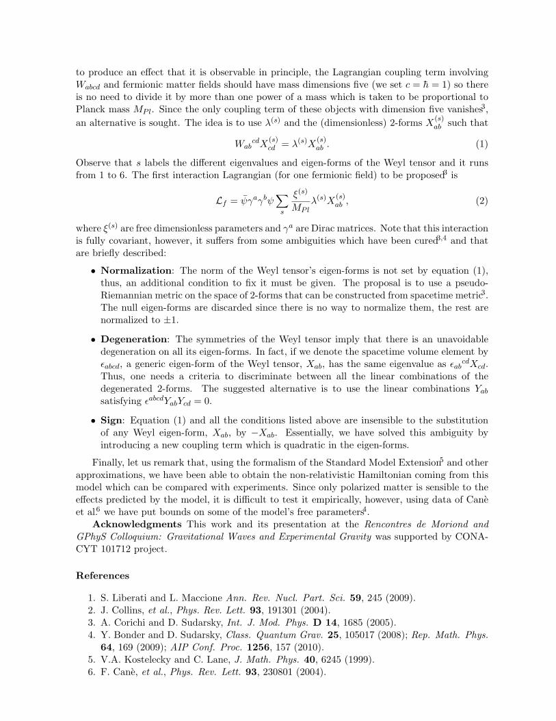
to produce an effect that it is observable in principle, the Lagrangian coupling term involvingWabcd and fermionic matter fields should have mass dimensions five (we set c = h = 1) so thereis no need to divide it by more than one power of a mass which is taken to be proportional toPlanck mass MPl. Since the only coupling term of these objects with dimension five vanishes3,an alternative is sought. The idea is to use λ(s) and the (dimensionless) 2-forms X(s)
ab such that
WabcdX
(s)cd = λ(s)X
(s)ab . (1)
Observe that s labels the different eigenvalues and eigen-forms of the Weyl tensor and it runsfrom 1 to 6. The first interaction Lagrangian (for one fermionic field) to be proposed3 is
Lf = ψγaγbψ∑s
ξ(s)
MPlλ(s)X
(s)ab , (2)
where ξ(s) are free dimensionless parameters and γa are Dirac matrices. Note that this interactionis fully covariant, however, it suffers from some ambiguities which have been cured3,4 and thatare briefly described:
• Normalization: The norm of the Weyl tensor’s eigen-forms is not set by equation (1),thus, an additional condition to fix it must be given. The proposal is to use a pseudo-Riemannian metric on the space of 2-forms that can be constructed from spacetime metric3.The null eigen-forms are discarded since there is no way to normalize them, the rest arenormalized to ±1.
• Degeneration: The symmetries of the Weyl tensor imply that there is an unavoidabledegeneration on all its eigen-forms. In fact, if we denote the spacetime volume element byεabcd, a generic eigen-form of the Weyl tensor, Xab, has the same eigenvalue as εab
cdXcd.Thus, one needs a criteria to discriminate between all the linear combinations of thedegenerated 2-forms. The suggested alternative is to use the linear combinations Yab
satisfying εabcdYabYcd = 0.
• Sign: Equation (1) and all the conditions listed above are insensible to the substitutionof any Weyl eigen-form, Xab, by −Xab. Essentially, we have solved this ambiguity byintroducing a new coupling term which is quadratic in the eigen-forms.
Finally, let us remark that, using the formalism of the Standard Model Extension5 and otherapproximations, we have been able to obtain the non-relativistic Hamiltonian coming from thismodel which can be compared with experiments. Since only polarized matter is sensible to theeffects predicted by the model, it is difficult to test it empirically, however, using data of Caneet al.6 we have put bounds on some of the model’s free parameters4.
Acknowledgments This work and its presentation at the Rencontres de Moriond andGPhyS Colloquium: Gravitational Waves and Experimental Gravity was supported by CONA-CYT 101712 project.
References
1. S. Liberati and L. Maccione Ann. Rev. Nucl. Part. Sci. 59, 245 (2009).2. J. Collins, et al., Phys. Rev. Lett. 93, 191301 (2004).3. A. Corichi and D. Sudarsky, Int. J. Mod. Phys. D 14, 1685 (2005).4. Y. Bonder and D. Sudarsky, Class. Quantum Grav. 25, 105017 (2008); Rep. Math. Phys.
64, 169 (2009); AIP Conf. Proc. 1256, 157 (2010).5. V.A. Kostelecky and C. Lane, J. Math. Phys. 40, 6245 (1999).6. F. Cane, et al., Phys. Rev. Lett. 93, 230801 (2004).
TOWARDS AN ULTRA-STABLE OPTICAL SAPPHIRE CAVITY SYSTEMFOR TESTING LORENTZ INVARIANCE
M. NAGEL and A. PETERSHumboldt-Universitat zu Berlin, Institut fur Physik, Newtonstr. 15,
12489 Berlin, Germany
We present a design for an ultra-stable cryogenically cooled sapphire optical cavity system,with fractional frequency stability better than 1× 10⁻¹⁶ at one second integration time. Weplan to use such ultra-stable cavities to perform a test of the isotropy of light propagation atthe 10−20 level.
1 Motivation
Many experimental and technical applications, e.g. optical atomic clocks, demand ultra-stablecavity systems for laser frequency stabilization. Nowadays, the main limiting factor in frequencystability for room temperature resonators has been identified to be the displacement noise withinthe resonator substrates and mirror coatings due to thermal noise. Different approaches are beingproposed right now to lower the influence of thermal noise, such as using higher order modes,longer cavities, or new types of coating materials. A straightforward method is to cool downthe resonators to cryogenic temperatures. Following this approach, we will set up an advancedcryogenic optical resonator system using specially designed sapphire cavities with the goal toreach a relative frequency stability of better than 1 × 10⁻¹⁶ up to long integration times.
2 Next Generation Cryogenic Optical Cavity System
Two normally opposing requirements need to be matched in designing a cryogenic resonatorand its mounting structure: high thermal conductivity towards the liquid helium bath and lowmechanical coupling of the optical path length to vibrations. We used FEM computations tooptimize the design of a resonator made of sapphire which reduces the influence of vertical andhorizontal vibrations and at the same time features large thermal contact areas for the mountingstructure (see Figure 1).
Calculations on the shot noise and thermal noise level show that the theoretical frequencystability at a temperature of 4.2K is in total an order of magnitude better than the best evervalue obtained with an optical resonator system (see Figure 1). We will also implement novelmeasures to enhance the long term performance of the optical cavity system in order to maintainthe potential relative frequency stability below 1 × 10⁻¹⁶ up to long integration times.
As a future perspective, we plan to exchange the Ta2O5/SiO2 mirror coatings, which are thethermal noise limiting source for these cryogenic optical sapphire resonators, with monocrys-talline coatings composed of AlxGa1−xAs.1 Those crystalline coatings will further reduce thestability limiting effects of thermal noise by more than an additional order of magnitude.
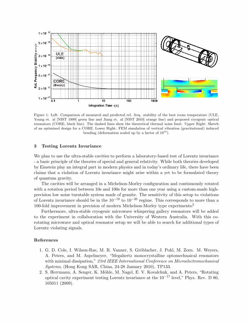
Figure 1: Left: Comparison of measured and predicted rel. freq. stability of the best room temperature (ULE,Young et. al [NIST 1999] green line and Jiang et. al [NIST 2010] orange line) and proposed cryogenic opticalresonators (CORE, black line). The dashed lines show the theoretical thermal noise limit. Upper Right: Sketchof an optimized design for a CORE. Lower Right: FEM simulation of vertical vibration (gravitational) induced
bending (deformation scaled up by a factor of 1010).
3 Testing Lorentz Invariance
We plan to use the ultra-stable cavities to perform a laboratory-based test of Lorentz invariance- a basic principle of the theories of special and general relativity. While both theories developedby Einstein play an integral part in modern physics and in today’s ordinary life, there have beenclaims that a violation of Lorentz invariance might arise within a yet to be formulated theoryof quantum gravity.
The cavities will be arranged in a Michelson-Morley configuration and continuously rotatedwith a rotation period between 10s and 100s for more than one year using a custom-made high-precision low noise turntable system made of granite. The sensitivity of this setup to violationsof Lorentz invariance should be in the 10−19 to 10−20 regime. This corresponds to more than a100-fold improvement in precision of modern Michelson-Morley type experiments.2
Furthermore, ultra-stable cryogenic microwave whispering gallery resonators will be addedto the experiment in collaboration with the University of Western Australia. With this co-rotating microwave and optical resonator setup we will be able to search for additional types ofLorentz violating signals.
References
1. G. D. Cole, I. Wilson-Rae, M. R. Vanner, S. Groblacher, J. Pohl, M. Zorn. M. Weyers,A. Peters, and M. Aspelmeyer, “Megahertz monocrystalline optomechnaical resonatorswith minimal dissipation,” 23rd IEEE International Conference on MicroelectromechanicalSystems, (Hong Kong SAR, China, 24-28 January 2010), TP133.
2. S. Herrmann, A. Senger, K. Mohle, M. Nagel, E. V. Kovalchuk, and A. Peters, “Rotatingoptical cavity experiment testing Lorentz invariance at the 10−17 level,” Phys. Rev. D 80,105011 (2009).
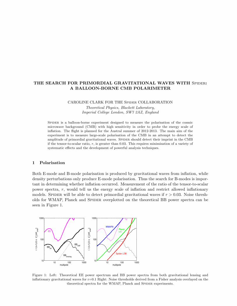
THE SEARCH FOR PRIMORDIAL GRAVITATIONAL WAVES WITH Spider:A BALLOON-BORNE CMB POLARIMETER
CAROLINE CLARK FOR THE Spider COLLABORATION
Theoretical Physics, Blackett Laboratory,Imperial College London, SW7 2AZ, England
Spider is a balloon-borne experiment designed to measure the polarisation of the cosmicmicrowave background (CMB) with high sensitivity in order to probe the energy scale ofinflation. The flight is planned for the Austral summer of 2012-2013. The main aim of theexperiment is to measure large-scale polarisation of the CMB in an attempt to detect theamplitude of primordial gravitational waves. Spider should detect their imprint in the CMBif the tensor-to-scalar ratio, r, is greater than 0.03. This requires minimisation of a variety ofsystematic effects and the development of powerful analysis techniques.
1 Polarisation
Both E-mode and B-mode polarisation is produced by gravitational waves from inflation, whiledensity perturbations only produce E-mode polarisation. Thus the search for B-modes is impor-tant in determining whether inflation occurred. Measurement of the ratio of the tensor-to-scalarpower spectra, r, would tell us the energy scale of inflation and restrict allowed inflationarymodels. Spider will be able to detect primordial gravitational waves if r > 0.03. Noise thresh-olds for WMAP, Planck and Spider overplotted on the theoretical BB power spectra can beseen in Figure 1.
10 100 100010
100
1000
multipole
! l (
l+1
)/2
" C
l [n
Kcm
b]
10 100 100010
100
1000
multipole
! l (
l+1
)/2
" C
l [n
Kcm
b] WMAP8
PlanckHFI
BBGW
Spider LDB
BBtot
EE
BBlensing
Figure 2: An illustration of the B-mode power spectra and the noise levels associated with theWMAP 8-year, Planck and Spider surveys. The left panel shows the theoretical spectra for the E-modes (labelled EE), gravitational lensing B-modes (labelled BBlensing), and the Inflationary grav-itational wave B-modes (labelled BBGW) for r = 0.1. The right panel shows the noise thresholdsper multipole (including both statistical noise and sample variance) for the three surveys, super-imposed on the same theory spectra. The curves for WMAP and Planck are derived from a simpleFisher analysis. For Spider, the Fisher errors are corrected for instrumental effects using ensem-bles of time domain simulations that include the scan strategy, noise correlations and stationarityboundaries. It is possible that foreground emission will limit Planck’s measurement of the low-!BB bump induced by reionization. The line for Spider has been truncated at a multipole of tenas the limited sky coverage will prevent us from probing larger scales; note that the anticipatedsignal-to-noise per multiple on the lensing signal (eg for r = 0) is of order unity from 10 < ! < 300.
scale of inflation (Turner and White, 1996). If Inflation happened near the GUT energy scale,then it is likely that its B-mode signature exists at a detectable level characterized by a tensor-to-scalar ratio r ! 0.01. The measurement of a non-zero tensor to scalar ratio would im-pose restrictions on the allowable classes of inflationary theories, ruling out both stringcosmology and cyclic universe hypothesis. A non-detection of the signature of gravita-tional waves corresponding to a limit on the tensor to scalar ratio of a few percent wouldexclude single field inflation models corresponding to energies near the scale of grandunification (Baumann et al., 2009; Kinney et al., 2008; Kallosh and Linde, 2007; Khouryand Steinhardt, 2010).
As illustrated in Figure 3, Spider is designed to measure the tensor to scalar ratio cor-responding to single field inflationary models near the GUT scale, or to experimentallyrule them out by setting an interesting upper limit r < 0.03 (at 3!). Spider’s sky coverageand sensitivity ensure that the data will be of lasting significance even upon successfulcompletion of the Planck mission. Planck, due to its relatively modest sensitivity, reliesentirely on a measurement of the large-scale reionization feature in the B-mode spectrumto probe the tensor to scalar ratio (see Figure 2). These are the scales most contaminatedby Galactic foreground emission.
D–4
Figure 1: Left: Theoretical EE power spectrum and BB power spectra from both gravitational lensing andinflationary gravitational waves for r=0.1 Right: Noise thresholds derived from a Fisher analysis overlayed on the
theoretical spectra for the WMAP, Planck and Spider experiments.
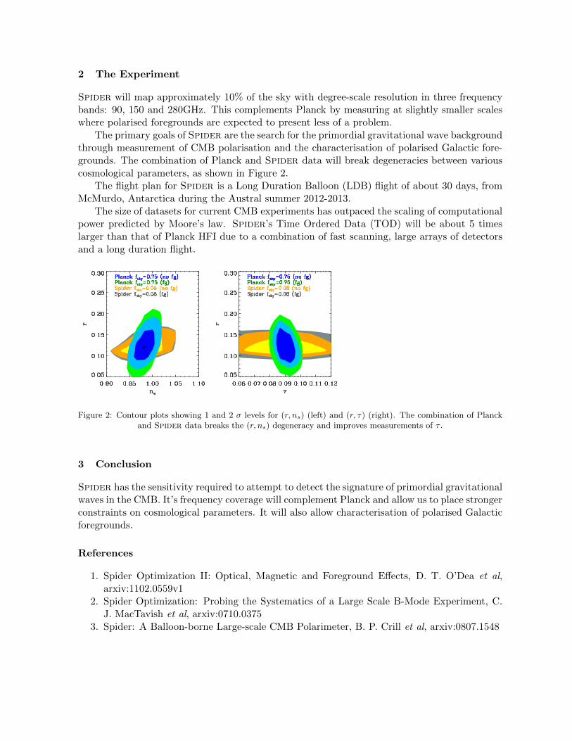
2 The Experiment
Spider will map approximately 10% of the sky with degree-scale resolution in three frequencybands: 90, 150 and 280GHz. This complements Planck by measuring at slightly smaller scaleswhere polarised foregrounds are expected to present less of a problem.
The primary goals of Spider are the search for the primordial gravitational wave backgroundthrough measurement of CMB polarisation and the characterisation of polarised Galactic fore-grounds. The combination of Planck and Spider data will break degeneracies between variouscosmological parameters, as shown in Figure 2.
The flight plan for Spider is a Long Duration Balloon (LDB) flight of about 30 days, fromMcMurdo, Antarctica during the Austral summer 2012-2013.
The size of datasets for current CMB experiments has outpaced the scaling of computationalpower predicted by Moore’s law. Spider’s Time Ordered Data (TOD) will be about 5 timeslarger than that of Planck HFI due to a combination of fast scanning, large arrays of detectorsand a long duration flight.
Figure 4: At left: The 1! and 2! contours for (r, ns) assuming a low tensor to scalar ratio, r = 0.001,and " = 0.09. At right: The same contours for (r, "), assuming relatively high tensor to scalar ratioof r = 0.12, corresponding to a slow roll m2#2 inflation. The addition of the Spider data with PlanckHFI powerfully constrain the (r, ns, ") parameter space.
2.3 Galactic Foregrounds
The recent results from WMAP confirm that both the E and B-mode signals are relativelyfaint in comparison with the polarized Galactic synchrotron emission at frequencies be-low 90 GHz (Gold et al., 2010). The contribution of dust polarization is poorly constrainedoutside of the Galactic plane. Confusion by these foregrounds will likely set the ultimatelimit to our ability to measure either the E or B mode signals at large angular scales; ac-curate treatment of foregrounds within the analysis is thus of primary importance.
These WMAP data provide accurate polarimetry of the synchrotron emission, whichprobes the structure of the galactic magnetic field and the nature of the interstellar medium(ISM). Spider will enable new galactic science by providing a deep survey of the high lat-itude polarized dust emission in the southern sky. These will complement existing full-sky maps of polarized synchrotron emission by probing higher density regions of the ISMthan are accessible via synchrotron. The new data will aid in understanding the transi-tion from magnetic field order in the diffuse ISM to disorder in the dense ISM, will helpin three-dimensional modeling of galactic magnetic fields, and will enable the study ofdust polarization in the local ISM via high-latitude clouds and cirrus.
Spider is designed to complement both WMAP, which has good sensitivity to polar-ized synchrotron emission, and Planck, which will precisely measure the spectral energydensity of the intensity of the dust component. To these data, Spider will add excellentsensitivity to the polarization of the thermal dust emission at high latitudes, where themodels of the interstellar medium are most simply applied. Planck’s frequency bands,centered at 100, 143, 217 and 353 GHz, are chosen to optimize the instrumental sensitivityto the Sunyaev-Zel’dovich effect. Spider’s 280 GHz band bridges the gap in Planck HFI’s
D–6
Figure 2: Contour plots showing 1 and 2 σ levels for (r, ns) (left) and (r, τ) (right). The combination of Planckand Spider data breaks the (r, ns) degeneracy and improves measurements of τ .
3 Conclusion
Spider has the sensitivity required to attempt to detect the signature of primordial gravitationalwaves in the CMB. It’s frequency coverage will complement Planck and allow us to place strongerconstraints on cosmological parameters. It will also allow characterisation of polarised Galacticforegrounds.
References
1. Spider Optimization II: Optical, Magnetic and Foreground Effects, D. T. O’Dea et al,arxiv:1102.0559v1
2. Spider Optimization: Probing the Systematics of a Large Scale B-Mode Experiment, C.J. MacTavish et al, arxiv:0710.0375
3. Spider: A Balloon-borne Large-scale CMB Polarimeter, B. P. Crill et al, arxiv:0807.1548
STRONG LENSING SYSTEM AND DARK ENERGY MODELS
B. MALECCopernicus Center for Interdisciplinary Studies, Gronostajowa 3,
30-387 Krakow, Poland
M. BIESIADADepartment of Astrophysics and Cosmology, Institute of Physics, University of Silesia, Uniwersytecka 4,
40-007 Katowice, Poland
Presently accelerating phase of cosmic expansion is a fundamental challenge to physics andcosmology. Cosmological concordance model (ΛCDM) although in agreement with a varietyof data is not a fully satisfactory solution. There is very little theoretical guidance in whichdirection beyond ΛCDM should one go. One approach is to use very general phenomenologyand look at the data for the evidence of evolving cosmic equation of state or the support forthe contrary claim. Therefore every alternative cosmological test becomes valuable on its own.Strong gravitationally lensed systems create opportunity to test cosmological models of darkenergy in a way alternative to Hubble diagrams (from SNIa or GRBs), CMBR or LSS.
1 Standard rulers versus standard candles
In this paper we would like to present our latest result concerning joint analysis involving datacoming from standard rulers and standard candles, done on five contemporary cosmologicalscenarios. First part of our diagnostic tools makes use of the angular diameter distance, therest use the luminosity distance. These are two distance concepts which, although theoreticallyrelated to each other, have clearly different systematic uncertainties and different parameterdegeneracies. Hence their joint analysis is more restrictive in the parameter space.
As standard rulers we used in first place strong lensing systems, namely a combined sampleof n = 20 constituents with good spectroscopic measurements of central dispersions from theSLACS 1 and LSD 2 surveys. Summary of data is given in Table 1 of paper 3. In a method usedhere cosmological models enter through a distance ratio, so results are independent of Hubbleconstant value. We also used CMBR and Barion Acoustic Oscillation (BAO) data. The so-called shift parameter R, related to the position of the first acoustic peak in the power spectrumof CMBR is adopted from recent results of WMAP7 4. Convenient BAO scale measurement,often quoted in the form of distance parameter A, is an observable, well constrained by data atredshift z = 0.35. Its current value is taken from 5. Data from supernovae Ia falls into categoryof standard candles. We use here the set of n = 556 supernovae6, known as Union2 compilation.
We considered five cosmological scenarios of dark energy, widely discussed in current liter-ature. These are ΛCDM , Quintessence, Chevalier-Polarski-Linder model, Chaplygin gas andBraneworld scenario. Models are parameterized by present density of matter Ωm and coefficientsin the effective equation of state of dark energy. Values are estimated by minimizing appropriateChi-square function (for details see 3,7).
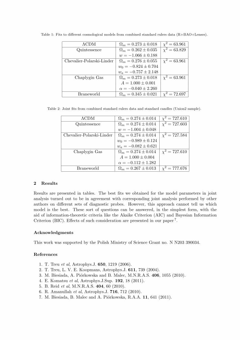
Table 1: Fits to different cosmological models from combined standard rulers data (R+BAO+Lenses).
ΛCDM Ωm = 0.273± 0.018 χ2 = 63.961Quintessence Ωm = 0.262± 0.035 χ2 = 63.829
w = −1.066± 0.188Chevalier-Polarski-Linder Ωm = 0.276± 0.055 χ2 = 63.961
w0 = −0.824± 0.704wa = −0.757± 2.148
Chaplygin Gas Ωm = 0.273± 0.018 χ2 = 63.961A = 1.000± 0.001
α = −0.040± 2.260Braneworld Ωm = 0.345± 0.021 χ2 = 72.697
Table 2: Joint fits from combined standard rulers data and standard candles (Union2 sample).
ΛCDM Ωm = 0.274± 0.014 χ2 = 727.610Quintessence Ωm = 0.274± 0.014 χ2 = 727.603
w = −1.004± 0.048Chevalier-Polarski-Linder Ωm = 0.274± 0.014 χ2 = 727.584
w0 = −0.989± 0.124wa = −0.082± 0.621
Chaplygin Gas Ωm = 0.274± 0.014 χ2 = 727.610A = 1.000± 0.004
α = −0.112± 1.282Braneworld Ωm = 0.267± 0.013 χ2 = 777.676
2 Results
Results are presented in tables. The best fits we obtained for the model parameters in jointanalysis turned out to be in agreement with corresponding joint analysis performed by otherauthors on different sets of diagnostic probes. However, this approach cannot tell us whichmodel is the best. These sort of questions can be answered, in the simplest form, with theaid of information-theoretic criteria like the Akaike Criterion (AIC) and Bayesian InformationCriterion (BIC). Effects of such consideration are presented in our paper 7.
Acknowledgments
This work was supported by the Polish Ministry of Science Grant no. N N203 390034.
References
1. T. Treu et al, Astrophys.J. 650, 1219 (2006).2. T. Treu, L. V. E. Koopmans, Astrophys.J. 611, 739 (2004).3. M. Biesiada, A. Piorkowska and B. Malec, M.N.R.A.S. 406, 1055 (2010).4. E. Komatsu et al, Astrophys.J.Sup. 192, 18 (2011).5. B. Reid et al, M.N.R.A.S. 404, 60 (2010).6. R. Amanullah et al, Astrophys.J. 716, 712 (2010).7. M. Biesiada, B. Malec and A. Piorkowska, R.A.A. 11, 641 (2011).
CONSTRAINTS ON A MODEL WITH EXTRA DIMENSIONS FOR THEBLACK HOLE AT THE GALACTIC CENTER
A.F. ZAKHAROVInstitute of Theoretical and Experimental Physics, 117259 Moscow, Russia
Bogoliubov Laboratory of Theoretical Physics, Joint Institute for Nuclear Research, 141980 Dubna,Russia
Different ways to find signatures of extra dimensions are discussing in the literature. If theRandall–Sundrum II braneworld scenario is adopted then a metric of black holes may bedifferent from a standard one and the Schwarzschild metric has to be changed with the Reissner– Nordstrom metric with a tidal charge. The model may be applied for the black hole at theGalactic Center. Since the Schwarzschild and Reissner – Nordstrom metrics are different fora significant charge one can expect that geodesics of bright stars near the black hole and theirobserved fluxes may be different for these metrics due to a difference in gravitational lensing.Therefore, a deviation from the Schwarzschild case flux may be measured for a significantcharge and the signature of extra dimensions may found. However, as a theoretical analysisshows that a tidal charge has to be very close to zero and a suggested charge value whichmay lead to measurable flux deviations for S2 like stars (or their essential displacements orastrometrical lensing) is not consistent with observational constraints on a shadow size.
Theories with extra dimensions admit astrophysical objects (supermassive black holes inparticular) which are rather different from standard ones. There were proposed tests which mayhelp to discover signatures of extra dimensions in supermassive black holes since the gravitationalfield may be different from the standard one in the GR approach. So, gravitational lensingfeatures are different for alternative gravity theories with extra dimensions and general relativity.Recently, Bin-Nun [1, 2, 3] discussed an opportunity that the black hole at the Galactic Centeris described by the tidal Reissner– Nordstrom metric [4] which may be admitted by the Randall–Sundrum II braneworld scenario. Bin-Nun suggested an opportunity of evaluating the black holemetric analyzing (retro-)lensing of bright stars around the black hole in the Galactic Center.Doeleman et al. evaluated a minimal size of a spot for the black hole at the Galactic Center [5].According to a theoretical consideration and simulations a minimal size of spot practically hasto coincide with the shadow size [6, 7, 8].
Measurements of the shadow size around the black hole may help to evaluate parametersof black hole metric [9, 10]. Another opportunity to evaluate parameters of the black hole isan analysis of trajectories bright stars near the Galactic Center [11]. We derive an analyticexpression for the black hole shadow size as a function of charge for the tidal Reissner– Nord-strom metric. We conclude that observational data concerning shadow size measurements arenot consistent with significant negative charges, in particular, the significant negative chargeQ/(4M2) = −1.6 (discussed in [1, 2, 3]) is practically ruled out with a very probability (thecharge is roughly speaking is beyond 9σ confidence level, but a negative charge is beyond 3σconfidence level).
It is known that a Reissner–Nordstrom metric cross-section for photons is described by thefollowing relation [10, 12]
l =(8q2 − 36q + 27) +
√(8q2 − 36q + 27)2 + 64q3(1− q)2(1− q)
, (1)
where ξ2 = l,Q2 = q (ξ and Q are impact parameter and the black hole charge in M units, Mis the black hole mass). If q = 0, we obtain the well-known result for the Schwarzschild metric,namely l = 27. If we consider the extreme Reissner–Nordstrom metric (q = 1) then l = 16. Atidal charge corresponds generally to a negative q or to imaginary Q values.
We could apply these relations for the black hole at the Galactic Center assuming that theblack hole mass is about 4∗106M¯ and a distance toward the Galactic Center is about 8kpc. Inthis case a diameter of shadow is about 52 µas for the Schwarzschild metric and about 40 µasfor the extreme Reissner–Nordstrom metric.
Doeleman et al. evaluated a size of the smallest spot near the black hole at the GalacticCenter such as 37+16
−10 microarcseconds at a wavelength of 1.3 mm with 3σ confidence level [5].Theoretical analysis and observations show that the size of shadow can not be smaller than aminimal spot size at the wavelength [6, 7, 8, 9, 10]. Roughly speaking, it means that a smallpositive q is consistent with observations but a significant negative q is not. For q = −6.4 (as itwas suggested by Bin-Nun [1, 2, 3]) we have a shadow size 84.38 µas. It means that the shadowsize is beyond of shadow size with a probability corresponding to a deviation about 9σ from anexpected shadow size. Therefore, a probability to have so significant tidal charge for the blackhole at the Galactic Center is negligible. So, we could claim that the tidal charge is ruled outwith observations and corresponding theoretical analysis.
Acknowledgments
AFZ thanks J. Dumarchez for his kind attention to this contribution.
References
[1] A. Y. Bin-Nun, Phys. Rev. D 81, 123011 (2010).
[2] A. Y. Bin-Nun, Phys. Rev. D 82, 064009 (2010).
[3] A. Y. Bin-Nun, arXiv:1011.5848 (2010).
[4] N. Dadhich, R. Maartens, Ph. Papadopoulos, V. Rezania, Phys. Lett. B 487, 1 (2001).
[5] S. S. Doeleman et al., Nature, 455, 78 (2008).
[6] H. Falcke, F. Melia, E. Agol, Astrophys. J., 528, L13 (2000).
[7] H. Falcke, F. Melia, E. Agol, in Cosmic Exposions: Tenth Astrophysics Conference, eds.W. W. Zhang & S. S. Holt, AIP Conference Proceedings, 522, 317 (2000).
[8] F. Melia, H. Falcke, Ann. Rev. Astron. Astrophys., 39, 309 (2001).
[9] A. F. Zakharov, A. A. Nucita, F. De Paolis, G. Ingrosso, New Astronomy, 10, 479 (2005).
[10] A. F. Zakharov, A. A. Nucita, F. De Paolis, G. Ingrosso, Astron. & Astrophys., 442, 795(2005).
[11] A. F. Zakharov, A. A. Nucita, F. De Paolis, G. Ingrosso, Phys. Rev. D 76, 062001 (2007).
[12] A. F. Zakharov, Class. Quantum Grav., 11, 1027 (1994).
Cosmological and solar-system constraints on tensor-scalar theory with chameleon
effect
A. Hees1,2, A. Fuzfa31 Royal Observatory of Belgium, Avenue Circulaire 3, 1180 Bruxelles, Belgium, [email protected]
2 LNE-SYRTE, Observatoire de Paris3 naXys, University of Namur (FUNDP), Belgium
General Relativity (GR) passed all solar system tests until now. However, cosmological obser-
vations are not directly compatible with GR and the standard model of elementary particles. A
way of modifying gravity at large scale without doing any modification at solar system scale is
achieved by the so-called Chameleon mechanism 1,2. This mechanism appears in tensor-scalar
theories of gravity with massive scalars. In this communication, we explore the sensitivity of
chameleon mechanism by constraining its parameters by cosmic acceleration on cosmological
scales and solar system constraints on small scales. This combined analysis will shed new light
on the question whether modified gravity can be safely invoked to solve cosmological problems
without any contradiction on Solar System scales.
1 Model
The model considered here is the one proposed by Khoury and Weltman 1,2 i.e. a tensor-scalartheory of gravitation with a runaway potential V (φ) (with c = 1):
S =
∫
d4x√
−g
[
m2p
16πR−
m2p
2∂µφ∂
µφ− V (φ)
]
+ SM (Ψm, A2(φ)gµν) (1)
where R is the scalar curvature, mp is the Planck mass (m2p = 1/G) and A(φ) is a coupling
function here given by A(φ) = ekφ.The action (1) is expressed in the so-called Einstein frame. This frame is useful for doing
calculations but all the physical interpretations are easily done in the Jordan frame wherematter is universally coupled to the metric gµν = A2(φ)gµν
3,4. Quantities expressed in Jordanframe are noted with a tilde and are directly observable.
The chosen potential is a Ratra-Peebles potential 5 parametrized by 2 constants α and ΛV (φ) = Λ
4+α
mαpφ
α .
2 Cosmological evolution and constraints
Fields equations have been derived by introducing a Friemann-Lemaitre-Robertson-Walker Einstein-frame metric (ds2 = −dt2+a2(t)dl2) and by replacing the Einstein frame matter density/pressureby the observable one (expressed in Jordan frame 3,4: ρ = A4(φ)ρ, p = A4(φ)p).
By integrating the field equations, it can be seen on Fig. 1 that the universe accelerationis mainly explained by the potential (in green), although a significant contribution from nonminimal coupling is present (in red).
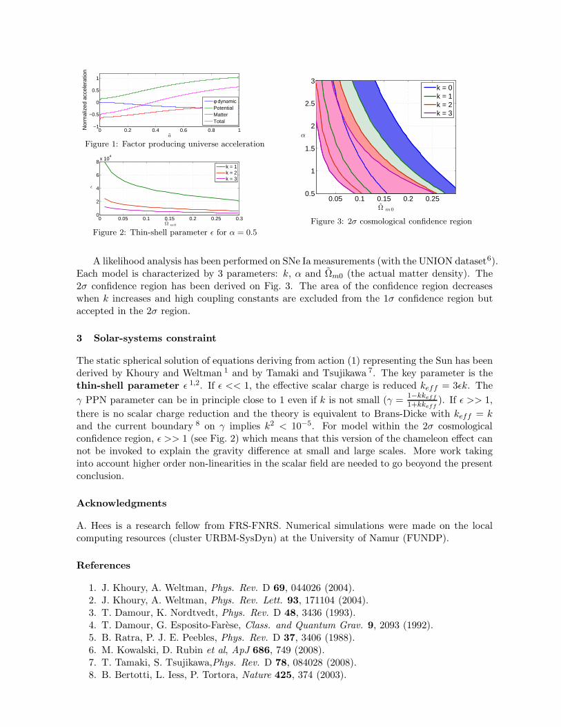
0 0.2 0.4 0.6 0.8 1−1
−0.5
0
0.5
1
a
Nor
mal
ized
acc
eler
atio
n
φ dynamicPotentialMatterTotal
Figure 1: Factor producing universe acceleration
0 0.05 0.1 0.15 0.2 0.25 0.30
2
4
6
8x 10
4
Ω m0
ǫ
k = 1k = 2k = 3
Figure 2: Thin-shell parameter ǫ for α = 0.5
0.05 0.1 0.15 0.2 0.250.5
1
1.5
2
2.5
3
Ω m0
α
k = 0k = 1k = 2k = 3
Figure 3: 2σ cosmological confidence region
A likelihood analysis has been performed on SNe Ia measurements (with the UNION dataset6).Each model is characterized by 3 parameters: k, α and Ωm0 (the actual matter density). The2σ confidence region has been derived on Fig. 3. The area of the confidence region decreaseswhen k increases and high coupling constants are excluded from the 1σ confidence region butaccepted in the 2σ region.
3 Solar-systems constraint
The static spherical solution of equations deriving from action (1) representing the Sun has beenderived by Khoury and Weltman 1 and by Tamaki and Tsujikawa 7. The key parameter is thethin-shell parameter ǫ 1,2. If ǫ << 1, the effective scalar charge is reduced keff = 3ǫk. The
γ PPN parameter can be in principle close to 1 even if k is not small (γ =1−kkeff1+kkeff
). If ǫ >> 1,
there is no scalar charge reduction and the theory is equivalent to Brans-Dicke with keff = kand the current boundary 8 on γ implies k2 < 10−5. For model within the 2σ cosmologicalconfidence region, ǫ >> 1 (see Fig. 2) which means that this version of the chameleon effect cannot be invoked to explain the gravity difference at small and large scales. More work takinginto account higher order non-linearities in the scalar field are needed to go beoyond the presentconclusion.
Acknowledgments
A. Hees is a research fellow from FRS-FNRS. Numerical simulations were made on the localcomputing resources (cluster URBM-SysDyn) at the University of Namur (FUNDP).
References
1. J. Khoury, A. Weltman, Phys. Rev. D 69, 044026 (2004).2. J. Khoury, A. Weltman, Phys. Rev. Lett. 93, 171104 (2004).3. T. Damour, K. Nordtvedt, Phys. Rev. D 48, 3436 (1993).4. T. Damour, G. Esposito-Farese, Class. and Quantum Grav. 9, 2093 (1992).5. B. Ratra, P. J. E. Peebles, Phys. Rev. D 37, 3406 (1988).6. M. Kowalski, D. Rubin et al, ApJ 686, 749 (2008).7. T. Tamaki, S. Tsujikawa,Phys. Rev. D 78, 084028 (2008).8. B. Bertotti, L. Iess, P. Tortora, Nature 425, 374 (2003).
The STAR Mission: SpaceTime Asymmetry Research
T. SCHULDT, A. KEETMAN, C. BRAXMAIER
University of Applied Sciences Konstanz, Brauneggerstr. 55,
78462 Konstanz, Germany
K. DORINGSHOFF, M. NAGEL, A. PETERS
Humboldt-University Berlin, Newtonstr. 15,
12489 Berlin, Germany
S. HERRMANN, C. LAMMERZAHL
Center for Applied Space Technology and Microgravity, Am Fallturm,
28359 Bremen, Germany
T. V. ZOEST, H. DITTUS
DLR-Institute for Space Systems, Robert-Hooke-Str. 7,
28359 Bremen, Germany
U. JOHANN
Astrium GmbH – Satellites, Claude-Dornier-Straße,
88090 Immenstaad, Germany
S. BUCHMAN, K.-X. SUN, J. LIPA, R. BYER
Stanford University,
Stanford, CA 94307, USA
B. JAROUX, P. WORDEN
NASA AMES research center,
Moffett Field, California 94035-1000, USA
J. HALL
JILA, University of Colorado,
UCB Campus, Boulder, Colorado 80309-0440, USA
M. ALMAJED, H. ALTWAIJIRY, T. AL-SAUD
King Abdulaziz City for Science and Technology,
King Abdullah Road, Riyadh, 11442, Saudi Arabia
The proposed space mission STAR (SpaceTime Asymmetry Research) aims for significantlyimproved tests of fundamental space-time symmetry and the foundations of special and gen-eral relativity. A series of missions is planned where the first mission focuses on a Kennedy-Thorndike experiment. Later missions will additionally carry out Michelson-Morley experi-ments as well as precision measurements of gravitational redshift and Local Position Invari-ance. STAR targets an improvement of at least two orders of magnitude compared to previousexperimental accuracy on ground.
The SpaceTime Asymmetry Research (STAR) program is a planned series of three missionstesting special and general relativity. It is an international cooperative effort of teams withvery strong background in experimental tests of relativity, their theoretical description andadvanced space technology; the mission lead is carried out by Stanford University (USA). Thefirst mission will perform a Kennedy-Thorndike (KT) experiment and measure the constancy(velocity invariance) of the speed of light to one part in 1019 and derive the KT coefficient ofthe Mansouri-Sexl test theory to 7 · 10−10. The experiment will be carried out by comparing anabsolute reference (baseline: a laser frequency stabilized to a transition in molecular iodine) witha highly stable resonator made e.g. from ULE (ultra low expansion) glass ceramics. Due to anorbital velocity of 7 km/s the sensitivity to a boost dependent violation of Lorentz invariance asmodelled by the KT term in the Mansouri-Sexl test theory or a Lorentz violating extension of thestandard model (SME) will be significantly enhanced as compared to Earth based experiments.Additional enhancement is obtained by low noise space environment. An overall improvementby a factor of approx. 100 – compared to current Earth-based experiments – is the goal.
The STAR mission program addresses three major goals: (i) perform tests of fundamentalphysics, (ii) develop small satellite and advanced instrumentation technology, and (iii) educatefuture scientists and engineers. A 180 kg small attitude, vibration and temperature controlledsatellite is used as foundation for all three STAR missions. The power consumption of thewhole spacecraft will be less than 185 W. The launch of STAR1 is foreseen for january 2018,the follow-on missions will be flown with an overlap with the previous mission by two to threeyears. The proposed orbit for STAR1 is a 650 km circular sun-synchronous orbit with a 2 yearmission lifetime.
STAR1 Payload Concept
STAR1 will utilize an ultrastable molecular Iodine clock and crossed ULE cavities with a finesse> 100.000. Both clocks require a minimum frequency stability of 9 · 10−16 at the orbit time of5800 s. The cavities will be placed in an ultra-stable thermal environment with ∼ 1µK stabilityusing a six-stage thermal isolation system with active and passive control. Both clocks arerealized in redundancy (2 molecular clocks and 4 cavities) mainly using commercially availablecomponents with high TRL for reducing risk and keeping costs low. The setup is fiber-coupledand realized in a modular configuration.
The four cavities are made out of one ULE block with a coefficient of thermal expansion of∼ 10−9 K−1 within the operating temperature range 10 to 20C. The four cavities are realized astwo pairs of crossed cavities which are stacked such that the cavity axes of one pair are rotatedby 45 degrees with respect to the other pair. This enables the investigation of systematic effects.The molecular clock is based on modulation transfer spectroscopy (MTS) of hyperfine transi-tions in molecular Iodine near 532 nm. The optical setup will be realized using thermally andmechanically highly stable materials such as Zerodur or ULE in combination with an appropriateassembly-integration technology.
The proposed baseline laser for STAR1 is an NPRO-type Nd:YAG laser at a wavelength of1064 nm which is commercially available in a space qualified version providing output powers upto 1.5 W in combination with a space qualified fiber amplifier. For the frequency stabilizationto Iodine, a frequency doubling of the laser to 532 nm with an output power of ∼ 20 mW isrequired.
ON THE MAXIMUM MASS OF DIFFERENTIALLY ROTATING NEUTRON
STARS
A. Snopek1, D. Gondek-Rosinska1, I. Kowalska2, L. Villain3, M. Kucaba1, M. Szkudlarek1, M. Ansorg4
1Institute of Astronomy, University of Zielona Gora, ul. Lubuska 2, 65-265 Zielona Gora, Poland2Astronomical Observatory, University of Warsaw, Al Ujazdowskie 4, 00-478 Warsaw, Poland
3LMPT, Univ. F. Rabelais, 37200 Tours, France4Theoretisch-Physikalisches Institut, Friedrich-Schiller-Universitat Jena,Germany
A binary neutron star merger leads to the formation of a massive differentially rotating neutronstar (or strange star) or to the prompt collapse to a black hole. The gravitational wave signalshould tell us whether a massive neutron star or a black hole is formed and should allow toput constraints on the (hot) neutron star equation of state. We study the effect of the degreeof differential rotation and of the stiffness of the equation of state on the maximum mass ofneutron stars. We numerically construct stellar models using a highly accurate relativisticcode based on a multi-domain spectral method (Ansorg, Gondek-Rosinska, Villain, 2009). Wefind various types of configurations, which were not considered in previous works, mainly dueto numerical limitations. Among other results, we obtain the largest increase of the maximummass for moderately stiff equation of state and for these new types of solutions.
1 The maximum mass of neutron stars
For a given equation of state (EOS), the maximum mass (Mmax,stat) of non-rotating neutronstars (NSs) is uniquely determined by the Tolman-Oppenheimer-Volkoff equations and is foundto be in the range 1.5-2.5 M⊙. It was shown that rotation allows this maximum mass to be17%-20 % larger for rigidly rotating NSs (Cook et al., 1994) and 34% larger for strange stars(Gondek-Rosinska et al., 2000; Gourgoulhon et al., 1999). It was also found that differential
rotation can be much more efficient in increasing (by more than 60%) the maximum allowedmass, especially for moderately stiff EOSs (Baumgarte et al., 2000; Lyford et al., 2003).
2 Equation of state and rotation law
We construct relativistic models of differentially rotating NSs for broad ranges of the degree ofdifferential rotation and of the maximal mass density (ρmax). We assume a polytropic EOS,P = Kρ
γ , where P is the pressure, ρ the mass density, K = 1 the polytropic constant and γ
the polytropic index. We consider EOS with three different indices (and consequently stiffness):soft (γ = 1.5), moderately soft (γ = 2) and stiff (γ = 3), in order to study both the effect of thestiffness of the EOS and of differential rotation on the maximum mass. We adopt the rotationlaw introduced by Komatsu et al. (1989) which is parametrized by Ωc, the angular velocity onthe rotation axis, and by a parameter R0, which measures the degree of differential rotation.We rescale R0 in terms of the equatorial radius Re and use A
−1 = Re/R0 (for rigid rotationR0 → ∞ and A
−1 = 0). Hence, the higher A−1, the higher the degree of differential rotation.
3 Results and conclusions
Following Baumgarte et al. (2000), for given EOS and A−1 we construct sequences of fixed
maximal mass density (in the range 0.01 to 0.6) parametrized by the ratio of the polar to theequatorial radius r = Rp/Re. Then for each sequence we look for the maximum mass and finallyfor the maximum of those maxima. Four types of sequences turn out to be useful to define.From A
−1 = 0 up to a first threshold value A−1 = AA, we find only one type of spheroidal
stars (so called type A). For A−1
> AA but smaller than a critical value AC (which dependson ρmax and on the EOS), we find types A or B sequences of differentially rotating stars.For A
−1> AC only types C or D stars exist. All types of solutions are described below (see
Ansorg, Gondek-Rosinska & Villain 2009 for details):
- type A start at a static and spherical body and end at the mass-shedding limit. They existfor all considered EOSs;
- type B start at the mass-shedding limit and terminate at r = 0 if we restrict calculations toconfigurations with a spheroidal topology. They exist only for r < 0.3;
- type C start at a static and spherical body and end at r = 0 (for spheroidal topology);
- type D both start and end at the mass-shedding limit and exist for a very narrow range ofA
−1. We shall not consider this type in our paper.
In the literature only type A and type C (with some limitations) sequences were considered.For small polytropic index (γ = 1.5) we don’t find type B or C sequences, up to A
−1 = 2,while for moderate and stiff EOSs (γ = 2 and 3), all types mentioned above exist.
We find that differential rotation is very effective in increasing the maximum mass. Inde-pendently on the stiffness of the EOS the value of Mmax,rot/Mmax,stat is a decreasing function ofA
−1 for sequences of type B and C and an increasing one for type A. The largest increase of themaximum mass is for the polytropic EOS with γ = 2 and for type B and C sequences of stars.The maximum value of the ratio is 4 reached at A
−1∼ 0.4 for type B and 2.55 at A
−1∼ 0.8 for
type C. For type A, the maximum value of the ratio is obtained for γ = 2 at A−1
∼ 0.7, andγ = 3 at A
−1∼ 0.4. In both cases the maximal masses are larger than the maximum mass of
the corresponding nonrotating star by over 70%. This confirms the results of Baumgarte et al.(2000) and Lyford et al. (2003).
Acknowledgments
This work was supported by the EGO-DIR-102-2007; the FOCUS 4/2007 Program of Founda-tion for Polish Science, the Polish grants NN 203 511 238 and DPN/N176/VIRGO/2009, byCompStar a Research Networking Programme of the European Science Foundation and by theAssociated European Laboratory “Astrophysics Poland-France”
References
1. Ansorg M., Gondek-Rosinska D., Villain L., MNRAS 396, 2359-2366 (2009)2. Baumgarte T.W., Shapiro S.L., Shibata M., ApJL 528, L29-L32 (2000).3. Cook G.B., Shapiro S.L, Teukolsky S.A. , ApJ 422, 227-242 (1994).4. Gondek-Rosinska D., et al., A&A 359, 143-147 (2000).5. Gourgoulhon et al., A&A 349, 851-862 (1999).6. Komatsu H., Eriguchi, Y., & Hachisu, I.,MNRAS 237, 355 (1989)7. Lyford et al, ApJ 583, 410-415 (2003).
Measurement of slow gravitational perturbations with gravitational waveinterferometers.
A.V.Gusev, V.N.Rudenko, I.S.YudinSternberg Astronomical Institute of Moscow State University, Universitetsky pr., 13,,
Moscow, Russia
Measurement of quasistatic gravity field variations using data of laser gravitational waveinterferometers is discussed. New method of taking data at the free spectral range frequencyis analized besides a direct read out the mirror correction voltage. Calculated values ofgeophysical signals are compared with observation at the LIGO interferometer.
Geophysical measurements as a by-product of GW interferometers were discussed early inpapers 1,2,3 Such possibility arises because there is no a seismic and gravitational isolation of theinterferometer test mass-mirrors at very low (quasi static) frequencies f < 1 Hz. First practicalsteps were performed by VIRGO collaboration during the VSR-1, VSR-2 series 4. It was adirect measurement of arm deformation through the error signal of control circuits keeping theinterferometer operational point (mirror coordinate and angular positions). Typical accuracyof the mirror coordinate fixation in Virgo setup 10−12m or δL/L ∼ 10−16. Thus the tidal armdisplacement amplitude at 3 km 100µkm or δL/L ∼ 10−8 can be measured with enough highprecision. So with this accuracy one can dream about the registration of very weak geodynamicalperturbation like the ”liquid core daily resonance”, ”inner core oscillation” etc. More over it wasseemed reasonable to investigate a direct measurement of the relativistic gravitational effectslike a light frequency shift and time travel delay using GW interferometers located at the Earthsurface.
A new method of tidal perturbation measurement was demonstrated during LIGO S5 se-ries. For long base interferometers the circulation (or free spectral range) frequency is so low( 104kHz) that the correspondent component appeares at the main differential (GW-signal)output. The effect of tidal amplitude modulation of this harmonic was discovered during the S5LIGO scientific run 5,6. A mechanism of such modulation obviously has to be associated witha shtocastic luminosity of the FP arm optical mode neighbor with the resonance one. Howevera calculated estimate of modulation index is ocurred to be in disagreement with the observedvalues.
Under the supposition that mirrors are fixed by control circuits (arm lengths are kept asconstant) a direct interaction of the optical pump with tidal gravity variations is consideredas a main reason of optical length changes. In the paper 7 the gravitational photon frequencyshift was used for this purpose, meanwhile the refractive index equivalent to the gravity fieldwas explored in 8. Numerically both effects leads to the same relativistic correction of opticalarm length. Calculation was carried out following the simplified scheme of GW interferometerpresented at the picture (recycling mirror is omitted) including the data readout procedure. FParms are considered as complex resonant mirrors. Spectrum of one mode resonant pump with
the central frequency ν0 ∼ 3 · 1014Hz was presented by narrow line of phase fluctuation in a fewHz width accompanied by a small spectral density pedestal of amplitude fluctuation having thewidth ∆ν ∼ 100kHz.Thus a neighbour FP cavity mode ν1 = ν0 +νfsr shifted at the free spectralrange νfsr = 2c/L is also illuminated with a small intensity so as for the 4 km arm νfsr ∼ 37kHz.
The light waves at frequency close to resonance modes of arms interfere with the followingphase difference:
δϕ ' 1
1 − r
(2∆L
L+
4L
λ
δn
n
)where ∆L/L is static shift due to arm lengths difference, δn/n is dynamical shift due to refractiveindex variation equivalent of tidal gravity changes.
Output signal ∼ δϕ contains permanent and variable parts. Estimate of the modulationindex in term of power (or amplitude) has resulted in δP/P ∼ 3 ·10−4 meanwhile the observableindex was much larger ∼ 2 · 10−2. Thus the relativistic effect can not explain the observabletidal modulation of the harmonic at free spectral range frequency.
More rigorous analysis (performed after critics) required a taking into account the stochasticexcitation a second neighbour mode symmetrical in respect of the carrier 9. The result wasunexpected one: an influence of the second (symmetrical) neighbour mode compensated theparametrical excitation produced by the first one. Output residual noise variance now containedonly quadratic term of arm optical length variations in contrast with the previous result.
It is possible to reconstruct the ”linear response” refusing from the condition of ‘”dark spot”at the main interferometer output ( at practice the ”dark spot” can be realized only with finiteaccuracy). Then introducing a detuning δl, i.e. passing to the condition of ”gray spot”, one canget the output noise variance in the form:
σ2 ' Const
1 − r
[(2L
λ
)2 ((1 − r)
2δl
L+ δξ
)2
+
(∆L
L
)2]
The time variable value in this formula is δξ. Its ratio to the maximal permanent term givesan estimate of the signal modulation index at free spectral range frequency:
m ' Lδξ
(1 − r)δl
Numerical estimates are the following. For the relativistic effect hypothesis: δξ ∼ 10−19,even for unrealistic tuning δl ∼ 10−4λ; the estimate of modulation index m∼0.04% is two orderof value less the observable one. In the case of residual (noncompensated) arm differentialdisplacements δξ ∼ 10−15 (less the control accuracy) a reasonable detuning δl = 10−2λ resultsin m∼4% that is in a good agreement with the observation.
Radical method for the linear parametric response reconstruction would be a using the twomode pump at neighbour frequencies ν0 and ν1 = ν0 + νfsr; the ”dark spot” condition has tobe kept for the mode ν0. A residual part of the mode ω1 interacting at photo diode with radiosideband ν1 will produce directly at the Pound-Drever mixer output a low frequency signal I(t)proportional to the optical length variations δl. A possibility of application this method for aregistering weak global geodynamical effects as well as the detection of very low frequency GWhas to be addressed.
Conclusions
It was demonstrated that VIRGO can be used as a two coordinate very long base strain me-ter. Geophysical signal reads out from drivers controlling the interferometer operation point.
However the quality of the data strongly depends on a number of locking brake during theobservational time.
Up to now the idea of relative angular variations of mirror’s plumb lines for a sensing puregravity perturbations was not realized and has to be tested in nearest future.
LIGO team demonstrated the possibility of tidal gravity registration through a specificmethod of read out the correspondent information in the main interferometer output at theFSR radio frequency.
It is seemed that the parametric mechanism provided such possibility is associated with theresidual arm deformations beyond the control accuracy. However details of this phenomenonhas to be studied more closely in respect of its application in geodynamical measurements.
1. Kopaev A.V.,Rudenko V.N., JETP Lett 59, 661 (1994)2. Rudenko V.N.,Phys. Lett. A 223, 421 (1996)3. Grishchuk L.,Kulagin V.,Rudenko V.et al.Class&Quantum Gravity. 22, 245 (2005)4. Gusev A.V.,Manukin A.B.,Rudenko V.N. et al.Measurement Technique 52, 3 (2009)5. Meliessinos A.,(Talk at MG-12 Paris, July 12-18, (2009) http://xxx.lanl.gov/PS,
cache/arxiv/pdf/1001/1001.558 v.2.pdf.)6. Forrest C.V., Tidal Effects on Laser Gravitational Wave Detectors, Thesis Univ. of
Rorester,LIGO Document P09 0000 v1 (2009).7. Forrest C., Meliessinos A. Technical Note LIGO-T0900507-V3-2 (22/03/2010)8. Gusev A.V., Rudenko V.N. JETP Letters 91, 10 (2010)9. Gusev A.V., Rudenko V.N., Yudin I.S.,Measurement Technique 59, 4 (2011) (english trans.
Springer Science+Business Media)

Spikes in Gravitational Wave Radiation from Quickly Rotating Galactic Centers
Avetis Abel SadoyanAstronomical Rechen Institute, Heidelberg, and Yerevan State University,
Department of Physics, 1 Alex Manoogian street, Yerevan 375025,Armenia
Rainer SpurzemAstronomical Rechen Institute, Heidelberg, and National Astronomical Observatory Beijing
Peter BerczikAstronomical Rechen Institute, Heidelberg, and National Astronomical Observatory Beijing
We report a work in progress: calculation of Gravitational wave radiation parameters forgalaxy models based on N-body simulations. Magnetic fields during the simulations are ne-glected, only evolution of galactic centers depending on self-gravitation is traced. Gravitationalwave frequencies are calculated for the whole timescale of evolution changing in the ultralowfrequency band from 10−13 to 10−10 Hz, average amplitudes are around 10−22. We had calcu-lated the total energy flax from the galaxy (Gravitational Luminosity) over all frequency bandand had found unexpectadly large energy spikes. We speculate that sources of such spikescould be those stars that are kicked out by the central binary with velocities enough to leavethe galaxy, we also underline that largest spikes are observed in the time period near to theend of simulation..
1 Introduction
Sources of gravitational radiation at ultra-low frequencies are galaxies, active Galactic Nuclei,star clusters, i.e. configurations with enormously large quadruple moments and large relax-ation times. Method of self-similar oscillation induced gravitational wave radiation 6 is used tocalculate main parameters of gravitational radiation. This method is giving maximal possiblevalues , upper limits for gravitational radiation. We had examined possible gravitational waveradiation from galaxies containing central engine 3, initially rotating as a solid body with givenrotational velocity. The initial distribution of stars in galaxy was taken according Aarseth1. Theevolution for galaxies containing 25000(25k), 50k and 100k elements is done on supercomputerswith GRAPE 4at Heidelberg. During the evolution of the galaxy a bar instability in galaxy wasformed which gave additional contribution to oblationes to ellipsoidal form of galaxy makingoverall gravitational wave radiation from galaxy stronger.
Energy of gravitational radiation from Galaxy
We had calculated the total energy flax from the galaxy (Gravitational Luminosity) over allfrequency band and found large energy spikes in Gravitational Luminosity of Galaxies. Weconsidered a supermassive black hole in the center of the galaxy. Such Binaries are formedin galaxy mergers, but their long-term evolution is uncertain, in spherical galaxies. N body
evolution shows that binary evolution stalls at separations much too large for significant emissionof gravitational waves 3. Unless the binary mass ratio is large, dynamical friction rapidly bringsthe binary into a separation of an order of 1 pc, when the central engine start to act like a”hard binary”, ejecting passing stars with velocities large enough to leave the galaxy 3 5. In theused simulations of galaxy evolution with super massive black holes a long term evolution ofmassive binary is followed in more realistic, triaxial and rotating galaxy models, where binarystalls only in initial phases of evolution, while a binary hardening with rates sufficient to allowclose coalescence can be observed later, approximately in 10 Gyear.3 Our simulations were madeup to 2501013s or around 1 Gyear.
Overall intensity of gravitational wave radiation from galaxy in all frequency domain isinvestigated. Unexpected spikes in Gravitational wave radiation with maximum 104 over theaverage are found. Spikes are becoming more intense with hardening of central binary. Thisspikes in gravitational luminosity may be conditioned by stars that are kicked out by the centralbinary. Kicked stars may have very large velocities3 enough to leave the galaxy, and we speculatethat when they pass the perihelion of their orbit, a spike in gravitational wave radiation energy isoccurring . Largest spikes are observed in the time period near to the end of evolution, becauseinitial conditions in N-body model do not let stars to approach central binary quickly, starsneeds some time to come close to central binary to be accelerated. The existence of spikes ingravitational wave luminosity, if confirmed experimentally can be a direct evidence of existenceof stars ejected from the galaxies by central binary.
Discussions
The question of changes of inner structure of ejected stars accelerated by central engine tovelocities high enough to leave the galaxy, is not considered in the scope of N-body problem, starsare considered point masses. Changes in star structure, possible mass losses or even destructionof the star can put additional limitations on the existence of spikes in GW radiation. N-bodysimulations of galaxy evolution were done in Newtonian limits, post-Newtonian simulations arealso done 2, showing that the picture of development of bar instabilities in galaxies are becomingsharper, so we expect that the appearance of spikes in gravitational radiation energy fromgalaxies will also be observed in post-Newtonian models, may be spikes would be sharper.
Acknowledgments
One of the authors, SA, acknowledges DAAD grant in scope of which the visit to ARI wasorganised .
References
1. Aarseth S. J.Gravitational N body simulations (Cambridge:Cambridge press) 2003.2. I.Berentzen, M.Preto, p.Bertzik, D.Mrrit, R.Spurzem Astrophys.J. 695, 455 (2009).3. Peter Berczik, D.Merritt ,R. Spurzem, Hans-Peter BischofEfficient Merger of Binary super-
massive black holes in nonaxisymmetric Galaxies, The Astrophysical Journal 642, L21-L24(2006).
4. J.Makino, T.Fukushige and M.Koga Grape-6:Massivly Parallel Special purpose computerfor Astrophysical particle simulations Publ.Astron.Soc.Japan 55, , ( 1163), 2003.
5. Makino J., Funato Y.ApJ. 602, 93 (2004)6. Sadoyan A.A. Gravitational Radiation of superdense objects from incompressible matter,
Astrophysics 49, 243 (2006).
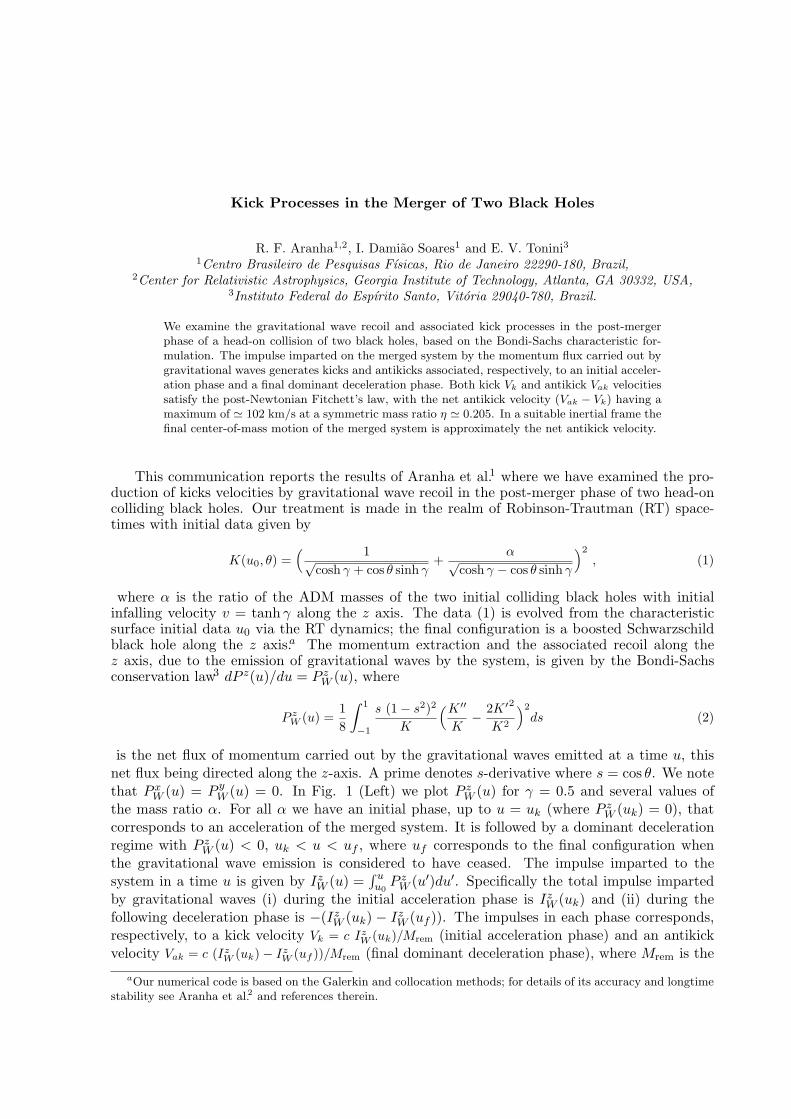
Kick Processes in the Merger of Two Black Holes
R. F. Aranha1,2, I. Damiao Soares1 and E. V. Tonini31Centro Brasileiro de Pesquisas Fısicas, Rio de Janeiro 22290-180, Brazil,
2Center for Relativistic Astrophysics, Georgia Institute of Technology, Atlanta, GA 30332, USA,3Instituto Federal do Espırito Santo, Vitoria 29040-780, Brazil.
We examine the gravitational wave recoil and associated kick processes in the post-mergerphase of a head-on collision of two black holes, based on the Bondi-Sachs characteristic for-mulation. The impulse imparted on the merged system by the momentum flux carried out bygravitational waves generates kicks and antikicks associated, respectively, to an initial acceler-ation phase and a final dominant deceleration phase. Both kick Vk and antikick Vak velocitiessatisfy the post-Newtonian Fitchett’s law, with the net antikick velocity (Vak − Vk) having amaximum of ' 102 km/s at a symmetric mass ratio η ' 0.205. In a suitable inertial frame thefinal center-of-mass motion of the merged system is approximately the net antikick velocity.
This communication reports the results of Aranha et al.1 where we have examined the pro-duction of kicks velocities by gravitational wave recoil in the post-merger phase of two head-oncolliding black holes. Our treatment is made in the realm of Robinson-Trautman (RT) space-times with initial data given by
K(u0, θ) =( 1√
cosh γ + cos θ sinh γ+
α√cosh γ − cos θ sinh γ
)2
, (1)
where α is the ratio of the ADM masses of the two initial colliding black holes with initialinfalling velocity v = tanh γ along the z axis. The data (1) is evolved from the characteristicsurface initial data u0 via the RT dynamics; the final configuration is a boosted Schwarzschildblack hole along the z axis.a The momentum extraction and the associated recoil along thez axis, due to the emission of gravitational waves by the system, is given by the Bondi-Sachsconservation law3 dP z(u)/du = P z
W (u), where
P zW (u) =
18
∫ 1
−1
s (1− s2)2
K
(K ′′
K− 2K ′2
K2
)2
ds (2)
is the net flux of momentum carried out by the gravitational waves emitted at a time u, thisnet flux being directed along the z-axis. A prime denotes s-derivative where s = cos θ. We notethat P x
W (u) = P yW (u) = 0. In Fig. 1 (Left) we plot P z
W (u) for γ = 0.5 and several values ofthe mass ratio α. For all α we have an initial phase, up to u = uk (where P z
W (uk) = 0), thatcorresponds to an acceleration of the merged system. It is followed by a dominant decelerationregime with P z
W (u) < 0, uk < u < uf , where uf corresponds to the final configuration whenthe gravitational wave emission is considered to have ceased. The impulse imparted to thesystem in a time u is given by Iz
W (u) =∫ uu0
P zW (u′)du′. Specifically the total impulse imparted
by gravitational waves (i) during the initial acceleration phase is IzW (uk) and (ii) during the
following deceleration phase is −(IzW (uk) − Iz
W (uf )). The impulses in each phase corresponds,respectively, to a kick velocity Vk = c Iz
W (uk)/Mrem (initial acceleration phase) and an antikickvelocity Vak = c (Iz
W (uk)− IzW (uf ))/Mrem (final dominant deceleration phase), where Mrem is the
aOur numerical code is based on the Galerkin and collocation methods; for details of its accuracy and longtimestability see Aranha et al.2 and references therein.
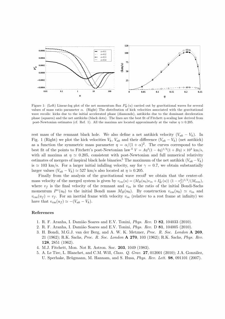
0.01 0.1 1 10 100
-0.0004
-0.0002
0.0000
0.0002
0.0004
0.0006
u
PWz
Α=0.4Α=0.3Α=0.2Α=0.1
æ
æ
æ
æ
æ
ææææ ææ
æ
æ
æ
í í í í í í ííííí í ííá
á
á
á
á
áááááá
á
á
á
0 0.05 0.1 0.15 0.2 0.25
25
50
75
100
120
Η
HkmsL
Figure 1: (Left) Linear-log plot of the net momentum flux P zW (u) carried out by gravitational waves for several
values of mass ratio parameter α. (Right) The distribution of kick velocities associated with the gravitationalwave recoils: kicks due to the initial accelerated phase (diamonds), antikicks due to the dominant decelerationphase (squares) and the net antikicks (black dots). The lines are the best fit of Fitchett η-scaling law derived frompost-Newtonian estimates (cf. Ref. 1). All the maxima are located approximately at the value η ' 0.205.
rest mass of the remnant black hole. We also define a net antikick velocity (Vak − Vk). InFig. 1 (Right) we plot the kick velocities Vk, Vak and their difference (Vak − Vk) (net antikick)as a function the symmetric mass parameter η = α/(1 + α)2. The curves correspond to thebest fit of the points to Fitchett’s post-Newtonian law 4 V = Aη2(1 − 4η)1/2(1 + Bη) × 103 km/s,with all maxima at η ' 0.205, consistent with post-Newtonian and full numerical relativityestimates of mergers of inspiral black hole binaries.5 The maximum of the net antikick (Vak−Vk)is ' 103 km/s. For a larger initial infalling velocity, say for γ = 0.7, we obtain substantiallylarger values (Vak − Vk) ' 527 km/s also located at η ' 0.205.
Finally from the analysis of the gravitational wave recoil1 we obtain that the center-of-mass velocity of the merged system is given by vcm(u) = (MB(u0)vin + Iz
W (u)) (1− v2f )1/2/(Mrem),
where vf is the final velocity of the remnant and vin is the ratio of the initial Bondi-Sachsmomentum P z(u0) to the initial Bondi mass MB(u0). By construction vcm(u0) ' vin andvcm(uf ) = vf . For an inertial frame with velocity vin (relative to a rest frame at infinity) wehave that vcm(uf ) ' −(Vak − Vk).
References
1. R. F. Aranha, I. Damiao Soares and E.V. Tonini, Phys. Rev. D 82, 104033 (2010).2. R. F. Aranha, I. Damiao Soares and E.V. Tonini, Phys. Rev. D 81, 104005 (2010).3. H. Bondi, M.G.J. van der Berg, and A. W. K. Metzner, Proc. R. Soc. London A 269,
21 (1962); R.K. Sachs, Proc. R. Soc. London A 270, 103 (1962); R.K. Sachs, Phys. Rev.128, 2851 (1962).
4. M.J. Fitchett, Mon. Not R. Astron. Soc. 203, 1049 (1983).5. A. Le Tiec, L. Blanchet, and C.M. Will, Class. Q. Grav. 27, 012001 (2010); J.A. Gonzalez,
U. Sperhake, Brugmann, M. Hannam, and S. Husa, Phys. Rev. Lett. 98, 091101 (2007).
COSMOLOGY MODELS AND GRAVITON COUNTING IN A DETECTOR
A.W. BECKWITHChongquing university department of physics 400044, Chonquing, PRC [email protected]
Initial relic entropy growth is presented We talk of how to count it as gravitons per unitphase space, and use it as an extension of gravitons interacting with a magnetic field of a GWdetector. We use it for obtaining values for choosing between cosmology models
1 Introduction
We start off with perturbative electromagnetic power flux, i.e. what was called(1)
T uv in terms ofa nonzero graviton rest mass, in a detector, in an uniform magnetic field, i.e. what if we havecurved space time with say an energy momentum tensor of the electro magnetic fields in GWfields as
T uv =1
µ0·[−FµαF να +
1
4· gµνFαβFαβ
](1)
Li et al1 state that Fµν = F(0)µν + F
(1)µν , with
∣∣∣F (1)µν
∣∣∣ ∣∣∣F (0)µν
∣∣∣ will lead to
T uv =(0)
T uv +(1)
T uv +(2)
T uv. (2)
The 1st term to the right hand side of Eq. (2) is the energy–momentum tensor of the background electro magnetic field, and the 2nd term to the right hand side of Eq. (1) is the firstorder perturbation of an electro magnetic field due to gravitational waves. The above Eq. (1)and Eq. (2) lead to Maxwell equations as 1√
−g ·∂∂xν ·
(√−g · gµαgνβFαβ
)= µ0J
µ as well as
F[µv,α = 0.
2 Making Sense of the Following Current Term Behavior
Eventually, with GW affecting the above two equations, we have a way to isolate(1)
T uv. If onelooks at if a four-dimensional graviton with a very small rest mass included,2 we can write
1√−g· ∂
∂xν·(√−g · gµαgνβFαβ
)= µ0J
µ + Jeffective, (3)
where for ε+ 6= 0 but very smallF[µv,α ∼ ε+. (4)
The claim which A. Beckwith made is that
Jeffective ' ncount ·m4-D Graviton. (5)
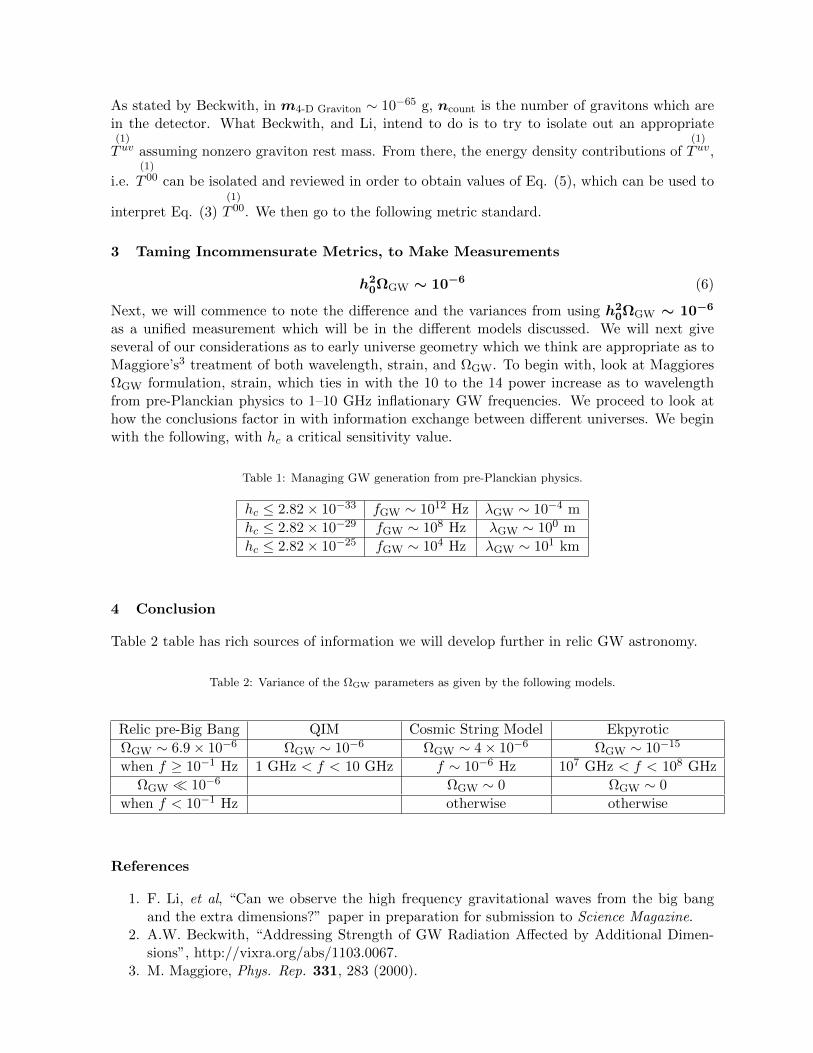
As stated by Beckwith, in m4-D Graviton ∼ 10−65 g, ncount is the number of gravitons which arein the detector. What Beckwith, and Li, intend to do is to try to isolate out an appropriate(1)
T uv assuming nonzero graviton rest mass. From there, the energy density contributions of(1)
T uv,
i.e.(1)
T 00 can be isolated and reviewed in order to obtain values of Eq. (5), which can be used to
interpret Eq. (3)(1)
T 00. We then go to the following metric standard.
3 Taming Incommensurate Metrics, to Make Measurements
h20ΩGW ∼ 10−6 (6)
Next, we will commence to note the difference and the variances from using h20ΩGW ∼ 10−6
as a unified measurement which will be in the different models discussed. We will next giveseveral of our considerations as to early universe geometry which we think are appropriate as toMaggiore’s3 treatment of both wavelength, strain, and ΩGW. To begin with, look at MaggioresΩGW formulation, strain, which ties in with the 10 to the 14 power increase as to wavelengthfrom pre-Planckian physics to 1–10 GHz inflationary GW frequencies. We proceed to look athow the conclusions factor in with information exchange between different universes. We beginwith the following, with hc a critical sensitivity value.
Table 1: Managing GW generation from pre-Planckian physics.
hc ≤ 2.82× 10⁻³³ fGW ∼ 1012 Hz λGW ∼ 10−4 m
hc ≤ 2.82× 10⁻²⁹ fGW ∼ 108 Hz λGW ∼ 100 m
hc ≤ 2.82× 10⁻²⁵ fGW ∼ 104 Hz λGW ∼ 101 km
4 Conclusion
Table 2 table has rich sources of information we will develop further in relic GW astronomy.
Table 2: Variance of the ΩGW parameters as given by the following models.
Relic pre-Big Bang QIM Cosmic String Model Ekpyrotic
ΩGW ∼ 6.9× 10⁻⁶ ΩGW ∼ 10−6 ΩGW ∼ 4× 10⁻⁶ ΩGW ∼ 10−15
when f ≥ 10−1 Hz 1 GHz < f < 10 GHz f ∼ 10−6 Hz 107 GHz < f < 108 GHz
ΩGW 10−6 ΩGW ∼ 0 ΩGW ∼ 0
when f < 10−1 Hz otherwise otherwise
References
1. F. Li, et al, “Can we observe the high frequency gravitational waves from the big bangand the extra dimensions?” paper in preparation for submission to Science Magazine.
2. A.W. Beckwith, “Addressing Strength of GW Radiation Affected by Additional Dimen-sions”, http://vixra.org/abs/1103.0067.
3. M. Maggiore, Phys. Rep. 331, 283 (2000).
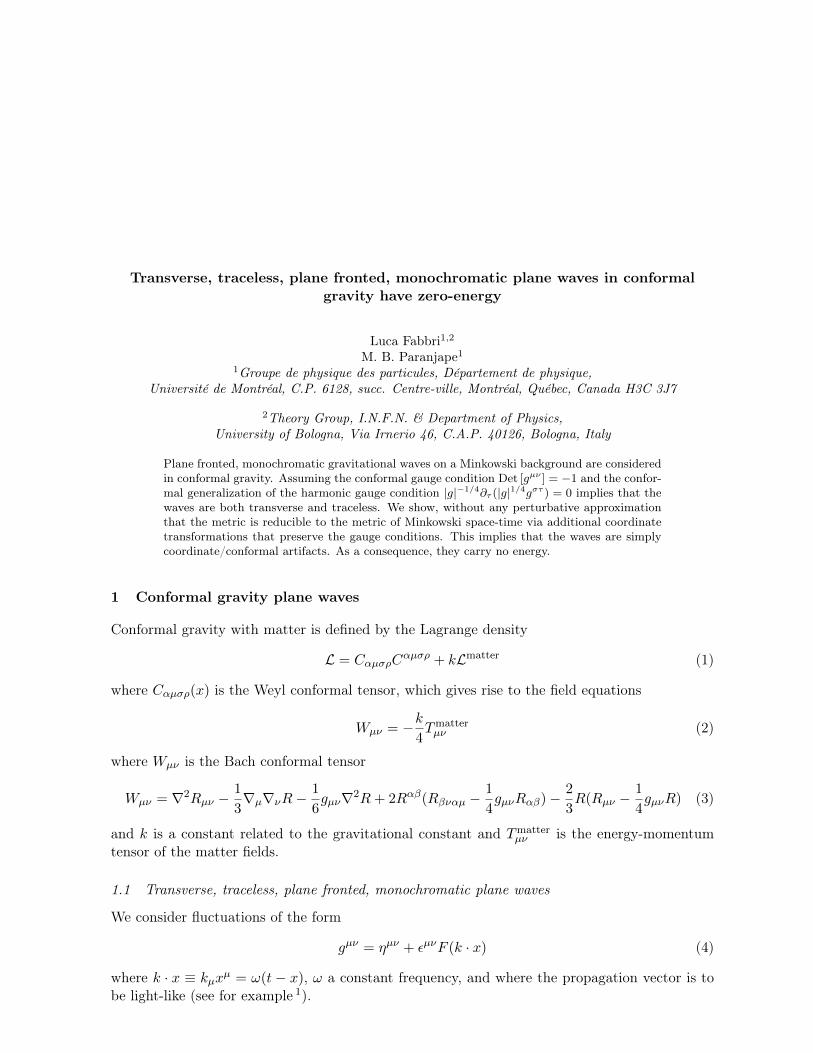
Transverse, traceless, plane fronted, monochromatic plane waves in conformalgravity have zero-energy
Luca Fabbri1,2M. B. Paranjape1
1Groupe de physique des particules, Département de physique,Université de Montréal, C.P. 6128, succ. Centre-ville, Montréal, Québec, Canada H3C 3J7
2Theory Group, I.N.F.N. & Department of Physics,University of Bologna, Via Irnerio 46, C.A.P. 40126, Bologna, Italy
Plane fronted, monochromatic gravitational waves on a Minkowski background are consideredin conformal gravity. Assuming the conformal gauge condition Det [gµν ] = −1 and the confor-mal generalization of the harmonic gauge condition |g|−1/4∂τ (|g|1/4gστ ) = 0 implies that thewaves are both transverse and traceless. We show, without any perturbative approximationthat the metric is reducible to the metric of Minkowski space-time via additional coordinatetransformations that preserve the gauge conditions. This implies that the waves are simplycoordinate/conformal artifacts. As a consequence, they carry no energy.
1 Conformal gravity plane waves
Conformal gravity with matter is defined by the Lagrange density
L = CαµσρCαµσρ + kLmatter (1)
where Cαµσρ(x) is the Weyl conformal tensor, which gives rise to the field equations
Wµν = −k4Tmatterµν (2)
where Wµν is the Bach conformal tensor
Wµν = ∇2Rµν −1
3∇µ∇νR−
1
6gµν∇2R+ 2Rαβ(Rβναµ −
1
4gµνRαβ)− 2
3R(Rµν −
1
4gµνR) (3)
and k is a constant related to the gravitational constant and Tmatterµν is the energy-momentum
tensor of the matter fields.
1.1 Transverse, traceless, plane fronted, monochromatic plane waves
We consider fluctuations of the form
gµν = ηµν + εµνF (k · x) (4)
where k · x ≡ kµxµ = ω(t − x), ω a constant frequency, and where the propagation vector is to
be light-like (see for example 1).
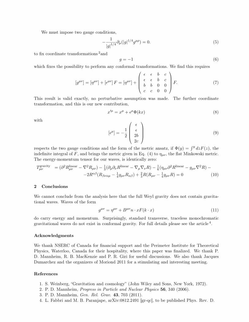
We must impose two gauge conditions,
− 1
|g|1/4∂µ(|g|1/4gµρ) = 0. (5)
to fix coordinate transformations 2andg = −1 (6)
which fixes the possibility to perform any conformal transformations. We find this requires
[gµν ] = [ηµν ] + [εµν ]F = [ηµν ] +
ε ε b cε ε b cb b 0 0c c 0 0
F. (7)
This result is valid exactly, no perturbative assumption was made. The further coordinatetransformation, and this is our new contribution,
x′µ = xµ + εµΦ(kx) (8)
with
[εµ] = −1
2
εε2b2c
(9)
respects the two gauge conditions and the form of the metric ansatz, if Φ(y) =∫ y dzF (z), the
indefinite integral of F , and brings the metric given in Eq. (4) to ηµν , the flat Minkowski metric.The energy-momentum tensor for our waves, is identically zero:
T gravityµν = (∂2Rlinear
µν −∇2Rµν)− 13(∂µ∂νR
linear −∇µ∇νR)− 16(ηµν∂
2Rlinear − gµν∇2R)−−2Rαβ(Rβναµ − 1
4gµνRαβ) + 23R(Rµν − 1
4gµνR) = 0 (10)
2 Conclusions
We cannot conclude from the analysis here that the full Weyl gravity does not contain gravita-tional waves. Waves of the form
gµν = ηµν +Bµνn · xF (k · x) (11)
do carry energy and momentum. Surprisingly, standard transverse, traceless monochromaticgravitational waves do not exist in conformal gravity. For full details please see the article 4.
Acknowledgments
We thank NSERC of Canada for financial support and the Perimeter Institute for TheoreticalPhysics, Waterloo, Canada for their hospitality, where this paper was finalized. We thank P.D. Mannheim, R. B. MacKenzie and P. R. Giri for useful discussions. We also thank JacquesDumarchez and the organizers of Moriond 2011 for a stimulating and interesting meeting.
References
1. S. Weinberg, “Gravitation and cosmology” (John Wiley and Sons, New York, 1972).2. P. D. Mannheim, Progress in Particle and Nuclear Physics 56, 340 (2006).3. P. D. Mannheim, Gen. Rel. Grav. 43, 703 (2011).4. L. Fabbri and M. B. Paranjape, arXiv:0812.2491 [gr-qc], to be published Phys. Rev. D.
Gravitational wave recoil in nonsymmetric Robinson-Trautman spacetimes
Rodrigo P. MacedoMax-Planck-Institut fur Gravitationsphysik, Albert Einstein Institut, Potsdam, Germany, and
Theoretical Physics Institute, University of Jena, 07743 Jena, Germany
Alberto SaaDepartamento de Matematica Aplicada, UNICAMP, 13083-859 Campinas, SP, Brazil
We present some preliminary results on the gravitational recoil due to gravitational wave
emission in the context of nonsymmetric Robinson-Trautman spacetimes. As in the axisym-
metric case, regular initial data evolve generically into a final configuration corresponding to
a Schwarzschild black-hole moving with constant speed. If the initial data is symmetric under
reflection by a given plan, the remnant black-hole velocity must be parallel to this plan. In
particular, for the case of completely reflection-symmetric initial configurations, the remnant
black-hole velocity vanishes and the final configuration can be determined exactly from the
initial data as in the axisymmetric case.
1 Introduction
We have recently 1 presented an analysis of the recoil due to gravitational wave emission 2 inthe context of axisymmetric Robinson-Trautman (RT) spacetimes. Several physically relevantsituations can be described by axisymmetric spacetimes. We mention, in particular, the casescorresponding to the evolution of the Brill-Lindquist initial data 3, which can be interpretedas the frontal collision of two black-holes 4,5. Clearly, however, realistic physical applicationsdemand the analysis of nonsymmetric situations.
We are now extending our previous analysis 1 to nonsymmetric RT spacetimes. We areparticulary interested in approximated or “empirical” formulas relating the recoil velocity andthe initial data 6, which could have potential application to the problem of the merging processof binary black-holes, where asymmetrical gravitational wave emission is known to make themerger remnant to recoil with velocities up to several thousands of km/s 7. Our idea is tointroduce an efficient full numerical approach based in the Galerkin spectral method to analyzethe non-linear regime of the nonsymmetric Robinson-Trautman equations, and we expect toshow that the direction and modulus of the recoil velocity can indeed be estimated with goodaccuracy from the initial data with fairly modest computational resources.
The Robinson-Trautman partial differential equation has been analyzed numerically in therecent literature8,9,10,11. The axisymmetric approach presented in1 includes some improvementson the Galerkin method implementation of Oliveira and Soares 10,11 which has allowed us toget simpler equations and a better overall accuracy. Nevertheless, as we will see, computationalcomplexity issues prevent us of applying the Galerkin method of 1 directly to the nonsymmet-ric case. A full-numerical approach with some intermediate projections is mandatory for thenonsymmetric case.
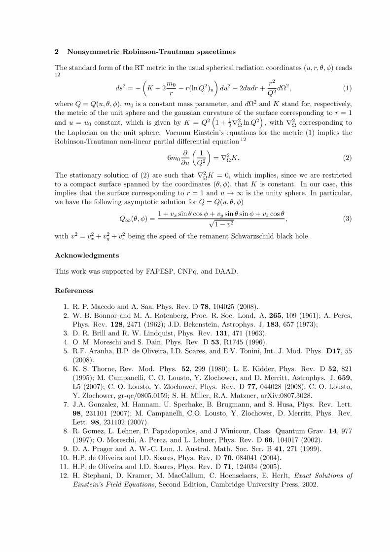
2 Nonsymmetric Robinson-Trautman spacetimes
The standard form of the RT metric in the usual spherical radiation coordinates (u, r, θ, φ) reads12
ds2 = −
(
K − 2m0
r− r(lnQ2)u
)
du2 − 2dudr +r2
Q2dΩ2, (1)
where Q = Q(u, θ, φ), m0 is a constant mass parameter, and dΩ2 and K stand for, respectively,the metric of the unit sphere and the gaussian curvature of the surface corresponding to r = 1
and u = u0 constant, which is given by K = Q2
(
1 + 1
2∇2
ΩlnQ2
)
, with ∇2
Ωcorresponding to
the Laplacian on the unit sphere. Vacuum Einstein’s equations for the metric (1) implies theRobinson-Trautman non-linear partial differential equation 12
6m0
∂
∂u
(
1
Q2
)
= ∇2
ΩK. (2)
The stationary solution of (2) are such that ∇2
ΩK = 0, which implies, since we are restricted
to a compact surface spanned by the coordinates (θ, φ), that K is constant. In our case, thisimplies that the surface corresponding to r = 1 and u → ∞ is the unity sphere. In particular,we have the following asymptotic solution for Q = Q(u, θ, φ)
Q∞(θ, φ) =
1 + vx sin θ cosφ+ vy sin θ sinφ+ vz cos θ√1− v2
, (3)
with v2 = v2x + v2y + v2z being the speed of the remanent Schwarzschild black hole.
Acknowledgments
This work was supported by FAPESP, CNPq, and DAAD.
References
1. R. P. Macedo and A. Saa, Phys. Rev. D 78, 104025 (2008).2. W. B. Bonnor and M. A. Rotenberg, Proc. R. Soc. Lond. A. 265, 109 (1961); A. Peres,
Phys. Rev. 128, 2471 (1962); J.D. Bekenstein, Astrophys. J. 183, 657 (1973);3. D. R. Brill and R. W. Lindquist, Phys. Rev. 131, 471 (1963).4. O. M. Moreschi and S. Dain, Phys. Rev. D 53, R1745 (1996).5. R.F. Aranha, H.P. de Oliveira, I.D. Soares, and E.V. Tonini, Int. J. Mod. Phys. D17, 55
(2008).6. K. S. Thorne, Rev. Mod. Phys. 52, 299 (1980); L. E. Kidder, Phys. Rev. D 52, 821
(1995); M. Campanelli, C. O. Lousto, Y. Zlochower, and D. Merritt, Astrophys. J. 659,L5 (2007); C. O. Lousto, Y. Zlochower, Phys. Rev. D 77, 044028 (2008); C. O. Lousto,Y. Zlochower, gr-qc/0805.0159; S. H. Miller, R.A. Matzner, arXiv:0807.3028.
7. J.A. Gonzalez, M. Hannam, U. Sperhake, B. Brugmann, and S. Husa, Phys. Rev. Lett.98, 231101 (2007); M. Campanelli, C.O. Lousto, Y. Zlochower, D. Merritt, Phys. Rev.Lett. 98, 231102 (2007).
8. R. Gomez, L. Lehner, P. Papadopoulos, and J Winicour, Class. Quantum Grav. 14, 977(1997); O. Moreschi, A. Perez, and L. Lehner, Phys. Rev. D 66, 104017 (2002).
9. D. A. Prager and A. W.-C. Lun, J. Austral. Math. Soc. Ser. B 41, 271 (1999).10. H.P. de Oliveira and I.D. Soares, Phys. Rev. D 70, 084041 (2004).11. H.P. de Oliveira and I.D. Soares, Phys. Rev. D 71, 124034 (2005).12. H. Stephani, D. Kramer, M. MacCallum, C. Hoenselaers, E. Herlt, Exact Solutions of
Einstein’s Field Equations, Second Edition, Cambridge University Press, 2002.
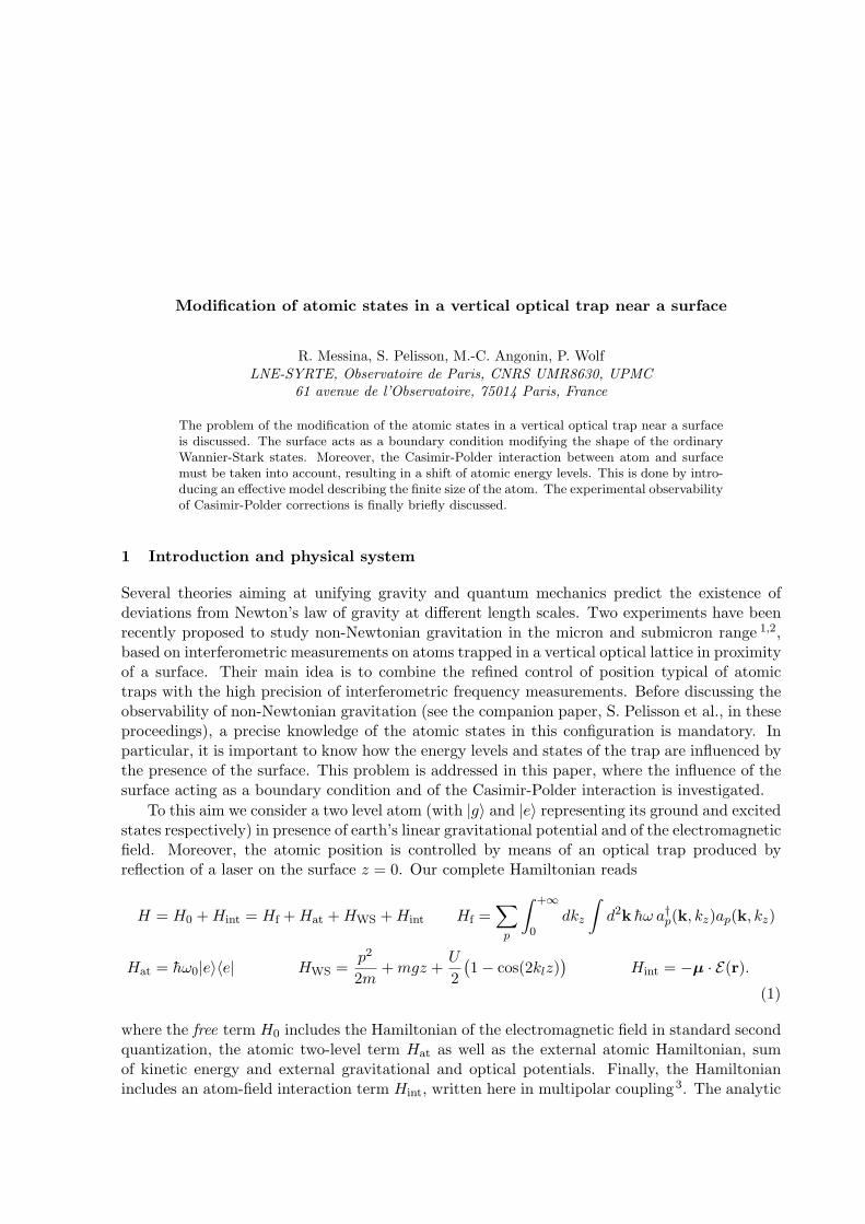
Modification of atomic states in a vertical optical trap near a surface
R. Messina, S. Pelisson, M.-C. Angonin, P. WolfLNE-SYRTE, Observatoire de Paris, CNRS UMR8630, UPMC
61 avenue de l’Observatoire, 75014 Paris, France
The problem of the modification of the atomic states in a vertical optical trap near a surfaceis discussed. The surface acts as a boundary condition modifying the shape of the ordinaryWannier-Stark states. Moreover, the Casimir-Polder interaction between atom and surfacemust be taken into account, resulting in a shift of atomic energy levels. This is done by intro-ducing an effective model describing the finite size of the atom. The experimental observabilityof Casimir-Polder corrections is finally briefly discussed.
1 Introduction and physical system
Several theories aiming at unifying gravity and quantum mechanics predict the existence ofdeviations from Newton’s law of gravity at different length scales. Two experiments have beenrecently proposed to study non-Newtonian gravitation in the micron and submicron range 1,2,based on interferometric measurements on atoms trapped in a vertical optical lattice in proximityof a surface. Their main idea is to combine the refined control of position typical of atomictraps with the high precision of interferometric frequency measurements. Before discussing theobservability of non-Newtonian gravitation (see the companion paper, S. Pelisson et al., in theseproceedings), a precise knowledge of the atomic states in this configuration is mandatory. Inparticular, it is important to know how the energy levels and states of the trap are influenced bythe presence of the surface. This problem is addressed in this paper, where the influence of thesurface acting as a boundary condition and of the Casimir-Polder interaction is investigated.
To this aim we consider a two level atom (with |g〉 and |e〉 representing its ground and excitedstates respectively) in presence of earth’s linear gravitational potential and of the electromagneticfield. Moreover, the atomic position is controlled by means of an optical trap produced byreflection of a laser on the surface z = 0. Our complete Hamiltonian reads
H = H0 +Hint = Hf +Hat +HWS +Hint Hf =∑p
∫ +∞
0dkz
∫d2k hω a†p(k, kz)ap(k, kz)
Hat = hω0|e〉〈e| HWS =p2
2m+mgz +
U
2(1− cos(2klz)
)Hint = −µ · E(r).
(1)
where the free term H0 includes the Hamiltonian of the electromagnetic field in standard secondquantization, the atomic two-level term Hat as well as the external atomic Hamiltonian, sumof kinetic energy and external gravitational and optical potentials. Finally, the Hamiltonianincludes an atom-field interaction term Hint, written here in multipolar coupling 3. The analytic
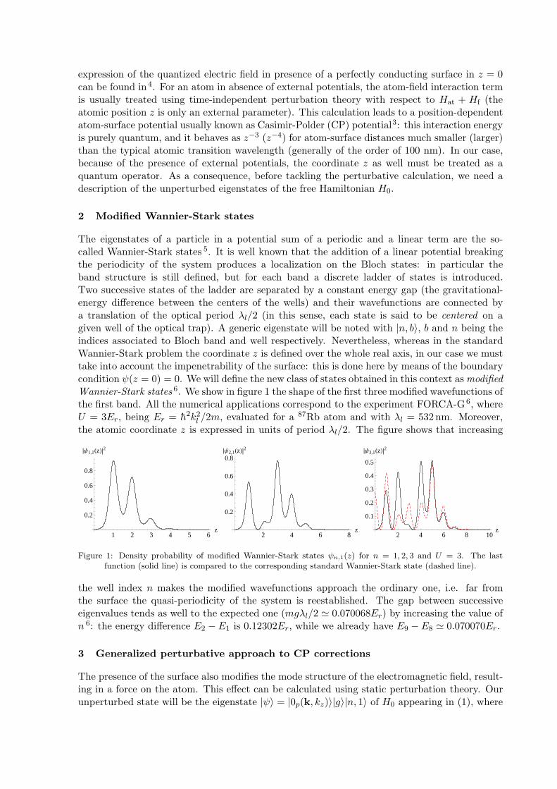
expression of the quantized electric field in presence of a perfectly conducting surface in z = 0can be found in 4. For an atom in absence of external potentials, the atom-field interaction termis usually treated using time-independent perturbation theory with respect to Hat + Hf (theatomic position z is only an external parameter). This calculation leads to a position-dependentatom-surface potential usually known as Casimir-Polder (CP) potential3: this interaction energyis purely quantum, and it behaves as z−3 (z−4) for atom-surface distances much smaller (larger)than the typical atomic transition wavelength (generally of the order of 100 nm). In our case,because of the presence of external potentials, the coordinate z as well must be treated as aquantum operator. As a consequence, before tackling the perturbative calculation, we need adescription of the unperturbed eigenstates of the free Hamiltonian H0.
2 Modified Wannier-Stark states
The eigenstates of a particle in a potential sum of a periodic and a linear term are the so-called Wannier-Stark states 5. It is well known that the addition of a linear potential breakingthe periodicity of the system produces a localization on the Bloch states: in particular theband structure is still defined, but for each band a discrete ladder of states is introduced.Two successive states of the ladder are separated by a constant energy gap (the gravitational-energy difference between the centers of the wells) and their wavefunctions are connected bya translation of the optical period λl/2 (in this sense, each state is said to be centered on agiven well of the optical trap). A generic eigenstate will be noted with |n, b〉, b and n being theindices associated to Bloch band and well respectively. Nevertheless, whereas in the standardWannier-Stark problem the coordinate z is defined over the whole real axis, in our case we musttake into account the impenetrability of the surface: this is done here by means of the boundarycondition ψ(z = 0) = 0. We will define the new class of states obtained in this context as modifiedWannier-Stark states 6. We show in figure 1 the shape of the first three modified wavefunctions ofthe first band. All the numerical applications correspond to the experiment FORCA-G 6, whereU = 3Er, being Er = h2k2
l /2m, evaluated for a 87Rb atom and with λl = 532 nm. Moreover,the atomic coordinate z is expressed in units of period λl/2. The figure shows that increasing
1 2 3 4 5 6z
0.2
0.4
0.6
0.8
ÈΨ1,1HzL2
2 4 6 8z
0.2
0.4
0.6
0.8ÈΨ2,1HzL
2
2 4 6 8 10z
0.1
0.2
0.3
0.4
0.5
ÈΨ3,1HzL2
Figure 1: Density probability of modified Wannier-Stark states ψn,1(z) for n = 1, 2, 3 and U = 3. The lastfunction (solid line) is compared to the corresponding standard Wannier-Stark state (dashed line).
the well index n makes the modified wavefunctions approach the ordinary one, i.e. far fromthe surface the quasi-periodicity of the system is reestablished. The gap between successiveeigenvalues tends as well to the expected one (mgλl/2 ' 0.070068Er) by increasing the value ofn 6: the energy difference E2 − E1 is 0.12302Er, while we already have E9 − E8 ' 0.070070Er.
3 Generalized perturbative approach to CP corrections
The presence of the surface also modifies the mode structure of the electromagnetic field, result-ing in a force on the atom. This effect can be calculated using static perturbation theory. Ourunperturbed state will be the eigenstate |ψ〉 = |0p(k, kz)〉|g〉|n, 1〉 of H0 appearing in (1), where
the field is in its vacuum state. Second-order perturbation theory is needed: Hint can connect|ψ〉 to any intermediate state having one photon in a given mode, while the atom can occupyany well of any band being nevertheless necessarily in its excited internal state. We then obtain
∆En,1 = −∑p
∫ +∞
0dkz
∫d2k
+∞∑
s=1
+∞∑
b=1
∣∣〈n, 1|〈g|〈0p(k, kz)|Hint|1p(k, kz)〉|e〉|s, b〉∣∣2
E(0)s,b − E(0)
n,1 + h(ω + ω0)(2)
where E(0)s,b is the unperturbed external atomic energy associated to the s-th well of the b-th Bloch
band. It can be shown6 that for our physical system the correction (2) approximately equals theaverage on the state |n, 1〉 of the standard CP potential. This interaction energy is theoreticallyknown for a neutral atom having dynamical polarizability α(ω), at an arbitrary temperatureT > 0 and for a surface having arbitrary dielectric properties 3. Since each wavefunction ofinterest ψn,1(z) tends to zero linearly in z for z → 0 and the CP potential behaves as z−3
near the origin, each correction ∆En,1 is indeed divergent. Nevertheless, the z−3 behaviour isa consequence of treating the atom as pointlike and can be corrected by replacing it with aprobability distribution ρ(r) different from zero over a spherical volume 7. In this case, for anyatomic effective radius R and choice of the probability distribution, the potential energy shows,a z−1 behaviour near the origin. This property regularizes our energy correction. The new CPpotential (to be averaged on the |n, 1〉 state in order to obtain the energy shift) is itself obtainedfrom the average over ρ(r) of the standard potential VCP(z). The energy corrections to eachwell can now be evaluated, after choosing an effective radius and a probability distribution. Wepresent in table 1 the results (in the case of a perfectly conducting surface) for the first twelvewells for a uniform distribution over a sphere having the effective radius R = 235 pm8. From the
Table 1: Absolute value (in units of Hertz) of the CP energy corrections (they are all changed in sign) to the first12 modified Wannier-Stark states for U = 3. The notation a[b] corresponds to a× 10b.
n ∆En,1 n ∆En,1 n ∆En,1 n ∆En,1 n ∆En,1 n ∆En,11 1.88[5] 3 9.37[4] 5 2.26[4] 7 1.51[3] 9 5.34[1] 11 6.762 1.38[5] 4 5.31[4] 6 6.80[3] 8 2.79[2] 10 1.47[1] 12 4.14
table we see that, in virtue of the absolute precision of approximately 10−4 Hz in the frequencymeasurement, the energy shift due to the CP interaction is detectable up to at least the twelfthwell. Two measurement schemes can be imagined. A first one is at short distances (say less than5µm) where the validity of the model can be tested: this would at the same time allow to give anestimation of the effective radius. A second one is at larger distances, for example between 5 and10µm, where the influence of regularization is below the experimental sensitivity: in this case,since the CP correction is still experimentally detectable (at 10µm we have VCP ' 0.06 Hz), wewould obtain a measurement of the electrodynamical effect.
References
1. P. Wolf et al., Phys. Rev. A 75, 063608 (2007).2. F. Sorrentino et al., Phys. Rev. A 79, 013409 (2009).3. S. Scheel and S. Y. Buhmann, Acta Phys. Slov. 58, 675 (2008) (and references therein).4. G. Barton, J. Phys. B 7, 2134 (1974).5. M. Gluck, A. R. Kolovsky, and H. J. Korsch, Phys. Rep. 366, 103 (2002).6. R. Messina, S. Pelisson, M.-C. Angonin, and P. Wolf, Phys. Rev. A 83, 052111 (2011).7. G. Compagno, R. Passante, and F. Persico, Europhys. Lett. 7, 399 (1988).8. J. C. Slater, J. Chem. Phys. 41, 3199 (1964).

TORSION PENDULUM WITH 2 DOF FOR THE STUDY OF RESIDUALCOUPLINGS BETWEEN THE TM AND THE GRS: APPROACHING
THERMAL NOISE LIMITED SENSITIVITY
L. MARCONI, R. STANGA, C. GRIMANI, M. BASSAN, L. DI FIORE, R. DE ROSA and F. GARUFIUniversita degli Studi di Firenze and INFN Firenze, ItalyUniversita degli Studi di Firenze and INFN Firenze, Italy
Universita di Urbino and INFN FIRENZE, ItalyUniversita di Roma Tor Vergata and INFN Roma 2, Italy
INFN Napoli, ItalyUniversita Federico II and INFN Napoli, ItalyUniversita Federico II and INFN Napoli, Italy
The LISA test-mass (TM) is sensitive to weak forces along all 6 Degrees of Freedom (DoFs).Extensive ground testing is required in order to evaluate the influence of cross-talks of read-outs and actuators operating on different DoFs. To best represent the flight conditions, wedeveloped in Firenze a facility with 2 soft DoFs. Using this facility we measure the forces andstiffnesses acting simultaneously along the 2 soft DoFs and, more specifically, we will measureactuation cross talks with closed feedback loop. The facility is now completed with a replicaof the GRS (Gravitational Reference Sensor) and the flight model of the electronics boards.
1 Introduction
In Firenze we developed a facility to verify the residual acceleration on 2 DoFs between the TMof LISA ? and the GRS ?. Following the previous experience from Trento ? and Washington ? inorder to have a TM in free fall condition on 2 DoFs (1 translation and 1 rotation) we have builta double torsion pendulum ?. With our choices (of materials and geometry) we will achieve asensitivity in acceleration for the 2 DoFs comparable with the sensitivity of LISA PF ?:
S1/2a = 3 · 10−14ms−2/
√Hz @ 1mHz, (1)
2 Commissioning
After some tests with a preliminary copy of the TM-GRS ? we are using now a flight modelreplica of the TM, GRS and the electronics. We started working with only the rotation DoF ofthe TM. In Fig. ?? we show the results of the feedback control. In the control loop we have alsointegrated the movement of the motorized stages, necessary to center the TM in the GRS. InFig. ?? we show the result of the first measurement of the noise on ϕ. In (a) panel the squareroot of the power spectral density of the angular displacement is presented, considering an armlength of 0.02m, equal to the sensing electrodes separation and a mass for the TM equal to themass of the TM of LISA PF, we derive the square root of the power spectral density of thelinear acceleration, shown in the (b) panel. As it can be seen, in the high frequency band we are
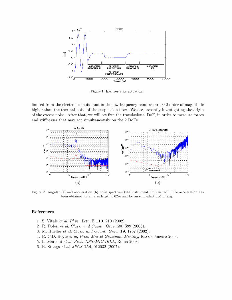
Figure 1: Electrostatics actuation.
limited from the electronics noise and in the low frequency band we are ∼ 2 order of magnitudehigher than the thermal noise of the suspension fiber. We are presently investigating the originof the excess noise. After that, we will set free the translational DoF, in order to measure forcesand stiffnesses that may act simultaneously on the 2 DoFs.
(a) (b)
Figure 2: Angular (a) and acceleration (b) noise spectrum (the instrument limit in red). The acceleration hasbeen obtained for an arm length 0.02m and for an equivalent TM of 2kg.
References
1. S. Vitale et al, Phys. Lett. B 110, 210 (2002).2. R. Dolesi et al, Class. and Quant. Grav. 20, S99 (2003).3. M. Hueller et al, Class. and Quant. Grav. 19, 1757 (2002).4. R. C.D. Hoyle et al, Proc. Marcel Grossman Meeting, Rio de Janeiro 2003.5. L. Marconi et al, Proc. NSS/MIC IEEE, Roma 2003.6. R. Stanga et al, JPCS 154, 012032 (2007).

Listof
Participants


Family name First name Institution Country Email addressAbele Hartmut Atominstitut - TU Wien Austria [email protected]
Adelberger Eric University of Washington - CENPA USA [email protected] Bruce MPI - Gravitational Physics Germany [email protected]
Angonin Marie-Christine SYRTE Observatoire de Paris / UPMC France [email protected] Reza LAL France [email protected]
Antoniadis Ignatios CERN - TH Switzerland [email protected] Cosimo IPMU - The University of Tokyo Japan [email protected]
Bassan Massimo Universitá Tor Vergata Italy [email protected] Andrew Chongquing University China [email protected]
Belczynski Chris Warsaw University Poland [email protected] Jacopo Universitá di Pisa Italy [email protected] Angus Institute for Gravitational Research UK [email protected]
Bender Peter L. JILA - Univ. of Colorado USA [email protected]é Olivier Astronomiacl Strasbourg Observatory France [email protected]
Bize Sébastien SYRTE, Observatoire de Paris France [email protected] David University of Western Australia Australia [email protected]
Blanchard Alain IRAP France [email protected] Luc IAP France [email protected]
Blas Diego EPFL Switzerland [email protected] Timothy LIGO - MIT USA [email protected] Yuri Universidad Nacional Autónoma Mexico [email protected] Philippe Lab. Photonique, Numériques & Nanosciences France [email protected]
Branchesi Marica INFN / Universitá di Urbino Italy [email protected] Frank University of Jena Germany [email protected]
Cacciapuoti Luigi European Space Agency / ESTEC The Netherlands [email protected] Abel Univ.Autonoma Metropolitana-Iztapalapa Mexico [email protected]
Canali Carlo Uiversitá degli Studi di Genova - INFN Italy [email protected] Fabien LAL France [email protected] Eleanor University of Birmingham UK [email protected]
Champion David Max-Planck-Institut für Radioastronomie Germany [email protected] Yanbei California Institute of Technology USA [email protected]
Christensen Nelson Carleton College USA [email protected] Bruno ONERA - DMPH France [email protected]
Clark Caroline Imperial College London UK [email protected] David University of Western Australia Australia [email protected]
Cruise Mike University of Birmingham UK [email protected] Gregorio Paolo Politecnico di Torino Italy [email protected]
Delva Pacôme SYRTE - Paris Observatory / UPMC France [email protected] Thomas Physics & Astronomy, Cardiff University UK [email protected]
Dumarchez Jacques LPNHE France [email protected]é Pierre CEA Saclay DSM/IRFU/SPP France [email protected]
Fafone Viviana University of Roma Tor Vergata Italy [email protected] Agnes Observatoire de Besançon / Inst. UTINAM France [email protected]
Figueroa Daniel University of Helsinki / HIP Finland [email protected] Ephraim Purdue University USA [email protected]
Gai Mario INAF- Osservatorio Astronomico di Torino Italy [email protected] Andrew University of Nevada USA [email protected] Hartmut AEI Hannover Germany [email protected]
Gualtieri Leonardo Sapienza Universitá di Roma Italy [email protected] Delphine LPNHE - UPMC France [email protected]
Hees Aurelien Royal Observatory of Belgium Belgium [email protected] Martin AEI Hannover Germany [email protected]
Hirtz-Léon Sylvie CNES France [email protected]
XLVIth Rencontres de Moriond
Gravitational Waves & Experimental Gravity
List of Participants

Family name First name Institution Country Email addressHohensee Michael University of California USA [email protected]
Hough James University of Glasgow UK [email protected] Cédric University of Zurich Switzerland [email protected]
Iorio Lorenzo MIUR Italy [email protected] Marc-Thierry LPT - ENS France [email protected] Tobias Atominstitut Austria [email protected]
Jenkins Jere Purdue Univ. School of Nuclear Engineering USA [email protected] Oliver European Space Agency The Netherlands [email protected]
Kandhasamy Shivaraj University of Minnesota USA [email protected] Mark Varian Physics USA [email protected] Wlodek Copernicus Astronomical Center Poland [email protected]
Kowalska Izabela University of Warsaw Poland [email protected] Andrzej Institute of Matheamtics - PAN Poland [email protected] Patrick AEI Germany [email protected]
Lamine Brahim UPMC - LKB France [email protected] Tiec Alexandre Maryland Center for Fundamental Physics USA [email protected]
Lemonde Pierre CNRS - LNE - SYRTE France [email protected] Benjamin ONERA France [email protected]
Levy Agnès ONERA France [email protected] Josh Indiana University USA [email protected]
Magneville Christophe CEA Saclay France [email protected] João Imperial College UK [email protected]
Malec Beata Copernicus Center For Interdisciplinary Studies Poland [email protected] Lorenzo Universitá di Firenze / INFN Italy [email protected] Julien European Gravitational Observatory Italy [email protected]
Mazur Pawel University of South Carolina USA [email protected] Paul ESA - ESTEC The Netherlands [email protected]
Messina Riccardo SYRTE, Observatoire de Paris France [email protected] Hinrich University of Wuppertal Germany [email protected]
Meynadier Frédéric SYRTE -- Observatoire de Paris France [email protected] Anthony Oak Ridge National Laboratory USA [email protected]
Mozaffari Ali Imperial College London UK [email protected] Moritz Humboldt-Universität / AG QOM Germany [email protected]
Nawrodt Ronny Friedrich-Schiller-University Jena Germany [email protected] Patrick IPNL France [email protected]
Nesvizhevsky Valery Institut Laue-Langevin France [email protected] Anna M Universitá di Pisa Italy [email protected]
Normandin Marc University of Texas USA [email protected] Cristiano INFN Italy [email protected]
Paranjape Manu Université de Montréal Canada [email protected] Sophie SYRTE, Observatoire de Paris France [email protected]
Pelle Bruno SYRTE - Observatoire de Paris France [email protected] Guy Observatoire de Paris / LESIA France [email protected] Achim Humboldt-Universitaet zu Berlin Germany [email protected] Ernst Maria Hannover Institute of Quantum Optics Germany [email protected]
Raymond Vivien Northwestern University - CIERA USA [email protected] Serge LKB France [email protected] Luciano Albert Einstein Institute Germany [email protected] Florent LAL France [email protected] Alessio INFN Roma Tor Vergata Italy [email protected]
Romalis Michael Princeton University USA [email protected] Dorota University of Zielona Góra Poland [email protected]
Rosowsky André CEA Saclay France [email protected] Sheila University of Glasgow UK [email protected]
Rudenko Valentin Sternberg Astronomical Institute - MSU Russia [email protected] Alberto University of Campinas Brazil [email protected]
Sadoyan Avetis Abel Astronomical Rechen Institute Germany [email protected] Vern LIGO Hanford Observatory USA [email protected]
Sathyaprakash Bangalore Cardiff University UK [email protected]

Family name First name Institution Country Email addressSchnabel Roman AEI Germany [email protected]
Schuldt Thilo University of Applied Sciences Germany [email protected] Anna University of Zielona Góra Poland [email protected] Ivano Damião Centro Brasileiro de Pesquisas Fisicas / MCT Brazil [email protected] Clive University of Birmingham UK [email protected]
Stairs Ingrid University of British Columbia Canada [email protected] Toshikazu KEK Japan [email protected] Jay Whitman College USA [email protected] William University of Washington CENPA USA [email protected] Daniel Imperial College UK [email protected]
Tobar Michael The University of Western Australia Australia [email protected] Pierre ONERA France [email protected]
Veitch John Cardiff University UK [email protected] Ashok Kumar Observatoire de Besançon / inst. UTINAM France [email protected]
Vinet Jean-Yves ARTEMIS, OCA France [email protected] Todd University of Washington - CENPA USA [email protected]
Ward Robert APC France [email protected] Michal LAL France [email protected]
Weber William Joseph Universitá di Trento Italy [email protected] Carol LIGO Hanford Observatory USA [email protected]
Wolf Peter LNE - SYRTE, Observatoire de Paris France [email protected] Igor LIGO Livingston Observatory USA [email protected] Lien Universita di Firenze Italy [email protected] Alexander ITEP Russia [email protected]

Related Documents