2. Theories of Learning - Imperial College London · 23 Chapter 2 2. Theories of Learning Learning in animals and humans has been intensively studied in the scientific manner since

23

Chapter 2

2. Theories of Learning

Learning in animals and humans has been intensively studied in the scientific

manner since the beginning of this century. Notwithstanding the quantity and

quality of research undertaken during this period radically new theories describing

the nature of the learning process in animals have appeared relatively infrequently.

The first part of this chapter will concentrate on the major theoretical stances of the

20th century. In particular the classical conditioning paradigm developed by

Russian academician Ivan P. Pavlov (1849-1936); reinforcement theories, initially

postulated by Edward L. Thorndike (1874-1949); and the operant conditioning

paradigm, established by B.F. Skinner (1904-1990). The second part of the chapter

concentrates on the cognitive viewpoint originally developed by Edward C.

Tolman (1886-1959). There are many comprehensive reviews of natural learning,

Hall (1966), Bolles (1979), Bower and Hilgard (1981), Schwartz (1989),

Lieberman (1990) and Hergenhahn and Olson (1993), to cite a selection. Bower

and Hilgard’s classic “Theories of Learning” , now in its fifth edition since first

publication in 1948, is used as a primary source for this work. Kearsley (1996) has

prepared summaries of some 50 “learning theories” , although many of these refer

to specific learning phenomena in humans or to theories of education and

instruction.

Given the quantity of experimental data accumulated supporting each of the

various approaches to learning it is well-nigh impossible to totally discount their

relevance, yet each will effectively explain or predict only a limited range of

experimentally obtained data. Indeed each position will have been modified, often

several times, in the light of new results. In the context of the “biologically

inspired” animat these existing theories and experimental studies provide the

underlying concepts and results used to guide design decisions. Emphasis will be

placed on determining the role played by any particular phenomenon in influencing

24

or determining the overall behaviour of the animat - a “systems approach” , rather

than a focus on exact duplication or representation of every phenomenon.

A parallel and more recent approach to the understanding of learning has arisen as

“machine learning” , which attempts to synthesise, describe and analyse learning

phenomena as a computational or algorithmic process (Carbonell, 1990; Langley,

1996, for reviews and summaries). There has been only limited cross-fertili sation of

ideas and the two approaches, natural and artificial, have tended to remain largely

distinct. Nevertheless the computer provides an effective platform on which to test

ideas and theories related to natural learning.

This chapter will discuss computational models of learning germane to the

development of a learning model later in this work. Each of the computational

models in the first part of the chapter is broadly recognisable as having a “stimulus-

response” or “behaviourist” format, models that select actions on the basis of

prevaili ng input stimuli. The basis of future choices being mediated by a (typically

externally) applied reward or error indication. Three main approaches will be

considered in some detail, the “reinforcement learning” model, the “classifier

system” model and the “connectionist” or “artificial neural network” (ANN)

model. The computer models of learning described in the second part of the

chapter clearly owe their origins to the cognitive standpoint.

2.1. Classical Conditioning and Associationism

Classical conditioning pairs an arbitrary sensory stimulus, such as the sound of a

bell, to an existing reflex action inherent in the subject animal, such as the blink of

an eyelid when a puff of air is directed into the eye. The phenomenon was first

described by Ivan Pavlov during the 1920’s, and the experimental procedure is

encapsulated by the earliest descriptions provided by Pavlov. Dogs salivate in

response to the smell or taste of meat powder. Salivation is the unconditioned

reflex (UR), instigated by appearance of the unconditioned stimulus (US), the meat

powder. Normally the sound of a bell does not cause the animal to salivate. If a bell

is sounded almost simultaneously with presentation of the meat powder over a

number of trials, it is subsequently found that the sound of the bell alone will cause

salivation. The sound has become a conditioned stimulus (CS).

25

Pavlov and his co-workers studied the phenomenon extensively. By surgically

introducing a fistula into the dog’s throat, saliva may be drained into a calibrated

phial and production measured directly as an indication of response strength.

Taking care to ensure that extraneous sensory signals are excluded, the strength of

association adopts a distinctive curve. Initial association trials show little response,

followed by a period during which the association gains effect rapidly, finally

reaching an asymptotic level, possibly due to the production capacity of the gland.

Each trial takes the form of one or more pairings of US and CS to establish the

association, followed by one or more presentations of the CS alone to test the

strength of the effect. Several additional features of the phenomena are

noteworthy. If, subsequent to establishing an association, the CS is presented

without further CS/US pairings the effect diminishes over following trials, a

procedure known as experimental extinction.

The animal’s response to the CS may be manipulated in a number of ways. The CR

will typically be evoked to a CS similar, but not identical, to that used for the initial

conditioning; for instance, tones of a similar but different frequency. This spread of

CS stimuli may be refined by randomly presenting positive trials, CS+, where the

association is present, and the CS tone is at the desired centre point frequency with

unassociated CS- trials where the tone is not at the desired frequency. After a

suitable number of trials the subject animal indeed responds to the CS+, but not the

CS- stimuli. The procedure is known as differentiation, and has been used in

various forms to determine the sensory acuity of various species. Similarly the

spread may be broadened by a complementary process of generalisation. It has

further been found that the speed and strength with which the conditioned

association may be formed is critically dependant on the timing relationship

between presentation of the CS and US. It is almost universally noted that the CS

must precede the US for the conditioned association to develop. This time may be

in the order of several hundred milli seconds, but the optimal interval depends on

the nature of the association and the species under test. This observation has lead

some observers to comment as to an anticipatory or predictive nature of the

phenomenon (Barto and Sutton, 1982).

26

Classical conditioning has been extensively researched. Razran (1971) indicates

that he has identified “ tens of thousands of ... published experiments and

discussions of Pavlov launched research and thought,” and provides a

bibliography of some 1,500 titles of (primarily) Russian and American research. It

is clear that the phenomenon is widespread and highly replicable. Bower and

Hilgard (1981, p58) have commented “almost anything that moves, squirts or

wiggles could be conditioned if a response from it can be reliably and repeatably

evoked by a controllable unconditioned stimulus.” Rescorla (1988) argues that

Pavlovian conditioning still has much to offer in our understanding of the learning

of relationship between events, rather than as a simple connection to the

unconditioned response. It is, however, clear that pure associationism of this form

provides limited opportunity to explain the majority of animal learning phenomena.

Several effective models of classical conditioning have been produced. Grey Walter

(Walter, 1953) constructed an electronic model (machina docilis) from thermionic

valves that produced a quite reasonable simulation of the phenomenon. The unit

was also designed to integrate with his ingenious free-roving, light-seeking

automata machina speculatrix; also constructed from miniature values, relays and

motors. Barto and Sutton (1982) and Klopf (1988) have produced computer

simulations of single neurone models capable of simulating a wide range of

experimentally observed conditioning effects. Scutt (1994) describes a simple

adaptive light seeking vehicle based on a classical conditioning learning strategy.

2.2. Reinforcement Learning

Reinforcement learning stands as one of the most enduring models of the learning

process. First described by Edward L. Thorndike (1874-1949) as the law of effect.

This model of learning arose from Thorndike’s observations of cat behaviour in its

attempts to escape from a cage apparatus incorporating a lever the cat may operate

to open an exit hatch. Cats react as if to escape on being enclosed in this manner.

Thorndike noted that at first the cat would exhibit a wide range of behaviours

including attempting to squeeze through any opening, clawing, biting and striking

at anything loose or shaky3. Eventually one of these actions by the animal operates

3Paraphrased from Thorndike (1911)

27

the lever and it can escape. When placed in the apparatus on successive occasions

the animal would typically escape sooner and eventually, after many trials, learn to

operate the lever immediately.

These observations introduced several ideas. First was that of learning by trial and

error; the subject makes actions essentially at random until some “satisfactory”

outcome is encountered. Second was that learning appeared to be an incremental

process; performance improves gradually with practice. Third was that of

reinforcement, the probabili ty that the animal will repeat some action is increased if

it has in the past been following directly by a “reinforcing” or “rewarding”

outcome. The more frequently the reinforcing outcome, the higher the probabili ty,

strength or frequency that the prior behaviour will be selected. It rapidly became

apparent that some outcomes were inherently reinforcing, such as presenting food

to a hungry animal, while others were not. Equally, the removal of an adverse

condition (such as being trapped in a cage) might be as effective a reinforcer as was

being presented with food when hungry. The presentation of a wholly adverse

outcome (aversion or punishment schedules), such as the application of electric

shock, leads to rather less predictable results. Reinforcement learning differs

substantially from that of classical conditioning in that it is contingent upon the

arrival of a reinforcing “reward” , whereas classical conditioning only depends on

contiguity of stimuli. Reinforced behaviours may also be subject to differentiation

and extinction under appropriate experimental conditions.

Such notions of reinforcement learning formed an ideal complement to the

behaviourist school of psychology, established by John B. Watson (1878-1958)

during the first decades of this century, and in particular the S-R (stimulus-

response) school of behaviourists. In its most extreme form S-R behaviourism

postulates that all behaviour can be explained in terms of actions selected on the

basis of current stimuli impinging on the organism. Learning reduced to simple

strengthening or weakening of connections between stimulus and response is

therefore very attractive. S-R behaviourism, along with the necessary

modifications, has been very influential throughout much of this century and finds

current expression in the ideas of Rodney Brooks (intelli gence without reason) and

Phili p Agre (reactive agents). Richard Sutton has been active in promoting

computer models of reinforcement learning, of which more in the next section.

28

It soon became apparent that many factors affected the amount and rate of

learning. Clark L. Hull (1884-1952) attempted to identify and subsequently

quantify these factors and the effects they may have. Hull’s work is extensively

reviewed and analysed by Koch (1954), and summarised in Bower and Hilgard

(1981, Ch. 5). Hull’s model changed over time in response to new experimental

observations. Equation 2-1 ill ustrates (and it is only ill ustrative) some of the major

factors he identified and the manner in which they may be related.

SER = (SHR � D) � V � SOR - (SIR + IR) (eqn. 2-1)

In Hull’s model net response strength, SER, is primarily related to “habit” , H, the

connection established through reinforcement learning between stimulus (S) and

response (R), and to motivation or drive, D, reflecting the current desirabili ty of the

reinforcement outcome. A satiated rat will not necessarily perform actions resulting

in reinforcing food rewards. Habit connection strength is built up over many

reinforcing trials, described by a negatively accelerating learning curve. V relates to

the “goodness of fit” between the evoking and training stimuli. An oscillatory

factor, SOR, provides temporary perturbations to response strength and is required

to explain the natural variation of behaviour experimentally observed. Extinction

phenomena are expressed as an inhibition factor, SIR, which counteracts the habit

strength (IR represents habituation due to response fatigue). Although Hull

performed extensive series of experiments to establish exact parameters for each

term the formulation fell into disuse. This was partly due to a reduction of interest

in reinforcement learning, and partly because Hull was eventually obliged to

postulate more than 15 separate terms. As a consequence this expression of

reinforcement learning became too unwieldy for effective analysis.

The theories of Thorndike, Hull and the other S-R behaviourists were

connectionist; a single link made between stimulus and response, strengthened and

weakened over time according to some schedule of reinforcement. It has become

clear that the development of the S-R link need neither be a smooth progression

from weak to strong, nor develop at equal rates between individual animals used in

a series of experimental trials. Generally, the smooth learning curve only becomes

apparent once the results from several individuals are averaged. Each individual’s

29

activity shows marked variation in performance, though invariably the task can be

completely learned. In some cases the animal attains apparently perfect task

performance in a single trial, an effect referred to as one-shot learning. William

Estes and his co-workers formulated a radically different approach, stimulus

sampling theory (Bower and Hilgard, 1981, Ch. 8). Stimulus sampling theory

provides a mechanism to account for one-shot learning observations and accounts

for the appearance of the negatively accelerating curve when many individual

learning trials are averaged. This approach subsequently developed into a more

general mathematical learning theory approach.

In the stimulus sampling formulation all connections between stimulus and

response were either absent or completely made. It also assumes that the individual

was subject to many individual stimuli. At any time some sub-set of these stimuli

would be active and so be subject to reinforcement. Therefore, at every reinforcing

trial some subset would be active. Given a limited set of stimuli available to the

animal, and a sampling regime that selected only a sub-set of the stimuli it is

relatively straightforward to demonstrate that, on average, the selected sub-set will

contain elements from the previously reinforced pairs with an increasing probability

which accurately mimics the negatively accelerating learning curves already

observed. This theory neatly explains the variability in performance between

individual trials - chance determines whether the stimuli sub-set selected contains

many or few previously reinforced pairings. If the initial set of reinforced parings

exactly matches those intended by the experimenter, one-shot learning appears to

take place. The formulation may also account for many of the other phenomena

associated with the reinforcement learning paradigm.

2.3. Computer Models of Reinforcement Learning

Recent years have shown a considerable revival in research interest in

reinforcement learning investigated as a form of machine learning (Sutton, 1992;

Kaelbling, 1994, 1996). Two specific problems have been the focus of this renewed

interest. First is the problem of delayed reward. This problem may be illustrated by

considering a game playing task in which the players repeatedly play and have the

task of improving their chances of winning. Reward is received at the conclusion of

30

the game4, credit for winning and debit for losing. During the game there is no

indication of whether a move was good or bad. Yet during the game the player

must make decisions about the move to be made on the basis of the current game

situation. In an early paper Minsky (1963) referred to this as the credit assignment

problem. If it is possible to accurately classify the current game situation, it should

then be possible to assign a weight or desirabili ty to this current situation that best

categorises the move that should be made to optimise the player’s overall chances

of success in the game taken as a whole. The second problem attracting attention is

how to react if the situation cannot be detected, fully recognised or accurately

classified (Whitehead and Ballard, 1991; Chrisman, 1992; Lin and Mitchell, 1993;

Whitehead and Lin, 1995; McCallum, 1995).

The solution to the former problem is critical if reinforcement learning is to

adequately explain how an animat may give the appearance of goal directed

behaviour in an ostensibly stimulus-response reinforcement paradigm. It is an

interesting problem in that it appears to contradict the overwhelming body of

experimental evidence from natural learning that indicates that reinforcement by

reward (or aversion by punishment) is only effective if applied almost directly

following the stimulus event. Sutton’s (1988) reinforcement system, the temporal

differences method (TD(�

)), exploits changes in successive predictions, rather than

any overall error between an individual prediction and the outcome of a sequence

of events to achieve the required disassociation of action now with later outcome.

Computation of changes of individual decision weights following individual

predictive steps followed a variant of the well-established Widrow-Hoff rule

(Widrow and Hoff, 1960). Sutton (1991) identifies several additional well-

established strategies by which reinforcement may be assigned to modify a

behavioural policy, ill ustrated with examples drawn from machine learning

algorithms dating back to the 1950’s.

Reinforcement learning can be made more tractable if the overall animat task is

split into a number of smaller tasks. Mahadevan and Connell (1991) describe a

4 This is only to ill ustrate the problem, current game playing algorithms do not necessaril y relyon the techniques of reinforcement learning.

31

robot controller based on reinforcement learning techniques, in which a simple5 box

pushing task is decomposed into three sub-tasks, “find” , “push” and “unwedge”,

incorporated into a subsumption priority architecture. Learning in each sub-task is

moderated by its own reward signal, “F-reward” , “P-reward” and “U-reward” .

Mill án and Torras (1991) describe an algorithm for learning to avoid obstacles in a

simulated 2-D environment using a reinforcement learning method. Lin (1991)

emphasises the role of a teacher in guiding reinforcement learning for a simulated

mobile robot. As in the Mahadevan and Connell approach there are set

reinforcement signals applied for completion of various sub-tasks, for instance,

+1.0 if the robot successfully negotiates a doorway, +0.5 if it succeeds but also

colli des with the door-post, but -0.5 if colli sion alone occurs. The door passing

task could be completed with or without a teacher, but a docking task required the

teacher’s intervention to be successfully learned. Lin’s algorithm overcame the

partitioning problem by recording past events in a trace, using a process of

experience replay. Giszter (1994) describes an extension to Maes’ action selection

network to allow a form of reinforcement learning in a simulation of various frog

spinal reflex behaviours. Maes and Brooks (1990) describe a learning algorithm

applied to development of co-ordinated locomotion in the six-legged robot

Genghis. Much recent attention in the field of reinforcement learning has focused

on the Q-learning technique developed by Christopher Watkins, and has utili sed the

Markov environment as an experimental platform - these two topics are considered

in some detail next.

2.3.1. Markov Environments

Markov environments (Puterman, 1994) represent a highly stylised description of

an environment and are commonly employed in reinforcement learning research. A

Markov environment is described in terms of four components:

S - a state-space, described by some set of individual states, s

A - the actions a possible in each state s

T - a transition function describing the consequence of applying any action

a in some state s

5 “Simple?” It is this author’s experience that the box pushing task with a robot of the formMahadevan and Connell describe is far from straightforward.

32

R - “reward” r obtained by entering some state s

The markov property defines that transitions and outcomes depend only on the

current state and the action; thus there is no need to know the system’s history.

This is a property of this particular model, not necessarily of any real process. A

policy is a mapping of states and actions into rules for deciding which action to

take in any of the states. A stationary policy indicates that the same action will

result in the same transition between states on each application, thus: T(xt,at) �

yt+1. The transition defined by the action a in state x at time t always results in the

state y at time t+1. It may be proved that an optimal strategy exists for the

selection of actions in a stationary markov process (Ross, 1983). This set of

conditions will be referred to later as a Finite Deterministic Markov State-Space

Environment (FDMSSE). A stochastic policy indicates that a transition will

transform between states on a probabili stic basis, thus: Pxy(a) = Pr(T(x,a) = y),

which describes the probabili ty that action a will transform the current state x to

some other state y. This set of conditions will be referred to later as a Finite

Stochastic Markov State-Space Environment (FSMSSE).

2.4. Q-learning

Watkins (1989) describes Q-learning, a novel incremental dynamic programming

technique by a Monte-Carlo method, and applies this technique to the animat

problem. Under well-defined conditions (the Markov assumptions) this method is

shown to converge to an optimal stationary deterministic policy solution (Watkins

and Dayan, 1992). The method concerns itself with determining a set of measures,

Q, for each action, a, in each state, x. Quality-values, Q(x,a), indicate the overall

reward that might be expected for taking action a in state x. At the conclusion of

the Q-learning procedure an animat may select an action a in any state x according

to the set of Q values and be assured that the action represents a step on the (or an)

optimal path to maximise reward.

33

2.4.1. Q-learning - Description of Process

For each step the animat takes some action a available to it in the current state x

and may receive some reward r on completion of the step. The quality-value,

Q(x,a), can then be updated according to:

Q(x,a) � (1 - � )Q(x,a) + � (r + � maxb� AQ(y,b)) eqn.(2-2)

The learning rate ( � , expressed as a fraction) determines the effect of the current

experience relative to past experiences on the learning process. The discount factor

( � , also expressed as a fraction) determines the relative importance of immediately

achievable rewards, as opposed to those which may be achieved at some point in

the future. For this procedure to converge to an optimal set of values, Q*(x,a),

each action a must be performed in every state x for which it is available an infinite

number of times. Up to this point the selection criteria, Q(x,a), allowing the

selection of an appropriate action (a = maxb� A Q(x,b)) remains an estimate of the

optimal strategy. To achieve convergence the learning rate � is successively

reduced towards zero. Initial values of Q(x,a) may be set arbitrarily, say at random.

Control must be maintained over the degree to which the animat has the

opportunity to explore its environment against pursuing the optimal known reward

path at any stage in the learning process. This is the exploration-exploitation

tradeoff. If a partially computed policy is adopted prematurely, exploration is

curtailed and learning is compromised. The animat pursues paths based on habit

and the discovery of the optimal path delayed. To tradeoff exploration to

exploitation Sutton has proposed the use of a Boltzmann distribution to

increasingly bias the selection of actions on the basis of Q in preference to an

exploratory strategy, say the selection of random actions. The probabili ty of

selecting the action a reflecting the current maximum Q(x,a) as opposed to some

other possible action is determined by the temperature coefficient T. As the

“temperature” is lowered towards zero the animat more frequently selects the

policy action. The Boltzmann (soft max) distribution employed is given by:

34

eqn. (2-3)

In a practical demonstration of Q-learning, Sutton (1990) defines the environment

as a matrix of states x in which the animat may make the transition to adjacent

states y by taking actions a. One state is defined as the goal g, and the animat will

receive one unit of reward r each time it enters state g. There is no other source of

reward. At the start of each trial the animat is placed at a starting state in the

matrix. The trial is concluded once the animat enters the goal state and receives the

reward. A new trial is begun with the animat again placed at the start. Learning

performance is conveniently measured by the rate reward is accumulated over time.

Initially, with a high value for T, the animat selects essentially random, exploratory,

actions. As learning progresses the animat increasingly selects actions based on the

learned policy it has created. Convergence is indicated when the animat always

selects the path that maximises reward accumulated in the long term. Sutton’s

research and results are considered again in more detail later.

2.4.2. Some Limitations to Q-learning Strategies

One obvious limitation of the strategy is the large number of trials that must be

performed before the effects of learning may propagate to states distant (in terms

of intervening states) from the reward state. Sutton (1990) proposed an alternative

algorithm, Dyna-Q, by which the animat records visits to states in a separate data

structure, and uses this to “rehearse” (in a process Sutton refers to as “planning”)

actions to increase the apparent, or observed, speed of learning. Peng and Willi ams

(1996) and Singh and Sutton (1996) both describe algorithms which record

information about states visited in the recent past (“traces”), making them eligible

for learning immediately whenever a reinforcing signal is encountered. Both

algorithms combine aspects of Q-learning and reinforcement learning with the

temporal differences method of Sutton (1988). Maclin and Shavlik (1996) have

described a method by which advice from an external observer can be inserted

directly into the Q-learner’s utili ty function to reduce the number of training trials

required and so speed learning.

Px(a) = e

Q(x,a)T

b � A

�e

Q(x,b)T

35

Once created the policy map is essentially “static”, changes to the shape of the

underlying state-space diagram are not readily reflected in the Q values. Sutton

(1990) describes the effects of an exploration bonus, which enables the animat to

continue some level of exploration throughout its existence. The animat may then

take advantage of shorter routes should they appear, or alternative paths should the

existing one become blocked. Arbitrary exploration of this form must affect the

optimality of the overall solution, and in turn compromise the abili ty of the

algorithm to generate convergent solutions. Moore and Atkeson (1993) describe a

similar mechanism, prioritized sweeping, which provides for an extra system

parameter (ropt) directing the system to explore areas of the environment that are

currently underdeveloped - “optimism in the face of uncertainty.” Novel transitions

are selected in preference to well-tried ones in the hope that a large, but as yet

undiscovered, reward state might be encountered. A separate system parameter

(Tbored) quenches this optimism once the calculated confidence that the long term

estimate of reward for the state reflects the true value. These modifications are

reported to give significant performance gains over both the original one-step Q-

learning algorithm and Sutton’s Dyna modifications.

A further limitation is presented by the nature of the goal state and the reward it

delivers. Several states may deliver reward and reward may be introduced at any

step in the learning process. It may be that the animat might have many goals (as

discussed earlier), the actions required to pursue each goal being different, and the

nature of the reward received dependent on the desirabili ty of the goal or goals

active at the current time. Tenenberg, Karlsson and Whitehead (1993) describe a

modular Q-learning architecture with many fixed size Q-learning modules each

responsible for achieving a specific goal; the final action presented to the

environment being selected by an arbiter module. Humphrys (1995) describes a

system of many Q-learners, each acting as an independent agent, which must

compete to provide the final output action for the animat. Competition between the

individual internal agents is mediated by an additional algorithm (W-learning).

2.5. Classifier Systems

Classifier Systems (Booker, Goldberg and Holland, 1990) represent an elegant

approach to the construction of stimulus-response artificial learning systems, which

36

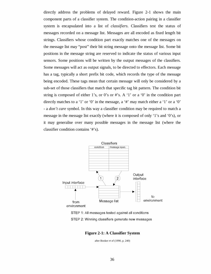
directly address the problems of delayed reward. Figure 2-1 shows the main

component parts of a classifier system. The condition-action pairing in a classifier

system is encapsulated into a list of classifiers. Classifiers test the status of

messages recorded on a message list. Messages are all encoded as fixed length bit

strings. Classifiers whose condition part exactly matches one of the messages on

the message list may “post” their bit string message onto the message list. Some bit

positions in the message string are reserved to indicate the status of various input

sensors. Some positions will be written by the output messages of the classifiers.

Some messages will act as output signals, to be directed to effectors. Each message

has a tag, typically a short prefix bit code, which records the type of the message

being encoded. These tags mean that certain message will only be considered by a

sub-set of those classifiers that match that specific tag bit pattern. The condition bit

string is composed of either 1’s, or 0’s or #’s. A ‘1’ or a ‘0’ in the condition part

directly matches to a ‘1’ or ‘0’ in the message, a ‘#’ may match either a ‘1’ or a ‘0’

- a don’ t care symbol. In this way a classifier condition may be required to match a

message in the message list exactly (where it is composed of only ‘1’s and ‘0’s), or

it may generalise over many possible messages in the message list (where the

classifier condition contains ‘#’s).

Figure 2-1: A Classifier System

after Booker et al (1990, p. 240)

37

Each classifier has associated with it a numeric quantity, the strength value of the

rule, which reflects the classifier rule’s “usefulness” to the system as a whole. In a

system of any size the likelihood that a matching classifier' s message will be written

to the message list is in proportion to its strength value. Strength values are

updated by the reinforcement learning component of the system in proportion to

the contribution the classifier rule made in garnering any reward. The algorithm for

apportioning credit amongst the various classifier rules, even though reward events

are sparse, is referred to as the bucket-brigade algorithm.

A classifier system operates with three basic sub-systems, a performance element, a

credit assignment element and a discovery element. Heitkötter and Beasley (1995)

provide a pseudo-code listing of the classifier system learning algorithm. The

performance element is responsible for matching classifier conditions to the

message list, maintaining the message list by adding new classifier message

specifications and selecting external output actions. The strength of each classifier

rule that successfully posts a message to the message list is reduced by a bid

amount. This bid amount is calculated on the basis of the current strength value

and the specificity of the rule (the number of “don’t cares” in the condition). The

strength of any classifier which bids but fails to post its message is left unchanged.

However, all the classifiers that previously posted messages used by the winning

classifier subsequently receive an increase in strength based on the value of the

successful bid.

Classifiers which bid and post messages just prior to external reward are credited

with strength increases directly by the credit assignment element. Those which

enable these classifiers receive a “share” of this reward - and so on throughout the

system. The overall effect is to increase the strength of classifiers that are

consistently implicated in successful or rewarding activities. In turn their greater

strength increases the probabili ty that they will be activated, and so receive reward.

In this way the bucket-brigade algorithm orders the usefulness of all the classifiers

in the system, and improves the external performance of the system. As with the Q-

learning algorithm, classifiers distribute their success to those which contributed to

it.

38

The discovery element allows for the creation of new classifier rules according to a

genetic algorithm (Holland, 1975; Dawkins, 1986). This discovery component

takes the best members of the population of classifiers and modifies or recombines

them to create offspring classifiers that may be better fitted to the environment and

task. The principal genetic method employed in classifier systems is that of the

genetic crossover, which randomly exchanges selected segments between the pair

of parent classifiers to create two new offspring classifiers. Mutation, in the form

of random inversion of elements in the bit string, may also be employed. To

maintain the size of the classifier list, the weakest classifiers may be discarded.

Wilson (1985), creator of the term “animat” , was the first to directly apply the

techniques of classifier systems to the animat problem. Ball (1994) describes an

animat control system combining a Kohonen feature map and conventional

classifier system to create a “hybrid learning system” (HLS). The Kohonen map

providing a self-organising element to pre-process sensory information into sub-

symbolic features passed to the classifier component. Similar maps have been

proposed as models of cerebral cortex function (as in Albus’ CMAC, q.v.) Dorigo

and Colombetti (1994) decompose the animat task into several classifier systems in

the ALECSYS algorithm to demonstrate learning and control in a small mobile

robot. Venturini (1994) describes the AGIL system. AGIL incorporates

modifications to the basic classifier system format that explicitly balance the effort

the animat will expend in exploration of its environment to that of exploiting its

learned knowledge. Riolo (1991) modifies the classifier system format to allow a

form of lookahead planning. Dorigo and Bersini (1994) argue that classifier

systems and Q-learning are essentially similar methods of reinforcement learning,

separated more by a research tradition than essential technical differences. They

demonstrate that a considerably simplified form of the classifier system may be

treated as equivalent to a tabular form of Q-learning.

2.6. Artificial Neural Networks

Artificial Neural Networks (connectionism) represent a distinct approach to

modelli ng and creating behaviour patterns. Much of the work in this area may be

traced back to an abstract model of the neurone developed by McCulloch and Pitts

(1943). The hope is that these units in some way provide a reasonable analogue of

39

the internal function of the brain and nervous system of animals6. Figure 2-2

ill ustrates some of the features of this type of model. The central component of the

model is a summation unit (�

) that accepts signals from several sensory inputs (S1

.. Sn) via weighted “synaptic” connections (W1 .. Wn). Individual weights may be

continuously adjusted between some negative value and some positive value. A

threshold unit on the output side of the summation unit converts the output into a

binary response from the simulated neurone.

An early implementation of the neural network approach as a simulation on a serial

computer, the Perceptron, was provided by Rosenblatt (1962). Rosenblatt’s

Perceptron augmented the basic neurone model with an additional layer of

association units that randomly connected each of the input points (S1 .. Sn) to the

sensory units via fixed positively (+1) or negatively (-1) weighted connections.

Rosenblatt defined a procedure to update the weights when the output response of

the unit differed from the desired one, as computed by an error comparator. The

Perceptron learning procedure computed an adjustment to the set of weights

implicated in an erroneous decision by an amount just sufficient to correct the

6 Leading to a early surge of optimism within the Machine Intelli gence community that perhapsnetworks of simple units, initiall y connected at random and subsequently subjected to simplelearning regimes would lead to complex self-organised behaviour. The idea is still seductive, butin the intervening half century has proved troublesome to attain in practice.

Figure 2-2: A Simple Neurone Model

40

decision. This method has subsequently been criticised for not stabili sing if there is

no set of weight values that correctly partitions the decision space. Several other

procedures for learning by weight adjustment have been described (Nilsson, 1965;

Hinton, 1990). More fundamental shortcomings of the connectionist approach

were described by Minsky and Papert (1969), who argued that there were

significant classes of recognition problems that this architecture could inherently

not discriminate. Examples included the exclusive-OR function and various

connected and disconnected figures. Research into Neural Networks went into

decline for some years until revived by Geoffrey Hinton and others in the mid-

1980’s.

A neural network with multiple-layers of adjustably weighted “neurones”

overcomes many of the criticisms levelled by Minsky and Papert, but introduces

problems of how the various individual weights in the “hidden” layers might be

adjusted. Figure 2-3 ill ustrates the architecture of a multi-layer artificial neural

network. Rumelhart, Hinton and Willi ams (1986) describe the backpropagation

algorithm, a method by which the effects of undesired classifications may be used

to adjust weights distributed across many layers. The backpropagation algorithm is

essentially a two-stage computation. In the first stage the activation of every unit in

the network is calculated. In the second stage an error derivative (�E) is computed

at the output layer and subsequently distributed to adjust the weights on

intermediate hidden layers.

41

The backpropagation algorithm has been applied with some success to a range of

tasks. Hinton (1986) describes a system for the discovery of “semantic features” in

data and Sejnowski and Rosenberg (1987) a system for converting text into

speech. Jochem, Pomerleau and Thorpe (1993) describe two systems ALVINN and

MANIAC, multi-layer neural controllers for road following in a mobile vehicle. The

ALVINN system comprised 960 input units (a 30 x 32 “retina”), 4 hidden units and

50 output units. The MANIAC system employed the same input and output

arrangement but incorporated additional hidden units (a total of 16) in two layers,

giving improved road following performance under a range of conditions.

Pomerleau (1994) describes a neural network to control a walking robot. Chesters

and Hayes (1994) describe experiments employing a connectionist model to

investigate the effects of adding context memory signals to control a small mobile

robot. Nehmzow and McGonigle (1994) describe their use of a supervised teaching

procedure to train the Edinburgh R2 robot in a variety of wall following and

obstacle avoidance tasks. Gaussier and Zrehen (1994) describe the use of Khepera

mobile robots in research to investigate building a neural topological map.

Connectionism is evidently an S-R approach; a set of sensory data presented at the

input units is translated into a set of output responses. It differs from the

Figure 2-3: A Multilayer Neural Network Model

42

reinforcement approach in that an error signal is propagated to adjust many

weights. In reinforcement learning a desired (or undesired) signal is typically used

to adjust activity units specifically implicated in the behaviour choice. As a positive

consequence of this, artificial neural networks are often considered to be robust in

the face of a noisy or disrupted input data vector. Neural network models

discussed thus far have all concentrated on supposed properties of collections of a

simple and simplified neurone. Hinton (1990, p. 209) points out that the

backpropagation algorithm is rather implausible as a biological model, as there is

“no evidence that synapses can be used in the reverse direction.” Other writers

have taken more care to link computer models of neural function to research

findings in the areas of neuroanatomy and neurophysiology. Albus (1981), for

instance, proposed a model based on the observed structure of the brain. Albus’

Cerebellar Model Architecture Computer (CMAC) postulates a table driven look-

up mechanism to map many sensory inputs to many motor outputs.

2.7. Operant Conditioning

The theories and models described so far are characterised by the stimulus-

response (S-R) approach. An action is primarily selected on the basis of incoming

sensory information. Once the strength value of a connection is computed,

information about the circumstances leading to the reward or reinforcement on

which the value is based is generally discarded. B.F. (Burrhus Frederic) Skinner

(1904-1990) proposed a radically different mechanism, that of instrumental or

operant conditioning. In the operant conditioning model responses are not

“elicited” by sensory conditions, but “emitted” by the animal. Reinforcement is

therefore between response and reward, not between sensory condition and

reward. The action is described as the “operant” or “ instrument” by which reward

is obtained. Reward may only be forthcoming in some of the many situations in

which the action can be taken. In this case it is referred to as a discriminated

operant, the various circumstances being distinguished by sensory conditions.

Skinner and his followers adopted a purely behaviourist standpoint and have used

their ideas to propose explanations for a wide range of human psychological

concepts such as “self, self-control, awareness, thinking, problem-solving,

43

composing, will -power, … repression and rationalization”7 which might otherwise

be addressed in a more nebulous “mentalistic” manner. Skinner did not reject

respondent behaviour or classical conditioning as valid phenomena, just their

central importance. Many largely retrospective and comprehensive reviews of

Skinner’s contribution are to be found, including Verplanck (1954), and Catania

and Harnad (1988).

Skinner applied his ideas to a wide range of areas, such as education, behavioural

and social control, and psychiatry. Of particular interest to the current work are the

experimental techniques developed by Skinner to investigate operant conditioning.

In an apparatus, now almost universally referred to as the Skinner box, certain

learning phenomena in animals may be investigated under highly controlled and

repeatable conditions. In a typical Skinner box apparatus the subject animal may

operate a lever to obtain a reward, say a small food pellet. The equipment may be

sound-proofed to exclude extraneous signals and different arrangements can be

adopted to suit different species of subject animal.

Typically the subject will be prepared to operate the lever to obtain the reward

before the start of an experiment. Once the subject is conditioned in this manner

various regimes can be established to record effects such as stimulus

differentiation, experimental extinction, the effects of adverse stimuli (“punishment

schedules”), and the effects of different schedules of reinforcement. Progress of the

learned response may be automatically recorded in a trace that shows the number

(and/or strength) of the emitted response in relation to the frequency of reward.

Figure 3-1 in the next chapter ill ustrates some results of this form and a number of

the experimental designs used in chapter six are influenced by these procedures.

For all the experimental evidence accumulated and effort expended in attempting to

apply their findings, Skinner and his followers did not place an over-emphasis on

theorising about the mechanisms that might be involved. As a consequence,

perhaps, few formal models of operant conditioning have been developed. One

such model, the Associative Control Process (ACP) model (Baird and Klopf, 1993;

Klopf, Morgan and Weaver, 1993) develops the two factor theorem of Mowrer

7 Quoted from Bower and Hilgard (1981, p. 170)

44

(Mowrer, 1956). The ACP model reproduces a variety of animal learning results

from both classical and operant conditioning. Schmajuk (1994) presents a two-part

model incorporating both classical and operant conditioning modules emulating

escape and avoidance learning behaviour.

2.8. Cognitive Models of Learning, Tolman and Expectancy Theory

The majority of models of learning discussed in this chapter so far - both natural

and as computer models, follow the premise that observable behaviour, the

“response” is primarily mediated by the appearance of stimuli. Learning is therefore

reduced to strengthening or weakening the connection between possible stimulus

sets paired to one of a number of available responses. Both the reinforcement and

classifier system computer models described extend this concept to allow credit (or

blame) associated with a reinforcement signal to be distributed to earlier events

with the aim of optimising or maximising overall reward, as received reinforcement

signal, which may be obtained. The associationism of classical conditioning is a

clear exception, and operant conditioning also takes a distinct, alternative

approach.

While forms of stimulus-response (S-R) behaviourism were highly influential for

much of the first half of the twentieth century, it became clear that the predictions

they made were inadequate to explain all of animal learning and much of human

learning and behaviour. An alternative view, developed by Edward Chance Tolman

(1886-1959) and others, was that behaviour was primarily mediated by the

situation which was to be achieved, rather than the prevaili ng situation (as in S-R

theory) or the action that would be taken (as postulated by operant conditioning

studies). This was termed the cognitive viewpoint. Toates (1994) has pointed out

that the term “cognitive” now encompasses a wide range of theories and

approaches to Psychology and Artificial Intelli gence. He notes that texts on

“Cognitive Psychology” will often incorporate descriptions of the behaviourist

standpoint with little comment as to the historical divisions once so strongly

argued.

Tolman’s keystone work “Purposive Behavior in Animals and Men” (Tolman,

1932) described a series of experimental observations and laid out the foundations

45

of expectancy theory. Much of the experimental evidence presented was derived

using rats in maze like experimental apparatus. It has been noted that while

Tolman’s theoretical position changed little over the years, his use of vocabulary to

describe concepts and processes within the theory underwent a continuous series of

changes and shifts. Tolman was a prolific author, with some 70 papers published

during a distinguished career. Tolman’s position is retrospectively described in an

analysis by MacCorquodale and Meehl (1954) and again, in a more accessible

form, by Bower and Hilgard (1981, Ch. 11).

One significant aspect of Tolman’s theorising was to identify a number of situations

that were, and continue to be, particularly diff icult to satisfactorily explain in purely

behaviourist-reinforcement terms. Bower and Hilgard (1981, pp. 330-342) review

this evidence in some detail. Two particular phenomena, latent learning and place

learning, ill ustrate these arguments. In latent learning Tolman argued that as

reinforcement learning requires a reward at the conclusion of the behaviour

sequence to establish its effectiveness, then, if learning could be demonstrated in

the absence of reinforcement, behaviourist-reinforcement theories would be shown

inadequate. Tolman convincingly demonstrated learning in rats in the absence of

reinforcement. Consequently his expectancy theory, which can account for the

phenomena, was supported.

Similarly stimulus-response theory maintains that every response is triggered by

some stimulus. Tolman argued that if the experimental animal could be placed in

circumstances where different responses were appropriate in apparently identical

stimulus conditions then stimulus-response theories would be again demonstrated

inadequate. Tolman and others subsequently successfully demonstrated that animal

subjects can indeed make different responses under apparently identical sensory

conditions. Such conditions include manipulation of the motivational state of the

animal (hunger, thirst, etc.); or by introducing obstructions into a specific maze

apparatus, forcing the response at different route choice points. Several variants on

the place learning experiments are described by Bower and Hilgard. All represent

significant challenges to the behaviourist viewpoint. Sections 6.6 and 6.7 in chapter

six replicate classic experimental procedures for latent learning and place learning

respectively.

46

2.9. MacCorquodale and Meehl’s Expectancy Postulates

For all the challenges that Tolman and expectancy theory present to the

behaviourists it was not without problems. Perhaps the most persistent criticism of

the approach was that the model was purely descriptive. The lack of formalised and

explicit theoretical constructs heavily constrained the predictive power and hence

usefulness of early expectancy models. Recognising this MacCorquodale and

Meehl (1953) proposed a set of 12 expectancy postulates in an attempt to provide

a testable and quantifiable basis for expectancy theory. MacCorquodale and Meehl

redefined Tolman’s notion of a Sign-Gestalt Expectancy (henceforth expectancy)

as a three part “basic cognitive unit” of the form:

S1 � R1

� S2 (basic expectancy)

The addition of an “S2” component over a stimulus-response model provides for a

form of instrumental or operant modus ponens; an implication of an outcome

condition (S2) caused by the action R1 rather than purely indicated as desirable by

the presence of the condition S1. This is largely equivalent in structure to the

notion of the three-term contingency “stimulus - response - consequence”, used by

Catania (1988) to express the fully discriminated Skinnerian operant class of

discriminated stimulus, response and contingent outcome of reward or punishment.

With the essential difference that it is the identity of the outcome that is recorded in

expectancy theory, not just a measure of its desirabili ty or quality as is recorded in

the operant, or reinforcement learning approaches.

MacCorquodale and Meehl’s twelve expectancy postulates refer to eight

underlying processes, namely “mnemonization” , “extinction” , “generalization” ,

“ inference”, “need”, “cathexis” , “valence” and “activation” . Postulate 1, the

mnemonization process, refers to an increment in “strength” of the expectancy

where the component parts S1, R1 and S2 are in close and ordered temporal

contiguity. This increment is described by a negatively accelerating function, where

the function acceleration rate is determined by the valence (q.v., a measure of

usefulness or desirabili ty) of the S2 component and the asymptote of the strength

determined by the relative frequency or probabili ty that S2 follows the sequence S1� R1. Postulate 2, the extinction process, refers to a decrement in strength where

47

the sequence S1 � R1 is not terminated by the expectandum8 S2. It will be argued

later that the relative frequency of contiguity, the function rate and the valence

level are better considered as separate and distinct values and should not be

convolved into a single “strength” parameter. MacCorquodale and Meehl did not

propose an explicit or quantifiable mathematical formulation for either of these

postulates.

Postulate 3, primary generalization, allows for sharing of expectancy strengths

where two expectancies share R1 and S2 components and their S1 components

“resemble” one another. Postulates 4 and 5, inference and generalized inference,

refer to processes by which temporal contiguity (S2S�

) between a known

expectandum S2 and another sign stimulus S�

increases or decreases the strength

of the expectancies sharing elements, or in which elements are “similar” , according

to the degree of temporal adjacency and frequency of occurrence. A different

approach to the evaluation of expectancies will be proposed later, which

considerably diminishes the importance placed on these postulated mechanisms of

generalisation and inference. As before MacCorquodale and Meehl did not proffer

any suggestions as to the nature of “similarity” or “resemblance”, or how they may

be evaluated, between components in these shared expectancies.

Cathexis9, postulate 11, refers to the strength of connection between a stimulus

sign S�

and a drive, motivation or goal state. Need strength, postulate 10,

describes the degree to which the subject is to be influenced by the cathectic

situation. The valence, postulate 9, of a sign S�

is then defined by the product of

the need (D) and cathexis (C�

) attached to that sign (D � C�

). It is perhaps

interesting to note, with hindsight, the pivotal role of innate mechanisms to control

and balance motivation and behaviour (such as those being described by Tinbergen

at about the same time) appears to have been largely unrecognised.

MacCorquodale and Meehl were therefore unable to propose effective mechanisms

for these postulated processes.

8From the gerundive form “... to be expected”9(OED) Cathexis: n (Psych.) Concentration of mental energy in one channel, [f. Gk kathexisretention]

48

Secondary cathexis, postulate 6, allows for the induction of cathexis to an

expectandum S2, where a contiguity S2S�

exists and S�

has valence. Induced

elicitor-cathexis, postulate 7, allows cathexis to be induced to an S1 component of

an expectancy where its expectandum has already acquired valence, to an extent

proportional to that acquired valence and the prevaili ng mnemonization strength of

the expectancy. Tolman’s (1932, p. 176) descriptions clearly indicate the notion of

a means-end-field (later cognitive map, Tolman, 1948) by chaining expectancies in

this manner10. Postulate 8, confirmed elicitor-cathexis, provides for additional

strengthening of the expectancy where the sequence it describes is confirmed, and

S2 has valence.

Finally, in a process of activation, postulate 12, the action R1 is evoked according

to a reaction potential determined by a multiplicative function of expectancy

strength and valence, when in the presence of the elicitor S1. MacCorquodale and

Meehl recognised that their postulate system for an expectancy theory was

“ incomplete, tentative and certainly nonsufficient,” but were able to present some

hand-worked examples to illustrate their model.

2.10. Computational Models of Low-level Cognitive Theories

Further development of expectancy theory, as with other psychological models, has

depended on the use of computer based formalisations. Information processing

models of cognitive processes impact theoretical development in several ways.

Firstly, the model must be complete to the extent that an algorithmic process can

be adequately defined for each essential element or component in the model.

Secondly, each of these essential elements must be sufficiently defined to permit

the creation of program code. Thirdly, they are testable and may be subjected to

experimental regimes to determine their performance under controlled and

repeatable conditions. In some instances their performance may subsequently be

compared with results obtained by experiment with, and observation of, natural

systems.

10 The term “cogniti ve map” has more recently tended to be interpreted more literall y, internal“maps” of spatial locations or terrain layout (Meyer and Guillot, 1991, for a compact review).

49

Three such models are presented in the next sections of this chapter, leading to the

development of a novel Dynamic Expectancy Model. None of these models make

direct reference to Tolman or expectancy theory, being described as “sensory-

motor” or “ intermediate-level” cognitive models, but the debt owed is nevertheless

clear to see. Each model adopts a schema representation11. The three models are

“JCM”, described by Joseph Becker (Becker, 1970, 1973); “ALP”, described by

David Mott (Mott, 1981; Bond and Mott, 1981); and a model of the early stages of

Piagetian development described by Gary Drescher (Drescher, 1987, 1991). Both

Becker and Drescher elected to discuss or demonstrate their work using simulated

environments, while Mott was able to demonstrate simple learning tasks utili sing a

real mobile robot.

2.11. Becker’s JCM Model

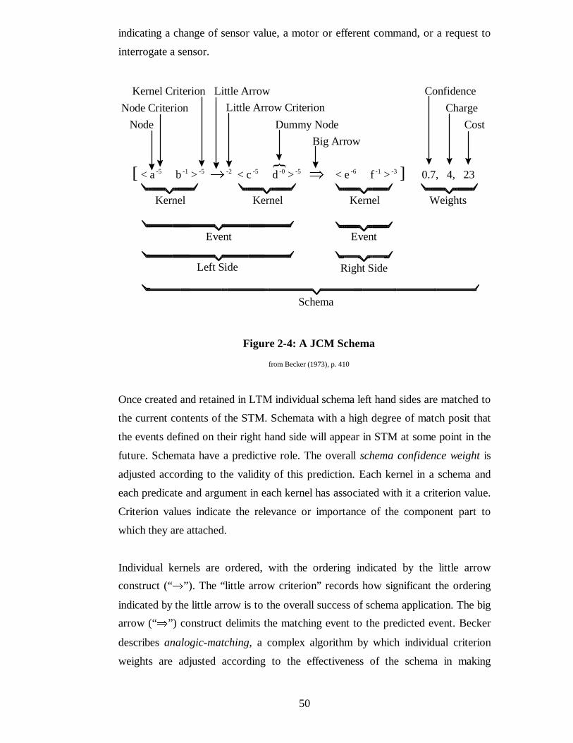
Becker’s JCM model of intermediate level sensory-motor cognitive behaviour

adopted a “stimulus - action - stimulus” representation. Figure 2-4 ill ustrates the

structure of the “schema”, the primary form of information storage in the model.

Many schemata are recorded by the system in a Long Term Memory (LTM).

Sensory and input information enters the system via an “input register” into a

limited capacity Short Term Memory (STM). STM acts as a FIFO buffer, and will

contain a small number, say six or so, items. As new items enter STM via the input

register older items are lost, or they may be recycled. Individual elements of

information, as entered into STM and recorded within schemata, are referred to as

kernels. In Becker’s representation each kernel takes the form of a predicate with

arguments, for instance:

<colorchange right bottom black red>

The predicate in this case refers to a sensory effect (a colour change from black to

red) in one of the sensory locations (right bottom cell in a simple 3 by 3 cell “eye”

viewing a greatly simplified simulated blocksworld environment). Kernels may be

defined as static sensory, indicating an absolute sensory value, differential sensory,

11Plural “schemata”, “schema” or “schemas”, following the preference of the original authors.

50

indicating a change of sensor value, a motor or efferent command, or a request to

interrogate a sensor.

Once created and retained in LTM individual schema left hand sides are matched to

the current contents of the STM. Schemata with a high degree of match posit that

the events defined on their right hand side will appear in STM at some point in the

future. Schemata have a predictive role. The overall schema confidence weight is

adjusted according to the validity of this prediction. Each kernel in a schema and

each predicate and argument in each kernel has associated with it a criterion value.

Criterion values indicate the relevance or importance of the component part to

which they are attached.

Individual kernels are ordered, with the ordering indicated by the little arrow

construct (“ � ” ). The “little arrow criterion” records how significant the ordering

indicated by the little arrow is to the overall success of schema application. The big

arrow (“ � ” ) construct delimits the matching event to the predicted event. Becker

describes analogic-matching, a complex algorithm by which individual criterion

weights are adjusted according to the effectiveness of the schema in making

[ < a -5 b -1 > -5 � -2 < c -5 d -0 > -5 � < e -6 f -1 > -3 ] 0.7, 4, 23

Node

Node Criterion

Kernel Criterion Little Arrow

Little Arrow Criterion

Dummy Node

Big Arrow

Confidence

Charge

Cost

{

Kernel Kernel Kernel Weights

Event

Right Side

Event

Left Side

Schema

Figure 2-4: A JCM Schema

from Becker (1973), p. 410

51

successful predictions. The “charge” weight associated with each schema indicates

the desirabili ty of the right hand side as a system goal. The greater the charge value

the greater the desirabili ty of obtaining kernels into STM that will allow the

complete matching of the schema. Kernels in partially matched schema may be

established as sub-goals in Becker’s method. Note that the cost weight associated

with the schema refers primarily to the “cognitive cost” , the computational effort

required to make the match between LTM and STM, rather than a cost of

performing the action embedded in the schema.

JCM was never implemented, partially, it might be suspected, as a result of the

complexity inherent in the analogic-matching process and the consequential

diff iculties in devising stable algorithms to manage all the different criterion and

schema weights. Nevertheless Becker’s JCM design introduced a number of

processes that were to be adopted later, notably in Mott’s ALP system. Primary

amongst these is the idea of schema creation by the process of STM to LTM

encoding. A pattern of kernels being extracted from the input STM and

reformulated as a LTM schema, which may in turn be verified by a predictive

matching process.

Becker also promoted the idea of schema refinement through the processes of

differentiation and specialization. In differentiation kernels are removed because

their accumulated criterion values indicate they are irrelevant to the effect of the

schema (as indicated by a small or zero criterion value). Negative criterion values

indicate that the absence of the kernel is essential for the effective matching of the

schema. Specialization is invoked to refine schemata where an intermediate

confidence weight indicates an incomplete specification of the conditions for its

application defined by the left hand side kernels. Specialization is achieved in JCM

by the addition of further kernels on the left hand side of the schema.

2.12. Mott’s ALP Model

Mott’s ALP system considerably refined and implemented an intermediate level

sensory-motor cognitive model and applied the result to developing behaviours in a

small mobile robot. Mott retained the central representation of schema recorded in

a long term memory, with a limited capacity STM. STM retains the input register,

52

but each time slot may contain multiple kernels for matching into LTM schema.

This modification overcame a dependence on a complex sensory attention

mechanism to identify and select items for entry to STM. Critically, Mott reduced

the complexity of the kernel, dispensing with the predicate and argument form. In

ALP kernels are either derived directly from a sensor condition, the sensory kernel,

or they represent an efferent action, the motor kernel. The little arrow notation,

retained from JCM, now represented the passing of exactly one execution cycle,

thereby reducing the “analogic-matching” process to manageable proportions.

Mott overcame the problem of goal motivation inherent in JCM by introducing two

new (sensory) motivational kernels, <HIGH>S and <LOW>S, respectively

representing a condition that the robot should seek and a condition it should avoid.

At a low level some conditions, such as “battery very low”, are associated with

motivational kernel (in this case <LOW>S).

ALP retained Becker’s JCM mechanisms for creating new schema by STM to

LTM encoding, triggered by the appearance in STM of novel kernels. Schema

validation, differentiation and specialisation remain substantially as in JCM. Goal

management is however substantially different. ALP is able to use schema to form

chains of predictions about possible future events. When either a <LOW>S or

<HIGH>S kernel is predicted this is treated as a goal definition, and a goal tree

can be formulated to either avoid the undesirable predicted event, or to attain

desirable ones. Paradoxically the system would not react to the direct appearance

of a motivational kernel, only its predicted occurrence. Schema may be chained to

form a goal solution, and actions selected to control the robot.

ALP was implemented in the POP-2 programming language and ran on an ICL

1900 series mainframe in an interactive mode. ALP was heavily processor bound.

The robot used was controlled by a local PDP-11 mini-computer, which packaged

sensory information from the robot for onward transmission to the mainframe and

interpreted commands sent from the mainframe. ALP was an essentially ad-hoc

system that demonstrated the acquisition of some simple robot behaviours by the

learning process. Its effectiveness as a behavioural system was severely restricted

by the rapid loss of schema confidence in future events in the predictive chains and

goal trees. Chains were limited to six goal cycles or three predictions. These

restrictions in part arose due to the method of computing these possible outcomes,

53

and in part to the uncertainty inherent in the experimental environment provided by

the robot test-bed.

2.13. Drescher’s Model

Drescher’s model further simplified the notion of a schema. The context of a

schema being reduced to a simple conjunction of sensory primary items

(Drescher’s term for a kernel), or their negation. All timing information was

abandoned. Figure 2-5 ill ustrates the form of the schema. Drescher used a

simplified simulated hand-eye co-ordination environment, similar in concept to that

proposed by Becker, but with a larger number of states that may be visited. None

of the tasks investigated required information about prior states and this limited

form of context definition was adequate for the environment chosen. In these

circumstances a Short Term Memory is redundant and was not used in the model.

Drescher describes the composite action, chains of individual schema defined with

respect to some goal state forming what is essentially a sub-routine that might

substitute as the “action” of a single schema. Figure 2-6 ill ustrates the form of the

composite action. Drescher also describes a process by which individual schema

are considered as synthetic items, the whole schema being used as a record of a

recent event in an attempt to simulate Piaget’s notion of object permanence.

Figure 2-5: A Schema in Drescher’s Cognitive Model

from Drescher (1991), p. 9

54

Drescher employed a radically different approach to the generation of schema from

the STM to LTM encoding used by JCM or ALP, the marginal attribution

process. Figure 2-7 ill ustrates the stages in creating schemas of arbitrary

complexity by this process. In step one “bare schema” are created, one for each of

the primitive actions available to the system (notated by Drescher as “ /a/ ” ). Bare

schema have empty context and result slots. The system is then run for a period

with actions being selected at random, a trial and error period. Exploration of a

new environment by a naïve system is a feature of the JCM and ALP systems also.

During this period of exploration each schema has associated with it an additional

structure, the extended result, which accumulates outcomes applicable to the new

schema.

At some point, after sufficient exploration has been completed, a set of new

schemas are “spun off” . This is shown as step two. In this example the new schema

“ \a\x” is created from the extended result. Many new schemas could be formed at

this point. As each new schema has no context information it is considered to be

“unreliable” and it is given an extended context structure, step three. This structure

accumulates a record of items active as the new schema is used in a manner similar

to the extended result. Following another suitable period of activity, items are

selected from the extended context for inclusion into the new schema’s context,

“p/a/x” in the example. This process may be repeated as often as required to

further refine the context of the prototype schemas, step four.

Figure 2-6: A Composite Action

from Drescher (1991), p. 91

55

This marginal attribution method for schema learning is inordinately inefficient, as

evidenced by the extensive computational resources required to execute the

procedure in the simulated environment described (Drescher, 1991, p. 141).

Furthermore, Drescher provides little clue as to its effectiveness, beyond indicating

the need to incorporate additional mechanisms to limit the creation of redundant

schemas, the redundant attribution process.

2.14. Other Related Work

Jones (1971) describes a computer model of new-born infant suckling behaviour.

Riolo (1991) presents a three term model (CFSC2) based on classifier systems

concepts. An additional form of the classifier rule (the “e#/t#” rule type) allowed

the system to describe transitions between either actual or hypothetical states. The

system might therefore determine expected reward on the basis of look-ahead

cycles. The CFSC2 model was used to demonstrate the latent learning

phenomena. Bonarini (1994) describes a three part operator exploiting fuzzy logic.

Figure 2-7: The Marginal Attribution Process

Prepared from a description in Drescher (1991)

56

Shen (1993, 1994) describes the LIVE system that creates, utili ses and refines new

GPS style operators from successful and failed prediction sequences while

performing problem solving tasks in its environment. LIVE models its environment

using a set of prediction rules, triples in the form <condition action prediction>.

Shen’s system employs a number of heuristics in the creation of new prediction

rules, and subsequently may revise them (through a process of “Complementary

Discrimination Learning”). Prediction failures trigger the system to search for

differences between the current failed instance, and stored instances of successful

predictions using the same rule. The rule revision algorithm is noise intolerant, but

has been demonstrated on a number of recognised tasks, including the Towers of

Hanoi.