Open Research Online The Open University’s repository of research publications and other research outputs Characterization of Residual Stress and Plastic Strain in Austenitic Stainless Steel 316L(N) Weldments Thesis How to cite: Moturu, Shanmukha Rao (2015). Characterization of Residual Stress and Plastic Strain in Austenitic Stainless Steel 316L(N) Weldments. PhD thesis The Open University. For guidance on citations see FAQs . c 2015 The Author https://creativecommons.org/licenses/by-nc-nd/4.0/ Version: Version of Record Link(s) to article on publisher’s website: http://dx.doi.org/doi:10.21954/ou.ro.0000f02b Copyright and Moral Rights for the articles on this site are retained by the individual authors and/or other copyright owners. For more information on Open Research Online’s data policy on reuse of materials please consult the policies page. oro.open.ac.uk

Welcome message from author
This document is posted to help you gain knowledge. Please leave a comment to let me know what you think about it! Share it to your friends and learn new things together.
Transcript
Open Research OnlineThe Open University’s repository of research publicationsand other research outputs
Characterization of Residual Stress and Plastic Strainin Austenitic Stainless Steel 316L(N) WeldmentsThesisHow to cite:
Moturu, Shanmukha Rao (2015). Characterization of Residual Stress and Plastic Strain in Austenitic StainlessSteel 316L(N) Weldments. PhD thesis The Open University.
For guidance on citations see FAQs.
c© 2015 The Author
https://creativecommons.org/licenses/by-nc-nd/4.0/
Version: Version of Record
Link(s) to article on publisher’s website:http://dx.doi.org/doi:10.21954/ou.ro.0000f02b
Copyright and Moral Rights for the articles on this site are retained by the individual authors and/or other copyrightowners. For more information on Open Research Online’s data policy on reuse of materials please consult the policiespage.
oro.open.ac.uk

q . inDOCTORAL THESIS
Characterization of Residual Stress and Plastic Strain in Austenitic Stainless Steel 316L(N) W eldments
Shanm ukha R ao M oturu
Septem ber 2015
Subm itted to the D epartm ent o f Engineering and Innovation, The Open University for the Degree o f Doctor o f Philosophy
Of -2.0 lo
£>f\TJ6. o P • r ?*X M e IS
0 200-210
□ 190 200
□ 180-190
n 170-180
■ 160 170
o 150 160
□ 140 150
■ 130 140
High T em p Sym m etric Vs A sym m etr ic E xp erim ental 1.25% at 4 e -4 /s e c
500
-500Total Strain
Sym m etricA sym m etric
9 11 13 15 17
104107 110 113 116 119 122 125128131 134137140143146 149152155158161 164 167170173176179
Three pass weld hardness contour m ap (x and y in mm and z in Hv5)
1 2 pass weld EBSD M ap500pm
ProQuest Number: 13835622
All rights reserved
INFORMATION TO ALL USERS The quality of this reproduction is dependent upon the quality of the copy submitted.
In the unlikely event that the author did not send a com p le te manuscript and there are missing pages, these will be noted. Also, if material had to be removed,
a note will indicate the deletion.
uestProQuest 13835622
Published by ProQuest LLC(2019). Copyright of the Dissertation is held by the Author.
All rights reserved.This work is protected against unauthorized copying under Title 17, United States C ode
Microform Edition © ProQuest LLC.
ProQuest LLC.789 East Eisenhower Parkway
P.O. Box 1346 Ann Arbor, Ml 48106- 1346
A b st r a c t
Fusion welding processes commonly involve the localized input of intense heat,
melting of dissimilar materials and the deposition of molten filler metal. The surrounding
material undergoes complex thermo-mechanical cycles involving elastic and plastic
deformation. This processing history creates large residual stress in and around the weld
bead, which can be particularly detrimental in reducing the lifetime of fabricated
structures, increasing their susceptibility to stress corrosion, fatigue and creep crack
growth as well as reducing the fracture load. It is very important to have a proper
knowledge of the residual stress distribution in and around the weld region of structured
components because knowing this allows their fitness to be assessed and the service life
of critical components to be predicted. Characterizing weld residual stress fields either by
measurement or finite element simulation is not straightforward because of the strain field
complexity, inhomogeneity o f the microstructure and the complex geometry of structural
weldments.
The residual stress distribution in a slot weld benchmark sample made from AISI
316L(N) austenitic stainless steel was analysed using the neutron diffraction at pulsed
source. The presence of crevices and hydrogen containing super glue in the stress-free
cuboids are some of the main issues effecting the neutron residual stress measurements.
A residual stress of 400-45OMPa was observed in first pass weld metal and in the HAZ
of a three pass welded plate.
The strain hardening behaviour of AISI 316L(N) steel around the slot weld was studied
taking account of the asymmetric cyclic deformation and the typical strain rates
experienced; inferences are drawn regarding how such effects Should be modelled in
finite element weld residual stress computations. The solution annealed material was
tested under symmetric and asymmetric cyclic loading at both room and 550°C. During
asymmetric cyclic loading, the 316L (N) material at room and high temperature was less
strain hardened than in the same number of cycles of symmetric cyclic loading. At room
temperature; the 316L (N) material deformed at fast strain rate showed higher strain
hardening than at the slow strain rate. However, at high temperature (550°C); the 316L
(N) material deformed at slow strain rate showed higher strain hardening than at the fast
strain rate due to dynamic strain ageing. A mixed hardening model was to predict the
strain hardening of the 316L (N) material at room and high temperature (550°C).
However, the published mixed hardening parameters were unsuccessful in predicting the
strain hardening o f the symmetric cyclic deformation at high temperature.
Finally, the accumulated cyclic plastic strain resulting from the addition of each weld
bead was studied using Electron Backscatter Diffraction (EBSD) and hardness
measurements. The EBSD metrics showed a gradual increase of plastic strain and
equivalent yield stress from the parent zone (approximately 0.02) to the fusion boundary
(approximately 0.05-0.09). Although, in strain controlled cyclic loading, none of the
EBSD metrics used were capable of assessing the plastic strain, below 58% cumulative
plastic strain path. The quantified plastic strain (from the EBSD) and hardness analysis
of the parent material indicates that the material deformed plastically. The EBSD derived
plastic strain and equivalent yield stress correlate well with hardness, finite element
prediction and von Mises equivalent residual stress.
r
The Library
2 3 FEB 2016
DONATION
Can&ui-bct.tion copuI
3
A c k n o w l e d g e m e n t
This doctoral thesis could not be possible without the technical and moral support of
numerous people in the department. I would like to thank my supervisors Prof. Peter John
Bouchard, Dr. Shirley Northover, Dr. Joe Kelleher and Dr. Jon James for their invaluable
guidance and constant encouragement during my studies. I am grateful to Dr. Satheesh
Krishnamurthy; Dr Mahesh Anand and Dr Abita Shyorotra Chimpri for their moral
support during the hard times of my life. I would also like to express my deepest gratitude
to Dr. Susan Storer for helping to review and edit the thesis.
I am indebted to the NeT consortium and the Open University for the financial support
and the provision of the benchmark samples. I am also thankful to Prof. Mike Smith, the
late Ann Smith and Dr. Ondrej Muransky for their very useful technical discussions and
sharing the data during this project. I am also thankful to beamline scientists of the
ENGIN-X (ISIS) and VULCAN (SNS) instruments for their valuable guidance and
training during my experimental work.
I am indebted to the support given by staff in our department: Stan Hiller, Paul
Courtnage (“Courtney”), Pete Ledgard, Gordon Imlach, Ian Norman, Dr. Colin Gagg,
Charlie Snelling and Heather Davies. Without their expertise and help, this work would
not have been a success. I would also like to thank my friends in the Engineering and
Innovation department: Dr. Abdul Kliader Syed, Avishek Dey, Jose Rodolpho Leo, Yeli
Traore, Shah Karim, Jino Matthews, David Githinji, Jeferson Oliveira, Gerardo,
Yadunandan Das, Abdullah-al-Mamun, Rahul Unnikrishnan, Safaa Lebjioui, Paheli
Ghosh, Dr. Murat Ozgun Acar, Dr. Asim Zeybek and Dr. Sanjooram Paddea who have
withstood everything I have thrown at them for the last few years and I will always be
indebted to them. I have enjoyed every minute of the last four years we spent in Milton
Keynes.

I would like say a heartfelt thanks to my beloved parents Mr and Mrs Durga Prasad
Moturu, Geetha Vani Moturu, my wife, Mrs Suneetha Koganti and my son Jeswant Sai
Moturu and my beloved brother, Mr. Phaneendra Babu and his family. Special thanks to
Mr Suresh Kakarla and his family for there support in achieving my goals. Finally, I am
grateful to Mr. Noel Ward, Mrs. Marian Ward, Miss. Collette Ward and Mr. Nicholas
Ward and his wife for their support and considering me as a family member. Without
their constant support and love, it was quite impossible for me to finish the thesis on time.
I am dedicating this work and all my future success to my family members with whom
I will spend the rest of my life.
5
P r e f a c e
This thesis is submitted for the degree of Doctor of Philosophy of The Open
University, United Kingdom. The work described in this thesis was carried out in the
Department of Engineering and Innovation, Faculty of Mathematics, Computing and
Technology, between October 2010 and October 2015, under the supervision of Prof.
Peter John Bouchard, Dr. Shirley Northover, Dr. Joe Kelleher and Dr. Jon James.
It is entirely the work of the author except where clearly referenced. None of this work
has been submitted for a degree or other qualification at this or any other university. Some
of the results of this work have been reported to Europen Network on Neutom Techniques
Standardization for Structural Integrity (NeT) as listed below:
1. Shanmukha Rao Moturu, J.James and P.J.Bouchard. NeT TG4 Project: Residual
stress measurement using the SNS VULCAN neutron diffractometer,
OU/MatsEng/033, December 2012.
2. Shanmukha Rao Moturu and P.J.Bouchard. NeT TG4 Project: Residual stress
measurement using the ENGIN-X neutron diffractometer at ISIS facility,
OU/MatsEng/045, November 2013.
Shanmukha Rao Moturu
October 2015
6
T a b l e o f C o n t e n t s
A bstract ...... 2
A cknow ledgem ent........................................................... 4
P re face ................. 6
Table of C ontents................... 7
N om enclature ..... .................................................. ........................................ . 12
A bbrev iations.......................... 12
Chapter 1. Introduction..... .... ....15
1.1 Background ........................................................................... 15
1.2 Purpose of this study.......................................... 16
1.3 Structure of thesis ........ 19
1.4 Figures ........................................................ 21
Chapter 2. L iterature R eview ........ ...22
2.1 Introduction..................................... ..22
2.2 Welding: Thermal History and Microstructure Effects..............................23
2.2.1 Tem perature distribution of a moving heat source ....... 24
2.3 Monotonic and Cyclic Deformation in 316L(N)-Mechanisra and
Effects..... ..... 27
2.3.1 Mechanism of plastic deform ation, ..... 27
2.3.2 Work harden ing .............................. 28
2.3.3 Dynamic strain ageing (DSA) ........................ 30
2.3.4 Cyclic loading.... ..................... 32
2.3.5 FE Elastic plastic constitutive m aterial m odels...................... 36
2.4 Residual Stresses Measurements Around Welds in 316L(N)................... 40
2.4.1 Principle of neutron m easurem ents of residual s tress:................... 41
2.4.2 Neutron diffraction instruments................................. 42
2.5 Evaluation of Residual Elastic Strain and Stress Using Neutron
Diffraction ....... 43
2.5.1 Issues affecting s tra in /s tre ss m easurem ent using neutron diffraction ....... 44
2.5.2 Weld residual stress N eT-benchm ark ...................... 48
2.5.3 Previous NeT TG4 benchm ark stu d ies ..................... 49
2.6 Plastic Strain Measurement Around Welds in 316L ............... 53
2.6.1 Electron Backscatter Diffraction (EBSD)....................... 54
2.6.2 Instrum ental factors in EBSD ................................. 55
2.6.3 EBSD data analysis.. ......... 56
2.6.4 Quantitative analysis of m iso rien ta tion .................................................................57
2.7 Welding plastic strain analysis using EBSD ......................... 59
2.7.1 Previous studies on weld plastic strain analysis using EBSD.......................... .60
2.7.2 Previous studies on cyclic accum ulated strain analysis using EBSD 61
2.8 Conclusion ................ ..62
2.9 Tables ............ ...65
2.10 Figures ............................................ 68
CHAPTER 3. Benchmark Weldment Design and Material Characterization
80
3.1 Introduction ..... ....80
3.2 Manufacturing of TG4 Benchmark Specimens............... ..81
3.2.1 Stress relief heat tre a tm e n t ....... 82
3.2.2 Three pass weld AIS1-316L (N) p late .......... ...82
3.2.3 Stress free cuboids extraction ......... 83
3.3 Material for Strain Controlled Cyclic T ests ...... 84
3.3.1 Design of strain controlled tes t specim ens 84
3.4 Sequential Weld Deposited P late ................. 85
3.4.1 Samples for plastic strain analysis ......... 85
3.5 Material Properties ............ 86
3.5.1 Specimen p rep ara tio n ................. 86
3.5.2 Optical m icroscopy........................................................................ .87
3.5.3 Grain size m easurem ent ..................................... . 89
3.5.4 Chemical com position .. 90
3.5.5 Texture analysis ........................................................... ....90
3.6 Conclusions .............................................. ....................................... ....91
3.7 Tables............................................................................... ...92
3.8 Figures........................ ......95
CHAPTER 4. Benchm ark W eldm ent Residual Stress C harac terisa tion .... 115
4.1 Introduction.... ................................................................................... 115
4.2 Sample and Instrument Preparations................ ................... 116
4.2.1 NeT TG4 proposed m easurem ent locations........................... .................... 116
4.2.2 Sample alignm ent ............... 118
4.2.3 Sample alignm ent facilities at neutron sou rces...................... 119
4.2.4 Instrum ent alignm ent calibrations.................................................................119
4.3 Stress Free Lattice Parameter (ao) ................................................. 120
4.3.1 VULCAN stress-free lattice param eter m easurem ents ...........................121
4.3.2 ENG1N-X stress free lattice param eter m easu rem en ts .................... ....124
4.4 Residua] stress measurement in the welded plate ............... 126
4.5 Validation of the Residual Stress Measurements............................ 127
4.6 Discussion.................................................................................. 128
4.6.1 ao analysis.............................. 128
4.6.2 Weld residual s tre ss ................................................................................. 131
4.7 Difference in lattice param eter measured at VULCAN and ENGIN-X
experiments .......... 136
4.8 Conclusions ................... 137
4.9 Tables.............................................................. 139
4.10 Figures ...................... 143
CHAPTER 5. Cyclic D eform ation B ehav iou r ............ 172
5.1 Introduction.............. 172
5.2 Choice of Test Conditions............................................................ 172
9

5.2.1 Strain range.................................... 173
5.2.2 T em perature .................... 173
5.2.3 Strain rate.... ......... a.....;..:............ ........................ 174
5.3 Cyclic Stress-Strain Tests ........ 174
5.3.1 Asymmetric cyclic deform ation ......... 175
5.4 Finite Element Modelling Of Cyclic Loading ........ 176
5.5 Discussion....... ........... 178
5.5.1 Discussion on experim ental re su lts ....... ,.................................... 179
5.5.2 Validation of predicted cyclic loading results............................. ......182
5.6 Conclusions ....................... 184
5.7 Tables................ 186
5.8 Figures........................... 188
Chapter 6. Weldment Plastic Strain Characterisation ...... 204
6.1 Introduction...................... 204
6.2 Uniaxial Tensile T est ............... 205
6.2.1 Uniaxial room tem peratu re tensile test (RTT)................ ..........205
6.2.2 Uniaxial high tem perature tensile test (HTT) .................. ...........206
6.2.3 Tensile test results from room tem peratu re and high tem peratu re
experim ents .......................... 206
6.3 EBSD Experimental Setup .................... 207
6.4 Hardness Test Setup (validation of EBSD results)............................... 207
6.5 Weld Plastic Strain Analysis .................... 208
6.5.1 Experimental setup... ...... ...208
6.6 Cyclic Plastic Strain Analysis.,.,............... ............... ..................... ............ . 209
6.7 Discussion ......... 209
6.7.1 EBSD plastic strain correlations for 316L(N) stainless s te e l ....... ...210
6.7.2 EBSD equivalent yield stress correlation for 316L(N) stainless s tee l .......211
6.7.3 Plastic strain and equivalent yield stress correlation for 316L(N) stainless
steel from macro hardness tes t ...... 212
6.7.4 Characterizing accum ulated m isorientation due to the deposit of each weld
bead ................................................................................ 213
10

6.7.5 Quantifying plastic strain and equivalent yield stress from macro hardness
218
6.7.6 Quantitative weld plastic strain and equivalent yield stress from EBSD
analysis................... 218
6.7.7 ABAQUS plastic strain pred iction ................................................ 222
6.7.8 Validating EBSD weld plastic strain resu lts ........................................................ 223
6.7.9 Characterizing cyclic loading plastic s tra in ................................ 223
6.8 Conclusion................................. 225
6.9 Tables ........................ -.227
6.10 Figures ............. 229
Chapter 7. Discussion...... ...... ...258
7.1 Issues affecting the reliability of residual stress measurement using
neutron diffraction............................................................ ....... 258
7.2 Effect of strain rate and asymmetric cyclic deformation on weld
simulation prediction........................................................ 262
7.3 Exploring the possibilities of quantifying plastic strain using different
EBSD m etrics :..... 265
7.4 Table....................... 268
7.5 Figures ........... 269
Chapter 8. Conclusions and F urther W ork ....... 277
8.1 * Conclusions................ 277
8.2 Suggested future w ork ....... 280
R eferences ....... 282
A ppendix ....... 304
11

N o m e n c l a t u r e
t Shear stress
ao Initial yield surface
G[ Achieved yield surface
0 Diffraction angle
X Wavelength of incident beam
ao or do Stress free lattice parameter
a o rd Measured lattice parameter
v Velocity of neutron
L Total flight path
t Time of Flight
s Strain
pe Micro strain
E Young’s modulus
u Poisson’s ratio
A b b r e v ia t io n s
TIG Tungsten Inert Gas
DCEN Direct Current Electrode Negative
DCEP Direct Current Electrode Positive
AC Alternating Current
HAZ Heat Affected Zone
FZ Fusion Zone
SAZ Strain Affected Zone
SCC Stress Corrosion Cracking
DSA Dynamic Strain Ageing
SNS Spallation Neutron Source
TOF Time Of Flight
NeT Neutron Techniques Standardization for Structural Integrity
TG Task Group
FE Finite Element
12
/
ND Neutron Diffraction
EDM Electro Discharge Machining
EBSD Electron Backscatter Diffraction
SEM Scanning Electron Microscope
CCD Charge Couple Device
GND Geometrically Necessary Dislocation
KAM Kernel Average Misorientation
LABf Low Angle Boundary fraction
AMISa Overall Average Intragrain Misorientation
SSGB Solidified Sub Grain Boundary
SGB Solidified Grain Boundary
SScanSS Strain Scanning Simulation Software
HV Vickers Hardness Test
n

14

C h a p t e r 1. In t r o d u c t io n
L I Background
Stainless steels are widely used in power generating plants, the pharmaceutical
industry and transport due to their high corrosion resistance, long service life, toughness,
strength and ability to operate at elevated temperatures '. Depending on the application
and required material properties, different types of steels are used in nuclear power plants,
as illustrated in Figure 1.1. The material of interest here is an austenitic stainless steel of
type AISI 316L, used in the primary loop system of pressurized water reactors. Due to
the complex architecture of a power plant, stainless steels are welded together with similar
or dissimilar metals to form components and systems. Welding is a process used for both
fabrication and repair of metal parts, where the parts are joined permanently by creating
interatomic bonds into an almost homogeneous u n it2. Welding is a widely used joining
process in many industrial sectors, due to its wide applicability and cost effectiveness .
However, welding processes and plastically deforming the structural components
causes the development of residual stresses (as described in Chapter 2). The magnitude
of these residual stresses can reach, or exceed, the yield stress of the material. These
stresses can be detrimental in increasing susceptibility to stress corrosion, fatigue and
creep degradation, thus potentially reducing the lifetime of a fabricated structure4. Thick
section ferritic weldments are usually post-weld heat treated (PWHT), which relieves the
residual stresses to some extent5, but austenitic stainless steel weldments are usually left
in the as-welded state to avoid introducing any unwanted microstructural changes
associated with heat treatment. Weld repairs, for example, in stainless steel structures of
light water reactors are susceptible to stress corrosion cracking, and creep damage in high
temperature environments 6-10. Problems can also arise because the joining material has
different material properties to the base material, such as grain size, chemical composition
and mechanical properties. During plant operation a structural component is subjected to
external stress. This additional stress is added to any existing residual stress within the
component, increasing the incidence of degradation and potential failure of the part
during service 11. The failure of critical structural components during service, such as a
primary loop pipe malfunction in a pressurized water reactor, may lead to severe
unacceptable environmental pollution. Accurate information on the distribution of
residual stress in welded structural components allows industries to assess their fitness
19for service and judge the remaining safe lifetime
1.2 Puipose o f this study
The purpose of this research is to understand to what extent modem measurement
techniques can be used to characterise and quantify the state of stress and strain in an
austenitic stainless steel benchmark weldment. The measurement techniques used include
time of flight neutron diffraction for residual stress, strain and texture; EBSD for
quantifying plastic strain and yield stress and texture; hardness mapping for plastic strain
hardening, and cyclic testing for determine the stress-strain response of material under
weld thermal loading.
In order to assess the integrity of a component for safety critical applications
assessment by numerical simulation is often needed. Where weld residual stresses play a
critical role, experimental validation of weld residual stress predictions may be required.
Characterising weld residual stress fields either by experimental measurement or by finite
element simulation is not straightforward, owing to the complex nature of the stress and
strain fields, the inhomogeneous microstructure and the complex geometry of structural
16
weldments. Different members of an international round robin consortium 13-15 have
investigated the residual stress distributions in benchmark weld components using a
variety of experimental methods and numerical simulations 16~2(l Various numerical
simulations are compared with each other and with diverse experimental data. The
experimental and numerical results have shown substantial scatter, as evidenced in the
i / ' )1work of Smith et al ’ . Estimation of a component’s fitness for sendee and lifetime,
based upon significantly scattered data is undesirable because of the resultant uncertainty
concerning the component’s reliability. In this thesis, the residual stress distribution in a
three pass benchmark weld has been characterised in order to identify the issues affecting
the reliability of residual stress measurements performed using neutron diffraction.
Material surrounding a deposited weld bead undergoes cyclic deformation at different
strain ranges and strain rates depending on how far a section of material is from heat
source. Finite element (FE) simulation is often used to model weld thermal cyclic loading
and to predict the evolution of stress and strain in weldments. However, the accuracy of
weld simulation predictions is reliant on the accuracy of the input material properties and
the assumptions made for the simulation. For instance, the following points play a key
role in the accurate prediction of weld residual stress and plastic strain.
1. Usually in FE weld simulation, the input material properties such as yield stress
and rate of strain hardening are derived from uniaxial symmetric cyclic loading
tests (tensile-compression)- However, in reality the material experiences
asymmetric cyclic loading during welding.
2. The FE input material properties used are often derived from measurement
made over a fixed strain range. However, the rate of strain hardening of
austenitic stainless steel (316L), at different strain ranges, varies significantly.
17
3. Similarly, most of FE weld simulations previously reported do not consider the
effect of strain rate on the strain hardening of material at both room and high
temperature. However with increasing strain rate, the rate of strain hardening
9 6 —9 0of austenitic stainless steel material changes significantly
For this thesis, strain hardening resulting from symmetric cyclic deformation and
asymmetric cyclic deformation of solution annealed AISI 316L parent material, at both
room and high temperatures, was examined. The effect of strain range and strain rate on
strain hardening, again for symmetric and asymmetric cyclic deformation was also
examined.
During welding, regions of material in and around the vicinity of the weld bead
experience different strain ranges and strain rates, depending on how far they are from
the heat source. Due to differences in the temperature gradient, the material deform
plastically to different extents across the thickness of weldment. The heat-affected zone
(HAZ), near the fusion boundary, deforms the most due to its proximity to the weld torch.
It is well known that heavily defonned austenitic stainless steel is more susceptible to
stress corrosion cracking than undeformed material ’ . Information on the accumulated
plastic strain around a weld is thus important when assessing a component’s fitness for
service and its lifetime. Finite Element (FE) simulations are often used to predict the
plastic strain in welded samples. However, validating the predicted plastic strain
experimentally is challenging due to the limitation of experimental techniques available.
Electron backscatter diffraction (EBSD) is an established technique increasingly being
used for the quantification of plastic strain 32,33 in strained samples.
This thesis, investigates the possibility of using EBSD for the quantification of the
accumulated plastic strain resulting from sequential weld bead deposits, through the
thickness of a welded benchmark sample. The results are compared with hardness testing
and finite element predictions. In addition, this research explores the limitations of
different EBSD misorientation metrics that can be used when quantifying the
accumulated plastic strain due to symmetric and asymmetric cyclic deformation of
solution annealed austenitic stainless steel AISI 316L.
1.3 Structure o f thesis
Chapter 2 reviews the background literature relevant to this thesis. The topics covered
include; austenitic stainless steel (316L), weld thermal analysis, the effect o f weld
parameters on microstructure, the relationship between the temperature distribution and
the magnitude of residual stress, plastic deformation, dynamic strain ageing, cyclic
deformation, residual stress, neutron diffraction methods for measuring residual stress
and EBSD for assessing the accumulated plastic strain due to welding and strain
controlled cyclic deformation.
Chapter 3 includes details of the specimens used for this research work, the benchmark
sample design, the design of tensile and cyclic loading samples and details of heat
treatment, grain size and texture. Also covered are the mechanical and physical properties
of the material used for finite element simulations.
Chapter 4 provides details of the neutron diffraction experiments undertaken at two*
facilities and the post processing of the collected data. The results, taken at different
depths in the benchmark specimen, are examined with respect to their positions relative
to the weld deposit. The neutron diffraction results are presented and compared.
Chapter 5 describes, with the choice of experimental parameters, the experimental
setup for fixed strain range cyclic deformation test at both room and high temperature,
and details of the finite element simulation models and their validation. The chapter
19

concludes by describing the effects of strain rate and the different cyclic deformation
conditions on the strain hardening of the material.
Chapter 6 describes the different experimental setups for the tensile tests performed at
room and high temperature, hardness tests, EBSD measurements and the EBSD strain
and stress calibration from the tensile test data. Finally quantified EBSD strain and stress
results are described and compared with hardness measurements and the finite element
predictions. Similarly EBSD derived yield stress results are compared with von Mises
equivalent yield stress.
Chapter 7 presents a general discussion of the investigations carried out and Chapter
8 draws conclusions and provides suggestions for further work.
20
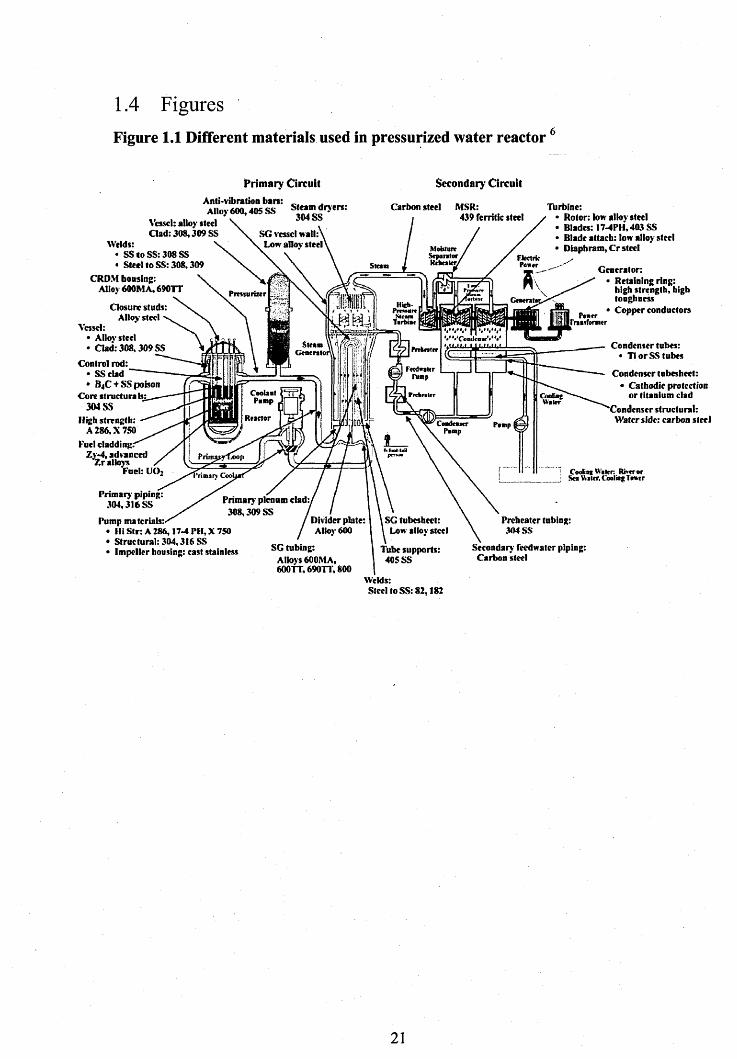
1.4 FiguresFigure 1.1 Different materials used in pressurized water reactor 6
Primary CircuitAnti-vibration bars:Alloy 600,405 SS
Vessel: alloy steel Clad: 308,309 SS
Secondary Circuit
Carbon steel MSR:439 fenitic steel
Steam driers:304 SS
Low allov steelElectric
PmsurizerH«hPmtttrtSitM
IirtHitO S ®
nxnormer
Stean h n n w
rwlw*»r
CoolxxlPxmp CnoKaj!
Walcr
Reactor
nnxrv C
Primary plenum clad
Divider plate tubcshect
Tube supports:405 SS
Welds:• SS to SS: 308 SS• Steel to SS: 308,309
CRDM bousing:Allov 600M A, 690TT
Closure studs: Alloy steel
Vessel:• Allov steel• Clad: 308,309 SS
Control rod:• SSclad• B4C + SS poison
Core structurab:304 SS
High strength:A 286, X 750
Fuel cladding.-'Zy-4, advanced
X r alloysFuel: U 02
Primary piping: 304,316 SS
Turbine:• Rotor: low alloy steel• Blades: 17-4PI1,403 SS• Blade attach: low alloy steel• Dlaph ram, C r steel
Generator:Retaining ring: high strength, high toughness Copper conductors
Condenser tubes:• T1 or SS tubes
Condenser tubcshect:• Cathodic protection
or titanium clad'Condenser structural:
Waterside: carbon steel
Cooliot W'tlrr R k trtr Sex Wilcr. Cooliag Tewtr
Pump materials:''• HI Str: A 286,17-4 PH, X 750• Structural: 304,316 SS• Impeller housing: cast stainless SG tubing:
Alloys 600MA,600TT, 690TT, 800
Prchcatcr tubing: 304 SS
Secondary feedwater piping: Carbon steel
Welds:Steel to SS: 82,182

C h a p t e r 2. L it e r a t u r e R e v ie w
This chapter is divided into two parts; part one gives basic information on AISI type
316L austenitic stainless steel, tungsten inert gas welding and the temperature
distributions plastic deformation mechanisms and residual stresses resulting from it. Part
two, reviews the experimental techniques available for characterizing residual stress and
plastic strain, and evaluates previous studies around welds in AISI type 316L steel. The
chapter concludes with the unanswered research questions revealed by this literature
review.
2.1 Introduction
In power plant applications, austenitic stainless steels are used because o f the stability
o f their tough, ductile austenitic phase which exists between room temperature and the
melting point, and because they are easily weldable. Tungsten Inert Gas (TIG) welding
provides precise control o f heat input and can produce very clean and high quality welded
• • 3 3 4 • •joints ’ .F o r this reason it is extensively used in the nuclear industries to join heat
sensitive components, thin gauge metal and pipes 34. This research study investigated
automatic tungsten inert gas welded plates o f AISI 3 16L(N) to analyse the residual stress
and plastic strain due to welding. The desirable features of this austenitic stainless steel
are, its resistance to corrosion, good creep resistance, ductility, formability and toughness
8 35’ . The chemical composition o f austenitic stainless steel 316L(N) is provided in Table
2.1. As specified in the table, the chromium forms a thin passive layer o f chromium oxide
on the surface of the steel to prevent corrosion and oxidation at elevated temperatures36
and nickel prevents the formation of ferrite36.
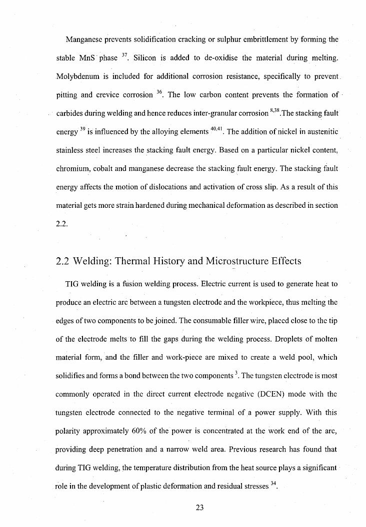
Manganese prevents solidification cracking or sulphur embrittlement by forming the
stable MnS phase 37. Silicon is added to de-oxidise the material during melting.
Molybdenum is included for additional corrosion resistance, specifically to prevent
pitting and crevice corrosion . The low carbon content prevents the formation of
Ocarbides during welding and hence reduces inter-granular corrosion ’ .The stacking fault
energy 39 is influenced by the alloying elements 40,41. The addition of nickel in austenitic
stainless steel increases the stacking fault energy. Based on a particular nickel content,
chromium, cobalt and manganese decrease the stacking fault energy. The stacking fault
energy affects the motion of dislocations and activation of cross slip. As a result of this
material gets more strain hardened during mechanical deformation as described in section
2 .2 .
2.2 Welding: Thermal History and Microstructure Effects
TIG welding is a fusion welding process. Electric current is used to generate heat to
produce an electric arc between a tungsten electrode and the workpiece, thus melting the
edges of two components to be joined. The consumable filler wire, placed close to the tip
of the electrode melts to fill the gaps during the welding process. Droplets of molten
material form, and the filler and work-piece are mixed to create a weld pool, which
solidifies and forms a bond between the two components3. The tungsten electrode is most
commonly operated in the direct current electrode negative (DCEN) mode with the
tungsten electrode connected to the negative terminal of a power supply. With this
polarity approximately 60% of the power is concentrated at the work end of the arc,
providing deep penetration and a narrow weld area. Previous research has found that
during TIG welding, the temperature distribution from the heat source plays a significant
role in the development of plastic deformation and residual stresses 34.
23
2.2.1 Tem perature distribution o f a m oving heat source •
In 1940, Rosenthal published an analytical heat distribution model representing steady
state autogenous welding 42. Whilst finite element based thermal analysis of welding is
now commonplace, the Rosenthal model provides useful insights 43. The model assumes
that a point heat source moves at uniform velocity, along the surface of a semi-infinite
plate. It uses a rectangular coordinate system whose origin coincides with the heat source.
Phase transformations and heat loss from the surface of the plate are ignored, and the
thermal properties are taken as independent of temperature. The Rosenthal heat flow
equation for the steady state temperature distribution is given as;
^(T^o)kr= a p fV S liO ) 2.1Q r v 2a J
Where T is the final temperature, To the initial temperature, k the thermal conductivity,
Q the heat transferred from the heat source to the workpiece, v is the source velocity, a
the thermal diffusivity, and r the radial distance from the origin. The temperature
distribution, in a plane perpendicular to the heat source, is determined by the radial
distance r from the centre of the heat source. The temperature distribution at any radius
from the heat source can be calculated from equation 2.1. For example, Chen et al. 44
have analysed numerically the effect of heat input, velocity of welding, thickness of the
plate and distance from the heat source on a temperature vs time profile. Mahapatra et
al.45 have analysed the effects of the welding parameters on temperature distributions
using three-dimensional numerical analysis. Experimentally measured temperature
distributions from the heat source, using an array of thermocouples, during the welding
process have been found to produce similar results 46. In all analyses, the heating and
cooling rates vary with the distance from the heat source. Most fusion welding processes
involve deposition of molten filler material alongside the melting part of the work piece
24
material close to the heat source. The volume in which the material has been heated up to
its melting point during welding is called the fusion zone3. Material adjacent to the fusion
zone.that has been metallurgically affected (in a away detectable metallographically) by
weld thermal transients is known as the “heat affected zone” (HAZ). Beyond the HAZ is
a “strain affected zone” (SAZ) that has undergone cyclic yielding 3, and compressive
yield. Further away the elastic zone (where deformation could be accommodated without
any plastic deformation). These zones are indicated in Figure 2.1 showing one of the
stainless steel weldments studied in this thesis. The weld thermal cycles determine the
metallurgical state of the material surrounding the heat source 45,47. The weld parameters
and number of weld bead depositions will significantly affect the development of
microstructure, the area of fusion boundaiy, grain size in HAZ and degree of plastic
deformation 48-50.
Even though 3 16L materials are readily weldable due to their low carbon content, they
commonly suffer from stress corrosion cracking (SCC) due to the welding process. The
magnitude of the plastic strains in the welded material has a significant effect on the SCC
T1growth . The SCC can be minimized effectively by optimizing the weld parameters
(travel speed, arc voltage etc.) and by using parent material as filler wire 51,S2. However,
local plastic deformation remains in the material due to the localized heat input, and the
non-uniform deformation arising from multi pass welding53. Numerous studies have been
earned out to help predict plastic deformation and residual stress (refer section 2.5.2) in
welds using finite elements models 17>19’46-54’55 However the magnitude and distribution
of the plastic strain and residual stress depends on the weld parameters and sequence etc.
Easterling 34 has qualitatively described the development of residual stress and plastic
strain as a function of temperature, as shown in Figure 2.2. During welding, as the
temperature increases, material close to the heat source initially expands, while the
material away from the heat source restrained from expansion due to lower temperature.
As a result of this, compressive stresses are generated during heating as shown
schematically in Figure 2.2 (i.e. 1 to 2). With further increase of temperature, the flow
resistance of the material near heat source decreases and the material becomes softer. This
results in the decline of the compressive stresses with increasing temperature and
considerable plastic strain may occur, as seen in Figure 2.2 (i.e. 2 to 3 and 4). However,
during cooling the material near the heat source contract, while the material away from
the heat source restrain the contract, as result of this tensile stress and strain are generated
with decreasing temperature as seen in Figure 2.2 (i.e. point 4-6).
Paradowska et al.56 analysed the effect of heat input on the residual stress distribution
in low carbon steel repair weld, using the neutron diffraction technique. The highest
stresses were noted in the middle of the weld bead. However, the work failed to show
clearly the effect of the heat input on the residual stress distribution. Muransky et a l 57
have numerically analysed the distribution of residual stress and plastic strain through the
thickness of a weld repair plate during multi-pass welding. Both numerical and neutron
diffraction analyses have exhibited peak longitudinal and transverse residual stresses in
the HAZ of the austenitic stainless steel. Murugan et al. 58 analysed the effect of heat
input, the geometry of the plate and the number of weld passes on the residual stress
distribution, in two different butt weld materials. However, with an increasing number of
weld deposits, the magnitude of the residual stress was found to decrease in the bottom
of the weld plate (i.e. root weld), whilst on the top weld cap of the butt weld plate it
increased. Jiang et al. 9 have analysed the effect of multiple weld repairs on
microstructure, hardness and residual stress in clad plate. Neutron diffraction results in
clad repair weld plate demonstrated a decrease in the residual stresses from the HAZ to
the weld cap, and from the HAZ to the parent material. Similarly, hardness test results in

clad repair weld plate have shown higher hardness values at the interface between the
weld metal and the base metal. Based on the residual stress, hardness test and
microstructure of repair clad plate, Jiang et al., recommends that the clad plate should not
be repaired more than 2 times.
Most of the numerical studies in austenitic stainless steel weldments 55’59~66 have not
considered the influence of the dynamic strain ageing effect on plastic deformation.
Before describing the effects of dynamic strain ageing, it is appropriate to review some
basics of cyclic deformation, dynamic strain ageing and its mechanism as associated with
welding.
2.3 Monotonic and Cyclic Deformation in 316L(N)-
Mechanism and Effects
The plastic deformation of 316L (N) can be described with the help of Figure 2.3.
When the applied stress exceeds the yield stress, the deformation stop being elastic and
the material is permanently deformed, this is known as plastic deformation.
2.3.1 Mechanism o f plastic deformation
When a metal is stressed above its yield point, energy is consumed in generating or
moving dislocations. During deformation, the motion of dislocations allows some parts
of the crystal to slide across another part of the. structure as shown in Figure 2.4. The
planes on which sliding occurs are called slip planes. Slip displacement usually occurs
along the close packed planes, where the energy required for dislocation motion is
minimized. The direction in which the slip occurs is called slip direction. In f.c.c
structures, slip normally occurs on planes of the type {111} and where the principal slip
27

direction is along <110>. The combination of slip plane and slip direction is called a slip
system .,.. : v . . v -
The plastic deformation of each material varies depending on its crystal structure. The
crystal structure o f austenitic stainless steels is a face-centred cubic (fee), a highly
symmetric structure, with 12 equivalent slip systems. This means that austenitic stainless
steel deforms more easily than other crystal structures, such as body-centred cubic (bcc)
crystal with fewer possible slip systems. The shear stress (refer Figure 2.5) required to
move a dislocation is given b y 67
Fx = - coscb. cosA 2.2A
Where the area of the slip plane is A/cos and the force acting in the slip plane in the
slip direction is Fcos X. The resolved shear stress is at maximum when both X and O are
at 45°, and tend to become zero when either X or 0 are at 90°.
If the angle between slip direction and direction of applied load (i.e. A) is less than 45°,
as the deformation of the material begins, X decreases. Hence, according to equation 2.2,
the resolved stress decreases as well. In order to deform the material plastically, the force
needed to be increased and maintained, so that the shear stress is always higher than
critical shear stress for continued plastic deformation. This phenomenon is known as
geometrical hardening 39. During plastic deformation, the increasing number of defects
in the material will impede the flow of dislocations. As a result, additional stress is
necessary for the continuation of plastic deformation. This phenomenon is called work
hardening or strain hardening.
2.3.2 W ork hardening
As deformation of the material proceeds, the material gets harder and stronger. At one
point the material reaches a state where further deformation of material leads to failure.
2R

At this stage the tensile strength and hardness of the material are at their maxima. The
material’s degree of work hardening depends 011 the density of defects, such as vacancies,
interstitials or dislocations (edge, screw or mixed) and on the stacking fault energy .
The work of Frank-Reed39 and Orowan68 on dislocation loop mechanisms has explained
the work hardening of material due to interactions between dislocation and defects.
Haojie et al. 69 have analysed numerically the work hardening of material due to
interaction between screw dislocations and different stacking faults. An excellent review
on the stages of strain hardening in monotonic deformation has been given by Kock et al
70. Both Cottrell71 and H irth72 have demonstrated the formation of immobile dislocations
due to the interaction of dislocations on the primary slip plane, with ones on the conjugate
slip plane.
There are two basic types of dislocation movement that take place; conservative
movement (i.e. glide) 01* non-conservative movement (i.e. climb). In non-conservative
movements, activated at high temperature, dislocations move out of their slip plane. At
low temperature, the plastic deformation of material mainly occurs by conservative
motions. At elevated temperatures, the mobility of the dislocation is high and dislocations
can take a new slip plane by cross slip.
Depending on a dislocation’s sign and direction, another dislocation moving on the
same slip will annihilate, repel it or form a sessile dislocation 39,73. Sessile dislocations
act as strong obstacles for moving dislocations. If the interacting dislocations move on
different slip systems, after interaction they will develop jogs or kinks 39. A jog is a sharp
break in the dislocation line moving it out of slip plane, whilst a kink is a sharp break in
IQthe dislocation line which remains in the same slip plane . Jogs are also formed by the
intersection of two screw dislocations, and play an important role in plastic deformation.
29
Jogs in screw dislocations can only move, by slip, along the dislocation’s line and the
only way a screw dislocation can move to a new slip plane, along with a jog, is by climb.
The presence of edge dislocations in a crystal induces compressive stress around an
extra half plane of atoms, and tensile stress below the extra half plane, as shown in Figure
2.6. Similarly, shear stresses are induced around screw dislocations. The presence of
stress around dislocations will attract defects such as interstitial or substitutional solute
atoms, and redistribute them to lower the energy around the dislocations. As a result, an
atmosphere builds up around the dislocation, which is known as the Cottrell atmosphere
67,74. Once an atmosphere has formed, the'dislocation can only move by breaking free
from the atmosphere or by dragging the atmosphere along with it. In both cases, the metal
becomes work hardened due to the restriction of dislocation movement. As a result of this
discontinuous motion of dislocations, stress-strain curves at high temperature show
serrated flow. This phenomenon is called dynamic strain ageing 75.
2.3.3 Dynamic strain ageing (DSA)
DSA occurs due to interactions between moving dislocations and solute atoms, either
n c nc.interstitial or substitutional ’ , when solute atoms gain enough velocity to keep up with
the moving dislocations and form a Cottrell atmosphere. DSA increases the material’s
work hardening rate and the ultimate tensile strength, whilst reducing its ductility11. One
important effect of DSA is negative strain rate sensitivity. The most important variables
affecting DSA are the temperature and strain rate 78.In the DSA regime, if, during sample
deformation at a given temperature and strain rate, the flow stress decreases with
increasing strain rate, this is called negative strain rate sensitivity.
Solute drag, lattice friction and the concentration of the diffusing solutes, all contribute
to DSA, as illustrated by Figure 2.7 re-constructed from the work of Blanc and Strudel
in
79. As seen in Figure 2.7, with increasing dislocation velocity, the lattice solute drag force
increases friction (see curves 1 and 2), while the effect of dislocation velocity on the
nearby concentration of the diffusing solutes is in the opposite direction (see curve 3).
The overall result of the contributions of curves 1, 2 and 3, is curve 4. At dislocation
velocities below Vm, the dislocation is in the drag zone. In this regime, the velocities of
the dislocation and diffusing solute are approximately equal and form a Cottrell
atmosphere around the dislocations. With increasing dislocation velocity, a critical force,
Fm, is achieved and the dislocation enters the instability zone, where it accelerates enough
to break away from the solute atmospheres. With further increases in dislocation velocity,
to V3, the lattice friction forces and dislocation interactions become dominant, and the
friction regime begins. This results in a decrease of the dislocation velocity of Vm and an
unstable zone is reached. Consequently, the dislocations re-enter the drag regime at Vj,
This cycle of drag, instability and friction velocity causes the stress-strain curve to be
serrated. Depending on the temperature, the carbon, nitrogen or chromium atoms may be
responsible for DSA 80,81.
The formation of Cottrell atmosphere requires long-distance diffusion of solute atoms
and therefore occurs only at high temperatures or after long term annealing. Before
Cottrell atmospheres form, the solute atoms can reduce their energy by merely changing
their position within the unit cell. However, the positions of the solute atoms change only
when the unit cell is distorted. Ordering of solute atoms, arising from their occupying
O')
preferred positions along certain directions, is called the Snoek order ". As a result of
Snoek order, an ordered atmosphere (called a Snoek atmosphere) may develop around
the dislocation before the formation of the Cottrell atmosphere. The formation of a Snoek
atmosphere around a dislocation, impedes its motion, and in order to move the
dislocation, a higher yield stress is required ’ .
31
In addition to Snoek ordering, the Suzuki effect also contributes to the serration of
flow stress. A perfect dislocation in a closed packed structure can split into two partial
dislocations, with an enclosed ribbon of stacking fault. As a result, the energy of the
dislocation decreases and a stacking fault is formed 82. As described earlier (section 2.1),
alloying elements can decrease the energy of stacking faults in austenitic stainless steel
40,41. In this case, the local chemical potential difference between a faulted region (for
example, between partial dislocations) and the surrounding fee matrix will provide a
driving force for preferential segregation of solute atoms to stacking faults. This Suzuki
segregation, resulting from the concentration dependence of the stacking fault energy,
lowers the stacking fault energy, causing the fault to become wider and reducing the
energy of the crystal.. An additional stress is then required to break the dislocation away
from its Suzuki atmosphere, which leads to a yield drop.
The mechanism of DSA has also been explained by an alternative theory. In the DSA
zone the solute atoms restrain the motion of the dislocations. In order to maintain the
strain rate, additional dislocations are generated 85. As a result the material gets more
work hardened.
2.3.4 Cyclic loading
When a material is subjected to defined number of repetitive tension to compression
or compression to tensile cycles, it is called cyclic loading. During cyclic deformation,
the dislocation density has been found to increase during the initial forward deformation
and decrease during the initial reverse deformation 73, due to the interaction and
annihilation of dislocations. Nevertheless, further reverse deformation leads to an
increase in dislocation density. A reduction of the yield stress of pre-strained material on
reverse loading, is known as the Bauschinger effect . With further cycles of deformation,
32

the dislocation density frequency increases, resulting in a cyclic hardening response.
However, a material’s hardness during cyclic deformation depends strongly on the
orientation of its grains, the stacking fault energy, any short range order and the active
slip ‘modes’ 87.
The relationship between slip mode and the type o f dislocation structure (e.g. tangles,
persistent slip bands, cell etc.) formed during the cyclic deformation was first explained
o o OQby Feltner and Laird ’ . Wavy slip mode implies that cross slip can occur easily and
that the cyclic stress-strain behaviour is history independent. In the planar slip mode,
cross slip is difficult and the material cyclic behaviour is history dependent90’91.
Austenitic stainless steel 316L has a low stacking fault energy92, so partial dislocations
are widely spaced. Wide stacking faults between partials impede the motion of
dislocations and reduce the activation of cross slip. Slip on secondary slip planes is also
inhibited in the early stages of deformation. As the deformation proceeds and the. density
of dislocations increases, activation of the secondary slip increases the interaction of
dislocation with defects, and leads to the formation of sessile dislocation and jogs. These
sessile dislocations will restrict further dislocation motion and assist the formation of
dislocation tangles. At one point cyclic hardening and cyclic softening occur
no QQ
simultaneously ' ’ . Hardening is due to the formation of hard structures within the
crystal pattern, such as dislocation walls, whilst the softening is due to activation of cross
slip, the fonnation of channels (low dislocation density), and depending on the strain
amplitude, activation of persistent slip bands 27’94~". After many cycles, the effects of
active persistent slip bands and the formation o f channels may surpass the hardening
effect, leading to cyclic softening and the formation of a stable cellular structure of
dislocations.
33
The DSA temperature range for austenitic stainless steel 316L is reported to be
between 300°C-650°C 78,100,101. Ivanchenko’s 102 thesis has analysed the dynamic strain
ageing effect on the work hardening of tensile deformed austenitic stainless steels andNi-
base alloys. The DSA for the austenitic stainless steel AISI 316 and Ni base alloys 600
and 690 materials was observed in the temperature range of 200°C-650°C at strain rate
from 10'6 to 10‘3 per second. With increasing nitrogen content, the amplitude of the flow
stress pulses decreases. This is due to nitrogen atoms accumulation on dislocations or due
to formation of multiple Luders bands structures. At 400°C long-range planarity
dislocation microstructure; at 288°C short range planarity dislocation microstructure and
at 200°C cellular dislocation microstructure was observed in 316NG austenitic stainless
steel. Calmunger’s 103 thesis has analysed the effects of DSA on the mechanical properties
and microstructural development in austenitic alloys. At elevated temperatures the
ductility of austenitic alloys increased at slow strain rate in comparison to the austenitic
alloys deformed at higher strain rate. However, in aged austenitic alloys, the ductility of
materials decreased at slow strain rate due to formation of precipitates in the grain
boundaries. During plastic deformation, the stresses are concentrated around precipitates,
as result o f this intergranular fracture develops. Pham 101 has analysed the effects of DSA
on the cyclic deformation response and dislocation microstructure. The DSA becomes
less active during the first two cyclic response stage (i.e. hardening and softening stage).
This is due to different short range interactions between dislocations and solute atoms.
However, the serration becomes more significant after the cyclic softening phase (i.e.
secondary cyclic hardening). Pham have shown the serration length is greater for reverse
loading transients from tensile peak stress than for during reverse loading transients from
compressive peak stress. This is due to vacancy mobility is promoted during reverse
loading transients from compressive peak stress and suppressed during reverse loading
transient from tensile peak stress. In DSA regime, the presence of vacancy in crystal
structure significantly effects the strain hardening-of the material. Gerland et a /.104,105
have shown the effect of DSA on the dislocation structure and the fatigue behaviour of
316L at temperatures between 20°C and 600°C. Gerland’s study showed a new
dislocation structure called corduroy structure, which are formed in vacuum cyclic
deformation of 316L material. The corduroy structure is responsible for secondary strain
hardening of 316L material at temperature range 200-500°C. The corduroy structure is
composed of alternative black (dislocations loops, debris and cavities) and white bands
(channels). At 400°C, the formation of corduroy structure is high. The DSA of this
material is due the interaction of corduroy structure and planar slip with solute atoms (G
and N solute atoms). Similarly, Hong et al 78’,0°’106 have analysed the effect of DSA on
slip mode initiation and propagation of multiple cracks, the mechanism of DSA with
respect to temperature and strain rate. Hong’s studies showed, austenitic stainless steel
AISI 316L material experience DSA only at specific temperature range and strain rates,
i.e. between 250°C -550°C at a strain rate o f 1 O'4 per second; between 250°C -600°C at
strain rate of 10'3 per second and between 250°C -650°C at strain rate of 10'2 per second.
In DSA regime, the material gets more strain hardening due to the change in mechanism
of plastic deformation, i.e. switching from wavy slip to planar slip mode. The fatigue
resistance of austenitic stainless steels AISI 316L was reduced in the regime of DSA.
Srinivasan et a l107 have studied the effect of DSA on the cyclic stress response and fatigue
life of solution annealed and prior cold worked 316L(N) samples. The solution annealed
austenitic stainless steel AISI 316L(N) exhibited DSA at 873K. At slow strain rate,
Srinivasan noticed post cold worked austenitic stainless steel exhibited higher fatigue
endurance as compared to solution annealed material. At temperature range 673-873K,
the fatigue life of the solution annealed material was decreased. This is due to, in DSA
regime, higher stress concentration taking place at dislocation pile-up. Which would
account for increased crack growth rates and hence reduction in the fatigue life. Samuel
80 has reviewed sample ageing effects on the appearance and disappearance of DSA, at
temperatures between 300°C and 650°C due to carbide formation. At low temperature
region i.e. 250°C-350°C, the diffusion of interstitial solute to dislocation is main
responsible for activation of DSA in 316 material, while at high temperature range i.e.
400°C-650°C, the substitutional solutes like Cr is responsible for activation of DSA in
3 16L material. The serrations are most distinct in aged material at 650°C. However at one
point the serrated flow suddenly ends in aged material at 650°C due to formation of
precipitation and resulting decrease of solute concentration by ageing.
The cyclic hardening and softening of a material at different temperatures can be
analysed numerically at the macro-scale using an appropriate elastic-plastic constitutive
material model. A material’s response to cyclic deformation can be described by a
hardening ‘rule’ which describes the behaviour and development of the yield surface.
Depending on the type of rule, the model will determine how the yield point changes with
the accumulation of plastic strain; this is illustrated in Figure 2.8. The types of rules
include isotropic hardening, kinematic hardening, mixed hardening and distortional
hardening 108.
2.3.5 FE Elastic plastic constitutive material models
In finite element modelling, isotropic, kinematic and mixed hardening models are
known as single surface models. These simple models only consider the change of the
yield surface, resulting from plastic strain accumulation. The loading surface defines the
boundary of the current elastic region, as seen in Figure 2.8(a). As the stress point moves
beyond the boundary of the elastic region, plastic strains are produced on the current
loading surface, changing its original configuration (as defined by the hardening rule).
36
An isotropic hardening model defines the change in size of the yield surface. This
model has been widely used in the literature to represent the cyclic stress-strain behaviour
of materials 108. When a uniaxial test specimen is subjected to tensile deformation beyond
the yield stress, as shown in Figure 2.8(a), plastic strain is introduced in the material. The
maximum stress achieved during tensile deformation determines a new yield limit that is
mirrored in compression loading. If the stress is further increased in compression,
additional yielding and material hardening will occur, and this further increases the yield
strength. Similar behaviour will occur in the next application of tension. An isotropic
hardening model is usually assumed for cases where the load is monotonically increased.
However, this model does not account for the Bauschinger effect and therefore does not
represent cyclic loading very w e ll108.
The isotropic hardening component defines the variation in cyclic stress hardening,
which in turn gives the yield surface size,a 0, as a function of the equivalent plastic strain
£~pl. It is derived by 108
er° = o i0+ 'Qm ( l - e~b£~pl>) 2.3
Where cr :0 is the size of the yield stress at zero equivalent plastic strain, obtained from
the first cycle (refer Figure 2.8 (c)). Q*. is the maximum change in the size of the yield
surface, which can be calculated as the difference between the asymptotic material
response and cr i0 (refer Figure 2.8 (c)). b is the rate at which the size of the yield surface
changes as the material plastically deforms. The size of the yield surface in the ith cycle, cr/3
can be evaluated from 108
Where of is the peak tensile stress in the plastic range and o f is the minimum
compressive stress in the elastic range as in Figure 2.8 (a).
37
Similarly, the equivalent plastic strain of the ith cycle can be obtained using the following
equation 108
£~vi = ± ( 4 i - 3 ) A £ - pi 2.5
Where Ae‘pl is the plastic strain range of cyclic deformation and the ith cycle. From Q<x,
o !0 and data pair o f, £ pl the rate at which the size of the yield surface changes b can be
A kinematic hardening model deals with translation of the yield surface in stress space;
see Figure 2.8(b). In this model, the equivalent stress defining the yield surface, o ; ,
remains constant and equal to the equivalent stress, Go, which defined the yield surface
at zero plastic strain, as seen in Figure 2.8(b). Therefore, when a test specimen is uni-
axially loaded beyond the yield limit and unloaded into compression, the new
compression yield limit is smaller in magnitude than the yield point in tension. In the
kinematic hardening model, the elastic range is fixed at twice the initial yield stress value,
and never increases.
i noThe kinematic hardening law is given by
Where Q is the initial kinematic hardening modulus and a is the deviatoric part of the
kinematic hardening tensor a, which is also known as the back stress tensor. Both
parameters Cj can be evaluated from stabilized cyclic test data, as shown in Figure 2.8
evaluated thus 108
2.6
a = YjiCi — ((r — a)e pl 2.700
(b), o is stress tensor, a 0 is the equivalent stress defining the size of the yield surface and
£ pl the equivalent plastic strain rate.
38
A mixed hardening model can represent both the size changes of the yield surface and
is widely used, where the evolution of the yield surface is formulated by combining two
components; the isotropic hardening component and a non-linear kinematic hardening
component. Its implementation in the ABAQUS finite element code can be found in the
user manual 110
The mixed hardening model describes the translation of the yield surface in the stress
space using the back stress cr, which is expressed as 24,108
Where Ci are the initial kinematic hardening moduli and yi determine the rate at which
the kinematic hardening moduli decrease with increasing plastic deformation. Ci and yi
are material parameters which are calibrated from monotonic or cyclic test data and i pl
is equivalent plastic strain or plastic path length, a is the stress tensor,o° is the equivalent
Where a s is the stabilized size of the yield surface. Using data pair cij and s~pl calculated
from equations 2.9 and 2.10, the non-liner kinematic hardening parameters are defined
using equation 2.8.
A mixed hardening model has been used widely to simulate the cyclic hardening in
weld simulations due to its accuracy in reproducing cyclic strain-controlled tests, thermo
its translation through the stress-strain space. A Lamaitre-Chaboche hardening model 109
2.8
stress defining the size of the yield surface. The data pair a\ and £* pl can be calculated
from the following equations 108
2.9
cr,- = Ci (01+02)2
2.10
_ ay+a2 2.11
mechanical fatigue and in predicting residual stress 21 ,?4,57,111. in this research study, this
mixed hardening model was used for predicting cyclic stress-strain curves. Further detail
on previous work using this model to predict cyclic deformation is discussed in section
2.5.3.
2.4 Residual Stresses Measurements Around Welds in
3 1 6 L ( N )
Residual stresses are the stresses which remain in a material in the absence of any
external force. Figure 2.9 shows various processes that can generate residual stresses at
7 112the macroscopic and microscopic levels ’ . In multi-pass welding, the residual stress
distribution is affected by different aspects of the welding process, such as the number o f
passes, the heat generated during welding, the depth and the width of the weld bead
56,i 13, 114 j ^ q presence of tensile residual stresses at a welded joint can reduce the lifetime
of the material by increasing its susceptibility to stress corrosion cracking, fatigue and
creep growth 4. Macro stresses are classified as type Iresidual stress, they are introduced
by fabrication processes such as welding or machining. They self-equilibrate over the
length scale of the specimen and they can be described by continuum mechanics1. Type
II residual stresses are inter-granular stresses and typically self-equilibrate between grains
or phases. Type III residual stresses are intra-granular stresses that self-equilibrate over a
few interatomic distances, and are associated with point defects and dislocations. This
thesis is concerned with the type I residual stresses, introduced by welding.
There are a wide range of mechanical and physical techniques developed to measure
residual strains or stresses in components and structures 112’115' 117. The strain sensitivity
and the spatial resolution of the various strain analysis techniques are represented in
40

Figure 2.10. Residual stress measurement techniques are broadly classified into two
categories: destructive and non-destructive. Destructive methods include hole drilling;
the slitting method, the contour method, FIB milling etc., and the non-destructive
methods includes X-ray diffraction, neutron diffraction, ultrasonic, Raman spectroscopy
etc. In this research study, type 1 residual stresses developed due to the welding process
were measured using neutron diffraction. The reasons for choosing neutron diffraction
were:
1. The test specimen could not be destroyed as it is part of an international round
robin, the NeT project (section 2.5.2).
2. Neutrons have sufficient penetration to measure strains and stresses to the depth
required.
3. The wavelength of the neutrons is of the order of the inter-planar spacing. As a
result of this, a diffraction angle (20) close to 90° enables the user to use a square
geometry gauge volume. This allowed measurement in three orthogonal
directions (unlike synchrotron diffraction).
2.4.1 Principle o f neutron measurements o f residual stress:
The crystalline lattice of the material acts as an atomic strain gauge. The spacing, W’,
between atoms in the crystalline lattice varies depending on the applied stress, as shown
in Figure 2.11. The increase or decrease of lattice spacing can be determined from the
angular shift (A20) in the diffracted neutron beam, as defined by Bragg’s law;
A = 2 dsinO 2.12
Where, / is the wavelength of incident beam, 0 is the angle of diffracted beam as shown
in Figure 2.11, and d is the inter-planar spacing of the measured direction defined by the
Q-vector. The d spacing for a particular lattice reflection can be determined if the
41
wavelength of the incident beam and the angular position of the diffracted peak are known
112,118,119. Two types of neutron source (continuous and spallation) are available for
117residual stress measurement . The main differences between spallation and reactor
sources are summarized in Table 2.2. In this study, spallation neutron diffraction was
used to measure strain in three-pass welded austenitic stainless steel.
2.4.2 Neutron diffraction instruments
The ENGIN-X diffractometer at the ISIS spallation source (Oxford, UK) and the
VULCAN diffractometer at the Spallation Neutron Source (SNS), Oakridge, USA were
used in the present research. At these facilities accelerated ‘bunches’ of high-energy
protons from a synchrotron ring collide with a heavy atomic target to generate neutrons
in sharp pulses. The neutrons pass through a moderator to achieve thermal equilibrium
and are guided to the experimental instruments. The layouts of the ENGIN-X instrument
at ISIS and VULCAN instrument at SNS are shown in Figure 2.12. The detectors on each
instrument are fixed at 90° to the incident neutron beam. The sample is placed with the
scattering vector (Q-vector) bisecting the incident and diffracted neutron beams. The
main advantages of a spallation neutron source over a reactor source are:
1. A single pulse of neutrons generated in a spallation process has higher neutron
intensity.
2. A ‘white’ beam with different neutron wavelengths enables various families of
lattice reflections to be measured simultaneously.
The velocity (v) of a neutron is defined by
v = L / t 2.13
42
Where L is the total flight path (from the moderator to the detector) and / is time of
flight (TOP). However, according to de-Broglie wave theory, the wavelength is
inversely proportional to the velocity.
X — h /m v ' 2.14
Where m is mass of neutron, h is is Planck’s constant, combining equation 2.14 and
equation 2.13 gives
X = (h t) /m L 2.15
Substituting equation, 2.15 into the Bragg equation 2.12 gives the TOF in
microseconds.
t = m L 2 d sin 6 /h 2.16
Therefore, at a constant diffraction angle 0, the variable d is directly proportional to
the variable t 120. Hence, the most energetic neutrons arrive at the specimen first and the
least energetic neutrons reach it last. In a spallation source the intensity of peaks is plotted
as a function of time of flight (TOF) as shown in Figure 2.13. To conclude, in a spallation
source the values of two variables in the Bragg equation are already known; the angle
(6=90°) and the wavelength (/); therefore the third unknown variable, td \ can be
measured. Further details about the ENGIN-X and VULCAN instruments are available
1 2 1 - P 7in published literature
2.5 Evaluation of Residual Elastic Strain and Stress Using
Neutron Diffraction
When a crystalline material is loaded, its inter-atomic spacing will change, depending
on the applied load. The difference in the inter-atomic spacing can be measured using
43
neutron diffraction. To measure the strain, the d spacing in both strain free material and
strained material is required, then the elastic strain can be calculated as; 63,64,73 . :
£ = ((d — d 0) ) / d 0 2.17
Where do is the unstrained lattice parameter and d is strained lattice parameter. By
calculating the strain values for each direction using equation 2.17, stress, a, can be
129determined using the following equation ;
<7** = I W ( ( 1 + v) * (1 - 2u))} * {(1 - v) £xx - v (£ yy - 8ZZ }] 2.18
Where, axv is stress in the ^-direction of the sample (say along the weld), E is the
Young’s modulus of the bulk material and v is Poisson’s ratio.
2.5.1 Issues affecting strain/stress measurement using neutron diffraction
In this section, important issues affecting the reliability of strain measurement using
neutron diffraction are described.
Stress free lattice parameter (an): from equation 2.17 it is clear that the unstrained
lattice parameter, ao also known as the stress-free lattice parameter, plays a key role in
n o i -jrv i TO
evaluating residual strain ’ . Small variations introduced by differences in
chemical composition, inter-granular strains and thermal history can lead to large
uncertainties in ao due to variations in intensity and/or peak broadening 10,108. In welded
samples, the non-uniform thermo-mechanical history introduces variations in grain size,
texture and degree of plastic deformation, which can shift the diffracted peaks. Due to
non-homogeneity in the sample, a number of stress free reference values are required to
1 1 Aproperly interpret the measured strain . A lot of underpinning research work was
performed in establishing the standards for residual stress measurement using neutron
diffraction 118’135. The recommendations for selecting and determining the stress-free
lattice parameters are available in the literature 135,136.
44
Many practitioners have used combs, matchsticks, or cylindrical pins and cubes, or
cuboids for stress free lattice parameter measurements 137~140. However, in extracting a
‘stress free’ sample, the relaxation of macroscopic stress significantly affects the inter-
granular stress state 140. Another effect has been noted in combs, where the comb teeth
have been reported to retain macro stress141. For weldments, the gradual changes in the
stress free lattice spacing resulting from the non-uniform thermal history, and the
associated variation in microstructure, necessitates the extraction of stress-free samples
from many different locations across a weldm entlj0.
Gauge Volume effect: The spatial resolution of neutron diffraction measurements
depends on the gauge volume chosen 142~146. The geometrical dimension of the gauge
volume depends upon the incident neutron beam and collimator dimensions. As described
earlier, the nominal gauge volume for both the ENGIN-X and VULCAN diffractometers
is a perfect cuboid 117. The centroid is defined by the intersection of the incident and the
diffracted neutron beams. However, in reality, the neutron beam is divergent, which
changes the shape and size of the true gauge volume 147,148. This is known as the
instrumental gauge volume, as shown in Figure 2.14. The centroid of the instrumental
gauge volume is the intensity-weighted centre of this volume. The instrumental gauge
volume and the nominal gauge volume are properties o f the diffractometer itself.
The sampling gauge volume is the volume from which measurements are obtained,
and it is part of instrumental gauge volume 149’150. The sampling gauge volume is strongly
affected by its geometrical location within the sample, as well as by material
characteristics such as texture, cold work, neutron beam absorption etc. 129’142’150’151. The
centroids of the instrumental gauge volume and sampling gauge volume are identical
when completely immersed in a non-neutron absorbing material. However, the sampling
gauge volume is affected by partial filling of the instrument gauge volume, attenuation of

neutrons within the sample and the wavelength distribution across the incident beam
145,15'-153. The centroid of the sampling gauge volume is the weighted centre of the gauge
volume after accounting for these effects 15°. -
The nominal gauge volume can most closely be achieved by positioning the slit close
to the sample, minimizing the divergence of the neutron beam. However, partial gauge
volume immersion, as shown in Figure 2.15, introduces a systematic shift in the diffracted
peak, known as a pseudo strain. In TOF, the pseudo strain can be given by 150
S t Sd . SlsinQ ' ^
— = — + - — - 2.19t d Isind
Where t is time of flight, 0 is the diffraction angle and / is the total distance travelled
by neutrons from the moderator to the detector. From equation 2.9, it is clear that the shift
in a peak is due to the contribution of lattice strain and the variation oi'IsinO ’. The term
‘IsinO’ in equation 2.19 represents a weighted average of ‘IsinO ’ over the whole gauge
volume. Pseudo strain also occur when analysing strain in highly absorbing material (such
as boron or hydrogen).
Creek et al. 154 investigated the effect of pseudo strain on measurement by pulsed
neutron sources but did not consider the effect of the incident beam divergence. Creek
modelling showed incomplete filling of the gauge volume will generate pseudo strain of
lOOOps in comparison to the resolution of instruments used to measure such strain (50
pe). Suzuki et a l .142 have proposed a new analytical model, which can be used to simulate
different effects of pseudo-strains. Using spallation source, Suzuki investigated the effect
of neutron attenuation, surface effects and a strain distribution on pseudo strains
generation. In completed filled gauge volume, the pseudo strains are developed due to
change in neutron-weighted center of gravity (ncog) position and it increased with an
increase in the size of the gauge volume. Typical pseudo strain distributions due to the
46
surface effect were noticed through the surface strain measurement regardless of gauge
size. Pseudo strains developed due to neutron attenuation and/or the surface-effect
exhibited a wavelength dependence associated with a wavelength dependence of the
neutron divergence in the super mirror guide tube. Wang et a l 151’155 have analysed the
issues contributing to the pseudo strain: variation of the wavelength across the incident
beam, an asymmetric clipping of the diffracted peak profile and lateral displacement of
the gauge volume relative to the detector. In Wang’s experimental investigation, the error
in strain measurement due to wavelength dependent attenuation were within ±50ps. The
small shift observed due to attenuation in the incident beam can be minimised by placing
the sample in preferable place in the diffracted beam. Whilst Hsu et al. 153 investigated
the multiple scattering and wavelength dependent attenuation effects in steel plates. Hus’s
systematic investigation has summarised the Bragg edge location between 1.4A and 3.0A
for a number of common metals. The neutron attenuation coefficient for polycrystalline
materials decreases suddenly for certain neutron wavelengths, this effect is known as
Bragg edges. Hsu’s investigation recommends, if the strain measurements are located at
depth of material then one should avoid using neutron wavelength within A A/A =
0.02A of the Bragg edge. This is because lower order Bragg edges tend to have a bigger
discontinuity in total cross section.
Grain Size Effects:
In neutron diffraction, uncertainties in a residual stress measurement depend on the
number of grains diffracted 156,157 and the number of grains diffracting depends on the
gauge volume size chosen. Therefore, for a given gauge volume, the uncertainties in
residual stress are lower for a fine grained sample than in a sample with a large grain size,
due to the former’s larger number of diffracting grains129,158.
47

In polycrystalline material, inhomogeneous plastic deformation due to welding can
1 7Qlead to the development of large inter-granular residual strains -. In grains, which are
orientated favourably in the loading direction, slip systems will activate and those grains
will deform plastically, due to the higher resolved stress. Upon unloading, the size o f the
plastically deformed grains remains largely unchanged, which hinders the elastic
recovery of the non-deformed grains. As a result, elastic strain is locked into the nom
deformed grains upon unloading 14°. These elastic strains, in different sets of hkl planes,
are measured by neutron diffraction 159-161.
The slit positions close to the specimen can cause ‘clipping’ of the diffracted peaks,
shifting their apparent position. These can introduce an error in the determined strain.
Webster et al 151 demonstrated that this effect was more severe in coarse grained
materials. The same paper also demonstrated that an uneven distribution of large grains
in the sampling volume can also shift the diffraction peak position on the detectors. Neov
et a l 162 analysed the residual stress in an SS347 grade welded stainless steel specimen.
The tensile strain measurements were affected significantly by the grain size of the plate,
by twice the real strains measured in the plate. However, by rocking the sample, more
grains were diffracted within a given gauge volume, which led to more realistic strain
distributions being measured.
2.5.2 Weld residual stress NeT-henchmark
Several different international consortium activities have been undertaken on the
prediction and characterization of weld residual stress and distortion of welded samples
13,14,163,164 Qne suc^ gr0Up js European Network on Neutron Techniques
Standardization for Structural Integrity (NeT)15. The main objective of this group was to
define recommendations for the prediction and measurement of welding residual stress.
48

Residual stress measurements using different techniques on benchmark weldments, under
well controlled conditions, have been performed by members of this round robin network
16 in order to assess and improve the reliability of residual stress measurements. The
measurement techniques applied include neutron diffraction, synchrotron x-ray
diffraction, the contour method, deep hole drilling and incremental surface hole drilling.
In parallel, round robin finite element analysis residual stress simulations have been
performed and compared with the results from the above stress measurements. Several
benchmarks have been defined, each managed by a different task group (TG). For
example TGI tackled a single pass weld TIG bead deposited on the surface of the
austenitic stainless steel 316L (180x120x17 mm3) 'M6,6i,66,157,165-168
TG4 is investigating residual stress developed around a three-pass slot weld in a 316
austenitic stainless steel plate (194x150x18 m m ). The specimen geometry is
representative of a weld repair. Several numerical and a few measurements studies have
been published related to the NeT TG4 round robin 21’22’24’57’,11’139> The present research
is based upon the NeT TG4 benchmark weldment.
2.5.3 Previous NeT TG4 benchm ark studies
The distribution of residual stress introduced into a welded austenitic stainless steel
component depends on its geometry, the welding parameters and the welding sequence
i i 3 , i i 4 , i 6 9 , i 7 o B e n c }i m a r k samples are valuable in that they allow analysts to evaluate and
improve the accuracy of residual stress measurement and weld modelling 171. Details of
the NeT TG4 benchmark weldment’s design and manufacture are given in Chapter 3. The
1 77residual stress measurement protocol recommended by the NeT consortium for TG4
analysis is described in Chapter 4.
The first experimental residual stress characterization of a NeT-TG4 weldment was
perfonned at the beamline ID 15a of the European Synchrotron Radiation Facility (ESRF)
49
1 9Qsee Figure 2.16. This experiment has analysed both macro strains and intergranular
strains (along line BD only, refer section 4.2.1, Chapter 4) in weldments. The measured
lattice parameters for top weld, bottom weld and parent stress free cuboids during this
experiment were 3.59653 A, 3.59716 A and 0.359752 A respectively. The differences
between the values are due to the slightly different chemical compositions of the filler
wire and the parent material. Along plane D (refer to Figure 3.3) the maximum
longitudinal residual stress was observed in the HAZ, while the maximum transverse
stress, was observed in the first and second weld beads. However, along plane B (refer to
Figure 3.3) the maximum transverse stress was noticed in the HAZ, not in the weld bead
as observed in Plane D. The residual stresses measurement at the bottom of the plate
exhibited stress of ±200 MPa at the centre and ends of plane D and B respectively. The
91
uncertainties recorded during this experiment are ±50 MPa . The longitudinal and
transverse stresses in the weld plate are remarkably well self-balanced. However, the
severe weld cyclic deformation significantly affected the inter-granular stress analyses
along line BD due to the weak diffracted peak intensity and broadening. The same
benchmark weld plate 3-1A analysed at ESRF, was later analysed at different reactor
sources as summarized in Table 2.3. Muransky 111 has analysed the residual stresses in 3-
1A using both neutron diffraction source and finite element (FE) analysis. The FE
analysis of weld residual stress was performed using two methods; 3D moving heat
source (MHS) and block dumped (BD). The complex 3D stresses using MHS were in
better agreement with neutron diffraction results than those analysed using the BD
method. However, both methods estimated the longitudinal and normal residual stresses
over by 100 MPa or 750 ps, in comparison to neutron diffraction results. Later in 2012
c*7Muransky et al. compared neutron diffraction results from ESRF with MHS FE
predictions. The predicted residual stress distribution and plastic deformation levels were
analysed as a function o f weld temperature. However, the effect of DSA on plastic
deformation of the material was not considered in the analysis. There is a large
discrepancy between the predicted and measured residual stresses in the weld metal. This
results from the non-availability of accurate weld metal mechanical properties, which are
22used as the input database in weld simulation. In later work of Muransky et ah ,
improved modelling has minimized the difference between predicted and measured
2~)residual stress. However, the papers have not explained the possible reasons for the
-) jdifference between the other neutron diffraction and those from ESRF. Smith et ah ~
have presented measurement o f the residual stress along line BD of 3-1A weldment (refer
to Chapter 4, section 4.2.1), made at different neutron diffraction sources as summarized
in Table 2.3. The mean of the measured residual stresses was compared with the predicted
stresses. All the diffraction results have shown an average peak residual stress of400MPa
along the weld direction and an average peak residual stress of 250MPa along the
transverse direction. However, the paper did not describe the possible reason for the
substantial scatter in the results as shown in Figure 2.16.
Smith et a l .24 found that the most accurate predictions of weld residual stresses were
achieved using a mixed isotropic-kinematic material constitutive model (refer section
2.3.5). However, the accuracy of the prediction depends on the constitutive model
selected and the material data used to fit the model parameters 171173. The general
constitutive model behaviour and its accuracy were validated by comparing the simulated
symmetric cyclic loading results with experimental symmetric cyclic loading at room and
high temperature 171. In the present study, the mixed hardening material constitutive
model was used to predict the stress-strain curve of cyclic loading. Due to the complexity
of austenitic stainless steel welds, the following assumptions were used to simplify the
mixed hardening constitutive model.

1. The isotropic hardening parameter Q<*, the maximum change in the yield surface
size, and b, the rate at which the size .of the yield surface changes, were defined
from a single strain range. These parameters were then applied to all strain ranges,
at room and high temperature.
2. Isotropic hardening b, and kinematic hardening ^ parameters are considered
constant at both room and high temperatures. Hence, in the mixed hardening
model, only C, and Qx will vary with temperature and strain range.
As described in section 2.3.4, the amount of cyclic hardening increases with the strain
7 7 7R Qf\ m i 1 (\fs 1 7 A 1 7 7 __range experienced • ’ . Therefore, a representative strain range was
chosen, based on the cyclic deformation experienced by the weld (±1.5% and ±2.5% at
strain rate 4><10'4/sec 16>63). Limited cyclic deformation data was available from the NeT
consortium. Smith et a/.21’24, Joostne et al.m and Muransky et al. 22,57,111 have used a
mixed hardening model and a pure kinematic hardening model to predict the weld cyclic
deformation. Smith et al 21,24 reported that the mixed isotropic-kinematic hardening
model, with two kinematic hardening parameters (Q and y*), has predicted the weld cyclic
deformation of material with high accuracy 16,21. The required material input data for the
weld cyclic loading simulations was derived from the second cycle of isothermal strain-
controlled symmetric cyclic testing of samples of the base metal and weld metal 21.
178However, Joostne et al. has reported that, at high temperature, the stress strain
prediction from a mixed hardening model underestimates the experimental cyclic loading
results.
1 7QDewees et al. has used a linear kinematic hardening .model for predicting cyclic
hardening. In his model, the parameters are evaluated from the saturated or stabilized
cycles. A stabilized cycle means that the stress does not change, with cycling at a fixed
strain range. The cyclic hardening predicted, using this saturated cyclic loading, agrees
52
well with experimental results both at room and high temperatures. This model is a much
1 7 8simpler approach than when fitting mixed hardening behaviour. Joostne et al. has
shown that this model, too, under predicts the stresses. In all the numerical analyses
described so far, the effect of strain rate on the strain hardening of the material was not
considered in either welding or cyclic deformation simulations.
2.6 Plastic Strain Measurement Around Welds in 316L
Various experimental methods such as hardness measurements, neutron diffraction
and electron backscatter diffraction (EBSD) provide indirect measures of the degree o f
plastic strain in deformed sample.
18 183Hardness measurement can be used to assess the plastic strain in a material .
Hardness is determined by measuring the material’s resistance to plastic deformation and
this often shows a good correlation with the level of plastic deformation of a material
182,184 ]-[owever? a p00r surfaCe finish can lead to incorrect indentation measurement, and
microstructure variations and heterogeneous deformation etc in the sample will limit the
accuracy of the hardness measurements. So, hardness testing is usually used for assessing
plastic strain at the macro level of a material.
In neutron diffraction, the width of a diffracted peak increases when a material has
undergone plastic strain. This broadening can be measured using the full width at half
maximum (FWHM) of the peak 129,185. The FWHM can be measured using a single peak
fitting routine. However, peak broadening can also arise from a non-uniform chemical
composition 132 and it is difficult to differentiate between the peak broadening effects of
plastic deformation and those due to non-uniform chemical segregation developed during
the fabrication process.
53
The electron backscatter diffraction technique (EBSD) has specific advantages over
the other techniques, such as the submicron scale spatial resolution, providing a direct
measure of the grain size and shape, phase identification, revealing crystallographic
orientations and correlations between various measures of the local misorientations
induced in the material, and plastic deformation . In this study, the EBSD technique was
used for evaluating the plastic strain distributions resulting from welding.
2.6.1 Electron Backscatter Diffraction (EBSD)
EBSD is used to analyse the microstructure of a crystalline material. Within an SEM
chamber, the interaction of the electron beam with atoms near the specimen surface
produces backscattered electrons as well as other types of scattering. Backscattered
electrons fall on a phosphor screen to form a pattern as shown in Figure 2.17. The
phosphor screen is placed closed to the sample to increase collection of the backscattered
electron (BE) signal. Tilting the sample, which allows more scattered electron to escape
from the surface, due to the shallower electron penetration, 186 also increases the BE
signal. Typically the sample is tilted by 70° for EBSD. Below this angle the signal to
noise ratio is lower, while above 70° the large intensity gradient across the phosphor
1 87screen make it difficult to obtain high quality patterns . Electrons satisfying the Bragg’s
condition (equation 2.14) are diffracted back from the specimen surface, forming patterns
on the phosphor screen, as shown in Figure 2.18 177. These lines are known as Kikuchi
186lines or bands. They arise from high angle diffraction cones from each set of planes
In EBSD the Bragg angle ‘0b’ is small, so the cone segments appear as straight lines and
the centreline of the Kikuchi bands represents the trace of an atomic plane. The
intersections between Kikuchi bands can be used to calculate a grain’s orientation in the
m aterial186.
54
2.6.2 Instrumental factors in EBSD
In order to build up an orientation map, the SEM electron beam is positioned
sequentially on the surface of the material specimen at a grid of points separated by a
uniform interval (step size), chosen by the user. At each step, the electrons diffracted from
the surface of the sample form a pattern on the phosphor screen. These patterns are
recorded using a charge coupled device (CCD) camera and transferred to a computer. The
EBSD online acquisition software receives the image and detects the position of the bands
using a Hough transformation 188. Based on the space group of the material, as input by
the user from a materials database, theoretically calculated patterns 188 from different
predefined orientations are compared with the experimental one to find the closest match.
The reliability of indexing is assessed through a pattern misfit parameter known as the
mean angular deviation (MAD) 189. A low MAD value indicates a good match to the
189theoretically calculated patterns and shows that the measured orientations are reliable
The quality of Kikuchi patterns depends on the exposure time; accelerating voltage,
step size, data binning, probe current and the working distance. A long acquisition time
for each point gives a high signal/noise ratio and generates good quality Kikuchi-pattems,
but leads to exposure times that are not suitable for in-situ experiments. Higher beam
currents also give more intense patterns.
The accelerating voltage controls the wavelength of the incident electrons, and so the
angular separation of the Kikuchi bands. At higher accelerating voltages narrower
Kikuchi bands are fonned on the phosphor screen. For narrow bands, the centrelines can
be located very accurately. However, increasing the acceleration voltage increases the
electron energy, and so the electrons penetrate deeper into the specimen, degrading the
spatial resolution. On other hand, reducing the accelerating voltage decreases the
penetration depth but the intensity of the Kikuchi patterns decreases 186. This problem can
55
be minimised by increasing the number o f frames averaged, but this increases the
acquisition time, per point.
The angular resolution of an EBSD system defines the smallest identifiable orientation
difference between pixels of a grain orientation map. During orientation mapping, poor
angular resolution results in “orientation noise” in the acquired data. The angular
resolution depends on both the quality of the Kikuchi patterns and on the resolution of
the CCD. The resolution of the CCD is controlled by the number of pixels the camera is
recording. At higher pixel rates, finer displacements in the Kikuchi patterns can be
recorded, allowing accurate orientation measurement, but the acquisition time increases
and more memory is needed to store the data 19°. The sensitivity of the CCD camera can
be changed through pixel binning. Binning effectively increases the pixel area and
reduces the angular resolution. The quality of the Kikuchi pattern and the precise indexing
of the Kikuchi pattern are very important in defining local orientations for EBSD data
analysis.
2.6.3 EBSD data analysis
The EBSD data recorded from each point contains infonnation on the phase
orientation, Kikuchi pattern quality, and its position in the image space. Where there is
no orientation infonnation available, the points are known as zero solutions. On well
prepared samples, these occur most commonly in severely deformed areas, or where
Kikuchi patterns overlap at sub-grain and grain boundaries. This section explains how
local plastic strain can be assessed from an EBSD grain orientation map using post
processing software. There are two methods by which localised plastic strain, resulting
from dislocations interactions and pile-ups, can be evaluated using EBSD
Method 1 is based on the quality of the EBSD map (image quality maps).
56
Method 2 is based on the degree of intra-granular misorientation shown on the map
32,191
'l')The image quality map is based on the quality of the diffracted pattern . Strained
regions in the microstructure give poorer patterns than unstrained regions. This is due to
diffracted patterns are superposition from each individual subgrain . However, the image
quality is also affected due to poor sample preparation and the camera settings, thus
preventing reliable quantitative measurement of strain. Further information on the image
quality method is available in a publication by Wright et al. 32. In this study, quantitative
analysis of misorientations is adopted for evaluating local plastic strain.
2.6.4 Quantitative analysis o f misorientation
During plastic deformation the material generates and accumulates dislocations which
can be divided into two classes: statistically stored dislocations (SSDs) and geometrically
necessary dislocations (GNDs) 32,188. The Burgers vectors of the statistically stored
dislocations sum to zero, whilst the sum is non-zero for geometrically necessary
dislocations. SSDs are accumulated by the statistical trapping of dislocation during plastic
deformation. Hence they are randomly distributed and have no geometrical consequence.
The diffraction patterns from the SSDs are degraded due to local perturbations of
diffraction lattice planes leading to incoherent scattering, while, the accumulation of
GNDs is a result of strain gradient fields due to geometrical constraints of crystal lattice.
During plastic deformation GNDs are formed in order to preserve the lattice continuity
through accommodating lattice misorientations.
In this research study, the following metrics have been used to quantify the plastic
strain from these lattice rotations: Kernel average misorientation (KAM), Low Angle
Boundary fraction (LABf) and Average Intragrain Misorientation (AMIS)32,192.
. 57
2.6.4.1 Kernel average misorientation (KAM)
This metric is used to measure the local lattice deformations by considering the
misorientations between each measurement point and all the points within a small ‘kernel’
about that point, but including only those misorientations of less than 2° (refer toFigure
2.19). The measured KAM from each point (for example using a kernel area of 3><3
measurement points) within the deformed crystal lattice can be presented as a frequency
distribution. The frequency distribution of KAM data can be fitted using a lognormal
distribution 193. The mean of this lognormal probability distribution has recently been
used to investigate the plastic strain in a deformed sample of 316H s tee l194.
2.6.4.2 Low angle boundary fraction (LABf)
In this m etricj2 the misorientation between adjacent points is measured, concentrating
on the angular misorientation range between 2° and 15°, which are taken to constitute a
low angle boundary. If the misorientation angle between two adjacent points is greater
than 15°, they are expected to be separated by high angle grain boundary. The low angle
boundary fraction is calculated by taking the ratio of the length of low angle boundaries
to the length of low angle boundary and length of high angle boundaries 192.
2.6.4.3 Average intragrain misorientation (AMIS)
AMIS considers the relative misorientation of all points within a grain. For each grain
this metric computes an average misorientation from the misorientations between each
measurement point within a grain, and the mean grain orientation. The AMISa is an
overall average of the average intra grain misorientations from a constituent EBSD grain
map, using the following equation 194.
AMISa= ^ i l j 2.20
'58

Where ‘m ’ is the total number o f grains in an EBSD map, and ‘I’ represents the AMIS
value of each individual grain being measured.
2.7 Welding plastic strain analysis using EBSD
The welding process introduces non-uniform plastic strain into a component. For the
TG4 benchmark, this has been predicted by NeT consortium members, using numerical
simulation22,51. Experimental results from this research study are contributing to the NeT
consortium database. For the first time, weld plastic strain is quantified and compared
using EBSD and hardness measurements. In addition, very few studies have been
published on evaluation of accumulated weld plastic strain using EBSD. The different
methods available for strain analysis using EBSD were described earlier, and further
infonnation is available in the literature 32,195.
59

2.7.1 Previous studies on weld plastic strain analysis using EBSD
Table 2.4 summarised the work done so far in quantifying the plastic strain in welded
sample using EBSD. Saukkonen et al. 196 both characterized the weld microstructure and
quantified the plastic strain in a prototype, boiling water reactor, pipe weld made of AISI
304 stainless steel. The plastic strain was quantified by comparing the weld intra-grain
misorientations with the calibrated misorientation vs strain curve measured from defined
tensile deformed samples. The highest levels of plastic strain (10-20%) were detected in
the HAZ of the weld pipe. However, some parameters, which play an important role in
determining the plastic strain, such as the temperature of the calibration tests, the weld
filler metal and the limiting misorientation angles used for the calibration curve, were
missing in this report.
1 Q7Saez Maderuelo et al. have characterized the plastic strain distribution in nickel
alloy 600, welded with weld metal 182, using the KAM metric and a metric similar to
AMIS. The plastic strain in the HAZ of alloy 600, with two different thermal treatments
has been estimated at between 8% and 10% strain, but the strains evaluated from the same
sample varied significantly from one metric to another.
1 OSHou et a l have analysed the plastic strain in the heat affected zone of a welded
joint, between alloy 690TT and alloy 52, using the metric grain average misorientation
(GAM) which is similar to AMISa. Using a GAM calibration curve evaluated from a
series of specimens of the alloy 690 base metal tensile deformed at room temperature, the
plastic strain increased from 15% at the weld top to 17% at the weld root, and 20% in the
HAZ close to the fusion boundary. For all samples, lower strains were measured in the
weld alloy 52 than in the HAZ.
60
Ming et al. 199 has quantitatively estimated the strain across dissimilar metal welds
between SA508 and 309L, and between 308L and 316L, using KAM. The analysis
indicated the dissimilar metal HAZ has a higher plastic strain than the weld metal.
The local deformation in 316GN welded pipe and alloy 600 base metal welded with
alloy 82 have also been evaluated using KAM 31,20°.
Despite the different weld parameters, number of weld deposits, the weld filler wires,
step sizes and different EBSD metrics used, all the published results so far have indicated
the peak strain is around the HAZ. This is due to cyclic deformation of the HAZ during
the multi weld processes, as described earlier. However, all the calibrated misorientation
metrics calibrations were obtained from room temperature tensile tests, while the
deformation processes in welded samples takes place at high temperature, so the obtained
absolute values of the plastic strain will be questionable 188.
2.7.2 Previous studies on cyclic accumulated strain analysis using EBSD
As described earlier, the cyclic deformation of a material can lead to complex
dislocation structures, and very few studies have quantified the accumulated plastic strain
induced by cyclic deformation of material in isotropic conditions (such as uniform
TO 1 •temperature, deformation etc.) using EBSD. Kamaya has quantified the degree of inter
granular misorientation developed due to the strain controlled cyclic deformation of 316
samples. The tensile sample deformed significantly more, and exhibited less fluctuation
in crystal orientation inside the grain, in comparison to cyclically deformed sample. Local
misorientations formed as a result of cyclic deformation were confined to clusters inside
some grains, whereas they developed throughout the tensile samples. The degree of local
misorientation increased with the strain amplitude. However, the paper did not account
for the effects of poor sample preparation, or the process of EBSD data cleaning. Poor
sample preparation will affect the quality of EBSD diffraction patterns and hence the raw
61

1 8 7 1 RQ 9 0 7 9 0 9data ’ ’ . K am aya^a/. have investigated cyclic deformation with another metric;
modified crystal deformation (MCD). The KAM analysis showed more data fluctuation
in the fatigued sample than the MCD analysis, because KAM evaluated the local
misorientation at each point, whereas MCD evaluated the misorientation across the whole
grain.
2.8 Conclusion
There are many publications in the literature characterising weld residual stress
distribution in austenitic stainless steel using neutron diffraction. However, variations in
weld parameters (such as heat input), the sequence of weld deposits, geometry (such as
pipe, plate, weld bead, etc.) produces highly scattered results. In structures whose
structural integrity is of critical importance, such as primary pipe components in a nuclear
power plant, a thorough and accurate assessment of the weld residual stress distribution
state is essential. The experimental research carried out in this study presents the first
attempts to identify all the issues affecting the reliability of residual stress characterization
in the NeT-TG4 weldment. New residual stress measurements were taken at two
spallation reactor sources, using the ENIGN-X and VULCAN neutron diffractometers.
The measured weld residual stresses are compared with published results for the same
benchmark sample (ID 3-1 A) as was measured by the members of the NeT consortium.
Localized weld thermal cycles lead to non-uniform deformation of material through
the thickness of the specimen. EBSD is a very promising technique in teims of assessing
localized deformation at high spatial resolution. Most published results have analysed
selective locations of multi-pass weld specimens using KAM and AMISa. All published
results have quantified the accumulated plastic strain due to multi-pass welding, using
room temperature based misorientation calibration curves. However, in real welding the
62
deformation takes place at high temperature. Therefore, the accuracy of such results is
questionable, because the dislocation interaction mechanisms at high temperature are
different from those at room temperature. The second objective of the present research is
to demonstrate whether EBSD can quantity accumulated plastic strain resulting from one,
two and three pass weld deposits in 3 16L steel using different EBSD metrics.
Finite element computational methods are increasingly being used for the prediction
of residual stresses in welded engineering structures. However, the precision of numerical
simulations is dependent on the accuracy of the material database and the assumptions
applied to simplify the complexity of non-linear analyses. Incorrect assumptions will
affect the reliability of the predicted residual stress values. One common assumption is to
ignore the strain rate. But the yield stress and the rate of cyclic hardening/softening of the
material vary significantly at different strain rates. At room temperature, a high strain rate
increases material hardening compared to a material deformed at a slow strain rate. In
contrast, at high temperatures (450°C - 650°C), the reverse is true because of DSA. This
means that, the weld-cooling rate (which determines the material’s strain rate) can affect
the material deformation properties. Ignoring this effect may introduce significant error
in predicted residual stress values. The results of this study will be used to investigate the
magnitude of the possible error arising from ignoring the strain rate effects. A further
source of error is that the input parameters for hardening models are usually evaluated
from symmetric (tensile-compressive) cyclic deformation testing. However, in reality
material cyclic deformation during welding is asymmetric (predominantly compressive).
From the literature review, it is clear that the same material subjected to different
symmetric cyclic deformation amplitudes will harden by different amounts. However,
there have been no previous studies investigating strain controlled asymmetric cyclic
deformation. The third objective of the present research is to examine how material

deforms under asymmetric and symmetric strain controlled conditions^ at different strain
rates and temperatures and how this may affect predicted stresses and strains around
welds.
64
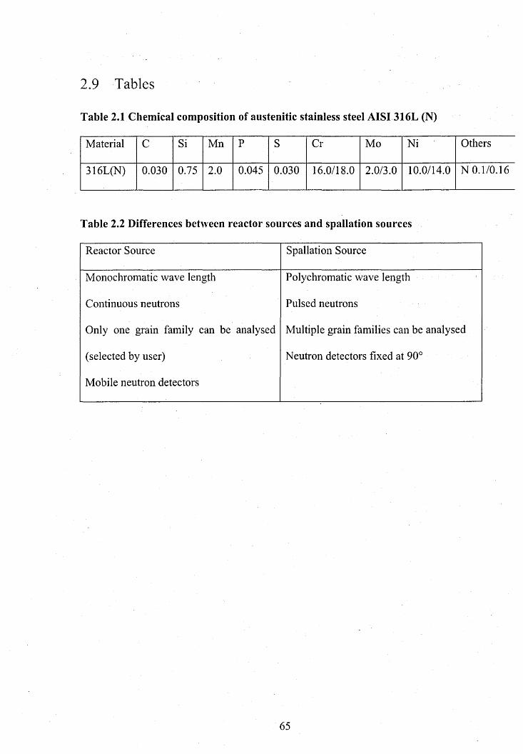
2.9 Tables
Table 2.1 Chemical composition of austenitic stainless steel AISI 316L (N)
Material C Si Mn P S Cr Mo Ni Others
316L(N) 0.030 0.75 2.0 0.045 0.030 16.0/18.0 2.0/3.0 10.0/14.0 N 0.1/0.16
Table 2.2 Differences between reactor sources and spallation sources
Reactor Source Spallation Source
Monochromatic wave length
Continuous neutrons
Only one grain family can be analysed
(selected by user)
Mobile neutron detectors
Polychromatic wave length
Pulsed neutrons
Multiple grain families can be analysed
Neutron detectors fixed at 90°
65
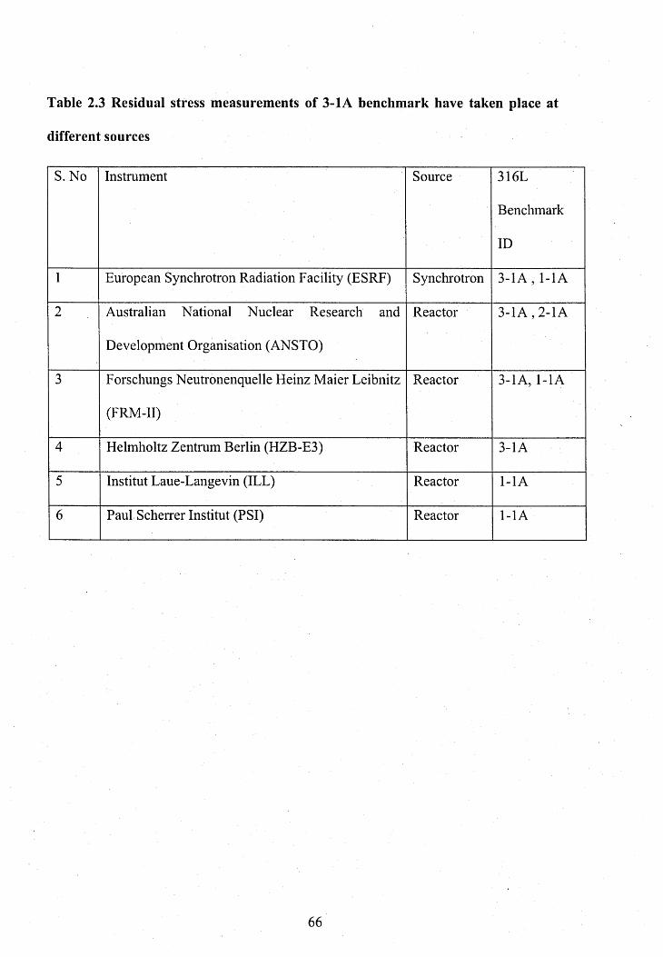
Table 2.3 Residual stress measurements of 3-1A benchmark have taken place at
different sources
S. No Instrument Source 316L
Benchmark
ID
1 European Synchrotron Radiation Facility (ESRF) Synchrotron 3-1A , 1-1A
2 Australian National Nuclear Research and
Development Organisation (ANSTO)
Reactor 3-1A , 2-1A
3 Forschungs Neutronenquelle Heinz Maier Leibnitz
(FRM-II)
Reactor 3-1A, 1-1A
4 Helmholtz Zentrum Berlin (HZB-E3) Reactor 3-1A
5 Institut Laue-Langevin (ILL) Reactor 1-1A
6 Paul Scherrer Institut (PSI) Reactor 1-1A
66

Table 2.4 Plastic strain analysis welded samples using EBSDS.No Material EBSD
Metrics
Quantified Plastic
Strain
Location Direction of analysis
with respective to weld
bead
1 A IS I304 196 AMISa 10-20% HAZ Perpendicular
2 Nickel alloy 600 197 KAM,
AMISa
8% and 10% HAZ Perpendicular
3 Alloy 690TT and
alloy 52 198
AMIS 15% at weld top
and 17% at the
weld root
HAZ Perpendicular
4 Dissimilar metal
199
KAM HAZ Perpendicular
67
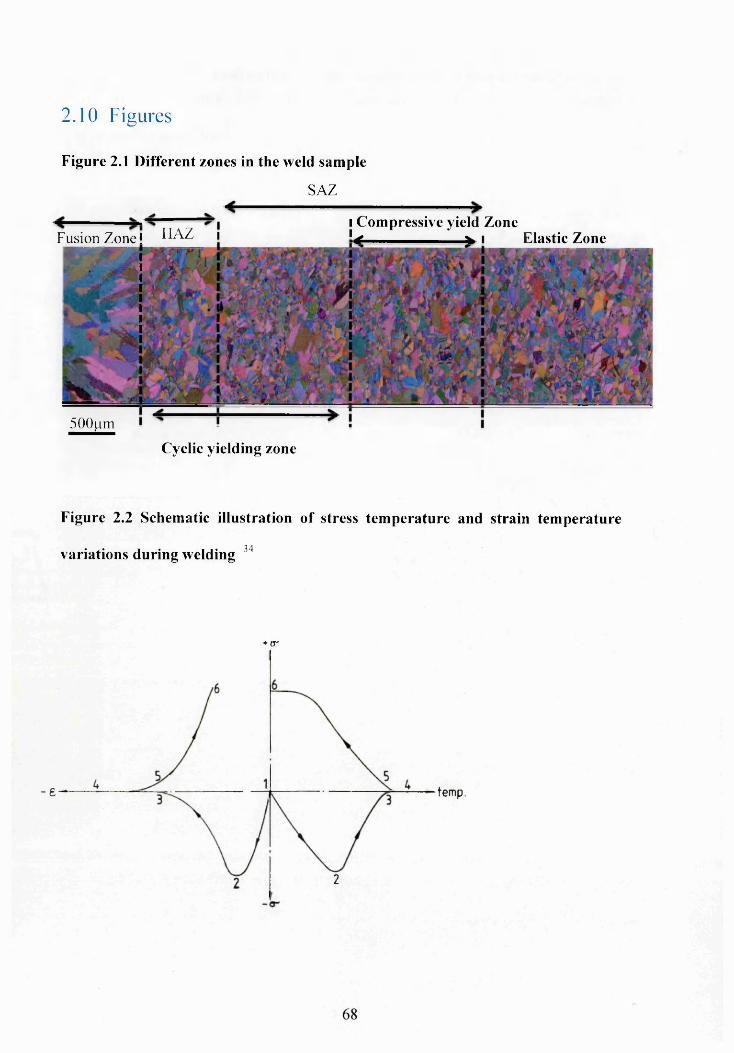
___
500pm
Cyclic yielding zone
2.10 Figures
Figure 2.1 Different zones in the weld sample
SAZ
I Compressive yield ZoneFusion Zone! HAZ i !# ^ i Elastic Zone
Figure 2.2 Schematic illustration of stress tem perature and strain tem perature
variations during welding 34
♦ <r
£ temp
2

Figure 2.3 Tensile stress vs. strain curve
a.
Yield Point
150
100
50
0 .1 80 .1 60 .1 40.120.10 .0 80 .0 60 .0 40.020- 0.02Eng Strain
Figure 2.4 Schematic illustration of slip in a single crystal (a) before slip (b) after
slip
Slip Plane
Atomic Plane
69
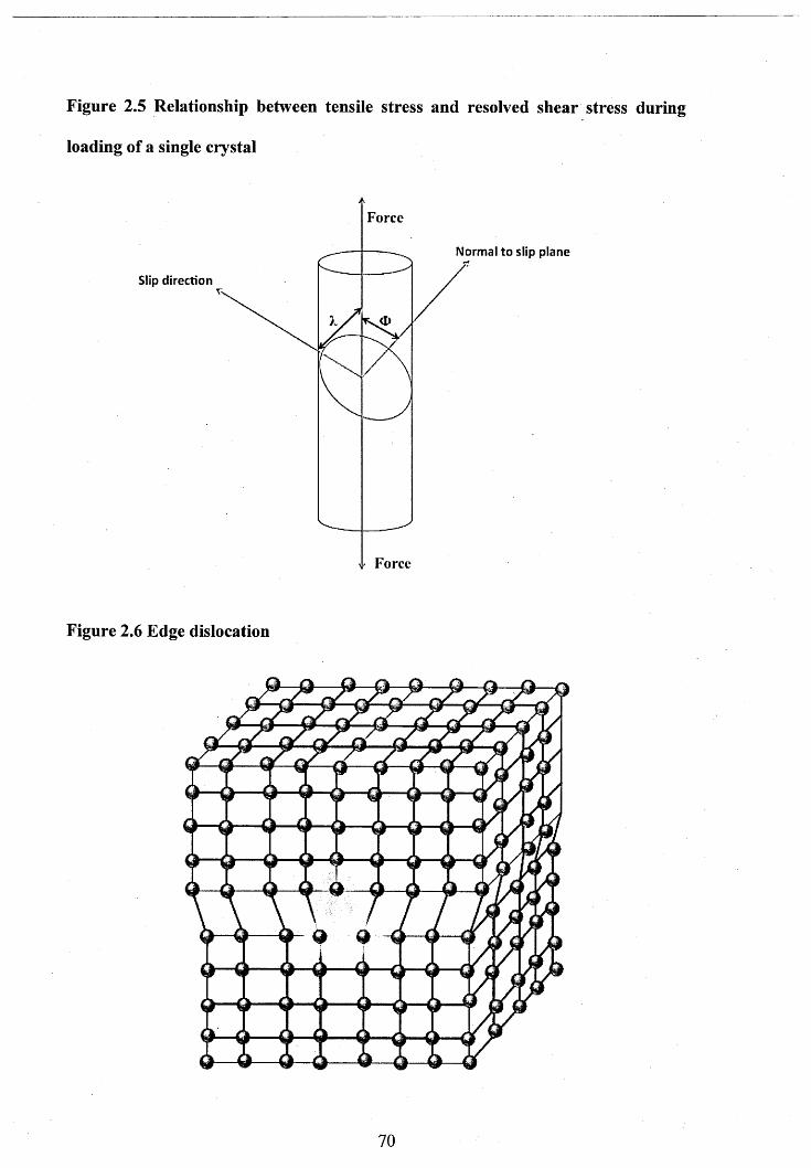
Figure 2.5 Relationship between tensile stress and resolved shear stress during
loading of a single crystal
Slip direction
Force
Normal to slip plane
• Force
Figure 2.6 Edge dislocation
0
70
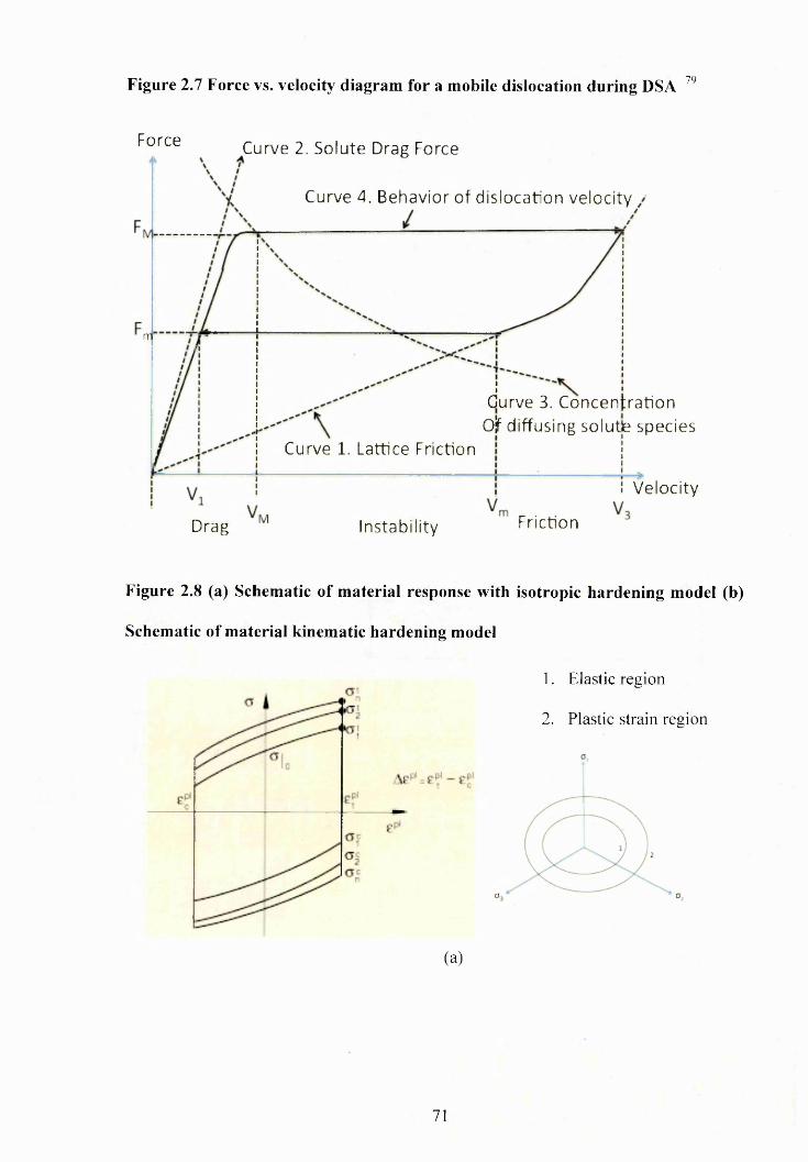
Figure 2.7 Force vs. velocity diagram for a mobile dislocation during DSA 79
Force Curve 2. S o lu t e Drag Force
Curve 4. B ehav ior o f d i s loca t ion ve lo c i ty
m
: [Curve 3. C o n c e n t r a t io n
Of diffusing solutie s p e c i e sCurve 1. Lattice Friction
V e loc i ty
FrictionInstabil ityDrag
Figure 2.8 (a) Schematic of m aterial response with isotropic hardening model (b)
Schematic of m aterial kinematic hardening model
1. Elastic region
2. Plastic strain region
o
(a)
71
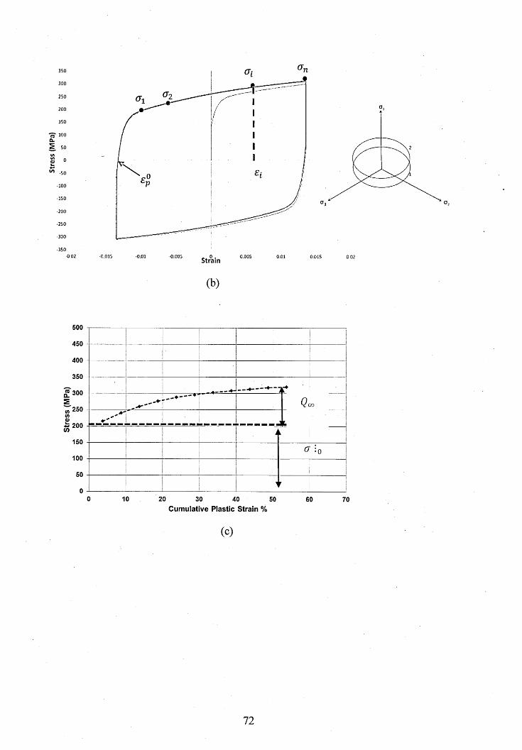
350
Strain
Cumulative Plastic Strain %
72
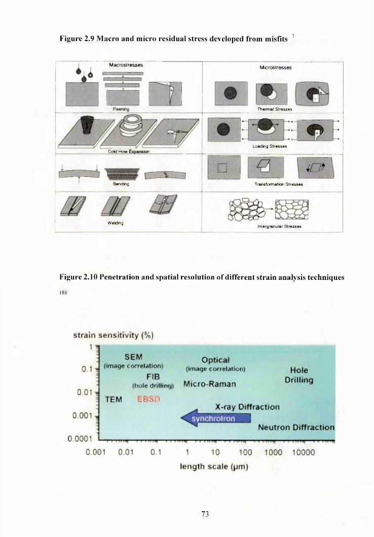
Figure 2.9 M acro and micro residual stress developed from misfits 7
Macrostresses
*Microstresses
Thermal Stresses
U W7--■
Cotd Hole ExpansionLoading Stresses
□ 40*Bending Transformation Stresses
///W elding
Intergranular Stresses
Figure 2.10 Penetration and spatial resolution of different strain analysis techniques
188
strain sensit iv ity (%)1 ^
SEM(image correlation)
FIB(hole drilling) Micro-Raman
0 1
0.01
0001
Optical(image correlation) Hole
Drilling
TEM EBSD
0 0001
synchrotronX-ray Diffraction
Neutron Diffraction
0 001 0 01 01 1 10
length s c a le (pm)
. L-U- L I- - . a U H I U JJ - iJ,iUJJLI ■
100 1000 10000
73
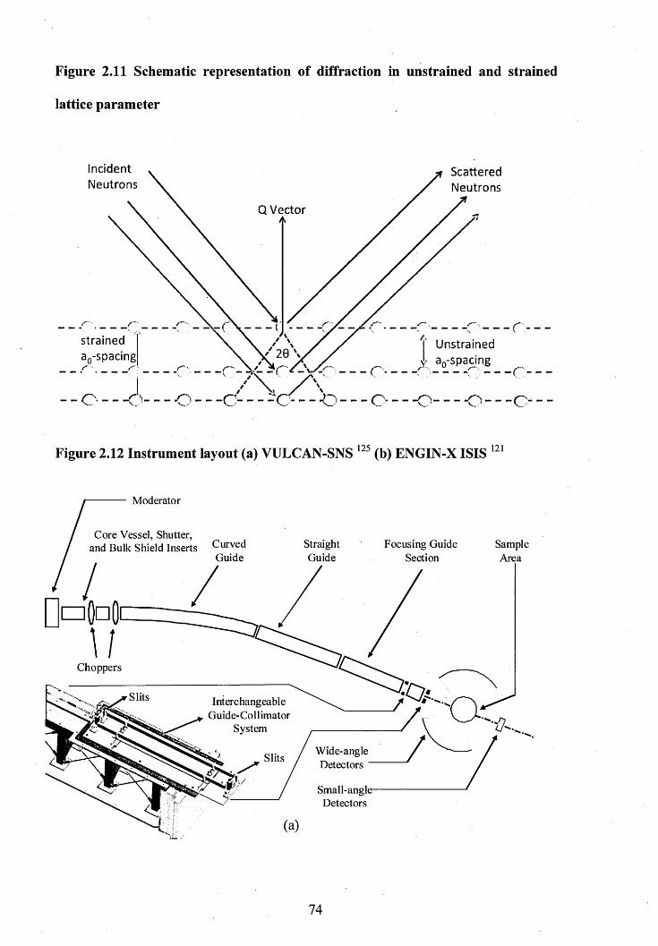
Figure 2.11 Schematic representation of diffraction in unstrained and strained
lattice parameter
IncidentNeutrons
ScatteredNeutrons
Q Vector
o o - o o
r
Figure 2.12 Instrument layout (a) VULCAN-SNS 125 (b) ENGIN-X ISIS 121
Moderator
Core Vessel, Shutter, and Bulk Shield Inserts Curved
GuideStraightGuide
Focusing Guide Section
SampleArea
Choppers
Slits Interchangeable Guide-Collimator
System
Wide-angle Detectors 'Slits
Small-angle-Detectors
74
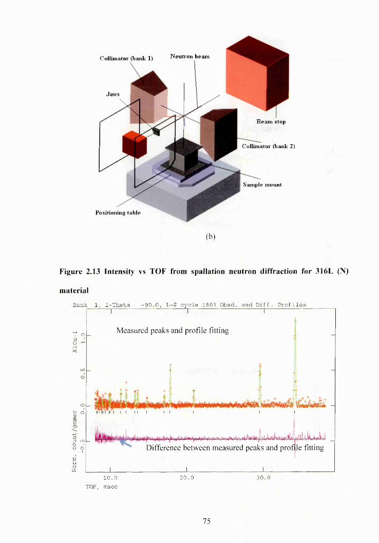
Collimator (bank 1) N eutron beam
B eam stop
Collimator (bank 2)
Sample mount
Jaws
Positioning table
(b)
Figure 2.13 Intensity vs TOF from spallation neutron diffraction for 316L (N)
m aterial
Bank 1, 2-Theta -90.0, L-S cycle 1803 Obsd. and Diff. Profiles
Measured peaks and profile fittingV oo ^T—IX
U O 0)£tnjj£3 LT)o •u o Difference between measured peaks and profile fitting£bOS3
2 0 . 0 30.01 0 . 0TOF, msec
75
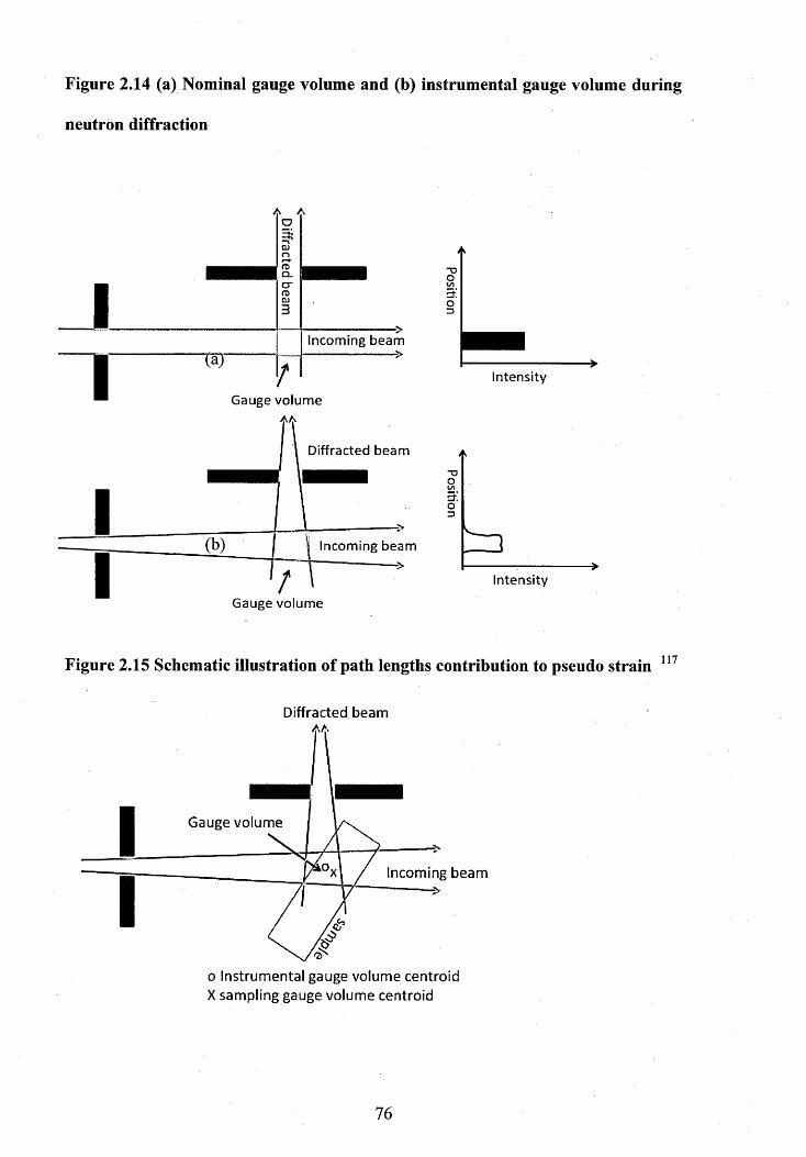
Figure 2.14 (a) Nominal gauge volume and (b) instrumental gauge volume during
neutron diffraction
II
A A OOJn<T>Q .cr <n
/Incoming beam
Gauge volumeAA
Diffracted beam
/Gauge volume
Incoming beam
Intensity
Intensity
Figure 2.15 Schematic illustration of path lengths contribution to pseudo strain 117
Diffracted beamAA
Gauge volume
Incoming beam->
o Instrumental gauge volume centroid X sampling gauge volume centroid
76
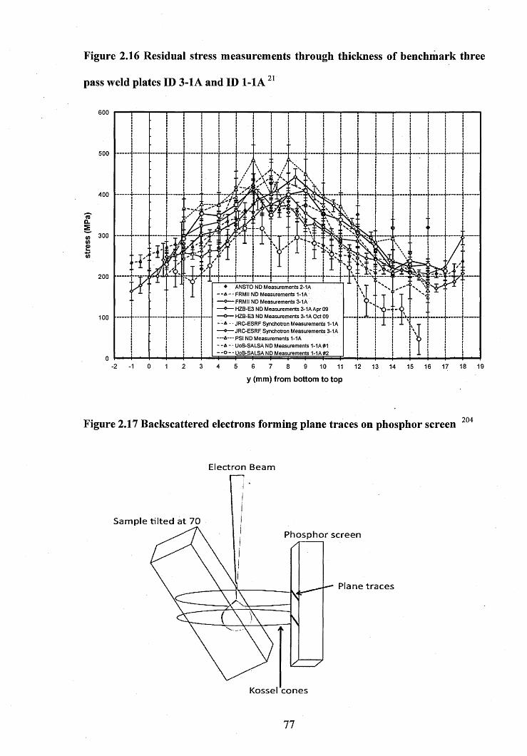
Figure 2.16 Residual stress measurements through thickness of benchmark three
pass weld plates ID 3-1A and ID 1-1A 21
6 0 0
5 0 0
4 0 0
3 0 0
200
100
ANSTO ND M easurements 2-1A FRMII ND Measurements 1-1A FRMII ND Measurements 3-1A HZB-E3 ND M easurements 3-1A Apr 09 HZB-E3 ND M easurements 3-1A Oct 09 JRC-ESRF Synchotron Measurements 1-1A JRC-ESRF Synchotron Measurements 3-1A
- PSI ND M easurements 1-1A UoB-SALSA ND M easurements 1-1A#1
■ UoB-SALSA ND Measurements 1-1A #2
-2 -1 4 5 6 7 8 9 10 11
y (mm) from bottom to top12 13 14 15 16 17 18 19
Figure 2.17 Backscattered electrons forming plane traces on phosphor screen 204
Electron B eam
S am p le tilted at 70P h osp h or screen
Plane tr a c e s
K ossel c o n e s
77
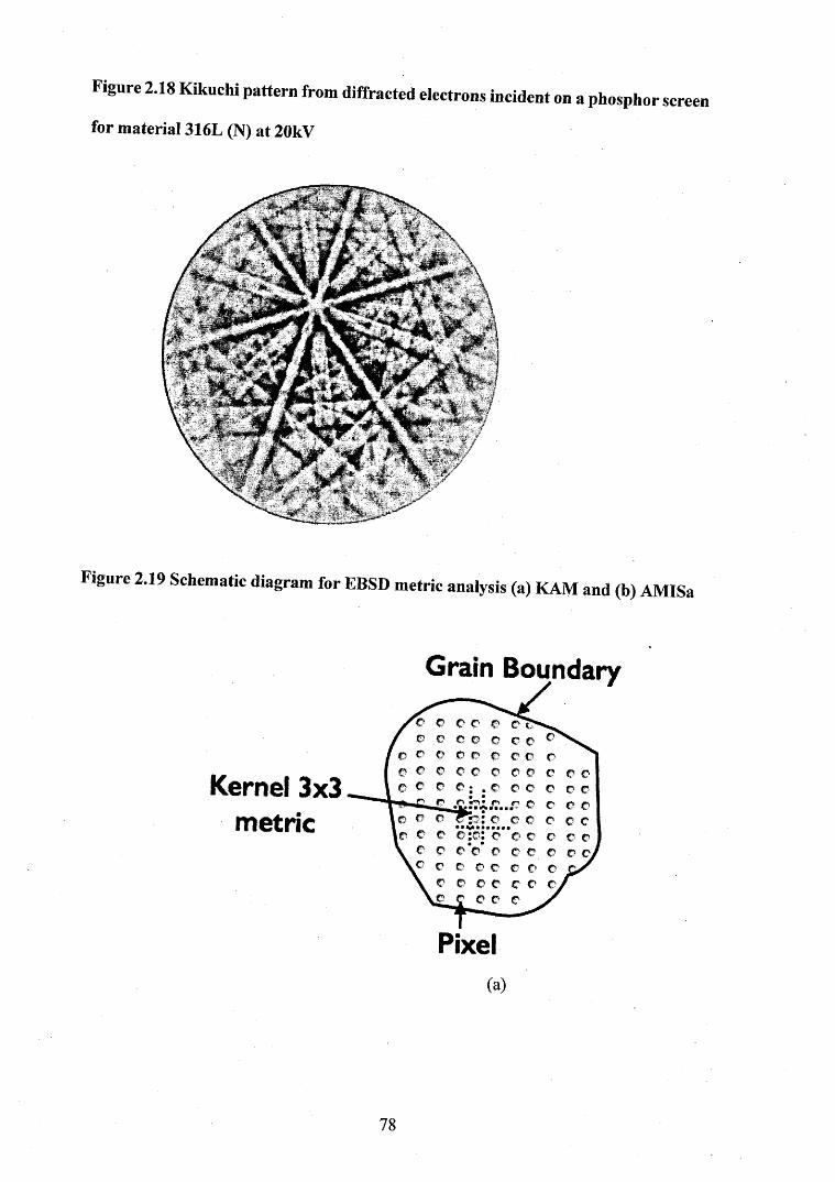
Figure 2.18 Kikuchi pattern from diffracted electrons incident on a phosphor screen
for material 316L (N) at 20kV
Figure 2.19 Schematic diagram for EBSD metric analysis (a) RAM and (b) AMISa
Grain Boundary
© ©
Kernel 3x3 metric
78

Step I: Calculate average orientation of grain
Step 2:The misorientation between the average orientation of grain and the
orientation of each pixel is evaluated
Grain Boundary
Pixel
(b)
79

CHAPTER 3. B e n c h m a r k W e l d m e n t D e s ig n
a n d M a t e r ia l C h a r a c t e r i z a t i o n
This chapter gives detailed background information on the design, manufacture and
material characterization o f welded test specimens used for the research presented in this
thesis. The work has been integrated with residual stress round robin studies of the NeT
task group 4 (TG4), see sections 2.5.2 and 2.5.3, on a three pass slot weld in a stainless
steel plate. Two o f these TG4 benchmark specimens were made available to the author
for neutron diffraction measurements. In addition, a quantity o f parent material plate was
supplied (refer to section 3.4 and Chapter 5) and three special slotted specimens were
received, comprising one, two and three pass welds (refer to section 3.3). These were
prepared for the plastic strain studies, using EBSD, presented in Chapter 6.
3.1 Introduction
Allocation of the AISI-316L benchmark plate, for determining the evolution of
residual stresses using neutron diffraction, is summarized in Figure 3.1 ’ . The
chemical composition, tensile properties, grain structure and the heat treatment test
certificate o f ' manufacture, stress relief heat treatment and weld parameters are described
in section 3.2 below. In total four welded samples were allocated for non-destructive
experiments, and were circulated to all groups within task group 4, for weld residual stress
measurements using neutron and/or synchrotron X-ray diffraction. In this research
project, a single three pass weld plate (ID 3-1 A) was used to measure the residual stress
; field using neutron diffraction at spallation facilities. The principles of neutron diffraction
at time o f flight sources have been given in Chapter 2, section 2.4.1. Details of the
80
experiments carried out so far by other members of the NeT consortium have been
described, in Chapter 2, section 2.5.3 172. This research project contributes towards filling
gaps noticed in the literature, by analyzing the following:
1. Residual stress measurements using two different spallation neutron diffraction (ND)
sources for the first time.
2. The quantification of the accumulated plastic strain resulting from three sequentially
deposited weld passes using electron backscattered diffraction (EBSD) and a
hardness testing method.
3. Welding stress-strain studies using symmetric and asymmetric cyclic loading,
including the effect of strain rate on strain hardening.
The evolution of residual stress and the accumulated plastic strain during welding has
been discussed in Chapter 2 as well as the basic working principles of neutron diffraction,
EBSD and Finite Element based weld simulation techniques.
3.2 Manufacturing o f TG4 Benchmark Specimens
All of the TG4 test specimens were made from a large piece of AISI type 316L
austenitic stainless steel plate (2650 * 2500 x 60 mm), as shown in Figure 3.2(a). Initially,
ten blocks (each 250 x 650 x 60 mm) were cut from the raw work piece using water jet
cutting. The blocks were further divided into four (Figure 3.2(b)) plates, each of which
was machined again to final size (194 x 150 x 18 mm) ready for welding (Figure 3.3 (a)
Benchmark specimen dimensions (b) Benchmark specimen dimensions and slot
configuration (a)). A weld groove (80 mm long, 6 mm deep) was then milled in the centre
of each prepared plate, as seen in Figure 3.3(b). The root of the slot had a radius of 4 mm,
which blended with the walls to make an angle of 20° to the plane of the weld centreline,
81
as shown in Figure 3.3(b) ’ ■ . The plates were marked with a co-ordinate system .(+/-■
z and +/- x) and an identification number, as shown in Figure 3.3(a), prior to the welding,
as specified in flowchart Figure 3.1. The z coordinate axis was positioned on the top
surface along the centreline of the weld groove, and the x coordinate axis was marked at
the mid-length position, across the groove.
3.2.1 Stress relief heat treatment
Manufacturing processes such as casting, hot rolling, and machining can lead to
residual stresses being introduced into material. In order to eliminate these residual
stresses or reduce them to an acceptable level, the material can be annealed using an
appropriate heat treatment process. For the TG4 project, each specimen was wrapped in
heat treatment foil prior to solution heat treatment at 1050°C in a furnace, for
approximately one hour. The plates were then left to cool in the furnace until they reached
a temperature of 300° C and then removed for natural cool down to room temperature
206,207
3.2.2 Three pass weld AISI-316L (N) plate
Figure 3.4 shows an image of the automated pulse Tungsten Inert Gas (TIG) welding
machine employed for welding the plates. A summary of the welding parameters is
provided in Table 3.1 206,207. The feed wire (0.9 mm diameter) AWS A5.0-93 (ER316L)
was used to weld the plates. The chemical composition of the filler wire is provided in
Table 3.2. During the welding process, the machined base plate (194 x 150 x 18 mm) was
left unclamped whilst on the welding table. The second and third weld passes were
deposited directly on top of the preceding pass at a travel speed of 76.2 mm/min. The
inter pass temperature for both second and third passes was 50°C (±10°C). A total of
82
seven welded plates were made in this way and labelled 1-1 a, 2 -la, 3-1 a, 1-lb, 2-lb and
3-lb.
3.2.3 Stress free cuboids extraction
‘Stress free’ specimens of both parent 316L(N) and weld material are required for
neutron diffraction130 measurements of the unstressed lattice parameters used in the
calculation of strain (and hence stress) at each measurement point within the weld plate
sample. NeT TG4 allocated two weld plates (ID 1-2B and 2-1B, shown in Figure 3.5(a,
b)) and one parent plate (ID 1-1 A, in Figure 3.5 (c)) for stress free reference specimen
extraction. Table 3.3 lists the stress-free cuboids extracted from each plate. After
machining the weld slot, plate ID 1-2B (Figure 3.5 (a)) was not heat treated before the
weld deposits were made, whilst plates ID 2-1B (Figure 3.5 (b)) and 1-1A (Figure 3.5 (c))
were solution heat treated before the weld deposits.
Plate ID 1-2B was milled with five-weld grooves (each 80 mm long and 6 mm deep)
as shown in Figure 3.5 (a), one slot for a single pass, one slot for the first and second
passes, and the third slot for a three-pass weld. The remaining two grooves were left
untouched. Each weld groove was separated from the next by a distance of 30mm,
measured from the center o f each groove. After welding, a transverse slice incorporating
the three filled slots, was extracted by electro discharge machining (EDM), as shown in
Figure 3.6. The slice was approximately 4 mm wide and 60 mm in length at the mid
length position.
From the extracted slices (i.e. along the weld direction as shown in Figure 3.6), a
further four 23x4><3 mm prisms of weld metal were extracted from the top weld metal
and bottom of the weld. Each of these prisms was further cut into four cuboids 5 x 4 x 3
mm using EDM. Then each set of four cuboids of weld material were glued together to
create larger ‘stress free’ samples 5 x 8 x 6 mm. Using wire EDM, parent material ‘stress
83
free’ cuboids (5 x 4><3 mm) were extracted from the + x, - z comer of plate ID 1-FA
(Figure 3.5 (c)) and assembled using a similar procedure to that described above. The 5
mm dimension was parallel to the welding direction, the 4 mm dimension parallel to the
transverse direction and the 3 mm dimension parallel to the normal direction. The three
sets of assembled stress free cuboids (upper weld, bottom weld and parent) were color
coded red, green and black respectively and are summarized in Table 3.3.
3.3 Material for Strain Controlled Cyclic Tests
A raw piece of the remaining parent austenitic stainless steel (600 x 50 x 62 mm) was
supplied by the NeT TG4 group for the present research (refer to Figure 3.1). This
material was specifically for the analysis of weldment cyclic deformation. The rationale
for this analysis is described in Chapter 2, section 2.3.4. The supplied work piece was
heat-treated using a similar process to that described in section 3.2.1. A thin sample (3 x
50 x 62 mm) was extracted using wire EDM, to enable identification of the rolling
direction in the 316L (N) block, using optical micrograph analysis. The rolling plane is
identified, in Figure 3.7(a).
3.3.1 Design o f strain controlled test specimens
Low cycle fatigue test specimens for the strain controlled cyclic tests were extracted
from the block of parent austenitic stainless steel. These specimens were designed
following guidelines contained in British Standard (BS) 7270 (1990) 20S. Using wire
EDM, cylindrical samples were extracted with their axes parallel to plane D, see Figure
3.7(b), i.e. along the weld direction. A test specimen designed without shoulders, for
cyclic loading is shown in Figure 3.8. This shape of sample was originally selected for
this research due to the limited availability of the material. However, following cyclic
loading, steps were seen on the stress vs. strain cyclic loop, as illustrated in Figure 3.9.
Q/1

This was due to the backlash between the sample and the collet, which resulted in
formation of steps with the load train, and (ii) the length of the M12 thread was longer
than required. Therefore, during initial loading, stress was applied to the excess threads,
which then deformed the sample at the zero stress point. These problems were addressed
by redesigning the cylindrical cyclic loading sample to include a shoulder at each end, as
shown in Figure 3.10. In addition to modifying the sample design, an Instron alignment
pro kit was also installed to the instrument to improve the alignment of the sample.
3.4 Sequential Weld Deposited Plate
An additional multi-pass weld plate was made by the NeT consortium for
quantification of accumulated plastic strain by the author. From the raw work piece, a
new parent plate test specimen was cut to dimensions 250 x 200 x 18 mm. Three weld
grooves were milled into the plate to a depth of 6mm; one central, and one either side, at
a lateral distance of 80 mm from the central groove, as shown in Figure 3.11. Prior to the
welding process the raw work piece was heat treated for stress relief as described in
section .3.2.1. The three weld grooves were deposited with a single pass, two passes and
three weld passes respectively, using tungsten inert gas welding, according to the details
shown in Table 3.1, and with the filler wire compositions listed in Table 3.2. The
sequence of the welding process is annotated in Figure 3.12.
3.4.1 Samples for plastic strain analysis
Wire EDM was used to divide the multi-pass weld plate (Figure 3.11) transversely,
into two halves, each one measuring 250 x 100 x 18 mm. This cut was made across the
centre of all three welds. Figure 3.11(b) shows where each half was cut again, to extract
two thin transverse slices, each one measuring 250 x 3 x 18 mm. One slice was left whole,
and allocated for hardness measurement testing. The other slice was cut into three pieces,
85

each covering one weld groove as shown in the optical macrograph Figure 3.11(c). These
individual pieces were allocated for texture, microstructure analysis (ref. section 3.5.3.
and 3.5.2.) and plastic strain analysis using EBSD as described in Chapter 6.
3.5 Material Properties
The mechanical properties and material characterization of the parent austenitic
stainless steel have been well defined by the NeT consortium. The chemical composition
and monotonic tensile properties, at different temperatures, on the parent material, have
all been documented 172’206. Data relevant to this thesis are reproduced in Table 3.2 and
Table 3.4. However, the NeT group lacked the following information;
• The grain size distribution in the three orthogonal planes (longitudinal,
transverse and normal),
The parent and weld material hardness
The texture of the weld metal
The extent of any Chemical compositional variations in the parent and
weld materials
This information was needed to support the neutron diffraction and EBSD studies
proposed for the present research and was obtained by the author as described in sections
3.5.1-3.5.6 below.
3.5.1 Specimen preparation
For optical, grain size, texture and chemical characterisations, a parent material sample
( 5 x 8 x 6 mm) was extracted from the end of the transverse slice as shown in Figure 3.13.
To mount the specimens ready for surface preparation, first, seventy five percent of
MetPrep conducting phenolic resin granules was added to the mounting mould, and then
twenty five percent of Struers Condufast powder, containing iron particles, was added on
86
the top o f the phenolic resin prior to hot mounting. When hardened, this resin mixture
provides excellent conductivity for electrolytic polishing of the specimen surface.
The aim of the specimen preparation was to produce stress free surfaces with a mirror
finish. The sample preparation steps and etching methods are summarised in Table 3.5.
This preparation method was used consistently for samples undergoing optical
microscopy, hardness measurement, Energy Dispersive X-ray spectroscope analysis
(EDX) and EBSD.
3.5.2 Optical microscopy
A Leica DM-I5000M optical microscope was employed for the optical examination.
The parent cuboid (5x8x6 mm) was examined in three orientations with respect to the
weld (longitudinal, transverse and normal), as shown in Figure 3.14. Micrographs of the
parent material in all three orientations are provided in Figure 3.15-3.17. Macrographs of
the weld beads and micrographs showing the heat affected zone (HAZ) for the single
pass, two pass and three pass welds, are presented in Figure 3.18-3.20 respectively.
Optical macro and micrographs of the single pass, two pass and three pass weld metals
were obtained from the sequential weld deposited plate samples (ID 1-2B refer Figure
3.5(a)) described in section 3.2.3. The optical images of the prepared surface of the parent
material show an approximately equiaxed grain size, with the presence of twin boundaries
and ridges along the planes D and B shown in Figure 3.3. Previous research 209210
suggests that the development of ridges in the rolling direction (i.e. visible as lines on the
transverse and normal sides), during solidification or casting, could be due to some of the
non-uniform segregation of chromium and molybdenum. These ridges are not
significantly reduced by a subsequent hot rolling process. The presence of a small
percentage of ferrite (below 1% or 2%) in the wrought microstructure is not considered
detrimental. However, the small amount of ferrite can form a preferential site for the
87

precipitation of M23C6 carbides and sigma phase 47. Nevertheless, the presence of delta
ferrite is beneficial in dissolving harmful impurities such as sulphur, phosphorus and
boron 21 \ An attempt was made, using EDX analysis, to investigate the chemical
composition of these ridges and the outcomes are reported in section 3.5.5.
The fusion region of the single, two and three pass weld zones has undergone ferritic
austenitic type solidification, where the austenite forms due to a peritectic-eutectic
reaction. Ferrite (black) boundaries were formed around the austenite (white), in the
material, at the end of the solidification process as seen in Figure 3.21. The columnar
microstructure, solidification sub-grain boundaries (SSGB) and the solidification grain
boundaries (SGB) are evident around and near the fusion boundaries. The SSGBs are
normally identified as around cells or dendrites, and/or the boundaries that separate
adjacent sub-grains as indicated in Figure 3.20. The SGBs are fonned around groups of
SSGB. At places where SSGBs and SGBs interact, boundaries with high angular mis-
orientation result47.
A skeletal ferrite morphology was observed in the single, two and three weld passes
cases. The moderate cooling rate of solidification causes the austenite to consume the
ferrite until the ferrite is enriched with elements promoting (chromium and molybdenum).
At the same time, austenite promoting elements (nickel, carbon and nitrogen) are rejected.
These rejected elements stabilize at lower temperatures, where diffusion is limited, and
form skeletal ferrite. The microstructures in the fusion zone are not uniform. This is due
to the difference in the cooling rate, resulting from the multi-pass welding. This leads to
fine columnar crystal grains being generated during the first pass, whilst a coarse
microstructure was observed near the weld cap of the second and third weld passes.
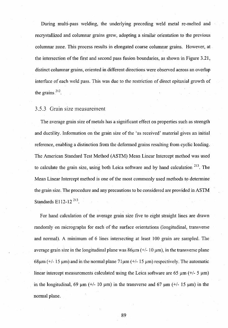
During multi-pass welding, the underlying preceding weld metal re-melted and
recrystallized and columnar grains grew, adopting a similar orientation to the previous
columnar zone. This process results in elongated coarse columnar grains. However, at
the intersection of the first and second pass fusion boundaries, as shown in Figure 3.21,
distinct columnar grains, oriented in different directions were observed across an overlap
interface of each weld pass. This was due to the restriction of direct epitaxial growth of
the grains 212.
3.5.3 Grain size measurement
The average grain size of metals has a significant effect on properties such as strength
and ductility. Information on the grain size of the ‘as received’ material gives an initial
reference, enabling a distinction from the deformed grains resulting from cyclic loading.
The American Standard Test Method (ASTM) Mean Linear Intercept method was used
’ 1 *2to calculate the grain size, using both Leica software and by hand calculation . The
Mean Linear Intercept method is one of the most commonly used methods to determine
the grain size. The procedure and any precautions to be considered are provided in ASTM
Standards El 12-12 2I3.
For hand calculation of the average grain size five to eight straight lines are drawn
randomly on micrographs for each of the surface orientations (longitudinal, transverse
and normal). A minimum of 6 lines intersecting at least 100 grain are sampled. The
average grain size in the longitudinal plane was 86pm (+/-10 pm), in the transverse plane
68pm (+/- 15 pm) and in the normal plane 71pm (+/- 15 pm) respectively. The automatic
linear intercept measurements calculated using the Leica software are 65 pm (+/- 5 pm)
in the longitudinal, 69 pm (+/- 10 pm) in the transverse and 67 pm (+/- 15 pm) in the
normal plane.
89
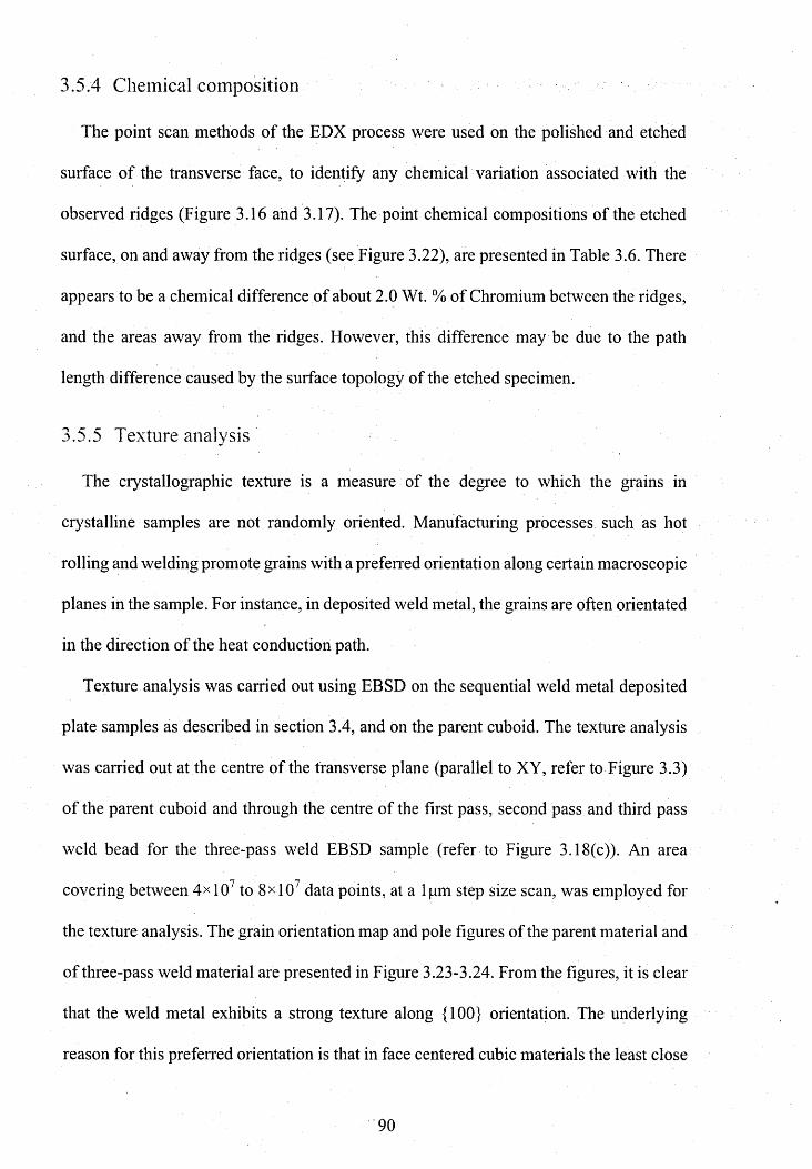
3.5.4 Chemical composition
The point scan methods of the EDX process were used on the polished and etched
surface of the transverse face, to identify any chemical variation associated with the
observed ridges (Figure 3.16 and 3.17). The point chemical compositions of the etched
surface, on and away from the ridges (see Figure 3.22), are presented in Table 3.6. There
appears to be a chemical difference of about 2.0 Wt. % of Chromium between the ridges,
and the areas away from the ridges. However, this difference may be due to the path
length difference caused by the surface topology of the etched specimen.
3.5.5 Texture analysis
The crystallographic texture is a measure of the degree to which the grains in
crystalline samples are not randomly oriented. Manufacturing processes such as hot
rolling and welding promote grains with a preferred orientation along certain macroscopic
planes in the sample. For instance, in deposited weld metal, the grains are often orientated
in the direction of the heat conduction path.
Texture analysis was carried out using EBSD on the sequential weld metal deposited
plate samples as described in section 3.4, and on the parent cuboid. The texture analysis
was carried out at the centre of the transverse plane (parallel to XY, refer to Figure 3.3)
of the parent cuboid and through the centre of the first pass, second pass and third pass
weld bead for the three-pass weld EBSD sample (refer to Figure 3.18(c)). An area
covering between 4><107 to 8><107 data points, at a 1pm step size scan, was employed for
the texture analysis. The grain orientation map and pole figures of the parent material and
of three-pass weld material are presented in Figure 3.23-3.24. From the figures, it is clear
that the weld metal exhibits a strong texture along {100} orientation. The underlying
reason for this preferred orientation is that in face centered cubic materials the least close
90
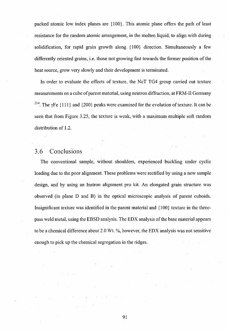
packed atomic low index planes are {100}. This atomic plane offers the path of least
resistance for the random atomic arrangement, in the molten liquid, to align with during
solidification, for rapid grain growth along {100} direction. Simultaneously a few
differently oriented grains, i.e. those not growing fast towards the former position of the
heat source, grow very slowly and their development is terminated.
In order to evaluate the effects of texture, the NeT TG4 group carried out texture
measurements on a cube of parent material, using neutron diffraction, at FRM-II Germany
214. The yFe {111} and {200} peaks were examined for the evolution of texture. It can be
seen that from Figure 3.25, the texture is weak, with a maximum multiple soft random
distribution of 1.2.
3.6 Conclusions
The conventional sample, without shoulders, experienced buckling under cyclic
loading due to the poor alignment. These problems were rectified by using a new sample
design, and by using an Instron alignment pro kit. An elongated grain structure was
observed (in plane D and B) in the optical microscopic analysis o f parent cuboids.
Insignificant texture was identified in the parent material and {100} texture in the three-
pass weld metal, using the EBSD analysis. The EDX analysis of the base material appears
to be a chemical difference about 2.0 Wt. %, however, the EDX analysis was not sensitive
enough to pick up the chemical segregation in the ridges.
91
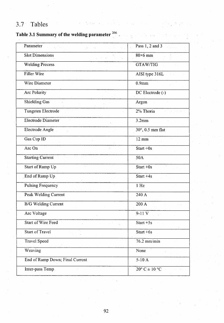
3.7 Tables
Table 3.1 Summary of the welding parameter206
Parameter Pass 1, 2 and 3
Slot Dimensions 80><6 mm
Welding Process GTAW/TIG
Filler Wire AISI type 316L
Wire Diameter 0.9mm
Arc Polarity DC Electrode (-)
Shielding Gas Argon
Tungsten Electrode 2% Thoria
Electrode Diameter 3.2mm
Electrode Angle 30°, 0.5 mm flat
Gas Cup ID 12 mm
Arc On Start +0s
Starting Current 50A
Start o f Ramp Up Start +0s
End o f Ramp Up Start +4s
Pulsing Frequency 1 Hz
Peak Welding Current 240 A
B/G Welding Current 200 A
Arc Voltage 9-11 V
Start o f Wire Feed Start +5s
Start o f Travel Start +6s
Travel Speed 76.2 mm/min
Weaving None
End o f Ramp Down; Final Current 5-10 A
Inter-pass Temp 20° C ± 10 °C
92
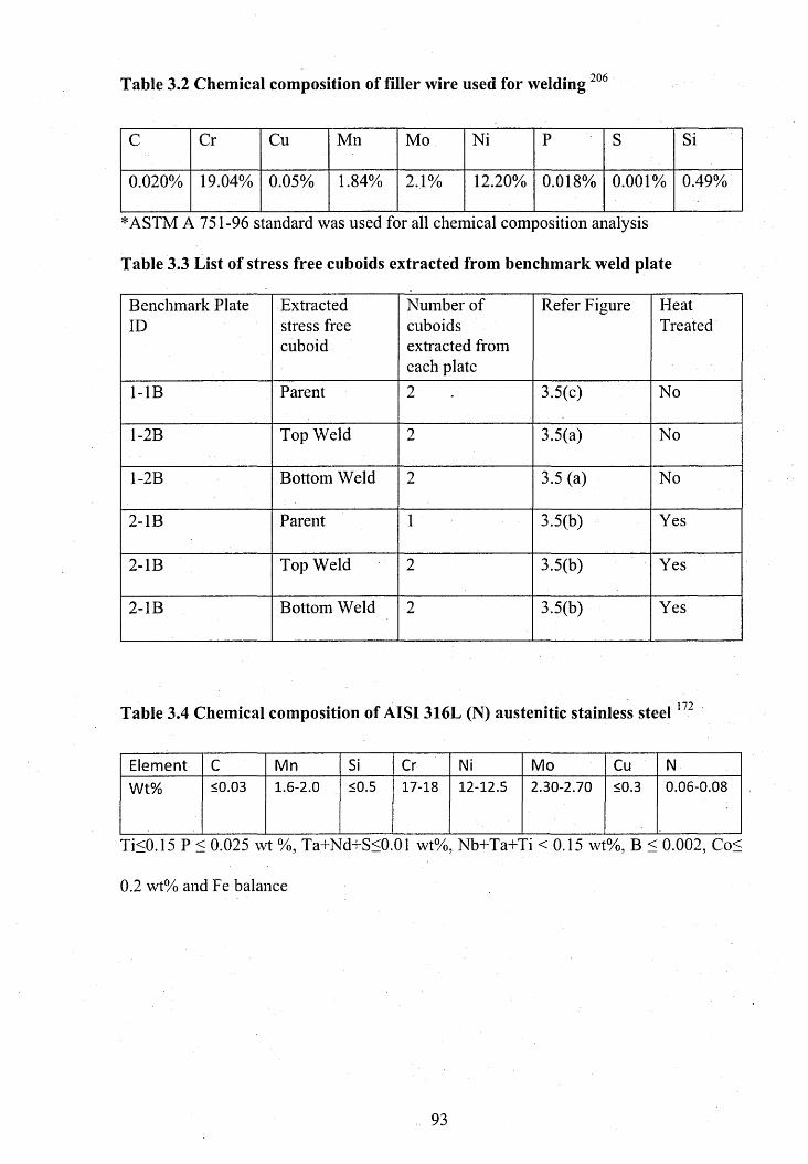
Table 3.2 Chemical composition of filler wire used for welding206
c Cr Cu Mn Mo Ni P S Si
0.020% 19.04% 0.05% 1.84% 2.1% 12.20% 0.018% 0.001% 0.49%
*ASTM A 751-96 standard was used for all chemical composition analysis
Table 3.3 List of stress free cuboids extracted from benchmark weld plate
Benchmark Plate ID
Extracted stress free cuboid
Number of cuboids extracted from each plate
Refer Figure HeatTreated
1-1B Parent 2 3.5(c) No
1-2B Top Weld 2 3.5(a) No
1-2B Bottom Weld 2 3.5 (a) No
2-1B Parent 1 3.5(b) Yes
2-1B Top Weld 2 3.5(b) Yes
2-1B Bottom Weld 2 3.5(b) Yes
Table 3.4 Chemical composition of AISI 316L (N) austenitic stainless steel172
Element C Mn Si Cr Ni Mo Cu NWt°/o <0.03 1.6-2.0 <0.5 17-18 12-12.5 2.30-2.70 <0.3 0.06-0.08
Ti<0.15 P < 0.025 wt %, Ta+Ts d+S<0.01 wt%, Nb+Ta+rfi < 0.15 wt%, B < 0.002, Co<
0.2 wt% and Fe balance
93
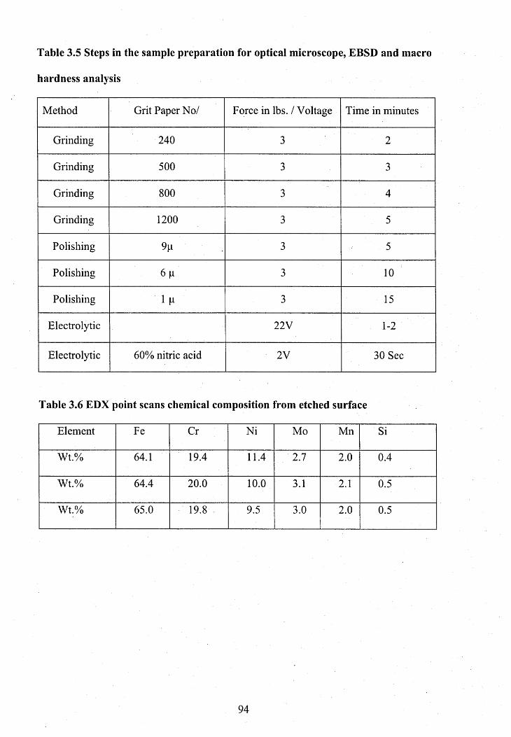
Table 3.5 Steps in the sample preparation for optical microscope, EBSD and macro
hardness analysis
Method Grit Paper No/ Force in lbs. / Voltage Time in minutes
Grinding 240 3 2
Grinding 500 3 3
Grinding 800 3 4
Grinding 1200 3 5
Polishing 9n 3 5
Polishing 6 p 3 10
Polishing 1 p 3 15
Electrolytic 22V 1-2
Electrolytic 60% nitric acid 2V 30 Sec
Table 3.6 EDX point scans chemical composition from etched surface
Element Fe Cr Ni Mo Mn Si
Wt.% 64.1 19.4 11.4 2.7 2.0 0.4
Wt.% 64.4 20.0 10.0 3.1 2.1 0.5
Wt.% 65.0 19.8 9.5 3.0 2.0 0.5
94

3.8 Figures
Figure 3.1 Manufacturing and specimen allocation flow chart
6 blanks 2 offcuts
Heat treatment
Machining
2 specimens with 5 slots each
1 specimen with no slot 1-1B
9 specimens with 1 slot each
r
Available for parent material properties
ID marking ID markingHeat treatment & ID & fiducial marking
1 unwelded controlspecimen 4-1A
Welding trials; one slot for 1 bead; one slot for 2 beads then last weld used for dO cuboids
4 specimens no instrumentation
1 specimen no special treatment 2-IB
specimen
1 weld pad for weld material properties
2 specimens with thermocouples 2-2B& 3-1B
2 specimens with additional scribed lines scanned using SScanSS 1-1A& 3-1A1 specimen to UBS
for instrumentation 4-1B
1 specimen with strain gauges and T/C 2-1A
Welding & record keeping
1 specimenfor DIC 2-2AWelding & record
keeping2 specimens re scanned using SScanSS 1-1A & 3-1AUBS instrumented
specimen retained 4-1R
1 specimen to OU for transverse contour measurement, weld profile macrographs, then parent and weld dO cuboids and through- wall comb manufacture 2 -1 B
r7 weldedspecimens
r4 specimens fornon-destructivemeasurements
2 specimens for destructive measurements (OU - contour; Bristol Univ - Deep hole drilling etc)
95
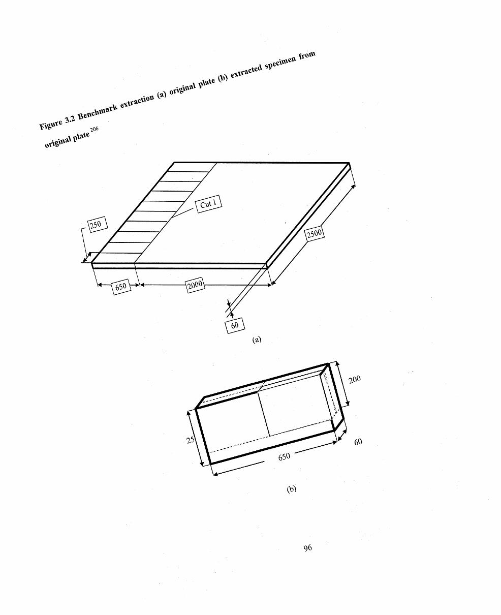
T , a ^ " cf W * * *6
* * * * *
e%«*Cnow ^
,\aiee*«aC
ecit»e,v
(a)
0o>
96

Figure 3.3 (a) Benchmark specimen dimensions (b) Benchmark specimen
• 206dimensions and slot configuration
en d
start
(line A) plane B line B (line C)line D plane D
x = transverse, y = normal; z = longitudinal
(a)
r ™ > D
150
45°
194R4
centre of plate and slot
— DSection D-D
20°
* \ J
All dimensions in mm.18 R4--------* 4
Section B-B
(b)
97
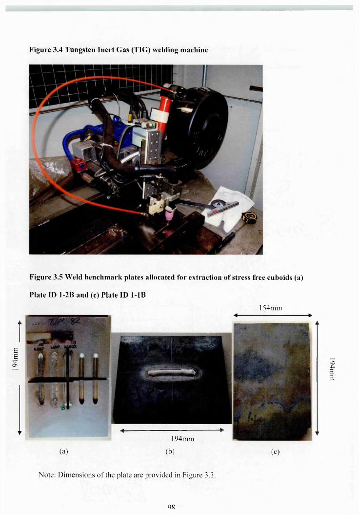
194m
m
F igure 3.4 Tungsten Inert Gas (TIG) welding machine
Figure 3.5 Weld benchmark plates allocated for extraction of stress free cuboids (a)
Plate ID 1-2B and (c) Plate ID 1-1B
154mm
194mm
(a) (b) (c)
Note: Dimensions of the plate are provided in Figure 3.3.
QR
194mm

Figure 3.6 Manufacture of stress free cuboids
Weld metal in slot
A
Weld
Top surface of plate
Four rectangular prisms to be extracted from weld metal (two upperD and two lowerD), each measuring ~ 23 x 4 x 3 mm.
Section B-B
Macrograph slices extracted at mid length of slot weld
Centre line
■ - 4 VLocations of prisms as seen looking along welding direction.
Each of the four long prisms to be cut into 4 cuboids measuring 5 x 4 x 3 mm. Those 4 cuboids then to be reassembled in to 5 x 8 x 6 mm prisms.
s sTwo prisms from the upper weld metal, each measuring 5 x 8 x 6 mm, and two from the lower weld metal, will be available for d0 measurements.
Figure 3.7 (a) Parent material block for cyclic loading analysis and (b) cyclic samples
extraction
50
62 mm
Ridg600 mm
99

Plane D
62mm
(b)
Figure 3.8 316L (N) cyclic loading samples design without shoulders
M12 Screw cut
C B S . A!! rrilirn t-lers. e a te s * w h e re in d ic a ted
S p e c in '* '1. in a c c o rd a n c e w th B n tish S tar* : a -a 72?o
D itri-V aion in d ic a te d a s 1c r r n is th e g a u g e le-'-gth
Shanm j*;ha Moturu
Fatigue Specim en - No Shoulders
100
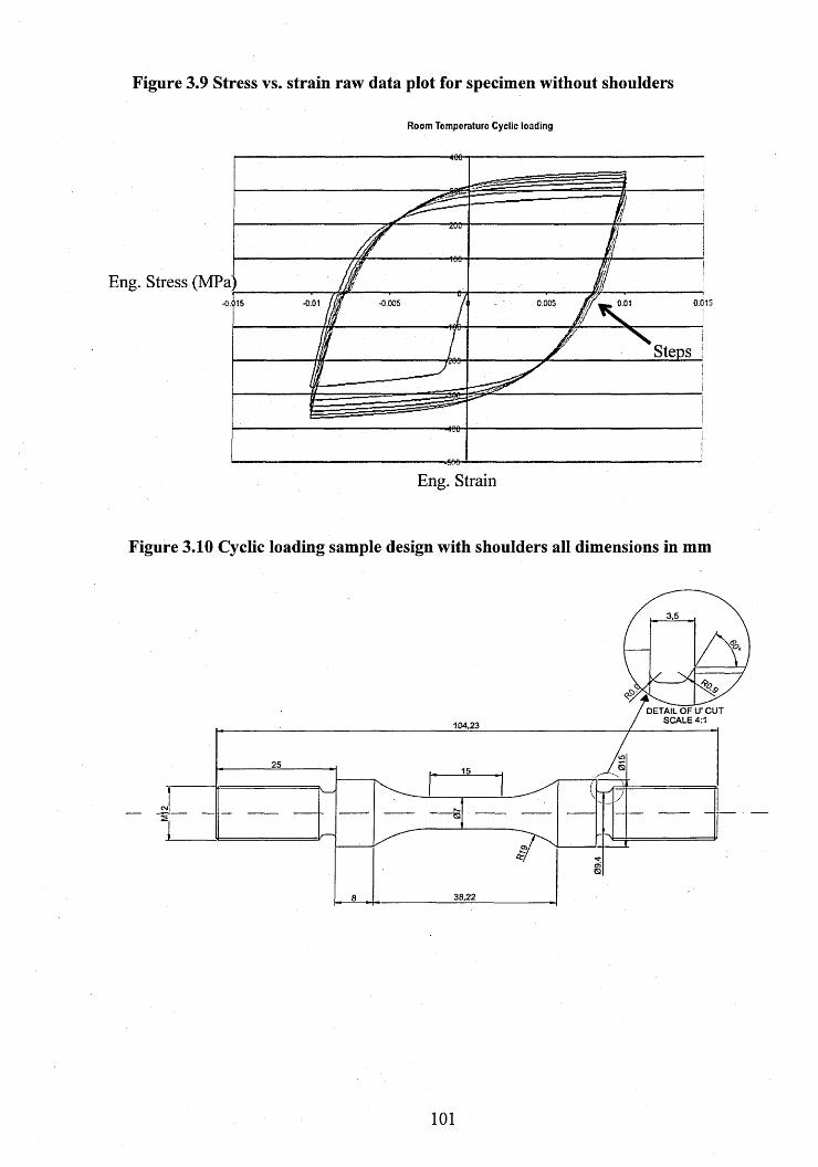
Figure 3.9 Stress vs. strain raw data plot for specimen without shoulders
Room T em perature Cyclic loading
-200-
Eng. Stress (MPa)-0:015 0.015-0.01 0.005-0.005
Steps Ifm-
------Eng. Strain
Figure 3.10 Cyclic loading sample design with shoulders all dimensions in mm
3,5
DETAIL O F U' CUT SCALE 4:1104,23
25
38,22
101


Figure 3.12 Multi pass weld sequences (dimensions of weld slots are similar to Figure
3.3(b))
Three Pass Two Pass Single Pass
80 mm 80 mm 18 mm
250 mmFigure 3.13 Weld transverse slice for material characterization
'Xtrael
Figure 3.14 Orientation of extracted parent material cuboid used for optical
metallography
Parallel to YZRefer Figure 3.3(a)
i VParallel to XY
6 mm
5 mm
8 mm
103
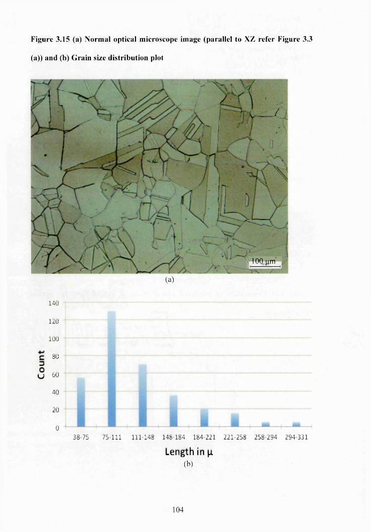
Figure 3.15 (a) Normal optical microscope image (parallel to XZ refer Figure 3.3
(a)) and (b) G rain size distribution plot
m
100 {im
(a)
140
120
100
C 30
U 60 I
40
20
0 ----38 75 75 111 111 148 148 184 184 221 221 258 258 294 294 331
Length in 11(b)
104
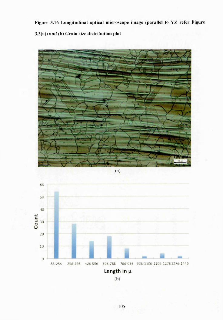
Cou
nt
Figure 3.16 Longitudinal optical microscope image (parallel to YZ refer Figure
3.3(a)) and (b) G rain size distribution plot
(a)
60
50
40
30
20
10
0
86 256 256 426 426 596 596 766 766 936 936 1106 1106 12761276 1446
L en gth in |i
(b)
105
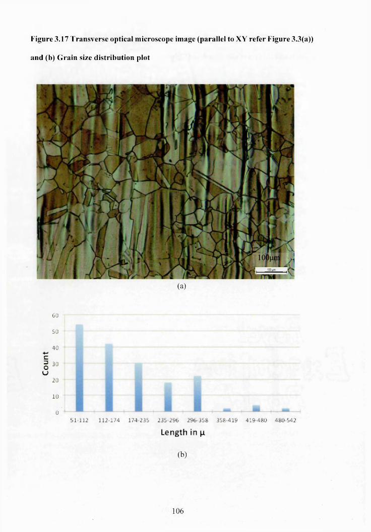
Cou
ntFigure 3.17 Transverse optical microscope image (parallel to XY refer Figure 3.3(a))
and (b) G rain size distribution plot
(a)
GO
SO
40
30
20
10
0 ~51 112 112 174 174 235 235*296 296 3SS 358 419 419 480 480 542
Length in [i
(b)
106
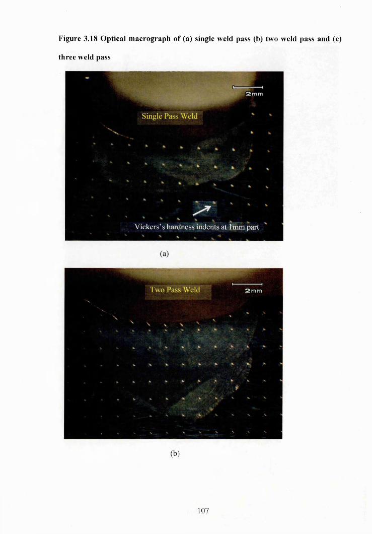
Figure 3.18 Optical m acrograph of (a) single weld pass (b) two weld pass and (c)
three weld pass
V ickers’s hardness indents at 1mm part1
(b)
107
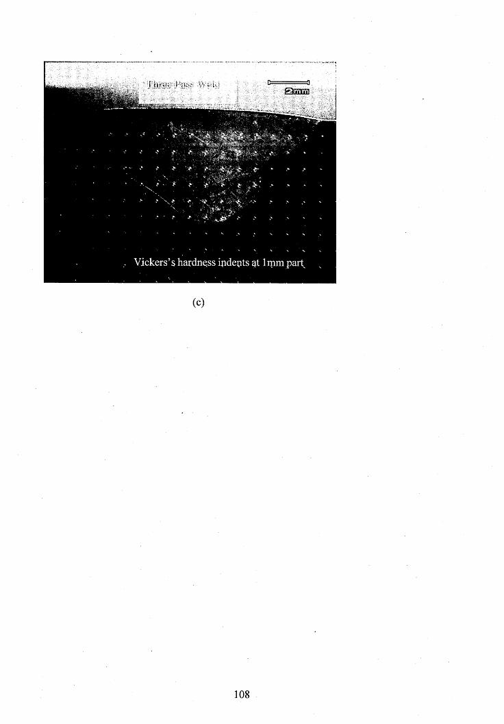
Vickers’s hardness indepts 1mm part
(C)
108
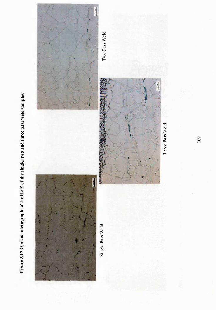
Figu
re
3.19
Opt
ical
mic
rogr
aph
of the
HA
Z of
the
sing
le,
two
and
thre
e pa
ss w
eld
sam
ples
32£m cnCUO£H
Thre
e Pa
ss
Wel
d

Figu
re
3.20
Fusio
n bo
unda
ry
optic
al m
icro
grap
h of
singl
e pa
ss,
two
pass
an
d th
ree
pass
we
ld sa
mpl
es
Thre
e Pa
ss
Wel
d

Figure 3.21 Recrystallized columnar grains at single and two pass weld boundaries
Columnar grains
Interface of two pa
SSGB
Figure 3.22 EDX point analysis location of SEM image
Away from ridges
500fim
111
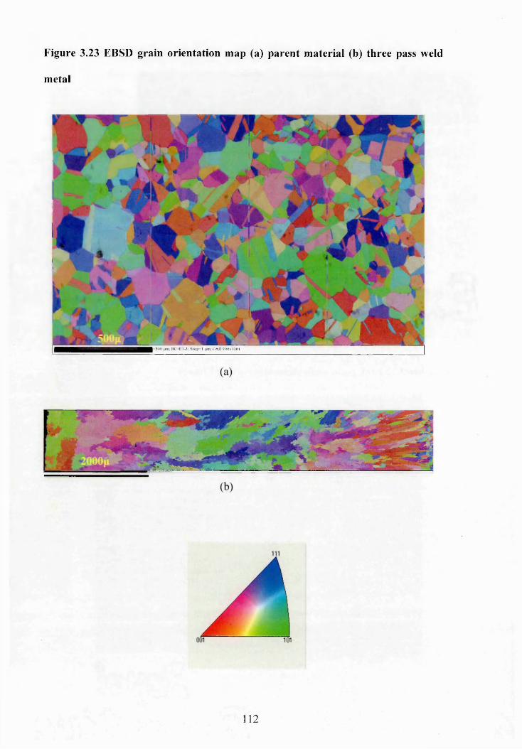
Figure 3.23 EBSD grain orientation map (a) parent m aterial (b) three pass weld
metal
Grid 1900x1001
112
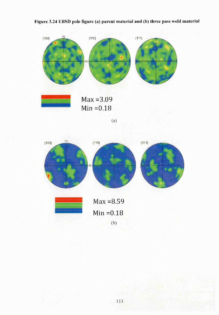
Figure 3.24 EBSD pole figure (a) parent m aterial and (b) three pass weld m aterial
M a x = 3 . 0 9
M i n = 0 . 1 8
(a)
f
M a x = 8 . 5 9
M i n = 0 . 1 8
(b)
113

Figure 3.25 Neutron diffraction pole figures for heat treated base material
specimens of (a) y Fe {111} and (b) {200} rolling direction vertical206
•X:
m O CX at 1 5 5 0 / C50 c-m 1 244 it 1 3 5 0 / £00
fM Ul.SifrcWcd
(a)
r«sm 1M6
o r 06-42 * 1 K 0 / 5 5 0 ttuu 1 IK? rt 13BC/ HID
Fl« ICO,!»-t<e2t»4t
(b)
114
CH APTER 4 . B e n c h m a r k W e l d m e n t
R e s i d u a l S t r e s s C h a r a c t e r i s a t io n
4.1 Introduction
This chapter describes how neutron diffraction was used to evaluate the residual
stresses present in a three-pass welded plate, a benchmark test component made from
AISI type 316L austenitic stainless steel. Residual stresses, caused by welding, arise
because of localized thermo-cyclic plastic deformation and differential contraction in the
materials. The presence of residual stress can have a significant impact on the
performance of the welded structure, as described in section 2.4 of Chapter 2. An accurate
assessment and evaluation of stress and strain in a welded benchmark component is
important in order to improve prediction methods and to understand the role of non-
uniform thermal cyclic plastic deformation.
Neutron diffraction is a particularly suitable experimental technique for this research
study, since it allows non-destructive measurement of residual elastic strain through the
whole thickness of the welded plate. The material and geometric details o f the test
components have already been described in sections 3.1 and 3.2. Welded plate (ID 3-1 A),
and two sets of “stress free cuboid assemblies” from two different plates (IDs 1-2B and
2-1B), were supplied for the present study. The manufacturing details of the stress free
cuboids have been described in section 3.3. Diffraction experiments earned out by other
members of the NeT consortium, involving several measurements on the same plate (ID
3-1 A), are listed in Table 4.1 List of residual stress measurements carried out on 3-1A
weld plate.
115
The objective of the round robin experimental measurements, using different
techniques, performed by separate teams, was to assess the accuracy and repeatability of
residual stress measurements on a well-controlled benchmark weldment, and to thereby
improve the reliability of measurements. Another objective was to compare the best
experimental characterisation with a simultaneous weld residual stress prediction round
robin exercise, aimed at improving weld computational mechanics and simulation
methods. For this research thesis, residual stresses in the benchmark-welded plate (ID 3-
1 A) were measured using the VULCAN diffractometer at SNS facility, USA and ENGIN-
X at the ISIS facility, UK. Details of these instruments have been described in section
2.4.1 of Chapter 2.
4.2 Sample and Instrument Preparations
To achieve the above objectives, and for the sake of a consistent comparison of
experimental and simulation data, the NeT TG4 group developed protocols 172,215 for both
measurements and simulations, defining the locations to be studied, in order of priority
and reporting requirements.
4.2.1 NeT TG4 proposed measurement locations
The residual stress measurement points, for the NeT TG4 weldment benchmark
defined in the measurement protocol 172 are grouped into nine sets listed in order of
priority, as shown below and as indicated in Figure 4.1. A total of 137 measurement
points, were written in MatLab vector style, where a colon specifies the distance
increment between two consecutive measurements. For example, the first priority set (line
BD) comprises 15 points, passing through the thickness of the plate (including the three
116

weld beads), where the first measurement point is located at 2 mm from the top surface
of the plate and the following measurements are located at consecutive increments of 1
mm (i.e. 3, 4, 5, 6, 7... and 16 mm from the top surface).
Priorities o f measurement points: cf. Figure 4.1
1) 15 positions onlineB D : x = z = 0 ,y = [2:1:16].
2) 19 positions on line D5: x = 0, y =5, z = [-90, -70, -50: 5: -30, -20:10:20, 30:5:50,
70.90].
3) 19 positions on line D9: x = 0, y =9, z = [-90, -70, -50: 5: -30, -20:10:20, 30:5:50,
70.90].
4) 19 positions on line D2: x = 0, y=2, z = [-90, -70, -50: 5: -30, -20:10:20, 30:5:50,
70, 90].
5) 15 positions on Line D16: x = 0, y = 16, z = [-90, -70, -50:10:50, 70, 90].
6) 17 positions on Line B2: x = [ -70, -50:10:-20, -15:5:15, 20:10:50, 70], y = 2, z
= 0 .
7) 8 additional positions on line B2: x = [-17.5:5:17.5], y = 2, z = 0.
8) 17 positions on Line B2: x = [ -70, -50:10:-20, -15:5:15, 20:10:50, 70], y = 16, z
=0.
9) 8 additional positions on line B2: x = [-17.5:5:17.5], y = 16, z = 0.
Following welding, due to the rippled surface of the weld bead, it was not possible to
identify exactly the origin of the welded plate at the top surface. Instead, a reference point
on the bottom surface of the welded plate was identified precisely. Hence, the
measurement positions, as defined by NeT TG4, are located relative to an origin at the
bottom surface of the plate, identified with the help of a 3D laser scan and Strain Scanning
Simulation Software (SScanSS)126.
117

4.2.2 Sample alignment '
During neutron diffraction experiments, the sample geometry and its alignment in the
diffractometers determine the precise positioning of the sample and the reliability of the
measurements. In order to achieve alignment, the following process was used:
1. Four steel balls, each of 12 mm diameter, were glued onto each comer of the
welded plate and away from the measurement positions. These balls were used as
reference points for the plate and are known as fiducial markers.
2. A 3D laser line scanner (see Figure 4.2) was used to generate a virtual, three-
dimensional computer aided design (CAD) model of the welded plate with its
fiducial markers as shown in Figure 4.3. The x, y, z co-ordinate points for each
fiducial marker were measured relative to the laser scanner datum.
3. The CAD model was then imported into SScanSS software in order to generate
and simulate a measurements plan.
4. With the welded plate specimen mounted on the instrument table, a laser tracker
on the VULCAN instmment and a laser probe on the ENGIN-X instrument were
used to measure the co-ordinate positions of the plate’s fiducial markers to an
accuracy within ±0.025 mm.
5. The SScanSS software merges the two different co-ordinate systems, of the
sample and of the instrument table, into one coordinate system, so that the two
components are aligned.
6. The table movement positions are verified with the facilities available to the user
during the experimental process, as described in section 4.2.3.
7. Using this single co-ordinate system, SScanSS is then used to generate a series of
co-ordinates for each proposed measurement point on the sample. Now the user
118
can specify which strain components are to be measured for each specific point
or groups of points.
8. Finally, the series of sample measurement coordinates are imported into the main
instrument control system to automatically drive the sample table movements.
4.2.3 Sample alignm ent facilities at neutron sources
Once the sample was aligned and the coordinates for each fiducial point generated by
SScanSS, measurement locations were verified by moving the sample table to one or
more fiducial points, before verifying any angular misalignment by rotating the table 90°
either in a clockwise or anti-clockwise direction. These verifications were carried out
with the help of an optical theodolite (available at ENGIN-X, ISIS UK) and a laser tracker
(available at VULCAN, SNS, USA; see Figure 4.2). For both the instruments, a
positioning accuracy of ±0.05 mm was achieved for the instrument table relative to the
beam line.
4.2.4 Instrument alignm ent calibrations
The alignment of jaws and collimator may change from one instrument user to another
and therefore it is good practice to check the jaws and collimator alignments prior to the
start of the experiments. This was achieved using the standard method of observing the
diffracted neutron intensity as a pin was scanned in directions parallel and perpendicular
to the beam with a gauge volume of 20 x 2 x 3 mm3 at the ENGIN-X instrument and 10
x 2 x 2 mm3 at the VULCAN instrument respectively.
Calibration measurements were undertaken by measuring the diffraction spectra for
materials of a known lattice parameter; for example iron and cerium oxide powders were
used for the ENGIN-X experiment. Similarly, vanadium, diamond and silicon powders
were used for the VULCAN experiment. The lattice parameters measured from the
119

experiment should match with reference values in the absence of any misalignment.
However, in practice, there will be small discrepancies between the lattice parameters
calculated from the calibration measurement in each detector bank, and the known lattice
parameter. These discrepancies may arise for various reasons, including small remaining
geometric misalignments. The discrepancy is accounted for by creating bank specific
correction constants, from the ratios of the reference values compared to the measured
values, and by multiplying all subsequent lattice parameter measurements by these
constants. The calibrated powders’ measurements during ISIS experiment are provided
in Table 4.2 The ISIS instrument calibration measurements.
4 3 Stress Free Lattice Parameter (a0)
The welding process, as described in section 2.2.1, deforms the material locally
introducing residual elastic strains, which manifest as changes in lattice spacing of the
material at the crystallographic length scale. In order to determine the strained lattice
spacing, the reference unstrained lattice spacing (ao) is necessary. The stress free lattice
spacing can be measured from representative samples of material that are free from
macroscopic stress. A representative stress free sample can be obtained simply by
extracting it from an unstressed plate using a stress free cutting process. When a
sufficiently small sample is extracted from a welded component, most of the macro
stresses will be relaxed in the extracted sample. However, micro stresses within the grains
and between the grains will remain in the extracted material. Likewise any changes in
lattice parameter resulting from chemistry are unaffected by the cutting process 130’216.
Type I stresses are directionally independent, whilst type II and III are directionally
dependent. For the present study, the strained lattice parameters were evaluated using
weld and parent macro-stress free cuboids supplied by the NeT consortium. The
120 .
manufacturing of the macro-stress free cuboids has been described in section 3.3 and the
calculation of the lattice strain (and hence the stress) in section 2.5.
The lattice parameters of stress-free cuboids set 1-2B were measured at both
VULCAN (SNS) and ENGIN-X (ISIS) instruments, while, the lattice parameters for
cuboids set 2-IB were measured only at ENGIN-X.
4.3.1 VULCAN stress-free lattice param eter measurements
Each ao cuboid was mounted onto a jig and measurements were performed under both
static and constant slow rotation conditions. The purpose of static and constant slow
rotation of stress free cuboids is to analyse the difference in measured stress free lattice
parameter due to difference in the number of grains diffracted from static and constant
slow rotation conditions of stress free cuboids. The jig comprised an electronic DC
stepper motor with a table, as shown in Figure 4.4. Throughout the experiment, the lattice
parameters in the longitudinal and transverse directions were measured from the north
bank (bank 1), while keeping the normal direction in common with the south bank (bank
2), as shown schematically in Figure 4.6. In order to align the cuboid with the centre of
the neutron beam, the sample table was moved manually until the centre of the cuboid
aligned with the centre of the laser tracker. The NeT measurement protocol recommended
a 3 x 3 x 3 mm3 gauge volume (described in section 2.5.1) for diffraction experiments.
This gauge volume was selected based on the grain size and the size of the cuboid. The
minimum number of grains required in a given gauge volume, for good counting statistics
is approx. 10,000 156,157. However, due to the lack of availability of a 3 mm collimator at-
the VULCAN instrument, a 2 mm collimator was adopted for this experiment giving a
gauge volume of 3x3x2 mm3. For these measurements, a counting time of approximately
10 minutes was allocated for each measuring point.
121
The ‘counting time’ is that required to achieve a high quality diffraction pattern from
exposure of the measurement point to the neutron beam. Counting times are expressed in
units o f micro-amps, a unit which is proportional to the number of neutrons striking the
heavy metal target, rather than an actual time.
4.3.1.1 ao Data analysis software
Data analysis software is used to read raw data collected from the neutron detectors,
and then plot the diffraction lattice parameter (dhkl) as a function of time of flight (TOF).
This plotted data is used for sequential Rietveld diffraction profile refinements, or single
peak fitting, to provide an average cell lattice parameter or hkl spacing, measured from
the neutrons diffracted within a given gauge volume. In this present measurement, a
Rietveld profile refinement method 217 was used for the data analysis. An example of
Rietveld profile fitting of raw data used in the evaluation of residual stress in a welded
plate is shown in Figure 4.5. The Rietveld refinement uses a least squares approach to
refine a theoretical line profile, until it matches the measured profile, thus providing an
average (unit cell) lattice spacing. The equations required to determine elastic strain from
lattice parameter measurements have been described in section 2.5. The General Structure
Analysis System (GSAS) and SmartWare codes were used for Rietveld profile
refinements analysis at VULCAN. At ENGIN-X, the ISIS in-house developed Open
Genie analysis software, with GSAS software running at the backend, was used for the
Rietveld profile refinements 218, using the space group and the lattice parameters
provided in Table 4.3.
4.3.1.2 VULCAN a0 results
As described above, during the VULCAN experiments, each cuboid was measured
whilst stationary and during constant rotation about its longitudinal and transverse axes,
122

with the help of the jig, as shown in Figure 4.6. Depending on which continuous rotation
axis is used, both bank 1 and 2 measured the average of longitudinal and normal direction,
or the average of the transverse and normal directions. Whilst, in static mode, bank 1
measured the longitudinal and transverse directions and bank 2 measured two normal
directions. A total of seven measurements were obtained for each ao cuboid from each
detector bank. Table 4.4 (a), summarises the average lattice parameter measured for each
cuboid for the respective detector banks.
As described in section 4.3, the extraction of small coupons should have relaxed the
Type I stresses 219. However, during an experiment, the path length from the sample to
each bank will be different depending on the sample thickness 129. As a result, bank
specific average lattice parameters are used here for the evaluation of residual stress in
the welded plate. The variation in lattice parameter, in terms of micro strain, is calculated
using equation 4.1
H E = * 1000000 4.1
Where ‘a’ is the measured lattice parameter and ‘ao’ is evaluated by taking an average
of the bank specific measurements in the stationary mode and whilst under constant
rotation. Figure 4.7-4.8 and Table 4.4 (b), illustrate the variation in the measured ao
expressed as the apparent micro-strain in the stationary mode and for constant rotation.
The micro strains summarised in Table 4.4(b) are the averages of the longitudinal and
transverse micro strains measured in Bankl and the average of the normal micro strains
measured in Bank 2. The micro strain variation for constant rotation is smaller than that
for the static mode. In static mode, a maximum micro-strain of approximately -164 in the
top weld ao cuboid was evident. Similarly, under constant rotation, a maximum micro
strain of approximately -105 in the top weld ao was measured, see Figure 4.8.
123
4.3.2 ENGIN-X stress free lattice parameter measurements
Both sets of aO cuboids (i.e. 1-2B and 2-IB) were mounted on a flat plate and carefully
aligned using a theodolite. Figure 4.9 shows the cuboids glued onto the flat plate. This
method of alignment was chosen, instead of the jig alignment used at VULCAN, as a
result of the jig being damaged during transportation to ISIS. The same bank specific
lattice parameter measurement approach was implemented in this experiment (i.e.
longitudinal and transverse from bank 1, and normal from bank 2). A gauge volume of 3
x 3 x 3 mm3 was used for this experiment. Each cuboid was rotated, at angular increments
of 30°, anti-clockwise from 30° to -270° about its longitudinal and transverse axes. A
counting time of 20 minutes (approximately) was used for this experiment. Open Genie
software was used for Rietveld profile fitting, covering more than ten peaks, as shown in
Figure 4.5, using the space group and initial lattice parameters, provided in Table 4.3.
4.3.2.1 ENGIN-X a0 results
The measured micro-strain variation in the two sets of stress free cuboids at 30°
increments of rotation about the longitudinal axis, and transverse axis, of each cuboid is
presented in Figure 4.10-4.11, for the 1-2B ao set and Figure 4.12 for the 2-IB ao set. The
average of the measured lattice parameter, at all angles for each rotational set, was used
to evaluate the variation in terms of micro strain. Table 4.5 provides the average lattice
parameters measured at 0°, 180°, 90° and 270°. Table 4.6 provides the average lattice
parameters measured and standard deviation of micro strain at all angles. The micro strain
was calculated using equation 4.1. The variations of measured micro strain in both weld
and parent cuboids were up to ±200. During the stress free cuboid experimental setup,
the possibility of the cuboid misaligning with the neutron beam is high, due to the
irregular shapes of the imperfect cuboids as seen in Figure 4.9. Therefore, the possibility
of the cuboids being incorrectly aligned was investigated, by undertaking repeat124
measurements for the weld (top) cuboid set 1-2B. These results are presented in Figure
4.11 and show a similar trend to the original measurements. The repeated measurements
show that the cuboids were aligned correctly and that the variation of measured micro
strain in both weld and parent cuboids was not due to alignment problems. Further
investigation was carried out to understand the variation in measured lattice parameters,
by comparing the results with average lattice spacing measurements from different
sources. Figure 4.13 shows the average lattice spacing measurement of the respective
cuboids at different sources 220. The average lattice spacing measurements performed at
the reactor source are higher than at the spallation sources (VULCAN and ENGIN-X).
One of the possible reasons is that at the reactor source, only single peak (i.e. 311 peak)
lattice spacings are measured, while at the spallation source more than 10 peak (refer to
Figure 4.5) lattice spacing measurements are averaged. Other possible reasons for this
difference are described in section 4.6.1.
4.3.2.2 Uncertainty of data analysis
Material factors such as texture (affecting the intensity of peaks), grain size (affecting
the number of neutrons diffracted) and partially immersed gauge volumes (affecting the
peaks positions) can contribute to inconsistences (scatter) in the stressed and un-stressed
lattice parameter measurements. These inconsistences in the experimental raw data were
analysed using an error propagation method. This method calculates the uncertainty in
lattice measurements, strain and stress, based on the statistical uncertainties associated
with the peak fittings, as output from the GSAS software. The derived uncertainties are
dependent on the.measurement counting time.
125
4.4 Residual stress measurement in the welded plate
The residual stress measurements of the three-pass weld austenitic stainless steel plate
are presented in two parts:
i) VULCAN and ENGIN-X results using 1-2B ao set
ii) ENGIN-X results using 1-2B and 2-IB ao sets
In both experiments, the lattice parameters, in the longitudinal and transverse
directions of the welded plate, were measured from the north bank (bank 1), while
keeping the normal direction as common in the south bank (bank 2). The residual stress
measurements were performed at prescribed positions, as recommended by the NeT TG4
Protocol, along lines BD, D2, D5, D9 and D16 (along the welding direction) and lines B2
and B16 (perpendicular to the welding direction) see section 4.2.1. Each prescribed line
of measurements was performed in order to investigate the effect of the weld thermal
cyclic deformation at different depths of material (i.e. near and far away from the heat
source). The average value of the top weld stress free lattice parameter was used for the
evaluation of the residual stress in the area between 0 and 3 mm from the top surface. The
bottom weld stress free lattice parameter was used for evaluation of the residual stress in
the area between 4 and 8 mm from the top surface. Finally, the parent stress free lattice
parameter was used for evaluation of the residual stress in the area between 9 and 16 mm
from the top surface.
VULCAN weld plate residual stress results using 1-2B an set
The residual stress measurements from the VULCAN and ENGIN-X instruments,
along the defined lines in the three-pass weldment (ID 3-1 A), are shown in Figure 4.14
to Figure 4.20. As the differences between the means of the rotated and non-rotated bank
specific 1-2B ao stress free values are very small (refer to Table 4.4), all stress values
were calculated using average non-rotated, bank-specific data. The average stress free
126
values of the top weld, the bottom weld and the parent materials were used, depending
on the measurement location, see section 4.2.2. The directions of the stress components
are defined, with reference to the weld bead, as indicated in Figure 3.8.
ENGIN-X weld plate residual stress results using 1-2B and 2-1B an sets
Table 4.5 and Table 4.6, summarise the average lattice parameters and standard
deviations of the micro strains for each cuboid. The residual stress measurements from
the weld plate using 1-2B and 2-1B ao sets are shown in Figure 4.21. The difference
between the measured strains and stresses, using stress free reference measurements from
sets 1-2B and 2 -IB ao. is small. This is because the stress-free lattice parameters for sets
2-1B and 1-2B were similar as evidenced in Table 4.6. Therefore, in the remainder of this
thesis, only VULCAN and ENGIN-X results using cuboid set 1-2B are discussed. The
average of eight ao measurements, i.e. two longitudinal direction measurements at 0° and
180° and two transverse direction measurements at 0° and 180° from bank-1, were used
for evaluating the longitudinal and transverse residual stresses in the welded plate.
Similarly four measurements of normal stress free lattice parameters from Bank 2 were
used for evaluating the normal residual stress.
4.5 Validation o f the Residual Stress Measurements
It is advantageous to compare the present measured residual stresses with independent
measurements made on the same weldment (ID 3-1 A) by other members o f the NeT
group 15-46-139’157’221-222 The residual stress measurements of weld plate ID 3-1A were
analysed at two different neutron reactor sources Helmholtz Zentrum Berlin (HZB) and
Forschungs Neutronenquelle Heinz Maier Leibnitz (FRM-II). Stress free cuboids (set 1-
2B), were measured at both reactor sources. At FRM-II, averages of the stress free lattice
parameter values were obtained by rotating the ao cuboids constantly around one axis as
127
described in section 4.3.2.1. At HZB, averages of the stress free lattice parameter values
were obtained by rotating the ao cuboids at different Omega angles (from 0° to 180° at 1°
increments) during an April 2009 experiment. A repeated experiment was conducted in
October 2009, where averages of the stress free lattice parameter values were obtained
by continuous rotation of the ao cuboids. The measured results obtained from FRM-II and
HZB are compared with the present ENGIN-X and VULCAN stresses in Figure 4.22-28.
At the HZB and FRM-II reactor neutron sources, 311 peaks were used to analyse the
residual stress in the welded plate. Figure 4.13 presents the average lattice parameters
measured at reactor and spallation sources for 1-2B set. The possible reasons for
differences in the measured lattice parameter are explained in section 4.6.1.
4.6 Discussion
The present study has tried to identify and understand the issues affecting residual
stress measurements in austenitic weldments and helped to improve the reliability of
residual stress measurements using neutron diffraction.
4.6.1 a0 analysis
Figure 4.10 to Figure 4.12 shows the variation in lattice parameters measurement
expressed as micro-strain, with rotational angles, for stress-free reference cuboid sets 1-
2B and 2-IB sets. The variations with angle are surprisingly high in the parent material
(±200 micro strain). The following factors could have caused these variations:
1. The presence of crevices was evident in the reconstructed cuboids which can
offset the centre of the sample gauge volume, as shown schematically in Figure
4.29 in the same way that partial gauge volume immersion can generate pseudo
strains as described in section 2.5.1 142.
128

2. The presence of super glue (containing hydrogen), used to bond the cuboid
assemblies, can introduce pseudo strains. Hydrogen has a very large attenuation
coefficient due to its large incoherent scattering cross section. The neutron
weighted centre of gravity shifts (towards the neutron beam) away from the
geometric centre of the measurement volume.
3. An inhomogeneous population of diffracting grains (i.e. average of plane D and
B elongated grains) at angles 30°, -30°, -60°, -120°, -150°, -210° and -240°, when
compared to the uniform grain sizes exposed at angles of 0°, 90°, 180° and 270°.
This is shown schematically in Figure 4.30. This will have particular marked
effect when there are anisotropy texture and grain size in the material.
4. At 30°, -30°, -60°, -120°, -150°, -210° and -240°, different elongated grain size
(i.e. plane D, B and through thickness of the plate) will reduce minimum number
of diffracting grains in a given gauge volume and generate pseudo strain in
measured residual stresses 223,224.
5. The edges of the cuboids are not parallel to each other as seen in Figure 4.9. When
ao cuboids are rotated from 0° to 180°, the possibility of a shift in the geometric
centre of the gauge volume is high. As a result of this, the population of the grains
changes, and the total number of grains diffracting alters with respect to the
previous position. This effect is shown on the diagram shown in Figure 4.31
6. The segregation of solute atoms can cause a steep variation in the strain free lattice
spacing of the parent material ,
7. At the spallation source the detectors are fixed, however at the reactor source the
detectors are not fixed. The possibility of misalignment of detectors and imperfect
alignment of ao cuboids 143 is high, due to imperfect edges of cuboids.
129
In comparison to the parent ao cuboids, in welded ao cuboids the micro-stresses will be
moderately high, due to the presence of bigger grains and chemical variations in the weld
metal. In addition the presence of texture in the weld metal can lead to higher error in
profile or single peak data analysis. Also, generation of significant pseudo strains can
117 131 225occurs, due to bigger grain size ’ ’ . The 1-2B weld ao cuboid showed higher micro
strain uncertainties in comparison to the 2-IB weld ao cuboid. The reasons for such
uncertainties in ao weld values could be associated with following effects.
i) As described in section 3.2.3, the 1-2B stress free cuboids were extracted
from the 1-2B trial plate, while 2 -IB cuboids were extracted from the 2-
1B three pass welded plate. In the 1-2B trial plate weld slots were
manufactured very close to each other and due to this, the sequence of weld
deposits in each slot interacted with each other. As a result of this, the
material’s plastic deformation was significantly higher in comparison to
that of the three-pass weld plate. Figure 4.32 shows evidence of the
interaction of the weld thermal cyclic loading for each slot, revealed by
Vickers hardness measurements.
During the ao extraction process, the macroscopic unloading of stress
may transfer unequal loads to the surrounding grains, due to the
anisotropic stress-strain properties of the grains. The unloading process
may induce elastic strain of those grains located adjacent to plastically
strained grains. This in turn hinders elastic relaxation and leads to a change
in the intergranular stress, between the welded plate and the welded ao
samples. These intergranular stress states will have a significant effect on
evaluation of residual stress of the welded plate at a reactor source 140.
130
ii) The 2-1 B ao cuboids were extracted from one of the seven welded plates.
These plates were solution annealed before welding; hence, any strain
developed, due to the machining process, was relaxed, unlike the 1-2B ao
cuboids.
iii) The 2-1B parent ao cuboids have much higher measured macro strain than
1-2B ao cuboids see Figure 4.10(c) and Figure 4.12(c). This is due to the
2-IB parent cuboid being heavily coated with paint and super glue
(containing hydrogen) see Figure 4.9. Due to this, the 2-IB parent cuboid
assemblies introduce higher pseudo strains than the 1-2B parent cuboid
assemblies.
4.6.2 W eld residual stress
Line BD: The aim of performing the line BD measurements was to measure the
distribution of stress through the 18mm thickness o f plate, and to also understand the
effect of the non-uniform thermal cyclic deformation through the thickness of the
specimen. Figure 4.14, shows the measured residual stress profiles in the longitudinal,
transverse and normal directions along line BD. The longitudinal and transverse stresses
measured at VULCAN and ENGIN-X increased gradually from the bottom of the plate
to the fusion boundary (i.e. 6 mm) and reduce slightly from the fusion boundary to the
weld cap (2mm). However, the normal stresses measured at VULCAN and ENGIN-X
remain constantly below ±60MPa from the bottom of the plate to the weld cap. The
variation between ENGIN-X and VULCAN stress measurements is typically,
approximately ±50 MPa. However, at two specific measurement points; at 6 and 7 mm
from the top surface, there is a greater variation of stress, up to 100 MPa (c.f. Figure 4.14).
ENGIN-X longitudinal stress appears to be systematically higher than VULCAN
longitudinal stress.131

Figure 4.22, compares measured stresses along line BD, obtained from different
neutron diffraction experiments at HZB, FRMII, SNS and ISIS. The residual stress
measurement profiles, even though from different instruments, follow a similar trend.
However, in the area below the weld between 6 and 18 mm from the top surface, the
variation in measured magnitude in the longitudinal direction is high (up to 150MPa). An
important contributor to these variations is the uncertainty in the stress free measurements
as discussed earlier. In addition, the reactor source is only sampling a single 311 peak,
whereas the spallation source samples several reflections covering more than 10 peaks.
Line D 2\ The aim of taking line D2 measurements was to evaluate the residual stress
distribution, along the welding direction in the plate, associated with the final weld pass.
The line is located only 2 mm below the surface of the plate. In Figure 4.15, it is clear
from the results that significant tensile residual stresses have developed in all three
directions, in the vicinity of the three-pass weld deposit. The longitudinal residual stress
profile exhibits a high magnitude of tensile stress along the welded region balanced by
compressive stress in the bulk material. At the weld start and stop positions, more
pronounced peaks in the residual stress profiles are noticed. At the weld start, the
deposition of the weld filler material will be continuous only when the required arc
voltage has been established. Similarly, at the weld stop, the deposition of filler material
terminates only when the arc voltage drops below threshold voltage. During this period
of time, the transient nature of the temperature field will lead to localised differences in
. . . . ~>~>1 microstructure and strain history " .
In the longitudinal direction, the VULCAN results are showing a clear stress peak at
the weld start and stop (i.e. -40 and +40 mm). The longitudinal stress variation between
the spallation (VULCAN) and the reactor source (FRM-II and HZB) was about ±50MPa
as shown in Figure 4.23. In the transverse direction, both the spallation and reactor source
132

measurements in the parent zone are in good agreement but in vicinity of weld material
i.e. from -40 to 40 mm the variation between the spallation and reactor source was about
±50MPa. Similarly in the normal direction the stress measured at spallation and HZB
reactor source shows variation of ±50MPa, while FRM-II shows variation of ±100MPa.
Line D 5 : The line D5 measurements were performed in order to quantify the extent to
which the first weld pass metal has cyclically hardened as a result o f localized heating
associated with the second and third weld passes. The line was located 5 mm below the
surface of the plate. Figure 4.16 shows a similar trend in residual stress results as occurred
in line D2 measurement results. The ENGIN-X and VULCAN results along line D5 are
in reasonably good agreement with each other, except in the normal direction (just prior
to the weld stop) at 20 and 30 mm see Figure 4.16. The residual stress measurements,
made at the different sources, along line D5, are compared in Figure 4.24. The stress
profiles in the longitudinal, transverse and normal directions show small variations,
except at 30mm and -30 mm as seen in Figure 4.24.
Line D 9\ The aim of taking the line D9 measurement was to quantify the extent to
which the parent metal has cyclically hardened as a result of localized heating associated
with three weld deposits. As described in section 2.2.1, this zone is expected to have
cyclically yielded. Figure 4.17 shows the residual stress results of the long line D9. The
ENGIN-X measurements along line D9, at a depth of 9 mm, as shown in Figure 4.17,
indicate residual stress levels up to 50 MPa greater than the VULCAN results. The
material in the area between -30 mm and 30 mm from the weld mid-length, parallel
(longitudinal) and perpendicular (transverse) to the welding direction, has undergone
cyclic yielding and developed a maximum residual stress of 350 (±50) MPa.
133
In the longitudinal direction, the ISIS, FRMII and HZB results are in good agreement
as seen in Figure 4.25. While in the transverse and normal direction the residual stresses
measured at different neutron sources correlated very well with each other.
Line D16: The aim of taking the line D16 measurement was to analyse the elastic strain
developed due to the distortion of plate and the effect of multi-pass welding 113,114.
Line D16 is located 16 mm below the surface of the plate. The ENGIN-X measured
stresses along line D 16 are up to 100 MPa higher than the VULCAN data, and this is
shown in Figure 4.18. The most marked discrepancy is in the longitudinal direction
distance between Z = -70 mm to +20 mm. The longitudinal stress profile rises smoothly
from approximately zero, at both ends of the line, to a central maximum of 250 MPa
(±50). The transverse component lies within the range ±100 MPa throughout the length
of the line, with an abrupt increase from -100 MPa to 100 MPa at between -40 and 40
mm. The residual stress measurements taken along line D16, at the different neutron
sources are presented in
Figure 4.26. The ENGIN-X residual stress measurement profile, in all three directions,
showed higher variations when compared to the other measurements already taken.
Line B2\ The aim of taking the line B2 measurements was to understand the effect of
radial weld thennal heating. Rosenthal has described that the weld heat distribution, in a
plane perpendicular to the heat source, is defined radially from the centre of the heat
source 42. Hence, the weld heat will be at a maximum nearest to the heat source and
gradually decreases as we move away from heat source. As a result, the material nearest
the heat source deforms cyclically, thereby developing tensile stress, while at the far end
of the plate, balancing compressive stresses have developed. The residual stress results
along line B2 are presented in Figure 4.19. Line B2 is located 2 mm below the surface of
the plate (c.f. Figure 4.3 Three dimensional point cloud mesh of test specimen with
134
fiducial points). The ENGIN-X residual stress measurements along line B2 are generally
in good agreement with the VULCAN results. The residual stress measurements along
line B2 as taken at the different neutron diffraction sources are presented in Figure 4.27.
The stresses along line B2 follow a similar trend of profile to earlier results.
Line B16: The reasons for taking line B 16 measurements are the same as those for line
D16. Line B16 is located 16 mm below the surface o f the plate (c.f. Figure 4.3). The
longitudinal and transverse stress profiles along this line again reveal compressive
stresses towards the ends o f the line, with more tensile stresses in the broader central
region see Figure 4.20. The longitudinal stress has a value of approximately -200 MPa
at either end of the line, rising to 200 MPa in the broader central region covering the
distance -20 mm to 20 mm. The transverse component is approximately zero outside of
this central region, and ~50 MPa within it. The normal component is between -50 Mpa
and 0 MPa throughout the length of the line, but with an apparent, slight increase in the
central region. The residual stress measurements along line B16 as taken at the different
neutron diffraction sources are presented in Figure 4.28. In all three directions, the stress
profiles along line B 16 are in good agreement with the FRM-II results.
To summarize, at both experiments (VULCAN and ENGIN-X) three orthogonal
components of stress were measured at different depths in the welded plate covering a
minimum of 76 common locations on the 3-1A welded plate. The residual stress
measurement carried out at the spallation sources showed a variation of approximately
±50MPa in all three orthogonal components. However, the measurements performed at
neutron spallation sources and reactor sources showed difference of approximately
±100MPa. Further investigations need to be carried out to understand the possible
contributions to these.
135
4.7 Difference in lattice parameter measured at VULCAN
and ENGIN-X experiments
In this section the potential origins of the difference between the measured residual
stress from ENGIN-X to VULCAN are discussed. At both instruments a LiF /ZnS
scintillator detector type was used to monitor the diffracted neutrons 121,123 Further details
of the instruments design and layout are described in section 2.4.2. Table 4.7 summarises
the average differences in bank-specific measured lattice parameters and micro strain for
the same stress free cuboids. The measured lattice parameter difference for the top weld
ao cuboid is approximately 0.0004 A from bank 1, and the measured lattice parameter
difference for the bottom weld and parent ao’s cuboid is approximately 0.0004 A, which
approximately equates to ±350 micro strain. The average lattice parameter difference for
the bottom and parent ao cuboid from bank 1 is 0.00002 A and 0.000005 A respectively,
while from bank 2 the top weld ao cuboid is 0.000075 A.
Similarly the residual stress measurements along line BD and line D9 from ENGIN-X
and VULCAN show large apparent discrepancies in the measured stress. The underlying
reason for these discrepancies was investigated further by comparing the lattice parameter
measurements as shown in Figure 4.33. The averages of the differences in lattice
parameters, for the longitudinal and transverse directions (measured from bank 1) are
0.0000102 A and 0.0000012 A respectively. While for the normal direction (measured
from bank 2), the average of the differences in lattice parameters is 0.0007483 A which
is much greater and approximately equal to ±640 micro-strain.
The lattice parameter difference in bank 2 is much higher than bank 1 for both stress
free cuboids and welded plate. The difference in lattice parameter measurements between
the instruments is one of the main contributors to the variation in residual stress from one
136

experimental measurement to other. The difference in lattice parameter for bank 2 may
be related to technical issues such as malfunction of electronic circuit o f the bank 2
detector or software issues in analysing the raw data from the bank 2 detector. These
technical issues will affect in recording TOF of neutron during experiments or detector
software interpretation the recording raw data wrongly. Further investigation is required
to understand the problem and to identify which instrument detector may have technical
issues. However, the micro strain variation, resulting from the different lattice parameters
measured in Bank 2, as seen in Figure 4.33(c), is not visible in Figure 4.33(d), because
differences in absolute magnitude of the lattice parameters measured in Bank 2, are
compensated for by using bank specific stress free reference measurements.
4.8 Conclusions
Residual stress measurements on the NeT TG4 benchmark specimen ID 3-1A were
carried out at the neutron spallation sources at the ISIS facilities (UK) and SNS facilities
(USA). At both experiments, three orthogonal components of stress were measured at 76
common locations on the same plate. Significant variations in stress free lattice
parameters were measured in both weld and parent materials; up to ±200 micro strain
relative to the average value. However, by averaging the multiple measurements (i.e. bank
specific) at different angles, a representative stress free lattice parameter was provided.
The ENGIN-X and VULCAN stress measurement results, shown here, are comparable
with those measurements earned out by the other NeT members, at different source
experiments, on the same test specimen. Many of the residual stress measurements from
the spallation and reactor source experiments vary within ±100 MPa. The following are
judged to be the main causes for the variations in measured residual stress.
137
1. Differences in the measured lattice parameter of stress free cuboids for both parent
material and weld metal.
2. The observed variation in stress free lattice parameters may be associated with
crevices and the use of super glue to create assembled stress free cuboids of
irregular shape that are difficult to align. The use of such composite cuboids
should be avoided in future.
3. Another possible contribution to the variation of residual stress measured at
reactor neutron sources versus spallation neutron sources comes from the
manufacturing history of the welded plates from which the stress free cuboids
were extracted.
4. The Bank 2 lattice parameters measurements appear to show a large systematic
difference between the ENGIN-X and VULCAN facilities that should be
investigated further.
138
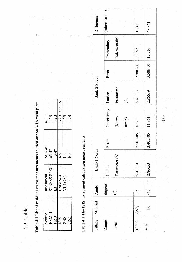
0-4-12a2"a3£
1G©
-4=»3O
T3
*ES~3U
a
•JjJDX>c3HOv
332’3?Qu
'’foJG3H
Ql—( OC3 1-
2B1-
2B1-2
B an
d 2-
1-2B
1-2B
Sam
ple oTj-1m
-H
o1ro
-H No
No
No
Inst
rum
ent
STRE
SS
SPEC
E3 EN
GIN
-XV
ULC
AN
Sour
ceFR
MII
HZB
ISIS
SNS
JRC
'H'
Dif
fere
nce 3Vh
w1OVhO£ 1.
848 "st-00
00
£33-h
3t:<DOcD
C/31O53
! , 5.35
93
12.2
10
mo inoo£
UJoOsWoin
r*| W (N <n3OOQ(Ni<—1 3CQ
Lat
tice
Para
met
er
w 5.41
113
2.86
639
r]cdt;d>or-1D (M
icro
-
stra
in)
4.62
0 VOoo
mo ino3-*Ofc
WoinWoTi
PQ <N ro
o£ w
£23PQ
Latti
ce
•—O4—>Q£3S-.3CL 5.
4111
4
2.86
653
Ang
le
degr
ee
o -45
-45
253 .3£
<NOCL) .u
Fe
Fitti
ng
Ran
ge
mse
c
1300
0-
40K
139

IICO.IIa
oOO '
C/5<C/5O
.sTJ0>
C/531/3!-<ya/s3i -C3a0/w
-2o
43-4-i-333a3C5 -exa>v«a
C/5
Vs3H
42i .
KVOr-mvoOnm>cn
D.3Os-
a<uo3CMoo
UUtu
&-<ua<wZ■<■U
£3>
o£
a>C/5
CO
uaT3a>3S"eSa>
C/3i-0/-w<UE3;*3a<u
—T3a>u3C/53Oa5/3
3*©433uo<U
C/3C/3Vi -■W
C/5,»—s3
Tfa/
33
H
Rot
atin
g-B
ank
2
S-iO£<Do
3
0.00
0115
50.
0001
115 ooo
ooooo
©3
l?.59
6366
^5.5
9633
13.
5970
935
O in<N int-H 53 o o r -
Go3 o o
oo
cd o o oCQi30
_S3
o o oo d
O'inCN
inin—H rn
O 3 <—1 (N ON2 NO VO VO
ONinr ' )
Onin<n
ONin<n
<N i- in vo vo-34 O cn ON ON33
CQ
5—15-> —-< o o<D o o o© o o ©
to 3 o o ©3 o o d3O 00 in
©©
2 © r - —*. ©■ 3 in VO r~~3 ON On ONO in in in
Z <n <n. !— ——H 00 ■3"M O cn 00 00&C3PQ
—i o ©CD o o ©o o o ©i
to 3 o o o. c o o d
2 ' cn o Ono 3" VO ©2i
o in <Nc VO VO r -
3 3 ON ON ON■ O ' in in in
Z in* rn2 2 ■ 42 3
uo .p2
22
3 .
22
o 3pC/5 O o 3C/5P H CQ CLh
C/5
3
<N4433CQiso
ocM
4433CQso
<N
3CQ3o
043O
Z
4 4c3
PQ3o
o04so
Z
o423U<Dp2
C/5
o£a>w3. r-nr vont-
(Ncnm
w3L
O<Dw3.
w3.
w3.
t--in
Tt
•3-m
<NO
VO©oo
VOm©in
ind
«>rn
m
vom
mr-VOm
vqinn-
o<N
O©
n-(N
inm
in*—Hm
in
m
©od
213
o .oH
213£
oCQ
3Oo
Not
e: a
o: Is
the
aver
age
of the
m
easu
red
stres
s fre
e lat
tice
para
met
ers
for
each
cu
boid
, an
d ao
erro
r: is
the
aver
age
fittin
g er
ror
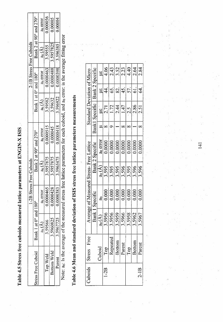
Tabl
e 4.5
St
ress
free
cu
boid
s m
easu
red
lattic
e pa
ram
eter
s at
ENGI
N-X
ISIS
oOr -< N
X3
s -O! -i -<Ue
Xi noooo
moooo
XOooo
0 30 3
od d
oOO S
C/3
3‘ oX
4-»0 3
C N
X <
m» nm
i n< N0 0r -
3.
59
63
85
3
u
<u<u
r j
CO
C Q
©£
Oi n
r n
i nO si n
r ns -
U h
C/3C/3 m o o o o<U i - X 0 0 O s .! _ O O N - x m
V OO u - O o oO O O o o o
C Q1 o o o
£ o o ©i
< N££
o
d d d
£
2
< N0 0i n
< NmX
3.
59
69
22
£
m
• © £
O Si n
c n
O 'i n
r n
m i n0 0
_ 4 -0 O i n XOt " -
f a oo
ooo
< N
X©
£
oo
©oo
c do
o0 3
oOO s4->
C/30 3 m i n i n
< N r -X
' o <0 0r ^ ~
0 0f -
N "i n
XCd
P Q
v — ^ i n i n X3 c O S O s O s
o03 i n i n i n
0 ) r n r n r n
<L>l -
X
C/3C/30 ) i n 0 0 ms— 1 - X < N 0 0
5 5 O x X mo O o
C Q t ) o o oC N o o o
i o r a o o oO0 0
x
o d o
c0 3
0 i n i nO X ( N ( N
, . X o o r -d i n o r - "
' — ' O S X Xc i n O S O s
CC3
r ni n
r n
i n
r n
C Q
3 3
" o 3 3
X3
u
a
£
£
£
4—•eot -
a>CD
Xo
H
o
o
03X
XP Q
0 3C/3
• a>t -
5 5
uioL<Dto
c0)OQkSt-o>c3<L>X
O £saCJ i- 3t/3 C3 0)S.
C3T3rjC3
oX)=5o
ctJj-icSX<Dac3
T3<us-l33C/3£3OEaxootoF33>c3
S-a/aE«uesaa»a
—a>QJth
C/5—C/5KMXo
’>0)-a-as--acC3
VO■ra>scsH
Stan
dard
D
evia
tion
of M
icro
Bank
2
Spec
ific
tozL 4.06
2.43
3.52
2.23
4.40
2.64
2.84
toX
inX
CNOO
in■r i>m X X
Ban
kl
Spec
ific
toX
r -n i
(N 'sf
CN
r -p in
CN
XooCN
in<N
X oo Os - 00 oo — oo
Ave
rage
of
Mea
sure
d St
ress
- Fr
ee
Latti
ceBa
nk
2 Sp
ecifi
cao
erro
r ooood
Ooood
OOOod 0.
0000 o
ooo©
©oood
©ooo©
wcC3
lOOsincn
mOsincn
mOsincn
Xo sincn
inOsincn 3.
596 X
OSincn
Bank
1
Spec
ific
c.03
oood
oood
oopd
oopd
oood
oopd
oood
oCO 3.59
563.
5956
3.59
593.
5966
3.59
583.
5962
3.59
67
Stre
ss
Free
Cub
oid Xo
H Rep
eate
dB
otto
mPa
rent
ao
H
£o4—<o
PQ Pare
nt
Cub
oids CQ
<NiCQ
1CN

Tabl
e 4.7
Di
ffere
nce
in lat
tice
para
met
er
mea
sure
men
ts f
or str
ess
free
cubo
id
mad
e us
ing
the
VULC
AN
and
ENGI
N-X
inst
rum
ents
<D<L>ecd
§ ^ CX i<D g
^ S"O -73 ^ C3C/3 ’”7 '
§ < S uG ^
8 > c go<uCDi - .£
<Djo!
GGPhooG
*0<d!—Gc/acdCD
CDMlcdCD><
. L-cd <D ■S3 >d333<i ^■‘3b H§ ^ Q G
t—J cd
XIg5zUJ
U"CD£
c/aC/2CDl«4->in
cn’H'o.OGu
CNT3Gcd
GG
PQ
CNyGG
CQ
G
G
GCQ
CNyGG
CQ
cG
£JG
PQ
CN
GG
G
<L)
G
G
G
G
CG
CQ
r"r-oo
ooo
mC"ooooo
ocooocoooo
inoooo
inr -oor-inOnin
mNOrtOOoo
NONOmONin
jd .mcooooooor-mONinco
ooporoG"oNOONinCO
’o
G-OH
oooooooo
inCNNOcoooo
inCNooooo
inof-Oo .oo
int-~oot--mONm
ooCN
oooo
inCN00oNOONinsd .NOONooopoinNOONinsd .0000oooo
oooNOONmcp
3o4-»+-»oCQ
oNOCNCNOO-o
inCNm'7fooo
inoooooo
"d"oooo
inf"G*inNOONin
coooCOoooo
inCNt -r-NOONin
sd .NOONoooo©
r-ONin
SSl
OOoooo
CNNOONin
GCL)i -GPh
CNrt-

« kk'
4.10 Figures
Figure 4.1 M easurem ent position m arked on a v irtual model of TG4 test specimen
3-1A according to priorities list
Line B16
tiLine B2
Line D9 * Line D16
Figure 4.2 Laser scanner (left), laser tracker (right)
Line BD
-Ll-ne- D- 2- Line D5: : U m - k * A -4. 4 -
143
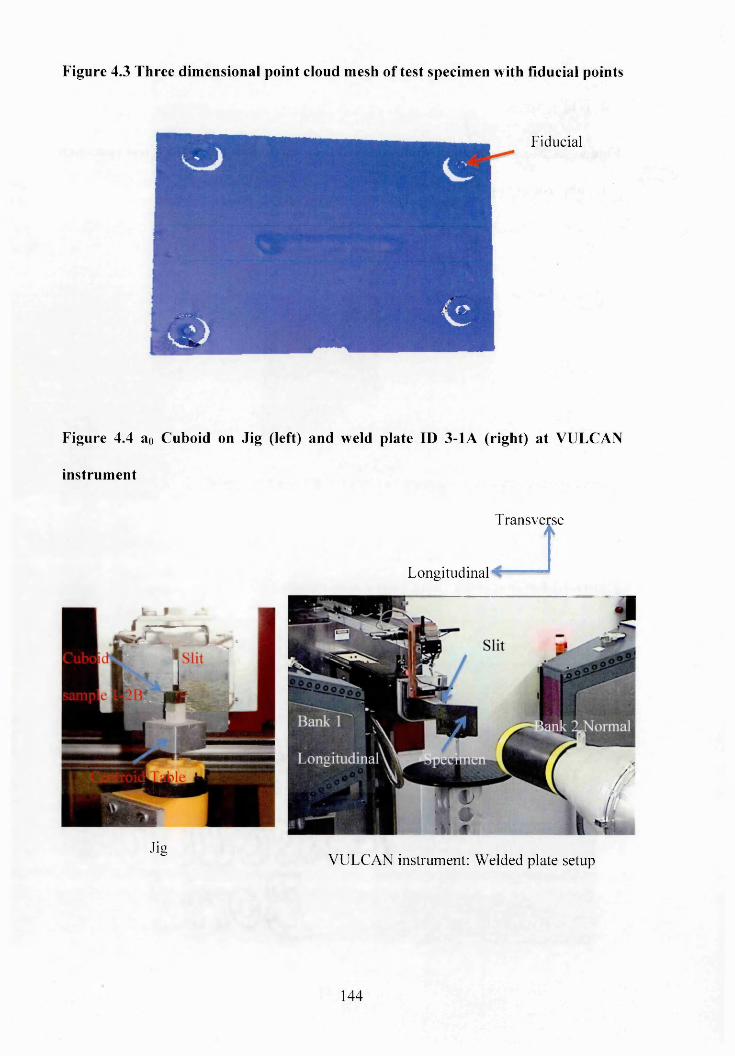
Figure 4.3 Three dimensional point cloud mesh of test specimen with fiducial points
Fiducial
Figure 4.4 ao Cuboid on Jig (left) and weld plate ID 3-1A (right) at VULCAN
instrum ent
TransverseAt
Longitudinal
VULCAN instrument: Welded plate setupJig
144
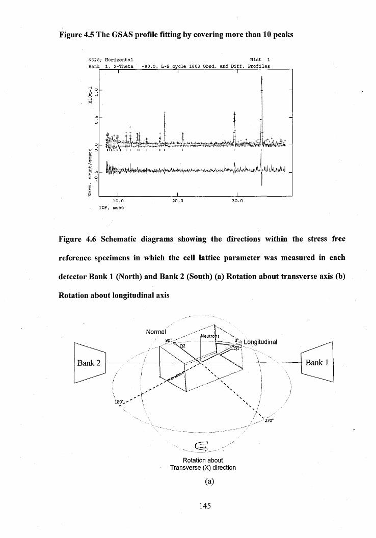
Figure 4.5 The GSAS profile fitting by covering more than 10 peaks
6 5 2 8 ; H o r i z o n t a l H i s t 1B a n k 1 , 2 - T h e t a - 9 0 . 0 , L -S c y c l e 1 8 0 3 O b s d . a n d D i f f . P r o f i l e s
o
■ i ii IT ii i i i li i i Io o<Dto£0>4->£2 IDo •U OI
3 0 .020.010.0TO F, m sec
Figure 4.6 Schematic diagrams showing the directions within the stress free
reference specimens in which the cell lattice parameter was measured in each
detector Bank 1 (North) and Bank 2 (South) (a) Rotation about transverse axis (b)
Rotation about longitudinal axis
NormalNeutrons
Longitudinal531,
Bank 1Bank 2
180'
270'
Rotation about Transverse (X) direction
(a)
145
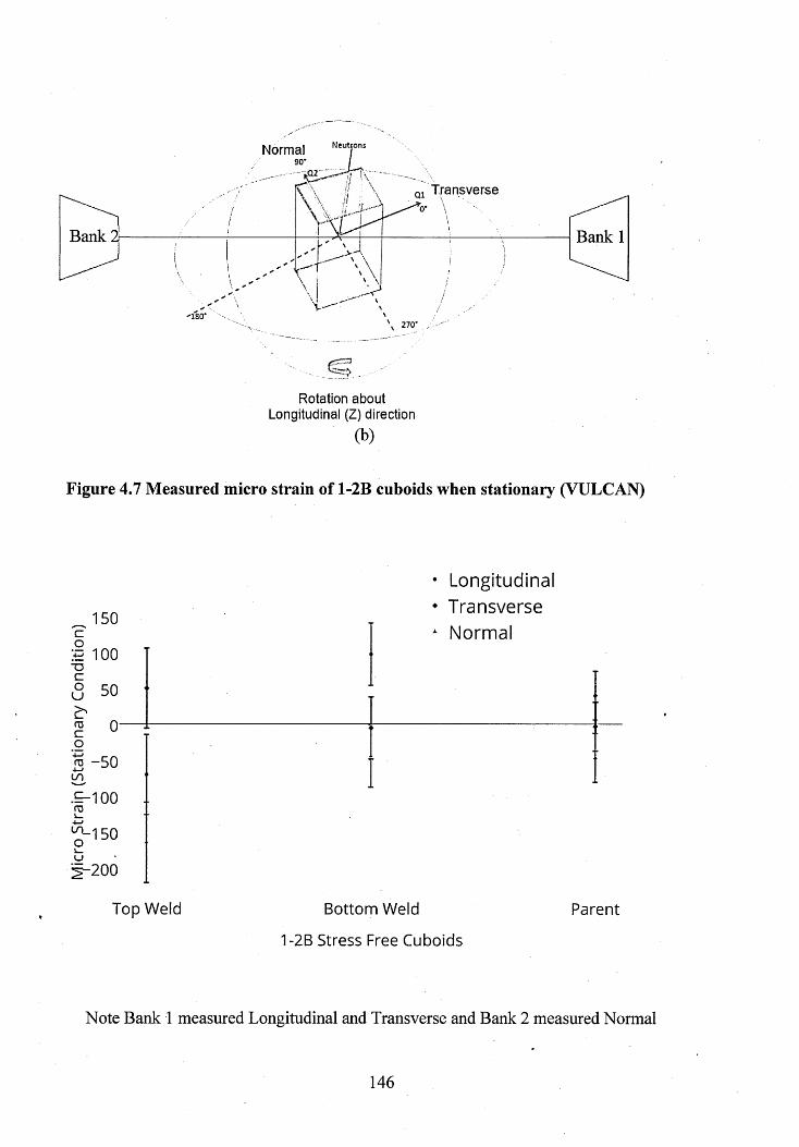
NeutronsNormal
,Q2Q1 Transverse
Bank Bank 1
270 '
Rotation about Longitudinal (Z) direction
(b)
Figure 4.7 Measured micro strain of 1-2B cuboids when stationary (VULCAN)
150
100
50
o-
c o~o c o u
to c o* -50 +->cn.^ 1 0 0TOv_
£-150
'1-200
Longitudinal
T r a n s v e r s e
N orm al
Top Weld Bottom Weld
1-2B Stress Free Cuboids
Parent
Note Bank 1 measured Longitudinal and Transverse and Bank 2 measured Normal
146

Mic
^o
Stra
in
(Con
stan
t R
ota
tio
n)
Figure 4.8 Measured micro strain of 1-2B cuboids under constant rotation
(VULCAN)
• Longitudinal Axis
♦ Transverse Axis
x A verage o f Longitudiraal and Transverse Axis
'J
100
- 1 5 0
Top W eld B ottom W eld P arent
1-2B Stress Free Cuboid
Note Bank 1 and 2 measured Longitudinal, Transverse and Normal depending on the
rotation axis
Figure 4.9 Stress free reference specimens mounted for measurements at ENGIN-X
instrument in order (left to right): weld (top), weld (bottom) and parent for set 1-2B
and set 2-1B
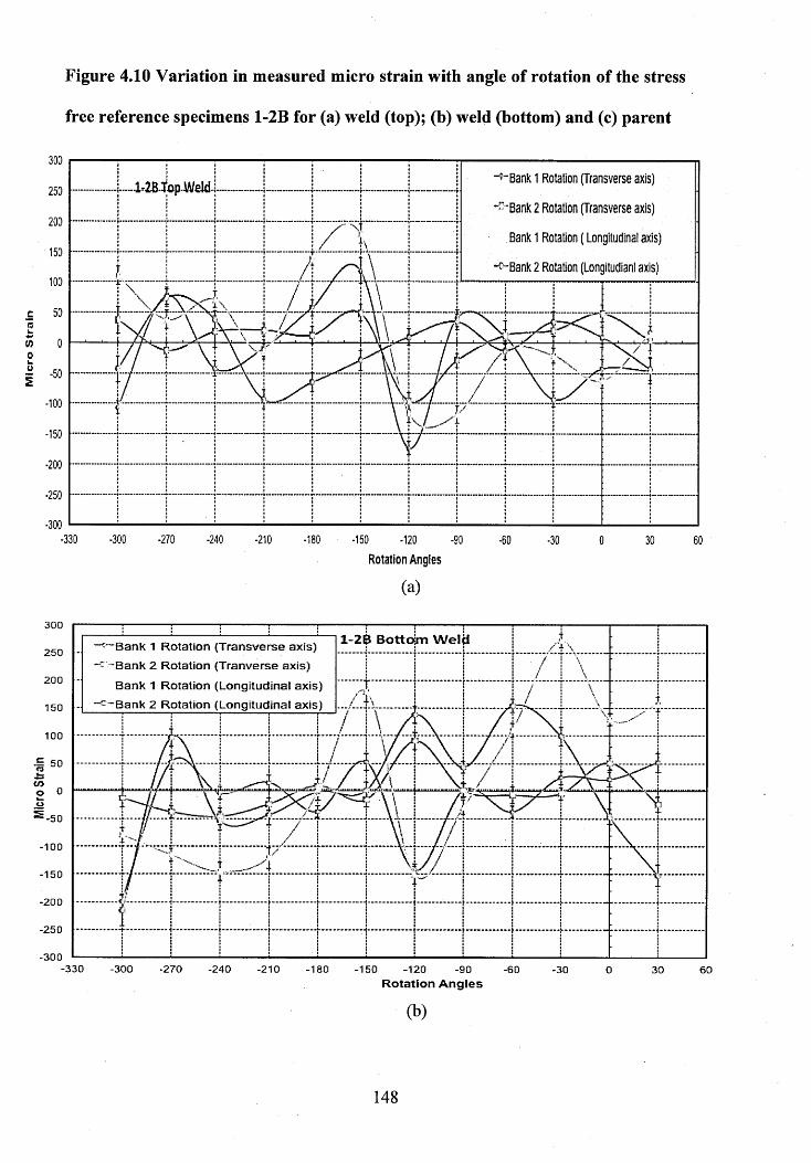
Mic
ro
Str
ain
Figure 4.10 Variation in measured micro strain with angle of rotation of the stress
free reference specimens 1-2B for (a) weld (top); (b) weld (bottom) and (c) parent
- ^ B a n k 1 Rotation (Transverse axis)
Bank 2 Rotation (Transverse axis)
Bank 1 Rotation ( Longitudinal axis)
"“ Bank 2 Rotation (Longitudianl axis)
......lr2Biop-Weld-|
Rotation Angles
(a)
3 0 0
^~B ank 1 Rotation (Transverse axis)
~-"Bank 2 Rotation (Tranverse axis)
Bank 1 Rotation (Longitudinal axis)
c~ B an k 2 Rotation (Longitudinal axis)
/-f2 5 0
200
1 5 0
100
to 0
- 5 0
-100
- 1 5 0
-200
- 2 5 0
- 3 0 0- 3 3 0 - 3 0 0 - 2 7 0 - 2 4 0 -210 - 1 8 0 - 1 5 0 -120 - 9 0 - 6 0 - 3 0 0 3 0 6 0
Rotation Angles
(b)
148
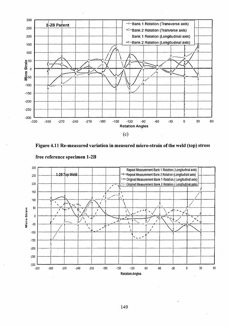
300-^ “ Bank 1 Rotation (Transverse axis)
""-“ Bank 2 Rotation (Tranverse axis)
Bank 1 Rotation (Longitudinal axis)
♦^“ Bank 2 Rotation (Longitudinal axis)
-2B Parent250
200
150
100
•50
-100
-150
-200
-250
-3006030-210 -180 -150 -30 0-270 -240 -120 -90 -60-330 -300
Rotation Angles
(C)
Figure 4.11 Re-measured variation in measured micro-strain of the weld (top) stress
free reference specimen 1-2B
300 R epeat M easurem ent Bank 1 Rotation ( Longitudinal axis) “ - “ R epeat M easurem ent Bank 2 Rotation (Longitudianl axis)
Original M easurem ent Bank 1 Rotation ( Longitudinal axis) - E - Original M easurem ent Bank 2 Rotation ( Longitudinal axis)
250
200
150
100
cIiuWO
■k ri-
-100
-150
-200
-250
-30030 600-180 -150 -120-300 -270 -240 -210 -90 -60 ■30-330
Rotation Angles
149

Micr
o St
rain
Mi
cro
Stra
in
Figure 4.12 Variation in measured micro strain with angle of rotation of the stress free
reference specimens 2-1B for (a) weld (top) (b) weld (bottom) and (c) parent
3 0 02-jlB Top WeldBank 1 Rotation (Transverse axis)
" “Bank 2 Rotation (Transverse axis)
Bank 1 Rotation ( Longitudinal axis)
r~Bank 2 Rotation (LongitudianI axis)
2 5 0
200
150
100
\ v
•330 •300 ■270 ■180 ■150■240 -210 •120 •90 -60 ■30 600 30
Rotation Angles
(a)
3002-1B B ottom W eldBank 1 Rotation (Transverse axis)
Bank 2 Rotation (Tranverse axis)
Bank 1 Rotation (Longitudinal axis)
Bank 2 Rotation (Longitudinal axis)
250
200,A \150
100
-210 600 30
Rotation Angles(b)
150
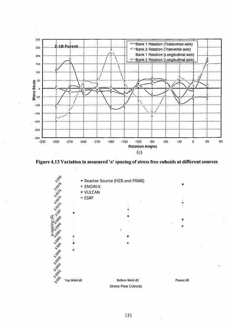
Micr
o St
rain
300“^“ Bank 1 Rotation {Transverse axis) -c -B ank 2 Rotation (Tranverse axis)
Bank 1 Rotation (Longitudinal axis) -o-B ank 2 Rotation (Longitudinal axis)
2S0
200
150
100
-50
-100
-150
-200
-2 5 0
-3 0 060300-210 -180 -150 -120 -60 -30-330 -300 -270 -240 -90
Rotation Angles
(C)
Figure 4.13 Variation in measured ’a’ spacing of stress free cuboids at different sources
o f'b* ® Reactor Source (HZB and FRMII)A*6 b ENGIN-X
e
« VULCAN- ESRF
▲
'b* a
c n < o
eA.
c❖
.E* <§> ca / b ' *
a-s
&
▲ ❖
y❖ n
'b'
sc
V/¥'b' Top Weld dO Bottom Weld dO Parent dO
Stress Free Cuboids
151

Figure 4.14 Residual stresses through the thickness of the plate along line BD,
measured at ENGIN-X (ISIS) and VULCAN (SNS), using 1-2B ao cuboids
500
450
400
350
300
250
200150
n—100
W -50
-100 ^ "L ong itud ina l 1-2B -^ -T ran sv e rse 1-2B
Normal 1-2B - c - SNS-Longitudinal 1-2B -c -S N S -T ran sv erse -*-SN S-N orm al
•150
-200-250
-300■2 2 3 5 5 70 8 9 10 11 12 13 14 15 16 171 4
y (mm)
Figure 4.15 Residual stresses 2 mm below the top surface along line D2, measured at
VULCAN (SNS), using unstressed lattice parameter of 1-2B aO cuboids
5 0 0Litfe D;
4 5 0 -^■SNS Longitudinal 1-2B4 0 0
SNS Transverse 1-2B3 5 0
3 00
-*-SN S Normal 1-2B2 5 0
200| j 150
100CD (/> O &_
W-50
-100-1 5 0 tx-200-2 5 0
-3 0 0-1 0 0 -9 0 -8 0 -7 0 -6 0 -5 0 -40 -3 0 -2 0 - 1 0 _ , 0 . 1 0 20 3 0 4 0 50 60 7 0 80 9 0 100
Z (mm)
152

Figure 4.16 Comparison of residual stresses 5 mm below the top surface along line D5,
measured at ENGIN-X (ISIS) and VULCAN (SNS), using 1-2B a0 cuboids
I L ideD fi Longitudinal 1-2B
-^ ’ Transverse 1-2B
- a- Normal 1-2B
-c-SN S Longitudinal 1-2B
- -SNS Transverse 1-2B
“A" SNS Norma! 1-2B
-1 0 0 -9 0 -8 0 -7 0 -6 0 -5 0 -4 0 -3 0 -2 0 -1 0 _ . 0 . 1 0 2 0 3 0 4 0 5 0 6 0 7 0 8 0 9 0 1 00Z mm
Figure 4.17 Comparison of residual stresses 9 mm below the top surface along line D9
measured at ENGIN-X(ISIS) and VULCAN (SNS) using 1-2B aO cuboids
5 0 0Line D -o-Longitudinal 1-2B
4 5 0
-^-Transverse 1-2B4 0 0
-a-N ormal 1-2B3 5 0
-c-S N S Longitudinal 1-2B
-c-SN S Transverse,1-2B
-a-S N S Normal 1-2B
3 0 0
2 5 0
2001 5 0
1005 0
0-5 0
-100-1 5 0
-200-2 5 0
-300
rsa.
(/)
- 1 0 0 -9 0 -8 0 -7 0 -6 0 -5 0 -4 0 -3 0 -2 0 -1 0 0 10 2 0 3 0 4 0 5 0 6 0 7 0 8 0 9 0 1C
Z (mm)
153

Stre
ss
(MPa
) St
ress
(M
Pa)
Figure 4.18 Comparison of residual stresses 16mm below the top surface along line
D16, measured at ENGIN-X (ISIS) and VULCAN (SNS), 1-2B a0 cuboids
5 0 0 Lines D16 ©-Longitudinal 1-2B
"©’ Transverse 1-2B
Normal 1-2B
4 5 0
4 0 0
3 5 0
•©’ SNS Longitudinal 1-2B
-C--SNS Transverse 1-2B
© “SNS Normal 1-2B
3 0 0
2 5 0
200150
100
-5 0
-100-1 5 0
-200-2 5 0
-3 0 0-1 0 0 -9 0 -8 0 -7 0 -6 0 -5 0 -4 0 -3 0 -2 0 -1 0 0 1 0 2 0 3 0 4 0 5 0 6 0 7 0 8 0 9 0 1 0 0
Z (mm)
Figure 4.19 Comparison of residual stresses 2 mm below the top surface along line B2,
measured at ENGIN-X (ISIS) and VULCAN (SNS), using 1-2B a0 cuboids
5 0 0
Line 8:2 ©-Longitudinal 1-28
©Transverse 1-2B
4 5 0
400
©-Norm al 1-2B
30 0 -c-SNS*longitudina! 1-2B2 5 0 -c-SNS-Transverse 1-2B200
©-SNS-Normal 1-2B
100 - ■ I -
—-J-........-J” -t— ■
■100
-200-2 5 0
-3 0 0- 1 0 0 - 9 0 -6 0 -7 0 -6 0 -5 0 -4 0 -3 0 -2 0 -1 0 0 10 2 0 3 0 4 0 5 0 6 0 7 0 8 0 9 0 100
X (mm)
154

Micr
o St
rain
St
ress
(M
Pa)
Figure 4.20 Residual stresses 16mm below the top surface along line B16 measured at
VULCAN (SNS), using unstressed lattice parameter of 1-2B ao cuboids
5 0 0Lifie B
4 5 0 -c-SNS-Longitudinal 1-2B4 0 0
3 5 0SNS-Transverse 1-2B
3 0 0
2 5 0»-^SNS-Norm al 1-2B200
15 0
100
-5 0 - i - (■-100-1 5 0
-200-2 5 0
-3 0 0-1 0 0 -9 0 -8 0 -7 0 -6 0 -5 0 -4 0 -3 0 -2 0 -1 0 8 0 9 0 1 000 10 2 0 30 4 0 5 0 6 0 7 0
X (mm)
Figure 4.21 ENGIN-X: (a) measured micro strain and (b) residual stress measurement
along line BD, using 1-2B and 2-1B ao cuboids
2 5 0 0Line 8-D
2000
1 5 0 0
1000
5 0 0
Longitudinal 1-2B Transverse 1-2B Normal 1-2B Longitudinal 2-1B Transverse 2-1B Normal 2-1B
0
~“v—
-10001 7■2 2 6 1 5 1 61 0 1 3 4 5 7 8 9 10 11 1 2 1 3 1 4
y (mm)
(a)
155
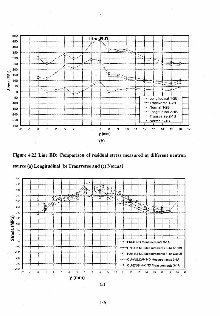
.500
450
400
350
300
250
200're'CL 150stn 100tncjis 50in
0
-50
-100
-150
-200
-250
-300
i IlinejB-D] 1 1 ] j ! 1 1j t ;........1.........j........j ........ f '......\ - —/ X ....... ♦— .........4- i 4-....... J....... 4------4-........\ ......—v.......• / I I S ! ! ! !
4-.......... -*-*■ -------5-
i-T : T—4----- i -^ 4 -! i / I
- J ,............) ............. 4 .............. 4-..............}...........j | j j f '
■4--------4------1—^c"}1---------i-------1------ 4------ i -I I I '^4 _j \ I I 4- t ......^......
f ”
■Longitudinal 1-2B -Transverse 1-2B Normal 1-2B Longitudinal 2-1B Transverse 2-1B Normal 2-1B
-2 -1 7 8y (mm)
10 11 12 13 14 15 16 17
(b)
Figure 4.22 Line BD: Comparison of residual stress measured at different neutron
source (a) Longitudinal (b) Transverse and (c) Normal
oOLD
'150-100350300250200
<13 150Q_s 100</) 50tn0)CO -50
-100-150-200-250-300
—1.....4.....1.......4... i......j\.—,4-j|—j............. 4..... 1—i....."f...... 1..... 4.....
: : i 1 --fe * , ' i i ' \ Z ' V i . . . . . s .- .........— j — — - «4- — —i ———4*— —‘i — ——4——— i - 4
;i i & ? l T ; T . T % j ! ! i ! ■■ I ■*.......4.......+............................................. -},....... | .......+ ....... | ......
....J.......4... {......4.....i 4...... 1 *h— —-€>.....r f..... i—-—f-..... t -t i..... -?•— j....
--i.....4..... i..... ]..... -j-
i......
"0 --F R M II ND Measurements 3-1A
HZB-E3 ND Measurements 3-1AApr 09
--0--HZB-E3 ND Measurements 3-1AOct09
--c— OU-VULCAN ND Measurements 3-1A
--C--OU-ENGIN-X ND Measurements 3-1A
0 1 2 3 A 5 6 7 8 9 10 11 12 13 14 1 5 16 17 18 IB
y (mm)(a)
156
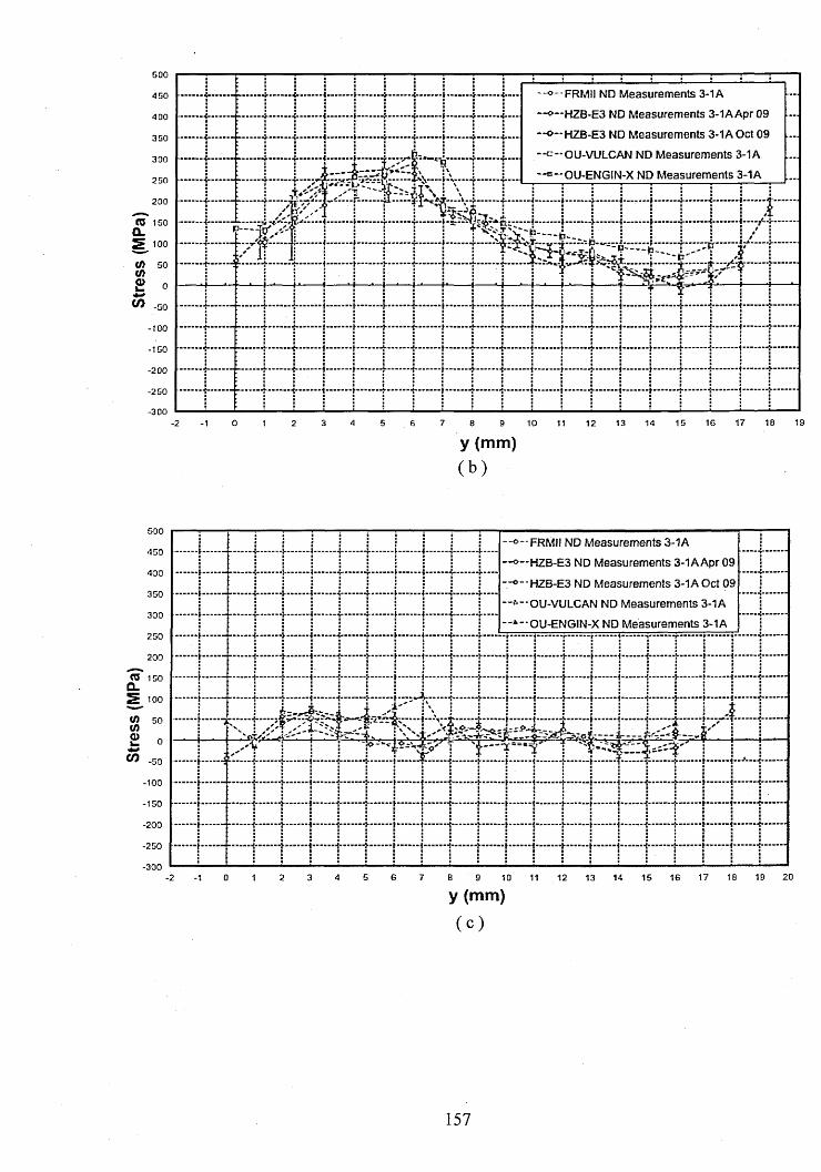
GOO
-o—FRMI1 ND Measurements 3-1A
-o--HZB-E3 ND Measurements 3-1A Apr 09
-o—HZB-E3 ND Measurements 3-1AOct09
-e— OU-VULCAN ND Measurements 3-1A3 GO
300
-*-*O U-ENG IN-X ND Measurements 3-1A250
200
(0 1 GO
10050
100150
■200
-250
■30017 18 19160 3 <1 5 7' 10 13 15■2 1 1 2 6 8 9 11 12 14
y (mm)( b )
-o—FRMIl ND Measurements 3-1A
HZB-E3 ND Measurements 3-1A Apr 09
-*-'H Z B -E 3 ND Measurements 3-1A Oct 09
450
350OU-VULCAN ND Measurements 3-1A
300OU-ENGIN-X ND Measurements 3-1A
250
■50
■100
•150
■200
■250
■3002017 18 192 5 6 B-2 0 1 3 4 7 9 10 11 12 13 14 15 16■1
y (mm)
( C )
157
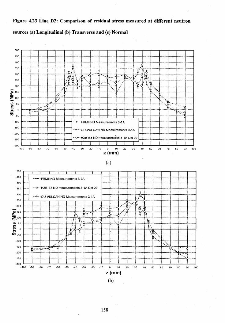
Figure 4.23 Line D2: Comparison of residual stress measured at different neutron
sources (a) Longitudinal (b) Transverse and (c) Normal
50*0
403
350
300
20003 150
CL2 100
{/> GO
0CO ■50
100 o -'F R M II ND Measurements 3-1A
-®— OU-VULCAN ND Measurements 3-1A-200
-o - HZB-E3 ND measurements 3-1A Oct 09
■300-100 -90 -80 -70 -GO -50 -40 -30 -20 -10 0 10 20 30 4 0 50 6 0 70 8 0 90 100
z (mm)
(a)500
0 --F R M II ND Measurements 3-1A
- HZB-E3 ND measurements 3-1A Oct 09350
300-o—OU-VULCAN ND Measurements 3-1A
25 0
200
-ioo
■150
-200
-250
-300100 -60 ■50 -40 -20 ■10■80 ■70 -30 0 10 3020 40 50 GO 70 80 90
z (mm)
(b)
158
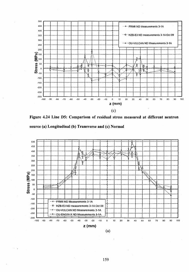
Stre
ss
(MPa
)
500
450 °*F R M II ND Measurements 3-1A
-©-• HZB-E3 ND measurements 3-1A Oct 09350
300■fc--OU-VULCAN ND Measurements 3-1A
250
200(0 150Q.S 100
---
if) 50
■50
■100
■150
-200-250
•300100 -90 -80 ■50 -10■70 -60 ■30 -20 0 80 90•10 10 20 50 GO 7030 40
z (mm)
(C)
Figure 4.24 Line D5: Comparison of residual stress measured at different neutron
source (a) Longitudinal (b) Transverse and (c) Normal
500
450
400
350
300
250
200150
10050
0-50
-100-150
-2 0 0
-250
—J— -
*>
i I i“ “ “ -V - - -X*F ! ■fr 1-3S-*S *'■ t........... ------------------ ( r t —{— — — —{--------. . ^ . . . . . . . j . . . . . . .
/?,' j.
V $
- r fir r r / *, V
'3!:I* /y ',/ r
t --t--4-.| ................4.
j j | .........| ......... j . ........
J V I .1 4 -!......!
H di 'V'©-. i iH B Z E i
-300
■+..........4-.......... 1---------4-.......... 4........... 4-..........4-..........4..........
—o—f r m ii ND Measurements 3-1A
- o - HZB-E3 ND measurements 3-1A Oct 09
—o—OU-VULCAN ND Measurements 3-1A
OU-ENGIN-X ND Measurements 3-1A
-100 -90 -80 -70 -60 -50 -10 -30 -20 -10
z (mm)10 20 30 40 90 100
(a)
159

500
400
350
300
250
200CU 150Q.s 100
o -F R M II ND Measurements 3-1A100
o HZB-E3 ND measurements 3-1A Oct 09-150
■<— OU-VULCAN ND Measurements 3-1A-200-250 OU-ENGIN-X ND Measurements 3 -iA-300
-100 -90 -83 -70 -00 -50 -40 -30 -20 ■to 0 10 20 30 40 GO 10000 70 80 50z (mm)
(b)
500
°"*FRM II ND Measurements 3-1A
400—0 -H Z B -E 3 ND measurements 3-1AOct09
350
OU-VULCAN ND Measurements 3-1A300
250 OU-ENGIN-X ND Measurements 3-1A200
•100-150
-200-250
-300-90 -80 -70 -60 -40 -30 -20 -10 0 10 20 30 10040 50 GO 70 83 90
z (mm)(C)
160
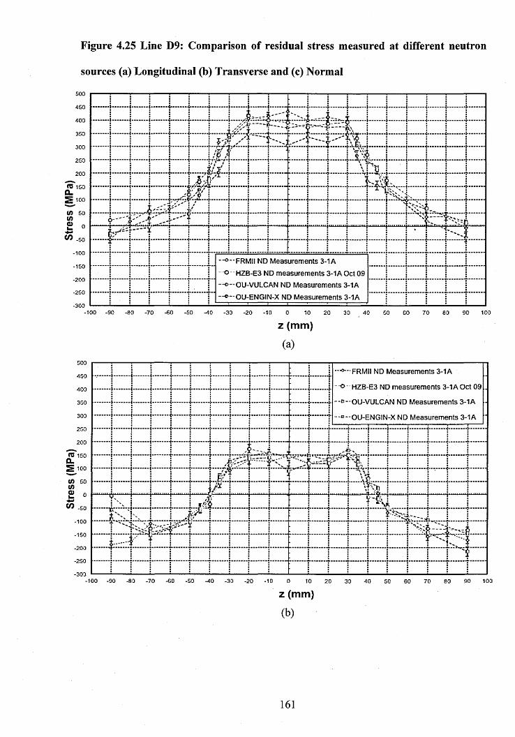
Figure 4.25 Line D9: Comparison of residual stress measured at different neutron
sources (a) Longitudinal (b) Transverse and (c) Normal
500
450
350
300
250
200HI 150CLS 100
</) 50O0
o«*FRMII ND Measurements 3-1A
o HZB-E3 ND measurements 3-1A Oct 09
~ o ~ OU-VULCAN ND Measurements 3-1A
--© —OU-ENGIN-X ND Measurements 3-1A
-20-0-250
-100 -90 -80 -70 -60 -GO -40 -30 -20 -10 0 10 20 30 40 50 GO 70 80 90 10-0
z (mm)
(a)503
■°~"FRMil ND Measurements 3-1A
--0--H ZB -E3 ND measurements 3-1AOct 09
-0-OU-VULCAN ND Measurements 3-1A
OU-ENGIN-X ND Measurements 3-1A250
Ui 50
-150
-250
-100 -90 -80 -70 -60 -GO -40 -3-0 -20 -10 0 10 20 30 40 50 GO 70 80 90 100
z (mm)
161
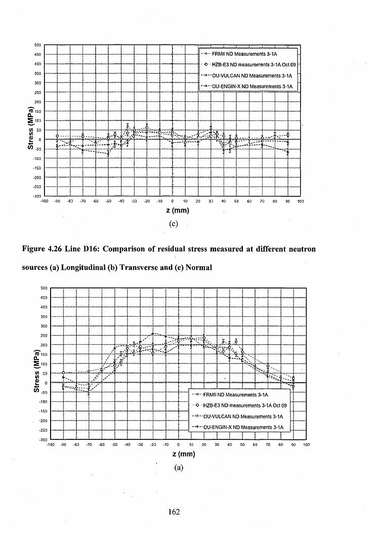
o-FR M II ND Measurements 3-1A
400 --o~ HZB-E3 ND measurements 3-1A Oct 09
3.50 •*"0U-VULCAN ND Measurements 3-1A
OU-ENGIN-X ND Measurements 3-1A
o
-1C-0
•203
•303-100 -90 -83 -70 -60 -GO -40 -30 -20 -10 0 10 20 30 40 50 60 70 80 90 103
z (mm)
(C)
Figure 4.26 Line D16: Comparison of residual stress measured at different neutron
sources (a) Longitudinal (b) Transverse and (c) Normal
350
300
250
203
RJ 150CLS 103
W 5-3 </>Q
-v- -i-
-}........ j........ |
-f........ i........ i
j-.... 4.....4......... [...I—-i-.........4 ..........4 .........
f- — --i-,—j i i ! X[..... |..... |.............................. %-.f- -
4 r.Q.'- -. -4 -0
-50
-103
-150
-200-253
]
...i
'■"■■j"-
Y-
</)
-303
! I ! I-}.............. 4-.....4.....4......[•''I
--o-FRMII ND Measurements 3-1A
--0--HZB-E3 ND measurements 3-1AOct 09
-e-'OU-VULCAN ND Measurements 3-1A
OU-ENGIN-X ND Measurements 3-1A
-100 -90 -80 -70 -60 -50 -40 -30 -20 -10 10 20 30 40 50 60 70 80 90 100
z (mm)
(a)
162
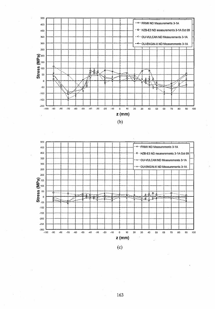
500
•^••FRMII ND Measurements 3-1A
O - HZB-E3 ND measurements 3-1A Oct 09
-«--OU-VULCAN ND Measurements 3-1A350
300 *®" OU-ENGIN-X ND Measurements 3-1A
25*0
50
0-50
-103
■150
-200-SO -70 -60 -50 -40 -30■100 -90 -20 ■10 10 20 1000 30 -JO GO 70 80 9050
z (mm)
(b)
500
-0--FRMII ND Measurements 3-1A
400 o --HZB-E3 ND measurements 3-1AOct09
-'---OU-VULCAN ND Measurements 3-1A300
-*-OU-ENGIN-X ND Measurements 3-1A25-0
200
to 160
0-50
•10D
•150
-200
-80 -70 -GO -30■100 -90 -20 ■10 0 10 20 30 10040 GO GO 70 80 90
z (mm)
(C)
163
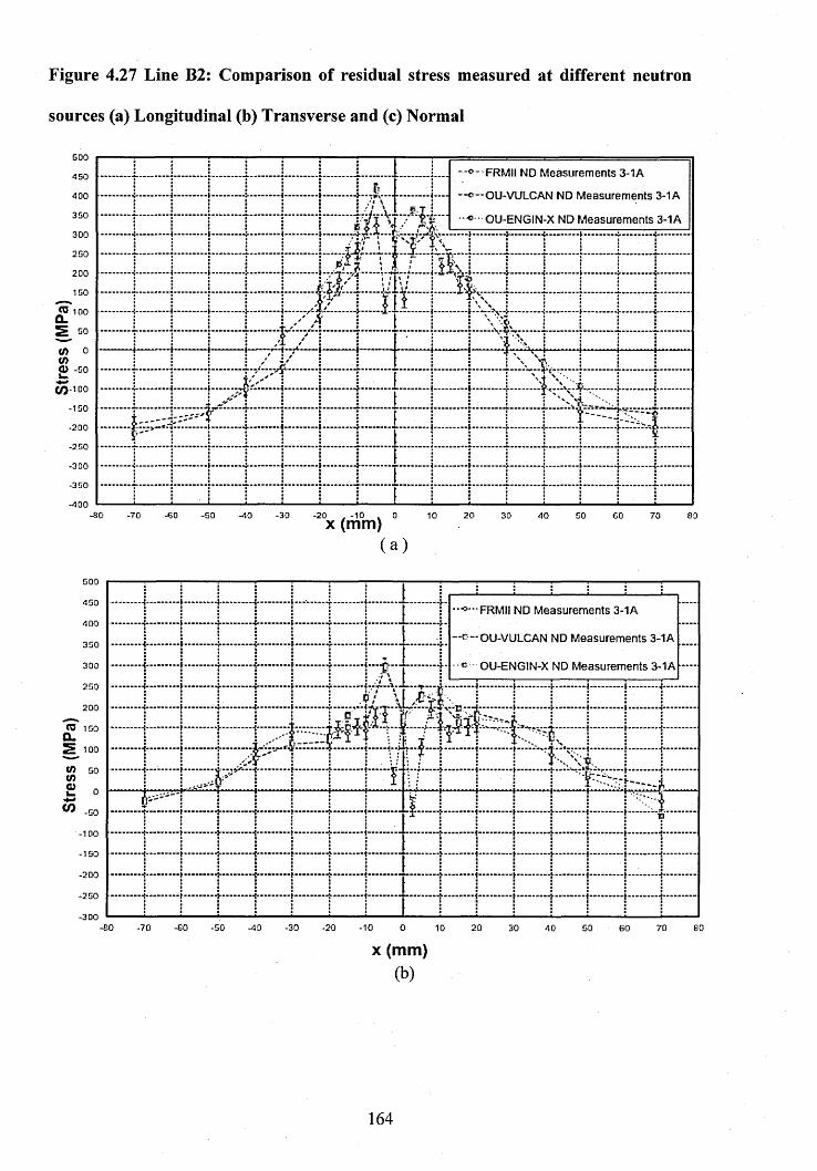
Figure 4.27 Line B2: Comparison of residual stress measured at different neutron
sources (a) Longitudinal (b) Transverse and (c) Normal
GOO
•o- FRMII ND Measurements 3-1A
- e —OU-VULCAN ND Measurements 3-1A
350 «-• OU-ENGIN-X ND Measurements 3-1A3 0 0
250
200
150
SP 10050
a> -so
</J-100-150
-80 -60 -20 , -10 . 0 x (mm)-40 2010 30 50 60 8070
GOO
« — FRMII n d Measurements 3-1A
OU-VULCAN ND Measurements 3-1A350
« - OU-ENGIN-X ND Measurements 3-1A300
250
200
50
-100
■150
-200
-250
-300-40 ■10-BO -70 -60 -50 -30 -20 0 20 7010 30 60 8060
x (mm)(b)
164

500
FRMII ND Measurements 3-1A
* - • OU-VULCAN ND Measurements 3-1A3 5 0
OU-ENGIN-X ND Measurements 3-1A3 0 0
2 5 0
200
'100
50
0-5 0
100
150
-2 5 0-SO -7 0 -60 -3 0 -20 GO 70 80-5 0 -1 0 0 10 20 30 4 0 GO
x (mm)(c)
Figure 4.28 Line B16: Comparison of residual stress measured at different neutron
sources (a) Longitudinal (b) Transverse and (c) Normal
o--FRMII ND Measurements 3-1A
•100
-® - OU-VULCAN ND Measurements 3-1A3 50
3 00
2 50
200
*0 150
10050
CO-50
-100
-1 5 0
-200
-2 5 0
-3 0 0 -SO -70 •60 -40 -30 -20 -10 60 7 0 800 10 20 3 0 50
x (mm)(a)
165
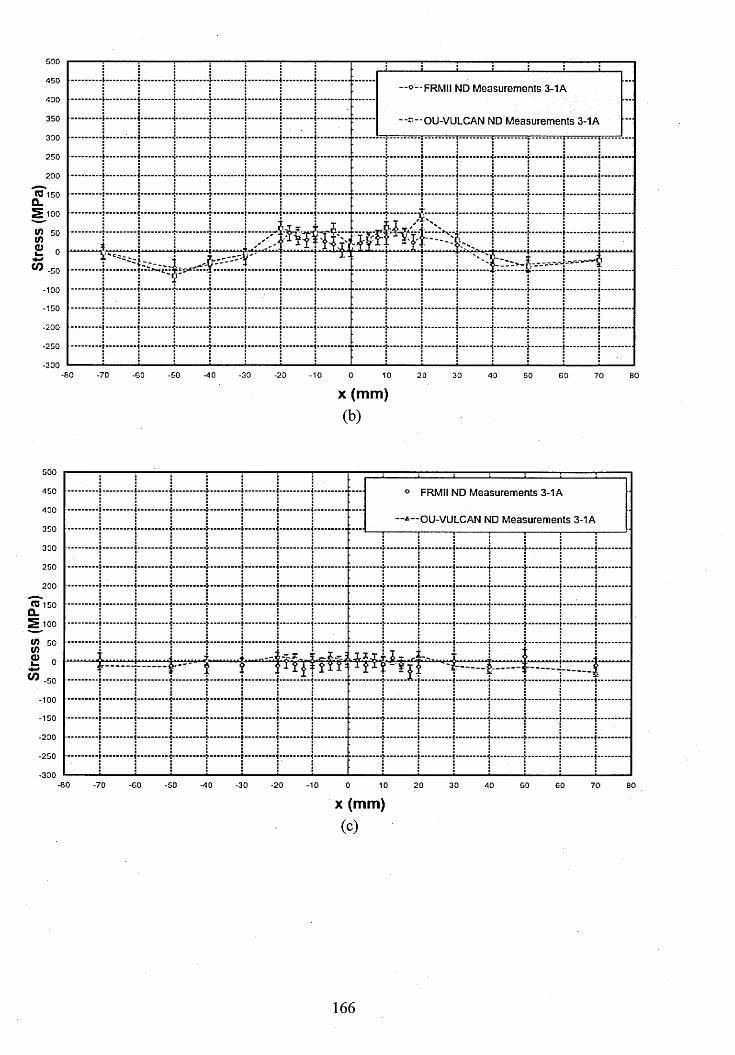
500
— FRMI I ND Measurements 3-1A
350 -OU-VULCAN ND Measurements 3-1A300
250
200
CO 150 Q_*S 100W 50
-100
-150
-250
-300-SO -70 -60 -50 -40 -30 -20 -10 0 10 20 30 50 GO 70 80
x (mm)(b)
500
° FRMII ND Measurements 3-1A
* - * OU-VULCAN ND Measurements 3-1A3 50
3 0 0
250
200
CO 150 Q_J » 100
cn so
0
-100
-150
-200
-250
-80 -70 -60 -50 -30 -1 0 0 10 20 30 GO 70 80
x (mm)(C)
166

Gauge Volume
Figure 4.29 Crevice effect on gauge volume
m m
8 m m
Figure 4.30 (a) Gauge volume m easuring grains in only one plane (i.e. Plane D or Plane
B refer Figure 3.3 (a)) at 0°, 180°, 90° and 270° and (b) gauge volume m easuring
average of two plane ( i.e. plane D and B) at 30°, 60°, 120°, 150°, 210°, 240° and 300°
Transverse Axis
Crevices a ,°‘
c Only one-plane grain populations
With presents o f crevices at angles 0°, 180°, 90°
and 270°
Volum e
167
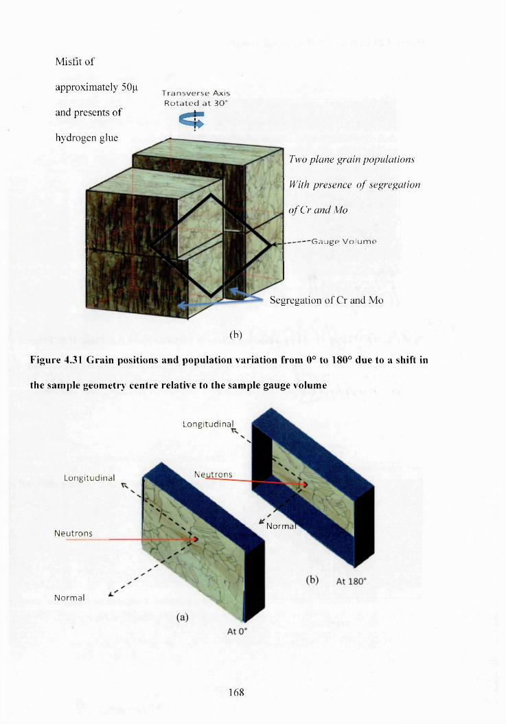
Misfit o f
Two plane grain populations
With presence o f segregation
o f Cr and Mo
G a u g e V o lu m e
Segregation of Cr and Mo
(b)
Figure 4.31 G rain positions and population variation from 0° to 180° due to a shift in
the sample geometry centre relative to the sample gauge volume
approximately 5Op
and presents of
hydrogen glue
T ra n s v e rs e Axis R o ta te d a t 30°
c
Longitudinal
N e u tr o n s
Normal
Longi tudina
N e u tr o n s
Norma
168
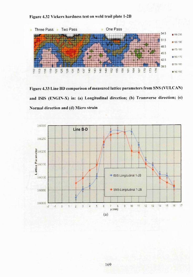
Figure 4.32 Vickers hardness test on weld trail plate 1-2B
Three Pass Two Pass One Pass■ 190-200
0 180-190
0 1 7 0 -1 8 0
0 1 6 0 -1 7 0
0 1 5 0 -1 6 0
0 140-150
Figure 4.33 Line BD comparison of measured lattice param eters from SNS (VULCAN)
and ISIS (ENGIN-X) in: (a) Longitudinal direction; (b) Transverse direction; (c)
Normal direction and (d) Micro strain
3.60300
3.60250
■2 3.60200 0)EBJi .CD
^ 3 .6 0 1 5 0 u75_i
3.60100
3.60050
3.60000
Line B-D
ISIS Longitudinal 1-2B
-•-SNS-Longitudina! 1-2B
-2 -1 0 1 2 3 4 5 6 7 8 9 10 11 12 13 14 15 16 17y (mm)
(a)
169
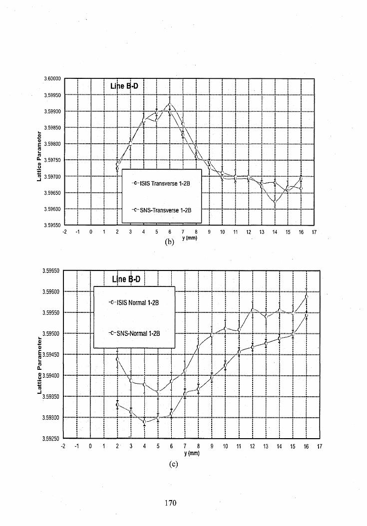
Lat
tice
P
ara
me
ter
Lat
tice
Par
amet
er
3.60000
Lijie B-D3.59950
3.59900
3.59850
3.59800
3.59750
3.59700-c—ISIS T ransverse 1-2B
3.59650
3.59600 -c~SN S-T ransverse 1-2B
3.59550■2 -1 2 3 40 5 6 7 8 9 10 11 12 13 14 15 16 17
(b ) V(mm)
3.59650
3.59600
-c-ISIS Normal 1-2B3.59550
-c-SNS-Normal 1-2B3.59500
3.59450
3.59350
3.59300
3.59250-2 -1 0 1 2 3 4 5 6 7 8 9
y(mm)
170
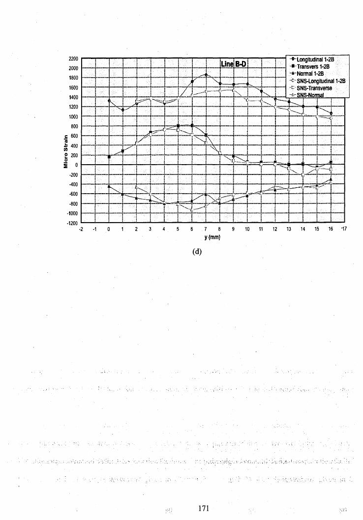
Mic
ro
Str
ain
2200 Longitudinal 1-2B -*-Transvers 1-2B
Normal 1-2B "° “SNS-Longitudinal 1-2B
SNS-Transverse ^SNS-Normal_______
LineiB-D2000
1800
1600
1400
1200
1000
800
600
400
200
-400
-600
-800
12 13 14 15 16 -173 4 5 6 7 8-2 2 9 10 11•1 0y(mm)
(d)
171
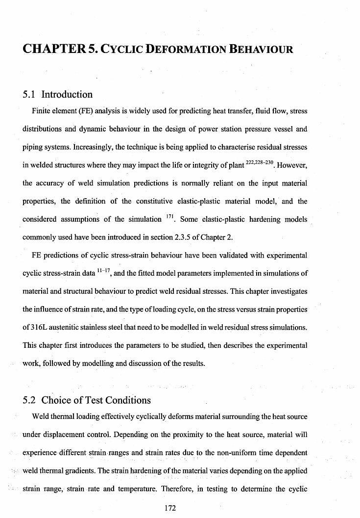
CHAPTER 5. C y c l ic D e f o r m a t io n B e h a v io u r
5.1 Introduction
Finite element (FE) analysis is widely used for predicting heat transfer, fluid flow, stress
distributions and dynamic behaviour in the design o f power station pressure vessel and
piping systems. Increasingly, the technique is being applied to characterise residual stresses
oo o o o o o o nin welded structures where they may impact the life or integrity o f plant ’ “ . However,
the accuracy o f weld simulation predictions is normally reliant on the input material
properties, the definition of the constitutive elastic-plastic material model, and the
considered assumptions o f the simulation 171. Some elastic-plastic hardening models
commonly used have been introduced in section 2.3.5 o f Chapter 2.
FE predictions o f cyclic stress-strain behaviour have been validated with experimental
cyclic stress-strain data 11_17, and the fitted model parameters implemented in simulations of
material and structural behaviour to predict weld residual stresses. This chapter investigates
the influence o f strain rate, and the type of loading cycle, on the stress versus strain properties
o f 3 16L austenitic stainless steel that need to be modelled in weld residual stress simulations.
This chapter first introduces the parameters to be studied, then describes the experimental
work, followed by modelling and discussion of the results.
5.2 Choice o f Test Conditions
Weld thermal loading effectively cyclically deforms material surrounding the heat source
under displacement control. Depending on the proximity to the heat source, material will
experience different strain ranges and strain rates due to the non-uniform time dependent
weld thermal gradients. The strain hardening of the material varies depending on the applied
strain range, strain rate and temperature. Therefore, in testing to determine the cyclic
172

deformation properties of a material it is very important to select an appropriate strain range,
strain fate and temperature. Material surrounding the weld heat source will first expand and
experience compressive strain due to constraint from material away from the heat source. In
contrast, during weld cooling, the material will contract with decreasing temperature, but is
constrained by the surrounding material. As a result of this, tensile strains are developed in
the material. In this research study, in order to replicate weld deformation behaviour, the
parent material is cyclically defoimed in compression-tension cycles. Table 5.1 lists the
strain controlled cyclic deformation tests of solution annealed parent material carried out at
both room and high temperatures.
5.2.1 Strain range
Strain ranges of ±1.25% for symmetric cyclic deformation, and -1.25% to 0.02% for
asymmetric cyclic deformation of parent material at both room and high temperature were
adopted. In multi-pass welding, the strain range of the weld defoimation cycle generally
reduces from one weld deposit to next with increasing distance from heat source, as
described in section 2.2.1 of Chapter 2. Depending on the weld heat input parameters, the
highest plastic strain range is observed close to the fusion boundary; during the welding of
austenitic stainless steel this is of the order of ±2.5% 63. Due to the limited material available
and the.high probability of losing data due to specimen buckling at high temperature, a strain
range of ±1.25% was adopted for this research study. This is expected to be close to the
mean strain range of multiple weld passes. For asymmetric cyclic loading approximately one
half of the symmetric strain range was chosen.
5.2.2 Temperature
The accumulated plastic strain due to each weld pass contributes to cyclic work hardening
of the material. However, at high temperature, the material can experience dynamic
173
recovery, annealing and softening. This can reduce the strain introduced at lower
temperatures. The cooling rate of the weld metal decreases very slowly from 600°C to room
temperature. In the temperature range 650°C-300°C austenitic stainless steel 316L (N)
experiences Dynamic Strain Ageing (DSA). As described in section 2.3.3 of Chapter 2, with
decreasing strain rate (i.e. cooling rate) the material gets more strain hardened than at a fast
strain rate. In this research study cyclic defoimation tests of parent material were performed
at 550°C. The reasons for selecting this temperature are; (a) above 600°C the recovery of
the plastic deformation of material is high and (b) there is a higher risk of sample buckling
during compression loading at higher temperatures.
5.2.3 Strain rate
As described in section 2.2.1 of Chapter 2, the heating rate and cooling rate of weld metal
varies with distance from the heat source. Likewise, the plastic strain rate associated with
the welding process varies during weld heating and cooling cycles. The strain rate during
heating is in excess of l x l 0 _2/sec , and during cooling reaches lxlO _3/sec between 750°C
and 350°C and falls steadily as the temperature drops 63. In this research study, due to
limitations of the test machine, strain rates of 4 x l0 _4/sec and 4xl0~5/sec were selected for
the cyclic deformation tests. Details of the design, extraction and heat treatment of the test
samples has been given in section 3.3. Using an Instron 8862, the test samples were
cyclically deformed at both room and elevated temperatures (550°C). Details of the cyclic
loading experimental setup are given in section 5.3.
5.3 Cyclic Stress-Strain Tests
The British standard BS7270208 was followed for the program of cyclic deformation tests
performed at room and high temperatures. An Instron 8862 slow strain servo electric test
instrument with a lOOkN capacity and equipped with a heating furnace was used for all the
174

tests. The alignment of the slow strain cyclic loading instrument is very important in
avoiding buckling of the samples, and to ensure a uniform distribution of load is applied to
the gauge volume of each sample. The instrument was aligned according to ASTM E l012-
14231. Alignment was achieved by using a sample fitted with eight strain gauges (as shown
in Figure 5.1), and using Instron AlignPro (IAP) fixture equipment and software ~ . Linear
strain gauges EA-09-062AQ-350/E were spaced at 90° intervals around the circumference,
glued with M-Bond 600 adhesive and protected with M-Coat C (both made by Vishay
Precision Group Ltd). The strain gauges were aligned parallel to the long axis of the test
specimen, with a tolerance of ±2 degrees. The IAP software allows the user to correct for
both concentric and angular misalignment, whilst the sample is preloaded at between 50-100
N.
A Eurotherm-3216 electronic controller was used to control the furnace to maintain a
uniform temperature. Two calibrated n-type thermocouples were used to monitor the
specimen temperature for the high temperature tests. These thermocouples were connected
at both ends of the gauge volume of the sample with the help of clamps, as shown in Figure
5.2. The cyclic loading tests were programmed using Instron Bluehill software. Symmetric
cyclic deformation is routinely used in examining the mechanical properties of materials
where the sample is deformed, as shown in Figure 5.3. However, this is not representative
of the asymmetric cycle deformation experienced close to real welds. In this research study,
a new approach of asymmetric cyclic deformation, as shown in Figure 5.4 Asymmetric
cyclic loading with the first cycle loading in compression (a) stress vs strain loops (b) strain
vs time was adopted.
5.3.1 Asymmetric cyclic deformation
As seen in Figure 5.4, an asymmetric cyclic test begins with compression, following the
path from tA" to *B' in the figure. Between *A’ and ‘IT, the sample is deformed in
175

compression up to -1.25% and then unloaded from ‘B ’ to ‘C \ However, from point ‘C ’
onwards, at each increment of tensile strain, the Bluehill software measures the strain
difference between point ‘C ’ and current strain, to evaluate whether the desired relative
strain range to ‘D ’ is achieved or not. Once the desired relative strain range ‘D ’ is achieved,
unloading commences from point ‘D ’ to tE \ From point ‘£”, the deformation of the sample
continues under relative strain control. This type of asymmetric cyclic deformation is more
representative of predicted real weld asymmetric cyclic loading as shown in Figure 5.5 66.
Symmetric cyclic loading test results, at both room and high temperature (550°C), are given
in Figure 5.6-5.8. Similarly, the asymmetric cyclic loading test results, at both room and
high temperature, are presented in Figure 5.9-5.13. The results were described in section
5.5.1. All experimental cyclic tests were performed on ‘solution annealed’ parent material.
These experimental test results are used to assess the performance of finite element
simulation of welding cycles based on a Lemaitre Chaboche hardening model 109 fitted to
symmetric cycle stress-strain data.
5.4 Finite Element Modelling O f Cyclic Loading
This section describes FE analysis performed to predict the hysteresis loops (i.e. stress vs
strain curves) resulting from the symmetric and asymmetric cyclic loading tests at room and
high temperatures. The simulations were carried out using Abaqus FE software. Figure 5.14
shows a schematic of the geometry simulated. To simplify the simulations, an axisymmetric
model was used with a symmetry plane at the sample mid-length as shown in Figure 5.14.
Second order quadrilateral elements with reduced integration were used. A total of 2625
elements were generated to create a uniform mesh of element size 0.1 mm. Using the Abaqus
tabular amplitude function, the sample loading was defined by applying a cycling
displacement on the top edge of the model, as shown in Figure 5.14.
176
The displacement for the asymmetric cyclic loading simulation was based on the
experimental strain range (i.e. -1.25% to 0.02%). The temperature was set at 25°C and 550°C
for the room and high temperatures models, respectively. An accurate elastic-plastic
constitutive material model is required to achieve reliable stress vs strain FE prediction for
symmetric and asymmetric cyclic hardening tests. A 5-parameter mixed hardening (refer to
section 2.3.5 of Chapter 2) Lemaitre-Chaboche 109 model is provided in Abaqus 24,46 and was
used in FE analysis. The mixed hardening model is designed to predict the stress-strain curve
at high accuracy in comparison to other models24,178. Chaboche parameters for the NeT TG4
9 9316L(N) stainless steel from Muransky were used in the present analysis, see Table 5.2.
Here it should be noted that Muransky ‘ fitted his model to symmetric cyclic stress-stram
data (strain range ±1.5% and strain rate 4><10'4/sec) relevant to the NeT TG4 components.
It is worth mentioning that the mixed hardening model takes into account both the
Bauschinger effect and cyclic hardening. Before simulating the behaviour of the test, the
9 9cyclic stress-strain results of Muransky were reproduced, see Figure 5.15. Predicted stress-
strain behaviour for symmetric vs asymmetric cyclic tests based on the Muransky model is
presented in Figure 5.16. Table 5.3 summarises the materials cyclic test data used for
deriving the five parameters of the mixed hardening model. The kinematic hardening
parameters C j and y j were fitted to the monotonic tensile tests results up to 5% true plastic
strain for the parent material, and 2% for the weld metal as recommended in the R6
procedures171. Whilst, from the cyclic test data, the locus of the peak stress values, of each
half cycle, versus the cumulative plastic strain, was used for fitting the isotropic hardening
of the material. For isotropic hardening, the parameters Qx and b are defined from the second
cycle of symmetric cyclic loading. Optimized parameters for the mixed hardening model for
316L stainless steel have been fitted by Smith e t.a l.21,233 so, these parameters are validated
and should be capable of predicting the stress-strain curve accurately.
177
5.5 Discussion
The material hardening constitutive model used in weld FE simulation has a crucial
influence on the accuracy of predicted residual stress and plastic strains in welded joints.
The input parameters for a hardening model are usually evaluated from the symmetric strain
controlled cyclic and monotonic tensile test data 22>m. However, in real welding processes
the material undergoes asymmetric cyclic hardening, see Figure 5.5. The tests show that
asymmetric cyclic deformation exhibits a different hardening rate in comparison to
symmetric cyclic loading; refer Figure 5.18 and Figure 5.20. The symmetric cyclic tests of
316L (N) material at both room and high temperature show a higher strain hardening rate
than the corresponding asymmetric tests. This suggests that in welding simulations, more
accurate results might be obtained from using a mixed hardening model where the input
parameters are derived from asymmetric cyclic hardening test data.
According to the Rosenthal equation (see section 2.2.1 of Chapter 2), near the weld heat
source, the peak temperature achieved during a weld thermal cycle is very high. The initial
cooling rate during the weld thermal cycle is also very fast, due to the heat sink of
surrounding parent material. However, as the distance from the weld increases, both the peak
temperature and the cooling rate decrease 46. Therefore, in a real welding process the heating
and cooling rates (and hence the strain rate) are non-uniform throughout the sample. Most
of the material hardening leading to tensile stress occurs during the cooling process. At
temperatures between 650°C to 300°C, the austenitic stainless steel exhibits Dynamic Strain
Ageing (DSA), see the serrated stress strain curve in Figure 5.8. While in this range of
temperature, the material experiencing a faster strain rate will exhibit less strain hardening
than that subjected to a slower strain rate, due to DSA. Thus, it is very important to test at
representative strain rates in this temperature range when generating data for calibrating
material hardening models.
178
5.5.1 Discussion on experimental results
Figure 5.6 presents stress-strain results for symmetric cyclic loading at room temperature
for a strain range of ±1.25% (strain rate 4><10'4/sec) and ±1.0% (strain rate 4><10'5/sec). It is
clear from the figure, that the material strain hardens more with a strain range of ±1.25%
than with ±1.0%. In addition, the faster strain rate, 4x 10'5/sec, increases the strain hardening.
The effect of strain rate is clearly evident in the first compression cycle, with the higher
strain rate giving greater monotonic strain hardening. At room temperature, material
deforming at a faster strain rate accelerates dislocations, piling up at grain boundaries and
increasing dislocation interactions with defects more than in the material deformed at the
slower strain rate.
During welding, both the peak temperature and the cooling rate in the parent material
decrease gradually with an increasing number Of passes, due to the increasing distance from
the heat source. As a result of this, as each weld is deposited, the material cyclically strain
hardens over a different strain range and at different strain rates, for example see Figure 5.5.
However, most weld simulations material mixed hardening models are based on constant
strain rate, constant symmetric strain range cyclic data 21 >22’46’233. However, the present
results show that strain rate at room temperature has a significant effect on hardening
behaviour see Figure 5.6.
After six cycles of symmetric deformation of 316L(N) material, (i.e. 30% to 40%
cumulative plastic strain), the rate of strain hardening of the material is much lower than in
the first three cycles (Figure 5.6). This is because, during the initial cycles, the rate of
increasing dislocations density, interactions between them and pile up of dislocation at grain
boundary is high in comparison to later cycles (>3 cycles), due to planar slip mode (refer
section 2.3.4). In planar slip mode, the activation of secondary slip (including cross slip) is
179

very difficult. As a consequence of this, higher dislocation density is noticed at the grain
boundary.
Pham et al. 27 177s dislocation structure studies in cyclically deformed 316L material, have
clearly indicated the formation of a higher density of planar dislocation structures piled up
at the grain boundary, with the help of TEM analysis. However, with an increasing number
of cycles, the applied energy is consumed by changing the dislocation structures, activating
more slip planes and annihilation of dislocations etc.
Figure 5.7 shows a comparison between the symmetric cyclic deformation results, tested
at 25°C versus 550°C, at a strain range of ± 1.25% and a strain rate of 4><10'4/sec. At high
temperatures, the material has lower monotonic yield strength in compression than at room
temperature, and cyclically hardens more, due to DSA (ref section 2.3.3). However, it is
evident that the rate of cyclic hardening decreases significantly from the eighth cycle
onwards. Figure 5.8 shows the effect of strain rate on cyclic hardening of the material tested
at 550°C, due to DSA (see Section 2.3.3). At high temperatures, the cyclic deformation of
the material at a faster strain rate exhibits a low yield point and lower strain hardening than
the material deformed at slower strain rates.
At slower strain rates, the mobility of dislocations reduced due to the pinning effect of
the formation of solute atmosphere around dislocations (refer section 2.3.3). In such
circumstances, in order to maintain the stress flow, additional dislocations are generated,
which results in higher strain hardening of the material. As a consequence, the material
undergoes more strain hardening at a slower strain rate than at a fast strain rate, due to
dynamic strain ageing (refer section 2.3.3). The effect of dynamic strain ageing at a slow
strain rate becomes more significant from the third cycle onwards. This is because, with
increasing numbers of cycles, the dislocation density and the interaction of solute atom with
dislocations increases, as a result material gets more strain hardened. Figure 5.9 and Figure
180
5.10 shows the results from asymmetric cyclic loading performed at room and high
temperature. These results are compared with symmetric cyclic loading, both at a strain rate
of 4><10'4/sec. It can be observed from the obtained results, asymmetric cyclic deformed
materials are less strain hardened than those undergone through symmetric cyclic
deformation (see Figure 5.18 and Figure 5.20).
The first monotonic compression (i.e. elastic deformation) of asymmetric cyclic loading
(see Figure 5.9) does not match with symmetric cyclic loading. This is due to the formation
of steps as described in section 3.3.1 of Chapter 3. However, in comparison to symmetric
cyclic hardening at room temperature, the strain hardening of material in asymmetric cyclic
deformations is significantly lower (see Figure 5.9 (a)). A similar difference is seen at high
temperature (see Figure 5.10). At high temperature, the material is relatively soft in
comparison to material at room temperature. As a result of this, material gets more strain
hardened than at room temperature. Figure 5.11(a,b) shows the effect of strain range on
asymmetric cyclic strain hardening at 25°C and 550°C. At a fixed strain rate of 4><10'4/sec,
the material gets more strain hardened at the high strain range than material deformed at the
low strain range. Unsurprisingly the proof stress in the first monotonic compression does not
change with strain range. However by changing the strain rate the first monotonic
compression does change as seen in Figure 5.6 and Figure 5.12.
Figure 5.12 (a,b), shows the effect of strain rate on asymmetric cyclic strain hardening at
25°C and 550°C. Reducing the strain rate, from 4><10'4/sec to 4*10'5/sec, reduces the proof
stress as seen in Figure 5.12 (a) in room temperature and increases the proof stress as seen
in Figure 5.12(b) at high temperature. Similar strain hardening of the material was noticed
in symmetric cyclic loading test results seen previously in Figure 5.6 and Figure 5.8. It is
clear from Figure 5.11 and Figure 5.12 that at both room and high temperature, changing the
strain rate, changes the degree of strain hardening of material. However, under asymmetric
181
cyclic loading, the strain hardening of the material tends to saturate at around 20%
accumulated plastic strain see Figure 5.20. Further details about the Figure 5.20 are
explained in next section. In symmetric cycling, the strain hardening of the material tends to
o/:saturate at around 50% accumulative plastic strain (see Figure 5.18). Paul et al. , Man et
al.234, Polak et al. 235 have studied the strain hardening of austenitic stainless steel material
at room temperature for different strain ranges. All of them noticed a significant variation in
strain hardening during symmetric cyclic loading with increasing strain range from 0.2% to
2.0%, whilst showing a tendency towards saturated strain hardening after 6 cycles. Similarly,
in this research study, we have noticed significant strain hardening of material with
increasing strain range at both room and high temperature and a tendency towards saturated
strain hardening after 6 cycles, as seen in Figure 5.6 and Figure 5.11.
Figure 5.13, shows a comparison between the results of asymmetric cyclic stress-strain
at both room temperature (25°C) and high temperature (550°C). At high temperature, the
material hardening is much higher than in the material tested at room temperature. In Figure
5.13(a), at high temperature the shift observed in the hysteresis loops are due to the way the
cyclic loading was programmed within the software (Bluehill software), but also due to the
serrations in the stress-strain loops.
5.5.2 Validation o f predicted cyclic loading results
Symmetric and asymmetric cyclic stress-strain behaviour, at both room and high
temperatures, for a strain range of ±1.25% shown Figure 5.16 has been predicted using the
7 7
5-parameters mixed hardening model fitted to symmetric stress-strain data by Muransky “ .
The simulated symmetric cyclic loading results show a similar cyclic hardening trend to that
observed in the experimental results (Figure 5.17). Likewise, the simulated asymmetric
cyclic stress-strain results show similar strain hardening to the experimental results as shown
in Figure 5.19.
182

Figure 5.17 compares predicted and experimental symmetric cyclic test results at both
room and high temperature. In the case of room temperature, a good correlation is obtained
between the two sets of results apart from the first quarter of the first cycle. But, at high
temperature large discrepancies are observed between the Muransky model and the present
experimental results. Similar discrepancies between experimental results and a mixed
170 thardening prediction at high temperature have also been observed by Joosten et al . Figure
5.19 compares the experimental asymmetrical cyclic data with FE predictions. As seen in
Figure 5.19, the predicted stress-strain loops are in good correlation with the experimental
results in comparison to the symmetric cyclic stress-strain predictions.
An alternative way of assessing the accuracy of the model’s prediction of plastic strain
and stress in a cyclic test is to compare the values of peak stress and accumulated plastic
strain at the tip of each loop with measurements, as shown in Figure 5.18(a). At room
temperature, the tensile peak stress predictions agree reasonably well with the experimental
results (showing a difference of up to 20MPa) and the experimental compression peak stress
is under predicted by up to 30MPa see Figure 5.18(a). At high temperature the predicted
stresses agree reasonable well with the experimental results for the first three cycles
performed at a strain rate of 10‘4, see Figure 5.18 (b), but with increasing cycles the peak
stresses results are significantly under predicted. The measured peak stresses are
considerably affected by decreasing in strain rate from 10'4 to 10'5 which is not accounted
for in the model. At slow strain rates (i.e. 10‘5), the dynamic strain ageing affect is
significantly enhanced with increasing cyclic deformation, as described earlier. Similarly the
peak stress vs. accumulated plastic strain trajectories for asymmetric stress-strain cycles at
both room and high temperature are presented in Figure 5.20. Interestingly the Muransky
22,57 model gives a reasonably good estimate of the peak stress vs. accumulated plastic strain
trajectories for asymmetric stress-strain cycles at both room and high temperature. But it
183
should be noted that, the peak stress prediction was affected by decreasing the strain rate
from 1CT4 to 10'5 at high temperature due to dynamic strain ageing, as seen in Figure 5.20(b).
9 9 c*7
Muransky ’ mixed hardening model was designed to predict symmetric cyclic stress-
strain behaviour accurately. But the model used data from different materials using a variety
of strain rates (see Table 5.3). This might explain why the model shows poor correlation
with the present symmetric cyclic tests done at 550°C. The results presented in Figure
5.17(b) and Figure 5.18(b) call into question the robustness of the validation for residual
i • "M 22 233stress simulations “ ' .
9 9 ^ 7In conclusion, the Chaboche model parameters of Muransky for 316L(N) stainless
steel poorly represent the high temperature symmetric cyclic hardening behaviour. However,
the published parameters represent well the asymmetric cyclic loading, which is the type of
deformation that occurs in parent or heat affected zone material during the welding process.
This may be due to, the parameter used in the simulation are derived from higher strain
amplitude than asymmetric cyclic loading. As result of this, the Chaboche model is capable
of predicting the low strain hardening of the material.
5.6 Conclusions
The cyclic hardening of NeT TG4 parent material type 316L(N) stainless steel has been
examined using constant strain range symmetric and asymmetric cyclic tests, at room
temperatures and 550°C, and at different strain rates. The cyclic hardening o f the austenitic
stainless steel material varied significantly depending on strain range and strain rate. The
material that cyclically deformed during asymmetric cyclic loading, sustained very less
plasticity than the material deformed symmetrically because of the smaller strain range.
316L(N) material at room temperature underwent more strain hardening at a faster strain
rate. However, at high temperatures, due to dynamic strain ageing, the material underwent
184

higher strain hardening at a slower strain rate. At 550°C, a published Chaboche hardening
model for 316L(N) stainless steel predicted less strain hardening during symmetric
deformation, than occurred in the experimental results. However, at both room and high
temperatures, the Chaboche model predicted reasonably well the maximum strain hardening
during asymmetric deformation, which is the type of deformation that occurs in the base
metal surrounding a weld deposit.
185
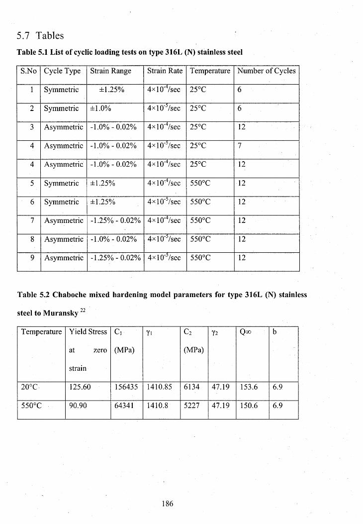
5.7 Tables
Table 5.1 List of cyclic loading tests on type 316L (N) stainless steel
S.No Cycle Type Strain Range Strain Rate Temperature Number of Cycles
1 Symmetric ±1.25% 4><10'4/sec 25°C 6
2 Symmetric ±1.0% 4><10'5/sec 25°C 6
3 Asymmetric -1.0% -0.02% 4 x l0 '4/sec 25°C 12
4 Asymmetric -1.0% -0.02% 4 x 10'5/sec 25°C 7
4 Asymmetric -1.0% -0.02% 4 x l0 '4/sec 25°C 12
5 Symmetric ±1.25% 4xlO’4/sec 550°C 12
6 Symmetric ±1.25% 4 x l0 ‘5/sec 550°C 12
7 Asymmetric -1.25% -0.02% 4 x l0 ’4/sec 550°C 12
8 Asymmetric -1.0% -0.02% 4 x l0 ’5/sec 550°C 12
9 Asymmetric -1.25% -0.02% 4 x l0 ’5/sec 550°C 12
Table 5.2 Chaboche mixed hardening model parameters for type 316L (N) stainless
steel to Muransky22
Temperature Yield Stress
at zero
strain
c ,
(MPa)
Yi c 2
(MPa)
72 Qoo b
20°C 125.60 156435 1410.85 6134 47.19 153.6 6.9
550°C 90.90 64341 1410.8 5227 47.19 150.6 6.9
186
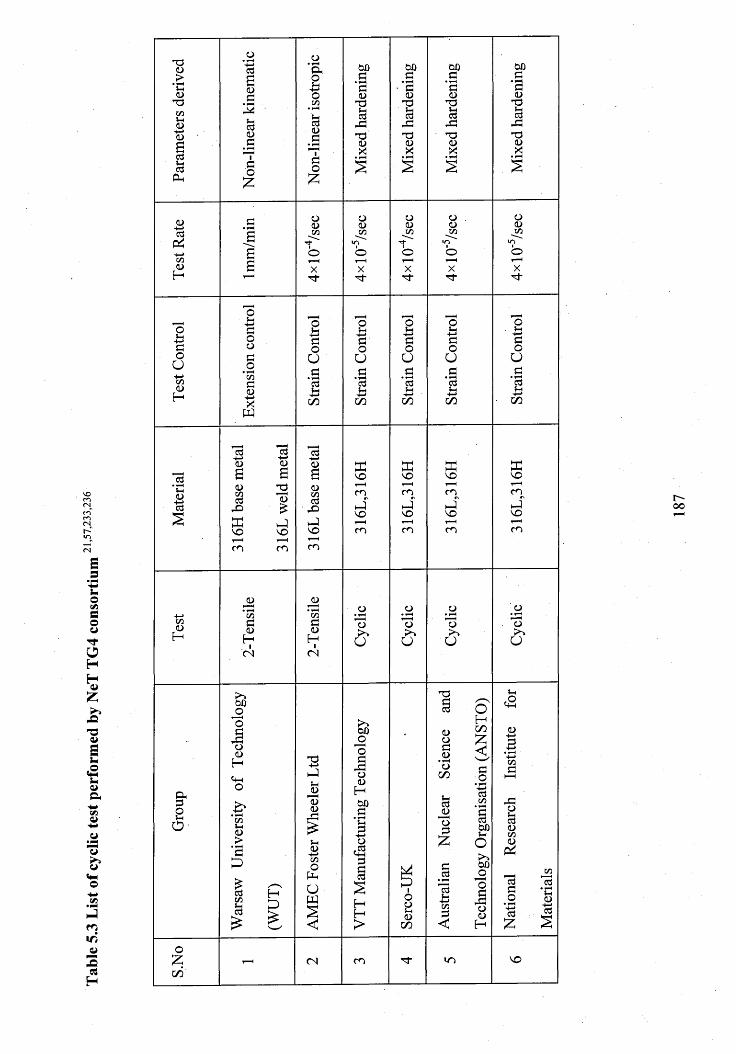
Tabl
e 5.3
Li
st of
cycli
c tes
t pe
rfor
med
by
NeT
TG4
cons
ortiu
m
SO
<Nf**TCOKin<N
Para
met
ers
deri
ved
Non
-line
ar
kine
mat
ic
Non
-line
ar
isot
ropi
c
Mix
ed
hard
enin
g
Mix
ed
hard
enin
g
Mix
ed
hard
enin
g
Mix
ed
hard
enin
g
Test
Rat
e
lmm
/min oQ
VX■'froX
o<DVX
v-%
oT—HX
oOV I
TtOX
o .<L>v x
OX
o<UVX
>o©
X
Test
Con
trol
Exte
nsio
n co
ntro
l
Strai
n C
ontr
ol
Strai
n C
ontr
ol
Strai
n C
ontro
l
Strai
n C
ontr
ol
Strai
n C
ontr
ol
Mat
eria
l
316H
ba
se
met
al
316L
we
ld m
etal
316L
ba
se
met
al
316L
,316
H
316L
,316
H
316L
,316
H
316L
,316
H
Tes
t
2-T
ensi
le
2-T
ensi
le
Cyc
lic
Cyc
lic
Cyc
lic
Cyc
lic
Gro
up
War
saw
Uni
vers
ity
of T
echn
olog
y
(WU
T)
AMEC
Fo
ster
Whe
eler
Ltd
VTT
Man
ufac
turin
g T
echn
olog
y
Serc
o-U
K
Aus
tralia
n N
ucle
ar
Scie
nce
and
Tech
nolo
gy
Org
anis
atio
n (A
NST
O)
Nat
iona
l Re
sear
ch
Insti
tute
fo
r
Mat
eria
ls
S.N
o
- <N m VO
oo
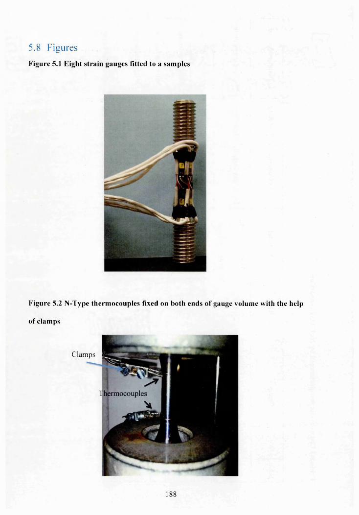
5.8 Figures
Figure 5.1 Eight strain gauges fitted to a samples
Figure 5.2 N-Type thermocouples fixed on both ends of gauge volume with the help
of clamps
Clamps
188
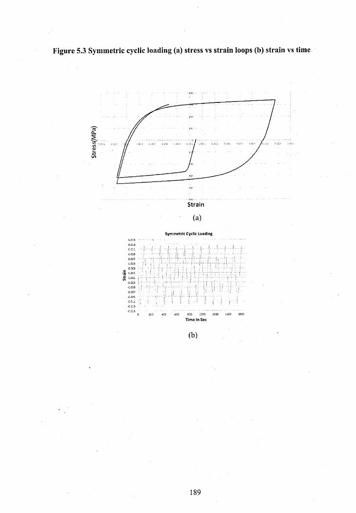
Figure 5.3 Symmetric cyclic loading (a) stress vs strain loops (b) strain vs time
61t .
«/)
Strain
(a)
Sym m etric Cyclic Loading0,015 ‘ ...........................................................................................
n
r.
1200
Time In Sec
(b)
189

Str
ess(
MP
a)Figure 5.4 Asymmetric cyclic loading with the first cycle loading in compression (a)
stress vs strain loops (b) strain vs time
-c.oij o.in -oo;:e -o.fcs
0..01S
C.Oii0.0110.0090.00/0.003O.OD30.001
-0.001
-0.003-0.003-0.007-0.000-0.0110.012
- o .o i s
■«SC '
Strain
(a)
Asvmmetric Cyclic loading
100 200 300 400 SCO 60S 700Time Sec
(b)
190
a.eoo- ocn cms obis
SCO
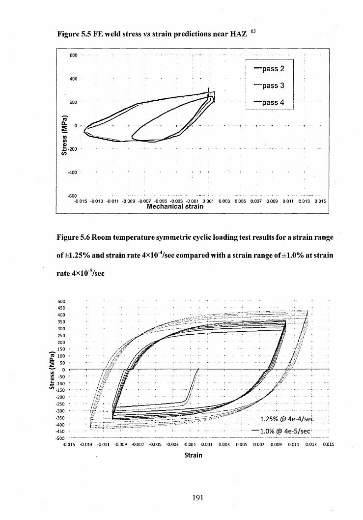
Stre
ss
(MP
a)
Figure 5.5 FE weld stress vs strain predictions near HAZ 63
600
p ass 2400
p ass 3
pass 4200
■200
-400
■0.015 0.013 *0011 *0009 *0007 *0,005 *0,003 *0 001 0.001 0.003 0.005 0,007 0 009 0 011 0.013 0.015M e c h a n ic a l s t r a in
Figure 5.6 Room temperature symmetric cyclic loading test results for a strain range
of ±1.25% and strain rate 4xl0'4/sec compared with a strain range of ±1.0% at strain
rate 4xl0‘5/sec
500 450 *
500•0.015 -0.013 -0.011 -0.009 -0.007 -0.005 -0.003 -0.001 0.001 0.003 O.OOS 0.007 0.009 0.011 0.013 0.015
S tra in
191

Figure 5.7 Room and high tem perature (550°C) symmetric cyclic loading result for
a strain range ±1.25% at strain rate 4*10 4/sec
5000.015 0.013 0.011 0.009 0.007 0.005 0.003 0.001 0001 0.003 0.005 0.007 0.009 0.011 0.013 0.015
Strain
Figure 5.8 High tem perature (550°C) symmetric cyclic loading results for a strain
range ±1.25% at strain rate of 4 x l0 ';7sec
500 450 400 350 300 250 200
"nT 150 100 — 50
0.013 0.011 0.009 -0.007 0.005 0.003 0.001 0.001 0.003 0.005 0.007 0.009 0.011 0.013 0.015
Strain
192
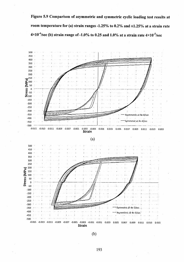
Figure 5.9 Comparison of asymmetric and symmetric cyclic loading test results at
room temperature for (a) strain ranges -1.25% to 0.2% and ±1.25% at a strain rate
4xl0'4/sec (b) strain range of -1.0% to 0.25 and 1.0% at a strain rate 4xl0'5/sec
500450400350300250200
—*150(Ua.1005E so
Si -50 # 1 0 0
•150 ■200 •250 •300 •350 ■400 •450 •500
Asymmetric at 4e-4/sec
'Symmetric at 4e-4/sec
•0.015 -0.013 -0.011 -0.009 -0.007 -0.005 -0.003 -0.001 0.001 0.003 0.005 0.007 0.009 0.011 0.013 0.015Strain
(a)500 - . - - - . . . . . . . . .450 • . . . . . . . . . . . . . . . . , , . . . . . . . . . . . . . . . . . . . . .400 ■ 1 .... . . . . , - ., ... . .,. .. . . . .
350 300 250
—*200 Q. 150
100
^ -50 •100 -150 •200
•250 •300 •350 -400 •450 •500
Symmetric <£> 4e -5/scc
Asymmetric @ 4e-5/sec
•0.015 -0.013 -0.011 -0.009 -0.007 -0.005 -0.003 -0.001 0.001 0.003 0.005 0.007 0.009 0.011 0.013 0.015Strain
(b)
193
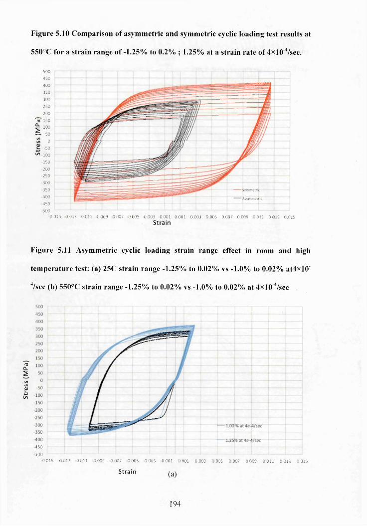
Stre
ss
(MP
a)Figure 5.10 Comparison of asymmetric and symmetric cyclic loading test results at
550°C for a strain range of -1.25% to 0.2% ; 1.25% at a strain rate of 4*10'4/sec.
SyTTmetnc
Asymrr.etriC
500 450 400 350 300 250 200
"nT 150 100 S. 50LA 0
50 ^ 100
150 200 250 300 350 400 450 500
0.015 0.013 0.011 0 009 0.007 0.005 0.003 0.001 0.001 0.003 0.005 0.007 0.009 0.011 0.013 0.015Strain
Figure 5.11 Asymmetric cyclic loading strain range effect in room and high
tem perature test: (a) 25C strain range -1.25% to 0.02% vs -1.0% to 0.02% at4><10'
4/sec (b) 550°C strain range -1.25% to 0.02% vs -1.0% to 0.02% at 4xl0'4/sec
450500
•0.015 0.013 0.011 0.009 0.007 -0.005 0.003 0.001 0.001 0.003 0.005 0.007 0.009 0.011 0.013 0.015
Strain / Q\
194
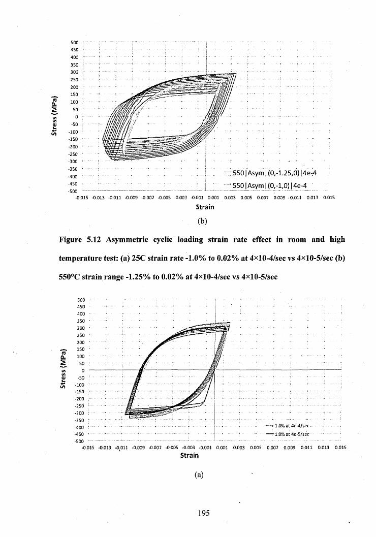
Stre
ss
(MP
a)
-0.015
r 5 5 0 1 Asym | (0,-1.25,0) 14e-4
5 5 0 1Asyni | (0,-1,0) 14e-4 '
0.013 -0.011 -0.009 -0.007 -0.005 -0.003 -0.001 0.001 0.003 0.005 0.007 0.009 -0.011 0.013 0.015
S train
Figure 5.12 Asymmetric cyclic loading strain rate effect in room and high
temperature test: (a) 25C strain rate -1.0% to 0.02% at 4xl0-4/sec vs 4xlO-5/sec (b)
550°C strain range -1.25% to 0.02% at 4xl(F4/sec vs 4xl0-5/sec
osex.
to
250 '
100 *
200
300 ‘350 •400 '
-0.015
. - — - 1.0% at4c-4/sec r
• • 1.0% at 4 c-5/s cc ...........
■0.013 -0.011 -0.009 -0.007 -0.005 -0.003 -0.001 0.001 0.003 0.005 0.007 0.009 0.011 0.013 0.015
S tra in
(a)
195

500450400350300250200150
re 100 50
. 0If)
3 -50*3 -100^ -150
-200 •250 •300 -350 -400 -450 •500
Strain Rate 4e-4/sec Strain Rate 4e-5/sec
>.015 -0.013 -0.011 -0.009 -0.007 -0.005 -0.003 -0.001 0.001 0.003 0.005 0.007 0.009 0.011 0.013 0.01SStrain
(b)
Figure 5.13 Room and high temperature asymmetric cyclic loading (a) strain range
-1.25% to 0.02% at strain rate 4*10'4/sec and (b) -1.0% to 0.025% at strain rate
4xl0'4/sec
500450400350■300250200
re^oCL ioo g, 50
£ o£? -50
U V 1 0 Q
-150 •200 -250 -300 ■350 ■400 •450 -500
-O.i
’■X/fif/f
!/(!//■■'/ ill! id s
il * * *
Room Temperature
High Tem perature-550 degrees
015 -0.013 -0.011 -0.009 -0.007 -0.005 -0.003 -0.001 0.001 0.003 0.005 0.007 0.009 0.011 0.013 0.015
‘ S tra in
(a)
196
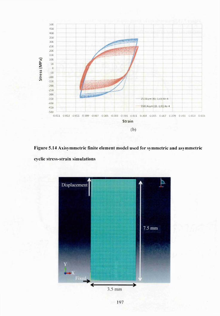
Stre
ss
(MP
a)
500 450 400 350 300 250 200 150 100
50 0
50 100
150 200
250 300 350 400 450 500
0.015 -0.013 0.011 0.009 0.007 0.005 0.003 0.001 0.001 0.003 0.005 0.007 0.009 0.011 0.013 0.015
Strain
(b)
Figure 5.14 Axisymmetric finite element model used for symmetric and asymmetric
cyclic stress-strain simulations
< >3.5 mm
2 5 iA sym f{0 ,- l , 0 ) |4 e 4
197
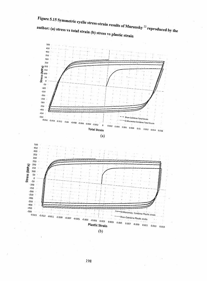
Figure 5.15 Symmetric cyclic stress-strain results of Muransky
author: (a) stress vs total strain (b) stress vs plastic strain22
reproduced by the
■0.016 .Q1014 -0.012 -o.0 1 -O .O O S - 0
006 -0.0M -O.o020 0.002 0 .
Shan Combine T o ta is train
D-Muransky Corribme Total Strain
Total Strain
(a)
004 0.006 o 008 0.01 0012 0.03 4 0.016
a. 350 5 300
•0.035 -o,... ....... . . — “"O.Muransky Combine Plastic strain
r " ' t i * " V Shan Cotnbine Plastic strain _ :................. ; _____ : ... -I ... .;
1013 -0.011 -0.009 -0.007 -0.005 -0.003 -0.001 0.001 0.003 0.005 0.007 0.009 0.011 0.
Plastic Strain •013 0.015
(b)
198

Figure 5.16 Comparison of mixed hardening predictions based upon Muransky 22
for symmetric and asymmetric cycles at (a) room temperature and (b) high
temperature (550°C)
500
450400350
300250200
150100ro
o.2
100
■150200250
300350 RT Symmetric FE
RT Asymmetric Fe400450500
•0.015 -0.013 -0.011 -0.009 -0.007 -0.005 -0.003 -0.001 0.001 0.003 0.005 0.007 0.009 0.011 0.013 0.015
T otal S tra in
(a)
mQ»
%AIAQ)4-»I/)
0.015
— HTSym m etric:FE
r™ HT Asymmetric FE
-0.013 -0.011 -0.009 -0.007 -0.005 -0.003 -0.001 0.001 0.003 0.005 0.007 0.009 0.011 0.013 0.015
T otal S train
(b)
199
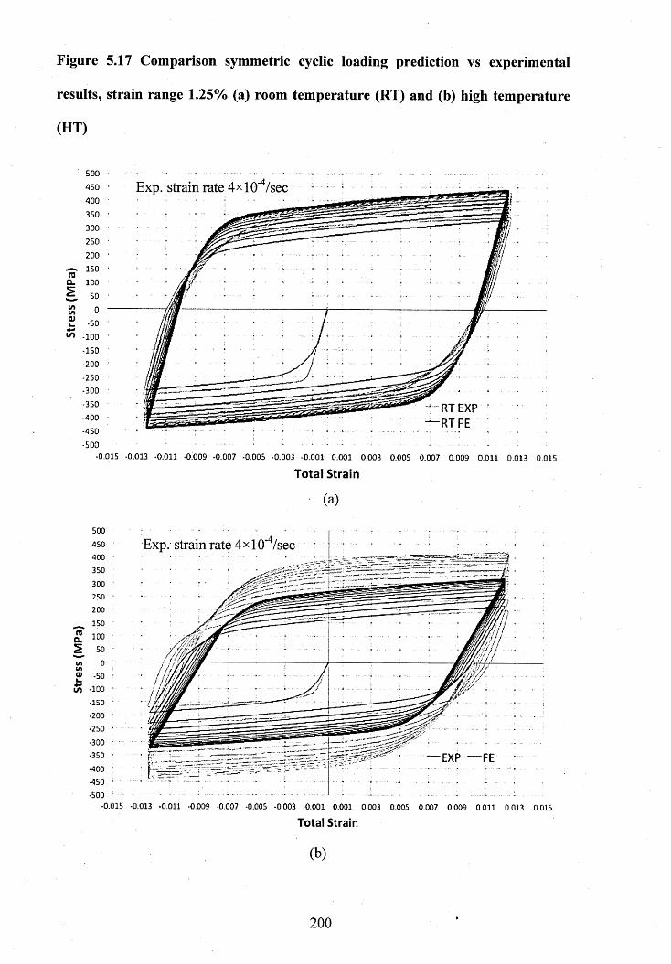
Figure 5.17 Comparison symmetric cyclic loading prediction vs experimental
results, strain range 1.25% (a) room temperature (RT) and (b) high temperature
(HT)
500450400350300250200
150100
Exp. strain rate 4x10' /sec
1/1 -100
-150 -200
-250 -300 -350 -400 -450 -500
RT EXP RT FE
■0.015 -0.013 -0.011 -0.009 -0.007 -0.005 -0.003 -0.001 0.001 0.003 0.005 0.007 0.009 0.011 0.013 0.015
T ota l S tra in
(a)
roCL
1/5
500
Exp. strain rate 4x 10 /sec450400350300250200
150100500
-50100
150200250300350 EXP400
■0.015 -0.013 -0.011 •0.009 -0.007 -0.005 -0.003 -0.001 0.001 0.003 0.005 0.007 0.009 0.011 0.013 0.015
Total Strain
(b)
200
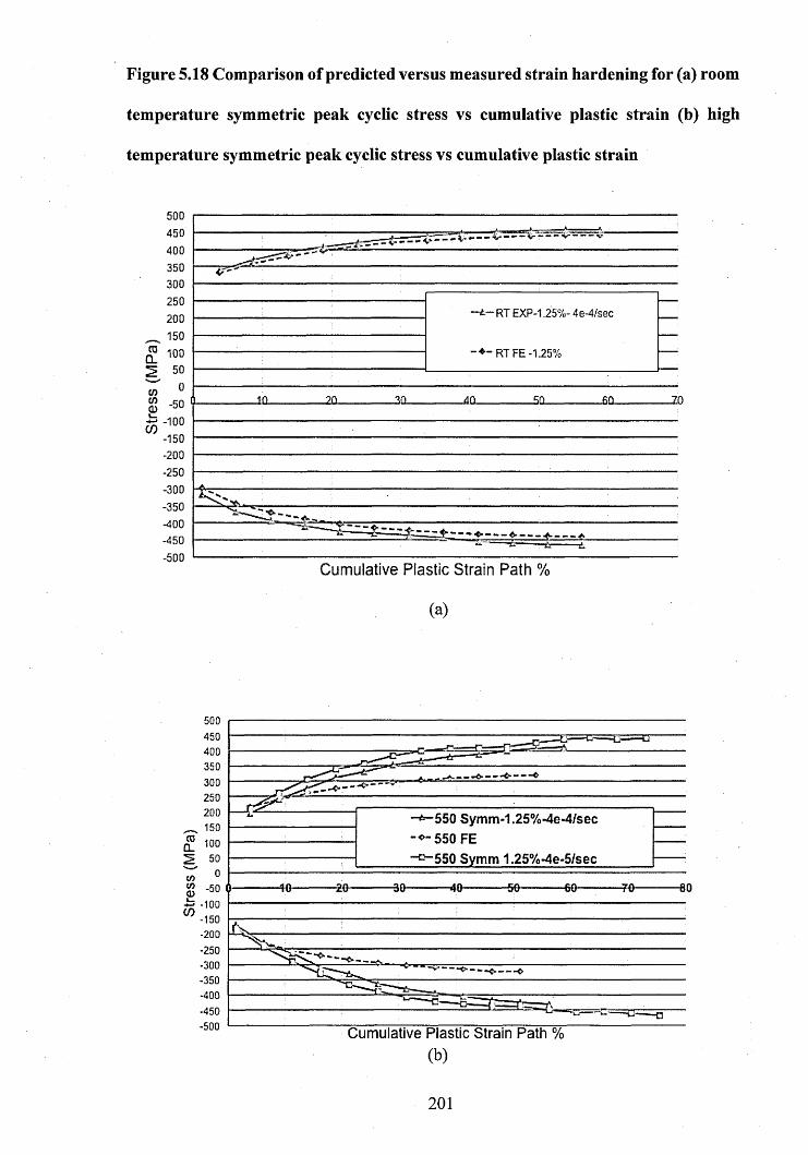
Stre
ss
(MP
a)
Figure 5.18 Comparison of predicted versus measured strain hardening for (a) room
temperature symmetric peak cyclic stress vs cumulative plastic strain (b) high
temperature symmetric peak cyclic stress vs cumulative plastic strain
500450400350300250200150100
500
-50-100
-150-200-250-300-350-400-450-500
RT EXP-1.25%- 4e-4/sec
-♦ -R T F E -1 .2 5 %
—==£
Cumulative Plastic Strain Path %
(a)
500450400350300 250 200
^ 150 100 2 50
-* -5 5 0 S y m m -I^ S y o ^ e^ /sec 550 FE
-°~ 5 5 0 Symm 1.25%-4e-5/sectotoCDL_~ -100
"-ISO -200 -250 -300 -350 -400 -450 -500 Cumulative Plastic Strain Path %
(b)
201
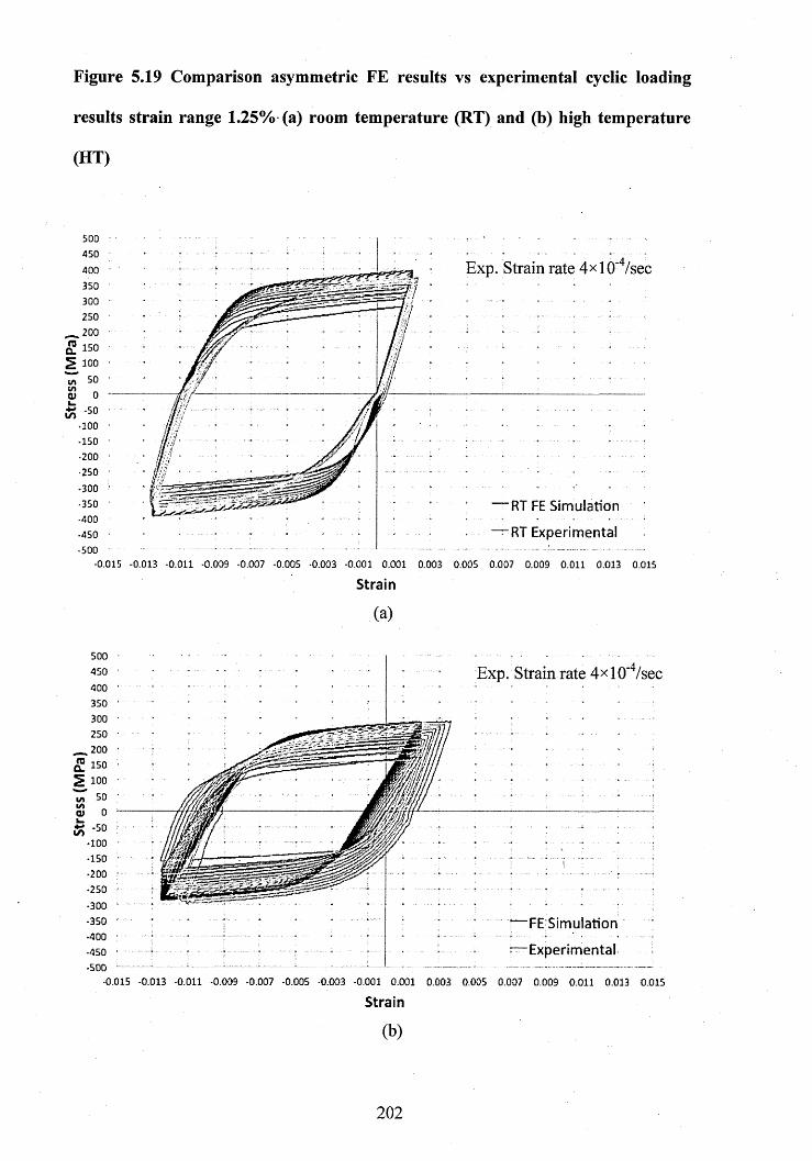
Figure 5.19 Comparison asymmetric FE results vs experimental cyclic loading
results strain range 1.25% (a) room temperature (RT) and (b) high temperature
(HT)
500 450 400 350 300 250
.— 200 S . 150
100
Exp. Strain rate 4x10' /sec
(A
£ 50 •100•150-200-250•300-350•400-450-500
RT FE Simulation
RT Experimental
-0.015 -0.013 -0.011 -0.009 -0.007 -0.005 -0.003 -0.001 0.001 0.003 0.005 0.007 0.009 0.011 0.013 0.015
Strain
(a)
500450400350300250
200
£ 150 5 100
Exp. Strain rate 4x10' /sec
E 50 ■100-150-200-250•300-350-400-450-500
FESimulation
Experimental
-0.015 -0.013 -0.011 -0.009 -0.007 -0.005 -0.003 -0.001 0.001 0.003 0.005 0.007 0.009 0.011 0.013 0.015
Strain
(b )
202
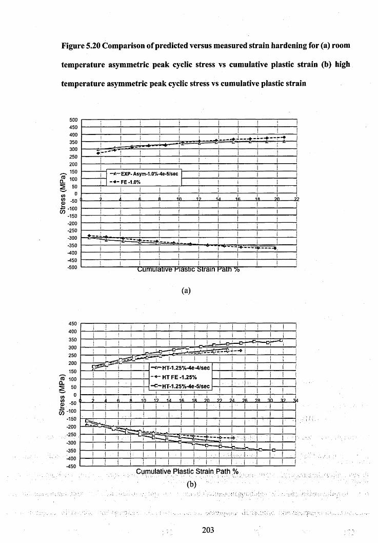
Figure 5.20 Comparison of predicted versus measured strain hardening for (a) room
temperature asymmetric peak cyclic stress vs cumulative plastic strain (b) high
temperature asymmetric peak cyclic stress vs cumulative plastic strain
500450400350300250200150100
— EXP- Asym-1,0%-4e-5/sec FE -1.0%
£ -50
<JT100-150-200-250-300-350-400-450-500 Cumulative M astic s tra in F atn %
(a)
450400350300250200150
S ' 100
-*--H T -1 .25% -4e-4 /sec
HT FE -1.25%
"C ” HT-1.25%-4e -5 /sec
0) -50
-100 -150 -200 -250
-300 -350
-450Cumulative Plastic Strain Path %
203
C h a p t e r 6. W e l d m e n t P l a st ic St r a in
C h a r a c t e r isa t io n
6.1 Introduction
Welding introduces plastic strain into the base materials being joined owing to material
yielding associated with differential thermal expansion/contraction. It is important to
quantity the plastic strain accumulated, since it can increase the susceptibility o f austenitic
stainless steel to stress corrosion cracking 10’30,193,198. Electron backscatter diffraction
(EBSD) has previously been used to map the distribution o f plastic strain on a microscopic
• J ' lH ' J I Q
scale . The influence o f the welding parameters, welding techniques and stress-
controlled cyclic loading, on microstructure and stress corrosion cracking, has been well
analysed by others using EBSD 49,170,240_244. However, to date, the accumulated plastic
strain due to each weld pass deposited has not been quantified. Moreover, little
experimental research has been done where EBSD measures of plastic strain have been
compared with hardness testing and finite element analysis.
The influence o f strain-controlled, or stress-controlled, symmetric cyclic deformation
on the microstructure, mechanical properties and lattice misorientations in austenitic
stainless steel,1 is well studied in the literature, where samples have been deformed up to
failure177’191’201’203’245’246 However, there is no published research work available to explain
the influence of strain-controlled asymmetric cyclic loading on lattice misorientations, after
only a small number o f cyclic loading cycles.
The objective o f this chapter is to quantify, using EBSD, the cumulative plastic strain
resulting from multi-pass welding and from uniaxial strain-controlled cyclic loading of
204
316L(N) materials. Two independent sets of samples; welded (multi-pass welded plate)
and both symmetrically and asymmetrically cyclically deformed, were deformed at room
and high temperature, to quantify the cumulative plastic strain. Cumulative plastic strain is
summation of the plastic strain, at the end of each cycle.
Following the EBSD experiments, Vickers macro hardness tests were performed on all
the samples to validate the EBSD results. This validation was further supported by
comparison with published finite element predictions, available from the NeT consortium
6.2 Uniaxia] Tensile Test
Using an electro discharge machine (EDM), several flat tensile samples were extracted
from the block of as received 316L(N) material (described in section 3.6). Figure 6.1
provides the design and dimensions of the flat tensile sample. The set of flat tensile samples
were deformed up to set levels of plastic strain (Table 6.1) under constant strain rate, at
both room temperature and at high temperature (550°C).
6.2.1 Uniaxial room temperature-tensile test (RTT)
An Instron screw-driven testing machine, with a 50 kN load cell, was used to deform
the 316L (N) material, under uniaxial tension, at room temperature. The specimens were
held in place using mechanical wedge grips, which were attached to the instrument.using
universal joints. Prior to the tensile test, the specimens were preloaded (to 70 MPa) and
then unloaded (to 0 MPa) to help the specimens settle in the grips. Table 6.1, lists the tensile
tests conducted at a constant extension rate of 1 mm per minute, until the required strain
was obtained. The machine was controlled by Instron Bluehill software. For room -
temperature testing, a calibrated extensometer was mounted onto the specimen gauge
205

length using a static axial clip (refer Figure 6.2). The results from the room temperature flat
tensile tests are discussed in section 6.2.3.
6.2.2 Uniaxial high tem perature tensile test (H IT )
An Instron 8862 machine with a load capacity of 100 kN was used for all high
temperature (550 °C) tensile tests. The machine was equipped with a split furnace, with a
side window. Eurotherm 3215 controllers were used to control the furnace temperature.
The tensile specimens were held securely using in-house manufactured holders refer Figure
6.3 . Calibrated type-N thermocouples, and a high temperature exterisometer, were mounted
onto the specimen gauge length, with the help of clamping device and ceramic cords
respectively refer Figure 6.4. Table 6.1 lists all the high temperature tensile tests, conducted
under strain control, and at a strain rate of 4x1 O'4 per second, until the required strain was
obtained. Prior to deforming, each specimen was held at 550 °C for 30 minutes, to enable
a steady temperature of within ±1°C to be sustained for the duration of the test.
6.2.3 Tensile test results from room temperature and high tem perature
experiments
From the recorded data, the true stress vs true strain graphs are provided in Figure 6.5.
The flow curve of the specimen tested at room temperature to 5% plastic strain shows
serrations with a variation of approximately 10 iMPa early on in the readings. This variation
was due to a slip of the strain gauge during the experiment. However, this small
experimental setup error will not affect the plastic strain calibration when using EBSD.
At high temperature, the yield stress of the material is lower than it is at room
temperature. Therefore, the material exhibits a lower flow stress at a given strain than in
the room temperature test. During the high temperature tensile tests, serrations were evident
206
on the stress vs. strain curves of Figure 6.5. This is due to dynamic strain ageing (ref.
Section 2.3.3).
6.3 EBSD Experimental Setup
For EBSD measurements, a Zeiss Supra 55VP, scanning electron microscope equipped
with a field emission gun (FE-SEM) and with a NordlysF EBSD detector, was used. The
SEM accelerating voltage was set to 20 keV. The working distance (WD) was 15±0.1 mm,
and the objective aperture size was set at 120pm (max) in the high current mode. Table 6.2
summarizes other parameters used in this EBSD experimental setup. The sample was
positioned at 70° (from the horizontal) and inserted into the vacuum chamber of the
scanning electron microscope (SEM). HKL fast acquisition software was utilized for data
acquisition, then Channel 5 software was used to analyse the data.
All EBSD measurements were performed on a rectangular grid of points with a step size
of 1 pm, using the beam-scanning mode under dynamic focus conditions and with a SEM
magnification of 200x. EBSD indexing was based on the HKL database of materials; Iron
FCC ciystal structure, with space group 225, F m3m. The orientation maps were collected
from an area of 500 * 1400 pm, covering more than 100 grains.
6.4 Hardness Test Setup (validation o f EBSD results)
Hardness is a measure of a material's resistance to plastic deformation or damage, for
example indentation or scratches. In this study, the Vickers maa'o hardness test method
was adopted to measure the hardness of the uniaxial tensile deformed samples, welded
samples and cyclically deformed samples. Hardness tests were performed according to the
British Standard ISO 6507-1:2005 241. The instrument used was a Struers Duramin A300
machine, equipped with a diamond pyramidal indenter. To make the indentations, a load
207
of 5 kgf was applied for 10 seconds. More details on the indents and spacing are given later
in section 6.7.3. The hardness test results for the multi weld pass sample are presented in
Figure 6.6.
6.5 Weld Plastic Strain Analysis
Section 3.5 has described the multi-pass welded plate, the welding parameters and the
extraction of the weld samples. The extracted samples underwent a similar surface
preparation to that described in section 3.4.2. The aim of the work presented in this section,
was to quantify the plastic strain that developed due to multi-pass welding.
6.5.1 Experimental setup
Using the screen crosshairs the edges of the samples were aligned and positioned parallel
to the electron beam scans. Each area was positioned along the central axis of the sample
with reference to the weld bead width, as seen in Figure 6.7. All EBSD maps were acquired
from the bottom of the plate to the weld cap along the Y-axis in plane B (refer to Figure
3.3).
Four measurements were performed on each scanned image or stage position. Once the
set of four measurements was completed, the SEM stage was moved manually to a new
location (with an approximate overlap of 10% with the previous area). The stage
movements were limited to the X-axis only, so the working distance could be maintained
constant throughout the experiments. At each new area, the SEM was refocused and the
working distance checked. The accumulated lattice misorientations, induced by each weld
deposit, were measured using three different EBSD metrics: Kernnel Average
Misorientation (KAM), Low Angle Grain Boundary fraction (LABf) and Average
Intragrain Misorientation (AMISa) see section 2.6.4. Figure 6.8-6.10, shows the EBSD
208
misorientation results of the welded samples. Once the EBSD analysis was completed on
each welded sample, the samples were allocated for macro hardness testing.
6.6 Cyclic Plastic Strain Analysis
The design of the uniaxial cyclic loading samples and their extraction from the bulk
material has been described in section 3.3. In section 5.3 of Chapter 5, the setup of the
cyclic loading experiments is reported. In this section, only the EBSD experimental setup
for analysing cyclic plastic strain is explained. The same EBSD settings as described in
section 6.3 were adopted for this analysis. Figure 6.11 shows the gauge length of the
cyclically deformed sample, bisected along the mid plane, parallel to the loading direction.
The extracted sample was surface treated as described in section 3.5.1. Four EBSD
measurements were taken at the centre of the mid plane, parallel to the loading direction.
Table 6.3 lists the experimental parameters used in the mechanical tests performed on the
cyclically deformed samples, at room and high temperature. Figure 6.12-13 show the
EBSD measured lattice misorientation induced by cyclic plastic strain. The remaining parts
of the bisected samples were used for Vickers hardness testing.
6.7 Discussion
When a material is deformed in tension or compression beyond its yield point, even
though the spatial distribution of the strain at the macroscopic level is uniform, at the
microscopic scale there is a non-uniform distribution of strain. This results from the
anisotropic mechanical properties of each grain. Due to these anisotropic properties, the
accumulated dislocations generate localized misorientations within, and between, the
grains. The density of dislocations increases with increasing strain and hence the degree of
lattice misorientation also increases 177’192>195’197’198’248’249. Despite this extensive literature,
209
there are no publications explaining the effects of plastic strain accumulation following
deposit of each bead during welding. In addition, no record has been found regarding the
influence of isotropic hardening on the lattice misorientations resulting from just a small
number of symmetric and asymmetric deformations (i.e. below 12 loading cycles). The
experimental findings presented here help to fill this knowledge gap.
6.7.1 EBSD plastic strain correlations for 316L(N) stainless steel
The degree of correlation between intragranular misorientations and induced plastic
strain was investigated. The surfaces of deformed 316L(N) stainless steel samples were
prepared as described in section 3.5.1 and the prepared samples inserted into the vacuum
chamber of the SEM mounted on a pre-tilted (70° from horizontal) sample holder. For flat
deformed samples, two to four orientation maps were collected from measurement areas
approximately at the centre of the gauge volume, along a plane parallel to the loading
direction (see Figure 6.14).
The accumulation of misorientations, as a function of plastic strain introduced by
uniaxial tensile load, was quantified using the AMISa metrics (refer section 2.6.4). The
AMISa vs. tensile plastic strain correlations are shown in Figure 6.15 (a). The KAM and
LABf tensile plastic strain correlations are provided in appendix Figure A.6.1 and A.6.2.
The error bars for each EBSD metric were calculated from the +/- standard error of the
mean metric values from all orientation maps collected at different locations on both the
deformed and non-deformed samples.
The KAM, LABf and AMISa increased approximately linearly with strain level. The
difference between the room temperature EBSD plastic strain calibrations and high
temperature EBSD plastic strain calibrations is significant. In evaluating the
misorientations of the deformed material, the KAM and LABf metrics consider only
210
intragranular misorientations between 0.15°-2° and 2°-15° respectively. However, as the
strain increases, the density of high angle misorientation >15° tends to increase, which
affects the misorientation evaluation when using KAM and LABf metrics. While at zero
strain the orientation noise and the presence of low angle boundaries in the material will
affect the EBSD metric results, offsetting the intercept on the Y axis, as seen in Figure
6.15(a)192’194. The AMISa metric evaluates the misorientation across the whole grains and
it is more sensitive, even at higher strains than KAM, or L A B f.
In Figure 6.16, EBSD plastic strain correlation for the 316L(N) material evaluated in
this research study are compared with published plastic strain correlation for 316H and
304L materials 194,25°. The room temperature EBSD correlation for 316L(N) agreed very
well with Angeliu et al. 25°. At high temperature, Githinji’s 28 EBSD correlation for 316H
material shows higher values of misorientation than in 316L (N) material. This is due to
Githinji’s use of aged 3 16H material and a strain rate of 1 * 10‘5/sec in his high temperature
(550°C) tests. The presence of carbides will increase the strain hardening of the material as
well using a slower strain rate due to dynamic strain ageing. However, in all material at
both room and high temperature the misorientation increases linearly with plastic strain up
to 10% ,95’197’251. Similarly, in this research study, the misorientation increased linearly with
plastic strain.
6.7.2 EBSD equivalent yield stress correlation for 316L(N) stainless steel
As describer earlier in section 6.2, the parent materials were monotonically deformed to
a defined series of plastic strains (refer to Figure 6.5). For each defined plastic strain, the
corresponding final peak tensile stress achieved during the test (refer to Figure 6.5) was
also used to establish an EBSD misorientation correlation with an equivalent yield stress at
that strain level. The AMISa vs. equivalent tensile yield stress correlations are shown in
Figure 6.15(b). This correlation is helpful to quantify the equivalent yield stress from EBSD
211

data and enables comparison with the results on the residual stress along line BD (refer
section 4.2.1 and Figure 4.1).
During each weld bead deposit, the base material is plastically deformed through strain
ranges (refer section 7.1 and Figure 7.5 of Chapter 7) that are different at each position
through the thickness. As a result, the base material develops anisotropy strains through the
thickness. This was evident in the residual stress measurements, evaluated along line BD
(refer Figure 4.22(a) of Chapter 4) using neutron diffraction. The longitudinal stress
through thickness of the plate are higher than the yield stress of the material. This enables
the author to compare the EBSD quantified equivalent yield stress (i.e. bulk ‘plastic stress’)
with the measured residual stress (i.e. ‘bulk elastic stress’). The results are discussed in
section 7.3 of Chapter 7.
6.7.3 Plastic strain and equivalent yield stress correlation for 316L(N)
stainless steel from macro hardness test
Once the EBSD analysis was completed on the flat tensile samples deformed to 2.5%,
5%, 10%, 15% or 20% strain at either room or high temperature, and on the gauge volumes
of the cyclically deformed samples, they were subjected to macro hardness testing. A total
of 90 to 100 indents were placed, in rows along the loading direction, on each deformed
sample. The horizontal and vertical spacing between each indent was 1 mm. The average
of the hardness measurements for the room and high temperature tensile specimens,
strained to 0%, 2.5%, 5%, 10%, 15% and 20% was calculated and is shown as a function
of induced strain in Figure 6.17(a). Similarly, the average of the hardness measurement as
a function of monotonic yield stress is shown in Figure 6.17(b), for both room and high
temperature tensile specimens. At both room and high temperatures, the hardness of the
material showed linear correlation with the induced strain and monotonic yield stress. The
212

hardness, plastic strain and equivalent yield stress correlations are consistent with EBSD
correlation results.
6.7.4 Characterizing accumulated m isorientation due to the deposit o f each
weld bead
The welded sample can be broadly divided into two; a predominantly monotonically
deformed zone and a predominantly cyclically deformed zone, depending on the thermal
and deformation histories of each volume. The weld metal (i.e. final weld deposit) comes
under the category of tensile deformed zone, due to the high peak temperature (above
1000°C). Any compressive strain during heating will be nullified once the material has
reached melting temperature. Therefore, only tensile deformation that has developed during
cooling will contribute to weld metal deformation. The grain size, texture and degree of
deformation in the weld metal is completely different from the base metal and therefore
any misorientation correlation with monotonically introduced plastic strain will differ from
those observed for the parent stainless steel material.
During welding, the temperatures in the HAZ and the parent material can reach up to
1000°C. As explained in section 2.3.3, stainless steel deformed at temperatures between
300-650°C exhibits dynamic strain ageing (DSA). Results of investigations on the
influence of strain rates, in ranges similar to those resulting from the non-uniform heating
and cooling rates of welding, were presented in Chapter 5. At the high temperature, the
relationship between misorientation and strain hardening is affected by DSA. From Figure
6.5, it is clear that the monotonic yield stress is not consistent at the higher temperature in
comparison to that at room temperature, due to this effect.
The varying temperature- time profiles at different distances away from the heat source,
through the thickness of the plate, during single pass and two pass welding, are shown in
Figure 6.18. From this graph, it is clear that welding causes temperature transients in the
213
plate around the heat, source, which can cause the material to deform asymmetrically (refer
to sections 5.3.1 of Chapter 5). Transverse slices extracted from the stainless steel plate
with a single-pass, a two-pass and a three-pass weld (as described in section 3.4.1) were
used to quantify the plastic strain resulting from each weld pass. The transverse slice (with
respect to the weld direction) is the best choice to characterize the accumulated plastic
strain. The transverse slice will show the total effect of the heat source on micro structure
changes and thermo-mechanical deformation around the weld. EBSD maps of the parent,
heat affected, fusion and weld zones (identified on the based of the microstructure of the
welded sample) are shown in Figure 6.19.
In Figure 6.19, the EBSD maps of the fusion zones show delineated patterns of colour
within the large columnar grains, these are solidification sub-grain boundaries (SSGB). The
grain boundaries of the dendrites in the fusion zone and the weld region were clearly
defined in the EBSD microstructure map although they were hard to identify in the optical
microscope images Figure 3.20. Figure 6.19 shows the colour variation between the grains
of the parent zone and the weld region, following each weld pass deposit. There is a
difference of degree of colour gradation within the grains. This is due to increasing plastic
strain in the region from the parent zone to the weld region. The sharply delineated regions
with small variation of colour with in the grains are due to low angle boundaries and the
diffuse colour gradations result from stored geometrically necessary dislocations.
The misorientation distributions within and between grains, following each weld
deposit, are shown in Figure 6.20-21. It is clear, as we move from the single pass to the
three-pass weld (refer A to B direction in Figure 6.20 for deformation in the parent zone,
HAZ and fusion zone), that the deformation of the material increases following each weld
pass. The observed deformation in the region from the bottom of the plate to the fusion
zone (refer to A to C direction in Figure 6.20) and the misorientation variation within a
214

grain, increase up to the fusion boundary. Figure 6.8-6.10 show the angular misorientations
introduced by single pass, two pass and three pass welding respectively, using different
EBSD metrics. Figure 6.22-25, compare the spatial variation of the KAM, LABf and
AMISa metrics with the measured harnesses for the parent, single pass, two pass and three
pass samples respectively. As noted in Figure 6.22-25, the pattern of variation of each
EBSD metric exhibited significant variation from one metric to another. The possible
reasons for this variation between each EBSD metric are described in sections 6.7.4.1 and
6.7.4.2. . *
6.7.4.1 Degree o f m isorientation variation from the bottom o f the plate to fusion boundary
due to each weld bead deposit.
1. During a single pass deposit, the peak temperature from the bottom of the plate to
the fusion boundary increases from 500°C-1100°C as shown in Figure 6.18(a). At
this temperature range the yield point of the material is lower than at room
temperature, so the material deforms more easily. At any point (say at the bottom
of the plate), with increasing temperature from room temperature to 500°C, the
magnitude of deformation increases, consequently the density of dislocation and
the interactions of those dislocations increase gradually. As a result of this, the low
angle misorientations included in the KAM (i.e. < 2°) will gradually increases and
eventually exceed the defined threshold limit and develop misorientation above 2°.
Hence, KAM value increases form bottom of the plate to fusion boundary
gradually as the material is deformed to higher strains. In contrast to KAM, the
LABf consider the misorientation between 2° to 15° as low angle grain boundary
and the misorientation above 15° as high angle grain boundary. With increasing
distance from bottom of the plate to stain affected zone (SAZ) (i.e 13 to 7mm),
LABf shows very less misorientation variation between each weld bead deposit.
215
At this region (i.e 13 to 7mm), the degree of deformation is less than in the SAZ
and HAZ. This is because the peak temperature in the HAZ and SAZ is higher than
the base metal. Due to this, the HAZ and SAZ material deforms more than in the
parent zone. However, from the SAZ to fusion boundary (i.e. 7 to 0 mm), LABf
clearly shows the additional accumulated misorientation due to each weld bead
deposit (refer Figure 6.9). The AMISa results too clearly indicate the accumulation
of misorientation due to each weld bead deposit (refer Figure 6.10).
2. In all EBSD metric results the degree of misorientation increases significantly in
the SAZ compared to the parent martial. This is because, by the end of first weld
bead deposit, the fusion boundary, HAZ and the SAZ region have experienced one
cycle of deformation (starting from compression during heating, and tensile during
cooling). While the deposited weld metal experiences only tensile stress, because
the strain developed during heating will be nullified by melting. During the second
weld pass deposit, the fusion boundary in the HAZ and SAZ region undergoes a
second cyclic deformation but at a lower temperature due to increases in distance
form heat source. Figure 6.18(b), shows the weld temperature distribution during
the single and two pass weld deposits from bottom of the plate to fusion boundary.
Therefore with increasing numbers of weld bead deposits, the fusion boundary in
the HAZ region and SAZ undergoes more cyclic deformation, as result the degree
of misorientation increases, as seen in Figure 6.8-6.10.
3. At 12 mm from the fusion boundary, the parent material of the single pass, shown
in Figure 6.23, LABf shows 0.25°, whilst AMISa shows 0.9° and KAM measured
0.32°. This is due to the presence of an elongated grain as shown in Figure 6.26.
The presence of an exceptional grain in the parent material raised further question
on the accuracy of the EBSD results. Because the LABf and AMISa are sensitive
216

to the grain size of the material. The grain size calculation was performed using
optical microscopy on single, two pass and three pass weld samples (i.e. from
parent zone to heat affected zone refer Figure 6.7) at 200x magnification. The
American Standard Test Method (ASTM) Mean Linear Intercept method was used
to calculate the grain size, using Leica optical microscopy software. The difference
of grain size at HAZ (i.e. 1 -3 mm) and parent zone (i.e. 7-11mm) for all sample are
differing approximately between 5-10pm, see Figure 6.27. While in SAZ (i.e. 3-
7mm), the grain size of single pass and two pass samples are agreeing well.
However, the grain size of three pass sample in SAZ are differing approximately
5- 10pm with single pass and two pass samples. The difference of grain size from
parent to HAZ in all three samples are not significant in comparison to the grain
noticed at 12mm in parent zone. Therefore the difference of grain size in each
sample will not have significant effect in EBSD analysis.
6.7.4.2 Misorientation variation in the weld metal
After the solidification of the weld metal, the microstructure of columnar grains,
solidification sub-grain boundaries (SSGB), and the solidification grain boundaries (SGB)
are seen the fusion zone, as seen in Figure 3.20. The SSGBs and columnar grains have
grown along <100> direction or along thermal gradients at higher temperatures. As a result
of this, the dislocation density between the SSGB and within the columnar grains, is low.
The SSGBs are characteristically low angle grain boundaries with a lower angle
4 7 •misorientation approaching zero . While, SGBs are high angle grain misorientations
characteristically greater than 30° and dislocation pile up along them 41. The presence of
SSGB and large grains will increase the values of LABf and AMISa within the weld metal
in comparison to the HAZ, SAZ and the parent metal.
217

6.7.5 Quantifying plastic strain and equivalent yield stress from macro
hardness
A transverse slice from the single pass, two pass and three pass-welded plate was
extracted using EDM. Hardness tests were performed on the welded samples to measure
the additional hardening of the material developed by each weld pass, and to identify any
interaction between each weld pass. The Vickers hardness map of the multi-pass welded
plate is also presented in Figure 6.6. Details of the sequential weld deposits for this weld
plate were given in section 3.4 of Chapter 3. The plate was distorted to some extent during
the three pass weld bead deposits. The distorted plate was positioned carefully in order to
avoid any slope during the two pass weld bead deposits. However, the distorted plate was
not positioned correctly during the single pass weld bead deposits. As a result, the single
pass weld bead was deposited at an angle. This effect was clearly noticed in the hardness
map shown in Figure 6.6.
Comparing the high temperature calibrated hardness curve, shown in Figure 6.17 (a and
b), with the measured hardness of the weld pass samples shown in Figure 6.6, through
thickness (along Line BD), gives the corresponding plastic strain and the equivalent yield
stress distribution in the respective weld pass samples, as presented in Figure 6.28. The
accumulation of yield stress and strain resulting from each weld deposit can be clearly
observed in Figure 6.28.
6.7.6 Quantitative weld plastic strain and equivalent yield stress from EBSD
analysis
Quantification of weld metal plastic strain using the misorientation calibration curve
obtained for the parent material is not appropriate because its microstructure and texture
are different from the base material. However, the cumulative plastic strain in the region
218

from the fusion boundary to the base material following each weld deposit can be quantified
using the high temperature plastic strain correlation curve, refer section 6.7.1. The plastic
strain and yield stress distributions resulting from each additional weld pass, were
evaluated by comparing the EBSD metrics from each weld with the high temperature
plastic strain and equivalent yield stress correlation curves, (refer to Figure 6.15 and in
appendix Figure A.6.1 and Figure A.6.2). The strain and equivalent yield stress
distributions, along line BD from the bottom of the plate to the HAZ (i.e. along the y-axis
of Figure 3.3), resulting from each weld pass, are shown in Figure 6.29-6.32.
In the parent zone (i.e. 10-13mm in Figure 6.30), approximately 4% plastic strain ( from
KAM) and 160 MPa of equivalent monotonic yield stress was recorded for each samples
(i.e. KAM derived plastic strains for all the parent, single pass, two pass and three pass
samples). However, from 10 to 0 mm the KAM derived plastic strains increase gradually
as we move from the parent material towards the fusion boundary (4.3% strain and 170
MPa yield stress for the single pass was recorded, see Figure 6.30). The second weld pass
developed a higher strain of 5.2% in the surrounding material than in the single pass deposit
(see Figure 6.31). Finally, the third weid pass deposit induced a strain of 6.3% plastic strain
and 245 MPa yield stress (see Figure 6.32). In all the welded samples the largest plastic
strains were in the HAZ.
The weld plastic strains and yield stress quantified from the LABf metric are presented
in Figure 6.29-32 and broadly correspond with those quantified from KAM. The LABf
quantification indicates strains of 3.75%, 2.5% and 4.5 % in the HAZ of the single pass,
two pass and three pass samples respectively. Similarly, the yield stresses observed in the
HAZs of the single pass, two-pass and three-pass welds are 130 MPa, 90 MPa and 158
MPa respectively. In the parent material, 0.5% strain and 20 MPa yield stress were recorded
for all of the samples.
219
The plastic strain quantified from the AMISa metric is presented in Figure 6.29-6.32. In
comparison to the strains calculated using KAM and LABf metric, the AMISa metric
consistently showed more strain. This is due to AMISa consider the misorientation from 1°
to higher degree of misorientation with in a grain. However, significant cumulative plastic
strain was evident when moving from the parent zone to the HAZ. The maximum plastic
strain in the HAZ adjacent to the fusion boundary was approximately 5.3% strain for the
single pass and two-pass, while 9% strain was seen in the three pass weld. Similarly, at the
fusion boundary, a yield stress of 192 MPa was obtained for the single pass and two pass
weld samples and 320 MPa for the three pass weld. The parent zone, i.e. 11-13 mm
approximately showed 3.0% plastic strain and 100 MPa yield stress.
The plastic strain and the equivalent yield stress through the thickness of the parent
material located at 80 mm, between the three pass and the two pass welds (as seen in Figure
6.6 of hardness map) was quantified using the KAM, LABf and AMISa metrics.
Throughout the thickness of the sample see Figure 6.29, approximately 3.6% (KAM), 0.5%
(LABf) and 2.5% (AMISa) of plastic strain was noticed for the parent material. Similarly,
yield stresses of 150 MPa (KAM), 20 MPa (LABf) and 80 MPa (AMISa) were obtained.
6.7.6.1 Com paring the quantified plastic strain with previous published work
Figure 6.33-35, compares the plastic strain results (using AMISa) obtained from the
present research work with those in the published literature. Figure 6.33(a) presents the
quantified plastic strain for a 304L weld sample (Angeliu et al. 25°) and the 3 16L(N) sample
used in this research study using the AMISa metric. Figure 6.33(b) shows the series of
selected areas used for plastic strain analysis in the welded 304L sample. While, Figure 6.7
shows a series o f selected areas used for plastic strain analysis in the welded 3 16L sample.
At the fusion boundary, the 304L sample showed a higher plastic strain of 10%, and 9%
showed in the three-pass 316L(N) sample. With increasing distance from the fusion
220
boundary to the parent, the plastic strain in the 304L sample decreased significantly faster
than the 316L three-pass sample. The average plastic strain difference between both
samples was 2.5%. However, in the parent zone (i.e. 11-13 mm), both samples showed a
plastic strain of 0.3% approximately. The distance from the heat source ‘r ’ (refer to
equation 2.1, section 2.2.1 of Chapter 2) to the areas used for the EBSD plastic strain
analysis, is higher than in the 316L(N) as illustrated in Figure 6.33(b). As a result of this,
the peak temperature at the areas selected in the 304L sample, used for EBSD measurement,
is lower than in the 316L(N) material. As a result, with increasing distance from the heat
source (i.e. perpendicular), the material deforms less in comparison to material through the
thickness.
Figure 6.34 compares the plastic strain for alloy 600 197 and 316L(N) using the AMISa
metric. At the fusion boundary 8% plastic strain was recorded in the alloy 600 weld sample,
while 9% plastic strain was recorded in the 316L(N) weld sample. Saez-Maderuelo 197
suggests that a large grain size has affected the plastic strain analysis at the fusion boundary
in 600 alloy. Whilst in the 316L(N) sample, the grain size is uniform throughout the
thickness of the sample, as shown in Figure 6.34. A plastic strain of 12% was measured at
1 mm from the fusion boundary of alloy 600 dropping to 2.3% in the base material 197.
Similarly 316L(N) showed 9% plastic strain at the fusion boundary decreasing to 2.3% in
the base material.
1 08Figure 6.35 compares the quantified plastic strain for alloy 690 and 316L(N) using
the AMISa metric. At the fusion boundary for alloy 690, 17% plastic strain for the bottom-
weld coupon (i.e. root weld) and 14% plastic strain for the middle and top weld coupons,
was recorded. While for 316L(N), 9% for three-pass, 5% for two-pass and 1-pass welds
were recorded at the fusion boundary. As described in Chapter 2 (section 2.2.1) and Chapter
7 (section 7.1 and Figure 7.5), the material near the fusion boundary undergoes cyclic
221
deformation during each weld bead deposition. The fusion boundary of alloy 690 has
undergone many more than 3 cyclic deformations due to multi pass deposition. As a result
of this, the weld root of alloy 690 deformed more than in the 3 16L(N) material. In addition,
the weld parameters (i.e. current, voltage, speed of weld, heat input and interpass
temperature) used for alloy 690 were higher than the weld parameter used for the 3 16L(N)
material. As described in section 2.2.1 of Chapter 2, the weld parameters define the
solidification structure, area of fusion boundary, grain size, and magnitude and distribution
of plastic strain from the heat source. Due to all these factors, the strain noticed in alloy
690 is higher than in the 316L(N) material.
The EBSD instrument parameters (such as acceleration voltage, step size scan, binning
rate, number of frames etc.), weld parameters and the material used by others for plastic
strain analysis were completely different from the parameters used in this research study.
However, both published literature studies and the present research study showed
consistently higher plastic strain around the fusion boundary that decreased when moving
from the fusion boundary to the parent zone.
6.7.7 ABAQUS plastic strain prediction
ABAQUS weld simulations were performed by the NeT TG4 consortium to predict the
plastic strains and residual stresses in and around three pass welds similar to those of the
present study 15’24’55’57’167'215 Details of the thermal and mechanical modelling of the welds
are available 22. The values of predicted equivalent plastic strain (PEEQ) at positions
through the thickness of the plate using a mixed hardening model (as described in section
2.3.5), were obtained from the authors (Muransky, Hamelin, Smith, et a l 2012 zz). The
results are presented in Figure 6.36.
222
6.7.8 Validating EBSD weld plastic strain results
Figure 6.37 (a, b, c) show comparisons between the plastic strain distributions through
the thickness of the plate immediately below the centre of the weld as calculated from
EBSD and macro hardness measurements and as predicted from ABAQUS (PEEQ)
calculations. The plastic strains calculated from the EBSD metrics are in relatively good
agreement with the ABAQUS prediction in the region from the parent zone to the HAZ.
The strains calculated from the AMISa and macro hardness test results are in good
agreement with predicted PEEQ. The strain and yield stress increases gradually from the
parent zone, and reduces at the fusion boundary. In general EBSD, macro hardness and the
simulation predictions (PEEQ and PE) all show the same pattern but at different
magnitudes. However, in the HAZ the PEEQ predicted much less strain than the hardness
and EBSD quantified plastic strains. Muransky et al. 22,57, considered an annealing model
in weld simulation. They predicted that the strain will be completely annihilated at the
fusion boundary near the HAZ area, since the temperature reaches or exceeds 1000 °C.
6.7.9 Characterizing cyclic loading plastic strain
The HAZ, SAZ and the parent material around the weld deposit undergo cyclic
deformation 222 at different strain rates (resulting from different cooling rates Figure 6.18).
As seen in Figure 6.12 and Figure 6.13, after six cycles of loading at 25°C, there was no
significant variation in the EBSD misorientation metrics: KAM, LABf or AMISa. This was
the case for both symmetric (i.e. from 0% to 43% total cumulative plastic strain) and
asymmetric (i.e. from 0% to 25% total cumulative plastic strain) cyclic loading. However,
after twelve symmetric cyclic loadings at 25°C (i.e. 58% cumulative plastic strain), a
significant increase in AMISa was noted in all the cyclically loaded samples but the KAM
and LABf results still showed very little increase. The possible reason for the difference
223
between the symmetric and asymmetric cyclic loading misorientation is described later in
this section.
At 550°C, symmetrically loaded samples deformed up to 58% strain, showed an increase
in AMISa compared to those similarly loaded at 25°C. Conversely, asymmetrically loaded
samples deformed to 25% at 550°C, show lower values of AMISa, LABf and KAM than
similarly deformed samples at 25°C. A possible reason for the reduced misorientation is
that during cyclic loading; the cyclic hardening and cyclic softening compete with each
other as described in section 2.3.4 of Chapter 2. When a material deformed at lower strain
range, less dislocation are generated than the material deformed at high strain range. As a
f\ 7result, the contribution of back stress towards the strain hardening of the material is less
in low strain range than the material deformed at high strain range. Due to this, the cyclic
softening of material will occur faster in a material deformed at low strain range than the
material deformed at high strain range 93. During the cyclic softening, the density of
statistically stored dislocations increases due to the formation of a low density cell type
microstructure. They are randomly distributed and have no geometrical consequence,
whereas EBSD analyses the strain from the geometrically necessary dislocations, and not
from statistically stored dislocations.
The factors influencing the significantly different behaviours of KAM, LABf and
AMISa for both symmetric and asymmetric cyclic loading at room and high temperatures
are:
1. In strain controlled cyclic loading, the dislocation density increases as a
consequence of the imposed strain amplitude. The dislocation density, the
dislocations structure, and the cyclic hardening or softening, is dependent of the
imposed strain amplitude 100-104>106>2 34>235,252,253 Therefore, in symmetric
deformation, the strain hardening of the material is higher than in asymmetrically
224
deformed material, which affects the EBSD metrics in asymmetric cycles (refer
Figure 6.12 and Figure 6.13).
2. During the reverse phase of the cyclic loading, some of the dislocations developed
in the first or previous cycles will annihilate themselves by interacting with opposite
sign dislocations. With increasing deformation, more planar tangled structures are
formed. This obstructs dislocation movement and cross slip is activated. This in
turn enhances dislocation annihilation mechanisms 254?255.
3. The low stacking fault energy of austenitic stainless steels impedes the cross-slip of
dislocations during the early cycles of defoimation. As a result high dislocation
densities are formed at the grain boundary, whilst in middle of the grain, much less
dense dislocations are form ed27’177’255. Hence KAM and LABf results show minute
change because they measure local misorientations within a grain.
6.8 Conclusion
This is the first comprehensive study using three EBSD metrics, KAM, LABf and
AMISa, to investigate the accumulation of plastic strain and hardening during multi pass
welding of austenitic stainless steel 316L, and to compare it with the hardening due to
strain-controlled symmetric and asymmetric cyclic loading. In the HAZ and SAZ, the
EBSD (KAM, LABf and AMISa), macro-hardness test results and the plastic strain
predictions, are in broad agreement with each other. In the HAZ and SAZ, each weld bead
deposit has introduced higher plastic strain. The EBSD metrics showed a gradual increase
of plastic strain and equivalent yield stress from the parent zone to the fusion boundary.
Quantified plastic strain from the EBSD and hardness analysis for the parent material
indicates that the material defoims plastically.
225
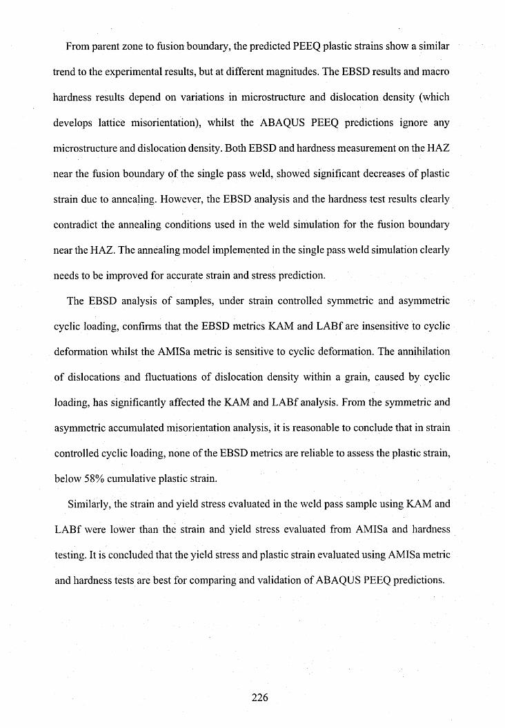
From parent zone to fusion boundary, the predicted PEEQ plastic strains show a similar
trend to the experimental results, but at different magnitudes. The EBSD results and macro
hardness results depend on variations in microstructure and dislocation density (which
develops lattice misorientation), whilst the ABAQUS PEEQ predictions ignore any
microstructure and dislocation density. Both EBSD and hardness measurement on the HAZ
near the fusion boundary of the single pass weld, showed significant decreases of plastic
strain due to annealing. However, the EBSD analysis and the hardness test results clearly
contradict the annealing conditions used in the weld simulation for the fusion boundary
near the HAZ. The annealing model implemented in the single pass weld simulation clearly
needs to be improved for accurate strain and stress prediction.
The EBSD analysis of samples, under strain controlled symmetric and asymmetric
cyclic loading, confirms that the EBSD metrics KAM and LABf are insensitive to cyclic
deformation whilst the AMISa metric is sensitive to cyclic defonnation. The annihilation
of dislocations and fluctuations of dislocation density within a grain, caused by cyclic
loading, has significantly affected the KAM and LABf analysis. From the symmetric and
asymmetric accumulated misorientation analysis, it is reasonable to conclude that in strain
controlled cyclic loading, none of the EBSD metrics are reliable to assess the plastic strain,
below 58% cumulative plastic strain.
Similarly, the strain and yield stress evaluated in the weld pass sample using KAM and
LABf were lower than the strain and yield stress evaluated from AMISa and hardness
testing. It is concluded that the yield stress and plastic strain evaluated using AMISa metric
and hardness tests are best for comparing and validation of ABAQUS PEEQ predictions.
226
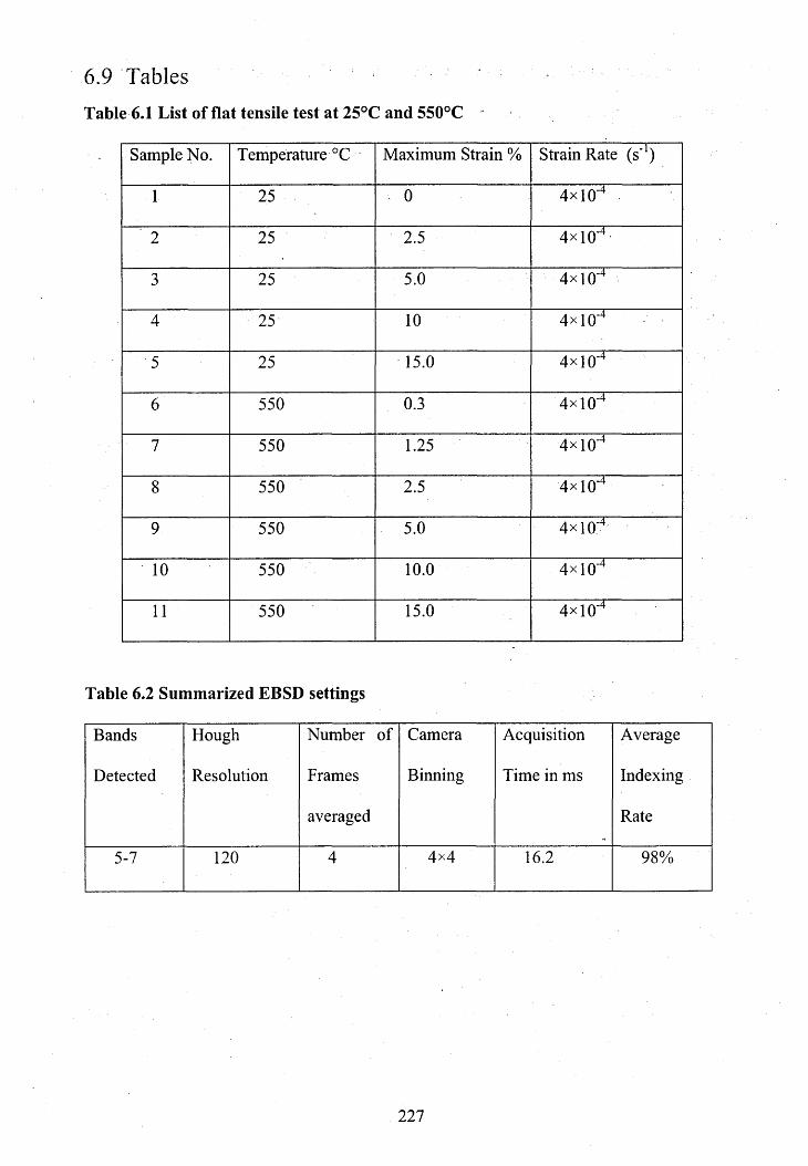
6.9 Tables
Table 6.1 List of flat tensile test at 25°C and 550°C
Sample No. Temperature °C Maximum Strain % Strain Rate (s'1)
1 25 - 0 ■p* X o
2 25 2.5 4><1 O'4
3 25 5.0
oX
4 25 10 4x1 O'4
■5 25 15.0
oXTl-
6 550 0.3 X H—» o -k
7 550 1.25 4X10"4
8 550 2.5 4x10'4
9 550 5.0
"4" . ©X
10 550 10.0 X o11 550 15.0 4x10'4
Table 6.2 Summarized EBSD settings
Bands
Detected
Hough
Resolution
Number of
Frames
averaged
Camera
Binning
Acquisition
Time in ms
Average
Indexing
Rate
5-7 120 4 4x4 16.2 98%
227

Table 6.3 List of cyclic loading test at 25°C and 550°C
Sample
No.
Temperature
°C
Number
of Cycles
Cycle Loading
Type
Strain Range
%
Strain Rate
(s '1)
1 25 12 Symmetric ±1.25
oX
2 25 6 Symmetric ±1.00 4x1 O’5
3 25 12 Asymmetric -1.25 to 0.02 4x10'4
4 25 7 Asymmetric -1.00 to 0.02 4x l0 ‘5
5 550 12 Symmetric ±1.25 4X 10‘4
6 550 12 Symmetric ±1.25 4x1 O'5
7 550 12 Asymmetric -1.25 to 0.02 4x 10'4
8 550 12 Asymmetric -1.25 to 0.02 4X10'5
9 550 12 Asymmetric -1.00 to 0.02 4X10⁻⁴
228
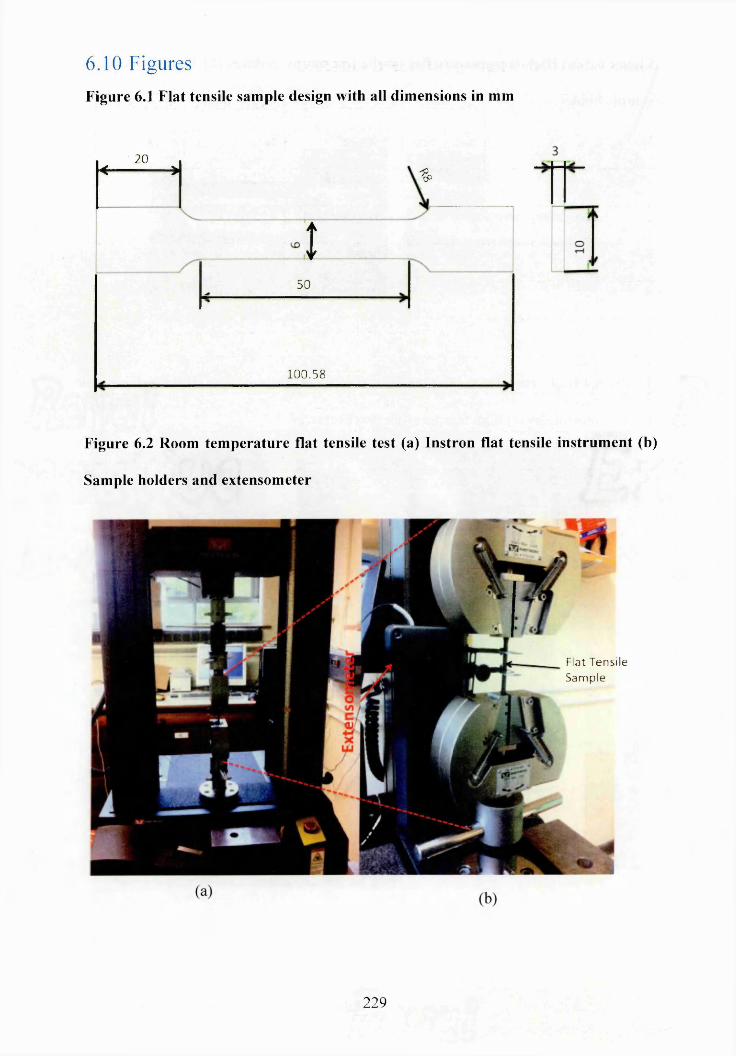
6.10 Figures
Figure 6.1 Flat tensile sample design with all dimensions in mm
20< >
I50
100.58
'PcP
Figure 6.2 Room tem perature flat tensile test (a) Instron flat tensile instrum ent (b)
Sample holders and extensometer
Flat Tensile Sam ple
229
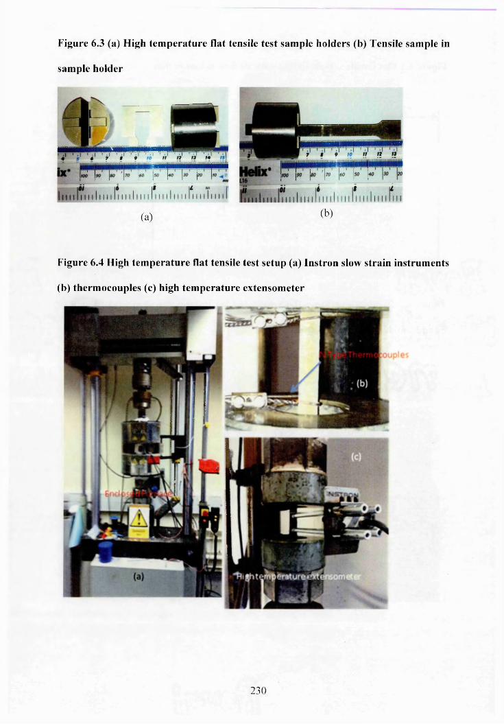
Figure 6.3 (a) High tem perature flat tensile test sample holders (b) Tensile sample in
sample holder
(a) (k)
Figure 6.4 High tem perature flat tensile test setup (a) Instron slow strain instruments
(b) thermocouples (c) high tem perature extensometer
230

True
St
ress
M
Pa
Figure 6.5 Tensile stress vs strain curves at 25°C and 550°C
Final peak stress achieved at the end of respective tensile test
25°C
— 550°C200
100
0.160 .120.1o.oa0.C2' 0.02 0True Strain
231
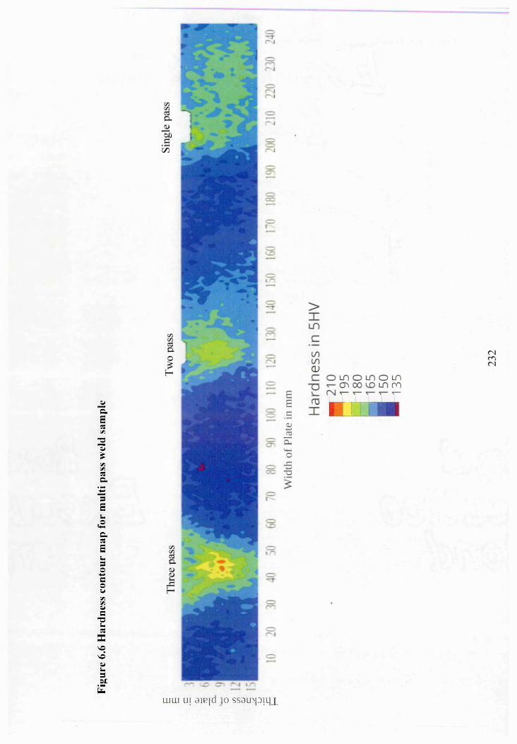
Figu
re
6.6
Har
dnes
s co
ntou
r m
ap
for
mul
ti pa
ss w
eld
sam
ple
UIUI UT 0}Efd JO S S 0 lD p T q i
13
5
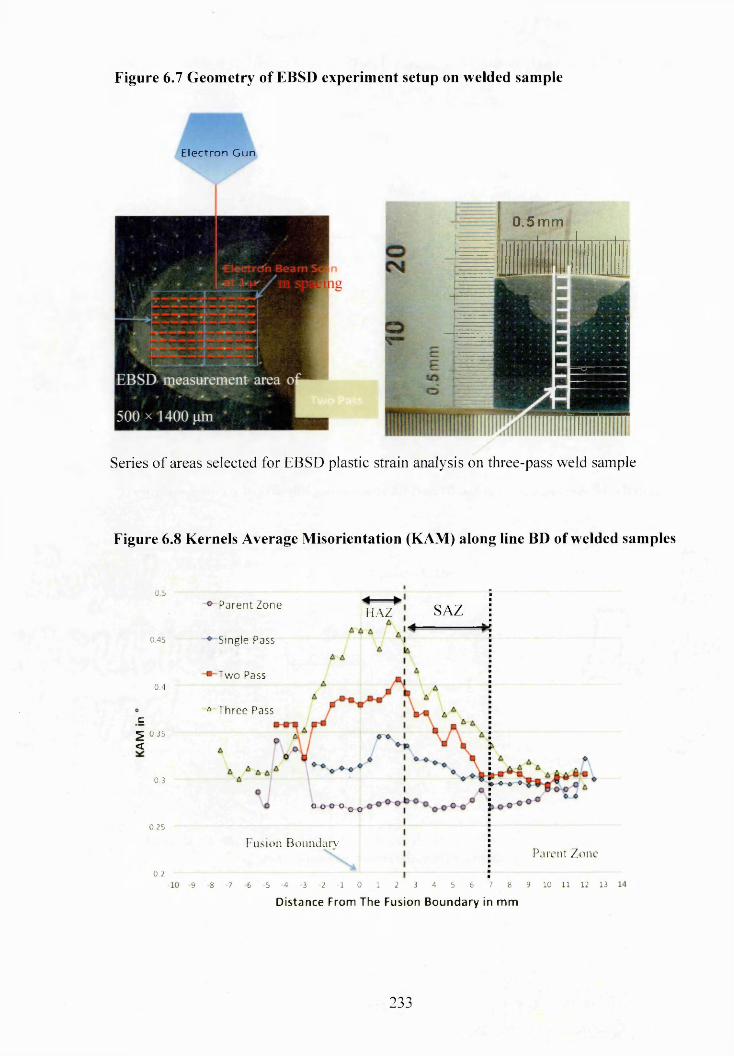
Figure 6.7 Geometry of EBSD experiment setup on welded sample
E lectron Gun
0 .5m m
Series o f areas selected for EBSD plastic strain analysis on three-pass weld sample
Figure 6.8 Kernels Average M isorientation (KAM) along line BD of welded samples
OS
0.45
0.4
C2 0.3S <
0.3
0.25
0.2
° Parent Zone SAZHAZ
Single Pass
Two Pass
6 Three Pass
O O o *
° o ° ° o O
Fusion BoundaryParent Zone
5 4 3 2 1 0 1 2 3 4 S 6 7 8 9 10 11 12 139 8 7 6D istance From The Fusion Boundary in m m
233
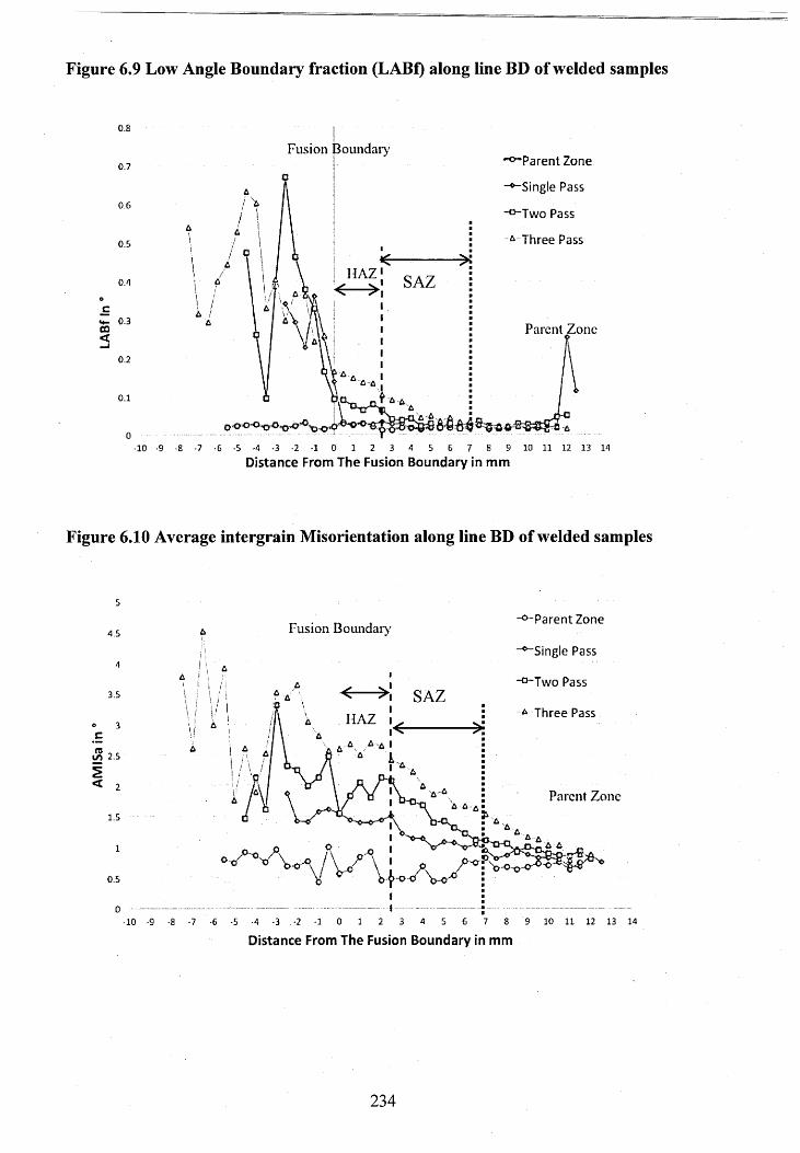
AMIS
a in
Figure 6.9 Low Angle Boundary fraction (LABf) along line BD of welded samples
CO<
o.s
0 .7
0.6
0 .5
0 .4
0 .3
0.2
-10 -9
Fusion Boundary“°"Parent Zone
“°“ Single Pass
’°~Two Pass
Three Pass
! HAZ SAZ
Parent Zone
a -a .
■8 *7 -6 -S -4 -3 -2 -1 0 1 2 3 4 5 6 7 8 9 10 11 12 13 14Distance From The Fusion Boundary in mm
Figure 6.10 Average intergrain Misorientation along line BD of welded samples
sParent Zone
Fusion BoundarySingle Pass
SAZ-* ■••Three Pass. HAZ
A
Parent ZoneA A-
•9
Distance From The Fusion Boundary in mm
234
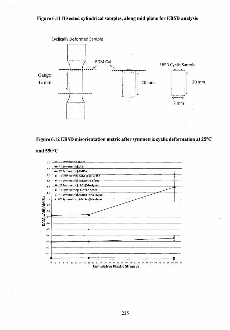
Figure 6.11 Bisected cylindrical samples, along mid plane for EBSD analysis
Cyclically Deformed Sample
Gauge 15 mm
(
1
EDM Cut\
EBSD Cyclic Sample
V
A
20 mm 20 mm
_____ Jv
7 mm
Figure 6.12 EBSD misorientation metric after symmetric cyclic deformation at 25°C
and 550°C
- f r - RT S y m m etric4 K A M
- * -R T S y m m e tr ic | LABf
RT S y m m e tr ic | AMISa
♦ HT S y m m e tr ic | KAM @ 4 e -4 /s e c
- o - HT S y m m e tric | KAM(g>4e-5/ s ge-
■ HT S y m m e tr ic I LABf(S>4e-4/sec
* HT S y m m e tr ic | LA B f"4e-5 /sec
a HT S y m m e tr ic ! AM ISa @ 4 e -5 /s e c
—A- H T~Sym m etric |AM1Sa © 4 e - 4 / s e cto
0 2 4 6 8 10 12 14 16 18 20 22 24 26 28 30 32 34 36 38 40 42 44 46 48 50 52 54 56 58 60 62
Cumulative Plastic Strain %
235
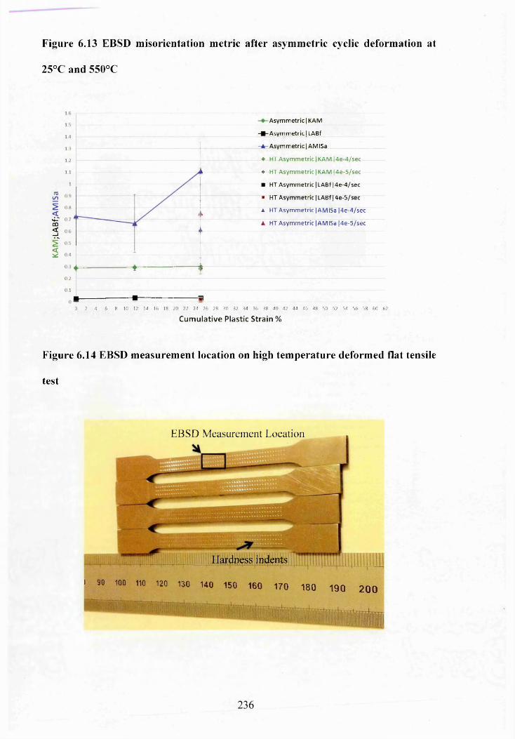
KA
M;L
AB
f;A
MIS
aFigure 6.13 EBSD misorientation metric after asymmetric cyclic deformation at
25°C and 550°C
Asymmetric | KAM
Asymmetric I LABf
- A - Asymmetric | AMISa
♦ HT Asymmetric | KAM |4e-4/sec
i ♦ HT Asymmetric | KAM 14e-5/sec
■ HT Asymmetric | LABf 14e-4/sec
■ HT Asymmetric |LABf|4e-5/sec
i k a HT Asymmetric | AMISa |4e-4/sec
A HT Asymmetric |AMISa |4e-5/seck
•i- - -S. ----jL♦------------------- ♦ I
■ -------------------------• ----------------------------30 2 4 6 8 10 12 14 16 18 20 22 24 26 28 30 32 34 36 38 40 42 44 46 48 50 52 54 56 58 60 62
Cumulative Plastic Strain %
Figure 6.14 EBSD m easurem ent location on high tem perature deformed flat tensile
test
EBSD Measurement Location
Hardness indents
) 90 100 110 120 130 140 150 160 170 180 19 0 2 0 0
^7390584416939955729755845259479550199189^1995^293^2
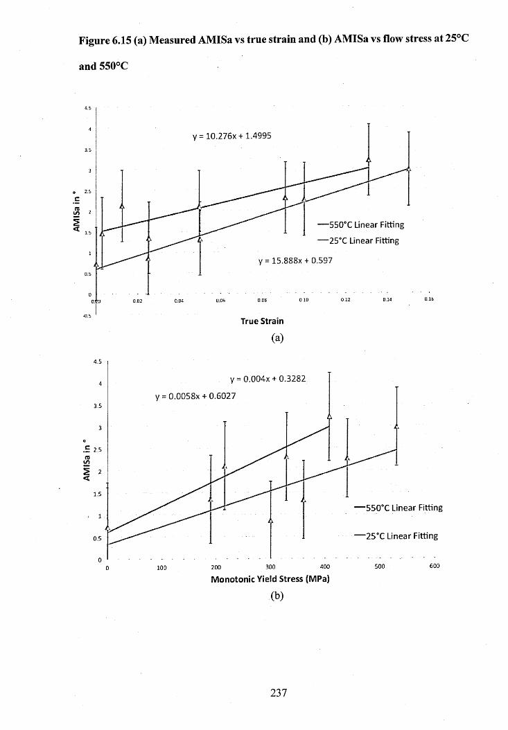
AMIS
a in
Figure 6.15 (a) Measured AMISa vs true strain and (b) AMISa vs flow stress at 25°C
and 550°C
y = 10.276X + 1.4995
i/>— 550°C Linear Fitting
— 25°C Linear Fitting
y= 15.888x + 0.597
0.12
True Strain
(a)
4.5
y = 0.004x + 0.3282
y = 0.0058x + 0.60273.5
o2.5
1.5
550°C Linear Fitting
— 25°C Linear Fitting0.5
6005004003002001000Monotonic Yield Stress (MPa)
(b)
237

Figure 6.16 Comparison of published AMISa correlation with present studies
y = 21.691x + 0.5
c 2.5
Linear (Shan 550°C)
- — 25°C Linear Fitting
— Githinji High Temperature
-Githinji Room Temperaturey= 16.773X + 0.5
Linear (Angeliu RT)
0.08 0.100.02 0.04 0.06 0.12 0.14 0.160.00
True Strain
Figure 6.17 Measured hardness vs true plastic strain (b) measured hardness vs
monotonic yield stress
24U
RT Strain Calibration from 5HV
HT Strain Calibration from 5HV
Linear ( RT Strain Calibration from 5HV)
Linear (HT Strain Calibration from 5HV)
0 0.02 0.02 0.03 O.CM 0.05 O.C6 0.02 'O.OB 0.00 0.1 0.11 0.12 C.13 D.1<1 0.15
True Strain
(a)
238
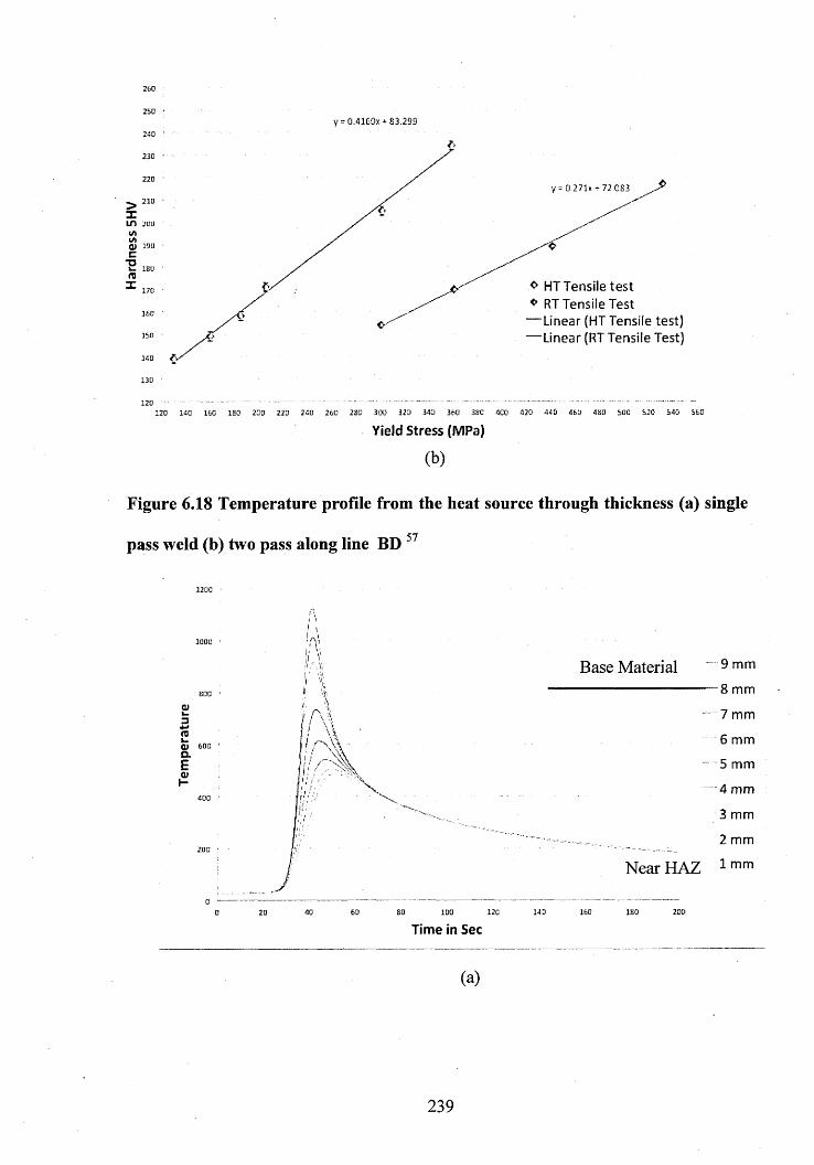
Hard
ness
5H
V250 '
240 :
230 ■
2 20 ‘
210 ' 200 ' 190 • ISO ’
170 • 160 ’ 150 '
140
130 ■
120 -
y = 0.41fS0x + 83 .299
y = 0.271x^ 72.083
^ HT T ensile te s t RT T ensile Test
— Linear (HT T ensile test) “ “ Linear (RT Tensile Test)
120 140 160 ISO 200 220 240 260 2SG 300 320 340 360 3SC 400 420 440 460 4BO 500 520 540 560
Yield Stress (MPa)
(b)
Figure 6.18 Temperature profile from the heat source through thickness (a) single
pass weld (b) two pass along line BD 57
0)i—3*->re(U 600Q.Ere
Base Material
x
9 mm
-8 mm
7 mm
6 mm
5 mm
4 m m
3 mm
2 mm
Near HAZ 1 mm
20 40 60 B0 120 140 160 ISO 200
Time in Sec
(a)
239
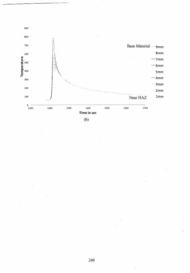
Tem
per
atu
re
900
800
700
600
500
400
300
200
100
H
\
Base Material 9mm
8mm
— 7mm
— 6mm
5mm
— 4mm
3mm
2mm
Near HAZ lmm
1100 1200 1300 1400 1500 1600 1700
Time in sec
lb)
240
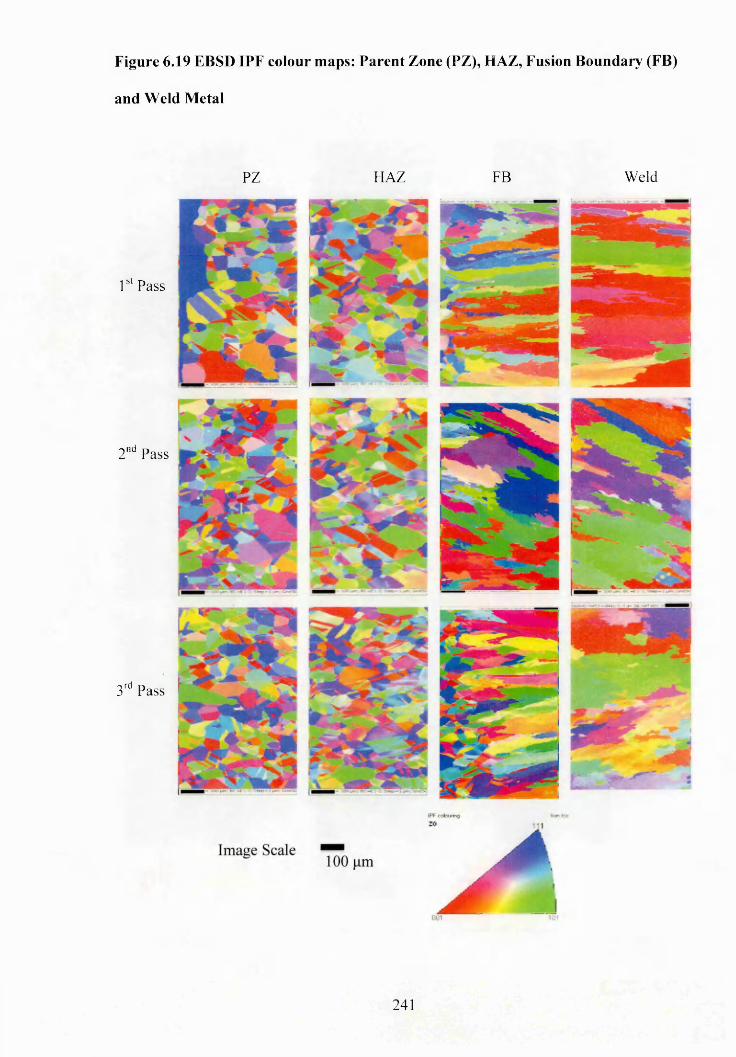
Figure 6.19 EBSD IPF colour maps: Parent Zone (PZ), HAZ, Fusion Boundary (FB)
and Weld Metal
1st Pass
2nd Pass
3rd Pass
PZ HAZ FB W eld
241
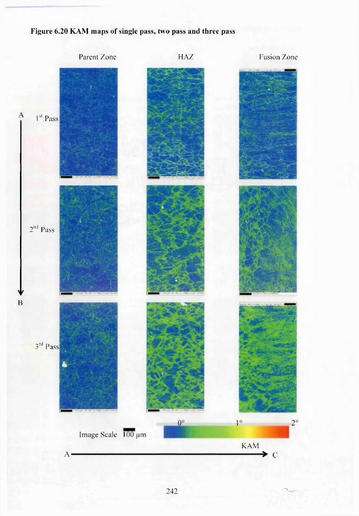
Figure 6.20 KAM maps of single pass, two pass and three pass
Parent Zone HAZ Fusion Zone
1sl Pass
2"d Pass
▼B
3rd Pass
Im age Scale 100 pm
KAMA' * C
■firal
242
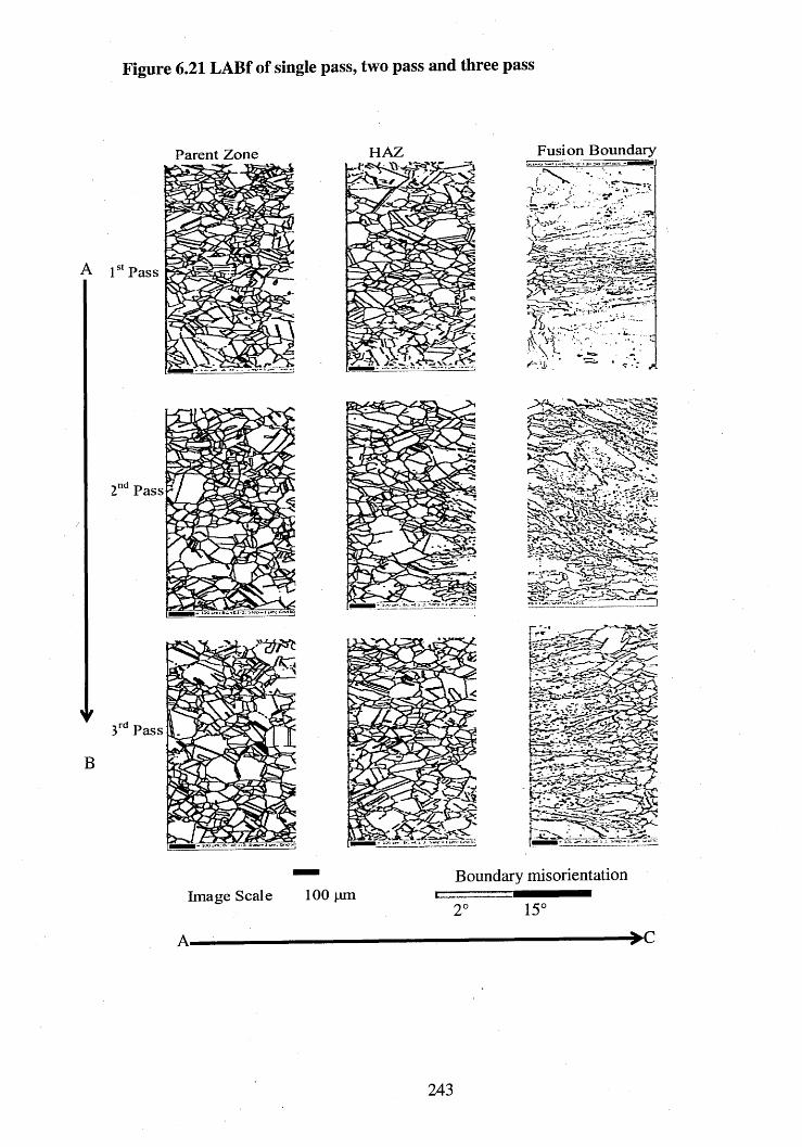
Figure 6.21 LABf of single pass, two pass and three pass
Fusion BoundaryParent Zone
Im age Scale 100 |imBoundary misorientation
2° 15°

Figu
re
6.22
Pare
nt m
ater
ial:
Com
pari
son
betw
een
the
diffe
rent
EBS
D m
etric
s m
isori
enta
tion
and
hard
ness
re
sult
mn_ in
o
- r--
- VD
- m
- N-
- m
- <N
- o
m
oo
o
o oID
O OO Ocn o00 oin o omCN CNISah ssaupjeH
—i—i—i—i—i—i—i—i—i—i—i—i—i—i—i—i—i—i—°°. ^ ^ ^ °°. ^ ^ ‘"S 00 °° ^ ''t ^ °°. ^ ^N-" ^ ■r "sf m’ no ro rn cn cn cn cn ^
CN CO ID N" <N Oo o d d
,in uopejusuosjiAl esiiAIV
1 iID im
-----------r ...................... i .............N- 00 ... 1.....CN
.... — o
o O o O ojavi
O o
IDN" ^ CN N" ^o d
'vfo '
00 ID CN CO 00 ID CN CNm CO CO CO o ' CN CN CN CN o*d o ' o ’ d o o o o0u| uope^U0UOSjiAl 1A1V>I
Dis
tanc
e fro
m bo
ttom
of
the
pl
ate
to to
p in
mm
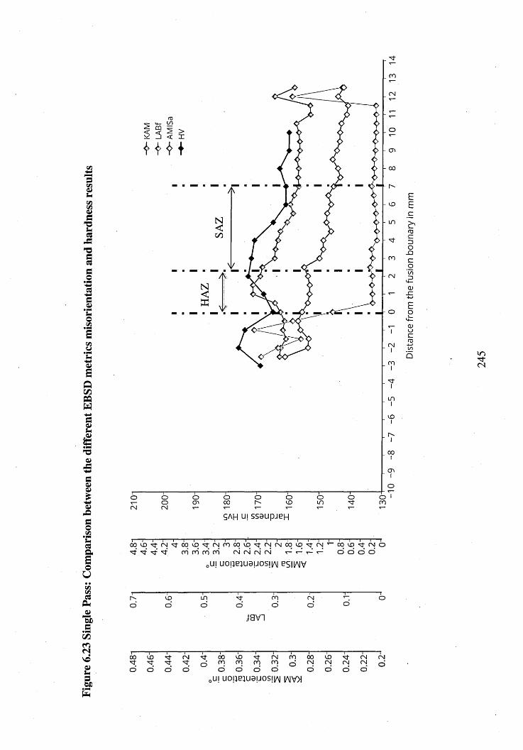
Figu
re
6.23
Sing
le Pa
ss:
Com
pari
son
betw
een
the
diffe
rent
EBS
D m
etric
s m
isori
enta
tion
and
hard
ness
re
sults
ro
fM
o
- cn
- oo
- LT)
- N-
- ro
o
CM
ro
LD
vo
oo
cno
o ovo oLD
o oroocn oooo ooCMCM
SAH IN ssaupjen
t—i—i—i—:—i—i—i—i—i—i—r1—i—i—i—i—i—i—i—i—i—i—i—i—r0 0 VO CN ^ 0 0 VO ^ CN CO 0 0 VO ^ CN CN 0 0 VO 's t; <N ^ 0 0 vD <3 ; (N O
^ N"’ N'* CO r o r o ro ’ CN c n <n " c n r - ‘ r - ‘ o o ’ o ’ o ’
0U| uopeiuauosiiAi esiiAIV
o’VO
o’LOo’
N"o’
roo’
(N
o’javi
00 VO N- CN N"N- N- N- N- q
O o ’ O o ’
00 VO CN rq 00 VO N" CN CNro ro ro ro d CN CN CN CN oo’ o’ o’ d o o o o’,m uope^u0uos!iA| 1AIVM
Dist
ance
fro
m the
fu
sion
bo
unar
y in
mm
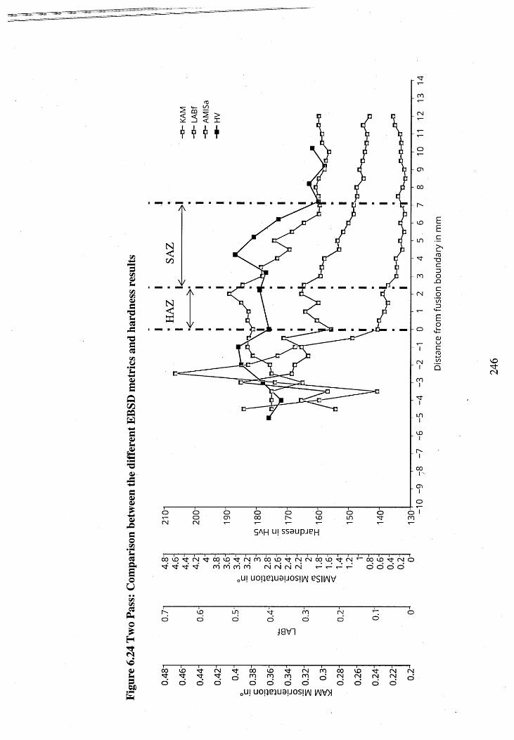
d<Z2o>uViVIa;C
ucs-=T3aC3vyWa»aQC/5PQWsQJU
&taa»
A
fi(V£vpfiCovt• PNSm03OnaoU«V i
PmO£HTfrjvo41U3W)
no
CM
o
- cn
- oo
- r-
- LO
- ■roo
- (N
- O
no
LO
oo
oo oo ocn ooo o o<£> o
LOo"sf ono
gAH uj s s a u p je n
00U0' ffNJrJ-0q^0 r(Nn000<JD -nsJfvJ00UD’ (nJr - 00c0'^(NO ^ ^ no’ no no" no cm* cm cm <N r-C r-’ r-C *-' o o o ’ o
0in uopeiuauosiiAi esiiAIV
r"-d
VO
oLOd
'sj-o
noo
rsjo’
javi
00 uo fNJ■r ''td o o' o’ o’
00 co ’’sf- CM no 00 CO ,3‘ CM CMno no no no o’ rsi CM 0M cm oo' o' o o' d d o' d
EEc
no*0co
JDCo
QVOCM
0uj uope^uauosjtM iajvm

Figu
re
6.25
Thre
e pa
ss:
Com
pari
son
betw
een
the
diffe
rent
EBS
D m
etric
s an
d ha
rdne
ss
resu
lts
roLOm
o
- co
- oo
- r-'-.
- N-
- no
- r\i
- o
<N
no
oo
cr>
oo oo
CN
OO O00 Or- oLO
oou o ro
CN
cjAH U| sseupjeH
i 1------ 1-------- 1---1--------- :-------1------ 1------ i--- :-------r— i----------1------- 1---1------1------- i---------- 1-------1---1------- 1--------- 1-------1-------1-------ro q l o N ; <n N- o q l o N ; c n r o o o l o N ; <n <n o q l o n - c n ^ o o l o n ; < n or f ■ 't L f r o r o c o r o <n cn cn c n t- ’ ^ ^ d o d o
0uj uopeiusuosjiA i esiiAIV
1----------- ----------1-----LO
---------- 1-----------u o
----------1---------------------- J------------N " r o <N
-----1----------- rOo o o o o O O
favi
i 1------------ 1------------ 1------------ 1------------ :------------1------------ 1------------1------------ 1------------ 1------------ 1 i 1 rO O L O N - C N N - O O L O ^ C N r O O O L O N - C N C N^ o rQ ° r! rr! n’] o r''J. rx! rsJrsi oo o o o’ o’ o" o‘ o o o o‘ o'
0ui uopeiu9uosii/\| iaiv»
Dis
tanc
e fro
m th
e fu
sion
bo
unda
ry
in m
m
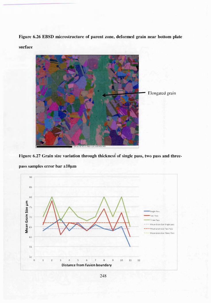
Figure 6.26 EBSD m icrostructure of parent zone, deformed grain near bottom plate
surface
Elongated grain
Figure 6.27 Grain size variation through thickness of single pass, two pass and three-
pass samples error bar ±10pm
80
75
£ a.CJ N
Pass
• E Two Passro /0
“ “"" T h re e PassOC - — — - Mean Grain Stze Single pass
2! 65<U - “ “ -M ean Grain Size TwoPass
I M ean Grain Size Three Pass
60
500
Distance from fusion boundary
248
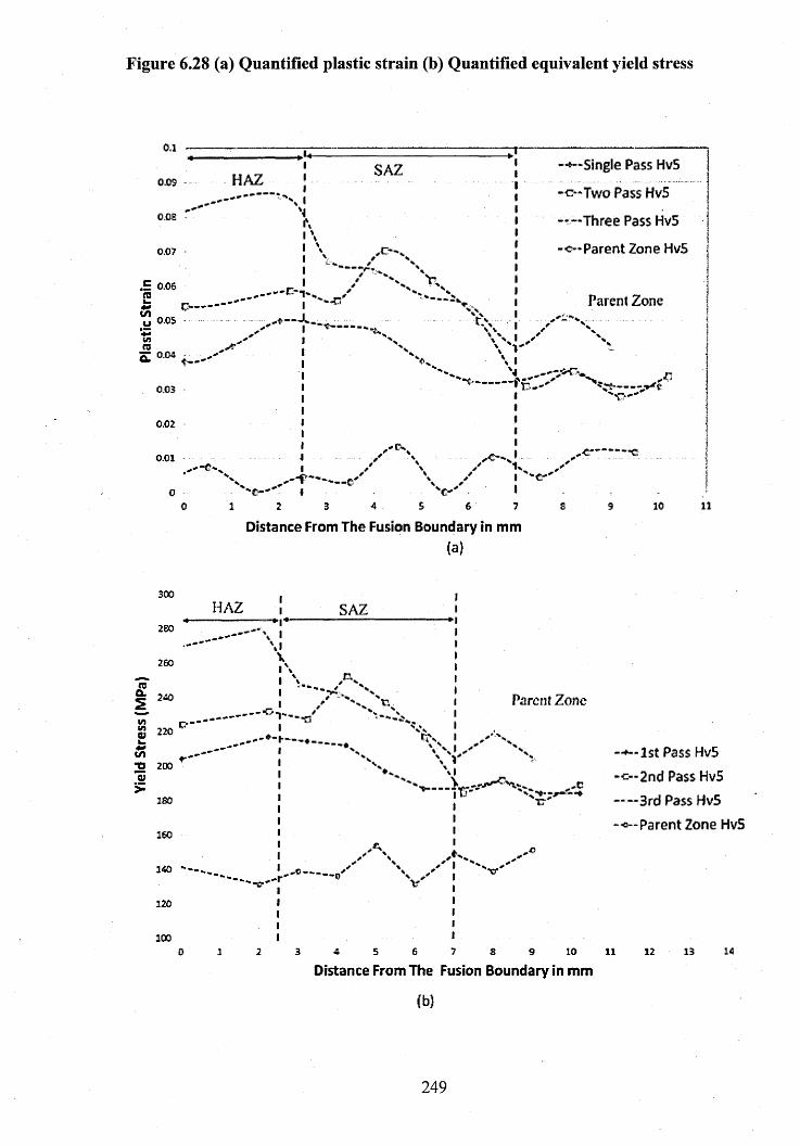
Yield
St
ress
(M
Pa)
Plas
tic
Stra
in
Figure 6.28 (a) Quantified plastic strain (b) Quantified equivalent yield stress
o.i
0 .09
O.OE
0 .07
0 .06
0.05
0.04
0.03
0.02
0-01
HAZ
___ _c—
t--*
.'f'
SAZ
*
%
-**—Single Pass HvS
-c -T w o Pass HvS
— Three Pass HvS
-o -P a re n t Zone HvS
Parent Zone
*
V * j X \ V '\ I
VJ „ _____■t--------------------- ^I I I I II c,« -*v
" C r mf i2 3 4
€■'S 6
I “t ' ' I
Distance From The Fusion Boundary in mm(a)
10 li
t?".......
___ i
300
280
260
240
220
200 ■
180
160
140
120
100
HAZ SAZ\ i
M \ i \ i \ . i i1 ' “-a l
r.x Parent Zone
trss i
—--r
W %\ i|l lI TTI I I
\ *<_ ^'r‘S i***
V ' 1v i i i i i
3 4 5 6 7 8 9 10
Distance From The Fusion Boundary in mm
—*—1st Pass HvS
- ’=--2nd Pass HvS
— —3rd Pass HvS
~®--Parent Zone HvS
11 12 13 14
(b)
249
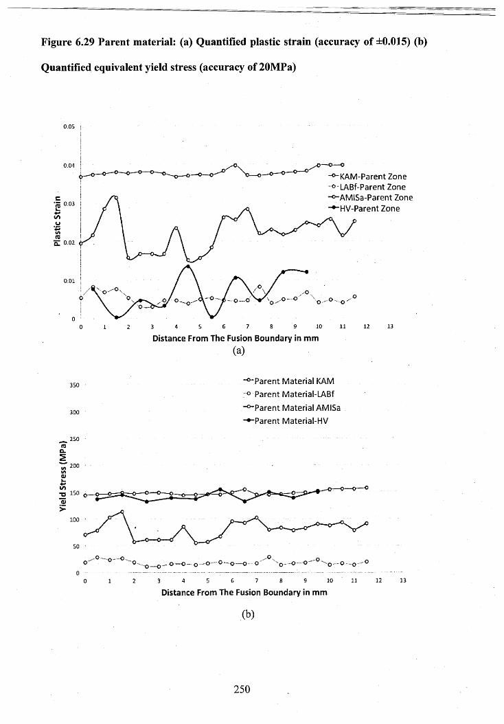
Figure 6.29 Parent material: (a) Quantified plastic strain (accuracy of ±0.015) (b)
Quantified equivalent yield stress (accuracy of 20MPa)
0.05
0.04
RAM-Parent Zone LABf-Parent Zone
-°-AMISa-Parent Zone “•“HV-Parent Zone
in
o.oi-o.
o -
136 7 9 10 11 1283 4 C0 1 2
Distance From The Fusion Boundary in mm(a)
350
300
250ro
D.5
200
- ° ‘ Parent Material RAM
o Parent Material-LABf
■^Parent Material AMISa
-•-Parent Material-HV
in*D 150 o—O—<t>
100
50
,o°"o~-o oo - ° o °- O —-O — o — O —O — O “ O — o O—O '
3 4 5 6 7 8 9 10
Distance From The Fusion Boundary in mm11 12 13
(b)
250

Figure 6.30 Single pass: (a) Quantified plastic strain (accuracy of ±0.015) (b)
Quantified equivalent yield stress (accuracy of ±20 MPa)
0.06 KAM-Single Pass
LABf-Single Pass
AMISa-Single Pass
HV-Single Pass
o.os
0.04
«/)•p 0.03
. 0.02
0.01
1312111097 8653 4210Distance From The Fusion Boundary in mm
(a)
-o-KAM Single Pass o LABf Single Pass
-fr-AMISa Single Pass
-*-HV Single Pass
na.5i/ ii/i<u
100
o — o -o —o0
o 1 2 3 4 5 6 7 8 9 10 11 12 13 14
Distance From The Fusion Boundary in mm
(b)
251
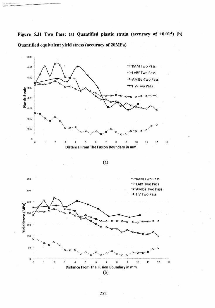
Yield
St
ress
(M
Pa)
Plas
tic
Stra
in
Figure 6.31 Two Pass: (a) Quantified plastic strain (accuracy of ±0.015) (b)
Quantified equivalent yield stress (accuracy of 20MPa)
-°~KAM Two Pass
-°*AM ISa-Two Pass
D istance From The Fusion B oundary in m m
(a)
3 5 0
3 0 0
-°-KAM Two Pass
LABf Two Pass -o-AMISa Two Pass -*-HV Two Pass
o o
o "o'
3 A 5 6 7 fi 9 1 0 1 1
D istance From The Fusion B oundary in m m
(b)
12 13
252
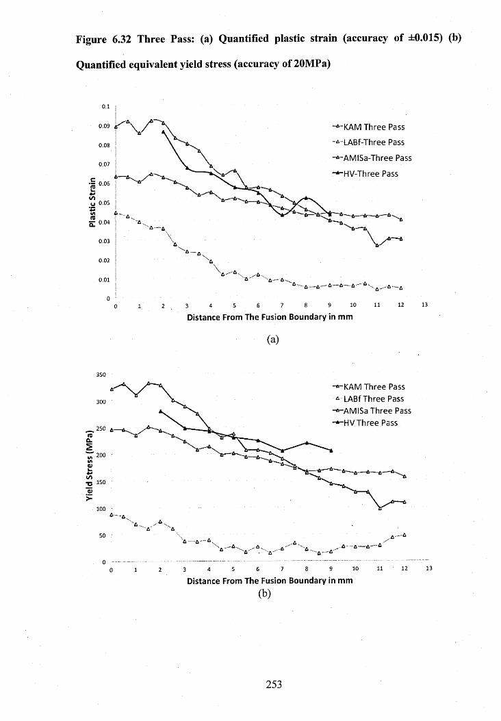
Yield
St
ress
(M
Pa)
Plas
tic
Stra
in
Figure 6.32 Three Pass: (a) Quantified plastic strain (accuracy of ±0.015) (b)
Quantified equivalent yield stress (accuracy of 20MPa)
0.1
KAM Three Pass0 . 0 9
-a-LABf-Three Pass.0 8
-*~AMISa-Three Pass.0 7
HV-Three PassA—6-.0 6
.OS
0 . 0 4 A0 . 0 3
A—,0.02
0.01“A .
0 1210 1197 86543210Distance From The Fusion Boundary in mm
(a)
1 3
3 5 0
-*~KAM Three Pass
a LABf T hree Pass -*~AMISa T hree Pass
-*-HV Three Pass2 5 0
100
5 0 A—A- _ ^ A ,-A " " " A , -A—A—-A—&
3 4 5 6 7 8 9 1 0
Distance From The Fusion Boundary in mm
(b)
11 12 13
253
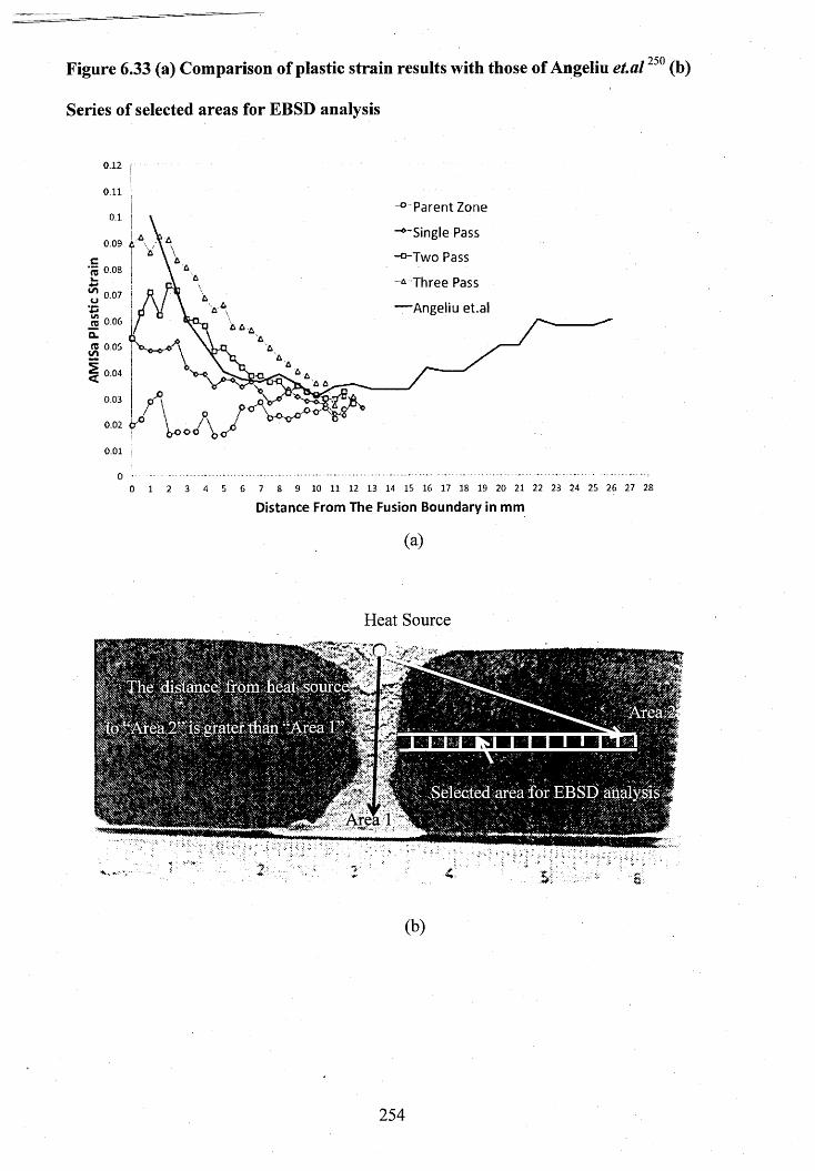
• 250Figure 6.33 (a) Comparison of plastic strain results with those of Angeliu et.al (b)
Series of selected areas for EBSD analysis
0.12
0.11
~°~Parent Zoneo.i“ “Single Pass
-° -T w o Pass0 . 0 9
~*~Three PassY!0 07
A ngeliu et.alTO 0 . 0 6
CLre o.os to
0 . 0 4& £
0 . 0 3
0.02
0.01
0 1 2 3 4 5 6 7 8 9 1 0 1 1 1 2 1 3 1 4 1 5 1 6 1 7 1 8 1 9 2 0 2 1 2 2 2 3 2 4 2 5 2 6 2 7 2 8
Distance From The Fusion Boundary in mm
(a)
Heat Source
The distance, from heat* sourc<
i#te “Afeh.2,f is .grater than ‘‘A rea 110^^ '' v'
(b)
254
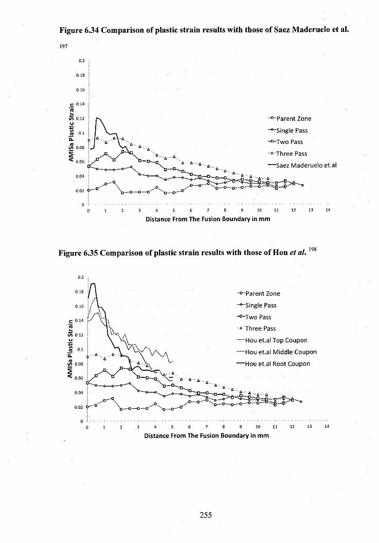
Figure 6.34 Comparison of plastic strain results with those of Saez Maderuelo et al.
197
0.2
0 . 1 8
0 . 1 6
0 . 1 4
-° -P a ren t Zone«75 o.i2
“ “Single Pass
-° -T w o PassA -t /1 0 . 0 8
0.06■Saez M aderuelo et.a l6 —.
& -0 . 0 4
0.02 p-^Cr
IB 1 48 10 127 9 115 632 40 1Distance From The Fusion Boundary in mm
Figure 6.35 Comparison of plastic strain results with those of Hou et al. 198
c 0 . 1 4
to 0 .12
t o 0 . 0 8
\
Parent Zone
^ “Single Pass
■°*Two Pass
* Three Pass
— Hou et.a l Top Coupon
-~“Hou et.a l M iddle C oupon
— Hou et.a l Root C oupon
3 4 5 6 7 8 9 1 0 1 1
Distance From The Fusion Boundary in mm
255
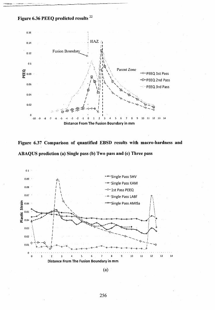
Figure 6.36 PEEQ predicted results 22
0 . 1 6
HAZ 4iif
Fusion Boundary j
||V;,i '\ \
O ' " Ifi \ \ Parent Zonea o.os \ :IH \ \, -c -P E E Q 1st Passa. . R , j 11\ V
/ / b - \ -Q -P E E Q 2nd Pass0 . 0 6 . " / \ | | 1 \ \ v
\ i \ \ . PEEQ 3rd Pass0 V i \ H . . .
eJ I V v "0.04 , /■ | ' S . ; , .
0 . 1 4
0.12 - i
0.1
0.02
1 I I ^ ^ 'S. •,
1 I 1
I■10 - 9 -8 -7 - 6 -5 -4 -3 -2 -1 0 1 2 3 4 5 6 7 S 9 1 0 1 1 1 2 1 3 1 4
Distance From The Fusion Boundary in mm
Figure 6.37 Comparison of quantified EBSD results with macro-hardness and
ABAQUS prediction (a) Single pass (b) Two pass and (c) Three pass
0.1
4 \
" ‘—Single Pass 5HV
-^ -S in g le Pass KAM
- ^ l s t Pass PEEQ
-^ " S in g le Pass LABf
—Single Pass AMISa
—- 0 .0 4
0 . 0 3 ’
<£ -r<£- —Q I0.01 v • ' ,
.. o -o — O — o o - o - o — o — O o
01 2 3 4 S 6 7 8
Distance From The Fusion Boundary in mm10 li 1 2 1 3
(a)
256
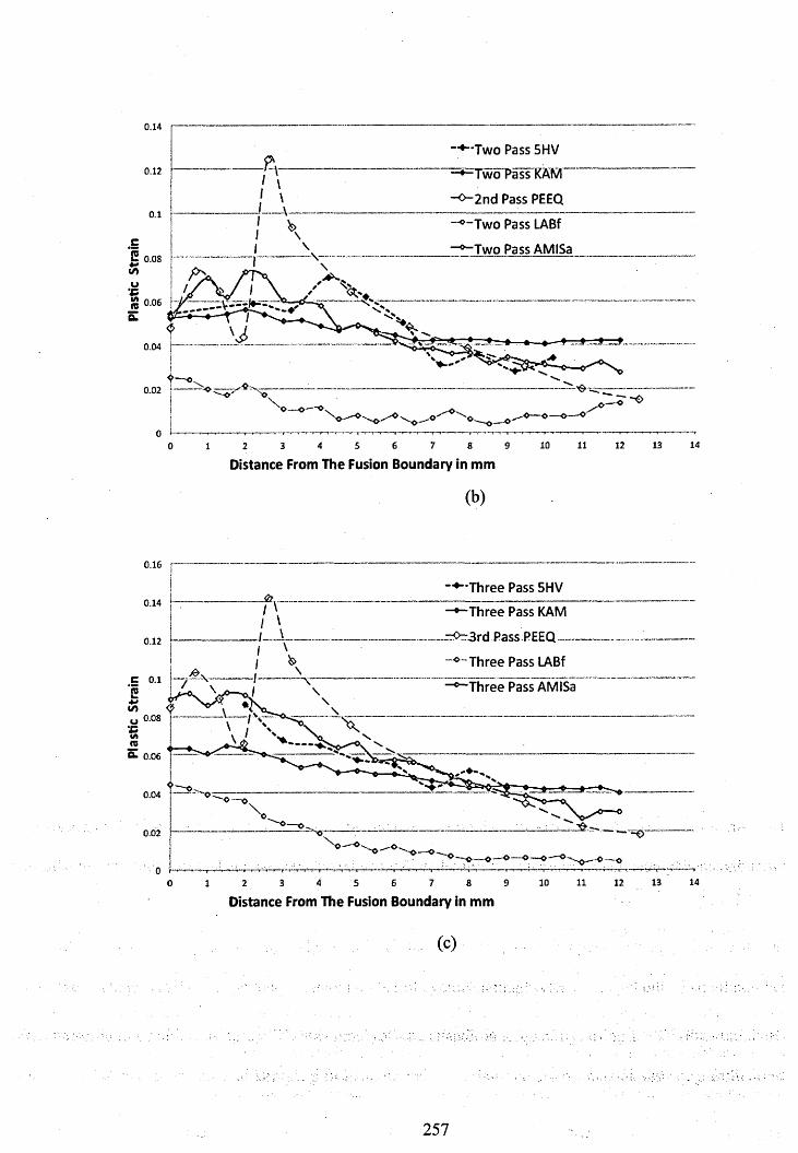
Plas
tic
Stra
in Pl
astic
St
rain
0.14
■•"’Two Pass 5HV
^TwoPassKAM0.12
-°~2nd Pass PEEQo.i
Two Pass LABf
Two Pass AMISa0.08
0.06
0.04
0.02
14137 10 11 124 5 6 8 930 21Distance From The Fusion Boundary in mm
(b)
0.16
■♦■'Three Pass 5HV0.14
Three Pass KAM
^o=-3rd Pass P£EQ-
~o~Three Pass LABf0.12
0.1 Three Pass AMISa
0.04
0.02 “O'
141311 124 6 7 8 9 102 3 50 1Distance From The Fusion Boundary in mm
(C)
257
C h a p t e r 7. D is c u s s io n
This chapter discusses the key research findings of the present work. As described
earlier, this research project has analysed the residual stress distribution in a three-pass
weld round robin benchmark plate and the potential origins of the measurement
uncertainties. It has also investigated the contributions to possible errors in weld residual
simulations of the cyclic isothermal stress-strain properties used; that is these properties
sensitivities to strain rate and the type of cycle (symmetric versus asymmetric). The
project has also explored the possibility of quantifying the accumulated plastic strain and
stress due to the each weld bead deposit using EBSD metrics and validated the results
with hardness measurements. In addition the project has investigated the limitation of
various EBSD metrics in determining the accumulated plastic strain due to strain
controlled cyclic loading.
7.1 Issues affecting the reliability of residual stress
measurement using neutron diffraction
This thesis has analysed the distribution of residual stress in a three pass weld
behchmarkiplate using strain diffractometers at two spallation source neutron facilities
: (i.e.-.VULCAN,iat SNS and ENGIN-X af the ISIS Facility). In total 76 different locations
in the welded plate were measured in three orthogonal directions. In Chapter 4, VULCAN
and ENGIN-X residual stress measurements have been compared independently with
other measurement carried out by members of the NeT consortium at reactor neutron; =
sourees;In thissection*; the-average of the residual stress measurementSj rootmean square j
5 / i and standard deviation- along, plane D (refer Figure 3 . 3 (a) Benchmark specimen ;-
258
dimensions (b) Benchmark specimen dimensions and slot configuration (a)) evaluated
from the spallation and reactor neutron sources were compared, refer Table 7.1 and Figure
7.1 to 7.4.
Figure 7.1 (b) and (c) show how the transverse and normal residual stresses measured
from the spallation and reactor neutron source are in very good agreement with each
other. However, the longitudinal residual stresses measured in the parent zone, i.e. from
10 to 17 mm below the top surface, differ by approximately 50 MPa, as seen in Figure
7.1(a). Figure 7.2 compares the residual stresses along a line at a depth of 5 mm beneath
the surface of the single pass weld bead. The residual stress measurements in the parent
zone (i.e. -90 to -40 mm and 40 to 90 mm) agree very well with each other, but differ by
about 50 MPa in the region of the weld slot (i.e. -40 mm to 40 mm) in all three directions.
Figure 7.3 compares the residual stress at depth of 9 mm from the top surface. The average
transverse and normal residual stresses from both neutron sources are in very good
agreement. However, the longitudinal residual stress results show a difference of
approximately 50 MPa along the length of the scan. Figure 7.4 shows how the residual
stresses at a depth of 16 mm from surface are in excellent agreement with each other.
Measurement uncertainties associated with the stress free cuboids, discussed in
Chapter 4, may be contributing to systematic differences in the results from the spallation
and reactor neutron sources. Perhaps more important is that at the reactor neutron sources
only one diffraction peak (the 311) was analysed, while at the spallation sources more
than 10 hid peaks were analysed. Therefore far fewer grains were sampled at the reactor
sources compared with the spallation sources. The grain size of the weld cuboids was
very big in comparison to the parent cuboids; refer Figure 6.19 of Chapter 6. As a result
of this, the number of grains diffracting in a given gauge volume in the weld cuboids was
lower than the parent cuboids. At the spallation neutron source, the average of multiple
259
measurements of the different stress-free cuboids were used in the residual stress analysis.
As a result of this, stress free cuboid issues such as the number of grains diffracting, the
effects of crevices and glue were reduced or averaged out. While, at the reactor sources
single value measurements of the different stress-free cuboids were used in the residual
stress analysis.
Another potential origin of uncertainty (described earlier in Chapters 3 and 4) is
associated with fact that the parent and weld stress free cuboids were extracted from
different weldments; the weld trial plate (ID 1-2B) and the three pass welded benchmark
plate (ID 2-IB). Hardness measurements for the weld trial plate (refer Figure 4.32 of
Chapter 4) clearly indicated an interaction between the thermal effects of the adjacent
three-pass and two pass welds.
Figure 7.5 schematically shows the cyclic deformation of material at a specific point
adjacent to a three-pass weld. During heating from room temperature to above 1000°C,
the material experiences compressive plastic strain from A to C as indicated in the Figure.
From A to B material undergoes elastic deformation and from B to C, plastic deformation.
While, in cooling from 1000°C to 0°C, the material experiences tensile plastic strain from
C to E, where, C to D is elastic deformation and from D to E is plastic deformation. By
the end of the cooling, the material stores tensile strain, due to constraint coming from
the neighbouring material. As a result of this there will be no tensile stress unloading and
the proof stress of the material has increased from its initial yield stress value. During the
second weld bead deposit, the distance from the heat source of the material at the point
of interest has increased, which reduces the degree of deformation (i.e. strain range) due
to the lower peak temperature experienced. During heating from the second weld pass,
the material undergoes a second cycle of compressive plastic strain from E to G (E to F
is elastic deformation and F to G plastic). The proof stress of the material during the
260
reverse cycle E to G will be less than the previous weld deposit, due to the Bauchinger
effect. However, during the cooling process (i.e. G to I) the material gets more strain
hardened, than during the first weld pass. A similar cyclic deformation mechanism occurs
during the third weld bead deposit (i.e. I to K during heating and K to M during cooling)
and the material gets a bit more strain hardened in comparison to the two pass weld
deposit. When a two-pass weld bead is deposited close enough to the three pass weld, the
possibility of interaction of the weld thermal history with that of the adjacent three-pass
weld is high. As a result of this, the original three-pass weld would have experienced two
additional stress-strain cycles due to the adjacent two-pass weld deposit.
The Line B2 longitudinal and transverse residual stress results from neutron diffraction
(refer Figure 4.22) and the EBSD AMISa yield stress in parent zone (refer section 6.7.4
and Figure 6.29 yield stress from parent zone to fusion boundary), indicated that the
material at 30 mm away from the centre of the three pass weld bead experiences a stress
about 50 to 100 MPa due to the three pass weld thermal history. In the weld trial plate
(ID 1-2B, from which the_l-2B stress free cuboids are extracted) at 30 mm distance from
centre of three-pass weld, the two-pass weld bead was deposited. Which means the
adjacent three-pass weld bead experienced a further two loading cycles. As a result of
this, the nominally stress free cuboids extracted from the weld trial plate may have had
higher inter-granular stress present than the three-pass weld benchmark plate. The effect
of the higher inter-granular stress is clearly visible in the Line D5 residual stress (i.e. -
40mm to 40mm). However, this hypothesis would only be valid if the two-pass weld was
made after the three-pass, but there is no recorded information regarding the actual
welding sequence for the trial plate.
Another possible reason contributing to the difference in the residual stresses measured
is that the alignment of the benchmark plate at each experimental setup would have
261
varied. The precise alignment of the sample allows the user to position the sample
accurately. However, the facilities available to the user at different diffractometer
instruments for aligning the sample vary.
The presence of crevices, the hydrogen content of the glue and the non-parallel edges
of the stress-free cuboids all contribute to experimental uncertainties in the measured
residual stress. In addition to experimental uncertainties, the inhomogeneity of the stress-
free cuboids such as in grain size (refer Figure 6.26), and the non-uniform chemical
segregation, lead to the generation of pseudo strains in a residual stress analysis.
7.2 Effect o f strain rate and asymmetric cyclic deformation
on weld simulation prediction
Chapter 5 has investigated the influence of strain rate and asymmetric versus
symmetric cyclic loading on the stress-strain response of parent 316L (N) stainless steel,
as asymmetric cyclic loading is a closer representation of real weld thermal cyclic
deformation. A series of isothermal cyclic loading tests have been conducted at room
temperature and 550°C for a constant total strain range and various strain rates. However,
in real welding, the rate of heating and cooling is not uniform. As a result of this the
material experiences a different total strain range and varying strain rates depending on
the distance of the material from the heat source and the component geometry. In addition,
the rate of strain hardening of the material during heating is less than that during the
cooling process.
As a first approximation, the strain rate experienced by material around a weld is
proportional to the rate of change of the temperature. During heating, the temperature
increases very fast from room temperature to the melting point, while the rate of cooling
262

from 1000°C to room temperature is very slow (refer Figure 6.20 of Chapter 6). In the
temperature range 300 °C to 650 °C, the material strain hardens more at a slower strain
rate due to dynamic strain ageing. This is because, at slow strain rates, in the dynamic
strain ageing regime, strong interactions between solute atoms and mobile dislocations
reduces the number of mobile dislocations available to accommodate the required plastic
deformation. As a result of this, the flow stress increases, and the material strain hardens.
Most weld simulations in the published literature ignore the effect of strain rate on the
strain hardening of the material at high temperature.
In welding, the material undergoes asymmetric cyclic deformation as described in
section 5.3.1 of Chapter 5. The material strain hardens less during asymmetric cyclic
loading than in symmetric cyclic loading both at room and high temperature. This is
because when the total strain range is low, fewer dislocations are generated and the planar
structure of dislocations continues to a higher number of cyclic loads. While with a higher
total strain range, i.e. symmetric cyclic loading, material gets strain hardens more due to
the increase in dislocations density.
The effective stress is the average of the initial yield stress and the final saturated peak
stress achieved during loading. While the back stress 67 is the average difference of the
saturated peak stress and initial yield stress (see Figure 7.6). The back stress is related to
the collective long-range interaction of dislocations which arise during reverse cyclic
loading and is due to the heterogeneous grain properties of the material. Minh-Son Pham
93 studied the relationship between microstructure and back stress in 316L stainless steel.
His studies showed the rate of change of back stress and effective stress decreases with
reducing total strain range at both room and high temperature.
In weld simulation the Chaboche mixed hardening model (refer section 2.3.5 of
Chapter 2) has been used to predict residual stress. The mixed hardening model describes
263
the translation of the yield surface in the stress space using the back stress a, which is
expressed in equation 2.8 of Chapter 2 as 24 -
a - Ci — (cr — a ) i pl — Y i a i pl
Where Ci, yi, £pl, o and o° are parameters usually evaluated from symmetric (tensile-
compressive) cyclic deformation testing as described in section 2.3.5 of chapter 2.
However, from Pham’s 93 studies, the back stress and effective stress (i.e. the size of the
yield surface) increase with increasing total strain range. This means that employing a
hardening model using input parameters evaluated from symmetric cyclic loading may
predict higher stress values than using a model based on input parameters derived from
asymmetric cyclic loading. In reality, during welding the surrounding material deforms
asymmetrically in compression over a lower total strain range than usually represented in
symmetric cyclic tests, see Chapter 5.
In addition, ignoring the effect of strain rate further increases the risk of predicting
higher stress values during weld simulations, because increasing or decreasing the strain
rate (which depend on the temperature) can lead to significant increases or decreases in
the initial yield stress, back stress, rate of strain hardening of the material and area of
stress-strain loops. However, in real welding the material experiences a range of strain
rates throughout the thickness of the material. It would be very expensive and challenging
to perform isothermal asymmetric cyclic test for each strain rate at different temperatures.
The results of this study would recommended to perform representative thermo
mechanical fatigue tests to collect data to calibrate weld simulation models.
264
7.3 Exploring the possibilities o f quantifying plastic strain
using different EBSD metrics
In the published literature different EBSD metrics have been used to quantify the
accumulated plastic strain due to multi-pass welding (generally with more than 1 0 weld
passes). However, none of the papers has explained the possibility of using different
EBSD metrics to quantify accumulated plastic strain weld pass by weld pass. Chapter 6
has presented results showing how plastic strain can be quantified using different EBSD
metrics. The results have been validated by hardness measurements and compared with
published finite element predictions. Chapter 6 also investigated the limitation of each
EBSD metric in assessing accumulated plastic strain due to symmetric and asymmetric
cyclic loading.
The density of the low angle misorientations (below 2°) increases linearly with
increasing monotonic plastic deformation. This is due to the fact that, with increasing
monotonic plastic deformation, formation of jogs and sessile dislocations increases the
density of dislocations within each grain. However, above 15% strain KAM and LABf
analysis tends to so saturation 196. In addition, at high temperatures, greater than 800°C,
dynamic recovery and recrystallization processes act in austenitic stainless steel to
annihilate dislocations of opposite sign. On the other hand, dislocations of the same sign
align themselves into walls to form low angle sub-grain boundaries. This leads to
pronounced changes in the internal stresses of the material. Thus both increasing plastic
strain and recovery processes at high temperature will affect KAM and LABf metrics.
In cyclic loading, the dislocation density introduced is relatively low compared with
monotonic tensile deformation because plastic strain is concentrated in small clusters
901 909rather than being homogeneously distributed ’ . During cyclic loading, the crystal
orientation fluctuates, which affects the average local misorientation significantly 74. As
265
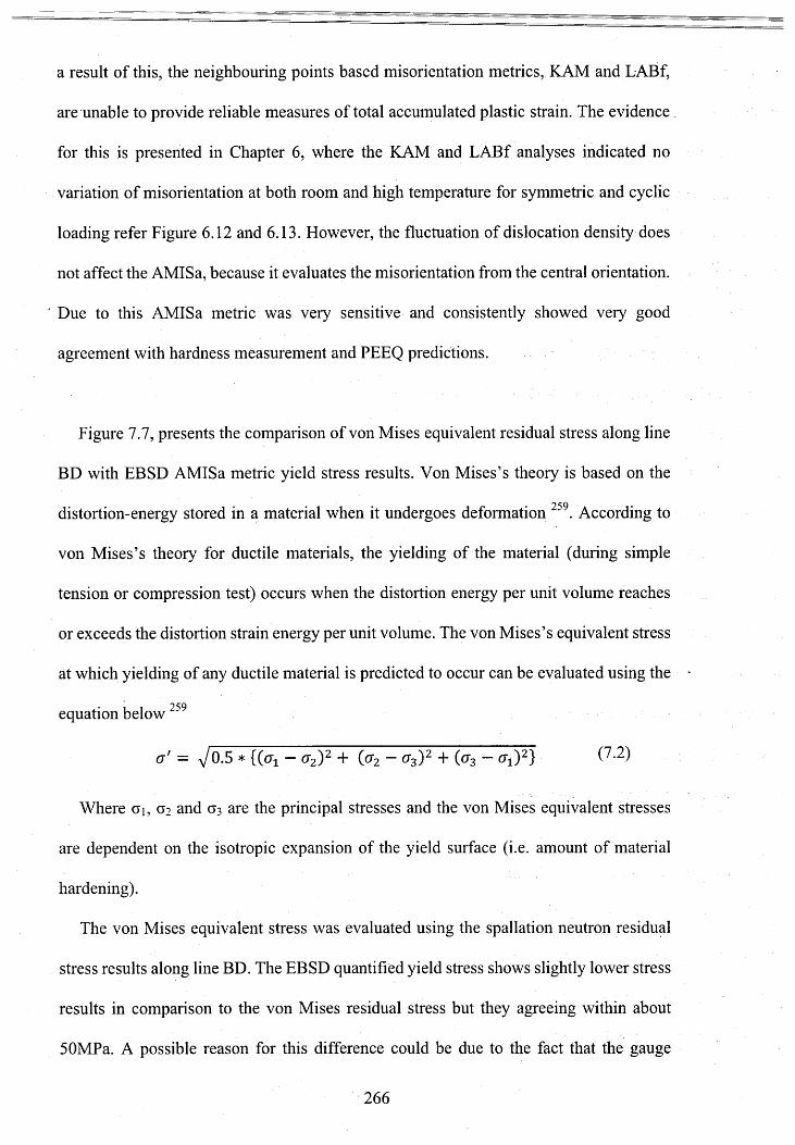
a result of this, the neighbouring points based misorientation metrics, KAM and LABf,
are unable to provide reliable measures of total accumulated plastic strain. The evidence
for this is presented in Chapter 6 , where the KAM and LABf analyses indicated no
variation of misorientation at both room and high temperature for symmetric and cyclic
loading refer Figure 6.12 and 6.13. However, the fluctuation of dislocation density does
not affect the AMISa, because it evaluates the misorientation from the central orientation.
Due to this AMISa metric was very sensitive and consistently showed very good
agreement with hardness measurement and PEEQ predictions.
Figure 7.7, presents the comparison of von Mises equivalent residual stress along line
BD with EBSD AMISa metric yield stress results. Von Mises’s theory is based on the
distortion-energy stored in a material when it undergoes deformation . According to
von Mises’s theory for ductile materials, the yielding of the material (during simple
tension or compression test) occurs when the distortion energy per unit volume reaches
or exceeds the distortion strain energy per unit volume. The von Mises’s equivalent stress
at which yielding of any ductile material is predicted to occur can be evaluated using the
9SQequation below
o' = V°-5 * (O i - o2)2 + {o2 - o3)2 + (cr3 - #1 )2} (7>2)
Where cti, 0 2 and 0 3 are the principal stresses and the von Mises equivalent stresses
are dependent on the isotropic expansion of the yield surface (i.e. amount of material
hardening).
The von Mises equivalent stress was evaluated using the spallation neutron residual
stress results along line BD. The EBSD quantified yield stress shows slightly lower stress
results in comparison to the von Mises residual stress but they agreeing within about
50MPa. A possible reason for this difference could be due to the fact that the gauge
266
volume 3><3X3 mm3 used for measuring residual stress in the neutron diffraction
experiment was higher than the selected area (1 x0.5 mm2) for EBSD analysis. As a result,
more diffracting grains were analysed in the neutron diffraction experiment.
The EBSD AMISa results constantly showed very good agreement with hardness,
PEEQ and von Mises equivalent stress. From the results (refer Figure 6.37 and Figure
7.7), it is evident that EBSD AMISa metric can quantify the accumulation of plastic strain
due to each weld pass. This means EBSD analysis can supports the NeT consortium to
improve the prediction of weld stresses and strains and the life time of the structural
components by validating the predicted results with EBSD AMISa plastic strain and yield
stress results.
267
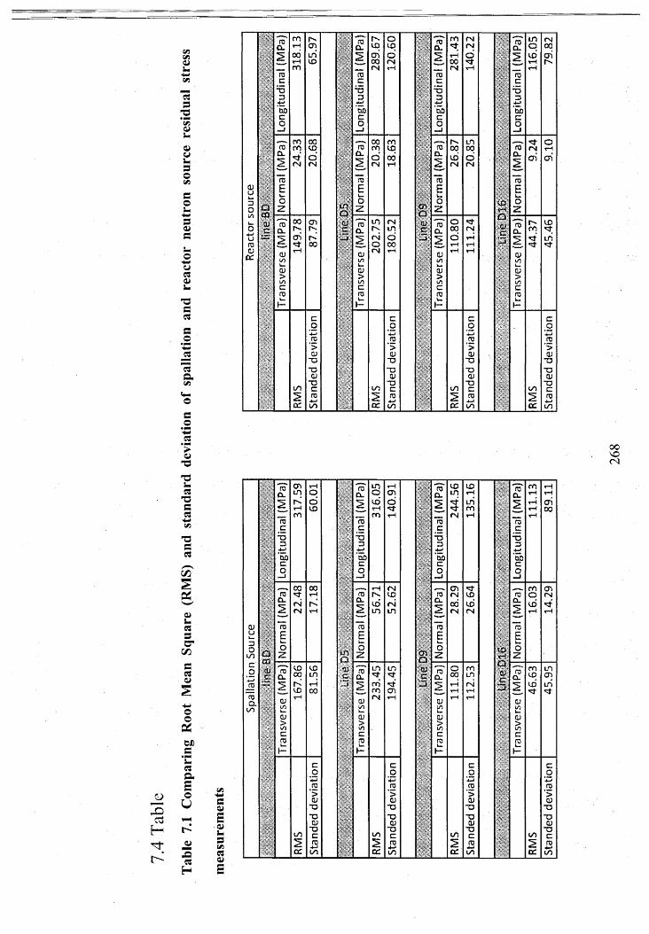
33T3•p*vs0>i-<uws«3Ovs3OL.-*->3Q3U©+*3OJU
-333
3#o*-*hJ2"3avs
03cuIX
r o
oorocTJD±;‘5bca
roEl.ozro
a .
CU>l/ScroItWt
00cri*tf
COIDdfM
I/)
IX
c.2ro>(UTJ
TJcuXcro
DC
tocx
in <No 0010 asrH rvrH
cx
oCD
3
<U73■aS.3T333
- a33
C«sDh
<us-33O ’
i/533<U
Oo0Cexs
*S3P .Eo
U
cuuL.Do
t o©o
roQ.to
<D
3c3 i-H
H ^^ £
3H
aCOoj
, c
COinKrHro
ro,ETJD
4-J
'5bco
roEoZ
tu>1/Scrol .I—
00«tf<Nrsi
to00KtorH 00
toDC
c.2rp
’>a;TJTJ0)•acro
"reT in rH "ro" to toCL o CO Cl in rH5 10rHro
orH
5 rtf«tfrsi
inrorH"ro 15.E .E=s D
4-> 4->‘5b '5bc co o—1
rH CM CO rtfro r-- to ro IN toCl
Etoin
rsiin
CL5 00tN
torN"ro ToE EL. L.o CO
no
z z*ro"CL
LO in cu "rcTCLO ro
c 00 LO5 ro rtf' 13 ■5 rH r4ro as tfpprr rH rHCU rsi rH cu rH rHto USL. l_cu CU> >to toc cro roh* d
C c.2 .240 Xjro ro'> >CU cuTJ TJTJ TJCU (UTJ to TJin C C
2 ro4-> 2 ro4-1DC to cx to
ro
t o
cx
268
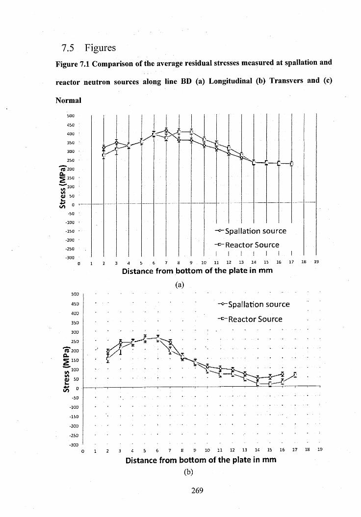
7.5 FiguresFigure 7.1 Comparison of the average residual stresses measured at spallation and
reactor neutron sources along line BD (a) Longitudinal (b) Transvers and (c)
Normal
3 0 0
(0 200 Q.
- I D G
Spallation sou rce
R eactor Source-200 '
- 3 0 0 '
0 1 2 1 3 1 4 1 5 1 6 1 7 I B7 9 10 1162 31Distance from bottom of the plate in mm
(a)5 0 3
-^ S p a lla tio n sou rce
-s -R ea c to r Source
4 5 0
ro 200 a.* 5 1 5 0
«/>103(AQ ) 5 D
-50
- 2 5 0
1 0 1 1 1 2 1 3 1 4 1 5 1 6 1 7 IB6 7 B5320Distance from bottom of the plate in mm
(b)
269
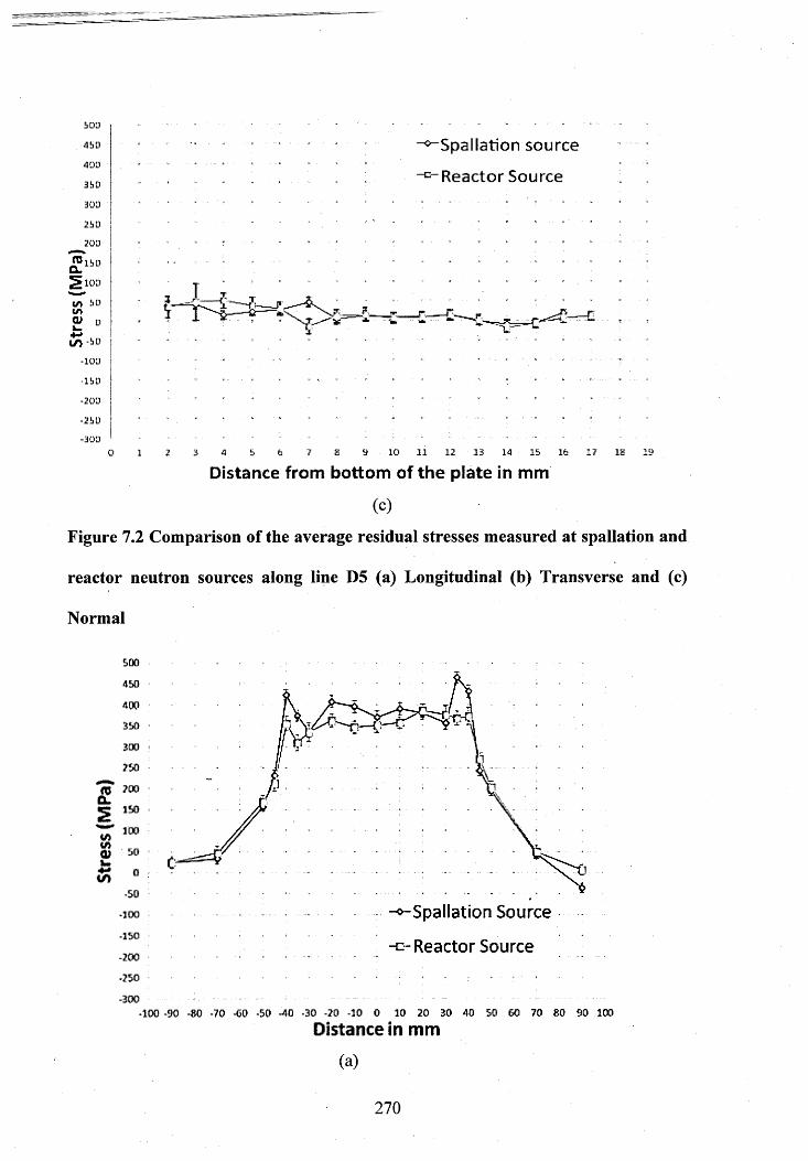
Spallation sou rce
R eactor Source
5 0 3
4 5 D
4 0 ’J
3 5 D
3 0 0
2 5 D
2013
P l5 DQ.S 10L1V\ 5 131/5a> d■*-* .I/) *5D
-1 0 1 3
- 1 5 D
-2 0 1 3
-25L 1
- 3 0 'J
0 I 2 3 4 5 6 7 £ 9 1 0 1 1 1 2 1 3 1 4 ■ 1 5 1 6 2 7 I S 1 9
Distance from bottom of the plate in mm
(c)
Figure 7.2 Comparison of the average residual stresses measured at spallation and
reactor neutron sources along line D5 (a) Longitudinal (b) Transverse and (c)
Normal
45 0
4 0 0
3 50 ■
250
CL2V) tn Q)
Spallation Source-100
-150-£> Reactor Source
-200
-250
-300■100 -90 -80 -70 -GO -5 0 -4 0 -30 -2 0 -10 0 1 0 2 0 3 0 4 0 5 0 GO 7 0 8 0 9 0 100
Distance In mm
(a)
270

Stre
ss
(MPa
)
500
Spallation Source
R eactor Source
4 5 0
4 0 0
350
300
250
200
150
100
50
0-50
-100
-150
-200
-250
-300100 -90 -80 -7 0 -60 -50 -40 -30 -20 -10 0 10 2 0 3 0 4 0 50 6 0 7 0 8 0 90 100
Distance in mm
(b)
500
-<^Spallation Source
-n- Reactor Source
4 50
4 00
3 50
300
250
100
50
0to-50
-100
-1 5 0
-200
-250
-300-1 0 0 -90 -80 -70 -60 -50 -40 -30 -2 0 -1 0 0 10 2 0 3 0 4 0 50 6 0 7 0 8 0 9 0 100
Distance in mm
(c)
271

Stre
ss
(MPa
)
Figure 7.3 Comparison of the average residual stresses measured at spallation and
reactor neutron sources along line D9 (a) Longitudinal (b) Transverse and (c)
Normal
bOO
4 5 0
4 0 0
2 0 0
200SO
^ S p a l la t io n S o u r c e
D R e a c to r S o u r c e-Ib O
-2 0 0
1GO -9 0 -SO -7 0 -6D -SO -4 0 -3 0 -2 0 -1 0 0 ID 2 0 3 0 4 0 SD 6 0 7 0 3 0 DO
D is ta n c e in m m(a)
5 0 0
"b° -^ -S p a lla t io n S o u r c e- *350 e R e a c to r S o u r c e
ro
1 0 3
I/>
- 1 0 3 ' ■vT-J 7'L-iso *
- 2 0 3 ‘
- 2 5 0 1
- 3 0 0 -------------------------------------------------------------------------------------------------------------------------------------------------------------------------1DD -DO -BD -7 0 -6 0 -5 0 -4 0 -3 0 - 2 0 -1 0 O 1 0 2 0 3D 4 0 5 0 6 0 7D UO 9 0
Distance in mm
(b)
00
103
272

-^"Spallation Source•3 CO
3ao c R e a c to r S o u r c e3 0 0 - ............................................................... ............
-ID D -3 0 -BO - 7 0 - 6 0 -5 0 - 4 0 - 3 0 - 2 0 - 1 0 D 1 0 2 0 3 0 4 0 5 0 5 0 7 0 BO 9 0 lO O
D istance in mm(C)
Figure 7.4 Comparison of the average residual stresses measured at spallation and
reactor neutron sources along line D16 (a) Longitudinal (b) Transverse and (c)
Normal
S p a lla t io n S o u r c e
R e a c to r S o u r c e
2 5 0
ICO
5 0
- 5 0
- 1 5 0
-200
- 2 5 0
.1 0 - 2 0 0 -S O -B D -7 D -5D - 5 0 - 4 0 - 3 0 - 2 0 - 1 0 0 1 0 2 0 3 0 4 0 5 0 5 0 7 0 BD 3D 1 0 0 1 1 0
D istance in m m(a)
273

S pa lla tion S o u rce
R e a c to r S o u r c e
TO 200 O.5 ISO
200m(A«u0
.00
.0-200
-110-100-30 -BG -70 -60 -SO -40 -30 -2D -ID 0 10 20 3D 40 SO 60 70 80 90 2D0 110
D istance in m m(b)
500
4b0
TOQ_
i/)tn<uto
-300
S p a lla t io n S o u r c e400
“- R e a c t o r S o u r c e
2 0 0
0-50
-200
-250
-110-100-90 -80 -70 -60 -SO -40 -3D -20 -ID 0 lO 20 3D 4D 50 60 70 80 90 2D0 11D
D istance in m m(c)
274

Figure 7.5 Schematic diagram showing stress-strain curves near HAZ of three pass
w eld63
Stress (MPa)
2nd P ass ,1st P a s s
3rd P a s s2nd P a s s
3rd P a s s
Strain3rd P a s s
1st P a s s
2nd P asi
Figure 7.6 (a) Schematic diagram of effective stress and back stress 93 (b) Effective
stress and back stress on cyclic stress-strain loops.
Yield Surface After plastic deformation
Back Stress
Initial Yield Surface
(a)
275
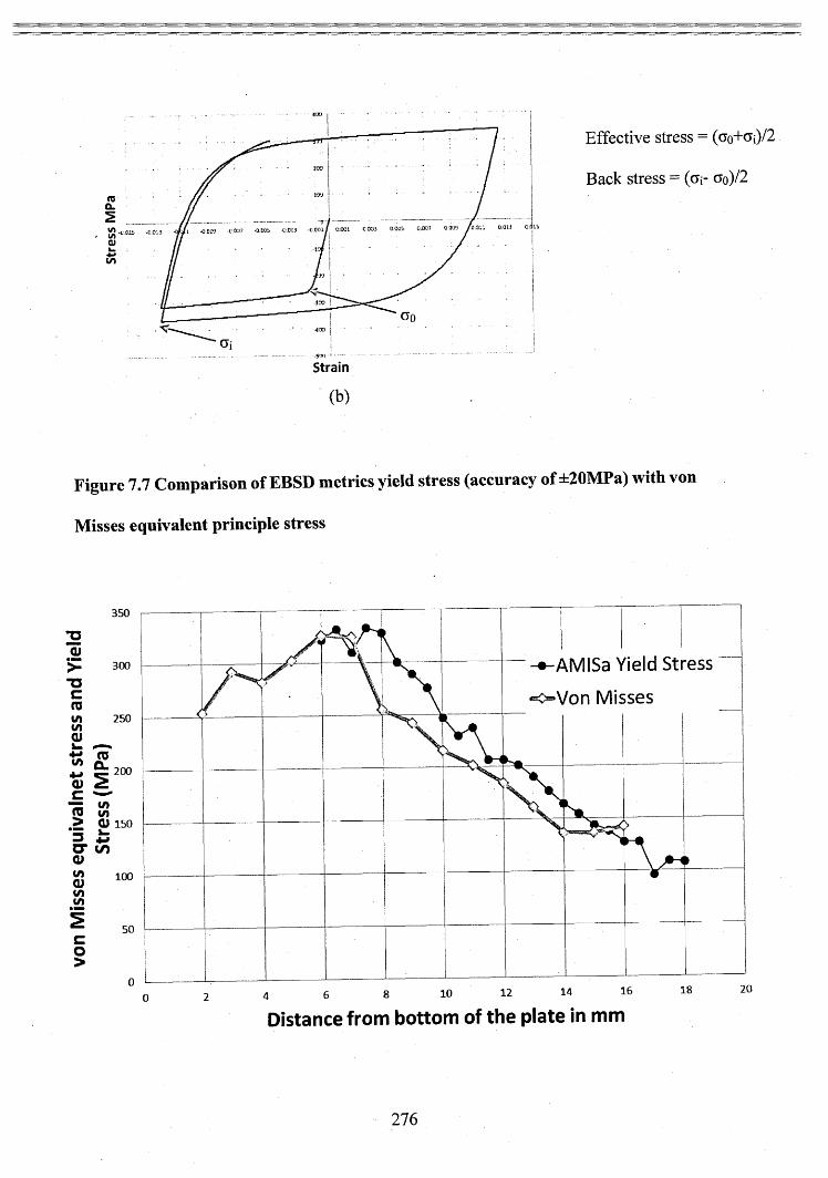
Strain
(b)
Figure 7.7 Comparison of EBSD metrics yield stress (accuracy of ±20MPa) with von
Misses equivalent principle stress
3 5 0
-•-A M IS a Yield S tress "
« o V o n M isse s
3 0 0
2 5 0inin
m n .“ 200
— in JO i/i > <U 1 5 0
g . 4=o* i/>m 100
5 0
0 201 81 614121086420Distance from bottom of the plate in mm
276

C h a p t e r 8 . C o n c l u s i o n s a n d F u r t h e r W o r k
This chapter draws conclusions from the investigations reported in this thesis and
recommends further work. The project has researched the residual stress distribution and
accumulated plastic strain in a benchmark welded AISI316L(N) austenitic stainless steel
plate and studied the strain hardening behaviour of the plate material under symmetric
and asymmetric cyclic loading, with different strain ranges and strain rates.
8.1 Conclusions
In the first part of this study (Chapter 4), the residual stress distribution in a three-pass
welded austenitic stainless steel plate was measured using neutron diffractometers at two
spallation sources (VULCAN at SNS and ENGIN-X at the ISIS Facility). The objective
of this work is to identify all the issues affecting the reliability of residual stress
characterization in the NeT-TG4 weldment. The following conclusions were reached:
M aterial Issues
1. According to the neutron diffraction standards and recommendations 135 by
Webster, stress free cuboids should be extracted from the original sample or an identical
sample. This is to minimize additional uncertainties developing due to using the wrong
stress free lattice parameter in residual stress evaluation. However, the stress cuboids
extracted from the weld trial plate 2-IB may not be identical to the analysed three pass
benchmark plate.
277
Experimental Issues
2. One of the potential issues contributing in systematic difference in measured
residual stress is due to large difference in measured lattice parameter between Bank 2 of
ENGIN-X and VULCAN. This differences is possibly associated with the one of the
detector components. Further investigation is required to identify, whether the cause of
this problem is due to some technical issues associated with instrument detector or
something else.
3. In addition to the measured lattice parameter variation, another main contribution
to generating pseudo strains is due to the presence of crevices, super glue and misfit
between the individual elements of the stress free cuboid. This leads to significant
difference in the measured residual stress.
Residual stress measurements
4. The highest tensile stresses were observed in the first pass weld metal (line D5)
and the heat-affected zone (line BD) at a magnitude of 400- 450 MPa.
5. The residual stress analysis was performed at different depths of the welded
benchmark plate with respect to weld bead at VULCAN and ENGIN-X neutron
diffractometers. Many of the residual stress results measured at different depths in the
various sets (i.e. Line BD, D2, D5, D9, D16, B2 and B16) of the welded plate were
observed to differ within ±100 MPa.
6 . The residual stress measurements results from ENGIN-X and VULCAN neutron
diffractometers are comparable (±50 MPa) with those measurements carried out by others
at FRM-II, HZB reactor source diffractometers.
In the second part of this research study (Chapter 5), the isothermal strain hardening
behaviour of solution annealed 316L material, during symmetric and asymmetric cyclic
loading, was measured and compared with predicted behaviour based upon a mixed
278

hardening model previously used for weld residual stress modelling. The objective of this
part is to investigate the magnitude of the possible errors arising from ignoring the strain
rate effects and input parameters which are evaluated from symmetric (tensile-
compressive) cyclic deformation testing for mixed hardening model. The following
conclusions were made:
7. The strain hardening of the solution annealed 316L(N) base plate material varied
according to whether symmetric or asymmetric cyclic loading was applied. Asymmetric
cyclic loading introduced, 50 MPa less strain hardening at room and high temperature
respectively than symmetric cyclic loading. As asymmetric cyclic loading more closely
represents material deformation around welds, it is recommended that the mixed
hardening parameters for weld residual stress hardening models should be derived from
asymmetric cyclic loading rather symmetric cyclic loading data.
8 . The strain rate of cyclic tests was found to affect the yield stress and rate of
hardening (50MPa at room and high temperature respectively) and therefore should be
accounted for in deriving mixed hardening parameters for weld residual stress hardening
models.
9. A mixed hardening model has previously been used for predicting residual
stresses in the NeT TG4 benchmark weldment. In the present work (Chapter 5), the same
reproduced model under predicted the measured cyclic strain-stress loops at high
temperature (by 65MPa). Therefore, there is a need to develop improved models based
upon more representative thermo-mechanical fatigue test data.
In the final part of this thesis (Chapter 6 ), the accumulation of plastic strain in parent
material surrounding single pass, two pass and three pass welds was investigated using
EBSD metrics and hardness mapping. In addition, the accumulated plastic strain
following symmetric and asymmetric cyclic loading was studied, at different strain ranges
279

and strain rates, at both room and high temperature. The objective, of this study is to
demonstrate whether EBSD can quantify accumulated plastic strain resulting from one,
two and three pass weld deposits in 316L(N) steel using different EBSD metrics. The
following conclusions were reached from these experimental studies:
10. Different EBSD metrics (KAM, LABf and AMISa) showed a similar trend of
increasing plastic strain from the bottom of the plate to the weld fusion boundary but of
different magnitudes.
11. Results from the AMISa metric and hardness measurements were in good
agreement with each other and could be used to validate finite element plastic strain
predictions in weld residual stress simulations.
12. The assessment of accumulated plastic strain due to symmetric and asymmetric
cyclic loading was analysed using the EBSD metrics KAM, LABf and AMISa. The
results show that the KAM and LABf metrics are insensitive to the accumulated plastic
strain at the end of each cycle under both room and high temperature cyclic loading.
AMISa metric was unable to assess the accumulated cyclic plastic strain up to 36%.
However, after 36% accumulated cyclic plastic strain, the AMISa metric showed the
accumulated misorientati on.
13. EBSD can quantify the accumulated plastic strain around welds using the AMISa
metric but not with KAM or LABf metric.
8.2 Suggested future work
This research project has identified issues affecting the reliability of residual stress
distribution results from neutron diffraction experiments. However, some key questions
require further research. For example, from the literature review 140>l41»151j it was clearly
evident that the extraction of, and the geometry of, the ‘stress free’ lattice sample, has
280
some significant consequence in determining the reliability of residual stress
measurements. Therefore, further research is required to understand the influence that the
geometry of stress free samples has in determining the residual stress.
Due to limitations in the supply of material, the accumulated plastic strain in the weld
itself metal was not quantified in this project. The deformation of the grains, the grain
size and the texture of weld metal is different from the base metal. In order to quantify
the accumulated plastic strain, a misorientation calibration curve evaluated from the weld
sample, at high temperature, is required.
In the real world, most of the time austenitic stainless steel, and other metals, undergo
asymmetric cyclic loading during service. For example, pipelines on the seabed undergo
complex asymmetric deformation, due to changes in environmental conditions. Similarly,
component materials , in power plants undergo asymmetric cyclic deformation due to
fluctuations in energy demands and environmental changes. For the first time, this
research study has investigated material strain hardening behavior during asymmetric
cyclic loading, at different strain ranges and strain rates, as well as providing an
assessment of accumulated plastic strain using EBSD and hardness testing. However,
dislocation structures and their role during asymmetric cyclic loading, was not analysed
using TEM. TEM examination would give the enhanced knowledge of dislocation
structure, fatigue life, fatigue crack propagation, etc., and will give better understanding
of materia] behaviour at different strain ranges and strain rates.
This project has analysed strain hardening of 316L material during asymmetric cyclic
loading, under strain controlled conditions. It would be interesting to extend this study to
understand the behaviour of materials during strain controlled ratcheting, and include an
analysis of dislocation structure, fatigue life, microstructure changes and crack
propagation.
281

R e f e r e n c e s
1. M.McGuire. Austenitic Stainless Steel. In: Stainless Steels For Design Engineers.Vol Ohio: ASM International; 2008.http://www.google.com/patents?hl=en&lr=&vid=USPAT3306736&id=0pxzAA AAEBAJ&oi=fnd&dq=Austenitic+Stainless+Steels&printsec=abstract. Accessed November 1, 2013.
2. ISO 9692-1:2013. Welding and Allied Processes - Types of Joint Preparation ~ Part 1: Manual Metal Arc Welding, Gas-Shielded Metal Arc Welding, Gas Welding, TIG Welding and Beam Welding of Steels.http://www.iso.org/iso/home/store/catalogue_tc/catalogue_detail.htm?csnumber=62520. Accessed March 13, 2015.
3. Kou S. Welding Metallurgy. Vol Second Edi. Wiley Interscience; 2002.
4. Bouchard PJ. Residual Stresses in Lifetime and Structural Integrity Assessment. In: Science and Technology. V o l; 2001:8134.
5. Ohms C, Neov D, Wimpory RC, Youtsos AG. Evaluation of Novel Post Weld Heat Treatment in Ferritic Steel Repair Welds Based on Neutron Diffraction. In: Gdoutos EE, ed. PROCEEDINGS OF THE EUROPEAN CONFERENCE ON FRACTURE. Vol European conference on fracture; Fracture of nano and engineering materials and structures. Dordrecht, Springer; 2006:1307-1308.http://libezproxy.open.ac.Uk/login7urHittp://search.ebscohost.com/login.aspx7direct=true&db=edsbl&AN=CN067270720&site=eds-live&scope=site.
6. Zinkle SJ, Was GS. Materials challenges in nuclear energy. Acta Materialia. 2013;61(3):735-758.doi:10.1016/j.actamat.2012.11.004.
7. Withers PJ. Residual stress and its role in failure. Reports on Progress in Physics. 2007;70:2211-2264. doi:10.1088/0034-4885/70/12/R04.
8. McGuire MF. Austenitic Stainless Steels. In: Materials Science and Technology. Vol 45. ; 2001:406-411.
9. Jiang W, Luo Y, Zhang G, Woo W, Tu ST. Experimental to study the effect of multiple weld-repairs on microstructure, hardness and residual stress for a stainless steel clad plate. Materials & Design. 2013;51 (0): 1052-1059. doi:http://dx.doi.org/10.1016/j.matdes.2013.05.027.
10. Li GF, Congleton J. Stress corrosion cracking of a low alloy steel to stainless steel transition weld in PWR primary waters at 292°C. Corrosion Science. 2000;42(6): 1005-1021. doi: 10.1016/S0010-938X(99)00131-6.
11. Cheng X, Prask HJ, Gnaeupel-herold T, Luzin V, Fisher JW. Neutron Diffraction Measurements for Residual Stresses in AL-6XN Stainless Steel Welded Beams.
282

12. Dong P. Recommendations for determining residual stresses in fitness-for-service applications. Welding Research Council Bulletin. 2002;(476): 1 -61.
13. Rathbun HJ, Fredette LF, Scott PM, Csontos A a, Rudland DL. NRC Welding Residual Stress Validation Program International Round Robin Program and Findings. In: Pressure Vessels and Piping Conference. V o l; 2011:1-7.
14. Dong P, Hong JK. Analysis of IIW.X/XV RSDP Phase I Round-Robin Residual Stress Results. Welding Research Abroad. 2003;49:1-8. http://libezproxy.open.ac.uk/login?url=http://search.ebscohost.com/login.aspx?di rect=true&db=edsbl&AN=RNl 34329977&site=eds-live&scope=site.
15. Ohms C, Martins R V, Youtsos AG, et al. The Europen Network on Neutron Techniques Standardization for Structural Integrity-NET. In: 2008 ASMEPressure Vessels and Piping Division Conference. Vol Chicago, Illinois: PVP; 2008:1-13.
16. Smith MC, Smith AC, Wimpory R, Ohms C. A review of the NeT Task Group 1 residual stress measurement and analysis round robin on a single weld bead-on- plate specimen. International Journal of Pressure Vessels and Piping. 2014; 120- 121:93-140.
17. Bouchard PJ. Experimental Validation for Multi Pass Weld Residual Stress Predictions. Bamwood Glasgow; 1997.
18. Bouchard PJ. Validated residual stress profiles for fracture assessments of stainless steel pipe girth welds. International Journal of Pressure Vessels and Piping. 2007;84(4): 195-222. doi: 10.1016/j.ijpvp.2006.10.006.
19. Withers PJ, Turski M, Edwards L, Bouchard PJ, Buttle DJ. Recent advances in residual stress measurement. International Journal of Pressure Vessels and Piping. 2008;85(3):118-127. doi:10.1016/j.ijpvp.2007.10.007.
20. Bouchard PJ, Withers PJ. The Appropriateness of Residual Stress Length Scales in Structural Integrity. Journal of Neutron Research. 2004;12(1): 1-3.
21. Smith MC, Muransky O, Austin C, Park B, Bendeich PJ, Edwards Optimised Modelling of Weld Metal Constitutive Behaviour In the NeT TG4/International Weld Simulation and Measurment bechmark. In: Pressure Vessels and Piping Conference. Vol PVP2012-78. ; 2012:1-13.
22. Muransky O, Hamelin CJ, Smith MC, Bendeich PJ, Edwards L. The effect of plasticity theory on predicted residual stress fields in numerical weld analyses. Computational Materials Science. 2012;54:125-134.doi: 10.1016/j.commatsci.2011.10.026.
23. Smith MC. Validation of Mixed Isotropic-Kinematic Material Hardening Models for Finite Element Prediction of Residual Stresses in A ustenitic Steel Welds.; 2007.
283
24. Smith MC, Bouchard PJ, Turski M, Edwards L, Dennis RJ. Accurate prediction of residual stress in stainless steel welds. Computational Materials Science. 2012;54:312-328. doi: 10.1016/j.commatsci.2011.10.024.
25. Smith MC, Bate S, Bouchard PJ. SIMPLE BENCHMARK PROBLEMS FOR FINITE ELEMENT WELD RESIDUAL. In: Pressure Vessels and Piping Conference. V o l; 2013:1-15.
26. Chandra SK, Shankar V, Mariappan K, Sandhya R, Chakraborty PC. Effect of Strain Rate on the Low Cycle Fatigue Behavior of 316L(N) Stainless Steel Weld Joints. 6th International Conference on Creep, Fatigue and Creep Fatigue Interaction. 2013;55:176-180. doi: 10.1016/j.proeng.20,13.03.239.
27. Pham MS, Holdsworth SR. Role of microstructural condition on fatigue damage development of AISI 316L at 20 and 300°C. International Journal of Fatigue. 2013;51:36-48. doi: 10.1016/j.ijfatigue.2013.02.005.
28. Puchi Cabrera ES. High temperature deformation of 316L stainless steel. Materials Science and Technology. 2001; 17(February): 155-161.
29. Lindgren L-E, Domkin K, Hansson S. Dislocations, vacancies and solute diffusion in physical based plasticity model for AISI 316L. Mechanics of Materials. 2008;40(11):907-919. doi: 10.1016/j.mechmat.2008.05.005.
30. Katayama Y, Tsubota M, Saito Y. Effect of the plastic strain level quantified by EBSP method on the stress corrosion cracking of L-grade stainless steels. In: 12th International Conference on Environmental Degradation of Materials in Nuclear Power System- Water Reactors-TMS. V o l; 2005.
31. Lu Z, Shoji T, Meng F, et al. Characterization of microstructure and local deformation in 316NG weld heat-affected zone and stress corrosion cracking in high temperature water. Corrosion Science. 2011;53(5):1916-1932. doi: 10.1016/j.corsci.2011.02.009.
32. Wright SI, Nowell MM, Field DP. A Review of Strain Analysis Using Electron Backscatter Diffraction. Microscopy and Microanalysis. 2011; 17(03):316-329. href="http://dx.doi.org/10.1017/S 1431927611000055.
3 3. Wright S. A pplications ofEBSD in Materials Research for Nuclear Energy>.; 2008.
34. Easterling K. Fusion welding-process variables. In: Introduction to the Physical Metallurgy’ of Welding. V o l; 1985:1-47.
35. Krauss G. STEELS Processing, Structure and Performance. ASM International; 2005.
36. Pickering FB. Physical Metallurgy of Stainless Steel Developments. InternationalMaterials Reviews; 1976.http://books.google.co.uk/books/about/Physical_Metallurgy_of_Stainless_Steel_ D.html?id=6AcnngEACAAJ&pgis=l. Accessed March 1, 2015.
284
37. Kutz M. Handbook of Materials Selection. John Wiley & Sons; 2002. http://eu.wiley.com/WileyCDA/WileyTitle/productCd-0471359246.html. Accessed June 11, 2015.
38. Cobb HM. The History of Stainless steel. In: ASM International. V o l; 2010:375. doi: 10.1016/S0026-0657( 10)80254-1.
39. Hull D. Introduction to Dislocations. Elsevier; 2011. doi:10.1016/B978-0-08- 096672-4.00001-3.
40. Vitos L, Nilsson J-O, Johansson B. Alloying effects on the stacking fault energy in austenitic stainless steels from first-principles theory. Acta Materialia. 2006;54(14):3821-3826. doi:10.1016/j.actamat.2006.04.013.
41. Lu S, Hu Q-M, Johansson B, Vitos L. Stacking fault energies of Mn, Co and Nb alloyed austenitic stainless steels. Acta Materialia. 2011;59(14):5728-5734. doi: 10.1016/j. actamat.2011.05.049.
42. Rosenthal D. Mathematical theory of heat distribution during welding and cutting. Welding journal. 1941:220 - s - 234 - s.http://scholar.google.com/scholar?hl=en&btnG=Search&q=intitle:Mathematical+ theory+of+heat+distribution+during+welding+and+cutting#0.
43. Goldak J, Chakravarti A, Bibby M. A new finite element model for welding heat sources. Metallurgical Transactions B. 1984;15B:299-305. doi:10.1007/BF02667333.
44. Chen BQ, Adak M, Soares CG. Numerical investigations to study the effect of weld parameters on the temperature-time history in steel plates. In: 1st International Conference on Maritime Technology and Engineering. Vol ; 2011:285-292.
45. Mahapatra MM, Datta GL, Pradhan B. Three-Dimensional Finite ElementAnalysis to Predict the Effects of Shielded Metal Arc Welding Process Parameters on Temperature Distributions and Weldment Zones in Butt and One-Sided Fillet Welds. In: Proceedings of the Institution ofMechanical Engineers, Part B: Journal of Engineering Manufacture. Vol 220. ; 2006:837-845.doi: 10.1243/09544054JEM371.
46. Bouchard PJ. The NeT bead-on-plate benchmark for weld residual stresssimulation. International Journal of Pressure Vessels and Piping. 2009;86(1):31- 42. doi: 10.1016/j.ijpvp.2008.11.019.
47. Lippold JC, Kotecki DJ. Welding Metallurgy and Weldability of Stainless Steels - John C. Lippold, Damian J. Kotecki. Wley; 2005. http://eu.wiley.com/WileyCDA/WileyTitle/productCd-0471473790.html. Accessed March 13, 2014.
48. Rajasekhar K, Harendranath CS, Raman R, Kulkami SD. Microstructuralevolution during solidification of austenitic stainless steel weld metals: A color
285

metallographic and electron, microprobe analysis study: MaterialsCharacterization. 1997;38(2):53-65. doi: 10.1016/S 1044-5803(97)80024-1.
49. Unnikrishnan R, Idury KSNS, Ismail TP, et al. Effect of heat input on the microstructure, residual stresses and corrosion resistance of 304L austenitic stainless steel weldments. Materials Characterization. 2014;93:10-23. doi: 10.1016/j .matchar.2014.03.013.
50. Alipooramirabad H, Paradowska A, Ghomashchi R, Kotousov A, Reid M. Quantification of residual stresses in multi-pass welds using neutron diffraction. Journal of Materials Processing Technology’. 2015;226:40-49. doi: 10.1016/j .jmatprotec.2015.07.002.
51. Kumar S, Shahi AS. Effect of heat input on the microstructure and mechanical properties of gas tungsten arc welded AISI 304 stainless steel joints. Materials & Design. 2011;32(6):3617-3623. doi: 10.1016/j.matdes.2011.02.017.
52. Hill H. Chloride stress corrosion cracking in austenitic stainless steel RR902 Chloride stress corrosion cracking in austenitic stainless steel. 2011:62.
53. Noyan I., Cohen J. Residual stress - measurement by diffraction and interpretation. In: Ciystal Research and Technology. Vol 24. ; 1989:K37-K37.doi: 10.1002/crat.2170240228.
54. Dong P, Hong JK, Bouchard PJ. Analysis of residual stresses at weld repairs. In: International Journal of Pressure Vessels and Piping. Vol 82. ; 2005:258-269. doi: 10.1016/j.ijpvp.2004.08.004.
55. Elcoate CD, Dennis RJ, Bouchard PJ, Smith MC. Three dimensional multi-pass repair weld simulations. In: International Journal of Pressure Vessels and Piping. Vol 82.; 2005:244-257. doi:10.1016/j.ijpvp.2004.08.003.
56. Paradowska AM, Price JWH, Ibrahim R, Finlay son TR. The effect of heat input on residual stress distribution of steel welds measured by neutron diffraction. Journal of Achievements in materials and manufacturing engineering. 2006; 17(1- 2):385-388.
57. Muransky O, Smith M, Bendeich PJ, et al. Comprehensive numerical analysis of a three-pass bead-in-slot weld and its critical validation using neutron and synchrotron diffraction residual stress measurements. International Journal of Solids and Structures. 2012;49(9):1045-1062. doi: 10.1016/j.ijsolstr.2011.07.006.
58. Murugan S, Rai SK, Kumar P., Jayakumar T, Raj B, Bose MS. Temperature distribution and residual stresses due to multipass welding in type 304 stainless steel and low carbon steel weld pads. In: International Journal of Pressure Vessels and Piping. Vol 78.; 2001:307-317. doi: 10.1016/S0308-0161 (01)00047-3.
59. Woo W, An GB, Kingston EJ, DeWald a. T, Smith DJ, Hill MR. Throughthickness distributions of residual stresses in two extreme heat-input thick welds:
286

A neutron diffraction, contour method and deep hole drilling study. Acta Materialia. 2013;61(10):3564-3574.doi: 10.1016/j.actamat.2013.02.034.
60. Smith MG, Smith AC. Report Generic NeT Task Group 1 Single Weld Bead on Plate: Review ofPhase 1 Weld Simulation Round Robin.; 2006.
61. Ficquet X, Smith DJ, Truman CE, Kingston EJ, Dennis RJ. Measurement and prediction of residual stress in a bead-on-plate weld benchmark specimen. In: International Journal of Pressure Vessels and Piping. Vol 86. Elsevier Ltd; 2009:20-30. doi:10.1016/j.ijpvp.2008.11.008.
62. Smith MC, Smith AC. NeT bead-on-plate round robin: Comparison of residual stress predictions and measurements. International Journal of Pressure Vessels and Piping. 2009;86(1): 79-95. doi: 10.1016/j.ijpvp.2008.11.017.
63. Smith MC. Report Hartlepool and Hey sham I Power Stations Development of Mixed Isotropic-Kinematic Material Hardening Models for Finite Element Simulation of Austenitic Steel Welds.; 2006.
64. Truman CE, Smith MC. The NeT residual stress measurement and modelling round robin on a single weld bead-on-plate specimen. International Journal of Pressure Vessels and Piping. 2009;86( 1): 1 -2. doi: 10.1016/j .ijpvp.2008.11.018.
65. Smith DJ, Bouchard PJ, George D. Measurement and prediction of residual stresses in thick-section steel welds. In: The Journal of Strain Analysis for Engineering Design. Vol 35.; 2000:287-305. doi.T 0.1243/0309324001514422.
66. Pratihar S, Turski M, Edwards L, Bouchard PJ. Neutron diffraction residual stress measurements in a 316L stainless steel bead-on-plate weld specimen. International Journal of Pressure Vessels and Piping. 2009;86(1): 13-19. doi: 10.1016/j. ijpvp.2008.11.010.
67. Cottrell A. Dislocations and Plastic Flow in Crystals.; 1953.doi: 10.1126/science. 119.3095.551.
68. Orowan EZK. Tieftemperaturplastizitiit und Beckersche Fomiel. Zeitschrift fur Phvsik A Hadrons and Nuclei. 1934;89:605.
69. Wei H, Wei Y. Interaction between a screw dislocation and stacking faults in FCC metals. Materials Science and Engineering A. 2012;541:38-44. doi:10.1016/j.msea.2012.01.115.
70. Kocks UF, Mecking H. Physics and phenomenology of strain hardening: The FCC case. Progress in Materials Science. 2003;48:171-273. doi:10.1016/S0079- 6425(02)00003-8.
71. Cottrell AH. LX. The formation of immobile dislocations during slip. The London, Edinburgh, and Dublin Philosophical Magazine and Journal of Science. 2010;43(341):645-647.doi:10.1080/14786440608520220.
287

72. Hirth JP. On Dislocation Interactions in the fccXattice: Journal ofApplied Physics <1961 ;32(4):700. doi: 10.1063/1.1736074.
73. Essmann U, Mughrabi H. Annihilation of dislocations during tensile and cyclic deformation and limits of dislocation densities. Philosophical Magazine A. 1979;40(February 2015):731-756. doi: 10.1080/01418617908234871.
74. Nabarro FRN. Distribution of solute atoms round a moving dislocation. Materials Science & Engineering A. 2005;400-401:22-24. doi:10.1016/j.msea.2005.03.046.
75. Mesarovic SD. Dynamic Strain Aging And Plastic Instablities. Mechanics and Physics of Solids. 1995;43(5):671-700.
76. Aboulfadl H, Deges J, Choi P, Raabe D. Dynamic strain aging studied at the atomic scale. Acta Materialia. 2015;86:34-42. doi:10.1016/j.actamat.2014.12.028.
77. Leslie WC. The Physical Metallurgy of Steels. Hempisphere Pub. Corp.; 1981. http://books.google.co.uk/books/about/The_physical_metallurgy_of_steels.html7i d=Q45TAAAAMAAJ&pgis=l. Accessed February 19, 2015.
78. Hong S-G, Lee S-B. Mechanism of dynamic strain aging and characterization of its effect on the low-cycle fatigue behavior in type 316L stainless steel. Journal of Nuclear Materials. 2005;340(2-3):307-314. doi:10.1016/j.jnucmat.2004.12.012.
79. Blanc D, Strudel JL. Strength of Metals and Alloys (ICSMA 7). Elsevier; 1985. doi: 10.1016/B978-0-08-031642-0.50065-9.
80. Samuel K., Mamian S., Rodriguez P. Serrated yielding in AISI 316 stainless steel. Acta Metallurgica. 1988;36(8):2323-2327. doi: 10.1016/0001-6160(88)90331 -8.
81. Kim DW, Ryu W-S, Hong JH, Choi S-K. Effect of nitrogen on high temperature low cycle fatigue behaviors in type 316L stainless steel. Journal of Nuclear Materials. 1998;254:226-233. doi: 10.1016/S0022-3115(97)00360-7.
82. Smallman R., Ngan AH. Modern Physical Metallurgy. Vol Eighth Edi. Elsevier;2014.
83. Asano S, Oshima K. Effect of Plastic Deformation on the Hydrogen-InducedInternal Friction Peak in Austenitic Stainless Steel. Transactions of the Japan Institute of Metals. 1982;23(9):530-534.http://www.jim.or .jp/joumal/e/pdf3/23/09/530.pdf.
84. Snoek JL. Effect of small quantities of carbon and nitrogen on the elastic and plastic properties of iron. Physica. 1941 ;8(7):711-733. doi:http://dx.doi.org/10.1016/S0031-8914(41)90517-7.
85. Prasad Reddy GV, Sandhya R, Bhanu Sankara Rao K, Sankaran S. Influence of nitrogen alloying on dynamic strain ageing regimes in low cycle fatigue of AISI 316LN stainless steel. Procedia Engineering. 2010;2(1):2181-2188. doi: 10.1016/j .proeng.2010.03.234.
288

86. Paul SKj Sivaprasad S, Dhar S, Tarafder S. Key issues in cyclic plastic deformation: Experimentation. Mechanics of Materials. 2011 ;43(11 ):705-720. doi: 10.1016/j .mechmat.2011.07.011.
87. Li P, Li SX, Wang ZG, Zhang ZF. Fundamental factors on formation mechanism of dislocation arrangements in cyclically deformed fee single crystals. Progress in Materials Science. 201 l;56(December 2010):328-377.doi: 10.1016/j.pmatsci.2010.12.001.
88. Feltner C., Laird C. Cyclic stress-strain response of F.C.C. metals and alloys—I. Phenomenological experiments. Acta Metallurgica. 1967; 15(10): 1621-1632. doi: 10.1016/0001 -6160(67)90
89. Feltner CL, Laird C. Cyclic stress-strain response of F.C.C. metals and alloys—II Dislocation structures and mechanisms. Acta Metallurgica. 1967; 15( 10): 1633- 1653. doi: 10.1016/0001-6160(67)90138-1.
90. Mughrabi H. Fatigue, an everlasting materials problem - still en vogue. Procedia Engineering. 2010;2( 1 ):3-26. doi: 10.1016/j.proeng.2010.03.003.
91. Grosskreutz J. Fatigue mechanism in the sub-creep range. In: Manson S., ed. Metal Fatigue Damage. Vol ASTM; 1971:5.
92. Schramm RE, Reed RP. Stacking fault energies of seven commercial austenitic stainless steels. Metallurgical Transactions A. 1975;6(7): 1345-1351. doi: 10.1007/BF02641927.
93. Pham M. Fatigue Behaviour Of AISI316L: Mechanical response , Microstructural evolution, Fatigue crack propagation, & Physically-based constitutive modelling. 2013;(20864).
94. Mughrabi H. Dislocation in Fatigue. In: Dislocations and Properties of Real Materials. V o l; 1985:244-262.
95. Kuhlmann-Wilsdorf D, Laird C. Dislocation behavior in fatigue. Materials Science and Engineering. 1977;27(2): 137-156. doi: 10.1016/0025-5416(77)90166-5.
96. Obrtlik K, Kruml T, Polak J. Dislocation structures in 316L stainless steel cycled with plastic strain amplitudes over a wide interval. Materials Science and Engineering: A. 1994; 187(1): 1-9. doi: 10.1016/0921 -5093(94)90325-5.
97. Li Y, Laird C. Cyclic response and dislocation structures of AISI 316L stainless steel. Part 2: polycrystals fatigued at intermediate strain amplitude. Materials Science and Engineering: A. 1994; 186(l-2):87-103. doi: 10.1016/0921-5093(94)90307-7.
98. Li Y, Laird C. Cyclic response and dislocation structures of AISI 316L stainless steel. Part 1: single crystals fatigued at intermediate strain amplitude. Materials Science and Engineering: A. 1994; 186(1-2):65-86. doi: 10.1016/0921-5093(94)90306-9.
289
99. Basinski ZS, Basinski SJ. Fundamental aspects of low amplitude cyclic deformation in face-centred cubiccrystals. Progress in Materials, Science. 1992;36:89-148. doi:10.1016/0079-6425(92)90006-S.
100. Hong S-G, Lee S-B. The tensile and low-cycle fatigue behavior of cold worked 316L stainless steel: influence of dynamic strain aging. International Journal of Fatigue. 2004;26(8):899-910. doi: 10.1016/j.ijfatigue.2003.12.002.
101. Pham MS, Holdsworth SR. Dynamic strain ageing of AISI 316L during cyclic loading at 300°C: Mechanism, evolution, and its effects. Materials Science and Engineering: A. 2012;556:122-133. doi:10.1016/j.msea.2012.06.067.
102. Ivanchenko M. Dynamic Strain Aging of Austenitic Stainless Steels and Ni Base Alloys. 2010. http://lib.tkk.fi/Diss/2010/isbn9789526034454.
103. Calmunger M. High-Temperature Behaviour of Austenitic Alloys. 2013;(1619).
104. Gerland M, Alain R, Ait Saadi B, Mendez J. Low cycle fatigue behaviour in vacuum of a 316L-type austenitic stainless steel between 20 and 600°C—-Part II: Dislocation structure evolution and correlation with cyclic behaviour. Materials Science and Engineering: A. 1997;229(l-2):68-86. doi: 10.1016/S0921- 5093(96)10560-8.
105. Gerland M, Mendez J, Violan P, Ait Saadi B. Evolution of disloction structures and cyclic behaviour of a 3 16L type austenitic stainless steel cycled in vacume at room temperature. Materials Science and Engineering. 1989;A118:83-95.
106. Hong S-G, Lee S-B, Byun T-S. Temperature effect on the low-cycle fatigue behavior of type 316L stainless steel: Cyclic non-stabilization and an invariable fatigue parameter. Materials Science and Engineering: A. 2007;457(l-2): 139-147. doi: 10.1016/j.msea.2006.12.035.
107. Srinivasan V. Comparative evaluation of strain controlled low cycle fatigue behaviour of solution annealed and prior cold worked 316L(N) stainless steel. International Journal of Fatigue. 2004;26(12): 1295-1302. doi:10.1016/j.ijfatigue.2004.05.003.
108. Lemaitre J, Chaboche J-L. Mechanics of Solid Materials. Cambridge University Press; 1999.
109. Chaboche JL. A review of some plasticity and viscoplasticity constitutive theories. International Journal of Plasticity. 2008;24( 10): 1642-1693. doi: 10.1016/j.ijplas.2008.03.009,
110. Abaqus 6.12. ABAQUS analysis user’s manual.
111. Muransky O, Bendeich PJ, Smith MC, Kristein O, Edwards L, Holden TM. Analysis of Residual Stresses in Three-Pass Slot Weld (NeT-TG4): Finite Element Modelling and Neutron Diffraction. In: Pressure Vessels and Piping Conference. Vol; 2010:1-7.
290
112. Withers PJ, Bhadeshia HKDH. Residual stress Part 1 - Measurement techniques. Material Science and Technology. 2001;17(April):355-365.
113. Sattari-Far I, Javadi Y. Influence of welding sequence on Welding distortions in pipes. International Journal of Pressure Vessels and Piping. 2008;85(4):265-274. doi:10.1016/j.ijpvp.2007.07.003.
114. Teng T-L, Chang P-H, Tseng W-C. Effect of welding sequences on residual stresses. Computers & Structures. 2003;81(5):273-286. doi: 10.1016/S0045- 7949(02)00447-9.
115. Rossini NS, Dassisti M, Benyounis KY, Olabi a. G. Methods of measuring residual stresses in components. Materials & Design. 2012;35:572-588. doi: 10.1016/j. matdes.2011.08.022.
116. Hutchings MT, Krawitz AD. Measurement of Residual and Applied Stress Using Neutron Diffraction. Vol (Hutchings MT, Krawitz AD, eds.). Oxford: Springer Science+Business Media, B.V; 1991.
117. Fitzpatrick ME, Lodini A. Analysis of Residual Stress by Diffraction Using Neutron and Synchrotron Radiation. Vol (Fitzpatrick ME, Lodini A, eds.). Taylor & Francis; 2003.
118. DD CEN ISO/TS 21432:2005. Non-Destructive Testing — Standard Test Method for Determining Residual Stresses by Neutron Diffraction.’, 2005. http://www.iso.org/iso/catalogue_detail.htm7csnumberf5868. Accessed January 6,2015.
119. Allen AJ, Hutchings MT, Windsor CG, Andreani C. Neutron diffraction methods for the study of residual stress fields. Advances in Physics. 2006;34(4):445-473. doi: 10.1080/00018738500101791.
120. MacEwen SR, Faber J, Turner APL. The Use of Time of Flight Neutron Diffraction to Study Grain Interaction Stresses. Acta Materialia. 1983;31(5):657-676.
121. Santisteban JR, Daymond MR, James JA, Edwards L. ENGIN-X: A third- generation neutron strain scanner. 2006. doi: 10.1107/S0021889806042245.
122. Wang X, Holden TM, Rennich GQ, et al. VULCAN — The engineering diffractometer at the SNS. 2006;386:673-675. doi: 10.1016/j.physb.2006.06.103.
123. Cooper RG. SNS detector plans. Nuclear Instruments and Methods in Physics Research Section A: Accelerators, Spectrometers, Detectors and Associated Equipment. 2004;529(l-3):394-398. doi:10.1016/j.nima.2004.05.018.
124. Gardner ISK. A Review of Spallation Neutom Source Accelerators. In: Accelerator Physics. V o l; 2000:98-102.
125. Wang X-L, Stoica AD. Focusing neutron guides for VULCAN—Design aspects, estimated performance, and detector deployment. Nuclear Instruments and
291
Methods in Physics Research Section A: Accelerators, Spectrometers, Detectors and Associated Equipment. 2009;600(1):309-312.doi:10.1016/j.nima.2008.11.050.
126. James JA, Santisteban JR, Edwards L, Daymond MR. A virtual laboratory for neutron and synchrotron strain scanning. Physica B: Condensed Mattel, 2004;350(1-3):E743-E746. doi:10.1016/j.physb.2004.03.194.
127. Santisteban JR, Edwards L, Steuwer A, Withers PJ. Time-of-flight neutron transmission diffraction. 2001. doi:10-l 107/S0021889801003260.
128. Krawitz AD. 25 year perspective neutron strain measurement. Materials Science and Technology. 2011;27(3):589.
129. Hutchings MT, Withers.P.J, Holden TM, Lorentzen T. Introduction toCharacterization of Residual Stress by Neutron Diffraction. Vol 8. Taylor & Francis Group; 2005. doi:10.1016/S1369-7021(05)00849-7.
130. Krawitz AD, Winholtz RA. Use of position-dependent stress-free standards fordiffraction stress measurements. Materials Science and Engineering: A.1994;185(1-2): 123-130. doi: 10.1016/0921-5093(94)90935-0.
131. Paradowska A, Finlay son TR, Price JWH, Ibrahim R, Steuwer A, Ripley M.Investigation of reference samples for residual strain measurements m a welded specimen by neutron and synchrotron X-ray diffraction. Physica B. Condensed Matter. 2006;385-386:904-907. doi:10.1016/j.physb.2006.05.245.
132. Withers PJ, Preuss M, Steuwer A, Ang JWL. Methods for obtaining the strain-free lattice parameter when using diffraction to determine residual stress . Journal of Applied Ciystallography. 2007;40(5):891-904. doi: 1 0 .1107/S0021889807030269,
133. Altenkirch J, Peel.M.J, Steuwer.A, Withers.P.J. Comparison of methods to determine variations in unstrained unit cell parameter across welds. Strain Analysis. 2011;46:651-661.
134. Babu SS. In-situ observations of lattice parameter fluctuations in austenite and transformation to bainite. Metallurgical and Materials Transactions A. 2005;36A:3281-3289.
135. Webster GA, Youtsos AG, Ohms C, Wimpory RC. Draft Standard for the Measurement of Residual Stresses by Neutron Diffraction. In: Daniel IM, Gdoutos EE, eds. Vol Recent advances in experimental mechanics. Kluwer Academic; 2002:467-476.h t t p : / / l i b e z p r o x y . o p e n . a c . u k / l o g i n 7 u r l—http://search.ebscohost.com/login.aspx. direct=true&db=edsbl&AN=CN046480715&site=eds-live&scope=site.
136. ISO. ISO/TTA 3:2001 - Polycrystalline materials -- Determination of residual stresses by neutron diffraction. 2001.http://www.iso.org/iso/catalogue_detail7csnumberf5397. Accessed February 20,2015.
292
137. Hughes DJ, Hattingh MNJDG, Webster PJ. The Use of Combs for Evaluation of Strain-free References for Residual Strain Measurements by Neutron and Synchrotron X-ray Diffraction. Journal of Neutron Research. 2003;1 l(December):289-293.
138. Daymond MR, Johnson MW. The determination of a stress-free lattice parameter within a stressed material using elastic anisotropy. Journal of Applied Crystallography. 2001 ;34(3):263-270. doi: 10.1107/S0021889801002497.
139. Martins R V, Ohms C, Decroos K. Full 3D spatially resolved mapping of residual strain in a 316L austenitic stainless steel weld specimen. Materials Science and Engineering: A. 2010;527( 18-19):4779-4787. doi: 10.1016/j.msea.2010.03.110.
140. Repper J, Hofmann M, Krempaszky C, et al. Effect of macroscopic relaxation on residual stress analysis by diffraction methods. Journal of Applied Physics. 2012; 112(6):064906. doi: 10.1063/1.4752877.
141. Ganguly S, Edwards L, Fitzpatrick ME. Problems in using a comb sample as a stress-free reference for the determination of welding residual stress by diffraction. Materials Science and Engineering: A. 2011 ;528(3):1226-1232.doi: 10.1016/j .msea.2010.10.039.
142. Suzuki H, Harjo S, Abe J, Xu P, Aizawa K, Akita K. Effects of gauge volume on pseudo-strain induced in strain measurement using time-of-flight neutron diffraction. Nuclear Instruments and Methods in Physics Research Section A: Accelerators, Spectrometers, Detectors and Associated Equipment. 2013 ;715:28-38. doi: 10.1016/j.nima.2013.03.031.
143. Wang X-L, Wang YD, Richardson J. Experimental error caused by sample displacement in time of flight neutron diffractometry. Applied Crystallography. 2002;35:533-537.
144. Spooner S, Wang XL. Diffraction Peak Displacement in Residual Stress Samples Due to Partial Burial of the Sampling Volume. Journal of Applied Crystallography. 1997;30(4):449-455. doi: 10.1107/S0021889897000174.
145. Taran YV, Balagurov a. M. Correction of a neutron diffraction peak shift due to a partial immersion of a gauge volume in an unstressed sample. Nuclear Instruments and Methods in Physics Research Section A: Accelerators, Spectrometers, Detectors and Associated Equipment. 2012;679:19-24. doi:10.1016/j.nima.2012.03.009.
146. Wang DQ. Strain Measurement Using Neutron Diffraction. 1996;(August).
147. Zeitelhack K, Schanzer C, Kastenmuller A, et al. Measurement of neutron flux and beam divergence at the cold neutron guide system of the new Munich research reactor FRM-II. Nuclear Instruments and Methods in Physics Research Section A: Accelerators, Spectrometers, Detectors and Associated Equipment. 2006;560(2):444-453. doi:10.1016/j.nima.2005.12.215.
293

148. Almeida GL De, Silvani MI, Furieri RC a a, Gone MJ, Lopes RT. Evaluation of the Divergence of a Thermal Neutron Beam using a Position Sensitive Detector. Practice. 2005;35(3).
149. Price JWH, Ziara-Paradowska A, Joshi S, Finlayson T, Semetay C, Nied H. Comparison of experimental and theoretical residual stresses in welds: The issue of gauge volume. International Journal of Mechanical Sciences. 2008;50(3):513- 521. doi: 10.1016/j.ijmecsci.2007.08.008.
150. Johnson M., Daymond M. Neutron pulsed source instrumentation. In: Analysis of Residual Stresses by Diffraction Using Neutron and Synchrotron Radiation. V o l; 2003:146.
151. Webster PJ, Mills G, Wang XD, Kang WP, Holden TM. Impediments to efficient through-surface strain scanning. Journal of Neutron Research. 1996;3(4):223-240. http://www.tandfonline.com/doi/abs/10.1080/1023 8169608200197#. V OdXSFOs VcA. Accessed February 20, 2015.
152. Wang X-L, Spooner S, Hubbard CR. Theory of the Peak Shift Anomaly due to Partial Burial of the Sampling Volume in Neutron Diffraction Residual Stress Measurements. Journal of Applied Crystallography. 1998;31(l):52-59. doi: 10.1107/S0021889897008261.
153. HSu T., Marsiglio F, Root J., Holden T. Effects of Multiple Scattering and Wavelength-Dependent Attenuation on Strain Measurements by Neutron Scattering. Journal of Neutron. 1995;3(1):27.http://iospress.metapress.com/content/f673222338343816/?genre=article&volum e=3&issue=l&spage=27&issn=1023-8166. Accessed February 20, 2015.
154. Creek SR, Santisteban JR, Edwards L. Modelling Pseudo-Strain Effects Induced in Strain Measurement Using Time-of-Flight Neutron Diffraction. http://www.isis.stfc.ac.uk/instruments/engin-x/publications/modelling-pseudo- strain-effects-induced-in-strain-measurement6516.pdf.
155. Wang D, Santisteban JR, Edwards L. Effect of wavelength-dependent attenuation on strain measurement using pulsed neutron diffraction. Nuclear Instruments and Methods in Physics Research Section A. 2001 ;460:381-390.
156. Wimpory RC, Martins R., Hofmann.M, et al. Determmining the microstructure grain size from diffraction data and its influennce on reesidual stress dete ermination in engineering materials. Journal of Applied Crystallography.: 1-31.
157. Wimpory RC, Ohms C, Hofmann M, Schneider R, Youtsos AG. Statistical analysis of residual stress determinations using neutron diffraction. International Journal of Pressure Vessels and Piping. 2009;86(l):48-62. doi: 10.1016/j.ijpvp.2008.11.003.
158. Wimpory RC, Ohms C. A Step towards a Complete Uncertainty Analysis of Residual Stress Determination Using Neutron Diffraction. In: Materials Science
2949

Forum. Vol 638-642. ; 2010:2487-2492. http://www.scientific.net/MSF.638- 642.2487. Accessed March 16, 2015.
159. Gonzalez D, Kelleher JF, Quinta da Fonseca J, Withers PJ. Macro and intergranular stress responses o f austenitic stainless steel to 90° strain path changes. Materials Science and Engineering: A. 2012;546:263-271.doi: 10.1016/j.msea.2012.03.064.
160. Wang Y-D, Tian H, Stoica AD, Wang X-L, Liaw PK, Richardson JW. The development of grain-orientation-dependent residual stressess in a cyclically deformed alloy. Nature materials. 2003;2(2): 101-106. doi:10.1038/nmat812.
161. Korsunsky AM, James KE, Daymond MR. Intergranular stresses in polycrystalline fatigue: diffraction measurement and self-consistent modelling. Engineering Fracture Mechanics. 2004;71(4-6):805-812. doi: 10.1016/S0013-7944(03)00018-3.
162. Neov D, Ohms C, Wimpory RC, Youtsos AG. Residual Stress Analyses by Neutron Diffraction in Irradiated Double-V Butt Welded Steel Plates. In: Materials Science Forum. Vol 571-572.; 2008:381-386. http://www.scientific.net/MSF.571- 572.381. Accessed March 16, 2015.
163. Wohlfahri H, Nitschke-Pagel T, Dilger K, et al. Residual Stress Calculations and Measurements Review and Assessment of the IIW Round Robin Results. WELDING IN THE WORLD -LONDON-. 2012;56(9/10): 120-140. http://libezproxy.open.ac.uk/login?url=http://search.ebscohost.com/login.aspx?di rect=true&db=edsbl&AN=RN318382552&site=eds-live&scope=site.
164. Janosch J-J. International Institute of Welding work on residual stress and its application to industry. International Journal of Pressure Vessels and Piping. 2008;85(3): 183-190. doi: 10.1016/j.ijpvp.2007.10.008.
165. Ohms C, Wimpory RC, Katsareas DE, Youtsos a. G. NET TGI: Residual stress assessment by neutron diffraction and finite element modeling on a single bead weld on a steel plate. International Journal of Pressure Vessels and Piping. 2009;86(l):63-72. doi:10 1016/j.ijpvp.2008.11.009.
166. Shan X, Davies CM, Wangsdan T, O’Dowd NP, Nikbin KM. Thermo-mechanical modelling of a single-bead-on-plate weld using the finite element method. International Journal of Pressure Vessels and Piping. 2009;86(1):110-121. doi: 10.1016/j.ijpvp.2008.11.005.
167. Ohms C, Uca O, Youtsos GA, et al. Network on Neutron Techniques Standardization for Structural Integrity. In: ASME Pressure Vessels and Piping Conference (PVP 2008). Vol Chicago, Illinois: ASME; 2008:1-13. http://www.enea.it/it/enea_informa/events/net_10-1 Ijunl3/NeT_leaflet_2009.pdf.
295
168. Smith MC, Smith AC. NeT bead-on-plate round robin: Comparison of transient thermal predictions and measurements .International Journal of Pressure Vessels and Piping. 2009;86(1):96-109. doi: 10.1016/j .ijpvp.2008.11.016.
169. Poorhaydari K, Patchett BM, Ivey DG. Estimation of Cooling Rate in the Welding of. Welding journal. 2005;(0ctober): 149-155.
170. Boumerzoug Z. Effect of Welding on Microstructure and Mechanical Properties of an Industrial Low Carbon Steel. Engineering. 2010;02(07):502-506. doi: 10.4236/eng.2010.27066.
171. R6 III. 15. Calculation of residual stress in weldments. In: Assessment of the Integrity of Structures Containing Defects. Vol 4. ; 2004.
172. Martins R V. Net-Task Group4: Three Pass Slot Weld Specimen in Austenitic Stainless Steel (Protocol for the Destructive and Non Destructive). Vol 3.3. 2009.
173. Goldak JA, Akhlaghi M. Computational Welding Mechanics.; 2005. doi: 10.1007/bl01137.
174. Pham MS, Holdsworth SR. Change of stress-strain hysteresis loop and its links with microstructural evolution in AISI 316L during cyclic loading. Procedia Engineering. 2011;10:1069-1074. doi: 10.1016/j.proeng.2011.04.176.
175. Kim J, Kim M, Lee J. Constitutive model for austenitic stainless steel of 316L , 321 and 347. In: 9th International Conference on Fracture and Strength of Solids. Vol; 2013:1-4.
176. Armas AF, Bettin OR, Alvarez-Armas I, Rubiolo GH. Strain aging effects on the cyclic behavior of austenitic stainless steels. Journal of Nuclear Materials. 1988; 155-157:644-649. doi: 10.1016/0022-3115(88)90388-1.
177. Pham MS, Holdsworth SR, Janssens KGF, Mazza E. Cyclic deformation response of AISI 316L at room temperature: Mechanical behaviour, microstructural evolution, physically-based evolutionary constitutive modelling. International Journal of Plasticity. 2013;47:143-164. doi: 10.1016/j.ijplas.20
178. Joosten MM, Gallegillo MS. A Study of the Effect of Hardening Model in the Prediction of Welding Residual Stress. In: Volume 6: Materials and Fabrication, Parts A andB. Vol ASME; 2012:1045. doi:10.1115/PVP2012-78055.
179. Dewees DJ, Prueter PE, Kummari SR. A Continued Evaluation of The Role of Material Hardening Behavior For The NeT TGI and TG4 Specimens. In: Pressure Vessels and Piping Conference. Vol PVP2014-28. ; 2014:1-12.
180. Pan B, Qian K, Xie H, Asundi A. Two-dimensional digital image correlation for in-plane displacement and strain measurement: a review. Measurement Science and Technology. 2009;20:062001. doi: 10.1088/0957-0233/20/6/062001.
296
181. Moturu SR, Muyupa E, Mukerjee S, et al. Measuring Grain Resolved Strains in Austenitic Stainless Steel Using Digital Image Correlation.’, 2014.
182. Tabor D. A Simple Theory of Static and Dynamic Hardness. In: Royal Society A: Mathematical, Physical and Engineering Sciences. Vol 192. ; 1948:247-274. doi: 10.1098/rspa. 1948.0008. .
183. Hutchings IM. The contributions of David Tabor to the science of indentation hardness. Journal of Materials Research. 2009;24:581-589. doi: 10.1557/jmr.2009.0085.
184. Pavlina EJ, Van Tyne CJ. Correlation of Yield strength and Tensile strength with hardness for steels. Journal of Materials Engineering and Performance. 2008; 17(December):888-893. doi: 10.1007/s 11665-008-9225-5.
185. Lewis SJ, Truman CE. Diffraction measurements for evaluating plastic strain in A533B ferritic steel—a feasibility study. Journal of Physics D: Applied Physics. 2010;43:265501. doi:10.1088/0022-3727/43/26/26550 L
186. Schwartz R., Field D., Adams B., Kumar M, Schwartz A. Present State of Electron Backscatter Diffraction and Prospective Developments. Vol LLNL-BOOK . 2nd ed.; 2008.
187. Nowell MM, Wright SI. Orientation effects on indexing of electron backscatterdiffraction patterns. Ultramicroscopy. 2005; 103(1):41 -58.doi: 10.1016/j.ultramic.2004.11.012.
188. Schwartz AJ, Kumar M, Adams BL, Field DP. Electron Backscatter Diffraction in Materials Science. Vol 40. 2001. doi: 10.1002/1521-3 773(20010316)40:6<9823:: AID-ANIE9823>3.3 .CO;2-C.
189. Baba-Kishi KZ. Review Electron backscatter Kikuchi diffraction in the scanning electron microscope for crystallographic analysis. Journal of Materials Science. 2002;37(9): 1715-1746. doi:10.1023/A:1014964916670.
190. Oxford Instruments. Nordlys and Fast Acquisition Software.', 2014. doi: 10.1016/S0026-0576(06)80026-7.
191. Szabo PJ, Szalai I. Effect of monotonic and cyclic deformation on the IQ-maps of austenitic stainless steel BT - 4th Hungarian Conference on Materials Science, Testing and Informatics, October 12, 2003 - October 14, 2003. In: Vol 473-474. Materials Science Forum. Budapest Univ. of Technol. and Econ., Dept, of Mat. Sci. and Engineering, Goldmann sqr. 3, H-1111 Budapest, Hungary: Trans Tech Publications Ltd; 2005:267-272.
192. Githinji DN. Characterisation of Plastic and Creep Strains From Lattice Orientation Measurements. 2013;(December).
193. Kamaya M, Quinta da Fonseca J, Li L., Preuss M. Local plastic strain measurement by EBSD. Applied Mechanics and Materials. 2007;7-8:173-179.
297
194. Githinji D, Northover S, Bouchard PJ, Rist M. An EBSD Study of the Deformation of Service-Aged 316 Austenitic Steel. Metallurgical and Materials Transactions A. 2013;44(9):4150-4167. doi: 10.1007/s 11661-013-1787-7.
195. Kamaya M, Wilkinson AJ, Titchmarsh JM. Measurement of plastic strain of poly crystalline material by electron backscatter diffraction. Nuclear Engineering and Design. 2005;235(6):713-725. doi:10.1016/j.nucengdes.2004.11.006.
196. Saukkonen T, Aalto M, Virkkunen I, Ehmsten U, Hanninen H. Plastic Strain and Residual Stress Distributions in an AISI 304 Stainless Steel BWR Pipe Weld. In: 15th International Conference on Environmental Degradation of Materials in Nuclear Power Systems-Water Reactors. Vol John Wiley & Sons, Inc.; 2012:2351 - 2367. doi: 10.1002/9781118456835.ch244.
197. Saez-Maderuelo a., Castro L, de Diego G. Plastic strain characterization in austenitic stainless steels and nickel alloys by electron backscatter diffraction. Journal of Nuclear Materials. 201 l;416(l-2):75-79.doi: 10.1016/j .jnucmat.2010.11.092.
198. Hou J, Shoji T, Lu ZP, et al. Residual strain measurement and grain boundary characterization in the heat-affected zone of a weld joint between Alloy 690TT and Alloy 52. Journal of Nuclear Materials. 2010;397(l-3): 109-115. doi:10.1016/j.jnucmat.2009.12.016.
199. Ming H, Zhang Z, Wang J, Han E-H, Ke W. Microstructural characterization of an SA508-309L/308L-316L domestic dissimilar metal welded safe-end joint. Materials Characterization. August 2014. doi:10.1016/j.matchar.2014.08.023.
200. Lu Z, Shoji T, Yamazaki S, Ogawa K. Characterization of microstructure, local deformation and microchemistry in Alloy 600 heat-affected zone and stress corrosion cracking in high temperature water. Corrosion Science. 2012;58:211-228. http://ac.els-cdn.eom/S0010938X12000637/l-s2.0-S0010938X12000637- main.pdf?_tid=2fd5134a-2fab-11 e4-9533-00000aab0f27&acdnat=1409337481_0a4280572eb2fd3f8bc8f258749afa30. Accessed August 29, 2014.
201. Kamaya M. Characterization of microstructural damage due to low-cycle fatigue by EBSD observation. Materials Characterization. 2009;60( 12): 1454-1462. doi:10.1016/j.matchar.2009.07.003.
202. Guo J, Amira S, Gougeon P, Chen X-G. Effect of the surface preparation techniques on the EBSD analysis of a friction stir welded AA1100-B4C metal matrix composite. Materials Characterization. 2011;62(9):865-877. doi: 10.1016/j .matchar.2011.06.007.
203. Kamaya M, Kuroda M. Fatigue Damage Evaluation Using Electron Backscatter Diffraction. Materials Transactions. 2011;52(6):1168-1176.doi: 10.2320/matertrans.M2011014.

204. Suwas S, Ray RK. Crystallographic Texture of Materials. Vol (Derbey B, ed.). Springer-Verlag London; 2014.
205. J.A.Francis, Smith MC, A.C.Smith. The Manufacture of the Three Pass Slot Weld Specimen in AISI Grade 316L Austenitic Stainless Steel. Vol 9. 2009.
206. Smith MC, Smith A. NeT Task Group 4: Three Pass Slot Weld Specimen in Austenitic Stainless Steel (NeT TG4 Manufacturing Histoiy). Vol 1.0. 2009.
207. Francis, J A, Smith MC, Smith, A C. The Manufacture of Three Pass Slot Weld Specimen in AISI Grade 3I6L Austenitic Stainless Steel.; 2009.
208. BS7270. Constant amplitude strain controlled fatigue testing. 1990.
209. Voort, G,F V. Metallography and Microstructures. In: ASM Handbook Volume 9. Vol ; 2012. http://www.goodreads.com/book/show/2775336-asm-handbook- volume-9.
210. Defilippi JD, Chao H-C. Effect of chromium and molybdenum segregation on the ridging behavior of type 434 stainless steel. Metallurgical and Materials Transactions B. 1971;2(11):3209-3216. doi: 10.1007/BF02814974.
211. Gage M. Ferrite-Fissuring Relationship in Austenitic Stainless Steel Weld Metals. 1975; (August):241 -246.
212. Gooch TG, Honeycomebe J. W e l d i n g Variables and Microfissuring in Austenitic Stainless Steel W e l d Metal. Welding reserach supplement. 1980:233-241.
213. ASTM El 12-12.ASTM El 12 - 12 Standard Test Methods for Determining Average Grain Size. Vol (Olcese E, ed.). West Conshohocken: ASTM International; 2010. doi: 10.1520/E0112-10.
214. Wimpory RC. NeT 13th Steering Commite Meetig. Lyon, France; 2008.
215. Smith MC, Smith A. NeT TG4 Finite Element Simulation Protocol.; 2009.
216. Holden TM, Suzuki H, Carr DG, Ripley MI, Clausen B. Stress measurements in welds: Problem areas. Materials Science and Engineering: A. 2006;437(l):33-37. doi:10.1016/j.msea.2006.04.055.
217. Rietveld HM. A profile refinement method for nuclear and magnetic structures. Journal of Applied Crystall'ography. 1969;2(2):65-71.doi: 10.1107/S0021889869006558.
218. Campbell SI, Akeroyd FA. Open GENIE - Analysis and Control.; 2002.
219. Holden TM. Applications of Neutron Diffraction to Engineering Problems Reference Material.; 2011.
299

220. Wimpory RC. NeT TG4: dO Story. NeT Steering Commite Meeting. 2014.
221. Martins R V, Ohms C, Decroos K. Full Depth-Resolved Strain Mapping of a Three-Pass Slot Weld Specimen in Austenitic Stainless Steel Using the Spiral Slit Technique. In: Materials Science Forum. Vol 652. ; 2010:74-79.http://www.scientific.net/MSF.652.74. Accessed October 9, 2014.
222. Gilles P, El-Ahmar W, Jullien J-F. Robustness analyses of numerical simulation of fusion welding NeT-TGl application: “Single weld-bead-on-plate.” In: International Journal of Pressure Vessels and Piping. Vol 86. ; 2009:3-12. doi: 10.1016/j.ijpvp.2008.11.012.
223. OHMS C. Residual stresses in Thick Bi-metallic Fusion Welds : a neutron diffraction study. 2013;(november).
224. Holden TM, Traore Y, James J, Kelleher J, Bouchard PJ. Determination and mitigation of the uncertainty of neutron diffraction measurements of residual strain in large-grained polycrystalline material. Journal of Applied Ciystallography. 2015;48(2):582-584. doi:10.1107/S1600576715002757.
225. Pang JWL, Rogge RB, Donaberger RL. Effects of grain size on intergranular strain evolution in Ni. Materials Science and Engineering: A. 2006;437(l):21-25. doi: 10.1016/j .msea.2006.04.056.
226. Turski M, Francis J a., Hurrell PR, Bate SK, Hiller S, Withers PJ. Effects of stop- start features on residual stresses in a multipass austenitic stainless steel weld. International Journal of Pressure Vessels and Piping. 2012;89:9-18. doi: 10.1016/j.ijpvp.2011.08.006.
227. Bouchard PJ, Santisteban JR, Edwards L, et al. Residual Stress Measurements Revealing Weld Bead Start and Stop Effects in Single and Multi-Pass Weld-Runs. In: Volume 6: Materials and Fabrication. Vol 2005. ASME; 2005:853-860. doi: 10.1115/PVP2005-71575.
228. Lindgren L-E. Numerical modelling of welding. Computer Methods in Applied Mechanics and Engineering. 2006;195:6710-6736.doi:10.1016/j.cma.2005.08 018.
229. Xu JJ, Gilles P, Duan YG, Yu C. Temperature and residual stress simulations of the NeT single-bead-on-plate specimen using SYS WELD. In: International Journal of Pressure Vessels and Piping. Vol 99-100. ; 2012:51-60. doi:10.1016/j.ijpvp.2012.08.002.
230. Duranton P, Devaux J, Robin V, Gilles P, Bergheau JM. 3D modelling of multipass welding of a 316L stainless steel pipe. Journal of Materials Processing Technology. 2004;153-154:457-463. doi:10.1016/j.jmatprotec.2004.04.128.
231. ASTM E1012 - 14. Standard Practice for Verification of Testing Frame and Specimen Alignment Under Tensile and Compressive Axial Force Application. 2014. http://www.astm.org/Standards/E1012.htm. Accessed December 3, 2014.
300
232. Instron. AlignPRO alignment system.Instron AlignPro Manual. 2014.
233. Smith MC, Nadri B, Smith AC, Carr DG, Bendeich PJ, Edwards LE. Optimisation of mixed hardening material constitutive models for weld residual stress simulation using the NeT task group 1 single bead on plat benchmark problem. In: Pressure Vessels and Piping Conference. Vol PVP2009-77. ; 2009:1-16.
234. Man J, Obrtlik K, Petrenec M, et al. Stability of austenitic 316L steel against martensite formation during cyclic straining. Procedia Engineering. 2011;10:1279-1284. doi:10.1016/j.proeng.2011.04.213.
235. Polak J, Obrtlik K, Hajek M. Cyclic plasticity in type 3161 austenitic stainless steel.pdf. Fatigue and Fracture of Engineering Materials and Structures. 1994; 17(7):773-782.
236. Austin C, Hayes J. A Constitutive Model For Parent Esshete 1250 and Associated Single Bead Weld Metal.', 2005.
237. Wilkinson a. J, Meaden G, Dingley DJ. High resolution mapping of strains and rotations using electron backscatter diffraction. Materials Science and Technology. 2006;22(11): 1271-1278. doi: 10.1179/174328406X130966.
238. Wilkinson a J, Clarke EE, Britton TB, Littlewood P, Karamched PS. High- resolution electron backscatter diffraction: an emerging tool for studying local deformation. The Journal of Strain Analysis for Engineering Design. 2010;45(5):365-376. doi:10.1243/03093247JSA587.
239. Mino K, Fukuoka C, Yoshizawa H. Evolution of intragranular misorientation during plastic deformation. Nippon Kinzoku Gakkaishi. 2000;64(l):50-55. http://cat.inist.fr/?aModele=afficheN&cpsidt=1316844. Accessed September 4, 2014.
240. Lan L, Qiu C, Zhao D. EBSD analysis of HAZ microstructure characteristics of a high strength low welding crack susceptibility steel. Advanced Materials Research. 2011; 152-153:852-855.
241. Kell J, Tyrer JR, Higginson RL, Thomson RC. Microstructural characterization of autogenous laser welds on 316L stainless steel using EBSD and EDS. Journal of microscopy. 2005;217(Pt 2):167-173. doi:10.1111/j. 1365-2818.2005.01447.x.
242. Claves SR, Paraventi DJ, Mills WJ. Characterization of Alloy 82H GTA Welds for SCC Studies and Structural Analyses. Microscopy and Microanalysis. 2012; 18(S2): 1348-1349. doi: 10.1017/S 1431927612008598.
243. Ranjbamodeha E, Weissb S, Hankeb S, Fischerb A. EBSD Characterization of the effect of welding parameters on HAZ of AISI 409. Journal of Mining and Metallurgy’, Section B: Metallurgy. 2012;48(1):115-121.doi:10.2298/JMMBl 10718015R. .
301
244. Coelho RS, Kostka a., dos Santos J, Pyzalla a. R. EBSD Technique Visualization of Material Flow in Aluminum to Steel Friction-stir Dissimilar Welding. Advanced Engineering Materials. 2008; 10(12): 1127-1133. doi: 10.1002/adem.200800227.
245. Yoda R, Yokomaku T, Tsuji N. Plastic deformation and creep damage evaluations of type 316 austenitic stainless steels by EBSD. Materials Characterization. 2010;61(10):913-922. doi: 10.1016/j.matchar.2010.05.006.
246. Li Y, Aubin V, Rey C, Bompard P. Polycrystalline numerical simulation of variable amplitude loading effects on cyclic plasticity and microcrack initiation in austenitic steel 304L. International Journal of Fatigue. 2012;42:71-81. doi: 10.1016/j.ijfatigue.2011.07.003.
247. BSi 6507-1. Metallic materials — Vickers hardness test— . 2005;3.
248. Kamaya M. Measurement of local plastic strain distribution of stainless steel by electron backscatter diffraction. Materials Characterization. 2009;60(2): 125-132. doi: 10.1016/j .matchar.2008.07.010.
249. Mirzadeh H, Cabrera JM, Najafizadeh a., Calvillo PR. EBSD study of a hot deformed austenitic stainless steel. Materials Science and Engineering: A. 2012;538:236-245. doi:10.1016/j.msea.2012.01.037.
250. Angeliu TM, Andresen P., Hall E, Sutiff J., Sitzman S, Horn R. Intergranular stress corrosion cracking of unsensitized stainless steel in BWR Environments. In: Bruemmer S, Ford P, Was G, eds. Ninth International Symposium on Environmental Degradation of Materials in Nuclear Power Systems-Water Reactors. Vol Hoboken, NJ, USA: John Wiley & Sons, Inc.; 1999:311-317. doi: 10.1002/978 111 8787618.
251. Kamaya M. Assessment of local deformation using EBSD: Quantification of local damage at grain boundaries. Materials Characterization. 2012;66:56-67. doi: 10.1016/j .matchar.2012.02.001.
252. Alain R, Violan P, Mendez J. Low cycle fatigue behavior in vacuum of a 316L type austenitic stainless steel between 20 and 600°C Part I: Fatigue resistance and cyclic behavior. Materials Science and Engineering: A. 1997;229(l-2):87-94. doi: 10.1016/S0921-5093(96) 10558-X.
253. Jiang Y, Zhang J. Benchmark experiments and characteristic cyclic plasticity deformation. International Journal of Plasticity. 2008;24(9): 1481-1515. doi: 10.1016/j .ijplas.2007.10.003.
254. Ye D, Matsuoka S, Nagashima N, Suzuki N. The low-cycle fatigue, deformation and final fracture behaviour of an austenitic stainless steel. Materials Science and Engineering: A. 2006;415(l-2): 104-117. doi:10.1016/j.msea.2005.09.081.
255. Pham MS, Solenthaler C, Janssens KGF, Holdsworth SR. Dislocation structure evolution and its effects on cyclic deformation response of AISI 316L stainless
302

steel. Materials Science and Engineering: doi:10.1016/j.msea.2011.01.015.
2011 ;528(7-8):3261-3269.
303
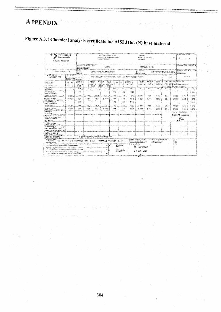
A p p e n d ix
F.gure A.3.1 Chemical analysis certificate for A1SI316L (N) base material
smmmi t m m
304
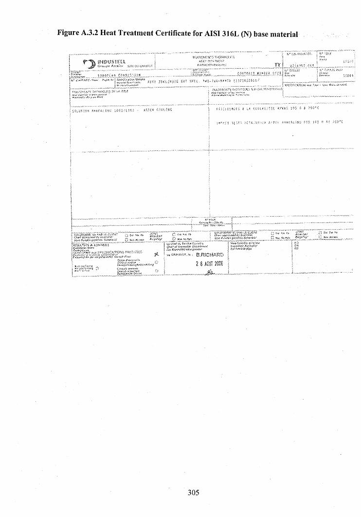
Figure A.3.2 Heat Treatment Certificate for AISI 316L (N) base material
IHpySTEIl<»r r :
* * - n - » * ' * .
TT' r^ !-' ' *, - V i i i
s v v !, *, >■'-% s . * I \ ~>*■«* jwjmmsM-stnf ’- ' * v
9W - » i! -M s >. 1..
Hill I U i« s » ?F't
p a t s M M U i i s i f s s * r i J I ^ C
K I V ,-
o ,*T9j *■* *:*« r»Q 5®*
TST
»/' '■»'# •» J1' i V ''
.« iKMNVt, v , B.MCMA!®i b y.r. as?
305
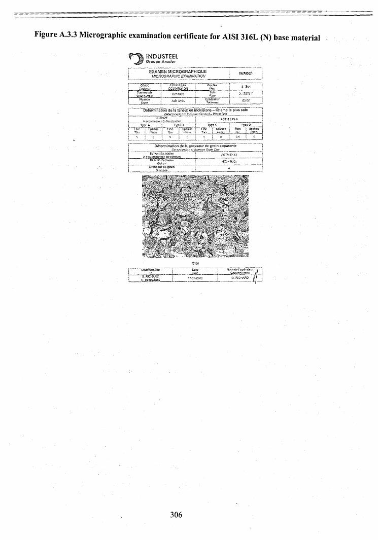
Figure A.3.3 Micrographic examination certificate for AISI316L (N) base material
I N D U S T E E LCroupe AreeJorEXAMEN MiCROGRAPHIQUE
MCROQRAPH1C EXAMINATION
mjROPSfinCOMMISSION
Determination do is tsneur en inclusions - Champ ie plus safe O aierm insiiof’ o f tr.cl-jsion Content - IVors? field ______
j Type A .j Type 8 f TYP&C Type C j: Fine r.patese ] fin ;; i Epstsse | Fine 1 £p«te«c Rne Epaisss •I "JTt/.-j Ha&vy j ?7)ir; | '< - T/WJ) 1 Tm: 1 rft&vy j
I t o i 0 | B i i | o OJ? 1 0 |
D ete rm ination d a la g ro s s e u r d e g ra in sp p a re n te
Orosssur (ie grain
,9v4r
l l P iNojn cte i!op£fat«urQp9rz?pr'$ Mm? j
G. RICHARD f l
306
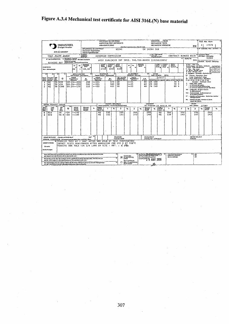
Figure A.3.4 Mechanical test certificate for AISI 316L(N) base material
I N D U S T E E LG ro vp e Arcelor
SITE OUCflEUSOT
ORGANISMS D£ CONTROLS inspect fort Crggn'uttlon A bnehm cgeseflschaft
CERTIFlCAt DE CONTRGLE INSPECTION TEST CERTIFICATE A8NAHMEZEUCNIS
(CtnKKat eonfor
ESSAtS ME*_,ifQUES MECHANICAL TESTS MECANISCHE VERSUCHE
U S I N E EH 1 0 2 0 4 3 1 6
TCLE Pbto Bltckt
X | 1 7 5 7 9 |
n * Cou lee H*»t scbmtue
[ N ' t d c client . .c o n t r a c tT O L E - P L A T E - B L E C H E U R O P E A N C O M M I S S I O N NUMBER 0 5 / 9
H* * C*> INDUSTEEL '
6 2 1 4 3 5 2 0 6 FA I S I 3 L 6 L ( N ) I G SVT S P E C . T W5 . - T V V - MA N T R ( 1 3 / 1 0 / 2 0 0 5 /
6 0 , 0 0
Lsmi/uemlz&, 1lmtT N- Nb hEr wl*i>rLonoueut Lengf/i Lingo 2t
“ Mewc ‘Weight
2 5 5 0 5 0 0 0 6 1 8 (
MacbMtch.
OIB.D* e
UMIVE EIAST1QUE *• Yiciti strength - Streekgeenke
RESISTANCE W TootX* sfttngth • Zvgfsstfaktit
ALLONCEMSIT i f fonget/on • Dn’muop
UNITES u n i t s MPA
impo*4Re
VS-SFcntfrr+menlS
SoflwrrteAm
Tr.YDIsl. cntr® A« Gttrgt fcnj/r/i^ BegwSvettis
S ? t£ S " 1... EHOJ 1 7 5 1 7 1
4(3 TR - 2 0 E 0 . 2 % > - 2 2 0 2 5 9 > = 5 2 5 5 7 4 5 0 > - 4 5 6 0 I k I HO 7 9 *6 Q TR - 2 0 E 0 . 2 * > - 2 2 0 2 6 6 > = 5 2 5 5 6 3 5 0 > - 4 5 6 0 I k I NO 7 9 %
2 4Q TR i 3 0 0 E 0 . 2 % > “ 1 3 C 1 5 3 > = 4 3 3 4 5 1 5 0 > - 3 3 4 0 I k I ND 8 0 V
COULEE INOX 5 5 Heat - Sc/m etze
S 1 8 6 4
Symbol® • SymtxJ - Abktjrzmg
. Milieu • AIrrfaie • tJiits ’P. Pted * Bottom * Fttss P_E. Epsisreur • Thicknsst - Dick&rchtunj TR :Tr*vcf» • Transverse- Qutr I : Long - Longiiutiimt • tings Pfc i Pttu- ftoffeti surface * WaltfUshe C 1/2 >D 1/3 • Q 1/4 • F 1/S - S 1/6
(psiuour - TMckness - Dicks |C : Autre -o/her. A«i*rv J t 4 12.6 m m tfebp
j 12.Sn jrhce! m 12.5 mm Absiand von tier Wahflidie
%F : %nbfosk4 - % af/etr frsetv/a % Zitibructi*nltH
V.C : % CriilBllinfci • % Bridie hectw*% KiiuaHinititsentcil
N* ; N iifntro «ja Pottou*ir>e - Weeksittm nur Werktpetitionnr.
Nb : Nembft* 6a xdet -Number o f plates Anz»h! tier Bit cbt
IMPOSE • Requirement • Soktvertet
Individ.
UNires ■ nmriio. J /C M 2
KCUKCU
..140
. . 1 0 02 9 21 5 1
2 9 21 5 1
3 0 41 4 3
2 9 61 4 8
3 0 01 3 9
3 0 01 4 3
2 9 61 4 7
2 9 91 4 3
OBSERVATIONS
fiemorks
Bcobtehtimgsn
T E N S I L E T E S T AT + 3 0 0 * A F T E R 5MH HOLD AT T E S T T E M P E R A T U R E I M P A C T T E S T S H E A T / O R D E R A F T E R A N N E A L I N G FOR 1 0 0 H AT 7 5 0 * C F E R R I T E S U R T 0 L E < 1 % 1 / 4 LARG EN T E T E - 0 8 T . : < J*/o
5 les rtsullit*. Conformc
^ ity
307
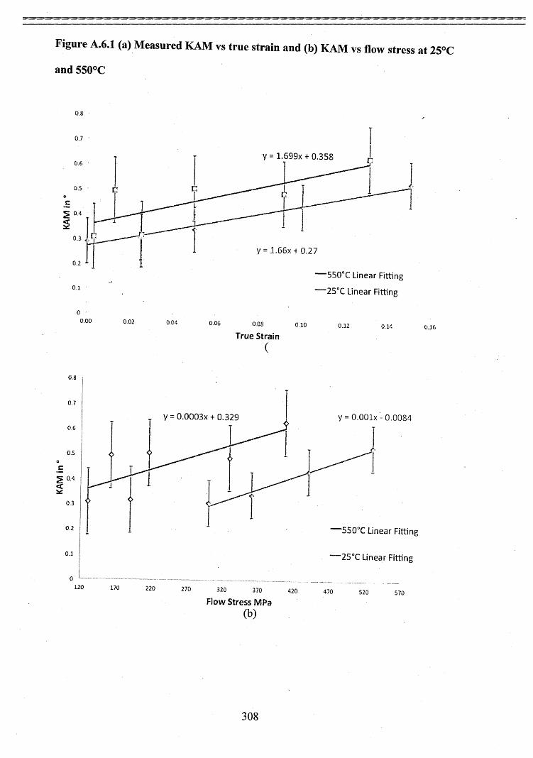
KAM
in
Figure A.6.1 (a) Measured KAM vs true strain and (b) KAM vs How stress at 25°C
and550°C
o.s
0 . 7
y = 1.699X + 0.3580.6
O.S
0 . 3
y= 1.65x4 0.270.2
550°C Linear Fitting
25°C Linear Fitting
O '0 . 0 0 0 . 0 2 0 . 0 4 0 . 0 6 0 .0 3
True Strain
(
y = 0.0003x + 0.329 y = 0.001x -0.00840.6
0 .5
J > 0 . 4
0 . 3
0.2 '550°C Linear Fitting
o.i 2 5 °C Linear Fitting
120 1 7 0 220 2 7 0 3 2 0 3 7 0 4 7 0 5 2 0 5 7 0
F low Stress MPa
0 . 1 6
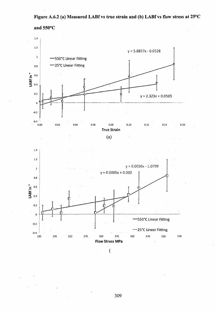
LABf
in
8 LA
Bf i
n
Figure A.6.2 (a) Measured LABf vs true strain and (b) LABf vs flow stress at 25°C
and 550°C
1 .4
1.2y = 5 .8 8 5 7 x - 0 .0 5 2 8
550°C Linear Fitting
25°C Linear Fitting
o0.6
0 .4
0.2y = 2 .323x + 0 .0 5 6 5
-0.2
- 0 .4
0 . 1 60 . 0 60.02 0.04 0.0S 0.10 0.12 0 . 1 40.00
True Strain
(a)
y = 0 .0036x -1 .0 7 9 9
y = 0 .0 0 0 5 x + 0 .0 0 2
0.6
0 .4
0.2
— 550°C Linear Fitting•0.2
— 2 5 °C Linear Fitting
4 7 0 5 7 0270 3 2 0 3 7 0 4 2 0 5 2 0120 1 7 0 220
Flow Stress MPa
(
309
Related Documents


