12 Lecture

© 2014 Pearson Education, Inc.

Chapter 12

Solutions

Sherril Soman,Grand Valley State University

Lecture Presentation


• Drinking seawater can cause dehydration.

• Seawater– Is a homogeneous mixture of salts with water– Contains higher concentrations of salts than the salt

content of your cells

• As seawater passes through your body, it pulls water out of your cells, due mainly to nature’s tendency toward spontaneous mixing.

• This reduces your cells’ water level and usually results in diarrhea as this extra liquid flows out with the seawater.

Thirsty Seawater


Seawater


• Drinking seawater will dehydrate you and give you diarrhea.

• The cell wall acts as a barrier to solute moving so the only way for the seawater and the cell solution to have uniform mixing is for water to flow out of the cells of your intestine and into your digestive tract.

Seawater


Seawater


• A mixture of two or more substances• Composition may vary from one sample to another• Appears to be one substance, though really

contains multiple materials

• Most homogeneous materials we encounter are actually solutions.– For example, air and seawater

• Nature has a tendency toward spontaneous mixing.– Generally, uniform mixing is more energetically favorable.

Homogeneous Mixtures


• The majority component of a solution is called the solvent.

• The minority component is called the solute.

• Solutions form in part because of intermolecular forces.– The particles of the solute interact with the particles

of the solvent through intermolecular forces.

Solutions


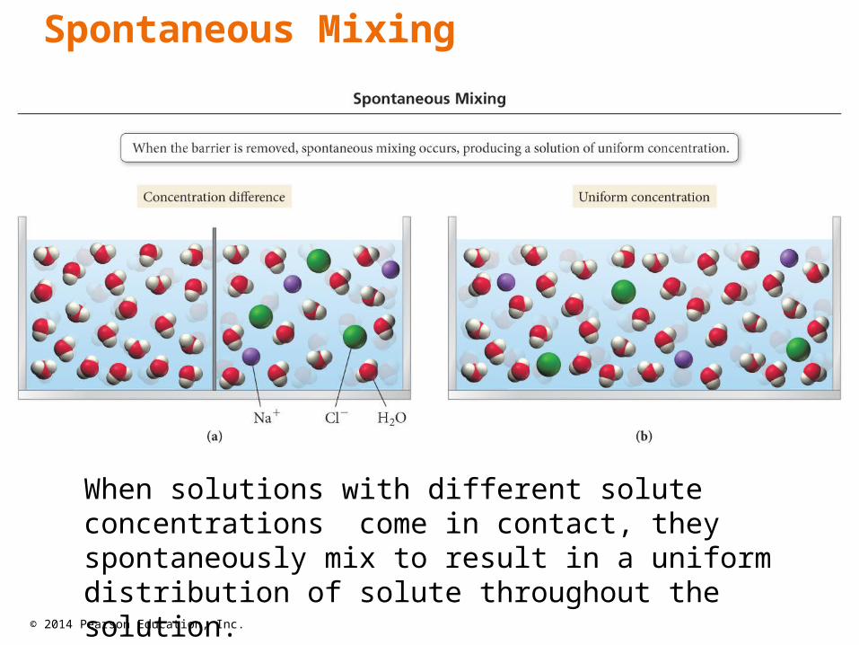
Spontaneous Mixing

When solutions with different solute concentrations come in contact, they spontaneously mix to result in a uniform distribution of solute throughout the solution.


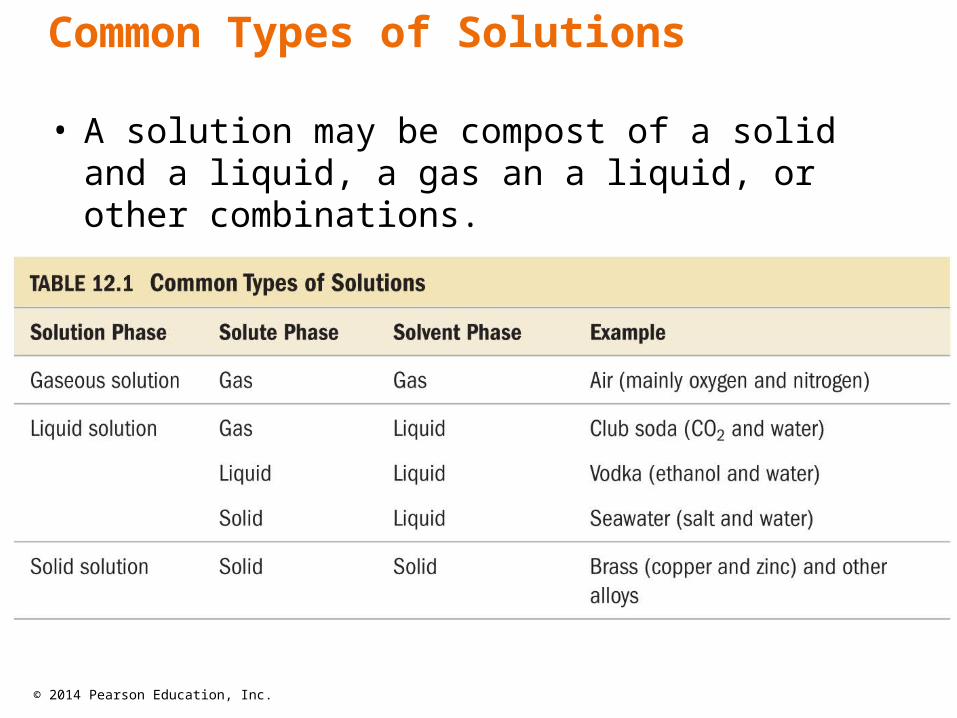
Common Types of Solutions

• A solution may be compost of a solid and a liquid, a gas an a liquid, or other combinations.


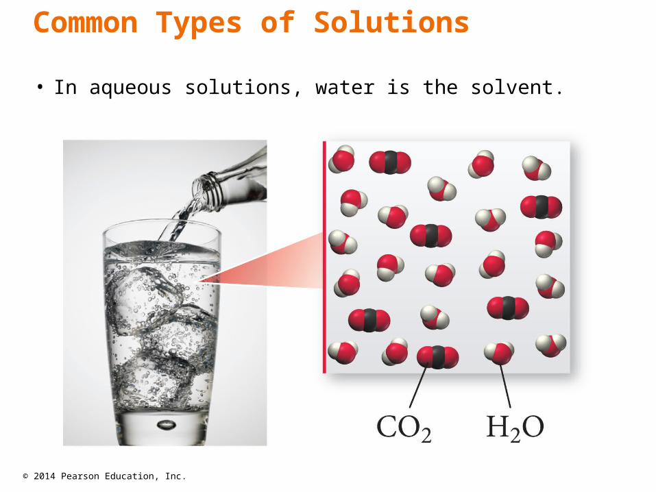
Common Types of Solutions

• In aqueous solutions, water is the solvent.


• When one substance (solute) dissolves in another (solvent) it is said to be soluble.– Salt is soluble in water.– Bromine is soluble in methylene chloride.

• When one substance does not dissolve in another it is said to be insoluble.– Oil is insoluble in water

• The solubility of one substance in another depends on1.nature’s tendency toward mixing, and

1. the types of intermolecular attractive forces.

Solubility


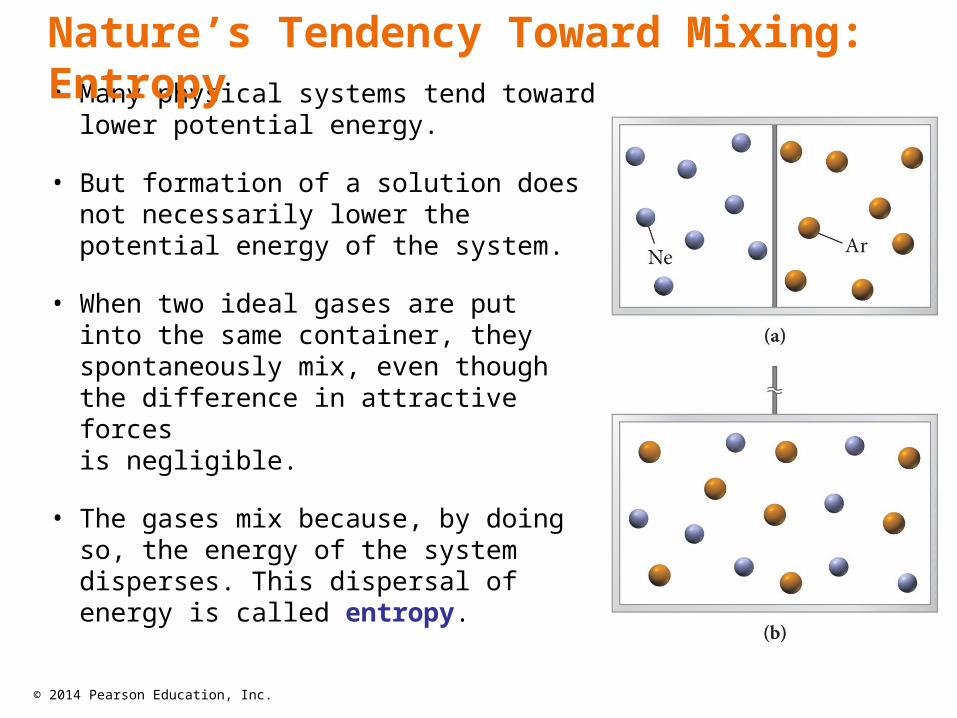
• Many physical systems tend toward lower potential energy.

• But formation of a solution does not necessarily lower the potential energy of the system.

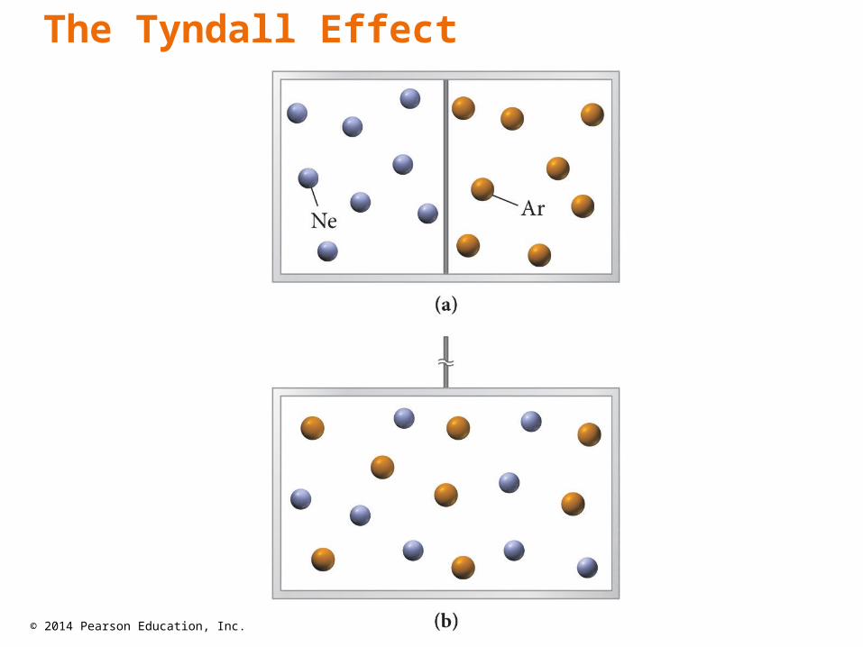
• When two ideal gases are put into the same container, they spontaneously mix, even though the difference in attractive forces is negligible.

• The gases mix because, by doing so, the energy of the system disperses. This dispersal of energy is called entropy.

Nature’s Tendency Toward Mixing: Entropy


• Entropy is the measure of energy dispersal throughout the system.

• Energy has a spontaneous drive to spread out over as large a volume as it is allowed.

• By each gas expanding to fill the container, it spreads its energy out and increases its entropy.

Mixing and the Solution Process Entropy


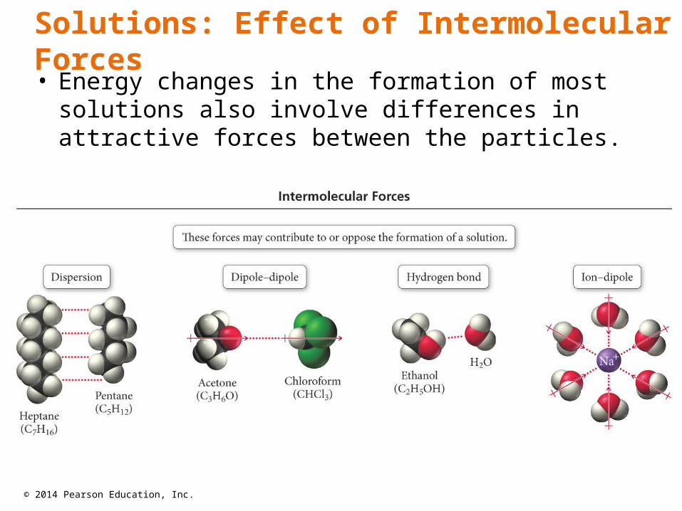
• Energy changes in the formation of most solutions also involve differences in attractive forces between the particles.

Solutions: Effect of Intermolecular Forces


• For the solvent and solute to mix you must overcome1. all of the solute–solute attractive forces, or

2. some of the solvent–solvent attractive forces.– Both processes are endothermic

• At least some of the energy to do this comes from making new solute–solvent attractions, which is exothermic.

Solutions: Effect of Intermolecular Forces


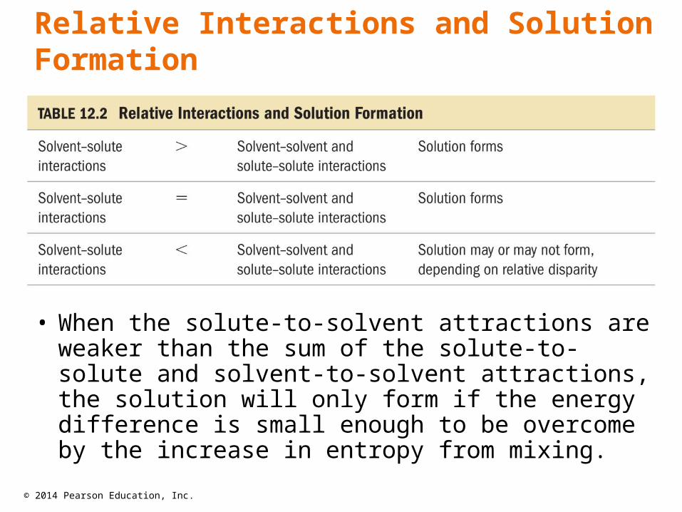
• When the solute-to-solvent attractions are weaker than the sum of the solute-to-solute and solvent-to-solvent attractions, the solution will only form if the energy difference is small enough to be overcome by the increase in entropy from mixing.

Relative Interactions and Solution Formation


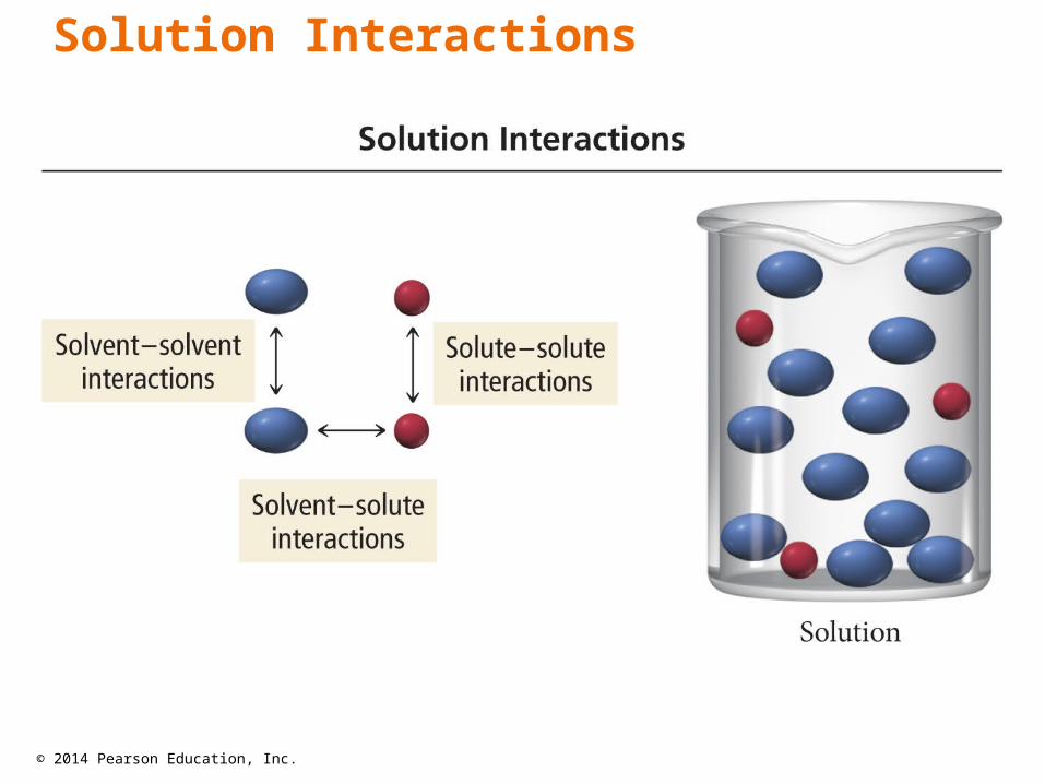
Solution Interactions


• The maximum amount of solute that can be dissolved in a given amount of solvent is called the solubility.

• There is usually a limit to the solubility of one substance in another.– Gases are always soluble in each other.– Two liquids that are mutually soluble are said to be

miscible. • Alcohol and water are miscible.• Oil and water are immiscible.

• The solubility of one substance in another varies with temperature and pressure.

Solubility


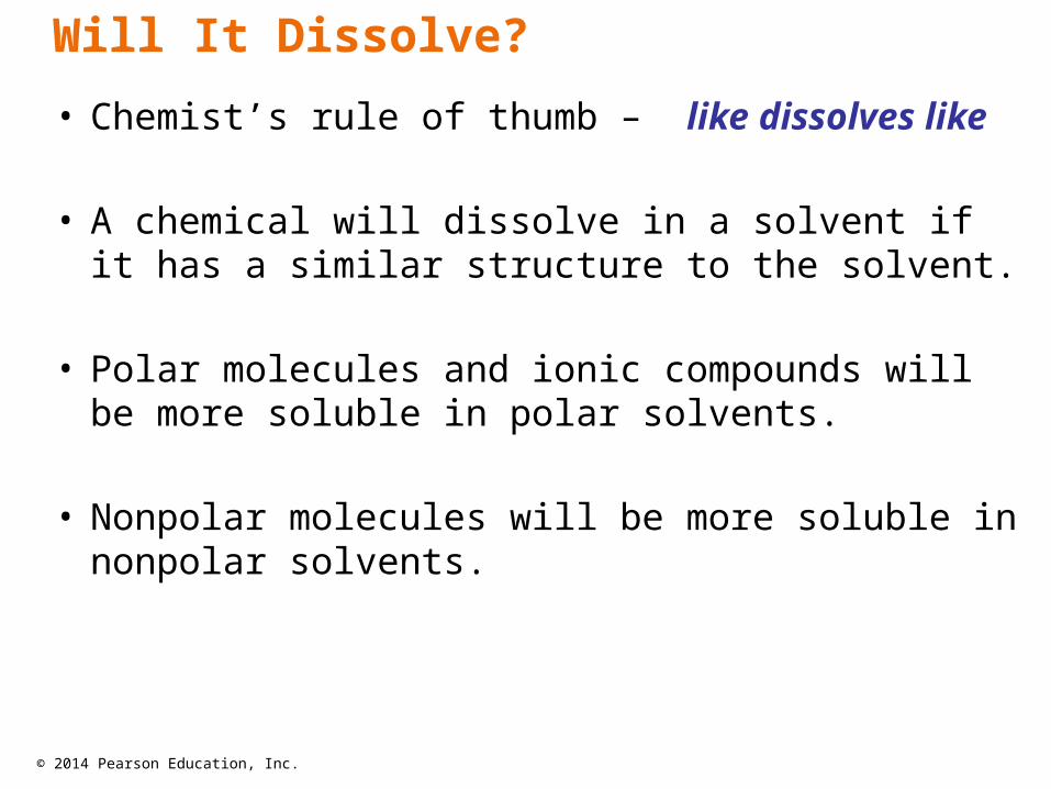
• Chemist’s rule of thumb – like dissolves like

• A chemical will dissolve in a solvent if it has a similar structure to the solvent.

• Polar molecules and ionic compounds will be more soluble in polar solvents.

• Nonpolar molecules will be more soluble in nonpolar solvents.

Will It Dissolve?


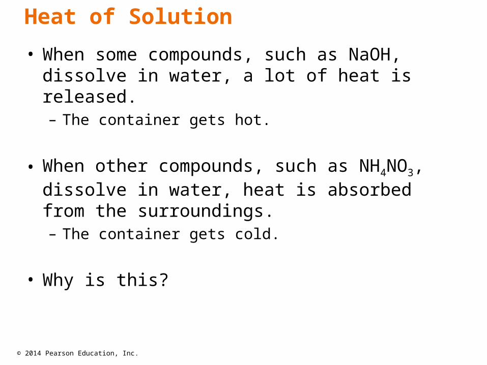
Heat of Solution

• When some compounds, such as NaOH, dissolve in water, a lot of heat is released.– The container gets hot.

• When other compounds, such as NH4NO3, dissolve in water, heat is absorbed from the surroundings.– The container gets cold.

• Why is this?


• To make a solution you must

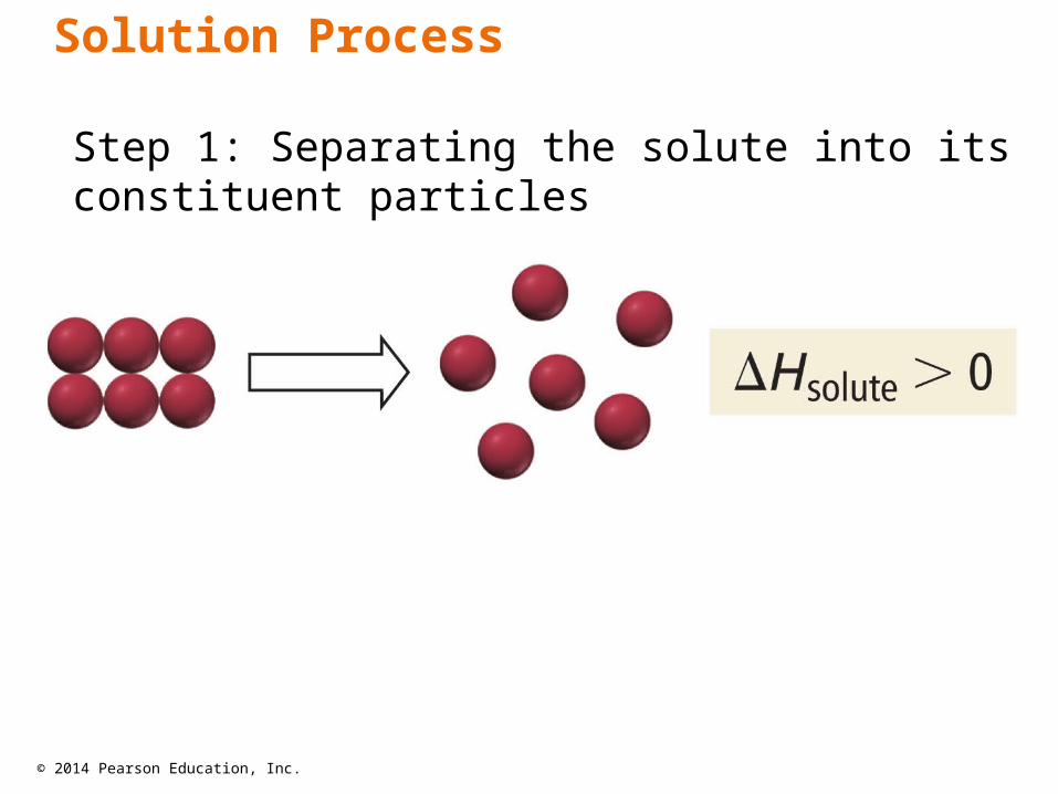
1. overcome all attractions between the solute particles; therefore, ΔHsolute is endothermic.

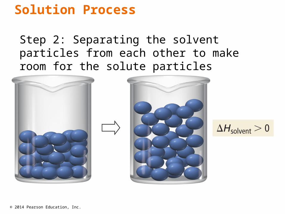
2. overcome some attractions between solvent molecules; therefore, ΔHsolvent is endothermic.

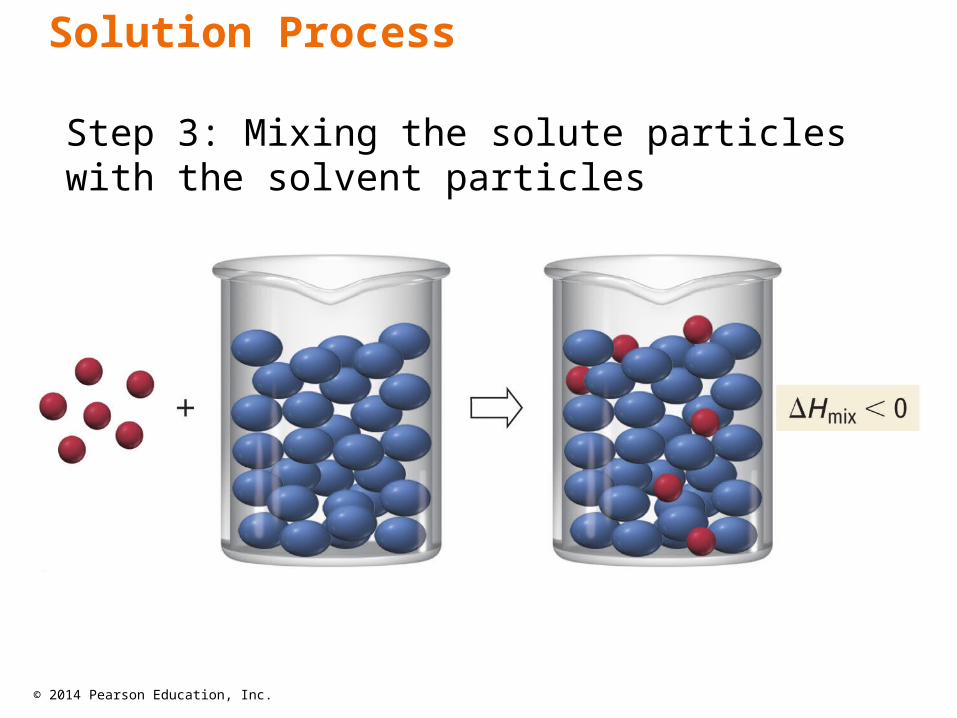
3. form new attractions between solute particles and solvent molecules; therefore, ΔHmix is exothermic.

1. The overall ΔH for making a solution depends on the relative sizes of the ΔH for these three processes.

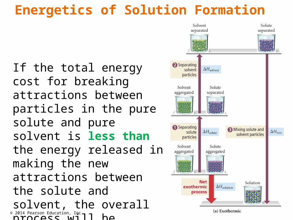
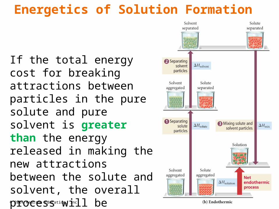
ΔHsol’n = ΔHsolute + ΔHsolvent + ΔHmix

Energetics of Solution Formation: The Enthalpy of Solution


Step 1: Separating the solute into its constituent particles

Solution Process


Step 2: Separating the solvent particles from each other to make room for the solute particles

Solution Process


Step 3: Mixing the solute particles with the solvent particles

Solution Process


If the total energy cost for breaking attractions between particles in the pure solute and pure solvent is less than the energy released in making the new attractions between the solute and solvent, the overall process will be exothermic.

Energetics of Solution Formation


If the total energy cost for breaking attractions between particles in the pure solute and pure solvent is greater than the energy released in making the new attractions between the solute and solvent, the overall process will be endothermic.

Energetics of Solution Formation


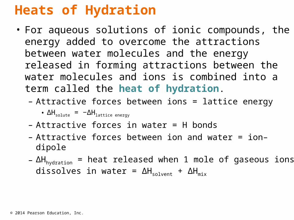
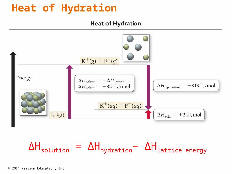
• For aqueous solutions of ionic compounds, the energy added to overcome the attractions between water molecules and the energy released in forming attractions between the water molecules and ions is combined into a term called the heat of hydration.– Attractive forces between ions = lattice energy

• ΔHsolute = −ΔHlattice energy

– Attractive forces in water = H bonds– Attractive forces between ion and water = ion–dipole

– ΔHhydration = heat released when 1 mole of gaseous ions dissolves in water = ΔHsolvent + ΔHmix

Heats of Hydration


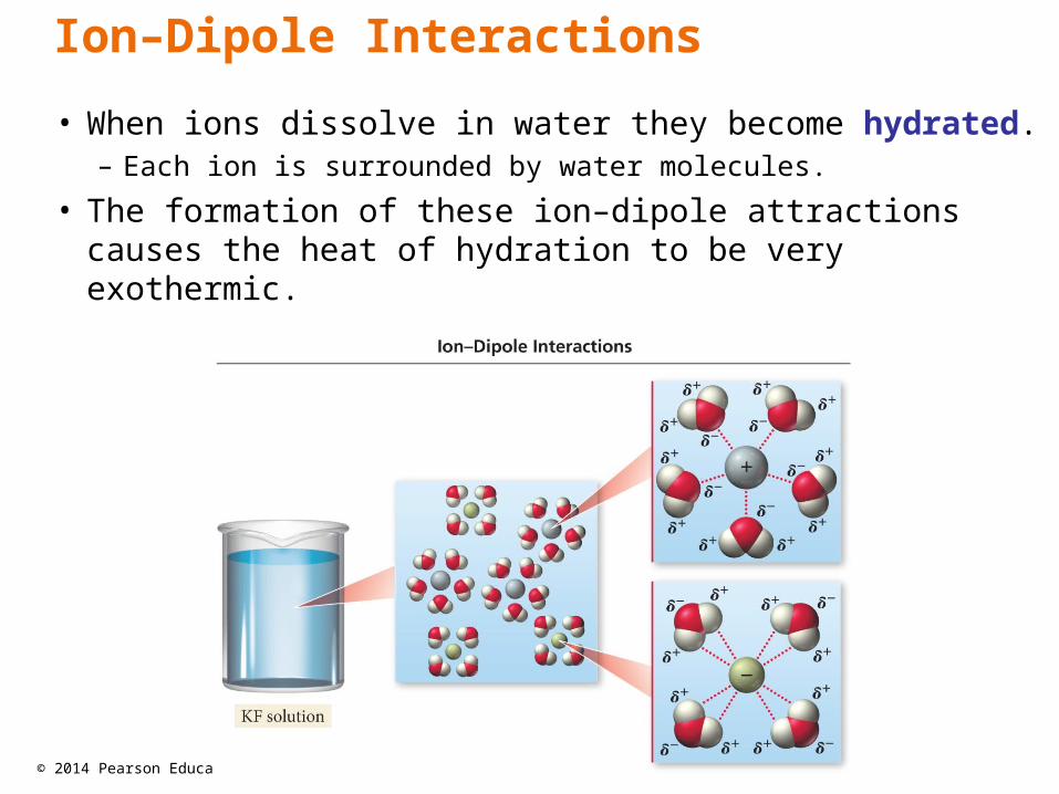
Ion–Dipole Interactions

• When ions dissolve in water they become hydrated.– Each ion is surrounded by water molecules.

• The formation of these ion–dipole attractions causes the heat of hydration to be very exothermic.


Heats of Solution for Ionic Compounds

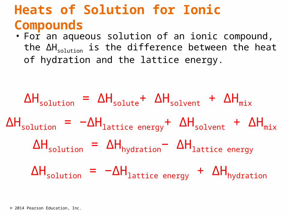
• For an aqueous solution of an ionic compound, the ΔHsolution is the difference between the heat of hydration and the lattice energy.

ΔHsolution = −ΔHlattice energy + ΔHhydration

ΔHsolution = ΔHsolute+ ΔHsolvent + ΔHmix

ΔHsolution = −ΔHlattice energy+ ΔHsolvent + ΔHmix

ΔHsolution = ΔHhydration− ΔHlattice energy


ΔHsolution = ΔHhydration− ΔHlattice energy

Heat of Hydration


Comparing Heat of Solution to Heat of Hydration

• Because the lattice energy is always exothermic, the size and sign on the ΔHsol’n tells us something about ΔHhydration.

• If the heat of solution is large and endothermic, then the amount of energy it costs to separate the ions is more than the energy released from hydrating the ions.

ΔHhydration < ΔHlattice when ΔHsol’n is (+)

• If the heat of solution is large and exothermic, then the amount of energy it costs to separate the ions is less than the energy released from hydrating the ions.

ΔHhydration > ΔHlattice when ΔHsol’n is (−)


• The dissolution of a solute in a solvent is an equilibrium process.

• Initially, when there is no dissolved solute, the only process possible is dissolution.

• Shortly after some solute is dissolved, solute particles can start to recombine to reform solute molecules, but the rate of dissolution >> the rate of deposition and the solute continues to dissolve.

• Eventually, the rate of dissolution = the rate of deposition—the solution is saturated with solute and no more solute will dissolve.

Solution Equilibrium


Solution Equilibrium


• A solution that has the solute and solvent in dynamic equilibrium is said to be saturated.– If you add more solute it will not dissolve.– The saturation concentration depends on the

temperature and pressure of gases.

• A solution that has less solute than saturation is said to be unsaturated.– More solute will dissolve at this temperature.

• A solution that has more solute than saturation is said to be supersaturated.

Solubility Limit


How Can You Make a Solvent Hold More Solute Than It Is Able To?

• Solutions can be made saturated at non-room conditions, and then can be allowed to come to room conditions slowly.

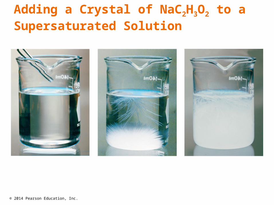
• For some solutes, instead of coming out of solution when the conditions change, they get stuck between the solvent molecules and the solution becomes supersaturated.

• Supersaturated solutions are unstable and lose all the solute above saturation when disturbed.– For example, shaking a carbonated beverage


Adding a Crystal of NaC2H3O2 to a Supersaturated Solution


• Solubility is generally given in grams of solute that will dissolve in 100 g of water.

• For most solids, the solubility of the solid increases as the temperature increases.– When ΔHsolution is endothermic

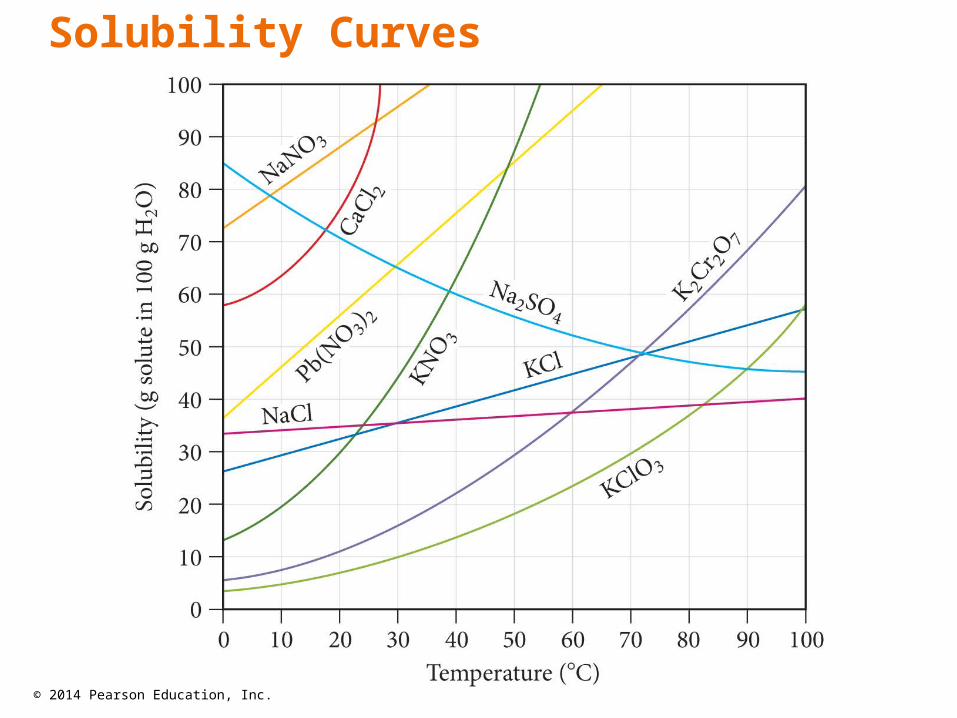
• Solubility curves can be used to predict whether a solution with a particular amount of solute dissolved in water is saturated (on the line), unsaturated (below the line), or supersaturated (above the line).

Temperature Dependence of Solubility of Solids in Water


Solubility Curves


Purification by Recrystallization

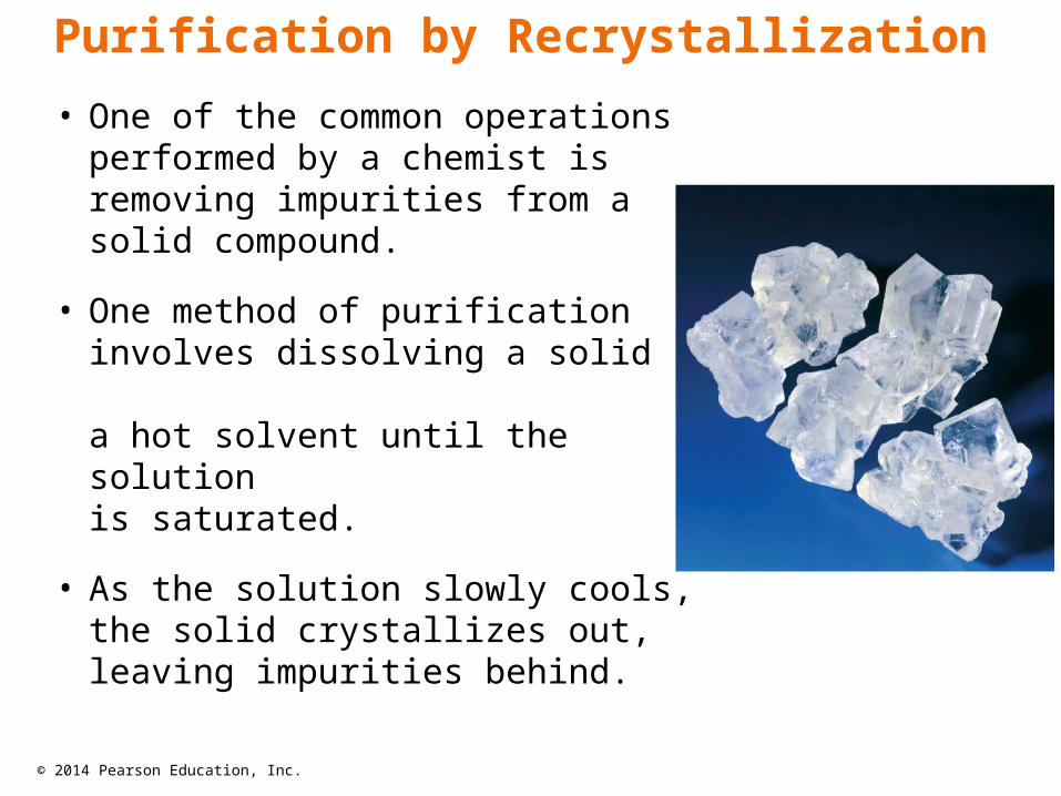
• One of the common operations performed by a chemist is removing impurities from a solid compound.

• One method of purification involves dissolving a solid in a hot solvent until the solution is saturated.

• As the solution slowly cools, the solid crystallizes out, leaving impurities behind.


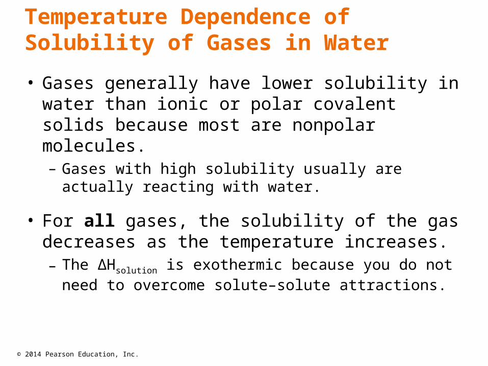
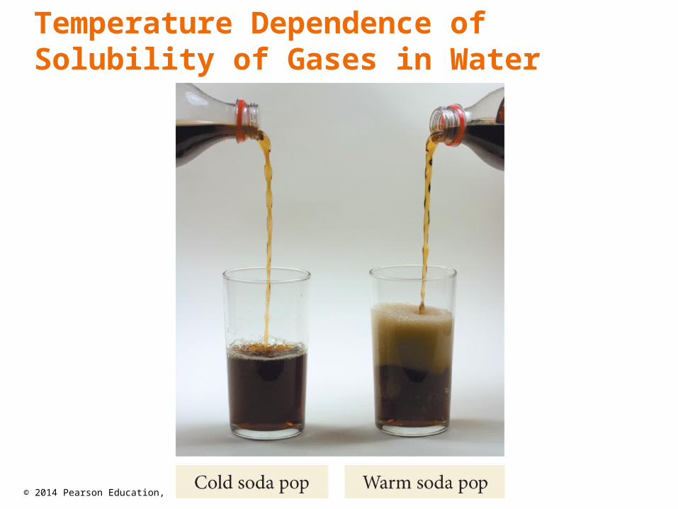
Temperature Dependence of Solubility of Gases in Water

• Gases generally have lower solubility in water than ionic or polar covalent solids because most are nonpolar molecules.– Gases with high solubility usually are actually reacting

with water.

• For all gases, the solubility of the gas decreases as the temperature increases.– The ΔHsolution is exothermic because you do not need to

overcome solute–solute attractions.


Temperature Dependence of Solubility of Gases in Water


Pressure Dependence of Solubility of Gases in Water

• The larger the partial pressure of a gas in contact with a liquid, the more soluble the gas is in the liquid.


Henry’s Law

• The solubility of a gas (Sgas) is directly proportional to its partial pressure, (Pgas).

Sgas = kHPgas

• kH is called the Henry’s law constant.


• Solutions have variable composition.• To describe a solution, you need to describe the

components and their relative amounts.• The terms dilute and concentrated can be

used as qualitative descriptions of the amount of solute in solution.

• Concentration = amount of solute in a given amount of solution.– Occasionally amount of solvent

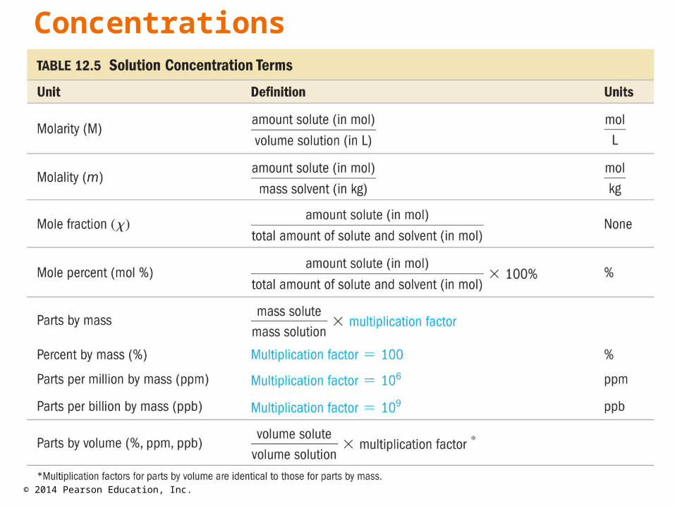
Concentrations


Concentrations


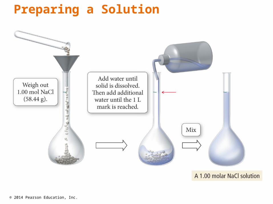
• Need to know amount of solution and concentration of solution

• Calculate the mass of solute needed– Start with amount of solution– Use concentration as a conversion factor

• 5% by mass ⇒5 g solute ≡ 100 g solution

– “Dissolve the grams of solute in enough solvent to total the total amount of solution.”

Preparing a Solution


Preparing a Solution


• Moles of solute per 1 liter of solution• Describes how many molecules of solute in

each liter of solution• If a sugar solution concentration is 2.0 M,

– 1 liter of solution contains 2.0 moles of sugar – 2 liters = 4.0 moles sugar – 0.5 liters = 1.0 mole sugar

Solution Concentration: Molarity


• Moles of solute per 1 kilogram of solvent– Defined in terms of amount of solvent, not solution

• Like the others

• Does not vary with temperature– Because based on masses, not volumes

Solution Concentration: Molality, m


• Parts can be measured by mass or volume.

• Parts are generally measured in the same units.– By mass in grams, kilogram, lbs, etc.– By volume in mL, L, gallons, etc.– Mass and volume combined in grams and mL

Parts Solute in Parts Solution


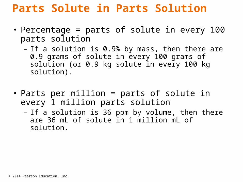
• Percentage = parts of solute in every 100 parts solution– If a solution is 0.9% by mass, then there are 0.9 grams

of solute in every 100 grams of solution (or 0.9 kg solute in every 100 kg solution).

• Parts per million = parts of solute in every 1 million parts solution– If a solution is 36 ppm by volume, then there are 36 mL

of solute in 1 million mL of solution.

Parts Solute in Parts Solution


• Grams of solute per 1,000,000 g of solution• mg of solute per 1 kg of solution• 1 liter of water = 1 kg of water

– For aqueous solutions we often approximate the kg of the solution as the kg or L of water.

• For dilute solutions, the difference in density between the solution and pure water is usually negligible.

PPM


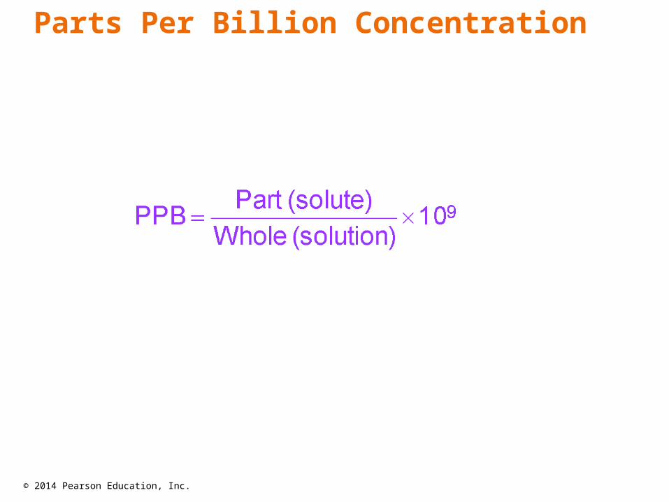
Parts Per Billion Concentration


• The mole fraction is the fraction of the moles of one component in the total moles of all the components of the solution.

• Total of all the mole fractions in a solution = 1.

• Unitless

• The mole percentage is the percentage of the moles of one component in the total moles of all the components of the solution.– = mole fraction × 100%

Solution Concentrations: Mole Fraction, XA


1. Write the given concentration as a ratio.

2. Separate the numerator and denominator.– Separate into the solute part and solution part

3. Convert the solute part into the required unit.

4. Convert the solution part into the required unit.

5. Use the definitions to calculate the new concentration units.

Converting Concentration Units


• Colligative properties are properties whose value depends only on the number of solute particles, and not on what they are.– Value of the property depends on the concentration of

the solution.

• The difference in the value of the property between the solution and the pure substance is generally related to the different attractive forces and solute particles occupying solvent molecules positions.

Colligative Properties


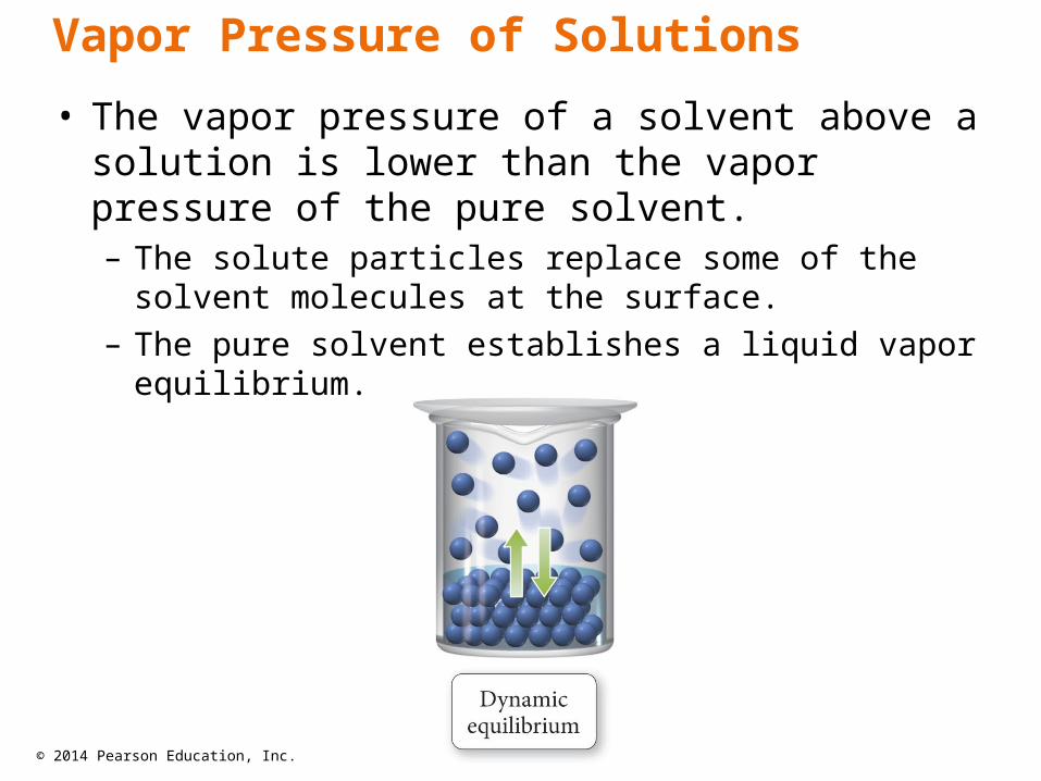
• The vapor pressure of a solvent above a solution is lower than the vapor pressure of the pure solvent.– The solute particles replace some of the solvent

molecules at the surface.– The pure solvent establishes a liquid vapor equilibrium.

Vapor Pressure of Solutions


• Addition of a nonvolatile solute reduces the rate of vaporization, decreasing the amount of vapor.



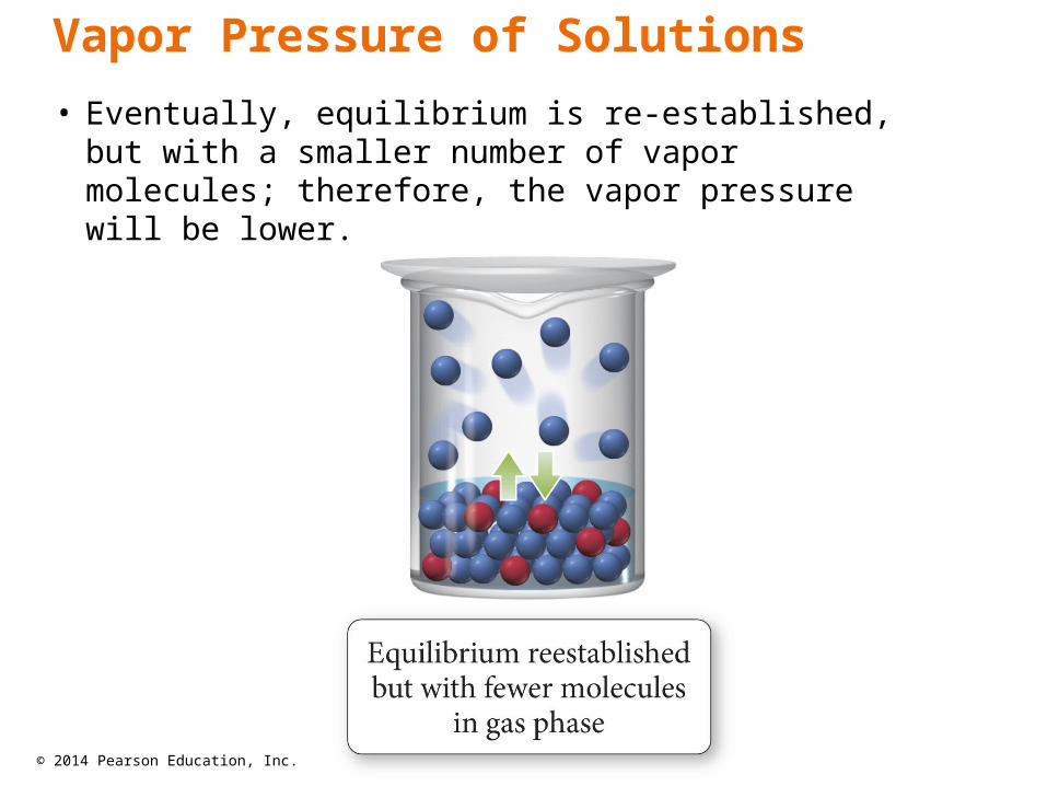
• Eventually, equilibrium is re-established, but with a smaller number of vapor molecules; therefore, the vapor pressure will be lower.



Thirsty Solutions Revisited

• A concentrated solution will draw solvent molecules toward it due to the natural drive for materials in nature to mix.

• Similarly, a concentrated solution will draw pure solvent vapor into it due to this tendency to mix.

• The result is reduction in vapor pressure.


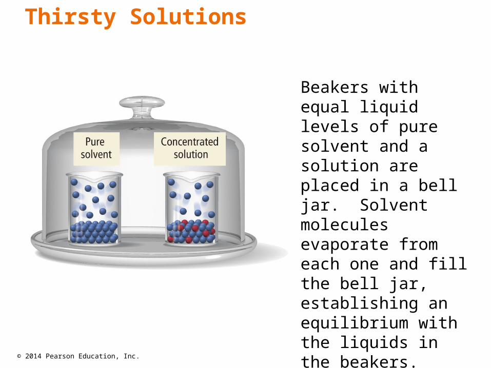
Beakers with equal liquid levels of pure solvent and a solution are placed in a bell jar. Solvent molecules evaporate from each one and fill the bell jar, establishing an equilibrium with the liquids in the beakers.

Thirsty Solutions


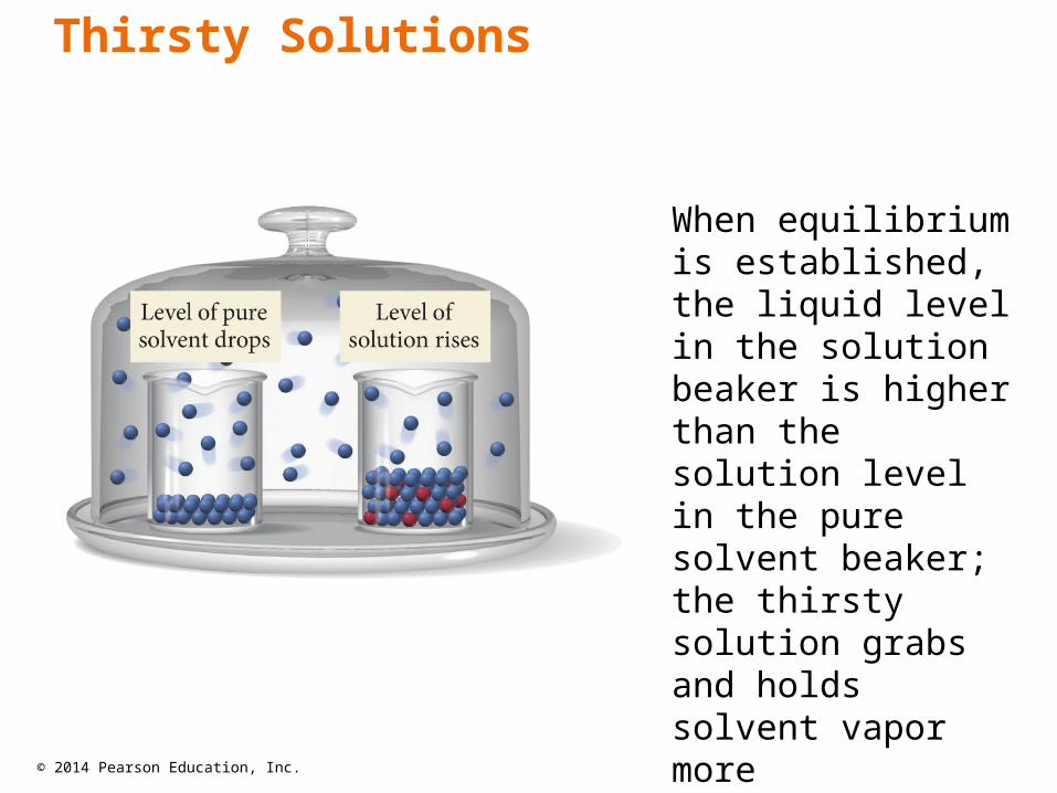
When equilibrium is established, the liquid level in the solution beaker is higher than the solution level in the pure solvent beaker; the thirsty solution grabs and holds solvent vapor more effectively.

Thirsty Solutions


Raoult’s Law

• The vapor pressure of a volatile solvent above a solution is equal to its normal vapor pressure, P°, multiplied by its mole fraction in the solution.

Psolvent in solution = χsolvent∙P°– Because the mole fraction is always less than 1, the

vapor pressure of the solvent in solution will always be less than the vapor pressure of the pure solvent.


• The vapor pressure of a solvent in a solution is always lower than the vapor pressure of the pure solvent.

• The vapor pressure of the solution is directly proportional to the amount of the solvent in the solution.

• The difference between the vapor pressure of the pure solvent and the vapor pressure of the solvent in solution is called the vapor pressure lowering.

ΔP = P°solvent − Psolution = χsolute ∙ P°solvent

Vapor Pressure Lowering


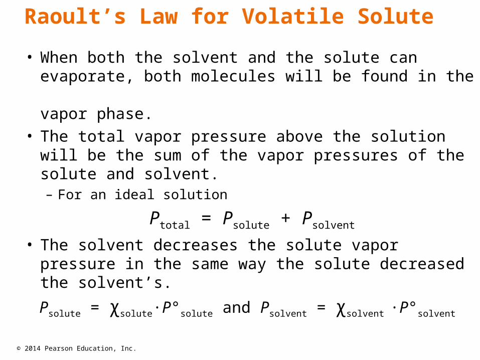
• When both the solvent and the solute can evaporate, both molecules will be found in the vapor phase.

• The total vapor pressure above the solution will be the sum of the vapor pressures of the solute and solvent.– For an ideal solution

Ptotal = Psolute + Psolvent

• The solvent decreases the solute vapor pressure in the same way the solute decreased the solvent’s.

Psolute = χsolute∙P°solute and Psolvent = χsolvent ∙P°solvent

Raoult’s Law for Volatile Solute


Ideal versus Nonideal Solution

• In ideal solutions, the made solute–solvent interactions are equal to the sum of the broken solute–solute and solvent–solvent interactions.– Ideal solutions follow Raoult’s law

• Effectively, the solute is diluting the solvent.• If the solute–solvent interactions are stronger or

weaker than the broken interactions the solution is nonideal.


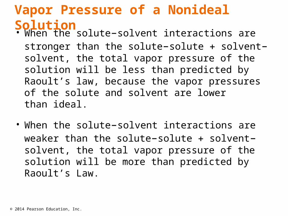
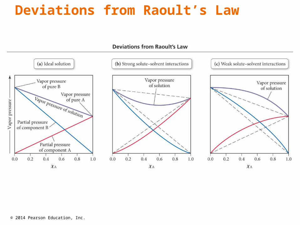
• When the solute–solvent interactions are stronger than the solute–solute solvent–solvent, the total vapor pressure of the solution will be less than predicted by Raoult’s law, because the vapor pressures of the solute and solvent are lower than ideal.

• When the solute–solvent interactions are weaker than the solute–solute solvent–solvent, the total vapor pressure of the solution will be more than predicted by Raoult’s Law.

Vapor Pressure of a Nonideal Solution


Deviations from Raoult’s Law


Other Colligative Properties Related to Vapor Pressure Lowering

• Vapor pressure lowering occurs at all temperatures.• This results in the temperature required to boil the

solution being higher than the boiling point of the pure solvent.

• This also results in the temperature required to freeze the solution being lower than the freezing point of the pure solvent.


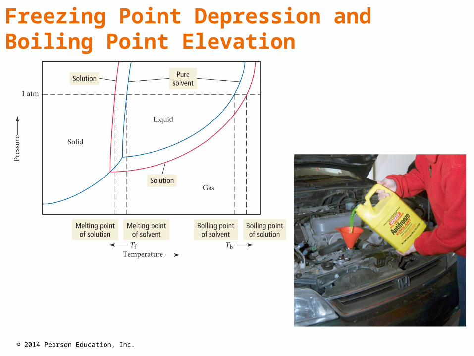
Freezing Point Depression and Boiling Point Elevation


• Pure water freezes at 0 °C. At this temperature, ice and liquid water are in dynamic equilibrium.

• Adding salt disrupts the equilibrium. The salt particles dissolve in the water, but do not attach easily to the solid ice.

• When an aqueous solution containing a dissolved solid solute freezes slowly, the ice that forms does not normally contain much of the solute.

• To return the system to equilibrium, the temperature must be lowered sufficiently to make the water molecules slow down enough so that more can attach themselves to the ice.

Freezing Salt Water


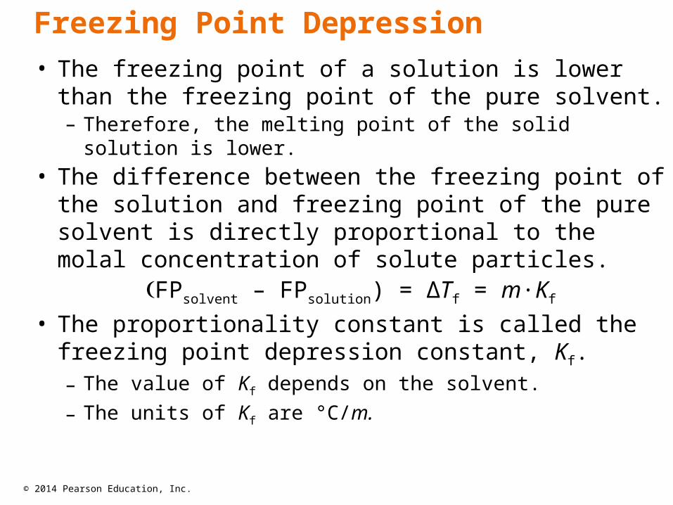
• The freezing point of a solution is lower than the freezing point of the pure solvent.– Therefore, the melting point of the solid solution is lower.

• The difference between the freezing point of the solution and freezing point of the pure solvent is directly proportional to the molal concentration of solute particles.

FPsolvent – FPsolution) = ΔTf = m∙Kf

• The proportionality constant is called the freezing point depression constant, Kf.– The value of Kf depends on the solvent.

– The units of Kf are °C/m.

Freezing Point Depression


Kf


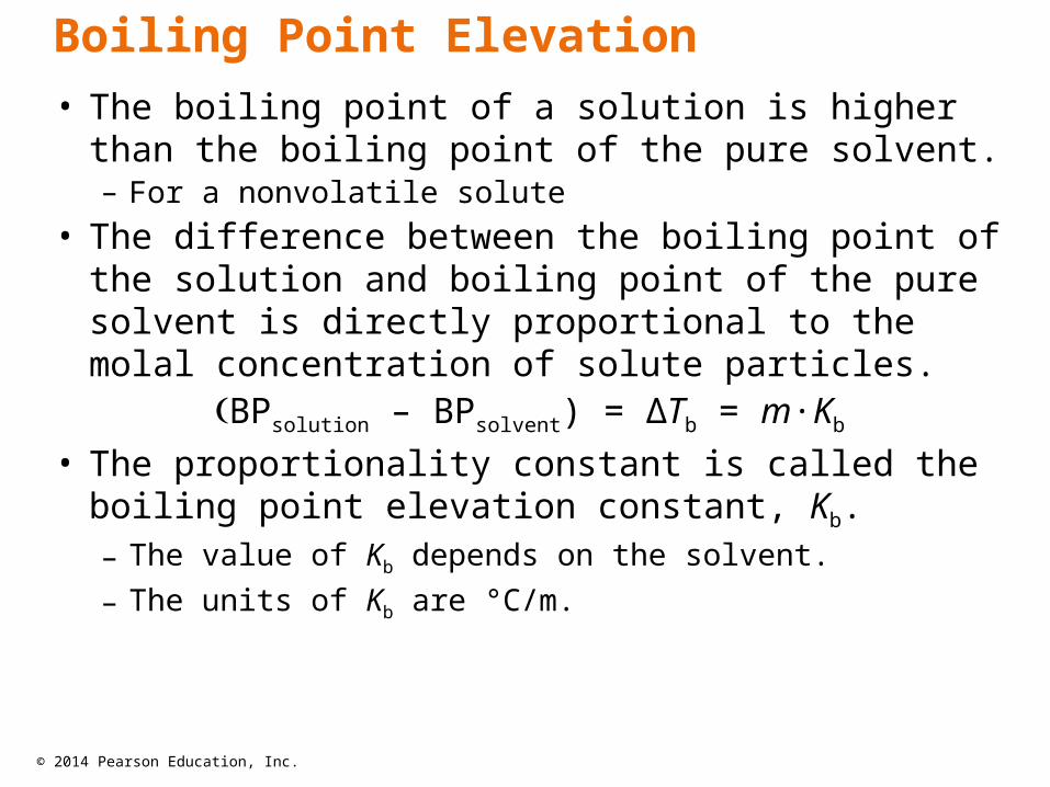
• The boiling point of a solution is higher than the boiling point of the pure solvent.– For a nonvolatile solute

• The difference between the boiling point of the solution and boiling point of the pure solvent is directly proportional to the molal concentration of solute particles.

BPsolution – BPsolvent) = ΔTb = m∙Kb

• The proportionality constant is called the boiling point elevation constant, Kb.– The value of Kb depends on the solvent.

– The units of Kb are °C/m.

Boiling Point Elevation


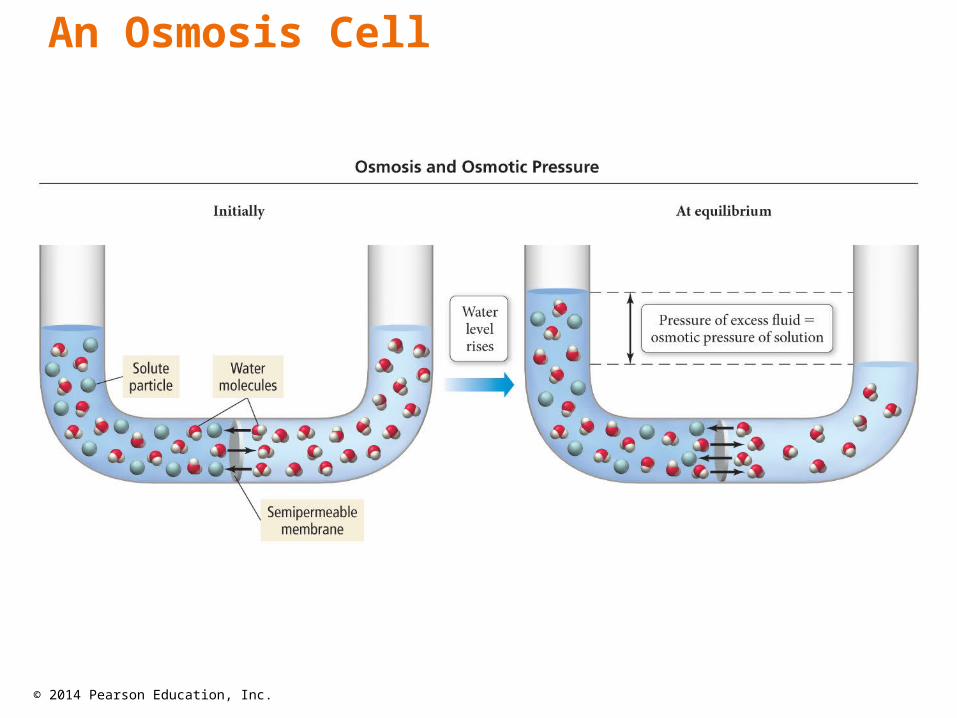
• Osmosis is the flow of solvent from a solution of low concentration into a solution of high concentration.

• The solutions may be separated by a semipermeable membrane.

• A semipermeable membrane allows solvent to flow through it, but not solute.

Osmosis


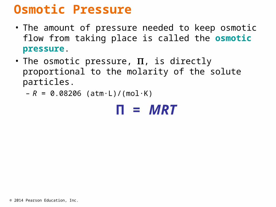
• The amount of pressure needed to keep osmotic flow from taking place is called the osmotic pressure.

• The osmotic pressure, , is directly proportional to the molarity of the solute particles.– R = 0.08206 (atm∙L)/(mol∙K)

Π = MRT

Osmotic Pressure


An Osmosis Cell


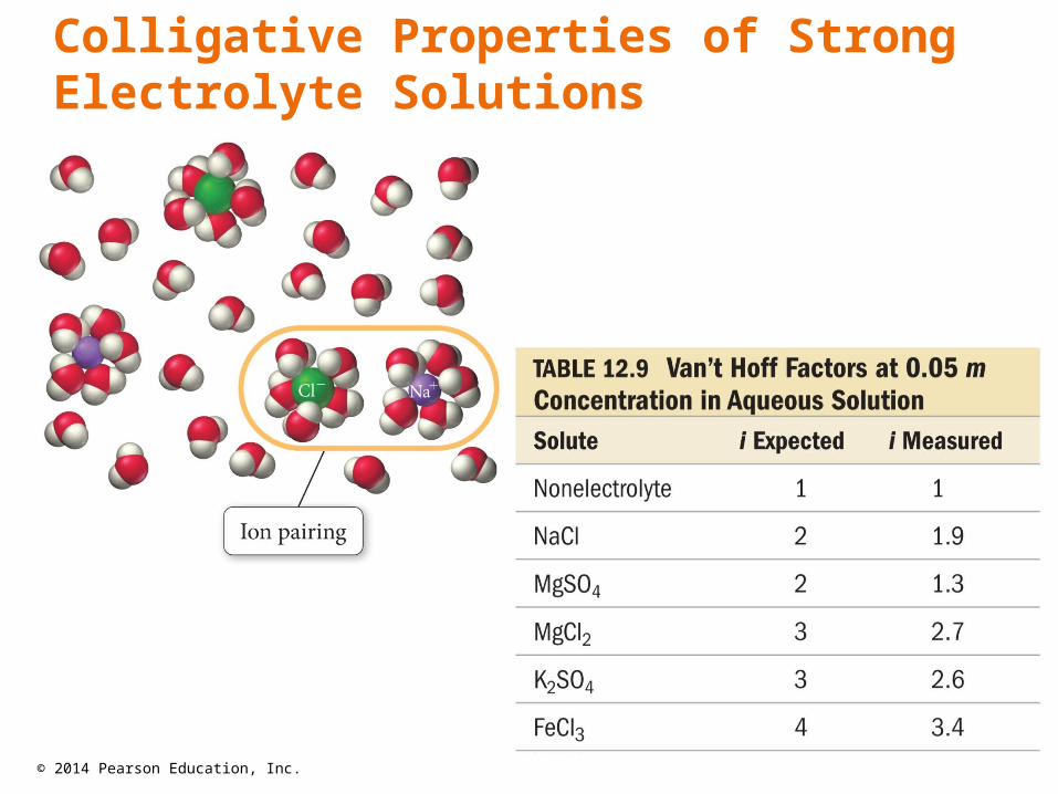
• Ionic compounds produce multiple solute particles for each formula unit.

• The theoretical van’t Hoff factor, i, is the ratio of moles of solute particles to moles of formula units dissolved.

• The measured van’t Hoff factors are generally less than the theoretical due to ion pairing in solution.– Therefore, the measured van’t Hoff factors often cause

the ΔT to be lower than you might expect.

Van’t Hoff Factors


Colligative Properties of Strong Electrolyte Solutions


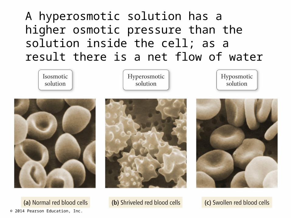
An isosmotic solution has the same osmotic pressure as the solution inside the cell; as a result there is no net flow of water into or out of the cell.


A hyperosmotic solution has a higher osmotic pressure than the solution inside the cell; as a result there is a net flow of water out of the cell, causing it to shrivel.


A hyposmotic solution has a lower osmotic pressure than the solution inside the cell; as a result there is a net flow of water into the cell, causing it to swell.


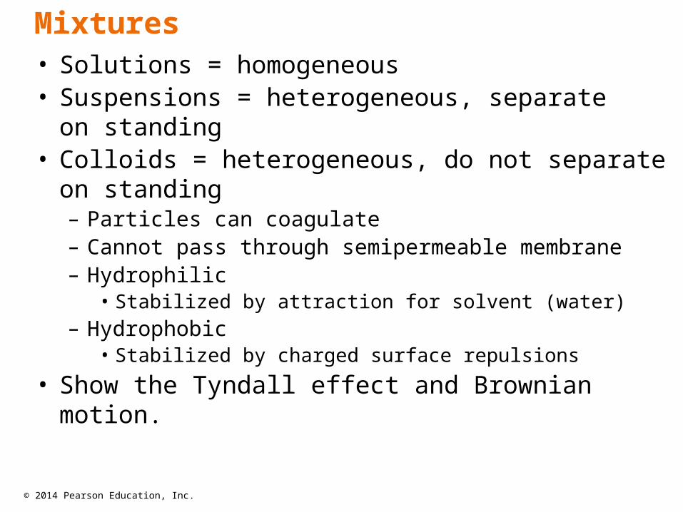
• Solutions = homogeneous• Suspensions = heterogeneous, separate

on standing• Colloids = heterogeneous, do not separate

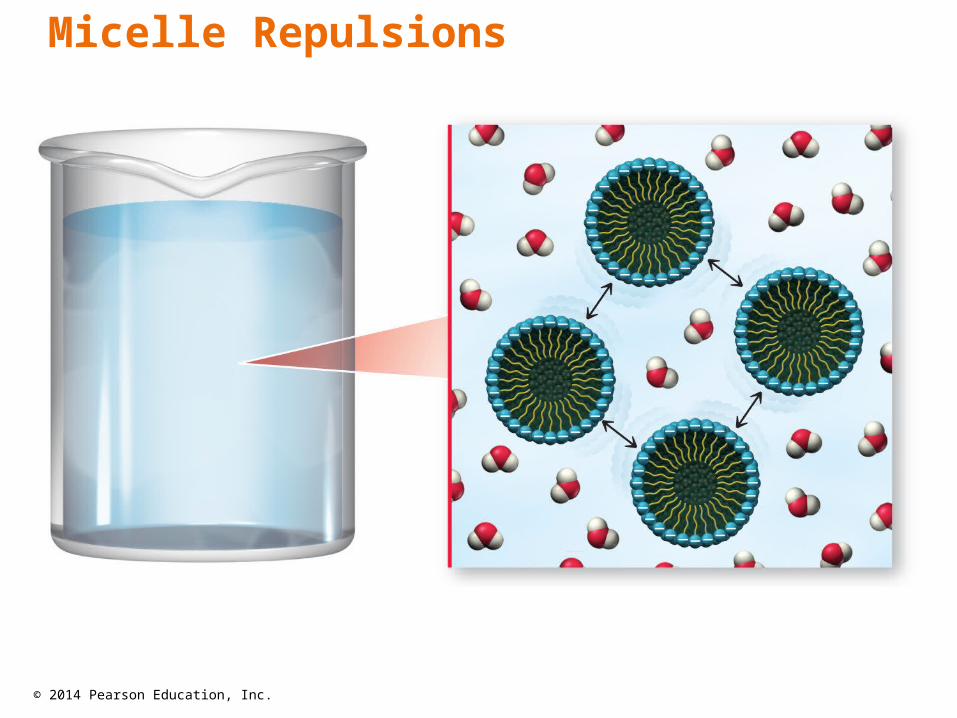
on standing– Particles can coagulate– Cannot pass through semipermeable membrane– Hydrophilic

• Stabilized by attraction for solvent (water)– Hydrophobic

• Stabilized by charged surface repulsions

• Show the Tyndall effect and Brownian motion.

Mixtures


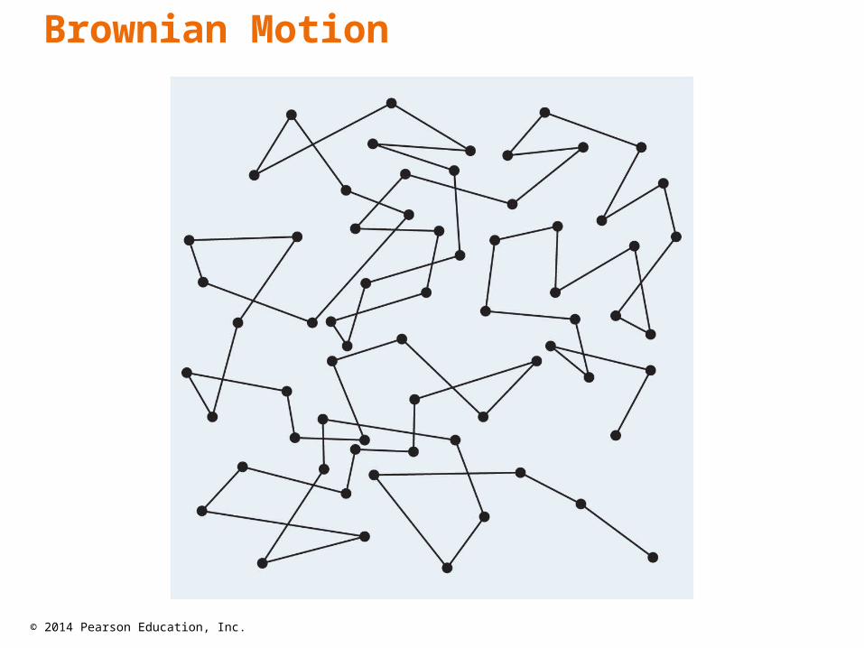
Brownian Motion


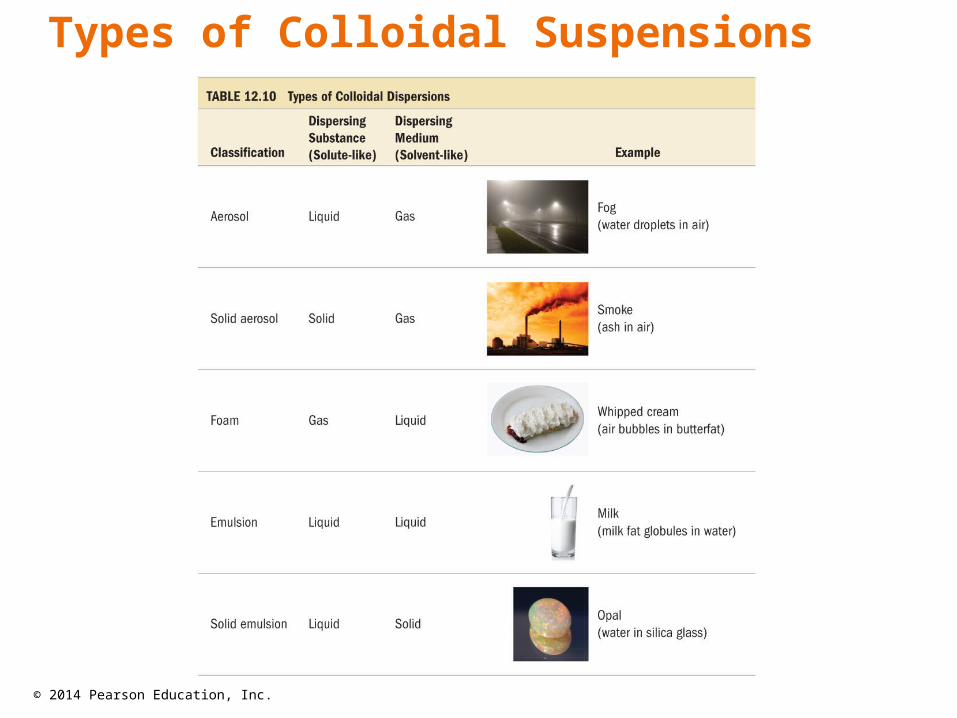
Types of Colloidal Suspensions


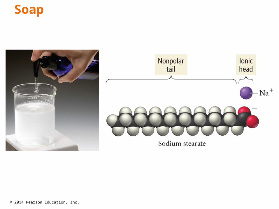
• Triglycerides can be broken down into fatty acid salts and glycerol by treatment with a strong hydroxide solution.

• Fatty acid salts have a very polar “head” because it is ionic and a very nonpolar “tail” because it is all C and H.– Hydrophilic head and hydrophobic tail

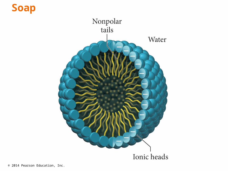
• This unique structure allows the fatty acid salts, called soaps, to help oily substances be attracted to water. – Micelle formation – Emulsification

Soaps


Soap


Soap


The Tyndall Effect


Micelle Repulsions

12 Lecture

Documents