10 Image Processing and Feature Extraction from a ... · – feature extraction or generation of structural image descriptions; and ﬁnally – the classiﬁcation of shapes and

273

10Image Processing and Feature Extraction from a Perspectiveof Computer Vision and Physical CosmologyHolger Stefan Janzer1), Florian Raudies1), Heiko Neumann, Frank Steiner

10.1Introduction

The main conjunction between Physical Cosmology and Computer Vision are im-ages. Commonly structures and objects in those images should be detected and rec-ognized. In this contribution we give a short survey of methods and assumptionsused in both disciplines. Applications and illustrative examples of those methodsare presented for the fields of Physical Cosmology and Medical Science.

In numerous scientific disciplines and applications areas high-dimensional sen-sory data needs to be analyzed for the detection of complex structures or for trigger-ing special events. From the beginning the acquisition and analysis of image dataformed the subject of image analysis. Nowadays many research disciplines workon the analysis of multi-dimensional images, namely engineering and computerscience, physics, mathematics and even psychology. Together they formed the re-search discipline of Computer Vision (or Computational Vision) which accounts forthe interpretation of images and image sequences rather than merely the raw pro-cessing of images [1, 2]. Computer Vision aims to be an umbrella for tasks thatcould be classified into:

(a) low-level vision, for example, image enhancement and filtering techniquesfor image processing;

(b) mid-level vision, for example, segmentation, feature extraction, and the de-tection of so-called intrinsic scene characteristics, in particular, the relativesurface orientation or depth discontinuities with respect to the viewer direc-tion; and

(c) high-level vision to generate and obtain, for example, descriptions of three-dimensional surfaces and volumes or the linking to steer a robot throughcomplex terrain [3, 4].

The observation of similar approaches and computational methods that havebeen developed in different disciplines, namely in Computer Vision and PhysicalCosmology, have motivated the writing of this contribution. This article high-

1) Corresponding authors.

page proof

274 10 Image Processing and Feature Extraction

lights common assumptions and methods which are used in both the fields ofPhysical Cosmology and Image Processing/Computer Vision, but which are of-ten not well known in other research communities. At various stages we giveinsights into current research, beyond the scope of the good, and usual, text-books as image processing or Physical Cosmology. Here we give a short surveyof methods and assumptions utilized for stages of basic image processing andthe extraction of meaningful features. Applications and illustrative examples ofthose methods are presented as images from Physical Cosmology and medicalimaging to highlight the broad scope of applicability. The focus of this overviewis restricted to the analysis of single images. It would be beyond the scope to dis-cuss approaches of multi-image processing such as in stereo vision or motionanalysis. For the interested reader, we refer to standard text books such as, forexample, [5].

10.1.1Overall View

The chapter is organized as follows. We start in Section 10.2 with a brief outlineof some definitions and architectural issues in image processing and (low-level)Computer Vision. In addition, a short summary of the background of PhysicalCosmology and its relation to image processing is presented in Section 10.3.In Section 10.4 properties of images are discussed, beginning with a sketch ofthe generation and representation of two-dimensional (2D) images. Image rep-resentations are often generated by a projective image acquisition process andinvolve a proper mapping of the scenic image onto an arbitrarily shaped sur-face. We briefly sketch some useful transformations often used in applications.Next, several main image properties are introduced. Then a brief overview ofbasic image characteristics is presented, including basic quantities such as, forexample, distribution and correlation measures of image intensities as well asuseful spectral measures such as the angular power spectrum and the two-pointcorrelation function. Finally, a generalized framework for image registration ispresented. Section 10.5 gives first an overview of the filtering process from sys-tems theory, including a study of filters in Fourier space. Second, some sim-ple methods for the analysis of structures inherent in images are discussed. InSection 10.6 invariance properties are introduced and representations accom-plishing these properties are defined. From the perspective of image processingthese are statistical moments dealing with continuously valued images. Fromthe perspective of Physical Cosmology we present methods from stochastic ge-ometry dealing with binary structures. We show feature extraction by meansof Minkowski Functionals, their generalization as Minkowski Valuations andwe present several applications. In Section 10.7 some concluding remarks aregiven.

page proof

10.2 Background from Computer Vision 275

10.2Background from Computer Vision

The goal of image analysis is the construction of meaningful descriptions of scenes(with their physical objects) from images and the subsequent interpretation of thisdescription. The result aims at serving functional and behavioral system perfor-mances such as, for example, the navigation and collision avoidance of a mobilerobot, the sensory-motor control in steering a gripper for object manipulation, orthe generation of a scene description in natural language output. For intrinsically2D scenes, that is scenes with negligible 3D layout, the processing could be de-picted in terms of a cascade of sequential processing steps. One operational goalis motivated by the processing and feature extraction for pattern recognition. Ina nutshell, such a processing sequence can be summarized by:

– image acquisition, projective mappings, and image enhancement;– image pre-processing by linear or nonlinear filtering and signal restoration;– image segmentation and grouping for item aggregation;– feature extraction or generation of structural image descriptions; and finally– the classification of shapes and objects.

We will present various examples which highlight the properties and character-istics of images. Our focus is on the primary steps of pre-processing to featureextraction. For example, we start with a display of simple properties based on thestatistics of the intensity distribution as well as the joint distribution of intensi-ties in multi-image representations and pairs of image locations and their values.Spectral properties of images are derived using basic integral transforms of imagesignals, such as the Fourier transform and variants of it. Issues of discrete repre-sentations and mappings for projection of planar images onto curved surfaces willbe introduced. Basic methods of image processing will be discussed, such as linearand space-invariant filters, which are precursory to the extraction of features fromimages.

10.3Background from Physical Cosmology

Cosmology is the scientific study of the large-scale properties of the Universe asa whole. Physical methods are used to understand the origin, evolution and ulti-mate fate of the entire Universe. The Universe is the entire space–time continuumin which we live, together with all the constituent parts.

Modern cosmology began with Einstein’s seminal paper from 1917 [6] in whichhe applied his general theory of relativity, published only two years earlier, to con-struct for the first time a relativistic model for the Universe. The Einstein universeis a static one and, furthermore, at the time was consistent with all available astro-nomical data. Thus it was a great surprise when in 1929 Edwin Hubble observedthat distant galaxies fade away, which indicates an expanding Universe. Observa-

page proof


tions show a hierarchy of structures. There are galaxies similar to our Milky Waycomposed of billions of stars similar to our Sun. Several galaxies form galaxy clus-ters where gravitational attraction is still dominant over expansion. Further galaxyclusters form galaxy superclusters which form, via filaments, a net-like structurethat has large cavities called voids. This structure is called the large-scale structure(LSS) of the Universe. On even bigger scales the Universe is, on average, homoge-neous and isotropic. Thereby one can define a mean mass density ρ(t).

On large scales only gravitational interaction is relevant. Thus Einstein’s gener-al relativity provides the appropriate theory to describe the Universe as a whole.Homogeneity and isotropy lead to solutions of the Einstein field equations corre-sponding to a class of universes called Friedmann–Lemaître universes. These solu-tions describe the evolution of the local space–time metric and depend on severalcosmological parameters, in particular on the energy content of the Universe. Ob-servations suggest, and theory states, that the Universe monotonously expandedsince it was generated by the Big Bang 13.7 ~ 109 years ago.

Had the Universe once been perfectly homogeneous, there would be no struc-tures today. However, the LSS of galaxies, galaxy clusters and galaxy superclustersshows fluctuations of the mass density ρ(t, x) about the mean ρ(t) measured bythe density contrast Δρ(t, x) = (ρ(t, x) – ρ(t))/ρ(t). These fluctuations are causedby primordial density fluctuations derived from the initial conditions at the BigBang. After the Big Bang the ingredients of the Universe have undergone sever-al phase transitions. 380 000 years after the Big Bang, called the decoupling agetrec, matter and radiation decoupled. Thereby the detectable radiation backgroundcalled the cosmic microwave background (CMB) resulted from free streaming pho-tons. Note that the CMB is an almost perfect isotropic radiation on the celestialsphere which satisfies the quantum mechanical law of temperature radiation, thatis Planck’s law, with a mean temperature of T = 2.725 K with an extraordinary pre-cision and possessing tiny temperature deviations from isotropy of relative orderof ΔT(θ, φ) = (T(θ, φ) – T)/T ∝ 10–5 only. These fluctuations are highly correlated2)

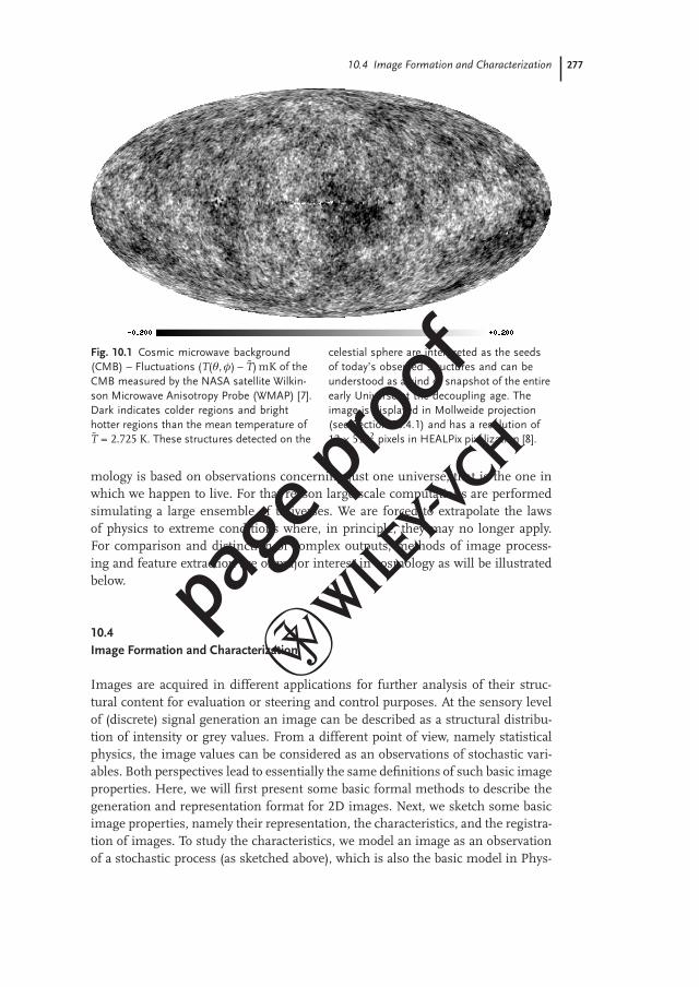
with the mass density contrast Δρ(trec, x) of the entire early universe at the decou-pling age trec. They are interpreted as the seed of todays observed structures andcan be understood as a kind of projected snapshot from the entire early universeat decoupling age. Thereby the CMB represents one of the most powerful toolsin cosmology and is the oldest accessible information with possibilities today. Thefluctuations of the CMB are shown in Figure 10.1.

Due to relativistic effects, that is, the finite speed of light, information of dis-tant objects can only be received from past events. Furthermore, the expansionof the Universe prohibits the access to the entire Universe. That part which is ac-cessible to observations is called the observable Universe. Since we cannot performexperiments with many universes, for example, we cannot repeat the Big Bang, cos-

2) In the full relativistic description there isa dependence on the total energy content.In the standard model there is radiation,baryonic matter, dark matter and darkenergy. One distinguishes between primary

effects, that is, effects at decoupling age, andsecondary effects, that are effects duringpropagation from decoupling age until theobservation time.

page proof

10.4 Image Formation and Characterization 277

Fig. 10.1 Cosmic microwave background(CMB) – Fluctuations (T(θ, φ) – T) mK of theCMB measured by the NASA satellite Wilkin-son Microwave Anisotropy Probe (WMAP) [7].Dark indicates colder regions and brighthotter regions than the mean temperature ofT = 2.725 K. These structures detected on the

celestial sphere are interpreted as the seedsof today’s observed structures and can beunderstood as a kind of snapshot of the entireearly Universe at the decoupling age. Theimage is displayed in Mollweide projection(see Section 10.4.1) and has a resolution of12 ~ 5122 pixels in HEALPix pixelization [8].

mology is based on observations concerning just one universe, that is the one inwhich we happen to live. For that reason large-scale computations are performedsimulating a large ensemble of universes. We are forced to extrapolate the lawsof physics to extreme conditions where, in principle, they may no longer apply.For comparison and distinction of complex outputs, methods of image process-ing and feature extraction are of major interest in cosmology as will be illustratedbelow.

10.4Image Formation and Characterization

Images are acquired in different applications for further analysis of their struc-tural content for evaluation or steering and control purposes. At the sensory levelof (discrete) signal generation an image can be described as a structural distribu-tion of intensity or grey values. From a different point of view, namely statisticalphysics, the image values can be considered as an observations of stochastic vari-ables. Both perspectives lead to essentially the same definitions of such basic imageproperties. Here, we will first present some basic formal methods to describe thegeneration and representation format for 2D images. Next, we sketch some basicimage properties, namely their representation, the characteristics, and the registra-tion of images. To study the characteristics, we model an image as an observationof a stochastic process (as sketched above), which is also the basic model in Phys-

page proof


ical Cosmology where it is assumed that the initial conditions of the Universe aredescribed by a homogeneous and isotropic Gaussian random field. Throughout thearticle u(x) denotes a field of scalar values which can be interpreted in two ways,namely, as intensity or probability distributions. Such scalar values in a field are ad-dressed for the spatial position of a vector in an arbitrary space. Multiple intensityvalues, which are measured by different sensory channels or registration methods,but in a spatially registered way, can be represented as a vector field u(x). In otherwords, such an image, at a spatial position u(x), contains a vector of dimension 2,3, or n, depending on the number of registered sensory channels. Examples are im-ages from magnetic resonance imaging (MRI) combining spin relaxation, T1 andT2, images taken by a color camera measuring in different bands of wavelengthsensitivity as red, green, blue (RGB), or a scalar image field of intensity valuescombined with another field of derived features, such as local variances measuredin a local image neighborhood.

10.4.1Generation and Representation of 2D Images

Our focus in this article will be on two-dimensional (2D) images which are acquiredfrom some environmental measurement space of arbitrary dimension. In the caseof the three-dimensional (3D) space of an outdoor scene the image acquisition pro-cess can be formally described by a projective transform. Most often the projectionresults in a 2D Cartesian coordinate system commonly named image plane. InPhysical Cosmology, instead, an image can be defined on a unit sphere. In suchcases the mapping of the (image) plane onto the curved surface can be describedby a geometric transform. If the topology of the two such surfaces is identical thenthe mapping can be inverted. In the case when the image acquisition is distort-ed, for example due to some geometric lens distortion, the proper registration isalso described by a proper warping transform. Here, we briefly sketch some pro-jective as well as mapping transformations. A more complete overview is givenin [9].

10.4.1.1Perspective ProjectionFor the perspective projection, a point in 3D space x ∈ R3 is projected in 2D spacey ∈ R2, for example, representing an image plane, by

(y1, y2) = (x1, x2) · f/x3 , (10.1)

where the third component is omitted because it equals the constant f. The geo-metric interpretation is that arbitrary points (normally x3 > f) are projected ontoan image plane positioned at a positive distance x3 = f from the coordinate center(0, 0, 0). If, instead, the distance from the projection center is taken to be negative,that is –f, the projection resembles a pinhole projection. A key characteristic is thatthe resulting image is upside down (negative image) while the former case yieldsa positive image. It should be noted that, in the extreme case of very distant scene

page proof


points with x3 >> f, for small objects relative to the field of view, and with only mi-nor relative depth variations, the perspective projection can be approximated by anorthographic projection, namely (y1, y2) = (x1, x2).

10.4.1.2Stereographic ProjectionIn various applications, specific surface properties, such as their 3D orientation,need to be represented in a flat space in order to build proper data structures.A useful approach is to map the spherical hemisphere of surface normals visiblefrom the observer’s viewpoint onto a tangential plane positioned in the sphere’snorth pole. If the center of projection is shifted into the south pole, then the upperhemisphere of the unit sphere is mapped into a circle of radius two (stereographicprojection; [10]). Though this mapping is complete it also has some shortcomings,namely that only one-half of the sphere is projected and that the projection is notarea-preserving.

10.4.1.3Mollweide ProjectionGenerally, images can be defined on arbitrary surfaces (see also Section 10.4.4).Examples are the surface of the earth, which is ideally defined on a unit sphere,or satellites which measure over the celestial sphere. Therefore, images defined onthe sphere play a special role. An approach that overcomes the limitations of thestereographic projection is the Mollweide projection,

y1 = (2√

2/π)Φ cos(Ψ/2) (10.2)

y2 =√

2 sin(Ψ/2) with Ψ + sin Ψ = π sin Θ and (10.3)

Φ = arg(x1 + ix2) , Θ = arctan(x3

/√x2

1 + x22

), (10.4)

where Φ ∈ (–π, +π] denotes the longitude from the central meridian, Θ ∈ (–π/2,+π/2) denotes the latitude, and Ψ denotes only an auxiliary angle. This projectsthe surface of the total unit sphere onto a plane forming an ellipse, where themajor axis is twice as long as the minor axis. Additionally, this projection is areapreserving. This property can be easily checked if one integrates over an arbitrary

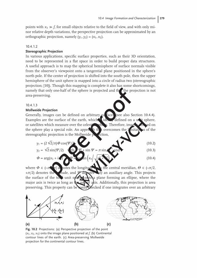
(a) (b) (c)

( )

Fig. 10.2 Projections: (a) Perspective projection of the point(x1, x2, x3) onto the image plane positioned at f. (b) Continentalcontour lines of the earth. (c) Area-preserving Mollweideprojection for the continental contour lines.

page proof


surface patch on the sphere and on the plane, and shows that the calculated areasare equal in size. Figure 10.2c shows the projection for the continental contours ofthe earth.

10.4.2Image Properties

In each image representation the following key properties can be identified: (i)The space or surface where the image is defined (see methods for projections inSection 10.4.1); (ii) the number of quantization levels; (iii) the resolution; and (iv)the scale. Although, the scale of an image is intertwined with the resolution, wediscuss these two properties separately. Figure 10.3 depicts all these properties.

10.4.2.1Quantization PropertyThe quantization levels are defined by the range of the data values. This proper-ty is determined by two criteria. First, the range of the acquisition sensor, and

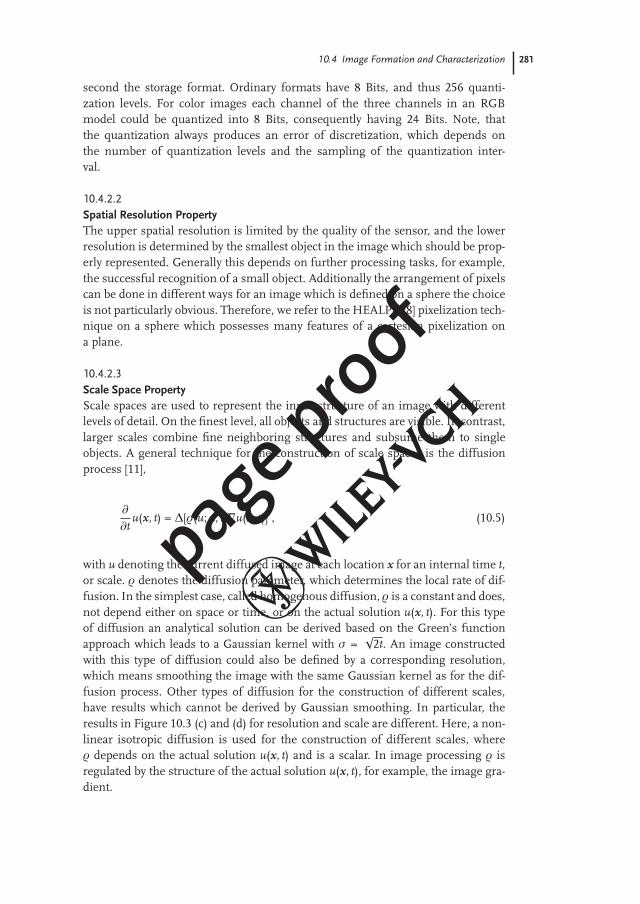
Fig. 10.3 Image properties: (a) 2D magneticresonance image mapped onto an arbitrarysurface, thus the image coordinates dependon the surface geometry. (b) Same image visu-alized with 4, 8, 16 and 32 quantization levels.(c) Image with a resolution of 32 ~ 32 px,

64 ~ 64 px, 128 ~ 128 px, and 256 ~ 256 px(original). (d) Scales of nonlinear isotropicdiffusion of the image for 1000, 100, 50, and10 iterations (λ = 0.02, σ = 1.5, parametersreferring to [11]).

page proof


second the storage format. Ordinary formats have 8 Bits, and thus 256 quanti-zation levels. For color images each channel of the three channels in an RGBmodel could be quantized into 8 Bits, consequently having 24 Bits. Note, thatthe quantization always produces an error of discretization, which depends onthe number of quantization levels and the sampling of the quantization inter-val.

10.4.2.2Spatial Resolution PropertyThe upper spatial resolution is limited by the quality of the sensor, and the lowerresolution is determined by the smallest object in the image which should be prop-erly represented. Generally this depends on further processing tasks, for example,the successful recognition of a small object. Additionally the arrangement of pixelscan be done in different ways for an image which is defined on a sphere the choiceis not particularly obvious. Therefore, we refer to the HEALPix [8] pixelization tech-nique on a sphere which possesses many features of a cartesian pixelization ona plane.

10.4.2.3Scale Space PropertyScale spaces are used to represent the inner structure of an image with differentlevels of detail. On the finest level, all objects and structures are visible. In contrast,larger scales combine fine neighboring structures and subsume them to singleobjects. A general technique for the construction of scale spaces is the diffusionprocess [11],

∂

∂tu(x, t) = Δ[ρ(u; x, t)∇u(x, t)] , (10.5)

with u denoting the current diffused image at each location x for an internal time t,or scale. ρ denotes the diffusion parameter, which determines the local rate of dif-fusion. In the simplest case, called homogenous diffusion, ρ is a constant and does,not depend either on space or time, or on the actual solution u(x, t). For this typeof diffusion an analytical solution can be derived based on the Green’s functionapproach which leads to a Gaussian kernel with σ =

√2t. An image constructed

with this type of diffusion could also be defined by a corresponding resolution,which means smoothing the image with the same Gaussian kernel as for the dif-fusion process. Other types of diffusion for the construction of different scales,have results which cannot be derived by Gaussian smoothing. In particular, theresults in Figure 10.3 (c) and (d) for resolution and scale are different. Here, a non-linear isotropic diffusion is used for the construction of different scales, whereρ depends on the actual solution u(x, t) and is a scalar. In image processing ρ isregulated by the structure of the actual solution u(x, t), for example, the image gra-dient.

page proof


10.4.3Basic Image Characteristics

For the analysis of image characteristics an image can be defined as the observationof a stochastic process in three ways. First, the image is modeled as the outcome ofone random variable (RV); second, as one observation of a random field (RF), andthird as a series of RVs. Each distinct modeling allows the study of distinct imagecharacteristics which contain information of the structure and distribution of im-age intensities. An overview of characteristics and modeling is given in Table 10.1.

10.4.3.1HistogramAssume that all intensities contained in an image are continuous and the outcomeof a single RV X. Additionally, the probability distribution function of X is u(x) forall x ∈ R of the random space. With this formalism the distribution of intensitiesin an image can be expressed by the normalized histogram

HN(Bε) := P(X ∈ Bε) =∫

x∈Bε

u(x)dx , (10.6)

with Bε := {x|b–ε/2 u x < b+ε/2}, which equals the probability distribution functionfor ε → 0. For images with continuous intensities the histogram has bins countingan interval of intensities which have only a finite number of levels. In this caseε defines the width of these bins. Figure 10.4a shows histograms of three imagefeatures. For the cumulative normalized histogram

HN,C(b) := Fu(b) =∫ b

–∞u(x)dx (10.7)

these bins are not necessary and one integrates from the lowest possible intensity–∞ to the intensity level b. This histogram equals the probability mass function Fu

of the RV X.

10.4.3.2Covariance and CorrelationFor two images modeled by RVs X and Y a comparison on the basis of their statis-tical behavior can be achieved by the covariance

CovX,Y =⟨(X – 〈X〉)(Y – 〈Y〉)

⟩= 〈XY〉 – 〈X〉〈Y〉 , (10.8)

Tab. 10.1 Formalism for the modeling of an image and the achieved image characteristics.

Model Single RV RF Series of RVs

One input histogram co-occurrence, Fourier transformation, joint distribution,two-point correlation Fourier transformation

Two inputs correlation joint histogram, correlation –

page proof


0 0.1 0.2 0.3 0.4 0.5 0.6 0.7 0.8 0.9 10

0.05

0.1

0.15

0.2

0.25

0.3

bin Ae

num

ber o

f int

ensi

ties

(a)

intensitydirection of intensity gradientmagnitude of intensity gradient

Aε (intensity )

Bε (

mag

nitu

de)

(b)0 0.5 1

0

0.2

0.4

0.6

0.8

1

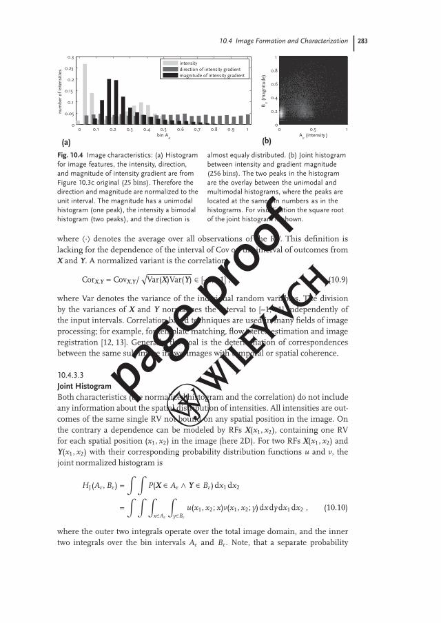
Fig. 10.4 Image characteristics: (a) Histogramfor image features, the intensity, direction,and magnitude of intensity gradient are fromFigure 10.3c original (25 bins). Therefore thedirection and magnitude are normalized to theunit interval. The magnitude has a unimodalhistogram (one peak), the intensity a bimodalhistogram (two peaks), and the direction is

almost equaly distributed. (b) Joint histogrambetween intensity and gradient magnitude(256 bins). The two peaks in the histogramare the overlay between the unimodal andmultimodal histograms, where the peaks arelocated at the same bin numbers as in thehistograms. For visualization the square rootof the joint histogram is shown.

where 〈·〉 denotes the average over all observations of the RV. This definition islacking for the dependence of the interval of Cov on the interval of outcomes fromX and Y. A normalized variant is the correlation

CorX,Y = CovX,Y/√

Var(X)Var(Y) ∈ [–1, +1] , (10.9)

where Var denotes the variance of the individual random variables. The divisionby the variances of X and Y normalizes the interval to [–1, +1] independently ofthe input intervals. Correlation-based techniques are used in many fields of imageprocessing; for example, for template matching, flow/stereo estimation and imageregistration [12, 13]. Generally, the goal is the determination of correspondencesbetween the same sub-image in two images with temporal or spatial coherence.

10.4.3.3Joint HistogramBoth characteristics (the normalized histogram and the correlation) do not includeany information about the spatial distribution of intensities. All intensities are out-comes of the same single RV not bound on any spatial position in the image. Onthe contrary a dependence can be modeled by RFs X(x1, x2), containing one RVfor each spatial position (x1, x2) in the image (here 2D). For two RFs X(x1, x2) andY(x1, x2) with their corresponding probability distribution functions u and v, thejoint normalized histogram is

HJ(Aε, Bε) =∫ ∫

P(X ∈ Aε ∧ Y ∈ Bε)dx1 dx2

=∫ ∫ ∫

x∈Aε

∫

y∈Bε

u(x1, x2; x)v(x1, x2; y)dxdydx1 dx2 , (10.10)

where the outer two integrals operate over the total image domain, and the innertwo integrals over the bin intervals Aε and Bε. Note, that a separate probability

page proof


distribution function u exists for each position (x1, x2) of the RF, and x denotes theargument of the function u, as in the 1D case u(x). In the joint histogram, pairedintensities according to the bins Aε and Bε are voted, where the intensity pair islocated at arbitrary positions (x1, x2) in the two RFs X and Y. In Figure 10.4 (b)a joint histogram between the feature channels intensity and magnitude of theintensity gradient is shown.

10.4.3.4Co-occurrenceFor images with multiple channels, as for example images acquired by multi-spectral sensors or color images, a joint histogram describes the correlation be-tween the intensity distributions of different channels. The joint occurrence of val-ues within one image or channel can be quantified by the co-occurrence matrix

Co(Aε, Bε) =∫ ∫ ∫

x∈Aε

∫

y∈Bε

u(x1, x2; x)u(T(x1, x2); y)dxdydx1 dx2 . (10.11)

Here, the first RF X(x1, x2) is defined by the image and the second RF XT(x1, x2)by a spatial transformation T(x1, x2) of the first RF. This characteristic highlightsperiodic structures and shifts of regions within one image.

10.4.3.5Fourier Transformation of One Observation of an RFMany applications in image processing profit from the analysis of images in theFourier space, especially the study of the effectiveness of filters (see Section 10.5).The Fourier transformation

u(k1, ..., kd; x) =∫

C

...∫

C

u(x1, ..., xd; x) exp

⎛⎜⎜⎜⎜⎜⎜⎝–i

d∑

l=1

klxl

⎞⎟⎟⎟⎟⎟⎟⎠ dx1...dxd , (10.12)

u(x1, ..., xd; x) =1

(2π)d

∫

C

...∫

C

u(k1, ..., kd; x) exp

⎛⎜⎜⎜⎜⎜⎜⎝i

d∑

l=1

klxl

⎞⎟⎟⎟⎟⎟⎟⎠ dk1....dkd ,

(10.13)

from the spatial domain u into the temporal domain u, is again based on the for-malism of the RF, where one concrete observation of the RF is transformed. Afterthe transformation into the Fourier space, u is a complex number. Therefore, u canbe analyzed in phase Φ and amplitude A

Φ = arg(u) , and A = |u| . (10.14)

In Figure 10.5b the amplitude of the transformed input image a is shown. The cor-responding inverse transformation of a filtered version is depicted in Figure 10.5d.For images the information about the spatial locality of structure is stored in thephase, and the information about the general periodicity is represented within theamplitude. To highlight this property consider a shift of the image in the spatialdomain, therefore only the phase is influenced, not the amplitude. Thus, no infor-mation of the locality is included in the amplitude.

page proof


Fig. 10.5 Fourier and inverse Fourier trans-formation: (a) Input image again fromFigure 10.3b (original) with superimposedregular grid. (b) Fourier spectra (amplitude)of the image with characteristic peaks rep-resenting the grid and their multiples. (c)

Boxed version of the fourier spectra. This hasa box filter, where frequencies representingthe first multitude of the grid are cut off. Forvisualization the square-root of the spectra isplotted. (d) Inverse Fourier transformation ofboxed spectra multiplied by the box filter.

10.4.3.6Fourier Transformation of a Common Distribution FunctionIn some cases the stochastic process is defined by a series of RVs (X1, ..., Xd), andthis models the dimensionality of the image. For example, an image is defined asthe outcome of a dD normally distributed RV. Analogous to the Fourier transforma-tion of RF, here the transformation is defined on the basis of the common densitydistribution function u(x1, ..., xd) which equals the product of the single distribu-tion function u(xi) if the RVs are independent. The Fourier transformation

u(k) =∫

Cdu(x) exp(–ikx)dx , u(x) =

1(2π)d

∫

Cdu(k) exp(ikx)dk , (10.15)

where x, k ∈ Rd is the joint characteristics function of the RVs X1, ..., Xd. In otherterms this is the expected value u =

⟨exp(–i

∑dl=1 klXl)

⟩of the series of RVs in respect

to the Fourier base. u can be interpreted as the probability distribution function ofnew RVs X1, ..., Xd, which are also independent, in fact, of the orthogonality of theFourier base.

10.4.3.7Two-Point Correlation Function and Power SpectrumIn cosmology, images of homogeneous and isotropic RFs are often studied. Here,characteristics of length scale or separation distance are of special interest. Thepower spectrum is given by an average over the Fourier modes u(k) with a wavenumber k = |k| of the field3) u(x) with x ∈ R3. In configuration space, a field can bequantified by the two-point correlation function

�(r) :=⟨u(x)u(x + r)

⟩, (10.16)

3) Note that we omitted the x for one realizationof the RF u(x, x) at the position x, becausecosmological observations always display onerealization.

page proof


where the average 〈·〉 is taken over all positions x and all orientations of the sepa-ration vector r, assuming homogeneity and isotropy. Hence there is only a depen-dence on r = |r|. The two-point correlation function of a field on a sphere is

C(ϑ) :=⟨u(θ, φ)u(θ′, φ′)

⟩, (10.17)

where now the average 〈·〉 is taken over all pairs of (θ, φ) and (θ′, φ′) which areseparated by the angle ϑ. Again a power spectrum

Cl :=⟨|alm|2

⟩=

12l + 1

l∑

m=–l

|alm|2 (10.18)

can be defined, where alm are the complex coefficients obtained from an expansioninto spherical harmonics Ylm(θ, φ) due to u(θ, φ) =

∑∞l=0∑l

m=–l almYlm. Here l pa-rameterizes the separation scale and m the direction. In cosmological applicationsthe so-called angular power spectrum

δT2l :=

l(l + 1)2π

Cl (10.19)

is used. Note that, in the case of statistical homogeneity and isotropy, a two-pointcorrelation function can be obtained by a transformation from its corresponding

0

1000

2000

3000

4000

5000

6000

7000

1 10 100 1000

δTl2 [μ

K2 ]

l(a)

ΛCDM (standard model)WMAP-3-year (measurement)

-1000

-500

0

500

1000

1500

2000

0 20 40 60 80 100 120 140 160 180

C(ϑ

) [μ

K2 ]

ϑ [deg](b)

ΛCDM (standard model)WMAP-3-year (measurement)

Fig. 10.6 Statistical quantities of the CMB: (a)Angular power spectrum δT2

l of the observedfluctuations in the cosmic microwave back-ground (CMB) measured by the WilkinsonMicrowave Anisotropy Probe (WMAP) [7]. Theerror bars include measurement errors andthe statistical variance. These characteristicsare very sensitive, i.e. the peak positions andpeak heights, to cosmological parameters.Independent cosmological determinations ofthe cosmological parameters are in excellentagreement with the best-fit standard modelΛCDM (gray line). The systematic deviationson largest scales (small l) cannot be explained

by the standard model and are possibleindications of a finite Universe [14]. (b) Two-point correlation function C(ϑ) of the best-fitstandard model ΛCDM (dark gray line andthe statistical variance as light gray area) andmeasurements of WMAP (black line). Thesecharacteristics highlight the largest scales(ϑ W 180◦/l) where the explanation by thestandard model is limited. Going beyond thestandard model, recent work shows [14], thatbeside the suppression of δT2

l on small l theshape of this characteristic can be reproducedwith high confidence, by studying universeswith a finite spatial extension.

page proof


power spectrum and vice versa. These characteristics carry the same information,but highlight different separation scales and thus different cosmological features.In Figure 10.6 the angular power spectrum and the two-point correlation functionof the measured cosmological microwave background (CMB) is shown where nowu(θ, φ) = T(θ, φ) – T (see Section 10.3). In addition to omitting the constant term(monopole) with l = 0, which is equivalent to T, the dipole with l = 1 is, also omitteddue to a superimposed dipole generated by the relative motion of the observer tothe CMB.

10.4.4Image Registration

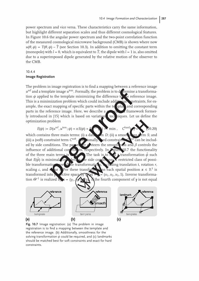
The problem in image registration is to find a mapping between a reference imageuref and a template image utem. Formally, the problem is to determine a transforma-tion φ applied to the template minimizing the difference to the reference image.This is a minimization problem which could include additional constraints, for ex-ample, the exact mapping of specific parts within the template and correspondingparts in the reference image. Here, we describe a generalized framework former-ly introduced in [15] which is based on variational techniques. Let us define theoptimization problem

E(φ) := D(uref, utem; φ) + αS(φ) + �Csoft(φ)φ––→ min , Chard(φ) = 0 , (10.20)

which contains three main terms: (i) a data term D; (ii) a smoothness term S; and(iii) a (soft) constraint term Csoft. Additionally, hard constraints Chard can be includ-ed by side conditions. The parameter α steers the smoothness and � controls theinfluence of additional constraints, respectively. In Figure 10.7 the functionalityof the three main terms is depicted. The task is to find a transformation φ suchthat E(φ) is minimal, considering the side conditions. A restricted class of possi-ble transformations are affine transformations, including translation t, rotation r,scaling c, and shear s. For these transformations each spatial position x ∈ R3 istransformed into projective space by Θ(x) = y = (x1, x2, x3, 1). Inverse transforma-tion Θ–1 is realized by x = (y1, y2, y3)/y4, if the fourth component of y is not equal

Fig. 10.7 Image registration: (a) The problem in imageregistration is to find a mapping between the template andthe reference image. (b) Additionally, smoothness for thesolving transformation φ could be required, and (c) landmarksshould be matched best for soft constraints and exact for hardconstraints.

page proof


Fig. 10.8 Affine transformations: (a) Reference for thetransformations. (b) Translation for t = (0.5, 0.5, 0). (c) Rotationfor r = (15, 0, 0) deg. (d) Scaling for c = (1.5, 1.75, 1.25). (e) Shearfor s = (85, 0, 0) deg.

to zero. Affine transformations in the projective space are realized by a sequentialchained multiplication of transformation matrices

φ(t, r, c, s; y) =

⎛⎜⎜⎜⎜⎜⎜⎜⎜⎜⎜⎜⎜⎜⎜⎝

1 0 0 t1

0 1 0 t2

0 0 1 t3

0 0 0 1

⎞⎟⎟⎟⎟⎟⎟⎟⎟⎟⎟⎟⎟⎟⎟⎠

⎛⎜⎜⎜⎜⎜⎜⎜⎜⎜⎜⎜⎜⎜⎜⎝

1 0 0 00 cos r1 sin r1 00 – sin r1 cos r1 00 0 0 1

⎞⎟⎟⎟⎟⎟⎟⎟⎟⎟⎟⎟⎟⎟⎟⎠

...

⎛⎜⎜⎜⎜⎜⎜⎜⎜⎜⎜⎜⎜⎜⎜⎝

c1 0 0 00 c2 0 00 0 c3 00 0 0 1

⎞⎟⎟⎟⎟⎟⎟⎟⎟⎟⎟⎟⎟⎟⎟⎠

⎛⎜⎜⎜⎜⎜⎜⎜⎜⎜⎜⎜⎜⎜⎜⎝

1 cot s1 0 01 1 0 00 0 1 00 0 0 1

⎞⎟⎟⎟⎟⎟⎟⎟⎟⎟⎟⎟⎟⎟⎟⎠

...y , (10.21)

where we indicated all three rotational matrices by the rotation around the x1-axis,and all three shearing matrices by the shear in the x1x2-plane. Figure 10.8 depictsexamples of those transformations. More advanced transformation techniques canbe found in [9].

For global affine transformations the parameters t, r, c, s ∈ R3 are defined onlyonce for the domain, while local affine transformations exist for each spatial po-sition t(x), r(x), c(x), and s(x). This approach is very extensive introducing twelveunknowns for each spatial position. A simplification assumes constant transfor-mations in small regions within the total spatial image domain.

10.4.4.1Data TermThe data term D compares the (gray) values of the reference image uref (or someextracted feature measure, such as edges, corners, etc.) with the values of the trans-formed template image utem. In this case several distance measures could be ap-plied. An intuitive measure of distances is the sum of squared distances (SSD):

D(uref, utem; φ) =∫ [

uref(x) – utem(Θ–1 (φ[t, r, c, s; Θ(x)]

))]2dx . (10.22)

This distance assumes that the intensities of corresponding values in uref and utem

are equal. If this assumption is not satisfied, correlation-based methods could beapplied, which assume a unimodal distribution of intensity values. For images witha multimodal histogram, mutual information (MI) related measures could be used,

page proof

10.5 Methods of Image Processing 289

which are based on the joint intensity histogram. In general, the data term D is alsocalled an external force, because this term is mainly driven by the intensity valuesof the template and reference.

10.4.4.2Smoothness TermIn contrast to the data term, the smoothness term S is defined by the mapping φwhich constitutes an internal force by imposing a condition on the set of possiblesolutions. The key observation is that in this framework any smoother which isGârteaux-derivable could be applied [15]. Because of its similarity with the diffusionequation in Section 10.4.2 we present as a smoothness condition, the diffusionsmoothness

S(φ) =∫

‖ ∇φ(t, r, c, s; Θ(x)) ‖22 dx . (10.23)

Here the integral, which ranges over the total image domain, induces globalsmoothness onto the mapping function φ, by squaring and summing up all first-order partial derivatives of φ according to the spatial change of the variables t, r, c,and s. Thus, each strong change in φ causes a high derivative, which is unwantedand therefore penalized.

10.4.4.3Constraint TermFinally, we discuss the inclusion of extra constraints that need to be achieved bythe optimized solution. Assume two sets of landmarks, the first set defined inthe reference image {xref

l }l=1...m, and the second set defined in the template image{xtem

l }l=1...m, where correspondence between the landmarks is expressed by the sameindex. A soft constraint term can be formalized by

Csoft(φ) =m∑

l=1

‖ Θ–1(φ[t, r, c, s; Θ(xteml )]) – xref

l ‖22 . (10.24)

This constraint enforces the transformed landmarks of the template to be closelymatched with the landmarks of the reference xref

l , but deviations are possible. Incontrast, for the hard constraint Chard a match should be exact.

10.5Methods of Image Processing

In this section we discuss some approaches for pre-processing image signals uti-lizing a filtering process. Many methods in image processing utilize mechanismthat can be described in terms of linear systems theory [2, 9, 16]. Filters can be de-fined according to their functional purpose, for example, smoothing by eliminationof high-frequency content, or discontinuity detection by extracting high-frequency

page proof


content. We briefly summarize the properties of linear systems and display Gaus-sian smoothing filters and some related derivative operations. So-called Gabor fil-ters define band-pass operations for combined smoothing and discontinuity detec-tion having localized spectral windowing properties. We also show how a bank offilters can be constructed. Finally, we briefly present approaches to nonlinear filter-ing as well as approaches that help to detect localized key points which obey local2D image structure properties.

10.5.1Filtering Process

We consider here a specific class of system operatorsH to model the filtering stage,namely those that are linear and space invariant.4) Such systems are commonlyassumed in image processing, since the computations can be fully described usinglinear systems theory. A system is linear if the identity

H{a u(x) + bw(x)} = a Hu(x) + bHw(x) , (10.25)

holds. Further, a system is space or shift invariant if

H{u(x – x0)} = v(x – x0) , for H{u(x)} = v(x) , (10.26)

to denote that the system operator response is position invariant given identicalinput conditions. Taken together, the system response for an arbitrary input is fullydefined by the correspondence

H{u(x)} = H(x) ∗ u(x) , ! H{u(k)} = H(k) · u(k) , (10.27)

where the left-hand side denotes the convolution of the input signal u(x) by thesystem’s impulse response function H(x) (∗ is the convolution operator). The cor-respondence (denoted by !) establishes that the same result can be computed inthe spatial as well as the spectral, or Fourier, domain. In the frequency domain kthe convolution is equivalent to a multiplication of the Fourier transforms of therespective signals. This property is useful to study the characteristics of systems.

10.5.2Linear and Space-Invariant Filters

10.5.2.1GaussianSmoothing for noise suppression is a key operation in early signal processing. Anideal low-pass filter T · rect(kT) is defined by a specific cut-off frequency 1/(2T)in the spectral domain. Due to the similarity theorem the corresponding spatial

4) Space invariance is the generalization ofthe time invariance property defined fortime-series analysis.

page proof


filter si(πx/T) (where si(x) = sin(x)/x) is of infinite extent with a damping that isproportional to the maximum frequency. In order to utilize a filter function thatis localized in the spatial as well as the frequency domain, a Gaussian low-pass isoften employed

HGauss(x) =exp(– ‖ x ‖2

2 /2σ2)

(√

2πσ)d! HGauss(k) = exp

(

–‖ k ‖2

2

2σ2

)

. (10.28)

The Fourier transform pair results in two Gaussians which are related by their stan-dard deviations, namely σ = 1/σ. Therefore a sharp spatial Gaussian correspondsto a flat Gaussian in the Fourier space and vice versa. (compare Figure 10.9a ande). Due to the Gaussian damping of higher spatial frequencies the filter applica-tion reduces the effective resolution of an image, resulting in a coarser scale (seeSection 10.4.2).

10.5.2.2First-Order DerivativeSpatial derivative operations can also be formulated by filtering operations. Forexample, the first-order derivative is denoted by

u(x + ej dx) = u(x)dx0 +∂

∂xju(x)dx1 + O(dx2), j = 1...d , (10.29)

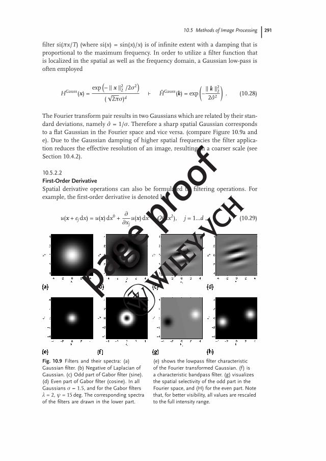
Fig. 10.9 Filters and their spectra: (a)Gaussian filter. (b) Negative of Laplacian ofGaussian. (c) Odd part of Gabor filter (sine).(d) Even part of Gabor filter (cosine). In allGaussians σ = 1.5, and for the Gabor filtersλ = 2, ψ = 15 deg. The corresponding spectraof the filters are drawn in the lower part.

(e) shows the lowpass filter characteristicof the Fourier transformed Gaussian. (f) isa characteristic bandpass filter. (g) visualizesthe spatial selectivity of the odd part in theFourier space, and (H) for the even part. Notethat, for better visibility, all values are rescaledto the full intensity range.

page proof


where ej denotes the j-th unit vector. Division by dx and rearranging terms resultsin the operator for the first-order derivative

H{u(x)} =u(x + ej · dx) – u(x)

dx+ O(dx) . (10.30)

All first-order partial derivatives for j = 1, ..., d together form the gradient of theinput image. In Fourier space the derivatives

H{u(x)} =∂

∂xju(x) ! H{u(k)} = iku(k) j = 1...d , (10.31)

lead to a multiplication of the original spectrum with ik, as the partial derivativescan be calculated within the second integral of (10.15). Multiplication of the spec-trum with a linear or faster-than-linear function amplifies noise. This effect can bereduced by appliance of a Gaussian filter kernel before calculating the derivative ofthe input image.

10.5.2.3Second-Order Derivative and Laplacian of Gaussian (LoG)The second-order derivatives are defined on the basis of the Hessian matrix

H{u(x)} =∂2

∂xj∂xlu(x) ! H{u} = –kjklu(k) j, l = 1...d . (10.32)

In Fourier space the Hessian matrix is the negative of the transformed image u(k)multiplied by the two frequency components kj and kl. In this case noise is ampli-fied twice which makes the second-order derivatives highly sensitive, especially forhigh-frequency noise.

The trace of this Hessian matrix defines the Laplacian operator L = trace({∂2/(∂xj∂xl)}j,l=1...n). For suppression of noise again the Gaussian filter could be applied,before the Laplacian. Due to the law of associativity the convolution of an imagewith the Laplacian operator can be applied directly to the Gaussian, resulting in theLaplacian-of-Gaussian (LoG)

HLoG(x) = L{HGauss(x)} =1

(√

2πσ)d

( ‖ x ‖22

σ4 –1σ2

)

exp(

–‖ x ‖2

2

2σ2

)

! HLoG(k) = – ‖ k ‖22 HGauss(k) , (10.33)

which is characteristic for a bandpass filter, where the frequency with maximalamplification is kj = ±

√2σ for each dimension j. The 2D version of this filter

defines a ring with radius√

2σ of maximum spectral sensitivity (see Figure 10.9f).

10.5.2.4Gabor FilterWhile the LoG operator specifies an isotropic band-pass filter, often orientation sen-sitive filter devices are needed, for example, to separate oriented texture patterns of

page proof


similar wavelength properties. Gabor filters specify an example in which a select-ed set of frequencies are passed which fall into the region of a pair of Gaussianwindows positioned along a given axis of orientation shifted in opposite directionswith respect to the origin (see Figure 10.9 g and h). The combined frequency/phaseshift (defined by the wavelength λ and direction ψ) of the Gaussian filter in the fre-quency domain leads to a modulation of the space domain Gaussian by the wavefunction exp(ik0x).

HGabor(x) = exp(ik0x)HGauss(x) , ! HGabor(k) = HGauss(k – k0) . (10.34)

Note, that the Gabor filter results in a quadrature filter with an odd (sine) shown inFigure 10.9 (c) and an even part (cosine) shown in (d),5) with their correspondingFourier transforms in (g) and (h), respectively. For the interpretation of these twoparts, again the phase and amplitude as defined in (10.14) are considered. Here,the amplitude can be interpreted as the power of the filtered image. The phase hashigh responses for parts of the image which are coincident with this phase and thespecified wavelength. A separated analysis of the two parts shows that the odd part(sine) behaves in a similar way to a bandpass filter, where the even part (cosine) hasa Direct Current (DC) level component, due to the residual response

DC(HGabor,even) =

∫

Rd 1 cos(k0x)HGauss(x)dx

(√

2πσ)d= exp

(

–‖ k0 ‖2

2

2σ2

)

, (10.35)

for a constant signal. For a DC-level free definition the constant value DC(HGabor,even)is subtracted from the even part of the Gabor filter, which can be recognized inFigure 10.9d by a slightly darker gray in the display of responses as in c, especiallyfor high frequencies.

10.5.2.5Gabor Filter BankUsing properly scaled and shifted Gaussian window functions the whole frequencydomain could be sampled using Gabor filters. This, in turn, leads to a signal rep-resentation by a population of Gabor filter responses (compare Figure 10.10). Thissampling can be achieved in two ways. (i) The Gaussian envelope σl is constantin all rings; and (ii) the number of Gaussians in each ring is constant, meaningthat Δψl is constant in all rings l. For this second approach the wavelengths andstandard deviations are

λl+1 = λl1 – 2 sin(Δψ/4)1 + 2 sin(Δψ/4)

, and σl = (4π/λl) sin(Δψ/4) , l v 0 , (10.36)

where l denotes the number of the ring, given λ0 the radius of the innermost ring.This scheme constructs Gabor wavelets, defined by a constant number of waves in

5) The Hilbert transform u(x) = u(x) ∗ 1/(πx) ofthe even part results in the negative odd partand the Hilbert transform of the odd partresults in the even part.

page proof


k1

k 2

−20 −10 0 10 20−20

−10

0

10

20

−20 −10 0 10 20−20

−10

0

10

20

k1

k 2

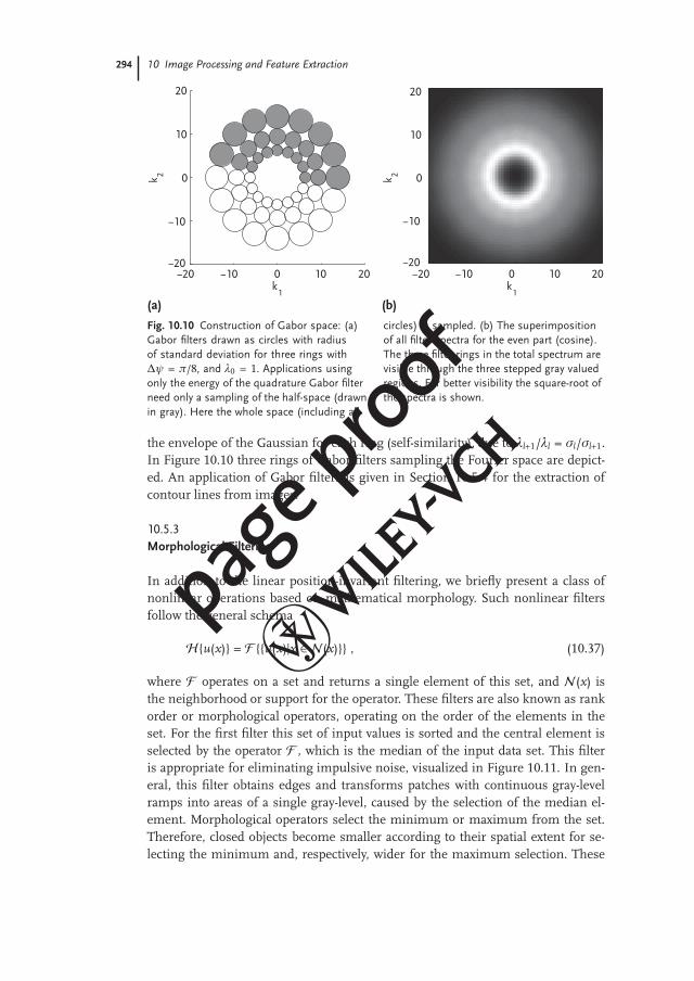
(a) (b)Fig. 10.10 Construction of Gabor space: (a)Gabor filters drawn as circles with radiusof standard deviation for three rings withΔψ = π/8, and λ0 = 1. Applications usingonly the energy of the quadrature Gabor filterneed only a sampling of the half-space (drawnin gray). Here the whole space (including all

circles) is sampled. (b) The superimpositionof all filter spectra for the even part (cosine).The three filter rings in the total spectrum arevisible through the three stepped gray valuedregions. For better visibility the square-root ofthe spectra is shown.

the envelope of the Gaussian for each ring (self-similarity), due to λl+1/λl = σl/σl+1.In Figure 10.10 three rings of Gabor filters sampling the Fourier space are depict-ed. An application of Gabor filters is given in Section 10.5.4 for the extraction ofcontour lines from images.

10.5.3Morphological Filtering

In addition to the linear position-invariant filtering, we briefly present a class ofnonlinear operations based on mathematical morphology. Such nonlinear filtersfollow the general schema

H{u(x)} = F {{u(x)|x ∈ N(x)}} , (10.37)

where F operates on a set and returns a single element of this set, and N(x) isthe neighborhood or support for the operator. These filters are also known as rankorder or morphological operators, operating on the order of the elements in theset. For the first filter this set of input values is sorted and the central element isselected by the operator F , which is the median of the input data set. This filteris appropriate for eliminating impulsive noise, visualized in Figure 10.11. In gen-eral, this filter obtains edges and transforms patches with continuous gray-levelramps into areas of a single gray-level, caused by the selection of the median el-ement. Morphological operators select the minimum or maximum from the set.Therefore, closed objects become smaller according to their spatial extent for se-lecting the minimum and, respectively, wider for the maximum selection. These

page proof


Fig. 10.11 Gaussian and median filter:A magnetic resonance image is distortedby Gaussian noise with standard deviationσ = 0.25 and mean μ = 0.5 (a), and impulsivenoise where 25% of all pixels are disturbed (b).Results of filtering with a Gaussian kernel withσ = 0.25 and length of 3 px are shown in (c1)for Gaussian noise and (c3) for outlier noise,and with a Gaussian kernel with σ = 1.75 and

length of 7 px in (c2) and (c4), respectively.Results for median filter with a neighborhoodof 3 ~ 3 px for Gaussian noise are in (d1) andoutlier noise in (d3), and with a neighborhoodof 7 ~ 7 px for Gaussian noise in (d2) andoutlier noise in (d4). Note that the medianfilter is appropriate to cope with impulsivenoise, and the Gaussian filter is appropriatefor handling Gaussian noise.

operations can be consecutively combined resulting in an opening or closing ofstructures. Further details for opening and closing are reported in Section 10.6.2.

10.5.4Extraction of Image Structures

The gradient and higher-order derivatives of an image are key approaches for theextraction of image structures. For the gradient, first-order derivatives (as statedin (10.30)) are calculated. Each position in the image contains a gradient directedinto the direction of the strongest increasing gray-value ramp (see Figure 10.12b).An analysis of the structure based on this gradient is not appropriate because un-correlated noise and a constant gray value patch cannot be distinguished. Thus,the orientation which best fitts the gradients in a neighborhood (for example, de-fined by the size of the patches) should be calculated. This could be defined as anoptimization problem,

∫

N(x0)‖ v(x0)∇u(x) ‖2

2 dx = v(x0)t[∫

N(x0)(∇u)t∇udx]v(x0)

v–→ max . (10.38)

The vector product of the gradient integrated in the local neighborhood is the struc-ture tensor

{J(u)}j,l :=∫

N(x0)uxj uxl dx , j, l = 1...d , (10.39)

for all positions x0. The eigenvalue decomposition of J is denoted by the eigenval-ues λk and eigenvectors vk ∈ Rd for k = 1...d. The main direction in the neighbor-hood is the eigenvector corresponding to the largest eigenvalue. For the 2D casethe full interpretation of the structure tensor is given in Table 10.2.

page proof


Fig. 10.12 Image gradient, edges and contour: (a) Magneticresonance image with marked region. (b) Intensity gradient inmarked region. (c) Magnitude of intensity gradient. (d) Contourconstructed of responses for oriented Gabor filters (σ = 1,Δψ = π/8, λ = π/3). For clarity in (c) and (d) the square- root isshown.

Tab. 10.2 Interpretation of the structure tensor for a 2D image.

Condition Interpretation

λ1 W λ2 W 0 constant gray-value in neighborhoodλ1 >> 0, λ2 W 0 directed structure in neighborhood (hint for edge)λ1 > λ2, λ2 >> 0 changes of gray-values in more directions (hint for corner)

Based on the structure tensor, measures for edges and corners in images canbe defined. A corner is present if both eigenvalues are significantly greater thanzero. A measure considering this condition is the Förstner corner detector [17]. Anedge can be identified by the ratio between the eigenvalues. A contour line simi-lar to edges is constructed with a small Gabor filter bank, consisting of one scaleand eight orientations, only using the amplitude of the complex filter responses.From this ensemble of filter responses corresponding to each specific orientationthe sum is calculated, resulting in the contour signal. This sum is depicted in Fig-ure 10.12d.

10.6Invariant Features of Images

Above, we have discussed some basic processing approaches for noise suppression,signal restoration, the detection of localized structures, and their proper coding.The main aim of signal processing is the extraction of relevant features from im-ages to generate compact descriptions. Such descriptions need to possess certaininvariance properties, mainly against transformations such as position, rotation, orscaling. Such descriptions serve as a basis for classification or matching differentrepresentations utilizing proper similarity measures. In this section we focus onfeatures and descriptions derived thereof which are relevant for Physical Cosmol-ogy. We first address the aim to find matchings between objects using representa-tions which are invariant to translation, rotation and scaling. Afterwards, we leavethe direct description of scalar fields and switch to methods of stereography, using

page proof

10.6 Invariant Features of Images 297

descriptions of binary fields. We present explicit relations of scalar fields to binaryfields and discuss the connectivity of structures by topological classification. ThenMinkowski functionals are shown as a full set of shape descriptors which obey ad-ditivity and are invariant to translations and rotations. We also present their gener-alization, namely Minkowski valuations. Finally, we end by illustrating applicationsin cosmology.

10.6.1Statistical Moments and Fourier Descriptors

Representations with invariant properties are helpful for finding and matching ob-jects and structures. Important invariance properties are translation, rotation, andscaling. These properties are depicted in Figure 10.8a–d. In the next paragraphsseveral representations which are invariant for at least some transformations arepresented.

10.6.1.1Statistical Joint Central MomentsThe statistical joint central moments of the two random variables (RV)s X1 and X2

with the joint probability distribution function u(x1, x2)

μp,q =⟨(X1 – 〈X1〉)p(X2 – 〈X2〉)q⟩

=∫ ∫

(x1 – x1)p(x2 – x2)qu(x1, x2)dx1 dx2 , (10.40)

are invariant with translation. If invariance with scale is additionally required weassume that u(x1, x2) = u(x1/α, x2/α). Through simple substitutions in the integralswe see that μp,q = αp+q+2μp,q. If we divide μp,q through the zeroth moment to thepower of (p + q + 2)/2 we obtain

μp,q = αp+q+2μp,q/(α2μ0,0)p+q+2/2 = μp,q/μp+q+2/20,0 , (10.41)

which is invariant with scaling. On the basis of the moments a tensor for the mo-ment of inertia

J =(

μ2,0 –μ1,1

–μ1,1 μ0,2

)

(10.42)

can be constructed. The orientation of the eigenvector corresponding to the small-est eigenvalue of J is Φ = 1/2 arctan(2μ1,1/(μ2,0 – μ0,2)), which is the smallest mo-ment of inertia. This criterion is invariant with scaling and translation, becauseof the invariance of μp,q with translation. The calculation of the ratio causes theinvariance with scaling.

10.6.1.2Fourier DescriptorsFourier descriptors are a general method used for the compact description andrepresentation of contours. Therefore, we assume that there exists a parameterized

page proof


description z(t) = z(t + lT) ∈ C, t ∈ [0, ..., T], l ∈ Z of the contour, which is periodicin T, and t is the parameter for the actual position of the curve. For the Fouriertransformation assume z(t) = x1(t) + ix2(t), that the first component of the curvedefines the real part and the second component defines the complex part. TheFourier transform

Z(ν) =1T

∫ T

0z(t) exp

(–2πiνt

T

)

dt , ν ∈ Z (10.43)

provides the Fourier coefficients Z(ν) for the curve. The first coefficient Z(0) is themean point or centroid of the curve. The second coefficient Z(1) describes a circle.Including the coefficient Z(–1), a arbitrarily ellipse can be constructed. For eachpair of Fourier coefficients Z(n) and Z(–n) an ellipse is constructed, which is runthrough n times. The reconstruction of the original parameter curve with the Fouri-er coefficients is

z(t) =+∞∑

ν=–∞Z(ν) exp

(–2πiνt

T

)

. (10.44)

Note that, in practical applications, for appropriate results only a small number ofFourier coefficients must be calculated. Now we consider the invariance proper-ties of this representation. A translational shift in the contour only influences theFourier coefficient Z(0). A scaling of the contour line influences all coefficients.The same holds for a rotation of the curve. An invariant representation can beconstructed in three steps. (i) Drop the coefficient Z(0), which gives translationalinvariance. (ii) Set the norm of Z(1) to unity, which gives invariance for arbitraryscaling. (iii) Set all phases in relationship to the phase of Z(1), which gives rotation-al invariance.

In summary, Fourier coefficients are a good representation of contours and mo-ments for the total intensities of objects.

In the following sections we leave the direct description of a scalar field anddiscuss methods of stereography, particularly binary fields which only have the fieldvalue 0 or 1. This leads to methods of shape description, which we shall discusslater.

10.6.2Stereography and Topology

First, we present several definitions and basic methods of stereography. Then wediscuss the topological classification of structures which measures their connectiv-ity. Furthermore this gives a motivation for the next subsection.

10.6.2.1StereographyTo analyze a scalar field u(x) using x ∈ Rd with methods of stereography one hasto generate a binary image called a structure Q. This can be done by thresholding.

page proof


One gets the excursion set

Q ν := {x|u(x) v ν} , (10.45)

by discriminating between regions with a higher and lower field value than thethreshold ν. The boundary ∂Q ν of the excursion set Q ν is then obviously given by∂Q ν := {x|u(x) = ν}. Varying the threshold ν causes in general a variation in themonochrome image Q ν. So the threshold can be used as a diagnostic parameter toanalyze the scalar field u(x).

Given a structure Q or even only a point distribution, that is a union of pointswhich can also be understood as a structure Q, one can generate the parallel set Qε.By putting a ball Bε with fixed radius ε at every point of the structure Q one gets

Q ε = Q ⊕ Bε . (10.46)

The sum is understood as the Minkowski sum C = A⊕B of two sets A and B, whichconsists of all points c = a+b that can be written as a vector sum of two points a ∈ Aand b ∈ B. The corresponding difference Q#Bε is called the Minkowski difference.In image processing these operations are called dilation and erosion. Again varyingthe radius ε causes, in general, a variation of the generated structure Qε. Thereforethe radius ε can also be used as a diagnostic parameter.

Note that, in general, (Q ⊕ Bε) # Bε =/ Q =/ (Q # Bε) ⊕ Bε holds true. Both have aneffect of smoothing on a length scale ε. Closing is understood as Q⊕,#

ε = (Q⊕Bε)#Bε

and opening as Q#,⊕ε = (Q#Bε)⊕Bε where, compared to Q, the structure Q⊕,#

ε losessmall holes and Q#,⊕

ε loses small cusps. As discussed in Section 10.5.3, effects ofclosing and opening can also be achieved by applying nonlinear and space-invariantfilters on scalar fields.

Another way to get a diagnostic parameter to analyze a scalar field u(x) is to applyan appropriate filter before thresholding. Then the individual filtering parameterscan be used as diagnostic parameters. In practice, it is useful to restrict oneself toone diagnostic parameter which reflects the feature of interest and hold the otherparameters fixed. For filter processes we refer to Sections 10.5.1–10.5.3.

10.6.2.2TopologyA useful feature to distinguish between different structures is their connectivity. Toanalyze the connectivity of a structure Q we use the topological measure called theEuler Characteristic (EC), denoted by �, which is related to the genus g by � = 1 – g.The definition we present here is not only motivated by historical reasons from settheory and convex geometry, but also provides a good access to its interpretation.For a convex body K the EC is defined by

�(K) :={

1 for K =/ ∅0 for K = ∅ (10.47)

and obeys the functional equation for adding two convex bodys K1 and K2

�(K1 ∪ K2) = �(K1) + �(K2) – �(K1 ∩ K2) and �(cK) = �(K) , (10.48)

page proof


the scaling property, for scaling a convex body K with a constant positive real num-ber c ∈ R+.

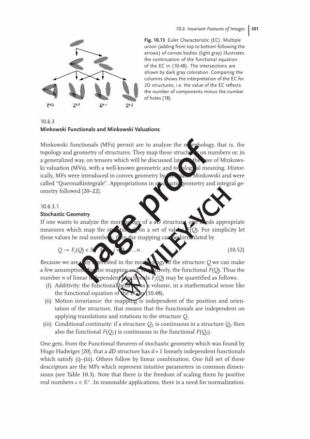
There is a demonstrative morphological interpretation of the value of the ECwhich is governed by the number N($) of objects with the characteristic $ in thestructure Q. For 2D structures, there are �(Q) = N(components) – N(holes). Pos-itive values are generated by isolated objects of a spot-like structure and negativevalues point to a mesh-like structure, where the absolute value reflects the strength.For 3D structures, there are �(Q) = N(components) + N(cavities) – N(tunnels). Ifthere is a connected structure then positive values reflect a cheese-like structureand negative values a sponge-like structure. The absolute value again reflects thestrength. Figure 10.13 illustrates the functional equation of the EC in (10.48) andits interpretation for 2D structures.

Given a smooth dD structure Q with d > 1 and a regular boundary ∂Q, thenevery point x ∈ Rd on its hypersurface has d – 1 principal curvature radii Ri(x)with i = 1, ..., d – 1. The local mean curvature H and Gaussian curvature G of thehypersurface are defined by

H :=1

d – 1

d–1∑

i=1

1Ri(x)

and G :=d–1∏

i=1

1Ri(x)

. (10.49)

Its EC follows from the Gauss–Bonnet theorem after surface integration

�(Q) =Γ(d/2)2πd/2

∫

∂Q

GdA , (10.50)

where dA denotes the element of the hypersurface ∂Q and Γ(x) the Γ-function.The EC of a dD excursion set Qν follows from the Morse theorem by counting thedifferent stationary points of the thresholded function which lie in the excursionset. It is

�(Qν) =d∑

k=0

(–1)kNk(Qν) , (10.51)

where Nk(Qν) denotes the number of stationary points (∇u = 0) to the index k,where k is the number of negative eigenvalues of the matrix {∂i∂ju} for every sta-tionary point. For a 2D excursion set Qν, which was generated from a function u(x)with x ∈ R2, we get �(Qν) = N(maxima)+N(minima)–N(saddle points), where nowN($) denotes the number of stationary points of kind $ which are in the excursionset [19].

In practice, the EC is a appropriate measure to study percolation, wetting andconnectivity where only the topology is of interest. To study also the geometry ofstructures one needs more measures. This leads to Minkowski functionals andtheir generalization, Minkowski valuations, which will be studied in the next sec-tion.

page proof


Fig. 10.13 Euler Characteristic (EC). Multipleunion (adding from top to bottom following thearrows) of convex bodies (light gray) illustratesthe continuation of the functional equationof the EC in (10.48). The intersections areshown by dark gray coloration. Comparing thecolumns shows the interpretation of the EC for2D structures, i.e. the value of the EC reflectsthe number of components minus the numberof holes [18].

10.6.3Minkowski Functionals and Minkowski Valuations

Minkowski functionals (MFs) permit are to analyze the morphology, that is, thetopology and geometry of structures. They map these structures on numbers or, ina generalized way, on tensors which will be discussed later in the case of Minkows-ki valuation (MVs), with a well-known geometric and topological meaning. Histor-ically, MFs were introduced in convex geometry by Hermann Minkowski and werecalled “Quermaßintegrale”. Appropriations in stochastic geometry and integral ge-ometry followed [20–22].

10.6.3.1Stochastic GeometryIf one wants to analyze the morphology of a dD structure, one needs appropriatemeasures which map the structure Q on a set of values F(Q). For simplicity letthese values be real numbers, then the mapping can be formulated by

Q → Fj(Q) ∈ R for j = 0, . . . , n . (10.52)

Because we are only interested in the morphology of the structure Q we can makea few assumptions for the mapping and, respectively, the functional F(Q). Thus thenumber n of linear independent functionals Fj(Q) may be quantified as follows.

(I) Additivity: the functional behaves as a volume, in a mathematical sense likethe functional equation of the EC in (10.48),

(ii) Motion invariance: the mapping is independent of the position and orien-tation of the structure, that means that the functionals are independent onapplying translations and rotations to the structure Q.

(iii) Conditional continuity: if a structure Q1 is continuous in a structure Q2 thenalso the functional F(Q1) is continuous in the functional F(Q2).

One gets, from the Functional theorem of stochastic geometry which was found byHugo Hadwiger [20], that a dD structure has d + 1 linearly independent functionalswhich satisfy (i)–(iii). Others follow by linear combination. One full set of thesedescriptors are the MFs which represent intuitive parameters in common dimen-sions (see Table 10.3). Note that there is the freedom of scaling them by positivereal numbers c ∈ R+. In reasonable applications, there is a need for normalization.

page proof


Tab. 10.3 Geometrical and topological interpretation of the d + 1Minkowski Functionals of structures in common dimensionsd = 1, 2, 3.

d = 1 d = 2 d = 3

F0 length area volumeF1 Euler Characteristic circumference surface areaF2 – Euler Characteristic total mean curvatureF3 – – Euler Characteristic

In any normalization the homogeneity of MF

Fj(cQ) = cd–jFj(cQ) for j = 0, . . . , d (10.53)

of a dD structure Q holds true. This is consistent with the scaling property of theEC in (10.48).

10.6.3.2Integral GeometryWith this interpretation in mind we can focus on an integral geometric approachwhich is suitable for the description of a smooth dD structure Q with d > 1 anda regular boundary ∂Q. This approach leads to a natural generalization of theframework by calculating higher moments. For this reason we add an extra up-per index in the notation of the MFs in (10.54) to show that they are tensors of rank0, namely scalars.

The MF of a structure Q for j = 0 follows by a volume integration and a set of dMFs for j = 1, . . . , d by a surface integration

F0j (Q) =

⎧⎪⎪⎪⎪⎪⎨⎪⎪⎪⎪⎪⎩

N00

∫

QdV for j = 0

N0j

∫

∂QSj dA for j = 1, . . . , d .

(10.54)

dV denotes the hypervolume element of the dD structure Q and dA the hyper-surface element of its (d – 1)D surface. The integrands of a set of the d MFs forj = 1, ..., d can be generated by the j-th elementary symmetric function Sj, which isdefined by

d∑

j=1

zd–jSj :=d–1∏

i=1

[z +

1Ri(x)

]. (10.55)

The functions Sj follow by comparing the coefficients of the polynomial in z andare functions of the j–1 principal curvature radii Rj–1(x) at the position x ∈ Rd. Withthe definitions in (10.49) one can see that for d = 2 we have S1 = 1 and S2 = G. Ford = 3 we have S1 = 1, S2 = H and S3 = G and for d > 3 always S1 = 1, S2 = H andSd = G. Note the consistency between the statements in Table 10.3. The prefactors

page proof


N0j for j = 0, ..., d are arbitrary but fixed normalization constants as explained before

are caused by the freedom of normalization [22].Compared to scalar MFs, one finds that tensor-valued MFs, further called

Minkowski Valuations (MVs) to distinguish clearly between MFs, also obey ad-ditivity (i) and conditional continuity (iii). But motion invariance (ii) breaks down.Therefore, MVs obey motion covariance and the number n of linear independentfunctionals Fj(Q) with j = 0, ..., n can again be quantified. Note that, for rank r > 1in d dimensions, n differs from d + 1 and n u d + r – 1 holds true [23].

By adding the position vector x ∈ Rd in the integrands in (10.54) one gets

F1j (Q) =

⎧⎪⎪⎪⎪⎪⎨⎪⎪⎪⎪⎪⎩

N10

∫

Qx dV for j = 0

N1j

∫

∂QSj x dA for j = 1, . . . , d

(10.56)

for the first-order MVs. Due to the multiplication by a dD vector, the mappingin (10.52) now reads Q → F1

j (Q) ∈ Rd for j = 0, . . . , d. Therefore these MVs be-come dD vectors, that are first-rank tensors.

As mentioned before, there is the possibility of constructing more than d + 1linear independent MVs of rank r > 1. Second-order MVs can be constructed using

F2j (Q) =

⎧⎪⎪⎪⎪⎪⎨⎪⎪⎪⎪⎪⎩

N20

∫

Qx2 dV for j = 0

N2j

∫

∂QSj xpnq dA for j = 1, . . . , d + r – 1

(10.57)

where n ∈ Rd denotes the normalized normal vector on the hypersurface ∂Q in thepoint x and p, q ∈ N0 with rank r = p + q = 2. The multiplication of the dD vectorsin the integrands is understood as a symmetric tensor product, which for two dDvectors a = (a1, ..., ad) and b = (b1, ..., bd) leads to a d ~ d matrix with the elementscij = aibj (i, j = 1, ..., d). The mapping in (10.52) now reads Q → F2

j (Q) ∈ Rd~d forj = 0, . . . , d+r–1. Therefore these MVs get second-rank tensors with d ~ d elements.

Although higher-rank tensors can be constructed, we will not consider themhere. Next, we show several applications of MFs and MVs motivated by cosmo-logical interest.

10.6.3.3ApplicationsIn practice, MFs and MVs turned out to be robust measures for a huge bandwidthof applications. Due to the intuitive interpretation, the individual measures can berelated to some physical properties like the EC for percolation studies. Also full setsof theoretical expected values of MFs for several randomly generated structures areknown [19, 21]. In cosmology, galaxy distributions were studied and compared toseveral Poisson point processes. Around every point a ball with radius ε was placed(see (10.46)), where the radius was varied and used as a diagnostic parameter. Thistechnique is known as the boolean Germ–Grain-Model.

In cosmology random fields also play an important role. Density fluctuationsof the very early universe as imprinted in the CMB, are assumed to be Gaussian.

page proof


To check the Gauss hypothesis, which is a fundamental aspect to allow highly-precision cosmology and is the basis for simulations, MFs are used [18, 22, 24].MFs of a thresholded Gaussian random field Qν (see (10.45)) are analytically wellknown [19, 22] being

F0j (Qν) =

⎧⎪⎪⎨⎪⎪⎩

N00

[1 – Φ

(ν – μ/

√2σ)]

for j = 0N0

j Hj–1

(ν – μ/

√σ)

for j = 1, . . . , d ,(10.58)

where

Φ(x) = 2/√

πx∫

0dt exp(–t2) and Hn(x) = (–1)n/

√2π (d/dx)n exp

(–x2/2

)

(10.59)

is the Gaussian error function Φ(x) and Hn(x) the nth Hermite function. Theseonly depend on parameters of the stochastic process, that is, the mean μ and thevariance σ of the field u(x) and not of the cosmological process, in particular, thecosmological parameters. Depending on the application it can be more convenientto simulate a huge set of realizations including additional numerical effects like dis-cretization, pixelation and masking, also dealt with by experimental data. Further,one then also gets the statistical variance to perform likelihood analyses and onecan define a confidence level. Applications to the CMB are shown in Figure 10.14.

Similarly, the evolution of the LSS of the universe, from its Gaussian origin to itscurrent observed net-like structure, can be studied by MFs of the total field. Sincehigh thresholds disentangle the cosmic web by yielding many isolated objects theconcept of shapefinders, which provide measures to distinguish between differentshape characteristics of single objects, is useful. An illustrative example in 2D, ac-tually on the sphere, as used for an analysis of hot and cold spots in the CMB [18], isto quantify the elongation of structures being approximately ellipses by the ratio oftheir area to their squared circumference E(Q) := F0

0(Q)/[F01(Q)]2. This is a dimen-

sionless, and thereby scale-invariant, shapefinder E, which immediately providesan axis ratio for expected shapes.

Let us come back to the example of the LSS in 3D. Three independent ratiosof MFs which have the dimension of length, namely thickness T , width W andlength L, can be defined:

T (Q) :=F0

0(Q)

2F01(Q)

, W(Q) :=2F0

1(Q)

πF02(Q)

and L(Q) :=3F0

2(Q)

4F03(Q)

. (10.60)

An appropriate normalization is N00

== 1, N01

== 1/6, N02

== 1/6π and N03

== 1/2π.Then for every convex body K the propertyL(K) v W(K) v T (K) holds true. Furtherdimensionless shapefinders called the

planarity P(Q) :=W – TW + T

and filamentarity F (Q) :=L –WL +W

(10.61)

page proof


Fig. 10.14 Minkowski Functionals (MFs).Test on Gaussianity of the fluctuations of thecosmic microwave background (CMB) withMinkowski Functionals (MFs). The normalizedsignal became thresholded (as illustrated in(a), where the analyzed structure is the blackarea). The corresponding normalized MFs F0

0,F0

1 and F02 are calculated (black dots in graphs

in (b)) and compared to the mean values(dark gray line) and statistical variances (3σas light gray area) of a Gaussian random field.The area functional F0

0 is equivalent to thecumulative normalized height distribution and

therefore drops monotonously. By increasingthe threshold, holes appear, get bigger andbecome connected. Isolated spots appear,get smaller and finally vanish. Thereforethe length functional F0

1 increases, reachesa maximum and decreases again. Negativevalues of the connectivity functional F0

2 reflectthe appearance of holes, and positive valuesthe appearance of isolated spots, where in theintermediate both balance each other. Withthese results likelihood analysis showed a highconfidence level for the CMB being a Gaussianrandom field [18].

can be defined, providing appropriate measures to discriminate between LSS of dif-ferent evolution scenarios of physical modeling and their comparison to real data.Their behavior is demonstrated in Figure 10.15. These shapefinders also providethe possibility of categorizing observed galaxy shapes. A real galaxy differs froma sphere by being an oblate spheroid, (like a pancake) known as the family of spiralgalaxies, or being a prolate spheroid, (like a cigar) known as the family of ellipticalgalaxies [22].

page proof


(a) (b)

Fig. 10.15 Shapefinders:. Different cylindersas test bodies (a). For illustration only theircover is shown. The ratio of their heightto their diameter is denoted by c. Varying cfrom zero to infinity causes a transition froma pancake to a filament (gray arrows). Notethe invariance of scaling. The scatter plot (b)of the corresponding shapefinders planarity P

and filamentarity F (black points). The resultsof varying c from zero to infinity continuouslyare shown as a gray line. Building a pancake(c → 0) the value of the shapefinder F staysstable, but P increases. On the other hand,by building a filament (c → ∞) the value ofthe shapefinder P stays stable, but now Fincreases.

MFs are useful for analyzing structures of a stochastic origin or single objectswith � = 1. Given more than one single object, MFs can have identical values fordifferent structures (compare (5) and (6) in Figure 10.16). When the relative po-sition of partial structures is important, as in analysis of the inner structure ofgalaxies [25], galaxy clusters or galaxy superclusters [26], one can use MVs for a rea-sonable description. Due to the concept of center of mass and moments of inertia,known from mechanics, a possible interpretation becomes obvious [23]. First-orderMVs can be interpreted as the geometrical center of the scalar measure and one candefine curvature centroids

pj(Q) = F1j (Q)/F0

j (Q) with N0j == N1

j == 1 for j = 0, ..., d . (10.62)

To fulfill the mentioned interpretation of Second-order MVs one considers onlya subset of (10.57) with r = p = 2 and executes an appropriate transformation.Then one gets the elements

{Pj(Q)

}

kl=

⎧⎪⎪⎪⎪⎪⎨⎪⎪⎪⎪⎪⎩

∫

Q(d2

pjδkl – xkxl) dV for j = 0

∫

∂QSj(d2

pjδkl – xkxl) dA for j = 1, ..., d

(10.63)

of the curvature tensors Pj(Q) for every corresponding scalar measure. d2pj

is the dis-tance to the corresponding curvature centroid pj, which is used as the origin of thecoordinate system, and δkl is the Kronecker δ. These tensors satisfy the eigenvalueequation

Pj(Q)vmj (Q) = λm

j (Q)vmj (Q) for j = 0, ..., d and m = 1, ..., d (10.64)

with λmj (Q) ∈ R, vm

j (Q) ∈ Rd and vmj (Q) · vn

j (Q) = 0 for m =/ n. Thus the scalarmeasures of the structure Q were vectorized, which means parameterized, by the

page proof

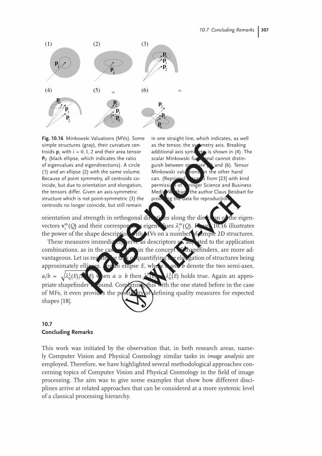
10.7 Concluding Remarks 307

(1)

pi

(2)

pi

(3)

p 0p 1p2

p0

(4)

p2

p1

(5)

pp

p2

1

0p

1

p2

(6)

p0

Fig. 10.16 Minkowski Valuations (MVs). Somesimple structures (gray), their curvature cen-troids pi with i = 0, 1, 2 and their area tensorP0 (black ellipse, which indicates the ratioof eigenvalues and eigendirections). A circle(1) and an ellipse (2) with the same volume.Because of point symmetry, all centroids co-incide, but due to orientation and elongation,the tensors differ. Given an axis-symmetricstructure which is not point-symmetric (3) thecentroids no longer coincide, but still remain

in one straight line, which indicates, as wellas the tensor, the symmetry axis. Breakingadditional axis symmetry is shown in (4). Thescalar Minkowski functional cannot distin-guish between structure (5) and (6). TensorMinkowski valuations on the other handcan. (Reprinted Figure 5 from [23] with kindpermission of Springer Science and BusinessMedia. We thank the author Claus Beisbart forproviding the data for reproduction.).

orientation and strength in orthogonal directions along the direction of the eigen-vectors vm

i (Q) and their corresponding eigenvalues λmj (Q). Figure 10.16 illustrates

the power of the shape description with MVs on a number of simple 2D structures.These measures immediately serve as descriptors or, adjusted to the application

combinations, as in the case of MFs in the concept of shapefinders, are more ad-vantageous. Let us restate the task of quantifying the elongation of structures beingapproximately ellipses. For an ellipse E, where a and b denote the two semi-axes,

a/b =√

λ10(E)/λ2

0(E) when a v b then λ10(E) v λ2

0(E) holds true. Again an appro-priate shapefinder is found. Combining this with the one stated before in the caseof MFs, it even provides the possibility of defining quality measures for expectedshapes [18].

10.7Concluding Remarks

This work was initiated by the observation that, in both research areas, name-ly Computer Vision and Physical Cosmology similar tasks in image analysis areemployed. Therefore, we have highlighted several methodological approaches con-cerning topics of Computer Vision and Physical Cosmology in the field of imageprocessing. The aim was to give some examples that show how different disci-plines arrive at related approaches that can be considered at a more systemic levelof a classical processing hierarchy.

page proof


Motivated by the recording of the cosmic microwave background (CMB) on thecelestial sphere, we started with projection methods, in particular, the Mollweideprojection (see Figure 10.2). Next, we discussed the representation of images andcharacterized four main properties, namely the space an image can be defined on,the quantization, the resolution and the scale space of intensities. Scale spacesare known from physics, but here the properties of scale spaces were adapted tomethods of image processing according to [11].

Images and their characteristics were not only defined in the plane, but alsoon arbitrary surfaces (see Figure 10.3a). For example, the two-point correlationfunction was defined on the sphere and, in addition, the angular power spec-trum. This angular power spectrum is a measure used to compare the expect-ed CMB for different models of the Universe with the measured CMB (see Fig-ure 10.6).

After consideration of image characteristics, the basic methods in image process-ing, modeled by a filtering process, were discussed. Besides the analysis of simplefilters like the Gaussian or the Laplacian of the Gaussian, we additionally discussedthe Gabor filter and specified a scheme for the construction of a Gabor filter bank(see Figure 10.10). On the basis of partial derivatives of image intensities an inten-sity gradient was constructed. This gradient denotes the steepest gray-value ramp.A structure tensor based on the gradient was defined, containing information ofthe local gray-value distribution. For the 2D case, an interpretation of this structuretensor was given (see Table 10.2).

In the last part we focused on invariant descriptions of image features, whereinvariance was restricted to scaling, translation and rotation. First, statistical mo-ments for continuously valued images and descriptions of contour lines weredescribed. Therefore, the contour lines were assumed to be defined as periodiccurves and a representation based on Fourier coefficients was employed. Thenwe changed to thresholded images, denoted by binary structures which could becharacterized by the Euler Characteristic as a simple measure. But, for the anal-ysis of the topology and geometry of structures, this measure was not sufficient,therefore scalar Minkowski functionals were considered. These measures are suit-able to analyze structures initiated by a random process, like investigating thestatistical properties of the CMB (see Figure 10.14) or for shape recognition ofsingle objects by means of shapefinders (see Figure 10.15). Also scalar Minkowskifunctionals do not reveal the full description of structures as explained in Fig-ure 10.16. Thus, we introduced tensor Minkowski valuations offering a moredetailed analysis of structures but also leaving motion invariance (translation androtation).

In summary, we have outlined the primal methods and general concept of imageanalysis. Generally, these methods are located within the first steps of an image-processing hierarchy, providing image enhancement and basic feature extraction –normally seen as low- and mid-level vision tasks. Based on these first steps, furthermethods like 3D scene reconstruction, optic flow estimation, or classification andidentification, can be realized. In particular, for the last two tasks the given invari-ant descriptions are essential. In conclusion, basic methods and general concepts

page proof

References 309

will also be useful in other research areas besides image processing, but so far,a starting point has been given for an exchange of problems and existing solutionsamong researchers studying our observable world.

References

1 Ballard, D.H. and Brown, C.M. (1982)Computer Vision, Prentice-Hall

2 Forsyth, D.A. and Ponce, J. (2003) Com-puter Vision – A Modern Approach, 3rd ed,Pearson Education International, UpperSaddle River, New Jersey.

3 Ullman, S. (1996) High-Level Vision, MITPress, Cambridge, Massachusetts.

4 Witkin, A.P. and Tenenbaum, J.S.

(1983) On the role of structure in vi-sion, in Human and Machine Vision (edsJ. Beck, B. Hope and A. Rosenfeld), Aca-demic Press.

5 Faugeras, O. (1993) Three-dimensionalComputer Vision, MIT Press, Cambridge,Massachusetts.

6 Einstein, A. (1917) Kosmologische Betra-chtungen zur allgemeinen Relativitätsthe-orie. Sitzungsberichte der PreußischenAkademie der Wissenschaften 1917 S.142–152 (also in: The Collected Papers ofAlbert Einstein Bd. 6 S. 540ff PrincetonUniversity Press 1996).

7 Spergel D.N. et al. (2007) Three-yearWilkinson Microwave Anisotropy Probe(WMAP) observations: Implications forcosmology. The Astrophysical Journal Sup-plement Series 170, 377–408.

8 Górski, K.M., Hivon, E., Banday,

A.J., Wandelt, B.D., Hansen, F.K.,

Reinecke, M. and Bartelmann, M.

(2005) HEALPix: A framework forhigh-resolution discretization and fastanalysis of data distributed on thesphere. The Astrophysical Journal 622,759–771.

9 Gomes, J., Darsa, L., Costa, B. and

Velho, L. (1999) Warping and Morphing

of Graphical Objects, Morgan KaufmannPublishers, San Francisco.

10 Hilbert, D., Cohn-Vossen, S. (1952) Ge-omtery and Imagination, Chelsea Publ.Company, New York.

11 Weickert, J. (1998) Anisotrope Diffu-sion in Image Processing, Teubner Verlag,Stuttgart.

12 Horn, B.K.P. (1986) Robot Vision, MITPress, Cambridge, Massachusetts.

13 Trucco, E. and Verri, A. (1998) Intro-ductory Techniques for 3-D Computer Vi-sion, Prentice-Hall, Upper Saddle River,New Jersey.

14 Aurich, R., Janzer, H.S., Lustig, S.

and Steiner, F.() Do we live in a „smallUniverse“?. arXiv:0708.1420, accepted forpublication in Classical and QuantumGravity, 2007 TSr .

15 Fischer, B. and Modersitzki, J. (2006)Image Fusion and Registration – a Vari-ational Approach. In Computational Sci-ence and High Performance Computing II,Notes on Numerical Fluid Mechanics andMultidisciplinatory Design, Springer, 193–205.

16 Jähne, B. (2005) Digital Image Processing,6th edn, Springer Verlag Berlin, Heidel-berg, New York.

17 Förstner, W. (1986) A feature based cor-respondence algorithm for image match-ing. ISP Comm. III, Rovaniemi 1986,International Archives of Photogrammetry,26-3/3.

18 Janzer, H.S. (2006) Untersuchung derkosmischen Hintergrundstrahlung mitMinkowskifunktionalen. Diploma thesis,Universität Ulm.

TSr Please update if possible.

page proof

310 References

19 Tomita, H. (1990) Statistics and Geome-try of Random Interface Systems. In For-mation, Dynamics and Statistics of Patterns(Kawasaki, K., Suzuki, M., and Onuki, A.eds), volume 1, World Sientific.

20 Hadwiger, H. (1957) Vorlesungen überInhalt, Oberfläche und Isoperimetrie.Springer.

21 Mecke, K.R. (1996) Integralgeometrie inder statistischen Physik: Perkolation, kom-plexe Flüssigkeiten und die Struktur desUniversums. Verlag Harri Deutsch.

22 Schmalzing, J. (1999) On Statistics andDynamics of Cosmic Structure. Doctoraldissertation, LMU München.

23 Beisbart, C., Dahlke, R., Mecke, K.

and Wagner, H. (2002) Vector- andTensor-valued Descriptors for Spatial Pat-terns, in Morphology of Condensed Matter.

Physics and Geometry of Spatial ComplexSystems (eds K. Mecke and D. Stoyan),Springer.

24 Eriksen, H.K., Novikov, D.I., Lilje,

P.B., Banday, A.J. and Gorski, K.M.

(2004) Testing for Non-Gaussianity in theWilkinson Microwave Anisotropy ProbeData: Minkowski Functionals and theLength of the Skeleton. Astrophys. J. 612,64–80.

25 Rahman, N. and Shandarin, S.F.

(2003) Measuring shapes of galaxy im-ages – I. Ellipticity and orientation.Monthly Notices of the Royal AstronomicalSociety 343(3), 933–948.

26 Beisbart, C., Buchert, T. and Wagner,

H. (2001) Morphometry of spatial pat-terns. Physica A 293, 592–604.

page proof

10 Image Processing and Feature Extraction from a ... · – feature extraction or generation of structural image descriptions; and ﬁnally – the classiﬁcation of shapes and

Documents