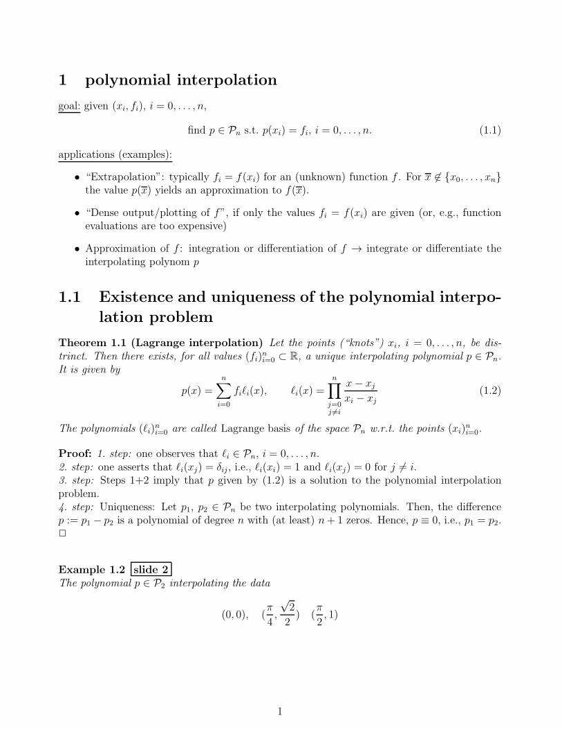
1 polynomial interpolation 1.1 Existence and uniqueness of ...

1 polynomial interpolation

goal: given (xi, fi), i = 0, . . . , n,

find p ∈ Pn s.t. p(xi) = fi, i = 0, . . . , n. (1.1)

applications (examples):

• “Extrapolation”: typically fi = f(xi) for an (unknown) function f . For x 6∈ {x0, . . . , xn}the value p(x) yields an approximation to f(x).

• “Dense output/plotting of f”, if only the values fi = f(xi) are given (or, e.g., functionevaluations are too expensive)

• Approximation of f : integration or differentiation of f → integrate or differentiate theinterpolating polynom p

1.1 Existence and uniqueness of the polynomial interpo-

lation problem

Theorem 1.1 (Lagrange interpolation) Let the points (“knots”) xi, i = 0, . . . , n, be dis-trinct. Then there exists, for all values (fi)

ni=0 ⊂ R, a unique interpolating polynomial p ∈ Pn.

It is given by

p(x) =

n∑

i=0

fiℓi(x), ℓi(x) =

n∏

j=0j 6=i

x− xj

xi − xj(1.2)

The polynomials (ℓi)ni=0 are called Lagrange basis of the space Pn w.r.t. the points (xi)

ni=0.

Proof: 1. step: one observes that ℓi ∈ Pn, i = 0, . . . , n.2. step: one asserts that ℓi(xj) = δij, i.e., ℓi(xi) = 1 and ℓi(xj) = 0 for j 6= i.3. step: Steps 1+2 imply that p given by (1.2) is a solution to the polynomial interpolationproblem.4. step: Uniqueness: Let p1, p2 ∈ Pn be two interpolating polynomials. Then, the differencep := p1 − p2 is a polynomial of degree n with (at least) n+ 1 zeros. Hence, p ≡ 0, i.e., p1 = p2.✷

Example 1.2 slide 2The polynomial p ∈ P2 interpolating the data

(0, 0), (π

4,

√2

2) (

π

2, 1)

1

is given by

p(x) = 0 · ℓ0(x) +√2

2· ℓ1(x) + 1 · ℓ2(x),

ℓ0(x) =(x− π/4)(x− π/2)

(0− π/4)(0− π/2)= 1− (1.909...)x+ (0.8105...)x2,

ℓ1(x) =(x− 0)(x− π/2)

(π/4− 0)(π/4− π/2)= (2.546...)x− (1.62...)x2

ℓ2(x) =(x− 0)(x− π/4)

(π/2− 0)(π/2− π/4)= −(0.636...)x+ (0.81...)x2.

That is, p(x) = (1.164...)x− (0.3357...)x2

Example 1.3 The data of Example 1.2 were chosen to be the values fi = sin(xi), i.e., f(x) =sin x. An approximation to f ′(0) = 1 could be obtained as f ′(0) ≈ p′(0) = 1.164.... An

approximation to∫ π/2

0f(x) dx = 1 is given by

∫ π/2

0p(x) dx = 1.00232...

1.2 Neville-Scheme

It is not efficient to evaluate the interpolating polynomial p(x) at a point x based on (1.2)since it involves many (redundant) multiplications when evaluating the ℓi. Traditionally, aninterpolating polynomial is evaluated at a point x with the aid of the Neville scheme:

Theorem 1.4 Let x0, . . . , xn, be distinct knots and let fi, i = 0, . . . n, be the correspondingvalues. Denote by pj,m ∈ Pm the solution of

find p ∈ Pm, s.t. p(xk) = fk for k = j, j + 1, . . . , j +m. (1.3)

Then, there hold the recursions:

pj,0 = fj , j = 0, . . . , n (1.4)

pj,m(x) =(x−xj)pj+1,m−1(x)−(x−xj+m)pj,m−1(x)

xj+m−xjm ≥ 1 (1.5)

The solution p of (1.1) is p(x) = p0,n(x).

Proof: (1.4) X(1.5) Let π := be the right-hand side of (1.5). Then:

• π ∈ Pm

• π(xj) = pj,m−1(xj) = fj

• π(xj+m) = pj+1,m−1(xj+m) = fj+m

2

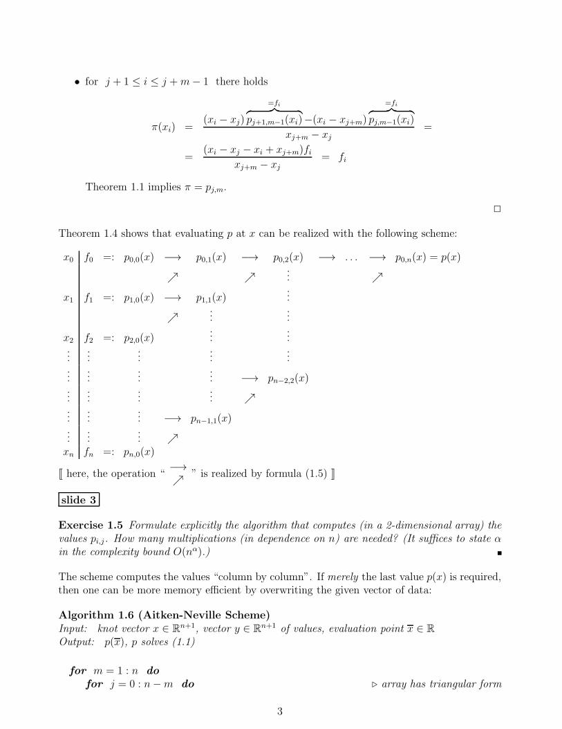
• for j + 1 ≤ i ≤ j +m− 1 there holds

π(xi) =(xi − xj)

=fi︷ ︸︸ ︷pj+1,m−1(xi)−(xi − xj+m)

=fi︷ ︸︸ ︷pj,m−1(xi)

xj+m − xj

=

=(xi − xj − xi + xj+m)fi

xj+m − xj= fi

Theorem 1.1 implies π = pj,m.

✷

Theorem 1.4 shows that evaluating p at x can be realized with the following scheme:

x0 f0 =: p0,0(x) −→ p0,1(x) −→ p0,2(x) −→ . . . −→ p0,n(x) = p(x)

ր ր... ր

x1 f1 =: p1,0(x) −→ p1,1(x)...

ր...

...

x2 f2 =: p2,0(x)...

......

......

......

......

...... −→ pn−2,2(x)

......

...... ր

......

... −→ pn−1,1(x)...

...... ր

xn fn =: pn,0(x)

J here, the operation “−→ր ” is realized by formula (1.5) K

slide 3

Exercise 1.5 Formulate explicitly the algorithm that computes (in a 2-dimensional array) thevalues pi,j. How many multiplications (in dependence on n) are needed? (It suffices to state αin the complexity bound O(nα).)

The scheme computes the values “column by column”. If merely the last value p(x) is required,then one can be more memory efficient by overwriting the given vector of data:

Algorithm 1.6 (Aitken-Neville Scheme)Input: knot vector x ∈ R

n+1, vector y ∈ Rn+1 of values, evaluation point x ∈ R

Output: p(x), p solves (1.1)

for m = 1 : n do

for j = 0 : n−m do ⊲ array has triangular form

3

yj :=(x−xj) yj+1−(x−xj+m) yj

xj+m−xj

end for

end for

return y0

Remark 1.7 • Cost of Alg. 1.6: O(n2)

• The knots xi need not be sorted.

• The Neville scheme, i.e., the algorithm formulated in Exercise 1.5 is particularly con-venient, if additional data points are added at a later time: one merely appends oneadditional row at the bottom.

finis 1.DS

1.3 Newton representation of the interpolating polyno-

mial (CSE)

The cost of evaluating the interpolating polynomial p at a single point x are O(n2). If theinterpolating polynomial has to be evaluated in many points x (e.g., for plotting), then it is ofinterest to reduce the cost (i.e., number of floating point operations) from O(n2) to O(n) perevaluation point x. The “classical” way to achieve this is with the Horner scheme.The Newton polynomials ωj, j = 0, . . . , n, w.r.t. the knots x0, x1, . . . , xn, are given by

ωj(x) :=

j−1∏

i=0

(x− xi) (an empty product is defined to be 1);

written explicitly:

1, (x−x0), (x−x0)(x−x1), (x−x0)(x−x1)(x−x2), . . . , (x−x0)(x−x1) · · · (x−xn−1). (1.6)

These polynomials form a basis of Pn. That is, for every polynomial p(x) of degree n there arecoefficients d0, . . . , dn, such that

p(x) = d0 · 1 + d1(x− x0) + d2(x− x0)(x− x1) + d3(x− x0)(x− x1)(x− x2) (1.7)

+ · · · + dn(x− x0)(x− x1) · · · (x− xn−1). (1.8)

Once the coefficients di are available, the polynomial p(x) can be evaluated very efficiently byrearranging (1.7) as follows:

p(x) = d0 + d1(x− x0) + d2(x− x0)(x− x1) + . . .+ dn(x− x0)(x− x1) . . . (x− xn−1) =

= d0 + (x− x0)

[d1 + (x− x1)

[d2 + (x− x2)

[. . .

[dn−1 + (x− xn−1)[dn]

]. . .

]]]

This procedure is formalized in the following “Horner scheme”:

4

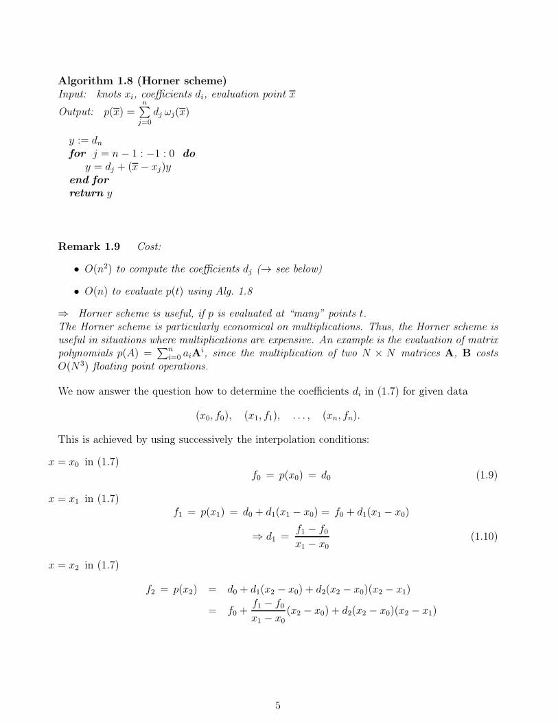
Algorithm 1.8 (Horner scheme)Input: knots xi, coefficients di, evaluation point x

Output: p(x) =n∑

j=0

dj ωj(x)

y := dnfor j = n− 1 : −1 : 0 do

y = dj + (x− xj)yend for

return y

Remark 1.9 Cost:

• O(n2) to compute the coefficients dj (→ see below)

• O(n) to evaluate p(t) using Alg. 1.8

⇒ Horner scheme is useful, if p is evaluated at “many” points t.The Horner scheme is particularly economical on multiplications. Thus, the Horner scheme isuseful in situations where multiplications are expensive. An example is the evaluation of matrixpolynomials p(A) =

∑ni=0 aiA

i, since the multiplication of two N × N matrices A, B costsO(N3) floating point operations.

We now answer the question how to determine the coefficients di in (1.7) for given data

(x0, f0), (x1, f1), . . . , (xn, fn).

This is achieved by using successively the interpolation conditions:

x = x0 in (1.7)f0 = p(x0) = d0 (1.9)

x = x1 in (1.7)f1 = p(x1) = d0 + d1(x1 − x0) = f0 + d1(x1 − x0)

⇒ d1 =f1 − f0x1 − x0

(1.10)

x = x2 in (1.7)

f2 = p(x2) = d0 + d1(x2 − x0) + d2(x2 − x0)(x2 − x1)

= f0 +f1 − f0x1 − x0

(x2 − x0) + d2(x2 − x0)(x2 − x1)

5

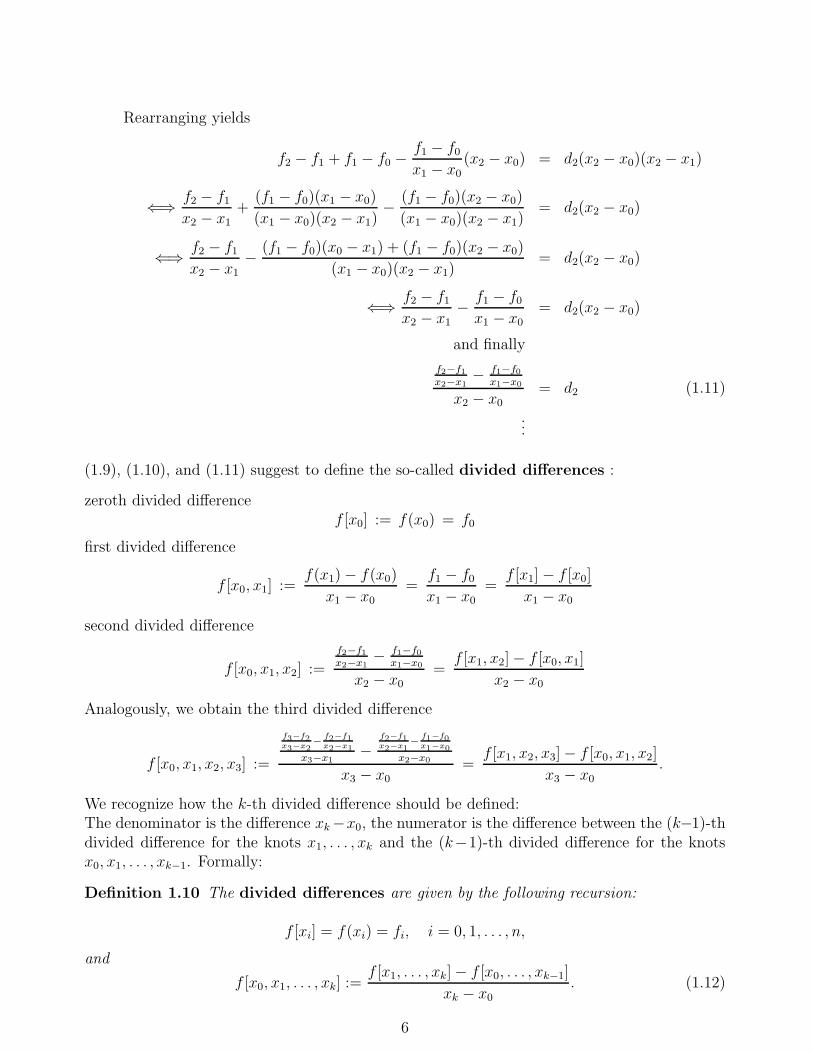
Rearranging yields

f2 − f1 + f1 − f0 −f1 − f0x1 − x0

(x2 − x0) = d2(x2 − x0)(x2 − x1)

⇐⇒ f2 − f1x2 − x1

+(f1 − f0)(x1 − x0)

(x1 − x0)(x2 − x1)− (f1 − f0)(x2 − x0)

(x1 − x0)(x2 − x1)= d2(x2 − x0)

⇐⇒ f2 − f1x2 − x1

− (f1 − f0)(x0 − x1) + (f1 − f0)(x2 − x0)

(x1 − x0)(x2 − x1)= d2(x2 − x0)

⇐⇒ f2 − f1x2 − x1

− f1 − f0x1 − x0

= d2(x2 − x0)

and finally

f2−f1x2−x1

− f1−f0x1−x0

x2 − x0= d2 (1.11)

...

(1.9), (1.10), and (1.11) suggest to define the so-called divided differences :

zeroth divided differencef [x0] := f(x0) = f0

first divided difference

f [x0, x1] :=f(x1)− f(x0)

x1 − x0

=f1 − f0x1 − x0

=f [x1]− f [x0]

x1 − x0

second divided difference

f [x0, x1, x2] :=

f2−f1x2−x1

− f1−f0x1−x0

x2 − x0

=f [x1, x2]− f [x0, x1]

x2 − x0

Analogously, we obtain the third divided difference

f [x0, x1, x2, x3] :=

f3−f2x3−x2

−f2−f1x2−x1

x3−x1−

f2−f1x2−x1

−f1−f0x1−x0

x2−x0

x3 − x0

=f [x1, x2, x3]− f [x0, x1, x2]

x3 − x0

.

We recognize how the k-th divided difference should be defined:The denominator is the difference xk−x0, the numerator is the difference between the (k−1)-thdivided difference for the knots x1, . . . , xk and the (k−1)-th divided difference for the knotsx0, x1, . . . , xk−1. Formally:

Definition 1.10 The divided differences are given by the following recursion:

f [xi] = f(xi) = fi, i = 0, 1, . . . , n,

and

f [x0, x1, . . . , xk] :=f [x1, . . . , xk]− f [x0, . . . , xk−1]

xk − x0. (1.12)

6

The above discussion suggests that the coefficients di in (1.7) are given by the divided differ-ences. This is indeed the case:

Theorem 1.11 Let the knots x0, . . . , xn be distinct. Then the interpolating polynomial p hasthe form

p(x) = f [x0] + f [x0, x1](x− x0) + f [x0, x1, x2](x− x0)(x− x1) (1.13)

+ · · · + f [x0, x1, . . . , xn](x− x0) · · · (x− xn−1).

Proof: For any polynomial π ∈ Pn of the form π(x) =∑n

i=0 aixi we define its leading coefficient

lc(π) := an. We show, with the notation of Theorem 1.4 that, for any j, k

lc(pj,k) = f [xj , . . . , xj+k]. (1.14)

To see (1.14), we proceed by induction on k. By definition, we have pj,0 = f [xj ] for all j. Letus assume that (1.14) holds true for all k ≤ K. Then with the aid of Theorem 1.4

lc(pj,K+1)Thm. 1.4

=lc(pj+1,K)− lc(pj,K)

xj+(K+1) − xj

induction hyp.=

f [xj+1, . . . , xj+1+K ]− f [xj, . . . , xj+K ]

xj+(K+1) − xj

Def. 1.10= f [xj , . . . , xj+K+1].

This shows (1.14). From (1.14) we obtain the claim of the theorem (why?). ✷

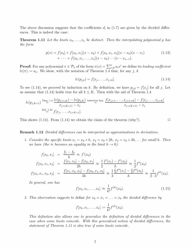
Remark 1.12 Divided differences can be interpreted as approximations to derivatives.

1. Consider the specific knots x1 = x0+h, x2 = x0+2h, x3 = x0+3h, . . . for small h. Thenwe have (the ≈ becomes an equality in the limit h → 0):

f [x0, x1] =f1 − f0

h≈ f ′(x0)

f [x0, x1, x2] =f [x1, x2]− f [x0, x1]

2h≈ 1

2

f ′(x1)− f ′(x0)

h≈ 1

2f ′′(x0)

f [x0, x1, x2, x3] =f [x1, x2, x3]− f [x0, x1, x2]

3h≈ 1

3

12f ′′(x1)− 1

2f ′′(x0)

h≈ 1

2 · 3f′′′(x0).

In general, one has

f [x0, x1, . . . , xk] ≈1

k!f (k)(x0). (1.15)

2. This observation suggests to define for x0 = x1 = . . . = xk the divided difference by

f [x0, x1, . . . , xk] :=1

k!f (k)(x0).

This definition also allows one to generalize the definition of divided differences to thecase when some knots coincide. With this generalized notion of divided differences, thestatement of Theorem 1.11 is also true if some knots coincide.

7

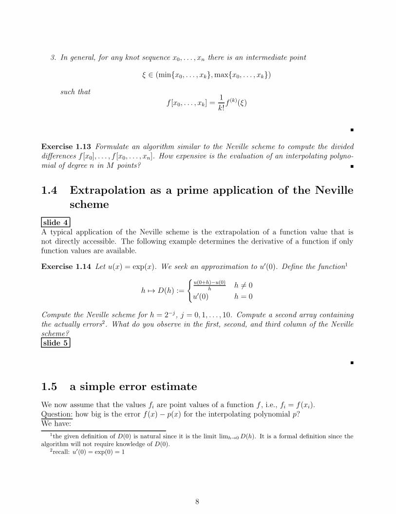
3. In general, for any knot sequence x0, . . . , xn there is an intermediate point

ξ ∈ (min{x0, . . . , xk},max{x0, . . . , xk})

such that

f [x0, . . . , xk] =1

k!f (k)(ξ)

Exercise 1.13 Formulate an algorithm similar to the Neville scheme to compute the divideddifferences f [x0], . . . , f [x0, . . . , xn]. How expensive is the evaluation of an interpolating polyno-mial of degree n in M points?

1.4 Extrapolation as a prime application of the Neville

scheme

slide 4A typical application of the Neville scheme is the extrapolation of a function value that isnot directly accessible. The following example determines the derivative of a function if onlyfunction values are available.

Exercise 1.14 Let u(x) = exp(x). We seek an approximation to u′(0). Define the function1

h 7→ D(h) :=

{u(0+h)−u(0)

hh 6= 0

u′(0) h = 0

Compute the Neville scheme for h = 2−j, j = 0, 1, . . . , 10. Compute a second array containingthe actually errors2. What do you observe in the first, second, and third column of the Nevillescheme?slide 5

1.5 a simple error estimate

We now assume that the values fi are point values of a function f , i.e., fi = f(xi).Question: how big is the error f(x)− p(x) for the interpolating polynomial p?We have:

1the given definition of D(0) is natural since it is the limit limh→0 D(h). It is a formal definition since thealgorithm will not require knowledge of D(0).

2recall: u′(0) = exp(0) = 1

8

0.0 0.2 0.4 0.6 0.8 1.0 1.2 1.4 1.6x

0.0

0.2

0.4

0.6

0.8

1.0 sin(x)interpol. poly.

0.0 0.2 0.4 0.6 0.8 1.0 1.2 1.4 1.6x

0.000

0.005

0.010

0.015

0.020

0.025

0.030 abs(error)upper bound

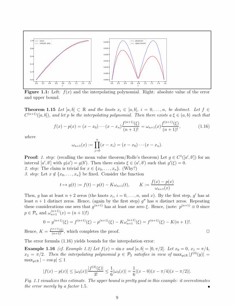
Figure 1.1: Left: f(x) and the interpolating polynomial. Right: absolute value of the errorand upper bound.

Theorem 1.15 Let [a, b] ⊂ R and the knots xi ∈ [a, b], i = 0, . . . , n, be distinct. Let f ∈C(n+1)([a, b]), and let p be the interpolating polynomial. Then there exists a ξ ∈ (a, b) such that

f(x)− p(x) = (x− x0) · · · (x− xn)f (n+1)(ξ)

(n + 1)!= ωn+1(x)

f (n+1)(ξ)

(n+ 1)!, (1.16)

where

ωn+1(x) :=

n∏

j=0

(x− xi) = (x− x0) · · · (x− xn).

Proof: 1. step: (recalling the mean value theorem/Rolle’s theorem) Let g ∈ C1([a′, b′]) for aninterval [a′, b′] with g(a′) = g(b′). Then there exists ξ ∈ (a′, b′) such that g′(ξ) = 0.2. step: The claim is trivial for x ∈ {x0, . . . , xn}. (Why?)3. step: Let x 6∈ {x0, . . . , xn} be fixed. Consider the function

t 7→ g(t) := f(t)− p(t)−Kωn+1(t), K :=f(x)− p(x)

ωn+1(x)

Then, g has at least n+ 2 zeros (the knots xi, i = 0, . . . , n, and x). By the first step, g′ has atleast n + 1 distinct zeros. Hence, (again by the first step) g′′ has n distinct zeros. Repeatingthese considerations one sees that g(n+1) has at least one zero ξ. Hence, (note: p(n+1) ≡ 0 since

p ∈ Pn and ω(n+1)n+1 (x) = (n+ 1)!)

0 = g(n+1)(ξ) = f (n+1)(ξ)− p(n+1)(ξ)−Kω(n+1)n+1 (ξ) = f (n+1)(ξ)−K(n + 1)!.

Hence, K = f(n+1)(ξ)(n+1)!

, which completes the proof. ✷

The error formula (1.16) yields bounds for the interpolation error:

Example 1.16 (cf. Example 1.2) Let f(x) = sin x and [a, b] = [0, π/2]. Let x0 = 0, x1 = π/4,x2 = π/2. Then the interpolating polynomial p ∈ P2 satisfies in view of maxy∈R |f (3)(y)| =maxy∈R | − cos y| ≤ 1

|f(x)− p(x)| ≤ |ω3(x)||f (3)(ξ)|

3!≤ 1

6|ω3(x)| =

1

6|(x− 0)(x− π/4)(x− π/2)|.

Fig. 1.1 visualizes this estimate. The upper bound is pretty good in this example: it overestimatesthe error merely by a factor 1.5.

9

h m=0 m=1 m=2 m=3 m=4 m=5 m=6 m=7

20 1.000 4.14−1 2.52−1 1.68−1 1.15−1 8.06−2 5.66−2 3.99−2

2−1 7.07−1 2.93−1 1.79−1 1.19−1 8.17−2 5.70−2 4.00−2 2.82−2

2−2 5.00−1 2.07−1 1.26−1 8.40−2 5.77−2 4.03−2 2.83−2

2−3 3.54−1 1.46−1 8.93−2 5.94−2 4.08−2 2.85−2

2−4 2.50−1 1.04−1 6.31−2 4.20−2 2.89−2

2−5 1.77−1 7.32−2 4.46−2 2.97−2

2−6 1.25−1 5.18−2 3.16−2

2−7 8.84−2 3.66−2

2−8 6.25−2

Fehler√h

√h

√h

√h

√h

√h

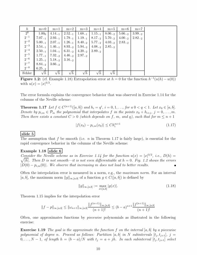
Figure 1.2: (cf. Example 1.18) Extrapolation error at h = 0 for the function h−1(u(h)−u(0))with u(x) = |x|3/2.

The error formula explains the convergence behavior that was observed in Exercise 1.14 for thecolumns of the Neville scheme:

Theorem 1.17 Let f ∈ C(n+1)([a, b]) and hi = qi, i = 0, 1, . . ., for a 0 < q < 1. Let x0 ∈ [a, b].Denote by pi,m ∈ Pm the polynomial that interpolates f in the points x0 + hi+j, j = 0, . . . , m.Then there exists a constant C > 0 (which depends on f , m, and q), such that for m ≤ n+ 1

|f(x0)− pi,m(x0)| ≤ Chm+1i (1.17)

slide 5The assumption that f be smooth (i.e. n in Theorem 1.17 is fairly large), is essential for therapid convergence behavior in the columns of the Neville scheme:

Example 1.18 slide 6Consider the Neville scheme as in Exercise 1.14 for the function u(x) = |x|3/2, i.e., D(h) =√

|h|. Then D is not smooth—it is not even differentiable at h = 0. Fig. 1.2 shows the errors|D(0)− pi,m(0)|. We observe that increasing m does not lead to better results.

Often the interpolation error is measured in a norm, e.g., the maximum norm. For an interval[a, b], the maximum norm ‖g‖∞,[a,b] of a function g ∈ C([a, b]) is defined by

‖g‖∞,[a,b] := maxx∈[a,b]

|g(x)|. (1.18)

Theorem 1.15 implies for the interpolation error

‖f − p‖∞,[a,b] ≤ ‖ωn+1‖∞,[a,b]

‖f (n+1)‖∞,[a,b]

(n+ 1)!≤ (b− a)n+1‖f (n+1)‖∞,[a,b]

(n+ 1)!

Often, one approximates functions by piecewise polynomials as illustrated in the followingexercise:

Exercise 1.19 The goal is the approximate the function f on the interval [a, b] by a piecewisepolynomial of degree n. Proceed as follows: Partition [a, b] in N subintervals [tj , tj+1], j =0, . . . , N − 1, of length h = (b − a)/N with tj = a + jh. In each subinterval [tj , tj+1] select

10

as the interpolation points xi,j := tj +1nih, i = 0, . . . , n, and approximate f on [tj, tj+1] by

the polynomial that interpolates f in the points xi,j, i = 0, . . . , n. In this way, one obtains afunction p that is a polynomial of degree n on each subinterval. Show:

‖f − p‖∞,[a,b] ≤1

(n+ 1)!hn+1‖f (n+1)‖∞,[a,b].

Sketch the function p for the case n = 1.

1.6 Extrapolation of function with additional structure

Sometimes, the function f to be approximated has additional structure that can (and should!)be exploited. We illustrate this phenomenon for the approximation of the derivative of afunction using symmetric difference quotients:

Example 1.20 slide 7Given a function u consider the function

Dsym(h) :=u(0 + h)− u(0− h)

2h= u′(0) +

1

3!u(3)(0)h2 +

1

5!u(5)h4 + · · ·

The goal is to approximate Dsym(0) using only evaluations of u. We recognize that Dsym is a

function of h2, i.e., Dsym(h) = D̃(h2). If (hi, Dsym(hi)), i = 0, . . . , n, are given, then one couldobtain an approximation of Dsym(0) in 2 ways:

1. Interpolate the data (hi, Dsym(hi)), i = 0, . . . , n, and evaluate the interpolating polynomialat h = 0.

2. Interpolate the data (h2i , Dsym(hi)) = (h2

i , D̃(h2i )), i = 0, . . . , n, and evaluate the interpo-

lating polynomial at h2 = 0.

Effectively, the first approach interpolates the function Dsym whereas the second approach in-

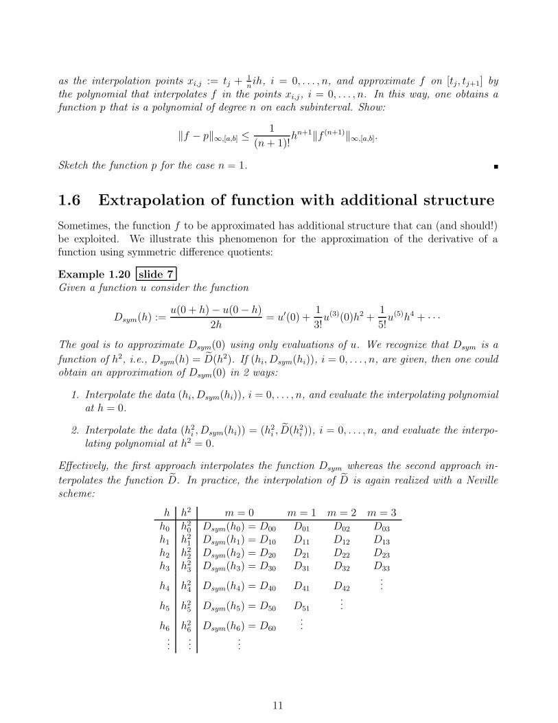
terpolates the function D̃. In practice, the interpolation of D̃ is again realized with a Nevillescheme:

h h2 m = 0 m = 1 m = 2 m = 3h0 h2

0 Dsym(h0) = D00 D01 D02 D03

h1 h21 Dsym(h1) = D10 D11 D12 D13

h2 h22 Dsym(h2) = D20 D21 D22 D23

h3 h23 Dsym(h3) = D30 D31 D32 D33

h4 h24 Dsym(h4) = D40 D41 D42

...

h5 h25 Dsym(h5) = D50 D51

...

h6 h26 Dsym(h6) = D60

......

......

11

h m = 0 m = 1 m = 2 m = 3 m = 4 m = 51 1.175201193643802 0.909180028331188 1.001883888526739 0.999862158028692 1.000000383252421 0.999999993723462

2−1 1.042190610987495 0.978707923477851 1.000114874340948 0.999991744175937 1.000000005896242 0

2−2 1.010449267232673 0.994763136625174 1.000007135446563 0.999999489538722 0 0

2−3 1.002606201928923 0.998696135741217 1.000000445277203 0 0 0

2−4 1.000651168835070 0.999674367893206 0 0 0 0

2−5 1.000162768364138 0 0 0 0 0

h h2 m = 0 m = 1 m = 2 m = 3 m = 4 m = 51 1 1.175201193643802 0.997853750102059 1.000003157261889 0.999999999319035 1.000000000000025 1.000000000000001

2−1 2−2 1.042190610987495 0.999868819314399 1.000000048661892 0.999999999997365 1.000000000000001

2−2 2−4 1.010449267232673 0.999991846827674 1.000000000757749 0.999999999999990

2−3 2−6 1.002606201928923 0.999999491137119 1.000000000011830

2−4 2−8 1.000651168835070 0.999999968207161

2−5 2−10 1.000162768364138

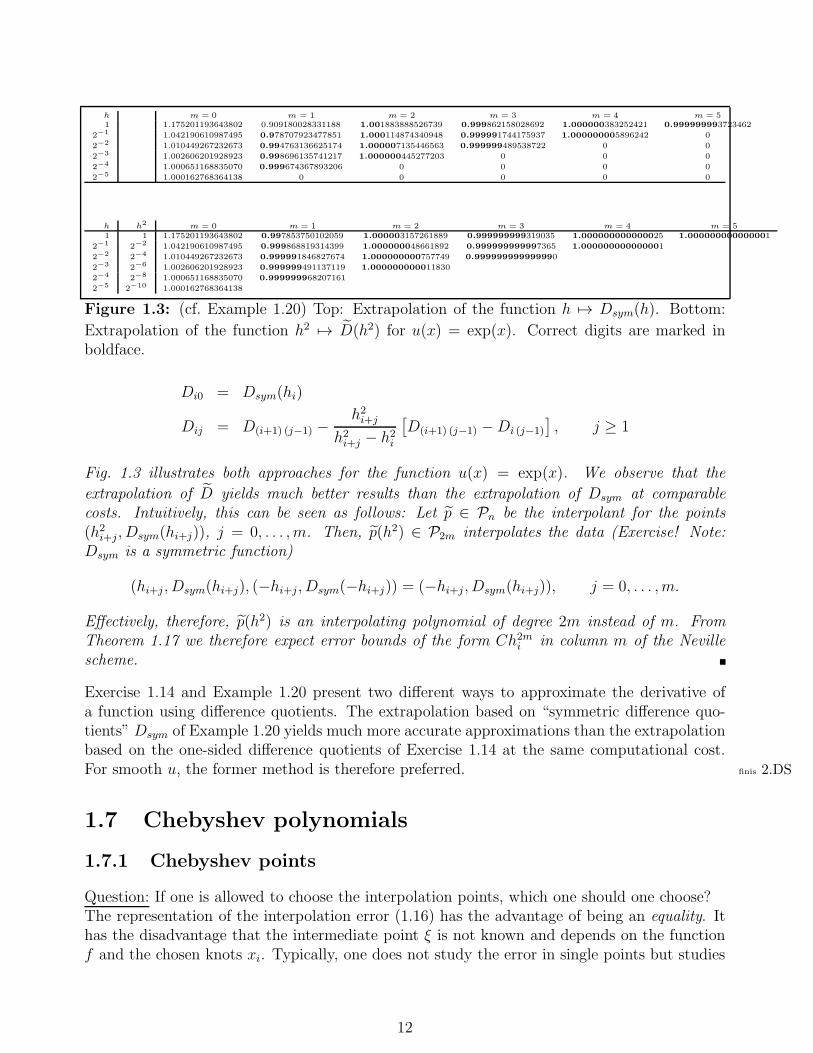
Figure 1.3: (cf. Example 1.20) Top: Extrapolation of the function h 7→ Dsym(h). Bottom:

Extrapolation of the function h2 7→ D̃(h2) for u(x) = exp(x). Correct digits are marked inboldface.

Di0 = Dsym(hi)

Dij = D(i+1) (j−1) −h2i+j

h2i+j − h2

i

[D(i+1) (j−1) −Di (j−1)

], j ≥ 1

Fig. 1.3 illustrates both approaches for the function u(x) = exp(x). We observe that the

extrapolation of D̃ yields much better results than the extrapolation of Dsym at comparablecosts. Intuitively, this can be seen as follows: Let p̃ ∈ Pn be the interpolant for the points(h2

i+j , Dsym(hi+j)), j = 0, . . . , m. Then, p̃(h2) ∈ P2m interpolates the data (Exercise! Note:Dsym is a symmetric function)

(hi+j , Dsym(hi+j), (−hi+j , Dsym(−hi+j)) = (−hi+j , Dsym(hi+j)), j = 0, . . . , m.

Effectively, therefore, p̃(h2) is an interpolating polynomial of degree 2m instead of m. FromTheorem 1.17 we therefore expect error bounds of the form Ch2m

i in column m of the Nevillescheme.

Exercise 1.14 and Example 1.20 present two different ways to approximate the derivative ofa function using difference quotients. The extrapolation based on “symmetric difference quo-tients” Dsym of Example 1.20 yields much more accurate approximations than the extrapolationbased on the one-sided difference quotients of Exercise 1.14 at the same computational cost.For smooth u, the former method is therefore preferred. finis 2.DS

1.7 Chebyshev polynomials

1.7.1 Chebyshev points

Question: If one is allowed to choose the interpolation points, which one should one choose?The representation of the interpolation error (1.16) has the advantage of being an equality. Ithas the disadvantage that the intermediate point ξ is not known and depends on the functionf and the chosen knots xi. Typically, one does not study the error in single points but studies

12

-1 -0.5 0 0.5 10

0.5

1Chebyshev points for n=5

-1 -0.5 0 0.5 10

0.5

1Chebyshev points for n=25

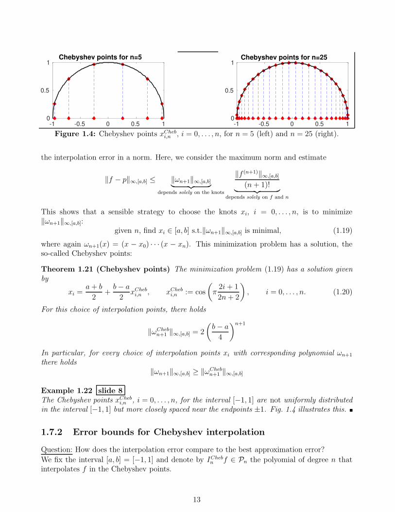
Figure 1.4: Chebyshev points xChebi,n , i = 0, . . . , n, for n = 5 (left) and n = 25 (right).

the interpolation error in a norm. Here, we consider the maximum norm and estimate

‖f − p‖∞,[a,b] ≤ ‖ωn+1‖∞,[a,b]︸ ︷︷ ︸depends solely on the knots

‖f (n+1)‖∞,[a,b]

(n+ 1)!︸ ︷︷ ︸depends solely on f and n

This shows that a sensible strategy to choose the knots xi, i = 0, . . . , n, is to minimize‖ωn+1‖∞,[a,b]:

given n, find xi ∈ [a, b] s.t.‖ωn+1‖∞,[a,b] is minimal, (1.19)

where again ωn+1(x) = (x − x0) · · · (x − xn). This minimization problem has a solution, theso-called Chebyshev points:

Theorem 1.21 (Chebyshev points) The minimization problem (1.19) has a solution givenby

xi =a+ b

2+

b− a

2xChebi,n , xCheb

i,n := cos

(π2i+ 1

2n+ 2

), i = 0, . . . , n. (1.20)

For this choice of interpolation points, there holds

‖ωChebn+1 ‖∞,[a,b] = 2

(b− a

4

)n+1

In particular, for every choice of interpolation points xi with corresponding polynomial ωn+1

there holds‖ωn+1‖∞,[a,b] ≥ ‖ωCheb

n+1 ‖∞,[a,b]

Example 1.22 slide 8The Chebyshev points xCheb

i,n , i = 0, . . . , n, for the interval [−1, 1] are not uniformly distributedin the interval [−1, 1] but more closely spaced near the endpoints ±1. Fig. 1.4 illustrates this.

1.7.2 Error bounds for Chebyshev interpolation

Question: How does the interpolation error compare to the best approximation error?

We fix the interval [a, b] = [−1, 1] and denote by IChebn f ∈ Pn the polyomial of degree n that

interpolates f in the Chebyshev points.

13

Exercise 1.23 The mapping f 7→ IChebn f is a linear map, i.e., for continuous functions f , g

and λ ∈ R there holds IChebn (f + g) = (ICheb

n f) + (IChebn g) as well as ICheb

n (λf) = λIChebn f .

Exercise 1.24 Show that IChebn f = f for all polynomials f ∈ Pn. Hint: Uniqueness of polyno-

mial interpolation, Theorem 1.1.

We define the Lebesgue number ΛChebn by

ΛChebn := max

x∈[−1,1]

n∑

i=0

|ℓChebi (x)|, (1.21)

where ℓChebi are the Lagrange interpolation polynomials for the Chebyshev points.

Theorem 1.25 (Chebyshev interpolation) There holds:

(i)‖ICheb

n f‖∞,[−1,1] ≤ Λn‖f‖∞,[−1,1] (1.22)

(ii) There holds:‖f − ICheb

n f‖∞,[−1,1] ≤ (1 + ΛChebn ) min

q∈Pn

‖f − q‖∞,[−1,1]

(iii) ΛChebn ≤ 2

πln(n + 1) + 1

Proof: Proof of (i):

‖IChebn f‖∞,[−1,1] = max

x∈[−1,1]|(ICheb

n f)(x)| = maxx∈[−1,1]

|n∑

i=0

f(xChebi,n )ℓCheb

i (x)|

≤ maxi=0,...,n

|f(xChebi,n )| max

x∈[−1,1]|

n∑

i=0

|ℓChebi (x)| ≤ ‖f‖∞,[−1,1]Λ

Chebn

Proof of (ii): We employ Exercise 1.23, 1.24 and obtain for arbitrary q ∈ Pn

‖f − IChebn f‖∞,[−1,1]

Exer. 1.23, 1.24= ‖f − q − ICheb

n (f − q)‖∞,[−1,1]

≤ ‖f − q‖∞,[−1,1] + ‖IChebn (f − q)‖∞,[−1,1]

(i)

≤ ‖f − q‖∞,[−1,1] + ΛChebn ‖(f − q)‖∞,[−1,1] = (1 + ΛCheb

n )‖f − q‖∞,[−1,1]

Proof of (iii): Literature. ✷

Remark 1.26 (Interpretation of ΛChebn ) 1. The factor 1+ΛCheb

n measures how much worsethe approximation of f by the Chebyshev interpolation is compared to the best possiblepolynomial approximation (in the norm ‖ · ‖∞,[−1,1]). The logarithmic growth of ΛCheb

n

is very slow so that Chebyshev interpolation is typically very good: for example, for (thealready rather high polynomial degree) n = 20 one has ΛCheb

n ≈ 2.9 and thus 1+ΛCheb20 ≤ 4.

14

2. ΛChebn can also be understood as an amplification factor: If, instead of the exact func-

tion values f(xChebi,n ), perturbed values f̃i with |f̃i − f(xCheb

i,n )| ≤ δ are employed, then the

“perturbed” interpolation polynomial∑

i f̃iℓChebi satisfies (Exercise!)

‖(n∑

i=0

f̃iℓChebi )− ICheb

n f‖∞,[−1,1] ≤ ΛChebn δ.

In other words: Since ΛChebn of Chebyshev interpolation is moderate, perturbations or

errors in the values f(xChebi,n ) have a rather small impact on the error in the interpolating

polynomial.

Chebyshev interpolation converges very rapidly for for smooth functions:

Exercise 1.27 Consider the function f(x) = (4−x2)−1. Give an upper bound for minq∈Pn‖f−

q‖∞,[−1,1] by selecting q as the Taylor polynomial of f about a suitable point.Determine the interpolating polynomials ICheb

n f for n = 1, . . . , 10. Plot the error semilogarith-mically (semilogy in matlab or matplotlib.pyplot.semilogy in python) versus n. To thatend, approximate the error ‖f − ICheb

n f‖∞,[−1,1] by simply computing the error in 100 pointsthat are uniformly distributed over [−1, 1].

1.7.3 Interpolation with uniform point distribution

For large n, the choice of the interpolation points may strongly impact the approximationquality of the interpolation process. Whereas interpolation in the Chebyshev points usuallyyields very good results, other systems of points may produce poor results even for functions fthat may seem “harmless’. The following example illustrates this:

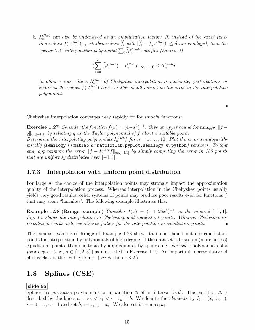
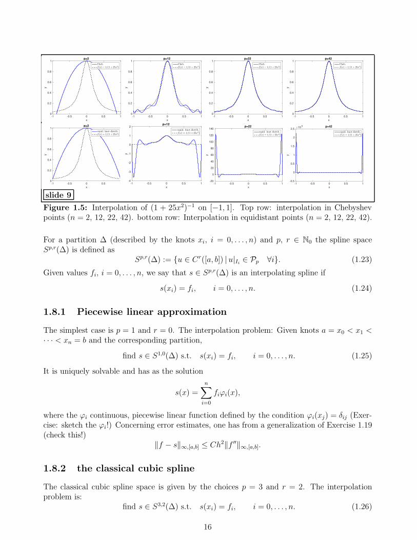
Example 1.28 (Runge example) Consider f(x) = (1 + 25x2)−1 on the interval [−1, 1].Fig. 1.5 shows the interpolation in Chebyshev and equidistant points. Whereas Chebyshev in-terpolation works well, we observe failure for the interpolation in equidistant points.

The famous example of Runge of Example 1.28 shows that one should not use equidistantpoints for interpolation by polynomials of high degree. If the data set is based on (more or less)equidistant points, then one typically approximates by splines, i.e., piecewise polynomials of afixed degree (e.g., n ∈ {1, 2, 3}) as illustrated in Exercise 1.19. An important representative ofof this class is the “cubic spline” (see Section 1.8.2.)

1.8 Splines (CSE)

slide 9aSplines are piecewise polynomials on a partition ∆ of an interval [a, b]. The partition ∆ isdescribed by the knots a = x0 < x1 < · · ·xn = b. We denote the elements by Ii = (xi, xi+1),i = 0, . . . , n− 1 and set hi := xi+1 − xi. We also set h := maxi hi.

15

x

-1 -0.5 0 0.5 1

y

0

0.2

0.4

0.6

0.8

1 p=2

Cheb.f(x) = 1/(1 + 25x2)

x

-1 -0.5 0 0.5 1

y

0

0.2

0.4

0.6

0.8

1 p=12

Cheb.f(x) = 1/(1 + 25x2)

x

-1 -0.5 0 0.5 1

y

0

0.2

0.4

0.6

0.8

1 p=22

Cheb.f(x) = 1/(1 + 25x2)

x

-1 -0.5 0 0.5 1

y

0

0.2

0.4

0.6

0.8

1 p=42

Cheb.f(x) = 1/(1 + 25x2)

x

-1 -0.5 0 0.5 1

y

0

0.2

0.4

0.6

0.8

1 p=2

equid. knot distrib.f(x) = 1/(1 + 25x2)

x

-1 -0.5 0 0.5 1

y

-4

-3

-2

-1

0

1

2 p=12

equid. knot distrib.f(x) = 1/(1 + 25x2)

x

-1 -0.5 0 0.5 1

y

-20

0

20

40

60

80

100

120

140 p=22

equid. knot distrib.f(x) = 1/(1 + 25x2)

x

-1 -0.5 0 0.5 1

y

×105

-0.5

0

0.5

1

1.5

2

2.5 p=42

equid. knot distrib.f(x) = 1/(1 + 25x2)

slide 9

Figure 1.5: Interpolation of (1 + 25x2)−1 on [−1, 1]. Top row: interpolation in Chebyshevpoints (n = 2, 12, 22, 42). bottom row: Interpolation in equidistant points (n = 2, 12, 22, 42).

For a partition ∆ (described by the knots xi, i = 0, . . . , n) and p, r ∈ N0 the spline spaceSp,r(∆) is defined as

Sp,r(∆) := {u ∈ Cr([a, b]) | u|Ii ∈ Pp ∀i}. (1.23)

Given values fi, i = 0, . . . , n, we say that s ∈ Sp,r(∆) is an interpolating spline if

s(xi) = fi, i = 0, . . . , n. (1.24)

1.8.1 Piecewise linear approximation

The simplest case is p = 1 and r = 0. The interpolation problem: Given knots a = x0 < x1 <· · · < xn = b and the corresponding partition,

find s ∈ S1,0(∆) s.t. s(xi) = fi, i = 0, . . . , n. (1.25)

It is uniquely solvable and has as the solution

s(x) =n∑

i=0

fiϕi(x),

where the ϕi continuous, piecewise linear function defined by the condition ϕi(xj) = δij (Exer-cise: sketch the ϕi!) Concerning error estimates, one has from a generalization of Exercise 1.19(check this!)

‖f − s‖∞,[a,b] ≤ Ch2‖f ′′‖∞,[a,b].

1.8.2 the classical cubic spline

The classical cubic spline space is given by the choices p = 3 and r = 2. The interpolationproblem is:

find s ∈ S3,2(∆) s.t. s(xi) = fi, i = 0, . . . , n. (1.26)

16

Obviously, (1.26) represents a system of n+1 equations. We now show that dimS3,2(∆) = n+3.Hence, we will have to impose addition constraints.

Lemma 1.29 Let ∆ be a partition given by n+ 1 (distinct) knots x0, . . . , xn. Then

dimSp,r(∆) = n(p + 1)− (n− 1)(r + 1) (1.27)

Proof: Instead of a formal proof, we simply count the number of degrees of freedom/parametersneeded to describe a spline: We have dimPp = p + 1 so that the space of discontinuouspiecewise polynomials of degree p is (p + 1)n. The condition of Cr continuity at the n − 1interior knots x1, . . . , xn−1 imposes (n − 1)(r + 1) conditions. Thus, we expect dimSp,r(∆) =n(p+ 1)− (n− 1)(r + 1). ✷

For the case p = 3, r = 2, we get dimS3,2(∆) = 4n − 3(n − 1) = n + 3. The interpolationconditions (1.26) yield n+1 conditions. Hence, two more conditions have to be imposed. Thesetwo extra conditions are selected depending on the application. Typically, one of the followingfour choices is made:

1. Complete/clamped spline: The user provides two additional values f ′0, f

′n ∈ R and imposes

the following two additional conditions:

s′(x0) = f ′0, s′(xn) = f ′

n. (1.28)

2. Periodic spline: one assumes f0 = fn and imposes additionally

s′(x0) = s′(xn), s′′(x0) = s′′(xn). (1.29)

3. Natural spline: one imposes

s′′(x0) = 0, s′′(xn) = 0. (1.30)

4. “not-a-knot condition”: one requires that the jump of s′′′ at the knots x1 and xn−1 bezero:

limx→x1−

s′′′(x) = limx→x1+

s′′′(x), limx→xn−1−

s′′′(x) = limx→xn−1+

s′′′(x). (1.31)

Concerning the accuracy of the interpolation method, we have:

Theorem 1.30 Let f ∈ C4([a, b]) and h := maxi hi. Let fi = f(xi), i = 0, . . . , n. Then theestimates

‖f − s‖∞,[a,b] ≤ Ch4‖f (4)‖∞,[a,b], ‖(f − s)′‖∞,[a,b] ≤ Ch3‖f (4)‖∞,[a,b]

hold in the following cases:

(i) s is the complete spline and f ′0 = f ′(x0) and f ′

n = f ′(xn).

(ii) s is the periodic spline and f is additionally periodic, i.e., f ∈ C4(R) and f(x+(b−a)) =f(x) for all x ∈ R.

(iii) s is the not-a-knot spline.

In particular, in each of these cases, the spline interpolation problem is uniquely solvable.

Remark 1.31 If only the values fi = f(xi) are available and a good spline approximation tof is sought, then typically the not-a-knot interpolation is chosen. This is the standard choiceof the spline command in matlab.

17

minimization property of cubic splines

By Theorem 1.30, the cubic spline interpolation problems with any of the above 4 extra condi-tions is uniquely solvable. In the three cases “complete spline”, “natural spline”, and “periodicspline” the interpolating spline has an optimality property:

Theorem 1.32 (“energy minimization” of cubic splines) Let I = [a, b] and ∆ be a par-tition given by a = x0 < x1 < · · ·xn = b. Let fi, i = 0, . . . , n, be given values.

(i) (complete spline) Let f ′0, f ′

n ∈ R be additionally be given. Then the complete splines ∈ S3,2(∆) satisfies

‖s′′‖L2(I) ≤ ‖y′′‖L2(I) ∀y ∈ Ccomplete,

where Ccomplete is given by

Ccomplete = {v ∈ C2(I) | v(xi) = fi for i = 0, . . . , n and v′(x0) = f ′0, v

′(xn) = f ′n}.

(ii) (natural spline) The natural spline s ∈ S3,2(∆) satisfies

‖s′′‖L2(I) ≤ ‖y′′‖L2(I) ∀y ∈ Cnat,

where Cnat is given by

Cnat = {v ∈ C2(I) | v(xi) = fi for i = 0, . . . , n and v′′(x0) = v′′(xn) = 0}.

(iii) (periodic spline) Assume f0 = fn. Then the periodic spline s ∈ S3,2(∆) satisfies

‖s′′‖L2(I) ≤ ‖y′′‖L2(I) ∀y ∈ Cper,

where Cper is given by

Cper = {v ∈ C2(I) | v(xi) = fi for i = 0, . . . , n and v′(x0) = v′(xn) and v′′(x0) = v′′(xn)}.

Remark 1.33 The minimization property explains the name “spline”. If one studies the de-flection of an elastic “spline”, then the theory of linear elasticity states that the deflection issuch that the spline’s elastic energy is minimized. If y describes the deflection of this spline,then in good approximation, the elastic energy of a spline is given by (ignoring physical units)12‖y′′‖2L2(I). Hence, if the spline is forced to pass through points (xi, fi), i = 0, . . . , n, then the

sought deflection s is the minimizer of the problem:

minimize1

2‖y′′‖2L2(I)

under the constraint y(xi) = fi, i = 0, . . . , n (plus possibly further conditions)

Theorem 1.32 states that the minimizer is the interpolating cubic spline if the additional con-straints are that the spline is the “complete”, ”natural”, or “periodic” one.

18

computation of the cubic spline

The computation of the interpolating spline can be reduced to the solution of a linear systemof equations. In principle, one could make the ansatz that s is a cubic polynomial on eachelement Ii = (xi, xi+1). The interpolation conditions s(xi) = fi, the continuity conditions

limx→xi−

s(j)(x) = limx→xi+

s(j)(x), i = 1, . . . , n− 1, j = 0, 1, 2

and the two additional conditions for complete/natural/periodic/not-a-knot splines describe alinear system of equations that can be solved.

1.8.3 remarks on splines

Exercise 1.34 Show: for r ≥ p, one has Sp,r(∆) = Pp irrespective of the partition ∆.

Remark 1.35 For fixed, (low) r the spaces Sp,r are much more local than then spaces Pp.In polynomial interpolation, changing one data value fi affects the interpolant everywhere.For splines (with small r), the effect is much more local, i.e., a value only affects the splineinterpolant in the neighborhood of the data point. This is of interest, e.g., in the followingsituations:

1. some data values have large errors (e.g., measurement errors): then the spline is onlywrong near the corresponding knot. In contrast, in polynomial interpolation, the approxi-mation is affected everywhere.

2. point evaluation: if a sline is truely local (e.g., in the case r = 0), then the evaluation ofa spline at a point x requires only the data points near x, i.e., a local calculation.

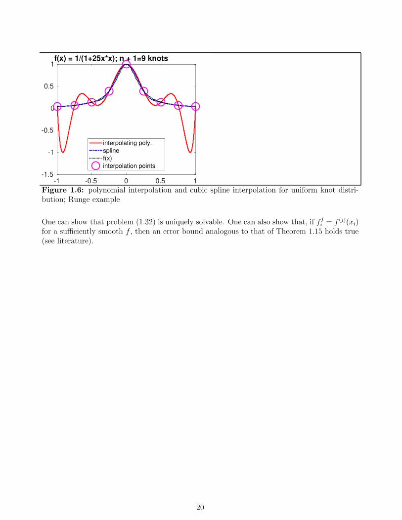
Example 1.36 Fig. 1.6 shows polynomial interpolation and the (complete) cubic spline inter-polation of the Runge example (cf. Example 1.28) on [−1, 1]. For n = 8, the n+1 = 9 knots areuniformly distributed in [−1, 1]. We observe that, while the polynomial interpolation is ratherpoor, the cubic spline is very good.

1.9 Remarks on Hermite interpolation

A generalization of polynomial interpolation is Hermite interpolation. Its most general form isas follows: Let x0, . . . , xn be n+1 distinct knots, and let di ∈ N0 be given for each i. Then, givenvalues f j

i , i = 0, . . . , n, j = 0, . . . , di, the Hermite interpolant is given by: Find p ∈ Pn+∑n

i=0 di

s.t.p(j)(xi) = f j

i , i = 0, . . . , n, j = 0, . . . , di. (1.32)

Remark 1.37 Hermite interpolation generalizes the polynomial interpolation problem (1.1):the choice d0 = d1 = · · · = dn = 0 reproduces (1.1). Another extreme case is n = 0 and

d0 = N . Then p(x) =∑N

j=0fj0

j!(x− x0)

j. In particular, for f j0 = f (j)(x0), we obtain the Taylor

polynomial of f of degree N .

19

-1 -0.5 0 0.5 1-1.5

-1

-0.5

0

0.5

1f(x) = 1/(1+25x*x); n + 1=9 knots

interpolating poly.

spline

f(x)

interpolation points

Figure 1.6: polynomial interpolation and cubic spline interpolation for uniform knot distri-bution; Runge example

One can show that problem (1.32) is uniquely solvable. One can also show that, if f ji = f (j)(xi)

for a sufficiently smooth f , then an error bound analogous to that of Theorem 1.15 holds true(see literature).

20