1 Fundamentals of Reliability Engineering and Applications Dr. E. A. Elsayed Department of Industrial and Systems Engineering Rutgers University ([email protected])

1

Fundamentals of Reliability Engineering and Applications

Dr. E. A. ElsayedDepartment of Industrial and Systems Engineering

Rutgers University ([email protected])

Systems Engineering DepartmentKing Fahd University of Petroleum and Minerals

KFUPM, Dhahran, Saudi ArabiaApril 20, 2009

2

Reliability Engineering Outline

• Reliability definition• Reliability estimation • System reliability calculations

2

3

Reliability Importance

• One of the most important characteristics of a product, it is a measure of its performance with time (Transatlantic and Transpacific cables)

• Products’ recalls are common (only after time elapses). In October 2006, the Sony Corporation recalled up to 9.6 million of its personal computer batteries

• Products are discontinued because of fatal accidents (Pinto, Concord)

• Medical devices and organs (reliability of artificial organs)

3

4

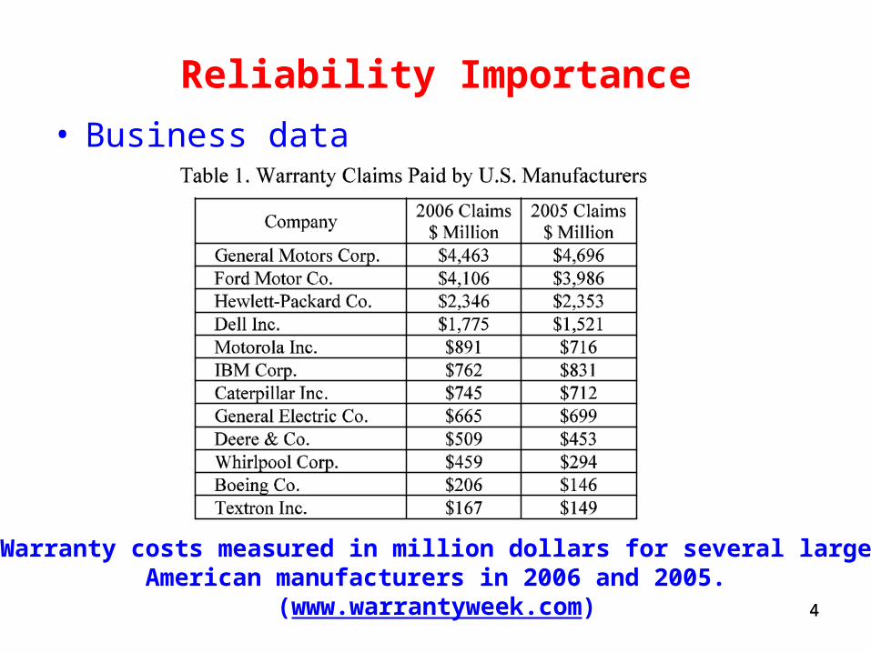
Reliability Importance

• Business data

4

Warranty costs measured in million dollars for several large American manufacturers in 2006 and 2005.

(www.warrantyweek.com)

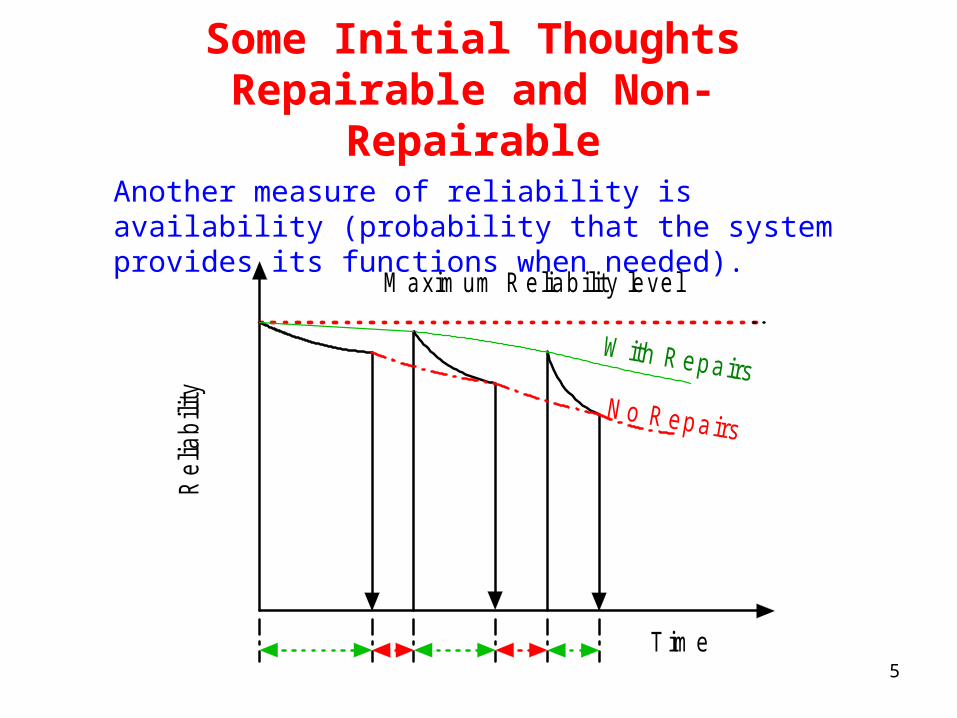
M axim um R eliability level

Rel

iabi

lity

W ith Repairs

T im e

N o R epairs

Some Initial ThoughtsRepairable and Non-Repairable

Another measure of reliability is availability (probability that the system provides its functions when needed).

5

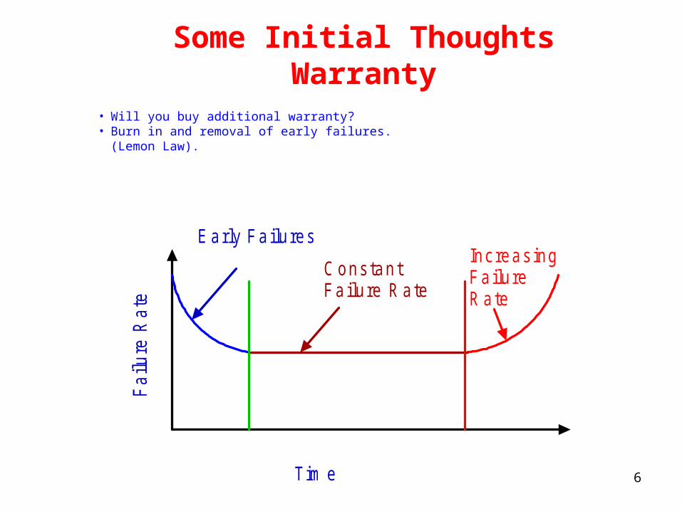
Some Initial ThoughtsWarranty

• Will you buy additional warranty?• Burn in and removal of early failures.

(Lemon Law).

Tim e

Fa

ilure

Rat

e

E arly Fa ilu res

C ons tantFa ilure R ate

Inc reas ingFailureR ate

6

7

Reliability Definitions

Reliability is a time dependent characteristic.

It can only be determined after an elapsed time but can be predicted at any time.

It is the probability that a product or service will operate properly for a specified period of time (design life) under the design operating conditions without failure.

7

8

Other Measures of Reliability

Availability is used for repairable systems

It is the probability that the system is operational at any random time t.

It can also be specified as a proportion of time that the system is available for use in a given interval (0,T).

8

9

Other Measures of Reliability

Mean Time To Failure (MTTF): It is the average

time that elapses until a failure occurs.

It does not provide information about the distribution

of the TTF, hence we need to estimate the variance

of the TTF.

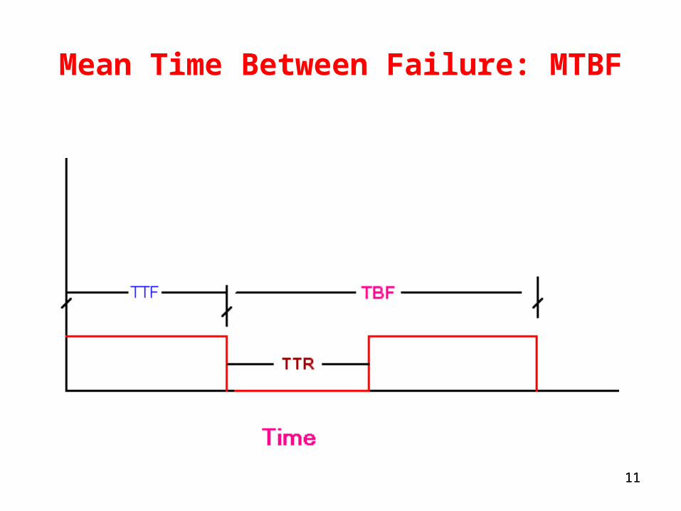
Mean Time Between Failure (MTBF): It is the

average time between successive failures.

It is used for repairable systems.

9

10

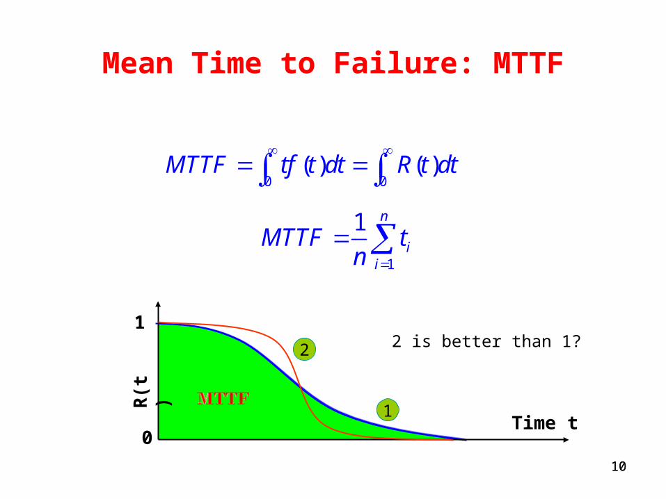
Mean Time to Failure: MTTF

1

1 n

ii

MTTF tn

0 0( ) ( )MTTF tf t dt R t dt

Time t

R(t

)

1

0

1

2 2 is better than 1?

10

11

Mean Time Between Failure: MTBF

11

12

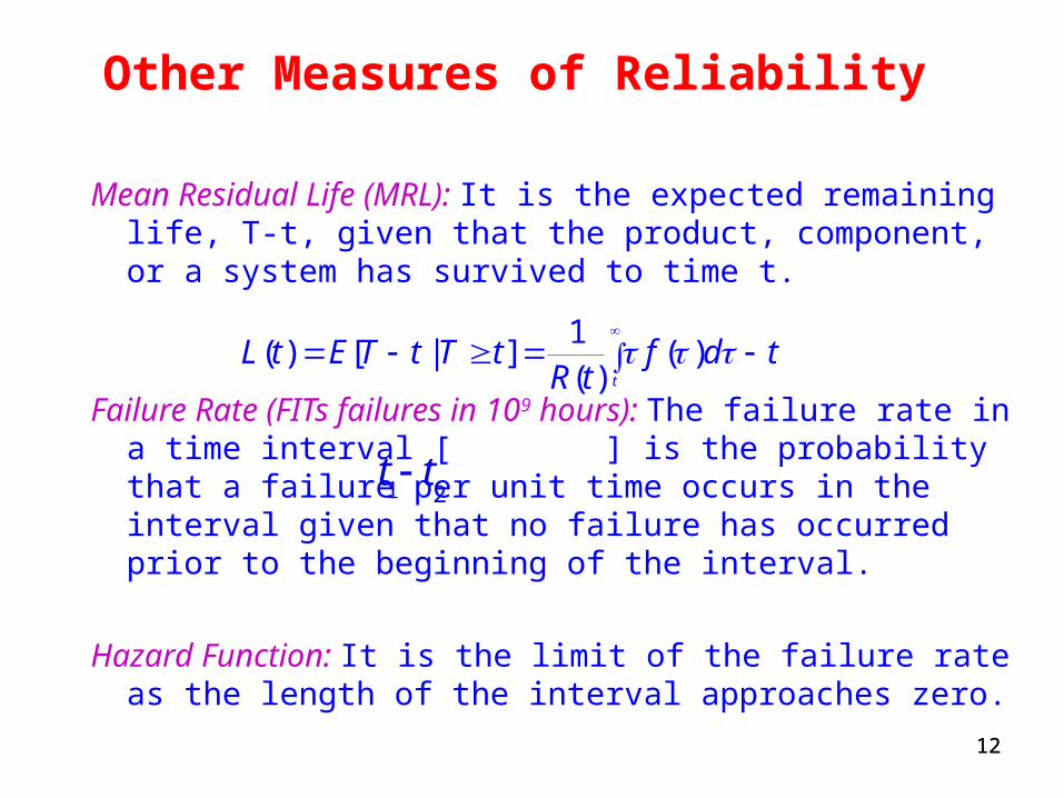
Other Measures of Reliability

Mean Residual Life (MRL): It is the expected remaining life, T-t, given that the product, component, or a system has survived to time t.

Failure Rate (FITs failures in 109 hours): The failure rate in a time interval [ ] is the probability that a failure per unit time occurs in the interval given that no failure has occurred prior to the beginning of the interval.

Hazard Function: It is the limit of the failure rate as the length of the interval approaches zero.

1 2t t

1( ) [ | ] ( )

( ) t

L t E T t T t f d tR t

12

13

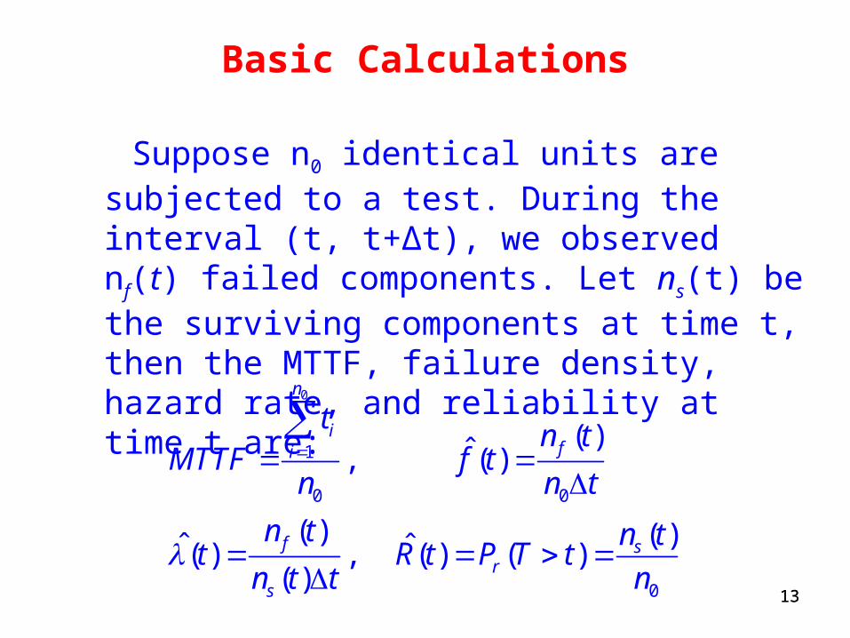
Basic Calculations

0

1

0 0

0

( )ˆ, ( )

( ) ( )ˆ ˆ( ) , ( ) ( )( )

n

ifi

f sr

s

tn t

MTTF f tn n t

n t n tt R t P T t

n t t n

Suppose n0 identical units are subjected to a test. During the interval (t, t+∆t), we observed nf(t) failed components. Let ns(t) be the surviving components at time t, then the MTTF, failure density, hazard rate, and reliability at time t are:

13

14

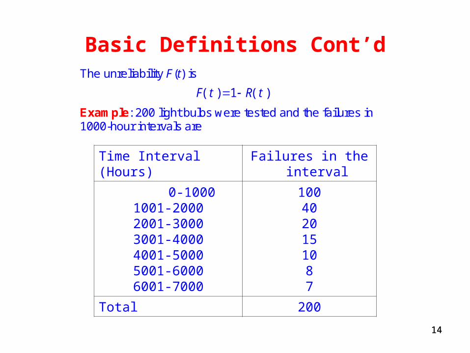
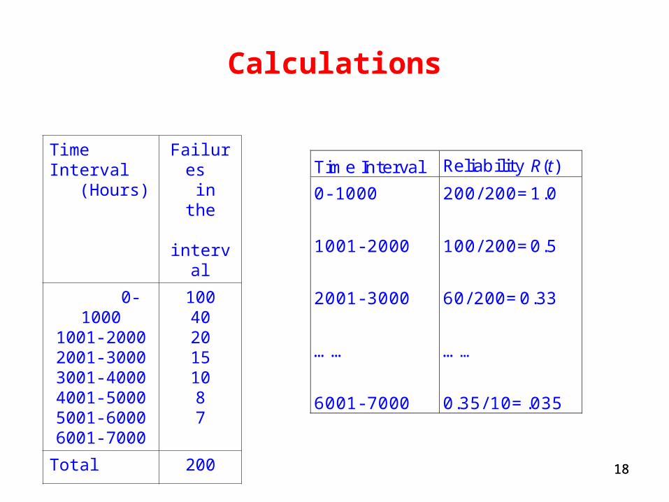
Basic Definitions Cont’dThe unreliability F(t) is

( ) 1 ( )F t R t

Example: 200 light bulbs were tested and the failures in 1000-hour intervals are

Time Interval (Hours)

Failures in the interval

0-10001001-20002001-30003001-40004001-50005001-60006001-7000

1004020151087

Total 200

14

15

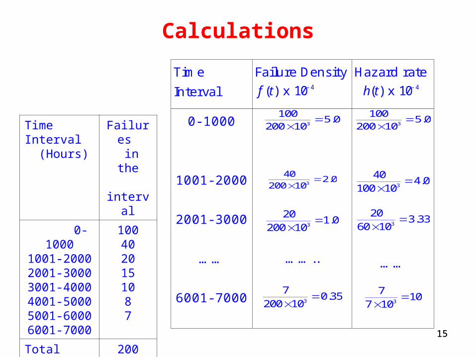
Calculations

Time

Interval

Failure Density

( )f t x 410

Hazard rate

( )h t x 410

0- 1000

1001- 2000

2001- 3000

……

6001- 7000

3

1005.0

200 10

3

402.0

200 10

3

201.0

200 10

……..

3

70.35

200 10

3

1005.0

200 10

3

404.0

100 10

3

203.33

60 10

……

3

710

7 10

Time Interval (Hours)

Failures in the

interval

0-10001001-20002001-30003001-40004001-50005001-60006001-7000

1004020151087

Total 200

15

16

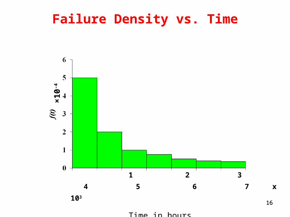
Failure Density vs. Time

1 2 3 4 5 6 7 x 103

Time in hours 16

×1

0-4

17

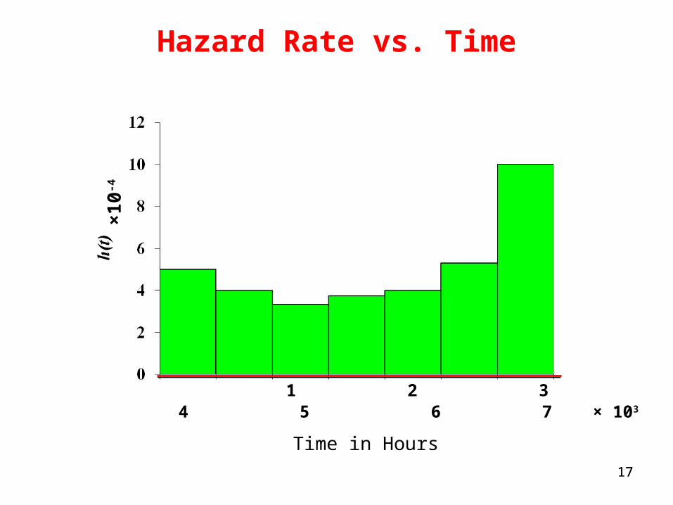
Hazard Rate vs. Time

1 2 3 4 5 6 7 × 103

Time in Hours

17

×1

0-4

18

Calculations

Time Interval Reliability ( )R t

0- 1000

1001- 2000

2001- 3000

……

6001- 7000

200/ 200=1.0

100/ 200=0.5

60/ 200=0.33

……

0.35/ 10=.035

Time Interval (Hours)

Failures in the

interval

0-10001001-20002001-30003001-40004001-50005001-60006001-7000

1004020151087

Total 200

18

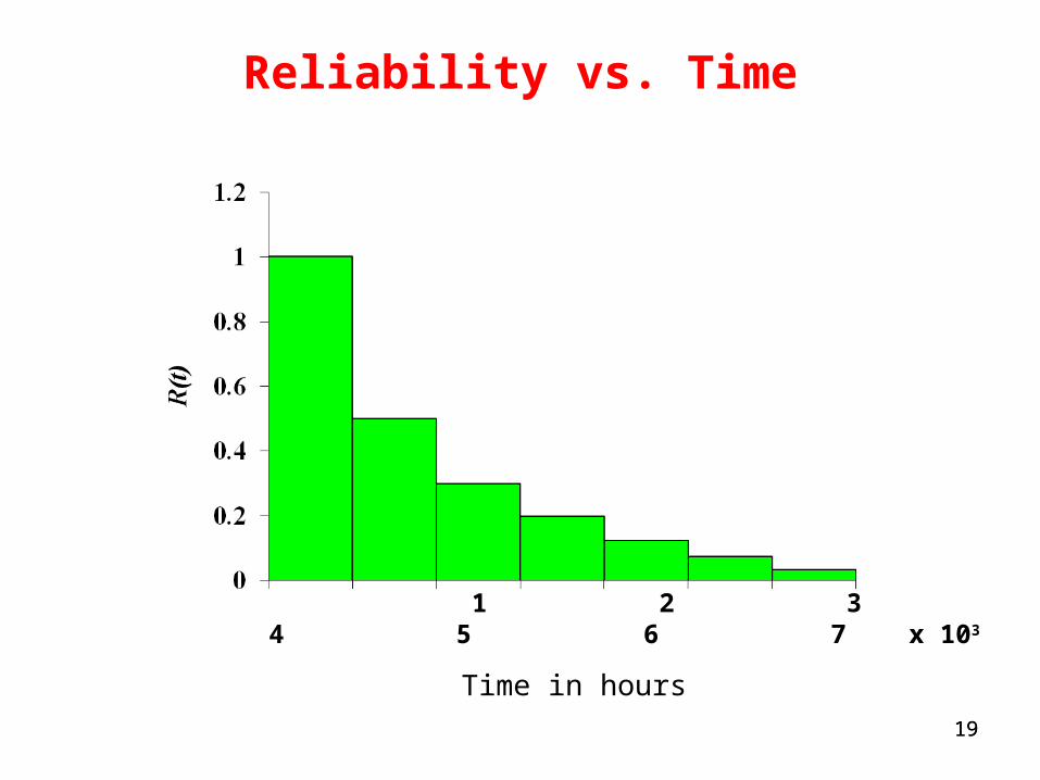
19

Reliability vs. Time

1 2 3 4 5 6 7 x 103

Time in hours

19

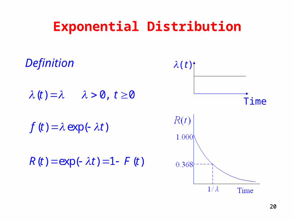
20

Exponential Distribution

Definition

( ) exp( )f t t

( ) exp( ) 1 ( )R t t F t

( ) 0, 0t t

(t)

Time

20

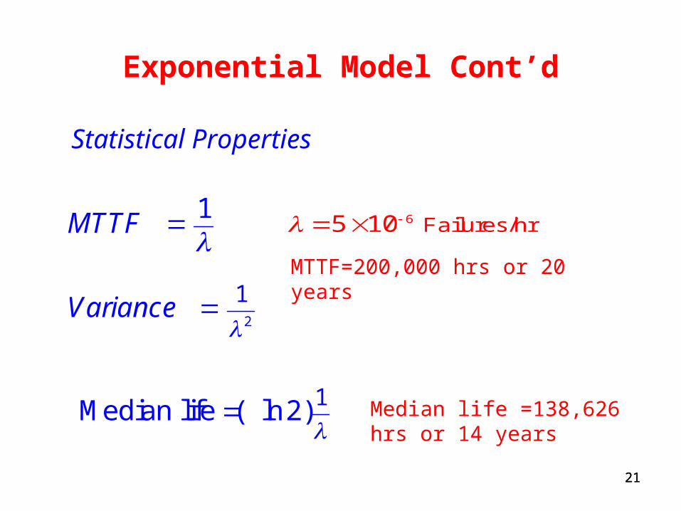
21

Exponential Model Cont’d

1MTTF

2

1Variance

12Median life ( ln )

Statistical Properties

21

6 Failures/hr5 10

MTTF=200,000 hrs or 20 years

Median life =138,626 hrs or 14 years

22

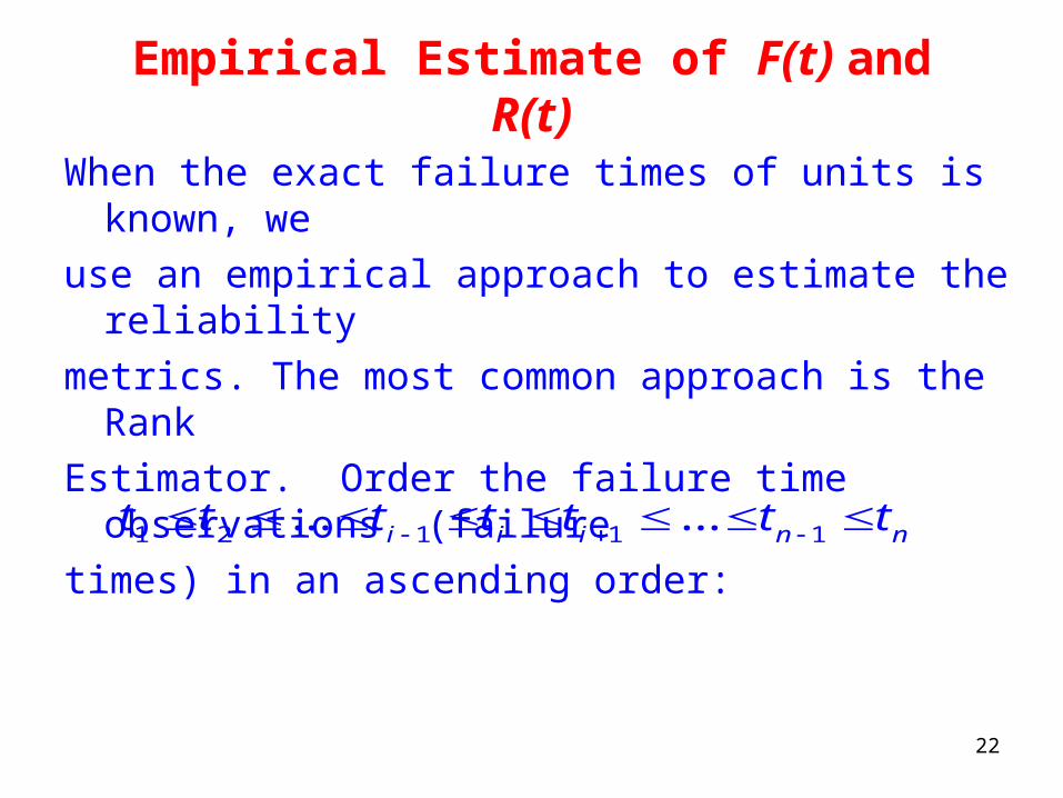
Empirical Estimate of F(t) and R(t)

When the exact failure times of units is known, we

use an empirical approach to estimate the reliability

metrics. The most common approach is the Rank

Estimator. Order the failure time observations (failure

times) in an ascending order:

1 2 1 1 1... ...i i i n nt t t t t t t

23

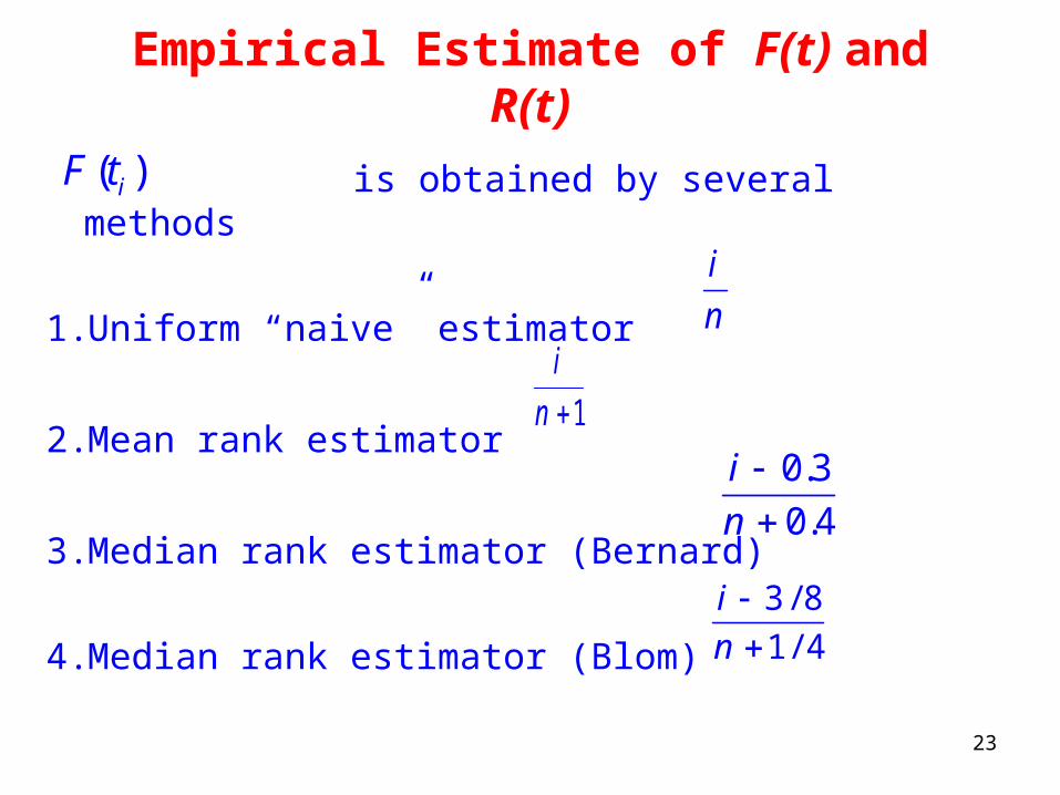
Empirical Estimate of F(t) and R(t)

is obtained by several methods

1. Uniform “naive” estimator

2. Mean rank estimator

3. Median rank estimator (Bernard)

4. Median rank estimator (Blom)

( )iF t

in

1

in

0 3

0 4

..

in

3 8

1 4

//

in

24

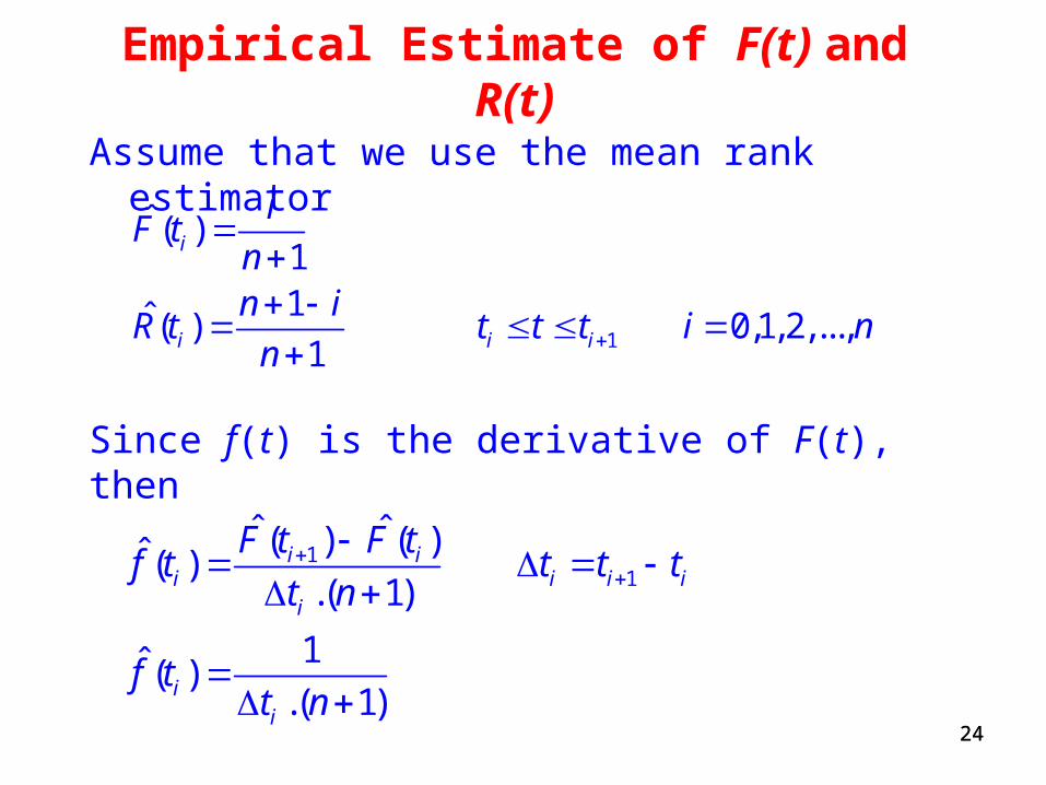
Empirical Estimate of F(t) and R(t)

Assume that we use the mean rank estimator

24

1

ˆ ( )11ˆ( ) 0,1,2,...,

1

i

i i i

iF t

nn i

R t t t t i nn

Since f(t) is the derivative of F(t), then

11

ˆ ˆ( ) ( )ˆ ( ).( 1)

1ˆ ( ).( 1)

i ii i i i

i

ii

F t F tf t t t t

t n

f tt n

25

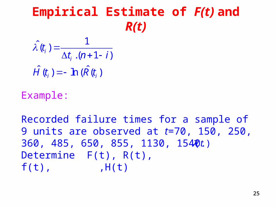
Empirical Estimate of F(t) and R(t)

25

1ˆ( ).( 1 )

ˆ ˆ( ) ln ( ( )

ii

i i

tt n i

H t R t

Example:

Recorded failure times for a sample of 9 units are observed at t=70, 150, 250, 360, 485, 650, 855, 1130, 1540. Determine F(t), R(t), f(t), ,H(t)( )t

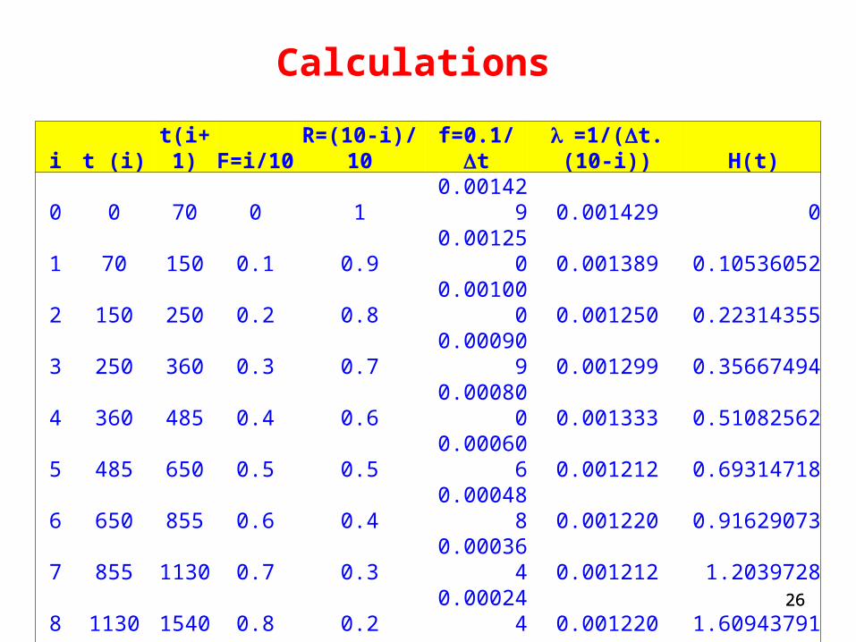
26

Calculations

26

i t (i) t(i+1) F=i/10 R=(10-i)/10 f=0.1/t =1/(t.(10-i)) H(t)

0 0 70 0 1 0.001429 0.001429 0

1 70 150 0.1 0.9 0.001250 0.001389 0.10536052

2 150 250 0.2 0.8 0.001000 0.001250 0.22314355

3 250 360 0.3 0.7 0.000909 0.001299 0.35667494

4 360 485 0.4 0.6 0.000800 0.001333 0.51082562

5 485 650 0.5 0.5 0.000606 0.001212 0.69314718

6 650 855 0.6 0.4 0.000488 0.001220 0.91629073

7 855 1130 0.7 0.3 0.000364 0.001212 1.2039728

8 1130 1540 0.8 0.2 0.000244 0.001220 1.60943791

9 1540 - 0.9 0.1     2.30258509

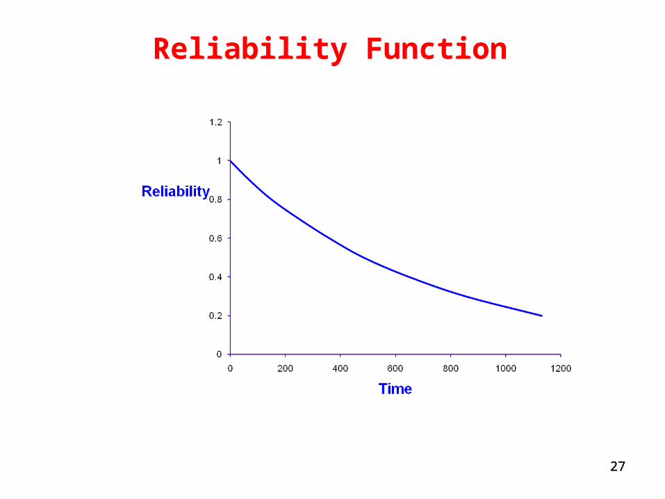
27

Reliability Function

27

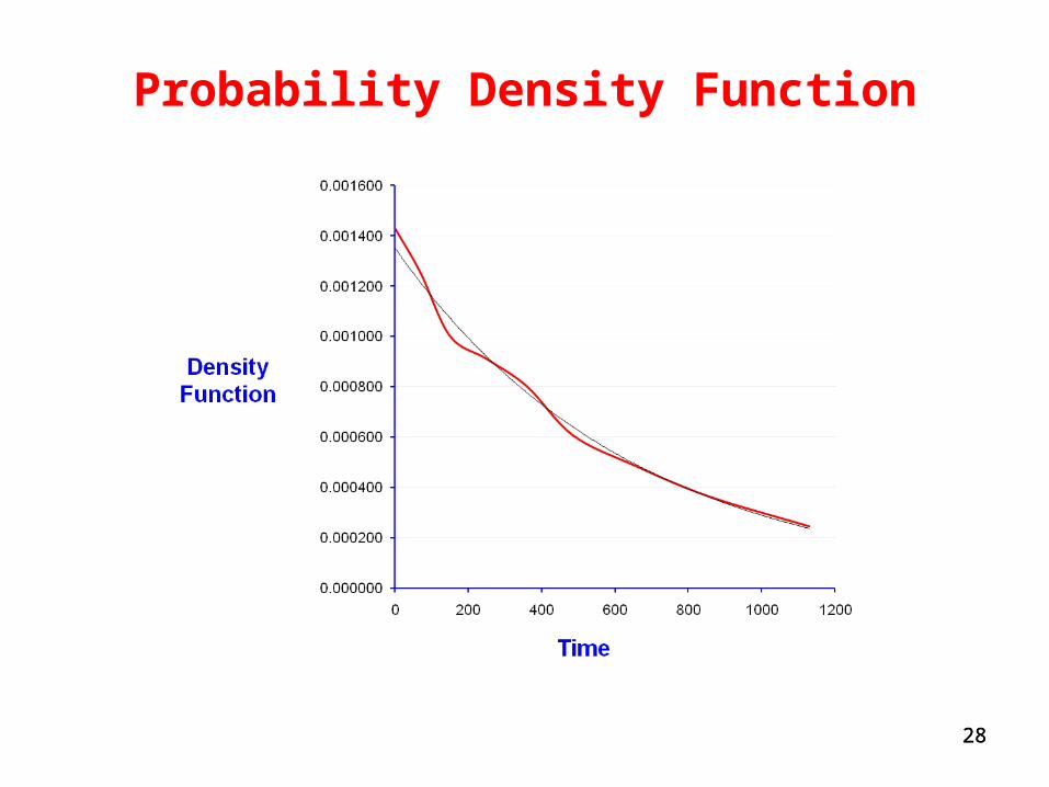
28

Probability Density Function

28

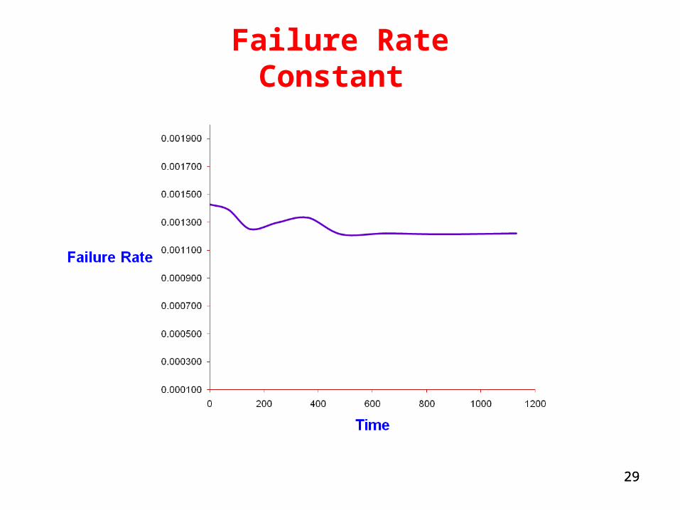
29

Failure RateConstant

29

30

Exponential Distribution: Another Example

Given failure data:

Plot the hazard rate, if constant then use the exponential distribution with f(t), R(t) and h(t) as defined before.

We use a software to demonstrate these steps.

30

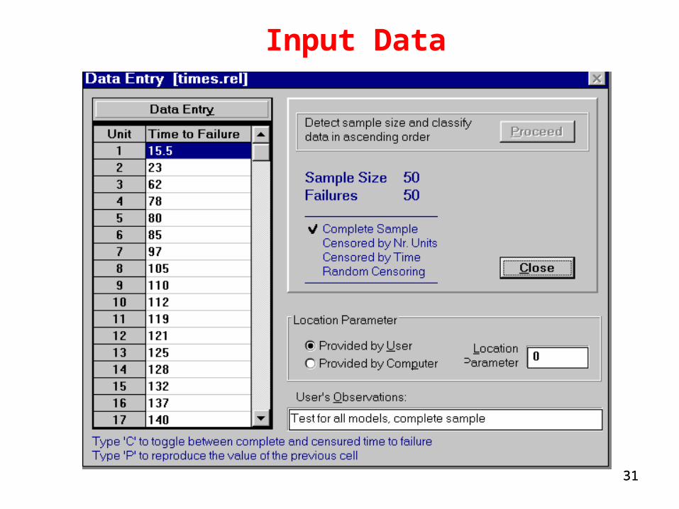
31

Input Data

31

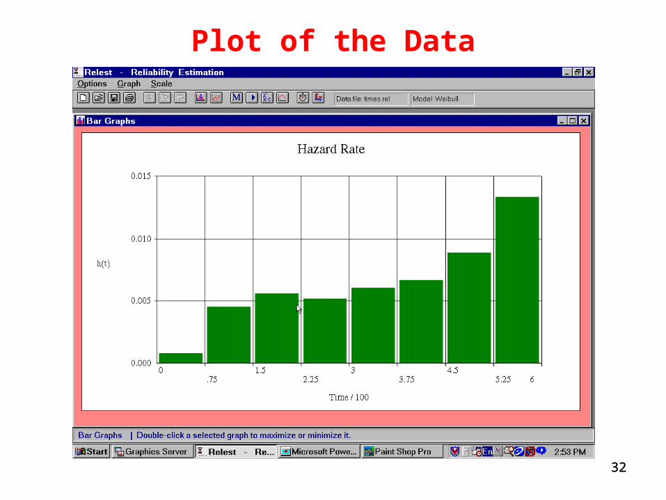
32

Plot of the Data

32

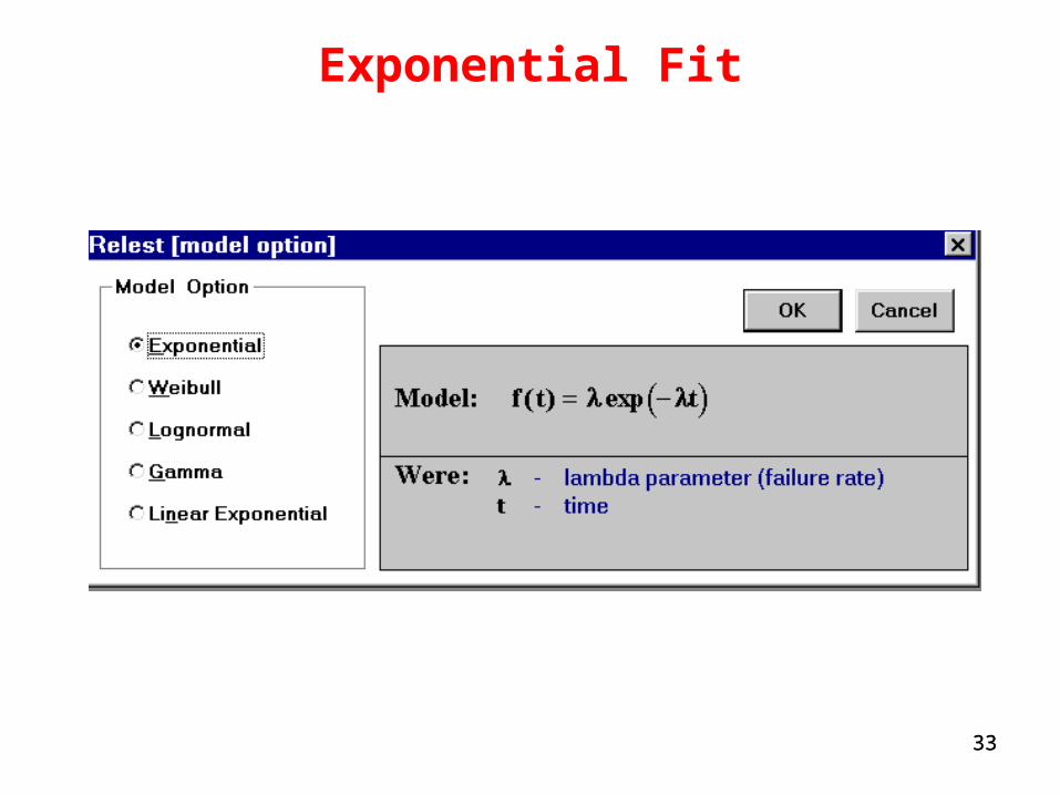
33

Exponential Fit

33

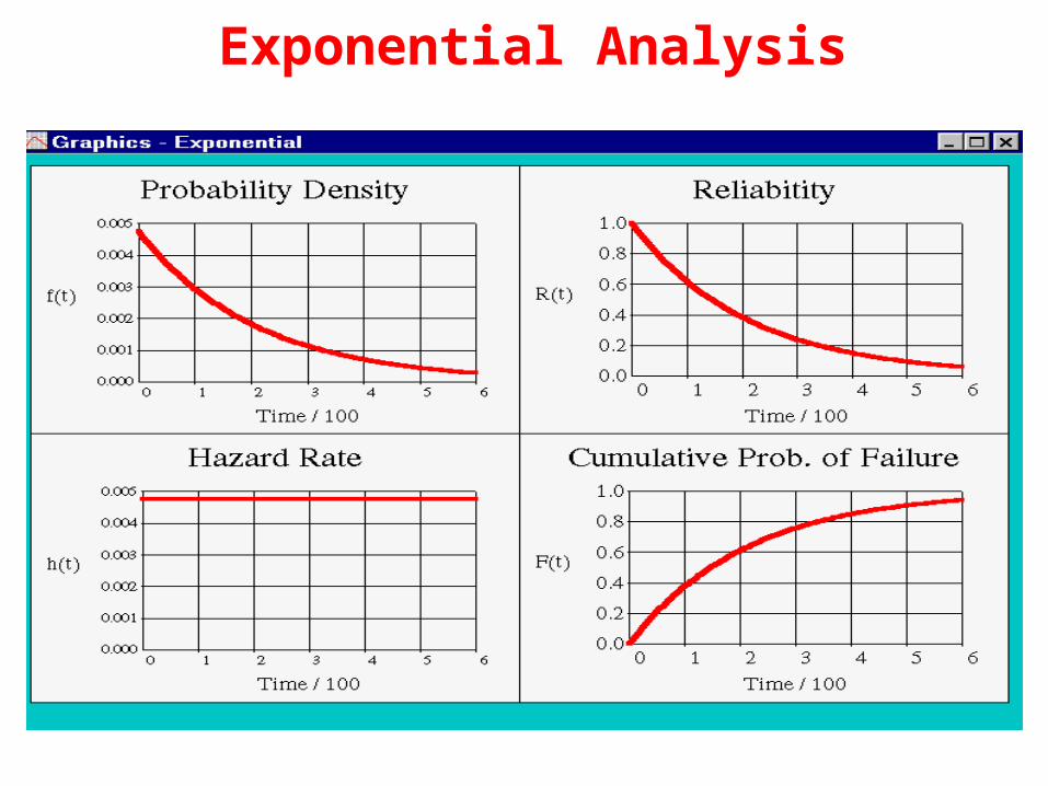
Exponential Analysis

35

Go Beyond Constant Failure Rate

- Weibull Distribution (Model) and

Others

35

36

The General Failure Curve

Time t

1

Early Life Region

2

Constant Failure Rate Region

3

Wear-Out Region

Failu

re R

ate

0

ABC Module

36

37

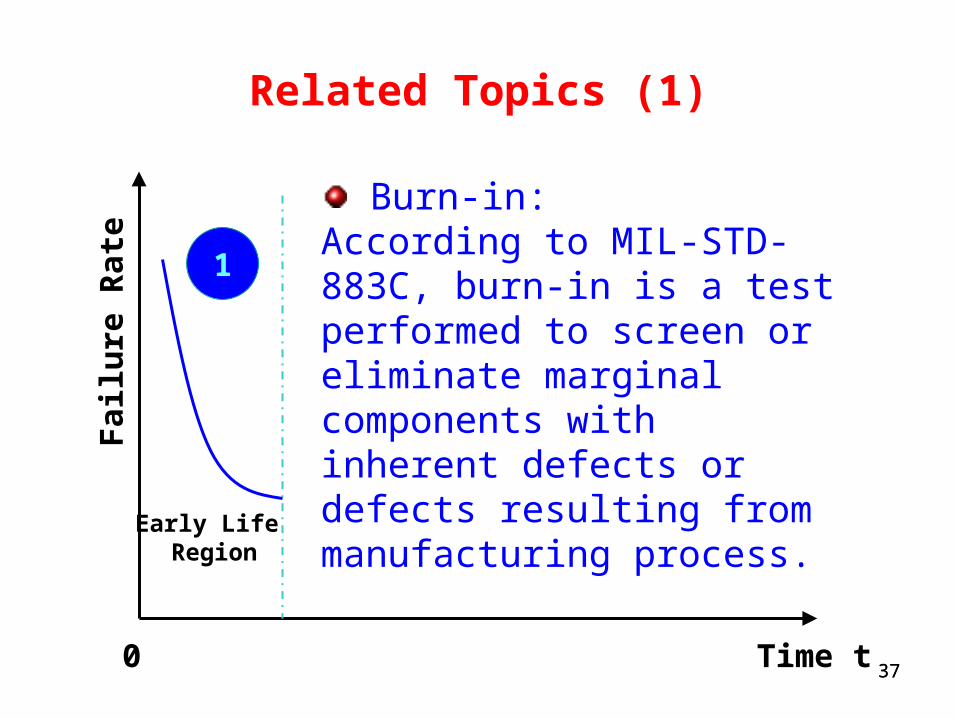
Related Topics (1)

Time t

1

Early Life Region

Failu

re R

ate

0

Burn-in:According to MIL-STD-883C, burn-in is a test performed to screen or eliminate marginal components with inherent defects or defects resulting from manufacturing process.

37

38

21

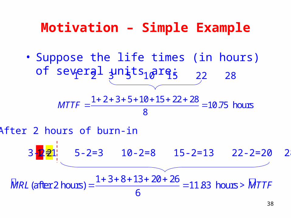
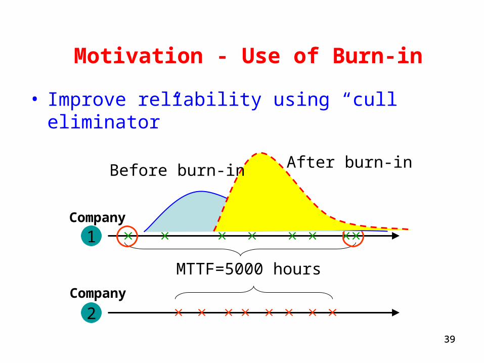
Motivation – Simple Example

• Suppose the life times (in hours) of several units are: 1 2 3 5 10 15 22 28

1 2 3 5 10 15 22 2810.75 hours

8MTTF

3-2=1 5-2=3 10-2=8 15-2=13 22-2=20 28-2=26

1 3 8 13 20 26(after 2 hours) 11.83 hours >

6MRL MTTF

After 2 hours of burn-in

39

Motivation - Use of Burn-in

• Improve reliability using “cull eliminator”

1

2

MTTF=5000 hours

Company

Company

After burn-inBefore burn-in

39

40

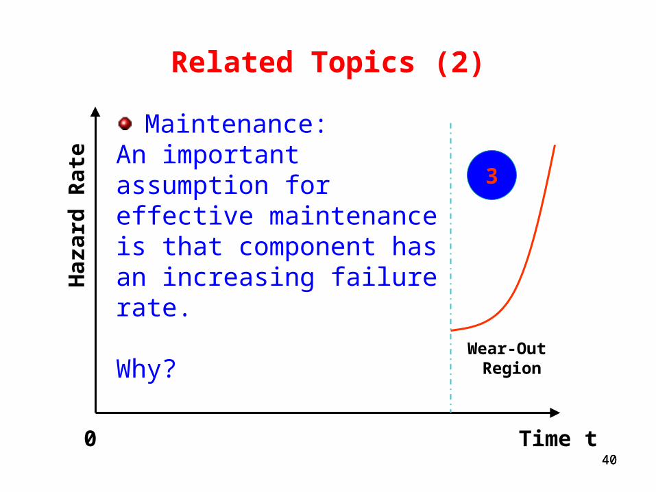
Related Topics (2)

Time t

3

Wear-Out Region

Haza

rd R

ate

0

Maintenance:An important assumption for effective maintenance is that component has an increasing failure rate.

Why?

40

41

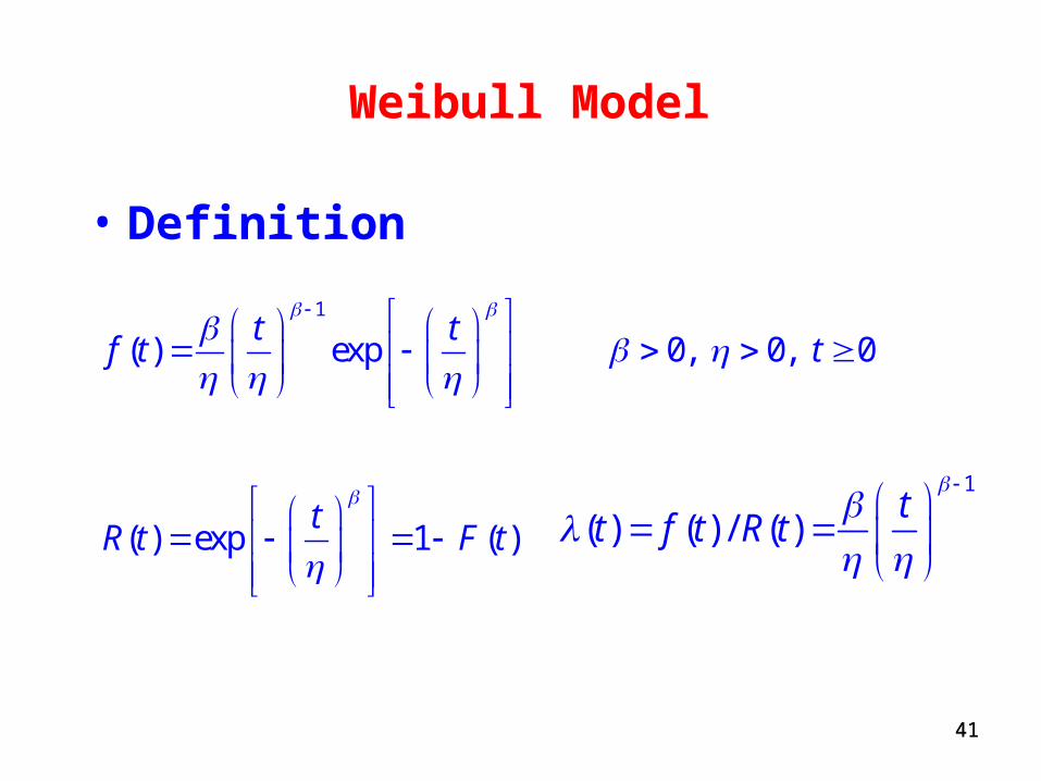
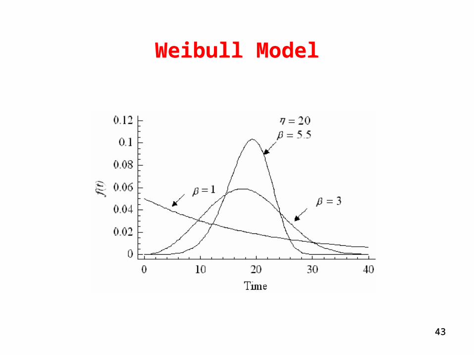
Weibull Model

• Definition

1

( ) exp 0, 0, 0t t

f t t

( ) exp 1 ( )t

R t F t

1

( ) ( ) / ( )t

t f t R t

41

42

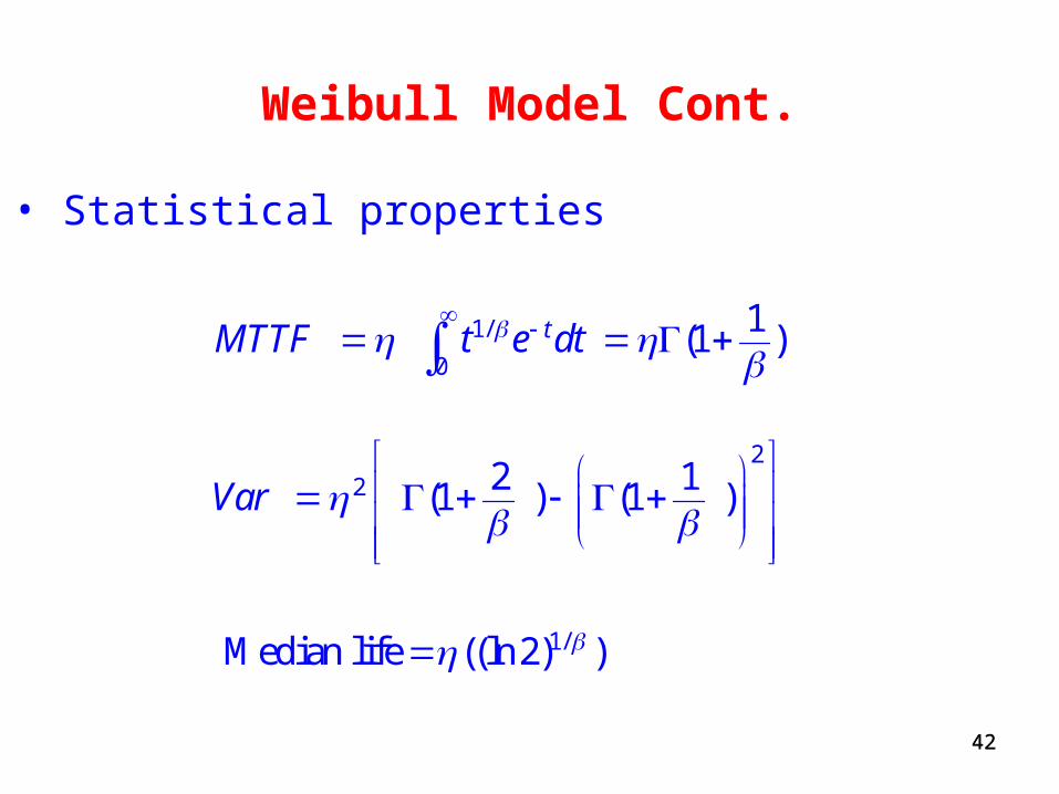
Weibull Model Cont.

1/

0

1(1 )tMTTF t e dt

22 2 1(1 ) (1 )Var

1/Median life ((ln 2) )

• Statistical properties

42

43

Weibull Model

43

44

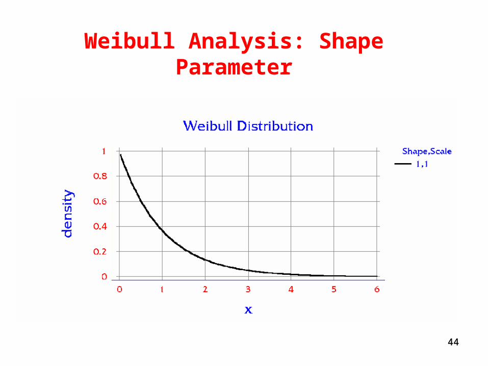
Weibull Analysis: Shape Parameter

44

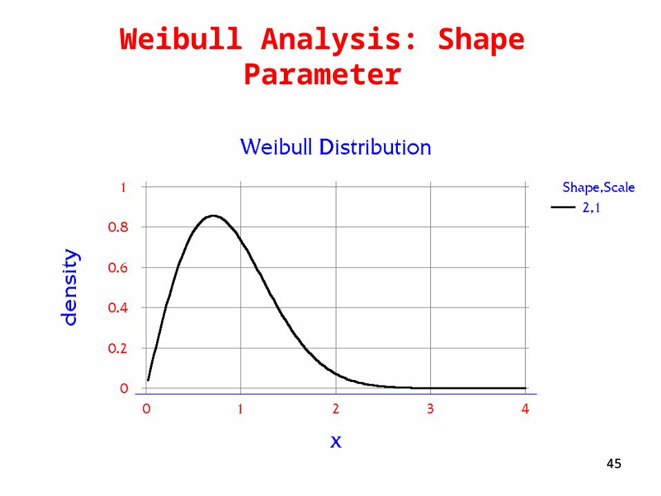
45

Weibull Analysis: Shape Parameter

45

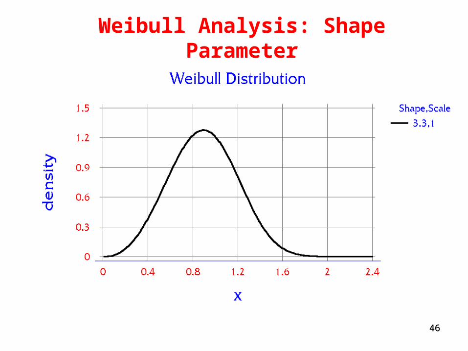
46

Weibull Analysis: Shape Parameter

46

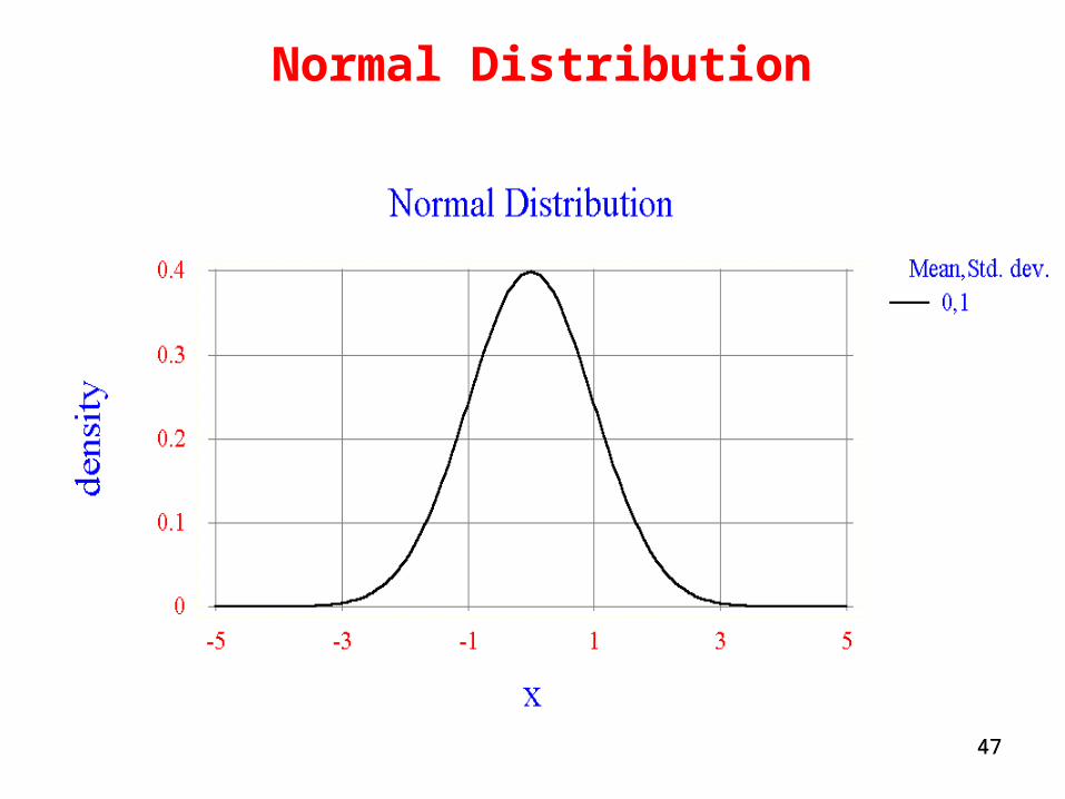
47

Normal Distribution

47

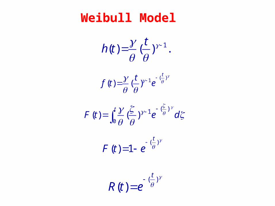
Weibull Model

1( ) ( ) .t

h t

( )1( ) ( )tt

f t e

0

( )1( ) ( )t

F t e d

( )( ) 1

t

F t e

( )( )

t

R t e

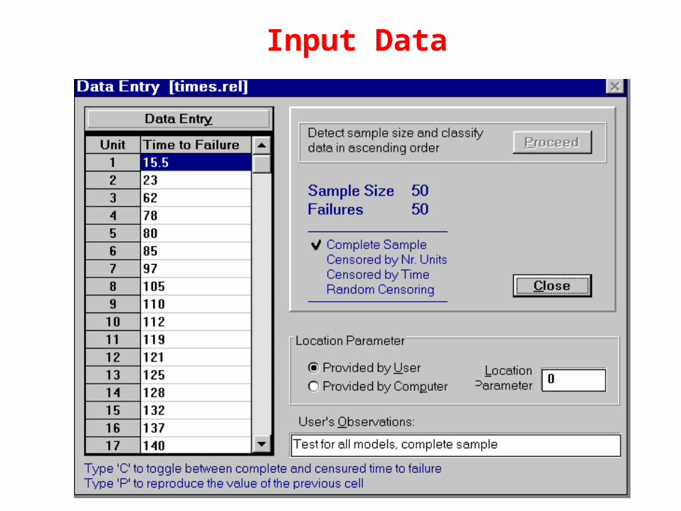
Input Data

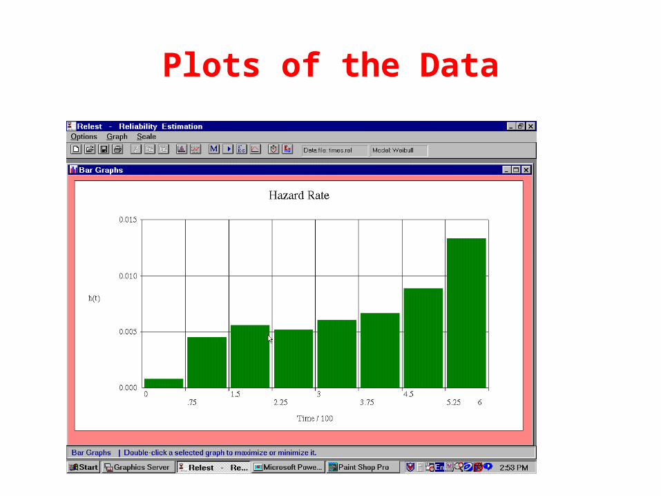
Plots of the Data

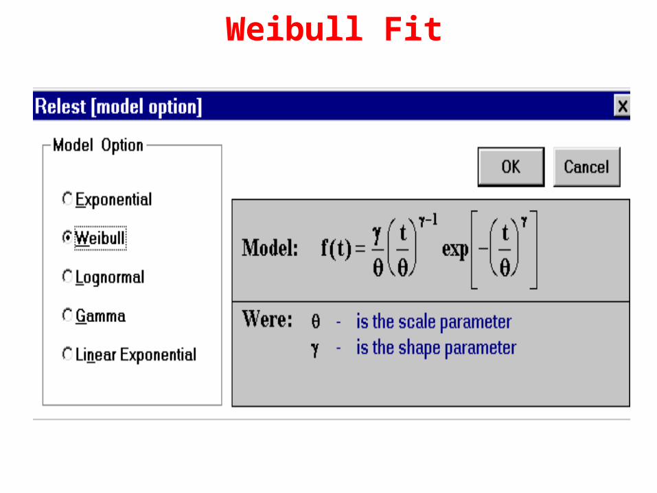
Weibull Fit

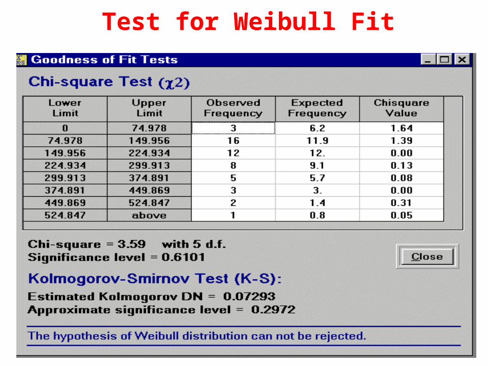
Test for Weibull Fit

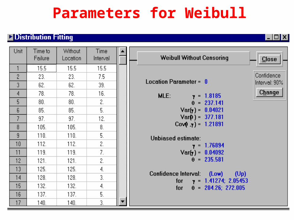
Parameters for Weibull

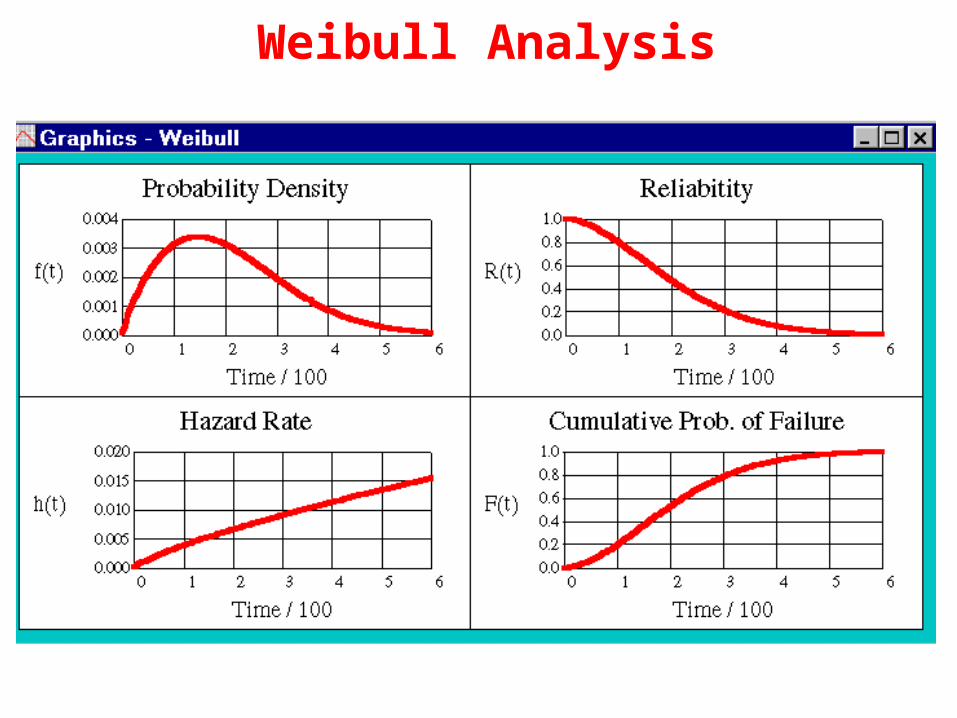
Weibull Analysis

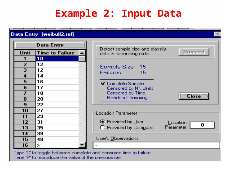
Example 2: Input Data

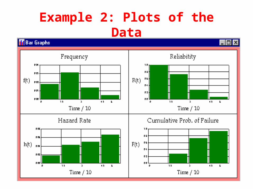
Example 2: Plots of the Data

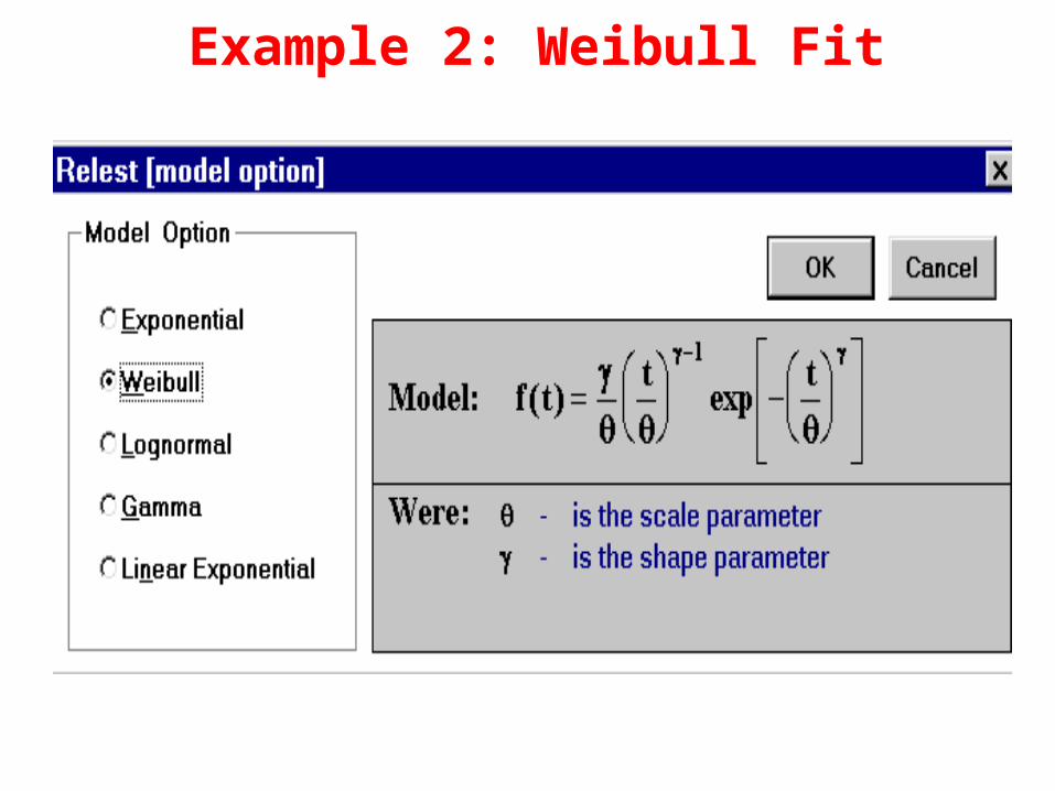
Example 2: Weibull Fit

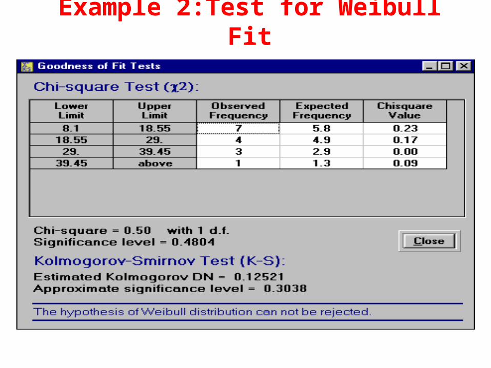
Example 2:Test for Weibull Fit

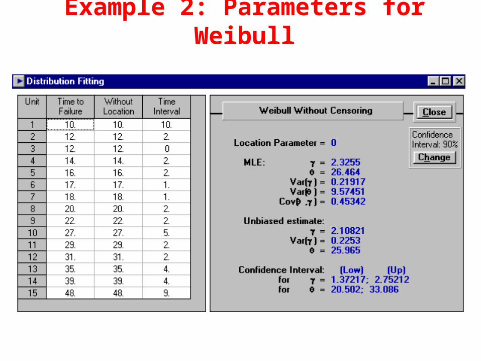
Example 2: Parameters for Weibull

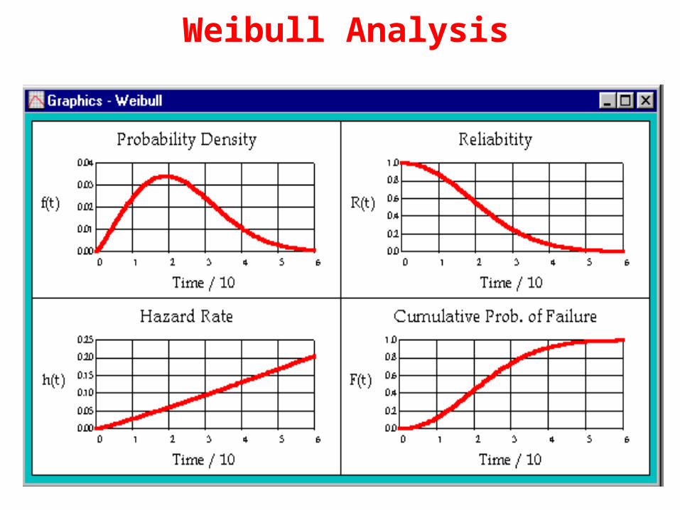
Weibull Analysis

61

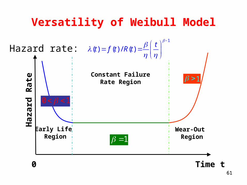
Versatility of Weibull Model

Hazard rate:

Time t

1

Constant Failure Rate Region

Haza

rd R

ate

0

Early Life Region

0 1

Wear-Out Region

1

1

( ) ( ) / ( )t

t f t R t

61

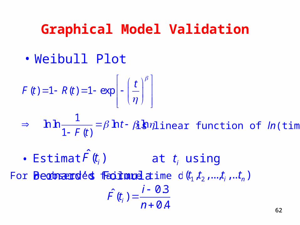
62

( ) 1 ( ) 1 exp

1 ln ln ln ln

1 ( )

tF t R t

tF t

Graphical Model Validation

• Weibull Plot

is linear function of ln(time).

• Estimate at ti using Bernard’s Formula ˆ ( )iF t

0.3ˆ ( )0.4i

iF t

n

For n observed failure time data 1 2( , ,..., ,... )i nt t t t

62

63

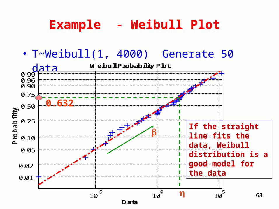
Example - Weibull Plot

• T~Weibull(1, 4000) Generate 50 data

10-5

100

105

0.01

0.02

0.05

0.10

0.25

0.50

0.75

0.90 0.96 0.99

Data

Pro

ba

bil

ity

Weibull Probability Plot

0.632

If the straight line fits the data, Weibull distribution is a good model for the data

63