1 Deriving ice thickness, glacier volume and bedrock ... · were collected in the form of 2806 samples within ... a 50 MHz wavelet travels at 0.1695 m/ns, ... Mono-offset GPR data

1

Deriving ice thickness, glacier volume and

bedrock morphology of the Austre

Lovenbreen (Svalbard) using

Ground-penetrating RadarA. Saintenoy∗, J.-M. Friedt†, A. D. Booth‡‖, F. Tolle§, E. Bernard§,

D. Laffly¶, C. Marlin∗ and M. Griselin§

∗IDES, UMR 8148 CNRS, Universite Paris Sud, Orsay, France

Email: [email protected]†FEMTO-ST, UMR 6174 CNRS, Universite de Franche-Comte, Besancon, France

‡Glaciology Group, Department of Geography, Swansea University, Swansea, Wales, UK§THEMA, UMR 6049 CNRS, Universite de Franche-Comte, Besancon, France¶GEODE, UMR 5602 CNRS, Universite de Toulouse, Toulouse, France

‖Now at: Department of Earth Science and Engineering, Imperial College London, South

Kensington Campus, London, SW7 2AZ, UK

June 12, 2013 DRAFT

arX

iv:1

306.

2539

v1 [

phys

ics.

geo-

ph]

11

Jun

2013

2

Abstract

The Austre Lovenbreen is a 4.6 km2 glacier on the Archipelago of Svalbard (79oN) that has been surveyed

over the last 47 years in order of monitoring in particular the glacier evolution and associated hydrological

phenomena in the context of nowadays global warming. A three-week field survey over April 2010 allowed for

the acquisition of a dense mesh of Ground-penetrating Radar (GPR) data with an average of 14683 points per km2

(67542 points total) on the glacier surface. The profiles were acquired using a Mala equipment with 100 MHz

antennas, towed slowly enough to record on average every 0.3 m, a trace long enough to sound down to 189 m

of ice. One profile was repeated with 50 MHz antenna to improve electromagnetic wave propagation depth in

scattering media observed in the cirques closest to the slopes. The GPR was coupled to a GPS system to position

traces. Each profile has been manually edited using standard GPR data processing including migration, to pick

the reflection arrival time from the ice–bedrock interface. Snow cover was evaluated through 42 snow drilling

measurements regularly spaced to cover all the glacier. These data were acquired at the time of the GPR survey

and subsequently spatially interpolated using ordinary kriging. Using a snow velocity of 0.22 m/ns, the snow

thickness was converted to electromagnetic wave travel-times and subtracted from the picked travel-times to the

ice–bedrock interface. The resulting travel-times were converted to ice thickness using a velocity of 0.17 m/ns.

The velocity uncertainty is discussed from a common mid-point profile analysis. A total of 67542 georeferenced

data points with GPR-derived ice thicknesses, in addition to a glacier boundary line derived from satellite images

taken during summer, were interpolated over the entire glacier surface using kriging with a 10 m grid size. Some

uncertainty analysis were carried on and we calculated an averaged ice thickness of 76 m and a maximum depth

of 164 m with a relative error of 11.9%. The volume of the glacier is derived as 0.3487±0.041 km3. Finally a

10-m grid map of the bedrock topography was derived by subtracting the ice thicknesses from a dual-frequency

GPS-derived digital elevation model of the surface. These two datasets are the first step for modelling thermal

evolution of the glacier and its bedrock, as well as the main hydrological network.

Keywords: Glacier; Ground-penetrating Radar; Ice Volume Estimation

June 12, 2013 DRAFT

3

I. INTRODUCTION

Long-term studies of the Spitsbergen Western coast glaciers reveal that they are retreating over the last

decades (Hagen et al., 2003; Kohler et al., 2007). Quantification of current mass-balance trends of these glaciers

is attempted by the evaluation of surface conditions (accumulation and ablation), basal conditions (melting

or freezing) and ice dynamics (mass movements). Surface changes can be evaluated from digital elevation

models (DEMs) derived, e.g. from photogrametric methods applied on aerial and satellite images, surface

GPS measurements or airborne LiDAR acquisitions or ground based high resolution photography (Cuffey and

Paterson, 2010; Bernard et al., in press) in addition to in situ ablation stake network height measurements.

However, the glacier volume estimate is necessary for either ice dynamical modelling or future mass balance

scenarios.

Ground-penetrating Radar (GPR) is a geophysical tool using radiofrequency electromagnetic waves for

sounding underground features. This method is especially efficient for mapping glaciers thanks to the good

penetration depth of the electromagnetic waves in a low loss medium such as ice. Common-offset radar profiling

has been successfully used for evaluating ice thickness of glaciers (e.g. (Hagen and Sætrang, 1991; Ramırez

et al., 2001; Fischer, 2009)), deriving at a decimetric scale the internal geometry of ice structures (Hambrey

et al., 2005), locating and characterizing englacial channels (Stuart et al., 2003) and analyzing the glacier base

for determining the thermal regime (Murray et al., 2000; Murray and Booth, 2009). Multi-offset profiles are

acquired for getting a wave velocity estimate or the water content variations of the glacier ice (Murray et al.,

2007). It is striking to see the evolution in the radar surveys since the 1990s when measurement positioning was

achieved using compass and visual navigation on the glacier and the main source of error in the ice thickness

estimation was considered to be ± 10 m mostly due to the digitizing of the profiles (Hagen and Sætrang,

1991). High resolution, real time positioning capability as provided by GNSS and, in our case, GPS, provides

the mandatory tool for high resolution bedrock mapping on challenging terrain.

The Austre Lovenbreen is a northward-flowing valley glacier situated in the Brøgger peninsula, Spitsbergen,

Norway (79oN) (Mingxing et al., 2010; Bernard, 2011). It extends from an altitude of 100 m to 560 m above

sea level. The mean annual precipitation is 391 mm and its mean annual temperature from 1969 to 1998 is

-5.77oC (source DNMI at http://eklima.met.no). Thanks to the geological configuration of its basin, all runoff

water is concentrated into two channels. With this specific hydrological configuration and being near the former

mining town of Ny-Alesund, this site has been the focus of intense scrutiny since the 1960s. A summary of

historical dataset since 1962, used for elevation models on this glacier as well as their relevance to evaluate mass

balance is described in (Friedt et al., 2012). The neighboring glacier, Midtre Lovenbreen, has been extensively

studied as well. It is known to be polythermal on the basis of radio echo sounding (Hagen and Sætrang, 1991;

Bjornsson et al., 1996; Rippin et al., 2003). A detailed description of its structure and dynamics can be found

in (Hambrey et al., 2005). Additionally to a high frequency GPR survey, a seismic reflection survey allowed

for determining the properties of the bed material (King et al., 2008).

In this paper we present results of a high density coverage GPR survey (120 profiles resulting in 67542 ice

thickness measurements) of the Austre Lovenbreen. We first show some internal structures observed on selected

radargrams, then present the ice volume estimation and finally the glacier substratum topography. We discuss

June 12, 2013 DRAFT

4

the different sources of uncertainties in those two data sets.

II. DATA COLLECTION AND PROCESSING

We used a Mala Ramac GPR operating at 50 and 100 MHz to collect more than 70 km of mono-offset profiles

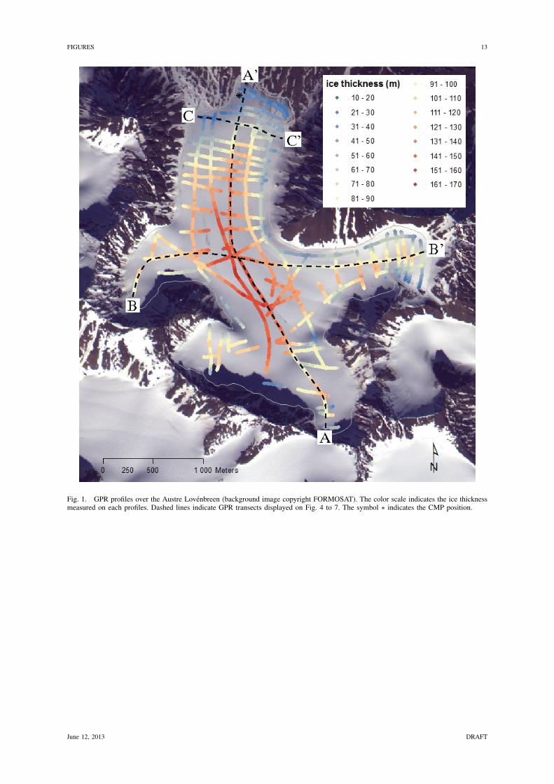
(Fig. 1) over the surface of the Austre Lovenbreen (Svalbard) during 3 weeks in April 2010. Both the 50 MHz

and 100 MHz antenna data, corresponding to a nominal wavelength in ice of 3.4 m and 1.7 m respectively,

were collected in the form of 2806 samples within a time window 2.224 µs. All data were stacked 8 times on

collection. Positioning of all GPR mono-offset profiles was done using a Globalsat ET-312 Coarse/Acquisition

(C/A) code GPS receiver connected to the control unit of the GPR, set to 1 measurement per second while

two operators were pulling the device at a comfortable walking pace. A trace was acquired every 0.5 s, and

the average distance between traces was later calculated at 0.3 m.

[Fig. 1 about here.]

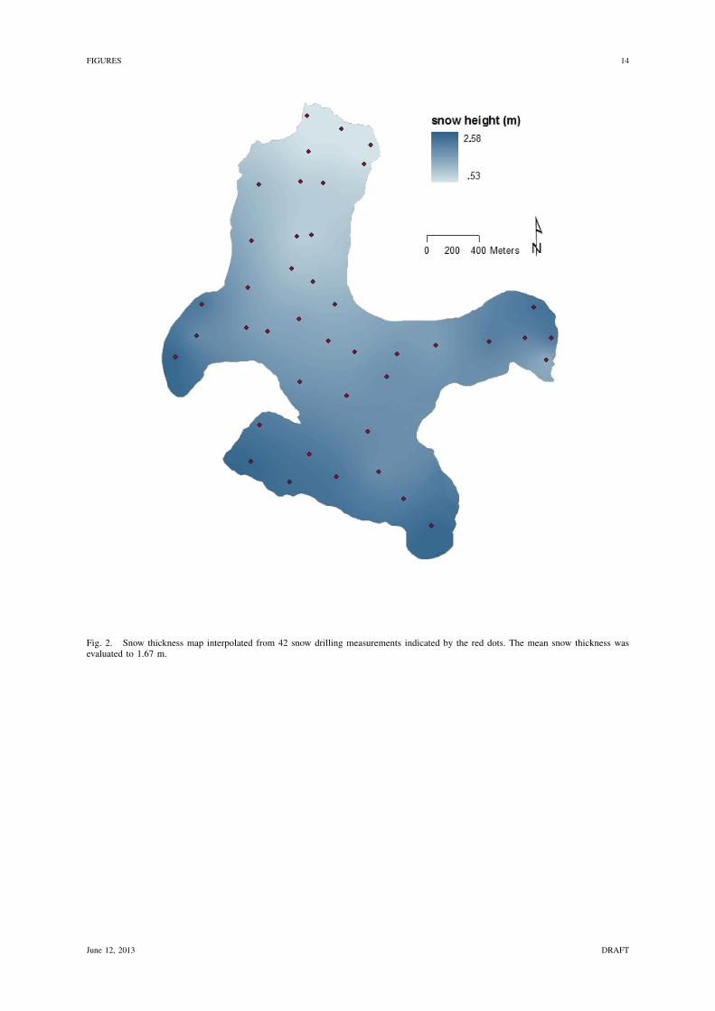
Snow cover was evaluated through 42 snow drilling measurements regularly spaced to cover all the glacier.

These data were acquired at the time of the GPR and dual GPS measurements and subsequently interpolated

using ordinary kriging. The resulting snow thickness map is shown on Fig. 2. The measurement root mean

square error is 20 cm (Webster and Oliver, 2001). The average snow thickness over the entire glacier on April

2010 was estimated to 1.67 m.

[Fig. 2 about here.]

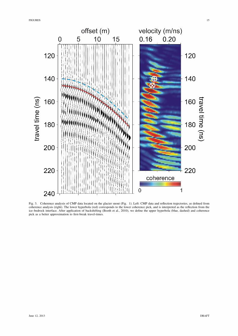
In addition to the mono-offset profiles, one Common Mid-Point (CMP) gather was acquired on the glacier

snout using the 100 MHz antennas (Fig 3). The initial separation between antennas was 0.5 m, with a spatial

stepsize of 0.5 m. CMP data were interpreted using coherence analysis, defined equivalently to semblance but

using an analysis window of one temporal sample (here, 0.8 ns). The basal reflection exhibits a velocity of

0.1715 m/ns (red trajectory in CMP gather, lower pick in coherence panel), but coherence delivers a root-mean-

square velocity that is biased systematically slow with respect to its true value (Booth et al., 2010). This occurs

because true velocity is only expressed by wavelet first-breaks, yet these are zero amplitude hence cannot

produce a coherence response. We therefore use the coherence response to simulate first-break travel-times,

using the ’backshifting’ method of Booth et al. (2010), and obtain an RMS velocity of 0.1747 m/ns and a

travel-time to the base of the ice of 140.0 ns (blue trajectory in CMP gather, upper pick in coherence panel).

This RMS velocity is then converted to interval velocity using Dix’s equation (Dix, 1955). At the location

of the CMP acquisition, the glacier was covered by 0.7 m of snow, which we assume to have a velocity

of 0.22 m/ns (Murray et al., 2007) and, hence, the two-way travel-time to the base of the snow is 6.3 ns.

Substituting our velocity-time model into Dix’s Equation gives 0.1723±0.0021 m/ns as the interval velocity

through the ice, and a local ice thickness of 10.21±0.16 m. The uncertainty in these values is obtained by

considering the resolution of coherence analysis (Booth et al., 2011), and is therefore representative of the error

between a given coherence pick and its true velocity value.

Successive depth conversions are made with a velocity value of 0.17 m/ns, which represents the lower-bound

of the error in interval velocity. We choose this value since the volumetric content of air is likely to decrease

June 12, 2013 DRAFT

5

in the thicker parts of the glacier (Gusmeroli et al., 2010) hence we anticipate that a slower velocity is more

widely representative. Although CMP surveys over the thickest ice could confirm this, the fiber optic cables of

our GPR system were only 20 m long, reducing our maximum offset-to-depth ratio and thereby producing a

poor coherence response. Finally, we will use the velocity derived from the 100 MHz dataset to depth-convert

50 MHz records. Ice is weakly dispersive: across the range 1-100 MHz, relative dielectric permittivity decreases

by 0.04 (Dowdswell and Evans, 2004). Accordingly, in terms of propagation velocity, if our 100 MHz wavelet

travels at 0.1700 m/ns, a 50 MHz wavelet travels at 0.1695 m/ns, a difference that we consider negligible in

depth conversion.

[Fig. 3 about here.]

Mono-offset GPR data have been processed using Seismic Unix software (Cohen and Stockwell, 2011;

Stockwell, 1999). A residual median filter was applied in vertical direction using a time window corresponding

to the cut-off frequency of 50 MHz, each trace has been normalized to its root mean square value and bandpass

filtered. Each profile was chopped above the arrival time of the minimum amplitude of the direct air wave

(manually selected). Based on the ET312 C/A GPS information, the mean distance a between traces is computed.

Equidistant trace positioning is achieved by searching for the acquired trace located closest to a periodic grid of

period a. The obtained profiles have then been migrated using a Stolt algorithm with a velocity of 0.17 m/ns.

When needed for visualization, elevation correction was implemented using the altitude given by the ET312

C/A GPS.

During the GPR survey, a dense elevation map was performed using GPS measurements with a snowmobile:

a Trimble Geo-XH dual frequency receiver, with electromagnetic delay correction post-processing using the

nearby (<10 km away) Ny-Alesund reference dataset, provided the raw data to generate a DEM of the glacier

after interpolation of the dataset. Data processing is performed in two steps. First the ice thickness is derived

from GPR profiles, with removal of the snow thickness contribution. In a second step, the bedrock surface is

interpolated and located in space by subtracting the ice thickness from the surface DEM.

III. GLACIER STRUCTURES

For giving an insight on our GPR data quality, four processed radargrams are shown on Fig. 4, 5, 6 and 7.

AA’ was acquired along the glacier central axis toward North while BB’ was acquired from West to East across

the glacier (see Fig. 1). CC’ was acquired across the glacier tongue.

[Fig. 4 about here.]

[Fig. 5 about here.]

[Fig. 6 about here.]

Along AA’, the strong continuous reflection is interpreted as the ice–bedrock interface. The main ice-flow

direction is South to North (Mingxing et al., 2010). At the beginning of the profile, multiple scattering occurs

partially masking the ice–bedrock interface, preventing sometime the picking of the arrival time of the radar

reflection on this interface. Similar zones are observed only on the western upper side of the glacier as in profile

June 12, 2013 DRAFT

6

BB’ beginning. We interpret these as reflections on fallen rocks incorporated into the ice, or infiltrated water.

Around 700 m, the bedrock topography rises by 50 m over a distance of 200 m creating a local topographical

high. This feature may be related to the geology of the area: a thrust fault between the Welderyggen thrust

sheet and the Nielsenfjellet thrust sheet is indicated in the southern part of the Lovenbreen glacier in geological

maps (Hjelle, 1993; Saalmann and Thiedig, 2002). Heading farther north the bedrock surface is easy to follow

all the way down to the glacier frontal moraine. At 3000 m along this profile, the ice thickness decreases as

the bedrock topography rises 70 m. The same trends are observed in other parallel profiles.

[Fig. 7 about here.]

On BB’ radargram, the bedrock reflection is very clear except in two areas. In the middle part of the glacier

(around 1300 m), an area with increased scattering appears in the deepest part of the glacier, and we attribute

this to the presence of temperate ice as described in the neighboring glacier (Hagen and Sætrang, 1991; Moore

et al., 1999; King et al., 2008). This multiple scattering area prevented us from picking the ice–bedrock interface

reflection resulting into a gap in ice thickness estimates as visible on Fig. 1. In this figure, other gaps in the

center part of the glacier result from the same difficulty to pick the ice–bedrock interface due to high scattering

zones, giving thus an idea of the horizontal extension of the probable temperate ice.

On the first 500 m of BB’, many scatterers are again observed, associated with either fallen rocks or infiltrated

water given the proximity to the surrounding mountain side. The bedrock reflection disappears among all the

scatterers but it becomes detectable in the profile acquired in this area using 50 MHz antenna (Fig. 6). This

50 MHz migrated profile was used to pick the ice–bedrock interface instead of the first 900 m of profile BB’.

At 1000 m along the profile, 30 m deep, some large hyperbolae are attributed to buried englacial channels. Our

data set does not present parallel profiles close enough to BB’ to determine the horizontal extension of this

channel.

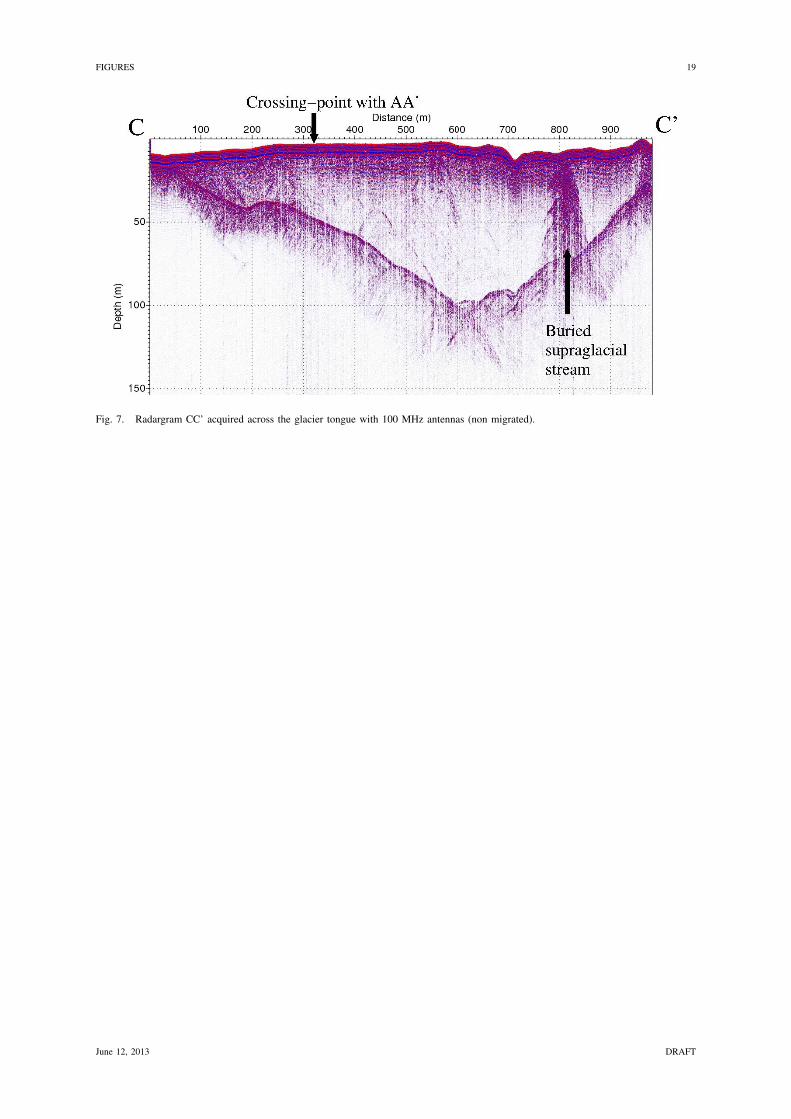
Fig. 7 shows one processed profile across the glacier tongue along the profile CC’ of Fig. 1. This profile

crosses a buried supraglacial stream, evident on the satellite image of June 26th 2007, copyright FORMOSAT.

Where this stream intersects CC’, at around 800 m, the radargram shows many diffraction hyperbolae. This

feature can be observed an all radargrams that cross the stream.

IV. ICE VOLUME ESTIMATION

The boundary of the glacier (grey line in Fig. 1), 14143 m long, was drawn on a summer 2009 FORMOSAT

image. Whenever visible, rimaye (bergschrunds) were considered as the limit between the glacier and slopes.

Moreover, slope angles were derived and used to differentiate steep angle slopes and low angle glacier. Field

knowledge and direct local GPS measurements were of great help as well. Visual inspection of all these elements

allowed us to determine as precisely as possible the limits of the glacier. We estimate that the glacier boundary

is identified with a ±10 m uncertainty. The area of the glacier is thus measured to be 4.6±0.28 km2. We have

decided to define a null ice thickness on the boundary. We will see that this choice will not significantly affect

the ice volume estimate: assuming a maximum of 20 m ice thickness error along this boundary, the volume

contribution is 0.0056 km3 (1.6% relative error).

June 12, 2013 DRAFT

7

In every migrated GPR profile, the arrival time of the basal reflection was picked using Reflexw soft-

ware (Sandmeier, 2007). No picking was done where the ice–bedrock interface was not clear. The two-way

travel time is translated into ice thickness using 0.17 m/ns velocity as derived earlier from CMP analysis: the

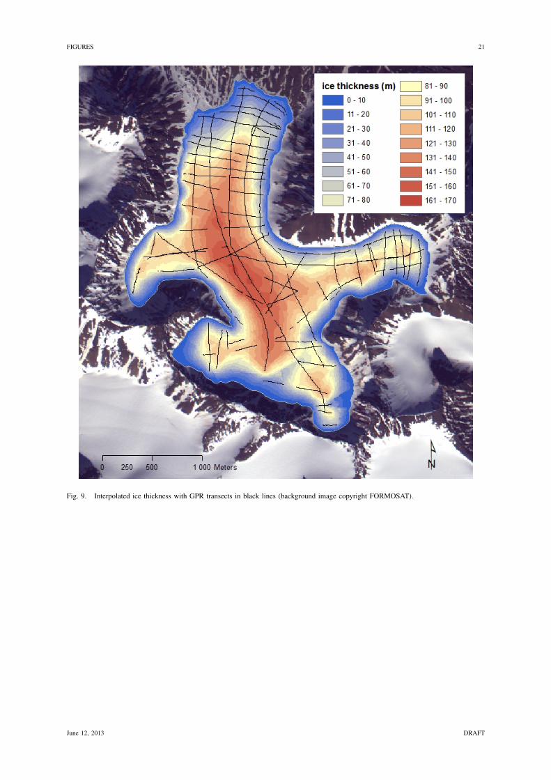
uncertainty on this velocity contributes to 1.2 % uncertainty on the glacier volume (Fig. 9). The snow layer

contribution (Fig. 2) to the radar wave propagation duration is removed by subtracting its corresponding time

delay assuming a velocity of 0.22 m/ns. The uncertainty on the snow thickness of 20 cm contributes to a volume

of 9.2×10−4 km3 (0.3% relative error).

The analysis ended-up with a total of 67542 georeferenced data points with GPR-derived ice thickness. All

ice-thickness measurements were interpolated over the entire glacier surface using a kriging method onto a

10 m grid (Fig. 9). The ice volume is 0.3487 km3. Notice that working on non migrated data as in Saintenoy et

al. (2011) yields a volume of 0.3427 km3, or a 1.1 % error with respect to the volume derived from migrated

data.

[Fig. 8 about here.]

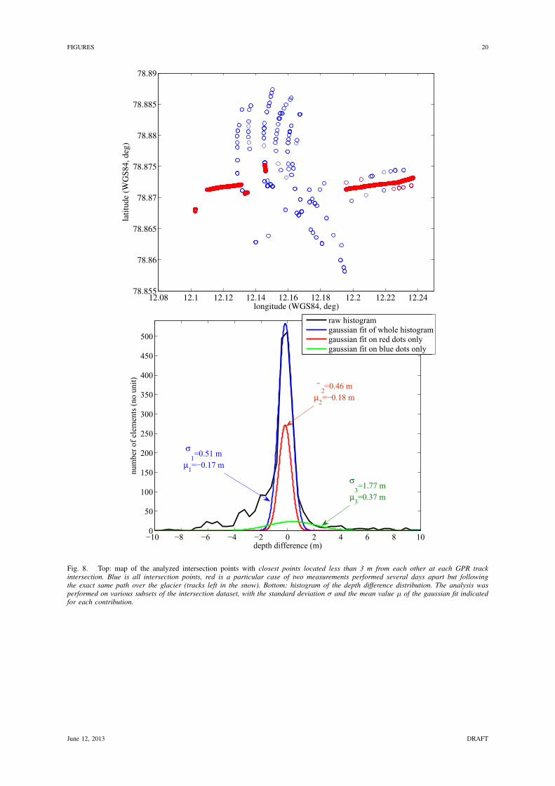
Depth estimate quality assessment was performed by analyzing the error between ice-thickness estimates

from closely-separated traces in distinct profiles: the thickness difference between the closest points lying less

than 3 m apart was computed and the histogram of the ice-thickness distribution is plotted (Fig. 8). A gaussian

fit of each histogram is performed using a constrained nonlinear optimization method: we analyze the whole

dataset including all traces intersections (blue dots) and separately the particular case of five transects acquired

3 to 5 days apart but following the same path (snow tracks). The global histogram exhibits a standard deviation

of 0.51 m and a negligible mean value of -0.17 m. These results, suggesting a better agreement than other

analysis found in the literature (Fischer, 2009; Hagen and Sætrang, 1991), is however optimistic by including

the five repeated transects with standard deviation 0.46 m and mean value of -0.18 m. Using only intersections

of traces crossing at high angles by excluding the five repeated transects (Fig. 8, top, red points), the standard

deviation of the histogram increases to 1.77 m with a mean value of 0.37 m.

This histogram of the ice thickness differences at intersections analysis is consistent with the result of the

surface interpolation by kriging, which provides an estimate of the root-mean square error between experimental

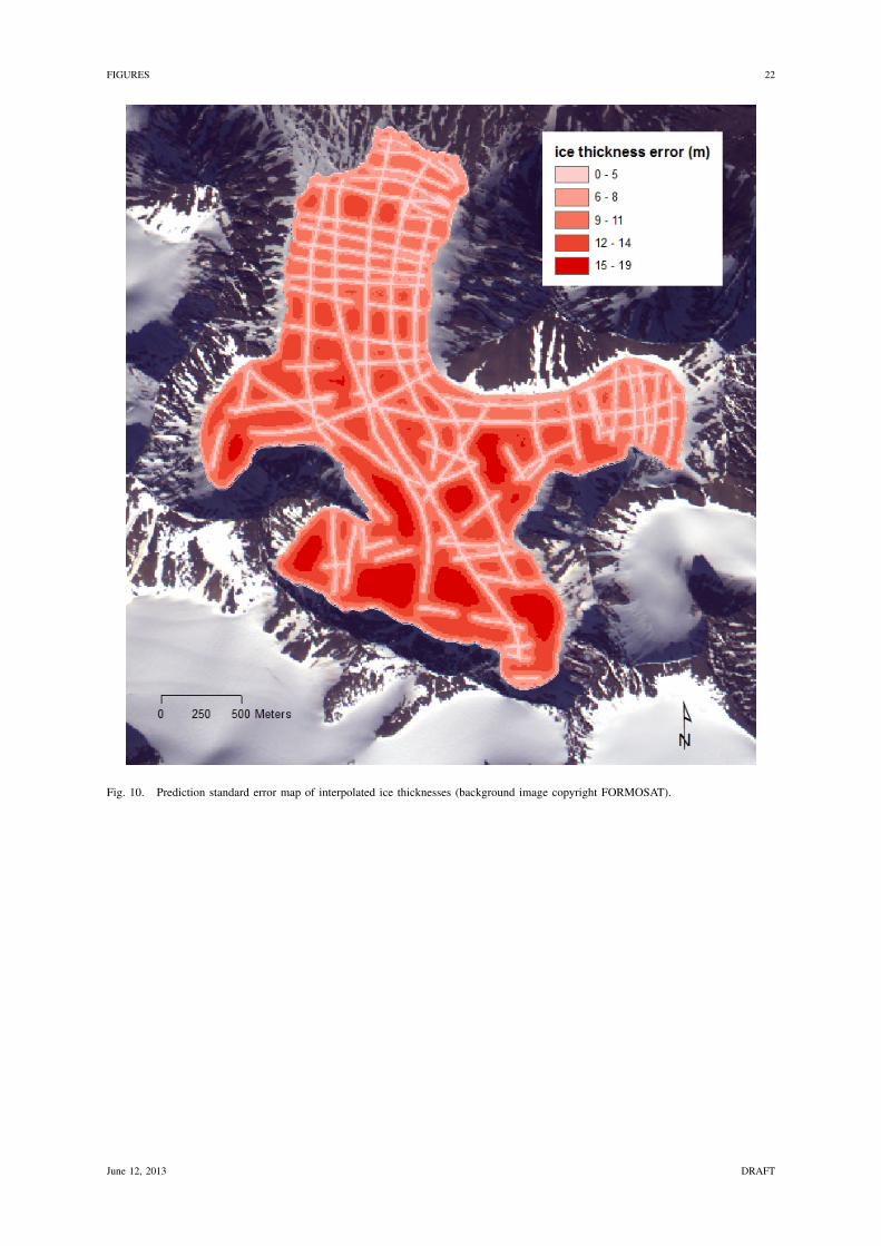
data and the interpolated surface of 0.7 m. However the interpolation of ice thickness outside of the tracks

yields the largest source of uncertainty, as provided by the kriging prediction standard error map shown on

Fig. 10, with a 11.5% contribution to the ice volume calculation (corresponding to an average error of 8.72 m

on the interpolated ice thickness).

As a result, the ice volume was estimated to 0.3487 ± 0.041 km3, with all contributions to the uncertainty

summarized in Table I. This result is to be compared with the empirical formula found in Hagen et al. (1993)

for outlet glaciers whose area A exceeds 1 km2: the mean depth is estimated as D = 33 log(A) + 25. In our

case, A = 4.6± 0.28 km2 yields a mean depth of 75±2 m, surprisingly close to the 76 m we found from our

analysis.

[TABLE 1 about here.]

June 12, 2013 DRAFT

8

V. BEDROCK DIGITAL ELEVATION MODEL

The Coarse/Acquisition (C/A) code GPS receiver that was used when GPR data was acquired is in the

range of a 3 m standard deviation in latitude and longitude but displays an unacceptable vertical accuracy with

respect to the DEM resolution. Therefore, only dual-frequency acquired GPS altitude measurements were used

as DEM reference for bedrock positioning. The accuracy of surface DEM is discussed in detail in Friedt et

al. (2012). The same uncertainty analysis carried on the dual-frequency GPS measurements yields an altitude

distribution with a standard deviation less than 0.6 m. Uncertainties on ice and snow thicknesses as well as on

the electromagnetic wave velocity estimation, sum up to 2.6 % error on the 76 m-mean depth glacier thickness,

or 2 m. Thus, considering a 0.6 m standard deviation on the DEM height, the bedrock topography uncertainty

(standard deviation of altitude error) is 2.6 m over the measurement points. The error analysis from the kriging

interpolation rises this error on the interpolated areas to 19.6 m for areas far from any experimental dataset (cf

Fig. 10).

[Fig. 9 about here.]

[Fig. 10 about here.]

[Fig. 11 about here.]

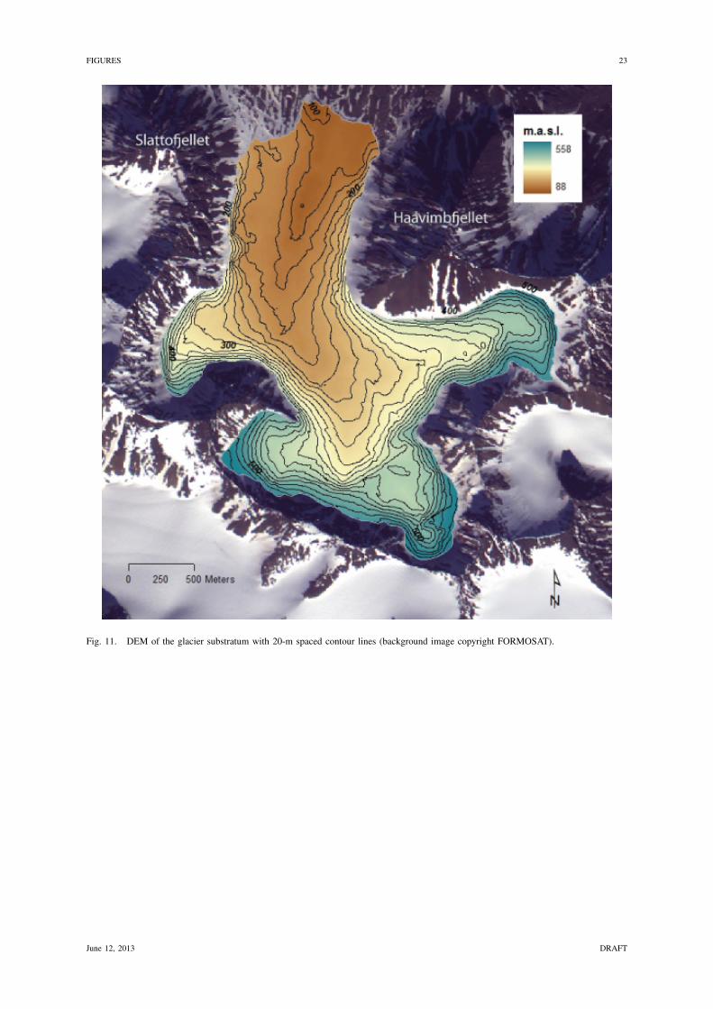
Figs. 9 and 11 show the asymmetry of the bedrock underneath the ice on the glacier snout. The substratum is

deeper on the easter side of the glacier. Furthermore, the ice–bedrock appears convex (bulging outward) on the

western side and concave (hollowed inward) on the eastern side as seen on the GPR profiles acquired across

the glacier snout (Fig. 7). This observation is consistent with a difference in the hardness of the underlying

rock, and possibly to the transform fault presented in the geological map of Saalmann and Thiedig (2002) in

between the Slatto and the Haavimb summits (Fig. 11).

VI. CONCLUSION

A high resolution mapping by 100-MHz and 50-MHz GPR of a polar glacier provides a detailed bedrock

topography information. While the average ice thickness of 76 m is consistent with empirical data derived from

glaciers in the Svalbard area, the high resolution dataset obtained by walking yields a rich information including

subsurface structures (crevasse fields, bedieres, supraglacial stream) and ice volume distribution amongst the

various glacier substructures (cirques). The resulting volume is estimated to 0.3487 ± 0.041 km3, with the

main source of error being the interpolation uncertainty of the ice thickness between tracks.

Such volume distribution provide the basic input for further mass balance investigations. Furthermore, high

density GPR data coverage coupled to accurate DEM obtained by dual frequency GPS provides a map of the

bedrock following an interpolation by kriging. This bedrock digital elevation model exhibits asymmetric features

consistent with geological structures (faults) in the area. Bedrock morphology can now be used to investigate

subglacial water flow paths, to be improved by considering the influence of ice pressure.

ACKNOWLEDGMENT

This program was funded by the ANR program blanc-0310, the IPEV program 304 and the CNRS-GDR 3062

Mutations polaires. Adam Booth is supported by the Leverhulme-funded GLIMPSE project. The authors would

June 12, 2013 DRAFT

9

like to thank AWIPEV for the logistical support in Ny-Alesund, Tavi Murray for her much helpful comments

to realize this work, Nerouz Boubaki and Emmanuel Leger for picking some GPR data and Melanie Quenet

for pointing out some references on the geology of the area.

June 12, 2013 DRAFT

10

VII. References

Bernard, E., Friedt, J.-M., Tolle, F., Griselin, M., Martin, G., Laffly, D., and Marlin, C., in press, Monitoring

seasonal snow dynamics using ground based high resolution photography (Austre Lovenbreen, Svalbard,

79o N): ISPRS Journal of Photogrammetry and Remote Sensing.

Bernard, E., 2011, Les dynamiques spatio-temporelles d’un petit hydrosysteme arctique : approche nivo-

glaciologique dans un contexte de changement climatique contemporain (bassin du glacier Austre

Lovenbreen, Spitsberg, 79 o N): Ph.D. thesis, Universite de Franche-Comte, Besancon.

Bjornsson, H., Gjessing, Y., Hamran, S., Ove Hagen, J., Liestøl, O., Palsson, F., and Erlingsson, B., 1996,

The thermal regime of sub-polar glaciers mapped by multi-frequency radio-echo sounding: Journal of

Glaciology, 42, 23–32.

Booth, A. D., Clark, R., and Murray, T., 2010, Semblance response to a ground-penetrating radar wavelet and

resulting errors in velocity analysis: Near Surface Geophysics, 8, no. 3, 235–246.

Booth, A. D., Clark, R., and Murray, T., 2011, Influences on the resolution of GPR velocity analyses and a

Monte Carlo simulation for establishing velocity precision: Near Surface Geophysics, 9, no. 5, 399–411.

Cohen, J., and Stockwell, J. CWP/SU: Seismic Un*x Release No. 42: an open source software package for

seismic research and processing:. www.cwp.mines.edu/cwpcodes, 2011.

Cuffey, K. M., and Paterson, W. S. B., 2010, The Physics of Glaciers: Boston, Elsevier, fourth edition.

Dix, C. H., 1955, Seismic velocities from surface measurements: Geophysics.

Dowdswell, J. A., and Evans, S., 2004, Investigations of the form and flow of ice sheets and glaciers using

radio-echo sounding: Reports on Progreess in Physics, 1821–1861.

Fischer, A., 2009, Calculation of glacier volume from sparse ice-thickness data, applied to Schaufelferner,

Austria: Journal of Glaciology, 55, no. 191, 453–460.

Friedt, J.-M., Tolle, F., Bernard, E., Griselin, M., Laffly, D., and Marlin, C., 2012, Assessing the relevance of

digital elevation models to evaluate glacier mass balance: application to Austre Lovenbreen (Spitsbergen,

79oN): Polar Record, 48, no. 244, 2–10.

Gusmeroli, A., Murray, T., Jansson, P., Pettersson, R., Aschwanden, A., and Booth, A. D., 2010, Vertical

distribution of water within the polythermal Storglaciaren, Sweden: Journal of Geophysical Research,

115, F04002.

Hagen, J. O., and Sætrang, A., 1991, Radio-echo soundings of sub-polar glaciers with low-frequency radar:

Polar Research, 9, no. 1, 99–107.

Hagen, J. O., Liestøl, O., Roland, E., and Jørgensen, T., 1993, Glacier Atlas of Svalbard and Jan Mayen: Norsk

Polarinstitutt.

Hagen, J. O., Kohler, J., Melvold, K., and Winther, J.-G., 2003, Glaciers in Svalbard: mass balance, runoff and

freshwater flux: Polar Research, 22, 145–159.

Hambrey, M. J., Murray, T., Glasser, N. F., Hubbard, A., Hubbard, B., Stuart, G., Hansen, S., and Kohler, J.,

2005, Structure and changing dynamics of a polythermal valley glacier on a centennial timescale: Midre

Lovenbreen, Svalbard: Journal of Geophysical Research (Earth Surface), 110, 1006–+.

Hjelle, A., 1993, Geology of Svalbard:, volume 7 Oslo: Norsk Polar Institute.

June 12, 2013 DRAFT

11

King, E. C., Smith, A. M., Murray, T., and Stuart, G. W., 2008, Glacier-bed characteristics of Midtre Lovenbreen,

Svalbard, from high-resolution seismic and radar surveying: Journal of Glaciology, 54, 145–156.

Kohler, J., James, T. D., Murray, T., Nuth, C., Brandt, O., Barrand, N. E., Aas, H. F., and Luckman, A., 2007,

Acceleration in thinning rate on Western Svalbard glaciers: Geophysical Research Letters, 34, 1–5.

Mingxing, X., Ming, Y., Jiawen, R., Songtao, A., Jiancheng, K., and Dongchen, E., 2010, Surface mass balance

and ice flow of the glaciers Austre Lovenbreen and Pedersenbreen, Svalbard, Arctic: Chine Journal of

Polar Science, 21, no. 2, 147–159.

Moore, J. C., Palli, A., Ludwig, F., Blatter, H., Jania, J., Gadek, B., Glowacki, P., Mochnacki, D., and Isaksson,

E., 1999, High-resolution hydrothermal structure of Hansbreen, Spitsbergen, mapped by ground-penetrating

radar: Journal of Glaciology.

Murray, T., and Booth, A. D., 2009, Imaging glacial sediment inclusions in 3-D using ground-penetrating radar

at Kongsvegen, Svalbard: Journal of Quaternary Science, 25, no. 5, 754–761.

Murray, T., Stuart, G. W., Miller, P. J., Woodward, J., Smith, A. M., Porter, P. R., and Jiskoot, H., 2000, Glacier

surge propagation by thermal evolution at the bed: Journal of Geophysical Research.

Murray, T., Booth, A., and Rippin, D. M., 2007, Water-content of glacier-ice: Limitations on estimates from

velocity analysis of surface ground-penetrating radar surveys: Journal of Environmental and Engineering

Geophysics, 12, no. 1, 87–99.

Ramırez, E., Francou, B., Ribstein, P., Descloitres, M., Guerin, R., Mendoza, J., Gallaire, R., Pouyaud, B.,

and Jordan, E., 2001, Small glaciers disappearing in the tropical Andes: a case-study in Bolivia: Glaciar

Chacaltaya (16◦ S): Journal of Glaciology, 47, no. 157, 187–194.

Rippin, D., Willis, I., Arnold, N., Hodson, A., Moore, J., Kohler, J., and Bjornsson, H., 2003, Changes in

geometry and subglacial drainage of Midre Lovenbreen, Svalbard, determined from digital elevation

models: Earth Surface Processes and Landforms, 28, no. 3, 273–298.

Saalmann, K., and Thiedig, F., 2002, Thrust tectonics on Broggerhalvoya and their relationship to the Tertiary

West Spitsbergen Fold-and-Thrust Belt: Geol. Mag., 139, 47–72.

Saintenoy, A., Friedt, J.-M., Tolle, F., Bernard, E., Laffly, D., Marlin, C., and Griselin, M., June 2011, High

density coverage investigation of the Austre Lovenbreen (Svalbard) using ground-penetrating radar: 6th

International Workshop on Advanced Ground Penetrating Radar (IWAGPR).

Sandmeier, K. J. Reflexw manual, version 4.5. www.sandmeier-geo.de, July 2007.

Stockwell, J. W., May 1999, The CWP/SU: Seismic Un*x Package: Computers and Geosciences, pages 415–

419.

Stuart, G., Murray, T., Gamble, N., Hayes, K., and Hodson, H., 2003, Characterization of englacial channels

by ground-penetrating radar: An example from Austre Brøggerbreen, Svalbard: Journal of Geophysical

Research, 108, no. B11, 2525–+.

Webster, R., and Oliver, M. A., 2001, Geostatistics for environmental scientists (Statistics in Practice): John

Wiley and Sons, Brisbane, Australia, 1st edition.

June 12, 2013 DRAFT

12

LIST OF FIGURES

1 GPR profiles over the Austre Lovenbreen (background image copyright FORMOSAT). The colorscale indicates the ice thickness measured on each profiles. Dashed lines indicate GPR transectsdisplayed on Fig. 4 to 7. The symbol ∗ indicates the CMP position. . . . . . . . . . . . . . . . . 13

2 Snow thickness map interpolated from 42 snow drilling measurements indicated by the red dots.The mean snow thickness was evaluated to 1.67 m. . . . . . . . . . . . . . . . . . . . . . . . . . . 14

3 Coherence analysis of CMP data located on the glacier snout (Fig. 1). Left: CMP data and reflectiontrajectories, as defined from coherence analysis (right). The lower hyperbola (red) corresponds tothe lower coherence pick, and is interpreted as the reflection from the ice–bedrock interface. Afterapplication of backshifting (Booth et al., 2010), we define the upper hyperbola (blue, dashed) andcoherence pick as a better approximation to first-break travel-times. . . . . . . . . . . . . . . . . . 15

4 Radargram AA’ acquired along the glacier axis with 100 MHz antennas including topographycorrections. . . . . . . . . . . . . . . . . . . . . . . . . . . . . . . . . . . . . . . . . . . . . . . . . 16

5 Radargram BB’ acquired across the glacier axis with 100 MHz antennas (non migrated). . . . . . 176 Repetition of the first 900 m of profile BB’ with 50 MHz antennas (after Stolt migration using a

velocity of 0.17 m/ns, with AGC gain but no topographic corrections). . . . . . . . . . . . . . . . 187 Radargram CC’ acquired across the glacier tongue with 100 MHz antennas (non migrated). . . . . 198 Top: map of the analyzed intersection points with closest points located less than 3 m from each

other at each GPR track intersection. Blue is all intersection points, red is a particular case of twomeasurements performed several days apart but following the exact same path over the glacier(tracks left in the snow). Bottom: histogram of the depth difference distribution. The analysis wasperformed on various subsets of the intersection dataset, with the standard deviation σ and themean value µ of the gaussian fit indicated for each contribution. . . . . . . . . . . . . . . . . . . 20

9 Interpolated ice thickness with GPR transects in black lines (background image copyright FOR-MOSAT). . . . . . . . . . . . . . . . . . . . . . . . . . . . . . . . . . . . . . . . . . . . . . . . . . 21

10 Prediction standard error map of interpolated ice thicknesses (background image copyright FOR-MOSAT). . . . . . . . . . . . . . . . . . . . . . . . . . . . . . . . . . . . . . . . . . . . . . . . . . 22

11 DEM of the glacier substratum with 20-m spaced contour lines (background image copyrightFORMOSAT). . . . . . . . . . . . . . . . . . . . . . . . . . . . . . . . . . . . . . . . . . . . . . . 23

June 12, 2013 DRAFT

FIGURES 13

Fig. 1. GPR profiles over the Austre Lovenbreen (background image copyright FORMOSAT). The color scale indicates the ice thicknessmeasured on each profiles. Dashed lines indicate GPR transects displayed on Fig. 4 to 7. The symbol ∗ indicates the CMP position.

June 12, 2013 DRAFT

FIGURES 14

Fig. 2. Snow thickness map interpolated from 42 snow drilling measurements indicated by the red dots. The mean snow thickness wasevaluated to 1.67 m.

June 12, 2013 DRAFT

FIGURES 15

Fig. 3. Coherence analysis of CMP data located on the glacier snout (Fig. 1). Left: CMP data and reflection trajectories, as defined fromcoherence analysis (right). The lower hyperbola (red) corresponds to the lower coherence pick, and is interpreted as the reflection from theice–bedrock interface. After application of backshifting (Booth et al., 2010), we define the upper hyperbola (blue, dashed) and coherencepick as a better approximation to first-break travel-times.

June 12, 2013 DRAFT

FIGURES 16

Fig. 4. Radargram AA’ acquired along the glacier axis with 100 MHz antennas including topography corrections.

June 12, 2013 DRAFT

FIGURES 17

Fig. 5. Radargram BB’ acquired across the glacier axis with 100 MHz antennas (non migrated).

June 12, 2013 DRAFT

FIGURES 18

Fig. 6. Repetition of the first 900 m of profile BB’ with 50 MHz antennas (after Stolt migration using a velocity of 0.17 m/ns, with AGCgain but no topographic corrections).

June 12, 2013 DRAFT

FIGURES 19

Fig. 7. Radargram CC’ acquired across the glacier tongue with 100 MHz antennas (non migrated).

June 12, 2013 DRAFT

FIGURES 20

12.08 12.1 12.12 12.14 12.16 12.18 12.2 12.22 12.2478.855

78.86

78.865

78.87

78.875

78.88

78.885

78.89

longitude (WGS84, deg)

lati

tude

(WG

S84, deg

)

−10 −8 −6 −4 −2 0 2 4 6 8 100

50

100

150

200

250

300

350

400

450

500

depth difference (m)

num

ber

of e

lem

ents

(no

uni

t)

raw histogramgaussian fit of whole histogramgaussian fit on red dots onlygaussian fit on blue dots only

σ3=1.77 m

µ3=0.37 m

σ2=0.46 m

µ2=−0.18 m

σ1=0.51 m

µ1=−0.17 m

Fig. 8. Top: map of the analyzed intersection points with closest points located less than 3 m from each other at each GPR trackintersection. Blue is all intersection points, red is a particular case of two measurements performed several days apart but followingthe exact same path over the glacier (tracks left in the snow). Bottom: histogram of the depth difference distribution. The analysis wasperformed on various subsets of the intersection dataset, with the standard deviation σ and the mean value µ of the gaussian fit indicatedfor each contribution.

June 12, 2013 DRAFT

FIGURES 21

Fig. 9. Interpolated ice thickness with GPR transects in black lines (background image copyright FORMOSAT).

June 12, 2013 DRAFT

FIGURES 22

Fig. 10. Prediction standard error map of interpolated ice thicknesses (background image copyright FORMOSAT).

June 12, 2013 DRAFT

FIGURES 23

Fig. 11. DEM of the glacier substratum with 20-m spaced contour lines (background image copyright FORMOSAT).

June 12, 2013 DRAFT

FIGURES 24

LIST OF TABLES

I Summary of contributions to glacier volume estimation error. The sum of all errors yields to a11.9 % accuracy. . . . . . . . . . . . . . . . . . . . . . . . . . . . . . . . . . . . . . . . . . . . . 25

June 12, 2013 DRAFT

TABLES 25

Cause of error Volume Relative errorIce thickness: ±1.77 m 0.008 km3 2.3 %

Glacier area 0.0056 km3 1.6 %Snow thickness 9.2 ×10−4 km3 0.3 %

Electromagnetic wave velocity 0.0042 km3 1.2 %Interpolation error 0.040 km3 11.5 %

TABLE ISUMMARY OF CONTRIBUTIONS TO GLACIER VOLUME ESTIMATION ERROR. THE SUM OF ALL ERRORS YIELDS TO A 11.9 % ACCURACY.

June 12, 2013 DRAFT