Supplementary materials for Seasonal divergence in the interannual responses of Northern Hemisphere vegetation activity to variations in diurnal climate Xiuchen Wu 1, 2, 3* , Hongyan Liu 4 , Xiaoyan Li 1, 2, 3 , Eryuan Liang 5 , Pieter S.A. Beck 6 , Yongmei Huang 1, 3 1. State Key Laboratory of Earth Processes and Resource Ecology, Beijing Normal University, Beijing, 100875, China 2. Joint Center for Global Change Studies, Beijing, 100875, China 3. College of Resources Science and Technology, Beijing Normal University, Beijing, 100875, China 4. College of Urban and Environmental Science, Peking University, Beijing, 100871, China 5. Key Laboratory of Tibetan Environment Changes and Land Surface Processes, Institute of Tibetan Plateau Research, Chinese Academy of Sciences, Beijing, 100085, China 6. Forest Resources and Climate Unit, Institute for Environment and Sustainability (IES), Joint Research Centre (JRC), European Commission, Ispra, VA, Italy

Welcome message from author
This document is posted to help you gain knowledge. Please leave a comment to let me know what you think about it! Share it to your friends and learn new things together.
Transcript

Supplementary materials for
Seasonal divergence in the interannual responses of Northern Hemisphere vegetation
activity to variations in diurnal climate
Xiuchen Wu1, 2, 3*, Hongyan Liu4, Xiaoyan Li1, 2, 3, Eryuan Liang5, Pieter S.A. Beck6, Yongmei
Huang1, 3
1. State Key Laboratory of Earth Processes and Resource Ecology, Beijing Normal
University, Beijing, 100875, China
2. Joint Center for Global Change Studies, Beijing, 100875, China
3. College of Resources Science and Technology, Beijing Normal University, Beijing,
100875, China
4. College of Urban and Environmental Science, Peking University, Beijing, 100871, China
5. Key Laboratory of Tibetan Environment Changes and Land Surface Processes, Institute of
Tibetan Plateau Research, Chinese Academy of Sciences, Beijing, 100085, China
6. Forest Resources and Climate Unit, Institute for Environment and Sustainability (IES),
Joint Research Centre (JRC), European Commission, Ispra, VA, Italy
Correspondence: [email protected], Phone, 0086-10-58807656, Fax, 0086-10-
58807656

This file contains:
1. Table S1-S4
2. Figure S1-S17
3. References

Table S1. Percentages of pixels showing positive and negative Spearman correlations between mean growing-season (April-October) NDVI and seasonal mean climate during 1982-2008 in temperate and boreal northern hemisphere.
Climate VariablesTemperate NH (°30N-°50N) Boreal NH (>50°N)
%+ %10+ %5+ %5- %10- %- %+ %10+ %5+ %5- %10- %-
45.3 9.3 4.5 9.3 15.8 54.7 68.
825.0 15.5 2.0 4.5 31.2
46.9 10.9 5.6 7.1 13.1 53.165.
322.1 13.3 3.1 6.2 34.7
57.4 15.0 8.1 4.4 8.2 42.668.
722.9 13.5 1.8 4.1 31.3
52.5 13.9 7.5 5.0 10.0 47.549.
410.6 5.2 6.2 11.8 50.6
47.4 10.1 5.1 5.9 11.6 52.654.
412.5 6.5 4.3 8.6 45.6
40.8 7.6 3.8 8.8 15.5 59.236.
65.4 2.5 9.6 17.5 63.4
68.2 25.3 16.2 2.3 4.8 31.843.
48.6 4.2 7.1 13.9 56.6
67.0 23.6 14.4 2.8 5.6 33.056.
114.1 7.4 4.3 8.6 43.9
47.7 10.4 5.3 6.2 12.1 52.336.
14.9 1.9 11.2 19.0 63.9
Note: %+ and %– indicate percentages of pixels showing positive and negative correlations between mean growing-season (April-October) NDVI and seasonal mean climate. %10 and %5 indicate percentages of pixels showing significant correlations between mean growing-season (April-October) NDVI and seasonal mean climate at 0.1 and 0.05 levels, respectively. R = ±0.39 and R = ±0.30 correspond to the 5% and 10% significance levels for the Spearman partial correlation between interannual variations of mean growing-season NDVI and seasonal mean climate, respectively.

Table S2. Same as Table S1 but for different climate zones.
Climate VariablesRegAR RegTH RegTA
%+ %10+ %5+ %5- %10- %- %+ %10+ %5+ %5- %10- %- %+ %10+ %5+ %5- %10- %-
38.4 7.0 3.4 13.6 21.8 61.6 44.
97.6 3.6 6.2 11.6 55.1 48.
68.7 4.4 7.6 14.3 51.4
39.9 7.8 3.8 9.7 17.4 60.147.
912.0 6.3 7.1 13.2 52.1
54.
511.8 5.7 3.5 7.4 45.5
57.9 15.8 9.0 4.4 8.2 42.161.
015.6 8.2 2.9 5.3 39.0
53.
514.7 7.8 6.5 12.3 46.5
54.6 17.5 9.8 4.8 9.5 45.454.
011.3 5.4 4.5 9.2 46.0
47.
111.4 5.5 5.8 11.6 52.9
53.4 12.9 7.0 5.1 10.1 46.641.
98.5 4.5 7.6 13.7 58.1
40.
57.4 3.5 7.2 14.4 59.5
39.1 6.4 2.7 11.0 17.8 60.936.
74.5 2.5 8.0 15.2 63.3
45.
48.9 4.4 5.7 10.6 54.6
78.7 34.1 23.1 0.5 1.6 21.353.
915.2 8.1 4.5 8.9 46.1
76.
836.3 24.5 1.2 2.3 23.2
73.4 28.6 18.3 1.1 2.6 26.665.
424.4 15.0 3.4 7.5 34.6
59.
314.8 8.0 3.6 6.5 40.7
44.9 8.7 4.5 6.6 12.7 55.1 53.
614.8 8.2 4.7 9.3 46.4 43.
76.1 2.4 6.3 12.1 56.3

Table S2. (Continued)
Climate
Variables
RegAH RegAS RegAW RegET
%+%10
+
%5
+%5-
%10
-%- %+
%10
+
%5
+%5-
%10
-%- %+
%10
+
%5
+%5-
%10
-%- %+
%10
+
%5
+%5-
%10
-%-
66.
723.9 14.7 2.8 5.9 33.3
57.
631.0 21.3 8.4 13.3 42.4 62.3 16.4 7.3 2.9 6.8 37.7 63.7 20.2 12.5 3.5 5.7
36.
3
61.
920.0 11.9 3.8 7.4 38.1
41.
99.1 4.0 7.4 13.5 58.1 64.8 23.4 13.6 3.7 7.2 35.2 68.7 22.8 13.6 1.6 3.8
31.
3
66.
922.1 13.1 2.4 5.1 33.1
60.
119.4 9.5 4.8 9.1 39.9 68.2 22.2 12.2 1.2 3.4 31.8 63.6 16.4 8.7 1.9 4.4
36.
4
50.
311.5 5.9 5.6 11.2 49.7
43.
913.5 8.4
15.
821.7 56.1 49.9 9.8 4.8 4.8 9.9 50.1 47.8 9.2 4.4 7.3 13.3
52.
2
52.
311.7 6.0 4.7 9.4 47.7
62.
020.3 11.8 3.2 6.1 38.0 49.7 7.9 3.4 4.1 9.2 50.3 59.9 15.1 8.0 3.1 6.4
40.
1
37.
35.8 2.8 9.7 17.4 62.7
45.
610.8 6.1 8.2 15.4 54.4 31.6 7.1 3.6 11.2 22.0 68.4 44.2 7.3 3.5 6.3 12.2
55.
8
47.
310.5 5.6 6.1 12.2 52.7
65.
315.2 8.5 3.6 6.3 34.7 59.5 16.8 9.3 2.6 6.6 40.5 34.2 5.1 2.4 11.1 20.1
65.
8
56.
414.9 7.9 4.4 8.6 43.6
57.
916.7 12.0 6.1 12.0 42.1 65.1 22.8 13.4 3.4 6.5 34.9 59.3 12.7 6.0 3.3 7.3
40.
7
37.
85.8 2.4
10.
618.0 62.2
39.
83.8 0.8
10.
117.3 60.2 40.0 7.9 3.3 9.8 17.8 60.0 38.4 5.2 2.2 10.1 18.7
61.
6

Note: %+ and %– indicate percentages of pixels showing positive and negative correlations between mean growing-season (April-October) NDVI and seasonal mean climate. %10 and %5 indicate percentages of pixels showing significant correlations between mean growing-season (April-October) NDVI and seasonal mean climate at 0.1 and 0.05 level, respectively. R = ±0.39 and R = ±0.30 correspond to the 5% and 10% significance levels for the Spearman partial correlation between interannual variations of mean growing-season NDVI and seasonal mean climate, respectively. Seven major climate zones based on Köppen–Geiger climate classification are considered in this study: RegAR (arid region, grouping of BWk, BWh, BSk, BSh), RegTH (temperate humid region, grouping of Cfa, Cfb, and Cfc), RegTA (temperate dry region, grouping of Csa, Csb, Csc, Cwa, Cwb and Cwc), RegAH (cold humid region, grouping of Dfa, Dfb, Dfc, and Dfd), RegAS (cold summer dry region, grouping of Dsa, Dsb, Dsc, and, Dsd), RegAW (cold winter dry region, grouping of Dwa, Dwb, Dwc, and, Dwd), and RegET (polar tundra, ET).

Table S3. Percentages of pixels showing positive and negative interannual sensitivity of growing-season (April-October) GPP to seasonal climate in different climate zones.
Climate VariablesRegAR RegTH RegTA
%+ %10+ %5+ %5- %10- %- %+ %10+ %5+ %5- %10- %- %+ %10+ %5+ %5- %10- %-
15.04 0.36 0.06 25.79 34.51 84.96 48.1
46.18 3.24 8.19 12.43 51.86 22.0
82.17 1.47 20.06 27.32 77.92
17.28 0.85 0.49 20.53 28.68 82.7235.2
26.22 4.10 13.40 18.95 64.78
52.1
36.71 3.77 4.89 7.20 47.87
56.17 11.45 6.87 3.80 6.23 43.8353.7
211.24 7.45 2.64 5.36 46.28
56.8
115.44 10.27 7.48 10.55 43.19
44.78 4.68 2.07 3.74 6.87 55.2245.5
72.83 1.27 4.80 8.34 54.43
36.0
64.12 1.61 8.32 12.72 63.94
42.01 3.77 1.61 5.92 9.42 57.9939.0
23.05 1.38 3.91 8.00 60.98
40.1
83.91 2.45 5.87 9.85 59.82
31.90 2.49 1.22 10.18 16.34 68.1036.3
72.76 1.79 3.16 6.89 63.63
41.7
95.03 2.94 4.54 8.39 58.21
92.01 51.61 41.74 0.03 0.27 7.9953.3
112.62 7.56 2.57 5.10 46.69
86.6
546.19 36.90 0.14 0.56 13.35
87.91 38.46 29.89 0.09 0.21 12.0970.8
124.01 18.39 1.38 3.31 29.19
67.8
513.91 8.87 1.26 2.66 32.15
46.84 6.32 3.74 3.74 6.77 53.16 51.0
48.97 5.55 4.43 8.27 48.96 43.0
53.00 1.33 5.38 9.85 56.95

Table S3. (Continued)
Climate VariablesRegAH RegAS RegAW RegET
%+ %10+ %5+ %5- %10- %- %+ %10+ %5+ %5- %10- %- %+ %10+ %5+ %5- %10- %- %+ %10+ %5+ %5- %10- %-
83.51 44.33 35.07 2.19 3.39 16.4950.5
827.91 19.96 17.64 23.06 49.42 59.68 21.27 14.92 4.59 7.78 40.32 80.9
832.21
24.2
6
0.6
81.14
19.0
2
75.09 31.21 23.04 6.58 8.35 24.9155.0
414.92 9.69 11.24 14.73 44.96 63.35 28.92 21.41 6.90 10.33 36.65
91.1
646.10
33.4
2
0.8
91.39 8.84
73.34 20.46 13.34 0.66 1.44 26.6671.5
118.41 10.08 2.33 3.68 28.49 73.54 16.03 8.85 0.14 0.42 26.46
73.1
714.57 8.51
0.1
10.43
26.8
3
82.64 30.90 22.75 0.76 1.41 17.3648.0
68.72 5.04 1.94 5.04 51.94 62.33 20.62 15.20 2.13 4.22 37.67
73.8
920.73
13.6
8
0.4
60.96
26.1
1
69.37 16.43 10.66 1.18 2.37 30.6362.0
215.31 10.08 1.16 3.10 37.98 59.45 8.76 5.00 4.31 6.77 40.55
88.1
735.95
26.2
6
0.2
10.36
11.8
3
45.95 4.50 2.30 4.96 7.84 54.0551.9
411.24 4.65 4.07 7.36 48.06 26.27 3.24 1.76 14.04 20.95 73.73
59.4
68.12 3.81
1.2
12.35
40.5
4
44.66 9.06 6.10 5.48 9.19 55.3466.0
922.48 16.47 2.13 4.26 33.91 62.56 13.39 8.39 2.55 4.63 37.44
33.8
81.25 0.50
9.7
6
15.0
3
66.1
2
50.88 12.03 8.26 4.85 8.24 49.1265.8
917.64 12.60 2.91 5.62 34.11 60.06 17.89 12.88 2.92 5.28 39.94
53.7
66.70 3.81
3.7
16.23
46.2
4
32.27 2.94 1.58 10.51 15.86 67.7322.2
90.39 0.00 6.78 11.63 77.71 29.98 1.20 0.65 12.97 19.51 70.02 31.9
61.67 0.86
8.3
7
13.3
6
68.0
4

Note: %+ and %– indicate percentages of pixels showing positive and negative interannual sensitivity of total growing-season (April-October) GPP to seasonal climate. %10 and %5 indicate percentages of pixels showing significant responses of growing-season (April-October) GPP to seasonal climate at 0.1 and 0.05 level, respectively. R = ±0.39 and R = ±0.30 correspond to the 5% and 10% significance levels for the Spearman partial correlation between interannual variations of total growing-season GPP and seasonal mean climate, respectively. Seven major climate zones based on Köppen–Geiger climate classification are considered in this study: RegAR (arid region, grouping of BWk, BWh, BSk, BSh), RegTH (temperate humid region, grouping of Cfa, Cfb, and Cfc), RegTA (temperate dry region, grouping of Csa, Csb, Csc, Cwa, Cwb and Cwc), RegAH (cold humid region, grouping of Dfa, Dfb, Dfc, and Dfd), RegAS (cold summer dry region, grouping of Dsa, Dsb, Dsc, and, Dsd), RegAW (cold winter dry region, grouping of Dwa, Dwb, Dwc, and, Dwd), and RegET (polar tundra, ET).

Table S4. Geographic locations and chronology characteristics for tree ring increment observations.
Serie No SiteID
Geography Location Chronology Characteristics Data Source
Latitude Longitude Altitude (m) Start year End yearSpecies
*No. Cores Data Sourceǂ
1 JAPA011 44.02 143.83 200 1693 2003 PCGN 58 ITRDB
2 KORE001 38.13 128.47 1500 1657 1998 PIKO 86 ITRDB
3 LEBA001 33.68 35.68 1775 1829 2002 CDLI 31 ITRDB
4 LEBA002 34.47 36.23 1175 1722 2001 ABCI 18 ITRDB
5 LEBA003 34.30 35.98 1640 1809 2001 CDLI 22 ITRDB
6 LEBA004 34.23 36.03 1900 1382 2002 CDLI 55 ITRDB
7 LEBA005 34.13 35.82 1780 1778 2002 CDLI 52 ITRDB
8 LEBA006 33.67 35.68 1720 1730 2002 CDLI 18 ITRDB
9 MONG011 48.15 100.28 1900 1513 2001 LASI 36 ITRDB
10 MONG012 48.98 103.23 1400 1511 2002 LASI 25 ITRDB
11 MONG013 48.77 97.12 1841 1638 1998 LASI 28 ITRDB
12 MONG014 49.48 100.83 1800 1557 2002 LASI 27 ITRDB
13 RUSS219 43.25 145.98 367 1585 2000 QUMO 31 ITRDB
14 SYRI001 35.60 36.22 1450 1837 2001 CDLI 20 ITRDB
15 SYRI002 35.57 36.20 1450 1795 2001 ABCI 35 ITRDB
16 SYRI003 35.78 36.02 480 1882 2001 PIBR 40 ITRDB
17 CANA150 49.87 -118.85 1700 1689 1998 PCEN 46 ITRDB
18 CANA151 49.87 -118.85 1700 1669 1998 PICO 23 ITRDB
19 CANA152 49.87 -118.85 1700 1725 1998 ABLA 50 ITRDB
20 CANA174 50.22 -126.35 1005 1394 1999 ABAM 64 ITRDB
21 CANA175 50.22 -126.35 1005 1200 1999 CHNO 66 ITRDB
22 CANA195 49.83 -97.20 230 1286 1999 QUMA 354 ITRDB
23 CANA211 61.90 -140.72 731 1679 1999 PCGL 17 ITRDB
24 CANA269 46.83 -71.17 30 1540 2005 THOC 21 ITRDB
25 CANA283 62.57 -114.35 209 1873 2005 PIBN 44 ITRDB
26 CANA284 62.52 -114.35 189 1862 2005 PIBN 54 ITRDB
27 CANA285 62.50 -114.35 194 1864 2005 PIBN 44 ITRDB
28 CANA286 62.48 -114.37 211 1858 2005 PIBN 46 ITRDB
29 CANA287 62.48 -114.42 208 1679 2005 PIBN 40 ITRDB
30 CANA288 62.42 -114.42 175 1828 2005 PIBN 44 ITRDB
31 CANA289 62.47 -114.30 191 1806 2005 PIBN 30 ITRDB
32 CANA290 62.60 -114.13 195 1829 2005 PIBN 52 ITRDB
33 CANA291 62.55 -113.85 197 1853 2005 PIBN 46 ITRDB
34 CANA292 62.52 -113.82 199 1936 2005 PIBN 39 ITRDB
35 CANA293 62.55 -113.87 214 1734 2005 PIBN 51 ITRDB

36 CANA294 62.50 -113.43 228 1804 2005 PIBN 48 ITRDB
37 BRIT053 53.37 -1.50 140 1759 2003 QURO 20 ITRDB
38 BRIT054 53.35 -6.32 52 1666 2008 QUSP 14 ITRDB
39 CYPR015 35.02 32.63 1050 1739 2002 PIBR 37 ITRDB
40 CYPR016 34.92 32.90 1550 1584 2002 PIBR 30 ITRDB
41 CYPR017 34.92 32.90 1640 1554 2002 PINI 23 ITRDB
42 CYPR018 34.93 32.87 1770 1379 2002 PINI 34 ITRDB
43 CYPR019 34.98 32.67 1400 1532 2002 CDBR 41 ITRDB
44 GERM034 48.92 12.58 370 1837 1998 PCAB 45 ITRDB
45 GREE008 40.30 20.90 1500 1751 2003 PINI 26 ITRDB
46 GREE009 36.92 22.35 1400 1657 1999 PINI 29 ITRDB
47 LITH011 55.07 22.48 25 1878 2002 QURO 20 ITRDB
48 LITH012 55.97 21.08 12 1816 2002 PISY 39 ITRDB
49 LITH013 55.43 26.03 140 1890 2003 PISY 93 ITRDB
50 SPAI054 39.38 -2.63 700 1924 1999 PIPN 25 ITRDB
51 SPAI055 39.38 -2.63 700 1920 1999 PIPN 22 ITRDB
52 SPAI056 39.33 -2.42 720 1882 1999 PIPN 13 ITRDB
53 SPAI057 40.67 -2.77 1055 1874 2001 PIPN 22 ITRDB
54 SPAI059 39.28 -1.35 705 1907 2001 PIPN 31 ITRDB
55 SWED317 64.53 19.00 290 1724 1998 ISY 12 ITRDB
56 SWED319 67.63 21.77 280 1656 1998 ISY 21 ITRDB
57 SWED324 62.33 18.48 250 1448 1998 PISY 36 ITRDB
58 SWED325 63.98 16.53 270 1520 1999 ISY 33 ITRDB
59 SWED326 63.12 13.33 700 1471 1998 PISY 36 ITRDB
60 SWED327 64.45 13.97 470 1500 2000 PISY 19 ITRDB
61 SWED328 59.18 18.27 60 1694 2000 PISY 18 ITRDB
62 TURK001 40.00 31.08 1400 1292 2001 PINI 36 ITRDB
63 TURK010 39.80 27.13 1200 1556 1999 PINI 16 ITRDB
64 TURK011 37.23 28.38 1200 1568 1999 PINI 14 ITRDB
65 TURK013 37.42 30.28 1601 1511 2001 PINI 35 ITRDB
66 TURK014 37.42 30.30 1862 1246 2000 JUEX 17 ITRDB
67 TURK015 37.40 30.63 1156 1730 2000 IBR 30 ITRDB
68 TURK016 36.60 30.02 1853 1017 2006 JUEX 81 ITRDB
69 TURK017 36.60 30.02 1937 1449 2000 CDLI 35 ITRDB
70 TURK018 37.08 30.52 1047 1152 2000 UEX 27 ITRDB
71 TURK019 37.38 30.60 1469 1693 2000 CDLI 25 ITRDB
72 TURK020 36.65 32.20 1633 1586 2000 PINI 24 ITRDB
73 TURK021 36.65 32.18 1723 1628 2000 CDLI 24 ITRDB
74 TURK023 36.45 32.52 1580 1444 2003 PINI 21 ITRDB
75 TURK025 36.45 32.52 1770 1423 2003 CDLI 23 ITRDB
76 TURK028 41.20 32.62 900 1699 2004 QUPE 19 ITRDB
77 TURK030 39.28 28.93 1600 1771 2002 PINI 79 ITRDB
78 TURK031 37.63 35.43 1500 1475 2001 PINI 18 ITRDB
79 TURK032 37.03 30.47 700 1738 2001 PIBR 15 ITRDB

80 TURK036 37.15 30.52 1047 1694 2000 IBR 35 ITRDB
81 AKST075 61.15 -142.08 1030 1580 1998 PCGL 27 ITRDB
82 AKST086 60.48 -154.33 550 1627 2003 PCGL 36 ITRDB
83 AKST087 60.50 -153.88 580 1672 2003 PCGL 51 ITRDB
84 AKST088 60.97 -153.92 400 1769 2003 PCGL 20 ITRDB
85 AKST089 60.65 -154.02 580 1600 2003 PCGL 33 ITRDB
86 AKST091 61.05 -147.10 90 1406 2002 TSME 73 ITRDB
87 AKST093 61.05 -146.98 200 1472 1999 TSME 33 ITRDB
88 AKST096 61.05 -146.98 200 616 2002 TSME 297 ITRDB
89 CAST614 35.30 -120.27 561 1455 2004 QUDG 91 ITRDB
90 CAST615 39.02 -122.82 426 1620 2004 QUDG 99 ITRDB
91 CAST616 37.72 -120.42 274 1531 2005 QUDG 64 ITRDB
92 CAST618 39.52 -121.43 305 1572 2004 QUDG 99 ITRDB
93 CAST619 40.27 -121.85 853 1393 2004 QUDG 103 ITRDB
94 CAST620 38.77 -121.10 167 1603 2003 QUDG 117 ITRDB
95 CAST621 35.52 -118.67 670 1585 2003 QUDG 75 ITRDB
96 CAST623 37.87 -121.95 185 1582 2004 QUDG 82 ITRDB
97 CAST625 37.05 -121.35 396 1510 2003 QUDG 109 ITRDB
98 CAST626 36.47 -121.18 350 1577 2003 QUDG 82 ITRDB
99 CAST628 40.15 -120.60 1480 1450 1998 PIPO 30 ITRDB
100 CAST629 41.45 -120.90 1302 1152 1998 JUOC 14 ITRDB
101 CAST631 39.52 -120.55 1921 930 1999 JUOC 12 ITRDB
102 CAST634 37.63 -121.77 149 1816 2003 PLRA 32 ITRDB
103 CAST635 37.63 -121.77 149 1896 2003 QULO 22 ITRDB
104 CAST645 37.67 -122.30 475 1697 2003 QUDG 42 ITRDB
105 CAST646 36.82 -121.47 1067 1379 2003 QUDG 48 ITRDB
106 CAST647 36.57 -120.87 1219 1409 2003 QUDG 28 ITRDB
107 CAST648 40.88 -120.03 396 1582 2004 QUDG 44 ITRDB
108 CAST649 39.35 -122.73 468 1546 2004 QUDG 42 ITRDB
109 CAST650 40.47 -122.75 421 1649 2004 QUDG 14 ITRDB
110 CAST651 36.48 -119.30 1132 1596 2003 QUDG 51 ITRDB
111 CAST652 40.42 -122.63 218 1519 2004 QUDG 42 ITRDB
112 CAST653 36.52 -119.12 1237 1448 2003 QUDG 62 ITRDB
113 CAST654 40.15 -122.05 143 1601 2005 QUDG 55 ITRDB
114 CAST655 38.00 -121.02 457 1695 2004 QUDG 30 ITRDB
115 CAST656 35.23 -120.00 1036 1293 2003 QUDG 55 ITRDB
116 CAST657 36.65 -121.92 755 1460 2004 QUDG 60 ITRDB
117 CAST658 36.20 -121.77 646 1494 2003 QUDG 34 ITRDB
118 CAST659 36.92 -119.48 701 1494 2004 QUDG 41 ITRDB
119 CAST660 35.53 -119.40 1051 1333 2004 QUDG 34 ITRDB
120 CAST661 40.40 -123.02 342 1532 2004 QUDG 51 ITRDB
121 CAST662 36.15 -120.43 558 1538 2004 QUDG 29 ITRDB
122 CAST663 39.12 -122.45 180 1534 2004 QUDG 21 ITRDB
123 CAST664 37.15 -120.25 345 1557 2004 QUDG 54 ITRDB

124 CAST665 38.45 -120.63 1194 1408 2004 QUDG 37 ITRDB
125 COST582 38.67 -108.35 1737 1569 1999 PIED 28 ITRDB
126 COST600 38.25 -108.33 1996 1536 2000 PIED 32 ITRDB
127 COST608 39.68 -105.20 1965 1487 2003 PIPO 22 ITRDB
128 COST640 38.40 -105.30 1900 1577 2003 PIED 24 ITRDB
129 COST641 39.80 -105.25 1920 1566 2003 PIPO 19 ITRDB
130 NEST005 42.70 -100.87 810 1728 1998 PIPO 35 ITRDB
131 NHST005 43.80 -71.83 300 1690 2008 PIRE 47 ITRDB
132 ORST085 45.50 -121.42 1002 1602 1999 PIPO 43 ITRDB
133 SDST020 45.28 -100.73 501 1840 2006 PPDE 25 ITRDB
134 TXST051 33.40 -98.08 275 1793 2006 QUST 51 ITRDB
135 VAST027 37.55 -79.07 230 1749 1998 QUAL 17 ITRDB
136 WIST006 42.67 -87.90 217 1807 2000 QUAL 15 ITRDB
137 CHIN001 43.82 93.31 1834 1924 2000 LASI 65 This Study
138 CHIN002 43.82 93.34 1954 1897 2000 LASI 63 This Study
139 CHIN003 43.89 88.67 1886 1915 2005 PCSH 119 This Study
140 CHIN004 43.90 88.68 1995 1902 2005 PCSH 49 This Study
141 CHIN005 43.28 87.18 1728 1923 2005 PCSH 42 This Study
142 CHIN006 43.43 87.24 1819 1938 2005 PCSH 46 This Study
143 CHIN007 43.24 116.39 1363 1876 2004 PITB 42Liang et al.
20071
144 CHIN008 43.09 116.60 1331 1840 2004 PITB 29 This Study
145 CHIN009 43.90 116.96 1285 1920 2004 PITB 40 This Study
146 CHIN010 42.90 116.96 1250 1930 2004 PITB 40 This Study
147 CHIN011 42.99 117.05 1329 1868 2004 PITB 41 This Study
148 CHIN012 43.63 117.72 1197 1873 2004 PITB 40 This Study
149 CHIN013 39.50 110.67 1354 1912 2003 PITB 41 This Study
* The species codes are coincide with that of The International Tree-Ring Data Bank (ITRDB). ǂ ITRDB (available from: http://www.ncdc.noaa.gov/data-access/paleoclimatology-data/datasets/tree-ring)
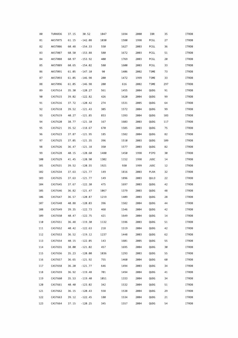
Figure S1
Figure S1. Spatial patterns of the interannual responses of the mean growing-season (April-October) NDVI and TRI to seasonal VDNC in the mid- and high-latitude NH. Spearman
partial correlation coefficients between the mean growing-season NDVI ( ) (during 1982-
2008) and TRI (dots) (during 1950-2008, if available) as well as between the seasonal mean
maximum temperature ( ), mean minimum temperature ( ) and water availability index
(WAI) from spring to autumn are shown. The labels 5%, 10% and 20% in the color bar indicate the corresponding significance level of Student’s t-test for the partial correlation analyses between
interannual variations of and TRI and seasonal mean climate. R = ±0.39, R = ±0.30, and
R = ±0.20 correspond to the 5%, 10% and 20% significance levels for the Spearman partial
correlation between interannual variations of and seasonal mean climate, respectively.
This figure is created by MATLAB (R2012b).

Figure S2
Figure S2. Latitudinal patterns of the interannual responses of growing season (April-October) NDVI to IAV of seasonal variations of maximum and minimum temperature and water availability index. Latitudinal patterns of the median of partial correlation coefficients (PR)
between and spring (green lines), summer (blue lines), and autumn (brown lines)
maximum temperature (a), minimum temperature (b) and water availability index (c). Percentage of pixels (within every 0.5 degree interval) showing significant (p < 0.1) positive and negative
correlation (PSR) of to spring (SP), summer (SU) and autumn (AU) maximum temperature
(a), minimum temperature (b) and water availability index (c) are indicated by the filled green and red areas, respectively. The black lines in inlets of a, b and c show the sampling depths (N) within each 0.5 degree interval. The vertical red lines in a), b) and c) indicate the latitudes north than it the sample depths are lower than 50.

Figure S3
Figure S3. Probability density functions of partial correlation coefficients between growing-season NDVI and seasonal variations of maximum and minimum temperature and water availability index in different climate regions. Probability density functions (PDF) of partial correlation coefficients (PR) between growing-season NDVI and spring (green lines), summer (blue lines) and autumn (brown lines) maximum temperature (left column), minimum temperature (middle column) and water availability index (right column). Percentage of pixels showing significant positive (dark and light green bars correspond to 10% and 5% significant level, respectively) and negative (dark and light red bars correspond to 10% and 5% significant level, respectively) correlation of growing-season NDVI to spring (SP), summer (SU) and autumn (AU) maximum temperature, minimum temperature and water availability index are shown in inlets, respectively. The Spearman correlation coefficients R ±0.51 and ±0.30 in x axis tick label correspond to 1% and 10% significance level of student’s t-test, respectively.

Figure S4.
Figure S4. Spatial patterns of the responses of growing-season (April-October) FAPAR to IAV of seasonal variations of maximum and minimum temperature and water availability index in mid- and high-latitudinal Northern Hemisphere during 1982-2008. Spearman partial
correlation coefficients between growing-season FAPAR, FAPARgs, and (spring maximum
temperature), (summer maximum temperature), (autumn maximum temperature),
(spring minimum temperature), (summer minimum temperature), (autumn minimum
temperature) are shown in a-f, respectively. Spearman partial correlation coefficients between FAPARgs and spring, summer and autumn WAI are shown in g-i, respectively. The Spearman correlation coefficients R ±0.53, ±0.39, ±0.30, and ±0.20 correspond to 1%, 5%, 10% and 20% significance level of student’s t-test, respectively. Blank regions are masked from our analysis (in detail see Methods). The map in this figure is created by MATLAB (R2012b).

Figure S5.
Figure S5. Latitudinal patterns of the responses of growing season (April-October) FAPAR to IAV of seasonal variations of maximum and minimum temperature and water availability index. Latitudinal patterns of the median of partial correlation coefficients (PR) between FAPARgs
and spring (green lines), summer (blue lines), and autumn (brown lines) maximum temperature (a), minimum temperature (b) and water availability index (c). Percentage of pixels (within every 0.5 degree interval) showing significant (p < 0.1) positive and negative correlation (PSR) of FAPARgs to spring (SP), summer (SU) and autumn (AU) maximum temperature (a), minimum temperature (b) and water availability index (c) are indicated by the filled green and red areas, respectively. The black lines in inlets of a, b and c show the sampling depths (N) within each 0.5 degree interval. The vertical red lines in a), b) and c) indicate the latitudes north than it the sample depths are lower than 50.

Figure S6.
Figure S6. Spatial patterns of the interannual sensitivity of growing-season (April-October) NDVI to seasonal variations of maximum and minimum temperature and water availability index in mid- and high-latitudinal Northern Hemisphere during 1982-2008. Interannual
sensitivity of to IAV of seasonal climate is estimated by ridge regression (in detail see
Methods). Interannual sensitivity of to (spring maximum temperature),
(summer maximum temperature), (autumn maximum temperature), (spring minimum
temperature), (summer minimum temperature), and (autumn minimum temperature) are
shown in a-f, respectively. Sensitivity of to spring, summer and autumn WAI are shown in
g-i, respectively. Blank regions are masked from our analysis (in detail see Methods). The map in this figure is created by MATLAB (R2012b).

Figure S7
Figure S7. Spatial patterns of the interannual sensitivity of growing-season (April-October) FAPAR to seasonal variations of maximum and minimum temperature and water availability index in mid- and high-latitudinal Northern Hemisphere during 1982-2008.
Interannual sensitivity of (with unit of %) to IAV of seasonal climate is estimated by
ridge regression (in detail see Methods). Interannual sensitivity of to (spring
maximum temperature), (summer maximum temperature), (autumn maximum
temperature), (spring minimum temperature), (summer minimum temperature), and
(autumn minimum temperature) are shown in a-f, respectively. Sensitivity of to
spring, summer and autumn WAI are shown in g-i, respectively. Blank regions are masked from our analysis (in detail see materials and methods). The map in this figure is created by MATLAB (R2012b).
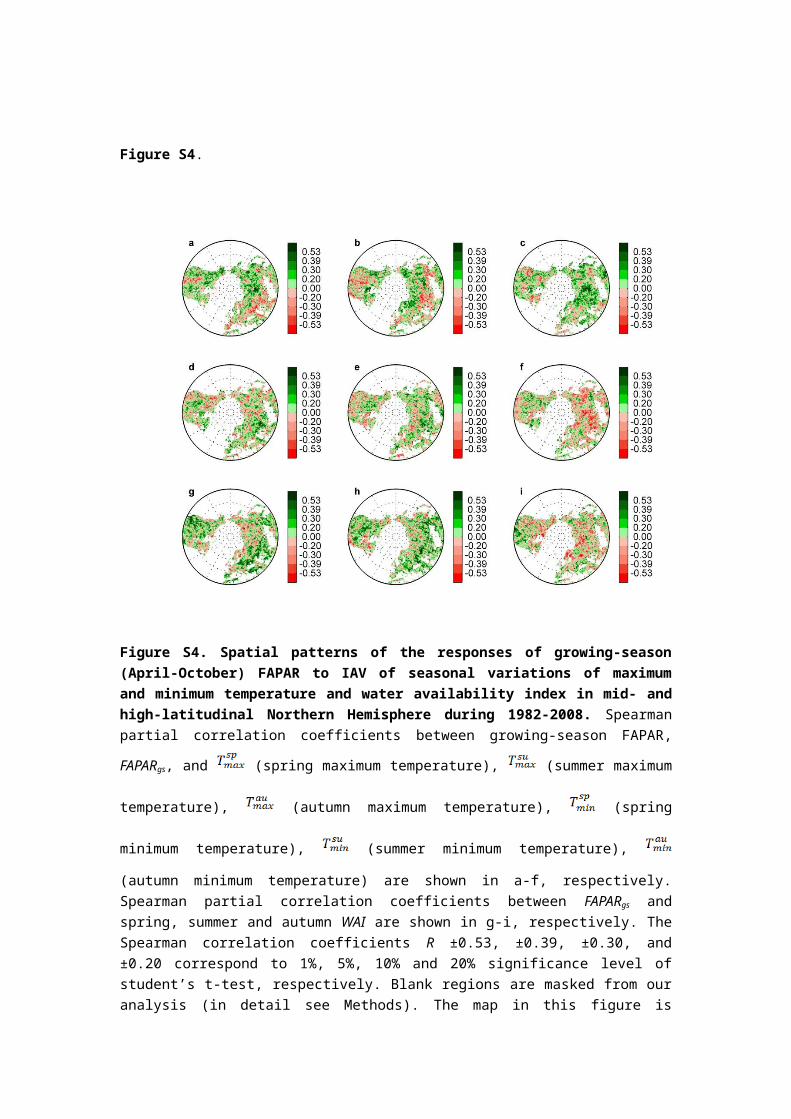
Figure S8
Figure S8. Spatial patterns of the interannual sensitivity of growing-season (April-October) GPP to seasonal variations of maximum and minimum temperature and water availability index in mid- and high-latitudinal Northern Hemisphere during 1982-2008. Interannual
sensitivity of (with unit of g C m-2 yr-1) to IAV of seasonal climate is estimated by ridge
regression. Sensitivity of to (spring maximum temperature), (summer maximum
temperature), (autumn maximum temperature), (spring minimum temperature),
(summer minimum temperature), and (autumn minimum temperature) are shown in a-f,
respectively. Sensitivity of to spring, summer and autumn WAI are shown in g-i,
respectively. Blank regions are masked from our analysis (in detail see Methods). The map in this figure is created by MATLAB (R2012b).

Figure S9
Figure S9. Spatial patterns of the responses of growing-season (April-October) GPP to IAV of seasonal maximum and minimum temperature and water availability index in mid- and high-latitudinal Northern Hemisphere during 1982-2008. Spearman partial correlation
coefficients between growing-season GPP, , and (spring maximum temperature),
(summer maximum temperature), (autumn maximum temperature), (spring minimum
temperature), (summer minimum temperature), and (autumn minimum temperature) are
shown in a-f, respectively. Spearman partial correlation coefficients between and spring,
summer and autumn WAI are shown in g-i, respectively. The Spearman correlation coefficients R ±0.53, ±0.39, ±0.30, and ±0.20 correspond to 1%, 5%, 10% and 20% significance level of student’s t-test, respectively. Blank regions are masked from our analysis (in detail see materials and methods). The map in this figure is created by MATLAB (R2012b).

Figure S10
Figure S10. Latitudinal patterns of the responses of growing season (April-October) GPP to IAV of seasonal climate. Latitudinal patterns of the median of partial correlation coefficients (PR)
between and spring (green lines), summer (blue lines), and autumn (brown lines) maximum
temperature (a), minimum temperature (b) and water availability index (c). Percentage of pixels (within every 0.5 degree interval) showing significant (p< 0.1) positive and negative correlation
(PSR) of to spring (SP), summer (SU) and autumn (AU) maximum temperature (a),
minimum temperature (b) and water availability index (c) are indicated by the filled green and red areas, respectively. The black lines in inlets of a, b and c show the sampling depths (N) within each 0.5 degree interval. The vertical red lines in a), b) and c) indicate the latitudes north than it the sample depths are lower than 50.

Figure S11
Figure S11. Spatial patterns of the interannual responses of growing-season (May-October) NDVI to seasonal variations of maximum and minimum temperature and water availability index in mid- and high-latitudinal Northern Hemisphere during 1982-2008. Spearman partial
correlation coefficients between growing-season NDVI, , and (spring maximum
temperature), (summer maximum temperature), (autumn maximum temperature),
(spring minimum temperature), (summer minimum temperature), and (autumn
minimum temperature) are shown in a-f, respectively. Spearman partial correlation coefficients
between and spring, summer and autumn WAI are shown in g-i, respectively. The
Spearman correlation coefficients R ±0.53, ±0.39, ±0.30, and ±0.20 correspond to 1%, 5%, 10% and 20% significance level of student’s t-test, respectively. Blank regions are masked from our analysis (in detail see materials and methods). The map in this figure is created by MATLAB (R2012b).


Figure S12
Figure S12. Spatial patterns of the interannual responses of growing-season (April-September) NDVI to seasonal variations of maximum and minimum temperature and water availability index in mid- and high-latitudinal Northern Hemisphere during 1982-2008.
Spearman partial correlation coefficients between growing-season NDVI, , and
(spring maximum temperature), (summer maximum temperature), (autumn maximum
temperature), (spring minimum temperature), (summer minimum temperature), and
(autumn minimum temperature) are shown in a-f, respectively. Spearman partial correlation
coefficients between and spring, summer and autumn WAI are shown in g-i, respectively.
The Spearman correlation coefficients R ±0.53, ±0.39, ±0.30, and ±0.20 correspond to 1%, 5%, 10% and 20% significance level of student’s t-test, respectively. Blank regions are masked from our analysis (in detail see materials and methods). The map in this figure is created by MATLAB (R2012b).

Figure S13
Figure S13. Spatial patterns of the interannual responses of tree ring index to seasonal climate during 1960-2008 (if applicable) in mid- and high-latitudinal Northern Hemisphere.
Spearman partial correlation coefficients between tree ring index (TRI) and (spring
maximum temperature), (summer maximum temperature), (autumn maximum
temperature), (spring minimum temperature), (summer minimum temperature), and
(autumn minimum temperature) are shown in a-f, respectively. Spearman partial correlation
coefficients between TRI and spring, summer and autumn WAI are shown in g-i, respectively. The labels of 5%, 10% and 20% in colorbars indicate the corresponding significance level of student’s t-test. Detailed information about the TRI see Methods and Supplementary Table S3. The map in this figure is created by MATLAB (R2012b).

Figure S14
Figure S14. Comparisons of mean water deficit in spring (green bars), summer (blue bars) and autumn (orange bars) for different climate zones (in detail see Methods). The error bars indicate the standard deviations of regional water deficit. The smaller negative values indicate much more severe water deficit and vice versa.

Figure S15
Figure S15. Interannual responses of growing-season (April-October) soil moisture to seasonal maximum and minimum temperature. Spearman partial correlation coefficients between mean growing-season (April-October) remotely sensed soil moisture (SM) (in detail see
Methods) and (spring maximum temperature), (summer maximum temperature),
(autumn maximum temperature), (spring minimum temperature), (summer minimum
temperature), and (autumn minimum temperature) are shown in a-f, respectively. The
Spearman correlation coefficients R ±0.49, ±0.36, ±0.28, and ±0.19 correspond to 1%, 5%, 10% and 20% significance level of student’s t-test, respectively. Blank regions are masked from our analyses (in detail see Methods). The map in this figure is created by MATLAB (R2012b).

Figure S16
Figure S16. Interannual response of total growing-season (April-October) water availability index to seasonal maximum and minimum temperature. Spearman partial correlation
coefficients between total growing-season (April-October) water availability index and
(spring maximum temperature), (summer maximum temperature), (autumn maximum
temperature), (spring minimum temperature), (summer minimum temperature), and
(autumn minimum temperature) are shown in a-f, respectively. The Spearman correlation
coefficients R ±0.49, ±0.36, ±0.28, and ±0.19 correspond to 1%, 5%, 10% and 20% significance level of student’s t-test, respectively. The map in this figure is created by MATLAB (R2012b).

Figure 17.
Figure S17. Relationships between autumn-summer difference of water deficit and partial
correlation coefficients between vegetation growth and seasonal . Relationship between
autumn-summer difference of water deficit (calculated as autumn water deficit minus summer water deficit, same for difference of partial correlation coefficients) and partial correlation
coefficients between vegetation growth and seasonal for RegAR (a), RegTH (b) and RegTA
(c) (in detail see Methods), respectively. Water deficit is calculated based on a simple water balance equation (in detail see Methods). Pixels with elevation lower than 75th percentile of elevation distribution in each of climate zones (in detail see Methods) are considered only to avoid the specific (e.g., mountain regions) characteristics in this relationship. The red and green lines in the figure are 75th and 50th percentile nonlinear (based on exponential equation) quantile regression lines, respectively. All nonlinear quantile fits are statistically significant (p < 0.05) except the 50th quantile regression for RegTH (p = 0.09) and RegTA (p = 0.12).

References
1 Liang, E., Shao, X., Liu, H. & Eckstein, D. Tree-ring based PDSI reconstruction since AD 1842 in the Ortindag Sand Land, east Inner Mongolia. Chinese Science Bulletin 52, 2715-2721 (2007).
Related Documents