Zhen Liu, Cosmin Safta, Khachik Sargsyan, Bart G. van Bloemen Waanders, Ray P. Bambha, Hope A. Michelsen Sandia National Laboratories, CA/NM Tao Zeng Georgia.

Verifying fossil fuel CO2 emissions with CMAQ

Zhen Liu, Cosmin Safta, Khachik Sargsyan, Bart G. van Bloemen Waanders, Ray P. Bambha, Hope A. Michelsen

Sandia National Laboratories, CA/NM

Tao ZengGeorgia Department of Natural Resources, GA

CMAS 2012 15 October 2012

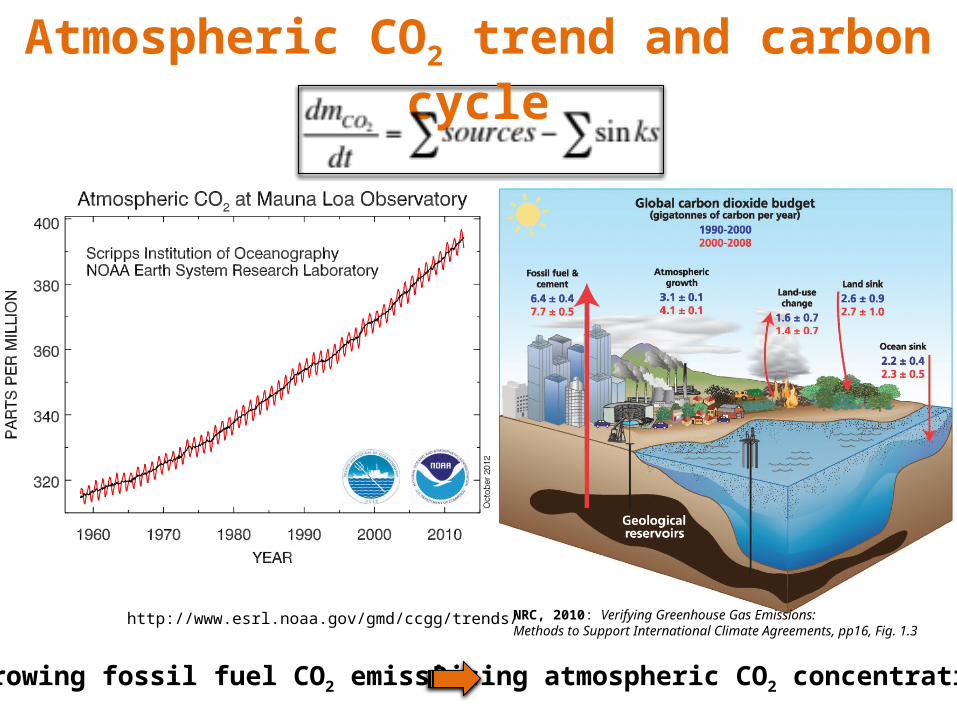
NRC, 2010: Verifying Greenhouse Gas Emissions: Methods to Support International Climate Agreements, pp16, Fig. 1.3

Atmospheric CO2 trend and carbon cycle

Growing fossil fuel CO2 emission Rising atmospheric CO2 concentrations

http://www.esrl.noaa.gov/gmd/ccgg/trends/

Uncertainty of Fossil Fuel CO2 emissions

Global Country State County 1 - 10km0

5

10

15

20

25

30

35

40

45

50

4.3% 4%

16%

> 50% > 50%Pe

rcen

tage

Global: NRC, 2010. Country: EPA, 2012. State, county and 1-10km: Gurney et al., 2009, ES&T

?

Verifying fossil CO2 emissions is

“firmly on the agenda of science, politics, and business”. [Marland, 2008, J. Ind. Ecol., 136–139]

?Annual average

(higher uncertainty after temporal allocation)

gridded

Verifying Fossil Fuel CO2 Emissions

Aircraft Satellite GOSAT (Los Angeles Basin, CA)

[Kort et al., 2012, GRL]

3.2±1.5 ppm

[Mays et al., 2009, ES&T]

(Indianapolis, IN)

Model? Model?

Can a state-of-the-art CTM help verify fossil fuel CO2 emissions?

“A signal-to-noise problem”

3-D Eulerian Regional CO2 Modelingusing CMAQ

Goals:Quantitatively examine model skills/errors on different

time/spatial scales;Develop model diagnostics and inverse modeling approach to

pinpoint fossil fuel emissions;Construct regional CO2 budget and quantify its uncertainties.

Add a CO2 module in CMAQWidely used and well tested CTM, large user community;Highly modularized codes makes adding species/processes easy;Adaptable nested model domains enables high resolution

modeling.

Configuration of the CMAQ CO2 module (done/under development)

CMAQ : version 5.0 Meteorology : WRF BC/IC : CarbonTracker (CT)

(3°× 2°; 3-hourly) Biosphere flux : (1) CarbonTracker (CASA) (1°×

1°) (2) VPRM (3) Sib3

Fossil fuel emission : (1) CDIAC (1°× 1°; monthly)(2)

VULCAN (2002; 10km; hourly) Fire emission : GFEDv3.1 (0.5°× 0.5°; 3-

hourly) Chemistry : CB-05 CO2

Oceans flux : CarbonTracker Benchmark : Oct. 2007, U.S. 36km,

22L

Benchmark simulation results (30m above ground) with CDIAC (1°× 1°, annual average) fossil fuel emission inventory

Root Mean Square Deviation (RMSD) = 0.47 ppm

CMAQ-CDIAC CarbonTracker

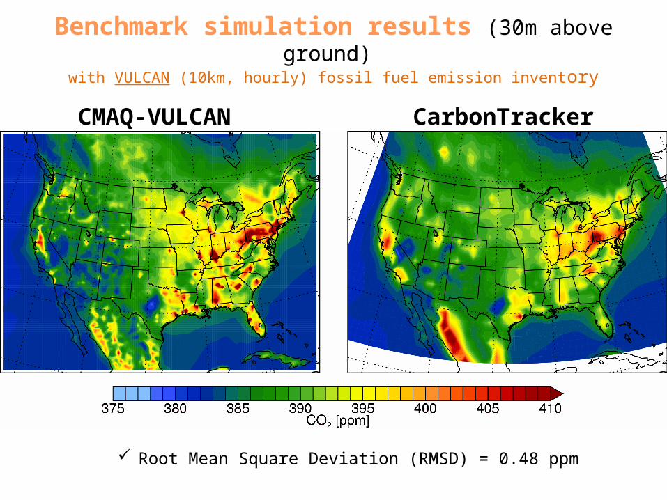
Benchmark simulation results (30m above ground) with VULCAN (10km, hourly) fossil fuel emission inventory

CMAQ-VULCAN CarbonTracker

Root Mean Square Deviation (RMSD) = 0.48 ppm

Benchmark simulation results (0-1500m average) with VULCAN (0.1°× 0.1°, hourly) fossil fuel emission inventory

CMAQ-VULCAN CarbonTracker

Some hotspots could still be seen (> 4ppm enhancement) Root Mean Square Deviation (RMSD) = 0.43 ppm

Model Evaluation: Boulder Atmospheric Observatory

40mile north of Denver; elev. 1584 masl; 300m above ground

http://www.esrl.noaa.gov/gmd/ccgg/towers/#bao

Summary and Future Plan Findings

Transport difference between CMAQ (36km) and TM5 (1°× 1°) only leads to 0.47 ppm Root Mean Square Deviation (RMSD) near the surface in terms of monthly mean CO2 distribution.

36km CMAQ with hourly VULCAN (10km) emission inventory is capable of capturing urban CO2 hotspots in the contiguous U.S. and diurnal pattern of CO2

downwind of urban Denver.

Some hotspots might be observed using the PBL column average metric.

To-dos Implementing finer resolution biosphere module (VPRM) and transport;

Adding secondary CO2 source (oxidation of CO and VOCs) in CMAQ;

Comprehensive model evaluation with tower and aircraft data.

Acknowledgement

CarbonTracker-2011 results are provided by NOAA ESRL (http://carbontracker.noaa.gov).

Tower CO2 data are provided by NOAA GMD.

WRF output and non-CO2 emission data are shared by the SESARM project (http://www.metro4-sesarm.org).

Funding for this work was provided by Sandia National Laboratories, Laboratory Directed Research And Development Program.

Thanks!

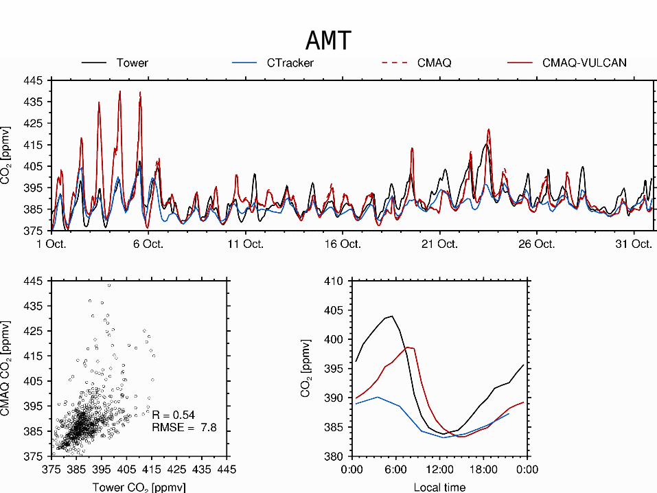
AMT

LEF

WKT

WBI

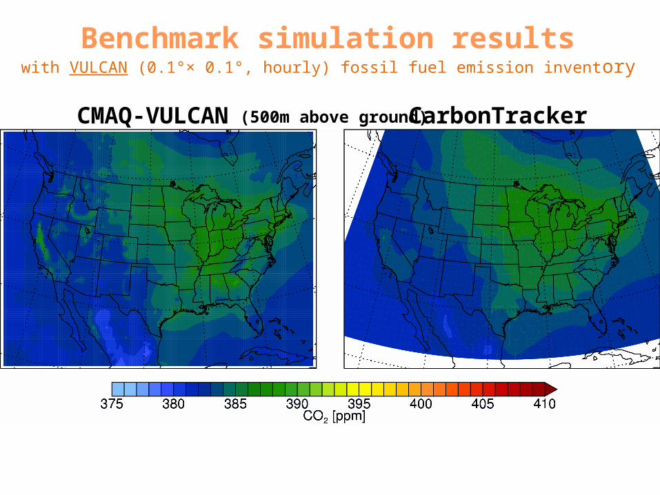
Benchmark simulation resultswith VULCAN (0.1°× 0.1°, hourly) fossil fuel emission inventory

CMAQ-VULCAN CarbonTracker(500m above ground)

CarbonTracker (CT2011)

Meteorology : ECMWF (1°× 1° nested over NA)Biosphere : Carnegie-Ames-Stanford-Approach (CASA) Ocean : [Jacobson et al., 2007]Fossil fuel : CDIAC [Oda and Maksyutov, 2011]Fire : GFEDv3.1Observations : NOAA ESRL, CSIRO, IPEN-CQMA

http://www.esrl.noaa.gov/gmd/ccgg/carbontracker/ [Peters et al., 2007, PNAS]