ZEF Bonn GLOWA-Volta Common Sampling Frame – Selection of ...

ZEF Bonn

GLOWA-Volta Common Sampling Frame –

Selection of Survey Sites

Thomas Berger, Felix Ankomah Asante, Isaac Osei-Akoto

ZEF Documentation of Research 1/2002

2

1. Introduction For several reasons constructing a common sampling frame (CSF), where different units of observation are hierarchically linked, provides advantages for interdisciplinary research teams. To give a short example: employing a CSF facilitates that the soil scientists collect soil samples from the plots of exactly those farmers who are interviewed by the agricultural economists and who are villagers in the communities being analyzed by the institutional analysts. Accordingly, a CSF ensures a maximum overlap of biophysical and socioeconomic field observations. This paper describes the multivariate data analysis of the CSF that led to the selection of survey sites for GLOWA-Volta. Section 2 provides a list of broad research questions that motivated the CSF and joint field campaigns of social and natural scientists. Section 3 discusses the advantages and disadvantages of the CSF, and section 4 sketches the interdisciplinary discussion process about operational selection criteria. Section 5 provides more details about the statistical procedure in selecting the observation units. Section 6 provides an overview about the different survey activities and field measurements during the field campaign in 2001. Section 7 concludes with a few final remarks that relate the field observations to the planned multi-agent modeling approach of GLOWA-Volta. It is important to note at the beginning of this documentation that from a socioeconomic point of view water and land use cannot be easily divided into two different research fields. Decision-making processes on water and land use are clearly interrelated at household, community, regional and national level. The CSF approach addresses this interrelatedness and therefore includes research activities both on water and land use. 2. Research questions and observation units In GLOWA-Volta six broad socioeconomic research questions closely relate to the research activities undertaken by the natural scientists: 1) safe access of households to water; 2) determinants of household water demand; 3) household expenditures on water; 4) water-related health aspects; 5) possible causal relationship with migration; 6) possible changes in the use of land. Evidently, all questions listed above require inputs from the natural sciences such as biophysical measurements and spatial data from remote-sensing techniques. In turn, the socioeconomic results will inform the natural scientists’ research directly (“ground-truthing” of remote sensing images) or feed into the joint integrated modeling exercises (modeling of land use change, intersectoral water allocation). For the economic subprojects, the main unit of observation is the individual household who takes decisions regarding the use of water and land resources. The research centers on understanding the households’ choices among different feasible alternatives of action and in particular on their strategies for coping with water variability, climate and land cover changes. The institutional analysts, on the other hand, focus on decision-making processes at higher levels of social organization, for example on community, regional and national level. The unit of observation is accordingly not the single household but the village assembly, the water user association, etc.

3

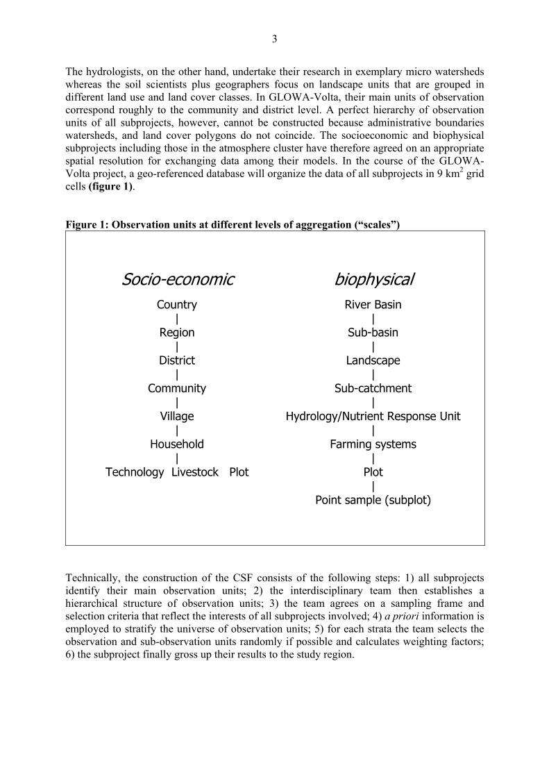
The hydrologists, on the other hand, undertake their research in exemplary micro watersheds whereas the soil scientists plus geographers focus on landscape units that are grouped in different land use and land cover classes. In GLOWA-Volta, their main units of observation correspond roughly to the community and district level. A perfect hierarchy of observation units of all subprojects, however, cannot be constructed because administrative boundaries watersheds, and land cover polygons do not coincide. The socioeconomic and biophysical subprojects including those in the atmosphere cluster have therefore agreed on an appropriate spatial resolution for exchanging data among their models. In the course of the GLOWA-Volta project, a geo-referenced database will organize the data of all subprojects in 9 km2 grid cells (figure 1). Figure 1: Observation units at different levels of aggregation (“scales”)

Country|

Region|

District|

Community|

Village|

Household|

Technology Livestock Plot

River Basin|

Sub-basin|

Landscape|

Sub-catchment|

Hydrology/Nutrient Response Unit|

Farming systems|

Plot|

Point sample (subplot)

Socio-economic biophysical

Technically, the construction of the CSF consists of the following steps: 1) all subprojects identify their main observation units; 2) the interdisciplinary team then establishes a hierarchical structure of observation units; 3) the team agrees on a sampling frame and selection criteria that reflect the interests of all subprojects involved; 4) a priori information is employed to stratify the universe of observation units; 5) for each strata the team selects the observation and sub-observation units randomly if possible and calculates weighting factors; 6) the subproject finally gross up their results to the study region.

4

3. Advantages and disadvantages of common sampling frames Employing a CSF provides several advantages for interdisciplinary research teams who plan to collect large amounts especially of primary data: • The CSF yields certain “agglomeration” benefits particularly for the project logistics.

Collecting information from hierarchically linked observation units usually implies a spatial concentration of field activities. As a consequence, transport and lodging costs for enumerators and technicians can be reduced, as well as training and interpreting costs since this concentration allows building larger teams of field assistants with knowledge of local languages. Additionally, costs of transforming and exchanging data between different scientific disciplines are usually lower.

• The CSF can make use of a priori information for stratification and therefore tends to increase precision and reliability as compared to a pure random sampling. Especially in the case of GLOWA-Volta, considerable amounts of socioeconomic data with high quality and large spatial extent are available. The a priori information additionally also helps developing research hypotheses and may guide the design of questionnaires or measurements.

• A hierarchical sampling frame permits the extrapolation (“grossing-up”) of sample measurements to the universe. The research findings at different locations can be generalized and may then be used for deriving conclusions at national or basin level. This is potentially a large advantage over nonrandom and purposeful selections of observations units that allows only for comparisons of case studies or “anecdotal” evidence. In GLOWA-Volta this advantage might, however, be rather moderate because for budgetary reasons the sample fraction has to be very small and the sampling error will thus be relatively large.

A common sampling frame implies on the other hand the following disadvantages: • Typically, interdisciplinary teams have to invest a lot of time to agree on a hierarchical

structure of observation units and operational selection criteria for stratification. The discussion process is therefore costly and implies quite uncertain benefits. In spite of this disadvantage, the discussion process might help clarifying the different viewpoints of the disciplines involved and in the longer run lead to a shared terminology or even methodology. In the case of GLOWA-Volta, the construction of the CSF was the first interdisciplinary research activity where different subprojects of the land and water cluster started working together scientifically and thereby laid the basis for future integrative research.

• The common sampling might also be inapplicable for some disciplines that will then opt for their exclusion. This is particularly relevant when certain subprojects can undertake only very few and long-term measurements. A stratified random sampling implies for them a high risk of missing the observation units of their specific interest. Nevertheless, the CSF might also provide the chance in these cases of at least comparing the findings of these out-of-frame subprojects with other subprojects as long as information on the joint selection criteria will be collected.

5

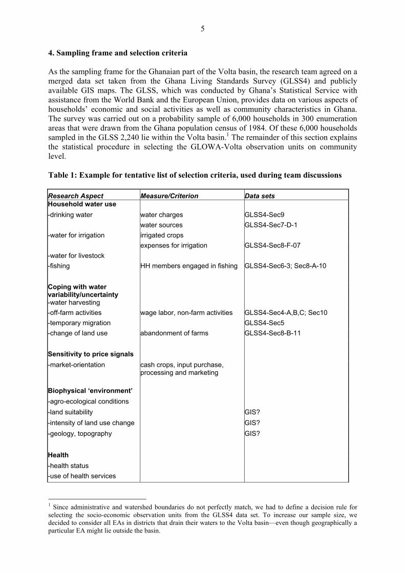
4. Sampling frame and selection criteria As the sampling frame for the Ghanaian part of the Volta basin, the research team agreed on a merged data set taken from the Ghana Living Standards Survey (GLSS4) and publicly available GIS maps. The GLSS, which was conducted by Ghana’s Statistical Service with assistance from the World Bank and the European Union, provides data on various aspects of households’ economic and social activities as well as community characteristics in Ghana. The survey was carried out on a probability sample of 6,000 households in 300 enumeration areas that were drawn from the Ghana population census of 1984. Of these 6,000 households sampled in the GLSS 2,240 lie within the Volta basin.1 The remainder of this section explains the statistical procedure in selecting the GLOWA-Volta observation units on community level. Table 1: Example for tentative list of selection criteria, used during team discussions Research Aspect Measure/Criterion Data sets Household water use -drinking water water charges GLSS4-Sec9 water sources GLSS4-Sec7-D-1 -water for irrigation irrigated crops expenses for irrigation GLSS4-Sec8-F-07 -water for livestock -fishing HH members engaged in fishing GLSS4-Sec6-3; Sec8-A-10 Coping with water variability/uncertainty

-water harvesting -off-farm activities wage labor, non-farm activities GLSS4-Sec4-A,B,C; Sec10 -temporary migration GLSS4-Sec5 -change of land use abandonment of farms GLSS4-Sec8-B-11 Sensitivity to price signals -market-orientation cash crops, input purchase,

processing and marketing

Biophysical ‘environment’ -agro-ecological conditions -land suitability GIS? -intensity of land use change GIS? -geology, topography GIS? Health -health status -use of health services

1 Since administrative and watershed boundaries do not perfectly match, we had to define a decision rule for selecting the socio-economic observation units from the GLSS4 data set. To increase our sample size, we decided to consider all EAs in districts that drain their waters to the Volta basin—even though geographically a particular EA might lie outside the basin.

6

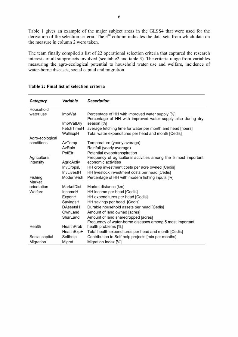
Table 1 gives an example of the major subject areas in the GLSS4 that were used for the derivation of the selection criteria. The 3rd column indicates the data sets from which data on the measure in column 2 were taken. The team finally compiled a list of 22 operational selection criteria that captured the research interests of all subprojects involved (see table2 and table 3). The criteria range from variables measuring the agro-ecological potential to household water use and welfare, incidence of water-borne diseases, social capital and migration. Table 2: Final list of selection criteria

Category Variable Description

Household water use ImpWat Percentage of HH with improved water supply [%]

ImpWatDry Percentage of HH with improved water supply also during dry season [%]

FetchTimeH average fetching time for water per month and head [hours] WatExpH Total water expenditures per head and month [Cedis] Agro-ecological conditions AvTemp Temperature (yearly average) AvRain Rainfall (yearly average) PotEtr Potential evapotranspiration Agricultural intensity AgricActiv

Frequency of agricultural activities among the 5 most important economic activities

InvCropsL HH crop investment costs per acre owned [Cedis] InvLivestH HH livestock investment costs per head [Cedis] Fishing ModernFish Percentage of HH with modern fishing inputs [%] Market orientation MarketDist Market distance [km] Welfare IncomeH HH income per head [Cedis] ExpenH HH expenditures per head [Cedis] SavingsH HH savings per head [Cedis] DAssetsH Durable household assets per head [Cedis] OwnLand Amount of land owned [acres] SharLand Amount of land sharecropped [acres]

Health HealthProb Frequency of water-borne diseases among 5 most important health problems [%]

HealthExpH Total health expenditures per head and month [Cedis] Social capital Selfhelp Contribution to Self-help projects [min per months] Migration Migrat Migration Index [%]

7

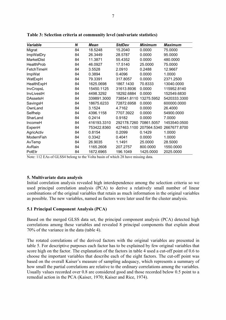
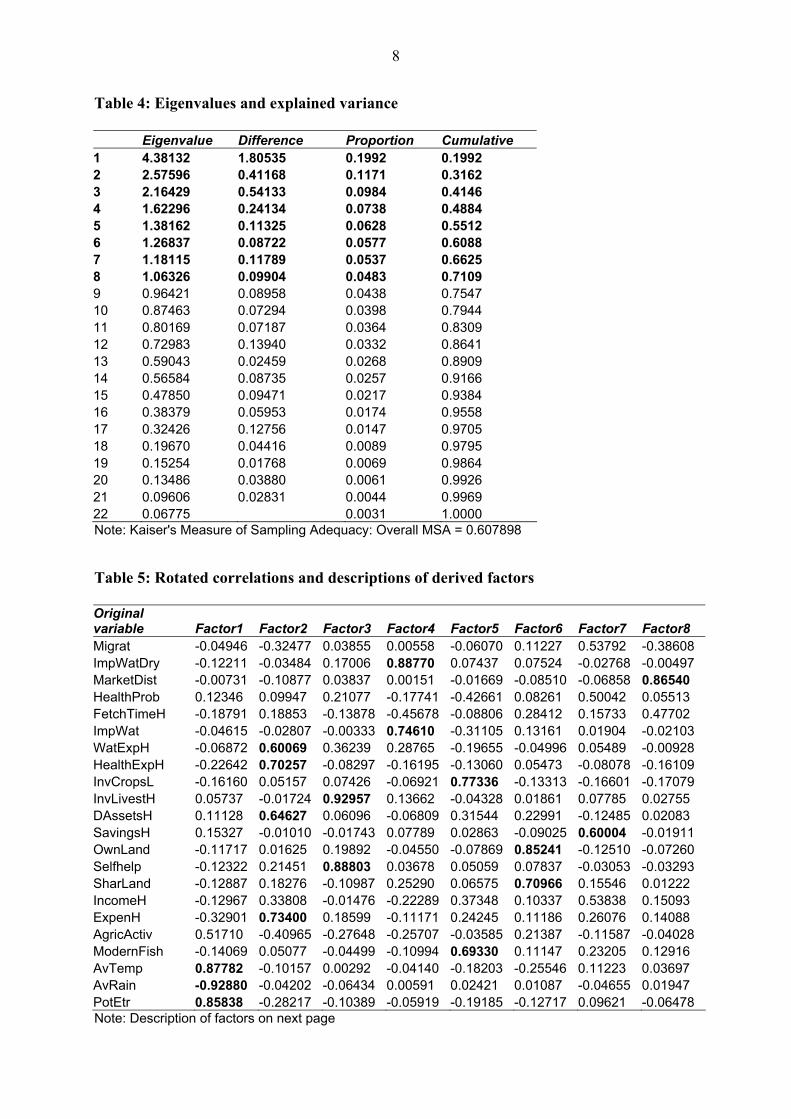
Table 3: Selection criteria at community level (univariate statistics) Variable N Mean StdDev Minimum Maximum Migrat 84 18.5248 15.2040 0.0000 75.0000 ImpWatDry 84 26.3449 28.5787 0.0000 95.0000 MarketDist 84 11.3871 55.4352 0.0000 480.0000 HealthProb 84 46.0927 17.5140 25.0000 75.0000 FetchTimeH 84 3.5528 2.0910 0.2488 12.9667 ImpWat 84 0.3894 0.4096 0.0000 1.0000 WatExpH 84 79.3391 317.8057 0.0000 2371.2500 HealthExpH 84 1625.0698 1867.1430 70.8333 13040.0000 InvCropsL 84 15450.1125 31613.8936 0.0000 115952.8140 InvLivestH 84 4498.3292 18292.6884 0.0000 152549.6830 DAssetsH 84 339891.3000 738541.8110 13275.5952 5420333.3300 SavingsH 84 18675.6233 72872.6958 0.0000 600000.0000 OwnLand 84 3.1524 4.7162 0.0000 26.4000 Selfhelp 84 4396.1158 7707.3922 0.0000 54900.0000 SharLand 84 0.2414 0.9182 0.0000 7.0000 IncomeH 84 416193.3310 292178.7260 70861.5057 1453540.0500 ExpenH 84 753422.8360 427463.1100 207564.5340 2667677.8700 AgricActiv 84 0.8154 0.2099 0.1429 1.0000 ModernFish 84 0.3342 0.4041 0.0000 1.0000 AvTemp 84 26.9035 1.1491 25.0000 28.5000 AvRain 84 1165.2608 207.2757 800.0000 1550.0000 PotEtr 84 1672.6965 196.1049 1425.0000 2025.0000 Note: 112 EAs of GLSS4 belong to the Volta basin of which 28 have missing data. 5. Multivariate data analysis Initial correlation analysis revealed high interdependence among the selection criteria so we used principal correlation analysis (PCA) to derive a relatively small number of linear combinations of the original variables that retain as much information in the original variables as possible. The new variables, named as factors were later used for the cluster analysis. 5.1 Principal Component Analysis (PCA) Based on the merged GLSS data set, the principal component analysis (PCA) detected high correlations among these variables and revealed 8 principal components that explain about 70% of the variance in the data (table 4). The rotated correlations of the derived factors with the original variables are presented in table 5. For descriptive purposes each factor has to be explained by few original variables that score high on the factor. The explanation of the factors in table 4 used a cut-off point of 0.6 to choose the important variables that describe each of the eight factors. The cut-off point was based on the overall Kaiser’s measure of sampling adequacy, which represents a summary of how small the partial correlations are relative to the ordinary correlations among the variables. Usually values recorded over 0.8 are considered good and those recorded below 0.5 point to a remedial action in the PCA (Kaiser, 1970; Kaiser and Rice, 1974).

8

Table 4: Eigenvalues and explained variance Eigenvalue Difference Proportion Cumulative 1 4.38132 1.80535 0.1992 0.1992 2 2.57596 0.41168 0.1171 0.3162 3 2.16429 0.54133 0.0984 0.4146 4 1.62296 0.24134 0.0738 0.4884 5 1.38162 0.11325 0.0628 0.5512 6 1.26837 0.08722 0.0577 0.6088 7 1.18115 0.11789 0.0537 0.6625 8 1.06326 0.09904 0.0483 0.7109 9 0.96421 0.08958 0.0438 0.7547 10 0.87463 0.07294 0.0398 0.7944 11 0.80169 0.07187 0.0364 0.8309 12 0.72983 0.13940 0.0332 0.8641 13 0.59043 0.02459 0.0268 0.8909 14 0.56584 0.08735 0.0257 0.9166 15 0.47850 0.09471 0.0217 0.9384 16 0.38379 0.05953 0.0174 0.9558 17 0.32426 0.12756 0.0147 0.9705 18 0.19670 0.04416 0.0089 0.9795 19 0.15254 0.01768 0.0069 0.9864 20 0.13486 0.03880 0.0061 0.9926 21 0.09606 0.02831 0.0044 0.9969 22 0.06775 0.0031 1.0000 Note: Kaiser's Measure of Sampling Adequacy: Overall MSA = 0.607898 Table 5: Rotated correlations and descriptions of derived factors Original variable Factor1 Factor2 Factor3 Factor4 Factor5 Factor6 Factor7 Factor8 Migrat -0.04946 -0.32477 0.03855 0.00558 -0.06070 0.11227 0.53792 -0.38608 ImpWatDry -0.12211 -0.03484 0.17006 0.88770 0.07437 0.07524 -0.02768 -0.00497 MarketDist -0.00731 -0.10877 0.03837 0.00151 -0.01669 -0.08510 -0.06858 0.86540 HealthProb 0.12346 0.09947 0.21077 -0.17741 -0.42661 0.08261 0.50042 0.05513 FetchTimeH -0.18791 0.18853 -0.13878 -0.45678 -0.08806 0.28412 0.15733 0.47702 ImpWat -0.04615 -0.02807 -0.00333 0.74610 -0.31105 0.13161 0.01904 -0.02103 WatExpH -0.06872 0.60069 0.36239 0.28765 -0.19655 -0.04996 0.05489 -0.00928 HealthExpH -0.22642 0.70257 -0.08297 -0.16195 -0.13060 0.05473 -0.08078 -0.16109 InvCropsL -0.16160 0.05157 0.07426 -0.06921 0.77336 -0.13313 -0.16601 -0.17079 InvLivestH 0.05737 -0.01724 0.92957 0.13662 -0.04328 0.01861 0.07785 0.02755 DAssetsH 0.11128 0.64627 0.06096 -0.06809 0.31544 0.22991 -0.12485 0.02083 SavingsH 0.15327 -0.01010 -0.01743 0.07789 0.02863 -0.09025 0.60004 -0.01911 OwnLand -0.11717 0.01625 0.19892 -0.04550 -0.07869 0.85241 -0.12510 -0.07260 Selfhelp -0.12322 0.21451 0.88803 0.03678 0.05059 0.07837 -0.03053 -0.03293 SharLand -0.12887 0.18276 -0.10987 0.25290 0.06575 0.70966 0.15546 0.01222 IncomeH -0.12967 0.33808 -0.01476 -0.22289 0.37348 0.10337 0.53838 0.15093 ExpenH -0.32901 0.73400 0.18599 -0.11171 0.24245 0.11186 0.26076 0.14088 AgricActiv 0.51710 -0.40965 -0.27648 -0.25707 -0.03585 0.21387 -0.11587 -0.04028 ModernFish -0.14069 0.05077 -0.04499 -0.10994 0.69330 0.11147 0.23205 0.12916 AvTemp 0.87782 -0.10157 0.00292 -0.04140 -0.18203 -0.25546 0.11223 0.03697 AvRain -0.92880 -0.04202 -0.06434 0.00591 0.02421 0.01087 -0.04655 0.01947 PotEtr 0.85838 -0.28217 -0.10389 -0.05919 -0.19185 -0.12717 0.09621 -0.06478 Note: Description of factors on next page

9

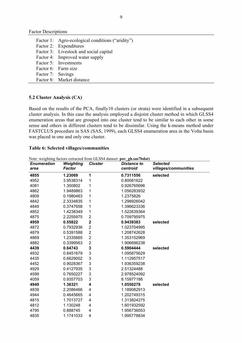
Factor Descriptions

Factor 1: Agro-ecological conditions (“aridity”) Factor 2: Expenditures Factor 3: Livestock and social capital Factor 4: Improved water supply Factor 5: Investments Factor 6: Farm size Factor 7: Savings Factor 8: Market distance

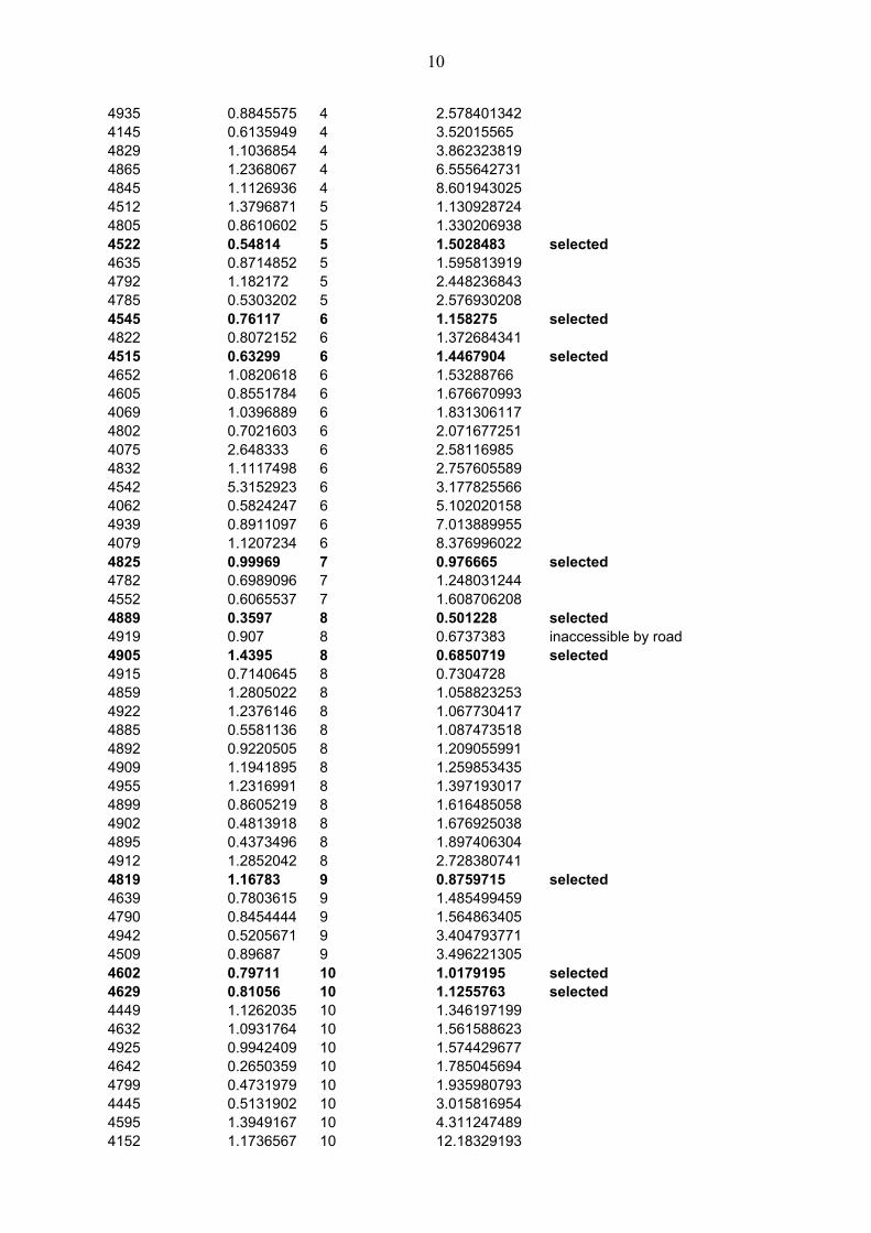
5.2 Cluster Analysis (CA) Based on the results of the PCA, finally10 clusters (or strata) were identified in a subsequent cluster analysis. In this case the analysis employed a disjoint cluster method in which GLSS4 enumeration areas that are grouped into one cluster tend to be similar to each other in some sense and others in different clusters tend to be dissimilar. Using the k-means method under FASTCLUS procedure in SAS (SAS, 1999), each GLSS4 enumeration area in the Volta basin was placed in one and only one cluster. Table 6: Selected villages/communities Note: weighting factors extracted from GLSS4 dataset: pov_gh.sas7bdat) Enumeration area

Weighting Factor

Cluster Distance to centroid

Selected villages/communities

4855 1.23069 1 0.7311556 selected 4952 3.9538314 1 0.80081622 4081 1.350802 1 0.926765696 4862 1.9489863 1 1.056283932 4809 0.1980463 1 1.2375826 4842 2.3334835 1 1.298926042 4849 0.3747658 1 1.396623336 4852 1.4238349 1 1.522639364 4875 2.2255975 2 0.709795975 4959 0.55822 2 0.9439383 selected 4872 0.7932936 2 1.023704995 4879 0.5391588 2 1.208742628 4869 1.2335665 2 1.353152969 4882 0.3399563 2 1.906696238 4439 0.64743 3 0.5904444 selected 4932 0.8451679 3 1.095875629 4435 0.6629002 3 1.112957517 4452 0.9028367 3 1.936359238 4929 0.4127935 3 2.51324488 4599 0.7650227 3 2.978524092 4059 0.9357703 3 8.15977188 4949 1.36321 4 1.0550278 selected 4839 2.2086466 4 1.189082913 4944 0.4645665 4 1.202749315 4815 1.7013727 4 1.313824275 4812 1.130248 4 1.601932592 4795 0.888745 4 1.956736053 4835 1.1741033 4 1.995778834

10

4935 0.8845575 4 2.578401342 4145 0.6135949 4 3.52015565 4829 1.1036854 4 3.862323819 4865 1.2368067 4 6.555642731 4845 1.1126936 4 8.601943025 4512 1.3796871 5 1.130928724 4805 0.8610602 5 1.330206938 4522 0.54814 5 1.5028483 selected 4635 0.8714852 5 1.595813919 4792 1.182172 5 2.448236843 4785 0.5303202 5 2.576930208 4545 0.76117 6 1.158275 selected 4822 0.8072152 6 1.372684341 4515 0.63299 6 1.4467904 selected 4652 1.0820618 6 1.53288766 4605 0.8551784 6 1.676670993 4069 1.0396889 6 1.831306117 4802 0.7021603 6 2.071677251 4075 2.648333 6 2.58116985 4832 1.1117498 6 2.757605589 4542 5.3152923 6 3.177825566 4062 0.5824247 6 5.102020158 4939 0.8911097 6 7.013889955 4079 1.1207234 6 8.376996022 4825 0.99969 7 0.976665 selected 4782 0.6989096 7 1.248031244 4552 0.6065537 7 1.608706208 4889 0.3597 8 0.501228 selected 4919 0.907 8 0.6737383 inaccessible by road 4905 1.4395 8 0.6850719 selected 4915 0.7140645 8 0.7304728 4859 1.2805022 8 1.058823253 4922 1.2376146 8 1.067730417 4885 0.5581136 8 1.087473518 4892 0.9220505 8 1.209055991 4909 1.1941895 8 1.259853435 4955 1.2316991 8 1.397193017 4899 0.8605219 8 1.616485058 4902 0.4813918 8 1.676925038 4895 0.4373496 8 1.897406304 4912 1.2852042 8 2.728380741 4819 1.16783 9 0.8759715 selected 4639 0.7803615 9 1.485499459 4790 0.8454444 9 1.564863405 4942 0.5205671 9 3.404793771 4509 0.89687 9 3.496221305 4602 0.79711 10 1.0179195 selected 4629 0.81056 10 1.1255763 selected 4449 1.1262035 10 1.346197199 4632 1.0931764 10 1.561588623 4925 0.9942409 10 1.574429677 4642 0.2650359 10 1.785045694 4799 0.4731979 10 1.935980793 4445 0.5131902 10 3.015816954 4595 1.3949167 10 4.311247489 4152 1.1736567 10 12.18329193

11

The procedures revealed Euclidean distances from the centriod of each cluster to its respective enumeration areas. The enumeration areas closest to the cluster centroid were then selected as representative communities according to the proportional-to-size rule (i.e. “large” clusters with many enumeration areas are represented with more survey sites)2. To ensure an overlap with other GLOWA-Volta subprojects researching at locations, which are not contained in the original GLSS sampling frame, additional sites were added to the sample. As a result of the sampling procedure, a list of 20 survey communities was compiled (see table 6 and figure 2). Figure 2: Survey communities of GLOWA Volta

2 In four cases, this selection rule could not be applied strictly because of data problems, and in one case because of road problems. The next closest EA was then selected. The sum of distances of all selected EAs, however, only increases by 5%, that is, the ‘selection error’ is rather moderate.

12

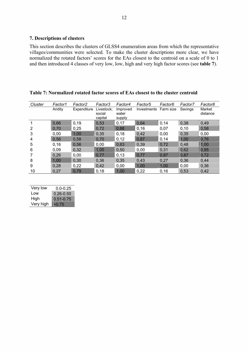
7. Descriptions of clusters This section describes the clusters of GLSS4 enumeration areas from which the representative villages/communities were selected. To make the cluster descriptions more clear, we have normalized the rotated factors’ scores for the EAs closest to the centroid on a scale of 0 to 1 and then introduced 4 classes of very low, low, high and very high factor scores (see table 7).

Table 7: Normalized rotated factor scores of EAs closest to the cluster centroid Cluster Factor1 Factor2 Factor3 Factor4 Factor5 Factor6 Factor7 Factor8 Aridity Expenditure Livestock;

social capital

Improved water supply

Investments Farm size Savings Market distance

1 0,66 0,19 0,53 0,17 0,64 0,14 0,38 0,49 2 0,70 0,25 0,72 0,88 0,16 0,07 0,10 0,58 3 0,00 1,00 0,35 0,18 0,42 0,00 0,35 0,00 4 0,56 0,58 0,70 0,12 0,87 0,14 1,00 0,76 5 0,16 0,56 0,00 0,63 0,39 0,72 0,48 1,00 6 0,09 0,32 1,00 0,50 0,00 0,31 0,62 0,95 7 0,26 0,00 0,77 0,13 0,77 0,87 0,87 0,72 8 1,00 0,30 0,36 0,35 0,43 0,27 0,36 0,44 9 0,28 0,22 0,42 0,00 1,00 1,00 0,00 0,36 10 0,27 0,79 0,18 1,00 0,22 0,16 0,53 0,42 Very low 0.0-0.25 Low 0.26-0.50 High 0.51-0.75 Very high >0.75

13

Cluster1 The enumeration areas in Cluster 1 are located in the middle to the eastern part of the Northern Region of Ghana. Households face arid conditions, have only poor water supply, and operate on small farms. Cluster 2 Cluster 2 is located in the north western corner of Ghana. Similar to cluster 1, arid conditions and small farm sizes prevail; however, households can count on highly improved water supply.

EA closest to centroid in Cluster 2

0

0.25

0.5

0.75

1

1 2 3 4 5 6 7 8Factors

Nor

mal

ized

Rot

ated

Sco

res


0

0.25

0.5

0.75

1

1 2 3 4 5 6 7 8Factors

Nor

mal

ized

Rot

ated

Sco

res

14

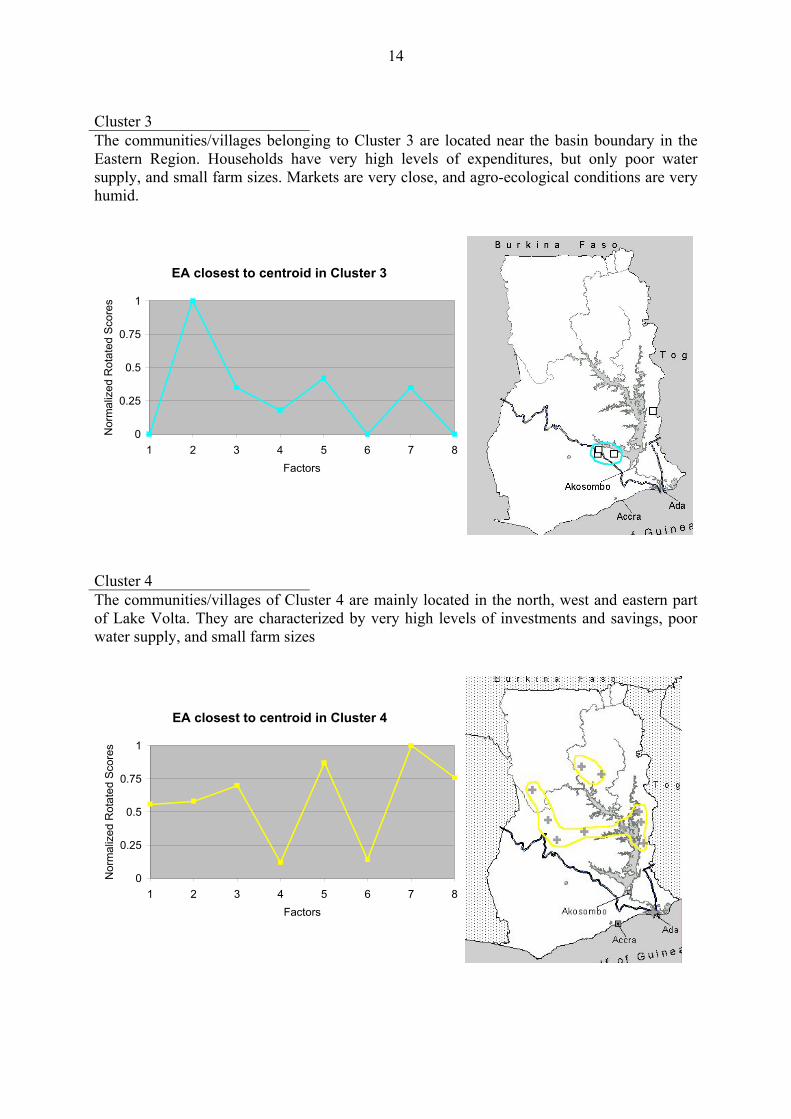
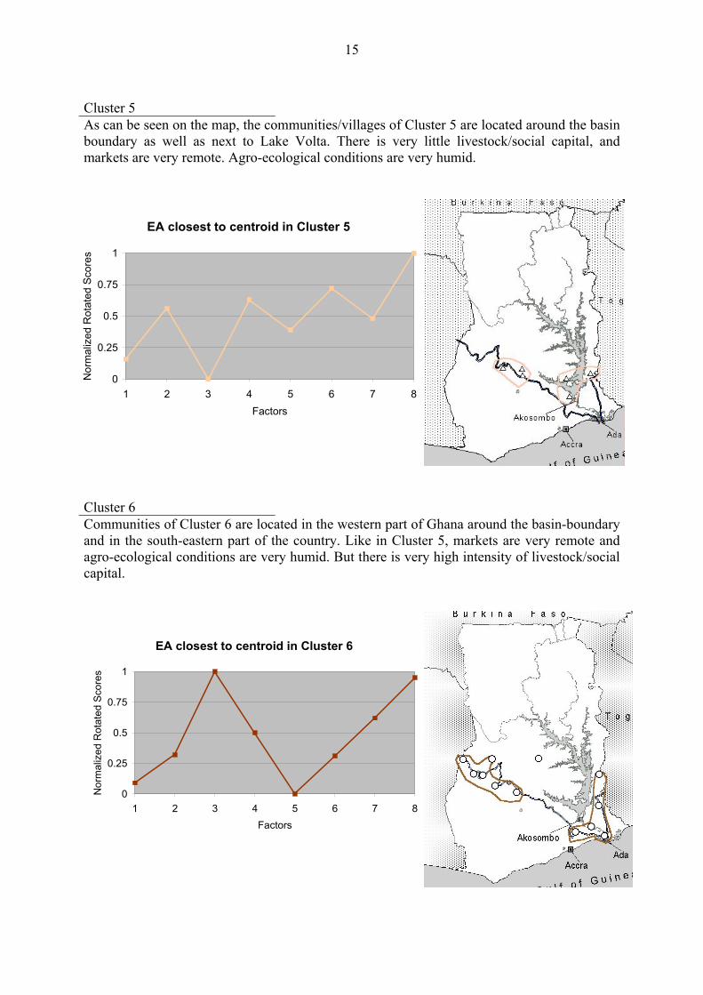
Cluster 3 The communities/villages belonging to Cluster 3 are located near the basin boundary in the Eastern Region. Households have very high levels of expenditures, but only poor water supply, and small farm sizes. Markets are very close, and agro-ecological conditions are very humid. Cluster 4 The communities/villages of Cluster 4 are mainly located in the north, west and eastern part of Lake Volta. They are characterized by very high levels of investments and savings, poor water supply, and small farm sizes


0

0.25

0.5

0.75

1

1 2 3 4 5 6 7 8Factors

Nor

mal

ized

Rot

ated

Sco

res


0

0.25

0.5

0.75

1

1 2 3 4 5 6 7 8Factors

Nor

mal

ized

Rot

ated

Sco

res

15

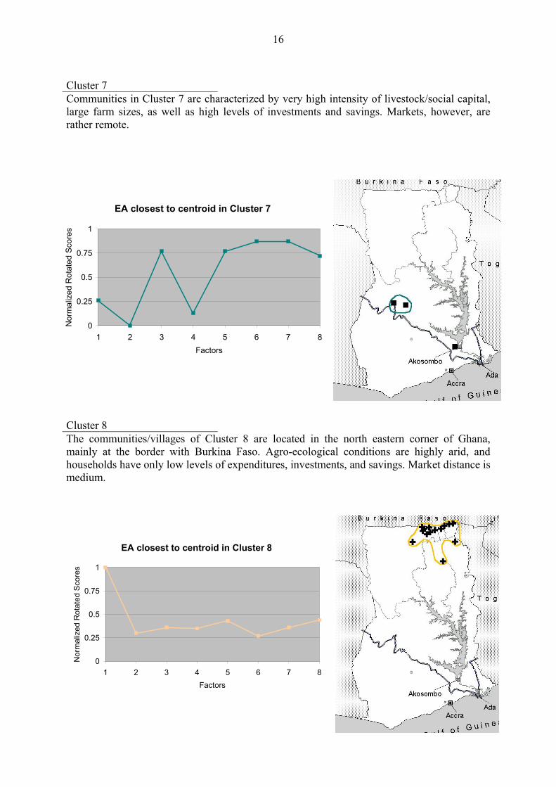
Cluster 5 As can be seen on the map, the communities/villages of Cluster 5 are located around the basin boundary as well as next to Lake Volta. There is very little livestock/social capital, and markets are very remote. Agro-ecological conditions are very humid.

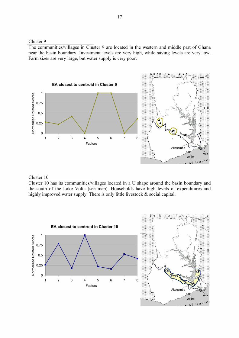
Cluster 6 Communities of Cluster 6 are located in the western part of Ghana around the basin-boundary and in the south-eastern part of the country. Like in Cluster 5, markets are very remote and agro-ecological conditions are very humid. But there is very high intensity of livestock/social capital.


0

0.25

0.5

0.75

1

1 2 3 4 5 6 7 8Factors

Nor

mal

ized

Rot

ated

Sco

res


0

0.25

0.5

0.75

1

1 2 3 4 5 6 7 8Factors

Nor

mal

ized

Rot

ated

Sco

res

16

Cluster 7 Communities in Cluster 7 are characterized by very high intensity of livestock/social capital, large farm sizes, as well as high levels of investments and savings. Markets, however, are rather remote.

Cluster 8 The communities/villages of Cluster 8 are located in the north eastern corner of Ghana, mainly at the border with Burkina Faso. Agro-ecological conditions are highly arid, and households have only low levels of expenditures, investments, and savings. Market distance is medium.


0

0.25

0.5

0.75

1

1 2 3 4 5 6 7 8Factors

Nor

mal

ized

Rot

ated

Sco

res


0

0.25

0.5

0.75

1

1 2 3 4 5 6 7 8Factors

Nor

mal

ized

Rot

ated

Sco

res

17

Cluster 9 The communities/villages in Cluster 9 are located in the western and middle part of Ghana near the basin boundary. Investment levels are very high, while saving levels are very low. Farm sizes are very large, but water supply is very poor.


0

0.25

0.5

0.75

1

1 2 3 4 5 6 7 8Factors

Nor

mal

ized

Rot

ated

Sco

res

Cluster 10 Cluster 10 has its communities/villages located in a U shape around the basin boundary and the south of the Lake Volta (see map). Households have high levels of expenditures and highly improved water supply. There is only little livestock & social capital.


0

0.25

0.5

0.75

1

1 2 3 4 5 6 7 8Factors

Nor

mal

ized

Rot

ated

Sco

res

18

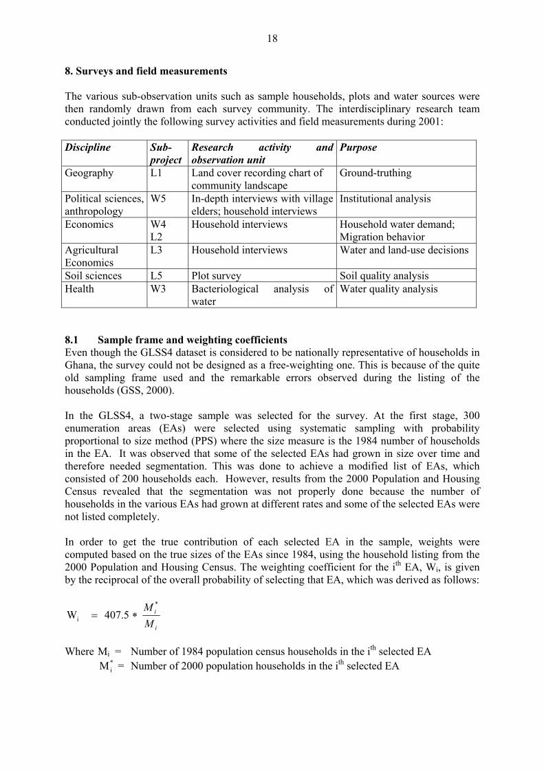
8. Surveys and field measurements The various sub-observation units such as sample households, plots and water sources were then randomly drawn from each survey community. The interdisciplinary research team conducted jointly the following survey activities and field measurements during 2001: Discipline Sub-

project Research activity and observation unit

Purpose

Geography L1 Land cover recording chart of community landscape

Ground-truthing

Political sciences, anthropology

W5 In-depth interviews with village elders; household interviews

Institutional analysis

Economics W4 L2

Household interviews Household water demand; Migration behavior

Agricultural Economics

L3 Household interviews Water and land-use decisions

Soil sciences L5 Plot survey Soil quality analysis Health W3 Bacteriological analysis of

water Water quality analysis

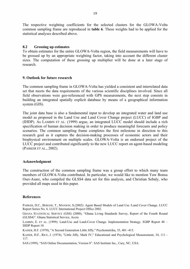
8.1 Sample frame and weighting coefficients Even though the GLSS4 dataset is considered to be nationally representative of households in Ghana, the survey could not be designed as a free-weighting one. This is because of the quite old sampling frame used and the remarkable errors observed during the listing of the households (GSS, 2000). In the GLSS4, a two-stage sample was selected for the survey. At the first stage, 300 enumeration areas (EAs) were selected using systematic sampling with probability proportional to size method (PPS) where the size measure is the 1984 number of households in the EA. It was observed that some of the selected EAs had grown in size over time and therefore needed segmentation. This was done to achieve a modified list of EAs, which consisted of 200 households each. However, results from the 2000 Population and Housing Census revealed that the segmentation was not properly done because the number of households in the various EAs had grown at different rates and some of the selected EAs were not listed completely. In order to get the true contribution of each selected EA in the sample, weights were computed based on the true sizes of the EAs since 1984, using the household listing from the 2000 Population and Housing Census. The weighting coefficient for the ith EA, Wi, is given by the reciprocal of the overall probability of selecting that EA, which was derived as follows:

i

i

MM *

i 5.407W ∗=

Where Mi = Number of 1984 population census households in the ith selected EA

*iM = Number of 2000 population households in the ith selected EA

19

The respective weighting coefficients for the selected clusters for the GLOWA-Volta common sampling frame are reproduced in table 6. These weights had to be applied for the statistical analyses described above. 8.2 Grossing up estimates To obtain estimates for the entire GLOWA-Volta region, the field measurements will have to be grossed up by an appropriate weighting factor, taking into account the different cluster sizes. The computation of these grossing up multiplier will be done at a later stage of research. 9. Outlook for future research The common sampling frame in GLOWA-Volta has yielded a consistent and interrelated data set that meets the data requirements of the various scientific disciplines involved. Since all field observations were geo-referenced with GPS measurements, the next step consists in building an integrated spatially explicit database by means of a geographical information system (GIS). The joint data base is also a fundamental input to develop an integrated water and land use model as proposed in the Land Use and Land Cover Change project (LUCC) of IGBP and (IHDP). As LAMBIN ET AL. (1999) argue, an integrated LUCC model should include a rich specification of human decision making in order to produce meaningful forecasts and policy scenarios. The common sampling frame completes the first milestone in direction to this research goal as it captures the decision-making processes of economic actors and their biophysical environment on multiple scales. GLOWA-Volta is an endorsed project of the LUCC project and contributed significantly to the new LUCC report on agent-based modeling (PARKER ET AL., 2002). Acknowledgment The construction of the common sampling frame was a group effort to which many team members of GLOWA-Volta contributed. In particular, we would like to mention Yaw Bonsu Osei-Asare, who compiled the GLSS4 data set for this analysis, and Christian Sebaly, who provided all maps used in this paper. References PARKER, D.C., BERGER, T., MANSON, S.(2002): Agent Based Models of Land Use /Land Cover Change. LUCC Report Series No. 6. LUCC International Project Office 2002. GHANA STATISTICAL SERVICE (GSS) (2000), “Ghana Living Standards Survey, Report of the Fourth Round (GLSS4)”. Ghana Statistical Service, Accra LAMBIN, E. ET AL. (1999): Land-Use and Land-Cover Change. Implementation Strategy. IGBP Report 48 – IHDP Report 10. KAISER, H.F. (1970), "A Second Generation Little Jiffy," Psychometrika, 35, 401 -415. KAISER, H.F., RICE, J. (1974), "Little Jiffy, Mark IV," Educational and Psychological Measurement, 34, 111 -117. SAS (1999), “SAS Online Documentation, Version 8”. SAS Institute Inc., Cary, NC, USA.

ZEF Bonn GLOWA-Volta Common Sampling Frame – Selection of ...

Documents