Zabalza, Jaime and Ren, Jinchang and Zheng, Jiangbin and Zhao, Huimin and Qing, Chunmei and Yang, Zhijing and Du, Peijun and Marshall, Stephen (2016) Novel segmented stacked autoencoder for effective dimensionality reduction and feature extraction in hyperspectral imaging. Neurocomputing, 185. pp. 1-10. ISSN 0925-2312 , http://dx.doi.org/10.1016/j.neucom.2015.11.044 This version is available at https://strathprints.strath.ac.uk/56131/ Strathprints is designed to allow users to access the research output of the University of Strathclyde. Unless otherwise explicitly stated on the manuscript, Copyright © and Moral Rights for the papers on this site are retained by the individual authors and/or other copyright owners. Please check the manuscript for details of any other licences that may have been applied. You may not engage in further distribution of the material for any profitmaking activities or any commercial gain. You may freely distribute both the url ( https://strathprints.strath.ac.uk/ ) and the content of this paper for research or private study, educational, or not-for-profit purposes without prior permission or charge. Any correspondence concerning this service should be sent to the Strathprints administrator: [email protected] The Strathprints institutional repository (https://strathprints.strath.ac.uk ) is a digital archive of University of Strathclyde research outputs. It has been developed to disseminate open access research outputs, expose data about those outputs, and enable the management and persistent access to Strathclyde's intellectual output.

Welcome message from author
This document is posted to help you gain knowledge. Please leave a comment to let me know what you think about it! Share it to your friends and learn new things together.
Transcript

Zabalza, Jaime and Ren, Jinchang and Zheng, Jiangbin and Zhao,
Huimin and Qing, Chunmei and Yang, Zhijing and Du, Peijun and
Marshall, Stephen (2016) Novel segmented stacked autoencoder for
effective dimensionality reduction and feature extraction in
hyperspectral imaging. Neurocomputing, 185. pp. 1-10. ISSN 0925-2312 ,
http://dx.doi.org/10.1016/j.neucom.2015.11.044
This version is available at https://strathprints.strath.ac.uk/56131/
Strathprints is designed to allow users to access the research output of the University of
Strathclyde. Unless otherwise explicitly stated on the manuscript, Copyright © and Moral Rights
for the papers on this site are retained by the individual authors and/or other copyright owners.
Please check the manuscript for details of any other licences that may have been applied. You
may not engage in further distribution of the material for any profitmaking activities or any
commercial gain. You may freely distribute both the url (https://strathprints.strath.ac.uk/) and the
content of this paper for research or private study, educational, or not-for-profit purposes without
prior permission or charge.
Any correspondence concerning this service should be sent to the Strathprints administrator:
The Strathprints institutional repository (https://strathprints.strath.ac.uk) is a digital archive of University of Strathclyde research
outputs. It has been developed to disseminate open access research outputs, expose data about those outputs, and enable the
management and persistent access to Strathclyde's intellectual output.

To appear in the Neurocomputing Journal, 2015
Novel Segmented Stacked AutoEncoder for Effective
Dimensionality Reduction and Feature Extraction in
Hyperspectral Imaging
Jaime Zabalza1, Jinchang Ren
1, Jiangbin Zheng
2, Huimin Zhao
3,
Chunmei Qing4, Zhijing Yang
5, Peijun Du
6, and Stephen Marshall
1
1 Department of Electronic and Electrical Engineering, University of Strathclyde, Glasgow, United Kingdom
2 School of Microelectronics and Software, Northwestern Polytechnical University, Xi’an, China
3 School of Electronic and Information, Guangdong Technic Normal University, Guangzhou, China
4 School of Electronic and Information Engineering, South China University of Technology, Guangzhou, China
5 School of Information Engineering, Guangdong University of technology, Guangzhou, China
6 Dept. of geographical Information, Nanjing University, Nanjing, China
Abstract—Stacked autoencoders (SAEs), as part of the deep learning (DL) framework, have been recently proposed for
feature extraction in hyperspectral remote sensing. With the help of hidden nodes in deep layers, a high-level abstraction is
achieved for data reduction whilst maintaining the key information of the data. As hidden nodes in SAEs have to deal
simultaneously with hundreds of features from hypercubes as inputs, this increases the complexity of the process and leads
to limited abstraction and performance. As such, segmented SAE (S-SAE) is proposed by confronting the original features
into smaller data segments, which are separately processed by different smaller SAEs. This has resulted in reduced
complexity but improved efficacy of data abstraction and accuracy of data classification.
Index Terms—Deep learning (DL), hyperspectral remote sensing, data reduction, segmented stacked autoencoder (S-SAE).
Corresponding Author:
Dr Jinchang Ren
Centre for excellence in Signal and Image Processing
University of Strathclyde
Glasgow, G1 1XW
United Kingdom
Tel. +44-141-5482384
Email: [email protected]

To appear in the Neurocomputing Journal, 2015
I. INTRODUCTION
Hyperspectral imaging (HSI) is a very motivating field dealing with several different challenges in the last decade. The HSI cameras
and devices provide a spatial 2-D image in hundreds of different wavelengths from the electromagnetic spectrum in nature (spectral
bands). As a result, a 3-D structure called hypercube is obtained, where each pixel in the 2-D image is represented by an array of
spectral values. Obviously, with such amount of information, the use of HSI data for applications including remote classification of
image pixels is proving promising, although it demands advanced signal processing applied to stages such as feature extraction or
data reduction [1-2].
In the last 2-3 decades, a number of methods have been proposed for feature extraction and data reduction in HSI, including both
well-known classical techniques and new approaches. These feature extraction and data reduction techniques aim to boost the
general data analysis procedures by improving the characterization of features (efficacy) and/or relieving computational complexity
(efficiency). For instance, features containing adequate information usually lead to higher classification accuracy of pixels and, in
many cases, this can be done along with a reduction in the number of features (feature dimensionality), which in turn increases the
overall efficiency. Although there are many methodologies, in this paper we focus on a particular approach related to a new and
really promising field, the deep learning (DL) framework, in particular with the study of stacked autoencoders (SAEs) [3-4].
Based on neural network architectures, SAEs are able to reduce feature dimensionality to few elements contained in the deep
layers of those networks. In SAEs, an input pixel of the HSI image is introduced in the network by the first layer (or input layer), with
as many nodes as original features (spectral bands) in the pixel. Then, the pixel information travels the network through subsequent
layers with reduced number of nodes or units, to finally achieve a reconstructed pixel at the output matching the original one.
Therefore, SAEs can be employed effectively for feature extraction, where the abstraction level achieved in deep layers leads to
representative reduced features. In that sense, the powerful capabilities from machine learning can be exploited to perform data
reduction in such context that seems promising and needs proper investigation.
However, the use of SAEs with HSI data can be complex, due to the hundreds of spectral bands available in the hypercubes.
Hidden units in the SAEs layers are required to evaluate the input and derived values from all the spectral bands simultaneously in
the same activation functions, and this complexity makes more difficult to find appropriate abstraction. As a result, the main
motivation of the present work is to evaluate the SAEs and to propose an alternative solution to address these two main problems:
the computational complexity in the implementations, and the lack of proper abstraction in the features, i.e., the limited accuracy in
classification analysis.
To this end, we propose a spectral segmentation in the pixels or samples that can divide the complexity and also allow local
extraction of features, eventually providing better extraction capability. In this paper, the segmented SAE (S-SAE) method is

To appear in the Neurocomputing Journal, 2015
introduced, where local SAEs are applied to different segments of the spectrum. By locally working in spectral regions, the
computational complexity is reduced and, at the same time, the resulting features are improved thus better classification accuracy is
obtained thanks to local extraction of information. From our results it is found that, yet with reduced complexity, S-SAE performs
better than the conventional SAE implementation and also other state-of-the-art methods in land-cover analysis, which leaves an
open door for future investigation and related ideas.
The organization of the paper is as follows. Section II gives a brief review of related work in HSI feature extraction and data
reduction, pointing out differences with the SAE methodology. Then, SAEs are introduced in Section III, while our proposal S-SAE
is presented in Section IV. Experimental analysis on real HSI data and results are available in Section V, including classification and
also computational complexity evaluations, with concluding remarks in Section VI.
II. RELATED WORK IN HSI FEATURES AND CLASSIFICATION
In HSI, currently it is possible to find several feature extraction and data reduction methods for subsequent benefits in the data
analysis. In general, these methods can be divided in many categorizations depending on the characteristics and functionality of the
related procedures. For instance, some methods focus only on the feature representation and require a classifier algorithm afterwards
to perform land-cover analysis, while some other methods can include the classification itself, i.e., the work with the features
directly provides a classification of the pixels.
Methods focusing on feature representation include widely known classical techniques and, on the other hand, more modern
approaches. Among the classical methods we can find principal component analysis (PCA) [5], independent component analysis
(ICA) [6], or maximum noise fraction (MNF) [7]. These techniques transform the data by means of a projection, with relation to
distribution of variance, statistical independence, and noise ratio, respectively. Although these approaches were introduced quite a
few years ago, they are still very employed in the HSI literature, and it is worth to highlight them. On the other hand, some recent
proposals comprise, for example, empirical mode decomposition (EMD) [8], singular spectrum analysis (SSA) [9], and
morphological profiles (MPs) [10]. The EMD [8] is based on empirical iterations, being able to capture few different components
related to frequency, yet its computational cost seems excessive. Meanwhile, the SSA [9] works with singular value decomposition
applied to an embedded signal, leading to de-noised pixels and improved classification. Finally, MPs [10] are based on
mathematical morphology (erosion and dilation), with opening and closing operators that can capture spatial structures in the
images, resulting in high classification accuracy. These works, focusing on feature representation, employed a support vector
machine (SVM) for posterior classification, as SVM is currently one of the most powerful and well-known classifiers.
In contrast, among the methods focusing on classification, we can find graph-based learning [11], sparsity-representation-based
techniques [12], random subspace ensembles (RSEs) [13], spectral-spatial-constrain method [14], and multi-feature-learning-based
To appear in the Neurocomputing Journal, 2015
classification [15]. Graph-based learning [11] addresses the spatial relationship among pixels considering semi-supervised learning.
This method achieves good results, yet large sizes of HSI images can lead to computational complexity. The approach in [12]
proposes a dictionary-based sparse representation, considering smoothing terms and joint-sparsity models, with accurate results.
Regarding the RSE methodology in [13], RSEs are combined with decision tree and extreme learning machine algorithms,
achieving state-of-the-art performances. In the spectral-spatial-constrain method [14], the spatial relationship among pixels is
translated into a hypergraph structure (being each pixel a vertex) to which a semi-supervised learning is applied, showing superiority
to other methods such as conditional random fields, among others. Finally, in [15], they propose a new classification framework
based on the integration of different features, including linear and non-linear ones. This method provides good results with no
significant increase in the computational complexity.
However, recently DL techniques are also being introduced and evaluated for feature representation and classification in HSI
[3-4]. Unlike the feature representation techniques mentioned above, the DL methodologies are based on machine learning, which is
reporting an increasing interest in the last years as this learning type is claimed to provide really powerful capabilities and successful
analysis. That is the reason why there is a high interest in the evaluation of these methods, where further analysis and research is still
required. From these methodologies, a really motivating approach is the one related to SAEs for feature representation, and this is
where our work is developed, using SVM as a classifier.
III. STACKED AUTOENCODERS
A basic AE is a DL-architecture model in which an original signal at the input is reconstructed at the output going through an
intermediate layer with reduced number of hidden nodes. The AE model tries to learn deep and abstract features in those reduced
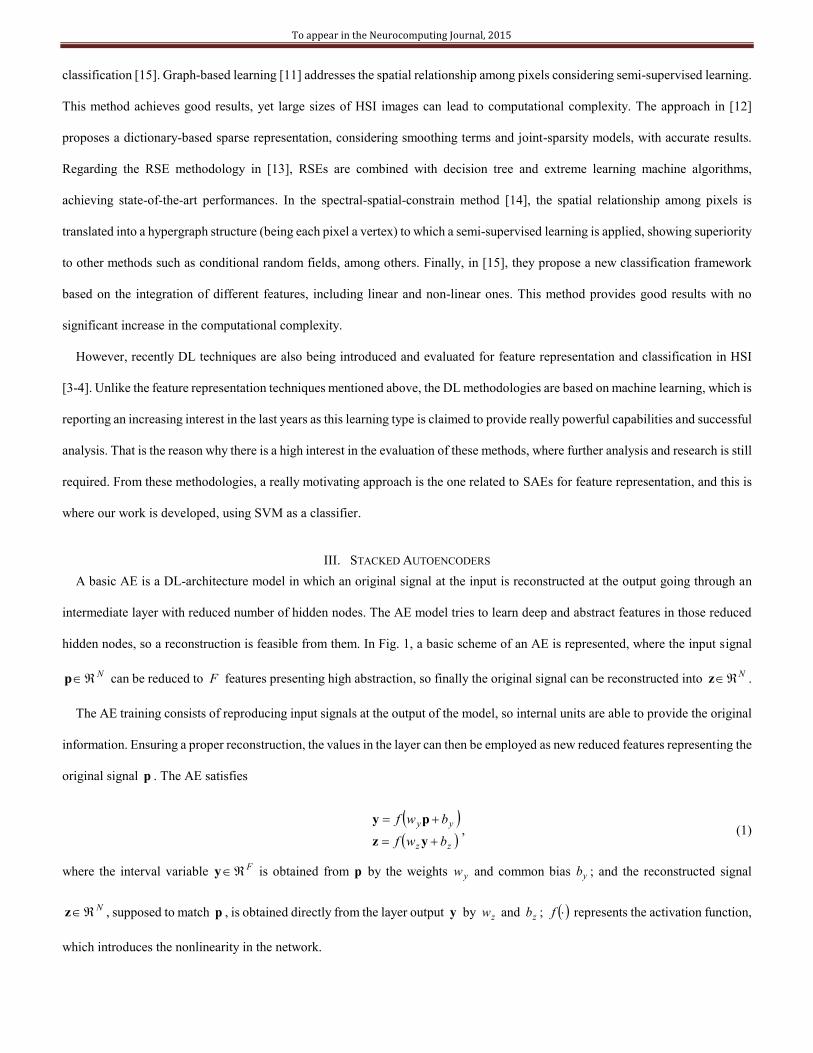
hidden nodes, so a reconstruction is feasible from them. In Fig. 1, a basic scheme of an AE is represented, where the input signal
Np can be reduced to F features presenting high abstraction, so finally the original signal can be reconstructed into Nz .
The AE training consists of reproducing input signals at the output of the model, so internal units are able to provide the original
information. Ensuring a proper reconstruction, the values in the layer can then be employed as new reduced features representing the
original signal p . The AE satisfies
zz
yy
bwf
bwf
yz
py, (1)
where the interval variable Fy is obtained from p by the weights yw and common bias yb ; and the reconstructed signal
Nz , supposed to match p , is obtained directly from the layer output y by zw and zb ; f represents the activation function,
which introduces the nonlinearity in the network.
To appear in the Neurocomputing Journal, 2015
Fig. 1. Basic AE scheme.
To train the AE and determine the optimized parameters, the error between p and z needs to be minimized, i.e.
zp,minarg,,,
errorzyzy bbww
. (2)
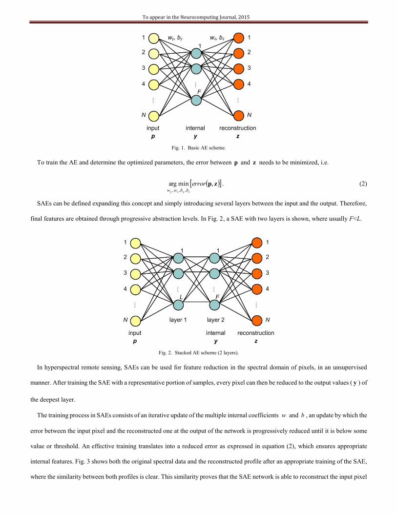
SAEs can be defined expanding this concept and simply introducing several layers between the input and the output. Therefore,
final features are obtained through progressive abstraction levels. In Fig. 2, a SAE with two layers is shown, where usually F<L.
Fig. 2. Stacked AE scheme (2 layers).
In hyperspectral remote sensing, SAEs can be used for feature reduction in the spectral domain of pixels, in an unsupervised
manner. After training the SAE with a representative portion of samples, every pixel can then be reduced to the output values ( y ) of
the deepest layer.
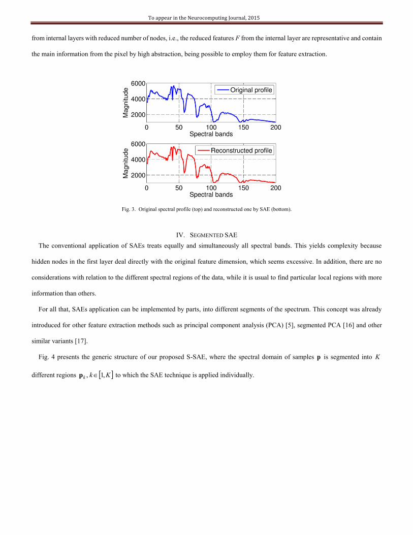
The training process in SAEs consists of an iterative update of the multiple internal coefficients w and b , an update by which the
error between the input pixel and the reconstructed one at the output of the network is progressively reduced until it is below some
value or threshold. An effective training translates into a reduced error as expressed in equation (2), which ensures appropriate
internal features. Fig. 3 shows both the original spectral data and the reconstructed profile after an appropriate training of the SAE,
where the similarity between both profiles is clear. This similarity proves that the SAE network is able to reconstruct the input pixel
To appear in the Neurocomputing Journal, 2015
from internal layers with reduced number of nodes, i.e., the reduced features F from the internal layer are representative and contain
the main information from the pixel by high abstraction, being possible to employ them for feature extraction.
Fig. 3. Original spectral profile (top) and reconstructed one by SAE (bottom).
IV. SEGMENTED SAE
The conventional application of SAEs treats equally and simultaneously all spectral bands. This yields complexity because
hidden nodes in the first layer deal directly with the original feature dimension, which seems excessive. In addition, there are no
considerations with relation to the different spectral regions of the data, while it is usual to find particular local regions with more
information than others.
For all that, SAEs application can be implemented by parts, into different segments of the spectrum. This concept was already
introduced for other feature extraction methods such as principal component analysis (PCA) [5], segmented PCA [16] and other
similar variants [17].
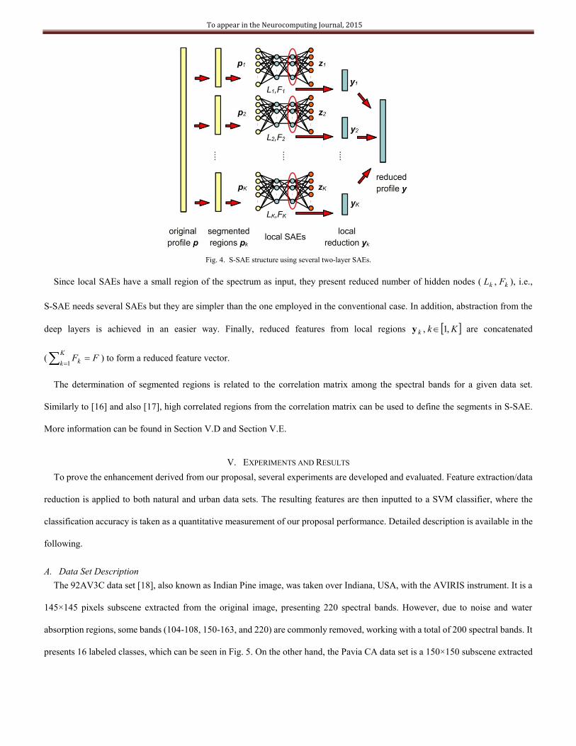
Fig. 4 presents the generic structure of our proposed S-SAE, where the spectral domain of samples p is segmented into K
different regions Kkk ,1, p to which the SAE technique is applied individually.
To appear in the Neurocomputing Journal, 2015
Fig. 4. S-SAE structure using several two-layer SAEs.
Since local SAEs have a small region of the spectrum as input, they present reduced number of hidden nodes ( kk FL , ), i.e.,
S-SAE needs several SAEs but they are simpler than the one employed in the conventional case. In addition, abstraction from the
deep layers is achieved in an easier way. Finally, reduced features from local regions Kkk ,1, y are concatenated
( FFK
k k 1) to form a reduced feature vector.
The determination of segmented regions is related to the correlation matrix among the spectral bands for a given data set.
Similarly to [16] and also [17], high correlated regions from the correlation matrix can be used to define the segments in S-SAE.
More information can be found in Section V.D and Section V.E.
V. EXPERIMENTS AND RESULTS
To prove the enhancement derived from our proposal, several experiments are developed and evaluated. Feature extraction/data
reduction is applied to both natural and urban data sets. The resulting features are then inputted to a SVM classifier, where the
classification accuracy is taken as a quantitative measurement of our proposal performance. Detailed description is available in the
following.
A. Data Set Description
The 92AV3C data set [18], also known as Indian Pine image, was taken over Indiana, USA, with the AVIRIS instrument. It is a
145×145 pixels subscene extracted from the original image, presenting 220 spectral bands. However, due to noise and water
absorption regions, some bands (104-108, 150-163, and 220) are commonly removed, working with a total of 200 spectral bands. It
presents 16 labeled classes, which can be seen in Fig. 5. On the other hand, the Pavia CA data set is a 150×150 subscene extracted
To appear in the Neurocomputing Journal, 2015
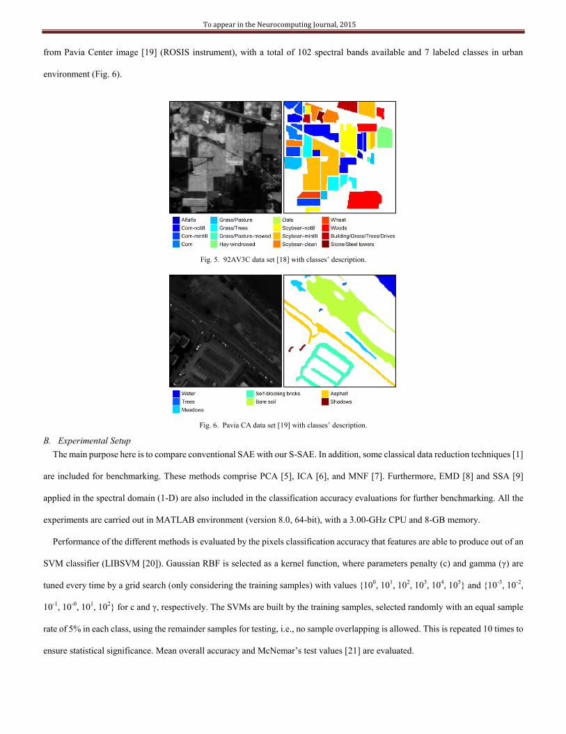
from Pavia Center image [19] (ROSIS instrument), with a total of 102 spectral bands available and 7 labeled classes in urban
environment (Fig. 6).
Fig. 5. 92AV3C data set [18] with classes’ description.
Fig. 6. Pavia CA data set [19] with classes’ description.
B. Experimental Setup
The main purpose here is to compare conventional SAE with our S-SAE. In addition, some classical data reduction techniques [1]
are included for benchmarking. These methods comprise PCA [5], ICA [6], and MNF [7]. Furthermore, EMD [8] and SSA [9]
applied in the spectral domain (1-D) are also included in the classification accuracy evaluations for further benchmarking. All the
experiments are carried out in MATLAB environment (version 8.0, 64-bit), with a 3.00-GHz CPU and 8-GB memory.
Performance of the different methods is evaluated by the pixels classification accuracy that features are able to produce out of an
SVM classifier (LIBSVM [20]). Gaussian RBF is selected as a kernel function, where parameters penalty (c) and gamma (け) are
tuned every time by a grid search (only considering the training samples) with values {100, 10
1, 10
2, 10
3, 10
4, 10
5} and {10
-3, 10
-2,
10-1
, 10-0
, 101, 10
2} for c and け, respectively. The SVMs are built by the training samples, selected randomly with an equal sample
rate of 5% in each class, using the remainder samples for testing, i.e., no sample overlapping is allowed. This is repeated 10 times to
ensure statistical significance. Mean overall accuracy and McNemar’s test values [21] are evaluated.

To appear in the Neurocomputing Journal, 2015
C. Configuration for SAE
The DL context usually entails some complexity in configuration and selection of parameters. In this case, conventional SAEs can
be implemented in several different ways. From [3], it is suggested the use of among 2-6 layers with 20-60 hidden units in each layer
except in the deepest one, where the number of units simply matches the number of desired features (F). In order to find an
appropriate configuration, we analyze the effect of parameters, layer depth and hidden units, as shown in Table I.
TABLE I
EFFECT OF LAYER DEPTH AND HIDDEN UNITS FOR F=10
Number of
units (L)
Number of layers
2 3 4 5 6
92AV3C
20 68.33 68.84 66.62 60.39 59.24
40 74.01 68.87 69.43 67.26 65.83
60 71.84 69.93 69.13 67.90 67.06
Pavia CA
20 97.06 96.92 96.87 96.52 96.71
40 97.16 96.77 96.71 96.75 96.77
60 96.69 97.00 96.98 96.78 96.95
As can be seen in Table I, higher number of layers or hidden units not necessarily improves the classification performance, as
already indicated in [3]. From these results, we state a two-layer configuration with 40 units, shown in Table II. All SAEs
implemented here employ scaled conjugate gradient backpropagation, with sigmoid activation function and a rather low 2000 epoch
(iterations) limit for training, for fast experiments and analysis.
TABLE II
CONVENTIONAL SAE CONFIGURATION FOR 92AV3C AND PAVIA CA
Region Layer-nodes Reduced features (F)
Original profile (N) 1st L=40
5, 10, 15, 20 2nd F
D. Configuration for S-SAE
Our proposal needs to define different segments of data to be computed separately. According to [16], the correlation among
spectral bands, i.e., the correlation matrix, can be used effectively for this purpose. The correlation matrix is closely related to the
covariance matrix. For that reason, usually the former one is defined by the latter. Given the definition of covariance matrix as
}}){})({({ TEEEov ppppC , where }{E is the mathematical expectation operator, then the elements ),( ji inside the
correlation matrix can be defined according to ),(),(/),(),( jjoviiovjiovjiorr CCCC . Please note that ),( iiovC and
),( jjovC represent the variance of the ith
and the jth
spectral bands from the hypercube, respectively. In that sense, ),( jiorrC
describes the correlation between the ith
and the jth
bands. The complete correlation matrix provides the correlation between every
pair of bands in the hypercube, which can be effectively used to define the segmented regions. To this end, correlation distribution
To appear in the Neurocomputing Journal, 2015
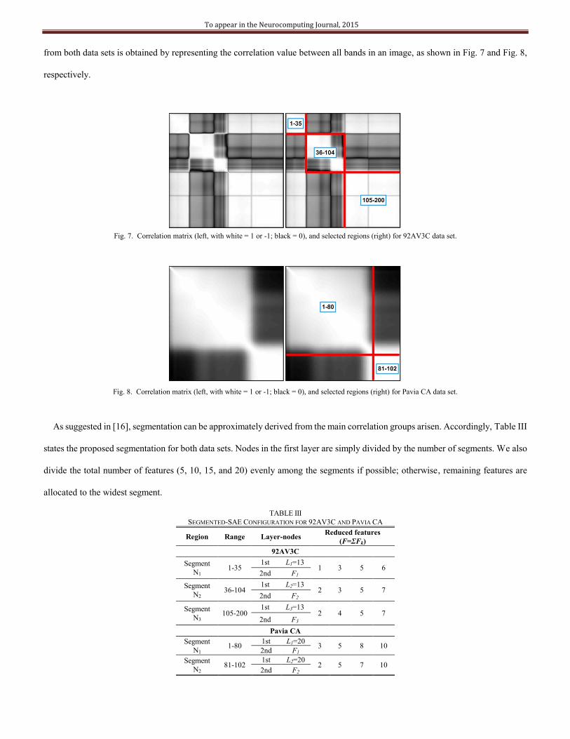
from both data sets is obtained by representing the correlation value between all bands in an image, as shown in Fig. 7 and Fig. 8,
respectively.
Fig. 7. Correlation matrix (left, with white = 1 or -1; black = 0), and selected regions (right) for 92AV3C data set.
Fig. 8. Correlation matrix (left, with white = 1 or -1; black = 0), and selected regions (right) for Pavia CA data set.
As suggested in [16], segmentation can be approximately derived from the main correlation groups arisen. Accordingly, Table III
states the proposed segmentation for both data sets. Nodes in the first layer are simply divided by the number of segments. We also
divide the total number of features (5, 10, 15, and 20) evenly among the segments if possible; otherwise, remaining features are
allocated to the widest segment.
TABLE III
SEGMENTED-SAE CONFIGURATION FOR 92AV3C AND PAVIA CA
Region Range Layer-nodes Reduced features
(F=ぇFk)
92AV3C
Segment
N1 1-35
1st L1=13 1 3 5 6
2nd F1
Segment
N2 36-104
1st L2=13 2 3 5 7
2nd F2
Segment
N3 105-200
1st L3=13 2 4 5 7
2nd F3
Pavia CA
Segment
N1 1-80
1st L1=20 3 5 8 10
2nd F1
Segment
N2 81-102
1st L2=20 2 5 7 10
2nd F2
To appear in the Neurocomputing Journal, 2015
E. Effect of the Segmentation Selection
The behavior of the S-SAE proposal is highly dependent on the segmented regions implemented. The information derived from
the correlation matrix of a given data set provides the solution in selecting these regions, as explained in Section IV and Section
V.D. However, from these correlation matrices sometimes is still possible to derive a few different segmentations. In this subsection,
we analyze this fact with clear examples.
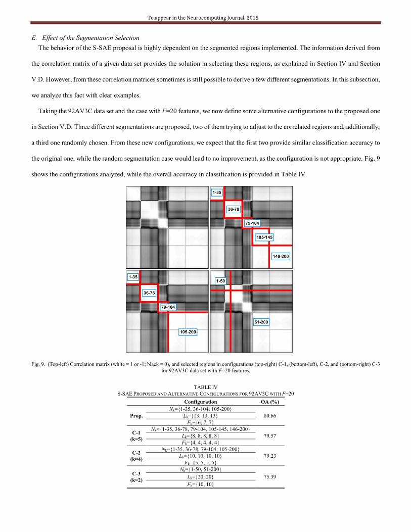
Taking the 92AV3C data set and the case with F=20 features, we now define some alternative configurations to the proposed one
in Section V.D. Three different segmentations are proposed, two of them trying to adjust to the correlated regions and, additionally,
a third one randomly chosen. From these new configurations, we expect that the first two provide similar classification accuracy to
the original one, while the random segmentation case would lead to no improvement, as the configuration is not appropriate. Fig. 9
shows the configurations analyzed, while the overall accuracy in classification is provided in Table IV.
Fig. 9. (Top-left) Correlation matrix (white = 1 or -1; black = 0), and selected regions in configurations (top-right) C-1, (bottom-left), C-2, and (bottom-right) C-3
for 92AV3C data set with F=20 features.
TABLE IV
S-SAE PROPOSED AND ALTERNATIVE CONFIGURATIONS FOR 92AV3C WITH F=20
Configuration OA (%)
Prop.
Nk={1-35, 36-104, 105-200}
80.66 Lk={13, 13, 13}
Fk={6, 7, 7}
C-1
(k=5)
Nk={1-35, 36-78, 79-104, 105-145, 146-200}
79.57 Lk={8, 8, 8, 8, 8}
Fk={4, 4, 4, 4, 4}
C-2
(k=4)
Nk={1-35, 36-78, 79-104, 105-200}
79.23 Lk={10, 10, 10, 10}
Fk={5, 5, 5, 5}
C-3
(k=2)
Nk={1-50, 51-200}
75.39 Lk={20, 20}
Fk={10, 10}

To appear in the Neurocomputing Journal, 2015
As shown by the results, the alternative configurations C-1 and C-2, with 5 and 4 segmented regions, respectively, are able to
produce good results similar to the original configuration proposed. On the other hand, randomly selected configuration C-3 leads to
degradation of the classification accuracy, as the two selected segments are not in accordance with the criterion suggested. In
summary, the performance of S-SAE is dependent on the correct selection procedure of segments, which must follow the criteria
introduced in Section IV and V.D.
F. Classification Accuracy Results
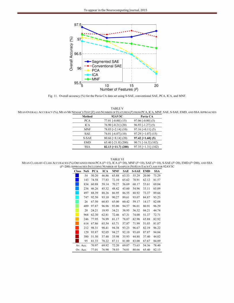
In Fig. 10 and Fig. 11, the overall accuracy obtained by PCA, ICA, MNF, conventional SAE, and S-SAE with different number
of features is shown for 92AV3C and Pavia CA, respectively. In addition, Table V provides a comparison of the best result obtained
by each method, now including the EMD and SSA methods that use the original dimensionality of features (N). For the 92AV3C
data set, conventional SAE seems to perform worse than the rest techniques except the EMD. However, for Pavia CA, SAE presents
the third best result. In both cases, S-SAE outperforms not only SAE but the rest of methods, only the SSA in the 92AV3C case
provides higher accuracy, but employing much more features, 200 instead of 20. McNemar’s test values having PCA as a reference
also validate these results.
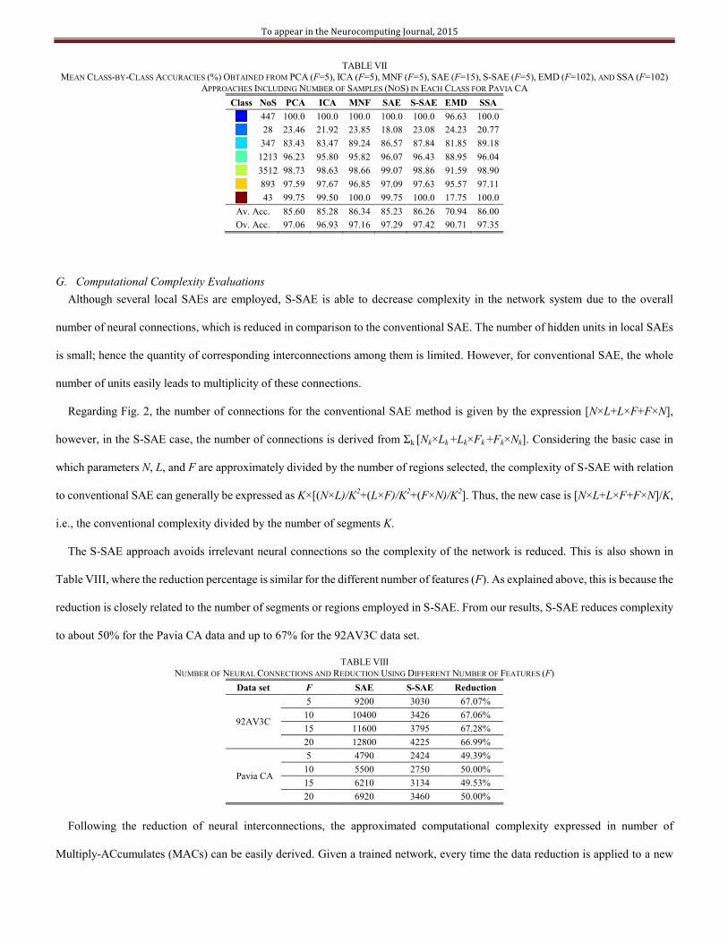
Further evaluation using the class-by-class and the average accuracy is given in Tables VI-VII, which demonstrates that the
proposed S-SAE approach generally leads to better or comparable accuracy in comparison to other state-of-the-art approaches.
However, MNF and SSA perform better in some classes, possibly owning the noise suppression model applied. As a result, it can be
interesting to investigate the combination of MNF/SSA and S-SAE for further improved classification accuracy.
It is also found that in few cases, especially for the 92AV3C dataset, conventional SAE slightly outperforms S-SAE for some
ground truth classes. This seems to be related to those classes with a really small number of samples available. Although this fact has
no negative impact on our proposal, further research is expected with relation to this particular point.
Fig. 10. Overall accuracy (%) for the 92AV3C data set using S-SAE, conventional SAE, PCA, ICA, and MNF.
To appear in the Neurocomputing Journal, 2015
Fig. 11. Overall accuracy (%) for the Pavia CA data set using S-SAE, conventional SAE, PCA, ICA, and MNF.
TABLE V
MEAN OVERALL ACCURACY (%), MEAN MCNEMAR’S TEST [Z] AND NUMBER OF FEATURES (F) FROM PCA, ICA, MNF, SAE, S-SAE, EMD, AND SSA APPROACHES
Method 92AV3C Pavia CA
PCA 77.01 [-0.00] (15) 97.06 [-0.00] (5)
ICA 76.90 [-0.21] (20) 96.93 [-1.27] (5)
MNF 78.03 [+2.14] (10) 97.16 [+0.11] (5)
SAE 74.01 [-6.07] (10) 97.29 [+1.07] (15)
S-SAE 80.66 [+8.14] (20) 97.42 [+1.60] (5)
EMD 65.40 [-21.9] (200) 90.71 [-16.3] (102)
SSA 82.13 [+11.7] (200) 97.35 [+1.31] (102)
TABLE VI
MEAN CLASS-BY-CLASS ACCURACIES (%) OBTAINED FROM PCA (F=15), ICA (F=20), MNF (F=10), SAE (F=10), S-SAE (F=20), EMD (F=200), AND SSA
(F=200) APPROACHES INCLUDING NUMBER OF SAMPLES (NOS) IN EACH CLASS FOR 92AV3C
Class NoS PCA ICA MNF SAE S-SAE EMD SSA
54 50.20 46.86 65.88 63.53 55.29 20.00 75.29
143 74.58 77.83 72.10 65.62 78.91 62.12 81.57
834 60.88 59.14 70.27 56.69 68.17 53.61 69.04
234 46.26 45.32 48.42 43.60 54.96 33.11 65.09
497 88.39 88.26 86.95 86.55 88.92 73.37 89.66
747 92.50 93.10 90.27 89.61 93.07 84.87 93.23
26 67.50 60.83 65.00 60.42 59.17 14.17 82.08
489 97.87 96.96 93.00 94.57 96.01 80.91 96.29
20 24.21 18.95 34.21 38.95 36.32 04.21 44.74
968 62.30 62.81 72.46 67.31 74.00 51.37 72.71
246 77.95 76.99 81.17 78.07 82.98 65.88 82.92
614 67.86 65.54 63.71 57.87 71.99 51.03 81.87
212 98.31 98.41 94.38 93.23 96.67 82.19 96.22
129 93.87 92.05 94.27 92.10 93.69 87.87 94.84
380 51.50 57.48 35.98 35.93 44.88 37.40 44.02
95 81.33 78.22 87.11 81.00 83.00 67.67 84.89
Av. Acc. 70.97 69.92 72.20 69.07 73.63 54.36 78.40
Ov. Acc. 77.01 76.90 78.03 74.01 80.66 65.40 82.13
To appear in the Neurocomputing Journal, 2015
TABLE VII
MEAN CLASS-BY-CLASS ACCURACIES (%) OBTAINED FROM PCA (F=5), ICA (F=5), MNF (F=5), SAE (F=15), S-SAE (F=5), EMD (F=102), AND SSA (F=102)
APPROACHES INCLUDING NUMBER OF SAMPLES (NOS) IN EACH CLASS FOR PAVIA CA
Class NoS PCA ICA MNF SAE S-SAE EMD SSA
447 100.0 100.0 100.0 100.0 100.0 96.63 100.0
28 23.46 21.92 23.85 18.08 23.08 24.23 20.77
347 83.43 83.47 89.24 86.57 87.84 81.85 89.18
1213 96.23 95.80 95.82 96.07 96.43 88.95 96.04
3512 98.73 98.63 98.66 99.07 98.86 91.59 98.90
893 97.59 97.67 96.85 97.09 97.63 95.57 97.11
43 99.75 99.50 100.0 99.75 100.0 17.75 100.0
Av. Acc. 85.60 85.28 86.34 85.23 86.26 70.94 86.00
Ov. Acc. 97.06 96.93 97.16 97.29 97.42 90.71 97.35
G. Computational Complexity Evaluations
Although several local SAEs are employed, S-SAE is able to decrease complexity in the network system due to the overall
number of neural connections, which is reduced in comparison to the conventional SAE. The number of hidden units in local SAEs
is small; hence the quantity of corresponding interconnections among them is limited. However, for conventional SAE, the whole
number of units easily leads to multiplicity of these connections.
Regarding Fig. 2, the number of connections for the conventional SAE method is given by the expression [N×L+L×F+F×N],
however, in the S-SAE case, the number of connections is derived from ぇk [Nk×Lk +Lk×Fk +Fk×Nk]. Considering the basic case in
which parameters N, L, and F are approximately divided by the number of regions selected, the complexity of S-SAE with relation
to conventional SAE can generally be expressed as K×[(N×L)/K2+(L×F)/K
2+(F×N)/K
2]. Thus, the new case is [N×L+L×F+F×N]/K,
i.e., the conventional complexity divided by the number of segments K.
The S-SAE approach avoids irrelevant neural connections so the complexity of the network is reduced. This is also shown in
Table VIII, where the reduction percentage is similar for the different number of features (F). As explained above, this is because the
reduction is closely related to the number of segments or regions employed in S-SAE. From our results, S-SAE reduces complexity
to about 50% for the Pavia CA data and up to 67% for the 92AV3C data set.
TABLE VIII
NUMBER OF NEURAL CONNECTIONS AND REDUCTION USING DIFFERENT NUMBER OF FEATURES (F)
Data set F SAE S-SAE Reduction
92AV3C
5 9200 3030 67.07%
10 10400 3426 67.06%
15 11600 3795 67.28%
20 12800 4225 66.99%
Pavia CA
5 4790 2424 49.39%
10 5500 2750 50.00%
15 6210 3134 49.53%
20 6920 3460 50.00%
Following the reduction of neural interconnections, the approximated computational complexity expressed in number of
Multiply-ACcumulates (MACs) can be easily derived. Given a trained network, every time the data reduction is applied to a new

To appear in the Neurocomputing Journal, 2015
pixel or sample, approximately a total of [N×L+L×F] MACs are required (from input to internal layer) in the conventional SAE
method. Similarly, [N×L+L×F]/K is the cost involved in the S-SAE, where again it is reduced by a saving factor equal to the number
of defined segments. Moreover, for the PCA technique (similar to MNF and ICA), the truncation projection consists of a simple
multiplication of the pixel with the Eigenvectors matrix, resulting in [N×F] MACs. On the other hand, for the EMD and SSA
methods, the complexity analysis is not included as it is much higher and independent to the number of features F. Giving some
numbers to these expressions, Fig. 12 and Fig. 13 show the complexity for 92AV3C and Pavia CA, with different number of features
F.
Fig. 12. Computational complexity (number of MACs) for the 92AV3C data set.
Fig. 13. Computational complexity (number of MACs) for the Pavia CA data set.
The conventional SAE method requires the maximum number of MACs, a number that slightly increases as long as more features
F are extracted, while the MACs involved in the S-SAE approach are simply divided by the number of regions in the segmentation.
On the other hand, classical techniques such as PCA present the lowest complexity, although when F increases it can surpass the
S-SAE complexity, which proves the general benefits achieved from the segmentation concept.

To appear in the Neurocomputing Journal, 2015
Finally, the approximated computation time can also be used for assessment comparison. This time is obtained from both the
conventional and the segmented SAE under the same conditions, measuring the elapsed time required in extracting the reduced
features F from a pixel given a trained two-layer SAE or S-SAE. This is done for several randomly selected pixels, providing the
mean values in Table IX. As can be seen, the reduction in number of neural interconnections and MACs explained above leads to
faster implementations as well, where the time required in extracting features from an original pixel is reduced in 60% and about
44% for the 92AV3C and Pavia CA data sets, respectively.
TABLE IX
APPROXIMATED COMPUTATION TIME IN MILLISECONDS USING DIFFERENT NUMBER OF FEATURES (F)
Data set F SAE S-SAE Reduction
92AV3C
5 4.6 2.0 56.52%
10 6.4 2.6 59.38%
15 8.0 3.2 60.00%
20 9.8 3.8 61.22%
Pavia CA
5 3.3 1.9 42.42%
10 5.0 2.8 44.00%
15 6.7 3.7 44.78%
20 8.7 4.7 45.98%
VI. CONCLUSIONS
As part of the DL framework being explored in the very recent years, SAEs are proved to be an effective method for feature
extraction/abstraction and data reduction in HSI. In this paper, a variant of SAEs, namely Segmented-SAEs, is proposed, where the
original spectral domain is divided in different regions to which individual SAEs are applied, reducing the complexity of the
learning processes and extracting local information that leads to better performance. This introductory analysis proves high
potential in applying DL algorithms and deriving variants from them, allowing improved classification accuracy in hyperspectral
remote sensing. Future work will explore the combination of most state-of-the-art techniques including 2D SSA [22], adaptive
sparse representation [23, 27], Hybrid and sampling-based clustering ensemble [24], weakly supervised learning [25], tensor rank
selection [26], gradient and subspace processing [28] and salient based deep learning [29].
VII. ACKNOWLEDGEMENTS
The authors wish to thank the anonymous reviewers and the Associate Editor for their constructive comments to further improve
the quality of this paper. The work is partially supported by the University of Strathclyde and the following grants: National Natural
Science Foundation of China (61272381, 61471132, 61401163), Science and Technology Major Project of Education Department
of Guangdong Province (2014KZDXM060), the Fundamental Research Funds for the Central Universities (No.2015ZZ032), and
Science and Technology Project of Guangzhou City (2014J4100078).
REFERENCES
[1] X. Jia, B-C. Kuo, and M.M. Crawford, “Feature mining for hyperspectral image classification,” Proceedings of the IEEE, vol. 101, no. 3, pp. 676-697, 2013.
To appear in the Neurocomputing Journal, 2015
[2] J. Ren, J. Zabalza, S. Marshall, and J. Zheng, “Effective feature extraction and data reduction in remote sensing using hyperspectral imaging,” IEEE Signal
Processing Magazine, vol. 31, no. 4, pp. 149-154, 2014.
[3] Y. Chen, Z. Lin, X. Zhao, G. Wang, and Y. Gu, “Deep learning-based classification of hyperspectral data,” IEEE Journal of Selected Topics in Applied Earth
Observations and Remote Sensing, no. 7, no. 6, pp. 2094-2107, 2014.
[4] M.E. Midhun, S.R. Nair, V.T.N. Prabhakar, and S.S. Kumar, “Deep model for classification of hyperspectral image using restricted Boltzmann machine,”
Proceedings in ICONIAAC, no. 35, 2014.
[5] I. Jolliffe, Principal Component Analysis. N. York: Springer-Verlag, 1986.
[6] A. Hyvrinen, J. Karhunen, and E. Oja, Independent Component Analysis. New York: Wiley, 2001.
[7] A. A. Green, M. Berman, P. Switzer, and M. D. Craig. “A transformation for ordering multispectral data in terms of image quality with implications for noise
removal,” IEEE Transactions on Geoscience and Remote Sensing, vol. 26, no. 1, pp. 65-74, 1998.
[8] B. Demir and S. Ertürk, “Empirical mode decomposition of hyperspectral images for support vector machine classification,” IEEE Transactions on
Geoscience and Remote Sensing, vol. 48, no.11, pp.4071-4084, 2010.
[9] J. Zabalza, J. Ren, Z. Wang, S. Marshall, and J. Wang, “Singular spectrum analysis for effective feature extraction in hyperspectral imaging,” IEEE
Geoscience and Remote Sensing Letters, vol. 11, no. 11, pp. 1886-1890, 2014.
[10] M. Fauvel, J.A. Benediktsson, J. Chanussot, and J.R. Sveinsson, “Spectral and spatial classification of hyperspectral data using SVMs and morphological
profiles,” IEEE Transactions on Geoscience and Remote Sensing, vol.46, no.11, pp.3804-3814, 2008.
[11] Y. Gao, R. Ji, P. Cui, Q. Dai, and G. Hua, “Hyperspectral image classification through bilayer graph-based learning,” IEEE Transactions on Image
Processing, vol. 23, no. 7, July 2014.
[12] Y. Chen, N.M. Nasrabadi, and T.D. Tran, “Hyperspectral image classification using dictionary-based sparse representation,” IEEE Transactions on
Geoscience and Remote Sensing, 2011.
[13] J. Xia, M. Dalla Mura, J. Chanussot, P. Du, and X. He, “Random subspace ensembles for hyperspectral image classification with extended morphological
attribute profiles,” IEEE Transactions on Geoscience and Remote Sensing, vol. 53, no. 9, pp. 4768–4786, 2015.
[14] R. Ji, Y. Gao, R. Hong, Q. Liu, D. Tao, and X. Li, “Spectral-spatial constraint hyperspectral image classification,” IEEE Transactions on Geoscience and
Remote Sensing, vol. 52, no.3, pp. 1811-1824, 2014.
[15] J. Li, X. Huang, P. Gamba, J. Bioucas, L. Zhang, J. A. Benediktsson, and A. Plaza, “Multiple feature learning for hyperspectral image classification,” IEEE
Transactions on Geoscience and Remote Sensing, vol. 53, no. 3, pp. 1592–1606, 2015.
[16] X. Jia and J.A. Richards, “Segmented principal components transformation for efficient hyperspectral remote-sensing image display and classification,”
IEEE Transactions on Geoscience and Remote Sensing, vol. 37, no. 1, pp. 538-542, January 1999.
[17] J. Zabalza, J. Ren, M. Yang, Y. Zhang, J. Wang, S. Marshall, and J. Han, “Novel Folded-PCA for improved feature extraction and data reduction with
hyperspectral imaging and SAR in remote sensing,” ISPRS Journal of Photogrammetry and Remote Sensing, vol. 93, pp. 112-122, July 2014.
[18] Purdue's university multispec site: 12/06/92 AVIRIS image Indian Pine Test Site [Online]. Available: https://engineering.purdue.edu/~biehl/
MultiSpec/hyperspectral.htm
[19] Hyperspectral Remote Sensing Scenes [Online]. Available: http://www.ehu.es/ccwintco/index.php?title=Hyperspectral_Remote_Sensing_Scenes
[20] C-C. Chang and C-J. Lin, LIBSVM: library for support vector machines. [Online]. Available: http://www.csie.ntu.edu.tw/~cjlin/libsvm
[21] G.M. Foody, “Thematic map comparison: Evaluating the statistical significance of differences in classification accuracy,” Photogrammetric Engineering &
Remote Sensing, vol. 70, no. 5, pp. 627–633, May 2004.

To appear in the Neurocomputing Journal, 2015
[22] J. Zabalza, J Ren, J. Zheng, J. Han, H. Zhao, S. Li and S. Marshall, “Novel 2D singular spectral analysis for effective feature extraction and data classification
in hyperspectral imaging,” IEEE Trans. Geoscience and Remote Sensing, vol. 53, no. 8, pp. 4418-4433, 2015
[23] C. Zhao, X. Li, J. Ren and S. Marshall, “Improved sparse representation using adaptive spatial support for effective target detection in hyperspectral imagery,”
Int. J. Remote Sensing, vol. 34, no. 24, pp. 8669-8684, 2013
[24] Y. Yang and J. Jiang, “Hybrid and sampling-based clustering ensemble with global and local constitutions,” IEEE Trans. Neural Networks and Learning
Systems, to appear
[25] J. Han, D. Zhang, G. Cheng, L. Guo and J Ren, “Object detection in optical remote sensing images based on weakly supervised learning and high-level feature
learning,” IEEE Trans. Geoscience and Remote Sensing, vol. 53, no. 6, pp. 3325-3337, 2015
[26] J. Zhang, Y. Han and J. Jiang, “Tensor rank selection for multimedia,” J. Visual Communication and Image Representation, 30, pp. 376-392, 2015
[27] K. Li, Y. Zhu, J. Yang and J. Jiang, “Non-rigid structure from motion via sparse representation,” IEEE Trans. Cybernetics, 45, pp. 1401-1413, Aug. 2015
[28] J. Ren, T. Vlachos, Y. Zhang, J. Zheng and J. Jiang, “Gradient-based subspace phase correlation for fast and effective image alignment,” J. Visual
Communication and Image Representation, 25(7): 1558-1565, 2014.
[29] J. Han, D. Zhang, X. Hu, L. Guo, J. Ren and F. Wu, “Background prior based salient object detection via deep reconstruction residual,” IEEE Trans. Circuits
and System for Video Technology, vol. 25, no. 8, pp. 1309-1321, 2014
Related Documents