Yu-Wing Tai Jiaya Jia Chi-Keung Tang The Hong Kong ...

Local Color Transfer via Probabilistic Segmentation by Expectation-Maximization∗

Yu-Wing Tai† Jiaya Jia∗ Chi-Keung Tang††The Hong Kong University of Science and Technology

∗The Chinese University of Hong Kong

AbstractWe address the problem of regional color transfer be-

tween two natural images by probabilistic segmentation. Weuse a new Expectation-Maximization (EM) scheme to im-pose both spatial and color smoothness to infer natural con-nectivity among pixels. Unlike previous work, our methodtakes local color information into consideration, and seg-ment image with soft region boundaries for seamless colortransfer and compositing.

Our modified EM method has two advantages in colormanipulation: First, subject to different levels of colorsmoothness in image space, our algorithm produces an op-timal number of regions upon convergence, where the colorstatistics in each region can be adequately characterized bya component of a Gaussian Mixture Model (GMM). Sec-ond, we allow a pixel to fall in several regions accordingto our estimated probability distribution in the EM step,resulting in a transparency-like ratio for compositing dif-ferent regions seamlessly. Hence, natural color transitionacross regions can be achieved, where the necessary intra-region and inter-region smoothness are enforced withoutlosing original details. We demonstrate results on a varietyof applications including image deblurring, enhanced colortransfer, and colorizing gray scale images. Comparisonswith previous methods are also presented.

1 IntroductionRecent advances in digital image processing and en-

hancement techniques have made new and useful applica-tions possible. One involves color manipulation betweenimages, which can be applied to perform color correction,noise reduction, and production of high-quality compositeimages [14, 8, 4, 5, 6].

In [9], Reinhard et al. reported a simple but very suc-cessful technique that transfers color characteristics from asource to a target image. In the target image It, the trans-ferred color at pixel Ct in the lαβ color space is:

g(Ct) = µs +σs

σt(Ct − µt) (1)

∗This research is supported by the Research Grant Council ofHong Kong Special Administration Region, China: AOE/E-01/99,HKUST6175/04E, and the Chinese University of Hong Kong (CUHK) Di-rect Grant: 2050332.

where µs, µt are the means of the underlying Gaussian dis-tribution in the lαβ color space of the respective sourceand target images. σs, σt are the respective standard devi-ations. We call this approach global color transfer becausethe color statistics are calculated by taking into account allpixels in the respective images.

Global color transfer does not have adequate spatial con-sideration, so it cannot avoid the following two problems.One is that if the source or target image contains differentcolor regions, the global transfer cannot distinguish the dif-ferent statistics and will mix regions up. The other problemis that if the color of the two images are very different, inthe lαβ color space, the chromaticity channels are easily ex-aggerated which will cause unnatural and saturated result.Swatches [9] can alleviate the errors in some situations, butthey cannot solve all problems because they do not providewithout sufficient clustering information.

In this paper, we address the above issues, and proposea method to establish spatial connectivity so that local colorstatistics can be inferred simultaneously with the optimalpartitioning of the image space. We call the transfer in thepresence of color correspondences and spatial relations aslocal color transfer. It has following three properties:Probabilistic segmentation. Pixel clustering is achievedvia probabilistic segmentation, where we estimate the prob-ability iPxy ∈ [0, 1] that pixel I(x, y) belongs to region i inimage I . Hence, I(x, y) may concurrently exist in severalregions according to its probability distribution Pxy . Pre-vious binary segmentation where iPxy ∈ {0, 1} is just aspecial case in our definition.

The advantage of using probabilistic segmentation overbinary segmentation is that inter-region smoothness can beenforced by encoding natural connectivity among pixels. Inour method, pixel I(x, y) tends to have a large probabilityfalling into a single region i when it is in the center of theregion, while it has a more uniform probability distributionamong several regions if it lies on boundary. This guaran-tees smooth color transition across regions without mixingup colors in the interior of the regions.Expectation-Maximization. We estimate these probabil-ity distributions through a novel propagation step by theExpectation-Maximization (EM) algorithm, and appropri-ately model all segments as Gaussian Mixtures where the

0-7695-2372-2/05/$20.00 (c) 2005 IEEE

color statistics of each segment is modelled by one compo-nent. This guarantees that if two regions respectively sat-isfy this model, both of them should have roughly one peakin the corresponding color statistics. Thus, in the transferprocess, dominant colors will not be mixed up and naturalcolor transition across regions can be maintained.Unified approach. Because of the generality of GMM, ourunified approach can be applied to a variety of applications,including image deblurring, image restoration and coloriza-tion of gray scale images.

The rest of this paper is organized as follows. Section 2reviews previous work in related areas. In Section 3, we de-scribe our method which includes the modified EM methodfor probabilistic segmentation, mapping function construc-tion and result compositing. We present our results in sec-tion 4, with detailed comparison with previous work. Thesummary and conclusion are given in section 5.

2 Previous workWe review previous work proposed for color manipula-

tion between two images, together with several image seg-mentation techniques related to our probabilistic segmenta-tion and EM techniques.

2.1 Color transfer and related applicationsReinhard et al. [9] first performed global color transfer

according to Eqn. 1 in [10], after converting the RGB spaceto the decorrelated color space lαβ. In their approach, if theimage contains different color regions, swatches are speci-fied by users and are used to divide the colors into clusters.However, for complex scenes, either swatches are inade-quate to discern different color statistics, or a lot of swatchesneed to be specified by user.

The method was extended to gray scale image coloriza-tion in [14], where chromaticity transfer is performed af-ter equalizing the luminance channels of both input images.In [7], Levin et al. colorized a gray scale image or movie byassuming that neighboring pixels in space-time with simi-lar intensities should have similar colors. A quadratic opti-mization was formulated which can be solved efficiently bystandard techniques. These colorization techniques requirea lot of human interactions if complex textures or patternsare present. Without human interaction, undesirable colormixture will be observed.

As for other related applications in color transfer, in [5],a Bayesian approach was proposed to correct image inten-sity. Without performing motion deblurring, a low/normalexposure image pair is used. Global color statistics aretransferred from the normal exposure (blurred) image tothe low exposure (sharp) image. Explicit spatial correspon-dence was used.

Later, two image restoration or denoising techniques us-ing flash/no-flash pairs were proposed independently in [4,8]. In comparison, [4] used a compositing approach to in-

MeaningGi Gaussian distribution Gi(i;µi, σi) for region iµt

i Mean of Gi at iteration tσt

i Standard deviation of Gi at iteration t

iPtxy Probability of pixel I(x, y) in Gi at iteration t

Ptxy Probability distribution of pixel I(x, y)

estimated at t. Ptxy = {iP

txy|i = 1, 2, · · ·}

Table 1: Notations used in this paper.

tegrate colors from flash/no flash pairs, while in [8], a jointbidirectional filter is used to perform de-noising. The latterapproach cannot avoid texture smoothing. Otherwise, noisewill be remained even with the guidance of details from theflashed image, due to the use of smoothing filter.

2.2 Color segmentationThe watershed algorithm [13] performs color segmenta-

tion which easily produces a large number of small regionswith hard boundaries. Mean shift segmentation [3] main-tains spatial consistency by incorporating the spatial coor-dinates into their feature space representation. In the filter-ing step, the kernel size is determined with the help of thespatial domain parameter.

An earlier work in [1] performs color and texture seg-mentation by EM, which models the joint distributionof color and texture with a mixture of Gaussians in 6-dimensional space (three dimensions for color and three fortexture). Since no spatial coordinates are incorporated, afterthe model has been inferred, it needs a spatial grouping stepby applying a maximum-vote filter and connected compo-nent algorithm.

In our new EM algorithm, we perform our model estima-tion in the 3D color space, which makes the EM estimationmore stable and run faster. To maintain spatial consistenciesand introduce natural probabilistic region boundaries, weintroduce an additional propagation step in the loop. Forprobabilistic segmentation, note that natural matting tech-niques (such as [2] and [11]) are not applicable in our work,since they do not guarantee smoothness for in certain situa-tions.

3 Our approachGiven an input image pair Is and It, we first construct a

probabilistic segmentation in each of them so that the col-ors in every segmented region ri can be fitted by a Gaussiancomponent Gi of a GMM appropriately. It guarantees thatany two regions in the two input images have similar sta-tistical model, and a natural mapping can be achieved be-tween them. Hence, region ri and Gaussian component Gi

are closely related. Table 1 shows the notation to be used inthe rest of the paper.

In this section, we first review in section 3.1 the originalEM algorithm for estimating general 3D GMM. Afterward,a detailed description on our new model construction and

mapping estimation will be presented. The outline of ourapproach is as follows:

• Segment the two input images into a set of regions withsoft boundaries. The optimal number of regions is alsodetermined automatically in this step (sections 3.2-3.3).

• Construct the mapping function from the source imageto the target with or without spatial correspondence.(section 3.4).

• Composite the final image where no visual artifactshould be observed among regions (section 3.5).

We will describe these steps in separate sections.

3.1 The original EM algorithm for 3D GMM esti-mation

Initially, we assume that the image can be partitionedinto N regions, namely, the underlying joint color distrib-ution in lαβ channels can be approximated by a set of NGaussians. It is equivalent to 3D GMM estimation:

E-step: The probability that a pixel color I(x, y) be-longs to the ith Gaussian Gi(i;µi, σi) is calculated as:

iPxy =exp(− (I(x,y)−µi)

2

2σ2i

)∑Nj=1 exp(− (I(x,y)−µj)2

2σ2j

)(2)

M-step: the mean µi and standard deviation σi of eachGaussian Gi are re-estimated in region i as:

µi =1Z

∑x,y

iP xyI(x, y) (3)

σi =

√∑x,y iP xy(I(x, y) − µi)2

Z(4)

where Z is the normalization factor, which is equal to∑x,y iP xy .The E-step and M-step are iterated until convergence.

Usually, the initial values of the above EM algorithm iscalculated by performing K-means. The EM algorithmworks well on estimating 3D GMM from only the proba-bility or the statistical point of view. However, for an imagewith 3 color channels, it does not take spatial correlationinto account. Note that it is also not practical to upgradethis method to 5D (including 2 image spatial dimensions),which may easily lead to local minima. Also, the numberof Gaussians converged is not guaranteed to be optimal.

3.2 Modified EM for estimating probabilistic seg-mentation

In our modified EM, we encode an additional spatialsmoothness step within the loop, in order to simultaneouslyconstrain spatial connectivity among pixels and refine the

number of Gaussians iteratively until no two Gaussian com-ponents are largely overlapping. Our output is optimized inthe number of Gaussian N .

Given an input image I , we iterate the following EMprocess.

1. Expectation Estimate probability distribution Ptxy in it-

eration t according to the result from iteration t − 1.Instead of using Eqn. 2, we introduce a new represen-tation, subjected to

∑Ni=1 iP

txy = 1:

iPtxy = iP

′t−1xy +

exp(− (I(x,y)−µt−1i

)2

2(σt−1i

)2)

∑Nj=1 exp(− (I(x,y)−µt−1

j)2

2(σt−1j

)2)

(5)

where iP′t−1xy is the result from spatial smoothness

propagation in step 2 of the last iteration. We initializeiP

′0xy using Eqn. 2. The explanation of Eqn. 5 will be

given in section 3.2.1.

2. Spatial smoothing In this step we perform spatialsmoothness propagation and update the expectationvalues as iP

′txy . Details of this step will be described

in section 3.2.2.

3. Maximization Re-estimate µti and σt

i using Eqn. 3 and4 with new probability distribution iP

′txy for each

Gaussian component i.

4. Refine Gaussians Given the new estimation ofGaussian parameters from the previous step, for everypair of Gaussian components in the same image, e.g.,Gi(i;µt

i, σti) and Gj(j;µt

j , σtj), if |µt

i − µtj | < δ for

some small δ, we merge them and re-estimate theirparameters. Subject to the tolerance δ, this step pro-duces an optimal number of Gaussians in each image.In practice, we iterate the algorithm for a fixed numberof Gaussians until it converges before applying regionmerging. This produces better convergence result.

5. Output If the difference of means and variances be-tween all corresponding pairs of Gaussian componentsbetween iterations t and t − 1 is small enough, andthere is no Gaussian merging in current iteration t,stop. Otherwise, go back to step 1 and begin iterationt + 1.

Steps 3–5 are straightforward. We give further descrip-tions on steps 1 and 2 in the following subsections.

3.2.1 Expectation

We explain step 1 of our modified EM algorithm. Supposethe region i to be inferred is shaped like a disc. If a pixel isin the center of region i, its probability of belonging to thisregion, or equivalently the corresponding Gaussian compo-nent Gi, should be very high. On the other hand, if the

region is elongated, or the pixel lies on boundary of regioni, we want the pixel to have non-zero probability to fall inother regions. This will introduce a transparency-like ratioamong regions to ensure boundary smoothness.

According to the above analysis, we explain how Eqn.5 operates in different situations. Let us denote iP

′′txy =

exp(− (I(x,y)−µt−1i

)2

2(σt−1i

)2)∑N

j=1exp(−

(I(x,y)−µt−1j

)2

2(σt−1j

)2)

, then:

• If both iP′xy

t−1 and iP′′t

xy have similar distributions,it is highly probable that the neighboring pixels havesimilar color values, which indicates that this pixel isnot lying on any region boundary. Hence, the addi-tion operation increases the probability that the pixelbelongs to some dominant Gaussian component.

• If iP′xy

t−1 and iP′′t

xy have disparate probability dis-tributions, the pixel receives different propagated valuefrom its neighbors. Hence, it indicates that the pixel islying close to the boundary of some regions. The addi-tion operation averages these distributions, so that thispixel will have similar probability of fitting into severalGaussian components concurrently.

3.2.2 Spatial smoothing

Step 2 in the previous section defines the spatial propa-gation operation. Denote N (x, y) as the neighborhood of(x, y), and also suppose (x′, y′) ∈ N (x, y). If I(x, y) andI(x′, y′) have similar colors, they should also be close inGaussian distributions considering spatial connectivity aftersmoothing, namely, iP xy ≈ iP x′y′ . Otherwise, their prob-ability distribution should not be affected so as to generatea spatial partition. According to this analysis, we define thesmoothing operation as:

iP′txy =

1Zi

∑(x′,y′)∈N(x,y)

D(I(x, y), I(x′, y′))iPtx′y′ (6)

where Zi =∑

i

∑(x′,y′)∈N(x,y) D(I(x, y), I(x′, y′))iP

tx′y′

is the normalization factor. For simultaneous color andspatial smoothness, we adopt the bilateral filter [12]:

D(I(x, y), I(x′, y′)) = exp(− (x − x′)2 + (y − y′)2

σd)

exp(−|I(x, y) − I(x′, y′)|2σg

) (7)

where σd and σg are parameters to control the strength ofsmoothing in the spatial and color spaces respectively.

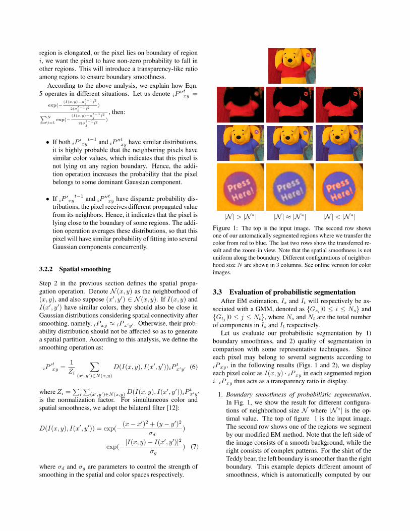
|N | > |N ∗| |N | ≈ |N ∗| |N | < |N ∗|Figure 1: The top is the input image. The second row showsone of our automatically segmented regions where we transfer thecolor from red to blue. The last two rows show the transferred re-sult and the zoom-in view. Note that the spatial smoothness is notuniform along the boundary. Different configurations of neighbor-hood size N are shown in 3 columns. See online version for colorimages.

3.3 Evaluation of probabilistic segmentationAfter EM estimation, Is and It will respectively be as-

sociated with a GMM, denoted as {Gsi|0 ≤ i ≤ Ns} and

{Gtj|0 ≤ j ≤ Nt}, where Ns and Nt are the total number

of components in Is and It respectively.Let us evaluate our probabilistic segmentation by 1)

boundary smoothness, and 2) quality of segmentation incomparison with some representative techniques. Sinceeach pixel may belong to several segments according toiP xy , in the following results (Figs. 1 and 2), we displayeach pixel color as I(x, y) · iP xy in each segmented regioni. iP xy thus acts as a transparency ratio in display.

1. Boundary smoothness of probabilistic segmentation.In Fig. 1, we show the result for different configura-tions of neighborhood size N where |N ∗| is the op-timal value. The top of figure 1 is the input image.The second row shows one of the regions we segmentby our modified EM method. Note that the left side ofthe image consists of a smooth background, while theright consists of complex patterns. For the shirt of theTeddy bear, the left boundary is smoother than the rightboundary. This example depicts different amount ofsmoothness, which is automatically computed by our

(a) (b) (c)

(d) (e) (f)

(g) (h) (i)

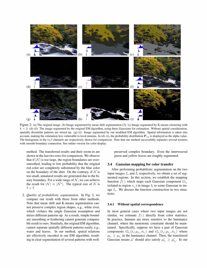
Figure 2: (a) The original image. (b) Image segmented by mean shift segmentation [3]. (c) Image segmented by K-means clustering withk = 3. (d)–(f): The image segmented by the original EM algorithm, using three Gaussians for estimation. Without spatial consideration,spatially dissimilar patterns are mixed up. (g)–(i): Image segmented by our modified EM algorithm. Spatial information is taken intoaccount, making the estimation less vulnerable to local minima. In (d)–(i), the probability distribution Pxy is displayed as the alpha value.The histograms in the lαβ channels are respectively shown for comparison. Note that our method successfully separates several textureswith smooth boundary connection. See online version for color display.

method. The transferred results and their zoom-in areshown in the last two rows for comparison. We observethat if |N | is too large, the region boundaries are over-smoothed, leading to low probability that the originalred color are completely substituted by the blue coloron the boundary of the shirt. On the contrary, if N istoo small, unnatural results are generated due to the bi-nary boundary. For a wide range of N , we can achievethe result for |N | ≈ |N ∗|. The typical size of N is7 × 7.

2. Quality of probabilistic segmentation. In Fig. 2, wecompare our result with those from other methods.Note that mean shift and K-means segmentation can-not preserve complex region shapes, e.g., white river,which violates the single Gaussian assumption andmixes different patterns up. As a result, simple bound-ary smoothing or feathering cannot generate compara-ble result to ours. Similarly, the original EM algorithm,cannot separate spatially different patterns easily, e.g.,water and leaves. In our method, spatial relationsare effectively encoded in our EM algorithm, result-ing in clear segmentation of several patterns with well-

preserved complex boundary. Even the interweavedgreen and yellow leaves are roughly segmented.

3.4 Gaussian mapping for color transferAfter performing probabilistic segmentation on the two

input images Is and It respectively, we obtain a set of seg-mented regions. In this section, we establish the mappingfunction f(·) which maps each Gaussian component Gtj

(related to region rtj) in image It to some Gaussian in im-

age Is. We discuss the function construction in two situa-tions:

3.4.1 Without spatial correspondence

In most general cases where two input images are notsimilar, we estimate f(·) directly from color statistics.In practice, humans are more sensitive to the luminancechannel, where the monotonic constraint should be main-tained. Specifically, suppose we have a pair of Gaussiancomponents Gti

(ti;µti, σti

) and Gtj(tj ;µtj

, σtj) where

µti≥ µtj

in the luminance channel. Then, the transferredGaussian means µ′ should also satisfy µ′

ti≥ µ′

tj. In our

method, Gtjis mapped to Gsi

where 1) their means in lu-minance channel are closest and 2) monotonic constraint isenforced simultaneously.

3.4.2 With spatial correspondence

In some applications, such as deblurring [5] and denois-ing [8], images Is and It are similar in content. We defineour mapping function f(·) as the region correspondence inIs and It, using the largest amount of overlapping in the re-spective regions as the mapping criterion. In other words,f(Gtj

) = Gsiif corresponding regions rtj

and rsiare over-

lapping significantly.

3.5 Result compositingAfter obtaining the mapping function f(·) which

maps Gaussian component from Gtj(tj ;µtj

, σtj) to

Gsi(si;µsi

, σsi), we compute the final transferred color in

pixel It(x, y) as:

g(It(x, y)) =∑

j

tjP

xy(σsi

σtj

(It(x, y) − µtj) + µsi

) (8)

where tjP

xyis the probability that I(x, y) belongs to region

tj of the target image. It guarantees the smoothness after thetransfer, especially in regions rich in colors.

4 Results and comparisonWe implement our method and apply it to a variety of

examples on a Pentium-M 1.4GHz laptop computer. Ournew EM algorithm converges within 4 minutes for an imageof size 512 × 512, starting with 20 Gaussians initially.

We show results on local color transfer as well as otherapplications, including motion deblurring, denoising usingflash/no flash image pairs, and colorizing gray scale images.Comparisons with previous methods are also given.

4.1 Local color transferFig. 3 and Fig. 4 show two results of local color transfer.

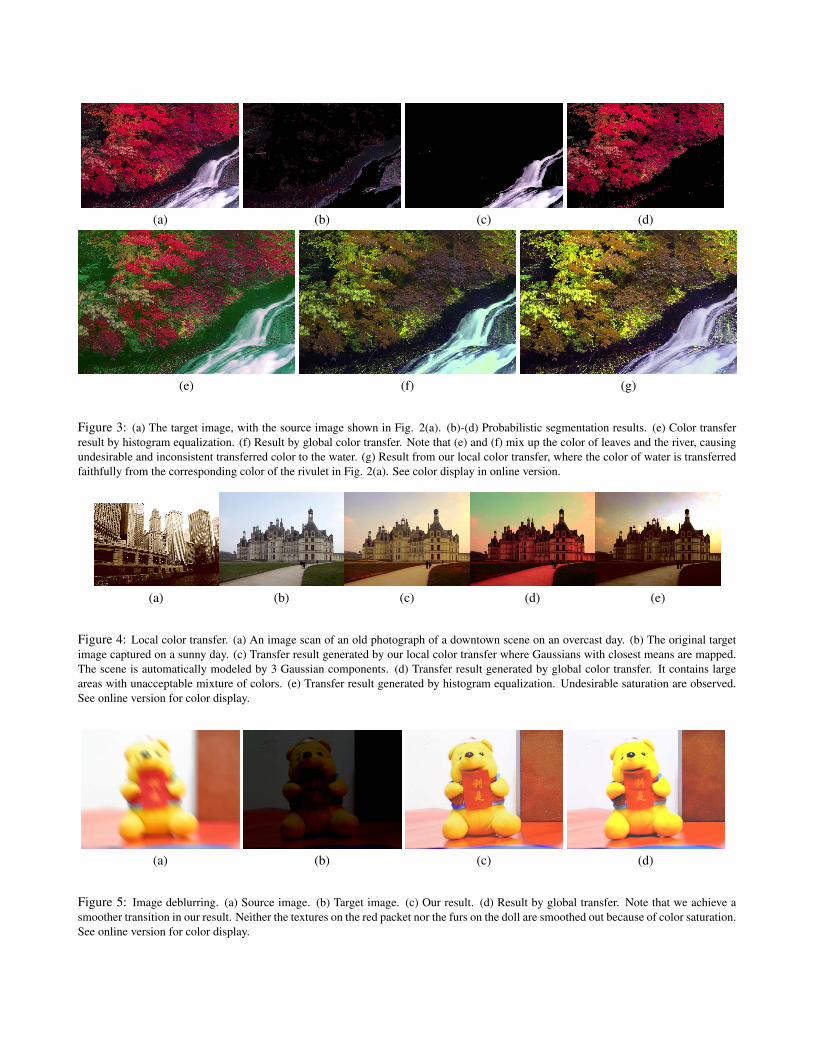
In Fig. 3, the source and the target images are shown inFig. 2(a) and Fig. 3(a) respectively. Fig. 2(g)-(i) show thesegmented regions in the source image while the segmentedregions in the target image are illustrated in Fig. 3(b)-(d).We use the mapping function defined in section 3.4.1. Thewhole process is automatic. Our result is shown in Fig. 3(g).

In Fig. 4, (a) and (b) are two input images. (c) is the re-sult generated by our automatic method. Comparing withresults generated by global color transfer in Fig. 4(d) andhistogram equalization in Fig. 4(e), our result is natural andless saturated. Our method not only determines the neces-sary color regions, but also maintains smooth color transi-tion in the entire image.

4.2 Motion deblurring from normal/low exposurepairs

Given two images: 1) one is acquired under normalexposure without a tripod and thus motion blurring is in-evitable, 2) the other is taken with short shuttle speed wherethe image is under-exposed but has crisp boundary, wetransfer the color from image 1 to image 2 to generate abright and crisp image composite. In this situation, becausethe source and the target images have strong spatial coher-ence, we estimate the mapping function using the followingrelation (section 3.4.2): for each region in the target image,we use the largest overlapping area as the criterion to selectmatched region in the source image. Fig. 5 shows the resultof deblurring via local color transfer.

4.3 Denoising using flash/no flash pairsSimilarly, we perform image restoration also using two

images: one is taken under flashing and the other is cap-tured using high ISO configuration, which causes a largeamount of noise. In [8], the flash image was used to guidedenoising in the image with high ISO setting for preservingappropriate colors. However, if the noisy image is severelycontaminated, smoothing and noise are inevitable in theirresult. As an alternative, in our method, we first use a me-dian filter to alleviate the effect of noise. Then, both thesource and target images are segmented probabilistically byour EM estimation. Finally, we map colors from the noisyimage to the flashed image to construct our noise-free andcrisp result. Fig. 6 shows the restoration result. Note thatour current method does not consider transferring shadow.

4.4 Colorizing gray scale imagesIn image colorization, we only have luminance channel

in the gray scale image. To constrain color transfer, we as-sume that two pixels in the same region should have similarcolors if they have similar luminance value, as described in[7]. Accordingly, in the source and target images, we alsoperform the probabilistic segmentation. The only modifica-tion of our method for this application is that we perform theEM method on the only l channel in the gray scale imageand assign the same distribution to the absent ab channels.Our method is automatic with the mapping function con-structed as in section 3.4.1. Fig. 7 shows one result. Byprobabilistic segmentation and mapping function construc-tion, we optimally generate 2 Gaussian components, andappropriately propagate blue and green colors in the targetimage. Note the smooth transition in our result betweenblue sky and green trees. The whole process is fully auto-matic.

5 Summary and conclusionIn this paper, we propose to perform local color trans-

fer to automatically and faithfully maintain color and spa-tial coherence. We propose probabilistic segmentation, and

(a) (b) (c) (d)

(e) (f) (g)

Figure 3: (a) The target image, with the source image shown in Fig. 2(a). (b)-(d) Probabilistic segmentation results. (e) Color transferresult by histogram equalization. (f) Result by global color transfer. Note that (e) and (f) mix up the color of leaves and the river, causingundesirable and inconsistent transferred color to the water. (g) Result from our local color transfer, where the color of water is transferredfaithfully from the corresponding color of the rivulet in Fig. 2(a). See color display in online version.

(a) (b) (c) (d) (e)

Figure 4: Local color transfer. (a) An image scan of an old photograph of a downtown scene on an overcast day. (b) The original targetimage captured on a sunny day. (c) Transfer result generated by our local color transfer where Gaussians with closest means are mapped.The scene is automatically modeled by 3 Gaussian components. (d) Transfer result generated by global color transfer. It contains largeareas with unacceptable mixture of colors. (e) Transfer result generated by histogram equalization. Undesirable saturation are observed.See online version for color display.

(a) (b) (c) (d)

Figure 5: Image deblurring. (a) Source image. (b) Target image. (c) Our result. (d) Result by global transfer. Note that we achieve asmoother transition in our result. Neither the textures on the red packet nor the furs on the doll are smoothed out because of color saturation.See online version for color display.

(a)

(b)

(c)

(d)

Figure 6: Image denoising comparison. (a) Source/non-flashedand target/flashed images from by using global color transfer, (c)from [8], (d) by using our automatic local color transfer. Ourmethod makes use of the strong spatial coherence between sourceand target images, so it does not mix up the red shade of the sofawith the bottles and stones, as suffered by global transfer in (b).The result using joint bidirectional filter in [8] still cannot elimi-nate all noise. See online version for color display.

model the set of regions as Gaussian Mixtures. A mod-ified EM algorithm is also introduced, by augmenting asmoothness propagation step to enforce spatial and colorconsistency among regions or Gaussian components. Ourunified approach is general, and can be applied to a rangeof applications, including deblurring, image restoration andcolorization of gray scale images. In our future work, wewill investigate spatially coherent texture transfer and videotransfer from examples.

.

References[1] S. Belongie, C. Carson, H. Greenspan, and J. Malik. Color-

and texture-based image segmentation using the expectation-maximization algorithm and its application to content-based imageretrieval. In ICCV98, pages 675–682, 1998.

[2] Yung-Yu Chuang, Brian Curless, David H. Salesin, and RichardSzeliski. A bayesian approach to digital matting. Proceedings of

(a) (b)

(c) (d)

Figure 7: Transfer color to gray scale image (a) The source im-age. (b) The target image. (c) Result by local color transfer. (d)Result by global color transfer. See online version for color dis-play.

CVPR’01, Vol. II, 264-271, 2001.

[3] D. Comaniciu and P. Meer. Mean shift: A robust approach towardfeature space analysis. PAMI, 24(5):603–619, May 2002.

[4] Elmar Eisemann and Fredo Durand. Flash photography enhancementvia intrinsic relighting. ACM Trans. Graph., 23(3):673–678, 2004.

[5] J. Jia, J. Sun, C.K. Tang, and H.Y. Shum. Bayesian correction ofimage intensity with spatial consideration. In ECCV04, pages VolIII: 342–354, 2004.

[6] J. Jia and C.K. Tang. Image registration with global and local lumi-nance alignment. In ICCV03, pages 156–163, 2003.

[7] Anat Levin, Dani Lischinski, and Yair Weiss. Colorization usingoptimization. ACM Trans. Graph., 23(3):689–694, 2004.

[8] Georg Petschnigg, Richard Szeliski, Maneesh Agrawala, MichaelCohen, Hugues Hoppe, and Kentaro Toyama. Digital photographywith flash and no-flash image pairs. ACM Trans. Graph., 23(3):664–672, 2004.

[9] Erik Reinhard, Michael Ashikhmin, Bruce Gooch, and Peter Shirley.Color transfer between images. IEEE CG&A, 21:34–41, 2001.

[10] D.L. Ruderman, T.W. Cronin, and C.C Chiao. Statistics of cone re-sponses to natural images: implications for visual coding. J. OpticalSoc. of America, 15(8):2036–2045, 1998.

[11] Jian Sun, Jiaya Jia, Chi-Keung Tang, and Heung-Yeung Shum. Pois-son matting. In Proceedings of ACM SIGGRAPH’04, pages 315–321. ACM SIGGRAPH, 2004.

[12] C. Tomasi and R. Manduchi. Bilateral filtering for gray and colorimages. In ICCV98, pages 839–846, 1998.

[13] Lee Vincent and Pierre Soille. Watersheds in digital spaces: An effi-cient algorithm based on immersion simulations. IEEE PAMI, 1991,13(6):583–598, 1991.

[14] Tomihisa Welsh, Michael Ashikhmin, and Klaus Mueller. Transfer-ring color to greyscale images. In SIGGRAPH, pages 277–280, 2002.