YIELD MONITORING WITH SENTINEL-2: A FIRST ASSESSMENT …

YIELD MONITORING WITH

SENTINEL-2:

A FIRST ASSESSMENT FOR THE

NETHERLANDS

KINGKAN CHAMNAN

JULY, 2021

SUPERVISORS:

Dr. A. Vrieling

Dr. M. Schlund

Thesis submitted to the Faculty of Geo-Information Science and Earth Observation of the University of Twente in

partial fulfilment of the requirements for the degree of Master of Science in Geo-information Science and Earth

Observation.

Specialization: Natural Resources Management

SUPERVISORS:

Dr. A. Vrieling

Dr. M. Schlund

THESIS ASSESSMENT BOARD:

Prof.dr. A.D. Nelson (Chair)

Dr. M. Meroni (External Examiner, European Commission - Joint Research Centre)

YIELD MONITORING WITH

SENTINEL-2:

A FIRST ASSESSMENT FOR THE

NETHERLANDS

KINGKAN CHAMNAN

Enschede, The Netherlands, July, 2021

DISCLAIMER

This document describes work undertaken as part of a programme of study at the Faculty of Geo-Information Science and

Earth Observation of the University of Twente. All views and opinions expressed therein remain the sole responsibility of the

author, and do not necessarily represent those of the Faculty.

i

ABSTRACT

Yield reductions have become more common for the Netherlands in recent years due to a changing climate

and more extreme weather events. Various studies applied satellite image time series for timely prediction

of yield. Although for larger regions, mostly coarse-resolution data were used, that do not allow observing

smaller individual fields without contamination from field surroundings. The primary objective of this study

is to assess if Sentinel-2 timeseries allow for an accurate yield prediction at a regional level. Following an

assessment of maize area and yield variability, silage maize was selected for this study, given that it is the

crop with the largest harvest area in the Netherlands and substantial yield variability in the past five years.

Using the full Sentinel-2 level 1C record available in Google Earth Engine, clouds and shadows were

masked, and monthly-maximum vegetation index (VI) composites were created to further reduce remaining

atmospheric effects. Given that yield data were available at the province level (12 provinces in the

Netherlands), the monthly VIs were spatially aggregated for all maize fields within each province. Annual

location and spatial extent of maize fields were obtained from a Dutch reference dataset, and a 10m internal

buffer was used on each field to avoid edge effects. The aggregated VIs were then regressed against

statistical yield. From the two VIs tested, i.e. NDVI and EVI, EVI correlated more strongly with yield,

probably due to the saturation of NDVI for high biomass conditions. The strongest correlation was

obtained for the cumulative EVI from July to August (EVIJA), which is during the maturity stage of maize.

The linear regression model revealed that EVIJA retrieved from Sentinel-2 could explain 76% of the yield

variation (R²=0.76, RMSE=2.26 (x1000kg-ha)). Cross-validation revealed that for the major maize

producing provinces like Noord-Brabant, Gelderland, and Overijssel, yield prediction was most accurate

with an RMSE of 0.91, 0.98, and 1.25 (x1000kg-ha), respectively. Taking only these three provinces, more

variability in yield could be explained (R²=0.95) as compared to the other nine provinces with smaller maize

areas (R²=0.72). When grouping provinces differently, more accurate predictions could be made for those

provinces where maize is predominantly cultivated on sandy soil (Drenthe, Overijssel, Noord-Brabant,

Gelderland, Groningen, Friesland, and Limburg). Nonetheless, municipal level anomaly maps of EVIJA

reveal substantial within-province variability of maize performance, suggesting the possibility to further

improve yield prediction by better accounting for this spatial variability. Given the continuing acquisition of

Sentinel-2 imagery for years to come, this study demonstrated its potential in accurate regional yield

estimation.

Keywords: Yield monitoring, Sentinel-2, Timeseries, Phenology, Maize, Agriculture, Vegetation indices

ii

ACKNOWLEDGEMENTS

I would like to thank my supervisors, Dr. Anton Vrieling and Dr. Michael Schlund for your insightful

feedback and your patience. Your comments really pushed me to sharpen my ideas. It was such a nice

experience to work with both of you. I also would like to thank the Netherlands government for providing

me the opportunity to pursue my MSc study in the Netherlands. Without the scholarship, I would not have

been here. Lastly, I would like to thank my family and Mateo for supporting me and thanks to my siblings

in NL, Wanwisa Jongtong and Lucia Guardamino Soto, for always cheering me up.

iii

TABLE OF CONTENTS

1. Introduction ........................................................................................................................................................... 5

1.1. Background ...................................................................................................................................................................5 1.2. Research objectives .....................................................................................................................................................7

2. Study area ............................................................................................................................................................... 8

3. Data ...................................................................................................................................................................... 10

3.1. Sentinel-2 imagery .................................................................................................................................................... 10 3.2. Crop parcel boundaries ........................................................................................................................................... 10 3.3. Crop yield statistics .................................................................................................................................................. 11 3.4. Soil data ...................................................................................................................................................................... 11

4. Methods ............................................................................................................................................................... 13

4.1. Interannual variability retrieval of crop yields from statistical data ................................................................. 14 4.2. Crop- and province-specific retrieval from Sentinel-2 NDVI/EVI time series ........................................... 14 4.3. Linking VI time series to crop yield variability ................................................................................................... 15 4.4. Assessing the importance of within-province yield variability ......................................................................... 16

5. Results .................................................................................................................................................................. 17

5.1. Interannual variability retrieval of crop yields from statistical data ................................................................. 17 5.2. Crop- and province-specific temporal profiles of VIs retrieval from Sentinel-2 timeseries ....................... 18 5.3. Identification of the best predictor and crop yield estimation ......................................................................... 19 5.4. Identicifation of within-province yield variability ............................................................................................... 25

6. Discussion ........................................................................................................................................................... 28

7. Conclusion .......................................................................................................................................................... 31

YIELD MONOTORING WITH SENTINEL-2: A FIRST ASSESSMENT FOR THE NETHERLANDS

5

1. INTRODUCTION

1.1. Background

Crop yields vary over time due to factors such as climate variability, farm management, pests, diseases, and land

degradation. If such variation impacts large regions, this may lead to yield and crop production losses and

therefore result in rising commodity prices and food insecurity (Mbow et al., 2019; Ray et al., 2015). Monitoring

yield variability over large areas is a prerequisite to identify potential shortfalls in production and anticipate its

effects. The increased frequency and intensity of extreme weather events due to global warming are leading to

greater temporal and spatial variations in yields and higher and more frequent yield losses caused by adverse

conditions during the cropping season (IPCC, 2012; Westra et al., 2014). For example, drought is one of the

main outcomes of climate variation as it is caused by an increase in temperature and less precipitation. Extreme

events like drought can affect yield reduction across the world due to its impact on plant-available water and

groundwater depletion (Campbell et al., 2016). Reduced crop yields of countries that comprise the world's biggest

exporters of agricultural commodities can affect global food prices. As a result, it is highly beneficial to have

timely information, particularly during the crop growing season, to effectively inform decision-makers regarding

potential shortages (van der Velde et al., 2019).

Ray et al. (2015) examined the relationship between climate and crop yield globally and discovered that climate

variation accounts for one-third of observed yield variability. The 2018 summer drought is an example of a

drought that reduced crop yields across Western Europe, threatening farmers' livelihoods, particularly those who

rely on the production of a single crop. Recently, droughts have occurred in the Netherlands due to a

combination of low precipitation and high temperatures, which causes excessive evapotranspiration (Philip et

al., 2020). The Netherlands experienced the worst drought anomalies during the prolonged heatwave in 2018,

resulting in crop failures (Kornhuber et al., 2019). However, how droughts affect yields can vary depending on

time and location since the local conditions such as localized rainfall, soil properties, irrigation water availability

are different from region to region (Buras et al., 2020). For instance, the East of the Netherlands, where the main

water supply is from local precipitation, was declared as a drought-affected area due to the prolonged dryness

during the summer of 2018; thus, the reduction of surface water and groundwater quality led to severe crop yield

reductions (Philip et al., 2020). After the remarkable event in 2018, water scarcity has remained a critical issue in

the country, with drought episodes continuing in 2019 and 2020. Some parts of the country have experienced

hot weather for a long period as the temperature in the south and southeast went up to 40°C in 2019, and this

event broke several weather records. Dutch farmers in the east were prohibited from irrigating their fields with

surface water and citizens were asked to reduce their water consumption and be more economical with the use

of tap water for their gardens (NL Times, 2019). In addition, in 2020, the maximum daily temperature exceeded

30°C for seven consecutive days for the first time. The drought conditions were present at different moments

of the growing season, with reduced soil moisture availability on agricultural lands. The high proportion of dry

soils subsequently led to increased nitrate leaching as less vegetation was on the field to take up the nutrients in

the applied manure (Veeteelt, 2020). The timing of drought is relevant to understand which crops are affected,

as their susceptibility to drought depends on each crop's developmental stages.

Crop yield forecasts can provide timely information on adverse impacts of climate-related stress and relevant

information on agricultural management (van der Velde et al., 2019). The increasing global demand for

agricultural commodities, combined with climate fluctuation, has become a serious global issue; thus, various

crop forecasting systems are being operated globally to allow timely policy action to prevent market disruptions


6

and food commodity price spikes (López-Lozano et al., 2015). For example, at the European level, crop

forecasting is performed by the Joint Research Centre (JRC) of the European Commission (EC). Their MARS-

Crop Yield Forecasting System (MCYFS) aims to provide timely information on crop production for European

countries using crop models, climatic reanalysis data, satellite imagery, and expert assessments. The system

assesses crop growth development and takes meteorological forecasts into account to produce a monthly

forecast of national crop yields. Subsequently, the crop yield forecast can be used by policymakers to plan for

possible interventions in agricultural markets. The data, such as crop maps, crop calendars, crop types, and

meteorological data, can vary depending on the regions (Fritz et al., 2019). Moreover, different stakeholders

across the continent have their own needs depending on their management scales and crop-specific products.

The forecasts are based on such generalized information, whereas more detailed spatially-explicit observational

data on crop performance could help to improve such forecasts.

Optical satellite remote sensing allows for retrieving spectral properties, which can describe biophysical and

biochemical characteristics of plant canopies (Asner, 1998). For example, the Normalized Difference Vegetation

Index (NDVI) correlates with crop characteristics such as leaf chlorophyll, canopy biomass, and density (Meroni

et al., 2021). Time series of optical satellite data allows to retrieve information on plant canopies in different

growth stages, and in this way provide timely information on crop productivity (Rembold et al., 2019) and crop

yields (Liu et al., 2019). For example, this can be achieved by comparing vegetation indices (VIs) between

different years to understand if the vegetation health in a particular season is above or below normal. Existing

crop monitoring systems largely rely on optical satellite data with a coarse spatial resolution (>250m) because

the coarse resolution data are freely available across the globe, have long time series, and are acquired with a

daily revisit time. This high revisit time is required for assessing plant canopies at different growth stages and

following crop growth through the season. Moreover, it can fill gaps based on clouds, shadows, and other

atmospheric contamination (Liu et al., 2019). At present, the timeseries vegetation index from coarse-resolution

data is commonly used for a long-term assessment of crop monitoring. Given the long (>20 years) availability

of many coarse-resolution optical satellite data, they are effective in assessing normal vegetation development

patterns, and analyze deviations from such patterns, referred to as anomalies. Based on such coarse-resolution

anomalies, several studies assessed seasonal crop status and provided productivity forecasts (Bolton et al., 2013;

Ji et al., 2021; Liu et al., 2019).

Despite the relevant information contained in coarse-resolution data, the main drawback is that the observed

signal is usually a composite signal from multiple land covers (Karlson et al., 2020). This is particularly true in

areas with heterogeneous vegetation and field sizes that are smaller than the spatial resolution of the sensor. This

makes it hard to discern the impact of adverse conditions, like drought, on a particular crop. Such mixed pixels

contain different land cover and crop types, and those have different information, and therefore they can respond

differently to drought and other farming conditions. Since crop monitoring during the crop developmental stages

is important for agricultural management practice and adaptation, the areas of concern need to be precisely

captured. By increasing the spatial resolution of the satellite sensor used, the observed reflectance can be better

related to individual fields. This allows for extracting purer crop signals, which likely bear a stronger relationship

with crop conditions and yield.

Fine-resolution optical sensors could properly represent crop signals that are not contaminated by other crops

or land covers. Although fine-resolution sensors acquire data at longer revisit intervals than coarse-resolution

sensors, recent sensor developments have also brought new satellite systems with a fine spatial resolution

combined with a good revisit time. For instance, Sentinel-2 is freely available satellite imagery. It has a relatively

high revisit time (~5 days), allowing for better chances of cloud-free observations throughout the crop season,

which in turn allows the study of crop development and phenology. For instance, Vrieling et al. (2018) used the

NDVI series from Sentinel-2 to retrieve the start to end of the season, and they showed the effectiveness of


7

Sentinel-2 in describing fine-scale spatial phenology patterns. Misra et al. (2020) recently investigated plant

phenology and demonstrated that Sentinel-2 provides insight into assessing vegetation behaviours due to its high

temporal and spatial resolution, which can capture crop development stages. Although several studies already

started using fine-resolution data to estimate crop yields, these data have not yet been effectively used to predict

crop yields at a regional level. Therefore, this study is a first attempt to use fine-resolution data from the Sentinel-

2 mission to investigate the performance of vegetation-temporal signal from the Multispectral Instrument (MSI)

and monitor the interannual variability of this signal with the aim to perform accurate prediction of regional crop

yield anomalies.

1.2. Research objectives

The main purpose of this study is to evaluate if Sentinel-2 timeseries allow for accurate prediction of regional

yield anomalies in the Netherlands. To achieve this aim, the research objectives are as follows:

(1) to evaluate the recent interannual variability of crop yields in the Netherlands for major crops at the

provincial level based on statistical yield data;

(2) to derive crop- and province-specific temporal profiles of vegetation indices from Sentinel-2 and existing

crop maps;

(3) to assess if temporal measures extracted from the VI time series can accurately predict crop yield variability;

and

(4) to assess the importance of within-province yield variability as a basis for discussing alternative approaches

of spatially aggregating VI time series.


8

2. STUDY AREA

This study focuses on the Netherlands, which is divided into 12 provinces (Figure 1). The provinces contain a

total of 355 municipalities (in 2020). With some exceptions, most of the country is relatively flat, with 26% of its

land surface below sea level and 29% vulnerable to river flooding. The total land surface is approximately 35,000

km², where a population of about 17 million people lives. The average precipitation is 855 mm per year, and the

mean annual temperature is 10°C. Figure 2 depicts the average monthly climate data from 1991 to 2020 (30

years) from the De Bilt weather station that is centrally located in the Netherlands and which has been collecting

data since 1901. The highest temperatures are experienced in summer (June to August), and the lowest

temperatures are in winter (from December to January) (Figure 2a). While average precipitation is equally spread

throughout the year, the spring months (March to May) tend to be a little drier than the other months (Figure

2b).

Although the climate is temperate and strongly influenced by the presence of the ocean (Cfb in the Köppen-

Geiger system), recent years have seen an increase in more extreme conditions. In summer 2018, the average

precipitation was less, and the temperature was higher than in other years. For example, in De Bilt station, the

July-August precipitation in 2018 was approximately 30 mm, compared to an average of 80 mm for the 1991-

2020 period, and the average daily temperature in July-August 2018 was 19°C against an average of 17°C for the

1991-2020 period. In July 2019, a national record temperature of 40.7°C was reached in De Bilt.

Based on the statistical crop data (2016-2020) from the Central Bureau of Statistics (CBS), the five major crops

that have the largest harvested area in the 2016-2020 period are silage maize (39%), winter wheat (21%), sugar

beets (16%), potatoes, comprised of consumption (15%) and starch potatoes (9%) (Figure 3).

Figure 1: The Netherlands with its 12 provinces.


9

Figure 2: Average monthly temperature (a) and precipitation (b) for the De Bilt weather station (52.10˚N, 5.18˚E) in the central Netherlands based on measurements over the past 30 years (1991 to 2020). Source: https://www.knmi.nl/nederland-nu/klimatologie

Figure 3: Five key crops with the largest harvested area from 2016 to 2020. (a) Silage maize, (b) winter wheat, (c) sugar beet, (d) consumption potatoes, and (e) starch potatoes. The maps show the mean harvested area for 2016-2020 for each crop, and maps are sequenced according to the largest harvested area at the national level. Source: StatLine (CBS).

https://www.knmi.nl/nederland-nu/klimatologie

https://opendata.cbs.nl/statline/#/CBS/nl/dataset/7100oogs/table?dl=4C86A


10

3. DATA

3.1. Sentinel-2 imagery

The Sentinel-2 mission consists of two identical satellites that both carry a multi-spectral instrument (MSI). The

290-km wide swath allows a large area of the earth surface to be captured and revisited frequently. Sentinel-2A

was launched on 23 June 2015 and followed by Sentinel-2B on 7 March 2017. A revisit frequency of a single

satellite is ten days, while the combination of both polar-orbiting satellites results in a 5-day revisit time at the

equator and every 2-3 days at higher latitudes where orbits overlap. This study used freely available data from

Sentinel-2 from 2016 to 2020 and was accessed through Google Earth Engine (GEE) using the collection

"COPERNICUS/S2". The 11 tiles (31UES, 31UET, 31UEU, 31UFS, 31UFT, 31UFU, 31UFV, 31UGS,

31UGT, 31UGU, and 31UGV) that cover the Netherlands were used in the analysis. Sentinel-2 data is provided

at two processing levels, namely level 1C and level 2A, which represent Top-Of-Atmosphere (TOA) and

Bottom-Of-Atmosphere (BOA) reflectance, respectively. Level 1C data was used because a longer time series of

readily available level 1C data exists compared to level 2A. Although the European Space Agency (ESA) provides

the Sen2Cor software, which is a processor for creating the TOA level-2A product, downloading all scenes for

the whole Netherlands and applying Sen2Cor would imply a major effort, with arguably little benefit for studying

spatially-aggregated vegetation indices. The Sentinel-2 MSI records reflected radiation in 13 spectral bands with

various spatial resolutions: four bands at 10 m, six bands at 20 m, and three bands at 60 m. The study used the

10-m resolution bands, which are band 2 (blue), band 3 (green), band 4 (red), and band 8 (NIR), for computing

vegetation indices. Besides, additional bands 1 (Coastal aerosol) and 10 (SWIR - Cirrus) were used for the cloud

detection algorithm, and all infrared bands were used for detecting cloud shadow (see Section 4.2).

3.2. Crop parcel boundaries

Agricultural fields of the Netherlands are derived from the Basis Registratie Percelen (BRP) of the Netherlands

Enterprise Agency provided by the Ministry of Economic Affairs and Climate Policy. The Dutch BRP contains

the boundaries of agricultural plots for which Dutch farmers have an obligation to register their cultivated area

and main crop annually. The crop parcel boundaries are based on the Agricultural Area of the Netherlands

(AAN). Every farmer is obliged to annually register their own crop fields, indicating what crop is being grown

in the current crop parcels. The farm plot registration is partially validated by the ministry, who uses high-

resolution satellite imagery to assess the accuracy of farmer-reported crops. Therefore, this ensures the high

quality and reliability of the BRP crop data. At the time of writing, the 12-year dataset from 2009 to 2020 has

been updated for the entire country, but this study used data only for 2016 to 2020 to match the availability of

Sentinel-2 imagery. The dataset contains about 800,000 crop fields for each year. The attribute table contains

crop categories, crop species, and crop codes based on the boundaries from AAN. Fields and crops may change

spatially every year, partially to avoid depletion of soil and nutrients (Figure 4).

http://geodata.nationaalgeoregister.nl/brpgewaspercelen/atom/brpgewaspercelen.xml


11

Figure 4: Sample maize parcels south of the Groesbeek village in the province of Gelderland (51.76˚N, 5.93˚E) for 2016, 2018, and 2019. These years were selected for illustration, given the availability of high-resolution imagery during the maize season in Google Earth (background image, and image dates reported under each panel). The green (2016), blue (2018), and orange (2019) polygons indicate the spatial variation of maize parcels across three years.

3.3. Crop yield statistics

Statistical crop data of the Netherlands is obtained from StatLine. It provides province-level data on the

cultivated area (ha), harvested area (ha), gross yield (kg/ha), and crop production (kg) from 1994 to 2020. The

cultivated area is primarily determined by the area of arable cropland permitted for cultivation each year. The

preliminary harvest estimate is based on the cultivated area (ha) as reported in the Agricultural Census and yield

estimates per hectare contributed by Delphy. In principle, the harvest area is roughly equal to the cultivated area,

but the final estimate may differ due to weather conditions (e.g. droughts, floods). Therefore, the harvested area

may be slightly less than the original cultivated area. Gross yield and production refer to the amount of crop

harvested, including the portion that is suitable for the original purpose and some that are not suitable but can

still be used for other purposes, such as crop for animal feeding.

StatLine is an open data source from the Central Bureau of Statistics (CBS) known as Statistics Netherlands,

which provides statistical data for the Netherlands for a wide range of themes, and this crop information is given

under the agriculture theme. This study used data from 2016 to 2020 because this is the time that coincides with

Sentinel-2 imagery. Yield data was used to compute and assess interannual variability by utilizing the coefficient

of variation of different crop types, which can provide yield variations over a five-year period. Currently, the

data used from 2016 to 2019 is a final estimate, whereas 2020 is a provisional estimate that will be finalized after

the end of the 2020 harvest. There are two major steps in collecting such information. To begin with, crop

preliminary estimates are based on the Agricultural Census of cultivated areas and expected yield per hectare

from Delphy. A preliminary harvest estimate is first made to publish yield figures on the website, which usually

occurs between August and October. Secondly, the final harvest estimates are done based upon cultivated areas

and sampling data of arable farms. Then, the data will be further analyzed and published on StatLine by the end

of January and March after the harvest year and eventually sent to European statistics (Eurostat). Typically, the

final estimation is from crop inspection by Delphy and random surveys among unharvested farms that represent

crop yield failures. Furthermore, the discussion with stakeholders in the concerned area is also part of their

survey process.

3.4. Soil data

Soil data of the Netherlands was used to assist in the analysis of this study. The primary reason is that different

soil types have different water retention potential. Although groundwater level also plays a role, higher water

retention can imply better water availability during droughts. Water retention is influenced by soil textures



12

referring to their particle size. For example, clay with smaller particles allows for better water infiltration and

permeability than coarser soils such as sand. Therefore, a soil map can be used to assess whether grouping

provinces with similar soils can result in a stronger relationship with yield. Soils may be a factor that partially

explains the stability of plant water availability and influences the changes in farm management after the season,

such as cover-crop cultivation which should be reflected in crop temporal profiles.

The soil map was obtained from Wageningen University and Research Centre. The primary goal of the map

development is to support fertilizer management in accordance with decree No. 645 on the fertilizers control

act. It was first compiled in 2005 on a scale of 1:10,000 to 1:50,000 and later updated in 2017 at the agricultural

parcel level to be used as a basis for determining the obligation to grow a winter cover crop, including an

assessment of the farmers' compliance. Farmers are also part of the validation process, as they can request a

revision if they think that their plots have been wrongly classified. According to the fertilizer standard, the map

is divided into four soil types: clay, sand, loess, and peat, and each type is assigned by soil dominance within the

plot. While the general soil map is openly available, the field level data set is not but was freely obtained from

Wageningen University and Research Centre following a request.

Figure 5 shows the percentage of the maize-covered area (2017 BRP definition) in each municipality classified

as clay, sand, loess, or peat according to the parcel-level soil map. For instance, if a municipality has two maize

fields, one of 30 ha (clay) and one of 10 ha (sand), the result would be 75% clay. The area without maize parcel

was not considered in the proportion. The four soil types were overlaid onto the maize parcels 2017 from BRP,

and the calculation was based on the total soil types of each municipality. Sandy soils are most dominant in the

east, and 48.88% of the total maize-grown area of the Netherlands is cultivated on sandy soils. Clay soils are

dominant in the west (41.12% of total maize area in the Netherlands), especially alongside the coasts. The

remaining fields are made up of loess (4.59%) and peat soils (5.41%). Note that no soil types are shown on the

map for some municipalities in Noord-Holland and South-Holland due to the absence of maize parcels in 2017

in these municipalities.

Figure 5: Spatial distribution of four different soil types, which shows what percentage of each municipality's maize area in 2017 is grown on the four soil types: (a) clay, (b) sand, (c) loess, and (d) peat. The white colors in North and South Holland municipalities indicate that no maize was grown there in 2017.

https://www.wur.nl/nl/Onderzoek-Resultaten/Onderzoeksprojecten-LNV/Expertisegebieden/kennisonline/Grondsoortenkaart-bij-het-uitvoeringsbesluit-Meststoffenwet.htm


13

4. METHODS

Figure 6 shows the flowchart of the methods used in this study. Firstly, the coefficient of variation (CoV) in crop

yield statistics from 2016-2020 was calculated to assess which crop displays the strongest interannual variability

in crop yield in order to select the main crop to focus on in this study. Secondly, Sentinel-2 level-1C data were

pre-processed by removing clouds and cloud shadows. From the cloud-masked Sentinel-2 images, time-series of

vegetation indices were generated and were temporally aggregated to monthly composites and spatially

aggregated for the same crop type within each municipality. For the selected crop, crop-specific monthly

vegetation index profiles were created for each municipality by considering all fields for that crop. These

temporal VI profiles were further aggregated to the provincial level. Based on the monthly crop-level VI series

per province, linear regression with statistical yield data was performed. Finally, the model performance was

evaluated by using leave-one-out cross-validation. The best predictor was then used to create the municipality-

level anomaly map which was used to discuss an alternative approach for spatial aggregation.

Figure 6 Overview of methods


14

4.1. Interannual variability retrieval of crop yields from statistical data

Five major crops were considered in the analysis based on the largest harvested area in the 2016-2020 period

(see Chapter 2 and Figure 3). These comprise silage maize (200,175 ha in 2017) that is mainly for cattle feeding,

winter wheat (105,269 ha) that is sown in autumn and harvested late spring/early summer, and sugar beet (80,380

ha) for which its roots are used to produce sugar. Potatoes are split into consumption potato (76,318 ha) and

starch potato (44,474 ha) which will be sent to the starch factories. Other crops with <70,000 ha in the

Netherlands were excluded from the study. For these crops, the provincial yields for 2016-2020 were used to

determine the coefficient of variation (CoV), calculated as the province-specific standard deviation (2016-2020)

divided by its average. To obtain more precise crop yield quantification than the yield figures directly provided

by CBS, the yield was calculated using the production and harvested area derived from the statistical data

obtained from CBS. Finally, the crop chosen for further analysis was the crop with the largest harvested area and

the highest production variability.

4.2. Crop- and province-specific retrieval from Sentinel-2 NDVI/EVI time series

NDVI and EVI are well-known VIs and are commonly used to assess vegetation greenness. NDVI employs a

ratio of red and NIR reflection to assess plant growth, biomass production and estimate crop yields (FAO, 2016;

Gao, 1996). It can also detect changes in chlorophyll content as well as plant water stress in green biomass. In

comparison to NDVI, EVI is more sensitive to higher-biomass conditions, making it suitable for crops with

dense canopy cover (Mirasi et al., 2019). EVI includes a blue band and takes into account other factors, such as

canopy structural variations, and is less sensitive to the effects of bare soil and atmospheric conditions (Didan

et al., 2015). NDVI and EVI time-series data were derived from level-1C data (TOA) of Sentinel-2 imagery using

GEE. GEE is an internet-accessible platform with an application programming interface (API) allowing to

access, visualize, and analyze large datasets, including archives of freely available satellite imagery (Gorelick et al.,

2017).

To obtain signals that relate purely to vegetation development, clouds and cloud shadows need to be masked

out given that otherwise, they reduce the extracted VI values (Vrieling et al., 2018). For this purpose, a cloud and

cloud shadow algorithm was applied in GEE, which is identical to the algorithm used by Meroni et al. (2021)

who adapted it from the algorithm developed by Housman et al. (2018). First, the cloud score was assigned by

considering the brightness levels in the blue and cirrus bands. The brighter pixels received a higher cloud score.

Secondly, the Normalized Difference Water Index (NDWI) was also considered because clouds are moist (Gao,

1996). Pixels with a higher NDWI value obtain a higher cloud score. Lastly, cloud shadow was detected by the

coincidence of dark pixels and cloud ground projection. The algorithm computed the mean of solar azimuth and

zenith angles and attempted to locate the cloud shadow together with cloud height. Dark pixels are derived from

the summation of all infrared bands, whereas the cloud ground projection is based on actual solar geometry. To

find bright and cold pixels, the algorithm used the spectral and thermal properties of the cloud. The pixels that

are greater than the specific threshold for each factor were masked out of the images. After that, the function

was then applied across the entire Sentinel-2 collection (2016-2020).

Following the removal of clouds and shadows, monthly vegetation index composites were obtained. The reasons

for creating monthly composites were to further remove the effects of (remaining) atmospheric contamination

and build a cloud-free product at regular intervals without data gaps caused by masked clouds/shadows or

contamination caused by unmasked clouds/shadows. The monthly compositing was performed using the

Maximum Value Composite (MVC) approach because MVC can partially help reduce remaining cloud and

atmospheric artefacts (Rembold et al., 2020). With this technique, the algorithm created monthly temporal

aggregates by taking for each Sentinel-2 pixel the maximum VI value of all available images during each month.

The monthly data was then extracted as the representative VI value from January to December (12 points).

Retrieving the best VI values with less noise and contamination by clouds leads to clear pixel-level VI trajectories.


15

The monthly VI composites were spatially aggregated per municipality, considering only those pixels that fall

within parcels that contain the crop of interest, as defined by the annual BRP information. This process results

in crop specific VI profiles for each municipality. To avoid contamination of the field surroundings and the

incorporation of mixed pixels, a 10-m internal buffer was applied. This is important to keep the crop signal pure

by avoiding incorporation of spectral signals from trees and other vegetation, tree shadows, roads, and ditches

surrounding the field. The municipal crop-specific VI values were further aggregated to the province-level using

a weighted average, whereby the weights were assigned according to the total maize area within each municipality.

4.3. Linking VI time series to crop yield variability

VI temporal metrics retrieved from Sentinel-2 such as peak, mean, or cumulative value from a phenological

profile are indicators of aboveground green biomass (Meroni et al., 2013). Yield could be estimated by observing

the relationship between historical yields and VI metrics in a specific of crop growing period. VI temporal

measures extracted from timeseries data at a provincial scale were regressed with the CBS crop yield statistics.

The monthly VI values that pertain to the crop growing cycle of the selected crop were used as predictors for

the most variable crop across five years that was identified in Section 4.1. The following predictors were

considered in the analysis:

• the monthly VI values pertaining to the growing period of the selected crop;

• the average VI values of consecutive months during the growing season.

In order to find the strongest relationship among all predictors, regression was performed between provincial

crop yield (2016-2020) as the dependent variable and each predictor. Although multiple regression approaches

have been used in crop yield monitoring studies, given the short (five-year) timeframe of this study, ordinary

least squares regression (OLS) was used (commonly called linear regression). Linear regression has been widely

used as it is simple and gives the relationships between observed and predicted values (Shastry et al., 2017).

Although the relationship between yield and RS-derive parameters may not necessarily be linear, it remains a

straightforward and simple approach to evaluate the relationship with multiple candidate predictors (Meroni et

al., 2013).

The retained VI predictors, based on crop phenology of the selected crop, were regressed against CBS crop yield

statistics. However, yields in some provinces may consistently have higher yields due to external factors such as

climatic conditions, farm management practices, and soil types. Such a spatial variability affects crop

development and therefore leads to yield reduction that may not necessarily captured by the VIs. Moreover, the

spatial variability is more suitable for describing the geographical variability than yield forecasting (Meroni et al.,

2013). Therefore, the study mainly focused on explaining temporal variability (anomalies) rather than spatial

variability of yields between provinces.

To assess the temporal variability between yields and VI between provinces, the raw VI and yield values were

transformed into a z-score. The z-score or standard score at a provincial level was calculated to assess the normal

annual conditions of VIs and yields by considering the mean and standard deviation on all years (Vrieling et al.,

2016). After transforming the raw values into a normal distribution with a mean of 0 and a standard deviation

of 1 for each province, VIs and yields became more constant and comparable over space with assuming that z-

scored variables in linear regression may explain the temporal variability better than raw yield values. However,

the regressions for the non z-scored version were still conducted to investigate whether some provinces have a

consistently higher or lower yield where the z-score cannot explain that.

The model with the highest R² was then chosen from multiple regressions, and the generated equation was used

to elaborate in the yield prediction model. Based on the regression of z-scores, the predicted yields were


16

transformed back into yields using the province-level mean and standard deviation. Hereafter, the predicted

yields (transformed) were regressed against crop yield statistics in order to evaluate whether the most important

variable of VI retrieved from Sentinel-2 can effectively be used to predict yields. Subsequently, R² and Root-

mean-square error (RMSE) were calculated between the statistical yields and predicted yields to evaluate the

goodness of fit for the linear regression model and measure to what extent the selected model performed.

High R² values do not necessarily provide greater predictive power, particularly for relatively small datasets that

may not capture the full range of variability (Balaghi et al., 2008). Given that the dataset of this study comprised

only 60 points (i.e. 5 years times 12 provinces), an alternative validation method was conducted to permit an

independent comparison between yield and the VI predictors. This is the Leave-One-Out (LOO) cross-

validation, which was used to assess the capacity of the model to provide accurate predictions for data that were

not used in model training. The cross-validation was applied in two ways: 1) by leaving a full year of observations

(i.e. for 12 provinces) out at the time, and 2) by leaving a full time series for a single province out at the time.

After that, the model used the generated equation from the regression model to predict the yield that was not

included in the model. The cross-validated R² and RMSE between modelled yield and observed yield were

calculated to assess the model prediction performance for each province or year.

4.4. Assessing the importance of within-province yield variability

Spatial variability within the same region could happen because the weather is spatially variable and in addition

because environmental conditions, such as soil, groundwater levels, may differ. Aggregating VIs from

municipality to province just by taking the mean directly might create a lot of variabilities in yield because some

regions may be more affected than others. Therefore, the anomaly map of the best predictor was developed to

see whether there is spatial variation among the municipality within the same province. It is also useful to report

as VI anomaly maps at a municipal level in order to geographically localize vegetation stress and indicate where

the anomaly is the most concentrated at a specific time of crop growth season. Furthermore, it can indicate every

part of the province based on the municipality-level whether it suffered more or less as compared to other parts

of the province.

VI anomaly is deviation with respect to normal behavior for a pixel or region at a specific time (Nanzad et al.,

2019). This study chose to present the standardized anomaly map using a z-score of the best predictor that can

explain yield the most. Z-score was used because it helped indicate how much yield in the current year has

deviated from the average value in the standard deviation unit (Rembold et al., 2019). The current year's anomaly

map was created using 5-year data from the same municipality, with a mean of 0 and a standard deviation of 1.

It provided the map by accounting for variability between years, making it easy to investigate whether the current

VI is above or below the average. Apart from the temporal variation, the spatial variation within a province could

be observed from the maps.


17

5. RESULTS

5.1. Interannual variability retrieval of crop yields from statistical data

Figure 7 represents the interannual yield variability for each province of the five major crop yields for a five-

year period (2016-2020). The crops in order of highest national yield numbers of CoV are starch potatoes

(9.91%), consumption potatoes (9.36%), silage maize (8.51%), sugar beet (8.06%), and winter wheat (6.82%).

The highest CoV values (>14%) were found in different regions of the country, depending on the crop. For

instance, Overijssel, Noord-Holland, and Utrecht have a relatively high CoV for consumption potatoes, starch

potatoes, and silage maize, respectively, whereas the lowest yield variation is found in Flevoland and Friesland,

where the CoV is consistently below 12% for all crops. However, crops with the highest CoV are not

necessarily the most critical crops on which to focus because the crop harvested area (Figure 3) was also taken

into account, given that for some crops, the high CoV corresponds to relatively minor cultivation of the

specific crop.

At province-level, the crop with the highest CoV (16%) is silage maize (Figure 7c). The top-five provinces

with the highest CoV for silage maize are Utrecht (16%), Zuid-Holland (14%), Noord-Brabant (13%), Noord-

Holland (13%), and Limburg (12%). However, the province with the largest maize harvested area is Noord-

Brabant, followed by Gelderland, Overijssel, Drenthe, and Friesland. Given that these CoV values translate

into a production variability of 308,275 tonnes for Noord-Brabant versus 50,474 tonnes for Utrecht, the

overall impact of the interannual variability on production is much stronger for Noord-Brabant despite the

lower CoV. As a result, silage maize was chosen as a focus of this study because it had the largest harvested

area and highest CoV with the highest production variability (standard deviation of production) at the

provincial level among the five crops for the period 2016-2020.

Figure 7: Coefficient of variation for yields of the five main crops using data between 2016 and 2020 for the twelve provinces of the Netherlands: (a) starch potatoes, (b) consumption potatoes, (c) silage maize, (d) sugar beet, and (e) winter wheat. Source: StatLine.



18

5.2. Crop- and province-specific temporal profiles of VIs retrieval from Sentinel-2 timeseries

Figure 8 depicts spatially-aggregated province-level monthly VI profiles for maize fields obtained from the MVC

of the cloud-masked Sentinel-2 level-1C data from 2016 to 2020 for Flevoland (Figure 8a) and Overijssel (Figure

8b). The remaining provinces are listed in Appendix (Figure 16-Figure 18). Both the NDVI and EVI profiles

have a temporal behaviour that can be expected for maize. Across the Netherlands, maize is generally planted in

May and harvested in September/October. Figure 8 clearly shows that the maize development takes place within

this window (here demarcated by the lines indicating the approximate start of the season (SOS) and end of the

season (EOS) for maize. Whereas VIs remain low during winter for Flevoland, for Overijssel also a winter green-

up is apparent, particularly for 2018-2020. This second green-up relates to the fact that farmers are obliged to

grow a winter cover crop after maize. Because this obligation holds only for sandy and loess soils due to more

nitrogen leaching on such soils, in Flevoland this practice is not required by law, but in Overijssel it is (see Figure

5). The relatively high VI values for the cover crop in the winter of 2018/2019 relate to the earlier harvest of

maize that year, allowing for more heat accumulation of the cover crop (Fan et al., 2020). From 2019 onwards

farmers are obliged to establish their cover crop by 1 October, resulting consequently in better cover crop

performance in 2019 and 2020 as compared to 2016 and 2017. While the focus of this study is on the maize

cultivation period only, the clear cover crop signal provides further confidence that the province-level VI

aggregation allows to pick up common agricultural practices for maize fields within the province. The remainder

of this section will focus on the maize growing period (May-October).

The maize temporal VI profiles have several clear features. First, in May both indices have a very low value (0-

0.2) which is caused by ploughing and sowing in that month, resulting overall in bare soils during May. Second,

from May to June, there is a rapid increase of VI values (from 0.2 to 0.6) due to the emergence and growth of

the maize crop. Third, peak values of approximately 0.75 for NDVI and nearly 1 for EVI are reached in July and

August, indicating that the maize reaches maturity and full green cover. Finally, a small decline in September due

to crop ripening (and yellowing/drying of the leaves) is followed by a larger drop in October, as the maize is

generally harvested in September and October. These temporal patterns are similar between provinces and for

all years.

Figure 8 presents the interannual variation of maize indicating in the window of May to October/September.

Maize seems to emerge late in 2016 and 2017. This could be because the spring (Mar to May) in those years were

wetter than the 5-year average (see Figure 2). As a result, farmers might find it difficult to plough their plots prior

to the actual maize cultivation season since the majority of Dutch farmers require heavy machinery to plough

their plots for maize cultivation. The use of heavy machinery for these tasks on their land may result in

irreversible soil compaction. Therefore, the green-up phase started later because maize might be sown later in

June as the emergence appeared from June to July, which is later compared to the remaining years. VI values in

2018 clearly show an early green-up phase, resulting in the highest VI among the 5-year profiles. The high VI

could be explained by Figure 2, where May and June 2018 are warmer than other years, so maize was sown earlier

and emerged and grew faster. Due to the summer drought in 2018, maize dried out and lost greenness then it

was also harvested earlier, leading to an earlier VI reduction in August/September. The maize trajectory for 2019

and 2020 seemed to follow the typical maize calendar because there were no strange features during the maize

cycle. Despite the fact that the temperature was high in the maturity stage, the accumulative heat was lower, and

precipitation was higher than in 2018. Therefore, 2019 and 2020 may not experience the same effects as 2018.

Figure 8 depicts the temporal VI profiles for Flevoland and Overijssel, which were selected here for illustration

purposes due to their distinct profiles. VI profiles for the other ten provinces are presented in Appendix. Figure

8 shows how the VI values in the two provinces differed in 2018. According to the graphs, the summer drought

in 2018 seemed to affect maize in Flevoland and Overijssel, but VIs in Flevoland still remained high in August,

while it suddenly dropped after July in Overijssel. Despite their vicinity, the average soil and groundwater


19

conditions are very distinct. While Overijssel is a sand-dominated province, Flevoland entirely a polder, has clay

soils (Figure 5), is below sea water level, and its groundwater level is to a great extent controlled by hydrological

infrastructures. Due to the combination of groundwater control and the higher water-holding capacity of the

clay soils, maize has suffered less from water stress as compared to Overijssel. Clay-dominated provinces such

as Noord-Holland (Figure 17f) and Zeeland (Figure 17h) in Appendix were also found to have similar features

as Flevoland, while sand-dominated provinces like Drenthe (Figure 16c) and Noord-Brabant (Figure 18e) have

similar profiles as Overijssel.

As a result, the maize-province-specific temporal profiles of VIs derived from Sentinel-2 VI timeseries appear

to effectively assess the timing of maize growth at the provincial level because the derived crop- and province-

specific signals can represent the maize growth cycle, which corresponds to the crop calendar. The year of known

drought in 2018 is clear evidence that results in significantly different vegetation profiles when compared to years

without droughts. This can be attributed to the efficiency of the vegetation indices towards crop development

elements such as canopy cover, leaf area, and the amount of green biomass. Therefore, VI parameters in different

maize growing stages were used to explain yield in the prediction model.

Figure 8: Maize- and province-specific temporal profiles of NDVI and EVI for: (a) Flevoland and (b) Overijssel. The five-year mean

NDVI and EVI are displayed in grey, while black dashed lines show start of the season (SOS) and end of season (EOS).

5.3. Identification of the best predictor and crop yield estimation

VI predictors obtained from Sentinel-2 timeseries were plotted against CBS maize yield statistics to determine a

relationship between VI and yield. Table 5-1 shows the coefficient of determination (R²) metrics for all

considered VI parameters. Both indices show both positive and negative relationships depending on the month

or month combination considered. EVI had a stronger relationship with yield, with NDVI-derived R2 ranging

from 0.00 to 0.29 against 0.00 to 0.47 for EVI. The VI From sowing (May), green-up (June-July), and senescence

(September-October) had a weak relationship with yields. Surprisingly, the sowing stage shows a higher R² than


20

the green-up stage and exhibits a negative relationship, indicating the greener vegetation and the lower yield. The

reason could be that some grass or cover crops from the previous growing season were left on the maize fields,

and their leaves were more developed than maize in the green-up stage. However, this could only explain a high

correlation but does not clearly explain the negative relationship with yield. Besides, it could be an indication of

later sowing or emergence of maize, and that could imply a poorer development throughout the season.

Incorporating VIs after the maximum greenness (July-August) reduced the R2, suggesting that VIs for the

senescence stage do not contribute to assessing yield variability.

The predictor with the highest R2 was the EVI for the July-August period (further referred to as EVIJA). Figure

9 shows the scatterplot for this predictor, which suggests a linear relationship: the four sub-plots show the same

scatterplot but with a different grouping of the data points. Figure 9a depicts data grouped by province; it shows

that while data points for main maize-producing provinces like Noord-Brabant and Overijssel generally remain

close to the regression line, points more remote from that line were observed for Utrecht, Zeeland, Flevoland,

and Groningen. For Friesland, all five years are below the regression line, suggesting that despite similar

greenness, yields are lower in that province. Figure 9b indicates which year (2016 to 2020) corresponds to the

data points. The years 2016 and 2018 clearly show low yields randomly distributed from the regression line, while

2017 seems to go align with the regression line. Figure 9c depicts data based on the maize-dominant area. Maize

producers were divided into two types based on the division of maize harvested area and total harvested area for

the Netherlands' five main crops: (1) major producers and (2) minor producers. The term major producer refers

to the provinces with the largest share of maize area, which together account for >60% of the total national

maize area, which includes five provinces: Noord-Brabant (25%), Gelderland (19%), and Overijssel (17%), while

the remaining provinces were minor producers. The graph shows that the R² major-producing provinces is

higher, and that its regression equation is closer compared to the overall regression that takes into account all

provinces. When regressing yield against EVIJA only for these three major maize-producing provinces, 92% of

the yield variation is explained, against 38% for the minor producers. Figure 9d shows the data points grouped

by the dominant soil type on which maize is cultivated in each province. Provinces with sand dominant (>60%)

are Drenthe, Friesland, Gelderland, Groningen, Limburg, Noord-Brabant, and Overijssel, while the rest are clay

dominated provinces. The relationship was much stronger for provinces dominated by sandy soils (R² = 0.73)

as compared to those dominated by clay soils (R² = 0.45).

Figure 10 shows that the CBS maize yield statistics from the historical records vary in both temporal and spatial

dimensions without any systematic yield trends. The original yields and VI values were transformed into a

province-level standard score because the study focused on temporal rather than spatial variation. To assess how

EVIJA relates to interannual yield variation in a normal condition, z-score was used to standardize values with

different distributions to make the data comparable by using the province-level average and its standard

deviation. The relationship between yield and VIs became stronger than the original yield numbers (Table 5-2).

The tables show R² results after transforming raw VIs and yields into a normal distribution based on all provinces

for all the maize growing stages. Figure 11 suggests that the best yield predictor is still from the maturity stage

of EVIJA, resulting in the highest R² (0.69), which is higher than the maximum R2 of 0.47 obtained before the

transformation. Figure 11a shows that the relationship between EVI and yield did not substantially change

compared to raw values. Some provinces such as Noord-Holland, Noord-Brabant, and Zeeland, for example,

were discovered to have negative z-scored values indicating yield below the mean of zero. Figure 11b shows that

negative z-scores correspond to the years 2016 and 2018, with the highest positive z-scores to 2017. Figure 11c

shows that provinces classified as major producers had a stronger relationship with yield than minor producers,

resulting in R² of 0.93 and 0.62, respectively. Figure 11d behaved similarly to the raw EVIJA values with a stronger

correlation for provinces dominated by sandy soil (R² = 0.79) than clay soil (R² = 0.56). Consequently, the overall

linear regression model revealed that EVIJA is the best predictor as the 69% yield variation can be explained.

Thus, predicted yields were then calculated using the equation generated from Figure 11a.


21

Table 5-1: Coefficient of determination (R²) matrix for NDVI (left) and EVI (right) of maize growing stage (May-October) against maize yield, with bold text indicating a positive relationship and italic text indicating a negative relationship.

Figure 9. Linear correlation between raw data of CBS maize yield statistics and raw EVI considered as the best predictor from the maturity stage of maize (July-August). The plotted were grouped by (a) province, (b) year, (c) maize-dominated provinces, and (d) soil-dominated provinces.

Start Month (NDVI)

End Month

May Jun Jul Aug Sep Oct

May 0.29

Jun 0.07 0.01

Jul 0.03 0.00 0.05

Aug 0.00 0.02 0.18 0.25

Sep 0.00 0.05 0.11 0.10 0.03

Oct 0.00 0.02 0.06 0.05 0.00 0.01

Start Month (EVI)

End Month


May 0.31

Jun 0.06 0.01

Jul 0.00 0.04 0.37

Aug 0.07 0.19 0.47 0.35

Sep 0.18 0.32 0.32 0.19 0.10

Oct 0.11 0.21 0.23 0.13 0.05 0.01


22

Table 5-2: Coefficient of determination (R²) matrix for z-scored NDVI (left) and z-scored EVI of maize growing stage (May-October), with bold text indicating a positive relationship and italic text indicating a negative relationship.

Start Month (z-scored NDVI)

End Month


May 0.39

Jun 0.04 0.00

Jul 0.02 0.00 0.04

Aug 0.00 0.02 0.23 0.33

Sep 0.02 0.07 0.10 0.09 0.02

Oct 0.00 0.05 0.12 0.09 0.01 0.03

Figure 10: Province-level maize yield for 2016-2020. Points indicate the data obtained from CBS, while horizontal black lines show the five-year average yield for each province.

Start Month (z-scored EVI)

End Month


May 0.41

Jun 0.04 0.00

Jul 0.00 0.04 0.55

Aug 0.10 0.23 0.69 0.48

Sep 0.41 0.49 0.40 0.22 0.10

Oct 0.30 0.40 0.36 0.19 0.07 0.04


23

Figure 11: Linear correlation between z-scored data of CBS maize yield statistics and z-scored EVI considered as the best predictor from the maturity stage of maize (July-August). The plotted were grouped by (a) province, (b) year, (c) maize-dominated provinces, and (d) soil-dominated provinces. Note that the intercept was dropped because it was close to zero and insignificant.

The general regression equation (zYield = 0.83 * zEVIJA) as displayed in Figure 11, was transformed back to the

real provincial yields using the province-level average yield and its standard deviation. The result is illustrated in

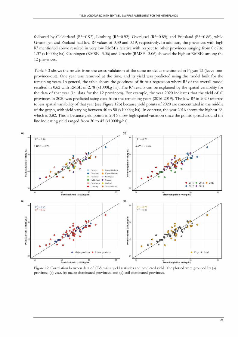
Figure 12. Figure 12 illustrates the statistical yield obtain from CBS and the predicted yield with an R² of 0.76

and RMSE of 2.26 (x1000kg-ha). The model indicates that the temporal measures extracted from the EVI

timeseries can potentially predict crop yield variability. Similar to Figure 9 and Figure 11, the data were divided

into four groupings, namely province, year, maize-dominated province, and soil-dominated province in order to

interpret yield in different dimensions. In general, the yield points scatter throughout the 1:1 line and there is no

substantial systematic deviation. Yields for Friesland, Noord-Brabant, Gelderland, Overijssel, and Limburg are

close to the line indicating an accurate yield estimation where in RMSE were 0.67, 0.91, 0.98, 1.25, 1.37 (x1000kg-

ha), respectively. Figure 12b shows that Noord-Holland, Limburg, Zuid-Holland, and Groningen of year 2018

are underpredicted unlike yield in 2017, indicating the most accurately predicted among the five years. Figure

12c shows data for provinces with major and minor producers. Yields retrieved from satellite data from the

major producers had a stronger correlation with the predicted yields (R² = 0.95), while the minor producers had

an R² of 0.72. Lastly, Figure 12d shows that provinces, where maize was grown in sandy and clay have an R² of

0.81 and 0.72, respectively.

Figure 13 shows the results from the cross-validation of the zYield versus zEVIJA model, which was then back

transformed to yield, whereby one province was left out at the time and subsequently its yield predicts based on

the model constructed for the other provinces. Overall, it was observed that the mean of all 12 models resulted

in R² = 0.72 and RMSE = 2.05 (x1000kg-ha). Based on the cross-validation, Noord-Brabant has and R² of 0.99,


24

followed by Gelderland (R²=0.92), Limburg (R²=0.92), Overijssel (R²=0.89), and Friesland (R²=0.86), while

Groningen and Zeeland had low R² values of 0.30 and 0.19, respectively. In addition, the provinces with high

R² mentioned above resulted in very low RMSEs relative with respect to other provinces ranging from 0.67 to

1.37 (x1000kg-ha). Groningen (RMSE=3.06) and Utrecht (RMSE=3.06) showed the highest RMSEs among the

12 provinces.

Table 5-3 shows the results from the cross-validation of the same model as mentioned in Figure 13 (leave-one-

province-out). One year was removed at the time, and its yield was predicted using the model built for the

remaining years. In general, the table shows the goodness of fit to a regression where R² of the overall model

resulted in 0.62 with RMSE of 2.78 (x1000kg-ha). The R² results can be explained by the spatial variability for

the data of that year (i.e. data for the 12 provinces). For example, the year 2020 indicates that the yield of all

provinces in 2020 was predicted using data from the remaining years (2016-2019). The low R² in 2020 referred

to less spatial variability of that year (see Figure 12b) because yield points of 2020 are concentrated in the middle

of the graph, with yield varying between 40 to 50 (x1000kg-ha). In contrast, the year 2016 shows the highest R²,

which is 0.82. This is because yield points in 2016 show high spatial variation since the points spread around the

line indicating yield ranged from 30 to 45 (x1000kg-ha).

Figure 12: Correlation between data of CBS maize yield statistics and predicted yield. The plotted were grouped by (a) province, (b) year, (c) maize-dominated provinces, and (d) soil-dominated provinces.


25

Figure 13: The maps show (a) Coefficient of determination (R²) and (b) root-mean-square errors of the prediction model based on province after applying a leave-one-province-out cross validation method.

Table 5-3 Coefficient of determination (R²) and root-mean-square errors of the perdition model based on year after applying a leave-one-year-out cross validation method

No. Year R² RMSE (x1000kg-ha)

1 2016 0.82 3.17

2 2017 0.71 2.59

3 2018 0.70 3.69

4 2019 0.56 2.18

5 2020 0.31 2.26

Average 0.62 2.78

5.4. Identicifation of within-province yield variability

Figure 14 illustrates the EVI anomaly map at the municipal level. The cumulative EVI from July to August was

used to create an anomaly map because it was the best predictor for yield estimation. The maps depict the z-

score anomaly by using the mean and standard deviation of each municipality so that each municipality had the

same distribution that the average of the 5-year z-scores for each municipality is 0. The difference between the

current year's z-scored values and the average of all years for the observation (2016-2020) was then used to

generate the anomaly map. In general, the maps confirm that the years 2016 and 2018 had the lowest maize

yields, with every province showing at least some areas with negative anomalies. Furthermore, in Noord-Holland

in any of the five years, municipalities were found with below-normal values. The majority of municipalities in

2017 appeared to be above-average in all provinces, but for some reasons, municipalities in Noord-Holland still

showed that it was below normal.

An example of a province where in the same year the zEVIJA shows both positive and negative anomalies at

municipal level is Overijssel. For example, for 2016 the map (Figure 14) displays six out of the seven z-score

classes (see from the legend) within its provincial boundaries, suggesting a strong spatial variability in maize

performance within the province. Negative z-scores were found in municipalities in the northwest of Overijssel,

whereas in the east z-scores indicated normal to above-average zEVIJA values. Similar variability can be observed

for Overijssel in other years and also for other provinces. This suggests that spatial variability is not accounted


26

for when pooling the EVI from all maize fields in a province. While the focus was on provincial-level yield (given

that reference data were only available at this administrative level), alternative ways to better account for within-

province maize performance can be envisaged.

Figure 14: Z-scored anomaly maps for cumulative EVI from July to August (zEVIJA) for the whole Netherlands. The zEVIJA values were calculated by comparing the municipal EVIJA to its 5-yr average and standard deviation.

Figure 15a depicts the different anomaly map intensities of four municipalities in Overijssel province:

Steenwijkerland (northwest), Deventer (southwest), Hardenberg (northeast), and Enschede (east). Furthermore,

the temporal profiles retrieved from Sentinel-2 and soil proportion were provided to highlight how much

variation exists in these exemplary municipalities within the same province. For instance, Steenwijkerland was

the only municipality below normal in 2016, and the temporal graph also showed relatively low EVI values in

July and August. However, all municipalities show a later green-up stage, resulting in low EVI values in June

(Figure 15b-(Figure 15e). According to the 2018 maps, the zEVIJA for the four regions was below average due to

the summer drought with extremely low precipitation and high temperature (Figure 2). These anomalies were

also visible in the temporal graphs, where an EVI drop occurred in every region after the maturity stage.

Steenwijkerland had a drop in August/September, whereas Deventer, Hardenberg and Enschede experienced a

rapid drop earlier in July/August. Given that different municipalities have different temporal signatures, anomaly

maps at the municipality level can provide more insight into spatial variability better than simply aggregating EVI

values directly from municipality to province. Therefore, the alternative approach for spatial aggregation can be

considered in future studies by using the anomaly maps (Figure 14) to indicate the intra-provincial variability.


27

Figure 15 : Z-scored anomaly maps for cumulative EVI from July to August for three different municipalities in Overijssel. Green indicates a positive anomaly, while dark brown represents a negative anomaly. Maize- and municipality- specific temporal profiles of EVI across five year retrieved from Sentinel-2 images were placed under to the maps. The five-year mean EVI is displayed in grey, while black dashed lines show start of the season (SOS) and end of season (EOS)


28

6. DISCUSSION

The results confirm that Sentinel-2 timeseries allow for accurate prediction of regional yield anomalies in the

Netherlands. According to the linear regression model, EVIJA from the maize maturity stage could explain 76%

of the yield variation. Several studies have also demonstrated that Sentinel-2 data can be used effectively for yield

prediction. Lambert et al. (2018) reported a strong relationship between yield and VIs for two crop types, namely

maize and millet, with R² values of the two crops were observed at 0.85 and 0.84, respectively. Another study

found that by using the peak value of VIs, Sentinel-2 data can explain crop production at a sub-field level,

resulting in relatively high accuracy (Karlson et al., 2020). The result agrees with the phenology and maize yield

assessment by Chirici et al. (2019) where they discovered that EVI has a strong correlation with yield. Their best

predictor was the maximum green-up, and the regression between yield and EVI field average in the first

infection point revealed a high R² of 0.82, while the maturity stage produced an R² of 0.29. Although all studies

reveal the same conclusion, which is that Sentinel-2 data can be effectively used for yield prediction. However,

comparing the performance of crop prediction models with existing studies is difficult due to the different study

areas, crop types, and the methods used to evaluate the model.

Spatial patterns of VI timeseries can vary depending on many factors such as temperature, precipitation, and

farm management practices. Due to data constraints, crop signals were spatially aggregated at the province level

because it is the finest unit of statical yield data that is freely available. The study discovered that the maize

temporal profile of different provinces produces different results, and those results correspond to the climate

and soil types of specific regions. For example, the VIs profiles of Overijssel from the year of known drought in

2018 show a rapid drop in July, while VIs of Flevoland remain steady until August before the drop. This is

because Flevoland is designed for agricultural activities because it is entirely a polder area and is close to the sea,

and the majority of the area contains clay soil with good water retention and groundwater is well regulated due

to its location on very low land (Nijhuis, 2019). On the other hand, Overijssel is a sand-dominated province with

less water-holding capacity, and all farmers adhere to the specific regulation from the government and EU

directives (Özerol et al., 2016). This spatial variation suggested that further studies should take the environmental

factors into consideration while interpreting the result between regions.

Apart from spatial variation, Sentinel-2 timeseries also showed different temporal patterns of maize which proves

that the maize signals extracted from the temporal profiles are aligned with the general maize crop calendar in

the Netherlands. The graphs suggest that SOS and EOS usually take place from May to October/November.

VIs of maize window in 2018 were found to behave differently from the remaining years, especially in the

maturity stage. VI values are expected to reach maximum and remain until August or September, but the graphs

show a sudden drop early after reaching the peak in July for Overijssel and August for Flevoland. According to

the climatic data obtain from the De Bilt station provided by KNMI, the temperature in 2018 was 1.2°C higher

than normal, and precipitation was lower, approximately 80 mm compared to the 30-year average. In addition,

Netherlands was reported as the drought-affected area where a combination of warm and dry conditions

negatively influences the south and east of the country (Philip et al., 2020). This corresponds to the temporal

profiles where the VIs during summer for maize reduced more in Overijssel as compared to Flevoland.

The delay in VI increase in 2016 is apparent for all 12 provinces. The likely explanation for this delay is the

above-normal precipitation and below-normal temperature for spring 2016. This situation coincides with the

fact that Dutch farmers rely on heavy machinery for cultivation and harvesting. As a result, they are unable to

harvest cover crops before the maize season. The high VI in May could be due to the presence of cover crops

on plots that are not yet completely ready for maize cultivation. Since maize is usually cultivated in May, land

needs to be ploughed before sowing the maize. If farmers use heavy tractors in the maize plots during a wetter


29

year than the average, it may cause soil compaction, resulting in decreased root growth which can negatively

affect maize development and production (Chyba et al., 2014; Government of Alberta, 2010). Therefore, the

lower VIs in June could be due to maize being sown one month later. The later start of maize growth could

imply that less heat accumulates, so maize does not fully develop as in other years with earlier sowing dates.

Since maize is a summer crop, it may need a certain amount of temperature requirement.

Both NDVI and EVI provide sufficient information for maize growth stages, but they have different sensitivity

to maize canopy structures. This is because EVI shows more variability within the growing season as compared

to NDVI. For example, NDVI in July-August remains steady for most years in the maturity stage, whereas EVI

shows much more spread. The study demonstrates NDVI tends to saturate in the maturity stage when maize

leaf becomes larger, whereas EVI can better capture when maize reaches the maturity stage or when maize leaves

fully cover the soil background. Because NDVI saturates in dense crop canopies and when chlorophyll is greater

than 150µmol/m², so NDVI does not increase when the biomass increases (Deines et al., 2020; Gitelson et al.,

2003; Ji et al., 2021). EVI is an improved version of NDVI because EVI can get a stronger vegetation signal in

dense leaf regions or high-biomass conditions by using the blue reflectance to correct for soil background signals

and reduce atmospheric influences, including aerosol scattering (Binyong et al., 2009; Rezapour et al., 2021). As

a result, EVI performed better than NDVI, especially in the maturity stage.

EVIJA in the maturity stage is the most important variable that can best explain yield variation. Therefore, it was

then used to assess the with-in province variability. The anomaly map of EVIJA shows that the spatial variability

at the municipality-level can be used to interpret how EVIJA varies in different years and regions. Since it is

beyond the scope of this study to address the questions of what an alternative way of spatial aggregation to a

province-level would be. The map shows that there is much variability within the province of maize performance

and that it could be possible to identify better ways of dealing with this variability. Further study is suggested to

include the anomaly map as one of the indicators to achieve the alternative way of aggregating data into a

province rather than taking a mean VI directly from municipality to province. The idea was based on the system

called Anomaly hot Spots of Agricultural Production (ASAP) using VI characterized by a standard score showing

a normal distribution, and the warning is issued if within an area (sub-national administrative level) has a certain

percentage of the pixels have a z-score below -1 (Rembold et al., 2017). As per the certain threshold used in

ASAP (-1), this critical value can also be used to produce a province-predictor for maize yield by taking the

percentage of area with z-score below -1 within the same province. Therefore, the predictor can be constructed

based on the z-scored anomaly map from EVIJA for further improvement, which considers the within-province

variability.

Fine resolution data (Sentinel-2) has a better capacity for crop-specific signal extraction and yield prediction as

compared to coarse resolution data. The performance of the prediction model can be compared to determine

whether the crop signals of the sensor can accurately predict yield. EVIJA can explain 76% of the yield variability

in this study, while Liu et al. (2019) estimated crop yield using MODIS and revealed the results of lower R². VI

can only explain 65% for maize and other crop types ranged from 30% to 63%. This suggests that Sentinel-2

can better extract the purer signal compared to MODIS (250m). Nevertheless, the capacity of the sensors

depends on the study area as well. For example, Ji et al. (2021) used NDVI from MODIS to assess the

phenological metric in different scales of regions within the central US Corn Belt. They conducted several models

by using leave-one-out cross validation and found that the models can explain 60-80% of the yield variability.

This could be explained by the size of the US maize plots as they are typically much larger as compared to the

Netherlands. Thus, MODIS may be suitable for maize plots in the US but not for the Netherlands or countries

in Europe because field sizes are much smaller, so it becomes much harder to retain pure pixels at 250m

resolution.


30

Aside from the purity of the crop signal, cloud and cloud-shadow contamination may have an impact on the

yield prediction results of this study. Although cloud and cloud shadow algorithms were attempted to use in a

pre-processing step, cloud effect contamination was not effectively removed because the thresholds for each

parameter were assigned for the EU region, it might not be appropriate to adapt to a smaller region like the

Netherlands. Since the temporal composite can help further reduce remaining atmospheric effects, it would have

been more beneficial if the study had better temporal compositing instead of one month in order to get a better

maize trajectory and monitor the signatures more frequently. It can increase data points to the study and fill the

gap of cloud contamination. Perhaps it can better capture some agricultural practices such as early sowing and

maize harvesting within a month as well.

The study is the first attempt at assessing yield at the regional level in the Netherlands, and the results appear

promising. Furthermore, the Copernicus program guarantees Sentinel-2 availability until 2027 and expects more

to follow, so the longer-timeseries analysis is worthwhile to investigate. The study can be used in the future by

increasing the number of crop types included in the study. It can be applied to other areas as well, but keep in

mind the limitations of crop parcels, which are not always freely available in some countries. However, remote

sensing can still help with data collection by obtaining crop parcels and vegetation indices to extract crop-specific

temporal information using the object-based analysis or any other methods.


31

7. CONCLUSION

This study showed that Sentinel-2 timeseries were effective in capturing a substantial amount of the maize yield

variability for provinces in the Netherlands. By focusing the 10-m resolution signal on maize fields in the

province, temporal vegetation index (VI) profiles revealed temporal patterns that correspond to the typical crop

calendar and expected winter cover crop growth. Particularly the summer drought of 2018 caused a substantial

change in the VI profiles, which related particularly for sandy and loess soil with poorer water retention

capabilities in reduced yields. EVI during the July-August period (EVIJA) was the most accurate predictor of

interannual yield variation, explaining 76% of the yield variability. The study provides promising results for yield

prediction with Sentinel-2, which will become more important as timeseries increase in length. Nonetheless,

further study could focus on: 1) comparing the predictive power of Sentinel-2 against similar indices derived

from MODIS to appreciate if relationships improve, 2) reduce the length of the compositing period from

monthly to 10- or 15-day to better capture the crop trajectory, 3) develop effective methods that allow accounting

for within-province yield variability

33

LIST OF REFERENCES

Asner, G. P. (1998). Biophysical and biochemical sources of variability in canopy reflectance. Remote Sensing of Environment, 64(3), 234–253. https://doi.org/10.1016/S0034-4257(98)00014-5

Balaghi, R., Tychon, B., Eerens, H., & Jlibene, M. (2008). Empirical regression models using NDVI, rainfall and temperature data for the early prediction of wheat grain yields in Morocco. International Journal of Applied Earth Observation and Geoinformation, 10(4), 438–452. https://doi.org/10.1016/j.jag.2006.12.001

Binyong, L., Haiping, T., & Donghua, C. (2009). Drought monitoring using the modified temperature/vegetation dryness index. Proceedings of the 2009 2nd International Congress on Image and Signal Processing, CISP’09. https://doi.org/10.1109/CISP.2009.5304333

Bolton, D. K., & Friedl, M. A. (2013). Forecasting crop yield using remotely sensed vegetation indices and crop phenology metrics. Agricultural and Forest Meteorology, 173, 74–84. https://doi.org/10.1016/j.agrformet.2013.01.007

Buras, A., Rammig, A., & Zang, C. S. (2020). Quantifying impacts of the 2018 drought on European ecosystems in comparison to 2003. Biogeosciences, 17(6), 1655–1672. https://doi.org/10.5194/bg-17-1655-2020

Campbell, B. M., Vermeulen, S. J., Aggarwal, P. K., Corner-Dolloff, C., Girvetz, E., Loboguerrero, A. M., … Wollenberg, E. (2016). Reducing risks to food security from climate change. Global Food Security, 11, 34–43. https://doi.org/https://doi.org/10.1016/j.gfs.2016.06.002

Chirici, G., & Gianinetto, M. (2019). Phenology and Yield assessment in maize seed crops using Sentinel-2 VIs’ timeseries. Trends in Earth Observation, 1(January 2021), 218. https://doi.org/10.978.88944687/17

Chyba, J., Kroulík, M., Krištof, K., Misiewicz, P. A., & Chaney, K. (2014). Influence of soil compaction by farm machinery and livestock on water infiltration rate on grassland. Agronomy Research, 12(1), 59–64.

Deines, J. M., Patel, R., Liang, S.-Z., Dado, W., & Lobell, D. B. (2020). A million kernels of truth: Insights into scalable satellite maize yield mapping and yield gap analysis from an extensive ground dataset in the US Corn Belt. Remote Sensing of Environment, 112174. https://doi.org/10.1016/j.rse.2020.112174

Didan, K., Barreto Munoz, A., Solano, R., & Huete, A. (2015). MODIS Vegetation Index User’s Guide (MOD13 Series). Retrieved from http://vip.arizona.edu

Fan, X., Vrieling, A., Muller, B., & Nelson, A. (2020). Winter cover crops in Dutch maize fields: variability in quality and its drivers assessed from multi-temporal Sentinel-2 imagery. International Journal of Applied Earth Observation and Geoinformation, 91, 102139. https://doi.org/10.1016/j.jag.2020.102139

FAO. (2016). Agricultural Informatio AMIS Agricultural Market Information System Crop Yield Forecasting: Methodological and Institutional Aspects. Retrieved from www.fao.org/publications

Fritz, S., See, L., Bayas, J. C. L., Waldner, F., Jacques, D., Becker-Reshef, I., … McCallum, I. (2019). A comparison of global agricultural monitoring systems and current gaps. Agricultural Systems, 168, 258–272. https://doi.org/10.1016/j.agsy.2018.05.010

Gao, B. C. (1996). NDWI - A normalized difference water index for remote sensing of vegetation liquid water from space. Remote Sensing of Environment, 58(3), 257–266. https://doi.org/10.1016/S0034-4257(96)00067-3

Gitelson, A. A., Gritz, Y., & Merzlyak, M. N. (2003). Relationships between leaf chlorophyll content and spectral reflectance and algorithms for non-destructive chlorophyll assessment in higher plant leaves. Journal of Plant Physiology, 160(3), 271–282. https://doi.org/10.1078/0176-1617-00887

Gorelick, N., Hancher, M., Dixon, M., Ilyushchenko, S., Thau, D., & Moore, R. (2017). Google Earth Engine: planetary-scale geospatial analysis for everyone. Remote Sensing of Environment, 202, 18–27. https://doi.org/10.1016/j.rse.2017.06.031

Government of Alberta. (2010). Soil compaction can be a serious form of soil degradation. Agricultural Soil Compaction: Causes and Management.

Housman, I. W., Chastain, R. A., & Finco, M. V. (2018). An evaluation of forest health insect and disease survey data and satellite-based remote sensing forest change detection methods: Case studies in the United States. Remote Sensing, 10(8), 1184. https://doi.org/10.3390/rs10081184

IPCC. (2012). Managing the risks of extreme events and disasters to advance climate change adaptation. Ji, Z., Pan, Y., Zhu, X., Wang, J., & Li, Q. (2021). Prediction of crop yield using phenological information

extracted from remote sensing vegetation index. Sensors (Switzerland), 21(4), 1–17. https://doi.org/10.3390/s21041406

Karlson, M., Ostwald, M., Bayala, J., Bazié, H. R., Ouedraogo, A. S., Soro, B., … Reese, H. (2020). The Potential of Sentinel-2 for Crop Production Estimation in a Smallholder Agroforestry Landscape,

34

Burkina Faso. Frontiers in Environmental Science, 8, 85. https://doi.org/10.3389/fenvs.2020.00085 Kornhuber, K., Osprey, S., Coumou, D., Petri, S., Petoukhov, V., Rahmstorf, S., & Gray, L. (2019). Extreme

weather events in early summer 2018 connected by a recurrent hemispheric wave-7 pattern. Environmental Research Letters, 14(5), 054002. https://doi.org/10.1088/1748-9326/ab13bf

Lambert, M. J., Traoré, P. C. S., Blaes, X., Baret, P., & Defourny, P. (2018). Estimating smallholder crops production at village level from Sentinel-2 time series in Mali’s cotton belt. Remote Sensing of Environment, 216, 647–657. https://doi.org/10.1016/j.rse.2018.06.036

Liu, J., Shang, J., Qian, B., Huffman, T., Zhang, Y., Dong, T., … Martin, T. (2019). Crop yield estimation using time-series MODIS data and the effects of cropland masks in Ontario, Canada. Remote Sensing, 11(20). https://doi.org/10.3390/rs11202419

López-Lozano, R., El Aydam, M., Baruth, B., Willems, E., & García Azcárate, T. (2015). Crop monitoring and yield forecasting at global level The GLOBCAST project from the European Commission. In Watch Letter n°32. Retrieved from http://marswiki.jrc.ec.europa.eu/agri4castwiki/index.php/Main_Page

Mbow, C., Rosenzweig, C., Barioni, L. G., Benton, T. G., Shukla, [ P R, Skea, J., … Malley, J. (2019). Food security. Retrieved from https://www.ipcc.ch/srccl/chapter/chapter-5/

Meroni, M., d’Andrimont, R., Vrieling, A., Fasbender, D., Lemoine, G., Rembold, F., … Verhegghen, A. (2021). Comparing land surface phenology of major European crops as derived from SAR and multispectral data of Sentinel-1 and -2. Remote Sensing of Environment, 253, 112232. https://doi.org/10.1016/j.rse.2020.112232

Meroni, M., Marinho, E., Sghaier, N., Verstrate, M. M., & Leo, O. (2013). Remote sensing based yield estimation in a stochastic framework - Case study of durum wheat in Tunisia. Remote Sensing, 5(2), 539–557. https://doi.org/10.3390/rs5020539

Mirasi, A., Mahmoudi, A., Navid, H., Valizadeh Kamran, K., & Asoodar, M. A. (2019). Evaluation of sum-NDVI values to estimate wheat grain yields using multi-temporal Landsat OLI data. Geocarto International, 1–16. https://doi.org/10.1080/10106049.2019.1641561

Misra, G., Cawkwell, F., & Wingler, A. (2020). Status of phenological research using sentinel-2 data: A review. Remote Sensing, 12(17). https://doi.org/10.3390/RS12172760

Nanzad, L., Zhang, J., Tuvdendorj, B., Nabil, M., Zhang, S., & Bai, Y. (2019). NDVI anomaly for drought monitoring and its correlation with climate factors over Mongolia from 2000 to 2016. Journal of Arid Environments, 164, 69–77. https://doi.org/10.1016/j.jaridenv.2019.01.019

Nijhuis, S. (2019). The noordoostpolder: A landscape planning perspective on the preservation and development of twentieth-century polder landscapes in the Netherlands. In Adaptive Strategies for Water Heritage: Past, Present and Future (pp. 213–229). https://doi.org/10.1007/978-3-030-00268-8_11

NL Times. (2019, July 18). Drought, low water levels trigger irrigation ban in eastern Netherlands |1 NL Times. Retrieved September 29, 2020, from https://nltimes.nl/2019/07/18/drought-low-water-levels-trigger-irrigation-ban-eastern-netherlands

Özerol, G., Troeltzsch, J., Larrue, C., Lordkipanidze, M., Browne, A. L., de Boer, C., & Lems, P. (2016). Drought awareness through agricultural policy: Multi-level action in Salland, the Netherlands. In Governance for Drought Resilience: Land and Water Drought Management in Europe (pp. 159–180). https://doi.org/10.1007/978-3-319-29671-5_8

Philip, S. Y., Kew, S. F., van der Wiel, K., Wanders, N., & Jan van Oldenborgh, G. (2020). Regional Differentiation in Climate Change Induced Drought Trends in the Netherlands. Environ. Res. Lett, 15. https://doi.org/10.1088/1748-9326/ab97ca

Ray, D. K., Gerber, J. S., Macdonald, G. K., & West, P. C. (2015). Climate variation explains a third of global crop yield variability. Nature Communications, 6. https://doi.org/10.1038/ncomms6989

Rembold, F., Korpi, K., & Rojas, O. (2020). Guidelines for using Remote Sensing Derived Information in support of the IPC analysis Guidelines for using Remote Sensing Derived Information in support of the IPC Analysis The Integrated Food Security Phase Classification. 1–18.

Rembold, F., Meroni, M., Urbano, F., Csak, G., Kerdiles, H., Perez-Hoyos, A., … Negre, T. (2019). ASAP: A new global early warning system to detect anomaly hot spots of agricultural production for food security analysis. Agricultural Systems, 168, 247–257. https://doi.org/10.1016/j.agsy.2018.07.002

Rembold, F., Meroni, M., Urbano, F., Lemoine, G., Kerdiles, H., Perez-Hoyos, A., & Csak, G. (2017). ASAP - Anomaly hot Spots of Agricultural Production, a new early warning decision support system developed by the Joint Research Centre. 2017 9th International Workshop on the Analysis of Multitemporal Remote Sensing Images, MultiTemp 2017. https://doi.org/10.1109/Multi-Temp.2017.8035205

Rezapour, S., Jooyandeh, E., Ramezanzade, M., Mostafaeipour, A., Jahangiri, M., Issakhov, A., … Techato,

35

K. (2021). Forecasting rainfed agricultural production in arid and semi-arid lands using learning machine methods: A case study. Sustainability (Switzerland), 13(9). https://doi.org/10.3390/su13094607

Shastry, A., Sanjay, H. A., & Bhanusree, E. (2017). Prediction of Crop Yield Using Regression Techniques. International J Ownal of Soft Computing, 12(2), 7.

van der Velde, M., Biavetti, I., El-Aydam, M., Niemeyer, S., Santini, F., & van den Berg, M. (2019). Use and relevance of European Union crop monitoring and yield forecasts. Agricultural Systems, 168, 224–230. https://doi.org/10.1016/j.agsy.2018.05.001

van der Velde, M., van Diepen, C. A., & Baruth, B. (2019, January 1). The European crop monitoring and yield forecasting system: celebrating 25 years of JRC MARS bulletins. Agricultural Systems, Vol. 168, pp. 56–57. https://doi.org/10.1016/j.agsy.2018.10.003

Veeteelt. (2020). More nitrate leaching on derogation farms due to drought. Retrieved September 29, 2020, from https://veeteelt.nl/nieuws/meer-nitraatuitspoeling-op-derogatiebedrijven-door-droogte

Vrieling, A., Meroni, M., Darvishzadeh, R., Skidmore, A. K., Wang, T., Zurita-Milla, R., … Paganini, M. (2018). Vegetation phenology from Sentinel-2 and field cameras for a Dutch barrier island. Remote Sensing of Environment, 215, 517–529. https://doi.org/10.1016/j.rse.2018.03.014

Vrieling, A., Meroni, M., Mude, A. G., Chantarat, S., Ummenhofer, C. C., & de Bie, K. C. A. J. M. (2016). Early assessment of seasonal forage availability for mitigating the impact of drought on East African pastoralists. Remote Sensing of Environment, 174, 44–55. https://doi.org/10.1016/j.rse.2015.12.003

Westra, S., Fowler, H. J., Evans, J. P., Alexander, L. V., Berg, P., Johnson, F., … Roberts, N. M. (2014, September 1). Future changes to the intensity and frequency of short-duration extreme rainfall. Reviews of Geophysics, Vol. 52, pp. 522–555. https://doi.org/10.1002/2014RG000464

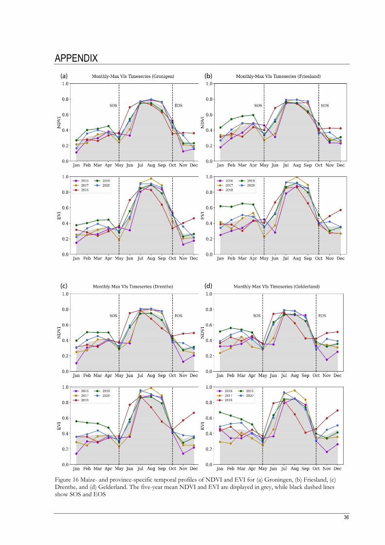
36

APPENDIX

Figure 16 Maize- and province-specific temporal profiles of NDVI and EVI for (a) Groningen, (b) Friesland, (c) Drenthe, and (d) Gelderland. The five-year mean NDVI and EVI are displayed in grey, while black dashed lines show SOS and EOS

37

Figure 17 Maize- and province-specific temporal profiles of NDVI and EVI for (e) Utrecht, (f) Noord-Holland, (g) Zuid-Holland, and (h) Zeeland. The five-year mean NDVI and EVI are displayed in grey, while black dashed lines show SOS and EOS

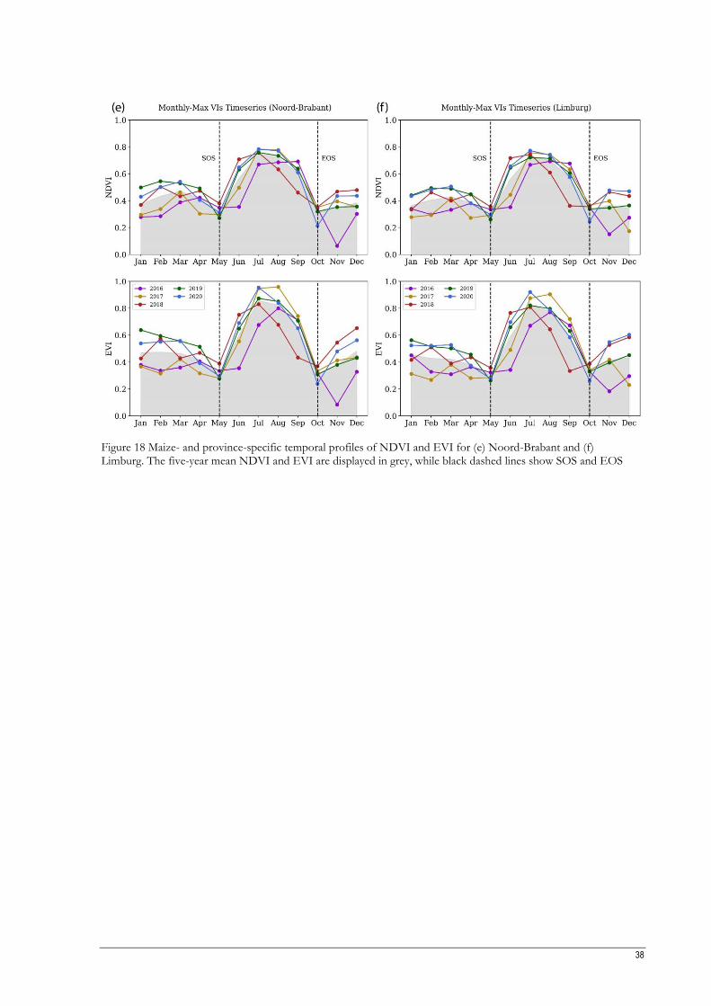
38

Figure 18 Maize- and province-specific temporal profiles of NDVI and EVI for (e) Noord-Brabant and (f) Limburg. The five-year mean NDVI and EVI are displayed in grey, while black dashed lines show SOS and EOS

YIELD MONITORING WITH SENTINEL-2: A FIRST ASSESSMENT …

Documents