YELP CHALLENGE REVIEWS SENTIMENT CLASSIFICATION CHENGENG MA Stony Brook University

Welcome message from author
This document is posted to help you gain knowledge. Please leave a comment to let me know what you think about it! Share it to your friends and learn new things together.
Transcript

YELP CHALLENGE REVIEWS SENTIMENT CLASSIFICATION
CHENGENG MA
Stony Brook University
0. MOTIVATION & DATA DESCRIPTION
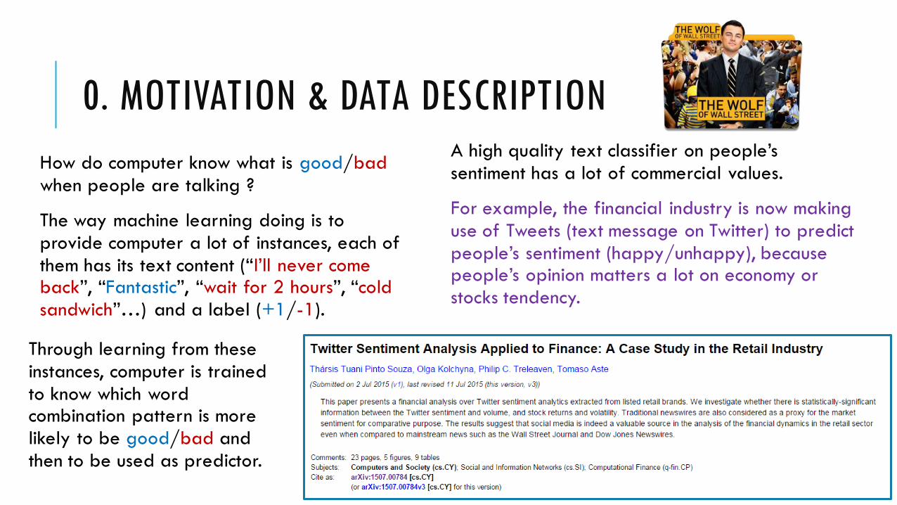
How do computer know what is good/bad
when people are talking ?
The way machine learning doing is to
provide computer a lot of instances, each of
them has its text content (“I’ll never come back”, “Fantastic”, “wait for 2 hours”, “cold
sandwich”…) and a label (+1/-1).
A high quality text classifier on people’s
sentiment has a lot of commercial values.
For example, the financial industry is now making
use of Tweets (text message on Twitter) to predict
people’s sentiment (happy/unhappy), because people’s opinion matters a lot on economy or
stocks tendency.
Through learning from these
instances, computer is trained
to know which word combination pattern is more
likely to be good/bad and
then to be used as predictor.

The yelp challenge dataset
contains about 1.6 million
reviews, collected over 10 cities, 6 of which are in US.
To build a text classifier that
works for US English and
predicts people’s feeling about restaurants, only the
reviews for restaurants within
the 6 US cities are considered.
Reviews with a star of 1 or 2
are labeled as bad, and 4 or 5 as good. Reviews with star 3
are ignored.
Finally, over 6 US cities’ 17, 670 restaurants,
totally 795, 667 reviews are used, which are made up by
618, 048 positive reviews and 177, 619 negative reviews.
Original text is 1.8 GB, stored in sparse matrix (Ndoc X Nword)
Parallelizing 11 threads, about 1 hour’s work.
We assume people are consistent with themselves, i.e. when people are giving a high/low rate star, the review text should also be a compliment/criticism.

1. DATA PREPROCESSING
Using NLTK package for language
processing, the ENCHANTED dictionary
package for spelling checking and suggestions, and some codes are provided
by Python Text Processing with NLTK 3.0
Cookbook.
1. Face emotion symbols
:-) I love it, I enjoy it !
:-( I hate it, I am unhappy !
2. Lowercase every word
3. Contraction restoring (don’t do not)
4. Tokenizing sentences into words ( punctuations
removed at this step , . : ! ? _ ‘ “ ` ~ + - * / ^ \ = > < @ # $ % & ( ) [ ] { } | )
5. Repeating words processing
looove love, aaammmzzzing amazing
6. Stemming
heated heat, enjoying enjoy, …
7. Removing Stop Words (the, you, I, am, …)

REPEATING WORDS: LOOOOVE, SOOOOO GOOOOD, NO WWWAAAYYY
Using the code from Python Text Processing with NLTK 3.0 Cookbook.But the code is too aggressive:
wwwaaayyy way
sooooo so
goooood good app ap
cannot canot cooked coked
unless unles off of
bloody blody shall shal
Using the ENCHANTED dictionary as a spelling checking tool.
new_word = NLTK_code(old_word)
dUS=Enchanted_Dictionary(en-US)
if old_word != new_word
if old_word not exist in dUS and new_word exist in dUS:
Replacing the old_word by new_word
Only when the old word is
not correctly spelled, and
the new word is correctly
spelled, then a
replacement will be made.
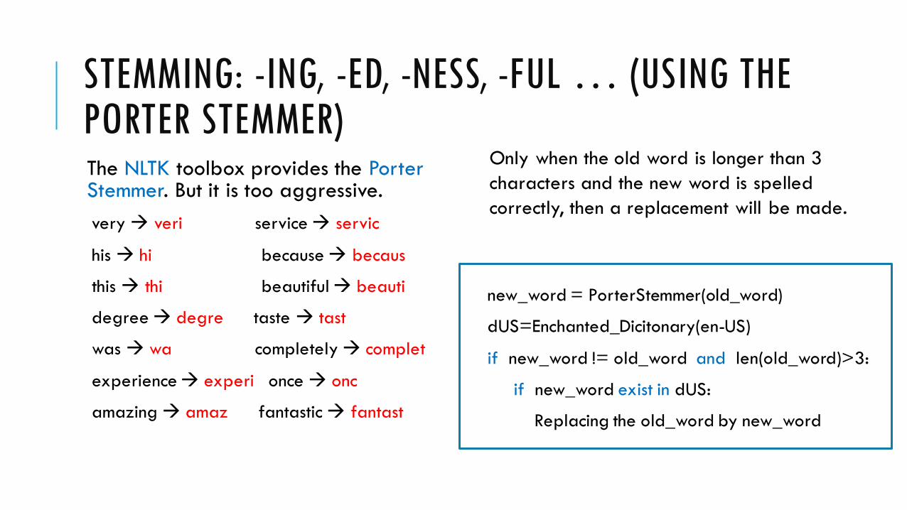
STEMMING: -ING, -ED, -NESS, -FUL … (USING THE PORTER STEMMER)The NLTK toolbox provides the Porter Stemmer. But it is too aggressive.
very veri service servic
his hi because becaus
this thi beautiful beauti
degree degre taste tast
was wa completely complet
experience experi once onc
amazing amaz fantastic fantast
new_word = PorterStemmer(old_word)
dUS=Enchanted_Dicitonary(en-US)
if new_word != old_word and len(old_word)>3:
if new_word exist in dUS:
Replacing the old_word by new_word
Only when the old word is longer than 3
characters and the new word is spelled
correctly, then a replacement will be made.

2. DIMENSION REDUCTION
Finally, totally 152,177 unique words
are found out.
But a most of them are just mistakenly
spelled words that the above language
processing fail to correct or sentences that have no blank.
aaaahhhhmzing ahmzing ?
aaaaaahhhhhh ah ?
Aaaccctually actualy ?
thisisthebestplaceasfarasIknow
To make our word terms statistically significant, I
calculate the Information Gain (IG) for each
words and sort words by IG from large to small.
The cumsum of IG is cut off by its 95% position.
Only 19,821 words are kept finally for training classifier.
𝐼𝐺 𝑋 = 𝑋𝑖∈{0, +} 𝑌𝑗∈{−1, 1} ln(𝑃(𝑋=𝑋𝑖, 𝑌=𝑌𝑗)
𝑃 𝑋𝑖 𝑃(𝑌𝑗))
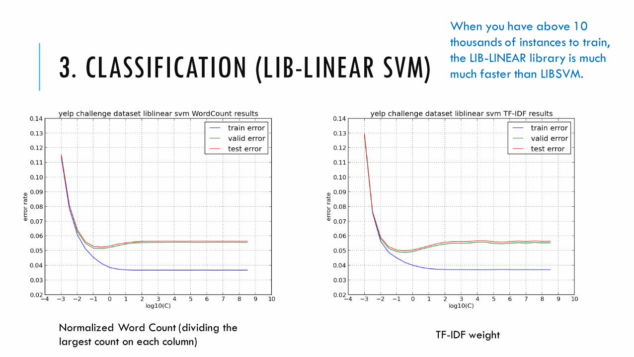
3. CLASSIFICATION (LIB-LINEAR SVM)
Normalized Word Count (dividing the
largest count on each column)TF-IDF weight
When you have above 10
thousands of instances to train,
the LIB-LINEAR library is much
much faster than LIBSVM.

Normalized Word Count, optimal C=10^(-0.5)
TF-IDF weight, optimal C=10^(-0.5)
Because we have a quite large dataset, this time we use 1/2 data for train (397,834), 1/4 for validation (198,917) and 1/4 for test (198,916).
The SVM is trained on a sparse matrix through Scikit-learn’s component package Lib-Linear, which takes about 5~100 seconds for a single training task.
𝑇𝐹 𝑖, 𝑗 =𝑛𝑖,𝑗
𝑘=1𝐷 𝑛𝑖,𝑘
𝐼𝐷𝐹 𝑗 = 𝑙𝑜𝑔2(𝑁
𝑖=1𝑁 𝐼(𝑛𝑖,𝑗 > 0)
)
𝑇𝐹_𝐼𝐷𝐹 𝑖, 𝑗 = 𝑇𝐹 𝑖, 𝑗 ∗ 𝐼𝐷𝐹(𝑗)
The TF-IDF method has 0.2523% smaller error rate than the simple normalized word count method on test data, which means another 502 reviews are correctly classified.
And on the validation data, the TF-IDF has more 528 reviews correctly classified than the other.

4. 100 MOST POSITIVE & NEGATIVE WORDS
By dividing each word’s largest count on
each column, the word counts are
normalized, so the SVM’s linear weight on each word can be used to represent
the extent how much a word is
positive/negative.
Generally, the SVM weight is consistent
with the difference of average word counts between (+) & (-) groups and
anti-symmetric with the Information Gain..
Now we show the SVM weights learned
from the training data and select the
largest 100 positive weight words and the largest 100 negative weight words.

100 MOST NEGATIVE WORDS

100 MOST POSITIVE WORDS
Related Documents