INTEGRATED CONCEPTUAL DESIGN OF JOINED-WING SENSORCRAFT USING RESPONSE SURFACE MODELS. THESIS Josh E. Dittmar, Lieutenant Commander, USN AFIT/GAE/ENY/07-D02 DEPARTMENT OF THE AIR FORCE AIR UNIVERSITY AIR FORCE INSTITUTE OF TECHNOLOGY Wright-Patterson Air Force Base, Ohio APPROVED FOR PUBLIC RELEASE; DISTRIBUTION UNLIMITED

Welcome message from author
This document is posted to help you gain knowledge. Please leave a comment to let me know what you think about it! Share it to your friends and learn new things together.
Transcript

INTEGRATED CONCEPTUAL DESIGN OF JOINED-WING SENSORCRAFT USING RESPONSE SURFACE MODELS.
THESIS
Josh E. Dittmar, Lieutenant Commander, USN AFIT/GAE/ENY/07-D02
DEPARTMENT OF THE AIR FORCE
AIR UNIVERSITY
AIR FORCE INSTITUTE OF TECHNOLOGY Wright-Patterson Air Force Base, Ohio
APPROVED FOR PUBLIC RELEASE; DISTRIBUTION UNLIMITED

The views expressed in this thesis are those of the author and do not reflect the official policy or position of the United States Air Force, Department of Defense, or the United States Government.

INTEGRATED CONCEPTUAL DESIGN OF JOINED-WING SENSORCRAFT USING RESPONSE SURFACE MODELS
THESIS
Presented to the Faculty
Department of Aeronautics and Astronautics
Graduate School of Engineering and Management
Air Force Institute of Technology
Air University
Air Education and Training Command
In Partial Fulfillment of the Requirements for the
Degree of Master of Science in Aeronautical Engineering
Josh E Dittmar, BS
LCDR, USN
Nov 2006
APPROVED FOR PUBLIC RELEASE; DISTRIBUTION UNLIMITED
AFIT/GAE/ENY/07-D02
INTEGRATED CONCEPTUAL DESIGN OF JOINED-WING SENSORCRAFT USING RESPONSE SURFACE MODELS.
Josh E Dittmar, B.S.
Lieutenant Commander, USN
Approved:

AFIT/GAE/ENY/07-D02
Abstract
This study performed a multidisciplinary conceptual design and analysis
of Boeing’s joined-wing SensorCraft. The joined wing aircraft concept fills a long dwell
multi-spectral reconnaissance DOD need, incorporating an integral embedded antenna
structure within the wing skin. This analysis was completed using geometrical
optimization, aerodynamic analyses, and response surface methodology on a composite
structural model. Structural optimization was not performed, but data connectivity
between the geometric model and the Finite Element Model was demonstrated, to enable
follow-on structural optimization efforts.
Phoenix Integration’s Model Center was used to integrate the sizing and analysis
codes found in Raymer’s text, “Aircraft Design: A Conceptual Approach” as well as
those from the NASA derived conceptual design tool AirCraft Synthesis (ACSYNT), and
a modified Boeing Finite Element Model (FEM). MATLAB codes were written to
modify a NASTRAN structural grid model based on any alteration of the design variables
throughout the structure. A concept validation model was also constructed based on the
S-3 Viking and Take-off Gross Weight (TOGW) values were found to be within 4 % of
actual published aircraft values.
Seven design variables were perturbed about the Boeing solution to determine the
response of the joined wing model to the design changes and response surfaces were
plotted and analyzed, to drive the solution to the lowest TOGW. The design variables are:
overall wing span (b), front wing sweep (Λib), aft wing sweep (Λia), outboard wing sweep
iv

(Λob), joint location as a percentage of half span (jloc), vertical offset of the aft-
wing root (zfa) and airfoil thickness to chord ratio (t/c).
This research demonstrated the utility of integrated low-order models for fast and
inexpensive conceptual modeling of unconventional aircraft designs. Wind tunnel and
flight data would allow a more in-depth evaluation of the performance and accuracy of
the codes, and a structural optimization based on several different load cases, including
gust loads at zero fuel weight (ZFW) would provide better predictions of structural
weight data.
v

Dedication
“To God belong wisdom and power; counsel and understanding are his.”
Job 12:13
I am most grateful to my God and Savior the Lord Jesus Christ, the author of all
things, for his guidance, and inspiration in this work. If anything is excellent, it is
because He had a hand in it. I am also deeply indebted to my wife, and my five children
for their patience and understanding while I was “working on my thesis.”
vi

Acknowledgements
I would like to express my sincere appreciation to my thesis advisor, Dr. Robert
Canfield for his guidance and instruction throughout this thesis effort. His abundant
patience and encouragement were immensely helpful.
I greatly appreciate the review of this work by Dr. David Jacques, Dr. Donald
Kunz, and Dr. Maxwell Blair. Their honest critique, insight, experience, and direction
were greatly valued.
Finally, I would like to recognize my family. I could not have completed this
endeavor without the loving support and encouragement of my wife and five children.
They deserve the lion’s share of appreciation.
“Sons are a heritage from the LORD, children a reward from him. Like arrows in
the hands of a warrior are sons born in one's youth. Blessed is the man whose quiver is
full of them.” Psalm 127:3-5
vii

Table of Contents
Page
Abstract.............................................................................................................................. iv
Dedication.......................................................................................................................... vi
Acknowledgements........................................................................................................... vii
List of Figures.................................................................................................................... xi
List of Tables ................................................................................................................... xiv
List of Tables ................................................................................................................... xiv
List of Symbols................................................................................................................. xv
I. Introduction ................................................................................................................ 1
Motivation................................................................................................................... 1 Problem Statement ...................................................................................................... 1 Overview..................................................................................................................... 3
II. Background ................................................................................................................. 7
Joined-Wing Design Overview........................................................................................... 7 Joined-Wing Design Genesis.............................................................................................. 8 Recent Local Joined-Wing Collaboration......................................................................... 11 SensorCraft Overview....................................................................................................... 13 Airframe Studies ............................................................................................................... 13 Boeing AEI Study............................................................................................................. 16
Mission Profile: ........................................................................................................ 17 Baseline Configuration (Model 410E)...................................................................... 19 Airfoil creation method ............................................................................................. 19 Improving Lift-to-Drag (L/D) Ratio.......................................................................... 20 Multi-Disciplinary Optimization (MDOPT) ............................................................. 21 Boeing Finite Element Model (FEM ) ...................................................................... 22 Aerodynamic Analysis Used ..................................................................................... 23 Summary of Boeing Findings of Joined Wing Benefits............................................. 23 Structural Weights Summary .................................................................................... 24 AEI Study Results ...................................................................................................... 25
Boeing Joined-Wing SensorCraft (Model 410E).............................................................. 26
III. Methodology ......................................................................................................... 29
Overview........................................................................................................................... 29 Tools Used ........................................................................................................................ 32
ModelCenter ............................................................................................................. 32 Model Coordinate System..................................................................................... 33
MATLAB ................................................................................................................... 33 Super-Elliptical Fuselage Shapes.......................................................................... 35
viii

AirCraft SYNthesis (ACSYNT) .................................................................................. 39 Primary ACSYNT Modules.................................................................................. 40 ACSYNT Operation.............................................................................................. 44
General Geometry Generator (GGG)....................................................................... 45 Initial Historical Sizing ..................................................................................................... 46
Weight Buildup.......................................................................................................... 47 Empty Weight Fraction ............................................................................................. 47 Fuel Fraction ............................................................................................................ 48 Specific Fuel Consumption (SFC) ............................................................................ 50 Lift-to-drag ratio (L/D) Estimation........................................................................... 50 First Order Design Method Overview ...................................................................... 52
Refined Sizing................................................................................................................... 53 Semi-empirical Sizing....................................................................................................... 55
ACSYNT .................................................................................................................... 55 Raymer Approximate and Group Weights Sizing Methods....................................... 57
Finite Element Model Structural Weight.......................................................................... 57
IV. Results and Discussion ......................................................................................... 58
Model Construction .......................................................................................................... 58 S-3 Validation Model........................................................................................................ 59
Objective ................................................................................................................... 59 S-3 Model .................................................................................................................. 59 Geometry................................................................................................................... 60 Trajectory.................................................................................................................. 60 Aerodynamics............................................................................................................ 62 Propulsion................................................................................................................. 62 Weights...................................................................................................................... 62 Results ....................................................................................................................... 64 Impact ....................................................................................................................... 66
Raymer’s Canarded ASW Aircraft ................................................................................... 66 Overview ................................................................................................................... 66 Geometry................................................................................................................... 67 Propulsion................................................................................................................. 70 Results ....................................................................................................................... 70 Impact ....................................................................................................................... 72
Boeing SensorCraft Joined Wing (410E) ......................................................................... 73 Introduction............................................................................................................... 73 Surrogate ACSYNT input Model ............................................................................... 74 Trajectory/Mission .................................................................................................... 76 Propulsion................................................................................................................. 76 Aerodynamics............................................................................................................ 77 Weights...................................................................................................................... 77 ACSYNT sizing .......................................................................................................... 78 Design Variables....................................................................................................... 85 Design of Experiments (DOE) .................................................................................. 85
ix

Sensitivity Analysis.................................................................................................... 85 Joined-Wing Response Surfaces ............................................................................... 87
V. Conclusions and Recommendations ......................................................................... 89
List of References ............................................................................................................. 92
Appendix A: ACSYNT Files............................................................................................ 95
Appendix B: Variable Interaction Plots.......................................................................... 128
Appendix C: MATLAB Code (Super-Elliptical Generator)........................................... 139
Appendix D: MATLAB Code (WingArea) .................................................................... 142
Appendix E: Excel Spreadsheet (Initial Sizing) ............................................................. 143
Appendix F: MATLAB FEM Manipulation (modxyz.m) .............................................. 144
Appendix G: Response Surface Model Standard Analysis of Variance (ANOVA) Summary ......................................................................................................................... 147
Appendix H: Effect of Laminar Flow (SFWF) in ACSYNT on TOGW........................ 148
x

List of Figures Figure Page
Figure 1 Boeing Joined-Wing SensorCraft (Model 410C) ................................................ 1
Figure 2 AFIT/AFRL Joined-Wing SensorCraft ................................................................ 2
Figure 3 Design Variables for Joined Wing ....................................................................... 6
Figure 4 Wolkovich Joined Wing Design........................................................................... 7
Figure 5 Visual Comparison of SensorCraft Designs (ref. 20)......................................... 13
Figure 6 Boeing SensorCraft 3-view and size comparison (Model 410C) (ref. 20)......... 16
Figure 7 Boeing Joined-Wing SensorCraft Mission (ref. 21)........................................... 17
Figure 8 Multi-Disciplinary Optimization System (ref. 21) ............................................. 22
Figure 9 Boeing Finite Element Model (FEM) Model 410E............................................ 23
Figure 10 CAD Model of 410E ........................................................................................ 27
Figure 11 Conformal Load-bearing Array Structure (CLAS) .......................................... 28
Figure 12 Simplified Integrated Sizing Method ............................................................... 30
Figure 13 ModelCenter 3-D Geometry............................................................................. 31
Figure 14 ModelCenter Integration Environment............................................................. 32
Figure 15 Model Coordinate System ................................................................................ 33
Figure 16 Fuselage Wireview Rendered in ModelCenter (Nose, Midsection and Aft).... 34
Figure 17 Sample of Super-Elliptical Cross Sections (ref. 28)......................................... 36
Figure 18 Super Elliptical Cross Sections for p and q Varied from 1 to 4. (ref. 28) ........ 36
Figure 19 MATLAB Display of Non-Axisymetric S-3 Model Aft Fuselage................... 37
Figure 20 S-3 Cylindrical Non-Axisymmetric Fuselage .................................................. 37
Figure 21 Square-to-Circle Shape Adapter....................................................................... 38
xi

Figure 22 S-3 Rounded Rectangle Non-Axisymmetric Fuselage..................................... 38
Figure 23 Example GGG Display..................................................................................... 45
Figure 24 Weight Fraction Empty Trends (ref. 2) ............................................................ 48
Figure 25 ASW Mission ................................................................................................... 48
Figure 26 Maximum Lift-to-Drag Ratio Trends (ref. 2).................................................. 51
Figure 27 First -Order Design Method (ref. 2) ................................................................. 52
Figure 28 Sensitivity Analysis of Empty Weight Fraction Equation ............................... 54
Figure 29 Response of Refined Weight to T/W and W/S Inputs for Model (2) Raymer ASW Aircraft ............................................................................................................ 55
Figure 30 Lockheed S-3 Viking........................................................................................ 59
Figure 31 Mission (1) HI-LO-HI ASW Mission (Actual S-3) ......................................... 61
Figure 32 Mission (2) HI-HI-HI ASW Mission (Raymer) ............................................... 61
Figure 33 ACSYNT Integration with ModelCenter ......................................................... 64
Figure 34 ASW Concept Sketches.................................................................................... 66
Figure 35 Comparison of Raymer’s ASW Sketch and ModelCenter Aircraft ................. 67
Figure 36 ASW Aircraft Modeled in ModelCenter .......................................................... 68
Figure 37 Model Center ASW Variants............................................................................ 69
Figure 38 Wing Canard Positioning as Fraction of Fuselage Radius ............................... 70
Figure 39 Boeing SensorCraft 410D Point-of-Departure Layout (ref. 21)....................... 73
Figure 40 Reference Areas for Wing................................................................................ 74
Figure 41 Surrogate ACSYNT Input Model..................................................................... 75
Figure 42 Simplified Fuselage with Constant Cross Section ........................................... 75
Figure 43 Comparison of Surrogate (left) and Original (right) Models ........................... 76
Figure 44 Joined Wing Finite Element Model Sections ................................................... 79
Figure 45 ModelCenter Structural Weight Incorporation................................................. 84
xii

Figure 46 Variable Sensitivity Analysis ........................................................................... 86
xiii
List of Tables Table Page
Table 1 Comparison of SensorCraft Designs (data from ref. 20) ..................................... 15
Table 2 Mission Profiles for Boeing Analysis and ACSYNT Analysis for Joined-Wing SensorCraft ............................................................................................................... 18
Table 3 JW Model 410E FEM Empty Weight Breakdown .............................................. 24
Table 4 Boeing SensorCraft Structural Weight Comparison (Baseline vs. Optimized)... 25
Table 5 Model Parameter Comparison ............................................................................. 27
Table 6 ACSYNT Default Engine Data (ref. 23) ............................................................. 43
Table 7 Approximate Mission Weight Fractions (ref. 2).................................................. 49
Table 8 Specific Fuel Consumption (ref. 2)...................................................................... 50
Table 9 Key Model Parameters......................................................................................... 58
Table 10 ASW Mission Comparison ................................................................................ 61
Table 11 S-3 Fixed Weights Breakdown.......................................................................... 63
Table 12 Comparison of TRANSPORT and BOMBER Weight Categories.................... 65
Table 13 S-3 NATOPS and ACSYNT Weight Comparison for Mission (1) ................... 65
Table 14 ASW Aircraft/Mission Requirements................................................................ 66
Table 15 Canarded ASW Aircraft and S-3 Weight Comparison for Mission (2)............. 71
Table 16 Comparison of Weight Estimation Methods for the Canarded ASW Aircraft .. 72
Table 17 Detail of ACSYNT Model Weight Slopes ........................................................ 77
Table 18 Joined Wing Weights Comparison .................................................................... 79
Table 19 FEM Manipulation Equations Matrix................................................................ 81
xiv

List of Symbols Symbol Definition
α..................................................................................................................Angle of Attack
ρ..........................................................................................................................Air Density
Λ.............................................................................................................Wing Sweep Angle
b...................................................................................................................Half-Wing Span
c……......................................................................................................Wing Chord Length
ft .....................................................................................................................................Feet
g................................................................................................Acceleration Due to Gravity
hr.....................................................................................................................................hour
ksi....................................................................................Thousand Pounds per Square Inch
m ............................................................................................................................... Meters
q............................................................................................................... Dynamic Pressure
s ……....................................................................................................................... Seconds
t …….......................................................................................................Element Thickness
x ...........................................................................................................Cartesian Coordinate
y........................................................................................................... Cartesian Coordinate
z............................................................................................................Cartesian Coordinate
C.................................................................................................Specific Fuel Consumption
D.....................................................................................................................................Drag
E............................................................................................................................Endurance
F ..................................................................................................................................Forces
L.......................................................................................................................................Lift
Pa……........................................................................................................................Pascals
xv
Symbol Definition
R...................................................................................................................................Range
S .............................................................................................................Wing Surface Area
V................................................................................................................Velocity, Volume
W................................................................................................................................Weight
X......................................................................................................................Sample Value
xvi

INTEGRATED CONCEPTUAL DESIGN OF JOINED-WING
SENSOR-CRAFT USING RESPONSE SURFACE MODELS
I. Introduction
Motivation
SensorCraft is an aircraft developmental concept, derived from a U.S. Air Force
need to provide next generation persistent multi-spectral intelligence, surveillance and
reconnaissance (ISR). The high-altitude long-endurance (HALE) unmanned air vehicle
(UAV) will exhibit long-dwell capabilities and integrate available and future sensors.
However, in order to achieve both high endurance and superior radar performance, new
aerodynamic designs are required. One candidate platform is based on a joined-wing
configuration (Fig. 1), permitting enhanced 360° radar coverage, increased endurance,
and a lighter structural weight, typically correlating to lower production costs.
Figure 1 Boeing Joined-Wing SensorCraft (Model 410C)
Problem Statement
These concepts are not without problems and their innovation in form casts a
great barrier to the use of conventional design and algorithms based on historical trends.
Non-linear responses and other obstacles prevent oversimplification achievable with a
linear system. The “build and fly” technique previously employed is simply not cost
feasible. The current thrust of industry is in reducing the effort, time and cost of
1
manufacturing and testing through use of computerized modeling and simulation and this
integrated modeling technique was investigated for the Boeing joined-wing SensorCraft
concept.
Aircraft design is by nature iterative and susceptible to large unforeseen responses
to small changes in design variables. In short, “everything affects everything else.” The
typical design scenario requires teams of experts in various disciplines (aerodynamics,
structural, control, etc.) working together and passing information “over the fence” to the
other teams. It is often unclear what the current baseline model is, and tenuous to keep
the teams utilizing exactly the same design data. Integration of data and effort is needed.
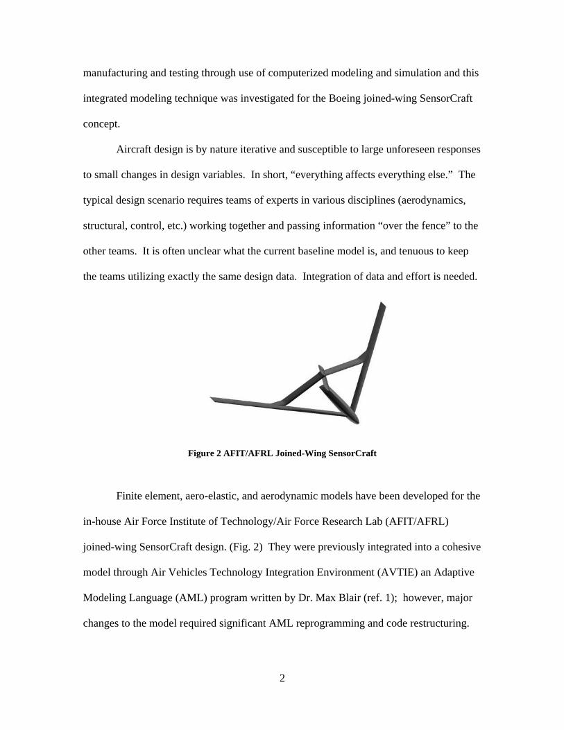
Figure 2 AFIT/AFRL Joined-Wing SensorCraft
Finite element, aero-elastic, and aerodynamic models have been developed for the
in-house Air Force Institute of Technology/Air Force Research Lab (AFIT/AFRL)
joined-wing SensorCraft design. (Fig. 2) They were previously integrated into a cohesive
model through Air Vehicles Technology Integration Environment (AVTIE) an Adaptive
Modeling Language (AML) program written by Dr. Max Blair (ref. 1); however, major
changes to the model required significant AML reprogramming and code restructuring.
2
A more easily adaptable model was desired, based on the current Boeing joined-wing
SensorCraft Model. The focus of this research is to develop an integrated, scalable model
in Phoenix Integration’s ModelCenter (ref. 6) that incorporates mission profiles, a
modifiable finite element model, and aerodynamics for the Boeing joined-wing
SensorCraft configuration, which can be adapted and refined if more fidelity is needed or
as requirements change.
Overview
This work attempts to mark out and evaluate a strategy to overcome some of the
design obstacles previously mentioned: namely, lack of integration, speed of redesign and
heavy reliance on historical data, when dealing with unconventional designs. Phoenix
Integration’s ModelCenter provided the integration environment to tie all of the model
data together in a single place, linking sizing routines and aerodynamic formulas from
Raymer (ref. 2), input/output data from AirCraft Synthesis (ACSYNT C), a legacy
NASA FORTRAN design code rewritten in C (ref. 3), as well as structural data from
Boeing’s Finite Element Model (FEM). Having all the data connected meant less time
rekeying input files and more time analyzing and optimizing the design. Instead of just
answering the question “Will the design fly?” an integrated approach allows one to ask
and answer the question “Is the design optimal?”
A primary purpose of this study was to establish a confidence level in the ability
of the NASA derived conceptual sizing code ACSYNT coupled to a NASTRAN Finite
Element Model (FEM) within ModelCenter to analyze unconventional designs such as
the joined wing. The first step consisted of creating and analyzing a validation model in
3

ModelCenter based on a current conventional aircraft design, the S-3 Viking. Expected
fidelity is a calculated Take-off Gross Weight (TOGW) within ten percent of the actual
aircraft TOGW.
Based on available aircraft data (refs. 4, 5), an S-3 model was constructed in
Model Center and analyzed with ACSYNT and historical codes. Two separate mission
profiles were attempted, one based on Raymer’s hypothetical Anti-Submarine Warfare
(ASW) mission (ref. 2 - chap3) and one based on one of the actual ASW missions
contained in the S-3 NATOPS (ref. 4). Results obtained were then compared with data
from the documented flight performance of the vehicle in NATOPS. Previous studies
have shown that ACSYNT is capable of calculating aircraft weights to within 10 % of the
actual weight. (ref. 5) This study showed that ACSYNT was within 4 % in calculating
the gross weight of the S-3 model and 12 % in predicting fuel weight for conventional
designs. Raymer’s (ref. 2) initial and refined approaches, discussed in chapters 3 and 6 of
the text, underestimated TOGW by 17 and 27% respectively.
Next a semi-conventional canarded ASW aircraft model was constructed, to serve
as an unconventional validation model, derived from Raymer’s ASW example (ref. 2),
described in chapter 3 of the text and detailed in chapter 3 of this document. Loosely
based on Lockheed’s S-3 Viking, the sizing can be expected to be within 10-15% of the
S-3’s actual weight – with similarly varying component weights, assuming the mission
given is comparable with typical S-3 mission profiles.
Finally a joined wing model was constructed from the available Boeing
SensorCraft data (ref. 21), and together with ACSYNT results, Finite Element Analysis
(FEA) structural weights were compared with the given Boeing technical data, providing
4

some idea of the fidelity of the model. Results gave a TOGW for the joined wing model
within 1.9 % of the baseline (410D) model.
The model was then perturbed to investigate the response of the joined wing
model to the seven design variables, creating an array of varying geometric
configurations for the joined-wing aircraft. The design variables are shown in figure 3
and include: half-wing span (b), leading-edge front wing sweep (Λib), trailing edge aft
wing sweep (Λia), leading-edge outboard wing sweep (Λob), joint location as a percentage
of half span (jloc), vertical offset of the aft-wing root (zfa) and airfoil thickness to chord
ratio (t/c). Geometric optimization, aerodynamic analyses, and response surface
methodology were tied together in ModelCenter to determine the optimum configuration
(lowest-weight) and to determine the relative impact of each design variable on the
design.
The use of response surface methodology allows the aircraft designer to more
completely comprehend the complex interactions between the design variables and
provide the optimal parameters for a joined-wing concept. As mathematical surrogates,
response surfaces allow very rapid run times on complex models: on the order of 12
times faster in this study. If well fitted, these mimic with great accuracy the behavior of
the complete model. This rapid run time enables the designer to flesh out the design
space in a fraction of the computational time that would be required for the entire model.
As a result of this research, response surfaces were generated for important
performance measures, a sensitivity analysis of the baseline joined-wing SensorCraft
design (model 410E) was accomplished and the design trade space was evaluated in order
5

to depict more fully the nature of the joined-wing SensorCraft design problem and guide
continuing joined wing design.
Figure 3 Design Variables for Joined Wing
6
II. Background
Joined-Wing Design Overview
Joined-wing aircraft are categorized as aircraft having an aft wing joined to a
front wing. The front wing root is attached to the fuselage, and the aft wing root is
attached atop the tail. Often, the front wing has aft sweep and the aft wing has forward
sweep. An outer wing section is usually present due to the joint location, where the front
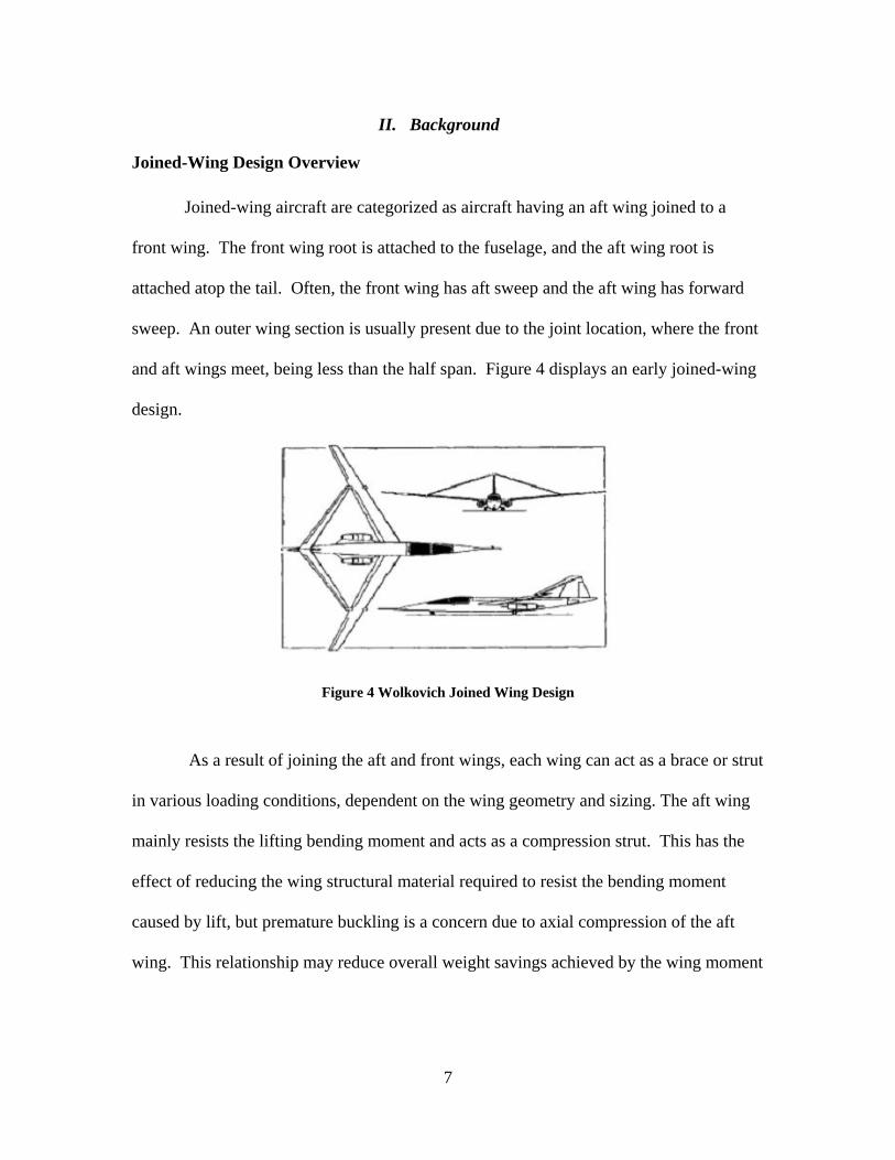
and aft wings meet, being less than the half span. Figure 4 displays an early joined-wing
design.
Figure 4 Wolkovich Joined Wing Design
As a result of joining the aft and front wings, each wing can act as a brace or strut
in various loading conditions, dependent on the wing geometry and sizing. The aft wing
mainly resists the lifting bending moment and acts as a compression strut. This has the
effect of reducing the wing structural material required to resist the bending moment
caused by lift, but premature buckling is a concern due to axial compression of the aft
wing. This relationship may reduce overall weight savings achieved by the wing moment
7
relief, if the aft wing now requires more structure to resist buckling due to carrying axial
loads.
Joined-Wing Design Genesis The pioneering work in joined-wing design was conducted by Wolkovich [7],
who holds the 1976 patent for a joined wing aircraft. Later in 1985, Wolkovich [8]
published results stemming from finite element and wind tunnel analysis of the joined-
wing concept. He detailed several distinct advantages of a joined-wing configuration
over a more traditional design, chiefly a lighter, stiffer airframe exhibiting lower induced
drag, a high trimmed maximum lift coefficient (CLmax), and bending moment relief at a
very small expense of the span efficiency factor. He also calculated that a joined-wing
design could carry 150% of the fuel in conventional designs, due to the additional volume
available in the aft wing. This study will investigate the response of a joined-wing design
to change in geometric parameters.
Fairchild [9] compared structural weights of a conventional and a joined wing.
Both wing types utilized the same airfoil (NACA 23012) with thickness-to-chord ratio
(t/c) and structural box size held constant. He showed for aerodynamically equal
configurations, the joined-wing design resulted in an approximate 12% reduction in
weight over the conventional wing. This study will compare the structural weights of an
“optimized” joined-wing and geometric perturbations of that model.
Following Wolkovich, Smith, Cliff and Stonum performed calculations and
wind tunnel testing on a 1/6th scale joined-wing research aircraft, based on three
geometric modifications of the oblique wing test aircraft NASA AD-1. [10, 11] The
8
demonstrator was analyzed in a Mach 0.8 transport role, at optimum cruise altitude. A
principal finding was that of optimum joint location at 60 percent of the fore wing
semispan. Wind tunnel data confirmed the design predictions for reduced bending
moment on the forward wing, and a span efficiency of greater than one; however, the
design displayed unstable stall characteristics, no flight test vehicle was built, and no
structural optimization performed. This study will investigate a joined-wing in an ISR
role at Mach 0.85 cruise, and optimum joint placement.
Kroo, Gallman and Smith [12] present findings of joined-wing optimization
based on a vortex-lattice code to trim for minimum drag, and a finite element code to
optimize structural weight. Principal in their results is that weight optimized joined-wing
designs were found to have a joint location of 70% of the forward wing half span, and
that in each configuration examined the aft-wing carried a negative lift load in order to
achieve trimmed flight. This study will investigate the placement of the joint location as
a design variable, and its effect on take-off gross weight (TOGW).
Gallman, Smith and Kroo, [13] present a quantitative comparison of joined-
wing and conventional aircraft (McDonnell Douglas DC-9) designed for the same
medium-range transport mission. Using a LinAir vortex-lattice model for aerodynamic
performance estimation, and a beam model for the lifting-surface structure, weight was
estimated using Fully Stressed Design (FSD), including a buckling constraint. Three
joined-wing aircraft with a joint location near 70% of the wing semispan and two
conventional aircraft were compared on the basis of direct operating cost (DOC), gross
weight, and cruise drag. When buckling of joined-wing designs is considered, DOCs
increase nearly 4%. If reanalyzed today, DOCs may prove cheaper for a joined wing with
9

lower fuel usage as jet fuel is no longer at $0.70/gallon, and one of the joined-wing
designs had a 2.5% cruise drag reduction over the most efficient conventional design.
This study uses ACSYNT (ref.3) to conduct the aerodynamic analysis and a non-
optimized finite element model to estimate the structural weight of the joined-wing,
based on geometric perturbations of the baseline model.
Gallman and Kroo [14]performed a single-configuration, single-mission joined-
wing transport study, evaluating minimum weight optimization and FSD methods in
terms of weight, stress, direct operating cost (DOC), and computational time. For a
medium-range transport mission (2000 nm at M=0.78), a joined-wing with a fixed joint-
location (70% of the wing semispan) was optimized for minimum weight and using FSD.
Results showed the minimum weight optimization method produced a structure that is
0.9% lighter than the FSD method, and led to a 0.02% DOC savings, but requires more
computational time. When the finite element model (FEM) was optimized for minimum
weight under gust load conditions, at zero fuel weight, with beam buckling added as a
design constraint for the horizontal tail, the structural weight grew 13% and the total
weight by 2%. Compared with a conventional design, the joined-wing proved to be 5%
more expensive to operate due to the weight increase brought on by considering buckling
as a constraint. This study will pave the way for cost analyses for the use of a joined wing
as an ISR sensor platform.
Nangia, Palmer and Tilmann [15] provide an overview of the SensorCraft
mission, joined-wing configuration considerations, prediction methods and design aspects.
Of note, they point out that “On novel layouts, often the experience is that the
complexities ‘defy’ an automatic ‘hands-off’ design process to be used with confidence.”
10

Their study of a joined-wing SensorCraft designed for cruise at Mach 0.6 shows near
elliptic spanwise loadings, with forward swept outboard wing offering an improved
spanwise loading consistent with neutral point location. This study will investigate
forward swept wing tips and its effect on the aircraft gross weight.
Livne [16] surveyed progress and obstacles in joined-wing design. He
determined joined-wing configurations cause complex interactions between
aerodynamics and structures, which require multidisciplinary design approach to
simultaneously design aerodynamics and structures. This study integrates aerodynamics
and structures through the use of an integrated modeling environment.
Recent Local Joined-Wing Collaboration
Blair and Canfield [1] originated an integrated design method for joined-wing
configurations. Using the Adaptive Modeling Language (AML), Blair developed a
geometric model and user interface called Air Vehicles Technology Integration
Environment (AVTIE). The model analyzed is the AFRL/AFIT joined-wing
configuration (Fig. 2) which can be structurally and aerodynamically analyzed by
external software, but requires extensive manual iteration by the user. Prime in their
conclusions was that nonlinear structural analysis is imperative to capture with fidelity
the large deformations that occur in this joined-wing configuration. This study aims to
advance the integrated modeling, providing a framework for further joined-wing research
and optimization of structural weight, applied to an advanced joined wing model
developed by Boeing.
11

Roberts [17] validated the assumption that for large span joined wing vehicles,
gust loading is the most critical design case. His work focused on ensuring an
aerodynamically trimmed aircraft, while optimizing the structure of an aluminum joined-
wing to ensure that it is buckling safe. The aircraft considered for analysis was a 210 ft
span joined wing, with a 3000 nm Range of Action (RoA) and a 24-hour loiter. This
study focuses on the 150 ft wingspan composite Boeing joined-wing model and the
reduced mission requirements of 3000 nm RoA and a 12.6-hour loiter.
Sitz [18] conducted a parallel study with Roberts, performing an aeroelastic
analysis of an aluminum structural model joined-wing SensorCraft splined to an
aerodynamic panel model. Force and pressure distributions were elliptic on the four
aerodynamic panels: aft wing, fore wing, joint, and outboard tip with the exception of the
fore wing near the joint area. This study uses ACSYNT to perform an empirically based
aerodynamic analysis on a Boeing joined-wing SensorCraft design.
Rasmussen [19] continued Roberts work, by geometrically optimizing the
AFIT/AFRL composite joined-wing model utilizing six design variables: leading-edge
front wing sweep (Λib), trailing edge aft wing sweep (Λia), leading-edge outboard wing
sweep (Λob), joint location as a percentage of half span (jloc), vertical offset of the aft-
wing root (zfa) and airfoil thickness to chord ratio (t/c). Through 74 different geometric
configurations he found non-unique solutions were possible for minimum weight. L/D
was fixed for the study at 24 for the purposes of fuel weight calculations. His analysis
assumed a fixed half wingspan of 32.25 m and constant chord lengths for fore and aft
wing, and a constant t/c for both forward and aft wings along span. This study
investigates the geometric optimization of the Boeing joined wing SensorCraft, with the
12

addition of aerodynamic analysis through ACSYNT, wingspan as an additional variable,
and t/c allowed to vary linearly over the span.
SensorCraft Overview
SensorCraft springs from a U.S.A.F. capability requirement for a high-altitude
long-endurance (HALE) unmanned air vehicle capable of providing greatly enhanced
coverage with radar and other sensors. The SensorCraft mission provides a unique
challenge to the aerospace community. Aggressive endurance goals, coupled with space,
power and cooling requirements for next-generation ISR sensors pose a conundrum.
Several designs and concepts have been proposed to meet this mission need, from
traditional scaled Global Hawk-like designs to unconventional joined wing designs.
SensorCraft’s initial mission requirements were to unite the sensing functionality
currently dispersed in several different wide-body aircraft into a single unmanned-aerial
vehicle with a minimum 30-hour endurance and a 3000 nm range. This mission was
designed to allow world-wide coverage with minimal basing footprint.
Airframe Studies
Lockheed Martin Wing-Body-Tail
Northrop-Grumman Flying Wing
Boeing Joined-wing
Figure 5 Visual Comparison of SensorCraft Designs (ref. 20)
Over a period of four years, six differing preliminary designs were forwarded
from Boeing, Lockheed-Martin and Northrop-Grumman, along with an even greater
13

number of conceptual designs. Lucia [20] provides an excellent summary of the genesis
of the SensorCraft mission and detailing the developments of the three major design
categories; Wing-body-tail, flying wing and joined-wing (fig. 5), design highlights are
shown in Table 1.
Laminar flow airfoils are used in all three major configurations, designed to
produce favorable pressure gradients up to 70% chord. These airfoils are prone to causing
shocks as low as Mach 0.6 due to their relative thickness, and flow separation is possible
without the presence of transonic shocks, due to the aggressive nature of the pressure
recovery scheme. Lucia [20] warns that “both shocks and flow separation must be
considered in an aeroelastic analysis of the SensorCraft configurations.”
Lucia [20] concludes his paper with a challenge to the technical community “to
unite and produce an interactive suite of computational tools that couple structural
responses to aerodynamic loads in a manner that accurately reflects non-linear behavior.”
This study is a step in that direction. He also addresses the need to incorporate static and
dynamic stability and control considerations and produce layered solutions from reduced-
order methods, to high fidelity solutions to provide cost effective modeling. The present
framework can provide the foundation for that approach.
14
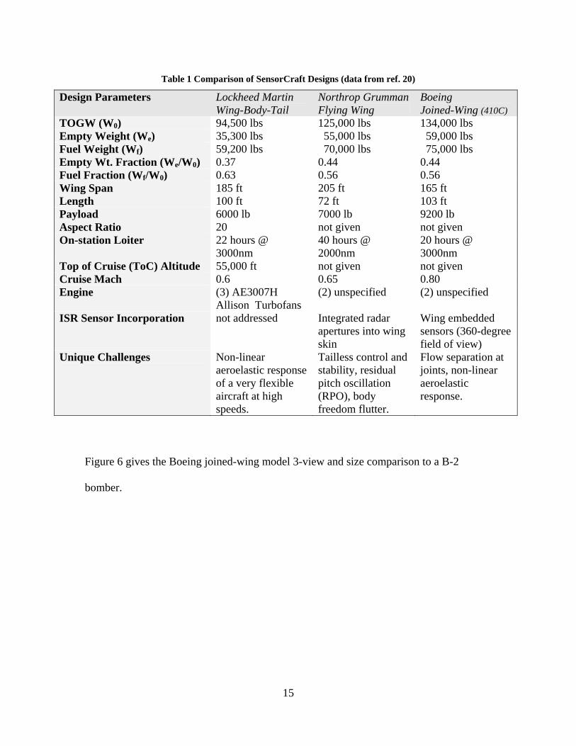
Table 1 Comparison of SensorCraft Designs (data from ref. 20)
Design Parameters Lockheed Martin Wing-Body-Tail
Northrop Grumman Flying Wing
Boeing Joined-Wing (410C)
TOGW (W0) 94,500 lbs 125,000 lbs 134,000 lbs Empty Weight (We) 35,300 lbs 55,000 lbs 59,000 lbs Fuel Weight (Wf) 59,200 lbs 70,000 lbs 75,000 lbs Empty Wt. Fraction (We/W0) 0.37 0.44 0.44 Fuel Fraction (Wf/W0) 0.63 0.56 0.56 Wing Span 185 ft 205 ft 165 ft Length 100 ft 72 ft 103 ft Payload 6000 lb 7000 lb 9200 lb Aspect Ratio 20 not given not given On-station Loiter 22 hours @
3000nm 40 hours @ 2000nm
20 hours @ 3000nm
Top of Cruise (ToC) Altitude 55,000 ft not given not given Cruise Mach 0.6 0.65 0.80 Engine (3) AE3007H
Allison Turbofans (2) unspecified (2) unspecified
ISR Sensor Incorporation not addressed Integrated radar apertures into wing skin
Wing embedded sensors (360-degree field of view)
Unique Challenges Non-linear aeroelastic response of a very flexible aircraft at high speeds.
Tailless control and stability, residual pitch oscillation (RPO), body freedom flutter.
Flow separation at joints, non-linear aeroelastic response.
Figure 6 gives the Boeing joined-wing model 3-view and size comparison to a B-2
bomber.
15

Figure 6 Boeing SensorCraft 3-view and size comparison (Model 410C) (ref. 20)
Boeing AEI Study
The Aerodynamic Efficiency Improvement (AEI) study focused on furthering the
aerodynamic and structural design of the Boeing SensorCraft. The final 306-page
PowerPoint report was delivered by Boeing to the U.S.A.F. on 17 July, 2006.
Highlights are summarized here.
According to Boeing, a joined-wing configuration promises to offer decreased life
cycle costs (LCCs) when compared to other potential SensorCraft configurations (e.g.,
flying wing and conventional wing), based on a utilization rate (UTR) of 360
hours/month and the requirement of a 3000 nm radius of action (RoA). It achieves
this savings by reducing squadron size, as only four vehicles are needed versus five
for the other designs, due to increased speed and sensor visibility differences of the
16
joined-wing.
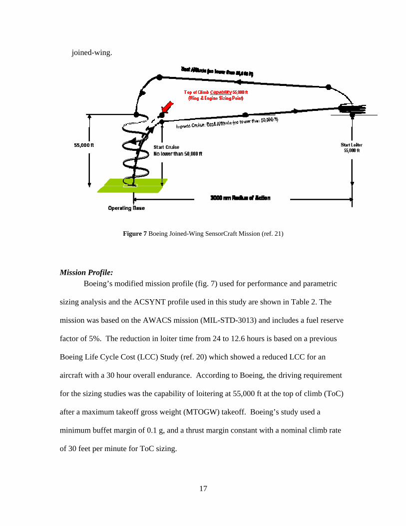
Figure 7 Boeing Joined-Wing SensorCraft Mission (ref. 21)
Mission Profile: Boeing’s modified mission profile (fig. 7) used for performance and parametric
sizing analysis and the ACSYNT profile used in this study are shown in Table 2. The
mission was based on the AWACS mission (MIL-STD-3013) and includes a fuel reserve
factor of 5%. The reduction in loiter time from 24 to 12.6 hours is based on a previous
Boeing Life Cycle Cost (LCC) Study (ref. 20) which showed a reduced LCC for an
aircraft with a 30 hour overall endurance. According to Boeing, the driving requirement
for the sizing studies was the capability of loitering at 55,000 ft at the top of climb (ToC)
after a maximum takeoff gross weight (MTOGW) takeoff. Boeing’s study used a
minimum buffet margin of 0.1 g, and a thrust margin constant with a nominal climb rate
of 30 feet per minute for ToC sizing.
17
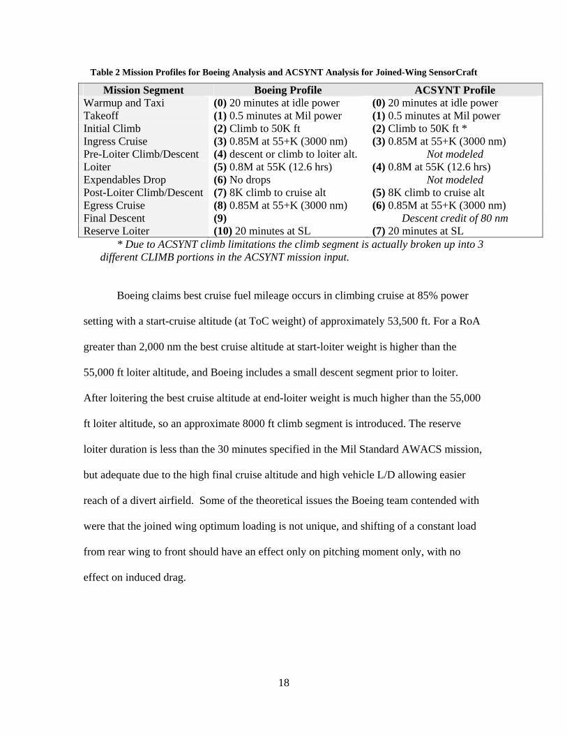
Table 2 Mission Profiles for Boeing Analysis and ACSYNT Analysis for Joined-Wing SensorCraft
Mission Segment Boeing Profile ACSYNT Profile Warmup and Taxi (0) 20 minutes at idle power (0) 20 minutes at idle power Takeoff (1) 0.5 minutes at Mil power (1) 0.5 minutes at Mil power Initial Climb (2) Climb to 50K ft (2) Climb to 50K ft * Ingress Cruise (3) 0.85M at 55+K (3000 nm) (3) 0.85M at 55+K (3000 nm) Pre-Loiter Climb/Descent (4) descent or climb to loiter alt. Not modeled Loiter (5) 0.8M at 55K (12.6 hrs) (4) 0.8M at 55K (12.6 hrs) Expendables Drop (6) No drops Not modeled Post-Loiter Climb/Descent (7) 8K climb to cruise alt (5) 8K climb to cruise alt Egress Cruise (8) 0.85M at 55+K (3000 nm) (6) 0.85M at 55+K (3000 nm) Final Descent (9) Descent credit of 80 nm Reserve Loiter (10) 20 minutes at SL (7) 20 minutes at SL
* Due to ACSYNT climb limitations the climb segment is actually broken up into 3 different CLIMB portions in the ACSYNT mission input.
Boeing claims best cruise fuel mileage occurs in climbing cruise at 85% power
setting with a start-cruise altitude (at ToC weight) of approximately 53,500 ft. For a RoA
greater than 2,000 nm the best cruise altitude at start-loiter weight is higher than the
55,000 ft loiter altitude, and Boeing includes a small descent segment prior to loiter.
After loitering the best cruise altitude at end-loiter weight is much higher than the 55,000
ft loiter altitude, so an approximate 8000 ft climb segment is introduced. The reserve
loiter duration is less than the 30 minutes specified in the Mil Standard AWACS mission,
but adequate due to the high final cruise altitude and high vehicle L/D allowing easier
reach of a divert airfield. Some of the theoretical issues the Boeing team contended with
were that the joined wing optimum loading is not unique, and shifting of a constant load
from rear wing to front should have an effect only on pitching moment only, with no
effect on induced drag.
18

Baseline Configuration (Model 410E) The baseline planform designed for the AEI study (1076-410E) is a modification of
the Point-of-Departure layout (1076-410D). The main wing has a span of 150 ft, a mean
aerodynamic chord (mac) of 161.287 inches (13.44 ft), 1980 ft2 forewing-only reference
area, and Taper Ratio (λ) = 0.61. This planform was developed for a mission with a top
of climb (ToC) at 55,000 ft, cruising at Mach 0.85, at 112,000 lb, with a CL of 0.58.
The initial AEI Performance Objectives corresponded to an earlier SensorCraft
predating the AEI study and having a wing span of 172 feet. The Point-of-Departure
configuration given to the AEI Team (Model 410E) had a wing-span of only 150 feet,
and correspondingly lower L/D target, 21 versus the original 24. In addition, the design
cruise Mach number for the 410E configuration was increased to 0.85M. Although stated
as objectives of the AEI program, descent L/D and lateral stability were not studied.
Airfoil creation method The critical station, a function of local t/c and sectional CL, was determined to be at
the 54% semi-span location for an elliptical spanload. Conditions at this station were
transformed using simple-sweep theory. At cruise conditions, the critical station 3D
sectional lift coefficient is about 0.66. Using simple-sweep theory, the resulting 2D
conditions are and 0.67 0.85cos(38) Mach = = 20.66 1.06 (cos(38))lC = = . The
optimal airfoil was then created using an inverse-design process based on Drela’s MSES
CFD code, a coupled Euler-BL method using a streamline grid. Then 2D pressure
distributions from MSES were analyzed by XTRANS to establish the extent of the
laminar run on both upper and lower surfaces. The airfoil was tweaked to enhance
19

laminar flow and the 2D section was transformed back to 3D, and incorporated into the
3D wing OML definition.
Simple-sweep theory broke down due to two primary reasons related to the
SensorCraft layout. The first is the aggressive trailing-edge break (aft strake or yehudi)
of the main wing, characterized by sweep angles of +/- 35 degrees. This trailing edge
break caused the shock system of the main wing to un-sweep, thus making the shock
much stronger and producing large wave drag. Flow also separates at the base of the
shock, which in turn increases the profile drag. This phenomenon affects the whole
configuration from about 65% semi-span of the main wing inward.
The second break-down of simple-sweep theory is related to the main-strut joint
geometry, which induces sufficient three-dimensional flow in its vicinity. Simple-sweep
theory worked well on the mid-region of the strut, due to its relatively small yehudi and
airfoils that are only lightly loaded by design.
Improving Lift-to-Drag (L/D) Ratio An initial goal of the AEI study was to design a joined-wing configuration that
achieves the L/D performance goals without a lifting strut, in order to reduce the buckling
tendency of the strut in compression and provide a more conservative estimate of the L/D
performance of the A/C in trim. Early assessments of the aircraft’s L/D only yielded a
value of 13.6. Two parallel efforts were then used to increase the baseline SensorCraft
410E toward the SensorCraft goal L/D of 21:
(1) The Multi-Disciplinary Optimization (MDOPT) system was used to optimize
the wing-design planform to meet purely aerodynamic performance criteria, and
20

(2) aerodynamic performance of the main wing was improved by applying
Professor Jameson’s SYN107 Transonic Wing Optimization code (Stanford University)
to a wing/pseudo-body configuration, and Boeing’s Divergent Trailing Edge (DTE)
Technology was inserted into the SYN107 Optimized wing (ref. 21).
Multi-Disciplinary Optimization (MDOPT) The main components of the MDOPT system (ref. 22) and process steps (fig. 8) in
an optimization are: (1) input geometry, (2) create surface grids/lofts, (3) define design
variables, (4) create design of experiments (DOE), which perturbs geometry and runs the
discipline analysis codes, (5) create interpolated response surfaces (IRS) for the
constraints and objective functions, (6) perform optimization on IRS models, (7) and
output final optimum geometry and design vector.
21

Two MDOPT runs were performed: The first run used 29 wing design variables,
3 thickness and 3 camber variables at each of 4 span stations, plus the 5 twist design
variables, and 6 design variables for the aft wing. The second run expanded the variable
space, with 35 wing design variables, 3 thickness and 3 camber variables at each of 5
span stations, plus the 5 twist design variables, and 13 design variables on the aft wing, 1
thickness and 2 camber at 4 wing span stations, twist at 4 stations. The MDOPT process
resulted in a much cleaner joint design, and achieved an efficiency 1.8 percent less than
the L/D design goal of 21.
Figure 8 Multi-Disciplinary Optimization System (ref. 21)
Boeing Finite Element Model (FEM ) The delivered finite element model (FEM) shown in Figure 9 is based on the new
configuration 410E Outer Mold Lines (OMLs) defined by the AEI aero group The
model’s mesh size is about 5 inch, considered sufficiently fine to capture local buckling
effects and provide good stress results. The structure’s composition is IM7/8552 graphite
22

and BMS 8-139 fiberglass. Sandwich construction was used extensively for its inherent
buckling stability. Fiberglass was used in the leading edge of the forward wing and
trailing edge structure of the aft wing that need to be radio transparent. In terms of size,
the model has: 81,550 nodes, 118,915 elements, and 490,000 Degrees of Freedom
(DOF). Structural elements were not sized to handle design loads, but were
approximately sized based on experience with prior configurations. Structural mass was
modeled largely with material density with concentrated mass items represented by
nonstructural mass elements.
Figure 9 Boeing Finite Element Model (FEM) Model 410E
Aerodynamic Analysis Used Boeing’s aerodynamic analysis consisted of a 2459-box doublet lattice
aerodynamic model, using a flat lifting surface representation of the actual geometry for
both static and dynamic aeroelastic analyses.
Summary of Boeing Findings of Joined Wing Benefits A joined wing SensorCraft offers the capacity for enhanced sensor integration,
structural efficiency, redundant controls, and aerodynamic rewards. The large surfaces
enable structurally-integrated low-band (UHF) apertures with a 360-degree field-of-view.
23
Structural deflections are reduced over a conventional wing of the same span, and there is
a promise of efficient load-sharing between wings. Multiple aerodynamic control
surfaces are possible effective about all axes providing control system redundancy, and
the moderately swept wings provide high subsonic speed capability, plus the non-planar
lifting system should provide induced drag benefits.
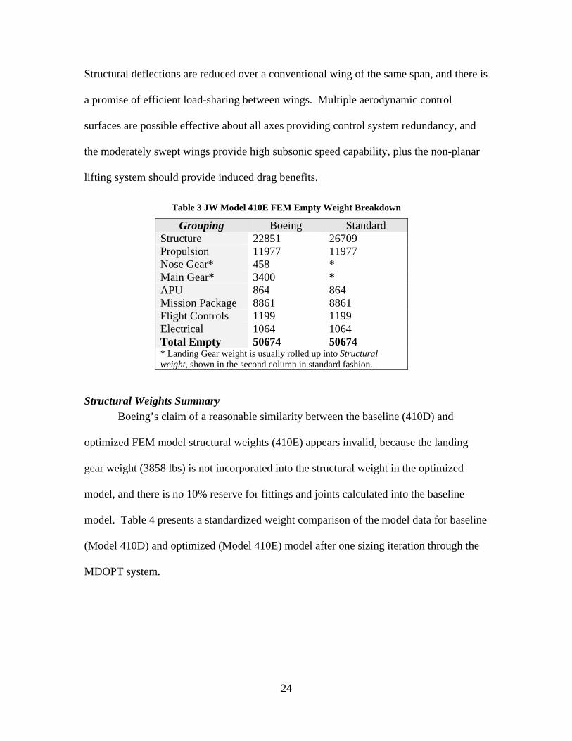
Table 3 JW Model 410E FEM Empty Weight Breakdown
Grouping Boeing Standard Structure 22851 26709 Propulsion 11977 11977 Nose Gear* 458 * Main Gear* 3400 * APU 864 864 Mission Package 8861 8861 Flight Controls 1199 1199 Electrical 1064 1064 Total Empty 50674 50674 * Landing Gear weight is usually rolled up into Structural weight, shown in the second column in standard fashion.
Structural Weights Summary Boeing’s claim of a reasonable similarity between the baseline (410D) and
optimized FEM model structural weights (410E) appears invalid, because the landing
gear weight (3858 lbs) is not incorporated into the structural weight in the optimized
model, and there is no 10% reserve for fittings and joints calculated into the baseline
model. Table 4 presents a standardized weight comparison of the model data for baseline
(Model 410D) and optimized (Model 410E) model after one sizing iteration through the
MDOPT system.
24
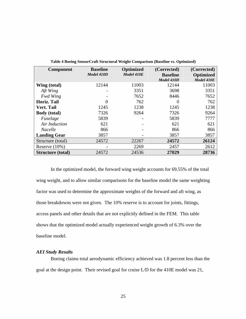
Table 4 Boeing SensorCraft Structural Weight Comparison (Baseline vs. Optimized)
Component BaselineModel 410D
OptimizedModel 410E
(Corrected) Baseline
Model 410D
(Corrected) OptimizedModel 410E
Wing (total) 12144 11003 12144 11003 Aft Wing - 3351 3698 3351 Fwd Wing - 7652 8446 7652Horiz. Tail 0 762 0 762Vert. Tail 1245 1238 1245 1238Body (total) 7326 9264 7326 9264 Fuselage 5839 - 5839 7777 Air Induction 621 - 621 621 Nacelle 866 - 866 866Landing Gear 3857 - 3857 3857Structure (total) 24572 22267 24572 26124Reserve (10%) - 2269 2457 2612Structure (total) 24572 24536 27029 28736
In the optimized model, the forward wing weight accounts for 69.55% of the total
wing weight, and to allow similar comparisons for the baseline model the same weighting
factor was used to determine the approximate weights of the forward and aft wing, as
those breakdowns were not given. The 10% reserve is to account for joints, fittings,
access panels and other details that are not explicitly defined in the FEM. This table
shows that the optimized model actually experienced weight growth of 6.3% over the
baseline model.
AEI Study Results Boeing claims total aerodynamic efficiency achieved was 1.8 percent less than the
goal at the design point. Their revised goal for cruise L/D for the 410E model was 21,
25

which means they achieved an L/D of 20.6. The stated intent at the onset of the AEI was
to produce a configuration with a zero-lifting aft wing. At the conclusion of the study the
decision was made to carry some positive load on the inboard aft wing.
Boeing’s results showed the design is elastically stable, and the nonlinear large-
deflection analysis showed a positive margin on all components with respect to buckling.
They recommended a further analysis to investigate the issue of follower forces if wing
deflections are large enough to create significant differences when not using follower
forces. Boeing data also showed the design to be aerodynamically stable, with the
detailed flutter analyses revealing a 2 degree AOA margin from the high speed cruise
point to severe pitching moment non-linearity onset. As predicted by Roberts [17],
Boeing also found that gust loads will size the aircraft, as they produced the largest loads
on the largest number of structural elements. As a final note the structural model
produced is not structurally optimized. The structural optimization process only just
began toward the end of the contract.
Boeing Joined-Wing SensorCraft (Model 410E)
The latest contract delivery of joined-wing SensorCraft data produced the
specifications and CAD model (fig. 10) for Model 410E. From this model and other
Boeing data (ref. 21) the ModelCenter joined-wing model was constructed.
26

Figure 10 CAD Model of 410E
The Boeing joined-wing SensorCraft (Model 410E) is defined by the following
characteristics (table 5); Model 410C, an earlier model and the AFIT joined wing concept
(fig. 2) are given for comparison.
Table 5 Model Parameter Comparison
Parameter AFIT Joined Wing (baseline) (ref. 19)
Boeing Sensor Craft Model410C (baseline)
Boeing Sensor Craft Model410E(optimized)
Wing span (b) 225 ft 165 ft 150 ft Tail Height (zfa) 23.13 ft 14.28 ft 16.13 ft Joint Location (jloc) 0.7647 0.7176 0.7117 Thickness/Chord (t/c) 0.20 varies with span 0.08/0.14 fore/aft(avg.) Inboard Sweep (Λib) 30 degrees 38 degrees 38 degrees Tail Sweep (Λia) 30 degrees 38 degrees 38 degrees Outboard Sweep (Λob) 30 degrees 38 degrees 38 degrees Length Overall (loa) - 103 ft 97.36 ft Airfoil LRN-1015 Custom Custom Forward Chord (cf) 8.36 ft varies with span cr = 16.4 ft, λ = 0.61Aft Chord (ca) 8.36 ft varies with span cr = 14.3 ft, λ = 0.97Height Overall (hoa) - 26 ft 19.13 ft Aspect Ratio Eff.(ARe) 15.41 7.54 8.17 Sref (wing) 3026.2 ft2 2928.3 ft2 2755.5ft2
Both the Boeing Models and the AFIT SensorCraft employ a conformal load-
bearing antenna structure (CLAS) embedded in the front and aft wings inboard of the
joint location. The Boeing Model also has CLAS outboard of the joint. This load-bearing
27

antenna structure is a composite sandwich of graphite/epoxy, carbon honeycomb foam
core, and fiberglass as shown in Figure 11.
Figure 11 Conformal Load-bearing Array Structure (CLAS)
The graphite/epoxy layers can support loads, which aids in minimizing wing
structural weight, potentially providing a significant weight savings over conventional
aircraft construction. Both the honeycomb core and fiberglass provide negligible
structural strength, but the fiberglass protects against external environmental effects and
is an electromagnetically clear material though which the radar antenna can freely receive
and transmit.
28

III. Methodology
Overview Today's aircraft systems are increasingly complex multidisciplinary systems.
Multi-disciplinary Optimization (MDO) or concurrent engineering (CE) are required as
aircraft grow in complexity, and aircraft engineers can become more specialized and
isolated in their distinct disciplines. Bringing their corporate knowledge and expertise
together in one location is critical to ensure a successful, balanced design. Along with
traditional design disciplines, manufacturing, support and cost considerations should also
be examined.
Multi-disciplinary system design is a computationally intensive process
combining individual discipline analysis with total design-space search and decision
making. Previous practice had been “stovepiped” disciplines performing independent
optimizations with limited direct interaction or communication with other disciplines.
Therefore the balancing of discipline analysis and creating “joint” data – shared
throughout the various disciplines becomes a non-trivial task, which can be eased by the
use of Integration Environments, such as ModelCenter.
The more one can front-load the design integration, pushing MDO considerations
into early conceptual design phases, the more impact the integration can have on the time,
cost and quality of the designed product, as integration only gets more difficult and
costlier in the preliminary and detailed design phases.
In the aircraft conceptual design process, there are five major design areas
requiring extensive time and effort: aircraft layout (geometry), aerodynamics, weights
29

(including payload), propulsion, and performance. For each discipline a design process is
followed including a large and complex series of decisions and calculations to determine
the design parameters of the aircraft. After initial parameters have been determined, the
design is compared to any specified requirements, appropriate changes are made, and
then another series of decisions and calculations is completed to refine the design. This
cycle is repeated until the aircraft design created meets the specified requirements.
Figure 12 Simplified Integrated Sizing Method
All of these tasks were accomplished in the integration environment ModelCenter.
(fig. 12) Three models were constructed (fig. 13) and analyzed in increasing fidelity and
depth; (1) an S-3 Viking, (2) Raymer’s ASW aircraft, and (3) Boeing’s Joined Wing
SensorCraft.
30

(1) S-3 Viking (2) Raymer’s ASW Aircraft (3) Boeing Joined-Wing
Figure 13 ModelCenter 3-D Geometry
Models were sized by differing methods, increasing in complexity and
dependence on analytical vice historical methods. For the first two models, Raymer’s
(ref. 2) methods for initial (chapter three) and refined sizing (chapter six) were followed,
along with approximate and group weight estimations (chapter fifteen). Finally an
ACSYNT model was tied into ModelCenter and the results were compared with previous
lower order routines and in the case of the S-3, actual flight test data from the S-3
NATOPS. (ref. 4)
The Joined-Wing model (410E) was sized based on the initial and refined
methods for comparison with actual Boeing data and the ACSYNT model was created
and calibrated to yield structural weights agreeing with the initial Boeing FEM data.
Once calibrated, the Joined Wing model could be perturbed to investigate various
responses to the design variables. Also the FEM of the joined-wing was wrapped in
ModelCenter to provide structural weights from NASTRAN in lieu of ACSYNT
structural data.
31
Tools Used
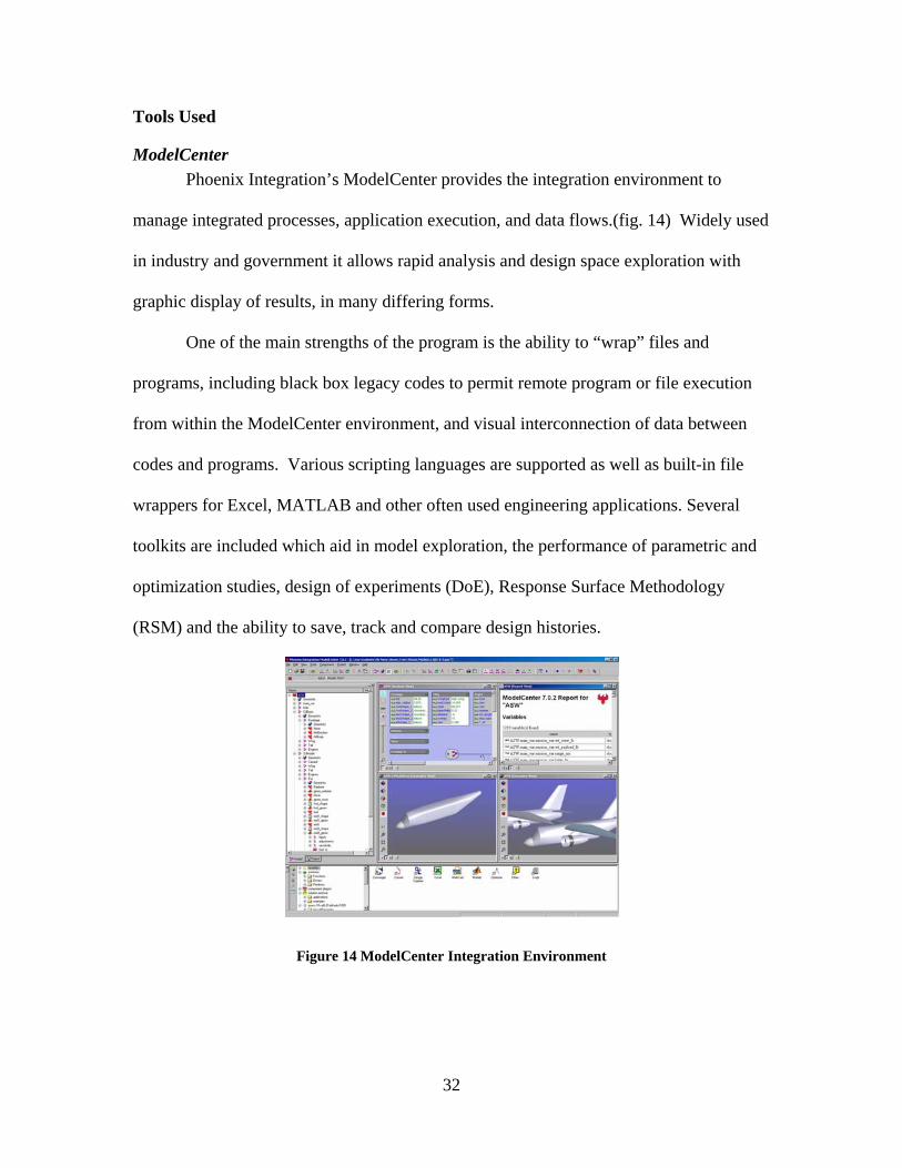
ModelCenter Phoenix Integration’s ModelCenter provides the integration environment to
manage integrated processes, application execution, and data flows.(fig. 14) Widely used
in industry and government it allows rapid analysis and design space exploration with
graphic display of results, in many differing forms.
One of the main strengths of the program is the ability to “wrap” files and
programs, including black box legacy codes to permit remote program or file execution
from within the ModelCenter environment, and visual interconnection of data between
codes and programs. Various scripting languages are supported as well as built-in file
wrappers for Excel, MATLAB and other often used engineering applications. Several
toolkits are included which aid in model exploration, the performance of parametric and
optimization studies, design of experiments (DoE), Response Surface Methodology
(RSM) and the ability to save, track and compare design histories.
Figure 14 ModelCenter Integration Environment
32

Model Coordinate System
The model coordinate system (fig. 15) chosen is traditional from a design
perspective. The X coordinate is measured as positive from the aircraft nose to the tail,
the Y coordinate is measured as positive out the right wing from aircraft centerline and
the Z coordinate is measured as positive from the longitudinal center toward the top of
the aircraft. In order to display ModelCenter models in such a coordinate system one
must make the following adjustments to the top level Model.GeomInfo.Orientation file.
Variable: Rotate_X = 270
Variable: Rotate_Z = 90
.
Figure 15 Model Coordinate System
MATLAB Model Center comes with several components preloaded, geometry primitives
such as cubes and spheres, as well as some parametrically derived shapes pertinent to
aerospace structures: wings (single and multi-section), and fuselage components (nose,
midsection, and aft, shown in figure 16.) These predefined aircraft components however
have some significant limitations.
33

(1) Wing components - do not have a calculated volume, or wetted area, although
they do have a plan area. The wing components are built on a baseline airfoil,
but that airfoil is not modifiable, without rewriting the java code and
repackaging as a .jar file. Multi-section wings offer some flexibility in
creating more non-traditional wing forms, but do not support dihedral or
anhedral. Several individual wing components can be tied together to create a
multi-section wing that can employ dihedral. As a lesson learned, the “type”
of wing is related to whether it is used as a vertical tail (type = 4) or
wing/horizontal tail (type = 6). This allows proper calculation of Aspect Ratio
(AR) and Planform Area with the span for each component defined as the
entire span.
(2) Fuselage components – also do not have a calculated volume or wetted area,
and can not model shapes other than circular or elliptical in circumference.
Although they can be tapered, they cannot be offset in the y or z directions,
preventing upsweep commonly seen in fore and aft sections.
Figure 16 Fuselage Wireview Rendered in ModelCenter (Nose, Midsection and Aft)
34

Without a calculation of the wetted areas and the volumes, the geometry does not
yield much for use in aerodynamic calculations, and the fuselage shapes will be less than
adequate for unconventionally shaped fuselage designs.
Therefore several MATLAB codes were written to (1) allow the calculation of
wing volume and surface areas (Swet), incorporating airfoil MAT files, and based on ref.
[2] equations, and (2) create super-elliptical fuselage shapes allowing features such as
square, rectangular, and rounded rectangular cross sections, advanced tapering and
calculation of areas and volumes. In addition, scripts written in VBScript were used to
convert MATLAB data into textual strings interpretable by Model Center in order to tie
the geometric parameters to Non-Uniform Rational B-Spline (NURBS) 3-D graphic
models.
Super-Elliptical Fuselage Shapes
Many aerodynamic bodies are not axisymmetric and often an upsweep or
downsweep is desired in fuselage shapes. Super-ellipses provide the ability to produce a
wide variation of shapes, from circular or elliptical cross sections, to rectangular or chine-
shaped sections.
A MATLAB code (App. C) was written to allow super-elliptical fuselage cross
sections (fig. 17), based on the Cartesian equation for a super-ellipse given as:
1p qx y
a b+ = or described parametrically as: 2cos px a t= and 2cos qy b t= , where
constants a and b correspond to the maximum half-breadth (the maximum width of the
body) and the upper or lower centerlines respectively, and p and q are exponents to shape
35

the ellipse. If a = b then the resulting shape will be symmetric in both x and y axes, and
when p = q the resulting shapes are similar to the samples indicated in fig. 17.
Figure 17 Sample of Super-Elliptical Cross Sections (ref. 28)
The below diagram (fig. 18) illustrates the possible cross-section possibilities
using a super-ellipse with a = b and p and q varying from 1 to 4. At very large positive
values of p and q the cross sectional shape approaches a rectangular or square shape.
Figure 18 Super Elliptical Cross Sections for p and q Varied from 1 to 4. (ref. 28)
36
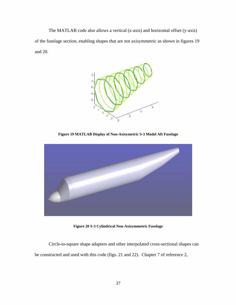
The MATLAB code also allows a vertical (z-axis) and horizontal offset (y-axis)
of the fuselage section, enabling shapes that are not axisymmetric as shown in figures 19
and 20.
Figure 19 MATLAB Display of Non-Axisymetric S-3 Model Aft Fuselage
Figure 20 S-3 Cylindrical Non-Axisymmetric Fuselage
Circle-to-square shape adapters and other interpolated cross-sectional shapes can
be constructed and used with this code (figs. 21 and 22). Chapter 7 of reference 2,
37

discusses in detail the subject of lofting, connecting splines and the utility of designing
toward flat wrapped fuselage lofts.
Figure 21 Square-to-Circle Shape Adapter
Figure 22 S-3 Rounded Rectangle Non-Axisymmetric Fuselage
Perimeters and areas were calculated for each cross-section and numerically
integrated to produce wetted surface areas and volumes of desired shapes (App. C and D).
38
AirCraft SYNthesis (ACSYNT)
Aircraft Synthesis (ACSYNT), a FORTRAN-based preliminary/conceptual
design code, was developed by NASA Ames Research Center and has been widely used
to perform aerodynamic and performance analyses on aircraft configurations, based on
semi-empirical formulas (ref. 3). It is a useful tool for performing rapid analysis with
very short runtimes, on the order of seconds. The downside is that the ACSYNT learning
curve is quite steep, several modules are error prone and the current user manual (ref. 3)
is lacking in clarity and completeness, causing the problem setup and formulation time to
be extensive. A better manual exists online It is now used under the name ACS but
many of the names and functions are still the same and the online manual has some of the
missing figures and pictures which enable comprehension of the program. It is available
online in html format, (ref. 24). Parker (ref. 23) details many of the undocumented
errors that plague ACSYNT especially in the TRAJECTORY module and gives four
examples of ACYSNT, including an A-10 ACSYNT model, that can be helpful in
troubleshooting.
The version of ACSYNT used in this study was v3.0, which was a rewrite of the
FORTRAN code into C supplied by Phoenix Integration. One problematic feature with
the C code is the errors are often generic and not traceable, as there is no specific module
or offending line of code displayed.
ACSYNT is modular in organization, with each module performing different
analysis functions or analyzing separate aircraft design disciplines. The main modules
are Geometry, Trajectory, Aerodynamics, Propulsion and Weights
39

These modules and others such as takeoff/landing and economics can each be called
separately. ACSYNT is run in MS_DOS and commands to run modules select output
data, and enter namelist data (for example, the wing namelist is $WING followed by
parameter names and values and terminated with $END) are contained in the input file
(filename.IN). For complete listing of modules and their use see refs. 3 and 25. Custom
modules can be even be added; O’donnell (ref. 5) uses a Navy-specific module in
ACSYNT for his analysis of a carrier based ASW Aircraft modified for STOL to ensure
Navy specific requirements are met for catapult launches and arrested landings.
Primary ACSYNT Modules
Geometry Module – This module calculates surface areas and volumes for input
component geometry based on primitive geometry calculations and the totals can be
shaped by weighting factors (SWFACT and others) to arrive at a more exact Swet and or
volume calculation. The fuselage is represented as a cone-shaped nose connected to a
constant radius mid-section and a cone-shaped tail section. The length of the sections
and their fineness ratio (length/maximum diameter) is entered via the $FUS namelist.
An ACSYNT limitation of a fixed number of namelist inputs hinders the
simulation of designs with multiple fuselages or bi-plane or staggered wings. Only one
$WING, $STRAKE, $HTAIL, $VTAIL and $FUS namelist can be included in the
geometry input file. This restricts the ability to conveniently model joined-wings.
Wing wetted area geometries (horizontal tail, vertical tail, wings, and canard) are
calculated by the following formula – printed incorrectly in both the ACSYNT manual
and the ACS website.
40
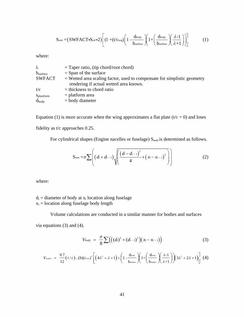
( ) body bodywet ref avg
surface surface
d d -S = SWFACT S 2 (1 +(t/c ) 1 - 1+b b +
λλ
11
⎡ ⎤⎛⎛ ⎞ ⎛ ⎞⎛ ⎞⎞⎢ ⎥⎜ ⎟ ⎜ ⎟⎜⎜⎝ ⎠ ⎝ ⎠⎝⎝ ⎠
⎟ ⎟⎠⎣ ⎦i i (1)
where:
λ = Taper ratio, (tip chord/root chord) bsurface = Span of the surface SWFACT = Wetted area scaling factor, used to compensate for simplistic geometry
rendering if actual wetted area known. t/c = thickness to chord ratio splanform = platform area dbody = body diameter
Equation (1) is more accurate when the wing approximates a flat plate (t/c = 0) and loses
fidelity as t/c approaches 0.25.
For cylindrical shapes (Engine nacelles or fuselage) Swet.is determined as follows.
( ) ( ) ( )2
1 2wet 1 1S =
4i i
i i i id d
d d x xπ−
−
⎛ ⎞⎛ ⎞−⎜ ⎟+ + −⎜⎜⎜ ⎟⎝ ⎠⎝ ⎠
∑ − ⎟⎟
(2)
where:
di = diameter of body at xi location along fuselage xi = location along fuselage body length
Volume calculations are conducted in a similar manner for bodies and surfaces
via equations (3) and (4).
( )( )( )2 21 ( ) ( )
8body i i i iV d d x 1xπ
−= + −∑ − (3)
( ) ( ) ( )body body2 2 2
surface surface
0.7 d d -1 / ( )( ) 4 1 1 - 1+ 3 2 1
12 b b +1rootsurface rootV t c b c
λλ λ λ λ
λ= + + +⎡ ⎛ ⎞⎛ ⎛ ⎞⎛ ⎞⎞
⎜ ⎟⎜ ⎜ ⎟⎜ ⎟⎟⎢ ⎥⎣ ⎝ ⎠⎝ ⎝ ⎠⎝ ⎠⎠+ + ⎤
⎦ (4)
41
Trajectory Module - This module determines the flight path of the aircraft for a
specified mission profile. It employs the Breguet Range and Endurance equations with
each phase being broken up into five smaller legs. This module is the most susceptible to
producing run-time errors for apparently good mission profiles. One quick check is to
ensure the number preceding the mission section matches the number of mission legs.
Aerodynamics Module – This module, based on compressible wing theory,
computes the coefficients of lift, minimum and induced drag and pitching moment for
wings and wing-body combinations with or without a horizontal tail.
Airfoil shapes are restricted to five different classes of airfoil (ALELJ variable
name): (1) sharp and near-sharp (2) 230XX and 00XX (3) 6-series airfoils (4) Whitcomb
supercritical airfoil and (5) leading edge radius-to-chord ratio specified.
Zero-lift drag (CD0) can be calculated directly based on input geometry data (with
$ADRAG namelist set ICDO = 0) or can be explicitly specified for an array of user
specified Mach numbers in using the CDONPUT, and SMNCDO fields.
Aerodynamic characteristics are input via the $ACHAR namelist, allowing the input of
an array of CL0 and Cm0 versus Mach values for the body, wing and canard. Lift curve
slopes and the drag polar shape can be modified as required by the altering of FVCAM
and FLDM values in the $ATRIM namelist. One important variable used in the joined-
wing portion of this study is SFWF, the laminar-turbulent skin friction weighting factor,
which determines the coefficient of friction to be applied in form drag calculations. This
is a critical point, because to achieve high L/Ds, there is a need for laminar flow airfoils.
42
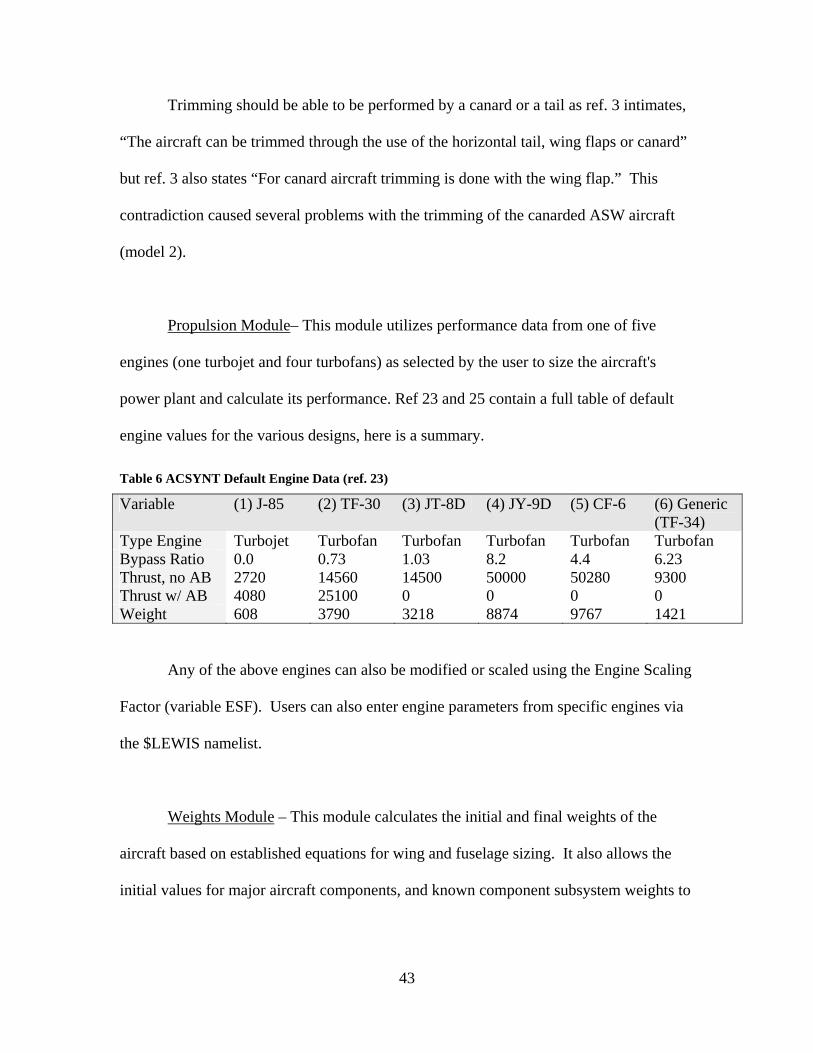
Trimming should be able to be performed by a canard or a tail as ref. 3 intimates,
“The aircraft can be trimmed through the use of the horizontal tail, wing flaps or canard”
but ref. 3 also states “For canard aircraft trimming is done with the wing flap.” This
contradiction caused several problems with the trimming of the canarded ASW aircraft
(model 2).
Propulsion Module– This module utilizes performance data from one of five
engines (one turbojet and four turbofans) as selected by the user to size the aircraft's
power plant and calculate its performance. Ref 23 and 25 contain a full table of default
engine values for the various designs, here is a summary.
Table 6 ACSYNT Default Engine Data (ref. 23)
Variable (1) J-85 (2) TF-30 (3) JT-8D (4) JY-9D (5) CF-6 (6) Generic (TF-34)
Type Engine Turbojet Turbofan Turbofan Turbofan Turbofan Turbofan Bypass Ratio 0.0 0.73 1.03 8.2 4.4 6.23 Thrust, no AB 2720 14560 14500 50000 50280 9300 Thrust w/ AB 4080 25100 0 0 0 0 Weight 608 3790 3218 8874 9767 1421
Any of the above engines can also be modified or scaled using the Engine Scaling
Factor (variable ESF). Users can also enter engine parameters from specific engines via
the $LEWIS namelist.
Weights Module – This module calculates the initial and final weights of the
aircraft based on established equations for wing and fuselage sizing. It also allows the
initial values for major aircraft components, and known component subsystem weights to
43
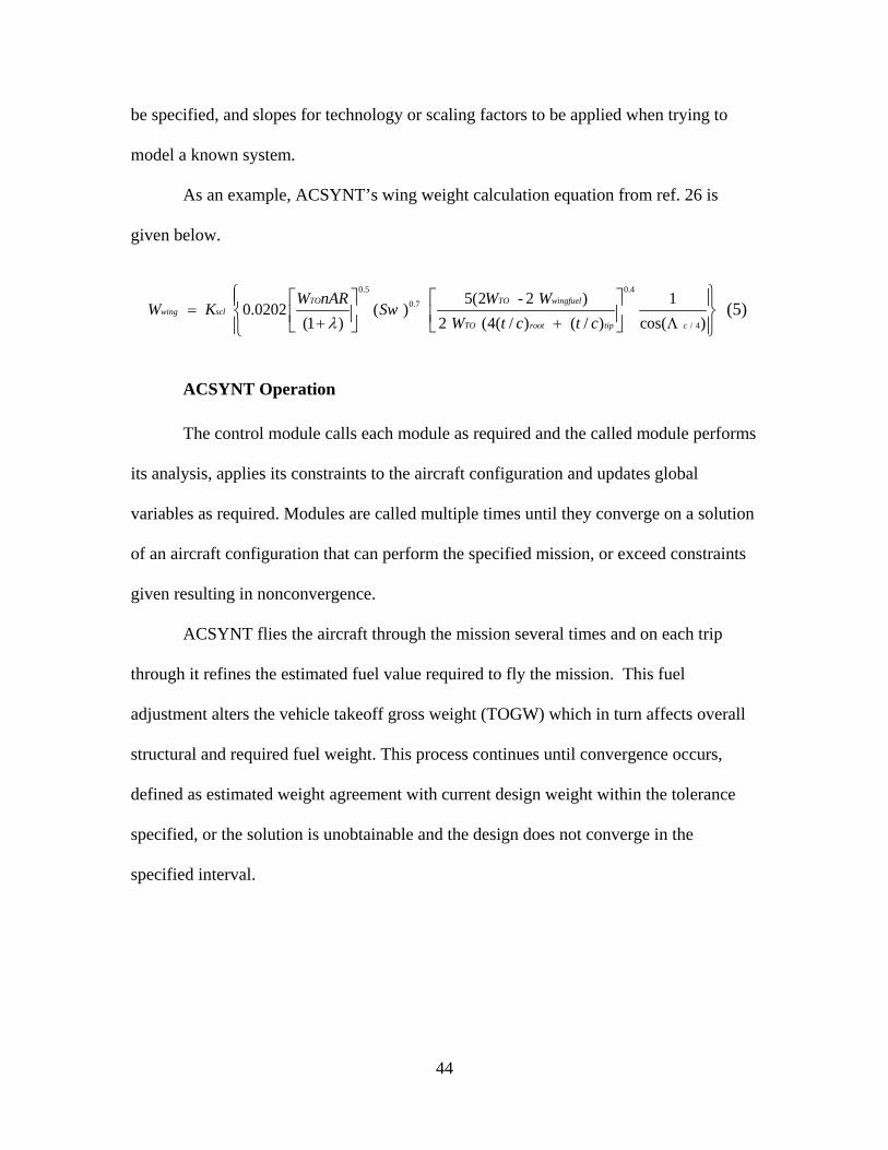
be specified, and slopes for technology or scaling factors to be applied when trying to
model a known system.
As an example, ACSYNT’s wing weight calculation equation from ref. 26 is
given below.
0.5 0.4
0.7
/ 4
5(2 - 2 ) 1 0.0202 ( )
(1 ) 2 (4( / ) ( / ) cos( )TO TO wingfuel
wing sclTO root tip c
W nAR W WW K Sw
W t c t cλ=
+ +
⎧ ⎫⎡ ⎤ ⎡ ⎤⎪ ⎪⎨ ⎬⎢ ⎥ ⎢ ⎥⎣ ⎦ ⎣ ⎦⎪ ⎪⎩ ⎭Λ
(5)
ACSYNT Operation
The control module calls each module as required and the called module performs
its analysis, applies its constraints to the aircraft configuration and updates global
variables as required. Modules are called multiple times until they converge on a solution
of an aircraft configuration that can perform the specified mission, or exceed constraints
given resulting in nonconvergence.
ACSYNT flies the aircraft through the mission several times and on each trip
through it refines the estimated fuel value required to fly the mission. This fuel
adjustment alters the vehicle takeoff gross weight (TOGW) which in turn affects overall
structural and required fuel weight. This process continues until convergence occurs,
defined as estimated weight agreement with current design weight within the tolerance
specified, or the solution is unobtainable and the design does not converge in the
specified interval.
44

General Geometry Generator (GGG)
A Boeing tool under development, the General Geometry Generator (GGG)
version 2.0, is a Python-based code which allows the generation and manipulation of
basic geometrical and aircraft specific shapes in order to produce “water-tight” outer
mold line (OML) geometry which can then be used in the creation of Computational
Fluid Dynamics (CFD) mesh grids. This software was evaluated in this study for
potential use and inclusion into ModelCenter, but due to time constraints and the
requirement to learn a new language in order to apply the software, it was not
incorporated. Parametrical in nature, strengths of the program include the ability to make
and see instant changes in the design and compute any number of outputs. GGG produces
geometry that is a continuous function of the input parameters, a property not typically
available in commercial systems, enabling geometry to morph continuously between
different shapes, and preventing downstream problems with geometry discontinuities.
Figure 23 Example GGG Display
There is a significant startup learning cost to the program as extensive coding
experience in Python is required to create the models. Once the models are formed they
45

can be wrapped into ModelCenter and used to interact with other model variables. The
current GGG process requires manual construction and assembly of the geometry using a
set of geometry generators, highly specialized tools to create loft surfaces for aircraft
components given a set of constraints such as locations, tangents, section curves and
parameters. The types of geometric generators are: Airfoils (wings, vertical and
horizontal stabilizers), Nacelles (tubes, engine cowling, fuselages), and Fairings (fairings,
cowlings, fuselages, pods).
The geometric components, and their relative positions are parameterized and
normalized to lie between 0 and 1, so that any combination of inputs within this
parametric hypercube will produce a valid aircraft configuration. Using a Design of
Experiments (DOE) the designer can explore the design space, producing a whole family
of designs, which can then be evaluated for performance. The data can then be used to
plot surrogate mathematical models (Response Surfaces), which can be used to find
design optima.
Initial Historical Sizing
Initial weight sizing was conducted according to chapter 3 of Raymer’s conceptual
design text “Aircraft Design: A Conceptual Approach”, (ref. 2) which contains many
equations and graphs based on historical trends and trend analysis. For many aircraft
types, history is a good benchmark for replacement designs. Using these equations one
can rapidly conduct a rapid “back of the napkin” design analysis for a number of different
types of aircraft. This simplest analysis is incapable of handling payload, ordnance or
46

fuel tank drops, and while somewhat crude, it provides a rapid ballpark figure (+/- 20%)
of the actual take-off gross weight (TOGW).
Weight Buildup
Design gross takeoff weight is comprised of crew weight, payload weight, fuel weight
and empty weight, which includes the structure, propulsion and fixed equipment as
shown in the equations below.
(6) 0 crew payload fuel emptyW W W W W= + + +
empty structure propulsion fixedW W W W= + + (7)
For the simplest analysis to find W0 , assuming both payload and crew weights are
given as requirements, one needs a empty weight fraction (Wempty/W0) and a fuel fraction
(Wfuel/W0) as both the fuel and the empty weight are dependent on W0.
Empty Weight Fraction
An empty weight fraction is calculated based on the type aircraft and the estimated
TOGW (W0) in Table 3.1 in (ref 2), displayed in chart form as figure 24 for a several
different aircraft types.
47

Figure 24 Weight Fraction Empty Trends (ref. 2)
These logarithmic curve fits are from Raymer’s own calculations using publicly
available data from Jane’s and other sources.
Fuel Fraction
For any given mission, the analysis is broken up into various portions or “legs.” The
ASW mission profile given by Raymer consists of seven legs as shown below.
Figure 25 ASW Mission
48

Some mission segment weight fractions are estimated using historical trends as given
in table 3.2 in reference 2.
Table 7 Approximate Mission Weight Fractions (ref. 2)
Mission Segment (Wi/W i-1) Warmup and takeoff 0.970
Climb 0.985 Landing 0.995
Cruise segments and loiter segments weight fractions are calculated using the Breguet
Range Equation (ref. 2, ch17) and the Endurance Equation. (ref. 2, ch17)
( )
-
- 1
RCV L D
ii
W eW
⎛ ⎞⎜ ⎟⎜ ⎟⎜⎝=
⎟⎠ (8)
where R = range (ft), C = specific fuel consumption (SFC), V = velocity (ft/s) and L/D is
lift-to-drag ratio.
( )
- 1
ECL D
ii
W eW
⎛ ⎞⎜ ⎟⎜ ⎟⎜⎝=
⎟⎠ (9)
where E = endurance or loiter time (in seconds or hours). Units need to be consistent. If
SFC is given in lbm/lbf-hr, then endurance can be given in hours.
By multiplying all the weight fractions for each segment, one can determine the ratio
of weight at mission end to starting weight (Wend/W0), where ending weight is the weight
after landing, taxiing, and shutting down. The empty weight fraction (Wempty/W0), then
can be calculated as (1-Wend/W0), assuming all fuel available is usable and end weight is
empty weight.
49
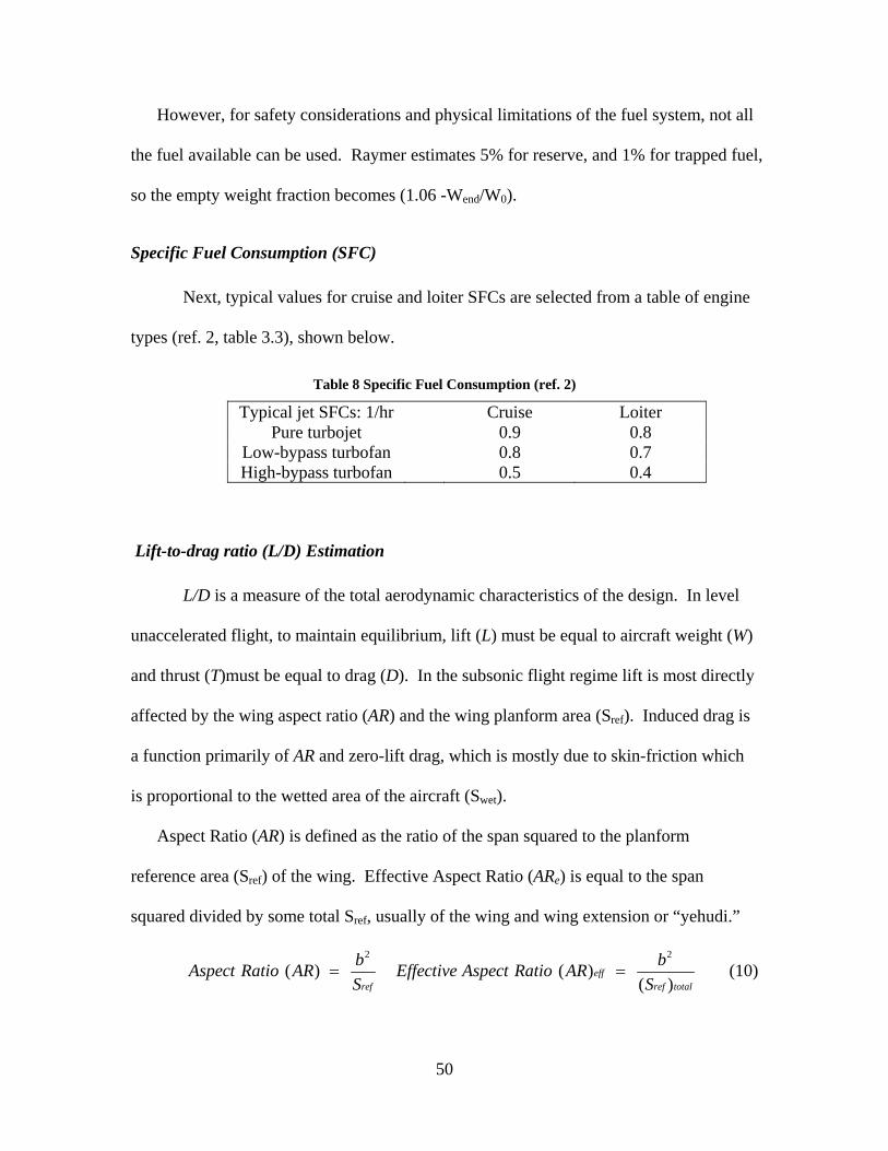
However, for safety considerations and physical limitations of the fuel system, not all
the fuel available can be used. Raymer estimates 5% for reserve, and 1% for trapped fuel,
so the empty weight fraction becomes (1.06 -Wend/W0).
Specific Fuel Consumption (SFC)
Next, typical values for cruise and loiter SFCs are selected from a table of engine
types (ref. 2, table 3.3), shown below.
Table 8 Specific Fuel Consumption (ref. 2)
Typical jet SFCs: 1/hr Cruise Loiter Pure turbojet 0.9 0.8
Low-bypass turbofan 0.8 0.7 High-bypass turbofan 0.5 0.4
Lift-to-drag ratio (L/D) Estimation
L/D is a measure of the total aerodynamic characteristics of the design. In level
unaccelerated flight, to maintain equilibrium, lift (L) must be equal to aircraft weight (W)
and thrust (T)must be equal to drag (D). In the subsonic flight regime lift is most directly
affected by the wing aspect ratio (AR) and the wing planform area (Sref). Induced drag is
a function primarily of AR and zero-lift drag, which is mostly due to skin-friction which
is proportional to the wetted area of the aircraft (Swet).
Aspect Ratio (AR) is defined as the ratio of the span squared to the planform
reference area (Sref) of the wing. Effective Aspect Ratio (ARe) is equal to the span
squared divided by some total Sref, usually of the wing and wing extension or “yehudi.”
2 2
( ) ( ) ( )
effref ref total
b bAspect Ratio AR Effective Aspect Ratio ARS S
= = (10)
50
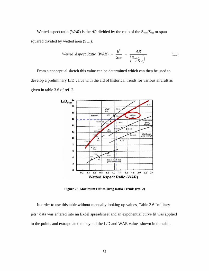
Wetted aspect ratio (WAR) is the AR divided by the ratio of the Swet/Sref or span
squared divided by wetted area (Swet).
( )
2
( ) wet wet
ref
b ARWetted Aspect Ratio WARS S
S= = (11)
From a conceptual sketch this value can be determined which can then be used to
develop a preliminary L/D value with the aid of historical trends for various aircraft as
given in table 3.6 of ref. 2.
Figure 26 Maximum Lift-to-Drag Ratio Trends (ref. 2)
In order to use this table without manually looking up values, Table 3.6 “military
jets” data was entered into an Excel spreadsheet and an exponential curve fit was applied
to the points and extrapolated to beyond the L/D and WAR values shown in the table.
51
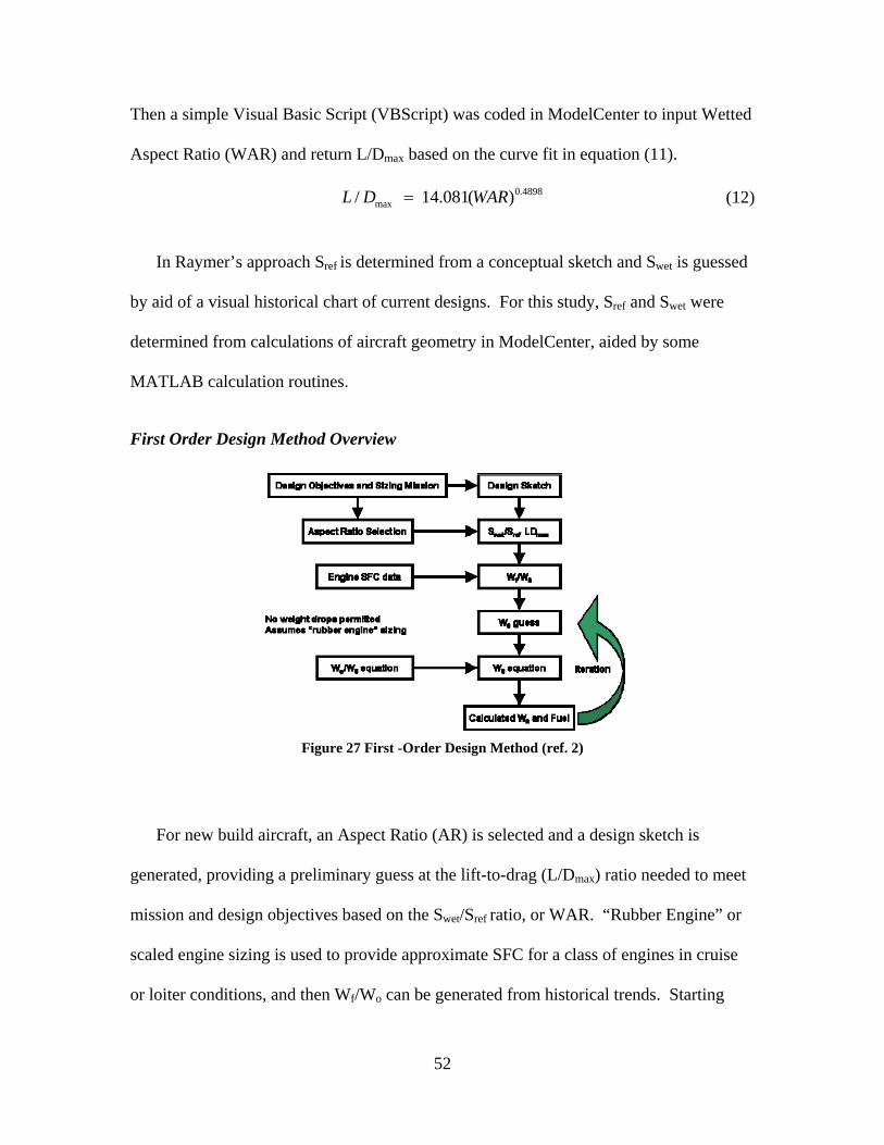
Then a simple Visual Basic Script (VBScript) was coded in ModelCenter to input Wetted
Aspect Ratio (WAR) and return L/Dmax based on the curve fit in equation (11).
(12) 0.4898max/ 14.081( )L D WAR=
In Raymer’s approach Sref is determined from a conceptual sketch and Swet is guessed
by aid of a visual historical chart of current designs. For this study, Sref and Swet were
determined from calculations of aircraft geometry in ModelCenter, aided by some
MATLAB calculation routines.
First Order Design Method Overview
Figure 27 First -Order Design Method (ref. 2)
For new build aircraft, an Aspect Ratio (AR) is selected and a design sketch is
generated, providing a preliminary guess at the lift-to-drag (L/Dmax) ratio needed to meet
mission and design objectives based on the Swet/Sref ratio, or WAR. “Rubber Engine” or
scaled engine sizing is used to provide approximate SFC for a class of engines in cruise
or loiter conditions, and then Wf/Wo can be generated from historical trends. Starting
52
from an initial Wo guess and using Breguet endurance and range equations Wo and Wfuel
can be calculated. This new Wo is then used as the Wo guess and the process is iterated
until the calculated Wo converges at the guess Wo. This process (fig. 26) can be sped by
inputting data into an Excel spreadsheet (App. E).
Of note, Raymer’s ASW sizing calculations (Box 3.1 ref. 2) are in error, the W7/W0
value should be 0.644 when cruise leg 5 weight fraction is input correctly. If correction is
carried through, the final converged weight becomes 56,732 lbs vice printed value of
59,309 lbs.
Refined Sizing
Refined weights were obtained by using an improved, semi-historical equation
(ref.2, Table 6.1) for the calculation of the empty weight fraction (Wempty/W0).
( ) ( ) ( )3 4 51 2
maxc c cc ce oo v
o oW WTa bW A M KW W S
⎡ ⎤= +⎢ ⎥⎣ ⎦s (13)
where a, b, c1, c2, c3, c4, c5 are constants for each type of aircraft. Kvs is 1.0 for a fixed
sweep wing and 1.04 for a variable sweep wing, A is Aspect Ratio, Wo is TOGW, (T/Wo)
is takeoff thrust-to-weight ratio, (Wo/S) is takeoff wing-loading, and Mmax is the maximum
design Mach number. In order to determine the wing loading (W/S) and thrust-to-weight
(T/W) the methods chapter 5, reference 2 were employed.
All of the models built were developed as Bomber aircraft, as that most closely
resembles the mission, role and sizing. For the “Military Cargo/Bomber” aircraft, a quick
analysis was conducted on the empty weight equation to determine the sensitivity of the
53

empty weight fraction to variable input (fig. 28). Variables selected were representative
of the design space for Bomber-type aircraft.
Figure 28 Sensitivity Analysis of Empty Weight Fraction Equation
Results show that the equation is primarily affected by the TOGW (W0) term,
minimally by Mmax, and nearly equally by the other three terms. Classic T/W versus W/S
plots could also be produced at this stage in order to constrain the design space. As no
specific performance values were given for turn, climb rate, takeoff, or landing this was
not required for the three models, but a sample response surface for the Raymer ASW
model is given in figure 29.
54

Figure 29 Response of Refined Weight to T/W and W/S Inputs for Model (2) Raymer ASW Aircraft
Semi-empirical Sizing
ACSYNT Sizing was then performed with ACSYNT, by “wrapping” an ACSYNT input file
(filename.IN) and its produced output file (filename.OUT) with an associated filewrapper.
The filewrapper saved to the ModelCenter Analysis Server can then be added to the
model and the parameters linked to model input values and ACSYNT outputs. Appendix
D contains input and output files for each model.
Many of the model problems and limitations stem from using this legacy code.
First of all are the geometric representation limitations. ACSYNT only allows one
$WING namelist, one $HTAIL namelist, one $VTAIL namelist and one $FUS namelist.
55

For the joined-wing configuration this created a problem, due to the joined wing having
two wings: a fore and aft wing. It was decided to model the aft wing as a horizontal tail
and the boom segment as a vertical tail. Because the $HTAIL namelist does not include
a provision for supplying the anhedral or dihedral, the projection of the aft wing onto the
horizontal plane was used, and the reference area, and aspect ratio for the vertical tail was
modified according to the aft wing’s projection onto the vertical plane. The wing was
modeled by a $WING namelist that extended to the centerline of the vehicle, and had a
rear extension that reduced the effective aspect ratio, by adding in additional Sref.
Secondly are trajectory errors. The trajectory module is highly error prone, even
for seemingly good profiles. This has been previously identified, but not solved.
Lastly are interface errors with ModelCenter. When running a wrapped ACSYNT
file, and the component has to be halted for any reason, ModelCenter would orphan the
process on the Analysis Server, with no direct indication to the user, other than the next
run would not complete. The spinning hourglass of death, and locked files on the
Analysis Server were indications that something was still executing ACSYNT. In order
to resolve the problem, the applications had to be terminated on the Analysis Server by
computer support technicians.
Other errors that are common with ACSYNT incorporation into ModelCenter are
the formatting of numbers, which is done according to FORTRAN formatting standards,
where fformat = F5.3, means “fixed number formatting with five total characters and
three characters after the decimal.” In this schema, the number 4.333 would be fine, but
the number -0.500 would produce errors, as it has six total characters, four numbers, the
period and the minus sign. ACSYNT input files contain both integer, real and Boolean
56

values, and it is important to distinguish among them. It is best to list all the reals
together, then integers and then the Boolean values.
Raymer Approximate and Group Weights Sizing Methods The formulas of reference 2, chapter 15 for Approximate Empty Weight Buildup
(Table 15.2) and the statistical weights method (15.3) were used to estimate the
component weight breakdown of the vehicle. Comparison of weights is shown in chapter
IV. Of note, the group weights sizing method is dependent on many additional
parameters, some of which are default values, in lieu of actual engineering design
information.
Finite Element Model Structural Weight
For the joined-wing model, the structural weight was also determined by utilizing
the FEM for the 410E model through NASTRAN queries. Due to the historical nature of
the empirical estimating codes (initial, refined, approximate weights, and group weights)
the joined-wing structural weight must be determined in an alternate manner. Although
not optimized, the model was evaluated for change in structural weight due to geometric
changes, via a MATLAB code, which is discussed in detail in the next chapter.
57

IV. Results and Discussion
Model Construction Before any model can be constructed, valid data sets need to be integrated from
the various sources of parameter information. Key model parameters and sources are
shown in table 9, details in appendix A.
Table 9 Key Model Parameters
Parameter S-3 Viking Raymer Canarded ASW Aircraft
Joined-Wing SensorCraft (410E)
Wingspan (b) 68 ft 8 in 68 ft 150 ft Length (LOA) 53 ft 4 in 51 ft 98 ft Sref 598 ft2 510.4 ft2 + 156.8 ft2 ** 1980 ft2 + 775.5 ft2 *** Wing airfoil (root) NACA 0016-53 NACA 0016-53 Custom airfoil Max internal fuel 13444 lbs (1,933 US gal) Limited by volume Limited by volume Max fuel 17617 lbs (2533 US gal) Limited by volume Limited by volume Empty Weight 26581 lbs Unknown (~30000 lb) 50674 lb Max GTOW 52539 lbs Unknown (~60000 lb) ~115000 lb Propulsion 2×GE TF-34-GE-2
turbofans 2× turbofans (improved) 2×turbofans
Engine Thrust (SL) 9300 lbf ~11000 lbf 30000 lbf Engine Weight 1421 lbs each ~1421 lbs each 11977 total propulsion Engine Length 8.33 ft ~8.33 ft - Engine Diameter 4.167 ft ~4.167 ft - Wing loading W/S): 68.5 lb/ft² ~60-100 lb/ft² - Thrust/weight T/W): 0.353 ~0.25-0.45 - Max Diameter 7.5 ft 8 ft 8.8 ft (fuselage height) Principal Information Sources
S-3 NATOPS (ref. 4) Wikipedia
Raymer text (ref. 2) Boeing FEM, CAD, Literature (ref. 21)
Calculations Derived from Geometric Parameters Swet 2811.0 ft² 2721.6 ft² 7782.9 ft² AReff 7.750 6.923 8.166 WAR 1.649 1.2984 2.89 Swet/Sref 4.7 5.33 2.82 L/Dmax 16.0 used (calc. 18.0)* 16.0 23.7
* For comparison L/D was manually held at 16 for initial/refined sizing ** Sref shown is for wing and canard areas
*** Sref shown is for forward wing including yehudi
58
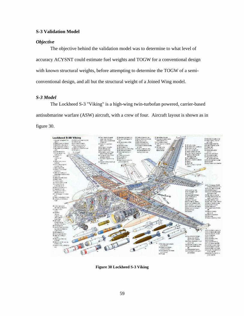
S-3 Validation Model
Objective The objective behind the validation model was to determine to what level of
accuracy ACYSNT could estimate fuel weights and TOGW for a conventional design
with known structural weights, before attempting to determine the TOGW of a semi-
conventional design, and all but the structural weight of a Joined Wing model.
S-3 Model The Lockheed S-3 "Viking" is a high-wing twin-turbofan powered, carrier-based
antisubmarine warfare (ASW) aircraft, with a crew of four. Aircraft layout is shown as in
figure 30.
Figure 30 Lockheed S-3 Viking
59
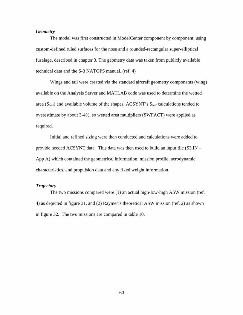
Geometry The model was first constructed in ModelCenter component by component, using
custom-defined ruled surfaces for the nose and a rounded-rectangular super-elliptical
fuselage, described in chapter 3. The geometry data was taken from publicly available
technical data and the S-3 NATOPS manual. (ref. 4)
Wings and tail were created via the standard aircraft geometry components (wing)
available on the Analysis Server and MATLAB code was used to determine the wetted
area (Swet) and available volume of the shapes. ACSYNT’s Swet calculations tended to
overestimate by about 3-4%, so wetted area multipliers (SWFACT) were applied as
required.
Initial and refined sizing were then conducted and calculations were added to
provide needed ACSYNT data. This data was then used to build an input file (S3.IN –
App A) which contained the geometrical information, mission profile, aerodynamic
characteristics, and propulsion data and any fixed weight information.
Trajectory The two missions compared were (1) an actual high-low-high ASW mission (ref.
4) as depicted in figure 31, and (2) Raymer’s theoretical ASW mission (ref. 2) as shown
in figure 32. The two missions are compared in table 10.
60
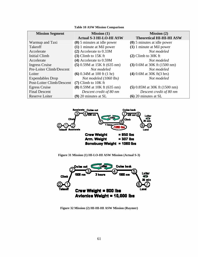
Table 10 ASW Mission Comparison
Mission Segment Mission (1) Actual S-3 HI-LO-HI ASW
Mission (2) Theoretical HI-HI-HI ASW
Warmup and Taxi (0) 5 minutes at idle power (0) 5 minutes at idle power Takeoff (1) 1 minute at Mil power (1) 1 minute at Mil power Accelerate (2) Accelerate to 0.33M Not modeled Initial Climb (3) Climb to 15K ft (2) Climb to 30K ft Accelerate (4) Accelerate to 0.59M Not modeled Ingress Cruise (5) 0.59M at 15K ft (635 nm) (3) 0.6M at 30K ft (1500 nm) Pre-Loiter Climb/Descent Not modeled Not modeled Loiter (6) 0.34M at 100 ft (1 hr) (4) 0.6M at 30K ft(3 hrs) Expendables Drop Not modeled (1060 lbs) Not modeled Post-Loiter Climb/Descent (7) Climb to 10K ft Egress Cruise (8) 0.59M at 10K ft (635 nm) (5) 0.85M at 30K ft (1500 nm) Final Descent Descent credit of 80 nm Descent credit of 80 nm Reserve Loiter (9) 20 minutes at SL (6) 20 minutes at SL
Figure 31 Mission (1) HI-LO-HI ASW Mission (Actual S-3)
Figure 32 Mission (2) HI-HI-HI ASW Mission (Raymer)
61

Aerodynamics The S-3 uses a symmetrical 0016-53 airfoil for the main wing and a NACA 0012
airfoil for the vertical tail, and a NACA 2410 for the horizontal tail. Flap settings for
takeoff and landing maneuvers are given in S-3 NATOPS manual (ref. 4).
CL0 values were determined from the given airfoils, applied to the wing. For both
the S-3 and ASW models the value was zero based on a symmetric airfoil mounted at
zero degrees incidence.
ACSYNT defaults to automatically perform a drag analysis (ICDO=0) based on
component geometry drag build up, and provides an estimated drag for each flight
condition analyzed. These output numbers were checked manually using an Excel
spreadsheet with component drag buildup equations of reference 2, chapter 12 at the
cruise flight condition and local Reynolds number for each component. For the S-3
model ACSYNT estimated CD0 to be 0.01270 for the outbound cruise portion, the manual
calculation determined a CD0 of 0.01355.
Propulsion The TF-34-GE-2 turbofan is one of the six standard engines contained within
ACSYNT, selection 6. It is a high-bypass turbofan engine with a bypass ratio of 6.24, a
seal-level static thrust of 9300 lbf, and an engine weight of 1425 lbs.
Weights Components of known weight were fixed in ACYSNT by way of the Fixed
Weights namelist ($FIXW). Fixed weights were as follows:
62
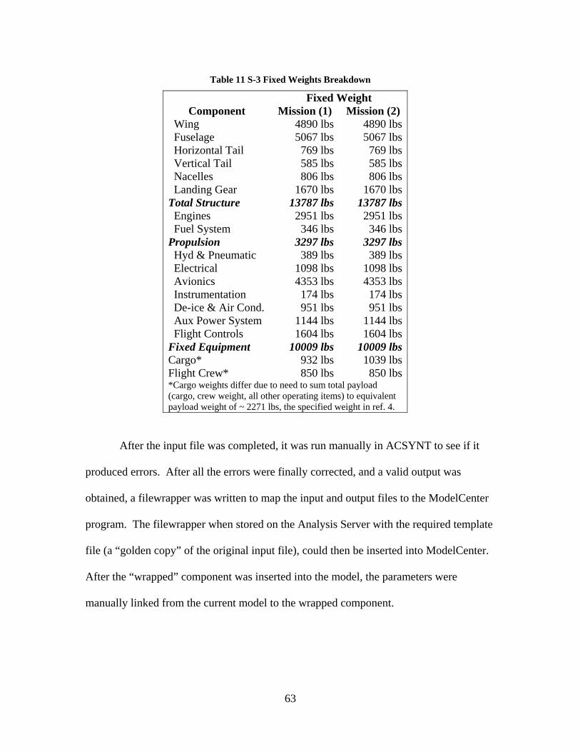
Table 11 S-3 Fixed Weights Breakdown
Fixed Weight Component Mission (1) Mission (2)
Wing 4890 lbs 4890 lbs Fuselage 5067 lbs 5067 lbs Horizontal Tail 769 lbs 769 lbs Vertical Tail 585 lbs 585 lbs Nacelles 806 lbs 806 lbs Landing Gear 1670 lbs 1670 lbsTotal Structure 13787 lbs 13787 lbs Engines 2951 lbs 2951 lbs Fuel System 346 lbs 346 lbsPropulsion 3297 lbs 3297 lbs Hyd & Pneumatic 389 lbs 389 lbs Electrical 1098 lbs 1098 lbs Avionics 4353 lbs 4353 lbs Instrumentation 174 lbs 174 lbs De-ice & Air Cond. 951 lbs 951 lbs Aux Power System 1144 lbs 1144 lbs Flight Controls 1604 lbs 1604 lbsFixed Equipment 10009 lbs 10009 lbsCargo* 932 lbs 1039 lbsFlight Crew* 850 lbs 850 lbs*Cargo weights differ due to need to sum total payload (cargo, crew weight, all other operating items) to equivalent payload weight of ~ 2271 lbs, the specified weight in ref. 4.
After the input file was completed, it was run manually in ACSYNT to see if it
produced errors. After all the errors were finally corrected, and a valid output was
obtained, a filewrapper was written to map the input and output files to the ModelCenter
program. The filewrapper when stored on the Analysis Server with the required template
file (a “golden copy” of the original input file), could then be inserted into ModelCenter.
After the “wrapped” component was inserted into the model, the parameters were
manually linked from the current model to the wrapped component.
63

Figure 33 ACSYNT Integration with ModelCenter
Results For the S-3 Model, the fuel was estimated to within 12% of the actual fuel
required for the S-3 NATOPS mission. The fuel numbers were high due the use of a
TRANSPORT type aircraft, when in fact the BOMBER type would have been more
appropriate. This was an unfortunate circumstance of licensing and support issues
surrounding the use of ACSYNT for aircraft types other than TRANSPORT. The
TRANSPORT type aircraft are restricted from the carriage of armaments (WARM) and
ammunition (WAMMUN) and lack the ability to expend weight (armaments or
ammunition) at some point in the mission. As a result, the additional weight had to be
carried throughout the mission, which resulted in a correspondingly higher fuel weight.
The weights are also grouped differently in the ACSYNT output as shown below.
64
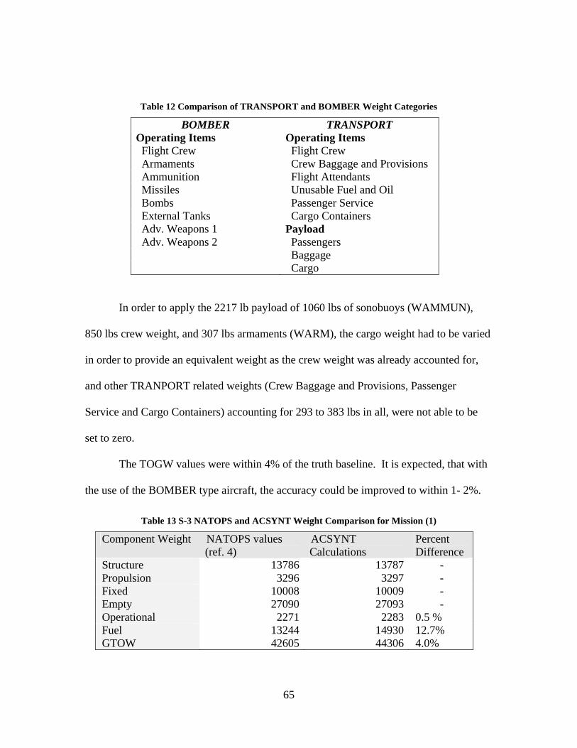
Table 12 Comparison of TRANSPORT and BOMBER Weight Categories
BOMBER TRANSPORT Operating Items Operating Items Flight Crew Flight Crew Armaments Crew Baggage and Provisions Ammunition Flight Attendants Missiles Unusable Fuel and Oil Bombs Passenger Service External Tanks Cargo Containers Adv. Weapons 1 Payload Adv. Weapons 2 Passengers Baggage Cargo
In order to apply the 2217 lb payload of 1060 lbs of sonobuoys (WAMMUN),
850 lbs crew weight, and 307 lbs armaments (WARM), the cargo weight had to be varied
in order to provide an equivalent weight as the crew weight was already accounted for,
and other TRANPORT related weights (Crew Baggage and Provisions, Passenger
Service and Cargo Containers) accounting for 293 to 383 lbs in all, were not able to be
set to zero.
The TOGW values were within 4% of the truth baseline. It is expected, that with
the use of the BOMBER type aircraft, the accuracy could be improved to within 1- 2%.
Table 13 S-3 NATOPS and ACSYNT Weight Comparison for Mission (1)
Component Weight NATOPS values (ref. 4)
ACSYNT Calculations
Percent Difference
Structure 13786 13787 - Propulsion 3296 3297 - Fixed 10008 10009 - Empty 27090 27093 - Operational 2271 2283 0.5 % Fuel 13244 14930 12.7% GTOW 42605 44306 4.0%
65

Impact ACSYNT should be able to provide accurate estimations of fuel required within
10% of the baseline value, but due to using a TRANSPORT-type aircraft, no mission
weight drops can be made. This effect will not be seen for the ASW model and the
joined-wing model as there are no payload or stores drops in the mission profile.
Raymer’s Canarded ASW Aircraft In his text (ref. 2), Raymer discusses a hypothetical ASW mission (fig. 31) and a
family of conceptual designs (fig. 33) that could be used to meet the mission.
Figure 34 ASW Concept Sketches
Mission and aircraft specifics are as shown below.
Table 14 ASW Aircraft/Mission Requirements
3 hr loiter @30K ft 10,000 lb = payload Wing AR = 10 High Bypass TF 1500 nm range 800 lb = crew wt WAR = 1.27 SFCloiter = 0.4 0.6 M cruise @30K ft L/Dmax = 16 AR effective = 7 SFCcruise = 0.5 L/Dcruise = 13.9 Swet/Sref = 5.5
Overview This model was originally to serve as the principal validation model, but due to
the fact that it is only a conceptual “paper airplane,” and not a production design, very
little information existed in order to build the model, and the only near comparison was
66
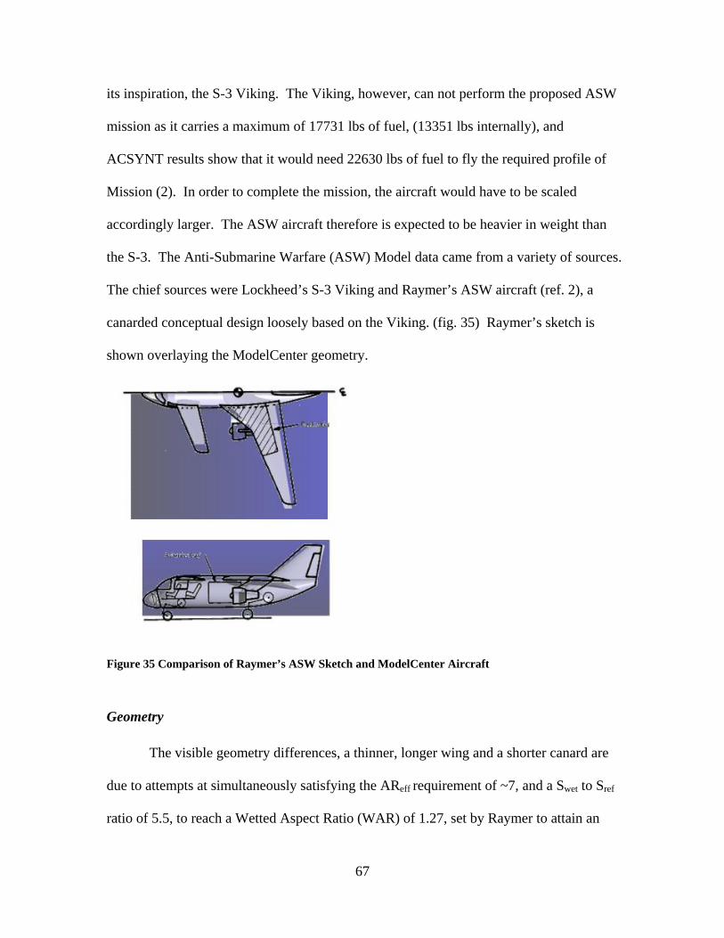
its inspiration, the S-3 Viking. The Viking, however, can not perform the proposed ASW
mission as it carries a maximum of 17731 lbs of fuel, (13351 lbs internally), and
ACSYNT results show that it would need 22630 lbs of fuel to fly the required profile of
Mission (2). In order to complete the mission, the aircraft would have to be scaled
accordingly larger. The ASW aircraft therefore is expected to be heavier in weight than
the S-3. The Anti-Submarine Warfare (ASW) Model data came from a variety of sources.
The chief sources were Lockheed’s S-3 Viking and Raymer’s ASW aircraft (ref. 2), a
canarded conceptual design loosely based on the Viking. (fig. 35) Raymer’s sketch is
shown overlaying the ModelCenter geometry.
Figure 35 Comparison of Raymer’s ASW Sketch and ModelCenter Aircraft
Geometry
The visible geometry differences, a thinner, longer wing and a shorter canard are
due to attempts at simultaneously satisfying the AReff requirement of ~7, and a Swet to Sref
ratio of 5.5, to reach a Wetted Aspect Ratio (WAR) of 1.27, set by Raymer to attain an
67

L/Dmax of 16. When the L/D table is coded ( ) an AR of
1.2984 equates with an L/D of 16, and was maintained to drive the model an L/D of 16.0.
0.4898max/ 14.081( )L D WAR=
Since no real flying model exists, several assumptions were made in the model’s
construction. The fuselage maximum diameter was set at 8.0 ft, and the length at 51 ft,
and the design tried to mimic the plan and profile shapes of the sketch while attempting
to meet a combined AR of 7, with a wing AR of 10. Actual combined or effective AR for
the model was 6.923, and Swet/Sref was 5.33.
Figure 36 ASW Aircraft Modeled in ModelCenter
Adaptability is a key component of the design of the ASW model; changes made
in the geometry echo into the analysis codes and allow rapid analysis, visualization and
recording of different designs. However, the ACSYNT input files must still be modified
for radical changes in design, for example the addition of a horizontal tail would require
the addition of the $HTAIL namelist to the ACSYNT input file, a modification of the
68

filewrapper and a relinking of components within ModelCenter, required any time the
filewrapper is changed.
Despite these difficulties the ability to tweak a given design for certain
performance and see changes in real time is exceptional. As a sample of the model’s
flexibility figure37 is presented. All but the S-3 design share exactly the same wing
planform, and engine size. None of these designs are presented as optimal or even flight
worthy, but serve as an example of the flexibility of the Visual Basic Script (VBS)
component location routine.
Figure 37 Model Center ASW Variants
Using enumerated values and integrated calculations embedded in Visual Basic
Scripts (VBS) the user can select from various drop-down menus in the Data Monitors
within ModelCenter the following options:
Wing/Canard z location – choice of high, medium, or low mounted wing.
69
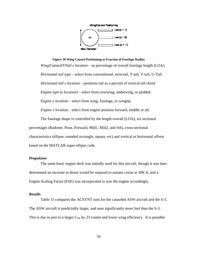
Figure 38 Wing Canard Positioning as Fraction of Fuselage Radius
Wing/Canard/VTail x location – as percentage of overall fuselage length (LOA).
Horizontal tail type – select from conventional, twin-tail, T-tail, V-tail, U-Tail.
Horizontal tail x location – positions tail as a percent of vertical tail chord
Engine type (z location) – select from overwing, underwing, or podded.
Engine y location – select from wing, fuselage, or wingtip.
Engine x location – select from engine position forward, middle or aft.
The fuselage shape is controlled by the length overall (LOA), six sectional
percentages (Radome, Nose, Forward, Mid1, Mid2, and Aft), cross-sectional
characteristics (ellipse, rounded rectangle, square, etc) and vertical or horizontal offsets
based on the MATLAB super-ellipse code.
Propulsion The same basic engine deck was initially used for this aircraft, though it was later
determined an increase in thrust would be required to sustain cruise at 30K ft, and a
Engine Scaling Factor (ESF) was incorporated to size the engine accordingly.
Results Table 15 compares the ACSYNT runs for the canarded ASW aircraft and the S-3.
The ASW aircraft is predictably larger, and uses significantly more fuel than the S-3.
This is due in part to a larger CD0 by 23 counts and lower wing efficiency. It is possible
70
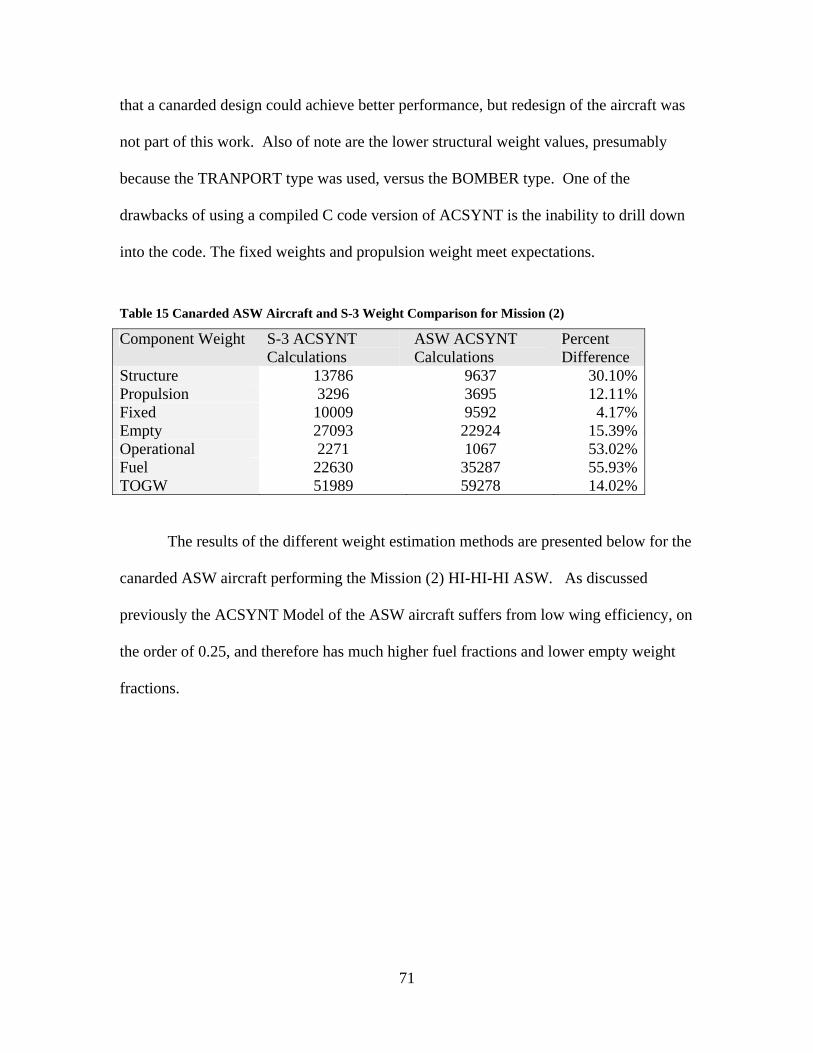
that a canarded design could achieve better performance, but redesign of the aircraft was
not part of this work. Also of note are the lower structural weight values, presumably
because the TRANPORT type was used, versus the BOMBER type. One of the
drawbacks of using a compiled C code version of ACSYNT is the inability to drill down
into the code. The fixed weights and propulsion weight meet expectations.
Table 15 Canarded ASW Aircraft and S-3 Weight Comparison for Mission (2)
Component Weight S-3 ACSYNT Calculations
ASW ACSYNT Calculations
Percent Difference
Structure 13786 9637 30.10% Propulsion 3296 3695 12.11% Fixed 10009 9592 4.17% Empty 27093 22924 15.39% Operational 2271 1067 53.02% Fuel 22630 35287 55.93% TOGW 51989 59278 14.02%
The results of the different weight estimation methods are presented below for the
canarded ASW aircraft performing the Mission (2) HI-HI-HI ASW. As discussed
previously the ACSYNT Model of the ASW aircraft suffers from low wing efficiency, on
the order of 0.25, and therefore has much higher fuel fractions and lower empty weight
fractions.
71

Table 16 Comparison of Weight Estimation Methods for the Canarded ASW Aircraft
Sizing Method Component Weight
Initial (ref.2)
Refined (ref.2)
ACSYNT Group Weights (ref. 2)
Approx. Weights (ref. 2)
Structure - - 9637 12369 13135 Propulsion - - 3695 4420 - Fixed - - 9592 15776 19644 Empty 24739 32090 22924 33504 26474 Operational 800 800 1067 1000 800 Fuel 21411 25343 35287 25343 25343 TOGW 56732 66742 59278 58907 61069 We/W0 0.44 0.48 0.39 0.57 0.42 Wf/W0 0.38 0.38 0.60 0.43 0.40
Impact The canarded ASW aircraft is not easily modeled in ACSYNT, due to the system
limitation of not permitting trimming canards. As a result, the associated trim drag is
higher than expected and the aircraft has low wing efficiency, producing a heavier than
expected aircraft. The joined-wing ACSYNTmodel will behave more like a conventional
aircraft in trim and should not suffer the same drag penalties.
72

Boeing SensorCraft Joined Wing (410E)
Introduction The ModelCenter integration environment was again utilized to construct and
store all the pertinent variables for Boeing’s joined-wing SensorCraft. First, a model
was built to match the 410E CAD data, based on manual 3-view measurement pickoffs.
After the AEI report was issued, the model was altered to reflect the more accurate
measurements. Data from the SensorCraft 410D model, (similar planform to 410E,
except pointed wing tips, and wider outboard chord), shown in inches, is shown in fig 39.
Figure 39 Boeing SensorCraft 410D Point-of-Departure Layout (ref. 21)
73
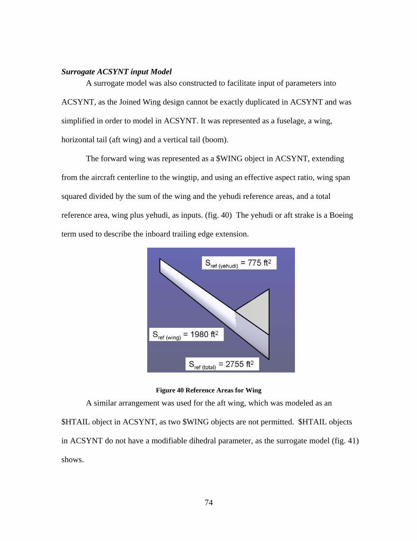
Surrogate ACSYNT input Model A surrogate model was also constructed to facilitate input of parameters into
ACSYNT, as the Joined Wing design cannot be exactly duplicated in ACSYNT and was
simplified in order to model in ACSYNT. It was represented as a fuselage, a wing,
horizontal tail (aft wing) and a vertical tail (boom).
The forward wing was represented as a $WING object in ACSYNT, extending
from the aircraft centerline to the wingtip, and using an effective aspect ratio, wing span
squared divided by the sum of the wing and the yehudi reference areas, and a total
reference area, wing plus yehudi, as inputs. (fig. 40) The yehudi or aft strake is a Boeing
term used to describe the inboard trailing edge extension.
Figure 40 Reference Areas for Wing
A similar arrangement was used for the aft wing, which was modeled as an
$HTAIL object in ACSYNT, as two $WING objects are not permitted. $HTAIL objects
in ACSYNT do not have a modifiable dihedral parameter, as the surrogate model (fig. 41)
shows.
74

Figure 41 Surrogate ACSYNT Input Model
ACSYNT is also unable to model wing twist, other than linear t/c and chord
distributions, and outboard wing sweep. The fuselage is modeled in ACYSNT as a $FUS
object, a constant cross section circular cylinder with a tapered nose cone and tail cone
(fig. 42). The fuselage diameter chosen is the overall fuselage height of the CAD model
of 8.82 ft, with fineness ratios (length/diameter) for the forward and aft section defined as
inputs into ACSYNT.
Figure 42 Simplified Fuselage with Constant Cross Section
75
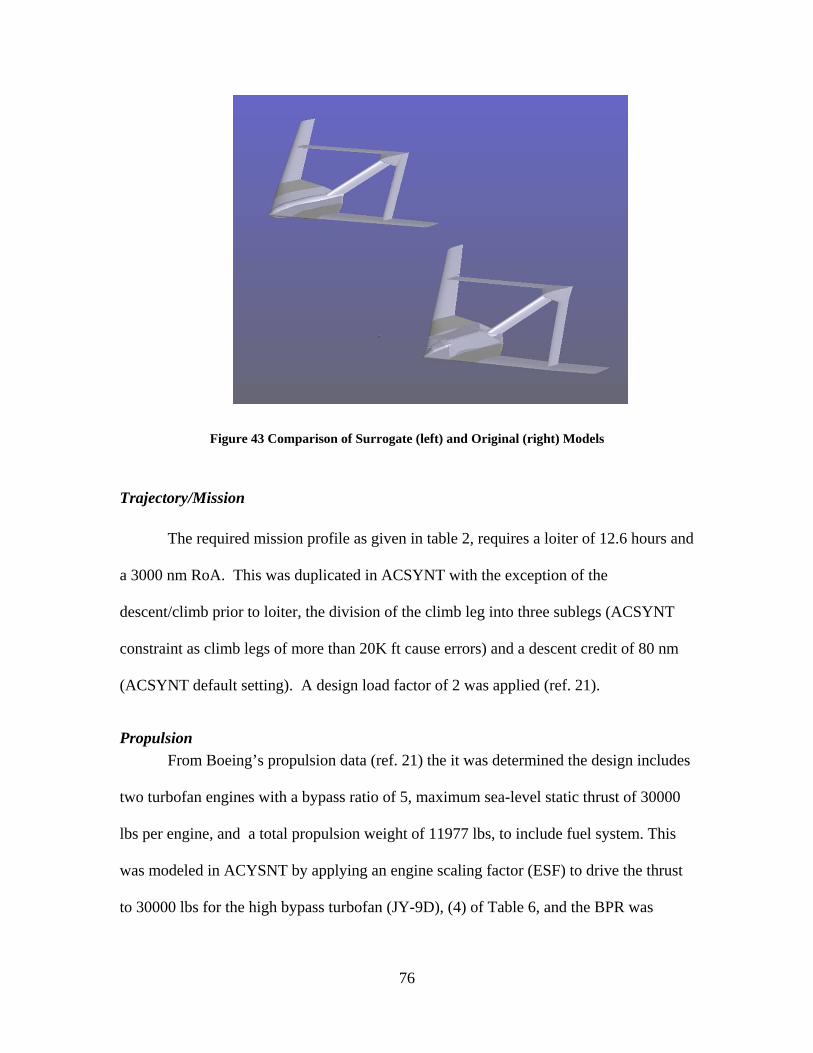
Figure 43 Comparison of Surrogate (left) and Original (right) Models
Trajectory/Mission
The required mission profile as given in table 2, requires a loiter of 12.6 hours and
a 3000 nm RoA. This was duplicated in ACSYNT with the exception of the
descent/climb prior to loiter, the division of the climb leg into three sublegs (ACSYNT
constraint as climb legs of more than 20K ft cause errors) and a descent credit of 80 nm
(ACSYNT default setting). A design load factor of 2 was applied (ref. 21).
Propulsion From Boeing’s propulsion data (ref. 21) the it was determined the design includes
two turbofan engines with a bypass ratio of 5, maximum sea-level static thrust of 30000
lbs per engine, and a total propulsion weight of 11977 lbs, to include fuel system. This
was modeled in ACYSNT by applying an engine scaling factor (ESF) to drive the thrust
to 30000 lbs for the high bypass turbofan (JY-9D), (4) of Table 6, and the BPR was
76

modified as well. Lastly, a propulsion weight scaling factor was used to fix the baseline
weight at 11977 lbs for the entire propulsion system, comprising engines and fuel system.
Aerodynamics The AEI report (ref. 21) showed laminar flow over nearly 40% of the wing
surface and this was modeled in ACSYNT by changing the default value of the laminar
to turbulent flow factor (SFWF variable in the $ACHAR namelist) to reflect a
conservative value of 0.63, or 37% laminar flow. Appendix H shows the effect of varying
this parameter for the baseline model in ACSYNT. The AEI report (ref. 21) also showed
a CL0 of approximately 0.4, which was used as well.
Weights To adjust the ACSYNT output component weights to the FEM measured
structural weights (ref. 21), in order to get an accurate prediction of fuel usage, the
baseline model was run once to determine the adjustments required. Through an iterative
procedure, as each variable affects the others, each variable was adjusted until it agreed
with the FEM 410E model within 1.00%.
Table 17 Detail of ACSYNT Model Weight Slopes
Component Unweighted Desired 1st Slope Final Slope Actual Difference Wing 34278 7652 0.223 0.237 7643 0.12% Fuselage 3128 6460 2.065 2.110 6460 0.00% Horiz. Tail 5783 4113 0.711 0.750 4142 0.71% Vert. Tail 3103 1238 0.399 0.420 1245 0.57% Nacelle 2743 866 0.316 0.315 864 0.23% Landing Gear 5200 3858 0.742 0.800 3853 0.13% APU 610 864 1.416 1.426 868 0.46% Electrical 2310 1064 0.461 0.520 1070 0.56% Control Surf. 2616 1199 0.458 0.458 1198 0.08%
Unweighted means the baseline 410E model run through ACSYNT with no fixed
77

or weighted values and default parameters: half-wing span (b) = 75, leading-edge front
wing sweep (Λib) = 38 deg, trailing edge aft wing sweep (Λia) = 38 deg, leading-edge
outboard wing sweep (Λob) = 38 deg, joint location as a percentage of half span (jloc) =
0.7117, vertical offset of the aft-wing root (zfa) = 16.13 ft and airfoil thickness to chord
ratio (t/c) = 0.08.
Desired represents the desired weight to match the 410E Model Structural weights
as given in ref. 21. ACSYNT uses slope values to increase or reduce certain weights in
order to match a given aircraft. The first slope represents the initial guess of desired over
unweighted. The final slope is what was used to determine the actual ACSYNT output
weights, which are given in column 6 of Table 17.
ACSYNT sizing The Joined wing model was not sized by initial or refined methods due to their
reliance on historical data. ACSYNT results for the baseline model (all variables default)
show good correlation with the available Boeing AEI data. There is no fuel weight or
TOGW given for the 410E model in the AEI report (ref.21), and nor is there an empty
weight given for the 410D model. The finite element model contains point masses for
fuel weight, but there is no indication as to what point of the mission those values are
valid. Also two different values are given for the 410E structural data, one of 22851 lbs is
included in the overall empty weight buildup (table 3) and the other of 26124 lbs is
derived from the structural component weight buildup (table 4). For the purpose of this
study a target structural weight value of 24187 was used, which is between the high and
low values of the Model 410E data and on par with the 410D data.
78

Table 18 Joined Wing Weights Comparison
Boeing Model (410D) (baseline)
Boeing Model (410E) (optimized)
ModelCenter (410E)
Model percent difference from baseline
Structural Weight 24572 22851 /26124 24161 1.67% Payload Weight 8860 8861 8862 0.02% Empty Weight ~49000* 50674 41404 15.50% ToC Weight 109570 112000 109281 0.26% Fuel Weight 65000 ~60000* 62003 4.61% Take-off Gross Weight (TOGW)
114630 ~111000* 112369 1.97%
* values starred represent best guess due to absence of explicit data FEM manipulation
The joined-wing model was broken up into six different sections to enable
modification and perturbation of the Boeing 410E Finite Element Model (FEM) as shown
in figure 44, variables are shown pictorially in figure 3..
Figure 44 Joined Wing Finite Element Model Sections
79

Each FEM point in each section has associated x, y, z GRID coordinates and
equations were written to modify the coordinates in each section based on a change to the
initial design variables. Coded in MATLAB, (App. F) the following table depicts the
effect of a change to each coordinate in each section by individual variable change. If
multiple variables are changed, they are calculated in sequential order, with the new
output coordinates assuming the role of the initial coordinates for the next equation.
Equations display delta values which can be used with eqn. (14) to determine the new
values.
'X X X= Δ + (14)
where X is the new coordinate of interest, ΔX is the change in the original value, and X’ is
the original value.
80
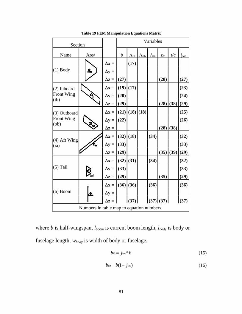
Table 19 FEM Manipulation Equations Matrix
Section Variables
Name Area b Λib Λob Λia zfa t/c jloc
Δx = (17)
Δy = (1) Body
Δz = (27) (28) (27)
Δx = (19) (17) (23)
Δy = (20) (24) (2) Inboard Front Wing (ib)
Δz = (29) (28) (38) (29)
Δx = (21) (18) (18) (25)
Δy = (22) (26) (3) Outboard Front Wing (ob)
Δz = (28) (38)
Δx = (32) (18) (34) (32)
Δy = (33) (33) (4) Aft Wing (ia)
Δz = (29) (35) (39) (29)
Δx = (32) (31) (34) (32)
Δy = (33) (33) (5) Tail
Δz = (29) (35) (29)
Δx = (36) (36) (36) (36)
Δy = (6) Boom
Δz = (37) (37) (37) (37) Numbers in table map to equation numbers.
where b is half-wingspan, lboom is current boom length, lbody is body or
fuselage length, wbody is width of body or fuselage,
*ib locb j b= (15)
(1 )ob locb b j= − (16)
81
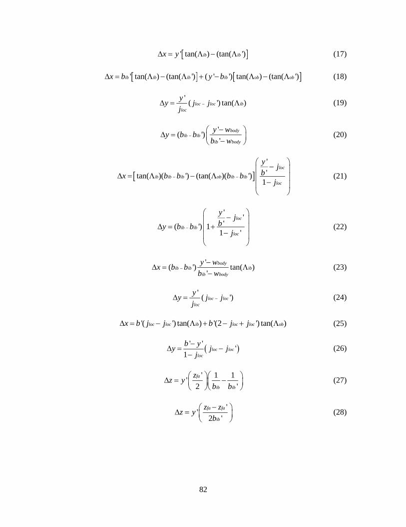
[ ]' tan( ) (tan( ')ib ibx yΔ = Λ − Λ (17)
[ ] [ ]' tan( ) (tan( ') ( ' ') tan( ) (tan( ')ib ib ib ib ob obx b y bΔ = Λ − Λ + − Λ − Λ (18)
' ( ') tan(loc loc ibloc
yy j jj
−Δ = Λ ) (19)
'( ')'
bodyib ib
ib body
y wy b bb w
−−⎛Δ = ⎜ −⎝ ⎠
⎞⎟
]
(20)
[''tan( )( ') (tan( )( ')
1
loc
ib ib ib ob ib ibloc
y jbx b b b b
j− −
⎛ ⎞−⎜ ⎟Δ = Λ − Λ ⎜ −⎜ ⎟
⎝ ⎠
⎟ (21)
' ''( ') 1
1 '
loc
ib ibloc
y jby b b
j−
⎛ ⎞−⎜ ⎟Δ = +⎜ −⎜ ⎟
⎝ ⎠
⎟ (22)
'( ') tan('
bodyib ib ib
ib body
y wx b bb w
− )−Δ = Λ
− (23)
' ( loc locloc
yy j jj
−Δ = ') (24)
(25) '( ') tan( ) '(2 ') tan( )loc loc ib loc loc obx b j j b j jΔ = − Λ + − + Λ
(' ' '1
loc locloc
b yy jj
)j−Δ = −
− (26)
' 1 1'2 'fa
ib ib
zz yb b
⎛ ⎞⎛Δ = −⎜ ⎟⎜⎝ ⎠⎝
⎞⎟⎠
(27)
''2 '
fa fa
ib
z zz yb−⎛Δ = ⎜
⎝ ⎠⎞⎟ (28)
82

'2 '
' ' '2 ' ' '
fa body body loc body
ib ib body ib
fa body body loc body
ib ib body ib
z w y w j wzb b w b
z w y w j wb b w b
⎛ ⎞− −⎛ ⎞⎛ ⎞ ⎛ ⎞Δ = +⎜ ⎟ ⎜ ⎟⎜ ⎟⎜ ⎟−⎝ ⎠ ⎝ ⎠⎝ ⎠⎝⎛ ⎞− −⎛ ⎞⎛ ⎞ ⎛ ⎞− +⎜ ⎟ ⎜ ⎟⎜ ⎟⎜ ⎟−⎝ ⎠ ⎝ ⎠⎝ ⎠⎝ ⎠
⎠ (29)
' ' ' ' ' ' ' 2 ' ' 2
ib fa ib fa
ib loc ib loc
y b z y b zzb b j b b j
⎛ ⎞ ⎛ ⎞− −⎛ ⎞ ⎛ ⎞Δ = −⎜ ⎟ ⎜⎜ ⎟ ⎜ ⎟− −⎝ ⎠ ⎝ ⎠⎝ ⎠ ⎝ ⎠⎟ (30)
( )' tan( ) tan( ')ib ib ibx bΔ = Λ − Λ (31)
( ) ( ) '' tan( ) ''
ibib ib ib ib ib
ib
b yx b b b bb−⎛Δ = − Λ + − ⎜
⎝ ⎠⎞⎟ (32)
(' ''
ib ibib
yy b bb
Δ = − ) (33)
( )' (tan( ) tan( '))ib ia iax b yΔ = − Λ − Λ (34)
( ') '12 '
fa fa ib
ib
z z b yzb
− ⎛Δ = +⎜⎝ ⎠
'− ⎞⎟ (35)
( ) (' tan( ) tan( ) ' tan( ') tan( ')ib ib ia ib ib iafa
zx b bz
Δ = Λ + Λ − Λ + Λ⎡ ⎤⎣ ⎦) (36)
( ) (' 'tan( ) tan( )
bodyfa fa
ib ib ia body
x lzb l
)z z−Δ = −
Λ + Λ − (37)
' ''2 'fa
ib
y z t cz zb t
⎛⎛ ⎞⎛ ⎞Δ = − ⎜⎜ ⎟⎜ ⎟⎝ ⎠⎝ ⎠⎝ ⎠c
⎞⎟ (38)
' ' ''2 2fa fa ib
ib
z z b y tz zb t
−⎡ ⎤ ⎛ ⎞⎛⎛ ⎞ ⎛ ⎞⎛ ⎞Δ = − + ⎜⎢ ⎜ ⎟ ⎜ ⎟⎜ ⎟⎜⎝ ⎠ ⎝ ⎠⎝ ⎠⎝ ⎠ ⎝ ⎠⎣ ⎦ 'cc
⎞⎟⎥⎟ (39)
83

Although a structural optimization was not accomplished on the joined-wing
SensorCraft model, the all the pieces are in place in order to conduct one. From the
joined wing FEM input (jw.dat) GRID data (xyz.txt), presorted by part, is extracted with
an include reference to the xyz.txt file. The xyz.txt file is then read into MATLAB by way
of readxyz.m, and coordinates are transformed according the modxyz.m script, which
links to ModelCenter for required variables and output back to the original xyz.txt file.
Then using a simple filewrapper, ModelCenter can execute a NASTRAN run and parse
the output file (jw.f06) for the structural weight data to include in the joined-wing model.
Figure 45 ModelCenter Structural Weight Incorporation
84

Design Variables The design variables (fig. 3) are: overall wing span (b), front wing sweep (Λib), aft
wing sweep (Λia), outboard wing sweep (Λob), joint location as a percentage of half span
(jloc), vertical offset of the aft-wing root (zfa) and airfoil thickness to chord ratio (t/c).
Design of Experiments (DOE) A design of experiments (DOE) table was built in ModelCenter, to vary the seven
design variables ± 10% about the Boeing solution. A 100-step Latin-squares DOE (100
runs) was utilized, which executed in about 30 minutes. For comparison, a Central
Composite DOE (143 runs), and a 3-step full factorial DOE were also constructed. The
Central Composite DOE executed in about 60 minutes, and the full factorial required
about 10 hours to complete the 2187 runs.
Sensitivity Analysis
From the Latin-squares DOE data, a variable sensitivity analysis (effect on
TOGW) was conducted on the design variables. Results showed that the main effects on
TOGW were inboard wing sweep (Λib) which accounts for nearly half (49%) of the
objective response, with vertical offset (zfa) and half-wing span (b) accounting for another
20% each. Previous studies [19] have shown a similar correlation between modifying
vertical offset and inboard sweep, and span was expected to have a significant part in the
response of the total weight. As expected modifications of outboard wing sweep (Λob)
had no effect on the TOGW, due to the modeling limitations of a sweeping outer wing in
ACSYNT. Thickness-to-chord (t/c) and aft wing sweep (Λia) had little effect on the
85

design, presumably because the changes resulted in no major aerodynamic effects and
areas affected were small compared with the forward wing or fuselage.
After a critical review of the initial data from the Latin-squares DOE, a sensitivity
analysis was also performed for the larger full-factorial DOE (2817 runs). This new study
showed drastically different results (fig. 46), primarily due to a better characterization of
the design space. The main effect shown is the half wing span (b), followed by joint
location (jloc), inboard sweep (Λib) and vertical offset (zfa). Outboard sweep as expected
showed no effect on the TOGW as expected, and the other two variables showed minimal
impact.
Figure 46 Variable Sensitivity Analysis
86

Joined-Wing Response Surfaces The purpose of response surfaces is to approximate complex relationships with
fast running surrogate equations in order to reduce the design space exploration time and
enable faster optimization. The optimization toolkit currently in ModelCenter is not
licensed and an optimization was not possible by that means. However from observing
the trends and parameter interaction as a result of running the DOE and from
investigating the response surface data, a vector toward a lower weight solution can be
established.
The Design of Experiments (DOE) tool was used to populate the DataCollector,
and then response surface models were created using the RSMToolkit, a Java and
FORTRAN90 based software tool. This response surface model then approximates the
GTOW over some range of the input variables, which can be used in conjunction with an
optimizer to perform a rapid design study. Highlight of the response surface Standard
Analysis of Variance (ANOVA) table for GTOW data is listed in appendix G, plots of
significant variable interaction are given in appendix B.
Some relevant statistics on the response surface model created are the standard
error of 2566 lbs, the average response of 115189 lbs, the coefficient of variation (COV)
of 2.23% , the ratio of the standard error to the average response and the R2 value of
79.72.%, which can be thought of as the percentage of the total variability of the data
which is explained by the response surface approximation. The R2(adj.) value of 78.54%
is close to the R2 value which indicates the response surface is not overfitted, and should
be usable for prediction. The fit is not terribly accurate, but provides a good starting
87

point for further design optimization. For a better fitting response surface, a larger DOE
should be conducted and outliers (points with a standardized residual (StdR) greater than
3), should be investigated to see if they are inaccurate, and if they are errant removed
from the fit.
88

V. Conclusions and Recommendations
The finite element modeling of structures is becoming more necessary for
advanced non-conventional structural weight prediction. Historical methods are
insufficient for estimation of novel designs. Integrated finite element analysis and
optimization, which incorporates the non-linear aeroelastic effects of the joined-wing
design for the critical load cases will be the beginning of the successful pursuit of an
efficient and safe joined wing design, and the seed for the next generation of
revolutionary design concepts.
Although not completed in this study, the template environment and linkages to
integrated finite element optimization was achieved through the use of ModelCenter as an
integration environment. The model can be expanded to include other codes and
aerodynamic calculations.
ACSYNT was proven as a powerful, but testy and unpredictable tool for the
calculation of component weights for conventional designs. The main drawbacks to its
use in a classroom environment are the lengthy learning time, the lack of good
documentation, and the dearth of technical support, as the program is no longer supported
by the vendor. For the power user, who has a thorough understanding of all of the
variables and drill-down access to the code, it will continue to be an excellent tool for the
sizing and performance predication of conventional craft. Its limitations though in
duplicating the design of an unconventional aircraft such as the joined-wing SensorCraft
are serious. ACSYNT would be a much more valuable tool in modeling unconventional
89

designs if it were able to create multiple $WING objects and a variety of $FUS objects,
with varying cross-sectional shapes.
ModelCenter is an excellent integration environment, with seemingly endless
expansion capability. The built-in toolkits for the Design of Experiments (DOE) and
Response Surface Models are excellent, as well as the data viewing application Data
Explorer. Weaknesses in modeling aircraft structures still remain. The inability to create
a wing from airfoil shapes, a twist and thickness schedule, prevents the use of the
NURBS rendered surfaces as more than cosmetic. Further integration attempts with
CAD software like Catia would prove useful for more accurate geometry determination,
and provide a handoff point for conceptual designs to the preliminary design teams in the
industry standard. Boeing’s General Geometry Generator looks promising, especially for
the rapid population of radical new designs, although the Python coding obstacle still
presents a challenge. Future integration within ModelCenter should be explored however,
especially as it concerns the development of meshes and grids for CFD and finite element
analysis
Advanced component geometry with integrated surface/volume calculation would
also provide a sleeker interface for the construction and maintenance of models. This
would also require a significant amount of coding and learning of Java. Should this be
accomplished it would be possible to integrate airfoil shapes into the wing, and possibly
to integrate 2-D foil generation software and aerodynamic calculations directly into the
model.
90

Considerations for stealthy and survivable design could also be pursued as a
welcome addition to the joined wing model. The integration of survivability concerns
early in the conceptual design phase prevents expensive redesign at a later stage.
Stability and control calculations were made for a radio controlled joined- wing
model [29], which could be compared to analytical calculations for the Boeing model and
integrated into ModelCenter. Initial experimental wind tunnel testing on the Boeing
joined-wing 410E model was also conducted [30] determining forces and moments
required for pitch control. Aeroelastic response will be investigated in follow-on testing.
This experimental data should be incorporated into the ModelCenter joined wing model.
Lastly, a Life Cycle Cost (LCC) model should be built and integrated in
ModelCenter with LCC set as a competing objective function to TOGW. This could
provide insight into multi-objective optimization for the joined-wing SensorCraft and
lead to a lower overall cost to the taxpayer, at the right level of performance.
91

List of References 1. Blair, M. Canfield, R.A. “A Joined-Wing Structural Weight Modeling Study”,
AIAA-2002-1337, presented at 43rd AIAA/ASME/ASCE/AHS/ASC Structures, Structural Dynamics, and Materials Conference, Denver, Colorado, 22-25 April 2002.
2. Raymer, Daniel P. “Aircraft Design: A Conceptual Approach”, American Institute
of Aeronautics and Astronautics, Washington, D.C., 1999. 3. ACSYNT (AirCraft SYNThesis) Version 3.0 User Guide, Phoenix Integration,
Blacksburg, VA, 1998. 4. S-3A NATOPS Flight Manual, Naval Air Systems Command, 01 April 1975. 5. O’Donnell, B.J. Application of the ACSYNT Computer Program for Aircraft
Design to V/STOL Aircraft., Thesis, Naval Postgraduate School, Monterey, CA, March 1978
6. ModelCenter 7.0, Phoenix Integration Inc., www.phoenix-int.com 7. Wolkovich, J. Joined Wing Aircraft, US Patent 3,942,747, March 1976. 8. Wolkovich, J. “The Joined Wing: An Overview”, AIAA-1985-0274, presented at
the 23rd AIAA Aerospace Sciences Meeting, Reno, NV, 14-17 January 1985. 9. Fairchild, M.P. “Structural Weight Comparison of a Joined Wing and a
Conventional Wing”, AIAA-81-0366, presented at the 19th AIAA Aerospace Sciences Meeting, Reno, NV, 12-15 January 1981.
10. Smith, S.C. and Cliff, S.E. “The Design of a Joined-Wing Flight Demonstrator
Aircraft”, AIAA-87-2930, presented at the AIAA/AHS/ASEE Aircraft Design, Systems and Operations Meeting, St. Louis, MO, 14-16 September 1987.
11. Smith, S. C., and Stonum, R. K., “Experimental Aerodynamic Characteristics of a
Joined-Wing Research Aircraft Configuration,” NASA TM 101083, April 1989. 12. Kroo, I.M., Gallman, J.W., and Smith, S.C., “Aerodynamic and Structural Studies
of Joined-Wing Aircraft”, Journal of Aircraft, Vol. 28, No. 1, January-February 1991, pp. 74-81.
13. Gallman, J.W., Smith, S.C., Kroo, I.M. “Optimization of Joined-Wing Aircraft”,
Journal of Aircraft,Vol. 30, No. 6, November-December 1993, pp. 897-905.
92

14. Gallman, J.W., Kroo, I.M. “Structural Optimization for Joined-Wing Synthesis”, Journal of Aircraft, Vol. 33, No. 1, January-February 1996, pp. 214-223.
15. Nangia, R.K., Palmer, M.E. and Tilmann, C.E., “Unconventional High Aspect
Ratio Joined-Wing Aircraft With Aft- & Forward- Swept Wing-Tips”, AIAA 2003-605, presented at 41st AIAA Aerospace Sciences Meeting & Exhibit, Reno, NV, 6-9 January 2003.
16. Livne, E. “Aeroelasticity of Joined-Wing Airplane Configurations: Past Work and
Future Challenges – A Survey”, AIAA-2001-1370, presented at the 42nd
AIAA/ASME/ASCE/AHS/ASC Structures, Structural Dynamics, and Materials Conference, Seattle, WA, 16-19 April 2001.
17. Roberts, Ronald W., Sensor-Craft Structural Optimization and Analytical
Certification, Thesis, Air Force Institute of Technology, School of Aeronautics and Astronautics, WPAFB, OH, March 2003.
18. Sitz, Jennifer J., Aeroelastic Analysis of a Joined-Wing Sensor-Craft, Thesis, Air
Force Institute of Technology, School of Aeronautics and Astronautics, WPAFB, OH, June 2004.
19. Rasmussen, Cody C., Optimization Process For Configuration Of Flexible
Joined-Wing, Thesis, Air Force Institute of Technology, School of Aeronautics and Astronautics, WPAFB, OH, March 2004
20. Lucia, D.J. “The SensorCraft Configurations: A Non-Linear AeroServoElastic
Challenge for Aviation”, AIAA 2005-1943, presented at 46th AIAA/ASME/ASCE/AHS/ASC Structures, Structural Dynamics, and Materials Conference, Austin, TX, 18-21 April, 2005,
21. AEI Aerodynamic Efficiency Improvement (AEI) PowerPoint report, Boeing, 17
July, 2006. Point of contact: Dr. Ken Iwanski Building 167, Area B 2310 8th St Wright Patterson AFB, OH 45433-7801 Contract No.: FA8650-05-C-3500
22. “MDOPT – A Multidisciplinary Design Optimization System Using Higher Order
Analysis Codes”, AIAA 2004-4567, 10th AIAA/ISSMO Multidisciplinary Analysis and Optimization Conference, Albany, NY, 30 August - 1 September 2004.
23. Parker, John T. Naval Postgraduate School Aircraft Synthesis Program (User’s
Manual). Thesis, Naval Postgraduate School, Monterey, CA, September 1991. 24. AVID ACS User’s Guide Version 4.1 , AVID LLC,
http://www.avidllc.biz/design_tools/AVID_ACS/_ACS_4.1_user's_guide/
93

25. Gelhousen, Paul, “ACSYNT Aircraft Synthesis Program,” NASA-AMES Research Center, September 1990.
26. Ardema, M.D. et al. “Analytical Fuselage and Wing Weight Estimation of
Transport Aircraft”, NASA TM 110392, May 1996. 27. General Geometry Generator (GGG) Software http://www.boeing.com/ 28. Super-Ellipse http://mathworld.wolfram.com/Superellipse.html 29. McClelland, William A. Inertia Measurement and Dynamic Stability Analysis of
A Radio-controlled Joined-wing Aircraft, Thesis, Air Force Institute of Technology, School of Aeronautics and Astronautics, WPAFB, OH, March 2006.
30. Bond, Vanessa “Wind Tunnel Testing of Twisted Wing for Longitudinal Control
in a Joined Wing Aircraft,” Presentation at Dayton Engineering Science Symposium, 30 Oct 2006.
94

Appendix A: ACSYNT Files
A-1 Canarded ASW Aircraft (Mission2-HI_HI_HI).IN A-2 Canarded ASW Aircraft (Mission2-HI_HI_HI).OUT A-3 S-3 (Mission2-HI_HI_HI).IN A-4 S-3 (Mission2-HI_HI_HI).OUT A-5 S-3 (Mission1-HI_LO_HI).IN A-6 S-3 (Mission1-HI_LO_HI).OUT A-7 JW.IN A-8 JW.OUT
95
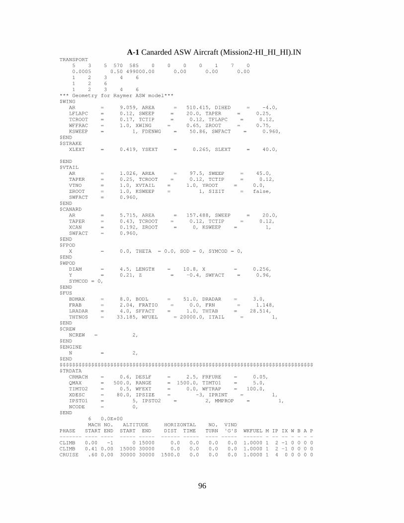
A-1 Canarded ASW Aircraft (Mission2-HI_HI_HI).IN TRANSPORT 5 3 5 570 585 0 0 0 0 1 7 0 0.0005 0.50 499000.00 0.00 0.00 0.00 1 2 3 4 6 1 2 6 1 2 3 4 6 *** Geometry for Raymer ASW model*** $WING AR = 9.059, AREA = 510.415, DIHED = -4.0, LFLAPC = 0.12, SWEEP = 20.0, TAPER = 0.25, TCROOT = 0.17, TCTIP = 0.12, TFLAPC = 0.12, WFFRAC = 1.0, XWING = 0.65, ZROOT = 0.75, KSWEEP = 1, FDENWG = 50.86, SWFACT = 0.960, $END $STRAKE XLEXT = 0.419, YSEXT = 0.265, SLEXT = 40.0, $END $VTAIL AR = 1.026, AREA = 97.5, SWEEP = 45.0, TAPER = 0.25, TCROOT = 0.12, TCTIP = 0.12, VTNO = 1.0, XVTAIL = 1.0, YROOT = 0.0, ZROOT = 1.0, KSWEEP = 1, SIZIT = false, SWFACT = 0.960, $END $CANARD AR = 5.715, AREA = 157.488, SWEEP = 20.0, TAPER = 0.43, TCROOT = 0.12, TCTIP = 0.12, XCAN = 0.192, ZROOT = 0, KSWEEP = 1, SWFACT = 0.960, $END $FPOD X = 0.0, THETA = 0.0, SOD = 0, SYMCOD = 0, $END $WPOD DIAM = 4.5, LENGTH = 10.8, X = 0.256, Y = 0.21, Z = -0.4, SWFACT = 0.96, SYMCOD = 0, $END $FUS BDMAX = 8.0, BODL = 51.0, DRADAR = 3.0, FRAB = 2.04, FRATIO = 0.0, FRN = 1.148, LRADAR = 4.0, SFFACT = 1.0, THTAB = 28.514, THTNOS = 33.185, WFUEL = 20000.0, ITAIL = 1, $END $CREW NCREW = 2, $END $ENGINE N = 2, $END $$$$$$$$$$$$$$$$$$$$$$$$$$$$$$$$$$$$$$$$$$$$$$$$$$$$$$$$$$$$$$$$$$$$$$$$$$$$$$$$ $TRDATA CRMACH = 0.6, DESLF = 2.5, FRFURE = 0.05, QMAX = 500.0, RANGE = 1500.0, TIMTO1 = 5.0, TIMTO2 = 0.5, WFEXT = 0.0, WFTRAP = 100.0, XDESC = 80.0, IPSIZE = -3, IPRINT = 1, IPSTO1 = 5, IPSTO2 = 2, MMPROP = 1, NCODE = 0, $END 6 0.0E+00 MACH NO. ALTITUDE HORIZONTAL NO. VIND PHASE START END START END DIST TIME TURN 'G'S WKFUEL M IP IX W B A P ------- ---- ---- ----- ----- ------ ----- ---- ----- ------ - -- -- - - - - CLIMB 0.00 -1 0 15000 0.0 0.0 0.0 0.0 1.0000 1 2 -1 0 0 0 0 CLIMB 0.41 0.00 15000 30000 0.0 0.0 0.0 0.0 1.0000 1 2 -1 0 0 0 0 CRUISE .60 0.00 30000 30000 1500.0 0.0 0.0 0.0 1.0000 1 4 0 0 0 0 0
96

LOITER .56 0.00 30000 30000 0.0 180.0 0.0 0.0 1.0000 1 4 0 0 0 0 0 CRUISE .60 0.00 35000 -1 1500.0 0.0 0.0 0.0 1.0000 1 4 0 0 0 0 0 LOITER 0.56 0.00 -1 0 0.0 20.0 0.0 0.0 1.0000 1 4 0 0 0 0 0 ***** AERODYNAMICS ***** $ACHAR ABOSB = 0.1, ALMAX = 15.0, AMC = 30.0, BDNOSE = 7.0, BTEF = 1.0, RCLMAX = 1.5, ROC = 0.02, ROCAN = 0.02, SFWF = 0.9, SMNDR = 0.93, SPANAC = 0.0, XCDC = 0.6, XCDW = 0.6, AJCAN = 2, ALELJ = 2, IDELTA = 0, INORM = 1, ISMNDR = 0, ISUPCR = 0, ITRAP = 0, IXCD = 1, ELLIPC = false, ELLIPH = false, ELLIPW = false, SMNSWP = 0.1, 0.15, 0.2, 0.25, 0.35, 0.45, 0.5, 0.55, 0.6, 0.65, CLOW = 0.0, 0.0, 0.0, 0.0, 0.0, 0.0, 0.0, 0.0, 0.0, 0.0, CLOW = 0.0, 0.0, 0.0, 0.0, 0.0, 0.0, 0.0, 0.0, 0.0, 0.0, CLOC = 0.05, 0.05, 0.05, 0.05, 0.05, 0.05, 0.05, 0.05, 0.05, 0.05, $END $AMULT CSF = 1.0, ESSF = 1.0, FCD = 1.0, FCDF = 1.0, FCDL = 1.0, FCDW = 1.0, FCDWB = 1.0, FENG = 1.0, FINTF = 1.0, FLBCOR = 1.0, FLECOR = 1.0, FMDR = 1.0, $END $ATRIM FVCAM = 1.0, 1.0, 1.0, 1.0, 1.0, 1.0, 1.0, 1.0, 1.0, 1.0, FLDM = 1.0, 1.0, 1.0, 1.0, 1.0, 1.0, 1.0, 1.0, 1.0, 1.0, ITRIM = 0, 0, 0, 0, 0, 0, 0, 0, 0, 0, CAND = 0.0, CFLAP = 0.2, CGM = 0.25, IT = 0.0, SM = -0.15, SPANF = 0.75, ZCG = 0.0, IVCAM = 1.0, $END $ADET IPLOT = 1, NALF = 10, NMDTL = 8, ICOD = 1, ALIN = -2.5, 0.0, 0.5, 1.0, 1.5, 2.0, 2.5, 3.0, 3.5, 4.0, ALTV = 38000.0, 40000.0, 42000.0, 44000.0, 38000.0, 40000.0, 42000.0, 44000.0, SMN = 0.56, 0.56, 0.56, 0.56, 0.6, 0.6, 0.6, 0.6, ISTRS = 0, 0, 0, 0, 0, 0, 0, 0, 0, 0, ITB = 0, 0, 0, 0, 0, 0, 0, 0, 0, 0, ITS = 0, 0, 0, 0, 0, 0, 0, 0, 0, 0, $END $ADRAG ICDO = 0, CDBMB = 10*0.0, CDEXTR = 10*0.0, CDTNK = 10*0.0, $END $ATAKE CLLAND = -1, CLTO = -1, DELFLD = 35.0, DELFTO = 25.0, DELLED = 25.0, DELLTO = 25.0, LDLAND = -1, LDTO = -1, $END $APRINT ECHOIN = 1, ECHOUT = 0, INTM = 0, IPBLNT = 0, IPCAN = 0, IPENG = 0, IPEXT = 0, IPFLAP = 0, IPFRIC = 0, IPINTF = 0, IPLIFT = 0, IPMIN = 0, IPWAVE = 0, KERROR = 0, $END *** Propulsion for ASW model SCALED (1.29) GE-TurboFan TF34-GE-2 turbofans, ~13950 lbf each (M=0.6) *** 6 $LEWIS AENDIA = 4.167, AENLE = 8.33, AENWT = 1421.0, TWOAB = 13950, $END
97

$AFTBD $END TRANSPORT ***** WEIGHTS ***** $OPTS WGTO =50000.000, AFMACH = 0.730, IDELT = 1, KBODY = 2, SLOPE = 1,1,1,1,1, 1,1,1,1,1, 1,1,1,1,1, 1,1,1,1,1, TECHI = 1,1,1,1,1,1,1,1,1, $END $FIXW WCREW = 800.000, WELT = 4353.000, WPA = 0.001, WPASS = 0.001, WBAG = 100.000, WCARGO = 0.001, $END
98

A-2 Canarded ASW Aircraft (Mission2-HI_HI_HI).OUT
***** WEIGHTS ***** Qmax: 500. Design Load Factor: 2.50 Ultimate Load Factor: 3.75 Structure and Material: Aluminum Skin, Stringer Wing Equation: Delta Wing Equation Body Equation: Air Force Equation Component Pounds Kilograms Percent Slope Tech Fixed Airframe Structure 9637. 4371. 16.26 No Wing 2356. 1069. 3.98 1.00 1.00 No Fuselage 2567. 1164. 4.33 1.00 1.00 No Horizontal Tail ( Low) 0. 0. 0.00 1.00 1.00 No Vertical Tail 490. 222. 0.83 1.00 1.00 No Canard 554. 251. 0.94 1.00 1.00 No Nacelles 965. 438. 1.63 1.00 1.00 No Landing Gear 2704. 1226. 4.56 1.00 1.00 No Propulsion 3695. 1676. 6.23 No Engines ( 2) 3410. 1547. 5.75 1.00 1.00 No Fuel System 284. 129. 0.48 1.00 1.00 No Fixed Equipment 9592. 4351. 16.18 1.00 No Hyd & Pneumatic 356. 161. 0.60 1.00 No Electrical 1572. 713. 2.65 1.00 No Avionics 4353. 1975. 7.34 1.00 Yes Instrumentation 761. 345. 1.28 1.00 No De-ice & Air Cond 246. 112. 0.41 1.00 No Aux Power System 600. 272. 1.01 1.00 No Furnish & Eqpt 0. 0. 0.00 1.00 Yes Seats and Lavatories 0. 0. 0.00 1.00 No Galley 0. 0. 0.00 1.00 No Misc Cockpit 234. 106. 0.40 1.00 No Cabin Finishing 798. 362. 1.35 1.00 No Cabin Emergency Equip 0. 0. 0.00 1.00 No Cargo Handling 348. 158. 0.59 1.00 No Flight Controls 1705. 773. 2.88 1.00 No Empty Weight 22924. 10398. 38.67 Operating Items 1067. 484. 1.80 No Flight Crew ( 2) 800. 363. 1.35 Yes Crew Baggage and Provisions 150. 68. 0.25 No Flight Attendents ( 0) 0. 0. 0.00 No Unusable Fuel and Oil 100. 45. 0.17 No Passenger Service 17. 8. 0.03 No Cargo Containers 0. 0. 0.00 No Operating Weight Empty 23991. 10882. 40.47 Fuel 35187. 15961. 59.36 Payload 100. 45. 0.17 No Passengers ( 0) 0. 0. 0.00 Yes Baggage 100. 45. 0.17 Yes Cargo 0. 0. 0.00 Yes -------- -------- ------ Calculated Weight 59278. 26888. 100.00 No Estimated Weight 59287. 26892. Percent Error -0.01
99

SUMMARY --- ACSYNT OUTPUT: ________________________________________________________________________________ GENERAL FUSELAGE WING CANARD VTAIL WG 59278. LENGTH 51.0 AREA 510.4 157.5 97.5 W/S 116.1 DIAMETER 8.0 WETTED AREA 870.5 199.6 188.5 T/W 0.47 VOLUME 2036.7 SPAN 68.0 30.0 10.0 N(Z) ULT 3.8 WETTED AREA 1118.8 L.E. SWEEP 23.3 23.4 52.3 CREW 2. FINENESS RATIO 6.4 C/4 SWEEP 20.0 20.0 45.0 PASENGERS 0. ASPECT RATIO 9.06 5.72 1.03 TAPER RATIO 0.25 0.43 0.25 ENGINE WEIGHTS T/C ROOT 0.17 0.12 0.12 T/C TIP 0.12 0.12 0.12 NUMBER 2. W WG ROOT CHORD 12.0 7.3 15.6 LENGTH 8.3 STRUCT. 9637. 16.3 TIP CHORD 3.0 3.2 3.9 DIAM. 5.0 PROPUL. 3695. 6.2 M.A. CHORD 8.4 5.5 10.9 WEIGHT 1421.0 FIX. EQ. 9592. 16.2 LOC. OF L.E. 30.1 9.8 35.4 TSLS 13950. FUEL 35287. 59.5 SFCSLS 0.36 PAYLOAD 100. 0.2 OPER IT 1067. 1.8 MISSION SUMMARY PHASE MACH ALT FUEL TIME DIST L/D THRUST SFC Q ======= ==== ====== ====== ===== ====== ===== ======= ===== ====== TAKEOFF 0.00 0. 263. 5.5 1980.8 CLIMB 0.41 15000. 490. 3.4 13.7 10.44 13293.7 0.541 141.4 CLIMB 0.52 30000. 695. 7.4 34.4 11.11 7652.7 0.607 119.6 CRUISE 0.60 31424. 13207. 246.9 1451.9 9.11 5164.3 0.574 148.7 LOITER 0.56 30000. 8158. 180.0 990.2 9.25 4827.5 0.563 138.2 CRUISE 0.60 35000. 10054. 260.2 1500.0 7.16 3959.9 0.567 125.8 LOITER 0.56 35000. 645. 20.0 107.6 7.58 3486.6 0.555 109.6 LANDING 4703.1 Block Time = 12.057 hr
Block Range = 4097.9 nm
100
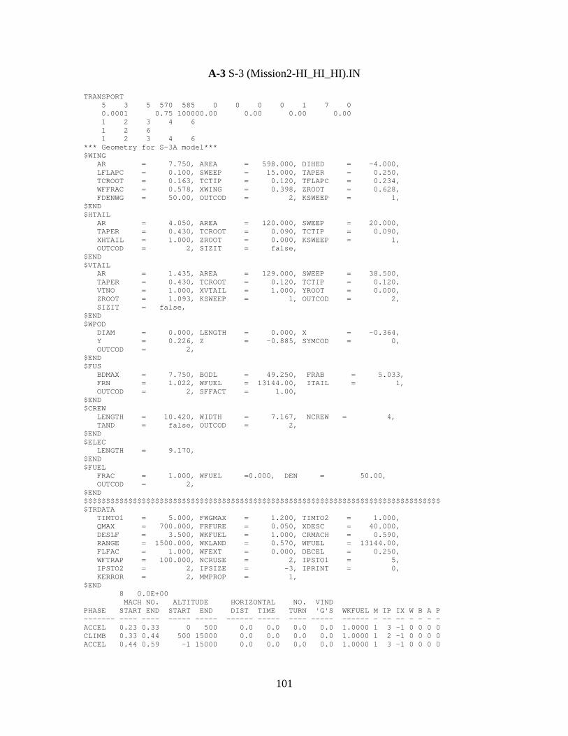
A-3 S-3 (Mission2-HI_HI_HI).IN
TRANSPORT 5 3 5 570 585 0 0 0 0 1 7 0 0.0001 0.75 100000.00 0.00 0.00 0.00 1 2 3 4 6 1 2 6 1 2 3 4 6 *** Geometry for S-3A model*** $WING AR = 7.750, AREA = 598.000, DIHED = -4.000, LFLAPC = 0.100, SWEEP = 15.000, TAPER = 0.250, TCROOT = 0.163, TCTIP = 0.120, TFLAPC = 0.234, WFFRAC = 0.578, XWING = 0.398, ZROOT = 0.628, FDENWG = 50.00, OUTCOD = 2, KSWEEP = 1, $END $HTAIL AR = 4.050, AREA = 120.000, SWEEP = 20.000, TAPER = 0.430, TCROOT = 0.090, TCTIP = 0.090, XHTAIL = 1.000, ZROOT = 0.000, KSWEEP = 1, OUTCOD = 2, SIZIT = false, $END $VTAIL AR = 1.435, AREA = 129.000, SWEEP = 38.500, TAPER = 0.430, TCROOT = 0.120, TCTIP = 0.120, VTNO = 1.000, XVTAIL = 1.000, YROOT = 0.000, ZROOT = 1.093, KSWEEP = 1, OUTCOD = 2, SIZIT = false, $END $WPOD DIAM = 0.000, LENGTH = 0.000, X = -0.364, Y = 0.226, Z = -0.885, SYMCOD = 0, OUTCOD = 2, $END $FUS BDMAX = 7.750, BODL = 49.250, FRAB = 5.033, FRN = 1.022, WFUEL = 13144.00, ITAIL = 1, OUTCOD = 2, SFFACT = 1.00, $END $CREW LENGTH = 10.420, WIDTH = 7.167, NCREW = 4, TAND = false, OUTCOD = 2, $END $ELEC LENGTH = 9.170, $END $FUEL FRAC = 1.000, WFUEL =0.000, DEN = 50.00, OUTCOD = 2, $END $$$$$$$$$$$$$$$$$$$$$$$$$$$$$$$$$$$$$$$$$$$$$$$$$$$$$$$$$$$$$$$$$$$$$$$$$$$$$$$$ $TRDATA TIMTO1 = 5.000, FWGMAX = 1.200, TIMTO2 = 1.000, QMAX = 700.000, FRFURE = 0.050, XDESC = 40.000, DESLF = 3.500, WKFUEL = 1.000, CRMACH = 0.590, RANGE = 1500.000, WKLAND = 0.570, WFUEL = 13144.00, FLFAC = 1.000, WFEXT = 0.000, DECEL = 0.250, WFTRAP = 100.000, NCRUSE = 2, IPSTO1 = 5, IPSTO2 = 2, IPSIZE = -3, IPRINT = 0, KERROR = 2, MMPROP = 1, $END 8 0.0E+00 MACH NO. ALTITUDE HORIZONTAL NO. VIND PHASE START END START END DIST TIME TURN 'G'S WKFUEL M IP IX W B A P ------- ---- ---- ----- ----- ------ ----- ---- ----- ------ - -- -- - - - - ACCEL 0.23 0.33 0 500 0.0 0.0 0.0 0.0 1.0000 1 3 -1 0 0 0 0 CLIMB 0.33 0.44 500 15000 0.0 0.0 0.0 0.0 1.0000 1 2 -1 0 0 0 0 ACCEL 0.44 0.59 -1 15000 0.0 0.0 0.0 0.0 1.0000 1 3 -1 0 0 0 0
101

CRUISE 0.59 0.59 15000 -1 635.0 0.0 0.0 0.0 1.0000 1 4 0 0 0 0 0 LOITER 0.34 0.34 100 100 0.0 60.0 0.0 0.0 1.0000 1 4 0 0 0 0 0 CLIMB 0.34 0.44 -1 10000 0.0 0.0 0.0 0.0 1.0000 1 2 -1 0 0 0 0 CRUISE 0.59 0.59 10000 -1 635.0 0.0 0.0 0.0 1.0000 1 4 0 0 0 0 0 LOITER 0.34 0.34 100 100 0.0 20.0 0.0 0.0 1.0000 1 4 0 0 0 0 0 ***** AERODYNAMICS ***** $ACHAR XCDW = 0.600, AMC = 40.000, SMNDR = 0.93, BTEF = 1.000, RCLMAX = 1.000, ROC = 0.02, SFWF = 1.000, ALELJ = 2, IDELTA = 0, INORM = 1, ISMNDR = 0, ISUPCR = 1, ITRAP = 0, IXCD = 1, ELLIPC = false, ELLIPH = false, ELLIPW = false, SMNSWP = 0.000, 0.200, 0.400, 0.600, 0.800, 1.000, 1.200, 1.400, 1.600, 1.800, CLOW = 0, 0, 0, 0, 0, 0, 0, 0, 0, 0, CMO = 0, 0, 0, 0, 0, 0, 0, 0, 0, 0, $END $AMULT CSF = 0.0, ESSF = 1.0, FCD = 1.0, FCDF = 0.95, FCDL = 1.0, FCDW = 1.0, FCDWB = 1.0, FENG = 1.0, FINTF = 1.0, FLBCOR = 1.0, FLECOR = 1.0, FMDR = 1.0, $END $ATRIM FVCAM = 1, 1, 1, 1, 1, 1, 1, 1, 1, 1, FLDM = 1, 1, 1, 1, 1, 1, 1, 1, 1, 1, ITRIM = 1, 1, 1, 1, 1, 1, 0, 0, 0, 0, CFLAP = 0.2, CGM = 0.25, IT = 0.0, SM = 0.1, SPANF = 0.75, ZCG = 0.0, IVCAM = 1, $END $ADET IPLOT = 1, NALF = 10, NMDTL = 6, ICOD = 1, ALIN = 0.0, 0.5, 1.0, 1.5, 2.0, 4.0, 6.0, 8.0, 10.0, 12.0, ALTV = 1000.0, 5000.0, 10000.0, 15000.0, 15000.0, 100.0, SMN = 0.33, 0.34, 0.35, 0.44, 0.59, 0.34, ISTRS = 0, 0, 0, 0, 0, 0, 0, 0, 0, 0, ITB = 0, 0, 0, 0, 0, 0, 0, 0, 0, 0, ITS = 0, 0, 0, 0, 0, 0, 0, 0, 0, 0, $END $ADRAG ICDO = 0, CDBMB = 10*0.0, CDEXTR = 10*0.0, CDTNK = 10*0.0, $END $ATAKE CLLAND = -1, CLTO = -1, DELFLD = 35.0, DELFTO = 25.0, DELLED = 25.0, DELLTO = 25.0, LDLAND = -1, LDTO = -1, $END $APRINT ECHOIN = 1, ECHOUT = 0, INTM = 0, IPBLNT = 0, IPCAN = 0, IPENG = 0, IPEXT = 0, IPFLAP = 0, IPFRIC = 0, IPINTF = 0, IPLIFT = 0, IPMIN = 0, IPWAVE = 0, KERROR = 0, $END *** Propulsion for ASW model GE-TurboFan TF34-GE-2 turbofans, 9,275 lbf (41.26 kN) each (M=0.6) *** 6 $LEWIS AENDIA = 4.167 AENLE = 8.33 AENWT = 1425.0 $END $AFTBD $END
102
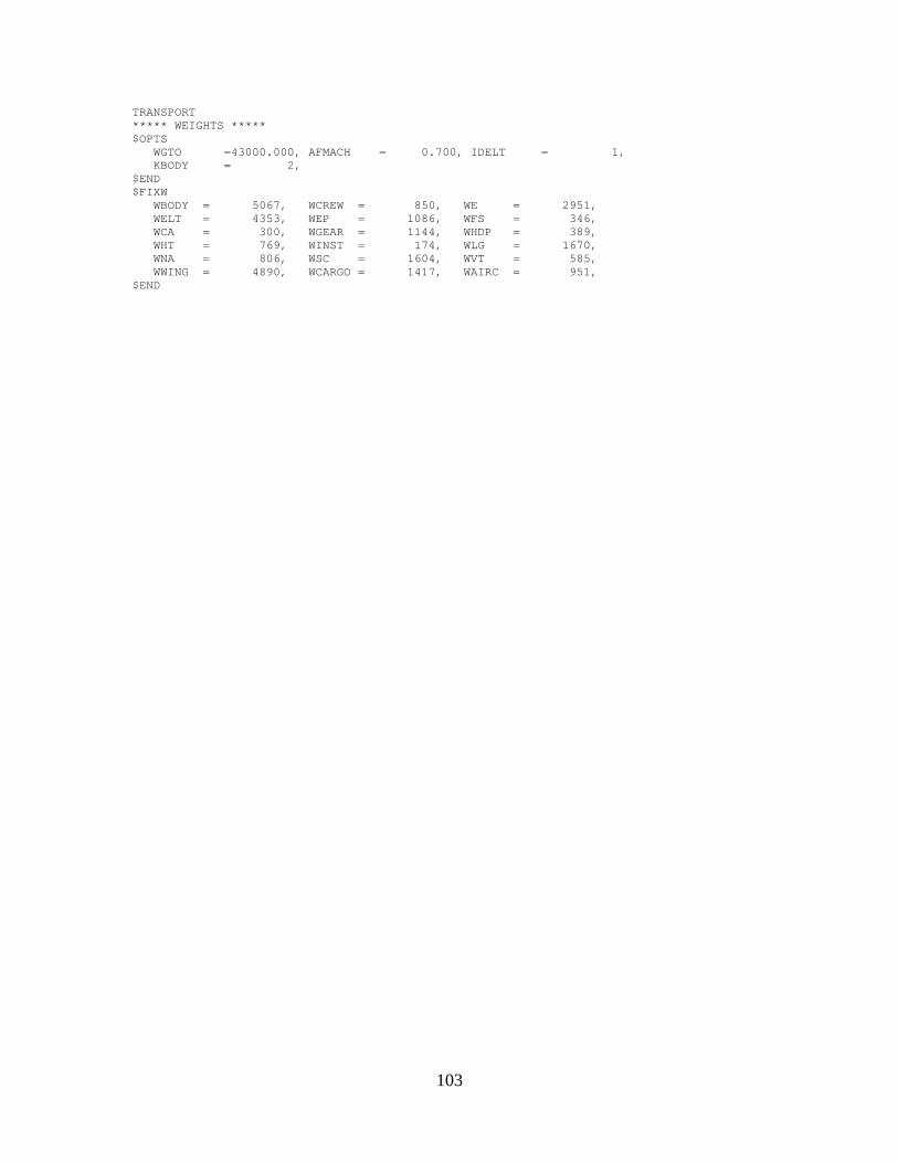
TRANSPORT ***** WEIGHTS ***** $OPTS WGTO =43000.000, AFMACH = 0.700, IDELT = 1, KBODY = 2, $END $FIXW WBODY = 5067, WCREW = 850, WE = 2951, WELT = 4353, WEP = 1086, WFS = 346, WCA = 300, WGEAR = 1144, WHDP = 389, WHT = 769, WINST = 174, WLG = 1670, WNA = 806, WSC = 1604, WVT = 585, WWING = 4890, WCARGO = 1417, WAIRC = 951, $END
103

A-4 S-3 (Mission2-HI_HI_HI).OUT ***** WEIGHTS ***** Qmax: 700. Design Load Factor: 3.50 Ultimate Load Factor: 3.75 Structure and Material: Aluminum Skin, Stringer Wing Equation: ______________________________ Body Equation: Air Force Equation Component Pounds Kilograms Percent Slope Tech Fixed Airframe Structure 13787. 6254. 26.52 No Wing 4890. 2218. 9.41 1.00 1.00 Yes Fuselage 5067. 2298. 9.75 1.00 1.00 Yes Horizontal Tail ( Low) 769. 349. 1.48 1.00 1.00 Yes Vertical Tail 585. 265. 1.13 1.00 1.00 Yes Nacelles 806. 366. 1.55 1.00 1.00 Yes Landing Gear 1670. 758. 3.21 1.00 1.00 Yes Propulsion 3297. 1496. 6.34 No Engines ( 2) 2951. 1339. 5.68 1.00 1.00 Yes Fuel System 346. 157. 0.67 1.00 1.00 Yes Fixed Equipment 10009. 4540. 19.25 1.00 Yes Hyd & Pneumatic 389. 176. 0.75 1.00 Yes Electrical 1098. 498. 2.11 1.00 Yes Avionics 4353. 1975. 8.37 1.00 Yes Instrumentation 174. 79. 0.33 1.00 Yes De-ice & Air Cond 951. 431. 1.83 1.00 Yes Aux Power System 1144. 519. 2.20 1.00 Yes Furnish & Eqpt 0. 0. 0.00 0.00 No Seats and Lavatories 0. 0. 0.00 0.00 No Galley 0. 0. 0.00 0.00 No Misc Cockpit 0. 0. 0.00 0.00 No Cabin Finishing 0. 0. 0.00 0.00 No Cabin Emergency Equip 0. 0. 0.00 0.00 No Cargo Handling 0. 0. 0.00 0.00 No Flight Controls 1604. 728. 3.09 1.00 Yes Empty Weight 27093. 12289. 52.11 Operating Items 1334. 605. 2.57 No Flight Crew ( 4) 850. 386. 1.63 Yes Crew Baggage and Provisions 200. 91. 0.38 No Flight Attendents ( 0) 0. 0. 0.00 No Unusable Fuel and Oil 100. 45. 0.19 No Passenger Service 34. 16. 0.07 No Cargo Containers 149. 68. 0.29 No Operating Weight Empty 28427. 12894. 54.68 Fuel 22630. 10265. 43.53 Payload 932. 423. 1.79 No Passengers ( 0) 0. 0. 0.00 No Baggage 0. 0. 0.00 No Cargo 932. 423. 1.79 Yes -------- -------- ------ Calculated Weight 51988. 23582. 99.43 No Estimated Weight 51988. 23582.
Percent Error 0.00
104

SUMMARY --- ACSYNT OUTPUT: ________________________________________________________________________________ GENERAL FUSELAGE WING HTAIL VTAIL WG 51988. LENGTH 49.3 AREA 598.0 120.0 129.0 W/S 86.9 DIAMETER 7.8 WETTED AREA 1042.4 241.0 259.9 T/W 0.36 VOLUME 1413.5 SPAN 68.1 22.0 13.6 N(Z) ULT 3.8 WETTED AREA 890.8 L.E. SWEEP 19.1 24.8 43.1 CREW 4. FINENESS RATIO 6.4 C/4 SWEEP 15.0 20.0 38.5 PASENGERS 0. ASPECT RATIO 7.75 4.05 1.43 TAPER RATIO 0.25 0.43 0.43 ENGINE WEIGHTS T/C ROOT 0.16 0.09 0.12 T/C TIP 0.12 0.09 0.12 NUMBER 2. W WG ROOT CHORD 14.1 7.6 13.3 LENGTH 8.3 STRUCT. 13787. 26.5 TIP CHORD 3.5 3.3 5.7 DIAM. 4.0 PROPUL. 3297. 6.3 M.A. CHORD 9.8 5.7 10.0 WEIGHT 1425.0 FIX. EQ. 10009. 19.3 LOC. OF L.E. 16.1 46.8 36.0 TSLS 9300. FUEL 22730. 43.7 SFCSLS 0.36 PAYLOAD 932. 1.8 OPER IT 1334. 2.6 MISSION SUMMARY PHASE MACH ALT FUEL TIME DIST L/D THRUST SFC Q ======= ==== ====== ====== ===== ====== ===== ======= ===== ====== TAKEOFF 0.00 0. 232. 6.0 3122.9 CLIMB 0.54 15000. 417. 4.2 22.0 14.01 8389.9 0.601 247.1 CLIMB 0.63 30000. 602. 9.0 54.8 15.16 5014.9 0.651 175.7 CRUISE 0.60 33392. 7416. 243.2 1423.1 15.07 2964.7 0.570 139.8 LOITER 0.69 30000. 6095. 180.0 1220.1 13.69 3163.1 0.642 209.8 CRUISE 0.60 33957. 6272. 256.7 1500.0 14.22 2259.1 0.591 136.9 LOITER 0.69 33957. 519. 20.0 133.2 12.65 2448.2 0.636 174.8 LANDING 3082.6 Block Time = 11.985 hr Block Range = 4353.4 nm
105

A-5 S-3 (Mission1 - HI_LO_HI).IN TRANSPORT 5 3 5 570 585 0 0 0 0 1 7 0 0.0001 0.75 100000.00 0.00 0.00 0.00 1 2 3 4 6 1 2 6 1 2 3 4 6 *** Geometry for S-3A model*** $WING AR = 7.750, AREA = 598.000, DIHED = -4.000, LFLAPC = 0.100, SWEEP = 15.000, TAPER = 0.250, TCROOT = 0.163, TCTIP = 0.120, TFLAPC = 0.234, WFFRAC = 0.578, XWING = 0.398, ZROOT = 0.628, FDENWG = 50.00, OUTCOD = 2, KSWEEP = 1, $END $HTAIL AR = 4.050, AREA = 120.000, SWEEP = 20.000, TAPER = 0.430, TCROOT = 0.090, TCTIP = 0.090, XHTAIL = 1.000, ZROOT = 0.000, KSWEEP = 1, OUTCOD = 2, SIZIT = false, $END $VTAIL AR = 1.435, AREA = 129.000, SWEEP = 38.500, TAPER = 0.430, TCROOT = 0.120, TCTIP = 0.120, VTNO = 1.000, XVTAIL = 1.000, YROOT = 0.000, ZROOT = 1.093, KSWEEP = 1, OUTCOD = 2, SIZIT = false, $END $WPOD DIAM = 0.000, LENGTH = 0.000, X = -0.364, Y = 0.226, Z = -0.885, SYMCOD = 0, OUTCOD = 2, $END $FUS BDMAX = 7.750, BODL = 49.250, FRAB = 5.033, FRN = 1.022, WFUEL = 13144.00, ITAIL = 1, OUTCOD = 2, SFFACT = 1.00, $END $CREW LENGTH = 10.420, WIDTH = 7.167, NCREW = 4, TAND = false, OUTCOD = 2, $END $ELEC LENGTH = 9.170, $END $FUEL FRAC = 1.000, WFUEL =0.000, DEN = 50.00, OUTCOD = 2, $END $$$$$$$$$$$$$$$$$$$$$$$$$$$$$$$$$$$$$$$$$$$$$$$$$$$$$$$$$$$$$$$$$$$$$$$$$$$$$$$$ $TRDATA TIMTO1 = 5.000, FWGMAX = 1.200, TIMTO2 = 1.000, QMAX = 700.000, FRFURE = 0.050, XDESC = 40.000, DESLF = 3.500, WKFUEL = 1.000, CRMACH = 0.590, RANGE = 1500.000, WKLAND = 0.570, WFUEL = 13144.00, FLFAC = 1.000, WFEXT = 0.000, DECEL = 0.250, WFTRAP = 100.000, NCRUSE = 2, IPSTO1 = 5, IPSTO2 = 2, IPSIZE = -3, IPRINT = 0, KERROR = 2, MMPROP = 1, $END 8 0.0E+00 MACH NO. ALTITUDE HORIZONTAL NO. VIND PHASE START END START END DIST TIME TURN 'G'S WKFUEL M IP IX W B A P ------- ---- ---- ----- ----- ------ ----- ---- ----- ------ - -- -- - - - - ACCEL 0.23 0.33 0 500 0.0 0.0 0.0 0.0 1.0000 1 3 -1 0 0 0 0 CLIMB 0.33 0.44 500 15000 0.0 0.0 0.0 0.0 1.0000 1 2 -1 0 0 0 0 ACCEL 0.44 0.59 -1 15000 0.0 0.0 0.0 0.0 1.0000 1 3 -1 0 0 0 0 CRUISE 0.59 0.59 15000 -1 635.0 0.0 0.0 0.0 1.0000 1 4 0 0 0 0 0
106
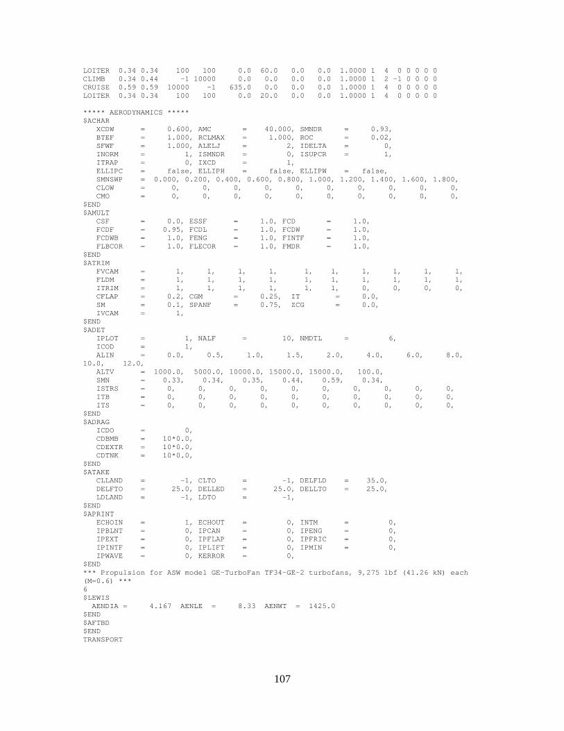
LOITER 0.34 0.34 100 100 0.0 60.0 0.0 0.0 1.0000 1 4 0 0 0 0 0 CLIMB 0.34 0.44 -1 10000 0.0 0.0 0.0 0.0 1.0000 1 2 -1 0 0 0 0 CRUISE 0.59 0.59 10000 -1 635.0 0.0 0.0 0.0 1.0000 1 4 0 0 0 0 0 LOITER 0.34 0.34 100 100 0.0 20.0 0.0 0.0 1.0000 1 4 0 0 0 0 0 ***** AERODYNAMICS ***** $ACHAR XCDW = 0.600, AMC = 40.000, SMNDR = 0.93, BTEF = 1.000, RCLMAX = 1.000, ROC = 0.02, SFWF = 1.000, ALELJ = 2, IDELTA = 0, INORM = 1, ISMNDR = 0, ISUPCR = 1, ITRAP = 0, IXCD = 1, ELLIPC = false, ELLIPH = false, ELLIPW = false, SMNSWP = 0.000, 0.200, 0.400, 0.600, 0.800, 1.000, 1.200, 1.400, 1.600, 1.800, CLOW = 0, 0, 0, 0, 0, 0, 0, 0, 0, 0, CMO = 0, 0, 0, 0, 0, 0, 0, 0, 0, 0, $END $AMULT CSF = 0.0, ESSF = 1.0, FCD = 1.0, FCDF = 0.95, FCDL = 1.0, FCDW = 1.0, FCDWB = 1.0, FENG = 1.0, FINTF = 1.0, FLBCOR = 1.0, FLECOR = 1.0, FMDR = 1.0, $END $ATRIM FVCAM = 1, 1, 1, 1, 1, 1, 1, 1, 1, 1, FLDM = 1, 1, 1, 1, 1, 1, 1, 1, 1, 1, ITRIM = 1, 1, 1, 1, 1, 1, 0, 0, 0, 0, CFLAP = 0.2, CGM = 0.25, IT = 0.0, SM = 0.1, SPANF = 0.75, ZCG = 0.0, IVCAM = 1, $END $ADET IPLOT = 1, NALF = 10, NMDTL = 6, ICOD = 1, ALIN = 0.0, 0.5, 1.0, 1.5, 2.0, 4.0, 6.0, 8.0, 10.0, 12.0, ALTV = 1000.0, 5000.0, 10000.0, 15000.0, 15000.0, 100.0, SMN = 0.33, 0.34, 0.35, 0.44, 0.59, 0.34, ISTRS = 0, 0, 0, 0, 0, 0, 0, 0, 0, 0, ITB = 0, 0, 0, 0, 0, 0, 0, 0, 0, 0, ITS = 0, 0, 0, 0, 0, 0, 0, 0, 0, 0, $END $ADRAG ICDO = 0, CDBMB = 10*0.0, CDEXTR = 10*0.0, CDTNK = 10*0.0, $END $ATAKE CLLAND = -1, CLTO = -1, DELFLD = 35.0, DELFTO = 25.0, DELLED = 25.0, DELLTO = 25.0, LDLAND = -1, LDTO = -1, $END $APRINT ECHOIN = 1, ECHOUT = 0, INTM = 0, IPBLNT = 0, IPCAN = 0, IPENG = 0, IPEXT = 0, IPFLAP = 0, IPFRIC = 0, IPINTF = 0, IPLIFT = 0, IPMIN = 0, IPWAVE = 0, KERROR = 0, $END *** Propulsion for ASW model GE-TurboFan TF34-GE-2 turbofans, 9,275 lbf (41.26 kN) each (M=0.6) *** 6 $LEWIS AENDIA = 4.167 AENLE = 8.33 AENWT = 1425.0 $END $AFTBD $END TRANSPORT
107

***** WEIGHTS ***** $OPTS WGTO =43000.000, AFMACH = 0.700, IDELT = 1, KBODY = 2, $END $FIXW WBODY = 5067, WCREW = 850, WE = 2951, WELT = 4353, WEP = 1086, WFS = 346, WCA = 300, WGEAR = 1144, WHDP = 389, WHT = 769, WINST = 174, WLG = 1670, WNA = 806, WSC = 1604, WVT = 585, WWING = 4890, WCARGO = 1417, WAIRC = 951, $END
108

A-6 S-3 (Mission1 - HI_LO_HI).OUT ***** WEIGHTS ***** Qmax: 700. Design Load Factor: 3.50 Ultimate Load Factor: 3.75 Structure and Material: Aluminum Skin, Stringer Wing Equation: ______________________________ Body Equation: Air Force Equation Component Pounds Kilograms Percent Slope Tech Fixed Airframe Structure 13787. 6254. 31.12 No Wing 4890. 2218. 11.04 1.00 1.00 Yes Fuselage 5067. 2298. 11.44 1.00 1.00 Yes Horizontal Tail ( Low) 769. 349. 1.74 1.00 1.00 Yes Vertical Tail 585. 265. 1.32 1.00 1.00 Yes Nacelles 806. 366. 1.82 1.00 1.00 Yes Landing Gear 1670. 758. 3.77 1.00 1.00 Yes Propulsion 3297. 1496. 7.44 No Engines ( 2) 2951. 1339. 6.66 1.00 1.00 Yes Fuel System 346. 157. 0.78 1.00 1.00 Yes Fixed Equipment 10009. 4540. 22.59 1.00 Yes Hyd & Pneumatic 389. 176. 0.88 1.00 Yes Electrical 1098. 498. 2.48 1.00 Yes Avionics 4353. 1975. 9.83 1.00 Yes Instrumentation 174. 79. 0.39 1.00 Yes De-ice & Air Cond 951. 431. 2.15 1.00 Yes Aux Power System 1144. 519. 2.58 1.00 Yes Furnish & Eqpt 0. 0. 0.00 0.00 No Seats and Lavatories 0. 0. 0.00 0.00 No Galley 0. 0. 0.00 0.00 No Misc Cockpit 0. 0. 0.00 0.00 No Cabin Finishing 0. 0. 0.00 0.00 No Cabin Emergency Equip 0. 0. 0.00 0.00 No Cargo Handling 0. 0. 0.00 0.00 No Flight Controls 1604. 728. 3.62 1.00 Yes Empty Weight 27093. 12289. 61.15 Operating Items 1244. 564. 2.81 No Flight Crew ( 4) 850. 386. 1.92 Yes Crew Baggage and Provisions 125. 57. 0.28 No Flight Attendents ( 0) 0. 0. 0.00 No Unusable Fuel and Oil 100. 45. 0.23 No Passenger Service 2. 1. 0.01 No Cargo Containers 166. 75. 0.38 No Operating Weight Empty 28337. 12854. 63.96 Fuel 14930. 6772. 33.70 Payload 1039. 471. 2.35 No Passengers ( 0) 0. 0. 0.00 No Baggage 0. 0. 0.00 No Cargo 1039. 471. 2.35 Yes -------- -------- ------ Calculated Weight 44305. 20097. 99.33 No Estimated Weight 44305. 20097. Percent Error 0.00
109
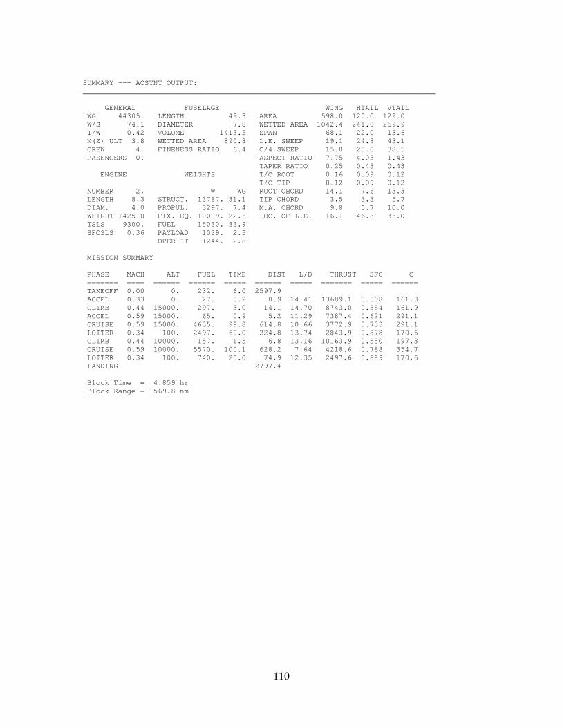
SUMMARY --- ACSYNT OUTPUT: ________________________________________________________________________________ GENERAL FUSELAGE WING HTAIL VTAIL WG 44305. LENGTH 49.3 AREA 598.0 120.0 129.0 W/S 74.1 DIAMETER 7.8 WETTED AREA 1042.4 241.0 259.9 T/W 0.42 VOLUME 1413.5 SPAN 68.1 22.0 13.6 N(Z) ULT 3.8 WETTED AREA 890.8 L.E. SWEEP 19.1 24.8 43.1 CREW 4. FINENESS RATIO 6.4 C/4 SWEEP 15.0 20.0 38.5 PASENGERS 0. ASPECT RATIO 7.75 4.05 1.43 TAPER RATIO 0.25 0.43 0.43 ENGINE WEIGHTS T/C ROOT 0.16 0.09 0.12 T/C TIP 0.12 0.09 0.12 NUMBER 2. W WG ROOT CHORD 14.1 7.6 13.3 LENGTH 8.3 STRUCT. 13787. 31.1 TIP CHORD 3.5 3.3 5.7 DIAM. 4.0 PROPUL. 3297. 7.4 M.A. CHORD 9.8 5.7 10.0 WEIGHT 1425.0 FIX. EQ. 10009. 22.6 LOC. OF L.E. 16.1 46.8 36.0 TSLS 9300. FUEL 15030. 33.9 SFCSLS 0.36 PAYLOAD 1039. 2.3 OPER IT 1244. 2.8 MISSION SUMMARY PHASE MACH ALT FUEL TIME DIST L/D THRUST SFC Q ======= ==== ====== ====== ===== ====== ===== ======= ===== ====== TAKEOFF 0.00 0. 232. 6.0 2597.9 ACCEL 0.33 0. 27. 0.2 0.9 14.41 13689.1 0.508 161.3 CLIMB 0.44 15000. 297. 3.0 14.1 14.70 8743.0 0.554 161.9 ACCEL 0.59 15000. 65. 0.9 5.2 11.29 7387.4 0.621 291.1 CRUISE 0.59 15000. 4635. 99.8 614.8 10.66 3772.9 0.733 291.1 LOITER 0.34 100. 2497. 60.0 224.8 13.74 2843.9 0.878 170.6 CLIMB 0.44 10000. 157. 1.5 6.8 13.16 10163.9 0.550 197.3 CRUISE 0.59 10000. 5570. 100.1 628.2 7.64 4218.6 0.788 354.7 LOITER 0.34 100. 740. 20.0 74.9 12.35 2497.6 0.889 170.6 LANDING 2797.4 Block Time = 4.859 hr Block Range = 1569.8 nm
110
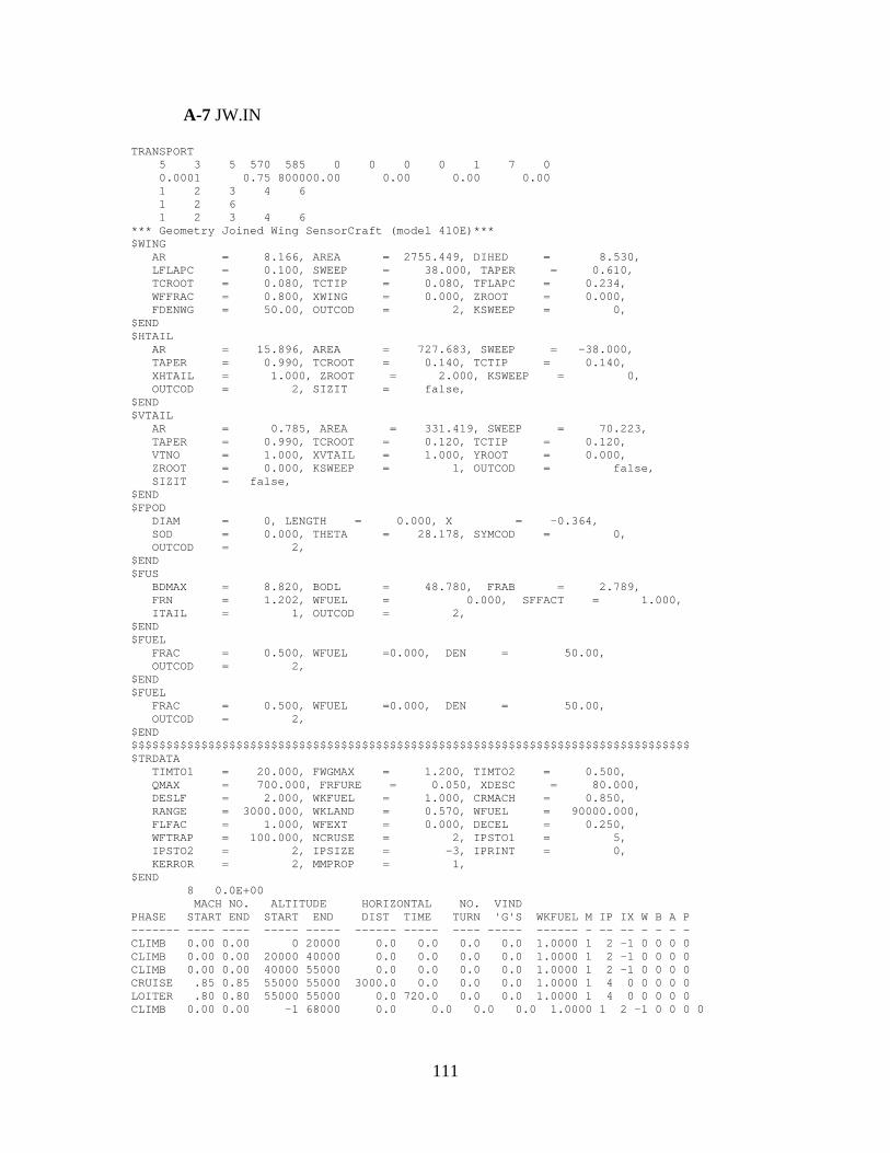
A-7 JW.IN
TRANSPORT 5 3 5 570 585 0 0 0 0 1 7 0 0.0001 0.75 800000.00 0.00 0.00 0.00 1 2 3 4 6 1 2 6 1 2 3 4 6 *** Geometry Joined Wing SensorCraft (model 410E)*** $WING AR = 8.166, AREA = 2755.449, DIHED = 8.530, LFLAPC = 0.100, SWEEP = 38.000, TAPER = 0.610, TCROOT = 0.080, TCTIP = 0.080, TFLAPC = 0.234, WFFRAC = 0.800, XWING = 0.000, ZROOT = 0.000, FDENWG = 50.00, OUTCOD = 2, KSWEEP = 0, $END $HTAIL AR = 15.896, AREA = 727.683, SWEEP = -38.000, TAPER = 0.990, TCROOT = 0.140, TCTIP = 0.140, XHTAIL = 1.000, ZROOT = 2.000, KSWEEP = 0, OUTCOD = 2, SIZIT = false, $END $VTAIL AR = 0.785, AREA = 331.419, SWEEP = 70.223, TAPER = 0.990, TCROOT = 0.120, TCTIP = 0.120, VTNO = 1.000, XVTAIL = 1.000, YROOT = 0.000, ZROOT = 0.000, KSWEEP = 1, OUTCOD = false, SIZIT = false, $END $FPOD DIAM = 0, LENGTH = 0.000, X = -0.364, SOD = 0.000, THETA = 28.178, SYMCOD = 0, OUTCOD = 2, $END $FUS BDMAX = 8.820, BODL = 48.780, FRAB = 2.789, FRN = 1.202, WFUEL = 0.000, SFFACT = 1.000, ITAIL = 1, OUTCOD = 2, $END $FUEL FRAC = 0.500, WFUEL =0.000, DEN = 50.00, OUTCOD = 2, $END $FUEL FRAC = 0.500, WFUEL =0.000, DEN = 50.00, OUTCOD = 2, $END $$$$$$$$$$$$$$$$$$$$$$$$$$$$$$$$$$$$$$$$$$$$$$$$$$$$$$$$$$$$$$$$$$$$$$$$$$$$$$$$ $TRDATA TIMTO1 = 20.000, FWGMAX = 1.200, TIMTO2 = 0.500, QMAX = 700.000, FRFURE = 0.050, XDESC = 80.000, DESLF = 2.000, WKFUEL = 1.000, CRMACH = 0.850, RANGE = 3000.000, WKLAND = 0.570, WFUEL = 90000.000, FLFAC = 1.000, WFEXT = 0.000, DECEL = 0.250, WFTRAP = 100.000, NCRUSE = 2, IPSTO1 = 5, IPSTO2 = 2, IPSIZE = -3, IPRINT = 0, KERROR = 2, MMPROP = 1, $END 8 0.0E+00 MACH NO. ALTITUDE HORIZONTAL NO. VIND PHASE START END START END DIST TIME TURN 'G'S WKFUEL M IP IX W B A P ------- ---- ---- ----- ----- ------ ----- ---- ----- ------ - -- -- - - - - CLIMB 0.00 0.00 0 20000 0.0 0.0 0.0 0.0 1.0000 1 2 -1 0 0 0 0 CLIMB 0.00 0.00 20000 40000 0.0 0.0 0.0 0.0 1.0000 1 2 -1 0 0 0 0 CLIMB 0.00 0.00 40000 55000 0.0 0.0 0.0 0.0 1.0000 1 2 -1 0 0 0 0 CRUISE .85 0.85 55000 55000 3000.0 0.0 0.0 0.0 1.0000 1 4 0 0 0 0 0 LOITER .80 0.80 55000 55000 0.0 720.0 0.0 0.0 1.0000 1 4 0 0 0 0 0 CLIMB 0.00 0.00 -1 68000 0.0 0.0 0.0 0.0 1.0000 1 2 -1 0 0 0 0
111

CRUISE .85 0.85 68000 68000 3000.0 0.0 0.0 0.0 1.0000 1 4 0 0 0 0 0 LOITER 0.80 0.80 100 100 0.0 20.0 0.0 0.0 1.0000 1 4 0 0 0 0 0 ***** AERODYNAMICS ***** $ACHAR XCDW = 0.600, AMC = 40.000, SMNDR = 0.930, BTEF = 0.000, RCLMAX = 1.000, ROC = 0.020, SFWF = 0.630, ALELJ = 2, IDELTA = 0, INORM = 1, ISMNDR = 0, ISUPCR = 0, ITRAP = 1, IXCD = 1, ELLIPC = false, ELLIPH = false, ELLIPW = false, SMNSWP = 0.000, 0.100, 0.200, 0.300, 0.400, 0.500, 0.600, 0.700, 0.800, 0.900, CLOW = 0.430, 0.430, 0.430, 0.430, 0.430, 0.430, 0.430, 0.430, 0.430, 0.430, CMO = 0.000, 0.000, 0.000, 0.000, 0.000, 0.000, 0.000, 0.000, 0.000, 0.000, $END $AMULT CSF = 0.000, ESSF = 0.000, FCD = 1.000, FCDF = 0.950, FCDL = 1.000, FCDW = 1.000, FCDWB = 1.000, FENG = 1.000, FINTF = 1.000, FLBCOR = 1.000, FLECOR = 1.000, FMDR = 1.000, $END $ATRIM FVCAM = 1.000, 1.000, 1.000, 1.000, 1.000, 1.000, 1.000, 1.000, 1.000, 1.000, FLDM = 1.000, 1.000, 1.000, 1.000, 1.000, 1.000, 1.000, 1.000, 1.000, 1.000, ITRIM = 1, 1, 1, 1, 1, 1, 1, 1, 1, 1, CFLAP = 0.200, CGM = 0.250, IT = 0.000, SM = .100, SPANF = 0.750, ZCG = 0.000, IVCAM = 1, $END $ADET IPLOT = 1, NALF = 10, NMDTL = 8, ICOD = 1, ALIN = 0.000, 0.500, 1.000, 1.500, 2.000, 4.000, 6.000, 8.000, 10.000, 12.000, ALTV = 50000.000, 50000.000, 50000.000, 65000.000, 65000.000, 65000.000, 65000.000, 55000.000, SMN = 0.600, 0.800, 0.700, 0.600, 0.700, 0.800, 0.850, 0.850, ISTRS = 0, 0, 0, 0, 0, 0, 0, 0, 0, 0, ITB = 0, 0, 0, 0, 0, 0, 0, 0, 0, 0, ITS = 0, 0, 0, 0, 0, 0, 0, 0, 0, 0, $END $ADRAG ICDO = 0, CDBMB = 10*0.0, CDEXTR = 10*0.0, CDTNK = 10*0.0, $END $ATAKE CLLAND = -1, CLTO = -1, DELFLD = 35.000, DELFTO = 25.000, DELLED = 25.000, DELLTO = 25.000, LDLAND = -1, LDTO = -1, $END $APRINT ECHOIN = 1, ECHOUT = 0, INTM = 0, IPBLNT = 0, IPCAN = 0, IPENG = 0, IPEXT = 0, IPFLAP = 0, IPFRIC = 0, IPINTF = 0, IPLIFT = 0, IPMIN = 0, IPWAVE = 0, KERROR = 0, $END *** Propulsion for JW model **Modified** SCALED 5 BPR, 50,000 lbf class (747-like) *** 4 $LEWIS ESF = 0.6085, TWOAB = 30425.000, SFSFC1 = 0.700, BA = 5.000, ALTD = 0, 30000, 40000, 50000, 50000, 60000, XMACH = 0, 0.6, 0.8, 0.8, 0.6, 0.6,
112

$END $AFTBD $END TRANSPORT ***** WEIGHTS ***** $OPTS WGTO =115000.000, AFMACH = 0.850, IDELT = 0, KBODY = 2, KWING = 1, SLOPE = 0.237,2.110,0.750,0.420,0.315,0.805,0.819,0.819,1.000,0.520,1.000,0.000,1.000,0.000,1.426,0.458,0.000,1.000,1.000,1.000, TECHI = 1.000,1.000,1.000,1.000,1.000,1.000,1.000,1.000,1.000, $END $FIXW WBODY = 0.000, WHT = 0.000, WLG = 0.000, WELT = 0.000, WNA = 0.000, WVT = 0.000, WWING = 0.000, WGEAR = 0.000, WPL = 8862.000, WAPU = 0.000, WSC = 0.000, WEP = 0.000, $END
113

A-8 JW.OUT AAAAAAA CCCCCCC SSSSSSS Y Y N N TTTTTTT A A C S Y Y NN N T A A C S Y Y N N N T AAAAAAA C SSSSSSS Y N N N T A A C S Y N N N T A A C S Y N N T A A CCCCCCC SSSSSSS Y N N T ACSYNT-C VERSION 3.0 COPYRIGHT 1999, PHOENIX INTEGRATION, INC. ALL RIGHTS RESERVED T I T L E ________________________________________________________________________________ AIRCRAFT TYPE - TRANSPORT 1 TITLE: JOINED WING SENSORCRAFT ________________________________________________________________________________ AIRCRAFT TYPE - TRANSPORT CONTROL PARAMETERS: READ CONTROL, MREAD = 5 EXECUTION CONTROL, MEXEC = 3 WRITE CONTROL, MWRITE = 5 NUMBER IDENTIFYING CONVERGENCE VARIABLE FOR CONVERGED VEHICLE, IOBJ = 570 NUMBER IDENTIFYING COMPARISON VARIABLE FOR CONVERGED VEHICLE, JOBJ = 585 SUMMARY OUTPUT PRINT CODE, IPSUM = 0 GLOBAL ERROR PRINT CODE, KGLOBP = 0 GLOBAL COMMON INITIALIZATION CODE, INIT = 0 DEBUG PRINT CODE, IPDBG = 0 GLOBAL PLOT CONTROL, IGPLT = 1 DATA TRANSFER INFORMATION FILE, IRDDTR = 7 DATA TRANSFER INFORMATION PRINT, IPDTR = 0 VEHICLE CONVERGENCE INFORMATION: CONVERGENCE TOLERANCE, TOL = 0.10000E-03 ESTIM WCALC VS WEXT SLOPE = 0.75000E+00 BOUNDING WEIGHT, WGMAX = 0.80000E+06 MODULE IDENTIFICATION NUMBERS: NUMBER MODULE 1 GEOMETRY 2 TRAJECTORY 3 AERODYNAMICS 4 PROPULSION 5 STABILITY AND CONTROL 6 WEIGHTS 8 SONIC BOOM 9 ECONOMICS 11 SUMMARY OUTPUT 12 AGILITY 14 TAKEOFF AND LANDING MODULES ARE CALLED FOR INPUT IN THE FOLLOWING ORDER: 1 2 3 4 6 MODULES ARE CALLED FOR EXECUTION IN THE FOLLOWING ORDER: 1 2 6 MODULES ARE CALLED FOR OUTPUT IN THE FOLLOWING ORDER: 1 2 3 4 6
114

Fuselage Definition (Type 2) Nose Length.................. 10.602 Nose Fineness Ratio.......... 1.202 Constant Section Length...... 13.579 Afterbody Length............. 24.599 Afterbody Fineness Ratio..... 2.789 Overall Length............... 48.780 Maximum Diameter............. 8.820 Body Planform Area........... 342.185 Fuselage Definition Nacelle Definition Nacelle Location X R Area X-Xnose R Area X Y Z 0.00 0.00 0.00 0.00 3.33 34.75 -17.76 6.82 3.65 0.53 0.77 1.86 5.93 3.33 34.75 -17.76 -6.82 3.65 1.06 1.27 5.06 17.80 3.33 34.75 1.59 1.69 8.93 23.74 3.33 34.75 2.12 2.05 13.20 2.65 2.37 17.68 3.18 2.66 22.25 3.71 2.92 26.81 4.24 3.16 31.28 4.77 3.37 35.59 5.30 3.55 39.68 5.83 3.72 43.51 6.36 3.87 47.04 6.89 4.00 50.22 7.42 4.11 53.04 7.95 4.20 55.46 8.48 4.28 57.47 9.01 4.34 59.05 9.54 4.38 60.18 10.07 4.40 60.87 10.60 4.41 61.10 11.96 4.41 61.10 13.32 4.41 61.10 14.68 4.41 61.10 16.03 4.41 61.10 17.39 4.41 61.10 18.75 4.41 61.10 20.11 4.41 61.10 21.47 4.41 61.10 22.82 4.41 61.10 24.18 4.41 61.10 25.41 4.40 60.87 26.64 4.38 60.18 27.87 4.34 59.05 29.10 4.28 57.47 30.33 4.20 55.46 31.56 4.11 53.04 32.79 4.00 50.22 34.02 3.87 47.04 35.25 3.72 43.51 36.48 3.55 39.68 37.71 3.37 35.59 38.94 3.16 31.28 40.17 2.92 26.81 41.40 2.66 22.25 42.63 2.37 17.68 43.86 2.05 13.20 45.09 1.69 8.93 46.32 1.27 5.06 47.55 0.77 1.86 48.78 0.00 0.00 Fuselage Nacelles - 2 Max. Diameter...... 8.820 ..... 6.652 Fineness Ratio..... 5.531 Surface Area....... 1095.477 ..... 496.058 (each) Volume............. 2096.445
115
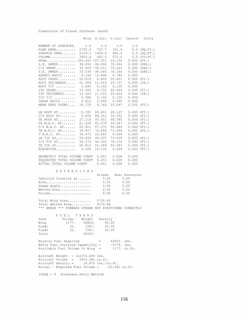
Dimensions of Planar Surfaces (each) Wing H.Tail V.Tail Canard Units NUMBER OF SURFACES. 1.0 1.0 1.0 1.0 PLAN AREA.......... 2755.4 727.7 331.4 0.0 (SQ.FT.) SURFACE AREA....... 5129.3 1469.6 484.4 0.0 (SQ.FT.) VOLUME............. 2803.4 482.5 572.0 0.0 (CU.FT.) SPAN............... 150.003 107.551 16.130 0.000 (FT.) L.E. SWEEP......... 38.000 -38.000 70.244 0.000 (DEG.) C/4 SWEEP.......... 36.929 -38.011 70.223 0.000 (DEG.) T.E. SWEEP......... 33.530 -38.045 70.160 0.000 (DEG.) ASPECT RATIO ...... 8.166 15.896 0.785 0.000 ROOT CHORD......... 22.819 6.800 20.651 0.000 (FT.) ROOT THICKNESS..... 21.906 11.424 29.737 0.000 (IN.) ROOT T/C .......... 0.080 0.140 0.120 0.000 TIP CHORD.......... 13.920 6.732 20.444 0.000 (FT.) TIP THICKNESS...... 13.363 11.310 29.439 0.000 (IN.) TIP T/C ........... 0.080 0.140 0.120 0.000 TAPER RATIO ....... 0.610 0.990 0.990 0.000 MEAN AERO CHORD.... 18.729 6.766 20.547 0.000 (FT.) LE ROOT AT......... -5.705 86.651 28.129 0.000 (FT.) C/4 ROOT AT........ 0.000 88.351 33.292 0.000 (FT.) TE ROOT AT......... 17.114 93.451 48.780 0.000 (FT.) LE M.A.C. AT....... 21.228 65.679 50.547 0.000 (FT.) C/4 M.A.C. AT...... 25.911 67.371 55.684 0.000 (FT.) TE M.A.C. AT....... 39.957 72.445 71.094 0.000 (FT.) Y M.A.C. AT........ 34.473 26.843 0.000 0.000 LE TIP AT.......... 52.893 44.637 73.039 0.000 (FT.) C/4 TIP AT......... 56.373 46.320 78.150 0.000 (FT.) TE TIP AT.......... 66.813 51.369 93.483 0.000 (FT.) ELEVATION.......... 0.000 16.130 0.000 0.000 (FT.) GEOMETRIC TOTAL VOLUME COEFF 0.651 0.028 0.000 REQUESTED TOTAL VOLUME COEFF 0.651 0.028 0.000 ACTUAL TOTAL VOLUME COEFF 0.651 0.028 0.000 E X T E N S I O N S Strake Rear Extension Centroid location at....... 0.00 0.00 Area....................... 0.00 0.00 Sweep Angle................ 0.00 0.00 Wetted Area................ 0.00 0.00 Volume..................... 0.00 0.00 Total Wing Area............ 2755.45 Total Wetted Area.......... 9170.88 *** ERROR *** FORWARD STRAKE NOT POSITIONED CORRECTLY F U E L T A N K S Tank Volume Weight Density Wing 1177. 58829. 50.00 Fus#1 32. 1587. 50.00 Fus#2 32. 1587. 50.00 Total 62003. Mission Fuel Required = 62003. lbs. Extra Fuel Carrying Capability = -3174. lbs. Available Fuel Volume in Wing = 1177. cu.ft. Aircraft Weight = 112372.648 lbs. Aircraft Volume = 5954.385 cu.ft. Aircraft Density = 18.872 lbs./cu.ft. Actual - Required Fuel Volume = -63.481 cu.ft. ICASE = 4 (Fineness Ratio Method)
116

Trajectory Output Mission 1 (PAYLOAD = 8862. LB) PHASE M H CL ALPHA WFUEL TIME VEL SFC(I) THRUST(I) CD GAMMA W WA Q SFC(U) THRUST(U) CDINST L/D THR/THA PR X WARM-UP 0. 721.2 20.00 9.90 218. TAKEOFF 0.11 0. 2.3796 13.71 134.1 0.50 119. 0.28 57848. 0.3552 21.72 111651.4 959.35 17. 0.28 57848. 0.0020 6.70 1.00 1.00 1666. 2ND SEG 0.11 400. 2.3796 13.71 119. 0.28 28924. 0.3552 6.38 111651.4 959.35 17. 0.28 57848. 0.0020 6.70 1.00 1.00 CLIMB 0.49 20000. 0.1656 -5.05 691.4 3.18 508. 0.40 25319. 0.0151 9.56 110825.9 543.40 164. Cycle 0.39 25574. 0.0006 10.97 1.00 1.00 15. CLIMB 0.66 40000. 0.2629 -3.69 768.8 6.40 643. 0.45 11746. 0.0147 3.54 110057.1 263.38 122. Cycle 0.44 11836. 0.0003 17.89 1.00 1.00 36. CLIMB 0.82 55000. 0.3901 -2.10 776.4 12.25 796. 0.48 5872. 0.0167 0.88 109280.7 145.80 91. Cycle 0.47 5972. 0.0004 23.31 1.00 1.00 90. CRUISE 0.85 55000. 0.3653 -2.50 14690.3 351.85 823. 0.47 4750. 0.0208 0.00 94590.4 138.37 97. Cycle 0.45 4937. 0.0007 17.58 0.81 1.00 2859. LOITER 0.80 55000. 0.3995 -2.01 21644.9 720.00 774. 0.45 4036. 0.0170 0.00 72945.5 129.68 86. Cycle 0.43 4185. 0.0006 23.45 0.69 1.00 5506. CLIMB 0.79 65600. 0.4811 -1.12 917.8 35.67 767. 0.45 2789. 0.0203 -0.05 72027.7 79.32 51. Cycle 0.43 2872. 0.0006 23.65 0.79 1.00 274. CRUISE 0.85 68000. 0.4369 -1.57 11012.0 436.00 824. 0.47 2554. 0.0214 0.00 61015.7 74.25 52. Cycle 0.45 2654. 0.0007 20.46 0.81 1.00 3548. LOITER 0.80 100. 0.0234 -6.21 7598.4 20.00 893. 0.51 45088. 0.0173 0.00 53417.4 1261.36 945. Cycle 0.49 41352. 0.0005 1.35 1.13 1.00 176. LANDING 0.12 0. 2.0356 7.32 131. 0.28 57289. 0.2998 28.10 85754.3 960.73 20. 0.28 57394. 0.0019 6.79 1.00 1.00 1571.
117

Fuel Summary Total Fuel = 62003. Takeoff Fuel: Fuel Load: Mission Fuel = 58955. Warmup = 721. External = 0. Reserve Fuel = 2948. Takeoff = 134. Internal = 62003. Trapped Fuel = 100. Block Time = 26.764 hrs Block Range = 12504.8 n.m. Block Fuel = 58955.3 lb. Takeoff Field Length (total run) = 1666. ft Landing Field Length (total run) = 1571. ft Decel @ .250 Gs Landing Field Length (ground run) = 837. ft Field Length Factor = 1.000 Weight for Landing calculation = 85754. lbs Landing Thrust to Weight ratio = 0.668 Takeoff Weight = 112373. lbs Landing Weight = 53417. lbs
118

Mach = 0.25 C.G. Location = 25.9 ft, 0.25 cbar Altitude = 0. Takeoff Configuration: Flaps and Slats Parasite Drag Induced Drag Friction .0072 Alpha Cl Cd L/D e Zone Cm Cdtrim Deltrim StMrg Body .0010 -0.3 1.163 0.0904 12.9 0.58 2 0.000 -.0025 1.3 0.340 Wing .0037 0.3 1.217 0.0988 12.3 0.58 2 0.000 -.0019 0.9 0.341 Strakes .0000 0.9 1.271 0.1074 11.8 0.58 2 0.000 -.0012 0.6 0.342 H. Tail .0020 1.4 1.324 0.1162 11.4 0.59 2 0.000 -.0005 0.2 0.342 V. Tail .0005 2.0 1.377 0.1252 11.0 0.59 2 0.000 0.0003 -0.1 0.343 Canard .0000 4.4 1.587 0.1628 9.8 0.60 2 0.000 0.0039 -1.6 0.346 6.7 1.794 0.2029 8.8 0.62 2 0.000 0.0082 -3.2 0.349 9.1 1.998 0.2501 8.0 0.62 2 0.000 0.0131 -4.7 0.352 11.4 2.200 0.3024 7.3 0.62 2 0.000 0.0185 -6.4 0.355 13.8 2.399 0.3599 6.7 0.62 2 0.000 0.0246 -8.1 0.358 Interference .0014 Wave .0000 External .0000 Slope Factors Tanks .0000 Cl/Alpha (per radian) 5.0318 Bombs .0000 Cdl/Cl^2 0.0626 Stores .0000 Alpha Transition Zone 2-3 16.189 Extra .0000 Camber .0090 Flap Setting 25. ___________________ Slat Setting 25. Cdmin .0175 Flap Type Single 388. sq. ft Mach = 0.25 C.G. Location = 25.9 ft, 0.25 cbar Altitude = 0. Landing Configuration: Flaps and Slats Parasite Drag Induced Drag Friction .0072 Alpha Cl Cd L/D e Zone Cm Cdtrim Deltrim StMrg Body .0010 -0.4 1.372 0.1419 9.7 0.52 2 0.000 -.0040 1.7 0.341 Wing .0037 0.2 1.424 0.1529 9.3 0.52 2 0.000 -.0034 1.4 0.342 Strakes .0000 0.8 1.476 0.1641 9.0 0.52 2 0.000 -.0027 1.1 0.343 H. Tail .0020 1.3 1.527 0.1755 8.7 0.52 2 0.000 -.0019 0.8 0.344 V. Tail .0005 1.9 1.578 0.1871 8.4 0.52 2 0.000 -.0011 0.4 0.344 Canard .0000 4.2 1.782 0.2349 7.6 0.53 2 0.000 0.0027 -1.0 0.348 6.5 1.982 0.2849 7.0 0.54 2 0.000 0.0072 -2.5 0.351 8.9 2.179 0.3389 6.4 0.55 2 0.000 0.0124 -4.0 0.355 11.2 2.375 0.3996 5.9 0.55 2 0.000 0.0180 -5.6 0.359 13.6 2.568 0.4651 5.5 0.55 2 0.000 0.0243 -7.2 0.363 Interference .0014 Wave .0000 External .0000 Slope Factors Tanks .0000 Cl/Alpha (per radian) 4.9035 Bombs .0000 Cdl/Cl^2 0.0706 Stores .0000 Alpha Transition Zone 2-3 16.189 Extra .0000 Camber .0090 Flap Setting 35. ___________________ Slat Setting 25. Cdmin .0175 Flap Type Single 388. sq. ft
119

Detailed Aerodynamics Output Mach = 0.60 C.G. Location = 25.9 ft, 0.25 cbar Altitude = 50000. Reynolds Number per foot = 711688. Parasite Drag Induced Drag Friction .0071 Alpha Cl Cd L/D e Zone Cm Cdtrim Deltrim StMrg Body .0010 -0.3 0.557 0.0231 24.1 0.51 2 0.000 -.0012 1.3 0.344 Wing .0037 0.3 0.607 0.0260 23.3 0.54 2 0.000 -.0008 0.8 0.344 Strakes .0000 0.9 0.656 0.0289 22.7 0.57 2 0.000 -.0003 0.3 0.344 H. Tail .0020 1.5 0.705 0.0320 22.0 0.60 2 0.000 0.0002 -0.2 0.344 V. Tail .0005 2.1 0.754 0.0354 21.3 0.62 2 0.000 0.0008 -0.6 0.345 Canard .0000 4.6 0.956 0.0535 17.9 0.66 2 0.000 0.0037 -2.6 0.379 7.1 1.185 0.0798 14.9 0.68 3 0.000 0.0012 -4.6 0.386 9.6 1.337 0.1168 11.4 0.59 3 0.000 0.0042 -6.5 0.397 12.1 1.479 0.1645 9.0 0.52 3 0.000 0.0093 -8.5 0.413 14.8 1.610 0.2236 7.2 0.45 3 0.000 0.0172 -10.6 0.434 Interference .0014 Wave .0000 External .0000 Slope Factors Tanks .0000 Cl/Alpha (per radian) 4.0113 Bombs .0000 Cdl/Cl^2 0.0864 Stores .0000 Alpha Transition Zone 2-3 4.367 Extra .0000 Camber .0090 Programmed Flap Setting 0. ___________________ Cdmin .0175 Flap Type Single 388. sq. ft Mach = 0.80 C.G. Location = 25.9 ft, 0.25 cbar Altitude = 50000. Reynolds Number per foot = 948917. Parasite Drag Induced Drag Friction .0067 Alpha Cl Cd L/D e Zone Cm Cdtrim Deltrim StMrg Body .0010 -0.2 0.564 0.0231 24.4 0.52 2 0.000 -.0011 1.2 0.340 Wing .0034 0.4 0.618 0.0262 23.6 0.55 2 0.000 -.0007 0.7 0.340 Strakes .0000 1.0 0.671 0.0295 22.8 0.58 2 0.000 -.0002 0.2 0.340 H. Tail .0019 1.6 0.725 0.0328 22.1 0.61 2 0.000 0.0004 -0.3 0.340 V. Tail .0005 2.2 0.817 0.0373 21.9 0.68 2 0.000 0.0012 -1.0 0.386 Canard .0000 4.7 1.040 0.0557 18.7 0.75 3 0.000 0.0005 -3.1 0.389 7.2 1.205 0.0854 14.1 0.66 3 0.000 0.0027 -5.1 0.396 9.7 1.360 0.1262 10.8 0.57 3 0.000 0.0070 -7.2 0.407 12.3 1.505 0.1785 8.4 0.49 3 0.000 0.0139 -9.3 0.423 15.0 1.640 0.2428 6.8 0.43 3 0.000 0.0240 -11.5 0.444 Interference .0014 Wave .0000 External .0000 Slope Factors Tanks .0000 Cl/Alpha (per radian) 4.0605 Bombs .0000 Cdl/Cl^2 0.0906 Stores .0000 Alpha Transition Zone 2-3 2.061 Extra .0000 Camber .0090 Programmed Flap Setting 0. ___________________ Cdmin .0171 Flap Type Single 388. sq. ft
120
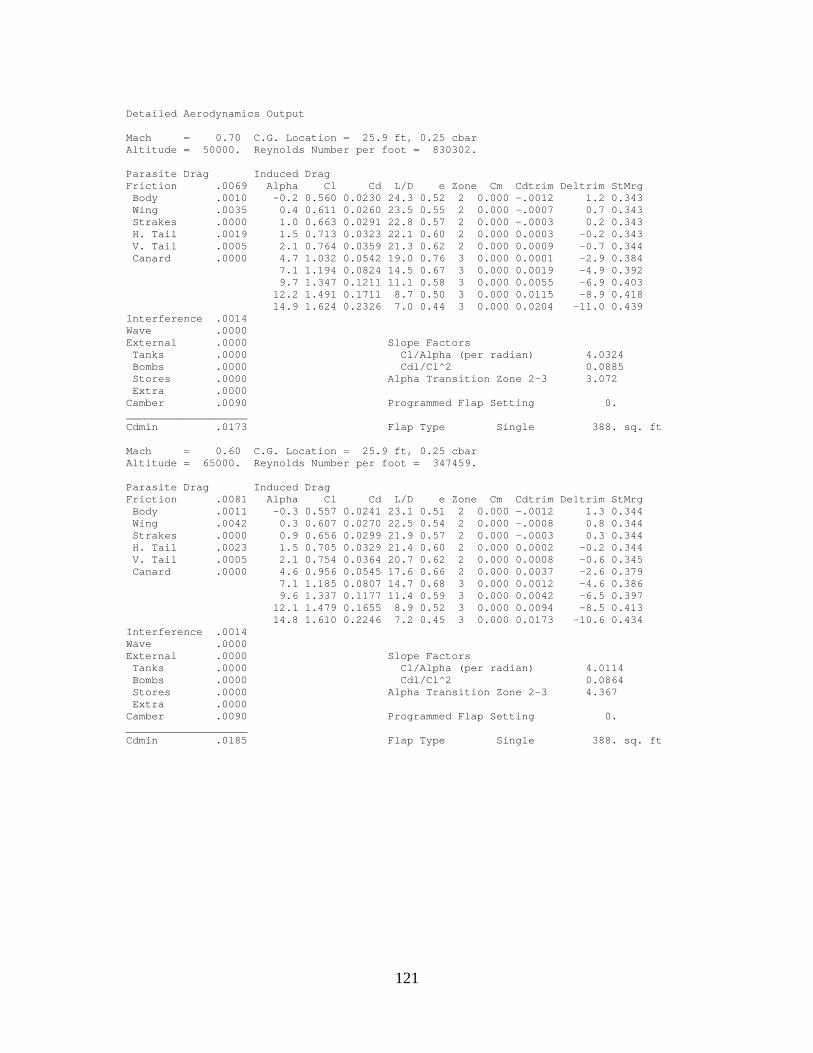
Detailed Aerodynamics Output Mach = 0.70 C.G. Location = 25.9 ft, 0.25 cbar Altitude = 50000. Reynolds Number per foot = 830302. Parasite Drag Induced Drag Friction .0069 Alpha Cl Cd L/D e Zone Cm Cdtrim Deltrim StMrg Body .0010 -0.2 0.560 0.0230 24.3 0.52 2 0.000 -.0012 1.2 0.343 Wing .0035 0.4 0.611 0.0260 23.5 0.55 2 0.000 -.0007 0.7 0.343 Strakes .0000 1.0 0.663 0.0291 22.8 0.57 2 0.000 -.0003 0.2 0.343 H. Tail .0019 1.5 0.713 0.0323 22.1 0.60 2 0.000 0.0003 -0.2 0.343 V. Tail .0005 2.1 0.764 0.0359 21.3 0.62 2 0.000 0.0009 -0.7 0.344 Canard .0000 4.7 1.032 0.0542 19.0 0.76 3 0.000 0.0001 -2.9 0.384 7.1 1.194 0.0824 14.5 0.67 3 0.000 0.0019 -4.9 0.392 9.7 1.347 0.1211 11.1 0.58 3 0.000 0.0055 -6.9 0.403 12.2 1.491 0.1711 8.7 0.50 3 0.000 0.0115 -8.9 0.418 14.9 1.624 0.2326 7.0 0.44 3 0.000 0.0204 -11.0 0.439 Interference .0014 Wave .0000 External .0000 Slope Factors Tanks .0000 Cl/Alpha (per radian) 4.0324 Bombs .0000 Cdl/Cl^2 0.0885 Stores .0000 Alpha Transition Zone 2-3 3.072 Extra .0000 Camber .0090 Programmed Flap Setting 0. ___________________ Cdmin .0173 Flap Type Single 388. sq. ft Mach = 0.60 C.G. Location = 25.9 ft, 0.25 cbar Altitude = 65000. Reynolds Number per foot = 347459. Parasite Drag Induced Drag Friction .0081 Alpha Cl Cd L/D e Zone Cm Cdtrim Deltrim StMrg Body .0011 -0.3 0.557 0.0241 23.1 0.51 2 0.000 -.0012 1.3 0.344 Wing .0042 0.3 0.607 0.0270 22.5 0.54 2 0.000 -.0008 0.8 0.344 Strakes .0000 0.9 0.656 0.0299 21.9 0.57 2 0.000 -.0003 0.3 0.344 H. Tail .0023 1.5 0.705 0.0329 21.4 0.60 2 0.000 0.0002 -0.2 0.344 V. Tail .0005 2.1 0.754 0.0364 20.7 0.62 2 0.000 0.0008 -0.6 0.345 Canard .0000 4.6 0.956 0.0545 17.6 0.66 2 0.000 0.0037 -2.6 0.379 7.1 1.185 0.0807 14.7 0.68 3 0.000 0.0012 -4.6 0.386 9.6 1.337 0.1177 11.4 0.59 3 0.000 0.0042 -6.5 0.397 12.1 1.479 0.1655 8.9 0.52 3 0.000 0.0094 -8.5 0.413 14.8 1.610 0.2246 7.2 0.45 3 0.000 0.0173 -10.6 0.434 Interference .0014 Wave .0000 External .0000 Slope Factors Tanks .0000 Cl/Alpha (per radian) 4.0114 Bombs .0000 Cdl/Cl^2 0.0864 Stores .0000 Alpha Transition Zone 2-3 4.367 Extra .0000 Camber .0090 Programmed Flap Setting 0. ___________________ Cdmin .0185 Flap Type Single 388. sq. ft
121

Detailed Aerodynamics Output Mach = 0.70 C.G. Location = 25.9 ft, 0.25 cbar Altitude = 65000. Reynolds Number per foot = 405369. Parasite Drag Induced Drag Friction .0078 Alpha Cl Cd L/D e Zone Cm Cdtrim Deltrim StMrg Body .0011 -0.2 0.560 0.0240 23.4 0.52 2 0.000 -.0012 1.2 0.343 Wing .0040 0.4 0.611 0.0269 22.7 0.55 2 0.000 -.0007 0.7 0.343 Strakes .0000 1.0 0.663 0.0300 22.1 0.57 2 0.000 -.0003 0.2 0.343 H. Tail .0022 1.5 0.713 0.0332 21.5 0.60 2 0.000 0.0003 -0.2 0.343 V. Tail .0005 2.1 0.764 0.0368 20.8 0.62 2 0.000 0.0009 -0.7 0.344 Canard .0000 4.7 1.032 0.0551 18.7 0.76 3 0.000 0.0001 -2.9 0.384 7.1 1.194 0.0833 14.3 0.67 3 0.000 0.0019 -4.9 0.392 9.7 1.348 0.1221 11.0 0.58 3 0.000 0.0055 -6.9 0.403 12.2 1.491 0.1720 8.7 0.50 3 0.000 0.0115 -8.9 0.418 14.9 1.624 0.2336 7.0 0.44 3 0.000 0.0204 -11.0 0.439 Interference .0014 Wave .0000 External .0000 Slope Factors Tanks .0000 Cl/Alpha (per radian) 4.0322 Bombs .0000 Cdl/Cl^2 0.0885 Stores .0000 Alpha Transition Zone 2-3 3.072 Extra .0000 Camber .0090 Programmed Flap Setting 0. ___________________ Cdmin .0182 Flap Type Single 388. sq. ft Mach = 0.80 C.G. Location = 25.9 ft, 0.25 cbar Altitude = 65000. Reynolds Number per foot = 463278. Parasite Drag Induced Drag Friction .0075 Alpha Cl Cd L/D e Zone Cm Cdtrim Deltrim StMrg Body .0011 -0.2 0.564 0.0239 23.6 0.52 2 0.000 -.0011 1.2 0.340 Wing .0039 0.4 0.618 0.0270 22.9 0.55 2 0.000 -.0007 0.7 0.340 Strakes .0000 1.0 0.671 0.0303 22.2 0.58 2 0.000 -.0002 0.2 0.340 H. Tail .0021 1.6 0.725 0.0337 21.5 0.61 2 0.000 0.0004 -0.3 0.340 V. Tail .0005 2.2 0.817 0.0381 21.4 0.68 2 0.000 0.0012 -1.0 0.386 Canard .0000 4.7 1.040 0.0566 18.4 0.75 3 0.000 0.0005 -3.1 0.389 7.2 1.205 0.0862 14.0 0.66 3 0.000 0.0027 -5.1 0.396 9.7 1.360 0.1270 10.7 0.57 3 0.000 0.0070 -7.2 0.407 12.3 1.505 0.1793 8.4 0.49 3 0.000 0.0139 -9.3 0.423 15.0 1.640 0.2437 6.7 0.43 3 0.000 0.0240 -11.5 0.444 Interference .0014 Wave .0000 External .0000 Slope Factors Tanks .0000 Cl/Alpha (per radian) 4.0602 Bombs .0000 Cdl/Cl^2 0.0906 Stores .0000 Alpha Transition Zone 2-3 2.061 Extra .0000 Camber .0090 Programmed Flap Setting 0. ___________________ Cdmin .0179 Flap Type Single 388. sq. ft
122

Detailed Aerodynamics Output Mach = 0.85 C.G. Location = 25.9 ft, 0.25 cbar Altitude = 65000. Reynolds Number per foot = 492233. Parasite Drag Induced Drag Friction .0074 Alpha Cl Cd L/D e Zone Cm Cdtrim Deltrim StMrg Body .0010 -0.2 0.566 0.0264 21.4 0.52 2 0.000 -.0011 1.2 0.337 Wing .0038 0.4 0.621 0.0296 21.0 0.55 2 0.000 -.0007 0.7 0.337 Strakes .0000 1.0 0.676 0.0330 20.5 0.58 2 0.000 -.0001 0.1 0.337 H. Tail .0021 1.6 0.767 0.0370 20.7 0.66 2 0.000 0.0006 -0.5 0.387 V. Tail .0005 2.2 0.860 0.0400 21.5 0.77 3 0.000 -.0001 -1.1 0.388 Canard .0000 4.7 1.045 0.0599 17.4 0.74 3 0.000 0.0006 -3.2 0.392 7.2 1.211 0.0904 13.4 0.65 3 0.000 0.0032 -5.3 0.399 9.7 1.367 0.1322 10.3 0.56 3 0.000 0.0079 -7.4 0.410 12.3 1.513 0.1858 8.1 0.49 3 0.000 0.0153 -9.5 0.425 15.0 1.649 0.2517 6.6 0.43 3 0.000 0.0260 -11.7 0.446 Interference .0012 Wave .0028 External .0000 Slope Factors Tanks .0000 Cl/Alpha (per radian) 4.0770 Bombs .0000 Cdl/Cl^2 0.0917 Stores .0000 Alpha Transition Zone 2-3 1.629 Extra .0000 Camber .0090 Programmed Flap Setting 0. ___________________ Cdmin .0203 Flap Type Single 388. sq. ft Mach = 0.85 C.G. Location = 25.9 ft, 0.25 cbar Altitude = 55000. Reynolds Number per foot = 793802. Parasite Drag Induced Drag Friction .0068 Alpha Cl Cd L/D e Zone Cm Cdtrim Deltrim StMrg Body .0010 -0.2 0.566 0.0258 21.9 0.52 2 0.000 -.0011 1.2 0.337 Wing .0035 0.4 0.621 0.0290 21.4 0.55 2 0.000 -.0007 0.7 0.337 Strakes .0000 1.0 0.676 0.0324 20.9 0.58 2 0.000 -.0001 0.1 0.337 H. Tail .0019 1.6 0.767 0.0364 21.1 0.66 2 0.000 0.0006 -0.5 0.387 V. Tail .0005 2.2 0.860 0.0394 21.8 0.77 3 0.000 -.0001 -1.1 0.388 Canard .0000 4.7 1.045 0.0593 17.6 0.74 3 0.000 0.0006 -3.2 0.392 7.2 1.210 0.0898 13.5 0.65 3 0.000 0.0032 -5.3 0.399 9.7 1.367 0.1316 10.4 0.56 3 0.000 0.0079 -7.4 0.410 12.3 1.513 0.1852 8.2 0.49 3 0.000 0.0153 -9.5 0.425 15.0 1.649 0.2511 6.6 0.43 3 0.000 0.0260 -11.7 0.446 Interference .0012 Wave .0028 External .0000 Slope Factors Tanks .0000 Cl/Alpha (per radian) 4.0771 Bombs .0000 Cdl/Cl^2 0.0917 Stores .0000 Alpha Transition Zone 2-3 1.629 Extra .0000 Camber .0090 Programmed Flap Setting 0. ___________________ Cdmin .0198 Flap Type Single 388. sq. ft
123
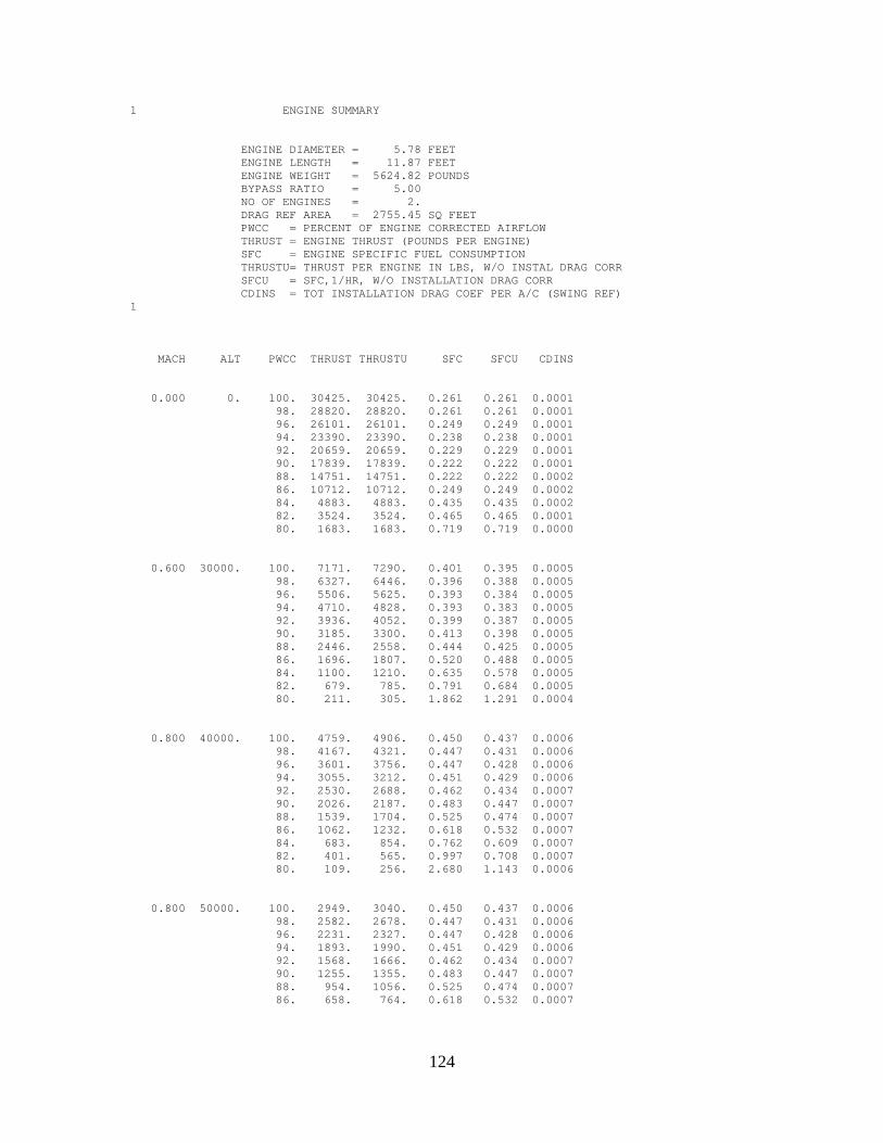
1 ENGINE SUMMARY ENGINE DIAMETER = 5.78 FEET ENGINE LENGTH = 11.87 FEET ENGINE WEIGHT = 5624.82 POUNDS BYPASS RATIO = 5.00 NO OF ENGINES = 2. DRAG REF AREA = 2755.45 SQ FEET PWCC = PERCENT OF ENGINE CORRECTED AIRFLOW THRUST = ENGINE THRUST (POUNDS PER ENGINE) SFC = ENGINE SPECIFIC FUEL CONSUMPTION THRUSTU= THRUST PER ENGINE IN LBS, W/O INSTAL DRAG CORR SFCU = SFC,1/HR, W/O INSTALLATION DRAG CORR CDINS = TOT INSTALLATION DRAG COEF PER A/C (SWING REF) 1 MACH ALT PWCC THRUST THRUSTU SFC SFCU CDINS 0.000 0. 100. 30425. 30425. 0.261 0.261 0.0001 98. 28820. 28820. 0.261 0.261 0.0001 96. 26101. 26101. 0.249 0.249 0.0001 94. 23390. 23390. 0.238 0.238 0.0001 92. 20659. 20659. 0.229 0.229 0.0001 90. 17839. 17839. 0.222 0.222 0.0001 88. 14751. 14751. 0.222 0.222 0.0002 86. 10712. 10712. 0.249 0.249 0.0002 84. 4883. 4883. 0.435 0.435 0.0002 82. 3524. 3524. 0.465 0.465 0.0001 80. 1683. 1683. 0.719 0.719 0.0000 0.600 30000. 100. 7171. 7290. 0.401 0.395 0.0005 98. 6327. 6446. 0.396 0.388 0.0005 96. 5506. 5625. 0.393 0.384 0.0005 94. 4710. 4828. 0.393 0.383 0.0005 92. 3936. 4052. 0.399 0.387 0.0005 90. 3185. 3300. 0.413 0.398 0.0005 88. 2446. 2558. 0.444 0.425 0.0005 86. 1696. 1807. 0.520 0.488 0.0005 84. 1100. 1210. 0.635 0.578 0.0005 82. 679. 785. 0.791 0.684 0.0005 80. 211. 305. 1.862 1.291 0.0004 0.800 40000. 100. 4759. 4906. 0.450 0.437 0.0006 98. 4167. 4321. 0.447 0.431 0.0006 96. 3601. 3756. 0.447 0.428 0.0006 94. 3055. 3212. 0.451 0.429 0.0006 92. 2530. 2688. 0.462 0.434 0.0007 90. 2026. 2187. 0.483 0.447 0.0007 88. 1539. 1704. 0.525 0.474 0.0007 86. 1062. 1232. 0.618 0.532 0.0007 84. 683. 854. 0.762 0.609 0.0007 82. 401. 565. 0.997 0.708 0.0007 80. 109. 256. 2.680 1.143 0.0006 0.800 50000. 100. 2949. 3040. 0.450 0.437 0.0006 98. 2582. 2678. 0.447 0.431 0.0006 96. 2231. 2327. 0.447 0.428 0.0006 94. 1893. 1990. 0.451 0.429 0.0006 92. 1568. 1666. 0.462 0.434 0.0007 90. 1255. 1355. 0.483 0.447 0.0007 88. 954. 1056. 0.525 0.474 0.0007 86. 658. 764. 0.618 0.532 0.0007
124

84. 423. 529. 0.762 0.609 0.0007 82. 248. 350. 0.997 0.708 0.0007 80. 68. 159. 2.680 1.143 0.0006 0.600 50000. 100. 2756. 2802. 0.387 0.381 0.0005 98. 2430. 2476. 0.382 0.375 0.0005 96. 2113. 2159. 0.379 0.371 0.0005 94. 1805. 1851. 0.380 0.370 0.0005 92. 1508. 1553. 0.385 0.374 0.0005 90. 1219. 1263. 0.399 0.385 0.0005 88. 935. 978. 0.430 0.411 0.0005 86. 646. 689. 0.505 0.473 0.0005 84. 417. 459. 0.620 0.563 0.0005 82. 253. 294. 0.783 0.675 0.0005 80. 71. 107. 2.046 1.361 0.0004 0.600 60000. 100. 1708. 1737. 0.387 0.381 0.0005 98. 1506. 1535. 0.382 0.375 0.0005 96. 1310. 1339. 0.379 0.371 0.0005 94. 1119. 1148. 0.380 0.370 0.0005 92. 935. 963. 0.385 0.374 0.0005 90. 756. 783. 0.399 0.385 0.0005 88. 579. 606. 0.430 0.411 0.0005 86. 401. 427. 0.505 0.473 0.0005 84. 258. 285. 0.620 0.563 0.0005 82. 157. 182. 0.783 0.675 0.0005 80. 44. 66. 2.046 1.361 0.0004 SEA-LEVEL STATIC THRUST = 30425. (MAX) SEA-LEVEL SFC = 0.261
125

Weight Statement - Transport ***** WEIGHTS ***** Qmax: 700. Design Load Factor: 2.00 Ultimate Load Factor: 3.75 Structure and Material: Aluminum Skin, Stringer Wing Equation: Sanders Equation Body Equation: Air Force Equation Component Pounds Kilograms Percent Slope Tech Fixed Airframe Structure 24161. 10959. 21.50 No Wing 7643. 3467. 6.80 0.24 1.00 No Fuselage 6443. 2923. 5.73 2.11 1.00 No Horizontal Tail ( Low) 4120. 1869. 3.67 0.75 1.00 No Vertical Tail 1238. 561. 1.10 0.42 1.00 No Nacelles 864. 392. 0.77 0.31 1.00 No Landing Gear 3853. 1748. 3.43 0.81 1.00 No Propulsion 11977. 5433. 10.66 No Engines ( 2) 11056. 5015. 9.84 0.82 1.00 No Fuel System 921. 418. 0.82 0.82 1.00 No Fixed Equipment 5265. 2388. 4.69 1.00 No Hyd & Pneumatic 674. 306. 0.60 1.00 No Electrical 1066. 483. 0.95 0.52 No Avionics 1460. 662. 1.30 1.00 No Instrumentation 0. 0. 0.00 0.00 No De-ice & Air Cond 0. 0. 0.00 1.00 No Aux Power System 868. 394. 0.77 1.43 No Furnish & Eqpt 0. 0. 0.00 0.00 No Seats and Lavatories 0. 0. 0.00 0.00 No Galley 0. 0. 0.00 0.00 No Misc Cockpit 0. 0. 0.00 0.00 No Cabin Finishing 0. 0. 0.00 0.00 No Cabin Emergency Equip 0. 0. 0.00 0.00 No Cargo Handling 0. 0. 0.00 0.00 No Flight Controls 1198. 544. 1.07 0.46 No Empty Weight 41404. 18781. 36.85 Operating Items 200. 91. 0.18 No Flight Crew ( 0) 0. 0. 0.00 No Crew Baggage and Provisions 100. 45. 0.09 No Flight Attendents ( 0) 0. 0. 0.00 No Unusable Fuel and Oil 100. 45. 0.09 No Passenger Service 0. 0. 0.00 No Cargo Containers 0. 0. 0.00 No Operating Weight Empty 41604. 18871. 37.02 Fuel 61903. 28079. 55.09 Payload 8862. 4020. 7.89 Yes Passengers ( 0) 0. 0. 0.00 No Baggage 0. 0. 0.00 No Cargo 0. 0. 0.00 No -------- -------- ------ Calculated Weight 112369. 50971. 92.11 No Estimated Weight 112373. 50972. Percent Error 0.00 Calculated Weight does not equal 100% because a group weight is being fixed.
126
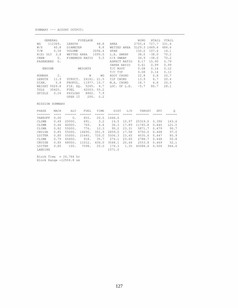
SUMMARY --- ACSYNT OUTPUT: ________________________________________________________________________________ GENERAL FUSELAGE WING HTAIL VTAIL WG 112369. LENGTH 48.8 AREA 2755.4 727.7 331.4 W/S 40.8 DIAMETER 8.8 WETTED AREA 5129.3 1469.6 484.4 T/W 0.54 VOLUME 2096.4 SPAN 150.0 107.6 16.1 N(Z) ULT 3.8 WETTED AREA 1095.5 L.E. SWEEP 38.0 -38.0 70.2 CREW 0. FINENESS RATIO 5.5 C/4 SWEEP 36.9 -38.0 70.2 PASENGERS 0. ASPECT RATIO 8.17 15.90 0.79 TAPER RATIO 0.61 0.99 0.99 ENGINE WEIGHTS T/C ROOT 0.08 0.14 0.12 T/C TIP 0.08 0.14 0.12 NUMBER 2. W WG ROOT CHORD 22.8 6.8 20.7 LENGTH 11.9 STRUCT. 24161. 21.5 TIP CHORD 13.9 6.7 20.4 DIAM. 5.8 PROPUL. 11977. 10.7 M.A. CHORD 18.7 6.8 20.5 WEIGHT 5624.8 FIX. EQ. 5265. 4.7 LOC. OF L.E. -5.7 86.7 28.1 TSLS 30425. FUEL 62003. 55.2 SFCSLS 0.26 PAYLOAD 8862. 7.9 OPER IT 200. 0.2 MISSION SUMMARY PHASE MACH ALT FUEL TIME DIST L/D THRUST SFC Q ======= ==== ====== ====== ===== ====== ===== ======= ===== ====== TAKEOFF 0.00 0. 855. 20.5 1666.0 CLIMB 0.49 20000. 691. 3.2 14.5 10.97 25319.0 0.396 163.6 CLIMB 0.66 40000. 769. 6.4 36.3 17.89 11745.8 0.445 121.5 CLIMB 0.82 55000. 776. 12.3 90.2 23.31 5871.7 0.479 90.7 CRUISE 0.85 55000. 14690. 351.9 2859.0 17.58 4750.0 0.468 97.0 LOITER 0.80 55000. 21645. 720.0 5506.3 23.45 4035.6 0.447 85.9 CLIMB 0.79 65600. 918. 35.7 274.1 23.65 2788.7 0.448 50.8 CRUISE 0.85 68000. 11012. 436.0 3548.1 20.46 2553.8 0.469 52.1 LOITER 0.80 100. 7598. 20.0 176.3 1.35 45088.4 0.506 944.6 LANDING 1571.0 Block Time = 26.764 hr Block Range =12504.8 nm
127
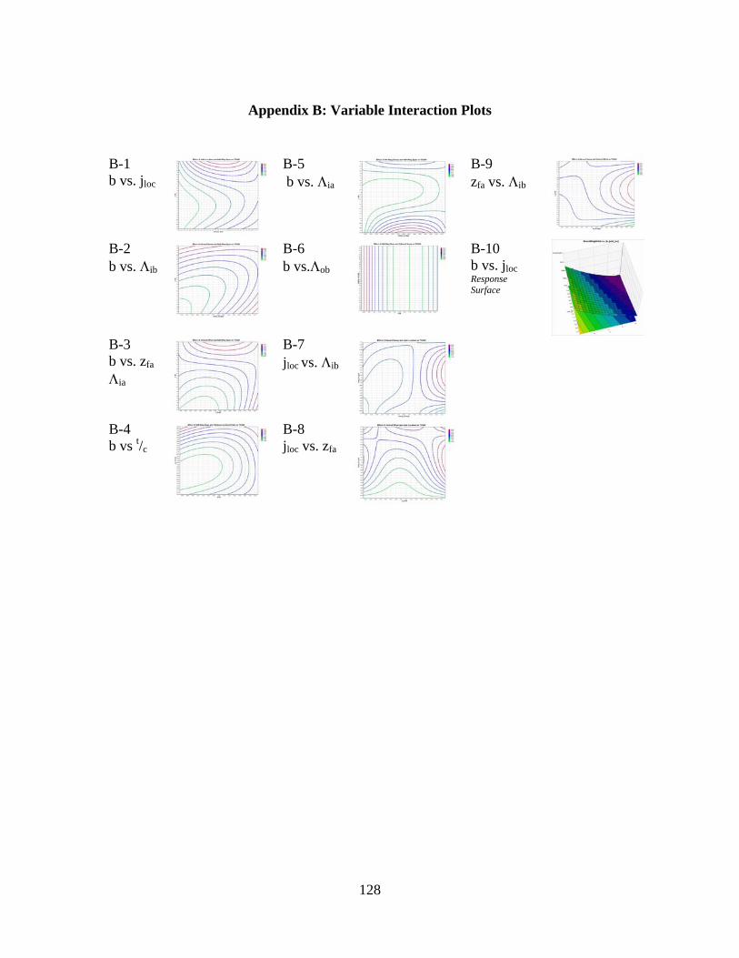
Appendix B: Variable Interaction Plots B-1 b vs. jloc
B-5 b vs. Λia
B-9 zfa vs. Λib
B-2 b vs. Λib
B-6 b vs.Λob
B-10 b vs. jloc Response Surface
B-3 b vs. zfa
Λia
B-7 jloc vs. Λib
B-4 b vs t/c
B-8 jloc vs. zfa
128

B-1
129

B-2
130

B-3
131

B-4
132

B-5
133

B-6
134

B-7
135
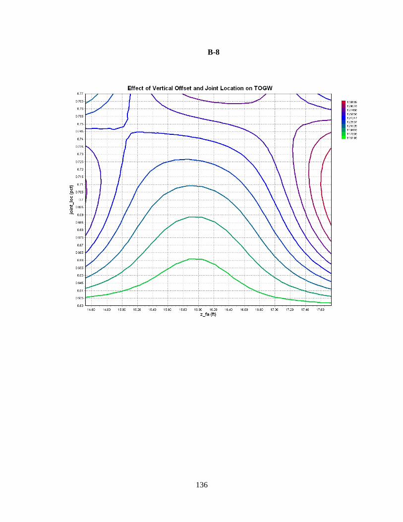
B-8
136

B-9
137

B-10
138

Appendix C: MATLAB Code (Super-Elliptical Generator)
% Fuselage Geometry - % this file calculates the geometry (Surf_A and Vol) for an superelliptical cylinder % Code is written in convention that x increases from nose to tail, y is positive out right wing, z is up % NOTE - variables must be at the top of the page with no space between them and the comments % setGroup "inputs" % variable: rad1 double input % variable: rad2 double input % variable: rad3 double input % variable: rad4 double input % variable: length double input % variable: superp double input % variable: superq double input % setGroup "adjustments" % variable: yoff double input % variable: zoff double input % setGroup "sensitivity" % variable: n double input % variable: nn double input % setGroup "" % variable: Surf_A double output % variable: Vol double output %default variables %rad1 = 0.1; %ft (Vertical radius) %rad2 = 0.1; %ft (Horizontal radius) %rad3 = 2; %ft (Vertical radius) %rad4 = 2; %ft (Horizontal radius) %length = 10; %ft %Superellipse parameters(if p=q=2 an elliptical shape follows, p=q=1 a diamond shape, p=q=4 rounded rectangle) %superp = 2; %Superellipse parameter p %superq = 2; %Superellipse parameter q %default adjustments (ellipse center offset(ft)) %assumes shape centered at (0,0,0) = (x,y,z) %yoff = 0;%far end %(Horizontal offset) %zoff = 0; %(Vertical offset) %default sensitivity adjustments %nn = 181; %radial step-size, number of radial sections (721 gives right answer to 2 decimals (181 is fine)) %n = 10; %longitudinal step size, number of longitudinal sections (10 is good) %superq_1 = 4 %far end shape %superp_1 = 4 %far end shape nn4 = (((nn-1)/4)+1); nn2 = (((nn-1)/2)+1); l = length/n; %incremental length x(1) = 0; r(1,1)= rad1; %vertical r(2,1)= rad2; %horizontal x(n+1) = length; r(1,n+1)= rad3; %vertical r(2,n+1)= rad4; %horizontal %initial vectors
139

rad(1,1) = atan2((r(1,n+1)-r(1,1)),length); deg(1,1) = rad2deg(atan2((r(1,n+1)-r(1,1)),length)); rad(2,1) = atan2((r(2,n+1)-r(2,1)),length); deg(2,1) = rad2deg(atan2((r(2,n+1)-r(2,1)),length)); for j=1:2; for i=2:n; % theta vector %Not needed? x(i) = (i-1)*l; % position in x rad(j,i) = atan2((r(j,n+1)-r(j,1)),length); deg(j,i) = rad2deg(atan2((r(j,n+1)-r(j,1)),length)); end for i =2:n; r(j,i)= (l * tan(rad(j,i-1))) + r(j,i-1); end end surfdist = []; for j = 1:2; for i = 1:n; surfdist(j,i) = sqrt((l)^2+(r(j,i+1)- r(j,i))^2); end end zero = [0;0]; surfdist = [surfdist, zero]; results = [x;r;surfdist]; yoffslope = -yoff/length; zoffslope = -zoff/length; % reset variables sa = []; vol = []; % Scroll through each ellipse for j=1:n+1; % Calculate points on ellipse - Super Ellipse Generator a = x(j); yoff(j) = yoffslope* a; zoff(j) = zoffslope* a; super_p(j) = superp + ((superp_1 - superp)/n)*j; super_q(j) = superq + ((superq_1 - superq)/n)*j; %First Quadrant for i=1:nn4; b = ((cos ((i-1)*(360/(nn-1))*pi/180))^(2/super_p(j)))*r(2,j); c = ((sin ((i-1)*(360/(nn-1))*pi/180))^(2/super_q(j)))*r(1,j); if abs(a) < .0000001 a = 0; end if abs (b) < .0000001 b = 0; end if abs (c) < .0000001 c = 0; end geom(i,3*j-2) = a; geom(i,3*j-1) = b; geom(i,3*j) = c; end %Second Quadrant for i=nn4+1:nn2; geom(i,3*j-2) = a; geom (i,3*j-1) = - geom (nn4-(i-nn4),3*j-1); %Opposite geom (i,3*j) = geom (nn4-(i-nn4),3*j); %Same end %Third and Fourth Quadrants for i=nn2+1:nn; geom(i,3*j-2) = a; geom (i,3*j-1) = geom (nn2-(i-nn2),3*j-1); %Same geom (i,3*j) = - geom (nn2-(i-nn2),3*j); %Opposite end
140

%apply offsets for i=1:nn; geom (i,3*j-1) = geom (i,3*j-1)- yoff(j); geom (i,3*j) = geom (i,3*j)- zoff(j); end %Determine distance between points for i=1:nn-1; diff (j,i)= sqrt((geom(i,3*j-1)-geom(i+1,3*j-1))^2 + (geom(i,3*j)-geom(i+1,3*j))^2); end %Calculate Area and Perimeter peri(j) = sum(diff(j,:),2)*(cos(yoffslope)*cos(zoffslope)); F = @(x) (1- (x./rad2).^super_p(j)).^(1/super_q(j)).*rad1; Q(j) = quadl(F,0,rad2); area(j) = 4*Q(j)*(cos(yoffslope)*cos(zoffslope))^2; end for j=1:n; % approximation of elliptical cylinder surface area (average of % perimeters * length) and volume (average area * length) sa (j) = (peri(j)+ peri (j+1))/2 * l/(cos(yoffslope)*cos(zoffslope)); vol (j) = (area(j) + area (j+1))/2 * l/(cos(yoffslope)*cos(zoffslope)) ; end sa = [sa, 0]; vol = [vol,0]; results = [results; sa ; vol]; Surf_A = sum(sa ,2); Vol = sum(vol,2); %Plot Ellipses %for j = 1:n+1; % plot3(geom(:,3*j-2),geom(:,3*j-1),geom(:,3*j),'LineWidth',2,'Color',[.6 1 0]) % axis equal % hold on %end %Check for circular case %VOLUME = rad1 ^2*pi*length %AREA = rad1*2*pi*length %Reduce Geometry %181X33 is a bit much to display reduce to 37 points around shape evenly spaced by six cross sections (3 x y z) for j = 1:6; %10 = n (for j = 1:6) - Take 6 cross sections for i = 1:((nn-1)/45)+1; % 361 points (for i = 1:9) - Take every 22.5 degrees (9 points) reduced_geom (i,(3*(j-1)+1)) = geom (45*(i-1)+1, 6*(j-1)+1); reduced_geom (i,(3*(j-1)+2)) = geom (45*(i-1)+1, 6*(j-1)+2); reduced_geom (i,(3*(j-1)+3)) = geom (45*(i-1)+1, 6*(j-1)+3); end end %for j = 1:6; % plot3(reduced_geom(:,3*j-2),reduced_geom(:,3*j-1),reduced_geom(:,3*j),'LineWidth',2,'Color',[0 .6 0]) % axis equal % hold on %end
141
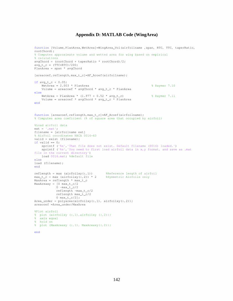
Appendix D: MATLAB Code (WingArea) function [Volume,PlanArea,WetArea]=WingArea_Vol(airfoilname ,span, RTC, TTC, taperRatio, rootChord); % Computes approximate volume and wetted area for wing based on empirical % calulations avgChord = (rootChord + taperRatio * rootChord)/2; avg_t_c = (TTC+RTC)/200; PlanArea = span * avgChord [areacoef,reflength,max_t_c]=AF_Acoef(airfoilname); if avg_t_c < 0.05; WetArea = 2.003 * PlanArea % Raymer 7.10 Volume = areacoef * avgChord * avg_t_c * PlanArea else WetArea = PlanArea * (1.977 + 0.52 * avg_t_c) % Raymer 7.11 Volume = areacoef * avgChord * avg_t_c * PlanArea end function [areacoef,reflength,max_t_c]=AF_Acoef(airfoilname); % Computes area coeficient (% of square area that occupied by airfoil) %Load airfoil data ext = '.mat'; filename = [airfoilname ext] % AirFoil coordinates NACA 0016-63 valid = exist (filename); if valid == 0; sprintf ('%s','That file does not exist. Default filename (0016) loaded.') sprintf ('%s','You need to first load airfoil data in x,y format, and save as .mat file in the current directory') load 0016.mat; %default file else load (filename); end reflength = max (airfoilxy(:,1)) %Reference length of airfoil max_t_c = max (airfoilxy(:,2)) * 2 %Symmetric Airfoils only MaxArea = reflength * max_t_c MaxAreaxy = [0 max_t_c/2 0 -max_t_c/2 reflength -max_t_c/2 reflength max_t_c/2 0 max_t_c/2]; Area_under = polyarea(airfoilxy(:,1), airfoilxy(:,2)); areacoef =Area_under/MaxArea %Plot airfoil % plot (airfoilxy (:,1),airfoilxy (:,2)); % axis equal % hold on % plot (MaxAreaxy (:,1), MaxAreaxy(:,2)); end
142
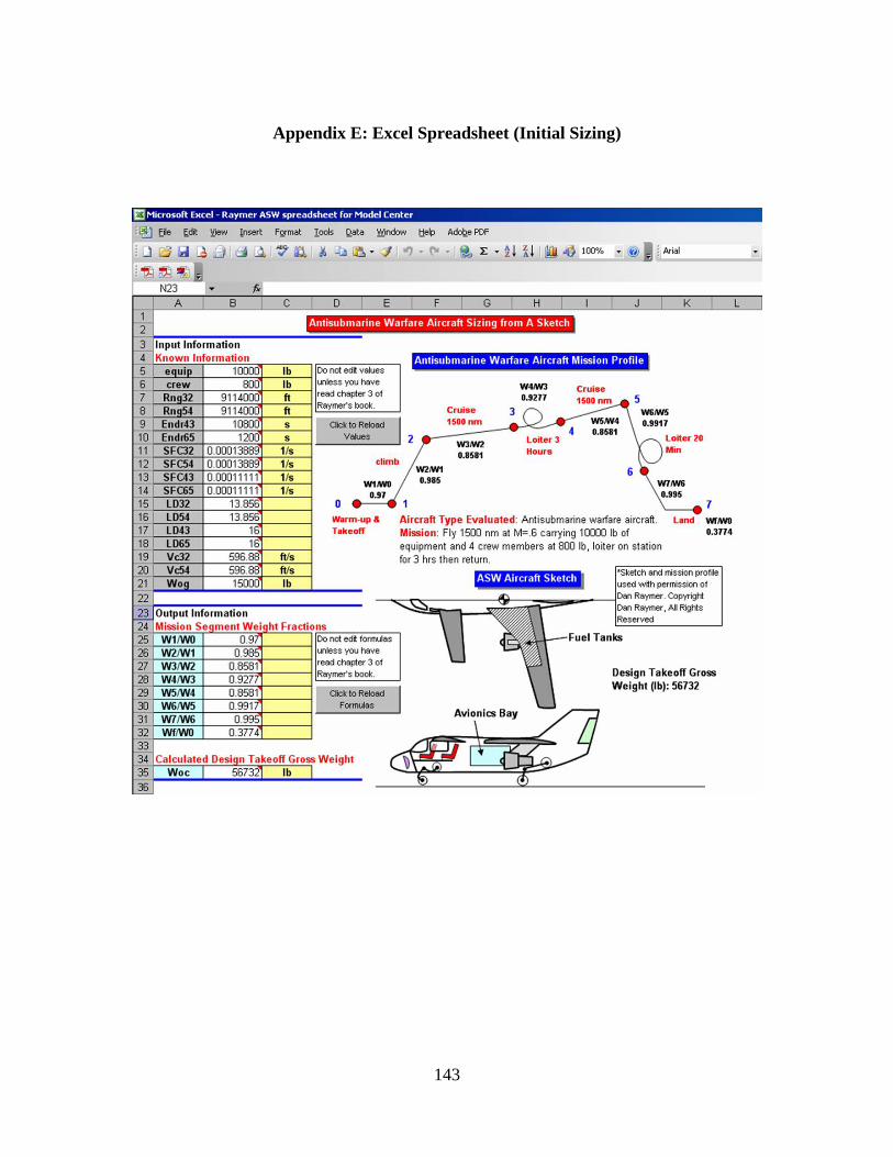
Appendix E: Excel Spreadsheet (Initial Sizing)
143

Appendix F: MATLAB FEM Manipulation (modxyz.m) function [xyzmod,bo,jloco,swiao,swibo,swobo,zfao,tco] = modxyz(xyz,b,jloc,swia,swib,swob,zfa,tc,wbody,lbody,bo,jloco,swiao,swibo,swobo,zfao,tco) %FEM transform equations for 410E model Joined_wing (for a sample xyz input) %Sort the data into parts for i =1:length (xyz); if xyz (i,4) == 1; in1 (i,:) = xyz (i,:); elseif xyz (i,4) == 2; in2 (i,:) = xyz (i,:); elseif xyz (i,4) == 3; in3 (i,:) = xyz (i,:); elseif xyz (i,4) == 4; in4 (i,:) = xyz (i,:); elseif xyz (i,4) == 5; in5 (i,:) = xyz (i,:); elseif xyz (i,4) == 6; in6 (i,:) = xyz (i,:); end end [r,c]= find(in1); in1 = in1 (min(r):max(r),:); [r,c]= find(in2); in2 = in2 (min(r):max(r),:); [r,c]= find(in3); in3 = in3 (min(r):max(r),:); [r,c]= find(in4); in4 = in4 (min(r):max(r),:); [r,c]= find(in5); in5 = in5 (min(r):max(r),:); [r,c]= find(in6); in6 = in6 (min(r):max(r),:); %Part (1) Body %Eqn x(17)y()z(27,28) %vars swob,swia,t/c,b no effect for j = 1:length(in1); xo(j) = in1 (j,1); yo(j) = in1 (j,2); zo(j) = in1 (j,3); delZ = yo(j)*(zfao/2)*((1/(b*jloc))-(1/(bo*jloco)))... %Eqn 27 + yo(j)*((zfa-zfao)/(2*jloco*bo)); %Eqn 28 delX = yo(j)*(tan(deg2rad(swib))- tan(deg2rad(swibo))); %Eqn 17 delY = 0; out1(j,1) = in1(j,1) + delX; out1(j,2) = in1(j,2) + delY; out1(j,3) = in1(j,3) + delZ; out1(j,4) = 1; end %Part (2) ib %Eqn x(17,19,23)y(20,24)z(29,38) %vars swob,swia no effect for j = 1:length(in2); xo(j) = in2 (j,1); yo(j) = in2 (j,2); zo(j) = in2 (j,3); delZ = zfa/2*((wbody/(jloc*b))+ ((yo(j)-wbody)/(jloco*bo - wbody))*((jloc*b-wbody)/(jloc*b)))... - zfao/2*(wbody/(jloco*bo)+ ((yo(j)-wbody)/(jloco*bo - wbody))*((jloco*bo-wbody)/(jloco*bo)))... %Eqn 29 + zo(j) - (yo(j)/(jloco*bo))*(zfao/2)*(tc/tco); %Eqn 38 delY1 = yo(j)/jloco*(jloc-jloco); %Eqn 24 delY2 = (jloc*b-jloco*bo)*((yo(j)-wbody)/(bo*jloco-wbody)); %Eqn 20 delY = delY1+delY2;
144

delX = delY1*(tan(deg2rad(swib)))... %Eqn 19 + delY2*(tan(deg2rad(swib)))... %Eqn 23 + yo(j)*(tan(deg2rad(swib))- tan(deg2rad(swibo))) ; %Eqn 17 out2(j,1) = in2(j,1) + delX; out2(j,2) = in2(j,2) + delY; out2(j,3) = in2(j,3) + delZ; out2(j,4) = 2; end %Part (3) ob %Eqn x(18,21,25)y(22,26)z(30,38) %vars swia no effect for j = 1:length(in3); xo(j) = in3 (j,1); yo(j) = in3 (j,2); zo(j) = in3 (j,3); delZ = ((yo(j)-jloco*bo)/(bo-jloco*bo))*((zfa/2)*(1/jloc))... - ((yo(j)-jloco*bo)/(bo-jloco*bo))*((zfao/2)*(1/jloco))... %Eqn 30 + zo(j) - (yo(j)/(jloco*bo))*(zfao/2)*(tc/tco); %Eqn 38 delY1 = (bo -yo(j))/(1-jloco)*(jloc-jloco); %Eqn 26 delY2 = (jloc*b-jloco*bo)*(1+ ((yo(j)/bo - jloco)/(1-jloco))); %Eqn 22 delY = delY1+delY2; delX = bo*jloco*(tan(deg2rad(swib))-tan(deg2rad(swibo)))+(yo(j)-bo*jloco)*(tan(deg2rad(swob))-tan(deg2rad(swobo)))... %Eqn 18 + tan(deg2rad(swib))* (jloc*b-jloco*bo)+ tan(deg2rad(swob))*(jloc*b-jloco*bo)* ((yo(j)/bo - jloco)/(1-jloco)); %Eqn 21 %+ bo*(jloc-jloco)*(tan(deg2rad(swib)))+ bo*(2-jloc+jloco)*(tan(deg2rad(swob))); %Eqn 25 out3(j,1) = in3(j,1) + delX; out3(j,2) = in3(j,2) + delY; out3(j,3) = in3(j,3) + delZ; out3(j,4) = 3; end %Part (4) ia %Eqn x(31,32,34)y(33)z(35,39) %vars swob no effect for j = 1:length(in4); xo(j) = in4 (j,1); yo(j) = in4 (j,2); zo(j) = in4 (j,3); delZ = ((zfa-zfao)/2)*(1+((jloco*bo-yo(j))/(jloco*bo)))... %Eqn 35 + (zo(j)- ((zfao/2)+(zfao/2)*((bo*jloco-yo(j))/(bo*jloco))))*tc/tco; %Eqn 39 (residual due to different model) delY = yo(j)/(bo*jloco)*(b*jloc-bo*jloco); %Eqn 33 delX = jloco*bo*(tan(deg2rad(swib))-tan(deg2rad(swibo)))... %Eqn 31 + (tan(deg2rad(swib)))*(b*jloc -bo*jloco) +... (tan(deg2rad(swia)))* (b*jloc -bo*jloco)*((bo*jloco-yo(j))/(bo*jloco))... %Eqn 32 + (jloco*bo - yo(j))*(tan(deg2rad(swia))- tan(deg2rad(swiao))) ; %Eqn 34 out4(j,1) = in4(j,1) + delX; out4(j,2) = in4(j,2) + delY; out4(j,3) = in4(j,3) + delZ; out4(j,4) = 4; end %Part (5) tail %Eqn x(31,32,34)y(33)z(35) %vars swob,tc no effect for j = 1:length(in5); xo(j) = in5 (j,1); yo(j) = in5 (j,2); zo(j) = in5 (j,3); delZ = ((zfa-zfao)/2)*(1+((jloco*bo-yo(j))/(jloco*bo))); %Eqn 35 delY = yo(j)/(bo*jloco)*(b*jloc-bo*jloco); %Eqn 33 delX = jloco*bo*(tan(deg2rad(swib))-tan(deg2rad(swibo)))... %Eqn 31 + (tan(deg2rad(swib)))*(b*jloc -bo*jloco) +... (tan(deg2rad(swia)))* (b*jloc -bo*jloco)*((bo*jloco-yo(j))/(bo*jloco))... %Eqn 32
145

+ (jloco*bo - yo(j))*(tan(deg2rad(swia))- tan(deg2rad(swiao))) ; %Eqn 34 out5(j,1) = in5(j,1) + delX; out5(j,2) = in5(j,2) + delY; out5(j,3) = in5(j,3) + delZ; out5(j,4) = 5; end %Part (6) boom %Eqn x(36)z(37) %vars swob,tc no effect for j = 1:length(in6); xo(j) = in6 (j,1); yo(j) = in6 (j,2); zo(j) = in6 (j,3); delZ = ((xo(j)- lbody)/((jloc*b)*(tan(deg2rad(swib))... + tan(deg2rad(swia)))- lbody))*(zfa-zfao); %Eqn 37 delY = 0; delX = (zo(j)/zfa)* (jloc*b*(tan(deg2rad(swib))+ tan(deg2rad(swia)))... - jloco*bo*(tan(deg2rad(swibo))+ tan(deg2rad(swiao)))); %Eqn 36 out6(j,1) = in6(j,1) + delX; out6(j,2) = in6(j,2) + delY; out6(j,3) = in6(j,3) + delZ; out6(j,4) = 6; end xyzmod = [out1;out2;out3;out4;out5;out6]; %AT END *** Need to reset new design variables to old design variables swibo = swib; swiao = swia; swobo = swob; zfao = zfa; jloco = jloc; tco = tc; bo = b;
146

Appendix G: Response Surface Model Standard Analysis of Variance (ANOVA) Summary
Full Quadratic plus Cubic Interaction Terms
Response Transformation: Z=Y (None)
SOURCE DF SS MS F Fsig(%)
REGRESSION 112 0.5000519E+00011 0.4464749E+00009 0.6780270E+00002 0.0000
RESIDUAL ERROR *** 0.1272205E+00011 0.6584913E+00007
TOTAL *** 0.6272724E+00011
--------------------------------
DATA FOR RESPONSE VARIABLE (Y)
--------------------------------
S = 0.2566108E+00004
Yavg = 0.1151893E+00006
CoV = 2.23%
R-Sq = 79.72%
R-Sq(adj) = 78.54%
147
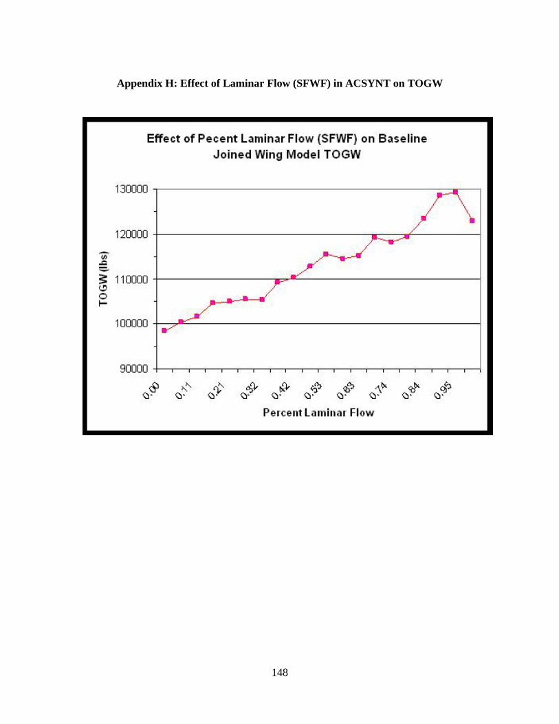
Appendix H: Effect of Laminar Flow (SFWF) in ACSYNT on TOGW
148

REPORT DOCUMENTATION PAGE Form Approved OMB No. 074-0188
The public reporting burden for this collection of information is estimated to average 1 hour per response, including the time for reviewing instructions, searching existing data sources, gathering and maintaining the data needed, and completing and reviewing the collection of information. Send comments regarding this burden estimate or any other aspect of the collection of information, including suggestions for reducing this burden to Department of Defense, Washington Headquarters Services, Directorate for Information Operations and Reports (0704-0188), 1215 Jefferson Davis Highway, Suite 1204, Arlington, VA 22202-4302. Respondents should be aware that notwithstanding any other provision of law, no person shall be subject to an penalty for failing to comply with a collection of information if it does not display a currently valid OMB control number. PLEASE DO NOT RETURN YOUR FORM TO THE ABOVE ADDRESS. 1. REPORT DATE (DD-MM-YYYY) 11-10-2006
2. REPORT TYPE Master’s Thesis
3. DATES COVERED (From – To) 09 NOV 04 - 10 NOV 06
5a. CONTRACT NUMBER
5b. GRANT NUMBER
4. TITLE AND SUBTITLE
Integrated Conceptual Design Of Joined-Wing SensorCraft Using Response Surface Models.
5c. PROGRAM ELEMENT NUMBER
5d. PROJECT NUMBER 5e. TASK NUMBER
6. AUTHOR(S) DITTMAR, JOSH E., Lieutenant Commander, USN
5f. WORK UNIT NUMBER
7. PERFORMING ORGANIZATION NAMES(S) AND ADDRESS(S) Air Force Institute of Technology Graduate School of Engineering and Management (AFIT/EN) 2950 Hobson Way WPAFB OH 45433-7765
8. PERFORMING ORGANIZATION REPORT NUMBER AFIT/GAE/ENY/07-D02
10. SPONSOR/MONITOR’S ACRONYM(S)
9. SPONSORING/MONITORING AGENCY NAME(S) AND ADDRESS(ES) Air Force Research Labs – Air Vehicles Directorate (AFRL-VA) Attn: Dr. Maxwell Blair 2210 Eighth Street Room 220 Wright-Patterson AFB OH 45433-7531 DSN: 785-8430
11. SPONSOR/MONITOR’S REPORT NUMBER(S)
12. DISTRIBUTION/AVAILABILITY STATEMENT APPROVED FOR PUBLIC RELEASE; DISTRIBUTION UNLIMITED.
13. SUPPLEMENTARY NOTES 14. ABSTRACT A multidisciplinary conceptual design and analysis of Boeing’s joined-wing SensorCraft has been conducted. This analysis was completed using geometrical optimization, aerodynamic analyses, and response surface methodology on a composite structural model. Phoenix Integration’s Model Center was used to integrate the sizing and analysis codes found in Raymer’s text, “Aircraft Design: A Conceptual Approach” as well as those from the NASA derived conceptual design tool AirCraft Synthesis (ACSYNT ), and a modified Boeing Finite Element Model (FEM). This research demonstrated the utility of integrated low-order models for fast and inexpensive conceptual modeling of unconventional aircraft designs.
15. SUBJECT TERMS SensorCraft, ModelCenter, Design of Experiments (DOE), Multi-Disciplinary Optimization (MDO), MATLAB
16. SECURITY CLASSIFICATION OF:
19a. NAME OF RESPONSIBLE PERSON ROBERT CANFIELD
REPORT U
ABSTRACT U
c. THIS PAGE U
17. LIMITATION OF ABSTRACT UU
18. NUMBER OF PAGES 166 19b. TELEPHONE NUMBER (Include area code)
(937) 255-3636 x4723, e-mail: [email protected]
Standard Form 298 (Rev: 8-98) Prescribed by ANSI Std. Z39-18
Related Documents