Introduction to FRP with a Haskell Implemented, Quake- like Game Functional Thursday #2 [email protected] Link to this slide: http://bit.ly/sntw-ypai

Welcome message from author
This document is posted to help you gain knowledge. Please leave a comment to let me know what you think about it! Share it to your friends and learn new things together.
Transcript

Introduction to FRP with a Haskell Implemented, Quake-like Game
Functional Thursday #[email protected]
Link to this slide: http://bit.ly/sntw-ypai

Frag
HaskellYampaOpenGLQuake-like FPS Game
Mun Hon Cheong2005License: GPL
GitHub Mirrorbit.ly/sntw-frag

Snowmantw
a ProgrammingLanguage Enthusiast
HaskellJavaScriptRust C/C++ PythonRuby ImplementedFluorine PDL4SMC
GitHub Profilegithub.com/snowmantw
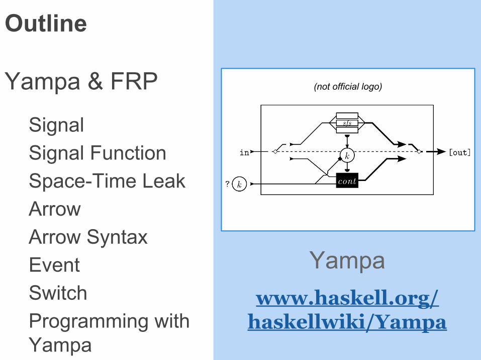
Outline
Yampa & FRP
SignalSignal FunctionSpace-Time LeakArrowArrow SyntaxEventSwitchProgramming withYampa
Yampawww.haskell.org/haskellwiki/Yampa
(not official logo)
Functional Reactive Programming
Signal vs. Event
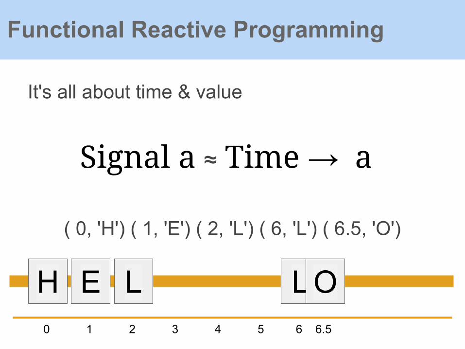
It's all about time & value
Functional Reactive Programming
H0 1
E L2 3 4 5 6 6.5
L O
Signal a ≈ Time → a
( 0, 'H') ( 1, 'E') ( 2, 'L') ( 6, 'L') ( 6.5, 'O')

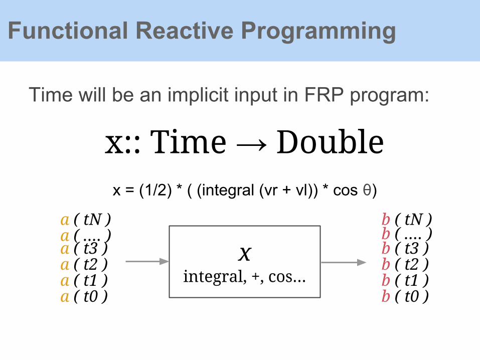
Time will be an implicit input in FRP program:
Functional Reactive Programming
x = (1/2) * ((integral (vr + vl)) * cos θ)θ = (1/l) * (integral (vr - vl))
function program() {
};
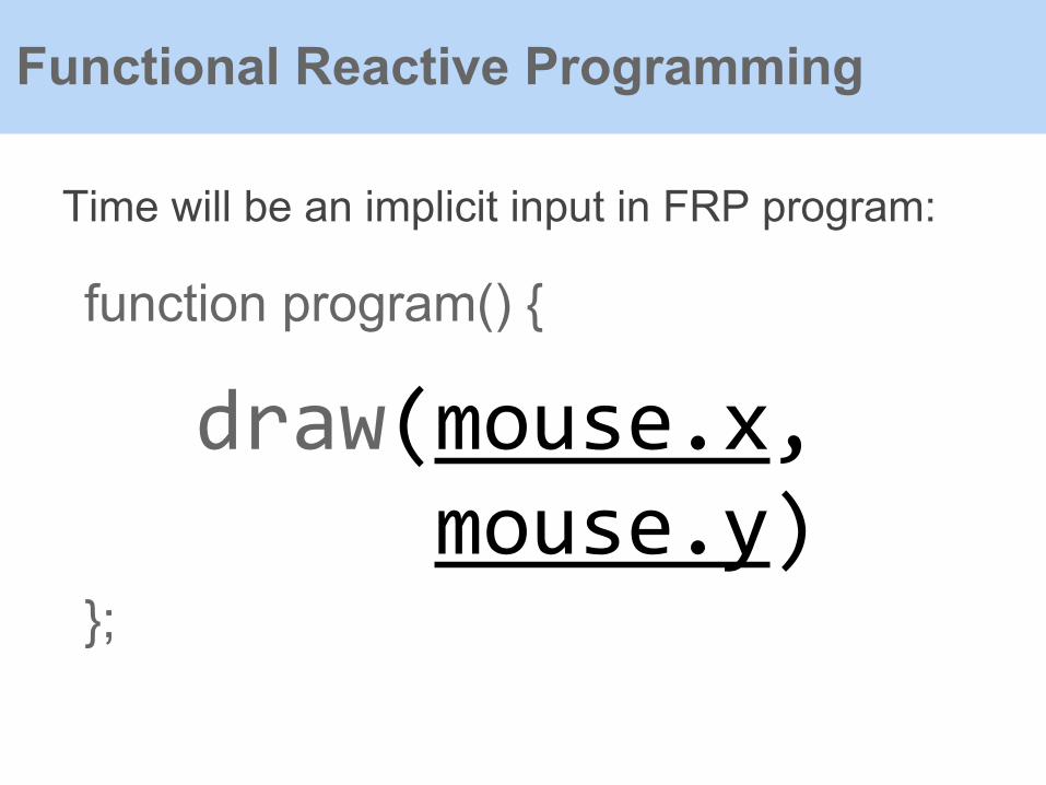
Time will be an implicit input in FRP program:
Functional Reactive Programming
draw(mouse.x, mouse.y)

function program() {
};
Time will be an implicit input in FRP program:
Functional Reactive Programming
draw(mouse.x, mouse.y)
The abstraction absorbed all explicit "event" handling
Time will be an implicit input in FRP program:
Functional Reactive Programming
xintegral, +, cos...
a ( t0 )a ( t1 )a ( t2 )a ( t3 )
a ( tN )a ( .... )
b ( t0 )b ( t1 )b ( t2 )b ( t3 )b ( .... )
x:: Time → Doublex = (1/2) * ( (integral (vr + vl)) * cos θ)
b ( tN )

Note that the `integral` is stateful (rely on time):
Functional Reactive Programming
x:: Time → Doublex = (1/2) * ( (integral (vr + vl)) * cos θ)
t = N, integral (vr + vl)t from 0 to N...
t = 2, integral (vr + vl)t from 0 to 2t = 1, integral (vr + vl)t from 0 to 1t = 0, integral (vr + vl)t from 0 to 0

In order to perform stateful computations, we must represent our signals in FRP as streams:
Functional Reactive Programming
newtype S a = S ([DTime] → [a])newtype C a = C (a, DTime → C a)
integralS :: Double → S Double → S DoubleintegralC :: Double → C Double → C Double
x = integralS 0 (vr + vl), where vr & vl are Signals x = integralC 0 (vr + vl), where vr & vl are Signals

In fact we can't touch any signal in Yampa. We can only compose Signal Functions
f[ state (t) ]
a ( t ) b ( t )
Signal Function
SF:: Signal a → Signal b
f:: SF a b

f:: SF a b
The `state (t)` summarizes input history:same `f` handle every `a` in different time
SF:: Signal a → Signal b
f[ state (t) ]
a ( t0 )a ( t1 )a ( t2 )a ( t3 )
a ( tN )a ( .... )
b ( t0 )b ( t1 )b ( t2 )b ( t3 )
b ( tN )b ( .... )
Signal Function

"Space-Time Leak"
Why Signal Functions ?

Space-Time Leak in FRP
It means that old records got heaped up and occurs the memory due to our expressions had been expanded improperly.
An analogous example
repeat x = λx → x : repeat x repeat x = λx → let xs = x:xs in xs
Leaks No-Leaks

Space-Time Leak in FRP
repeat x = λx → x : repeat xrepeat 3
↪ (λx → x : repeat x) (3)
↪ 3 : repeat 3
↪ 3 : (λx → x : repeat x) (3)
↪ 3 : 3 : repeat 3
↪ 3 : 3 : (λx → x : repeat x) (3)
↪ 3 : 3 : 3 : repeat 3
↪ ...
It must create new nodes for every `repeat 3`

Space-Time Leak in FRP
repeat x = λx → let xs = x:xs in xsrepeat 3
↪ (λx → let xs = x:xs in xs) (3)
↪ xs, where `xs` was defined as above:
↪ 3: xs, where `xs` was defined as above:
↪ 3: 3: xs, where `xs` was defined as above:
↪ 3: 3: 3: xs, where `xs` was defined as above:
↪ ...
The `let` bind the same `xs` "reference" in every expanded expression, thus there is no need to create new nodes in memory.
Space-Time Leak in FRP
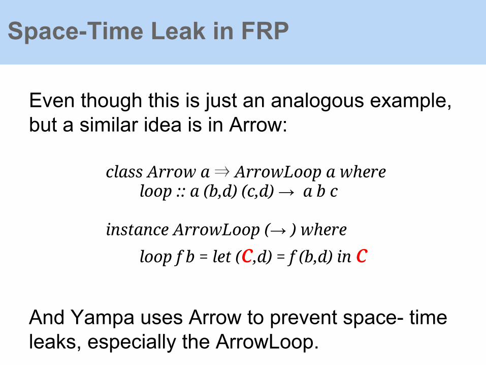
Even though this is just an analogous example, but a similar idea is in Arrow:
class Arrow a ⇒ ArrowLoop a where loop :: a (b,d) (c,d) → a b c
instance ArrowLoop (→ ) where
loop f b = let (c,d) = f (b,d) in c
And Yampa uses Arrow to prevent space- time leaks, especially the ArrowLoop.

Space-Time Leak in FRP
RECURSIVE CODES MAY DESTRUCT YOUR MIND
Space-Time Leak in FRP
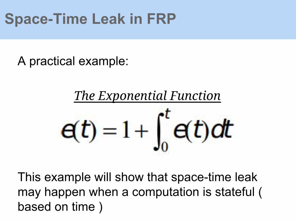
A practical example:
This example will show that space-time leak may happen when a computation is stateful ( based on time )
The Exponential Function

Space-Time Leak in FRP
Because in practical systems we only care about how to compute on continuous streams of values, we can represent our Signals as streams in two forms:
newtype S a = S ([DTime] → [a])newtype C a = C (a, DTime → C a)
-- delta time, for samplingtype DTime = Double
The later one will expand its second (C a) to make a continuing stream.
Space-Time Leak in FRP
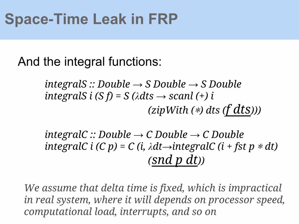
And the integral functions:
integralS :: Double → S Double → S DoubleintegralS i (S f) = S (λdts → scanl (+) i (zipWith (∗) dts (f dts)))
integralC :: Double → C Double → C DoubleintegralC i (C p) = C (i, λdt→integralC (i + fst p ∗ dt) (snd p dt))
We assume that delta time is fixed, which is impractical in real system, where it will depends on processor speed, computational load, interrupts, and so on

Space-Time Leak in FRP
Remember that the integral need to accumulate each values at every DTime:
DTime
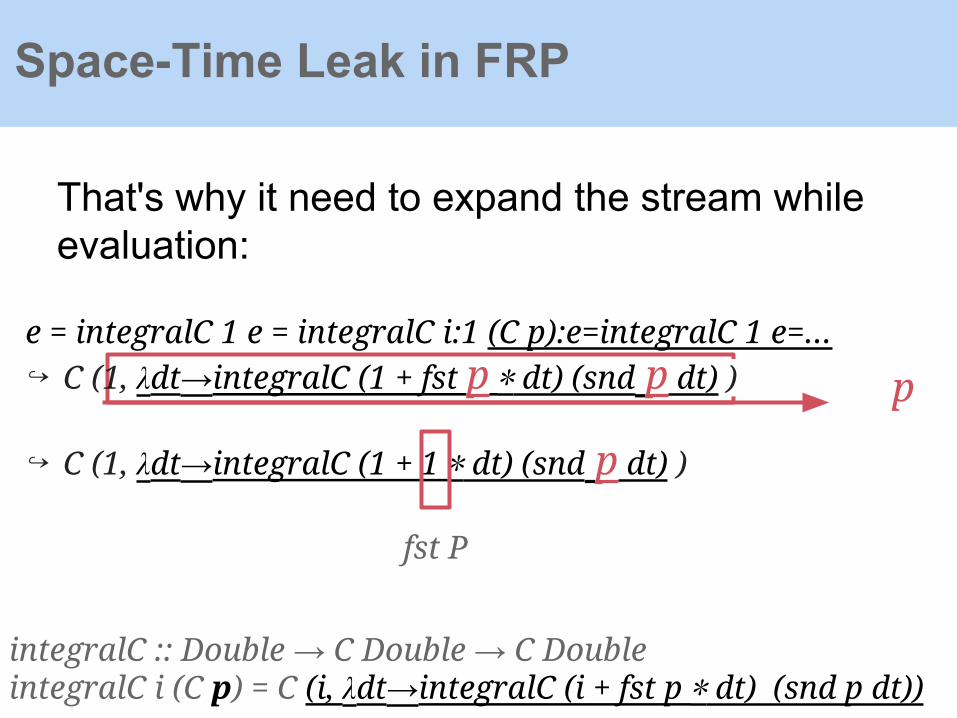
That's why it need to expand the stream while evaluation:
e = integralC 1 e = integralC i:1 (C p):e=integralC 1 e=...↪ C (1, λdt→integralC (1 + fst p ∗ dt) (snd p dt) )
↪ C (1, λdt→integralC (1 + 1 ∗ dt) (snd p dt) )
Space-Time Leak in FRP
p
fst P
integralC :: Double → C Double → C DoubleintegralC i (C p) = C (i, λdt→integralC (i + fst p ∗ dt) (snd p dt))

That's why it need to expand the stream while evaluation:
e = integralC 1 e = integralC i:1 (C p):e=integralC 1 e=...↪ C (1, λdt→integralC (1 + fst p ∗ dt) (snd p dt) )
↪ C (1, λdt→integralC (1 + 1 ∗ dt) (snd p dt) )
Space-Time Leak in FRP
psnd p

That's why it need to expand the stream while evaluation:
e = integralC 1 e = integralC i:1 (C p):e=integralC 1 e=...↪ C (1, λdt→integralC (1 + fst p ∗ dt) (snd p dt) )
↪ C (1, λdt→integralC (1 + 1 ∗ dt) (sndp dt) )
Space-Time Leak in FRP
psnd p

That's why it need to expand the stream while evaluation:
e = integralC 1 e = integralC i:1 (C p):e=integralC 1 e=...↪ C (1, λdt→integralC (1 + fst p ∗ dt) (snd p dt) )
↪ C (1, λdt→integralC (1 + 1 ∗ dt) (sndp dt) )
↪ C (1, q )
Space-Time Leak in FRP
psnd p

Now we may want to "run" the stream to see what will happen:
run :: C Double → [Double]run (C p) = fst p : run (snd p dt)
Space-Time Leak in FRP

Now we may want to "run" the stream to see what will happen:
run e, where run (C p) = fst p : run (snd p dt)
↪ run C (1, q ), because e = C (1, q ); then evaluate the run:
↪ 1 : run (q dt)
↪ 1 : run ((λdt→integralC (1 + 1 ∗ dt) (q dt) ) dt)
↪ 1 : run (integralC (1 + 1 ∗ dt) (q dt) )
↪ let's expand the horrible q now...
Space-Time Leak in FRP

run e, where run (C p) = fst p : run (snd p dt)
↪ run C (1, q ), because e = C (1, q ); then evaluate the run:
↪ 1 : run (q dt)
↪ 1 : run ((λdt→integralC (1 + 1 ∗ dt) (qdt) ) dt)
↪ 1 : run (integralC (1 + 1 ∗ dt) (q dt) )
↪ 1 : run (C ( (1 + 1 ∗ dt),
(λdt→integralC (1 + fst p ∗ dt) (snd p dt) ) (dt) )
Space-Time Leak in FRP

run e, where run (C p) = fst p : run (snd p dt)
↪ run C (1, q ), because e = C (1, q ); then evaluate the run:
↪ 1 : run (q dt)
↪ 1 : run ((λdt→integralC (1 + 1 ∗ dt) (qdt) ) dt
↪ 1 : run (integralC (1 + 1 ∗ dt) (q dt) )
↪ 1 : run (C ( (1 + 1 ∗ dt),
(λdt→integralC (1 + fst p ∗ dt) (snd p dt) ) (dt) )
↪ 1 : run (C ( (1 + 1 ∗ dt),
(λdt→integralC (1 + fst p ∗ dt) (snd p dt) ) (dt) )
Space-Time Leak in FRP
new P new Q

↪ 1 : run (C ( (1 + 1 ∗ dt),
(λdt→integralC (1 + fst p ∗ dt) (snd p dt) ) (dt) )
↪ 1 : run (C ( (1 + 1 ∗ dt), q ))↪ 1 : run ((1 + 1 ∗ dt): run (q dt)) ↪ ...
Space-Time Leak in FRP
This leads to O(n) space ,and O(n2) time similar to the simplifier `repeat` example
We hope to reduce it to O(Const) space, and O(n) time to compute it

Space-Time Leak in FRP
The main issue here is the progress of evaluation can't recognize this:
Is the same with:
Just like the `repeat` example
f = λdt → integralC (1 + dt) (f dt)
f = λdt → let x = integralC (1 + dt) x in x
Space-Time Leak in FRP
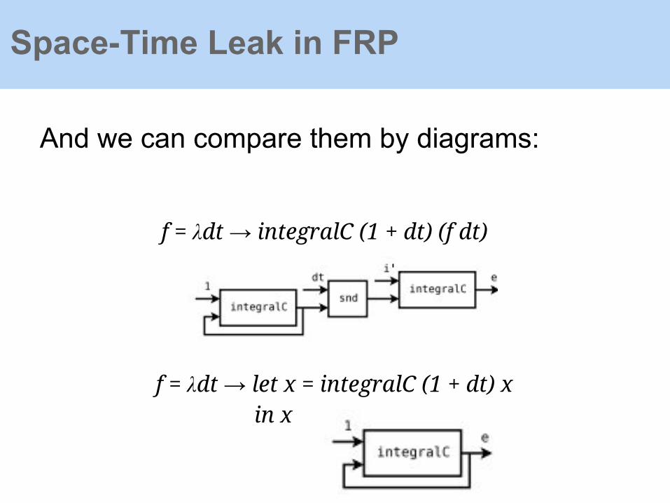
And we can compare them by diagrams:
f = λdt → integralC (1 + dt) (f dt)
f = λdt → let x = integralC (1 + dt) x in x

Space-Time Leak in FRP
In the `repeat` example:
repeat x = λx → x : repeat x
repeat x = λx → let xs = x:xs in xs

Space-Time Leak in FRP
So, in Yampa, we can't touch and handle signals directly, and need to use predefined combinators to compose our program.
This can greatly reduce possible leaks, and keep our program is still similar with the most intuitive version.
e = integralC 1 e e = proc () → do rec e ← integral 1 ↢e returnA ↢ e

Space-Time Leak in FRP
integralSF :: Double → SF Double DoubleintegralSF i = SF (λx → (i, λdt → integralSF (i + dt ∗ x)))
integralC :: Double → C Double → C DoubleintegralC i (C p) = C (i, λdt→integralC (i + fst p ∗ dt) (snd p dt))
Versus the previous version:
Our integral function now become:
Signal handling become implicit. We now raise customized functions to SFs.
Space-Time Leak in FRP
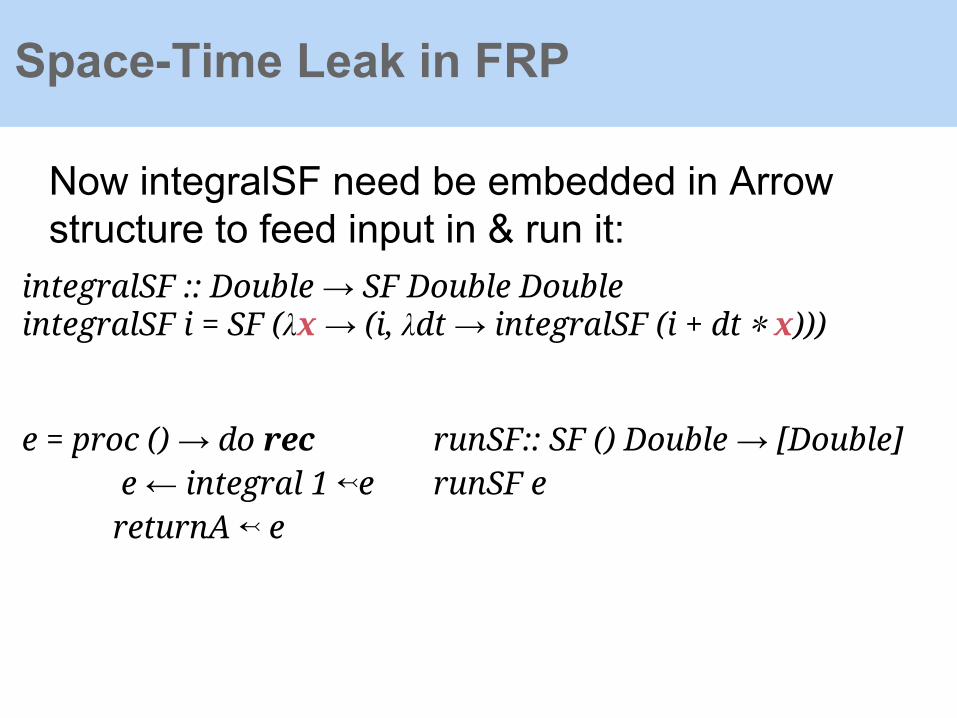
integralSF :: Double → SF Double DoubleintegralSF i = SF (λx → (i, λdt → integralSF (i + dt ∗ x)))
Now integralSF need be embedded in Arrow structure to feed input in & run it:
e = proc () → do rec e ← integral 1 ↢e returnA ↢ e
runSF:: SF () Double → [Double]runSF e

Back to Yampa
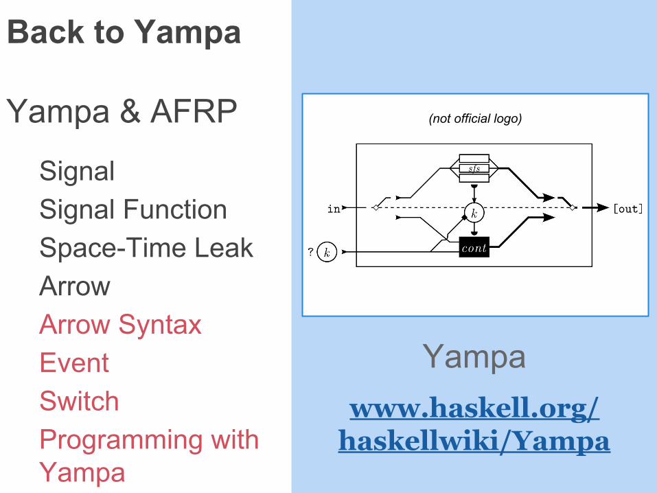
Yampa & AFRP
SignalSignal FunctionSpace-Time LeakArrowArrow SyntaxEventSwitchProgramming withYampa
Yeah ! Just escaped from the black hole !
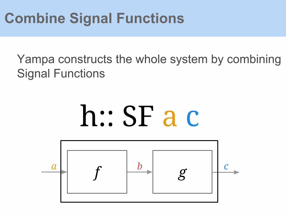
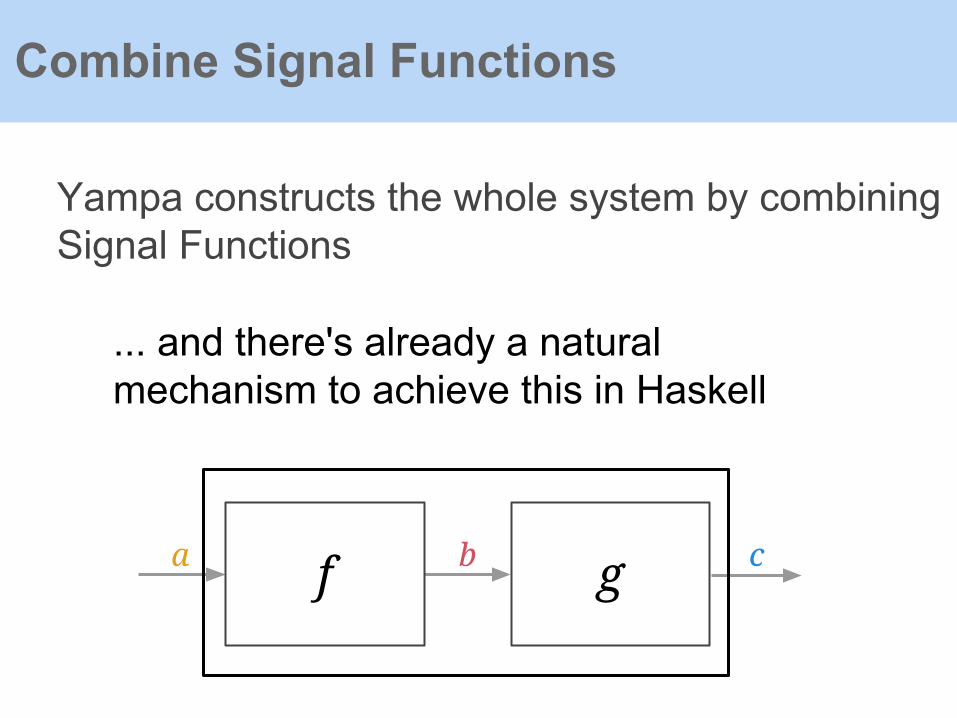
Yampa constructs the whole system by combining Signal Functions
Combine Signal Functions
gfa b c
h:: SF a c
Yampa constructs the whole system by combining Signal Functions
Combine Signal Functions
gfa b c
... and there's already a natural mechanism to achieve this in Haskell
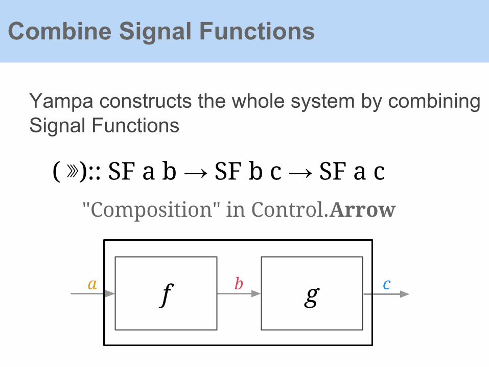
Yampa constructs the whole system by combining Signal Functions
Combine Signal Functions
gfa b c
( ⋙):: SF a b → SF b c → SF a c
"Composition" in Control.Arrow
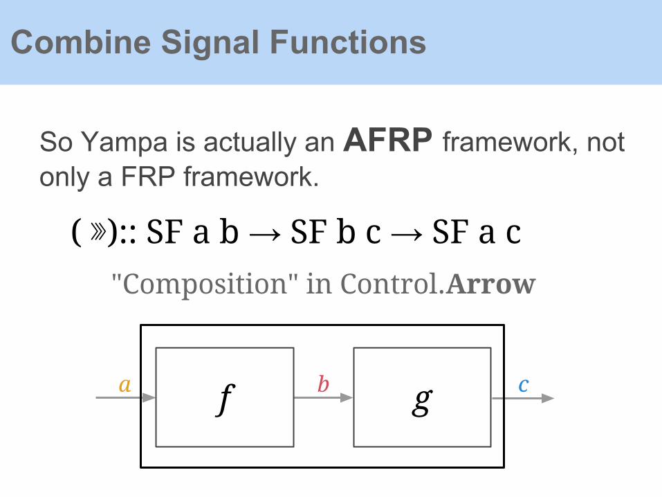
So Yampa is actually an AFRP framework, not only a FRP framework.
Combine Signal Functions
gfa b c
( ⋙):: SF a b → SF b c → SF a c
"Composition" in Control.Arrow

Arrow
We're here:
Typeclassopediawww.haskell.org/haskellwiki/
Typeclassopedia

Arrow Basics
"Unlike Monad and Applicative, whose types only reflect their output, the type of an Arrow computation reflects both its input and output"
( ≫= ):: M a → (a → M b) → M b
( ⋙ ):: A a b → A b c → A a c

Arrow Basics
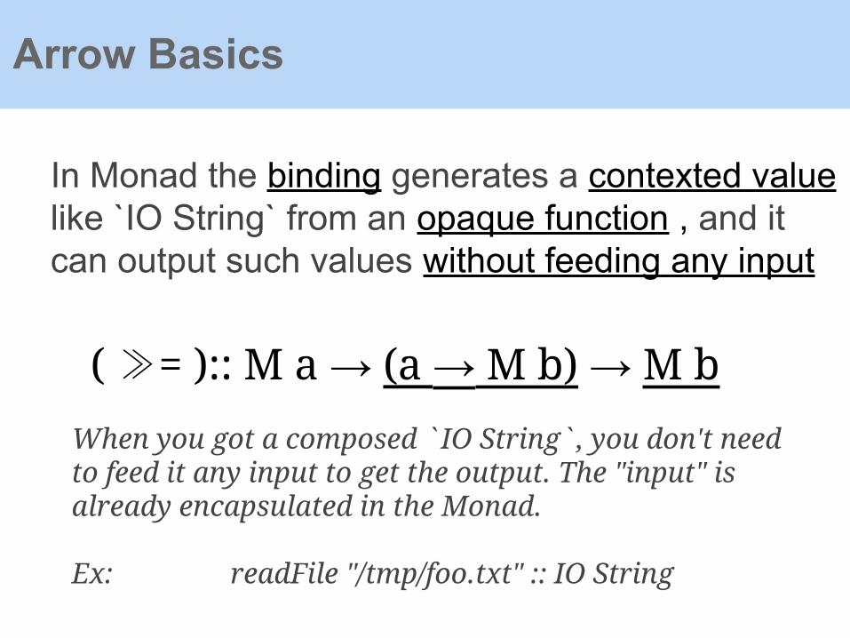
In Monad the binding generates a contexted value like `IO String` from an opaque function , and it can output such values without feeding any input
( ≫= ):: M a → (a → M b) → M b
Arrow Basics
In Monad the binding generates a contexted value like `IO String` from an opaque function , and it can output such values without feeding any input
( ≫= ):: M a → (a → M b) → M b
When you got a composed `IO String`, you don't need to feed it any input to get the output. The "input" is already encapsulated in the Monad.
Ex: readFile "/tmp/foo.txt" :: IO String

Arrow Basics
Arrows, on the other hand, can only be composed by other arrow combinators, and keep it still crystal clear after the composition
( ⋙ ):: A a b → A b c → A a c

Arrow Basics
Arrows, on the other hand, can only be composed by other arrow combinators, and keep it still crystal clear after the composition
( ⋙ ):: A a b → A b c → A a cYou can't get any meaningful value without executing the composed Arrow, which will also require you to feed it an input value.
Ex: let area = runF ( pow ⋙ mulpi ) r

Arrow Basics
So Arrows are just like pipelines, and Monads are more like pipeline plus self-contained pumps

There are many combinators in Control.Arrow
Arrow Basics
Compose First
f g f
Split
f
g
f
Loop ( self-feedback )

They will make your application like circuits
Arrow Basics
Back to Yampa
Yampa & AFRP
SignalSignal FunctionSpace-Time LeakArrowArrow SyntaxEventSwitchProgramming withYampa
Yampawww.haskell.org/haskellwiki/Yampa
(not official logo)
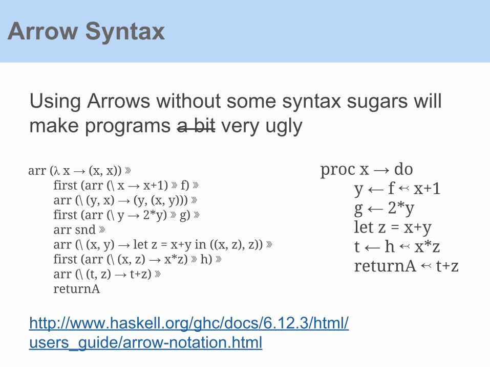
Using Arrows without some syntax sugars will make programs a bit very ugly
Arrow Syntax
proc x → do y ← f ↢ x+1 g ← 2*y let z = x+y t ← h ↢ x*z returnA ↢ t+z
arr (λ x → (x, x)) ⋙ first (arr (\ x → x+1) ⋙ f) ⋙ arr (\ (y, x) → (y, (x, y))) ⋙ first (arr (\ y → 2*y) ⋙ g) ⋙ arr snd ⋙ arr (\ (x, y) → let z = x+y in ((x, z), z)) ⋙ first (arr (\ (x, z) → x*z) ⋙ h) ⋙ arr (\ (t, z) → t+z) ⋙ returnA
http://www.haskell.org/ghc/docs/6.12.3/html/users_guide/arrow-notation.html

Using Arrows without some syntax sugars will make programs a bit very ugly
Arrow Syntax
proc x → do y ← f ↢ x+1 g ← 2*y let z = x+y t ← h ↢ x*z returnA ↢ t+z
proc <pattern> = λ→ <pattern>
<pattern> ← <arrf> ↢<expr> ≈let <pattern> = <arrf> <expr>
rec <do block> = ArrowLoop
http://stackoverflow.com/questions/5405850/how-does-the-haskell-rec-keyword-work

In Yampa, Event is just a Maybe-like type, representing discrete signals
Event
data Event a = NoEvent | Event atag:: Event a → b → Event b
We usually use events to trigger switchers, which will change the structure of our system dynamically.

Arrows will make your application like circuits. But you own a dynamic system now, not a static one.
Switches
Time 0Time 1Time 2Time 3Time 4Time 5Time 6Time 7Time ...Time N

This means circuits won't change unless we introduce Switches
Switches
Normal signals will be SFs' input; only events will go through the line toward the `k` function with data `mng`. If so the continuation function `k` will spawn a new SF or kill old SFs in the system.

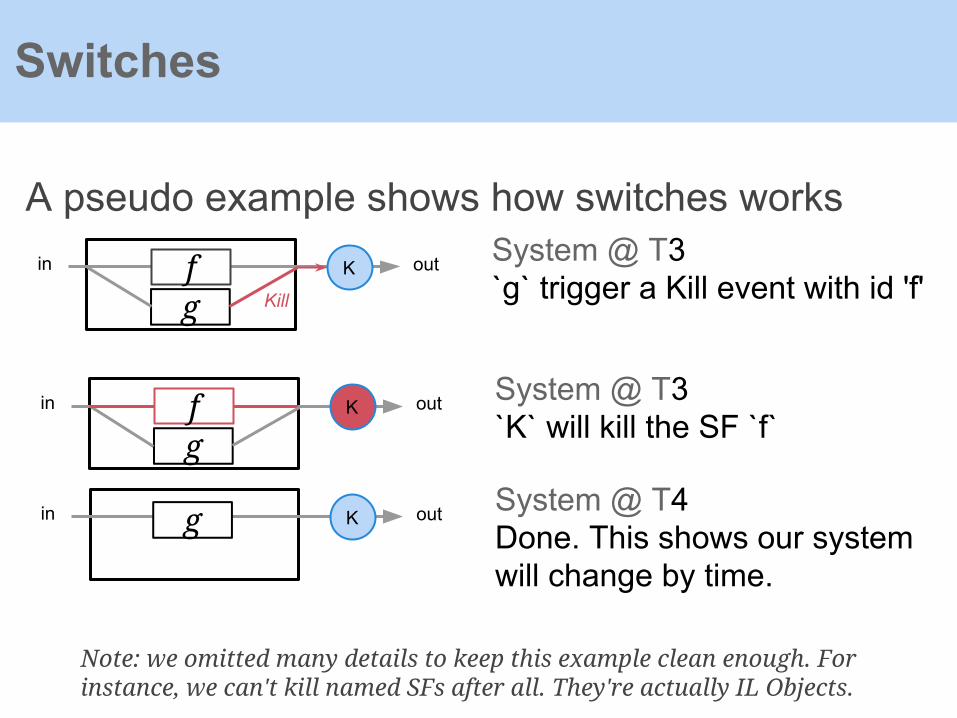
A pseudo example shows how switches works
Switches
f Kin out System @ T01 SF inside a Switch. Switch will let normal signal pass
f Kin out System @ T1`f` generate an Event Spawn,rather than a Signal with data
Spawn
f Kin out System @ T1`K` captured the event, and generate a new SF `g`
g

A pseudo example shows how switches works
Switches
f Kin out System @ T1Then `K` put the new SF in our system.g
System @ T2Now we've 2 SFs and inputs will be dispatched to them all
f Kin out
g
A pseudo example shows how switches works
Switches
f Kin out System @ T3`g` trigger a Kill event with id 'f'
g Kill
Kin out System @ T3`K` will kill the SF `f`
gf
Kin out System @ T4Done. This shows our system will change by time.
g
Note: we omitted many details to keep this example clean enough. For instance, we can't kill named SFs after all. They're actually IL Objects.

Switches, more switches... ( cry )
Switches

Switches, more switches... ( cry )
Switches

Switches, more switches... ( cry )
Switches
http://www.haskell.org/haskellwiki/Yampa/switch

How is it possible to use these stuff making a 3D game ?
Switches
Programming withYampa
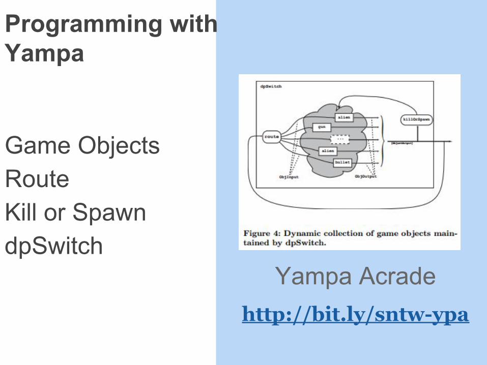
Game ObjectsRouteKill or SpawndpSwitch
Yampa Acradehttp://bit.ly/sntw-ypa
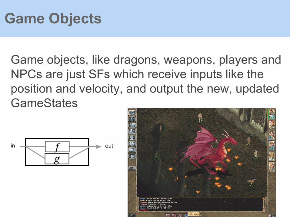
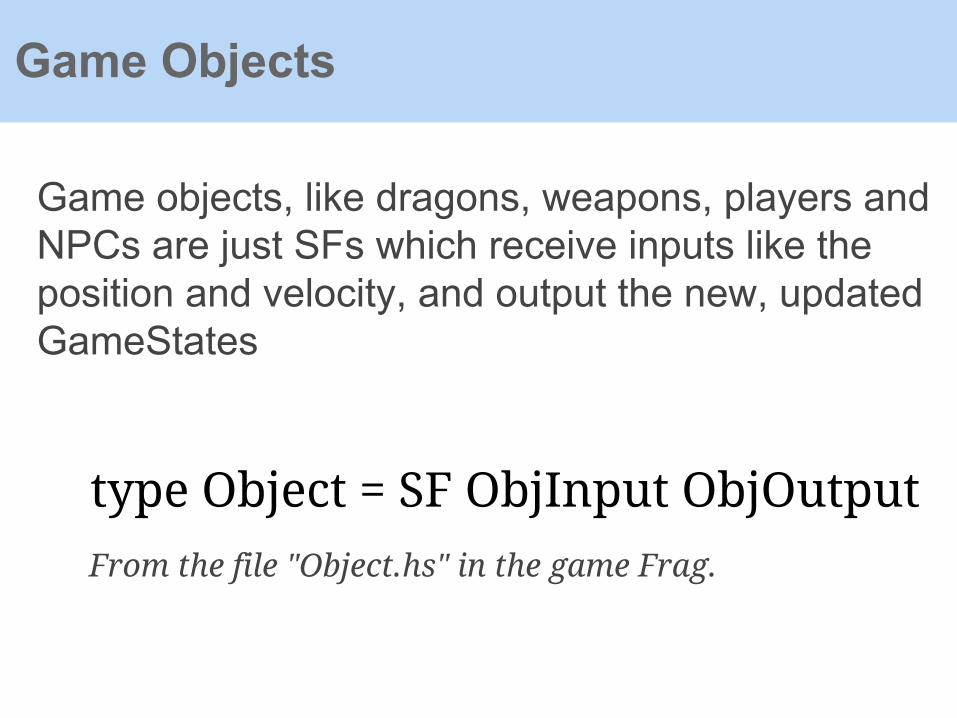
Game objects, like dragons, weapons, players and NPCs are just SFs which receive inputs like the position and velocity, and output the new, updated GameStates
Game Objects
fin out
g
Game objects, like dragons, weapons, players and NPCs are just SFs which receive inputs like the position and velocity, and output the new, updated GameStates
Game Objects
type Object = SF ObjInput ObjOutputFrom the file "Object.hs" in the game Frag.
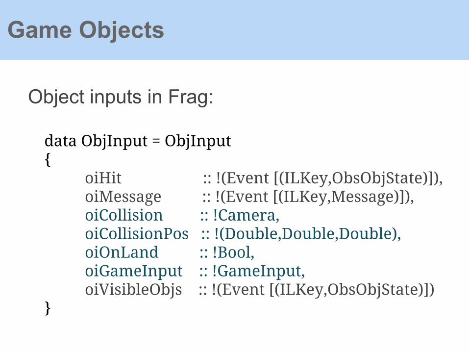
Object inputs in Frag:
Game Objects
data ObjInput = ObjInput { oiHit :: !(Event [(ILKey,ObsObjState)]), oiMessage :: !(Event [(ILKey,Message)]), oiCollision :: !Camera, oiCollisionPos :: !(Double,Double,Double), oiOnLand :: !Bool, oiGameInput :: !GameInput, oiVisibleObjs :: !(Event [(ILKey,ObsObjState)])}

Object outputs in Frag:
Game Objects
data ObjOutput = ObjOutput { ooObsObjState :: !ObsObjState, ooSendMessage :: !(Event [(ILKey,(ILKey,Message))]),
ooKillReq :: (Event ()), ooSpawnReq :: (Event [ILKey->Object])}

A simple game object from Yampa Arcade
Game Objects
data SimpleGunState = SimpleGunState { sgsPos :: Position2, sgsVel :: Velocity2, sgsFired :: Event ()}
type SimpleGun = SF GameInput SimpleGunState
Source code:http://hackage.haskell.org/package/SpaceInvaders

A simple game object from Yampa Arcade
Game Objects
gun
GameInput
Mouse PositionMouse ButtonKeyboard Input
Calculate new position and velocity of the gun
SimpleGunState
sgsPossgsVelsgsFired Event

In fact we don't define a SF. We define a SF generator :
Game Objects
simpleGun :: Position2 → SimpleGun
simpleGun (Point2 x0 y0) = proc gi → do (Point2 xd _) ← ptrPos ↢ gi rec let ad = 10 * (xd - x) - 5 * v v ← integral ↢ clampAcc v ad {- ...... -} returnA -< SimpleGunState { sgsPos = (Point2 x y0), sgsVel = (vector2 v 0), sgsFired = fire }

This allow us to embed it into our circuits and change the initial value as we need to:
Game Objects
game g nAliens vydAlien score0 = proc gi -> do rec oos <- game' objs0 -< (gi, oos {- oosp -}) {- ...... -} returnA -< ((score, map ooObsObjState (elemsIL oos)), (newRound `tag` (Left score)) `lMerge` (gameOver `tag` (Right score))) where objs0 = listToIL (gun (Point2 0 50))

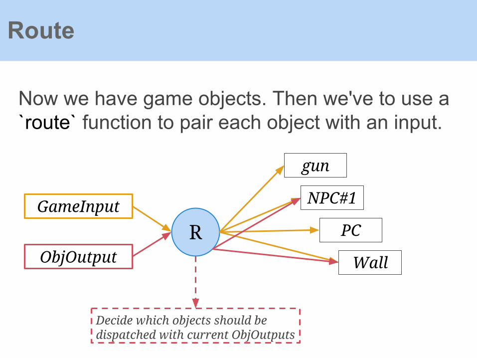
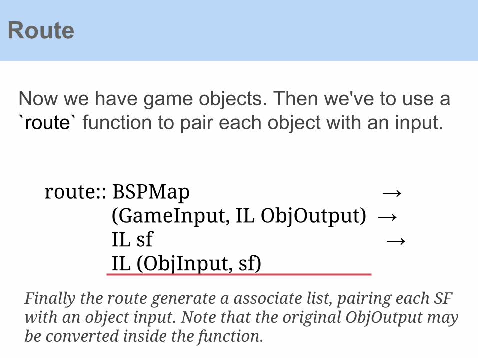
Now we have game objects. Then we've to use a `route` function to pair each object with an input.
Route
route:: BSPMap → (GameInput, IL ObjOutput) → IL sf → IL (ObjInput, sf)
From the file "Game.hs" in the game Frag.

Now we have game objects. Then we've to use a `route` function to pair each object with an input.
Route
route:: BSPMap → (GameInput, IL ObjOutput) → IL sf → IL (ObjInput, sf)
Route will broadcast GameInput to all game object which are like keyboard & mouse state , and handle outputs from game objects to send messages or detect collisions, then only pair it with those related objects.
Now we have game objects. Then we've to use a `route` function to pair each object with an input.
Route
gun
NPC#1
PC
Wall
RGameInput
ObjOutput
Decide which objects should be dispatched with current ObjOutputs

Now we have game objects. Then we've to use a `route` function to pair each object with an input.
Route
route:: BSPMap → (GameInput, IL ObjOutput) → IL sf → IL (ObjInput, sf)
`IL a` means a "identity list", which is actually a associate list contains `(ILKey , a)`. Frag use it to store named game objects ( just SFs ) .
Now we have game objects. Then we've to use a `route` function to pair each object with an input.
Route
route:: BSPMap → (GameInput, IL ObjOutput) → IL sf → IL (ObjInput, sf)
Finally the route generate a associate list, pairing each SF with an object input. Note that the original ObjOutput may be converted inside the function.

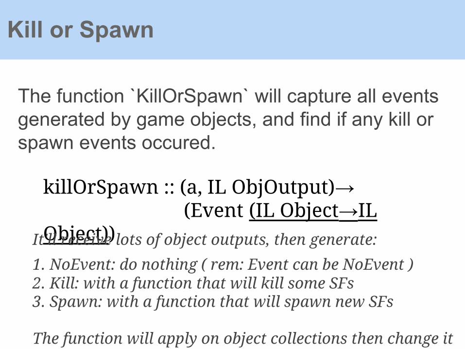
The function `KillOrSpawn` will capture all events generated by game objects, and find if any kill or spawn events occured.
Kill or Spawn
killOrSpawn :: (a, IL ObjOutput)→ (Event (IL Object→IL Object))
From the file "Game.hs" in the game Frag.
The function `KillOrSpawn` will capture all events generated by game objects, and find if any kill or spawn events occured.
Kill or Spawn
killOrSpawn :: (a, IL ObjOutput)→ (Event (IL Object→IL Object))It'll receive lots of object outputs, then generate:
1. NoEvent: do nothing ( rem: Event can be NoEvent )2. Kill: with a function that will kill some SFs3. Spawn: with a function that will spawn new SFs
The function will apply on object collections then change it

The function `KillOrSpawn` will capture all events generated by game objects, and find if any kill or spawn events occured.
Kill or Spawn
f Kin out
g
ooKillReqWill generate an Event to kill some SFs in the collection
f Kin out
g
ooSpawnReq
Will generate an Event to spawn new SFs in the collection

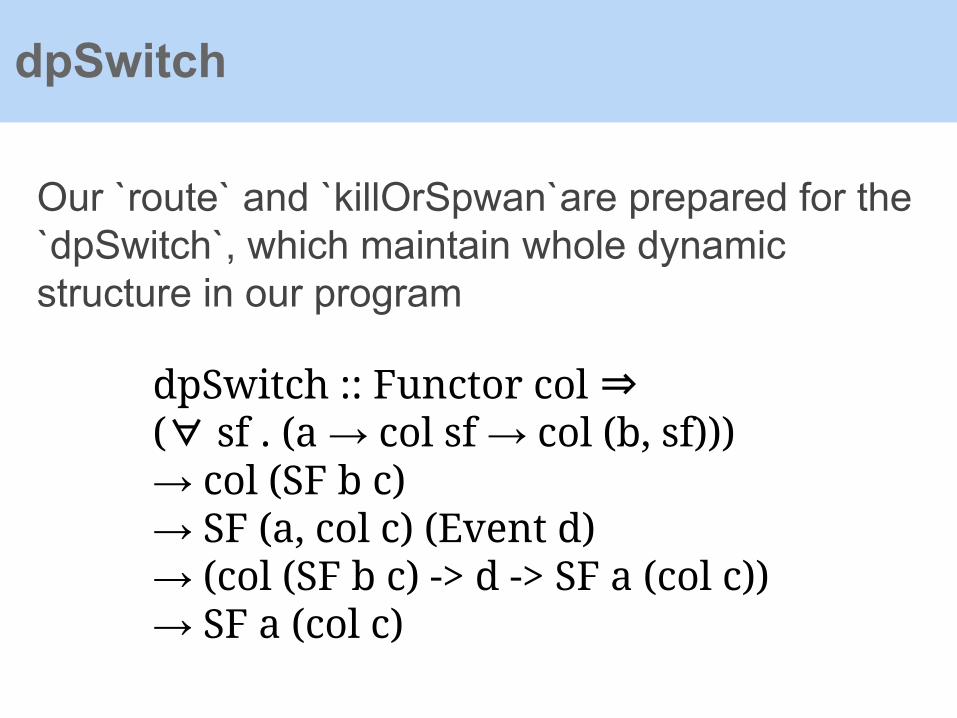
Our `route` and `killOrSpwan` are prepared for the `dpSwitch`, which maintain whole dynamic structure in our program
dpSwitch
Our `route` and `killOrSpwan`are prepared for the `dpSwitch`, which maintain whole dynamic structure in our program
dpSwitch
dpSwitch :: Functor col ⇒(∀ sf . (a → col sf → col (b, sf)))→ col (SF b c)→ SF (a, col c) (Event d)→ (col (SF b c) -> d -> SF a (col c))→ SF a (col c)
dpSwitch :: Functor col ⇒(∀ sf . (a → col sf → col (b, sf)))→ col (SF b c)→ SF (a, col c) (Event d)→ (col (SF b c) -> d -> SF a (col c))→ SF a (col c)
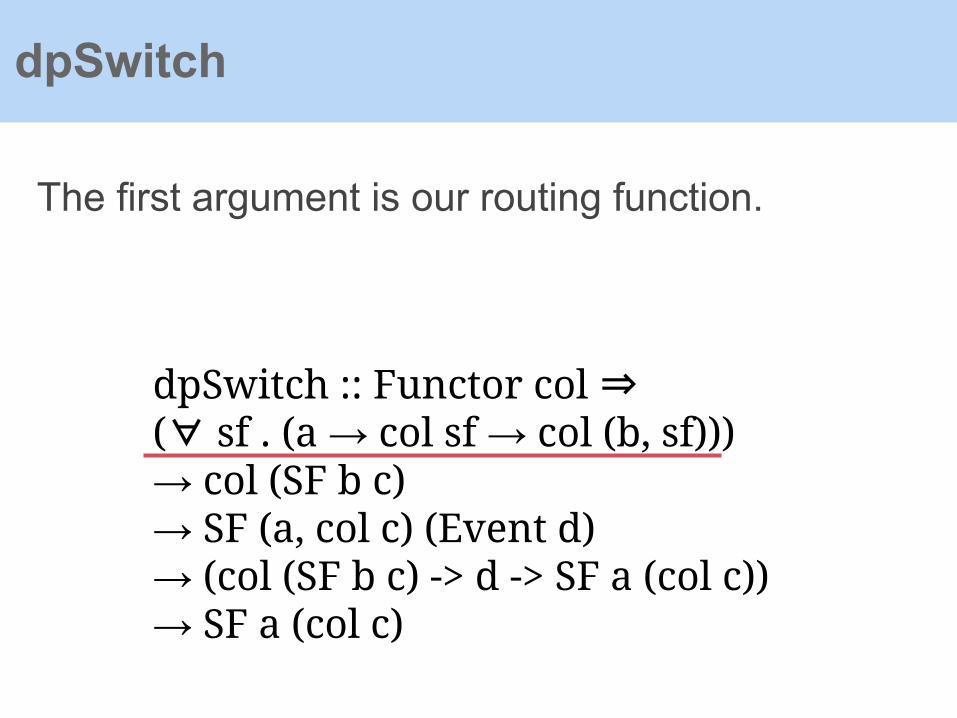
The first argument is our routing function.
dpSwitch

dpSwitch :: Functor col ⇒(∀ sf . (a → col sf → col (b, sf)))→ col (SF b c)→ SF (a, col c) (Event d)→ (col (SF b c) -> d -> SF a (col c))→ SF a (col c)
The second one is the initial collection of game objects.
dpSwitch

dpSwitch :: Functor col ⇒(∀ sf . (a → col sf → col (b, sf)))→ col (SF b c)→ SF (a, col c) (Event d)→ (col (SF b c) -> d -> SF a (col c))→ SF a (col c)
And the third argument is our `killOrSpawn`.
dpSwitch

dpSwitch :: Functor col ⇒(∀ sf . (a → col sf → col (b, sf)))→ col (SF b c)→ SF (a, col c) (Event d)→ (col (SF b c) -> d -> SF a (col c))→ SF a (col c)
The fourth function will be invoked while switching event occurs, yielding a new switch function and switch into, based on the collection previous transformed.
dpSwitch

dpSwitch :: Functor col ⇒(∀ sf . (a → col sf → col (b, sf)))→ col (SF b c)→ SF (a, col c) (Event d)→ (col (SF b c) -> d -> SF a (col c))→ SF a (col c)
This allows the collection to be updated and then switched back in, typically by employing `dpSwitch` again.
dpSwitch
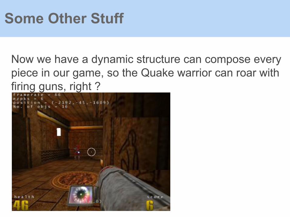
Now we have a dynamic structure can compose every piece in our game, so the Quake warrior can roar with firing guns, right ?
Some Other Stuff

Still Missing
NPC & AILevelsOpenGL Binding...
There is no royal road to Haskell. —Euclid ( typeclassopedia )

Maybe we're still not apt to create a 3D game with the AFRP framework, Yampa, but ideas in FRP & Arrow still inspire us.
Conclusion

And FRP is also a generic way to construct any "Event-Driven" like system, from 3D FPS games to HTTP servers.
Conclusion
http://stackoverflow.com/questions/13486293/is-frp-a-proper-way-to-implement-most-event-driven-things

Some differences between FRP and so-called "Event-Driven" pattern:
Conclusion
FRP based on continuing Streams of values, and we compute on them as we compute on a single value.
dt1 dt2 dt3 dt4 dt5
sf
sf can be primitive SF, composed SF or Switch
Some differences between FRP and so-called "Event-Driven" pattern:
Conclusion
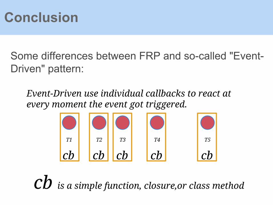
Event-Driven use individual callbacks to react at every moment the event got triggered.
T1 T2 T3 T4 T5
cb
cb is a simple function, closure,or class method
cb cb cb cb

Conclusion
This can be obvious in JavaScript and Node.js, which use Event-Driven as their reactive pattern
DOM.addEventListener('click', function(e){ // do something})
fs.readFile( '/tmp/test.txt', function(err, data){ // do something})
Conclusion
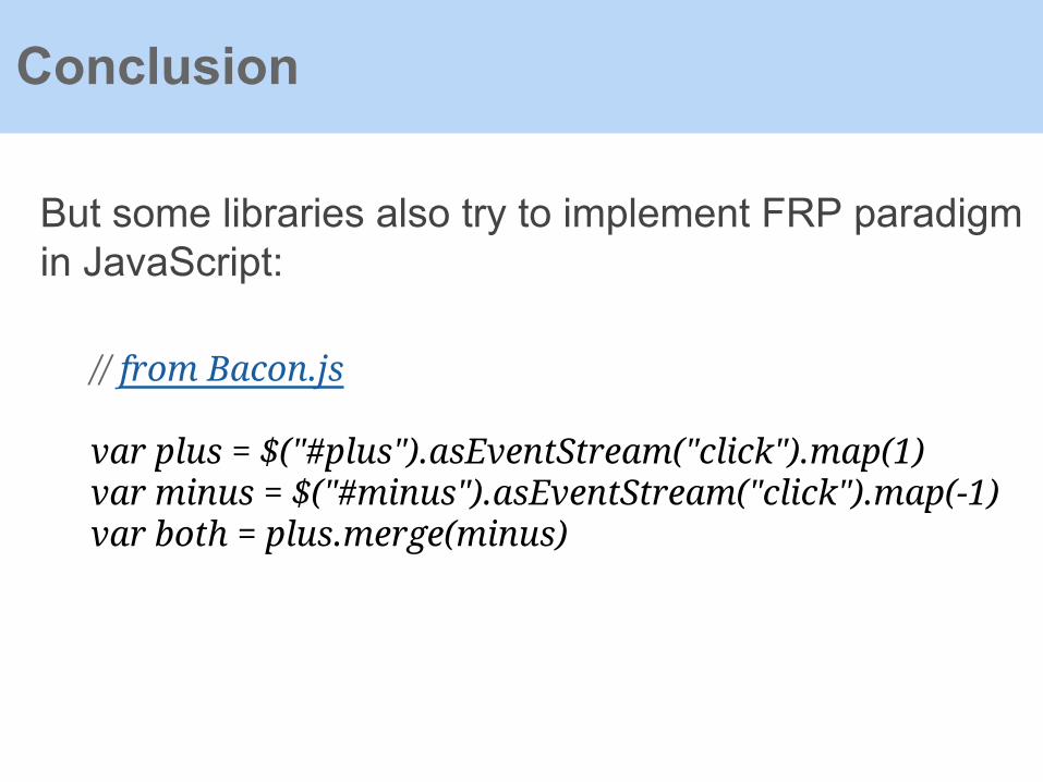
But some libraries also try to implement FRP paradigm in JavaScript:
// from Bacon.js
var plus = $("#plus").asEventStream("click").map(1)var minus = $("#minus").asEventStream("click").map(-1)var both = plus.merge(minus)

Conclusion
But some libraries also try to implement FRP paradigm in JavaScript:
// from Flapjax.js, compiler mode
<div><h1> You caught up <span style="color: white; background-color: black"> {! caughtUpB.toString() !} </span>times</h1>hit up with your mouse</div>

Conclusion
But some libraries also try to implement FRP paradigm in JavaScript:
http://elm-lang.org/learn/What-is-FRP.elm

Conclusion
And you may notice that in FRP, events/signals are handled "globally", but in JavaScript, they're handled "locally":
DOM → click, mouse hover...
click, mouse hover → Event DOM// FRP
// Event-Driven

References
There's a lot of resources in Haskell Wikihttp://www.haskell.org/haskellwiki/Yampa

References
Two useful articles about Yampa and game
http://www.cse.unsw.edu.au/~pls/thesis/munc-thesis.pdfhttp://haskell.cs.yale.edu/wp-content/uploads/2011/01/yampa-arcade.pdf
Yampa and robot control
http://citeseerx.ist.psu.edu/viewdoc/download?doi=10.1.1.5.2886&rep=rep1&type=pdf
References
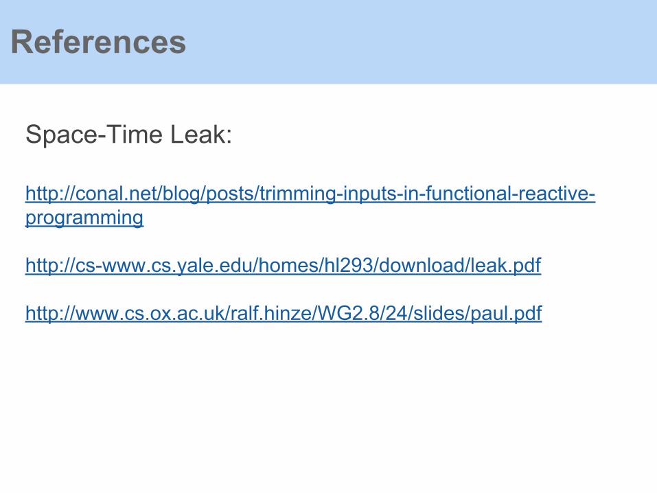
Space-Time Leak:
http://conal.net/blog/posts/trimming-inputs-in-functional-reactive-programming
http://cs-www.cs.yale.edu/homes/hl293/download/leak.pdf
http://www.cs.ox.ac.uk/ralf.hinze/WG2.8/24/slides/paul.pdf
Related Documents


