xcxcxcxcxcxcxxc

7/17/2019 xcxcxcxcxcxcxxc

http://slidepdf.com/reader/full/xcxcxcxcxcxcxxc 1/19

JOURNAL OF

SOUND AND

VIBRATION

www.elsevier.com/locate/jsvi

Journal of Sound and Vibration 262 (2003) 1113–1131

Vibration analysis of planar serial-frame structures

H.P. Lin*, J. Ro

Department of Mechanical and Automation Engineering, Da-Yeh University, 112 Shan-Jiau Rd.,

Da-Tsuen, Chang-Hua 51505, Taiwan, ROC

Received 8 April 2002; accepted 1 July 2002

Abstract

A hybrid analytical/numerical method is proposed that permits the efficient dynamic analysis of planar

serial-frame structures. The method utilizes a numerical implementation of a transfer matrix solution to the

equation of motion. By analyzing the transverse and longitudinal motions of each segment simultaneously

and considering the compatibility requirements across each frame angle, the undetermined variables of the

entire frame structure system can be reduced to six which can be determined by application of the boundary

conditions. The main feature of this method is to decrease the dimensions of the matrix involved in the

finite element methods and certain other analytical methods.

r 2002 Elsevier Science Ltd. All rights reserved.

1. Introduction

Frame structures are usually used in engineering designs, i.e., cranes, bridges, aerospace

structures, etc. The dynamic behaviors of frame structures can be predicted by using certain

analytical and numerical methods such as the dynamic stiffness methods (DSM) and the finite

element methods (FEM). The DSM employs the solutions of governing equations under

harmonic nodal excitations as shape functions to formulate an analytical stiffness matrix. The

method requires closed-form solutions of the governing equations which restrict the applicationareas [1]. The FEM has been very commonly used in recent years in this field. However, the FEM

requires a large amount of computer memory and computation time, since many degrees of

freedom are required for accurately solving dynamic problems for these structures [2,3]. To solve

this problem, various methods have been studied to overcome the disadvantages [2–5]. In most of

the previous studies, the Euler–Bernoulli beam-theory model obtained by deriving the differential

equation and the associated boundary conditions for a basic uniform Euler–Bernoulli beam are

*Corresponding author. Tel.: +886-4-8511888; fax: +886-4-8511895.

E-mail address: [email protected] (H.P. Lin).

0022-460X/03/$ - see front matterr 2002 Elsevier Science Ltd. All rights reserved.

PII: S 0 0 2 2 - 4 6 0 X ( 0 2 ) 0 1 0 8 9 - 1



often used and discussed. Some researchers have also studied the different results between the

Euler–Bernoulli beam-theory models and the Timoshenko beam theory. Finally, it is possible to

evaluate natural frequencies simply by finding roots of the high order determinant of the coefficient

matrix of the linear system if accuracy of the eigensolutions is required.This investigation presents a hybrid analytical/numerical method that permits the efficient

computation of the eigensolutions for planar serial-frame structures with various boundary

conditions. The method is based on partitioning the frame structure to the sub-beam segments

and considering the transverse and longitudinal motions of each segment and, by the

compatibility requirements across each frame angle, the relationship of the six integration

constants of the eigenfunctions between adjacent sub-beams can be determined. By using the

transfer matrix method [9,10], as a consequence, the entire system has only six unknown

constants, which can be solved through the satisfaction of six boundary conditions. In this article,

the eigenvalue problem is solved by using closed-form transfer matrix methods.

2. Theoretical model

A typical planar serial-frame structure with K frame angles y1; y2; y; yK is shown in Fig. 1. This

structure is partitioned into K þ 1 components at the angle positions enabling a substructure

approach. There are K þ 1 sub-beams with lengths L1; L2; y; LK þ1; and the positions of the frame

angles are located by X 1; X 2; :::; X K ; respectively, in Fig. 1. In doing the vibration analysis of this

system for this study, each component member (sub-beam) is analyzed by its transverse and

longitudinal motions, respectively. Let the X -axis represent the longitudinal direction and the Y -

axis the transverse direction of each component member; then, the traditional vibration theories

of an Euler–Bernoulli beam and the axial vibration of a rod are considered. The vibration

amplitudes of the transverse and longitudinal displacements of the component i (sub-beam) are

Fig. 1. A planar serial-frame structure with K frame angles y1; y2; y; yk located at positions X 1; X 2; y; X K ;respectively; lengths of sub-beams are L1; L2; y; Lk ; Lk þ1 where L1 þ L2 þ?þ Lk þ Lk þ1 ¼ L:

H.P. Lin, J. Ro / Journal of Sound and Vibration 262 (2003) 1113–11311114



denoted by Y i ðX ; T Þ and U i ðX ; T Þ on the interval X i 1o

X o

X i where the sub-index i representsthe i th segment and i ¼ 1; 2; y; K þ 1; as shown in Fig. 2. The entire system is now divided into

K þ 1 segments, wherein the total length of this frame system is L ð¼ L1 þ L2 þ?þ LK þ1Þ:According to Refs. [6–8], the equations of motion for each segment, assumed with a uniform

cross-section, are

transverse motion:

EI @4Y i ðX ; T Þ

@X 4 þ rA

@2Y i ðX ; T Þ

@T 2 ¼ 0; X i 1oX oX i ; i ¼ 1; 2; y; K þ 1; ð1Þ

longitudinal motion:

E @2U i ðX ; T Þ

@X 2 r

@2U i ðX ; T Þ

@T 2 ¼ 0; X i 1oX oX i ; i ¼ 1; 2; y; K þ 1; ð2Þ

where E is Young’s modulus of the material, I is the moment of inertia of the beam cross-section,

r is the density of material and A is the cross-section area of the beam.

The boundary conditions, the fixed–fixed supported case for this example, are

Y ð0; T Þ ¼ Y ðL; T Þ ¼ 0; ð3aÞ

Y 0ð0; T Þ ¼ Y 0ðL; T Þ ¼ 0; ð3bÞ

U ð0; T Þ ¼ U ðL; T Þ ¼ 0: ð3cÞThe transverse and the longitudinal motions at the end of the segment before each frame angle

constrain the motions of the adjacent segment after the same frame angle. So the ‘‘compatibility

conditions’’ enforce continuities in the displacement field (in both transverse and longitudinal),

slope, bending moment, shear force and axial force, respectively, across each frame angle yi ; as

shown in Fig. 3a (displacements) and Fig. 3b (forces), which can be expressed as

Y i þ1ðX þi ; T Þ ¼ Y i ðX i ; T Þ cos yi þ U i ðX i ; T Þ sin yi ; displacement continuity; ð4aÞ

U i þ1ðX þi ; T Þ ¼ Y i ðX i ; T Þ sin yi þ U i ðX i ; T Þ cos yi ; displacement continuity; ð4bÞ

Fig. 2. Transverse and longitudinal motions of a segment.

H.P. Lin, J. Ro / Journal of Sound and Vibration 262 (2003) 1113–1131 1115



Y 0i þ1ðX þi ; T Þ ¼ Y 0i ðX i ; T Þ; slope continuity; ð4cÞ

Y 00i þ1ðX þi ; T Þ ¼ Y 00i ðX i ; T Þ; moment continuity; ð4dÞ

EIY 000i þ1ðX þi ; T Þ ¼ EIY 000i ðX i ; T Þ cos yi EAU 0i ðX i ; T Þ sin yi ; shear continuity; ð4eÞ

EAU 0i þ1ðX þi ; T Þ ¼ EIY 000i ðX i ; T Þ sin yi EAU 0i ðX i ; T Þ cos yi ; axial force continuity; ð4f Þ

where the symbols X þi and X i denote the locations immediately above and below the angle

position X i : All the assumptions in the above compatibility conditions are the same as the

traditional analysis of the transverse vibrations of an Euler–Bernoulli beam and the axial

vibrations of a rod. The frame angles are also assumed to be unchanged during the motions of the

frame.

In the above, the following quantities are introduced:

y ¼ Y

L; x ¼

X

L; u ¼

U

L; t ¼

T ffiffiffiffiL

p ; l i ¼ Li

L; xi ¼

X i

L: ð5Þ

Thus, in each segment, Eqs. (1) and (2) can then be expressed in a non-dimensional form as

EI

L3

@4 yi ðx; tÞ

@x4 þ rA

@2 yi ðx; tÞ

@t2 ¼ 0; xi 1oxoxi ; i ¼ 1; 2; y; K þ 1; ð6Þ

E

L

@2ui ðx; tÞ

@x2 r

@2ui ðx; tÞ

@t2 ¼ 0; xi 1oxoxi ; i ¼ 1; 2; y; K þ 1: ð7Þ

The non-dimensional ‘‘compatibility conditions’’ across each frame angle are (from Eqs.

(4a)–(4f))

yi þ1ðxþi ; tÞ ¼ yi ðx

i ; tÞ cos yi þ ui ðxi ; tÞsin yi ; ð8aÞ

Fig. 3. (a) Displacement compatibility requirements across i th frame angle yi : Y i and U i are transverse and longitudinal

displacements of segment i at position X i : (b) Force compatibility requirements across i th frame angle yi : V i and F i are

shear and axial forces of segment i at position X i :




ui þ1ðxþi ; tÞ ¼ yi ðx

i ; tÞ sin yi ui ðxi ; tÞ cos yi ; ð8bÞ

y0i þ1ðx

þi ; tÞ ¼ y

0i ðx

i ; tÞ; ð8cÞ

y00i þ1ðxþ

i ; tÞ ¼ y00i ðx

i ; tÞ; ð8dÞ

y000i þ1ðxþ

i ; tÞ ¼ y000i ðx

i ; tÞ cos yi AL2

I u0

i ðxi ; tÞ sin yi ; ð8eÞ

u0i þ1ðxþ

i ; tÞ ¼ I

AL2 y000

i ðxi ; tÞ sin yi u0

i ðxi ; tÞ cos yi ; ð8f Þ

where i ¼ 1; 2; :::; K : Similarly, the non-dimensional boundary conditions from Eqs. (3a)–(3c), for

the example of fixed–fixed ends, can be written as

yð0; tÞ ¼ yð1; tÞ ¼ 0; ð9aÞ

y0ð0; tÞ ¼ y0ð1; tÞ ¼ 0; ð9bÞ

uð0; tÞ ¼ uð1; tÞ ¼ 0: ð9cÞ

3. Calculation of eigensolutions

The eigensolutions for cases of commonly used different boundary conditions are derived. The

solutions of the other boundary conditions can also be obtained easily through a similar

procedure. Using the separable solutions: yi ðx; tÞ ¼ wi ðxÞe jot and ui ðx; tÞ ¼ vi ðxÞe jot in Eqs. (6) and

(7) leads to an associated eigenvalue problem,

w0000i ðxÞ l4wi ðxÞ ¼ 0; xi 1oxoxi ; i ¼ 1; 2; y; K þ 1; ð10Þ

v00i ðxÞ þ g2vi ðxÞ ¼ 0; xi 1oxoxi ; i ¼ 1; 2; y; K þ 1; ð11Þ

where

l4 ¼ rAL3o2

EI and g2 ¼

rLo2

E : ð12Þ

From Eq. (12), the relationship between l and g can be expressed as

g ¼

ffiffiffiffiI

A

r 1

Ll2 ¼ al2; ð13Þ

where a is a constant ða ¼ ffiffiffiffiffiffiffiffiffi

I =Ap

ð1=LÞÞ; for a square cross-section of the segment with width B

and height H ; a can be expressed as a ¼ ffiffiffiffiffiffiffiffiffi

I =Ap

ð1=LÞ ¼ ffiffiffiffiffiffiffiffiffiffi

1=12p

ðH =LÞ: From Eqs. (8a)–(8f), the

corresponding compatibility conditions across each frame angle lead to

wi þ1ðxþi Þ ¼ wi ðx

i Þ cos yi þ vi ðxi Þ sin yi ; ð14aÞ




vi þ1ðxþi Þ ¼ wi ðx

i Þ sin yi vi ðxi Þ cos yi ; ð14bÞ

w0i þ1ðxþ

i Þ ¼ w0i ðx

i Þ; ð14cÞ

w00i þ1ðxþ

i Þ ¼ w00i ðx

i Þ; ð14dÞ

w000i þ1ðxþ

i Þ ¼ w000i ðx

i Þ cos yi AL2

I v0

i ðxi Þ sin yi ; ð14eÞ

v0i þ1ðxþ

i Þ ¼ I

AL2 w000

i ðxi Þ sin yi v0

i ðxi Þ cos yi ð14f Þ

for i ¼ 1; 2; y; K : The boundary conditions, from Eqs. (9a)–(9c), are

wð0Þ ¼ 0; wð1Þ ¼ 0; w0ð0Þ ¼ 0; ð15a2cÞ

w0ð1Þ ¼ 0; vð0Þ ¼ 0; vð1Þ ¼ 0: ð15d2f Þ

A closed-form solution to this eigenvalue problem can be obtained by employing transfer matrix

methods [9,10]. The general solutions of Eqs. (10) and (11), for each segment, are

wi ðxÞ ¼ Ai sin lðx xi 1Þ þ B i cos lðx xi 1Þ þ C i sinh lðx xi 1Þ

þ Di cosh lðx xi 1Þ; xi 1o

xo

xi ; i ¼ 1; 2; y

; K þ 1; ð16Þ

vi ðxÞ ¼ E i sin gðx xi 1Þ þ F i cos gðx xi 1Þ

¼ E i sin al2ðx xi 1Þ þ F i cos al2ðx xi 1Þ; xi 1oxoxi ; i ¼ 1; 2; y; K þ 1; ð17Þ

where A i ; B i ; C i ; Di ; E i and F i are constants associated with the i th segment ði ¼ 1; 2; y; K þ 1Þ:The constants in the (i þ 1)th segment (Ai þ1; B i þ1; C i þ1; Di þ1; E i þ1 and F i þ1) are related to those in

the i th segment (Ai ; B i ; C i ; Di ; E i and F i ) through the compatibility conditions in Eqs. (14a)–(14f),

which can be expressed as

Ai þ1

B i þ1

C i þ1

Di þ1

E i þ1

F i þ1

8>>>>>>>>><>>>>>>>>>:

9>>>>>>>>>=>>>>>>>>>;

¼

t11 t12 t13 t14 t15 t16

^

^

y t65 t66

26664

37775

ði Þ

Ai

B i

C i

Di

E i

F i

8>>>>>>>>><>>>>>>>>>:

9>>>>>>>>>=>>>>>>>>>;

¼%T

ði Þ66

Ai

B i

C i

Di

E i

F i

8>>>>>>>>><>>>>>>>>>:

9>>>>>>>>>=>>>>>>>>>;

; ð18Þ

where%T

ði Þ66 is the 6 6 transfer matrix which depends on the eigenvalue l; for which the elements

are derived in Appendix A.




Through repeated applications of Eq. (18), the six constants in the first segment ( A1; B 1; C 1; D1;E 1 and F 1) can be mapped into those of the last segment, thereby reducing the number of

independent constants of the entire system to six:

AK þ1

B K þ1

C K þ1

DK þ1

E K þ1

F K þ1

8>>>>>>>>><>>>>>>>>>:

9>>>>>>>>>=>>>>>>>>>;

¼%T

ðK Þ66

AK

B K

C K

DK

E K

F K

8>>>>>>>>><>>>>>>>>>:

9>>>>>>>>>=>>>>>>>>>;

¼%T

ðK Þ66

%T

ðK 1Þ66

AK 1

B K 1

C K 1

DK 1

E K 1

F K 1

8>>>>>>>>><>>>>>>>>>:

9>>>>>>>>>=>>>>>>>>>;

¼%T

ðK Þ66

%T

ðK 1Þ66 y

%T

ð1Þ66

A1

B 1

C 1

D1

E 1

F 1

8>>>>>>>>><>>>>>>>>>:

9>>>>>>>>>=>>>>>>>>>;

: ð19Þ

These six remaining constants (A1; B 1; C 1; D1; E 1 and F 1) can be determined through the

satisfaction of the boundary conditions in Eqs. (15a)-(15f). For the example case of a planar

serial-frame with fixed–fixed ends, beginning with those at the left support, Eqs. (16), (17), (15a),(15c) and (15e) lead to

B 1 þ D1 ¼ 0; A1 þ C 1 ¼ 0; F 1 ¼ 0: ð20a2cÞ

Satisfaction of the boundary conditions of Eqs. (16) and (17) at the right support, Eqs. (15b),

(15d) and (15f), requires

AK þ1 sin ll K þ1 þ B K þ1 cos ll K þ1 þ C K þ1 sinh ll K þ1 þ DK þ1 cos hll K þ1 ¼ 0; ð20dÞ

AK þ1 cos ll K þ1 B K þ1 sin ll K þ1 þ C K þ1 cosh ll K þ1 þ DK þ1 sinh ll K þ1 ¼ 0; ð20eÞ

E K þ1 sin al2

l K þ1 þ F K þ1 cos al2

l K þ1 ¼ 0; ð20f Þ

which can be expressed in matrix form as

0

0

0

8><>:

9>=>; ¼

sin ll K þ1 cos ll K þ1 sinh ll K þ1 cosh ll K þ1 0 0

cos ll K þ1 sin ll K þ1 cosh ll K þ1 sinh ll K þ1 0 0

0 0 0 0 sin al2l K þ1 cos al2l K þ1

264

375

AK þ1

B K þ1

C K þ1

DK þ1

E K þ1

F K þ1

8>>>>>>>>><>>>>>>>>>:

9>>>>>>>>>=>>>>>>>>>;

¼ %B 36

AK þ1

B K þ1

C K þ1

DK þ1

E K þ1

F K þ1

8>>>>>>>>><>>>>>>>>>:

9>>>>>>>>>=>>>>>>>>>;

; ð21Þ

where

%B 36 ¼




264

375: ð22Þ




Substitution of Eq. (19) into Eq. (21) and use of Eq. (20a)-(20c) leads to

0

0

0

8><>:

9>=>; ¼

%B 36

AK þ1

B K þ1

C K þ1

DK þ1

E K þ1

F K þ1

8>>>>>>>>><>>>>>>>>>:

9>>>>>>>>>=>>>>>>>>>;

¼%B 36

%T

ðK Þ66

%T

ðK 1Þ66 y

%T

ð1Þ66

A1

B 1C 1

D1

E 1

F 1

8>>>>>>>>><>>>>>>>>>:

9>>>>>>>>>=>>>>>>>>>;

;

0

00

8><>: 9>=>; ¼ %R36

A1

B 1

C 1

D1

E 1

F 1

8>>>>>>>>><>>>>>>>>>:

9>>>>>>>>>=>>>>>>>>>;

¼

r11 r12 r13 r14 r15 r16

r21 r22 r23 r24 r25 r26r31 r32 r33 r34 r35 r36

264 375

A1

B 1

A1

B 1

E 1

0

8>>>>>>>>><>>>>>>>>>:

9>>>>>>>>>=>>>>>>>>>;

; ð23Þ

where

%R36 ¼

%B 36

%T

ðK Þ66

%T

ðK 1Þ66 y

%T

ð1Þ66 ¼

r11 r12 r13 r14 r15 r16

r21 r22 r23 r24 r25 r26

r31 r32 r33 r34 r35 r36

264

375:

Thus, the existence of non-trivial solutions requires

det

r11ðlÞ r13ðlÞ r12ðlÞ r14ðlÞ r15ðlÞ



264

375 ¼ 0: ð24Þ

This determinant provides the single (characteristic) equation for the solution of the eigenvalue ln:This equation is solved using the standard Newton–Raphson iterations or, for simplification,

using the method shown in Fig. 4 to obtain the eigenvalues. The coefficients of the eigenfunctions,

wnðxÞ and vnðxÞ; are obtained by back-substitution into Eqs. (23) and (18) followed by Eqs. (16)

and (17).

For cases of other usually used boundary conditions, through a similar procedure, the following

relationships can be obtained:(a) Fixed–hinged boundary conditions: The existence of non-trivial solutions for the

constants A1; B 1;C 1; D1; E 1 and F 1 is the same as in Eq. (24), but the matrix%B 36 in Eq. (21)

now becomes

%B 36 ¼




264

375:

ð25Þ




(b) Fixed–free boundary conditions: The existence of non-trivial solutions is the same as in

Eq. (24), but the matrix

%

B 36 in Eq. (21) now becomes

%B 36 ¼



0 0 0 0 cos al2l K þ1 sin al2l K þ1

264

375:

ð26Þ

(c) Hinged-hinged boundary conditions: The existence of non-trivial solutions now requires

det

r11ðlÞ r13ðlÞ r15ðlÞ



264

375 ¼ 0; ð27Þ

the matrix%B 36 in Eq. (21) is now the same as in Eq. (25).

(d) Free–free boundary conditions: The existence of non-trivial solutions requires

det

r11ðlÞ þ r13ðlÞ r12ðlÞ þ r14ðlÞ r16ðlÞ



264

375 ¼ 0; ð28Þ

and the matrix%B 36 in Eq. (21) is now the same as Eq. (26).

0 0.2 0.4 0.6 0.8 1 1.2 1.4 1.6 1.8 2

-0.5

-0.4

-0.3

-0.2

-0.1

0

0.1

0.2

0.3

0.4

0.5

------> eigenvalues

d e t e r m i n a n t

first second third

Fig. 4. Simple calculation of eigenvalues.




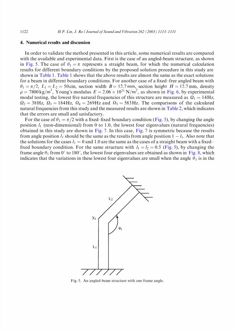
4. Numerical results and discussion

In order to validate the method presented in this article, some numerical results are compared

with the available and experimental data. First is the case of an angled-beam structure, as shownin Fig. 5. The case of y1 ¼ p represents a straight beam, for which the numerical calculation

results for different boundary conditions by the proposed solution procedure in this study are

shown in Table 1. Table 1 shows that the above results are almost the same as the exact solutions

for a beam in different boundary conditions. For another case of a fixed–free angled beam with

y1 ¼ p=2; L1 ¼ L2 ¼ 50 cm; section width B ¼ 12:7 mm; section height H ¼ 12:7 mm; density

r ¼ 7800 kg=m3; Young’s modulus E ¼ 2:06 1011 N=m

2; as shown in Fig. 6, by experimental

modal testing, the lowest five natural frequencies of this structure are measured as O1 ¼ 14 Hz,

O2 ¼ 38 Hz, O3 ¼ 184 Hz, O4 ¼ 269Hz and O5 ¼ 583 Hz. The comparisons of the calculated

natural frequencies from this study and the measured results are shown in Table 2, which indicates

that the errors are small and satisfactory.For the case of y1 ¼ p=2 with a fixed–fixed boundary condition (Fig. 5), by changing the angle

position l 1 (non-dimensional) from 0 to 1.0, the lowest four eigenvalues (natural frequencies)

obtained in this study are shown in Fig. 7. In this case, Fig. 7 is symmetric because the results

from angle position l 1 should be the same as the results from angle position 1 l 1: Also note that

the solutions for the cases l 1 ¼ 0 and 1:0 are the same as the cases of a straight beam with a fixed–

fixed boundary condition. For the same structure with l 1 ¼ l 2 ¼ 0:5 (Fig. 5), by changing the

frame angle y1 from 01 to 1801; the lowest four eigenvalues are obtained as shown in Fig. 8, which

indicates that the variations in these lowest four eigenvalues are small when the angle y1 is in the

X1

L1

θ1

L2

Fig. 5. An angled-beam structure with one frame angle.




range from 401 to 1401: It can be considered that the dynamic stiffness of this frame structure is

close within this frame angle range. Also note that in Fig. 8, there is a ‘‘cross-over’’ phenomenon

for the first and the second modes near the angle y1 above 1601: Before this cross-over point, the

first mode is anti-symmetric and the second mode is symmetric in the transverse motion

(dominant). After this cross-over point, the first mode now becomes symmetric and the second

mode becomes anti-symmetric. This can be distinguished from the mode shapes shown in Figs. 9

and 10 for different y1 angles ðy1 ¼ 1401; 1601; 1701 and 1801Þ: The third mode in Fig. 8 also has a

Table 1

Comparisons for an angled-beam structure with angle y1 ¼ 1801 (H =L ¼ 0:05)

Different

B.C’s

Eigenvalues

l1 l2 l3

Calculated

from this

study

Exact

solution

Calculated

from this

study

Exact

solution

Calculated

from this

study

Exact

solution

Hinged–

hinged

3.1426 p 6.2842 2p 9.4258 3p

Fixed–free 1.8801 1.8735 4.6991 4.6736 7.8598 7.8549

Fixed–fixed 4.7350 4.7296 7.8582 7.8524 11.0006 10.9955

Fig. 6. An experimental fixed–free angled-beam structure.




0 0.1 0.2 0.3 0.4 0.5 0.6 0.7 0.8 0.9 14

6

8

10

12

14

16

18fixed-fixed angle beam with H/L=0.024, theta=90 degree

non-dimensional angle position

t h e l o w e s t f o u r e i g e n v a l u e s

Fig. 7. Lowest four eigenvalues for an angled-beam structure by changing angle position l 1:

0 20 40 60 80 100 120 140 160 1800

2

4

6

8

10

12

14

16

18fixed-fixed angle beam with H/L=0.024, L1=L2=0.5

angle degree

t h e l o w

e s t f o u r e i g e n v a l u e s

anti-symmetric mode

symmetric mode

anti-symmetric mode

symmetric mode

Fig. 8. Lowest four eigenvalues for an angled-beam structure by changing angle y1:




phenomenon similar to the first mode. There is also a ‘‘cross-over’’ point at the third and the

fourth modes near the position y1 below 1401: The third mode shapes for different y1 values

ðy1 ¼ 201; 301; 1001; 1401; 1601 and 1801Þ are shown in Fig. 11, which indicated that before the

Table 2

Experimental comparisons of a fixed–free angled-beam structure with angle y ¼ p=2; L1 ¼ L2 ¼ 50 cm; section height

H ¼ 1:27 cm, section width B ¼ 1:27 cm, density r ¼ 7800 kg=m3

and Young’s modulus, E ¼ 2:06 1011 N=m2

Measured natural frequencies (Hz) Calculated natural frequency

Calculated from this study (Hz) Error (%)

O1 ¼ 14 14.2 1.4

O2 ¼ 38 38.3 0.79

O3 ¼ 184 188.9 3.2

O4 ¼ 269 276.6 2.8

O5 ¼ 583 603.2 3.5

0 0.1 0.2 0.3 0.4 0.5 0.6 0.7 0.8 0.9 1-0.8

-0.6

-0.4

-0.2

0

0.2

0.4

0.6

0.8

second mode, theta=140 degree

non-dimensional length

t r a n s v e r s e a n d l o n g i t u d i n a l m o d e d i s p l a c e m e n t

0 0.1 0.2 0.3 0.4 0.5 0.6 0.7 0.8 0.9 1-0.8

-0.6

-0.4

-0.2

0

0.2

0.4

0.6

0.8

second mode, theta=160 degree



0 0.1 0.2 0.3 0.4 0.5 0.6 0.7 0.8 0.9 1-0.8

-0.6

-0.4

-0.2

0

0.2

0.4

0.6

0.8

first mode, theta=170 degree


t r a n

s v e r s e a n d l o n g i t u d i n a l m o d e d i s p l a c e m e n t

0 0.1 0.2 0.3 0.4 0.5 0.6 0.7 0.8 0.9 1-0.8

-0.6

-0.4

-0.2

0

0.2

0.4

0.6

0.8 first mode, theta=180 degree



Fig. 9. Transverse symmetric mode shapes near cross-over point for y1 ¼ 1401; 1601; 1701; and 1801: solid curve,

transverse displacement; dashed curve, longitudinal displacement.




cross-over point ðy1o1401Þ the transverse motion of the third mode is anti-symmetric, and after

this cross-over point the third mode becomes symmetric.

For a frame structure with multiple frame angles, as shown in Fig. 12a, by the proposed

solution procedure in this study, the eigensolutions (natural frequencies and mode shapes) can

easily be obtained. The geometry of the frame structure in Fig. 12a is l 1 ¼ 0:3; l 2 ¼ 0:4; l 3 ¼ 0:3;

y1 ¼ p=2; y2 ¼ p=2 with a fixed–fixed boundary condition. The lowest three eigenvalues areobtained as: l1 ¼ 5:5992; l2 ¼ 9:5904; l3 ¼ 14:3330; the corresponding eigenfunctions (mode

shapes) of which are shown in Figs. 12b–d.

5. Conclusions

A hybrid analytical/numerical solution method that permits the efficient evaluation of

eigensolutions for planar serial-frame structures has been developed. The method utilizes a

numerical implementation of a transfer matrix solution to the analytical equation of motion.

0 0.1 0.2 0.3 0.4 0.5 0.6 0.7 0.8 0.9 1-0.8

-0.6

-0.4

-0.2

0

0.2

0.4

0.6

0.8 second mode, theta=180 degree



0 0.1 0.2 0.3 0.4 0.5 0.6 0.7 0.8 0.9 1-0.8

-0.6

-0.4

-0.2

0

0.2

0.4

0.6

0.8 second mode, theta=170 degree



0 0.1 0.2 0.3 0.4 0.5 0.6 0.7 0.8 0.9 1-0.8

-0.6

-0.4

-0.2

0

0.2

0.4

0.6

0.8first mode, theta=160 degree



0 0.1 0.2 0.3 0.4 0.5 0.6 0.7 0.8 0.9 1-0.8

-0.6

-0.4

-0.2

0

0.2

0.4

0.6

0.8first mode, theta=140 degree



Fig. 10. Transverse anti-symmetric mode shapes near cross-over point for y1 ¼ 1401; 1601; 1701; and 1801: solid curve,

transverse displacement; dashed curve, longitudinal displacement.




Unlike all the other methods, in which the dimensions of the matrix increase with the complexity

of the structure, there are only six undetermined coefficients in the method proposed in this study.

The main feature of this method is to decrease the dimension of the matrix involved in the finite

element method and certain other analytical methods.

0 0.1 0.2 0.3 0.4 0.5 0.6 0.7 0.8 0.9 1-0.8

-0.6

-0.4

-0.2

0

0.2

0.4

0.6

0.8 the third mode, theta=20 degree


t r a n s v e r s e a n d l o n g i t u d i n a l m o d e d i s p

l a c e m e n t

0 0.1 0.2 0.3 0.4 0.5 0.6 0.7 0.8 0.9 1-0.8

-0.6

-0.4

-0.2

0

0.2

0.4

0.6



t r a n s v e r s e a n d l o n g i t u d i n a l m o d e d i s p

l a c e m e n t

0 0.1 0.2 0.3 0.4 0.5 0.6 0.7 0.8 0.9 1-0.8

-0.6

-0.4

-0.2

0

0.2

0.4

0.6



t r a n s v e r s e a n d l o n g i t u d i n a l m o d e d i s p l a c e m e

n t

0 0.1 0.2 0.3 0.4 0.5 0.6 0.7 0.8 0.9 1-0.8

-0.6

-0.4

-0.2

0

0.2

0.4

0.6

0.8 the thirdmode, theta=140 degree


t r a n s v e r s e a n d l o n g i t u d i n a l m o d e d i s p l a c e m

e n t

0 0.1 0.2 0.3 0.4 0.5 0.6 0.7 0.8 0.9 1-0.8

-0.6

-0.4

-0.2

0

0.2

0.4

0.6

0.8

the third mode, theta=160 degree



0 0.1 0.2 0.3 0.4 0.5 0.6 0.7 0.8 0.9 1-0.8

-0.6

-0.4

-0.2

0

0.2

0.4

0.6




Fig. 11. Third mode shape for different y1 angles ðy1 ¼ 201; 301; 1001; 1403; 1601 and 1801Þ: solid curve, transverse

displacement; dashed curve, longitudinal displacement.




Acknowledgements

The authors gratefully acknowledge the support of the National Science Council of Taiwan,

R.O.C. under grant number NSC 90-2745-P-212-003. The authors also wish to express

appreciation to Dr. Cheryl Rutledge for her editorial assistance.

Appendix A. Transfer matrix derivation

The compatibility conditions across the i th angle ði ¼ 1; 2; y; K Þ are represented in

Eqs. (14a)–(14f).

From Eq. (14a),

wi þ1ðxþi Þ ¼ wi ðx

i Þ cos yi þ vi ðxi Þ sin yi ;

wi þ1ðxþi Þ ¼ B i þ1 þ Di þ1;

wi ðxi Þ ¼ Ai sin ll i þ B cos ll i þ C i sinh ll i þ Di cosh ll i ;

vi ðxi Þ ¼ E i sin al2l i þ F i cos al2l i ;

frame structure first mode shape

x

y

frame structure third mode shapeframe structure second mode shape

-0.05 0 0.05 0.1 0.15 0.2 0.25 0.3 0.35 0.4 0.450

0.05

0.1

0.15

0.2

0.25

0.3

0.35

0.4

0.45

0.5original frame structure

x

y

-0.05 0 0.05 0.1 0.15 0.2 0.25 0.3 0.35 0.4 0.450

0.05

0.1

0.15

0.2

0.25

0.3

0.35

0.4

0.45

0.5

x

-0.05 0 0 .05 0 .1 0.15 0.2 0.25 0.3 0.35 0.4 0.45

x

y

0

0.05

0.1

0.15

0.2

0.25

0.3

0.35

0.4

0.45

0.5

y

original frame structure first mode shape: 1 = 5.5992,

second mode shape: 2 = 9.5984, third mode shape: 3 = 14.3330,

(a) (b)

(d)(c)

0

0.05

0.1

0.15

0.2

0.25

0.3

0.35

0.4

0.45

0.5

-0.05 0 0 .05 0 .1 0.15 0.2 0.25 0.3 0.35 0.4 0.45

Fig. 12. Lowest three eigensolutions of a multi-angle frame structure.




B i þ1 þ Di þ1 ¼ ðAi sin ll i þ B i cosll i þ C i sinh ll i þ Di cosh ll i Þ cos yi

þ ðE i sin al2l i þ F i cos al2l i Þ sin yi ; i ¼ 1; 2; y; K : ðA:1Þ

From Eq. (14b),

vi þ1ðxþi Þ ¼ wi ðx

i Þ sin yi vi ðxi Þ cos yi ;

vi þ1ðxþi Þ ¼ F i þ1;

F i þ1 ¼ ðAi sin ll i þ B i cos ll i þ C i sinh ll i þ Di cosh ll i Þ sin yi

ðE i sin al2l i þ F i cos al2l i Þ cos yi ; i ¼ 1; 2; y; K : ðA:2Þ

From Eq. (14c),

w0i þ1ðxþ

i Þ ¼ w0i ðx

i Þ;

w0i þ1ðxþ

i Þ ¼ Ai þ1l þ C i þ1l;

w0i ðx

i Þ ¼ Ai l cos ll i B i l sin ll i þ C i l cosh ll i þ Di l sinh ll i ;

Ai þ1 þ C i þ1 ¼ Ai cos ll i B i sin ll i þ C i cosh ll i þ Di sinh ll i ; i ¼ 1; 2; y; K : ðA:3Þ

From Eq. (14d),

w00i þ1ðxþ

i Þ ¼ w00i ðx

i Þ;

w00i þ1ðxþ

i Þ ¼ B i þ1l2 þ Di þ1l

2;

w00

i ðx

i Þ ¼ A

i l2 sin ll

i B

i l2 cos ll

i þ C

i l2 sinh ll

i þ D

i l2 cosh ll

i B i þ1 þ Di þ1 ¼ Ai sin ll i B i cos ll i þ C i sin ll i þ Di cosh ll i ;

i ¼ 1; 2; y; K : ðA:4Þ

From Eq. (14e),

w000i þ1ðxþ

i Þ ¼ w000i ðx

i Þ cos yi AL2

I v0

i ðxi Þ sin yi ;

w000i þ1ðxþ

i Þ ¼ Ai þ1l3 þ C i þ1l

3;

w000i ðx

i Þ ¼ Ai l3 cos ll i þ B i l

3 sin ll i þ C i l3 cosh ll i þ Di l

3 sinh ll i ;

v0i ðx

i Þ ¼ E i al2 cos al2l i F i al2 sin al2l i ;

Ai þ1 þ C i þ1 ¼ ðAi cos ll i þ B i sin ll i þ C i cosh ll i þ Di sinh ll i Þ cos yi

aAL2

I l ðE i cos al2l i F i sin al2l i Þ sin yi ; i ¼ 1; 2; y; K : ðA:5Þ

Here

a ¼

ffiffiffiffiI

A

r 1

L




so

aAL2

I l ¼ ffiffiffiffiffiffiffiffiffiAL2

I s 1

l ¼ ffiffiffiffiffi12p

ðH =LÞl ðfor square cross-sectionÞ:

From Eq. (14f),

v0i þ1ðxþ

i Þ ¼ I

AL2 w000

i ðxi Þ sin yi v0

i ðxi Þ cos yi ;

v0i þ1ðxþ

i Þ ¼ E i þ1al2;

E i þ1 ¼ I l

aAL2ðAi cos ll i þ B i sin ll i þ C i cosh ll i þ Di sinh ll i Þ sin yi

ðE i cos al2l i F i sin al2l i Þ cos yi

¼ 1 ffiffiffiffiffi12

p H L

lðAi cos ll i þ B i sin ll i þ C i cosh ll i þ Di sinh ll i Þsin yi

ðE i cos al2l i F i sin al2l i Þ cos yi ; i ¼ 1; 2; y; K : ðA:6Þ

Solving for Eqs. (A.1)–(A.6) leads to the following recursion formulae for the constants Ai þ1;B i þ1; C i þ1; Di þ1; E i þ1 and F i þ1:

Ai þ1

B i þ1

C i þ1

Di þ1

E i þ1

F i þ1

8>>>>>>>>><>>>>>>>>>:

9>>>>>>>>>=>>>>>>>>>;

¼

t11 t12 t13 t14 t15 t16

^

^y t65 t66

2

6664

3

7775

ði Þ

Ai

B i

C i

Di E i

F i

8>>>>>>>>><>>>>>>>>>:

9>>>>>>>>>=>>>>>>>>>;

¼%T

ði Þ66

Ai

B i

C i

Di E i

F i

8>>>>>>>>><>>>>>>>>>:

9>>>>>>>>>=>>>>>>>>>;

; i ¼ 1; 2; y; K :

Here,%T

ði Þ66 is a transfer matrix composed of the elements:

t11 ¼ 12½cos ll i ð1 cos yi Þ; t12 ¼ 1

2 ½sin ll i ð1 cos yi Þ;

t13 ¼ 12½cosh ll i ð1 þ cos yi Þ; t14 ¼ 1

2½sinh ll i ð1 þ cos yi Þ;

t15 ¼ 1

2

ffiffiffiffiffi12

p ðH =LÞl

cos al2l i sin yi

" #; t16 ¼

1

2

ffiffiffiffiffi12

p ðH =LÞl

sin al2l i sin yi

" #;

t21 ¼ 12½sin ll i ð1 cos yi Þ; t22 ¼ 1

2½cos ll i ð1 cos yi Þ;

t23 ¼ 12 ½sinh ll i ð1 þ cos yi Þ; t24 ¼ 1

2 ½cosh ll i ð1 þ cos yi Þ;

t25 ¼ 12½sin al2l i sin yi ; t26 ¼ 1

2½cos al2l i sin yi ;

t31 ¼ 12½cos ll i ð1 þ cos yi Þ; t32 ¼ 1

2 ½sin ll i ð1 þ cos yi Þ;

t33 ¼ 12½cosh ll i ð1 cos yi Þ; t34 ¼ 1

2½sinh ll i ð1 cos yi Þ;




t35 ¼ 1

2

ffiffiffiffiffi12

p ðH =LÞl

cos al2l i sin yi

" #; t36 ¼

1

2

ffiffiffiffiffi12

p ðH =LÞl

sin al2l i sin yi

" #;

t41 ¼ 12

½sin ll i ð1 þ cos yi Þ; t42 ¼ 12

½cos ll i ð1 þ cos yi Þ;

t43 ¼ 12½sinh ll i ð1 cos yi Þ; t44 ¼ 1

2½cosh ll i ð1 cos yi Þ;

t45 ¼ 12½sin al2l i sin yi ; t46 ¼ 1

2½cos al2l i sin yi ;

t51 ¼ 1 ffiffiffiffiffi

12p H

L

l cos ll i sin yi ; t52 ¼

1 ffiffiffiffiffi12

p H

L

l sin ll i sin yi ;

t53 ¼ 1

ffiffiffiffiffi12p H

L l cosh ll i sin yi ; t54 ¼ 1

ffiffiffiffiffi12p H

L l sinh ll i sin yi ;

t55 ¼ cos al2l i cos yi ; t56 ¼ sin al2l i cos yi ;

t61 ¼ sin ll i sin yi ; t62 ¼ cos ll i sin yi ;

t63 ¼ sinh ll i sin yi ; t64 ¼ cosh ll i sin yi ;

t65 ¼ sin al2l i cos yi ; t66 ¼ cos al2l i cos yi :

References

[1] A.Y.T. Leung, Dynamic stiffness for structures with distributed deterministic or random loads, Journal of Sound

and Vibration 242 (3) (2001) 377–395.

[2] D.H. Moon, M.S. Choi, Vibration analysis for frame structures using transfer of dynamic stiffness coefficient,

Journal of Sound and Vibration 234 (5) (2000) 725–736.

[3] N.S. Sehmi, Large Order Structural Eigenanalysis Techniques Algorithm for Finite Element Systems, Ellis

Horwood, New York, 1989.

[4] M. Geradin, S.L. Chen, An exact model reduction technique for beam structures: combination of transfer and

dynamic stiffness matrices, Journal of Sound and Vibration 185 (3) (1995) 431–440.

[5] M. Ohga, T. Shigematsu, T. Hara, Structural analysis by a combined finite element transfer matrix method,

Computers and Structures 17 (1983) 321–326.

[6] L. Meirovitch, Fundamentals of Vibrations, International Edition, McGraw-Hill Higher Education, Singapore,

2001.[7] W.C. Hurty, M.F. Rubinstein, Dynamics of Structures, Prentice-Hall, Englewood Cliffs, NJ, 1964.

[8] L. Meirovitch, Elements of Vibration Analysis International Edition, McGraw-Hill, Singapore, 1986.

[9] H.P. Lin, N.C. Perkins, Free vibration of complex cable/mass system: theory and experiment, Journal of Sound

and Vibration 179 (1) (1995) 131–149.

[10] H.P. Lin, C.K. Chen, Analysis of cracked beams by transfer matrix method, The 25th National Conference on

Theoretical and Applied Mechanics, Taichung, Taiwan, ROC, 2001, pp. 3123–3132.


xcxcxcxcxcxcxxc

Documents