WSN :Physical Layer - UM

Computer Networks Group

Universität Paderborn

WSN :Physical Layer

SS 05 Ad hoc & sensor networs - Ch 4: Physical layer 2

Physical Layer Transmission Process

Binary Data fromPPDU

Bit to Symbol Conversion

O-QPSKModulator

Symbol to Chip Conversion

RF Signal


Radio spectrum for communication

Which part of the electromagnetic spectrum is used for

communication

Not all frequencies are equally suitable for all tasks – e.g., wall

penetration, different atmospheric attenuation (oxygen resonances,

…)

VLF = Very Low Frequency UHF = Ultra High Frequency

LF = Low Frequency SHF = Super High Frequency

MF = Medium Frequency EHF = Extra High Frequency

HF = High Frequency UV = Ultraviolet Light

VHF = Very High Frequency

1 Mm

300 Hz

10 km

30 kHz

100 m

3 MHz

1 m

300 MHz

10 mm

30 GHz

100 m

3 THz

1 m

300 THz

visible lightVLF LF MF HF VHF UHF SHF EHF infrared UV

optical transmissioncoax cabletwisted

pair

© Jochen Schiller, FU Berlin


Frequency allocation

Some frequencies are allocated

to specific uses

Cellular phones, analog

television/radio broadcasting,

DVB-T, radar, emergency

services, radio astronomy, …

Particularly interesting: ISM

bands (“Industrial, scientific,

medicine”) – license-free

operation

Some typical ISM bands

Frequency Comment

13,553-13,567 MHz

26,957 – 27,283 MHz

40,66 – 40,70 MHz

433 – 464 MHz Europe

900 – 928 MHz Americas

2,4 – 2,5 GHz WLAN/WPAN

5,725 – 5,875 GHz WLAN

24 – 24,25 GHz


Example: US frequency allocation


Overview

Frequency bands

Modulation

Signal distortion – wireless channels

From waves to bits

Channel models

Transceiver design


Transmitting data using radio waves

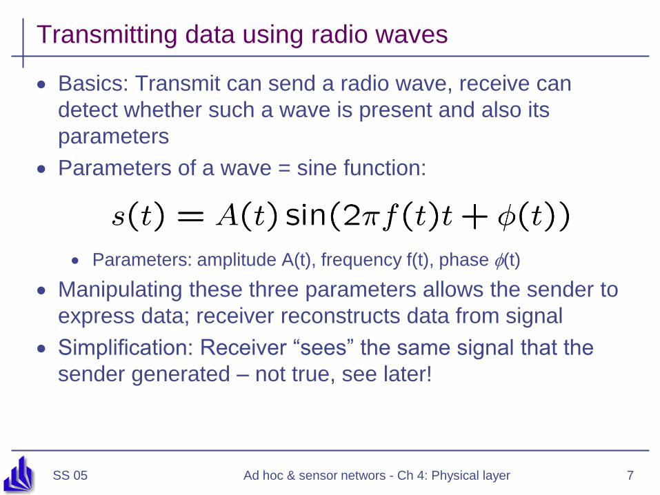
Basics: Transmit can send a radio wave, receive can

detect whether such a wave is present and also its

parameters

Parameters of a wave = sine function:

Parameters: amplitude A(t), frequency f(t), phase (t)

Manipulating these three parameters allows the sender to

express data; receiver reconstructs data from signal

Simplification: Receiver “sees” the same signal that the

sender generated – not true, see later!


Modulation and keying

How to manipulate a given signal parameter?

Set the parameter to an arbitrary value: analog modulation

Choose parameter values from a finite set of legal values: digital

keying

Simplification: When the context is clear, modulation is used in

either case

Modulation?

Data to be transmitted is used select transmission parameters as a

function of time

These parameters modify a basic sine wave, which serves as a

starting point for modulating the signal onto it

This basic sine wave has a center frequency fc

The resulting signal requires a certain bandwidth to be

transmitted (centered around center frequency)


Modulation (keying!) examples

Use data to modify the amplitude of a carrier frequency ! Amplitude Shift Keying

Use data to modify the frequency of a carrier frequency ! FrequencyShift Keying

Use data to modify the phase of a carrier frequency ! Phase Shift Keying

© Tanenbaum, Computer Networks


Receiver: Demodulation

The receiver looks at the received wave form and matches

it with the data bit that caused the transmitter to generate

this wave form

Necessary: one-to-one mapping between data and wave form

Because of channel imperfections, this is at best possible for digital

signals, but not for analog signals

Problems caused by

Carrier synchronization: frequency can vary between sender and

receiver (drift, temperature changes, aging, …)

Bit synchronization (actually: symbol synchronization): When does

symbol representing a certain bit start/end?

Frame synchronization: When does a packet start/end?

Biggest problem: Received signal is not the transmitted signal!


Overview

Frequency bands

Modulation


From waves to bits

Channel models

Transceiver design


Transmitted signal <> received signal!

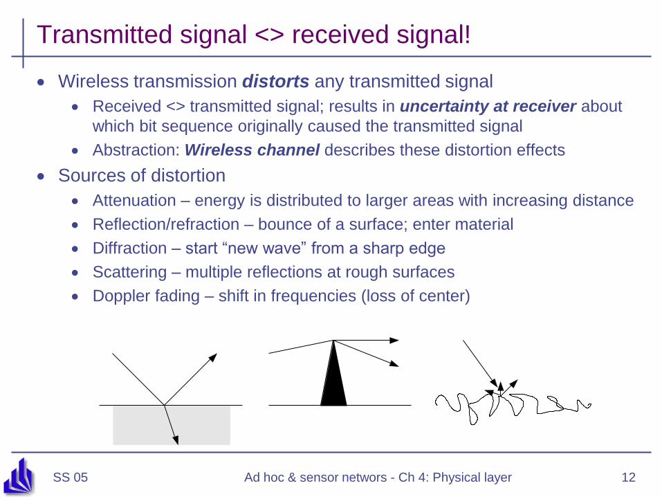
Wireless transmission distorts any transmitted signal

Received <> transmitted signal; results in uncertainty at receiver about

which bit sequence originally caused the transmitted signal

Abstraction: Wireless channel describes these distortion effects

Sources of distortion

Attenuation – energy is distributed to larger areas with increasing distance

Reflection/refraction – bounce of a surface; enter material

Diffraction – start “new wave” from a sharp edge

Scattering – multiple reflections at rough surfaces

Doppler fading – shift in frequencies (loss of center)


Attenuation results in path loss

Effect of attenuation: received signal strength is a function

of the distance d between sender and transmitter

Captured by Friis free-space equation

Describes signal strength at distance d relative to some reference

distance d0 < d for which strength is known

d0 is far-field distance, depends on antenna technology


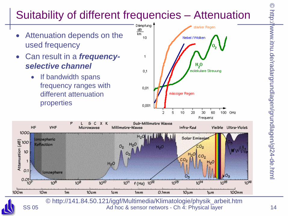
Suitability of different frequencies – Attenuation

Attenuation depends on the

used frequency

Can result in a frequency-

selective channel

If bandwidth spans

frequency ranges with

different attenuation

properties

© h

ttp://w

ww

.itnu

.de

/rad

arg

run

dla

ge

n/g

run

dla

ge

n/g

l24

-de

.htm

l

© http://141.84.50.121/iggf/Multimedia/Klimatologie/physik_arbeit.htm


Distortion effects: Non-line-of-sight paths

Because of reflection, scattering, …, radio communication is not limited to direct line of sight communication Effects depend strongly on frequency, thus different behavior at

higher frequencies

Different paths have different lengths = propagation time Results in delay spread of the wireless channel

Closely related to frequency-selective fading properties of the channel

With movement: fast fading

Line-of-

sight path

Non-line-of-sight path

signal at receiver

LOS pulsesmultipath

pulses



Wireless signal strength in a multi-path environment

Brighter color = stronger signal

Obviously, simple (quadratic)

free space attenuation formula

is not sufficient to capture these

effects



To take into account stronger attenuation than only caused

by distance (e.g., walls, …), use a larger exponent > 2

is the path-loss exponent

Rewrite in logarithmic form (in dB):

Take obstacles into account by a random variation

Add a Gaussian random variable with 0 mean, variance 2 to dB

representation

Equivalent to multiplying with a lognormal distributed r.v. in metric

units ! lognormal fading

Generalizing the attenuation formula


Overview

Frequency bands

Modulation


From waves to bits

Channel models

Transceiver design


Noise and interference

So far: only a single transmitter assumed Only disturbance: self-interference of a signal with multi-path

“copies” of itself

In reality, two further disturbances Noise – due to effects in receiver electronics, depends on

temperature

Typical model: an additive Gaussian variable, mean 0, no correlation in time

Interference from third parties

Co-channel interference: another sender uses the same spectrum

Adjacent-channel interference: another sender uses some other part of the radio spectrum, but receiver filters are not good enough to fully suppress it

Effect: Received signal is distorted by channel, corrupted by noise and interference What is the result on the received bits?


Symbols and bit errors

Extracting symbols out of a distorted/corrupted wave form

is fraught with errors

Depends essentially on strength of the received signal compared

to the corruption

Captured by signal to noise and interference ratio (SINR)

SINR allows to compute bit error rate (BER) for a given

modulation

Also depends on data rate (# bits/symbol) of modulation

E.g., for simple DPSK, data rate corresponding to bandwidth:


Examples for SINR ! BER mappings

1e-07

1e-06

1e-05

0.0001

0.001

0.01

0.1

1

-10 -5 0 5 10 15

Coherently Detected BPSKCoherently Detected BFSK

BER

SINR


Overview

Frequency bands

Modulation


From waves to bits

Channel models

Transceiver design


Some transceiver design considerations

Strive for good power efficiency at low transmission power

Some amplifiers are optimized for efficiency at high output power

To radiate 1 mW, typical designs need 30-100 mW to operate the

transmitter

WSN nodes: 20 mW (mica motes)

Receiver can use as much or more power as transmitter at these

power levels

! Sleep state is important

Startup energy/time penalty can be high

Examples take 0.5 ms and ¼ 60 mW to wake up

Exploit communication/computation tradeoffs

Might payoff to invest in rather complicated coding/compression

schemes


Going from Watts to dBm

1mW

mW)P(in 10logdBm)P(in

+20dBm=100mW

+10dBm=10mW

+7dBm=5mW

+6dBm = 4mW

+4dBm=2.5mW

+3dBm=2mW

0dBm=1mW

-3dBm=.5mW

-10dBm=.1mW


Friss Free Space Propagation Model

22

44

d

cGG

dGG

P

PRTRT

T

R

er transmittandreceiver between distance -

light of speed -

metersin h wavelengt-

antenna receiving and ing transmittfor the gainspower theare and

(in watts) antennas ing transmittand receiving at the espower valu - and

d

c

GG

PP

RT

RT

Same formula in dB path loss form (with Gain constants filled in):

kmMHzB dfdBL 1010 log20log2044.32)(

How much is the range for a 0dBm transmitter 2.4 GHz band transmitterand pathloss of 92dBm?


Friss Free Space Propagation Model

22

44

d

cGG

dGG

P

PRTRT

T

R

er transmittandreceiver between distance -

light of speed -

metersin h wavelengt-

antenna receiving and ing transmittfor the gainspower theare and

(in watts) antennas ing transmittand receiving at the espower valu - and

d

c

GG

PP

RT

RT

Same formula in dB path loss form (with Gain constants filled in):

kmMHzB dfdBL 1010 log20log2044.32)(

How much is the range for a 0dBm transmitter 2.4 GHz band transmitterand pathloss of 92dBm?

Highly idealized model. It assumes:• Free space, Isotropic antennas• Perfect power match & no interference• Represent the theoretical max transmission range


A more realistic model: Log-Normal Shadowing

Model

XdnfndBL kmMHzB 1010 log10log1044.32)(

• Model typically derived from measurements

dB)(in deviation

standard with dB)(in r.vGaussian mean -zero is

X

• Statistically describes random shadowing effects

• values of n and σ are computed from measured data using linear regression

• Log normal model found to be valid in indoor environments!!!


Radio Energy Model: the Deeper Story….

Wireless communication subsystem consists of three components with

substantially different characteristics

Their relative importance depends on the transmission range of the radio

Tx: Sender Rx: Receiver

ChannelIncoming

informationOutgoing

information

Tx

elecE Rx

elecERFE

Transmit

electronics

Receive

electronics

Power

amplifier


Radio Energy Cost for Transmitting 1-bit of Information

in a Packet

The choice of modulation scheme is important for energy vs. fidelity and

energy tradeoff

level Modulation

scheme modulationary -Man for rate Symbol

synthesisfrequency for

circuitry electronic ofn consumptiopower

lengthheader packet

length payloadpacket

startup radio with dasssociateenergy

1*log*

)(

2

M

R

P

H

L

E

L

H

MR

MPP

L

EE

s

elec

start

S

RFelecstartbit



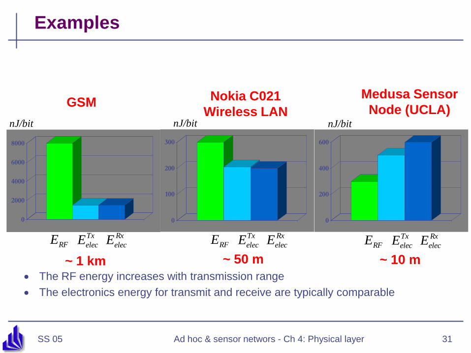
Examples

0

2000

4000

6000

8000

The RF energy increases with transmission range

The electronics energy for transmit and receive are typically comparable

0

100

200

300

0

200

400

600

Tx

elecE Rx

elecERFE Tx

elecE Rx

elecERFE Tx

elecE Rx

elecERFE

nJ/bit nJ/bit nJ/bit

GSMNokia C021

Wireless LAN

Medusa Sensor

Node (UCLA)

~ 1 km ~ 50 m ~ 10 m


Power Supply

Where Does The Power Go?B

att

ery

DC-DC

Converter

Communication

Radio

Modem

RF

Transceiver

Processing

Programmable

Ps & DSPs(apps, protocols etc.) Memory

ASICs

Peripherals

Disk Display

WSN :Physical Layer - UM

Documents