warwick.ac.uk/lib-publications Manuscript version: Author’s Accepted Manuscript The version presented in WRAP is the author’s accepted manuscript and may differ from the published version or Version of Record. Persistent WRAP URL: http://wrap.warwick.ac.uk/143835 How to cite: Please refer to published version for the most recent bibliographic citation information. If a published version is known of, the repository item page linked to above, will contain details on accessing it. Copyright and reuse: The Warwick Research Archive Portal (WRAP) makes this work by researchers of the University of Warwick available open access under the following conditions. Copyright © and all moral rights to the version of the paper presented here belong to the individual author(s) and/or other copyright owners. To the extent reasonable and practicable the material made available in WRAP has been checked for eligibility before being made available. Copies of full items can be used for personal research or study, educational, or not-for-profit purposes without prior permission or charge. Provided that the authors, title and full bibliographic details are credited, a hyperlink and/or URL is given for the original metadata page and the content is not changed in any way. Publisher’s statement: Please refer to the repository item page, publisher’s statement section, for further information. For more information, please contact the WRAP Team at: [email protected].

Welcome message from author
This document is posted to help you gain knowledge. Please leave a comment to let me know what you think about it! Share it to your friends and learn new things together.
Transcript

warwick.ac.uk/lib-publications
Manuscript version: Author’s Accepted Manuscript The version presented in WRAP is the author’s accepted manuscript and may differ from the published version or Version of Record. Persistent WRAP URL: http://wrap.warwick.ac.uk/143835 How to cite: Please refer to published version for the most recent bibliographic citation information. If a published version is known of, the repository item page linked to above, will contain details on accessing it. Copyright and reuse: The Warwick Research Archive Portal (WRAP) makes this work by researchers of the University of Warwick available open access under the following conditions. Copyright © and all moral rights to the version of the paper presented here belong to the individual author(s) and/or other copyright owners. To the extent reasonable and practicable the material made available in WRAP has been checked for eligibility before being made available. Copies of full items can be used for personal research or study, educational, or not-for-profit purposes without prior permission or charge. Provided that the authors, title and full bibliographic details are credited, a hyperlink and/or URL is given for the original metadata page and the content is not changed in any way. Publisher’s statement: Please refer to the repository item page, publisher’s statement section, for further information. For more information, please contact the WRAP Team at: [email protected].
October 2020, to appear in: Operations Research
Atomic Dynamic Flow Games:Adaptive versus Nonadaptive Agents
Zhigang CaoSchool of Economics and Management, Beijing Jiaotong University, Beijing 100044, China
Bo ChenWarwick Business School, University of Warwick, Coventry, CV4 7AL, United Kingdom
Xujin ChenAcademy of Mathematics and Systems Science, Chinese Academy of Sciences;
School of Mathematical Sciences, University of Chinese Academy of Sciences, Beijing, China
Changjun WangFaculty of Science, Beijing University of Technology, Beijing, 100124, China
We propose a game model for selfish routing of atomic agents, who compete for use of a network to travel
from their origins to a common destination as fast as possible. We follow a frequently used rule that the
latency an agent experiences on each edge is a constant transit time plus a variable waiting time in a queue. A
key feature that differentiates our model from related ones is an edge-based tie-breaking rule for prioritizing
agents in queueing when they reach an edge at the same time. We study both nonadaptive agents (each
choosing a one-off origin-destination path simultaneously at the very beginning) and adaptive ones (each
making an online decision at every nonterminal vertex they reach as to which next edge to take). On the one
hand, we constructively prove that a (pure) Nash equilibrium (NE) always exists for nonadaptive agents, and
show that every NE is weakly Pareto optimal and globally first-in-first-out. We present efficient algorithms
for finding an NE and best responses of nonadaptive agents. On the other hand, we are among the first
to consider adaptive atomic agents, for which we show that a subgame perfect equilibrium (SPE) always
exists, and that each NE outcome for nonadaptive agents is an SPE outcome for adaptive agents, but not
vice versa.
Key words : Selfish atomic routing; deterministic queuing; adaptive routing; subgame perfect equilibrium;
Nash equilibrium.
1. Introduction
Selfish routing is a fundamental model for network traffic, with diverse applications (Wardrop 1952,
Roughgarden and Tardos 2002, Roughgarden 2007). The problem is dynamic in essence. However,
most of the literature is based on latency functions, which are good approximations of static
flows, but not fully satisfactory due to the following weaknesses. First, a latency function is overly
symmetric in that agents choosing the same road segment impede each other in the same way,
1
Cao, Chen, Chen, Wang: Atomic Dynamic Flow Games2 Operations Research 00(0), pp. 000–000, © 2020 INFORMS
which is usually not the case, as earlier agents may delay the later ones but not vice versa. Second,
a latency function imposes the same delay upon all agents who travel along the road segment at
any time, even if their travel periods along the segment do not overlap, which is unreasonable, as
for example travel in peak hours takes more time than in off-peak hours. A well-recognized method
to overcome the above weaknesses is to apply the deterministic queuing (DQ) rule (Vickrey 1969,
Hendrickson and Kocur 1981, Koch and Skutella 2011, Cominetti et al. 2015, Scarsini et al. 2018).
However, the previous DQ-based atomic models of selfish routing usually suffer from the problems
of non-existence of a (pure strategy Nash) equilibrium or hardness in computing an equilibrium or
a best response, especially when there are multiple origins.
One of the key features that differentiate various DQ-based atomic models is how to break ties
when more agents than the capacity limit are trying to enter a road segment at the same time. In
this paper, by introducing an edge-priority tie-breaking rule, we propose a new DQ-based atomic
dynamic flow model, which we prove possesses several desirable properties and consequently leads
to a solution of the aforementioned problems.
1.1. Atomic dynamic flows
Instead of a latency function, two integer parameters are used in DQ to characterize each network
edge (road segment) e: its capacity ce and length te. The travel cost that an agent bears for using
edge e is a variable waiting time in the queue at edge e plus the fixed transit time te (i.e., the
travel speed is normalized to 1). Time is discretized. At each time step, a (possibly empty) queue
of completely ranked agents are waiting at the entrance of each edge. As many as possible up to ce
agents ranked highest in the queue start moving along different lanes of edge e, while the remaining
agents (if any) still wait in the queue for the next time steps. Once an agent starts moving along
edge e, he will reach e’s terminal te time units later. In reality, one traffic paradigm that exhibits
this atomic DQ feature is the expressway traffic. Imagine that an expressway road e consists of ce
lanes, and at the entrance of each lane, there is a toll booth collecting a toll from each car passing
it. For each booth, at most one car can pass through it each time and begin to travel along the
corresponding lane with a uniform speed (meaning the transit time of road e can be viewed as a
constant te). In this paper, based on this atomic DQ rule, we propose a model that is very similar
to the one in Scarsini et al. (2018) but has a crucial difference on the tie-breaking rules.
Network and inflows. We are given an acyclic directed network in which neighboring vertices
may be joined by one or more edges. Since we allow for multiple edges, we may assume that each
edge models a lane, and thus has a unit capacity. The network has one or more origins and a
single common destination. At each time point and each origin, a (possibly empty) set of selfish
Cao, Chen, Chen, Wang: Atomic Dynamic Flow GamesOperations Research 00(0), pp. 000–000, © 2020 INFORMS 3
agents enter the network, trying to reach the destination as quickly as possible. Initially, the agents
who enter the network at the same time and from the same origin are associated with an original
ranking among them, which is temporarily valid only when they enter the network.
Edge-priority tie-breaking rule. The queue at each edge is updated according to two cri-
teria: (i) the local first-in-first-out (FIFO) principle — an agent who reaches the queue of an edge
earlier also leaves the queue earlier, and (ii) the pre-specified edge priorities — if two agents reach
the queue at the same time, their queue ranks are determined by the priorities of the preceding
edges from which they enter the edge: higher priority gives higher rank. Our edge-priority tie-
breaking is generalized from various real-world traffic regulation rules, such as right turning traffic
should give way to oncoming traffic and side-road traffic should give way to main-road traffic.
1.2. Nonadaptive agents versus adaptive agents
We consider two types of selfish agents, referred to as nonadaptive and adaptive, respectively.
Nonadaptive agents make their routing decisions only at the very beginning (i.e., time 0) as to
which origin-destination path to take, no matter what time they enter the network. On the other
hand, adaptive agents make routing decisions at every nonterminal vertex they reach as to which
next edge to take. In particular, their decisions at a vertex may depend on the choices of other
agents in the history.
In accordance, we investigate two submodels of the game, denoted as ΓN and ΓA, which are played
by nonadaptive and adaptive agents, respectively. In terms of game theory, ΓN is a normal-form
game (a.k.a. a static game), whose standard solution concept is Nash equilibrium (NE), and ΓA is an
extensive-form game (a.k.a. a dynamic game), whose standard solution concept is subgame perfect
equilibrium (SPE). (See Sections 4 and 5.1 for formal definitions of the equilibrium concepts.) The
following warmup example illustrates what equilibria of the two submodels may look like, as well
as their possible differences.
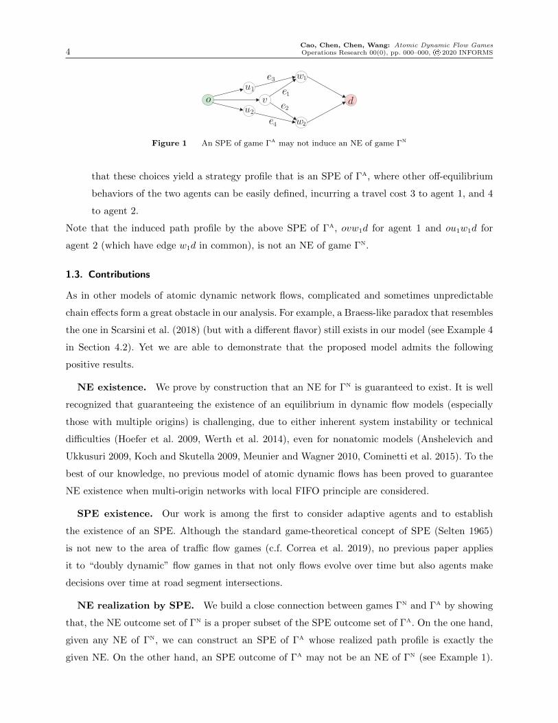
Example 1. In the network of Figure 1, every edge has a unit capacity and a unit length. Edge
e1 (resp. e2) has a higher priority than e3 (resp. e4). The game has only two agents, 1 and 2, who
enter the network via the common origin o at the same time 1, and make their ways to the common
destination d. Agent 1 has a higher original rank than agent 2.
• Game ΓN admits six NEs, where the two agents adopt edge-disjoint o-d paths, all bringing
them the same travel cost of 3.
• In game ΓA, agent 1 takes an adaptive strategy in the following sense. He initially chooses
edge ov, and then chooses e1 unless (at vertex v he finds that) agent 2 used edge ou2, in which
case he chooses edge e2. Agent 2 always follows the upper path ou1w1d. It can be checked
Cao, Chen, Chen, Wang: Atomic Dynamic Flow Games4 Operations Research 00(0), pp. 000–000, © 2020 INFORMS
Figure 1 An SPE of game ΓA may not induce an NE of game ΓN
that these choices yield a strategy profile that is an SPE of ΓA, where other off-equilibrium
behaviors of the two agents can be easily defined, incurring a travel cost 3 to agent 1, and 4
to agent 2.
Note that the induced path profile by the above SPE of ΓA, ovw1d for agent 1 and ou1w1d for
agent 2 (which have edge w1d in common), is not an NE of game ΓN.
1.3. Contributions
As in other models of atomic dynamic network flows, complicated and sometimes unpredictable
chain effects form a great obstacle in our analysis. For example, a Braess-like paradox that resembles
the one in Scarsini et al. (2018) (but with a different flavor) still exists in our model (see Example 4
in Section 4.2). Yet we are able to demonstrate that the proposed model admits the following
positive results.
NE existence. We prove by construction that an NE for ΓN is guaranteed to exist. It is well
recognized that guaranteeing the existence of an equilibrium in dynamic flow models (especially
those with multiple origins) is challenging, due to either inherent system instability or technical
difficulties (Hoefer et al. 2009, Werth et al. 2014), even for nonatomic models (Anshelevich and
Ukkusuri 2009, Koch and Skutella 2009, Meunier and Wagner 2010, Cominetti et al. 2015). To the
best of our knowledge, no previous model of atomic dynamic flows has been proved to guarantee
NE existence when multi-origin networks with local FIFO principle are considered.
SPE existence. Our work is among the first to consider adaptive agents and to establish
the existence of an SPE. Although the standard game-theoretical concept of SPE (Selten 1965)
is not new to the area of traffic flow games (c.f. Correa et al. 2019), no previous paper applies
it to “doubly dynamic” flow games in that not only flows evolve over time but also agents make
decisions over time at road segment intersections.
NE realization by SPE. We build a close connection between games ΓN and ΓA by showing
that, the NE outcome set of ΓN is a proper subset of the SPE outcome set of ΓA. On the one hand,
given any NE of ΓN, we can construct an SPE of ΓA whose realized path profile is exactly the
given NE. On the other hand, an SPE outcome of ΓA may not be an NE of ΓN (see Example 1).
Cao, Chen, Chen, Wang: Atomic Dynamic Flow GamesOperations Research 00(0), pp. 000–000, © 2020 INFORMS 5
The proper inclusion reaffirms the intuition that ΓA is more flexible than ΓN (see also Example 7)
and builds a bridge between them. In particular, ΓN is more technique-friendly than ΓA; all results
established for NEs of ΓN automatically hold for a subset of SPEs of ΓA.
NE characterization. We provide a characterization of all NEs of ΓN. Given a path profile of
nonadaptive agents, let them be batched according to their arrival times at the common destination.
A path profile is called iteratively batch-dominant if there is no way for agents in a later batch (no
matter how they coordinate) to affect any agent in an earlier batch, provided all earlier agents
follow their routes in the path profile. We prove that a path profile is an NE of ΓN if and only if
it is iteratively batch-dominant. Applying this characterization, we show that each NE of ΓN (and
hence a significant proportion of SPEs of ΓA) possesses many desirable properties, including:
• Strong NE: each NE is a strong NE, and thus weakly Pareto efficient, i.e., there are no routing
choices that could make every agent strictly better off; and
• Global FIFO: if agent i enters the network earlier than agent j from the same origin, then i
exits the network no later than j.
Note that the above characterization and properties are satisfied by all NEs of game ΓN without
any additional constraints on agent behaviors or network topologies, whereas the literature usually
can establish the properties for only some special NEs or NEs on special networks (Harks et al.
2018, Scarsini et al. 2018). In particular, while the existence of a strong NE (which must be an NE
by definition) is known in the literature of atomic dynamic flow games (e.g., Werth et al. 2014),
we are the first to show the equivalence between NEs and strong NEs for a class of these games.
Computational results. We design algorithms that efficiently construct an NE of ΓN, a best
response of any agent to any strategy profile of ΓN, and an SPE of ΓA. Our algorithms exploit a
somewhat surprising fact that a greedy Dijkstra-like approach, which takes maximum advantage
of the edge priority rule, is able to identify a path that can circumvent the intricate chain effects.
Such computability is in sharp contrast with previous hardness results on related games of atomic
dynamic flows, e.g., NP-completeness for determining NE existence (Werth et al. 2014) and NP-
hardness for computing a best response (Hoefer et al. 2009, 2011, Ismaili 2017).
To summarize, this paper offers modelling, theoretical, technical as well as computational contri-
butions to the literature of atomic dynamic flow games. Given that there has been little consensus
on the characteristics of a canonical model for atomic dynamic flow games due to the inherent
intractability (c.f. Correa and Stier-Moses 2010), our model (or its variation) arguably may have
a potential to serve as a candidate for standard models in future studies.
Cao, Chen, Chen, Wang: Atomic Dynamic Flow Games6 Operations Research 00(0), pp. 000–000, © 2020 INFORMS
2. Related literature
Compared with the relatively mature theory of static flow games, the study for the dynamic flow
games, a.k.a. routing games over time, is still in its early stage. Vickrey (1969) and Yagar (1971)
initialize the investigation of dynamic flow games, where they focus on analyzing NEs for small-
sized concrete examples. Subsequent studies are extensive since the last two decades, encompass
various models to investigate equilibrium behaviors of selfish agents, and adopt a wide variety of
methodologies from mathematical programming, optimal control, variational inequalities, algorith-
mic game theory, and simulations (see Peeta and Ziliaskopoulos 2001, Koch and Skutella 2009,
Cominetti et al. 2017, and the references therein). Under dynamic queuing, little is known about
general equilibrium properties, until recent exciting progress on deriving equilibrium existence,
uniqueness, characterizations and constructions (Meunier and Wagner 2010, Koch and Skutella
2011, Cominetti et al. 2015, Scarsini et al. 2018). We discuss the study of equilibria for two major
subbranches of dynamic flow games, atomic models and nonatomic models, in the following two
subsections, respectively.
2.1. Atomic dynamic flow games
To the best of our knowledge, almost all of the related atomic models studied are of nonadaptive
agents, and their solution concepts are NEs. A recent important development on DQ-based games
of atomic dynamic flows is Scarsini et al. (2018), which is one of the most related references to our
studies in this paper. This study has several notable differences from our work. First, to break ties,
Scarsini et al. (2018) place priorities on agents rather than on edges, i.e., a fixed priority ordering
of all the agents is applied globally. Second, they only study nonadaptive agents in single-origin
single-destination networks. In fact, when agents are adaptive in their model, an SPE may not
exist. Third, they focus on seasonal inflows and how the transient phases impact the long-run
steady outcomes, whereas their notion of steady outcome does not apply in our model because the
inflows we consider are not restricted to be seasonal. Finally, they concentrate on a special kind of
NE named uniformly fastest route (UFR) equilibrium, for which they prove the existence on single-
origin single-destination networks. Scarsini et al. (2018) also obtain a variant of Braess’s paradox:
adding some initial queues in the network may decrease the worst average travel cost at an NE. The
paradox differs from ours in that it involves route changes (see Section 4.2). Under the model of
Scarsini et al. (2018), Ismaili (2017) shows many negative results when multiple origin-destination
pairs are involved, including non-existence of an NE, and the NP-hardness and inapproximability
of computing a best response, etc.
In Werth et al. (2014), more variants of atomic dynamic flow games are considered under a
discrete-time DQ model, where finitely many agents are ready to start from their origin(s) at
Cao, Chen, Chen, Wang: Atomic Dynamic Flow GamesOperations Research 00(0), pp. 000–000, © 2020 INFORMS 7
the very beginning. Apart from the sum-type objective as considered in Scarsini et al. (2018)
and in this paper, Werth et al. (2014) also study the bottleneck-type objective, where each agent
tries to minimize his expense on the slowest edge of his chosen path. To break ties, the global
priorities placed on agents as in Scarsini et al. (2018) are discussed for both the sum-objective
and bottleneck-objective models, while the local priorities placed on edges as in this paper are
investigated only for the bottleneck-objective model. Werth et al. (2014) focus on computational
issues on NEs. On the positive side, a greedy algorithm is proposed to efficiently compute an NE
in the single-origin single-destination game with sum-type objective and agent priorities. On the
negative side, the multi-origin multi-destination game with bottleneck-type objective is shown to
suffer from intractabilities, such as non-existence of an NE under either agent or edge priorities,
the NP-completeness for determining NE existence and the co-NP-completeness for testing NE in
an acyclic directed network under edge priorities.
Among the earliest papers studying atomic dynamic routing games, Hoefer et al. (2009, 2011)
are concerned with computing NEs and best responses for a finite number of weighted agents (with
sum-type objectives) in a unit-capacitated directed network, where in a continuous-time setting the
transit speed of each agent is inversely proportional to his weight. When the local FIFO principle is
coupled with the global agent priorities for tie-breaking, the game turns out to be a generalization
of the sum-objective model of Werth et al. (2014), and for unweighted agents (i.e., those with a
uniform transit speed) in a single-origin network, the game admits a strong NE, which can be
computed efficiently. Somewhat surprisingly, computing best responses is NP-hard even in the case
of single-origin single-destination networks with unweighted agents. Harks et al. (2018) study an
atomic DQ-based dynamic flow game without the local FIFO principle. They analyze the impact
of global agent priority ordering on the efficiency of NEs, and show that an NE is polynomially
computable. Other related works include Koch (2012) and Kulkarni and Mirrokni (2015).
2.2. Nonatomic dynamic flow games
More previous works investigate nonatomic models, which are usually more tractable than their
atomic counterparts. In the nonatomic setting, every agent, aiming at earliest arrival at his desti-
nation, represents an infinitesimal amount of flow (a.k.a. fluid), for which neither tie-breaking rules
nor road lanes play a role. Different scholars generalize the Wardrop equilibrium (Wardrop 1952)
to dynamic versions from different perspectives. These solution concepts resemble more or less
NEs where each agent follows a dynamic shortest path (in various sense) that takes time-varying
delay into account. The solutions and other dynamic equilibrium concepts developed for nonatomic
dynamic flow games do not consider off-equilibrium situations — this is a key difference from SPE.
Cao, Chen, Chen, Wang: Atomic Dynamic Flow Games8 Operations Research 00(0), pp. 000–000, © 2020 INFORMS
Since the emergence of the purely existential results (Meunier and Wagner 2010), significant
efforts have been made to understand the structure and computational properties of dynamic
equilibria in nonatomic queuing networks. Koch and Skutella (2009, 2011) are the first to apply a
DQ rule with local FIFO principle to study nonatomic dynamic flow games. They investigate the
continuous-time single-origin single-destination case (called a temporal routing game) with uniform
inflow rates. They characterize the so-called Nash flows over time with the universal FIFO condition
that no flow overtakes another, and equivalently with an analogue to the Wardrop principle that
flow is only sent along dynamic shortest paths. Cominetti et al. (2015) prove by construction the
existence and uniqueness of the Nash flow over time of temporal routing games in a more general
setting with piecewise constant inflow rates. For the multi-origin multi-destination case, Cominetti
et al. (2015) prove in a nonconstructive way that a Nash flow over time exists when the inflow rates
belong to the space of p-integrable functions with 1< p<∞. Macko et al. (2013) show that Braess’s
paradox happens more frequently in the temporal routing model than in its static counterpart.
Anshelevich and Ukkusuri (2009) consider a dynamic routing game whose monotone increasing
edge-latency functions are more general than DQ models but still obey the local FIFO principle. For
the single-origin single-destination case, they show the existence, uniqueness and polynomial-time
computability of the Nash flow over time. For the multi-origin multi-destination case, examples are
presented to show that neither the existence nor the uniqueness can be guaranteed.
In the related works discussed above, as in our nonadaptive model, agents’ strategies are their
origin-destination paths. Sometimes these path-based models have alternative edge-based represen-
tations (c.f. the literature review in Long and Szeto (2019)). For other representations studied in
the literature, the interested reader is referred to Long et al. (2013). In the rest of this subsection,
we discuss more works that are closely related to agents’ adaptive behaviors, where their strategies
are richer than mere path selections.
Among these works, Graf and Harks (2019) is closest to our adaptive model in that agents also
make decisions over time. However, agents in their model are not completely rational as in our
model, but myopic in that whenever they face the choice of which next edge to take, they always
choose the one that is on a currently shortest path that is evaluated by current travel times and
queuing delays. Graf and Harks show that an equilibrium under these dynamic behaviors exists in
multi-origin multi-destination networks with measurable inflow rates.
Hamdouch et al. (2004) study a dynamic flow game on an edge-capacitated network. At the
very beginning of this game, for every nonterminal vertex of the network, all agents simultaneously
choose a time-dependent preference order, referred to as a list, of some of the outgoing edges. This
is a random model, and the probability that an agent moves along an edge depends on his chosen
list at the edge’s tail vertex, the residual edge capacities, and the number of his competitors as
Cao, Chen, Chen, Wang: Atomic Dynamic Flow GamesOperations Research 00(0), pp. 000–000, © 2020 INFORMS 9
well as their lists. The strategies of an agent in their model, though also adaptive in some sense,
are not so adjustable as in our adaptive model and less demanding for the intelligence level of the
agent. Using a variational inequality approach explored by Marcotte et al. (2004), Hamdouch et al.
(2004) prove the existence of an NE, which is called a strategic equilibrium following Marcotte
et al. (2004), but they do not consider SPE as in our paper.
A large body of related literature considers both path choice and departure time as decision
variables, but none of these works applies SPE as a solution concept (the reader is referred to
Guo et al. (2018) for a literature review along this line of research). Besides the usual approach
of variational inequalities, the approach of differential equations also turns out to be successful in
studying these problems. Based on conservation laws (which are popular in differential equations)
where the flow speed function is density dependent or density and location dependent, Bressan and
Han (2013) and Han et al. (2013) prove that NEs exist in multi-origin multi-destination networks
under some constraints on functional properties and trip volumes.
The rest of this paper is organized as follows. In Section 3, we present a formal mathematical
model of our atomic dynamic flows. In Sections 4 and 5, we study its normal-form game setting
ΓN for nonadaptive agents and its extensive-form setting ΓA for adaptive agents, respectively. In
Section 6, we conclude our paper with some remarks on future research directions. All proofs and
further discussions are provided in the Electronic Companion.
3. The flow model
All paths discussed in this paper are directed and simple. In our model of atomic dynamic flows,
we are given a finite acyclic directed multi-graph G= (V,E), with V being the vertex set and E
the edge set. There is a distinguished vertex d called the destination; for each vertex v ∈ V , there
is at least one path from v to d, called a v-d path.
Further to our unit-capacity assumption discussed in Section 1.1, which can be viewed as part of
our modeling related to edge priorities, we also assume unit edge-length throughout the paper for
the convenience of our exposition. The generality of this additional assumption will be discussed
in Section 6.
Unit Assumption. Each edge of the input network has a unit capacity and a unit length.
For each v ∈ V , a complete priority order ≺v is pre-specified over all edges incoming to v. We
denote by e1 ≺v e2 if edge e1 has a higher priority than edge e2. Time is discretized as 0,1,2, . . .,
and may be infinite. Initially, at time 0, there is a (possibly empty) initial ranked queue Q0e of
agents at the tail part of each edge e ∈E. (NB: This initial setting is slightly more general than
usual empty networks.) At each integer time point r≥ 1 and each vertex v ∈ V , a (possibly empty)
Cao, Chen, Chen, Wang: Atomic Dynamic Flow Games10 Operations Research 00(0), pp. 000–000, © 2020 INFORMS
set ∆r,v of finitely many agents enter G from their common origin v. They are associated with
original ranks among them, which are temporarily valid only at time r. Henceforth, we assume
∆r,v is an ordered set with agents ordered by their original ranks. Throughout this paper, ∆ :=
(∪e∈EQ0e)∪ (∪r≥1,v∈V ∆r,v) denotes the set of all agents.
For brevity, we consider w.l.o.g. every vertex as a possible origin: If vertex v is not an origin in
the usual sense, then all sets in ∆r,v : r≥ 1 are empty. Note that no agent in ∆r,d has impact on
the game, as he never touches any edge of the network. To ease our writing, we frequently write
v ∈ V instead of v ∈ V \d.
Each agent in ∆ goes through some path in G ending at destination d and leaves G from d. The
starting vertex of this path is called the starting vertex of this agent. Each agent, when reaching
a vertex v (6= d), immediately enters an edge e outgoing from v without any delay. We assume
that all agents (if any) in Q0e enter e at time 0. At any integer time s≥ 0, all agents (if any) who
have entered e but not yet exited queue at the tail part of e, and only the unique head of the
queue (namely the one with the highest rank) leaves (recall the Unit Assumption). This queue
head spends one time unit in traversing e from its tail to its head and exits e at time s+ 1.
If both agents i and j go through edge e (with tail vertex ue), they are ranked for entering and
therefore exiting the queue at e according to the following ranking rules (R0)–(R4), exactly one of
which applies (by checking sequentially in the same order as their indices).
(R0) If i and j are both in the initial queue Q0e, then their ranks agree with the ranks in Q0
e.
(R1) If i enters e earlier than j, then i has a higher rank.
(R2) If they enter e at the same time through two different edges incoming to ue, then ranks at
e are determined by the priority order ≺ue on the two edges, higher priority giving higher
rank.
(Note that if neither i nor j takes ue as his origin, then the queuing rules (R0)–(R2) are enough to
rank the agents. Otherwise, the following (R3) or (R4) will be needed.)
(R3) If only one of them, say i, takes ue as his origin, then i has a higher rank than j (who must
have entered e through an edge incoming to ue).
(R4) If they both take ue as their common origin, then their ranks on e are determined by their
original ranks.
The above flow regulations will be referred to as the edge-priority DQ rule. Following this rule, by
assuming different rationality levels of agents, we study in the following two sections two submodels,
denoted as ΓN and ΓA, for games of nonadaptive agents and adaptive ones, respectively. In both
games, each agent tries to arrive at the common destination d as early as possible. We shall slightly
abuse ΓN and ΓA to denote both game models and corresponding game instances.
Cao, Chen, Chen, Wang: Atomic Dynamic Flow GamesOperations Research 00(0), pp. 000–000, © 2020 INFORMS 11
4. The game of nonadaptive agents
The first submodel ΓN assumes that agents are of a relatively low rationality level, or alternatively,
they do not have updated information about other agents. Specifically, the agents are nonadaptive
in that they each select a path from their own origins to the common destination d simultaneously
at the very beginning, i.e., time 0. As soon as the agents enter the network G at the time points
specified by the game input (Q0e)e∈E and (∆r,v)r≥1,v∈V , they will always follow the chosen paths and
never deviate from them at any intermediary vertex. It is worth noting that agents in ∪r≥1,v∈V ∆r,v
make their decisions before they enter the network.
For each agent i ∈∆, let Pi denote his strategy set. If i ∈ Q0e, then Pi is the set of paths in
G starting from edge e and ending at destination d. If i ∈∆r,v, then Pi is the set of v-d paths
in G. For any agent i ∈∆ and path profile p= (Pj)j∈∆ with Pj ∈Pj for all j ∈∆, we use tdi (p)
to denote the arrival time of i at destination d under p. We will use the terms “path profile” and
“routing” interchangeably. In terms of game theory, ΓN is a normal-form game, for which we apply
the standard solution concept of Nash equilibrium (NE).
Definition 1 (NE). A path profile p of ∆ is a Nash equilibrium (NE) of ΓN if no agent can gain
by uniliteral deviation, i.e., tdi (p)≤ tdi (P ′i ,p−i) for all i ∈∆ and P ′i ∈Pi, where p−i is the partial
path profile of p for agents in ∆\i.
4.1. NE existence
In this subsection, we constructively prove that every game ΓN admits an NE. Recall from game
theory that a dominant NE is a strategy profile where every agent uses a dominant strategy in
that it is always optimal for him regardless of how other agents act. Observe that the following
strategy profile that extends the idea of dominance is still an NE: the agents can be ordered such
that the strategy of the first agent is a dominant one; and for any k ≥ 2, subject to the condition
that the first k− 1 agents follow their respective strategies, the strategy of agent k is optimal for
him regardless of the choices of the remaining agents. To prove NE existence for game ΓN, we
refine this idea on usual type of dominance to be a more specific and stronger iterative dominance
defined as follows.
For any nonnegative integer k, we write [k] for the set of all positive integers no more than k.
Before providing a formal definition, we call a path profile p an iteratively dominant NE, or an
IDNE for short, if the agents can be reindexed (ordered) as 1,2, . . . such that small-index agents
dominate large-index agents in the following iterative sense:
• No matter what paths other agents in ∆\1 choose, by following his path in p, agent 1
reaches every vertex of the path (including the destination d) at the earliest possible time
that an agent in ∆ can achieve among all path profiles.
Cao, Chen, Chen, Wang: Atomic Dynamic Flow Games12 Operations Research 00(0), pp. 000–000, © 2020 INFORMS
• Iteratively for every k= 2,3, . . ., assume that the first k−1 agents 1, . . . , k−1 fix their paths
as in p. No matter what paths other agents outside [k] choose, by following his path in p,
agent k reaches every vertex of the path (including the destination d) at the earliest possible
time that an agent outside [k− 1] can achieve among all path profiles where the first k− 1
agents follow the given paths in p.
For convenience, we call the above reindex of agent an iterative dominant order for p, and call
the paths in p the agents’ (associated) dominant paths. Formally, we have the following definition,
where for path profile p and agent subset S, the partial path profile of p for agents in S is written
as pS.
Definition 2 (IDNE). A path profile p of ∆ is an iteratively dominant NE (IDNE) of ΓN if the
agents can be reindexed as 1,2, . . . such that for any index k≥ 1, vertex v on agent k’s path in p,
and partial path profile q for agents in ∆\[k], the following sequential optimality holds:
tvk(p[k],q) = mintvj (p[k−1],r) : j ∈∆\[k− 1],r is a partial path profile for ∆\[k− 1].
The goal of this subsection is to construct an IDNE of ΓN, which proves the following main
result.
Theorem 1. Every normal-form game ΓN admits an IDNE.
Before going into details, it is worth noting that Definition 2 directly implies that every IDNE
possesses the following properties, which are crucial for studying SPE in Section 5.2.
• No overtaking: If agents i and j enter G from the same origin, but i does so earlier than j,
and they both pass through some vertex v under the NE, then i reaches and leaves v no later
than j does. The property in the special case of v= d is known as Global FIFO.
• Earliest arrival: Given the other agents’ choices in the NE, each agent using his path in the
NE reaches each vertex on the path (not only the destination d) at an earliest time among
all of his possible choices.
• Sequential independence: For each k ≥ 1, if all the agents with iterative dominant orders at
most k fix their paths as in the NE, then their arrival times at all vertices along their paths
(including destination d) are independent of the choices of all the agents with indices larger
than k.
To better understand our construction of an IDNE, we first give an example to illustrate this
solution concept.
Example 2. Consider game ΓN with input network illustrated in Figure 2, where at vertices y1,
y2 and d, the right, left and upper edges have higher priorities, respectively (i.e., x1y1 ≺y1 o1y1,
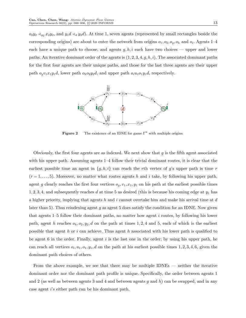
Cao, Chen, Chen, Wang: Atomic Dynamic Flow GamesOperations Research 00(0), pp. 000–000, © 2020 INFORMS 13
o2y2 ≺y2 x2y2, and y1d≺d y2d). At time 1, seven agents (represented by small rectangles beside the
corresponding origins) are about to enter the network from origins o1, o2, og, oh and oi. Agents 1–4
each have a unique path to choose, and agents g,h, i each have two choices — upper and lower
paths. An iterative dominant order of the agents is (1,2,3,4, g, h, i). The associated dominant paths
for the first four agents are their unique paths, and those for the last three agents are their upper
path ogv1x1y1d, lower path oho2y2d, and upper path oiu1o1y1d, respectively.
Figure 2 The existence of an IDNE for game ΓN with multiple origins
Obviously, the first four agents are as indexed. We next show that g is the fifth agent associated
with his upper path. Assuming agents 1–4 follow their trivial dominant routes, it is clear that the
earliest possible time an agent in g,h, i can reach the rth vertex of g’s upper path is time r
(r = 1, . . . ,5). Moreover, no matter what routes agents h and i take, by following his upper path,
agent g clearly reaches the first four vertices og, v1, x1, y1 on his path at the earliest possible times
1,2,3,4, and subsequently reaches d at time 5 as desired (this is because his coming edge at y1 has
a higher priority, implying that agents h and i cannot overtake him and make his arrival time at d
later than 5). Thus reindexing agent g as agent 5 does satisfy the condition for an IDNE. Now given
that agents 1–5 follow their dominant paths, no matter how agent i routes, by following his lower
path, agent h reaches oh, o2, y2, d on the path at times 1,2,4 and 5, each of which is the earliest
possible that agent h or i can achieve. Thus agent h associated with his lower path is qualified to
be agent 6 in the order. Finally, agent i is the last one in the order; by using his upper path, he
can reach all vertices oi, u1, o1, y1, d on the path at his earliest possible times 1,2,3,4,6, given the
dominant path choices of others.
From the above example, we see that there may be multiple IDNEs — neither the iterative
dominant order nor the dominant path profile is unique. Specifically, the order between agents 1
and 2 (as well as between agents 3 and 4 and between agents g and h) can be swapped, and in any
case agent i’s either path can be his dominant path.
Cao, Chen, Chen, Wang: Atomic Dynamic Flow Games14 Operations Research 00(0), pp. 000–000, © 2020 INFORMS
We briefly describe the idea of how to make full use of edge priorities (e.g., edge priority w.r.t.
the destination d in Example 2 that has been ignored in our previous discussion) to pin down a
special IDNE (a unique iterative dominant order combined with a unique dominant path profile),
which always exists and hence proves Theorem 1.
Suppose now the first k− 1 agents as well as their associated dominant paths have been deter-
mined. We are to identify the kth agent, whom we relabel as k, and his associated dominant path
Pk ∈Pk. Define the “ideal arrival time” at any vertex for each of the remaining agents as the
earliest time when this agent can reach the vertex, under the assumption that all other agents in
the network are the identified k− 1 ones, who follow their associated dominant paths previously
determined. This ideal arrival time is defined as infinity if the vertex is unreachable by this agent.
In the following, we will first choose a set C = C(k) of candidate pairs (j,Pj) with j ∈∆\[k− 1]
and Pj ∈Pj, and then prune C by backtracking the path Pj of one of the candidate pairs, starting
from d edge by edge, and eliminating unqualified candidates discovered during the process, until
only one candidate pair is left. The corresponding agent and path are thus identified as the kth
agent and his dominant path, respectively.
A more detailed pruning process goes as follows. Initially, pair (j,Pj) is a candidate in C if and
only if j is one of the remaining unidentified agents and Pj ∈Pj, i.e., Pj is a path from his starting
vertex to d. Let u= d and proceed with the following three steps in sequence:
(S1) A candidate (j,Pj) ∈C is retained in C if and only if the ideal arrival time of agent j at u
is the earliest among all candidate agents in the current C, and Pj is a path along which j
achieves this ideal arrival time at u;
(S2) A candidate (j,Pj) ∈C is retained in C if and only if the incoming edge to u on Pj has the
highest edge priority among all candidate paths in the current C;
(S3) If there are more than one candidate left in the current C, then the candidate paths in the
current C must share the same incoming edge e to u (whose tail vertex is denoted as ue) and
we backtrack along e: update u with ue and go back to step (S1).
It can be seen that either the above process is terminated at some step when only one candidate
is left in C, in which case we are done, or all agents corresponding to the current candidate pairs
are in the same initial queue or enter G simultaneously at the same origin (thus with the same
candidate path). In this case, we identify among all the candidates the one, (j,Pj), such that agent
j has the highest initial queue rank or original rank among all candidate agents in the current C.
It turns out that the path profile (Pk)k∈∆ constructed as above is indeed an IDNE. We call
it a special IDNE. As an illustration, the order (1,2, . . . ,7) of agents and their dominant paths
given in Example 2 constitute the special IDNE. For example, the order between agents 1 and
2 (resp. 3 and 4) is determined by the edge priorities w.r.t. d; the order between agents 2 and 3

Cao, Chen, Chen, Wang: Atomic Dynamic Flow GamesOperations Research 00(0), pp. 000–000, © 2020 INFORMS 15
(resp. 4 and g (= 5)) is determined by the arrival times at d; the order between g (= 5) and h (= 6)
is determined by backtracking from d to y1 and checking the edge priorities at y1. The precise
algorithmic description for the aforementioned process together with a formal proof of Theorem 1
is presented in Section EC.2 of the Electronic Companion.
We would like to remark that placing priorities on edges is crucial to the NE existence of the
game model ΓN with multiple origins. Example 3 below shows that, if priorities were placed on
agents (i.e., when two agents enter an edge at the same time, the agent with a higher priority will
be ranked higher in the queue), one could not guarantee the NE existence when there are more
than one origins, though an NE does exist in the single-origin single-destination case (Scarsini et al.
2018). A more detailed discussion about why this critical tie-breaking rule matters is provided in
Section EC.11 of the Electronic Companion.
Example 3. Consider an example modified from Figure 2, where global priorities are placed on
the agents in a way that i ranks higher than g and g higher than h. Agents i, g, h are our focus,
as the remaining four agents do not make substantial decisions, and are not affected by i, g, h. The
lowest ranked agent h reaches o1 (or o2) one time unit earlier than the highest ranked agent i if they
choose to pass the same vertex o1 (or o2); otherwise, they reach y1, y2 at the same time as agent
g reaches y1 or y2. It can be verified that h, i and g have a Rock-Paper-Scissors-like relationship,
and hence this game does not have any NE.
4.2. Braess-like paradoxes
A well-known phenomenon in selfish routing is the Braess’s paradox: building a new road may
make the network more congested. Recently, Scarsini et al. (2018) discovered a Braess-like paradox
under their model of atomic dynamic flows: removing an initial queue may reduce the system
performance. This paradox occurs in a single-origin single-destination extension-parallel network,
which has been known to be free of the classical Braess’s paradox based on latency functions. An
apparent cause is that removing an initial queue may bring about route changes of agents, leading
them to a less efficient NE (despite of the presence of a more efficient one). This type of paradox is
also present in our model as shown in Section EC.12 of the Electronic Companion by an adaptation
from the example of Scarsini et al. (2018).
The following example demonstrates a different paradoxical phenomenon in the sense that it
stems from unpredictable chain effects of agents’ interactions. In our example, no route changes
are involved.
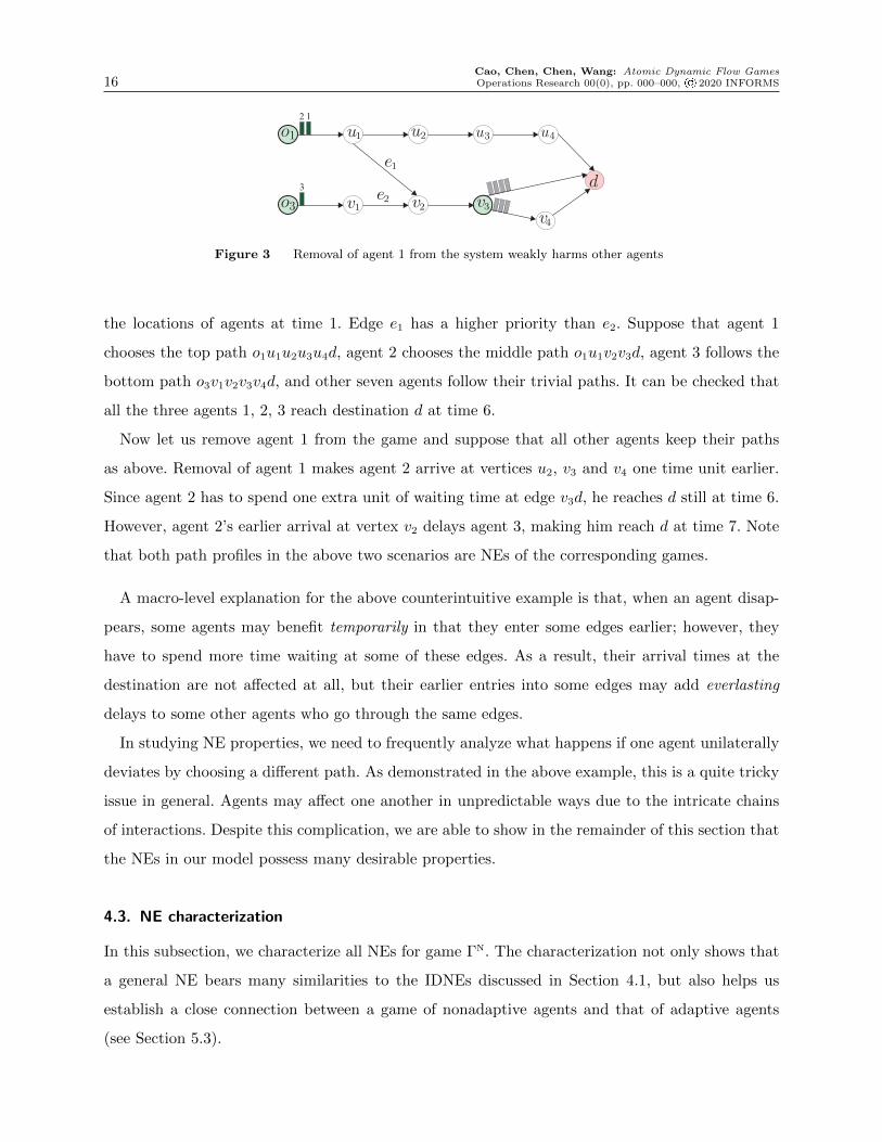
Example 4. Consider an instance of game ΓN as depicted in Figure 3. There are a total of ten
agents (shown as small rectangles on edges), with agents 1, 2 and 3 being our focus. Figure 3 shows
Cao, Chen, Chen, Wang: Atomic Dynamic Flow Games16 Operations Research 00(0), pp. 000–000, © 2020 INFORMS
Figure 3 Removal of agent 1 from the system weakly harms other agents
the locations of agents at time 1. Edge e1 has a higher priority than e2. Suppose that agent 1
chooses the top path o1u1u2u3u4d, agent 2 chooses the middle path o1u1v2v3d, agent 3 follows the
bottom path o3v1v2v3v4d, and other seven agents follow their trivial paths. It can be checked that
all the three agents 1, 2, 3 reach destination d at time 6.
Now let us remove agent 1 from the game and suppose that all other agents keep their paths
as above. Removal of agent 1 makes agent 2 arrive at vertices u2, v3 and v4 one time unit earlier.
Since agent 2 has to spend one extra unit of waiting time at edge v3d, he reaches d still at time 6.
However, agent 2’s earlier arrival at vertex v2 delays agent 3, making him reach d at time 7. Note
that both path profiles in the above two scenarios are NEs of the corresponding games.
A macro-level explanation for the above counterintuitive example is that, when an agent disap-
pears, some agents may benefit temporarily in that they enter some edges earlier; however, they
have to spend more time waiting at some of these edges. As a result, their arrival times at the
destination are not affected at all, but their earlier entries into some edges may add everlasting
delays to some other agents who go through the same edges.
In studying NE properties, we need to frequently analyze what happens if one agent unilaterally
deviates by choosing a different path. As demonstrated in the above example, this is a quite tricky
issue in general. Agents may affect one another in unpredictable ways due to the intricate chains
of interactions. Despite this complication, we are able to show in the remainder of this section that
the NEs in our model possess many desirable properties.
4.3. NE characterization
In this subsection, we characterize all NEs for game ΓN. The characterization not only shows that
a general NE bears many similarities to the IDNEs discussed in Section 4.1, but also helps us
establish a close connection between a game of nonadaptive agents and that of adaptive agents
(see Section 5.3).
Cao, Chen, Chen, Wang: Atomic Dynamic Flow GamesOperations Research 00(0), pp. 000–000, © 2020 INFORMS 17
Batching agents according to their arrival times at the destination d is useful for our analysis on
the NEs. For any path profile q of ΓN, let τ(q,1)< τ(q,2)< τ(q,3)< · · · be the arrival times of all
agents at d under q. For each integer k≥ 1, let
∆(q, k) := i∈∆ | tdi (q) = τ(q, k)
denote the set of agents in ΓN who reach d under q at the kth earliest time τ(q, k); we often refer
to ∆(q, k) as the kth batch. We use
∆(q, [k]) :=∪j∈[k]∆(q, j)
to denote the set of agents reaching d no later than time τ(q, k), i.e., those in the first k batches.
For notational convenience, we set ∆(q, [0]) := ∅ to be the 0th batch, and let ∆(q, [∞]) := ∆ denote
the disjoint union of all batches.
It can be shown that the interactions between agents of different batches at an NE are hierarchal.
That is, every NE is iteratively batch-dominant in that there is no way for agents in a later batch
(no matter how they coordinate) to affect any agent in an earlier batch, provided all earlier agents
follow their routes in the NE. This iterative batch-dominance, formally defined below, actually
characterizes all NEs of game ΓN.
Definition 3 (Iterative batch-dominance). A path profile q = (Qh)h∈∆ of ΓN is iteratively
batch-dominant if, for any batch index k≥ 1, agent i∈Ω := ∆(q, [k]), vertex v ∈Qi, agent j ∈∆\Ω,
and partial path profile r−Ω for agents in ∆\Ω, the following inequalities hold:
tvi (q) = tvi (qΩ,r−Ω)≤ tvj (qΩ,r−Ω) and tdj (qΩ,r−Ω)≥ τ(q, k+ 1)> tdi (qΩ,r−Ω).
Theorem 2. A path profile is an NE for game ΓN if and only if it is iteratively batch-dominant.
Using Theorem 2, we can establish that all NEs are strong NEs (see definition below) and global
FIFO (see Theorem EC.6).
Definition 4 (Strong NE). A path profile p of ∆ is a strong NE of ΓN if no group of agents
can gain by deviation, i.e., there exists no group S ⊆∆ and partial path profile p′S of agents in S
such that tdi (p′S,p−S)< tdi (p) for all i∈ S, where p−S is the partial path profile (determined by p)
of agents not in S.
Theorem 3. All NEs of every game ΓN are strong NEs and global FIFO.
Since each strong NE is also an NE, Theorem 3 actually establishes the equivalence between an
NE and a strong NE in our model. Note that the strong NE property implies that every NE of ΓN
is weakly Pareto optimal. Moreover, it follows from Theorem 2 that every NE of game ΓN has a
hierarchal structure that resembles the sequential structure of IDNEs. More specifically, we have
the following properties:
Cao, Chen, Chen, Wang: Atomic Dynamic Flow Games18 Operations Research 00(0), pp. 000–000, © 2020 INFORMS
• Every NE is hierarchically independent in that, for every k≥ 1, if agents in the first k batches
all follow their NE routes, then their arrival times at any vertex are independent of other
agents’ choices.
• Every NE is hierarchically optimal in that, for every k≥ 1, the arrival time of each agent in
the kth batch under the NE is the smallest among the arrival times of all agents outside the
first k− 1 batches under any routing in which agents in the first k− 1 batches follow their
NE routes.
Two other properties of the IDNEs, no overtaking and earliest arrival, do not hold in general for
the NEs of game ΓN (see Section EC.12 for examples). This is in contrast to nonatomic dynamic
flow games for which every NE must be no overtaking and earliest arrival (Koch and Skutella
2011). On the other hand, every NE of game ΓN is temporally overtaking in that, if agent i enters
the network G earlier than j from the same origin, but j overtakes i at some vertex v ∈ V \d(i.e., j reaches v earlier than i), then they must reach the destination d at the same time. Omitted
proofs and more properties possessed by the NEs of game ΓN are presented in Section EC.7 of the
Electronic Companion.
4.4. Computations
In this subsection we show that a best response and an NE of game ΓN can be computed efficiently.
The computation works with a kind of “naive” greedy idea, which is validated using the notion of
preemption. Throughout this subsection, i denotes a fixed agent and q−i = (Qj)j∈∆\i a partial
path profile of all other agents. We consider the scenario where only agent i is allowed to change
his path and the others always follow q−i.
4.4.1. Preempt relations We say that agent i preempts agent j at vertex v if either (i) the
earliest time i reaches v is earlier than the earliest time j reaches v (among all path profiles in
which all agents but i adopt the same paths as in q−i), or (ii) their earliest times are the same
and additionally, either (ii.a) agent i can reach v via an edge that has a higher priority (w.r.t. v)
than an edge that j uses to reach v, or (ii.b) vertex v is agent i’s but not j’s starting vertex, or
(ii.c) vertex v is the starting vertex of both agents i and j, and i has a higher initial queue rank or
original rank than j. This notion of preemption (see Definition EC.1 in Section EC.4 for a formal
description) combines the optimization (minimization) on arrival times and the speciality on the
best available choice w.r.t. edge priorities.
The preempt relation, together with the following lemma, plays a critical role in designing our
algorithm for computing best responses.
Lemma 1. For any agent j ∈∆\i and vertex v ∈Qj, if there exist paths Pi, P′i ∈Pi such that
tvj (Pi,q−i) 6= tvj (P′i ,q−i), then i preempts j at v under q−i.
Cao, Chen, Chen, Wang: Atomic Dynamic Flow GamesOperations Research 00(0), pp. 000–000, © 2020 INFORMS 19
The above lemma implies in particular that if agent i’s unilateral change from Pi to P ′i can affect
the arrival time of agent j at vertex v, making it earlier or later, then by using some path in Pi
(not necessarily Pi or P ′i ), agent i is able to reach v no later than j under (Pi,q−i) and under
(P ′i ,q−i). In contrast, this property does not necessarily hold in the model where ties are broken
using agent priorities (see Remark EC.1 in Section EC.4). Furthermore, we can show that if agent i
preempts j at vertex v ∈Qj, then i preempts j at all vertices on the subpath of Qj from v to d
(see Corollary EC.1 in Section EC.4).
Lemma 1 enables us to classify all agents but i into two categories, the “slow” ones S whom
agent i can preempt and the “fast” ones F whom agent i cannot preempt.
(C1) Agents of F are always no later than agent i at any vertex along their paths (regardless of
the choice of i). Hence the flows resulting from the travels of F agents can be viewed as an
exogenous environment for i.
(C2) In contrast, when agent i follows a special optimal path (denoted O∗i ), whose existence can
be deduced from Lemma 1, he reaches each vertex of a final segment of O∗i no later than
any agent of S under path profile (Pi,q−i) for any Pi ∈Pi, which results in that agent i is
“faster” than all agents of S in the final segment. To put it differently, no agent of S can
influence i in the final segment when he follows path O∗i , which attains the optimality w.r.t.
the exogenous environment of F agents and possesses the speciality w.r.t. edge priorities.
In summary, when agent i follows the special optimal path, the intricate chain effects are decou-
pled in the above sense and our analysis is greatly alleviated. We remark that Lemma 1 is also an
important tool for us to establish the NE characterization discussed in Section 4.3.
4.4.2. Computing best responses When we talk about algorithm efficiency, only the case
of finite agent set and finite network is concerned unless otherwise stated. Given a game ΓN with
agent set ∆, an agent i ∈∆, and a partial path profile q−i = (Qj)j∈∆\i, our algorithm computes
a special best response of i to q−i defined as follows.
Definition 5 (EE best-response). Given a partial path profile q−i, a path Q∗i ∈Pi of agent i
is called the edge-priority-oriented earliest-arrival best-response (EE best-response) if for each non-
starting vertex v of Q∗i ,
• Agent i’s arrival time at v when he goes along Q∗i is the earliest he can achieve;
• The incoming edge to v on Q∗i has the highest priority among the incoming edges to v on all
paths of Pi along each of which i reaches v at the earliest time.
By definition, agent i has a unique EE best-response to any given q−i. It can be seen that the
EE best-response is exactly the special optimal path Q∗i discussed in (C2) in Section 4.4.1. Our
algorithm for finding Q∗i resembles the classical Dijkstra algorithm for computing a shortest path.
However, its correctness proof is nontrivial.
Cao, Chen, Chen, Wang: Atomic Dynamic Flow Games20 Operations Research 00(0), pp. 000–000, © 2020 INFORMS
Definition 6. For each edge e∈E and time r≥ 0, let Qre denote its queue at time r produced by
routing q−i = (Qj)j∈∆\i. For any edge e′ (if any) incoming to the tail vertex of e, let Qre,e′ denote
the subset of agents in Qre who enter e at r from edges with priorities no higher than e′.
We slightly abuse notation Qre,e′ in the following two settings: (i) If i is in the initial queue Q0e
with e= v1v2, we abuse Q0e,ev1
to denote the set of agents in Q0e who queue after i. (ii) If i∈∆v1,r
with some r≥ 1, then for any edge e ∈E with tail vertex v1, we abuse Qre,ev1 to denote the set of
agents in Qre who either enter e at time r from edges incoming to v1, or belong to ∆v1,r and have
original ranks lower than i.
Note that Q0e = Q0
e\i for all e ∈E. Given v ∈ V , let τ v denote the earliest time when agent i
can reach v provided other agents follow q−i. Let Y := v ∈ V |τ v <+∞ denote the set of vertices
in G that i can reach through some paths, i.e., i’s reachable vertices. In particular, if i is in the
initial queue Q0e, the tail vertex of e belongs to Y . Since G is acyclic, one can find in polynomial
time a complete “acyclic” order on the vertices in Y such that for each edge with both end-vertices
in Y, its tail vertex has an order smaller than its head vertex. Let v1, v2, . . . , v|Y | be the vertices in
Y ranked by such an order. Then it must be the case that v|Y | = d, and v1 is i’s starting vertex,
i.e., either i ∈Q0v1v2
or i enters G from v1 at some time r ≥ 1. For any vertex v ∈ Y \v1, let ev
denote the incoming edge to v with the highest priority (w.r.t. ≺v) that agent i can use to reach
v at time τ v, provided q−i is fixed. Now we are ready to describe our Dijkstra-like algorithm.
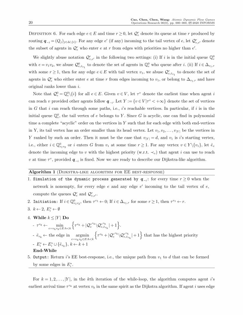
Algorithm 1 (Dijkstra-like algorithm for EE best-response)
1. Simulation of the dynamic process generated by q−i: for every time r ≥ 0 when the
network is nonempty, for every edge e and any edge e′ incoming to the tail vertex of e,
compute the queues Qre and Qre,e′ .
2. Initiation: If i∈Q0v1v2
, then τ v1← 0; If i∈∆v1,r for some r≥ 1, then τ v1← r.
3. k← 2, E∗i ←∅
4. While k≤ |Y | Do
- τ vk← mine=vhvk∈E:h<k
τ vh + |Qτvhe \Qτ
vh
e,evh|+ 1
.
- evk← the edge in argmine=vhvk∈E:h<k
τ vh + |Qτvhe \Qτ
vh
e,evh|+ 1
that has the highest priority
- E∗i ←E∗i ∪evk, k← k+ 1
End-While
5. Output: Return i’s EE best-response, i.e., the unique path from v1 to d that can be formed
by some edges in E∗i .
For k = 1,2, . . . , |Y |, in the kth iteration of the while-loop, the algorithm computes agent i’s
earliest arrival time τ vk at vertex vk in the same spirit as the Dijkstra algorithm. If agent i uses edge
Cao, Chen, Chen, Wang: Atomic Dynamic Flow GamesOperations Research 00(0), pp. 000–000, © 2020 INFORMS 21
e= vhvk to travel from vh to vk, the fastest way is that he reaches vh at the earliest possible time
τ vh (which has been derived in a previous iteration), waits at e for |Qτvhe \Qτvh
e,evh| time units, and
then spends 1 unit of transit time going through e to vk. Thus τ vk is obtained by taking minimum
over all possible edges e incoming to vk, as stated in the first item of Step 4. The nontrivial part of
our algorithm is determining the queuing time to be |Qτvhe \Qτvh
e,evh|. Among the agents who queue
at edge e at time τ vh (i.e., those in Qτvhe ), the ones whom i can overtake at e are those in Qτvhe,evh
and they are exactly the agents in Qτvhe who are preempted by i at vh.
Theorem 4. Given any partial path profile q−i, the EE best-response of agent i can be computed
by the Dijkstra-like algorithm efficiently.
The correctness proof of the algorithm can be found in Section EC.5. We discuss here the time
efficiency. To compute the queues in Step 1, we simulate the transit and queuing process in a way
that we only keep records for all nonempty queues during the process. Note that the queue state
varies only when an agent just reaches an edge or just leaves a queue. So the number of records
contributed by an agent is at most twice the number of edges on his path. It follows that all queues
stated in Step 1 can be found in polynomial time. On the other hand, the while-loop at Step 4 is
a standard dynamic program and its time complexity is O(|V |2). Therefore, the EE best-response
of each agent is polynomially computable if the agent set and network are finite. Otherwise, the
computational efficiency is achieved via ignoring agents who are sufficiently far from the destination
d or enter the network at time points sufficiently later (i.e., those who are doubtlessly not in F).
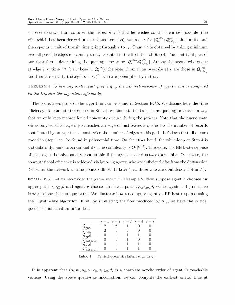
Example 5. Let us reconsider the game shown in Example 2. Now suppose agent h chooses his
upper path oho1y1d and agent g chooses his lower path ogv2x2y2d, while agents 1–4 just move
forward along their unique paths. We illustrate how to compute agent i’s EE best-response using
the Dijkstra-like algorithm. First, by simulating the flow produced by q−i, we have the critical
queue-size information in Table 1.
r= 1 r= 2 r= 3 r= 4 r= 5|Qr
o1y1| 2 2 1 0 0
|Qro2y2| 2 1 0 0 0
|Qry1d| 0 1 1 1 0
|Qry1d,o1y1
| 0 1 1 0 0|Qr
y2d| 0 1 1 1 0
|Qry2d,o2y2
| 0 1 1 1 0
Table 1 Critical queue-size information on q−i
It is apparent that (oi, u1, u2, o1, o2, y1, y2, d) is a complete acyclic order of agent i’s reachable
vertices. Using the above queue-size information, we can compute the earliest arrival time at
Cao, Chen, Chen, Wang: Atomic Dynamic Flow Games22 Operations Research 00(0), pp. 000–000, © 2020 INFORMS
each vertex for agent i as follows: τ oi = 1, τu1 = 2, τu2 = 2, τ o1 = 3, τ o2 = 3, τ y1 = 5, τ y2 = 4 and
τd = minτ y1 +
∣∣Q5y1d\Q5
y1d,o1y1
∣∣+ 1, τ y2 +∣∣Q4
y2d\Q4
y2d,o2y2
∣∣+ 1
= min5+0+1,4+(1−1)+1= 5,
ed = y2d. Thus agent i’s EE best-response is his lower path oiu2o2y2d.
4.4.3. Computing the special IDNE In Section 4.1, we have constructed the special IDNE
for game ΓN. Now let us show that this construction can be executed efficiently. It suffices to show
that, when the partial path profile (P1, . . . , Pi−1) for agents 1, . . . , i− 1 has been computed, we can
efficiently find the next agent, whom we label as i, and his associated dominant path Pi.
It is worth noting that Pi is actually the EE best-response of i to (P1, . . . , Pi−1). Therefore, to
identify the agent i, we employ the Dijkstra-like algorithm to compute the EE best-response Pj of
each agent j ∈∆\[i− 1] to (P1, . . . , Pi−1) and their earliest arrival times at each vertex. (Note that
when we simulate the flow generated by (P1, . . . , Pi−1) for every agent j ∈∆\[i− 1], the subsets of
agents preempted by j are always empty, since no agent in ∆\[i− 1] can affect the agents in [i− 1]
according to the iterative dominance property, i.e., there is no intricate chain effects under this
circumstance.) Starting with a candidate set (j,Pj) : j ∈∆\[i−1], we repeatedly implement steps
(S1)–(S3) in Section 4.1 to prune the set until only one candidate is left. This candidate consists
of the desired agent i and path Pi. Therefore, the total number of times we run the Dijkstra-like
algorithm is∑|∆|
i=1(|∆| − (i− 1)) = (1 + |∆|)|∆|/2. As mentioned earlier, if infinitely many agents
are involved, our computation may ignore agents whose entry times to G are sufficiently late.
We remak that there is another natural algorithm to efficiently compute the special IDNE by
making the utmost of the above EE best-responses and the iterative dominance property. Given
an arbitrary initial path profile q(0) = (Q(0)i )i∈∆ with Q
(0)i ∈Pi, define a sequence of path profiles
q(k) = (Q(k)i )i∈∆, k = 1,2, . . . , |∆|, where Q
(k)i is agent i’s EE best-response to q
(k−1)−i , i.e., at each
round k, every agent makes EE best-response to other agents’ strategies in the preceding round.
For our game ΓN, using this iterative approach of simultaneous EE best-responses, the path profiles
converge to the special IDNE quickly (in at most |∆| rounds). To see the convergence, note that
regardless of the initial paths of other agents, the EE best-response of agent 1 in the first round
must be exactly his path in the special IDNE, which will never change in subsequent rounds. Similar
observations are applicable to the EE best-response of agent 2 from the second round onwards,
and so on and so forth. Finally, in the |∆|th round, all agents choose the paths as in the special
IDNE, where everyone’s path is his EE best-response to others. We illustrate the algorithm using
a simple example as follows.
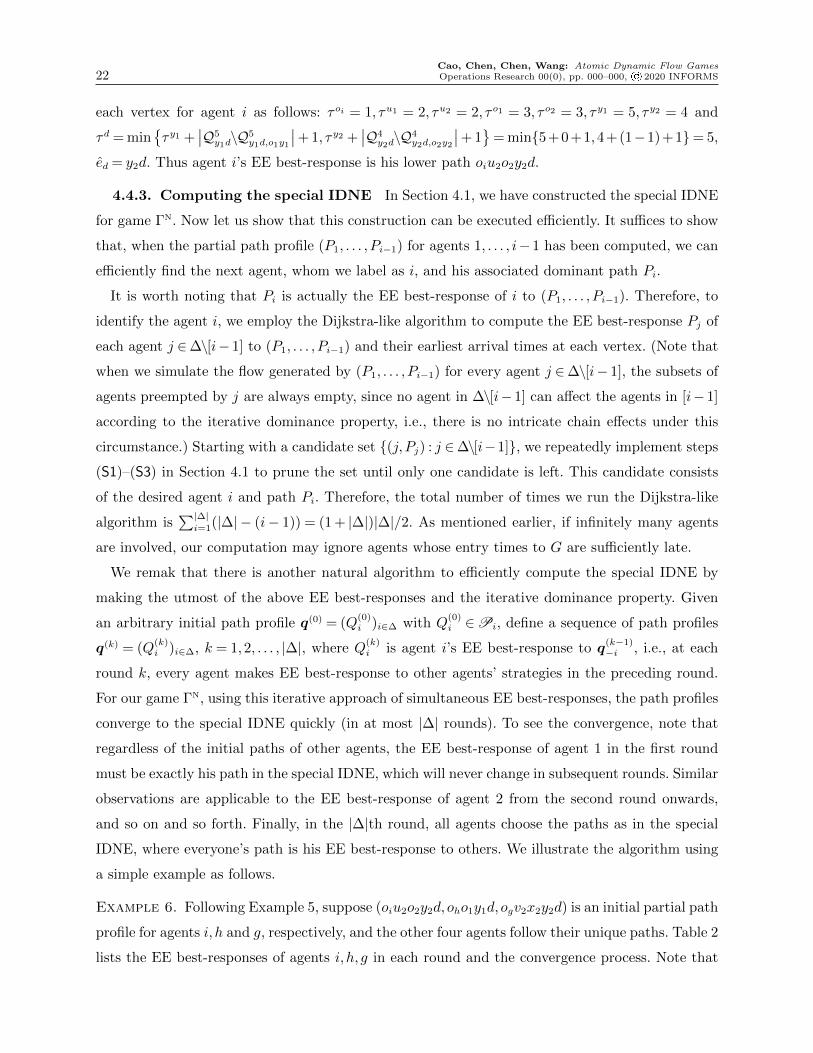
Example 6. Following Example 5, suppose (oiu2o2y2d, oho1y1d, ogv2x2y2d) is an initial partial path
profile for agents i, h and g, respectively, and the other four agents follow their unique paths. Table 2
lists the EE best-responses of agents i, h, g in each round and the convergence process. Note that
Cao, Chen, Chen, Wang: Atomic Dynamic Flow GamesOperations Research 00(0), pp. 000–000, © 2020 INFORMS 23
Agent i Agent h Agent gRound 0 oiu2o2y2d oho1y1d ogv2x2y2dRound 1 oiu2o2y2d oho1y1d ogv1x1y1dRound 2 oiu2o2y2d oho2y2d ogv1x1y1dRound 3 oiu1o1y1d oho2y2d ogv1x1y1dRound 4 oiu1o1y1d oho2y2d ogv1x1y1d
Table 2 The iterative process of simultaneous EE best-responses
(ogv1x1y1d,oho2y2d,oiu1o1y1d) is the partial path profile for agents g,h, i in the special IDNE
for this example.
Note that, in the above process, we do not need to identify the iterative dominant order of
the agents. It resembles a natural learning process in the real world, where agents update their
strategies in a distributed way from an arbitrary initial path profile. This kind of algorithms are
quite common in the study of day-to-day models, where convergence within a finite number of
steps is rare and even convergence may not be guaranteed (Guo et al. 2018).
5. The game of adaptive agents
Our second submodel ΓA of dynamic atomic flow game assumes that agents are of a relatively
high rationality level. Specifically, agents are adaptive in that they make routing decisions at every
nonterminal vertex they reach as to which next edge to take. Their decisions at a vertex may
depend on the choices of other agents in the history. The following example demonstrates that it is
natural to assume that agents use adaptive strategies, when they have updated information about
others, and they may gain by using more flexible adaptive strategies than simply choosing fixed
origin-destination paths at the very beginning.
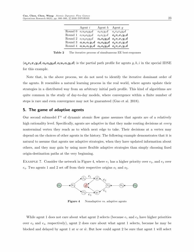
Example 7. Consider the network in Figure 4, where e1 has a higher priority over e2, and e3 over
e4. Two agents 1 and 2 set off from their respective origins o1 and o2.
Figure 4 Nonadaptive vs. adaptive agents
While agent 1 does not care about what agent 2 selects (because e1 and e3 have higher priorities
over e2 and e4, respectively), agent 2 does care about what agent 1 selects, because he may be
blocked and delayed by agent 1 at w or w. But how could agent 2 be sure that agent 1 will select
Cao, Chen, Chen, Wang: Atomic Dynamic Flow Games24 Operations Research 00(0), pp. 000–000, © 2020 INFORMS
the upper (or lower) path? Suppose now agent 2 postpones his decision making on vertex v2 to the
time he reaches it, then he will select e4 if he observes that agent 1 has chosen the upper path and
e2 otherwise. In fact, this is exactly what adaptive agent 2 does in both SPEs of the game ΓA.
5.1. Game setting
For the extensive-form game ΓA, the notion of a strategy is much more complicated than for the
normal-form game ΓN. While a nonadaptive agent in ΓN has only one decision point, at which he
selects an origin-destination path, an adaptive agent in ΓA typically has multiple decision points.
On the other hand, while the choice of a nonadaptive agent is an origin-destination path, the
choice of an adaptive agent at each decision point is an edge. A strategy of an adaptive agent is a
“complete plan” that is responsive to all possible scenarios, i.e., a profile of decisions at all decision
points. We next present a rigorous definition of a strategy in the extensive-form game ΓA in terms
of “configurations” and “histories”.
Given time point r≥ 0, we use Qre to denote the queue at edge e at time r, which will be considered
as both a sequence of agents and the corresponding set. We call cr = (Qre)e∈E a configuration w.r.t.
time r if Qre ∩Qr
e′ = ∅ for different edges e and e′. In particular,
• Let c0 = (Q0e)e∈E denote the unique initial configuration given by the input (see Section 3);
• Let ∆(cr) := (∪e∈EQre)∪ (∪v∈V ∆r+1,v) denote the set of agents involved in configuration cr
and inflows at time r+ 1;
• Let D(cr) := (∪e∈EQre)∪ (∪v∈V,s≥r+1∆s,v) denote the set of agents involved in configuration
cr and afterwards.
We say that configurations cr and cr+1 are consecutive if cr+1 is reachable from cr after one time
unit under the given inflows and the edge-priority DQ rule (recalling Section 3). A precise definition
of consecutiveness is provided in Section EC.8 of the Electronic Companion, using a notion of
action profiles.
Definition 7 (History/Decision point). For each time point r≥ 0, a sequence of consecutive
configurations hr = (c0, . . . , cr) starting from the initial configuration c0 is called a history at time r.
In particular, h0 = (c0) is called the initial history. The set of all histories at time r is denoted as
Hr. Each history hr corresponds to a decision point of all agents in ∆(cr).
Definition 8 (Strategy). A strategy of agent i ∈ ∆ is a mapping σi that maps each history
hr = (c0, . . . , cr) with i ∈ ∆(cr) to σi(hr) such that, based on cr and the edge-priority DQ rule,
either σi(hr) is the “next” edge along which i travels (i.e., i could stand at its tail part at time
r+ 1) or σi(hr) is a null element when under cr agent i will exit G at time r+ 1. The strategy set
of agent i is denoted as Σi. A vector σ= (σi)i∈∆ is called a strategy profile of ΓA.
Cao, Chen, Chen, Wang: Atomic Dynamic Flow GamesOperations Research 00(0), pp. 000–000, © 2020 INFORMS 25
Note in the above definition that when an agent is not the head of a queue, the “next” edge he
“chooses” must be the same edge he is queuing at, i.e., he waits for at least one more time unit.
Remark 1. The number of decision points of an adaptive agent is generally much larger than
the number of vertices he passes. Taking Example 1 as an illustration, each agent has 4 decision
points before arriving at vertex w: 1 point at origin o, and 3 points at vertex v (corresponding to
the opponent choosing ou1, ou2 and ov, respectively). Suppose agent 2 has decided to choose edge
ou1 at origin o. Agent 2 still needs to specify in his strategy the choices at vertex v in 3 different
scenarios, even if he will never reach v when he follows the strategy. This is a remarkable difference
between a strategy in an extensive-form game and a strategy in daily languages.
A strategy profile is an SPE if and only if each agent has no incentive to deviate from his strategy
at any decision point, assuming that other agents do not deviate. A more rigorous definition is given
in terms of “game tree” as follows. The game tree of ΓA is a tree with nodes corresponding to ΓA’s
histories (i.e., decision points of agents). At each game tree node (history) hr = (c0, c1, . . . , cr), agents
in ∆(cr) need to make their own decisions simultaneously, and the collection of these decisions
forms their action profile, which leads to a new node (history) hr+1 as a child (continuation) of hr.
For each history hr = (c0, c1, . . . , cr), the subtree of the game tree rooted at hr can be viewed as a
separate game (with agent set D(cr) starting from cr at time r), which is referred to as a subgame
of ΓA. A subtree is also called a subgame tree.
Given a strategy profile σ = (σi)i∈∆ of ΓA, the restriction of each strategy σi with i ∈ D(cr)
to a subgame tree rooted at hr = (c0, c1, . . . , cr) is also a strategy of agent i in the corresponding
subgame starting from hr. All these restricted strategies form a strategy profile for the subgame.
Under the routing induced by the strategy profile for the subgame, the time when agent i∈∆(cr)
exits G is denoted as ti(σ|hr).
Definition 9 (SPE). A strategy profile σ = (σi)i∈∆ is a subgame perfect equilibrium (SPE) of
ΓA if for any r ≥ 0 and any history hr ∈ Hr, ti(σ|hr)≤ ti(σ′i, σ−i|hr) holds for all i ∈∆(cr) and all
σ′i ∈Σi such that strategy profile (σ′i, σ−i) still leads to history hr, where σ−i is the partial strategy
profile of σ for agents in ∆\i.
5.2. SPE existence
The standard way to prove the existence of an SPE is by backward induction (and usually the
one-deviation property). However, in game ΓA, time horizon is typically infinite and more than one
agent may move at each time step, hence the usual approach does not work here in general. In this
subsection, we establish the SPE existence for ΓA using a constructive approach.
Theorem 5. Each extensive-form game ΓA admits an SPE.
Cao, Chen, Chen, Wang: Atomic Dynamic Flow Games26 Operations Research 00(0), pp. 000–000, © 2020 INFORMS
The basic idea for constructing an SPE of ΓA is to assemble the special IDNEs of various game
instances ΓN that are associated with configurations of ΓA. To be more specific, given a game
instance ΓA with input (G,∆), every configuration cr of the extensive-form game ΓA is associated
with a normal-form game instance under model ΓN, denoted as ΓN(cr), which starts at time r
on network G with initial queues cr = (Qre)e∈E, and is played by nonadaptive agents in D(cr) =
(∪e∈EQre)∪ (∪v∈V,s≥r+1∆s,v). Using the method in Section 4.1, we obtain the special IDNE of game
ΓN(cr). In our assembling, at every configuration cr, the action that each agent of ∆(cr) takes in
ΓA is determined by his path in the special IDNE of ΓN(cr): just choose the first edge of the path
when he is the head of the current queue or keep staying in the queue otherwise. It can be shown
that such a strategy profile is an SPE for ΓA. The proof (see Section EC.9) relies on the properties
of these NEs for all games ΓN(cr): the iterative dominance as well as the sequential independence
and optimality discussed in Section 4.1.
The realized paths of the SPE constructed above form a path profile that is exactly the special
IDNE we construct for game ΓN(c0). Hence, this special SPE possesses all the nice properties
discussed in Section 4.1, and also satisfies the following additional properties:
• Markovian: the action each agent takes at each decision point depends only on the current
configuration and its associated time r, not on earlier configurations in the history. (Note
that different histories, which correspond to different decision points of agents, may lead to
the same configuration w.r.t. the same time point.)
• Anonymous: the action each agent takes at each decision point does not depend on the
identities of other agents.
As a corollary of the efficient computation of NEs discussed in Section 4.4.3, we can efficiently
find the action profile at any history under this SPE of game ΓA assembled from special IDNEs.
Remark 2. If priorities were placed on agents, then an SPE may not exist even if the network
has only one single origin. This can be seen from Example 3, which can be considered as a part of
some more complex single-origin network game (we omit the construction of the whole game).
5.3. NE realization from an SPE
Each strategy profile σ of game ΓA induces a path profile, which is a strategy profile of the corre-
sponding game ΓN. Recall from Example 1 that an SPE of ΓA does not necessarily induce an NE
of ΓN. A natural question arises: are all NEs of ΓN inducible by SPEs of ΓA? The answer is yes,
as formally presented in the following theorem, whose technical proof, relegated to Section EC.10,
relies on both the hierarchical independence of general NEs (see Section 4.3) and the iterative
dominance of special NEs (see Section 4.1).
Cao, Chen, Chen, Wang: Atomic Dynamic Flow GamesOperations Research 00(0), pp. 000–000, © 2020 INFORMS 27
Theorem 6. For every NE profile p of game ΓN, there exists an SPE σ of game ΓA such that the
path profile induced by the initial history h0 and σ is exactly p.
Combined with Example 1, the above theorem shows that the NE outcome set of ΓN is typically
a proper subset of the SPE outcome set of ΓA, reaffirming the intuition that model ΓA is more
flexible than ΓN. Since model ΓN is relatively easier to study, also natural and more frequently
analyzed in the literature, Theorem 6 can serve as a bridge between models ΓA and ΓN. Recall that
in general game theory, each SPE is also an NE. Our result does not contradict this well-known
result because strategies have different meanings in ΓN and ΓA.
In addition, Theorem 6 gives an alternative answer to the question of how an NE could be
possible. This question is quite challenging both in the general game theory and in the trans-
portation study. While there are standard (but not completely satisfactory) answers, including
pre-communication and rational expectation (Sheffi 1985), to defend the relevance of the NE notion,
we provide an alterative answer via allowing the adaptiveness of agents. We argue that, when
agents are able to make more flexible adaptive decisions than the usual rigid ones addressed in the
previous literature, NE outcomes have more chances to be realized (by SPE).
6. Concluding remarks
In this paper, we have proposed a new network game model of atomic dynamic flows for both
adaptive and nonadaptive agents. Our model is arguably promising thanks to its many desirable
properties, including the equilibrium existence, equivalence between NEs and strong NEs, global
FIFO, and computational efficiency for finding equilibria and best responses, which stand in stark
contrast with existing related negative results on atomic dynamic flow games. In particular, the
equivalence between NEs and strong NEs has rarely been seen in atomic routing games, even in a
static setting, where rather restrictive conditions are often needed to guarantee their equivalence
(Holzman and Law-Yone 1997).
We now briefly discuss the generality of the Unit Assumption. Our unit-capacity assumption
goes inevitably together with the lane priorities, which constitute part of the input network. Gluing
parallel lanes together, all the derived results without regard to computational complexity hold for
networks with arbitrary capacities. When the input size of lane priorities is polynomial in that of
the capacitated network, e.g., left lanes having higher priorities than the right ones, the running
times of our algorithms are polynomial in the network’s input size plus the number of agents. Our
unit-length assumption is merely for the sake of easy description. When an edge does not have
unit length, one can subdivide it into unit-length edges. An agent waits at the original edge if and
only if he does so at the resulting unit-length edge that has the same tail vertex as the original
edge, no queue being built up at any other resulting unit-length edges. Clearly, all our theoretical
Cao, Chen, Chen, Wang: Atomic Dynamic Flow Games28 Operations Research 00(0), pp. 000–000, © 2020 INFORMS
results (on equilibrium existence and properties) are still valid when the unit-length assumption is
dropped. Moreover, as our algorithms only record nonempty queues in simulating the transit and
queuing process (see the discussion following Theorem 4 in Section 4.4.2), the efficient computation
can also be guaranteed for networks with arbitrary edge lengths.
Our results may also help us better understand the connections and differences between DQ-
based games of atomic dynamic flows and those of nonatomic ones. It is known that NE flows,
earliest arrival flows and global FIFO flows are all identical in related nonatomic models (Koch
and Skutella 2011). In our atomic model, however, earliest arrival flows are NE flows, which are
in turn global FIFO flows, but neither of the other ways around is generally valid. In addition, no
overtaking is valid for nonatomic NE flows (Koch and Skutella 2011), which is not the case in our
atomic model.
Our results provide some managerial insights and policy implications. First, back to the real
world, the tie-breaking rule used in our model, which is based on edge priorities, plays a comple-
mentary role to the traffic-light system in coordinating the traffic. (A difference between our model,
as well as almost all known related ones, and the real world is that the cross conflicts mediated
by traffic lights are not considered.) Our theoretical results indicate that this kind of system pos-
sesses more nice properties, and is thus more reasonable than the system based on agent priorities.
Second, our Braess-like paradox (Example 4) indicates that, in certain extreme scenarios, fewer
vehicles may lead to a worse equilibrium. This raises, at least theoretically, a challenge to traffic
restriction policies practiced in many cities all over the world in various ways.
This paper is our first attempt to understand games of atomic dynamic flows, especially with the
introduction of agents’ flexibility of online decision making. Many interesting problems are widely
open. For example, is there an upper bound on the SPE (or NE) queue lengths for general single-
origin single-destination networks when the inflow rate is no more than the minimum capacity
of an origin-destination cut? Does a long-run steady state exist when the inflow is constant or
seasonal? How efficient is this steady state if it does exist? What if agents are allowed to choose
their departure times? The queue notion used in our model is also referred to as point-queue in the
traffic community, i.e., queues have no physical lengths. Spillback models (Daganzo 1998, Bressan
and Nguyen 2015, Sering and Koch 2019) that consider the physical lengths of queues are also
important future directions.
One drawback of our nonadaptive model is that agents make their decisions simultaneously at
the very beginning, which is before they enter the network. Investigating a more realistic model
which rests between the adaptive and nonadaptive models in that agents make their route-choice
decisions when they enter the network, as has been assumed in many nonatomic models, is also
meaningful. Exploring such issues will undoubtedly help us better understand games of atomic
Cao, Chen, Chen, Wang: Atomic Dynamic Flow GamesOperations Research 00(0), pp. 000–000, © 2020 INFORMS 29
dynamic flows. As a positive step in this spirit of pursuit, we consider a hybrid model, suggested
by an anonymous reviewer, of agents who are between adaptive and nonadaptive, in the sense
that an agent contemplates at every nonterminal vertex switching paths with a given probability.
The SPE existence result for our model of adaptive agents is still valid for this hybrid model (see
Section EC.13 of the Electronic Companion for details).
References
Anshelevich, E. and Ukkusuri, S. (2009). Equilibria in dynamic selfish routing. In International Symposium
on Algorithmic Game Theory, pages 171–182. Springer.
Bressan, A. and Han, K. (2013). Existence of optima and equilibria for traffic flow on networks. Networks
and Heterogeneous Media, 8(3):627–648.
Bressan, A. and Nguyen, K. T. (2015). Optima and equilibria for traffic flow on networks with backward
propagating queues. Networks & Heterogeneous Media, 10(4):717–748.
Cao, Z., Chen, B., Chen, X., and Wang, C. (2017). A network game of dynamic traffic. In Proceedings of
the 2017 ACM Conference on Economics and Computation, EC ’17, pages 695–696. ACM.
Cominetti, R., Correa, J., and Larre, O. (2015). Dynamic equilibria in fluid queueing networks. Operations
Research, 63(1):21–34.
Cominetti, R., Correa, J., and Olver, N. (2017). Long term behavior of dynamic equilibria in fluid queuing
networks. In International Conference on Integer Programming and Combinatorial Optimization, pages
161–172. Springer.
Correa, J., de Jong, J., De Keijzer, B., and Uetz, M. (2019). The inefficiency of Nash and subgame perfect
equilibria for network routing. Mathematics of Operations Research, 44(4):1286–1303.
Correa, J. R. and Stier-Moses, N. E. (2010). Wardrop equilibria. Wiley Encyclopedia of Operations Research
and Management Science.
Daganzo, C. F. (1998). Queue spillovers in transportation networks with a route choice. Transportation
Science, 32(1):3–11.
Graf, L. and Harks, T. (2019). Dynamic flows with adaptive route choice. In International Conference on
Integer Programming and Combinatorial Optimization, pages 219–232. Springer.
Guo, R.-Y., Yang, H., and Huang, H.-J. (2018). Are we really solving the dynamic traffic equilibrium problem
with a departure time choice? Transportation Science, 52(3):603–620.
Hamdouch, Y., Marcotte, P., and Nguyen, S. (2004). A strategic model for dynamic traffic assignment.
Networks and Spatial Economics, 4(3):291–315.
Han, K., Friesz, T. L., and Yao, T. (2013). Existence of simultaneous route and departure choice dynamic
user equilibrium. Transportation Research Part B: Methodological, 53:17–30.
Cao, Chen, Chen, Wang: Atomic Dynamic Flow Games30 Operations Research 00(0), pp. 000–000, © 2020 INFORMS
Harks, T., Peis, B., Schmand, D., Tauer, B., and Koch, L. V. (2018). Competitive packet routing with
priority lists. ACM Transactions on Economics and Computation (TEAC), 6(1):4.
Hendrickson, C. and Kocur, G. (1981). Schedule delay and departure time decisions in a deterministic model.
Transportation Science, 15(1):62–77.
Hoefer, M., Mirrokni, V. S., Roglin, H., and Teng, S.-H. (2009). Competitive routing over time. In Interna-
tional Workshop on Internet and Network Economics, pages 18–29. Springer.
Hoefer, M., Mirrokni, V. S., Roglin, H., and Teng, S.-H. (2011). Competitive routing over time. Theoretical
Computer Science, 412(39):5420–5432.
Holzman, R. and Law-Yone, N. (1997). Strong equilibrium in congestion games. Games and Economic
Behavior, 21(1-2):85–101.
Ismaili, A. (2017). Routing games over time with FIFO policy. In R. Devanur, N. and Lu, P., editors, Web
and Internet Economics, pages 266–280, Cham. Springer International Publishing.
Koch, R. (2012). Routing games over time. Ph.D. thesis, Technische Universitat Berline.
Koch, R. and Skutella, M. (2009). Nash equilibria and the price of anarchy for flows over time. In International
Symposium on Algorithmic Game Theory, pages 323–334. Springer.
Koch, R. and Skutella, M. (2011). Nash equilibria and the price of anarchy for flows over time. Theory of
Computing Systems, 49(1):71–97.
Kulkarni, J. and Mirrokni, V. (2015). Robust price of anarchy bounds via LP and Fenchel duality. In
Proceedings of the Twenty-sixth Annual ACM-SIAM Symposium on Discrete Algorithms, SODA ’15,
pages 1030–1049, Philadelphia, PA, USA. Society for Industrial and Applied Mathematics.
Long, J., Huang, H.-J., Gao, Z., and Szeto, W. Y. (2013). An intersection-movement-based dynamic user
optimal route choice problem. Operations Research, 61(5):1134–1147.
Long, J. and Szeto, W. Y. (2019). Link-based system optimum dynamic traffic assignment problems in
general networks. Operations Research, 67(1):167–182.
Macko, M., Larson, K., and Steskal, L. (2013). Braess’s paradox for flows over time. Theory of Computing
Systems, 53(1):86–106.
Marcotte, P., Nguyen, S., and Schoeb, A. (2004). A strategic flow model of traffic assignment in static
capacitated networks. Operations Research, 52(2):191–212.
Meunier, F. and Wagner, N. (2010). Equilibrium results for dynamic congestion games. Transportation
Science, 44(4):524–536.
Peeta, S. and Ziliaskopoulos, A. K. (2001). Foundations of dynamic traffic assignment: The past, the present
and the future. Networks and Spatial Economics, 1(3):233–265.
Roughgarden, T. (2007). Routing games. Algorithmic Game Theory, 18:459–484.
Cao, Chen, Chen, Wang: Atomic Dynamic Flow GamesOperations Research 00(0), pp. 000–000, © 2020 INFORMS 31
Roughgarden, T. and Tardos, E. (2002). How bad is selfish routing? Journal of the ACM, 49(2):236–259.
Scarsini, M., Schroder, M., and Tomala, T. (2018). Dynamic atomic congestion games with seasonal flows.
Operations Research, 66(2):327–339.
Selten, R. (1965). Spieltheoretische behandlung eines oligopolmodells mit nachfragetragheit: Teil i: Bestim-
mung des dynamischen preisgleichgewichts. Zeitschrift fur die gesamte Staatswissenschaft/Journal of
Institutional and Theoretical Economics, (H. 2):301–324.
Sering, L. and Koch, L. V. (2019). Nash Flows Over Time with Spillback, pages 935–945.
Sheffi, Y. (1985). Urban transportation networks, volume 6. Prentice-Hall, Englewood Cliffs, NJ.
Vickrey, W. S. (1969). Congestion theory and transport investment. The American Economic Review,
59(2):251–260.
Wardrop, J. G. (1952). Road paper: Some theoretical aspects of road traffic research. In ICE Proceedings:
Engineering Divisions, volume 1, pages 325–362. Thomas Telford.
Werth, T., Holzhauser, M., and Krumke, S. (2014). Atomic routing in a deterministic queuing model.
Operations Research Perspectives, 1(1):18–41.
Yagar, S. (1971). Dynamic traffic assignment by individual path minimization and queuing. Transportation
Research, 5(3):179–196.
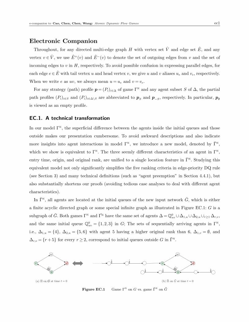
e-companion to Cao, Chen, Chen, Wang: Atomic Dynamic Flow Games ec1
Electronic Companion
Throughout, for any directed multi-edge graph H with vertex set V and edge set E, and any
vertex v ∈ V , we use E+(v) and E−(v) to denote the set of outgoing edges from v and the set of
incoming edges to v in H, respectively. To avoid possible confusion in expressing parallel edges, for
each edge e∈ E with tail vertex u and head vertex v, we give u and v aliases ue and ve, respectively.
When we write e as uv, we always mean u= ue and v= ve.
For any strategy (path) profile p= (Pi)i∈∆ of game ΓN and any agent subset S of ∆, the partial
path profiles (Pi)i∈S and (Pi)i∈∆\S are abbreviated to pS and p−S, respectively. In particular, p∅
is viewed as an empty profile.
EC.1. A technical transformation
In our model ΓN, the superficial difference between the agents inside the initial queues and those
outside makes our presentation cumbersome. To avoid awkward descriptions and also indicate
more insights into agent interactions in model ΓN, we introduce a new model, denoted by ΓN,
which we show is equivalent to ΓN. The three seemly different characteristics of an agent in ΓN,
entry time, origin, and original rank, are unified to a single location feature in ΓN. Studying this
equivalent model not only significantly simplifies the five ranking criteria in edge-priority DQ rule
(see Section 3) and many technical definitions (such as “agent preemption” in Section 4.4.1), but
also substantially shortens our proofs (avoiding tedious case analyses to deal with different agent
characteristics).
In ΓN, all agents are located at the initial queues of the new input network G, which is either
a finite acyclic directed graph or some special infinite graph as illustrated in Figure EC.1: G is a
subgraph of G. Both games ΓN and ΓN have the same set of agents ∆ =Q0uv ∪∆1,u∪∆2,u∪r≥1 ∆r,v,
and the same initial queue Q0uv = 1,2,3 in G; The sets of sequentially arriving agents in ΓN,
i.e., ∆1,u = 4, ∆2,u = 5,6 with agent 5 having a higher original rank than 6, ∆1,v = ∅, and
∆r,v = r+ 5 for every r≥ 2, correspond to initial queues outside G in ΓN.
Figure EC.1 Game ΓN on G vs. game ΓN on G
ec2 e-companion to Cao, Chen, Chen, Wang: Atomic Dynamic Flow Games
Recall that the input of a game instance ΓN consists of network G= (V,E) with initial queues
(Q0e)e∈E and inflows of agents ∆r,v (r ≥ 1, v ∈ V ) along with original ranks among them. Corre-
sponding to this game instance, an instance of game ΓN is specified by the same set ∆ := ∆ =
(∪e∈EQ0e)∪ (∪r≥1,v∈V ∆r,v) of nonadaptive agents, but with a modified network input G= (V , E),
which is obtained from G by adding a (typically infinite) number of pendant paths and specifying
initial locations of the agents ∪r≥1,v∈V ∆r,v at the newly added pendant paths, as detailed below:
(T1) Network G: For each vertex v ∈ V , we add a number maxr≥1 |∆r,v| (which is possibly zero)
of paths P v1 , P
v2 , . . . directed to v, each intersecting G only at v. Outside G, all added paths
are mutually vertex-disjoint.
(T2) Priority preservation: For each v ∈ V , the decreasing priority ordering of the added incoming
edges to v agrees with the (subscript) ordering of added paths containing them: the unique
edge in P v1 incoming to v has the highest priority, the one in P v
2 incoming to v has the second
highest priority, and so on. This ordering is followed by the given ordering of incoming edges
to v in G, which makes a complete priority order over all incoming edges to v in G.
(T3) Rank preservation: Agent i∈∆r,v in game ΓN with the hth highest original rank corresponds
to agent i∈ ∆ in game ΓN, who is the only agent queuing at time 0 on path P vh at a distance
r from v, where distance is measured by the number of edges. Particularly, agent i in ΓN will
reach v at time r through the (added) incoming edge to v with the hth highest priority.
With the above transformation, it is easy to see that the agent set ∆ of game ΓN is simply the
disjoint union of its initial queues, which we still denote as Q0e, over all e∈ E. The game ΓN starts
at time 0 with the input G and (Q0e)e∈E. No entries of agents into the network G are involved
throughout the game and all agents are in G from the very beginning. Therefore, no original ranks
are needed to break ties. (Note that we have transformed the original ranks among ∆r,v to the
priorities of the added edges incoming to v.)
Due to the simpler form of the input for ΓN, the edge-priority DQ rule (see Section 3) when
applied to ΓN is simplified: we do not need rules (R3) and (R4) any more. Regarding any fixed edge
e (with tail vertex ue) and any pair of agents, the agent who enters e earlier has a higher queue
rank at e. Ties are broken via (R2) only: higher priority is given to the agent who enters e through
an incoming edge to ue that has a higher priority according to ≺ue . Another simplification resulted
from our transformation is that in ΓN all information about agent set is contained in the initial
queues (Q0e)e∈E. The chronological order of entrances into G in ΓN is visualized by the lengths of
paths of G in ΓN, which makes the task of investigating agent interactions easier. For instance, in
the example illustrated in Figure EC.1, game ΓN provides a faster way for one to find that agent
7 will preempt agent 3 at vertex v.
e-companion to Cao, Chen, Chen, Wang: Atomic Dynamic Flow Games ec3
Each agent i∈ ∆ selects a path starting from his initial edge (the edge where he queues at time
0) and ending at the common destination vertex d. Such paths form his strategy set, which we
write as Pi to distinguish it from Pi in game ΓN. We use oi to denote the tail vertex of initial
edge of agent i∈ ∆ in G. The following fact is obvious by our transformation from game ΓN on G
to game ΓN on G.
Lemma EC.1. Given game ΓN with input (G,∆), let game ΓN with input (G, ∆) be constructed
as in (T1)–(T3). Then the game ΓN is exactly the restriction of the game ΓN to G: the strategies
and movements of agents together with their arrival times at vertices along their paths in ΓN are
identical with those in the restriction of ΓN to G.
In view of agents’ trivial movements outside G in game ΓN, the above lemma enables us to turn
our attention to ΓN when studying ΓN. These two games are essentially identical. The notation
and definitions introduced for game model ΓN apply to game model ΓN, as the latter is simply a
special case of the former.
EC.2. Algorithm for finding an IDNE
In this section, we construct an IDNE for every game ΓN (see Definition 2). The result along with
Lemma EC.1 directly yields an IDNE for every game ΓN. Recall that, [0] = ∅, and for any positive
integer k, [k] denotes the set of all positive integers no more than k.
Algorithm. We are able to reindex the agents of ∆ as 1,2, . . . and find the associated path
profile p= (P1, P2, . . .) such that, each agent k ∈ ∆ is a dominator in ∆\[k−1] and Pk is a dominant
path in the following sense: under the assumption that agents in [k − 1] all follow p[k−1], as long
as agent k takes Pk, he will be among the first in ∆\[k − 1] to reach every vertex of the path.
Specifically, for any vertex v on Pk, and partial path profile q−[k] for agents in ∆\[k], we have
tvk(p[k],q−[k]
)= min
tvj (p[k−1],r−[k−1]) : j ∈∆\[k− 1],
and r−[k−1] is partial profile for ∆\[k− 1]. (EC.1)
We call such a path profile iteratively dominant. As explained in Section 4.1, it is actually an NE,
i.e., IDNE, of game ΓN.
For completeness, we repeat the sketch of the algorithm in the context of ΓN. Our algorithm
runs roughly as follows. Initially, let agent subset [0] of ∆ and partial routing p[0] of agents in [0]
be empty. Then recursively, assuming agents in [k− 1] go along their paths as specified in p[k−1],
we enlarge [k− 1] with a new agent k ∈ ∆\[k− 1] and enlarge p[k−1] with a path Pk ∈ Pk in the
following way. For each agent j ∈ ∆\[k− 1] and vertex v ∈ V , we define
τ vj = mintvj (p[k−1],Rj) |Rj ∈ Pj
ec4 e-companion to Cao, Chen, Chen, Wang: Atomic Dynamic Flow Games
as the “ideal arrival time” of agent j at vertex v, where tvj (p[k−1],Rj) is j’s arrival time at v assuming
that all agents in G are only those in [k− 1] ∪ j and they follow (p[k−1],Rj). We select the
candidates j and Pj for agent k and his path Pk step by step. Initially, let u denote the destination
vertex d. Let j ∈ ∆\[k− 1] and Pj ∈ Pj be such that
(S1) tuj (p[k−1], Pj) equals mini∈∆\[k−1] τui , the earliest ideal arrival time at u among all agents in
∆\[k− 1];
(S2) If more than one candidate (j, Pj) satisfy (S1), then the choice of (j, Pj) from the candidates
is made such that the incoming edge to u on Pj has the highest possible priority;
(S3) If still more than one candidate (j, Pj) satisfy (S1) and (S2), then the paths Pj involved must
share the same incoming edge e to u (whose tail vertex is denoted as ue), and at least one
such Pj satisfies that tuej (p[k−1], Pj) is the earliest ideal arrival time at vertex ue among all
agents in ∆\[k− 1]; we update u with ue and go back to (S1) for further selections from the
current candidates (i.e., those satisfying all (S1), (S2), (S3) checked), unless e is the initial
edge of all candidate agents j.
The above process is repeated until either only one candidate pair (j, Pj) is left or the edge e∈ E
in (S3) becomes the initial edge of all the remaining candidate agents. In the former case, we set
(k, Pk) = (j, Pj). In the latter case, all candidate paths must be identical, and we choose agent k to
be the head of queue Q0e and set Pk to be the identical candidate path. In either case, we enlarge
[k− 1] by k, augment p[k−1] with Pk, obtaining a larger agent subset [k] and the associated path
profile p[k]. We then iterate the above procedure based on [k] and p[k]. A formal description of the
process is presented in Algorithm 2 on page ec5.
Proofs. Let the game instance ΓN on (G, ∆) be as specified in the input of Algorithm 2. To
facilitate our discussions, we introduce some new notations. Given any path P in G, a u-v subpath
of P is often written as P [u, v]; furthermore, we write P (u, v] = P [u, v]\u, P [u, v) = P [u, v]\v
and P (u, v) = P [u, v]\u, v.
Recall that oi denotes the tail vertex of the initial edge of agent i ∈ ∆. Let agents 1,2, . . . of ∆
be indexed and path profile p= (Pk)k∈∆ be computed as in Algorithm 2. Recall that [0] = ∅ and
p[0] is the null profile. For any nonnegative integer k, any agent index j with j > k and any vertex
v ∈ V , let
`vj JkK := mintvj (p[k],Rj) |Rj ∈ Pj
denote the value `vj computed for agent j in Step 3 at the (k+ 1)st iteration of Algorithm 2, i.e.,
the earliest time for agent j to reach vertex v, based only on the partial routing p[k] of agents in
[k]. In particular, by definition, tvj (p[j]) = `vj Jj− 1K for every agent j and every vertex v ∈ Pj.

e-companion to Cao, Chen, Chen, Wang: Atomic Dynamic Flow Games ec5
Algorithm 2 (Iteratively Dominant NE)
Input: game instance ΓN: network G = (V , E) with initial queues Q0e, e ∈ E, where agent set
∆ =∪e∈EQ0e.
Output: the special IDNE p= (Pk)k∈∆ along with the corresponding agent indices 1, 2, . . .
1. Initiate p[0]←∅, k← 0.
2. k← k+ 1.
(NB: Start to search for a new dominator k and his associated dominant path Pk.)
3. For each agent j ∈ ∆\[k− 1] and vertex v ∈ V Do
- `vj ←mintvj (p[k−1],Rj) |Rj ∈ Pj
;
(NB: `vj is the earliest time for j to reach vertex v, assuming that all other agents in G are those in
[k− 1] and they go along their paths specified in p[k−1]. Note that `vj (<∞) is computable by the
Dijkstra-like algorithm in Theorem EC.4 with partial path profile p[k−1] and agent j in place of q−i
and i over there, whose output τ v is exactly `vj .)
- Pvj ←
Rj[oj, v] |Rj ∈ Pj and tvj (p[k−1],Rj) = `vj
.
(NB: Pvj denotes the set of all paths starting with j’s initial edge and ending at v along which j
can reach v at time `vj , under the above assumption. If there is no such a path in G, then `vj =∞
and Pvj = ∅.)
End-For
4. C← ∆\[k− 1], P ←∅, w← d.
(NB: In the following while-loop, C is a set of candidates j for selecting k that will be pruned step by
step; P is a subpath of Pj that will grow edge by edge starting from d; w is the latest vertex added to
P ; the value ` is strictly decreasing, which guarantees the termination of the while-loop.)
5. While ` := minj∈C `wj ≥ 1 Do
C←j ∈C | `wj = `;
uw← the edge of the highest priority among all ending edges of paths in ∪j∈C
Pwj ;
P ← P ∪uw;
w← u;
End-While
(NB:at the end of the while-loop the starting edge of P is the common initial edge of all agents in C.)
6. Let k ∈C be the agent who, at the very beginning, stands first (among all agents in C) on
the starting edge of P .
(NB: The agent k selected is called the dominator of ∆\[k− 1].)
7. Let k be associated with Pk← P, p[k]← (p[k−1], Pk).
(NB: The algorithm outputs agent k and his associated dominant path Pk.)
8. If k < |∆|, Then go to Step 2.
ec6 e-companion to Cao, Chen, Chen, Wang: Atomic Dynamic Flow Games
Lemma EC.2. Let agent indices j, k and agent subset S satisfy j ∈ S ⊆ ∆\[k− 1]. Then for every
vertex v ∈ Pk and every path profile q= (Qh)h∈∆ of game ΓN, it holds that
tvk(p[k],qS\k) = `vkJk− 1K≤ tvj (p[k−1],qS) (EC.2)
This lemma exhibits some invariance and dominance properties possessed by the agent order 1,
2, . . . and the path profile p computed by Algorithm 2. Specifically, for every agent index k, as long
as all agents in [k] follow p[k], the following properties hold, no matter what paths other agents
outside [k] choose (even if some or all of them are missing):
• Invariant arrival times of agents in [k]: the arrival times at any vertex of their paths in p[k]
can never be affected. (This is what the equality in (EC.2) says.)
• Universal domination of agents in [k]: no agent j ≥ k+1 can overtake any agent i∈ [k] at any
vertex of his route Pi, which is what the inequality in (EC.2) says. In particular, it follows
that if j queues before some agent, then this agent is outside [k].
• Invariant influence of agents in [k]: due to their arrival-time invariance, the agents in [k] who
queue at an edge at some time depends only on the time and the edge under consideration
(but not on the choices of agents outside [k]), which implies that the agents in [k] exert
invariant influence on the movements of other agents outside [k].
• Property of no speed-up for agents in ∆\[k]: due to the invariant influence of agents in [k],
no agent j ∈ ∆\[k] can be sped up by other agent(s) in ∆\[k]. More specifically, assuming
j follows a path Rj ∈ Pj and agents in [k] follow p[k], the earliest arrival time of j at each
vertex of Rj is attained when no other agents are involved — involving some or all agents
from ∆\([k] ∪ j) in the routing cannot make j’s arrival time earlier at any vertex of Rj.
(Note that this seemingly quite natural property does not hold in general. See Example 4 for
more discussions.)
Proof of Lemma EC.2. Let e denote the incoming edge to d that has the highest priority w.r.t.
≺d. For convenience, we may assume w.l.o.g. that e is the initial edge of some agent. Otherwise,
we could add a dummy agent to Q0e, which does not exert any influence on the original agents, nor
the output of Algorithm 2 with the dummy agent and his unique path e ignored. (Note that the
dummy agent would be the first output by the algorithm.)
We prove (EC.2) by induction on k. For the base case k = 1, under the above assumption,
agent 1 is the head of Q0e and P1 = e. In any case, agent 1 reaches d at time 1, and (EC.2) is
trivial. Suppose now k ≥ 2 and (EC.2) is valid when k is smaller. This means that the invariant
arrival times, universal domination and hence the invariant influence (resp. no speed-up property),
as stated above, are true for agents in [k− 1] (resp. ∆\[k− 1]).
e-companion to Cao, Chen, Chen, Wang: Atomic Dynamic Flow Games ec7
We claim `vkJk− 1K≤ `vj Jk− 1K. Otherwise, there would be a path Rj ∈ Pj with tvj (p[k−1],Rj) =
`vj Jk− 1K such that based on p[k−1], agent j would be able to use path Rj[oj, v]∪ Pk[v, d] ∈ Pj to
reach v earlier than k and subsequently reach all vertices of Pk(v, d], including d, no later than k,
contradicting the choices of k and Pk. The inequality part of (EC.2) thus follows from
`vkJk− 1K≤ `vj Jk− 1K≤ tvj (p[k−1],Qj)≤ tvj (p[k−1],qS),
where the second inequality is by definition and the third is due to the no speed-up property of
∆\[k− 1]: agent j cannot be sped up by agents in S\j.
Note that tvk(p[k−1], Pk)≤ tvk(p[k−1], Pk,qS\k), because k cannot be sped up by agents in S\k.
Thus, tvk(p[k]) = `vkJk− 1K implies
tvk(p[k],qS\k)≥ `vkJk− 1K.
So it remains to show that tvk(p[k],qS\k) ≤ `vkJk − 1K, i.e., agents in S \k do not slow down
agent k. Suppose on the contrary that tvk(p[k],qS\k)> `vkJk− 1K = tvk(p[k]) for some vertex v ∈ Pk.
Let v be the first such vertex encountered when traveling along Pk, indicating that
(1) twk (p[k],qS\k) = `wk Jk− 1K for every vertex w ∈ Pk[ok, v) = Pk[ok, v]\v.
In view of the invariant influence from agents in [k− 1] who follow p[k−1], there must exist some
agent i∈ S\k and an edge xy ∈ Pk[ok, v] such that i slows down k on xy, or more precisely, under
(p[k],qS\k), agent i enters xy earlier than k, or enters xy at the same time as k and queues before
k at xy. Let xy be the first such edge encountered when traveling along Pk[ok, v]. Observe that
x∈ Pk[ok, v). By (1), we have
(2) under routing (p[k],qS\k), agent i reaches vertex x and enters edge xy at time txi (p[k],qS\k)≤
txk(p[k],qS\k) = `xkJk− 1K.
Construct a path Ri :=Qi[oi, x]∪ Pk[x,d]∈ Pi for agent i. Note that
(3) txi (p[k−1],Ri) = txi (p[k−1],Qi)≤ txi (p[k],qS\k),
where the equality follows from the definition of Ri and the inequality is due to the no speed-up
property of ∆\[k−1]: agent i 6∈ [k] cannot be sped up by agents in (S∪k)\i. In turn, we deduce
from (3) and (2) that txi (p[k−1],Ri)≤ `xkJk− 1K = txk(p[k−1], Pk). Consequently,
(4) twi (p[k−1],Ri)≤ twk (p[k]) = `wk Jk− 1K for each vertex w ∈Ri[x,d] = Pk[x,d].
By the definition of agent k from Algorithm 2, we derive from (4) that
twi (p[k−1],Ri) = `wk Jk− 1K for each vertex w ∈Ri[x,d] = Pk[x,d].
Consider w= x in the above equation, we derive from (3) and (2) that
`xkJk− 1K = txi (p[k−1],Ri)≤ txi (p[k],qS\k)≤ txk(p[k],qS\k) = `xkJk− 1K.
ec8 e-companion to Cao, Chen, Chen, Wang: Atomic Dynamic Flow Games
The string of inequalities enforces that under (p[k],qS\k), agents i and k enter xy at the same
time, and therefore i queues before k at xy (recall that i slows down k on xy). So it must be the
case that
• either (if Ri and Pk have different incoming edges to x) Ri has a higher priority incoming
edge into x than Pk does,
• or (by the choice of edge xy, i.e., ok’s proximity to xy) i, k ⊆Q0xy, and agent i queues before
agent k at their common initial edge xy.
However, the choice made at the kth iteration of Algorithm 2 excludes the possibilities of both
cases. This completes the proof. Q.E.D.
By Lemma EC.1, profile p is an IDNE of ΓN if and only if the restriction of p to G is an IDNE
of ΓN. The following establishes Theorem 1.
Theorem EC.2. Algorithm 2 finds an IDNE of game ΓN.
Proof. For any agent j ∈∆\ [k−1], partial path profiles q−[k] and r−[k−1] for ∆\[k] and ∆\[k−1],
it is instant from (EC.2) that tvk(p[k],q−[k]) = `vkJkK≤ tvj (p[k−1],r−[k−1]), which shows the validity of
(EC.1) and thus that p is an IDNE of ΓN. Q.E.D.
EC.3. Generalized iterative dominance
As can be seen from the proof of Lemma EC.2, our induction hypothesis only involves the equation
part of (EC.2), which guarantees the critical invariant influence property. This leads us to the
following generalization of Algorithm 2 (see page ec9), which computes an iteratively dominant
partial path profile based on a fixed routing of some special agents.
The verbatim adaption of the proof of Lemma EC.2 gives the following generalization for iterative
dominance. It plays critical roles in proving the equilibrium properties presented in Sections 4.3
and 5.3.
Lemma EC.3. Regarding Algorithm 3, if j ∈ S ⊆ ∆\(U ∪ [i− 1]), then for every vertex v ∈ Pi and
path profile q of game ΓN, it holds that
tvi (b, p[i],qS\[i]) = minRi∈Pi
tvi (b, p[i−1],Ri)≤ tvj (b, p[i−1],qS).
EC.4. Agent preemptions
This section elaborates on the notion of preemption (introduced in Section 4.4.1) for game ΓN.
Recall that, under some routing, if an agent does not reach a vertex, then we regard his arrival
time at the vertex as infinity.
e-companion to Cao, Chen, Chen, Wang: Atomic Dynamic Flow Games ec9
Algorithm 3 (Iteratively Dominant Partial Path Profile with a Base)
Input: game instance ΓN: network G with agent set ∆, a partial path profile b = (Bh)h∈U for a
(possibly empty) finite subset U ⊆ ∆ that satisfies the following arrival-time invariance: for every
agent h ∈ U and every vertex v ∈ Bh, the arrival time tvh(b,qS) of h at v is an invariant against
changing partial path profile qS, i.e., it is the same over all path profiles q of ΓN and agent subsets
S ⊆ ∆\U .
Output: the special iteratively dominant partial path profile (routing) p= (Pi)i∈∆\U for ∆\U along
with the corresponding agent indices 1, 2, . . . .
1. Initiate p[0]←∅, i← 0.
2. i← i+ 1
(NB: Start to search for a new dominator i and his associated dominant path Pi.)
3. For each agent j ∈ ∆\(U ∪ [i− 1]) and vertex v ∈ V Do
- `vj ←mintvj (b, p[i−1],Rj) |Rj ∈ Pj
- Pvj ←Rj[oj, v] |Rj ∈ Pj and tvj (b, p[i−1],Rj) = `vj
End-For
4. C← ∆\(U ∪ [i− 1]), P ←∅, w← d.
5. Run Steps 5 to 7 of Algorithm 2 to identify dominator i of ∆\(U ∪ [i−1]) and his associated
dominant path Pi.
(NB: The algorithm returns agent i and his associated dominant path Pi.)
6. Set p[i]← (p[i−1], Pi).
7. If i < |∆| − |U |, Then go to Step 2.
Throughout this section, given game ΓN on network G= (V , E) with agent set ∆, let i denote
a fixed agent in ∆, and q−i = (Qj)j∈∆\i denote a fixed partial path profile of all other agents.
We consider the scenario where only agent i is allowed to change his path. For each vertex v ∈ V ,
define
τ v := minPi∈Pi
tvi (Pi,q−i)
as the earliest time at which agent i can reach vertex v by unilaterally changing his path (if Pi
contains no path through v, then we set τ v := +∞). Analogously, for each agent j ∈ ∆\i and
vertex v ∈Qj, define
τ vj := minPi∈Pi
tvj (Pi,q−i)
as the earliest time at which agent j can reach vertex v when agent i unilaterally changes his path.
We emphasize that j keeps following his path Qj (specified by q−i) in the definition of τ vj .
ec10 e-companion to Cao, Chen, Chen, Wang: Atomic Dynamic Flow Games
In the following, for any non-singleton path P in G and any non-starting vertex v of P , we
use ev(P ) to denote the incoming edge to v on P . By virtue of the technical transformation in
Section EC.1, the preempt relation defined for game ΓN in Section 4.4.1 translates to the following
simplified definition for preemptions in ΓN.
Definition EC.1 (Preemption). For every agent j ∈ ∆\i and vertex v ∈Qj\oj, we say that
agent i preempts agent j at vertex v under q−i if either τ v < τ vj , or τ v = τ vj and v 6= oi is on some
path Pi ∈ Pi such that tvi (Pi,q−i) = τ v and ev(Pi)v ev(Qj).
Define vertex subset
Y := v ∈ V | τ v <∞.
For each v ∈ Y , let Ovi ∈ Pi denote the path achieving τ v = tvi (O
vi ,q−i) such that the priority of
ev(Ovi ) w.r.t. ≺v is as high as possible. It is clear that
If i preempts j at v, then either tvi (Ovi ,q−i)< τ
vj ,
or tvi (Ovi ,q−i) = τ vj and ev(O
vi )v ev(Qj).
(EC.3)
For each vertex v ∈ V , we denote Av ⊂ ∆ as the set of agents j other than i whose arrival times
at v can be affected by i (with his unilateral path change), i.e., there exist Pi, P′i ∈ Pi such that
tvj (Pi,q−i)< tvj (P
′i ,q−i).
Lemma EC.4. If Av 6= ∅, then v is on some path in Pi, i.e., τ v <∞.
Proof. Suppose j ∈ Av and agent j’s arrival time at v can be influenced. Let ev(Qj) = uv be
the incoming edge to v on Qj. If Au = ∅ and uv is not contained in any path in Pi, then no
matter which path agent i switches to, the arrival times at u of all agents in ∆\i and hence j’s
queuing time at edge uv remain the same as those under q, which shows a contradiction to j ∈Av.
Therefore, either uv and hence v are contained in some path in Pi, in which case we are done, or
Au 6= ∅, to which we can apply backward induction (as G is acyclic) to derive a path P ∈ Pi that
contains u, giving v ∈ P [oi, u]∪uv∪Qj[v, d]∈ Pi, as desired. Q.E.D.
Lemma EC.5. For any agent j ∈ ∆\i and vertex v ∈ Qj, if there exist paths Pi, P′i ∈ Pi such
that tvj (Pi,q−i) 6= tvj (P′i ,q−i), then v ∈Qj\oj and i preempts j at v under q−i.
Proof. Recall from the Unit Assumption that all edges of network G have a unit capacity and
a unit length. Apparently, if j ∈ Av, then it must be the case that v ∈Qj(oj, d]. The lemma can
be restated as: agent i preempts all agents of Av at vertex v. Notice from Lemma EC.4 that
v |Av 6= ∅ ⊆ Y . To prove the lemma, it suffices to prove that
For any vertex v ∈ Y , agent i preempts every agent j ∈Av at vertex v. (EC.4)
e-companion to Cao, Chen, Chen, Wang: Atomic Dynamic Flow Games ec11
Since G is acyclic, there exists a complete order on the vertices in Y which is acyclic in that for
each edge with both end-vertices in Y , its tail vertex has an order smaller than its head vertex.
We will verify (EC.4) by induction on the order of the vertices in Y .
Suppose that oia is the initial edge of agent i, which is contained in every path in Pi. Therefore,
a ∈ Y . Apparently, the order of vertex a is the smallest, and the base case where v = a is trivial
because of Aa = ∅. To proceed inductively, assume that (EC.4) is true for all vertices in Y with
orders smaller than v.
Since the case Av = ∅ is trivial, we suppose now Av 6= ∅ and consider an arbitrary agent j ∈Avwith ev(Qj) = uv. In the following, we prove first that agent i preempts agent j at vertex u, then
show the preemption at vertex v.
If j ∈ Au, since u has a smaller order than v, then by induction hypothesis, agent i preempts
agent j at vertex u. If j 6∈ Au, then no matter how i changes his path, agent j’s arrival time
at u cannot be influenced by i. On the other hand, since j ∈ Av, there exist Pi, P′i ∈ Pi such
that tvj (Pi,q−i)< tvj (P′i ,q−i). Then, combining j 6∈ Au and j ∈Av, we deduce that one of the two
following cases must happen:
(a) There exists agent h ∈ Au with uv ∈ Qh ∩ Qj such that tuh(P ′i ,q−i) < tuj (P ′i ,q−i), or
tuh(P ′i ,q−i) = tuj (P ′i ,q−i) and eu(Qh)≺u eu(Qj), i.e., j queues at uv under (P ′i ,q−i) for a longer
time than he does under (Pi,q−i) due to h’s presence (resp. absence) at uv at the time j
reaches u under (P ′i ,q−i) (resp. (Pi,q−i)).
(b) Edge uv ∈ P ′i ∩Qj and tui (P ′i ,q−i) < tuj (P ′i ,q−i), or tui (P ′i ,q−i) = tuj (P ′i ,q−i) and eu(P ′i ) ≺ueu(Qj), i.e., the role of h in the above case is played by i here.
In case (a), by the induction hypothesis, i preempts all agents in Au and in particular h at vertex
u. Thus by (EC.3), we have τu = tui (Oui ,q−i) ≤ τuh ≤ tuh(P ′i ,q−i) ≤ tuj (P ′i ,q−i) and the inequalities
hold with equalities only if eu(Oui )≺u eu(Qh)≺u eu(Qj). Since j 6∈ Au, it follows that tuj (P ′i ,q−i) =
τuj , and further that agent i preempts agent j at vertex u.
In case (b), τu = tui (Oui ,q−i)≤ tui (P ′i ,q−i)≤ tuj (P ′i ,q−i) = τuj and the inequalities hold with equal-
ities only if eu(Oui )u eu(P ′i )≺u eu(Qj), which shows that i preempts agent j at vertex u. Hence,
no matter whether j belongs to Au or not, agent i always preempts agent j at vertex u.
Next we prove i preempts j at vertex v. Suppose that path Ri ∈ Pi satisfies τ vj = tvj (Ri,q−i).
Notice that Oi :=Oui [oi, u]∪Qj[u,d] ∈ Pi. Under the path profile (Oi,q−i), consider first the case
where i moves along edge uv immediately after he reaches u, i.e., there is no queue before him
over there. In this case, tvi (Oi,q−i) = τu+1≤ τuj +1≤ tuj (Ri,q−i)+1≤ tvj (Ri,q−i) = τ vj . Combining
this with the facts that τ v ≤ tvi (Oi,q−i) and ev(Oi) = uv = ev(Qj), we can deduce that i preempts
j at v. Now we are left with the case where under (Oi,q−i) agent i spends at least one time unit
queuing at uv, i.e., there is a nonempty queue before him at the time he reaches u. Let B be the
ec12 e-companion to Cao, Chen, Chen, Wang: Atomic Dynamic Flow Games
set of agents in this queue and those who pass through uv earlier than that queue. Let h ∈ B be
the last agent in that queue, i.e., he queues at uv right before i: tvi (Oi,q−i) = tvh(Oi,q−i) + 1. Since
tui (Oi,q−i) = τu (by the definition of Oi), it follows from Definition EC.1 that i cannot preempt
any agent in B at vertex u. Now as i preempts all agents in Au at u by the inductive hypothesis,
we see that B∩Au = ∅ and further that, no matter how i changes his path, every agent in B travels
along uv at the same time and his arrival time at v is not affected, which gives B ∩Av = ∅. Thus,
tvh(Ri,q−i) = τ vh = tvh(Oi,q−i). Recall that i preempts j at vertex u and uv ∈Qh∩Qj. Therefore, no
matter how i chooses his path, agent j will always arrive at vertex v at least one time unit later
than h. So, by the definition of path Ri, we have τ vj = tvj (Ri,q−i)≥ tvh(Ri,q−i)+1 = tvh(Oi,q−i)+1 =
tvi (Oi,q−i). This along with the facts that τ v ≤ tvi (Oi,q−i) and ev(Oi) = ev(Qj) implies that agent
i preempts agent j at vertex v, as desired. Q.E.D.
Note that what the last paragraph of the above proof does is to derive agent i’s preemption over
agent j at vertex v from his preemption at vertex u, where uv is an edge of Qj. This particularly
gives the following stronger result.
Corollary EC.1. Given i and q−i, if agent i preempts agent j ∈ ∆\i at vertex v ∈Qj, then i
preempts j at all vertices on the subpath Qj[v, d].
Remark EC.1. Edge priorities play an important role in defining the preemption and validating
Lemma EC.5 (equivalently, Lemma 1 in Section 4.4.1) and several results that follow from it. The
properties implied by Lemma 1 might be invalid if global priorities were placed on agents (as in
Scarsini et al. 2018). For example, consider a modification of the game presented in Example 3,
where the edge y2d is subdivided by a newly added vertex. Suppose that the path profile (Ph,q−h)
is such that agents g and i both choose their upper paths and agent h chooses his lower path.
Under this path profile, agent g reaches destination d at time 5, one time unit after agent i. Note
that agent h is able to affect g’s arrival time at vertex d (decrease it to 4) by switching to his upper
path P ′h. However, fixing q−h (i.e., the upper path choices of g and i), agent h is unable to reach d
at time 4 or earlier in any case.
EC.5. Computation of EE best-responses
By virtue of Lemma EC.5 established for agent preemptions, we prove in this section the correctness
of the Dijkstra-like algorithm presented in Section 4.4.2 for computing EE best-responses.
Given an arbitrarily fixed agent i ∈ ∆ and an arbitrarily fixed partial path profile q−i for other
agents in game ΓN, the EE best-response of agent i to q−i is defined as in Definition 5 with Pi
in place of Pi. The agent sets Qre and Qre,e′ given in Definition 6 are now defined w.r.t. (G, ∆)
instead of (G,∆). We have denoted, for each vertex v ∈ V , agent i’s earliest achievable arrival
e-companion to Cao, Chen, Chen, Wang: Atomic Dynamic Flow Games ec13
time at v as τ v := mintvi (Pi,q−i) |Pi ∈ Pi. As in Section EC.4, there exists an acyclic complete
order on the vertices of Y = v ∈ V | τ v <∞ such that for each edge of E with both end-vertices
in Y , its tail vertex has an order smaller than its head vertex. Recalling the transformation in
Section EC.1, it is apparent that the vertices in Y \V have smaller orders (if any) than those in
Y ∩ V = Y = v ∈ V | τ v <∞, which is defined in Section 4.4.2. When Y \V 6= ∅, there is only
one edge between Y \V and Y , i.e., the one incoming to i’s origin vertex at G. So, it is clear
from Lemma EC.1 that the correctness of the Dijkstra-like algorithm for ΓN implies directly its
correctness for ΓN.
Since all agents are inside G at time 0, the initial setting of our dynamic program is now
simplified: If e = uv is the initial edge of agent i, then trivially τu = 0, and we initially use the
symbol Q0e,eu
to denote the set of agents in Q0e who queue after i. The following result shows the
correctness of the Dijkstra-like algorithm (Algorithm 1) for computing EE best-responses.
Theorem EC.4. Let E′ denote the set of edges on paths in Pi. For any vertex v ∈ Y that is not
i’s starting vertex, it holds that
τ v = minu:uv∈E′
τu +
∣∣∣Qτuuv\Qτuuv,eu∣∣∣+ 1, (EC.5)
where, when u is not i’s starting vertex, eu is the edge wu in argminwu∈E′τw + 1 +
∣∣Qτwwu\Qτwwu,ew ∣∣that has the highest priority (w.r.t. ≺u).
Proof. We prove (EC.5) by induction on the order of those vertices in Y . The base case where
v is the head of i’s initial edge is trivial. Let us consider the case where v is not the head of i’s
initial edge, and suppose (EC.5) is true for vertices u∈ Y with orders smaller than v.
We claim that, for every edge uv ∈ E′, no matter how i chooses his path, the arrival times
of agents in Qτuuv \ Qτu
uv,euat vertex u will never be influenced. Suppose the contrary. Then, by
Lemma EC.5, agent i preempts at least one agent j ∈ Qτuuv \ Qτu
uv,euat vertex u under q−i. Note
first from the definition of Qτuuv that τuj ≤ τu, where τuj is the earliest time j can reach u when i
changes his path. By Definition EC.1, it can only be the case that τuj = τu and i is able to arrive
at u at time τu via an edge e′ that has a priority no lower than the one taken by j. By induction
hypothesis, τu = minwu∈E′τw + 1 +
∣∣Qτwwu\Qτwwu,ew ∣∣; in turn the definition of eu implies that the
priority of eu is not lower than that of e′, and hence not lower than that of the edge taken by j.
However, this is impossible because j /∈ Qτuuv,eu . Hence the claim is valid. Therefore, regardless of
i’s choice, all agents in Qτuuv \Qτu
uv,euarrive at u no later than τu and those arriving at time τu (if
any) use incoming edges to u with priorities higher than edge eu. It follows from the definition of
τu = mintui (Pi,q−i) |Pi ∈ Pi, induction hypothesis on u and definition of eu that i cannot move
along uv until all agents in Qτuuv \Qτu
uv,euexit uv.
ec14 e-companion to Cao, Chen, Chen, Wang: Atomic Dynamic Flow Games
Consequently, if agent i uses edge uv ∈ E′ to reach v, his arrival time at v is at least τu +
|Qτuuv \ Qτu
uv,eu| + 1. On the other hand, by the induction hypothesis, this value is obtainable by
reaching u at time τu via eu. It follows that the earliest time i can reach v via edge uv is exactly
τu + |Qτuuv \Qτu
uv,eu|+ 1. Since i must use one edge uv ∈E′ to reach v, the correctness of (EC.5) is
established. Q.E.D.
The subgraph of G spanned by all edges ev, v ∈ Y \oi defined in Theorem EC.4 contains a
unique oi-d path. By Definition 5, it is the EE best-response of agent i to q−i.
EC.6. Characterization of NEs
In this section, we first make some observations on agent interactions, then establish the iterative
batch-dominance characterization of all NEs of game ΓN and hence ΓN.
EC.6.1. Agent precedence
We investigate the precedence relations between agents under the same (partial) routing of ΓN.
These relations are much more direct and visible than the preemption relations (see Defini-
tion EC.1), which generally involve two different routings.
Given game ΓN on (G, ∆), every (partial) path profile qS = (Qi)i∈S of ΓN for agents in S ⊆ ∆ is
often considered as a routing for the game restricted to agents in S, where each agent i∈ S follows
Qi. For any agent i∈ S and vertex v ∈ G, we use tvi (qS) to denote agent i’s arrival time at v under
routing qS.
Definition EC.2 (Precedence). Given a (partial) path profile qS of game ΓN, and agents i, j ∈
S, we say that agent i strongly precedes agent j through vertex v under qS at time tvi (qS) if under
routing qS they both pass v and i reaches v earlier than j. We say that i precedes j through vertex
v under qS at time tvi (qS) if either i strongly precedes j through vertex v, or i and j reach v at
the same time but i comes from an edge (incoming to v) with a higher priority than the edge from
which agent j comes.
Observe from the above definition that if agent i precedes agent j through a vertex u and both i
and j choose to enter the same edge uv, then i strongly precedes j through vertex v. It is possible
that agent i strongly precedes agent j through some vertex and j strongly precedes i through
another vertex, even under NEs (see Example EC.2 in Section EC.12). We emphasize again that
while the notion of preemption (Definition EC.1) compares the arrival times of two agents at the
same vertex under possibly different path profiles, precedence compares two arrival times under
the same (partial) path profile. Unlike the Braess-like paradox presented in Example 4, as far as
precedence is concerned, the following lemma accords with the intuition that fewer agents lead to
faster travel.
e-companion to Cao, Chen, Chen, Wang: Atomic Dynamic Flow Games ec15
Lemma EC.6. Let S and T be agent subsets with ∅ 6= S ⊂ T ⊆ ∆, and qT be a partial path profile
for agents in T . If under qT some agent in T\S precedes an agent in S at some time τ , then there
exists agent i∈ T\S such that under qS∪i agent i precedes some agent in S no later than τ .
Proof. Suppose that under qT , agent i ∈ T \S precedes agent j ∈ S through some vertex v,
and further that tvi (qT ) is as small as possible. The minimality implies that tvi (qT )≤ τ , and under
qT no agent in T\(S ∪ i) precedes any agent in S before time tvi (qT ). So removing qT\(S∪i)
(i.e., removing agents of T\(S ∪i) and their paths) from routing qT can only possibly reduce i’s
queuing time before the time when he reaches v, accelerating his arrival time at v, which implies
tvi (qS∪i) ≤ tvi (qT ) ≤ τ . Moreover, since under qT before time tvi (qS∪i) ≤ tvi (qT ), all agents of
T\(S ∪ i) run after or reach no common vertices with all agents of S, we see that removing
qT\(S∪i) does not change the routing status of agents in S before time tvi (qS∪i). Therefore, i
precedes j through v under qS∪i at time tvi (qS∪i)≤ τ . Q.E.D.
EC.6.2. Characterization of iterative batch-dominance
Building on the lemmas (established in Sections EC.4 and EC.6.1) for agent preemption and
precedence, we prove the NE characterization in this subsection. The notation and definitions
presented in Section 4.3 apply directly to ΓN, with the only symbolic replacement of ∆ by ∆ to
indicate that we are in the setting of ΓN. For example, the kth batch of a routing q for ΓN is written
as ∆(q, k).
Lemma EC.7. Let p= (Ph)h∈∆ be an NE of game ΓN. For every k ≥ 1 and every agent j ∈ ∆ \∆(p, [k]), agent j cannot preempt any agent i∈ ∆(p, [k]) at any vertex of path Pi under p−j.
Proof. Suppose on the contrary that agent j ∈ ∆\∆(p, [k]) preempts agent i∈ ∆(p, [k]) at some
vertex of Pi under p−j. Then from Corollary EC.1 (with i and j switching their roles over there),
we deduce that under p−j agent j also preempts agent i at vertex d. This means that there exists
a path P ∗j ∈ Pj such that
tdj (P∗j ,p−j)≤ min
Rj∈Pj
tdi (Rj,p−j) ≤ tdi (p)≤ τ(p, k).
However, tdj (p)> τ(p, k) due to j ∈ ∆\∆(p, [k]), indicating that j has an incentive to switch to P ∗j ,
which violates the fact that p is an NE. Q.E.D.
Given a partial path profile qS = (Qi)i∈S of ΓN on agent set S ⊆ ∆, for every agent j ∈ S and
vertex v ∈Qj, we consider (Qj[oj, v],qS\j) as the (incomplete) routing in which j follows Qj[oj, v]
and agents in S\j follow qS\j = (Qi)i∈S\j. It is clear that for every vertex u ∈Qj[oj, v], the
arrival time of agent j at u under (Qj[oj, v],qS\j), denoted as tuj (Qj[oj, v],qS\j), is the same as
that under qS, i.e., tuj (qS).
ec16 e-companion to Cao, Chen, Chen, Wang: Atomic Dynamic Flow Games
Lemma EC.8. Let p= (Ph)h∈∆ be an NE of game ΓN. For any batch index k ≥ 1, agent i ∈Ω :=
∆(p, [k]), vertex v ∈ Pi, agent j ∈ ∆\Ω, and partial path profile q−Ω for agents in ∆\Ω, the following
hold:
tvi (p) = tvi (pΩ) = tvi (pΩ,q−Ω)≤ tvj (pΩ,q−Ω), (EC.6)
tdj (pΩ,q−Ω)≥ τ(p, k+ 1)> tdi (pΩ,q−Ω). (EC.7)
Proof. For each agent j ∈ ∆\Ω, define rj as the earliest time when j can precede (recall Defi-
nition EC.2) some agent of Ω under (partial) path profile (pΩ,Rj) among all paths Rj ∈ Pj. If for
any Rj ∈ Pj, under (pΩ,Rj) agent j can never precede any agent in Ω, we set rj :=∞. Define
r∗ := minrj | j ∈ ∆\Ω.
It follows from Lemma EC.6 that for any agent subset S ⊆ ∆\Ω and any partial path profile xS of
agents in S,
Under (pΩ,xS) no agent of S can precede any agent of Ω before time r∗. (EC.8)
Validity of (EC.6) is implied by r∗ =∞. Indeed, if r∗ =∞, then applying (EC.8) with S = ∆\Ω
and xS = q−Ω, Definition EC.2 directly gives the inequality in (EC.6). The equalities in (EC.6)
will also be valid, because as long as agents in Ω follow pΩ, they are not affected by the remaining
agents, none of whom can precede agents in Ω.
Suppose on the contrary that r∗ <∞. By the definition of r∗, there exist agent i ∈ Ω, agent
j∗ ∈ ∆\Ω, path Rj∗ ∈ Pj∗ and vertex v ∈ Pi∩Rj∗ such that under (pΩ,Rj∗) agent j∗ precedes agent
i through vertex v at time
tvj (pΩ,Rj∗) = r∗.
Therefore, there exists vertex u ∈ Pi[oi, v] such that under (pΩ,Rj∗) agent i reaches u at time
tui (pΩ,Rj∗) = r∗. Moreover, applying (EC.8) with xS =Rj∗ and xS = q−Ω, respectively, we derive
tui (pΩ,Rj∗) = r∗ = tui (pΩ) and tui (pΩ) = r∗ = tui (pΩ,q−Ω).
The trivial relation tvi (pΩ,q−Ω) ≥ tui (pΩ,q−Ω) (as u ∈ Pi[oi, v]) and the precedence of j∗ over i
through v give the following:
tvi (pΩ,q−Ω)≥ r∗ for any partial path profile q−Ω of agents in ∆\Ω, andev(Rj∗)≺ ev(Pi) if u= v.
(EC.9)
Moreover, notice from (EC.8) that as long as agents in Ω follow pΩ, from time 0 till time r∗, the
arrival times of all agents in Ω at the corresponding vertices are invariant against route changes of
agents outside Ω. These invariant arrival times lead to invariant influence of agents in Ω on agents in
e-companion to Cao, Chen, Chen, Wang: Atomic Dynamic Flow Games ec17
∆\Ω till time r∗. Therefore, we may define j ∈ ∆\Ω, using an adaptation of Algorithm 3 with vertex
v (resp. Ω and pΩ) in place of destination d (resp. U and b) over there, as the “dominator” agent
of ∆\Ω (the first agent output by the adaptation) who is associated with an oj-v path Q starting
with the initial edge of j. Recalling that tvj∗(pΩ,Rj∗) = r∗, the dominance of j gives tvj (pΩ, Q)≤ r∗.
In turn, the minimality of r∗ enforces tvj (pΩ, Q) = r∗, which along with the dominance of j implies
ev(Q) ev(Rj∗). (EC.10)
Combining tvj (pΩ, Q) = r∗ and Ω’s invariant influence on ∆\Ω till time r∗, we deduce as in
Lemma EC.3 that, assuming pΩ, the “dominator” agent j is not preceded by any agent in ∆\(Ω∪
j) when he travels along Q, regardless of the choices of agents in ∆\(Ω ∪ j). In particular,
we have tvj (Q,p−j) = r∗. Define path Qj := Q∪Pi[v, d] ∈ Pj. Then tvj (Qj,p−j) = r∗, and it follows
from (EC.9) and (EC.10) that under (Qj,p−j) agent j precedes agent i through vertex v at time
r∗. Thus j arrives at d no later than i under routing profile (Qj,p−j), i.e., tdj (Qj,p−j)≤ tdi (Qj,p−j),
because of Qj[v, d] = Pi[v, d]. (Note equation tdj (Qj,p−j) = tdi (Qj,p−j) holds only when v= d.)
Now we turn our attention from precedence (Definition EC.2) to preemption (Definition EC.1).
If twi (Qj,p−j) 6= twi (p) for some vertex w ∈ Pi, then by Lemma EC.5 agent j preempts i at w under
p−j, which is a contradiction to Lemma EC.7. We are left with the case where twi (Qj,p−j) = twi (p)
holds for all vertices w ∈ Pi. It follows that tdj (Qj,p−j)≤ tdi (Qj,p−j) = tdi (p) = τ(p, k)< tdj (p), where
the last inequality follows from j 6∈ Ω. However, tdj (Qj,p−j)< tdj (p) contradicts the fact that p is
an NE. This proves the correctness of (EC.6).
Now let us prove (EC.7). Once the agents in Ω have chosen their paths as specified by pΩ, thanks
to (EC.6) about the invariant influence of Ω on ∆\Ω, we can apply Algorithm 3 with U := Ω and
b := pΩ, which provides us a dominator f ∈ ∆\Ω and his associated path Pf ∈ Pf such that (by
Lemma EC.3) tdf (p−f , Pf ) = tdf (pΩ, Pf ) ≤ tdf (p) and tdj (pΩ,q−Ω) ≥ tdf (pΩ, Pf ) for any j ∈ ∆\Ω and
partial path profile q−Ω of ∆\Ω.
Since p is an NE of ΓN, we have tdf (p−f , Pf )≥ tdf (p), and hence tdf (pΩ, Pf ) = tdf (p)≥ τ(p, k+ 1),
where the last inequality is due to f 6∈Ω. On the other hand, tdf (pΩ, Pf )≤mintdh(p) |h∈ ∆\Ω=
τ(p, k + 1), from which we deduce that tdj (pΩ,q−Ω) ≥ tdf (pΩ, Pf ) = τ(p, k + 1), yielding the first
inequality in (EC.7). The second inequality in (EC.7) follows from tdi (pΩ,q−Ω)≤ τ(p, k), which is
guaranteed by the equalities in (EC.6). Q.E.D.
We are ready to prove Theorem 2 in the language of game ΓN (recalling Lemma EC.1).
Theorem EC.5. A path profile is an NE for ΓN if and only if it is iteratively batch-dominant.
ec18 e-companion to Cao, Chen, Chen, Wang: Atomic Dynamic Flow Games
Proof. By Lemma EC.8, it suffices to prove the “if” part. Suppose q is an iteratively batch-
dominant path profile of ΓN as specified in Definition 3. Consider an arbitrary agent j ∈ ∆ and
suppose he belongs to the kth batch ∆(q, k), i.e., tdj (q) = τ(q, k). For any Rj ∈ Pj, it follows from
Definition 3 that tdj (q−j,Rj)≥ τ(q, k) = tdj (q), which states that q is indeed an NE of ΓN. Q.E.D.
EC.7. More NE properties
In this section, we first verify that every NE of game ΓN (equivalently game ΓN) possesses the
properties that have been mentioned in Section 4.3. Then we discuss more NE properties implied
by the EE best-response and global FIFO.
Theorem EC.6. Let p be an NE of game ΓN. The following properties are satisfied.
(i) Hierarchical independence. If agents in a batch and those in earlier batches all follow their
equilibrium strategies as in p, then their arrival times at any vertex are independent of other
agents’ strategies.
(ii) Hierarchal optimality. The arrival time of each agent in the first batch ∆(p,1) is the smallest
among the arrival times of all agents under any routing of ΓN. In general, for all k ≥ 2, the
arrival time of each agent in the kth batch ∆(p, k) is the smallest among the arrival times of
all agents outside the first k− 1 batches (i.e., those in ∆ \ ∆(p, [k− 1])) under any routing of
ΓN in which agents in the first k− 1 batches ∆(p, [k− 1]) follow their routes specified by p.
(iii) General FIFO. Under p, if agent i precedes agent j through some vertex (see Definition EC.2),
then i reaches the destination d no later than j. (Apparently, the property of general FIFO
includes the global FIFO as a special case.)
(iv) Strong NE. Profile p is a strong NE of game ΓN, and thus it is weakly Pareto optimal.
Proof. (i) The hierarchical independence is simply an interpretation of tvi (p) = tvi (pΩ,q−Ω) with
Ω = ∆(p, [k]) for each k≥ 1 in Lemma EC.8.
(ii) For each k ≥ 1, let Ω := ∆(p, [k − 1]), and let r∗ denote the earliest time an agent in ∆\Ωreaches d among all routings of ΓN in which agents in Ω take their routes as in pΩ. We need to
verify the hierarchical optimality that τ(p, k) = r∗. Clearly,
r∗ ≤ τ(p, k).
The equalities in (EC.6) (i.e., Ω’s invariant influences on ∆\Ω) enable us to apply Algorithm 3 and
Lemma EC.3, which provides us a dominator agent i∈ ∆\Ω, who is associated with a path Pi ∈ Pi,
provided the agents in Ω follow their routes as in pΩ. It follows from Lemma EC.3 that tdi (p−i, Pi) =
mintvi (pΩ,Ri) |Ri ∈ Pi ≤ r∗. On the other hand, since i cannot be better off by switching to
Pi, we have tdi (p−i, Pi) ≥ tdi (p) ≥ r∗. Therefore, tdi (p) = r∗, which along with r∗ ≤ τ(p, k) ≤ tdi (p)
enforces τ(p, k) = r∗ as desired.
e-companion to Cao, Chen, Chen, Wang: Atomic Dynamic Flow Games ec19
(iii) If under p= (Ph)h∈∆ agent i reaches d later than agent j, i.e., i 6∈ ∆(p, k) 3 j for some k,
then by Lemma EC.8 we claim that
For every v ∈ Pj and every Qi ∈ Pi, it holds that tvj (p) = tvj (p−i,Qi)≤ tvi (Qi,p−i).
As i precedes j at some vertex u, it must be the case that tui (p) = tuj (p) and eu(Pi) ≺u eu(Pj).
As tdi (p) > tdj (p), we see that u 6= d and suppose that uw is the outgoing edge from u on Pj. If
uw ∈ Pi, then at time tui (p) agent i queues before agent j at edge uw, yielding twj (p)≥ twi (p) + 1,
a contradiction to the above claim. So we are left with the case of uw 6∈ Pi. Considering Qi :=
Pi[oi, u]∪Pj[u,d]∈ Pi with w ∈Qi, we have twj (Qi,p−i) = twi (Qi,p−i) + 1 (because the capacity of
edge uw is 1, and i comes from the edge eu(Qi) = eu(Pi) with a higher priority than edge eu(Pj)),
which is a contradiction to the above claim. So we have proved the general FIFO property.
(iv) Suppose on the contrary that there exists a set S ⊆ ∆ of agents who can be strictly better
off through collectively deviating from an NE p of game ΓN. Let k be the smallest batch index
such that S ∩ ∆(p, k) 6= ∅. Due to the hierarchical optimality stated in (ii), all agents in ∆(p, k)
obtain their earliest arrival times since no agent in ∆(p, [k− 1]) deviates from p, a contradiction.
Q.E.D.
According to Theorem EC.4, in game ΓN every agent possesses a best response that is a path
for the earliest arrival. This implies the following NE property.
Corollary EC.2 (Weak earliest arrival). Any NE for a new game building on ΓN with the
additional restriction that all agents take earliest-arrival paths is still an NE of the game ΓN that
does not have this restriction.
For ease of exposition, in the next corollary, we restrict our attention to game ΓN on network
G = (V,E) with a single origin. Recalling the original ranks defined in Section 3, let agents in
∆ be indexed as 1,2, . . . according to their entry times into G and their original ranks (smaller
indices correspond to earlier entry times and higher ranks in the case of equal entry time). We
have the following straightforward corollary of the global FIFO property stated in Theorem 3 or
in Theorem EC.6(iii).
Corollary EC.3. If p is an NE of ΓN with a single origin o, then the following properties are
satisfied:
(i) Consecutive exiting. The indices of agents within the same batch under p are consecutive.
That is, if i, j ∈∆(p, k) with i < j, then h∈∆(p, k) for all i≤ h≤ j.
(ii) Temporal overtaking. If under p agent j strongly precedes agent i (< j) at some vertex v ∈
V \ o, i.e., j reaches v earlier than i, then under p they reach the destination d at the same
time.
ec20 e-companion to Cao, Chen, Chen, Wang: Atomic Dynamic Flow Games
When focusing on agents originating from the same origin, the above two properties can be
extended to networks with multiple origins.
EC.8. Actions and consecutive configurations in game ΓA
Given configuration cr = (Qre)e∈E, the action set of agent i ∈ ∆(cr) = (∪e∈EQr
e) ∪ (∪v∈V ∆r+1,v),
denoted by E(i, cr), is defined as follows. If i∈∆r+1,v, then E(i, cr) =E+(v). Suppose i∈Qre, where
e= uv.
• If v= d and i queues first in Qre, then E(i, cr) := ∅, i.e., i simply exits G at time r+ 1 (from
d).
• If v 6= d and i queues first in Qre, then E(i, cr) := E+(v), i.e., agent i selects the next edge
that is available at v.
• Otherwise (i.e., i is not the head of Qre), agent i has to stay at e with E(i, cr) := e.
Given a configuration cr and an action profile a= (ai)i∈∆(cr) with ai ∈E(i, cr), the edge-priority
DQ rule leads to a new configuration cr+1 = (Qr+1e )e∈E at time r+ 1, referred to as a consecutive
configuration of cr:
• As a set, Qr+1e = i∈∆(cr) |ai = e consists of agents choosing e in action profile a.
• As a sequence, Qr+1e is obtained from Qr
e by removing its head and making its tail followed
by agents in Qr+1e \Qr
e whose positions are determined according to the priority order ≺u at
the tail vertex u of edge e= uv.
EC.9. Construction of a special SPE
This section is devoted to proving the SPE existence in game ΓA, which has been discussed in
Section 5.2. We call the normal-form game ΓN(cr) introduced in Section 5.2 the intermediary game
of ΓN starting from cr. For any time point r≥ 0, let Cr denote the set of all possible configurations
at time r; in particular C0 = c0 consists of the unique initial configuration given by initial queues
in G at time 0.
Proof of Theorem 5. Given any history hr = (c0, . . . , cr) ∈ Hr for any time point r ≥ 0, recall
that D(cr) = ∆(cr)∪ (∪s≥r+2,v∈V ∆s,v) is the agent set of game ΓN(cr). According to Lemma EC.1,
let ΓN(cr) denote the game instance of model ΓN transformed from game ΓN(cr) using (T1)–(T3).
So the agent set of ΓN(cr) is D(cr), and the restriction of ΓN(cr) to G is ΓN(cr). Suppose that the
agents in D(cr) are named as 1r,2r, . . . such that agent ir is the ith agent added to D in Step 13 of
Algorithm 2 with input being the game instance ΓN(cr). For each agent ir ∈D(cr), let P crir
denote
the dominant path associated to ir in Algorithm 2.
Consider any agent ir ∈∆(cr) = (∪e∈EQre)∪ (∪v∈V ∆r+1,v). Note that at the beginning of ΓN(cr),
agent ir queues at the first edge of P crir
. If ir ∈ ∪e∈EQre, then P cr
iris a path in G; otherwise, the
e-companion to Cao, Chen, Chen, Wang: Atomic Dynamic Flow Games ec21
first edge of P crir
is the only edge of P crir
that is outside G and ir is the only agent queuing, at the
beginning of ΓN(cr), at that edge (i.e., he will enter G at the next time point). A configuration in
Cr+1 will result from cr according to action profile acr defined as follows:
The action of ir =
the first edge of P crir, if i queues after another agent;
∅, if i will exit G from d at the next time point;the second edge of P cr
ir, otherwise;
where the second condition is equivalent to i queuing first at the last edge of P crir
. Observe that in
any case the action defined above (if not ∅) is an edge of graph G. The set ∪r≥0∪cr∈Cr acr of action
profiles defines a strategy profile σ∗ = (σ∗i )i∈∆ of ΓA. We will prove that σ∗ is an SPE of game ΓA.
Let (cr, cr+1, . . .) be the list of configurations and (P ∗i )i∈D(cr) be the path profile induced by hr
and σ∗. It can be deduced from Lemma EC.2 and Algorithm 2 that
• For any s ≥ r + 1, agent sequence (1s,2s, . . .) is a subsequence of (1s−1,2s−1, . . .) such that
D(cs−1)\D(cs) consists of the first |D(cs−1)\D(cs)| agents of 1s−1,2s−1, . . .;
• For any s≥ r+ 1 and i∈∆(cs)\∪v∈V ∆s+1,v, Pcsi is a subpath of P
cs−1i (P cs
i is either Pcs−1i or
Pcs−1i with its first vertex and edge removed).
Therefore, the path P ∗i formed by the actions of each agent i ∈D(cr) is exactly the restriction of
P cri to G. According to Lemma EC.2 (the equation in (EC.2)), we have
tir(σ∗|hr) = r+ mintdir(P cr
1r , . . . , Pcr(i−1)r
,Rir) |Rir ∈ Pir
for every i≥ 1.
Moreover, for any j ≥ 1 and any strategy profile σ′ of ΓA with σ′ir = σ∗ir for all i ∈ [j], considering
the path profile (P ′i )i∈D(cr) induced by hr and σ′, we can deduce from an inductive argument that
for each i= 1, . . . , j, P ′ir is exactly P ∗ir , i.e., the restriction of P crir
to G.
Now given any k ≥ 1 and any σ′kr ∈ Σkr , we consider strategy profile σ′ = (σ′kr , σ∗−kr) and the
path profile p′ = (P ′i )i∈D(cr) induced by hr and σ′. We have P ′ir = P ∗ir for all i∈ [k− 1], and
tkr(σ′kr , σ∗−kr |hr) = r+ tdkr(p′) = r+ tdkr(P ∗1r , . . . , P
∗(k−1)r
,p′−1r,...,(k−1)r).
It follows from Lemma EC.2 (the inequality in (EC.2)) that
tkr(σ′kr , σ∗−kr |hr)≥ r+ min
tdkr(P cr
1r , . . . , Pcr(k−1)r
,Rkr) |Rkr ∈ Pkr
= tkr(σ∗|hr).
The arbitrary choices of k and σ′kr imply that σ∗ is an SPE of game ΓA. Q.E.D.
1 That is, i queues first at the last edge of P crir
.
ec22 e-companion to Cao, Chen, Chen, Wang: Atomic Dynamic Flow Games
EC.10. Realization of NEs from SPEs
In this section, we establish by construction that with the same input, each NE outcome of game
ΓN is a certain SPE outcome of game ΓA.
Recall from Section 5.2 that each configuration cr of the extensive-form game ΓA corresponds
to a normal-form game ΓN(cr) on network G= (V,E) with agent set D(cr), i.e., the intermediary
game of ΓN starting from cr at time r. For every agent i∈D(cr), let Pcri denote his strategy set in
ΓN(cr), i.e., the set of paths in G along which i could travel (during a time period no earlier than
r) given his position specified by cr and ∪s≥r+1,v∈V ∆s,v.
Given any path profile q= (Qi)i∈D(cr) of game ΓN(cr), agent j ∈D(cr) and vertex v ∈Qj, we use
tvj (q)cr to denote the time when j reaches v under q.
EC.10.1. Outline
Given any NE profile p of game ΓN, we construct, for every history hr = (c0, . . . , cr) of game ΓA, an
NE p(hr) of game ΓN(cr), i.e., the intermediary game of ΓN starting from cr with agent set D(cr).
In particular, we set p(h0) := p. Then, we construct an SPE of ΓA by assembling these NEs such
that starting from any history hr (r ≥ 0) the outcome of the SPE is exactly the NE p(hr). Note
that the reference of each NE constructed is a history instead of a configuration. Since different
histories may have the same ending configuration cr, we may construct multiple NEs for the same
intermediary game ΓN(cr).
Such an NE-based assembling is more complicated than the one discussed in Sections 5.2 and
EC.9, which aims at producing nothing more than an SPE. What is more complicated here is that
we are unable to design a Markovian SPE. In particular, the natural idea of constructing the NEs
p(hr), r ≥ 1, directly using Algorithm 2 does not work anymore. For example, an agent outside
the first batch under p may have an incentive to deviate at the game tree root of ΓA to another
child node for which the special IDNE computed by Algorithm 2 chooses different routes (with
unchanged arrival times) for agents in earlier batches, which creates room for the agent to minimize
his own arrival time.
EC.10.2. Inductive construction of history-based NEs
Our (inductive) construction of the NEs p(hr) is done iteratively on the game tree of ΓA starting
from the root h0 = (c0). Initially, the constructed NE p(h0) for h0 is simply the given NE p. For
each r ≥ 1, suppose inductively that for a history hr−1 = (c0, . . . , cr−1) ∈ Hr−1, the NE p(hr−1) of
game ΓN(cr−1), written for convenience as α= (Ai)i∈D(cr−1), has been constructed. We construct
in two steps the NE p(hr), denoted β = (Bi)i∈D(cr), for each child history hr = (c0, . . . , cr−1, cr) of
hr−1. In the first step, we identify a subset U of D(cr) and let Bi, for each i ∈ U , be the subpath
e-companion to Cao, Chen, Chen, Wang: Atomic Dynamic Flow Games ec23
of Ai that i has not visited until time r under α. In the second step, based on βU determined, we
find an iteratively dominant partial path profile βD(cr)\U for the remaining agents, who can by no
means affect the agents in U provided the latter follow βU .
The first step. Let (ai)i∈∆(cr−1) be the action profile at game tree node hr−1 determined by
α, i.e, no action in the profile deviates from α. More specifically,
- ai is the first edge of Ai if under α agent i does not move during time period [r− 1, r];
- ai is the second edge of Ai if under α agent i queues at the second edge of Ai at time r;
- ai is the null action φ if under α agent i exits G at time r.
Let (bi)i∈∆(cr−1) be the action profile that leads history hr−1 to its child history hr (or equivalently
leads cr−1 to cr).
Recall that ∆(α, [k]) denotes the first k batches of agents reaching d under routing α, where
k ≥ 0. Define k≥ 0 to be the maximum nonnegative integer k such that the action of each agent
of ∆(α, [k])∩∆(cr−1) under (ai)i∈∆(cr−1) is the same as that under (bi)i∈∆(cr−1), i.e., we set
k := supk |ai = bi for all i∈∆(α, [k])∩∆(cr−1). (EC.11)
It is possible that k= 0 with ∆(α, [0]) = ∅ or k=∞ with ∆(α, [∞]) = D(cr−1). Define
Ω := ∆(α, [k]) and U := Ω∩D(cr). (EC.12)
The set U consists of agents who under α are in the first k batches and will not exit G from d by
time r.
In the following construction of Bi for each i∈U , we let i “keep” his path under α, which yields
an invariance of arrival times as specified below in Lemma EC.9. For each agent i ∈ ∆(cr−1) =
(∪e∈EQre)∪ (∪v∈V ∆r+1,v), let ei denote the first edge of Ai.
Construction I: (Construction of βU with Invariant Arrival Times)
For each agent i∈U , set
Bi :=
Ai\ei, if ai = bi is the second edge of Ai (which implies i∈∪e∈EQr
e ⊆∆(cr−1));Ai, otherwise.
(NB: The if-condition in the above construction is equivalent to stating that when configuration
cr−1 changes to configuration cr, from time r− 1 to time r, agent i ∈ U travels along the edge ei
in G whose tail vertex is not the destination d, i.e., at time r agent i queues at the second edge of
Ai. When the condition is satisfied, we set Bi to be Ai\ei, which is the path obtained from Ai
by deleting its starting vertex and first edge ei.)
ec24 e-companion to Cao, Chen, Chen, Wang: Atomic Dynamic Flow Games
The NE paths Bi ∈ Ai,Ai\ei kept for agents i in U = ∆(α, [k])∩D(cr) particularly guarantee
invariant arrival times at any vertex for these agents regardless of other agents’ choices. To be
specific, with the hierarchical independence of α (as an NE of game ΓN(cr−1)) stated in Section 4.3
and Theorem EC.6(i), we see that, as long as the chosen paths of agents in Ω = ∆(α, [k]) remain as
in αΩ, no matter what paths the agents in D(cr−1)\Ω choose, the latter agents have no impact on
the arrival times of the former agents at any vertex. This along with Construction I above implies
the following lemma, which is the base of our construction of βD(cr)\U in the second step.
For notational convenience, for all i ∈D(cr−1)\∆(cr−1) (i.e., agents who enter G at times later
than r), we set ei to be the null element φ.
Lemma EC.9 (Invariant Arrival Times). For any agent i∈U , any vertex v ∈Bi ⊆Ai, and any
partial path profile qD(cr)\U = (Qj)j∈D(cr)\U in game ΓN(cr), where Qj ∈Pcrj for every j ∈D(cr)\U ,
it holds that
tvi (α)cr−1= tvi (αΩ, (ej∪Qj)j∈D(cr)\U)cr−1
= tvi ((Bj)j∈U ,qD(cr)\U)cr .
Before proving the lemma, we make some observations. For any agent j ∈D(cr) and any path
Qj ∈Pcrj , it is clear that ej ∪Qj ∈P
cr−1j . Observe that either D(cr−1) = D(cr), or D(cr−1)\
D(cr) 6= ∅ and each agent in D(cr−1)\D(cr) exits G at time r, giving D(cr−1)\D(cr) = ∆(α,1)⊆∆(α, [k]). In any case we have
D(cr−1)\D(cr)⊆Ω = ∆(α, [k]) and D(cr)\U = D(cr)\Ω = D(cr−1)\Ω.
Therefore, (αΩ, (ej∪Qj)j∈D(cr)\U) in Lemma EC.9 is simply (αΩ, (ej∪Qj)j∈D(cr−1)\Ω), a strat-
egy profile of game ΓN(cr−1), in which the agents, including i, of the first k batches (defined w.r.t.
α) follow their paths as in α.
Proof of Lemma EC.9. The first equality of the conclusion follows from the hierarchical inde-
pendence in Theorem EC.6(i). The second equality is straightforward from Construction I and the
fact that each agent in Ω\U = Ω\D(cr)⊆D(cr−1)\D(cr) (if any) exits G at time r, and he only has
the null action under cr−1, which has no effect on other agents. Q.E.D.
The second step. Based on the partial path profile βU constructed (i.e., inherited from αU)
in the first step, we call Algorithm 3 to find an iteratively dominant path profile (Bi)i∈D(cr)\U for
the remaining agents.
Recalling Lemma EC.1, let ΓN(cr) be the game on G whose restriction to G is the game ΓN(cr).
The partial path profile (Bi)i∈U constructed in Construction I naturally extends to a partial path
profile (Bi)i∈U of ΓN(cr), where the restriction of each Bi to G is Bi.
Construction II: (Construction of Iteratively Dominant βD(cr)\U)
e-companion to Cao, Chen, Chen, Wang: Atomic Dynamic Flow Games ec25
1. Run Algorithm 3 with input ΓN(cr) and b= (Bi)i∈U , which outputs (Pi)i∈D(cr)\Ω.
2. For each agent i∈D(cr)\U , set Bi to be the restriction of Pi to G.
For easy expression of the null actions Bj of agents in j ∈D(cr−1)\D(cr) = ∆(cr−1)\∆(cr), we
reserve symbol φ for the profile (Bj)j∈D(cr−1)\D(cr) of the null actions.
Lemma EC.10. Profile β is an NE of game ΓN(cr).
Proof. We need to prove that tdi (β)cr ≤ tdi (B′i,βD(cr)\i)cr for every agent i ∈D(cr) and every
path B′i ∈Pcri .
Case 1: i∈U ⊆Ω. Suppose i∈∆(α, k) for some k≤ k. Then for any path profile q= (Qj)j∈D(cr)
of ΓN(cr), with f := ∆(α, [k− 1])⊂Ω, we have
tdi (β)cr = tdi (α)cr−1≤ tdi (αf, (ej∪Qj)j∈D(cr)\f,φD(cr−1)\D(cr)\f)cr−1
= tdi (βD(cr)∩f,qD(cr)\f)cr ,
where the first equality is by Lemma EC.9, the inequality is from hierarchical optimality in The-
orem EC.6(ii), and the last equality is due to Construction I. In particular, when taking Qi =B′i
(noting i /∈ f) and Qj = Bj for every j ∈ D(cr)\f\i, we obtain tdi (β)cr ≤ tdi (B′i,βD(cr)\i)cr as
desired.
Case 2: i∈D(cr)\U = D(cr)\Ω. By Construction II, we deduce from Lemma EC.3 that the path
Bi is i’s best response to other agents’ choices, giving tdi (β)cr ≤ tdi (B′i,βD(cr)\i)cr . Q.E.D.
With Lemma EC.10, we complete our inductive constructions of history-based NEs p(hr) for all
histories hr of game ΓA.
EC.10.3. Assembling an SPE from NEs
The partial hierarchical independence and iterative dominance guaranteed by Constructions I and
II enable us to accomplish our task of assembling all the NEs p(hr), hr ∈Hr, r≥ 0, constructed in
Section EC.10.2 into an SPE of ΓA.
Let σ = (σi)i∈∆ be a strategy profile of ΓA defined as follows: at each history hr = (c0, . . . , cr),
agents in D(cr) take actions as specified by the NE p(hr) constructed in Section EC.10.2 for hr,
where p(c0) is the given NE p of game ΓN.
Theorem EC.7. The strategy profile σ is an SPE of game ΓA such that the path profile induced
by the initial history h0 and σ is exactly p.
Proof. Similar to the proof of Theorem 5 (see Section EC.9), it can be deduced from Construc-
tions I and II (and Lemma EC.3) that, for each history hr, the path profile induced by hr and σ is
exactly p(hr).
ec26 e-companion to Cao, Chen, Chen, Wang: Atomic Dynamic Flow Games
To see that σ is an SPE of ΓA, we fix an arbitrary r≥ 0 and an arbitrary history hr = (c0, . . . , cr)∈
Hr. Let β = (Bi)i∈D(cr) denote the NE p(hr) of ΓN(cr) we have constructed for hr. In the case
of r = 0, we set β := p. Moreover, we consider any i ∈ D(cr), any σ′i ∈ Σi, and the path profile
q= (Qj)j∈D(cr) induced by hr and σ′ := (σ′i, σ−i). We need to verify that ti(σ|hr)≤ ti(σ′|hr).
If r = 0, then we suppose that i ∈ ∆(p, k) and write f = ∆(p, [k − 1]). By the hierarchical
independence of p (Theorem EC.6(i)), no action change of agent i can alter the batch index of
any agent in f. Therefore, using an inductive argument, we deduce from Construction I that at
each history node hs = (c0, . . . , cs) on the path (in the game tree of ΓA) induced by σ′, all agents
of D(cs) ∩f belong to the set Ω defined w.r.t. p(hs) (cf. (EC.12), where Ω is defined w.r.t. α).
It follows that Qj = Pj =Bj for all j ∈f. In turn, p’s hierarchical optimality (Theorem EC.6(ii))
states that ti(σ|h0) = tdi (p)≤ tdi (pf,q∆\f)c0 = tdi (q)c0 = ti(σ′|h0).
So we assume now r≥ 1. Then hr is a child history of some (unique) history hr−1 = (c0, . . . , cr−1)∈
Hr−1. Let α denote the NE p(hr−1) of ΓN(cr−1), and let k and Ω = ∆(α, [k]) be defined as in
(EC.11) and (EC.12).
If i∈∆(α, k)⊆Ω for some k≤ k, then Construction I implies that Qj =Bj for all j ∈D(cr)∩f,
where f := ∆(α, [k − 1]). As in Case 1 of the proof of Lemma EC.10, we deduce that ti(σ|hr) =
tdi (β)cr ≤ tdi (βD(cr)∩f,qD(cr)\f)cr = tdi (q)cr = ti(σ′|hr).
It remains to consider the case of i∈D(cr) \Ω = D(cr)\U . Assume w.l.o.g. that i is exactly the
ith agent in the ordering 1,2, . . . of agents in D(cr) \Ω associated with the iteratively dominant
path profile constructed in Construction II. Again Construction I guarantees qU = βU . It follows
from Lemma EC.3 (i.e., the iterative dominance) that q[i−1] = β[i−1], and ti(σ|hr) = tdi (β)cr ≤
tdi (βU ,β[i−1],qD(cr)\U\[i−1])cr = tdi (q)cr = ti(σ′|hr), which completes the proof. Q.E.D.
EC.11. NE existence: edge priorities vs. agent priorities
We have proved that our game ΓN admits an NE, where edge priorities play a crucial role. In
contrast, as Example 3 shows, an NE may not exist in the multi-origin case under the model of
Scarsini et al. (2018), where priorities are placed on agents. On the other hand, in the case of
single origin, their model does guarantee the NE existence. In this section, we explain why the NE
existence result on single-origin networks extends to the multi-origin case in our model, but not in
the model of Scarsini et al. (2018).
The critical reason lies in whether we are able to order all agents in some way such that former
agents in this order have absolute advantages over latter ones, using their heterogeneities, such
as initial priorities, entering times, and different origins, etc. This is possible in the single-origin
case of Scarsini et al. (2018), because a proper combination of the agents’ entry times into the
network and their initial priorities works. In this combination, entry times play a dominant role
e-companion to Cao, Chen, Chen, Wang: Atomic Dynamic Flow Games ec27
over initial priorities and hence the two factors are actually combined in a lexicographical way.
To be more specific, since there is a single origin, agents entering the network earlier are always
ordered before later ones; for agents entering the network at the same time, priorities associated
with them can be used to break ties. Along with the local FIFO principle, we have seen that this
ordering, a lexicographical combination of entry times and initial priorities, is decisive in that as
long as an agent has some advantage over another at the origin, he will have advantages at all
subsequent vertices. This idea is the essence of almost all related NE existence results in atomic
dynamic routing games.
As Example 3 demonstrates, the above idea does not extend to the multi-origin case for the
model of Scarsini et al. (2018), because Rock-Paper-Scissor relationships may occur. When agents
enter the network from different origins, the same two factors, entry times and agent priorities,
are still important. But they cannot be reconciled so well as in the single-origin case. The power
of entry times is significantly weakened: when two agents come into the network from different
origins, their entry times might not so important, while the locations of their entry points matter.
However, the original locations and agent priorities cannot work together in a lexicographical way
to determine a decisive ordering: sometimes original locations are more powerful and some other
times agent priorities are more powerful, and this may lead to cyclic phenomenon as demonstrated
in Example 3, making the existence of an NE impossible. To be more specific, we have shown in
Example 3 that the first prioritized agent g may be blocked by the last prioritized agent i in every
possible path for him (due to i’s original location advantage); the last prioritized agent i may be
blocked by the second prioritized agent h (due to h’s priority over i), and the second prioritized
agent h may be blocked by the first prioritized agent g (due to g’s priority over h). The three
agents form a Rock-Paper-Scissor cycle, destroying the existence of NE.
One advantage of our model is that we introduce edge priorities, which may be viewed as a
tool of space, to help us untangle the complicated relationships among all agents. (Note that this
kind of space information is ignored in the model of Scarsini et al. (2018).) We have seen that
the combination of time and space plays a decisive role in the routing from a new perspective: as
long as an agent is able to reach the destination earlier than another, he is able to do so for any
intermediary vertex. To be more specific, the location of an agent’s origin and fixed edge priorities
of the network under our model can induce a space advantage for the agent, while the entry time
of an agent can be viewed as his time advantage. The agents can be linearly ordered according to
a kind of “combination” of their space and time advantages so that an agent with a higher order
can find a path from his origin to the destination such that he dominates all agents with lower
orders all the way along the path. Intuitively, the agent priorities (though consistent with the time
advantages) in the model of Scarsini et al. (2018) may not reconcile with the space advantages,
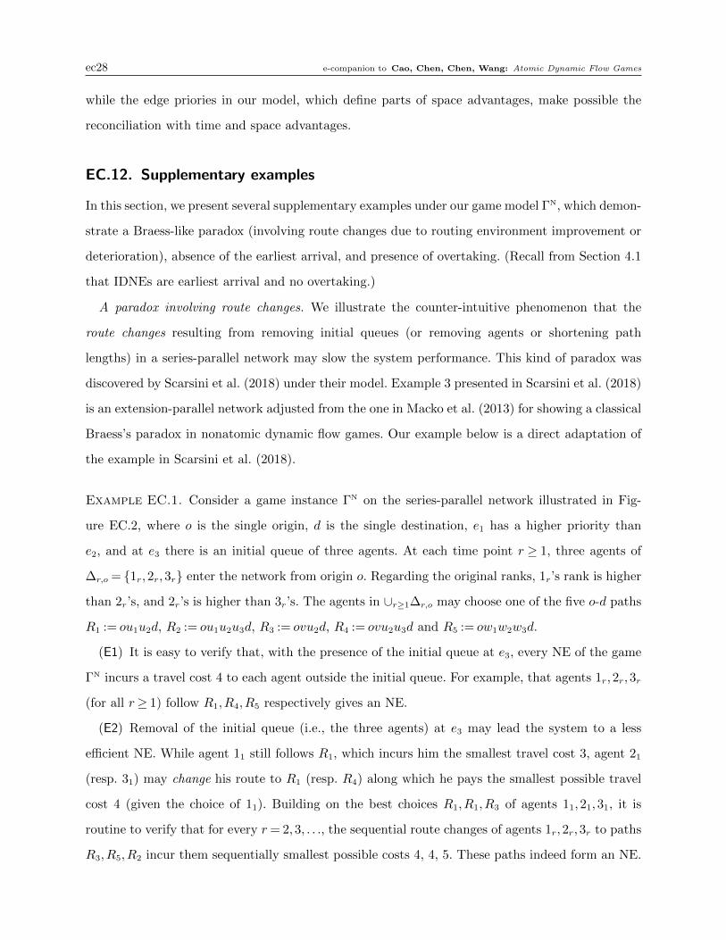
ec28 e-companion to Cao, Chen, Chen, Wang: Atomic Dynamic Flow Games
while the edge priories in our model, which define parts of space advantages, make possible the
reconciliation with time and space advantages.
EC.12. Supplementary examples
In this section, we present several supplementary examples under our game model ΓN, which demon-
strate a Braess-like paradox (involving route changes due to routing environment improvement or
deterioration), absence of the earliest arrival, and presence of overtaking. (Recall from Section 4.1
that IDNEs are earliest arrival and no overtaking.)
A paradox involving route changes. We illustrate the counter-intuitive phenomenon that the
route changes resulting from removing initial queues (or removing agents or shortening path
lengths) in a series-parallel network may slow the system performance. This kind of paradox was
discovered by Scarsini et al. (2018) under their model. Example 3 presented in Scarsini et al. (2018)
is an extension-parallel network adjusted from the one in Macko et al. (2013) for showing a classical
Braess’s paradox in nonatomic dynamic flow games. Our example below is a direct adaptation of
the example in Scarsini et al. (2018).
Example EC.1. Consider a game instance ΓN on the series-parallel network illustrated in Fig-
ure EC.2, where o is the single origin, d is the single destination, e1 has a higher priority than
e2, and at e3 there is an initial queue of three agents. At each time point r ≥ 1, three agents of
∆r,o = 1r,2r,3r enter the network from origin o. Regarding the original ranks, 1r’s rank is higher
than 2r’s, and 2r’s is higher than 3r’s. The agents in ∪r≥1∆r,o may choose one of the five o-d paths
R1 := ou1u2d, R2 := ou1u2u3d, R3 := ovu2d, R4 := ovu2u3d and R5 := ow1w2w3d.
(E1) It is easy to verify that, with the presence of the initial queue at e3, every NE of the game
ΓN incurs a travel cost 4 to each agent outside the initial queue. For example, that agents 1r,2r,3r
(for all r≥ 1) follow R1,R4,R5 respectively gives an NE.
(E2) Removal of the initial queue (i.e., the three agents) at e3 may lead the system to a less
efficient NE. While agent 11 still follows R1, which incurs him the smallest travel cost 3, agent 21
(resp. 31) may change his route to R1 (resp. R4) along which he pays the smallest possible travel
cost 4 (given the choice of 11). Building on the best choices R1,R1,R3 of agents 11,21,31, it is
routine to verify that for every r= 2,3, . . ., the sequential route changes of agents 1r,2r,3r to paths
R3,R5,R2 incur them sequentially smallest possible costs 4, 4, 5. These paths indeed form an NE.
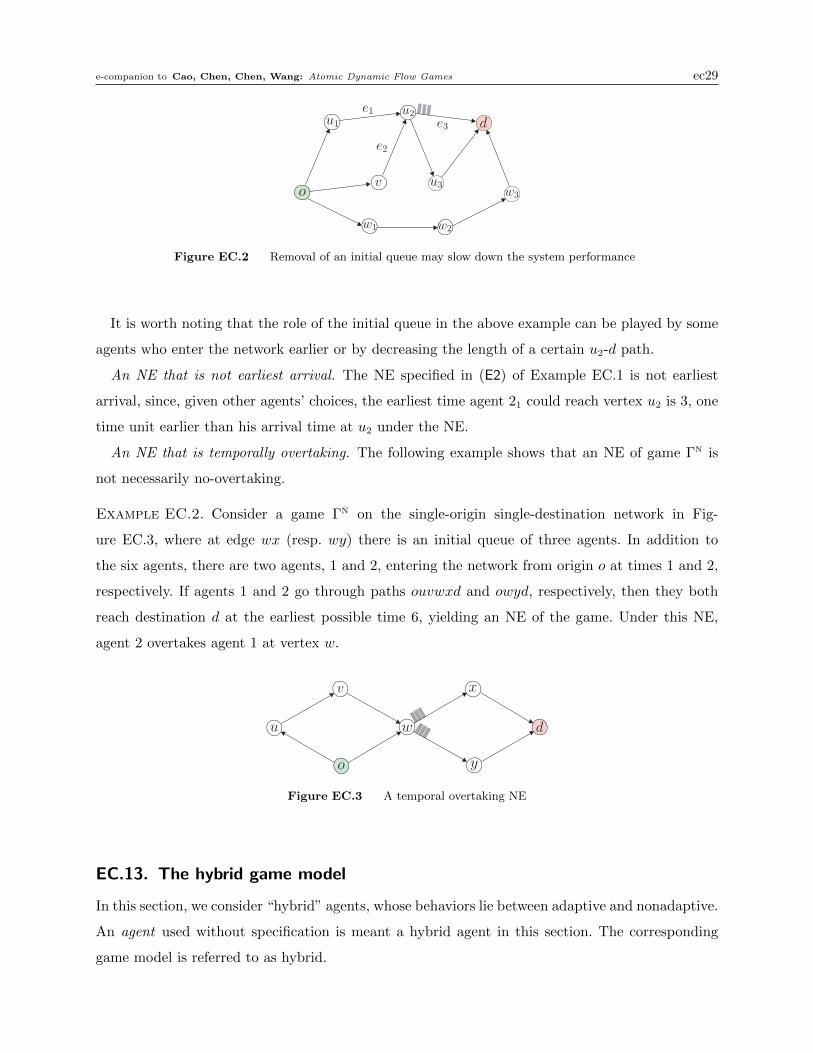
e-companion to Cao, Chen, Chen, Wang: Atomic Dynamic Flow Games ec29
Figure EC.2 Removal of an initial queue may slow down the system performance
It is worth noting that the role of the initial queue in the above example can be played by some
agents who enter the network earlier or by decreasing the length of a certain u2-d path.
An NE that is not earliest arrival. The NE specified in (E2) of Example EC.1 is not earliest
arrival, since, given other agents’ choices, the earliest time agent 21 could reach vertex u2 is 3, one
time unit earlier than his arrival time at u2 under the NE.
An NE that is temporally overtaking. The following example shows that an NE of game ΓN is
not necessarily no-overtaking.
Example EC.2. Consider a game ΓN on the single-origin single-destination network in Fig-
ure EC.3, where at edge wx (resp. wy) there is an initial queue of three agents. In addition to
the six agents, there are two agents, 1 and 2, entering the network from origin o at times 1 and 2,
respectively. If agents 1 and 2 go through paths ouvwxd and owyd, respectively, then they both
reach destination d at the earliest possible time 6, yielding an NE of the game. Under this NE,
agent 2 overtakes agent 1 at vertex w.
Figure EC.3 A temporal overtaking NE
EC.13. The hybrid game model
In this section, we consider “hybrid” agents, whose behaviors lie between adaptive and nonadaptive.
An agent used without specification is meant a hybrid agent in this section. The corresponding
game model is referred to as hybrid.
ec30 e-companion to Cao, Chen, Chen, Wang: Atomic Dynamic Flow Games
EC.13.1. Model description
For every agent i and every vertex v that is neither i’s origin nor the destination d, we are given
a probability θi,v that agent i contemplates switching to other paths at v. Let θ denote the vector
of these probabilities. We use Γ](θ) to denote the hybrid game with parameter vector θ.
While adaptive agents make routing decisions at every nonterminal vertex they reach as to which
edge to take next, hybrid agents make decisions at every nonterminal vertex as to which path to
take in the future if they are given the chances (by Nature) to reconsider their plans, and just
follow their previous plans otherwise. Intuitively, each agent always holds a plan (a path from his
current edge to the destination) and may update it with a new one when chances are given. A
precise definition of a strategy is presented as follows.
Definition EC.3 (Strategy). A strategy of agent i∈∆ is a mapping σ]i that maps each history
hr = (c0, . . . , cr) till time r with i ∈∆(cr) to σ]i (hr) such that, based on cr and the edge-priority
DQ rule, either σ]i (hr) is a path from the current edge where i stays to the destination d, or σ]i (hr)
is a null element when under cr agent i will exit G at time r+ 1.
The strategy set of agent i is denoted as Σ]i. A vector σ] = (σ]i )i∈∆ is called a strategy profile of
the hybrid game Γ](θ). Note that this game is typically a stochastic model. We use E[ti(σ]|hr)]
to denote the expected arrival time of agent i at the destination under strategy profile σ] starting
from history hr.
Definition EC.4 (SPE in the hybrid game). A strategy profile σ] = (σi)i∈∆ is a subgame per-
fect equilibrium (SPE) of Γ](θ) if for any time r ≥ 0 and any history hr ∈ Hr, E[ti(σ]|hr)] ≤
E[ti(σ]i
′, σ]−i|hr)] holds for all i∈∆(cr) and all σ]i
′∈Σ]
i such that (σ]i′, σ]−i) still leads to history hr,
where σ]−i is the partial strategy profile of σ] for agents in ∆\i.
EC.13.2. Results
As intuitively expected, we have the following observation.
Lemma EC.11. For the hybrid model Γ](θ), the case θ= 0 corresponds to the nonadaptive model
ΓN and the case θ= 1 corresponds to the adaptive model ΓA.
Proof. In fact, when θ= 0, all the plans at the non-origin vertices will never be used and hence
a strategy for a hybrid agent reduces to a strategy of a nonadaptive agent. On the other hand,
when θ= 1, all the plans at the non-origin vertices will always be given the chances to realize and
hence only the immediate next edges are meaningful for the plans and the set of these immediate
next edges is equivalent to a strategy of the adaptive agent. Q.E.D.
e-companion to Cao, Chen, Chen, Wang: Atomic Dynamic Flow Games ec31
Suppose that we are given an SPE σ for game ΓA that is constructed from an NE p of game ΓN,
as discussed in Sections 5.3 and EC.10. We construct a strategy profile σ] for the hybrid model
Γ](θ) as follows. For each history hr = (c0, . . . , cr), if all players carry out their strategies in σ, then
for each player i, a path from his current edge to the destination will be determined. We set σ]i (hr)
as this path. This defines a strategy profile σ] for the hybrid model Γ](θ).
Theorem EC.8. The strategy profile σ] constructed above is an SPE for the hybrid game Γ](θ).
Proof. By definition, it suffices to prove that, for any time r ≥ 0 and any history hr ∈ Hr,
E[ti(σ]|hr)]≤E[ti(σ
]i
′, σ]−i|hr)] holds for all i∈∆(cr) and all σ]i
′∈Σ]
i such that (σ]i′, σ]−i) still leads
to history hr, where σ]−i is the partial strategy profile of σ] for agents in ∆\i.
Consider the subgame starting from history hr. At the starting time r, all agents i at their initial
positions in the subgame hold σ]i (hr) their initial plans. Then all agents i act during time [r, r+ 1]
according to σ]i (hr), which leads to a history hr+1. By our construction presented in Section EC.10,
agent i’s new plan σ]i (hr+1) at time r + 1 is consistent with his old plan σ]i (hr) at time r, i.e.,
he does not switch his path even if he is given the chance to do so. Inductively, we see that the
realized path profiles of the two strategy profiles σ] (in game Γ](θ)) and σ (in game ΓA) are the
same. Therefore, the arrival time ti(σ]|hr) of i at the destination is also deterministic, and equals
ti(σ|hr).
Suppose that i is in the kth batch in the routings determined by σ] and hr. Consider the single-
deviation of agent i. By the construction of the SPE σ, all agents in the first k−1 batches will keep
their plans unchanged in the histories following hr. In other words, regardless of the chances given
by Nature, all agents in the first k− 1 batches will always follow their paths in the corresponding
NE p(hr) of game ΓN(cr) (see Section EC.10). Recalling the hierarchically optimality property for
any NE of game ΓN(cr), we see that ti(σ]|hr) = ti(σ|hr), the exit time of agent i, is the smallest
among all the exit times of all agents outside the first k− 1 batches under any routing in which
agents in the first k− 1 batches follow their NE routes (see Sections 4.3 and EC.7). This proves
that i cannot be better off by a unilateral deviation in game Γ](θ) and hence the constructed σ] is
an SPE. Q.E.D.
Related Documents