CHAPTER 1 WORST-CASE ANALYSIS OF TANDEM QUEUEING SYSTEMS USING NETWORK CALCULUS Anne Bouillard, 1 , Giovanni Stea, 2 1 Department of Informatics at ENS/INRIA, 45 Rue d’Ulm, 75230 Paris CEDEX 05, France ([email protected]) 2 Department of Information Engineering at University of Pisa, Largo L. Lazzarino 1, 56122, Pisa, Italy ([email protected]) Abstract. In this chapter we show how to derive performance bounds for tandem queueing systems using Network Calculus, a deterministic theory for performance analysis. We introduce the basic concepts of Network Calculus, namely arrival and service curves, and we show how to use them to compute performance bounds in an end-to-end perspective. As an application of the above theory, we evaluate tandems of network nodes with well-known service policies. We present the theory for two different settings: a simpler one, called ”per-flow scheduling”, where service poli- cies at each node discriminate traffics coming from different flows and buffer them separately, and ”per-aggregate scheduling”, where schedulers manage a small num- ber of traffic aggregates, and traffic of several flows may end up in the same queue. We show that, in the latter case, methodologies based on equivalent service curves cannot compute tight delay bounds and we present a different methodology that re- lies on input-output relationships and uses mathematical programming techniques. Keywords. Network Calculus, Worst-case Delay, Performance Bounds. Please enter \offprintinfo{(Title, Edition)}{(Author)} at the beginning of your document. 1

Welcome message from author
This document is posted to help you gain knowledge. Please leave a comment to let me know what you think about it! Share it to your friends and learn new things together.
Transcript
CHAPTER 1
WORST-CASE ANALYSIS OF TANDEMQUEUEING SYSTEMS USINGNETWORK CALCULUS
Anne Bouillard, 1, Giovanni Stea, 2
1Department of Informatics at ENS/INRIA, 45 Rue d’Ulm, 75230 Paris CEDEX 05, France([email protected])
2Department of Information Engineering at University of Pisa, Largo L. Lazzarino 1, 56122,Pisa, Italy ([email protected])
Abstract. In this chapter we show how to derive performance bounds for tandemqueueing systems using Network Calculus, a deterministic theory for performanceanalysis. We introduce the basic concepts of Network Calculus, namely arrival andservice curves, and we show how to use them to compute performance bounds in anend-to-end perspective. As an application of the above theory, we evaluate tandemsof network nodes with well-known service policies. We present the theory for twodifferent settings: a simpler one, called ”per-flow scheduling”, where service poli-cies at each node discriminate traffics coming from different flows and buffer themseparately, and ”per-aggregate scheduling”, where schedulers manage a small num-ber of traffic aggregates, and traffic of several flows may end up in the same queue.We show that, in the latter case, methodologies based on equivalent service curvescannot compute tight delay bounds and we present a different methodology that re-lies on input-output relationships and uses mathematical programming techniques.
Keywords. Network Calculus, Worst-case Delay, Performance Bounds.
Please enter \offprintinfo{(Title, Edition)}{(Author)}at the beginning of your document.
1
2 WORST-CASE ANALYSIS OF TANDEM QUEUEING SYSTEMS USING NETWORK CALCULUS
1.1 Introduction
Many of today’s networked applications rely on the underlying network providingQuality of Service (QoS) guarantees. For instance, playback applications (such asvideo or voice) require bounds on the worst-case traversal time of packets, on anend-to-end basis, the deadline being the playback instant of the video/voice packet.Moreover, there is a growing interest in new types of networked applications requir-ing firm end-to-end delay guarantees. For instance, those based on remote sensingand control, favored by the emerging of the Machine-to-Machine (M2M) commu-nication paradigm. Some of these are safety-critical, e.g., assisted driving, smartelectrical grid control, factory automation, telemedicine, etc., hence packets cannotmiss their deadlines without serious consequences. A common trait of all the aboveapplication is that they are expected to run in a multi-hop networked environment,where their traffic will experience multiple queueing, contending for resources (i.e.,bandwidth and buffers space) with traffic from heterogeneous applications.
Despite the abundance of literature on the matter, in the past decades the prob-lem of QoS guarantees has been tackled by network providers mainly through blindoverprovisioning: overdimensioning links with respect to the traffic they had tocarry, achieving utilization factors far below saturation, was in fact enough to en-sure, at least statistically, that end-to-end delays were small enough to allow delay-sensitive applications to run smoothly. This trend cannot go on forever for severalreasons: first, bandwidth availability traditionally spawns bandwidth-hungry appli-cations, leading to an arms race which will settle on links being close to saturationbefore a new technological breakthrough occurs. Second, network overprovisioningis not cost-effective, as it requires both larger investments and higher operational ex-penditures. With respect to the latter, network energy efficiency has recently becomean issue, attracting itself a noticeable amount of research: one of the keys to energyefficiency is to disable the portions of a network that are not strictly necessary toensure a given level of service, which amounts to keeping the rest of the networkmuch closer to saturation than an overprovisioning strategy would otherwise have.Last, but not least, some services just cannot do without firm, a priori guarantees,as opposed to measurement-based, a posteriori statistical assurances. To begin with,even non-critical applications such as high-definition IPTV may require such guar-antees: for instance, if they are to be sold to a large consumer audience which mightnot tolerate even occasional video glitches. Moreover, it is self evident that, with re-mote sensing/control or safety-critical applications, delay guarantees define the verycorrectness of the applications’ behavior.
Network Calculus (NC) is a theory that allows one to compute bounds on signif-icant quantities (most notably, the end-to-end delay) in a queueing network. It hasbeen devised in the ’90s, thanks to the seminal works of Cruz [21, 22], Chang [19],and Le Boudec and Thiran [26]. It relies on a deterministic service and traffic char-acterization (as opposed, for instance, to Markov Chains, which rely on stochasticcharacterizations), hence it is particularly useful for assessing worst-case measures,such as the maximum delay. NC has already been used in several domains. As faras the Internet is concerned, the Guaranteed Service of the IP IntServ architecture

INTRODUCTION 3
[15], standardized in 1994, is based on delay bounds computed through NC. Morerecently, NC has been used to assess the performance of AFDX avionic networks [1],which require a certification of the maximum end-to-end delay before being madeoperational. Furthermore, it has been applied to design or assess the performanceof Network-on-Chips [24], Systems-on-Chips, e.g., [18], Wireless Sensor Networks[25, 32, 39], Wireless Mesh Networks [16, 17], and industrial Ethernet installations[37].
Performance analysis through Network Calculus is normally carried out with re-spect to a single flow of traffic, which traverses a tandem network from its source toits destination, and contends for bandwidth with similar flows at each hop (e.g., theoutput port of a switch or router). Contention is usually arbitrated by a schedulingpolicy (e.g., non-preemptive strict priority, round-robin, etc.), in either of the fol-lowing settings: a per-flow scheduling approach, where each flow has a dedicatedFIFO queue, and the scheduler determines the flow that gets access to the outputbandwidth at each time, or an aggregate-multiplexing approach, where traffics fromdifferent flows may be buffered in the same queue (which may or may not also com-pete with others for access to a link’s bandwidth). In this last case, embodied inInternet standards such as IP DiffServ architecture [5], the buffering policy becomesrelevant as well: if flows are buffered FIFO, then what gets in will eventually get out,hence the delay of a packet will stay finite as long as the queue does not grow indef-initely, although it will depend on the arrival profile of all the flows that are bufferedin the same queue. On the other hand, if non-FIFO queueing is adopted, a packetmay sit forever in the buffer, being constantly pushed at the back by other incomingpackets, even if the queue length stays finite.
It turns out that the main watershed in NC modeling is whether a per-flow or anaggregate-multiplexing network is analyzed: in the former case, it is easy to deriveservice guarantees for single flows at a node, and to compose these guarantees alonga path to compute an end-to-end guarantee. Perhaps the most interesting feature ofNC is that – in this case – the composition of service guarantees preserves tightness:if the individual service guarantees allow one to compute the true worst-case delay ateach node, then their composition will yield the true end-to-end worst-case delay, andnot just a bound on the latter: in other words, all the relevant information is preservedwhen composing service guarantees. In the second case, i.e., aggregate-multiplexing,per-node guarantees are harder to obtain, to begin with, and composing them along amulti-hop path leads to a loss of tightness [2, 34]: the end-to-end delay that one getsby composing per-node service guarantees is often a loose, pessimistic upper boundon the worst-case delay. Thus, in this case, a different method is required, which doesnot exploit composition, but relies instead on mathematical programming techniques.
This chapter presents the theory of Network Calculus in a tutorial way, focusingon its practical implications whenever possible, using examples that a reader who ismildly familiar with packet scheduling will find easy to understand. It is divided intotwo parts: in the first part we explain the basics of NC, describing the concepts ofservice curve and arrival curve. Then, we show how to derive performance boundsfor a network flow in a per-flow scheduling approach. The second part builds ontop of these basic concepts to explain how to compute the worst-case delay in an
4 WORST-CASE ANALYSIS OF TANDEM QUEUEING SYSTEMS USING NETWORK CALCULUS
aggregate-multiplexing network, describing both the cases of FIFO and non-FIFOqueueing.
Despite the fact that this chapter is written using computer networks as a casestudy, most of the modeling shown herein can be applied – with few modifications– to other contexts where there is contention for resources and scheduling, notablydistributed systems.
1.2 Basic Network Calculus Modeling: per-flow scheduling
Assume that you are observing the traffic of a given flow at the input and outputof a network element, e.g., a scheduler. That network element may, of course, betraversed by several flows simultaneously, however we are interested in what happensto a particular flow, which we call the tagged flow. Denote with A(t) and D(t)the functions of time that count how much traffic belonging to the tagged flow hasbeen observed in [0, t), respectively at the input and output of the network element.We call these the Cumulative Arrival Function (CAF) and the Cumulative DepartureFunction (CDF) for the flow. Assume that the system is time-continuous, i.e., arrivalsand departures can occur at any time, unlike in a slotted system (different, simplermodels can be used to describe the latter). CAFs and CDFs need not be continuous,to reflect that a discrete quantity of traffic (e.g., a burst) can arrive and leave at once.
Furthermore, assume that the network element is lossless, that it does not generatetraffic, and that it serves the traffic of the tagged flow in FIFO order. For a networkelement to be lossless, traffic must be buffered, and the buffer must be large enoughnot to overflow. For now, we will just state that overflows do not occur, and later onwe will quantify the buffer required in order for this hypothesis to hold.
Obviously enough, both A(t) and D(t) – being cumulative functions of time –must be wide-sense increasing. Furthermore, for the element to be causal it must beA(t) ≥ D(t). When there is no ambiguity, we will write A ≥ D to denote that thelatter holds for any time instant t. Unless stated otherwise, all cumulative functionsR are defined as R : R+ → R+, are left-continuous and such that R(0) = 0.
If one can measure the CAF and CDF of a network element, then it is fairly easy tocompute some quantities, namely the delay of a bit and the backlog at any one time.As Figure 1.1 shows, the vertical distance B(τ) = A(τ) − D(τ), which is alwaysnon-negative, is the element’s backlog at time τ . Conversely, the horizontal distancebetween point (τ, a) on A and point (τ ′, a) on D, i.e., d(τ) = τ ′ − τ , is the delay ofthe bit that enters the element at time τ . Note that, if the CDF has a plateau at quotaa, then the definition still holds, provided that we set τ ′ = inf{s : D(s) ≥ a}. Moreformally, the delay of a bit arriving at time τ is equal to:
d(τ) = inf{s ≥ 0 : A(τ) ≤ D(τ + s)}.

BASIC NETWORK CALCULUS MODELING: PER-FLOW SCHEDULING 5
Figure 1.1 CAF and CDF at a network element
1.2.1 Service curve
If a network element provides some QoS guarantees, as most schedulers do (e.g., aminimum departure rate), then it stands to reason that – given an input CAF A – thepossible output CDFs D should be lower-bounded, and that the lower bound shouldbe a function of both the CAF and some inherent property of the network elementitself. In fact, we say that the network element can be modeled through the servicecurve β if:
∀t ≥ 0, D(t) ≥ inf0≤s≤t
(A(s) + β(t− s)). (1.1)
The right-hand side of eq. (1.1) is the lower bound to the CDFD we were just talkingabout, and in this case the flow is said to be guaranteed the (minimum) service curveβ. The infimum at the right side of eq. (1.1), as a function of t, is called the min-plusconvolution of A and β, and is denoted by A⊗β. The name “min-plus convolution”stems from the fact that the operation resembles systems theory convolution, if onereplaces the sum with the infimum operator and the product with the sum. Theservice curve of a network element is not something that can be observed by justmeasuring one CAF and the related CDF. It is instead a property of the networkelement, such that eq. (1.1) holds for any CAF. In fact, a network element may bestateful (schedulers usually are), hence one trajectory alone cannot provide muchinformation regarding worst-case behavior.
Before delving deeper into the properties of the convolution operation, which areimportant to understand the rest of the chapter, we show how to derive a service curvein a couple of practical cases, namely strict-priority and round-robin schedulers.
1.2.1.1 Example – strict-priority scheduler Assume that the tagged flow is be-ing scheduled by a non-preemptive strict-priority scheduler. The latter serves onepacket from the highest-priority backlogged flow, and waits for a packet to be trans-mitted before making another decision (hence being non-preemptive). Assume thatthe tagged flow is the top-priority one, and that there are other flows with lower pri-orities. Let C be the speed of the link managed by the scheduler, and let M be theMaximum Transfer Unit on the link (i.e., the maximum-sized packet allowed on the

6 WORST-CASE ANALYSIS OF TANDEM QUEUEING SYSTEMS USING NETWORK CALCULUS
link). Assume that the tagged flow sends an infinite amount of traffic in a singleburst at time t = 0, i.e., A(t) = δ0(t), and let us compute what the lower boundon its CDF will be. Notation δx(t) denotes a function which is null for t ≤ x, andinfinite for t > x. In a worst-case scenario, at time 0 the scheduler is busy servingsome other lower-priority flow. The server may be at it for a maximum time equalto T = M/C, then – by the very definition of strict priority – it must switch to serv-ing the tagged flow. Once it starts (since the tagged flow is always backlogged), itwill keep transmitting traffic from it. Therefore, the CDF for the tagged flow will beD(t) = (C · t−M)+. Notation x+ means max(x, 0). Figure 1.2 depicts the abovescenario. Now, it is D(0) = A(0) = 0, hence we can write:
D(t) ≥ A(0) + (C · (t− 0)−M)+ (1.2)
By setting s = 0 in eq. (1.1) , eq. (1.2) implies that β(t) = (C · (t − 0) −M)+ =C · (t − T )+ is a service curve for the tagged flow. The shape of this service curveis very common in practice, as we shall see, and its name is rate-latency curve: therate is the long-term slope, i.e., C, and the latency is its horizontal offset, i.e., T .
Note that, to keep the parallel with classical systems theory, the service curve hasbeen computed by giving an impulse as an input to the system and measuring itsworst-case output. Therefore, the service curve can be thought of as a worst-caseimpulse response for a network element.
Finally, note that the above reasoning cannot be generalized to flows having lowerpriority. In fact, unless all higher-priority flows are somewhat regulated, i.e., pre-vented to keep their queues always backlogged, lower-priority flows will simplystarve. This means that (without calling in additional mechanisms, at least) theworst-case impulse response for a lower-priority flow in a strict-priority scheduleris flat.
Figure 1.2 Strict-priority scheduling scenario
1.2.1.2 Example – round-robin scheduler Assume that the tagged flow is servedby a weighted round-robin scheduler. The scheduler managesN queues, one for eachflow, and each flow i has a quantum φi, a positive quantity representing the amountof time that the server spends in transmitting traffic from queue i before moving on
BASIC NETWORK CALCULUS MODELING: PER-FLOW SCHEDULING 7
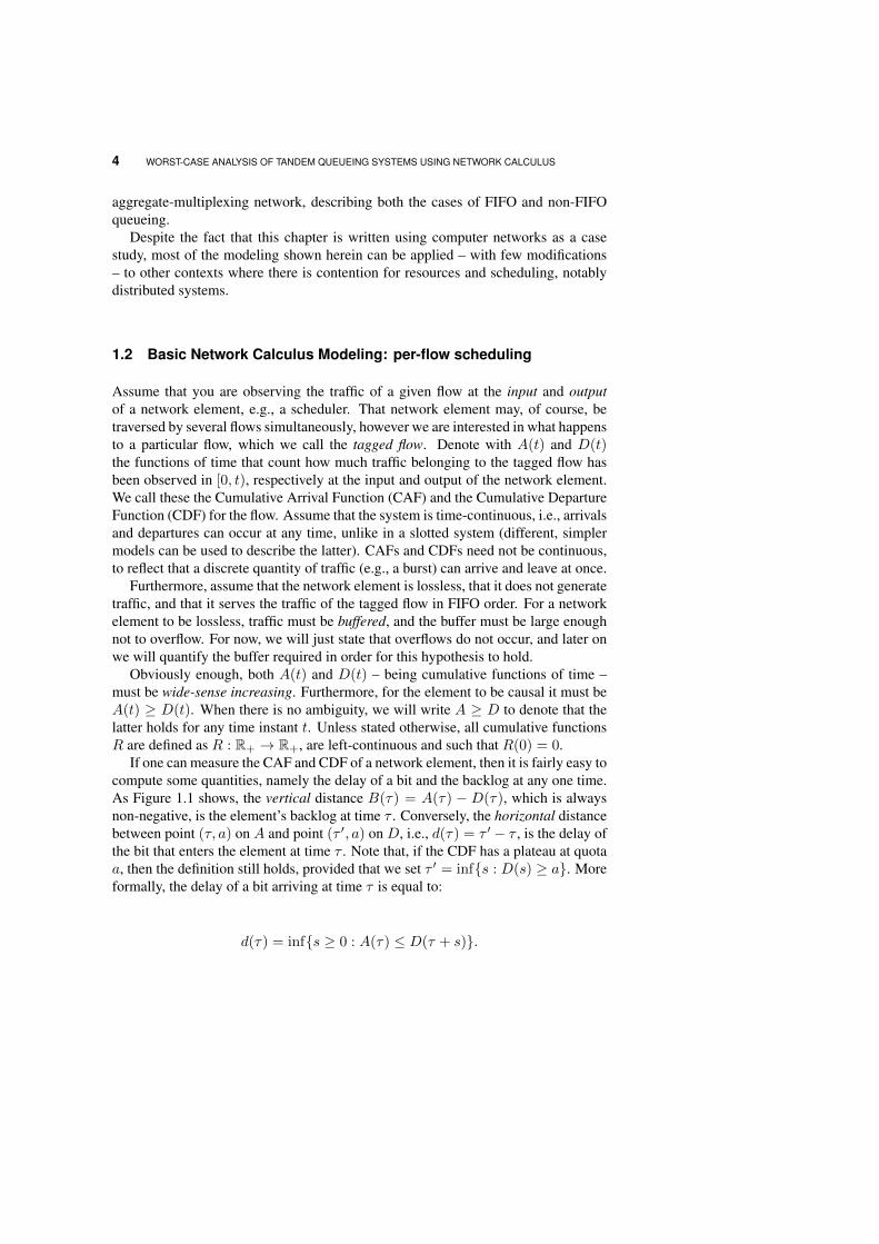
to queue (i + 1) mod N . Let the link speed be equal to C again, and assume forsimplicity that traffic may be arbitrarily fragmented, so that each flow may fill thequantum entirely if it has enough backlog. Without loss of generality, assume that thetagged flow is flow 1, and let its CAF be again the impulse at time 0, A(t) = δ0(t).The worst-case CDF is observed when: a) all flows 2 . . . N are always backlogged,and b) the server is at the beginning of the service period for flow 2 at time 0. In thiscase, the CDF of tagged flow 1 will be null until time T1 =
∑i=2...N φi, and then
increases with a slope C until time P = T1 + φ1 =∑i=1...N φi. The same pattern
repeats indefinitely, as shown in Figure 1.3.Using the same reasoning as in the previous example, one may conclude that the
worst-case impulse response CDF is again the system’s service curve for the taggedflow. Note that the long-term guaranteed rate of the tagged flow r1 can be expressedas a proportion of the quanta of the various flows, i.e., r1 = C · φ1/(
∑i=1...N φi).
This holds, rather obviously, for any flow j being scheduled.Note that the shape of the service curve for a round-robin scheduler is not a rate-
latency one. However, it is easy to see that one rate-latency curve exists that boundsthat service curve from below: it is the one with a latency equal to T1 and a rate equalto r1, i.e., β(t) = r1 · (t−T1)+. Curve β still verifies eq. (1.1), since it bounds frombelow a curve that does. Moreover, it is the largest rate-latency one that does, sinceit touches the worst-case impulse response CDF at abscissas T1 + k · P,∀k ≥ 0.Therefore, one may use β as a service curve for the tagged flow as well. We will seethat this makes computations simpler, but it comes with a price.
Finally, let us observe what happens if all the quanta are doubled. On one hand,the minimum guaranteed rate ri of each flow will remain the same, since it dependson the ratio of the quanta. On the other hand, the latency of the β service curvewill double: this hints at the fact that each flow (including the tagged one) will havethe same throughput, but – in general – higher delays, something that we will proveformally later on.
Figure 1.3 Round-robin scheduling scenario
1.2.1.3 Other types of service curves Links and nodes (i.e., routers or switches)can also be seen as network elements providing service-curve guarantees. Morespecifically, following the same approach used in the previous two cases, it is fairly

8 WORST-CASE ANALYSIS OF TANDEM QUEUEING SYSTEMS USING NETWORK CALCULUS
easy to observe that a link with a constant rate C (often called a constant-rate server)has a service curve β(t) = C · t, which we also represent by λC . By the same token,a link with a minimum rate C (e.g., a wireless link that can switch its rate betweena minimum and a maximum) has the same service curve. The two are clearly notequal in all respects: with the former, we can obtain the exact CDF given the CAF,whereas with the latter we can only know a lower bound on the CDF. However, asfar as service guarantees are concerned, the two can be described in the same way. Itcan also be observed that several fair queueing schedulers, including Weighted FairQueueing [31], Deficit Round Robin [36, 28] and others [38] all exhibit rate-latencyservice curves.
Some elements (e.g., network switches) exhibit a bounded transit delay, at leastunder appropriate testable hypotheses (e.g., in the absence of overload). This isalso the case, for instance, of deadline-based schedulers, such as Earliest DeadlineFirst scheduling, if the admission control (or schedulablity) test is passed. For theseelements, the service curve is the delayed impulse δT .
Figure 1.4 reports both the above service curves. It is interesting to observe thatboth a minimum-rate and a delay service curve are special cases of a rate-latencyservice curve. More specifically, if βR,T denotes a rate-latency curve with a rate Rand a latency T , it is λR = βR,0 and δT = β∞,T .
Figure 1.4 A constant/minimum-rate-server service curve (left) and a delay-element servicecurve (right)
1.2.1.4 Useful properties of the convolution operator The result of the convo-lution operation A⊗β can easily be found graphically. Recalling eq. (1.1), it is easyto see that D can be found by sliding the service curve over the CAF, as shown inFigure 1.5, and taking the minimum of the results at each time instant.
Some properties of convolution that will be used later on in this chapter are thefollowing:
convolution is commutative and associative: A⊗B ⊗ C = (B ⊗A)⊗ C;
the neutral element with respect to convolution is the impulse δ0: A⊗ δ0 = A;

BASIC NETWORK CALCULUS MODELING: PER-FLOW SCHEDULING 9
Figure 1.5 Graphical interpretation of the convolution operation
conversely, convolution with a delayed impulse δT just shifts a function rightby T : (A⊗ δT )(t) = A(t− T );
the convolution of two concave curves taking value 0 at 0 is equal to their min-imum: if A,B are concave, A⊗B = min{A,B}.
The proof of the above properties is trivial and is thus left to the reader. Anotheruseful property of convolution is given by the following lemma:
Lemma 1 [6] If f and g are left-continuous and wide-sense increasing, then for allt ≥ 0, there exists s ≤ t such that f ⊗ g(t) = f(s) + g(t− s).
1.2.1.5 Composition of service curves Suppose now that the tagged flow tra-verses a tandem of n network elements: for instance, a multi-hop path in a networkdomain, at each hop of which the flow is scheduled by some scheduler, as shown inFigure 1.6. Suppose that, at each network element i, the tagged flow is guaranteed aservice curve β(i). Clearly, the CDF at node i of the path will be equal to the CAFat node i + 1, ∀i < n. Therefore, we simply use F (i) to denote the CDF at node i,and assume that F (0) is the CAF at node 1. The service curve property ensures thatF (i) ≥ F (i−1) ⊗ β(i). Therefore, by the associativity of convolution, we get:
F (N) ≥ F (0) ⊗{β(1) ⊗ β(2) ⊗ ...⊗ β(n)
}= F (0) ⊗
{n⊗i=1
β(i)
}(1.3)
Figure 1.6 A tandem of network elements traversed by a flow

10 WORST-CASE ANALYSIS OF TANDEM QUEUEING SYSTEMS USING NETWORK CALCULUS
The last term in eq. (1.3) can be regarded as the service curve that the wholetandem offers to the tagged flow. In fact, it computes a lower bound to the CDFat the exit of the tandem, given the CAF at the ingress. Note that no hypothesisis required on each network element, other than that it provides the tagged flowwith a service curve guarantee. For instance, the above result holds for a two-hoppath where the tagged flow traverses a strict-priority scheduler and a round-robinscheduler. Therefore, the only thing that is needed to allow for multi-node analysisis to compute the convolution of the service curves at each node.
Convolution of rate-latency service curves is particularly easy to compute. Letus compute the convolution of β(i) = βRi,Ti , i = 1, 2. Without loss of generality,assume that R1 ≥ R2 (convolution is in fact commutative). Recalling Figure 1.5,one has to “slide” one rate-latency curve along the other and consider the minimumordinate for each abscissa. As shown in Figure 1.7, this implies that the resultingcurve will be null until T = T1 + T2. Then, the result will increase with a rate equalto R = min{R1, R2}.
Figure 1.7 Convolution of two rate-latency service curves
By iterating the reasoning n times, we obtain that the convolution of n rate-latencyservice curves is as follows:
n⊗i=1
βRi,Ti = βmini{Ri},∑n
i=1 Ti(1.4)
Equation (1.4) makes sense intuitively: the minimum guaranteed rate for a flowtraversing a tandem of node is the minimum among those guaranteed at each node.Furthermore, in a worst-case scenario, the flow will experience the maximum latencyat each node, hence latencies should add up.
Finally, we observe that a rate-latency service curve βR,T may be obtained as theconvolution of a minimum-rate service curve λR and a delay service curve δT .
1.2.1.6 Strict service curves In some cases, network elements provide tighterservice guarantees than those captured by the service curve property. A commonguarantee is that of the strict service curve. We say that a network element offersa strict service curve β to a flow if, for any period ]s, t] during which the flow is

BASIC NETWORK CALCULUS MODELING: PER-FLOW SCHEDULING 11
backlogged, then it is:
D(t)−D(s) ≥ β(t− s). (1.5)
It is straightforward to prove that if β is a strict service curve, then it is alsoa service curve. In fact, since eq. (1.5) holds for any backlogged period, it alsoholds if s is the beginning of a backlogged period, which we denote start(t). Inthis case, it is A(s) = D(s) by definition, hence we have found one instant whenD(t) ≥ A(s) + β(t − s), which implies eq. (1.1). The reverse, however, is false,thus the strict service curve property is – in fact – a stricter guarantee than the servicecurve.
With reference to the examples of the previous subsections, the service curvesof a strict-priority and round-robin scheduler, and of a constant- and minimum-rateserver, are also strict service curves. On the other hand, the delay element servicecurve is not a strict service curve. The proof of this result can be found in [26,Chapter 7].
An interesting – though unfortunate – result is that the strict service curve prop-erty is not preserved through composition: if β(1) and β(2) are strict service curvesoffered by two nodes traversed by the tagged flow, then we cannot say that the two-node tandem offers a strict service curve equal to β = β(1) ⊗ β(2). In fact, it turnsout that β is a service curve (because strict service curves are service curves, in anycase), but not a strict one.
Over the years, several other proposals of service guarantees have appeared inthe literature, with the aim to find stricter guarantees than the service-curve ones,which are still preserved through composition – unlike the strict service curve prop-erty. A comprehensive description on the subject can be found in [6]. Strict servicecurves will come again into play later in this chapter, when we examine aggregate-multiplexing architectures.
1.2.2 Arrival Curve
The theory expressed so far allows us to compute a lower bound on the CDF ofa tagged flow at the exit of a tandem of network elements, given its CAF and theservice curve of each element. Furthermore, by plotting the CAF and the CDF onthe same reference, we can assess the delay of each bit, and the amount of traffic intransit (i.e., the backlog) at each time instant. To compute the maximum delay thata bit of the tagged flow experiences, we must find the maximum horizontal distancebetween the CAF and CDF. Obviously, the maximum delay will depend on the CAFitself: in general, assuming a rate-latency service curve, we can say that the delayincreases whenever the slope of the CAF exceeds the minimum guaranteed rate ofthe service curve, whereas it decreases when the opposite is true. If we can limit therate of the arrivals, then, in such a way that – in a long term – the arrival rate will notexceed the minimum guaranteed rate, we should be able to compute a finite boundon the maximum delay. A common way to represent constraints on the arrivals of a

12 WORST-CASE ANALYSIS OF TANDEM QUEUEING SYSTEMS USING NETWORK CALCULUS
flow in Network Calculus is the concept of arrival curve.1 A wide-sense increasingfunction α is said to be an arrival curve for a flow characterized by a cumulativefunction A (or, equivalently, A is α-upper constrained) if:
∀τ ≤ t, A(t)−A(τ) ≤ α(t− τ). (1.6)
The alert reader may check that eq. (1.6) is equivalent to A ≤ A⊗α. Graphicallyspeaking, the constraint can be visualized by sliding the arrival curve over the CAF:if the CAF never crosses one arrival curve, then eq. (1.6) holds. This is shown inFigure 1.8.
A commonplace network element that enforces an arrival curve is the leaky-bucketshaper. The latter is often placed at the ingress of a network path, in order to limitthe amount of traffic injected by the flow, thus preventing it from causing excessivequeueing in the network. A leaky-bucket arrival curve is characterized by a sustain-able rate ρ and a burst size σ, and its expression is γσ,ρ(t) = σ + ρt if t > 0 andγσ,ρ(0) = 0. Roughly speaking, it means that the flow is allowed to inject traffic at arate up to ρ. It can only exceed that rate by a maximum of σ bits over any interval oftime. This means that a flow cannot buy any extra credit by not sending traffic at itsmaximum allowed rate for some time. This is evident in Figure 1.8, where, at timet1, the CAF of the flow is considerably below α(t), but is still subject to the tighterupper constraint represented by α(t− t1) +A(t1) in any case.
Figure 1.8 Leaky-bucket arrival curve
In most practical cases, arrival curves are concave (such as the leaky-bucket one).It is not uncommon to find piecewise-linear, concave arrival curves (taking value0 at 0), which are practically implemented by using multiple leaky-bucket shapers.For instance, the Guaranteed Service of the IntServ architecture [15] provides a flowwith delay guarantees under the hypothesis that its traffic is shaped by a doubleleaky-bucket, whose arrival curve is depicted in Figure 1.9: a first stage limits thepeak rate to p with a burst size of one packet M , and a second stage allows for asmaller sustainable rate ρ, with ρ ≤ p and a burst σ, with σ ≥ M . This means thatonly the traffic that obeys both the peak-rate and the sustainable-rate constraints will
1Mind the distinction between cumulative arrival function and arrival curve.

BASIC NETWORK CALCULUS MODELING: PER-FLOW SCHEDULING 13
be allowed in. A piecewise-concave arrival curve can be constructed as the minimumof affine curves. For instance, the one in Figure 1.9 can be easily observed to beα = min{γM,p, γσ,ρ}. Therefore, by the properties of convolution, we can alsowrite α = γM,p ⊗ γσ,ρ. This means that any piecewise concave arrival curve can bewritten as the convolution of as many affine arrival curves as its linear pieces.
Figure 1.9 Double leaky-bucket arrival curve
1.2.3 Delay and backlog bounds
Knowing both the arrival curve α and service curve β of a flow allows one to computea bound on the backlog and delay. The bounds are the following (proofs are omitted,and the interested reader can find them in [26, Chapter 1]):
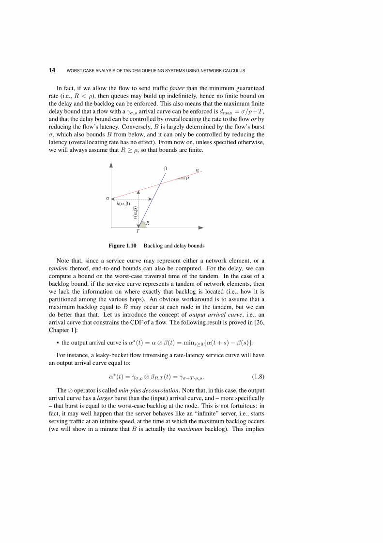
a bound on the delay is given by the maximum horizontal deviation between αand β:
h(α, β) = maxt≥0{inf s ≥ 0 : α(t) ≤ β(t+ s)};
a bound on the backlog is given by the maximum vertical deviation between αand β:
v(α, β) = maxt≥0{α(t)− β(t)}.
The meaning of the above expressions (also shown in Figure 1.10) is the follow-ing: given a CAF that conforms to the arrival curve α, fed as input to a system whoseservice curve is β, the maximum delay (backlog) that a bit experiences will not ex-ceed the ones reported above. The backlog bound can thus be used to dimension thequeue at a node so that no overflows occur.
For instance, for a leaky-bucket-shaped flow, whose arrival curve is γσ,ρ, travers-ing a rate-latency network element whose service curve is βR,T , the bounds on thedelay and backlog are:
d =
{+∞ R < ρ
σ/R+ T R ≥ ρ,B =
{+∞ R < ρ
σ + T · ρ R ≥ ρ.(1.7)
14 WORST-CASE ANALYSIS OF TANDEM QUEUEING SYSTEMS USING NETWORK CALCULUS
In fact, if we allow the flow to send traffic faster than the minimum guaranteedrate (i.e., R < ρ), then queues may build up indefinitely, hence no finite bound onthe delay and the backlog can be enforced. This also means that the maximum finitedelay bound that a flow with a γσ,ρ arrival curve can be enforced is dmax = σ/ρ+T ,and that the delay bound can be controlled by overallocating the rate to the flow or byreducing the flow’s latency. Conversely, B is largely determined by the flow’s burstσ, which also bounds B from below, and it can only be controlled by reducing thelatency (overallocating rate has no effect). From now on, unless specified otherwise,we will always assume that R ≥ ρ, so that bounds are finite.
Figure 1.10 Backlog and delay bounds
Note that, since a service curve may represent either a network element, or atandem thereof, end-to-end bounds can also be computed. For the delay, we cancompute a bound on the worst-case traversal time of the tandem. In the case of abacklog bound, if the service curve represents a tandem of network elements, thenwe lack the information on where exactly that backlog is located (i.e., how it ispartitioned among the various hops). An obvious workaround is to assume that amaximum backlog equal to B may occur at each node in the tandem, but we cando better than that. Let us introduce the concept of output arrival curve, i.e., anarrival curve that constrains the CDF of a flow. The following result is proved in [26,Chapter 1]:
the output arrival curve is α∗(t) = α� β(t) = mins≥0{α(t+ s)− β(s)}.
For instance, a leaky-bucket flow traversing a rate-latency service curve will havean output arrival curve equal to:
α∗(t) = γσ,ρ � βR,T (t) = γσ+T ·ρ,ρ. (1.8)
The� operator is called min-plus deconvolution. Note that, in this case, the outputarrival curve has a larger burst than the (input) arrival curve, and – more specifically– that burst is equal to the worst-case backlog at the node. This is not fortuitous: infact, it may well happen that the server behaves like an “infinite” server, i.e., startsserving traffic at an infinite speed, at the time at which the maximum backlog occurs(we will show in a minute that B is actually the maximum backlog). This implies
BASIC NETWORK CALCULUS MODELING: PER-FLOW SCHEDULING 15
that, at the output, a burst equal to the maximum backlog must be observable in prac-tice. This also confirms a remarkable phenomenon, often observed in networking:queueing may increase the burstiness of a flow. In fact, as a flow traverses a net-work, the alternance of periods where it is served at full speed and periods where itis not served (typical, for instance, of round-robin schedulers), creates bursts evenwhen the original traffic is smooth. We can use the above result to compute tighterbacklog bounds at each node in a tandem, where the CDF at a node is the CAF atthe subsequent one. Call α(j) the arrival curve at the output of node j of an n-nodetandem, and assume α(0) = γσ,ρ to be the arrival curve at the input. Then, assumingthat ρ ≤ min1≤i≤n{Ri}, the backlog bound at node j is the burst of the followingarrival curve:
α(j) = γσ,ρ � (j⊗i=1
βRi,Ti) = γσ+
∑ji=1 Ti·ρ,ρ. (1.9)
Moreover, the backlog bound for the whole system is equal to σ+∑ni=1 Ti ·ρ, i.e., to
the backlog bound at node n. This means that the buffer space required for losslessoperation increases from node 1 to node n, and at node n it is equal to the maximumamount of traffic in transit at any time in the whole tandem.
We now show that the above bounds are tight. We do this by constructing aworst-case scenario, i.e., a trajectory of the CAF and CDF of the system such thattheir maximum horizontal/vertical distances are those predicted by the equations. Welimit ourselves to a leaky-bucket-shaped flow traversing a rate-latency service curve,hence making reference to eq. (1.7). However, the result holds for arbitrary arrivaland service curves. Assume that the CAF is the greedy function, i.e., A = γσ,ρ. Inother words, the flow sends as much traffic as allowed by its arrival curve, startingat time t = 0. Furthermore, assume that the network element (e.g., a strict-priorityscheduler) is lazy (or exact), meaning that it behaves so that D = A ⊗ β, withβ = βR,T . The CDF can be computed algebraically using some of the properties ofthe convolution operator that we have explained earlier, i.e.:
D = γσ,ρ ⊗ βR,T = γσ,ρ ⊗ δT ⊗ γ0,R = min{γσ,ρ, γ0,R}(t− T ). (1.10)
Figure 1.11 shows the CAF and the CDF. By visual inspection, it is straightfor-ward to observe that d = d(0+) and B = A(T ) −D(T ) when R ≥ ρ. Conversely,when R < ρ, then the horizontal and vertical distance between A and D are increas-ing functions of t, hence the bounds are infinite. Thus, we have a scenario where thebounds of eq. (1.7) are attained.
Therefore, in this case, B is the worst-case backlog, and d is the worst-case delay(WCB/WCD for short, hereafter). Note that the worst-case scenario needs not beunique. For instance, the WCD is the same for: i) any CAF A such that: A(0+) = b,and ii) any CDF D such that D ≤ A, D ≥ A ⊗ β and D(d) = b. The alert readercan easily construct an infinity of scenarios that verify the above two properties.Furthermore, we observe that the WCB needs not be experienced by the same bitthat experiences the WCD. The output arrival curve is a tight constraint as well. Infact, we can obtain a CDF D = γσ+T ·ρ,ρ(t + T ) by giving as input to the node thegreedy CAFA = γσ,ρ and assuming that the node serves traffic at an “infinite” speedafter sleeping for its latency T , as already anticipated.

16 WORST-CASE ANALYSIS OF TANDEM QUEUEING SYSTEMS USING NETWORK CALCULUS
Figure 1.11 Worst-case scenario for a leaky-bucket-shaped flow traversing a rate-latencyservice curve element. Left: R ≥ ρ. Right: R < ρ.
Another example, this time involving a multi-node scenario, is shown in Fig-ure 1.12. A leaky-bucket-shaped flow traverses a tandem of n rate-latency servicecurves β(i) = βRi,Ti , with ρ ≤ min1≤i≤n{Ri} so as to ensure that the delay boundis finite. Eq. (1.4) tells us that the tandem is equivalent to a rate-latency service curve,hence a delay bound is:
d = h(γσ,ρ,n⊗i=1
βRi,Ti) =σ
mini{Ri}+∑n
i=1Ti. (1.11)
A bit of a CAF experiences a delay equal to d in the following scenario:
the CAF is greedy, hence A = F (0) = γσ,ρ;
node j = arg min{Ri} is lazy, i.e., F (j) = F (j−1) ⊗ β(j);
each node i 6= j serves traffic at an infinite slope after sleeping for its latency Ti.In other words, it translates a CAF F (i−1)(t) into a CDF F (i)(t) = F (i−1)(t−Ti).
Figure 1.12 Worst-case scenario in a multi-node traversal.
Figure 1.12 shows that the delay of bit (0+, σ) of the CAF is exactly d. Thefollowing observations are in order: first of all, the position of node j does not matter:

BASIC NETWORK CALCULUS MODELING: PER-FLOW SCHEDULING 17
it can be any node in the tandem, including the first/last. This is in perfect accordwith the fact that convolution is commutative and associative. Second, once more,this is not the only worst-case scenario. The alert reader can easily check that thesame delay would have been experienced by the same bit, if all nodes had been lazy,or if any subset of them including node j had been lazy. This means that node j,acting as a bottleneck, is the one whose behavior matters the most. Increasing itsrate, for instance, will reduce the WCD, whereas increasing some other node’s ratewill not. Equation (1.11) has a deep significance. In fact, a bound on the end-to-enddelay could also be computed – in principle – by adding up the WCD that the flowcan experience at each node. Call d(j) the WCD experienced at node j. The lattercan be computed as d(j) = h(α(j), β(j)), with α(j) being given by eq. (1.9). Aftersome straightforward algebraic manipulations, we obtain:
d′ =∑n
i=1d(i) =
∑n
i=1(Ti +
σ +∑i−1j=1 Tj · ρRi
). (1.12)
It is straightforward to observe that d < d′ if n ≥ 2. Furthermore, the gap betweend and d′ increases with the number of nodes in the path. Therefore, d is the WCD,and d′ is a loose, pessimistic bound on the WCD. The pessimism is due to the factthat d contains one burst term σ/(mini{Ri}), whereas d′ sums up n terms σ/Ri. Inother words, summing up per-node delay bounds does not give you a tight end-to-end delay bounds, even though the per-node bounds themselves are tight (which theyare, in this case). This is because, by summing up per-node delay bounds, you areimplicitly assuming that the traffic of the tagged flow experiences simultaneously,and at each node, both the scenario that leads to the WCD and the one that leads tothe output arrival curve. This is clearly impossible: with reference to the previousexamples, the latter assumes infinite speed when the former requires the node to belazy. The principle according to which a tight delay bound should include only oneburst term (instead of n) is called Pay Burst Only Once (PBOO), and is practicallyembodied in the IP IntServ architecture [15]. Figure 1.13 shows how using the PBOOprinciple improves on summing up per-node delay bounds, assuming that a flowcharacterized by a burst σ = 1 Mb and a rate ρ = 0.67 Mbps traverses a tandem ofn identical servers, with Ti = 0.1 s and Ri = 10 Mbps. The improvement becomesmore significant as the number of servers increases.
As a final observation, we remark that the tightness of the bounds depends onthe fact that arrival and service curve are good models of the traffic and serviceconstraints for the tagged flow. For instance, given a round-robin scheduler, wemight model it using either the periodic staircase service curve shown in Figure 1.3,or its rate-latency lower bound. The latter is clearly easier to manage, as far ascomputations are concerned, but it allows one to obtain lower bounds on the CDFsthat cannot be observed at the output in practice. With reference to Figure 1.14, ifwe use the rate-latency service curve, we obtain an upper bound on the WCD, andnot necessarily the WCD itself.
As another example, consider a flow whose arrivals are constrained by the spo-radic traffic model [14]: the latter consists of a constraint on the maximum packetlength M , and on the minimum interarrival time τ . Any sequence of packets no

18 WORST-CASE ANALYSIS OF TANDEM QUEUEING SYSTEMS USING NETWORK CALCULUS
02468
1012141618
0 2 4 6 8 10 12 14 16 18 20number of servers
PBOO
• • • • • • • • • • • •• • • • • • • •
•per-node
O O O O O O O O O O OO
OO
OO
OO
OO
O
Figure 1.13 Computing the delay using the Pay Burst Only Once principle vs. summing upper-node delays.
longer than M spaced at least τ from each other verifies the constraint. It is straight-forward to observe that a leaky-bucket arrival curve γM,M/τ is an arrival curve fora sporadic flow. However, there is no way that we can get (e.g.) a greedy CAFA = γM,M/τ without violating the sporadic constraint. Therefore, using a γM,M/τ
arrival curve to model a sporadic flow will allow you to compute bounds on theWCD, but not necessarily the WCD itself.
The important lesson is that – under per-flow scheduling – Network Calculusmanipulations do not introduce any pessimism themselves. If the modeling is exact,then the bounds you compute will be tight.
Figure 1.14 Two different delay bounds with a round-robin scheduler.
1.2.4 Numerical examples
We now instantiate some of the above results in a case study. Assume a tagged flowcharacterized by a burst σ and a rate ρ = 1 Mbps traverses a round-robin scheduler,which is shared by N flows (including the tagged one), and manages a link whose

ADVANCED NETWORK CALCULUS MODELING: AGGREGATE MULTIPLEXING 19
speed is C = 10 Mbps. Assume M = 12 kbit (roughly corresponding to an EthernetMTU), and that φi = M/C. Note that the above settings imply that all flows havethe same long-term rate R = C/N , which means that the tagged flow will have afinite bound only as long as C/N ≥ ρ, i.e., N ≤ 10. Figure 1.15 shows the delaybound as a function of σ, for several values of N . The figure shows that the delaybound increases in sharp steps whenever the burst surpasses an integer multiple ofthe quantum. Furthermore, the delay bound depends on the number of cross-flows,which add to the overall latency.
00.005
0.010.015
0.020.025
0.030.035
0.040.045
0.05
0 5 10 15 20 25 30 35 40 45 50
Del
aybo
und
(s)
Size of the burst (kbits)
N = 2
••••••••••••••••••••••••••••••••••••••
•••••••••••••
•N = 3N = 5
∗∗∗∗∗∗∗∗∗∗∗∗∗∗∗∗∗∗∗∗∗∗∗∗∗
∗∗∗∗∗∗∗∗∗∗∗∗∗∗∗∗∗∗∗∗∗∗∗∗∗∗
∗N = 10
◦◦◦◦◦◦◦◦◦◦◦◦
◦◦◦◦◦◦◦◦◦◦◦◦◦
◦◦◦◦◦◦◦◦◦◦◦◦◦
◦◦◦◦◦◦◦◦◦◦◦◦◦
◦
Figure 1.15 Delay bound as a function of the number of flows being scheduled
Assume now instead that φi = k ·M/C, with k ≥ 1. Figure 1.16 shows the delaybound as a function of k, for several values of N and σ = 10M . The figure shows ajaggy behavior, with local minima when the burst is evenly divided by the quantum:this makes sense intuitively, since as soon as the burst exceeds an integer number ofquanta, one more round is required to transmit it entirely.
1.3 Advanced Network Calculus modeling: aggregate multiplexing
So far we have described properties of Network Calculus that hold if a flow has aprivate FIFO queue, a paradigm known as per-flow scheduling (or queueing). Per-flow queueing is, however, not the only option. Aggregate-multiplexing architectureshave received an increasing attention in the last fifteen years, following the standard-ization of the IP DiffServ architecture [5]. In DiffServ, in fact, per-flow queueing isabandoned due to scalability reasons: identifying flows through their 5-tuple, in fact,requires too many operations (e.g., memory reads, hashing, etc.). This becomes aproblem when the speed of the link allows only few nanoseconds to make a decision.Moreover, the complexity of advanced schedulers (e.g., Weighted Fair Queueing,WFQ [31]) grows with the number of flows, making it impossible to arbitrate thou-sands or millions of flows in a packet transmission time at the current link speeds.Instead, in DiffServ, a flow is mapped to a Class of Service (CoS) based on a single

20 WORST-CASE ANALYSIS OF TANDEM QUEUEING SYSTEMS USING NETWORK CALCULUS
0.010.020.030.040.050.060.070.080.09
0.10.11
0 2 4 6 8 10 12 14 16
Del
aybo
und
(s)
k
N = 2
••••••••••••••••••••••••••••••
••••••••••••••••••••••••
••••••••••••••••••••••••••
•N = 3N = 5
◦◦◦◦◦◦◦◦◦◦◦◦◦◦◦◦◦◦◦◦◦◦◦◦◦◦◦◦◦
◦◦◦◦◦◦◦◦◦◦◦◦◦◦◦◦◦◦◦◦◦◦◦◦◦
◦◦◦◦◦◦◦◦
◦◦◦◦◦◦◦◦◦◦◦◦◦◦
◦◦◦◦◦
Figure 1.16 Delay bound as a function of the quantum φ = k ·M/C.
field in the IP packet (which does away with the first problem, allowing classificationwith a single memory read operation), and packets of the same CoS get queued inthe same queue, regardless of the flow they belong to. Then, a scheduler arbitratesamong few CoSs (typically fewer than ten), which allows scheduling decisions to betaken in few nanoseconds. Packets of the same CoS should – in theory – be queuedFIFO. However, in practice, this may be difficult to guarantee. In fact, dependingon the architecture of the network node, packets arriving at different input lines maytraverse different internal paths, with variable delays, before getting queued at theoutput link. Thus, even if the traffic of each single flow is queued FIFO (which itnormally is), at an aggregate level the queueing discipline may appear to be non-FIFO to an external observer.
The drawback of aggregate-multiplexing architectures is that – since no provisioncan be made for a single flow at a node – it becomes much harder to predict theperformance of a flow, especially in a multi-hop path. It should be self-evident, infact, that the queueing a flow is subject to at the various nodes does not depend onits arrival function alone, as it was under per-flow scheduling, but also on the arrivalfunctions of all the flows that share the same queue. Thus, the least that we canexpect is that computations will get more involved in this framework. Moreover, thecomposition of aggregates (i.e., the set of flows that share the same queue at a node)changes from one node to the other, due to the fact that their respective paths mergeand diverge based on the destination of each flow. This means – in practice – that wecannot compose the service curves of two neighboring hops of a tagged flow, sincewe cannot guarantee that the two-hop tandem is lossless and does not create traffic:flows that leave after the first hop will in fact count as losses, and flows that enter atthe second hop will count as created traffic.
However, it also stands to reason that, if all the flows of an aggregate are regulatedby some arrival curve (e.g., a leaky bucket), and their overall rate does not exceed

ADVANCED NETWORK CALCULUS MODELING: AGGREGATE MULTIPLEXING 21
the one of the aggregate service curve, then it must be possible to compute boundson the backlog and the delay at that node. Furthermore, if the same happens at allthe nodes of a tandem, then it should also be possible to compute bounds on the end-to-end delay as well. However, the issue of whether these bounds are tight becomesrelevant.
In the rest of this chapter we show what Network Calculus has to offer for theanalysis of aggregate-multiplexing tandem networks. We begin by recalling the ex-isting Network Calculus theorems, and clearly point out why using these does notallow one to compute tight bounds. We then present an alternative method, based onmathematical programming, which allows one to analyze both FIFO and non-FIFOaggregate-multiplexing networks, and that always computes the WCD, though at theprice of complex computations. We terminate this chapter with a review of the re-lated work and some numerical examples showing the effectiveness of our approach.
1.3.1 Aggregate-multiplexing schemes
We now present the baseline Network Calculus results related to aggregate-multiplex-ing networks. We start with “blind” multiplexing, i.e., a multiplexing scheme wherewe can make no assumptions on what the queueing policy is. Under blind multiplex-ing, traffic of a given flow may be treated, for instance, at the lowest priority, i.e., bedelayed whenever some other flow’s traffic is also backlogged. Then, we move toFIFO multiplexing, which is – rather counterintuitively – slightly more complex.
Blind Multiplexing Under blind multiplexing, traffic of flows belonging to the sameCoS are served in an arbitrary order. This policy then encompasses every possibleservice policy, and can be used when the latter is not known, hence the name blind.Intuitively, the worst-case scenario for a tagged flow will happen when it is given thelowest priority. As a consequence, the service elements are requested to offer strictservice curves: indeed, in case of stability (i.e., when the aggregate input rate isstrictly smaller than the service curve’s rate), a strict service curve guarantee ensuresthat backlogged periods have finite duration. This, in turn, guarantees that the thetagged flow will receive some service. For this reason, it is possible to compute anequivalent service curve, that holds for a single flow, based on the aggregate servicecurve: it suffices to remove from the service offered by the network element themaximum service that can be taken by the other flows, i.e., the sum of their arrivalcurves. This is shown in the following theorem:
Theorem 1.1 [26, Chapter 6.1] Consider a node serving two flows, 1 and 2. Assumethat the node guarantees a minimum strict service curve β to the aggregate of thetwo flows and that flow 2 has α2 as an arrival curve. Then
β1(t) = [β(t)− α2(t)]+
is a minimal (equivalent) service curve for flow 1.
Note that the equivalent service curve is not a strict service curve anymore. How-ever, if the service policy is known to be strict priority (i.e., flow 1 has the lowest

22 WORST-CASE ANALYSIS OF TANDEM QUEUEING SYSTEMS USING NETWORK CALCULUS
priority and flow 2 the highest), then β1 and (β −M)+ are, respectively, strict ser-vice curves for flows 1 and 2, where M is the maximum size of a packet.
FIFO Multiplexing When FIFO multiplexing is in place, traffic of flows that havethe same CoS are buffered First-Come-First-Served in the same queue. Therefore, abit of the tagged flow arriving at time t is transmitted only when all the traffic arrivedbefore time t (belonging to any flow traversing that node) has been transmitted. Net-work Calculus allows one to derive equivalent service curves for individual flows aswell, through the following theorem.
Theorem 1.2 [26, Chapter 6.2] Consider a node serving two flows, 1 and 2, in FIFOorder. Assume that the node guarantees a minimum service curve β to the aggregateof the two flows and that flow 2 has α2 as an arrival curve. Define the family offunctions:
β1τ (t) = [β(t)− α2(t− τ)]+1t>τ ,
For any τ ≥ 0 such that β1τ (t) is wide-sense increasing, then flow 1 is guaranteed
the (equivalent) service curve β1τ (t).
Unfortunately, Theorem 1.2 does not lend itself to an intuitive interpretation, asfor the blind multiplexing case. The above theorem states that a flow is guaranteedan infinity of service curves, each obtained by giving τ a nonnegative value. Thisimplies that a delay bound for flow 1 as d = h(α, β1
τ (t)), is itself a function of τ .Hence, the best delay bound is the minimum value of that function, computed on allthe values of τ ≥ 0 [4].
However, the fact that the node is FIFO (henceforth referred to as the FIFO hy-pothesis) is indeed a strong hypothesis. In fact, it allows one to compute the CDFsof single flows, given their CAFs, without resorting to equivalent service curves. Allit takes is the aggregate CDF, or at least - if only a service curve is known - a lowerbound on that CDF, as per eq. (1.1). The operations required for computing the CDFof a tagged flow at a node are:
FIFO multiplexing of several CAFs at the entrance of a node, so as to computethe aggregate CAF;
Input-output transformation from the aggregate CAF to the aggregate CDF, ac-cording to a node’s service curve ( i.e., to eq. (1.1));
FIFO de-multiplexing of flows at the exit of a node, i.e., computation of per-flow CDFs from the aggregate CDF, exploiting the FIFO hypothesis.
The procedure is exemplified in Figure 1.17, using two piecewise-linear CAFs,A1 and A2, and a rate-latency service curve β (this can obviously be generalized toany number and shape of CAFs and any service curve). FIFO multiplexing (bottomleft) is a summation of CAFs: A = A1 + A2. I-O transformation (top) correspondsto computing an aggregate CDF which is wide-sense increasing and satisfies eq.(1.1), e.g., the one obtained by assuming that equality holds in eq. (1.1). FIFO de-multiplexing (bottom right) exploits the FIFO hypothesis: more specifically, for all

ADVANCED NETWORK CALCULUS MODELING: AGGREGATE MULTIPLEXING 23
t ∈ R+, there is a unique τ ≤ t such that A(τ) ≤ D(t) ≤ A(τ+). Then, D1(t)and D2(t) must satisfy Ai(τ) ≤ Di(t) ≤ Ai(τ+), i ∈ {1, 2} (and D1(t) +D2(t) =D(t)). However,D1(t) andD2(t) may not be uniquely defined, when neitherA1 norA2 are continuous in τ . In that case, any wide-sense increasingD1 andD2 satisfyingthe above equalities are possible CDFs.
If A2 is discontinuous in τ (e.g., A2(τ+) = A2(τ) + σ), but A1 is not, then onsome non trivial interval D1 is constant, while D2 has the same slope as D. If in theinterval [t1, t2], D is affine with slope R, and on the corresponding interval [τ1, τ2](i.e., the interval when the bits that depart in [t1, t2] arrive at the input), Ai is affinewith slope ρi, i ∈ {1, 2}, then Di is affine on the interval [t1, t2] with slope ρi
ρ1+ρ2R.
multiplexing demultiplexing
I/O tran
sform
ation
tτ
flow
1flo
w2
aggr
egat
eflo
w
bits
time
bits
bitstime
time
R
ρ2
A1
ρ1ρ1+ρ2
R
D
R
A
A2 D2
D1
ρ1
Figure 1.17 Input-output relationship at a FIFO node.
We now show how to compute the WCD in both blind- and FIFO-multiplexingtandems traversed by several flows.

24 WORST-CASE ANALYSIS OF TANDEM QUEUEING SYSTEMS USING NETWORK CALCULUS
1.4 Tandem systems traversed by several flows
1.4.1 Model
We analyze a tandem of n nodes, numbered from 1 to p, connected by forwardlinks from node h to h + 1, 1 ≤ h < n. The tandem is traversed by p flows, i.e.,distinguishable streams of traffic. For each flow i, 1 ≤ i ≤ p, we set fst(i) thenode at which this flow enters the network, and lst(i) the node at which it departs.In other words, flow i traverses all nodes from fst(i) to lst(i) included, and thendeparts. Throughout the chapter, the exponent h corresponds to server h and theindex i corresponds to a flow. We note h ∈ i or i 3 h if flow i traverses node h.
We make the following assumptions and will use the following notations in therest of the chapter:
F(h)i is the CDF of flow i at node h ∈ [i, j];
F(fst(i)−1)i represents the CAF of flow i at node fst(i). In some cases, this
CAF will also be denoted F (0)i ;
the aggregate CAF at node h is A(h) =∑i3h F
(h−1)i and the aggregate CDF is
D(h) =∑i3h F
(h)i ;
node h offers a service curve β(h) to the aggregate CAF at node h, A(h), andβ(h) is assumed to be wide-sense increasing, piecewise affine and convex;
the arrival process of flow i, F (fst(i)−1)i , is αi-upper constrained, where αi is
assumed to be wide-sense increasing, piecewise affine and concave.
A system is said to be stable if there exists a constant C such that for each server,the backlog is always upper bounded by C. Let Rh = limt→∞ β(h)(t)/t and ρi =limt→∞ αi(t)/t. We assume that the system is stable, that is, ∀h ∈ [1, n], Rh ≥∑i3h ρi (see [26] for example).A scenario for an n-node tandem described as above is a family of functions
(F(h)i )1≤i≤p,h∈i such that:
1. ∀i, h, F (h)i is wide-sense increasing, left-continuous and F (h)
i (0) = 0;
2. ∀i 3 h, F (h−1)i ≥ F (h)
i ;
3. ∀i, F (fst(i)−1)i is αi-upper constrained;
4. ∀h ∈ [1, n], D(h) ≥ A(h)⊗βh if βh are simple service curve; conversely, ∀h ∈[1, n], ∀s < t in the same backlogged period, D(h)(t)−D(h)(s) ≥ β(h)(t− s)if βh are strict service curves.
TANDEM SYSTEMS TRAVERSED BY SEVERAL FLOWS 25
1.4.2 Loss of the tightness
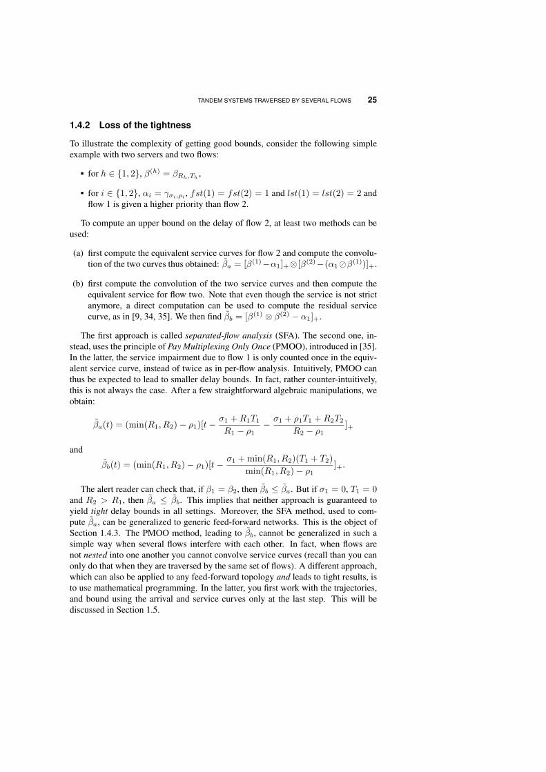
To illustrate the complexity of getting good bounds, consider the following simpleexample with two servers and two flows:
for h ∈ {1, 2}, β(h) = βRh,Th,
for i ∈ {1, 2}, αi = γσi,ρi , fst(1) = fst(2) = 1 and lst(1) = lst(2) = 2 andflow 1 is given a higher priority than flow 2.
To compute an upper bound on the delay of flow 2, at least two methods can beused:
(a) first compute the equivalent service curves for flow 2 and compute the convolu-tion of the two curves thus obtained: βa = [β(1)−α1]+⊗ [β(2)−(α1�β(1))]+.
(b) first compute the convolution of the two service curves and then compute theequivalent service for flow two. Note that even though the service is not strictanymore, a direct computation can be used to compute the residual servicecurve, as in [9, 34, 35]. We then find βb = [β(1) ⊗ β(2) − α1]+.
The first approach is called separated-flow analysis (SFA). The second one, in-stead, uses the principle of Pay Multiplexing Only Once (PMOO), introduced in [35].In the latter, the service impairment due to flow 1 is only counted once in the equiv-alent service curve, instead of twice as in per-flow analysis. Intuitively, PMOO canthus be expected to lead to smaller delay bounds. In fact, rather counter-intuitively,this is not always the case. After a few straightforward algebraic manipulations, weobtain:
βa(t) = (min(R1, R2)− ρ1)[t− σ1 +R1T1
R1 − ρ1− σ1 + ρ1T1 +R2T2
R2 − ρ1]+
and
βb(t) = (min(R1, R2)− ρ1)[t− σ1 + min(R1, R2)(T1 + T2)
min(R1, R2)− ρ1]+.
The alert reader can check that, if β1 = β2, then βb ≤ βa. But if σ1 = 0, T1 = 0and R2 > R1, then βa ≤ βb. This implies that neither approach is guaranteed toyield tight delay bounds in all settings. Moreover, the SFA method, used to com-pute βa, can be generalized to generic feed-forward networks. This is the object ofSection 1.4.3. The PMOO method, leading to βb, cannot be generalized in such asimple way when several flows interfere with each other. In fact, when flows arenot nested into one another you cannot convolve service curves (recall than you canonly do that when they are traversed by the same set of flows). A different approach,which can also be applied to any feed-forward topology and leads to tight results, isto use mathematical programming. In the latter, you first work with the trajectories,and bound using the arrival and service curves only at the last step. This will bediscussed in Section 1.5.

26 WORST-CASE ANALYSIS OF TANDEM QUEUEING SYSTEMS USING NETWORK CALCULUS
1.4.3 Separated-flow analysis
Algorithm 1.1 gives the general way of computing the equivalent service curve fora tagged flow traversing a tandem. It first computes an arrival curve for each flowat each intermediate server: α(h)
i is an arrival curve for F (h)i . Then, it computes the
equivalent service curve for each flow at each server: β(h)i is the equivalent service
curve of server h for flow i. Finally it computes the end-to-end service curve for theeach flow, and a bound on its WCD can be computed using that curve.
Algorithm 1.1
General Separated-flow Analysis Algorithm {for h = 1 to n{
for each i such that h ∈ i{
β(h)i ← (β(h) −
∑j3h−{i} α
(h−1)j )+;
α(h)i ← α
(h−1)i � β(h)
i ;}
}for i = 1 to m do{
βi = ∗h∈iβ(h)i
}
Algorithm 1.1 is valid for blind multiplexing (and thus for any service policy) ifthe servers offer strict service curves. If the service policy is known to be FIFO (inwhich case the service curves need not be strict), it is also possible to compute β(h)
i
with the formula of Theorem 1.2 (instantiated for any nonnegative value of τ ).
1.5 Mathematical programming approach
In this section, we present a method for computing exact worst-case performancein tandem networks. The method can be generalized to arbitrary acyclic networks,but for sake of notational and algorithmic simplicity, we detail the method only fortandem networks, and give the idea and the additional difficulties that arise in thegeneral case at the end.
1.5.1 Blind multiplexing
Consider a single server traversed by one flow. To compute the WCD at time t, weuse the following ingredients:
strict service curve: F (1)(t)− F (1)(s) ≥ β(1)(t− s);
choose s = start(t): F (1)(s) = F (0)(s);

MATHEMATICAL PROGRAMMING APPROACH 27
introduce the arrival date, u, of the bit that departs at time t: s ≤ u ≤ t andF (0)(u) ≥ F (1)(t);
arrival curve: F (0)(u)− F (0)(s) ≤ α1(u− s).
As we assumed α1 piecewise affine concave (i.e., the minimum of a finite numberof affine curves) and β(1) piecewise affine convex (i.e., the maximum of a finitenumber of affine curves), all those constraints are either linear or easily explodedinto a finite number of linear ones. To compute the WCD, the only remaining step isto maximize t− u under these constraints. Therefore, this is a linear program.
In a tandem network of n nodes, the WCD can be computed by generalizing theabove linear program backwards, i.e., starting from server n and going back to server1.
1.5.1.1 The linear program
Variables Let us first define the variables of the linear program. Note that, to em-phasize the meaning of the variables, we denote them the same way as the date ofthe function value they represent. Thus, they will mainly be named tk or F (h)
i (tk).
time variables: we have n + 2 relevant time instants, i.e., t0, . . . , tn and u,with the following interpretation: consider a bit of data that exists the systemat time tn: then tn−1 is the start of the backlogged period of server n at timetn (tn−1 = startn(tn)) and more generally, ti−1 = starti(ti). Variable urepresents the arrival date of the bit of data considered;
functional variables: the relevant variables are F (fst(i)−1)i (tk) and F (h)
i (tk) fori ∈ h and k ∈ {h, h− 1}. Intuitively, F (h)
i (tk) represents the value of the CAFF
(h)i at time tk. The important dates for F (h)
i are th, i.e., the date at which thebit of interest exits server h and th−1, i.e., the start of the backlogged period ofserver h. Variable F (fst(i)−1)
i (tk) represents the CAF of flow i. The variableF
(fst(i)−1)i (u) will also be used to compute the WCD of flow i.
Linear constraints Without loss of generality, we can assume that lst(1) = n, i.e.,flow 1 traverses all the tandem and is the one whose WCD we want to compute. Wehave the following constraints:
time constraints ∀h, th−1 ≤ th;
service constraints ∀h,∑i3h F
(h)i (th) ≥ F (h)
i (th−1) + β(h)(th − th−1);
start of backlogged period constraints ∀h, ∀i 3 h, F (h)i (th−1) = F
(h−1)i (th−1);
causality constraints ∀h, ∀i 3 h and k ∈ {h, h − 1}, F (fst(i)−1)i (tk) ≥
F(h−1)i (tk) ≥ F (h)
i (tk);

28 WORST-CASE ANALYSIS OF TANDEM QUEUEING SYSTEMS USING NETWORK CALCULUS
non-decreasing constraints ∀i, ∀h 3 i, F (fst(i)−1)i (th) ≥ F
(fst(i)−1)i (th−1)
and F (h)i (th) ≥ F (h)
i (th−1);
arrival constraints ∀i, ∀k < h 3 i,F (fst(i)−1)i (th)−F (fst(i)−1)
i (tk) ≤ αi(th−tk);
constraints on u: t0 ≤ u ≤ tn; F (fst(1)−1)1 (u)−F (fst(1)−1)
1 (tfst(1)) ≤ α1(u−tfst(1)) and F (fst(1)−1)
1 (u) ≥ F (n)1 (tn)
Objective function: In order to compute the WCD of flow 1, we just need to maxi-mize the distance between the time at which it exits node n and the time at which itenters the tandem, i.e.:
Maximize tn − u.The same variables and constraints, can also be used to compute the maximum
backlog at node n. In this case, the objective is:
Maximize∑i3n
F(fst(i)−1)i (tn)−
∑i3n
F(n)i (tn).
Note that time variable u and the related functional variables and constraints are notrequired in this case.
Let us denote with Λ the linear program defined above and let dΛ (resp. bΛ) itsoptimal solution, if the objective is the WCD (resp. the maximum backlog). Thefollowing theorem holds:
Theorem 1.3 Consider a tandem network with n servers and p flows. The LP in-stance Λ has O(pn) variables and O(pn2) constraints and is such that the optimumis the worst end-to-end delay for flow 1 is dΛ (resp. the maximum backlog at server nis bΛ).
The above theorem is formally proved in [10]. Here, we just explain the principleof the proof using an example. It is based on the construction of an admissiblescenario that satisfies the solution of the LP.
t2 t3t1t0
α2
α1
α3β(1) β(2) β(3)
Figure 1.18 Tandem network with three nodes and three flows.
1.5.1.2 Example Consider the tandem of Figure 1.18. The latter has been exten-sively studied in [34], where it is shown that the exact WCD cannot be computedusing the application of (min,plus) algebraic methods. To compute the WCD of flow1, we have the following linear program:

MATHEMATICAL PROGRAMMING APPROACH 29
time constraints
– t3 ≥ t2 ≥ t1 ≥ t0;
– t3 ≥ u ≥ t0;
service constraints
– F(3)1 (t3) + F
(3)3 (t3) ≥ F (3)
1 (t2) + F(3)3 (t2) + β(3)(t3 − t2);
– F(2)1 (t2)+F
(2)2 (t2)+F
(2)3 (t2) ≥ F (2)
1 (t1)+F(2)2 (t1)+F
(2)3 (t1)+β(2)(t2−
t1);
– F(1)1 (t1) + F
(1)2 (t1) ≥ F (1)
1 (t0) + F(1)2 (t0) + β(3)(t1 − t0);
start of backlogged period constraints
– F(3)i (t2) = F
(2)i (t2), i ∈ {1, 3};
– F(2)i (t1) = F
(1)i (t1), i ∈ {1, 2, 3};
– F(1)i (t0) = F
(0)i (t0), i ∈ {1, 2};
arrival constraints
– F(0)1 (tk)−F (0)
1 (t`) ≤ α1(tk−t`), (k, `) ∈ {(1, 0), (2, 1), (2, 0), (3, 2), (3, 1), (3, 0)};
– F(0)1 (u)− F (0)
1 (t0) ≤ α1(u− t0);
– F(0)2 (tk)− F (0)
2 (t`) ≤ α2(tk − t`), (k, `) ∈ {(1, 0), (2, 1), (2, 0)};
– F(1)3 (tk)− F (1)
3 (t`) ≤ α3(tk − t`), (k, `) ∈ {(2, 1), (3, 2), (3, 1)};
causality constraints
– F(0)1 (tk) ≥ F (1)
1 (tk), k ∈ {1, 2, 3};
– F(0)2 (tk) ≥ F (1)
2 (tk), k ∈ {1, 2};
– F(1)3 (tk) ≥ F (2)
3 (tk), k ∈ {2, 3};
non-decreasing constraints
– F(0)1 (t0) ≤ F (0)
1 (t1) ≤ F (0)1 (t2) ≤ F (0)
1 (t3); F (0)1 (t0) ≤ F (0)
1 (u); F (3)1 (t2) ≤
F(3)1 (t3); F (2)
1 (t1) ≤ F (2)1 (t2); F (1)
1 (t0) ≤ F (1)1 (t1);
– F(0)2 (t0) ≤ F (0)
2 (t1) ≤ F (0)2 (t2); F (2)
2 (t1) ≤ F (2)2 (t2); F (1)
2 (t0) ≤ F (1)2 (t1);
– F(1)3 (t1) ≤ F (1)
3 (t2) ≤ F (1)3 (t3); F (3)
3 (t2) ≤ F (3)3 (t3); F (2)
3 (t1) ≤ F (2)3 (t2);
delay at t3
– F (3)(t3) ≤ F (0)1 (u);
Objective

30 WORST-CASE ANALYSIS OF TANDEM QUEUEING SYSTEMS USING NETWORK CALCULUS
– Maximize t3 − u.
Figure 1.19 explains the relation between the linear program and the trajectories.Given an admissible trajectory, the assignment variables can be read from the fig-ure: let t3 be the exit time of the bit whose the delay is computed. Variables tiare defined as the beginning of the backlogged period at each server. Then, vari-ables F (h)
i (tk) are assigned the value of the CAF F (h)i at time tk. Those variables
satisfy of course all the constraints, that are derived from Network Calculus basics.Conversely, to construct the trajectories from a solution of the linear program, it isenough to linearly interpolate the CAFs: F (fst(i)−1)
i between tfst(i)−1 and tlst(i);and F (h)
i between th−1 and th. Before th−1, one can set F (h)i = F
(h−1)i and after
th, F (h)i = F
(fst(i)−1)i .
F(3)1
F(0)2
F(1)3
F(1)1
F(1)2
t1u t2 t3t0
F(2)1
F(0)1
F(2)1
F (0)
F(2)3
F(3)1
F(0)2
F(1)3
F(1)1
F(1)2
t1u t2 t3t0
F(2)1
F(0)1
F(2)1
F (0)
F(2)3
delay delay
Figure 1.19 From the trajectories to the linear program and back to the trajectories for blindmultiplexing.
1.5.1.3 Equivalent service curve The above method allows one to compute theWCD for a tagged flow, under constraints (αi)i∈F and (βj)j∈S . One may also wantto measure how the network affects flow 1, in particular whether the flow can beguaranteed some end-to-end service curve. We call a universal end-to-end servicecurve a service curve β which is independent of α1 (i.e., β remains an end-to-endservice curve for any α1). Precomputing such a universal curve can be useful toquickly compute a bound on the end-to-end delay for flow 1 for several differentcurves α1, instead of having to write down and solve a linear program every time.
For tandem networks, it is possible to compute such a universal end-to-end servicecurve, which is optimal in the sense that it is maximal for all the universal servicecurves. It can be computed as follows: compute the WCD for the network when α1
is a constant function equal to σ, call it d(σ). Then, β1, the residual service curve forflow 1 is the inverse function d−1.
The LP that we have defined above to compute d(σ) can be schematically rewrit-ten as

MATHEMATICAL PROGRAMMING APPROACH 31
Maximize AXSubject to BX ≤ C(σ), X ≥ 0,
where only C depends on σ. Indeed, σ never appears within coefficient matrix B.Then, by the strong duality theorem of linear programming, the following LP has thesame optimal solution.
Minimize Ct(σ)YSubject to BtY ≤ At, Y ≥ 0.
The constraints of the dual LP are independent of σ, and for any σ, its optimalvalue is reached at a vertex of the convex polyhedron defined by the constraintsBtY ≤ At and Y ≥ 0. Hence, function d(σ) is the minimum of a finite set of linearfunctions (whose cardinality can be exponential in the size of the network).
1.5.1.4 Generalization to feed-forward networks The same method can be ap-plied to general feed-forward networks. In this case, several difficulties arise, makingthe problem much more difficult. More specifically:
The number of relevant dates grows exponentially with the size of the net-work. Indeed, starting from the date that marks the beginning of the backloggedperiod of one given server, several dates must be defined for the beginning ofthe backlogged period of all the predecessors of this servers. As a consequence,the number of required dates is the number of paths from any node to the lastserver visited by the tagged flow.
Those dates are not totally ordered and every order compatible with the NCconstraints must be generated, leading to a different linear program for eachorder. Thus, the WCD is the maximum solution of an exponential number oflinear programs.
To illustrate this fact, consider the example of Figure 1.20. The departure date ofthe bit of interest is t∅, and we can define t4 = start4(t∅), t24 = start2(t4) andt34 = start3(t4). But then, for server 1, two starts of backlogged period have to bedefined: t134 and t124. Four orders have to be consider: either t24 and t34 belongto different backlogged period, in which case we have t124 ≤ t24 ≤ t134 ≤ t34 ort134 ≤ t34 ≤ t124 ≤ t24, or they belong to the same backlogged period, in whichcase we have t134 = t124 ≤ t34 ≤ t24 or t134 = t124 ≤ t24 ≤ t34. Date u alsohas to be inserted in these orders, inducing even more linear programs. The otherconstraints depending of the order of the dates (arrival, non-decreasing) have to begenerated according to these orders.
A reduction of X3C (Exact-three-cover, [23]) to this problem shows that it is infact NP-hard to compute the WCD under those assumptions.
1.5.1.5 Generalization to other service policies Assuming blind multiplexing,or arbitrary multiplexing may yield very pessimistic bounds for some networkswhere the service policy is known. It may not always be possible to find a linear

32 WORST-CASE ANALYSIS OF TANDEM QUEUEING SYSTEMS USING NETWORK CALCULUS
β1
β3
β4
t∅
t34
β2
t4
F(3)2
F(2)1
t24
F(1)2
F(1)1F
(0)1
t124
t134
F(4)1
F(4)2F
(0)2
Figure 1.20 Example of a feed-forward network.
program that computes the exact worst-case performance efficiently, even for tandemnetworks. For example, an attempt to find a linear program encoding Static Prioritiescan be found in [11]. In these cases, a good strategy is to mix Algorithm 1.1 withthe linear programming approach used for blind multiplexing. This can be done asfollows:
1. Generate the LP assuming blind multiplexing;
2. Using Algorithm 1.1, compute the intermediate arrival curves for each flow ateach node it traverses;
3. Add linear constraints corresponding to these intermediate arrival curves to theLP;
4. Compute the optimal solution of the LP thus modified.
1.5.2 FIFO multiplexing
Under FIFO multiplexing it is also possible to compute tight bounds using math-ematical programming. The fundamental modeling difference with respect to theblind multiplexing case are:
exploit the FIFO hypothesis to infer input-output relationships;
consider simple service curves instead of strict service curves.
Consider the trivial example of a single server traversed by two flows. The abovetwo elements induce the following linear constraints: if t1 is the departure date ofthe bit of interest,
(FIFO hypothesis) there exists t2 ∈ [t3, t1] such that F (0)1 (t2) = F
(1)1 (t1) and
F(0)2 (t2) = F
(1)2 (t1), and
(simple service curve) there exists t3 ≤ t1 such that we haveF (1)1 (t1)+F
(1)2 (t1) ≥
(F(0)1 + F
(0)2 )⊗ β(t1) = F
(0)1 (t3) + F
(0)2 (t3) + β(1)(t1 − t3),
Furthermore, the monotonicity, causality and arrival curves constraints are stillvalid. Note that for one date (t1), two new dates have been introduced, t2 and t3.
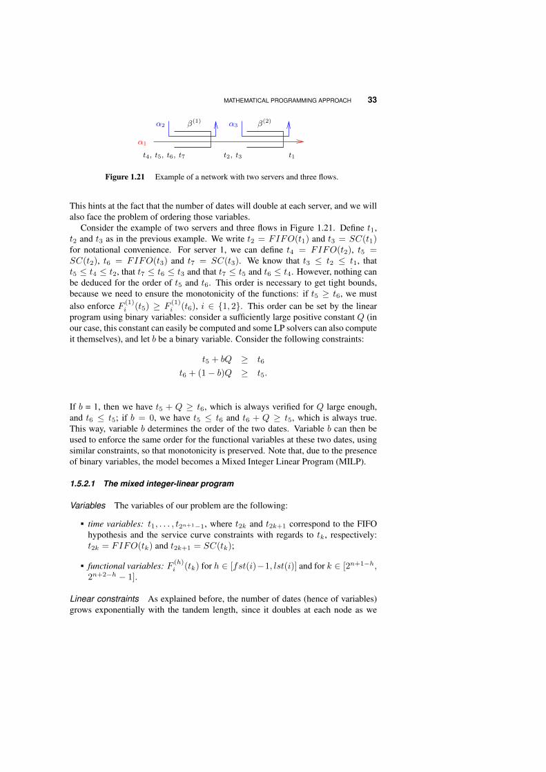
MATHEMATICAL PROGRAMMING APPROACH 33
t2, t3 t1t4, t5, t6, t7
α3
α1
α2 β(1) β(2)
Figure 1.21 Example of a network with two servers and three flows.
This hints at the fact that the number of dates will double at each server, and we willalso face the problem of ordering those variables.
Consider the example of two servers and three flows in Figure 1.21. Define t1,t2 and t3 as in the previous example. We write t2 = FIFO(t1) and t3 = SC(t1)for notational convenience. For server 1, we can define t4 = FIFO(t2), t5 =SC(t2), t6 = FIFO(t3) and t7 = SC(t3). We know that t3 ≤ t2 ≤ t1, thatt5 ≤ t4 ≤ t2, that t7 ≤ t6 ≤ t3 and that t7 ≤ t5 and t6 ≤ t4. However, nothing canbe deduced for the order of t5 and t6. This order is necessary to get tight bounds,because we need to ensure the monotonicity of the functions: if t5 ≥ t6, we mustalso enforce F (1)
i (t5) ≥ F(1)i (t6), i ∈ {1, 2}. This order can be set by the linear
program using binary variables: consider a sufficiently large positive constant Q (inour case, this constant can easily be computed and some LP solvers can also computeit themselves), and let b be a binary variable. Consider the following constraints:
t5 + bQ ≥ t6
t6 + (1− b)Q ≥ t5.
If b = 1, then we have t5 + Q ≥ t6, which is always verified for Q large enough,and t6 ≤ t5; if b = 0, we have t5 ≤ t6 and t6 + Q ≥ t5, which is always true.This way, variable b determines the order of the two dates. Variable b can then beused to enforce the same order for the functional variables at these two dates, usingsimilar constraints, so that monotonicity is preserved. Note that, due to the presenceof binary variables, the model becomes a Mixed Integer Linear Program (MILP).
1.5.2.1 The mixed integer-linear program
Variables The variables of our problem are the following:
time variables: t1, . . . , t2n+1−1, where t2k and t2k+1 correspond to the FIFOhypothesis and the service curve constraints with regards to tk, respectively:t2k = FIFO(tk) and t2k+1 = SC(tk);
functional variables: F (h)i (tk) for h ∈ [fst(i)−1, lst(i)] and for k ∈ [2n+1−h,
2n+2−h − 1].
Linear constraints As explained before, the number of dates (hence of variables)grows exponentially with the tandem length, since it doubles at each node as we
34 WORST-CASE ANALYSIS OF TANDEM QUEUEING SYSTEMS USING NETWORK CALCULUS
go backwards. Moreover, in a multi-node scenario, these dates are only partiallyordered. For k < 2n, we have (*) t2k+1 ≤ t2k ≤ tk. Moreover, if 2h ≤ k, k′ < 2h+1
and (**) if tk ≤ tk′ , then t2k ≤ t2k′ (cumulative functions are non-decreasing)and t2k+1 ≤ t2k′+1 (same as above, plus βj is convex). These relations and thetransitivity only lead to a partial order of t2h , . . . , t2h+1−1.
We must order the dates tk, t′k if there exists h such that 2h ≤ k, k′ < 2h+1 byintroducing binary variables. We do this recursively backwards as follows:
For server n, we have t2 ≥ t3:
Suppose that dates are ordered for all k ∈ [2h−1, 2h−1] and now consider datestk, k ∈ [2h, 2h+1 − 1].
– First generate the partial known order using (*) and (**);
– For k = 2` and k′ = 2`′ or k = 2` + 1 and k′ = 2`′ + 1, use the samebinary variable used to order t` and t`′ ;
– For any other pair, introduce a new binary variable.
If variables x and y are ordered by the variable b, we note x ≤b y to represent theconstraints
x+ bQ ≥ y
y + (1− b)Q ≥ x.
Moreover, if no binary variable is needed, we write x ≤∅ y to represent the constraintx ≤ y.
We can now write the linear constraints:
time and monotonicity constraints: for any tk ≤b tk′ , tk ≤b tk′ , F (h)i (tk) ≤b
F(h)i (tk′) are constraints;
FIFO hypothesis: if fst(i) < h, F (h)i (tk) = F
(h−1)i (t2k) is a constraint;
service constraints: if k ∈ [2n−h, 2n+1−h − 1], D(h)(tk) ≥ A(h−1)(t2k+1) +βh(tk − t2k−1) is a constraint;
arrival constraints: if h = fst(i) and tk ≤∅ tk′ , F(h)i (t′k) − F
(h)i (tk) ≤
αi(tk′−tk) is a constraint; if h = fst(i) and ∃b 6= ∅, tk ≤b tk′ then F (h)i (tk′)−
F(h)i (tk) ≤ αi(tk′ − tk) + (1 − b) · Q and F (h)
i (tk) − F (h)i (tk′) ≤ αi(tk −
tk′) + b ·Q are constraints.
Objective function If the objective is to compute the WCD, then the objective ofthe MILP is max t1 − t2n .

MATHEMATICAL PROGRAMMING APPROACH 35
As for the blind multiplexing case, we can exploit the same model to computethe maximum backlog at server n too. In order to do this, one has to introduce newvariables F (fst(i)−1
i (t1) for i ∈ n and the constraints
F(fst(i)−1i (t1)− F (fst(i)−1
i (t2n−fst(i)+1) ≤ αi(t1 − t2n−fst(i)+1);
then the objective of the MILP is max∑i∈n F
(fst(i)−1)i (t1)−
∑i∈n F
(n)i (t1).
Let us denote with Λ the MILP defined above and dΛ (resp. bΛ ) its optimalsolution if the objective is the WCD (resp. the maximum backlog at server n). Thefollowing theorem holds.
Theorem 1.4 For a tandem network with n servers and p flows. The MILP instanceΛ is such that the optimum is the WCD for flow 1 is dΛ (resp. the maximum backlogat server n is bΛ).
This can be generalized with no difficulty to any flow. The proof of this theorem canbe found in [12]. Here, we illustrate the concept using the example of Figure 1.20.
1.5.2.2 Example The MILP for computing the WCD of the tandem of of Fig-ure 1.20 is:
Maximize t1 − t4 such that:
time constraints:
– tk ≥ t2k ≥ t2k+1, k ∈ {1, 2, 3};– t4 ≥ t6;
– t5 + (1− b) ·Q ≥ t6 and t6 + b ·Q ≥ t5;
service constraints:
– F(2)1 (t1) + F
(2)3 (t1) ≥ F (1)
1 (t3) + F(1)3 (t3) + β2(t1 − t3);
– F(1)1 (tk)+F
(1)2 (tk) ≥ F (0)
1 (t`)+F(0)2 (t`)+β
1(tk−t`), (k, `) ∈ {(2, 5), (3, 7)};
FIFO constraints:
– F(2)i (t1) = F
(1)i (t2), i ∈ {1, 3};
– F(1)i (tk) = F
(0)i (t2k), i ∈ {1, 2}, k ∈ {2, 3};
monotonicity constraints:
– F(1)i (t3) ≤ F (1)
i (t2), i ∈ {1, 3};
– F(0)i (tk) ≥ F (0)
i (t`), i ∈ {1, 2}, (k, `) ∈ {(4, 5), (4, 6), (4, 7), (5, 7), (6, 7)};
– F(0)i (t5) + (1− b) ·Q ≥ F (0)
i (t6), i ∈ {1, 2};
– F(0)i (t5) ≤ b ·Q+ F
(0)i (t6), p ∈ {1, 2};

36 WORST-CASE ANALYSIS OF TANDEM QUEUEING SYSTEMS USING NETWORK CALCULUS
arrival constraints:
– F(1)3 (t2)− F (1)
3 (t3) ≤ α3(t2 − t3);
– F(0)i (tk)−F (0)
i (t`) ≤ αi(tk−t`), i ∈ {1, 2}, (k, `) ∈ {(4, 5), (4, 6), (4, 7), (5, 7), (6, 7)};
– F(0)i (t5)− F (0)
i (t6) ≤ αi(t5 − t6) + (1− b) ·Q, i ∈ {1, 2};
– F(0)i (t6)− F (0)
i (t5) ≤ αi(t6 − t5) + b ·Q, i ∈ {1, 2}.
delay delay
F(1)1 + F
(1)3
F(2)1 + F
(2)3
F(0)1
F(1)1
F(2)1
t7 t1t2t3t4t5
F(0)1 + F
(0)2
F(1)1 + F
(1)2
t6
F(1)1 + F
(1)3
F(2)1 + F
(2)3
F(0)1
F(1)1
F(2)1
t7 t1t2t3t4t5
F(0)1 + F
(0)2
F(1)1 + F
(1)2
t6
server1
flow 1
server 2
Figure 1.22 From the trajectory to the MILP and back to the trajectories for the network ofFigure 1.20. Left: from the trajectory to the MILP: the circles represent the values associatesto the variables of the form F
(h)i (tk). Right: from those variables, it is possible to draw a
new trajectory satisfying the constraints where the arrival are maximized according to theirconstraints, staircase shaped for the intermediate flows, and follows the service curve for thelast server.
1.6 Related Work
The study of tandem networks under blind multiplexing has already been addressedin [34]. The authors compute tight end-to-end delay bounds for some tandem net-works, pointing out the difficulties we mentioned earlier in this chapter. They detailtheir computations for a network with three servers and three flows and a more gen-eral approach is suggested in the corresponding technical report [33]. The main dif-ference between this approach and the linear programming one is that they directly

RELATED WORK 37
compute equivalent service curves, with some free parameters to optimize. More-over, this approach is basically intended for leaky-bucket/rate-latency arrival/servicecurves and can be generalized only in a very inefficient way.
Another approach has been developed in [7, 8] and can deal with concave/convexarrival/service curves, but loses the tightness of the bounds. The idea is to definea multi-dimensional convolution to directly compute an equivalent service curve forthe flow of interest. This would correspond to the computation of βb in Section 1.4.2.Besides the fact that tight bounds may not be computed, this convolution might bealgorithmically complex to compute.
As far as FIFO networks are concerned, the first paper to determine some boundson the delay has been [20], which shows that, for a generic FIFO network (i.e.,not necessarily feed-forward), upper bounds on the WCD can only be computed forsmall utilization factors. A critical utilization factor ν is defined, which is inverselyproportional to the maximum path length. The paper shows two fundamental limits:
For a utilization u ≤ ν the bound is proportional to 1/(ν−u), hence approachesinfinity as the utilization approaches ν.
For any utilization u > ν and finite delay d, it is possible to construct a (nonfeed-forward) network where some traffic exhibits a delay larger than d.
The above finding can be interpreted as implying that better results can only beobtained by adding some more hypothesis. For instance, the feed-forward hypothesisis relevant in practice and hardly constraining at all. A tandem network is in fact afeed-forward network, and the latter are known to be stable for any utilization up to100%. This means that we can find better bounds under that hypothesis than thosecomputed using the method in [20]. Several papers dealing with computing delaybounds in FIFO tandem networks have appeared recently [29, 27, 30, 2, 3, 4, 13, 24].All these papers rely on equivalent service curves, i.e., those computed by usingTheorem 1.2. A method known as Least Upper Delay Bound (LUDB) is describedin those papers. The method is based on removing the cross flows by iterativelyapplying Theorem 1.2. Depending on the paths of the cross flows, two situationsmay arise: in a so-called “nested” tandem, i.e., one where either any two flow pathsare disjoint or one includes the other, it is possible to compute an equivalent end-to-end service curve for the tagged flow [30]. Otherwise, no end-to-end servicecurve can be computed: first, the tandem has to be cut into (possibly many) nestedsub-tandems; then, bounds on the WCD of each sub-tandem must be computed andsummed up to obtain a bound on the end-to-end WCD. In both cases, the delaybound (whether for the whole tandem or for sub-tandems) is computed by solving apiecewise-linear programming (P-LP) problem. A tool called DEBORAH has beendevised to solve the problem [3]. It transforms the P-LP problem into a number ofLPs, each one of which produces an upper bound on the WCD, solves all the LPsand takes the minimum solution (i.e., the least upper bound). The LUDB method,in general, does not compute the WCD. It does in sink-tree networks ([27]), where,besides, a faster algorithm not relying on LP can be used, and in some more specialcases ([4]), but this is not always the case, even in simple nested tandems, as proved

38 WORST-CASE ANALYSIS OF TANDEM QUEUEING SYSTEMS USING NETWORK CALCULUS
in [2]. Moreover, authors of[4] argue that, in non-nested tandems, the LUDB may begrossly overrated, due to the fact that cutting the tandem entails assuming separate,non compatible worst-case scenarios at each sub-tandem, much as summing per-node WCDs would do in a per-flow scheduling tandem. The upside of the LUDBmethod is that it is relatively efficient from a computational standpoint. Computingthe LUDB is still an exponential problem, but an optimized implementation thatexploits some structure in the problem, described in [4], allows one to analyze up to30-node tandems in minutes on off-the shelf hardware. For shorter tandems (e.g., upto 10 nodes), the LUDB can indeed be computed online, in split-second times. Oneof the downsides, instead, is that it can only work with single leaky-bucket arrivalcurves and rate-latency curves. Works [13, 24] discuss the advantages of includingpeak constraints (i.e., double-leaky-bucket arrival curves) in the model, but limitthemselves to the tagged flow. Authors in [13] show that a double leaky bucketcannot be assumed for cross flows, since this makes Theorem 1.2 yield curves whichare not always wide-sense increasing, hence cannot be assumed to be equivalentservice curves.
With respect to these works, the linear-programming approach described in thischapter is:
more general: it allows arbitrary piecewise-concave arrival curves, and arbitrarypiecewise-convex service curves;
capable of computing the WCD, whereas the other is not.
Obviously enough, the above advantages are paid for by a higher complexity: LP-based WCD computation is difficult to achieve in practice for more than 10 nodesin the current implementation of the solver. However, the latter is not optimizedfor speed: more specifically, there has been – as of today – no effort to obtain anoptimized ILP solution strategy, relying instead on the prowess of a general-purposesolver such as CPLEX. We expect that the current speed figures can be improvedconsiderably by both reformulating the model in a more efficient way and integratingan optimized solution strategy in our solver.
1.7 Numerical Results
In this section, we illustrate the effectiveness of the linear programming approach bycomparing it to the classical approaches on a tandem scenario. Consider the scenariogiven in Figure 1.23. Every cross-flow traverses two servers (except those at theextremities, i.e., servers 1 and n, which only traverse one). The tagged flow traversesevery server. Every server has the same characteristics: a latency of 0.1 s and aservice rate of 10 Mbps. Flows have a maximum burst σ of 1 Mb and an arrival rateρ of 0.67 Mbps.
Fig. 1.24 shows the delay obtained with the separated flow analysis approach(SFA) and the tight LP method assuming blind multiplexing. Unsurprisingly, thetwo methods give the same result when there is only one server. For a network

NUMERICAL RESULTS 39
Figure 1.23 Tandem scenario with 4 servers.
012345678
0 2 4 6 8 10 12 14 16 18 20
Del
aybo
und
(s)
Number of servers
SFA
• •• •
• •• •
• •• •
• •• •
• •• •
•WCD
◦ ◦ ◦◦ ◦ ◦
◦ ◦ ◦◦ ◦ ◦
◦ ◦ ◦◦ ◦ ◦
◦ ◦◦
Figure 1.24 Upper bounds for the delay of the scenario of Fig. 1.23.
with 20 servers, the LP method reduces the SFA bound by a factor 8/5, for a linkutilization of 20%.
Fig. 1.25 depicts the distance between SFA and LP methods when the utilizationof the servers varies, with 20 servers. The arrival rate of the flows varies so as toobtain the utilization shown in the horizontal axis. As the utilization grows, the gainbecomes huge (note that the vertical scale is logarithmic).
100
101
102
103
104
105
0.1 0.2 0.3 0.4 0.5 0.6 0.7 0.8 0.9
Del
aybo
und
(s)
Utilization
SFA
• • • • ••
•
•
••
WCD
◦ ◦ ◦ ◦ ◦ ◦ ◦ ◦ ◦
◦
Figure 1.25 Upper bounds for the delay of the scenario of Fig. 1.23 for 20 servers and whenthe utilization varies.

40 WORST-CASE ANALYSIS OF TANDEM QUEUEING SYSTEMS USING NETWORK CALCULUS
0.5
1
1.5
2
2.5
3
3.5
4
3 4 5 6 7 8 9 10
Del
aybo
und
(s)
Number of servers
LUDB
••
••
••
•••
WCD
◦ ◦ ◦ ◦ ◦ ◦ ◦ ◦
◦
Figure 1.26 Upper bounds for the delay of the scenario of Fig. 1.23 (with FIFO multiplexing).
Assume now the same scenario in Figure 1.23, this time with FIFO multiplexing.We compare the linear-programming approach with the LUDB one ([4]).
Fig. 1.26 compares the LUDB and the linear-programming exact WCD as thenumber of servers increases. Note that computing the exact WCD takes longerwith FIFO, due to the presence of binary variables, hence we stick to smaller-sizetandems. The figure shows that the overrating of the LUDB method increases withthe number of nodes. Note that the WCD increases linearly with the number ofnodes.
Fig. 1.27 compares the LUDB and the linear-programming exact WCD then thenumber of servers is equal to eight. It is evident that the LUDB overrating increaseswith the utilization.
02468
1012141618
0.1 0.2 0.3 0.4 0.5 0.6 0.7 0.8 0.9
Del
aybo
und
(s)
Utilization
LUDB
• ••
••
••
•
••
WCD
◦ ◦ ◦ ◦ ◦ ◦ ◦ ◦ ◦
◦
Figure 1.27 Upper bounds for the delay of the scenario of Fig. 1.23 for eight servers andwhen the utilization varies (with FIFO multiplexing).

CONCLUSIONS 41
1.8 Conclusions
In this chapter we have shown how Network Calculus can be used to computeworst-case delay bounds in tandem networks. Computations are easy when per-flow scheduling is in place: in that case, given a good model of the arrivals of aflow and the service at each node, we quickly obtain tight bounds on the delay byexploiting the Pay Burst Only Once principle, which clearly outperforms per-nodeanalysis. When, instead, per-aggregate multiplexing is in place, computations getconsiderably more involved. We have shown that methods based on equivalent ser-vice curves do not lead to tight delay bounds, which can instead be obtained througha linear-programming approach. We have exemplified such an approach on twowell-known paradigms: blind multiplexing, where the queueing policy is assumedto be arbitrary, and FIFO multiplexing. Our results show that, in both cases, thelinear-programming approach outperforms the others.

REFERENCES
1. H. Bauer, J.-L. Scharbarg, and C. Fraboul. Improving the worst-case delay analysisof an AFDX network using an optimized trajectory approach. IEEE Transactions onIndustrial Informatics, 6(4):521–523, 2010.
2. L. Bisti, L. Lenzini, E. Mingozzi, and G. Stea. Estimating the worst-case delay in FIFOtandems using network calculus. In proceedings of Valuetools’08, 2008.
3. L. Bisti, L. Lenzini, E. Mingozzi, and G. Stea. Deborah: A tool for worst-case analysisof FIFO tandems. In proceedings of ISoLA’10, Special Track on Worst-case TraversalTime, 2010.
4. L. Bisti, L. Lenzini, E. Mingozzi, and G. Stea. Numerical analysis of worst-case end-to-end delay bounds in FIFO tandem networks. Springer Real-Time Systems Journal,2012.
5. S. Blake, D. Black, M. Carlson, E. Davies, Z. Wang, and W. Weiss. An Architecture forDifferentiated Services. IETF, 1998.
6. A. Bouillard. Composition of service curves in network calculus. In Proceedings ofWCTT 2011, pages 25–42, 2011.
7. A. Bouillard, B. Gaujal, S. Lagrange, and E. Thierry. Optimal routing for end-to-endguarantees using network calculus. Performance Evaluation, 65(11-12):883–906, 2008.
8. A. Bouillard, L. Jouhet, and E. Thierry. Computation of a (min,+) multi-dimensionalconvolution for end-to-end performance analysis. In proceedings of Valuetools’08, 2008.
9. A. Bouillard, L. Jouhet, and E. Thierry. Service curves in Network Calculus: dos anddon’ts. Research Report RR-7094, INRIA, 2009.
Please enter \offprintinfo{(Title, Edition)}{(Author)}at the beginning of your document.
43

44 REFERENCES
10. A. Bouillard, L. Jouhet, and E. Thierry. Tight performance bounds in the worst-caseanalysis of feed-forward networks. In proceedings of INFOCOM’10, 2010.
11. A. Bouillard and A. Junier. Worst-case delay bounds with fixed priorities using networkcalculus. In proceedings of Valuetools’11, 2011.
12. A. Bouillard and G. Stea. Exact worst-case delay for FIFO-multiplexing tandems. Inproceedings of VALUETOOLS, pages 158–167, 2012.
13. M. Boyer. Half-modeling of shaping in FIFO net with network calculus. In proceedingsof RTNS’12, 2012.
14. M. Boyer, J. Migge, and N. Navet. An efficient and simple class of functions to modelarrival curve of packetised flows. In Proceedings of WCTT 2011, pages 43–50, 2011.
15. R. Braden, D. Clark, and S. Shenker. Integrated Services in the Internet Architecture:an Overview. IETF, 1994.
16. P. Cappanera, L. Lenzini, A. Lori, G. Stea, and G. Vaglini. Efficient link schedulingfor online admission control of real-time traffic in wireless mesh networks. ElsevierComputer Communications, 34(8):922–934, 2011.
17. P. Cappanera, L. Lenzini, A. Lori, G. Stea, and G. Vaglini. Optimal joint routing andlink scheduling for real-time traffic in tdma wireless mesh networks. Elsevier ComputerNetworks, 57(11):2301–2312, 2013.
18. S. Chakraborty, S. Kunzli, L. Thiele, A. Herkersdorf, and P. Sagmeister. Performanceevaluation of network processor architectures: Combining simulation with analyticalestimation. Computer Networks, 41(5):641–665, 2003.
19. C. S. Chang. Performance Guarantees in Communication Networks. TNCS, Springer-Verlag, 2000.
20. A. Charny and J.-Y. L. Boudec. Delay bounds in a network with aggregate scheduling.In proceedings of QoFIS, pages 1–13, 2000.
21. R. L. Cruz. A calculus for network delay, part I: Network elements in isolation. IEEETransactions on Information Theory, 37(1):114–131, 1991.
22. R. L. Cruz. A calculus for network delay, part II: Network analysis. IEEE Transactionson Information Theory, 37(1):132–141, 1991.
23. M. Garey and D. Johnson. Computers and Intractability: A Guide to the Theory ofNP-Completeness. W. H. Freeman & Co., New York, NY, USA, 1979.
24. F. Jafari, A. Jantsch, and Z. Lu. Worst-case delay analysis of variable bit-rate flows innetwork-on-chip with aggregate scheduling. In proceedings of DATE, pages 538–541,2012.
25. A. Koubaa, M. Alves, and E. Tovar. Modeling and worst-case dimensioning of cluster-tree wireless sensor networks. In proceedings of IEEE RTSSS’06, pages 412–421, 2006.
26. J.-Y. Le Boudec and P. Thiran. Network Calculus: A Theory of Deterministic QueuingSystems for the Internet, volume LNCS 2050. Springer-Verlag, revised version 4, may10, 2004 edition, 2001.
27. L. Lenzini, L. Martorini, E. Mingozzi, and G. Stea. Tight end-to-end per-flow de-lay bounds in FIFO multiplexing sink-tree networks. Performance Evaluation, 63(9-10):956–987, 2006.

REFERENCES 45
28. L. Lenzini, E. Mingozzi, and G. Stea. Tradeoffs between low complexity, low latencyand fairness with deficit round robin schedulers. IEEE/ACM Transactions on Network-ing, 12(4):681–693, August 2004.
29. L. Lenzini, E. Mingozzi, and G. Stea. Delay bounds for FIFO aggregates: a case study.Computer Communications, 28(3):287–299, 2005.
30. L. Lenzini, E. Mingozzi, and G. Stea. A methodology for computing end-to-end delaybounds in FIFO-multiplexing tandems. Performance Evaluation, 65(11-12):922–943,2008.
31. A. K. Parekh and R. G. Gallager. A generalized processor sharing approach to flowcontrol in integrated services networks: the single-node case. IEEE/ACM Transactionson Networking (TON), 1, 1993.
32. J. B. Schmitt and U. Roedig. Sensor network calculus: A framework for worst caseanalysis. In proceedings of 1st International Conference on Distributed Computing inSensor Systems, pages 141–154, 2005.
33. J. B. Schmitt, F. A. Zdarsky, and M. Fidler. Delay bounds under arbitrary multiplexing.Technical report, University of Kaiserslautern, 2007.
34. J. B. Schmitt, F. A. Zdarsky, and M. Fidler. Delay bounds under arbitrary multiplexing:When network calculus leaves you in the lurch ... In proceedings of INFOCOM’08,2008.
35. J. B. Schmitt, F. A. Zdarsky, and I. Martinovic. Improving performance bounds in feed-forward networks by paying multiplexing only once. In proceedings of MMB’08, 2008.
36. M. Shreedhar and G. Varghese. Efficient fair queueing using deficit round robin.IEEE/ACM Transactions on Networking, 4:375–385, June 1996.
37. T. Skeie, S. Johannessen, and O. Holmeide. Timeliness of real-time IP communicationin switched industrial ethernet networks. IEEE Transactions on Industrial Informatics,2:25–39, 2006.
38. D. Stiliadis and A. Varma. Latency-rate servers: a general model for analysis of trafficscheduling algorithms. IEEE/ACM Transactions on Networking, 6(5):611–624, October1998.
39. Y. Xu, F. Ren, T. He, C. Lin, C. Chen, and S. Das. Real-time routing in wireless sensornetworks: A potential field approach. ACM Transactions on Sensor Networks, 9(3),2013.
Related Documents


![08 Queueing Models.ppt [Kompatibilitätsmodus] ... KeyelementsofqueueingsystemsKey elements of queueing systems ... • Customer is pendingwhen the customer is outside the queueing](https://static.cupdf.com/doc/110x72/5b236bc17f8b9a92298b6c18/08-queueing-kompatibilitaetsmodus-keyelementsofqueueingsystemskey-elements.jpg)