WORKSHOP ON DISTANCE GEOMETRY AND APPLICATIONS … · Alessandro Andrioni University of Campinas, Campinas, Brazil Rosiane de Freitas IComp, Federal University of Amazonas, Manaus,

WORKSHOP ON DISTANCE GEOMETRYAND APPLICATIONS 2013

Edited by

Alessandro AndrioniUniversity of Campinas, Campinas, Brazil

Rosiane de FreitasIComp, Federal University of Amazonas, Manaus, Brazil

Carlile LavorUniversity of Campinas, Campinas, Brazil

Leo LibertiLIX, École Polytechnique, Palaiseau, FranceIBM “T. J. Watson” Research Center, Yorktown Heights, USA

Nelson MaculanFederal University of Rio de Janeiro, Rio de Janeiro, Brazil

Antonio MucherinoIRISA, University of Rennes I, Rennes, France

Preface

Welcome to the workshop on Distance Geometry and Applications (DGA13)! This is, to thebest of our knowledge, the first workshop wholly dedicated to Distance Geometry (DG).

DG sets the concept of distance at the basis of Euclidean geometry. The fundamentalproblem of DG is an inverse problem, i.e., finding a set of points in Euclidean space, such thata given subset of their pairwise distances are equal to some given values. Besides the beauty ofthe mathematical theory associated to DG, the interest in this research topic is explained by therichness and variety of its applications. To cite the main ones: structural biology, mobile sensornetworks, statics, analysis of data, robotics, clock synchronization, astronomy and music.

Some time ago, we noticed that the academic community working on DG is fragmented. Itseems that the primary interest is in the applications, rather than the theory and methodsthat stand behind it. Researchers focusing on molecular structures publish regularly in bioin-formatics and global optimization journals; those focusing on sensor networks often publish innetwork-related as well as on SIAM journals; those working on structural rigidity mostly pub-lish on graph theory and combinatorics journals. Other communities (for example in roboticsor data analysis) target yet other journals. All of us send papers to a very diverse varietyof conferences: discrete mathematics, computer science, network technology, robotics, statis-tics and more. Although these boundaries are far from strict, the most visible effect of thisfragmentation is the different formalizations of very similar ideas across the application fields.Although it is certainly very positive to have such a diverse and seemingly all-encompassingapplication range at our disposal, we feel we can all profit from referring to a somewhat betterdefined “DG community”.

This workshop is part of a set of actions some of us are carrying out as an effort towardsshaping the DG community: an edited book and several surveys were recently published (onewill appear in SIAM Review). We hope this is just the beginning, and shall work towardsmaking DGA2013 the first of a long sequence. A special issue of Discrete Applied Mathematics(DAM) will be dedicated to this workshop. All participants are invited to submit full papers.

We wish to thank the invited speakers, the scientific and local organizing committee mem-bers, the referees of the contributed papers, as well as our funding sponsors: CNPq, CAPES,FAPESP, FAPEAM, EMC2, MCM, iNdT, SECTI, Ecole Polytechnique (France).

Alessandro Andrioni (Campinas, Brazil)Rosiane de Freitas (Manaus, Brazil)Carlile Lavor (Campinas, Brazil)Leo Liberti (Yorktown Heights, USA)Nelson Maculan (Rio de Janeiro, Brazil)Antonio Mucherino (Rennes, France)

iv Preface

Scientific Committee

Alberto Krone-Martins Universidade de Lisboa, PortugalAntonio Mucherino Université de Rennes 1, FranceBruce Donald Duke University, USACelina Herrera de Figueiredo Universidade Federal do Rio de Janeiro, BrazilDaniel Aloise Universidade Federal do Rio Grande do Norte, BrazilDeok-Soo Kim Hanyang University, South KoreaDi Wu Western Kentucky University, USADieter Rautenbach Universität Ulm, GermanyFabio Schoen Universitá di Firenze, ItalyGuilherme Fonseca Universidade Federal do Estado do Rio de Janeiro, BrazilGuilherme Liberali Erasmus University, The NetherlandsHans Colonius Universität Oldenburg, GermanyJayme Szwarcfiter Universidade Federal do Rio de Janeiro, BrazilJose Mario Martinez Universidade Estadual de Campinas, BrazilJulius Zilinskas Vilnius University, LithuaniaKelson Mota Universidade Federal do Amazonas, BrazilKim-Chuan Toh National University of Singapore, SingaporeLeo Liberti École Polytechnique, France; and IBM TJ Watson Research Center, USALu Yang East China Normal University, ChinaManfred Sippl University of Salzburg, AustriaMarcelo Firer Universidade Estadual de Campinas, BrazilMichael Nilges Institut Pasteur, FranceMichel Petitjean Université Paris 7, FranceMitre Costa Dourado Universidade Federal do Rio de Janeiro, BrazilMonique Laurent CWI and Tilburg University, The NertherlandsNair Abreu Universidade Federal do Rio de Janeiro, BrazilRamachrisna Teixeira Universidade de São Paulo, BrazilRaphael Machado Instituto Nacional de Metrologia, Qualidade e Tecnologia, BrazilRosiane de Freitas Universidade Federal do Amazonas, BrazilRumen Andonov Université de Rennes 1, FranceSueli Costa Universidade Estadual de Campinas, BrazilTibérius Bonates Universidade Federal do Semi-Árido, Brazil

Sponsors

Conselho Nacional de Desenvolvimento Científico e Tecnológico - CNPq BrazilComissão de Aperfeiçoamento de Pessoal de Nível Superior - CAPES BrazilÉcole Polytechnique FranceFundação de Amparo à Pesquisa do Estado do Amazonas - FAPEAM BrazilFundação de Amparo à Pesquisa do Estado de São Paulo - FAPESP Brazil

Contents

Preface iii

Invited Speakers

Fábio AlmeidaDiscrete conformational states and the energy landscape of proteins: demand for computationalmethods for structure calculation of excited states 3

Gordon CrippenAn Alternative Approach to Distance Geometry Using L∞ Distances 5

Michel-Marie DezaDistances and Geometry 7

Floor van LeeuwenThe self-calibrating solutions of all-sky space astrometry 9

Leo LibertiDistance Geometry: the past and the present 11

Thérèse MalliavinThe protein structures as constrained geometric objects 13

Antonio MucherinoDiscretization Orders for Distance Geometry 15

Nicolas RojasDistance-based formulations for the position analysis of kinematic chains 17

Vin de SilvaTopological Dimensionality Reduction 19

vi Contents

Amit SingerLocalization by Global Registration 21

Zhijun WuDistance Geometry Optimization and Applications 23

Janez ŽerovnikMulticoloring of 3D hexagonal graphs 25

Extended Abstracts

Germano Abud and Jorge AlencarCounting the number of solutions of the Discretizable Molecular Distance Geometry Problem 29

Arseniy AkopyanCombinatorial generalizations of Jung’s theorem 33

Jorge Alencar, Estevão Esmi and Laécio C. BarrosClustering of Fuzzy Data via Spectral Method 35

Jorge Alencar, Tibérius Bonates, Guilherme Liberali and Daniel AloiseBranch-and-prune algorithm for multidimensional scaling preserving cluster partition 41

Jorge Alencar, Cristiano Torezzan, Sueli I. R. Costa and Alessandro AndrioniThe Kissing Number Problem from a Distance Geometry Viewpoint 47

Ana Camila Rodrigues Alonso and Aurelio R. L. OliveiraComparison of branch-and-prune algorithm for metric multidimensional scalingwith principal coordinates analysis 53

Júlio C. Alves, Ricardo M. A. Silva, Geraldo R. Mateus and Mauricio G.C. ResendeA distance based sensor location algorithm 59

Rafael Alves, Andrea Cassioli, Antonio Mucherino, Carlile Lavor and Leo LibertiAdaptive Branching in iBP with Clifford Algebra 65

Alessandro AndrioniA Clifford Algebra approach to the Discretizable Molecular Distance Geometry Problem 71

Anderson Avila, Fabiano Prado, Guiou Kobayashi and Eduardo RochaPerformance Comparison of Overdetermined Multilateration Algorithms for EstimatingAircraft Position 77

Caio Lucidius Naberezny Azevedo and Jose R. S. SantosOn the using of distances to measure goodness of fit in Item Response Theory models:a Bayesian perspective 83

Eduardo Bezerra, Leonardo Lima and Alberto Krone-MartinsA Formulation of Stellar Cluster Membership Assignment as a Distance Geometry Problem 89

Contents vii

Manoel Campêlo, Cristiana G. Huiban and Rudini SampaioThe Hardness of the d-Distance Flow Coloring Problem 93

Virginia Costa, Antonio Mucherino, Luiz Mariano Carvalho and Nelson MaculanOn the Discretization of iDMDGP instances regarding Protein Side Chains with rings 99

Eurinardo R. Costa, Mitre C. Dourado and Rudini M. SampaioThe monophonic convexity in bipartite graphs 103

Bruno Dias, Rosiane de Freitas and Jayme SzwarcfiterOn graph coloring problems with distance constraints 109

Nikolay P. Dolbilin, Herbert Edelsbrunner, Alexey Glazyrin, and Oleg R. MusinOptimality of Functionals on Delaunay Triangulations 115

Felipe Fidalgo and Jaime RodriguezQuaternions as a tool for merging multiple realization trees 119

Felipe Fidalgo, Douglas Maioli and Eduardo AbreuUpdated T Algorithm for the resolution of Molecular Distance Geometry Problems by meansof linear systems 125

Guilherme da Fonseca, Vinícius Pereira de Sá, Raphael Machado and Celina de FigueiredoA geometric trigraph model for unit disk graph recognition 131

L. R. Foulds, H. A. D. do Nascimento and H. Longo A rotation-invariant image processing operationtransformed into the k-nearest neighbours problem 137

Gastão Coelho Gomes, Sergio Camiz, Christina Abreu Gomes and Fernanda Duarte SennaUsing Correspondence Analysis And its Distance To Evaluate The Components of A NamingTest For Studying Aphasia 143

Warley Gramacho, Douglas Gonçalves, Antonio Mucherino and Nelson MaculanA new algorithm to finding discretizable orderings for Distance Geometry 149

Saurabh R. Gujarathi and Phillip M. DuxburyAb-initio nanostructure determination 153

David P. Jacobs, Vilmar Trevisan, and Fernando C. TuraDistance Eigenvalue Location in Threshold Graphs 157

Mario Salvatierra JuniorA Space Filling Global Optimization Algorithm to Solve Molecular Distance Geometry Problems 163

Henrique P. L. LunaFrom Star Configuration to Minimum Length Spanning Tree: The Role of Distances in OptimalAccess Networks 169

R. S. Marques, D. A. Machado, G. Giraldi, and A. ConciA new algorithm for efficient computation of Hausdorff distance in evaluation of digital imagesegmentation 175

viii Contents

Rafael Gregorio Lucas D’Oliveira and Marcelo FirerDoes the packing radius depend on the distance? The Case for Poset Metrics 181

Mirlem R. Ribeiro and Eulanda M. Dos SantosDistance-Based Imputation on Classification Problems with Missing Features 187

Ivan Sendin and Siome Klein GoldensteinProteins Structure Determination with Imprecise Distances 193

Petra Šparl, Rafał Witkowski, and Janez ŽerovnikMulticoloring of cannonball graphs 199

Ramachrisna Teixeira, Alberto Krone-Martins, Christine Ducourant and Phillip A.B. GalliGeometric distances in relative astrometry 205

Filidor Vilca, Camila Borelli Zeller and Victor Hugo LachosInfluence Analyses of Skew–Normal/IndependentLinear Mixed Models 209

Adilson Elias Xavier and Helder Manoel VenceslauSolving the Distance Geometry Problem by the Hyperbolic Smoothing Approach 215

Lu Yang and Zhenbing ZengTetrahedra Determined by Volume, Circumradius and Face Areas 219

Author Index 225

INVITED SPEAKERS

DGA 2013, pp. 3 – 3.

Discrete conformational states and the energy landscape ofproteins: demand for computational methods for structurecalculation of excited states

Fábio Almeida1

1Federal University of Rio de Janeiro, Brazil

Abstract Proteins are dynamic entities that move in a hierarchy of timescales that goes from picoseconds toseconds. The energy landscape of a protein defines the thermally accessible conformational states.The energy of each state defines the relative population and the energy of the transition-statedefines protein dynamics. Motions that occur in microseconds to seconds are a result of energybarriers that are bigger than thermal energy. They are known as conformational exchange anddefine biologically relevant processes that are frequently involved in binding and allostery. In thistalk we will show the importance of computational methods to calculate the structure of discreteexcited states and to evaluate the energy landscape of proteins. We will show how the mappingof regions in conformational exchange leaded to the discovery of membrane binding sites in plantdefensins. Defensins share the same fold, but display significant difference in dynamics. Structureof excited states reveals the reason of success of Cys-knot folding of defensins. We will also showhow water-permeable excited states contribute to proton transfer and catalysis of thioredoxins.

DGA 2013, pp. 5 – 5.

An Alternative Approach to Distance Geometry Using L∞Distances

Gordon Crippen1

1University of Michigan, USA

Abstract A standard task in distance geometry is to calculate one or more sets of Cartesian coordinates for aset of points that satisfy given geometric constraints, such as bounds on some of the L2 distances.Using instead L∞ distances is attractive because distance constraints can be expressed as simplelinear bounds on coordinates. Likewise, a given matrix of L∞ distances can be rather directlyconverted to coordinates for the points. It can happen that multiple sets of coordinates correspondprecisely to the same matrix of L∞ distances, but the L2 distances vary only modestly. Practicalexamples are given of calculating protein conformations from the sorts of distance constraints thatone can obtain from nuclear magnetic resonance experiments.

DGA 2013, pp. 7 – 7.

Distances and Geometry

Michel-Marie Deza1

1École Normale Supérieure, France

Abstract It is a tutorial-like survey, focused on definitions, of main distances used in Geometry. The Con-tents is: 1-) Application example: distances in Data Clustering, 2-) Birdview on metric spaces(Metric repairs, Generalizations of metric spaces, Metric transforms, Dimension, radii and othernumeric invariants of metric spaces, Relevant notions: special subsets, mappings, completeness,Main classes of metric spaces), 3-) Example: distance geometry and similar graph problems, 4-)Metric/Geodesic Geometry: curves, convexity etc., and 5-) Other geometric distances (Projectiveand A ne Geometry, Distances on surfaces and knots, Distances on convex bodies and cones).

DGA 2013, pp. 9 – 9.

The self-calibrating solutions of all-sky space astrometry

Floor van Leeuwen1

1University of Cambridge, England

Abstract In space astrometry we determine positions of stars on the sky as a function of time, to derive theirdistances, distribution and motions in space. This is done by measuring at very high accuracy largeangular distances between stars on the sky over a period of several years. One such experimentis finished (the Hipparcos satellite mission), and one is to be launched later this year (the Gaiasatellite mission). Although this is not directly an application of distance geometry, the solutionmechanisms that transfer the 13 million one-dimensional measurements of large arcs on the sky,collected over a three-year period by the Hipparcos satellite, to a final catalogue of positionalinformation for 118000 (moving) stars, is based on similar processes and faces similar problems. Iwill present a brief background of space astrometry, the way it is done, and its possibilities andlimitations. Then I will show the basic measurements and their characteristic features, and howone gets from these measurements to a full-sky catalogue of positional information. In particularthe measurement of the stellar parallax and the overall importance in astrophysics of distancemeasurements will be described. Finally, some statistical properties of the catalogue are shown fora case where the calibration of the instrumental effects has not been completely successful.

DGA 2013, pp. 11 – 11.

Distance Geometry: the past and the present

Leo Liberti1,2

1École Polytechnique, France

2IBM TJ Watson Research Center, USA

Abstract We present an overview of the themes and trends in Distance Geometry (DG) from its birth to cur-rent research. Although DG appeared formally in the 1930s, some applications delve their roots inmore ancient times. Famous mathematicians (such as Godel) worked in DG. Nowadays, DG is beingdeveloped by researchers in the following application fields: proteomics, wireless networks, statics,robotics and statistics. Techniques for solving DG problems include local and global optimization,semi-definite programming, differential equations, polynomial rings, combinatorial analysis, grouptheory, oriented matroids and others.

DGA 2013, pp. 13 – 13.

The protein structures as constrained geometric objects

Thérèse Malliavin1

1Institut Pasteur, France

Abstract Proteins are polypeptides of amino-acids involved in most of the biological processes. In the last50 years, the study of their structures at the molecular level revolutionized the vision of biology.The three-dimensional structures of the proteins are geometric objects defined by the relativepositions of the protein atoms. The determination of these objects attract much interest as it isclosely related to the identification of their biological function. These objects can be determinedfrom inter-atomic distances measured by Nuclear Magnetic Resonance (NMR), and the lack ofprecision of the measure produces variability in the protein structure. But the variability of theprotein structure does not only come from measurement imprecision, but is also due to proteinconformational equilibrium, which plays a major role into biological processes. Due to this intrinsicvariability, the protein structure is calculated by repeating the same optimization procedure withchanging the initialization seed. The algorithm for this iterative procedure stops when the repeatedprotein structures are sufficiently superimposed to each other. The choice of the required level ofsuperimposition from a Bayesian analysis of the structure determination problem permits to obtaina least-biased geometry in agreement with the best measure fit. As the protein structures are 3DEuclidean geometric objects, the inter-atomic distances are linked by triangle inequalities. In thatway, the distances can be hierarchized through the estimation of their redundancy. I shall showthat this redundancy can be related to experimental observations on the energetic bases of proteinstability, and to protein dynamics and function.

DGA 2013, pp. 15 – 15.

Discretization Orders for Distance Geometry

Antonio Mucherino1

1Université de Rennes 1, France

Abstract The discretization of Distance Geometry Problems (DGPs) allows to reduce their search domainsto trees which are binary when all distances are exact. DGPs can be therefore seen as combinatorialoptimization problems, which we solve by employing an ad-hoc Branch & Prune (BP) algorithm,that is potentially able to enumerate the entire solution set. Essential for the discretization aresome assumptions to be verified by DGP instances (we say that such instances belong to theDMDGP class). When DGPs related to molecules are considered, the order given to the atoms ofthe molecule plays an important role, because the discretizability of the instance is strongly relatedto this order. In this talk, I will discuss on different approaches to this ordering problem, whichbecomes a fundamental pre-processing step for applying BP. The case in which all distances areexact, as well as the more realistic one in which there are imprecise distances, will be discussed indetails.

DGA 2013, pp. 17 – 17.

Distance-based formulations for the position analysis ofkinematic chains

Nicolas Rojas1

1SUTD-MIT International Design Center, Singapore

Abstract This talk addresses the problem of finding all possible assembly modes that a multi-loop linkagecan adopt. This problem arises when solving, for instance, the inverse kinematics of serial robotsor the forward kinematics of parallel robots. The first step to solve it consists in deriving a setof closure conditions, that is, a set of equations that are satisfied if, and only if, the linkage iscorrectly assembled. Most of the current techniques use as closure conditions a set of independentloop equations. The use of independent loop equations has seldom been questioned despite theresulting system of equations becomes quite involved even for simple linkages. In this talk, it willbe shown how Distance Geometry is of great help to get simpler sets of closure conditions. Thedeveloped technique will be exemplified using different Baranov trusses, Assur kinematic chains,and pin-jointed Grübler kinematic chains. As by-product of this technique, an efficient procedurefor tracing coupler curves of pin-jointed linkages will be also presented.

DGA 2013, pp. 19 – 19.

Topological Dimensionality Reduction

Vin de Silva1

1Pomona College, USA

Abstract High-dimensional data sets often carry meaningful low-dimensional structures. There are differentways of extracting such structural information. The classic (circa 2000, with some anticipation inthe 1990s) strategy of nonlinear dimensionality reduction (NLDR) involves exploiting geometricstructure (geodesics, local linear geometry, harmonic forms etc) to find a small set of useful real-valued coordinates. The classic (circa 2000, with some anticipation in the 1990s) strategy ofpersistent topology calculates robust topological invariants based on a parametrized modificationof homology theory. In this talk, I will describe a marriage between these two strategies, and showhow persistent cohomology can be used to find circle-valued coordinate functions. I will go on todescribe some applications to dynamical systems. This is joint work with Dmitry Morozov, PrimozSkraba, and Mikael Vejdemo-Johansson.

DGA 2013, pp. 21 – 21.

Localization by Global Registration

Amit Singer1

1Princeton University, USA

Abstract The distance geometry problem consists of estimating the locations of points from noisy measure-ments of a subset of their pair-wise distances. The problem has received a great deal of attention inrecent years, due to its importance in applications such as wireless sensor networks and structuralbiology. This talk will focus on recent divide-and-conquer approaches that solve the problem intwo steps: In the first step, the points are partitioned into smaller subsets and each subset is local-ized separately into a local map, whereas in the second step a global map is obtained by stitchingtogether all the local maps. Results of numerical simulations demonstrate the advantages of thisapproach in terms of accuracy and running time.

DGA 2013, pp. 23 – 23.

Distance Geometry Optimization and Applications

Zhijun Wu1

1Iowa State University, USA

Abstract A distance geometry problem is to find the coordinates for a set of points in a given metric spacegiven the distances for the pairs of points. The distances can be dense (given for all pairs of points)or sparse (given only for a subset of all pairs of points). They can be provided with exact values orwith small errors. They may also be given with a set of ranges (lower and upper bounds). In anycase, the points need to be determined to satisfy all the given distance constraints. The distancegeometry problem has many important applications such as protein structure determination inbiology, sensor network localization in communication, and multidimensional scaling in statisticalclassification. The problem can be formulated as a nonlinear system of equations or a nonlinearleast-squares problem, but it is computationally intractable in general. On the other hand, inpractice, many problem instances have tens of thousands of points, and an efficient and optimalsolution to the problem is required. In this talk, I will give a brief review on the formulation ofthe distance geometry problem and its solution methods. I will then present a so-called geometricbuildup method and show how it can be applied to solve a distance geometry problem efficientlyand deal with various types of distance data, dense or sparse, exact or inexact, effectively. I willalso show how the method can be applied to a set of distance bounds and obtain an ensembleof solutions to the problem. Some computational results on protein structure determination andsensor network localization will be demonstrated.

DGA 2013, pp. 25 – 25.

Multicoloring of 3D hexagonal graphs

Janez Žerovnik1

1Fakulteta za strojništvo Ljubljana, Slovenia

Abstract A fundamental problem that appeared in the design of cellular networks is to assign sets of channelsto transmitters in order to avoid unacceptable interferences. In the 2D case, good approximationalgorithms exist that use the coordinates of the nodes that run in linear time (and even constanttime in parallel mode). Some results for the 3D have been recently obtained, again the coordinatesare assumed to be known. Because of the importance of this information it is interesting to askhow difficiult it is, knowing the distances to the neighbors, to find an embedding of the graph thatwould allow assigning at least approximate coordinates. This may provide efficient methods forassigning channels to ad-hoc sensor networks.

EXTENDED ABSTRACTS

DGA 2013, pp. 29 – 32.

Counting the number of solutions of the DiscretizableMolecular Distance Geometry Problem ∗

Germano Abud1,2 and Jorge Alencar1

1Universidade Estadual de Campinas, IMECC- Unicamp, Campinas, São Paulo, Brazil. [email protected]

2Universidade Federal de Uberlândia, FAMAT-UFU, Uberlândia, Minas Gerais, Brazil. [email protected]

Abstract The Discretizable Molecular Distance Geometry Problem (DMDGP) is a subset of the MolecularDistance Geometry Problem, where the solution space has a finite number of solutions. We proposea way to count this value, based on the symmetric properties of the DMDGP.

Keywords: Branch-and-Prune, molecular distance geometry problem, number of solutions

1. Introduction

The Molecular Distance Geometry Problem (MDGP) arises in nuclear magnetic resonance(NMR) spectroscopy analysis, which provides a set of inter-atomic distances dij for certainpairs of atoms (i, j) of a given protein [3]. The question is how to use this set of distances inorder to calculate the positions x1, . . . , xn ∈ R3 of the atoms forming the molecule [11].

A simple undirected graph G = (V,E, d) can be associated to the problem, where V repre-sents the set of atoms, E models the set of atom pairs for which a Euclidean distance is available,and the function d : E → R+ assigns distance values to each pair in E. The MDGP can thenbe formally defined as the following: given a weighted simple undirected graph G = (V,E, d),is there a function x : V → R3 such that

||xi − xj || = dij ∀(i, j) ∈ E? (1)

Many algorithms have been proposed for the solution of the MDGP, and most of them arebased on a search in a continuous space [15].

Exploring some rigidity properties of the graph G, the search space can be discretized wherea subset of MDGP instances is defined as the Discretizable MDGP (DMDGP) [14]. The mainidea behind the discretization is that the intersection of three spheres in the three-dimensionalspace consists of at most two points under the hypothesis in which their centers are not aligned.The definition of an ordering on the atoms of the protein satisfying the conditions that distancesto at least three immediate predecessors are known and suggests a recursive search on a binarytree containing the potential coordinates for the atoms of the molecule [5]. The binary tree ofpossible solutions is explored starting from its top, where the first three atoms are positioned

∗Thanks to CAPES for financial support

30 Germano Abud and Jorge Alencar

and by placing one vertex per time. At each step, two possible positions for the current vertexv are computed, and two new branches are added to the tree. As soon as a position is found tobe infeasible, the corresponding branch is pruned and the search is backtracked. This strategydefines an efficient algorithm called Branch and Prune (BP) [5].

We propose a way to count the number of solutions of the DMDGP, based on its symmetricproperties established in [8].

2. The Euclidean Distance Matrix Completion Problem

Functions (or realizations) x : V → R3 satisfying (1) are called valid realizations. Once a validrealization is found, distances between all pairs of vertices can be determined, which extendsd : E → R+ to a function d′ : V ×V → R+, where the values of the function d′ can be arrangedinto a square Euclidean distance matrix on the set D = xv : v ∈ V ⊂ R3. The pair (D, d′) isknown as a distance space [1].

In the Euclidean Distance Matrix Completion Problem (EDMCP) [9], the input is a partialsquare symmetric matrix M and the output is a pair (M ′, k), where M ′ is a symmetric com-pletion of M and k ∈ N such that: (a) M ′ is a Euclidean distance matrix in Rk and (b) k isminimum as possible. We consider a variant of the EDMCP, called EDMCPk, where k = 3 isactually given as part of the input and the output certificate for YES instances only consistsof the completion matrix M ′ of the partial matrix M as a Euclidean distance matrix (M ′ iscalled a valid completion) [7].

There is a strong relationship between the MDGP and the EDMCP3: each MDGP instanceG can be transformed in linear time to an EDMCP3 instance (and vice versa [11]) by justconsidering the weighted adjacency matrix of G where vertex pairs u, v /∈ E correspond toentries missing from the matrix related to the EDMCP3 instance.

3. Counting the number of solutions of the DMDGP

As remarked in [10], the completion in R3 of a partial distance matrix with the structure0 d12 d13 d14 ?d21 0 d23 d24 d25d31 d32 0 d34 d35d41 d42 d43 0 d45? d52 d53 d54 0

can be carried out in constant time by solving a quadratic system in the unknown d15, rep-resented as a question mark in the matrix above derived from setting the Cayley-Mengerdeterminant [1] of the related distance space to zero.

The matrix above is an EDMCP3 instance related to some DMDGP instance. In fact, forany DMDGP instance, we have an EDMCP3 instance given by a matrixM such that (at least)the elements (Mij) satisfying |i− j| ≤ 3 are known [14].

We need now some results related to the symmetric properties of the DMDGP [8] (for a givenDMDGP instance G = (V,E) with |V | = n, let the distances dij of the associated EDMCP3instance given according to the ordering on V that guarantees that all dij satisfying |i− j| ≤ 3are known and consider that x1, x2, x3, x4 are fixed):

Theorem 1. Given an EDMCP3 instance of order n, related to some DMDGP instance, theresults below hold with probability 1 [8].

1. If the distance d1,n is known, there is just one solution to the given EDMCP3 instance.

Counting the number of solutions of the Discretizable Molecular Distance Geometry Problem 31

2. If all the distances di,i+4, i = 1, . . . n− 4, are known, there is also just one solution to thegiven EDMCP3 instance.

3. There are just 2 possible (distinct) values for the unknown distances di,i+4, i = 1, . . . n−4,related to the EDMCP3 instance.

In order to illustrate how to count the number of solutions of the DMDGP, consider thefollowing example of the EDMCP3 associated to some DMDGP instance (by the symmetry, weonly consider dij such that i ≤ j, for i, j = 1, · · · , n):

0 d12 d13 d14 ? d16 ? ? ? ? ? ?0 d23 d24 d25 ? ? ? ? ? ? ?

0 d34 d35 d36 ? ? ? ? ? ?0 d45 d46 d47 ? ? d4,10 ? ?

0 d56 d57 d58 ? ? ? ?0 d67 d68 d69 ? ? ?

0 d78 d79 d7,10 ? ?0 d89 d8,10 d8,11 ?

0 d9,10 d9,11 d9,120 d10,11 d10,12

0 d11,120

.

Define the k-diagonal as the subdiagonal of a simmetric matrix A of order n, whose elements(Aij) satisfy |j − i| = k, k = 0, . . . , n− 1.

Since the distance d16 is known, there is just one possible value for the distances d15 andd26 (by Result 1, considering V = v1, v2, v3, v4, v5, v6). Also, since the distance d4,10 isknown, there is just one possible value for the distances d48, d49,d59,d5,10 and d6,10 (by Result1, considering V = v4, v5, v6, v7, v8, v9, v10). In order to complete the 4-diagonal, the onlymissing distances are d37, d7,11, and d8,12. So, by Results 2 and 3, there are 23 possible solutionsto this EDMCP3 instance.

Based on these ideas, it is possible to define an efficient algorithm to count the number ofsolutions of a given EDMCP3 instance related to some DMDGP instance. From the exampleabove, we can also notice that if we know, in fact, any k-diagonal of the matrix related to theEDMCP3 instance, for k = 4, . . . , n−1, there is also just one solution to the EDMCP3 instance.

Now given a DMDGP instance, if we know the number of solutions to the related EDMCP3then we also known the number of solutions (realizations) to the DMDGP instance. In fact,each solution of the given EDMCP3 is asociated to two realizations (solutions) of the relatedDMDGP, up to rotations and translations.

In [7], it is proposed a coordinate-free BP, called the dual BP, that takes decisions aboutdistance values on missing edges rather than on realizations of vertices in R3. The originalalgorithm (the primal BP) decides on points xv ∈ R3 to assign to the next vertex v, whereasthe dual BP decides on distances δ to assign to the next missing distance incident to v and toa predecessor of v. In addition to the formalization of the results of this work, we are studyingthe possibilities to define a primal-dual BP algorithm in order to get a more efficient methodto solve DMDGP instances.

Acknowledgments

The authors would like to thank the Brazilian research agency CAPES for their financialsupport.

32 Germano Abud and Jorge Alencar

References

[1] L. Blumenthal, Theory and Applications of Distance Geometry, Oxford University Press, Oxford, 1953.[2] G. Crippen and T. Havel, Distance Geometry and Molecular Conformation, Wiley, New York, 1988.[3] B. Donald, Algorithms in Structural Molecular Biology, MIT Press, Boston, 2011.[4] C. Lavor, L. Liberti, N. Maculan, and A. Mucherino, The discretizable molecular distance geometry problem,

Computational Optimization and Applications, 52 (2012), 115–146.[5] C. Lavor, L. Liberti, and A. Mucherino, The interval branch-and-prune algorithm for the discretiz-

able molecular distance geometry problem with inexact distances, Journal of Global Optimization,(DOI:10.1007/s10898-011-9799-6).

[6] L. Liberti, C. Lavor, A. Mucherino, and N. Maculan, Molecular distance geometry methods: from continuousto discrete, International Transactions in Operational Research, 18 (2010), 33–51.

[7] L. Liberti and C. Lavor, On a relationship between graph realizability and distance matrix completion, inOptimization theory, decision making, and operational research applications, A. Migdalas, ed., Proceedingsin Mathematics, pp. 2-9, Springer, Berlin, 2012.

[8] L. Liberti, B. Masson, J. Lee, C. Lavor, and A. Mucherino, On the number of realizations of certain Hen-neberg graphs arising in protein conformation, Discrete Applied Mathematics, (accepted).

[9] M. Laurent, Cuts, matrix completions and graph rigidity, Mathematical Programming, 79 (1997), pp. 255–283.

[10] J. Porta, L. Ros, and F. Thomas, Inverse kinematics by distance matrix completion, in Proceedings of the12th International Workshop on Computational Kinematics, 2005, pp. 1–9.

[11] Q. Dong and Z. Wu, A linear-time algorithm for solving the molecular distance geometry problem withexact inter-atomic distances, Journal of Global Optimization, 22:365?375, 2002.

DGA 2013, pp. 33 – 34.

Combinatorial generalizations of Jung’s theorem∗

Arseniy Akopyan1Institute for Information Transmission Problems, Russian Academy of Sciences and P. G Demidov Yaroslavl State Univer-sity, Russia. [email protected]

Abstract We consider combinatorial generalizations of Jung’s theorem on covering the set with unit diameterby a ball. We prove “fractional” and “colorful” versions of the theorem.

Keywords: Jung’s theorem, Helly’s theorem

The famous theorem of Jung states that any set with diameter 1 in Rd can be covered by aball of radius Rd =

√d

2(d+1) (see [1]).The proof of this Theorem is based on Helly’s theorem:

Theorem 1 (Helly’s theorem). Let P be a family of convex compact sets in Rd such that aintersection of any d+ 1 of them is not empty, than the intersection of all of the sets from Pis not empty.

Helly’s theorem has many generalizations. M. Katchalski and A. Liu in 1979 [3] proved“fractional” version of Helly’s theorem and G. Kalai in 1984 [2] gave a strongest version ofit. L. Lovász in 1979 suggested a “colorful” version of Helly’s theorem. We give analoguesgeneralizations of Jung’s theorem.

Theorem 2 (The fraction version of Jung’s theorem). For every d ≥ 1 and every α ∈ (0, 1]there exists a β = β(d, α) > 0 with the following property. Let V be a n-point set in Rd suchthat for at least αC2

n of pairs x, y (x, y ∈ V) distance between x and y less than 1. Thenthere exists a ball with radius Rd, which covers βn points of V. And β → 1 as α→ 1.

We will use the following definition,

Definition 3. We call two nonempty sets V1 and V2 close, if for any points x ∈ V1 and y ∈ V2,the distance between x and y is not greater than 1.

It is easy to see that if two close sets V1 and V2 are given, diameter of each of them is notgreater than 2. Moreover, the following theorem holds.

Theorem 4. Union of several pairwise close sets in Rd can be covered by a ball of radius 1.

It is clear that the diameter of the cover ball in this theorem could not be decreased. Thefollowing two question have sense.

Suppose a family of pairwise close sets V1, V2, . . . , Vn in Rd is given.

1. What is the minimal R, so that at least one of the sets Vi can be covered by a ball ofradius R.

∗This research is supported by the Dynasty Foundation, Russian Foundation for Basic Research grants 12-01-31281 and11-01-00735, and the Russian government project 11.G34.31.0053.

34 Arseniy Akopyan

2. What is the minimal D, so that at least one of the sets Vi has diameter no greater than D.

Theorem 5. Let V1, V2, . . . , Vn be pairwise close sets in Rd. Then one of the set Vi can becovered by a ball with radius R.

R = 1√2 if n ≤ d;

R = Rd =√

d2(d+1) if n > d.

Through Dd(n) we denote the minimal diameter of optimal spherical antipodal code ofcardinality 2n on the unit sphere Sd−1.

Theorem 6. Let V1, V2, . . . , Vn be pairwise close sets in Rd. Then one of the set Vi hasdiameter not greater than

D = 2√4−Dd(n)2 .

References

[1] L. Danzer, B. Grünbaum, and V. Klee. Helly’s theorem and its relatives. In Proc. Sympos. Pure Math., Vol.VII, pages 101–180. Amer. Math. Soc., Providence, R. I., 1963.

[2] G. Kalai. Intersection patterns of convex sets. Israel Journal of Mathematics, 48(2):161–174, 1984.[3] M. Katchalski and A. Liu. A problem of geometry in Rn. Proceedings of the American Mathematical Society,

75(2):284–288, 1979.

DGA 2013, pp. 35 – 39.

Clustering of Fuzzy Data via Spectral Methods

Jorge Alencar,1 Estevão Esmi1 and Laécio C. Barros,1

1University of Campinas, Campinas, Brazil, jorge.fa.lima,[email protected], [email protected]

Abstract Clustering are widely found in various applications on pattern recognition area as a tool for dataanalysing. The vague and uncertain nature of data from many practical problems suggests theneed to develop clustering algorithms able to deal with such kind of datasets. Since the fuzzy settheory provide a mathematical basis to handle uncertain concepts and informations, we introducea clustering method for datasets whose elements are represented by fuzzy sets. Our approachcorresponds to a modified version of a clustering algorithm of the literature for partitioning of thesets of graphs that is based on spectral theory.

Keywords: Clustering, Fuzzy Sets, Spectral Methods, Graph, Distance Matrix.

1. Introduction

Clustering algorithms aim to divide the dataset in groups or clusters according to some rule,so that, in the end, elements of a same cluster are similar while elements of disjoint clustersare dissimilar in a certain sense [11]. Thus, clustering tasks depend on the choice of a certain(dis)similarity measure for evaluating the (dis)similarity between elements of the considereddataset. Clustering plays a important rule for data analysing and its application can foundedin a variety of areas, such as pattern recognition, image segmentation, genetics, and etc. [3, 5].

In this work, we introduce a new clustering algorithm based on spectral theory for dealingwith uncertain data represented by the class of fuzzy sets. In the following, we will recall somebasic concepts of fuzzy set theory.

A fuzzy subset A of non-empty universe U is represented by a function ϕA : U −→ [0, 1],called membership function of A, where the value ϕA(u) denotes the degree of membership ofu ∈ U in the fuzzy subset A. In particular, a classic (crisp) subset A of U is a fuzzy subsetsuch that its membership function is its the characteristic function χA : U −→ 0, 1. Forall α ∈ (0, 1], we define the α-cut of a fuzzy subset A of U , denoted by [A]α, by means ofset u ∈ U |ϕA(u) ≥ α ⊆ U . By definition, we set [A]0 as the closure of the set supp(A) =u ∈ U |ϕA(u) > 0. Every fuzzy subset A of U is uniquely identified by its family of α-cuts([A]αα∈[0,1]) [8]. From now on, for simplicity, we assume that U = R.

Let F(R) be the symbol that denotes the class of fuzzy set such that their α-cut are compactsubset of R for all α ∈ [0, 1]. The proposed clustering algorithm aims to partition F(R) froma given finite subset of F(R). To this end, we consider as dissimilarity measure the metric Don F(R) defined as

D(A,B) = sup0≤α≤1

dH([A]α, [B]α), ∀A,B ∈ F(R), (1)

36 Jorge Alencar, Estevão Esmi and Laécio C. Barros,

where dH denotes Hausdorff’s metric for compact subset of R, i.e. for compact subsets I, J ofR we have

dH(I, J) = max

supx∈I

(infj∈J|x− j|

), supy∈J

(infi∈I|y − i|

). (2)

By definition, the metric D extends dH , that is, if A,B ∈ F(R) represent compact crisp setsthen D(A,B) = dH(A,B). In particular, we have D(a, b) = |a− b| if a, b ∈ R.

2. Methodology

Using the metric D on F(R) given in Equation (1), we propose a spectral-based clustering algo-rithm for classes of fuzzy sets based on the algorithms named unnormalized spectral clustering[6], normalized spectral clustering of Shi and Malik [9], and normalized spectral clustering of Nget al. [7]. In contrast with these algorithms, our approach takes account of a different set ofeigenvectors as well as includes a pre-processing in the input adjacency matrix of graph andautomatically adjusts the number of clusters. Let us point out such changes into following twosynthetic examples.

Let R1 = pi15i=1 be a subset of R given as

R1 =

p1 = 8.147E − 001, p2 = 9.058E − 001, p3 = 1.270E − 001,p4 = 9.134E − 001, p5 = 6.324E − 001, p6 = 5.098E + 000,p7 = 5.278E + 000, p8 = 5.547E + 000, p9 = 5.958E + 000,p10 = 5.965E + 000, p11 = 1.016E + 001, p12 = 1.097E + 001,p13 = 1.096E + 001, p14 = 1.049E + 001, p15 = 1.080E + 001

.The set R1 comprises five elements of three disjoint clusters C1, C2, and C3. More specifically,we have

C1 = p1, p2, p3, p4, p5,C2 = p6, p7, p8, p9, p10,C3 = p11, p12, p13, p14, p15.

We can interpret R1 as a set of fuzzy sets pi15i=1 whose respective membership functions

ϕi : R −→ [0, 1] are given by

ϕi(x) =

1, if x = pi0, if x 6= pi

for i = 1, . . . , 15. Using these fuzzy sets, we can yield a distance matrix D = (dij), where dij isthe distance with respect to the metric D between the fuzzy sets pi e pj for i, j = 1, . . . , 15. Weassociate the matrix D to a weighted complete simple graph G such that its adjacency matrix,denoted by A(G), is the matrix D, i.e. A(G) = D. Moreover, we can produce a minimumspanning tree T from the graph G.

The number of produced clusters is an user-defined parameter of algorithms described in [6].Our approach adjusts automatically a suitable number of cluster based on edge’s weight of thetree T . Let p be the number of edges in T that their weights are greater than the sum of themean value and standard deviation of all weight values of edges in T . For j = 2, . . . , p+ 1, weapply the spectral algorithms in order to determine j clusters. Thus, in the end, we have pfamilies of clusters for each spectral algorithm.

We chose the family of cluster among the p families that one with greatest value of Dunn’sindex [2, 10] by means of the following equation

min1≤i1<i2≤j

dC(i1, i2)

max1≤i3≤j d′(i3)

Fuzzy Spectral Clustering Algorithms 37

where j denotes the number of clusters, dC(i1, i2) denotes the distance between the clusters i1and i2, and d′(i3) denotes the greatest distance among the elements of cluster i3.

Given the maximum number of clusters, we can produce a subgraph H in G such thatH = ∪p+1

i=1Ti, where T1 = T and Ti, for i = 2, . . . , p + 1, denotes, respectively, the minimumspanning tree of G[E(G) \ ∪i−1

j=1E(Tj)], i.e., the minimum spanning tree of the subgraph whichwas obtained by cutting the edges in ∪i−1

j=1E(Tj) from the original graph G.Let A(H) = (aij) be the adjacency matrix of H, we can obtain the graph H ′ such that the

coefficients of the adjacency A(H ′) = (a′ij) are given by

a′ij = 1− 12 · ‖A(H)‖max

aij , if i ∼ j in H,

where ‖A(H)‖max = maxi,j |aij |. In the resulting graph H ′, we apply the three aforementionedspectral methods [6]. Each one uses, respectively, the eigenvectors of the following Laplacianmatrices from the matrix A′ = A(H ′):

L = E −A′ (3)Lrw = E−1L (4)

Lsym = E−12LE−

12 (5)

where E = (eij) is a n× n diagonal matrix such that eii = Σnj=1a

′ij for i = 1, . . . , n. Equation

(3) is said to be unnormalized, while the Equations (5) and (4) are said to be normalized.Each algorithm presented in [6] uses a subset of the normalized eigenvectors of one of above

matrices which are obtained from a diagonalization method. However, the proposed methodconsiders a subset of eigenvectors such that their magnitudes are equal to the root squareof the corresponding eigenvalue. Since that the graph H is connected, the second smallesteigenvalues of three matrices above are strictly positive [6], avoiding pathologies which involvethe zero vector.

Note that, for the set R1 we have the p = 2. Thus, we applied each spectral clusteringalgorithm twice, searching from 2 to 3 clusters on R1. In all cases, the family with 3 clustersreached the greatest Dunn’s index. Moreover, as expected, the families of clusters produced bythe algorithms were identical since the corresponding graph H ′ is very regular and at most ofits vertices have approximately the same degree.

The next example illustrates a generalization of the above idea to deal with fuzzy sets. Tothis end, we consider the following family of fuzzy triangular numbers R2 = ti15

i=1 ⊂ F(R):

R2 =

t1 = (1; 2; 8), t2 = (3; 9; 10), t3 = (1; 5; 10),t4 = (5; 9; 10), t5 = (6; 8; 10), t6 = (51; 57; 58),t7 = (50; 54; 57), t8 = (54; 58; 59), t9 = (57; 58; 59),t10 = (52; 57; 60), t11 = (104; 107; 108), t12 = (100; 104; 107),t13 = (103; 103; 108), t14 = (100; 108; 110), t15 = (100; 101; 102)

Recall that the membership function of a fuzzy triangular number t = (a; b; c) is given by

ϕt(x) =

0, if x ≤ ax−ab−a , if a < x ≤ bx−cb−c , if b < x ≤ c0, if x > c

.

Figure 1 shows the membership functions of fuzzy sets in R2 which are clearly separated intothree clusters or groups.

Following the same approach of the last example, we obtained the same 3 clusters on R2for each one of three the spectral clustering under consideration. Figure 1 reveals that thealgorithms identified perfectly the all three clusters as desired.

38 Jorge Alencar, Estevão Esmi and Laécio C. Barros,

0 10 20 30 40 50 60 70 80 90 100 1100

0.2

0.4

0.6

0.8

1

Figure 1: Fuzzy sets in R2 for each one of three cluster.

3. Simulations on Fisher’s Dataset

In this section we test the proposed clustering method in the well-known Fisher’s dataset [4].This dataset is composed of 150 samples of Iris flower that are equally divided into 3 species(setosa, virginica, and versicolor).

In order to use our method, we have to extend the metric D to deal with n-tuples of fuzzy sets.Let F1, F2 ∈ F(R)n, where the symbol F(R)n denotes the set of n-tuples of fuzzy sets in F(R),and let D be the metric given in Equation (1). We define the metric Dn : F(R)n×F(R)n → Ras

Dn(F1, F2) =

√√√√ n∑i=1D(F1(i), F2(i))2.

Note that, if F1, F2 ∈ Rn, i.e, if F1 and F2 are n-tuples of real numbers, then we have thatDn(F1, F2) coincides to the usual Euclidean distance between the n-tuples F1 and F2.

Let F = Fi : i = 1, . . . , 150, where Fi ∈ Rn coresponds to the ith sample of Fisher’sdataset. We obtain 3 clusters by applying the proposed clustering method to the distancematrix D = (dij), where dij = D150(Fi, Fj) for i, j = 1 . . . , 150.

In general, clustering algorithms yield an indexes vector p such that the ith element ofdataset is associated to the cluster pi ∈ Nk = 1, . . . , k, where k denotes the number ofresulting clusters. Thus, in order to compare different clustering approaches, we use the clustermisclassification function dM : Nnk × Nnk → Z+ defined in [1].

We compare our methodology to the well-known k-means algorithm in the Fisher’s dataset,with k = 3, by means of the metric dM . Let v be the desired indexes vector (which correspondsto the three groups, i.e. clusters, of species of Iris flowers) and let p,q be the resulting indexesvectors from the proposed algorithm and k-means algorithm, respectively.

In conclusion, the values dM (p,v) = 10 and dM (v,q) = 16 indicate that our method pro-duced clusters that are more similar to the original groups than the ones produced using thek-means algorithm.

4. Conclusion and Future Works

On the one hand, the results obtained on two examples above indicate that the proposed ap-proach works well on data with high value of Dunn’s indices. In order to verify this hypothesis,we intend to apply our method in other sets of general fuzzy sets, not only those with triangular

Fuzzy Spectral Clustering Algorithms 39

membership function, with more number of clusters. On the other hand, the preliminary resulton the Fisher’s dataset suggests the potential of our method in real clustering tasks.

Since our method yields group of fuzzy sets, it can apply for analysing and reduction of fuzzyrule-based systems. The idea is to find conflicting or redundant rules by means of clusteringof both antecedents and consequences fuzzy sets. We will compare the performances of fuzzyrule-based systems obtained before and after applying of reduction via our method.

Acknowledgments

This work was partially support by CAPES, FAPESP under grant no. 2009/16284-2, andCNPq under grant no. 306872/2009-9.

References

[1] J. Alencar, C. Lavor, T. Bonates, G. Liberali, and D. Aloise. Multidimensional scaling of clustered data. InProceedings of the Workshop on Distance Geometry and Applications, 2013.

[2] J. C. Dunn. Well-separated clusters and optimal fuzzy partitions. Journal of Cybernetics, 4(1):95–104, 1974.[3] Brian S. Everitt, Sabine Landau, and Morven Leese. Cluster Analysis. Wiley, 4th edition, January 2009.[4] R. A. Fisher. The use of multiple measurements in taxonomic problems. Annals of Eugenics, 7(2):179–188,

1936.[5] John A. Hartigan. Clustering Algorithms. John Wiley & Sons, Inc., New York, NY, USA, 99th edition,

1975.[6] Ulrike Luxburg. A tutorial on spectral clustering. Statistics and Computing, 17(4):395–416, December 2007.[7] Andrew Y. Ng, Michael I. Jordan, and Yair Weiss. On spectral clustering: Analysis and an algorithm. In

Advances in Neural Information Processing Systems, pages 849–856. MIT Press, 2001.[8] C. V. Nogoita and D. A. Ralescu. Applications of fuzzy sets to systems analysis. John Wiley & Sons, Inc.,

New York, NY, USA, 1975.[9] Jianbo Shi and Jitendra Malik. Normalized cuts and image segmentation. IEEE Trans. Pattern Anal. Mach.

Intell., 22(8):888–905, August 2000.[10] Rui Xu and Don Wunsch. Clustering (IEEE Press Series on Computational Intelligence). Wiley-IEEE

Press, October 2008.[11] Rui Xu and II Wunsch, D. Survey of clustering algorithms. Neural Networks, IEEE Transactions on,

16(3):645 –678, may 2005.

DGA 2013, pp. 41 – 45.

Branch-and-prune algorithm for multidimensional scalingpreserving cluster partition ∗

Jorge Alencar1, Tibérius Bonates2, Guilherme Liberali3 and Daniel Aloise4

1Universidade Estadual de Campinas, IMECC-Unicamp, Campinas, São Paulo, Brazil. [email protected]

2Universidade Federal do Semiárido, UFERSA, Mossoró, Rio Grande do Norte, Brazil. [email protected]

3Erasmus University Rotterdam, EUR, Rotterdam, Netherlands. [email protected]

4Universidade Federal do Rio Grande do Norte, UFRN, Natal, Rio Grande do Norte, Brazil. [email protected]

Abstract In standard Multidimensional Scaling (MDS) one is concerned with finding a low-dimensionalrepresentation of a set of n objects, so that pairwise dissimilarities among the original objectsare represented as distances in the embedded space with minimum error. We propose an MDSalgorithm that simultaneously optimizes the distance error and the cluster membership discrepancybetween a given cluster structure in the original data and the resulting cluster structure in thelow-dimensional representation. We report on preliminary computational experience, which showsthat the algorithm is able to find MDS representations that preserve the original cluster structurewhile incurring a relatively small increase in the distance error, as compared to standard MDS.

Keywords: Branch-and-Prune, Distance Geometry, Multidimensional Scaling

1. Introduction

Multidimensional scaling (MDS) is a set of techniques concerned with variants of the followingproblem: given the information on pairwise dissimilarities between elements of a set of n objects,find a low-dimensional representation of the given objects, while minimizing a loss functionthat measures the error between the original dissimilarities and the distances resulting fromthe low-dimensional embedding [3]. This low-dimensional embedding of the given objects isusually referred to as an MDS representation.

Let us consider a set P of points in RN to which a clustering procedure (e.g., k-means) hasbeen applied. The application of a standard MDS procedure to P provides no guarantee that,if the clustering procedure were also applied to the MDS representation, a cluster structuresimilar to the one obtained for the original data would result.

Despite this fact, attempts at integrating MDS and clustering into a single technique arenot entirely absent from the MDS literature. Cluster Differences Scaling (CDS) is one suchtechnique [5]. Given pairwise distances between a set of objects, CDS assigns objects to clus-ters and creates a low-dimensional representation for each cluster. Therefore, the resulting

∗Thanks to CAPES and CNPq for financial support

42 Jorge Alencar, Tibérius Bonates, Guilherme Liberali and Daniel Aloise

representation includes as many points as the number of clusters. The distance error is mea-sured over the cluster representations for pairs of points that are assigned to different clusters.Another line of work relating clustering and MDS is the one described in [7]. There, an MDSrepresentation is determined with the property that a k-means partition of the embedded datais identical to the optimal partition in the original space given by a so-called pairwise clusteringcost function. One of the advantages of such an approach is that, instead of carrying out anexpensive pairwise clustering cost procedure on the original data, one can apply a standardk-means algorithm to the embedded data and recover precisely the same information.

Unlike these approaches, in which clusters are determined as part of the process, our approachrequires a cluster partition obtained a priori. More specifically, we assume that, in addition tothe pairwise dissimilarity information, cluster membership data is given as part of the input,specifying to which cluster each point is assigned. The current availability of highly specializedoptimization algorithms for clustering (see, e.g., [2]) allows for instances to be solved withgood accuracy, even when the data involves a large number of entities and/or complex datatypes. Thus, it is justified to argue for an MDS algorithm that preserves cluster partitionbut does not enforce the use of a specific clustering method, unlike [5, 7]. By consideringthe cluster partition structure as part of the input, the approach pursued in this paper canbe applied in conjunction with virtually any clustering algorithm, including ones that are notbased exclusively on dissimilarities. Given an appropriate cluster partition for the original data,the question is whether or not there is a low-dimensional representation of the data, whichpreserves the dissimilarities to an extent that makes it still possible to recover the originalcluster partition structure.

This presentation is organized as follows. In Section 2 we describe an existing combinatorialalgorithm for MDS and how it can be modified in order to take into account the preservationof cluster membership in the resulting MDS representation. In Section 3 we discuss the resultsof computational experiments carried out on a classic clustering dataset.

2. A Cluster-Partition Preserving MDS Algorithm

Let us consider a set V ⊂ RN of n points, for which pairwise Euclidean distances (to whichwe shall refer as dissimilarities) δij are known. In [1] a Branch-and-Prune (BP) algorithm wasproposed for finding an MDS representation in R3 while minimizing a Stress function given by

S(x) =n∑i=1

n∑j=1

(d(xi, xj)− δij)2 , (1)

where x = (x1, . . . , xn) is the resulting MDS representation and d(xi, xj) stands for the Eu-clidean distance between points xi and xj .

Given a total order on the original points, the BP assigns standard positions for the first3 points in such a way as to exactly match the dissimilarities among them. From the 4-thpoint and on, the algorithm determines the possible coordinates of each point xi by exactlymatching distances and dissimilarities of xi with respect to the previous 3 points in the order.It is possible to show that, with probability 1, there are two possible positions for each suchpoint [6].

This fact naturally leads to a combinatorial procedure, which is the basis of the tree-searchBP algorithm. Since the algorithm determines the placement of points in a sequential manner,we shall say that a point has been mapped if its coordinates have already been determined.Thus, MDS representations are available at the (n−2)-th level of the search tree, once all pointshave been mapped. Moreover, since the algorithm does not enforce that all distances matchthe corresponding dissimilarities, different MDS representations might have different values of

Branch-and-prune algorithm for multidimensional scaling preserving cluster partition 43

the Stress function. An implicit enumeration scheme can then be applied based on the valueof the Stress function, with tree nodes that correspond to Stress values higher than that of thebest known MDS representation being removed from further investigation.

We next show how to extend this algorithm to incorporate cluster membership informa-tion, assumming that a clustering procedure was applied to the original data and that suchinformation is available. First, we include among the input points a reference point for eachcluster. This reference point can be, for instance, a cluster centroid, or simply an original pointbelonging to the cluster and preferably occupying a somewhat “central” position with respectto other points in the cluster. The only requirement on the choice of a reference point y is thatthe dissimilarities between y and all other points (including other reference ones) are known.

Thus, based on a total order on this augmented set of input points, we can apply the BPalgorithm with the caveat that nodes corresponding to MDS representations having a highnumber of cluster-partition discrepancies (with respect to the original partition) are pruned.A cluster-partition discrepancy can be detected in a node of the search tree whenever a pointthat has already been mapped is closer (in the embedded space) to the mapped reference pointof a different cluster than to the mapped reference point of its own cluster. Note that, for thiskind of pruning to take place, it is necessary to have some reference points already mapped.We propose to order the input points in such a way that points belonging to the same clusterare grouped together, with the reference point of each cluster preceding the remaining pointsof its cluster.

Algorithm 1 summarizes the procedure. In line 10 of Alg. 1, we refer to the property ofa node being prunable. A node s is said to be prunable if it has a larger Stress value (orcluster-partition discrepancy) than that of the best known MDS representation.

Algorithm 1 Pseudocode of cluster-partition preserving BP algorithm.Require: Pairwise dissimilarities δij between n points (i, j = 1, . . . , n).Ensure: An MDS representation.

1: Establish total order on points, reference ones included;2: T ← r, where r is the initial node, with positions for the first 3 points;3: while (T 6= ∅) do4: Select a node t ∈ T , T ← T \ t;5: for each (possible position of the first not yet mapped point in t) do6: Create new node s, updated with newly placed point;7: if (s is an MDS representation) then8: Consider updating best known MDS representation;9: else10: if (s is not prunable) then11: T ← T ∪ s;12: end if13: end if14: end for15: end while

Among all solutions produced during the search, the algorithm will report, as the bestsolution found, one with the smallest value of cluster misclassification, a concept that weintroduce in what follows. Let p, q ∈ Nnk , with Nk = 1, . . . , k, be cluster index vectors, eachof which assigns a cluster index i (1 ≤ i ≤ k) to each point in V . In order to compare twosuch point-cluster assignments, we must account for a possible permutation of cluster labels.Thus, we define cluster misclassification as the function dM : Nnk × Nnk → Z+, such thatdM (p, q) = minσ∈Pk dH(σ(p), q), where Pk is the set of permutations of Nk, dH is the Hamming

44 Jorge Alencar, Tibérius Bonates, Guilherme Liberali and Daniel Aloise

Standard BP [1] Partition-Preserving BPk Stress Misclass. Discr. Stress Misclass. Discr.3 9.8625e+002 2 2 1.9366e+003 0 05 8.3719e+002 2 8 6.9674e+003 0 08 1.0173e+003 12 5 3.0981e+004 0 2

Table 1: Comparison between the standard BP algorithm and the proposed cluster-partitionpreserving BP algorithm.

distance, and σ(p) is an index vector obtained from p via the application of σ ∈ Pk (withσ(p)i = σ(pi), for i = 1, . . . , n). Function dM is a metric that allows us to assess how dissimilarthe index vector p produced by a clustering procedure applied to the embedded data is withrespect to the original index vector q, obtained by clustering the original data.

3. Computational Experiments

In order to validate the proposed MDS algorithm we conducted a series of computational ex-periments using the classical Fisher data set [4]. Prior to the application of the MDS algorithm,duplicate points were removed and the data was clustered using a standard k-means procedure,with the number k of clusters equal to 3, 5 and 8. We used as the reference point of each clusterits centroid, defined as the average of the points belonging to the cluster.

To allow for pruning to take place since early levels of the search tree – and still focus onproducing MDS representations with small deviations from the given dissimilarities δij – weattempted to minimize the Stress function given by (1), while using the following function aspruning criterion:

σ(x) = maxi,j=1...,n

|d(xi, xj)− δij | . (2)

The first column of Table 1 displays the number of clusters used for clustering the originaldata. The next three columns refer to: (i) the value of the Stress function corresponding tothe best MDS representation found by applying the original BP algorithm of [1], (ii) the valueof the cluster misclassification metric and (iii) the corresponding number of cluster-partitiondiscrepancies. The following three columns provide similar information concerning our cluster-partition preserving BP algorithm. In both cases, the BP search was limited to a maximum of5 · 106 nodes.

The results show that our algorithm was able to construct MDS representations with low(in fact, zero) misclassification counts and low cluster-partition discrepancies, while incurringa relatively small increase in the value of the Stress function.

It is important to remark that Table 1 shows a simultaneous decrease in misclassificationand discrepancy for the Partition-Preserving BP, for all values of k. On the other hand, theStress value for the Partition-Preserving BP is greater than that for the standard BP, for allvalues of k. Since the search tree is pruned with respect to discrepancy, this scenario is tobe expected: discarding certain solutions that were taken into consideration by the StandardBP search might lead to an increase in Stress. However, since both BP searches were limitedto exploring 5 million nodes, it is conceivable that the search carried out by the Partition-Preserving BP could lead to a solution with better Stress value than that of the best solutionfound by the Standard BP search.

As far as running time is concerned, the Partition-Preserving BP search has practically thesame performance as that of the Standard BP search, since we introduce a negligible amount ofextra computation in each node of the tree due to the discrepancy calculation. The computation

Branch-and-prune algorithm for multidimensional scaling preserving cluster partition 45

of the cluster misclassification metric is currently carried out as a post-processing phase, appliedonly to a set of elite solutions generated during the search.

While different orders of the points – as well as different reference points – may be used,our preliminary experiments showed that the order suggested here provides a good compromisebetween quality of the MDS representation and running time.

References

[1] Alonso, A., Carvalho, S., Lavor, C., Oliveira, A. (2012). “Escalonamento Multidimensional: uma AbordagemDiscreta”, Proceedings of the Congreso Latino-Iberoamericano de Investigación Operativa, Rio de Janeiro,Brazil.

[2] Aloise, D., Hansen, P., Liberti, L. (2012). “An improved column generation algorithm for minimum sum-of-squares clustering”, Mathematical Programming, v. 131, p. 195-220.

[3] Borg, I., Groenen, P. (2005). Modern Multidimensional Scaling: Theory and Applications, Springer.[4] Fisher, R. (1936). “The use of multiple measurements in taxonomic problems”, Annals of Eugenics, v. 7, p.

179-188.[5] Heiser, W., Groenen, P. (1997). “Cluster differences scaling with a within-clusters loss component and a

fuzzy successive approximation strategy to avoid local minima”, Psychometrika, v. 62, p. 63-83.[6] Lavor, C., Liberti, L., Maculan, N., Mucherino, A. (2012). “The discretizable molecular distance geometry

problem”, Computational Optimization and Applications, v. 52, p. 115-146.[7] Roth, V., Laub, J., Kawanabe, M., Buhmann, J. (2003). “Optimal cluster preserving embedding of nonmetric

proximity data”. IEEE Transactions on Pattern Analysis and Machine Intelligence, v. 25, p. 1540-1551.

DGA 2013, pp. 47 – 50.

The Kissing Number Problem from a Distance GeometryViewpoint ∗

Jorge Alencar1, Cristiano Torezzan1, Sueli I. R. Costa1, Alessandro Andrioni1

1University of Campinas, SP, [email protected], [email protected], [email protected], [email protected]

Abstract In this paper we present a formulation for the generalized kissing number problem from a distancegeometry point of view. The formulation allows for to construct lower bounds for the maximalnumber of non overlapping spheres of radius r that can touch a unit sphere the 3 dimensionalspace. The solution is obtained by finding iteratively the intersection between 3 spheres and thensearching for the clique number of an attached representation graph. Besides the main idea, apseudo-code algorithm is included and charts of an example are presented. An extension of whatis presented here might be extended to approach the problem in higher dimensions.

Keywords: Kissing Number, Discretizable Distance Geometry, Graphs, Spherical Codes

1. Introduction

The kissing number problem is a classical geometric problem in which the goal is to find thelargest number KN(n) of equal nonoverlapping spheres in Rn that can touch another sphereof the same radius. If we arrange coins in a table, it easy to see (and also to prove) that theanswer in R2 is exactly six, i.e. KN(2) = 6.In three dimensions the kissing number problem is also called the thirteen spheres problem dueto a famous discussion between Isaac Newton and David Gregory in 1694. Newton believedthat KN(3) = 12 while Gregory thought that 13 might be possible

The most symmetrical configuration of 12 balls around another is achieved when the ballsare placed at positions corresponding to the vertices of a regular icosahedron concentric withthe central ball. However, these 12 outer balls do not kiss each other and may all be movedfreely. So perhaps a 13th ball would possibly fit in. If we look at the correspond packing ofnon overlapping caps on the surface of the central sphere and divide the area of the centralsphere by the area of one spherical cap of angular radius α = π

6 , we may get an upper boundfor the kissing number in R3. In this case, KN(3) 6 14.99282 which somehow argue in favourof Gregory. After some preliminary works (see [7] and references therein), the problem wasformally solved only in 1953 by Shütte van der Waerden [2] in behalf of Newton, KN(3) = 12.

For dimensions greater than 3 optimal solutions are known only in three cases:KN(4) = 24 [4], KN(8) = 240 [5], KN(24) = 196.560 [6]. In each of them the center ofthe spheres coincide with the shortest vectors of high symmetry lattices, namely, D4, E8 andLeech lattices, respectively. For all other dimensions there are only upper and lower bounds onKN(n). Good references on this subject can be found in [7].

∗The authors would like to thank the Brazilian research agencies FAPESP, CAPES and CNPq for their financial support.

48 Jorge Alencar, Cristiano Torezzan, Sueli I. R. Costa, Alessandro Andrioni

α

Figure 1: On the left, the perfect kissing number arrangements for n = 2. At the center, 12spherical caps of angular radius π

6 . On the right, 12 equal balls placed on the vertices of aicosahedron concentric with the central ball

Besides the geometric aspects, the battle for new records of KN(n) is also an interestingproblem in mathematical programming and several formulations have been proposed (see, forinstance [8]).

1.1 The Generalized Kissing Number Problem - GKNP

We can generalize the KNP by considering a different radius for the surrounding spheres. Inthis case we are interested in the largest number GKN(n, r) of n−dimensional spheres of radiusr that can be placed around a central unit sphere in Rn, so that each of the surrounding spherestouches the central one without overlapping.

This problem is equivalent to the problem of maximize the number of spherical caps packedon the surface of a unit sphere, which is related to the design of spherical codes for signaltransmissions over a Gaussian Channel [9, 10].

In this paper we look to this problem from a discrete distance geometry point of viewand present a constructive method to obtain lower bounds on GKN(3, r) by finding the cliquenumber1 of an attached representation graph. The ideas introduced here can be directly appliedto the GKNP(2,r), as a particular case, and might be extended to approach the GKNP in Rn.In the next section we summarize the Discretizable Distance Geometry Problem and in Section3 we present our approach. The ideas introduced here might be extended to approach theGKNP in Rn.

2. The Discretizable Distance Geometry Problem

The Discretizable Distance Geometry Problem (DDGP) is a subclass of the Distance GeometryProblem (DGP), where the solution space can be discretized [14]. The interest of the DGPresides in its possible applications (molecular conformation, wireless sensor networks, statics,data visualization and robotics among others), as well as in the mathematical theory behindthe results [14].

The DGP can then be formally defined as the following question: given a weighted simpleundirected graph G = (V,E, d), is there a function x : V → RK such that ||xi − xj || =dij ∀(i, j) ∈ E?

When G is a complete graph (all the distances are given), a unique three-dimensional struc-ture can be determined by a linear time algorithm [12]. Otherwise, DGP is strongly NP-complete when K = 1 and strongly NP-hard for general K > 1 [16].

1We remark that the clique number of a graph is the number of vertices of a maximal clique with largest number of vertices

Kissing Number Problem 49

The DGP can be naturally formulated as a nonlinear global minimization problem, wherethe objective function can be written as f(x1, . . . , xn) =

∑(i,j)∈E(||xi− xj ||2− d2

ij)2. Assumingthat all the distances are correctly given, a set x1, . . . , xn ⊂ RK is a solution if and only iff(x1, . . . , xn) = 0. Many algorithms have been proposed for the solution of the DGP, and mostof them are based on a search in a continuous space [15].

By exploring some rigidity properties of the graph G, the search space can be discretizedand a the DDGP problem come into the place. For this case and when the given distances areprecise, the algorithm Branch-and-Prune (BP) can be used to solve the DDGP [14].

The main idea behind of the discretization, and behind of the algorithm BP, is that theintersection among K spheres in RK can produce at most two points under the hypothesis oftheir centers are in a hyperplane but not in a (K − 2)-dimensional affine subspace. Consider(K+ 1) points uiKi=1 and v. If the coordinates for uiKi=1 are known, as well as the distancesd(ui, v)Ki=1 then K spheres can be defined and their intersection provides the two possiblepositions for the point v.

The definition of an ordering on a set of vertices satisfying such conditions suggests a recursivesearch on a binary tree containing the potential coordinates for the vertices [14]. The binary treeof possible solutions is explored starting from its top, where the first K points are positioned,and by placing one vertex per time. At each step, two possible positions for the current vertexv are computed, and two new branches are added to the tree. As a consequence, the size of thebinary tree can increase quite quickly, but the presence of additional distances (not employedin the construction of the tree) can help in verifying the feasibility of the computed positions.As soon as a position is found to be infeasible, the corresponding branch can be pruned andthe search can be backtracked.

3. The Kissing Number as a Distance Geometry Problem

Let c0 = (0, 0, 0) be the center of the central unit sphere s0. We wish to place a collection S of3-dimensional spheres S = s1, s2, · · · , sM of radius r, centered at the points (c1, c2, · · · , cM )respectively, such that ||ci|| = (1 + r) and ||ci − cj || ≥ 2r for all i 6= j, i, j = 1, 2, · · · ,M . Thegoal in GKNP is to increase M is as much as possible.

Our approach starts by setting c1 = (0, 0, 1 + r) and then adding the spheres s2, · · · , s6tangent to s0 and s1 (Figure 2). Then, new spheres will be included by solving the problem ofintersection among 2 existent spheres and s0. In each step, the method will design a kind of“belt” around s0, going from up to down, as illustrated in Figure 2, where s0 is represented inorange.

Figure 2: Belts designed using Algorithm 1 for the GKN(3, 1).

After designing all possible “belts” there will be many overlapping spheres which must beeliminated in order to get the final solution. This elimination process will be done by searching

50 Jorge Alencar, Cristiano Torezzan, Sueli I. R. Costa, Alessandro Andrioni

for maximal cliques of a representation graph GM associated to the matrix M where:

mij =

0 if (i = j or ||ci − cj || < 2r)1 if ||ci − cj || ≥ 2r

A lower bound for GKN(3, r) will be the clique number ω(G) of GM . In Algorithm 1 wepresent a pseudo code for the algorithm which places the spheres around s0 and, in Figure 2,we show the steps for a lower bound of the classical GKN(3, 1) = KN(3) = 12, which is, in thiscase, equals to the exact solution.

References

[1] G.G. Szpiro, Newton and the kissing problem, http://plus.maths.org/issue23/features/kissing/.[2] Schutte, K. and van der Waerden, B. Das problem der drizehn kugeln. Math. Ann. 125 (1953), 325-334.[3] J. Leech, The problem of the thirteen spheres, Math. Gazette 41 (1956), 22-23.[4] O. R. Musin, The kissing number in four dimensions, Ann. of Math., 168 (2008), 1-32.[5] V.qual I. Levenshtein, On bounds for packing in n-dimensional Euclidean space. Sov. Math. Dokl. 20(2),

1979, 417-421.[6] A.M. Odlyzko and N.J.A. Sloane, New bounds on the number of unit spheres that can touch a unit sphere

in n dimensions, J. of Combinatorial Theory A, 26 (1979), 210-214.[7] Pfender, F., Ziegler, G. M., Unter, G., and Ziegler, M. Kissing numbers, sphere packings, and some unex-

pected proofs. Notices Amer. Math. Soc 51 (2004), 873-883.[8] Sergei Kucherenko and Pietro Belotti and Leo Liberti and Nelson Maculan. New formulations for the kissing

number problem. Discrete Applied Mathematics. Vol. 155, 2007.[9] T Ericson and V Zinoviev. Codes on Euclidean Spheres. North-Holland Mathematical Library, 2001.[10] Torezzan, C.; Costa, S.I.R.; Vaishampayan, V.A.; , "Spherical codes on torus layers," Information Theory,

2009. ISIT 2009. IEEE International Symposium on , vol., no., pp.2033-2037, June 28 2009-July 3 2009.[11] G. Crippen and T. Havel, Distance Geometry and Molecular Conformation, Wiley, New York, 1988.[12] Q. Dong and Z. Wu, A linear-time algorithm for solving the molecular distance geometry problem with

exact inter-atomic distances, Journal of Global Optimization 22 (2002), 365-375.[13] L. Liberti, C. Lavor, N. Maculan, A. Mucherino, Euclidean Distance Geometry and Applications, Tech.

Rep. 1205.0349v1 [q-bio.QM], arXiv, 2012.[14] A. Mucherino, C. Lavor, L. Liberti, The Discretizable Distance Geometry Problem, Optimization Letters

6(8), 1671-1686, 2012.[15] L. Liberti, C. Lavor, A. Mucherino, and N. Maculan, Molecular distance geometry methods:from continuous

to discrete, International Transactions in Operational Research, 18 (2010), 33–51.[16] J. Saxe, Embeddability of weighted graphs in k-space is strongly NP-hard, in Proc. of 17th Allerton Con-

ference in Communications, Control, and Computing (1979), 480-489.

Kissing Number Problem 51

Algorithm 1 Algorithm to place spheres around c0. In this code f(x, y, z) represents a pro-cedure to find the two solutions for the problem of intersection 3 tangent spheres in R3.Require: Old = c1 and Rec = c2, c3, c4, c5, c6.Ensure: A set of centers in belts around central sphere.

1: r∗ ←− 4r1 + r

√1 + 2r;

2: test←− 0;3: while (test = 0) do4: New ←− ∅;5: for all (ci, cj ∈ Rec such that 2r ≤ ‖ci − cj‖ ≤ r∗) do6: Calculate S = n1, n2 ←− f(c, ci, cj);7: for (k = 1, 2) do8: if (∃s ∈ Old such that ‖s−nk‖ < 2r) OR (∃s ∈ Rec∪New such that ‖s−nk‖ =

0) then9: S ←− S \ nk;10: end if11: end for12: New ←− New ∪ S;13: end for14: Aux←− ∅;15: while (New 6= ∅) do16: J ←− ∅;17: for all (ci ∈ Rec ∧ cj ∈ New such that ‖ci − cj‖ = 2r) do18: Calculate S = n1, n2 ←− f(c, ci, cj);19: for (k = 1, 2) do20: if (∃s ∈ Old such that ‖s−nk‖ < 2r) OR (∃s ∈ Rec∪New∪Aux such that‖s− nk‖ = 0) then

21: S ←− S \ nk;22: end if23: end for24: J ←− J ∪ S;25: end for26: Aux←− Aux ∪New;27: New ←− J ;28: end while29: Old←− Old ∪Rec;30: if (Aux = ∅) then31: test←− 1;32: else33: Rec←− Aux;34: end if35: end while

DGA 2013, pp. 53 – 57.

Comparison of branch-and-prune algorithm formetric multidimensional scaling with principal coordinatesanalysis

Ana Camila Rodrigues Alonso ∗,1 Aurelio R. L. Oliveira †2

1Departamento de Matemática Aplicada - IMECC-UNICAMP [email protected]

2Departamento de Matemática Aplicada - IMECC-UNICAMP, [email protected]

Abstract The metric multidimensional scaling (MDS) originates from a set of techniques for analyzing prox-imity of data, which is obtained through the judgment of participants who concomitantly compareseveral stimuli in various dimensions. In this work, we propose an approach to the problem ofmultidimensional scaling using a Branch-and-Prune algorithm. Moreover, we will compare it withthe Principal Coordinates Analysis technique which is a classical approach for data compression(or dimensionality reduction).

Keywords: Principal Coordinates Analysis, Branch-and-Prune Algorithm, Metric Multidimensional Scaling.

1. Introduction

Multidimensional scaling (MDS) is a method that represents measurements of similarity (ordissimilarity) among pairs of objects through distances between points of a low-dimensionalmultidimensional space[2]. Multidimensional scaling is most often used to visualize data whenonly their distances or dissimilarities are available. However, when the original data are avail-able, multidimensional scaling can also be used as a dimension reduction method, by reductionthe data to a distance matrix, creating a new configuration of points [3].

The graphical display of the correlations provided by MDS enables the data analyst toliterally look at the data and visually exploit their structure. This often shows regularities thatremain hidden when studying arrays of numbers [2].

Pairwise Euclidean distances among n objects are given by the matrix (δij), i, j = 1, . . . , n.A set of points in an embedding metric space is considered as an image of the objects set.Usually, an m-dimensional vector space is used, and xi ∈ Rm, i = 1, ..., n, should be foundwhose inter-point distances fit the given Euclidean distances. Images of the considered objectscan be found minimizing a fit criterion, e.g. the most frequently used least squares stressfunction [6]:

S(x) =n∑i=1

n∑j=1

ωij(d(xi, xj)− δij)2, (1)

∗bolsista de Doutorado CNPq - Processo 140239/2009-0†Bolsista de Produtividade CNPq - Processo 309561/2009-4, Projeto Fapesp: 2010/06822-4

54 Ana Camila Rodrigues Alonso , Aurelio R. L. Oliveira

d(xi, xj) =( 3∑k=1|xik − xjk|p

) 1p

, (2)

where x = (x1, . . . , xn), xi = (xi1, xi2, . . . , xim); d(xi, xj) denotes the distance between thepoints xi and xj ; it is assumed that the weights are positive: wij > 0, i, j = 1, . . . , n.

One way of obtaining a representation in R3 for this data is to determine xi ∈ R3, i = 1, . . . , n,using the classical multidimensional scaling. Classical multidimensional scaling, also known asprincipal coordinates analysis (PCoA), takes a matrix of interpoint distances, and creates aconfiguration of points. Ideally, those points can be constructed in two or three dimensions, andthe Euclidean distances between them approximately reproduce the original distance matrix.Thus, scatter plot of the those points provides a visual representation of the original distances[3].

In this study, we investigate an alternative approach for obtaining the points xi ∈ R3. Thisapproach consists of an Branch-and-Prune type algorithm [4], allowing greater accuracy incomparison with the technique of principal coordinates analysis.

2. Mathematical Formulation

Consider a sequence of n points with Cartesian coordinates given by x1, . . . , xn ∈ R3. TheEuclidean distance between points i − 1 and i is denoted by ri for all i = 2, . . . , n, the angleθi ∈ [0, π] is formed by the segments joining points i − 2, i − 1 and i, for all i = 3, . . . , n, andthe torsion angle ωi ∈ [0, 2π] is formed by the normals through the planes defined by the pointsi− 3, i− 2, i− 1 and i− 2, i− 1, i, for all i = 4, . . . , n.

Once ri, θi and ωi are known, it is possible to fix the first three points according to determinedsequence. The fourth point is determined by the torsion angle ω4, r2, r3 and θ3, the fifth point,in turn, is determined by torsion angles ω4 and ω5, and so on. The Cartesian coordinatesxi = (xi1, xi2, xi3), for each point i, can be obtained using the following relations [5]:

xi1xi2xi31

= B1B2 . . . Bi

0001

∀i = 1, . . . , n, (3)

where B1 is the identity matrix of dimension 4,

B2 =

−1 0 0 −r20 1 0 00 0 −1 00 0 0 1

, (4)

B3 =

− cos θ3 − sin θ3 0 −r3 cos θ3sin θ3 − cos θ3 0 r3 sin θ3

0 0 1 00 0 0 1

(5)

and

A Discrete Approach for Multidimensional Scaling 55

Bi =

− cos θi − sin θi 0 −ri cos θi

sin θi cosωi − cos θi cosωi − sinωi ri sin θi cosωisin θi sinωi − cos θi sinωi cosωi ri sin θi sinωi

0 0 0 1

, (6)

for i = 4, . . . , n.Given the distances r2, r3 and the angle θ3, it is possible to compute the torsion matrices B2

and B3 to determine the first three points:

x1 =

000

,x2 =

−r200

and

x3 =

r3 cos θ3 − r2r3 sin θ3

0

.The sin of the torsion angle ω4 can have only two possible values: sinω4 = ±

√1− (cosω4)2

[4]. Consequently, we obtain only two possible positions x4 and x′4 for the fourth point:

x4 =

−r2 + r3 cos θ3 − r4 cos θ3 cos θ4 + r4 sin θ3 sin θ4 cosω4r3 sin θ3 − r4 sin θ3 cos θ4 − r4 cos θ3 sin θ4 cosω4

−r4 sin θ4√

1− (cosω4)2

,

x′4 =

−r2 + r3 cos θ3 − r4 cos θ3 cos θ4 + r4 sin θ3 sin θ4 cosω4r3 sin θ3 − r4 sin θ3 cos θ4 − r4 cos θ3 sin θ4 cosω4

r4 sin θ4√

1− (cosω4)2

.In the metric multidimensional scaling problem, instead of R3 points, the n points are in

Rm. It is possible do define any order among these points such that the triangle inequalityis strictly satisfied: ∀i ∈ 2, . . . , n− 1, δi−1,i+1 < δi−1,i + δi,i+1. However, in R3, we obtaina representation of n points which maintains the same distances given in Rm between pointsi − 1 and i, for i = 2, . . . , n, and also between points i − 2 and i, for i = 3, . . . , n [1]. Withthis R3 representation, and using the known distances among points on Rm, we apply theBranch-and-Prune algorithm for the Cartesian coordinates to project the points on R3.

3. The Branch-and-Prune Algorithm

In this section, we shall present a Branch-and-Prune algorithm designed for solving the consid-ered problem. The approach is very simple and mimics the structure of the problem closely: ateach step, we can place the ith point in two possible positions xi and x

′i [4]. We, then, branch

the search and prune away the infeasible branches. More precisely, each of these possible posi-tions must satisfy, for all pairs of preceding distances dij , |‖xi − xj‖ − dij | ≤ ε, where ε > 0 isa given tolerance. There are four possible outcomes:

1. xi and x′i are feasible: in this case we store both positions and exploit both branches in

a depth-first fashion;

56 Ana Camila Rodrigues Alonso , Aurelio R. L. Oliveira

2. only xi is feasible: we only store the feasible position xi and prune the infeasible branchx′i;

3. only x′i is feasible: we only store the feasible position x′i and prune the infeasible branchxi;

4. neither position is feasible: we prune both branches and backtrack the search.

In the original approach of the Branch-and-Prune algorithm pruning is performed basedupon computational errors, since the data are from the same space in which the structure mustbe built. The pruning strategy for MDS is based on the Dijkstra’s algorithm. In this case, onlythe best results obtained thus far are used, ignoring, but not discarding, the remaining ones,since, in another further step, they can become the best results obtained that far. The pruningstrategy was modified because we can work with data that are in different spaces in which thestructure must be built.

4. Computational Results

In this section, we compare the Branch-and-Prune algorithm for MDS as the principal coor-dinates analysis technique. The first method minimizes stress function (1) and second oneminimizes the function strain, both generate approximate solutions. The errors

Max Norm = max1≤i≤n

n∑j=1‖δij − dij‖

and

2-Norm =

n∑i=1

n∑j=1

(δij − dij)2

2

are used in the presentation of the results. The algorithm was implemented in Matlab2010,in a processor Intel Core 2 duo 2.66GHz and operating system MAC OSX.

Table 1: Comparison between the two approaches. 10 points in R4.

Norms Algorithm Test 1 Test 2 Test 3 Test 4 Test 5

Max Norm PCoA 2.4447e+001 2.4549e+001 1.2968e+001 2.4845e+001 1.8924e+001BP 6.3943e+001 6.3591e+001 4.8128e+001 6.8481e+001 3.3440e+001

2-Norm PCoA 5.6808e+001 5.5648e+001 3.3469e+001 4.9149e+001 3.9135e+001BP 1.0944e+002 1.1.95e+002 8.5909e+001 1.2072e+002 4.8618e+001

Table 1 presents an 10 points instance in R4. As we can see, the clear advantage that theprincipal coordinates analysis algorithm has over the Branch-and-Prune algorithm in the twotested norms.

In Tables 2 and 3, the tests are performed for 50 points in Euclidean space with dimensions30 and 50, respectively. It can be obsereved that the branch-and-prune approcah performsbetter as the number of points increases.

A Discrete Approach for Multidimensional Scaling 57

Table 2: Comparison between the two approaches. 50 points in R30.

Norms Algorithm Test 1 Test 2 Test 3 Test 4 Test 5

Max Norm PCoA 7.3033e+002 7.1910e+002 6.7215e+002 8.3959e+002 6.9022e+002BP 7.4140e+002 7.6529e+002 7.3575e+002 7.1736e+002 7.5809e+002

2-Norm PCoA 1.9101e+004 1.8804e+004 1.8232e+004 1.9057e+004 1.8871e+004BP 6.7788e+003 7.4840e+003 6.2412e+003 6.4460e+003 6.7704e+003

Table 3: Comparison between the two approaches. 50 points in R50.

Norms Algorithm Test 1 Test 2 Test 3 Test 4 Test 5

Max Norm PCoA 1.1228e+003 1.1568e+003 1.1757e+003 1.1305e+003 1.0819e+003BP 2.3067e+001 1.1817e+003 1.1257e+003 1.2390e+003 1.1842e+003

2-Norm PCoA 3.3441e+004 3.4091e+004 3.3082e+004 3.3131e+004 3.2803e+004BP 1.1755e+004 1.1717e+004 1.0973e+004 1.1312e+004 1.0866e+004

5. Conclusion

The proposed algorithm has been tested with data generated randomly. It is well known thatthe principal coordinates analysis algorithm accumulates errors as the source dimension. Incomparison with the principal coordinates analysis algorithm, the branch-and-prune algorithmfor metric multidimensional scaling accumulates fewer errors increase as the amount of dataand size data source. Which confirmed that the efficiency of branch-and-prune algorithm formetric multidimensional scaling is better than the efficiency of principal coordinates analysis.

References

[1] Alencar, J., Alonso, A., Carvalho, S., Lavor, C., Oliveira, A. (2012), Different orders for discretization ofmultidimensional scaling problems, Em Preparação.

[2] Borg, I. and Groenen, P. (2010), Modern Multidimensional Scaling: Theory and Applications, (Springer,Berlin).

[3] Classical Multidimensional Scaling, disponível em: <http://www.mathworks.com/products/statistics/examples.html>Acesso em: 25 de março de 2013. Às 10:00hs.

[4] Liberti, L., Lavor, C., Maculan, N. (2008), A Branch-and-Prune algorithm for the Molecular Distance Ge-ometry Problem, International Transactions in Operational Research, 15:1-17.

[5] Phillips, A.T., Rosen, J.B., and Walke, V.H. (1996), Molecular structure determination by convex underesti-mation of local energy minima, DIMACS Series in Discrete Mathematics and Theoretical Computer Science,23:181-198.

[6] Ziilinskas, A., Ziilinskas, J. (2009), Branch and Bound algorithm for multidimensional scaling with city-blockmetric, Journal of Global Optimization, 43:357-372.

DGA 2013, pp. 59 – 64.

A distance based sensor location algorithm

Júlio C. Alves1,3, Ricardo M. A. Silva2, Geraldo R. Mateus3, and Mauricio G.C. Resende4

1 Department of Computer Science, Federal University of Lavras, Lavras, MG 37200-000, Brazil, [email protected]

2 Center of Informatics, Federal University of Pernambuco, Recife, PE 50740-560, Brazil, [email protected]

3 Department of Computer Science, Federal University of Minas Gerais, BH, MG 31270-010, Brazil, [email protected]

4 Algorithms and Optimization Research Department, AT&T Labs Research, 180 Park Avenue, Room C241, FP, NJ 07932,USA, [email protected]

Abstract The sensor location problem (SLP) in a wireless sensor network consists in estimating the positionor sensors geographic coordinates from (1) a subset of all pair-wise distances between sensors(often affected by noise) and (2) the positions previously known of some of them. In this paper, wepropose a heuristic for the SLP. Experimental results illustrate the effectiveness of the algorithmon four instances of Niewiadomska-Szynkiewicz and Marks (2009) [6].

Keywords: Wireless sensor network, sensor location, optimization heuristic

1. Introduction

Let X = 1, 2, . . . , n be a set of sensors, A = 1, 2, . . . ,m be a set of anchors with knownlocations a1,a2, . . . ,am : ai ∈ Rk, dij : i, j ∈ X, i 6= j and eik : i ∈ X, k ∈ A bedistances between two sensors and between sensors and anchors, respectively. The sensorlocation problem consists in finding location for the sensors in X, say, x1,x2, . . . ,xn : xi ∈Rk, such that

‖xi − xj‖22 = d2ij ∀ i, j ∈ X, i 6= j, (1)

‖xi − ak‖22 = e2ik ∀ i ∈ X, k ∈ A. (2)

Since this polynomial system may be inconsistent if the distances dij or eik have errors or noise,the sensor location problem can be formulated as a global optimization problem of finding theminimizer x1,x2, . . . ,xn of∑

i,j∈X,i 6=j|‖xi − xj‖22 − d2

ij |+∑

i∈X,k∈A|‖xi − ak‖22 − e2

ik|. (3)

If the minimum of objective function (3) is zero for x1,x2, . . . ,xn, then the constraints inEquations (1) and (2) are also satisfied, and thus the formulations are equivalent. On the otherhand, second formulation is relaxed in the sense that it allows approximate solutions whilequantifying the approximation error.

The most frequently used approach to solve the sensor location problem is based on Semidef-inite Programming (SDP) or Second-Order Conic Programming (SOCP) relaxations. In [1, 4],the authors show that if the optimal solution is unique and noise is additive and multiplicative,then the SDP is able to find the solution. In [7], further SDP relaxations have been proposed

60 Júlio C. Alves, Ricardo M. A. Silva, Geraldo R. Mateus, and Mauricio G.C. Resende

to reduce the dimension of the SDP relaxations, both in variables and constraints, while in[2] the author proposes an heuristic multistage approach to solve the problem formulated as abox-constrained optimization problem.

The remainder of this paper is organized as follows. In Sections 2 and 3 the algorithm isdescribed and related computational results are discussed, respectively. Finally, concludingremarks are made in Section 4.

2. Heuristic for the sensor location problem

At a glance, the proposed heuristic is an iterative procedure that determines the location ofone sensor at a time. We process the sensors with unknown location in decreasing order ofneighbors with known position, be them anchors or sensors whose location were determinedin the previous iterations. Having selected a sensor i ∈ X, xi is determined via trilaterationfirst, if possible, falling back to circles intersection if two reference neighbors are available, andthen to a neighbor’s radius. Trilateration determines the position of a given sensor based ondistances to three reference nodes whose locations are known. However, at least two problemsmay arise when relying on trilateration alone: (1) we cannot ignore the possible existenceof noise in the distance labels; and (2) there might exist sensors for which no three referencenodes exist at all. Under such circumstances, we may adopt a tolerance parameter to accept theresulting location. For those sensors with only two neighbors with known position, we employcircles intersection. Knowing that it results in two distinct positions, an extra step is requiredto decide which one should be accepted as the true location of the sensor. Finally, for sensorswith just one reference neighbor, we must rely on the circumference around such a neighbor,i.e., the neighbor’s radius alone. To improve the resulting locations even further, the heuristicapplies the path-relinking intensification strategy ([3]). The basic element of path-relinking isthe construction of an elite set of top and diverse solutions (with respect to Equation 3).

Before we detail the algorithm described in Figure 1, let us first introduce its input param-eters: X: set of sensors; A: set of anchors; inf : network’s lower bound; sup: network’s upperbound; d: distances between sensors; e: distances between sensors and anchors; f : functionthat returns the average error in node distances; ar: radio reach; nf : noise factor; ne: numberof solutions in the elite-set; t: error lower bound, i.e., errors less than or equal to t are consid-ered zero; ft: tolerance with respect to noise; ftmin: tolerance with respect to the networkarea; maxI: maximum tries with the same error tolerance.

The heuristic is called multi-start, that is, it repeats the instructions in lines 1–30 until astopping condition is not reached, e.g., a given number of iterations, running time, solutionquality, etc. For each start, in line 2 a tolerance of any node’s error ε is defined as the maximumbetween (1) the network’s coverage divided by ftmin and (2) the noise divided by ft. We let Tbe the set of nodes whose position is already determined and S be the elite-set, both initializedwith the empty set in line 3. For convenience, in line 2 we also set s as the input data tothe problem, and then build a list P of nodes with unknown location — those that are to belocated —, sorted in decreasing order of neighbors with known location.

In the inner loop spanning lines 4–20, we try to determine the location of any sensor inP by trilateration (line 5), if unsuccessful then by circles intersection (line 6), and finally byneighbor’s radius (line 7) if still unsuccessful. If, on the one hand, a node’s position, say xpn,is successfully determined, we update the error associated with each neighbor of pn (line 17),update T by adding sensor pn to the set, and update P (line 18). On the other hand, if thereis no node whose location can be deducted (line 8), we increase the number i of iterationswithout success (line 9) and repeat the inner loop, since our implementation of trilateration,circles intersection, and neighbor radius are randomized and can yield different outcomes ineach run. However, if no solution can be found after i = maxI iterations (line 10), we increase

A distance based sensor location algorithm 61

Algorithm LocRSSF (X,A, low, up, d, e, f, r, nf, ec, t, nc, ft, ftmin,maxI)1 while (stopping condition not reached) do2 s := X,A, d, e; P :=BuildPending(s); ε := max(((up− low)/ftmin), (nf/ft));3 i := 0; T := ∅; S := ∅; nrr := false;4 while (|P | > 0) do5 pn :=TryTrilateration(s, P, t, ε, nc)6 if (pn = null) then pn := Try2CircleInt(s, P, rr, nf, t, ε, nc);7 if (pn = null) then pn := TryNeighborRadius(s, P, t, ε, nc, nrr);8 if (pn = null) then9 i := i+ 1;10 if (i ≥ maxI) then11 if (nf > 0 and ε < nf) then

ε := ε+ nf/ft; i := 0; 12 else nrr := true; ε := ε ∗ 10; 13 endif14 else15 i := 0;16 if (nrr) then nrr := false; ε := ε/10; 17 for each neighbor n already positioned of pn do

n.e := ComputeNodeError(n, s, n.x, n.y, nf);18 T := T ∪ pn; P := BuildPending(s);19 endif20 endwhile21 s.e := f(s);22 if (|S| < ec and NewSolution(s, S)) then S.InsertInOrder(s);23 else24 if (s.e < S[1].e) then S.InsertAtHead(s); S := S \ MostSimilar(s); 25 else26 i := Random(|S|); s′ := PathRelinking(.., s, S[i], t);27 if (s′.e > S[|S|].e and SolutionIsDifferent(s′, S)) then

S.InsertInOrder(s′); S := S \ MostSimilar(s′); 28 endif29 endif30 endwhile;31 return (S[1]);end LocRSSF

Figure 1: WSNL algorithm.

the error tolerance in lines 11–12: for instances with noise, we increment ε with nf/ft (line11), whereas for instances without noise we simply increase it ten times (line 12), also relaxingthe subsequent calls to neighbor’s radius back.

When a solution is built, or equivalently, when the set of sensors whose position is unknownis empty, we consider adding it to the elite-set S (lines 22–29) that will feed the path-relinkingheuristic (line 26). In this process, if the elite-set is full but the current solution is attractive(i.e., different from those already in S), it then enters S replacing a solution in S worse thanthe current one and most similar to the current one (line 27). Otherwise, if the elite-set is notfull, the current solution is inserted, in increasing order of error, into S in line 22. Moreover, ifthe solution is not the best among those already in S, the path-relinking procedure is executed.

62 Júlio C. Alves, Ricardo M. A. Silva, Geraldo R. Mateus, and Mauricio G.C. Resende

Otherwise, it is inserted at head of S, replacing a solution most similar to it (line 24). Given twosolutions K1 and K2 such that the error of of K1 is smaller than the error of K2, path-relinkingiteratively transforms K1 into K2 as follows: for each iteration, an "unmarked" sensor of K2 israndomly selected, "marked", and its position is copied into K1. At the end of each iteration,we evaluate the error in the updated K1, saving the best solution among all iterations. At theend of the procedure, we save this best solution into S. When finished, the algorithm returnsthe best solution in the elite-set as the ideal solution to the problem.

3. Experimental results

In this section, we report the experimental results comparing our heuristic with the four algo-rithms introduced by Niewiadomska-Szynkiewicz and Marks in 2009 [6] for the WSNL problem:Semidefinite programming (SDP), Simulated Annealing (SA), Trilateration with SimulatedAnnealing (TSA), and Trilateration with Genetic Algorithm (TGA). Among the five test in-stances used by Niewiadomska-Szynkiewicz and Marks, we selected four: evenly, unevenlyA,unevenlyB, and unevenlyC. The instances have 200 sensors, 20 anchors, a radio range (rr)equals to 0.18 and a noise factor equals to 0.1. While the instance evenly has sensors uniformlydistributed, the instances unevenlyA, B and C have sensors concentraded in some place, withunevenlyC having anchors also concentrated.

All experiments were run on a 2 GHz Core 2 Duo CPU with 2 GBytes memory, runningunder Linux. The algorithm was implemented in C++ and compiled with GCC version 4.3.3.For each test instance, we made 100 independent runs of the algorithm, using as random-number generator an implementation of the Mersenne Twister algorithm performed by [5].After a parameter tuning phase, we set the input parameters as follows: stopping criteria= 20 iterations, ne = 10, t = 0.001, ft = 10, ftmin = 10, and maxI = 10. Besides this,we adopted as quality measure of the solutions the error metric ε used by Niewiadomska-Szynkiewicz and Marks in [6] and its corresponding standard deviation (s.d.), as well as theaverage running times of the algorithms in seconds as performance measure. Although theaverage running times coming from our heuristic are considerably higher than all of otheralgorithm’s, once that it generates multiple greedy randomized solutions while also executingpath-relinking in between; Table 1 shows that, except for the instance evenly, the quality ofour results was always better than those presented in [6]. For example, while the best errorfound by Niewiadomska-Szynkiewicz and Marks’s algorithms (in this case, the TGA method)was 133.78% on instance unevenlyC, our heuristic achieved 3.74%. Therefore, contradictingthe authors’ statement described in [6]: "As a final result, we can say that it is not suggested toapply distance-based location methods to networks with unevenly distributed non-anchor andanchor nodes". Representing through a line segment the error between the real and estimatedposition of the sensors given by the algorithms, Figures 2 and 3 illustrate in more detailsthe differences among positions calculated by our heuristic on instance unevenlyC, and thosegenerated by the algorithms of Niewiadomska-Szynkiewicz and Marks (2009). While the firstone determines with high precision the positions of sensors, the others do not.

Table 1: Summary of results for the four algs. of Niewiadomska-Szynkiewicz and Marks (2009)and our heuristic (Alg) on four instances: evenly, unevenlyA, B, and C [6]. Times are given inseconds and errors in percentage.

Instance ε SDP t SDP ε SA t SA ε TSA t TSA ε TGA t TGA ε Alg s.d.(ε Alg) t Algevenly 0.18 6.95 2.76 3.04 0.13 0.46 3.80 2.85 0.27 0.060 13.13unevenlyA 174.91 5.51 233.89 2.85 1.78 0.44 20.61 2.34 1.21 0.548 24.41unevenlyB 330.56 6.25 293.01 3.06 1.81 0.47 56.06 2.90 0.65 0.209 18.47unevenlyC 434.83 8.95 446.13 3.84 433.09 0.61 133.78 3.46 3.74 2.934 27.97

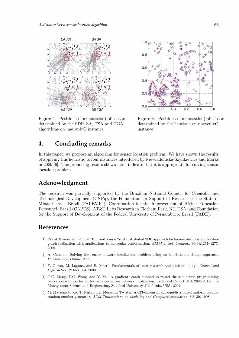
A distance based sensor location algorithm 63

Figure 2: Positions (star notation) of sensorsdetermined by the SDP, SA, TSA and TGAalgorithms on unevenlyC instance

Figure 3: Positions (star notation) of sensorsdetermined by the heuristic on unevenlyCinstance.

4. Concluding remarks

In this paper, we propose an algorithm for sensor location problem. We have shown the resultsof applying this heuristic to four instances introduced by Niewiadomska-Szynkiewicz and Marksin 2009 [6]. The promising results shown here, indicate that it is appropriate for solving sensorlocation problem.

Acknowledgment

The research was partially supported by the Brazilian National Council for Scientific andTechnological Development (CNPq), the Foundation for Support of Research of the State ofMinas Gerais, Brazil (FAPEMIG), Coordination for the Improvement of Higher EducationPersonnel, Brazil (CAPES), AT&T Labs Research in Florham Park, NJ, USA, and Foundationfor the Support of Development of the Federal University of Pernambuco, Brazil (FADE).

References

[1] Pratik Biswas, Kim-Chuan Toh, and Yinyu Ye. A distributed SDP approach for large-scale noisy anchor-freegraph realization with applications to molecular conformation. SIAM J. Sci. Comput., 30(3):1251–1277,2008.

[2] A. Cassioli. Solving the sensor network localization problem using an heuristic multistage approach.Optimization Online, 2009.

[3] F. Glover, M. Laguna, and R. Martí. Fundamentals of scatter search and path relinking. Control andCybernetics, 39:653–684, 2000.

[4] T.C. Liang, T.C. Wang, and Y. Ye. A gradient search method to round the semidenite programmingrelaxation solution for ad hoc wireless sensor network localization. Technical Report SOL 2004-2, Dep. ofManagement Science and Engineering, Stanford University, California, USA, 2004.

[5] M. Matsumoto and T. Nishimura. Mersenne Twister: A 623-dimensionally equidistributed uniform pseudo-random number generator. ACM Transactions on Modeling and Computer Simulation, 8:3–30, 1998.

64 Júlio C. Alves, Ricardo M. A. Silva, Geraldo R. Mateus, and Mauricio G.C. Resende

[6] Ewa Niewiadomska-Szynkiewicz and Michał Marks. Optimization schemes for wireless sensor networklocalization. International Journal of Applied Mathematics and Computer Science, 19(2):291–302, 2009.

[7] Z. Wang, S. Zheng, Y. Ye, and S. Boyd. Further Relaxations of the Semidefinite Programming Approachto Sensor Network Localization. SIAM Journal on Optimization, 19(2):655–673, 2008.

DGA 2013, pp. 65 – 69.

Adaptive Branching in iBP with Clifford Algebra

Rafael Alves,1 Andrea Cassioli,2 Antonio Mucherino,3 Carlile Lavor,1 and Leo Liberti 2

1IMECC-UNICAMP, Campinas-SP, Brazil. [email protected],[email protected]

2LIX, École Polytechnique, Palaiseau, France. [email protected],[email protected]

3IRISA, University of Rennes 1, Rennes, France. [email protected]

Abstract We consider the interval Discretizable Molecular Distance Geometry Problem (iDMDGP). Thisis a subclass of instances of the Distance Geometry that can be discretized; they are relatedto biological molecules and can contain imprecise measurements of the available distances. Theinterval branch-and-prune (iBP) is an algorithm for the iDMDGP. In this short paper, we integrateiBP with Clifford algebra, with the aim of improving the branching phase of the algorithm, bymaking it adaptive.

Keywords: molecular conformations, distance geometry, branch-and-prune, Clifford algebra

1. Introduction

Experiments of Nuclear Magnetic Resonance (NMR) are able to identify a subset of distancesbetween pairs of atoms of a given protein. This information, together with some additionalinformation on the chemical structure of the protein, can be exploited for finding the possiblethree-dimensional conformations for the molecule. This problem is known as the intervalMolecular Distance Geometry Problem (iMDGP) [3].

In this context, we are working on a subclass of iMDGPs that can be discretized. In otherwords, we consider all instances of this problem for which the search domain can be reducedto a tree, whose nodes at level j represent all possible Cartesian coordinates for the jth atomof the molecule. We say that such instances belong to the class of the interval DiscretizableMolecular Distance Geometry Problem (iDMDGP) [1].

The discretization allows for employing an interval Branch & Prune (iBP) algorithm forthe solution of iDMDGPs [1]. The idea is to explore the search tree recursively and to verify,as soon as they are generated, the feasibility of the computed atomic positions. Infeasiblepositions are immediately pruned, so that the search can be focused on the feasible parts ofthe tree. On each layer of the tree, a finite number of possible Cartesian coordinates for thecurrent atom are computed by intersecting three Euclidean objects in the three-dimensionalspace. Two of such objects always consist of spheres, whereas the third one may be either asphere or a spherical shell, depending on the fact the available distance is precise or representedby an interval, respectively.

When the three Euclidean objects are three spheres, their intersection, in our assumptions,always gives two disjoint points in R3, with probability one (the set of DMDGP instances forwhich this fails has zero Lebesgue measure in the set of all possible DMDGP instances; manyof our statements hold with probability one). However, when one of the three objects is aspherical shell, this intersection gives two curves in the three-dimensional space. A curve is

66 Rafael Alves, Andrea Cassioli, Antonio Mucherino, Carlile Lavor, and Leo Liberti

a continuous object, and therefore, in order to discretize it, it was proposed in [1] to take acertain predefined number D of points from such curves, and to include a new branch in thetree for each new generated point.

Computational experiments, reported in some previous publications [4, 4–1], showed thatthe solutions to iDMDGPs can be strongly influenced by the choice of D. If D is too small,only infeasible branches may be generated, so that the whole tree is pruned and no solutionscan be found. On the other hand, if D is too large, the consequent combinatorial explosionmight make the experiments too computationally expensive. Finding a trade-off D value is notan easy task in general.

This work presents a strategy for an adaptive branching during the execution of the iBPalgorithm, which is based on the so-called Clifford algebra [3, 7]. The main idea is to generatebranches that comply with the pruning distances, i.e. a minimal number of branches are keptin the tree, while the tree width can be controlled.

In Section 2, we shortly describe how to extend the iBP algorithm by implementing a strategybased on Clifford algebra. Section 5 shows some preliminary computational experiments.

2. Extending iBP with Clifford algebra

The Clifford algebra Cl3 over the real numbers is a 8-dimensional space with basis elements1, e1, e2, e3, e12, e13, e23, e123 representing scalars, vectors, bivectors and trivectors. The bivec-tors and trivectors are obtained by the geometric product, the main product in a Clifford algebra.This product is represented by the juxtaposition of the elements, and its rules for basis vectorsare shown in Equations (1) and (2). Other two products can be derived from the geometricproduct: the outer product “∧” and the contractions, left “c” and right “b”. For vectors, thecontractions are equivalent to the scalar product in R3 “·”. Some relations among these prod-ucts are shown in Equations (3) and (4) below. The geometric product between two vectorsis the sum of the scalar and the exterior products between them. In general, the geometricproduct between a vector and an arbitrary element of Cl3, called a multivector, is the sum ofthe left contraction and the exterior product.

e2i = 1, (1)

eiej = −ejei, (2)uv = u · v + u ∧ v, (3)uB = ucB + u ∧B. (4)

In Equations (3) and (4), u and v are vectors and B is a multivector of Cl3.With the addition of two vectors to the R3 basis (e∞ and e0), it is possible to construct a

model of geometry that allows us to handle with several basic geometric entities in a simpleway. We refer to the Clifford algebra associated to this model as the Conformal GeometricAlgebra (CGA) [3]. The basis elements for the conformal space are e1, e2, e3, e∞, e0, wheree∞ represents a point at infinity and e0 represents the origin of R3 in the conformal space.

In the CGA, basic geometric entities such as points, spheres, circles, lines and planes arerepresented in a simple way, and their intersections are performed intuitively. The outer productis used to compute intersections or to construct objects from points. The contractions can alsobe used for intersections, and are often used to compute orthogonal projections, distances andangles. Our approach is based on the geometric interpretation of the iDMDGP. A sphere isrepresented by Eq. (5), while the circle can be defined simply as a two sphere intersection, Eq.(6). Another important element is called a Point Pair, which is the result of a three sphere

Adaptive Branching in iBP with Clifford Algebra 67

intersection, Eq. (7). These elements are the most important ones in our approach:

S = X − 12r

2e∞, (5)

C = S1 ∧ S2, (6)Pp = S1 ∧ S2 ∧ S3. (7)

In Eq. (5), r is the sphere radius and X = x+ 12x

2e∞ + e0 is the projection of a point x ∈ R3

in the conformal space.The basic idea behind the proposed strategy is the following. Every time the current atom

has one reference distance that is represented by an interval, two spheres Si−1 and Si−2, relatedrespectively to the atomic positions xi−1 and xi−2, are intersected with the spherical shell S′i−3,related to the atomic position xi−3 such that the distance di−3,i is an interval. Due to thediscretization assumptions, this intersection produces up to two disjoint curves c′i−3 and c′′i−3 inthe three-dimensional space. These two curves belong to the circle C obtained by intersectingthe two spheres Si−1 and Si−2 (Figure 1). In symbols, c′i−3, c

′′i−3 ∈ C.

Figure 1: Intesection between two spheres and a spherical shell.

Let us suppose that there is an atom k that is already positioned, for which dk,i is a knowndistance. This distance generates another spherical shell S′k, which can be intersected with thecircle C, by producing other two curves: c′k, c′′k ∈ C (Figure 3). The same intersection can becomputed for any other atom j for which dj,i is known. After all the intersections have beencomputed, the remaining curves contain only feasible points. These curves can be describedby the rotation of its endpoints (Figures 2 and 3). In other words, if Ep is the set of all knowndistances, and Ep(i) is the subset of Ep containing only the distances related to the atom i,the feasible points on the circle C can be computed by the following formula:

F (i) =⋂

j∈Ep(i)∪i−3

(c′j ∪ c′′j

).

The set F (i) is a curve segment in Euclidean space. It only contains feasible points, i.e. pointsthat satisfy all the available distances for the current atom. As a consequence, for any relativelysmall value for D, there is no risk of pruning all the feasible points in the pruning phase. Insome sense, D can be considered as the precision of the conformations that are going to beincluded in iBP solution set.

68 Rafael Alves, Andrea Cassioli, Antonio Mucherino, Carlile Lavor, and Leo Liberti

Figure 2: Intersection with a pruning dis-tance d(i, k).

Figure 3: The curve c′′k is the only feasibleregion.

name naa na l C-iBP iBPhm30 4 18 28 4/13803 6/9292jmy-s 5 26 42 3/5220 4/39022jmy-m 10 51 90 3/11172 6/1402702kxa 23 117 206 3/1275 8/79422ppz 36 170 323 4/15618 6/430732jmy 15 77 134 3/19063 12/47681

Table 1: Computational results: for each instance we report D/#nodes.

3. Preliminary computational experiments

In this section, we summarize our preliminary experiments on the iBP algorithm with Cliffordalgebra. We show that the number of discretization points that are necessary for finding at leastone feasible solution decreases when the new strategy based on Clifford algebra is employed.

Both algorithms are coded in C++ and share most of the code, which has been compiledwith the g++ compiler version 4.7 with optimization flags -O3 -DNDEBUG. The tests have beenperformed on a laptop having an i3 Intel processor and running Linux.

Our instances contain real data from NMR experiments, that can be downloaded from theProtein Data Bank [4, 8]. They have different sizes, and they are related to protein backbonesonly [1]. For each instance, we report the number of aminoacids naa, the number of atoms na,the order length l, i.e. the tree depth, the minimum number of discretization points to find atleast one solution D, and number of generated nodes #nodes. We refer to iBP with Cliffordalgebra as C-iBP.

The results in Table 1 clearly show that the use of the Clifford algebra allows for a greatreduction of the branching factor to find feasible solutions.

References

[1] H.M. Berman, J. Westbrook, Z. Feng, G. Gilliand, T.N. Bhat, H. Weissig, I.N. Shindyalov, P.E. Bourne,The protein data bank, Nucleic Acids Research, 28, 235–242, 2000.

[2] V. Costa, A. Mucherino, C. Lavor, L.M. Carvalho, N. Maculan, On Suitable Orders for Discretizing Molecu-lar Distance Geometry Problems related to Protein Side Chains, IEEE Conference Proceedings, FederatedConference on Computer Science and Information Systems (FedCSIS12), Workshop on ComputationalOptimization (WCO12), Wroclaw, Poland, 397–402, 2012.

Adaptive Branching in iBP with Clifford Algebra 69

[3] L. Dorst, D. Fontijne, S. Mann, Geometric Algebra for Computer Science: An object-oriented approach forgeometry, Morgan Kaufmann Publishers Inc., 2007.

[4] C. Lavor, L. Liberti, A. Mucherino, On the Solution of Molecular Distance Geometry Problems with IntervalData, IEEE Conference Proceedings, International Workshop on Computational Proteomics (IWCP10),International Conference on Bioinformatics & Biomedicine (BIBM10), Hong Kong, 77–82, 2010.

[5] C. Lavor, L. Liberti, A. Mucherino, The interval Branch-and-Prune Algorithm for the Discretizable Molec-ular Distance Geometry Problem with Inexact Distances, to appear in Journal of Global Optimization,2013.

[6] L. Liberti, C. Lavor, N. Maculan, A. Mucherino, Euclidean Distance Geometry and Applications,Tech. Rep. 1205.0349v1 [q-bio.QM], arXiv, 2012.

[7] P. Lounesto, Clifford Algebras and Spinnors, Cambridge University Press, 2001.[8] A. Mucherino, C. Lavor, T. Malliavin, L. Liberti, M. Nilges, N. Maculan, Influence of Pruning Devices

on the Solution of Molecular Distance Geometry Problems, Lecture Notes in Computer Science 6630,P.M. Pardalos and S. Rebennack (Eds.), Proceedings of the 10th International Symposium on ExperimentalAlgorithms (SEA11), Crete, Greece, 206–217, 2011.

DGA 2013, pp. 71 – 75.

A Clifford Algebra approach to theDiscretizable Molecular Distance Geometry Problem

Alessandro Andrioni1

1IMECC, University of Campinas, Campinas, Brazil, [email protected]

Abstract The Discretizable Molecular Distance Geometry Problem (DMDGP) consists in a subclass of theMolecular Distance Geometry Problem for which an embedding in R3 can be found using a Branch& Prune (BP) algorithm in a discrete search space. We propose a Clifford Algebra model of theDMDGP with an accompanying version of the BP algorithm.

Keywords: Distance geometry, Clifford algebra, Branch and prune

1. The discretizable molecular distance geometry problem

The molecular distance geometry problem (MDGP) consists in finding coordinates in a three-dimensional space of a set of points x1, x2, . . . , xn for which some of the Euclidean distancesbetween them are known [4]. Let G = (V,E, d) be a simple weighted undirected graph whereeach vertex in V corresponds to a point in R3, and the weight of an edge corresponds to thedistance d between the respective points. Formally, the MDGP can be defined as follows [12]:

Definition 1. (MDGP). Let G = (V,E, d) be a simple weighted undirected graph. The MDGPis the problem of finding a function

x : V → R3

such that∀(u, v) ∈ E, ||xu − xv|| = duv,

where xu = x(u) and xv = x(v).

The discretizable molecular distance geometry problem (DMDGP) is a subset of the MDGP,but with two extra assumptions [12]:

Definition 2. (DMDGP). Let G = (V,E, d) be a simple weighted undirected graph associatedto an instance of the MDGP. Let us suppose that there is a total order relation on the verticesof V . The DMDGP consists in all the instances of the MDGP satisfying the following twoassumptions:

1. E contains all cliques on quadruplets of consecutive vertices;

2. the following strict triangular inequality must hold:

∀v ∈ 1, . . . , n− 2, dv,v+2 < dv,v+1 + dv+1,v+2,

where n is the number of vertices in V .

72 Alessandro Andrioni

The reasons why these assumptions are useful and realistic is outside of the scope of thiswork, and is extensively addressed in [12] and [14], but they allow us to discretize the problemin the following manner: suppose we have three points in R3, and the distances to a fourthpoint. We can then construct three spheres, each one centered in one of the points and with aradius of its distance to the fourth one. These three spheres have an intersection characterizedby two points (with probability 1, thanks to the assumptions above [14]): the two possibilitiesfor the fourth point. However, if we have additional information, we can decide whether one ofthem is invalid or not. Repeating this process, we have at most 2n−3 ways to position n points(up to rotation and translation).

The Branch & Prune (BP) is an algorithm proposed in [13] to solve the DMDGP by exploitingthis discretization. The BP was further developed [15] to use another characteristic of thediscretization, namely that when constructing a new point, the two possibilities are symmetricin regard to the plane determined by the three previous points. This means we can constructother realizations from an initial one by knowing just the different branches taken and thenapplying reflections through the right planes.

2. Clifford algebra

Clifford algebras are a refinement of both the Hamilton quaternions and the extensive algebra ofHermann Grassmann [3] condensed in one structure. Clifford himself called his work geometricalgebra [2], but the term most commonly used now is Clifford algebra. His work had a geometricflavor, and was heavily explored by both mathematicians and physicists, including Élie Cartanand Paul Dirac, usually in the context of differential geometry and quantum mechanics [5].

A revival of the use of real Clifford algebras for geometric purposes was spearheaded byDavid Hestenes [10], and culminated in the modern geometric algebra and its operationalmodels of Euclidean geometry, including conformal geometric algebra (CGA) [9]. CGA allowsa rich representation of Euclidean motions in a coordinate-free manner, and the link betweendistance geometry and conformal geometric algebra was already studied by Dress and Havel [6].

We try to follow the notation and the formulation introduced in [5], and recommend it as agood introduction to the subject, but we give a summary of central Clifford algebra ideas usedin this work.

There are two main products which are used: the geometric (or Clifford) product, andthe outer (or wedge) product1. Both of them algebraically encode the idea of working withoriented subspaces of a vector space, allowing a “multivector” representation of points, lines,planes and hyperplanes. An interesting fact is that the geometric product allows the inverse ofsome multivectors to be defined, and thus it permits the representation of orthogonal or evenconformal (in CGA) transformations using an object called versor.

A versor is the result of a multiplication of vectors using the geometric product, it is alwaysinvertible and it is applied to another multivector by “sandwiching”, that is, if V is a versorand A a multivector, we can apply the versor by calculating V AV −1. Versors also correctlypreserve its underlying geometric structure without need for adaptations, being then a suitablebasis for the representation of geometric computations.

Definition 3. (Conformal geometric algebra of the three-dimensional Euclidean space). Theconformal geometric algebra (CGA) of the three-dimensional Euclidean space is an extensionof R3 by means of two extra vectors e and e, which square respectively to 1 and −1. However, itis more convenient to use ∞ = e− e and o = 1

2(e+ e), both of which square to 0, and represent

1The geometric product of a and b is denoted by ab, and their outer product by a ∧ b.

A Clifford Algebra approach to the Discretizable Molecular Distance Geometry Problem 73

a point at infinity and a point at the origin, respectively. This permits a fully coordinate-freerepresentation of Euclidean geometry, a fact which will be exploited in our algorithm.

In CGA, versors encode all conformal transformations, including isometries and homotheties.In fact, it is the smallest known model of Euclidean geometry which allows the full represen-tation of Euclidean transformations as versors. For convenience, we introduce special namesto two kinds of versors: those which represent rotations (rotors), and those which representtranslations (translators).

Composition of rotors and translators is more efficient than that of rotation matrices inup to 10 dimensions and uses less storage in up to 6 dimensions, a good evidence of theappropriateness of using CGA for geometric computing. It is also simple to convert versors tomatrices, if the need arises [5].

3. BP with Clifford algebra

We assume that our instance is a molecule of n atoms for which we denote the bond lengthsdi−1,i for i = 2, . . . , n, the bond angles θi−2,i for i = 3, . . . , n and the dihedral angles ωi−3,i fori = 4, . . . , n.

The main idea of the BP with Clifford Algebra is to use rotors and translators to representthe calculation of a point from its predecessors, instead of transformation matrices based onhomogeneous coordinates [12]. Since a combination of rotor and translator needs at most 8coordinates to be represented, this represents a memory gain against the traditional 4 × 4matrices.

Another advantage of using CGA to work on the DMDGP is to exploit the inherent symme-tries in the problem, since reflection through a plane is a simple operation in CGA representedby a reflection versor, cheapening considerably the cost of calculating alternative conformations.

An algorithm to calculate the two possible points from its predecessors is presented here asAlgorithm 2. It creates two rotors: one for the bond angle and one for the dihedral angle, andapply them to a translator to generate F , an Euclidean transformation which takes xi−1 to xi.Notice in the algorithm the particular way the rotors are constructed, which is reminiscent ofEuler’s formula and the polar forms of complex numbers or quaternions. The pruning phase isimplemented as in the original BP [14].

A computer implementation of this new version of the BP already exists for the GAViewersoftware [5], but as the software was not made with efficiency needs in mind, it is only useful as avisualization tool. A “production-ready” implementation using the software Gaigen [7] capableof using data extracted from the Protein Data Bank is currently being written, and should becomplete in time for the DGA2013, along with a performance analysis and a comparison withthe existing implementations of the original BP [13].

Algorithm 1 Initial potential solutionprocedure Initial potential solution(n, d, θ, ω)

solution ← the three initial pointsi← 4while i ≤ n do

5: Compute i-th point and add to solutionend whilereturn solution

end procedure

74 Alessandro Andrioni

Algorithm 2 Compute i-th pointprocedure Algorithm I: Compute i-th point(xi−3, xi−2, xi−1, θ, ω, d)

Π ← xi−3 ∧ xi−2 ∧ xi−1 ∧∞;R1 ← e

θ2 ((Πxi−2∧xi−1)∧∞)∗ ; . Create the bond angle rotor

v ← xi−1 − xi−2;5: ω′ ← ω − π

2 ;R2 ← e

ω′2 (xi−2∧xi−1∧∞)∗ ; . Create the dihedral angle rotor

T ← 1− d2

v||v||∞; . Create the translator

F ← R2R1 TR−11 R−1

2 ; . Combine two rotors and a translator in one versorxi ← F xi−1F

−1 . Apply it xi−110: x′i ← ΠxiΠ−1 . Reflect xi

return xi, x′i

end procedure

4. Conclusions and future work

This is one of the first practical applications of conformal geometric algebra in distance ge-ometry and it shows its excellence in representing complex geometric operations in a simplemanner. The subsumption of both quaternions and homogeneous coordinates by CGA allowsit to clarify the notation and to better expound inherent geometric properties in problems.

We expect to see more developments in that regard in the future, as more accessible, efficientand high-level implementations of geometric algebra appear, as it is suited for scientific com-puting and is already being used in the fields of robotics, computer graphics, computer visionand artificial neural networks [1] [5] [16].

An extension of this work to handle generalizations of the DMDGP is expected, as conformalgeometric algebra has a great richness in ways of creating and manipulating its objects. Anotherpossible line of work would be to try to apply CGA techniques to other problems involvingmolecular symmetries and rotations, such as [8] and [11].

Acknowledgments

The authors would like to thank the Brazilian research agencies FAPESP, CNPq and CAPESfor the financial support.

References

[1] E. Bayro-Corrochano. Geometric Computing - for Wavelet Transforms, Robot Vision, Learning, Controland Action. Springer, 2010.

[2] W. Clifford. Applications of Grassmann’s extensive algebra. American Journal of Mathematics, 1:350–358,1878.

[3] J. Collins. An elementary exposition of Grassmann’s “Ausdehnungslehre,” or theory of extension. TheAmerican Mathematical Monthly, 6:193–198, 1899.

[4] G. Crippen and T. Havel. Distance Geometry and Molecular Conformation. Wiley, New York, 1988.

[5] L. Dorst, D. Fontijne, and S. Mann. Geometric Algebra for Computer Science: An Object-Oriented Approachto Geometry. Morgan Kaufmann Publishers Inc., San Francisco, 2007.

[6] A. Dress and T. Havel. Distance geometry and geometric algebra. Foundations of Physics, 23:1357–1374,1993.

A Clifford Algebra approach to the Discretizable Molecular Distance Geometry Problem 75

[7] D. Fontijne. Gaigen 2: a geometric algebra implementation generator. In Proceedings of the 5th internationalconference on Generative programming and component engineering, GPCE ’06, New York, 2006. ACM.

[8] H. Fritzer. Molecular symmetry with quaternions. Spectrochimica Acta Part A: Molecular and BiomolecularSpectroscopy, 57:1919–1930, 2001.

[9] D. Hestenes. Old wine in new bottles: A new algebraic framework for computational geometry. In Advancesin Geometric Algebra with Applications in Science and Engineering, pages 1–14, 2001.

[10] D. Hestenes and G. Sobczyk. Clifford Algebra to Geometric Calculus: A Unified Language for Mathematicsand Physics. Fundamental Theories of Physics. Springer, 1987.

[11] C. Karney. Quaternions in molecular modeling. Journal of Molecular Graphics and Modelling, 25:595–604,2007.

[12] C. Lavor, L. Liberti, N. Maculan, and A. Mucherino. The discretizable molecular distance geometryproblem. Computational Optimization and Applications, 52:115–146, 2012.

[13] L. Liberti, C. Lavor, and N. Maculan. A branch-and-prune algorithm for the molecular distance geometryproblem. International Transactions in Operational Research, 15:1–17, 2008.

[14] L. Liberti, C. Lavor, N. Maculan, and A. Mucherino. Euclidean distance geometry and applications. Tech.Report q-bio.qm/1205.0349, arXiv, 2012.

[15] A. Mucherino, C. Lavor, and L. Liberti. Exploiting symmetry properties of the discretizable moleculardistance geometry problem. Journal of Bioinformatics and Computational Biology, 10, 2012.

[16] C. Perwass. Geometric Algebra with Applications in Engineering. Springer Berlin Heidelberg, 2009.

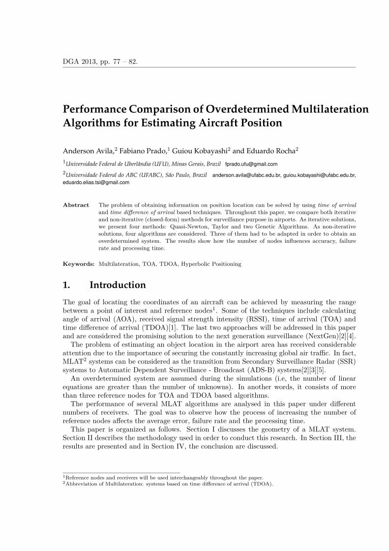
DGA 2013, pp. 77 – 82.

Performance Comparison of Overdetermined MultilaterationAlgorithms for Estimating Aircraft Position

Anderson Avila,2 Fabiano Prado,1 Guiou Kobayashi2 and Eduardo Rocha2

1Universidade Federal de Uberlândia (UFU), Minas Gerais, Brazil [email protected]

2Universidade Federal do ABC (UFABC), São Paulo, Brazil [email protected], [email protected],[email protected]

Abstract The problem of obtaining information on position location can be solved by using time of arrivaland time difference of arrival based techniques. Throughout this paper, we compare both iterativeand non-iterative (closed-form) methods for surveillance purpose in airports. As iterative solutions,we present four methods: Quasi-Newton, Taylor and two Genetic Algorithms. As non-iterativesolutions, four algorithms are considered. Three of them had to be adapted in order to obtain anoverdetermined system. The results show how the number of nodes influences accuracy, failurerate and processing time.

Keywords: Multilateration, TOA, TDOA, Hyperbolic Positioning

1. Introduction

The goal of locating the coordinates of an aircraft can be achieved by measuring the rangebetween a point of interest and reference nodes1. Some of the techniques include calculatingangle of arrival (AOA), received signal strength intensity (RSSI), time of arrival (TOA) andtime difference of arrival (TDOA)[1]. The last two approaches will be addressed in this paperand are considered the promising solution to the next generation surveillance (NextGen)[2][4].

The problem of estimating an object location in the airport area has received considerableattention due to the importance of securing the constantly increasing global air traffic. In fact,MLAT2 systems can be considered as the transition from Secondary Surveillance Radar (SSR)systems to Automatic Dependent Surveillance - Broadcast (ADS-B) systems[2][3][5].

An overdetermined system are assumed during the simulations (i.e, the number of linearequations are greater than the number of unknowns). In another words, it consists of morethan three reference nodes for TOA and TDOA based algorithms.

The performance of several MLAT algorithms are analysed in this paper under differentnumbers of receivers. The goal was to observe how the process of increasing the number ofreference nodes affects the average error, failure rate and the processing time.

This paper is organized as follows. Section I discusses the geometry of a MLAT system.Section II describes the methodology used in order to conduct this research. In Section III, theresults are presented and in Section IV, the conclusion are discussed.

1Reference nodes and receivers will be used interchangeably throughout the paper.2Abbreviation of Multilateration: systems based on time difference of arrival (TDOA).

78 Anderson Avila, Fabiano Prado, Guiou Kobayashi and Eduardo Rocha

2. Multilateration System and its Geometric Interpretation

In a Multilateration system, the signal transmitted by a source (e.g, a transponder) and receivedby three or more ground based receiver sites is denominated time of arrival (TOA). Consideringa 2-dimensional Euclidean space, let Si = (xi, yi) be the reference node locations and ti therespective arrival time, where i = 1, ..., N . The unknowns aircraft position and time of emission(TOE) are given by Sa = (xa, ya) and te, respectively.

Assuming a Line of Sight scenario (LOS), the distance between Si and Sa can be representedby (1), being c the speed of light.

c (ti − te) =√

(xi − xa)2 + (yi − ya)2 (1)

If we consider that the emission occurs at time 0, the TOA based techniques will requireat least three equations (i.e, three reference nodes) for two unknowns (xa, ya)[11]. Figure 1-adepicts an overdetermined system, where N > 3.

(a) Overdetermined system (TOA based) (b) Hyperbolas intersection (TDOA based)

Figure 1: Multilateration schemes

Notice that using only two receivers, e.g, S1 and S2, gives us two solutions, A and B, depictingan ambiguity. Thus, it is necessary the use of at least another reference node, S3, in order todetermining A as the correct solution. The fourth node characterizes an overdetermined system.

Another approach for estimating an aircraft position is to calculate the difference in timeof arrival (TOA) between pairs of reference nodes. Hyperbolic positioning, or time differenceof arrival (TDOA), is a technique that consider the intersection of hyperbolas as the mobileposition[7][8]. The distance-difference to a source can be represented by (2).

c (ti − tj) =√

(xi − xa)2 + (yi − ya)2 −√

(xj − xa)2 + (yj − ya)2 (2)

The emission time is common for all the receivers, thus the equation above eliminates theunknown te which is in accordance with our goal, since we are only interested in measuring thearrival time range. The system is depicted in Figure 1-b3.

3Font: A Passive Localization Algorithm and Its Accuracy Analysis.[9]

Performance Comparison of Overdetermined Multilateration Algorithms for Estimating Aircraft Position 79

3. Performance Assessment and Experiments

3.1 Algorithms

Eight location estimation algorithms form the object of interest of this research. Four of themare non-iterative methods4: Bancroft [11], Bucher[7], Bakhoum[10], Least Squares[12]. Amongthese algorithms, only Bancroft[11] is based on TOA. The Least Squares method can optionallybe implemented as TOA or TDOA based[12]. All closed-form algorithms, except for the LeastSquares, required an adaptation to ensure an overdetermined approach.

As iterative methods, four solutions were considered. Two genetic algorithms based onheuristic search were implemented, besides Taylor and Quasi-Newton methods [13][12][14][15].All of these solutions are based on TDOA, except for one of the genetic algorithms.

3.2 Surveillance Area

Although, all the algorithms were implemented using the C++ programming language, to builda simulation environment, we used Matlab. We were able to link our C++ code with Matlabthrough an interface named MEX5.

The airport surface was assumed to be 1Km2 of surveillance area discretized in m2. Thereference nodes were placed arbitrarily in 16 fixed sites as shown in Figure 2. For each algorithm,

Figure 2: Position of the reference nodes

the simulation started with the number of 4 receivers (S1, S2, S3, S4), geometrically forming asquare. The other nodes were added up sequentially, according to its number. Sensors 1 to8 were located outside of the surveillance area and Sensors 9 to 16 were located inside thatarea. Since the errors associated to the hardware are unknown, we hypothetically assumed aGaussian error distribution associated to the TOA measurements, where µ = 0 and σ = 1,2,3.

3.3 Simulation

To obtain the three parameters analysed in this paper, all algorithms were submitted to estimate500 random points in the surveillance area. This process were repeated 31 times6 for eachalgorithm and every time a reference node were added up to the system. Therefore, for aspecific number of receivers, 15.500 points were estimated by each algorithm. The averageerror were obtained by summing up the error and dividing it by the number of processed

4In this paper, the non-iterative methods will be referred as Bancroft, Bucher and Bakhoum5http://www.mathworks.com/help/matlab/matlab_external/introducing-mex-files.html631 showed to be a suited number to reach a reliable result.

80 Anderson Avila, Fabiano Prado, Guiou Kobayashi and Eduardo Rocha

points. The failure rate were characterized by the number of times that the algorithm couldnot define the coordinates (i.e, NaN7 or Inf8 were returned) or the coordinates represented anerror above 20 meters. Finally, the processing time were determined by summing up the timerequired for estimation and dividing it by the number of processed points.

4. Results

The goal of the simulations were to measure the performance of each algorithm as the numberof reference nodes were increased. It is clear that the Taylor method has the worst precisionas we can see on Figure 3-a and 3-c and the performance remains the same as the numberof receivers grows. The same behaviour is not experienced by the other algorithms. Bothaverage error and failure rate improves as the number of reference nodes are increased. Thiseffect is even more evident on Bancroft’s and Bucher’s algorithms. As expected, the mostcomputationally demanding algorithms are those base on iterative methods, especially theones that use evolutionary approach, as we can verify on Figure 3-b.

(a) Average error (b) Processing time

(c) Failure rate (d) Failure rate without Taylor results

Figure 3: Performance comparison: mean and processing time

Except for the Taylor method, Table 1 shows that increasing the number of reference nodesincreases the processing time and decreases the average error.

7Not a number.8Divided by zero

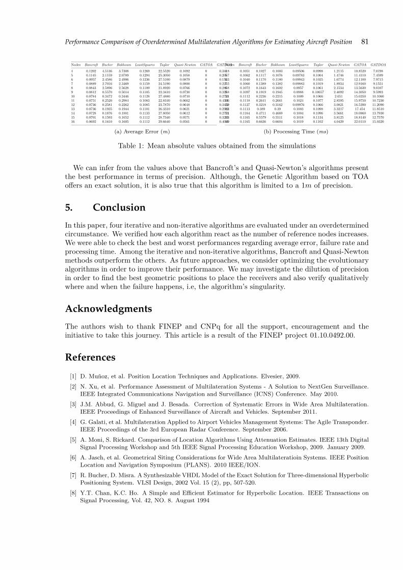
Performance Comparison of Overdetermined Multilateration Algorithms for Estimating Aircraft Position 81

Nodes Bancroft Bucher Bakhoum LeastSquares Taylor Quasi-Newton GATOA GATDOA

4 0.1202 4.5136 3.7308 0.1269 22.5520 0.1092 0 0.34185 0.1145 2.1159 2.0789 0.1294 25.3050 0.1058 0 0.20576 0.0957 2.4586 2.4906 0.1236 27.5100 0.0879 0 0.15337 0.0889 2.7016 2.3469 0.1159 24.5190 0.0800 0 0.22558 0.0843 2.5896 2.5628 0.1109 21.8920 0.0766 0 0.28589 0.0812 0.5570 0.5014 0.1105 22.3410 0.0730 0 0.325810 0.0784 0.3472 0.3446 0.1128 27.4880 0.0710 0 0.272111 0.0751 0.2520 0.2984 0.1083 22.8340 0.0662 0 0.430612 0.0736 0.2581 0.2262 0.1085 23.7870 0.0648 0 0.345913 0.0736 0.1935 0.1944 0.1101 26.3310 0.0621 0 0.298314 0.0728 0.1876 0.1881 0.1133 27.8050 0.0612 0 0.277115 0.0701 0.1593 0.1652 0.1112 28.7340 0.0571 0 0.326316 0.0692 0.1610 0.1605 0.1112 29.6640 0.0561 0 0.4049

(a) Average Error (m)

Nodes Bancroft Bucher Bakhoum LeastSquares Taylor Quasi-Newton GATOA GATDOA

4 0.1051 0.1027 0.1003 0.09506 0.0998 1.2115 10.8520 7.01985 0.1062 0.1117 0.1076 0.09783 0.1004 1.4746 11.4110 7.45996 0.1040 0.1170 0.1180 0.09943 0.1035 1.6774 12.1100 7.97157 0.1060 0.1389 0.1382 0.09883 0.1019 1.8934 12.9160 9.15518 0.1072 0.1643 0.1602 0.0957 0.1061 2.1534 13.5630 9.01079 0.1097 0.1919 0.1945 0.0988 0.10657 2.4092 14.3050 9.599310 0.1112 0.2236 0.2215 0.1009 0.1066 2.651 15.0350 10.106011 0.1118 0.2641 0.2661 0.1024 0.1077 2.8595 15.9750 10.723012 0.1127 0.3218 0.3162 0.09976 0.1066 3.0821 16.5390 11.209013 0.1113 0.389 0.39 0.1003 0.1098 3.3217 17.454 11.851014 0.1164 0.4711 0.4669 0.1004 0.1096 3.5661 18.0860 13.793015 0.1165 0.5579 0.5511 0.1018 0.1134 3.8125 18.8140 12.757016 0.1165 0.6636 0.6604 0.1019 0.1102 4.0429 22.0110 15.0320

(b) Processing Time (ms)

Table 1: Mean absolute values obtained from the simulations

We can infer from the values above that Bancroft’s and Quasi-Newton’s algorithms presentthe best performance in terms of precision. Although, the Genetic Algorithm based on TOAoffers an exact solution, it is also true that this algorithm is limited to a 1m of precision.

5. Conclusion

In this paper, four iterative and non-iterative algorithms are evaluated under an overdeterminedcircumstance. We verified how each algorithm react as the number of reference nodes increases.We were able to check the best and worst performances regarding average error, failure rate andprocessing time. Among the iterative and non-iterative algorithms, Bancroft and Quasi-Newtonmethods outperform the others. As future approaches, we consider optimizing the evolutionaryalgorithms in order to improve their performance. We may investigate the dilution of precisionin order to find the best geometric positions to place the receivers and also verify qualitativelywhere and when the failure happens, i.e, the algorithm’s singularity.

Acknowledgments

The authors wish to thank FINEP and CNPq for all the support, encouragement and theinitiative to take this journey. This article is a result of the FINEP project 01.10.0492.00.

References

[1] D. Muñoz, et al. Position Location Techniques and Applications. Elvesier, 2009.[2] N. Xu, et al. Performance Assessment of Multilateration Systems - A Solution to NextGen Surveillance.

IEEE Integrated Communications Navigation and Surveillance (ICNS) Conference. May 2010.[3] J.M. Abbud, G. Miguel and J. Besada. Correction of Systematic Errors in Wide Area Multilateration.

IEEE Proceedings of Enhanced Surveillance of Aircraft and Vehicles. September 2011.[4] G. Galati, et al. Multilateration Applied to Airport Vehicles Management Systems: The Agile Transponder.

IEEE Proceedings of the 3rd European Radar Conference. September 2006.[5] A. Moni, S. Rickard. Comparison of Location Algorithms Using Attenuation Estimates. IEEE 13th Digital

Signal Processing Workshop and 5th IEEE Signal Processing Education Workshop, 2009. January 2009.[6] A. Jasch, et al. Geometrical Siting Considerations for Wide Area Multilateratioin Systems. IEEE Position

Location and Navigation Symposium (PLANS). 2010 IEEE/ION.[7] R. Bucher, D. Misra. A Synthesizable VHDL Model of the Exact Solution for Three-dimensional Hyperbolic

Positioning System. VLSI Design, 2002 Vol. 15 (2), pp, 507-520.[8] Y.T. Chan, K.C. Ho. A Simple and Efficient Estimator for Hyperbolic Location. IEEE Transactions on

Signal Processing, Vol. 42, NO. 8. August 1994

82 Anderson Avila, Fabiano Prado, Guiou Kobayashi and Eduardo Rocha

[9] B. Friedlander. A Passive Localization Algorithm and Its Accuracy Analysis. IEEE Journal of OceanicEngineering, Vol. OE-12, NO. 1. January 1987.

[10] E.G. Bakhoum. Closed-Form Solution of Hyperbolic Geolocation Equations. IEEE Transactions onAerospace and Eletronics Systems, VOL. 42, NO. 4. October 2006.

[11] M. Geyer, A. Daskalakis. Solving Passive Multilateration Equations Using Bancrofts’ Algorithm. TheAIAA/IEEE/SAE Digital Avionics Systems Conference. Proceeding 17th DASC. October 1998.

[12] G. Shen, R. Zetik, R.S. Thomä. Performance Comparison of TOA and TDOA Based Location EstimationAlgorithms in LOS Environment. IEEE Proceedings of the 5th Workshop on Positioning, Navigating andCommunication 2008.

[13] S. Forrest. Genetic Algorithms:Principles of Natural Selection Applied to Computation. Science, NewSeries, Vol. 261, No. 5123, pp 872-878. August 1993.

[14] Yu, et al. UWB location and tracking for wireless embedded networks. Signal Processing 86 (2006), pp2153-2171.

[15] R. Fletcher. Practical Methods of Optimization, 2000. Chapters 1,2 and 3.

DGA 2013, pp. 83 – 88.

On the using of distances to measure goodness of fit inItem Response Theory models: a Bayesian perspective

Caio Lucidius Naberezny Azevedo1 and Jose R. S. Santos2

1,2Department of Statistics, University of Campinas, Brazil [email protected],[email protected]

Abstract Many statistical tools for model validation and comparison are based on some suitable measuresof distance (discrepance). Examples are: deviance residual, chi-squared type statistics, odds ratioand Mahalanobis distance. In Item Response Theory (IRT), which comprises a widely used setof psychometric models, some of these distance-type statistics can be used to verify the validityof many important assumptions such as: unidimensionality, the adequability of the item responsefunction, the adequability of the latent trait distribution, the presence of DIF (Differential itemfunctioning) among others. However, under a frequentist approach, the using of these statisticscan be complicated because their distributions, under the null and alternative hypothesis, areusually not known. On the other hand, under the Bayesian paradigm, the obtaining of the so-called Bayesian p-values, related to these statistics, through MCMC algorithms, is feasible andstraightforward. In this work, we explore the using of some of these statistics, under the Bayesianparadigm, to verify the validity of some usual assumptions for unidimensional IRT models fordichotomous responses. More specifically, through simulation studies, we intend to verify therelationship of some of these measures of distance with the departing of some assumptions. Withthe results we intend to understandig how suitable the aforementioned measures of distance are indetecting the departing of the aforementioned assumptions.

Keywords: Item response theory, Model fit assessmente, Bayesian Inference

1. Introduction

The Item Response Theory (IRT) comprises a set of widely used psychometric models. Themost basic elements of this class of models, establish relationships between the so-called itemparameters and the latent traits, through statistical models. In their turn, these models considerthe probability of subjects get a certain score in each item, based on the responses of thesesubjects to these items. In general, the items are clustered in some measurement instrument, asa cognitive test or a psychiatric questionnaire. See [4] and [5], for more details. In this work, wewill focus on our attention in dichotomous items, or item which are corrected as right/wrong.In addition, we will consider the most basic IRT models, that is, models that consideres onlythe item parameters and the latent traits.

As in any statistical model, it is necessary to consider some assumptions in order to estimatethe parameters and to obtain results that are both interpretable and useful. Therefore, for agiven data set, the model used to analyze it, must be fit to the data, properly. For the unidimen-sional IRT models to dichotomous responses, the usual assumptions are: the unidimensionalityof the latent traits, the adequability of the item response function (IRF) and the adequabilityof the latent traits distribution. Several methods have been proposed in the literature for modelfit assessment. The works of [9], [10], [11], [12] and [13], present some reviews concerning this

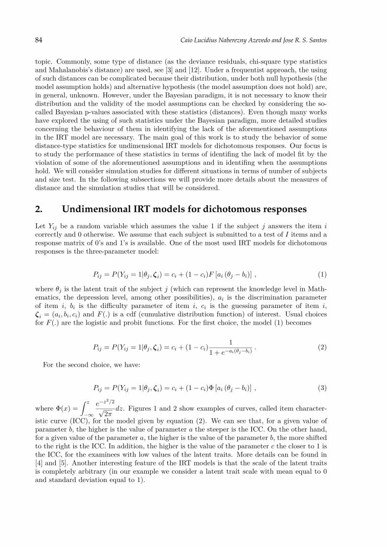
84 Caio Lucidius Naberezny Azevedo and Jose R. S. Santos

topic. Commonly, some type of distance (as the deviance residuals, chi-square type statisticsand Mahalanobis’s distance) are used, see [3] and [12]. Under a frequentist approach, the usingof such distances can be complicated because their distribution, under both null hypothesis (themodel assumption holds) and alternative hypothesis (the model assumption does not hold) are,in general, unknown. However, under the Bayesian paradigm, it is not necessary to know theirdistribution and the validity of the model assumptions can be checked by considering the so-called Bayesian p-values associated with these statistics (distances). Even though many workshave explored the using of such statistics under the Bayesian paradigm, more detailed studiesconcerning the behaviour of them in identifying the lack of the aforementioned assumptionsin the IRT model are necessary. The main goal of this work is to study the behavior of somedistance-type statistics for undimensional IRT models for dichotomous responses. Our focus isto study the performance of these statistics in terms of identifing the lack of model fit by theviolation of some of the aforementioned assumptions and in identifing when the assumptionshold. We will consider simulation studies for different situations in terms of number of subjectsand size test. In the following subsections we will provide more details about the measures ofdistance and the simulation studies that will be considered.

2. Undimensional IRT models for dichotomous responses

Let Yij be a random variable which assumes the value 1 if the subject j answers the item icorrectly and 0 otherwise. We assume that each subject is submitted to a test of I items and aresponse matrix of 0’s and 1’s is available. One of the most used IRT models for dichotomousresponses is the three-parameter model:

Pij = P (Yij = 1|θj , ζi) = ci + (1− ci)F [ai (θj − bi)] , (1)

where θj is the latent trait of the subject j (which can represent the knowledge level in Math-ematics, the depression level, among other possibilities), ai is the discrimination parameterof item i, bi is the difficulty parameter of item i, ci is the guessing parameter of item i,ζi = (ai, bi, ci) and F (.) is a cdf (cumulative distribution function) of interest. Usual choicesfor F (.) are the logistic and probit functions. For the first choice, the model (1) becomes

Pij = P (Yij = 1|θj , ζi) = ci + (1− ci)1

1 + e−ai(θj−bi). (2)

For the second choice, we have:

Pij = P (Yij = 1|θj , ζi) = ci + (1− ci)Φ [ai (θj − bi)] , (3)

where Φ(x) =∫ z

−∞

e−z2/2

√2π

dz. Figures 1 and 2 show examples of curves, called item character-

istic curve (ICC), for the model given by equation (2). We can see that, for a given value ofparameter b, the higher is the value of parameter a the steeper is the ICC. On the other hand,for a given value of the parameter a, the higher is the value of the parameter b, the more shiftedto the right is the ICC. In addition, the higher is the value of the parameter c the closer to 1 isthe ICC, for the examinees with low values of the latent traits. More details can be found in[4] and [5]. Another interesting feature of the IRT models is that the scale of the latent traitsis completely arbitrary (in our example we consider a latent trait scale with mean equal to 0and standard deviation equal to 1).

On the using of distances to measure GOF in IRT 85

For a (n× I) matrix of (0,1) responses, the parameters (θ, a, b, c) can be estimated by usingseveral methods as the marginal maximum likelihood, marginal maximum a posterior, CADEM(Condicional Augmented Data EM) algorithm and by using a fully Bayesian approach troughMCMC (Monte Carlo Markov Chain) algorithms, see [4], [1], [8] and [2], for example.

−4 −2 0 2 4

0.0

0.2

0.4

0.6

0.8

1.0

latent trait

pro

bab

ility

of

corr

ect re

spo

nse

a = 0.6

a = 0.8

a = 1

a = 1.2

a = 1.4

Figure 1: Examples of ICC’s for the three-parameter logistic model for different values ofdiscrimination parameter (b=0.0;c=0.20)

3. Measuring the Goodness of fit in IRT models throughdistance type statistics

3.1 Chi-square type distance

Let NCk denote the number of examinees getting exactly k items correct, k = 0, 1, 2, ..., I.[6] and [7] suggest compare the observed and predicted score distributions to measure theoverall model fit. To summarize the model fit to the observed score distribution in a sin-gle number, Beguin and Glas (2001) suggested the using of the discrepancy measure χ2

NC =∑Ik=1

(NCk−E(NCk))2

E(NCk) , where E(NCk) is the expectation of NCk. Although the statistic χ2NC

does not follow a chi-square distribution, the Bayesian p-value provides a measure of overallgoodness of fit. Clearly, the discrepancy measure χ2

NC is a distance, once that measures thedifference between the observed value NCk and the expeceted value E(NCk).

3.2 Residual type distance

For each Yij , i = 1, ..., I; j = 1, ..., n we can define the deviance residual, that is

DRij =[√−2 ln (1− Pij)

]1−yij [√2 lnPij

]yij.

86 Caio Lucidius Naberezny Azevedo and Jose R. S. Santos

−4 −2 0 2 4

0.0

0.2

0.4

0.6

0.8

1.0

latent trait

pro

ba

bili

ty o

f co

rrect

resp

on

se

b = −2

b = −1

b = 0

b = 1

b = 2

Figure 2: Examples of ICC’s for the three-parameter logistic model for different values ofdifficulty parameter (a=1.0;c=0.20)

It is clear that, depending on the value of the response (yij), the value of the devianceresidual changes. Therefore, it can be seen that the above quantity measures the differencebeteween the observed response and the expected reponse.

3.3 Other type distance

Consider an item pair in the test. Let nkk′ , k, k′ ∈ 0, 1, the number of subjects scoring k onthe first item and k′on the second item. The odds-ratio is defined as:

OR =n00n01n10n11

= n00n11n01n10

in other words, we are measuring the distance between the proportion of incorrecet/correctanswers among each pair of items.

4. Calculating Bayesian p-values for the distance typestatistics

Let yobs be the matrix of observed responses, and yrep the matrix of replicated responsesgenerated from its posterior predictive distribution. The posterior predictive distribution ofthe response data of group k is represented by

p(yrep | yobs

)=

∫p (yrep | ϑ) p

(ϑ | yobs

)dϑ,

where ϑ denotes the set of model parameters considered in the discrepancy measure. Generally,given a discrepancy measure D (y,ϑ), the replicated data can be used to evaluate whether the

On the using of distances to measure GOF in IRT 87

discrepancy value given the observed data is typical under the model. A p-value can be definedthat quantifies the extremeness of the observed discrepancy value,

p0(y(obs)

)= P

(D(y(rep),ϑ

)≥ D

(y(obs),ϑk

)| y(obs)

), (4)

where the probability is taken over the joint posterior of (y(rep),ϑ). Consider, for example,the χ2

NC distance. In this case NCk = f(yobs),E(NCk) =∑nj=1 Pij and ϑ = (θ,a, b, c)′.

Therefore, in this case, D(y,ϑ) = χ2NC . In general, the distances can be defined in order to

provide a overall, by item (adequability of the IRF) or by subject (adequability of the latenttraits distribution) measure of model fit. The Bayesian p-value can be easily estimated byusing the MCMC outputs as simply evaluating the observed proportion as defined in (4). Thehigher is the value of value of the Bayesian p-value, equation (4), better is the model fit.

5. Simulation study

We will generated a several number of replicas (matrix with responses of the subjects to theitems) from different IRT models (one, two and three parameter), with one, two and threelatent trait dimension and considering different latent trait distribution (normal, left skewed,right skewed and uniform). With these replicas we will estimate the parameters and calculatethe bayesian p-values related to the aforementioned measures of distance, using the one, twoan three onedimensional IRT models and a standard normal distribution for the latent traits.Therefore, we wil, study the behavior of the bayesian p-values in detecting the departing ofthe usual model assumptions (unidimensionality, the correct specification of the item responsefunction and the correct specficitation of the latent traits distribution).

Acknowledgments

The authors wish to thank CNPq and CAPES (Brazilian agencies of financial support forresearch) for the finnancial support.

References

[1] Azevedo, C. L. N., Bolfarine, H. and Andrade, D. F. (2011). Bayesian inference for a skew-normal IRTmodel under the centred parameterization, Comput. Statist. Data Anal., 55, 353–365.

[2] Azevedo, C. L. N. and Andrade, D. F. (2011). CADEM: A conditional augmented data EM algorithm forfitting one parameter probit models, Brazilian Journal of Probability and Statistics, Accepted for publication.

[3] Azevedo, C. L. N., Andrade, D. F. and Fox, J.-P. (2012). A Bayesian generalized multiple group IRT modelwith model-fit assessment tools, Comput. Statist. Data Anal., 56, 4399–4412.

[4] Baker, F. B. and Kim, Seock-Ho. (2004). Item Response Theory: Parameter Estimation Techniques. NewYork, NY: Marcel Dekker.

[5] Linde, W. J. van der and Hambleton, R. K. (2010). Handbook of Modern Item Response Theory. New York,NY: Springer-Verlag.

[6] Ferrando, P. J. and Lorenzo-seva, U. (2001). Checking the appropriateness of item response theory mod-els by predicting the distribution of observed scores: The program EP-fit, Educational and PsychologicalMeasurement, 61, 5, 895—902.

[7] Hambleton, R. K. and Han, N. (2004). Assessing the fit of IRT models: Some approaches and graphicaldisplays. Paper presented at the annual meeting of the National Council on Measurement in Education, SanDiego, CA.

[8] Patz, R. J. and Junker, B. W. (1999). A Straightforward Approach to Markov Chain Monte Carlo Methodsfor Item Response Models, Journal of educational and behavioral Statistics, 24, 146–178.

88 Caio Lucidius Naberezny Azevedo and Jose R. S. Santos

[9] Sandip, S. H. and Stern, H. S. (2003). Posterior predictive model checking in hierarchical models, Journal ofStatistical Planning and Inference, 111, 209-221.

[10] Sandip, S. H. (2002). Practical Applications of Posterior Predictive Model Checking for Assessing Fit ofCommon Item Response Theory Models, Technical Report, Educational and Testing Service.

[11] Sandip, S. H. (2005). Assessing Fit of Unidimensional Item Response Theory Models Using a BayesianApproach, Journal of Educational Measurement, 42, 375–394.

[12] Sandip, S. H. (2006). Bayesian item fit analysis for unidimensional item response theory models, BritishJournal of Mathematical and Statistical Psychology, 59, 429–449.

[13] Sandip, S. H., Johnson, S. M. and Stern, H. S. (2006). Posterior Predictive Assessment of Item ResponseTheory Models, Applied Psychological Measurement, 30, 298–321.

DGA 2013, pp. 89 – 92.

A Formulation of Stellar Cluster MembershipAssignment as a Distance Geometry Problem

Eduardo Bezerra1, Leonardo Lima 2 and Alberto Krone-Martins 3

1Federal Center of Technological Education Celso Suckow da Fonseca, Informatics Department, Brazil [email protected]

2Federal Center of Technological Education Celso Suckow da Fonseca, Production Engineering Department, Brazil, [email protected]

3Universidade de Lisboa, Faculdade de Ciências, Portugal, [email protected]

Abstract Methods designed to solve the Distance Geometry Problem (DGP) aim at finding a valid embeddingto a given weighted simple undirected graph, given a set of pairwise distances between points. DGPhas been applied to several practical problems such as protein structure detection and NuclearMagnetic Resonance Spectroscopy. On the other hand, the Stellar Cluster Membership Problem(SCMP) rises from astronomy domain and consists in segregating the field and cluster stars fromcatalogues which are generated from images taken from a telescope. In this paper, we sketch aformulation of SCMP as a variation of the DGP through the use of concepts from Spectral GraphTheory.

Keywords: molecular distance geometry, astronomy, star clustering

1. Introduction

Open clusters are stellar systems that share a common origin. They have widespread usage inAstronomy as they are key to understanding star formation and evolution as well as galaxydynamics and structure (see for instance [3, 9, 10]). Certain photometric characteristics of starsin a cluster can point out that they formed from a same primordial cloud within a relativelyshort time scale. This is important, since all cluster member stars should have approximatelythe same age and share chemical properties. Furthermore, studies comprising several openclusters can help us to understand both the formation and kinematics of the Galactic diskdue to the spread of the cluster age and mass distributions. Thus, the study of open clusterages, distances, masses, luminosity and mass functions constitute important research topics inAstronomy. In this context, one of the most fundamental challenges is the problem of findingwhich are the stellar cluster members in a given stellar field.

This problem consists in segregating the field and cluster stars in a given field from catalogueswhich are generated from images of a telescope. Such procedure is known as membershipassignment, or membership segregation (here we adopt Stellar Cluster Membership Assignment,or SCMP). Usually, the most widespread data available to solve the problem are the positionsof each star as well as their photometric parameters. These parameters are related to themeasurement of magnitude of each star in each wavelength passband.

The Distance Geometry problem has been intensively studied due to its applications to var-ious real life problems. In particular, many of these problems are defined in three dimensionalspace and can be modeled as a Molecular Distance Geometry Problem (MDGP). In [8], ap-

90 Eduardo Bezerra, Leonardo Lima and Alberto Krone-Martins

plications in diverse domains are presented, such as in protein conformation, robotics, graphrigidity, data visualization and wireless sensor networks. Usually, the MGDP can be formu-lated as a minimization of an objective function consisting of a sum of error terms, which turnsout to be a continuous Global Optimization problem. A survey of continuous methods to thisspecific problem can be found at [6]. It is also possible to model the MDGP in a discrete space.A very recent algorithm to solve the discrete version of the problem, called Branch and Prune,was developed by [5].

A common issue when solving SCMP is that there might exist some correlation betweenthe random variables that represent the photometric measurements of each star. Therefore,dimensionality reduction is a step before applying some clustering algorithm. In this paper, wesketch a Spectral Graph Theory based dimensionality reduction approach that can be appliedin the context of SCMP.

2. Problem Formulation

The positions projected on the celestial sphere and photometric measurements of astronom-ical objects are the most widespread type of information accessible to researchers about theUniverse. These photometric measurements are based on filters which allow only a certain re-gion of the electromagnetic spectrum to be observed, as different information can be obtainedabout the stars using different filters and different filter combinations (which are called colors).Hence, astronomical observations usually are performed using different sets of filters, and thusfor each star different magnitude measurements are obtained. Examples of photometric filtersare U (ultraviolet), B (blue), V (visible), R (red) and I (infrared). Even if usually there issome redundancy between some of these values, and their linear combinations (colors), theycan be used to infer some properties of the stars (such as its temperature) or of the interstellarmedium between the star and the Earth (the reddening).

In addition to this photometric data, each image also provides the position of the object inthe image, which can be converted to a position on the celestial sphere. Although one could firstguess that by considering the coordinates of two stars in the picture (i.e, their x-y position),that they are close in 3-dimensional space, this is not true due to the projection effect: in the3-dimensional space these stars may be very distant. Hence, the challenge is to segregate thefield and cluster stars, taking as input the positions and photometric data for each star.

According to the above description, our input data is a dataset of records, each one ofthem representing a single star in the original telescope image. This dataset can be modeledas a collection of (m + 2)-vectors, where m is the number of photometric bands used in themeasurement, and they also can be modeled as an weighted undirected graph. Before presentingour proposed model, we introduce some relevant notation and concepts.

2.1 Notation and Problem definition

Let G be an undirected and simple graph. We denote by V = V (G) and E = E(G) its vertexand edge sets, respectively, such that the number of vertices is given by |V (G)| = n. Also, weconsider G as a weighted graph with a weight function

w : V (G)× V (G)→ R+

which assigns a real nonnegative weight w(u, v) or wuv to each pair u, v of vertices. It is requiredthat wuv > 0 if uv ∈ E(G) and wuv = 0 if uv /∈ E(G). Since G is undirected, wuv = wv,u and,if e = uv, we write w(e) instead of w(u, v). An embedding of G in Rl is a function x : V → Rl.For simplicity, we write xv to x(v) for any vertex v ∈ V . Also, an embedding is valid for G if

‖ xu − xv ‖= wuv

Stellar Cluster Membership Assignment 91

for every edge uv ∈ E, where ‖ · ‖ is the Euclidean norm. The Distance Geometry Problemconsists of finding a valid embedding in Rl to a given weighted simple undirected graph G.That can also be thought as the following unrestricted optimization problem:

minx

∑uv∈E

(‖ xu − xv ‖2 − w2uv)2,

where the distances wuv are known and the vectors xu =(x1u, . . . , x

lu

)Tfor each vertex u ∈ V

are unknown.Let us define the position of a star u in 3-dimensional space by the vector xu = (xu, yu, zu). If

the coordinates of the vectors xu = (xu, yu, zu) for each star u of the field were known, one couldeasily determine the open cluster, if any. The point is that, while the coordinates xu and yu areavailable, we do not have the coordinate zu for every star u. On the other hand, for every staru, a collection of n photometric parameters denoted by pi, i = 1, . . . , n are available. Besides,this photometric data encode information about the unknown coordinate. To better clarify theproblem definition, we introduce some notation. Let S be the set of stars with cardinality kand let m = n+2 be the quantity of available parameters for each star. So, we write P ∈ Rk×mas a matrix such that each row u is given by the vector Pu = xu, yu, pu1 , . . . , pun. Next, wedefine the SCMP.

Definition 1. Let S be the set of stars and let P be the matrix of parameters associated toS. The Stellar Cluster Membership Problem consists in using the vectors P u to determine thesubset of stars S′ ⊂ S that corresponds to the open cluster.

Observe that the main challenge here is to extract information from each row P u of P inorder to segregate the stars from the field, i.e., to determine which stars are in fact clusteredin 3-dimensional space. In the following, we present our proposed formulation to the SCMP.

3. Proposed model

Consider each star u as a vertex of a graph G. Since each star u is related to a vector Pu ∈ Rmwe can easily obtain the matrix of weightsW computing the Euclidian distances between everypair of vertices u and v, where u 6= v. Note that G is a complete undirected weighted graphon the vectorial space Rm. An interesting question that drives our work is the following:

Which is the smallest l such that there is a feasible embedding to G in Rl ?

Originally, we have a graph G in Rm and we want to reduce the dimensionality of this space.We do this in order to latter identify the stars of the open cluster in a lower dimensional space,by applying some clustering algorithm.

We now describe a spectral graph theory based approach to dimensionality reduction for theSCMP. Spectral graph theory studies properties of graphs by applying concepts from Algebraand Linear Algebra in a matrix related to a given graph. Thus, the use of eigenvalues andeigenvectors of a given graph matrix and finding their relation to graph invariants are two ofthe main topics in this area. One interesting graph matrix is the Laplacian. If G is a weightedundirected graph, the Laplacian matrix is defined by

L(G) = D(G)−W (G),

where W (G) is the weight matrix and D(G) is the diagonal weight matrix and its entries arerow sums of W . Laplacian is a symmetric, positive semidefinite matrix which can be thoughtof as an operator on functions defined on vertices of G. A survey of this matrix can be found

92 Eduardo Bezerra, Leonardo Lima and Alberto Krone-Martins

at [7]. The authors in [1] proposed an algorithm to the dimensionality reduction and clusteringusing the eigenvectors and eigenvalues of the Laplacian matrix of G. This algorithm is basedon four basic steps:

(i) build the graph (in our case the graph G is complete and it has been built already);

(ii) use the Heat kernel function to determine modified weights to the edges of G as a functionof the W matrix entries;

(iii) compute the eigenvalues and eigenvectors to the generalized eigenvalue problem

Ly = λDy,

where λ and y are the eigenvalue and the eigenvector of L, respectively.

(iv) choose some entries of the eigenvectors yi, for i = 1, . . . ,m to obtain the dimensionalityreduction.

By applying the above steps to the matrix P ∈ Rk×n, we find a new matrix P ∈ Rk×l. Inparticular, if we choose l = 3, and compute the Euclidean distance between all possible pairs ofpoints, we end up with a variantion the classical Distance Geometry Problem, namely, we havea set of distances between points in R3 for which we only know two of their three coordinates.Hence, some DG algorithm can be applied in order to find the complete embedding in R3.

After applying one of the above described approach to reduce the dimensionality of theoriginal space, some clustering algorithm, or more elaborated methods which enable takingmeasurement errors into account (such as [4]) can be applied to the embedded graph in orderto segregate the stellar cluster from the field.

References

[1] Belkin, M., Niyogi, P. (2001) Laplacian Eigenmaps and spectral techniques for embedding and clustering,Advances in Neural Information Processing Systems 14, pp. 585–591, MIT Press.

[2] Cvetković, D., Rowlinson, P., Simić, S. (1997) Eigenspaces of graphs, Encyclopedia of Mathematics and itsapplications 66, Cambridge University Press.

[3] Friel, E.D. (1995) The Old Open Clusters of the Milky Way, Annual Review of Astronomy and Astrophysics,vol. 33, pp. 381-414.

[4] Krone-Martins, A., Moitinho, A. (2013) UPMASK: Unsupervised Photometric Membership Assignment inStellar Clusters, submitted to Astronomy&Astrophysics.

[5] Lavor, C., Liberti, L. , Maculan, N., Mucherino, A. (2012) Recent advances on the Discretizable MolecularDistance Geometry Problem , European Journal of Operational Research, vol. 219, pp. 698—706.

[6] Liberti, L., Lavor, C., Mucherino, A., Maculan, N. (2010) Molecular distance geometry methods: From con-tinuous to discrete, International Transactions in Operational Research 18, pp. 33-51.

[7] Merris, R. (1994) Laplacian matrices of graphs: a survey, Linear Algebra and its Applications, 197/198,143-176.

[8] Mucherino, A., Lavor, C., Liberti, L., Maculan, N. (2013) Distance Geometry: Theory, Methods and Appli-cations. Springer.

[9] Soderblom, D.R. (2010) The Ages of Stars, Annual Review of Astronomy and Astrophysics, vol. 48, pp.581-629.

[10] Portegies Zwart, S.F., McMillan, S.L.W. and Gieles, M. (2010) Young Massive Star Clusters, Annual Reviewof Astronomy and Astrophysics, vol. 48, pp. 431-493.

DGA 2013, pp. 93 – 97.

The Hardness of the d-Distance Flow Coloring Problem

Manoel Campêlo1, Cristiana G. Huiban2 and Rudini Sampaio1

1Universidade Federal do Ceará, Fortaleza, Brazil mcampelo,[email protected]

2Universidade Federal de Pernambuco, Recife, Brazil, [email protected]

Abstract Let G = (V,E) be a graph with a subset Vs ⊂ V of source nodes, a gateway g ∈ V \ Vs and afunction b : Vs → N. A flow φu of a source node u is a multiset of b(u) paths in G from u to g.A flow φ on G is a set with one flow for each source node. Every flow φ defines a multigraph Gφwith vertex set V and all edges in the paths on φ. A d-distance edge coloring of a flow φ is an edgecoloring of Gφ such that edges with the same color are at distance at least d in G. The d-distanceflow coloring problem (FCPd) is the problem of obtaining a flow φ on G with a minimum d-distanceedge coloring. We prove that FCPd is NP-hard, for any fixed distance d ≥ 2, even with just onesource node on general graphs. We also study several cases of FCPd proving their NP-hardness onbipartite graphs. Finally, we show that a list version of the problem is inapproximable by a factorof O(logn) even on paths for any distance d ≥ 1.

Keywords: Flow coloring, distance on graphs, chromatic index, NP-hardness

1. Introduction

Flow and Coloring are two classical problems in Graph theory. Usually, simple flow problemsare easy whereas coloring problems are hard. One could think of combining them in severalways. What happens, for instance, if we want to color the edges of a subgraph induced by theedges carrying flow in a network?

Before putting this question more precisely, let us say that a similar scenario has alreadybeen considered in the Round Weighting Problem - RWP [5]. Motivated by wireless networkapplications, the definition of RWP states that a flow must be sent, from sources to sink,through a network by rounds. A round is a set of links that can transmit simultaneouslywithout interference, and therefore could share the same frequency. The distance betweenlinks is one of the parameters that are taken into account to define a round.

Recently, the idea of combining flow and coloring was formalized and the term flow col-oring was adopted [3]. Instead of rounds, color classes are used to cover the links carryingflow. Counterparts of classical coloring parameters appear naturally. It is the case of the flowchromatic index [3]. Here, we consider more general color classes.

Let G be a simple graph with a special subset Vs ⊂ V of vertices called source nodes, aspecial vertex g ∈ V \ Vs called gateway, and a function b : Vs → N which associates an integerdemand b(u) to every source node u.

A flow φu of a source node u is a multiset of b(u) paths from u to the gateway g (these pathsare not necessarily distinct nor disjoint). A flow φ on G is a set containing one flow φu for eachsource node u. Every flow φ defines a multigraph Gφ with vertex set V and all edges from thepaths on φ (the number of times an edge from G appears in Gφ is the same as the number ofpaths on φ containing this edge).

94 Manoel Campêlo, Cristiana G. Huiban and Rudini Sampaio

Table 1: Our results for FCPd

Problem Distance Graph type Source ComplexityFCPd d ≥ 3 Bipartite One source NP-hardFCPd d = 2 Bipartite Multiple sources NP-hardFCPd d = 2 Bipartite One source OpenFCP1 d = 1 General Multiple sources OpenList FCPd d ≥ 1 Path One source NP-hard

A d-distance edge coloring of a flow φ is an edge coloring of Gφ such that edges with thesame color are at distance at least d in the original graph G (the distance between two edgesis the minimum distance between their end vertices). Let Φ stand for the set of all possibleinteger flows φ : E → Z+. The d-distance flow coloring problem (FCPd) consists in obtaininga flow φ ∈ Φ with a minimum d-distance edge coloring. The minimum number of used colorsis called the d-distance flow chromatic index χ′Φ,d(G). If, for each edge, a list of possible colorsis given, the d-distance list flow coloring problem (LFCPd) is similarly defined.

The FCPd as defined here is studied in [2, 4] as a variant of the RWP and, tools to obtainlower and upper bounds for general graphs were developed. A d+1

d d+12 e

-approximation algorithmfor FCPd was then presented. Exact and constructive results for grids are also obtained, inparticular for the case of FCPd with uniform demands. More recently, a polynomial timealgorithm for FCPd with d = 1 in any 3-connected graph and in several cases of 2-connectedgraphs was obtained [3] extending the results in [2, 4] related to FCP1. However, the hardnessof FCPd, including the case d = 1, was still open.

Here, we address exactly the computational complexity of FCPd. In Section 2, we provethat FCPd is NP-hard, for any fixed distance d ≥ 2, even with just one source node on generalgraphs. For d ≥ 3, the same result is obtained even on bipartite graphs. In Section 3, we provethe NP-hardness on bipartite graphs with multiple sources and d even. In Section 4, we provethat LFCPd is inapproximable by a factor of O(logn) even on paths for any d ≥ 1. Our resultsare summarized in the Table 1.

2. Hardness of FCPd with one source node for distance d ≥ 2

We prove that FCPd with only one source node is NP-hard for d ≥ 2 on general graphs and,if d ≥ 3, on bipartite graphs. Let G be an instance of FCPd with only one source node u anddemand b(u) = 2. A cycle C = v1 . . . vk is interference free (d+ 1)-labeled if k is a multiple ofd+ 1 and, the edges vivi+1 and vjvj+1 are at distance ≥ d in G for |i− j| multiple of d+ 1.

Lemma 1. Let G be a graph with only one source node u and b(u) = 2. For d ≥ 2, χ′Φ,d(G) =d+ 1 if and only if G has an interference free (d+ 1)-labeled cycle containing u and g.

Let IFLCd be the problem of deciding if a graph has an Interference free (d+1)-labeled Cyclecontaining two given vertices. We prove that IFLCd is NP-hard by a reduction from 3SAT.

Theorem 2. IFLCd≥2 is NP-hard. Consequently, FCPd≥2 with one source node is also NP-hard. If d ≥ 3, they are NP-hard even on bipartite graphs.

We sketch the main ideas of the proof. Given a 3SAT formula with variables x1, . . . , xnand clauses C1, . . . , Cm, create for each xi a gadget shown in the Figure 1a, where the valuesα, β, γ, δ (defined on Table 1) on the dashed lines are paths with α, β, γ, δ edges, respectively.

It is important to notice that α+ β = d, α+ γ + δ = d, β + γ = d− 2, if d ≥ 3 is even, andβ + γ = d− 1, if d ≥ 3 is odd. This implies that the distance d(ti,k, t′i,k) = d(fi,k, f ′i,k) = d, for

The Hardness of the d-Distance Flow Coloring Problem 95

Table 2: The sizes of the paths in the dashed lines of Figure 1a

Path d = 2 d ≥ 3 even d ≥ 3 oddα 1 d/2 (d− 1)/2β 1 d/2 (d+ 1)/2γ 0 (d− 4)/2 (d− 3)/2δ 1 2 2

...

...

...

...

ti,2ti,1 ti,m

true

false

t′i,1 t′i,2 t′i,m

fi,1 fi,2 fi,m

f ′i,1 f ′i,2 f ′i,m

γ γ γ

ββ βγ γ γ

αα α

δ δ

βββ

α α α

xi

biai

b′ia′i

δ

(a) Variable gadget

zk

yk dk

wkCk

ck

(b) Clause gadget

Figure 1: Gadgets for FCPd with one source node.

every i = 1, . . . , n and k = 1, . . . ,m. In this reduction, the dashed lines represent paths, whichwe call dashed paths (we will prove that the cycle has no dashed path).

For each clause Ck = (wk∨yk∨zk), where wk, yk, zk are literals, create 5 vertices ck, dk, wk, yk, zkand join them as described in the Figure 1b.

Also replace every non-dashed line in all gadgets by a path with 2(d + 1) edges, except,for d odd, the lines aiti,1, aifi,1, which we replace by a path with 2d + 1 edges, and the linesbiti,m, bifi,m, which we replace by a path with 2d+ 3 edges, for every 1 ≤ i ≤ n.

Join bi to ai+1 with a path of size 2(d+1) (i < n). Join dj to cj+1 with a path of size 2(d+1)(j < m). Join bn to c1 with a path of size 2(d + 1). Create special vertices u and v, join u toa1 and a′1 with paths of sizes 2(d+ 1) and join v to b′n and dm with paths of sizes 2(d+ 1).

Finally, if the literal wk is xi for some 1 ≤ i ≤ n, then connect the vertex wk to fi,k and f ′i,kwith paths of sizes d− δ and δ, respectively (that is, with d− δ and δ edges, respectively). Ifwk is xi for some 1 ≤ i ≤ n, then connect the vertex wk to ti,k and t′i,k with paths of sizes d− δand δ, respectively. Analogously, we do the same for yk and zk, for every 1 ≤ k ≤ m. Considerall paths of this paragraph as dashed (forbidden for the cycle). This finishes the reduction.

Given a 3SAT formula Γ, let (G, u, v) be an instance of IFLCd≥2 obtained by the reductionabove. With some effort, it is possible to prove that G is bipartite for d ≥ 3. It is also possibleto prove that Γ is satisfiable if and only if G has an interference free (d + 1)-labeled cyclecontaining u and v. The main ideia is to prove that any interference free (d+ 1)-labeled cyclecontaining u and v cannot contain a dashed path.

96 Manoel Campêlo, Cristiana G. Huiban and Rudini Sampaio

g

Layer 4

Layer 3

Layer 1

Layer 2

C1 C2 C3

Tx1 Fx1 Tx2 Fx2

x1 x1 x2 x1 x1 x2

x2x1

x1x1 x2

Figure 2: Reduction from 3SAT to FCPd for d = 2 and multiple source nodes.

3. Hardness of FCPd with multiple sources for distance d ≥ 2

We show that FCPd=2 is NP-hard on bipartite graphs by a reduction from 3SAT to FCP2inspired by [1]. Figure 2 shows an example for the formula Γ with clauses C1 = (x1 ∨ x1 ∨ x2),C2 = (x1 ∨ x1 ∨ x2) and C3 = (x1 ∨ x2 ∨ x2). A truth assignment of Γ appears in bold.

In general, given a 3SAT instance Γ with n variables and m clauses, we construct a bipartitegraph G with 4 layers of vertices. In layer 4 (the top layer), create n + m vertices associatedwith the variables and clauses of Γ. In layer 3, create vertices Fx and Tx (representing Falseand True) for each variable x and connect them to the vertex x on layer 4. For each clause,create a vertex and connect it to the associated vertex on layer 4. In layer 2, create a vertexfor each variable x and connect it to Fx and Tx on layer 3. For each clause C = (z1 ∨ z2 ∨ z3),create 3 new vertices z1, z2 and z3 and connect them to the associated clause in layer 3. Fori ∈ 1, 2, 3, connect each literal zi = x (resp. zi = x) to the vertex Fx (resp. Tx) on layer 3.In layer 1, create the gateway g and connect it to every vertex on layer 2. Every vertice onlayer 4 is a source node u with demand b(u) = 1.

Theorem 3. If Γ is satisfiable, then χ′Φ,2(G) = n+m+ 1. Otherwise, χ′Φ,2(G) = n+m+ 2.Consequently, FCPd=2 is NP-hard on bipartite graphs.

4. Inapproximability of LFCPd≥1 in path graphs

We prove that LFCPd is inapproximable by a factor of O(logn), with an approximation pre-serving reduction from the Set Cover Problem (SCP). Given a set S = s1, . . . , sn and afamily F with m subsets of S, the objective of SCP is to obtain a minimum number of sub-sets in F that cover S (that is, their union is S). Raz and Safra [6] proved that SCP isO(logn)-inapproximable. This holds even for instances where |F| ≤ |S|.

Given an instance (S,F) of SCP, we construct a graph G, which will be a path. For everyelement si ∈ S, create two vertices xi and yi, connect them with an edge and set the list L(xiyi)of the possible colors of the edge xiyi to be all subset in F that contains si. For every i < n,connect yi and xi+1 with a path of length d, where the list of possible colors of the k-th edgeof each path has only the color k (1 ≤ k ≤ d). Graph G has only one source node, that is x1with demand b(x1) = 1, and the gateway is the vertex yn.

Given a solution (a flow coloring) for LFCPd in G, it is possible to prove that the colors usedin the edges x1y1, . . . , xnyn form a set cover of S. The number of colors in G is the size of theset cover of S plus d. Therefore, the size of the minimum set cover is equal to χ′Φ,d(G) − d.Since d is constant, it is an AP-reduction, which, together with [6] implies the following:

Theorem 4. If P 6= NP, LFCPd≥1 is O(logn)-inapproximable even on paths.

The Hardness of the d-Distance Flow Coloring Problem 97

References

[1] J-C. Bermond, J. Galtier, R. Klasing, N. Morales, and S. Perennes. Hardness and approximation of gatheringin static radio networks. Parallel Processing Letters, 16(2):165–183, June 2006.

[2] J-C. Bermond, C. G. Huiban, and P. Reyes. Round Weighting Problem and gathering in wireless networkswith symmetrical interference. Rapport de recherche hal inria-00408502, INRIA/UNSA, 2009.

[3] M. Campelo, R. Correa, C. G. Huiban, and D. Rodrigues. The flow coloring problem. In Congreso Latino-Iberoamericano de Investigacion Operativa (CLAIO, SBPO), RJ, Brazil, September 2012.

[4] C. G. Huiban. Radio Mesh Networks and the Round Weighting Problem. PhD thesis, Université de Nice-Sophia Antipolis (UNS), Sophia Antipolis, France, December 2009.

[5] R. Klasing, N. Morales, and S. Pérennes. On the complexity of bandwidth allocation in radio networks.Theoretical Computer Science, 406(3):225–239, October 2008.

[6] Ran Raz and Shmuel Safra. A sub-constant error-probability low-degree test, and a sub-constant error-probability pcp characterization of np. In Proceedings of the twenty-ninth annual ACM symposium onTheory of computing, STOC ’97, pages 475–484, New York, NY, USA, 1997. ACM.

DGA 2013, pp. 99 – 102.

On the Discretization of iDMDGP instancesregarding Protein Side Chains with rings ∗

Virginia Costa1, Antonio Mucherino2, Luiz Mariano Carvalho3 and Nelson Maculan1

1COPPE, Federal University of Rio de Janeiro, Rio de Janeiro-RJ, Brazil, virscosta, [email protected]

2IRISA, University of Rennes 1, Rennes, France, [email protected]

3IME, State University of Rio de Janeiro, Rio de Janeiro-RJ, Brazil, [email protected]

Abstract The interval Discretizable Molecular Distance Geometry (iDMDGP) consists in a subclass ofdistance geometry problems that can be discretized. Instances of the iDMDGP can be solved byemploying an efficient interval Branch & Prune (iBP) algorithm. However, instances can belongto the iDMDGP class only if some particular assumptions are satisfied, that are mainly based onthe order on which the atoms of the molecule are considered. In this short paper, we present 5special orders for the side chains of 5 amino acids, the ones that contain rings in their structure.

Keywords: protein conformations, distance geometry, combinatorial optimization, Branch & Prune, sidechains.

1. Introduction

We consider the interval Discretizable Molecular Distance Geometry Problem (iDMDGP) [3],which is the subclass of distance geometry problems where the distance information can berepresented by suitable intervals and a discretization of the search space can be performed. Weare particularly interested in problems arising in biology, and therefore our instances representmolecules, and specifically proteins, in the Euclidean three-dimensional space.

An instance of the iDMDGP can be represented by a weighted undirected graphG = (V,E, d)where each vertex v ∈ V represents an atom of a given molecule and each edge (u, v) ∈E represents the known distance between the vertices (atoms) u and v. The weight d(u, v)associated to an edge (u, v) can correspond either to a precise distance or to a suitable intervalwhere the actual distance is supposed to be contained. Supposing that there exists a total orderrelationship for the vertices of V , we consider iDMDGP instances that satisfy the followingassumptions:

1. (1, 2, 3) ⊂ V is a clique and all distances are precise,2. ∀v ∈ 3, . . . , n, (i− 2, i) and (i− 1, i) correspond to precise distances,3. ∀v ∈ 4, . . . , n, ∀j, k ∈ v − 3, . . . , v, (j, k) ∈ E,4. ∀v ∈ 2, . . . , n− 1, d(v − 1, v + 1) < d(v − 1, v) + d(v, v + 1).

∗The authors wish to thank CAPES, that funded a 4-month visit to Rennes for Virginia Costa (part of this work wasperformed during such a visit). We are also thankful to the French Embassy in São Paulo and to UNICAMP, whichfunded a 2-month visit (chaire) to UNICAMP for Antonio Mucherino. Finally, a special thank to Prof. Carlile Lavor forhis fruitful comments.

100 Virginia Costa, Antonio Mucherino, Luiz Mariano Carvalho and Nelson Maculan

We remark that only precise distances are concerned in the strict triangular inequalities.These assumptions allow to compute the possible positions for the generic atom v as theintersection among three Euclidean objects, which are related to the three immediate precedingatoms v − 3, v − 2 and v − 1. Each Euclidean object can be either a sphere (when its radiusis precise) or a spherical shell (when it is represented by an interval). The intersection amongthree spheres consists of, with probability one, two points in the three-dimensional space [2].If one of the distances is represented by an interval, one of the spheres to be intersected isreplaced by a spherical shell, so that the intersection generally consists of two disjoint curves.

The interval Branch & Prune (iBP) algorithm is based on the idea of building the searchdomain (a tree) recursively, and to verify the feasibility of its branches “on the fly”, in order toprune the infeasible branches as soon as possible. In order to apply the algorithm, an order onthe vertices of G must be available such that the above assumptions are satisfied. More detailsabout iBP and the orders that allow for discretization can be found in [1].

As it is well known, proteins are chains of amino acids that fold in unique conformations,that imply a certain function for the molecule. Only 20 amino acids can be involved in theprotein synthesis, and each of them has a different side chain. In a previous work [4], weproposed special orders that allow for the discretization to the 8 smallest side chains that canbe part of an amino acid. In this short paper, we consider other 5 side chains, the ones thatcontain rings, i.e. local rigid conformations formed by 5 or 6 Carbon atoms that are bonded ina way to form this particular structure.

The rest of this paper is organized as follows. In Section 2 we remind the definition ofrepetition order (re-order) and present the 5 re-orders for the 5 considered side chains. Section 3presents some computational experiments, while Section 4 concludes the paper.

2. Orders for side chains with rings

Let us consider that the set of edges E of G can be partitioned into those edges u, v ∈ E′ forwhich d(u, v) is a real nonnegative number, and those edges u, v ∈ E′′ for which d(u, v) is afinite set of points belonging to a positive rational interval. Let V ′ = V ∪ 0. A repetitionorder (re-order) is a sequence r : N→ V ′ with length |r| ∈ N (for which ri = 0 for all i > |r|)such that:

G[r1, r2, r3] is a cliquefor all i ∈ 4, . . . , |r| the sets ri−2, ri, ri−1, ri are edges in E′

for all i ∈ 4, . . . , |r| the set ri−3, ri is either a singleton (i.e. ri−3 = ri ) or an edge inE′ ∪ E′′.

It is possible to easily verify that any re-order r represents an iDMDGP instance.Fig. 1 shows the 5 re-orders that we hand-crafted for the 5 side chains containing rings. As

in the previously proposed orders [1, 4], for artificially adding precise distances in our instances(distances between two copies of the same atom), Carbon atoms can be considered more thanonce in the orderings. Side chains with rings are generally larger than the others: the smallestwe consider is the proline, where the re-order is composed by 18 vertices, while the largest isthe tryptophan, whose re-order contains 40 vertices.

3. Computational Experiments

In this section, we present some computational experiments on iDMDGP instances, which wererandomly generated considering the 5 side chains shown in Fig. 1. We suppose that all thecovalent bond lengths are equal to 1.33Å and the angles between two covalent bonds are equalto 110. All codes were written in C programming language and all the experiments were

On the Discretization of iDMDGP instances regarding Protein Side Chains with rings 101

Figure 1: Hand-crafted orders for the side chains with rings: Histidine (HIS), Phenylalanine(PHE), Proline (PRO), Tryptophan (TRP) and Tyrosine (TYR).

102 Virginia Costa, Antonio Mucherino, Luiz Mariano Carvalho and Nelson Maculan

Amino Acid Sequences Number of Vertices min(D) CPU timePRO-PHE-HIS-TRP 123 9 174.84PHE-PRO-TYR-HIS 123 8 252.07HIS-TYR-PRO-TRP 128 11 5.12PRO-PHE-PRO-HIS 104 8 0.57TYR-TYR-HIS-PRO 126 8 44.74TRP-TRP-PHE-PRO 132 8 58.76

Table 1: Some computational experiments on the proposed orders for the 5 side chains

carried out on an Intel Core i7 2.30GHz with 8B RAM, running Linux. The codes have beencompiled by the GNU C compiler v.4.7.2.

Table 1 shows some experiments on some small instances. In this table, we provide thetotal number of vertices forming our instances, the minimum number D of points selectedfrom each interval (i − 3, i) for obtaining at least one solution [1], and the CPU time (inseconds) necessary for finding this solution. We can observe that the presented orders allowto discretize the considered instances, and that the CPU time ranges from about 1 second toabout 4 minutes. It is important to observe that the iBP algorithm can return more thanone solution and the number of found solutions, as well as the CPU time, is related to thedistances between hydrogens and to the pruning techniques. The first can be supplied byNMR experiments, while the second one can be developed and improved using, for example,information about the protein structure.

4. Conclusions

We provided 5 new special orders for 5 side chains containing rings. These orders allow todiscretize instances containing this kind of side chains. Only information about the chemicalstructure of the amino acids is exploited for the conception of such orders, while NMR dis-tances are supposed to be used only for pruning purposes in the iBP algorithm. Preliminarycomputational experiments showed the effectivity of the proposed orders.

References

[1] C. Lavor, L. Liberti, A. Mucherino, The interval Branch-and-Prune Algorithm for the Discretizable MolecularDistance Geometry Problem with Inexact Distances, to appear in Journal of Global Optimization, 2013.

[2] C. Lavor, L. Liberti, N. Maculan, A. Mucherino, The Discretizable Molecular Distance Geometry Problem,Computational Optimization and Applications 52, 115–146, 2012.

[3] L. Liberti, C. Lavor, N. Maculan, A. Mucherino, Euclidean Distance Geometry and Applications, to appearon SIAM Review, 2013.

[4] V. Costa, A. Mucherino, C. Lavor, L.M. Carvalho, N. Maculan, On Suitable Orders for Discretizing Molec-ular Distance Geometry Problems related to Protein Side Chains, IEEE Conference Proceedings, FederatedConference on Computer Science and Information Systems (FedCSIS12), Workshop on Computational Op-timization (WCO12), Wroclaw, Poland, 397–402, 2012.

DGA 2013, pp. 103 – 107.

The monophonic convexity in bipartite graphs

Eurinardo R. Costa1, Mitre C. Dourado2 and Rudini M. Sampaio1

1Universidade Federal do Ceará, Fortaleza, Brazil eurinardo,[email protected]

2Universidade Federal do Rio de Janeiro, Rio de Janeiro, Brazil, [email protected]

Abstract We investigate several parameters of the monophonic convexity on graphs. In 2010, it was provedthat the m-interval number and the m-convexity number are NP-hard on general graphs [4]. Inthis paper, we prove that deciding if the m-interval number is at most 4 and deciding if the m-percolation time is at most 1 are NP-Complete problems in bipartite graphs. We also prove thatthe m-Radon number and the m-convexity number are as hard to approximate as the maximumclique problem. Finally, we present a polynomial time algorithm to determine the m-convexitynumber on graphs with bounded clique number (as planar graphs and bipartite graphs).

Keywords: Monophonic convexity, bipartite graphs, NP-completeness, inapproximability

1. Introduction

Consider the following problem motivated by Distance Geometry applications: given a set Uof points in the plane, obtain the minimum subset S ⊆ U such that every point of U lies in theline segment between two points of S.

We can view the points of S as infected. Given two infected points x and y, we say that vis infected by x and y if v is in the line segment between them. We can also ask what is theminimum subset S ⊆ U such that all vertex of U is infected after a finite number of sucessiveinfections. We can also ask what is the maximum proper subset S ⊂ U which does not infecta vertex.

In this paper, we investigate these questions in a different structure. The points are verticesof a graph and the line segment between two vertices are the induced paths between them.

Such problems are intensively studied by the Theory of Convexity Spaces, which form a clas-sical topic, studied in some different branches of mathematics. The study of convexities appliedto graphs has started later, about 50 years ago. Then the convexity parameters motivated thedefinition of some graph parameters, whose study has been one of the central issues in graphconvexities. In particular, complexity aspects related to the computation of these parametershas been the main goal of various recent papers.

Let G be a simple finite graph, with vertex set V (G) and C a family of subsets of V (G). Thepair (G, C) is a graph convexity when ∅ ∈ C, V (G) ∈ C and, if S1, S2 ∈ C, then S1 ∩ S2 ∈ C.The subsets C ∈ C are called convex sets. The convex hull of a subset S ⊂ V (G), denoted byhull(S), is the minimum convex set which contains S. If hull(S) = V (G), we say that S is ahull set.

Next, we describe some graph parameters related to a graph convexity. The hull numberhn(G) of G is the size of a minimum hull set. The interval number in(G) is the size of theminimum subset S ⊆ V (G) such that S is contained in no convex set, except V (G). The

104 Eurinardo R. Costa, Mitre C. Dourado and Rudini M. Sampaio

convexity number cx(G) is the size of the maximum convex set distinct from V (G). The Radonnumber rd(G) is the minimum k such that every subset V ′ of V (G) of size at least k has aRadon partition, which is a partition (V ′1 , V ′2) such that hull(V ′1)∩hull(V ′2) 6= ∅. Alternatively,rd(G) is the size of a maximum anti-Radon set plus one, where a set is anti-Radon if it has noRadon partition.

Clearly, the computation of these parameters for a graph would depend on the particularconvexity being considered. Among the existing convexities we can mention the following,whose convex sets are based on paths of the graph: monophonic, geodesic and P3. They aredefined by letting the convex sets be closed, respectively, under induced paths, shortest pathsand paths of order 3.

Let the m-interval number be the interval number on the monophonic convexity. Analo-gously, we define the same for the other parameters.

In 2010, it was proved that the m-interval number and the m-convexity number are NP-hardon general graphs [4]. Interestingly, they obtained a polynomial time algorithm to compute them-hull number of a graph.

In this paper, we extend some of these results. We prove that deciding if the m-intervalnumber is at most 4 is NP-Complete in bipartite graphs. We also prove that the m-Radonnumber is as hard to approximate as the maximum clique problem. Finally, we present apolynomial time algorithm to determine the m-convexity number on graphs with boundedclique number (as planar graphs and bipartite graphs).

2. The interval number of the monophonic convexity

In 2010, it was proved the following theorem [5], which is very useful in this section.

Theorem 1 ([5]). Given a bipartite graph G and three distinct vertices x, y, z, deciding whetherthere is an induced path from x to y passing through z is NP-complete.

Given a subset S ⊆ V (G), we define the monophonic interval I(S) as the set with thevertices in S and all vertices in an induced path between two vertices of S. If I(S) = V (G),we say that S is a monophonic set of G. The following corollary is a direct consequence of theTheorem 1.

Corollary 2. Given a connected bipartite graph G and three distinct vertices x, y, z, decidingwhether z ∈ I(x, y) is NP-complete.

From the above corollary, the problem of determining the monophonic interval of a set X isNP-hard, even if X has only two elements and the graph is bipartite.

The following theorem proves that deciding if a set S of vertices is a monophonic set isNP-Complete, even if the graph is bipartite and S has at most 4 elements.

Theorem 3. Given a connected bipartite graph G and a set S with at most 4 vertices of G,deciding whether S is a monophonic set is NP-complete.

Sketch of the proof. A certificate that this problem belongs to NP is a set of at most |V (G)|−|S|induced paths, each one beginning and finishing in distinct vertices of S, such that every vertexof V (G) \ S appears in at least one of these paths.

We describe a reduction from the decision problem given in Corollary 2. Let H be a bipartitegraph with bipartition (A,B) and let x, y, z be three distinct vertices of H. Without loss ofgenerality, suppose that z ∈ B. Define a bipartite graph G by adding to H six new verticesa1, a2, b1, b2, c1, c2 such that a1 and a2 are adjacent to all vertices in B \ z, b1 and b2 areadjacent to all vertices in A. Also include the edges a1b1, b1c1, a2b2, b2c2. Clearly G is bipartitewith bipartition (A ∪ a1, a2, c1, c2, B ∪ b1, b2). Set S = x, y, c1, c2.

The monophonic convexity in bipartite graphs 105

We have to show that z ∈ I(x, y) in H if and only if S is a monophonic set of G. Noticethat A ⊆ I(c1, c2), since, for every vertex v ∈ A, there is the induced path c1b1vb2c2. Alsonotice that B \ z ⊆ I(c1, c2), since, for every vertex v ∈ B \ z, there is the induced pathc1b1a1va2b2c2. Thus I(c1, c2) = V (G)\z, since every induced path containing z must havetwo neighbors of z, which are in A and are adjacent to b1 and b2. Finally, notice that there isno induced path containing z between a vertex in x, y and a vertex in c1, c2, since everyinduced path containing c1 must contain b1, which is adjacent to all neighbors of z.

Assume that z ∈ I(x, y) in H. Since every induced path of H is also an induced path ofG, then z ∈ I(x, y) in G. Consequently I(x, y, c1, c2) = V (G).

Now assume that I(x, y, c1, c2) = V (G). Since I(c1, c2) = V (G)\z, then z ∈ I(x, y),since, as already mentioned, z is not in any induced path between a vertex in x, y, c1, c2 anda vertex in c1, c2.

Finally, we prove that deciding if in(G) ≤ 4 is NP-Complete, even if G is bipartite.

Theorem 4. Given a bipartite graph G, deciding whether in(G) ≤ 4 is NP-complete.

Sketch of the proof. A certificate that this problem belongs to NP is a set S with at most 4vertices and a set of at most |V (G)| − |S| induced paths between two vertices of S, such thatevery vertex of V (G) \ S belongs to at least one of these paths.

We now show a reduction from the decision problem of Theorem 2: deciding whether a givensubset S is a monophonic set of a connected bipartite graph H with at most 4 vertices (weassume that H has at least two vertices). Let S = x1, . . . , xk, where 2 ≤ k = |S| ≤ 4, be asubset of vertices of a bipartite graph H.

Define a bipartite graph G by adding to H a set S′ = x′1, . . . , x′k of k new vertices and knew edges x1x

′1, . . . , xkx

′k. We have to prove that S is a monophonic set of H if and only if

m(G) ≤ k.At first, suppose that S is a monophonic set of H. We claim that S′ is a monophonic set of

G and then m(G) ≤ k. For this, let z ∈ V (G) \S. Since z ∈ I(S) in H, then z is in an inducedpath between two vertices xi and xj in H. By the construction, z belongs to an induced pathbetween x′i and x′j in G. Now let z = xi ∈ S. Let P be a minimum path in G between z and avertex in xj ∈ S \ xi. Since G is connected, P exists and is induced. Then z = xi is in theinduced path x′ixiPxjx′j .

Now suppose that m(G) ≤ k. Since S′ has k vertices of degree 1, then S′ is the onlymonophonic set of G with k vertices. Consequently every vertex of G belongs to an inducedpath between two vertices in S′. This implies directly that every vertex of H belongs to aninduced path between two vertices in S.

3. The percolation time of the monophonic convexity

Given a graph G and a set S of vertices of G, let t(S) be the minimum k such that Ik(S) =Ik+1(S), where Ik is the k-th iterate of the function I(·). The m-percolation time t(G) is themaximum t(S) among all hull sets S in the monophonic convexity.

Regarding the percolation time of the P3-convexity, it was proved that it is polynomial timesolvable in grids [1, 2], it is polynomial time solvable to decide if it is at most 2 [3], but it isNP-Complete to decide if it is at most 4 [3]. The question about the percolation time 3 in theP3-convexity is still open.

With some arguments similar to the ones in the proof of Theorem 4, we obtain the following.

Theorem 5. Given a bipartite graph G, it is NP-hard to decide if the m-percolation time ofthe monophonic convexity is at most 1.

106 Eurinardo R. Costa, Mitre C. Dourado and Rudini M. Sampaio

4. The Radon number of the monophonic convexity

Given a maximization problem P , let optP (I) denote the optimal solution value for someinstance I of P and, for a solution S of I, let valP (I, S) denote the associated value.

Given two optimization problems P and Q, we say that P is L-reducible to Q (P ≤L Q) (orthat there is an L-reduction from P to Q) if there is a triple (f, g, α, β), where α, β ≥ 1, f andg are polynomial time computable functions such that f maps P -instances into Q-instances,

given a P -instance I and a feasible solution S of f(I), g(I, S) is a feasible solution of I,

optQ(f(I)) ≤ α · optP (I), and∣∣∣optP (I)− val(I, g(I, S))∣∣∣ ≤ β ·

∣∣∣optQ(f(I))− val(f(I), S)∣∣∣.

From this definition, it follows that the relative errors are linearly related:

|optP (I)− valP (I, g(I, S))|optP (I) ≤ αβ |optQ(f(I))− valQ(f(I), S)|

optQ(f(I)) .

Hence, the existence of a(

11−ε

)-approximation algorithm for Q implies the existence of a(

11−αβε

)-approximation algorithm for P .

Let Clique be the problem of compute ω(G): the size of a maximum complete subgraph ofa given graph G.

Theorem 6. The m-Radon number is NP-hard and there is an L-reduction from the cliquenumber to the m-Radon number. Consequently, for every ε > 0, approximating the m-Radonnumber to within a factor n1−ε is NP-hard.

Sketch of the proof. We prove that Clique ≤L AntiRadon, where AntiRadon is the maximiza-tion problem of return the size of a maximum anti-Radon set of a given graph plus one.

Let a graph G be an input instance of Clique. Let G′ = f(G) be the graph such thatV (G′) = V (G) ∪ x, y, where x and y are new vertices, and E(G′) = E(G) ∪ vx, vy : v ∈V (G).

Given a feasible solution R of G′ (that is, R is an anti-Radon set of G′), let C = g(G,R) =R \ x, y. Notice that R has no pair of non-adjacent vertices. Otherwise, if R has two non-adjacent vertices u,w, then the partition (u,w, R\u,w) of R is a Radon partition, sincex, y ∈ hull(u,w) and V (G′) ⊆ hull(x, y). Consequently, R is a clique of G′ and we canassume that R contains either x or y. Thus C is a clique of G. Moreover, |C| = |R| − 1. Recallthat valAntiRadon(G,R) = |R|+ 1.

Furthermore, since every clique of G is an anti-Radon set of G′, this implies that ω(G) ≤rd(G′) − 2 ≤ 2rd(G′). Moreover, ω(G) − |C| = (rd(G′) − 2) − (|R| − 1) = rd(G′) − (|R| + 1).This proves that (f, g, 2, 1) is an L-reduction.

In 2006, it was proved that, for every ε > 0, approximating the clique number to within afactor n1−ε is NP-hard [6]. Then, this is also true for the m-Radon number.

5. The convexity number of the monophonic convexity

In [4], it was proved that the m-convexity number is NP-Complete. The same idea of the proofof Theorem 6 can be used to prove a stronger statement.

Theorem 7. The m-convexity number is as hard to approximate as the maximum clique prob-lem.

The monophonic convexity in bipartite graphs 107

In [4], it was obtained a polynomial time algorithm to compute the m-hull number of agraph. This algorithm applies a decomposition based on clique cutsets.

In our paper, we can use the main ideas of this algorithm to obtain a polynomial timealgorithm to determine the m-convexity number on graphs with bounded clique number (asplanar graphs and bipartite graphs). Roughly speaking, if G has no clique cutset, then cx(G) =1. Otherwise, for every clique cutset C, let HC be the smallest component of G − C. Thencx(G) is close to n−minC |HC |.

References

[1] Fabrício Benevides, Michal Przykucki. On slowly percolating sets of minimal size in bootstrap percolation,submited, 2012.

[2] Fabrício Benevides, Michal Przykucki. Maximum percolation time in two-dimensional bootstrap percolation,submitted, 2012.

[3] Fabrício Benevides, Victor Campos, Mitre Dourado, Rudini Sampaio, Ana Silva. The percolation time of theP3-convexity. Submitted (2013).

[4] Mitre C. Dourado, Fábio Protti, Jayme L. Szwarcfiter. Complexity results related to monophonic convexity.Discrete Applied Mathematics 158 (12), 2010, 1268–1274.

[5] Mauro Mezzini. On the complexity of finding chordless paths in bipartite graphs and some interval operatorsin graphs and hypergraphs. Theoretical Computer Science 411 (7-9), 2010, 1212–1220.

[6] David Zuckerman. Linear degree extractors and the inapproximability of max clique and chromatic number.Proceedings of STOC’2006 (ACM symposium on Theory of computing), 2006, 681–690.

DGA 2013, pp. 109 – 114.

On graph coloring problems with distance constraints ∗

Bruno Dias1, Rosiane de Freitas1 and Jayme Szwarcfiter2

1Institute of Computing, Federal University of Amazonas, Manaus - AM, Brazil, bruno.dias,[email protected]

2NCE, IM and COPPE, Federal University of Rio de Janeiro, Rio de Janeiro - RJ, Brazil, [email protected]

Abstract Graph coloring composes a large and important class of combinatorial optimization problems, andhas been extensively studied in the literature. One of its key applications is in the planning ofresource allocation in mobile wireless networks, for which some models have been proposed, wherethe coloring should to respect certain geography and technological distance constraints. In thiswork, we show some coloring problems as the positioning of the vertices on the integer line (Z+),where the point where the vertex is placed equals to its color, according to the distances betweenadjacent vertices, and propose a branch-prune-and-bound algorithm for solving them. An empiricalanalysis was made considering equality and inequality distance contraints.

Keywords: Algorithms, combinatorial optimization, graph theory, telecommunications.

1. Introduction

Let G = (V,E) be an undirected graph. A k-coloring of G is an assignment of colors 1, 2, . . . , kto the vertices of G so that no two adjacent vertices share the same color [2]. The chromaticnumber χG of a graph is the minimum value of k for which G is k-colorable. The classic graphcoloring problem (CP), which consists in finding the chromatic number of a graph, is one ofthe most important combinatorial optimization problems and it is known to be NP-hard [4].

There are several versions of this classic vertex coloring problem [13], involving additionalconstraints, in both edges as vertices of the graph, with a number of practical applicationsas well as theoretical challenges. One of the main applications of such problems involves theassignment of channels to transmitters in a mobile wireless network [12]. Each transmitteris responsible for the calls made in the area which it covers and the communication amongdevices is made through a channel consisting of a discrete slice of the electromagnetic spectrum.However, the channels cannot be assigned to calls in an arbitrary way, since there is the problemof interference among devices located near each other using approximate channels. There arethree main types of interferences: co-channel, among calls of two transmitters using the samechannels; adjacent channel, among calls of two transmitters using adjacent channels and co-site, among calls on the same cell that do not respect a minimal separation. It is necessary toassign channels to the calls such that interference is avoided and the usage of the spectrum isminimized [1, 6, 7].

The separation among channels is a type of distance constraint, so we can see the channelassignment as a type of geometry distance problem, since we have to place the channels in

∗This work was supported by CAPES (Coordenação de Aperfeiçoamento de Pessoal de Ensino Superior) and CNPq(Conselho Nacional de Desenvolvimento Científico e Tecnológico) - Brazil.

110 Bruno Dias, Rosiane de Freitas and Jayme Szwarcfiter

2 km

1 kHz

3 kHz

1 kHz

3 kHz

1 kHz

1,5 km

2 kHz

1,75 km

2 kHz

1,25 km

2 kHz

3,25 km 0 kHz

3 km0 kHz

1

2

2

2

A

B

C

D

1 2 3 ℕ

1

1

33

Figure 1: Example of channel assignment with distance constraints. In the left image, betweentwo transmitters, if their geographical distance is between 0 and 2 km, the channels assignedto them must be apart at least 2 other channels. If the distance is between 2 and 3 km, thechannels must be different and if the distance is greater than or equal 3 km, the transmitterscan use the same channel. The distances (geographical and channel separation) are given ineach edge. The bold number next to each transmitter is the channel assigned to it. The rightimage shows the network as an undirected graph and the projection of vertices in the naturalnumber line.

the transmitters respecting some distances imposed in the edges, as can be seen on Figure 1.One method to solve GD problems is the branch-and-prune approach [8, 9], where a solutionis constructed and, if at some point a distance constraint is violated, then we stop the buildingof the current solution (prune) and try another option in the search space.

The remainder of this paper is organized as follows. Section 2 states theoretical models forsome channel assignment problems. Section 3 gives some coloring models stated as distancegeometry problems. Section 4 formulates a branch-prune-and-bound (B&P&B) algorithm forthe problems. Section 5 shows results of some experiments done with the B&P&B algorithm.Finally, Section 6 concludes the paper and states the next steps of ongoing research.

2. Preliminaries

In [5] various theoretical models for channel assignment problems are given. Some of thesemodels are defined below.

In some instances of channel assignment problems,we have both frequency and distance con-straints, that is, the channels attributed to calls must respect separation constraints accordingto channel proximity and geographic localization of the cells. We can formally define suchscenarios as the following problem.

Definition 1. Frequency constrained minimum span assignment problem (F-CAP):Let V be a set of labels representing the radio transmitters, and T a constraint matrix, whereeach element T (u, v) consists of a set of positive integers where u, v ∈ V , T (u, v) = T (v, u)and T (u, u) = ∅. A feasible channel assignment for this scenario is a vector a where a(v) isthe channel assigned to the point v ∈ V and, for a pair of distinct points u and v, we havethat |a(u)− a(v)| /∈ T (u, v). The span s of this assignment is equivalent to the maximum usedchannel (s = maxv∈V a(v)). The problem consists of finding a feasible assignment a whose spanis the minimum possible.

F-CAP can be modelled as a graph coloring problem, as we show in following.

On graph coloring problems with distance constraints 111

Definition 2. Generalized graph coloring problem (GCP): Let G = (V,E) be an undi-rected graph. For each edge uv ∈ E, there is a set t(uv) of values (where T =

⋃uv∈E t(uv))

called the edge constraint t(uv) of values (if there is no constraint associated to the edge, thent(uv) = ∅). A feasible coloring for G and T consists of a set a, where a(v) is the color assignedto v and, for each edge uv, the condition |a(u)− a(v)| /∈ t(uv) holds. The objective is to find afeasible assignment whose coloring span is the minimum possible.

It’s possible to add some more constraints to the graph colorings to model some otherscenarios. For example, in multicoloring, each vertex u in the graph has a weight cu which isthe number of different colors - in this situation, we have now that t(uu) 6= ∅, since there isa separation among multiple colors in the same vertex. Each element a(u) of the assignmentwill be a set of cu integers. In list coloring, each vertex u has a set l(u) of colors and the colorassigned to u must be in the set, that is, a(u) ∈ l(u).

3. Graph colorings as distance geometry problems

An important case of the GCP occurs when the set T (uv) of forbidden distances is composedof contiguous integers. Based on the definition of the Molecular Distance Geometry Problemgiven in [8], we can define the following problem.Definition 3. Coloring Distance Geometry Problem (GCDGP): Given a simple weightedundirected graph G = (V,E, d), with d : E → Z+, find an embedding a : V → N such that|a(u)− a(v)| = duv for each uv ∈ E and maxv∈V a(v) is the minimum possible.

When, for all uv ∈ E, duv = 1, we have the classic graph coloring problem. Also, coloring acomplete graph can be done in linear time, since each vertex will have a different color. Thedistance geometry (DG) problem with a complete graph where all distances are known can alsobe solved in linear time [3]. The equality constraint of CDGP is applied in the context of channelassignment, when two transmitters are communicating between each other - one channel willbe used for the downlink and the other for the uplink [11]. When the communication is onlyone-way, these distances are, instead of a value which of the difference among colors of adjacentvertices must be equal, a lower bound for that difference [10], as stated below.Definition 4. Coloring Min-Distance Geometry Problem (CMDGP): Given a simpleweighted undirected graph G = (V,E, d), with d : E → Z+, find an embedding a : V → N suchthat |a(u)− a(v)| ≥ duv for each uv ∈ E and maxv∈V a(v) is the minimum possible.

Since, in a wireless network, we can have multiple types of links, a more general modelincludes both equality and inequality distance constraints, defined in the following model.Definition 5. Mixed Coloring Distance Geometry Problem (MCDGP): Given a sim-ple weighted undirected graph G = (V,E, d), with d : E → Z+, and a binary edge functionf : E → 0, 1, find an embedding a : V → N such that, for each uv ∈ E, |a(u)−a(v)| ≥ duv if,and only if, f(uv) = 0; or |a(u)−a(v)| = duv if, and only if, f(uv) = 1, and where maxv∈V a(v)is the minimum possible.

4. Branch-Prune-and-Bound for MCDCP-Multi-List

Consider the MCDCP problem stated in the previous section. By adding list coloring con-straints and multicoloring demands, we have the MCDCP-Multi-List problem that is statedbelow.Definition 6. Mixed List-Multicoloring Distance Geometry Problem (MCDCP-Multi-List): Let G = (V,E) be an undirected graph. For each edge uv ∈ E, there is an integer value

112 Bruno Dias, Rosiane de Freitas and Jayme Szwarcfiter

d(uv) and a binary value f(uv). For each vertex, there is a weight cv which is the number ofdifferent colors that must be assigned to v and a list l(v) of possible colors that can be assignedto v. A feasible coloring for G, c and d consists of a set A, where A(v) is the set of colorsassigned to v such that |A(v)| = cv; for all 1 ≤ k ≤ cv, A(v, k) is the k-th assigned color ofv, A(v, k) ∈ l(v) and, for each edge uv, |A(v, k) − A(u, h)| ≥ duv if, and only if, f(uv) = 0;or |A(v, k) − A(u, h)| ≥ duv if, and only if, f(uv) = 1. The objective is to find a feasibleassignment whose coloring span is the minimum possible.

Algorithm 1 Branch-Prune-and-Bound for optimization version of MCDCP-Multi-Listfunction Branch-Prune-and-Bound(V, c, t, l, A,B, Ub, Lb,Block)

if all demands have been satisfied thenif span of assignment A is less than Ub then

B ← A; Ub← assignment of span Aif Ub = Lb then return B (optimal solution)end if

end ifelse for all v ∈ V

if demands of v have not yet been fully satisfied thenfor all k ∈ l(v) do

if Block(v, k) = 0 thenAssign color k to v (and decrement current demand of v)if current span of A is less than Ub then

for each vertex u such that cvu > 0 dofor all m ∈ l(u) do

if |k −m| ≤ cuv then Block(u,m)← Block(u,m) + 1end if

end forend forBranch-Prune-and-Bound(V, c, t, l, A,B,M,Block)for each vertex u such that cvu > 0 do

for all m ∈ l(u) doif |k −m| ≤ cuv then Block(u,m)← Block(u,m)− 1end if

end forend for

end ifend ifRemove color k from v (and increment current demand of v)

end forend if

end ifreturn B

end function

For solving this problem, we propose a branch-prune-and-bound algorithm. First, we choosea vertex with demands that have not yet been fulfilled. Then, a color from the list associated tothe vertex is picked and, if it is not blocked for the vertex, it is added to the current assignment.If all colors from the list are blocked, the node is pruned. Then we check if the span of thecurrent assignment is greater than or equal a given upper bound Ub. If it is, the node is cut,otherwise, the method is recursively applied. The algorithm is then recursively applied, andwhen all the demands are satisfied, we have a full feasible solution for the problem, and if itscost is lower than Ub, then it becomes the new upper bound. To check for the blocked colors,we use a matrix Block, with all elements initially set to 0, where Blockvk > 0 if color k isblocked for v and Blockvk = 0 otherwise. When the current upper bound is equal to the givenlower bound Lb, we have the optimal solution for the instance. The algorithm can be executed

On graph coloring problems with distance constraints 113

more efficiently when good bounds (a upper bound found by a heuristic and a lower boundfound by a linear relaxation, for example) are given. Pseudocode for the B&P&B is given inAlgorithm 1.

5. Computational experiments

The Branch-Prune-and-Bound algorithm was implemented in C language and executed in acomputer equipped with a Intel Core i7 processor (3.4GHz) and 12GB of RAM. Some instanceswere generated with n vertices (n ∈ [4, 10]), where we derived scenarios for problems CMDGP-List, MCDGP-List (with distinct and equal lists), CMDGP-Multi-List and MCDGP-Multi-List.

The results of the experiments are given in Table 1 and Figure 2. The multicoloring instancesare harder to solve (since, for each color demand, we are essentially duplicating the vertex),so the time needed to obtain the optimal solutions for n ≥ 7 in these problems was too high.When equal distances are allowed in the problem, the runtime is lower, since there are lessoptions for assigning colors that respect equality constraints. However, when we introduceequal lists, the time increases, since each vertex has more options now.

Table 1: Results for the Branch-Prune-and-Bound algorithm for generated instances of varioustypes and sizes. Column |V| indicates the number of nodes in the graph; column SP gives thecoloring span; column BND is the number of cuts by bounding; column PRN is the number ofcuts by pruning; column SOL is the number of solutions and column T is the total CPU timefor the algorithm.

CMDGP-List MCDGP-List MCDGP-List (Equal Lists)|V| SP BND PRN SOL T SP BND PRN SOL T SP BND PRN SOL T4 7 1165 280 1 0.000 7 1165 280 1 0.000 4 6066 2301 2 0.0005 8 10174 6385 1 0.000 8 10174 6385 1 0.000 5 147910 81783 2 0.0206 10 305652 2875327 2 0.160 10 72589 109671 2 0.070 6 2175875 1731638 5 0.5807 13 3759459 84146237 3 4.630 15 352338 4421436 1 2.390 9 97921297 164055357 4 42.9508 13 73343425 1708180121 3 112.420 13 73343425 1708180121 3 86.890 9 535223979 915288021 4 301.1709 13 557401766 450263944 3 877.640 - - - - - - - - - -

Running time for the B&P&B algorithm

Tim

e (s

)

0

5

10

15

Number of vertices3,5 4 4,5 5 5,5 6 6,5

22222

CMDGP-List MCDGP-List MCDGP-List (Eq. Lists) CMDGP-Multi-List MCDGP-Multi-List

Figure 2: Number of vertices times running time for the B&P&B algorithm and problemsused.

CMDGP-Multi-List MCDGP-Multi-List|V| SP BND PRN SOL T SP BND PRN SOL T4 7 4151 1191 1 0.000 7 1907 42714 1 0.0005 10 2722793 3400106 3 0.560 10 508274 11309799 3 1.2106 10 18391637 136594416 4 18.940 10 3575337 91939693 4 8.750

114 Bruno Dias, Rosiane de Freitas and Jayme Szwarcfiter

6. Concluding remarks

In this work, we presented some graph coloring models with distance constraints which arisein channel assignment planning in cellular networks. These problems can be seen as the posi-tioning of color points according to the distances of the vertices, so it’s possible to solve themas distance geometry problems using branch-prune-and-bound method.

Ongoing research includes applying other algorithmic strategies to determine lower and upperbounds for the problem so the bounding occurs faster, analyzing the problem structure to makethe pruning more effective, and applying these strategies to both real and artificial benchmarkinstances.

References

[1] G. K. Audhya, K. Sinha, S. C. Ghosh, and B. P. Sinha. A survey on the channel assignment problem inwireless networks. Wireless Communications and Mobile Computing, 2011.

[2] J. A. Bondy and U. S. R. Murty. Graph Theory and its Applications. MacMillan Press, 1976.[3] Q. Dong and Z. Wu. A linear-time algorithm for solving the molecular distance geometry problem with

exact inter-atomic distances. Journal of Global Optimization, 22(1–4):365–375, 2002.[4] M. R. Garey and D. S. Johnson. Computers and Intractability: A Guide to the Theory of NP-Completeness.

W. H. Freeman, 1979.[5] W. K. Hale. Frequency assignment: theory and applications. Proc. of IEEE, 68(12):1497–1514, 1980.[6] A. M. C. A. Koster. Frequency assignment: models and algorithms. Universiteit Maastricht, 1999.[7] A. M. C. A. Koster and X. Muñoz. Graphs and algorithms in communication networks on seven league

boots. In Graphs and Algorithms in Communication Networks, pages 1–59. 2010.[8] C. Lavor, L. Liberti, N. Maculan, and A. Mucherino. The discretizable molecular distance geometry

problem. European Journal of Operational Research, 52(1):115–146, 2012.[9] C. Lavor, L. Liberti, N. Maculan, and A. Mucherino. Recent advances on the discretizable molecular

distance geometry problem. Computational Optimization and Applications, 219(3):698–706, 2012.[10] A. Lim, Y. Zhu, Q. Lou, and B. Rodrigues. Heuristic Methods for Graph Coloring Problems. In Proc. of

2005 ACM Symposium on Applied Computing, pages 933–939, 2005.[11] R. A. Murphey, P. M. Pardalos, and M. G. C. Resende. Frequency Assignment Problems. In Handbook of

Combinatorial Optimization, pages 295–377. Kluwer Academic Publishers, 1999.[12] R. Rodrigues, B. Dias, and N. Maculan. Global and local optimization approaches for channel assign-

ment in wireless networks. Journal of Global Optimization, 2013. Submitted (Special edition for GlobalOptimization Workshop 2012).

[13] R. Rodrigues, M. Dourado, and J. Szwarcfiter. Graph coloring and scheduling problems. 4th Latin AmericanWorkshop on Cliques in Graphs, 2010.

DGA 2013, pp. 115 – 118.

Optimality of Functionals on Delaunay Triangulations∗

Nikolay P. Dolbilin,1 Herbert Edelsbrunner,2 Alexey Glazyrin,3 and Oleg R. Musin3

1Steklov Mathematics Institute, Moscow, Russian Federation.2IST Austria (Institute of Science and Technology Austria), Klosterneuburg, Austria, Departments of Computer Science andof Mathematics, Duke University, Durham, North Carolina, and Geomagic, Research Triangle Park, North Carolina.

3Mathematics Department, University of Texas at Brownsville, Texas, USA.

Abstract We study densities of functionals over uniformly bounded triangulations of a Delaunay set ofvertices, and prove that the minimum is attained for the Delaunay triangulation if this is the casefor finite sets.

Keywords: Delaunay sets, triangulations, Delaunay triangulations, uniformly bounded triangulations, func-tionals, densities.

1. Background

In this section, we introduce the background on Delaunay sets, their uniformly bounded trian-gulations, and functionals on such triangulations.

1.1 Delaunay Sets

X ⊆ Rd is a Delaunay set if there are positive constants r < R such that (I) every open ballof radius r contains at most one point of X, and (II) every closed ball of radius R contains atleast one point of X. Hence, X has no tight cluster and leaves no large hole.

1.2 Delaunay triangulations

Following the original idea of Boris N. Delaunay, we consider d-simplices with vertices from Xsuch that the open ball bounded by the (d − 1)-dimensional circumsphere contains no pointsof X. We call such d-simplices empty. Here, it is convenient to assume that X is generic inthe sense that no d + 2 points in X lie on a common (d − 1)-sphere. Under this assumption,the empty d-simplices fit together without gap and overlap.

Theorem 1 (Delaunay Triangulation Theorem [2]). Let X be a generic Delaunay set in Rd.The collection of empty d-simplices together with their faces form a triangulation of X, com-monly known as the Delaunay triangulation, Del(X).

∗This research is partially supported by the Russian Government under the Mega Project 11.G34.31.0053, RFBR grant11-01-00735, DMS 1101688, and the European Science Foundation (ESF) under the Research Network Programme.

116 Nikolay P. Dolbilin, Herbert Edelsbrunner, Alexey Glazyrin, and Oleg R. Musin

1.3 Uniformly Bounded Triangulations

Let X be a generic Delaunay set in Rd, and let T be a triangulation of X. This means that Tis a simplicial complex with vertex set X whose underlying space is Rd. T is called uniformlybounded if there is a real number q = q(T ) such that the radius of the circumsphere of everyd-simplex in T is smaller than or equal to q. It follows that no edge of T is longer than 2q.Note that the Delaunay triangulation of X is uniformly bounded with q = R.

1.4 Functionals

Let Sd be the set of all d-simplices in Rd, including degenerate ones. We are interested infunctionals that have constant upper and lower bounds for the simplices that arise in uniformlybounded triangulations of Delaunay sets. For other degenerate simplices we also allow infinityas a value.

Definition 2. Let E be the class of functionals F : Sd → R for which there are constantse = e(r, q, d) and E = E(r, q, d) such that e ≤ F (σ) ≤ E for all d-simplices σ with edges oflength at least 2r and radius of the circumsphere at most q.

1.5 Densities

We define the density of a functional on a triangulation by taking the lower limit over a growingball, of the sum of values over all d-simplices in the ball divided by the volume of the ball:

f(T ) = lim infα→∞

1V ol(Bα)

∑Bα⊇σ∈T

F (σ). (1)

1.6 Subclasses

We are interested in two subclasses of functionals, G ⊆ F ⊆ E , which we now introduce. Todefine F , let Y be a generic set of d+ 2 points in Rd such that no point lies inside the convexhull of the others. The non-degenerate d-simplices spanned by the points cover the convex hulltwice; see Radon [10]. Indeed, we can split them into two collections such that each formsa triangulation of Y : the Delaunay triangulation, D = Del(Y ), and the other triangulation,T . Changing one triangulation into the other is a flip, a name motivated by the planar casein which it replaces one diagonal of a convex quadrilateral with the other. We give the flip adirection, leading from T to D. Let now F be a functional, let ΣT be the sums of F (σ) overall d-simplices in T , and define ΣD similarly.

Definition 3. The class F consists of all functionals F ∈ E for which ΣD ≤ ΣT .

In R2, the extra property of functionals in F suffices to prove our main result. In Rd, ford ≥ 3, we need more structure. The reason is the existence of triangulations that cannot beturned into the Delaunay triangulation by a sequence of directed flips; see [5] for finite examplesin R3. Such examples do not exist in R2; see [7].

Let now Y be a finite set of points in Rd. As before, we assume that Y is generic. LetT ′ be a simplicial complex with vertex set Y , but note that we do not require that T ′ be atriangulation of Y . For example, we could start with a triangulation of Y and construct T ′ asthe subset of d-simplices that do not belong to the Delaunay triangulation together with theirfaces. Let D′ be the subset of simplices in Del(Y ) contained in the underlying space of T ′.Finally, let ΣT ′ be the sum of F (σ) over all d-simplices in T ′, and define ΣD′ similarly.

Definition 4. The class G consists of all functionals F ∈ E for which ΣD′ ≤ ΣT ′.

Optimality of Functionals on Delaunay Triangulations1 117

The condition for F to belong to G is at least as strong as that for F to belong to F , whichimplies G ⊆ F .

2. Results

2.1 Main Theorem

The main result of this paper is an extension of optimality results for Delaunay triangulationsfrom finite sets to Delaunay sets, which are necessarily infinite.

Main Theorem 5. Let X be a Delaunay set in Rd.

(i) In R2, F ∈ F implies f(Del(X)) ≤ f(T ) for all uniformly bounded triangulations T ofX.

(ii) In Rd, F ∈ G implies f(Del(X)) ≤ f(T ) for all uniformly bounded triangulations T ofX.

2.2 Implications in the Plane

There are many functionals on triangles that are known to be in F . Applying the Main Theoremthus gives many optimality results for Delaunay triangulations of Delaunay sets.

Corollary 6. Let σ be a triangle in R2, with edges of length a, b, c, let c1 > 0 and c2 ≥ 1 beconstants, and consider the following list of functionals:F1(σ) = Circumradiusc1(σ); F2(σ) = Circumradiusc2(σ)·Area(σ); F3(σ) = −Inradius(σ);

F4(σ) = (a2 + b2 + c2)/Area(σ); F5(σ) = (a2 + b2 + c2) · Area(σ); F6(σ) = ||Centroid(σ) −Circumcenter(σ)||2 ·Area(σ).

Then fi(Del(X)) ≤ fi(T ) for every Delaunay set X ⊆ R2, for every uniformly boundedtriangulation T of X, and for 1 ≤ i ≤ 6.

2.3 Implication in d Dimensions

We have one example of a functional on d-simplices that is in G, namely the extension of F5to three and higher dimensions. Writing a1 to ak for the lengths of the k =

(d+12)edges of a

d-simplex σ, we define FR(σ) = V ol(σ)∑i a

2i ; see also [1]. Rajan proved that for finite sets in

Rd, the density of FR attains its minimum for the Delaunay triangulation. We extend his proofto show that FR belongs to G. With this, we get another consequence of the Main Theorem.

Corollary 7. We have fR(Del(X)) ≤ fR(T ) for every Delaunay set X ⊆ Rd and for everyuniformly bounded triangulation T of X.

References

[1] A. V. Akopyan. Extremal properties of Delaunay triangulations. Trudy ISA RAS 46 (2009), 174–187.[2] B. N. Delaunay. Sur la sphère vide. Izv. Akad. Nauk SSSR, Otdelenie Matematicheskikh i Estestvennykh

Nauk 7 (1934), 793–800.[3] B. N. Delone. Geometry of positive quadratic forms. Uspekhi Mat. Nauk 3 (1937) 16–62.[4] N. P. Dolbilin, O. R. Musin and H. Edelsbrunner. On the optimality of functionals over triangulations

of Delaunay sets Uspekhi Mat. Nauk 67 (2012), 189–190.[5] B. Joe. Three-dimensional triangulations from local transformations. SIAM J. Sci. Statist. Comput. 10

(1989), 718–741.

118 Nikolay P. Dolbilin, Herbert Edelsbrunner, Alexey Glazyrin, and Oleg R. Musin

[6] T. Lambert. The Delaunay triangulation maximizes the mean inradius. In “Proc. 6th Canad. Conf. Comput.Geom., 1994” 201–206.

[7] C. L. Lawson. Software for C1 surface interpolation. In Mathematical Software III, Academic Press, NewYork, 1977, 161–194.

[8] O. R. Musin. Properties of the Delaunay triangulation. In Proc. 13th Ann. Sympos. Comput. Geom., 1997”424–426.

[9] O. R. Musin. About optimality of Delaunay triangulations. Geometry, Topology, Algebra and NumberTheory, Applications, Internat. Conf. dedicated to 120th anniversary of B. N. Delone, 2010, 166–167.

[10] J. Radon. Mengen konvexer Körper, die einen gemeinschaftlichen Punkt enthalten. Math. Ann. 83 (1921),113–115.

[11] V. T. Rajan. Optimality of the Delaunay triangulation in Rd. Discrete Comput. Geom. 12 (1994), 189–202.[12] G. F. Voronoi. Nouvelles applications des parametres continus a la theorie des formes quadratiques. J.

Reine Angew. Math. 34 (1908), 198–287.

DGA 2013, pp. 119 – 124.

Quaternions as a tool for merging multiple realization trees∗

Felipe Fidalgo1 and Jaime Rodriguez2

1Department of Applied Mathematics, IMECC - UNICAMP, Campinas, Brazil, [email protected]

2Department of Mathematics, UNESP, Ilha Solteira, Brazil, [email protected]

Abstract This work uses Quaternion Algebra as a tool to improve the resolution of the Multiple RealizationTrees method which solves the Discretizable Molecular Distance Geometry Problem (DMDGP)by dividing the instances into smaller pieces producing more than one binary tree of realizations.Quaternion Rotations are used here to merge such trees, saving positions of memory and causinga decreasing in the number of operations.

Keywords: Molecular Geometry, Quaternion Algebra, Distance Geometry, Branch-and-Prune Algorithm

1. Introduction

From known distance values for pairs of atoms in a molecule, it is possible to formulate aninverse problem called Molecular Distance Geometry Problem (MDGP) [1, 5] which consistsof finding a 3-D conformation for the molecule such that it satisfies the distance constraints.Such data usually come from chemical knowledge (like atomic bond lengths and bond angles)combined with a physical experimental method called Nuclear Magnetic Resonance (NMR) [3].With additional assumptions, Lavor et. al [5] proposed a discrete formulation for a subclassof the MDGP, which is called Discretizable Molecular Distance Geometry Problem (DMDGP).In addition, an efficient method was also proposed for solving this problem, the Branch-and-Prune (BP) algorithm, which generates a binary tree with all possible solutions [5]. To makethis method faster, Nucci et. al [6] proposed another one which uses the BP algorithm morethan once, generating more than one tree, as shown in Section 2. Finally, Section 3 shows howto use quaternions in order to make the method, proposed by Nucci et. al, even more efficient,comparing it with the rotation matrix approach.

2. Multiple Realization Trees

Given a molecule M in a backbone-chain shape, with an order < on its set of atoms 1, . . . , n,we can split it into an union of intervals in an increasing order like

M = M1 ∪M2 ∪ . . . ∪Mk, (1)

where Mj = [aj , bj ], a1 = 1, bk = n, 1 ≤ aj ≤ aj+1 ≤ n, bj − aj+1 ≥ 2 and j = 2, . . . , k − 1.The whole molecule can be represented as the interval M = [1, n]. For example: let M = [1, 6]

∗The authors would like to thank to the brazilian research agencies CNPq and FAPESP for the financial support.

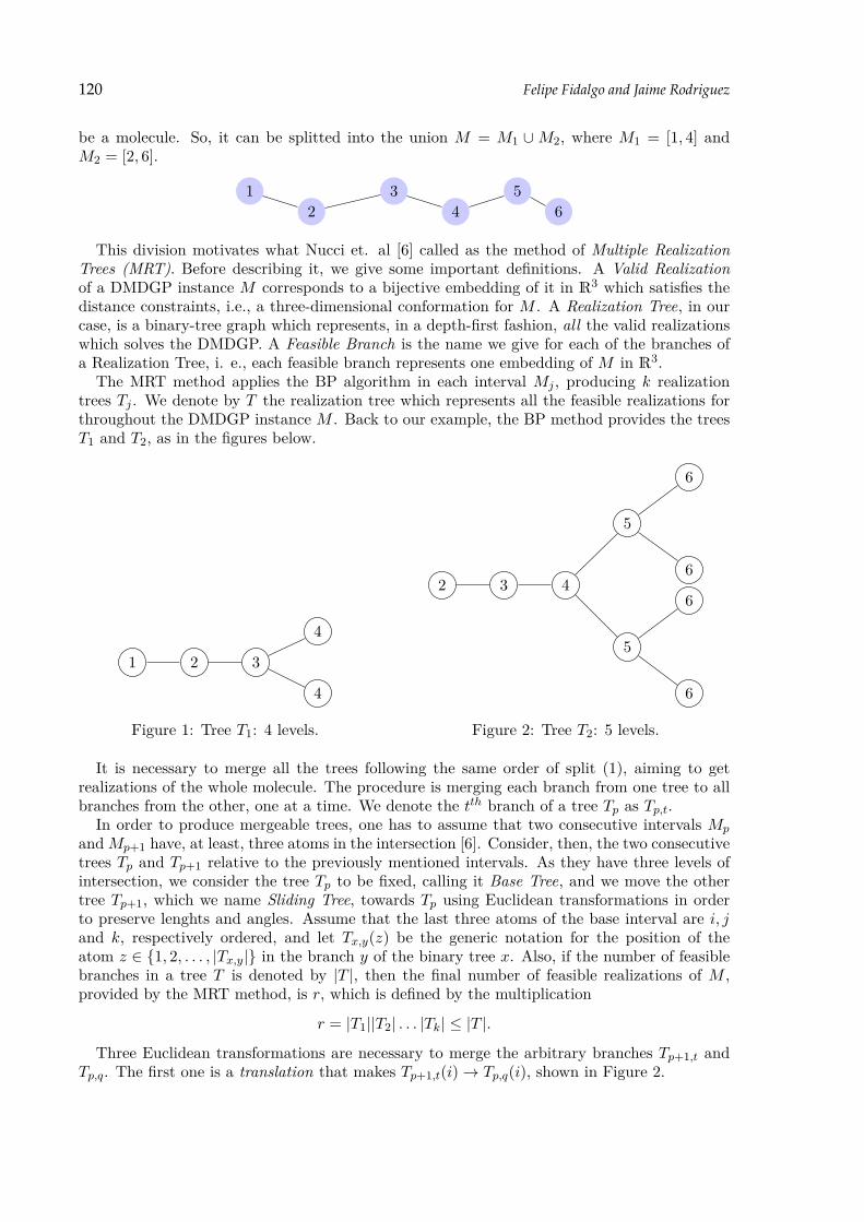
120 Felipe Fidalgo and Jaime Rodriguez

be a molecule. So, it can be splitted into the union M = M1 ∪M2, where M1 = [1, 4] andM2 = [2, 6].

12

34

56

This division motivates what Nucci et. al [6] called as the method of Multiple RealizationTrees (MRT). Before describing it, we give some important definitions. A Valid Realizationof a DMDGP instance M corresponds to a bijective embedding of it in R3 which satisfies thedistance constraints, i.e., a three-dimensional conformation for M . A Realization Tree, in ourcase, is a binary-tree graph which represents, in a depth-first fashion, all the valid realizationswhich solves the DMDGP. A Feasible Branch is the name we give for each of the branches ofa Realization Tree, i. e., each feasible branch represents one embedding of M in R3.

The MRT method applies the BP algorithm in each interval Mj , producing k realizationtrees Tj . We denote by T the realization tree which represents all the feasible realizations forthroughout the DMDGP instance M . Back to our example, the BP method provides the treesT1 and T2, as in the figures below.

1 2 3

4

4

Figure 1: Tree T1: 4 levels.

2 3 4

5

6

6

5

6

6

Figure 2: Tree T2: 5 levels.

It is necessary to merge all the trees following the same order of split (1), aiming to getrealizations of the whole molecule. The procedure is merging each branch from one tree to allbranches from the other, one at a time. We denote the tth branch of a tree Tp as Tp,t.

In order to produce mergeable trees, one has to assume that two consecutive intervals Mp

andMp+1 have, at least, three atoms in the intersection [6]. Consider, then, the two consecutivetrees Tp and Tp+1 relative to the previously mentioned intervals. As they have three levels ofintersection, we consider the tree Tp to be fixed, calling it Base Tree, and we move the othertree Tp+1, which we name Sliding Tree, towards Tp using Euclidean transformations in orderto preserve lenghts and angles. Assume that the last three atoms of the base interval are i, jand k, respectively ordered, and let Tx,y(z) be the generic notation for the position of theatom z ∈ 1, 2, . . . , |Tx,y| in the branch y of the binary tree x. Also, if the number of feasiblebranches in a tree T is denoted by |T |, then the final number of feasible realizations of M ,provided by the MRT method, is r, which is defined by the multiplication

r = |T1||T2| . . . |Tk| ≤ |T |.

Three Euclidean transformations are necessary to merge the arbitrary branches Tp+1,t andTp,q. The first one is a translation that makes Tp+1,t(i)→ Tp,q(i), shown in Figure 2.

Quaternions as a tool for merging multiple realization trees 121

Tp,q(i)

Tp,q(j)

Tp,q(k)

Tp+1,t(i)

Tp+1,t(j)

Tp+1,t(k)

Tp,q(i)

Tp,q(j)

Tp,q(k)

Tp+1,t(j)

Tp+1,t(k)

Figure 3: First Euclidean transformation: a translation of both realized branches.

We also want to make Tp+1,t(j) → Tp,q(j), without losing what we have built with thetranslation. Let us denote Ep = Tp,q(j)− Tp,q(i) and Ep+1 = Tp+1,t(j)− Tp+1,t(i) and let θ bethe angle between Ep and Ep+1. We apply a plane rotation of θ in the branch Tp+1,t, as onecan see in Figure 4.

Tp,q(i)

Tp,q(j)

Tp,q(k)

θTp+1,t(j)

Tp+1,t(k)

Tp,q(i)

Tp,q(j)

Tp,q(k)

Tp+1,t(k)

Figure 4: Second Euclidean transformation: a plane rotation in terms of θ.

Finally, after one translation and one rotation, consider Fp = Tp,q(k) − Tp,q(j) and Fp+1 =Tp+1,t(k)−Tp+1,t(j). We want to move the sliding branch Tp+1,t such that it satisfies Tp+1,t(k)→Tp,q(k), without moving anything else which has been already transformed previously. Wedefine the rotation axis, whose attitude L is spanned by Tp,q(j) − Tp,q(i), and consider theplane P, orthogonal to this axis. Let P = I3 − LLT be the matrix that gives the orthogonalprojection to P.

122 Felipe Fidalgo and Jaime Rodriguez

Then, the projections of Fp and Fp+1 in P are, respectively,

Pp = PFp and Pp+1 = PFp+1.

Now, let ϕ be the angle between Pp and Pp+1. Thus, we rotate Fp+1 towards Fp in ϕ aboutthe axis spanned by L, as it is shown in Figure 5. So we do with the remaining structure.Therefore, both realizations are connected and supposed to respect all original distance andangle constraints.

P

Tp,q(i)

Tp,q(j)

Tp,q(k)

Tp+1,t(k)

Pp+1

Ppϕ

P

Tp,q(i)

Tp,q(j)

Tp,q(k)

Pp

Figure 5: Third transformation: a spatial rotation in terms of the projected angle ϕ.

Following this outline, all the trees are connected and their branches consist of feasible pointsthat solve the DMDGP. In addition, we remark that all rotations are computed using matrices.

3. Merging Trees with Quaternion Rotations

All general rotations in real 3-D space can be represented by an axis, spanned by a unitaryvector n, and an angle θ. Using this information, one can build the matrix Rn,θ which carriesout a general rotation and can be determined by using the matrix form of Rodrigues’ RotationFormula [7]

Rn,θ = I + sin(θ)J(n) + (1− cos(θ))J(n)2, (2)where J(n) is a skew-symmetric 3× 3 - matrix generated by the elements of n as

J(n) =

0 −n3 n2n3 0 −n1−n2 n1 0

Such rotation matrices need 37 arithmetic operations to be determined, according to Equation(2), and 9 positions of memory to be stored. In addition, it is necessary to use more 15operations to multiply it for a vector v we want to rotate, totalizing 52 arithmetic operations.

This work aims to propose a theoretical modification on the tools which are used to make ro-tations on three-dimensional structures in order to decrease the storage space and, consequently,the number of operations to accelerate this process. Our approach uses the Quaternion AlgebraH [4] to do that.

Consider the unit quaternion q = q0 + qv, where q0 ∈ R and qv ∈ R3. It is possible to provethat there is an unique angle 0 ≤ θ ≤ π such that q0 = cos(θ) and ‖qv‖ = sin(θ). Then, wecan rewrite q = cos(θ) + u sin(θ), where u = qv

‖qv‖ [4]. The conjugate of q can be written asq∗ = cos(θ) − u sin(θ) [4]. Now, the following outcome characterizes a quaternion rotation bymeans of a linear operator[4].

Theorem 1 (Quaternion Rotation Operator). For a unit quaternion q = cos(θ) +u sin(θ), theoperator Rq : R3 −→ R3, whose action on the vector v ∈ R3 is given by Rq(v) = qvq∗, is a

Quaternions as a tool for merging multiple realization trees 123

rotation operator which rotate vectors about the axis spanned by the unit vector u through anangle 2θ in clockwise sense.

Explicitly, the action of Rq in a vector v ∈ R3 can be derived as the Rodrigues’ RotationFormula

Rq(v) = cos(2θ)v + (1− cos(2θ))pu(v) + sin(2θ)(u× v), (3)where pu(v) = (u · v)u is the orthogonal projection of v in the direction of u.

First of all, one improvement we can realize on the use of quaternions is that it is easier toencode a rotation in a unit quaternion than in an orthogonal matrix. Moreover, Equation (3)shows that each quaternion rotation creates a local frame (v,pu(v),u × v) to represent therotated vector and, also, gives us a route on how to localize it in the space more easily.

On computational complexity, quaternion rotations require the storage of only four positionsinstead of nine, necessary in the use of three-dimensional matrices. In addition, 25 arithmeticoperations are used to compute such rotations, fashioned such as in Equation (3). As we cansee, this number of operations is reasonably less than the one used in the matrix approach.When considering more than one rotation, it seems to be even more efficient by saving spaceand floating-point-arithmetic operations.

Therefore, we apply these ideas as efficient tools in the merging of BP-trees. According tothe MRT procedure described previously, we have to carry out two rigid rotations in the slidingstructure. For each one of them, it is necessary first to determine the cosine of the rotationangle by using the usual dot product in R3, restricting the domain of the cosine function to therange [0, π] in order not to allow it to reach the position determined by the angle 2π − θ sinceboth angles have the same cosine value. Moreover, the unitary vector which spans the orientedrotation axis can be chosen by applying the usual cross product in 3-D Euclidian Space, whosesignal induces the orientation of the rotation, following the so-called Right-Hand Rule. Thus,the order in the cross product really matters: indeed, the axis for a rotation of a vector xtowards another vector y is spanned by the vector x × y, while the axis for the rotation of ytowards x is spanned by the vector y × x. As they satisfy the relation of anticommutativityy × x = −(x × y), the direction of the rotation is, therefore, encoded in the sign of the crossproduct.

The first rotation is supposed to take Ep+1 into Ep, since they have the same origin. Thus, thecosine of the angle and the unitary vector which spans the correspondent axis are, respectively,

cos(θ) = 〈Ep+1, Ep〉‖Ep+1‖ ‖Ep‖

and n = Ep+1 × Ep‖Ep+1 × Ep‖

. (4)

Using the parameters developed above, we associate the following quaternion element to suchrotation

qθ,n = cos( θ2) + n sin( θ2).

Then, employing the result displayed in Theorem 1, we apply the rotation in the sliding struc-ture Tp+1,t

Tp+1,t(u)← Rqθ,n(Tp+1,t(u)), for u = 2, . . . , |Tp+1,t|, (5)where |Tp+1,t| is the number of vertices in this feasible branch of the realization tree Tp+1.Further, assume L = Ep/ ‖Ep‖, Fp = Tp,q(k) − Tp,q(j) and Fp+1 = Tp+1,t(k) − Tp+1,t(j).

The orthogonal projection matrix, associated to the plane P, is given by M = I3 − LLT , aswe have seen. Then, the projections are given by the vectors Pp = MFp and Pp+1 = MFp+1.Analogously to (4), the second rotation is generated by the parameters

cos(ϕ) = 〈Pp+1, Pp〉‖Pp+1‖ ‖Pp‖

and m = Pp+1 × Pp‖Pp+1 × Pp‖

. (6)

124 Felipe Fidalgo and Jaime Rodriguez

After calculating them, we define the associated quaternion to the respective rotation by

qϕ,m = cos(ϕ2 ) + m sin(ϕ2 ).

Therefore, we rotate the sliding structure, again as in Theorem 1, by making

Tp+1,t(u)← Rqω,m(Tp+1,t(u)), for u = 3, . . . , |Tp+1,t|, (7)

concluding the merging of the two structures Tp,q and Tp+1,t.There are two rotations in this approach. The first one fixes the first vertex of the sliding

structure and the second one fixes both the first and the second vertices. Then, compoundingboth the rotations in only one and applying it in the sliding structure leads us to reach thesame resulting structure. It is reasonably easier and computationally cheaper to compose twoquaternion rotations than multiplying two rotation matrices [4, 2]. Using this, we can savehalf of the storage space and carry out less than the half of arithmetic operations for thetransformation of each point.

As a conclusion, using quaternion rotations, instead of matrices, can bring improvementseither about computational time or about simplifying the method. We are in the process ofimplementing these ideas in order to illustrate computationally the theoretical improvements.

References

[1] G. Crippen and T. Havel. Distance Geometry and Molecular Conformation. Research Studies Press, U.K.,1988.

[2] D. Eberly. Rotation Representation and Performance Issues. A summary of representations of rotations andperformance available in http://www.geometrictools.com/Documentation/RotationIssues.pdf, 2002.

[3] T. Havel. Distance Geometry. In D. Grant and R. Harris, editors, Encyclopedia of Nuclear MagneticResonance, pp. 1701–1710. Wiley, New York. 1995.

[4] J. Kuipers. Quaternions and Rotation Sequences. Princeton University Press, Princeton, 1998.[5] C. Lavor, L. Liberti, N. Maculan, and A. Mucherino. The discretizable molecular distance geometry problem.

Computational Optimization and Applications, 52:115–146, 2012.[6] P. Nucci, L. Nogueira, and C. Lavor. Solving the Discretizable Molecular Distance Geometry Problem by

multiple realization trees. In Mucherino, A., Lavor, C., Liberti. L., and Maculan, N., editors, DistanceGeometry: Theory, Methods and Applications. Springer, New York, 2013.

[7] C. Taylor and D. Kriegman. Minimization on the lie group SO(3) and related manifolds. Technical Report,Yale University, 1994.

DGA 2013, pp. 125 – 129.

Updated T Algorithm for the resolution of MolecularDistance Geometry Problems by means of linear systems ∗

Felipe Fidalgo, Douglas Maioli and Eduardo Abreu

Department of Applied Mathematics, IMECC - UNICAMP, Campinas, Brazil,[email protected], [email protected], [email protected]

Abstract The Molecular Distance Geometry Problem (MDGP) has several attempts for its resolution, such asthose from the class of Geometric Build-up methods. This work deals with a new approach namedUpdated T Algorithm. It consists on solving linear systems, with LU factorization, together withthe so-called re-initialization and a sequence of Euclidian transformations in order to build linearsystems with better-condition-number properties. Numerical experiments with PDB (Protein DataBank) intances are shown, comparing this method with one from the literature, aiming to bear outthis approach.

Keywords: Molecular Distance Geometry, UT Algorithm, Root-Mean-Square Deviation, Geometric Build-UpAlgorithms

1. Introduction

It is possible to obtain distance values corresponding to pairs of atoms in a molecule M froma combination of chemical knowledge (such as bond angles and bond lengths) with NuclearMagnetic Resonance (NMR) data [5]. From them, we can formulate the Molecular DistanceGeometry Problem (MDGP) as MDGP Given an n - atom molecule M , consider the set SMof known distances dij between pairs of atoms (i, j) ∈ 1, . . . , n2. Is it possible to find a 3- D conformation x1, . . . ,xn for M? This problem is NP-hard [4]. In this work, we presenta method to solve it with relatively low CPU time that brings evidences of the possibility oftreating uncertainties on distance data, which is still under investigation for a future work. Itis called Updated T (UT) Algorithm. Numerical experiments of tests with proteins are shown,using the Root-Mean-Square Deviation (RMSD) as error estimator.

2. Updated T Algorithm

LetM be a molecule and SM its associate pairwise-distance set. The method starts by choosingfour non-coplanar atoms whose all distances between each other are known. It is reasonablysimple to determine coordinates for this subset, which are called Base Atoms (see, e.g., [2],p. 325). If they are not found, stop. Let F be the set of the positioned atoms. Then, theiterating process starts: let j be the undetermined atom and xj ∈ R3 the position the methodwants to find. It looks for a subset with four base atoms Bj = xj1,xj2,xj3,xj4 ⊆ F whosedistances to j are in S. If it is not found, stop. The next step is called re-initialization: the

∗We want to thank to CNPq, CAPES and FAPESP (2011/11897-6) for financial support.

126 Felipe Fidalgo, Douglas Maioli and Eduardo Abreu

four determined base atoms of the iteration have their positions changed in order to dependonly on the distances. This is done following the same procedure for the first four atoms and itaims to avoid error accumulation from the iterative process of solving linear systems, as donein [3]. The new base atoms are Bt

j = yj1,yj2,yj3,yj4, which are ilustrated in the figure.

xj1

xj2

xj3

xj4

yj1

yj2

yj3

yj4

Figure 1: The re-initialization process: changing the coordinates of the Base Atoms.

These new positions, together with the distances in SM , establish a quadratic system ofequations

‖yj1 − yj‖ = dj1, ‖yj2 − yj‖ = dj2, ‖yj3 − yj‖ = dj3 and ‖yj4 − yj‖ = dj4, (1)

where yj is the position of the undetermined atom in the transformed framework. The nextresult is the core of the method: yj is calculated by the solution of a linear system to bedescribed in what follows.Theorem 1 (Fidalgo, [3]). Let Bt

j = yj1, yj2, yj3, yj4 be a set of base atoms for j whosedistances to it are all known. If yj is a solution for the quadratic system (1), then x =[tj yTj

]T, where tj = −‖yj‖

2

2 , is the unique solution of the linear system Ax = b with

A =

1 yTj11 yTj21 yTj31 yTj4

and b =

d2j1 − ‖yj1‖

2

d2j2 − ‖yj2‖

2

d2j3 − ‖yj3‖

2

d2j4 − ‖yj4‖

2

.After calculating yj , the method ought to put it back to its position xj in the original

framework. For this, we work with rigid Euclidean transformations, also used by Wu et. al[1, 6]. Consider the matrices X and Y , whose rows consists on the positions of the base atomsxi and yi, respectively. Thus, the geometric center of both structures, represented by thesematrices, can be determined by

xc(k) = 14

4∑i=1

X(i, k) and yc(k) = 14

4∑i=1

Y (i, k) (k = 1, 2, 3).

Then, we work out the translation on Y below so that both structures have the same geometriccenter

Y (i, j) = Y (i, j)− [yc(j)− xc(j)], (j = 1, 2, 3). (2)The same translation is applied to the position yj we want to transform.

Finally, following Wu et. al [6], we have to find an orthogonal matrix Q so that the structureof Y is rotated into X, in order to achieve the RMSD value between both matrices. This isdone by the resolution of the Orthogonal Procrustes Problem

mins. to QTQ=I

‖X − Y Q‖F . (3)

Updated T Algorithm for the resolution of Molecular Distance Geometry Problems by means of linear systems127

The matrix Q = UV T solves this problem. U and V are the orthogonal matrices of the SingularValue Decomposition of the matrix Y TX [3]. Applying the same rotation to yj , we find theposition xj and include it in F . It follows a picture illustrating this and the outline of the UTalgorithm.

yj1

yj2

yj3

yj4

yj

xj1

xj2

xj3

xj4

xj

Figure 2: After a sequence of Euclidian transformations, the atom j is put back on its originalposition.

Algorithm 1 Updated T Algorithm1: Find four base atoms, determine x1,x2,x3 and x4 and let F be the set of determined atoms;2: if They are not found then3: return4: end if5: loop6: For each unpositioned atom j, find four base atoms xj1,xj2,xj3 and xj4;7: Re-initialize the base atoms into yj1,yj2,yj3 and yj4 and find the position yj (Theorem

1);8: Put back yj to the original structure into xj and include xj in F ;9: end loop

3. Computational Issues and Numerical Experiments

The implementation and the computational tests have been done using MATLAB in a computerIntel Core i3, 3.07 GHZ processor and RAM memory with 4 GB. All the linear systems weresolved by using LU factorization with partial pivoting. We used a subgroup of the proteinstested by Wu et al. [6] and Davis et. al [1], from the Protein Data Bank (PDB), and thenumerical experiments with the UT algorithm are compared to the Updated Geometric Build-Up (UGB) Algorithm [1, 6] results. Both methods have similar outlines, but their cores consiston resolutions of different linear systems. In addition, UT solves only one system per iterationinstead of four ones, as it is in UGB. For the tests, we used the RMSD as an error estimator

RMSD(X,Y ) = mins. to QTQ=I

‖X − Y Q‖F√n

, (4)

where the original and the calculated instances are stored as rows in the matrices X and Y ,respectively.

A subset of the results for these instances is shown in Table 1. Such tests were carriedout using 6 Å as the cut-off value for the distances. The first and second columns bring,

128 Felipe Fidalgo, Douglas Maioli and Eduardo Abreu

respectively, the name of the tested PDB instance and its number of atoms, which are alsodisplayed in Figure 3. The third and fifth columns store CPU time for the UT and the UGBmethods, respectively. One can see that the first method exhibits better performance in all thecases. Having less systems may save more time. Figure 3 also shows this fact. The last columnshows a relative time, when comparing the time values: it indicates an improvement averageof 60.78% for the UT. Finally, the fourth and sixth columns bring RMSD values for both themethods. These values are precisely close to each other in all the tests. Then, UT is able tosolve an MDGP with the same accuracy order of UGB, but demanding less CPU time, whatis promising desirable.

PDB Name # atoms UT time (s) UT RMSD UGB Time (s) UGB RMSD Time(UT/UGB)1ID7 189 4,74E-02 3,12E-09 8,27E-02 3,12E-09 57,32%

1FW5 332 7,19E-02 1,18E-08 1,19E-01 1,18E-08 60,42%1JAV 360 7,66E-02 1,38E-07 1,26E-01 1,38E-07 60,70%1MEQ 405 8,39E-02 6,39E-11 1,36E-01 6,42E-11 61,51%1AMB 438 8,86E-02 8,22E-06 1,45E-01 8,22E-06 61,15%1R7C 532 1,07E-01 8,39E-07 1,68E-01 8,38E-07 63,83%1HLL 540 1,06E-01 1,59E-07 1,71E-01 1,59E-07 61,96%1VII 596 1,12E-01 9,19E-07 1,92E-01 9,19E-07 58,55%1HIP 617 1,13E-01 3,15E-09 1,95E-01 3,14E-09 57,98%1ULR 677 1,24E-01 2,82E-09 2,09E-01 2,81E-09 59,20%1KVX 954 1,61E-01 1,65E-06 2,77E-01 1,65E-06 58,19%1VMP 1166 2,04E-01 1,97E-07 3,63E-01 1,97E-07 56,25%1RGS 2015 3,11E-01 1,37E-08 5,63E-01 1,37E-08 55,23%1BPM 3671 5,94E-01 5,08E-06 1,04E+00 5,08E-06 57,11%

Table 1: Numerical experiments of tests with PDB instances - 6 Å cut-off

Figure 3: Graphic representation of the RMSD results for the computational tests with proteinsfrom the PDB.

4. Conclusions

Concluding, this work deals with the Updated T (UT) Algorithm which solves the MolecularDistance Geometry Problem (MDGP) by applying a sequence of linear-system resolutions andEuclidean rigid transformations based on Root-Mean-Square Deviation (RMSD) techniques.It has shown as good numerical stability and accuracy as the Updated Geometric Build-Upmethod (from the literature) does and has taken less CPU time to determine protein structures.Such instances have been extracted from the Protein Data Bank (PDB). For future work, our

Updated T Algorithm for the resolution of Molecular Distance Geometry Problems by means of linear systems129

Figure 4: Graphic representation of the time results for the computational tests with proteinsfrom the PDB.

main outlook is the aplication of our numerical method in order to treat noisy distances, i.e.,sparse and inexact ones, through a stochastic modeling of the Molecular Distance GeometryProblem (MDGP) by means of a Monte Carlo approach. In addition, we also need to makea numerical complexity analysis and understand better the advantages and limitations of thevariable tj , specially in connection with error estimators aiming to quantify uncertainties inUT, since there are some evidences that it would be suitable.

References

[1] Davis, R., Ernst, C. and Wu, D. Protein structures determination via an efficient geometric build-upalgorithm. BMC Structural Biology, 10:1–10, 2010.

[2] Q. Dong and Z. Wu. A Geometric Build-up Algorithm for solving the Molecular Distance Geometry Problem.Journal of Global Optimization, 26:321–333, 2003.

[3] F. Fidalgo. Algorithms for problems of molecular geometry. Master’s thesis, University of Campinas,Campinas, 2011.

[4] J. Saxe. Embeddability of weighted graphs in k - space is strongly NP - Hard. In Proceedings of 17thAllerton Conference in Communications, Control and Computing, Monticello, pages 480–489, 1979.

[5] T. Schlick. Molecular modeling and simulation: an interdisciplinary guide. Springer, New York, 2002.[6] D. Wu and Z. Wu. An Updated Geometric Build-up Algorithm for solving the Molecular Distance Geometry

Problem with sparse distance data. Journal of Global Optimization, 37:661–673, 2007.

DGA 2013, pp. 131 – 135.

A geometric trigraph model for unit disk graph recognition∗

Guilherme da Fonseca1, Vinícius Pereira de Sá2, Raphael Machado3 and Celina de Figueiredo4

1Universidade Federal do Estado do Rio de Janeiro, Brazil [email protected]

2DCC/IM, Universidade Federal do Rio de Janeiro, Brazil [email protected]

3Inmetro — Instituto Nacional de Metrologia, Qualidade e Tecnologia, Brazil [email protected]

4COPPE, Universidade Federal do Rio de Janeiro, Brazil [email protected]

Abstract A unit disk graph G is a graph whose vertices can be mapped to points on the plane and whoseedges are defined by pairs of points within unitary Euclidean distance from one another. Therecognition of unit disk graphs is no easy feat. Indeed, the fastest known algorithm to decidewhether a given graph is a unit disk graph is doubly exponential. In this paper, we introduce apractical algorithm to produce certified answers to the question “is G a unit disk graph?” in eitherway, for any given graph G. By imposing that the points’ coordinates belong to discrete sets ofincreasing granularity, our method builds a sequence of trigraphs G′, i.e. graphs with mandatoryand optional edges, until either some G′ is found possessing properties which certify that G is aunit disk graph, or the sequence of trigraphs has to be interrupted, certifying that G is not a unitdisk graph. The proposed method was actually implemented, and we were able to obtain our firstcertificates for some small graphs.

Keywords: unit disk graphs, graph recognition, trigraphs, geometric algorithms

1. Motivation

A unit disk graph (UDG) is a graph whose n vertices can be mapped to points on the plane andwhose m edges are defined by pairs of points within Euclidean distance at most 1 from oneanother. Alternatively, one can regard the vertices of a UDG as mapped to coplanar congruentclosed disks, so that two vertices are adjacent whenever the corresponding disks intersect. Unitdisk graphs have been widely studied in recent times due to their applications to wireless sensornetworks [1].

In the present paper, we consider the problem of recognizing unit disk graphs. Though aYES answer can be verified in polynomial time assuming the Real RAM model, the size ofcertificates comprising the coordinates of the disk centers may not be polynomially boundedunder the classic model of computation over finite strings [4]. Indeed, it is not known for thetime being whether the problem belongs to NP, and the fastest known recognition algorithm isdoubly exponential [5]. Since no practical algorithm is available, there are graphs with as fewas ten vertices which have never been proved as being (or not being) UDG [6].

∗Research partially supported by FAPERJ and CNPq.

132 Guilherme da Fonseca, Vinícius Pereira de Sá, Raphael Machado and Celina de Figueiredo

Figure 1: Graph conjectured [6] not to be aUDG.

x∗

c∗1

c∗2 c∗3

c∗4

Figure 2: Graph that corresponds to thelower bound for the approximation factor ofthe algorithm introduced in [2] for minimum(independent) dominating sets in unit diskgraphs.

A practical method to certify whether a graph is a UDG is of utmost importance. Indeed,many of the existing bounds for approximation factors of algorithms for hard problems on unitdisk graphs are based on the fact that certain graphs are (or are not) UDG, but each one ofthose graphs demanded their own ad-hoc geometric proof. For an example, [6] conjectures thatthe graph in Figure 1 is not a UDG. The correctness of their conjecture would imply a decreasefrom 3.8 to 3.6 in the maximum ratio (except for an additive constant) between the size of amaximal independent set and the size of a connected dominating set in any given UDG, andthat would immediately tighten the approximation factor of algorithms that estimate the sizeof minimum connected dominating sets by computing maximal independent sets.

Another example was obtained in [2]. Denote by Gp,q the graph that has one p-clique suchthat one of its vertices is adjacent to q pendant vertices, and each of the other p− 1 vertices isadjacent to a degree-2 vertex that in turn is a pendant vertex of an induced K1,5. The graphG5,4 of Figure 2 is known to be a UDG (a geometric model with only integral coordinates isavailable [3]) and is the worst known instance for an algorithm that approximates the minimum(independent) dominating set of a unit disk graph, establishing a lower bound of 4.8 for theapproximation factor of that algorithm. On the other hand, the graph G9,4 is known not tobe a UDG (the proof is based on numerous geometric lemmas), and this fact is central in theproof of the (upper bound for the) approximation factor of 44/9 = 4.888 . . . of such algorithm.Further knowledge about the family Gp,q, closing the gap between what is currently known tobe a UDG (graph G5,4) and what is known not to be a UDG (graph G9,4), would immediatelytighten the existing bounds on the approximation factor of the aforementioned algorithm.

The difficulty in developing a certifier for unit disk graphs, even a “brute force” one, comesfrom the fact that the solution space — namely (R2)n — is uncountable. In the present paper,we formulate a strategy to reduce the solution space to a countable, finite set, whose granularityis subsequently refined, leading to a YES/NO certificate in many cases. An inconclusive answer,however, may possibly be obtained.

2. The proposed model

The central idea of our strategy is to discretize the solution space by defining an enumerableset of 2-dimensional coordinates where the points associated to the input graphs’ vertices maybe placed at. For a positive ε ∈ R, consider the set Nε := x ∈ R | x = dε, d ∈ N, and letCε := Nε ×Nε be a discrete set of 2-dimensional coordinates. We call such Cε a mesh and wesay Cε1 is thinner than Cε2 if ε1 < ε2. Clearly, any subset of points Mε ⊆ Cε determines a unit

A geometric trigraph model for unit disk graph recognition 133

disk graph G whose vertices are pairwise adjacent whenever their corresponding points in Mε

are within unitary distance of one another. We say Mε is an ε-discrete model for G.

Trigraph embodiments. Given a mesh Cε and a set Mε ⊆ Cε of n points, we define thetrigraph GMε = (V,E1 ∪E2) as the graph whose vertex set V corresponds to the points in Mε,and whose edges can be partitioned into E1, the set of mandatory edges, and E2, the set ofoptional edges. A mandatory edge is associated to a pair of points v, w ∈ Mε that are atdistance d(v, w) < 1 − ε

√2 from one another. An optional edge, on its turn, is associated to

a pair of points v, w ∈ Mε satisfying 1 − ε√

2 ≤ d(v, w) ≤ 1 + ε√

2. We say GMε is a trigraphembodiment of graph G(V,E) if, and only if, E ⊆ E1 ∪ E2 and E1 \ E = ∅, i.e. all edges of Gare either mandatory or optional edges in GMε , and no edge that does not belong to G appearsas a mandatory edge in GMε .

If GMε is a trigraph embodiment of G, and GMε has no optional edges, then Mε is a unitdisk model for G, hence G is certainly a UDG. Moreover, if GMε does have optional edges,but all optional edges in GMε correspond to pairs of adjacent vertices in G, then G is a UDGas well. (The same goes for the case where all optional edges in GMε correspond to pairs ofnon-adjacent vertices in G.) This is the core of the YES certificates produced by our method.

It can be shown that, if G is a UDG, then G admits a trigraph embodiment GMε , for allε > 0. Conversely, if, for some ε, there is no possible trigraph embodiment GMε for G, then Gis not a UDG. Our NO certificates come from this fact.

Our strategy to recognize unit disk graphs can therefore be summarized in the following steps:

INPUT: A connected graph G = (V,E)OUTPUT: YES, if G is a UDG; NO, if it is not a UDG; or INCONCLUSIVE.

1. Choose a value for ε and consider the corresponding mesh Cε.

2. For each possible discrete model Mε ⊆ Cε with |M | = |V |, obtain the respective trigraphGMε = (V,E1, E2).

(a) If E = E1 then a disk model was found for G, hence G is a UDG. Return YES.(b) If E ⊆ E1 ∪ E2 and E1 \ E = ∅, then GMε is a trigraph embodiment for G.

3. If a trigraph embodiment was found for G, then let ε ← ε/2. If ε is still greater thansome previously defined constant εmin, then restart the algorithm with the new valuefor ε; otherwise, return INCONCLUSIVE.

4. If no trigraph embodiment was found for G, then G is not a UDG. Return NO.Note that, in spite of the apparent infinite number of possible discrete models, we may

assume that G is connected1, so any model of G must be enclosed in a disk of diameter 2|V |.Notice also that, whenever the algorithm produces a conclusive answer, then an appropriate

certificate has been found. However, as discussed in Section 4, the input graph may not be aUDG, but still be such that, no matter how thin the mesh is, a trigraph model can always befound, leading the algorithm to an inconclusive answer.

3. Results

To validate our proposed model, we implemented it using the Python language. Our implemen-tation includes some nice refinements aimed at reducing the number of candidate placementsof each vertex in the considered mesh, such as

1Trivially, a graph is a UDG if and only if all its connected components are UDG.

134 Guilherme da Fonseca, Vinícius Pereira de Sá, Raphael Machado and Celina de Figueiredo

(i) taking the maximum and minimum distances between pairs of vertices as input;

(ii) taking the maximum and minimum angle between two vertices with respect to a thirdone as input;

(iii) allowing the imposition of a fixed circular order of vertices around a reference point.

Naturally, such features can only be used if some previous geometric analysis determines suchdistances and angles constraints. With this preliminary implementation, we could alreadycorrectly classify some small graphs as being (or not being) UDG.

4. Future directions

In spite of the nice results it has enabled us to obtain, the proposed method does presents somelimitations, one of which is disclosed by the following “pathological” example.

Let G be the K1,6 graph, which is known (by geometric methods) not to be a UDG. Ourprocedure is doomed to give an inconclusive answer for G no matter how thin the mesh is. Thereason is that, for all ε > 0, there is always a trigraph embodiment GMε for G, in which thecenter of the star and one of the leaves coincide (see Figures 3, 4 and 5).

A second weakness of the method is its worst-case time complexity, since the time demandedto produce a certificate for certain graphs may be as long as unforeseeable.

Figure 3: Graph K1,6.

Figure 4: Discrete model for graphK1,6. Thecircles are not the unit-diameter disks them-selves, but rather represent their centers. Thetwo overlapping circles represent the centersof coincident disks.

Figure 5: Trigraph corresponding to Figure 4.

The previous observations lead to the following open questions, which are currently underinvestigation.

1. Is it possible to characterize such “pathological” graphs, those which deny our methodany chance of recognizing them in either way?

A geometric trigraph model for unit disk graph recognition 135

2. Is it possible to modify our method so that it always stop with a conclusive questionwithin a reasonable, predetermined time?

Notwithstanding the open questions above, there seem to be several promising ways ourmethod can be improved upon. We list some of them below.

The exhaustive enumeration of possible trigraph embodiments for G can be achieved bya backtracking-based approach. First, a sequence v1, . . . , vn of vertices of G must bedetermined, in such a way that the subgraph Gk of G induced by v1, . . . , vk is connectedfor all k ∈ 1, . . . , n. Each vertex vk is then positioned, one at a time, at some point ofthe mesh, in such a way that the set of already occupied points of the mesh (includingthe one assigned to vk) defines a trigraph embodiment for Gk. By doing so, the searchspace for trigraph embodiments for G shall decrease considerably.

By the end of the k-th iteration of the algorithm, after some trigraph embodimentswere found, the value of ε is halved, so each former grid point p gives rise to four gridpoints p1, p2, p3, p4 to be considered (as possible vertex locations) during the (k + 1)-th iteration. It shall now be possible to eliminate at once from the list of candidatelocations for a vertex v all points pi corresponding to a point p that was not occupiedby v in any trigraph embodiment obtained in the k-th iteration. By so doing, the searchfor trigraph embodiments on the thiner mesh becomes limited to “refining” previouslyobtained trigraph embodiments, instead of a search that would otherwise have begunfrom scratch.

Proving geometric results such as “if G is a UDG, then G admits a disk model whereno two vertices are either vertically aligned, or horizontally aligned, or coincident” mayallow for the earlier elimination of a considerable number of discrete models, thereforealso speeding up the algorithm.

References

[1] Marathe, M.V., H. Breu, H. B. Hunt III, S. S. Ravi, and D. J. Rosenkrantz (2005). Simple heuristics forunit disk graphs. Networks 25 (2): 59–68.

[2] Fonseca, Guilherme D., Celina M. H. de Figueiredo, Vinícius G. P. de Sá, and Raphael Machado (2012).Linear Time Approximation for Dominating Sets and Independent Dominating Sets in Unit Disk Graphs.Proc. Workshop on Approximate and Online Algorithms (WAOA 2012).

[3] Fonseca, Guilherme D., Celina M. H. de Figueiredo, Vinícius G. P. de Sá, and Raphael Machado (2012).Linear-time sub-5 approximation for dominating sets in unit disk graphs. http://arxiv.org/abs/1204.3488.

[4] McDiarmid, Colin, and Tobias Mueller (2013). Integer realizations of disk and segment graphs. Journal ofCombinatorial Theory, Series B 103 (1): 114–143, http://arxiv.org/abs/1111.2931

[5] Spinrad, J. (2003). Efficient Graph Representations. Fields Inst. monographs. AMS.[6] Zou, F., Y. Wang, X.-H. Xu, X. Li, H. Du, P. Wan, and W. Wu (2011). New approximations for minimum-

weighted dominating sets and minimum-weighted connected dominating sets on unit disk graphs. TheoreticalComputer Science 412 (3): 198–208.

DGA 2013, pp. 137 – 142.

A rotation-invariant image processing operation transformedinto the k-nearest neighbours problem

L. R. Foulds, H. A. D. do Nascimento∗, H. Longo

Instituto de Informática, Universidade Federal de Goiás, Goiânia–GO, Brasil, lesfoulds,hadn,[email protected].

Keywords: Image processing, non-Euclidean metrics, problem transformation, k-nearest neighbours, approxi-mation algorithms, hierarchical tree decomposition, locality-sensitive hashing.

1. Introduction

Taking keypoints of an object in a reference image and searching for similar keypoints in acollection of candidate images is an important operation in image processing. The numberof keypoints in the reference image is usually quite small (10 . . 100), but the number of key-points among the candidates can be very large (105 . . 107). Hence it is important to developefficient identification methods for neighbours of reference keypoints. This is the subject of thepresent abstract. A recently developed similarity measure (based on dual trees and an orientedcomplex-valued wavelet transform) has proved to be highly beneficial for multi-dimensionalsignal processing [10]. This measure has the advantage over a commonly used former measure[9] of the efficient matching of keypoint pairs in a rotationally invariant way. In order to pre-serve rotational invariance, each reference keypoint must be represented by a set of m cyclicvectors of m dimensions, where m is usually about 200. This multiplicity of vectors means thata non-Euclidean metric must be used to calculate distances between reference and candidatekeypoints, which is computationally burdensome for image processing projects of practical size.We explain how this rotationally invariant operation can be transformed into the well-knownk-nearest neighbours problem (KNN) with the Euclidean distance metric. This is of inter-est since there exist fast approximation algorithms for KNN, some of which we describe anddiscuss.

Let m be the dimension of both the reference and candidate keypoints, both having real-valued elements. Let Y denote the set of initial reference keypoints, with elements denoted byyp = (yp1 , y

p2 , . . . , y

pm)T , p ∈ 1, 2, . . . , r, where r = |Y |. Let yp,q, q = 1, 2, . . . ,m; denote the

complete set of m keypoints that represent the pth reference, being cyclic versions of yp:

yp,q = (yps(q,0), yps(q,1), . . . , y

ps(q,m−1))

T , p ∈ 1, 2, . . . , r, (1)

where, for any t, u ∈ Z+, s(t, u) = t+ u, if t+ u ≤ m and = t+ u (mod m), otherwise.LetX ′ denote the set of candidate keypoints, with elements denoted by xi = (xi1, xi2, . . . , xim)T ,

i ∈ 1, 2, . . . , n′, where n′ = |X ′|. The metric for calculating the distance between any candi-date keypoint xi ∈ X ′ and any initial reference keypoint yp ∈ Y is:

d′ip = minq∈1,2,...,m

d(xi, yp,q), (2)

∗Hugo do Nascimento is partially sponsored by a Scholarship of Research Productivity from CNPq (309463/2009-2).

138 L. R. Foulds, H. A. D. do Nascimento, H. Longo

where d(a, b) = ||a− b||2 = (m∑i=1

(ai− bi)2)12 , the `2 norm (Euclidean distance) between a and b.

Let Y ′ = yp,q | p = 1, 2, . . . , r; q = 1, 2, . . . ,m. Suppose X ′ and Y are given and Y ′ hasbeen constructed from Y . The original image processing operation is denoted by Pk(X ′, Y ′).For given positive integer k ≤ n′, Pk(X ′, Y ′) involves finding the k nearest neighbours in X ′

for each reference keypoint in Y according to the metric d′ip.The main contribution of the present abstract is to suggest that Pk(X ′, Y ′) can be solved by

formulating it as KNN: given a collection of candidate keypoints, build a data structure which,given any reference keypoint, reports the k candidate keypoints that are closest to the referencekeypoint, with all data points being in a given metric space [8]. The metric in the space neednot necessarily be Euclidean distance although it is the one commonly used and it is usedhere from now on. KNN is of major importance in similarity searching and has significationapplication in many areas including: image processing, statistical measure estimation, machinelearning, data mining, data compression, information retrieval and pattern recognition.

We now explain a transformation that enables Pk(X ′, Y ′) to be performed by any KNN al-gorithm with Euclidean distance. The basic idea is to construct a set of “candidate keypoints”,based on cyclic versions of each candidate keypoint, in the same way that Y ′ was constructedfrom Y . The motivation for this is that (2) is an awkward metric to evaluate, as it involvesm reference keypoints as well as a candidate keypoint. To avoid this, we deal with Y , theset of initial reference keypoints rather than with Y ′. We augment X ′ by element cycling.The augmentation means that each distance calculation involves just one initial reference key-point and one candidate keypoint. Let xi,j , j = 1, 2, . . . ,m; denote the m keypoints that areconstructed from xi, i ∈ 1, 2, . . . , n′, for the augmentation. The xi,j ’s are cyclic versions ofxi and are defined in the same vein as (1). That is, let xi,j = (xis(j,0), x

is(j,1), . . . , x

is(j,m−1))

T ,j = 1, 2, . . . ,m, with s defined as in (1).

Let X = x1,1, x1,2, . . . , x1,m, x2,1, . . . , x2,m, . . . , xn′,1, . . . , xn

′,m denote the augmented set ofkeypoints constructed from X ′. The metric for calculating the distance between any candidatekeypoint xi,j ∈ X and any reference keypoint yp ∈ Y is:

dijp = d(xi,j , yp), i ∈ 1, 2, . . . , n′; p ∈ 1, 2, . . . , r, (3)

where d(a, b), once again, denotes the `2 norm, the Euclidean distance between vectors a andb.

As usual, when minimising relative distance, the “1/2” power of Euclidean distance can beneglected. Calculating dijp requires O(m2) time. (The m distances computed each requireapproximately 2·m additions/subtractions and m multiplications and the sort of the distancesrequires O(m· logm) time.) Furthermore, the fact that the candidate keypoints are rotatedleads to additional savings in computation.

The newly transformed image processing operation is denoted by Pk(X,Y ). It involvesfinding the k nearest neighbours in X for element in Y according to the metric dijp. Note thatthe neighbours returned must arise from distinct elements of X.

2. Problem Transformation

The transformation Pk(X,Y ) is the k-nearest neighbours problem (KNN). We show thatPk(X ′, Y ′) and Pk(X,Y ) are equivalent.Lemma 1. If x is a nearest neighbour of some yp ∈ Y ′ for P1(X ′, Y ′), then solving problemP1(X,Y ) will produce a nearest neighbour that is the same distance from yp as x.Proof. Suppose for some i ∈ 1, 2, . . . , n′, xi = (xi1, xi2, . . . , xim)T ∈ X ′ is a nearest neighbourof Y ′ produced by P1(X ′, Y ′). Suppose further, for some q ∈ 1, 2, . . . ,m, yp,q = (ypq , y

pq+1,

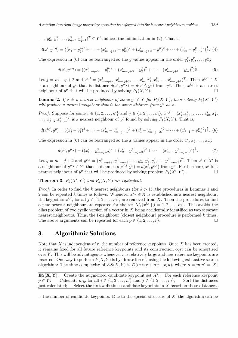
A rotation-invariant image processing operation transformed into the k-nearest neighbours problem 139

. . . , ypm, yp1 , . . . , y

pq−2, y

pq−1)T ∈ Y ′ induces the minimisation in (2). That is,

d(xi, yp,q) = ((xi1 − ypq )2 + · · ·+ (xim−q+1 − ypm)2 + (xim−q+2 − yp1)2 + · · ·+ (xim − y

pq−1)2)

12 . (4)

The expression in (6) can be rearranged so the y values appear in the order yp1 , yp2 , . . . , y

pm:

d(xi, yp,q) = ((xim−q+2 − yp1)2 + (xim−q+3 − y

p2)2 + · · ·+ (xim−q+1 − ypm)2)

12 . (5)

Let j = m − q + 2 and xi,j = (xim−q+2, xim−q+3, . . . , x

im, x

i1, x

i2, . . . , x

im−q+1)T . Then xi,j ∈ X

is a neighbour of yp that is distance d(xi, yp,q) = d(xi,j , yp) from yp. Thus, xi,j is a nearestneighbour of yp that will be produced by solving P1(X,Y ).

Lemma 2. If x is a nearest neighbour of some yp ∈ Y for P1(X,Y ), then solving P1(X ′, Y ′)will produce a nearest neighbour that is the same distance from yp as x.

Proof. Suppose for some i ∈ 1, 2, . . . , n′ and j ∈ 1, 2, . . . ,m, xi,j = (xij , xij+1, . . . , xim, xi1,. . . , xij−2, x

ij−1)T is a nearest neighbour of yp found by solving P1(X,Y ). That is,

d(xi,j , yp) = ((xij − yp1)2 + · · ·+ (xim − y

pm−j+1)2 + (xi1 − y

pm−j+2)2 + · · ·+ (xij−1 − ypm)2)

12 . (6)

The expression in (6) can be rearranged so the x values appear in the order xi1, xi2, . . . , xim:

d(xi, yp,q) = ((xi1 − ypm−j+2)2 + (xi2 − y

pm−j+3)2 + · · ·+ (xim − y

pm−j+1)2)

12 . (7)

Let q = m − j + 2 and yp,q = (ypm−q+2, ypm−q+3, . . . , y

pm, y

p1 , y

p2 , . . . , y

pm−q+1)T . Then xi ∈ X ′ is

a neighbour of yp,q ∈ Y ′ that is distance d(xi,j , yp) = d(xi, yp,q) from yp. Furthermore, xj is anearest neighbour of yp that will be produced by solving problem P1(X ′, Y ′).

Theorem 3. Pk(X ′, Y ′) and Pk(X,Y ) are equivalent.

Proof. In order to find the k nearest neighbours (for k > 1), the procedures in Lemmas 1 and2 can be repeated k times as follows. Whenever xi,j ∈ X is established as a nearest neighbour,the keypoints xi,j , for all j ∈ 1, 2, . . . ,m, are removed from X. Then the procedures to finda new nearest neighbour are repeated for the set X\xi,j | j = 1, 2, . . . ,m. This avoids thealias problem of two cyclic version of a vector in X being accidentally identified as two separatenearest neighbours. Thus, the 1-neighbour (closest neighbour) procedure is performed k times.The above arguments can be repeated for each p ∈ 1, 2, . . . , r.

3. Algorithmic Solutions

Note that X is independent of r, the number of reference keypoints. Once X has been created,it remains fixed for all future reference keypoints and its construction cost can be amortisedover Y . This will be advantageous whenever r is relatively large and new reference keypoints areinserted. One way to perform P (X,Y ) is by “brute force”, using the following exhaustive searchalgorithm: The time complexity of ES(X,Y ) is O(m·n·r + n·r· logn), where n = m·n′ = |X|

ES(X,Y): Create the augmented candidate keypoint set X ′. For each reference keypointp ∈ Y : Calculate dijp for all i ∈ 1, 2, . . . , n′ and j ∈ 1, 2, . . . ,m; Sort the distancesjust calculated; Select the first k distinct candidate keypoints in X based on these distances.

is the number of candidate keypoints. Due to the special structure of X ′ the algorithm can be

140 L. R. Foulds, H. A. D. do Nascimento, H. Longo

speeded up by parallel computing. We shall discuss data structures that can reduce this hugetime complexity.

When m is relatively small, the metric space (X, dijp) can be fruitfully partitioned by usingk-d trees [3, 6] in order to compute distances only within specific nearby volumes. However,the performance of k-d tree-based algorithms declines as m increases. If the metric is non-Euclidean, or if m is relatively large, ball trees [12] often provide more useful results in practicalsituations [5]. Although distance sorting is not an issue with the hierarchical tree decompositionalgorithms discussed so far, the fact that their space requirements are exponential in m is amajor concern. Cover trees have been developed to address this difficulty and to enable fastapproximate KNN searches. Indeed, cover tree-based algorithms use implicit representation tokeep track of repeated points and thus require only O(n) space, independent of any assumptionsregarding m [2].

Like the other hierarchical tree decomposition algorithms mentioned, cover trees allow forKNN searches in O(b·logn) time where b is a constant derived from m. However, when m isrelatively large, b is of significant size and must be taken into account in complexity analysis,implying that performance declines with increasing m. But cover tree algorithms are uniqueamong tree-based methods in that a theoretical bound on b is available. This bound is c12,where c is an expansion constant for exact algorithms and a doubling constant for approximationalgorithms [2], leading to a bound on search time of O(c12· logn). Although cover trees providereasonably fast KNN searches, the speed comes with the additional cost of maintaining the datastructure. In exhaustive search, the time to add a new point to the dataset can be neglectedbecause order does not need to be preserved, but in a cover tree it can take up to O(c6· logn)time. Samet [11] provided a survey of hierarchical tree decomposition algorithms for KNN.

Practical data for Pk(X ′, Y ′) often has dimensions: m ≈ 200, n ≈ 105 . . 107, k ≈ 50 andr ≈ 10 . . 100. Clearly, the strategy of transforming the image processing operation and solvingPk(X,Y ) with such dimensions will be computationally effective only if approximation algo-rithms are used, possibly in conjunction with parallel computing. “Approximation” in thecontext of KNN implies, given y ∈ Y and an approximation parameter ε > 0, find elementsx1, x2, . . . , xk ∈ X such that d(xi, y) ≤ (1 + ε)·d(X, y), i ∈ 1, 2, . . . , k and xi is the ith nearestneighbour of y. The notion of approximation is appealing here as it has been found for manypractical datasets that the approximately nearest neighbours identified are very close to theexact ones and the differences are often unimportant [4]. Tree cover approximation algorithmsshow promise in this regard. Indeed, Beygelzimer et al. [2] provide such an algorithm that isof practical interest. It has a time requirement at most c12 · log ∆ + (1/ε)O(log c), where c is thedoubling constant and ∆ is the aspect ratio (the ratio of the largest to the smallest interpointdistance). The space bound is O(n), which is independent of c.

Locality-sensitive hashing (LSH) is another suitable KNN approximation method where mis probabilistically reduced when it is relatively large [7]. The basic idea is to hash the inputitems using several hash functions so that similar items are mapped to the same buckets withmuch higher probability than for dissimilar items (the number of buckets being significantlysmaller than n). When the reference keypoints are included, one can then determine their nearneighbours by hashing a reference keypoint and retrieving the elements in its buckets.

Gionis et al. [4] and Andoni and Indyk [1] have developed fast LSH approximation algorithmsthat can be used to solve Pk(X,Y ) when m and n are both relatively large. Their methods arebased on LSH families that are simple, easy to use and can accommodate the situation wherenew reference keypoints are inserted dynamically. The Gionis et al. algorithm is O(m·d1/(1+ε)).The authors solved particular KNN problems with n = 270, 000, m = 64 and k = 10, in betterthan an order of magnitude faster than tree-based algorithms, requiring O(n) space and withless than 4% error. Andoni and Indyk [1] describe an LSH-based algorithm for m-dimensional

A rotation-invariant image processing operation transformed into the k-nearest neighbours problem 141

Euclidean space that is provably near-optimal in the class of the LSH algorithms regarding theseparation of collision probabilities of close and far points.

4. Computing

Suppose for some i ∈ 1, . . . , n and j ∈ 1, . . . ,m, xi,j = (xij(1), xij(2), . . . , x

ij(m))

T is oneof the candidate keypoints and for some p ∈ 1, 2, . . . ,m, one of the reference keypoints isrepresented by the vector yp = (yp1 , y

p2 , y

p3 , . . . , y

pm−1, y

pm)T . Suppose further, that for a given

non-negative finite real number ε:

|xij(q) − ypq | ≤ ε, ∀ q = 1, 2, . . . ,m. (8)

This relationship implies dijp ≤√m·ε. Rather than performing all them calculations necessary

to calculate dijp, one might instead perform element-to-element comparisons of xi,j and yp basedon (8). During the comparison process, whenever (8) does not hold xi,j could be eliminatedfrom further consideration as a potential k-nearest neighbour of yp. As with the doublingconstant for cover trees, the bound ε could be increased until k candidate keypoints have beenidentified.

5. Conclusion

The transformation introduced above may be viewed as a means of linking the two classes ofk-nearest neighbours problems, so that theoretical results for P (X,Y ) (for which relatively fastapproximation algorithms exist) can be extended to P (X ′, Y ′). No claims are made, however,as to the computational utility of this transformation. The authors are in the process ofinvestigating its usefulness for rotation-invariant image processing operations of practical sizevia approximation algorithms and parallel computing.

References

[1] A. Andoni and P. Indyk. Near-optimal hashing algorithms for approximate nearest neighbor in highdimensions. Communications of the ACM, 51(1):117–128, 2008.

[2] A. Beygelzimer, S. Kakade, and J. Langford. Cover trees for nearest neighbor. In Proceedings of the 23rdInternational Conference on Machine Learning, pages 97–104, 2006. http://hunch.net/~jl/projects/cover_tree.

[3] J. Friedman, J. Bentley, and R. Finkel. An algorithm for finding best matches in logarithmic expectedtime. ACM Transactions on Mathematical Software, 3(4):209–226, 1977.

[4] A. Gionis, P. Indyk, and R. Motwani. Similarity search in high dimensions via hashing. In Proceedings ofthe 25th Very Large Database (VLDB) Conference, Edinburgh, UK, 1999.

[5] A. Gray and A. Moore. n-body problems in statistical learning. Advances in Neural Information ProcessingSystems (NIPS), 13:266–272, 2000.

[6] P. Indyk. Nearest neighbors in high-dimensional spaces. In J. E. Goodman and J. O’Rourke, editors,Handbook of Discrete and Computational Geometry, chapter 39. CRC Press, London, UK, 2004.

[7] P. Indyk and R. Motwani. Approximate nearest neighbors: towards removing the curse of dimensionality.In Proceedings of 30th Symposium on Theory of Computing, pages 604–613, 1998.

[8] L. Jiang, Z. Cai, D. Wang, and S. Jiang. Survey of improving k-nearest-neighbor for classification. InFourth International Conference on Fuzzy Systems and Knowledge, pages 679–683, 2007.

[9] D. G. Lowe. Distinctive image features from scale-invariant keypoints. International Journal of ComputerVision, 60(2):91–110, 2004.

[10] J. Nelson and N. G. Kingsbury. Enhanced shift and scale tolerance for rotation-invariant polar matchingwith dual-tree wavelets. IEEE Transactions on Image Processing, 20(3):814–821, 2011.

142 L. R. Foulds, H. A. D. do Nascimento, H. Longo

[11] H. Samet. Foundations of Multidimensional and Metric Data Structures. Elsevier, Holland, 2006.[12] J. Uhlmann. Satisfying general proximity/similarity queries with metric trees. Information Processing

Letters, 40:175–179, 1991.

DGA 2013, pp. 143 – 148.

Using Correspondence Analysis Andits Distance To Evaluate The Componentsof A Naming Test For Studying Aphasia

Gastão Coelho Gomes,1 Sergio Camiz,2 Christina Abreu Gomes3 and Fernanda Duarte Senna4

1DME– IM– UFRJ, Brazil [email protected]

2Dipartimento di Matematica–Sapienza Università di Roma, Italia [email protected]

3Departamento de Linguística, UFRJ, Cidade Universitária, Brazil [email protected]

4Doutoranda Programa de Pós-Graduação de Linguística, UFRJ, Brazil [email protected]

Abstract Exploratory Multidimensional Data Analyses were used to manage two components of a namingtest for studying lexical access in aphasic patients, i.e., the naming agreement of images andage of acquisition of the names themselves from an original international test. In order to bereliable the images should be easily and unequivocally named by any subject using the same word.Theoretical assumptions about word learning states that words acquired later tend to be the firstto be lost due to brain damage in aphasia. Thus, these two variables are important predictors ofthe patient’s word retrieval. We first selected the images according to normal judges recognitionagreement; then, to range them based on their primitiveness, these images were submitted to twosets of judges, that had to answer according to two different scales. Data were analyzed withseveral exploratory multidimensional techniques, including Simple and Multiple CorrespondenceAnalyses, Principal Component and Multiple Factor Analyses. A comparison suggested that nomayor differences existed due to the two scales’ differences.

Keywords: Chi-square Distance, Correspondence Analysis, Factor Analysis, Linguistics, Aphasia

1. Introduction

This study is the continuation of a previous one [4] and concerns the evaluation of a set of 260images [8] internationally used to test the lexical access in aphasia, i.e. the loss of some abilitiesrelated to language production and/or comprehension due to brain damage. The test, that aimsat measuring to what extent the disease affects the word retrieval, is based on the recognitionof familiar objects submitted as images to the patients and their consequent verbalization.In order to be reliable, we considered that a selection of these images ought to be done tosuit the Brazilian reality and we based it on two criteria: i) the images should be easily andunequivocally recognizable, and ii) the primitiveness of the word, say its age of acquisition,should be measured. Indeed, it is theoretically assumed (based on word learning) that wordsacquired later tend to be the first to be lost in aphasic patients affected by brain damage. Thus,these two characters are important predictors of the patient’s word retrieval. Thus, we selectedrandomly three groups of non-affected people to act as judges, and asked one to identify theimages and the other two to estimate the degree of primitivity of the corresponding names. As

144 Gastão Coelho Gomes, Sergio Camiz, Christina Abreu Gomes and Fernanda Duarte Senna

our study was based mainly both on judges and scale evaluation, we show in the following howwe dealt with the judges’ reliability and the scale definition.

2. The data

For the selection of the images, all of them (260) were submitted to a panel of 38 judgesrandomly selected among non-affected people. The answers have been coded as 1 =recognized, 0 = not recognized. From this selection, 161 images resulted.

To measure primitiveness, we asked 128 non-affected judges to estimate how primitivewere the 161 represented objects, according to their personal experience. This estimationwas based on two different scales: i) the first panel, with 60 judges, labelled E, has beenasked to measure the age of acquisition on a scale from 1 to 7 according to how early intheir life each word was first known, but without specifically mentioning the age; here 1corresponds to very early in life and 7 to most late; ii) the second panel, with 68 subjects,labelled I, has been asked a measure based on a scale 1-7 as well, but this time based onage classes: the classes are: 1=0-2 years, 2=2-4 years, 3=4-6 years, 4=6-8 years, 5=8-10years, 6=10-12 years and 7=13 and further.

3. Theoretical Framework

The consistency of judges is of high importance in several frameworks, as in sensorial analysis.For this task, specific estimation methods have been developed (see, e.g. [7]). Here, we pre-ferred to consider the problem on another point of view, as no objective primitiveness may bemeasured, but only identify a central tendence stastistics. Thus, we only removed those judgeswhose results appeared clearly far from all others. For what concerns the scale definition, wetried to compare two possible scales: a free one and one based on age intervals, and we studiedtheir agreement. Thus, we considered of interest to use for our study exploratory multidimen-sional analysis methods, since their graphical representations allowed a visual inspection ofmost of the questions that we might ask.

An interesting feature of the analyses that we adopted is that they are all based on the sameprinciple, the Singular Value Decomposition (SVD, [2]) of some transformation of the originaldata matrix T : X → A = T (X). The SVD of a matrix A is given by A = UΛ1/2V ′, withU and V the matrices of the (vertical) eigenvectors of A′A and AA′ respectively, and Λ the(diagonal) matrix of their corresponding eigenvalues, sorted in descending order. The theoremstates the highest importance, in terms of represented inertia, of the first generated axes inrespect to the following ones.

According to the data at hand, the analyses have been submitted to Simple CorrespondenceAnalysis (SCA, [1], [5]) to identify both judges and items with critical recognition behavior, andMultiple Correspondence Analysis (MCA, ibid.) to identify those judges with biased evaluationof primitiveness in respect to others. Multiple Factor Analysis (MFA, [3]) has been used tocompare the primitiveness of the words given by the two panels of judges according to the twodifferent scales, and eventually Principal Component Analysis (PCA, ibid., see also [6]) hasbeen used to define the primitivity index of our interest.

The data transformations, according to the different methods may be described as follows:

PCA xij → zij = xij−xj√nσj

standardization

MFA xijk → zijk = xijk−xjk√λ1k

√nσjk

std. adjusted to group’s coherence

Using Correspondence Analysis In Aphasia 145

SCA xij → sij = xij√xi.x.j

−√xi.x.jx..

deviation from independence

MCA xijq → sijq = 1√Q

( xijq√xi.−√xi.x..

)deviation from average profile

4. Selecting Images

The results of first submission reported 10 images that no judge could identify, so that wewithdrew them immediately. On the other side, 66 images have been recognized by all judges,thus automatically included. Therefore, we applied SCA to the remaining images to get agraphical representation of the pattern of both judges and images on factor planes. Accordingto Figure 1(a) below, six judges, P13, P17, P25, P32, P34, and P36, appear further fromthe origin than all others, whose central pattern seems homogeneous, thus they have beenwithdrawn.

Figure 1: Analysis for the selection of the images. The items on the first factor plane of SCA:(a) The judges, (b) The names.

As well, some items, such as baby stroller, toe, celery, and chalk, were identified by no morethan 5 judges. They are located at the border of the cloud as can be seen on Figure 1(b)above. We re-ran SCA with only 32 judges and also all the items whose frequency of correctidentification was lower than 50%. From the homogeneous results we could conclude that nofurther removal of judges seemed necessary. Eventually, we decided to keep all the imagesthat were correctly identified by at least 90% of judges. Based on 32 judges: 97 images wereidentified by all of them, 26 by only 31 (97%), 24 by 30 (94%), 14 by 29 judges (91%), summingup to 161 images.

5. Defining word primitiveness

In order to examine first the homogeneity of the judges, we started by running MCAs on eachof two tables. Their behavior is represented by a trajectory that connects the seven levels ofthe scale. Observing the two graphics in Figure 2, one may observe that the trajectories of thejudges that measured freely (Figure 2(a)) are much longer than those of judges based on age(Figure 2(b)). This may be explained by a reduced use of the first levels by the latter.

146 Gastão Coelho Gomes, Sergio Camiz, Christina Abreu Gomes and Fernanda Duarte Senna

Figure 2: Analysis of the primitiveness judgements. The judges’ trajectories represented onthe first factor plane of MCA: (a) free judgements, (b) judgements based on age intervals.

The pattern of trajectories on both tables on the first factor plane is very homogenousamong both sets of judges: Only five of them (E12, E23, E59, I2, and I58 ) showed verystrange trajectories (see them in Figure 3), thus were removed.

Figure 3: Analysis of the primitiveness judgements. The outlier judges’ trajectories representedon the first factor plane of the respective MCA: (a) free judgements, (b) judgements based onage intervals.

Then, we ran a MFA, considering the two groups of reduced judges (57 that used the freescale (E) and 66 with age-scale (I ). A specific advantage of MFA in respect to PCA it its abilityto represent on factor planes not only the global units, but also the partial ones, that is, inour case, the projection of the words seen by either group of judges. Indeed, the total word issituated on the centroid of the two partial words. Therefore, distances between partial words

Using Correspondence Analysis In Aphasia 147

Figure 4: Analysis of the age of acquisition judgements. All the words represented on theplane spanned by the first two factors of MFA. Only the words with the largest trajectories arelabelled, with the word (the compromise) and either E or I the partial ones.

are a measure of their dissimilarity according to the two sets of measurements and they maybe decomposed according to the different axes. The words with highest negative differencesalong the first factor are burro, gravata, lâmpada, mala, and patins and those with highestpositive ones are borboleta, cigarro, cinzeiro, escada, galinha, ônibus, and vestido. Thus, thefirst might be words judged more primitive by the free-scale judges, whereas the second mightbe judged more primitive by the age-scale ones. Here, we deal only with the first axis thatclearly represents primitivity of words (51.51% of total inertia), since the following explain toolittle inertia to deserve being taken into account (the second only 3.64%). In Figure 4 all wordsare represented both totally and partially, with the total units at the centroid of the respectivepartials. Looking at the extreme of the first axis it is interesting to find the words with thelargest differences on the second axis and in particular a reverse behaviour: this reflects thesmall rotation of the first factors of partial tables, but does not deserve a true interest for ourpurposes.

As the partial first factors of the two tables where most correlated among each other (.98)and with the MFA one (over .99), we decided to merge the two data sets , so that as measureof the words’ primitivity was taken the first principal component of this unified table’s PCA.

6. Conclusions

The study aiming at both selecting images with high naming agreement and measuring the de-gree of primitiveness of their correspondent words, has been carried out using only exploratorymultidimensional data analyses. This allowed to withdraw judges with a clearly biased behav-ior in respect with the others and select a set of words that have been recognized by nearlythe totality of judges. The free scale resulted a little better performing than the other, since itallowed a more instinctive estimate.

References

148 Gastão Coelho Gomes, Sergio Camiz, Christina Abreu Gomes and Fernanda Duarte Senna

[1] Benzécri J.P. and coll. (1973–82), L’analyse des données, 2 voll., Paris, Dunod.[2] Eckart C. and G. Young (1936), The approximation of one matrix by another of lower rank, Psychometrika,

Vol. 1: pp. 211–218.[3] Escofier B. and J. Pagés (1998). Analyses factorielles simples et multiples, 3e ed., Paris, Dunod.[4] Camiz S., G.C. Gomes, F.D. Senna, and C.A. Gomes (2010). Correspondence Analysis in

a Study of Aphasic Patients, XLII SBPO 2010, Bento Gonçalves (RS) Brazil, 30/8-3/9.http://www.sobrapo.org.br/sbpo2010/xliisbpo pdf/72251.pdf

[5] Greenacre M. (1983), Theory and Applications of Correspondence Analysis, London, Academic Press.[6] Jolliffe I.T. (2002), Principal Components Analysis, Berlin, Springer.[7] Rust R.T. and B. Cooil (1994), Reliabilty Measures for Qualitative Data: Theory and Implications. Journal

of Marketing Research, Vol. 31: pp. 1–14.[8] Snodgrass J.G. and M. Vanderwart (1980), A standardized set of 260 pictures: Norms for name agreement,

familiarity and visual complexity. Journal of Experimental Psychology: Human Learning & Memory, Vol.6(2): pp. 174–215.

DGA 2013, pp. 149 – 152.

A new algorithm to finding discretizable orderings forDistance Geometry

Warley Gramacho1, Douglas Gonçalves2, Antonio Mucherino2 and Nelson Maculan3

1Federal University of Tocantins, Palmas-TO,Brazil, [email protected]

2IRISA, University of Rennes 1, Rennes, France, douglas.goncalves,antonio.mucherino @irisa.fr

3COPPE, Federal University of Rio de Janeiro, Rio de Janeiro-RJ,Brazil, [email protected]

Abstract We present a new algorithm to finding suitable orderings for instances of the Distance GeometryProblem (DGP) that can allow for discretization. We present some preliminary computationalresults showing that the new algorithm outperforms a previously proposed one.

Keywords: Distance Geometry, Discretizing Vertex Order Problem, Sensor Network Localization

1. Introduction

Given an integer K > 0 and a weighted undirected graph G = (V,E, d), with d : E −→ R+,the Distance Geometry Problem (DGP) asks whether there exists a function x : V −→ RKsuch that:

∀(u, v) ∈ E ||xu − xv|| = d(u, v),

where xu = x(u) and xv = x(v) [6].The DGP is usually formulated as a continuous optimization problem, but, under some

assumptions, it can be formulated as a combinatorial problem.

Definition 1.1. The Discretizable Distance Geometry Problem (DDGP) [7].Let G = (V,E, d) be a weighted undirected graph associated to a DGP instance. Let us supposethat there is a partial order relation on the vertices of V . The DDGP in dimension K consistsin all the DGP instances satisfying the following two assumptions:

Assumption 1: there exists a subset V1 of V such that

|V1| = K;V1 is a clique;the order relation on V1 is total;∀v0 ∈ V1 ∀v ∈ V \ V1, v0 < v.

Assumption 2: ∀v ∈ V \ V1,∃u1, u2, . . . , uK ∈ V such that:

u1 < v, u2 < v, . . . , uK < v;(u1, v), (u2, v), . . . , (uK , v) ∈ E;

150 Warley Gramacho, Douglas Gonçalves, Antonio Mucherino and Nelson Maculan

the Cayley-Menger determinant of the distance matrix related to u1, u2, . . . , uK isnot 0.

We say that an ordering for the vertices of V is a discretizing ordering if it makes theassumptions of the DDGP satisfied.

DDGP instances can be solved by employing a branch-and-prune (BP) algorithm [5] thatis potentially able to enumerate the whole solution set. This is a major difference betweenthe BP algorithm and other algorithms for the DGP. However, in order to apply BP, theDDGP assumptions have to be satisfied. Finding an order for the vertices in V such thatthese assumptions are satisfied represents an important pre-processing step for the solution ofDDGPs [7]. We refer to this problem as the Discretizing Vertex Order Problem (DVOP) [4].

The rest of the paper is organized as follows. In Section 2, we introduce the DVOP andpresent the new algorithm. Some preliminary computational results are presented in Section 3.

2. Suitable orderings for the DDGP

Let G = (V,E, d) be a weighted undirected graph related to a DGP instance, and let us supposethat a total order is associated to the vertices in V (it is known that, from any partial order onV , a total order can be derived). For referring to an order, we will consider the usual symbol<, and we will add subscripts when it will be necessary to distinguish among different orders(e.g. <1 or <2 ). Similarly, the symbol (u, v)<1 will refer to the arc involving the vertices uand v in the order <1. We will refer to an order < for which the assumptions in Def. 1.1 aresatisfied in dimension K as a DDGP K-order.

Let α<(v) be, for v ∈ V , the number of adjacent predecessors of v in the order <, that is:

α<(v) = cardu ∈ V : (u, v)< ∈ E.

Equivalently, let β<(v), for v ∈ V , be the number of adjacent successors of v, in the order <:

β<(v) = cardu ∈ V : (v, u)< ∈ E.

Definition 2.1. The Discretizing Vertex Order Problem (DVOP).Given an undirected graph G = (V,E) and a positive integer K, establish whether there is anorder < on V such that: (a) the first vertices in the order form a K-clique, and (b) for eachv ∈ V , α<(v) ≥ K.

We observe that the DVOP does not verify whether the order satisfies the assumption onCayley-Menger determinant given in Def. 1.1. This is because the set of distance matricesyielding Cayley-Menger determinant having value exactly zero has Lebesgue measure zerowithin the set of all possible (real) distance matrices [4]. The probability for this to happenis therefore 0 in a mathematical sense. The NP-completeness of the DVOP follows from NP-completeness of the K-clique problem, because finding a DDGP K-order implies finding Kvertices forming a clique in G. When K is fixed, however, as in real applications, the DVOPcan be solved in polynomial time [4].Proposition 2.1. Given a weighted undirected graph G = (V,E, d) and an order < on V ,there do not exist DDGP K-orders if some vertex has degree less than K.

Note that Prop. 2.1 cannot be inverted, i.e. there can exist instances that do not admit anyDDGP K-order even if, for all v ∈ V , α<(v) + β<(v) ≥ K.

2.1 The new algorithm

Let us consider that an order <1 for the vertices in G is already available. We suppose thatthis order is not a DDGP K-order, and, for each v ∈ V , α<1(v)+β<1(v) ≥ K, for guaranteeing

A new algorithm to finding discretizable orderings for Distance Geometry 151

that such an order may exist. The basic idea behind this algorithm is to select all v for whichα<1(v) < K, and to modify their position so that, in the new order <2, we have α<2(v) = Kand β<2(v) = β<1(v) + α<1(v)−K.

By considering the order <1, let us suppose that v′ is such that α<1(v′) < K. Let h =K − α<1(v′), and Ξ = u ∈ V : (v′, u)<1 ∈ E. From the order <1, an order on the vertices ofΞ can be obtained, so that the hth element can be selected, say v′′. In this new order <2, wecan move v′ just after v′′, implying that α<2(v′) = K. The vertices between the old and thenew position for v′ can be affected by this change, whereas the situation remains unchangedfor all others. If a vertex v is between the old and new position for v′, then the value of α<1(v)might decrease. In such a case, the position of the vertex in the order needs to be modified,and this can be simply done by applying the procedure above to the vertices following the oldposition of v′ in the order <1. A sketch of the new algorithm we propose is in Alg. 1. Thisalgorithm requires an order <1 in input; as a consequence, the performances of this algorithmare dependent on the given initial order.

Algorithm 1 Algorithm for finding suitable orders for the DDGP1: reorder(G,<1)2: copy order <1 in <2;3: define ordered set B such that each v ∈ V is in the order <24: for each v ∈ B, in order <2 do5: if α<2(v) < K then6: let Ξ = u ∈ V : (v, u)<2 ∈ E;7: let h = K − α<2(v);8: let w = hth element, in the order <2, in Ξ;9: move, in the set B, v just after w;10: update order <2 (from updated B);11: end if12: end for

We remark that this algorithm could cycle. When there is a subset of vertices that are se-lected in repetition, it means that they form a subset of vertices having less than K connectionswith the rest. When the algorithm cycles, we can stop the execution, and no DDGP K-ordersmay exist.

3. Computational experiments

In this section, we present some computational results on a set of instance of the WirelessSensor Network Localization (WSNL) problem [1, 2, 8]. It is supposed that K = 2 and thatall distances are precisely known. The instances were generated in similar way as in [3]: on asquare in R2 having side 1, all distances between randomly placed points, that are closer thana predefined radio range distance R, are supposed to be known.

We compared the running time of Alg. 1 to the greedy algorithm proposed in [4]. All codeshave been written in C and compiled with the gcc compiler by GNU, version 4.7.1, under Linuxon an Intel(R) Core(TM) i3-2120 [email protected] with 8Gb RAM.

Table 1 shows some computational experiments for different sizes n and different radio rangesR. It can be easily remarked that the greedy algorithm is strongly dependent on the size n andon the cardinality of E, because the computational experiments are more expensive when thevalues of n and |E| are larger. On the other side, Alg. 1 shows this behavior only in relationwith n, while it improves its performances when |E| is larger.

152 Warley Gramacho, Douglas Gonçalves, Antonio Mucherino and Nelson Maculan

Table 1: Comparison between Alg 1 and Greedy algorithm proposed in [4] on a set of WSNLinstances

Instances Alg. 1 Greedy Instances Alg. 1 Greedyn R |E| CPU time CPU time n R |E| CPU time CPU time

4000 0.05 60351 1.23 0.98 8000 0.05 241590 3.35 5.834000 0.06 85815 0.76 1.13 8000 0.06 343873 1.21 7.594000 0.07 115511 0.47 1.33 8000 0.07 466346 1.07 9.714000 0.08 149606 0.32 1.62 8000 0.08 601909 0.57 11.964000 0.09 187789 0.25 1.91 8000 0.09 750550 0.43 14.714000 0.10 230116 0.19 2.29 8000 0.10 918520 0.36 17.016000 0.05 136532 1.71 2.64 10000 0.05 378545 3.77 11.096000 0.06 195323 0.98 3.39 10000 0.06 536711 2.70 14.616000 0.07 262742 0.73 4.24 10000 0.07 723071 0.97 17.816000 0.08 337476 0.40 5.07 10000 0.08 936524 0.68 22.186000 0.09 426764 0.32 5.27 10000 0.09 1182242 0.44 27.56000 0.10 518907 0.29 7.48 10000 0.10 1440175 0.49 32.69

In future works, we plan to develop in more details the theory behind the new proposedalgorithm. Moreover, we will work for extending this new algorithm for solving instances ofthe DVOP where not all the available distances are precise. We will also explore the possibilityto combine the two algorithms compared in this paper in the attempt of bringing their bestproperties into a hybrid one.

Acknowledgments

The authors would like to thank Professor Carlile Lavor by his encouragement, suggestions andhelp all the time.

References

[1] P. Biswas, T.-C. Liang, K.-C. Toh, T.-C. Wang, and Y. Ye, Semidefinite programming approaches forsensor network localization with noisy distance measurements, IEEE Transactions on Automation Scienceand Engineering, 3:360–371, 2006.

[2] S. Kim, M. Kojima, and H. Waki, Exploiting sparsity in SDP relaxation for Sensor Network Localization,SIAM Journal of Optimization, 20:192–215, 2009.

[3] N. Krislock and H. Wolkowicz. Explicit sensor network localization using semidefinite representations andfacial reductions. SIAM Journal on Optimization, 20:2679–2708, 2010.

[4] C. Lavor, L. Jon, J. Lee S., L. Liberti, A. Mucherino, and M. Sviridenko. Discretization Orders for DistanceGeometry Problems. Optimization Letters, 6:783–796, 2012.

[5] C. Lavor, L. Liberti, N. Maculan, and A. Mucherino. The discretizable molecular distance geometryproblem. Computational Optimization and Applications, 52:115–146, 2012.

[6] L. Liberti, C. Lavor, A. Mucherino, and N.n Maculan. Molecular distance geometry methods: from con-tinuous to discrete. International Transactions in Operational Research, 18:33–51, 2011.

[7] A. Mucherino, C. Lavor, and L. Liberti. The discretizable distance geometry problem. Optimization Letters,6:1671–1686, 2012.

[8] Y. Yemini. The positioning problem - a draft of an intermediate summary. In Proceedings of the Conferenceon distributed Sensor Network, pages 137–145. Carnegie-Mellon, Pittsburgh, 1978.

DGA 2013, pp. 153 – 155.

Ab-initio nanostructure determination

Saurabh R. Gujarathi 1 and Phillip M. Duxbury 2

1Dept. of Physics and Astronomy, Michigan State University, East Lansing, MI 48824, USA. [email protected]

2Dept. of Physics and Astronomy, Michigan State University, East Lansing, MI 48824, USA. [email protected]

Abstract Many complex materials at the nanoscale do not have periodic long range order and hence theirstructures cannot be solved by traditional crystallographic methods. The "nanostructure problem"is determining, with high precision, the arrangement of atoms in such irregular nanostructures. Ourapproach to this inverse problem is the use of distance geometry methods, which can reconstructstructures using only the interatomic distances obtained from the atomic pair distribution function,which is generated from scattering data.

Keywords: Structure determination, Nanoparticles, Inverse problem

Reconstruction of complex structures using pair distance information is an inverse problemthat occurs in many branches of science and engineering [1–5]. Given a set of inter atomicdistances we need to find the location of the atoms, up to global rotations and translations ofthe structure. This pair distance inverse problem may be interpreted as a complex networkreconstruction problem where the edge weights are equal to the Euclidean distances betweennodes in the network [6, 7].

In material physics, crystallography is the gold standard for structure determination. Whencrystals are not available, other methods are used. Determination of protein structure insolution has been successfully done by using the pair distance information extracted fromNOESY NMR data [3, 4, 8–10]. In proteins, the list of residues or the sequence of a protein isknown, enabling experiments to be carried out to specify the points between which each distancelies. This leads to the assigned case of the inverse problem. Algorithms for solving this typeof problem are known to be easy, being of order the number of atoms in the structure (N).However, the NMR data has large uncertainties in the experimentally obtained interatomicdistances, with imprecisions typically of the order of 25% or higher [11], making the problemcomputationally hard [12, 13].

In contrast, for problems concerning materials and most heterogeneous media, the pair dis-tances are not assigned, as we do not know which nodes lie at the end of each distance. Thismakes reconstruction significantly harder and is the unassigned case of the inverse problem.The pair distribution function (PDF) method is used for the analysis of the local structureof nanoparticles and complex materials. In many complex materials, such as high perfor-mance thermoelectric materials [14], high temperature superconductors [15] and manganites[16], crystalline order and heterogeneous local distortions co-exist so that crystallographic andPDF methods are complementary. Crystallography finds the average structure and the PDFgives the local structure [17, 18]. The PDF gives a direct measure of the list of interatomicdistances arising in the local structure, however the end points of the distances are not known.We face a computationally challenging problem known as the "nanostructure problem"[19].

In collaboration with Professor Billinge and his group at Columbia University, we developedan efficient algorithm for reconstructing structures which have a high symmetry, such as C60

154 Saurabh R. Gujarathi and Phillip M. Duxbury

0

30

60

90

120

150

0 1 2 3 4 5 6 7 8

Mu

ltip

lici

ty

d

−→

0

0.5

1

1.5

2

0 2 4 6 8 10 12

Mu

ltip

lici

ty

d

−→

Figure 1: Some examples of the different types of structures we have reconstructed usingEuclidean distance lists. The figures on the left are the distance lists while those on the rightare the reconstructed structures. The plot on the top left is for C60 fullerene molecule thathas a degenerate distance list and at the bottom left is that for a random set of 10 points inthe plane that has a non-degenerate distance list. The multiplicity is on the Y axis while thedistance is on the X axis (in arbitrary units). The structure of the C60 fullerene (top right)was found using the Liga algorithm and the structure of the random point set (bottom right)was found using the Tribond algorithm from the given distance lists.

and a range of crystal structures. The novel “Liga algorithm” [20–22] is inspired by the Spanishsoccer league and is based on tournaments and promotion and relegation. Although this methodworks well for structures with relatively high symmetry, it fails miserably for low symmetrycases such as random point sets, due to the fact that there are a large number of unique pairdistances in random structures. Thus, they fail for the general problem of complex Euclideannetworks.

To overcome this problem we came up with the Tribond algorithm, which is specificallydesigned for solving structures which have low symmetry (Fig. 1). It makes use of the factthat any over-constrained cluster (core) will be very likely part of the final structure. Tribondfinds such a cluster and then does the remaining buildup, all in polynomial time. We havesuccessfully implemented the algorithm using C++ in two and three dimensions. In 2D, wehave been able to reconstruct low symmetry structures consisting of a thousand atoms in about24 hours on a desktop computer. Our Tribond algorithm solves the unassigned case of theinverse problem problem given precise distances and we also have some success in solving theproblem when given imprecise distances. A hybrid algorithm that combines Tribond and Liga

Ab-initio nanostructure determination 155

algorithm would be able to solve structures which fall in between those having high symmetryand low symmetry.

References

[1] G. M. Crippen and T. F. Havel, Distance Geometry and Molecular Conformation. Wiley and Sons, NewYork, 1988.

[2] G. Crippen, “Chemical distance geometry: current realization and future projection,” Journal of mathe-matical chemistry, vol. 6, no. 1, pp. 307–324, 1991.

[3] K. Wuthrich, “The development of nuclear magnetic resonance spectroscopy as a technique for proteinstructure determination,” Accounts of Chemical Research, vol. 22, pp. 36–44, Jan. 1989.

[4] K. Wuthrich, “Protein structure determination in solution by nuclear magnetic resonance spectroscopy,”Science, 1989.

[5] M. Li, Y. Otachi, and T. Tokuyama, “Efficient algorithms for network localization using cores of underlyinggraphs,” Algorithms for Sensor Systems, pp. 101–114, 2012.

[6] L. Liberti, C. Lavor, A. Mucherino, and N. Maculan, “Molecular distance geometry methods: from contin-uous to discrete,” International Transactions in Operational Research, vol. 18, no. 1, pp. 33–51, 2011.

[7] L. Liberti, C. Lavor, N. Maculan, and A. Mucherino, “Euclidean distance geometry and applications,”ArXiv e-print, arXiv:1205.0349v1, May 2012.

[8] J. Yoon, Y. Gad, and Z. Wu, “Mathematical modeling of protein structure using distance geometry,” tech.rep., 2000.

[9] J. C. Kendrew, Dickerson R. E., B. E. Strandberg, R. G. Hart, D. R. Davies, D. C. Phillips, and V. C.Shore, “Structure of Myoglobin,” Nature, vol. 185, pp. 422–427, 1960.

[10] M. F. Perutz, M. Rossmann, A. Cullis, H. Muirhead, G. Will, and A. C. T. North, “Structure ofHaemoglobin,” Nature, vol. 185, pp. 416–422, 1960.

[11] M. Nilges and S. I. O’Donoghue, “Ambiguous NOEs and automated NOE assignment,” Progress in NuclearMagnetic Resonance Spectroscopy, vol. 32, pp. 107–139, Apr. 1998.

[12] B. Hendrickson, “The molecule problem: Exploiting structure in global optimization,” SIAM Journal onOptimization, vol. 5, no. 4, pp. 835–857, 1995.

[13] B. Berger, J. Kleinberg, and T. Leighton, “Reconstructing a three-dimensional model with arbitrary errors,”Journal of the ACM (JACM), pp. 1–16, 1999.

[14] H. Lin, E. Božin, S. Billinge, E. Quarez, and M. Kanatzidis, “Nanoscale clusters in the high performancethermoelectric AgPbmSbTem+2,” Physical Review B, vol. 72, pp. 1–7, Nov. 2005.

[15] L. Malavasi, G. a. Artioli, H. Kim, B. Maroni, B. Joseph, Y. Ren, T. Proffen, and S. J. L. Billinge, “Localstructural investigation of SmFeAsO(1-x)F(x) high temperature superconductors.,” Journal of physics.Condensed matter, vol. 23, p. 272201, July 2011.

[16] T. Proffen and S. Billinge, “Probing the local structure of doped manganites using the atomic pair distri-bution function,” Applied Physics A, vol. 74, pp. 1770–1772, 2002.

[17] S. J. Billinge, “Nanoscale structural order from the atomic pair distribution function (PDF): There’s plentyof room in the middle,” Journal of Solid State Chemistry, vol. 181, pp. 1695–1700, July 2008.

[18] S. J. L. Billinge and M. G. Kanatzidis, “Beyond crystallography: the study of disorder, nanocrystallinityand crystallographically challenged materials with pair distribution functions.,” Chemical communications(Cambridge, England), pp. 749–60, Apr. 2004.

[19] S. J. L. Billinge and I. Levin, “The problem with determining atomic structure at the nanoscale.,” Science(New York, N.Y.), vol. 316, pp. 561–5, Apr. 2007.

[20] P. Juhás, D. M. Cherba, P. M. Duxbury, W. F. Punch, and S. J. L. Billinge, “Ab initio determination ofsolid-state nanostructure.,” Nature, vol. 440, pp. 655–8, Mar. 2006.

[21] P. Juhás, L. Granlund, P. M. Duxbury, W. F. Punch, and S. J. L. Billinge, “The Liga algorithm for abinitio determination of nanostructure.,” Acta crystallographica. Section A, Foundations of crystallography,vol. 64, pp. 631–40, Nov. 2008.

[22] P. Juhas, L. Granlund, S. R. Gujarathi, P. M. Duxbury, and S. J. L. Billinge, “Crystal structure solutionfrom experimentally determined atomic pair distribution functions,” Journal of Applied Crystallography,vol. 43, pp. 623–629, 2010.

DGA 2013, pp. 157 – 161.

Distance Eigenvalue Location in Threshold Graphs∗

David P. Jacobs1, Vilmar Trevisan2, and Fernando C. Tura3

1School of Computing, Clemson University, USA, [email protected]

2 Instituto de Matemática, UFRGS, Brazil, [email protected]

3Campus Alegrete, UNIPAMPA, Brazil, [email protected]

Abstract Let G be a threshold graph of order n with distance matrix Θ. We give an O(n) algorithmfor constructing a diagonal matrix congruent to Bx = Θ + xI for any real x. An applicationusing Sylvester’s Law of Inertia can determine, in linear-time, how many eigenvalues of Θ lie inany interval, allowing fast divide-and-conquer approximation. We also show that any distanceeigenvalue λ 6= −1,−2 must be simple.

Keywords: eigenvalue, distance matrix, threshold graph

1. Introduction

Distance in graph theory is a simple but powerful idea, upon which many parameters depend,including diameter, radius, average distance and Wiener index. A path in a graph is a sequenceof distinct vertices, such that adjacent vertices in the sequence are adjacent in the graph. Thelength of a path is the number of edges on the path. For connected graphs, the distance betweentwo vertices u and v, denoted d(u, v), is the length of a shortest u− v path.

The diameter of a connected graph G, denoted diam(G), is the maximum distance betweentwo vertices. The eccentricity of a vertex is the maximum distance from it to any other vertex.The radius, denoted rad(G), is the minimum eccentricity among all vertices of G.

The average distance of a graph G of order n, denoted µ(G), is the expected distance betweena randomly chosen pair of distinct vertices. The study of the average distance began with thechemist Wiener [14], who noticed that the melting point of certain hydrocarbons is proportionalto the sum of all distances between unordered pairs of vertices of the corresponding graph. Thissum, denoted by W (G), is called the Wiener index of G. Clearly,

W (G) =(n

2

)µ(G).

The Wiener index and its applications to chemistry have received much attention (See, forexample, [1, 2, 4, 10, 12, 13]).

The distance matrix Θ of a connected graph G is the matrix whose rows and columns areindexed by its vertices such that its (u, v)-entry is equal to d(u, v). If 1 denotes the all 1’s

∗The second author was partially supported by CNPq (Grants 309531/2009-8 and 473815/2010-9) and FAPERGS (Grant11/1619-2). The third author was on leave from UNIPAMPA and supported by CAPES (Grant 0283/12-6).

158 David P. Jacobs, Vilmar Trevisan, and Fernando C. Tura

column vector, the Wiener index may be written in the form

W = 1TΘ12 .

The eigenvalues of Θ are called the distance eigenvalues of G, form the distance spectrum,and have several real-world applications. Distance eigenvalues were first studied by Grahamand Pollack in 1971 to solve a data communication problem [6]. The distance matrix containsinformation on various walks in chemical graphs. It is useful in the computation of topologicalindices and thermodynamic properties such as pressure and temperature coefficients. It con-tains more structural information than the adjacency matrix [7]. In the chemistry literature,the largest eigenvalue of Θ(G) helps to model the boiling point of alkanes [1]. In addition tochemistry, distance matrices find applications in music theory, ornithology, molecular biology,psychology, archeology etc. (See [3] and the papers cited therein.)

This paper is concerned with the distance eigenvalues of threshold graphs. Threshold graphshave several applications in psychology, scheduling, and synchronization of parallel processes[11]. They can be characterized in many ways, but a simple way of obtaining a threshold graphis through an iterative process which starts with an isolated vertex, and where, at each step,either a new isolated vertex is added, or a vertex adjacent to all previous vertices (dominatingvertex) is added. We represent the graph with a binary sequence (b1, . . . , bn), ordering thevertices in the way they are created. The adjacency matrix A and distance matrix Θ of thethreshold graph represented by (0, 1, 0, 1) are

A =

0 1 0 11 0 0 10 0 0 11 1 1 0

Θ =

0 1 2 11 0 2 12 2 0 11 1 1 0

(1)

If Θ = [aij ] is the distance matrix of a threshold graph G represented with (b1, . . . , bn), thenit is easy to see that if bi = 1, aij = aji = 1, for j < i. And if bi = 0, aij = aji = 2, for j < i.

2. Diagonalizing Θ + xI

Recall that two matrices R and S are congruent if there exists a nonsingular matrix P such thatR = P TSP . Our main result is an O(n) algorithm for constructing a diagonal matrix congruentto Bx = Θ + xI, where Θ is the distance matrix of a threshold graph, and x is an arbitraryscalar. The algorithm proceeds in n−1 stages and works bottom-up, and right-to-left. At eachstage, adjacent rows and columns m and m − 1 participate in operations. Diagonalization isachieved because at the end of this stage, all entries of row and column m, will be zero exceptthe diagonal element. For Θ in (1) and x = 1, the algorithm would proceed as follows:

1 1 2 11 1 2 12 2 1 11 1 1 1

→

1 1 2 01 1 2 02 2 0 00 0 0 1

4

→

1 1 0 01 1 0 00 0 −1 00 0 0 1

4

→

0 0 0 00 1

4 0 00 0 −1 00 0 0 1

4

Congruence is guaranteed because at each stage of the algorithm we use the same pair ofelementary row and column operations. For example, in transforming the first matrix aboveto the second, we employed the row and column operations

R4 ← R4 −12R3, C4 ← C4 −

12C3

Distance eigenvalues 159

Algorithm Diagonalize(G, x)initialize d(i)← x, for all ifor m = n to 2

α← d(m)if bm = 0

α← α4

if bm−1 = 1if α+ x 6= 2

d(m− 1)← αx−1α+x−2

d(m)← α+ x− 2else if x = 1

d(m− 1)← 1d(m)← 0

elsed(m− 1)← 1d(m)← −(1− x)2

m← m− 1else if bm−1 = 0

if α+ x4 6= 1

d(m− 1)← αx−1α+ x

4−1d(m)← α+ x

4 − 1else if x = 2

d(m− 1)← 2d(m)← 0

elsed(m− 1)← 2d(m)← − 1

2 (1− x2 )2

m← m− 1end loop

Figure 1: Diagonalizing Θ + xI.

and then

R3 ← R3 − 2R4, C3 ← C3 − 2C4

What is remarkable is that we do not need to store the entire matrix, only the diagonal andthe representation (b1, . . . , bn) of G. Our O(n) time and space algorithm is shown in Figure 1.The proof of correctness appears in the full-length version of our paper.

Theorem 1. For inputs G and x, where G is a threshold graph with distance matrix Θ,algorithm Diagonalize computes a diagonal matrix D, which is congruent to Θ + xI.

3. Finding distance eigenvalues

We seek the eigenvalues of Θ, the distance matrix of a threshold graph G. The proof of thefollowing theorem, which depends on Sylvester’s Law of Inertia, may be found in [8, 9].

Theorem 2. Let D be a diagonal matrix congruent to Θ− αI, where Θ is real symmetric.

i. The number of eigenvalues of Θ greater than α is the number of positive entries in D.

ii. The number of eigenvalues of Θ less than α is the number of negative entries in D.

iii. The multiplicity of eigenvalue α is the number of zero entries in the diagonal of D.

160 David P. Jacobs, Vilmar Trevisan, and Fernando C. Tura

Corollary 3. Counting multiplicities, the number of eigenvalues of Θ in (α, β], is the numberof positive entries in the diagonalization of Θ − αI, minus the number of positive entries inthe diagonalization of Θ− βI.

This observation shows that we may determine the number of eigenvalues in an intervalby making two calls to algorithm Diagonalize. As an example, consider G represented by(0, 1, 0, 1) and x = 1. After initialization, when m = 4, we will have α = x = 1, b4 = 1 andb3 = 0, so the first step will assign d3 ← αx−1

α+x4−1 = 0 and d4 ← α + x

4 − 1 = 14 . Next, when

m = 3, we will have α = 0, x = 1, b2 = 1 and b3 = 0. This second step will assign α← α4 = 0,

d2 ← αx−1α+x−2 = 1, d3 ← α+x−2 = −1. Finally, when m = 2, we will have α = 1, x = 1, b1 = 0

and b2 = 1, so we assign: d1 ← αx−1α+x

4−1 = 0, d2 ← α+ x4 − 1 = 1

4 . The following table illustratesthe sequence of states.

bi di0 11 10 11 1initial

bi di0 11 10 01 1

4after m=4

bi di0 11 10 −11 1

4after m=3

bi di0 01 1

40 −11 1

4after m=2

By Theorem 2, this means that x = −1 is an eigenvalue of G of multiplicity 1, there aretwo eigenvalues greater than −1 and one eigenvalue is smaller than −1. When applying thealgorithm to the same graph and x = 0, the final sequence is given by d = (7/3,−3/7,−7/4,−1).This implies that 3 eigenvalues are negative and 1 is positive. We conclude that there is a singledistance eigenvalue λ ∈ (−1, 0]. This technique allows fast divide-and-conquer approximation:Letting x = −1

2 will locate λ in (−1,−.5] or (−.5, 0].An eigenvalue is simple if its multiplicity is one. Using our algorithm, we can prove:

Theorem 4. In the distance matrix of a threshold graph, an eigenvalue λ is simple if λ 6=−1,−2.

4. Research Problem

In [6] it was shown that det(Θ) = (−1)n−1(n − 1)2n−2, where Θ is the distance matrix of atree of order n. We seek a formula for det(Θ), for distance matrices of threshold graphs G, interms of the representation of G.

References

[1] A.T. Balaban, D. Ciubotariu and M. Medeleanu, Topological indices and real number vertex invariantsbased on graph eigenvalues and eigenvectors, J. Chem. Inf. Comput. Sci. 31 (1991) 517–523.

[2] A.T. Balaban and M.V. Diudea, Real number vertex invariants: regressive distance sums and relatedtopological indices, J. Chem. Inf. Comput. Sci. 33 (1993), 421–428.

[3] K. Balasubramanian, Computer generation of distance polynomials of graphs, Journal of ComputationalChemistry 11 (1990), 829–836.

[4] A.A. Dobrynin, R. Entringer and I. Gutman, Wiener index of trees: theory and applications, Acta Ap-plicandae Mathematicae: An International Survey Journal on Applying Mathematics and MathematicalApplications, 66(3), (2001), 211–249.

[5] W. Goddard and O.R. Oellermann. Distance in graphs, In Structural Analysis of Complex Networks, pages49–72. Birkhäuser, 2011.

Distance eigenvalues 161

[6] R. L. Graham and H. O. Pollak, On the addressing problem for loop switching, Bell System Tech. J. 50(1971) 2495–2519.

[7] G. Indulal, Distance spectrum of graph compositions, Ars Mathematica Contemporanea 2 (2009) 93–100.[8] D. P. Jacobs and V. Trevisan, Locating the eigenvalues of trees, Linear Algebra and its Applications 434

(2011) 81–88.[9] D. P. Jacobs, V. Trevisan and F. Tura, Eigenvalue location in threshold graphs, 2012, manuscript.[10] D.J. Klein, Z.Milanic, D. Plavsic and N. Trinajstic, Molecular topological index: a relation with the Wiener

index, J. Chem. Inf. Compu. Sci. 32 (1992), 304–305.[11] N. V. R. Mahadev and U. N. Peled, Threshold graphs and related topics, Elsevier, 1995.[12] B. Mohar, A novel definition of the Wiener index of trees, J. Chem. Inf. Comp. Sci. 33 (1993), 153–154.[13] M. Randic, A.F. Kleiner and L.M. DeAlba, Distance matrices, J. Chem. Inf. Comp. Sci. 34 (1994), 277–286.[14] H. Wiener, Structural determination of paraffin boiling points. J. Amer. Chem. Soc., 69(1), (1947), 17–20.

DGA 2013, pp. 163 – 167.

A Space Filling Global Optimization Algorithmto Solve Molecular Distance Geometry Problems

Mario Salvatierra Junior1

1UFAM, Manaus, AM,Brazil, [email protected]

Abstract In this work we consider a global optimization algorithm based on a space filling curve, the LissajousCurve, for the Molecular Distance Geometry Problem (MDGP). We will deal with the problemthrough its continuous nature.

Keywords: Global optimization, Distance geometry, Space filling curve.

1. Introduction

The problem of determining molecular structures has attracted great interest due to its appli-cation in relevant areas such as medicine, pharmacy, biology, design of materials, and chemistry[1]. The Molecular Distance Geometry Problem (MDGP) consists on estimate relative posi-tions of all atoms of a molecule, given a subset of all the pair-wise distances between the atoms.Then, the MDGP can be defined as determine positions for m points x1, x2, . . . , xm ∈ R3 suchthat, for a given set of pairs D and given bounds lij , uij :

lij ≤‖ xi − xj ‖≤ uij , ∀i, j ∈ D.

Where each point xi, i ∈ 1, . . . ,m represents (the center of) an atom and D ⊆ 1, . . . ,m ×1, . . . ,m is a set that identifies the available lower lij and upper uij bounds for the pair-wiseEuclidean distances.So, the MDGP can be reformulated as a mathematical programming problem:

minf(x) = 12∑

(i,j)∈Dmax2

(l2ij− ‖ xi − xj ‖2

l2ij, 0)

+max2(‖ xi − xj ‖2 −u2

ij

u2ij

, 0)

where x = (x1, . . . , xm) ∈ R3m,xk ∈ R3, ∀k ∈ 1, . . . ,m

(1)

It is easy to see that f (x1, . . . , xm) = 0 if and only if all the restrictions lij ≤‖ xi − xj ‖≤ uijare satisfied. Thus, as the function f(x) ≥ 0, ∀x ∈ R3m, our goal is to find a global minimumof f .

164 Mario Salvatierra Junior

2. Regularized hessians

Different approaches to the MDGP (1) have been explored and someones are about smoothingtechniques [6].

The problem (1) has the following general form:

min f(x) = 12

N∑i=1

max2 (0, gi(x)) +max2 (0, hi(x)) (2)

It is easy to see that f(x) has continuous first (but not second) derivatives. The secondderivatives of f(x) are, in general, discontinuous at the points where gi(x) = 0. This is andisadvantage for minimization algorithms based on quadratic models, like Newton’s method,which enjoys good convergence properties.

Consider the associated problem:

min Ψ(x, z, w) = 12

N∑i=1

[gi(x) + z2

i

]2+[hi(x) + w2

i

]2(3)

In the following lemma we prove that problems (2) and (3) are equivalent. Problem (3) has con-tinuous second derivatives but depends on the additional variables z1, . . . , zN and w1, . . . , wN .

Lemma 1. The point x ∈ R3m is a global minimizer of (2) if, and only if, there exists z, w ∈ RNsuch that (z, w) is a global minimizer of (3). Moreover f(x) = Ψ (x, z, w).

Proof. Firstly, note that given any x ∈ R3m, define for each i = 1, . . . , N

zi = zi(x) = √

−gi(x), if gi(x) ≤ 00, otherwise. (4)

andwi = wi(x) =

√−hi(x), if hi(x) ≤ 0

0, otherwise. (5)

Then, f(x) = Ψ(x, z, w), for z, w as in equations (4) and (5). If x ∈ R3m is a global minimizerof f, set z = z(x), w = w(x) as (4) and (5). Given another x ∈ R3m, let be z′ = z′(x), w′ = w′(x)as (4) and (5). Then for all z, w, Ψ (x, z, w) = f(x) ≤ f(x) = Ψ(x, z′, w′) ≤ Ψ(x, z, w). So,(x, z, w) is a global minimizer of Ψ. Conversely, if (x, z, w) is a global minimizer of Ψ, we havethat Ψ (x, z, w) = Ψ(x, z∗, w∗) = f(x), for z∗ = z∗(x), w∗ = w∗(x) as (4) and (5). For anotherx ∈ R3m, let be z′ = z′(x), w′ = w′(x) as (4) and (5). Thus, f(x) = Ψ(x, z∗, w∗) = Ψ (x, z, w) ≤Ψ(x, z′, w′) = f(x). So, x is a global minimizer of f.

This equivalence motivates us to study Newton-like minimization methods for solving (3).Computing the gradient and the Hessian matrix of Ψ, we get

∇Ψ(x, z, w) =

N∑i=1

[gi(x) + z2

i

]· ∇gi(x) +

[hi(x) + w2

i

]· ∇hi(x)

2[g1(x) + z2

1]z1

...2[gN (x) + z2

N

]zN

2[h1(x) + w2

1]w1

...2[hN (x) + w2

N

]wN

, (6)

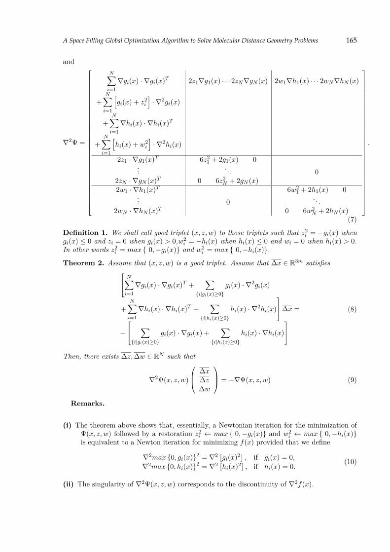
A Space Filling Global Optimization Algorithm to Solve Molecular Distance Geometry Problems 165

and

∇2Ψ =

N∑i=1∇gi(x) · ∇gi(x)T 2z1∇g1(x) · · · 2zN∇gN (x) 2w1∇h1(x) · · · 2wN∇hN (x)

+N∑i=1

[gi(x) + z2

i

]· ∇2gi(x)

+N∑i=1∇hi(x) · ∇hi(x)T

+N∑i=1

[hi(x) + w2

i

]· ∇2hi(x)

2z1 · ∇g1(x)T 6z21 + 2g1(x) 0

... . . . 02zN · ∇gN (x)T 0 6z2

N + 2gN (x)2w1 · ∇h1(x)T 6w2

1 + 2h1(x) 0... 0 . . .

2wN · ∇hN (x)T 0 6w2N + 2hN (x)

.

(7)

Definition 1. We shall call good triplet (x, z, w) to those triplets such that z2i = −gi(x) when

gi(x) ≤ 0 and zi = 0 when gi(x) > 0,w2i = −hi(x) when hi(x) ≤ 0 and wi = 0 when hi(x) > 0.

In other words z2i = max 0,−gi(x) and w2

i = max 0,−hi(x).

Theorem 2. Assume that (x, z, w) is a good triplet. Assume that ∆x ∈ R3m satisfies N∑i=1∇gi(x) · ∇gi(x)T +

∑i|gi(x)≥0

gi(x) · ∇2gi(x)

+N∑i=1∇hi(x) · ∇hi(x)T +

∑i|hi(x)≥0

hi(x) · ∇2hi(x)

∆x =

−

∑i|gi(x)≥0

gi(x) · ∇gi(x) +∑

i|hi(x)≥0hi(x) · ∇hi(x)

(8)

Then, there exists ∆z,∆w ∈ RN such that

∇2Ψ(x, z, w)

∆x∆z∆w

= −∇Ψ(x, z, w) (9)

Remarks.

(i) The theorem above shows that, essentially, a Newtonian iteration for the minimization ofΨ(x, z, w) followed by a restoration z2

i ← max 0,−gi(x) and w2i ← max 0,−hi(x)

is equivalent to a Newton iteration for minimizing f(x) provided that we define

∇2max 0, gi(x)2 = ∇2 [gi(x)2] , if gi(x) = 0,∇2max 0, hi(x)2 = ∇2 [hi(x)2] , if hi(x) = 0. (10)

(ii) The singularity of ∇2Ψ(x, z, w) corresponds to the discontinuity of ∇2f(x).

166 Mario Salvatierra Junior

Theorem 3. Assume that (x, z, w) is a good triplet. Given ε > 0, assume that ∆x ∈ R3m

satisfies ∑i|gi(x)<0

ε

ε− 2gi(x)∇gi(x) · ∇gi(x)T +∑

i|gi(x)≥0

[∇gi(x) · ∇gi(x)T + gi(x) · ∇2gi(x)

]

+∑

i|hi(x)<0

ε

ε− 2hi(x)∇hi(x) · ∇hi(x)T +∑

i|hi(x)≥0

[∇hi(x) · ∇hi(x)T + hi(x) · ∇2hi(x)

]∆x =

−

∑i|gi(x)≥0

gi(x) · ∇gi(x) +∑

i|hi(x)≥0hi(x) · ∇hi(x)

(11)

Then, there exists ∆z,∆w ∈ RN such that

∇2Ψ(x, z, w)

∆x∆z∆w

= −∇Ψ(x, z, w) (12)

Remarks.

(i) Unlike Theorem 2, in Theorem 3 we see that the (∆z,∆w)-part of the solution of (12) isuniquely determined. This is due to the regularizing perturbation. Defining as (10), thesystem (11) can be written as∇2

[12

N∑i=1

max 0, gi(x)2]

+∑

i|gi(x)<0

ε

ε− 2gi(x)∇gi(x) · ∇gi(x)T

+∇2[

12

N∑i=1

max 0, hi(x)2]

+∑

i|hi(x)<0

ε

ε− 2hi(x)∇hi(x) · ∇hi(x)T∆x =

−∇[

12

N∑i=1

max 0, gi(x)2]

+∇[

12

N∑i=1

max 0, hi(x)2]

,

(13)

or, equivalently,∇2f(x) +∑

i|gi(x)<0

ε

ε− 2gi(x)∇gi(x) · ∇gi(x)T

+∑

i|hi(x)<0

ε

ε− 2hi(x)∇hi(x) · ∇hi(x)T∆x = −∇f(x).

(14)

The reasoning above leads us to define the Regularized Hessian of f , given ε > 0, as

∇2f(x, ε) = ∇2f(x)+∑

i|gi(x)<0

ε

ε− 2gi(x)∇gi(x)∇gi(x)T +∑

i|hi(x)<0

ε

ε− 2hi(x)∇hi(x)∇hi(x)T

(15)The Regularized Hessian in (15) do not exhibit discontinuities on the boundaries gi(x) = 0 andhi(x) = 0. Since the perturbation is positive semidefinite, the perturbed Hessian is positivesemidefinite provided that ∇2f(x) is. This is an advantage for minimization algorithms basedon quadratic models.

A Space Filling Global Optimization Algorithm to Solve Molecular Distance Geometry Problems 167

3. The Global Optimization Algorithm

The global optimization algorithm presented here is based on idea to cover the domain Ωthrough a dense curve. Suppose that Ω ⊂ Rn is a closed box with nonempty interior. This is:

Ω = x ∈ Rn|l ≤ x ≤ u.

The Lissajous curve is:

γ(t) = (cos(θ1t+ ϕ1), . . . , cos(θnt+ ϕn)). (16)

Given x0 ∈ Ω and choosing appropriately ϕ1, . . . , ϕn we can find a Lissajous curve such thatγ(0) = x0. Clearly, the Lissajous curves are smooth. Under certain conditions in the coef-ficients θ1, . . . , θn ∈ R, the image of a Lissajous curve is dense on [−1, 1]n and under lineartransformations it is dense in Ω [5].

The strategy to solve the problem (1) is to use Newton-like minimization local methods usingthe regulrized hessians and then use the Lissajous curve to try to escape from local minimizerto a better one.

4. Computational experiments

The instances that will be considered are generated from data in the Protein Data-Bank [2, 4]and we will adopt some instances from the work by Moré and Wu [3].

References

[1] T. Schlick. Molecular Modeling and Simulation: an Interdisciplinary Guide. Springer, 2002.[2] H.M. Berman, J. Westbrook, Z. Feng, G. Gilliland, T.N. Bhat, H. Weissig, I.N. Shindyalov, P.E. Bourne.

The protein data bank. Nucleic Acids Research, 28:235–242, 2000.[3] J. Moré, and Z. Wu. Distance geometry optimization for protein structures. J. Glob. Optim., 15:219–234,

1999.[4] www.pdb.org[5] L.T. Santos, F. Yano, M. Salvatierra, J.M. Martínez, R. Andreani and M. Tygel. A global optimization

algorithm applied to the common reflection surface (CRS) problem. Journal of Seismic Exploration, 14:217–233,2005.

[6] M. Souza, A.E. Xavier, C. Lavor and N. Maculan. Hyperbolic smoothing and penalty techniques applied tomolecular structure determination. Operations Research Letters, 39:461–465,2011.

DGA 2013, pp. 169 – 174.

From Star Configuration to Minimum Length Spanning Tree:The Role of Distances in Optimal Access Networks

Henrique P. L. Luna1

1Instituto de Computação, Universidade Federal de Alagoas, 57072-970, Maceió, AL Brasil, [email protected]

Abstract Given a set of n + 1 points on the two-dimensional plane, indexed by i = 0, 1, 2, ..., n, supposethat point 0 is the source of a single commodity that must be delivered to the other n points. Foreach of these customer points a specific demand qi is required. Local access design concerns theproblem of finding the minimum cost network that connects all points, using only lines joiningpairs of points from the given set. Fixed (structural) and variable (operational) costs are takeninto account in the connecting network. For each used line both the fixed and the variable costto install and to use link (ij) are directly proportional to the distance dij between points i andj. A spanning tree is a natural candidate for the underlined structure of an optimal local accessdesign. Two specific solutions plays a major role to calculate a lower bound for the total cost. Astar configuration, with degree n at the origin node 0, that minimizes the sum of variable costs.And a minimum length spanning tree, that minimizes the sum of fixed costs. The lower bound isexpressed is terms of the used line distances dij , the customer demands qi and the parameters βand γ, where β express the fixed cost per unit of distance and γ is the variable cost per unit of flowand per unit of distance. Necessary and sufficient conditions are derived to verify the optimalityof a feasible solution. For given demands and line distances among the points, there exists anopen interval for the fixed over variable cost ratio β/γ for which neither a star configuration nor aminimum length spanning tree corresponds to an optimal network.

Keywords: network design, distance in fixed cost, minimum length spanning tree, distance in variable cost,shortest paths, computer networks, geometric structures , graph theory

1. Introduction

The spatial nature and hierarchical organization of telecommunication and transportation sys-tems can be found in several real world applications, such as the location of switching centresor postal offices, and plays a major role in operations research and management science models.Minimum distances are crucial for the objective of cost minimization in these public systems.Together with values of the spatially distributed demands, the influence of distances mustbe taken into account to find optimized levels of customer concentrations, what enables theeconomies of scale of aggregating the flows in the related networks. The main differencesamong the models concern the hierarchical level of network design, typically backbone versuslocal access network, and how the relevant aspects of connectivity, capacity, reliability, demandpatterns, routing, pricing, performance and quality of service are considered for such networks([6] [3]). Depending on the context or application, hub nodes are called switches, warehouses,water sources, facilities, concentrators or access points. Likewise, backbones may be referredto as hub-level networks and local access networks may be called distribution or tributary net-works. Normally, backbone links carry larger volumes of traffic than tributary links. Trafficoriginating at a specific customer location can pass through a local access network to get to

170 Henrique P. L. Luna

a hub node. After passing through the backbone network, the traffic again uses a local accessnetwork to travel from a hub to its final destination at another location. The influence ofdistance in cost occurs in all levels of an hierarchical network, but plays a major role in theaccess networks.

For each level of network design, a wide range of model formulations has been covered bythe related literature, which may be classified as having a deterministic or stochastic character,and also according to the continuous or discrete nature of the model. Because of the complex-ity of these problems, local access network design and backbone design are often consideredindependently. The papers [1], [4] and [7] are some examples that treat specifically local accessnetwork design problems. This is the class of problems of our interest in this paper, in such away that we discard any reference to a considerable body of literature that treats topologicaldesign, capacity planning and flow assignment questions at the hub-level of transportation ortelecommunication networks.

We also focus on a deterministic problem in which a single hub location is chosen fromamong a continuous set of points. Most of the literature on public utility networks has only ahalf of century, but the min− sum location problems originated in the 17th century, whenFermat posed the question of, given three points in a plane, find a median point in the planesuch that the sum of the distances from each point to the median point is minimized. In thelast century, many studies have addressed extensions of the Fermat problem. A remarkablecontribution has been done by Alfred Weber, that studied the problem for a general number nof points, also adding weights qi on each point i to consider customer demand qt that point.The Weber problem locates facilities (medians) at continuous locations in the Euclidian plane.We assume in this paper that, given the n customer points, the location of the source node 0is an optimal solution of the Weber problem. The idea behind the Fermat problem has beenintroduced in graphs by (Hakimi, 1964), who defined the absolute median as the point on agraph that minimizes the sum of the weighted distances between that point and the vertices ofthe graph. He allowed this point to lie anywhere along the edges of the graph, but proved thatan optimal absolute median is always located at a node of the graph, thus providing a discreterepresentation of a continuous problem.

Given a set of points on the two-dimensional plane, the problem of finding the shortestconnecting network that connects all the points, using only lines joining pairs of points fromthe given set is one of the nicest and simplest problems in network optimization, and arises inmany applications. If the length between every pair of points is positive, the shortest connectingnetwork is clearly a spanning tree, that is called a minimum length spanning tree (MLST). Thisproblem is closely related to the local access network design LAND problem. This paper showsthat, for a sufficiently high value of the fixed over variable cost ratio β/γ, an optimal topologyfor the LAND problem is also an optimal topology for the MLST problem. On the other hand,the paper also shows that, for a sufficiently low value of the fixed over variable cost ratio β/γ,a star centered in in source node 0 is an optimal topology for the LAND problem. The nexttwo sections formalizes the LAND problem and provides theoretical results concerning cost anddistance relationships in the problem, while a summary section concludes the paper.

2. A Flow Formulation for Tree Network Design

The problem is to find a minimum cost tree over a graph G(N,E), where N is a set of n + 1nodes and E is a set of m edges. Unless stated otherwise, the graph is complete, with a numberof m = n(n+ 1)/2 edges. The number of selected edges in an optimal tree connecting networkis n. The model parameters are provided by one square matrix, D, of order n + 1, a demandvector q, of order n, and the two scalars β and γ, both indicating cost per unit of distance.Each element dij of the symmetric matrix D refers to the distance between nodes i and j, that

Role of Distances in Optimal Networks 171

is assumed to be equal to the distance between nodes j and i. The diagonal of D has elementsdii = 0 and if nodes i and j are not linked by an edge in E then dij =∞.

Consider the binary variables x(ij), for i = 0, 1, ..., n−1 and j = i+1, ..., n, such that x(ij) = 1if and only if edge (ij) ∈ E belongs to an optimal tree design. Consider also the directed flowvariables fij ≥ 0, for i = 0, 1, ..., n and j = 1, ..., n with i 6= j, which specify a single commodityflow between nodes i and j.

A mixed integer linear program for the local access network design (LAND) problem is

min βn−1∑i=0

n∑j=i+1

dij x(ij) + γn∑i=0

n∑j=1

dij fij (1)

subject to the constraints

n−1∑i=0

n∑j=i+1

x(ij) = n (2)

n∑j=1

f0j =n∑h=1

qh (3)

n∑h=0

fhi −n∑j=1

fij = qi ∀ i = 1, ..., n (4)

f0j ≤ (n∑h=1

qh) x(0j) ∀ (0j) ∈ E (5)

fij ≤ (n∑h=1

qh) x(ij) ∀ (ij) ∈ E (6)

fji ≤ (n∑h=1

qh) x(ij) ∀ (ij) ∈ E (7)

x(ij) ∈ 0, 1 ∀ (ij) ∈ E (8)fij ≥ 0 ∀ i = 0, ..., n, j = 1, ..., n (9)

This single-commodity flow formulation is a simplified version of more elaborated models con-cerning spanning trees or local access network problems ([5],[2], [4], [7]). Remark that the linearprogramming relaxation of some of these multi-commodity versions provides integer solutionsfor the problem, but any computational issue concerning this class of problems is out of scopein this paper. Apart notation questions, the essential results that follows neither are dependentfrom the (LAND) problem formulation nor from the used algorithm to solve the problem.

3. Cost and Distances Relationships

3.1 Cost and length definitions

For any feasible solution (xt, f t) in the mixed integer linear programming model (1-9) weidentify two parts of the objective function:

172 Henrique P. L. Luna

zt = βn−1∑i=0

n∑j=i+1

dij xt(ij) (10)

vt = γn∑i=0

n∑j=1

dij ftij (11)

in such way that zt+vt is the total cost of the designed network. Let T (N,Et) be the spanningtree corresponding to this solution and linking the origin 0 to all demand nodes h = 1, ..., n(x(ij) = 1 ∀ (ij) ∈ Et and x(ij) = 0 ∀ (ij) ∈ E − Et). Assume that Lt is the total length ofthe spanning tree T (N,Et). Let P t0h be the set of edges in the path from the origin 0 to thedemand node h, with lt0h being the correspondent length, obtained by summing the distancesdij across the edges of P t0h. Then equations (10) and (11) can be rewritten in terms of treesand paths lengths:

zt = β Lt (12)

vt = γn∑h=1

qh lt0h (13)

3.2 Lower bounds for costs

Two specific feasible solutions, for which we use the indices t = 0 and t = 1, provides informationto determine a lower bound for any feasible solution of the LAND problem. We say thatT (N,E0) is the trivial solution of a star configuration, with the source node 0 being directlylinked to each of the other nodes i = 1, ..., n. And we define T (N,E1) as being an optimaltopology for the MLST problem over the graph G(N,E). We call any of the spanning treesT (N,E0) or T (N,E1) an extremal solution for the problem.

For T (N,E0), by definition, we have l00h = d0h = lmin0h for all h = 1, ..n, where lmin0h indicatesthe length of a shortest path from the source 0 to the customer point h, that is of course thestraight line between points 0 and h. On the other hand, by definition, we have L1 = Lmin,where Lmin indicates the minimum length spanning tree. The following results, that are notproved here to reduce space, are easily shown:

Lemma 1. Every feasible solution (xt, f t), related to an enumerated spanning tree T (N,Et),has a variable cost not smaller than that of the star configuration T (N,E0), that is

v0 ≤ vt ∀ T (N,Et).

Lemma 2. Every feasible solution (xt, f t), related with an enumerated spanning tree T (N,Et),has a fixed cost not smaller than that of the minimum length spanning tree T (N,E1), that is

z1 ≤ zt ∀ T (N,Et).

Theorem 3. The spanning tree minimum length L1 = Lmin and the shortest path l00h = d0h =lmin0h from the origin 0 to each demand node h are such that

β Lmin + γn∑h=1

qh d0h

is a lower bound for the total cost of any enumerated tree T (N,Et) related to a feasiblesolution (xt, f t) .

Role of Distances in Optimal Networks 173

3.3 Necessary optimality conditions

Let (x∗, f∗), related with a spanning tree T (N,E∗), be an optimal solution for the (LAND)problem (1-7). The following results hold:

Theorem 4. The total length L∗ of a spanning tree associated with an optimal solution (x∗, f∗)must satisfy

L1 = Lmin ≤ L∗ ≤ L0 =n∑h=1

d0h

Theorem 5. If z∗ + v∗ is the objective function value of an optimal solution (x∗, f∗) then

v∗ ≤ v1

3.4 Sufficient optimality conditions for extremal solutions

A star configuration centered in 0 is better then any given tree T (N,Et) if

βn∑h=1

d0h + γn∑h=1

qh d0h < β Lt + γn∑h=1

qh lt0h

In particular, for any non-trivial case where L0 > L1, that is∑nh=1 d0h > Lmin, we can de-

termine the value β′ for which the shortest path solution has the same cost of the minimumlength spanning tree. This kind of consideration leads to a series of results concerning suffi-cient optimality conditions for extremal solutions. A detailed specification of these interestingproperties is left for our workshop presentation and for a complete version of this paper.

4. Summary

The concept of distance is essential to the objective of cost minimization in public utility net-works. This paper puts this concept as the main object to find an optimal geometric structureof a local access network. For a given set of n customer points in a two-dimensional plane,with known distances between all pairs of these points, the fundamental problem addressedhere concerns the optimal location of a single source node 0 and an adequate choice of a treeconnecting network in order to minimize the total cost to install and to use the distributionnetwork.

Besides the beauty of the mathematical theory associated to cost and distance relationships,the interest in this research topic is explained by the richness and variety of its applications.Among the best known we find the examples of computer and telecommunication networks,logistics of distribution systems, water supply management and electrical energy distribution.The influence of distance plays a major role to optimize the geometric structure and the oper-ational access to all these public utility networks.

Acknowledgments

The author wish to thank for the financial support of CNPq, the brazilian council of scientificresearch and technological development.

References

174 Henrique P. L. Luna

[1] Gavish, B. (1982). “Topological design of centralized computer networks – formulations and algorithms”,Networks 12, 355-377.

[2] Gouveia, L. (1996). “Multicommodity flow models for spanning trees with hop constraints”, European Jour-nal of Operational Research 95, 178-190.

[3] Luna, H. P. L. Network planning problems in telecommunications. In: Mauricio G. C. Resende; PanosM. Pardalos. (Org.). Handbook of Optimization in Telecommunications. 1ed.New York: Springer, 2006, p.213-240.

[4] Luna, H. P. L., Ziviani, N. and Cabral, R. (1987). “The telephonic switching centre network problem:Formalization and computational experiments”, Discrete Applied Mathematics 18, 199-210.

[5] Maculan, N. (1986). “A new linear programming formulation for the shortest s-directed spanning tree prob-lem”, Journal of Combinatorics, Information & Systems Sciences 11, 53-56.

[6] Magnanti, T. and Wong, R. (1984). “Network design and transportation planning: Models and algorithms”,Transportation Science 18, 1-55.

[7] Randazzo, C. and Luna, H. P. L. (2001). “A comparison of optimal methods for local access uncapacitatednetwork design”, Annals of Operations Research 106, 263-286.

DGA 2013, pp. 175 – 179.

A new algorithm for efficient computation of Hausdorffdistance in evaluation of digital image segmentation

R. S. Marques,1 D. A. Machado,2 G. Giraldi,2 and A. Conci1

1Universidade Federal Fluminense - UFF, rmarques,[email protected]

2Laboratório Nacional de Computação Científica - LNCC, danubiad,[email protected]

AbstractLarge ground truth databases are necessary to evaluate and validate computer-aided diagnosis

systems. Images used for diagnosis purposes usually have their regions of interests segmented asa first step of the patterns recognition procedures. Automatic segmentation of medical images isan open issue in image processing where there is an important need for validation and comparisonamong new results with available image databases. The limits of such regions of interests arefrequently very irregular and to verify the adequacy of several approaches numerical and not onlyvisual techniques must be used. In this paper, a new algorithm for the Hausdorff distance com-putation in discrete curves and areas is presented. The proposed algorithm finds the exact resultin much less computational time than the traditional method. Results of its use on comparisonof two automatic segmentation methods for breast infrared images are presented to illustrate thealgorithm.

Keywords: Discrete imaging, Hausdorff distance, Digital image segmentation, Ground Truth

1. Introduction

The use of new technologies (as infrared and electrical impedance tomography) can improveearly and correct diagnosis, especially if considered in computer-aided diagnosis (CADx) sys-tems [1]. These systems uses artificial intelligence (AI) and mining techniques to improve earlydiagnosis and it needs classified databases for knowledge acquisition [2]. To accomplish this,the development of databases with proven cases is fundamental and it is the main goal of theproject on execution at the Hospital of Fluminense Federal University (HUAP/UFF) aimingto improve the breast diseases detection using infrared (IR) images [3]. This research aimsto assist the development of CADx based on a fusion of exams (mammography, ultrasound,MRI, thermography) considering a new way to compare the results of different discrete imagesegmentation approaches. In this paper we present a new method that allow numerical com-parisons among breast segmentations by improving Hausdorff distance calculation algorithm,considering particular aspects of discrete objects (curves and areas) [5]. Moreover, this articledescribes experiments on real breast images used to evaluate the segmentations methodologies.Results compares two forms of achieve this information using the proposed algorithm and thetraditional one. The result of this research aims to assist the generation of diagnostic systemsor at least to be a tool to compare biological segmentation results based on discrete images.This work is divided in more three parts: Description of the Hausdorff distance in continuousgeometry and its new formulation for discrete geometry (DG); The developed algorithm andsome aspects of its implementation; Its results on infrared exams (thermographic images) and

176 R. S. Marques, D. A. Machado, G. Giraldi, and A. Conci

conclusion about this new technique on the 2D discrete curves of the breast boundaries de-tected from the IR acquisition. Validations were made comparing the real breasts of volunteerssubmitted at same time to at least two segmentations considered very satisfactory visually andthat must be numerically compared.

2. Preliminaries

We begin by describing Hausdorff metric or distance. Let D be a closed subset of Rn (contin-uous space) and S denote the class of all non-empty compact subset of D ([6] p.113). Thereare some alternative (equivalent) ways of defining Hausdorff metric on all non-empty compactsubset S, of closed subset D, of Rn. The one presented by Falconer ([6] p.114) considering theδ-parallel body of A ∈ S is very adequate to transform S to a discrete ZM subspace and it isthe one used here. We define Aδ , i.e. the parallel body of A ∈ S as:

Aδ = x ∈ D : |x− a| ≤ δ for some a ∈ A, (1)

We make S into a metric space by defining the distance d(A,B) between two sets A,B to bethe least δ such that the δ-parallel body of A,Aδ, contains B and the δ-parallel body of B,Bδ,contains A (see first image on Figure 1):

d(A,B) = infδ : A ⊂ Bδ and B ⊂ Aδ, (2)

Figure 1: Hausdorff distance between two sets A, B and the δ-parallel body ([6] p.114). Result of a splinebased segmentation [5] (pink) for IR0100 overlapped with the ground truth (green). Refined result for the sameimage [11]. Manual segmentation, ground truth composition [9] and ROI defined in a binary black and whiteversion.

Then the two sets A,B is now subsets of the metric space S. Considering the definition ofthe closure of A and B, denoted by A− and B− ( [7] p.114) we have

d(A−, B−) = infδ : A− ⊂ Bδ− and B− ⊂ Aδ− = infδ : A ⊂ Bδ and B ⊂ Aδ = d(A,B),(3)

Moreover by definition of the boundary of A and B : ∂A and ∂B ([7] p.181) we have:

d(∂A, ∂B) = d(A−, B−) = d(A,B), (4)

It is plausible to consider a discrete version of (4) by replacing A with a discrete version ofit, say AM . Allowing a slight abuse of notation, let ∂AM denote the intersection of AM with ∂A.Carefully note that this is not the boundary of AM (in fact, it makes no sense to talk aboutthe boundary of a discrete subset of Rn). The same argument applied to the set B and yieldsa discrete version BM of it. In this way, we can think of AM and BM as subsets of a discreteversion of Rn , say ZM , and so we proceed to compute a discrete version of the Hausdorffdistance between AM and BM based on following discrete version of (2):

d(AM, BM) = d(∂AM, ∂BM), (5)

A new algorithm for efficient computation of Hausdorff distance in evaluation of digital image segmentation177

Although this new expression (5) for discrete images follows from equation (2) and variousdefinitions, we not yet have known it from elsewhere in the literature. In next section, this newexpression for Hausdorff distance is used to create a new algorithm to compare binary digitalimages. Although few examples are presented here, it has been extensively tested for us in theIR segmentation evaluation as will be commented [3].

3. Proposed Algorithm

Using equation (5) instead of the equation (2), we greatly improve any traditional algorithmfor calculating the distance between two sets. To illustrate this statement a very commonalgorithm (brute force) was applied in these two forms and used for images of 2 resolutions,the results can be seen in Table 1. Moreover, this section presents some considerations to(5) that can turn its computation on discrete images even faster. Let AM be an image ofthe automatic segmented region of interest (ROI) and let BM be its ground truth respectively(for instance the pink and green curves in the second image of Figure 1). These images canbe represented as binary images, i.e. with white (value 1) representing ROI’s pixels and black(value 0) representing the background (Figure 1, right image). In this way, the boundary pointsof A and B (pink and green curves in the right image of Figure 1) can be defined by a list ofconnected pixels in a given resolution, i.e.:

∂AM = ai ∈ AM : ∃pj ∈ Ac, pj ∈ N8(ai) and ∂BM = bi ∈ BM : ∃pm ∈ Bc, pm ∈ N8(bi),(6)

where N8(p) denotes the 8-neighborhood of the discrete point p (or pixel p) ([8] p. 210) andAc, Bc denotes the complement of sets A and B.

To find d(∂AM, ∂BM) through an exhaustive algorithm, it must be calculated for each ak ∈ AM

the distance |ak − bi| (for i = 1...n, where n = |B|). It is possible to simplify this search bytesting when the pixel ak of coordinates (xk, yk) has a corresponding pixel in same coordinatesin the image ∂BM, that is (xk, yk) is equal to value in ∂BM. In this case, the distance of akand B equals zero: this means n − 1 comparisons will not be accomplished, simplifying thesearch. The proposed algorithm to calculate (5) is presented in algorithm below (The Hausdorffdistance algorithm ([5] p.109). To facilitate this calculation the index of the pixels (i.e. xk, yk)can be used to compute the distance between them.

1 : ∂AM := ai ∈ AM : ∃pj ∈ Ac, pj ∈ N8(ai) and ∂BM = bi ∈ BM : ∃pm ∈ Bc, pm ∈ N8(bi)2 : h := 0;3 : for each ak = (xk, yk) ∈ ∂AM do

4 : if value(bk) ≡ value(ak) then

5 : h := 06 : else

7 : h2 := |bi − ak|2 = |xi − xk|2 + |yi − yk|2

8 : end if

9 : end for

10 : return h

This algorithm can be used for the entire discrete binary ROI (Figure 1 the rightmost image)if they are presented on this way. Discrete images in two resolutions (320×240 and 640×480)were tested. The Hausdorff distance was calculated using the entire image (d(A,B)) and onlyits boundary (d(∂AM, ∂BM)) with the proposed algorithm and the traditional method. Althoughthe result was the same (exact Hausdorff Distance), the computation time was very differentas can be seem in line 2 of Table 1 ([5] p.110).

178 R. S. Marques, D. A. Machado, G. Giraldi, and A. Conci

Table 1: Execution time in seconds for same images using force brute and the proposed algorithm [5].

Time d(∂AM, ∂BM)320× 240 d(A,B)320× 240 d(∂AM, ∂BM)640× 480 d(A,B)640× 480Traditional algorithm 9.57 37.78 76.51 610.65Proposed algorithm 0.75 1.49 3.98 20.6

4. Results on Infrared Exams and ConclusionsNumerical results on ten real breast segmentation using two different approaches were con-sidered for illustrative purposes and presented in Table 2. For the ground truth generationthree manual segmented images for each patient were used. They were manually defined usinga Samsung Galaxy P7510 tablet with stylus pen by a specialist in breast radiology and twotrained users (Figure 1). A specialized software was developed for it [9].To facilitate, all threemanual segmentations results were combining to a unique ground truth using the voting policyproposed by Li et al. [10]. The first segmentation technique evaluated is based on QuadraticUniform B-Splines presented by Marques [5]. The results of the second approach were obtainedby a refinement of the previous approach using Level Set [11] (post-processing). More detailsabout these techniques can be found in [5, 11]. The second and third image of Figure 1 showsthe results of the segmentation methods that was evaluated by the Hausdorff distance. Thereis not a visual significant difference between the automatic segmentations used, this illustratethe need of numerical comparison. They are then compared by the proposed algorithm (Table2).

Table 2: Hausdorff distance between the Ground-Truth and segmented images.

Images IR 0100 0149 0213 0756 0973 0990 3416 3743 3748 3825

Splines 12.76 5.00 9.22 15.56 16.97 7.07 16.28 7.28 7.81 28.28Posproces. 12.73 5.00 9.22 14.87 16.97 7.07 16.28 7.28 7.81 29.00

5. Summary

This paper is concerned with the application of Hausdorff metric or distance for imaging. Itshould be of interest to a broad readership involved in segmentations methods and its validationby using a typical strategy of comparison with ground truth of available databases. This workshows how Hausdorff metric computation could have its computation time reduced by usingtheoretical and numerical techniques. Summing up, the steps are: Binarize the segmentedimages (continuous closed sets); Subtract the inside, yielding the image boundaries; Discretizethe boundaries and calculate the distance between the sets. Validations are made by comparingresults of images in two resolutions, using well-known algorithm and ten real breast infraredexams of volunteer who accepted to have their data included in the public database developmentby the projects that support this work.

Acknowledgments

The authors thank to CAPES for financial support (projects PROENG PE021/2008 and ProCad no. 540/2009)and to UFF-Telemedicine Group an Associated Laboratory of INCT-MACC.

A new algorithm for efficient computation of Hausdorff distance in evaluation of digital image segmentation179

References

[1] Ng, E. Y-K and N. M. Sudharsan. Computer Simulation in Conjunction with Medical Thermography asan Adjunct Tool for Early Detection of Breast Cancer. BMC Cancer, 4(17):6, 2004.

[2] M. Moghbel and S. Mashohor. A review of Computer Assisted Detection/Diagnosis (CAD) in breastthermography for breast cancer detection. Artificial Intelligence Review, 2011.

[3] PROENG. Image processing and image analyses applied to mastology. http://visual.ic.uff.br/en/proeng/.[4] I. Cheng, C. Flores-Mir, P. Major and A. Basu. Measuring and evaluating ground truth for boundary

detection in medical images. Annual International Conference of the IEEE Engineering in Medicine andBiology Society, pages 5889–92, 2008.

[5] R.S. Marques. Segmentação automática das mamas em imagens térmicas. M.Sc. thesis, IC-UFF, 2012.[6] K.J. Falconer. Fractal Geometry: Mathematical foundations and applications. Wiley, 1990.[7] C.S. Kubrusly. Elements of operator theory. MIT Press, Cambridge, MA, 1994.Birkhauser, 2001.[8] A. Conci, E. Azevedo and F.R. Leta. Computação Gráfica. Campus/Elsevier, v.2, 2008.[9] GTMAKER. Ground Truth Maker. http://visual.ic.uff.br/en/proeng/software.php, 2012.[10] X. Li, B. Aldridge, R. Fisher and J. Rees. Computer Simulation in Conjunction with Medical Thermog-

raphy as an Adjunct Tool for Early Detection of Breast CancerEstimating the ground truth from multipleindividual segmentations incorporating prior pattern analysis with application to skin lesion segmentation.IEEE International Symposium on Biomedical Imaging From Nano to Macro, pages 1438–1441, 2011.

[11] D.A. Machado. Segmentação de Imagens via Método dos Conjuntos de Níveis e Derivada Topológica. M.Sc.thesis, LNCC, 2012.

DGA 2013, pp. 181 – 185.

Does the packing radius depend on the distance? The Casefor Poset Metrics

Rafael Gregorio Lucas D’Oliveira1 and Marcelo Firer2

1IMECC-UNICAMP, Universidade Estadual de Campinas, CEP 13083- 859, Campinas, SP, Brazil, [email protected]

2IMECC-UNICAMP, Universidade Estadual de Campinas, CEP 13083- 859, Campinas, SP, Brazil, [email protected]

Abstract Until this work, the packing radius of a poset code was only known in the cases where the posetwas a chain, a hierarchy, a union of disjoint chains of the same size, and for some families of codes.Our objective is to approach the general case of any poset and any code. To do this, we will dividethe problem into two parts.

The first part consists in finding the packing radius of a single vector. We will show that thisis equivalent to a generalization of a famous NP-hard problem known as “the partition problem”.Then, we will review the main results known about this problem giving special attention to the al-gorithms to solve it. The main ingredient to these algorithms is what is known as the differentiatingmethod, and therefore, we will extend it to the general case.

The second part consists in finding the vector that determines the packing radius of the code.For this, we will show how it is sometimes possible to compare the packing radius of two vectorswithout calculating them explicitly.

Keywords: Error Correction Codes, Packing Radius, Partitioning Problems, Poset Codes

1. Introduction

Let (V, d) be a finite metric space and let C ⊂ V be a nonempty subset. The minimal distanceof C is

d (C) = min d (x, y) : x, y ∈ C, x 6= yand the packing radius of C is

Rd (C) = max R : B (x,R) ∩B (y,R) = ∅, x, y ∈ C, x 6= y

where B (x,R) is the ball centered at x with radius R, i.e.

B(x,R) = y ∈ V : d(x, y) ≤ R.

The question we pose in this work is to analyze the relation between these quantities, theminimum distance and the packing radius, in a specific context, that of the Theory of ErrorCorrecting Codes, where V = Fnq is a n−vector space over a finite field with q elements, C is alinear subspace and d belongs to a family of metrics that assumes the integer values between 0and n = dimV . If we denote by bxc the floor function, it is straightforward to show that⌊

d (C)− 12

⌋≤ Rd (C) ≤ d (C)− 1

(the floor function is only a consequence of the values of d (·, ·) being integers).

182 Rafael Gregorio Lucas D’Oliveira and Marcelo Firer

Due to the importance of this question for the Theory of Error Correcting Codes, we keepthe notation used in this context. The usual metric used in this context, the Hamming metricdH , is defined as the cardinality |i;xi 6= yi|, where x = (x1, ..., xn) and y = (y1, ..., yn) areelements in Fnq . In this case, it is well known that

RdH (C) =⌊dH(C)− 1

2

⌋.

In this work we will consider the problem of finding the packing radius in the case of posetmetrics. These metrics where first introduced by Brualdi et al. [1] generalizing on the workof Niederreiter [9]. An interesting property of these metrics is that the packing radius is notnecessarily determined by the minimum distance. Until this work, to the authors’ knowledge,the packing radius of a poset code was only known in the following cases: chain posets [3],hierarchical posets [2], disjoint union of chains of the same size (L. Panek, M. Muniz, M. Firer,personal communication), and for some families of codes [4]. We will approach the generalposet case. To do this we will divide our problem in two.

The first part consists in determining the packing radius of a single vector. We will see thatthis is equivalent to solving a generalization, which we will call “the poset partition problem”,of a famous NP-hard problem known as “the partition problem”. We will then take a lookat one of the fastest known algorithms for solving the partition problem (in some cases) andgeneralize it to the poset partition problem. The first time the problem of finding the packingradius of a poset code was identified, in some sense, as a partitioning problem was in [5].

The second part consists in finding which code-word determines the packing radius of thecode. To do this we will show how sometimes it is possible to compare the packing radius oftwo vectors without calculating them explicitly.

2. The Poset Metric

Let [n] = 1, 2, . . . , n be a finite set and be a partial order on [n]. We call the pairP = ([n],) a poset and often identify P with [n]. An ideal in P is a subset J ⊆ P with theproperty that if x ∈ J and y x then y ∈ J . The ideal generated by a subset X ⊆ P isthe smallest ideal containing X and is denoted by 〈X〉. A poset is called a chain if every twoelements are comparable, and an anti-chain if none are. The length of an element x ∈ P is thecardinality of the largest chain contained in 〈x〉.

Let q be the power of a prime, Fq the field with q elements and Fnq the vector space ofn-tuples over Fq. We denote the coordinates of a vector x ∈ Fnq by x = (x1, x2, . . . , xn).

A poset P = ([n],) induces a metric dP , called the P -distance, in Fnq defined as

dP (v, w) = |〈supp(v − w)〉|

where supp(x) = i ∈ [n] : xi 6= 0. The distance ωP (v) = dP (v, 0) is called the P -weight of v.Note that if P is an anti-chain then dP is the Hamming distance. Because of this, when P

is an anti-chain we will denote it by H.Given a linear code (subspace) C ⊆ Fnq and a poset P = ([n],), we denote the minimum

distance of C as dP (C) and the packing radius of C as RdP (C). We remark that, since dP istranslation invariant, if we define the P -weight as ωP (x) = dP (x, 0) then dP (C) = minωP (v) :v ∈ C − 0. Since C is linear, z = x− y ∈ C and therefore the packing radius is the largestpositive integer such that

BP (0, RdP (C)) ∩BP (z,RdP (C)) = ∅

for every z ∈ C − 0.

Does the packing radius depend on the distance? The Case for Poset Metrics 183

3. The Packing Radius of a Vector

We begin this section by defining the packing radius of a vector.Definition 1. Let x ∈ Fnq and d be a metric over Fnq . The packing radius of x is the largestinteger r such that

B(0, r) ∩B(x, r) = ∅and is denoted by Rd(x).

Next, we show that the packing radius of a linear code is the smallest of the packing radiiof its code-words.Proposition 1. Let C ⊆ Fnq be a linear code and d a metric over Fnq . Then,

Rd(C) = minx∈C−0

Rd(x).

Thus, to find the packing radius of a linear code, we need to find the code-word with thesmallest packing radius, which we will call the packing vector of the code. We then approachthe problem of finding the packing radius of a vector proving the following result:Theorem 1. Let P be a poset and v ∈ Fnq . Then,

RdP (v) = minA,B⊆Msupp(v)

max|〈A〉|, |〈B〉| − 1,

where (A,B) is a partition of Msupp(v), the set of maximal elements of supp(v).Therefore, the packing radius of a vector is a property of its support. We then show that

the problem can be interpreted as a poset partitioning problem.Definition 2. Let P be a poset and MP be the set of its maximal elements. We define thepacking radius of the poset P as

R(P ) = minA,B⊆MP

max|〈A〉|), |〈B〉| − 1,

where (A,B) is a partition of MP .Applying Theorem 1 to the definition we have that the packing radius of a vector v is

RdP (v) = R(〈supp(v)〉).The problem of finding the packing radius of a vector is then equivalent to the problem of

finding the packing radius of a poset, which we will call the poset partition problem. Thisproblem is a generalization of the famous NP-hard problem known as “the partition problem”.

4. The Partition Problem

The partition problem is defined as follows: Given a finite list S of positive integers, find apartition (S1, S2) of S that minimizes

max

∑x∈S1

x,∑y∈S2

y

.This is equivalent to minimizing the discrepancy

∆(S1, S2) =

∣∣∣∣∣∣∑x∈S1

x−∑y∈S2

y

∣∣∣∣∣∣ .This problem is of great importance both from the practical and theoretical point of view.

In [7], Karp proves that it is NP-hard.

184 Rafael Gregorio Lucas D’Oliveira and Marcelo Firer

5. The Poset Partition Problem

In the poset partition problem we must minimize not the discrepancy, but what we call thediscordancy.

Definition 3. Let P be a poset and (A,B) a partition of MP , the maximal elements of P . Wedefine the discordancy between A and B as

Λ(A,B) = ||〈A〉| − |〈B〉||+ |〈A〉 ∩ 〈B〉|,

and the minimum discordancy of P as

Λ∗(P ) = minXtY=MP

Λ(X,Y ).

The packing radius of a poset can then be written in terms of its minimum discordancy.

Theorem 2. Let P be a poset of size n. Then, the packing radius of P is

R(P ) = n

2 + Λ∗(P )2 − 1.

One of the main heuristics used in solving the partition problem is known as the KK(Karmarkar-Karp) heuristic [6], or as the differencing heuristic. We can generalize this heuris-tic for the poset partition problem and also generalize one of the best known algorithms, forsome cases, that heavily uses the KK heuristic known as the CKK (Complete Karmarkar-Karp)algorithm [8].

6. Finding the Packing Vector

To find the packing radius of a poset code we need to find its packing vector, the code-wordwith minimum packing radius. One way to do this would be to calculate the packing radiusof each code-word, but as we have seen that would be a big problem since we would have tosolve a poset partition problem for each code-word. We can show some ways in which we cansometimes compare the the packing radius of two posets without explicitly determining them.

References

[1] Richard A. Brualdi, Janine S. Graves, and K. Mark Lawrence. Codes with a poset metric. Discrete Mathe-matics, 147:57–72, 1995.

[2] Luciano V. Felix and Marcelo Firer. Canonical-systematic form of hierarchical codes. Advances in Mathe-matics of Communication, 2011. to appear.

[3] Marcelo Firer, Luciano Panek, and Marcelo Muniz Silva Alves. Classification of niederreiter-rosenbloom-tsfasman block codes. IEEE Transactions on Information Theory, 56:5207–5216, 2010.

[4] Marcelo Firer, Luciano Panek, and Laura Rifo. Coding in the presence of semantic value of information:Unequal error protection using poset decoders, 2011.

[5] Jong Yoon Hyun and Hyun Kwang Kim. The poset structures admitting the extended binary hammingcode to be a perfect code. Discrete Mathematics, 288:37–47, 2004.

[6] Narendra Karmarkar and Richard M. Karp. The differencing method of set partitioning. Technical report,Computer Science Division (EECS), University of California, Berkley, 1982.

[7] Richard M. Karp. Reducibility among combinatorial problems. In Complexity of Computer Computations,pages 85–103, 1972.

[8] Richard E. Korf. A complete anytime algorithm for number partitioning. Artificial Intelligence, 106:181–203,1998.

Does the packing radius depend on the distance? The Case for Poset Metrics 185

[9] Harald Neiderreiter. A combinatorial problem for vector spaces over finite fields. Discrete Mathematics,96:221–228, 1991.

DGA 2013, pp. 187 – 191.

Distance-Based Imputation on Classification Problems withMissing Features

Mirlem R. Ribeiro1 and Eulanda M. Dos Santos1

1Federal University of Amazonas, Manaus, Brazil,[email protected]@icomp.ufam.edu.br

Abstract This paper presents a comparison between two different imputation methods, mean and k NearestNeighbors (kNN), applied to classification problems with missing features. This comparison isconducted using two classification methods: Decision Tree and kNN classifier. The former is anunstable classifier, while the latter is stable. It is shown that the distance-based imputation method(kNN) is less prone to introduce data distortion, leading to higher recognition rates.

Keywords: Missing Features, Imputation Methods, Classification Problems.

1. Introduction

Classification methods are learning algorithms used to solve tasks for which the design ofsoftware using traditional programming techniques is difficult. Biometric recognition, filter forelectronic mail messages and DNA recognition are examples of these tasks. Several differentlearning algorithms have been proposed in the literature such as Decision Tree, kNN, NeuralNetworks, Support Vector Machines, etc. Considering a supervised classification problem withthe following set of class labels Ω = ω1, ω2 . . . , ωc, samples xi,t contained in a training datasetare used by learning algorithms to the design of a robust well-suited classifier to the problemconcerned. Then, this classifier is used to predict the label of the test samples xi,g contained ina test dataset, focusing on estimating the generalization performance of the trained classifier.Each training sample xi,t is an n-dimensional vector xi,t = [x1, ..., xn]T ∈ Rn, where the realspace Rn is called feature space. Traditionally, it is assumed that the test samples are alson-dimensional vectors xi,g = [x1, ..., xn]T ∈ Rn. Nonetheless, several real-world applicationsmay be prone to missing features on test data set due to bad sensors, data corruption, refusalof respondents to answer certain questions, failed pixels, and others.

Even though discarding all instances with missing features may be used to cope with sucha problem, this is not a suitable solution since is not frequently possible to reject to takea decision in real applications. Consequently, several methods have been proposed in theliterature to treat missing features. According to Garcia-Laencina et al. [2], the methods forpattern classification with missing features may be divided into three groups: (1) model-basedprocedures; (2) machine learning-based methods; and (3) missing data imputation. In thefirst group, a model defining the distribution of the data is constructed using strategies likeexpectation-maximization. In the second group, missing features are dealt with directly bya classifier, for instance Decision Tree [3]. Finally, imputation methods focus on substitutingmissing values with meaningful estimates.

188 Mirlem R. Ribeiro and Eulanda M. Dos Santos

Imputation methods are divided into statistical and machine learning-based imputation[2].Mean and multiple imputation are examples of statistical methods, while kNN and NeuralNetworks are examples of imputation based on machine learning. The second group is assumedto outperform statistical methods [4], especially mean. However, imputation introduces datadistortion, whatever the method used to perform it. In this paper, we show that a distance-based imputation method (kNN) introduces less data distortion than a statistical method(mean). This comparison is conducted on five different databases, that represent five differentclassification problems, and using two different classifiers: kNN and Decision Tree (DT), stableand unstable classifier respectively. It is important to take into account the distinction betweenunstable or stable classifiers [1]. The first group, for instance DT and Neural Networks, isstrongly dependent on the training samples, while the second group, classifiers like kNN andFischer linear discriminant, is less sensitive to changes on the training dataset.

This paper is organized as follows. Section 2 presents research work related to this paper.Then, the parameters employed in the experiments and the results obtained are presented insection 3. Conclusions and suggestions for future work are discussed in section 4.

2. Related Work

In [4], Batista and Monard investigated four imputation methods, namely mean, kNN andinternal missing features treatment strategies used by two DT algorithms. Missing data wasinserted completely at random (MCAR) in the following percentages: 10%, 20%, 30%, 40%,50% and 60%. The authors concluded that kNN can outperform all the other three methods.However, only DT was used as a classifier to measure the impact of imputation methods in itsperformance.

Ding and Ross [5] compared the following four groups of imputation methods: kNN, likelihood-based methods, Bayesian-based methods and multiple imputation, applied to the biometricfusion problem. Using MCAR, 10% and 25% of missing rates were generated for the test set.Their results indicated that kNN was better than the other methods investigated. It is impor-tant to mention that a technique for score-level fusion, instead of a classifier, was employed toclassify samples from the test set.

In [2], four missing features estimation techniques have been compared: kNN imputation,self-organizing map (SOM) imputation, Multylayer Perceptron (MLP) imputation, and theexpectation-maximization algorithm. The following missing rates were inserted based onMCAR: 5%, 10%, 20%, 30% and 40%. Taking into account that three different databaseswere investigated, the authors concluded that there was not a unique best method for all clas-sification domain tested. Again, only one classifier was used to measure the effect of missingfeatures estimation techniques, that is an artificial neural network.

Finally, Branden and Verboven [6] have compared original kNN, a modified version of kNN,an iterative procedure imputation method, a Bayesian-based method and a sequential imputa-tion technique in three real databases. They have also proposed an imputation method. Theirobjective was to evaluate how all these methods handle outliers in the data set. They testedseven different percentages of missing rates introduced by MCAR: 1%, 3%, 5%, 10%, 15% , 20%and 30%. The results showed that their proposed method outperformed the other imputationmethods employed, due to the fact that this method was designed to be robust to outliers.Only one classifier (distance-based) was used in their experiments, similar to previous works.

In this paper, two imputation methods are investigated, mean and kNN, using two differentclassification methods: DT (unstable classifier) and kNN (stable classifier). Mean consists ofreplacing the missing feature by the mean or mode, of all known values of that feature. In aclassical kNN imputation, each missing feature is completed by taking an average (or mode) of

Distance-Based Imputation on Classification Problems with Missing Features 189

the corresponding values of the k nearest samples. A distance function, for instance Euclideandistance, is considered as the similarity measure.

3. Experiments and Discussion

Experiments have been carried out to verify whether or not the distance-based imputationmethod helps to reduce data distortion in both unstable and stable classifiers. We used fivedatabases in our experiments. It is important to note that the number of features was takeninto account when selecting the databases for our experiments, since the chosen databases rangefrom relatively high-dimensional feature spaces to small feature spaces, as it is shown in Table1.

Even though problems with missing features are frequently detected in real applications,few databases containing real classification problems with missing features are available in theliterature. Due to this limitation, missing features were artificially implanted into the test setsof the databases investigated in our experiments. The following percentages of missing featureswere introduced based on MCAR: 2.5%, 5%, 7.5%, 10%, 15%, 25%, 35% and 45%. The smallestmissing rates were not used in databases with small feature spaces, for instance, Feltwell doesnot have 2.5%, 5%, while Ship, has not 2.5%, 5%, 7.5% of missing features, since there was notenough features to obtain all missing rates.

Table 1: Specifications of the databases used in the experiments.

Dataset Number of Number of Training Validation Testclasses features Dataset Dataset Dataset

Dna 3 180 1300 700 1186Feltwell 5 15 4376 2188 4380NIST 10 132 5000 10000 68089Ship 8 11 1020 508 1017Texture 11 40 3080 1100 1320

Table 2: Error rates obtained using the unstable DT classifier on comparing mean and kNNimputation methods.

Database Imputation 0% 2.5% 5% 7.5% 10% 15% 25% 35% 45%

DNA mean 22.30 23.50 25.50 25.70 25.70 28.80 32.90 34.80 37.40kNN 22.30 23.20 25.50 25.50 25.70 28.40 32.80 34.80 37.50

Feltwell mean 17.50 - - 23.60 28.50 34.50 39.10 43.00 47.90kNN 17.50 - - 17.60 17.80 18.20 18.90 19.10 20.00

NIST mean 10.30 18.40 24.10 28.90 35.30 43.20 55.50 65.70 68.80kNN 10.30 10.30 10.40 10.30 10.40 10.50 10.60 10.90 11.10

Ship mean 10.90 - - - 21.60 31.40 40.30 49.00 54.90kNN 10.90 - - - 12.40 13.60 17.20 18.50 22.90

Texture mean 9.70 13.80 18.90 22.70 25.50 30.20 41.60 53.80 61.70kNN 9.70 9.10 9.30 9.60 9.30 9.50 8.20 8.30 8.50

190 Mirlem R. Ribeiro and Eulanda M. Dos Santos

Figure 1: Error rates obtained on experiments comparing kNN and mean imputation methodsusing DT and kNN classifiers.

Especially noteworthy is the fact that the kNN imputation method may be critically affectedby values of its parameter k (number of neighbors), and distance functions. We used k = 5for kNN imputation by fine-tuning this parameter using the validation data sets. Euclideandistance was employed as distance measure. Experimental tests were also conducted to set upthe k value to kNN classifier. The best results were obtained when using k = 1. Finally, DTdoes not need any parameter to be set.

The obtained results are summarized in Table 2 for DT and in Table 3 for kNN classifier.These tables show the error rates attained when varying the missing rates. In Figure 1, plotsof the error rates reached by both kNN and DT classifiers versus missing rates are illustratedto better compare the investigated methods.

Based on these results, it may be observed that:

1. Both imputation methods introduced high level of data distortion, since error rates in-creased as the missing features rates increased. However, mean introduced more datadistortion than kNN impute, especially when DT was employed as classification method.These results were expected since unstable classifiers are very sensitive to small changeson the data.

2. The distance-based imputation method is more stable as the missing rates increase.

3. Although this paper is not focused on comparing classification methods in terms of per-formance, our results indicate that kNN is better than DT, as well as more robust tomissing features.

Distance-Based Imputation on Classification Problems with Missing Features 191

Table 3: Error rates obtained using the stable kNN classifier on comparing mean and kNNimputation methods.

Database Imputation 0% 2.5% 5% 7.5% 10% 15% 25% 35% 45%

DNA mean 15.35 15.77 17.03 18.89 18.72 21.33 25.21 30.52 33.31kNN 15.35 16.44 17.12 19.22 18.72 20.74 25.38 30.44 33.31

Feltwell mean 16.53 - - 18.65 21.48 23.63 27.44 27.47 31.78kNN 16.53 - - 16.74 16.74 16.64 17.40 17.60 18.65

NIST mean 4.57 4.80 4.96 5.02 5.57 6.22 8.51 14.22 17.74kNN 4.57 4.60 4.65 4.68 4.47 4.88 5.19 5.73 5.83

Ship mean 12.39 - - - 19.57 27.04 33.73 43.76 48.97kNN 12.39 - - - 13.67 14.36 18.09 19.96 25.27

Texture mean 1.52 2.27 2.50 3.33 4.47 7.35 13.71 26.21 38.71kNN 1.52 1.59 1.21 1.59 1.52 1.44 1.89 1.67 2.27

4. Conclusion

In this paper we have presented an experimental study on comparing two imputation methods,mean and kNN, using two different classification methods: DT (unstable classifier) and kNN(stable classifier). The experiments demonstrated that the distance-based imputation method(kNN), introduces less data distortion since both classifiers present higher performance whenusing kNN imputation. Moreover, the unstable classifier is more prone to data distortionintroduced by imputation.

References

[1] L.I. Kuncheva and M.Skurichina and R.P.W. Duin An Experimental study on diversity for bagging andboosting with linear classifiers. Information Fusion, 3(4):245-258, 2002.

[2] P.J. Garcia-Laencina and J.L. Sancho-Gomez and A.R. Figueiras-Vidal Pattern classification with missingdata: a review. Neural Computing & Applications, 12(2):263-282, 2010.

[3] M. Saar-Tsechansky and F. Provost Handling Missing Values when Applying Classification Models Journalof Machine Learning Research, 8:1625-1657, 2007.

[4] G. E. Batista and M. C. Monard An analysis of four missing data treatment methods for supervised learningApplied Artificial Intelligence, 17(5-6):519-533, 2003.

[5] Y. Ding and A. Ross A comparison of imputation methods for handling missing scores in biometric fusionPattern Recognition, 45(2012):919-933, 2012.

[6] K.V. Branden and S. Verboven Robust data imputation Computational Biology and Chemistry, 33(2009):07-13, 2009.

DGA 2013, pp. 193 – 197.

Proteins Structure Determinationwith Imprecise Distances∗

Ivan Sendin1 and Siome Klein Goldenstein2

1Dept. of Computer Science-CAC, Federal University of Goias, Catalao, Brazil, [email protected]

2Institute of Computing, IC/Unicamp, Campinas, Brazil, [email protected]

Abstract The Molecular Distance Geometry Problem is related to protein structure determination usingNuclear Magnetic Resonance information which is imprecise distances of some proteins atoms.Most current methods available to solve this problem work with exact distances. We proposethree new methods to propagate uncertainty: using particles, using affine forms and hybrid affine-particles. We use these new methods to propagate uncertainty and determine the protein backboneusing NMR like information.

Keywords: proteins structure, uncertainty propagation affine arithmetic, particles

1. Introduction

Proper knowledge of three-dimensional protein structure is a major step in many bioinfor-matic tasks. On important method to obtain protein structure is the Nuclear Magnetic Res-onance(NMR)[15] . This process can detect the interaction between pairs of atoms near toeach other. So the information given by an NMR experiment is an imprecise distance of somepairs of atoms [6].

The computational problem to determine a protein structure from inter-atomic distances istheMolecular Distance Geometry Problem (MDGP)[10]. Usually, we view this problemas a graph problem, where each atom is mapped to one vertex and the edges are the known inter-atomic distances, so this problem is also called graph embedding problem. The problem todecide if a graph can be embedded in some k-dimensional space is known to be NP-Complete,even for one dimensional case [13, 12]. For a complete graph with exact distances, this is atrivial problem. Dong and Wu[4] presented the Geometric Build-Up(GBU) algorithm that usesa sufficient dense graph with exact distances to iteratively build a solution for the problem inpolynomial time.

Most current methods used to address MDGP use exact distances or an optimization process,like Simulated Annealing [9]. In this work, we introduce the use of particles and present a newhybrid method to propagate uncertainty. Applied to GBU, we can reconstruct a protein usinga sparse graph with intervalar distances.

∗This research was partly supported by CAPES and FAPESP.

194 Ivan Sendin and Siome Klein Goldenstein

1.1 Uncertainty Propagation

Uncertainty representation and propagation is an important field in information theory [8].Inthis work uncertainty means imprecise information, i.e. the unknown true value lies in aninterval. An uncertainty propagation method should represent the uncertainty of each systemstate and control the uncertainty growth: if the uncertainty grows too much the informationcan be useless.

We will use two well known methods for uncertainty propagation: Particles and Affine Forms.Also, we will introduce a new hybrid method. All three methods will be applied to the GBUalgorithm and tested in protein structure determination.

Particles. Particles is a non-parametric uncertainty representation method [14]. Modellingwith particles is straightforward, a set of samples - called particles - is created for each unknownvalue and computation is applied on these particles.

This approach is interesting because the computational framework is the same as that usedon exact values, the selection, filtering and optimization already available can be applied overparticles. In this work, we will use two methods to control particles:

Selection To control the amount of uncertainty to be propagated a subset of particles is se-lected to represent one state. This selection is performed using Mahalanobis Distance [11].

Sample Importance Ressample Using a problem dependent scoring function, the score ofeach particle is calculated and this score is used to determine the propagation probabilityof each particle [2].

Affine Forms. A partially known value x is defined by its central value and symbolic sum ofnoise terms

x = x0 +n∑i=1

xiei,

with xi ∈ R and ei ∈ [−1, 1]. The unknown terms ei models the uncertainty of one affine form.To measure the uncertainty of one affine form x, one can use the range function:

range(x) =n∑i=1|xi|.

In [3], an Affine Arithmetic (AA) is defined, arithmetical operations with real numbers aretrivial, other mathematical operations require approximations that create new unknowns valuesand enlarge the range. One important feature of AA is that noise terms can be cancelled:

x− x = 0.

Affine arithmetic ensures that the resulting affine form contains the true value provided thatthe operands contain the true value. This property, useful for reliable computing, in general isnot desirable because it causes the growth of noise range, because unlikely regions are reachedby an affine form.

Another drawback of affine representation is its distance to exact representation, that makesthe optimization process harder to design and implement.

One can create an exact representation from affine forms sampling values for unknown termsand replacing the sampled values in all affine forms. As the affine correlation is held on unknownsharing, this sampling process can create consistent values for a set of affine forms. Also, it ispossible to create a particles representation using this method.

Proteins Structure Determination with Imprecise Distances 195

Hybrid Method. Here, we introduce a hybrid method for uncertainty propagation. Like in[7] and in [5], the uncertainty is represented both in parametrical and non-parametrical forms.Our method starts with an affine representation of the problem. Then a exact representation isobtained sampling values for the unknown. The sampling process is repeated and a set of exactinstances is created. Now these instances are filtered and optimized (as seen on Section 1.1).We expect that this process will produce narrower limits and use those particles to control theaffine forms.

2. Computational Experiments

Three versions of the GBU were created to propagate uncertainty: particles-GBU, affine-GBUand a hybrid-GBU. For particles and hybrid method, at each GBU step we create 60 particlesfor each state. The uncertainty is controlled as follows: the SIR process uses a quadratic penaltyfunction, and is repeated until the average score is stabilized, and a range that contains 85% ofthe particles is propagated. After the proteins is determined an interval version of StochasticEmbedding Proximity [1] improves the final structure.

2.1 Dataset and Distances Determination

We obtained all NMR proteins structures available in October 2012 at the PDB bank. As theproposed method uses covalent and Cα distances (see below), we are able to use only proteinswhose distances were well defined in PDB bank, making 367 proteins.

The distances used in the tests were determined as follows:

1. RMN-like distances With atoms separated up to 5A , we use a intervalar distance:

2 to 3A , 3 to 4

A and 4 to 5

A ,in accordance with the observed real distance;

2. Molecular Geometry distances For atoms separated by one or two covalent bondsand for consecutive Cα its exact distance is used;

2.2 Results

The affine GBU method did not work: this method does not control the uncertainty, the rangegrows too fast and the computation does not work. The results for particles and hybrid methodsare summarized on Table 1. The results are grouped by the size of the protein backbone, andwe show the percentage of distance restraints satisfied and the RMSD to the original protein.In Figure 1 we show the result for the 2gp8 protein.

Table 1: First the average percentage of distance restraints satisfied by the reconstructedprotein and, in parentheses, the average RMSD to the original protein, in Angströms.

Method/Backbone Size 50 100 150 200 >200

Particles 65,9 (2,8) 68,4 (4,6) 63,0 (7,2) 64,5 (8,4) 63,2 (10,5)Hybrid 73,2 (3,2) 73,8 (4,6) 62,3 (6,7) 63,7 (8,1) 64,2 (9,9)

3. Conclusions

In this work we presented three methods to build protein structures using imprecise inter-atomicdistances. The pure affine approach did not work. The statistical uncertainty propagation -

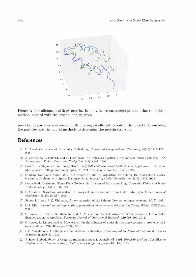
196 Ivan Sendin and Siome Klein Goldenstein

0510152025

5

0

5

10

5

0

5

10

15

Figure 1: The alignment of 2gp8 protein. In blue, the reconstructed protein using the hybridmethod, aligned with the original one, in green.

provided by particles selection and SIR filtering - is efficient to control the uncertainty enablingthe particles and the hybrid methods to determine the protein structure.

References

[1] D. Agrafiotis. Stochastic Proximity Embedding. Journal of Computational Chemistry, 24(10):1215–1221,2003.

[2] J. Carpenter, P. Clifford, and P. Fearnhead. An Improved Particle Filter for Non-linear Problems. IEEProceedings - Radar, Sonar and Navigation, 146(1):2–7, 1999.

[3] Luiz H. de Figueiredo and Jorge Stolfi. Self-Validated Numerical Methods and Applications. BrazilianMathematics Colloquium monographs. IMPA/CNPq, Rio de Janeiro, Brazil, 1997.

[4] Qunfeng Dong and Zhijun Wu. A Geometric Build-Up Algorithm for Solving the Molecular DistanceGeometry Problem with Sparse Distance Data. Journal of Global Optimization, 26:321–333, 2003.

[5] Leyza Baldo Dorini and Siome Klein Goldenstein. Unscented feature tracking. Computer Vision and ImageUnderstanding, 115(1):8–15, 2011.

[6] P. Guntert. Structure calculation of biological macromolecules from NMR data. Quarterly reviews ofbiophysics, 31(2):145–237, 1998.

[7] Simon J. J. and J. K. Uhlmann. A new extension of the kalman filter to nonlinear systems. SPIE, 1997.[8] G.J. Klir. Uncertainty and information: foundations of generalized information theory. Wiley-IEEE Press,

2006.[9] C. Lavor, L. Liberti, N. Maculan, and A. Mucherino. Recent advances on the discretizable molecular

distance geometry problem. European Journal of Operational Research, 219:698–706, 2012.[10] C. Lavor, L. Liberti, and a. Mucherino. On the solution of molecular distance geometry problems with

interval data. BIBMW, pages 77–82, 2010.[11] P.C. Mahalanobis. On the generalised distance in statistics. Proceedings of the National Institute of Sciences

of India, 2(1):49–55, 1936.[12] J. Saxe. Embeddability of weighted graphs in k-space is strongly NP-hard. Proceedings of the 17th Allerton

Conference on Communication, Control, and Computing, pages 480–489, 1979.

Proteins Structure Determination with Imprecise Distances 197

[13] J. Saxe. Two Papers on Graph Embedding Problems. Technical Report 10-102, Department of ComputerScience, Carnegie-Mellon University, 1980.

[14] L. Wasserman. All of nonparametric statistics. Springer-Verlag New York Inc, 2006.[15] D.M. Webster. Protein Structure Prediction: Methods and Protocols. Methods in Molecular Biology.

Humana Press, 2000.

DGA 2013, pp. 199 – 203.

Multicoloring of cannonball graphs

Petra Šparl,1,2 Rafał Witkowski,3 and Janez Žerovnik4,2

1FOV, University of Maribor, Slovenia, [email protected]

2Institute of Mathematics, Physics and Mechanics, Ljubljana, Slovenia

3Adam Mickiewicz University, FMCS, Poznan, Poland, [email protected]

4FME, University of Ljubljana, Slovenia, [email protected]

Abstract In the frequency allocation problem, we are given a cellular telephone network whose geographicalcoverage area is divided into cells, where phone calls are serviced by assigned frequencies, so thatnone of the pairs of calls emanating from the same or neighboring cells is assigned the samefrequency. The problem is to use the frequencies efficiently, i.e. minimize the span of frequenciesused. The frequency allocation problem can be regarded as a multicoloring problem on a weightedhexagonal graph, where each vertex knows its position in the graph. We can generalize this probleminto higher dimension. In this paper we present algorithm for multicoloring so called cannonballgraphs.

1. Introduction

A fundamental problem that appeared in the design of cellular networks is to assign setsof frequencies to transmitters in order to avoid unacceptable interferences. The number offrequencies demanded at a transmitter may vary between transmitters. The problem appearedin the sixties and was soon related to multicoloring of graphs (see [2]). Besides the mobiletelephony there are several applications of frequency assignment including radio and televisionbroadcasting, military applications, satellite communication and wireless LAN (see [1]). Asizable part of theoretical studies is concentrated on the simplified model when the underlyinggraph which has to be multicolored is a subgraph of triangular lattice. This is a naturalchoice because it is well known that hexagonal cells provide a coverage with optimal ratioof the distance between centers compared to the area covered by each cell. Such graphs arecalled hexagonal graphs [7–12]. Although the multicoloring of hexagonal graphs seems to be avery simplified optimization problem, some interesting mathematical problems were asked atthe time that are still open. An example is the Reed McDiarmid conjecture saying that themultichromatic number of any hexagonal graph G is between ω(G) and 9ω(G)/8, where ω(G)is the weighted clique number [5]. On the other hand, the hexagonal graph model is knownto be practically useless in urban areas, where high concrete buildings on one hand preventpropagation of radio signals and on the other hand allow very high concentration of users.Loosely speaking, a three dimensional model may be needed in contrast to the hexagonal graphsthat are good model for two dimensional networks. In this paper we discuss a generalizationof the multicoloring problem on hexagonal graphs from planar case to three dimensions, wherethe situation is much more interesting as in two dimensions. Obviously, optimal cells wouldbe nearly balls, and the question is how to position centers of the balls to achieve an optimal

200 Petra Šparl, Rafał Witkowski, and Janez Žerovnik

diameter to volume ratio. The famous Kepler conjecture 1 was a longstanding conjecture aboutball packing in three-dimensional Euclidean space. It says that no arrangement of equally sizedballs filling space has greater average density than that of the cubic close packing (face-centeredcubic) and hexagonal close packing arrangements.

Recently Thomas Hales, following an approach suggested by Fejes Toth, published a proof ofthe Kepler conjecture (see [3, 4]). Given an optimal arrangement of balls, we define a graph bytaking the balls (or centers of balls) as vertices and connect touching balls with edges. We callthese graphs cannonball graphs, as Keplers motivation for studying the arrangements of ballswas optimal arrangements of cannonballs. Nonnegative weights are assigned to each vertex andwe are interested in multicoloring of the graph induced on vertices of positive weight. Looselyspeaking, we generalize the problem of multicoloring of hexagonal graphs from two dimensionsto three dimensions.

More formally, we are interested in multicoloring of weighted graphs G = (V (G), E(G), d)where V = V (G) is the set of vertices, E = E(G) is the set of edges, and d assigns a positiveinteger d(v) to a vertex v ∈ V . A proper multicoloring of G is a mapping f from V (G) tosubsets of integers such that |f(v)| ≥ d(v) for any vertex v ∈ V (G) and f(v) ∩ f(u) = ∅ forany pair of adjacent vertices u and v in the graph G. The minimal cardinality of a propermulticoloring of G, χm(G), is called the multichromatic number. Another invariant of interestin this context is the (weighted) clique number, ω(G), defined as follows: The weight of a cliqueof G is the sum of weights on its vertices and ω(G) is the maximal clique weight on G. Clearly,χm(G) ≥ ω(G).

No approximation algorithm and no upper bound was previously known for multichromaticnumber of cannonball graphs. Here we give an upper bound using some structural propertiesof the cannonball graphs as well as constructions of polynomial approximation algorithms. Themain result of this paper that gives the first answer to the problem asked in [6] isTheorem 1.1. There is an approximation algorithm for multicoloring cannonball graphs whichuses at most 11

6 ω(G) +O(1) colors. Time complexity of the algorithm is polynomial.

2. Basic definitions and useful facts

First we formally define hexagonal and cannonball graphs. Recall the definition of hexagonalgraphs: the position of each vertex is an integer linear combination x~p + y~q of two vectors~p = (1, 0) and ~q = (1

2 ,√

32 ) and the vertices of the triangular lattice are identified with pairs

(x, y) of integers. Put an edge if the points representing the vertices are at distance one inthis grid. To construct a hexagonal graph G, positive weights are assigned to a finite subsetof points in the grid and G is the subgraph induced on V (G), the set of grid vertices withpositive weights. Cannonball graphs are constructed in a similar way. However, we have manypossibilities already when constructing the underlying grid, which consists of tetrahedrons andwill be called a tetrahedron grid T . Optimal arrangement of balls in one layer is to put thecenters of balls in points of triangular grid. Then, there are exactly two possibilities to put asecond layer on the top of the first layer. These two arrangements are obviously symmetric,however, when choosing a position for the third layer, there are two possibilities that give riseto different arrangements (see figure 1).

Consequently, we have an infinite number of tetrahedron grids, that all came from optimalball arrangements. One of the arrangements (see case (a) of figure 1), can be described nicelyby introducing a third vector ~r = (1

2 ,√

36 ,√

63 ) in addition to ~p = (1, 0, 0) and ~q = (1

2 ,√

32 , 0).

1The solution of Kepler’s conjecture is included as a part of 18th problem in the famous list of Hilbert’s problem list backin 1900 [13].

Multicoloring of cannonball graphs 201

position (a) position (b)

Figure 1: Two different arrangements of the third layer.

Now the position of each vertex is an integer linear combination x~p+y~q+z~r and vertices of thetriangular lattice may be identified with a triplet (x, y, z) of integers. For other arrangements(case (b) of figure 1) there is no such an easy extension of the notation from hexagonal graphs.A cannonball graph G is obtained by assigning integer weights to the points of the tetrahedrongrid T , taking as V (G) the vertices in the grid with positive weights, and introducing edgesbetween vertices at euclidean distance one. Clearly, from the construction it follows that anylayer of a cannonball graph is a hexagonal graph (maybe not connected).

Formally, cannonball graph is a graph induced on vertices of positive weight.There are natural basic 4-colorings of the (unweighted) cannonball graphs. Start with any

layer and call it the base layer. Introduce coordinates (x, y, 0) in this layer and define a basecoloring by the formula bc(v) = x mod 2 + 2(y mod 2). Colors of vertices of the next layersare then determined exactly as follows. It is obvious that whenever we store a new layer on(or under) the previous one with fixed coloring, we know that each ball from the new layer isconnected to exactly three balls from the previous layer, and all of those balls have differentcolors. Thus there is exactly one extension of the four coloring to the next layer (see Figure1). It is easy to see that this rule gives a proper coloring of the next layers.

The cliques in the cannonball graphs can have at most four vertices. The (weighted) cliquenumber, ω(G), is the maximal clique weight on G, where the weight of a clique is the sum ofweights on its vertices. We can define invariants ωi(G) which denote the maximal weight of aclique of size at most i on G.

It was proved in [5] that for any weighted bipartite graph H, χm(H) = ω(H), and it can beoptimally multicolored by the following procedure:

Procedure 2.1. [9] Let H = (V ′, V ′′, E, d) be a weighted bipartite graph. We get an optimalmulticoloring of H if to each vertex v ∈ V ′ we assign a set of colors 1, 2, . . . , d(v), while witheach vertex v ∈ V ′′ we associate a set of colors m(v) + 1,m(v) + 2, . . . ,m(v) + d(v), wherem(v) = maxd(u) : u, v ∈ E.

In a graph G = (V,E), we call a coloring f : V → 1, . . . , k k-good if for every odd cycle inG and for every i, 1 ≤ i ≤ k, there is a vertex v ∈ V in the cycle such that f(v) = i. A graph is

202 Petra Šparl, Rafał Witkowski, and Janez Žerovnik

k-good if such coloring exists. The notions of k-good colorings and graphs was first defined in[12]. We can give a procedure for k

k−1ω(G)-coloring of any k-good graph in the following way:

Procedure 2.2. [12] Since for 1 ≤ i ≤ k we know that every odd cycle in G has at leastone vertex assigned color i, the graph remaining after the removal of vertices of color i can betwo-colored. Repeating this for i = 1...k, and using procedure 2.1, we get k

k−1ω(G)-coloring ofG.

For each vertex v ∈ G, define a base function κ as κ(v) = maxa(v, u, t) : v, u, t ∈ τ(T ),where a(u, v, t) =

⌈d(u)+d(v)+d(t)

3

⌉, is an average weight of the triangle u, v, t ∈ τ(T ).

Clearly, the following fact holds.

Fact 2.1. For each v ∈ G, κ(v) ≤⌈ω3(G)

3

⌉≤⌈ω(G)

3

⌉We call vertex v heavy if d(v) > κ(v), otherwise we call it light. If d(v) > 2κ(v) we say that

the vertex v is very heavy.To color vertices of G we use colors from an appropriate palette. For a given color c, its palette

is defined as a set of pairs (c, i)i∈N. A palette is called a base color palette if c ∈ 0, 1, 2, 3is one of the base colors, and it is called additional color palette if c /∈ 0, 1, 2, 3.

If a vertex v does not have a neighbor of color i in G, we call such color a free color of v.

3. Algorithm for multicoloring cannonball graphs

Input: Weighted cannonball graph G = (V,E, d).

Output: A proper multicoloring of G, using at most 116 · ω (G) +O(1) colors.

Step 0 For each vertex v ∈ V compute its base color bc(v) and its base function value

κ(v) = max⌈

d(u) + d(v) + d(t)3

⌉: v, u, t ∈ τ(T )

,

where τ(T ) is a set of all triangles in tetrahedron grid T .

Step 1 For each vertex v ∈ V assign minκ(v), d(v) colors from its base color palette tov. Construct a new weighted triangle-free cannonball graph G1 = (V1, E1, d1) whered1(v) = maxd(v)− κ(v), 0, V1 ⊆ V is the set of vertices with d1(v) > 0 (heavy verticesin G) and E1 ⊆ E is the set of all edges in G with both endpoints from V1 (G1 is inducedby V1).

Step 2 For each vertex v ∈ V1 with d1(v) > κ(v) (very heavy vertices in G) assign the firstunused κ(v) colors of the base color palettes of its neighbors in tetrahedron grid T .Construct a new graph G2 = (V2, E2, d2) where d2 (v) is the difference between d1(v) andthe number of colors assigned in this step, V2 ⊆ V1 is the set of vertices with d2(v) > 0and E2 ⊆ E1 is the set of all edges in G1 with both endpoints from V2 (G2 is induced byV2).

Step 3 For each vertex v ∈ V2 with deg(v) = 4 assign unused colors from the free color basepalette. Construct a new 3-colorable graph G3 = (V3, E3, d3) where d3 (v) is the differencebetween d2(v) and the number of colors assigned in this step, V3 ⊆ V2 is the set of verticeswith d3(v) > 0 and E3 ⊆ E2 is the set of all edges in G2 with both endpoints from V3(G3 is induced by V3).

Step 4 Apply Procedure 2.2 for graph G3 by using colors from new additional color palettes.

Multicoloring of cannonball graphs 203

4. Conclusion

In this paper we provide an algorithm for a proper multicoloring of cannonball graphs that usesat most 11

6 ω(G) + C colors. We believe that further improvements can be done. The interest-ing problems that remain open are, improvement of the competitive ratio 11/6, finding somedistributed algorithms for multicoloring cannonball graphs or finding some k-local algorithmsfor some k, similarly as in 2D case for hexagonal graphs. We already mentioned that in 2D casebetter bounds were obtained for triangle-free hexagonal graphs. It is very likely that also forcannonball graphs exist some "forbidden" subgraphs H, maybe tetrahedrons, such that betterbounds can be obtained for H-free cannonball graphs.

References

[1] K. Aardal, S van Hoesel, A koster, C. Mannino, A.Sassano, Models and solution techniques for frequencyassignment problems, Annals of Operations Research 153, 79-129, 2007.

[2] Hale, W.K. Frequency assignment: theory and applications, Proceedings of the IEEE, vol 68(12), 1497-1514,1980.

[3] T. Hales, Cannonballs and honeycombs, Notices of the American Mathematical Society 47, 2000, 440—449.[4] T. Hales, A proof of the Kepler conjecture, Annals of Mathematics. Second Series 162, 2005, 1065—1185.[5] McDiarmid, C., Reed, B. Channel assignment and weighted coloring, Networks, vol. 36(2), 114-117, 2000.[6] Algorithmische Graphentheorie, Oberwolfach, December 8-14, 2002. (Report No. 55/2002). Oberwolfach:

Mathematisches Forschungsinstitut, 2002. (seminar page http://www.mfo.de/occasion/0250/www view,link to report www.mfo.de/document/0250/Report55 2002.ps).

[7] Sau, I., Šparl, P., Žerovnik, J. 7/6-approximation Algorithm for Multicoloring Triangle-free HexagonalGraphs, Discrete Mathematics, vol. 312, 181-187, 2012.

[8] Šparl, P., Witkowski, R. Žerovnik, J. A Linear Time Algorithm for 7− [3]-coloring Triangle-free HexagonalGraphs, Information Processing Letters, vol. 112, 567-571, 2012.

[9] Šparl, P., Witkowski, R. Žerovnik, 1-local 7/5-Competitive Algorithm for Multicoloring Hexagonal Graphs,Algorithmica, vol. 64(4), 564-583, 2012.

[10] Šparl, P., Žerovnik, J. 2-local 4/3-competitive Algorithm for Multicoloring Hexagonal Graphs, Journal ofAlgorithms, vol. 55(1), 29-41, 2005.

[11] Šparl, P., Žerovnik, J. 2-local 5/4-competitive algorithm for multicoloring triangle-free hexagonal graphs,Information Processing Letters, vol. 90(5), 239-246, 2004.

[12] Sudeep, K.S., Vishwanathan, S. A technique for multicoloring triangle-free hexagonal graphs, Discrete Math-ematics, vol. 300, 256-259, 2005.

[13] Benjamin H. Yandell, The Honors Class. Hilbert’s Problems and Their Solvers, A K Peters, 2002.

DGA 2013, pp. 205 – 208.

Geometric distances in relative astrometry

Ramachrisna Teixeira,1 Alberto Krone-Martins, 2 Christine Ducourant3 and Phillip A.B. Galli1

1IAG - Universidade de São Paulo, São Paulo, Brasil, [email protected], [email protected]

2SIM - Universidade de Lisboa, Lisboa, Portugal, [email protected]

3LAB - Université de Bordeaux, Bordeaux, France, [email protected]

Abstract In this work we present a brief introduction on the adoption of geometric distances in relativeastrometry. We quickly describe the observational and data-reduction principles, as well as theprecision that has been obtained in contemporary studies.

Keywords: Astronomy, Relative Astrometry, Distance Measurements

1. Introduction

Although the word Astrometry has a broad meaning, in daily astronomical research it representsthe branch of Astronomy concerned with the position of celestial bodies in space, and associatedvariations in time. This includes from the definition and materialization of a reference systemto the study of the movements of the observer, the astronomical source’s intrinsic kinematics,the Galactic structure and the measurement of the most fundamental quantity in Astronomy:the stellar trigonometric parallax. It is this quantity that provides the best estimation of stellardistances from the Solar System, and thus it is the first step in a cosmic distance ladder.

Usually, the word “position of an astronomical object” means the direction in which we areable to observe this object: in other words, it is a projection of the object’s spatial position at thesurface of an unitary sphere centered at the observer, the celestial sphere. In most astronomicalstudies, this position is estimated from the measurement of angular distances between the targetobject and several other objects with known celestial positions – in a certain way, this is notdissimilar to the adoption of anchor nodes in the Distance Geometry formulation of the sensornetwork location problem (e.g. [1]), using euclidean distances in the case of images coordinatesor spherical distances in the case of the objects at the celestial sphere.

Most of contemporary relative astrometric works are based in observations with CCD cam-eras or infrared detectors. These observations result in image matrices that must be analyzedin order to allow the determination of the coordinates of the photocenters. Depending on theadopted data reduction system, the photocenter determination may be based on brightnessmomenta (e.g. [2]), profile fitting (e.g. [3]), or point-spread-function analyses (e.g. [4]). As anexample, the data reduction system employed in Valinhos and Bordeaux CCD meridian circles,adopts a profile fitting method. For each source, the method determines the rectangular coor-dinates (x0, y0) of their photocenters, relative to an arbitrary origin, using a bivariate gaussianfunction:

206 Ramachrisna Teixeira, Alberto Krone-Martins, Christine Ducourant and Phillip A.B. Galli

φ(x, y) = Φ2πσxσy

√1− ρ2 exp− 1

2(1− ρ2) [(x− x0σx

)2+(y − y0σy

)2

− 2ρ(x− x0σx

)(y − y0σy

)]

where Φ is the object’s total flux, (x0, y0) are the photocenter coordinates, σx and σy are thestandard deviations, and ρ is the correlation coefficient.

Then, in order to obtain celestial positions of astronomical objects from the rectangularcoordinates of the photocenters of all the detected objects in an image, it is necessary to identifywhich are those with already known positions from some reference catalogue. Adopting theseobjects with already known celestial coordinates, a least-squares problem is setup (e.g. [5], [6],[7], [8], [9]), enabling the determination of instrumental parameters and the conversion betweenthe rectangular coordinates of all the target objects into celestial coordinates. In this way, thelink established by the reference objects materializes a fraction of the celestial sphere whoseorientation is defined by their known positions. Thus the target objects’ celestial positions maybe determined with respect to this materialization.

Figure 1: A field observed with the CCD meridian circle of the Observatório Abrahão de Moraesat IAG/USP – Valinhos. The objects adopted as references are marked in red.

In Fig. 1 a typical observation of a stellar field performed by the Valinhos CCD meridiancircle is represented. In this image, the objects with red identifiers have known coordinatesfrom a reference catalogue – in this case, the Tycho 2 catalogue [10], that was constructed fromobservations performed by the ESA Hipparcos satellite. This catalogue provides a reliablematerialization of the International Celestial Reference System [11] in the optical wavelengths.

Naturally, the scientific contribution and even the meaning of the astrometric observationsare directly linked to the precision attained by their measurements. However, the precision andaccuracy of these measurements depend on several factors. First, the atmosphere and opticsplay a major role, limiting the possible attainable resolution at each observation (e.g. [12]).

Geometric distances in relative astrometry 207

Then, the noise sources1 as well as the apparent brightness of the target, limits the photocenterdetermination. Afterwards, the quality of the adopted reference system also play a role – byits on, the quality of a reference system is dependent on how it is materialized, or what (andhow many) are the reference sources present in the field. Finally, the precision and accuracyof these measurements depend on the rigidity of the link between all the individual imagestogether – and this is ruled by the determination of geometric distances between the sources.

Using the CCD meridian circles such as Valinho’s or Bordeaux’s, for instance, it is possible toobtain positions from ∼ 6 observations with mean precisions of ∼ 50 mas (or milliarcseconds).If more observations are performed, it is feasible to obtain positions with mean precisions of∼ 10 to 30 mas, depending on the target’s magnitude (the best range is V ∼ 9 to 14 mag).Proper-motions can be obtained by these instruments with precisions better than 5 mas/yr,using observation baselines of several years (e.g. [13]).

If instruments with bigger optics are adopted, and thus greater spatial resolution, such as theESO NTT telescope, it is possible to obtain positions and proper motions with more than tentimes the above quoted precisions. Also, these instruments enable reliable determinations ofstellar trigonometric parallaxes, which are the first steps towards the determination of physicaldistances in the Universe.

Acknowledgments

R.T and P.A.B.G. thank the Brazilian agencies FAPESP and CAPES for financial support.A.K.M. thanks the Portuguese agency Fundação para Ciência e Tecnologia, FCT (SFRH/BPD/ 74697/ 2010) for financial support. C.D. thanks the French agency COFECUB.

References

[1] Caoa, M., Anderson, B.D.O., Morsea, A. S. (2006). “Sensor network localization with imprecise distances”,Systems & Control Letters, v. 55, p. 887.

[2] Bertin, E. and Arnouts, S. (1996). “SExtractor: Software for source extraction”. Astronomy & AstrophysicsSupplement Series, v. 317, p. 393.

[3] Viateau, B., Réquième, Y., Le Campion, J.F., Benevides-Soares, P., Teixeira, R., et. al. (1998). “The Bor-deaux and Valinhos CCD meridian circles”. Astronomy & Astrophysics Supplement Series, v. 134, p. 173.

[4] Stetson, P.B. (1987). “DAOPHOT - A computer program for crowded-field stellar photometry”. Publicationsof the Astronomical Society of the Pacific, v. 99, p. 191.

[5] Eichhorn H. (1960).“Über die Reduktion von photographischen Sternpositionen und Eigenbewegungen”.Astronomische Nachrichten, v. 285, p. 233.

[6] Jefferys, W.H. (1987). “Quaternions as astrometric plate constants”. Astronomical Journal, v. 93, p. 755.[7] Brosche, P., Wildermann, E., Geffert, M. (1989). “Astrometric plate reductions with orthogonal functions”.

Astronomy and Astrophysics, v.211, n.1, p. 239.[8] Benevides-Soares, P., Teixeira, R. (1992). “On the relationship between conventional and overlap reduction

techniques in positional astronomy”. Astronomy and Astrophysics, v. 253, n. 1, p. 307.[9] Teixeira, R., Requieme, Y., Benevides-Soares, P., Rapaport, M. (1992). “Global treatment of the Bordeaux

meridian observations”. Astronomy and Astrophysics, v. 264, n. 1, p. 307.[10] Hog, E., Fabricius, C., Makarov, V. V., Urban, S. et. al. (2000). “The Tycho-2 catalogue of the 2.5 million

brightest stars”. Astronomy and Astrophysics, v. 355, p. L27.[11] Arias, E.F., Charlot, P., Feissel, M. and Lestrade, J.F., (1995). "The extragalactic reference system of the

International Earth Rotation Service, ICRS". Astronomy and Astrophysics, v.303, 604-608.

1The noise sources can be physically intrinsic due to poissonian photon processes and/or generated by detector electronics.

208 Ramachrisna Teixeira, Alberto Krone-Martins, Christine Ducourant and Phillip A.B. Galli

[12] Lindegren, L. (1980). “Atmospheric limitations of narrow-field optical astrometry”. Astronomy and Astro-physics, v. 89, n. 1-2, p. 41.

[13] Teixeira, R., Galli, P.A.B, Benevides-Soares, P. et al. (2011). "Proper motion and densification of theInternational Celestial Reference Frame in the direction of the Galactic bulge". Astronomy and Astrophysics,v. 534, A91.

DGA 2013, pp. 209 – 214.

Influence Analyses of Skew–Normal/IndependentLinear Mixed Models

Filidor Vilca,1 Camila Borelli Zeller,2 and Victor Hugo Lachos1

1 University of Campinas, Brazil, [email protected]

2Universidade de Juiz de Fora, Brazil, [email protected]

2 University of Campinas, Brazil [email protected]

Abstract Linear mixed models were developed to handle clustered data, and these models have increasedsignificantly in the last fifty years. In general, the normality (or symmetry) of the random effectsis a common assumption, but this kind of assumption may be unrealistic, obscuring importantfeatures of among-subjects variations.

We have extended the classical linear mixed model herein, allowing the random effects andthe random errors to jointly follow a multivariate skew–normal/independent distribution, and weconsider diagnostic analyses following the ideas from Cook’s well–known approach which is basedon the likelihood displacement. We developed local influence measures according to Zhu andLee’s (2001) approach for skew–normal/independent linear mixed model (SNI-LMM). Perturba-tions schemes are discussed as well as the use the Mahalanobis distance for identifying potentialoutlying observations. Finally, a real data set has been analyzed in order to illustrate the usefulnessof the proposed methodology.

Keywords: Mahalanobis distance, local influence, outliers

1. Introduction

Estimating the distance between two points or more general between objects of interest areof fundamental concern different area as well as in statistical applications, for example, thedistance between two observations. In statistics, is usual to find applications based on theMahalanobis distance is a metric which is better adapted than the usual Euclidean distance tosettings involving non spherically symmetric distributions. It is more particularly useful whenmultivariate distributions are involved.

Influence diagnostics techniques consist in evaluating the sensitivity of the parameter esti-mates of a particular model when perturbation occurs in the data set or in the assumptions ofthe model. Case deletion (Cook, 1977) is a common approach to analyze one or more fittedmodels after excluding observations that is direct assessed by some metrics such as the likeli-hood displacement and the Cook’s distance. This method is also known as the global influencemethod. The influence of the ith observation on the parameter estimate can be assessed bystudying the difference between θ and θ(i), where θ(i) denotes the maximum likelihood(ML)estimate of θ obtained from the sample of size n − 1 excluding the ith observation. To assessthe influence of the ith case on the ML estimate θ, the basic idea is to compare the differencebetween θ(i) and θ. The generalized Cook’s distance is defined as a standardized norm of

210 Filidor Vilca, Camila Borelli Zeller, and Victor Hugo Lachos

θ(i) − θ, i.e.,GDi = (θ(i) − θ)>M(θ(i) − θ), (1)

where M is a non-negative definite matrix. Another measure of distance between θ(i) and θis the likelihood displacement defined as LDi(θ) = 2`(θ) − `(θ(i)), where `(.) is the log-likelihood function.

Cook (1986) proposed an unified approach for assessment of local influence in minor per-turbations of a statistical model and it can be viewed as a generalization of the robustnessconcept to study and detect the influential subsets of data. A alternative approach was pro-posed by Zhu and Lee (2001) that is based on the EM algorithm, that requires the evaluation ofQ(θ|θ) = E[`c(θ|yc)|y, θ]. To evaluate the departure of the models, Cook (1986) proposed touse the likelihood displacement that is defined below: let ω be a g×1vector of perturbation re-stricted to some open subset of Rg. The perturbations are made in the likelihood function suchthat it takes the form `(θ|ω), and consider ω0 such that `(θ|ω0) = `(θ). To asses the influenceof the perturbations on the ML estimate, one may consider the likelihood displacement

LD(ω) = 2`(θ)− `(θω),

where θ is the ML estimate of θ under the proposed model and θω denotes the ML estimateunder the perturbed model.

The multivariate skew-normal/independent (SNI) distribution (Branco and Dey, 2001) isdefined through the probability density function (pdf)

f(y) = 2∫ ∞

0φp(y|µ, u−1Σ) Φ(u1/2λ>Σ−1/2 (y− µ)) dH(u;ν), y ∈ Rp, (2)

where φp(·;µ,Σ) denotes the pdf of the p-variate normal distribution with a mean vector µ anda covariance matrix Σ, Φ(·) denotes the cumulative distribution function (cdf) of the standardnormal distribution, U is a positive random variable with a cdf H(u;ν), where ν is a scalar orparameter vector indexing the distribution of U . The distribution defined in (2) in denoted bySNIp(µ,Σ,λ;H). When λ = 0, the SNI distribution in (2) reduces to the normal/independent(NI) distribution. That is, Y ∼ NIp(µ,Σ;H); see Lange and Sinsheimer (1993).

2. The skew–normal/independent linear mixed model

In this section, we consider the skew–normal/independent linear mixed model (SNI-LMM). Ingeneral, a normal linear mixed effects model (N-LMM hereafter) is defined as (Arellano–Valleet al, 2005)

Yi = Xiβ + Zibi + εi, , , (3)whereYi is a (ni×1) vector of observed continuous responses for sample unit i, Xi of dimension(ni×p) is the design matrix corresponding to the fixed effects, β of dimension (p×1) is a vectorof population-averaged regression coefficients called fixed effects, Zi of dimension (ni × q) isthe design matrix corresponding to the (q × 1) random effects vector bi, and εi of dimension(ni × 1) is the vector of random errors. It is assumed that the random effects bi and theresidual components εi are independent with bi

iid∼ Nq(0,D) and εiind∼ Nni(0,Σi). The q × q

covariance matrix D may be unstructured or structured. The ni × ni covariance matricesΣi = Σi(γ), i = 1, . . . ,m, are typically assumed to depend on i through their dimension,being parameterized by a fixed, generally small, parameter set γ as, for instance, with an AR(1)covariance structure. As in Lachos et al. (2009), the SNI-LMM is defined by considering

biiid∼ SNIq(0,D,λ;H) and εi

ind∼ NIni(0, σ2eRi;H), i = 1, . . . ,m. (4)

Influence Analyses 211

From (??), we can write the SNI-LMM as follows

Yi|bi, Ui = uiind∼ Nni(Xiβ + Zibi, u−1

i σ2eRi), (5)

bi|Ti = ti, Ui = uiind∼ Nq(∆ti, u

−1i Γ), (6)

Ti|Ui = uiind∼ HN1(0, u−1

i ), (7)

Uiiid∼ H(ui;ν), (8)

for i = 1, . . . ,m, all independent, ∆ = D1/2δ, Γ = D−∆∆>, with δ = λ/√

1 + λ>λ, and D1/2

is the square root of D containing q(q+1)/2 distinct elements, say α, andHN1(0, σ2) is the half-N1(0, σ2) distribution. When Ui = 1 (i = 1 . . . ,m), the SNI–LMM reduces to the SN–LMM asdefined in Arellano–Valle et al. (2005), and if λ = 0, the SNI-LMM reduces to the usual NI-MLM which has been discussed quite extensively in the the literature. The EM-type algorithmrequires the evaluation of Q(θ|θ) = E[`c(θ|yc)|y, θ] =

∑mi=1Qi(θ|θ), where the expectation is

taken with respect to the joint conditional distribution of b, u and t, given y and θ. Thus, wehave that Qi(θ|θ) = Q1i(β, σ2

e |θ) +Q2i(α,λ|θ), where Q1i(β, σ2e |θ) = −1

2 log |σ2eRi|− ui

2σ2e(yi−

Xiβ)>R−1i (yi − Xiβ) + 1

σ2e(yi − Xiβ)>R−1

i ziubi − 12σ2etr(R−1i ziub2

iz>i), Q2i(α,λ|θ) =

−12 log |Γ| − 1

2tr(Γ−1ub2

i

)+ ∆>Γ−1utbi − ut2i

2 ∆>Γ−1∆, with ui, ubi, ub2i, utbi and ut2i

i = 1, . . . ,m, are all as given in Lachos et al. (2009).

3. Local influence

Consider a perturbation vector ω in an open region Ω. To apply the local influence approach,we consider Q(θ,ω|θ) = E[`c(θ,ω|Yc)|y, θ], where `c(θ,ω|Yc), θ ∈ Rh, be the complete-datalog-likelihood of the perturbed model. We consider the following perturbation schemes:1. Perturbation of case weights: The complete-data log-likelihood function (perturbedQ-function) is given by Q(θ,ω|θ) =

∑mi=1wiQ1i(β, σ2

e |θ) +∑mi=1wiQ2i(α,λ|θ), where ω =

(ω1, . . . , ωm)> is an m× 1 vector.2. Perturbation of the scale matrix D:To study the effects of departure from the assumptionregarding the scale matrix D of the random effects, we consider the following perturbation∆(ωi) = ω

−1/2i ∆ and Γ(ωi) = ω−1

i Γ.3. Perturbation of explanatory variables: Here is perturbed explanatory matrix Xi(ω) =(xi1, . . . ,xiu(ωi), . . . ,xip), where xiu(ωi) = xiu + ωi1ni , u = 1, . . . , p, xiu is the uth column ofthe matrix Xi, and 1ni is an ni × 1 vector of ones.4. Perturbation of response variables: A perturbation of the response variables (y>1 , . . . ,y>n )>is introduced by replacing yi by yi(ω) = yi + ωi1ni , i = 1, . . . ,m.

4. Application

We illustrate the developed method with the Framingham cholesterol data set from Zhang andDavidian (2001). We fit a LMM model to the data as specified by Zhang and Davidian (2001)

Yij = βo + β1sexi + β2agei + β3tij + b0i + b1itij + εij , (9)

where Yij is the cholesterol level, divided by 100, at the j-th time for subject i; tij is (time −5)/10, with time measured in years from the start of the study; agei is age at the start of thestudy; sexi is the gender indicator (0 = female, 1 = male). Thus, xij = (1, sexi, agei, tij)>,

212 Filidor Vilca, Camila Borelli Zeller, and Victor Hugo Lachos

bi = (b0i, b1i)> and Zij = (1, tij)>, i = 1, . . . , 200. First, we have fitted the SNI-LMMfor the Framingham cholesterol data set. Although not being formal tests, as in Zhang andDavidian (2001), we compare the SNI-LMM and the NI-LMM (specifically, models normal,t-Student, slash and contaminated normal) by inspecting some information criteria. Next, wehave identified influential observations for the Framingham cholesterol data set.

Now, we revisit the Framingham cholesterol data in order to study the local influence ap-proach in the context of SNI-LMM. In our analysis we will assume SN, ST, SSL and SCNdistributions from the SNI class for comparative purposes. In order to detect outlying obser-vations, we use the Mahalanobis distance

d2i (θ) = 1

σ2e

e>i R−1i ei + µ>biD

−1µbi = d2

ei + d2bi , (10)

We can use as cutoff points the quantile of the distribution of d2i . Figure 1 displays these dis-

tances for the four fitted models. The cutoff lines correspond to the quantile υ = χ24(ξ), with ξ =

0.99.We can see from these figures that observations 8, 15, 26, 69, 74, 90, 111, 122, 138, 146, 160, 162, 174, 175and 187 appear to be outliers.

0 50 100 150 200

010

20

30

40

50

index

Mahala

nobis

dis

tance

SN

8

15

2669

74

90

111122

138

146

160

162

174

175

187

0 50 100 150 200

010

20

30

40

50

index

Mahala

nobis

dis

tance

ST

90 138

146

160

175

0 50 100 150 200

010

20

30

40

50

index

Mahala

nobis

dis

tance

SCN

2669

90

138

146

160

175

0 50 100 150 200

010

20

30

40

50

index

Mahala

nobis

dis

tance

SSL

90

146

175

Figure 1: Index plots of the Mahalanobis distances for the four fitted models.

The estimated distances d2ei (Error) and d2

bi (Random Effect–R.E.), obtained from (10),provide useful diagnostic statistics for identifying subjects with outlying observations. Figure2 presents these diagnostic statistics for SN-LMM. The observations 69, 90, 138, 145 and 175presents large value of d2

ei , suggesting an e-outlier. Moreover, observations 8, 26 and 160 presentlarge values of d2

bi suggesting a b-outlier. The d2bi plots gives some indication that observations

2, 131 and 172 are possibly a b-outliers, which cannot be concluded from Figure 1. For SNIdistributions with heavy tails, we observed the same results and so they are not shown here.

Perturbation of case weights: From Figure 3 is noted that under for the four fitted models,the observation 39 is identified as influential. As expected, the influence of such observation isreduced when we consider distributions with heavier tails than the skew-normal ones.

Influence Analyses 213

0 50 100 150 200

05

10

15

20

25

Error

Index

69

90

138

146

175

0 50 100 150 200

02

46

8

R.E.

Index

2

8

26

131

160

172

Figure 2: Estimated d2ei (error) and d2

bi (R.E.) to the skew-normal fit.

0 50 100 150 200

0.0

00.0

40.0

8

index

M(0

)

SN

39 146

160

0 50 100 150 200

0.0

00.0

40.0

8

index

M(0

)

ST

2

39

0 50 100 150 200

0.0

00.0

40.0

8

index

M(0

)

SSL

2

39

0 50 100 150 200

0.0

00.0

40.0

8

index

M(0

)

SCN

39

Figure 3: Index plots of M(0) under case weights perturbation for the four fitted models. Thehorizontal lines delimit the Lee and Xu (2004) benchmark for M(0) with c∗ = 5.

References

[1] Arellano-Valle, R. B., Bolfarine, H. and Lachos, V. H. (2005). Skew-normal linear mixed models, Journal ofData Science, 3, 415-438.

[2] Branco, M. D. and Dey, D. K. (2001). A general class of multivariate skew-elliptical distribution. Journal ofMultivariate Analysis 79: 93-113.

[3] Cook, R. D. (1977). Detection of influential observations in linear regression. Technometrics, 19, 15-18.

[4] Cook, R. D. (1986). Assessment of local influence (with discussion), Journal of the Royal Statistical Society,Series B, 48, 133-169.

[5] Lachos, V. H., Ghosh, P. and Arellano–Valle, R. B. (2009). Likelihood based inference for skew–normal/independent linear mixed models, Statistica Sinica.

214 Filidor Vilca, Camila Borelli Zeller, and Victor Hugo Lachos

[6] Lange, K. and Sinsheimer, J. S. (1993). Normal/independent distributions and their applications in robustregression, Journal of Computational and Graphical Statistics, 2, 175-198.

[7] Zhang, D. and Davidian, M. (2001). Linear mixed models with flexible distributions of random effects forlongitudinal data, Biometrics, 57, 795-802.

[8] Zhu, H. and Lee, S. (2001). Local influence for incomplete-data models, Journal of the Royal StatisticalSociety, Series B, 63, 111-126.

DGA 2013, pp. 215 – 217.

Solving the Distance Geometry Problemby the Hyperbolic Smoothing Approach

Adilson Elias Xavier1 and Helder Manoel Venceslau2

1Federal University of Rio de Janeiro - Brazil, [email protected]

2Federal University of Rio de Janeiro - Brazil, [email protected]

Abstract The geometrical distance problem in graphs is characterized by determining the positions of thenodes in a Euclidian space, according to the given distances associated with the arcs. It is a non-convex and non-differentiable problem, having a myriad of local minima. The presented methodol-ogy addopts a smoothing strategy named Hyperbolic Smoothing Technique. Computational resultsobtained in the resolution of large instances of a difficult canonic problem show the efficiency androbustness of the method. The geometrical distance problem has a relevant application in thedetermination of geometrical structures of proteins.

Keywords: Protein Folding, Nondifferentiable Programming, Smoothing

1. Solving the DGP by the HS Approach

The presented methodology adopts a smoothing strategy named Hyperbolic Smoothing Tech-nique. By a smoothing approach, we fundamentally mean the substitution of an intrinsicallynon-differentiable problem by a C∞ differentiable alternative. In the Hyperbolic Smoothing(HS) methodology, the solution is obtained by solving a sequence of smooth problems whichgradually approaches the original one.

First, we will consider the smoothing of the absolute value function |u |, where u ∈ R.For this purpose, for γ > 0, let us define the function

θ(u , γ ) =√u2 + γ2 (1)

The considered Distance Geometry problem has the following specification. Let G = (V,E)denote a graph, in which for each arc (i, j) ∈ E, it is associated a measure aij > 0. Theproblem consists of associating a vector xi ∈ Rn for each knot i ∈ V, basically addressedto represent the position of this knot into a n−dimensional space, so that Euclidean distancesbetween knots, ‖xi − xj‖, corresponds appropriately to the given measures aij :

minimize f(x) =∑

(i,j)∈E( ‖xi − xj‖ − aij)2. (2)

This formulation presents the non-differentiable property due the presence of the Euclideannorm term. Moreover, the objective function is non-convex, so the problem has a large numberof local minima. For solving the problem (2) by using the HS technique it is only necessary touse the function θ(u , γ ) and to take u = ‖xi − xj‖ :

216 Adilson Elias Xavier and Helder Manoel Venceslau

minimize fs(x) =∑

(i,j)∈E( θ(‖xi − xj‖, γ) − aij)2. (3)

Besides its smoothing properties, Xavier [6] shows the important convexification power ofthe function θ :

Proposition 1: There is a number γ such that, for all values γ > γ, the Hessian matrix∇2fs(x) will be positive definite.

Souza [4] and Souza et al [5] considers an alternative formulation, where the distances ‖xi−xj‖ must be inside given intervals [li,j , ui,j ] :

minimize f(x) =∑

(i,j)∈Emax[(lij − ‖xi − xj‖ ) , 0] +

∑(i,j)∈E

max[(‖xi − xj‖ − uij) , 0]

By using function φ(y, τ) =(y +

√y2 + τ2

)/2 in the place of function max(0, y), and

by using function θ(u) in the place of the Euclidean distance u = ‖xi − xj‖, it is possibleto obtain the smooth formulation:

minimize fs(x) =∑

(i,j)∈Eφ(lij − θ(‖xi − xj‖ , γ), τ) +

∑(i,j)∈E

φ(θ(‖xi − xj‖ − uij , γ), τ)

Souza [4] and Souza et al [5] extends the previous theoretical result of Proposition 1 showingthe convexification of the above problem for all values γ > max(i,j)∈E uij .

In order to show the computational properties of the HS methodology, we took a traditionaltest problem considered in: Moré and Wu [3], Hoai and Tao [1], Macambira [2] and Xavier [6].This instance is a synthetic problem, where the knots are located on the intersection of splanes that cut a cube in the three principal directions in equal intervals.

Following Moré and Wu [3], the knot positions are refereed by their coordinates indexes(i1, i2, i3), 0 ≤ i1 ≤ s, 0 ≤ i2 ≤ s, 0 ≤ i3 ≤ s. The relative position i of the knot xi isgiven by the rule i = 1 + x1 + si2 + s2i3. The distances aij associated to the arcs (i, j) areexactly given by aij = ‖ xi − xj ‖2 for each arc (i, j) ∈ S, where S = (i, j) || i− j |< s2.The set of the m = s3 knots is represented by x = (x1, . . . , xm) ∈ R3s3

. So, the problem hasn = 3s3 components and p = s5 + s3 + s arcs.

Table 1 presents the computational results produced by the HS methodology. The numericalexperiments have been carried out on a Intel Core i7-2620M Windows Notebook with 2.70GHzand 8 GB RAM. The programs are coded with Intel(R) Visual Fortran Composer XE 2011Update 7 Integration for Microsoft Visual Studio* 2010. The unconstrained minimizationtasks were carried out by means of a conjugate gradients algorithm employing the Fletcher &Reeves updating formula from the Harwell Library, routine VA08ad, obtained in the site:

(www.cse.scitech.ac.uk/nag/hsl/).The initial smoothing parameter γ1 was fixed γ1 = 10. In all experiments, the decreasing

rate parameter ρ of the parameter γ was fixed ρ = (10)1/32 and the number of iterationsassumed the value equal to 108. Ten different randomly chosen start points were used.

The columns of Table 1 show the number of splits of the cube (s), the number of knots(m = s3), the number of variables of the problem (m = 3 s3), the number of arcs (p), theoccurrences of correct solutions obtained in 10 tentative solutions (Occur.), the average valueof the correct solutions (fMed), the mean CPU time (Time) given in seconds associated to10 tentative solutions, and, whenever considered relevant, the occurrences of correct solutionsobtained in 100 tentative solutions using a non smoothed version (Occ.n.s.) .

Solving the DGP by the HS Approach 217

s m = s3 n = 3s3 p Occur. fMed Time Occ.n.s.3 27 81 198 0 - 0.1 84 64 192 888 6 0.27E-6 0.7 55 125 375 2800 8 0.29E-5 2.8 76 216 648 7110 8 0.19E-4 7.6 47 343 1029 15582 5 0.16E-4 19 58 512 1536 30688 8 0.29E-3 45 39 729 2187 55728 6 0.86E-3 97 010 1000 3000 94950 7 0.95E-3 45 111 1331 3993 153670 6 0.17E-2 81 012 1728 5184 238392 8 0.15E-1 143 013 2197 6591 356928 7 0.32E-1 222 -14 2744 8232 518518 8 0.18E-1 380 -15 3375 10125 733950 6 0.65E-1 543 -16 4096 12288 1015680 7 0.42E-1 835 -17 4913 14739 1377952 6 0.16E0 1270 -18 5832 17496 1836918 7 0.21E0 1853 -19 6859 20577 2410758 8 0.24E0 2335 -20 8000 24000 3119800 8 0.59E0 3187 -

Table 1: Results of HS Technique applied to Moré-Wu Instance

In view of the computational results obtained, where the proposed HS methodology per-formed efficiently and robustly solving large instances, in comparison with Moré and Wu [3] orHoai and Tao [1], we believe that it, alone or in combination with another algorithm, can rep-resent a possible approach for dealing with real applications involving large geometric distanceproblems, such as protein folding problems.

References

[1] Hoai An, L. T. and Tao, P. D. (2000). “Large-Scale Molecular Conformation Via the Exact Distance Geom-etry Problem", Lecture Notes in Economics and Mathematical Systems, Vol. 481, pp. 260-277.

[2] Macambira, A.F.U.S. (2003). “Determinação de Estruturas de Proteínas via Suavização e Penalização Hiper-bólica", M.Sc. Thesis COPPE UFRJ.

[3] Moré, J. J. and Wu, Z. (1997). “Global Continuation for Distance Geometry Problems", SIAM J. Optimiza-tion Vol. 7, no 3, pp. 814-836.

[4] Souza, M.F. (2010). “Suavização Hiperbólica Aplicada à Otimização de Geometria Molecular", D.Sc. ThesisCOPPE UFRJ.

[5] Souza, M.F., Xavier, A.E., Lavor, C. and Maculan, N. (2011). “Hyperbolic Smoothing and Penalty Tech-niques Applied to Molecular Structure Determination", Operations Research Letters, Vol. 39, pp. 461-465,2011, doi:10.1016/j.orl.2011.07.007.

[6] Xavier, A.E. (2003). “Convexificação do Problema de Distância Geométrica através da Técnica de SuavizaçãoHiperbólica", Workshop em Biociências COPPE UFRJ.

DGA 2013, pp. 219 – 223.

Tetrahedra Determined by Volume, Circumradius and FaceAreas ∗

Lu Yang1,2 and Zhenbing Zeng1

1 Shanghai Key Laboratory of Trustworthy Computing, East China Normal University200062 Shanghai, China lyang,[email protected]

2Chengdu Institute of Computer Application, Chinese Academy of Sciences200062 Chengdu, China, [email protected]

Keywords: Tetrahedron, Volume, Circumradius, Area, Polynomial Equation.

1. The Problem and the Background

A tetrahedron is a polyhedron in the three dimensional space R3 composed of four triangularfaces, three of which meet at each vertex. It is clear that the freedom of a tetrahedron issix, and therefore, given four appropriate positive numbers there may exist infinitely manynon-isometric tetrahedra which four face areas are the given numbers. M. Mazur asked in [5]whether or not a tetrahedron is uniquely determined by its volume V , circumradius R andface areas A1, A2, A3, A4. A negative answer to this question was given by P. Lisoněk andB. Israel in [4] through constructing two or more non-congruent tetrahedra that have the samevolume, circumradius and face areas. In [7] L. Yang and Z. Zeng showed that for the caseA2 = A3 = A4 a family of infinitely many non-congruent tetrahedra T(x,y) can be constructed,where (x, y) varies over a component of a cubic curve, such that all tetrahedra T(x,y) sharethe same volume, circumradius and face areas, and conjectured that for any six given positiveconstants V,R,A1, A2, A3, A4 where A1, A2, A3, A4 are pairwise distinct there are at most ninenon-congruent tetrahedra can be constructed from the given parameters. One of the refereesto that paper investigated the problem and observed that in this case it always leads to anequation R(u) = 0 of degree nine with at least one negative real root, where u is an edge oftetrahedron, which means that the number of the tetrahedra satisfying the given parametersis at most eight. In this paper, we present a proof to this fact by using the metric equations oftetrahedra and symbolic algebra. Our main result is the following theorem.

Theorem 1. Given six positive numbers V,R,A1, A2, A3, A4. Then there are at most eighttetrahedra with volume V , circumradius R and four face areas A1, A2, A3, A4, except in thecase that three of the values A1, A2, A3, A4 are equal.

2. A Sketch of Proof of the Main Theorem

The proof of this theorem relies on the following five known results concerning metric invariantsof tetrahedra and one new result on a necessary and sufficient condition for a tetrahedron to

∗Supported by the 973 Program No. 2011CB302402 of China, NNSFC Grant No. 61021004, and the MOE ProjectNo. 20110076110010 of China. Corresponding author: Zhenbing Zeng.

220 Lu Yang and Zhenbing Zeng

have a right angle dihedron. To state the following lemmas we first introduce the notation formetric invariants of tetrahedra. Let T = P1P2P3P4 be a tetrahedron in R3, Ai(1 ≤ i ≤ 4) thearea of the face Fi opposite with vertex Pi, that is,

F1 = P2P3P4, F2 = P3P4P1, F3 = P4P1P2, F4 = P1P2P3,

V the volume and R the circumradius of the tetrahedron, respectively. Let θi,j(1 ≤ i, j ≤ 4)the dihedral angle formed by Fi and Fj , di,j the distance between vertices Pi and Pj , as shownin the Fig. 1.

P1

P2

P3

P4

P’1

N1

d1,2

R

R

O

θ12

Figure 1: A tetrahedron T = P1P2P3P4 with circumcenter at O and circumradius R.

The following lemma shows that the algebraic sum of the projections of the three faces meetat vertex Pi on the face Fi equals to Ai.Lemma 1. Let T = P1P2P3P4 be a tetrahedron in R3. Then

A2 · cos(θ1,2) +A3 · cos(θ1,3) +A4 · cos(θ1,4) = A1,A3 · cos(θ2,3) +A4 · cos(θ2,4) +A1 · cos(θ2,1) = A2,A4 · cos(θ3,4) +A1 · cos(θ3,1) +A2 · cos(θ3,2) = A3,A1 · cos(θ4,1) +A2 · cos(θ4,2) +A3 · cos(θ4,3) = A4.

(1)

Note that θi,j = θj,i in (1) for all i, j. The next lemma is a formula for computing volume oftetrahedra through face areas and dihedra (cf. Lee [2]).Lemma 2. Let T = P1P2P3P4 be a tetrahedron in R3 and V , Ai (1 ≤ i ≤ 4), θi,j , di,j (1 ≤i, j ≤ 4) as described before. Then

3 d1,2 V = 2A3A4 sin(θ3,4), 3 d3,4 V = 2A1A2 sin(θ1,2),3 d1,3 V = 2A2A4 sin(θ2,4), 3 d2,4 V = 2A1A3 sin(θ1,3),3 d1,4 V = 2A2A3 sin(θ2,3), 3 d2,3 V = 2A1A4 sin(θ1,4).

(2)

Tetrahedra Determined by Volume, Circumradius and Face Areas 2 221

The following result is the well-known Cayley-Menger determinant (cf. [1] and[3]) for com-puting the volume of a tetrahedron through its six edges.

Lemma 3. Let T = P1P2P3P4 be a tetrahedron in R3. Let gij = d 2i,j (1 ≤ i, j ≤ 4) and

MV =

0 g12 g13 g14 1

g12 0 g23 g24 1

g13 g23 0 g34 1

g14 g24 g34 0 1

1 1 1 1 0

.

ThenV 2 = det(MV )/288, (3)

where det(·) is the determinant of a square matrix.

Let M be any square matrix and det(minor(M, i, j)) the determinant of the submatrix ofA obtained by removing its i-th row and j-th column. The following formula (cf. [2]) is ageneralization of the law of cosines to the tetrahedron.

Lemma 4. Let T = P1P2P3P4 be a tetrahedron in R3 and MV the matrix defined in Lemma 3.Then

16AiAj cos(θi,j) + det(minor(MV , i, j)) = 0 (4)

The circumradius R of a tetrahedron is connected with the six edges by the following result,see [1], [3] and [6].

Lemma 5. Let T = P1P2P3P4 be a tetrahedron in R3 and MV the matrix defined in Lemma 3.Then

2R2 = −det(minor(MV , 5, 5))/ det(MV ). (5)

The following lemma is a new result to be proved in this paper. Note that we need only toassure the existence of the polynomial F in the proof of Theorem 1.

Lemma 6. Let V the volume, R the circumradius, A1, A2, A3, A4 face areas, and θi,j(1 ≤i, j ≤ 4) dihedral angles of the tetrahedron T = P1P2P3P4. Then there exists a polynomialF (x−1, x0, x1, x2, x3, x4) of real coefficients satisfying that

θ1,2 = π/2⇔ F (V,R,A1, A2, A3, A4) = 0.

The proof of Theorem 1 can be sketched very briefly as following. Assume that V,R,A1, · · · , A4are given positive real numbers and T = P1P2P3P4 is a tetrahedron which volume, circumradiusand face area are V,R,A1, · · · , a4 with respectively. If

F (V,R,A1, A2, A3, A4)=F (V,R,A1, A3, A2, A4)=F (V,R,A1, A4, A3, A4) = 0,

then θ1,2 = θ1,3 = θ1,4 = π/2 according to lemma 6. It is clear that no tetrahedron in R3 satisfiesthis condition, so without loss of generality we may assume that F (V,R,A1, A2, A3, A4) 6= 0.Let x = cos(θ1,2), y = cos(θ1,3). In the first step, we express all other cos(θi,j) into rationalfractions of x, y,A1, A2, A3, A4 by applying Lemma 1. Secondly, we use Lemma 2 to constructsix equations that connect the edges with face areas and cosine of dihedral angles, namely

gi,j = 4A2kA

2l (1− cos2(θk,l))

9V 2 = ℘i,j(x, y,A1, A2, A3, A4), (6)

(1 ≤ i < j ≤ 4, k, l ∈ 1, 2, 3, 4 \ i, j, k < l).

222 Lu Yang and Zhenbing Zeng

In the third step, we construct the Cayley-Menger determinant and construct an equationp1(x, y, V,A1, A2, A3, A4) that connects the cosine of dihedral angles with volume and faceareas according to Lemma 4, and construct an equation that relates the circumradius toedges and hence to face areas and cosine of dihedral angles, according to Lemma 5, calledp2(x, y, V,R,A1, A2, A3, A4). Under the assumption −1 < x < 1, x 6= 0, these two equationscan be simplified to the following triangular form by symbolic computation.

r1 := e0 + e1 x+ e2 x2 + · · ·+ e9 x

9 = 0, r2 := A(x) +B(x) y = 0, (7)

where e0, e1, · · · , e8, e9 are polynomial of V,R,A1, A2, A3, A4,

e9 = −512A92A

91(A2

4 −A21)(A2

3 −A21)(A2

4 −A22)(A2

3 −A22),

and A(x), B(x) are polynomials of V,R,A1, A2, A3, A4. In the final step, we prove the followingfacts:

1. r1(1) = (A2 −A1)2 · r211 · r2

12 ≥ 0, r1(−1) = (A2 +A1)2 · r221 · r2

22 ≥ 0,

2. If ¬♦(A1, A2, A3, A4), then deg(r1, x) ≥ 1 and e0 6= 0.

where r11, r12, r21, r22 are polynomials of V,R,A1, A2, A3, A4, and ♦(A1, A2, A3, A4) stands for(A2 = A3 = A4) ∨ (A1 = A3 = A4) ∨ (A1 = A2 = A4) ∨ (A1 = A2 = A3), This immediatelyimplies that r1(x) = 0 has at most eight roots in the interval (−1, 1). After getting x =cos(θ1,2), y = cos(θ1,3), the six edges di,j of the tetrahedra can be obtained from (6).

3. An Unsolved Problem

Substituting randomly selected V,R,A1, · · · , A4 into r1(x) = 0 one may search the maximalnumber of real roots of (7) with numerical computation. However, we have not found anyexample of V,R,A1, · · · , A4 so that r1(x) = 0 has eight real roots in (−1, 1) yet. Fig. 3 showsthe record of a Monte Carlo experiment of this computation.

Figure 2: The numbers of real roots of r1(x) = 0 in (−1, 1) for 500 randomly generated examples.

We conjecture that the maximal number of tetrahedra in Theorem 1 is six.

References

[1] L. M. Blumenthal, Theory and Applications of Distance Geometry, Chelsea, New York, 1970.[2] J. R. Lee, The Law of Cosines in a Tetrahedron. J. Korea Soc. Math. Ed. Ser. B: Pure Appl. Math. 4, 1-6,

1997.[3] D. Michelucci, S. Foufou, Using Cayley-Menger determinants for geometric constraint solving. Proceedings

of the ninth ACM symposium on Solid modeling and applications, pp.285-290, 2004.

Tetrahedra Determined by Volume, Circumradius and Face Areas 3 223

[4] Petr Lisoněk, Robert B. Israel, Metric invariants of tetrahedra via polynomial elimination, Proceedings of the2000 international symposium on Symbolic and algebraic computation, p.217-219, July 2000, St. Andrews,Scotland

[5] Problem 10717 (proposed by M. Mazur). Amer. Math. Monthly 106 (February 1999), 167.[6] Lu Yang, Distance coordinates used in geometric constraint solving, in Automated Deduction in Geometry,

F. Winkler (Ed.), LNAI 2930, pp. 216–229, Springer-Verlag 2004.[7] Lu Yang, Zhenbing Zeng, An open problem on metric invariants of tetrahedra, Proceedings of the 2005

international symposium on Symbolic and algebraic computation, p.362-364, July 24-27, 2005, Beijing,China

Author Index

Abreu, EduardoDepartment of Applied Mathematics, IMECC -UNICAMP, Campinas, Brazil,[email protected], 125

Abud, GermanoUniversidade Estadual de Campinas, IMECC-Unicamp, Campinas, São Paulo, Brazil andUniversidade Federal de Uberlândia, FAMAT-UFU,Uberlândia, Minas Gerais, Brazil,[email protected], 35

Akopyan, ArseniyInstitute for Information Transmission Problems,Russian Academy of Sciences and P. G DemidovYaroslavl State University, Russia,[email protected], 33

Alencar, JorgeUniversidade Estadual de Campinas, IMECC-Unicamp, Campinas, São Paulo, Brazil,[email protected], 29, 35, 41, 47

Almeida, FábioFederal University of Rio de Janeiro, Brazil,[email protected], 3

Aloise, DanielUniversidade Federal do Rio Grande do Norte,UFRN, Natal, Rio Grande do Norte, Brazil,[email protected], 41

Alonso, Ana C. R.Departamento de Matemática Aplicada -IMECC-UNICAMP, Brazil, [email protected],53

Alves, Júlio C.Department of Computer Science, Federal Universityof Lavras, Lavras, MG 37200-000, Brazil,[email protected], 59

Alves, Rafael,IMECC-UNICAMP, Campinas, Brazil,[email protected], 65

Andrioni, AlessandroIMECC, University of Campinas, Brazil,[email protected], 47, 71

Avila, AndersonUniversidade Federal do ABC (UFABC), São Paulo,Brazil, [email protected], 77

Azevedo, Caio L. N. A.Department of Statistics, University of Campinas,Brazil, [email protected], 83

Barros, Laécio C.University of Campinas, Brazil,[email protected], 35

Bezerra, EduardoFederal Center of Technological Education CelsoSuckow da Fonseca, Brazil, [email protected],89

Bonates, TibériusUniversidade Federal do Semiárido, UFERSA,Mossoró, Rio Grande do Norte, Brazil,[email protected], 41

Camiz, SergioDipartimento di Matematica–Sapienza Università diRoma, Italia, [email protected], 143

Campêlo, ManoelUniversidade Federal do Ceará, Fortaleza, Brazil,[email protected], 93

Carvalho, Luiz M.IME, State University of Rio de Janeiro, Rio deJaneiro, Brazil, [email protected], 99

Cassioli, AndreaLIX, École Polytechnique, Palaiseau, France,[email protected], 65

Conci, A.Universidade Federal Fluminense - UFF,[email protected], 175

Costa, Eurinardo R.Universidade Federal do Ceará, Fortaleza, Brazil,[email protected], 103

Costa, Sueli, I. R.University of Campinas, Brazil,[email protected], 47

Costa, VirginiaCOPPE, Federal University of Rio de Janeiro, Riode Janeiro, Brazil, [email protected], 99

Crippen, GordonUniversity of Michigan, USA, [email protected], 5

Deza, Michel-MarieÉcole Normale Supérieure, France,[email protected], 7

Dias, BrunoFederal University of Amazonas, Institute ofComputing, Manaus, Brazil,[email protected], 109

226 Author Index

Dolbilin, Nikolay P.Steklov Mathematics Institute, Moscow, RussianFederation, 115

Doutrado, Mitre C.Universidade Federal do Rio de Janeiro, Rio dejaneiro, Brazil, [email protected], 103

Ducourant, ChristineLAB - Université de Bordeaux, Bordeaux, France,[email protected], 205

Duxbury, Phillip M.Dept. of Physics and Astronomy, Michigan StateUniversity, East Lansing, MI 48824, USA,[email protected], 153

Edelsbrunner, HerbertIST Austria, Klosterneuburg, Austria, Departmentsof Computer Science and of Mathematics, DukeUniversity, Durham, North Carolina, and Geomagic,Research Triangle Park, North Carolina, 115

Esmi, EstevãoUniversity of Campinas, Brazil,[email protected], 35

Fidalgo, FelipeDepartment of Applied Mathematics, IMECC -UNICAMP, Campinas, Brazil,[email protected], 119, 125

Figueiredo, Celina deCOPPE, Universidade Federal do Rio de Janeiro,Brazil, [email protected], 131

Firer, MarceloIMECC-UNICAMP, Universidade Estadual deCampinas, CEP 13083- 859, Campinas, SP, Brazil,[email protected], 181

Fonseca, Guilherme daUniversidade Federal do Estado do Rio de Janeiro,Brazil, [email protected], 131

Foulds, L. R.Instituto de Informática, Universidade Federal deGoiás, Goiânia, Brasil, [email protected], 137

Freitas, Rosiane deFederal University of Amazonas, Institute ofComputing, Manaus, Brazil,[email protected], 109

Galli, Phillip A. B.IAG - Universidade de São Paulo, São Paulo, Brasil,[email protected], 205

Giraldi, G.Laboratório Nacional de Computação Científica -LNCC, [email protected], 175

Glazyrin, AlexeyMathematics Department, University of Texas atBrownsville, Texas, USA, 115

Goldenstein, Siome K.Institute of Computing, IC/Unicamp, Campinas,Brazil, [email protected], 193

Gomes, Christina A.Departamento de Linguística, UFRJ, Cidade

Universitária, Brazil, [email protected],143

Gomes, Gastão C.DME– IM– UFRJ, Brazil, [email protected], 143

Gonçalves, DouglasIRISA, University of Rennes 1, Rennes, France,[email protected], 149

Gramacho, WarleyFederal University of Tocantins, Palmas,Brazil,[email protected], 149

Gujarathi, Saurabh R.Dept. of Physics and Astronomy, Michigan StateUniversity, East Lansing, MI 48824, USA,[email protected], 153

Huiban, Cristiana G.Universidade Federal de Pernambuco, Recife, Brazil,[email protected], 93

Jacobs, David P.School of Computing, Clemson University, USA,[email protected], 157

Junior, Mario S.UFAM, Manaus, Brazil, [email protected],163

Kobayashi, GuiouUniversidade Federal do ABC (UFABC), São Paulo,Brazil, [email protected], 77

Krone-Martins, AlbertoUniversidade de Lisboa, Portugal, [email protected],89, 205

Lachos, Victor H.University of Campinas, Brazil,[email protected], 209

Lavor, CarlileIMECC, University of Campinas, Brazil,[email protected], 65

Leeuwen, Floor vanUniversity of Cambridge, England,[email protected], 9

Liberali, GuilhermeErasmus University Rotterdam, EUR, Rotterdam,Netherlands, [email protected], 41

Liberti, LeoÉcole Polytechnique, France and IBM TJ WatsonResearch Center, USA, [email protected],11, 65

Lima, LeonardoFederal Center of Technological Education CelsoSuckow da Fonseca, Brazil, [email protected],89

Longo, H.Instituto de Informática, Universidade Federal deGoiás, Goiânia–GO, Brasil, [email protected], 137

Luna, Henrique P. L.Instituto de Computação, Universidade Federal deAlagoas, 57072-970, Maceió, Brazil,[email protected], 169

Author Index 227

Machado, D. A.Laboratório Nacional de Computação Científica -LNCC, [email protected], 175

Machado, RaphaelInmetro — Instituto Nacional de Metrologia,Qualidade e Tecnologia, Brazil,[email protected], 131

Maculan, NelsonCOPPE, Federal University of Rio de Janeiro, Riode Janeiro, Brazil, [email protected], 99, 149

Maioli, DouglasDepartment of Applied Mathematics, IMECC -UNICAMP, Campinas, Brazil,[email protected], 125

Malliavin, ThérèseInstitut Pasteur, France, [email protected], 13

Marques, R. S.Universidade Federal Fluminense - UFF,[email protected], 175

Mateus, Geraldo R.Department of Computer Science, Federal Universityof Minas Gerais, BH, MG 31270-010, Brazil,[email protected], 59

Mucherino, AntonioIRISA, University of Rennes 1, Rennes, France,[email protected], 15, 65, 99, 149

Musin, Oleg R.Mathematics Department, University of Texas atBrownsville, Texas, USA, 115

Nascimento, H. A. D. doInstituto de Informática, Universidade Federal deGoiás, Goiânia, Brasil, [email protected], 137

Oliveira, Aurelio R. L.Departamento de Matemática Aplicada -IMECC-UNICAMP, Brazil, [email protected],53

D’Oliveira, Rafael G. L.IMECC-UNICAMP, Universidade Estadual deCampinas, CEP 13083- 859, Campinas, SP, Brazil,[email protected], 181

Prado, FabianoUniversidade Federal de Uberlândia (UFU), MinasGerais, Brazil, [email protected], 77

Resende, Mauricio G. C.Algorithms and Optimization Research Department,AT&T Labs Research, 180 Park Avenue, RoomC241, FP, NJ 07932, USA, [email protected],59

Ribeiro, Mirlem R.Federal University of Amazonas, Manaus, Brazil,[email protected], 187

Rocha, EduardoUniversidade Federal do ABC (UFABC), São Paulo,Brazil, [email protected], 77

Rodriguez, JaimeDepartment of Mathematics, UNESP, Ilha Solteira,Brazil, [email protected], 119

Rojas, NicolasSUTD-MIT International Design Center, Singapore,nicolas [email protected], 17

Sá, Vinícius P. deDCC/IM, Universidade Federal do Rio de Janeiro,Brazil, [email protected], 131

Sampaio, RudiniUniversidade Federal do Ceará, Fortaleza, Brazil,[email protected], 93, 103

Santos, Eulanda M. dosFederal University of Amazonas, Manaus, Brazil,[email protected], 187

Santos, Jose R. S.Department of Statistics, University of Campinas,Brazil, [email protected], 83

Sendin, IvanDept. of Computer Science-CAC, Federal Universityof Goias, Catalao, Brazil, [email protected], 193

Senna, Fernanda D.Departamento de Linguística, UFRJ, CidadeUniversitária, Brazil, [email protected],143

Silva, Ricardo M. A.Center of Informatics, Federal University ofPernambuco, Recife, PE 50740-560, Brazil,[email protected], 59

Silva, Vin dePomona College, USA, [email protected], 19

Singer, AmitPrinceton University, USA, [email protected], 21

Šparl, PetraFOV, University of Maribor, Slovenia and Instituteof Mathematics, Physics and Mechanics, Ljubljana,Slovenia, [email protected], 199

Szwarcfiter, JaymeFederal University of Rio de Janeiro, Rio de Janeiro,Brazil, [email protected], 109

Teixeira, RamachrisnaIAG - Universidade de São Paulo, São Paulo, Brasil,[email protected], 205

Torezzan, CristianoUniversity of Campinas, Brazil,[email protected], 53

Trevisan, VilmarInstituto de Matemática, UFRGS, Brazil,[email protected], 157

Tura, Fernando C.Campus Alegrete, UNIPAMPA, Brazil,[email protected], 157

Venceslau, Helder M.Federal University of Rio de Janeiro, Brazil,[email protected], 215

Vilca, FilidorUniversity of Campinas, Brazil, [email protected],209

228 Author Index

Witkowski, RafałAdam Mickiewicz University, FMCS, Poznań,Poland, [email protected], 199

Wu, ZhijunIowa State University, USA, [email protected], 23

Xavier, Adilson E.Federal University of Rio de Janeiro, Brazil,[email protected], 215

Yang, LuShanghai Key Laboratory of TrustworthyComputing, East China Normal University 200062Shanghai, China and Chengdu Institute of ComputerApplication, Chinese Academy of Sciences 200062

Chengdu, China, [email protected],[email protected], 219

Zeller, Camila B.Universidade de Juiz de Fora, Brazil,[email protected], 209

Zeng, ZhenbingShanghai Key Laboratory of TrustworthyComputing, East China Normal University 200062Shanghai, China, [email protected], 219

Žerovnik, JanezFakulteta za strojništvo Ljubljana, Slovenia,[email protected], 25, 199