WORKING PAPER The Rise of Niche Consumption

5757 S. University Ave.

Chicago, IL 60637

Main: 773.702.5599

bfi.uchicago.edu

WORKING PAPER · NO. 2019-102

The Rise of Niche ConsumptionBrent Neiman and Joseph S. VavraAUGUST 2019

THE RISE OF NICHE CONSUMPTION

Brent NeimanJoseph S. Vavra

We thank David Argente, Anhua Chen, Levi Crews, and Agustin Gutierrez for providing exceptional research assistance and Rodrigo Adao, Jonathan Dingel, J.P. Dubé, Austan Goolsbee, Pete Klenow, Thomas Mertens, Esteban Rossi-Hansberg, and Tom Wollmann for helpful comments and suggestions. Our analyses are calculated or derived based in part on data from The Nielsen Company (US), LLC and marketing databases provided through the Nielsen Datasets at the Kilts Center for Marketing Data Center at The University of Chicago Booth School of Business. The conclusions drawn from these Nielsen data are those of the researchers and do not reflect the views of Nielsen. Nielsen is not responsible for, had no role in, and was not involved in analyzing and preparing the results reported herein. This paper supplants a previous draft circulated as “The Rise of Household Spending Concentration.”

© 2019 by Brent Neiman and Joseph S. Vavra. All rights reserved. Short sections of text, not to exceed two paragraphs, may be quoted without explicit permission provided that full credit, including © notice, is given to the source.

The Rise of Niche Consumption Brent Neiman and Joseph S. Vavra August 2019JEL No. D12,D4,E21,E31

ABSTRACT

We show that over the last 15 years, the typical household has increasingly concentrated its spending on a few preferred products. However, this is not driven by “superstar” products capturing larger market shares. Instead, households increasingly focus spending on different products from each other. As a result, aggregate spending concentration has in fact decreased over this same period. We use a novel heterogeneous agent model to conclude that increasing product variety is a key driver of these divergent trends. When more products are available, households can select a subset better matched to their particular tastes, and this generates welfare gains not reflected in government statistics. Our model features heterogeneous markups because producers of popular products care more about maximizing profits from existing customers, while producers of less popular niche products care more about expanding their customer base. Surprisingly, however, our model can match the observed trends in household and aggregate concentration without any resulting change in aggregate market power.

Brent NeimanUniversity of ChicagoBooth School of Business5807 South Woodlawn AvenueChicago, IL 60637and [email protected]

Joseph S. VavraBooth School of BusinessUniversity of Chicago5807 South Woodlawn AvenueChicago, IL 60637and [email protected]

1 Introduction

Recent decades have played host to important changes in how goods are designed, produced, mar-

keted, and delivered. In this paper, we explore the ramifications of the rapidly changing retail envi-

ronment using household-level data on product spending. We first document striking trends in the

concentration of household spending across products. We then develop a novel model that matches

these trends and delivers important implications for welfare, market power and other aggregates that

could not be gleaned using producer-, retailer-, or industry-level data alone.

We start by documenting that from 2004-2016, the typical household’s spending has become sig-

nificantly more concentrated on their set of preferred products. Further, the number of products

consumed by the typical household within a given category has declined. These facts might on their

own point toward an increasing importance of “superstar” products in retail bundles, but a similar

analysis of aggregate spending paints quite a different picture. Pooling households together, we see

that total spending has become more evenly distributed across the product space over the same period.

How can this simultaneous increase in household concentration and decline in aggregate concentra-

tion be reconciled? Each household increasingly concentrates spending on its own preferred products,

but households also increasing differ on which products they consume. We refer to this greater frag-

mentation of the product space as a rise in “niche” consumption.

For example, the typical household in 2004 purchased an average of 16.6 UPCs in detailed product

categories such as "Carbonated Beverages", "Laundry Supplies", and "Butter and Margarine", but by

2016 this had declined to 15.6 UPCs. Various measures of household spending concentration increased

over this same time period. For example, the average household-category Herfindahl increased by

roughly 8 percent (2.2 percentage points) from 2004-2016. However, we next add up product spending

across all households in a category to compute aggregate market shares and concentration. We find

that the aggregate Herfindahl in the typical category declined by more than 20 percent from 2004-2016.

These divergent trends occur fairly steadily over time, are highly statistically significant, and are robust

to a variety of specification and measurement choices.

The rise in niche consumption is also highly robust to the inclusion of a variety of observable con-

trols. The divergence between household and aggregate concentration is not driven by a widening

gap between the goods purchased by rich and poor households, between consumers in one region and

another, or by other obvious demographic characteristics. Instead, we find that household consump-

tion bundles are becoming more differentiated even when measuring within geographies, within store

chains, and within demographic groups defined by income, race, education, and age. While there is

variation in the magnitude, niche consumption grows in almost all product categories.

We next show that the rise of niche consumption in the data is strongly associated with product

entry. The categories and the retail chains that have the largest aggregate variety growth also see

1

the largest increases in niche consumption. In addition, both household and aggregate concentration

trends significantly attenuate when we eliminate product churn and apply our measure to a constant

panel of goods. That is, the products accounting for rising spending shares for each household within

narrow categories are predominantly products which are new to that household.

Exploring the dynamics of product market shares within particular categories further reinforces

the role of product entry and differentiation for these trends. For example, Yoplait and Dannon lost

substantial market share within the yogurt category over our sample period to products from new

competitors like Chobani, Fage, and Wallaby. Similar increases in differentiation have also occurred

within existing brands. Tostitos chips, for example, now complements its original line of chips with

products such as “Scoops” and “Cantina Traditional”, but most households tend to concentrate pur-

chases in one of these varieties rather than spreading evenly over the three. Overall this evidence

suggests that the simultaneous rise in household concentration and decline in aggregate concentration

is driven in part by the introduction of new products which cater to heterogeneous preferences.

In the second half of the paper, we develop a new model of product demand to better understand

the underlying forces driving these trends, and to interpret their magnitudes and implications for

welfare and market power. Many standard models cannot be used to confront these new empirical

facts. For instance, the most common symmetric love-of-variety models imply that spending is evenly

distributed across all goods. Standard discrete choice models imply that household spending within

categories is completely concentrated on a single product. Any representative household model will,

by construction, exhibit identical aggregate and household concentration. Instead, our model follows

Li (2018) in featuring constant elasticity of substitution (CES) preferences but with product-specific

taste shocks and a utility cost borne per variety consumed, which implies households consume only

an endogenously determined subset of the available products. Assuming these tastes for products,

adjusted for prices, are distributed Pareto, we obtain a closed-form expression relating the household’s

Herfindahl to structural parameters in the model.

To move from an analysis of individual households to an analysis of aggregate spending, we in-

troduce a continuum of households. We assume that tastes for all households decline identically from

their favorite product to their second favorite, and so on (i.e. they have identical taste distributions).

However, the actual identity of these first- and second-favorite products can differ from one household

to the next. To capture this, we introduce a “rank” function, which maps each product to a relative

position in each household’s tastes. The rank function is a weighted average of a common aggre-

gate component and a random household-specific component. If the aggregate component receives

all the weight, the environment collapses to a representative household economy with all households

consuming the same products and with equal household and aggregate spending concentration. Con-

versely, if the household-specific component receives all the weight, there will be uniform aggregate

spending across products and low aggregate concentration, even if individual household spending

2

is highly concentrated. We analyze an empirically-disciplined intermediate case and obtain another

closed-form expression relating the aggregate Herfindahl to structural parameters in the model.

We start our analysis of the model by confirming that its basic predictions for spending patterns

are broadly in line with relevant empirical moments. For example, the relationship between household

Herfindahls and the number of consumed varieties that is implied by the model aligns well with the

data. Further, the shape of the aggregate market share distribution in the model is consistent with

that in the data for most product categories. Next, we confront the model’s analytical expressions

with the empirical trends in household and aggregate concentration to back out the key driving forces.

The model is not fully identified, and multiple combinations of parameter values can allow it to fit

the trends, but we demonstrate that we can limit or eliminate the salience of a number of otherwise

plausible shocks, such as changes in the distribution of each household’s tastes or the elasticity of

substitution across products in demand. Instead, we show that quantitatively matching the relative

movements in the Herfindahls requires an increase in the number of available varieties of about 70

percent, or a bit less than 5 percent per year, regardless of the other shocks involved in matching other

moments.1

Why does this increase in product availability matter? In our model, an increase in the total

number of varieties available leads to an increase in the number of varieties consumed by an individual

household. As is standard in CES environments, this increase in the number of varieties consumed is

welfare enhancing. However, this is not the primary effect of changing aggregate variety availability in

our model. Rather, an increase in the total number of varieties available allows households to select a

subset of products better matched to their particular tastes, resulting in welfare increases even with no

increase in the number of varieties consumed by individual households. In a counterfactual exercise

where we hold all else equal and raise the count of varieties available by the 70 percent implied by

our model, we find that households experience consumption-equivalent welfare gains of 9.5 percent.

This welfare gain from selection shows up in the ideal price index, but need not be captured by typical

matched-model price indices used by national statistical agencies.

We note that while the model can generate the divergence in household and aggregate Herfindahls

with expanded product availability, additional shocks are required to match the increase in household

concentration. The model suggests that the two parameters in the per-consumed-variety utility cost,

together with expanded product varieties, are the most likely candidates to allow the model to deliver

both Herfindahl trends, rather than just their difference. Adding these shocks to the counterfactual

does not dramatically alter our conclusions about overall welfare or the importance of selection gains.

Finally, given that changes in concentration are often referenced as proxies for changes in market

power, we turn our focus to the implied distribution of markups in the model. Different products

have different elasticities of demand because expansions in overall sales come in part from selling

1As discussed in our empirical results, there are a number of data challenges with directly measuring aggregate varietyavailability, so the strength of this channel is difficult to measure without our model structure.

3

more to existing customers (the intensive margin) and in part from selling to new customers (the

extensive margin), and the relative importance of each margin varies across the product distribution.

For example, the product with the largest amount of sales in the economy has many existing customers.

Its elasticity of demand will mostly reflect the price-sensitivity of those customers, leading its producer

to charge some non-zero markup. By contrast, the marginal product in the economy, with zero sales,

effectively faces an infinite elasticity of demand as lowering its price may cause sales to jump from

zero to non-zero. Its producer will set price at marginal cost.

We can characterize each product’s markup analytically as a decreasing function of its percentile

in the ranking of purchased products, with larger market-share products ranked lower and charging

higher markups. Increases in the number of available products improves selection, which makes the set

of incumbent products less preferable (i.e. shifts them to higher percentiles) and leaves them charging

lower markups. By contrast, the newly consumed products, on average, are more preferable and have

higher markups than those products that are dropped and are no longer consumed. In the aggregate,

these two opposing forces exactly offset each other. Despite significant changes in both household and

aggregate concentration measures, the cost-share weighted average of product markups – equal to the

ratio of aggregate sales to aggregate costs – does not change when the product space expands.

We proceed as follows. Section 2 discusses the related literature, Section 3 demonstrates the em-

pirical divergence between household and aggregate spending concentration, Section 4 develops a

theoretical heterogeneous household model to interpret this empirical evidence, and Section 5 con-

cludes.

2 Related Literature

Our work touches on and draws connections between a number of important themes in recent research.

Several important papers document changes in top sales shares and industrial structure, including

Autor, Dorn, Katz, Patterson, and Reenen (2017) and Furman and Orszag (2015). Our finding that

household and aggregate concentration trends move in opposite directions is reminiscent of Rossi-

Hansberg, Sarte, and Trachter (2018), who demonstrate that concentration trends also diverge when

comparing measures done at the zip-code and national levels. Our work is also related to Kaplan

and Menzio (2015), Argente and Lee (2017), and Jaravel (2019), who focus on inflation rather than

concentration, but similarly use micro data to demonstrate that patterns at the household level may

differ significantly from aggregate trends. Like Jaravel (2019), we conclude that innovation and product

entry plays a large role in generating this mismatch.

The model with CES preferences, Pareto-distributed (price-adjusted) tastes, and endogenous choice

of consumed varieties follows those in Li (2018) and Arkolakis, Demidova, Klenow, and Rodriguez-

Clare (2008). Given heterogeneity across households, our structure generates heterogeneous markups

because some producers adjust sales by selling more to existing customers while others adjust by sell-

4

ing non-zero amounts to more customers. To our knowledge, Levin and Yun (2008) is the only other

paper in the recent literature that emphasizes this mechanism, though it also relates to Hottman, Red-

ding, and Weinstein (2016), who emphasize heterogeneity in the degree to which price declines for

one product cannibalize sales for others in multiproduct firms. Our emphasis on differences across

firms in the importance of the intensive versus extensive margin contrasts with the more commonly

used frameworks for generating variable markups, such as the linear demand environment in Melitz

and Ottaviano (2008), nested-CES setup in Atkeson and Burstein (2008), translog preferences in Feen-

stra and Weinstein (2017), and Kimball (1995) kinked-demand curves as incorporated in Gopinath and

Itskhoki (2010).

Our framework delivers analytical expressions for the full distribution of markups, a topic of in-

creasing focus, such as in the work of De Loecker and Eeckhout (2017), Edmond, Midrigan, and Xu

(2018), Stroebel and Vavra (2019) and Anderson, Rebelo, and Wong (2018). We note, however, that our

model can easily deliver large trends in aggregate and household concentration without requiring any

change in aggregate market power. Our work is therefore consistent with the skepticism expressed

in Syverson (2018) and Berry, Gaynor, and Morton (2019) of the simple linkage often made between

concentration trends and market power.

Our framework suggests that the divergent concentration trends reflect an increase in the number

of products, which benefits consumers through a selection effect above-and-beyond the standard love-

of-variety effect emphasized in Feenstra (1994) or Broda and Weinstein (2004, 2006).2 In concurrent

work, Michelacci, Paciello, and Pozzi (2019) document cyclical fluctuations in household variety adop-

tion and model this phenomenon using a discrete choice model. Their empirical focus is on higher

frequency business cycle effects, and their theoretical framework is very different from ours, but they

reach similar conclusions about the important role of product selection for welfare. Argente, Lee, and

Moreira (2018a,b) show that product introduction plays a key role in understanding patterns of firm

growth. More broadly, our analysis relates to the large set of rich discrete choice models used in indus-

trial organization to quantify welfare gains from particular new varieties or industries, such as those

used in Petrin (2002) or Berry, Eizenberg, and Waldfogel (2016).3 Our model allows for gains from

selection which are often stressed in this literature but are absent from typical macro models.

Finally, although the underlying causes are potentially different, the rise in niche consumption

of retail goods parallels the increasing segmentation or polarization witnessed in culture and digital

content (Aguado, Feijoo, and Martinez (2015); Alwin and Tufis (2015)), in political idiology (Pew

Research Center (2014); Gentzkow, Shapiro, and Taddy (2017)), in jobs and income (Autor, Katz, and

2Handbury and Weinstein (2014) emphasize the need to account for differences in variety availability when comparingthe price level across U.S. cities. Redding and Weinstein (2016) demonstrate that welfare measures in CES environments arebiased unless they account for heterogeneity in consumer tastes across products. Atkin, Faber, and Gonzalez-Navarro (2018)use similar scanner data on grocery purchases to calculate the welfare gains associated with entry of global retail chains intothe Mexican market.

3See Kroft, Laliberté, Leal-Vizcaíno, and Notowidigdo (2017) for a sufficient statistic approach to the gains from newvarieties.

5

Kearney (2006); Piketty, Saez, and Zucman (2016)), and in the geography of where households consume

(Davis, Dingel, Monras, and Morales (2017)).4 Our findings indicate that, along with these other

manifestations of fragmentation in modern life, even our grocery purchases increasingly differ from

the national average.5

3 Diverging Household and Aggregate Concentration

We start this section with a discussion of the aspects of the data that are particularly salient for our

analysis, relegating a more detailed description to Appendix A. We then present our key finding that

the concentration of household spending across products increased while, at the same time, aggregate

concentration among the same goods decreased. Finally, we provide evidence that these trends are

associated with product churning.

3.1 AC Nielsen Homescan Data

We use Homescan data from AC Nielsen to measure household-level shopping behavior.6 The data set

contains a weekly household-level panel for the period 2004-2016. The panel has large coverage, with

roughly 170,000 households in over 22,000 zip codes recording prices for almost 700 million unique

transactions covering a large fraction of non-service retail spending.

Products are allocated by Nielsen into three levels of category aggregation: roughly 1304 product

modules, 118 product groups, and 11 department codes. For example, "vegetables - peas - frozen" are

a typical product module within the "vegetables - frozen" product group within the "frozen foods" de-

partment. Our baseline analysis focuses on annual spending by all households in the Nielsen sample

and computes household spending shares across products within product groups, but all results are

qualitatively robust to instead calculating household product spending shares within the more dis-

aggregated product modules or within the more aggregated department codes.7 We focus on the full

sample of households for a number of reasons discussed in Appendix C, but this is relatively conserva-

tive since the magnitudes of our trends increase when we restrict to a balanced panel of households.8

4The fact that our results are not driven by a widening gap between the goods purchased by rich and poor householdsor between consumers in one region and another is also consistent with the finding in Bertrand and Kamenica (2018) thatcultural distance between rich and poor has not grown over time.

5Our findings are also broadly consistent with forecasts of growing importance of “long-tail" consumption (Anderson(2006)) and shows that this phenomenon extends beyond e-commerce to broader retail spending.

6These data are available for academic research through a partnership with the Kilts Center at the University of Chicago,Booth School of Business. See http://research.chicagobooth.edu/nielsen for more details on the data. They have also beenanalyzed recently in Stroebel and Vavra (2019), Jaravel (2019), and Allcott, Diamond, Dube, Handbury, Rahkovsky, andSchnell (2017).

7All results weight each household using sampling weights provided by Nielsen, which are designed to make the Nielsenpanel demographically representative of the broader U.S. population. Appendix Figure A2 shows that aggregate spendinggrowth in our sample tracks government data on aggregate spending growth in comparable categories.

8In the appendix we also discuss the relevance for our results of additional measurement-related issues, such as the(unimportant) role of online shopping.

6

In our baseline analysis, we define a product as a Universal Product Code (UPC). Appendix B

demonstrates, however, that our results are robust to instead defining a product as a "brand". Nielsen

assignes UPCs to brands, which are more aggregated than UPCs but are still fairly disaggregated.

"Pepsi", for example, is a brand and includes many different flavors and package sizes of the Pepsi

drinks. "Caffeine Free - Pepsi", however, is considered a distinct brand. The UPC is our preferred

notion of a product in part because UPCs are directly assigned by the manufacturer, whereas the

brand variable is constructed by Kilts/Nielsen in a way that involves judgment and may differ across

categories and over time. Further, although each generic has a unique UPC, all generics are assigned

the same brand in order to preserve the anonymity of the stores in the Nielsen sample. Sales of generics

are large and growing, so their inclusion, by construction, distorts concentration measures that define

products as brands.9 Finally, some of our analyses decompose expenditure changes into price and

quantity effects, which is straightforward for the case of UPCs but not for brands.

We restrict our analysis to the set of product modules in the data for all years during 2004-2016.

We exclude modules that enter or exit since this reflects changes in Nielsen’s measurement – not actual

household behavior – and could therefore lead to spurious changes in measured concentration. We

also exclude fresh produce and other items without barcodes (these are labeled as "magnet" items in

the data).

3.2 Household Spending Concentration

We begin our analysis by exploring how the concentration of household spending across products has

changed over time. For each household i, UPC j, and product group c we calculate total expenditure

Ei,j,c,t in year t and associated expenditure share:

si,j,c,t =

(Ei,j,c,t

∑j Ei,j,c,t

). (1)

Our primary measure of household product concentration for a product category c at time t is the

Herfindahl and equals the sum of the square of these expenditure shares:

HHHi,c,t = ∑

j

(si,c,j,t

)2 . (2)

Next, we take the weighted average across households to generate the Household Herfindahl for

product category c:

HHHc,t = ∑

isharei,c,tHHH

i,c,t , (3)

9See, for example, Dube, Hitsch, and Rossi (2018). Our robustness checks using the brand definition of product excludegenerics. Results using UPCs also remain qualitatively robust if we exclude generics.

7

where we use weights capturing household i’s share of aggregate spending in category c:

sharei,c,t =∑j

(ωi,tEi,j,c,t

)∑i ∑j

(ωi,tEi,j,c,t

) , (4)

and where ωi,t is a household’s sampling weight provided to make the Nielsen sample representative

of aggregate consumption. Finally, we calculate the overall Household Herfindahl by averaging the

category-specific Household Herfindahl in equation (3) across all categories:

HHHt = ∑

csharecHHH

c,t , (5)

where sharec is the average share of category c in total spending across our entire sample.

Unlike the weights used in equation (3), we use fixed category spending shares over time in equa-

tion (5) to focus on concentration changes occurring within categories, rather than emerging from

shifts in spending across categories with different levels of concentration. We do this to better interact

with recent interest in changing market power and technological disruption, typically perceived to

be occuring within sectors. Our results are qualitatively robust, though a bit noisier, when we allow

compositional shifts across categories to influence our concentration measures.

Figure 1a plots HHHt and reveals a nearly monotonic increase in Household concentration from

2004-2016.10 Figure 1b shows that this increase in concentration is also associated with a decline in

the average number of products consumed per household within a product category.11 We delay

interpreting the quantitative magnitude of these changes until we develop our model in Section 4 but

note now that fitting these data with linear trends yields precise and highly significant estimates.

3.3 Aggregate Spending Concentration

What underlies this increase in the concentration of household expenditures? One possible explanation

is that there has been an increase in the importance of "super-star products", along the lines of the rise

of "super-star firms" documented in Autor, Dorn, Katz, Patterson, and Reenen (2017). This explanation,

natural though it may be, finds no support in our data: we demonstrate in this subsection that at

the same time the typical household’s expenditures have grown more concentrated across products,

aggregate spending has in fact become more evenly distributed across these same products.

We sum spending on product j in category c across all households in our data and define the

10All results in the paper hold for alternative concentration measures such as the share of spending accounted for by thetop 1 or the top 2 products. We use the Herfindahl as our primary concentration measure as it can be more easily interpretedthrough the lens of the structural model described in Section 4.

11Average product number counts are constructed using the same weights as were used in equations (3) and (5).

8

Figure 1: Household Product Concentration

(a): Household Herfindahl

.26

.265

.27

.275

.28

.285

2004

2008

2012

2016

(b): Ave # Products Per Household

15.5

16

16.5

17

2004

2008

2012

2016

aggregate market share of j in c as:

sj,c,t =∑i

(ωi,tEi,j,c,t

)∑i ∑j

(ωi,tEi,j,c,t

) , (6)

and the Aggregate Herfindahl in category c as:

HAggc,t = ∑

j

(sj,c,t

)2 . (7)

Just as with the Household Herfindahl, we average these category Herfindahls using fixed category

expenditure weights over time to generate the Aggregate Herfindahl of overall spending. Figure 2a

plots this Aggregate Herfindahl and shows that the trend in product spending at the aggregate level is

the reverse of what we see at the household level: aggregate spending concentration is declining, not

rising.

A decline in the number of products consumed by the typical household contributed to the rising

Household Herfindahl measure, but we cannot easily observe the equivalent notion for the aggregate

economy. The existence of thousands of products with tiny amounts of overall sales and incomplete

coverage of households and stores in the data render a simple product count highly volatile, dependent

on assumptions, and sensitive to measurement error. We therefore treat the total number of products

as unobservable and, in Section 4, will use our model to infer it. To get a basic idea, however, we

keep a constant number of households over time and count only products purchased by at least two

households and with at least $50 in aggregate annual spending, which generates a relatively stable

measure, plotted in Figure 2b. This measure of the number of aggregate products is rising, a trend

9

that is also the reverse of its household-level equivalent.12

This result may, at first, seem at odds with the rise in sales concentration measured in Census

data by papers including Autor, Dorn, Katz, Patterson, and Reenen (2017). Our aggregate concentra-

tion measure, however, captures expenditures at the product level whereas Census-based estimates

aggregate products to the producer level.13 The resulting trends may therefore differ significantly,

particularly in the face of changes in the number of goods each manufacturer produces.

In the Appendix, we first show that production concentration measures from the Census for the

relevant NAICS categories – “Food Manufacturing” (code 311) and “Beverage and Tobacco Product

Manufacturing” (312) – are in fact flat or declining during the years covered in our sample. Next,

we use a mapping of UPCs to manufacturers to generate a comparable producer-level concentration

measure based on the sales in our Nielsen data. We offer a number of important caveats, including

that the UPC-to-manufacturer mapping is highly imperfect for this purpose, but nonetheless find

similar trends in manufacturer concentration in Nielsen and Census data.14 We therefore conclude

that our results are broadly consistent with the Census-based literature. Whether producer or product

concentration is of greater interest depends, of course, on the question at hand. Our theory below

will treat each good as produced and marketed independently such that it maps most naturally to our

product-based concentration measure.

Figure 2: Aggregate Product Concentration

(a): Aggregate Herfindahl

.0028

.003

.0032

.0034

.0036

2004

2008

2012

2016

(b): Ave # Varieties Per Category

4000

4200

4400

4600

4800

2004

2008

2012

2016

How can it be that aggregate concentration is declining if households are individually concentrating

their spending on a smaller number of products? These divergent trends imply that households are

12Results are qualitatively similar with different spending thresholds and are also similar when using retail scanner data,although the latter is not a census of all stores.

13The categories within which we calculate concentration are also far less aggregated and cover a smaller set of economicactivity than what is done in most Census-based studies. Further, our data begin in 2002, far later than the 1970s or 1980sstart date commonly found in that literature.

14We further measure in our data an increase in the share of the top retailers or stores, a finding unrelated to our focus butone that closely resembles the results for the Retail industry in Autor, Dorn, Katz, Patterson, and Reenen (2017).

10

concentrating more and more spending on their top products over time, but that these top products

increasingly differ across households. We view these divergent trends and resulting fragmentation of

the product space as characterizing a rise in "niche" consumption.

3.4 The Pervasive Rise of Niche Consumption

This rise in niche consumption – the increase in the Household Herfindahl and decrease in the Ag-

gregate Herfindahl – is highly robust to various measurement related choices. For example, Appendix

Figures A3-A8 show that these divergent trends continue to hold if we exclude generics, compute

concentration using more disaggregated categories (modules instead of groups), define products as

brands instead of UPCs, use time-varying category weights, use alternative concentration measures

instead of the Herfindahl, or focus on a balanced panel of households over time.

Is the rise of niche consumption driven by shifts in the importance of different groups, such as old

and young or rich and poor? While there are differences in the level of concentration across different

groups, the trends are primarily driven by within group variation.15 To show this, we re-calculate

annual Household and Aggregate Herfindahls using only expenditures by households with particular

demographic characteristics such as income bracket, race, education, and age. Figures 3a and 3b show

that rising household and declining aggregate concentration occurs within demographic groups.16

The rising Household and falling Aggregate Herfindahls do not simply owe to changes in composition

across groups with different levels of concentration.

Figure 3: Trends within demographic group

(a): Household Concentration

.24

.26

.28

.3

.32

Her

finda

hl

2004

2005

2006

2007

2008

2009

2010

2011

2012

2013

2014

2015

2016

<$20k $20−35k $35−60k >$60k

Trend by Income

.26

.27

.28

.29

Her

finda

hl

2004

2005

2006

2007

2008

2009

2010

2011

2012

2013

2014

2015

2016

College Non−College

Trend by Education

.26.265

.27.275

.28.285

Her

finda

hl

2004

2005

2006

2007

2008

2009

2010

2011

2012

2013

2014

2015

2016

White Black

Trend by Race

.24

.26

.28

.3

.32

Her

finda

hl

2004

2005

2006

2007

2008

2009

2010

2011

2012

2013

2014

2015

2016

<35 35−49 50−64 >=65

Trend by Age

(b): Aggregate Concentration

.003

.0035

.004

.0045

Her

finda

hl

2004

2005

2006

2007

2008

2009

2010

2011

2012

2013

2014

2015

2016

<$20k $20−35k $35−60k >$60k

Trend by Income

.0025

.003

.0035

.004

Her

finda

hl

2004

2005

2006

2007

2008

2009

2010

2011

2012

2013

2014

2015

2016

College Non−College

Trend by Education

.003

.0035

.004

.0045

.005

Her

finda

hl

2004

2005

2006

2007

2008

2009

2010

2011

2012

2013

2014

2015

2016

White Black

Trend by Race

.003

.0035

.004

.0045

Her

finda

hl

2004

2005

2006

2007

2008

2009

2010

2011

2012

2013

2014

2015

2016

<35 35−49 50−64 >=65

Trend by Age

15While we primarily emphasize trends, the level differences in household concentration are similar to those documentedin Hansen and Singh (2015). See also Bornstein (2018) for an analysis of age-specific results.

16See also Appendix Figure A9 showing divergent trends within households of different size. We also find divergingtrends also obtain when computing concentration in more and less dense cities and cities with higher and lower Republicanvote shares as a proxy for political polarization, which is unsurprising in light of Appendix Figure A10 discussed below.

11

While Figure 3 focuses on one set of demographics at a time, Appendix Table A1 reports estimated

trends in household concentration when we control simultaneously for multiple demographic indica-

tors, including household size. The positive trend in the Household Herfindahl is largely unchanged

and remains highly statistically significant.17

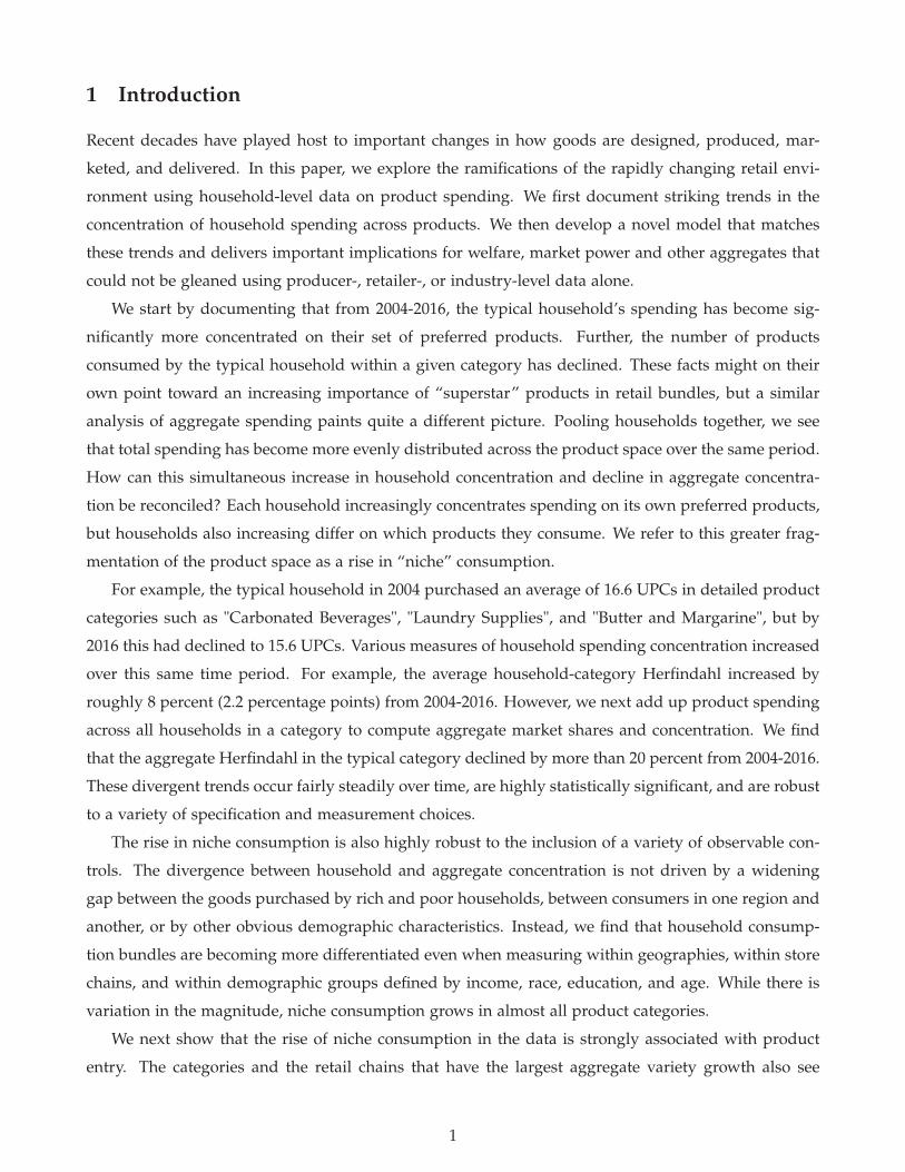
As a simple summary statistic for the prominence of niche consumption, we consider the ratio of

the Household Herfindahl to the Aggregate Herfindahl. A higher value for this “niche ratio” means

that household consumption is more segmented into different niches. Figure 4 shows that the rise of

niche consumption is pervasive across product categories, with three-quarters of product categories

exhibiting increases in HHHc,t , eighty percent of product categories exhibiting decreases in HAgg

c,t , and

growth in the niche ratio in 92 percent of the categories.18

In Appendix Figure A10, we also show that the rise of niche consumption is occurring in the vast

majority of locations, implying that shifts in the relative economic importance of cities and regions

are not behind our findings. The niche ratio is highest in cities like Chicago, Washington DC, Tampa,

Los Angeles, and Boston and lowest in Des Moines, Little Rock, Las Vegas, and "West Texas", but it is

increasing in most locations. Finally, Appendix Figure A11 shows that the rise in niche consumption

is found within roughly two-thirds of the individual retailers in our data, so the aggregate patterns we

observe are not simply driven by shifts in where households shop.19 Together these results all imply

that whatever forces are driving the rise in niche consumption, they are pervasive across demographics,

geographies, retail chains, and product categories.

The level of the niche ratio is highest in “Cosmetics" and “Fragrances-Women" and is lowest for

“Charcoal" and “Dough Products". The rise in niche consumption is pervasive, but it is also clear

from Figure 4 that there is substantial heterogeneity across categories in the extent of its ascent. The

niche ratio has grown most rapidly for "Coffee", "Hardware, Tools", "Fresheners and Deodorizers", and

"Disposable Diapers". It has declined by most for "Cottage Cheese", "Eggs", "Milk", and "Bread and

Baked Goods".

3.5 The Role of Product Churn

Interestingly, there is a common observable linking together the categories with the most rapid in-

creases in niche ratios: they are also the categories with the fastest growth in the number of aggregate

products, measured using the same assumptions as were used for Figure 2b above. We emphasize this

17Since HHHi is measured for each household i, it is straightforward to regress household concentration measures on a

variety of simultaneous demographics which vary across households. A similar exercise for aggregate concentration requiresrecalculating aggregate market shares and Hagg separately for each demographic group. This makes these calculationssubstantially more computationally burdensome. Even more importantly, measurement error in aggregate market sharesincreases rapidly for more narrow demographic groups.

18To improve visual exposition, Figures 4 and 5a drop 5 outlier categories whose variety counts more than double ordecrease by more than 50 percent from 2004-2016: "Frozen Juices", "Yeast", "Canning Supplies", "Greeting Cards" and "Pho-tographic Supplies". This does not affect any conclusions.

19We also show that our results are not driven by trends in the frequency of shopping and bulk purchasing (Coibion,Gorodnichenko, and Koustas (2017)).

12

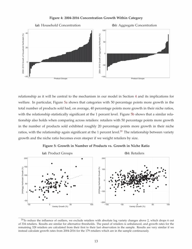
Figure 4: 2004-2016 Concentration Growth Within Category

(a): Household Concentration

−20

0

20

40

2004

−201

6 G

row

th o

f Hou

seho

ld H

erfin

dahl

(%)

Product Groups

(b): Aggregate Concentration

−100

−50

0

50

100

2004

−201

6 G

row

th o

f Agg

rega

te H

erfin

dahl

(%)

Product Groups

relationship as it will be central to the mechanism in our model in Section 4 and its implications for

welfare. In particular, Figure 5a shows that categories with 50 percentage points more growth in the

total number of products sold had, on average, 40 percentage points more growth in their niche ratios,

with the relationship statistically significant at the 1 percent level. Figure 5b shows that a similar rela-

tionship also holds when comparing across retailers: retailers with 50 percentage points more growth

in the number of products sold exhibited roughly 20 percentage points more growth in their niche

ratios, with the relationship again significant at the 1 percent level.20 The relationship between variety

growth and the niche ratio becomes even steeper if we weight retailers by size.

Figure 5: Growth in Number of Products vs. Growth in Niche Ratio

(a): Product Groups

−50

0

50

100

150

200

(HH

/Agg

) Her

finda

hl G

row

th (%

)

−50 0 50 100Variety Growth (%)

(b): Retailers

−200

−100

0

100

200

(HH

/Agg

) Her

finda

hl G

row

th (%

)

−100 −50 0 50 100Variety Growth (%)

20To reduce the influence of outliers, we exclude retailers with absolute log variety changes above 2, which drops 6 outof 334 retailers. Results are similar for alternative thresholds. The panel of retailers is unbalanced, and growth rates for theremaining 328 retailers are calculated from their first to their last observation in the sample. Results are very similar if weinstead calculate growth rates from 2004-2016 for the 179 retailers which are in the sample continuously.

13

We now provide additional evidence that product churn plays a key role in the rise of niche con-

sumption by comparing concentration trends measured only among “continuing" products that are

purchased by a household in two consecutive years with those measured using all spending by that

household.21 For each household i that is observed in both t and t + 1, we measure concentration of

“continuing products” by using only those that are purchased by that household in both t and t + 1.

These continuing products account for about 30 percent of transactions and 40 percent of spending.

We also calculate Herfindahls for those same households using all their spending. We form an index

by chaining together changes in these Herfindahls from t and t + 1 and pin down the level using the

values in the initial period.22 Figure 6a shows the upward trend in household concentration is much

stronger when using all UPCs than when restricting to continuing products, growing by 29 percent

compared to 5 percent.23 This implies a large role for product entry and exit in generating household

concentration increases. Figure 6b shows that when focusing only on continuing products, aggregate

concentration actually rises instead of declines.24

Figure 6: 2004-2016 Concentration growth for continuing vs. all products

(a): Household Herfindahl

.25

.3

.35

.4

.45

.5

Hou

seho

ld H

erfin

dahl

2004

2005

2006

2007

2008

2009

2010

2011

2012

2013

2014

2015

2016

Continuing Households:All Products

Continuing Households:Continuing Products

(b): Aggregate Herfindahl

.003

.004

.005

.006

.007

Aggr

egat

e H

erfin

dahl

2004

2005

2006

2007

2008

2009

2010

2011

2012

2013

2014

2015

2016

Continuing Households:All Products

Continuing Households:Continuing Products

4 Modeling the Rise of Niche Consumption

In this section, we develop a model able to match the rise of niche consumption documented in Section

3 and we use it to identify key driving forces and understand the resulting implications for welfare and

21For these results, therefore, we move to a panel specification since we require at least two time periods for a householdto measure which products for that household are new and which are continuing.

22We report cumulative changes rather than levels since this procedure results in two levels of the Herfindahl for each year(one initial and one continuation year), so the levels are not meaningful.

23The trend for “All Products” is larger than that in Figure 1a as Figure 6a is calculated using within-household variation.See Appendix C for details.

24While this analysis shows that the diverging concentration trends are largely driven by extensive rather than intensivemargin effects, for continuing products we can nevertheless decompose intensive margin concentration trends into P vs. Qeffects. Appendix Figure A12 shows that changes in quantity rather than price are more important.

14

markups. Many standard models are not useful for studying a simultaneous increase in household

concentration and decline in aggregate concentration because they either assume that all households

consume a single product, assume that household tastes are symmetric across products, or assume that

all households are identical. In our model, households choose how many products to consume, spend

different amounts on each good, and differ from other households in their choice of which products

to buy.

Following Li (2018), we assume that households must pay a fixed cost per consumed product,

which implies they only consume a subset of available products despite their CES preferences that

embed a “love of variety”. As in Arkolakis, Demidova, Klenow, and Rodriguez-Clare (2008), we

assume each household’s tastes for products, adjusted for price, are distributed Pareto, which allows us

to write the Household Herfindahl analytically. Further, we introduce a rank function that implies the

preference ordering of products will differ across households, which allows us to write the Aggregate

Herfindahl analytically.

Using the analytical expressions for the Household and Aggregate Herfindahl, we confront the

model with empirical trends from 2004-2016 and back out the implied driving forces. We find that

an increase in the number of available products is required to quantitatively match the rise of niche

consumption. In the model, this increase leads to significant welfare gains as it implies that con-

sumers can choose a consumption bundle better tailored to their tastes without raising their fixed cost

expenditures.

Finally, the model features heterogeneous markups across products. Growth in the sales of prod-

ucts with larger aggregate market shares primarily reflect growth in spending by existing customers, or

intensive margin adjustment. By contrast, growth in the sales of small products are more likely to come

from the addition of new customers, or extensive margin adjustment. Intensive and extensive margin

adjustments are characterized by different elasticities of demand, and this results in heterogeneous

markups. While changes in the number of products shift markups across products, we demonstrate

that they do not impact the aggregate degree of market power in the economy.

4.1 Household Problem

We assume that a continuum of households i ∈ [0, 1] spend E on a continuum of varieties k ∈ [0, N] to

maximize:25

Ui =

(∫k∈Ωi

(γi,kCi,k)σ−1

σ dk) σ

σ−1

− F × (|Ωi|)ε , (8)

where Ωi is the set of products consumed by i (with |Ωi| ≤ N), γi,k is a household-specific taste

for product k, and the term multiplied by F captures a fixed cost that increases exponentially in the

25To ease notation, we do not index k by i, but importantly note that the same k may represent a different actual productfor each different households. This is unimportant for the analysis of individual households, but will be crucial when wemove to the aggregate analysis.

15

measure of varieties consumed.

We write the price of product k as pk, so γi,k = γi,k/pk captures the price-adjusted taste of household

i for k. We assume price-adjusted tastes are distributed Pareto:

Pr (γi,k < y) = G (y) = 1 − (y/b)−θ ,

where y ≥ b > 0 and where we assume θ > 2 (σ − 1). Since larger θ means a flatter distribution of

tastes, the latter condition simply ensures that tastes are not "too concentrated" relative to σ and that

the model delivers a finite Household Herfindahl. We also assume ε > 1/(1− σ)− 1/θ, which implies

that higher fixed costs F lead to less purchased products |Ω|. Household i will consume the set of

goods with γi,k ∈ [γ∗, ∞) for some γ∗ ≥ b.

The ideal price index in this environment will be equal for all households and is defined as:

Pi = P =

(∫k∈Ωi

(γi,k)σ−1 dk

) 11−σ

=

(1 +

1 − σ

θ

) 1σ−1

b−1

︸ ︷︷ ︸Average Price

× (|Ωi|)1

1−σ︸ ︷︷ ︸Variety Gains

×( |Ωi|

N

) 1θ

︸ ︷︷ ︸Selection Effects

. (9)

The price index has three terms, each with an intuitive interpretation. We refer to the first term as the

average price since it summarizes the full distribution of price-adjusted tastes for available products

as if there were a single purchase price for one unit of the full bundle. It varies with the shape θ and

scale b of the Pareto distribution as well as with the elasticity of substitution σ. The second term is

the standard love-for-varieties term in CES models, which decreases with the measure of consumed

products and with the elasticity of substitution (given |Ωi| > 1). Finally, the third term represents a

selection effect from the fact that when households only consume a subset Ωi of the full measure N of

products, they choose the subset they like best. This term decreases in the share of products that are

consumed and in the extent to which households prefer some products to others.

The index reduces to more standard expressions in special cases. For example, consider θ → ∞,

which implies that households value all products identically at b, i.e. γi,k = b for all i and k. In such

a case, the expression reduces to b−1|Ωi|1/(1−σ), which is the standard price index for symmetric CES

preferences. Alternatively, imagine some products are preferred to others, θ < ∞, but all products are

nonetheless purchased, Ωi = N. In this case, the last term reduces to 1 as there are no selection effects

and the average price term fully captures impact of heterogeneity in the desirability of the products.

The properties of the CES price index imply we can re-write equation (8) as:

Ui =EP− F × (|Ωi|)ε .

16

Consumers choose |Ωi| to maximize utility. The first order condition implies that the optimal number

of products is:

|Ωi| = |Ω| =⎛⎝( 1

1−σ − 1θ

) (1 + 1−σ

θ

) 11−σ N

1θ

Fε

⎞⎠(ε− 1

1−σ+1θ )

−1

, (10)

where F = F/(bE) is a parameter which shifts spending, aggregate prices, and variety costs.26 Impor-

tantly, the optimal choice of varieties yields a "cutoff" taste γ∗ that satisfies: G (γ∗) = 1 − |Ω|N , and the

share of household i′s expenditure on variety k is then given by

si,k =

⎧⎨⎩(Pγi,k)

σ−1 , γi,k > γ∗

0, γi,k ≤ γ∗(11)

with∫

k si,kdk = 1.

4.2 Household Herfindahls

Given equation (11), it follows that the Household Herfindahl HHH will be equal for all i and can be

written as:

HHH = HHHi =

∫k∈Ωi

(si,k)2 dk = N

∫ ∞

γ∗i

(Piγi,k)2(σ−1) dG (y)

=(η + 1)2

4η

1|Ω| , (12)

where we introduce the variable η = 1− 2(σ− 1)/θ. The above parameter restrictions imply η ∈ (0, 1).

For fixed θ and σ, which implies fixed η, household concentration declines monotonically with the

number of consumed varieties. And for fixed |Ω|, concentration declines monotonically with η. All

else equal, flatter taste distributions (higher θ) or less substitutability across products in preferences

(lower σ) reduce Household Herfindahls.

How well does this model fit household spending data? Interpreting our model as applying to

each household’s spending decisions for a given product category c in a given year, we have the

testable prediction that HHHi,c is proportional to 1/|Ωi,c|. Indeed, when we pool categories, years, and

households and regress ln |Ωi,c| on − lnHHHi,c (with category-year fixed effects), we get a coefficient

of 0.89 – close to the model-consistent value of 1 – and a large R2 of 0.82. The upper left panel of

Figure 7 shows a binscatter (with category-year fixed effects) of the 54 million observations underlying

this regression to demonstrate that linearity with a coefficient of 1 is a close approximation to the raw

data.27 In the upper right panel, we estimate these regressions separately for each category in 2016 and

26When N = 1, this expression is the same as that in Li (2018) after substituting in his special case for b.27This specification has large explanatory power even though it only allows η to vary across category-years and not across

households. With arbitrary heterogeneity in η across households within category-years, there would be as many parametersas observations so it would be trivial to perfectly fit the data.

17

Figure 7: Model Fit on Household-Category Data

1

2

3

4

Log(

Ω)

0 1 2 3−Log(Household Herfindahl)

Bin ScatterData: Linear FitModel (Slope=1)

Model Fit by HH−Product Groups−Years

0

1

2

3

4

Den

sity

.7 .8 .9 1 1.1 1.2Estimated Slope

Slope by Product Group

0

1

2

3

4

Den

sity

0 .2 .4 .6 .8 1Estimated η

Estimated η by Product Group

0

1

2

3

4

Den

sity

.2 .4 .6 .8 1R2

R2 of Predictions Within Product Group

plot a histogram of the estimated slopes. The values are largely clustered around the model-consistent

value of 1.

Next, rather than estimating the slope, we constrain it to equal 1 and back out the η values implied

for each category. The model imposes the restriction that 0 < η < 1 and the bottom left panel of

Figure 7 shows that this restriction is satisfied in every category. The values of η range from lows of

0.08 (Baby Food) and 0.10 (Carbonated Beverages) to highs of 0.69 (Greeting Cards) and 0.97 (Yeast).28

Finally the lower right panel shows that the R2’s from these restricted regressions are generally high.

Overall, we conclude that the empirical relationship between household-level concentration measures

and the number of consumed products is consistent with the relationships implied in our model.

4.3 Aggregation

In order to account for divergent trends in household and aggregate concentration measures, we must

specify how tastes for particular products differ across households. We index all products in the

28The value of 0.08 for baby food implies that the typical household in this category has spending which is almost 4 timesmore concentrated than if that household spent evenly on all the baby food products they consumed, while the value of 0.97for yeast implies that household spending in that category is essentially evenly divided across products. With homogeneoustastes across products (i.e. θ → ∞) – the setup in many standard models – we cannot capture this large extent of sectoralheterogeneity in concentration as η → 1.

18

economy with j ∈ [0, N], and assume each household assigns each product a “rank”, where lower

ranks indicate higher price-adjusted tastes. Households will consume all goods which they rank less

than or equal to |Ω|.We introduce the following rank function for each household i:

ri,j = (1 − α)j + αxi,j, (13)

where j identifies a common aggregate rank for a product, xi,j is an i.i.d. draw from the uniform

distribution with support [0, N] representing a household-specific taste component, and α ∈ (0, 1). If

α is close to zero, the model approximates a representative agent model where all households rank

products in the same order. If α approaches 1, tastes are purely idiosyncratic and resulting aggregate

spending will be evenly distributed over all consumed products even if individual household tastes

are very concentrated. Thus, even though all households have identical distributions of taste-adjusted

prices, this rank function allows for different households to have different ranks for the exact same

product j.

To compute the aggregate spending share on product j, we need to know the cumulative distribu-

tion function (CDF) of product ranks R(r), integrating over all household and products. Without loss

of generality, we assume α < 1/2 and write:29

R(r) =

⎧⎪⎪⎪⎪⎪⎪⎨⎪⎪⎪⎪⎪⎪⎩

12

( rN

)2 1α (1 − α)

, 0 ≤ r < αN

rN

11 − α

− 12

α

1 − α, αN ≤ r < (1 − α) N

−12

( rN

)2 1α (1 − α)

+rN

1α (1 − α)

− 12

(α

1 − α+

1 − α

α

), (1 − α) N ≤ r ≤ N.

(14)

Note that this CDF satisfies the properties that R(0) = 0, R(N) = 1, is continuous at r = αN and

r = (1 − α) N, and is monotonically increasing.

There are three distinct regions in R(r) with different functional forms. If households only consume

goods with ranks in the first region, this implies that there is no single product in the economy that

is purchased by all households. If households consume so many varieties that some have ranks in

the second region, this implies that at least one product is purchased by everyone. Finally, if even the

worst possible product in the economy is purchased by at least one household, then the ranks of some

consumed goods will fall into the third region.30 As long as 0 ≤ |Ω|N < α

2(1−α)< 1

2 , it can be shown that

29Replacing α with 1 − α in all instances in equation (14) yields the corresponding R(r) for the alternative case of α > 1/2.Furthermore, this leaves the rank function unchanged for the first of the three regions of R(r), which will be the focus of ouranalysis.

30More specifically, the product with the best aggregate taste shock is j = 0. The worst possible idiosyncratic rank for thisproduct occurs when xi,j = N, in which case r = αN, so if we are in the first region of the parameter space, even the bestproduct is not purchased by some households. Conversely, the product with the worst aggregate taste shock is j = N. Thebest possible idiosyncratic rank for this product occurs when xi,j = 0, in which case r = (1 − αN). This means that if we arein the third region of the CDF, this worst product will still be consumed by some household.

19

all consumed products in the economy will have an r value confined to the first region of R(r). This

is the empirically relevant region of the parameter space, since the number of varieties purchased by

an individual household is orders of magnitude less than the aggregate number of varieties, and there

are no varieties in the data that are consumed by all households. To simplify analytical solutions, we

thus impose this parameter restriction for the remainder of the analysis.

Noting that γi,j = G−1 (1 − R(ri,j

)), the spending share of household i that is dedicated to product

j can be written as a function of j’s rank:

si,j = Pσ−1γσ−1i,j = (Pb)σ−1 (R

(ri,j

))− σ−1θ =

η + 12

Nη−1

2 |Ω|− η+12(

R(ri,j

)) η−12 , (15)

if R(ri,j

) ≤ |Ω|/N and zero otherwise. To determine the products for which the share si,j in equation

(15) jump from positive to zero, we solve for the rank of the marginal, or least-preferred, variety that

is consumed in positive quantities by household i. Note that this good’s identity will differ across

households, but its rank r∗ will be the same and satisfies R(r∗) = |Ω|/N. Substituting into equation

(14) under the assumption that 0 ≤ |Ω|N < α

2(1−α), we get:

r∗ = (2α (1 − α) |Ω|N)12 . (16)

Under our parameter restrictions, individual households each consume only a fraction of the to-

tal products available N, but the exact products consumed will differ across households. However,

even when aggregating across all households, there are some products which are consumed by no

households. This means that for the economy as a whole, there is a difference between the measure

of available goods N and the measure of goods that are actually consumed, which we denote j∗. This

marginal consumed good for the economy as a whole, j∗, is that j for which the best possible idiosyn-

cratic taste draw – a draw of zero – yields rank r∗ for the household with that zero draw. Solving for

this cutoff, j∗ = r∗/ (1 − α), we get:

j∗ =(

2α|Ω|N1 − α

) 12

. (17)

Importantly, since ri,j is strictly increasing in j, all goods with j < j∗ will have positive aggregate

sales and all goods with j ≥ j∗ will have zero aggregate sales. Finally, substituting in the definition of

the rank function from equation (13) into the expression (16), and using the definition of j∗ in equation

(17), we can write the highest value or “cutoff” random draw x∗j that yields positive consumption of j

as:

x∗j =1 − α

α(j∗ − j) . (18)

20

4.4 The Aggregate Herfindahl

We now integrate spending shares across households i to get the aggregate spending share on good j:

sj =1∫

i Edi

∫iEsi,jdi

=η + 1

2N

η−12 |Ω|− η+1

2

∫ 1−αα (j∗−j)

02

1−η2 N1−η

(α (1 − α)

1−η2

) ((1 − α) j + αxi,j

)η−1 dxN

= (η + 1) (2N|Ω|)− η+12 (α (1 − α))

1−η2

∫ 1−αα (j∗−j)

0((1 − α) j + αxz,i)

η−1 dx

=η + 1

η

(2αN|Ω|

1 − α

)− η+12 (

(j∗)η − jη)

=η + 1η j∗

(1 −

(jj∗

)η). (19)

Using equation (19), we immediately obtain the Aggregate Herfindahl:

HAgg =∫ j∗

j=0s2

j dj =(

η + 1η j∗

)2 ∫ j∗

j=0

(1 −

(jj∗

)η)2

dj

=

(η + 1η j∗

)2

j∗(

1 − 2η + 1

+1

2η + 1

)

=2 (η + 1)(2η + 1)

1j∗

=2 (η + 1)(2η + 1)

(1

2N|Ω|) 1

2

, (20)

where we define N = Nα/(1 − α). Aggregate concentration declines monotonically with N. For fixed

θ and σ, aggregate concentration declines monotonically with the number of consumed products. And

for fixed |Ω|, concentration declines monotonically with η. Importantly, changes in |Ω| and η move

the Household Herfindahl and Aggregate Herfindahl in the same direction. As we discuss in the next

subsection, this imposes strong restrictions on the set of possible forces which can explain the opposite

empirical trends for HHH and HAgg and implies an important role for increases in N.

How well do these model-based relationships fit aggregate sales distributions in the data? To

assess this, we start by measuring |Ω| directly in the data and then solve for the two remaining free

parameters, η and N, to match HHH and HAgg in equations (12) and (20). Figure 8 then plots the

market share distribution across products implied by our model in equation (19) (the red dashed line)

against the actual market share distribution in the data (the solid blue line). We do this for total

spending in Figure 8a as well as separately for a number of product categories in Figure 8b. In several

categories such as cereal and yogurt, the model fits extremely well, while it is notably less successful

in others such as greeting cards or canned seafood. Overall, however, we consider these good fits

as validating our use of the model, particularly given the distributions are fully determined by only

21

Figure 8: Model Fit on Aggregate Category Data

(a): Aggregate Market Shares

0 100 200 300 400 500Product Rank (j)

0

0.005

0.01

0.015

0.02

0.025

0.03

0.035

Shar

e

DataModel

(b): Sectoral Market Shares

0 200 400 600Product Rank (j)

0

0.01

0.02

0.03

Shar

e

"CEREAL"

DataModel

0 500 1000Product Rank (j)

0

0.01

0.02

0.03

Shar

e

"YOGURT"

DataModel

0 50 100 150Product Rank (j)

0

0.05

0.1

Shar

e

"SEAFOOD - CANNED"

DataModel

0 1000 2000 3000Product Rank (j)

0

0.005

0.01

0.015

Shar

e

"PET FOOD"

DataModel

three parameters and reflect parametric assumptions and functional forms chosen largely for analytical

convenience.

4.5 Understanding the Empirical Trends

We now confront our model with concentration measures and other moments from the data to infer

which structural forces led to the rise in niche consumption. Collecting previous results, our model

implies that:

HHH =(η + 1)2

4η

1|Ω|

HAgg =2 (η + 1)(2η + 1)

(1

2N|Ω|) 1

2

.

Since HHH, HAgg, and |Ω| are directly observable in the data, this produces a system of two

equations that can be solved to determine η and N for each year. Figure 9 shows the time-series for

N and η necessary to hit these observables in each year. Through the lens of the model, given the

observed path for |Ω|, matching the concentration trends requires nearly constant values for η and a

strong upward trend in N. From 2004-2016, η falls by 2 percent while N rises by 70 percent.

Inspecting the equations for the two concentration measures, it is clear that increases in N push the

Aggregate Herfindahl down relative to the Household Herfindahl. Is it obvious that N must necessarily

rise to explain opposite trends in the two concentration measures? In Appendix D, we demonstrate

that the answer is no. Theoretically, there are combinations of |Ω| and η that deliver increases in HHH

and decreases in HAgg, even without a change in N. These combinations, however, are grossly at odds

22

Figure 9: Modeling the Rise of Niche Consumption

2005 2010 20150.045

0.05

0.055

0.06

0.065

0.07

0.075

0.08

0.085

0.09

2005 2010 20150.8

0.9

1

1.1

1.2

1.3

1.4

1.5 104

with multiple moments of the data. Multiple factors can cause the observed changes in |Ω|, but all

explanations of the data require an increase in N, so we focus our analysis on this force.

Mechanically, increases in N can arise from increases in α or N. Changes in α are straightforward

to interpret, since α is simply an exogenous parameter governing preference heterogeneity. While

increases in α could easily rationalize the data, our empirical results show that the rise of niche con-

sumption occurs pervasively across all of our narrowly-defined demographic groups. The within-

group trends are far more important than across-group trends in generating our aggregate results.

While this does not rule out increases in α as a driving force, it seems unlikely that fundamental

preferences within narrow groups have become dramatically more heterogeneous over a twelve-year

period. Based on this logic, we hold α fixed and explore the effects of increases in N in the model,

holding constant all other parameters, including the price-adjusted taste distribution.

4.6 Implications of An Increase in the Number of Products

We set all parameter values to match key empirical moments in 2004 and increase N by 70 percent

to generate the increase in N backed out in Figure 9.31 We then calculate the change in household

31The exact initial parameters are not important for our qualitative conclusions, but we set α = 0.36, ε = 2, E = 35,σ = 3.76, b = 1, F = 0.14 and θ = 5.9. E is set to match average household category expenditures, θ and σ are set to match

23

welfare, expressed as the percentage change in expenditures on the initial set of goods that would

bring the same change in household utility as that delivered by the increase in N. We find that a 70

percent increase from N2004 to N2016 generates total welfare gains of 9.5 percent, or about 0.8 percent

per year. That is:

U2016 =E

PN2016

− F × (|ΩN2016 |)ε = 1.095 × EPN2004

− F × (|ΩN2004 |)ε , (21)

where we change N and calculate the endogenous change in P and Ω, but hold fixed all other param-

eters.

These welfare gains of 9.5 percent arise from three sources. First, as seen clearly in the third term

of the ideal price index in equation (9), an increase in N for a given |Ω| leads to gains from selection.

With more choices, households consume those products better suited to their particular tastes. Second,

as seen clearly in equation (10), increases in N lead to increases in |Ω|. As seen in the second term

of the ideal price index, this leads to welfare gains from the love-for-variety effect on welfare, even

if selection effects |Ω|/N are held constant. Third, increases in |Ω| lead to increases in the fixed

costs paid by households, which reduces welfare. Selection effects account for the bulk of the gains

(8.5 percent), with love-for-variety effects improving welfare by 1.8 percent and the increase in fixed

costs causing welfare losses of approximately 1.0 percent (these do not sum perfectly to 9.5 due to

non-linearity).

An increase in N (or α) is a necessary part of any explanation that quantitatively matches the

simultaneous rise in HHH and decline in HAgg.32 Other parameters must change as well, however, in

order to fully fit the concentration trends. After all, as just discussed, an increase in N on its own

causes |Ω| to rise and generates a (small) decline rather than an increase in HHH.

Equation (10) shows that if N increases, declines in |Ω| must reflect declines in measured real

expenditures(

E (1 + (1 − σ) /θ)1

1−σ b)

, increases in effective costs per number of products consumed

(F or ε), or declines in an "effective curvature" of utility term( 1

1−σ − 1θ

).33 Expenditures, however,

increase in the data, and while changes in either σ or θ could change the curvature term, they would

have to change in a very particular way so as to match the decline in |Ω| without leading to changes

in η. We therefore find it most plausible that the decline in |Ω| reflected an increase in F or ε.34

How does our inference about welfare change when we consider joint increases in N and in F

(or ε) that are chosen to match both the rise of HHH and the declines in HAgg and |Ω|? Repeating

the initial η in the data given observed Ω subject to generating a ratio of aggregate sales to aggregate costs of 1.2 percent.Given b and ε, we choose F to match Ω.

32N impacts the extent of selection effects while α does not, so if one considers that growth in N is driven in part by growthin α, the welfare gains will be smaller.

33Real measured expenditures equal E divided by the expression labeled “Average Price” in equation (9).34While some technological advances such as the rise of the internet or better advertising technology might be expected to

lower variety costs, it is also likely that increases in the number of available varieties N make it more costly to sort throughand identify the particular products a household wants to purchase. An increase in F or ε can be interpreted as a simpleproxy for these latter forces when it is accompanied by the increase in N.

24

our comparative statics exercise when we vary both N and F, we find that welfare rises by about 7.5

percent instead of 9.5 percent. This decomposes into selection gains above 10 percent, love-for-variety

losses of about 2 percent, and an additional loss of 1 percent from the higher fixed costs. Results are

vary similar when we vary N and ε instead of N and F.

Finally, we note that if one simply viewed our data through the lens of a representative household

model with CES preferences, it might be natural to only consider this love-of-variety loss and mis-

leadingly conclude that welfare declined from 2004-2016, since the typical household consumed fewer

varieties in 2016 than in 2004. Heterogeneity in product consumption across households is crucial for

capturing the divergent concentration trends in our data. Representative agent models abstract from

this heterogeneity, and our results show that this can potentially lead to misleading conclusions about

the welfare effects arising from changes in the number of products households consume.

4.7 Elasticities of Demand, Markups, and Aggregate Profits

Concentration measures like the Herfindahl are often used as proxies for market power. What implica-

tions does the divergence in Aggregate and Household Herfindahls have for markups and aggregate

profits in our model? In typical CES environments, the elasticity of demand and markups are fully

determined by the exogenous elasticity of substitution σ. By contrast, we show in this section that

the elasticity of demand in our model depends both on this standard “intensive margin" force as well

as on an endogenous “extensive margin” force that arises from the possibility for products to gain

new customers (or lose existing ones). Since these forces are of different importance for products with

different aggregate market shares, the model generates heterogeneous markups.

How does an increase in N influence markups? On the one hand, competition from new products

pushes existing consumed products closer to the margin where they are no longer consumed, increas-

ing their elasticity of demand and decreasing their markups. On the other hand, selection effects mean

those new products are on average more desirable and have higher markups than those in the bundle

prior to the change in N. We show that in the aggregate, these opposing forces exactly cancel and the

ratio of total revenues to total costs remains unchanged. Our model therefore shows how the economy

can exhibit large changes in aggregate and household concentration without any change in aggregate

market power.35

To solve for the price elasticity of aggregate demand for product j, we start by expressing its total

sales as the integral of each household’s spending on j, taken over all households:

sj =1N

∫ x∗j

0six ,jdx, (22)

35We note that if each consumer’s taste for each good remains fixed, and markups change for any reason, this would resultin a change in the price-adjusted taste distribution and would affect the expressions above that were derived assuming thatprice-adjusted tastes were distributed a la Pareto. We explore this in more detail in Appendix E, but here note that in order topreserve the Pareto distribution of price-adjusted tastes in the face of increases in N and endogenous markups, the changesin tastes that we additionally require are relatively minor.

25

where we use the notation six ,j to denote the spending share of a household with taste draw on product

j equal to x. Since j will only be purchased by those households with a sufficiently high idiosyncratic

taste for it, we need only integrate from households drawing xi,j = 0 to the marginal household that

draws xi,j = x∗j .

We take the partial derivative of sj in equation (22) with respect to pj to get:

∂sj

∂pj=

1N

(∫ x∗j

0

∂six ,j

∂pjdx + six∗j ,j

∂x∗j∂pj

), (23)

where the right hand side of equation (23) follows from Leibniz’s rule. The first term can be solved

using equation (15) as:∂six ,j

∂pj=

∂Pσ−1 p1−σj γσ−1

i,j

∂pj= (1 − σ)

six ,j

pj, (24)

where we take the aggregate price index P as fixed. Moving on to the second term, we can evaluate

equation (15) at the marginal household with taste x∗j to get:

six∗j ,j∂x∗j∂pj

=η + 1

2N

η−12 |Ω|− η+1

2 (R (r∗))η−1

2∂x∗j∂pj

. (25)

Substituting equations (24) and (25) back into equation (23), we get:

∂sj

∂pj= (1 − σ)

1pj

1N

∫ x∗j

0six ,jdx +

1N

six∗j ,j∂x∗j∂pj

= (1 − σ)sj

pj+

1N

η + 12

Nη−1

2 |Ω|− η+12 (R (r∗))

η−12

∂x∗j∂pj

= (1 − σ)sj

pj+

1N

η + 12

Nη−1

2 |Ω|− η+12

(12

N−2α−1 (1 − α) (j∗)2) η−1

2 ∂x∗j∂pj

= (1 − σ)sj

pj+

η + 12N|Ω|

∂x∗j∂pj

. (26)

We cannot directly consider a price change, required to exactly solve for ∂x∗j /∂pj, because the full

distribution of price-adjusted tastes in our model is set exogenously and must be maintained as Pareto.

Instead, to approximate the change in mass of households consuming a product when that product’s

price increases, we start with the relationship:36

12

(ri,j

N

)2 1α (1 − α)

= R((1 − α) j + αxi,j

)= 1 − G

(γi,j

pj

)= bθγ−θ

i,j pθj , (27)

36In Appendix E we use numerical simulations which do not require any distributional assumption on tastes to verify thatthe approximation that follows is highly accurate.

26

and differentiate to yield:ri,j

1 − α

1N2

∂xi,j

∂pj= θbθγ−θ

i,j pθ−1j , (28)

where we’ve substituted ∂ri,j/∂xi,j = α. We then evaluate equation (28) at ri,j = r∗ and γi,j = γ∗ using

equation (16), and add a minus sign to reflect the fact that increase in the price of good j should reduce

the set of households purchasing that good, to get:

dx∗jdpj

= − θ

j∗|Ω|N 1

pj. (29)

Inserting this into equation (26), we have:

∂sj

∂pj= (1 − σ)

sj

pj− η + 1

2N|Ω|θ

j∗|Ω|N 1

pj

= (1 − σ)sj

pj− ηθ

2(

1 −(

jj∗

)η) sj

pj. (30)

Equation (30) implies that product j’s price elasticity of demand ε j can be written as:

ε j = 1 − ∂sj

∂pj

pj

sj

= σ︸︷︷︸Intensive Margin

+

(1 −

(jj∗

)η)−1

[θ/2 − (σ − 1)]︸ ︷︷ ︸Extensive Margin

> σ. (31)

In addition to the standard intensive margin term σ, there is a strictly positive contribution from the

extensive margin, since lowering the price of a product can induce new households to start consuming

the product. Low j or "mass-market" products are consumed by many households, so the intensive

margin is relatively more important for them. High j or "niche" products are consumed by few house-

holds, so the extensive margin is relatively more important. As a result, the elasticity of demand

increases as market share falls.37 As j → j∗ and a product approaches the point where it is dropped

from the aggregate consumption bundle, the elasticity approaches infinity, i.e. ε → ∞. The markup μj

can then be written (in gross terms) as:

μj =ε j

ε j − 1=

σ + θ(η+1)2j∗sj

σ + θ(η+1)2j∗sj

− 1, (32)

and ranges from a high of (1 + 2/θ) for the largest good j = 0 to a low of 1 for j = j∗.

37Interestingly, for good j = 0, which has the largest aggregate demand, the positive impact of σ on the elasticity comingthrough the intensive margin exactly cancels with the negative impact of σ coming from the extensive margin, leaving atotal elasticity of (θ/2 + 1). This result echos a closely related point in Chaney (2008), where the impact of the equivalentparameter for the elasticity of trade flows to trade costs also fully cancels when combining the intensive and extensive margineffects.

27

What are the implications of the rise in niche consumption for the distribution of products and for

market power? The “aggregate markup” is equal to the ratio of aggregate sales to aggregate costs.

Using equations (19) and (31), it can be written as:

μAgg =

∫ j∗0 sjdj∫ j∗

0 sjε j−1

ε jdj

=

[θ + (σ − 1)2

σ2 − 12

ηθ2

σ2

(η + 12 + θ

)× 2F1

(1,

1η

; 1 +1η

;2σ

2 + θ

)]−1

, (33)

where 2F1 (·) is the hypergeometric function.38 Importantly, while this aggregate profit share is a

relatively complicated function of σ and θ, it is not a function of N, F, or ε, the key model forces

we argued drove the rise in niche consumption. Changes in N, F, and ε may have implications for

the distribution of markups across products in the economy, since they impact j∗, but these changes

leave the “aggregate markup” exactly constant, since j∗ drops out of equation (33). Given the common

association of changes in concentration with changes in market power, we find this to be a surprising

and useful result.

More intuitively, this result arises from two opposing forces which exactly cancel when j∗ changes.

On the one hand, the jth good in an economy with a low j∗ is closer to being the marginal consumed

good and will therefore have a lower markup then the jth good in an economy with a high j∗. This

can be seen in equation (31), which shows that the elasticity of demand is strictly increasing in the

ratio of j to j∗. The solid blue line in Figure 10a plots markups as a function of product rank j using

the same calibrated values meant to represent 2004 in the exercise in Section 4.6, and the red dashed

line plots this relationship after increasing both N and F to fit the rise of niche consumption seen by

2016. The entire distribution of markups on consumed products shifts upward, with the top product

(j = 0) as the only exception. On the other hand, in the new economy with more product options, the

top high-markup products account for a smaller share of aggregate spending, as shown in Figure 10b.

Both forces are individually quite powerful, but in our model they exactly offset such that there is no

change in the aggregate profit share.39

While Figure 10 demonstrates the impact of this change in N and F on the joint distribution of

markups and market shares, additional structure is required if one wishes to comment on the impli-

cations of entry for a given product. For example, in response to changes in α or F, it is natural to

assume that a particular product j’s aggregate rank does not change, i.e. jpost = jpre. A comparison

of the lines in Figure 10 evaluated at a particular product rank j, therefore, would capture the change

impacting that particular product. By contrast, a given product’s j would likely change in response

to a change in N, depending on whether the new expanded set of products are drawn from a better,

38The hypergeometric function is defined as follows: 2F1 (a, b; c; z) = ∑∞n=0

(a)n(b)n(c)n

zn

n! . (x)n is the Pochhammer symbol,

which equals (x+n−1)!(x−1)! for all n > 0 and equals 1 for n = 0.

39Putting Figures 10a and 10b together, the distribution of actual profits flattens across j values, as shown in AppendixFigure A13.

28

Figure 10: Effects of N ↑ and F ↑ on Markup and Market Share Distributions

(a): Markups

0 100 200 300 400 500Product Rank (j)

1

1.05

1.1

1.15

1.2

1.25

1.3

1.35

Mar

kup

PrePost

(b): Market Shares

0 100 200 300 400 500Product Rank (j)

0

0.002

0.004

0.006

0.008

0.01

0.012

Mar

ket S

hare

s

PrePost

worse, or identical distribution as the original smaller set of products. For example, if the new and

old products have the same quality distribution, it is most natural to think of a given product’s j as

evolving according to: jpost = jpre × (Npost/Npre). Since we cannot pin down the change in markup or

market share of any particular incumbent product in our model without making further assumptions

on the nature of entry, and given we do not have data on product markups suitable to empirically

measure such changes, we leave this to future work to explore.

5 Conclusions

This paper empirically documents a rise in what we call "niche" consumption. Households are in-

creasingly concentrating their spending. This pattern, however, does not appear to be driven by the

emergence of superstar products. Rather, households are increasingly buying different goods from one

another. The increase in segmentation seen in many other walks of modern life also applies to con-

sumption: our grocery baskets look less and less similar. As a result, aggregate spending has become

less concentrated.

We develop a new model of product demand in order to explore the drivers and implications of the

rise in niche consumption. In our model, households choose how many products to consume, spend

different amounts on each good, and differ from other households in their choice of which products

to buy. The model delivers simple analytical expressions for household and aggregate concentration

indices, and these closed form solutions allow us to match the model to data and infer the drivers

of our empirical findings. Increases in product availability played a critical role in the divergent

concentration trends, and led to welfare gains from households being able to consume a subset of

29

products that better satisfied their tastes. This welfare effect would be difficult to find using standard

statistics such as measured price indices. Finally, our model delivers endogenous and heterogeneous

markups. Matching the trends in household and aggregate concentration carries implications for the

distribution of markups, but does not imply changes in aggregate market power.

Our model highlights the importance of greater product choice but treats the set of available prod-

ucts as an exogenous parameter. We suspect the nature of product introduction and development,

however, reflects recent progress in supply chain integration, big-data marketing research, targeted

advertising, and the growing importance of online sales. Unpacking the product innovation process

and relating it to these important trends is a fruitful avenue for future research on consumption be-

havior.

30

References

Aguado, J. M., C. Feijoo, and I. Martinez (2015): Emerging Perspectives on the Mobile Content Evolution.IGI Global.

Allcott, H., R. Diamond, J.-P. Dube, J. Handbury, I. Rahkovsky, and M. Schnell (2017): “FoodDeserts and the Causes of Nutritional Inequality,” Working Paper 24094, National Bureau of Eco-nomic Research.

Alwin, D., and P. Tufis (2015): “The Changing Dynamics of Class and Culture in American Politics: aTest of the Polarization Hypothesis,” The Annals of the American Academy of Political and Social Science,663.

Anderson, C. (2006): The Long Tail: Why the Future of Business Is Selling Less of More. Hyperion.

Anderson, E., S. Rebelo, and A. Wong (2018): “Markups Across Space and Time,” Working Paper24434, National Bureau of Economic Research.

Argente, D., and M. Lee (2017): “Cost of Living Inequality During the Great Recession,” mimeo.

Argente, D., M. Lee, and S. Moreira (2018a): “How do firms grow? The life cycle of productsmatters,” .

(2018b): “Innovation and product reallocation in the great recession,” Journal of MonetaryEconomics, 93, 1–20.

Arkolakis, C., S. Demidova, P. J. Klenow, and A. Rodriguez-Clare (2008): “Endogenous variety andthe gains from trade,” American Economic Review, 98(2), 444–50.

Atkeson, A., and A. Burstein (2008): “Pricing-to-market, trade costs, and international relativeprices,” American Economic Review, 98(5), 1998–2031.

Atkin, D., B. Faber, and M. Gonzalez-Navarro (2018): “Retail globalization and household welfare:Evidence from mexico,” Journal of Political Economy, 126(1), 1–73.

Autor, D., D. Dorn, L. F. Katz, C. Patterson, and J. V. Reenen (2017): “The Fall of the Labor Shareand the rise of Superstar Firms,” Working Paper 23396, National Bureau of Economic Research.

Autor, D. H., L. F. Katz, and M. S. Kearney (2006): “The Polarization of the U.S. Labor Market,” TheAmerican Economic Review, 96(2).

Berger, D., and J. Vavra (2015): “Consumption Dynamics During Recessions,” Econometrica, 83(1).

Berger, D., and J. Vavra (2019): “Shocks vs. Responsiveness: What Drives Time-Varying Dispersion?,”Journal of Political Economy.

Berry, S., A. Eizenberg, and J. Waldfogel (2016): “Optimal product variety in radio markets,” TheRAND Journal of Economics, 47(3), 463–497.

Berry, S. T., M. Gaynor, and F. S. Morton (2019): “Do Increasing Markups Matter? Lessons fromEmpirical Industrial Organization,” Working Paper 26007, National Bureau of Economic Research.

Bertrand, M., and E. Kamenica (2018): “Coming apart? Lives of the Rich and the Poor Over Time,”Discussion paper.

Bornstein, G. (2018): “Entry and Profits in an Aging Economy: The Role of Consumer Inertia,” .

31

Broda, C., and D. E. Weinstein (2006): “Globalization and the Gains from Variety,” The Quarterlyjournal of economics, 121(2), 541–585.

Broda, C., and D. W. Weinstein (2004): “Variety growth and world welfare,” American EconomicReview, 94(2), 139–144.

Chaney, T. (2008): “Distorted gravity: the intensive and extensive margins of international trade,”American Economic Review, 98(4), 1707–21.

Coibion, O., Y. Gorodnichenko, and D. Koustas (2017): “Consumption Inequality and the Frequencyof Purchases,” Discussion paper.

Davis, D. R., J. I. Dingel, J. Monras, and E. Morales (2017): “How Segregated is Urban Consump-tion?,” .

De Loecker, J., and J. Eeckhout (2017): “The Rise of Market Power and the Macroeconomic Implica-tions,” Working Paper 23687, National Bureau of Economic Research.

Dube, J.-P., G. Hitsch, and P. Rossi (2018): “Income and Wealth Effects on Private-Label Demand:Evidence from the Great Recession,” Marketing Science.

Edmond, C., V. Midrigan, and D. Y. Xu (2018): “How costly are markups?,” Discussion paper, Na-tional Bureau of Economic Research.

Feenstra, R. C. (1994): “New product varieties and the measurement of international prices,” TheAmerican Economic Review, pp. 157–177.

Feenstra, R. C., and D. E. Weinstein (2017): “Globalization, markups, and US welfare,” Journal ofPolitical Economy, 125(4), 1040–1074.

Furman, J., and P. Orszag (2015): “A firm-level perspective on the role of rents in the rise in in-equality,” Presentation at âAIJA Just SocietyâAI Centennial Event in Honor of Joseph Stiglitz ColumbiaUniversity, 16.

Gentzkow, M., J. M. Shapiro, and M. Taddy (2017): “Measuring Polarization in High-DimensionalData: Method and Application to Congressional Speech,” Working Paper 22423, National Bureau ofEconomic Research.

Gopinath, G., and O. Itskhoki (2010): “Frequency of price adjustment and pass-through,” The Quar-terly Journal of Economics, 125(2), 675–727.

Handbury, J., and D. E. Weinstein (2014): “Goods prices and availability in cities,” The Review ofEconomic Studies, 82(1), 258–296.

Hansen, K., and V. Singh (2015): “Choice Concentration,” Discussion paper.

Hottman, C. J., S. J. Redding, and D. E. Weinstein (2016): “Quantifying the sources of firm hetero-geneity,” The Quarterly Journal of Economics, 131(3), 1291–1364.

Jaravel, X. (2019): “The Unequal Gains from Product Innovations: Evidence from the US Retail Sec-tor,” Quarterly Journal of Economics, 134(2).

Kaplan, G., and G. Menzio (2015): “The morphology of price dispersion,” International EconomicReview, 56(4), 1165–1206.

Kimball, M. S. (1995): “The Quantitative Analytics of the Basic Neomonetarist Model,” Journal ofMoney, Credit and Banking, 27(4), 1241–1277.

32

Kroft, K., J.-W. P. Laliberté, R. Leal-Vizcaíno, and M. J. Notowidigdo (2017): “Quantifying theWelfare Gains of Variety: A Sufficient Statistics Approach,” Discussion paper, Mimeo, available athttp://korykroft. com/wordpress/KKLN variety july2017. pdf.

Levin, A., and T. Yun (2008): “Reconsidering the microeconomic foundations of price-setting behav-ior,” Unpublished Manuscript, Board of Governors of the Federal Re serve System.

Li, N. (2018): “An Engel curve for variety,” Working Paper.

Melitz, M. J., and G. I. Ottaviano (2008): “Market size, trade, and productivity,” The review of economicstudies, 75(1), 295–316.

Michelacci, C., L. Paciello, and A. Pozzi (2019): “The Extensive Margin of Aggregate ConsumptionDemand,” Mimeo.

Neiman, B., and J. Vavra (2018): “The Rise of Household Spending Concentration,” Mimeo.

Petrin, A. (2002): “Quantifying the benefits of new products: The case of the minivan,” Journal ofpolitical Economy, 110(4), 705–729.

Pew Research Center (2014): “Political Polarization in the American Public,” Discussion paper.

Piketty, T., E. Saez, and G. Zucman (2016): “Distributional National Accounts: Methods and Esti-mates for the United States,” Working Paper 22945, National Bureau of Economic Research.

Redding, S. J., and D. E. Weinstein (2016): “Measuring aggregate price indexes with demand shocks:Theory and evidence for CES Preferences,” Discussion paper, National Bureau of Economic Re-search.

Rossi-Hansberg, E., P.-D. Sarte, and N. Trachter (2018): “Diverging trends in national and localconcentration,” Discussion paper, National Bureau of Economic Research.

Stroebel, J., and J. Vavra (2019): “House Prices, Local Demand and Retail Prices,” Journal of PoliticalEconomy, 127(3).

Syverson, C. (2018): “Remarks at ‘Changing Market Structure and Implications for Monetary Policy’,”Remarks, 2018 Jackson Hole Symposium.

33