WORKING PAPER SERIES - Boston College

EC

B

EZ

B

EK

T

BC

E

EK

P

WO R K I N G PA P E R S E R I E S

WORKING PAPER NO. 6

THE DEMAND FOR M3IN THE EURO AREA

BYGÜNTER COENEN

ANDJUAN-LUIS VEGA

SEPTEMBER 1999

WO R K I N G PA P E R S E R I E S

WORKING PAPER NO. 6

THE DEMAND FOR M3IN THE EURO AREA

BYGÜNTER COENEN

ANDJUAN-LUIS VEGA*

SEPTEMBER 1999

* The authors are grateful to the many European Central Bank colleagues who have made helpful comments and suggestions. The authors also thank D. Gerdesmeier and P. Vlaar for insightfuldiscussions. In addition, the paper has greatly benefited from comments from two anonymous referees and from staff in the research departments of a number of national central banks. Viewsexpressed represent exclusively the opinion of the authors and do not necessarily reflect those of the European Central Bank. Any remaining errors are of course the sole responsibility of the authors.

© European Central Bank, 1999

Address Kaiserstrasse 29

D-60311 Frankfurt am Main

GERMANY

Postal address Postfach 16 03 19

D-60066 Frankfurt am Main

Germany

Telephone +49 69 1344 0

Internet http://www.ecb.int

Fax +49 69 1344 6000

Telex 411 144 ecb d

All rights reserved.

Reproduction for educational and non-commercial purposes is permitted provided that the source is acknowledged.

The views expressed in this paper are those of the author and do not necessarily reflect those of the European Central Bank.

,661 ���������

Abstract

In this paper, an empirically stable money demand model for M3 in the euro area is

constructed. Starting with a multivariate system, three cointegrating relationships with

economic content are found: (i) the spread between the long- and the short-term nominal

interest rates, (ii) the long-term real interest rate, and (iii) a long-run demand for broad

money M3. There is evidence that the determinants of M3 money demand are weakly

exogenous with respect to the long-run parameters. Hence, following a general-to-specific

modelling approach, a parsimonious conditional error-correction model for M3 money

demand is derived which can be interpreted economically. For the conditional model, long-

and short-run parameter stability is extensively tested and not rejected. Insights into the

dynamics of money demand are gained by means of SVAR techniques exploring the

impulse response functions of the cointegrated multivariate system.

JEL Classification System: C22, C32, E41

Keywords: Money demand, euro area, cointegration, error-correction model, impulse

response analysis

1

I Introduction

In October and December 1998, the Governing Council of the European Central Bank

announced the key elements of the monetary policy strategy of the Eurosystem. These

comprise a quantitative definition of the primary objective, namely price stability, and the

“two pillars” used for achieving this objective: a prominent role for money, as signalled by

the publication of a reference value for the growth rate of broad money M3, and a broadly

based assessment of the outlook for, and risks to, price stability in the euro area.1

Whilst the role assigned to money in the strategy is primarily based on theoretical grounds

(namely that inflation is ultimately a monetary phenomenon), empirical evidence, together

with conceptual considerations, may indeed play an important role in selecting the

particular monetary aggregate that best serves the purposes at hand. The existence of a

stable and predictable relationship between the demand for a given monetary aggregate and

its macroeconomic determinants has traditionally been considered a key element in this

respect. Further considerations refer to leading indicator and controllability properties.2

Against this background, this paper presents some results of recent empirical research

carried out at the European Central Bank on the demand for broad money M3 in the euro

area. The paper is organised as follows. Section 2 briefly discusses our benchmark long-run

specification for the estimation of the demand for broad money M3 in the euro area and the

data underlying the empirical analysis. The data set is reproduced in Annex 1. Section 3

investigates the cointegration properties of the data by means of the application of the

Johansen procedure to a set of variables consisting of real holdings of M3 (m-p), real GDP

(y), short- (s) and long-term (l) interest rates and the inflation rate as measured by the

annualised quarterly changes in the log of the GDP deflator (�/4= ûS). In the light of the

results, Section 4 develops a conditional model for M3 money demand in the euro area. We

proceed in two steps and follow a general-to-specific modelling approach. Firstly, an

unrestricted autoregressive distributed lag (ADL) model in m-p, y, s, l DQG � is estimated

and its long-run solution computed. And secondly, the results obtained in the first step are

then used for deriving a parsimonious, economically interpretable, conditional error-

correction model for û(m-p).3

1 See ECB (1999a). Angeloni et al. (1999) discusses the analytical foundations of the monetary policystrategy of the ECB.2 See ECB (1999b).3 Computations in Sections 3 and 4 were made using PcGive and CATS.

2

Some insight into the dynamics of money demand can be gained by looking at the lag

weights of the dynamic single-equation model estimated in Section 4. It is noted, however,

that the simulation experiment involves a rather unrealistic assumption, namely that the

variables on the r.h.s. of the money demand equation are orthogonal. Against this

background, Section 5 makes an attempt to overcome this drawback by conducting a more

realistic impulse response analysis within a multivariate framework which allows for the

interplay of all variables within the system.4 This section heavily builds on results in Vlaar

(1998) and Vlaar and Schuberth (1999). A brief review of the methodology is given in

Annex 2. Finally, Section 6 draws the main conclusions from the analysis.

2 The economic model and the data

2.1 The model

Whilst money is held for a number of purposes5, most theories of money demand lead, as

argued in Ericsson (1999), to a long-run specification of the form:

)~

,(/ RYgPM d = (1.a)

where Md , P, Y and R~

stand for nominal money, the price level, a scale variable and a

vector of returns on various assets. In applied work, a (semi-) log-linear form is often found

to be an acceptable empirical approximation to equation (1), namely:

tout

town

tttd

t RRypm πγγγγγ 43210 ++++=− (1.b)

where variables in lower case indicate logs, �/4=ûS, and Rown and Rout stand, respectively,

for the nominal rates of return on financial assets included in and excluded from the

definition of the monetary aggregate.

In (1.b) above, �1 measures the long-run elasticity of money demand with respect to the

scale variable, whilst �2, �3 and �4 are, in turn, the long-run semi-elasticities with respect to

the own and alternative rates of money and with respect to the inflation rate. Expected signs

for the parameters in (1.b) are �1>0, �2>0, �3<0, �4<0 and, possibly, �2 ��3. In the latter

case, long-run money demand can be expressed as a function of the spread Rout-Rown, which

in turn is interpretable as the opportunity cost of holding money.

4 The impulse response analysis was conducted using Malcolm and MATLAB.5 Traditionally, a number of distinct motives for holding money are pointed out in the literature, givingrise to a transactions demand, a precautionary demand and a speculative demand for money. See Goldfeldand Sichel (1990) and Laidler (1993).

3

Long-run price homogeneity of money demand has been assumed in (1.b), as predicted by

most theories, but this can be empirically tested. Some theories also predict particular

values for �1. For instance, �1=0.5 in the Baumol-Tobin model or �1=1.0 under some

formulations of the quantity theory of money. Values �1>1.0 are also found with some

frequency in the empirical literature for broad definitions of money, which in turn is

customarily interpreted as proxying omitted wealth effects in equation (1.b). Extension of

equation (1.b) to include wealth can be justified under a standard portfolio approach to

asset demand theory. This is not pursued here, however, due to the lack of reliable wealth

data for the euro area.

The inclusion of the inflation rate in (1.b) is the subject of some ongoing controversy in the

literature. However, separate consideration of the inflation rate in dynamic models of

money demand may be of particular interest for a number of reasons. Firstly, it permits a

reparameterisation of the models in terms of real money holdings and the inflation rate.

Such reparameterisation allows for the theoretically plausible hypothesis of long-run price

homogeneity of money demand but does not impose any untested (and frequently

empirically rejected) common factor restriction of short-run price homogeneity. In the

context of cointegrated systems, it may also permit some convenient simplifications when

the money stock and the price level are found to be CI(2,1), i.e. m and p are I(2) but m-p is

I(1), such that the I(2) system can be mapped into an I(1) system.6

Secondly, numerous authors have forcefully argued for the inclusion of the inflation rate as

an important determinant of constant-parameter empirical models of money demand.7 This

is customarily justified on the basis that it represents the opportunity cost of holding money

rather than real assets.8 On different grounds, within a cost-minimising framework similar

to that in Hendry and von Ungern-Sternberg (1981), Wolters and Lütkepohl (1997) show

that, in the presence of a short-run nominal adjustment mechanism and under inflation

persistence, the inflation rate may enter the long-run relation even if it does not appear in

the desired long-run demand for money function.

And thirdly, it could be argued that the inclusion or exclusion of inflation in models of real

money demand is an issue of dynamic specification to be settled at the empirical level. In

this sense, whilst some ambiguity would necessarily remain on the interpretation of the role

of the inflation rate, the consideration of inflation as one of the variables entering the long-

6 See, for instance, Johansen (1992).7 For instance, seven out of the fourteen articles included in the book Money Demand in Europe recentlyedited by H. Lütkepohl and J. Wolters include inflation as a determinant of the long-run demand for money.8 See, for instance, Ericsson (1999).

4

run demand for money or, alternatively, affecting only the process of dynamic adjustment to

the long-run equilibrium would have little empirical content, since both interpretations lead

to observationally equivalent empirical models.9

2.2 The data

The long-run specification given by equation (1.b) is our maintained hypothesis for

estimation of the demand for broad money M3 in the euro area. Following earlier work

carried out at the European Monetary Institute in the context of preparatory work for Stage

Three10, the following empirical counterparts proxying the variables in the r.h.s. of (1.b)

were chosen: real GDP (y) for the scale variable, the GDP deflator (p) for the price level,

the short-term money market rate (s) for the return on assets included in the definition of

M3, and the long-term bond yield (l) for the return on assets excluded from the monetary

aggregate. The choice of real GDP and the GDP deflator as the scale and price variables in

the money demand function is standard in existing empirical work, though alternative

measures such as total final expenditure, consumption or wealth are also frequently found.

The choices of the short- and long-term interest rates could be justified on the basis of the

broadness of the M3 aggregate, which includes assets that are remunerated at or close to

market rates, though alternative measures of the own rate deserve being explored as longer

area-wide time series on deposit rates become available.

The data on y, p, s and l are taken from the ECB area-wide model database and their

construction can be briefly described as follows. Euro area real GDP and the GDP deflator

are seasonally adjusted and obtained from EUROSTAT for the period in which these time

series are available; for earlier periods, they are calculated from different national sources

and are then aggregated using fixed weights based on 1995 GDP at PPP rates. The short-

and long-term interest rates are obtained from the BIS database as weighted averages of

national rates using also fixed weights based on 1995 GDP at PPP rates.

As defined in December 1998 by the Governing Council of the ECB, M3 consists of

holdings by euro area residents of currency in circulation plus certain liabilities issued by

Monetary Financial Institutions (MFIs) and, in the case of deposits, liabilities issued by

some institutions which are part of the central government (such as Post Offices and

Treasuries). These include: overnight deposits, deposits with agreed maturity up to 2 years,

9 See Goldfeld and Sichel (1987).10 See Fagan and Henry (1999).

5

deposits redeemable at notice up to three months, repurchase agreements, money market

fund shares, money market paper, and debt securities with maturity up to two years.11

As from January 1999, the ECB publishes regularly data on euro area monetary aggregates

(M1, M2 and M3) denominated in euro. The monetary aggregates are compiled on the basis

of the consolidated balance sheet of the MFI sector from data collected under the new

harmonised system of money and banking statistics within the framework of ECB

Regulation of 1 December 1998 (ECB/1998/16). This consolidated balance sheet in euro is,

in turn, available with the same degree of detail only back to September 1997. For periods

prior to September 1997, the ECB is not in a position to produce historical data on euro

area monetary aggregates according to its regular compilation procedures and, therefore,

longer time series can only be constructed on the basis of the aggregation of estimated

national contributions to the euro area aggregates compiled from a number of not fully

harmonised national statistical sources12, including — as far as information is available —

cross-border positions of MFIs within the euro area. In its February 1999 Monthly Bulletin

the ECB released some historical estimates back to 1980. The time series were expressed in

euro, with the estimated historical national contributions aggregated by their conversion

into the single currency using the irrevocable conversion rates fixed on 31 December 1998.

It is fair to say that there is no uncontroversial aggregation method for linking euro area

pre- and post-1999 data, reflecting the fundamental problem that it is only from 1999

onwards that a single currency is in place.13 The existing empirical literature on area-wide

money demand has indeed addressed this issue and a number of methods have been

employed in this respect. Thus, in Monticelli and Strauss-Kahn (1992) area-wide

aggregates are computed in a single currency using current exchange rates vis-à-vis the

ECU. In Fase and Winder (1999) fixed exchange rates are, instead, employed. Fagan and

Henry (1999) propose to weight national aggregates according to a fixed weighting scheme

based on GDP at PPP. Fase and Winder (1997) discussed the effects of alternative

aggregation methods. The use of a consistent aggregation method for monetary aggregates,

on the one hand, and for the r.h.s. variables in (1.b), on the other, is often stressed in the

literature as an important requirement to bear in mind when developing empirical models of

money demand in the euro area. 11 A detailed description of euro area monetary aggregates can be found in ECB (1999b).12 National contributions’ to euro area monetary aggregates need to be distinguished from old nationalmonetary aggregates. In particular, the euro area definition of M3 does not coincide (in terms of assetcoverage and sector/instrument/maturity classification) with national definitions of broad money in placeduring Stage Two. These national contributions have been estimated on the basis of national data following aset of across-countries common specifications compatible with the new system of money and bankingstatistics. A description of the construction of historical estimates can be found in the statistical annex toECB (1999b).13 See Winder (1997) for a discussion on aggregation methods.

6

Against the background of the choice of r.h.s. variables explained above, we proceed as

follows throughout the paper. From September 1997 onwards, M3 as regularly published

by the ECB is always employed. For the period prior to September 1997, the fixed-weights

method proposed in Fagan and Henry (1999) is used to aggregate the historical national

contributions and to produce back-estimates of area-wide M3 starting from September

1997 levels. This method of aggregation ensures full compliance with the conceptual

consistency requirement highlighted above and, therefore, it is used throughout the paper,

bar Section 4.3.14 This way of proceeding, however, has one drawback, namely that it

departs from the compilation procedures for M3 based on the use of fixed conversion rates

which are in place since the start of Stage Three. Since this may potentially have some

implications if the estimated models were to be used out of the estimation sample, we

explore in Section 4.3 the effects that the aggregation of the estimated national

contributions using fixed conversion rates (as published in ECB 1999b) would have on our

estimates when no change is introduced in the way in which the r.h.s. variables in (1.b) are

computed.

Finally, it needs to be born in mind that the use of euro area historical data for monetary

aggregates compiled using a set of across-countries common specifications as compatible

as possible with the sector/instrument/maturity classification laid down in the new system

of euro area money and banking statistics, marks a significant departure from the data used

in previous empirical research on area-wide money demand. Regardless of the aggregation

issue, the new data set minimises the risks that the move to the new system of statistics

introduced a sizeable break in the estimates, rendering empirical evidence useless in the new

context. On the other hand, it makes it difficult to compare the results with previous

analyses and, accordingly, this avenue is not pursued in this paper.

Figures 1.a and 1.b plot the time series used in the empirical analysis:15 real holdings of M3

and real GDP (Figure 1.a), the short- and long-term interest rates and the inflation rate

measured by the annualised quarterly changes in the GDP deflator (Figure 1.b). From

visual inspection, the trending behaviour which often characterises non-stationary series is

apparent in the plots of m-p and y. Furthermore, s, l and � appear to share a common,

possibly stochastic, nominal trend during the sample under investigation. The latter

14 Alternatively, historical series for euro area nominal and real GDP at fixed conversion rates could becomputed and the corresponding implicit GDP deflator be calculated. Whilst ensuring consistentaggregation, this procedure cannot be applied to interest rates. Moreover, area-wide GDP inflation sodefined would, in general, be different from the weighted average of countries’ developments, which is theconcept most used in economic analysis.15 The lack of reliable non-seasonally adjusted series for area-wide real GDP and the GDP deflator limitsour choice between seasonally adjusted and unadjusted data. Thus, quarterly averages of seasonally adjustedM3 monthly data are used in the analysis. Seasonal adjustment has been made using SEATS.

7

observation is more visible in Figures 1.c, 1.d and 1.e, which depict time series for the real

long-term interest rate (Figure 1.c), the real short-term rate (Figure 1.d) and the spread

between the long- and the short-term rates (Figure 1.e). All of them look much more

stationary than their individual counterparts in Figure 1.b and the application of the

Johansen procedure below will confirm that they indeed constitute simple cointegrating

relationships within our set of variables. Finally, Figure 1.f plots the income velocity of

M3, showing the downward trending behaviour which has been reported elsewhere. Income

velocity of M3 has declined by a cumulated 13% since the early 80s, representing a -0.7%

annual decline per year. It has tended to stabilise, however, in the most recent years. This

pattern in velocity parallels to some extent the developments in area-wide inflation shown in

Figure 1.b.

ADF tests for unit roots support the view that m-p, y, s, and l are I(1) for the sample under

investigation.16 The same outcome applies to income velocity y+p-m. Less clear-cut results

are obtained, however, for m and p. On the one hand, ADF tests tend to reject a second unit

root for the full sample under consideration when the alternative contains a deterministic

trend, i.e. ûP and ûS could be trend-stationary. On the other hand, recursive computation

of the corresponding ADF tests indicates that this finding is not robust to the choice of

sample and provides support for assuming that both variables can be better described as

I(2). Additionally, since univariate tests are known to have low power against some

stationary alternatives, multivariate tests for starionarity will be conducted as well within

the application of the Johansen procedure in Section 3. The results therein provide further

empirical support for the hypothesis that the inflation rate is not stationary during the

period analysed.

3 The cointegration analysis

In this section the cointegration properties of the data are investigated by means of the

application of the Johansen17 procedure to the set of variables z=(m-p, y, s, l, �)' consisting

of real holdings of M3 (m-p), real GDP (y), short- (s) and long-term (l) interest rates and

the inflation rate as measured by the annualised quarterly changes in the log of the GDP

deflator (�). An unrestricted constant, allowing for a linear trend in the variables but not in

the cointegrating relationships and a dummy variable (DUM86)18 are also included in the

16 Detailed results are available from the authors upon request.17 See Johansen (1995).18 DUM86 equals: 0.5 in the first, third and fourth quarters of 1986, 1 in the second quarter of 1986, and0 elsewhere. This dummy variable is needed for taking account of special developments in German dataaround the period in which debt securities were subjected to reserve requirements, leading to substantialdifferences in the annual growth rates of German broad money with and without debt securities.

8

system. The data are quarterly and the estimation sample spans the period 1980:Q4 to

1997:Q2. The monetary aggregate, the GDP deflator and real GDP are seasonally adjusted.

The interest rates are measured as percent per annum, expressed as fractions.

The results from the application of the Johansen procedure are summarised in Table 1. The

top panel of the table reports the Schwarz (SC) and Hannan-Quinn (HQ) information

criteria for the selection of lag-length (k) and various diagnostic statistics on the system

residuals: Lagrange-multiplier tests for first- (LM(1)), fourth- (LM(4)) and up to eighth-

order (LM(1-8)) residual autocorrelation, Doornik and Hansen (1994) multivariate test for

normality (NORM), and a White-type test for heteroskedasticity (HET).

According to the test statistics above, the VAR with k=2 appears reasonably well specified

over the estimation sample, although some residual non-normality is revealed by the

Doornik and Hansen test. Excess kurtosis in the residuals of the equations for the short-

term rate and, to a lesser extent, for real income, due to the presence of some outliers at the

beginning of the estimation period, appears primarily responsible for this finding.

As regards cointegration, Table 1 shows the results for the trace test, since this is

considered to be robust to the non-normality encountered in the data.19 Furthermore, as

critical values are affected by the inclusion of dummy variables, the rank test statistics

reported in Table 1 refer to the system both with and without DUM86 (the latter in square

brackets). After small sample corrections are made as suggested in Cheung and Lai (1993),

the results point to the existence of three cointegrating vectors at the 90% confidence level.

Conditional on the choice of cointegration rank r=3, tests for long-run exclusion,

stationarity and weak exogeneity of each variable as well as tests for structural hypothesis

on � are then reported in the table. The tests conducted do not allow to reject at standard

confidence levels the stationarity of both the spread between the long- and the short-term

interest rate (H01), consistent with the term structure of interest rates, and the real long-term

interest rate (H02), consistent with the Fisher parity. The stationarity of the real short-term

interest rate is in turn implied by the non-rejection of the joint hypothesis H01@+0

2. On the

contrary, long-run homogeneity of real money and real income is rejected at standard

confidence levels, both when the hypothesis is tested in isolation and when it is tested jointly

with H01@+0

2. The tests yield ]020[.90.923 =χ and ]065[.38.102

5 =χ , respectively.

19 See Cheung and Lai (1993).

9

The estimated cointegrating vectors are reported in Table 1 in the form of irreducible

cointegrating relations (IC), following Davidson (1998).20 Besides the two over-identified

relationships, namely the spread (l-s) [ß2'=(0, 0, -1, 1, 0) ] and the real long-term rate �O���

[�3'=(0, 0, 0, 1, -1)], an additional just-identified cointegrating vector [�1' ��� �/� ��� �� ��@

expressing real holdings of M3 as a function of the real and nominal stochastic trends

driving the system is reported in the table:

tttt vsypm ˆ

)17(.

26.1

)034(.

17.1)( +−=−

)2(

Just-identification of β1 has been obtained by setting arbitrarily to zero the coefficients of

the long-term interest rate and the inflation rate. It should be noticed that, whilst this

normalisation has been chosen as to make (2) look like a traditional textbook money

demand function, nothing so far guarantees its structural interpretation.21 In particular, any

linear combination 332211 βσβσβσβ ++= is also a cointegrating relationship and, for

some parameter values, would be a plausible candidate for constituting our relationship of

interest. Normalising in real money holdings (11=1), �'zt can be written as follows:

tttt

ttttttt

lsy

lslsykpm

πγγγγγπσσηδ

43210

32 )()()(

++++=−−−−++=−

)b.3(

)a.3(

where economic theory suggests that money demand would correspond to equation (3.b)

with: �1>0; �2>0 (if the short-term rate proxies the own rate of money), �3<0 (if the long-

term rate measures the return of financial assets alternative to those included in the

monetary aggregate) and, possibly, �2 ��3 (if the spread is the relevant opportunity cost of

holding money relative to financial assets not included in the definition of money), and �4<0

(if money is a substitute for real assets). Equation (3.b) corresponds to our benchmark

long-run specification for the estimation of the demand for broad money M3 in the euro

area and the parameters γ in (3.b) constitute our long-run parameters of interest.

It is also straightforward to show that the parameters in (3.a) and (3.b) are related as

follows:

��

���

��

��

σ=γσ+σ−=γ

σ+η=γ= /�1

)(3.f

(3.e)

(3.d)

.c)3(

20 A set of I(1) variables is called irreducibly cointegrated (IC) if they are cointegrated, but dropping anyof the variables leaves a set that is not cointegrated.21 As opposed to a solved form, following the terminology in Davidson (1998).

10

From (3.c) to (3.f) some results of interest concerning the parameters / and � in the first

cointegrating vector �1 follow. Firstly, the parameter / identifies unambiguously the long-

run income elasticity of money demand. Secondly, � identifies unambiguously the effect

that the common nominal trend has on M3 real balances, i.e. 432 γγγη ++= . It does not

identify the parameter measuring the semi-elasticity of money demand with respect to the

short-term rate (�2) unless 043 =+γγ , which runs against economic intuition since both

�3 and �4 are expected to be of negative sign. Thirdly, if the two interest rates entered the

long- run money demand as a spread (�2 ��3), � would correspond to the long-run semi-

elasticity of money demand with respect to inflation (� �4). And finally, if the inflation rate

does not enter the long-run demand for money function (�4=0), the results reported in Table

1 (i.e. the significance of �) would rule out the spread formulation for long-run money

demand.

Interestingly enough, weak exogeneity of real income, the short- and long-term interest rates

and the inflation rate when the parameters of interest are those of the first cointegrating

vector is not rejected by the tests reported in Table 1 (H03).22 One implication of this result

is that, given the structure of the estimated cointegration space, weak exogeneity is not

rejected either for the parameters of any linear combination involving �1, on the one hand,

and the two other over-identified cointegrating vectors �2 and �3, on the other. This holds in

particular for the parameters � of the long-run demand for money function which, as

derived above, can be expressed as such a linear combination. That in turn indicates that, as

far as the parameters of the long-run money demand are concerned, nothing can be learnt

from the equations in the system other than the equation for real balances. Accordingly,

efficient inference on the parameters of long-run money demand will be made in the next

section on the basis of a parsimonious, conditional, single-equation model for area-wide

money demand.23

4 A dynamic model of money demand in the euro area

In view of the results on cointegration and weak exogeneity obtained from the application of

the Johansen procedure in Section 3, a conditional model for M3 money demand in the euro

area is developed in this section. We proceed in two steps and follow a general-to-specific

22 Estimation of / DQG � LQ �1 under H0

1@+0

2@+0

3 provides the following results (standard errors inparentheses): /=1.136 (.027) and �=-1.458 (.120)23 The results from the tests for weak exogeneity, however, need to be interpreted with caution since the‘weak exogeneity’ status of a given variable may change when the system is augmented with additionalvariables. By contrast, cointegration is a property which is invariant to expansions of the system.

11

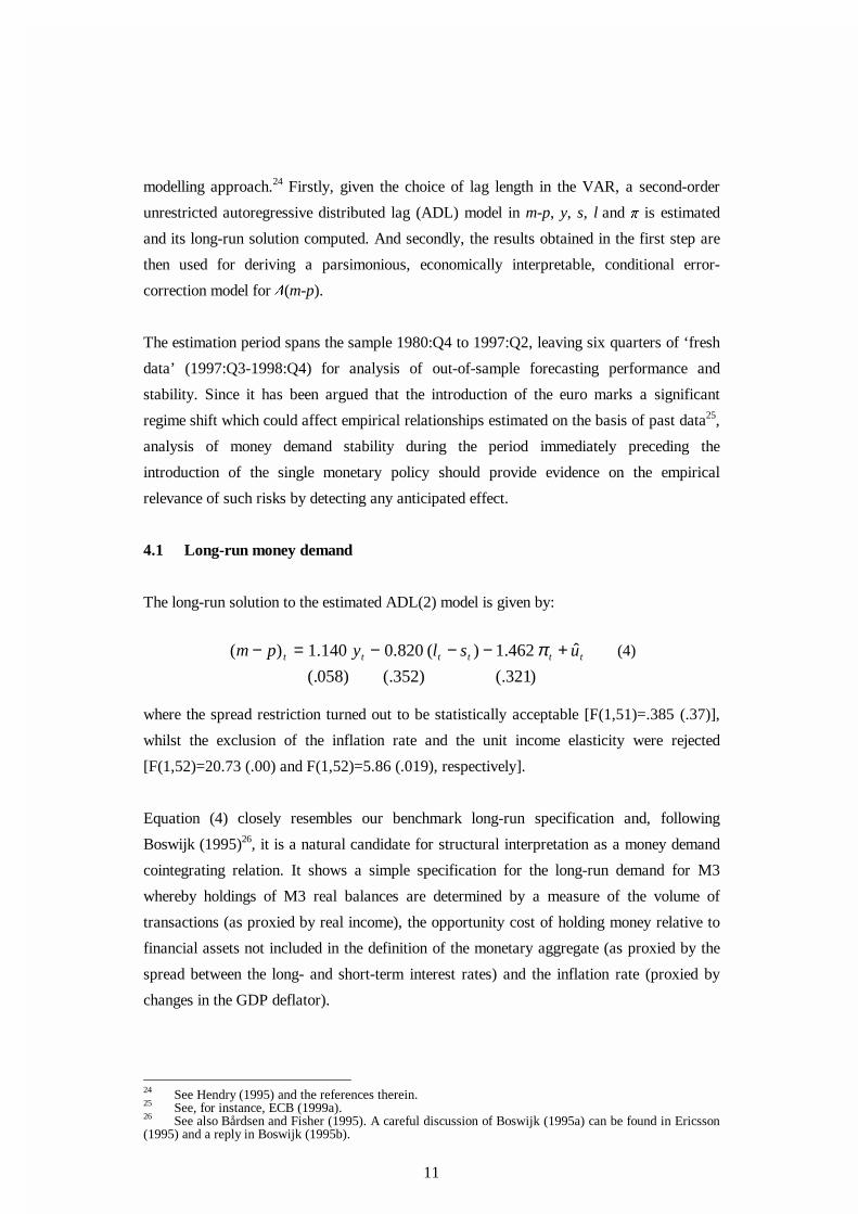
modelling approach.24 Firstly, given the choice of lag length in the VAR, a second-order

unrestricted autoregressive distributed lag (ADL) model in m-p, y, s, l and � is estimated

and its long-run solution computed. And secondly, the results obtained in the first step are

then used for deriving a parsimonious, economically interpretable, conditional error-

correction model for û(m-p).

The estimation period spans the sample 1980:Q4 to 1997:Q2, leaving six quarters of ‘fresh

data’ (1997:Q3-1998:Q4) for analysis of out-of-sample forecasting performance and

stability. Since it has been argued that the introduction of the euro marks a significant

regime shift which could affect empirical relationships estimated on the basis of past data25,

analysis of money demand stability during the period immediately preceding the

introduction of the single monetary policy should provide evidence on the empirical

relevance of such risks by detecting any anticipated effect.

4.1 Long-run money demand

The long-run solution to the estimated ADL(2) model is given by:

tttttt uslypm ˆ

)321(.

462.1)(

)352(.

820.0

)058(.

140.1)( +−−−=− π (4)

where the spread restriction turned out to be statistically acceptable [F(1,51)=.385 (.37)],

whilst the exclusion of the inflation rate and the unit income elasticity were rejected

[F(1,52)=20.73 (.00) and F(1,52)=5.86 (.019), respectively].

Equation (4) closely resembles our benchmark long-run specification and, following

Boswijk (1995)26, it is a natural candidate for structural interpretation as a money demand

cointegrating relation. It shows a simple specification for the long-run demand for M3

whereby holdings of M3 real balances are determined by a measure of the volume of

transactions (as proxied by real income), the opportunity cost of holding money relative to

financial assets not included in the definition of the monetary aggregate (as proxied by the

spread between the long- and short-term interest rates) and the inflation rate (proxied by

changes in the GDP deflator).

24 See Hendry (1995) and the references therein.25 See, for instance, ECB (1999a).26 See also Bårdsen and Fisher (1995). A careful discussion of Boswijk (1995a) can be found in Ericsson(1995) and a reply in Boswijk (1995b).

12

The signs and magnitudes of the estimated long-run coefficients also appear quite plausible

on theoretical grounds. The long-run income elasticity is estimated significantly above one

(1.14), a finding which is often interpreted as proxying omitted wealth effects in the demand

for money function.27 The estimated long-run semi-elasticities with respect to the spread

and the inflation rate are, respectively, -0.82 and -1.46 (though in both cases less precisely

estimated than the income coefficient).28 Equation 4 provides an explanation for the

downward trending behaviour of income velocity of M3 depicted in Figure 1.f in terms of

two main factors: firstly, the income elasiticity of money demand higher than one; and

secondly, the significant fall in the inflation rate witnessed by the euro area during the

sample period. The spread between the long- and the short-term interest rates, which shows

no particular trending behaviour when the entire sample is considered, does not appear to

contribute significantly to this long-term pattern of velocity. However, the low speed of

adjustment of this variable to its estimated long-run equilibrium indicates that its

contribution cannot be disregarded at medium-term horizons.

The income elasticity and the inflation semi-elasticity do not differ significantly from the

estimates obtained within the system approach in Section 3, providing further evidence on

the validity of weak exogeneity when the parameters of interest are the long-run parameters

of money demand. In this latter respect, formal statistical tests do not reject at standard

confidence levels that the long-run relationship given by (4) lies in the cointegration space

estimated within the system approach used in Section 3. The tests yield $22 =.43 [.43] (if the

cointegration space is estimated unrestrictedly), $62 =5.60 [.47] (if the cointegration space is

estimated under H01@+0

2) and $102 =9.71 [.47] (if the cointegration space is estimated under

H01@+0

2@+0

3).

The parameters of equation (4) above turn out to be pretty stable in recent times, both

within and out of the estimation sample. In this respect, Figure 2 shows their recursive

estimates from 1993:Q4 onwards when the equation is estimated over the extended period

up to 1998:Q4. More precisely, the figure plots the deviations of the long-run income,

spread and inflation parameters with respect to the values reported in (4) above. Similar

recursive estimates for the deviations from the hypothesis of long-run price homogeneity are

also shown in the graph. In this latter respect, the recursive estimates suggest that long-run

27 Some evidence at the MU level on the relevance of wealth in the long-run demand for money functioncan be found in Fase and Winder (1997,1999).28 The relative size of these two coefficients is somewhat counter-intuitive if the latter were to beinterpreted as the sensibility of money demand to non-financial assets. As argued in Section 2.1, however,this is not the only possible interpretation for the inclusion of the inflation rate in dynamic models of moneydemand.

13

price homogeneity, which was assumed in Section 2 and which is maintained throughout the

paper, is an acceptable characterisation for our estimates of long-run money demand.

4.2 A dynamic model of money demand

Whilst the unrestricted ADL model is valuable for computing the long-run equation (4), it

is clearly over-parameterised for many other purposes. Therefore, we proceeded in a second

step to estimate a parsimonious dynamic model for money demand which were both

economically interpretable and statistically acceptable. The estimation results for the period

1980:Q4-1997:Q2 are summarised in equation (5) below (t-ratios in parentheses):

( ) ttt

ttttt

DUMslypm

lsypm

12

12

ˆ86

)92.4(

009.]462.1)(820.140.1[

)17.11(

136.

)73.10(

526.

)43.4(

359.

)63.2(

194.

)86.1(

075.

)07.11(

739.)(

ωπ

π

+−+−+−−−

∆−∆−∆+∆+−=−∆

−

−

(5)

T=67 (1980:Q4-1997:Q2) R2=0.80 1=0.231% DW=2.17

LM(1)= .478 [.49] LM(4)=.137 [.71] LM(1,4)=.787 [.13]

ARCH(4)=.286 [.89] HET=.650 [.79] NORM=.824 [.66]

RESET=.164 [.69] RED=.456 [.81] HANS1=.060

HANS2=.589 FOR(6)=6.28 [.39] CHOW(6)=1.02 [.42]

where 2

1−∆+∆=∆ tt

t

sss and

21−∆+∆

=∆ ttt

πππ , and where LM(i) and LM(1,i) stand

for the Lagrange multiplier F-tests for residual autocorrelation of order ith and up to the ith

order, respectively,29 ARCH is the Engle (1982) F-test for autoregressive conditional

heteroskedasticity, HET is the White (1980) F-test for heteroskedasticity, NORM is the

Doornik and Hansen (1994) χ2-test for normality, RESET is the regression specification F-

test due to Ramsey (1969), RED tests whether model (5) parsimoniously encompasses the

unrestricted ADL(2) model, HANS1 and HANS2 are tests for variance and parameter

within-sample stability, following Hansen (1992), FOR and CHOW are the out-of-sample

forecast test and the Chow test for parameter stability over the period 1997:Q3-1998:Q4.

Figure 3 records the time series of fitted and actual values for û�P�S�, the scaled residuals

29 See Harvey (1990) for a description.

14

from the model, the residual correlogram and the sequence of 1-step forecasts of û�P�S� for

the period 1997:Q3-1998:Q4.

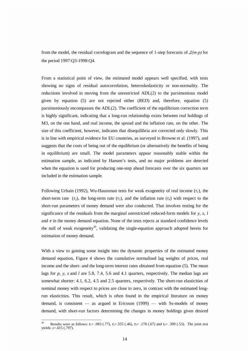
From a statistical point of view, the estimated model appears well specified, with tests

showing no signs of residual autocorrelation, heteroskedasticity or non-normality. The

reductions involved in moving from the unrestricted ADL(2) to the parsimonious model

given by equation (5) are not rejected either (RED) and, therefore, equation (5)

parsimoniously encompasses the ADL(2). The coefficient of the equilibrium correction term

is highly significant, indicating that a long-run relationship exists between real holdings of

M3, on the one hand, and real income, the spread and the inflation rate, on the other. The

size of this coefficient, however, indicates that disequilibria are corrected only slowly. This

is in line with empirical evidence for EU countries, as surveyed in Browne et al. (1997), and

suggests that the costs of being out of the equilibrium (or alternatively the benefits of being

in equilibrium) are small. The model parameters appear reasonably stable within the

estimation sample, as indicated by Hansen’s tests, and no major problems are detected

when the equation is used for producing one-step ahead forecasts over the six quarters not

included in the estimation sample.

Following Urbain (1992), Wu-Haussman tests for weak exogeneity of real income (21), the

short-term rate (22), the long-term rate (23), and the inflation rate (24) with respect to the

short-run parameters of money demand were also conducted. That involves testing for the

significance of the residuals from the marginal unrestricted reduced-form models for y, s, l

and � in the money demand equation. None of the tests rejects at standard confidence levels

the null of weak exogeneity30, validating the single-equation approach adopted herein for

estimation of money demand.

With a view to gaining some insight into the dynamic properties of the estimated money

demand equation, Figure 4 shows the cumulative normalised lag weights of prices, real

income and the short- and the long-term interest rates obtained from equation (5). The mean

lags for p, y, s and l are 5.8, 7.4, 5.6 and 4.1 quarters, respectively. The median lags are

somewhat shorter: 4.1, 6.2, 4.5 and 2.5 quarters, respectively. The short-run elasticities of

nominal money with respect to prices are close to zero, in contrast with the estimated long-

run elasticities. This result, which is often found in the empirical literature on money

demand, is consistent — as argued in Ericsson (1999) — with Ss-models of money

demand, with short-run factors determining the changes in money holdings given desired

30 Results were as follows: 21= .083 (.77), 22=.555 (.46), 23= .178 (.67) and 24= .399 (.53). The joint testyields: 2=.415 (.797).

15

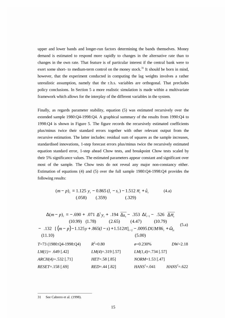
upper and lower bands and longer-run factors determining the bands themselves. Money

demand is estimated to respond more rapidly to changes in the alternative rate than to

changes in the own rate. That feature is of particular interest if the central bank were to

exert some short- to medium-term control on the money stock.31 It should be born in mind,

however, that the experiment conducted in computing the lag weights involves a rather

unrealistic assumption, namely that the r.h.s. variables are orthogonal. That precludes

policy conclusions. In Section 5 a more realistic simulation is made within a multivariate

framework which allows for the interplay of the different variables in the system.

Finally, as regards parameter stability, equation (5) was estimated recursively over the

extended sample 1980:Q4-1998:Q4. A graphical summary of the results from 1990:Q4 to

1998:Q4 is shown in Figure 5. The figure records the recursively estimated coefficients

plus/minus twice their standard errors together with other relevant output from the

recursive estimation. The latter includes: residual sum of squares as the sample increases,

standardised innovations, 1-step forecast errors plus/minus twice the recursively estimated

equation standard error, 1-step ahead Chow tests, and breakpoint Chow tests scaled by

their 5% significance values. The estimated parameters appear constant and significant over

most of the sample. The Chow tests do not reveal any major non-constancy either.

Estimation of equations (4) and (5) over the full sample 1980:Q4-1998:Q4 provides the

following results:

tttttt uslypm ˆ

)329(.

512.1)(

)359(.

865.0

)058(.

125.1)( +−−−=− π (4.a)

( ) ttt

ttttt

DUMslypm

lsypm

12

12

ˆ86

)00.5(

0095.]512.1)(865.125.1[

)10.11(

132.

)79.10(

526.

)47.4(

353.

)65.2(

194.

)78.1(

071.

)99.10(

690.)(

ωπ

π

+−+−+−−−

∆−∆−∆+∆+−=−∆

−

−

(5.a)

T=73 (1980:Q4-1998:Q4) R2=0.80 1=0.230% DW=2.18

LM(1)= .649 [.42] LM(4)=.319 [.57] LM(1,4)=.734 [.57]

ARCH(4)=.532 [.71] HET=.58 [.85] NORM=1.53 [.47]

RESET=.158 [.69] RED=.44 [.82] HANS1=.041 HANS2=.622

31 See Cabrero et al. (1998).

16

4.3 Some results on aggregation

As pointed out in Section 2.2, a number of methods for the calculation of historical

aggregated series for the euro area have been employed in existing empirical work. It is also

fair to say that any choice between them is somewhat arbitrary, reflecting the fundamental

problem that it is only from 1999 onwards that a single currency is in place. In particular,

the time series for area-wide M3 employed above is calculated backwards from September

1997 M3 levels in euro, using an output-weighted average of participating countries’

developments. As discussed, this method of aggregation provides for a coherent historical

calculation of euro area monetary aggregates, on the one hand, and the r.h.s. variables in

the money demand equation, on the other. Of particular interest is that the resulting growth

rates for M3 are consistent with the concept of area-wide inflation most widely used in

economic analysis, i.e. a weighted average of countries’ inflation rates.

One drawback, however, is that the aggregation method departs from the compilation

procedures for euro area monetary which are in place since the start of Stage Three,

whereby national data are aggregated in a common currency, the euro, using the irrevocable

conversion rates announced on 31 December 1998. Since this may potentially have

implications if the estimated models were to be used in the new context, we explore below

the effect that the use of euro area M3 compiled on the basis of fixed conversion rates (as

published in ECB, 1999b) may have on our estimates whilst noting that a discrepancy with

respect to the way in which the remaining variables in our analysis are calculated is

introduced.

On a conceptual basis, M3 growth figures resulting from both aggregation procedures can

be interpreted as weighted averages of the estimated historical national contributions with

weights depending on the method employed. Under the first aggregation method, weights

are fixed and are calculated as countries’ shares in area-wide GDP evaluated at PPP rates.

Under the second, weights are time varying and depend on countries’ shares on area-wide

money M3 evaluated at fixed conversion rates. On average, the second method gives more

weight to countries with higher liquidity ratios.

At the empirical level, a first conclusion that can be drawn from visual inspection of Figure

6 is that the difference between the two aggregation procedures cannot be overstated. The

figure plots the levels (Figure 6a) and the quarterly growth rates (Figure 6b) of M3

resulting from the application of the two aggregation methods. Both series in levels move

closely together for most of the sample period with differences mainly concentrated at the

17

beginning of the eighties. The differences in the quarterly growth rates are of moderate size

in statistical terms when compared, for instance, with the standard error reported in

equation (5) above. They are quite persistent, however, implying long-lasting effects when

the levels of the series are considered. Thus, during the first half of the eighties the output-

weighted M3 grew around 5% more in cumulative terms than the corresponding aggregate

computed using the fixed conversion rates.

Formal analysis using the Johansen procedure confirms that both time series do cointegrate

with cointegrating vector (1, -1). That in turn suggests that the cointegration results

reported in Section 3 would be little affected by the change in the aggregation method for

M3. Table 2 confirms this intuition by reproducing the analysis in Section 3 and Table 1

for the monetary aggregate M3 computed using the fixed conversion rates. None of the

conclusions in Section 3 are changed by the evidence presented in the table.

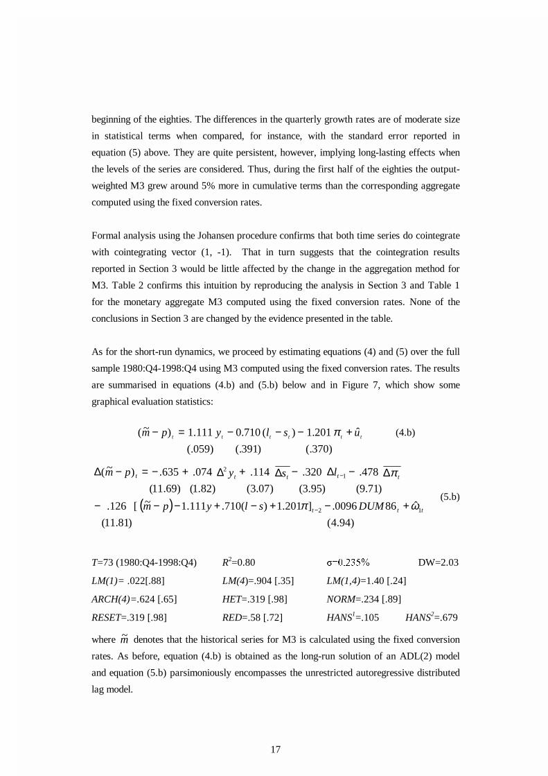
As for the short-run dynamics, we proceed by estimating equations (4) and (5) over the full

sample 1980:Q4-1998:Q4 using M3 computed using the fixed conversion rates. The results

are summarised in equations (4.b) and (5.b) below and in Figure 7, which show some

graphical evaluation statistics:

tttttt uslypm ˆ

)370(.

201.1)(

)391(.

710.0

)059(.

111.1)~( +−−−=− π (4.b)

( ) ttt

ttttt

DUMslypm

lsypm

12

12

ˆ86

)94.4(

0096.]201.1)(710.111.1~[

)81.11(

126.

)71.9(

478.

)95.3(

320.

)07.3(

114.

)82.1(

074.

)69.11(

635.)~(

ωπ

π

+−+−+−−−

∆−∆−∆+∆+−=−∆

−

−

(5.b)

T=73 (1980:Q4-1998:Q4) R2=0.80 1 ������ DW=2.03

LM(1)= .022[.88] LM(4)=.904 [.35] LM(1,4)=1.40 [.24]

ARCH(4)=.624 [.65] HET=.319 [.98] NORM=.234 [.89]

RESET=.319 [.98] RED=.58 [.72] HANS1=.105 HANS2=.679

where m~ denotes that the historical series for M3 is calculated using the fixed conversion

rates. As before, equation (4.b) is obtained as the long-run solution of an ADL(2) model

and equation (5.b) parsimoniously encompasses the unrestricted autoregressive distributed

lag model.

18

Comparison of (4.b) and (5.b) with (4.a) and (5.a) indicates that the change of aggregation

method for M3 does not have any noticeable impact either on the long- or the short-run

parameters of money demand, with differences in point estimates always well within one

standard error. That in turn suggests that it is unlikely that the shift to the calculation of

euro area M3 using fixed conversion rates may in itself render our results useless in the

context of Stage Three.

Although (based on the respective estimated standard errors) there appears to be little to

choose between both aggregation procedures, encompassing tests were conducted with a

view to discriminating between the two competing models (5.a) and (5.b). In order to deal

with different dependent variables, we follow the approach that Ericsson, Hendry and Tran

(1994) take for testing models with seasonal adjusted data versus models with non-

seasonally adjusted data. In this context, the hypothesis that (5.a) encompasses (5.b) [H0a]

can be tested by adding )~( mm −∆ and the error correction term in (5.b) to equation (5.a)

and testing for their joint significance. Conversely, the null that (5b) encompasses model

(5a) [H0b] can be tested by adding )~( mm −∆ and the error correction term in (5.a) to

equation (5.b). Likelihood ratio tests for these hypotheses provide the following results (p-

YDOXHV LQ SDUHQWKHVHV�� $2��� ���� ������ DQG $

2(2)= 4.25 (.120) for the nulls H0a and H0

b,

respectively. Therefore, although neither H0a nor H0

b can be formally rejected at standard

confidence levels, it appears that the evidence for H0b is less compelling, somewhat

favouring (5.a) over (5.b). Recursive computation of the encompassing tests tends to

confirm this conclusion.

5 An impulse response analysis of the multivariate money demand system

In order to overcome the rather unrealistic assumptions which underlie the analysis of the

dynamic properties of money demand in Section 4.2, we now step back to the multivariate

money demand system and investigate the dynamic interactions of all its variables by means

of the system's impulse response functions. The computation of the impulse response

functions starts from the system incorporating the long-run money demand relationship (4)

within the cointegration space estimated under H01@+0

2@+0

3. The employed methods which

are extensions of structural VAR methods to cointegrated systems have recently been

developed in Vlaar (1998) and are briefly reviewed in Annex 2. In Vlaar and Schuberth

(1999) these methods are applied to address the issue of controllability of a broad monetary

aggregate which was computed from old harmonised M3 data for the EU countries without

Luxembourg.

19

5.1 The identification of the structural innovations

Given the outcome of our empirical analysis of the 5 - dimensional money demand system

with 3 cointegrating vectors, we explore the system's dynamic properties by means of its

impulse responses, ∞=0}{ iiB , to a set of underlying structural innovations. The identification

of these structural innovations will be achieved by separating them along two dimensions.

First, we separate 2 structural innovations having permanent effects from 3 innovations

with merely transitory effects. Within each of the two subsets, we then identify innovations

which are assumed to be related to monetary policy. In view of this objective, let us

tentatively label the innovations — in order of their occurrence within the system — as an

aggregate supply shock, a change in the monetary policy objective, an aggregate demand

shock, a money demand shock and an interest rate shock with the first two having

permanent effects.32

Following Vlaar and Schuberth (1999), the two monetary policy shocks are assumed to

have either permanent or merely transitory effects. The first, which is labelled as a change

in the monetary policy objective, is thought to capture the nominal stochastic trend within

our sample. The second is assumed to capture the transitory element of monetary policy.

Our label suggests that it should be likely to show up as an innovation to the short-term

nominal interest rate which is supposed to be the monetary policy instrument.33 Aggregate

demand and aggregate supply shocks are considered to be the most important factors

driving real GDP which, in turn, acts as the scale variable determining money demand.

Beyond being orthogonal to the other structural innovations, the money demand shock is

assumed to be orthogonal to any contemporaneous variable affecting money demand. It

should thus closely resemble the error term in our conditional money demand model.

Starting from an estimate of the system's covariance matrix Σ and its so-called total impact

matrix )1(C , we have to impose a set of at least 10 independent restrictions on either its

contemporaneous impact matrix BB =0 , where BB ′=Σ , or its long-run impact matrix

32 As a matter of fact, the economic variables comprising the system will be subject to a larger number ofshocks (shocks to the term structure, foreign interest rate shocks, exchange rate shocks, etc.). In thisconnection, it is clear that the empirical model under investigation is unlikely to encompass all the relevantaspects of the monetary transmission process. From a methodological point of view, that raises the questionof whether the identified shocks can be interpreted as structural as incorporated in the underlyingassumption of their orthogonality. The choice of the above labels reflects the underlying untested assumptionthat the respectively labelled shocks are the most relevant ones for purposes at hand. Ericsson, Hendry andMizon (1998) provide an insightful discussion of the problems involved in interpreting impulse responseanalysis.33 The identification of the monetary policy shocks disregards any problem which may be due to theoperation of the EMS according to which a number of participating countries had to use the short-terminterest rate as an instrument for fixing the exchange rate instead of gearing it directly to the ultimateobjective of monetary policy.

20

BCB )1(=∞ in order to identify the vector of structural innovations.34 Since any particular

set of identifying restrictions will be subject to controversial discussion, we have chosen to

follow a conservative two-step identification strategy. In the first step, we impose a set of

exactly identifying restrictions which borrow as far as possible from the outcome of our

empirical analysis but leave the effects of the two monetary policy shocks unconstrained. In

the second step, we then impose a set of additional, over-identifying restrictions which are

designed to characterise the latter. As these additional restrictions must be considered

crucial a priori, they will be tested for their compatibility with the data.

To separate the 2 shocks having permanent effects from the 3 shocks with merely transitory

effects we start with restricting the long-run impact of the latter:

(R.1) The aggregate demand shock, the money demand shock and the interest rate shock

have a zero long-run impact on the levels of all the variables within the cointegrated

system, i.e. 0))1(( =ijBC for 5,...,1=i and 5,4,3=j .

In order to mutually identify the 2 shocks with permanent effects, i.e. to separate the effects

of the aggregate supply shock from those of the change in the monetary policy objective, we

impose a single restriction on the long-run impact of the former:

(R.2) The aggregate supply shock does not affect GDP inflation in the long run, i.e.

0))1(( 51 =BC .

Restriction (R.2) implies that monetary policy anchors inflation which is consistent with the

widely held view that inflation is a monetary phenomenon in the long run.

To mutually identify the 3 shocks with merely transitory effects, a set of at least 3

restrictions have to be imposed on their contemporaneous impacts. Here, we assume:

(R.3) GDP inflation is not contemporaneously affected by the aggregate demand shock,

i.e. 053 =B .

(R.4) The money demand shock does not contemporaneously affect real GDP, the nominal

short and long-term interest rates and GDP inflation, i.e. 054443424 ==== BBBB .

Restriction (R.3) corresponds to the assumption that inflation adjustment is sluggish,35

while the restrictions given by (R.4) reflect our assumption that the money demand shock is

34 Refer to Annex 2 for details.35 This view is widely supported by empirical evidence and has been adopted, for instance, by Fuhrer andMoore (1995) in modelling the inflation process.

21

orthogonal to all contemporaneous variables entering the conditional money demand model.

Thereby it is implicitly assumed that money supply fully accommodates contemporaneous

movements in money demand which, in turn, is in line with our presumption that the short-

term nominal interest rate serves as the monetary policy instrument.

Up to now a set of 21 restrictions are imposed. Due to the reduced rank of the total impact

matrix )1(C , however, only 6 out of the 15 zero restrictions given by (R.1) are linearly

independent. Similarly, only 2 out of the 4 zero restrictions given by (R.4) turn out to be

independent.36 Disregarding the 11 redundant restrictions, there are in total 10 independent

restrictions which indeed exactly identify B and, thus, the structural innovations.

The effects of the monetary policy shocks have been left unrestricted for the time being.

The identification of these shocks may thus suffer from capturing influences which affect

the variables of our money demand system but which are not due to monetary policy.

Therefore, in order to end up with a more thorough characterisation of the effects of

monetary policy, we impose a set of over-identifying restrictions. Firstly, we assume:

(R.5) Real GDP is not contemporaneously affected by both the change in the monetary

policy objective and the interest rate shock, i.e. 02522 == BB .

These restrictions are consistent with the assumption that monetary policy shocks affect

real activity only with some delay which seems plausible for a system based on quarterly

data. In structural VAR analyses of quarterly US data, for instance, the restriction on the

impact response of real GDP proves to be an identifying assumption which makes the

impulse responses of the VAR models match the a priori views on the effects of a monetary

policy shock.37

Secondly, we impose:

(R.6) A change in the monetary policy objective does not affect real GDP in the long run,

i.e. 0))1(( 22 =BC .

36 This outcome is due to the particular set of zero restrictions we have imposed on the vector of theloading matrix corresponding to the long-run money demand relationship. These zero restrictions imply thatthe orthogonal complement of the loading matrix has a zero row which, in turn, implies that the total impactmatrix of the system's reduced-form representation has a zero column. Given two zero restrictions on thecontemporaneous impact vector of the money demand shock, we then end up with a homogenous linearequation system which determines the two remaining elements of the contemporaneous impact vector that donot correspond to real money holdings to be zero too. But this means that any pair of zero restrictionsimposed on its contemporaneous impact will suffice to identify the money demand shock.37 See Bernanke and Blinder (1992) and Bernanke and Mihov (1995).

22

This restriction implies that real GDP will be exclusively driven by supply shocks in the

long run, where the supply shocks may be interpreted as realisations of an underlying

stochastic productivity trend.

Since the level of real GDP will not be affected by the level of the inflation rate in the long

run, neutrality, indeed super-neutrality of monetary policy is implied by restriction (R.6),

whereas restriction (R.2) guarantees that inflation is a monetary phenomenon in the long

run. Taken together, these two restrictions imply that the long-run outcome of the impulse

response analysis is dichotomous. Although this may be overly rigid in view of empirical

findings, it will be useful in discussing the impulse response functions of the multivariate

money demand system by providing a benchmark.

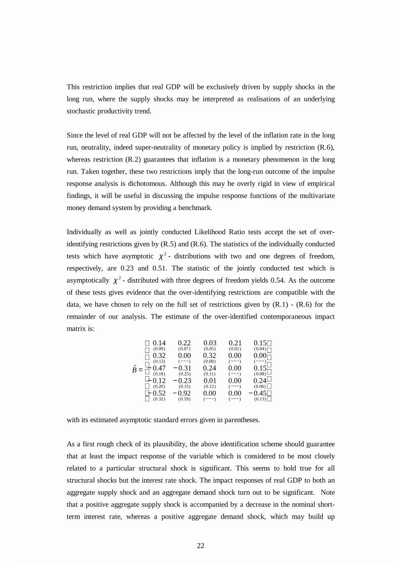
Individually as well as jointly conducted Likelihood Ratio tests accept the set of over-

identifying restrictions given by (R.5) and (R.6). The statistics of the individually conducted

tests which have asymptotic 2χ - distributions with two and one degrees of freedom,

respectively, are 0.23 and 0.51. The statistic of the jointly conducted test which is

asymptotically 2χ - distributed with three degrees of freedom yields 0.54. As the outcome

of these tests gives evidence that the over-identifying restrictions are compatible with the

data, we have chosen to rely on the full set of restrictions given by (R.1) - (R.6) for the

remainder of our analysis. The estimate of the over-identified contemporaneous impact

matrix is:

−−−

−−

−−=

−−−−−−

−−−

−−−

−−−−−−−−−

)13.0()()()19.0()32.0(

)06.0()()12.0()15.0()20.0(

)08.0()()11.0()25.0()18.0(

)()()08.0()()13.0(

)04.0()02.0()05.0()07.0()09.0(

45.000.000.092.052.0

24.000.001.023.012.0

15.000.024.031.047.0

00.000.032.000.032.0

15.021.003.022.014.0

B̂

with its estimated asymptotic standard errors given in parentheses.

As a first rough check of its plausibility, the above identification scheme should guarantee

that at least the impact response of the variable which is considered to be most closely

related to a particular structural shock is significant. This seems to hold true for all

structural shocks but the interest rate shock. The impact responses of real GDP to both an

aggregate supply shock and an aggregate demand shock turn out to be significant. Note

that a positive aggregate supply shock is accompanied by a decrease in the nominal short-

term interest rate, whereas a positive aggregate demand shock, which may build up

23

inflationary pressures, is accompanied by an increase in the nominal short-term interest

rate. Both interest rate responses which are consistent with an easing or a tightening of

monetary policy, respectively, prove to be significant.

A downward change in the monetary policy objective results in a significant decline in the

inflation rate though merely in an insignificant move of the nominal interest rates. As

imposed, a positive money demand shock induces solely an increase in real money holdings.

Note that the impact response of real money holdings is of the same order of magnitude as

the estimated standard error of the residuals of the conditional money demand model. The

impact effect turns out to be 0.21 while the estimated standard error of the residuals is 0.23.

With respect to the identification of the structural innovation which was labelled as an

interest rate shock some doubts arise. The estimated impact response of the nominal short-

term interest rate proves to be merely borderline significant. On the contrary, the impact

responses of real money holdings, the long-term nominal interest rate and, in particular, the

inflation rate turn out to be significant. But let us postpone addressing this issue until

discussing the results of the impulse response analysis. These are presented in the next

subsection.

5.2 The structural impulse response functions

Based on the full set of restrictions given by (R.1) - (R.6), the Figures 8 - 12 show the

structural impulse response functions of the variables of the cointegrated system, i.e. real

money holdings pm − , real GDP y , the short- and long-term nominal interest rates s and

l , and (annualised) GDP inflation π . In addition, we report the impulse response functions

for a set of derived variables: the spread sl − , the short- and long-term real interest rates

π−s and π−l , the GDP deflator p , which is obtained by integrating the (quarterly) rate

of GDP inflation 4/π , and nominal money holdings m . In order to give an indication of

the underlying statistical uncertainty, the figures display the impulse response functions

plus/minus twice their asymptotic standard errors. As shown by these standard errors quite

a few of the impulse response functions are statistically insignificant. Clearly this reflects

the sampling variability in the estimated parameters of the cointegrated system and the large

amount of uncertainty due to the system's stochastic trends. Any interpretation of the

impulse response functions has therefore to bear in mind that they may provide only

imprecise information about the true underlying economic relations.

24

(a) A positive aggregate supply shock

A shock to aggregate supply (Figure 8) moves real GDP and GDP inflation in opposite

directions on impact. These movements are consistent with the assumption that firms are

operating under monopolistic competition by setting prices as a mark-up on average

production costs: If a positive aggregate supply shock resembles an upward shift in

productivity, production will increase while prices will decline due to the reduction in

average production costs. Whereas the effect on GDP is permanent, inflation returns to its

steady-state level in the long run, as has been imposed in (R.2) above. Due to the temporary

fall in inflation there is some leeway for monetary policy to ease. While there is a

significant instantaneous fall in the nominal short-term interest rate, however, the short-

term real interest rate declines only gradually. Consistent with the expectation theory of the

term structure, the long-term nominal interest rate decreases but less than the short-term

rate, thereby inducing a temporary increase in their spread. Both the short and long-term

nominal interest rates return to their original steady-state levels. Given that the effect of the

supply shock on GDP inflation dies out, this outcome reflects our empirical findings that

the long-term real interest rate as well as the spread constitute cointegrating relationships

which are automatically accounted for when computing the system's impulse response

functions. Similarly, real money holdings increase in line with the long-run money demand

specification as obtained from our conditional analysis. Whereas the effect on nominal

money holdings can be neglected, there is a permanent decrease in the price level which is

due to the temporary fall in inflation.

(b) A downward change in the monetary policy objective

Changes in the monetary policy objective are thought to capture the nominal stochastic

trend in the sample. Given the historical evidence for the member countries of the monetary

union, a downward change in the monetary policy objective has a natural interpretation in

terms of a possibly pre-announced commitment to lower inflation. Of course, as there was

no single monetary policy authority which could have announced a decline in its inflation

objective, the chosen label remains fictitious but nevertheless serves as an intuitive means

of interpreting the average disinflation policies within the member countries. At a

theoretical level, we can separate the liquidity effect of a disinflation policy from its

expectation effect.38 As long as the commitment to decrease inflation is perfectly credible

and prices are flexible it would be feasible to reduce inflation on impact. Moreover, the

lowering of inflation would even be achievable by adjusting the nominal short-term interest

38 See Christiano and Eichenbaum (1992) for a thorough discussion of the operation of the liquidity andexpectation effects in a dynamic general equilibrium setting; and Christiano, Eichenbaum and Evans (1996) for related empirical evidence.

25

rate downwards instantaneously if monetary policy operated exclusively via the expectation

channel.

Although disregarding the liquidity effect seems somewhat unrealistic in view of empirical

findings, the computed impulse response functions (Figure 9) are indeed in line with such a

perception: Inflation falls on impact, even overshooting its new steady state level, and the

nominal short-term interest rate declines. Real GDP is not contemporaneously affected

since it has been imposed in (R.5) but the short-term real interest rate rises on impact. Due

to the temporary rise of the short-term real interest rate, real GDP is transitorily suppressed

in the subsequent periods but returns to its steady state level in the long run, as imposed in

(R.6). This hump-shaped adjustment path of real GDP suggests that disinflation is costly

even if there is a strong initial expectation effect. Given the stationarity of the real rates,

both nominal interest rates decline by the same amount as the inflation rate in the long run.

Furthermore, consistent with our long-run money demand relationship, real money holdings

stabilise at a higher level reflecting the lower opportunity costs of holding money due to the

decline in the steady-state inflation rate. The price level and nominal money holdings drift

away as implied by the permanently lower inflation rate.

(c) A positive aggregate demand shock

The impulse responses to the aggregate demand shock (Figure 10) are in line with what we

would have expected a priori. The significant increase in real GDP creates inflationary

pressures which are counteracted by a tightening of monetary policy in a forward-looking

manner via an increase in the nominal short-term interest rate. Due to the sluggishness of

inflation, as imposed in (R.3), this response feeds through to the real short-term interest rate

one to one. In line with the expectation theory, the long-term nominal interest rate shows a

more moderate rise than the short-term rate, thereby implying a flattening of the yield

curve. Whereas real GDP declines monotonously, GDP inflation follows a typical humped-

shaped adjustment path. Real money holdings build up with some delay but return to their

steady state in the long run. On the other hand, nominal money holdings increase

permanently. As real, but not nominal money holdings are restricted to be unaffected in the

long run, the increase in the latter just compensates for the permanent increase in the GDP

deflator which is caused by the temporary rise in inflation.

(d) A positive money demand shock

Given the restrictions imposed in (R.4), the shock in money demand (Figure 11) affects

only real money holdings contemporaneously. In the subsequent periods, however, real

GDP rises significantly. This response may be interpreted in terms of a wealth effect

26

operating through temporarily accumulated real balances. The increase in real GDP, in

turn, causes a rise in GDP inflation which is counteracted by a tightening of monetary

policy. In view of these findings, it is evident that the system's impulse responses to the

money demand shock closely resemble the pattern of the impulse responses to an aggregate

demand shock as far as the lag due to the operation of the real balance effect is taken into

account. Accordingly, both the GDP deflator and nominal money holdings increase

permanently, whereas the effects on real money holdings die out in the long run. Note that

the rise in nominal money holdings proves to lead the increase in the price level due to the

sluggish adjustment of inflation. Of course, as this outcome is specific to the money

demand shock under investigation it does not follow that nominal money is in general a

leading indicator for future price level developments.

(e) A positive interest rate shock

The interest rate shock (Figure 12) is assumed to capture the transitory element of monetary

policy. Consistent with the commonly-held view on the outcome of a monetary contraction,

the impulse responses of real GDP show a hump-shaped pattern: Real GDP starts to

decline with some delay, as implied by the contemporaneous restriction in (R.5), reaches a

trough after a few periods and starts to recover subsequently. As in the case of the change

in the monetary policy objective, the decline in real GDP follows an increase in the short-

term real interest rate driven by both the tightening of monetary policy and the initial drop

in the inflation rate.

Real money holdings increase on impact in response to the interest rate shock. Since real

GDP is not affected contemporaneously, there remain three variables which simultaneously

account for the response of real money holdings. Firstly, the demand for real money

holdings is stimulated by the increase in the nominal short-term interest rate (measuring the

rate of return of the interest bearing components within the broad monetary aggregate under

investigation). Secondly, the increase in the nominal long-term interest rate (measuring the

opportunity cost of real money holdings in terms of alternative financial assets) dampens

the demand for real money holdings. Thirdly, the demand for real money holdings is

increased by the initial drop in inflation (measuring the opportunity cost of real money

holdings in terms of real assets). Subsequent to their initial increase, real money holdings

start to fall. This fall is presumably driven by the temporary decline in real GDP since the

joint effect of the nominal interest rates, as measured by their spread, and inflation appears

to be of second order magnitude.

27

Given the impulse responses of real money holdings and the GDP deflator, nominal money

holdings, though imprecisely estimated, decline in the medium to long run. This outcome

gives some tentative evidence that, over those horizons, the money stock is controllable via

the various channels of transmission through which monetary policy operates. To the

contrary, the mute short-run response of nominal money holdings appears to indicate that

short-term controllability of M3 would likely be problematic. These results, however, may

be adversely affected by the strong impact response of the inflation rate which turns out to

be implausible. On the one hand, the impact response of inflation might capture effects

which are due to monetary policy but which are operating through channels not accounted

for in our system as, for instance, the exchange rate channel. On the other hand, the impact

response of inflation might be the outcome of shocks which are of relevance for the system

but which are not separately identified. Therefore, further investigation is required to obtain

a more reliable characterisation of the monetary policy shock and its ultimate effects on

money holdings.

6 Conclusions

Given the prominent role assigned to monetary aggregates in the monetary policy strategy

of the Eurosystem, the present paper has analysed some empirical evidence on the demand

for broad money M3 in the euro area. An attempt to account for the different dynamic

interactions between broad money, prices, real income and short and long-term interest

rates was also made using SVAR techniques by means of an impulse response analysis of

the cointegrated system. A number of conclusions can be drawn from the analysis.

Starting with the system results, three long-run relationships with economic content were

found: first, the spread between the long- and the short-term nominal interest rates,

consistent with the term structure of interest rates; second, the long- and short-term real

interest rates, consistent with the Fisher parity; and third, a long-run demand for broad

money M3 in the euro area. Furthermore, the impulse response analysis of the cointegrated

system provided an overall picture of the responses of the different variables to a number of

structural shocks which we tentatively labelled as: an aggregate demand shock, an

aggregate supply shock, a money demand shock, a transitory monetary policy shock and a

permanent monetary policy shock. The general patterns of the estimated dynamic responses

were broadly consistent with economic theory, though some of the results deserve further

investigation.

28

Turning to our central relation of interest, money demand, the empirical findings are

plausible from a number of perspectives. From an economic point of view, the long-run

demand for M3 in the euro area shows a simple specification whereby holdings of M3 real

balances are determined by real income, the opportunity cost of holding money relative to

financial assets not included in the definition of the monetary aggregate and the inflation

rate. The signs and magnitudes of the estimated long-run coefficients also appear quite

plausible on theoretical grounds. The long-run income elasticity is estimated significantly

above one (1.14), a finding which is often interpreted as proxying omitted wealth effects in

the demand for money function. The estimated long-run semi-elasticities with respect to the

spread and the inflation rate are, respectively, -0.82 and -1.46.

In the short run, changes in M3 holdings were modelled via an equilibrium correction model

whereby growth in real M3 is explained by the changes in income, interest rates and

inflation, on the one hand, and the extent to which M3 differs from its equilibrium level, on

the other. As surveyed in Browne et al. (1997), equilibrium correction models have proven

successful in modelling the demand for money in a number of EU countries and in the area

as a whole during the last decade. From a statistical point of view, the estimated models for

money demand show no sign of mis-specification and appear to be a congruent statistical

representation of the ‘average’ process which has driven broad money M3 in the euro area

during the sample period under investigation. When compared with the existing empirical

evidence on money demand in individual euro area-countries and in the euro-area as a

whole, as surveyed for instance in Browne et al. (1997), the estimated models fare quite

well in terms of stability, fit, residual standard errors, etc. In particular, the estimates

presented support the view reached by many previous studies that area-wide money demand

equations outperform most national equations.

The demand for broad money M3 equation turns out to be reasonably constant when

estimated recursively. This holds in the face of the dramatic economic changes which euro

area countries undertook during the estimation sample and poses the question of whether

the estimated models are of any use for monetary policy purposes in the context of Stage

Three. This issue is of utmost relevance, as it has been argued that the adoption of a single

monetary policy marks a significant regime shift, which could affect empirical economic

relationships estimated on the basis of pre-1999 data. The potential effects of the adoption

of a single currency are also argued to be of particular importance at the outset of Stage

Three in the financial sector of the economy, thereby affecting the behaviour of monetary

aggregates in the euro area. Unfortunately, it is not possible to test explicitly for parameter

invariance against such historical event, since it has no parallel within our estimation

29

sample, but the estimated models constitute useful benchmarks for monitoring structural

change in the early stages of Stage Three and for the evaluation of rival models as they

become available. Nonetheless, the empirical finding that the area-wide money demand

equation remains constant against a changing background in monetary policy co-ordination

between euro area countries during the sample period under investigation suggests that

instabilities in the models should not arise because of the introduction of the single currency

itself. Parameter constancy when the estimation sample is extended to cover 1997:Q3-

1998:Q4, a period in which the alleged instabilities should likely have shown up in

anticipation of EMU, is a further argument along this line of reasoning.

30

References

Angeloni, I., V. Gaspar and O. Tristani (1999), “The monetary policy strategy of theECB”, forthcoming in D. Cobham and G. Zis (eds.), From EMS to EMU, (Macmillan)London.Bå rdsen, G. and P.G. Fisher (1995), “The importance of being structured”, ArberdsnotatNorges Bank, 1995-1, Oslo.Blanchard, O.J. (1989), “A traditional interpretation of macroeconomic fluctuations”,American Economic Review, 79, 1146-1164.Blanchard, O.J. and D. Quah (1989), “The dynamic effect of aggregate demand andsupply disturbances”, American Economic Review, 79, 655-673.Boswijk, H.P. (1995a), “Efficient inference on cointegration parameters in structural errorcorrection models: Reply”, Journal of Econometrics, 69, 173-175.Boswijk, H.P. (1995b), “Efficient inference on cointegration parameters in structural errorcorrection models”, Journal of Econometrics, 69, 133-158.Bernanke, B.S. and A.S. Blinder (1992), “The Federal Funds Rate and the channels ofmonetary transmission”, American Economic Review, 82, 901-921.Bernanke, B.S. and I. Mihov (1995), “Measuring monetary policy”, NBER WorkingPaper No. 5145, Cambridge, MA.Browne, F., G. Fagan and J. Henry (1997), “Money demand in EU countries: a survey”,EMI Staff Papers, 7.Cabrero, A., J.L. Escrivá , E. Muñ oz and J. Peñ alosa (1998), “The controllability of amonetary aggregate in EMU”, Banco de España, Servicio de Estudios, Documento deTrabajo 9817.Cheung, Y. and K.S. Lai (1993), “Finite-sample sizes of Johansen’s likelihood ratio testsfor cointegration”, Oxford Bulletin of Economics and Statistics, 55, 313-328.Christiano, L.J. and M. Eichenbaum (1992), “Liquidity effects and the monetarytransmission mechanism”, American Economic Review, 82, 346-353.Christiano, L.J., M. Eichenbaum and C. Evans (1996), “Sticky price and limitedparticipation models of money: a comparison”, Northwestern University, Evanston, IL.Davidson, J. (1998), “Structural relations, cointegration and identification: some simpleresults and their application”, Journal of Econometrics, 87, 87-113.Doornik, J.A. and H. Hansen (1994), “An omnibus test for univariate and multivariatenormality”, Discussion Paper No. W4&91, Nuffield College, Oxford.ECB (1999a), “The stability-oriented monetary policy strategy of the Eurosystem”, ECBMonthly Bulletin, January.ECB (1999b), “Euro area monetary aggregates and their policy role in the Eurosystem’smonetary policy strategy”, ECB Monthly Bulletin, February.Engle, R.F. (1982), “Autoregressive conditional heteroscedasticy with estimates of thevariance of United Kingdom inflation”, Econometrica, 50, 987-1007.Engle, R.F. and C.W.J. Granger (1987), “Co-integration and error correction:representation, estimation and testing”, Econometrica, 55, 251-276.Ericsson, N.R. (1995), “Conditional and structural error correction models”, Journal ofEconometrics, 69, 159-171.Ericsson, N.R. (1999), “Empirical modelling of money demand”, in H. Lütkepohl and J.Wolters (eds.), Money Demand in Europe, (Physica-Verlag) Heidelberg, 29-49.Ericsson, N.R., D.F Hendry and G.E. Mizon (1998): “Exogeneity, cointegration andeconomic policy analysis”, Journal of Business and Economic Statistics, 16, 370-387.Ericsson, N.R, D.F. Hendry and H. Tran (1994): “Cointegration, seasonality,encompassing and the demand for money in the United Kingdom”, Chapter 7 in C.P.

31

Hargreaves (ed.), Nonstationary Time Series Analysis and Cointegration, (OxfordUniversity Press) Oxford, 179-224.Fagan, G. and J. Henry (1999), “Long-run money demand in the EU: evidence for area-wide aggregates”, in H. Lütkepohl and J. Wolters (eds.), Money Demand in Europe,(Physica-Verlag) Heidelberg, 217-240.Fase, M.M.G. and C.C.A. Winder (1997), “Wealth and the demand for money in theEuropean Union”, BIS Conference Papers, Vol. 4, 634-362.Fase, M.M.G. and C.C.A. Winder (1999), “Wealth and the demand for money in theEuropean Union”, in H. Lütkepohl and J. Wolters (eds.), Money Demand in Europe,(Physica-Verlag) Heidelberg, 241-258.Fuhrer, J.C. and G.R. Moore (1995), “Inflation persistence”, Quarterly Journal ofEconomics, 110, 127-159.Goldfeld S.M. and D.E. Sichel (1987), “Money demand: the effects of inflation andalternative adjustment mechanisms”, Review of Economics and Statistics, 69, 511-515.Goldfeld S.M. and D.E. Sichel (1990), “The demand for money”, in B.M. Friedman andF.H. Hahn (eds.), Handbook of Monetary Economics, Vol. 1, (North-Holland) Amsterdam,Chap. 8, 299-356.Hansen, B.E. (1992), “Testing for parameter instability in linear models”, Journal ofPolicy Modelling, 14, 517-533.Harvey, A.C. (1990), The Econometric Analysis of Time Series, (Philip Allan) HemelHempstead.Hendry, D.F. (1995), Dynamic Econometrics, (Oxford University Press) Oxford.Hendry, D.F. and T. von Ungern-Sternberg (1981), “Liquidity and inflation effects onconsumers’ expenditure”, in A.S. Deaton (ed.), Essays in the theory and measurement ofconsumers’ behaviour, (Cambridge University Press) Cambridge.Johansen, S. (1992), “Testing weak exogeneity and the order of cointegration in UKmoney demand data”, Journal of Policy Modelling, 14, 313-334.Johansen, S. (1995), Likelihood-based Inference in Cointegrated Vector AutoregressiveModels, (Oxford University Press) Oxford.Laidler, D.E.W. (1993), The demand for money: theories, evidence and problems,(Harper Collins College Publishers) New York.Lü tkepohl, H. (1991), Introduction to Multiple Time Series Analysis, (Springer-Verlag)Berlin.Lü tkepohl, H. and H.-E. Reimers (1992), “Impulse response analysis of cointegratedsystems”, Journal of Economics Dynamics and Control, 16, 53-78.Monticelli, C. and M.O. Strauss-Kahn (1992), “European integration and the demand forbroad money”, Bank for International Settlements, BIS WP no. 19, Basle.Ramsey, J.B. (1969), “Tests for specification errors in classical least squares regressionanalysis”, Journal of the Royal Statistical Society B, 31, 350-371.Stock, J.H. and M.W. Watson (1988), “Testing for common trends”, Journal of theAmerican Statistical Association, 83, 1097-1107.Urbain, J.-P. (1992), “On weak exogeneity in error correction models”, Oxford Bulletin ofEconomics and Statistics, 54, 187-208.Vlaar, P.J.G. (1998), “On the asymptotic distribution of impulse response functions withlong-run restrictions”, De Nederlandsche Bank, Research Memorandum WO&E nr539/9809, Amsterdam.Vlaar, P.J.G. and H. Schuberth (1999), “Monetary transmission mechanism andcontrollability of money in Europe: a structural vector error correction approach”, DeNederlandsche Bank, DNB Staff Reports, 36, Amsterdam.

32

Warne, A. (1993), “A common trends model: identification, estimation and inference”,Seminar Paper No. 555, Institute for International Economic Studies, StockholmUniversity, Stockholm.White, H. (1980), “A heteroskedasticity-consistent covariance matrix estimator and adirect test for heteroskedasticity”, Econometrica, 48, 817-838.Winder, C.C.A. (1997), “On the construction of European-wide aggregates: a review ofthe issues and empirical evidence”, Irving Fisher Committee of Central-Bank statistics, IFCBulletin 1, 15-23.Wolters, J. and H. Lü tkepohl (1997), “Die Geldnachfrage für M3: Neue Ergebnisse fürdas vereinigte Deutschland”, Ifo Studien, 4, 35-54.

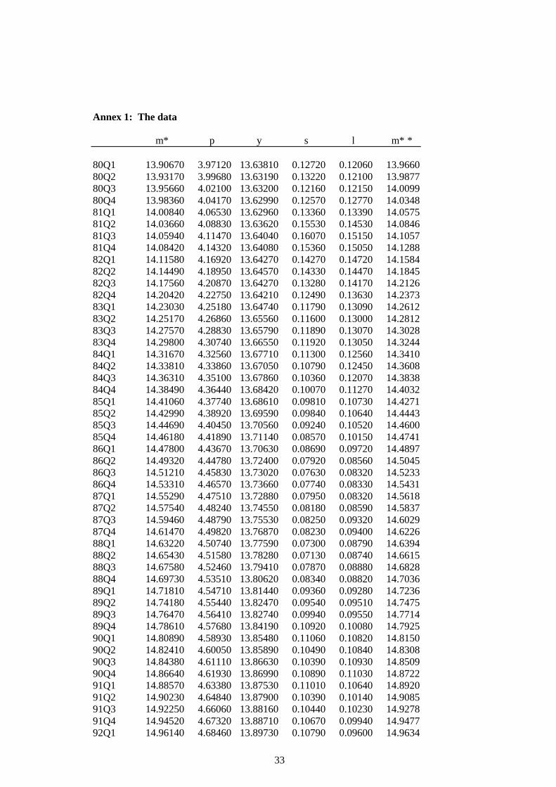
33

Annex 1: The data

m* p y s l m**

80Q1 13.90670 3.97120 13.63810 0.12720 0.12060 13.966080Q2 13.93170 3.99680 13.63190 0.13220 0.12100 13.987780Q3 13.95660 4.02100 13.63200 0.12160 0.12150 14.009980Q4 13.98360 4.04170 13.62990 0.12570 0.12770 14.034881Q1 14.00840 4.06530 13.62960 0.13360 0.13390 14.057581Q2 14.03660 4.08830 13.63620 0.15530 0.14530 14.084681Q3 14.05940 4.11470 13.64040 0.16070 0.15150 14.105781Q4 14.08420 4.14320 13.64080 0.15360 0.15050 14.128882Q1 14.11580 4.16920 13.64270 0.14270 0.14720 14.158482Q2 14.14490 4.18950 13.64570 0.14330 0.14470 14.184582Q3 14.17560 4.20870 13.64270 0.13280 0.14170 14.212682Q4 14.20420 4.22750 13.64210 0.12490 0.13630 14.237383Q1 14.23030 4.25180 13.64740 0.11790 0.13090 14.261283Q2 14.25170 4.26860 13.65560 0.11600 0.13000 14.281283Q3 14.27570 4.28830 13.65790 0.11890 0.13070 14.302883Q4 14.29800 4.30740 13.66550 0.11920 0.13050 14.324484Q1 14.31670 4.32560 13.67710 0.11300 0.12560 14.341084Q2 14.33810 4.33860 13.67050 0.10790 0.12450 14.360884Q3 14.36310 4.35100 13.67860 0.10360 0.12070 14.383884Q4 14.38490 4.36440 13.68420 0.10070 0.11270 14.403285Q1 14.41060 4.37740 13.68610 0.09810 0.10730 14.427185Q2 14.42990 4.38920 13.69590 0.09840 0.10640 14.444385Q3 14.44690 4.40450 13.70560 0.09240 0.10520 14.460085Q4 14.46180 4.41890 13.71140 0.08570 0.10150 14.474186Q1 14.47800 4.43670 13.70630 0.08690 0.09720 14.489786Q2 14.49320 4.44780 13.72400 0.07920 0.08560 14.504586Q3 14.51210 4.45830 13.73020 0.07630 0.08320 14.523386Q4 14.53310 4.46570 13.73660 0.07740 0.08330 14.543187Q1 14.55290 4.47510 13.72880 0.07950 0.08320 14.561887Q2 14.57540 4.48240 13.74550 0.08180 0.08590 14.583787Q3 14.59460 4.48790 13.75530 0.08250 0.09320 14.602987Q4 14.61470 4.49820 13.76870 0.08230 0.09400 14.622688Q1 14.63220 4.50740 13.77590 0.07300 0.08790 14.639488Q2 14.65430 4.51580 13.78280 0.07130 0.08740 14.661588Q3 14.67580 4.52460 13.79410 0.07870 0.08880 14.682888Q4 14.69730 4.53510 13.80620 0.08340 0.08820 14.703689Q1 14.71810 4.54710 13.81440 0.09360 0.09280 14.723689Q2 14.74180 4.55440 13.82470 0.09540 0.09510 14.747589Q3 14.76470 4.56410 13.82740 0.09940 0.09550 14.771489Q4 14.78610 4.57680 13.84190 0.10920 0.10080 14.792590Q1 14.80890 4.58930 13.85480 0.11060 0.10820 14.815090Q2 14.82410 4.60050 13.85890 0.10490 0.10840 14.830890Q3 14.84380 4.61110 13.86630 0.10390 0.10930 14.850990Q4 14.86640 4.61930 13.86990 0.10890 0.11030 14.872291Q1 14.88570 4.63380 13.87530 0.11010 0.10640 14.892091Q2 14.90230 4.64840 13.87900 0.10390 0.10140 14.908591Q3 14.92250 4.66060 13.88160 0.10440 0.10230 14.927891Q4 14.94520 4.67320 13.88710 0.10670 0.09940 14.947792Q1 14.96140 4.68460 13.89730 0.10790 0.09600 14.9634

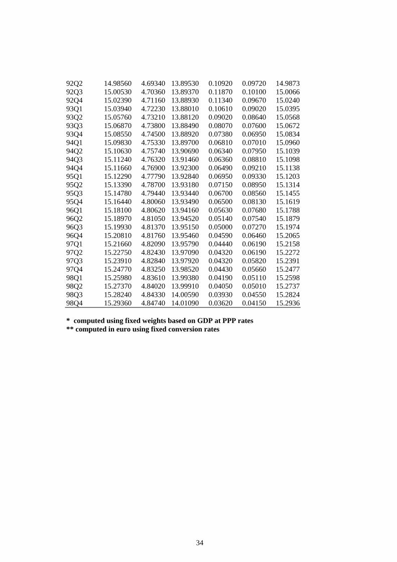
34

92Q2 14.98560 4.69340 13.89530 0.10920 0.09720 14.987392Q3 15.00530 4.70360 13.89370 0.11870 0.10100 15.006692Q4 15.02390 4.71160 13.88930 0.11340 0.09670 15.024093Q1 15.03940 4.72230 13.88010 0.10610 0.09020 15.039593Q2 15.05760 4.73210 13.88120 0.09020 0.08640 15.056893Q3 15.06870 4.73800 13.88490 0.08070 0.07600 15.067293Q4 15.08550 4.74500 13.88920 0.07380 0.06950 15.083494Q1 15.09830 4.75330 13.89700 0.06810 0.07010 15.096094Q2 15.10630 4.75740 13.90690 0.06340 0.07950 15.103994Q3 15.11240 4.76320 13.91460 0.06360 0.08810 15.109894Q4 15.11660 4.76900 13.92300 0.06490 0.09210 15.113895Q1 15.12290 4.77790 13.92840 0.06950 0.09330 15.120395Q2 15.13390 4.78700 13.93180 0.07150 0.08950 15.131495Q3 15.14780 4.79440 13.93440 0.06700 0.08560 15.145595Q4 15.16440 4.80060 13.93490 0.06500 0.08130 15.161996Q1 15.18100 4.80620 13.94160 0.05630 0.07680 15.178896Q2 15.18970 4.81050 13.94520 0.05140 0.07540 15.187996Q3 15.19930 4.81370 13.95150 0.05000 0.07270 15.197496Q4 15.20810 4.81760 13.95460 0.04590 0.06460 15.206597Q1 15.21660 4.82090 13.95790 0.04440 0.06190 15.215897Q2 15.22750 4.82430 13.97090 0.04320 0.06190 15.227297Q3 15.23910 4.82840 13.97920 0.04320 0.05820 15.239197Q4 15.24770 4.83250 13.98520 0.04430 0.05660 15.247798Q1 15.25980 4.83610 13.99380 0.04190 0.05110 15.259898Q2 15.27370 4.84020 13.99910 0.04050 0.05010 15.273798Q3 15.28240 4.84330 14.00590 0.03930 0.04550 15.282498Q4 15.29360 4.84740 14.01090 0.03620 0.04150 15.2936

* computed using fixed weights based on GDP at PPP rates** computed in euro using fixed conversion rates

35

Annex 2: A brief review of the methodology

The impulse response analysis of cointegrated systems, which was originally explored in

Lütkepohl and Reimers (1992), relied on the Cholesky decomposition of the systems’

covariance matrix in order to end up with a structural interpretation of their innovations. It

is well known, however, that the identification scheme thus obtained is to some extent

arbitrary. In particular, it implies a contemporaneous recursive structure among the

systems’ variables that depends on their ordering. Similar in vein, Warne (1993) proposed

a recursive identification scheme based on the common trend representation of

cointegrated systems, which separately identifies the innovations having permanent effects

— the so-called common trends — and the innovations with only transitory effects.

In an extension of these approaches, Vlaar (1998) has recently suggested to identify the

innovations of cointegrated systems in terms of an underlying theoretical structure by

imposing contemporaneous as well as long-run restrictions on their impulse response

functions, i.e. the coefficients of their vector moving average representation. Similar to the

one proposed by Warne, this identification scheme proves to be more parsimonious than a

scheme merely based on contemporaneous restrictions. But in addition, it proves to be

more flexible than an identification scheme relying on a particular recursive ordering of

the system's variables. Thereby, Vlaar closes the gap between the impulse response

analysis of cointegrated systems, which has suffered from the lack of a sound structural

interpretation so far, and the analysis of ‘structural’ vector autoregressive (SVAR) systems

as introduced by Blanchard (1989) and Blanchard and Quah (1989), which was confined

to stationary variables.

In order to discuss the method proposed by Vlaar in a bit more detail, let }{ tz be a

sequence of a n - dimensional vector of variables which is generated by an unrestricted

vector autoregressive (VAR) process of order k ,

tktktt zAzAz εµ ++++= −− !11

where the sequence of the n - dimensional vector of innovations }{ tε has a positive-

definite covariance matrix Σ=′ ][E ttεε .

If }{ tz is cointegrated of order )1,1( with cointegrating rank r , then, according to the

Engle/Granger representation theorem (see Engle and Granger (1987) or Johansen

(1995)), the data generating process has the following two equivalent representations:

36

(a) the vector error correction (VEC) representation

tktktktt zzzz εβαµ +′+∆Γ++∆Γ+=∆ −+−−− 1111 !

where βα , are )( rn × - dimensional matrices with nr <=′< ][rank0 βα , and

(b) the vector moving average (VMA) representation

))(( tt LCz εµ +=∆

where ∑∞

=−≡

1)(

i

iin LCILC is a matrix polynomial of infinite order in the lag operator

L , such that ittiL −= εε , and ⊥

−⊥

−

=⊥⊥ ′Γ−′= ∑ αβαβ 11

1))(()1(

k

i inIC with

)]1([rank C rn −= .

The infinite order VMA representation in first differences can be integrated to obtain a

finite order VMA representation in levels,

t

t

t LCCtCzz εεµτ

τ )(~

)1()1(1

0 +++= ∑=

where )1)((~

)1()( LLCCLC −+= with ∑∞

+=−=

1

~ij ji CC .

Due to the reduced rank of the total impact matrix )1(C only rn − linear combinations of

the innovations — the common trends — have permanent effects on the levels, whereas

the effects of the remaining r linear combinations die out in the long run.1

The above representations are reduced-form representations. In order to give them a

structural interpretation, the sequence of the vector of reduced-form innovations }{ tε is

assumed to be related to the sequence of a n - dimensional vector of orthogonal

innovations }{ te with covariance matrix normalised to be ntt Iee =′ ][E . The

contemporaneous relationship between the reduced-form and the structural innovations is

modelled via the non-singular )( nn × - dimensional matrix B ,

tt Be====ε

In view of this relationship, the covariance matrices of the reduced-form and the structural

innovations are related by BeeB tttt ′′=′ ][E][E εε , i.e. BB ′=Σ . Due to the symmetry of Σ

and the normalisation of the variances of the structural innovations, already 2/)1( +nn

non-linear restrictions are imposed on the 2n elements of the matrix B . Therefore, we

1 This system property is exploited extensively in the common trend literature. See, e.g., Stock andWatson (1988) and Warne (1993).

37

have to impose at least 2/)1( −nn additional independent restrictions on B in order to

identify its elements.

The sequence of the system's impulse responses to the structural innovations, ∞=0}{ iiB , has

an illuminating representation in terms of the coefficients of its VMA representation and

the matrix B ,2

BCCB ii )~

)1(( +≡ , ",1,0=i

Of course, since )1(~

0 CIC n −= and 0~

lim =∞→ ii C , the contemporaneous impact of the

structural innovations is just given by BB =0 , while their long-run impact is measured by

BCBii )1(lim =∞→ . In view of these relationships, the identification of the structural

innovations can thus be achieved by imposing appropriate restrictions on their long-run

impact, i.e. on the elements of the matrix BC )1( , and by imposing appropriate restrictions

on their contemporaneous impact, i.e. on the elements of the matrix B .

If it is assumed that the rn − common trends of the cointegrated system relate to a

particular subset of rn − structural innovations, the effects of the r remaining structural

innovations will die out in the long run. This can easily be accomplished by imposing zero

restrictions on the corresponding columns of the long-gun impact matrix BC )1( . Due to

the reduced rank of )1(C , however, only rrn )( − out of these nr zero restrictions will be

linearly independent. Given the separation of the innovations with permanent effects from

those with transitory effects, it will then suffice to impose any set of at least

2/)1)(( −−− rnrn independent restrictions on BC )1( or B to mutually identify the

innovations with permanent effects. To mutually identify the innovations with transitory

effects, we can impose any set of at least 2/)1( −rr independent restrictions on B .

If B is identified, its estimate can subsequently be obtained by means of a constrained

two-step Maximum Likelihood procedure starting from the reduced-form estimates of the

covariance matrix Σ and the long-run impact matrix )1(C , where the latter is incorporated

in the formulation of the constraints for estimating B . This procedure also permits to test

over-identifying restrictions (given a particular set of exactly identifying restrictions).

Thereby, the identification of the system's structure is completed and its impulse response

functions can be computed.

2 Whereas the representation of the impulse response functions in terms of the VMA coefficients isillustrative, it is more convenient, from a computational point of view, to derive the impulse responsefunctions from the companion form of the VAR representation of the cointegrated system. For details see, forinstance, Lütkepohl (1991), Chap. 2.

38

To assess the precision of the computed impulse response functions, it is convenient to

report their confidence intervals. These may alternatively be obtained by analytical

methods based on asymptotic theory or by Bootstrap and simulation-based methods. As

the numerical burden of the latter proves to be prohibitive, the approach proposed by

Vlaar confines itself to analytical methods. The analytical derivation of confidence

intervals starts from the result that the distribution of the estimated coefficients of the

underlying VAR model is asymptotically normal. This result, which was originally proved

for stationary VAR models, was extended to cointegrated VAR models by Lütkepohl and

Reimers. They derived the distribution of the VAR coefficients from the asymptotic

distribution of the estimated VEC coefficients assuming the coefficients of the

cointegrating relationships known.

In extension of the results by Lütkepohl and Reimers, Vlaar showed that the covariance

matrix of the estimator of the VEC coefficients and the estimator of the contemporaneous

impact matrix does not have a block-diagonal structure. This is due to the stochastic

nature of the imposed long-run restrictions which are non-linear functions of the estimated

VEC coefficients. To take account of this stochastic element, Vlaar proposes a first order

correction based on the delta method in deriving the analytical confidence intervals of the

impulse response functions. He demonstrates that this analytical correction has

considerable impact on the shape of the confidence intervals. This holds in particular for

the impulse response functions of the transitory shocks that are enforced to die out in the

long run due to the imposed zero restrictions.

Table 1. Summary of results from the application of the Johansen procedure: M3 (fixed GDP PPP rates)Informat. criteria k=1 k=2 k=3 k=4

SC -51.87 -51.93 -50.66 -49.98HQ -52.58 -53.14 -52.38 -52.51

Test diagnostics LM(1) LM(4) LM(1-8) N HET(k=2) 0.50 0.84 0.99 22.19** 0.72

.Cointegration rank r=0 r<=1 r<=2 r<=3 r<=4

trace test 122.99 76.13 39.46 15.44 0.13[107.72**] [62.25**] [31.03*] [11.84] [0.01]

Chi-square tests for m-p y s l ππππexclusion 26.43** 23.28** 12.79** 16.73** 26.02**stationarity 23.70** 23.82** 15.61** 19.36** 19.61**weak-exogeneity 23.14** 1.92 11.41** 16.77** 12.72**

Tests for structural hypotheses H0

1 H02 H0

1^H02

(0,0,-1,1,0) (0,0,0,1,-1)

3.93 0.52 5.21(0.14) (0.77) (0.27)

The cointegrating vectors ββββ1111 s.e. ββββ2222 s.e. ββββ3333 s.e.

m-p 1.000 - - - - -y -1.170 0.034 - - - -s 1.260 0.170 -1.000 - - -l - - 1.000 - 1.000 -ππππ - - - - -1.000 -

The loadings αααα1111 s.e. αααα2222 s.e. αααα3333 s.e.m-p -0.138 0.026 -0.250 0.063 0.045 0.062

y 0.029 0.037 0.258 0.090 -0.162 0.084s -0.078 0.038 0.028 0.091 -0.186 0.086l -0.026 0.024 -0.023 0.059 -0.236 0.056ππππ 0.015 0.069 -0.009 0.167 0.480 0.159

H03 H0

1^H02^H0

3

( αααα21212121=α=α=α=α31313131=α=α=α=α41414141=α=α=α=α51515151=0 )=0 )=0 )=0 )

2.79 9.65(0.25) (0.29)

Note: The superscripts * and ** indicate rejections at 10% and 5% significance levels, repectively.

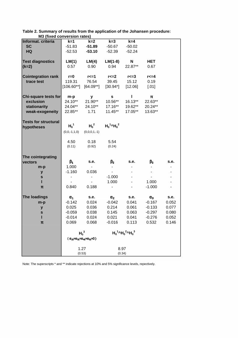
Table 2. Summary of results from the application of the Johansen procedure: M3 (fixed conversion rates)Informat. criteria k=1 k=2 k=3 k=4

SC -51.83 -51.89 -50.67 -50.02HQ -52.53 -53.10 -52.39 -52.24

Test diagnostics LM(1) LM(4) LM(1-8) N HET(k=2) 0.57 0.90 0.94 22.87** 0.67

Cointegration rank r=0 r<=1 r<=2 r<=3 r<=4trace test 119.31 76.54 39.45 15.12 0.19

[106.60**] [64.09**] [30.94*] [12.06] [.01]

Chi-square tests for m-p y s l ππππexclusion 24.10** 21.90** 10.56** 16.13** 22.63**stationarity 24.04** 24.10** 17.16** 19.62** 20.24**weak-exogeneity 22.85** 1.71 11.45** 17.05** 13.63**

Tests for structural hypotheses H0

1 H02 H0

1^H02

(0,0,-1,1,0) (0,0,0,1,-1)

4.50 0.18 5.54(0.11) (0.92) (0.24)

The cointegrating vectors ββββ1111 s.e. ββββ2222 s.e. ββββ3333 s.e.

m-p 1.000 - - - - -y -1.160 0.036 - - - -s - - -1.000 - - -l - - 1.000 - 1.000 -ππππ 0.840 0.188 - - -1.000 -

The loadings αααα1111 s.e. αααα2222 s.e. αααα3333 s.e.m-p -0.142 0.024 -0.042 0.041 -0.167 0.052

y 0.025 0.036 0.214 0.061 -0.133 0.077s -0.059 0.038 0.145 0.063 -0.297 0.080l -0.014 0.024 0.021 0.041 -0.276 0.052ππππ 0.069 0.068 -0.016 0.113 0.532 0.146

H03 H0

1^H02^H0

3

( αααα21212121=α=α=α=α31313131=α=α=α=α41414141=α=α=α=α51515151=0 )=0 )=0 )=0 )

1.27 8.97(0.53) (0.34)

Note: The superscripts * and ** indicate rejections at 10% and 5% significance levels, repectively.

Figure 1. The data

Fig. 1.a

0.90

1.00

1.10

1.20

1.30

1.40

1.50

1.60

80Q1

81Q1

82Q1

83Q1

84Q1

85Q1

86Q1

87Q1

88Q1

89Q1

90Q1

91Q1

92Q1

93Q1

94Q1

95Q1

96Q1

97Q1

98Q1

real M3 real GDP

Fig. 1.b

0.00

0.02

0.04

0.06

0.08

0.10

0.12

0.14

0.16

0.18

80Q1

81Q1

82Q1

83Q1

84Q1

85Q1

86Q1

87Q1

88Q1

89Q1

90Q1

91Q1

92Q1

93Q1

94Q1

95Q1

96Q1

97Q1

98Q1

short-rate long-rate inflation

Fig. 1.c

0.000

0.051

80Q1

81Q1

82Q1

83Q1

84Q1

85Q1

86Q1

87Q1

88Q1

89Q1

90Q1

91Q1

92Q1

93Q1

94Q1

95Q1

96Q1

97Q1

98Q1

real long-rate

Fig. 1.e

-0.0235

0.0065

80Q1

81Q1

82Q1

83Q1

84Q1

85Q1

86Q1

87Q1

88Q1

89Q1

90Q1

91Q1

92Q1

93Q1

94Q1

95Q1

96Q1

97Q1

98Q1

spread

Fig. 1.d

0.000

0.045

0.090

80Q1

81Q1

82Q1

83Q1

84Q1

85Q1

86Q1

87Q1

88Q1

89Q1

90Q1

91Q1

92Q1

93Q1

94Q1

95Q1

96Q1

97Q1

98Q1

real short-rate

Fig. 1.f

-0.16

-0.14

-0.12

-0.10

-0.08

-0.06

-0.04

-0.02

0.00

0.02

80Q1

81Q1

82Q1

83Q1

84Q1

85Q1

86Q1

87Q1

88Q1

89Q1

90Q1

91Q1

92Q1

93Q1

94Q1

95Q1

96Q1

97Q1

98Q1

velocity

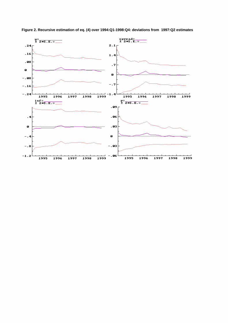
Figure 2. Recursive estimation of eq. (4) over 1994:Q1-1998:Q4: deviations from 1997:Q2 estimates

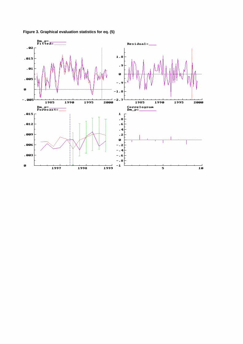
Figure 3. Graphical evaluation statistics for eq. (5)

Figure 4. Cumulative normalised lag weights

-0.2

0

0.2

0.4

0.6

0.8

1

1.2

0 2 4 6 8 10 12 14 16 18 20 22 24 26 28 30 32 34 36

prices income

0

0.2

0.4

0.6

0.8

1

1.2

0 2 4 6 8 10 12 14 16 18 20 22 24 26 28 30 32 34 36

short-term rate long-term rate

Figure 5. Recursive estimation of eq. 5 over 1990:Q1-1998:Q4

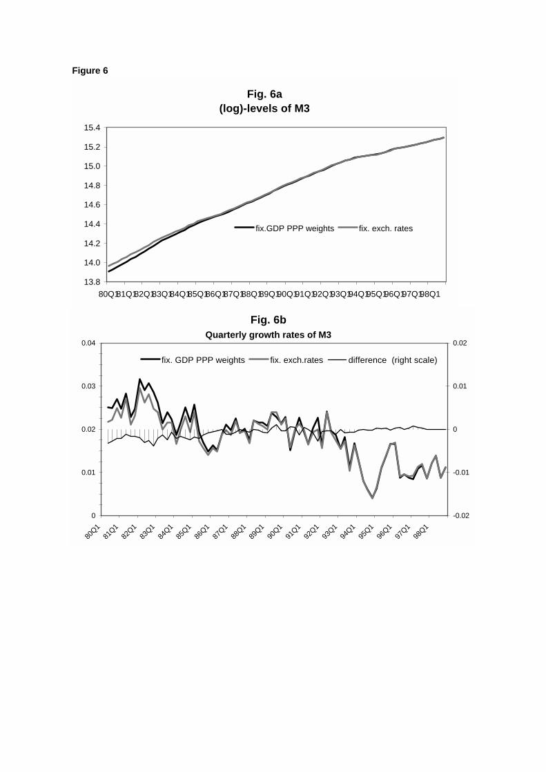
Figure 6

Fig. 6bQuarterly growth rates of M3

0

0.01

0.02

0.03

0.04

80Q1

81Q1

82Q1

83Q1

84Q1

85Q1

86Q1

87Q1

88Q1

89Q1

90Q1

91Q1

92Q1

93Q1

94Q1

95Q1

96Q1

97Q1

98Q1

-0.02

-0.01

0

0.01

0.02

fix. GDP PPP weights fix. exch.rates difference (right scale)

Fig. 6a(log)-levels of M3

13.8

14.0

14.2

14.4

14.6

14.8

15.0

15.2

15.4

80Q181Q182Q183Q184Q185Q186Q187Q188Q189Q190Q191Q192Q193Q194Q195Q196Q197Q198Q1

fix.GDP PPP weights fix. exch. rates

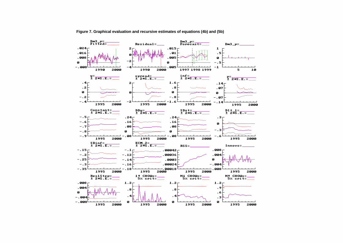
Figure 7. Graphical evaluation and recursive estimates of equations (4b) and (5b)

Figure 8. Impulse responses to a positive aggregate supply shock

0 5 10 15 20 25 30 35 40−0.5

0

0.5

1

1.5

2

2.5

3

3.5

m−p

0 5 10 15 20 25 30 35 40−0.5

0

0.5

1

1.5

2

2.5

3

y

0 5 10 15 20 25 30 35 40−2

−1.5

−1

−0.5

0

0.5

s

0 5 10 15 20 25 30 35 40−1.2

−1

−0.8

−0.6

−0.4

−0.2

0

0.2

0.4

0.6

l

0 5 10 15 20 25 30 35 40−1.2

−1

−0.8

−0.6

−0.4

−0.2

0

0.2

0.4

π

0 5 10 15 20 25 30 35 40−0.2

0

0.2

0.4

0.6

0.8

1

1.2

l−s

0 5 10 15 20 25 30 35 40−0.8

−0.6

−0.4

−0.2

0

0.2

0.4

0.6

s−π

0 5 10 15 20 25 30 35 40−0.2

0

0.2

0.4

0.6

0.8

1

1.2

l−π

0 5 10 15 20 25 30 35 40−5

−4

−3

−2

−1

0

1

2

p

0 5 10 15 20 25 30 35 40−4

−3

−2

−1

0

1

2

3

4

m

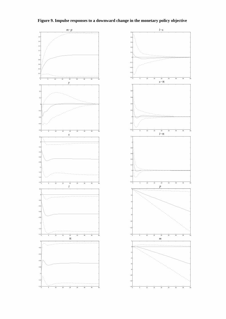
Figure 9. Impulse responses to a downward change in the monetary policy objective

0 5 10 15 20 25 30 35 400

0.2

0.4

0.6

0.8

1

1.2

1.4

1.6

1.8

2

m−p

0 5 10 15 20 25 30 35 40−0.4

−0.3

−0.2

−0.1

0

0.1

0.2

0.3

y

0 5 10 15 20 25 30 35 40−1.6

−1.4

−1.2

−1

−0.8

−0.6

−0.4

−0.2

0

0.2

s

0 5 10 15 20 25 30 35 40−1.4

−1.2

−1

−0.8

−0.6

−0.4

−0.2

0

0.2

l

0 5 10 15 20 25 30 35 40−1.4

−1.2

−1

−0.8

−0.6

−0.4

−0.2

0

π

0 5 10 15 20 25 30 35 40−0.4

−0.3

−0.2

−0.1

0

0.1

0.2

0.3

0.4

0.5

l−s

0 5 10 15 20 25 30 35 40−0.4

−0.2

0

0.2

0.4

0.6

0.8

1

s−π

0 5 10 15 20 25 30 35 40−0.4

−0.2

0

0.2

0.4

0.6

0.8

1

1.2

l−π

0 5 10 15 20 25 30 35 40−14

−12

−10

−8

−6

−4

−2

0

p

0 5 10 15 20 25 30 35 40−14

−12

−10

−8

−6

−4

−2

0

2

m

Figure 10. Impulse responses to a positive aggregate demand shock

0 5 10 15 20 25 30 35 40−0.2

−0.1

0

0.1

0.2

0.3

0.4

0.5

m−p

0 5 10 15 20 25 30 35 40−0.2

−0.1

0

0.1

0.2

0.3

0.4

0.5

y

0 5 10 15 20 25 30 35 40−0.1

0

0.1

0.2

0.3

0.4

0.5

0.6

0.7

s

0 5 10 15 20 25 30 35 40−0.3

−0.2

−0.1

0

0.1

0.2

0.3

0.4

l

0 5 10 15 20 25 30 35 40−0.15

−0.1

−0.05

0

0.05

0.1

0.15

0.2

0.25

0.3

0.35

π

0 5 10 15 20 25 30 35 40−0.5

−0.4

−0.3

−0.2

−0.1

0

0.1

0.2

l−s

0 5 10 15 20 25 30 35 40−0.1

0

0.1

0.2

0.3

0.4

0.5

0.6

s−π

0 5 10 15 20 25 30 35 40−0.4

−0.3

−0.2

−0.1

0

0.1

0.2

0.3

l−π

0 5 10 15 20 25 30 35 40−0.2

0

0.2

0.4

0.6

0.8

1

1.2

p

0 5 10 15 20 25 30 35 40−0.2

0

0.2

0.4

0.6

0.8

1

1.2

m

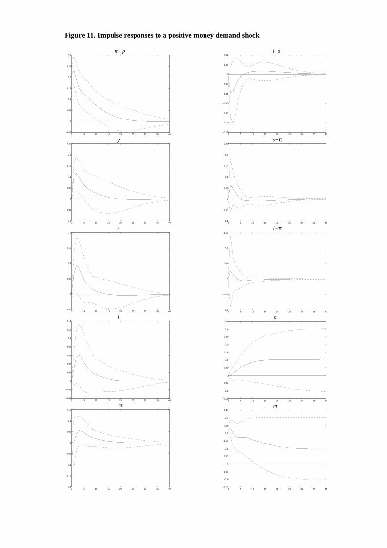
Figure 11. Impulse responses to a positive money demand shock

0 5 10 15 20 25 30 35 40−0.05

0

0.05

0.1

0.15

0.2

0.25

0.3

m−p

0 5 10 15 20 25 30 35 40−0.1

−0.05

0

0.05

0.1

0.15

0.2

0.25

y

0 5 10 15 20 25 30 35 40−0.05

0

0.05

0.1

0.15

0.2

s

0 5 10 15 20 25 30 35 40−0.04

−0.02

0

0.02

0.04

0.06

0.08

0.1

0.12

0.14

l

0 5 10 15 20 25 30 35 40−0.2

−0.15

−0.1

−0.05

0

0.05

0.1

0.15

π

0 5 10 15 20 25 30 35 40−0.12

−0.1

−0.08

−0.06

−0.04

−0.02

0

0.02

0.04

l−s

0 5 10 15 20 25 30 35 40−0.1

−0.05

0

0.05

0.1

0.15

0.2

0.25

s−π

0 5 10 15 20 25 30 35 40−0.1

−0.05

0

0.05

0.1

0.15

l−π

0 5 10 15 20 25 30 35 40−0.15

−0.1

−0.05

0

0.05

0.1

0.15

0.2

0.25

0.3

0.35

p

0 5 10 15 20 25 30 35 40−0.15

−0.1

−0.05

0

0.05

0.1

0.15

0.2

0.25

0.3

0.35

m

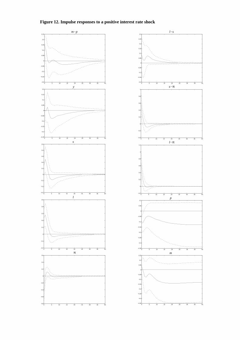
Figure 12. Impulse responses to a positive interest rate shock

0 5 10 15 20 25 30 35 40−0.2

−0.15

−0.1

−0.05

0

0.05

0.1

0.15

0.2

0.25

m−p

0 5 10 15 20 25 30 35 40−0.25

−0.2

−0.15

−0.1

−0.05

0

0.05

0.1

0.15

0.2

y

0 5 10 15 20 25 30 35 40−0.3

−0.2

−0.1

0

0.1

0.2

0.3

0.4

0.5

s

0 5 10 15 20 25 30 35 40−0.2

−0.1

0

0.1

0.2

0.3

0.4

0.5

l

0 5 10 15 20 25 30 35 40−0.8

−0.6

−0.4

−0.2

0

0.2

0.4

0.6

π

0 5 10 15 20 25 30 35 40−0.2

−0.15

−0.1

−0.05

0

0.05

0.1

0.15

0.2

0.25

0.3

l−s

0 5 10 15 20 25 30 35 40−0.4

−0.2

0

0.2

0.4

0.6

0.8

1

s−π

0 5 10 15 20 25 30 35 40−0.2

0

0.2

0.4

0.6

0.8

1

1.2

l−π

0 5 10 15 20 25 30 35 40−0.35

−0.3

−0.25

−0.2

−0.15

−0.1

−0.05

0

0.05

0.1

p

0 5 10 15 20 25 30 35 40−0.35

−0.3

−0.25

−0.2

−0.15

−0.1

−0.05

0

0.05

0.1

0.15

m

European Central Bank Working Paper Series∗∗∗∗

1 “A global hazard index for the world foreign exchange markets” by V. Brousseau andF. Scacciavillani, May 1999

2 “What does the single monetary policy do? A SVAR benchmark for the EuropeanCentral Bank” by O. Tristani and C. Monticelli, May 1999

3 “Fiscal policy effectiveness and neutrality results in a non-Ricardian world” byC. Detken, May 1999

4 “From the ERM to the euro: new evidence on economic and policy convergenceamong EU countries” by I. Angeloni and L. Dedola, May 1999

5 “Core inflation: a review of some conceptual issues” by M. Wynne, May 1999

6 “The demand for M3 in the euro area” by G. Coenen and J.-L. Vega, September 1999

7 “A cross-country comparison of market structures in European banking” by O. deBandtand E. P. Davis, September 1999

∗ Publication date in italics