WORKING PAPER SERIES 12 Josef Bajzík, Tomáš Havránek, Zuzana Iršová, Jiří Schwarz The Elasticity of Substitution between Domestic and Foreign Goods: A Quantitative Survey

Welcome message from author
This document is posted to help you gain knowledge. Please leave a comment to let me know what you think about it! Share it to your friends and learn new things together.
Transcript

WORKING PAPER SERIES 12
Josef Bajzík, Tomáš Havránek, Zuzana Iršová, Jiří Schwarz The Elasticity of Substitution between Domestic and Foreign Goods:
A Quantitative Survey


WORKING PAPER SERIES
The Elasticity of Substitution between Domestic and Foreign Goods: A Quantitative Survey
Josef Bajzík Tomáš Havránek
Zuzana Iršová Jiří Schwarz
12/2019

CNB WORKING PAPER SERIES The Working Paper Series of the Czech National Bank (CNB) is intended to disseminate the results of the CNB’s research projects as well as the other research activities of both the staff of the CNB and collaborating outside contributors, including invited speakers. The Series aims to present original research contributions relevant to central banks. It is refereed internationally. The referee process is managed by the CNB Economic Research Division. The working papers are circulated to stimulate discussion. The views expressed are those of the authors and do not necessarily reflect the official views of the CNB. Distributed by the Czech National Bank. Available at http://www.cnb.cz. Reviewed by: Maria Cipollina (University of Molise) Oxana Babecká Kucharčuková (Czech National Bank)
Project Coordinator: Ivan Sutóris
© Czech National Bank, December 2019 Josef Bajzík, Tomáš Havránek, Zuzana Iršová, Jiří Schwarz

The Elasticity of Substitution between Domestic and Foreign Goods: AQuantitative Survey
Josef Bajzík, Tomáš Havránek, Zuzana Iršová, and Jirí Schwarz ∗
Abstract
A key parameter in international economics is the elasticity of substitution between domesticand foreign goods, also called the Armington elasticity. Yet estimates vary widely. We collect3,524 reported estimates of the elasticity from 42 studies over 1977–2018, construct 34 variablesthat reflect the context in which researchers obtain their estimates, and examine what drives theheterogeneity in the results. To account for the inherent model uncertainty, we employ Bayesianand frequentist model averaging. We present the first application of newly developed non-lineartechniques to correct for publication bias. Our main results are threefold. First, there is publicationbias against small and statistically insignificant elasticities. Second, the differences in the resultsare best explained by differences in data: aggregation, frequency, size, and dimension. Third, themean elasticity implied by the literature after correcting for both publication bias and potentialmisspecifications is 2.
Abstrakt
Elasticita substituce mezi domácími a zahranicními statky, nazývaná též Armingtonova, tvorí klí-cový parametr v mezinárodní ekonomii. Její odhady se však výrazne ruzní. Shromáždili jsmevzorek 3 524 odhadu elasticity ze 42 studií z let 1977–2018. Konstruujeme 34 promenných, kterépopisují souvislosti jednotlivých odhadu, a zkoumáme, co zpusobuje odlišnosti výsledku. Z du-vodu inherentní modelové nejistoty používáme bayesovské a frekventistické metody prumerovánímodelu. Predkládáme první aplikaci nove vyvinutých nelineárních technik ocištení o publikacníselektivitu. Výsledkem jsou tri základní zjištení. Za prvé, publikacní selektivita potlacuje nízké astatisticky nevýznamné elasticity. Za druhé, odlišnosti ve výsledcích nejlépe vysvetlují rozdíly vdatech: jejich agregace, frekvence, velikost a rozmer. Za tretí, po ocištení o publikacní selektivitua potenciální nedostatky ve specifikacích modelu literatura implikuje prumernou elasticitu 2.
JEL Codes: C83, D12, F14.Keywords: Armington, Bayesian model averaging, meta-analysis, publication bias, trade
elasticity.
∗ Josef Bajzík, Czech National Bank and Charles UniversityTomáš Havránek, Charles UniversityZuzana Iršová, Charles University, [email protected]; corresponding authorJirí Schwarz, Czech National Bank and Charles UniversityAn online appendix with data and codes is available at meta-analysis.cz/armington. We thank Maria Cipol-lina, Oxana Babecká Kucharcuková, Jan Bruha, and seminar participants at the Czech National Bank for theirhelpful comments. Earlier version of this paper circulated under the title “Estimating the Armington Elasticity:The Importance of Data Choice and Publication Bias.” The views expressed here are ours and not necessarily thoseof the Czech National Bank.

2 Josef Bajzík, Tomáš Havránek, Zuzana Iršová, and Jirí Schwarz
1. Introduction
How does the demand for domestic versus foreign goods react to a change in relative prices? Theanswer is central to a host of research and policy problems in international trade and macroeco-nomics: the welfare effects of globalization (Costinot and Rodriguez-Clare, 2014), trade balanceadjustments (Imbs and Mejean, 2015), and the exchange rate pass-through of monetary policy (Auerand Schoenle, 2016), to name but a few. Any attempt to evaluate the effect of tariffs in particulardepends crucially on the assumed reaction of relative demand to relative prices. In most models, thereaction is governed by the (constant) elasticity of substitution between domestic and foreign goods.The size of the elasticity used for calibration often drives the conclusions of the model, as shown bySchurenberg-Frosch (2015), who recomputes the results of 50 previously published models usingdifferent values of the elasticity. She finds that, with plausible changes in the elasticity, the resultschange qualitatively in more than half of the cases. As Hillberry and Hummels (2013, p. 1217) putit, “it is no exaggeration to say that [the elasticity] is the most important parameter in modern tradetheory.”
Yet no consensus on the magnitude of the elasticity exists. In different contexts, researchers tend toobtain substantially different estimates, as observed by Feenstra et al. (2018) and many commen-tators before them. In this paper we assign a pattern to these differences, a pattern that we hopewill be useful for calibrating models in international trade and macroeconomics. The elasticity ofsubstitution between domestic and foreign goods is commonly called the Armington elasticity, inhonor of Armington (1969), who first formulated a theoretical model featuring goods distinguishedsolely by the place of origin. The first estimates of the elasticity followed soon afterward, and manythousands have been published since. As the Armington-style literature turns 50, the time is ripefor taking stock. We collect 3,524 estimates of the elasticity of substitution between domestic andforeign goods and construct 34 variables that reflect the context in which researchers produce theirestimates.
Figure 1: The Reported Elasticities Are Often Around 1 but Can Vary Widely
020
040
060
080
010
00Fr
eque
ncy
-2 0 2 4 6 8Estimate of the Armington elasticity
Note: The figure shows the histogram of the estimates of the macro-level Armington elasticity reported inindividual studies. Large values are winsorized for ease of exposition.
A bird’s-eye view of the literature (Figure 1 and Figure 2) shows four stylized facts, three of whichcorroborate the common knowledge in the field. First, the estimates of the elasticities vary substan-

The Elasticity of Substitution between Domestic and Foreign Goods: A Quantitative Survey 3
Figure 2: The Mean and Variance of Reported Elasticities Increase Over Time
02
46
8M
edia
n es
timat
e of
the
Arm
ingt
on e
last
icity
1970 1980 1990 2000 2010Median year of data
Note: The vertical axis measures median estimates of the macro-level Armington elasticity reported inindividual studies. The horizontal axis measures the median year of the data used in thecorresponding study.
tially. A researcher wishing to calibrate her policy model has plenty of degrees of freedom; she caneasily find empirical evidence for any value of the elasticity between 0 and 8. Such plausible (thatis, justifiable by some empirical evidence) changes in the elasticity can have decisive effects onthe results of the model. For example, Engler and Tervala (2018) show that changing the elasticityfrom 3 to 8 more than doubles the estimated welfare gains from the Transatlantic Trade and Invest-ment Partnership. Second, the median estimated elasticity in the literature is 1, and many estimatesare close to that value. Third, the reported elasticity seems to be increasing in time, but it is notclear whether the apparent trend reflects fundamental changes in preferences or improved data andtechniques used by more recent studies.
Finally, the fourth stylized fact is that newer studies show more disagreement on the value of theelasticity of substitution. That is, instead of converging to a consensus value, the literature is di-verging. The increased variance in the estimated elasticities provides additional rationale for asystematic evaluation of the published results. For this evaluation we use the methods of meta-analysis, which were originally developed in (or inspired by) medical research. Recent applicationsof meta-analysis in economics include Card et al. (2018) on the effectiveness of active labor marketprograms, Anderson et al. (2018) on the impact of government spending on poverty, and Havranekand Irsova (2017) on the border effect in international trade. An important problem inherent inmeta-analysis is model uncertainty, because for many control variables capturing the study design,little theory exists that can help us determine whether they should be included in the baseline model.To address this issue, we use both Bayesian (Raftery et al., 1997; Eicher et al., 2011) and frequentist(Hansen, 2007; Amini and Parmeter, 2012) methods of model averaging (Steel, 2020, provides anexcellent description of these techniques).
Meta-analysis also allows us to correct for potential publication bias in the literature. Publicationbias arises when, holding other aspects of study design constant, some results (for example, thosethat are statistically insignificant at standard levels or have the “wrong” sign) have a lower proba-bility of publication than other results (Stanley, 2001). For example, in the context of the elasticity
4 Josef Bajzík, Tomáš Havránek, Zuzana Iršová, and Jirí Schwarz
of substitution, it is safe to assume that its sign is positive: a negative value is not compatible withany commonly applied model of preferences. Similarly, it is difficult to interpret a zero elasticity.Thus, from the point of view of an individual study, it makes sense not to report such unintuitiveestimates—or find a specification where the elasticity is positive—because non-positive elasticitysuggests that something is wrong with the data or the estimation technique. Nevertheless, non-positive estimates will occur from time to time simply because of sampling error; for the samereason, researchers will sometimes obtain estimates much larger than the true value. If large esti-mates (which are still intuitive) are kept but non-positive ones are omitted, an upward bias arises.Paradoxically, publication bias can thus improve the inferences drawn from individual studies (ifthey avoid making central conclusions based on negative or zero elasticities) but inevitably biasesinferences drawn from the literature as a whole. Ioannidis et al. (2017) shows that, in economics,the effects of publication selection are dramatic and exaggerate the mean reported estimate twofold.
To correct for publication bias, we use meta-regression techniques based on Egger et al. (1997)and their extensions and three new non-linear techniques developed specifically for meta-analysisin economics. The first one is due to Ioannidis et al. (2017) and relies on estimates that are ade-quately powered. The second technique was developed by Andrews and Kasy (2019) and employsa selection model that estimates the probability of publication for results with different p-values.The third non-linear technique is the “stem-based method” by Furukawa (2019), a non-parametricestimator that exploits the variance-bias trade-off. As far as we know, the latter two estimators havenot been applied so far, apart from the illustrative examples outlined by Andrews and Kasy (2019)and Furukawa (2019).
In all the models we run, linear or non-linear, Bayesian or frequentist, we find evidence of strongpublication bias in the estimates of the long-run Armington elasticity. The bias results in the meanestimate being exaggerated by more than 50%. In contrast, we find no publication bias among theestimates of the short-run elasticity. One explanation consistent with these results is that the short-run elasticity is commonly believed to be small and less important for policy questions, so thereare few incentives to discriminate against insignificant (and even potentially negative) estimates ofthe elasticity. Large estimates of the long-run elasticity, in contrast, appear intuitive and desirableto many researchers (see, for example, the discussion in McDaniel and Balistreri, 2003; Hillberryet al., 2005).
Our findings indicate that study characteristics are systematically associated with the reported re-sults. Among the 34 variables we construct, the most important are the ones related to the data usedin the estimation. We find that, ceteris paribus, using more aggregated data yields smaller estimatesof the elasticity. Annual data yield substantially smaller elasticities than monthly and quarterly data.If a study uses cross-sectional data, it is more likely to report larger estimates of the elasticity thanif time-series data are used. Our results also suggest that employing a small number of observationsand ignoring endogeneity in the estimation yields a downward bias. Finally, we find systematic cor-relation between measures of quality and the magnitude of the reported elasticity. Studies of higherquality (as measured by the number of citations, publication in a refereed journal, and the RePEcimpact factor of the outlet) tend to report larger estimates.
Therefore, while publication selection creates an upward bias, many questionable method choicesseem to create a downward bias. We exploit the relationships unearthed by Bayesian model av-eraging to compute a mean effect corrected for publication bias and misspecification biases, andconditional on maximum quality defined based on the peer-review status, the publication outlet, andthe number of citations. However, given the nature of the Armington elasticity and its multiple uses,there is very probably no single correct value of this parameter. The long-run elasticity estimated

The Elasticity of Substitution between Domestic and Foreign Goods: A Quantitative Survey 5
using long time series with annual frequency will be the most suitable one for models from theinternational trade category, such as for estimating the welfare effects of trade unions. In such case,short-run fluctuations not only are unimportant, but can obscure the true and necessarily delayedeffects of policy changes.
On the other hand, monetary policy is more interested in the dynamic response to price shocks. Asa consequence, the short-run elasticity estimated on monthly data is considerably more relevant,whereas the long-run effects are only of secondary importance. Therefore, we compute separatebest-practice elasticities for these two major use cases. Interestingly, the two elasticities turn out tobe almost identical at 2. We interpret the number as our best guess (based on the available empiricalliterature published during the last five decades) for how to calibrate a model that allows for only oneparameter to govern the aggregate elasticity of substitution between domestic and foreign goods—be it, for example, an open economy dynamic stochastic general equilibrium model of the type usedin many central banks, or a computable general equilibrium trade policy model. We also reportthese aggregate elasticities for individual countries and provide information in the online appendixthat allows other researchers to use our data to compute the elasticities for individual industries.
The remainder of the paper is structured as follows. Section 2 briefly describes how the Armingtonelasticity is estimated and how we collect data from primary studies. Section 3 tests for publica-tion bias in the literature. Section 4 explores heterogeneity and computes the aggregate elasticitycorrected for publication and misspecification biases. Section 5 concludes the paper. An onlineappendix at meta-analysis.cz/armington provides the data and codes.
2. Collecting the Elasticity Dataset
The derivation of the Armington elasticity follows a two-stage optimization process (please re-fer to Hillberry and Hummels, 2013; Feenstra et al., 2018, for a more detailed treatment thanwe have the space to offer here): in the first stage, the consumer with a CES utility function
u(QD,QM) =(
β ·Q(σ−1)/σ
D +(1−β ) ·Q(σ−1)/σ
M
)(σ/(σ−1)allocates her total spending to various
product categories following her budget constraint with a given general price index. The consumerthus chooses a quantity of the composite good QD+QM, her aggregate demand for goods producedin her home country (D) and foreign countries (M). In the second stage, the consumer decideswhat proportion of domestic and foreign goods to consume while minimizing her expendituresQD ·PD +QM ·PM or maximizing her utility. Utility maximization subject to the budget constraintor cost minimization subject to the utility function both imply that the marginal rate of substitutionbetween domestic and foreign goods should equal the corresponding price ratio (Welsch, 2008).The first-order condition follows:
QMQD
=
[β
1−β· PD
PM
]σ
, (1)
where the quantity of domestic goods QD and foreign goods QM is related to the correspondingdomestic price PD and import price PM. β is a distribution parameter between the domestic and theforeign good, and σ denotes the Armington elasticity. For estimation, the first-order condition iscommonly log-linearized:

6 Josef Bajzík, Tomáš Havránek, Zuzana Iršová, and Jirí Schwarz
log(
QMQD
)= σ log
(β
1−β
)︸ ︷︷ ︸
Constant
+ σ︸︷︷︸Armington elasticity
log(
PDPM
)+ e. (2)
As the main building block of our dataset, we collect estimates of σ from the literature. Several re-cent papers, such as Aspalter (2016) and Feenstra et al. (2018), call this type of Armington elasticitya macro-elasticity. A macro-elasticity governs the substitution between home and foreign goods,where varieties from different foreign countries are aggregated into one composite good. A micro-elasticity, on the other hand, governs the substitution among the varieties of foreign goods and thusdifferentiates among the specific countries of origin (Balistreri et al., 2010). Given the relativelysmall sample size of micro-elasticity estimates, and given the problematic direct comparability be-tween the different types of Armington elasticities needed to perform a meta-analysis, we focus inthis paper on macro-elasticities only.
Even this choice, as we show below, leads to rather substantial methodological variability and en-compasses a wide range of models and estimation strategies. We find that some of the estimationmethod choices significantly influence the elasticity estimates. To account for this heterogeneityand allow a preference for more up-to-date methodological approaches in the best-practice calcula-tion, we have to create categories capturing these various estimation techniques. Including yet morefamilies of models from the micro-elasticity literature would make it impossible to capture all themethodological heterogeneity in a meaningful way.
We need each study to report a measure of the uncertainty of its estimates. This measure, which isnecessary to test for the potential presence of publication bias in the literature, can be either the stan-dard error or other metrics recomputable to the standard error. This requirement prevents us fromusing a dozen empirical papers, including the highly cited contribution by Broda and Weinstein(2006). For similar reasons, we drop a few estimates for which uncertainty measures are incorrectlyreported (for example, when the reported standard errors are negative or when the reported confi-dence intervals do not include a point estimate).1 The final dataset is an unbalanced one, becausesome studies report more estimates than others. We choose to include all the reported estimates,as it is often unclear which estimate is the one preferred by the author; moreover, including moreestimates obtained using alternative methods or datasets increases the variation we can exploit bymeta-analysis.
The first step in a meta-analysis is the search for relevant studies. Building on the comprehensivesurveys by McDaniel and Balistreri (2003) and Cassoni and Flores (2008), we design our searchquery in Google Scholar in a way that shows the well-known studies estimating the Armingtonelasticity among the first hits. The final query, along with the dataset, is available online at meta-analysis.cz/armington. We also go through the references of the most recent studies and obtainother papers that might provide empirical estimates of the elasticity. While the keywords we useare specified in English, we do not exclude any study based on the language of publication: severalpapers written in Spanish (e.g. Hernandez, 1998; Lozano Karanauskas, 2004) and Portuguese (Fariaand Haddad, 2014) are included. We add the last study in March 2018 and terminate the literaturesearch. The final set of studies that fulfill all the requirements for meta-analysis is reported inTable 1; our sample consists of 3,524 estimates from 42 papers.1 In cases where semi-elasticities were reported, both the estimates and their standard errors were recalculated tobe comparable.

The Elasticity of Substitution between Domestic and Foreign Goods: A Quantitative Survey 7
Figure 3: Estimates Vary both Within and Across Studies
Alaouze (1977)Alaouze et al. (1977)
Aspalter (2016)Bilgic et al. (2002)
Cassoni & Flores (2008)Cassoni & Flores (2010)
Corado & de Melo (1983)Corbo & Osbat (2013)
Faria & Haddad (2011)Feenstra et al. (2014)Gallaway et al. (2003)
Gan (2006)Gibson (2003)
Hernández (1998)Huchet-Bourdon & Pishbahar (2009)
Hummels (1999)Imbs & Méjean (2015)
Ivanova (2005)Kawashima & Sari (2010)
Lozano Karanauskas (2004)Lundmark & Shahrammehr (2011a)Lundmark & Shahrammehr (2011b)
Lundmark & Shahrammehr (2012)Lächler (1984)
Mohler & Seitz (2012)Nganou (2005)
Németh et al. (2011)Ogundeji et al. (2010)
Olekseyuk & Schürenberg-Frosch (2014)Reinert & Roland-Holst (1992)
Reinert & Shiells (1991)Saikkonen (2015)
Saito (2004)Sauquet et al. (2011)
Shiells & Reinert (1993)Shiells et al. (1986)
Tourinho et al. (2003)Tourinho et al. (2010)
Turner et al. (2012)Warr & Lapiz (1994)
Welsch (2006)Welsch (2008)
-5 0 5 10 15outliers outliersEstimate of the Armington elasticity
Note: The figure shows a box plot of the estimates of the Armington elasticity reported in individual studies.The length of each box represents the interquartile range (P25–P75), and the dividing line inside thebox is the median value. The whiskers represent the highest and lowest data points within 1.5 timesthe range between the upper and lower quartiles. The dots show the outlying estimates with extremevalues stacked at the values denoted as “outliers.” The solid vertical line denotes unity.

8 Josef Bajzík, Tomáš Havránek, Zuzana Iršová, and Jirí Schwarz
Figure 4: Estimates Vary both Within and Across Countries
AustraliaAustria
BelgiumBrazil
BulgariaColombia
CyprusCzech Republic
DenmarkEstoniaFinlandFrance
GermanyGreece
HungaryIreland
ItalyJapanLatvia
LesothoLithuania
LuxembourgMalta
NetherlandsPoland
PortugalRomania
RussiaSlovak Republic
SloveniaSouth Africa
SpainSwedenThailand
USAUnited Kingdom
Uruguay
-5 0 5 10 15outliers outliersEstimate of the Armington elasticity
Note: The figure shows a box plot of the estimates of the Armington elasticity reported for individualcountries. The length of each box represents the interquartile range (P25–P75), and the dividing lineinside the box is the median value. The whiskers represent the highest and lowest data points within1.5 times the range between the upper and lower quartiles. The dots show the outlying estimates withextreme values stacked at the values denoted as “outliers.” The solid vertical line denotes unity.

The Elasticity of Substitution between Domestic and Foreign Goods: A Quantitative Survey 9
Table 1: Studies Included in the Meta-Analysis
Alaouze (1977) Huchet-Bourdon and Pishbahar (2009) Olekseyuk and Schurenberg-Frosch (2016)Alaouze et al. (1977) Hummels (1999) Reinert and Roland-Holst (1992)Aspalter (2016) Ivanova (2005) Reinert and Shiells (1991)Bilgic et al. (2002) Kawashima and Sari (2010) Saikkonen (2015)Cassoni and Flores (2008) Lachler (1984) Saito (2004)Cassoni and Flores (2010) Lozano Karanauskas (2004) Sauquet et al. (2011)Corado and de Melo (1983) Lundmark and Shahrammehr (2011a) Shiells and Reinert (1993)Corbo and Osbat (2013) Lundmark and Shahrammehr (2011b) Shiells et al. (1986)Faria and Haddad (2014) Lundmark and Shahrammehr (2012) Tourinho et al. (2003)Feenstra et al. (2018) Imbs and Mejean (2015) Tourinho et al. (2010)Gallaway et al. (2003) Mohler and Seitz (2012) Turner et al. (2012)Gan (2006) Nemeth et al. (2011) Warr and Lapiz (1994)Gibson (2003) Nganou (2005) Welsch (2006)Hernandez (1998) Ogundeji et al. (2010) Welsch (2008)
The oldest study in our sample was published in 1977 and the most recent one in 2018, hencewe cover more than 40 years of research. The mean reported elasticity is 1.5. Given that thereare a few dramatic outliers in our data (their values climb to approximately 50 in absolute value),we winsorize the estimates at the 2.5% level; the mean is not affected by the winsorization, andour results hold with alternative winsorizations at the 1% and 5% levels. Approximately 10% ofthe estimates are negative and commonly believed to occur due to misspecifications in the demandfunction and problems with import prices (Shiells et al., 1986). More than half of the estimates arelarger than unity, which suggests that domestic and foreign goods can often be expected to formgross substitutes. Nevertheless, the estimates differ greatly both within and between individualstudies and home countries, as Figure 3 and Figure 4 demonstrate. To assign a pattern to thisvariance, for each estimate, we collect 43 explanatory variables describing various characteristicsof data, home countries, methods, models, and quality; these sources of heterogeneity are examinedin detail in Section 4.
Table 2 provides a first indication of the potential causes of heterogeneity. We compute the meanvalues of the Armington elasticity estimates for different groups of data based on temporal dynam-ics (short- or long-run),2 data frequency, structural variation, and publication characteristics. Toaccount for the unbalancedness of our dataset, we also compute mean estimates weighted by theinverse of the number of estimates reported per study so that each study gets the same weight. Thetable shows that the long-run elasticities are approximately twice as large as the short-run ones,which corroborates the arguments of Gallaway et al. (2003) and the common notion that short-runelasticities are smaller. In fact, Cassoni and Flores (2008) argue that smaller short-run estimatesare given by the estimation design itself, unless overshooting occurs. Quarterly and annual data aretypically used to capture the long-run effects (Gallaway et al., 2003) and thus can be expected toproduce larger elasticities than monthly data, which is supported by the statistics shown in the table.
The smaller elasticities reported for the primary sector (with respect to other sectors) suggest thatthe products of agriculture, forestry, fishing, mining, and quarrying are more difficult to substitutewith their foreign alternatives. Concerning agriculture, this finding can be explained, as Kuiper andvan Tongeren (2006) point out, by common explicit or implicit support for domestic (or even local)
2 In the vast majority of cases, short-run elasticities are obtained from regressing the current period change inrelative prices on the current period change in relative demand. That is, they capture the instantaneous reaction.

10 Josef Bajzík, Tomáš Havránek, Zuzana Iršová, and Jirí Schwarz
Tabl
e2:
Arm
ingt
onE
last
iciti
esfo
rDiff
eren
tSub
sets
ofD
ata
Unw
eigh
ted
Stud
y-w
eigh
ted
Prec
isio
n-w
eigh
ted
No.
ofob
s.M
ean
95%
conf
.int
.M
ean
95%
conf
.int
.M
ean
95%
conf
.int
.
Tem
pora
ldyn
amic
sSh
ort-
run
effe
ct55
60.
880.
830.
930.
910.
850.
981.
010.
971.
05L
ong-
run
effe
ct2,
968
1.56
1.49
1.63
1.74
1.65
1.82
1.25
1.21
1.28
Dat
ach
arac
teri
stic
sM
onth
lyda
ta48
81.
040.
971.
111.
181.
121.
240.
950.
920.
99Q
uart
erly
data
745
1.22
1.09
1.34
2.64
2.41
2.87
1.09
1.02
1.17
Ann
uald
ata
2,29
11.
621.
541.
701.
321.
251.
401.
231.
201.
26
Stru
ctur
alva
riat
ion
Prim
ary
sect
or36
60.
830.
700.
950.
730.
610.
851.
351.
251.
46A
gric
ultu
re,f
ores
try,
and
fishi
ng26
00.
920.
771.
060.
770.
630.
911.
491.
371.
62M
inin
gan
dqu
arry
ing
103
0.58
0.33
0.84
0.38
0.14
0.62
0.63
0.46
0.80
Seco
ndar
yse
ctor
3,04
41.
461.
401.
521.
401.
341.
461.
091.
071.
12M
anuf
actu
ring
2,96
31.
461.
401.
521.
401.
341.
461.
051.
071.
10U
tiliti
es54
1.85
1.29
2.40
1.84
1.39
2.28
1.61
1.39
1.83
Con
stru
ctio
n24
0.60
0.10
1.10
0.67
0.15
1.19
1.74
1.37
2.11
Tert
iary
sect
or75
1.42
1.13
1.71
1.25
0.90
1.61
1.49
1.33
1.66
Trad
e,ca
teri
ng,a
ndac
com
mod
atio
n23
0.97
0.65
1.28
0.84
0.53
1.16
1.23
0.91
1.56
Tran
spor
t,st
orag
e,an
dco
mm
unic
atio
n16
1.92
0.75
3.09
2.10
0.71
3.50
1.44
1.00
1.88
Fina
nce,
insu
ranc
e,re
ales
tate
,and
busi
ness
81.
070.
431.
720.
570.
031.
101.
410.
782.
03Se
rvic
es21
1.63
1.35
1.92
1.47
1.19
1.76
1.69
1.42
1.96
Dev
elop
ing
coun
trie
s85
61.
831.
691.
961.
541.
431.
661.
501.
441.
56D
evel
oped
coun
trie
s73
81.
241.
161.
321.
241.
151.
340.
910.
880.
94
Pub
licat
ion
stat
usPu
blis
hed
pape
rs1,
385
1.23
1.13
1.32
1.65
1.52
1.78
0.97
0.92
1.02
Unp
ublis
hed
pape
rs2,
139
1.60
1.53
1.68
1.61
1.53
1.68
1.27
1.24
1.31
All
estim
ates
3,52
41.
451.
401.
511.
641.
561.
711.
171.
151.
20
Not
e:T
hede
finiti
ons
ofth
esu
bset
sar
eav
aila
ble
inTa
ble
4.St
udy-
wei
ghte
d=
estim
ates
wei
ghte
dby
the
inve
rse
ofth
enu
mbe
rofe
stim
ates
repo
rted
pers
tudy
.Pr
ecis
ion-
wei
ghte
d=
estim
ates
wei
ghte
dby
the
inve
rse
ofth
est
anda
rder
roro
fthe
part
icul
ares
timat
e.Se
vera
lela
stic
ities
inou
rdat
aset
are
estim
ated
fora
llin
dust
ries
orac
ross
mul
tiple
sect
ors;
thes
eob
serv
atio
nsar
eex
clud
edfr
omth
eta
ble.

The Elasticity of Substitution between Domestic and Foreign Goods: A Quantitative Survey 11
produce. In contrast, the largest elasticities are typically found for utilities (approximately 1.85)and transport, storage, and communication (1.92). The elasticity also tends to be 50% larger fordeveloping countries than for developed countries. Finally, although the means suggest a differencebetween the typical results of published and unpublished papers, the weighted means, in which eachstudy has the same weight, suggest that the publication process is not associated with the magnitudeof the estimates of the Armington elasticity. This simple analysis suggests there is potential for sys-tematic differences among the reported elasticities, but any particular conclusion may be misleadingwithout accounting for the correlation between individual aspects of data and methodology, whichwe address in Section 4. It may also be misleading without correcting for publication bias, and weturn to this problem in the following section.
3. Testing for Publication Bias
Publication bias is widespread in science, and economics is no exception: Ioannidis et al. (2017)document that the typical estimate reported in economics is exaggerated twofold because of publi-cation selection. Publication selection arises because of the general preference of authors, editors,and referees for estimates that have the “right” sign and are statistically significant. Of course, thisis not to say that publication selection equals cheating: on the contrary, it makes sense for (andimproves the value of) an individual study not to focus on estimates that are evidently wrong. Butwhen most authors follow the strategy of ignoring estimates that have the “wrong” sign or are sta-tistically insignificant, our inference from the literature as a whole (and also from many individualstudies) becomes distorted. Given the degrees of freedom available to researchers in economics,estimates with the “right” sign and statistical significance at the 5% level can almost always be ob-tained after a sufficiently large number of specifications have been tried. A useful analogy providedby McCloskey and Ziliak (2019) is the Lombard effect, in which speakers increase their vocal effortin the presence of noise: given noisy data or estimation techniques, the researcher has more in-centives to search through more specifications for a significant effect. When statistical significancebecomes the implicit requirement for publication, significance will be produced but will no longerreflect what the statistical theory expects of it.
A conspicuous feature of the Armington elasticity is that it must be positive if both domestic andforeign goods are useful to the consumer. Therefore, from the very beginning, the literature hasshunned negative and zero estimates as clear artifacts of data or method problems. One of thefirst studies, Alaouze (1977, p. 8), notes, “we shall concentrate on the ...[industries]... for whichthe elasticity of substitution has the correct [positive] sign.” Among the latest studies, Feenstraet al. (2018, p. 144) find that the estimated elasticity is negative for some varieties and isolate themfrom the dataset: “these data are faulty or incompatible with our model.” As we have noted, thisapproach can improve the inference drawn from an individual study but generally creates a bias.Given the inherent noise in trade data, the estimated elasticities for some industries or specificationswill always be insignificant, negative, or both. For other industries or specifications, the same noiseproduces estimates that are much larger than the true effect. However, there is no upper boundthat immediately renders elasticities implausible; some domestic and foreign goods are perfectlysubstitutable in theory. Therefore, the large estimates will be kept in the paper and interpreted. Thispsychological asymmetry between zero and infinity, coupled with the inevitable imprecision in thedata and estimation, creates publication bias. One apparent solution is symmetrical trimming: whenthe authors ignore ten negative or insignificant estimates, they should also ignore the ten largestpositive estimates. Winsorizing would be better still, but it is rarely employed in practice.

12 Josef Bajzík, Tomáš Havránek, Zuzana Iršová, and Jirí Schwarz
A common tool used to assess the extent of publication bias is the “funnel plot” (Egger et al.,1997). The funnel plot shows the magnitude of the estimated effect on the horizontal axis andthe precision of the estimate (the inverse of the standard error) on the vertical axis. There shouldbe no relation between these two quantities, because virtually all techniques used by researchersto estimate the Armington elasticity guarantee that the ratio of the estimate to its standard errorhas a symmetrical distribution (typically a t-distribution). Therefore, regardless of their magnitudeand precision, the estimates should be symmetrically distributed around the true mean effect. Withdecreasing precision, the estimates become more dispersed around the true effect and thus form asymmetrical inverted funnel. In the presence of publication bias, the funnel becomes either hollow(because insignificant estimates are omitted), asymmetrical (because estimates of a certain sign orsize are excluded), or both.
The funnel plot in Figure 5 gives us a mixed message, as we show short- and long-run estimates ofthe Armington elasticity separately. The short-run elasticities are symmetrically distributed aroundtheir most precise estimates, which are slightly less than 1. The long-run elasticities, in contrast,form an asymmetrical funnel: the most precise estimates are also close to 1, but among the impreciseestimates there are many more that are much larger than 1 compared to those that are smaller than 1.This finding is consistent with no publication selection among short-run elasticities and publicationselection against negative and insignificant elasticities among long-run elasticities. Nevertheless, thefunnel plot is only a simple visual test, and the dispersion of the long-run estimates could suggestheterogeneity in data and methods, the other systematic factor driving the estimated coefficients.Regression-based funnel asymmetry tests provide a more concrete way to test for publication bias.As we have noted, if publication selection is present, the reported estimates and standard errors arecorrelated (Stanley, 2005; Stanley and Doucouliagos, 2010; Havranek, 2015):
σi j = σ0 +δ ·SE(σi j)+µi j, (3)
Figure 5: The Funnel Plot Suggests Publication Bias among Long-Run Elasticities
010
020
030
040
0
Prec
isio
n of
the
estim
ate
(1/S
E)
-10 -5 0 5 10 15Estimate of the Armington elasticity
long-runshort-run
Note: In the absence of publication bias, the funnel should be symmetrical around the most precise estimatesof the elasticity. The dashed vertical line denotes the simple mean of the full sample of elasticities.Outliers are excluded from the figure for ease of exposition but included in all statistical tests.

The Elasticity of Substitution between Domestic and Foreign Goods: A Quantitative Survey 13
where σi j denotes the i-th estimate of the Armington elasticity with the standard error SE(σi j) esti-mated in the j-th study; µi j is the error term. σ0 is the mean underlying effect beyond publicationbias (that is, conditional on maximum precision), and the coefficient δ of the standard error SE(σi j)
represents the strength of publication bias. If δ = 0, no publication bias is present. If δ 6= 0, the σ ’sand their standard errors are correlated; the correlation can arise either because researchers discardnegative elasticity estimates (in which case the correlation occurs due to the apparent heteroskedas-ticity) or because researchers compensate for large standard errors with large elasticity estimates(the Lombard effect).
Table 3 presents the results of (3) using various estimation techniques run for three samples: thepooled set of elasticities, short-run elasticities, and long-run elasticities. Panel A uses unweighteddata. In the baseline OLS model, the coefficient δ from (3) is not statistically significant for theshort-run sample, and the estimated corrected mean is the same as the simple mean of 0.9. In thesample of long-run elasticities, in contrast, we find strong publication bias that reduces the under-lying mean from 1.56 (the uncorrected mean) to 0.9 (the mean corrected for publication bias). Theresult for a pooled sample of short- and long-run elasticities is close to that of long-run elasticities,because long-run elasticities dominate the dataset.
In the next model, we add study-level fixed effects to the baseline specification, which slightlywidens the difference between the mean short- and long-run effects beyond bias. Finally, forPanel A, we use a multilevel estimation technique that implements partial pooling at the studylevel and uses the data to influence the pooling weights. Given that the estimated elasticities arenested within each study, hierarchical modeling is a convenient choice to analyze the variance inthe elasticities: one can expect the stochastic term of (3) to depend on the design of each individualstudy and therefore not to have the same dispersion across individual studies. It follows that theregression coefficients δ are probably not the same across studies. Nevertheless, the δ ’s should berelated, and the hierarchical modeling treats them as random variables of yet another linear regres-sion at the study level. We apply a hierarchical Bayes model and implement the Gibbs samplerfor hierarchical linear models with a standard prior, following Rossi et al. (2005). The hierarchicalmodel corroborates the evidence presented earlier but finds slightly weaker publication bias amongthe estimates of the long-run elasticity.
Panel B of Table 3 presents weighted alternatives to the baseline OLS model of Panel A. First, theregression is weighted by the inverse of the number of estimates reported by each study, so that bothsmall and large studies are all assigned the same importance. Second, the regression is weightedby the inverse of the standard error so that more precise estimates are assigned greater importance.Panel B shows results that support the conclusions from Panel A. Finally, Panel C shows the latestalternatives to linear meta-analysis models. The problem with the linear regression that we haveused so far is the implicit assumption that publication bias is a linear function of the standard error.If this assumption does not hold, our conclusion concerning publication bias may be misleading.Here, we apply three non-linear techniques that relax this assumption. The corrected means of boththe short- and long-run Armington elasticity remain close to unity in all three alternative approaches:the weighted average of adequately powered estimates by Ioannidis et al. (2017), the stem-basedmethod by Furukawa (2019), and the selection model by Andrews and Kasy (2019).
Based on a survey involving more than 60,000 estimates, Ioannidis et al. (2017) document that themedian statistical power among the published results in economics is 18%. They show how thelow power is associated with publication bias and then propose a simple correction procedure thatfocuses on the estimates with power above 80%. Monte Carlo simulations presented in Ioannidiset al. (2017) suggest that this simple technique outperforms the commonly used meta-regression

14 Josef Bajzík, Tomáš Havránek, Zuzana Iršová, and Jirí Schwarz
Table 3: All Tests Indicate Publication Bias among Long-Run Armington Elasticities
All Short-run Long-run
PANEL A: Unweighted estimations
OLSSE (publication bias) 0.808
∗∗∗0.0791 0.805
∗∗∗
(0.0652) (0.0826) (0.0630)Constant (effect beyond bias) 0.873
∗∗∗0.867
∗∗∗0.901
∗∗∗
(0.133) (0.0249) (0.168)Fixed effects
SE (publication bias) 0.621∗∗∗
-0.00578 0.627∗∗∗
(0.0588) (0.104) (0.0580)Constant (effect beyond bias) 1.007
∗∗∗0.883
∗∗∗1.047
∗∗∗
(0.0423) (0.0192) (0.0476)Hierarchical Bayes
SE (publication bias) 0.500∗∗
-0.0810 0.630∗∗∗
(0.190) (0.480) (0.190)Constant (effect beyond bias) 1.200
∗∗∗0.887
∗∗1.250
∗∗∗
(0.240) (0.310) (0.0476)
PANEL B: Weighted OLS estimations
Weighted by the inverse of the number of estimates reported per studySE (publication bias) 1.017
∗∗∗0.0975
∗1.033
∗∗∗
(0.249) (0.0514) (0.251)Constant (effect beyond bias) 1.011
∗∗∗0.893
∗∗∗1.046
∗∗∗
(0.254) (0.0694) (0.303)Weighted by the inverse of the standard error
SE (publication bias) 1.559 2.698 0.906∗∗
(0.969) (2.213) (0.431)Constant (effect beyond bias) 0.761
∗∗∗0.510 0.922
∗∗∗
(0.217) (0.325) (0.205)
PANEL C: Non-linear estimations
Weighted average of adequately powered (Ioannidis et al., 2017)Effect beyond bias 1.049
∗∗∗0.872
∗∗∗1.101
∗∗∗
(0.017) (0.024) (0.021)Selection model (Andrews and Kasy, 2019)
Effect beyond bias 0.911∗∗∗
0.863∗∗∗
0.943∗∗∗
(0.015) (0.018) (0.021)Stem-based method (Furukawa, 2019)
Effect beyond bias 0.992∗∗∗
1.031∗∗∗
0.994∗∗∗
(0.024) (0.070) (0.042)
Observations 3,524 556 2,968
Note: The uncorrected mean of the estimates of the long-run Armington elasticity is 1.56. Panels A and B report the resultsof regression σi j = σ0 +δ ·SE(σi j)+µi j, where σi j denotes the i-th Armington elasticity estimated in the j-th studyand SE(σi j) denotes the corresponding standard error. All = the entire dataset, Short-run = short-run Armingtonelasticities, Long-run = long-run Armington elasticities, SE = standard error. Standard errors, clustered at the studyand country level, are reported in parentheses (except hierarchical Bayes, which has the posterior standard deviation inparentheses). The available number of observations is reduced for Ioannidis et al. (2017)’s estimation (all 3,440;short-run 555; long-run 2,885) and Furukawa (2019)’s estimation (all 1,850; short-run 105; long-run 965).
∗p < 0.10,
∗∗p < 0.05,
∗∗∗p < 0.01. Stars are presented for hierarchical Bayes only as an indication of the parameter’s statistical
importance to keep visual consistency with the rest of the table.

The Elasticity of Substitution between Domestic and Foreign Goods: A Quantitative Survey 15
estimators. The intuition of the model presented by Furukawa (2019) rests on the fact that themost precise estimates suffer from little bias: with very small standard errors, the authors can easilyproduce estimates that are statistically significant. While previous authors have recommended meta-analysts to focus on a fraction of the most precise estimates in meta-analysis (for example, Stanleyet al., 2010), Furukawa (2019) finds a clever way to estimate this fraction based on exploiting thetrade-off between bias and variance (omitting studies increases the variance). Andrews and Kasy(2019) use the observation reported by many researchers (for instance, Havranek, 2015; Brodeuret al., 2016) that the standard cut-offs for the p-value (0.01, 0.05, 0.1) are associated with jumpsin the distribution of the reported estimates. Andrews and Kasy (2019) build on Hedges (1992)and construct a selection model that estimates the publication probability for each estimate in theliterature given its p-value. They show that, in several areas, the technique gives results similar tothose of a large-scale replication.
Several important findings can be distilled from the estimations reported in Table 3. First, we findpublication bias among long-run elasticities but not among short-run elasticities. One explanationconsistent with this result is that short-run elasticities are typically deemed less important than long-run elasticities, especially for trade policy purposes. They are often reported only as complementsto the central findings of the paper. It can take time before consumers shift their demand betweendomestic and foreign goods; consequently, insignificant estimates of the short-run elasticity aremore likely to survive the publication process than insignificant estimates of the long-run elasticity.Second, publication bias inflates the mean estimate of the long-run Armington elasticity by at least50%, which may have a strong impact on the results of a model informed by the empirical literaturein terms of the calibration of the elasticity. Third, the large difference between the short- and long-run elasticities reported in Table 2 (and observed in many studies; see Gallaway et al., 2003) is all buterased once publication bias is taken into account. In sum, we find robust evidence of publicationbias in this literature. However, some of the apparent correlations between the estimated elasticitiesand their standard errors may be due to data and method heterogeneity. We turn to this issue in thenext section.
4. Why Elasticities Vary
4.1 Potential Factors Explaining Heterogeneity
Three reasons for the systematic differences in the estimates of the Armington elasticity have beenfrequently discussed in the literature. First, studies using disaggregated data are often observed toyield larger estimates than studies using aggregate data (Imbs and Mejean, 2015). Second, cross-sectional studies tend to yield larger estimates than time-series studies (Hillberry and Hummels,2013). Third, multi-equation estimation techniques typically give larger estimates than single-equation techniques (Goldstein and Khan, 1985). Many literature reviews (including Cassoni andFlores, 2008; Marquez, 2002; McDaniel and Balistreri, 2003), moreover, stress other characteristicsof estimates and studies that can significantly influence the results. We present the first attempt toshed light on the sources of the heterogeneity in Table 2. To investigate the heterogeneity amongthe estimates of the Armington elasticity more systematically, we codify 43 characteristics of studydesign and augment equation (3) by adding these characteristics as explanatory variables.3 Giventhat publication bias affects only the long-run elasticity, we replace the standard error in the equa-tion by an interaction term between the standard error and a dummy variable that equals one if theestimate corresponds to a long-run elasticity.
3 In the analysis, we pick one variable from each group as the reference category. Therefore, we end up with 34variables and coefficients to estimate.

16 Josef Bajzík, Tomáš Havránek, Zuzana Iršová, and Jirí Schwarz
Table 4 lists all the codified variables, their definitions, and summary statistics, including the simplemean, the standard deviation, and the mean weighted by the inverse of the number of observationsreported in a study. For ease of exposition, we divide the variables into groups reflecting data char-acteristics (11 aspects), structural variations (11 aspects), estimation techniques (14 aspects), andpublication characteristics potentially related to quality that are not captured by data and estima-tion characteristics (3 aspects). The distinction between short- and long-run elasticities is amongthe most important factors stressed in the literature (Gallaway et al., 2003). Nevertheless, in theprevious section, we find that publication bias plagues the estimates of long-run elasticities and thatbeyond publication bias, short- and long-run elasticities have comparable magnitudes. In this sec-tion, we will examine whether the claim still holds when other possible systematic influences on theestimates of the Armington elasticity are taken into account.
Table 4: Description and Summary Statistics of the Regression Variables
Variable Description Mean SD WM
Armington elasticity The reported estimate of the Armington elasticity. 1.45 1.78 1.64Standard error (SE) The reported standard error of the Armington elasticity
estimate.0.72 1.18 0.61
SE * Long-run effect The interaction between the standard error and the esti-mated long-run Armington elasticity.
0.69 1.19 0.59
Temporal dynamicsShort-run effect =1 if the estimated Armington elasticity is short-term
and captures an instantaneous reaction (reference cate-gory for the group of dummy variables describing tem-poral dynamics).
0.16 0.36 0.12
Long-run effect =1 if the estimated Armington elasticity is long-term. 0.84 0.36 0.88
Data characteristicsData disaggregation The level of data aggregation according to the SIC clas-
sification (min = 1 if fully aggregated, max = 8 if disag-gregated).
6.49 1.58 6.20
Results disaggregation The level of results aggregation according to the SICclassification (min = 1 if fully aggregated, max = 8 ifdisaggregated).
5.06 1.21 5.34
Monthly data =1 if the data are in monthly frequency. 0.14 0.35 0.08Quarterly data =1 if the data are in quarterly frequency (reference cat-
egory for the group of dummy variables describing datafrequency).
0.21 0.41 0.25
Annual data =1 if the data are in yearly frequency. 0.65 0.48 0.67Panel data =1 if panel data are used (reference category for the
group of dummy variables describing the time andcross-sectional dimension of the data).
0.34 0.47 0.27
Time series =1 if time-series data are used. 0.58 0.49 0.65Cross-section =1 if cross-sectional data are used. 0.08 0.27 0.08Data period The length of the time period in years. 14.24 9.76 17.08Data size The logarithm of the total number of observations used
to estimate the elasticity.4.64 1.93 4.55
Midyear The median year of the time period of the data used toestimate the elasticity.
23.45 11.54 22.48
Continued on next page

The Elasticity of Substitution between Domestic and Foreign Goods: A Quantitative Survey 17
Table 4: Description and Summary Statistics of the Regression Variables (continued)
Variable Description Mean SD WM
Structural variationPrimary sector =1 if the estimate is for the primary sector (agriculture
and raw materials; reference category for the group ofdummy variables describing sectors).
0.10 0.31 0.31
Secondary sector =1 if the estimate is for the secondary sector (manufac-turing).
0.86 0.34 0.58
Tertiary sector =1 if the estimate is for the tertiary sector (services). 0.02 0.14 0.03Developing countries =1 if the estimate is for a developing country (reference
category for the group of dummy variables describingthe level of development).
0.24 0.43 0.28
Developed countries =1 if the estimate is for a developed country. 0.79 0.41 0.74Market size The logarithm of the market size of the home country
(GDP in billions of USD, 2015 prices).6.45 1.86 5.94
Tariffs The tariff rate of the home country (weighted mean, allproducts, %).
6.78 7.15 6.07
Non-tariff barriers Additional cost to import of the home country (USD percontainer).
0.94 0.26 0.97
FX volatility The volatility of the exchange rate using the DEC al-ternative conversion factor (home country currency unitper USD).
0.29 0.97 0.76
National pride Home bias captured by the percentage of “I am veryproud of my country” answers from the World ValuesSurvey.
0.53 0.22 0.51
Internet usage The number of fixed broadband subscriptions of thehome country (per 100 people).
2.91 5.02 1.23
Estimation techniqueStatic model =1 if a static model is used for estimation. 0.23 0.42 0.30Distributed lag andtrend model
=1 if a distributed lag or trend model is used. 0.10 0.30 0.27
Partial adjustmentmodel
=1 if a partial adjustment model is used for estimation. 0.15 0.35 0.11
First-difference model =1 if a first-difference model is used. 0.09 0.29 0.05Error-correction model =1 if an error-correction model is used. 0.04 0.20 0.04Non-linear model =1 if a non-linear model is used. 0.28 0.45 0.13Other models =1 if another model is used (reference category for the
group of dummy variables describing the models used).0.11 0.31 0.10
OLS =1 if the OLS or GLS estimation method is used. 0.48 0.50 0.67CORC =1 if the Cochrane-Orcutt or FGLS estimation method
is used.0.16 0.37 0.13
TSLS =1 if the instrumental method is used. 0.09 0.28 0.06GMM =1 if the GMM estimation method is used. 0.24 0.43 0.10Other methods =1 if other types of estimation are used (reference cat-
egory for the group of dummy variables describing theestimation method used).
0.03 0.17 0.05
Import constraint =1 if the study includes some measure of import restric-tion.
0.03 0.18 0.06
Seasonality =1 if the study controls for seasonality. 0.20 0.40 0.12
Publication characteristicsImpact factor The recursive discounted impact factor from RePEc. 0.12 0.24 0.17
Continued on next page

18 Josef Bajzík, Tomáš Havránek, Zuzana Iršová, and Jirí Schwarz
Table 4: Description and Summary Statistics of the Regression Variables (continued)
Variable Description Mean SD WM
Citations The logarithm of the number of Google Scholar cita-tions normalized by the number of years since the firstdraft of the paper appeared in Google Scholar.
1.26 1.01 1.00
Published =1 if a study is published in a peer-reviewed journal. 0.39 0.49 0.65
Note: SD = standard deviation, WM = mean weighted by the inverse of the number of estimates reported perstudy, SIC = Standard Industrial Classification system for classifying industries by a four-digit code.Market size, tariff and non-tariff barriers, FX volatility, and internet usage are collected from theWorld Bank database (WB, 2017) and data on national pride from the World Values Survey (Inglehartet al., 2014). The impact factor is downloaded from RePEc and the number of citations from GoogleScholar. The rest of the variables are collected from studies estimating the Armington elasticity.
Data characteristics. Many studies (Feenstra et al., 2018; McDaniel and Balistreri, 2003; Welsch,2008, among others) argue that because intra-industry diversity decreases with an increasing level ofsectoral aggregation, more aggregated data should yield smaller elasticities. Feenstra et al. (2018)note that some recent macro-studies (Bergin, 2006; Heathcote and Perri, 2002) estimate the ag-gregate elasticities around unity, while studies focusing on individual product groups (Broda andWeinstein, 2006; Imbs and Mejean, 2015) imply much stronger responses. McDaniel and Balistreri(2003) compare two articles on US data that use 3-digit SIC level (Reinert and Roland-Holst, 1992)and 4-digit SIC level (Gallaway et al., 2003) aggregations and come to the same conclusion: higherdisaggregation brings higher substitutability. We codify the data disaggregation variable accordingto the SIC classification. Fully aggregated, whole-economy data acquire the value of 1; in contrast,fully disaggregated product-level data acquire the value of 8. Given the consensus in the literature,we expect the variable to show a positive association with the reported elasticities. Furthermore, insome papers (such as Aspalter, 2016; Mohler and Seitz, 2012), the level of aggregation of the inputdata differs from the level of aggregation of the reported results. Imbs and Mejean (2015) arguethat a pooled estimate that ignores heterogeneity across sectors tends to be biased downwards. Toreflect the problem of aggregating the results, we create an additional variable based on the sameprinciples as the variable for data aggregation.
Another commonly discussed issue is data frequency. It is related to the short- or long-run nature ofthe elasticity, but we control for this feature separately. Cassoni and Flores (2008) show that aggre-gation from monthly to quarterly data removes short-term adjustment patterns, such as overshooting(Cassoni and Flores, 2010) and J-curve effects (Backus et al., 1994). They also note that monthlydata often contain atypical observations that could misrepresent the underlying trade data. Gall-away et al. (2003), on the other hand, estimate long-run elasticities based on monthly and quarterlydata and find no systematic difference in the estimates. Given that quantity measures are notoriouslynoisy, Hillberry and Hummels (2013) state that the measurement error often becomes exacerbatedwith monthly or quarterly data and high product disaggregation. The use of quarterly instead ofyearly data may be necessary to gain a sufficiently large dataset, but Hertel et al. (1997) arguethat problems associated with quarterly data could lead to overly inelastic estimates. A number ofstudies, including Aspalter (2016), Olekseyuk and Schurenberg-Frosch (2016), and Feenstra et al.(2018), use annual data, especially when the authors want to identify both micro and macro elas-ticities. Aspalter (2016) also suggests that annual data frequency often leads to a more consistentcross-country dataset.

The Elasticity of Substitution between Domestic and Foreign Goods: A Quantitative Survey 19
We further distinguish among time series, cross-section, and panel data, using panel data as thereference category. The survey by McDaniel and Balistreri (2003) reports that cross-sectional dataare associated with larger reported elasticities, because cross-sectional estimates also consider sup-ply conditions. Cassoni and Flores (2008), however, argue that the conclusion of McDaniel andBalistreri (2003) stems from comparing results based on heterogeneous analyses and data and pointout that the impact of data cross-sectionality depends on the correct specification of the modeland the estimation technique employed. The variable data period reflects how estimates differwhen obtained over longer time periods, while the variable data size captures the potential ef-fects of small-sample bias. We also control for the age of the data by including a variable thatreflects the midpoint year of the sample (variable midyear) with which the Armington elasticity isestimated. Figure 2 suggests that the elasticity is increasing in time (and some studies, for exam-ple Schurenberg-Frosch, 2015; Welsch, 2008, observe a similar pattern). In this vein, Hubler andPothen (2017) argue that globalization might have increased the Armington elasticity by decreasingthe heterogeneity of products and reducing the market power of individual countries.
Structural variation. The elasticity of substitution might depend systematically on the character-istics of the product, industry, or country in question. Blonigen and Wilson (1999) suggest that withgreater physical differences, the elasticity of substitution between products decreases. Shiells et al.(1986) and more recent papers such as Faria and Haddad (2014), Nemeth et al. (2011), and Saikko-nen (2015) provide evidence of how the Armington elasticity differs across industries. Moreover,Saito (2004) shows that heterogeneous goods (e.g., final products such as automobiles or medicalequipment) are more difficult to substitute across countries than more homogeneous goods (e.g.,intermediate products such as glass or metals). Because we do not have enough variation in ourdataset to control for the many individual product categories or industries (if all these controls wereincluded, collinearity would skyrocket), we control for sectoral differences by dividing the sampleinto three groups: the primary sector with industries related to raw materials, the secondary sectorwith manufacturing industries, and the tertiary sector of services. Nevertheless, the data that weprovide in the online appendix include more details, and researchers can use these data and codesto construct implied elasticities for the individual industries in which they are interested.
We also control for the characteristics of the country for which the elasticity is estimated (the homecountry). Developing countries can be expected to face a larger pool of substitutable productsabroad, because the rest of the world encompasses the production of all levels of technology. Incontrast, for developed countries with better production technologies, it might be more difficultto find adequate substitutes abroad. Moreover, Kapuscinski and Warr (1999) note that developingcountries often provide poor data, and the resulting biases could lead to larger elasticities. Wedivide the countries into two categories: a group of developed countries, which includes Centraland Western Europe, North America, Australia, New Zealand, and Japan; and a group of developingcountries, which covers the rest of Asia, Latin America, and Africa.
It has been shown in the literature that even physically identical goods can be differentiated byaspects such as availability, customer service, and perception of quality. Linder (1961) suggests thatcountries with similar income per capita should trade more because their consumers have similartastes, as reflected in the production of goods in each country (more details are provided in Francoisand Kaplan, 1996). Ideally, to capture these features of consumers’ preferences, we follow the studyon the border effect by Havranek and Irsova (2017) and create a variable representing the incomedissimilarity of the home country and the corresponding foreign country. Because this bilateralapproach is not feasible for the Armington elasticity literature, we use another representation ofconsumer preferences: we include a proxy variable national pride to capture consumer bias forhome goods over foreign ones (Trefler, 1995; Kehoe et al., 2017). The variable is constructed as the

20 Josef Bajzík, Tomáš Havránek, Zuzana Iršová, and Jirí Schwarz
percentage of “very proud” answers to the question “How proud are you of your country?” from theWorld Values Survey (Inglehart et al., 2014). Wolf (2000), for example, shows that the home biascould go beyond the influence of typical quantifiable trade barriers and also exist on a sub-nationallevel.
Several potential country-level determinants of the Armington elasticity have a strong connectionto the border effect first presented by McCallum (1995). One of the common border effect determi-nants is market size: any border barrier increases the ratio of within-country trade more in a smalleconomy than in a large economy. We thus expect this variable to have a positive association withthe reported elasticity. To proxy for market size, we use GDP for the midpoint of the data periodused in the study. Moreover, trade barriers and other extra transaction costs associated with crossingthe border have also been considered an important determinant of the Armington macro-elasticity(Lopez and Pagoulatos, 2002). These trade frictions are captured by the variables tariff (repre-senting the tariff rate) and non-tariff barriers (representing the cost to import); all these data areobtained from WB (2017).
According to Parsley and Wei (2001), contracting costs and insecurity represent other potentialdeterminants that affect cross-country trade and possibly the Armington elasticity. We approximatethese additional trade frictions by the volatility of the exchange rate in the home country versusthe US dollar (variable FX volatility). Parsley and Wei (2001) suggest that exchange rate volatilitymay not only contribute to cross-border market insecurities, but also explain the price dispersion ofsimilar goods across the border. Finally, we account for information barriers and use the number ofbroadband subscriptions per 100 people as a measure of internet usage. The expansion of internetuse creates new types of tradable services and is believed to have increased cross-border trade(IBRD, 2009).
Estimation technique. A large variety of models and methods exist to estimate the Armingtonelasticity. To simplify, denoting the expression log(QM/QD) in (2) as y, log(PD/PM) as x, andlog(β/1−β ) as σ0, we obtain the static model yt = σ0 + σ1xt + et , where σ1 is the Armingtonelasticity and e is the error term. Static models constitute approximately 23% of our dataset. Anothercategory, labeled distributed lag and trend model, includes elasticities estimated using distributedlag models (Tourinho et al., 2003) and models with a time trend variable added to achieve datastationarity (Lundmark and Shahrammehr, 2012): yt = σ0 +∑
τl=0 σl+1xt−l +στ+1t + et , τ ≥ 0. The
partial adjustment model, on the other hand, allows for non-instantaneous adjustment of the demandstructure to changes in relative prices (for example Ogundeji et al., 2010) by including the laggeddependent variable yt−1 among the explanatory variables, and reads yt = σ0 +σ1xt +σ2yt−1 + et(Alaouze, 1977, shows that the omission of the lagged dependent variable in cases where it issignificant biases the estimates downwards).
If the corresponding levels of time series are not stationary or cointegrated, authors take first differ-ences (see Gibson, 2003, for example). In some cases, the lagged value of the level of the explana-tory variable is also included, and the authors end up with ∆yt = σ0 +σ1∆xt +σ2xt−1 + et . Whenthe time series are cointegrated, authors also use an error-correction model to estimate the elasticity(such as Gan, 2006, does); then, the model reads ∆yt = σ0 +σ1∆xt +σ2yt−1 +σ3xt−1 + et . Severalstudies, including Corado and de Melo (1983), Feenstra et al. (2018), and Saikkonen (2015), em-ploy different forms of non-linear models. The non-linear model category constitutes 28% of ourdataset. There is no unifying specification presentable in this case, as the individual approachesdiffer. The reference category for the group of dummy variables describing the models used to esti-mate the Armington elasticity is the variable other models, which covers the rest of the approachesthat do not fall under any of the above-mentioned categories.

The Elasticity of Substitution between Domestic and Foreign Goods: A Quantitative Survey 21
Shiells and Reinert (1993) use the GLS technique, ML estimation, and a simultaneous equation esti-mator that employs a distributed lag model to estimate the elasticities. They find the estimates to berelatively insensitive to the three alternative estimation procedures. Not all studies, however, cometo the same conclusion of methodological indifference. To account for the potential effect of esti-mation techniques, we group the most frequently used methods of estimation into five categories:OLS estimation together with the GLS estimator (variable OLS), Cochrane-Orcutt estimation to-gether with the FGLS (variable CORC), two-stage least squares and related techniques (variableTSLS), a separate group of GMM estimates, and all other methods, which represent the referencecategory for this group of dummies. We also include a control that equals one if the specificationincludes some measures of import constraints. Alaouze (1977) stresses that quantitative and tariffquota restrictions could bias the estimates of the elasticity, because importers cannot fully utilize theadvantages of price changes or must pay a fee when exceeding a certain amount of imported goods.Another coded aspect of the data is whether the authors control for seasonality in the demand func-tion (Tourinho et al., 2010), which is a particularly important characteristic of agricultural products.Seasonality is commonly captured by quarterly dummies (see, for example, Ogundeji et al., 2010).
Publication characteristics. Despite the large number of variables we collect, the list of aspectspotentially related to quality is unlimited. Therefore, we also employ several publication character-istics that can be expected to be correlated with the unobserved features of the quality of the paper.To see if published studies yield systematically different results, we include a dummy variable thatequals one if the study is published in a peer-reviewed journal. To take into account the differencesin the quality of publication outlets, we include the discounted recursive RePEc impact factor ofthe study (this impact factor is available for both journals and working paper series). Finally, foreach study, we create a variable reflecting the logarithm of the number of Google Scholar citationsnormalized by the number of years since the first draft of the study appeared in Google Scholar.
4.2 Estimation
To relate the variables introduced above to the magnitude of the estimated Armington elasticities,one could run a standard regression with all the variables. But such an estimation would ignorethe model uncertainty inherent in meta-analysis: while we have a strong rationale to include someof the variables, others are considered mainly as controls for which there is no theory on how theycould affect the results of studies estimating the Armington elasticity. To address model uncertainty,we employ Bayesian model averaging (BMA). BMA runs many regressions with different subsetsof the 234 possible combinations of explanatory variables. We do not estimate all possible combi-nations but employ the Monte Carlo Markov Chain (specifically, the Metropolis-Hastings algorithmof the bms package for R by Zeugner and Feldkircher, 2015), which walks through the most likelymodels. In the Bayesian setting, the likelihood of each model is represented by the posterior modelprobability. The estimated BMA coefficients for each variable are represented by posterior meansand are weighted across all models by their posterior probability. Each coefficient is then assigneda posterior inclusion probability that reflects the probability of the variable being included in theunderlying model and is calculated as the sum of the posterior model probabilities across all themodels in which the variable is included. Further details on BMA can be found in, for example,Raftery et al. (1997) and Eicher et al. (2011). BMA has been used in meta-analysis, for example,by Havranek et al. (2015).
In the baseline specification, we employ the priors suggested by Eicher et al. (2011), who recom-mend using the uniform model prior (giving each model the same prior probability) and the unitinformation g-prior (giving the prior the same weight as one observation of the data). These priorsreflect the lack of prior knowledge regarding the probability of individual specifications, model size,

22 Josef Bajzík, Tomáš Havránek, Zuzana Iršová, and Jirí Schwarz
and parameter values. We use unweighted data to estimate the baseline but later provide weightedalternatives to evaluate the robustness of our results. Furthermore, as a robustness check, we fol-low Ley and Steel (2009) and apply the beta-binomial random model prior, which gives the sameweight to each model size, as well as Fernandez et al. (2001), who advocate for the “BRIC g-prior.”In addition, to avoid using priors entirely, we also apply frequentist model averaging (FMA). Fol-lowing Hansen (2007), we use Mallow’s criterion for model averaging and the approach of Aminiand Parmeter (2012) to the orthogonalization of the covariate space. Amini and Parmeter (2012)provide a comprehensive comparison of different averaging techniques, including Mallow’s weightsand other frequentist alternatives.
4.3 Results
Figure 6 visualizes the results of Bayesian model averaging. The columns of the figure denotethe individual regression models, and the column widths indicate the posterior model probability.The columns are sorted by posterior model probability from left to right. The rows of the figuredenote the individual variables included in each model. The variables are ordered by their posteriorinclusion probability from top to bottom in descending order. If a variable is excluded from themodel, the corresponding cell is left blank. Otherwise, the blue color (darker in grayscale) indicatesa positive sign of the variable’s coefficient in the particular model; the red color (lighter in grayscale)indicates a negative sign. Figure 6 shows that approximately half of our variables are included inthe best models, and the signs of these variables are robust across specifications.
The numerical results of the BMA exercise with priors according to Eicher et al. (2011) are re-ported in Table 5. Additionally, we show two alternative estimations. First, we estimate simpleOLS, which excludes the 16 variables that were deemed unimportant by the BMA exercise (accord-ing to Eicher et al., 2011, the effect of a variable is considered decisive if the posterior inclusionprobability is between 0.99 and 1, strong between 0.95 and 0.99, substantial between 0.75 and 0.95,and weak between 0.5 and 0.75). The OLS results mostly correspond with the results of BMA: thecoefficients display the same signs and similar magnitudes, and their p-values typically correspondto the information extracted from the respective posterior inclusion probabilities (with the notableexception of the non-tariff barriers variable, which is no longer statistically significant). Second, weestimate frequentist model averaging, which includes all the variables used in the BMA model. TheFMA conclusions are mostly in line with the baseline, except that FMA, unlike BMA, considersestimation techniques to be important factors driving the magnitude of the Armington elasticity.
The complete set of robustness checks, including BMA exercises with alternative priors andweights, can be found in Table A2 and Table A3. When using alternative priors (according toFernandez et al., 2001; Ley and Steel, 2009), we obtain evidence that supports the conclusions ofour baseline model. BMA weighted by the inverse of the number of estimates reported per studyconfronts our baseline model on estimation techniques and some country-level variables, and wewill discuss the differences later on. We also report BMA with precision weights, which is to alarge degree consistent with the baseline model results.
In the baseline specification, FX volatility is calculated as an average over the period of estimation.An alternative specification using the volatility measure in the midyear of the sample is also pro-vided in Table A2. As an additional robustness check, we removed rather outlying estimates basedon data from countries which went through a volatile period of economic transformation: Estonia,Latvia, Lithuania, Slovakia, and Slovenia (see Figure 4). The results were almost identical, bothqualitatively and quantitatively, and are not reported.

The Elasticity of Substitution between Domestic and Foreign Goods: A Quantitative Survey 23Fi
gure
6:M
odel
Incl
usio
nin
Bay
esia
nM
odel
Aver
agin
gM
odel
Incl
usio
n B
ased
on
Bes
t 12
80 M
odel
s
Cum
ulat
ive
Mod
el P
roba
bilit
ies
00.
290.
420.
470.
510.
550.
60.
650.
690.
730.
770.
810.
850.
890.
930.
971
Non
−lin
ear
mod
el
Impo
rt c
onst
rain
t
GM
M
Mid
year
Nat
iona
l prid
e
Sec
onda
ry s
ecto
r
Firs
t−di
ffere
nce
mod
el
Tert
iary
sec
tor
EC
M
Long
−ru
n ef
fect
Inte
rnet
usa
ge
Dev
elop
ed c
ount
ries
Sta
tic m
odel
CO
RC
Par
tial−
adju
stm
ent m
odel
Dis
trib
uted
lag
& tr
end
mod
el
Mon
thly
dat
a
OLS
TS
LS
Non
−ta
riff b
arrie
rs
Sea
sona
lity
Impa
ct fa
ctor
Pub
lishe
d
Cita
tions
FX
vol
atili
ty
Tarif
fs
Mar
ket s
ize
Dat
a si
ze
Dat
a pe
riod
Cro
ss−
sect
ion
Tim
e−se
ries
Ann
ual d
ata
Res
ults
dis
aggr
egat
ion
Dat
a di
sagg
rega
tion
SE
x lo
ng−
run
effe
ct
Not
e:T
hefig
ure
depi
cts
the
resu
ltsof
Bay
esia
nm
odel
aver
agin
gw
itha
unif
orm
mod
elpr
ior
and
unit
info
rmat
ion
prio
r(E
iche
ret
al.,
2011
).O
nth
eve
rtic
alax
is,t
heex
plan
ator
yva
riab
les
are
rank
edac
cord
ing
toth
eir
post
erio
rin
clus
ion
prob
abili
ties
from
the
high
esta
tthe
top
toth
elo
wes
tatt
hebo
ttom
.T
heho
rizo
ntal
axis
show
sth
eva
lues
ofth
ecu
mul
ativ
epo
ster
ior
mod
elpr
obab
ility
fore
ach
mod
elra
nked
from
the
high
esto
nth
ele
ftto
the
low
esto
nth
eri
ght.
All
the
vari
able
sar
ede
scri
bed
inTa
ble
4.N
umer
ical
resu
ltsar
ere
port
edin
Tabl
e5.
The
blue
colo
r(d
arke
rin
gray
scal
e)m
eans
that
the
estim
ated
para
met
erof
the
corr
espo
ndin
gex
plan
ator
yva
riab
leis
posi
tive.
The
red
colo
r(lig
hter
ingr
aysc
ale)
indi
cate
sth
atth
ees
timat
edpa
ram
eter
isne
gativ
e.N
oco
lord
enot
esth
atth
eco
rres
pond
ing
expl
anat
ory
vari
able
isno
tinc
lude
din
the
mod
el.T
here
sults
are
base
don
the
unw
eigh
ted
spec
ifica
tion.
The
robu
stne
ssch
ecks
inw
hich
the
spec
ifica
tion
isw
eigh
ted
byth
enu
mbe
rof
estim
ates
repo
rted
per
stud
yan
dby
the
stan
dard
erro
rof
the
estim
ate
are
prov
ided
inTa
ble
A2
inth
eA
ppen
dix.
Det
aile
ddi
agno
stic
sar
epr
ovid
edin
Tabl
eA
1an
dFi
gure
A1.

24 Josef Bajzík, Tomáš Havránek, Zuzana Iršová, and Jirí SchwarzTa
ble
5:W
hyE
last
iciti
esVa
ry
Res
pons
eva
riab
le:
Bay
esia
nm
odel
aver
agin
gFr
eque
ntis
tche
ck(O
LS)
Freq
uent
istm
odel
aver
agin
gE
stim
ate
ofth
eA
rmin
gton
elas
ticity
Post
.mea
nPo
st.S
DPI
PC
oef.
SEp-
valu
eC
oef.
SEp-
valu
eC
onst
ant
-1.6
0N
A1.
00-1
.45
0.72
0.04
-1.8
90.
530.
00SE
*L
ong-
run
effe
ct0.
720.
021.
000.
740.
050.
000.
740.
030.
00L
ong-
run
effe
ct0.
000.
020.
030.
120.
110.
27D
ata
char
acte
rist
ics
Dat
adi
sagg
rega
tion
0.23
0.04
1.00
0.18
0.10
0.09
0.23
0.05
0.00
Res
ults
disa
ggre
gatio
n-0
.25
0.03
1.00
-0.2
30.
110.
03-0
.24
0.04
0.00
Mon
thly
data
-0.2
20.
180.
66-0
.57
0.30
0.05
-0.2
70.
140.
06A
nnua
ldat
a-0
.78
0.10
1.00
-1.1
90.
410.
00-0
.57
0.15
0.00
Tim
ese
ries
0.62
0.12
1.00
0.55
0.47
0.24
0.89
0.17
0.00
Cro
ss-s
ectio
n1.
830.
161.
002.
300.
420.
001.
700.
220.
00D
ata
peri
od0.
020.
001.
000.
040.
010.
000.
020.
010.
00D
ata
size
0.32
0.02
1.00
0.31
0.09
0.00
0.33
0.02
0.00
Mid
year
0.00
0.00
0.02
0.01
0.01
0.51
Stru
ctur
alva
riat
ion
Seco
ndar
yse
ctor
0.00
0.01
0.02
0.04
0.09
0.70
Tert
iary
sect
or0.
000.
030.
02-0
.09
0.18
0.62
Dev
elop
edco
untr
ies
0.01
0.03
0.05
0.05
0.14
0.73
Mar
kets
ize
-0.1
30.
021.
00-0
.11
0.06
0.07
-0.1
40.
030.
00Ta
riff
s0.
040.
011.
000.
030.
010.
010.
040.
010.
00N
on-t
ariff
barr
iers
0.49
0.11
1.00
0.32
0.21
0.12
0.52
0.16
0.00
FXvo
latil
ity0.
320.
031.
000.
310.
160.
050.
260.
050.
00N
atio
nalp
ride
0.00
0.03
0.02
-0.0
40.
210.
85In
tern
etus
age
0.00
0.00
0.04
0.01
0.01
0.35
Est
imat
ion
tech
niqu
eSt
atic
mod
el0.
000.
040.
06-0
.39
0.15
0.01
Dis
trib
uted
lag
and
tren
dm
odel
-0.0
60.
120.
23-0
.67
0.21
0.00
Part
iala
djus
tmen
tmod
el-0
.02
0.07
0.11
-0.5
50.
180.
00Fi
rst-
diff
eren
cem
odel
0.00
0.04
0.02
-0.4
30.
180.
02E
CM
0.00
0.05
0.03
-0.5
30.
200.
01N
on-l
inea
rmod
el0.
000.
020.
02-0
.45
0.28
0.10
OL
S-0
.24
0.13
0.85
-0.1
80.
150.
24-0
.14
0.16
0.37
CO
RC
0.02
0.07
0.10
-0.0
50.
170.
76T
SLS
0.43
0.12
0.99
0.40
0.15
0.01
0.46
0.21
0.03
GM
M0.
000.
020.
020.
030.
200.
90Im
port
cons
trai
nt0.
000.
020.
020.
010.
150.
97Se
ason
ality
-0.5
60.
101.
00-0
.45
0.32
0.16
-0.3
80.
130.
00P
ublic
atio
nch
arac
teri
stic
sIm
pact
fact
or0.
630.
121.
000.
400.
140.
000.
600.
190.
00C
itatio
ns0.
310.
051.
000.
520.
170.
000.
310.
070.
00Pu
blis
hed
0.85
0.09
1.00
0.58
0.30
0.05
0.91
0.19
0.00
Stud
ies
4242
42O
bser
vatio
ns3,
524
3,52
43,
524
Not
e:SD
=st
anda
rdde
viat
ion.
SE=
stan
dard
erro
r.PI
P=
post
erio
rinc
lusi
onpr
obab
ility
.Bay
esia
nm
odel
aver
agin
g(B
MA
)em
ploy
sth
epr
iors
sugg
este
dby
Eic
here
tal.
(201
1).T
hefr
eque
ntis
tch
eck
(OL
S)in
clud
esth
eva
riab
les
reco
gniz
edby
BM
Ato
com
pris
eth
ebe
stm
odel
and
ises
timat
edus
ing
stan
dard
erro
rscl
uste
red
atth
est
udy
and
coun
try
leve
ls.
Freq
uent
istm
odel
aver
agin
g(F
MA
)em
ploy
sM
allo
w’s
wei
ghts
(Han
sen,
2007
)usi
ngth
eor
thog
onal
izat
ion
ofth
eco
vari
ate
spac
esu
gges
ted
byA
min
iand
Parm
eter
(201
2).A
llth
eva
riab
les
are
desc
ribe
din
Tabl
e4.
Add
ition
alde
tails
onth
eB
MA
exer
cise
can
befo
und
inth
eA
ppen
dix.

The Elasticity of Substitution between Domestic and Foreign Goods: A Quantitative Survey 25
The BMA results from Table 5 testify to the decisive importance of the effects caused by data andresults disaggregation, the use of annual data, time-series and cross-section type of input data, dataperiod and data size of a study, the country’s market size, imposed tariff and non-tariff barriers,FX volatility, a control for seasonality, the number of citations, published studies, and the qualityof the outlet measured by the impact factor. The results further point to strong evidence of effectscaused by instrumental variable method, substantial evidence of effects caused by OLS estimationmethod, and weak evidence of effects caused by the use of monthly data. We will concentrate onthe variables for which we have the most robust evidence.
The presence of publication bias in the estimates of the long-run Armington elasticity is supportedby evidence across all the models we run. The reported long-run elasticities, therefore, are foundto be systematically exaggerated due to publication bias even if we control for various data andmethod characteristics of the individual studies. The inclusion of these controls lowers the estimatedmagnitude of publication bias reported in Table 3, but only slightly (the coefficient decreases from0.8 to approximately 0.7). At the same time, our results suggest that, after controlling for publicationbias and other aspects of study design, the difference between the estimated short-run and long-runelasticity is, on average, close to zero.
Data characteristics. The evidence on the effect of data disaggregation is consistent with theprevalent opinion in the literature following mostly Hummels (1999): higher disaggregation of dataleads to more homogeneous products and brings higher international substitutability. The bias isthus believed to originate in the heterogeneity of goods included in aggregated categories. Our re-sults suggest that the effect is statistically important; still, the economic importance of the effectseems relatively low (the coefficient equals 0.2 in Table 5) in comparison to other sources of hetero-geneity. In the majority of the studies in our dataset, data disaggregation and results disaggregationhave the same value, but some of the studies use disaggregated data while reporting aggregatedelasticities. Imbs and Mejean (2015) show that if elasticities are heterogeneous, the aggregate elas-ticity of substitution is given by an adequately weighted average of good-specific elasticities. Wefind that, contrary to Imbs and Mejean (2015), the output data granularity (the disaggregation of theresulting elasticities) is negatively associated with the reported elasticities.
Data frequency is another systematic factor that influences the estimates of the Armington elastic-ity. Table 2 shows that elasticities estimated using datasets with annual and quarterly frequenciestend to be larger than when monthly data are employed for estimation. Hertel et al. (1997) statesthat, in general, with lower data frequencies, more inelastic estimates are to be expected, as adjust-ment patterns become lost in aggregation. When we control for publication bias and other aspectsof study design, the elasticities estimated with quarterly data appear to be robustly higher—byapproximately 0.8—than what any other data frequencies produce.
Our results also corroborate the importance of using cross-sectional data versus time-series data.When the time dimension of the data is accounted for, the estimated elasticities tend to be smallerby at least 1.5 (the observation-weighted BMA in Table A2 puts the cross-sectional coefficient at 1.6and the unweighted baseline at 1.8), although the length of the time series does not seem to play asubstantial additional role. Studies with a small number of observations produce small estimates ofthe elasticity, which might reflect small-sample bias. Although some commentators in the literaturenote that the estimates of the Armington elasticity are increasing in time (Schurenberg-Frosch, 2015;Welsch, 2008; Hubler and Pothen, 2017), we argue that once the study design is controlled for, nosuch pattern remains.

26 Josef Bajzík, Tomáš Havránek, Zuzana Iršová, and Jirí Schwarz
Structural variation. Given that the majority of studies deal with either the United States or Eu-rope (and the economies of the United States, Germany, and France alone account for approximately1,500 observations in our sample), our data sample suffers from a lack of cross-country variation,and the conclusions concerning the country-level variables should be taken with a grain of salt. In-deed, some of the country-level variables lose statistical significance in the frequentist check, wherestandard errors are clustered at the country level. With that disclaimer in mind, we briefly describethe results. Zhang and Verikios (2006) argue that small countries feature relatively low Armingtonelasticities, because they are rather import-dependent and tend to boast highly specialized industries.The negative coefficient of the variable market size across all models, albeit small, is not in line withthis argument. Our results suggest that larger markets tend to have rather smaller Armington elastic-ities; some evidence from our study-weighted specification suggests that developed countries alsofeature smaller elasticities. Zhang and Verikios (2006), on the other hand, argue that developingcountries have underdeveloped domestic industries that are often unable to compete with imports,which should contribute to smaller Armington elasticities.
Blonigen and Wilson (1999) find evidence that barriers to entry lower the elasticity of substitu-tion between domestic and foreign goods. Our results indicate that barriers to trade have positiveimpacts on the reported Armington elasticity, but the evidence is not entirely conclusive, becausetariffs have an economically unimportant effect across all specifications, and non-tariff barriers losestatistical significance in some of the robustness checks. Still, it is possible to interpret such a resulteconomically similarly to how Zhang and Verikios (2006) explain low Armington elasticities forsmall countries: If a country feels the need to protect its market using import barriers, it probablyproduces close substitutes to the goods traded on the international market. The higher is the substi-tutability, the higher will be the need for domestic market protection. But, at the same time, higherArmington elasticities should be estimated once import prices include import costs.
Volatility in the exchange rate, moreover, shows a statistically and economically important robustpositive effect. We can speculate that consumers get more sensitive to price changes if import priceschange frequently due to exchange rate volatility. With greater attention and sensitivity to importprice changes, the Armington elasticity may increase as well. Finally, we do not find our proxy forhome bias or the spread of internet use important for the magnitude of the elasticity of substitution.
Estimation techniques. The evidence on the systematic importance of model and estimation tech-niques is rather mixed. The baseline unweighted specification suggests that lower reported elastici-ties are associated with OLS and that larger elasticities are associated with a control for endogeneity.In the study-weighted specification, the use of the static model, non-linear model, and GMM seemto have not only statistically but also economically important effects. The static model is often usedto capture the long-run effect using OLS. Non-linear models also typically apply GMM to capturethe long-run Armington elasticity. Goldstein and Khan (1985) argue that single-equation estima-tion techniques commonly generate price elasticities biased downward, because they constitute aweighted average of the actual demand and supply elasticity. GMM is also commonly applied tohelp with endogeneity issues in the estimation procedures (Aspalter, 2016). The non-linear esti-mation technique is applied differently in different studies, but many follow Feenstra et al. (2018),which is currently considered the best practice in the literature. Next, Huchet-Bourdon and Pishba-har (2009) show that estimation ignoring import tariffs, for example, may produce biased results.Our results suggest that measures of tariff and non-tariff barriers already capture the effect of im-port constraints sufficiently. The control for seasonality in the estimation model, on the other hand,seems to diminish the estimated elasticities.

The Elasticity of Substitution between Domestic and Foreign Goods: A Quantitative Survey 27
Publication characteristics. Our results indicate a remarkably strong association between publi-cation characteristics (publication in a peer-reviewed journal, the impact factor of the outlet, andthe number of citations) and the reported results of a study. We interpret this association as theeffect of quality on the results: higher-quality studies tend to report substantially larger Armingtonelasticities. However, a qualification is in order. Publication bias can influence this association, forexample, if peer-reviewed journals and generally better outlets prefer larger elasticities. Moreover,if researchers calibrating their models also prefer large elasticities, they may preferentially cite stud-ies that deliver such estimates. We experimented with adding additional interactions of the standarderror and the publication characteristics, but none proved important. Therefore, we find no evidencethat the association between quality and the size of the reported Armington elasticity is driven bypublication bias.
The results presented so far suggest that publication bias exaggerates the mean Armington elasticitybut that many questionable data and method choices may result in a downward bias (and some mayalso result in an upward bias). Finally, studies of higher quality tend to report larger elasticities. Inthe remainder of this section, we attempt to put all of this information together and derive the meanArmington elasticity implied by the literature and corrected for all biases related to publication se-lection, data and methods, and quality. As argued in Section 1, it is possible to build a case fortwo distinct mean Armington elasticities—first, a long-run elasticity suitable for models from theinternational trade category, such as for estimating the welfare effects of trade unions, and second,a short-run elasticity more useful for dynamic monetary policy modeling. To this end, we constructtwo synthetic studies that use all 3,524 estimates but give each estimate a weight based on our base-line BMA results and our definition of a “best-practice” study. Such best practices are inherentlysubjective, depending on our decision about the best choices for data, method, and publication. Weexecute several robustness checks to ensure that the important results hold in different but plausiblesettings.
The best-practices estimate is a result of a linear combination of the BMA coefficients from thebaseline specification in Table 5 and our chosen values for the respective variables. We preferthe most precise estimates (and, as a consequence, no publication bias), so we plug in zero forthe standard error. We prefer full disaggregation of data and results. We also prefer panel dataand a large dataset. We plug in the maximum for the midyear of data used in individual studies,because we want to give more weight to recent information. We also prefer studies published inpeer-reviewed journals with a large impact factor and those with a high number of citations.4
To estimate the best-practice mean elasticity for our entire sample, we evaluate all the structuralvariables, including the country-specific variables, at the sample mean. The estimates for individualcountries in Table 6, on the other hand, are estimated using the latest available country-specificvalues for the cross-country variables (these include developed economies, market size, tariffs, non-tariff barriers, FX volatility, national pride, and internet usage). We prefer estimates obtained usingnon-linear models and the GMM estimator and estimations controlling for import constraints andseasonality.
For the long-run best-practice estimate we prefer annual data, because they abstract from short-termfluctuations that might obscure the estimates of the elasticity; in meta-analysis, there is no lack of
4 Three variables display large outliers: the number of citations, data size, and impact factor. To ensure that ourestimates are not driven by the outliers, we take the 90th percentile of the value of these variables in our dataset. Ifwe took the maximum, our resulting estimate of the elasticity would be larger.

28 Josef Bajzík, Tomáš Havránek, Zuzana Iršová, and Jirí Schwarz
Table 6: Long-Run Armington Elasticities Implied for Individual Countries
Mean 95% conf. int.
Australia 2.1 0.0 4.2Austria 2.0 0.1 4.0Belgium 2.1 0.1 4.0Brazil 2.7 0.2 5.2Bulgaria 2.4 0.3 4.5Colombia 2.9 0.2 5.7Cyprus 2.3 0.1 4.4Czech Republic 2.1 0.2 4.1Denmark 1.8 -0.2 3.8Estonia 2.2 0.2 4.3Finland 1.8 -0.2 3.8France 2.0 0.1 3.9Germany 2.0 0.1 3.9Greece 2.0 0.1 4.0Hungary 2.0 -0.1 4.1Ireland 2.0 0.1 4.0Italy 1.9 -0.1 3.9Japan 1.6 -0.3 3.5Latvia 2.2 0.1 4.3Lesotho 3.1 0.3 5.9Lithuania 2.1 0.1 4.2Luxembourg 2.4 0.3 4.5Malta 2.4 0.2 4.6Netherlands 1.8 -0.1 3.7Poland 2.0 -0.1 4.1Portugal 2.2 0.0 4.3Romania 2.3 0.3 4.4Russia 2.9 0.4 5.4Slovak Republic 2.4 0.3 4.5Slovenia 2.1 0.0 4.2South Africa 2.6 -0.1 5.3Spain 2.0 0.0 4.0Sweden 1.8 -0.2 3.7Thailand 2.1 -0.7 4.9United Kingdom 1.9 0.0 3.8United States 1.7 -0.3 3.7Uruguay 2.5 -0.1 5.2
Euro area 1.6 -0.3 3.5All countries 2.0 -0.3 4.4
Note: The table presents the mean estimates of the Armington elasticity implied by the Bayesian modelaveraging exercise and our definition of best practices. The confidence intervals are approximate andconstructed using the standard errors estimated by OLS.

The Elasticity of Substitution between Domestic and Foreign Goods: A Quantitative Survey 29
Table 7: Short-Run Armington Elasticities Implied for Individual Countries
Mean 95% conf. int.
Australia 2.1 0.3 3.9Austria 2.0 0.3 3.8Belgium 2.1 0.4 3.8Brazil 2.7 0.3 5.1Bulgaria 2.4 0.6 4.2Colombia 2.9 0.5 5.4Cyprus 2.3 0.5 4.1Czech Republic 2.1 0.4 3.9Denmark 1.8 0.1 3.6Estonia 2.2 0.4 4.0Finland 1.8 0.0 3.6France 2.0 0.3 3.7Germany 2.0 0.3 3.7Greece 2.0 0.3 3.8Hungary 2.0 0.1 3.8Ireland 2.0 0.3 3.8Italy 1.9 0.1 3.8Japan 1.6 -0.3 3.5Latvia 2.2 0.4 4.0Lesotho 3.1 0.6 5.6Lithuania 2.1 0.4 3.9Luxembourg 2.4 0.6 4.2Malta 2.4 0.6 4.2Netherlands 1.8 0.1 3.5Poland 1.9 0.0 3.9Portugal 2.2 0.3 4.0Romania 2.3 0.5 4.1Russia 2.9 0.6 5.2Slovak Republic 2.4 0.6 4.2Slovenia 2.1 0.3 3.9South Africa 2.6 0.1 5.1Spain 2.0 0.2 3.8Sweden 1.8 0.0 3.6Thailand 2.1 -0.6 4.8United Kingdom 1.9 0.2 3.6United States 1.7 -0.1 3.6Uruguay 2.5 0.2 4.9
Euro area 1.6 -0.3 3.4All countries 2.0 -0.3 4.4
Note: The table presents the mean estimates of the Armington elasticity implied by the Bayesian modelaveraging exercise and our definition of best practices. The confidence intervals are approximate andconstructed using the standard errors estimated by OLS.

30 Josef Bajzík, Tomáš Havránek, Zuzana Iršová, and Jirí Schwarz
power forcing us to move to a higher (and noisier) frequency. Also, we use the maximum length ofthe data period. On the other hand, for the short-run estimate we prefer monthly data, because insuch case the instantaneous reaction is preferred. Also, we no longer use the maximum length of thedata period, but rather the 90th percentile, because the short-run elasticity would be more influencedby structural changes in the economy, and extremely long time-series could potentially obscure therelationship.
Table 6 and Table 7 report the results of our long-run and short-run best-practice exercises. Con-firming our previous finding that the difference between the short-run and long-run elasticities stemsmainly from publication bias, the two best-practice estimates are practically identical. The elastic-ities implied for different countries after correction for publication and other biases range from 1.6to 3.1; the mean estimate for the entire world is 2.0. The mean elasticities would be even larger ifwe preferred quarterly data instead of annual data, pushing the corrected mean to 2.8 for the overallsample (2.4 for the European Union and 2.5 for the United States). The elasticity would also belarger if we took the maxima instead of the 90th percentiles for data size, the impact factor of theoutlet, and the number of citations, and if we preferred TSLS instead of GMM and cross-sectionaldata instead of panel data. The 95% confidence intervals, although quite wide in both cases, implythat the uncertainty regarding the aggregate Armington elasticity of substitution is higher for thelong-run than for the short-run elasticity.
5. Concluding Remarks
We present the first quantitative synthesis of the vast empirical literature on the elasticity of sub-stitution between domestic and foreign goods, also known as the macro-level Armington elasticity(Feenstra et al., 2018). The elasticity is a key parameter for both international trade and internationalmacroeconomics. In the computable general equilibrium models commonly used to evaluate tradepolicy, the elasticity of substitution governs the effects of newly introduced tariffs, among otherthings. In the open-economy dynamic stochastic general equilibrium models used by many centralbanks to evaluate and plan monetary policy, the elasticity of substitution governs the strength andspeed of the exchange rate pass-through.
Consider, for example, two European central banks that, in the wake of the Great Recession, in-troduced exchange rate floors to limit their currencies’ appreciation against the euro: the SwissNational Bank and the Czech National Bank. Currency depreciation (relative to the counterfactualwithout the currency floor) produces two effects relevant to the aggregate price level. First, im-ported goods become more expensive, which directly increases inflation. With a large elasticity ofsubstitution between domestic and foreign goods, however, this effect becomes muted and delayed,because consumers shift toward relatively cheaper domestic goods. Second, currency depreciationstimulates the economy by encouraging exports and discouraging imports, which raises inflationin the medium term. With a larger elasticity of substitution, this effect strengthens. Because boththe Swiss National Bank and the Czech National Bank use open-economy dynamic stochastic gen-eral equilibrium models for policy analysis, the assumed size of the Armington elasticity played animportant (if implicit) role in the decision on when and how to implement the exchange rate floor.
We collect 3,524 previously reported estimates of the Armington elasticity, which makes our paperone of the largest meta-analyses conducted in economics so far. Ioannidis et al. (2017) survey 159economics meta-analyses and report that the mean analysis uses 400 estimates. We also construct34 variables that reflect the context in which researchers obtain their estimates. Several character-istics of the studies and individual estimates might affect the results systematically, as was claimed

The Elasticity of Substitution between Domestic and Foreign Goods: A Quantitative Survey 31
by previous studies: for example, the level of data aggregation (Hummels, 1999), data frequency(Hertel et al., 1997), the distinction between short- and long-run effects (Gallaway et al., 2003),and estimation strategy (Cassoni and Flores, 2008). Other studies stress the potential importance ofstructural determinants of the Armington elasticity at the industry or country level (Blonigen andWilson, 1999; Lopez and Pagoulatos, 2002; McDaniel and Balistreri, 2003). Our aim in this paperis to assign a pattern to the great variation observed among the reported estimates of the elasticity.
Our results, based primarily on Bayesian and frequentist model averaging, which addresses themodel uncertainty inherent to meta-analysis, suggest that the single most important variable forexplaining the variation in the reported elasticities is the standard error. Large standard errors areassociated with large estimates, which is inconsistent with a property of almost all techniques usedto estimate the elasticity: the ratio of the estimate to its standard error has a t-distribution (or othersymmetrical distribution). This property implies that estimates and standard errors should be sta-tistically independent quantities. The violation of independence suggests a preference for large es-timates that compensate for large standard errors, which we further corroborate by employing newnon-linear techniques by Ioannidis et al. (2017), Andrews and Kasy (2019), and Furukawa (2019).This publication selection results in long-run estimates being exaggerated by more than 50% onaverage. After correcting for publication bias, we observe no systematic difference between thereported sizes of the short- and long-run elasticities.
We find that a large part of the variation in the reported elasticities can be explained by data charac-teristics. In particular, data aggregation, low frequency, and small samples are typically associatedwith smaller estimates. In contrast, the use of cross-sectional data tends to result in large estimates:on average, 1.2 larger than when time-series data are used. After controlling for these data charac-teristics, we find no association between data age and the size of the reported elasticity. Thus, thelarger elasticities reported by more recent studies are typically given by the move from time-seriesto cross-sectional data analysis. Our results also suggest that study quality (roughly approximatedby publication status, the RePEc impact factor of the outlet, and the number of citations) is robustlyassociated with the study results: higher-quality studies tend to report larger elasticities. We use allof this information to construct a synthetic study that draws on all 3,524 estimates but gives moreweight to better estimates and controls for publication bias. While defining “better” estimates isinevitably subjective, we argue that, given plausible definitions of best practice, the best possibleguess concerning the aggregate Armington elasticity is close to 2—at least based on the empiricalresearch of the last 50 years since Armington (1969).
Three qualifications of our results are in order. First, the 3,524 estimates that we collect are notindependent but probably correlated within studies and countries. We try to account for this problemby using Bayesian hierarchical analysis and clustering the standard errors (where possible) at thelevel of both studies and countries. Second, while we control for 34 aspects of studies and estimates,one could still add more variables, as the pool of potential controls is unlimited. We omit industry-level variables, for example, because their inclusion would cause serious collinearity. However,the entire dataset together with the code is provided in the online appendix, allowing interestedresearchers to focus on different subsets of variables. Third, while we do our best to include allstudies reporting an estimate of the macro-level Armington elasticity, we might have missed some.This potential omission does not create a bias in meta-analysis as long as it is not conditional on thestudy results.

32 Josef Bajzík, Tomáš Havránek, Zuzana Iršová, and Jirí Schwarz
References
ALAOUZE, C. M. (1977): “Estimates of the Elasticity of Substitution between Imported andDomestically Produced Goods Classified at the Input-Output Level of Aggregation.” Centreof Policy Studies/IMPACT Project Working Paper o-13/1977, Victoria University, Centre ofPolicy Studies/IMPACT Centre, Melbourne
ALAOUZE, C. M., J. S. MARSDEN, AND J. ZEITSCH (1977): “Estimates of the Elasticity ofSubstitution between Omported and Domestically Produced Commodities at the Four DigitASIC Level.” Centre of Policy Studies/IMPACT Project Working Paper o-11/1977, VictoriaUniversity, Centre of Policy Studies/IMPACT Centre, Melbourne
AMINI, S. M. AND C. F. PARMETER (2012): “Comparison of Model Averaging Techniques:Assessing Growth Determinants.” Journal of Applied Econometrics, 27(5):870–876.
ANDERSON, E., M. A. J. D’OREY, M. DUVENDACK, AND L. ESPOSITO (2018): “Does Govern-ment Spending Affect Income Poverty? A Meta-Regression Analysis.” World Development,103(C):60–71.
ANDREWS, I. AND M. KASY (2019): “Identification of and Correction for Publication Bias.”American Economic Review, 109(8):2766–2794.
ARMINGTON, P. S. (1969): “A Theory of Demand for Products Distinguished by Place of Pro-duction.” IMF Staff Papers, 16(1):159–178.
ASPALTER, L. (2016): “Estimating Industry-Level Armington Elasticities for EMU Countries.”Working Paper 217/2016, Department of Economics, Vienna University of Economics andBusiness, Vienna
AUER, R. A. AND R. S. SCHOENLE (2016): “Market Structure and Exchange Rate Pass-Through.”Journal of International Economics, 98(C):60–77.
BACKUS, D., P. KEHOE, AND F. KYDLAND (1994): “Dynamics of the Trade Balance and theTerms of Trade: The J-Curve?.” American Economic Review, 84(1):84–103.
BALISTRERI, E. J., A. AL-QAHTANI, AND C. A. DAHL (2010): “Oil and Petroleum ProductArmington Elasticities: A New-Geography-of-Trade Approach to Estimation.” The EnergyJournal, 31(3):167–179.
BERGIN, P. (2006): “How Well Can the New Open Economy Macroeconomics Explain the Ex-change Rate and Current Account.” Journal of International Money and Finance, 25(5):675–701.
BILGIC, A., S. KING, A. LUSBY, AND D. F. SCHREINER (2002): “Estimates of U.S. RegionalCommodity Trade Elasticities of Substitution.” Journal of Regional Analysis and Policy, 32(2):79–98.
BLONIGEN, B. A. AND W. W. WILSON (1999): “Explaining Armington: What DeterminesSubstitutability between Home and Foreign Goods?.” The Canadian Journal of Economics/ Revue canadienne d’Economique, 32(1):1–21.
BRODA, C. AND D. E. WEINSTEIN (2006): “Globalization and the Gains from Variety.” TheQuarterly Journal of Economics, 121(2):541–585.
BRODEUR, A., M. LE, M. SANGNIER, AND Y. ZYLBERBERG (2016): “Star Wars: The EmpiricsStrike Back.” American Economic Journal: Applied Economics, 8(1):1–32.

The Elasticity of Substitution between Domestic and Foreign Goods: A Quantitative Survey 33
CARD, D., J. KLUVE, AND A. WEBER (2018): “What Works? A Meta Analysis of Recent ActiveLabor Market Program Evaluations.” Journal of the European Economic Association, 16(3):894–931.
CASSONI, A. AND M. FLORES (2008): “Methodological Shortcomings in Estimating ArmingtonElasticities.” MPRA Working Paper 34544/2008, Munich Personal RePEc Archive, Munich
CASSONI, A. AND M. FLORES (2010): “Armington Elasticities: Estimates for Uruguayan Man-ufacturing Sectors.” Serie Documentos de Trabajo (working papers) 7/2010, Departamentode Economía, Facultad de Ciencias Sociales, Universidad de la República
CORADO, C. AND J. DE MELO (1983): “An Ex-Ante Model for Estimating the Impact onTrade Flows of a Country’s Accession to a Customs Union.” Departmental Working Pa-per DRD67/1983, Development Research Department, World Bank
CORBO, V. AND C. OSBAT (2013): “Trade Adjustment in the European Union - A StructuralEstimation Approach.” ECB Working Paper 1535/2013, European Central Bank, Frankfurta. M.
COSTINOT, A. AND A. RODRIGUEZ-CLARE (2014): “Trade Theory with Numbers: Quantifyingthe Consequences of Globalization.” In Gopinath, G., E. Helpman, and K. S. Rogoff, editors,Handbook of International Economics, volume 4. Elsevier Ltd., Oxford.
EGGER, M., G. D. SMITH, M. SCHNEIDER, AND C. MINDER (1997): “Bias in Meta-AnalysisDetected by a Simple, Graphical Test.” British Medical Journal, 315(7109):629–634.
EICHER, T. S., C. PAPAGEORGIOU, AND A. E. RAFTERY (2011): “Default Priors and PredictivePerformance in Bayesian Model Averaging, with Application to Growth Determinants.”Journal of Applied Econometrics, 26(1):30–55.
ENGLER, P. AND J. TERVALA (2018): “Welfare Effects of TTIP in a DSGE Model.” EconomicModelling, 70:230–238.
FARIA, W. R. AND E. A. HADDAD (2014): “Estimacao das Elasticidades de Substituicao doComercio Regional do Brasil [Estimations of Elasticities of Regional Trade in Brazil].”Nova Economia, 24(1):141–168.
FEENSTRA, R. C., P. LUCK, M. OBSTFELD, AND K. N. RUSS (2018): “In Search of the Arm-ington Elasticity.” The Review of Economics and Statistics, 100(1):135–150.
FERNANDEZ, C., E. LEY, AND M. F. J. STEEL (2001): “Benchmark Priors for Bayesian ModelAveraging.” Journal of Econometrics, 100(2):381–427.
FRANCOIS, J. F. AND S. KAPLAN (1996): “Aggregate Demand Shifts, Income Distribution, andthe Linder Hypothesis.” The Review of Economics and Statistics, 78(2):244–250.
FURUKAWA, C. (2019): “Publication Bias under Aggregation Frictions: Theory, Evidence, and aNew Correction Method.” Working paper, MIT
GALLAWAY, M. P., C. A. MCDANIEL, AND S. A. RIVERA (2003): “Short-Run and Long-RunIndustry-Level Estimates of US Armington Elasticities.” The North American Journal ofEconomics and Finance, 14(1):49–68.
GAN, J. (2006): “Substitutability between US Domestic and Imported Forest Products: TheArmington Approach.” Forest Science, 52(1):282–306.

34 Josef Bajzík, Tomáš Havránek, Zuzana Iršová, and Jirí Schwarz
GIBSON, K. L. (2003): “Armington Elasticities for South Africa: Long- and Short-Run IndustryLevel Estimates.” TIPS Working Paper Series 12/2003, Trade and Industrial Policy Strate-gies, Johannesburg
GOLDSTEIN, M. AND M. S. KHAN (1985): Income and Price Effects in Foreign Trade. InJones, R. W. and P. B. Kenen, editors, Handbook of International Economics, volume 2 of,chapter 20, pages 1041–1105. Amsterdam: North-Holland.
HANSEN, B. (2007): “Least Squares Model Averaging.” Econometrica, 75(4):1175–1189.
HAVRANEK, T. (2015): “Measuring Intertemporal Substitution: The Importance of MethodChoices and Selective Reporting.” Journal of the European Economic Association, 13(6):1180–1204.
HAVRANEK, T. AND Z. IRSOVA (2017): “Do Borders Really Slash Trade? A Meta-Analysis.”IMF Economic Review, 65(2):365–396.
HAVRANEK, T., R. HORVATH, Z. IRSOVA, AND M. RUSNAK (2015): “Cross-Country Hetero-geneity in Intertemporal Substitution.” Journal of International Economics, 96(1):100–118.
HEATHCOTE, J. AND F. PERRI (2002): “Financial Autarky and International Business Cycles.”Journal of Monetary Economics, 49(3):601–627.
HEDGES, L. V. (1992): “Modeling Publication Selection Effects in Meta-Analysis.” StatisticalScience, 7(2):246–255.
HERNANDEZ, G. (1998): “Elasticidades de Sustitucion de las Importaciones para la EconomiaColombiana.” Revista de Economia del Rosario, 1(2):79–89.
HERTEL, T. W., E. IANCHOVICHINA, AND B. J. MCDONALD (1997): Multi-Region GeneralEquilibrium Modeling. In Francois, J. F. and K. A. Reinert, editors, Applied Methods forTrade Policy Analysis: A Handbook, chapter 9, pages 258–299. Cambridge: CambridgeUniversity Press.
HILLBERRY, R. H. AND D. HUMMELS (2013): Trade Elasticity Parameters for a ComputableGeneral Equilibrium Model. In Dixon, P. B. and D. W. Jorgenson, editors, Handbook ofComputable General Equilibrium Modeling, volume 1 of, chapter 18, pages 1213–1269.Elsevier.
HILLBERRY, R. H., M. A. ANDERSON, E. J. BALISTRERI, AND A. K. FOX (2005): “TasteParameters as Model Residuals: Assessing the ‘Fit’ of an Armington Trade Model.” Reviewof International Economics, 13(5):973–984.
HUBLER, M. AND F. POTHEN (2017): “Trade-Induced Productivity Gains Reduce Incentives toImpose Strategic Tariffs.” Economic Modelling, 61:420–431.
HUCHET-BOURDON, M. AND E. PISHBAHAR (2009): “Armington Elasticities and Tariff Regime:An Application to European Union Rice Imports.” Journal of Agricultural Economics, 60(3):586–603.
HUMMELS, D. (1999): “Toward a Geography of Trade Costs.” GTAP Working Paper 17/1999,Purdue University, West Lafayette, Indiana
IBRD (2009): “2009 Information and Communications for Development: Extending Reach andIncreasing Impact.” Technical report, International Bank for Reconstruction and Develop-ment, The World Bank, Washington DC

The Elasticity of Substitution between Domestic and Foreign Goods: A Quantitative Survey 35
IMBS, J. M. AND I. MEJEAN (2015): “Elasticity Optimism.” American Economic Journal:Macroeconomics, 7(3):43–83.
INGLEHART, R., C. HAERPFER, A. MORENO, C. WELZEL, K. KIZILOVA, J. DIEZ-MEDRANO, M. LAGOS, P. NORRIS, E. PONARIN, AND B. PURANEN
(2014): “World Values Survey: All Rounds - Country-Pooled Datafile athttp://www.worldvaluessurvey.org/WVSDocumentationWVL.jsp.” Technical report,Madrid: JD Systems Institute
IOANNIDIS, J. P., S. T. D., AND D. H. (2017): “The Power of Bias in Economics Research.”Economic Journal, 127(605):F236–F265.
IVANOVA, N. (2005): “Estimation of Own- and Cross-Price Elasticities of Disaggregated Im-ported and Domestic Goods in Russia.” EERC Working Paper Series 13/2005, EconomicsEducation and Research Consortium Research Network, Moscow, Russia
KAPUSCINSKI, C. A. AND P. G. WARR (1999): “Estimation of Armington Elasticities: AnApplication to the Philippines.” Departmental Working Papers 1996-08, Australian NationalUniversity, Economics RSPAS
KAWASHIMA, S. AND D. A. P. SARI (2010): “Time-Varying Armington Elasticity and Country-of-Origin Bias: From the Dynamic Perspective of the Japanese Demand for Beef Imports.”Australian Journal of Agricultural and Resource Economics, 54(1):27–41.
KEHOE, T. J., P. S. PUJOLAS, AND J. ROSSBACH (2017): “Quantitative Trade Models: Develop-ments and challenges.” Staff Report 537, Federal Reserve Bank of Minneapolis
KUIPER, M. AND F. VAN TONGEREN (2006): “Using Gravity to Move Armington: An EmpiricalApproach to the Small Initial Trade Share problem in General Equilibrium Models.” Tech-nical report, Global Trade Analysis Project (GTAP). Paper prepared for the Ninth AnnualConference on Global Economic Analysis, June 15-17, 2006 in Addis Ababa, Ethiopia
LACHLER, U. (1984): “The Elasticity of Substitution between Imported and Domestically Pro-duced Goods in Germany.” Kiel Working Papers 200/1984, Kiel Institute of World Eco-nomics, Kiel
LEY, E. AND M. F. STEEL (2009): “On the Effect of Prior Assumptions in Bayesian ModelAveraging with Applications to Growth Regression.” Applied Econometrics, 24:651–674.
LINDER, S. B. (1961): An Essay on Trade and Transformation. Almqvist & Wiksells boktryckeri:Uppsala.
LOPEZ, E. AND E. PAGOULATOS (2002): “Estimates and Determinants of Armington Elasticitiesfor the U.S. Food Industry.” Journal of Industry, Competition and Trade, 2(3):247–258.
LOZANO KARANAUSKAS, C. (2004): “Elasticidades de Sustitucion Armington para Colombia.”Archivos de Economia 271/2004, Direccion de Estudios Economicos, Departamento Na-cional de Planeacion, Republica de Colombia
LUNDMARK, R. AND S. SHAHRAMMEHR (2011): “Forest Biomass and Armington Elasticities inEurope.” Biomass and Bioenergy, 35(1):415–420.
LUNDMARK, R. AND S. SHAHRAMMEHR (2011): “Sweden’s Import Substitution Possibilities forRoundwood.” Scandinavian Journal of Forest Research, 26(2):146–153.
36 Josef Bajzík, Tomáš Havránek, Zuzana Iršová, and Jirí Schwarz
LUNDMARK, R. AND S. SHAHRAMMEHR (2012): “Armington Elasticities and Induced IndustrialRoundwood Specialization in Europe.” Journal of Natural Resources Policy Research, 4(3):161–170.
MARQUEZ, J. (2002): Estimating Trade Elasticities. Boston: Kluwer.
MCCALLUM, J. (1995): “National Borders Matter: Canada–U.S. Regional Trade Patterns.” Amer-ican Economic Review, 85:615–623.
MCCLOSKEY, D. N. AND S. T. ZILIAK (2019): “What Quantitative Methods Should We Teach toGraduate Students? A Comment on Swann’s Is Precise Econometrics an Illusion?.” Journalof Economic Eduation, 50(4):356–361.
MCDANIEL, C. A. AND E. J. BALISTRERI (2003): “A Discussion on Armington Trade Substitu-tion Elasticities.” Economie Internationale, 94-95(2):301–313.
MOHLER, L. AND M. SEITZ (2012): “The Gains from Variety in the European Union.” Review ofWorld Economics, 148(3):475–500.
NEMETH, G., L. SZABO, AND C. JUAN-CARLOS (2011): “Estimation of Armington Elasticitiesin a CGE Economy-Energy-Environment Model for Europe.” Economic Modelling, 28(4):1993–1999.
NGANOU, J.-P. (2005): “Estimates of Armington Parameters for a Landlocked Economy.” MPRAWorking Paper 31459/2005, Munich Personal RePEc Archive, Munich
OGUNDEJI, A. A., J. ANDRE, AND D. UCHEZUBA (2010): “Econometric Estimation of Arming-ton Elasticities for Selected Agricultural Products in South Africa.” South African Journalof Economic and Management Sciences, 13(2):123–134.
OLEKSEYUK, Z. AND H. SCHURENBERG-FROSCH (2016): “Are Armington Elasticities Differentacross Countries and sectors? A European Study.” Economic Modelling, 55:328–342.
PARSLEY, D. C. AND S.-J. WEI (2001): “Explaining the Border Effect: The Role of ExchangeRate Variability, Shipping Costs, and Geography.” Journal of International Economics, 55(1):87–105.
RAFTERY, A. E., D. MADIGAN, AND J. HOETING (1997): “Bayesian Model Averaging for LinearRegression Models.” Journal of the American Statistical Association, 92:179–191.
REINERT, K. A. AND D. W. ROLAND-HOLST (1992): “Armington Elasticities for United StatesManufacturing Sectors.” Journal of Policy Modelling, 14(5):631–639.
REINERT, K. A. AND C. R. SHIELLS (1991): “Estimated Elasticities of Substitution for Analysisof a North American Free Trade Area.” Technical report, Presented at the Conference onModeling North American Economic Integration, March 1-2, 1991, Federal Reserve Bankof Minneapolis
ROSSI, P. E., G. M. ALLENBY, AND R. MCCULLOCH (2005): Markov Chain Monte CarloMethods. In Barnett, V., J. S. Hunter, and D. G. Kendall, editors, Bayesian Statistics andMarketing, volume 1 of Wiley Series in Probability and Statistics, chapter 3, pages 49–102.John Wiley & Sons, Ltd.
SAIKKONEN, L. (2015): “Estimation of Substitution and Transformation Elasticities for SouthAfrican Trade.” UNU-WIDER Working Paper 104/2015, United Nations University, WorldInstitute for Development, Helsinki, Finland

The Elasticity of Substitution between Domestic and Foreign Goods: A Quantitative Survey 37
SAITO, M. (2004): “Armington Elasticities in Intermediate Inputs Trade: A Problem in UsingMultilateral Trade Data.” The Canadian Journal of Economics, 37(4):1097–1107.
SAUQUET, A., F. LECOCQ, P. DELACOTE, S. CAURLA, A. BARKAOUI, AND S. GARCIA (2011):“Estimating Armington Elasticities for Sawnwood and Application to the French ForestSector Model.” Resource and Energy Economics, 33(4):771–781.
SCHURENBERG-FROSCH, H. (2015): “We Could Not Care Less About Armington Elasticities–ButShould We? A Meta-Sensitivity Analysis of the Influence of Armington Elasticity Mis-specification on Simulation Results.” Ruhr Economic Papers 594/2015, Ruhr-UniversitätBochum, Germany
SHIELLS, C. R. AND K. A. REINERT (1993): “Armington Models and the Terms-of-Trade Effects:Some Econometric Evidence for North America.” The Canadian Journal of Economics, 26(2):299–316.
SHIELLS, C. R., R. M. STERN, AND A. V. DEARDORFF (1986): “Estimates of the Elasticities ofSubstitution between Imports and Home Goods for the United States.” WeltwirtschaftlichesArchiv, 122(3):497–519.
STANLEY, T. AND H. DOUCOULIAGOS (2010): “Picture This: A Simple Graph That RevealsMuch Ado About Research.” Journal of Economic Surveys, 24(1):170–191.
STANLEY, T. D. (2001): “Wheat from Chaff: Meta-Analysis as Quantitative Literature Review.”Journal of Economic Perspectives, 15(3):131–150.
STANLEY, T. D. (2005): “Beyond Publication Bias.” Journal of Economic Surveys, 19(3):309–345.
STANLEY, T. D., J. S. B., AND D. H. (2010): “Could It Be Better to Discard 90% of the Data? AStatistical Paradox.” The American Statistician, 64:70–77.
STEEL, M. F. J. (2020): “Model Averaging and its Use in Economics.” Journal of EconomicLiterature, (forthcoming.
TOURINHO, O., A. FONTES, H. KUME, AND A. C. DE SOUZA PEDROSO (2003): “ArmingtonElasticities for Brazil – 1986-2002: New Estimates.” IPEA Discussion Papers 974/2003,Institute for Applied Economic Research, Rio de Janeiro, Brazil
TOURINHO, O., A. FONTES, H. KUME, AND A. C. DE SOUZA PEDROSO (2010): ArmingtonElasticities for Brazil. In de Miguel, C., J. D. Lima, P. Giordano, J. Guzmán, A. Schuschny,and M. Watanuki, editors, Modeling Public Policies in Latin America and the Caribbean,chapter 9, pages 285–316. United Nations Publication, Santiago, Chile.
TREFLER, D. (1995): “The Case of the Missing Trade and Other Mysteries.” American EconomicReview, 85(5):1029–46.
TURNER, K., S. Y. HA, G. HEWINGS, P. MCGREGOR, AND K. SWALES (2012): “Economet-ric Estimation of Armington Import Elasticities for a Regional CGE Model of the IllinoisEconomy.” Economic Systems Research, 24(1):1–19.
WARR, P. G. AND E. A. LAPIZ (1994): “Estimation of Elasticities of Substitution/Transformationbetween Domestic and Imported/Exported Commodities.” Technical report, mimeo
WB (2017): “World Development Indicators (WDI): Public Database.” Database, The WorldBank: Washington, DC. Online at https://data.worldbank.org/ [Accessed Sept-5, 2017]

38 Josef Bajzík, Tomáš Havránek, Zuzana Iršová, and Jirí Schwarz
WELSCH, H. (2006): “Armington Elasticities and Induced Intra-Industry Specialization: The Caseof France, 1970-1997.” Economic Modelling, 23(3):556–567.
WELSCH, H. (2008): “Armington Elasticities for Energy Policy Modeling: Evidence from FourEuropean Countries.” Energy Economics, 30(5):2252–2264.
WOLF, H. (2000): “Intranational Home Bias in Trade.” Review of Economics and Statistics, 82:555–563.
ZEUGNER, S. AND M. FELDKIRCHER (2015): “Bayesian Model Averaging Employing Fixed andFlexible Priors: The BMS Package for R.” Journal of Statistical Software, 68(4):1–37.
ZHANG, X.-G. AND G. VERIKIOS (2006): “Armington Parameter Estimation for a Com-putable General Equilibrium Model: A Database Consistent Approach.” Economics Dis-cussion/Working Papers 10/2006, The University of Western Australia, Department of Eco-nomics

The Elasticity of Substitution between Domestic and Foreign Goods: A Quantitative Survey 39
Appendix A: Diagnostics of BMA and Robustness Checks
Table A1: Diagnostics of the Baseline BMA Estimation
Mean no. regressors Draws Burn-ins Time No. models visited19.3261 3 ·105 1 ·105 1.121379 mins 26,169Modelspace Visited Topmodels Corr PMP No. obs.3.4 ·1010 0.000076% 100% 0.9997 3,524Model prior g-prior Shrinkage-statsUniform UIP Av = 0.9997
Note: We employ the priors suggested by Eicher et al. (2011), who recommend using the uniform modelprior (each model has the same prior probability) and the unit information prior (the prior provides thesame amount of information as one observation in the data). The results of this BMA exercise arereported in Table 5.
Figure A1: Model Size and Convergence of the Baseline BMA Estimation
0.0
0.1
0.2
0.3
0.4
0.5
Posterior Model Size Distribution Mean: 19.3262
Model Size
0 1 2 3 4 5 6 7 8 9 10 12 14 16 18 20 22 24 26 28 30 32 34
Posterior Prior
0 200 400 600 800 1000 1200
0.00
0.10
0.20
0.30
Posterior Model Probabilities(Corr: 0.9997)
Index of Models
PMP (MCMC) PMP (Exact)
Note: The figure depicts the posterior model size distribution and the posterior model probabilities of theBMA exercise reported in Table 5.

40 Josef Bajzík, Tomáš Havránek, Zuzana Iršová, and Jirí Schwarz
Table A2: Why Elasticities Vary (Alternative Prior and Volatility)
Response variable: Alternative BMA prior Midyear volatility
Armington elasticity Post. mean Post. SD PIP Post. mean Post. SD PIP
Constant -1.62 NA 1.00 -1.54 NA 1.00SE * Long-run effect 0.72 0.02 1.00 0.73 0.02 1.00Long-run effect 0.00 0.03 0.04 0.00 0.03 0.03
Data characteristics
Data disaggregation 0.23 0.04 1.00 0.19 0.04 1.00Results disaggregation -0.25 0.03 1.00 -0.22 0.03 1.00Monthly data -0.23 0.18 0.68 -0.26 0.18 0.74Annual data -0.78 0.10 1.00 -0.80 0.13 1.00Time series 0.63 0.12 1.00 0.60 0.14 1.00Cross-section 1.82 0.16 1.00 1.92 0.16 1.00Data period 0.02 0.00 1.00 0.02 0.00 1.00Data size 0.32 0.02 1.00 0.32 0.02 1.00Midyear 0.00 0.00 0.02 0.00 0.00 0.02
Structural variation
Secondary sector 0.00 0.02 0.03 0.00 0.01 0.02Tertiary sector 0.00 0.04 0.03 0.00 0.04 0.03Developed countries 0.01 0.04 0.05 0.01 0.04 0.05Market size -0.13 0.02 1.00 -0.13 0.02 1.00Tariffs 0.04 0.01 1.00 0.04 0.01 1.00Non-tariff barriers 0.49 0.11 1.00 0.49 0.11 1.00FX volatility 0.32 0.03 1.00 0.18 0.02 1.00National pride 0.00 0.03 0.03 0.00 0.03 0.02Internet usage 0.00 0.00 0.05 0.00 0.00 0.03
Estimation technique
Static model 0.00 0.07 0.08 -0.07 0.18 0.16Distributed lag and -0.08 0.15 0.29 -0.13 0.30 0.20Partial adjustment model -0.03 0.10 0.16 -0.12 0.26 0.24First-difference model -0.01 0.08 0.05 -0.10 0.25 0.16ECM -0.01 0.09 0.05 -0.10 0.26 0.16Non-linear model 0.00 0.03 0.02 -0.01 0.06 0.03OLS -0.23 0.13 0.84 -0.25 0.14 0.82CORC 0.02 0.07 0.11 0.01 0.07 0.08TSLS 0.44 0.12 0.99 0.34 0.16 0.89GMM 0.00 0.02 0.02 -0.01 0.04 0.03Import constraint 0.00 0.03 0.02 0.00 0.02 0.01Seasonality -0.56 0.10 1.00 -0.55 0.11 1.00
Publication characteristics
Impact factor 0.63 0.13 1.00 0.59 0.14 1.00Citations 0.31 0.05 1.00 0.39 0.04 1.00Published 0.86 0.09 1.00 0.82 0.11 1.00
Studies 42 42Observations 3,524 3,524
Note: SD = standard deviation. SE = standard error. PIP = posterior inclusion probability. Both panelspresent the results of Bayesian model averaging (BMA). The first panel employs an alternative modelprior, the beta-binomial prior advocated by Ley and Steel (2009); Zellner’s g prior is set according toFernandez et al. (2001). The second one uses an alternative measure of volatility. Instead of theaverage volatility over the time span of each primary data set, we use only the midyear volatility foreach primary data set. All the variables are described in Table 4.
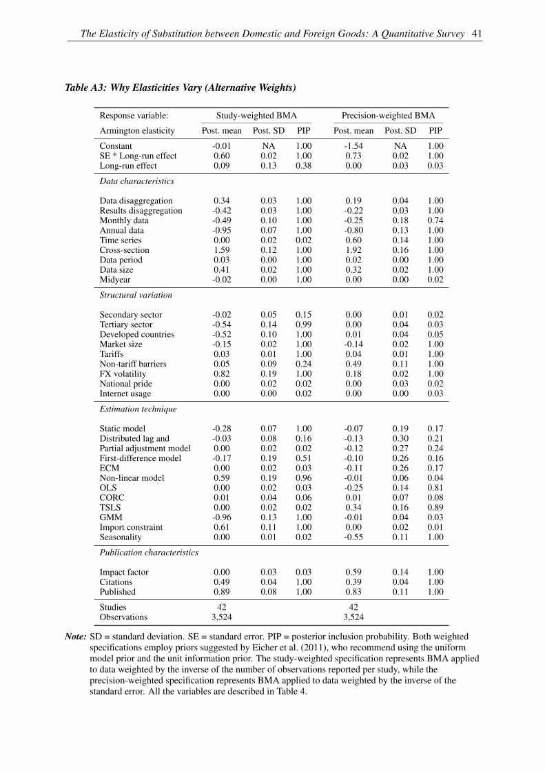
The Elasticity of Substitution between Domestic and Foreign Goods: A Quantitative Survey 41
Table A3: Why Elasticities Vary (Alternative Weights)
Response variable: Study-weighted BMA Precision-weighted BMA
Armington elasticity Post. mean Post. SD PIP Post. mean Post. SD PIP
Constant -0.01 NA 1.00 -1.54 NA 1.00SE * Long-run effect 0.60 0.02 1.00 0.73 0.02 1.00Long-run effect 0.09 0.13 0.38 0.00 0.03 0.03
Data characteristics
Data disaggregation 0.34 0.03 1.00 0.19 0.04 1.00Results disaggregation -0.42 0.03 1.00 -0.22 0.03 1.00Monthly data -0.49 0.10 1.00 -0.25 0.18 0.74Annual data -0.95 0.07 1.00 -0.80 0.13 1.00Time series 0.00 0.02 0.02 0.60 0.14 1.00Cross-section 1.59 0.12 1.00 1.92 0.16 1.00Data period 0.03 0.00 1.00 0.02 0.00 1.00Data size 0.41 0.02 1.00 0.32 0.02 1.00Midyear -0.02 0.00 1.00 0.00 0.00 0.02
Structural variation
Secondary sector -0.02 0.05 0.15 0.00 0.01 0.02Tertiary sector -0.54 0.14 0.99 0.00 0.04 0.03Developed countries -0.52 0.10 1.00 0.01 0.04 0.05Market size -0.15 0.02 1.00 -0.14 0.02 1.00Tariffs 0.03 0.01 1.00 0.04 0.01 1.00Non-tariff barriers 0.05 0.09 0.24 0.49 0.11 1.00FX volatility 0.82 0.19 1.00 0.18 0.02 1.00National pride 0.00 0.02 0.02 0.00 0.03 0.02Internet usage 0.00 0.00 0.02 0.00 0.00 0.03
Estimation technique
Static model -0.28 0.07 1.00 -0.07 0.19 0.17Distributed lag and -0.03 0.08 0.16 -0.13 0.30 0.21Partial adjustment model 0.00 0.02 0.02 -0.12 0.27 0.24First-difference model -0.17 0.19 0.51 -0.10 0.26 0.16ECM 0.00 0.02 0.03 -0.11 0.26 0.17Non-linear model 0.59 0.19 0.96 -0.01 0.06 0.04OLS 0.00 0.02 0.03 -0.25 0.14 0.81CORC 0.01 0.04 0.06 0.01 0.07 0.08TSLS 0.00 0.02 0.02 0.34 0.16 0.89GMM -0.96 0.13 1.00 -0.01 0.04 0.03Import constraint 0.61 0.11 1.00 0.00 0.02 0.01Seasonality 0.00 0.01 0.02 -0.55 0.11 1.00
Publication characteristics
Impact factor 0.00 0.03 0.03 0.59 0.14 1.00Citations 0.49 0.04 1.00 0.39 0.04 1.00Published 0.89 0.08 1.00 0.83 0.11 1.00
Studies 42 42Observations 3,524 3,524
Note: SD = standard deviation. SE = standard error. PIP = posterior inclusion probability. Both weightedspecifications employ priors suggested by Eicher et al. (2011), who recommend using the uniformmodel prior and the unit information prior. The study-weighted specification represents BMA appliedto data weighted by the inverse of the number of observations reported per study, while theprecision-weighted specification represents BMA applied to data weighted by the inverse of thestandard error. All the variables are described in Table 4.

CNB WORKING PAPER SERIES (SINCE 2018)
12/2019 Josef Bajzík Tomáš Havránek Zuzana Iršová Jiří Schwarz
The elasticity of substitution between domestic and foreign goods: A quantitative survey
11/2019 Martin Hodula Simona Malovaná Jan Frait
Too much of a good thing? Households’ macroeconomic conditions and credit dynamics
10/2019 Martin Hodula Simona Malovaná Jan Frait
Introducing a new index of households’ macroeconomic conditions
9/2019 Jiří Panoš Petr Polák
How to improve the model selection procedure in a stress-testing framework?
8/2019 Sebastian Gechert Tomáš Havránek Zuzana Iršová Dominika Kolcunová
Death to the Cobb-Douglas production function? A quantitative survey of the capital-labor substitution elasticity
7/2019 Alexis Derviz Coexistence of physical and crypto assets in a stochastic endogenous growth model
6/2019 Dominika Ehrenbergerová Simona Malovaná
Introducing macro-financial variables into semi-structural model
5/2019 Martin Hodula Monetary policy and shadow banking: Trapped between a rock and a hard place
4/2019 Simona Malovaná Žaneta Tesařová
Banks’ credit losses and provisioning over the business cycle: Implications for IFRS 9
3/2019 Aleš Bulíř Jan Vlček
Monetary policy is not always systematic and data-driven: Evidence from the yield curve
2/2019 Dominika Kolcunová Simona Malovaná
The effect of higher capital requirements on bank lending: The capital surplus matters
1/2019 Jaromír Baxa Tomáš Šestořád
The Czech exchange rate floor: Depreciation without inflation?
19/2018 Jan Brůha Jaromír Tonner
Independent monetary policy versus common currency: The macroeconomic analysis for the Czech Republic through lens of an applied DSGE model
18/2018 Tomáš Adam Filip Novotný
Assessing the external demand of the Czech economy: Nowcasting foreign GDP using bridge equations
17/2018 Kamil Galuščák Jan Šolc Pawel Strzelecki
Labour market flows over the business cycle: The role of the participation margin
16/2018 Martin Hodula Off the radar: Exploring the rise of shadow banking in the EU
15/2018 Lukáš Pfeifer Martin Hodula Libor Holub Zdeněk Pikhart
The leverage ratio and its impact on capital regulation
14/2018 Martin Gürtler What influences private investment? The case of the Czech Republic
13/2018 Václav Hausenblas Jitka Lešanovská
How do large banking groups manage the efficiency of their subsidiaries? Evidence from CEE
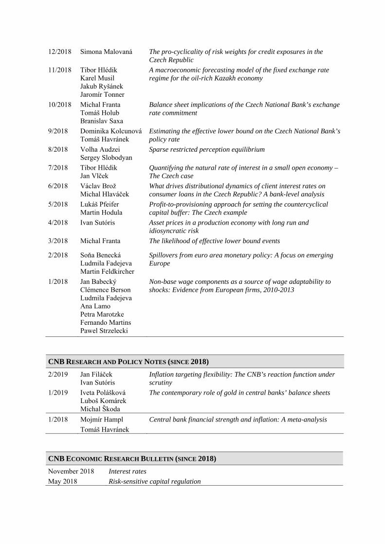
12/2018 Simona Malovaná The pro-cyclicality of risk weights for credit exposures in the Czech Republic
11/2018 Tibor Hlédik Karel Musil Jakub Ryšánek Jaromír Tonner
A macroeconomic forecasting model of the fixed exchange rate regime for the oil-rich Kazakh economy
10/2018 Michal Franta Tomáš Holub Branislav Saxa
Balance sheet implications of the Czech National Bank’s exchange rate commitment
9/2018 Dominika Kolcunová Tomáš Havránek
Estimating the effective lower bound on the Czech National Bank’s policy rate
8/2018 Volha Audzei Sergey Slobodyan
Sparse restricted perception equilibrium
7/2018 Tibor Hlédik Jan Vlček
Quantifying the natural rate of interest in a small open economy – The Czech case
6/2018 Václav Brož Michal Hlaváček
What drives distributional dynamics of client interest rates on consumer loans in the Czech Republic? A bank-level analysis
5/2018 Lukáš Pfeifer Martin Hodula
Profit-to-provisioning approach for setting the countercyclical capital buffer: The Czech example
4/2018 Ivan Sutóris Asset prices in a production economy with long run and idiosyncratic risk
3/2018 Michal Franta The likelihood of effective lower bound events
2/2018 Soňa Benecká Ludmila Fadejeva Martin Feldkircher
Spillovers from euro area monetary policy: A focus on emerging Europe
1/2018 Jan Babecký Clémence Berson Ludmila Fadejeva Ana Lamo Petra Marotzke Fernando Martins Pawel Strzelecki
Non-base wage components as a source of wage adaptability to shocks: Evidence from European firms, 2010-2013
CNB RESEARCH AND POLICY NOTES (SINCE 2018)
2/2019 Jan Filáček Ivan Sutóris
Inflation targeting flexibility: The CNB’s reaction function under scrutiny
1/2019 Iveta Polášková Luboš Komárek Michal Škoda
The contemporary role of gold in central banks’ balance sheets
1/2018 Mojmír Hampl
Tomáš Havránek
Central bank financial strength and inflation: A meta-analysis
CNB ECONOMIC RESEARCH BULLETIN (SINCE 2018)
November 2018 Interest rates
May 2018 Risk-sensitive capital regulation

Czech National Bank Economic Research Division
Na Příkopě 28, 115 03 Praha 1 Czech Republic
phone: +420 2 244 12 321 fax: +420 2 244 12 329
http://www.cnb.cz e-mail: [email protected]
ISSN 1803-7070
Related Documents