WORKING PAPER - Leuphana

WO

RK

ING

PAP

ER

On Entrepreneurial Risk–Takingand the Macroeconomic Effects

of Financial Constraints

by

Christiane Clemens and Maik Heinemann

University of LüneburgWorking Paper Series in Economics

No. 103

October, 2008

www.uni-lueneburg.de/vwl/papers

ISSN 1860–5580

On Entrepreneurial Risk–Taking and the

Macroeconomic Effects of Financial Constraints†

Christiane Clemens∗

University of Hamburg

Maik Heinemann∗∗

University of Lüneburg

October 22, 2008

Abstract

This paper deals with credit market imperfections and idiosyncratic risks

in a two–sector heterogeneous agent dynamic general equilibrium model of

occupational choice. We focus especially on the effects of tightening finan-

cial constraints on macroeconomic performance, entrepreneurial risk–taking,

and social mobility. Contrary to many models in the literature, our compar-

ative static results cover a broad range for borrowing constraints, from an

unrestrained to a perfectly constrained economy. In our baseline model, we

find substantial gains in output, welfare, and wealth equality associated with

credit market improvements. The marginal gains from relaxing constraints are

largest for empirically relevant debt–equity ratios. Interestingly, the entrepren-

eurship rate and social mobility respond non–monotonically to a change in the

tightness of financial constraints. The results crucially depend on the degree of

income persistence and feedback effects in general equilibrium, where optimal

firm sizes and the demand for credit are determined endogenously.

Keywords: CGE, occupational choice, financial constraints, wealth distribution

JEL classification: C68, D3 , D8, D9, G0, J24

†We are grateful to Robert E. Lucas, Ian P. King, Richard Rogerson, and Nancy L. Stokey for help-

ful comments, and thank seminar participants at the 2008 Southern Workshop in Macroeconomics,

and on the 2007 / 2008 meetings of the Econometric Society, the Royal Economic Society, the So-

ciety for Computational Economics, the Society for Economic Dynamics, and the German Economic

Association.∗University of Hamburg, Germany, [email protected]∗∗University of Lüneburg, Germany, [email protected]

1 Introduction

This paper examines the effects of financial constraints and idiosyncratic risks in a

dynamic equilibrium model of occupational choice. We determine the qualitative

and quantitative response of aggregate macroeconomic activity, social mobility, and

the wealth distribution to credit market improvements.

Our analysis contributes to recent literature on dynamic stochastic heteroge-

neous agent general equilibrium models concerned with risk and distributional dy-

namics, for instance Quadrini (2000), Meh (2005, 2008), Bohác̆ek (2006, 2007)

and Cagetti and De Nardi (2006a,b,c). All these contributions share as common

feature that including entrepreneurship and occupational choice into a Huggett

(1993) / Aiyagari (1994)–type economy provides a much better explanation of the

empirically observed wealth inequality, especially in the upper tail of the distri-

bution. The implications of our model regarding wealth inequality are in accor-

dance with this strand of literature, although our focus is more directed towards

the general effects of financial constraints and the question of how sensitive the

macroeconomy as a whole responds to a reduction in credit market imperfections.

To this end we develop a model which is more closely related to modern growth

theory. Regarding the role of entrepreneurship, we assume a more sophisticated sec-

toral structure than e.g. Bohác̆ek (2006) or Cagetti and De Nardi (2006a). We com-

bine occupational choice under risk à la Kihlstrom and Laffont (1979) and Kanbur

(1979a,b) with the two–sector approach of Romer (1990), but without endogenous

growth. In each period of time, the risk–averse agents choose between between

two alternative occupations. They either set up an enterprise in the intermediate

goods industry which is characterized by monopolistic competition. Or, they supply

their labor endowment to the production of a final good in a perfectly competitive

market. Producers of the final good use capital and labor inputs, and differenti-

ated varieties of the intermediate good. All households are subject to an income

risk. Managerial ability and productivity as a worker follow independent random

processes. Entrepreneurial activity is rewarded with a higher expected income.1

Similar to Lucas (1978), there is no aggregate risk.

The economic performance in the intermediate goods industry crucially depends

on two factors: uncertainty and credit constraints. Business owners face an firm–

specific productivity shock, and there are no markets for pooling risks. An en-

trepreneurs maximizes his profit if the business operates at the optimal firm size,

which is endogenously determined and governed by market demand from the final

goods industry. For an individual wealth too small to maintain the optimal firm

size, the firm–owner would want to borrow the remaining amount on the credit

market, where he might be subject to financial constraints. The individual demand

for loans, too, is endogenous. If the entrepreneur is wealthy enough, he operates

1See also Clemens (2006a,b, 2008) and Clemens and Heinemann (2006) for entrepreneurial risk–

taking in a general equilibrium context.

2

his business at the profit–maximizing level and supplies the rest of his wealth to the

capital market.

Due to the two–sector general equilibrium nature of our model, the optimal

business size and the demand for credit are endogenously determined, and we do

not have to fall back on fixed investment projects (or entry costs respectively) in

order to analyze the effects of credit market frictions.2 There is no further portfolio

choice in our framework. To this end, our approach draws a simple picture of

the empirical result, stated by Heaton and Lucas (2000), that the entrepreneurial

households’ business wealth on average constitutes a relevant fraction of their total

wealth.

We are especially interested in the question of how tightening (or relaxing) fi-

nancial constraints affects the macroeconomy regarding aggregate output, the sec-

toral allocation of capital and labor, factor prices, the income and wealth distribu-

tion, occupational choice, as well as the between–group mobility of households.

Our comparative static analysis covers a broad range of values for borrowing con-

straints, from an unconstrained to a perfectly constrained economy. This is a novel

approach since many models of the literature consider a fixed debt–equity ratio, or

rest with a comparison of a complete vis–à–vis a specific incomplete market, or they

focus on the no–credit market scenario.

The model is broadly consistent with macro data from industrialized countries.

Naturally, the model cannot draw a realistic picture of the economy over the entire

domain of financial constraints under consideration. For this reason, we define a

benchmark economy with an empirically plausible debt–equity ratio, and calibrate

the model to match macroeconomic key variables, for instance, for the U.S. and

other OECD members.

We find substantial gains of relaxing constraints, amounting to 20% of aggregate

output, and observe likewise improvements in average wealth holdings and welfare.

The associated marginal gains of credit market improvements in the intermediate

goods industry are substantial for debt–equity ratios in the empirically relevant

domain and increasing.

The macroeconomic effects can primarily be attributed to an inefficient allo-

cation of capital across sectors, and only secondly to adjustments in occupational

choice, employment, and the entrepreneurship rate. In moving from an uncon-

strained to a completely credit–constrained economy, the average firm size drops

down to a mere 50% of optimal business activity. Capital accumulation plays a

twofold role in this context: On the one hand, it endows individuals with the wealth

necessary to set–up and operate a firm. On the other hand, buffer–stock saving

provides a self–insurance on intertemporal markets against the non–diversifiable

income risk. Accordingly, we find that wealthier households are more likely to be

2It is a standard approach in the literature to assume entry costs, often combined with a decreasing

returns technology, to generate some kind of ‘monopolistic’ market structure, which is an innate part

of our model.

3

members of the entrepreneurial class than poorer ones and there is a marked con-

centration of wealth in the hands of entrepreneurs which is consistent with recent

empirical findings (cf. Quadrini, 1999; Holtz-Eakin et al., 1994a). Upward mobil-

ity of entrepreneurs in our model is primarily accumulation driven. The riskiness

of entrepreneurial incomes looses its importance for occupational choice once the

household’s income share generated from profits declines relative to his capital in-

come. Nevertheless, in accordance with Hamilton (2000), many entrepreneurs of

our model enter and persist in business despite the fact that they have lower initial

earnings than average wage incomes.

Regarding empirical evidence, there is strong support in the literature for the hy-

pothesis that financial constraints are an impediment to entering entrepreneurship;

see Evans and Leighton (1989), Evans and Jovanovic (1989), Holtz-Eakin et al.

(1994b), Blanchflower and Oswald (1998), Moskowitz and Vissing-Jørgensen

(2002), and Desai et al. (2003). Gentry and Hubbard (2004) point out that exter-

nal financing has important implications for individual investment and saving. This

evidence is challenged by Hurst and Lusardi (2004), who find that the likelihood

of entering entrepreneurship relative to initial wealth is flat over a large range of

the wealth distribution and increasing only for higher wealth levels of workers.

The general equilibrium nature of our approach generates surprising and almost

counter–intuitive results regarding the impact of financial constraints on occupa-

tional choice under risk. The entrepreneurship rate and social mobility respond

non–monotonically to a change in the tightness of constraints. Because individual

income persistence can be identified as an important determinant of occupational

choice and mobility, we analyze two settings which only differ with respect to the

serial correlation of the underlying idiosyncratic shocks. The entrepreneurship rate

of the baseline model rises with an increase in credit market efficiency, which is in

accordance with economic intuition. If, however, the persistence of entrepreneurial

talent shocks is reduced, we predominantly observe a decline in the entrepren-

eurship rate. This outcome can primarily be attributed to the general equilibrium

nature of our model.

Wealth inequality is not necessarily reduced, if we relax borrowing constraints.

Regarding social mobility, the response to changes in credit availability also is non–

monotonic. In general we find that workers and entrepreneurs with high individual

productivity tend to remain in their present occupation, whereas low productivity

individuals are more likely to switch professions.

Regarding the functional distribution of income, we find that credit constraints

have a redistributive effect by raising the profit income share at the cost of capital

incomes. The results indicate that the stochastic nature of the underlying idio-

syncratic shocks also plays an important role for the explanation of the general

equilibrium effects of credit market imperfections.

Recent contributions in this area of research suffer from several shortcomings

which our approach aims to overcome. In Quadrini (2000), occupational choice

4

and the level of entrepreneurship is (more or less) entirely governed by the under-

lying productivity shocks. Li (2002) and Bohác̆ek (2006) discuss economies with

a single sector of production which does not allow for factor movements between

industries and therefore neglects factor substitution. In our model, producers of

the intermediate and the final good are subject to competition, especially with re-

spect to capital demand. Our approach does not have fixed entry costs (in terms

of discrete investment projects) of entrepreneurship as in Ghatak et al. (2001),

Fernández-Villaverde et al. (2003) or Clementi and Hopenhayn (2006). Instead,

we have an endogenously determined optimal firm size and no discontinuities in

individual credit demand. Occupational choice, entrepreneurial activity and per-

formance crucially depend on monopoly profits, market shares and relative factor

scarcity in the two sectors of production. Also different to Cagetti and De Nardi

(2006a) or Kitao (2008), the entrepreneurs of our economy are essential for aggre-

gate output. As will become obvious below, the interdependence of sectors is impor-

tant for the general equilibrium results on occupational choice, between–group mo-

bility and the income and wealth distribution, and contributes to the understanding

of how financial constraints affect the macroeconomy.

The paper is organized as follows: Section 2 develops the two–sector model. We

describe the equilibrium associated with a stationary earnings and wealth distribu-

tion. Since the formal structure of the model does not allow for analytical solu-

tions, we perform numerical simulations of a calibrated model in order to examine

the general equilibrium effects of an increase in the tightness of credit constraints.

Section 3 gives information on the calibration procedure and related empirical ev-

idence. Section 4 discusses the simulation results. Section 5 concludes. Technical

details are relegated to the Appendix.

2 The Model

2.1 Overview

We consider a neoclassical growth model with two sectors of production. Draw-

ing from Quadrini (2000) and Romer (1990), we consider a corporate sector with

perfectly competitive large firms who hire capital and labor services and use an

intermediate good in order to produce a homogeneous output which can be con-

sumed or invested respectively. The intermediate goods industry (non–corporate

sector) consists of a large number of small firms operating under the regime of

monopolistic competition. Each firm in this sector is owned and managed by an

entrepreneur. Both sectors of production are essential.

Market activity in the intermediate goods industry is constrained. In order to

run the business at the profit–maximizing firm size, entrepreneurs either possess

sufficient wealth of their own, or they need to compensate for their lack of eq-

uity by borrowing on the credit market, where they might be subject to borrowing

5

constraints. The two–sector setting allows us to endogenously relate financial con-

straints to individual characteristics and overall market activity.

The economy is populated by a continuum [0,1] of infinitely–lived households,

each endowed with one unit of labor.3 In each period of time, individuals follow

their occupation predetermined from the previous period and make a decision re-

garding their future profession, which is either to become producers of the inter-

mediate good or to supply their labor services to the production of the final good.

Labor efficiency as well as entrepreneurial productivity are idiosyncratic random

variables. Regarding the associated income risk, we assume that wage incomes are

less risky than profit incomes. There is no aggregate risk.

With respect to the timing of events, we assume that individual occupational

choice takes place before the resolution of uncertainty. Once the draw of nature

has occurred, entrepreneurs as well as workers in the final goods sector know their

individual productivity. Those monopolists, who now discover their own wealth

being too low to operate at the optimal firms size, will express their capital demand

on the credit market, probably become subject to credit–constraints, and then start

production. After labor and profit income is realized, the households decide on

how much to consume and to invest. There is no capital income risk and no risk of

production in the corporate sector.

2.2 Final Goods Sector

The representative firm of the final goods sector produces a homogeneous good

Y using capital KF , labor L, and varieties of an intermediate good x(i), i ∈ [0,λ] as

inputs. Production in this sector takes place under perfect competition and the

price of Y is normalized to unity. The production function is of the generalized

CES–form4

Y =(

KγF L1−γ)1−α

Z λ

0x(i)α di , 0 < α < 1, 0 < γ < 1 . (1)

Each type of intermediate good employed in the production of the final good is

identified with one monopolistic producer in the intermediate goods sector. Con-

sequently, the number of different types is identical with the population share λof entrepreneurs in the population. The number of entrepreneurs is determined

endogenously through occupational choices of the agents, which will be described

below. Additive–separability of (1) in intermediate goods ensures that the marginal

product of input i is independent of the quantity employed of i′ 6= i. Intermediate

goods are close but not perfect substitutes in production.

3It would be a straightforward extension of the model to include the life–cycle dimension, inter-

generational altruism and bequests as in De Nardi (2004), Cagetti and De Nardi (2006a), or issues

of firm growth, but this is beyond the scope of the present paper.4All macroeconomic variables are time–dependent. For notational convenience, we will drop the

explicit time–notation unless necessary. If needed, the ′ symbol denotes next period variables.

6

The profit of the representative firm in the final goods sector, πF , is given in

each period by

πF = Y−wL− (r + δ)KF −

Z λ

0p(i)x(i) di , (2)

where p(i) denotes the price of intermediate good i. We further assume physical

capital to depreciate over time at the constant rate δ, such that the interest factor

is given by R= 1+ r −δ. Optimization yields the profit maximizing factor demands

consistent with marginal productivity theory

KF = (1−α)γY

r + δ, (3)

L = (1−α)(1− γ)Yw

(4)

x(i) = KγFL1−γ

(

αp(i)

)1

1−α

. (5)

The monopolistic producer of intermediate good x(i) faces the isoelastic demand

function (5), where the direct price elasticity of demand is given by −1/(1−α).

Condition (4) describes aggregate labor demand in efficiency units. Equation (3) is

the final good sector demand for capital services.

2.3 Intermediate Goods Sector

The intermediate goods sector consists of the population fraction λ of entrepren-

eurs who self–employ their labor endowment by operating a monopolistic firm.

Each monopolist produces a single variety i of the differentiated intermediate good

by employing capital from own wealth and borrowed resources according to the

identical constant returns to scale technology of the form

x(i) = θ(i)e k(i) . (6)

Firm owners are heterogeneous in terms of their talent as entrepreneurs. They

differ with respect to the realization of an idiosyncratic productivity shock θ(i)e

which is assumed to be non–diversifiable and uncorrelated across firms. We will

give more details on the properties of the shock below. Entrepreneurs hire capital

after the draw of nature has occurred. The firm problem essentially is a static one.

Under perfect competition of the capital market, the producer treats the rental rate

to capital as exogenously given and maximizes his profit

π(k(i),θ(i)e) = p(i)x(i)− (r + δ)k(i) . (7)

Utilizing the demand function for intermediate good type–i, (5), and the pro-

duction technology (6), the optimal firm decision can be expressed in terms of the

7

optimal firm size k(i)∗, given by:

k(i)∗ = L θ(i)α

1−αe

(

γw(1− γ)(r + δ)

)γ ( α2

r + δ

)

11−α

. (8)

Because capital demand takes place after the draw of nature has occurred, there is

no individual capital risk and no under–employment of input factors. The optimal

firm size increases with random individual productivity θ(i)e, such that more pro-

ductive business owners demand more capital on the capital market. The aggregate

labor input in efficiency units determines the optimal firm size by means of the de-

mand function for intermediate good type i. Aggregate employment is a weighted

average and depends on the size of the labor force 1−λ, i.e. the population fraction

of agents choosing the occupation of a worker, and the idiosyncratic shock on labor

productivity θw. The larger the labor force 1−λ, the higher—ceteris paribus—will

be aggregate employment L. This goes along with fewer monopolists in the inter-

mediate goods industry, less competition, and a larger market share, as measured

by the optimal firm size.

2.4 Incomes and Equilibrium Income Shares in the Unconstrained Economy

Households derive income from three sources: labor income, capital income and

monopolistic profits. The technology parameters α and γ determine the division

of aggregate income among the three income sources in the absence of financial

constraints on entrepreneurial activity. According to marginal productivity theory,

we obtain from (1) a labor share of (1−α)(1− γ) and a capital share of (1−α)γ.The remaining income share α accrues to the two types of income generated in the

intermediate goods sector, and splits on profits with α(1−α) and capital income

with α2, respectively, such that the economy–wide capital share amounts to (1−α)γ+ α2.

2.5 Capital Market and Financial Constraints

Firms of the final goods sector and the intermediate goods industry differ with re-

spect to access to financial markets. While the first are not constrained in their

financing, the latter face greater difficulties in diversifying the risk from their en-

trepreneurial activities and, moreover, are subject to borrowing constraints. En-

trepreneurs of the intermediate goods industry, who are wealth–constrained in op-

erating their business at the optimal size (8), seek external financing from finan-

cial intermediaries. The credit market is imperfect with respect to lenders not be-

ing able to enforce loan–repayment due to limited commitment of borrowers (cf.

Banerjee and Newman, 1993). In order not to default on loan contracts, borrowing

amounts are limited, and individual wealth acts as collateral. We do not explic-

itly model financial intermediaries and assume that there is no difference between

borrowing and lending rates.

8

In case of default, the financial intermediator is able to seize a fraction of the

borrowers gross capital income (1+ r)a(i). Alternatively, one could assume the

entrepreneur’s profit income to act as collateral. The major difference between the

two approaches is that, in the first case, borrowing amounts are entirely determined

by the debtors individual wealth a(i), whereas in the second, they also depend on

his entrepreneurial talent θ(i)e, which might be private information.5

The creditor will lend to the borrower only the amount consistent with the bor-

rower’s incentive–compatibility constraint, such that it is in the borrower’s interest

to repay the loan, and there is no credit default in equilibrium.

Let k(i) = a(i)+b(i) be the firm size an entrepreneur is able to operate at from

own wealth a(i) and borrowed resources b(i). This operating capital k(i) is not

necessarily equal to the optimal firm size k(i)∗ determined in (8). An entrepreneur

with individual wealth a(i) lower than k(i)∗ will consider loans from the credit

market k(i)∗ − a(i). In case of k(i) < k(i)∗ the firm faces a borrowing constraint.

Incentive–compatibility requires a self–enforcing contract. It is never optimal for

the borrower to default, if

π(i)+ (1+ r)a(i) > π(i)+b(i)(1+ r)+ (1−φ)(1+ r)a(i)

which reduces to

b(i) 6 φa(i) . (9)

The borrowing amount is limited such that the maximum possible loan is propor-

tional to the borrowers individual wealth a(i). The parameter φ is a measure for the

extent to which a lender can use the borrower’s wealth income as collateral. Credit

constraints become less tight with rising φ and vanish for large φ. The limiting cases

consequently reflect the two cases of either complete enforceability (φ → ∞) or no

enforceability (φ = 0), such that in the first case the borrower is considered solvent,

whereas in the second one he is not.

Using the collateral constraint in the entrepreneurial budget constraint yields

k(i) 6 (1+ φ)a(i). The operating firm size k(i) of entrepreneur i with productivity

θ(i)e and wealth a(i) can then be written as:

k(θ(i)e ,a(i)) = min[k(i)∗,(1+ φ)a(i)] . (10)

The subsequent numerical analysis shows that the high–productivity entrepreneurs

are more likely to be constrained than the low–productivity ones, because the opti-

mal firm size and henceforth the capital demand increase in the productivity shock.

An entrepreneur, whose individual wealth exceeds the level needed to operate

his business at the optimal firm size will lend the amount a(i)− k(i)∗ on the capi-

tal market at the equilibrium interest rate. The supply side of the capital market

5The qualitative implications for the model are identical under both assumptions. If borrowing

amounts also depend on entrepreneurial productivity, the response to an increase in the tightness in

financial constraints is smaller in magnitude. The results are available from the authors upon request.

9

altogether consists of those entrepreneurs whose wealth exceeds their individual

optimal firm size and of workers, who supply their savings. On the demand side

we have the credit–constrained entrepreneurs and firms from the final goods indus-

try. From this follows immediately that the size of the intermediate goods industry

relative to the final goods sector essentially depends on occupational choice and

individual wealth accumulation, both determined endogenously in equilibrium.

2.6 Idiosyncratic Risks

In each period of time, workers are endowed with one unit of raw labor and are

subject to an idiosyncratic shock θw affecting labor supply in efficiency units, and

exposing each of them to an uninsurable income risk. We assume that labor produc-

tivity θw evolves according to a first–order Markov process with h = 1, . . . ,H states,

and θw,h > 0. The transition matrix associated with the Markov process is Pw .

Entrepreneurial productivity θe also evolves according to a first–order Markov

process with h = 1, . . . ,H different states θe,1, . . . ,θe,H ; θe,h > 0, and transition prob-

ability Pe. Since agents can be either workers or entrepreneurs, it is possible to

identify the occupational status of an agent with his productivity in the respective

occupation. We assume worker productivities to be more evenly distributed than

managerial skills, such that profit incomes in general are more risky than wage

incomes. As is well–known from the literature, entrepreneurs on average are com-

pensated with a positive income differential (aka ‘risk premium’) for bearing the

production risk.

By modeling two distinct random processes for workers and entrepreneurs, we

take into account that the two professions demand different talents, for instance

specific managerial skills. We assume the processes θw and θe to be uncorrelated,

such that for an individual the conditional expectation of entrepreneurial produc-

tivity is independent of the labor efficiency, if employed as a worker. A high produc-

tivity as a worker in the present does not necessarily indicate an equivalently high

future productivity as an entrepreneur, if the individual should decide to switch be-

tween occupations in the next period. The associated probabilities are summarized

in a H ×H transition matrices Pj, j ′ describing the transition from productivity state

θ j,h to state θ j ′,h′ for h,h′ = 1, . . . ,H, j = e,w and j 6= j ′.As the subsequent analysis will show, assuming different degrees of income

persistence crucially affects the pattern of how occupational choice interacts with

a change in the magnitude of financing constraints. If the income process is highly

persistent, then e.g. lowly productive workers and entrepreneurs are more likely

to be lowly productive in the future. The individual can infer from his present

productivity how his future productivity in the same occupation probably will be.

We consider two different specifications regarding the Markov processes for

entrepreneurial talent and worker efficiency respectively. By assuming a high

(medium) serial correlation for entrepreneurs (workers) in our baseline model,

10

we are able to generate results which closely match empirical findings regarding

the macroeconomic key variables and the wealth distribution. In the second setting

we customize the persistence of entrepreneurial income processes to match those

for workers, and focus on the effects on occupational choice and social mobility.

2.7 Intertemporal Decision and Occupational Choice

Each household i has preferences over consumption and maximizes discounted ex-

pected lifetime utility

E0

∞

∑t=0

βt U [ct(i)] 0 < β < 1 .

E0 is the expectation operator conditional on information at date 0 and β is the

discount factor. Individuals are assumed to be identical with respect to their pref-

erences regarding momentary consumption c(i) which are described by constant

relative risk aversion

U [c(i)] =

c(i)1−ρ

1−ρfor ρ > 0,ρ 6= 1

lnc(i) for ρ = 1 ,

where ρ denotes the Arrow/Pratt measure of relative risk aversion.

Besides intertemporal consumption choice, the single household also makes a

decision on his future occupation in each period, which is either to become a self–

employed producer of an intermediate good in the monopolistically competitive

market or to inelastically supply his labor services in efficiency units to the produc-

tion of the final good. Occupational choice, once made, is irreversible in the same

period.

Let Vw(a(i),θ(i)w) denote the optimal value function of an agent currently being

a worker with wealth a, who is in a given productivity state θw. If he decides to re-

main a worker, his productivity evolves according to the transition matrix Pw of the

underlying Markov process. If, instead, he becomes an entrepreneur in the follow-

ing period, he gets a new draw θ′e from the invariant distribution of entrepreneurial

productivities. The next period productivity is determined by the transition matrix

Pw,e (see model calibration below).

There are no markets for pooling idiosyncratic risks. In addition to the financial

constraints of the intermediate goods industry, we also have incomplete insurance

markets. There is limited scope to which agents are able to smooth their intertem-

poral consumption flow by borrowing and lending. The standard approach of the

literature is to assume that individual asset holdings are bounded from below. In

what follows, we assume a lowest possible wealth level of a = 0.

11

The maximized value function for a typical individual currently being a worker

is given by

Vw (a(i),θ(i)w) = maxc(i)>0,a(i)′>a

{

U [c(i)]

+β maxq(i)′∈{0,1}

(1−q(i)′)E[

Vw(

a(i)′,θ(i)′w)

|θ(i)w]

+q(i)′ E[

Ve(

a(i)′,θ(i)′e)]

}

s.t. a(i)′ = (1+ r)a(i)+ θ(i)w w−c(i) .

(11)

q is a boolean variable which takes on the values 0 or 1, depending on whether or

not the agent decides to switch between occupations. r and w denote the equilib-

rium returns to capital and labor in efficiency units, which are constant over time

for a stationary distribution of wealth and occupational statuses over agents. The

optimal decision associated with the problem (11) is described by the two decision

rules for individual asset holdings a(i)′w = Aw(a(i), θ(i)w) and the future professional

state q(i)′w = Qw(a(i), θ(i)w).

Let Ve(a(i),θ(i)e) denote the maximized value function of an entrepreneur with

wealth a in productivity state θe, who faces a decision problem similar to those of a

worker. If he decides to remain an entrepreneur, his productivity evolves according

to the transition matrix Pe of the underlying Markov process. If, instead, he decides

to switch between occupations by becoming a worker in the next period, his future

productivity θ′w is determined by the transition matrix Pe,w. With k(i)∗ denoting the

optimal firm size, the intertemporal problem of an entrepreneur can be written as

Ve(a(i),θ(i)e) = maxc(i)>0,a(i)′>a

{

U [c(i)]

+β maxq(i)′∈{0,1}

(1−q(i))′)E[

Ve(

a(i)′,θ(i)′e)

|θ(i)e]

+q(i)′ E[

Vw(

a(i)′,θ(i)′w)]

}

s.t. a(i)′ = (1+ r)a(i)+ π(k(i),θ(i)e)−c(i)

k(i) = min[k(i)∗,(1+ φ)a(i)]

π(θ(i)e,k(i)) = p(x(i))x(θ(i)e,k(i))− (r + δ)k(i)

(12)

Again, q is a boolean variable, indicating the agent’s decision on leaving or remain-

ing in his present occupation. The optimal decision is described by the decision

rules for individual asset holdings a(i)′e = Ae(a(i), θ(i)e) and the future professional

state q(i)′e = Qe(a(i), θ(i)e).6

6Note that the value functions (11) and (12) may not be concave because of the boolean variable

q, indicating binary choice between occupations. Similar to Fernández-Villaverde et al. (2003), we

12

In general, our model generates the same implications for individual savings

and wealth accumulation under risk as, for instance, discussed in Aiyagari (1994)

or Huggett (1996). Similar to Quadrini (2000), we additionally consider occupa-

tional choice. Consequently, wealth accumulation plays a two–fold role: On the one

hand, the shocks to worker efficiency and entrepreneurial productivity generate an

income risk which households respond to with buffer–stock saving. On the other

hand, higher wealth levels protect entrepreneurs against the danger of being sub-

ject to financial constraints. In terms of Sandmo (1970) there is only an income but

no capital risk in our model, such that the share of risky incomes in total household

income declines with growing wealth. Accordingly, the importance of risky prof-

its providing negative incentives towards entrepreneurship fades for high levels of

wealth.

2.8 Stationary Recursive Equilibrium

A stationary recursive competitive general equilibrium is an allocation, where equi-

librium prices generate a distribution of wealth and occupations over agents which

is consistent with these prices given the exogenous process for the idiosyncratic

shocks and the agents’ optimal decision rules.

We obtain aggregate labor supply by summing up individual labor supplies in ef-

ficiency units over the population fraction 1−λ of workers. The stationary recursive

equilibrium is a set of value functions Vw (a,θw), Ve(a,θe), decision rules Aw(a,θw),

Qw(a,θw) and Ae(a,θe), Qe(a,θe), prices w, r, p(i) and a distribution λ,1−λ of house-

holds over occupations such that:7

(i) the decision rules Aw (a,θw), Qw(a,θw) and Ae(a,θe), Qe(a,θe) solve the work-

ers’ and entrepreneurs’ problems (11) and (12) at prices w, r, p(i),

(ii) the aggregate demands of consumption, labor, capital and intermediate goods

are the aggregation of individual demands. Factor and commodity markets

clear at constant prices w, r, p(i), where factor inputs are paid according to

their marginal product.

(iii) the stationary distribution Γ of agents over individual wealth holdings, occu-

pations and associated productivities is the fixed point of the law of motion

which is consistent with the individual decision rules and equilibrium prices.

The distribution λ,1−λ of agents over occupations is time–invariant.

The decision rules for workers, Aw(a, θw), Qw(a, θw), and entrepreneurs, Ae(a, θe),

Qe(a, θe), together with the stochastic processes for individual labor productivity

would like to stress that the dynamic programming algorithm underlying our computational modeling

does not require concavity but monotonicity to converge to the true value function; see also Bohác̆ek

(2007, fn. 4).7See Appendix A for the equilibrium conditions of the discrete formulation of the model underlying

the numerical simulations.

13

and entrepreneurial productivity, determine the stationary distribution Γ at equilib-

rium prices w, r. The stationary distribution Γ governs the population share of en-

trepreneurs (i.e. the mass of firms in the intermediate goods sector), the efficiency

units of labor supplied by workers, capital demand of the intermediate goods sec-

tor, and the aggregate capital supply, the latter equaling the mean of individual

wealth holdings. Once the population share of entrepreneurs λ is derived, this to-

gether with the stationary distribution of entrepreneurial productivities determines

the supply of intermediate goods (for details, see Appendix A).

3 Calibration

In order to evaluate the macroeconomic effects of changes in the tightness of fi-

nancial constraints, our first step is to define a benchmark economy which matches

standard macro data from OECD countries. We calibrate the model to replicate em-

pirical observations regarding the functional and personal distribution of income

and wealth, capital return, entrepreneurship rates, and social mobility. The bench-

mark value for the debt–equity ratio is set to φ = 1, i.e., the maximum loan is

limited to half the amount of the operating capital (cf. Evans and Jovanovic, 1989;

Gentry and Hubbard, 2004). Table 1 summarizes the parameterization of the model

and our calibration targets. We find that it is sufficient to mimic unlimited access to

credit (φ → ∞) in our simulations by choosing the largest value for φ = 1000, where

virtually no entrepreneur is restrained.

We adopt a broad notion of entrepreneurship and consider an entrepreneur as

someone, who owns and operates a small business, and who is willing to take risks,

to be innovative, and to exploit profit opportunities (Knight, 1921; Schumpeter,

1930; Kirzner, 1973). Definitions of self–employment and entrepreneurial activity

differ widely across countries.8 According to the OECD, self–employment encom-

passes “. . . those jobs, where the remuneration is directly dependent upon the profits

derived from the goods and services produced. The incumbents make the operational

decisions affecting the enterprise, or delegate such decisions while retaining responsi-

bility for the welfare of the enterprise.” (OECD, 2000, Ch. 5, p. 191). Our model gen-

erates self–employment business ownership rates around 20%, which is somewhat

more at the upper range of values for OECD countries (including owner–managers),

matching countries like New Zealand (20.8%), Italy (24.8%), or Spain (18.3%);

see also the annual Global Entrepreneurship Monitor (GEM 2005, Minniti et al.)

for data on total entrepreneurial activity.

Regarding preferences, we set the discount factor β and the coefficient of rela-

tive risk aversion ρ according to estimates from the literature, in order to generate

equilibrium interest rates on safe assets around 3% which is consistent with em-

pirical findings (cf. Mehra and Prescott, 1985; Obstfeld, 1994). The parameters of

8Often, the agricultural sector is excluded from the computation of entrepreneurship rates.

14

Table 1: Calibration Values for the Baseline Model

Calibrated parameter Calibration target (approx. ) Source

Technology Interest rate r 2–4% (Mehra and Prescott,

1985; Quadrini, 2000)α γ δ0.33 0.06 0.1 Factor income shares

labor 0.63 (King and Rebelo,

1999, PSID)Preferences profit 0.22

ρ β capital 0.15

2.0 0.91

Gini index of wealth 0.75–0.78 (PSID, SCE)

Shocks

σw pw σe pe Income persistence pw (Aiyagari, 1994;

Guvenen, 2007, &

references therein)

0.2 0.6 1.8 0.9 0.5–0.9

Financial frictions Entrepreneurship rate 15–25% (GEM, 2005)

φ Exit / entry rates 20–35% (Quadrini, 2000; Vale,

2006; Aghion et al.,

2007)

0↔ 1000

production technology, α and γ, are chosen such as to generate an equilibrium labor

income share of 0.63 which matches empirical observations e.g. for the U.S. econ-

omy (King and Rebelo, 1999) or the average of EU 15. The corresponding capital

and profit income shares of the unconstrained economy (φ → ∞) are 0.16 and 0.21.

PSID data report a income share for entrepreneurs of around 22%. The depreciation

rate is fixed at 6%, which also is a standard choice in the literature.

The steady state of the simulated benchmark economy replicates the Gini co-

efficient of wealth inequality for the U.S. (PSID, 1989) but also matches OECD

countries like Sweden, France, and Switzerland.

To take account of empirically observed income persistence, we assume that the

processes for labor efficiency θw and entrepreneurial productivity θe are lognormal

with normalized mean lnθw ∼ N(

−σ2w/2,σ2

w

)

, lnθe ∼ N(

−σ2e/2,σ2

e

)

and AR(1) of

the general form:

lnθ′w = (pw−1)σ2

w

2+ pw lnθw + σw

√

1− p2w ε , (13)

lnθ′e = (pe−1)σ2

e

2+ pe lnθe+ σe

√

1− p2e ε , (14)

where ε ∼ N (0,1). The process (13) is parameterized following Aiyagari (1994)

with pw = 0.6 and σw = 0.2. With respect to the entrepreneurial income process

(14), our baseline model assumes a higher serial correlation pe = 0.9 and a larger

variance σe = 1.8 in order to reproduce the higher risk associated with entrepren-

15

eurial activity and to generate empirically plausible exit / entry rates and wealth

inequality. We assume identical correlations pe,w = 0.6 in our second setting to

highlight that occupational choice and social mobility crucially depend on income

persistence.

Entry rates into entrepreneurship equal exit rates in the stationary recursive

equilibrium. Our model is calibrated to generate exit rates of around 4% of the

population (≈ 20% of intermediate industry members) which consistent with the

evidence reported by Quadrini (2000) but higher than the rates documented by

Evans (1987) for the U.S., and also in the upper range of empirically plausible

values for OECD countries (cf. Vale, 2006; Aghion et al., 2007).

The income processes are approximated with a five–state Markov chain by using

the method described in Tauchen (1986). The transition matrices for individuals

who decide to switch between occupations are derived from the stationary distri-

butions of the Markov processes. The probability for a worker (entrepreneur) of

ending up in a specific state of entrepreneurial (worker) productivity θe,h (θw,h) is

given by the stationary (unconditional) probabilities of this state. The algorithm for

finding the equilibrium consists of three nested loops, starting from an initial guess

on factor prices w, r and employment L, then iterating until markets clear and the

conditions of a stationary recursive equilibrium are met (see Appendix A).

4 Results

Our baseline model describes an economy where agents choose between two un-

correlated occupational lotteries with different degrees of income persistence. The

benchmark economy is subject to moderate constraints on the credit market and

calibrated such as to match empirical evidence for the U.S. and other OECD coun-

tries. We now proceed with investigating the effects of a change in the tightness of

financial constraints on (a) inequality and the distribution of wealth, (b) on output,

factor prices, and the factor income distribution, and (c) on occupational choice

and social mobility.

A common finding for models with credit market imperfections is that the prop-

erties of the equilibrium often respond non–monotonically to parameter changes.

If we look at the literature, we find models assessing the effects of credit market

imperfections by assuming no credit market at all (e.g. Bohác̆ek, 2007). Other

approaches compare imperfect to perfect markets.9 As Matsuyama (2007, p. 3)

points out, there is no reason to believe that, first, the effects of an imperfect mar-

ket equal those of no credit market, and second, the effects of improving credit mar-

kets are similar to those of completely eliminating market imperfections. Instead of

discussing only a single case by assuming a predetermined magnitude of financial

constraint, we vary the tightness of constraints in our simulations to cover the range

9see Matsuyama (2007) and references therein.

16

Table 2: Wealth Distribution

Top percentiles (in %)Gini

1% 5% 10% 20% 30%

PSID 1994 22.6 44.8 59.1 75.9 85.9 0.75

SCF 1992 29.5 53.5 66.1 79.5 87.6 0.78

φ = 0 21.95 56.59 72.07 87.79 94.32 0.835

φ = 1.0 20.24 54.57 66.60 79.13 86.85 0.774

φ = 1000 20.16 56.16 69.61 79.45 85.98 0.770

Source: PSID and SCF data, Quadrini (2000, p. 6)

from no credit market (φ = 0) to an unconstrained market (φ → ∞).10 Although the

value of φ is fixed exogenously, the credit demand as well as the magnitude of ra-

tioning is determined endogenously and depends on firm specific factors, such as

optimal business size (8), individual wealth, factor prices and the ability shock.

Regarding the comparative static results, we observe that the properties of the

equilibrium respond sensitive to a change in serial correlation. To gain some un-

derstanding of the underlying forces at work, we contrast the baseline model with

the case of identical serial correlation for the idiosyncratic shocks and find reversed

implications of a change in the tightness of constraints for the equilibrium entre-

preneurship rate and mobility.

Our analysis proceeds as follows: We first investigate to what extent our model

is able to replicate empirical evidence on wealth distributions. We then examine

how the presence of credit constraints affects the key macroeconomic variables,

such as aggregate output, average firm size, factor prices and factor income shares

as well as individual incomes, household wealth, and the degree of inequality, the

latter measured by the Gini coefficient. In a next step, we analyze mobility between

occupations.

4.1 Results for the Baseline Model

Distribution of Wealth and Business Size Table 2 reports the percentiles and Gini co-

efficients for household wealth computed from the PSID and SCF (Quadrini, 2000)

and the associated values of our model economy for three different degrees of fi-

nancial constraints, φ ∈ {0,1,1000}. Similar to related work by Quadrini (2000),

Cagetti and De Nardi (2006a), and Bohác̆ek (2006) we find that introducing occu-

pational choice into Aiyagari (1994)–type models of uninsurable shocks and bor-

rowing constraints improves the prediction of wealth inequality, especially in the

upper tail of the distribution. Our benchmark model economy (φ = 1) replicates the

10Tables 2, 3 and 5 display only selected cases with values for φ ∈ {0,1,1000}. Figures 2 and 3

cover a broader range of values for φ from our simulations.

17

-4 -3 -2 -1 0 10

0.2

0.4

0.6

0.8

1

Firm size k (logarithmic scale)

CDF(k)

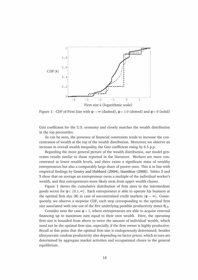
Figure 1: CDF of Firm Size with φ → ∞ (dashed), φ = 1.0 (dotted) and φ = 0 (solid)

Gini coefficient for the U.S. economy and closely matches the wealth distribution

in the top percentiles.

As can be seen, the presence of financial constraints tends to increase the con-

centration of wealth at the top of the wealth distribution. Moreover, we observe an

increase in overall wealth inequality, the Gini coefficient rising by 6.5 p.p.

Regarding the more general picture of the wealth distribution, our model gen-

erates results similar to those reported in the literature. Workers are more con-

centrated at lower wealth levels, and there exists a significant mass of wealthy

entrepreneurs but also a comparably large share of poorer ones. This is in line with

empirical findings by Gentry and Hubbard (2004), Hamilton (2000). Tables 3 and

5 show that on average an entrepreneur owns a multiple of the individual worker’s

wealth, and that entrepreneurs more likely stem from upper wealth classes.

Figure 1 shows the cumulative distribution of firm sizes in the intermediate

goods sector for φ ∈ {0,1,∞}. Each entrepreneur is able to operate his business at

the optimal firm size (8) in case of unconstrained credit markets (φ → ∞). Conse-

quently, we observe a stepwise CDF, each step corresponding to the optimal firm

size associated with one out of the five underlying possible productivity states θe,h.

Consider next the case φ = 1, where entrepreneurs are able to acquire external

financing up to maximum sum equal to their own wealth. Here, the operating

firm size is bounded from above to twice the amount of individual wealth, which

need not be the optimal firm size, especially, if the firm owner is highly productive.

Recall at this point that the optimal firm size is endogenously determined; besides

idiosyncratic random productivity also depending on factor prices, which in turn are

determined by aggregate market activities and occupational choice in the general

equilibrium.

18

The first observation is that the optimal firm sizes rise slightly for each possible

state of entrepreneurial talent θe,h. This increase in firm sizes can be ascribed to the

factor price effect. Borrowing constraints prevent the efficient allocation of capital

among sectors such that too much capital is employed in the production of the final

good. This is associated with a decline in the real interest rate, which in turn raises

the optimal firm size in the intermediate sector for each state of productivity.

The second, major observation in the credit–constrained economy is that there

exists a positive mass of entrepreneurs between each two subsequent steps of op-

timal firm sizes, and the distribution is more concentrated at smaller firm sizes.

Constraints become binding for many entrepreneurs, who have to operate their en-

terprise at a suboptimally low scale. Non–surprisingly, this effect is aggravated, if we

reduce the availability of external financing to naught. For φ = 0, steps in the CDF

almost vanish, which means that more business owners are subject to constraints.

The optimal levels of firm sizes for the different states of productivity rise even

further, due to the factor price effect. In numbers, if we compare the unrestrained

with the completely constrained economy, businesses in the entrepreneurial sector

on average operate at 48% of their respective optimal firm size.

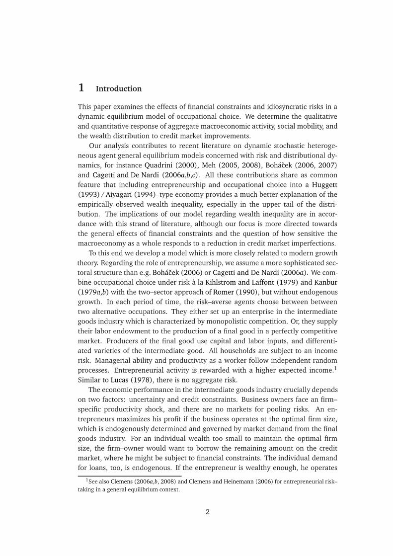
Macroeconomic Effects Table 3 and Figure 2 summarize the results for the macroe-

conomic key variables of the calibrated baseline model. The general picture reflects

the outcome one would expect from credit market improvements. Aggregate output

Y, aggregate wealth holdings a, factor prices r,w and incomes, as well as welfare

increase if we relax borrowing constraints.

Figure 2 shows that, except for wealth inequality, social mobility and the entre-

preneurship rate, the response of the macroeconomic variables to a change in φ is

monotonous. The overall loss in output in a perfectly constrained compared to the

unconstrained economy (φ → ∞) lies at about 21%, and average wealth holdings

decline by 23%. Tightening financial constraints goes along with a substantial drop

in economic performance. The associated welfare loss, too, is substantial. The non–

monotonic behavior of wealth inequality, social mobility and the entrepreneurship

rate is systematic and will be discussed in more detail below.

We also see from Figure 2 that the response of output, wealth, factor prices,

and welfare to a change in φ is concave. The marginal gains from improving credit

markets are much higher for small values of φ, especially in the range of debt–

equity ratios between 0 < φ < 2, which is the empirically plausible domain. This

interval accounts for more than three–quarter of the overall output loss associated

with financial constraints.

Given the general equilibrium nature of the underlying model, one would ex-

pect several adjustments to take place following a reduction in external financing as

borrowing constraints become more tight. If there is only limited or no capital de-

mand from the intermediate goods industry, we observe a capital–relocation effect

between sectors. More capital is employed in the final goods industry. This amounts

19

Table 3: Simulation Results

Tightness of constraints

φ → ∞ φ = 1.0 φ = 0entrepreneurship rate (%) 0.201 0.197 0.185

∅ firm size total 0.964 0.839 0.699

∅ credit rationing total 0.000 0.295 0.761

∅ profits total 0.278 0.281 0.281

aggregate output Y 0.253 0.232 0.200

capital input for Y KF 0.270 0.306 0.365

interest rate r 0.042 0.028 0.008

factor price ratio w/(r + δ) 1.362 1.396 1.406

factor income shares labor 0.630 0.630 0.630

capital 0.149 0.131 0.110

profits 0.221 0.239 0.260

∅ income workers 0.215 0.193 0.159

entrepreneurs 0.403 0.392 0.377

risk premium 0.399 0.542 0.825

∅ wealth total 0.265 0.239 0.203

workers 0.111 0.083 0.048

entrepreneurs 0.876 0.871 0.888

wealth total 0.770 0.774 0.835

inequality workers 0.655 0.669 0.779

(Gini) entrepreneurs 0.677 0.592 0.534

mobility 0.042 0.041 0.039

to shifting about 9.5% of the aggregate capital stock from the intermediate to the

final goods sector over the entire range 0 6 φ < ∞. The average excess demand for

capital in the intermediate goods industry amounts to about 110% of the average

firm size if credit markets are completely closed; see Table 3.

With diminishing marginal returns, the equilibrium interest rate r, and accord-

ingly the factor price for capital r + δ, decline by almost 3.5 p. p. in both sectors of

the economy. Recalling that entrepreneurial households receive income from two

sources, profits and capital incomes, the income share reflecting the user costs of

capital declines for any given level of individual wealth, whereas the profit share

rises. Altogether, we observe a shift in the functional income distribution from

capital to profit incomes of 3.9 p.p. over the entire domain of φ.

The presence of credit constraints not necessarily implies that only those agents

choose to become an entrepreneur, who have sufficient own wealth and borrowed

resources to operate their business at the optimal firm size k∗. These are the only

firms who actually maximize their profits, whereas the constrained entrepreneurs

are forced to operate at suboptimally small business sizes. Consequently, the aver-

age firm size in the intermediate goods industry decreases substantially as financial

20

constraints become more tight, and highly productive entrepreneurs are more af-

fected by the constraints than those with a low θe. Figure 2a shows that in a com-

pletely constrained economy the average firm size only amounts to around 48% of

its optimal operating size.

The overall employment effect of tightening financing constraints is astonish-

ingly small. The entrepreneurship rate decreases by 1.6 p.p. over the entire range of

φ. Credit constraints are an impediment to entrepreneurship, as is stated through-

out the theoretical and empirical literature; see e.g. Evans and Leighton (1989);

Evans and Jovanovic (1989); Blanchflower and Oswald (1998). Nevertheless, the

rather modest response of the entrepreneurship rate to an increase in credit ra-

tioning is quite surprising. Economic intuition would have suggested a more pro-

nounced reaction in occupational choice.

There are several factors explaining this result, which can mainly be traced back

to the general equilibrium nature of our approach. Credit constraints are only one

out of several determinants of occupational choice. First of all, competition between

the final and intermediate goods sector for capital determines the equilibrium in-

terest rate, the firm size and, most importantly, expected profits of the monopolistic

enterprises. The lower the user costs of capital, the higher are c.p. profits, which

increase if financial constraints become more tight (cf. Table 3). Borrowers benefit

from a decrease in the interest rate, whereas lenders and capital owners in gen-

eral loose for a given capital stock. Financial constraints affect especially business

owners with little wealth. Those, for whom the distribution of future profits be-

comes unfavorable, will exit the market, whereas other constrained entrepreneurs

(continue to) operate at a suboptimally low scale.

The reallocation of capital into the production of the final good induces an

increase in the demand for intermediate goods; see eq. (5). This, together with a

reduction in the interest rate, leads to an associated rise in expected entrepreneurial

profits, albeit by a mere 1.1%. The question is to what extent market exits due to

financial constraints are compensated by market entries due to the rise in expected

profits. The fraction of business owners, who are subject to constraints, increases

for smaller values of φ. Here, the negative effects of financial constraints dominate

and the entrepreneurship rate decreases.

The choice of entering into entrepreneurship, however, is also determined by

opportunity costs in terms of foregone wage income and the expected earnings dif-

ferential (‘risk premium’) between the two types of income. Last, there is also the

question of income persistence, since households continuously decide between two

lotteries and possess (at least subjective) knowledge regarding the stochastic prop-

erties of the underlying shocks. If shocks are serially correlated, a low–productivity

worker is aware of the fact that being also lowly productive in the future is a more

probable outcome than otherwise. Consequently, he might be inclined to take his

chances with entrepreneurship, knowing that his current productivity as a worker

is not related to his future productivity as a business owner.

21

2 4 6 8 10

0.5

0.6

0.7

0.8

0.9

1

replacements

φ(a) % of optimal average firm size

2 4 6 8 100.185

0.1875

0.19

0.1925

0.195

0.1975

0.2

φ(b) Entrepreneurship rate

2 4 6 8 10

0.8

0.85

0.9

0.95

1

φ(c) Y relative to φ → ∞

2 4 6 8 10

−6.2

−6

−5.8

−5.6

−5.4

−5.2

−5

φ(d) Welfare

2 4 6 8 10

0.21

0.22

0.23

0.24

0.25

0.26

φ(e) Wealth holdings

2 4 6 8 100.76

0.77

0.78

0.79

0.8

0.81

0.82

0.83

φ(f) Gini of total wealth

2 4 6 8 10

0.12

0.14

0.16

0.18

0.2

0.22

0.24

0.26

capital

profit

(g) Functional distribution of income

2 4 6 8 100.05

0.1

0.15

0.2

0.25

0.008

0.016

0.024

0.032

0.04

w (left scale)

r (right scale)

(h) Factor prices

Figure 2: Macroeconomic Effects of a Change in φ, Baseline Model

22

2 4 6 8 100.4

0.5

0.6

0.7

0.8

φ(i) Risk premium on entrepreneurial activity

2 4 6 8 10

0.039

0.0395

0.04

0.0405

0.041

0.0415

0.042

φ(j) Mobility (% of population)

Figure 2: Macroeconomic Effects of a Change in φ, Baseline Model (cont.)

The risk premium on entrepreneurial activity more than doubles if we compare

the unconstrained to the completely credit–constrained economy, thereby providing

incentives towards entrepreneurship. A closer inspection of Figure 2 reveals the

non–monotonic behavior of the entrepreneurship rate and social mobility. If we

relax borrowing constraints, we first observe a sharp rise in the variables for small

φ < 2, but also a moderate decrease for large values of φ > 7.5.

In the interval of values for φ between 4–7.5, the entrepreneurship rate is al-

most constant, which is also true for the wage rate and social mobility, although

aggregate output and average firm sizes already display a more pronounced de-

crease. The environment under which occupational choice takes place does not

undergo substantial changes in the range of intermediate values for φ between 4–

7.5, thereby keeping the entrepreneurship rate comparatively stable. Once finan-

cial constraints become more severe (φ < 2), we observe a more pronounced shift

in employment.

Summing up: Whereas we have clear–cut substantial, negative effects of finan-

cial constraints on overall macroeconomic performance, we observe an ambiguous

response in the entrepreneurship rate. Counteracting forces on occupational choice

give rise to a non–monotonic behavior of the entrepreneurship rate. Increases in

the tightness of financial constraints work against business ownership by limiting

firm sizes to suboptimally low levels. On the contrary, changes in the real interest

rate, expected profits, and the risk premium provide incentives towards entrepren-

eurship. As turns out, the structure of the occupational lottery, especially the degree

of income persistence is crucial to the question of what force prevails in the end.

We explore this issue more deeply in Section 4.2 for an alternative calibration of

the model.

Regarding the wealth distribution, we first observe a sharp decline in the Gini

coefficient for a rise in φ from 0.84 to 0.76, which is then followed by a gradual

increase in overall wealth inequality back to a value of 0.77. This non–monotonic

23

Table 4: Transition Probabilities for Households in a given Wealth Quintile and Pro-

ductivity State(a) Workers

Tightness of constraints

φ = 1000 φ = 1 φ = 01st 2nd 3rd 4th 5th 1st 2nd 3rd 4th 5th 1st 2nd 3rd 4th 5th

θw,1 0 0 1 1 1 0 0 0.49 1 1 0 0 0 0.88 1

θw,2 0 0 0.87 1 1 0 0 0.50 1 1 0 0 0 0.67 1

θw,3 0 0 0 0 0.07 0 0 0 0 0.55 0 0 0 0.08 1

θw,4 0 0 0 0 0 0 0 0 0 0.01 0 0 0 0 0.08

θw,5 0 0 0 0 0 0 0 0 0 0 0 0 0 0 0

(b) Entrepreneurs

Tightness of constraints

φ = 1000 φ = 1 φ = 0

1st 2nd 3rd 4th 5th 1st 2nd 3rd 4th 5th 1st 2nd 3rd 4th 5th

θe,1 – – 1 1 1 – – 1 1 1 – – 1 1 1

θe,2 – – 1 1 1 – – 1 1 1 – – 1 1 1

θe,3 – – 1 1 1 – – 1 1 1 – – 1 1 1

θe,4 – – 0 0 0 – – 0 0 0 – – 0 0 0

θe,5 – – 0 0 0 – – 0 0 0 – – 0 0 0

bars (–) indicate that 0% of entrepreneurs are in the associated wealth quintile

behavior of total wealth inequality can be explained, if we look at the within–

group inequality for workers and entrepreneurs respectively. Table 3 shows that

wealth becomes more unevenly distributed among workers, whereas wealth in-

equality among entrepreneurs declines.

Social Mobility We now discuss in more detail the question of how tightened fi-

nancial constraints affect occupational choice and social mobility. Table 3 shows

that an increase in the tightness of financial constraints leads to a decline in the

entrepreneurship rate by 1.6 p.p. Between 3.9 to 4.2% of the population switch

occupations in each period of time, which amounts to an exit rate of about 20% of

all firms in the intermediate goods industry. Overall mobility declines, if constraints

become more tight.

To understand mobility of entrepreneurs, we have to consider several factors.

The future occupation is determined (a) by the present level of wealth, (b) the

current draw of productivity governing present income, consumption and saving,

(c) the choice between two lotteries with unconditional probabilities governing fu-

ture income, consumption and saving, where the lottery over worker efficiencies is

less risky than the lottery over entrepreneurial productivities, and (d) the expected

market equilibrium of the next period, determining factor prices and factor income

differentials.

24

We are especially interested in two dimensions of social mobility: Based on the

steady state distribution of agents across occupations, we first focus on the individ-

ual level and determine the probabilities of transition between occupations in the

next period for agents in a given wealth quintile and productivity state. The associ-

ated results are displayed in Table 4. Second, we take a more aggregate viewpoint

and analyze the inflow of entrants into entrepreneurship and the workforce respec-

tively by decomposing the entire flow with respect to the distributional character-

istics of agents regarding wealth levels and productivity classes. This enables us to

determine the probability with which switching households come from alternative

(productivity–cum–wealth) backgrounds in the actual macroeconomic equilibrium.

If we look the transition probabilities of Table 4, the picture is striking for in-

dividuals, who currently are low and medium productivity entrepreneurs. All en-

trepreneurs of the lowest three productivity states change their occupation, even if

they belong to the upper wealth quintiles. They, with certainty, will exit the market

to seek employment as a worker in the next period. This results holds irrespective

of the degree of constraint. There are no entrepreneurs in the lowest two wealth

quintiles. Rich and highly productive business owners never change their occupa-

tion.

Regarding workers we find that generally rich workers, in particular rich and

relatively unproductive workers switch occupations in the next period. The gen-

eral mobility pattern is robust over different levels of φ. The intuition behind this

result is as already outlined above. Serially correlated shocks provide agents with

a signal regarding future productivity. Since we assumed mutually uncorrelated

processes for labor efficiency and entrepreneurial ability, a worker can infer from a

low productivity today a probably low labor efficiency tomorrow, but this not nec-

essarily indicates an equally low future ability as entrepreneur, which is given by

the unconditional probability of states.

Poor workers will not enter into business ownership, independent of their pro-

ductivity. This situation becomes more severe and even stretches to the third wealth

quintile, if financial constraints become more tight. New entrepreneurs are mainly

recruited among the group of wealthy workers. More tight credit constraints strik-

ingly decrease the probabilities of becoming an entrepreneur for poorer workers,

while the corresponding probabilities for richer workers (especially for those in the

fourth and fifth quintile) increase. If financial constraints become more tight, the

income premium for a poor worker entering entrepreneurship is smaller than for a

rich worker. We observe an increasing spread in the distribution of premiums on

profits over wages, which increases transition probabilities for rich workers.

While Table 4 provides us with information regarding the transition probability

of agents who currently are in a certain wealth class and productivity state, Table 5

allows us trace back where switching households most likely come from in macroe-

conomic equilibrium in terms of productivity and wealth characteristics. A general

insight from our model is that mobility over occupations is confined to agents who

25

Table 5: Decomposition of Flows: Probability of Wealth / Productivity–Class Back-

ground of Switching Households

(a) Workers

Tightness of constraints

φ = 1000 φ = 1 φ = 0

1st 2nd 3rd 4th 5th 1st 2nd 3rd 4th 5th 1st 2nd 3rd 4th 5th

θw,1 0 0 0.004 0.007 0.002 0 0 0.004 0.009 0.001 0 0 0 0.008 0.004

θw,2 0 0 0.227 0.453 0.215 0 0 0.209 0.445 0.074 0 0 0 0.234 0.101

θw,3 0 0 0 0 0.093 0 0 0 0 0.252 0 0 0 0.181 0.438

θw,4 0 0 0 0 0 0 0 0 0 0.007 0 0 0 0 0.035

θw,5 0 0 0 0 0 0 0 0 0 0 0 0 0 0 0

∑ 0 0 0.231 0.460 0.310 0 0 0.213 0.454 0.334 0 0 0 0.423 0.578

(b) Entrepreneurs

Tightness of constraints

φ = 1000 φ = 1 φ = 01st 2nd 3rd 4th 5th 1st 2nd 3rd 4th 5th 1st 2nd 3rd 4th 5th

θe,1 0 0 0.015 0.009 0.002 0 0 0.013 0.008 0.005 0 0 0 0.015 0.011

θe,2 0 0 0.114 0.072 0.050 0 0 0.104 0.062 0.073 0 0 0 0.117 0.119

θe,3 0 0 0.358 0.178 0.203 0 0 0.202 0.157 0.379 0 0 0 0.246 0.492

θe,4 0 0 0 0 0 0 0 0 0 0 0 0 0 0 0

θe,5 0 0 0 0 0 0 0 0 0 0 0 0 0 0 0

∑ 0 0 0.487 0.259 0.255 0 0 0.319 0.227 0.457 0 0 0 0.378 0.622

are not (or have not been) successful in their professions. Households continuously

decide between two serially correlated lotteries. Generally speaking, they have little

incentive to stay in their occupation, if they receive a low talent shock.

Table 5 shows that, independent of wealth levels, a new entrepreneur never is

recruited from high productivity workers and vice versa. Likewise, we never observe

a low–productivity worker from the lower wealth quintiles to make an entry into

entrepreneurship. Mobility over occupations crucially depends on membership in

wealth quintiles. New entrepreneurs have been rich workers with larger probability.

Interestingly, new entrepreneurs most probably are recruited among those workers

of the two lowest productivity states in the 4th wealth quintile. Here we observe

a combination of two incentive effects: on the one hand, the poor future income

prospects of a currently low productivity; on the other hand, the attractiveness

of entrepreneurship due to the risk premium on entrepreneurial activity. Because

members of the 5th wealth quintile receive a substantial share of their income

from riskless capital investment, they are less exposed to income risk and therefore

less likely to switch occupations, even if they are comparably unproductive. In

accordance with economic intuition, it is more likely to observe rich workers to

switch occupations, if financial constraints become more tight.

26

Table 6: Wealth Distribution

Top percentilesGini

1% 5% 10% 20% 30%

PSID 1994 22.6 44.8 59.1 75.9 85.9 0.75

SCF 1992 29.5 53.5 66.1 79.5 87.6 0.78

φ = 0 18.48 50.60 70.10 86.24 93.70 0.822

φ = 1.0 17.64 47.01 64.19 80.14 88.42 0.772

φ = 1000 15.76 45.39 61.96 76.99 84.64 0.729

Table 5b, displaying the probability that a new worker is recruited from a given

wealth quintile and productivity level, has zero entries in the lower two wealth

quintiles, because all entrepreneurs belong to the upper three wealth quintiles in

the macroeconomic equilibrium. A rich and highly productive entrepreneur has

no incentive to change occupations. Therefore, workers are only recruited from

low levels of entrepreneurial productivity, and the probability is increasing, if the

financial constraints become more tight.

4.2 Alternative Calibration of the Model

We want to conclude our numerical simulations with a short discussion of an alter-

natively calibrated model. The analysis is motivated by one of the major findings

of the baseline model, namely the non–monotonic and in magnitude very modest

response of the entrepreneurship rate and social mobility to tightening financial

constraints. We show for an empirically equally plausible calibration that the en-

trepreneurship rate actually might increase in a more constrained economy. The

implications for overall macroeconomic performance, however, remain unchanged.

A parameter crucial for the response of the entrepreneurship rate is the degree

of serial correlation in the income processes. While entrepreneurial productivity

shocks are assumed to be more persistent in the baseline model, we now postulate

identical serial correlations for both, workers and entrepreneurs, pw = pe = 0.6. We

additionally customize the rate of time preference to β = 0.89 and the variance of

entrepreneurial shocks to σe = 2.0 to generate an empirically plausible interest rate

and wealth inequality, and keep the remaining model parameters; see Table 1.

Table 6 shows that the new calibration also generates a wealth distribution

which matches empirical evidence, for instance for the U.S., regarding the Gini

coefficient but also with respect to the upper tail of the distribution.

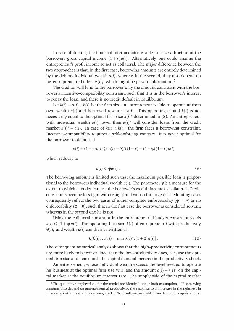
Figure 3 displays selected results for the macroeconomic effects of an increase in

the tightness of constraints under the new parameterization of the model. Table 7

in the Appendix gives a summary of the numerical results. We find that the gen-

eral pattern of how macroeconomic performance responds to tightened constraints

27

2 4 6 8 100.3

0.4

0.5

0.6

0.7

0.8

0.9

1

replacements

φ(a) % of optimal average firm size

2 4 6 8 10

0.195

0.1975

0.2

0.2025

0.205

0.2075

φ(b) Entrepreneurship rate

2 4 6 8 10

0.7

0.75

0.8

0.85

0.9

0.95

1

φ(c) Y relative to φ → ∞

2 4 6 8 100.07

0.08

0.09

0.1

0.11

0.12

φ(d) Mobility (% of population)

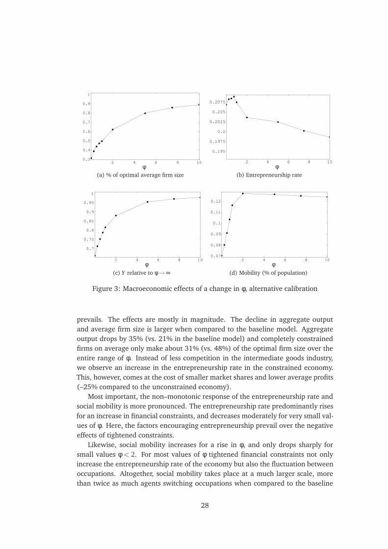
Figure 3: Macroeconomic effects of a change in φ, alternative calibration

prevails. The effects are mostly in magnitude. The decline in aggregate output

and average firm size is larger when compared to the baseline model. Aggregate

output drops by 35% (vs. 21% in the baseline model) and completely constrained

firms on average only make about 31% (vs. 48%) of the optimal firm size over the

entire range of φ. Instead of less competition in the intermediate goods industry,

we observe an increase in the entrepreneurship rate in the constrained economy.

This, however, comes at the cost of smaller market shares and lower average profits

(–25% compared to the unconstrained economy).

Most important, the non–monotonic response of the entrepreneurship rate and

social mobility is more pronounced. The entrepreneurship rate predominantly rises

for an increase in financial constraints, and decreases moderately for very small val-

ues of φ. Here, the factors encouraging entrepreneurship prevail over the negative

effects of tightened constraints.

Likewise, social mobility increases for a rise in φ, and only drops sharply for

small values φ < 2. For most values of φ tightened financial constraints not only

increase the entrepreneurship rate of the economy but also the fluctuation between

occupations. Altogether, social mobility takes place at a much larger scale, more

than twice as much agents switching occupations when compared to the baseline

28

model. The implications regarding the transition probabilities between occupations

are identical to the baseline model and therefore omitted.

5 Concluding Remarks

In this paper, we examined the effects of borrowing constraints and idiosyncratic

risks on macroeconomic performance, wealth inequality, and social mobility in a

two–sector heterogeneous agent dynamic general equilibrium model. Workers and

firm owners are subject to idiosyncratic shocks. Entrepreneurship in the interme-

diate (non–corporate) goods industry is the riskier occupation. Our comparative

static results cover a broad range for borrowing constraints, from an unrestrained

to a perfectly constrained economy.

The stationary wealth distribution generated in the model is consistent with em-

pirical findings. Entrepreneurial households own a substantial share of household

wealth and their share increases throughout the wealth distribution.

Independent of the persistence of the idiosyncratic shocks, we find that tighten-

ing financial constraints is accompanied by substantial losses in aggregate output,

consumption, wealth holdings, and welfare. The inefficient allocation of capital

across sectors accounts for this result in the first place and only second the associ-

ated changes in employment and the entrepreneurship rate. To the extent firms of

the intermediate goods industry are barred from participation in the credit market,

more capital is employed in the final (corporate) goods sector. The associated de-

cline in the interest rate causes a shift in the functional income distribution towards

profit incomes.

The response of the macroeconomic variables to a change in credit availability

is monotonous and concave. We find that the marginal gains of relaxing constraints

are especially large for small (enforced) debt–equity ratios. This indicates that it

is a worthwhile question to explore in more detail the marginal gains from credit

market improvement, which at this point is left for future research.

The general equilibrium context of our model, where optimal firm sizes and the

demand for credit are determined endogenously, gives rise to interesting implica-

tions regarding the change in the entrepreneurship rate and in social mobility, as

we vary the degree of credit availability in the non–corporate sector. Contrary to

economic intuition, there is only a slight difference in magnitude between the en-

trepreneurship rates of the completely constrained and the unrestrained economy.

The overall employment effects of relaxing financial constraints are very small. We

also observe a non–monotonic response in both the entrepreneurship rate and in

social mobility to changes in the tightness of financial constraints.

This result can primarily be attributed to two factors: first, the general equilib-

rium nature of our approach. While financial constraints deter entrepreneurs from

operating at the optimal firm size, they also induce capital flows between sectors

which ultimately end up in lower interest rates and higher expected profits. Second,

29

the degree of income persistence. Workers and entrepreneurs with high individual

productivity tend to remain in their present occupation, whereas low productivity

individuals are more likely to switch between professions. Regarding exit and en-

try rates into entrepreneurship, we find that a lower persistence of entrepreneurial

shocks generally increases between–group mobility and also raises the entrepren-

eurship rate over a broad range of financial constraints.

So what are the general implications of our model? The extent, to which the

industry is subject to financial constraints and firm sizes as well as production pos-

sibilities are limited is more important for the macroeconomy as a whole, than

the question of how many entrepreneurs there are and how occupational choice

responds to a change in the tightness of constraints. Even an increase in the en-

trepreneurship rate (i.e. the number of businesses in the market) is not sufficient

to prevent or mitigate the overall loss in output, consumption and welfare, if the

access to external financing becomes increasingly difficult.

There are many important issues this paper does not address. The model lacks

a fully micro–founded formulation of credit constraints and a more detailed model-

ing of financial intermediation. Also, testing the robustness of results with respect

to varying attitudes towards risk is left for future research. So far, we assume

worker efficiency and entrepreneurial ability to be uncorrelated. However, as al-

ready Cagetti and De Nardi (2006a) pointed out, it is difficult to measure correlated

talent shocks in the data, which to some extent justifies our approach.

References

Aghion, Philippe, Fally, Thibault, and Scarpetta, Stefano (2007), Credit Constraintsas a Barrier to the Entry and Post–entry Growth of Firms, Economic Policy, Octo-ber 2007, 731–779.

Aiyagari, S. Rao (1994), Uninsured Idiosyncratic Risk and Aggregate Saving, Quar-terly Journal of Economics, 109 (3), 659–684.

Banerjee, Abhijit V. and Newman, Andrew F. (1993), Occupational Choice and theProcess of Development, Journal of Political Economy, 101, 274–298.

Blanchflower, David G. and Oswald, Andrew J. (1998), What Makes an Entrepren-eur?, Journal of Labor Economics, 16 (1), 26–60.

Bohác̆ek, Radim (2006), Financial Constraints and Entrepreneurial Investment,Journal of Monetary Economics, 53, 2195–2212.

— (2007), Financial Intermediation with Credit Constrained Agents, Journal ofMacroeconomics, 29, 741–759.

Cagetti, Marco and De Nardi, Mariacristina (2006a), Entrepreneurship, Frictions,and Wealth, Journal of Political Economy, 114 (5), 835–870.

— (2006b), Taxation, Entrepreneurship, and Wealth, Working Paper 2006–07, Fed-eral Reserve Bank of Chicago, Chicago, IL.

30

— (2006c), Wealth Inequality: Data and Models, NBER Working Paper 12550,National Bureau of Economic Research, Cambridge, MA.

Clemens, Christiane (2006a), Monopolistic Competition and Entrepreneurial Risk–Taking, Economics Letters, 93 (1), 68–74.

— (2006b), Status Concerns and Occupational Choice under Uncertainty, Advancesin Theoretical Economics, 6 (1), Article 4, BEPress.

— (2008), Imperfect Competition and Growth with Entrepreneurial Risk, GermanEconomic Review, 9 (2), 179–205.

Clemens, Christiane and Heinemann, Maik (2006), On the Effects of Redistributionon Growth and Entrepreneurial Risk–Taking, Journal of Economics, 88 (2), 131–158.

Clementi, Gian Luca and Hopenhayn, Hugo A. (2006), A Theory of Financing Con-straints and Firm Dynamics, Quarterly Journal of Economics, 121 (1), 229–265.

De Nardi, Mariacristina (2004), Wealth Inequality and Intergenerational Links, Re-view of Economic Studies, 71 (3), 743–768.

Desai, Mihir, Gompers, Paul, and Lerner, Josh (2003), Institutions, Capital Con-straints and Entrepreneurial Firm Dynamics: Evidence from Europe, NBER Work-ing Paper 10165, National Bureau of Economic Research, Cambridge, MA.

Evans, David S. (1987), Test of Alternative Theories of Firm Growth, Journal ofPolitical Economy, 95 (4), 657–674.

Evans, David S. and Jovanovic, Boyan (1989), An Estimated Model of Entrepren-eurial Choice under Liquidity Constraints, Journal of Political Economy, 97 (4),808–827.

Evans, David S. and Leighton, Linda S. (1989), Some Empirical Aspects of Entre-preneurship, American Economic Review, 79 (3), 519–535.

Fernández-Villaverde, Jesús, Galdón-Sánchez, José Enrique, and Carranza, Luis(2003), Entrepreneurship, Financial Intermediation and Aggregate Activity.

Gentry, William M. and Hubbard, R. Glenn (2004), Entrepreneurship and House-hold Saving, Advances in Economic Analysis and Policy, 4 (1), Article 8.

Ghatak, Maitreesh, Morelli, Massimo, and Sjöstrom, Tomas (2001), OccupationalChoice and Dynamic Incentives, Review of Economic Studies, 68, 781–810.

Guvenen, Fatih (2007), An Empirical Investigation of Labor Income Processes,NBER Working Paper 13394, National Bureau of Economic Research, Cambridge,MA.

Hamilton, Barton H. (2000), Does Entrepreneurship Pay? An Empirical Analysis ofthe Returns to Self–Employment, Journal of Political Economy, 108 (3), 604–631.

Heaton, John and Lucas, Deborah (2000), Portfolio Choice and Asset Prices: TheImportance of Entrepreneurial Risk, Journal of Finance, 55 (3), 1163–1198.

Holtz-Eakin, D., Joulfaian, D., and Rosen, Harvey S. (1994a), Entrepreneurial De-cisions and Liquidity Constraints, Rand Journal of Economics, 25 (2), 334–347.

31

— (1994b), Sticking it Out: Entrepreneurial Survival and Liquidity Constraints,Journal of Political Economy, 102 (1), 53–75.

Huggett, Mark (1993), The Risk-Free Rate in Heterogeneous–Agent Incomplete–Insurance Economies, Journal of Economic Dynamics and Control, 17 (5–6), 953–969.

— (1996), Wealth Distribution in Life–Cycle Economies, Journal of Monetary Eco-nomics, 38, 469–494.

Hurst, Erik and Lusardi, Annamaria (2004), Liquidity Constraints, HouseholdWealth, and Entrepreneurship, Journal of Political Economy, 112, 319–347.

Kanbur, S. M. (1979a), Impatience, Information and Risk Taking in a General Equi-librium Model of Occupational Choice, Review of Economic Studies, 46, 707–718.

— (1979b), Of Risk Taking and the Personal Distribution of Income, Journal ofPolitical Economy, 87, 769–797.

Kihlstrom, Richard E. and Laffont, Jean-Jacques (1979), A General EquilibriumEntrepreneurial Theory of Firm Formation based on Risk Aversion, Journal ofPolitical Economy, 87, 719–748.

King, Robert G. and Rebelo, Sergio T. (1999), Resuscitating Real Business Cycles,in: John B. Taylor and Michael Woodford (eds.), Handbook of Macroeconomics,North–Holland, Amsterdam, vol. Ib, pp. 927–1007.

Kirzner, I. (1973), Competition and Entrepreneurship, University of Chicago Press,Chicago.

Kitao, Sagiri (2008), Entrepreneurship, Taxation and Capital Investment, Review ofEconomic Dynamics, 11, 44–69.

Knight, Frank (1921), Risk, Uncertainty and Profit, University of Chicago Press,(reprint) Chicago, 1979.

Li, Wenli (2002), Entrepreneurship and Government Subsidies: A General Equilib-rium Analysis, Journal of Economic Dynamics and Control, 26, 1815–1844.

Lucas, Robert E. (1978), On the Size Distribution of Business Firms, Bell Journal ofEconomics, 9, 508–523.

Matsuyama, Kiminori (2007), Aggregate Implications of Credit Market Imperfec-tions, NBER Working Paper 13209, National Bureau of Economic Research, Cam-bridge, MA.

Meh, Césaire A. (2005), Entrepreneurship, Wealth Inequality, and Taxation, Reviewof Economic Dynamics, 8, 688–719.

— (2008), Business Risk, Credit Constraints, and Corporate Taxation, Journal ofEconomic Dynamics and Control, 32, 2971–3008.

Mehra, Rainish and Prescott, Edward C. (1985), The Equity Premium. A Puzzle,Journal of Monetary Economics, 15, 145–161.

Minniti, Maria, Bygrave, William D., and Autio, Erkko (2005), Global Entrepren-eurship Monitor. 2005 Executive Report.

32

Moskowitz, Tobias J. and Vissing-Jørgensen, Annette (2002), The Returns to En-trepreneurial Investment: A Private Equity Premium Puzzle, American EconomicReview, 92 (4), 745–778.

Obstfeld, Maurice (1994), Evaluating Risky Consumption Paths: The Role of In-tertemporal Substitutability, European Economic Review, 38, 1471–1486.

OECD (2000), OECD Employment Outlook 2000, OECD Publishing, Paris.

Quadrini, Vincenzo (1999), The Importance of Entrepreneurship for Wealth Con-centration and Mobility, Review of Income and Wealth, 45 (1), 1–19.

— (2000), Entrepreneurship, Saving and Social Mobility, Review of Economic Dy-namics, 3 (1), 1–40.

Romer, Paul M. (1990), Endogenous Technological Change, Journal of PoliticalEconomy, 98 (5), S71–S102.

Sandmo, Agnar (1970), The Effect of Uncertainty on Savings Decisions, Review ofEconomic Studies, 37, 353–360.

Schumpeter, Joseph (1930), The Theory of Economic Development, Oxford Univer-sity Press, (reprint) Oxford, 1961.

Tauchen, George (1986), Finite State Markov-Chain Approximation to Univariateand Vector Autoregressions, Economics Letters, 20, 177–181.

Vale, Steven (2006), The International Comparability of Business Start–Up Rates.Final Report, OECD Statistics Working Paper STD/DOC(2006)4, OECD, Paris.

A Computational Issues

The state space of wealth is approximated by a grid of N wealth levels an for n= 1, · · · ,N with

a1 = a and aN = k̄. The macroeconomic equilibrium is recursively computed. We start with

a initial guess on factor prices w̃, r̃, and the equilibrium level of employment in efficiency

units L̃. Let µ={

w̃, r̃, L̃}

denote the vector of the initial guesses. From this first solution trial

we obtain factor proportions in the final goods sector according to the marginal produc-

tivity conditions. The underlying production technology implies K̃F = L̃ w̃r̃+δ

γ1−γ . Moreover,

(

K̃γF , L̃1−γ)1−α

equals L̃(

w̃r̃+δ

γ1−γ

)γ.

Let kn,h(µ) denote the firm size an entrepreneur with productivity θe,h and wealth an is

able to operate at for a given extent of borrowing constraints and the initial guess µ. His

profit is given by

πn,h(µ) = α (θe,h kn,h(µ))α L̃

(

w̃r̃ + δ

γ1− γ

)γ− (r̃ + δ)kn,h(µ) .

Let Awn,h(µ) and Qw

n,h(µ) as well as Aen,h(µ) and Qe

n,h(µ) for n = 1, . . . ,N and h = 1, . . . ,Hdenote the optimal policies associated with the discrete formulation of the optimization

problems (11) and (12) for the given initial guess µ on prices and employment. We charac-

terize agents by their wealth holdings an, their occupational status ζ, where ζ ∈ {w, e} and

their current productivity state θh, h = 1, . . . ,H.

Knowing the policy functions and transition matrices for the underlying productivity

shocks, we are able to compute a stationary distribution and the probability for an agent

33

to have wealth an, occupational status ζ and productivity state θh. Let Ψn,ζ,h(µ) denote the

respective probability for n = 1, . . . ,N, ζ = {w, e} and h = 1, . . . ,H given the initial guess µ.

These probabilities can now be used to compute aggregate quantities. The aggregate capital

stock (i.e. mean wealth holdings) can be determined as:

K(µ) =N

∑n=1

∑ζ∈w,e

H

∑h=1

Ψn,ζ,h(µ)an

The population share of entrepreneurs results as

λ(µ) =N

∑n=1

H

∑h=1

Ψn,e,h(µ)

while labor supply in efficiency units is given by

L(µ) =N

∑n=1

M

∑h=1

Ψn,w,h(µ)θw,h

Capital demand of the intermediate goods sector can be computed as:

KDI (µ) =

N

∑n=1

H

∑h=1

Ψn,e,h(µ)kn,h(µ)

The supply of capital to the final goods sector is thus given by KSF(µ) = K(µ)−KD

I (µ). Finally,

the initial guess µ together with the production decision of entrepreneurs generates an

aggregate output of

Y(µ) =(

K̃γF L̃1−γ)1−α N

∑n=1

H

∑j=1

Ψn,e,h(µ) (θe,h kn,h)α

The initial solution guess represents an equilibrium only if the following conditions

hold:

(i) Labor supply in efficiency units must equal the initial guess, i.e.

L(µ) = L̃ (A.1)

(ii) Labor demand in the final goods sector equals labor supply:

L(µ) = (1−α)(1− γ)Y(µ)

w̃(A.2)

(iii) Capital demand in the final goods sector equals supply of capital to the final goods

sector:

KSF(µ) = K(µ)−KD

I (µ) = (1−α)γY(µ)

r̃ + δ(A.3)

The algorithm for finding the equilibrium values consists of three nested loops over L̃, w̃and r̃. The first loop iteratively computes the value L̃ which meets condition (A.1) for given

factor prices w̃ and r̃ . Then, factor prices w̃ and r̃ are adjusted according to the resulting

excess demands for labor and capital according to conditions (A.2) and (A.3). The whole

procedure is repeated until the equilibrium conditions (A.1) to (A.3) are satisfied, except

for a tolerably small approximation error.

To implement the algorithm, we used the programming language C++. The underlying

source code and the data are available from the authors upon request.

34

B Alternative Model Calibration: Macroeconomic Effects

Table 7: Simulation results

Tightness of constraints

φ → ∞ φ = 1.0 φ = 0entrepreneurship rate (%) 0.193 0.207 0.207

∅ firm size total 0.474 0.294 0.209

∅ credit rationing total 0.000 0.299 0.459

∅ profits total 0.136 0.119 0.104

final goods sector Y 0.119 0.097 0.078

capital input for Y KF (%) 0.230 0.352 0.415

interest rate r 0.041 0.017 0.003

factor price ratio w/(r + δ) 0.630 0.637 0.596

factor labor 0.630 0.630 0.630

income capital 0.149 0.114 0.097

shares profits 0.221 0.256 0.273

∅ income workers 0.103 0.081 0.064

entrepreneurs 0.183 0.155 0.133

risk premium 0.464 0.553 0.665

∅ wealth total 0.126 0.094 0.074

workers 0.075 0.038 0.018

entrepreneurs 0.338 0.308 0.288

wealth total 0.729 0.772 0.822

inequality workers 0.697 0.736 0.794

(Gini) entrepreneurs 0.602 0.578 0.523

mobility 0.121 0.116 0.070

35

Working Paper Series in Economics (see www.leuphana.de/vwl/papers for a complete list)

No.102: Helmut Fryges & Joachim Wagner: Exports and Profitability – First Evidence for German Manufacturing Firms. October 2008

No.101: Heike Wetzel: Productivity Growth in European Railways: Technological Progress, Efficiency Change and Scale Effects. October 2008

No.100: Henry Sabrowski: Inflation Expectation Formation of German Consumers: Rational or Adaptive? October 2008

No.99: Joachim Wagner: Produktdifferenzierung in deutschen Industrieunternehmen 1995 – 2004: Ausmaß und Bestimmungsgründe, Oktober 2008

No.98: Jan Kranich: Agglomeration, vertical specialization, and the strength of industrial linkages, September 2008

No.97: Joachim Wagner: Exports and firm characteristics - First evidence from Fractional Probit Panel Estimates, August 2008

No.96: Nils Braakmann: The smoking wage penalty in the United Kingdom: Regression and matching evidence from the British Household Panel Survey, August 2008

No.95: Joachim Wagner: Exportaktivitäten und Rendite in niedersächsischen Industrieunternehmen, August 2008 [publiziert in: Statistische Monatshefte Niedersachsen 62 (2008), 10,552-560]

No.94: Joachim Wagner: Wirken sich Exportaktivitäten positiv auf die Rendite von deutschen Industrieunternehmen aus?, August 2008 [publiziert in: Wirtschaftsdienst, 88 (2008) 10, 690-696]

No.93: Claus Schnabel & Joachim Wagner: The aging of the unions in West Germany, 1980-2006, August 2008 [forthcoming in: Jahrbücher für Nationalökonomie und Statistik]

No.92: Alexander Vogel and Stefan Dittrich: The German turnover tax statistics panels, August 2008 [forthcoming in: Schmollers Jahrbuch 128 (2008)]

No.91: Nils Braakmann: Crime does pay (at least when it’s violent!) – On the compensating wage differentials of high regional crime levels, July 2008

No.90: Nils Braakmann: Fields of training, plant characteristics and the gender wage gap in entry wages among skilled workers – Evidence from German administrative data, July 2008

No.89: Alexander Vogel: Exports productivity in the German business services sector: First evidence from the Turnover Tax Statistics panel, July 2008

No.88: Joachim Wagner: Improvements and future challenges for the research infrastructure in the field Firm Level Data, June 2008

No.87: Markus Groth: A review of the German mandatory deposit for one-way drinks packaging and drinks packaging taxes in Europe, June 2008

No.86: Heike Wetzel: European railway deregulation. The influence of regulatory ans environmental conditions on efficiency, May 2008

No.85: Nils Braakmann: Non scholae, sed vitae discimus! - The importance of fields of study for the gender wage gap among German university graduates during market entry and the first years of their careers, May 2008

No.84: Markus Groth: Private ex-ante transaction costs for repeated biodiversity conservation auctions: A case study, May 2008

No.83: Jan Kranich: R&D and the agglomeration of industries, April 2008 No.82: Alexander Vogel: Zur Exporttätigkeit unternehmensnaher Dienstleister in Niedersachsen -

Erste Ergebnisse zu Export und Produktivität auf Basis des Umsatzsteuerstatistikpanels, April 2008

No.81: Joachim Wagner: Exporte und Firmenerfolg: Welche Firmen profitieren wie vom internationalen Handel?, März 2008

No.80: Stefan Baumgärtner: Managing increasing environmental risks through agro-biodiversity and agri-environmental policies, March 2008

No.79: Thomas Huth: Die Quantitätstheorie des Geldes – Eine keynesianische Reformulierung, März 2008

No.78: Markus Groth: An empirical examination of repeated auctions for biodiversity conservation contracts, March 2008

No.77: Nils Braakmann: Intra-firm wage inequality and firm performance – First evidence from German linked employer-employee-data, February 2008

No.76: Markus Groth: Perspektiven der Nutzung von Methanhydraten als Energieträger – Eine Bestandsaufnahme, Februar 2008

No.75: Stefan Baumgärtner, Christian Becker, Karin Frank, Birgit Müller & Christian Quaas: Relating the philosophy and practice of ecological economics. The role of concepts, models, and case studies in inter- and transdisciplinary sustainability research, January 2008 [publisched in: Ecological Economics 67 (2008), 3 , 384-393]

No.74: Thorsten Schank, Claus Schnabel & Joachim Wagner: Higher wages in exporting firms: Self-selection, export effect, or both? First evidence from German linked employer-employee data, January 2008

No.73: Institut für Volkswirtschaftslehre: Forschungsbericht 2007, Januar 2008 No.72: Christian Growitsch and Heike Wetzel:Testing for economies of scope in European

railways: An efficiency analysis, December 2007 [revised version of Working Paper No. 29, forthcoming in: Journal of Transport Economics and Policy]

No.71: Joachim Wagner, Lena Koller and Claus Schnabel: Sind mittelständische Betriebe der Jobmotor der deutschen Wirtschaft?, Dezember 2007 [publiziert in: Wirtschftsdienst 88 (2008), 2, 130-135]

No.70: Nils Braakmann: Islamistic terror, the war on Iraq and the job prospects of Arab men in Britain: Does a country’s direct involvement matter?, December 2007

No.69: Maik Heinemann: E-stability and stability learning in models with asymmetric information, December 2007

No.68: Joachim Wagner: Exporte und Produktivität in Industriebetrieben – Niedersachsen im interregionalen und internationalen Vergleich, Dezember 2007

No.67: Stefan Baumgärtner and Martin F. Quaas: Ecological-economic viability as a criterion of strong sustainability under uncertainty, November 2007

No.66: Kathrin Michael: Überbrückungsgeld und Existenzgründungszuschuss – Ergebnisse einer schriftlichen Befragung drei Jahre nach Gründungsbeginn, November 2007

No.65: The International Study Group on Export and Productivity: Exports and Productivity – Comparable Evidence for 14 Countries, November 2007 [forthcoming in: Review of World Economics 144 (2008), 4]

No.64: Lena Koller, Claus Schnabel und Joachim Wagner: Freistellung von Betriebsräten – Eine Beschäftigungsbremse?, November 2007 [publiziert in: Zeitschrift für Arbeitsmarktforschung, 41 (2008), 2/3, 305-326]

No.63: Anne-Kathrin Last: The Monetary Value of Cultural Goods: A Contingent Valuation Study of the Municipal Supply of Cultural Goods in Lueneburg, Germany, October 2007

No.62: Thomas Wein und Heike Wetzel: The Difficulty to Behave as a (regulated) Natural Monopolist – The Dynamics of Electricity Network Access Charges in Germany 2002 to 2005, September 2007

No.61: Stefan Baumgärtner und Martin F. Quaas: Agro-biodiversity as natural insurance and the development of financial insurance markets, September 2007 [published in: A. Kontoleon, U. Pascual and M. Smale (eds.): Agrobiodiversity, conservation and economic development, Routledge, London, 293-317]

No.60: Stefan Bender, Joachim Wagner, Markus Zwick: KombiFiD - Kombinierte Firmendaten für Deutschland, September 2007

No.59: Jan Kranich: Too much R&D? - Vertical differentiation in a model of monopolistic competition, August 2007

No.58: Christian Papilloud und Ingrid Ott: Convergence or mediation? Experts of vulnerability and the vulnerability of experts’ discourses on nanotechnologies – a case study, July 2007 [published in: European Journal of Social Science Research 21 (2008), 1, 41-64]

No.57: Ingrid Ott und Susanne Soretz: Governmental activity, integration and agglomeration, July 2007 [published in: ICFAI Journal of Managerial Economics 5 (2008), 2, 28-47]

No.56: Nils Braakmann: Struktur und Erfolg von Ich-AG-Gründungen: Ergebnisse einer Umfrage im Arbeitsagenturbezirk Lüneburg, Juli 2007 [revidierte Fassung erscheint in: Richter, J., Schöning, S. & Wetzel, H., Mittelstand 2008. Aktuelle Forschungsbeiträge zu gesellschaftlichen und finanzwirtschaftlichen Herausforderungen, Frankfurt am Main: Peter Lang, 2008]

No.55: Nils Braakmann: Differences in the earnings distribution of self- and dependent employed German men – evidence from a quantile regression decomposition analysis, July 2007

No.54: Joachim Waagner: Export entry, export exit, and productivity in German Manufacturing Industries, June 2007 [published in: International Journal of the Economics of Business 15 (2008), 2, 169-180]

No.53: Nils Braakmann: Wirkungen der Beschäftigungspflicht schwerbehinderter Arbeitnehmer – Erkenntnisse aus der Einführung des „Gesetzes zur Bekämpfung der Arbeitslosigkeit Schwerbehinderter“, Juni 2007 [revidierte Fassung erscheint in: Zeitschrift für Arbeitsmarktforschung/ Journal for Labour Market Research 41 (2008),1]

No.52: Jan Kranich und Ingrid Ott: Regionale Spitzentechnologie auf internationalen Märkten, Juni 2007 [erscheint in: Merz, J. und Schulte, R. (Hrsg.): Neue Ansätze der MittelstandsForschung, Münster, 2007]

No.51: Joachim Wagner: Die Forschungspotenziale der Betriebspaneldaten des Monatsberichts im Verarbeitenden Gewerbe, Mai 2007 [erscheint in: AStA – Wirtschafts- und Sozialwirtschaftliches Archiv]

No.50: Stefan Baumgärtner, Frank Jöst und Ralph Winkler: Optimal dynamic scale and structure of a multi-pollution economy, May 2007 [forthcoming in: Ecological Economics]

No.49: Helmut Fryges und Joachim Wagner: Exports and productivity growth – First evidence from a continuous treatment approach, May 2007 [forthcoming in: Review of World Economics]

No.48: Ulrich Kaiser und Joachim Wagner: Neue Möglichkeiten zur Nutzung vertraulicher amtlicher Personen- und Firmendaten, April 2007 [publiziert in: Perspektiven der Wirtschaftspolitik 9 (2008), 3, 329-349]

No.47: Joachim Wagner: Jobmotor Mittelstand? Arbeitsplatzdynamik und Betriebsgröße in der westdeutschen Industrie, April 2007 [publiziert in: Vierteljahrshefte zur Wirtschaftsforschung, 76 (2007), 3, 76-87]

No.46: Christiane Clemens und Maik Heinemann: Credit Constraints, Idiosyncratic Risks, and the Wealth Distribution in a Heterogenous Agent Model, March 2007

No.45: Jan Kranich: Biotechnologie und Internationalisierung. Ergebnisse der Online-Befragung, März 2007

No.44: Joachim Wagner: Entry, exit and productivity. Empirical results for German manufacturing industries, March 2007 [forthcoming in: German Economic Review]

No.43: Joachim Wagner: Productivity and Size of the Export Market Evidence for West and East German Plants, 2004, March 2007 [publiziert in: Jahrbücher für Nationalökonomie und Statistik, 227 (2007), 4, 403-408]

No.42: Joachim Wagner: Why more West than East German firms export, March 2007 No.41: Joachim Wagner: Exports and Productivity in Germany, March 2007

[publiziert in: Applied Economics Quarterly 53 (2007), 4, 353-373] No.40: Lena Koller, Klaus Schnabel und Joachim Wagner: Schwellenwerte im Arbeitsrecht.

Höhere Transparenz und Effizienz durch Vereinheitlichung, Februar 2007 [publiziert in: Perspektiven der Wirtschaftspolitik, 8 (2007), 3, 242-255]

No.39: Thomas Wein und Wiebke B. Röber: Sind ausbildende Handwerksbetriebe erfolgreicher?, Januar 2007

No.38: Institut für Volkswirtschaft: Forschungsbericht 2006, Januar 2007

No.37: Nils Braakmann: The impact of September 11th, 2001 on the job prospects of foreigners with Arab background – Evidence from German labor market data, January 2007

No.36: Jens Korunig: Regulierung des Netzmonopolisten durch Peak-load Pricing?, Dezember 2006

No.35: Nils Braakmann: Die Einführung der fachkundigen Stellungnahme bei der Ich-AG, November 2006 [erscheint in: Schulte, Reinhard: Neue Ansätze der MittelstandsForschung, Münster etc.: Lit, 2008]

No.34: Martin F. Quaas and Stefan Baumgärtner: Natural vs. financial insurance in the management of public-good ecosystems, October 2006 [published in: Ecological Economics 65 (2008), 2, 397-406]

No.33: Stefan Baumgärtner and Martin F. Quaas: The Private and Public Insurance Value of Conservative Biodiversity Management, October 2006

No.32: Ingrid Ott and Christian Papilloud: Converging institutions. Shaping the relationships between nanotechnologies, economy and society, October 2006 [published in: Bulletin of Science, Technology & Society 2007 (27), 4, 455-466]

No.31: Claus Schnabel and Joachim Wagner: The persistent decline in unionization in western and eastern Germany, 1980-2004: What can we learn from a decomposition analysis?, October 2006 [published in: Industrielle Beziehungen/The German Journal of Industrial Relations 14 (2007), 118-132]

No.30: Ingrid Ott and Susanne Soretz: Regional growth strategies: fiscal versus institutional governmental policies, September 2006 [published in: Economic Modelling 25 (1008), 605-622]

No.29: Christian Growitsch and Heike Wetzel: Economies of Scope in European Railways: An Efficiency Analysis, July 2006

No.28: Thorsten Schank, Claus Schnabel and Joachim Wagner: Do exporters really pay higher wages? First evidence from German linked employer-employee data, June 2006 [published in in: Journal of International Economics 72 (2007), 1, 52-74]

No.27: Joachim Wagner: Markteintritte, Marktaustritte und Produktivität Empirische Befunde zur Dynamik in der Industrie, März 2006 [publiziert in: AStA – Wirtschafts- und Sozialwirtschaftliches Archiv 1 (2007), 3, 193-203]

No.26: Ingrid Ott and Susanne Soretz: Governmental activity and private capital adjustment, March 2006 [forthcoming in: Icfai Journal of Managerial Economics]

No.25: Joachim Wagner: International Firm Activities and Innovation: Evidence from Knowledge Production Functions for German Firms, March 2006 [published in: The Icfai Journal of Knowledge Management VI (2008), 2, 47-62]

No.24: Ingrid Ott und Susanne Soretz: Nachhaltige Entwicklung durch endogene Umweltwahrnehmung, März 2006 publiziert in: Clemens, C., Heinemann, M. & Soretz, S., Auf allen Märkten zu Hause (Gedenkschrift für Franz Haslinger), Marburg: Metropolis, 2006, 233-256

No.23: John T. Addison, Claus Schnabel, and Joachim Wagner: The (Parlous) State of German Unions, February 2006 [published in: Journal of Labor Research 28 (2007), 3-18]

No.22: Joachim Wagner, Thorsten Schank, Claus Schnabel, and John T. Addison: Works Councils, Labor Productivity and Plant Heterogeneity: First Evidence from Quantile Regressions, February 2006 [published in: Jahrbücher für Nationalökonomie und Statistik 226 (2006), 505 - 518]

No.21: Corinna Bunk: Betriebliche Mitbestimmung vier Jahre nach der Reform des BetrVG: Ergebnisse der 2. Befragung der Mitglieder des Arbeitgeberverbandes Lüneburg Nordostniedersachsen, Februar 2006

No.20: Jan Kranich: The Strength of Vertical Linkages, July 2006 No.19: Jan Kranich und Ingrid Ott: Geographische Restrukturierung internationaler

Wertschöpfungsketten – Standortentscheidungen von KMU aus regionalökonomischer Perspektive, Februar 2006 [publiziert in: Merz, J. und Schulte, R. (Hrsg.): Fortschritte in der MittelstandsForschung, Münster, 2006, 113-129]

No.18: Thomas Wein und Wiebke B. Röber: Handwerksreform 2004 – Rückwirkungen auf das Ausbildungsverhalten Lüneburger Handwerksbetriebe?, Februar 2006

No.17: Wiebke B. Röber und Thomas Wein: Mehr Wettbewerb im Handwerk durch die Handwerksreform?, Februar 2006

No.16: Joachim Wagner: Politikrelevante Folgerungen aus Analysen mit wirtschaftsstatistischen Einzeldaten der Amtlichen Statistik, Februar 2006 [publiziert in: Schmollers Jahrbuch 126 (2006) 359-374]

No.15: Joachim Wagner: Firmenalter und Firmenperformance Empirische Befunde zu Unterschieden zwischen jungen und alten Firmen in Deutschland, September 2005 [publiziert in: Lutz Bellmann und Joachim Wagner (Hrsg.), Betriebsdemographie (Beiträge zur Arbeitsmarkt- und Berufsforschung, Band 305), Nürnberg: IAB der BA, 83-111]

No.14: Joachim Wagner: German Works Councils and Productivity: First Evidence from a Nonparametric Test, September 2005 [published in: Applied Economics Letters 115 (2008), 727-730]

No.13: Lena Koller, Claus Schnabel und Joachim Wagner: Arbeitsrechtliche Schwellenwerte und betriebliche Arbeitsplatzdynamik: Eine empirische Untersuchung am Beispiel des Schwerbehindertengesetzes, August 2005 [publiziert in: Zeitschrift für ArbeitsmarktForschung/ Journal for Labour Market Research 39 (2006), 181-199]

No.12: Claus Schnabel and Joachim Wagner: Who are the workers who never joined a union? Empirical evidence from Germany, July 2005 [published in: Industrielle Beziehungen/ The German Journal of Industrial Relations 13 (2006), 118-131]

No.11: Joachim Wagner: Exporte und Produktivität in mittelständischen Betrieben Befunde aus der niedersächsischen Industrie (1995 – 2004), June 2005 [publiziert in: Niedersächsisches Landesamt für Statistik, Statistische Berichte Niedersachsen, Sonderausgabe: Tagung der NLS am 9. März 2006, Globalisierung und regionale Wirtschaftsentwicklung - Datenlage und Datenbedarf in Niedersachsen. Hannover, Niedersächsisches Landesamt für Statistik, Juli 2006, 18 – 29]

No.10: Joachim Wagner: Der Noth gehorchend, nicht dem eignen Trieb. Nascent Necessity and Opportunity Entrepreneurs in Germany. Evidence from the Regional Entrepreneurship Monitor (REM), May 2005 [published in: RWI: Mitteilungen. Quarterly 54/ 55 (2003/04), 287-303 {published June 2006}]

No. 9: Gabriel Desgranges and Maik Heinemann: Strongly Rational Expectations Equilibria with Endogenous Acquisition of Information, March 2005

No. 8: Joachim Wagner: Exports, Foreign Direct Investment, and Productivity: Evidence from German Firm Level Data, March 2005 [published in: Applied Economics Letters 13 (2006), 347-349]

No. 7: Thomas Wein: Associations’ Agreement and the Interest of the Network Suppliers – The Strategic Use of Structural Features, March 2005

No. 6: Christiane Clemens and Maik Heinemann: On the Effects of Redistribution on Growth and Entrepreneurial Risk-Taking, March 2005

No. 5: Christiane Clemens and Maik Heinemann: Endogenous Redistributive Cycles – An overlapping Generations Approach to Social Conflict and Cyclical Growth, March 2005

No. 4: Joachim Wagner: Exports and Productivity: A Survey of the Evidence from Firm Level Data, March 2005 [published in: The World Economy 30 (2007), 1, 60-82]

No. 3: Thomas Wein and Reimund Schwarze: Is the Market Classification of Risk Always Efficient? - Evidence from German Third Party Motor Insurance, March 2005

No. 2: Ingrid Ott and Stephen J. Turnovsky: Excludable and Non-Excludable Public Inputs: Consequences for Economic Growth, June 2005 (Revised version) [published in: Economica 73 (2006), 292, 725-742 also published as CESifo Working Paper 1423]

No. 1: Joachim Wagner: Nascent and Infant Entrepreneurs in Germany. Evidence from the Regional Entrepreneurship Monitor (REM), March 2005 [erschienen in: Joachim Merz, Reinhard Schulte (Hrsg.), Neue Ansätze der MittelstandsForschung, Berlin: Lit Verlag 2008, S.395-411]