WORKING PAPER 8 52 Patient Loyalty in Hospital Choice ...

1126 E. 59th St, Chicago, IL 60637 Main: 773.702.5599

bfi.uchicago.edu

WORKING PAPER · NO. 2018-52

Patient Loyalty in Hospital Choice:

Evidence from New YorkMariano IraceJuly 2018

Patient Loyalty in Hospital Choice:

Evidence from New York

Mariano Irace∗

July 16, 2018

Abstract

When choosing a hospital, patients favor facilities they have used in the past.

Using data from New York, I investigate the sources of patient loyalty to hospitals.

To distinguish persistent unobserved heterogeneity and state dependence, I exploit

shocks that induce patients to try a new hospital: emergency hospitalizations

and temporary hospital closures due to Hurricane Sandy. I find evidence of state

dependence under minimal assumptions about the data generating process. State

dependence has an impact on health outcomes by preventing the reallocation

of patients to high quality hospitals. In the context of hospital choice for heart

surgery, patients would switch to hospitals with lower risk-adjusted mortality

absent state dependence, leading to a 3% reduction in expected mortality relative

to the actual state of the world.

1. Introduction

This paper studies persistence in hospital choices of patients. The conventional wisdom is

that patients patronize one hospital and use it for all of their medical care needs. The idea of

patient loyalty is consistent with views of industry analysts about the business practices of

∗This paper is a slightly modified version of the first chapter of my Ph.D. dissertation at Northwestern

University. I would like to express my sincere gratitude to Igal Hendel, Robert Porter, Leemore Dafny,

and Gaston Illanes for their patience, motivation, and invaluable advice. This paper has benefited from

conversations with Alex Torgovistky, Martin Gaynor, Amanda Starc, Christopher Ody, Frank Limbrock,

Matthew Notowidigdo, Elena Prager, and Matias Escudero. I thank participants in the Industrial Organization

Student Seminar Group and the Seminar in Industrial Organization at Northwestern University for helpful

comments and suggestions. I gratefully acknowledge support from the Becker Friedman Institute’s Health

Economics Initiative. All errors are mine.

1

hospitals. For example, many view maternity services as loss leaders: hospitals offer these

services not because maternity patients are profitable per se, but because they expect mothers

and their families to continue using the hospital in the future for more profitable services.

Another example concerns “data blocking” activities. It has been argued (Miller and Tucker,

2009; Miller and Tucker, 2014; HITPC, 2015; Desai, 2016) that hospitals hinder the sharing

of patient data with other providers for competitive reasons: patients might find it easier to

switch hospitals once their clinical data can follow them across providers.

As pointed out by Heckman (1981), the empirical observation that a patient repeatedly

uses the same hospital (beyond what would be expected based on patient and facility

characteristics) can be explained by either unobserved heterogeneity or state dependence. In

the first case, the patient has strong and persistent latent preferences for the hospital. In the

second case, previous choices have a causal impact on the current decision. The stories in the

previous paragraph rest implicitly on the idea that hospital choices of patients are “sticky”,

but their implications depend on whether preference heterogeneity or state dependence drives

the stickiness in patients’ behavior. If the observed choice persistence is due to unobserved

heterogeneity, hospitals cannot control the evolution of patients’ preferences. In this case,

there are no dynamic incentives to invest in unprofitable service lines (e.g. maternity services)

in the hope of developing long-standing relationships with patients. Under state dependence,

on the other hand, hospitals’ investments in loss leader services influence future demand.

Similarly, if the continued use of a hospital reflects patients’ latent preferences for that

provider, then data blocking activities do not have any impact on future demand.

Although the idea of patient loyalty towards hospitals is consistent with the views of people

in the industry, there is little supporting evidence. Few studies document persistence in the

hospital choices of patients or analyze the determinants of persistence. In particular, whether

persistence results from stable preferences or state dependence remains an open question.

In this paper, I fill this gap by investigating empirically the determinants of persistence in

hospital choices of patients in the state of New York.

The study of persistence in hospital choices of patients is interesting for several reasons.

Previous studies have documented the existence of state dependence in consumers’ choices in a

variety of industries. I provide additional insights about the sources of patients’ preferences by

analyzing whether patients display similar purchase patterns. Characterizing patient behavior

is important to improve our understanding of the forces that drive the allocation of patients

to hospitals and to inform the design of policies that influence patient demand. Although

there is some market discipline in the hospital industry (in the sense that better performing

hospitals have higher and increasing market shares), many patients choose hospitals that are

far from the quality frontier (Chandra et al., 2016). I investigate whether state dependence

plays a role in this process: does it stand in the way of the reallocation of patients to high

2

quality providers? If so, then, for example, the benefits from better sorting of patients across

facilities should be considered when evaluating policies aimed at achieving interoperability

of hospitals’ electronic health record (EHR) systems. Second, previous use of a hospital

is a strong determinant of the current hospital choice of a patient. However, whether this

preference is due to state dependence or unobserved heterogeneity matters for welfare analysis

and policy evaluation. For example, state dependence implies a less durable preference for a

facility that has been used in the past: if the patient needs to switch hospitals, then she has

to pay a one time cost, while unobserved heterogeneity implies that the utility loss from going

to a less preferred alternative is permanent (Shepard, 2016; Raval and Rosenbaum, 2017).

The distinction can affect policy conclusions: if state dependence drives the persistence in

patient behavior, the long-run welfare loss of excluding a hospital from an insurer’s network

will be lower than if persistence reflects unobserved heterogeneity (Shepard, 2016; Raval and

Rosenbaum, 2017).

The primary concern is to distinguish between persistence in choice due to state dependence

and persistence in choice due to unobserved preference heterogeneity. It is difficult for

researchers to separate the sources of persistence in a credible way. Most previous studies

have relied, at least in part, on functional form assumptions about preference heterogeneity

for identification. The concern is that parametric assumptions might lead to overestimates of

the magnitude of state dependence. This is a natural concern in my context, where I expect

unobserved heterogeneity to be empirically relevant, given that there are multiple attributes

of patients and hospitals that I cannot control for properly (such as religious affiliation and

location of the workplace of the patient, and hospital amenities). Given this, the burden of

proof is to show that there is state dependence. I use an event-study approach that relies on

transparent assumptions about the data generating process (dgp). In particular, I exploit

quasi-exogenous shocks that shift the loyalty state of patients: emergency hospitalizations

and temporary hospital closures due to a natural disaster.

In the first case, I find that patients who visit a new hospital during an emergency

hospitalization are more likely to continue using that same facility in subsequent episodes

than observationally similar patients. Patients who, for the emergency hospitalization, visit

the same hospital they had been using before it exhibit a higher repurchase rate, which

suggests that unobserved heterogeneity is also empirically relevant. The observed patterns

are similar across different types of emergencies, hospitals, and patients.

In the second case, I exploit the temporary closures of three hospitals in New York City due

to Hurricane Sandy. I show that patients who needed hospital care during the time an affected

hospital was closed for repairs were less likely to use the facility after its reopening than

similar patients who did not have hospital visits during the unavailability window. Moreover,

patients continue using the hospital they visited during the time their usual hospital was

3

unavailable.

To provide more credible evidence of the presence of state dependence, I cast the second

case study into the nonparametric framework of Torgovitsky (2016). In this model, each

consumer has a type given by a vector of dynamic potential choices. The potential choices

in a given period indicate the alternatives the consumer would choose under exogenous

manipulations of the previous period choice. If I knew the distribution of types in the

population, I could determine the proportion of consumers who exhibit state dependence.

However, I do not know this distribution. Therefore, I consider all the distributions that

could have generated the data. I restrict the set of admissible distributions to those that are

consistent with the distribution of observables and satisfy an independence restriction between

preferences and the timing of hospital visits. Then, I search for the admissible distributions for

which state dependence is lowest and highest. I am able to bound the proportion of patients

who exhibit state dependence away from zero without imposing parametric assumptions

about the nature of preference heterogeneity.

Given that there is state dependence in my setting, I next analyze its implications. The

focus of most studies of switching costs has been to determine their impact on pricing, by

analyzing whether the investment motive (reduce prices to expand the customer base) or

the harvesting motive (raise prices to exploit locked-in consumers) dominates (Farrell and

Klemperer, 2007). Given the institutional features of the US hospital industry, I expect

dynamic pricing to be a less relevant issue in my context1. Instead, I focus on the allocative

role of state dependence. The resulting lock-in limits the ability of patients to react to

changes in the choice environment. In particular, it might discourage a patient from seeking

treatment in hospitals that are more suitable than her previous choice for treating her current

medical condition: any quality differential must compensate for switching costs. Absent state

dependence, more patients may obtain treatment at high-quality hospitals.

Hospital quality may be disease-specific. Moreover, quality measures are difficult to

compare across different medical conditions. I therefore study the allocative role of state

dependence in the context of hospital choice for a specific procedure: heart surgery (Coronary

artery bypass grafting, CABG). Ideally, I would exploit the same quasi-exogenous shocks

used in the first part of the paper to conduct this analysis. However, small sample sizes

prevent me from doing so. I therefore rely on observational data to recover the parameters of

interest, following a more traditional but less transparent identification strategy.

I compare the allocation of patients to hospitals in the actual state of the world and in

the counterfactual scenario where there is no state dependence. The allocative role of state

1Dynamic considerations could affect quality choices of hospitals. For example, hospitals could invest in

the quality of certain services to attract patients, and then exploit locked-in patients with low quality for

other services.

4

dependence is large: previous use of a hospital increases the probability that the patient

chooses that facility for CABG more than three times above the baseline. Absent state

dependence, patients would switch to higher quality hospitals: in this scenario, ex-ante

expected mortality would be 3% lower than the observed mortality rate.

In the context of hospital choice, state dependence might arise from a variety of sources.

First, patients face monetary and/or time costs of transferring medical records between

providers. These switching costs result in part from the data blocking activities mentioned

above. Improvements in the interoperability of EHRs and the diffusion of health information

exchanges (HIE) have the potential to reduce these costs. More generally, the existence of

switching costs is associated with relationship-specific investments that cannot be transferred

seamlessly across providers.

Second, state dependence might originate from search and evaluation costs. Choosing a

hospital is a complex activity. Patients need to collect information about different alternatives.

Hospitals are complicated objects to evaluate, so cognitive limitations might be substantial.

Search costs may be such that inertia is the “efficient way to deal with moderate or temporary

changes in the environment” (Stigler and Becker, 1977). Then, state dependence might

capture the use of heuristics by patients for choosing a hospital. The presence of search costs

also suggests that a patient might not consider all possible alternatives in a choice occasion.

It is possible that hospitals used in the recent past are more likely to be included in the

patient’s consideration set (Samuelson and Zeckhauser, 1988; Andrews and Srinivasan, 1995),

which would mean that they are more likely to be chosen.

Third, the presence of state dependence can be explained by learning costs. Uncertainty

about the quality of hospitals leads risk averse patients to remain with familiar hospitals.

Then, state dependence arises from the premium that patients are willing to pay for greater

familiarity with a facility.

It is likely that state dependence arises from a combination of the factors mentioned above.

For example, in a two-stage decision process, previous use of a hospital might have an impact

on both the consideration and the evaluation stages: hospitals used in the recent past are

more likely to enter the consideration set, and patients pay a cost conditional on switching

hospitals due to the transfer of medical records between providers.

My analysis focuses on the overall impact of state dependence on patients’ hospital choices,

without distinguishing between the potential underlying mechanisms. However, disentangling

the various sources of state dependence is important in order to craft policies to overcome

inertia. Moreover, the welfare implications of eliminating state dependence will be different

if it results from a tangible cost, as opposed to something that only affects choices. Data

limitations prevent me from decomposing the sources of state dependence in a credible way

in the current setting, but this is an interesting avenue for future work.

5

Previous studies have documented the presence of state dependence in consumers’ choices

of a variety of products (orange juice and margarine (Dube et al., 2010), internet portals

(Goldfarb, 2006a), pension funds (Luco, 2016; Illanes, 2016), health insurance plans (Nosal,

2012; Handel, 2013; Ericson, 2014; Polyakova, 2016; Ho et al., 2017), among others). There is

a more limited number of studies of persistence in patients’ choices of medical providers. The

papers most closely related to my study are Jung et al. (2011), Shepard (2016), and Raval

and Rosenbaum (2017). Jung et al. (2011) study the factors that affect hospital choices of

employees at a large self-insured company. They use stated preference data from a survey:

employees were asked to indicate the hospitals they would be most likely to consider if they

needed to be hospitalized for a surgical procedure. The authors find that prior use of a

hospital and patient satisfaction with a facility from prior experiences have a large effect on

future hospital choices; the effect of prior use is smaller in cases where the previous admission

occurred through the emergency department. While their analysis is based on hypothetical

future choices, I study actual sequences of choices; moreover, I study what drives the observed

choice persistence. Shepard (2016) provides evidence of adverse selection against health

insurance plans covering prestigious and costly hospitals. These plans attract consumers

with strong preferences for these type of providers, particularly consumers who have used

them in the past. These consumers are likely to choose these hospitals for all of their medical

care needs, driving up costs for the insurer, which leads to exclusion of the facilities from

the network. In this setting, previous use of a provider is useful for identifying patients

with strong preferences for the hospital: whether patient loyalty is due to state dependence

or to durable preference heterogeneity is irrelevant, and the empirical analysis does not

attempt to separate them. Shepard (2016) emphasizes the effect of choice persistence on

medical costs, while I consider how persistence might prevent a patient from switching to

a hospital that is better at treating her current medical condition. Raval and Rosenbaum

(2017) analyze patients’ hospital choices for childbirth in Florida. They use a panel data

fixed effects estimator to separate persistence in choice due to switching costs and persistence

in choice due to unobserved preference heterogeneity. They consider women who have three

children and switch hospitals between their first and second births. For identification, they

compare the hospital choices (for the third birth) of women who attended the same two

hospitals for the first two births but in different order. They find that approximately 40% of

choice persistence reflects switching costs. The current work differs from their study in two

dimensions. First, I do not restrict attention to a particular medical condition, but study

persistence in hospital choices of patients more generally (as patients might seek treatment

for different medical conditions over time). Second, I use a different identification strategy to

separate the sources of choice persistence.

The remainder of the paper proceeds as follows. Section 2 describes the data used in

6

the empirical analysis. Section 3 discusses the empirical challenges present in my setting.

Sections 4 and 5 provide evidence of state dependence in hospital choices of patients by

exploiting shocks that shift the loyalty state of patients: emergencies and temporary hospital

closures, respectively. Section 6 quantifies the impact of state dependence on health outcomes

in the context of hospital choice for cardiac surgery. Section 7 provides concluding remarks.

2. Data

I use detailed patient level data on the universe of visits to hospitals in the state of New York

for inpatient and outpatient care. The dataset was obtained from the Statewide Planning

and Research Cooperative System (SPARCS). It includes data on inpatient discharges (IP)

(1995-2015), ambulatory surgery visits (AS) (1995-2015), and emergency department visits

(ED) (2003-2015). In this section, I provide a brief overview of the data. Details about the

specific samples used for the different applications are discussed in the corresponding sections.

Each record in the dataset is a hospital visit. The data includes an encrypted patient

identifier that allows me to track patients’ visits over time, hospital and physician identifiers,

patient demographics (age, gender, race, ethnicity, zip code of residence), admission and

discharge dates, type and source of admission, discharge status, diagnosis and treatment

information, primary payer, charges, length of stay, and indicators for mortality within 7,

15, 30, 180, and 365 days of the discharge date2. The patient identifier is missing in 1.7% of

records; I exclude these observations in the analysis.

The dataset is therefore a panel that follows the hospital choices of patients in New York.

Given that data on hospital visits is more complete for the period from 2005 to 2015 and

that information about hospitals characteristics before 2005 is scarcer, I analyze hospital

choices of patients in the period from 2005 to 2015. However, I use all the available data to

create individual histories of hospital visits.

For the empirical analysis, I want different hospital visits of a patient to correspond to

different episodes of care. I refer to the initial hospital visit of a patient to treat a certain

condition as the index event, and I treat readmissions or visits for follow-up care as part of

the same episode rather than as different episodes. In the latter case, persistence would be

inflated by counting a visit for follow-up care to the same hospital where the patient originally

received treatment as a repurchase. The general criterion I follow is to aggregate visits by

a patient to the same hospital within a short period of time for related medical conditions

into a single episode of care. If a visit is erroneously categorized as a readmission using this

criterion, I expect the choice situation to be similar to the (erroneously) associated index visit

2A complete list of variables can be found at: https://www.health.ny.gov/statistics/sparcs/

datadic.htm

7

https://www.health.ny.gov/statistics/sparcs/datadic.htm


and I do not want persistence to be driven by these cases. If anything, I prefer to err on the

side of understating, rather than overstating, the extent of persistence. I tried different time

windows (30, 60, 90, and 120 days) to identify readmissions; the qualitative results are robust

to the use of different specifications. To identify hospital visits for related medical conditions,

I use the Multi-level Clinical Classifications Software (CCS) developed by the Agency for

Healthcare Research and Quality3. This classification system groups diagnoses (ICD-9-CM)

into 18 Level 1 CCS categories (these are broad condition categories such as “Diseases of

the circulatory system”, “Diseases of the digestive system”, and “Diseases of the respiratory

system”). Visits assigned to the same Level 1 CCS category based on principal diagnosis are

considered to be related to the same medical condition for aggregation purposes.

I combine the patient data with data on hospital characteristics from SPARCS, the New

York State Department of Health, Institutional Cost Reports, Hospital Compare, and the

American Hospital Association (AHA). I used Google Maps to calculate the driving distance

from the geographic centroid of a patient’s zip code of residence to each hospital.

3. Framework

Several studies have documented, in a variety of contexts, that consumers who have purchased

a product in the past are more likely to choose that same product in the current choice

occasion than consumers who bought alternative products before. As Heckman (1981) points

out, there are two explanations for this empirical regularity. First, current choices might

change relevant elements of the choice environment (such as prices, preferences, or choice sets)

for future purchase occasions. This is referred to as “true” state dependence (Heckman, 1981).

Second, consumers might have serially correlated unobserved preferences that make them

choose the same alternative over time. If these unobserved preferences are not adequately

controlled for, then past purchases and current choice probabilities would be linked even if

past choices do not modify the current choice environment. This is referred to as “spurious”

state dependence (Heckman, 1981). Therefore, persistence in choices is not enough proof of

the presence of state dependence. In the context of hospital choice, if I observe a patient

who chooses the same hospital each time she needs medical care, it might be the case that

she evaluates the characteristics (quality, convenience, etc) of different alternatives in each

occasion and then decides to visit the same hospital.

As mentioned in the introduction, the primary goal of this study is to distinguish between

state dependence and unobserved heterogeneity. In order to provide a reference point for the

empirical analysis, I consider the identification problem in the context of a model of hospital

choice. The discussion only intends to illustrate the empirical challenges that I face and

3https://www.hcup-us.ahrq.gov/toolssoftware/ccs/ccsfactsheet.jsp

8

https://www.hcup-us.ahrq.gov/toolssoftware/ccs/ccsfactsheet.jsp

the possible strategies to deal with them; each section of the empirical analysis will use a

particular framework to address the questions of interest. Patients experience health shocks

over time. These shocks determine the medical conditions for which a patient needs medical

care. In each episode, a patient visits a hospital. I treat the incidence and timing of hospital

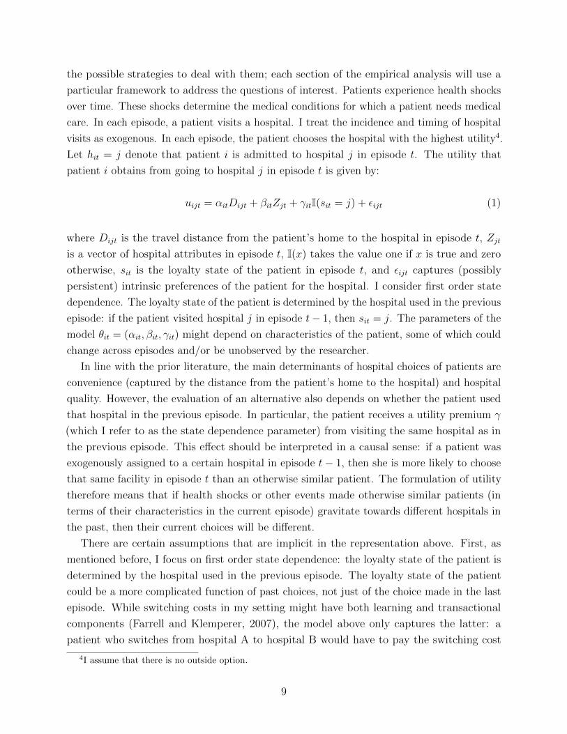
visits as exogenous. In each episode, the patient chooses the hospital with the highest utility4.

Let hit = j denote that patient i is admitted to hospital j in episode t. The utility that

patient i obtains from going to hospital j in episode t is given by:

uijt = αitDijt + βitZjt + γitI(sit = j) + εijt (1)

where Dijt is the travel distance from the patient’s home to the hospital in episode t, Zjt

is a vector of hospital attributes in episode t, I(x) takes the value one if x is true and zero

otherwise, sit is the loyalty state of the patient in episode t, and εijt captures (possibly

persistent) intrinsic preferences of the patient for the hospital. I consider first order state

dependence. The loyalty state of the patient is determined by the hospital used in the previous

episode: if the patient visited hospital j in episode t− 1, then sit = j. The parameters of the

model θit = (αit, βit, γit) might depend on characteristics of the patient, some of which could

change across episodes and/or be unobserved by the researcher.

In line with the prior literature, the main determinants of hospital choices of patients are

convenience (captured by the distance from the patient’s home to the hospital) and hospital

quality. However, the evaluation of an alternative also depends on whether the patient used

that hospital in the previous episode. In particular, the patient receives a utility premium γ

(which I refer to as the state dependence parameter) from visiting the same hospital as in

the previous episode. This effect should be interpreted in a causal sense: if a patient was

exogenously assigned to a certain hospital in episode t− 1, then she is more likely to choose

that same facility in episode t than an otherwise similar patient. The formulation of utility

therefore means that if health shocks or other events made otherwise similar patients (in

terms of their characteristics in the current episode) gravitate towards different hospitals in

the past, then their current choices will be different.

There are certain assumptions that are implicit in the representation above. First, as

mentioned before, I focus on first order state dependence: the loyalty state of the patient is

determined by the hospital used in the previous episode. The loyalty state of the patient

could be a more complicated function of past choices, not just of the choice made in the last

episode. While switching costs in my setting might have both learning and transactional

components (Farrell and Klemperer, 2007), the model above only captures the latter: a

patient who switches from hospital A to hospital B would have to pay the switching cost

4I assume that there is no outside option.

9

if she later goes back to A. I focus on first order state dependence because in my setting:

i) Many of the factors that drive state dependence operate through the choice made in the

immediately preceding episode, and; ii) I expect that the effect of the immediately preceding

episode is stronger than the effect of more distant episodes.

Second, I assume that patients are myopic: the evaluation of different alternatives only

depends on the characteristics of the current episode. In particular, patients do not consider

that current choices will affect future decisions due to lock-in.

Third, some of the drivers of state dependence discussed in the introduction do not modify

the utility function directly. For example, state dependence could arise as the hospital used in

the previous episode is more likely to enter the consideration set of the patient in the current

episode, but with no utility premium from choosing this hospital over other alternatives in

the consideration set. In this case, Equation 1 is a reduced form representation of the decision

process of the patient.

Suppose that I estimate the model from data on patients’ actual choices. The identification

problem arises from the potential endogeneity of the loyalty state variable. The fact that

patient i chooses hospital j in episode t implies that she might have strong unobserved

preferences for that alternative. If the random component of utility is correlated across

episodes, then part of the choice persistence captures the underlying unobserved propensity of

the consumer to choose alternative j, and not just the structural effect of the previous choice

on current utility. This is a standard selection problem. Note that the serial correlation of

the error term can arise from several sources, such as misspecification of the distribution of

the taste coefficients αit and βit, omitted variables, and measurement error. This concern

seems particularly well founded in my setting, where there are many attributes of patients

and hospitals that I do not observe (religious affiliation of the patient, details about amenities

of the hospital, etc). Therefore, a positive value of the estimated γ is not conclusive evidence

of the presence of state dependence.

To deal with this issue, the ideal design would randomly assign patients to hospitals in

episode t− 1 and analyze their choices in episode t; in this case, the loyalty state variable

in episode t is uncorrelated with the preferences of the patient5. Given that most studies

use observational data for the analysis, identification has typically relied on both parametric

assumptions about preference heterogeneity and choice set variation across choice occasions

(Sudhir and Yang, 2014). As Torgovitsky (2016) points out, the first strategy addresses

the identification problem from a mathematical point of view, but its validity depends on

correctly specifying the distribution of unobserved heterogeneity. As Dube et al. (2010) point

5This allows us to deal with the selection problem and therefore identify state dependence given the

structure imposed by Equation 1. However, random assignment is not enough to point identify state

dependence in a more general sense. See Subsection 5.4.

10

out, any persistent preference heterogeneity not captured by the model will be loaded onto the

econometric error term, leading us to incorrectly inflate the magnitude of state dependence.

For example, Dube et al. (2010) show that allowing for a flexible pattern of heterogeneity can

lead to different conclusions than more traditional approaches. Most studies rely (at least in

part) on parametric assumptions to separately identify the sources of persistence. Exceptions

are Torgovitsky (2016) and Illanes (2016), who recover the values of the parameters that

are consistent with the identifying restrictions under different distributions of preference

heterogeneity.

Exploiting choice set variation across episodes provides more transparent and credible

evidence on the determinants of choice persistence. The idea is to break the link between

the previous choice and unobserved preferences of the consumer, so the selection problem is

eliminated or at least attenuated. Heckman (1981) argues that to distinguish state dependence

from latent heterogeneity I need a sufficiently large variation in the choice set to induce

purchases that would not have been made otherwise. Dube et al. (2010) exploit temporary

price changes to identify state dependence in the context of choice of branded products.

Suppose that consumers are induced to switch away from their preferred products by price

discounts on other goods. If consumers continue purchasing the “less-preferred” products

after prices return to normal levels, then this points to state dependence as the source of

choice persistence. Goldfarb (2006b) studies consumers’ website choices and exploits product

unavailability (caused by Internet denial of service attacks) to identify lock-in. Sudhir and

Yang (2014) exploit the mismatch between previous choice and previous consumption created

by free upgrades (which are mainly due to inventory shortages) in the context of car rentals

to separate state dependence from unobserved heterogeneity. Israel (2005) points out that I

can compare two individuals that face the same decision today and have identical loyalty

states: one that was forced to use a certain alternative j in the previous episode by an

exogenous shock, and another one who chose that same product voluntarily. Under selection,

the exogenous shock would produce a relatively high number of suboptimal matches among

the affected population, which will make consumers depart from alternative j once we return

to the usual choice environment.

I follow this strategy to provide credible evidence about the sources of persistence in

hospital choices of patients. In particular, I exploit quasi-exogenous shocks that shift the

loyalty state of patients: emergency hospitalizations (Section 4) and temporary hospital

closures (Section 5).

11

4. Emergencies

In this section, I exploit emergencies as a quasi-exogenous source of variation in the loyalty

state of patients. The strategy is to analyze the hospital choice of a patient in episode t

following an emergency hospitalization in episode t− 1. By emergency, I mean an episode

in which the patient needs immediate medical care and there is little scope for choosing a

particular hospital. Consider the case in which the emergency episode induces the patient

to go to a hospital other than the one she had been using. I analyze whether the patient

continues using this “new” hospital in the future. As the loyalty state of the patient is

initiated by an emergency hospitalization, and to the extent that the new hospital choice is

responsive to her preferences, repurchase behavior reflects the extent of state dependence.

The first step is to define emergencies. The identifying assumption is that the facility

visited for an emergency hospitalization is determined by factors other than the preferences

of the patient: the ambulance transport decision and the location of the patient at the time

of the health shock (Doyle et al., 2015). This assumption would be violated if: 1) The patient

or any of her surrogates requests transportation to a particular hospital during the emergency

episode; 2) Patients choose where to live based on health status, so the locus of treatment

during an emergency was “chosen” prior to that episode6,7. Since the assumption that the

hospital used in an emergency is not determined by the preferences of the patient is not

verifiable, I take several steps to make the assumption more plausible.

Ideally, I would define emergencies as episodes where the patient suffers a severe and

unexpected health shock and arrives to the hospital by ambulance. Unfortunately, I cannot

distinguish in my data whether a patient arrived to the hospital by ambulance or self-transport.

Given this limitation, I define emergencies as episodes in which the patient is admitted to

the hospital through the emergency department (ED) for a severe medical condition that

requires immediate care. These non-deferrable conditions correspond to admitting diagnoses

(ICD-9-CM) with similar admission rates through the ED on weekdays and weekends (Card

et al., 2009). These conditions represent 6% of all ED admissions, and are extremely acute

and often life-threatening. Table 1 shows the most common non-deferrable conditions in

6For example, patients with heart disease might decide to locate close to their preferred hospital, so in the

event of a heart attack they are likely to be taken to that facility.7Even if the patient is not involved in the choice process, the emergency hospital could reflect her

preferences. Consider two patients who live on opposite sides of the same zip code. I only observe the zip code

of residence of a patient, but not her exact address. There are two hospitals, one on each side of the zip code.

If patients are taken to the closest facility in an emergency, then the two patients go to different hospitals in

that episode. Then, the facility visited for the emergency hospitalization indicates which hospital is more

convenient for the patient. If the disutility of travel is high, repurchase behavior could reflect unobserved

preferences for the emergency hospital (actual distance to the emergency hospital is smaller than in the data).

This should be less of a concern the smaller the zip code. I control for this consideration in the analysis below.

12

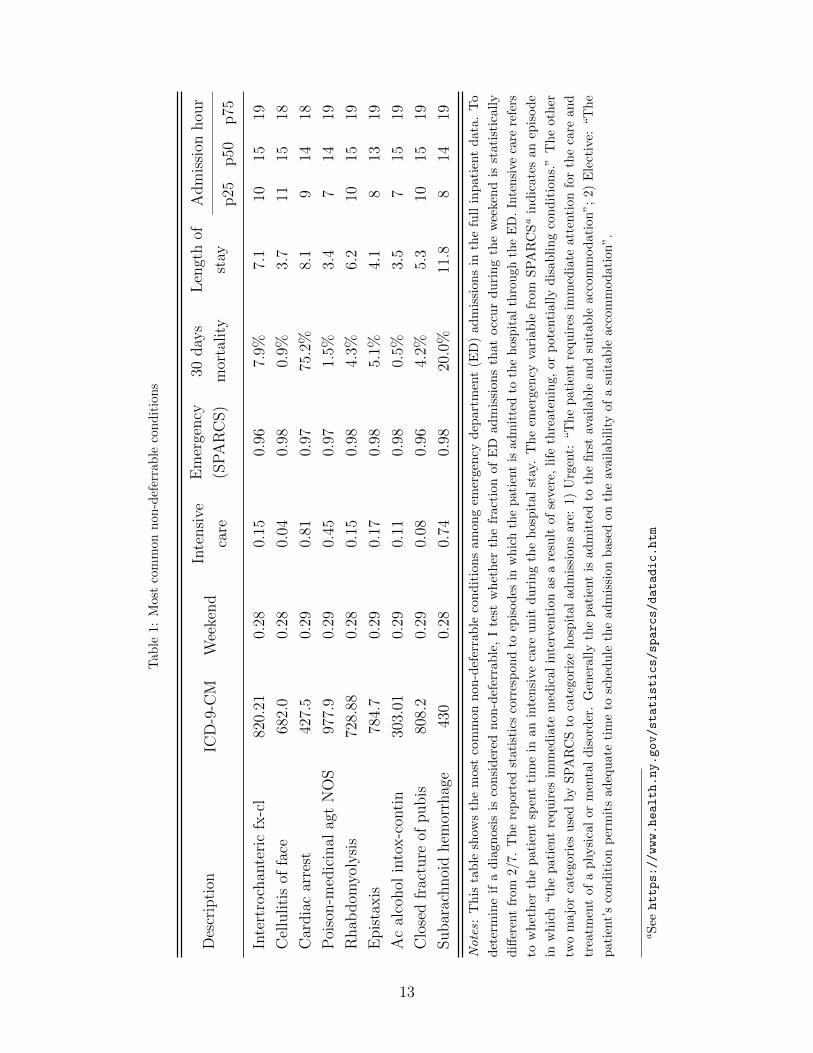
Tab

le1:

Most

com

mon

non

-def

erra

ble

con

dit

ion

s

Des

crip

tion

ICD

-9-C

MW

eeke

nd

Inte

nsi

ve

care

Em

erge

ncy

(SP

AR

CS)

30day

s

mor

tality

Len

gth

of

stay

Adm

issi

onhou

r

p25

p50

p75

Inte

rtro

chan

teri

cfx

-cl

820.

210.

280.

150.

967.

9%7.

110

1519

Cel

luliti

sof

face

682.

00.

280.

040.

980.

9%3.

711

1518

Car

dia

car

rest

427.

50.

290.

810.

9775

.2%

8.1

914

18

Poi

son-m

edic

inal

agt

NO

S97

7.9

0.29

0.45

0.97

1.5%

3.4

714

19

Rhab

dom

yoly

sis

728.

880.

280.

150.

984.

3%6.

210

1519

Epis

taxis

784.

70.

290.

170.

985.

1%4.

18

1319

Ac

alco

hol

into

x-c

onti

n30

3.01

0.29

0.11

0.98

0.5%

3.5

715

19

Clo

sed

frac

ture

ofpubis

808.

20.

290.

080.

964.

2%5.

310

1519

Subar

achnoi

dhem

orrh

age

430

0.28

0.74

0.98

20.0

%11

.88

1419

Notes:

This

table

show

sth

em

ost

com

mon

non-d

efer

rable

condit

ions

am

ong

emer

gen

cydep

art

men

t(E

D)

adm

issi

ons

inth

efu

llin

pati

ent

data

.T

o

det

erm

ine

ifa

dia

gnosi

sis

consi

der

ednon-d

efer

rable

,I

test

whet

her

the

fract

ion

of

ED

adm

issi

ons

that

occ

ur

duri

ng

the

wee

ken

dis

stati

stic

ally

diff

eren

tfr

om2/

7.T

he

rep

orte

dst

atis

tics

corr

esp

ond

toep

isodes

inw

hic

hth

epat

ient

isad

mit

ted

toth

ehos

pit

alth

rough

the

ED

.In

tensi

veca

rere

fers

tow

het

her

the

pati

ent

spen

tti

me

inan

inte

nsi

ve

care

unit

duri

ng

the

hosp

ital

stay

.T

he

emer

gen

cyva

riable

from

SP

AR

CSa

indic

ate

san

epis

ode

inw

hic

h“th

epati

ent

requir

esim

med

iate

med

ical

inte

rven

tion

as

are

sult

of

sever

e,life

thre

ate

nin

g,

or

pote

nti

ally

dis

abling

condit

ions.

”T

he

oth

er

two

ma

jor

cate

gori

esu

sed

by

SP

AR

CS

toca

tegori

zeh

osp

ital

ad

mis

sion

sare

:1)

Urg

ent:

“T

he

pati

ent

requ

ires

imm

edia

teatt

enti

on

for

the

care

an

d

trea

tmen

tof

aphysi

cal

or

men

tal

dis

ord

er.

Gen

erally

the

pati

ent

isadm

itte

dto

the

firs

tav

ailable

and

suit

able

acc

om

modati

on”;

2)

Ele

ctiv

e:“T

he

pat

ient’

sco

ndit

ion

per

mit

sad

equ

ate

tim

eto

sch

edu

leth

ead

mis

sion

base

don

the

avail

ab

ilit

yof

asu

itab

leacc

om

mod

ati

on

”.

aS

eehttps://www.health.ny.gov/statistics/sparcs/datadic.htm

13


the full dataset and characteristics of these episodes. In addition, I exclude emergencies in

which the patient is admitted to the hospital from a health care facility (e.g. a skilled nursing

facility). As the patient is likely to have chosen a health care facility close to her preferred

hospital, the use of a hospital during the emergency probably reflects strong preferences for

the facility. In summary, I am confident that the emergencies that I consider are episodes

with limited scope for the patient to choose the hospital.

Once I identify an emergency according to the criteria outlined above, I analyze the hospital

choice of the patient in the first episode following the emergency (I refer to this episode as

the current episode)8. In this episode, the loyalty state of the patient is determined by the

hospital used for the emergency hospitalization (I refer to this hospital as the emergency

hospital). For example, if the patient used hospital A in the emergency episode, then the

patient is loyal to hospital A at the time of the next episode. In the analysis, I consider two

situations:

1. The current loyalty state was initiated by the emergency. Moreover, the emergency

hospital had never been used by the patient before9. Therefore, I exclude emergencies

in which the patient goes to a hospital different from the last one she used before the

emergency but that she used at some point in the past. As a result, the emergency

produces a strong shift in the loyalty state of the patient: her choices before the

emergency reveal that she does not have strong preferences for the facility used in

that episode. Therefore, the repurchase behavior of the patient in the current episode

reflects the extent of state dependence.

2. The current loyalty state was initiated before the emergency: the emergency hospital

is the same facility that the patient had been using before. In this case, there is a

selection issue: the choices of the patient before the emergency reveal that she has strong

preferences for that facility. Therefore, the repurchase behavior of the patient in the

current episode captures both state dependence and persistent preference heterogeneity.

The repurchase rate is the fraction of patients who in the current episode choose the same

hospital used for the emergency hospitalization. The raw repurchase probability is not very

informative about the impact of previous choices on current behavior. For example, in cases

8As explained in Section 2, I drop readmissions from the working sample. Therefore, I analyze whether

the patient continues going to the emergency hospital for episodes not directly related to the emergency

itself. In the main specification, I use a 90 days window to identify readmissions. To ensure robustness, I also

performed the analysis using other time windows (30, 60, and 120 days), without any substantial change in

the nature of the results. These results are available upon request.9More precisely, the patient did not visit the hospital between 1995 (the first year for which I have patient

data) and the day of the emergency. Because I only consider emergencies that take place on or after 2005,

this restriction means that the patient had not used the facility for at least 10 years before the emergency.

14

where the previous hospital does not offer the medical services required in the current episode,

the repurchase rate would be zero even in the presence of state dependence. If the hospital

used during the emergency is the best hospital for treating the current medical condition of

the patient, then a high repurchase rate reflects both state dependence and the quality of

the match between the patient and the facility. Therefore, I compare the repurchase rate

to the marginal probability of choosing the emergency hospital based on characteristics of

the current episode. This way, I measure the likelihood that a patient who used a certain

hospital in episode t− 1 chooses that same hospital in episode t relative to an observationally

similar patient. To calculate the patient’s marginal probability of choosing the emergency

hospital, I assume that it is equal to the market share of that hospital within the group of

similar patients (see Raval et al. (2017a) and Carlson et al. (2013)). I follow the next steps:

1. Using the full dataset, I define cells of equivalent episodes based on zip code, diagnosis,

type of visit, and admission year. Note that a patient might transition across different

cells over time (for example, if she moves or if she seeks hospital care for different

medical conditions). I denote the market share of hospital j within cell k by sjk.

2. I assign each episode following an emergency hospitalization to the corresponding cell.

I denote the hospital used in episode i by hi and the hospital used by the same patient

in her previous episode (the emergency hospitalization) by hbi .

3. For each episode, the marginal probability of choosing the emergency hospital is the

market share of this facility within the episode’s cell. I denote the marginal probability

of choosing the emergency hospital in episode i by p(i) = swk, where i ∈ k and w = hbi .

4. For each p ∈ [0, 1], the corresponding excess repurchase probability is given by the

mean of xi = I{hi = hbi} − p(i) over episodes with p(i) = p.

The idea is to look at patients with different loyalty states (they used different hospitals for

the emergency episode) but with the same probability p of choosing the emergency hospital in

the current episode. Consider episodes where the loyalty state was initiated by the emergency.

If previous choices do not have an impact on current decisions, then we should expect the

repurchase rate to be p (so the excess repurchase probability is zero). If the excess repurchase

probability is positive, then this point to the presence of state dependence. For episodes

where the loyalty state was initiated before the emergency, the excess repurchase probability

captures both state dependence and unobserved heterogeneity. Doing the same exercise for

all possible values of p, I recover the excess repurchase probability schedule.

In practice, I pool current episodes into bins of size 0.1 according to p(i) and compute the

mean excess repurchase probability within each bin. The first bin includes current episodes

15

Table 2: Episodes following an emergency hospitalization

Emergency hospital

New Usual

Number of cases 40,549 105,390

Episodes before emergency:

Number of episodes 1.6 3.8

Propensity to use emergency hospital 0 0.82

Episode after emergency:

Days since emergency 393 349

Repurchase rate 0.42 0.78

Marginal choice probability 0.24 0.39

Inpatient 0.27 0.31

Emergency Department 0.59 0.57

Ambulatory Surgery 0.14 0.12

Notes: This table shows summary statistics of the episodes following an emergency hospitalization. I

distinguish episodes based on whether the emergency hospital was being used by the patient before the

emergency or is a new hospital. The prior propensity to use the emergency hospital is defined as the proportion

of the patient’s hospital visits prior to the emergency episode that were to the emergency hospital. The

repurchase rate is the proportion of patients who chose the emergency hospital in the episode following

the emergency. Inpatient, Ambulatory Surgery and Emergency Department categorize hospital visits. The

marginal choice probability is the probability of choosing the emergency hospital based on characteristics of

the patient in the current episode (the next episode after the emergency hospitalization).

in which the marginal probability of choosing the emergency hospital is lower than 0.1,

the second bin includes current episodes in which the marginal probability of choosing the

emergency hospital is between 0.1 and 0.2, and so on. In the main specification, I only

consider cases where the marginal choice probability is higher than 0.01. If the marginal

probability is lower than this value, it most likely corresponds to a case where the patient

will not consider the facility for hospital care. I follow Raval et al. (2017a) and keep current

episodes in cells with a minimum number of observations (20 in the main specification), so

market shares can be computed reliably.

Table 2 shows summary statistics of the current episodes used in the analysis. I distinguish

episodes depending on whether the emergency hospital had never been used before the

emergency or was the usual hospital of the patient. There are two main differences between

16

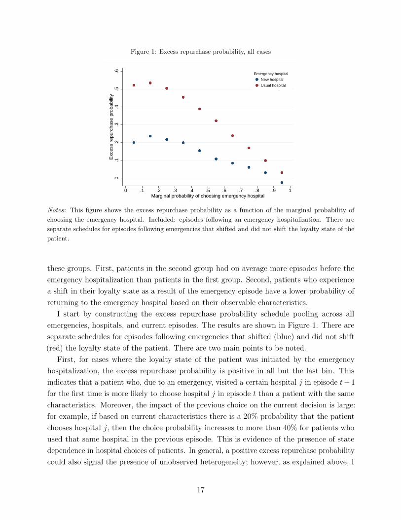
Figure 1: Excess repurchase probability, all cases

0.1

.2.3

.4.5

.6E

xces

s re

purc

hase

pro

babi

lity

0 .1 .2 .3 .4 .5 .6 .7 .8 .9 1Marginal probability of choosing emergency hospital

New hospital

Usual hospital

Emergency hospital

Notes: This figure shows the excess repurchase probability as a function of the marginal probability of

choosing the emergency hospital. Included: episodes following an emergency hospitalization. There are

separate schedules for episodes following emergencies that shifted and did not shift the loyalty state of the

patient.

these groups. First, patients in the second group had on average more episodes before the

emergency hospitalization than patients in the first group. Second, patients who experience

a shift in their loyalty state as a result of the emergency episode have a lower probability of

returning to the emergency hospital based on their observable characteristics.

I start by constructing the excess repurchase probability schedule pooling across all

emergencies, hospitals, and current episodes. The results are shown in Figure 1. There are

separate schedules for episodes following emergencies that shifted (blue) and did not shift

(red) the loyalty state of the patient. There are two main points to be noted.

First, for cases where the loyalty state of the patient was initiated by the emergency

hospitalization, the excess repurchase probability is positive in all but the last bin. This

indicates that a patient who, due to an emergency, visited a certain hospital j in episode t− 1

for the first time is more likely to choose hospital j in episode t than a patient with the same

characteristics. Moreover, the impact of the previous choice on the current decision is large:

for example, if based on current characteristics there is a 20% probability that the patient

chooses hospital j, then the choice probability increases to more than 40% for patients who

used that same hospital in the previous episode. This is evidence of the presence of state

dependence in hospital choices of patients. In general, a positive excess repurchase probability

could also signal the presence of unobserved heterogeneity; however, as explained above, I

17

address this concern by focusing on loyalty states initiated by emergencies.

Second, the excess repurchase probability is higher for episodes following an emergency

that did not shift the loyalty state of the patient. As explained above, in this case repurchase

behavior not only reflects state dependence, but it also captures the latent propensity of the

patient to choose the facility used in previous episodes. Therefore, the higher repurchase rate

for these cases reflects the presence of substantial unobserved preference heterogeneity. As a

result, a naive analysis that does not take into account the endogeneity of previous choices

will overstate the magnitude of state dependence.

In what follows, I restrict attention to episodes following an emergency that induced a

shift in the loyalty state of the patient, so repurchase behavior reflects state dependence. To

evaluate the robustness of my findings, I construct the excess repurchase probability schedule

for episodes following different types of emergencies. As shown in Figure 2, the qualitative

results are the same as in the main analysis.

The previous results could mask heterogeneity in persistence across different types of

hospitals. In particular, there might be differences in loyalty towards high and low quality

hospitals. The pattern of heterogeneity might provide insights about the determinants of

state dependence. I distinguish cases based on the quality of the emergency hospital. Quality

is not observable, so I use teaching status as a proxy for high quality10. Figure 3 shows that

the excess repurchase probability schedules of teaching and non-teaching hospitals are similar.

Although not conclusive evidence, this suggests that learning is not the primary driver of the

observed persistence: patients are equally loyal to high and low quality hospitals.

10Teaching status is obtained from the AHA Annual Survey Database and refers to hospital membership in

the Council of Teaching Hospitals (COTH).

18

Figure 2: Excess repurchase probability, by type of emergency

(a) Intensive care

0.1

.2.3

Exc

ess

repu

rcha

se p

roba

bilit

y


(b) Injury or poisoning

0.1

.2.3

Exc

ess

repu

rcha

se p

roba

bilit

y


(c) Night admission

0.1

.2.3

Exc

ess

repu

rcha

se p

roba

bilit

y


(d) Heart attack and stroke

0.1

.2.3

Exc

ess

repu

rcha

se p

roba

bilit

y


Notes: These figures show the excess repurchase probability as a function of the marginal probability of

choosing the emergency hospital. Included: episodes following an emergency hospitalization that shifted the

loyalty state of the patient. Different figures correspond to different types of emergencies: a) During the

emergency hospitalization, the patient spent time in an intensive care unit; b) The emergency was coded as

injury or poisoning; c) The emergency admission took place during the night (between 9PM and 5AM), and;

d) The emergency was coded as heart attack or cerebrovascular accident.

19

Figure 3: Excess repurchase probability, by type of hospital

(a) Teaching

−.1

0.1

.2.3

Exc

ess

repu

rcha

se p

roba

bilit

y


(b) Non-teaching

−.1

0.1

.2.3

Exc

ess

repu

rcha

se p

roba

bilit

y


Notes: These figures show the excess repurchase probability as a function of the marginal probability of

choosing the emergency hospital. Included: episodes following an emergency hospitalization that shifted the

loyalty state of the patient. Different figures correspond to different types of emergency hospital.

5. Temporary hospital closures: Hurricane Sandy

5.1. Setting

Hurricane Sandy hit the New York Metropolitan area at the end of October 201211. Damage

from the storm led to the temporary closures of three hospitals in New York City: NYU

Langone Medical Center, Bellevue Hospital Center, and Coney Island Hospital. Bellevue and

NYU Langone are located in Manhattan next to each other, while Coney Island Hospital

is located in Brooklyn. Table 3 provides a basic description of the affected hospitals. The

facilities differ along various dimensions, so there is heterogeneity in the settings that I analyze.

NYU Langone is an academic medical center with a high proportion of privately insured

patients. The other two hospitals are part of the city’s Health and Hospitals Corporation

and attract mostly Medicare, Medicaid, and uninsured patients. NYU Langone and Bellevue

are large hospitals (more than 900 beds), while Coney Island Hospital is a medium size

facility (371 beds). In terms of service offerings and designations, NYU Langone is the most

sophisticated, followed by Bellevue. Although Coney Island Hospital offers a wide range of

services, it does not provide the most complex services.

11For details about the timeline and the impact of the storm, see Raval et al. (2017b), https://

www.cbsnews.com/pictures/nyc-hospitals-evacuated-for-superstorm/, https://www.reuters.com/

article/storm-sandy-bellevue-idUSL1N0B78OY20130207, and https://www.nytimes.com/2012/10/

30/nyregion/patients-evacuated-from-nyu-langone-after-power-failure.html

20

https://www.cbsnews.com/pictures/nyc-hospitals-evacuated-for-superstorm/

https://www.cbsnews.com/pictures/nyc-hospitals-evacuated-for-superstorm/

https://www.reuters.com/article/storm-sandy-bellevue-idUSL1N0B78OY20130207

https://www.reuters.com/article/storm-sandy-bellevue-idUSL1N0B78OY20130207

https://www.nytimes.com/2012/10/30/nyregion/patients-evacuated-from-nyu-langone-after-power-failure.html

https://www.nytimes.com/2012/10/30/nyregion/patients-evacuated-from-nyu-langone-after-power-failure.html

Table 3: Characteristics of affected hospitals

Coney Island Hospital Bellevue NYU Langone

Visits:

Ambulatory Surgery 4,487 7,697 17,710

Emergency Department 60,621 93,538 36,475

Inpatient 17,580 26,763 33,095

Demographics, inpatient:

Age 50.6 42.7 43.6

Female 0.53 0.39 0.58

Medicare 0.35 0.17 0.27

Medicaid 0.48 0.49 0.08

Private 0.09 0.08 0.62

Other insurance 0.08 0.25 0.03

Certified beds:

Total 371 912 987

Services:

Perinatal Designation Level 2 Regional Center Regional Center

CABG No Yes Yes

Transplant Center No No Yes

Notes: This table describes the hospitals affected by Hurricane Sandy. The number of visits and the

demographic profile of patients correspond to the 12 month period preceding the storm (November 2011 -

October 2012).

21

The affected hospitals remained closed for repairs and renovations during several weeks,

forcing patients usually served by these facilities to find an alternative hospital for their

medical care needs. Consider, for example, a patient who receives medical care at Coney

Island Hospital and had never gone elsewhere before. If the patient needed medical care

during the time this facility was closed, she would have had to go to another hospital, such

as Maimonides Medical Center. In this section, I study whether the temporary unavailability

of the affected hospitals had a long-lived impact on patients’ preferences: Does the patient

in the example continue going to Maimonides Medical Center once Coney Island Hospital

reopens or does she return to her usual hospital? Do affected patients become long-term

patients of the new facilities? Anecdotal evidence suggests that the possibility of permanently

losing patients was a concern for administrators at the shuttered hospitals12.

This natural experiment is particularly useful to study the dynamics of hospital choice.

First, the type of choice set variation produced by the storm is ideal given the institutional

characteristics of the hospital industry. Second, the hospital closures were unexpected and

unrelated to patients’ preferences for different facilities, thus providing a quasi-exogenous

source of variation in hospital choice. Third, the data allows me to identify those patients

most likely to have been affected by the temporary hospital closures: patients with strong

preferences for an affected facility who needed hospital care during the unavailability window.

Therefore, I can identify patients who would have chosen one of the affected hospitals had it

been available, but were forced to choose a second-best option. There are two main limitations

of my analysis. First, I only observe hospital choices of patients for less than three years

after the affected facilities reopened. Second, I analyze a specific empirical context, which

places limitations on the external validity of my conclusions. In particular, the analysis is

not designed to provide estimates of the extent of state dependence in other settings.

Raval et al. (2017b) exploit unexpected hospital closures in different markets following

a natural disaster to analyze the substitution patterns predicted by different models of

hospital choice. One of the natural disasters that they consider is Hurricane Sandy. In

one of their specifications, the authors identify patients who used the affected hospitals in

the pre-storm period as those most likely to have experienced the closure of their preferred

hospital. However, whether their continued preference for the shuttered facilities is due to

switching costs or unobserved heterogeneity is irrelevant for their analysis, so they do not

attempt to separate the channels. The main objective of my analysis is to separately identify

state dependence from persistent unobserved heterogeneity, while the nature of substitution

patterns is not a primary concern.

There are two steps in the analysis. First, following Goldfarb (2006b), I show that patients

12http://www.nytimes.com/2012/12/04/nyregion/with-some-hospitals-closed-after-

hurricane-sandy-others-overflow.html?mcubz=1

22

http://www.nytimes.com/2012/12/04/nyregion/with-some-hospitals-closed-after-hurricane-sandy-others-overflow.html?mcubz=1

http://www.nytimes.com/2012/12/04/nyregion/with-some-hospitals-closed-after-hurricane-sandy-others-overflow.html?mcubz=1

who needed hospital care while a hospital was closed (treatment group) are less likely to

visit that facility in the future than patients who did not have hospital visits during the

unavailability window (control group). Moreover, non-returning patients in the treatment

group favor the facility used during the unavailability window. Second, I cast the setting into

a nonparametric framework. By imposing an independence restriction between preferences

and the timing of hospital visits, I can reject the hypothesis of no state dependence under

minimal assumptions about the nature of unobserved preference heterogeneity.

5.2. Sample construction

For each case study13, I construct a panel of patients’ hospital choices. As explained in Section

2, readmissions and visits for follow-up care are excluded from the analysis, so hospital visits

correspond to different episodes of care. I divide episodes into three periods based on the

date of the patient’s admission to the hospital: period 0 corresponds to the pre-storm period,

period 1 is the time window during which the affected hospital remained closed for repairs,

and period 2 goes from the reopening of the shuttered facility trough the end of the sample

period. For each patient, I only consider episodes that took place while the patient was living

in the service area of the affected hospital: I want to use information on those episodes where

the patient is likely to consider this facility for hospital care. In the case of CIH, this step

would remove, for example, episodes that take place while the patient lives in Buffalo or

Manhattan - so CIH is not viewed as a practical alternative - but would keep hospital visits

by the same patient while she lives in southern Brooklyn.

To construct the service area of a hospital, I follow the methodology of Raval et al. (2017b).

First, I identify the smallest collection of zip codes that accounted for 90% of inpatient

discharges from the facility in the year prior to the storm. Second, I exclude zip codes where

the facility had a market share below 4% in the year before the storm. Finally, I make

adjustments to achieve geographic contiguity of the resulting service area. Figures 7 through 9

in Appendix A show the service area of each of the affected hospitals. I repeated the analysis

using alternative thresholds to determine the inclusion of zip codes in the service area and

the qualitative results (not reported) are consistent with the baseline results discussed here.

Given the effects that I am trying to identify, I construct the working sample as follows. I

keep patients from the full sample who: 1) Had at least one hospital visit in both periods

0 and 214, and; 2) Did not have any hospital visits while the affected facility was closed

13In what follows, I emphasize the case of Coney Island Hospital (CIH, henceforth), because the definitions

of service area and the competitive set are more transparent for CIH than for Bellevue and NYU Langone.

However, the methodology outlined below applies to all three cases.14The restriction that patients have at least one episode in period 0 has the benefit that I can use information

on actual hospital choices to infer the strength of their preferences for the affected hospital.

23

or visited only one hospital during that time window. For each individual in the resulting

sample, I keep the last episode of period 0, all episodes (if any) of period 1, and the first

episode of period 2. Therefore, for each patient I know: 1) The hospital visited in the last

episode before the storm; 2) Whether she needed hospital care while the affected facility was

closed and, if so, which hospital she used, and; 3) The hospital chosen in the first episode of

period 2. I distinguish patients based on whether they visited a hospital in period 1. I refer

to the set of patients who needed hospital care while the affected hospital was closed as the

treatment group, while the other patients constitute the control group.

For the analysis, I focus on the hospital choices of patients in the first episode of period

2. I exclude a small number of cases where the affected hospital does not seem to be in the

market for the type of medical care required by the patient in that episode. I consider that

the affected hospital provides the services required by the patient if at least three patients

with the same type of claim and diagnosis category were treated in that facility during the

corresponding semester. This step removes approximately 5% of patients.

I refer to the sample that results from the selection steps outlined above as sample #1.

I define two subsamples that I use in the subsequent analysis. Sample #2 contains those

patients who were loyal to the affected hospital at the moment of the storm (they visited that

facility in the last episode of period 0), while sample #3 contains those patients who visited

either the shuttered hospital or one of its main competitors in all the episodes considered. To

identify the main competitors of an affected hospital, I compute the diversion ratio from that

facility to other hospitals in the year before the storm. I define the six hospitals with the

highest diversion ratios as the main competitors of the affected facility. Tables 11 through

13 in Appendix A show information on the demographic profile and other characteristics of

patients in the three samples. There are two main differences between control and treatment

groups. First, the treatment group is older and sicker: it has a higher proportion of inpatient

episodes and Medicare/Medicaid patients than the control group. Second, patients in the

treatment group used the affected hospital in the pre-storm period less frequently than

patients in the control group. Although I control for these differences in the analysis below,

the imbalance along the latter dimension points to potential threats to identification.

5.3. Reduced form evidence

I now discuss the patterns in the data that help identify state dependence. Consider two

patients with similar underlying preferences for CIH (idiosyncratic tastes or unobserved

characteristics - separate from state dependence - that make them gravitate towards this

hospital) and who were loyal to that hospital at the moment of the storm. The first patient

needs hospital care in period 1 and therefore goes to a hospital other than CIH (given that

this facility is closed), while the second patient does not need hospital care in period 1. I

24

compare the hospital choices that these patients make in the first episode of period 2. In this

episode, the patients have different loyalty states: the patient who got sick during period 1 is

not loyal to CIH, while the patient who did not seek hospital care in period 1 remains loyal

to CIH. If the temporary unavailability of CIH did not change the underlying preferences

of patients for hospitals, then differences in choice probabilities between the two patients

capture the impact of state dependence.

The identifying assumption is that the timing of hospital visits is exogenous. In other

words, whether a patient seeks hospital care in period 1 or not is independent of her tastes for

different facilities. In this case, the distribution of preferences is the same for patients in the

treatment and control groups. The assumption seems a priori reasonable in my setting, given

that patients most likely visit a hospital due to a health shock. However, there are ways in

which the assumption could be violated. I discuss the potential threats to the validity of my

approach at the end of the section.

I start by showing that patients who needed hospital care while an affected hospital was

closed were less likely to return to that hospital in the first episode of period 2 than similar

patients who did not have hospital visits in period 1. I use sample #2 for the analysis, so all

the patients considered were loyal to the affected hospital at the moment of the storm.

Figure 4 shows, for both the treatment and control groups, the probability of choosing

CIH in the first episode of period 2 as a function of the prior propensity to use the facility.

This propensity is defined as the proportion of the patient’s hospital visits prior to the storm

that were to this facility15. There are two things to note. First, the probability of choosing

CIH in the first episode of period 2 increases with the prior propensity to use that facility,

for both the treatment and control groups. This is not surprising, given that the pre-storm

propensity to use the affected facility captures the strength of the patient’s preferences for

that hospital. Second, patients in the treatment group are less likely to return to CIH after

its reopening than patients in the control group with similar prior propensity. The gap in

choice probabilities reflects a lasting effect of the temporary unavailability of the affected

hospital on patients’ choices. Figures 5 and 6 show the results for Bellevue and NYU Langone,

respectively. For NYU Langone, the difference between treatment and control groups is not

as clear as in the other two cases; however, the analysis below shows that the differences in

patient behavior are significant in this case.

To control for preference heterogeneity related to observables, I estimate a probit of

choosing the affected hospital in the first episode of period 2 on the prior propensity to use the

facility, zip code fixed effects, diagnosis fixed effects, a spline of the number of days between

the reopening of the shuttered facility and the episode, and an indicator for treatment status.

15Consider, for example, a patient who had five hospital visits in the pre-storm period. If three of these

visits were to the affected hospital, then the prior propensity to use this facility is 0.6.

25

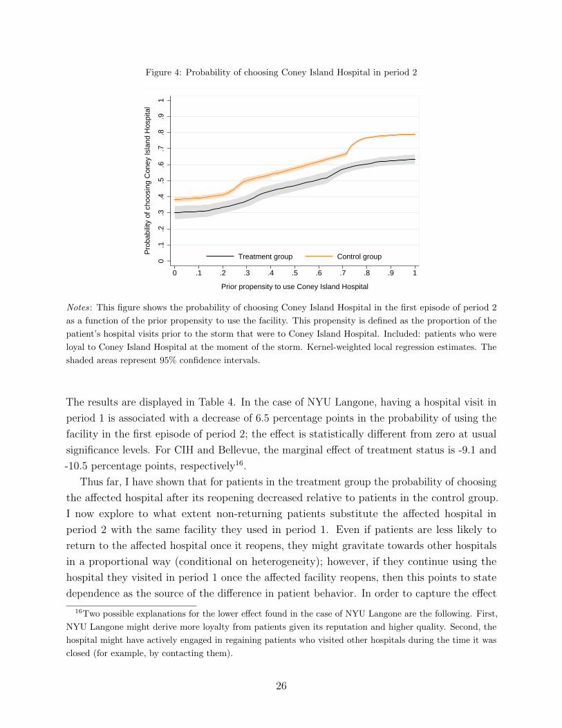
Figure 4: Probability of choosing Coney Island Hospital in period 2

0.1

.2.3

.4.5

.6.7

.8.9

1

Pro

babi

lity

of c

hoos

ing

Con

ey Is

land

Hos

pita

l

0 .1 .2 .3 .4 .5 .6 .7 .8 .9 1

Prior propensity to use Coney Island Hospital

Treatment group Control group

Notes: This figure shows the probability of choosing Coney Island Hospital in the first episode of period 2

as a function of the prior propensity to use the facility. This propensity is defined as the proportion of the

patient’s hospital visits prior to the storm that were to Coney Island Hospital. Included: patients who were

loyal to Coney Island Hospital at the moment of the storm. Kernel-weighted local regression estimates. The

shaded areas represent 95% confidence intervals.

The results are displayed in Table 4. In the case of NYU Langone, having a hospital visit in

period 1 is associated with a decrease of 6.5 percentage points in the probability of using the

facility in the first episode of period 2; the effect is statistically different from zero at usual

significance levels. For CIH and Bellevue, the marginal effect of treatment status is -9.1 and

-10.5 percentage points, respectively16.

Thus far, I have shown that for patients in the treatment group the probability of choosing

the affected hospital after its reopening decreased relative to patients in the control group.

I now explore to what extent non-returning patients substitute the affected hospital in

period 2 with the same facility they used in period 1. Even if patients are less likely to

return to the affected hospital once it reopens, they might gravitate towards other hospitals

in a proportional way (conditional on heterogeneity); however, if they continue using the

hospital they visited in period 1 once the affected facility reopens, then this points to state

dependence as the source of the difference in patient behavior. In order to capture the effect

16Two possible explanations for the lower effect found in the case of NYU Langone are the following. First,

NYU Langone might derive more loyalty from patients given its reputation and higher quality. Second, the

hospital might have actively engaged in regaining patients who visited other hospitals during the time it was

closed (for example, by contacting them).

26

Figure 5: Probability of choosing Bellevue in period 2

0.1

.2.3

.4.5

.6.7

.8.9

1

Pro

babi

lity

of c

hoos

ing

Bel

levu

e

0 .1 .2 .3 .4 .5 .6 .7 .8 .9 1

Prior propensity to use Bellevue


Notes: This figure shows the probability of choosing Bellevue in the first episode of period 2 as a function of

the prior propensity to use the facility. This propensity is defined as the proportion of the patient’s hospital

visits prior to the storm that were to Bellevue. Included: patients who were loyal to Bellevue at the moment

of the storm. Kernel-weighted local regression estimates. The shaded areas represent 95% confidence intervals.

Figure 6: Probability of choosing NYU Langone in period 2

0.1

.2.3

.4.5

.6.7

.8.9

1

Pro

babi

lity

of c

hoos

ing

NY

U L

ango

ne

0 .1 .2 .3 .4 .5 .6 .7 .8 .9 1

Prior propensity to use NYU Langone


Notes: This figure shows the probability of choosing NYU Langone in the first episode of period 2 as a

function of the prior propensity to use the facility. This propensity is defined as the proportion of the patient’s

hospital visits prior to the storm that were to NYU Langone. Included: patients who were loyal to NYU

Langone at the moment of the storm. Kernel-weighted local regression estimates. The shaded areas represent

95% confidence intervals.

27

Table 4: Probit estimates

Days since reopening 0 30 60 90 120 150

Panel A: Coney Island Hospital

Treatment status -0.091 -0.084 -0.080 -0.080 -0.075 -0.072

(Std Error) (0.009) (0.010) (0.010) (0.011) (0.011) (0.012)

Sample size 41,153 38,640 36,318 34,174 32,084 30,095

Panel B: Bellevue


(Std Error) (0.012) (0.013) (0.014) (0.015) (0.016) (0.017)

Sample size 25,550 23,684 21,891 20,287 18,856 17,560

Panel C: NYU Langone


(Std Error) (0.014) (0.015) (0.015) (0.016) (0.017) (0.017)

Sample size 21,295 20,155 19,056 17,967 16,914 15,944

Notes: This table shows the results from the estimation of probit models where the dependent variable is

one if the patient visited the affected hospital in the first episode of period 2. The explanatory variables are

an indicator for treatment status, propensity-bin fixed effects, zip code fixed effects, diagnosis group fixed

effects, and a spline of the number of days between the reopening of the affected hospital and the episode.

The indicator for treatment status is one if the patient needed hospital care while the affected hospital was

closed for repairs. The estimates reported correspond to the average marginal effect of treatment status.

Days since reopening refers to the episodes included in the estimation sample: if days since reopening is x,

then only episodes that took place at least x days after the reopening of the affected hospital are included in

the estimation sample.

28

of interest, I estimate a conditional logit model of hospital choice using the first episode of

period 2. Explanatory variables include hospital-type of visit fixed effects, the distance from

the centroid of the patient’s zip code of residence to the facility, interactions between the

type of insurance of the patient and an indicator for public hospital, and an indicator for

whether the hospital was used in the previous episode of care; in addition, I allow the utility

from choosing the affected hospital to vary with the prior propensity to use that facility.

The estimates from the model are reported in Table 5. Previous use of a facility is a strong

predictor of the hospital choice of a patient: having used a hospital in period 1 increases the

probability of choosing that same facility in period 2 more than four times above the baseline

probability (the magnitude of this effect is similar across the three case studies).

In summary, I have provided evidence that patients who experienced a forced shift in their

loyalty state are less likely to return to their usual hospital than similar unaffected patients.

Moreover, patients who do not return to the affected hospital favor the new facility they used

in period 1. These patterns indicate the presence of state dependence in hospital choices of

patients. I now discuss in more detail the assumptions underlying my empirical strategy in

order to identify potential problems.

First, I assume that the timing of hospital visits is independent of patients’ preferences

for hospitals. In other words, I assume that whether a patient seeks hospital care in period

1 or not is independent of her preferences for different hospitals. If patients with very

strong preferences for the affected hospital postponed elective medical care until this facility

reopened, then there is a selection problem. In particular, the control group would include a

higher proportion of patients with strong preferences for the affected facility, which might

explain the gap in choice probabilities between the two groups.

Second, the affected hospitals restored services gradually and sometimes at reduced

capacity. If capacity constraints were important, I might be artificially inflating persistence

due to state dependence: some patients might have wanted to receive care at CIH in period

2 but were unable to do so due to capacity constraints. For this to bias the results, it must

be the case that patients in the treatment group were more affected by capacity constraints

than patients in the control group.

To address these concerns, I perform the same analysis excluding episodes that took place

close to the start of period 2. Capacity constraints likely were more of an issue during the first

days after affected hospitals resumed operations, so inference using episodes that occurred

later in period 2 should be less affected by bias from this channel. In addition, using episodes

further away from the reopening date should lower the impact of selection into treatment

status by patients who delay care. I estimate a probit of choosing the affected hospital in

period 2 as described above, but excluding cases that took place less than 30, 60, 90, 120,

and 150 days after the reopening date. The results are shown in columns 3 through 7 of

29

Table 5: Logit estimates

Case study


Used in previous episode 1.968 2.109 1.890

(0.068) (0.101) (0.091)

Distance -0.130 -0.476 -0.321

(0.003) (0.008) (0.008)

Affected hospital x Prior propensity

Prior propensity: 0 - 0.25 0.011 -0.058 -0.036

(0.104) (0.092) (0.111)

Prior propensity: 0.25-0.50 0.338 0.419 0.381

(0.067) (0.072) (0.077)

Prior propensity: 0.50-0.75 0.774 0.871 0.795

(0.054) (0.061) (0.064)

Prior propensity: 0.75-1 1.217 1.442 0.999

(0.040) (0.044) (0.043)

Public hospital x Insurance

Insurance: Medicare 0.027 0.877 1.022

(0.045) (0.058) (0.099)

Insurance: Medicaid 0.350 1.052 1.724

(0.037) (0.050) (0.122)

Insurance: Other 1.315 1.969 2.290

(0.044) (0.058) (0.115)

Notes: This table shows estimates of the conditional logit model of hospital choice in the first episode of

period 2. The previous use variable is an indicator for whether the hospital considered was chosen by the

patient in her previous episode of care. Prior propensity is defined as the proportion of the patient’s hospital

visits prior to the storm that were to the affected hospital. The model also includes hospital - type of visit

fixed effects (not shown). The effect of previous hospital use is economically significant: having used a hospital

in period 1 increases the probability of choosing that same facility in the first episode after the reopening of

the affected hospital 4.4, 4.6, and 3.9 times above the baseline probability, respectively.30

Table 4. The decrease in the probability of choosing CIH associated with treatment group

status is between 7.2 and 8.4 percentage points, depending on the time window considered.

Although the effect is smaller than in the main specification, it remains large and significant.

For Bellevue and NYU Langone, the effect of treatment status also decreases as I focus on

episodes further away from the reopening date, although the magnitude of the change is

smaller than for CIH.

Third, I assume that the closure and unavailability of an affected hospital did not have

any impact on patients’ underlying preferences for the facility. In particular, this means that

the quality of the hospital did not change and that patients did not update their beliefs about

the quality of the hospital. If patients in the control and treatment groups were equally

affected along this dimension, this would not be a problem because identification is based

on differences in choice probabilities. However, if patients in the treatment group are more

likely to adjust their beliefs about the quality of the affected hospital (or if they feel that

some aspects about the facility that they liked changed after its reopening), then this would

be a confounding factor in the analysis. I believe that the latter scenario is unlikely: the

closure was directly related to the damage produced by the storm, which was particularly

destructive and affected many areas of the city.

In conclusion, while deviations from the identifying assumptions are certainly possible, the

robustness of my results suggests that the potential effects are of second-order importance.

However, there are several assumptions implicit in the analysis whose effects are not easily

ascertained. First, I assumed a specific distribution for the unobservable portion of utility.

The choice of probit or logit responds more to convention than to economic rationale. One

could wonder whether I would still find that there is state dependence in hospital choices

of patients under other (possibly “non-standard”) distributional assumptions. Second, I

have assumed that switching costs are symmetric: the utility premium from sticking to the

previous choice is independent of the hospital visited in period 1. However, it is possible that

some hospitals induce more loyalty from patients than others. Third, the results previously

discussed are informative about the mean effect of state dependence, but they provide limited

information about heterogeneity in the impact of previous choices on current behavior. Fourth,

I have assumed that utility is linear in its different components. I may need to explore the

effects of non-separability of preferences on measured state dependence. Fifth, I have assumed

that patients are myopic when choosing hospitals: they do not consider the implications of

their current choices for future episodes of care. The question remains whether conclusions

change once I allow for forward looking behavior. In summary, although the main source of

identification in my setting is evident, there are several modeling choices that could affect the

results. In the next section, I address this concern and show evidence of state dependence

using a nonparametric model of dynamic discrete choice.

31

5.4. Nonparametric analysis

In this section, I quantify state dependence in hospital choices of patients using the nonpara-

metric approach proposed by Torgovitsky (2016), adapted to the particulars of my case study.

I start by providing an overview of the basic framework. I follow the original formulation

of Torgovitsky (2016), as well as his discussion of the identification strategy, as closely as

possible.

There are N patients and three periods (t = 0, 1, 2). All patients choose a hospital in

periods 0 and 2, and some patients also have to choose a hospital in period 1. There are J

hospitals; however, hospital 1 is not available in period 1 and therefore cannot be chosen

by patients who need hospital care in that period. If Jt denotes the choice set in period t,

then J0 = J2 = {1, ..., J} and J1 = {2, ..., J}. This is the setting described in the previous

subsection: hospital 1 is the hospital shuttered by Hurricane Sandy and the same definitions

of time periods apply. Each patient has a type determined by:

1. Her choice in period t = 0, denoted h0.

2. Her potential choices in each period t ≥ 1 in which she has to choose a hospital:

ht(k) denotes the alternative the patient would choose in period t had her previous

choice counterfactually been k. For a patient who has to choose a hospital in period 1,

h1(k) is the alternative the patient would choose in period 1 had her period 0 choice

counterfactually been k, while h2(k) is the alternative the patient would choose in

period 2 had her period 1 choice counterfactually been k. For a patient who does not

have to choose a hospital in period 1, h2(k) is the alternative the patient would choose

in period 2 had her period 0 choice counterfactually been k. There are J counterfactual

choices {ht(k)}Jk=1 in period t. As Torgovitsky (2016) points out, the model places no

restrictions on the temporal dependence of potential choices across periods.

3. Whether she needed hospital care in period t = 1, indicated by z ∈ {0, 1}.

4. Other variables that indicate time-varying or time-invariant characteristics of the patient,

captured by vector x ∈ X . I restrict attention to discrete covariates, so the set X is

discrete.

In what follows, H denotes the set of all possible types, h denotes a generic type in H,

and ht = [ht(1), ..., ht(J)] denotes the corresponding set of potential choices in period t.

Let yt denote the hospital actually chosen by a given patient in period t. A patient in

my data is associated with a vector of observables y = {y0, y1, y2, z, x}. I observe the actual

hospital choices of patients and their characteristics, but not their types. However, types and

observables are related. In particular, a patient with type h makes the following choices:

32

y0 = h0 (2a)

For z = 1 : y1 = h1(y0) and y2 = h2(y1) (2b)

For z = 0 : y2 = h2(y0) (2c)

Therefore, for any patient only one element of the vector of potential choices in a given

period is known to the researcher. The remaining potential choices are counterfactual. Going

forward, Y is the set of all possible vectors of observables, y denotes a generic element of

Y, and y(h) ∈ Y is the vector of observables generated by a patient with type h through

relationships (2a)-(2c). Note that while type h generates a unique vector of observables

y(h) = y, the latter could have been generated by more than one type.

The data is given by P : Y → [0, 1], where P is a probability mass function (p.m.f.) with

support in Y. In other words, for each possible vector y ∈ Y, I know the proportion of

patients with those observables. For now, I assume that the distribution of observables is

known by the researcher.

The notion of state dependence arises naturally in this setting, as a patient might make

different choices in different counterfactual scenarios. A patient with type h exhibits state

dependence in period t > 0 if there are two previous counterfactual choices k, j ∈ {1, ..., J}for which the corresponding period t potential choices are different: ht(k) 6= ht(j). Let

sdt(h) be an indicator of whether a patient with type h exhibits state dependence in period

t. Identifying state dependence at the individual level requires information on at least two

potential choices in a period. As explained above, the data reveals only one component of

the vector of potential choices in a period. Therefore, whether there is state dependence at

the individual level is untestable. However, we might be able to learn something about the

extent of state dependence in the population.

The primitive of the model is the distribution of types in the population. With this

distribution, I can define various measures of state dependence. In particular, I want to learn

about the proportion of patients who exhibit state dependence in period 2 (which I refer to

generically as θ). Then, I view this feature of the distribution of types in the population as

the object of interest. If the distribution of types is given by the probability mass function P,

then the corresponding parameter is:

θ(P) =∑h∈H

P(h)sd2(h) (3)

which is linear in the probabilities of types.

The problem is that the distribution of types is not known by the researcher. Let W be

the set of admissible distributions. For the moment, we take W as given. This set contains

33

all the distributions that the researcher considers could have generated the data, based on

the assumptions about the data generating process that s/he is willing to maintain. We only

consider distributions in W and any of those distributions could in principle be the true one.

In general, there are many admissible distributions and therefore the parameter of interest is

partially identified. The identified set for the parameter of interest is:

Θ(W ) = {θ(P) : P ∈ W} = [θl(W ), θu(W )] (4)

In other words, to recover the identified set we need to compute the proportion of patients

with state dependence in period 2 under each admissible distribution using Equation (3). The

last equality in Equation (4) states that the identified set is a closed interval with extreme

points θl(W ) and θu(W ). This characterization of the identified set only holds under certain

conditions on θ(P) and W , which are satisfied in my setting. Therefore, to characterize the

identified set I only need to find the admissible distributions with the lowest and highest

state dependence:

θl(W ) = minP∈W

∑h∈H

P(h)sd2(h) (5)

θu(W ) = maxP∈W

∑h∈H

P(h)sd2(h) (6)

Before discussing the restrictions that define the set of admissible distributions and the

computational approach to recover the identified set, let me briefly discuss the two main

identification issues we need to deal with.

First, from ordinary (non-experimental) data on patients’ hospital choices, I can recover

P [yt = v|yt−1 = w] = P[ht(w) = v|yt−1 = w] for v ∈ Jt, w ∈ Jt−1. However, this object

might differ from P[ht(w) = v] due to persistent unobserved heterogeneity. Therefore, the

marginal distributions of potential choices in a given period are generally not identified from

observational data.

Even if I deal with selection bias (for example, by using experimental data), there is a

second identification issue: it is generally not possible to recover the joint distribution of

potential choices from the marginal distributions (Heckman et al., 1997). This issue stresses

the fact that it is not possible to point identify the extent of state dependence even with

experimental data. This notion seems to have been overlooked by many empirical studies of

persistence in consumer choice that focus almost exclusively on dealing with the selection

bias issue17.

The set of admissible distributions consists of those p.m.f. over H that are compatible with

the observed data and the institutional setting, and that satisfy the additional identifying

17It should be noted that dealing with selection bias is in general quite complicated.

34

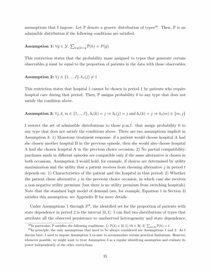
assumptions that I impose. Let P denote a generic distribution of types18. Then, P is an

admissible distribution if the following conditions are satisfied:

Assumption 1: ∀y ∈ Y ,∑

h:y(h)=y P(h) = P (y)

This restriction states that the probability mass assigned to types that generate certain

observables y must be equal to the proportion of patients in the data with those observables.

Assumption 2: ∀j ∈ {1, .., J}, h1(j) 6= 1

This restriction states that hospital 1 cannot be chosen in period 1 by patients who require

hospital care during that period. Then, P assigns probability 0 to any type that does not

satisfy the condition above.

Assumption 3: ∀j, k,m ∈ {1, .., J}, ht(k) = j ⇒ ht(j) = j and ht(k) = j ⇒ ht(m) ∈ {m, j}

I restrict the set of admissible distributions to those p.m.f. that assign probability 0 to

any type that does not satisfy the conditions above. There are two assumptions implicit in

Assumption 3: 1) Monotone treatment response: if a patient would choose hospital A had

she chosen another hospital B in the previous episode, then she would also choose hospital

A had she chosen hospital A in the previous choice occasion; 2) No partial compatibility:

purchases made in different episodes are compatible only if the same alternative is chosen in

both occasions. Assumption 3 would hold, for example, if choices are determined by utility

maximization and the utility that a patient receives from choosing alternative j in period t

depends on: 1) Characteristics of the patient and the hospital in that period; 2) Whether

the patient chose alternative j in the previous choice occasion, in which case she receives

a non-negative utility premium (but there is no utility premium from switching hospitals).

Note that the standard logit model of demand (see, for example, Equation 1 in Section 3)

satisfies this assumption; see Appendix B for more details.

Under Assumptions 1 through 319, the identified set for the proportion of patients with

state dependence in period 2 is the interval [0, 1]: I can find two distributions of types that

attribute all the observed persistence to unobserved heterogeneity and state dependence,

18In particular, P satisfies the following conditions: 1) P(h) ∈ [0, 1],∀h ∈ H; 2)∑

h∈H P(h) = 119In principle, the only assumptions that need to be always considered are Assumptions 1 and 2. As I

discuss later, I need to impose Assumption 3 ex-ante to accommodate certain practical limitations. However,

whenever possible, we might want to treat Assumption 3 as a regular identifying assumption and evaluate its

power independently of the other restrictions.

35

respectively. In order to get more informative results, I need to impose additional structure.

In particular, I translate the identifying assumption discussed in the previous subsection into

the following restriction on the set of admissible distributions:

Assumption 4: ∀j, k ∈ {1, .., J} ∀x ∈ X , P[h2(k) = j|z = 0, x] = P[h2(k) = j|z = 1, x]

This is a conditional independence assumption. It states that the potential choices in period 2

are independent of the treatment status indicator z, conditional on the other covariates x. In

other words, the distribution of preferences in period 2 is the same for patients who required

hospital care in period 1 and for patients who did not, conditional on other covariates.

This was the main identifying assumption for the analysis in Section 5.3. Here, the

meaning of this assumption is more clear. If patients in the treatment and control groups

have different loyalty states in period 2, then their choices reveal different elements of the

vector of potential choices in that period. If the distribution of potential choices is the same

for both groups, then I can combine the information obtained from each group to learn about

the joint distribution of potential choices.

Assumptions 1 through 4 determine the set of distributions W that I need to consider

for identification. As discussed above, I could recover the identified set by computing the

parameter of interest for each admissible distribution. However, this approach is not practical.

While an analytical characterization seems too complicated, we can exploit the structure of

the problem to characterize the identified set in a computationally simple way (Torgovitsky,

2016; Laffers, 2015). As mentioned before, the identified set is a closed interval. Therefore, I

only need to recover the lower and upper bounds on the proportion of patients with state

dependence in period 2 to fully characterize the identified set. Consider the problem of

recovering the lower bound (the same reasoning applies to the problem of recovering the

upper bound). As Equation (5) shows, the problem is to find the admissible distribution

(probabilities of types) that minimizes the parameter of interest. The latter is linear in

the probabilities of types. The set of admissible distributions is defined by Assumptions

1 through 4, which impose linear restrictions on the probabilities of types. Therefore, the

lower and upper bounds on the parameter of interest can be found by solving a set of linear

programming problems.

To implement this approach, I take certain steps to accommodate practical limitations.

The main issue is the size of the set of types: the number of possible vectors of potential

choices in any period t ≥ 1 when the cardinality of the choice set is J is JJ , so the number of

possible types (without any covariates) is JJT+1 if t = 0, .., T . To keep the dimensions of the

problem to manageable proportions, I make the following modeling choices: 1) I only consider

36

Table 6: Proportion of patients who exhibit state dependence in period 2: lower bound


0.091 0.092 0.129

Notes : This table shows, for each case study, the lower bound on the proportion of patients who exhibit state

dependence in period 2 under Assumptions 1 through 4.

three periods (T = 2); 2) I only consider patients who visit the affected hospital or any of

its main competitors in any period in which they need hospital care (then, I use sample #3

for the analysis); 3) I impose Assumption 3 ex-ante. Without doing this, the dimensions of

the optimization problem would be prohibitive in my application. However, I stress that

Assumption 3 has economic content beyond its usefulness to reduce the dimensionality of the

problem.

For each case study, I compute the identified set under Assumptions 1 through 4. The

results are shown in Table 6. The data and the restrictions that I impose on the distribution

of preferences allow me to conclude that at least 9.1% of patients in the sample for Coney

Island Hospital exhibit state dependence in period 2. In other words, there is no distribution

of patient types consistent with Assumptions 1 through 4, such that the proportion of patients

with state dependence in period 2 is lower than 9.1%. In the case of Bellevue and NYU

Langone, the lower bounds on the proportion of patients with state dependence are 9.2%

and 12.9%, respectively. In all three cases, the upper bound is equal to 1: I cannot reject

the hypothesis that all patients exhibit state dependence in period 2 under Assumptions 1

through 4.

The interpretation of the results is the following. I consider the case of Coney Island

Hospital to fix ideas. If I knew the distribution of types in the population, then I would

be able to compute the proportion of patients who exhibit state dependence in period 2.

However, I do not know what the true distribution is. Therefore, I need to consider all the

distributions that are consistent with the data. I cannot get informative results from the data

alone, so I need to impose additional structure. One possibility would be to specify a fully

parametric model of patient behavior (for example, a random utility model), map the full

structure of the model into the potential choices framework, estimate the parameters of the

model, and use these estimates to compute the proportion of patients with state dependence

in period 2. However, it is difficult to assess the sources of identification with this approach

and therefore it is not clear how measured state dependence would change under different

modeling assumptions. The results obtained using the nonparametric approach indicate that

no model with a richer structure will produce less than 9.1% of patients with state dependence

37

in period 2, as long as it is consistent with the identifying assumptions imposed. Therefore, I

can reject the hypothesis of no state dependence under transparent assumptions: the finding

of state dependence is not an artifact of particular parametric assumptions but is supported

by a more fundamental source of identification (Torgovitsky, 2016). I gain transparency in

results at the cost of set identification: there are many values of the parameter of interest

that are compatible with the data and the identifying assumptions that I impose.

In summary, this approach allows me to provide robust evidence of the presence of state

dependence in hospital choices of patients. I can rule out that persistence in patient behavior

is only due to unobserved heterogeneity under minimal assumptions about the data generating

process. On the other hand, the identified set is quite wide, so we need to impose additional

structure if we want to get more informative results. Therefore, I see this approach as

complementary to parametric models of consumer choice: we use these richer models to

obtain more meaningful conclusions, but we do this having already shown that the finding of

state dependence is not an artifact of the parametric assumptions we impose.

In the previous analysis, I recovered the identified set assuming that the distribution

of observables was known, without accounting for sampling error. To conduct statistical

inference on the identified set, I follow the strategy proposed by Torgovitsky (2016). The idea

is to express the potential choices model as a moment inequalities model. To characterize the

identified set, we define a criterion function that penalizes deviations from the identifying

assumptions. Then, a sample analog of this criterion function is used as the basis for statistical

inference. Specifically, I use it as a test statistic for the null hypothesis that the parameter

of interest takes a specific value. To recover the distribution of the test statistic, I use the

subsampling approach of Romano and Shaikh (2008). This approach requires solving a

linearly-constrained quadratic program for many subsamples. Given that I am interested

in bounding the extent of state dependence away from zero, I test the hypothesis that the

proportion of patients with state dependence in period 2 is equal to zero. Even though the

test is conservative, as pointed out by Torgovitsky (2016), the hypothesis is rejected at usual

significance levels.

6. The impact of state dependence on health outcomes

In previous sections, I presented evidence that past hospital choices of a patient influence

her current choice. If health or other shocks made a patient gravitate towards a certain

hospital in the past, then the patient is more likely to choose that same facility for her current

medical needs than an otherwise similar patient. Therefore, absent state dependence, demand

patterns would be different.

In this section, I analyze the impact of state dependence on health outcomes. Lock-in

38

might prevent patients from re-optimizing after a change in the choice environment. In

particular, lock-in might prevent a patient from switching to hospitals that are more suitable

than her previous choice at treating her current medical condition. Then, absent state

dependence, patients would choose hospitals that produce better health outcomes. However,

this is an empirical matter. It is possible that, absent state dependence, patients would

switch to lower quality facilities, in which case the impact of state dependence on health

outcomes is reversed.

I study this in the context of hospital choice for heart surgery (Coronary artery bypass

grafting, CABG). I estimate a model of hospital choice that quantifies patients’ preferences

for hospital attributes and incorporates state dependence. I use the estimates of the model to

compare expected mortality in the actual state of the world and in a counterfactual scenario

in which there is no state dependence.

There are two reasons why I focus on a particular medical condition rather than doing a

more general analysis. First, risk adjustment and estimation of hospital quality are better

defined when they are disease specific. Second, quality measures are difficult to compare

across different procedures; therefore, it is hard to find a single measure of health outcomes

that is appropriate for a wide range of medical conditions. I focus on CABG surgery for

various reasons (Gaynor et al., 2016). First, it is a common procedure. Second, it is mostly

an elective intervention. Third, risk-adjusted mortality is a well accepted quality metric for

CABG surgery. Fourth, there are many studies that analyze hospital choices of patients for

CABG surgery, which provide me with a benchmark for assessing any effects I find.

In the analysis, I hold hospital quality fixed as observed in the data: I ignore any feedback

between patients’ demand patterns and quality choices of hospitals. In order to account for

feedback, I would need a formal model of hospital behavior, which is beyond the scope of

this study. Therefore, in assessing the impact of state dependence on health outcomes, I only

consider the direct effect that takes into account how it affects the allocation of patients to

hospitals.

Ideally, I would use the natural experiment discussed in Section 5 for this exercise. However,

this is not feasible due to the size of the resulting sample: the number of patients in the

treatment group who undergo CABG is very small20. As a result, I must rely on observational

data to identify the parameters of interest, at the cost of less clean identification than in the

previous section. However, I showed in previous sections that past hospital choices of patients

have a causal impact on current behavior. Moreover, the identification of state dependence in

those settings did not rely on arbitrary parametric assumptions. This lends credibility to the

conclusions obtained from models with a richer structure like the one used in this section.

20Sample sizes are also small for other medical conditions studied in the literature.

39

6.1. Framework

The framework I use is largely based on Gaynor et al. (2016). A patient has T ≥ 1 episodes

of care, where episode T corresponds to CABG surgery. Even though patients seek treatment

for the same condition in the last episode, they might have received hospital care for different

medical conditions in the past. The utility that a patient obtains from visiting a particular

hospital for CABG surgery is a function of observed patient and hospital characteristics

(which capture the quality of the match between them), the loyalty state of the patient, and

factors unobserved by the researcher. The patient chooses the hospital in the choice set

J = {1, .., J} that gives her the highest utility. In what follows, PSDij is the ex-ante probability

that patient i chooses hospital j in the actual state of the world (taking the loyalty state

of the patient as given), and PNSDij is the choice probability in the counterfactual scenario

where there is no state dependence.

The ultimate goal of the analysis is to evaluate the impact of state dependence on the

ex-ante probability of death following CABG surgery. Let Yi = 1 denote that patient i dies

within 30 days of CABG surgery. For each hospital, there is a potential outcome Yij that

denotes the outcome that would have been observed had patient i counterfactually chosen

hospital j for CABG surgery. Potential outcomes are related to observed variables as follows:

Yi =J∑

j=1

Yijhij (7)

where hij = 1 indicates that patient i chose hospital j.

Following the notation introduced above, the ex-ante expected mortality of patient i in

scenario K ∈ {SD,NSD} is given by:

EMKi =

J∑j=1

PKijE(Yij) (8)

This is the expected probability of death taking as given the loyalty state of the patient

and before the choice and mortality errors are realized. The impact of state dependence on

mortality across all patients who undergo CABG surgery is:

∆EM =∑i

[EMSD

i − EMNSDi ] =

∑i

∑j

[PSDij − PNSD

ij

]E(Yij) (9)

As discussed before, hospital-specific mortality is the same in both scenarios and therefore

the difference in health outcomes is only due to different sorting of patients across hospitals.

Then, the elements that I need to recover are: 1) The choice probabilities that govern the

data generating process; 2) The choice probabilities in the scenario where there is no state

dependence, and; 3) Hospital-specific mortality. The choice probabilities are computed from

40

the estimates of a hospital demand model, while I compute hospital quality using patient

discharge and mortality data. After describing the data used for the analysis, I discuss these

parts of the model in turn.

6.2. Data

I construct the sample for the analysis as follows. First, I identify all patients who had CABG

surgery in a New York hospital during the period from 2013 to 2015. I identify CABG cases

based on the procedures listed in the discharge record of the patient. I then exclude patients

who had valve surgery or another major cardiac surgical procedure during the same hospital

stay, and patients who were transferred to the hospital from another health care facility.

Second, I exclude CABG surgeries performed during an emergency episode. This way, I only

study hospital choices of patients who are able to evaluate the different alternatives available.

Third, I exclude a small number of patients who are more than 85 years old and patients with

insurance other than Medicare, Medicaid, or private insurance. Fourth, I assume that the

choice set of a patient consists of all hospitals in the market for CABG surgery (see below)

that are within 100 miles of her home (25 miles for patients in New York City). Then, I drop

patients who went to a hospital outside this area. The final sample consists of 7,509 patients.

For each patient, I construct the history of hospital visits before the CABG episode. The

loyalty variable is an indicator for whether the hospital considered was used in the previous

episode of care. I consider all visits for cardiac care to the hospital chosen for CABG during

the 60 days prior to the surgery as part of the CABG episode (so past hospital use directly

related to the latter does not determine the loyalty state of the patient).

The set of hospitals that offer CABG surgery is limited: 39 hospitals out of a total of 264

facilities in the State of New York offered this service during the period from 2013 to 201521.

Table 7 shows summary statistics for these hospitals.

Table 8 reports summary statistics of the CABG episodes in the working sample. Almost

80% of patients are male. The average patient is around 66 years old, and more than half

of the patients are covered by Medicare. On average, a patient had 4.6 episodes before the

CABG surgery. The observed 30-day mortality rate is 0.99%. The average distance to the

chosen hospital is 17.6 miles and 41% of patients go the closest hospital. On average, there

are 14 hospitals in a patient’s choice set.

In 2,905 cases (39% of the total), the hospital used in the previous episode is in the choice

set of the patient. On average, this hospital was used in 59% of previous episodes and in 82%

of previous visits to hospitals in the choice set; in 63% of the cases, it is the only hospital in

the choice set that was used before. The average time elapsed since the last episode is 2.2

21Given my sample restrictions, there are two hospitals that were not chosen by any patient in the resulting

dataset. Therefore, in the analysis, the set of hospitals in the market for CABG surgery contains 37 hospitals.

41

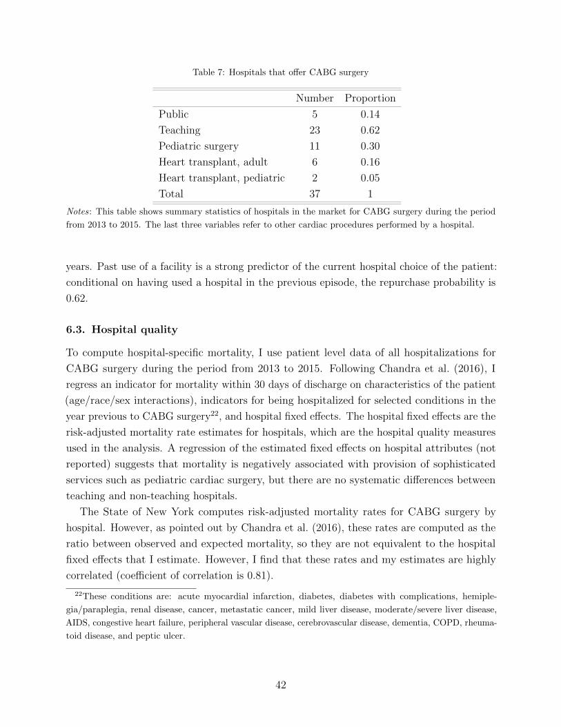
Table 7: Hospitals that offer CABG surgery

Number Proportion

Public 5 0.14

Teaching 23 0.62

Pediatric surgery 11 0.30

Heart transplant, adult 6 0.16

Heart transplant, pediatric 2 0.05

Total 37 1

Notes: This table shows summary statistics of hospitals in the market for CABG surgery during the period

from 2013 to 2015. The last three variables refer to other cardiac procedures performed by a hospital.

years. Past use of a facility is a strong predictor of the current hospital choice of the patient:

conditional on having used a hospital in the previous episode, the repurchase probability is

0.62.

6.3. Hospital quality

To compute hospital-specific mortality, I use patient level data of all hospitalizations for

CABG surgery during the period from 2013 to 2015. Following Chandra et al. (2016), I

regress an indicator for mortality within 30 days of discharge on characteristics of the patient

(age/race/sex interactions), indicators for being hospitalized for selected conditions in the

year previous to CABG surgery22, and hospital fixed effects. The hospital fixed effects are the

risk-adjusted mortality rate estimates for hospitals, which are the hospital quality measures

used in the analysis. A regression of the estimated fixed effects on hospital attributes (not

reported) suggests that mortality is negatively associated with provision of sophisticated

services such as pediatric cardiac surgery, but there are no systematic differences between

teaching and non-teaching hospitals.

The State of New York computes risk-adjusted mortality rates for CABG surgery by

hospital. However, as pointed out by Chandra et al. (2016), these rates are computed as the

ratio between observed and expected mortality, so they are not equivalent to the hospital

fixed effects that I estimate. However, I find that these rates and my estimates are highly

correlated (coefficient of correlation is 0.81).

22These conditions are: acute myocardial infarction, diabetes, diabetes with complications, hemiple-

gia/paraplegia, renal disease, cancer, metastatic cancer, mild liver disease, moderate/severe liver disease,

AIDS, congestive heart failure, peripheral vascular disease, cerebrovascular disease, dementia, COPD, rheuma-

toid disease, and peptic ulcer.

42

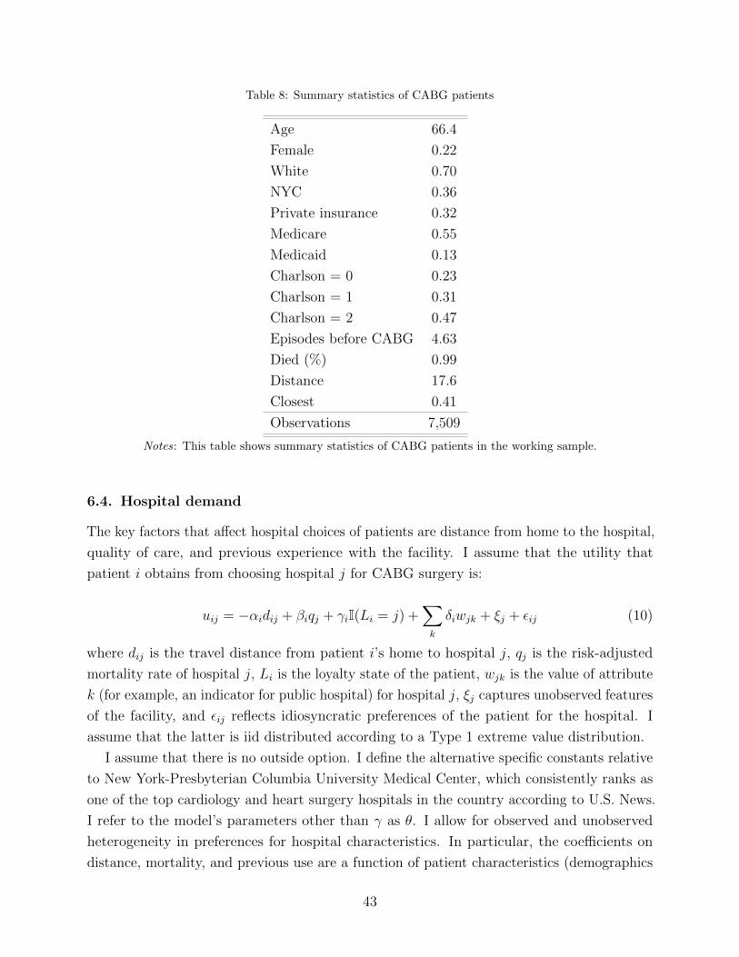
Table 8: Summary statistics of CABG patients

Age 66.4

Female 0.22

White 0.70

NYC 0.36

Private insurance 0.32

Medicare 0.55

Medicaid 0.13

Charlson = 0 0.23

Charlson = 1 0.31

Charlson = 2 0.47

Episodes before CABG 4.63

Died (%) 0.99

Distance 17.6

Closest 0.41

Observations 7,509

Notes: This table shows summary statistics of CABG patients in the working sample.

6.4. Hospital demand

The key factors that affect hospital choices of patients are distance from home to the hospital,

quality of care, and previous experience with the facility. I assume that the utility that

patient i obtains from choosing hospital j for CABG surgery is:

uij = −αidij + βiqj + γiI(Li = j) +∑k

δiwjk + ξj + εij (10)

where dij is the travel distance from patient i’s home to hospital j, qj is the risk-adjusted

mortality rate of hospital j, Li is the loyalty state of the patient, wjk is the value of attribute

k (for example, an indicator for public hospital) for hospital j, ξj captures unobserved features

of the facility, and εij reflects idiosyncratic preferences of the patient for the hospital. I

assume that the latter is iid distributed according to a Type 1 extreme value distribution.

I assume that there is no outside option. I define the alternative specific constants relative

to New York-Presbyterian Columbia University Medical Center, which consistently ranks as

one of the top cardiology and heart surgery hospitals in the country according to U.S. News.

I refer to the model’s parameters other than γ as θ. I allow for observed and unobserved

heterogeneity in preferences for hospital characteristics. In particular, the coefficients on

distance, mortality, and previous use are a function of patient characteristics (demographics

43

and severity) and unobserved factors. More precisely, I assume that:

αi = α +∑r

αorzir + αuµi (11)

βi = β +∑r

βorzir + βuνi (12)

γi = γ +∑r

γorzir + γuηi (13)

where zir is the value of (observed) attribute r for patient i, and (µi, νi, ηi) ∼ N(0, I) represent

idiosyncratic preferences of consumer i for distance, quality, and loyalty, respectively.

This specification of patient utility is similar to past work on hospital demand, although

it allows for richer heterogeneity. The third term in Equation 10 captures the impact of

loyalty on current utility. Specifically, the patient gets a utility premium γ from choosing

the hospital to which she is loyal. This implies that for patient i to switch hospitals, she

must prefer an alternative facility by γi more than the hospital used in her previous episode

(Handel, 2013).

One possibility would be to use Equation 10 to define the likelihood of the sequence of

hospital choices of a patient23. This way, I can exploit changes in choice set across episodes

for a given patient to learn about her preferences. However, I would need to assume that

preferences are stable across episodes. This would imply, for example, that the disutility of

travel of the patient is the same for CABG and for other types of episodes. That assumption

seems too strong. Instead, I model the choice of hospital in episode Ti (CABG) alone. As

discussed in previous sections, the main identification concern is the endogeneity of the

previous choice variable.

Given that the set of hospitals that offer CABG surgery is small, there are many patients

who did not visit any hospital in the market for CABG before undergoing this procedure. For

these consumers, state dependence does not affect preferences between hospitals. Then, the

parameters in θ are identified from the choices of these “new” patients. This identification

strategy has been used in the literature (see, for example, Handel (2013) and Luco (2016)).

The state dependence parameter is then identified by the repurchase behavior of patients

who are loyal to a particular facility.

I estimate the model by Maximum Simulated Likelihood (Train, 2009). From the estimates

of the model, I recover two sets of choice probabilities: (1) Pij(θ, γ) is the ex-ante probability

that patient i chooses hospital j in the actual state of the world: these are the predicted

probabilities obtained using the estimated coefficients of the utility function and the actual

23The different covariates would need to be indexed by t, as characteristics of patients and hospitals might

change across episodes (for example, the patient might need hospital care for different diagnoses over time).

44

data; (2) Pij(θ, 0) is the choice probability when the state dependence parameter is set equal

to zero.

6.5. Results

The estimates from the demand model (see Table 9) indicate that patients dislike traveling

for hospital care and value hospital quality. On average, a patient is willing to travel 12

additional miles to visit a hospital with one percentage point lower (risk-adjusted) mortality.

The impact of state dependence on patients’ choices is large: if a hospital was used by the

patient in her previous episode, then the probability of choosing that facility for CABG is

about 3.4 times higher than what would be expected based on other covariates.

The impact of state dependence on health outcomes depends on the locations and qualities

of hospitals in the market for CABG and the characteristics of the patient population.

Therefore, although the effects of state dependence on choices are substantial, the effects on

health outcomes might not be as large. Moreover, it is not clear that eliminating the frictions

driving state dependence will make patients switch to better hospitals in terms of quality.

I consider the impact on health outcomes of a number of thought experiments. Following

Handel (2013), I compare the ex-ante expected mortality under different counterfactual

scenarios, relative to the actual state of the world. In each scenario, the state dependence

parameter is set to a fraction of the baseline estimate: the lower the fraction, the less

contaminated by state dependence the hospital choices of patients. We can think of these

counterfactuals as illustrating the impact of policies that are partially effective in dealing with

the sources of state dependence, or as capturing the possibility that some residual unobserved

heterogeneity is picked up by the state dependence parameter. The results are reported in

Panel A of Table 10. To provide a reference point to analyze the magnitude of these effects, I

also compute the changes in mortality relative to the baseline scenario from reducing patients’

disutility from travel. The results are reported in Panel B of Table 10.

There are two points to be noted. First, I find that reducing the magnitude of the state

dependence coefficient leads to reductions in ex-ante expected mortality. In a counterfactual

world where there is no state dependence, one extra person is expected to survive, which

implies a 3% reduction in mortality relative to the baseline scenario (there were 33 actual

deaths). In other words, state dependence prevents a stronger allocation of patients to higher-

quality hospitals. To provide a benchmark for assessing the magnitude of this reduction in

mortality, consider the findings of Gaynor et al. (2016). They study the impact of a reform

in the English National Health Service that removed constraints on patient choice. They

find that CABG patients became more responsive to clinical quality: the reallocation to

higher quality hospitals led to a 3% reduction in expected mortality. Second, the impact

of eliminating state dependence is similar to the effect of reducing patients’ preferences for

45

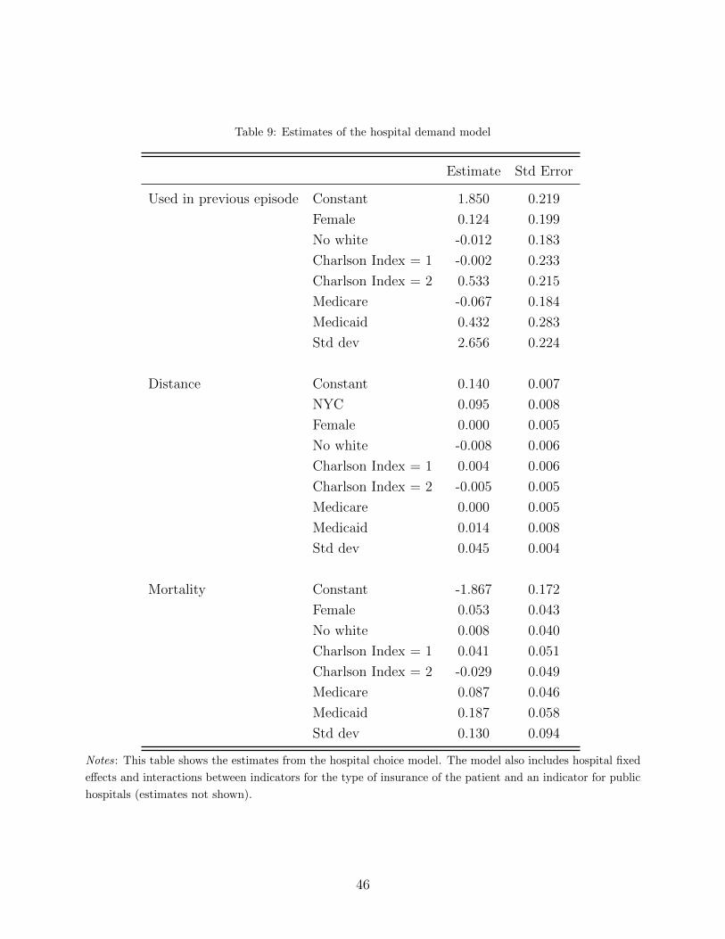
Table 9: Estimates of the hospital demand model

Estimate Std Error

Used in previous episode Constant 1.850 0.219

Female 0.124 0.199

No white -0.012 0.183

Charlson Index = 1 -0.002 0.233

Charlson Index = 2 0.533 0.215

Medicare -0.067 0.184

Medicaid 0.432 0.283

Std dev 2.656 0.224

Distance Constant 0.140 0.007

NYC 0.095 0.008

Female 0.000 0.005

No white -0.008 0.006



Medicare 0.000 0.005


Std dev 0.045 0.004

Mortality Constant -1.867 0.172

Female 0.053 0.043

No white 0.008 0.040



Medicare 0.087 0.046


Std dev 0.130 0.094

Notes : This table shows the estimates from the hospital choice model. The model also includes hospital fixed

effects and interactions between indicators for the type of insurance of the patient and an indicator for public

hospitals (estimates not shown).

46

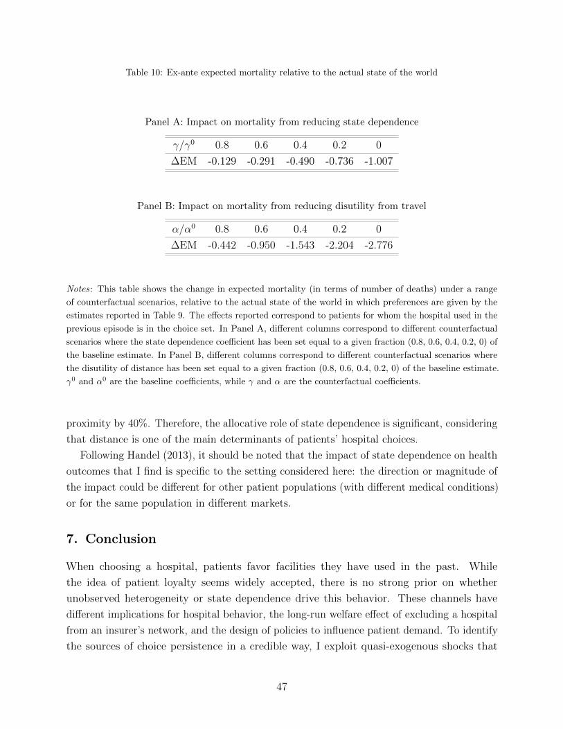
Table 10: Ex-ante expected mortality relative to the actual state of the world

Panel A: Impact on mortality from reducing state dependence

γ/γ0 0.8 0.6 0.4 0.2 0

∆EM -0.129 -0.291 -0.490 -0.736 -1.007

Panel B: Impact on mortality from reducing disutility from travel

α/α0 0.8 0.6 0.4 0.2 0

∆EM -0.442 -0.950 -1.543 -2.204 -2.776

Notes: This table shows the change in expected mortality (in terms of number of deaths) under a range

of counterfactual scenarios, relative to the actual state of the world in which preferences are given by the

estimates reported in Table 9. The effects reported correspond to patients for whom the hospital used in the

previous episode is in the choice set. In Panel A, different columns correspond to different counterfactual

scenarios where the state dependence coefficient has been set equal to a given fraction (0.8, 0.6, 0.4, 0.2, 0) of

the baseline estimate. In Panel B, different columns correspond to different counterfactual scenarios where

the disutility of distance has been set equal to a given fraction (0.8, 0.6, 0.4, 0.2, 0) of the baseline estimate.

γ0 and α0 are the baseline coefficients, while γ and α are the counterfactual coefficients.

proximity by 40%. Therefore, the allocative role of state dependence is significant, considering

that distance is one of the main determinants of patients’ hospital choices.

Following Handel (2013), it should be noted that the impact of state dependence on health

outcomes that I find is specific to the setting considered here: the direction or magnitude of

the impact could be different for other patient populations (with different medical conditions)

or for the same population in different markets.

7. Conclusion

When choosing a hospital, patients favor facilities they have used in the past. While

the idea of patient loyalty seems widely accepted, there is no strong prior on whether

unobserved heterogeneity or state dependence drive this behavior. These channels have

different implications for hospital behavior, the long-run welfare effect of excluding a hospital

from an insurer’s network, and the design of policies to influence patient demand. To identify

the sources of choice persistence in a credible way, I exploit quasi-exogenous shocks that

47

induce a patient to try a new hospital: emergency hospitalizations and temporary hospital

closures.

In the first case, I find that patients who visit a new hospital during an emergency

hospitalization are more likely to continue using that same facility in subsequent episodes than

observationally similar patients. This provides evidence of the presence of state dependence

in hospital choices of patients. In cases where the emergency did not shift the loyalty state of

the patient, repurchase rates are higher, which indicates that unobserved heterogeneity is

also empirically relevant.

In the second case, I exploit the temporary closures of three hospitals in New York

City due to Hurricane Sandy. I find that patients who needed hospital care during the

time an affected hospital was closed for repairs were less likely to use the facility after its

reopening than similar patients who did not have hospital visits during the unavailability

window. Moreover, non-returning patients continued using the same hospital they visited

during the time their usual facility was unavailable. The difference in behavior of these

patients points to the presence of state dependence. To provide more credible evidence, I

analyze patients’ hospital choices using the nonparametric framework of Torgovitsky (2016).

I am able to bound the proportion of patients who exhibit state dependence away from

zero under a conditional independence restriction between the preferences of the patient

and the timing of hospital visits, but without making parametric assumptions about the

nature of preference heterogeneity. The higher transparency of this approach (relative to

more traditional frameworks to analyze dynamic discrete choice) comes at the cost of set

identification.

After showing that state dependence affects patients’ choices, I consider its implications

for health outcomes. In the context of hospital choice for heart surgery, I find that, absent

state dependence, patients would switch to hospitals that are better at producing health

outcomes. In particular, in this counterfactual scenario, ex-ante expected mortality would be

3% lower than in the actual state of the world.

There are interesting avenues for future research that originate from the results in this

paper. The first one is to investigate the microeconomic fundamentals that drive state

dependence in this setting. Quantifying switching costs created by hospital policies regarding

the sharing of patient data would be particularly interesting given the diffusion of Electronic

Health Records (EHR) during the last years and policy efforts to achieve interoperability of

different systems.

It would also be interesting to quantify the contribution of state dependence in hospital

choices of patients to inertia in consumers’ choices of health insurance plan. This is particularly

relevant given the diffusion of narrow networks after implementation of the Affordable Care

Act.

48

Another interesting question is how state dependence distorts hospitals’ incentives to invest

in quality. For example, hospitals might display bargain-then-ripoff behavior using quality as

the adjustment variable. In addition, the possibility of developing long-term relationships

with patients might lead hospitals to overinvest in services that patients use early in their

lives.

References

Andrews, R. L. and T. Srinivasan (1995). “Studying consideration effects in empirical choice

models using scanner panel data”. Journal of Marketing Research, pp. 30–41.

Card, D., C. Dobkin, and N. Maestas (2009). “Does Medicare save lives?” Quarterly Journal

of Economics 124 (2), pp. 597–636.

Carlson, J. A., L. S. Dafny, B. A. Freeborn, P. M. Ippolito, and B. W. Wendling (2013).

“Economics at the FTC: Physician acquisitions, standard essential patents, and accuracy

of credit reporting”. Review of Industrial Organization 43 (4), pp. 303–326.

Chandra, A., A. Finkelstein, A. Sacarny, and C. Syverson (2016). “Health Care Exceptional-

ism? Performance and Allocation in the US Health Care Sector”. American Economic

Review 106 (8), pp. 2110–44.

Desai, S. (2016). “The Role of Interoperability in Hospital Digitization: Network Effects and

Information Blocking”.

Doyle, J., J. Graves, J. Gruber, and S. Kleiner (2015). “Measuring returns to hospital

care: Evidence from ambulance referral patterns”. Journal of Political Economy 123 (1),

pp. 170–214.

Dube, J.-P., G. J. Hitsch, and P. E. Rossi (2010). “State dependence and alternative explana-

tions for consumer inertia”. RAND Journal of Economics 41 (3), pp. 417–445.

Ericson, K. M. M. (2014). “Consumer inertia and firm pricing in the Medicare Part D

prescription drug insurance exchange”. American Economic Journal: Economic Policy

6 (1), pp. 38–64.

Farrell, J. and P. Klemperer (2007). “Coordination and lock-in: Competition with switching

costs and network effects”. Handbook of Industrial Organization 3, pp. 1967–2072.

Gaynor, M., C. Propper, and S. Seiler (2016). “Free to Choose? Reform, Choice, and

Consideration Sets in the English National Health Service”. American Economic Review

106 (11), pp. 3521–57.

49

Goldfarb, A. (2006a). “State dependence at internet portals”. Journal of Economics &

Management Strategy 15 (2), pp. 317–352.

— (2006b). “The medium-term effects of unavailability”. Quantitative Marketing and Eco-

nomics 4 (2), pp. 143–171.

Handel, B. R. (2013). “Adverse selection and inertia in health insurance markets: When

nudging hurts”. American Economic Review 103 (7), pp. 2643–2682.

Heckman, J. J. (1981). “Heterogeneity and state dependence”. Studies in labor markets.

University of Chicago Press, pp. 91–140.

Heckman, J. J., J. Smith, and N. Clements (1997). “Making the most out of programme

evaluations and social experiments: Accounting for heterogeneity in programme impacts”.

Review of Economic Studies 64 (4), pp. 487–535.

HITPC (2015). “Challenges and Barriers to Interoperability, Report to Congress”.

Ho, K., J. Hogan, and F. Scott Morton (2017). “The impact of consumer inattention on

insurer pricing in the Medicare Part D program”. RAND Journal of Economics 48 (4),

pp. 877–905.

Illanes, G. (2016). “Switching Costs in Pension Plan Choice”.

Israel, M. (2005). “Tenure dependence in consumer-firm relationships: An empirical analysis

of consumer departures from automobile insurance firms”. RAND Journal of Economics,

pp. 165–192.

Jung, K., R. Feldman, and D. Scanlon (2011). “Where would you go for your next hospital-

ization?” Journal of Health Economics 30 (4), pp. 832–841.

Laffers, L. (2015). “Bounding average treatment effects using linear programming”. Empirical

Economics, pp. 1–41.

Luco, F. (2016). “Switching Costs and Competition in Retirement Investment”.

Miller, A. R. and C. Tucker (2009). “Privacy protection and technology diffusion: The case

of electronic medical records”. Management Science 55 (7), pp. 1077–1093.

— (2014). “Health information exchange, system size and information silos”. Journal of

Health Economics 33, pp. 28–42.

Nosal, K. (2012). “Estimating switching costs for medicare advantage plans”.

50

Polyakova, M. (2016). “Regulation of insurance with adverse selection and switching costs:

Evidence from Medicare Part D”. American Economic Journal: Applied Economics 8 (3),

pp. 165–95.

Raval, D. and T. Rosenbaum (2017). “Why Do Previous Choices Matter for Hospital Demand?

Decomposing Switching Costs from Unobserved Preferences”.

Raval, D., T. Rosenbaum, and S. A. Tenn (2017a). “A Semiparametric Discrete Choice Model:

An Application to Hospital Mergers”. Economic Inquiry 55 (4), pp. 1919–1944.

Raval, D., T. Rosenbaum, and N. Wilson (2017b). “Using Disaster Induced Closures to

Evaluate Discrete Choice Models of Hospital Demand”.

Romano, J. P. and A. M. Shaikh (2008). “Inference for identifiable parameters in partially

identified econometric models”. Journal of Statistical Planning and Inference 138 (9),

pp. 2786–2807.

Samuelson, W. and R. Zeckhauser (1988). “Status quo bias in decision making”. Journal of

Risk and Uncertainty 1 (1), pp. 7–59.

Shepard, M. (2016). Hospital Network Competition and Adverse Selection: Evidence from

the Massachusetts Health Insurance Exchange. Working Paper 22600. National Bureau of

Economic Research.

Stigler, G. J. and G. S. Becker (1977). “De gustibus non est disputandum”. American

Economic Review 67 (2), pp. 76–90.

Sudhir, K and N. Yang (2014). “Exploiting the choice-consumption mismatch: A new approach

to disentangle state dependence and heterogeneity”.

Torgovitsky, A. (2016). “Nonparametric Inference on State Dependence with Applications to

Employment Dynamics”.

Train, K. E. (2009). Discrete choice methods with simulation. Cambridge University Press.

51

Appendix A. Additional figures and tables

52

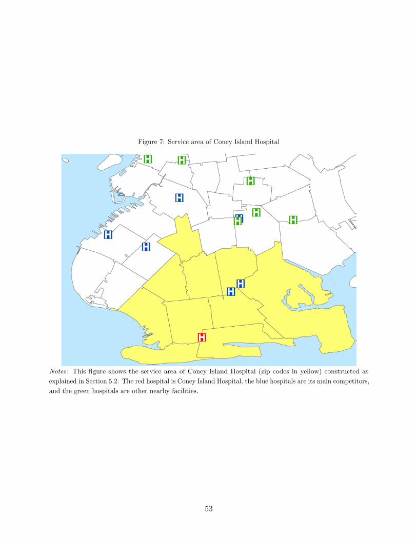
Figure 7: Service area of Coney Island Hospital

Notes: This figure shows the service area of Coney Island Hospital (zip codes in yellow) constructed as

explained in Section 5.2. The red hospital is Coney Island Hospital, the blue hospitals are its main competitors,

and the green hospitals are other nearby facilities.

53

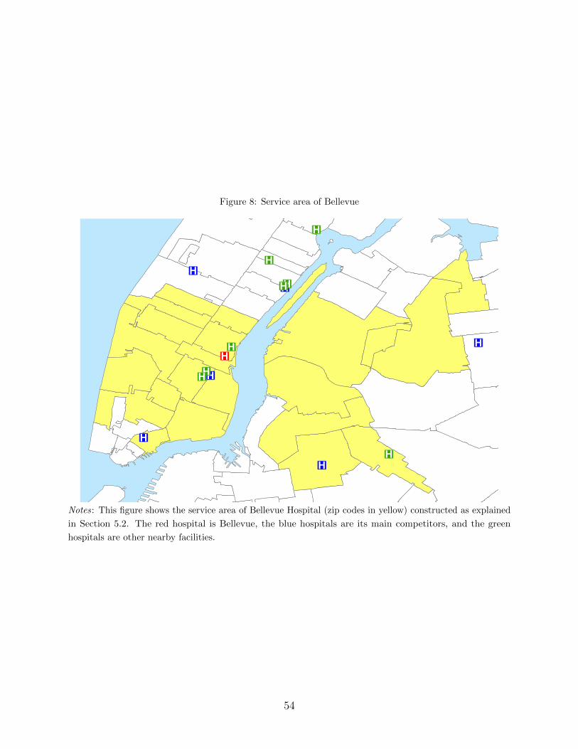
Figure 8: Service area of Bellevue

®v

®v

®v

®v

®v

®v

®v

®v

®v

®v

®v

®v

®v

®v

®v

Notes: This figure shows the service area of Bellevue Hospital (zip codes in yellow) constructed as explained

in Section 5.2. The red hospital is Bellevue, the blue hospitals are its main competitors, and the green

hospitals are other nearby facilities.

54

Figure 9: Service area of NYU Langone

®v

®v

®v®v

®v

®v

®v

®v

®v®v

®v®v

®v

®v

®v®v

Notes: This figure shows the service area of NYU Langone (zip codes in yellow) constructed as explained in

Section 5.2. The red hospital is NYU Langone, the blue hospitals are its main competitors, and the green

hospitals are other nearby facilities.

55

Table 11: Summary statistics, Coney Island Hospital

Sample 1 Sample 2 Sample 3

Control Treatment Control Treatment Control Treatment

Type of visit:

Inpatient 0.21 0.26 0.15 0.25 0.22 0.30

Emergency Department 0.58 0.55 0.73 0.66 0.69 0.62

Ambulatory Surgery 0.21 0.19 0.12 0.10 0.09 0.09

Demographics:

Age 46.1 49.5 39.6 44.8 43.1 47.6

Female 0.56 0.57 0.53 0.56 0.56 0.58

Medicare 0.24 0.33 0.15 0.27 0.23 0.35

Medicaid 0.31 0.33 0.40 0.44 0.37 0.40

Private insurance 0.28 0.23 0.15 0.11 0.22 0.17

Other insurance 0.17 0.11 0.30 0.17 0.17 0.08

Prior propensity:

0 0.75 0.77 0.10 0.13 0.63 0.71

0-0.25 0.02 0.04 0.01 0.04 0.02 0.04

0.25-0.50 0.03 0.04 0.04 0.09 0.03 0.05

0.50-0.75 0.04 0.05 0.09 0.15 0.05 0.06

0.75-1 0.18 0.10 0.77 0.59 0.28 0.14

Patients 193,222 19,577 38,615 2,541 102,867 8,882

Notes : This table presents summary statistics of the patients used for the case study of Coney Island Hospital.

Treatment status refers to whether the patient had a hospital visit in period 1. The different samples are

described in detail in Section 5.2. Sample #1 contains patients who had at least one hospital visit in both

periods 0 and 2. Sample #2 contains those patients in sample #1 who visited Coney Island Hospital in the

last episode of period 0. Sample #3 contains those patients in sample #1 who chose either Coney Island

Hospital or one of its main competitors in the last episode of period 0, in period 1 (if in the treatment

group), and in the first episode of period 2. Characteristics correspond to the first episode of period 2. Prior

propensity is defined as the proportion of the patient’s hospital visits prior to the storm that were to Coney

Island Hospital.

56

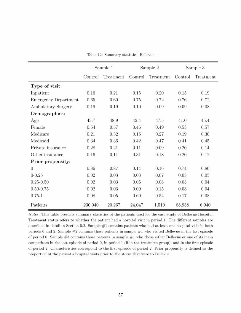
Table 12: Summary statistics, Bellevue



Type of visit:

Inpatient 0.16 0.21 0.15 0.20 0.15 0.19



Demographics:

Age 43.7 48.9 42.4 47.5 41.0 45.4

Female 0.54 0.57 0.46 0.49 0.53 0.57

Medicare 0.21 0.32 0.16 0.27 0.19 0.30

Medicaid 0.34 0.36 0.42 0.47 0.41 0.45


Other insurance 0.16 0.11 0.31 0.18 0.20 0.12

Prior propensity:

0 0.86 0.87 0.14 0.16 0.74 0.80

0-0.25 0.02 0.03 0.03 0.07 0.03 0.05

0.25-0.50 0.02 0.03 0.05 0.08 0.03 0.04

0.50-0.75 0.02 0.03 0.09 0.15 0.03 0.04

0.75-1 0.08 0.05 0.69 0.54 0.17 0.08

Patients 230,040 20,267 24,047 1,510 88,938 6,940

Notes: This table presents summary statistics of the patients used for the case study of Bellevue Hospital.



periods 0 and 2. Sample #2 contains those patients in sample #1 who visited Bellevue in the last episode

of period 0. Sample #3 contains those patients in sample #1 who chose either Bellevue or one of its main

competitors in the last episode of period 0, in period 1 (if in the treatment group), and in the first episode

of period 2. Characteristics correspond to the first episode of period 2. Prior propensity is defined as the

proportion of the patient’s hospital visits prior to the storm that were to Bellevue.

57

Table 13: Summary statistics, NYU Langone



Type of visit:

Inpatient 0.20 0.22 0.26 0.31 0.28 0.27



Demographics:

Age 48.2 48.7 50.9 62.5 48.0 50.0

Female 0.55 0.57 0.61 0.59 0.60 0.58

Medicare 0.26 0.31 0.27 0.49 0.27 0.36

Medicaid 0.22 0.32 0.06 0.09 0.17 0.29


Other insurance 0.12 0.11 0.06 0.04 0.06 0.06

Prior propensity:

0 0.91 0.92 0.19 0.24 0.84 0.89

0-0.25 0.01 0.02 0.02 0.08 0.01 0.03

0.25-0.50 0.01 0.02 0.05 0.12 0.02 0.02

0.50-0.75 0.02 0.02 0.09 0.15 0.02 0.02

0.75-1 0.06 0.03 0.65 0.42 0.11 0.04

Patients 299,009 28,933 20,182 1,118 91,773 8,022

Notes: This table presents summary statistics of the patients used for the case study of NYU Langone.



periods 0 and 2. Sample #2 contains those patients in sample #1 who visited NYU Langone in the last

episode of period 0. Sample #3 contains those patients in sample #1 who chose either NYU Langone or one

of its main competitors in the last episode of period 0, in period 1 (if in the treatment group), and in the first

episode of period 2. Characteristics correspond to the first episode of period 2. Prior propensity is defined as

the proportion of the patient’s hospital visits prior to the storm that were to NYU Langone.

58

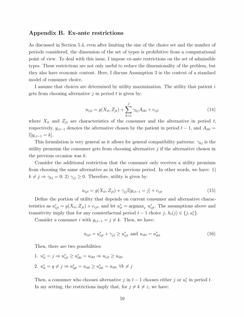
Appendix B. Ex-ante restrictions

As discussed in Section 5.4, even after limiting the size of the choice set and the number of

periods considered, the dimension of the set of types is prohibitive from a computational

point of view. To deal with this issue, I impose ex-ante restrictions on the set of admissible

types. These restrictions are not only useful to reduce the dimensionality of the problem, but

they also have economic content. Here, I discuss Assumption 3 in the context of a standard

model of consumer choice.

I assume that choices are determined by utility maximization. The utility that patient i

gets from choosing alternative j in period t is given by:

uijt = g(Xit, Zjt) +J∑

k=1

γkjAikt + eijt (14)

where Xit and Zjt are characteristics of the consumer and the alternative in period t,

respectively, yi,t−1 denotes the alternative chosen by the patient in period t− 1, and Aikt =

I[yi,t−1 = k].

This formulation is very general as it allows for general compatibility patterns: γkj is the

utility premium the consumer gets from choosing alternative j if the alternative chosen in

the previous occasion was k.

Consider the additional restriction that the consumer only receives a utility premium

from choosing the same alternative as in the previous period. In other words, we have: 1)

k 6= j ⇒ γkj = 0; 2) γjj ≥ 0. Therefore, utility is given by:

uijt = g(Xit, Zjt) + γjjI[yi,t−1 = j] + eijt (15)

Define the portion of utility that depends on current consumer and alternative charac-

teristics as u∗ijt = g(Xit, Zjt) + eijt, and let u∗it = argmaxj u∗ijt. The assumptions above and

transitivity imply that for any counterfactual period t− 1 choice j, ht(j) ∈ {j, u∗t}.Consider a consumer i with yi,t−1 = j 6= k. Then, we have:

uijt = u∗ijt + γjj ≥ u∗ijt and uikt = u∗ikt (16)

Then, there are two possibilities:

1. u∗it = j ⇒ u∗ijt ≥ u∗ikt = uikt ⇒ uijt ≥ uikt

2. u∗it = q 6= j ⇒ u∗iqt = uiqt ≥ u∗ikt = uikt ∀k 6= j

Then, a consumer who chooses alternative j in t− 1 chooses either j or u∗t in period t.

In my setting, the restrictions imply that, for j 6= k 6= z, we have:

59

1. ht(k) = j ⇒ ht(j) = j

2. ht(k) = j ⇒ ht(z) ∈ {z, j}

In the application, these restrictions are imposed ex-ante because of dimensionality issues,

effectively restricting the set of possible types. However, whenever the number of alternatives

and time periods is not restrictive we might want to treat them as regular identifying

assumptions and evaluate their power independently of other restrictions.

60

WORKING PAPER 8 52 Patient Loyalty in Hospital Choice ...

Documents