30 September 2013 WORKING GROUP I CONTRIBUTION TO THE IPCC FIFTH ASSESSMENT REPORT CLIMATE CHANGE 2013: THE PHYSICAL SCIENCE BASIS Final Draft Underlying Scientific-Technical Assessment A report accepted by Working Group I of the IPCC but not approved in detail. Note: The final draft Report, dated 7 June 2013, of the Working Group I contribution to the IPCC 5th Assessment Report "Climate Change 2013: The Physical Science Basis" was accepted but not approved in detail by the 12th Session of Working Group I and the 36th Session of the IPCC on 26 September 2013 in Stockholm, Sweden. It consists of the full scientific and technical assessment undertaken by Working Group I. The Report has to be read in conjunction with the document entitled “Climate Change 2013: The Physical Science Basis. Working Group I Contribution to the IPCC 5th Assessment Report - Changes to the underlying Scientific/Technical Assessment” to ensure consistency with the approved Summary for Policymakers (IPCC-XXVI/Doc.4) and presented to the Panel at its 36th Session. This document lists the changes necessary to ensure consistency between the full Report and the Summary for Policymakers, which was approved line-by-line by Working Group I and accepted by the Panel at the above- mentioned Sessions. Before publication the Report will undergo final copyediting as well as any error correction as necessary, consistent with the IPCC Protocol for Addressing Possible Errors. Publication of the Report is foreseen in January 2014. Disclaimer: The designations employed and the presentation of material on maps do not imply the expression of any opinion whatsoever on the part of the Intergovernmental Panel on Climate Change concerning the legal status of any country, territory, city or area or of its authorities, or concerning the delimitation of its frontiers or boundaries.

Welcome message from author
This document is posted to help you gain knowledge. Please leave a comment to let me know what you think about it! Share it to your friends and learn new things together.
Transcript

30 September 2013
WORKING GROUP I CONTRIBUTION TO THE IPCC FIFTH ASSESSMENT REPORT CLIMATE CHANGE 2013: THE PHYSICAL SCIENCE BASIS Final Draft Underlying Scientific-Technical Assessment
A report accepted by Working Group I of the IPCC but not approved in detail.
Note: The final draft Report, dated 7 June 2013, of the Working Group I contribution to the IPCC 5th Assessment Report "Climate Change 2013: The Physical Science Basis" was accepted but not approved in detail by the 12th Session of Working Group I and the 36th Session of the IPCC on 26 September 2013 in Stockholm, Sweden. It consists of the full scientific and technical assessment undertaken by Working Group I. The Report has to be read in conjunction with the document entitled “Climate Change 2013: The Physical Science Basis. Working Group I Contribution to the IPCC 5th Assessment Report - Changes to the underlying Scientific/Technical Assessment” to ensure consistency with the approved Summary for Policymakers (IPCC-XXVI/Doc.4) and presented to the Panel at its 36th Session. This document lists the changes necessary to ensure consistency between the full Report and the Summary for Policymakers, which was approved line-by-line by Working Group I and accepted by the Panel at the above-mentioned Sessions. Before publication the Report will undergo final copyediting as well as any error correction as necessary, consistent with the IPCC Protocol for Addressing Possible Errors. Publication of the Report is foreseen in January 2014. Disclaimer: The designations employed and the presentation of material on maps do not imply the expression of any opinion whatsoever on the part of the Intergovernmental Panel on Climate Change concerning the legal status of any country, territory, city or area or of its authorities, or concerning the delimitation of its frontiers or boundaries.
IPCC Secretariat
c/o WMO • 7bis, Avenue de la Paix • C.P. 2300 • 1211 Geneva 2 • Switzerland telephone : +41 (0) 22 730 8208 / 54 / 84 • fax : +41 (0) 22 730 8025 / 13 • email : [email protected] • www.ipcc.ch
WORKING GROUP I – TWELFTH SESSION Stockholm, 23-26 September 2013
WG-I: 12th/Doc. 2b, CH13, Add.1
(22.IX.2013) Agenda Item: 5
ENGLISH ONLY
WORKING GROUP I CONTRIBUTION TO THE IPCC FIFTH ASSESSMENT REPORT (AR5), CLIMATE CHANGE 2013: THE PHYSICAL SCIENCE BASIS Chapter 13 – Sea Level Change - Final Draft Underlying Scientific-Technical Assessment (Submitted by the Co-Chairs of Working Group I) Confidential – This document is being made available in preparation of WGI-12 only and should not be cited, quoted, or distributed CORRIGENDUM Section 13.6.1 in paragraph 3, lines 2-3 should read: “… a sea level rise of 5.4 ± 0.3 mm yr–1 in the Sea of Japan from 1993 to 2001 is nearly two times the GMSL trend …” DISCLAIMER TO BE INCLUDED IN THE FRONT MATTER OF THE REPORT: The designations employed and the presentation of material on maps do not imply the expression of any opinion whatsoever on the part of the Intergovernmental Panel on Climate Change concerning the legal status of any country, territory, city or area or of its authorities, or concerning the delimitation of its frontiers or boundaries.
NOTE: The Final Draft Underlying Scientific-Technical Assessment is submitted to the Twelfth Session of Working Group I for acceptance. The IPCC at its Thirty-sixth Session (Stockholm, 26 September 2013) will be informed of the actions of the Twelfth Session of Working Group I in this regard.
IPCC Secretariat
c/o WMO • 7bis, Avenue de la Paix • C.P. 2300 • 1211 Geneva 2 • Switzerland telephone : +41 (0) 22 730 8208 / 54 / 84 • fax : +41 (0) 22 730 8025 / 13 • email : [email protected] • www.ipcc.ch
WORKING GROUP I – TWELFTH SESSION Stockholm, 23-26 September 2013
WG-I: 12th/Doc. 2b, CH13
(12.VIII.2013) Agenda Item: 5
ENGLISH ONLY
WORKING GROUP I CONTRIBUTION TO THE IPCC FIFTH ASSE SSMENT REPORT (AR5), CLIMATE CHANGE 2013: THE PHYSICAL SCI ENCE BASIS Chapter 13: Sea Level Change - Final Draft Underlyi ng Scientific-Technical Assessment (Submitted by the Co-Chairs of Working Group I) Confidential – This document is being made availabl e in preparation of WGI-12 only and should not be cited, quoted, or distribute d
NOTE:
The Final Draft Underlying Scientific-Technical Assessment is submitted to the Twelfth Session of Working Group I for acceptance. The IPCC at its Thirty-sixth Session (Stockholm, 26 September 2013) will be informed of the actions of the Twelfth Session of Working Group I in this regard.
Final Draft (7 June 2013) Chapter 13 IPCC WGI Fifth Assessment Report
Do Not Cite, Quote or Distribute 13-1 Total pages: 121
Chapter 13: Sea Level Change
Coordinating Lead Authors: John A. Church (Australia), Peter U. Clark (USA) Lead Authors: Anny Cazenave (France), Jonathan M. Gregory (UK), Svetlana Jevrejeva (UK), Anders Levermann (Germany), Mark A. Merrifield (USA), Glenn A. Milne (Canada), R. Steven Nerem (USA), Patrick D. Nunn (Australia), Antony J. Payne (UK), W. Tad Pfeffer (USA), Detlef Stammer (Germany), Alakkat S. Unnikrishnan (India) Contributing Authors: David Bahr (USA), Jason E. Box (USA), David H. Bromwich (USA), Mark Carson (Germany), William Collins (UK), Xavier Fettweis (Belgium), Piers Forster (UK), Alex Gardner (USA), W. Roland Gehrels (UK), Rianne Giesen (Netherlands), Peter J. Gleckler (USA), Peter Good (UK), Rune Grand Graversen (Sweden), Ralf Greve (Japan), Stephen Griffies (USA), Edward Hanna (UK), Mark Hemer (Australia), Regine Hock (USA), Simon J. Holgate (UK), John Hunter (Australia), Philippe Huybrechts (Belgium), Gregory Johnson (USA), Ian Joughin (USA), Georg Kaser (Austria), Caroline Katsman (Netherlands), Leonard Konikow (USA), Gerhard Krinner (France), Anne Le Brocq (UK), Jan Lenaerts (Netherlands), Stefan Ligtenberg (Netherlands), Christopher M. Little (USA), Ben Marzeion (Austria), Kathleen L. McInnes (Australia), Sebastian H. Mernild (USA), Didier Monselesan (Australia), Ruth Mottram (Denmark), Tavi Murray (UK), Gunnar Myhre (Norway), J.P. Nicholas (USA), Faezeh Nick (Norway), Mahé Perrette (Germany), David Pollard (USA),Valentina Radić (Canada), Jamie Rae (UK), Markku Rummukainen (Sweden), Christian Schoof (Canada), Aimée Slangen (Netherlands), Jan H. van Angelen (Netherlands), Willem Jan van de Berg (Netherlands), Michiel van den Broeke (Netherlands), Miren Vizcaíno (Netherlands), Yoshihide Wada (Netherlands), Neil J. White (Australia), R.Winkelmann (Germany), Jianjun Yin (USA), Masakazu Yoshimori (Japan), Kirsten Zickfeld (Canada) Review Editors: Jean Jouzel (France), Roderik van de Wal (Netherlands), Philip L. Woodworth (UK), Cunde Xiao (China) Date of Draft: 7 June 2013 Table of Contents Executive Summary ........................................................................................................................................ 3 13.1 Components and Models of Sea Level Change ..................................................................................... 6
13.1.1 Introduction and Chapter Overview .............................................................................................. 6 13.1.2 Fundamental Definitions and Concepts ......................................................................................... 7 13.1.3 Processes Affecting Sea Level ........................................................................................................ 7 13.1.4 Models Used to Interpret Past and Project Future Changes in Sea Level .................................... 8
13.2 Past Sea Level Change .......................................................................................................................... 10 13.2.1 The Geological Record ................................................................................................................ 10 13.2.2 The Instrumental Record (~1700–2012) ...................................................................................... 12
FAQ 13.1: Why Does Local Sea Level Change Differ from the Global Average? .................................. 13 13.3 Contributions to Global Mean Sea Level Rise During the Instrumental Period ............................. 14
13.3.1 Thermal Expansion Contribution ................................................................................................ 14 13.3.2 Glaciers ........................................................................................................................................ 16 13.3.3 Greenland and Antarctic Ice Sheets ............................................................................................ 17 13.3.4 Contributions from Water Storage on Land ................................................................................ 20 13.3.5 Ocean Mass Observations from GRACE ..................................................................................... 21 13.3.6 Budget of GMSL Rise ................................................................................................................... 21
Box 13.1: The Global Energy Budget .......................................................................................................... 23 13.4 Projected Contributions to Global Mean Sea Level ........................................................................... 25
13.4.1 Ocean Heat Uptake and Thermal Expansion .............................................................................. 25 13.4.2 Glaciers ........................................................................................................................................ 27 13.4.3 Greenland Ice Sheet ..................................................................................................................... 29 13.4.4 Antarctic Ice Sheet ....................................................................................................................... 36
Final Draft (7 June 2013) Chapter 13 IPCC WGI Fifth Assessment Report
Do Not Cite, Quote or Distribute 13-2 Total pages: 121
Box 13.2: History of the Marine Ice Sheet Instability Hypothesis ............................................................ 42 FAQ 13.2: Will the Greenland and Antarctic Ice Sheets Contribute to Sea Level Change Over the Rest
of the Century? ...................................................................................................................................... 43 13.4.5 Anthropogenic Intervention in Water Storage on Land ............................................................... 45
13.5 Projections of Global Mean Sea Level Rise ........................................................................................ 46 13.5.1 Process-Based Projections for the 21st Century ......................................................................... 46 13.5.2 Semi-Empirical Projections for the 21st Century ........................................................................ 48 13.5.3 Confidence in Likely Ranges and Bounds .................................................................................... 51 13.5.4 Long-Term Scenarios ................................................................................................................... 54
13.6 Regional Sea Level Changes ................................................................................................................. 58 13.6.1 Regional Sea Level Changes, Climate Modes and Forced Sea Level Response ......................... 59 13.6.2 CMIP5 GCM Projections on Decadal to Centennial Time Scales .............................................. 59 13.6.3 Response to Atmospheric Pressure Changes ............................................................................... 60 13.6.4 Response to Freshwater Forcing ................................................................................................. 61 13.6.5 Net Regional Sea Level Changes .................................................................................................. 62 13.6.6 Uncertainties and Sensitivity to Ocean/Climate Model Formulations and Parameterizations ... 64
13.7 Projections of 21st Century Sea Level Extremes and Waves ............................................................ 65 13.7.1 Observed Changes in Sea Level Extremes ................................................................................... 65 13.7.2 Projections of Sea Level Extremes ............................................................................................... 65 13.7.3 Projections of Ocean Waves ........................................................................................................ 67
13.8 Synthesis and Key Uncertainties .......................................................................................................... 69 References ...................................................................................................................................................... 71 Figures ............................................................................................................................................................ 89
Final Draft (7 June 2013) Chapter 13 IPCC WGI Fifth Assessment Report
Do Not Cite, Quote or Distribute 13-3 Total pages: 121
Executive Summary This chapter considers changes in global mean sea level, regional sea level, sea level extremes and waves. Confidence in projections of global mean sea level rise has increased since the AR4 because of the improved physical understanding and the improved agreement of process-based models with observations, and the inclusion of ice-sheet dynamical changes. Past Sea Level Change Paleo sea level records from warm periods during the last 3 million years indicate that global mean sea level exceeded 5 m above present (very high confidence)1 when global temperature was up to 2°C warmer than pre-industrial (medium confidence). During the last interglacial period (~129–116 ka), peak global warmth was not more than 2°C above pre-industrial temperatures (medium confidence) and global mean sea level was 5 m higher than present (very high confidence) to 10 m higher than present (high confidence), implying substantial contributions from the Greenland and Antarctic ice sheets. [5.3.4, 5.6.1, 5.6.2, 13.2.1] Based on proxy and instrumental data, it is virtually certain2 that the rate of global mean sea level rise has accelerated during the last two centuries, marking the transition from relatively low rates of change during the late Holocene (order tenths of mm yr–1) to modern rates (order mm yr–1). It is very likely that the mean rate was 1.7 [1.5 to 1.9] mm yr–1 between 1901 and 2010 for a total sea level rise of 0.19 [0.17 to 0.21] m. Between 1993 and 2010, the rate was very likely higher at 3.2 [2.8 to 3.6] mm yr–1; similarly high rates likely occurred between 1930 and 1950. It is likely that global mean sea level has accelerated since the early 1900s, with estimates ranging from 0.000 to 0.013 [–0.002 to 0.019] mm yr–2. [3.7.2, 3.7.4, 5.6.3, 13.2.1–13.2.2, Figure 13.3] Understanding of Sea Level Change Ocean thermal expansion and glacier melting have been the dominant contributors to 20th century global mean sea level rise. Observations since 1971 indicate that thermal expansion and glaciers (excluding the glaciers in Antarctica) explain 75% of the observed rise (high confidence). The contribution of the Greenland and Antarctic ice sheets has increased since the early 1990s, partly from increased outflow induced by warming of the immediately adjacent ocean. Natural and human-induced land water storage changes have made only a small contribution; the rate of groundwater depletion has increased and now exceeds the rate of reservoir impoundment. Since 1993, when observations of all sea level components are available, the sum of contributions equals the observed global mean sea level rise within uncertainties (high confidence). [Chapter 3; Chapter 4; 13.3.6; Figure 13.4; Table 13.1] There is high confidence in projections of thermal expansion, high confidence in projections of Greenland surface mass balance, and medium confidence in projections of Antarctic surface mass balance and glacier mass loss. There has been substantial progress in ice-sheet modelling, particularly for Greenland. Process-based model calculations of contributions to past sea level change from ocean thermal expansion, glacier mass loss and Greenland ice-sheet surface mass balance are consistent with available observational estimates over recent decades. Ice sheet flow-line modelling is able to reproduce observed acceleration of the main outlet glaciers in the Greenland Ice Sheet, thus allowing estimates of the 21st century dynamic response (medium confidence). Significant challenges remain in the process-based projection of the dynamics response of marine terminating glaciers and the Antarctic Ice Sheet. Alternative
1 In this Report, the following summary terms are used to describe the available evidence: limited, medium, or robust; and for the degree of agreement: low, medium, or high. A level of confidence is expressed using five qualifiers: very low, low, medium, high, and very high, and typeset in italics, e.g., medium confidence. For a given evidence and agreement statement, different confidence levels can be assigned, but increasing levels of evidence and degrees of agreement are correlated with increasing confidence (see Section 1.4 and Box TS.1 for more details). 2 In this Report, the following terms have been used to indicate the assessed likelihood of an outcome or a result: Virtually certain 99–100% probability, Very likely 90–100%, Likely 66–100%, About as likely as not 33–66%, Unlikely 0–33%, Very unlikely 0–10%, Exceptionally unlikely 0–1%. Additional terms (Extremely likely: 95–100%, More likely than not >50–100%, and Extremely unlikely 0–5%) may also be used when appropriate. Assessed likelihood is typeset in italics, e.g., very likely (see Section 1.4 and Box TS.1 for more details).
Final Draft (7 June 2013) Chapter 13 IPCC WGI Fifth Assessment Report
Do Not Cite, Quote or Distribute 13-4 Total pages: 121
means of projection (extrapolation within a statistical framework and informed judgement) provide medium confidence in a likely range. There is currently low confidence in projecting the onset of large-scale grounding line instability in the marine sectors of the ice sheet. [13.3.1–13.3.3, 13.4.3, 13.4.4] The sum of thermal expansion simulated by CMIP5 AOGCMs, glacier mass loss computed by global glacier models using CMIP5 climate change simulations, and estimates of land water storage explain 65% of the observed global mean sea level rise for 1901–1990 and 90% for 1971–2010 and 1993–2010 (high confidence). When observed climate parameters are used, the glacier models indicate a larger Greenland glacier contribution in the first half of the 20th century such that the sum of thermal expansion, glacier mass loss and changes in land water storage and a small ongoing Antarctic ice-sheet contribution are within 20% of the observations throughout the 20th century. In all periods, the residual is small enough to be attributed to the ice sheets. Model-based estimates of ocean thermal expansion and glacier contributions indicate that the greater rate of rise since 1990 is a response to radiative forcing (both anthropogenic and natural) and increased loss of ice-sheet mass and not part of a natural oscillation (medium confidence). [13.3.6; Figures 13.4 and 13.7; Table 13.1] The Earth’s Energy Budget Independent estimates of effective radiative forcing of the climate system, the observed heat storage, and surface warming combine to give an energy budget for the Earth that is very likely closed within uncertainties, and is consistent with the likely range of climate sensitivity. The largest increase in the storage of heat in the climate system over recent decades has been in the oceans; this is a powerful observation for the detection and attribution of climate change. [Box 3.1 and Box 13.1] Global Mean Sea Level Rise Projections It is very likely that the rate of global mean sea level rise during the 21st century will exceed the rate observed during 1971–2010 for all RCP scenarios due to increased ocean warming and loss of mass from glaciers and ice sheets. For the period 2081–2100, compared to 1986–2005, global mean sea level rise is likely (medium confidence) to be in the 5–95% range of process-based models, which give 0.26–0.54 m for RCP2.6, 0.32–0.62 m for RCP4.5, 0.33–0.62 m for RCP6.0, and 0.45–0.81 m for RCP8.5. For RCP8.5, the rise by 2100 is 0.53–0.97 m with a rate during 2081–2100 of 7–15 mm yr–1. We have considered the evidence for higher projections and have concluded that there is currently insufficient evidence to evaluate the probability of specific levels above the likely range. Based on current understanding, only the collapse of marine-based sectors of the Antarctic Ice Sheet, if initiated, could cause global mean sea level to rise substantially above the likely range during the 21st century. This potential additional contribution cannot be precisely quantified but there is medium confidence that it would not exceed several tenths of a meter of sea level rise during the 21st century. [13.5.1, Table 13.5, Figures 13.10 and 13.11] Some semi-empirical models project a range that overlaps the process-based likely range while others project a median and 95-percentile that are about twice as large as the process-based models. In nearly every case, the semi-empirical model 95-percentile is higher than the process-based likely range. Despite their successful calibration and evaluation against the observed 20th century sea level record, there is low agreement in their projections and no consensus in the scientific community about the reliability of SEM projections, and there is low confidence in their projections [13.5.2-3; Figure 13.12]. It is virtually certain that global mean sea level rise will continue beyond 2100, with sea level rise due to thermal expansion to continue for many centuries. Longer term sea level rise depends on future emissions. The few available process-based models indicate global mean sea level rise by 2300 to be less than 1 m for greenhouse gas concentrations that peak and decline and do not exceed 500 ppm CO2-equivalent but 1–3 m for concentrations above 700 ppm CO2-equivalent (medium confidence). The amount of ocean thermal expansion increases with global warming (0.2–0.6 m °C–1) but the glacier contribution decreases over time as their volume (currently 0.43 m sea level equivalent) decreases. The contribution from the ice sheets will likely continue beyond 2100, but confidence in projections is low. Sea level rise of 1–3 m per degree of warming is expected if the warming is sustained for several millennia (low confidence). [13.5.4, Figures 13.13, 13.14]

Final Draft (7 June 2013) Chapter 13 IPCC WGI Fifth Assessment Report
Do Not Cite, Quote or Distribute 13-5 Total pages: 121
The available evidence indicates that global warming greater than a certain threshold would lead to the near-complete loss of the Greenland Ice Sheet over a millennium or more, causing a global mean sea level rise of about 7 m. Studies with fixed ice sheet topography indicate the threshold is greater than 2°C but less than 4°C of global mean surface temperature rise with respect to preindustrial. The one study with a dynamical ice sheet suggests the threshold could be as low as 1°C. We are unable to quantify a likely range. Whether or not a decrease in the Greenland Ice Sheet mass loss is irreversible also depends on the duration and degree of exceedance of the threshold. [13.4.3.3] Regional Sea Level Change Projections It is very likely that in the 21st century and beyond, sea level change will have a strong regional pattern, with some places experiencing significant deviations of local and regional sea level change from the global mean change. Over decadal periods, the rates of regional sea level change as a result of climate variability can differ from the global average rate by more than 100% of the global average rate. By the end of the 21st century, it is very likely that over about 95% of the world ocean, regional sea level rise will be positive, while most regions experiencing a sea level fall are located near current and former glaciers and ice sheets. About 70% of the global coastlines are projected to experience a sea level change within 20% of the global mean sea level change. [13.6.5, Figures 13.18–13.20] Projections of 21st Century Sea Level Extremes and Surface Waves It is very likely that there will be a significant increase in the occurrence of future sea level extremes by 2050 and 2100. This increase will primarily be the result of an increase in mean sea level (high confidence), with the frequency of a particular sea level extreme increasing by an order of magnitude or more in some regions by the end of the 21st century. There is low confidence in region-specific projections of storminess and associated storm surges. [13.7.2, Figure 13.25] It is likely (medium confidence) that annual mean significant wave heights will increase in the Southern Ocean as a result of enhanced wind speeds. Southern Ocean generated swells are likely to affect heights, periods, and directions of waves in adjacent basins. It is very likely that wave heights and the duration of the wave season will increase in the Arctic Ocean as a result of reduced sea-ice extent. In general, there is low confidence in region-specific projections due to the low confidence in tropical and extratropical storm projections, and to the challenge of downscaling future wind fields from coarse-resolution climate models. [13.7.3; Figure 13.26]
Final Draft (7 June 2013) Chapter 13 IPCC WGI Fifth Assessment Report
Do Not Cite, Quote or Distribute 13-6 Total pages: 121
13.1 Components and Models of Sea Level Change 13.1.1 Introduction and Chapter Overview Changes in sea level occur over a broad range of temporal and spatial scales, with the many contributing factors making it an integral measure of climate change (Milne et al., 2009; Church et al., 2010). The primary contributors to contemporary sea level change are the expansion of the ocean as it warms and the transfer of water currently stored on land, particularly from land ice (glaciers and ice sheets) (Church et al., 2011b). Observations indicate the largest increase in the storage of heat in the climate system over recent decades has been in the oceans (Section 3.2) and thus sea level rise from ocean warming is a central part of the Earth’s response to increasing greenhouse gas concentrations. The First IPCC Assessment laid the groundwork for much of our current understanding of sea level change (Warrick and Oerlemans, 1990). This included the recognition that sea level had risen during the 20th century, that the rate of rise had increased compared to the 19th century, that ocean-thermal expansion and the mass loss from glaciers were the main contributors to the 20th century rise, that during the 21st century the rate of rise was projected to be faster than during the 20th century, that sea level will not rise uniformly around the world, and that sea level would continue to rise well after greenhouse gas emissions were reduced. They also concluded that no major dynamic response of the ice sheets was expected during the 21st century, leaving ocean-thermal expansion and the melting of glaciers as the main contributors to the 21st century rise. The Second Assessment Report came to very similar conclusions (Warrick et al., 1996). By the time of the Third Assessment Report, coupled atmosphere-ocean general circulation models (AOGCMs) and ice sheet models largely replaced energy-balance climate models as the primary techniques supporting the interpretation of observations and the projections of sea level (Church et al., 2001). This approach allowed consideration of the regional distribution of sea level change in addition to the global average change. By the time of the Fourth Assessment Report (AR4), there were more robust observations of the variations in the rate of global average sea level rise for the 20th century, some understanding of the variability in the rate of rise, and the satellite altimeter record was long enough to reveal the complexity of the time-variable spatial distribution of sea level (Bindoff et al., 2007). Nevertheless, three central issues remained. First, the observed sea level rise over decades was larger than the sum of the individual contributions estimated from observations or with models (Rahmstorf et al., 2007; Rahmstorf et al., 2012b), although in general the uncertainties were large enough that there was no significant contradiction. Second, it was not possible to make confident projections of the regional distribution of sea level rise. Third, there was insufficient understanding of the potential contributions from the ice sheets. In particular, the AR4 recognised that existing ice-sheet models were unable to simulate the recent observations of ice-sheet accelerations and that understanding of ice-sheet dynamics was too limited to assess the likelihood of continued acceleration or to provide a best estimate or an upper bound for their future contributions. Despite changes in the scenarios between the four Assessments, the sea level projections for 2100 (compared to 1990) for the full range of scenarios were remarkably similar, with the reduction in the upper end in more recent reports reflecting the smaller increase in radiative forcing in recent scenarios due to smaller greenhouse gas (GHG) emissions and the inclusion of aerosols, and a reduction in uncertainty in projecting the contributions: 31 to 110 cm in the FAR, 13 to 94 cm in the SAR, 9 to 88 cm in the TAR, and 18 to 59 cm in AR4 (not including a possible additional allowance for a dynamic ice-sheet response). Results since the AR4 show that for recent decades, sea level has continued to rise (Section 3.7). Improved and new observations of the ocean (Section 3.7) and the cryosphere (Chapter 4) and their representation in models have resulted in better understanding of 20th century sea level rise and its components (this chapter). Records of past sea level changes constrain long-term land-ice response to warmer climates as well as extend the observational record to provide a longer context for current sea level rise (Section 5.6). This chapter provides a synthesis of past and contemporary sea level change at global and regional scales. Drawing on the published refereed literature, including as summarised in earlier chapters of this Assessment, we explain the reasons for contemporary change, and assess confidence in and provide global and regional projections of likely sea level change for the 21st century and beyond. We discuss the primary factors that cause regional sea level to differ from the global average and how these may change in the
Final Draft (7 June 2013) Chapter 13 IPCC WGI Fifth Assessment Report
Do Not Cite, Quote or Distribute 13-7 Total pages: 121
future. In addition, we address projected changes in surface waves and the consequences of sea level and climate change for extreme sea level events. 13.1.2 Fundamental Definitions and Concepts The height of the ocean surface at any given location, or sea level, is measured either with respect to the surface of the solid Earth (relative sea level, RSL) or a geocentric reference such as the reference ellipsoid (geocentric sea level). RSL is the more relevant quantity when considering the coastal impacts of sea level change, and it has been measured using tide gauges during the past few centuries (Sections 13.2.2 and 3.7) and estimated for longer time spans from geological records (Sections 13.2.1 and 5.6). Geocentric sea level has been measured over the past two decades using satellite altimetry (Sections 13.2.2 and 3.7). A temporal average for a given location, known as Mean Sea Level (MSL; see Glossary), is applied to remove shorter period variability. Apart from Section 13.7, which considers high-frequency changes in ocean surface height, the use of ‘sea level’ elsewhere in this chapter refers to MSL. It is common to average MSL spatially to define Global Mean Sea Level (GMSL; see Glossary). In principle, integrating RSL change over the ocean area gives the change in ocean water volume, which is directly related to the processes that dominate sea level change (changes in ocean temperature and land-ice volume). In contrast, a small correction (–0.15 to –0.5 mm yr–1) needs to be subtracted from altimetry observations to estimate ocean water volume change (Tamisiea, 2011). Local RSL change can differ significantly from GMSL because of spatial variability in changes of the sea-surface and ocean-floor height (see FAQ 13.1 and Section 13.7). 13.1.3 Processes Affecting Sea Level This chapter focuses on processes within the ocean, atmosphere, land ice, and hydrological cycle that are climate sensitive and are expected to contribute to sea level change at regional to global scales in the coming decades to centuries (Figure 13.1). Figure 13.2 is a navigation aid for the different sections of this chapter and sections of other chapters that are relevant to sea level change. [INSERT FIGURE 13.1 HERE] Figure 13.1: Climate sensitive processes and components that can influence global and regional sea level and are considered in this chapter. Changes in any one of the components or processes shown will result in a sea level change. The term ‘ocean properties’ refers to ocean temperature, salinity and density, which influence and are dependent on ocean circulation. Both relative and geocentric sea level vary with position. Note that the geocenter is not shown. [INSERT FIGURE 13.2 HERE] Figure 13.2: Schematic representation of key linkages between processes and components that contribute to sea level change and are considered in this report. Colouring of individual boxes indicates the types of models and approaches used in projecting the contribution of each process or component to future sea level change. The diagram also serves as an index to the sections in this report that are relevant to the assessment of sea level projections via the section numbers given at the bottom of each box. Note gravity and solid Earth effects change the shape of the ocean floor and surface and thus are required to infer changes in ocean water volume from both relative and geocentric sea level observations. Changes in ocean currents, ocean density and sea level are all tightly coupled such that changes at one location impact local sea level and sea level far from the location of the initial change, including changes in sea level at the coast in response to changes in deep-ocean temperature (Landerer et al., 2007; Yin et al., 2010). While both temperature and salinity changes can contribute significantly to regional sea level change (Church et al., 2010), only temperature change produces a significant contribution to global average ocean volume change due to thermal expansion/contraction (Gregory and Lowe, 2000). Regional atmospheric pressure anomalies also cause sea level to vary through atmospheric loading (Wunsch and Stammer, 1997). All of these climate-sensitive processes cause sea level to vary on a broad range of space and time scales from relatively short lived events, such as waves and storm surges, to sustained changes over several decades or centuries that are associated with atmospheric and ocean modes of climate variability (White et al., 2005; Miller and Douglas, 2007; Zhang and Church, 2012). Water and ice mass exchange between the land and the oceans leads to a change in GMSL. A signal of added mass to the ocean propagates rapidly around the globe such that all regions experience a sea level change within days of the mass being added (Lorbacher et al., 2012). In addition, an influx of freshwater changes
Final Draft (7 June 2013) Chapter 13 IPCC WGI Fifth Assessment Report
Do Not Cite, Quote or Distribute 13-8 Total pages: 121
ocean temperature and salinity and thus changes ocean currents and local sea level (Stammer, 2008; Yin et al., 2009), with signals taking decades to propagate around the global ocean. The coupled atmosphere-ocean system can also adjust to temperature anomalies associated with surface freshwater anomalies through air-sea feedbacks, resulting in dynamical adjustments of sea level (Okumura et al., 2009; Stammer et al., 2011). Water mass exchange between land and the ocean also results in patterns of sea level change called ‘sea level fingerprints’ (Clark and Lingle, 1977; Conrad and Hager, 1997; Mitrovica et al., 2001) due to change in the gravity field and vertical movement of the ocean floor associated with visco-elastic Earth deformation (Farrell and Clark, 1976). These changes in mass distribution also affect the Earth’s inertia tensor and therefore rotation, which produces an additional sea level response (Milne and Mitrovica, 1998). There are other processes that affect sea level but are not associated with contemporary climate change. Some of these result in changes that are large enough to influence the interpretation of observational records and sea level projections at regional and global scales. In particular surface mass transfer from land ice to oceans during the last deglaciation contributes significantly to present-day sea level change due to the on-going visco-elastic deformation of the Earth and the corresponding changes of the ocean floor height and gravity (referred to as glacial isostatic adjustment, GIA) (Lambeck and Nakiboglu, 1984; Peltier and Tushingham, 1991). Ice sheets also have long response times and so continue to respond to past climate change (Section 13.1.5). Anthropogenic processes that influence the amount of water stored in the ground or on its surface in lakes and reservoirs, or cause changes in land-surface characteristics that influence runoff or evapotranspiration rates, will perturb the hydrological cycle and cause sea level change (Sahagian, 2000; Wada et al., 2010). Such processes include water impoundment (dams, reservoirs), irrigation schemes, and ground water depletion (Section 13.4.5). Sea level changes due to tectonic and coastal processes are beyond the scope of this chapter. With the exception of earthquakes, which can cause rapid local changes and tsunamis (Broerse et al., 2011) and secular RSL changes due to post-seismic deformation (Watson et al., 2010), tectonic processes cause, on average, relatively low rates of sea level change (order 0.1 mm yr–1 or less) (Moucha et al., 2008). Sediment transfer and compaction (including from ground water depletion) in the coastal zone are particularly important in deltaic regions (Blum and Roberts, 2009; Syvitski et al., 2009). While they can dominate sea level change in these localised areas, they are less important as a source of sea level change at regional and global scales and so are not considered further in this chapter (See they are discussed in WGII Chapter 5). Estimates of sediment delivery to the oceans (Syvitski and Kettner, 2011) suggest a contribution to GMSL rise of order 0.01 mm yr–1. 13.1.4 Models Used to Interpret Past and Project Future Changes in Sea Level Atmosphere-ocean general circulation models (AOGCMs) have components representing the ocean, atmosphere, land and cryosphere and simulate sea-surface height changes relative to the geoid resulting from the natural forcings of volcanic eruptions and changes in solar irradiance, and from anthropogenic increases in greenhouse gases and aerosols (Chapter 9). AOGCMs also exhibit internally generated climate variability, including such modes as the El Niño Southern Oscillation (ENSO), the Pacific Decadal Oscillation (PDO), the North Atlantic Oscillation (NAO), and others which affect sea level (White et al., 2005; Zhang and Church, 2012). Critical components for global and regional changes in sea level are changes in surface wind stress and air-sea heat and freshwater fluxes (Lowe and Gregory, 2006; Timmermann et al., 2010; Suzuki and Ishii, 2011) and the resultant changes in ocean density and circulation, for instance in the strength of the Atlantic meridional overturning circulation (AMOC) (Yin et al., 2009; Lorbacher et al., 2010; Pardaens et al., 2011a). As in the real world, ocean density, circulation, and sea level are dynamically connected in AOGCMs and evolve together. Offline models are required for simulating glacier and ice-sheet changes (Section 13.1.4.1). Geodynamic surface-loading models are used to simulate the RSL response to past and contemporary changes in surface water and land-ice mass redistribution and contemporary atmospheric pressure changes. The sea surface height component of the calculation is based solely on water mass conservation and perturbations to gravity, with no considerations of ocean dynamic effects. Application of these models has focused on annual and interannual variability driven by contemporary changes in the hydrological cycle and
Final Draft (7 June 2013) Chapter 13 IPCC WGI Fifth Assessment Report
Do Not Cite, Quote or Distribute 13-9 Total pages: 121
atmospheric loading (Clarke et al., 2005; Tamisiea et al., 2010), and on secular trends associated with past and contemporary changes in land ice and hydrology (Lambeck et al., 1998; Mitrovica et al., 2001; Peltier, 2004; Riva et al., 2010). Semi-empirical models (SEMs) project sea level based on statistical relationships between observed GMSL and global mean temperature (Rahmstorf, 2007a; Vermeer and Rahmstorf, 2009; Grinsted et al., 2010) or total radiative forcing (Jevrejeva et al., 2009; Jevrejeva et al., 2010). The form of this relationship is motivated by physical considerations, and the parameters are determined from observational data—hence the term “semi-empirical” (Rahmstorf et al., 2012a). SEMs do not explicitly simulate the underlying processes, and they use a characteristic response time that could be considerably longer than the timescale of interest (Rahmstorf, 2007a) or explicitly determined by the model (Grinsted et al., 2010). Storm-surge and wave-projection models are used to assess how changes in storminess and MSL impact sea level extremes and wave climates. The two main approaches involve dynamical (Lowe et al., 2010) and statistical models (Wang et al., 2010). The dynamical models are forced by near-surface wind and mean sea level pressure fields derived from regional or global climate models (Lowe et al., 2010). In this chapter, we use the term “process-based models” (see Glossary) to refer to sea level and land-ice models (Section 13.1.5.1) that aim to simulate the underlying processes and interactions, in contrast to “semi-empirical models” which do not. While these two approaches are distinct, semi-empirical methods are often employed in components of the process-based models (e.g., glacier models in which surface mass balance is determined by a Degree Day method (Braithwaite and Olesen, 1989)). 13.1.4.1 Models Used to Project Changes in Ice Sheets and Glaciers The representation of glaciers and ice sheets within AOGCMs is not yet at a stage where projections of their changing mass are routinely available. Additional process-based models use output from AOGCMs to evaluate the consequences of projected climate change on these ice masses. The overall contribution of an ice mass to sea level involves changes to either its surface mass balance (SMB) or changes in the dynamics of ice flow that affect outflow (i.e., solid ice discharge) to the ocean. SMB is primarily the difference between snow accumulation and the melt and sublimination of snow and ice (ablation). An assessment of observations related to this mass budget can be found in Section 4.4.2. Although some ice-sheet models used in projections incorporate both effects, most studies have focussed on either SMB or flow dynamics. It is assumed that the overall contribution can be found by summing the contributions calculated independently for these two sources, which is valid if they do not interact significantly. While this can be addressed using a correction term to SMB in ice-sheet projections over the next century, such interactions become more important on longer time scales when, for example, changes in ice-sheet topography may significantly affect SMB or dynamics. Projecting the sea level contribution of land ice requires comparing the model results with a base state that assumes no significant sea level contribution. This base state is taken to be either the preindustrial period or, because of our scant knowledge of the ice sheets before the advent of satellites, the late 20th century. In reality, even at these times, the ice sheets are likely to have been contributing to sea level change (Huybrechts et al., 2011; Box and Colgan, 2013) and this contribution, although difficult to quantify, should be included in the observed sea level budget (Gregory et al., 2013b) and the projections. Regional climate models (RCMs), which incorporate or are coupled to sophisticated representations of the mass and energy budgets associated with snow and ice surfaces, are now the primary source of ice-sheet SMB projections. A major source of uncertainty lies in the ability of these schemes to adequately represent the process of internal refreezing of melt water within the snowpack (Bougamont et al., 2007; Fausto et al., 2009). These models require information on the state of the atmosphere and ocean at their lateral boundaries, which are derived from reanalysis data sets or AOGCMs for past climate, or from AOGCM projections of future climate. Models of ice dynamics require a fairly complete representation of stresses within an ice mass in order to represent the response of ice flow to changes at the marine boundary and the governing longitudinal stresses

Final Draft (7 June 2013) Chapter 13 IPCC WGI Fifth Assessment Report
Do Not Cite, Quote or Distribute 13-10 Total pages: 121
(Schoof, 2007b). For Antarctica, there is also a need to employ high spatial resolution (<1 km) to capture the dynamics of grounding line migration robustly so that results do not depend to an unreasonable extent on model resolution (Durand et al., 2009; Goldberg et al., 2009; Morlighem et al., 2010; Cornford et al., 2013; Pattyn et al., 2013). One-dimensional flowline models have been developed to the stage that modelled iceberg calving is comparable with observations (Nick et al., 2009). The success of this modelling approach relies on the ability of the model’s computational grid to evolve to continuously track the migrating calving front. Although this is relatively straightforward in a one-dimensional model, this technique is difficult to incorporate into three-dimensional ice sheet models that typically use a computational grid that is fixed in time. The main challenge faced by models attempting to assess sea level change from glaciers is the small number of glaciers for which mass budget observations are available (~380) (Cogley, 2009a) (see Sections 4.3.1 and 4.3.4) as compared to the total number (the World Glacier Inventory contains more than 181,500) (Arendt et al., 2012). Statistical techniques are used to derive relations between observed SMB and climate variables for the small sample of surveyed glaciers, and then these relations are used to upscale to regions of the world. These techniques often include volume-area scaling to estimate glacier volume from their more readily observable areas. Although tidewater glaciers may also be affected by changes in outflow related to calving, the complexity of the associated processes means that most studies limit themselves to assessing the effects of SMB changes. 13.2 Past Sea Level Change 13.2.1 The Geological Record Records of past sea level change provide insight into the sensitivity of sea level to past climate change as well as context for understanding current changes and evaluating projected changes. Since the AR4, important progress has been made in understanding the amplitude and variability of sea level during past intervals when climate was warmer than pre-industrial, largely through better understanding of and accounting for the effects of proxy uncertainties and GIA on coastal sequences (Kopp et al., 2009; Raymo et al., 2011; Dutton and Lambeck, 2012; Lambeck et al., 2012; Raymo and Mitrovica, 2012; Kopp et al., 2013) (Chapter 5). Here we summarize the constraints provided by the record of past sea level variations during times when global temperature was similar to or warmer than today. 13.2.1.1 The Middle Pliocene During the warm intervals of the middle Pliocene (3.3 to 3.0 Ma), there is medium confidence that global mean surface temperatures were 2°C–3.5°C warmer than for pre-industrial climate (Section 5.3.1). There are multiple lines of evidence that GMSL during these middle Pliocene warm periods was higher than today, but low agreement on how high it reached (Section 5.6.1). The most robust lines of evidence come from proximal sedimentary records that suggest periodic deglaciation of the WAIS and parts of the EAIS (Naish et al., 2009; Passchier, 2011) and from ice-sheet models that suggest near-complete deglaciation of GIS, WAIS and partial deglaciation of the EAIS (Pollard and DeConto, 2009; Hill et al., 2010; Dolan et al., 2011). The assessment by Chapter 5 suggests that GMSL was above present, but that it did not exceed 20 m above present, during the middle Pliocene warm periods (high confidence). 13.2.1.2 Marine Isotope Stage 11 During marine isotope stage 11 (MIS 11; 401–411 ka ago), Antarctic ice-core and tropical Pacific paleo-temperature estimates suggest that the global temperature was 1.5°C–2.0°C warmer than pre-industrial (low confidence) (Masson-Delmotte et al., 2010). Studies of the magnitude of sea level highstands from raised shorelines attributed to MIS 11 have generated highly divergent estimates. Since the AR4, studies have accounted for GIA effects (Raymo and Mitrovica, 2012) or reported elevations from sites where the GIA effects are estimated to be small (Muhs et al., 2012; Roberts et al., 2012). From this evidence, our assessment is that MIS 11 GMSL reached 6–15 m higher than present (medium confidence), requiring a loss of most or all of the present Greenland and West Antarctic Ice Sheets plus a reduction in the EAIS of up to 5 m equivalent sea level if sea level rise was at the higher end of the range.
Final Draft (7 June 2013) Chapter 13 IPCC WGI Fifth Assessment Report
Do Not Cite, Quote or Distribute 13-11 Total pages: 121
13.2.1.3 The Last Interglacial Period New data syntheses and model simulations since the AR4 indicate that during the Last Interglacial Period (LIG, ~129–116 ka), global mean annual temperature was not more than 2oC above pre-industrial (medium confidence). Data syntheses suggest peak global warmth was 1°C–2°C above pre-industrial temperatures, with peak global annual sea surface temperatures that were 0.7°C ± 0.6°C warmer (medium confidence) (Section 5.3.4). There is robust evidence and high agreement that under this warmer climate, sea level was higher than present. There have been a large number of estimates of the magnitude of LIG GMSL rise from localities around the globe, but they are generally from a small number of RSL reconstructions, and do not consider GIA effects, which can be substantial (Section 5.6.2). Since the AR4, two approaches have addressed GIA effects in order to infer LIG sea level from RSL observations at coastal sites. Kopp et al. (2009, 2013) obtained a probabilistic estimate of GMSL based on a large and geographically broadly distributed database of LIG sea level indicators. Their analysis accounted for GIA effects (and their uncertainties) as well as uncertainties in geochronology, the interpretation of sea level indicators, and regional tectonic uplift and subsidence. Kopp et al. (2013) concluded that GMSL was 6.4 m (95% probability) and 7.7 m (67% probability) higher than present, and with a 33% probability that it exceeded 8.8 m. The other approach, taken by Dutton and Lambeck (2012), used data from far-field sites that are tectonically stable. Their estimate of 5.5–9 m LIG GMSL is consistent with the probabilistic estimates made by Kopp et al. (2009, 2013). Chapter 5 thus concluded there is very high confidence that the maximum GMSL during the LIG was at least 5 m higher than present and high confidence it did not exceed 10 m. The best estimate is 6 m higher than present. Chapter 5 also concluded from ice-sheet model simulations and elevation changes derived from a new Greenland ice core that the Greenland Ice Sheet very likely contributed between 1.4 and 4.3 m sea level equivalent. This implies with medium confidence a contribution from the Antarctic Ice Sheet to the global mean sea level during the last interglacial period, but this is not yet supported by observational and model evidence. There is medium confidence for a sea level fluctuation of up to 4 m during the LIG, but regional sea level variability and uncertainties in sea level proxies and their ages cause differences in the timing and amplitude of the reported fluctuation (Kopp et al., 2009; Thompson et al., 2011; Kopp et al., 2013). For the time interval during the LIG in which GMSL was above present, there is high confidence that the maximum 1000-year average rate of GMSL rise associated with the sea level fluctuation exceeded 2 m kyr–1 but that it did not exceed 7 m kyr–1 (Chapter 5) (Kopp et al., 2013). Faster rates lasting less than a millennium cannot be ruled out by these data. Therefore, there is high confidence that there were intervals when rates of GMSL rise during the LIG exceeded the 20th century rate of 1.7 [1.5 to 1.9] mm yr–1. 13.2.1.4 The Late Holocene Since the AR4, there has been significant progress in resolving the sea level history of the last 7000 years. From ~7 to 3 ka, RSL records indicate that GMSL likely rose 2–3 m to near present-day levels (Chapter 5). Based on local sea level records spanning the last 2000 years, there is medium confidence that fluctuations in GMSL during this interval have not exceeded ~ ±0.25 m on time scales of a few hundred years (Section 5.6.3, Figure 13.3a). The most robust signal captured in salt marsh records from both northern and southern hemispheres supports the AR4 conclusion for an acceleration that marks the transition from relatively low rates of change during the late Holocene (order tenths of mm yr–1) to modern rates (order mm yr–1) (Section 5.6.3, Figure 13.3b). However, there is variability in the magnitude and the timing (1840–1920) of this acceleration in both paleo and instrumented (tide gauge) records (Section 3.7). By combining paleo sea level records with tide gauge records at the same localities, Gehrels and Woodworth (2013) concluded that sea level began to rise above the late Holocene background rate between 1905 and 1945 CE, consistent with the conclusions by Lambeck et al. (2004). [INSERT FIGURE 13.3 HERE] Figure 13.3: (a) Paleo sea level data for last 3000 years from Northern and Southern Hemisphere sites. The effects of glacial isostatic adjustment (GIA) have been removed from these records. Light green = Iceland (Gehrels et al., 2006), purple = Nova Scotia (Gehrels et al., 2005), bright blue = Connecticut (Donnelly et al., 2004), blue = Nova Scotia (Gehrels et al., 2005), red = United Kingdom (Gehrels et al., 2011), green = North Carolina (Kemp et al., 2011), brown = New Zealand (Gehrels et al., 2008), gray = mid-Pacific Ocean (Woodroffe et al., 2012). (b) Paleo sea level data from salt marshes since 1700 from Northern and Southern Hemisphere sites compared to sea level reconstruction from tide gauges (blue time series with uncertainty) (Jevrejeva et al., 2008). The effects of GIA have been removed from these
Final Draft (7 June 2013) Chapter 13 IPCC WGI Fifth Assessment Report
Do Not Cite, Quote or Distribute 13-12 Total pages: 121
records. Green and light green = North Carolina (Kemp et al., 2011), orange = Iceland (Gehrels et al., 2006), purple = New Zealand (Gehrels et al., 2008), dark green = Tasmania (Gehrels et al., 2012), brown = Nova Scotia (Gehrels et al., 2005). (c) Yearly average GMSL reconstructed from tide gauges (1900–2010) by three different approaches. Orange from Church and White (2011), blue from Jevrejeva et al. (2008), green from Ray and Douglas (2011) (see Section 13.7). (d) Altimetry data sets from five groups (CU, NOAA, GSFC, AVISO, CSIRO) with mean of the five shown as bright blue line (see Section 13.7). (e) Comparison of the paleo data from salt marshes (purple symbols, from panel b), with tide gauge and altimetry data sets (same line colors as in panels c and d). All paleo data were shifted by mean of 1700–1850 derived from the Sand Point, North Carolina data. The Jevrejeva et al. (2008) tide gauge data were shifted by their mean for 1700–1850; other two tide gauge data sets were shifted by same amount. The altimeter time series has been shifted vertically upwards so that their mean value over the 1993–2007 period aligns with the mean value of the average of all three tide gauge time series over the same period. 13.2.2 The Instrumental Record (~1700–2012) The instrumental record of sea level change is mainly comprised of tide gauge measurements over the past two to three centuries (Figure 13.3b) and, since the early 1990s, of satellite-based radar altimeter measurements (Figure 13.3c). 13.2.2.1 The Tide Gauge Record (~1700–2012) The number of tide gauges has increased since the first sites at some northern Europe ports were installed in the 18th century; Southern Hemisphere measurements only started in the late 19th century. Section 3.7 assesses 20th century sea level rise estimates from tide gauges (Douglas, 2001; Church and White, 2006; Jevrejeva et al., 2006; Holgate, 2007; Jevrejeva et al., 2008; Church and White, 2011; Ray and Douglas, 2011), and concludes that even though different strategies were developed to account for inhomogeneous tide gauge data coverage in space and time, and to correct for vertical crustal motions (also sensed by tide gauges, in addition to sea level change and variability), it is very likely that long-term trend estimates in GMSL are 1.7 [1.5 to 1.9] mm yr–1 between 1900 and 2010 for a total sea level rise of 0.19 [0.17–0.21] m (Figure 13.3c). Interannual and decadal-scale variability is superimposed on the long-term MSL trend, but Chapter 3 noted that discrepancies between the various published MSL records are present at these shorter time scales. Section 3.7 also concludes that it is likely that the rate of sea level rise increased from the 19th century to the 20th century. Taking this evidence in conjunction with the proxy evidence for a change of rate (Sections 5.6.3, 13.2.1, Figure 13.3b), it is virtually certain that the rate of global mean sea level rise has accelerated during the last two centuries. Because of the presence of low-frequency variations (e.g., multidecadal variations seen in some tide gauge records; Chambers et al. (2012), sea level acceleration results are sensitive to the choice of the analysis time span. When a 60-year oscillation is modeled along with an acceleration term, the estimated acceleration in GMSL (twice the quadratic term) computed over 1900–2010 ranges from: 0.000 [–0.002 to 0.002] mm yr–2 (90% confidence) in the Ray and Douglas (2011) record, 0.013 [0.007 to 0.019] mm yr–2 in the Jevrejeva et al. (2008) record, and 0.012 [0.009 to 0.015] mm yr–2 (90% confidence) in the Church and White (2011) record. For comparison, Church and White (2011) estimated the acceleration term to be 0.009 [0.004 to 0.014] mm yr–2 over the 1880–2009 time span when the 60-year cycle is not considered. 13.2.2.2 The Satellite Altimeter Record (1993–2012) The high-precision satellite altimetry record started in 1992 and provides nearly global (±66°) sea level measurements at 10-day intervals. Ollivier et al. (2012) showed that Envisat, which observes to ±82° latitude, provides comparable GMSL estimates. Although there are slight differences at interannual time scales in the altimetry-based GMSL time series produced by different groups (Masters et al., 2012), there is very good agreement on the 20-year long GMSL trend (Figure 13.3d). After accounting for the ~ –0.3 mm yr–1 correction related to the increasing size of the global ocean basins due to GIA (Peltier, 2009), a GMSL rate of 3.2 [2.8 to 3.6] mm yr–1 over 1993–2012 is found by the different altimetry data processing groups. The current level of precision is derived from assessments of all source of errors affecting the altimetric measurements (Ablain et al., 2009) and from tide gauge comparisons (Beckley et al., 2010; Nerem et al., 2010). Chapter 3 concluded that the higher GMSL trend since 1993 compared to mean rates over the 20th century is real (high confidence), and that it is likely that GMSL rose between 1920 and 1950 at a rate
Final Draft (7 June 2013) Chapter 13 IPCC WGI Fifth Assessment Report
Do Not Cite, Quote or Distribute 13-13 Total pages: 121
comparable to that observed since 1993. This higher rate is also seen in tide gauge data over the same period, but on the basis of observations alone it does not necessarily reflect a recent acceleration, considering the previously reported multi-decadal variations of mean sea level. The rapid increase in GMSL since 2011 is related to the recovery from the 2011 La Niña event (Section 13.3.5) (Boening et al., 2012). [START FAQ 13.1 HERE] FAQ 13.1: Why Does Local Sea Level Change Differ from the Global Average? Shifting surface winds, the expansion of warming ocean water, and the addition of melting ice can alter ocean currents which, in turn, lead to changes in sea level that vary from place to place. Past and present variations in the distribution of land ice affect the shape and gravitational field of the Earth, which also cause regional fluctuations in sea level. Additional variations in sea level are caused by the influence of more localised processes such as sediment compaction and tectonics. Along any coast, vertical motion of either the sea or land surface can cause changes in sea level relative to the land (known as relative sea level). For example, a local rise can be caused by an increase in sea surface height, or by a decrease in land height. Over relatively short time spans (hours to years), the influence of tides, storms and climatic variability—such as El Niño—dominates sea level variations. Earthquakes and landslides can also have an effect by causing changes in land height and, sometimes, tsunamis. Over longer time spans (decades to centuries), the influence of climate change—with consequent changes in volume of ocean water and land ice—is the main contributor to sea level change in most regions. Over these longer time scales, various processes cause vertical motion of the land surface, which can also result in substantial changes in relative sea level. Since the 1970s, satellites have measured the height of the ocean surface relative to the center of the Earth (known as geocentric sea level). These measurements show differing rates of geocentric sea level rise around the world during the past two decades (see FAQ 13.1, Figure 1). For example, in the western Pacific Ocean, rates were about three times greater than the global mean value of about three millimeters a year. In contrast, those in the eastern Pacific Ocean are lower than the global mean value, with much of the west coast of the Americas experiencing a fall in sea surface height from 1993 to 2012. Much of the spatial variation shown in FAQ 13.1, Figure 1 is a result of natural climate variability—such as El Niño and the Pacific Decadal Oscillation—over time scales from about a year to several decades. These climate variations alter surface winds, ocean currents, temperature and salinity, and hence affect sea level. The influence of these processes will continue during the 21st century, and will be superimposed on the spatial pattern of sea level change associated with longer term climate change, which also arises through changes in surface winds, ocean currents, temperature and salinity, as well as ocean volume. However, in contrast to the natural variability, the longer term trends accumulate over time and so are expected to dominate over the 21st century. The resulting rates of geocentric sea level change over this longer period may therefore exhibit a very different pattern to that shown in FAQ 13.1, Figure 1. Tide gauges measure relative sea level, and so they include changes resulting from vertical motion of both the land and the sea surface. Over many coastal regions, vertical land motion is small, and so the long-term rate of sea level change recorded by coastal and island tide gauges is similar to the global mean value (see records at San Francisco and Pago Pago in FAQ 13.1, Figure 1). In some regions, vertical land motion has had an important influence. For example, the steady fall in sea level recorded at Stockholm (FAQ 13.1, Figure 1) is caused by uplift of this region after the melting of a large (>1 km thick) continental ice sheet at the end of the last Ice Age, between ~20,000 and ~9,000 years ago. Such on-going land deformation as a response to the melting of ancient ice sheets is a significant contributor to regional sea level changes in North America and northwest Eurasia, which were covered by large continental ice sheets during the peak of the last Ice Age. In other regions, this process can also lead to land subsidence, which elevates relative sea levels, as it has at Charlottetown, where a relatively large increase has been observed, compared to the global mean rate (FAQ 13.1, Figure 1). Vertical land motion due to movement of the Earth’s tectonic plates can also cause departures from the global mean sea level trend in some areas—most significantly, those located near active
Final Draft (7 June 2013) Chapter 13 IPCC WGI Fifth Assessment Report
Do Not Cite, Quote or Distribute 13-14 Total pages: 121
subduction zones, where one tectonic plate slips beneath another. For the case of Antofagasta (FAQ 13.1, Figure 1) this appears to result in steady land uplift and therefore relative sea level fall. In addition to regional influences of vertical land motion on relative sea level change, some processes lead to land motion that is rapid, but highly localised. For example, the greater rate of rise relative to the global mean at Manila (FAQ 13.1, Figure 1) is dominated by land subsidence caused by intensive ground water pumping. Land subsidence due to natural and anthropogenic processes, such as the extraction of ground water or hydrocarbons, is common in many coastal regions, in particular in large river deltas. It is commonly assumed that melting ice from glaciers, or the Greenland and Antarctic ice sheets, would cause globally uniform sea level rise, much like filling a bath tub with water. In fact, such melting results in regional variations in sea level due to a variety of processes, including changes in ocean currents, winds, the Earth’s gravity field, and land height. For example, computer models that simulate these latter two processes predict a regional fall in relative sea level around the melting ice sheets, because the gravitational attraction between ice and ocean water is reduced, and the land tends to rise as the ice melts (FAQ 13.1, Figure 2). However, further away from the ice sheet melting, sea level rise is enhanced, compared to the global average value. In summary, a variety of processes drive height changes of the ocean surface and ocean floor, resulting in distinct spatial patterns of sea level change at local to regional scales. The combination of these processes produces a complex pattern of total sea level change, which varies through time as the relative contribution of each process changes. The global average change is a useful single value which reflects the contribution of climatic processes—land-ice melting and ocean warming, and represents a good estimate of sea level change at many coastal locations. At the same time, however, where the various regional processes result in a strong signal, there can be large departures from the global average value. [INSERT FAQ 13.1, FIGURE 1 HERE] FAQ13.1, Figure 1: Map of rates of change in sea surface height (geocentric sea level) for the period 1993–2012 from satellite altimetry. Also shown are relative sea level changes (grey lines) from selected tide gauge stations for the period 1950–2012. For comparison, an estimate of global mean sea level change is also shown (red lines) with each tide gauge time series. The relatively large, short-term oscillations in local sea level (grey lines) are due to the natural climate variability described in the main text. For example, the large, regular deviations at Pago Pago are associated with the El Niño-Southern Oscillation. [INSERT FAQ 13.1, FIGURE 2 HERE] FAQ13.1, Figure 2: Model output showing relative sea level change due to melting of the Greenland Ice Sheet and the West Antarctic Ice Sheet at rates of 0.5 mm yr–1 each (giving a global mean value for sea level rise of 1 mm yr–1). The modelled sea level changes are less than the global mean value in areas near the melting ice but enhanced further afield. Adapted from Milne et al. (2009). [END FAQ 13.1 HERE] 13.3 Contributions to Global Mean Sea Level Rise During the Instrumental Period In order to assess our understanding of the causes of observed changes and our confidence in projecting future changes, we compare observational estimates of contributions with results derived from AOGCM experiments, beginning in the late 19th century, forced with estimated past time-dependent anthropogenic changes in atmospheric composition, and natural forcings due to volcanic aerosols and variations in solar irradiance (Section 10.1). This period and these simulations are often referred to as “historical”. 13.3.1 Thermal Expansion Contribution 13.3.1.1 Observed Important progress has been realized since AR4 in quantifying the observed thermal expansion component of global mean sea level rise. This progress reflects (1) the detection of systematic depth-varying biases affecting historical expendable bathythermograph data (Gouretski and Koltermann, 2007)) (Chapter 3), (2) the newly available Argo ocean (temperature and salinity) data with almost global coverage (not including

Final Draft (7 June 2013) Chapter 13 IPCC WGI Fifth Assessment Report
Do Not Cite, Quote or Distribute 13-15 Total pages: 121
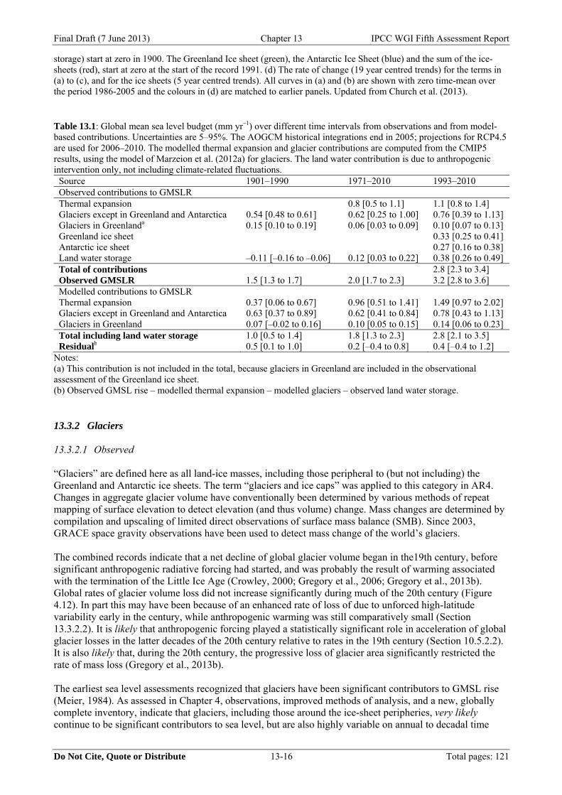
ice-covered regions and marginal seas) of the oceans down to 2000 m since 2004–2005, and (3) estimates of the deep-ocean contribution using ship-based data collected during the World Ocean Circulation Experiment and revisit cruises (Johnson and Gruber, 2007; Johnson et al., 2007; Purkey and Johnson, 2010; Kouketsu et al., 2011). For the period 1971–2010, the rate for the 0–700 m depth range is 0.6 [0.4–0.8] mm yr–1 (Section 3.7.2 and Table 3.1). Including the deep-ocean contribution for the same period increases the value to 0.8 [0.5–1.1] mm yr–1 (Figure 13.4a). Over the altimetry period (1993–2010), the rate for the 0–700 m depth range is 0.8 [0.5–1.1] mm yr–1 and 1.1 [0.8–1.4] mm yr–1 when accounting for the deep ocean (Section 3.7.2 and Table 3.1). 13.3.1.2 Modelled GMSL rise due to thermal expansion is approximately proportional to the increase in ocean heat content (Section 13.4.1). Historical GMSL rise due to thermal expansion simulated by CMIP5 models is shown in Table 13.1 and Figure 13.4a. The model spread is due to uncertainty in radiative forcing and modelled climate response (Sections 8.5.2, 9.4.2.2, 9.7.2.3, 13.4.1). In the time-mean of several decades, there is a negative volcanic forcing if there is more volcanic activity than is typical of the long term, and a positive forcing if there is less. In the decades after major volcanic eruptions, the rate of expansion is temporarily enhanced, as the ocean recovers from the cooling caused by the volcanic forcing (Church et al., 2005; Gregory et al., 2006) (Figure 13.4a). During 1961–1999, a period when there were several large volcanic eruptions, the CMIP3 simulations with both natural and anthropogenic forcing have substantially smaller increasing trends in the upper 700 m than those with anthropogenic forcing only (Domingues et al., 2008) because the natural volcanic forcing tends to cool the climate system, thus reducing ocean heat uptake (Levitus et al., 2001). The models including natural forcing are closer to observations, though with a tendency to underestimate the trend by about 10% (Sections 9.4.2.2, 10.4.1). Gregory (2010) and Gregory et al. (2013a) proposed that the AOGCMs underestimate ocean heat uptake in their historical simulations because their control experiments usually omit volcanic forcing, so the imposition of historical volcanic forcing on the simulated climate system represents a time-mean negative forcing relative to the control climate. The apparent long persistence of the simulated oceanic cooling following the 1883 eruption of Krakatau (Delworth et al., 2005; Gleckler et al., 2006a; Gleckler et al., 2006b; Gregory et al., 2006) is a consequence of this bias, which also causes a model-dependent underestimate of up to 0.2 mm yr–1 of thermal expansion on average during the 20th century (Gregory et al., 2013a; Gregory et al., 2013b). This implies that CMIP5 results may be similarly underestimated, depending on the details of the individual model control runs. Church et al. (2013) proposed a correction of 0.1 mm yr–1 to the model mean rate, which we apply in the sea level budget in Table 13.1 and Figure 13.7. The corrected CMIP5 model-mean rate for 1971–2010 is close to the central observational estimate; the model-mean rate for 1993–2010 exceeds the central observational estimate but they are not statistically different given the uncertainties (Table 13.1, Figure 13.4a). This correction is not made to projections of thermal expansion because it is very small compared with the projected increase in the rate (Section 13.5.1). In view of the improvement in observational estimates of thermal expansion, the good agreement of historical model results with observational estimates, and their consistency with understanding of the energy budget and radiative forcing of the climate system (Box 13.1), we have high confidence in the projections of thermal expansion using AOGCMs. [INSERT FIGURE 13.4 HERE] Figure 13.4: Comparison of modelled and observed components of global mean sea level change since 1900. Changes in glaciers, ice sheets and land water storage are shown as positive sea level rise when mass is added to the ocean. (a) Ocean thermal expansion. Individual CMIP5 AOGCM simulations are shown in grey, the AOGCM average is black, observations in teal with the 5–95% uncertainties shaded. (b) Glaciers (excluding Antarctic peripheral glaciers). Model simulations by Marzeion et al. (2012a) with input from individual AOGCMs are shown in grey with the average of these results in bright purple. Model simulations by Marzeion et al. (2012a) forced by observed climate are shown in light blue. The observational estimates by Cogley (2009b) are shown in green (dashed) and by Leclercq et al. (2011) in red (dashed). (c) Changes in land water storage (yellow/orange, the sum of groundwater depletion and reservoir
Final Draft (7 June 2013) Chapter 13 IPCC WGI Fifth Assessment Report
Do Not Cite, Quote or Distribute 13-16 Total pages: 121
storage) start at zero in 1900. The Greenland Ice sheet (green), the Antarctic Ice Sheet (blue) and the sum of the ice-sheets (red), start at zero at the start of the record 1991. (d) The rate of change (19 year centred trends) for the terms in (a) to (c), and for the ice sheets (5 year centred trends). All curves in (a) and (b) are shown with zero time-mean over the period 1986-2005 and the colours in (d) are matched to earlier panels. Updated from Church et al. (2013). Table 13.1: Global mean sea level budget (mm yr–1) over different time intervals from observations and from model-based contributions. Uncertainties are 5–95%. The AOGCM historical integrations end in 2005; projections for RCP4.5 are used for 2006–2010. The modelled thermal expansion and glacier contributions are computed from the CMIP5 results, using the model of Marzeion et al. (2012a) for glaciers. The land water contribution is due to anthropogenic intervention only, not including climate-related fluctuations.
Source 1901–1990 1971–2010 1993–2010 Observed contributions to GMSLR Thermal expansion 0.8 [0.5 to 1.1] 1.1 [0.8 to 1.4] Glaciers except in Greenland and Antarctica 0.54 [0.48 to 0.61] 0.62 [0.25 to 1.00] 0.76 [0.39 to 1.13] Glaciers in Greenlanda 0.15 [0.10 to 0.19] 0.06 [0.03 to 0.09] 0.10 [0.07 to 0.13] Greenland ice sheet 0.33 [0.25 to 0.41] Antarctic ice sheet 0.27 [0.16 to 0.38] Land water storage –0.11 [–0.16 to –0.06] 0.12 [0.03 to 0.22] 0.38 [0.26 to 0.49] Total of contributions 2.8 [2.3 to 3.4] Observed GMSLR 1.5 [1.3 to 1.7] 2.0 [1.7 to 2.3] 3.2 [2.8 to 3.6] Modelled contributions to GMSLR Thermal expansion 0.37 [0.06 to 0.67] 0.96 [0.51 to 1.41] 1.49 [0.97 to 2.02] Glaciers except in Greenland and Antarctica 0.63 [0.37 to 0.89] 0.62 [0.41 to 0.84] 0.78 [0.43 to 1.13] Glaciers in Greenland 0.07 [–0.02 to 0.16] 0.10 [0.05 to 0.15] 0.14 [0.06 to 0.23] Total including land water storage 1.0 [0.5 to 1.4] 1.8 [1.3 to 2.3] 2.8 [2.1 to 3.5] Residualb 0.5 [0.1 to 1.0] 0.2 [–0.4 to 0.8] 0.4 [–0.4 to 1.2]
Notes: (a) This contribution is not included in the total, because glaciers in Greenland are included in the observational assessment of the Greenland ice sheet. (b) Observed GMSL rise – modelled thermal expansion – modelled glaciers – observed land water storage. 13.3.2 Glaciers 13.3.2.1 Observed “Glaciers” are defined here as all land-ice masses, including those peripheral to (but not including) the Greenland and Antarctic ice sheets. The term “glaciers and ice caps” was applied to this category in AR4. Changes in aggregate glacier volume have conventionally been determined by various methods of repeat mapping of surface elevation to detect elevation (and thus volume) change. Mass changes are determined by compilation and upscaling of limited direct observations of surface mass balance (SMB). Since 2003, GRACE space gravity observations have been used to detect mass change of the world’s glaciers. The combined records indicate that a net decline of global glacier volume began in the19th century, before significant anthropogenic radiative forcing had started, and was probably the result of warming associated with the termination of the Little Ice Age (Crowley, 2000; Gregory et al., 2006; Gregory et al., 2013b). Global rates of glacier volume loss did not increase significantly during much of the 20th century (Figure 4.12). In part this may have been because of an enhanced rate of loss of due to unforced high-latitude variability early in the century, while anthropogenic warming was still comparatively small (Section 13.3.2.2). It is likely that anthropogenic forcing played a statistically significant role in acceleration of global glacier losses in the latter decades of the 20th century relative to rates in the 19th century (Section 10.5.2.2). It is also likely that, during the 20th century, the progressive loss of glacier area significantly restricted the rate of mass loss (Gregory et al., 2013b). The earliest sea level assessments recognized that glaciers have been significant contributors to GMSL rise (Meier, 1984). As assessed in Chapter 4, observations, improved methods of analysis, and a new, globally complete inventory, indicate that glaciers, including those around the ice-sheet peripheries, very likely continue to be significant contributors to sea level, but are also highly variable on annual to decadal time
Final Draft (7 June 2013) Chapter 13 IPCC WGI Fifth Assessment Report
Do Not Cite, Quote or Distribute 13-17 Total pages: 121
scales. It is assumed that all glacier losses contribute to sea level rise, but the potential role of terrestrial interception of runoff, either in lakes formed following future ice retreat or in groundwater, has yet to be evaluated. For the period 2003–2009, the sea level contribution of all glaciers globally, including those glaciers surrounding the periphery of the two ice sheets, is 0.71 [0.64–0.79] mm yr–1 sea level equivalent (SLE) (Section 4.3.3, Table 4.4). Depending upon the method used, however, loss-rate measurements of the two ice sheets can be very difficult to separate from losses from the peripheral glaciers. To avoid double counting, total cryospheric losses are determined by adding estimates of glacier losses excluding the peripheral glaciers to losses from the ice sheets plus their peripheral glaciers. The sea level contribution of all glaciers excluding those glaciers surrounding the periphery of the two ice sheets was 1901–1990: 0.54 [0.48–0.61] mm yr–1 SLE; for 1971–2009: 0.62 [0.25–1.00] mm yr–1 SLE; for 1993–2009: 0.76 [0.43–1.09] mm yr–1 SLE; for 2005–2009: 0.83 [0.70–0.97] mm yr–1 SLE (Section 4.3.3.4). 13.3.2.2 Modelled Global glacier mass balance models are calibrated using data from the few well-observed glaciers. Approximately 100 glacier mass balance records are available in any given year over the past half-century; only 17 glaciers exist with records of 30 years or more (Dyurgerov and Meier, 2005; Kaser et al., 2006; Cogley, 2012). Confidence in these models for projections of future change (Section 13.4.2) depends on their ability to reproduce past observed glacier change using corresponding climate observations as forcing (Raper and Braithwaite, 2005; Meier et al., 2007; Bahr et al., 2009; Radić and Hock, 2011; Marzeion et al., 2012b; 2012a; Giesen and Oerlemans, 2013). Model validation is challenging due to the scarcity of independent observations (unused in model calibration) but uncertainties have been evaluated by methods such as cross-validation of hindcast projections for individual glaciers drawn from the sample of glacier observations averaged for calibration (Marzeion et al., 2012a; Radić et al., 2013). Confidence in the use of AOGCM climate simulations as input to glacier projections is gained from the agreement since the mid-20th century of glacier models forced by AOGCM simulations with glacier models forced by observations (Marzeion et al., 2012a) (Figure 13.4b). In the earlier 20th century, around the 1930s, glaciers at high northern latitudes lost mass at an enhanced rate (Oerlemans et al., 2011; Leclercq et al., 2012); in the model, observed forcings produced larger glacier losses than did AOGCM forcings (Marzeion et al., 2012a) (Figure 13d). This is judged likely to be due to an episode of unforced, regionally variable warming around Greenland (Box, 2002; Chylek et al., 2004) rather than to radiative forcing of the climate system, and is consequently not reproduced by AOGCM experiments (Section 10.2). In our analysis of the budget of GMSL rise (Section 13.3.6), we take the difference between the simulations using AOGCM forcing and the simulation using observations as an estimate of the influence of unforced climate variability on global glacier mass balance (Figure 13.4b). There is medium confidence in the use of glacier models to make global projections based on AOGCM results. The process-based understanding of glacier surface mass balance, the consistency of models and observations of glacier changes, and the evidence that AOGCM climate simulations can provide realistic input all give confidence, which on the other hand is limited because the set of well-observed glaciers is a very small fraction of the total. 13.3.3 Greenland and Antarctic Ice Sheets 13.3.3.1 Observed Mass Balance The Greenland Ice Sheet’s mass balance comprises its surface mass balance and outflow, whereas Antarctica’s mass budget is dominated by accumulation and outflow in the form of calving and ice flow into floating (and therefore sea level neutral) ice shelves. Knowledge of the contribution of the Greenland and Antarctic ice sheets to observed sea level changes over the last two decades comes primarily from satellite and airborne surveys. Three main techniques are employed: the mass balance, volumetric, and gravimetric methods (Section 4.4.1). Observations indicate that the Greenland contribution (all rates quoted here are 5–95%) to GMSL has very likely increased from 0.09 [–0.02–0.20] mm yr–1 for 1992–2001 to 0.59 [0.43–0.76] mm yr–1 for 2002–2011 (Section 4.4.2.2, Figure 13.4). The average rate of the Antarctica contribution to sea level rise likely
Final Draft (7 June 2013) Chapter 13 IPCC WGI Fifth Assessment Report
Do Not Cite, Quote or Distribute 13-18 Total pages: 121
increased from 0.08 [–0.10–0.27] mm yr–1 for 1992–2001 to 0.40 [0.20–0.61] mm yr–1 for 2002–2011 (Section 4.4.2.3). For the budget period 1993–2010, the combined contribution of the ice sheets is 0.60 [0.42–0.78] mm yr–1. For comparison, the AR4’s assessment for the period 1993–2003 was 0.21 ± 0.07 mm yr–1 for Greenland and 0.21 ± 0.35 mm yr–1 for Antarctica. 13.3.3.2 Modelled Surface Mass Balance Projections of changes in the SMB of the Antarctic and Greenland ice sheets are obtained from regional climate model (RCM) or downscaled AOGCM simulations (Sections 13.4.3.1 and 13.4.4.1). A spatial resolution of a few 10s km or finer is required in order to resolve the strong gradients in SMB across the steep slopes of the ice-sheet margins. While simulations of SMB at particular locations may have errors of 5-20% compared with in-situ observations, there is good agreement between methods involving RCMs and observational methods of evaluating ice-sheet mass balance (Shepherd et al., 2012). In the present climate, for both Greenland and Antarctica, the mean SMB over the ice-sheet area is positive, giving a negative number when expressed as sea level equivalent (SLE). In Greenland, the average and standard deviation of accumulation (precipitation minus sublimation) estimates for 1961–1990 is –1.62 ± 0.21 mm yr–1 SLE from the models in Table 13.2, agreeing with published observation-based accumulation maps, for example –1.42 ± 0.11 mm yr–1 SLE by Bales et al. (2009) and –1.63 ± 0.23 mm yr–1 SLE by Burgess et al. (2010). For SMB (accumulation minus runoff, neglecting drifting snow erosion, which is small), the models give –0.92 ± 0.26 mm yr–1 SLE for 1961–1990 (Table 13.2). All of these models indicate that Greenland Ice Sheet SMB showed no significant trend from the 1960s to the 1980s, then started becoming less positive (becoming less negative expressed as SLE) in the early 1990s, on average by 3% yr–1. This results in a statistically significant and increasing (i.e., becoming more positive) contribution to the rate of GMSL rise (SMB trend column of Table 13.2, Figure 13.5). The largest trends are found in models with coupled snow and atmosphere simulations using the RACMO2 and MAR models. Van den Broeke et al. (2009) concluded that the mass loss during 2000–2008 is equally split between SMB and dynamical change. Rignot et al. (2011) indicated that SMB change accounts for about 60% of the mass loss since 1992 and Sasgen et al. (2012) showed that SMB change, simulated by RACMO2 (Ettema et al., 2009, an earlier version of the model in Table 13.2), accounts for about 60% of the observed rate of mass loss during 2002–2010, with an observational estimate of the increase in ice outflow accounting for the remainder. This satisfactory consistency, within uncertainties, in estimates for the Greenland Ice Sheet mass budget gives confidence in SMB simulations of the past, and hence also in the similar models used for projections of SMB changes (Section 13.4.3.1). This recent trend towards increasingly less positive SMB is caused almost entirely by increased melting and subsequent runoff, with variability in accumulation being comparatively small (Sasgen et al., 2012; Vernon et al., 2013) (Figure 13.5). This tendency is related to pronounced regional warming, which may be attributed to some combination of anthropogenic climate change and anomalous regional variability in recent years (Hanna et al., 2008; 2012; Fettweis et al., 2013). Greenland SMB models forced by boundary conditions from AOGCM historical simulations (Rae et al., 2012; Fettweis et al., 2013) do not show statistically significant trends towards increasing contributions to GMSL, implying that the dominant contribution is internally generated regional climate variability, which is not expected to be reproduced by AOGCM historical simulations (Section 10.2). We have high confidence in projections of future warming in Greenland because of the agreement of models in predicting amplified warming at high northern latitudes (Sections 12.4.3.1, 14.7.2) for well-understood physical reasons, although there remains uncertainty in the size of the amplification, and we have high confidence in projections of increasing surface melting (Section 13.4.3.1) because of the sensitivity to warming demonstrated by SMB models of the past. Table 13.2: SMB and rates of change of SMB of the Greenland Ice Sheet, calculated from ice sheet SMB models using meteorological observations and reanalyses as input, expressed as sea level equivalent (SLE). A negative SLE number for SMB indicates that accumulation exceeds runoff. A positive SLE for SMB anomaly indicates that accumulation has decreased, or runoff has increased, or both. Uncertainties are one standard deviation. Uncertainty in individual model results reflects temporal variability, that is one standard deviation of annual values; the uncertainty in the model average is one standard deviation of variation across models.
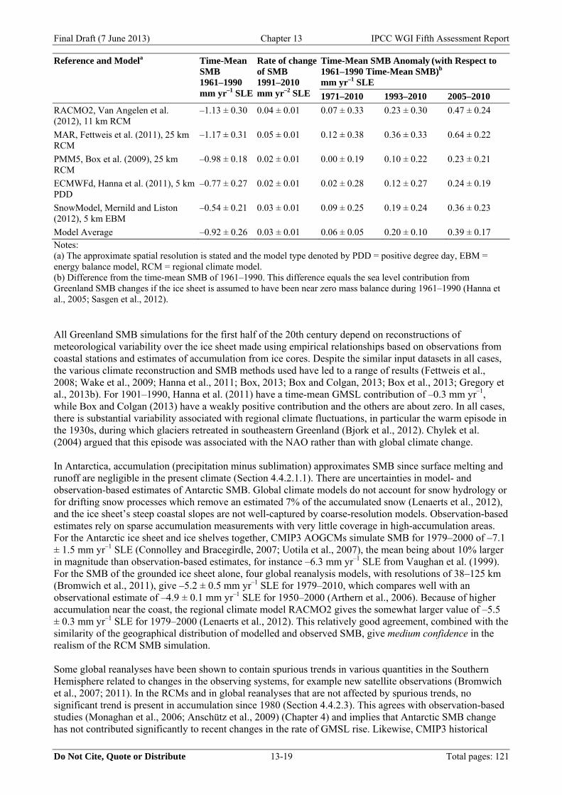
Final Draft (7 June 2013) Chapter 13 IPCC WGI Fifth Assessment Report
Do Not Cite, Quote or Distribute 13-19 Total pages: 121
Reference and Modela Time-Mean SMB 1961–1990 mm yr–1 SLE
Rate of change of SMB 1991–2010 mm yr–2 SLE
Time-Mean SMB Anomaly (with Respect to 1961–1990 Time-Mean SMB)b mm yr–1 SLE
1971–2010 1993–2010 2005–2010
RACMO2, Van Angelen et al. (2012), 11 km RCM
–1.13 ± 0.30 0.04 ± 0.01 0.07 ± 0.33 0.23 ± 0.30 0.47 ± 0.24
MAR, Fettweis et al. (2011), 25 km RCM
–1.17 ± 0.31 0.05 ± 0.01 0.12 ± 0.38 0.36 ± 0.33 0.64 ± 0.22
PMM5, Box et al. (2009), 25 km RCM
–0.98 ± 0.18 0.02 ± 0.01 0.00 ± 0.19 0.10 ± 0.22 0.23 ± 0.21
ECMWFd, Hanna et al. (2011), 5 km PDD
–0.77 ± 0.27 0.02 ± 0.01 0.02 ± 0.28 0.12 ± 0.27 0.24 ± 0.19
SnowModel, Mernild and Liston (2012), 5 km EBM
–0.54 ± 0.21 0.03 ± 0.01 0.09 ± 0.25 0.19 ± 0.24 0.36 ± 0.23
Model Average –0.92 ± 0.26 0.03 ± 0.01 0.06 ± 0.05 0.20 ± 0.10 0.39 ± 0.17 Notes: (a) The approximate spatial resolution is stated and the model type denoted by PDD = positive degree day, EBM = energy balance model, RCM = regional climate model. (b) Difference from the time-mean SMB of 1961–1990. This difference equals the sea level contribution from Greenland SMB changes if the ice sheet is assumed to have been near zero mass balance during 1961–1990 (Hanna et al., 2005; Sasgen et al., 2012). All Greenland SMB simulations for the first half of the 20th century depend on reconstructions of meteorological variability over the ice sheet made using empirical relationships based on observations from coastal stations and estimates of accumulation from ice cores. Despite the similar input datasets in all cases, the various climate reconstruction and SMB methods used have led to a range of results (Fettweis et al., 2008; Wake et al., 2009; Hanna et al., 2011; Box, 2013; Box and Colgan, 2013; Box et al., 2013; Gregory et al., 2013b). For 1901–1990, Hanna et al. (2011) have a time-mean GMSL contribution of –0.3 mm yr–1, while Box and Colgan (2013) have a weakly positive contribution and the others are about zero. In all cases, there is substantial variability associated with regional climate fluctuations, in particular the warm episode in the 1930s, during which glaciers retreated in southeastern Greenland (Bjork et al., 2012). Chylek et al. (2004) argued that this episode was associated with the NAO rather than with global climate change. In Antarctica, accumulation (precipitation minus sublimation) approximates SMB since surface melting and runoff are negligible in the present climate (Section 4.4.2.1.1). There are uncertainties in model- and observation-based estimates of Antarctic SMB. Global climate models do not account for snow hydrology or for drifting snow processes which remove an estimated 7% of the accumulated snow (Lenaerts et al., 2012), and the ice sheet’s steep coastal slopes are not well-captured by coarse-resolution models. Observation-based estimates rely on sparse accumulation measurements with very little coverage in high-accumulation areas. For the Antarctic ice sheet and ice shelves together, CMIP3 AOGCMs simulate SMB for 1979–2000 of –7.1 ± 1.5 mm yr–1 SLE (Connolley and Bracegirdle, 2007; Uotila et al., 2007), the mean being about 10% larger in magnitude than observation-based estimates, for instance –6.3 mm yr–1 SLE from Vaughan et al. (1999). For the SMB of the grounded ice sheet alone, four global reanalysis models, with resolutions of 38–125 km (Bromwich et al., 2011), give –5.2 ± 0.5 mm yr–1 SLE for 1979–2010, which compares well with an observational estimate of –4.9 ± 0.1 mm yr–1 SLE for 1950–2000 (Arthern et al., 2006). Because of higher accumulation near the coast, the regional climate model RACMO2 gives the somewhat larger value of –5.5 ± 0.3 mm yr–1 SLE for 1979–2000 (Lenaerts et al., 2012). This relatively good agreement, combined with the similarity of the geographical distribution of modelled and observed SMB, give medium confidence in the realism of the RCM SMB simulation. Some global reanalyses have been shown to contain spurious trends in various quantities in the Southern Hemisphere related to changes in the observing systems, for example new satellite observations (Bromwich et al., 2007; 2011). In the RCMs and in global reanalyses that are not affected by spurious trends, no significant trend is present in accumulation since 1980 (Section 4.4.2.3). This agrees with observation-based studies (Monaghan et al., 2006; Anschütz et al., 2009) (Chapter 4) and implies that Antarctic SMB change has not contributed significantly to recent changes in the rate of GMSL rise. Likewise, CMIP3 historical
Final Draft (7 June 2013) Chapter 13 IPCC WGI Fifth Assessment Report
Do Not Cite, Quote or Distribute 13-20 Total pages: 121
simulations do not exhibit any systematic trend in Antarctic precipitation during the late 20th century (Uotila et al., 2007). No observational assessments have been made of variability in SMB for the whole ice sheet for the earlier part of the 20th century, or of its longer term mean. GCM and RCM projections consistently indicate significant Antarctic warming and concomitant increase in precipitation. We have high confidence in expecting a relationship between these quantities on physical grounds (Section 13.4.4.1) and from ice-core evidence (Van Ommen et al., 2004; Lemieux-Dudon et al., 2010; Stenni et al., 2011). The absence of a significant trend in Antarctic precipitation up to the present is not inconsistent with the expected relationship, because observed temperature trends over the majority of the continent are weak (Section 10.5.2.1) and trends in Antarctic precipitation simulated for recent decades are much smaller than interannual variability (van den Broeke et al., 2006; Uotila et al., 2007). Taking all these considerations together, we have medium confidence in model projections of future Antarctic SMB increase, implying a negative contribution to GMSL rise (see also Sections 13.4.4.1, 13.5.3 and 14.7.14). [INSERT FIGURE 13.5 HERE] Figure 13.5: Annual-mean surface mass balance (accumulation minus ablation) for the Greenland Ice Sheet, simulated by regional climate models for the period 1960–2010. 13.3.4 Contributions from Water Storage on Land Changes in water storage on land in response to climate change and variability (i.e., water stored in rivers, lakes, wetlands, the vadose zone, aquifers, and snow pack at high latitudes and altitudes) and from direct human-induced effects (i.e., storage of water in reservoirs and groundwater pumping) have the potential to contribute to sea level change. Based on satellite observations of the northern hemisphere snowpack, Biancamaria et al. (2011) found no significant trend in the contribution of snow to sea level. Estimates of climate-related changes in land water storage over the past few decades rely on global hydrological models because corresponding observations are inadequate (Milly et al., 2010). In assessing the relation between terrestrial water storage and climate, Milly et al. (2003) and Ngo-Duc et al. (2005) found no long-term climatic trend in total water storage, but documented large interannual to decadal fluctuations, equivalent to several millimetres of sea level. Recent studies have shown that interannual variability in observed GMSL is correlated with ENSO indices (Nerem et al., 2010) and is inversely related to ENSO-driven changes of terrestrial water storage, especially in the tropics (Llovel et al., 2011). During El Niño events, sea level (and ocean mass) tends to be higher because ocean precipitation increases and land precipitation decreases in the tropics (Cazenave et al., 2012) . The reverse happens during La Niña events, as seen during 2010–2011, when there was a decrease in GMSL due to a temporary increase in water storage on the land, especially in Australia, northern South America, and southeast Asia (Boening et al., 2012) (Section 13.3.5). Direct human interventions on land water storage also induce sea level changes (Sahagian, 2000; Gornitz, 2001; Huntington, 2008; Lettenmaier and Milly, 2009). The largest contributions come from impoundment in reservoirs and groundwater withdrawal. Over the past half-century, storage in tens of thousands of reservoirs has offset some of the sea level rise that would otherwise have occurred. Chao et al. (2008) estimated that the nearly 30,000 reservoirs built during the 20th century resulted in nominal reservoir storage up to 2007 equivalent to ~23 mm of sea level fall (mostly since 1940), with a stabilization in recent years. Chao et al. further assumed that the reservoirs were 85% full, and by including seepage into groundwater as estimated from a model, they obtained a total of 30 mm of sea level fall (equivalent to a rate of sea level fall of 0.55 mm yr–1 from 1950 to 2000). Their seepage estimate was argued to be unrealistically large, however, because it assumes aquifers are infinite and have no interfering boundary conditions (Lettenmaier and Milly, 2009; Konikow, 2013). Chao et al. (2008) argued that sedimentation of reservoirs does not reduce their sea level contribution, but their argument is disputed (Gregory et al., 2013b). Lettenmaier and Milly (2009) suggested a loss of capacity due to sedimentation at 1% yr–1. Given the uncertainty about them, neither the seepage nor the effect of sedimentation is included in the budget (Section 13.3.6). Here the (negative) GMSL contribution from reservoir storage is estimated as 85% [70–100%] of the nominal capacity (with the lower limit coming from Pokhrel et al. (2012)). Konikow (2011) estimated that human-induced groundwater depletion contributed 0.26 ± 0.07 mm yr–1 to GMSL rise over 1971–2008 and 0.34 ± 0.07 mm yr–1 over 1993–2008 (based mostly on observational methods), whereas Wada et al. (2012) estimated values of 0.42 ± 0.08 mm yr–1 over 1971–2008 and 0.54 ±
Final Draft (7 June 2013) Chapter 13 IPCC WGI Fifth Assessment Report
Do Not Cite, Quote or Distribute 13-21 Total pages: 121
0.09 mm yr–1 over 1993–2008 (based on modelling of water fluxes). The average of these two series with the difference as a measure of the uncertainty is used in the sea level budget (Section 13.3.6). Pokhrel et al. (2012) estimated a larger groundwater depletion, but Konikow (2013) (disputed by Pohkrel et al. (2013)) argued that their underlying assumptions of defining depletion as equivalent to groundwater use, and allowing unlimited extraction to meet water demand, lead to substantial overestimates of depletion. In summary, climate-related changes in water and snow storage on land do not show significant long-term trends for the recent decades. However, direct human interventions in land water storage (reservoir impoundment and groundwater depletion) have each contributed at least several tenths of mm yr–1 of sea level change (Figure 13.4, Table 13.1). Reservoir impoundment exceeded groundwater depletion for the majority of the 20th century but groundwater depletion has increased and now exceeds current rates of impoundment, contributing to an increased rate of GMSL rise. The net contribution for the 20th century is estimated to be small. 13.3.5 Ocean Mass Observations from GRACE As discussed in Chapter 3, it has been possible to directly estimate changes in ocean mass using satellite gravity data from GRACE since 2002 (Chambers et al., 2004; Chambers, 2006; Cazenave et al., 2009; Leuliette and Miller, 2009; Chambers et al., 2010; Llovel et al., 2010). These measurements represent the sum of total land-ice plus land-water components, and thus provide an independent assessment of these contributions. However, GRACE is also sensitive to mass redistribution associated with GIA and requires that this effect (on the order of –0.7 to –1.3 mm yr–1 when averaged over the ocean domain) (Paulson et al., 2007; Peltier, 2009; Chambers et al., 2010; Tamisiea, 2011) be removed before estimating the ocean-mass component. Most recent estimates (Leuliette and Willis, 2011; von Schuckmann and Le Traon, 2011) report a global mean ocean-mass increase of 1.8 [1.4 to 2.2] mm yr–1 over 2003-2012 after correcting for the GIA component. The associated error results from the low signal-to-noise ratio over the ocean domain and uncertainty in the model-based GIA correction (Quinn and Ponte, 2010). Chapter 3 notes that, in terms of global averages, the sum of the contribution to GMSL due to change in global ocean mass (the barystatic contribution), measured by GRACE, and the contribution due to global ocean thermal expansion (the thermosteric contribution), measured by Argo, agrees within uncertainties with the GMSL change observed by satellite altimetry (Leuliette and Willis, 2011; von Schuckmann and Le Traon, 2011), although there is still a missing contribution from expansion in the deep ocean below 2000 m. These datasets have allowed an investigation of the cause of variability in sea level over the last few years (Figure 13.6). In particular, Boening et al. (2012) concluded that the decrease in GMSL over 2010–2011 followed by a rapid increase since 2011 was related to the 2011 La Niña event, whereby changes in land/ocean precipitation patterns caused a temporary increase in water storage on the land (and corresponding decrease in GMSL) during the La Niña event, especially in Australia, northern South America, and southeast Asia (Boening et al., 2012). [INSERT FIGURE 13.6 HERE] Figure 13.6: Global mean sea level from altimetry from 2005 to 2012 (blue line). Ocean mass changes are shown in green (as measured by GRACE) and thermosteric sea level changes (as measured by Argo) are shown in red. The black line shows the sum of the ocean mass and thermosteric contributions (updated from Boening et al. (2012)). 13.3.6 Budget of GMSL Rise Drawing on Sections 13.3.1–13.3.5, the budget of GMSL rise (Table 13.1, Figure 13.7) is analysed using models and observations for the periods 1901–1990 (the 20th century, excluding the period after 1990 when ice-sheet contributions to GMSL rise have increased; Sections 4.4 and 13.3.3.1), since 1971 (when significantly more ocean data became available and systematic glacier reconstructions began), and since 1993 (when precise satellite sea level altimetry began). The 2005–2010 period when Argo and GRACE data are available is short and strongly affected by interannual climate variability, as discussed in the previous subsection (Section 13.3.5, Figure 13.6). Such variability is not externally forced and is therefore not expected to be reproduced in AOGCM historical experiments. For the contribution from land water storage (Figure 13.4c) we use the estimated effect of human intervention, neglecting climate-related variation, whose effect is unimportant on multidecadal timescales (Section 13.3.4). Contributions due to runoff from thawed

Final Draft (7 June 2013) Chapter 13 IPCC WGI Fifth Assessment Report
Do Not Cite, Quote or Distribute 13-22 Total pages: 121
permafrost, change in atmospheric moisture content, and sedimentation in the ocean are not considered in the budget because they are negligible compared with observed GMSL rise and the uncertainties. For 1993–2010, allowing for uncertainties, the observed GMSL rise is consistent with the sum of the observationally estimated contributions (Table 13.1, Figure 13.7e). The two largest terms are ocean thermal expansion (accounting for about 35% of the observed GMSL rise) and glacier mass loss (accounting for a further 25%, not including those in Greenland and Antarctica). Observations indicate an increased ice-sheet contribution over the last two decades (Sections 4.4.2.2, 4.4.2.3 and 13.3.3.1) (Shepherd et al., 2012). The closure of the observational budget since 1993, within uncertainties, represents a significant advance since the AR4 in physical understanding of the causes of past GMSL change, and provides an improved basis for critical evaluation of models of these contributions in order to assess their reliability for making projections. The observational budget cannot be rigorously assessed for 1901–1990 or 1971–2010 because there is insufficient observational information to estimate ice-sheet contributions with high confidence before the 1990s, and ocean data sampling is too sparse to permit an estimate of global mean thermal expansion before the 1970s. However, a closed observational GMSL budget since the 1970s can be demonstrated with reasonable estimates of ice-sheet contributions (Church et al., 2011a; Moore et al., 2011) (Table 13.1, Figure 13.7). For 1971–2010, the observed contributions from thermal expansion and mass loss from glaciers (not including those in Antarctica) alone explain about 75% of the observed GMSL. AOGCM-based estimates of the thermal expansion, which agree well with observations since 1971, observational estimates of the glacier contribution, and the estimated change in land water storage (Figure 13.4c), which is relatively small, can all be made from the start of the 20th century (Sections 13.3.1.2, 13.3.2.2 and 13.3.4, Table 13.1). Model estimates of Greenland Ice Sheet SMB changes give an uncertain but relatively small contribution during most of the 20th century, increasing since the early 1990s (Section 13.3.2.2). There could be a small constant contribution from the Antarctic Ice Sheet (Huybrechts et al., 2011; Gregory et al., 2013b) due to long-term adjustment to climate change in previous millennia. Any secular rate of sea level rise in the late Holocene was small (order of few tenths mm yr–1) (Section 13.2.1.4), probably less than 0.2 mm yr–1 (see discussion in Gregory et al. (2013b)). Including these ice-sheet contributions (but omitting Antarctic SMB variations, for which no observationally based information for the ice sheet as a whole is available for the majority of the 20th century), GMSL rise during the 20th century can be accounted for within uncertainties, including the observation that the linear trend of GMSL rise during the last 50 years is little larger than for the 20th century, despite the increasing anthropogenic forcing (Gregory et al., 2013b). Model-based attribution of sea level change to radiative forcings is discussed in Section 10.4.3. The sum of CMIP5 AOGCM thermal expansion (Section 13.3.1.2), glacier model results with CMIP5 AOGCM input (not including glaciers in Antarctica; Section 13.3.2.2; Marzeion et al. (2012a)) and anthropogenic intervention in land water storage (Section 13.3.4) accounts for about 65% of the observed rate of GMSL rise for 1901–1990, and 90% for 1971–2010 and 1993–2010 (Table 13.1; Figure 13.7). In all periods, the residual is small enough to be attributed to the ice sheets (Section 13.3.2.2). The unusually warm conditions in the Arctic during the 1930s (Chylek et al., 2004), which are attributed to unforced climate variability (Delworth and Knutson, 2000) and are not therefore expected to be simulated by AOGCMs, likely produced a greater mass loss by glaciers in high northern latitudes (Section 13.3.2.2). The difference between the glacier mass loss calculated with the Marzeion et al. (2012a) model when it is forced with observed climate rather than AOGCM simulated climate (the purple and blue curves in Figure 13.4b) is an estimate of this effect. If the glacier model results for observational input are used (Marzeion et al. (2012a), not including glaciers in Antarctica) and an illustrative value of 0.1 mm yr–1 is included for a long-term Antarctic contribution, the model mean is within 20% of the observed GMSL rise (Figure 13.7a,c, dashed line), and 10% since 1993 (Figure 13.7d, dashed line; Church et al. (2013)). When the observed ice-sheet contributions since 1992 are included as well, the sum is almost equivalent to the observed rise (dotted line in Figure 13.7). Both observations and models have a maximum rate of rise in the 1930–1950 period, a minimum rate in the 1960s, and a maximum rate over the last two decades (Figure 13.7b). This agreement provides evidence that the larger rate of rise since 1990, with a significant component of ocean thermal expansion (Figure 13.4d),
Final Draft (7 June 2013) Chapter 13 IPCC WGI Fifth Assessment Report
Do Not Cite, Quote or Distribute 13-23 Total pages: 121
results from increased radiative forcing (both natural and anthropogenic) and increased ice-sheet discharge, rather than a natural oscillation (Church et al., 2013). In summary, the evidence now available gives a clearer account of observed GMSL change than in previous IPCC assessments, in two respects. First, reasonable agreement can be demonstrated throughout the period since 1900 between GMSL rise as observed and as calculated from the sum of contributions. From 1993, all contributions can be estimated from observations; for earlier periods, a combination of models and observations is needed. Second, when both models and observations are available, they are consistent within uncertainties. These two advances give confidence in the 21st century sea level projections. The ice-sheet contributions have the potential to increase substantially due to rapid dynamical change (Sections 13.1.5.1, 13.4.3.2 and 13.4.4.2) but have been relatively small up to the present (Sections 4.4 and 13.3.2.2). Therefore, the closure of the sea level budget to date does not test the reliability of ice-sheet models in projecting future rapid dynamical change; we have only medium confidence in these models, on the basis of theoretical and empirical understanding of the relevant processes and observations of changes up to the present (13.4.3.2, 13.4.4.2). [INSERT FIGURE 13.7 HERE] Figure 13.7: Comparison of the observed global mean sea level rise with the sum of the modelled contributions from ocean thermal expansion, glaciers (excluding glaciers peripheral to the Antarctic ice sheet; from Marzeion et al. (2012a)) and changes in land-water storage. In panels (a)-(d): the grey lines are results for individual CMIP5 AOGCMs; the black line is the model mean plus a correction for the omission of volcanic forcing in the AOGCM control experiments (see Section 13.3.1.2); the adjusted model mean (dashed black line) is the sum of the corrected model mean thermal expansion, the change in land-water storage, the Marzeion et al. (2012a) glacier estimate using observed (rather than modelled) climate, and an illustrative long-term ice-sheet contribution (of 0.1 mm yr–1); the adjusted model mean including the observed ice sheet contribution (dotted black line) begins in 1993 and includes the ice-sheet contributions (from Section 4.4), but excludes the glaciers peripheral to the both the Greenland Ice Sheet and the Antarctic Ice Sheet, to avoid double counting because the observational ice-sheet estimates include the peripheral glaciers; the estimates of global mean sea level are from Church and White (2011), Ray and Douglas (2011) and Jevrejeva et al. (2008), with the shading indicating the uncertainty estimates (two standard deviations); the satellite altimeter data since 1993 are shown in red. The modelled sea level is given (a) for the period 1900 to 2010, (b) the rates of sea level change for the same period, with the satellite altimeter data shown as a red dot for the rate, (c) for 1961 to 2010 and (d) for 1990 to 2010. Panel (e) compares the sum of the observed contributions (orange) and the observed sea level from the satellite altimeter data (red). (Figure and caption updated from Church et al. (2013)) [START BOX 13.1 HERE] Box 13.1: The Global Energy Budget The global energy balance is a fundamental aspect of the Earth’s climate system. At the top of the atmosphere (TOA), the boundary of the climate system, the balance involves shortwave radiation received from the sun, shortwave radiation reflected and long-wave radiation emitted by the Earth (Section 1.2.2). The rate of storage of energy in the Earth system must be equal to the net downward radiative flux at the TOA. The TOA fluxes (Section 2.3) have been measured by the Earth Radiation Budget Experiment (ERBE) satellites from 1985 to 1999 (Wong et al., 2006) and the Cloud and the Earth’s Radiant Energy System (CERES) satellites from March 2000 to the present (Loeb et al., 2009). The TOA radiative flux measurements are highly precise, allowing identification of changes in the Earth’s net energy budget from year to year within the ERBE and CERES missions (Kato, 2009; Stackhouse et al., 2010; Loeb et al., 2012), but the absolute calibration of the instruments is not sufficiently accurate to allow determination of the absolute TOA energy flux or to provide continuity across missions (Loeb et al., 2009). The ocean has stored over 90% of the increase in energy in the climate system over recent decades (Box 3.1), resulting in ocean thermal expansion and hence sea level rise (Sections 3.7, 9.4, 13.4). Thus the energy and sea level budgets are linked and must be consistent (Church et al., 2011b). This Box focuses on the Earth’s global energy budget since 1970 when better global observational data coverage is available. The radiative forcings (from Chapter 8), the global averaged surface temperatures (HadCRUT4) (Morice et al., 2012) and the rate of energy storage are relative to the time mean of 1860 to 1879. Otto et al. (2013) used an
Final Draft (7 June 2013) Chapter 13 IPCC WGI Fifth Assessment Report
Do Not Cite, Quote or Distribute 13-24 Total pages: 121
energy imbalance over this reference period of 0.08 ± 0.03 W m–2, which is subtracted from the observed energy storage. Since 1970, the effective radiative forcing (ERF) of the climate system has been positive as a result of increased greenhouse gas concentrations (well-mixed and short-lived greenhouse gases, tropospheric and stratospheric ozone and stratospheric water vapour) and a small increase in solar irradiance (Box 13.1, Figure 1a). This positive ERF has been partly compensated by changes in tropospheric aerosols which predominantly reflect sunlight and modify cloud properties and structure in ways that tend to reinforce the negative ERF, although black carbon produces positive forcing. Explosive volcanic eruptions (such as El Chichón in Mexico in 1982 and Mount Pinatubo in the Philippines in 1991) can inject sulphur dioxide into the stratosphere, giving rise to stratospheric aerosol, which persists for several years. This reflects some of the incoming solar radiation, and thus gives a further negative forcing. Changes in surface albedo from land-use change have also led to a greater reflection of shortwave radiation back to space and hence a negative forcing. Since 1970, the net ERF of the climate system (including black carbon on snow and combined contrails and contrail induced cirrus, not shown) has increased (Chapter 8) resulting in a cumulative total energy inflow over this period (Box 13.1, Figure 1a). [INSERT BOX 13.1, FIGURE 1 HERE] Box 13.1, Figure 1: The Earth’s energy budget from 1970 through 2011. (a) The cumulative energy flux into the Earth system from changes in well-mixed and short-lived greenhouse gases, solar forcing, changes in tropospheric aerosol forcing, volcanic forcing and surface albedo, (relative to 1860–1879) are shown by the coloured lines and these are added to give the cumulative energy inflow (black; including black carbon on snow and combined contrails and contrail induced cirrus, not shown separately). (b) The cumulative total energy inflow from (a, black) is balanced by the sum of the warming of the Earth system (blue; energy absorbed in warming the ocean, the atmosphere and the land and in the melting of ice) and an increase in outgoing radiation inferred from changes in the global averaged surface temperature. The sum of these two terms is given for a climate feedback parameter α of 0.82, 1.23 and 2.47 W m–2 °C–1, (corresponding to an equilibrium climate sensitivity of 4.5, 3.0 and 1.5ºC). The energy budget would be closed for a particular value of α if that line coincided with the total energy inflow. For clarity, all uncertainties (shading) shown are for a likely range. If the ERF were fixed, the climate system would eventually warm sufficiently that the radiative response would balance the ERF, and there would be zero net heat flux into the system. As the ERF is increasing, the ocean’s large capacity to store heat means the climate system is not in equilibrium (Hansen et al., 2005), and continues to store energy (Box 3.1; Box 13.1, Figure 1b). This storage provides strong evidence of a changing climate. The majority of this additional heat is in the upper 700 m of the ocean but there is also warming in the deep and abyssal ocean (Box 3.1). The associated thermal expansion of the ocean has contributed about 40% of the observed sea level rise since 1970 (Section 13.4.2.2.6; Church et al., (2011b)). A small amount of additional heat has been used to warm the continents, warm and melt glacial and sea ice, and warm the atmosphere (Box 3.1). As the climate system warms, energy is lost to space through increased outgoing radiation. This radiative response by the system is predominantly due to increased thermal grey-body radiation emitted by the atmosphere and surface, but is modified by climate feedbacks, such as changes in water vapour, surface albedo and clouds, which affect both outgoing longwave and reflected shortwave radiation. Following Murphy et al. (2009), Box 13.1, Figure 1b relates the cumulative total energy inflow to the Earth system to the change in energy storage and the cumulative outgoing radiation. Calculation of the latter is based on the observed globally averaged surface temperature change ΔΤ relative to a reference temperature for which the Earth system would be in radiative balance. This temperature change is multiplied by the climate feedback parameter α, which in turn is related to the equilibrium climate sensitivity. For equilibrium climate sensitivities of 4.5°C, 3.0°C to 1.5°C (Box 12.2) and an ERF for a doubled CO2 concentration of 3.7 ± 0.74 W m–2 (Sections 8.1, 8.3), the corresponding estimates of the climate feedback parameter α are 0.82, 1.23 and 2.47 W m–2 °C–1. In addition to these forced variations in the Earth’s energy budget, there is also internal variability on decadal time scales. Observations and models indicate that because of the comparatively small heat capacity of the atmosphere, a decade of steady or even decreasing surface temperature can occur in a warming world (Easterling and Wehner, 2009; Palmer et al., 2011). GCM simulations indicate that these periods are associated with a transfer of heat from the upper to the deeper ocean, of order 0.1 W m–2 (Katsman and van
Final Draft (7 June 2013) Chapter 13 IPCC WGI Fifth Assessment Report
Do Not Cite, Quote or Distribute 13-25 Total pages: 121
Oldenborgh, 2011; Meehl et al., 2011), with a near steady (Meehl et al., 2011) or an increased radiation to space (Katsman and van Oldenborgh, 2011), again of order 0.1 W m–2. While these natural fluctuations represent a large amount of heat, they are significantly smaller than the anthropogenic forcing of the Earth’s energy budget (Huber and Knutti, 2012), particularly when looking at time scales of several decades or more (Santer et al., 2011). These independent estimates of ERF, observed heat storage and surface warming combine to give an energy budget for the Earth that is consistent with the assessed range of climate sensitivity (2°C to 4.5°C; Box 12.2) to within estimated uncertainties. Quantification of the terms in the Earth’s energy budget and verification that these terms balance over recent decades provides strong evidence for our understanding of anthropogenic climate change. Changes in the Earth’s energy storage are a powerful observation for the detection and attribution of climate change (Section 10.3) (Gleckler et al., 2012; Huber and Knutti, 2012). [END BOX 13.1 HERE] 13.4 Projected Contributions to Global Mean Sea Level 13.4.1 Ocean Heat Uptake and Thermal Expansion Over 90% of the net energy increase of the climate system on multiannual timescales is stored in the ocean (Box 3.1). GMSL rise due to thermal expansion is approximately proportional to the increase in ocean heat content. The constant of proportionality is 0.11 ± 0.01 m per 1024 J in CMIP5 models (Kuhlbrodt and Gregory, 2012); it depends on the vertical and latitudinal distribution of warming in the ocean, because the expansion of sea water per degree of warming is greater at higher temperature and higher pressure (Russell et al., 2000; Hallberg et al., 2012; Körper et al., 2013; Perrette et al., 2013). For the early decades of the 21st century, the upper ocean dominates the ocean heat uptake, and ocean heat content rises roughly linearly with global mean surface air temperature (SAT) change (Pardaens et al., 2011b; Körper et al., 2013). On multidecadal timescales under scenarios of steadily increasing radiative forcing, the rate of increase of ocean heat content is approximately proportional to the global mean SAT change from equilibrium (Gregory, 2000; Meehl et al., 2007; Rahmstorf, 2007a; Gregory and Forster, 2008; Katsman et al., 2008; Schwartz, 2012), with the constant of proportionality (in W m–2 K–1) being the ocean heat uptake efficiency . The ocean heat uptake efficiency quantifies the effect of ocean heat uptake on moderating time-dependent climate change; neglecting the small fraction of heat stored elsewhere in the climate system, the surface warming can be approximated as F/(+), where F is the radiative forcing and is the climate feedback parameter (Raper et al., 2002), and hence the rate of ocean heat uptake is approximately F/(+). In CMIP3 and CMIP5, the model spread in projections of surface warming is dominated by the spread in F and , but the spread in accounts for a substantial part of the spread in projections of ocean heat uptake (Dufresne and Bony, 2008; Gregory and Forster, 2008; Knutti and Tomassini, 2008; Geoffroy et al., 2012; Sriver et al., 2012; Forster et al., 2013). The spread in relates to differences among models in heat-transport processes within the ocean. The warming spreads downwards from the surface over time, and the greatest increases in projected ocean heat content occur where the warming penetrates most deeply, in the Southern Ocean and the North Atlantic (Figure 12.12; Section 12.4.7.1) (Kuhlbrodt and Gregory, 2012). Changes in convection and the large-scale vertical circulation are particularly important to heat uptake in the North Atlantic (Banks and Gregory, 2006; Rugenstein et al., 2013). Heat is also transported vertically by eddies, especially in the Southern Ocean, and by turbulent mixing. These processes are parameterised in models when they occur at unresolved scales. Observed ocean heat uptake has been used in conjunction with observed global SAT change to constrain the ocean effective thermal diffusivity representing all unresolved vertical transports in simple climate models and EMICs (Forest et al., 2008; Knutti and Tomassini, 2008; Marčelja, 2010; Sokolov et al., 2010). The simulated ocean vertical temperature profile and the depth of penetration of the warming in AOGCMs have also been evaluated by comparison with observations, and both bear a relationship to (Hallberg et al., 2012; Kuhlbrodt and Gregory, 2012). Such comparisons suggest that model projections might be biased towards overestimating ocean heat uptake and thermal expansion for a given surface warming (Sections
Final Draft (7 June 2013) Chapter 13 IPCC WGI Fifth Assessment Report
Do Not Cite, Quote or Distribute 13-26 Total pages: 121
9.4.2.2, 10.8.3, and 13.3.1.2). The physical causes of this tendency are unclear. Although the simulated vertical temperature profile is affected by the model representation of vertical heat transport processes, Brierley et al. (2010) found only a small effect on from variation of model parameters that influence interior heat transport. Because the ocean integrates the surface heat flux, thermal expansion projections following different scenarios do not significantly diverge for several decades. Scenarios assuming strong mitigation of greenhouse gas emissions begin to show a reduced rate of thermal expansion beyond about 2040; the amount by 2100 is about one-third less than in a non-mitigation scenario (Washington et al., 2009; Pardaens et al., 2011b; Körper et al., 2013), and half as much in RCP2.6 as in RCP8.5 (Yin, 2012a); Section 13.5.1). The integrating effect means that thermal expansion depends on the pathway of CO2 emissions, not only on the cumulative total; reducing emissions earlier rather than later, for the same cumulative total, leads to a larger mitigation of sea level rise due to thermal expansion (Zickfeld et al., 2012; Bouttes et al., 2013). The integrating effect also means that annual time series of global ocean thermal expansion show less interannual variability than time series of global SAT. For the present assessment of GMSL rise, projections of ocean heat uptake and thermal expansion up to 2100 have been derived from the CMIP5 AOGCMs (Yin, 2012a). Methods are described in Section 13.5.1 and the Supplementary Material and the results for ocean heat uptake are shown in Figure 13.8, and for thermal expansion in Table 13.5 and Figures 13.10 and 13.11. [INSERT FIGURE 13.8 HERE] Figure 13.8: Heat uptake by the climate system during the 21st century relative to 1986–2005 projected by CMIP5 AOGCMs under RCP scenarios (1 YJ = 1024 J). The heat uptake is diagnosed by two different methods. The thick solid lines, and the coloured ranges for RCP2.6 and RCP8.5, are the time- and global integral of the net downward radiative flux perturbation at the top of the atmosphere, from the 21 AOGCMs used to make the global mean sea level projections (in some cases estimated from other scenarios, as described in the Supplementary Material). The broken solid lines, and the thin solid lines delimiting ranges for RCP2.6 and RCP8.5, are the global volume integral of ocean temperature change, in a smaller and different set of AOGCMs for each scenario. The difference between the two diagnoses is due partly to the different sets of models (which is a consequence of diagnostics available in the CMIP5 dataset), and partly to heat uptake in other parts of the simulated climate system than the ocean water. In both methods, climate drift in the pre-industrial control run has been subtracted. Ocean heat uptake efficiency is not constant on timescales of many decades or in scenarios of stable or decreasing radiative forcing (Rahmstorf, 2007a; Schewe et al., 2011; Bouttes et al., 2013). A good representation of AOGCM behaviour is obtained by distinguishing a shallow layer, which is associated with surface temperature variations on decadal timescales, from a deep layer, which has the majority of the heat capacity (Hansen et al., 1985; Knutti et al., 2008; Held et al., 2010; Olivié et al., 2012; Schwartz, 2012; Bouttes et al., 2013; Geoffroy et al., 2013). Ocean heat uptake and thermal expansion take place not only while atmospheric GHG concentrations are rising, but continue for many centuries to millennia after stabilization of radiative forcing, at a rate which declines on a centennial time scale (Stouffer, 2004; Meehl et al., 2005; 2007; Solomon et al., 2009; Hansen et al., 2011; Meehl et al., 2012; Schwartz, 2012; Bouttes et al., 2013; Li et al., 2013; Zickfeld et al., 2013). This is because the timescale for warming the deep ocean is much longer than for the shallow ocean (Gregory, 2000; Held et al., 2010). The rate and the stabilization timescale for thermal expansion depend on the GHG stabilization level. For the highest scenario (RCP8.5), GMSL rise due to thermal expansion can reach up to 2 m above the pre-industrial level by the year 2500 (Section 12.5.2, Figure 12.44, Figure 13.14a), and is still rising at that time. Changes in ocean circulation, particularly due to a reduction in deep water formation, can also have a large effect on global ocean heat uptake, and may relate non-linearly to global surface warming (Levermann et al., 2005; Fluckiger et al., 2006; Vellinga and Wood, 2008). As the rate of ocean heat uptake decreases, the surface warming approaches the level determined by the equilibrium climate sensitivity. On a multi-millennial time scale, the range from Earth System Models of Intermediate complexity suggests that thermal expansion contributes between 0.20–0.63 m per °C of global mean temperature increase (Meehl et al., 2007; Zickfeld et al., 2013) (Section 12.5.2, Figure 13.14a). The median of the six models of 0.38 m °C–1 is consistent with a uniform increase in ocean temperature from the presently observed temperature and salinity distribution (Levitus et al., 2009). Uncertainty arises due to the different spatial distribution of the warming in models and the dependence of the expansion on local temperature and salinity.
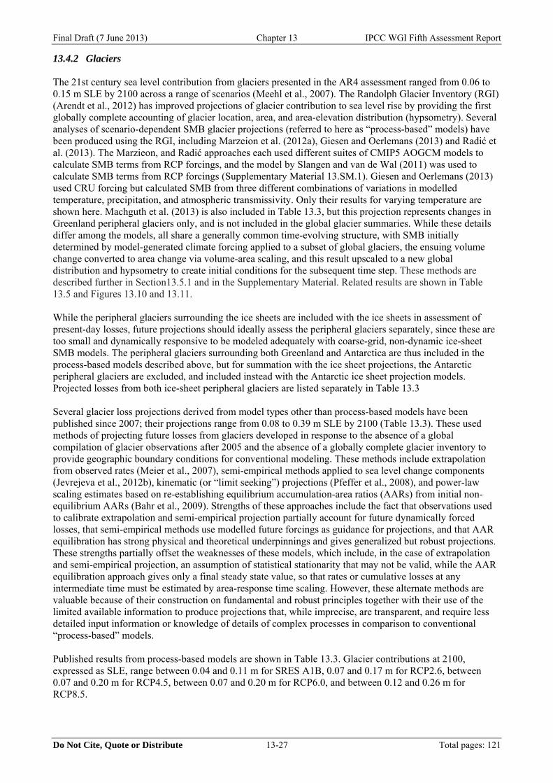
Final Draft (7 June 2013) Chapter 13 IPCC WGI Fifth Assessment Report
Do Not Cite, Quote or Distribute 13-27 Total pages: 121
13.4.2 Glaciers The 21st century sea level contribution from glaciers presented in the AR4 assessment ranged from 0.06 to 0.15 m SLE by 2100 across a range of scenarios (Meehl et al., 2007). The Randolph Glacier Inventory (RGI) (Arendt et al., 2012) has improved projections of glacier contribution to sea level rise by providing the first globally complete accounting of glacier location, area, and area-elevation distribution (hypsometry). Several analyses of scenario-dependent SMB glacier projections (referred to here as “process-based” models) have been produced using the RGI, including Marzeion et al. (2012a), Giesen and Oerlemans (2013) and Radić et al. (2013). The Marzieon, and Radić approaches each used different suites of CMIP5 AOGCM models to calculate SMB terms from RCP forcings, and the model by Slangen and van de Wal (2011) was used to calculate SMB terms from RCP forcings (Supplementary Material 13.SM.1). Giesen and Oerlemans (2013) used CRU forcing but calculated SMB from three different combinations of variations in modelled temperature, precipitation, and atmospheric transmissivity. Only their results for varying temperature are shown here. Machguth et al. (2013) is also included in Table 13.3, but this projection represents changes in Greenland peripheral glaciers only, and is not included in the global glacier summaries. While these details differ among the models, all share a generally common time-evolving structure, with SMB initially determined by model-generated climate forcing applied to a subset of global glaciers, the ensuing volume change converted to area change via volume-area scaling, and this result upscaled to a new global distribution and hypsometry to create initial conditions for the subsequent time step. These methods are described further in Section13.5.1 and in the Supplementary Material. Related results are shown in Table 13.5 and Figures 13.10 and 13.11. While the peripheral glaciers surrounding the ice sheets are included with the ice sheets in assessment of present-day losses, future projections should ideally assess the peripheral glaciers separately, since these are too small and dynamically responsive to be modeled adequately with coarse-grid, non-dynamic ice-sheet SMB models. The peripheral glaciers surrounding both Greenland and Antarctica are thus included in the process-based models described above, but for summation with the ice sheet projections, the Antarctic peripheral glaciers are excluded, and included instead with the Antarctic ice sheet projection models. Projected losses from both ice-sheet peripheral glaciers are listed separately in Table 13.3 Several glacier loss projections derived from model types other than process-based models have been published since 2007; their projections range from 0.08 to 0.39 m SLE by 2100 (Table 13.3). These used methods of projecting future losses from glaciers developed in response to the absence of a global compilation of glacier observations after 2005 and the absence of a globally complete glacier inventory to provide geographic boundary conditions for conventional modeling. These methods include extrapolation from observed rates (Meier et al., 2007), semi-empirical methods applied to sea level change components (Jevrejeva et al., 2012b), kinematic (or “limit seeking”) projections (Pfeffer et al., 2008), and power-law scaling estimates based on re-establishing equilibrium accumulation-area ratios (AARs) from initial non-equilibrium AARs (Bahr et al., 2009). Strengths of these approaches include the fact that observations used to calibrate extrapolation and semi-empirical projection partially account for future dynamically forced losses, that semi-empirical methods use modelled future forcings as guidance for projections, and that AAR equilibration has strong physical and theoretical underpinnings and gives generalized but robust projections. These strengths partially offset the weaknesses of these models, which include, in the case of extrapolation and semi-empirical projection, an assumption of statistical stationarity that may not be valid, while the AAR equilibration approach gives only a final steady state value, so that rates or cumulative losses at any intermediate time must be estimated by area-response time scaling. However, these alternate methods are valuable because of their construction on fundamental and robust principles together with their use of the limited available information to produce projections that, while imprecise, are transparent, and require less detailed input information or knowledge of details of complex processes in comparison to conventional “process-based” models. Published results from process-based models are shown in Table 13.3. Glacier contributions at 2100, expressed as SLE, range between 0.04 and 0.11 m for SRES A1B, 0.07 and 0.17 m for RCP2.6, between 0.07 and 0.20 m for RCP4.5, between 0.07 and 0.20 m for RCP6.0, and between 0.12 and 0.26 m for RCP8.5.
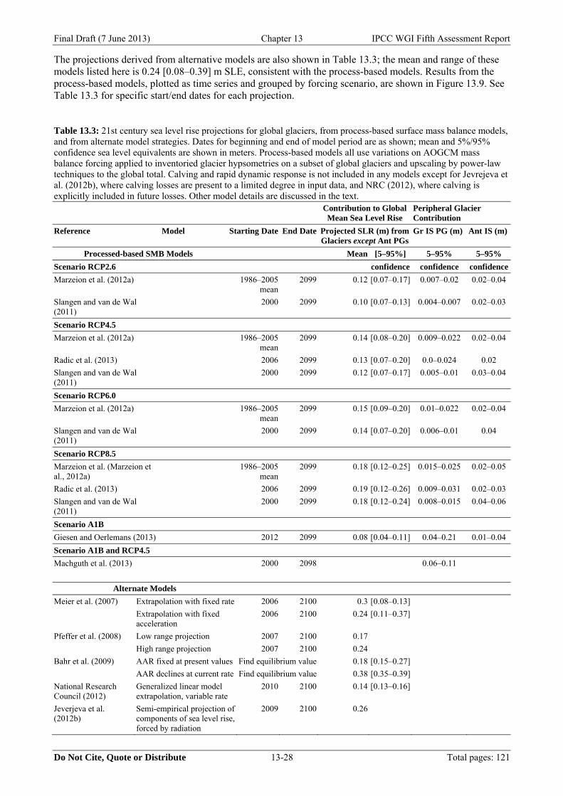
Final Draft (7 June 2013) Chapter 13 IPCC WGI Fifth Assessment Report
Do Not Cite, Quote or Distribute 13-28 Total pages: 121
The projections derived from alternative models are also shown in Table 13.3; the mean and range of these models listed here is 0.24 [0.08–0.39] m SLE, consistent with the process-based models. Results from the process-based models, plotted as time series and grouped by forcing scenario, are shown in Figure 13.9. See Table 13.3 for specific start/end dates for each projection. Table 13.3: 21st century sea level rise projections for global glaciers, from process-based surface mass balance models, and from alternate model strategies. Dates for beginning and end of model period are as shown; mean and 5%/95% confidence sea level equivalents are shown in meters. Process-based models all use variations on AOGCM mass balance forcing applied to inventoried glacier hypsometries on a subset of global glaciers and upscaling by power-law techniques to the global total. Calving and rapid dynamic response is not included in any models except for Jevrejeva et al. (2012b), where calving losses are present to a limited degree in input data, and NRC (2012), where calving is explicitly included in future losses. Other model details are discussed in the text. Contribution to Global
Mean Sea Level Rise Peripheral Glacier Contribution
Reference Model Starting Date End Date Projected SLR (m) from Glaciers except Ant PGs
Gr IS PG (m) Ant IS (m)
Processed-based SMB Models Mean [5–95%] 5–95% 5–95%
Scenario RCP2.6 confidence confidence confidence
Marzeion et al. (2012a) 1986–2005 mean
2099 0.12 [0.07–0.17] 0.007–0.02 0.02–0.04
Slangen and van de Wal (2011)
2000 2099 0.10 [0.07–0.13] 0.004–0.007 0.02–0.03
Scenario RCP4.5
Marzeion et al. (2012a) 1986–2005 mean
2099 0.14 [0.08–0.20] 0.009–0.022 0.02–0.04
Radic et al. (2013) 2006 2099 0.13 [0.07–0.20] 0.0–0.024 0.02
Slangen and van de Wal (2011)
2000 2099 0.12 [0.07–0.17] 0.005–0.01 0.03–0.04
Scenario RCP6.0
Marzeion et al. (2012a) 1986–2005 mean
2099 0.15 [0.09–0.20] 0.01–0.022 0.02–0.04
Slangen and van de Wal (2011)
2000 2099 0.14 [0.07–0.20] 0.006–0.01 0.04
Scenario RCP8.5
Marzeion et al. (Marzeion et al., 2012a)
1986–2005 mean
2099 0.18 [0.12–0.25] 0.015–0.025 0.02–0.05
Radic et al. (2013) 2006 2099 0.19 [0.12–0.26] 0.009–0.031 0.02–0.03
Slangen and van de Wal (2011)
2000 2099 0.18 [0.12–0.24] 0.008–0.015 0.04–0.06
Scenario A1B
Giesen and Oerlemans (2013) 2012 2099 0.08 [0.04–0.11] 0.04–0.21 0.01–0.04
Scenario A1B and RCP4.5
Machguth et al. (2013) 2000 2098 0.06–0.11
Alternate Models
Meier et al. (2007) Extrapolation with fixed rate 2006 2100 0.3 [0.08–0.13]
Extrapolation with fixed acceleration
2006 2100 0.24 [0.11–0.37]
Pfeffer et al. (2008) Low range projection 2007 2100 0.17
High range projection 2007 2100 0.24
Bahr et al. (2009) AAR fixed at present values Find equilibrium value 0.18 [0.15–0.27]
AAR declines at current rate Find equilibrium value 0.38 [0.35–0.39]
National Research Council (2012)
Generalized linear model extrapolation, variable rate
2010 2100 0.14 [0.13–0.16]
Jeverjeva et al. (2012b)
Semi-empirical projection of components of sea level rise, forced by radiation
2009 2100 0.26
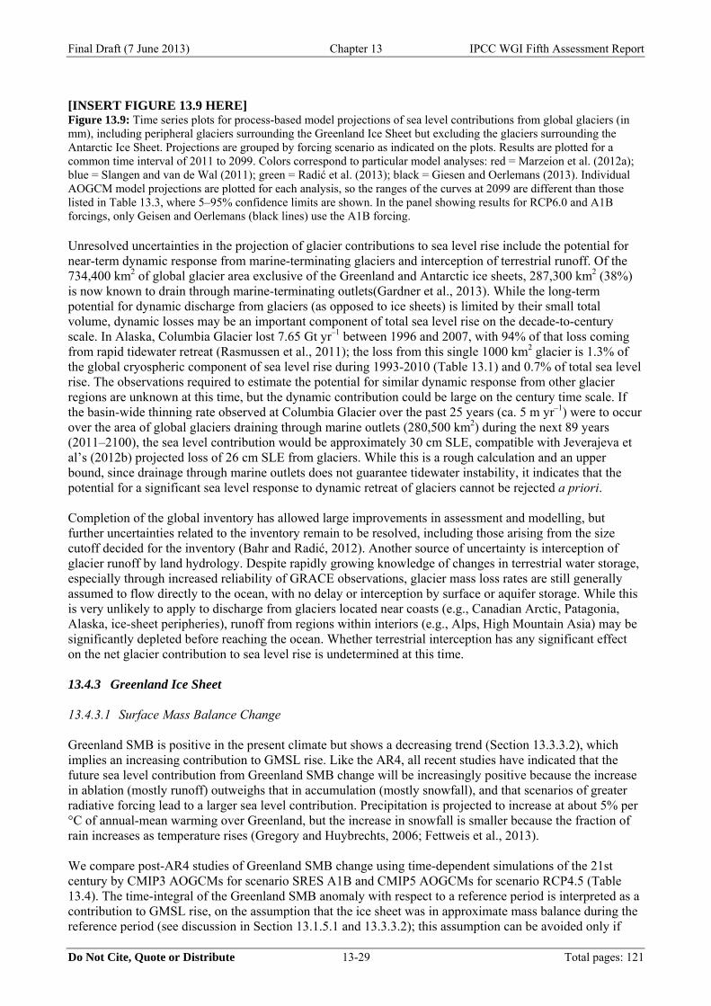
Final Draft (7 June 2013) Chapter 13 IPCC WGI Fifth Assessment Report
Do Not Cite, Quote or Distribute 13-29 Total pages: 121
[INSERT FIGURE 13.9 HERE] Figure 13.9: Time series plots for process-based model projections of sea level contributions from global glaciers (in mm), including peripheral glaciers surrounding the Greenland Ice Sheet but excluding the glaciers surrounding the Antarctic Ice Sheet. Projections are grouped by forcing scenario as indicated on the plots. Results are plotted for a common time interval of 2011 to 2099. Colors correspond to particular model analyses: red = Marzeion et al. (2012a); blue = Slangen and van de Wal (2011); green = Radić et al. (2013); black = Giesen and Oerlemans (2013). Individual AOGCM model projections are plotted for each analysis, so the ranges of the curves at 2099 are different than those listed in Table 13.3, where 5–95% confidence limits are shown. In the panel showing results for RCP6.0 and A1B forcings, only Geisen and Oerlemans (black lines) use the A1B forcing. Unresolved uncertainties in the projection of glacier contributions to sea level rise include the potential for near-term dynamic response from marine-terminating glaciers and interception of terrestrial runoff. Of the 734,400 km2 of global glacier area exclusive of the Greenland and Antarctic ice sheets, 287,300 km2 (38%) is now known to drain through marine-terminating outlets(Gardner et al., 2013). While the long-term potential for dynamic discharge from glaciers (as opposed to ice sheets) is limited by their small total volume, dynamic losses may be an important component of total sea level rise on the decade-to-century scale. In Alaska, Columbia Glacier lost 7.65 Gt yr–1 between 1996 and 2007, with 94% of that loss coming from rapid tidewater retreat (Rasmussen et al., 2011); the loss from this single 1000 km2 glacier is 1.3% of the global cryospheric component of sea level rise during 1993-2010 (Table 13.1) and 0.7% of total sea level rise. The observations required to estimate the potential for similar dynamic response from other glacier regions are unknown at this time, but the dynamic contribution could be large on the century time scale. If the basin-wide thinning rate observed at Columbia Glacier over the past 25 years (ca. 5 m yr–1) were to occur over the area of global glaciers draining through marine outlets (280,500 km2) during the next 89 years (2011–2100), the sea level contribution would be approximately 30 cm SLE, compatible with Jeverajeva et al’s (2012b) projected loss of 26 cm SLE from glaciers. While this is a rough calculation and an upper bound, since drainage through marine outlets does not guarantee tidewater instability, it indicates that the potential for a significant sea level response to dynamic retreat of glaciers cannot be rejected a priori. Completion of the global inventory has allowed large improvements in assessment and modelling, but further uncertainties related to the inventory remain to be resolved, including those arising from the size cutoff decided for the inventory (Bahr and Radić, 2012). Another source of uncertainty is interception of glacier runoff by land hydrology. Despite rapidly growing knowledge of changes in terrestrial water storage, especially through increased reliability of GRACE observations, glacier mass loss rates are still generally assumed to flow directly to the ocean, with no delay or interception by surface or aquifer storage. While this is very unlikely to apply to discharge from glaciers located near coasts (e.g., Canadian Arctic, Patagonia, Alaska, ice-sheet peripheries), runoff from regions within interiors (e.g., Alps, High Mountain Asia) may be significantly depleted before reaching the ocean. Whether terrestrial interception has any significant effect on the net glacier contribution to sea level rise is undetermined at this time. 13.4.3 Greenland Ice Sheet 13.4.3.1 Surface Mass Balance Change Greenland SMB is positive in the present climate but shows a decreasing trend (Section 13.3.3.2), which implies an increasing contribution to GMSL rise. Like the AR4, all recent studies have indicated that the future sea level contribution from Greenland SMB change will be increasingly positive because the increase in ablation (mostly runoff) outweighs that in accumulation (mostly snowfall), and that scenarios of greater radiative forcing lead to a larger sea level contribution. Precipitation is projected to increase at about 5% per °C of annual-mean warming over Greenland, but the increase in snowfall is smaller because the fraction of rain increases as temperature rises (Gregory and Huybrechts, 2006; Fettweis et al., 2013). We compare post-AR4 studies of Greenland SMB change using time-dependent simulations of the 21st century by CMIP3 AOGCMs for scenario SRES A1B and CMIP5 AOGCMs for scenario RCP4.5 (Table 13.4). The time-integral of the Greenland SMB anomaly with respect to a reference period is interpreted as a contribution to GMSL rise, on the assumption that the ice sheet was in approximate mass balance during the reference period (see discussion in Section 13.1.5.1 and 13.3.3.2); this assumption can be avoided only if
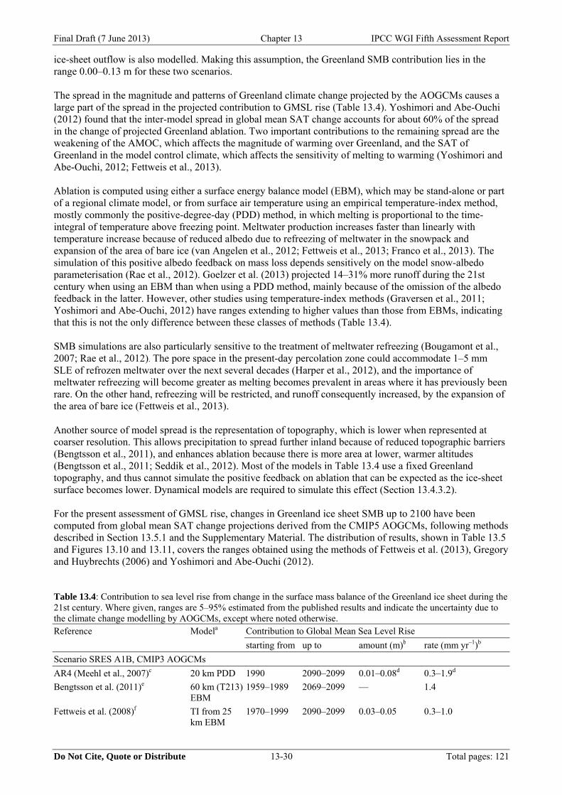
Final Draft (7 June 2013) Chapter 13 IPCC WGI Fifth Assessment Report
Do Not Cite, Quote or Distribute 13-30 Total pages: 121
ice-sheet outflow is also modelled. Making this assumption, the Greenland SMB contribution lies in the range 0.00–0.13 m for these two scenarios. The spread in the magnitude and patterns of Greenland climate change projected by the AOGCMs causes a large part of the spread in the projected contribution to GMSL rise (Table 13.4). Yoshimori and Abe-Ouchi (2012) found that the inter-model spread in global mean SAT change accounts for about 60% of the spread in the change of projected Greenland ablation. Two important contributions to the remaining spread are the weakening of the AMOC, which affects the magnitude of warming over Greenland, and the SAT of Greenland in the model control climate, which affects the sensitivity of melting to warming (Yoshimori and Abe-Ouchi, 2012; Fettweis et al., 2013). Ablation is computed using either a surface energy balance model (EBM), which may be stand-alone or part of a regional climate model, or from surface air temperature using an empirical temperature-index method, mostly commonly the positive-degree-day (PDD) method, in which melting is proportional to the time-integral of temperature above freezing point. Meltwater production increases faster than linearly with temperature increase because of reduced albedo due to refreezing of meltwater in the snowpack and expansion of the area of bare ice (van Angelen et al., 2012; Fettweis et al., 2013; Franco et al., 2013). The simulation of this positive albedo feedback on mass loss depends sensitively on the model snow-albedo parameterisation (Rae et al., 2012). Goelzer et al. (2013) projected 14–31% more runoff during the 21st century when using an EBM than when using a PDD method, mainly because of the omission of the albedo feedback in the latter. However, other studies using temperature-index methods (Graversen et al., 2011; Yoshimori and Abe-Ouchi, 2012) have ranges extending to higher values than those from EBMs, indicating that this is not the only difference between these classes of methods (Table 13.4). SMB simulations are also particularly sensitive to the treatment of meltwater refreezing (Bougamont et al., 2007; Rae et al., 2012). The pore space in the present-day percolation zone could accommodate 1–5 mm SLE of refrozen meltwater over the next several decades (Harper et al., 2012), and the importance of meltwater refreezing will become greater as melting becomes prevalent in areas where it has previously been rare. On the other hand, refreezing will be restricted, and runoff consequently increased, by the expansion of the area of bare ice (Fettweis et al., 2013). Another source of model spread is the representation of topography, which is lower when represented at coarser resolution. This allows precipitation to spread further inland because of reduced topographic barriers (Bengtsson et al., 2011), and enhances ablation because there is more area at lower, warmer altitudes (Bengtsson et al., 2011; Seddik et al., 2012). Most of the models in Table 13.4 use a fixed Greenland topography, and thus cannot simulate the positive feedback on ablation that can be expected as the ice-sheet surface becomes lower. Dynamical models are required to simulate this effect (Section 13.4.3.2). For the present assessment of GMSL rise, changes in Greenland ice sheet SMB up to 2100 have been computed from global mean SAT change projections derived from the CMIP5 AOGCMs, following methods described in Section 13.5.1 and the Supplementary Material. The distribution of results, shown in Table 13.5 and Figures 13.10 and 13.11, covers the ranges obtained using the methods of Fettweis et al. (2013), Gregory and Huybrechts (2006) and Yoshimori and Abe-Ouchi (2012). Table 13.4: Contribution to sea level rise from change in the surface mass balance of the Greenland ice sheet during the 21st century. Where given, ranges are 5–95% estimated from the published results and indicate the uncertainty due to the climate change modelling by AOGCMs, except where noted otherwise. Reference Modela Contribution to Global Mean Sea Level Rise
starting from up to amount (m)b rate (mm yr–1)b
Scenario SRES A1B, CMIP3 AOGCMs
AR4 (Meehl et al., 2007)c 20 km PDD 1990 2090–2099 0.01–0.08d 0.3–1.9d
Bengtsson et al. (2011)e 60 km (T213) EBM
1959–1989 2069–2099 — 1.4
Fettweis et al. (2008)f TI from 25 km EBM
1970–1999 2090–2099 0.03–0.05 0.3–1.0
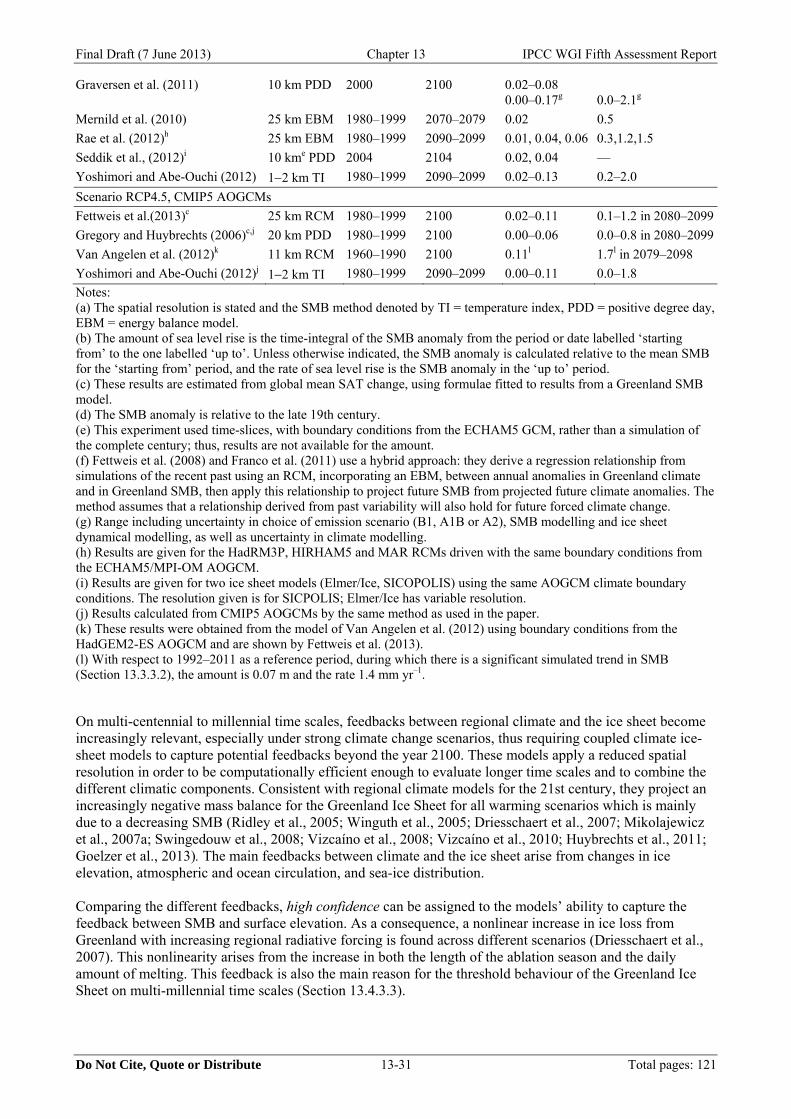
Final Draft (7 June 2013) Chapter 13 IPCC WGI Fifth Assessment Report
Do Not Cite, Quote or Distribute 13-31 Total pages: 121
Graversen et al. (2011) 10 km PDD 2000 2100 0.02–0.08 0.00–0.17g
0.0–2.1g
Mernild et al. (2010) 25 km EBM 1980–1999 2070–2079 0.02 0.5
Rae et al. (2012)h 25 km EBM 1980–1999 2090–2099 0.01, 0.04, 0.06 0.3,1.2,1.5
Seddik et al., (2012)i 10 kme PDD 2004 2104 0.02, 0.04 —
Yoshimori and Abe-Ouchi (2012) 12 km TI 1980–1999 2090–2099 0.02–0.13 0.2–2.0
Scenario RCP4.5, CMIP5 AOGCMs
Fettweis et al.(2013)c 25 km RCM 1980–1999 2100 0.02–0.11 0.1–1.2 in 2080–2099
Gregory and Huybrechts (2006)c,j 20 km PDD 1980–1999 2100 0.00–0.06 0.0–0.8 in 2080–2099
Van Angelen et al. (2012)k 11 km RCM 1960–1990 2100 0.11l 1.7l in 2079–2098
Yoshimori and Abe-Ouchi (2012)j 12 km TI 1980–1999 2090–2099 0.00–0.11 0.0–1.8
Notes: (a) The spatial resolution is stated and the SMB method denoted by TI = temperature index, PDD = positive degree day, EBM = energy balance model. (b) The amount of sea level rise is the time-integral of the SMB anomaly from the period or date labelled ‘starting from’ to the one labelled ‘up to’. Unless otherwise indicated, the SMB anomaly is calculated relative to the mean SMB for the ‘starting from’ period, and the rate of sea level rise is the SMB anomaly in the ‘up to’ period. (c) These results are estimated from global mean SAT change, using formulae fitted to results from a Greenland SMB model. (d) The SMB anomaly is relative to the late 19th century. (e) This experiment used time-slices, with boundary conditions from the ECHAM5 GCM, rather than a simulation of the complete century; thus, results are not available for the amount. (f) Fettweis et al. (2008) and Franco et al. (2011) use a hybrid approach: they derive a regression relationship from simulations of the recent past using an RCM, incorporating an EBM, between annual anomalies in Greenland climate and in Greenland SMB, then apply this relationship to project future SMB from projected future climate anomalies. The method assumes that a relationship derived from past variability will also hold for future forced climate change. (g) Range including uncertainty in choice of emission scenario (B1, A1B or A2), SMB modelling and ice sheet dynamical modelling, as well as uncertainty in climate modelling. (h) Results are given for the HadRM3P, HIRHAM5 and MAR RCMs driven with the same boundary conditions from the ECHAM5/MPI-OM AOGCM. (i) Results are given for two ice sheet models (Elmer/Ice, SICOPOLIS) using the same AOGCM climate boundary conditions. The resolution given is for SICPOLIS; Elmer/Ice has variable resolution. (j) Results calculated from CMIP5 AOGCMs by the same method as used in the paper. (k) These results were obtained from the model of Van Angelen et al. (2012) using boundary conditions from the HadGEM2-ES AOGCM and are shown by Fettweis et al. (2013). (l) With respect to 1992–2011 as a reference period, during which there is a significant simulated trend in SMB (Section 13.3.3.2), the amount is 0.07 m and the rate 1.4 mm yr–1. On multi-centennial to millennial time scales, feedbacks between regional climate and the ice sheet become increasingly relevant, especially under strong climate change scenarios, thus requiring coupled climate ice-sheet models to capture potential feedbacks beyond the year 2100. These models apply a reduced spatial resolution in order to be computationally efficient enough to evaluate longer time scales and to combine the different climatic components. Consistent with regional climate models for the 21st century, they project an increasingly negative mass balance for the Greenland Ice Sheet for all warming scenarios which is mainly due to a decreasing SMB (Ridley et al., 2005; Winguth et al., 2005; Driesschaert et al., 2007; Mikolajewicz et al., 2007a; Swingedouw et al., 2008; Vizcaíno et al., 2008; Vizcaíno et al., 2010; Huybrechts et al., 2011; Goelzer et al., 2013). The main feedbacks between climate and the ice sheet arise from changes in ice elevation, atmospheric and ocean circulation, and sea-ice distribution. Comparing the different feedbacks, high confidence can be assigned to the models’ ability to capture the feedback between SMB and surface elevation. As a consequence, a nonlinear increase in ice loss from Greenland with increasing regional radiative forcing is found across different scenarios (Driesschaert et al., 2007). This nonlinearity arises from the increase in both the length of the ablation season and the daily amount of melting. This feedback is also the main reason for the threshold behaviour of the Greenland Ice Sheet on multi-millennial time scales (Section 13.4.3.3).
Final Draft (7 June 2013) Chapter 13 IPCC WGI Fifth Assessment Report
Do Not Cite, Quote or Distribute 13-32 Total pages: 121
Medium-to-low confidence is assigned to the models’ representation of the atmospheric and ocean circulation and sea-ice changes. On multi-centennial time scales, Swingedouw et al. (2008) find enhanced ice loss from Greenland in a coupled simulation (compared to the uncoupled version) in which ice topography and melt-water flux influence the ocean and atmospheric circulation as well as sea-ice distribution. Vizcaíno et al. (2010) found reduced ice loss due to the coupling, mainly caused by the effect of topographic changes on the surface temperature, but less pronounced in amplitude compared with Swingedouw et al. (2008). Both the atmospheric circulation and the ocean currents, especially in coastal areas, are poorly resolved by these models. It is therefore likely that the time scales associated with ocean transport processes are distorted and there is low confidence that these feedbacks, while existent, can be quantified accurately by the applied models. The AMOC exerts a strong influence on regional climate around the Greenland Ice Sheet and consequently its SMB. Most CMIP5 models show a reduction of the AMOC under future warming during the 21st century and beyond (Section 12.4.7.2). While coupled climate-ice sheet models show some influence of melt water from Greenland on the AMOC, the uncertainty between models with respect to the AMOC response to warming is significantly larger than the difference between simulations with or without this feedback within one model. In the coupled climate-ice sheet model applied by Mikolajewicz et al. (2007a) and Vizcaíno et al. (2008), the AMOC shows a strongly non-linear response to global warming. A weak AMOC reduction is found for 1%-per-year-CO2-increase scenarios up to 560 and 840 ppm, and a near-complete cessation of the AMOC for 1120 ppm. As a consequence, after 600 years of integration, the sea level contribution for the 1120 ppm scenario is similar to that of the 560 ppm scenario, but doubles for the medium scenario which stabilizes at 840 ppm. In the most recent model version (Vizcaíno et al., 2010), the AMOC shows a strong weakening of the AMOC in all scenarios (~60% reduction in 560 ppm scenario; ~80% for 1120 ppm). The total sea level contribution from Greenland, including the effect of the AMOC weakening, is ~1 m (corresponding to an average rate of 1.7 mm yr–1) for 560 ppm CO2 and ~3 m (5 mm yr–1) for 1120 ppm CO2. Even though the AMOC weakening in the model by (Huybrechts et al., 2011) is less pronounced (10–25%), the ice loss through melting is significantly weaker in this model. During the first 1000 years of integration, the Greenland Ice Sheet contributes 0.36 m (corresponding to an average rate of 0.36 mm yr–1) for 560 ppm CO2 and 2.59 m (2.59 mm yr–1) for 1120 ppm CO2. In (Huybrechts et al., 2011), the respective increases in global mean SAT are 2.4°C (2 CO2) and 6.3°C (4 CO2) after 1000 years with respect to pre-industrial. This relatively weak warming response to GHG forcing compared to CMIP5 models and the climate model used in Vizcaíno et al. (2010) explains the relatively low sea level response. Using the same model as Huybrechts et al. (2011), albeit with a slightly higher polar warming, Goelzer et al. (2012) computed temperatures and sea level under the SRES scenarios B1, A1B and A2, with subsequent GHG stabilization after the year 2100. As in Huybrechts et al. (2011), the ice-sheet evolution is dominated by the SMB. They find sea level contributions of 1.4, 2.6 and 4.2 m in the year 3000 for the scenarios B1, A1B and B2, which correspond to mean rates of sea level rise of 1.4 mm yr–1, 2.6 mm yr–1, and 4.2 mm yr–1, respectively. In summary, coupled climate-ice sheet models consistently show an increasingly negative mass balance of the Greenland Ice Sheet mainly due to a decreasing SMB under warming scenarios on centennial time scales beyond 2100. On multi-millennial time scales, these models show a threshold temperature beyond which the melting of the Greenland Ice Sheet self-amplifies and the ice volume is reduced to less than 30% of its present volume (Section 13.4.3.3). 13.4.3.2 Dynamical Change Observations suggest three main mechanisms by which climate change can affect the dynamics of ice flow in Greenland (Sections 4.4.3 and 4.4.4): by directly affecting ice loss (outflow) through the calving of ice bergs and marine melt from marine-terminating outlet glaciers; by altering basal sliding through the interaction of surface melt water with the glacier bed; and indirectly through the interaction between SMB and ice flow. We assess the consequences of each of the processes.
Final Draft (7 June 2013) Chapter 13 IPCC WGI Fifth Assessment Report
Do Not Cite, Quote or Distribute 13-33 Total pages: 121
Section 4.4.3.2 presents the observational basis on which concerns about increased ice loss by calving and marine melt are based. In particular, recent increases in loss are thought to be linked to the migration of subtropical water masses around the coast of Greenland (Holland et al., 2008) and its occupation of coastal fjords (Straneo et al., 2010; Christoffersen et al., 2011). Output from 19 AOGCMs under scenario A1B showed warming of 1.7°C to 2.0°C around Greenland over the course of the 21st century (Yin et al., 2011), suggesting that the trend towards increased outflow triggered by warming coastal waters will continue. Although projections of outflow are at a fairly early stage, literature now exists to make an assessment. Flow-line modelling has successfully simulated the observed retreat and associated acceleration of the main outlet glaciers of the Greenland ice sheet (Helheim and Petermann Glaciers (Nick et al., 2009; Nick et al., 2012); Jakobshavn Isbræ (Vieli and Nick, 2011)). The same model has been used to project mass loss from these glaciers (Nick et al., 2013), as well as Kangerdlugssuaq Glacier, using ocean and atmosphere forcing based on scenarios A1B and RCP8.5. At 2100, total projected SLR spans 8–13 mm for A1B and 11–17 mm for RCP8.5. These figures generalise to 40–63 mm and 57–85 mm, respectively, for the whole ice sheet based on a simple scaling between modelled and total ice-sheet area (a factor ~5). Price et al. (2011) modelled the century-scale response of the ice sheet to the observed recent retreat of three outlet glaciers (Jakobshavn Isbræ, and Helheim and Kangerdlugssuaq Glaciers). At 2100, the projected SLR associated with the three modelled outlet glaciers is 0.6–1.4 mm, which equates to SLR of 4–8 mm after scaling (by a factor of ~6) to all outlet glaciers based on observed mass loss (van den Broeke et al., 2009). Total projected SLR then varies between 10 and 45 mm at 2100 if successive retreats are specified with a notional repeat interval between 50 and 10 years. Goelzer et al. (2013) implemented the Nick et al. (2013) retreat chronology within a 5-km resolution ice-sheet model along with their own generalization for including unsampled outlet glaciers. Associated SLR at 2100 is projected to vary between 8 and 18 mm. Graversen et al. (2011) attempted to capture the effect of increased outflow by enhancing basal sliding and generated SLR of 9–24 mm at 2100. Two estimates of the effect of dynamical change on Greenland’s contribution to SLR by 2100 have been made on the basis of physical intuition. Pfeffer et al. (2008) developed a low scenario by assuming a first-decade doubling of outlet glacier velocity throughout the ice sheet that equates to 93 mm SLR, while a high scenario that assumes an order of magnitude increase on the same time scale contributes 467 mm. Katsman et al. (2011) used a similar methodology to obtain an estimate of 100 mm SLR. Based primarily on Nick et al. (2013), we assess the upper limit of the likely 5–95% model range of this dynamical effect to be 85 mm for RCP8.5 and 63 mm for all other RCP scenarios. We have medium confidence in this as an upper limit because it is compatible with Katsman et al. (2011), the low scenario of Pfeffer et al. (2008), and Price et al. (2011) in the probable event of a sub-decadal recurrence interval. Although the likely upper limit is less than the high scenario of Pfeffer et al. (2008), process modelling gives no support to the order of magnitude increase in flow on which this scenario is based. It is higher than the contributions found by Goelzer et al. (2013) and Graversen et al. (2011) for which there are two potential explanations. First, the generalization used to extrapolate from the modelled sample to all outlet glaciers differs. Nick et al. (2013) used a scaling similar to the independently derived value of Price et al. (2011), while the implied scaling used by Goelzer et al. (2013) is substantially lower. Second, Goelzer et al. (2013) suggested that surface ice melt and calving compete to remove marginal ice (see below) implying that overall mass loss may be over predicted by the flow-line model of Nick et al. (2013). At present, these studies cannot be reconciled and we therefore use the more inclusive range. The lower limit of the likely 5–95% range is assessed as 20 mm for RCP8.5 and 14 mm for all other RCP scenarios. This reflects the individual outlet glacier projections of Nick et al. (2013) but uses a lower generalization more similar to that found by Goelzer et al. (2013). This assessment of the lower limit is compatible with Price et al. (2011) and Graversen et al. (2011). Section 4.4.3.2 assesses understanding of the link between abundant summer meltwater, lubrication of the ice-sheet base and enhanced ice flow. While this mechanism appears important in modulating present-day ice flow, it is not supported as the cause of recent mass loss. Goelzer et al. (2013) incorporated a parameterisation of this effect based on field observations, which results in less than a millimetre SLR by 2100 in their projections. Bindschadler et al. (2013) and Nowicki et al. (2013) reported a suite of

Final Draft (7 June 2013) Chapter 13 IPCC WGI Fifth Assessment Report
Do Not Cite, Quote or Distribute 13-34 Total pages: 121
experiments assessing this effect in an eight-model ensemble, but their parameterization appears overly simplistic and may well exaggerate the importance of the effect. These projections do not incorporate the effect on ice flow of the latent heat released by increased future quantities of melt water within the ice sheet (Phillips et al., 2010; 2013), for which no projections are currently available. Basal lubrication is therefore assessed as making an insignificant contribution to the likely range of SLR over the next century and is omitted in the remainder of the assessment. We have medium confidence in projections of this effect primarily because recent improvements in process-based understanding show that it has little contribution to mass loss (Section 4.4.3.2); the potential of latent-heat effects in the future limits a higher level of confidence. Finally, we assess the level of interaction between SMB change and ice flow. In AR4, this effect is assessed as 0 ± 10% (likely range) of SMB, based on Huybrechts and de Wolde (1999) and Gregory and Huybrechts (2006). This assessment included both the positive feedback between SMB and the height of the ice sheet, and a countering negative feedback involving ice flow and depletion effects. The latter effect is partly included in our assessment of the direct impacts of climate change on ice flow, and we therefore limit our assessment to SMB-height feedback. Few studies explicitly determine this effect, but Goelzer et al. (2013) reported that it amounts to 5–15% of SMB over the course of the 21st century, which we extend slightly (0–15%) to reflect possible interaction with mass loss by calving (Goelzer et al., 2013). Goelzer et al. (2013) and Gillet-Chaulet et al. (2012) suggested that SMB and ice dynamics cannot be assessed separately because of the strong interaction between ice loss and climate due to, for instance, calving and SMB. The current assessment has by necessity separated these effects because the type of coupled ice sheet—climate models needed to make a full assessment do not yet exist. These interactions may well combine to reduce SLR in comparison to the assessed range because of the mass-depletion effect of retreating outlet glaciers. Another source of uncertainty is the bedrock topography of Greenland, although recent improvements in data coverage (Bamber et al., 2013) suggest that the majority of the ice sheet rests on bedrock above sea level and the number of deep bedrock troughs penetrating into the interior of Greenland is limited, thus limiting the potential for marine ice-sheet instability (see Box 13.2). Although not strictly comparable because they contain a different balance of ice-dynamical effects, the assessment is consistent with Bindschadler et al. (2013) and Nowicki et al. (2013) who reported an extensive model inter-comparison exercise in which standardised experiments are combined to represent the impact of climate change under RCP8.5 on the Greenland Ice Sheet. The resultant projection included contributions from lubrication, marine melt and SMB-coupling and generated a mean SLR at 2100 of 162 mm over five models, or 53 mm if an outlier with anomalously high response is removed (including SMB results in SLR at 2100 of 223 and 114 mm for five- and four-model means, respectively). This comparison lends further weight to our confidence. In summary, dynamic change within the Greenland Ice Sheet is likely (medium confidence) to lead to SLR during the next century with a range of 20–85 mm for RCP8.5, and 14–63 mm for all other scenarios. The latter are assumed to have uniform SLR in the absence of literature allowing these scenarios to be assessed individually, although dependency on scenario is expected to exist. In addition, mass loss associated with SMB-height feedback is likely to contribute a further 0–15% of SMB (in itself scenario dependent). This equates to, for example, 0 to 11 mm based on the central estimate of RCP8.5 in Table 13.5. The peripheral glaciers of Greenland are not included here but are in the assessment of global glaciers’ contribution to SLR (Section 13.4.2). All the available literature suggests that this dynamical contribution to sea level rise will continue well beyond 2100. 13.4.3.3 Possible Irreversibility of Greenland Ice Loss and Associated Temperature Threshold A number of model results agree in showing that the Greenland Ice Sheet, like other climatic subsystems (Lenton et al., 2008; Levermann et al., 2012) (see Section 12.5.5), exhibits a strongly nonlinear and potentially irreversible response to surface warming. The mechanism of this threshold behaviour is the SMB-height feedback (Section 13.4.3.2); that is, as the surface is lowered due to ice loss, the associated warming of the near surface increases ablation, leading to further ice loss. This feedback is small but not negligible in the 21st century (Section 13.4.3.2) and becomes important for projections for the 22nd century (Goelzer et
Final Draft (7 June 2013) Chapter 13 IPCC WGI Fifth Assessment Report
Do Not Cite, Quote or Distribute 13-35 Total pages: 121
al. 2013). This nonlinear behaviour may be accelerated by a reduced surface albedo caused by surface melting which tends to further decrease the surface mass balance (Box et al., 2012) (Section 13.4.3.1). While the ice-sheet mean SMB is positive, in a steady state it must be balanced by ice outflow, so the ice sheet must extend to the coast. In a warmer climate, the mean SMB is reduced (Section 13.4.3.1) and the steady-state ice sheet will have a lower surface and volume. Models show a threshold in surface warming beyond which self-amplifying feedbacks result in a partial or near complete ice loss on Greenland (Greve, 2000; Driesschaert et al., 2007; Charbit et al., 2008; Ridley et al., 2010; Robinson et al., 2012). If a temperature above this threshold is maintained over a multi-millennial time period, the majority of the Greenland Ice Sheet will be lost by changes in SMB on a millennial to multi-millennial time scale (equivalent to a sea level rise of about 7 m, Table 4.1). During the Middle Pliocene warm intervals, when global mean temperature was 2°C–3.5°C higher than pre-industrial, ice-sheet models suggest near-complete deglaciation of Greenland. A simplifying assumption is that the threshold is the warming required with the current ice-sheet topography to reduce the mean SMB to zero, on the argument that the ice sheet must then retreat from the coast. Using this criterion, Gregory and Huybrechts (2006) estimated that the SMB threshold occurs for a global mean surface temperature increase of 3.1 [1.9 to 4.6]°C (5–95% confidence interval, 4.5 [3.0 to 6.0]°C for Greenland surface temperature) above pre-industrial (assumed to be a steady state). More recent studies have found thresholds below or in the lower part of this range. In a coupled ice sheet-climate model of intermediate complexity, (Huybrechts et al., 2011) found this threshold at 2.5°C of annual average Greenland SAT. Comparing three regional climate models, (Rae et al., 2012) found a strong dependence of the threshold on the model formulation of the SMB. Based on the model’s performance against observations and the physical detail of its surface scheme, MAR is considered the most realistic model, and yields a threshold value 2.8 [2.1–3.4] °C for changes in Greenland annual average temperature compared to preindustrial. Using MAR driven with output from various CMIP5 AOGCMs, Fettweis et al. (2013) evaluated the threshold as ~3°C in global mean surface temperature above 1980–1999 (hence about 3.5°C relative to pre-industrial), and found that it is not exceeded in the 21st century under the RCP4.5 scenario but is reached around 2070 under the RCP8.5 scenario. Some of the uncertainty in the threshold results from the value assumed for the steady-state ice-sheet SMB (see Table 13.2), and whether this is assumed to be pre-industrial or a more recent period. For 400 Gt yr–1 (Fettweis et al., 2013), the parametrisation of Greenland ice-sheet SMB used for present assessment of 21st century changes (Section 13.4.3.1, Supplementary Material) gives a global warming threshold of 3.0 [2.14.1]°C with respect to 18601879 (the reference period used in Box 13.1); for 225 Gt yr–1 (Gregory and Huybrechts, 2006, following Church et al., 2001), the threshold is 2.1 [1.53.0]°C. While a negative SMB is a sufficient condition for passing the threshold, it will overestimate the value of the threshold quantitatively, because the SMB-height feedback (even without passing the threshold) means that the steady-state SMB is reduced by more than is calculated assuming fixed topography. The actual SMB change will depend on the dynamical response of the ice sheet that determines its topography. Constraining simulations with a dynamic ice sheet model to changes during the last interglacial, Robinson et al. (2012) estimated the threshold as 1.6 [0.9–2.8]°C (5–95% confidence interval) global averaged temperature above pre-industrial. In these simulations they find that the threshold is passed when southeastern Greenland has a negative SMB. The near-complete ice loss then occurs through ice flow and SMB. The complete loss of the ice sheet is not inevitable because it has a long timescale (tens of millennia near the threshold and a millennium or more for temperatures a few degrees above the threshold). If the surrounding temperatures decline before the ice sheet is eliminated, the ice sheet might regrow. In the light of future GHG emissions, the time scale of ice loss is competing with the time scale of temperature decline after a reduction of GHG emissions (Allen et al., 2009; Solomon et al., 2009; Zickfeld et al., 2009). The outcome therefore depends on both the CO2 concentration and on how long it is sustained. Charbit et al. (2008) found that loss of the ice sheet is inevitable for cumulative emissions above about 3000 GtC, but a partial loss followed by regrowth occurs for cumulative emissions less than 2500 GtC. Ridley et al. (2010) identified three steady states of the ice sheet. If the CO2 concentration is returned to pre-industrial when more than 20–40% of the ice sheet has been lost, it will regrow only to 80% of its original volume due to a local climate feedback in one region; if 50% or more, it regrows to 20–40% of the original. Similar states with ice volume
Final Draft (7 June 2013) Chapter 13 IPCC WGI Fifth Assessment Report
Do Not Cite, Quote or Distribute 13-36 Total pages: 121
around 20, 60–80 and 100% of the initial ice volume are also found in other models (Langen et al., 2012; Robinson et al., 2012). If all the ice is lost, temperatures must decline to below a critical threshold for regrowth of the ice sheet (Robinson et al., 2012; Solgaard and Langen, 2012). On the evidence of paleo data and modelling (Section 5.6.2.4, 13.2.1), it is likely that during the LIG, when global mean temperature never exceeded 2oC pre-industrial, the Greenland Ice Sheet contributed no more than 3 m to GMSL. This could indicate that the threshold for near-complete deglaciation had not been passed, or that it was not greatly exceeded so that the rate of mass loss was low; however, the forcing responsible for the LIG warming was orbital rather than from CO2 (van de Berg et al., 2011), so it is not a direct analogue and the applicable threshold may be different. Studies with fixed-topography ice-sheets indicate a threshold of 2°C or above of global warming with respect to pre-industrial for near-complete loss of the Greenland ice-sheet, while the one study presently available with a dynamical ice-sheet suggests that the threshold could be as low as about 1°C (Robinson et al. 2012). Recent studies with fixed-topography ice-sheets indicate that the threshold is less than about 4°C. With currently available information, we do not have sufficient confidence to assign a likely range for the threshold. If the threshold is exceeded temporarily, an irreversible loss of part or most of the Greenland Ice Sheet could result, depending on for how long and by how much the threshold is exceeded. 13.4.4 Antarctic Ice Sheet 13.4.4.1 Surface Mass Balance Change Since the ice loss from Antarctic due to surface melt and runoff is about 1% of the of the total mass gain from snowfall, most ice loss occurs through solid ice discharge into the ocean. In the 21st century, ablation is projected to remain small on the Antarctic ice sheet because low surface temperatures inhibit surface melting, except near the coast and on the Antarctic Peninsula, and meltwater and rain continue to freeze in the snowpack (Ligtenberg et al., 2013). Projections of Antarctic SMB changes over the 21st century thus indicate a negative contribution to sea level because of the projected widespread increase in snowfall associated with warming air temperatures (Krinner et al., 2007; Uotila et al., 2007; Bracegirdle et al., 2008). Several studies (Krinner et al., 2007; Uotila et al., 2007; Bengtsson et al., 2011) have shown that the precipitation increase is directly linked to atmospheric warming via the increased moisture holding capacity of warmer air, and is therefore larger for scenarios of greater warming. The relationship is exponential, resulting in an increase of SMB as a function of Antarctic SAT change evaluated in various recent studies with high-resolution (~60 km) models as 3.7% °C–1 (Bengtsson et al., 2011), 4.8% °C– (Ligtenberg et al., 2013) and ~7% °C–1 (Krinner et al., 2007). These agree well with the sensitivity of 5.1 ± 1.5% °C–1 (one standard deviation) of CMIP3 AOGCMs (Gregory and Huybrechts, 2006). The effect of atmospheric circulation changes on continental-mean SMB is an order of magnitude smaller than the effect of warming, but circulation changes can have a large influence on regional changes in accumulation, particularly near the ice-sheet margins (Uotila et al., 2007) where increased accumulation may induce additional ice flow across the grounding line (Huybrechts and De Wolde, 1999; Gregory and Huybrechts, 2006; Winkelmann et al., 2012). Simulated SMB is strongly and non-linearly influenced by ocean surface temperature and sea ice conditions (Swingedouw et al., 2008). This dependence means that the biases in the model-control climate may distort the SMB sensitivity to climate change, suggesting that more accurate predictions may be obtained from regional models by using boundary conditions constructed by combining observed present-day climate with projected climate change (Krinner et al., 2008). There is a tendency for higher resolution models to simulate a stronger future precipitation increase because of better representation of coastal and orographic precipitation processes (Genthon et al., 2009). For the present assessment of GMSL rise, changes in Antarctic ice sheet SMB up to 2100 have been computed from global mean SAT change projections derived from the CMIP5 AOGCMs, using the range of sensitivities of precipitation increase to atmospheric warming summarized above, and the ratio of Antarctic to global warming evaluated from CMIP3 AOGCMs by Gregory and Huybrechts (2006) (see also Section 13.5.1 and Supplementary Material). The results are shown in Table 13.5 and Figures 13.10 and 13.11. The projected change in ice outflow is affected by the SMB because of the influence of topography on ice dynamics (Section 13.4.4.2 and Supplementary Material). Ozone recovery, through its influence on atmospheric circulation at high southern latitudes (Section 10.3.3.5), may offset some effects of greenhouse
Final Draft (7 June 2013) Chapter 13 IPCC WGI Fifth Assessment Report
Do Not Cite, Quote or Distribute 13-37 Total pages: 121
gas increase in the 21st century, but Antarctic precipitation is nonetheless projected to increase (Polvani et al., 2011). Bintanja et al. (2013) suggested that Antarctic warming and precipitation increase may be suppressed in the future by expansion of Antarctic sea ice, promoted by freshening of the surface ocean, caused by basal melting of ice shelves, and they conduct an AOGCM sensitivity test of this hypothesis. We consider these possibilities in Section 13.5.3. Beyond the year 2100, regional climate simulations run at high spatial resolution (5–55 km) but without climate-ice sheet feedbacks included show a net ice gain until the year 2200 (Ligtenberg et al., 2013). During the 22nd century, the ice gain is equivalent to an average rate of sea level fall of 1.2 mm yr–1 for the A1B scenario and 0.46 mm yr–1 the E1 scenario. For multi-centennial to multi-millennial projections, feedbacks between the ice sheet and regional climate need to be accounted for. This is currently done using ice-sheet models coupled to climate models of intermediate complexity, which have a significantly lower spatial resolution in the atmospheric component than regional climate models used to assess future SMB within the 21st century. These coarser resolution models capture the increase in snowfall under future warming, but the regional distribution is represented less accurately. Accordingly, there is low confidence in their ability to model spatial melting and accumulation patterns accurately. In contrast, medium confidence can be assigned to the models’ projection of total accumulation on Antarctica, since it is controlled by the large-scale moisture transport toward the continent. In idealized scenarios of 1% increase of CO2 yr–1 up to 560 ppm with subsequent stabilization, Vizcaíno et al. (2010) and Huybrechts et al. (2011) found an initial increase of ice volume due to additional snowfall during the first 600 years of integration. In both models, the changes in SMB dominate the mass changes during and beyond the first 100 years. After 600 years of integration, Vizcaíno et al. (2010) found a mass gain corresponding to a sea level fall of 0.15 m (–0.25 mm yr–1 on average). For the same experiment and the same period, Huybrechts et al. (2011) found a similar sea level fall of 0.08 m (–0.13 mm yr–1 on average). In a similar experiment but allowing GHG concentrations to reach 1120 ppm CO2 before being stabilized, both models show a net positive sea level contribution after 600 years of integration. Huybrechts et al. (2011) found a weak sea level contribution during the first 500 years of integration followed by a stronger and relatively constant long-term average rate of ~2 mm yr–1 after 1000 years of integration up to a total contribution of ~4 m SLE after 3000 years of integration. While they found some grounding line retreat due to basal ice-shelf melt, the multi-centennial evolution of the ice sheet is dominated by changes in SMB while the solid-ice discharge after an initial increase shows a significant decrease during the scenario. For the same scenario, Vizcaíno et al. (2010) found that the initial mass gain is followed by a weak mass loss. After 250 years of integration, the contribution is stronger and relatively constant at a rate of about 3 mm yr–1, corresponding to a net contribution of 1.2 m to global mean sea level rise after 600 years. The same model as in Huybrechts et al. (2011), although with a slightly stronger polar amplification, was applied to the three SRES scenarios used in the AR4 (B1, A1B, A2) with stabilization in the year 2100 (Goelzer et al., 2012). For the lowest scenario (B1), they found practically no net Antarctic contribution to sea level in the year 3000. Under the medium scenario (A1B), the ice sheet contributes 0.26 m, and under the highest scenario (A2), it contributes 0.94 m SLE in the year 3000. These simulations include a negative feedback on the regional climate by ice-sheet melt through which summer temperatures can be significantly reduced over Antarctica (Swingedouw et al., 2008). However, due to the coarse resolution and the high polar amplification, there is low confidence in the model´s representation of oceanic circulation changes around Antarctica. In both models (Vizcaíno et al., 2010; Huybrechts et al., 2011), the ice sheets are not equilibrated with the surrounding climate after the integration period under the 1120 ppm CO2 forcing. Though GHG concentrations were stabilized after 120 years of integration, the Antarctic Ice Sheet continues to contribute to sea level rise at a relatively constant rate for another 480 years in Vizcaíno et al. (2010) and 2880 years in Huybrechts et al. (2011). This is consistent with a positive sea level contribution from Antarctica during past warmer climates (Sections 13.2.1, 13.5.2).
Final Draft (7 June 2013) Chapter 13 IPCC WGI Fifth Assessment Report
Do Not Cite, Quote or Distribute 13-38 Total pages: 121
In summary, both coupled ice sheet-climate models consistently show that for high-emission scenarios, the surface melt increases and leads to an ice loss on multi-centennial time scales. The long time period over which the Antarctic Ice Sheet continues to lose mass indicates a potential role of the feedback between climate and ice sheet. Consistent with regional climate models for the 21st and 22nd centuries, both coarse-resolution coupled models show a positive SMB change for most of the first 100 years of climate change. Due to the inertia in the climate system, regional temperatures continue to rise after that. Together with enhanced solid ice discharge, this results in mass loss of AIS. The corresponding decline in surface elevation increases the surface temperature and leads to additional ice loss. 13.4.4.2 Dynamical Change The Antarctic Ice Sheet represents the largest potential source of future SLR; the West Antarctic Ice Sheet (WAIS) alone has the potential to raise sea level by ~4.3 m (Fretwell et al., 2013). The rate at which this reservoir will be depleted and cause sea level to rise, however, is not easily quantifiable. In this section, we focus on dynamical changes (i.e., those related to the flow of the ice sheet) which affect SLR by altering the flux of ice across the grounding line (or outflow) that separates ice resting on bedrock (some of which does not currently displace ocean water) from floating ice shelves (which already displace ocean water and have only a negligible effect on sea level) (Jenkins and Holland, 2007). Issues associated with the inability of models to reproduce recently observed changes in the dynamics of the Antarctic Ice Sheet prevented the AR4 from fully quantifying the effect of these changes on future sea level. Since the AR4, progress has been made in understanding the observations (Sections 4.4.3 and 4.4.4), and projections are becoming available. It must be stressed, however, that this field has yet to reach the same level of development that exists for modelling many other components of the Earth system. There is an underlying concern that observations presage the onset of large-scale grounding line retreat in what is termed the Marine Ice Sheet Instability (MISI; Box 13.2), and much of the research assessed here attempts to understand the applicability of this theoretical concept to projected SLR from Antarctica. There are three distinct processes that could link climate change to dynamical change and potentially trigger increased outflow directly through the increased potential for melt ponds to form on the upper surface of ice shelves, which may destabilize them, or by increases in submarine melt experienced by ice shelves as a consequence of oceanic warming, which leads to their thinning, and indirectly by coupling between SMB and ice flow. Section 4.4.3.2 presents the observational basis on which understanding of these processes is based, while their potential future importance is assessed here. Literature on two mechansims directly linked to climate change will be assessed first, followed by their relation to outflow change and lastly SMB coupling. There is strong evidence that regional warming and increased melt water ponding in the Antarctic Peninsula led to the collapse of ice shelves along the length of Antarctic Peninsula (Cook and Vaughan, 2010), most notably the Larsen B ice shelf (MacAyeal et al., 2003). Substantial local warming (~5-7 C) would, however, be required before the main Antarctic ice shelves (the Ross and Filchner-Ronne ice shelves) would become threatened (Joughin and Alley, 2011). An assessment of the AR4 AOGCM ensemble under scenario A1B yielded an Antarctic continental-average warming rate of 0.034 ± 0.01C yr–1 (Bracegirdle et al., 2008), suggesting that the required level of warming may not be approached by the end of the century. Using an intermediate complexity model with scenario A2, Fyke et al. (2010) found that melt starts to reach significant levels over these ice shelves around 2100 to 2300. Barrand et al. (2013) made a process-based assessment of the effect of ice-shelf collapse on outflow from the Antarctic Peninsula, which yields a range of SLR at 2100 between 10 and 20 mm, with a bounding maximum of 40 mm. There is good evidence linking the focus of current Antarctic mass loss in the Amundsen Sea sector of WAIS (containing Pine Island and Thwaites Glaciers) (Shepherd and Wingham, 2007; Rignot et al., 2008; Pritchard et al., 2009) to the presence of relatively warm Circumpolar Deep Water on the continental shelf (Thoma et al., 2008; Jenkins et al., 2010). However, it is not possible to determine whether this upwelling was related directly or indirectly to a rise in global mean temperature. Yin et al. (2011) assessed output from 19 AOGCMs under scenario A1B to determine how subsurface temperatures are projected to evolve around the West and East Antarctic ice sheets. They showed decadal-mean warming of 0.4°C–0.7C and 0.4°C–
Final Draft (7 June 2013) Chapter 13 IPCC WGI Fifth Assessment Report
Do Not Cite, Quote or Distribute 13-39 Total pages: 121
0.9C around West and East Antarctica, respectively (25th to 75th percentiles of ensemble) by the end of the 21st century. More detailed regional modelling using scenario A1B illustrates the potential for warm water to invade the ocean cavity underlying the Filchner-Ronne ice shelf in the second half of the 21st century, with an associated 20-fold increase in melt (Hellmer et al., 2012). Based on the limited literature, there is medium confidence that oceanic processes may potentially trigger further dynamical change particularly in the latter part of the 21st century, while there is also medium confidence that atmospheric change will not affect dynamics outside of the Antarctic Peninsula. Several process-based projections of the future evolution of Pine Island Glacier have now been made, and some of the issues that this modelling faced (such as the need for sub-kilometre resolution to ensure consistent results; Cornford et al. (2013), Durand et al. (2009)) are being resolved (Pattyn et al., 2013). In experiments using an idealised increase in marine melt, Joughin et al. (2010) demonstrated only limited (~25 km) retreat of the grounding line before a new equilibrium position was established. Gladstone et al. (2012) used a flow-line model forced with ocean-model output (Hellmer et al., 2012) to identify two modes of retreat: one similar to that identified by Joughin et al. (2010), and a second characterized by complete collapse from 2150 onwards. More sophisticated ice-flow modelling (albeit with idealized forcing) suggests grounding line retreat of ~100 km in 50 years (Cornford et al., 2013). These studies support the theoretical finding of Gudmundsson et al. (2012) that grounding line retreat, if triggered, does not inevitably lead to MISI but may halt if local buttressing from ice rises or channel sidewalls is sufficient. Parizek et al. (2013) used a flow-line model to study Thwaites Glacier and found that grounding line retreat is only possible under extreme ocean forcing. It is also thought that considerably less back pressure is exerted by Thwaites’ ice shelf in comparison to Pine Island’s (Rignot, 2001; 2008), which may make it less sensitive to forcing by submarine melt (Schoof, 2007b; Goldberg et al., 2012). Based on this literature, there is high confidence that the retreat of Pine Island Glacier (if it occurs) can be characterised by a SLR measured in centimetres by 2100, although there is low confidence in the models’ ability to determine the probability or timing of any such retreat. There is also moderate confidence (in the light of the very limited literature) that Thwaites Glacier is probably less prone to undergo ocean-driven grounding line retreat than its neighbour in the 21st century. No process-based modelling is available on which to be base projections of EAIS glaciers currently losing mass, such as Totten and Cook Glaciers. Bindschadler et al. (2013) reported a model inter-comparison exercise on the impact of climate change under RCP8.5 on the Antarctic Ice Sheet. The resultant projection includes contributions from increased marine melt in the Amundsen Sea and Amery sectors, and generated a mean SLR at 2100 of ~100 mm over four models (with overall SLR of 81 mm when SMB change was included). There is, however, low confidence in the projection because of the unproven ability of many of the contributing models to simulate grounding line motion. Bindschadler et al. (2013) also reported idealized experiments in which ice-shelf melt is increased by 2, 20 and 200 m yr–1. The resulting five-model mean SLR of 69, 693 and 3477 mm by 2100, respectively, can only be considered as a general indication because of the shortcomings of the contributing models (e.g., two do not include ice shelves) which may be offset by the use of a multi-model mean. While grounding line migration in the 20 m yr–1 experiment is extensive in some models and consistent with what might be expected under MISI (Nowicki et al., 2013), the 200 m yr–1 experiment is unrealistic, even if used as a proxy for the improbable atmosphere-driven collapse of the major ice shelves, and is not considered further. We now assess two alternatives to process-based modelling that exist in the literature: the development of plausible high-end projections based on physical intuition (Pfeffer et al., 2008; Katsman et al., 2011) and the use of a probabilistic framework for extrapolating current observations of the ice sheet’s mass budget (Little et al., 2013a; 2013b). Pfeffer et al. (2008) postulated a possible but extreme scenario of 615 mm SLR based on vastly accelerated outflow in the Amundsen Sea sector and East Antarctica, whereas a more plausible scenario involving reduced acceleration in the Amundsen Sea sector yields 136 mm. Katsman et al. (2011) used similar assumptions in a “modest” scenario that generates SLR of 70–150 mm, and a “severe” scenario that attempts to capture the consequences of the collapse of the WAIS through the MISI and has a SLR contribution of 490 mm. The NRC (2012) extrapolated mass-budget observations of the ice sheet to generate a projection of 157–323 mm (including future SMB change), with an additional 77–462 mm accounting for 21st-century increases in outflow (summing as 234 to 785 mm). Little et al. (2013a) applied a range of linear growth rates to present-day SMB and outflow observations of Antarctic sectors (Rignot et al., 2008; Shuman et al., 2011; Zwally and Giovinetto, 2011), which are then

Final Draft (7 June 2013) Chapter 13 IPCC WGI Fifth Assessment Report
Do Not Cite, Quote or Distribute 13-40 Total pages: 121
weighted using a continental-scale observational synthesis (Shepherd et al., 2012) (consistent with the assessment of Chapter 4). In the case of Pine Island Glacier, growth rates are based on the process-based modelling of Joughin et al. (2010). Within this framework, SLR at 2100 has a 5–95% range of –20 to 185 mm for dynamical change only, and –86 to 133 mm when SMB change is included (based on Uotila et al. (2007)). Projections for the Antarctic Peninsula are consistent with the process-based modelling of Barrand et al. (2013). Further, Little et al. (2013a) found that the upper (95%) limit of the projected range can only approach 400 mm under scenarios expected for MISI (such as the immediate collapse of Pine Island and Thwaites Glaciers or all marine-based sectors experiencing the same rates of mass loss as Pine Island Glacier). Our assessment of the likely (17 to 83%) range of SLR by 2100 is based around Little et al. (2013a). Their weighted 5–95% range of –20 to 185 mm is consistent with the lower scenarios of Katsman et al. (2011) (70–150 mm) and Pfeffer et al. (2008) (136 mm), and with the RCP8.5 projection and low-melt experiment of Bindschadler et al. (2013) (~100–69 mm, respectively). The base projection of the NRC (2012) (157–323 mm including future SMB change), however, is less compatible. This moderate level of consistency across a range of techniques suggests medium confidence in this assessment. We assess this as the likely (as opposed to very likely) range because it is based primarily on perturbations of the ice-sheet’s present-day state of mass imbalance and does not include the potentially large increases in outflow that may be associated with the MISI discussed below. The probability of extensive grounding line retreat being both triggered and continuing to the extent that it contributes to significant SLR in the 21st century is very poorly constrained, as the results of a recent expert elicitation indicate (Bamber and Aspinall, 2013). We have medium confidence, however, that this probability lies outside of the likely range of SLR (i.e, with probability less than 17%). Five arguments support this assessment. First, the partial loss of Pine Island Glacier is included by Little et al. (2013a) in their range and the full loss of the ice stream (if it were to occur) is thought to raise sea level by centimetres only (consistent with the use of the Little et al. (2013a) 9–95% range as the assessed likely 17–83% range). Second, the current grounding line position of the neighbouring Thwaites Glacier appears to be more stable than that of Pine Island Glacier (Parizek et al., 2013) so that its potentially large contribution to SLR by 2100 is assessed to have a significantly lower probability. Third, there is a low probability that atmospheric warming in the 21st century will lead to extensive grounding line retreat outside of the Antarctic Peninsula because summer air temperatures will not rise to the level where significant surface melt and ponding occur. Fourth, while this retreat may be triggered by oceanic warming during the 21st century (in particular, under the Filchner-Ronne ice shelf), current literature suggests that this may occur late in the century (Hellmer et al., 2012), reducing the time over which enhanced outflow could affect end-of-century SLR. Finally, there are theoretical grounds to believe that grounding line retreat may stabilise (Gudmundsson et al., 2012) so that MISI (and associated high SLR) is not inevitable. We next assess the magnitude of potential SLR at 2100 in the event that MISI affects the Antarctic Ice Sheet. Bindschadler et al. (2013), Katsman et al. (2011), the NRC (2012), and Pfeffer et al. (2008) presented contrasting approaches that can be used to make this assessment, which are upper-end estimates of 693, 490, 785 and 615 mm, respectively. Together this literature suggests with medium confidence that this contribution would be several tenths of a metre. The literature does not offer a means of assessing the probability of this contribution, however, other than our assessment (above) that it lies above the likely range (i.e, less than 17% probability). Literature investigating the relation between the SLR generated by dynamical change and emission scenario does not currently exist. There is also a lack of literature on the relation between emission scenario and the intrusions of warm water into ice-shelf cavities thought to be important in triggering observed mass loss (Jacobs et al., 2011) and potentially important in the future (Hellmer et al., 2012). It is therefore premature to attach a scenario-dependence to projections of dynamical change, even though such a dependency is expected to exist. Likely increases in snowfall over the next century (Section 13.4.4.1) will affect the amount of ice lost by outflow across the grounding line because of local changes in ice thickness and stress regime (Huybrechts and De Wolde, 1999). This effect was incorporated in AR4 projections for 2100 as a compensatory mass loss amounting to 0-10% of the SMB mass gain (Gregory and Huybrechts, 2006). Winkelmann et al. (2012) re-
Final Draft (7 June 2013) Chapter 13 IPCC WGI Fifth Assessment Report
Do Not Cite, Quote or Distribute 13-41 Total pages: 121
evaluated the effect and reported a range of 15–35% for the next century (30–65% after 500 years). The two studies are difficult to compare because of differences in model physics and experimental design so that the use of their joint range (0-35%) is an appropriate assessment of the likely range of this effect. This range is supported by Barrand et al. (2013) who quantified the effect for the Antarctic Peninsula as ~15% of SMB. Moreover, because this contribution relies on similar physics to the grounding line migration discussed above, it is appropriate to assume that their uncertainties are correlated. Winkelmann et al. (2012) showed that the fractional size of this compensatory effect is independent of scenario. Accounting for this effect equates to SLR of 0–32 mm by 2100 based on the SMB range over all emission-scenario projections in Section 13.5.1.1. Beyond the 21st century, only projections with coarse-resolution ice sheet-climate models are available (Vizcaíno et al., 2010; Huybrechts et al., 2011). Confidence in the ability of these two models to capture both change in the oceanic circulation around Antarctica and the response of the ice sheet to these changes, especially a potential grounding line retreat, is low. The model applied by Vizcaíno et al. (2010) is lacking a dynamic representation of ice shelves. Since dynamic ice discharge from Antarctica occurs predominately through ice shelves, it is likely that the projections using this model considerably underestimate the Antarctic contribution. In summary, it is likely that dynamical change within the Antarctic ice sheet will lead to SLR during the next century with a range of –20 to 185 mm. SLR beyond the likely range is poorly constrained and considerably larger increases are possible, which will probably be associated with the MISI (Box 13.2). Although the likelihood of such SLR cannot yet be assessed more precisely than falling above the likely range, literature suggests (with medium confidence) that its potential magnitude is several tenths of a metre. We are unable to assess SLR as a function of emission scenario, although a dependency of SLR on scenario is expected to exist. In addition, coupling between SMB and dynamical change is likely to make a further contribution to SLR of 0–35% of the SMB. All the available literature suggests that this dynamical contribution to sea level rise will continue well beyond 2100. 13.4.4.3 Possible Irreversibility of Ice Loss from West Antarctica Due to relatively weak snowfall on Antarctica and the slow ice motion in its interior, it can be expected that the West Antarctic Ice Sheet (WAIS) would take at least several thousand years to regrow if it was eliminated by dynamic ice discharge. Consequently any significant ice loss from West Antarctic that occurs within the next century will be irreversible on a multi-centennial to millennial time scale. We discuss here the possibility of abrupt dynamic ice loss from West Antarctica (see Section 12.5.5 for definition of abrupt). Information on the ice- and bed-topography of WAIS suggest that it has about 3.3 m of equivalent global sea level grounded on areas with downward sloping bedrock (Bamber et al., 2009). As detailed in Box 13.2, large areas of WAIS may therefore be subject to potential ice loss via the marine ice-sheet instability (MISI). As it is the case for other potential instabilities within the climate system (Section 12.5.5), there are four lines of evidence to assess the likelihood of a potential occurrence: theoretical understanding, present-day observations, numerical simulations, and paleo-records. The MISI is based on a number of studies which indicated the theoretical existence of the instability (Weertman, 1961; Schoof, 2007b) (see also Box 13.2). The most fundamental derivation, i.e. starting from a first-principle ice-equation, states that in one-dimensional ice flow the grounding line between grounded ice sheet and floating ice shelf cannot be stable on a landward sloping bed. The limitation of the one-dimensional case disregards likely stabilizing effects of the ice shelves (Dupont and Alley, 2005). While it is clear that ice shelves that are laterally constrained by embayments inhibit ice flow into the ocean, the effect has not been quantified against the MISI. The same is true for other potentially stabilizing effects such as sedimentation near the grounding line (Alley et al., 2007) or the influence of large-scale bedrock roughness (i.e. topographic pinning points) on ice flow. While these stabilizing effects need to be further investigated and quantified against the destabilizing effect of the MISI, no studies are available that would allow dismissing the MISI on theoretical grounds. Although direct observations of ice dynamics are available, they are neither detailed enough nor cover a sufficiently long period to allow the monitoring of the temporal evolution of an MISI. Most Antarctic ice
Final Draft (7 June 2013) Chapter 13 IPCC WGI Fifth Assessment Report
Do Not Cite, Quote or Distribute 13-42 Total pages: 121
loss that has been detected during the satellite period has come from WAIS (Rignot et al., 2008; Pritchard et al., 2012). Some studies have found an acceleration of ice loss (Rignot et al., 2011) as well as enhanced basal ice-shelf melting (Pritchard et al., 2012), but the short period of observations does not allow one to either dismiss or confirm that these changes are associated with destabilization of WAIS. Paleo records suggest that WAIS may have deglaciated several times during warm periods of the last 5 million years, but they contain no information on rates (Naish et al., 2009). While coarse-resolution models are in principle capable of modelling the MISI, there is medium confidence in their ability to simulate the correct response time to external perturbations on decadal to centennial time scales (Pattyn et al., 2013). One of these models (Pollard and DeConto, 2009) reproduced paleo-records of deglaciation with a forced ice-sheet model at 40 km resolution and parameterized ice flow across the grounding line according to Schoof (2007b). These simulations showed a sea level rise of about 7 m over time spans of 1000–7000 years with approximately equal contributions from West and East Antarctica. However, no available model results or paleo records have indicated the possibility of self-accelerated ice discharge from these regions. In summary, based on ice-dynamics theory, numerical simulations, and paleo records, it is likely that abrupt and irreversible ice loss from WAIS is possible. However, theoretical considerations, current observations, numerical models, and paleo records currently do not allow a quantification of the perturbation that is necessary to destabilize the ice sheet. [START BOX 13.2 HERE] Box 13.2: History of the Marine Ice Sheet Instability Hypothesis Marine ice sheets rest on bedrock that is submerged below sea level (often by 2–3 km). The most well-researched marine ice sheet is the West Antarctic Ice Sheet (WAIS) where approximately 75% of the ice sheet’s area currently rests on bedrock below sea level. The East Antarctic Ice Sheet (EAIS), however, also has appreciable areas grounded below sea level (~35%), in particular around the Totten and Cook Glaciers. These ice sheets are fringed by floating ice shelves, which are fed by flow from grounded ice across a grounding line (GL). The GL is free to migrate both seawards and landwards as a consequence of the local balance between the weight of ice and displaced ocean water. Depending on a number of factors, which include ice-shelf extent and geometry, ice outflow to the ocean generally (but not always) increases with ice thickness at the GL. Accordingly, when the ice sheet rests on a bed that deepens towards the ice-sheet interior (see Box 13.2, Figure 1a), the ice outflow to the ocean will generally increase as the GL retreats. It is this feature that gives rise to the marine ice sheet instability (MISI), which states that a GL cannot remain stable on a landward-deepening slope. Even if snow accumulation and outflow were initially in balance (Box 13.2, Figure 1b), natural fluctuations in climate cause the GL to fluctuate slightly (Box 13.2, Figure 1c). In the case of a retreat, the new GL position is then associated with deeper bedrock and thicker ice, so that outflow increases (Box 13.2, Figure 1d). This increased outflow leads to further, self-sustaining retreat until a region of shallower, seaward-sloping bedrock is reached. Stable configurations can therefore only exist where the GL rests on slopes that deepen towards the ocean. A change in climate can therefore potentially force a large-scale retreat of the GL from one bedrock ridge to another further inland. The MISI has a long history based on theoretical discussions that were started by Weertman (1974) and Mercer (1978), and has seen many refinements over the subsequent years. The advent of satellite-based observations has given fresh impetus to this debate, in particular work on the GL retreat and associated thinning of Pine Island (PIG), Thwaites (TG) and Smith Glaciers (all part of WAIS), which are collectively responsible for most of Antarctica’s present mass loss (Rignot et al., 2008). These observations highlighted the need to develop a better understanding of the MISI to make more accurate projections of the ice sheet’s future contribution to sea level rise. Early studies of the MISI were not based on a formal derivation from the basic laws of mechanics thought to control ice-sheet flow and the robustness of their results was therefore difficult to assess. An open question was the expected impact of changes at the GL on the ice-sheet flow (Hindmarsh, 1993). Recently, however, a more complete analysis from first principles has been developed that suggests that the fundamental relation between thickness and flux at the GL exists and has a power ~5 (i.e., that a 10% increase in thickness leads
Final Draft (7 June 2013) Chapter 13 IPCC WGI Fifth Assessment Report
Do Not Cite, Quote or Distribute 13-43 Total pages: 121
to a 60% increase in flux) (Schoof, 2007a, 2011). This analysis, however, does not include ice shelves that occupy laterally constrained embayments, which is often the case (for instance at PIG). In such situations, drag from ice-shelf sidewalls may suppress the positive feedback between increasing ice thickness and ice flux at the GL (Dupont and Alley, 2005; Goldberg et al., 2009; Gudmundsson et al., 2012). Other factors that could suppress the instability include a sea level fall adjacent to the GL resulting from the isostatic and gravitational effects of ice loss (Gomez et al., 2010a). Two processes that could trigger GL retreat are particularly relevant to contemporary polar climate change. The first is the presence of warmer ocean water under ice shelves, which leads to enhanced submarine ice-shelf melt (Jacobs et al., 2011). The second is the presence of melt water ponds on the surface of the ice shelf, which can cause stress concentrations allowing fractures to penetrate the full ice-shelf thickness. This process appears to have been a primary factor in the collapse of the Larsen B Ice Shelf (LBIS) over the course of two months in 2002 (MacAyeal et al., 2003). The collapse of the LBIS provided a natural demonstration of the linkage between the structural integrity of an ice shelf and the flow of grounded ice draining into it. Following the breakup of LBIS, the speeds of the glaciers feeding the collapsed portion of the shelf increased two-to-eightfold, while the flow of glaciers draining into a surviving sector was unaltered (Rignot et al., 2004; Scambos et al., 2004; Rott et al., 2011). This indicates that a mechanical link does indeed exist between shelf and sheet, and has important implications for the future evolution of the far more significant PIG and TG systems of the WAIS. The recent strides made in placing MISI on a sound analytical footing are, however, limited to the analysis of steady states. Numerical modelling is needed to simulate the GL retreat rates that are required to make accurate SLR projections. There are major challenges in designing models whose results are not controlled by the details of their numerical design. Problems arise at the GL because, in addition to flotation, basal traction is dramatically reduced as the ice loses contact with the underlying bedrock (Pattyn et al., 2006). This is a topic of active research, and a combination of more complete modelling of the GL stress regime (Favier et al., 2012) and the use of high-resolution (sub kilometre) models (Durand et al., 2009; Cornford et al., 2013) shows promise towards resolving these problems. Much progress has also been made by using model inter-comparison as a means of understanding these effects (Pattyn et al., 2013). [INSERT BOX 13.2, FIGURE 1 HERE] Box 13.2, Figure 1: Schematic of the processes leading to the potentially unstable retreat of a grounding line showing (a) geometry and ice fluxes of a marine ice sheet, (b) the grounding line in steady state, (c) climate change triggering mass outflow from the ice sheet and the start of grounding line retreat, and (d) self-sustained retreat of the grounding line. [END BOX 13.2 HERE] [START FAQ 13.2 HERE] FAQ 13.2: Will the Greenland and Antarctic Ice Sheets Contribute to Sea Level Change Over the Rest
of the Century? The Greenland, West and East Antarctic ice sheets are the largest reservoirs of freshwater on the planet. As such, they have contributed to sea level change over geological and recent times. They gain mass through accumulation (snowfall) and lose it by surface ablation (mostly ice melt) and outflow at their marine boundaries, either to a floating ice shelf, or directly to the ocean through iceberg calving. Increases in accumulation cause global mean sea level to fall, while increases in surface ablation and outflow cause it to rise. Fluctuations in these mass fluxes depend on a range of processes, both within the ice sheet and without, in the atmosphere and oceans. Over the course of this century, however, sources of mass loss appear set to exceed sources of mass gain, so that a continuing positive contribution to global sea level can be expected. This FAQ summarises current research on the topic and provides indicative magnitudes for the various end-of-century sea level contributions from the full assessment, which are reported as the 17 to 83% probability range across all emission scenarios. Over millennia, the slow horizontal flow of an ice sheet carries mass from areas of net accumulation (generally, in the high-elevation interior) to areas of net loss (generally, the low-elevation periphery and the
Final Draft (7 June 2013) Chapter 13 IPCC WGI Fifth Assessment Report
Do Not Cite, Quote or Distribute 13-44 Total pages: 121
coastal perimeter). At present, Greenland loses roughly half of its accumulated ice by surface ablation, and half by calving. Antarctica, on the other hand, loses virtually all its accumulation by calving and submarine melt from its fringing ice shelves. Ice shelves are floating, so their loss has only a negligible direct effect on sea level, although they can affect sea level indirectly by altering the mass budget of their parent ice sheet (see below). In East Antarctica, some studies using satellite radar altimetry suggest that snowfall has increased, but recent atmospheric modelling and satellite measurements of changes in gravity find no significant increase. This apparent disagreement may be because relatively small long-term trends are masked by the strong inter-annual variability of snowfall. Projections suggest a substantial increase in 21st century Antarctic snowfall, mainly because a warmer atmosphere would be able to carry more moisture into polar regions. Regional changes in atmospheric circulation probably play a secondary role. For the whole of the Antarctic Ice Sheet, this process is projected to contribute between 0 and 70 mm to sea level fall. Currently, air temperatures around Antarctica are too cold for substantial surface ablation. Field and satellite-based observations, however, indicate enhanced outflow—manifested as ice surface lowering—in a few localised coastal regions. These areas (Pine Island and Thwaites Glaciers in West Antarctica, and Totten and Cook Glaciers in East Antarctica) all lie within kilometre-deep bedrock troughs towards the edge of Antarctica’s continental shelf. The increase in outflow is thought to have been triggered by regional changes in ocean circulation, bringing warmer water in contact with floating ice shelves. On the more northerly Antarctic Peninsula, there is a well-documented record of ice-shelf collapse, which appears to be related to the increased surface melting caused by atmospheric warming over recent decades. The subsequent thinning of glaciers draining into these ice shelves has had a positive—but minor—effect on sea level, as will any further such events on the Peninsula. Regional projections of 21st century atmospheric temperature change suggest that this process will probably not affect the stability of the large ice shelves of both the West and East Antarctica, although these ice shelves may be threatened by future oceanic change (see below). Estimates of the contribution of the Antarctic ice sheets to sea level over the last few decades vary widely, but great strides have recently been made in reconciling the observations. There are strong indications that enhanced outflow (primarily in West Antarctica) currently outweighs any increase in snow accumulation (mainly in East Antarctica), implying a tendency towards sea level rise. Before reliable projections of outflow over the 21st century can be made with greater confidence, models that simulate ice flow need to be improve; especially of any changes in the grounding line that separates floating ice from that resting on bedrock and of interactions between ice shelves and the ocean. The concept of “marine ice-sheet instability” is based on the idea that the outflow from an ice sheet resting on bedrock below sea level increases if ice at the grounding line is thicker and, therefore, faster flowing. On bedrock that slopes downward towards the ice-sheet interior, this creates a vicious cycle of increased outflow, causing ice at the grounding line to thin and go afloat. The grounding line then retreats down slope into thicker ice that, in turn, drives further increases in outflow. This feedback could potentially result in the rapid loss of parts of the ice sheet, as grounding lines retreat along troughs and basins that deepen towards the ice sheet’s interior. Future climate forcing could trigger such an unstable collapse, which may then continue independently of climate. This potential collapse might unfold over centuries for individual bedrock troughs in West Antarctica and sectors of East Antarctica. Much research is focused on understanding how important this theoretical concept is for those ice sheets. Sea level could rise if the effects of marine instability become important, but there is not enough evidence at present to unambiguously identify the precursor of such an unstable retreat. Change in outflow is projected to contribute between –20 (i.e., fall) and 140 mm to sea level rise, although the uncertain impact of marine ice-sheet instability could increase this figure by several tenths of a metre. Overall, increased snowfall seems set to only partially offset sea level rise caused by increased outflow. In Greenland, mass loss through more surface ablation and outflow dominates a possible recent trend towards increased accumulation in the interior. Estimated mass loss due to surface ablation has doubled since the early 1990s. This trend is expected to continue over the next century as more of the ice sheet experiences surface ablation for longer periods. Indeed, projections for the 21st century suggest that increasing mass loss will dominate over weakly increasing accumulation. The refreezing of melt water within the snow pack high up on the ice sheet offers an important (though perhaps temporary) dampening effect on the relation between atmospheric warming and mass loss.
Final Draft (7 June 2013) Chapter 13 IPCC WGI Fifth Assessment Report
Do Not Cite, Quote or Distribute 13-45 Total pages: 121
While the observed response of outlet glaciers is both complex and highly variable, iceberg calving from many of Greenland’s major outlet glaciers has increased substantially over the last decade, and constitutes an appreciable additional mass loss. This seems to be related to the intrusion of warm water into the coastal seas around Greenland, but it is not clear whether this phenomenon is related to inter-decadal variability, such as the North Atlantic Oscillation, or a longer term trend associated with greenhouse-gas induced warming. Projecting its effect on 21st century outflow is therefore difficult, but it does highlight the apparent sensitivity of outflow to ocean warming. The effects of more surface melt water on the lubrication of the ice sheet’s bed, and the ability of warmer ice to deform more easily, may lead to greater rates of flow, but the link to recent increases in outflow is unclear. Change in the net difference between surface ablation and accumulation is projected to contribute between 10 and 160 mm to sea level rise, while increased outflow is projected to contribute a further 10 to 70 mm. The Greenland Ice Sheet has contributed to a rise in global mean sea level over the last few decades, and this trend is expected to increase during this century. Unlike Antarctica, Greenland has no known large-scale instabilities that might generate an abrupt increase in sea level rise over the 21st century. A threshold may exist, however, so that continued shrinkage might become irreversible over multi-centennial timescales, even if the climate were to return to a pre-industrial state over centennial time scales. While mass loss through the calving of icebergs may increase in future decades, this process will eventually end when the ice margin retreats onto bedrock above sea level where the bulk of the ice sheet resides. [INSERT FAQ 13.2, FIGURE 1 HERE] FAQ 13.2, Figure 1: Illustrative synthesis of projected changes in SMB and outflow by 2100 for (a) Greenland and (b) Antarctic ice sheets. Colours shown on the maps refer to projected SMB change between 1990–2009 and 2079–2098 using the RACMO2 regional climate model under scenarios A1B (Antarctic) and RCP4.5 (Greenland) AOGCMs. For Greenland, average equilibrium line altitudes during both these time periods are shown in purple and green, respectively. Ice perimeter and grounding lines are shown as black lines, as are ice sheet sectors. For Greenland, results of flow-line modelling for four major outlet glaciers are shown as inserts, while for Antarctica the coloured rings reflect projected change in outflow on the basis of a statistical extrapolation of observed trends. The outer and inner radius of each ring indicate the 17th and 83rd percentiles, respectively (scale in upper right); red refers to mass loss (sea level rise) while blue refers to mass gain (sea level fall). Finally, total sea level contribution is shown for each ice sheet (insert located above maps) with light grey referring to SMB (model experiment used to generate the SMB map is shown as a dashed line) and dark grey to outflow. All projections refer to the 17–83% probability range across all scenarios. Data provided by F. M. Nick, C. M. Little, J. H. van Angelen, S. R. M. Ligtenberg, J. T. M. Lenaerts and M. R. van den Broeke. [END FAQ 13.2 HERE] 13.4.5 Anthropogenic Intervention in Water Storage on Land The potential future effects that human activities have on changing water storage on land, thus affecting sea level, have been little studied in the published peer-reviewed scientific literature. For depletion of groundwater arising from extraction (for agriculture and other uses), we consider two possibilities. The first assumes that this contribution to GMSL rise continues throughout the 21st century at the rate of 0.40 ± 0.11 mm yr–1 (mean ± SD) assessed for 2001–2008 by Konikow (2011), amounting to 38 [21–55, 90% confidence] mm by 2081–2100 relative to 1986–2005 . The second uses results from land-surface hydrology models (Wada et al., 2012) with input from climate and socioeconomic projections for SRES scenarios, yielding 70 [51–90] mm for the same time interval. Because of the improved treatment of groundwater recharge by Wada et al. (2012), this is less than Rahmstorf et al. (2012a) obtained by assuming that the groundwater extraction estimates of Wada et al. (2010) can be scaled up in the future with global population. These two possibilities indicate a range of about 20–90 mm for the contribution of groundwater depletion to GMSL rise. For the rate of impoundment of water in reservoirs, we evaluate two possibilities. The first assumes it will continue throughout the 21st century (e.g., (Lempérière, 2006) at the average rate of –0.2 ± 0.05 mm yr–1 SLE (mean ± SD) estimated for 1971–2010 using data updated from Chao et al. (2008), giving a negative contribution to GMSL rise of –19 [–11 to –27, 90% confidence] mm by 2081–2100 relative to 1986–2005. The second assumes it will be zero after 2010 (i.e., no further net impoundment), as shown for the 1990s and
Final Draft (7 June 2013) Chapter 13 IPCC WGI Fifth Assessment Report
Do Not Cite, Quote or Distribute 13-46 Total pages: 121
2000s by Lettenmaier and Milly (2009) (see Section 13.3.4 for discussion). A zero contribution implies a balance between further construction of reservoir capacity and reduction of storage volume by sedimentation, each of which could plausibly have a rate of about 1% yr–1 of existing capacity (Lempérière, 2006; Lettenmaier and Milly, 2009). These two possibilities together indicate a range of about 0–30 mm of GMSL fall for the contribution of reservoir impoundment. Our assessment thus leads to a range of –10 to +90 mm for the net contribution to GMSL rise from anthropogenic intervention in land water storage by 2081–2100 relative to 1986–2005. This range includes the range of 0–40 mm assumed by Katsman et al. (2008). Because of the limited information available, we do not have sufficient confidence to give ranges for individual RCP scenarios. 13.5 Projections of Global Mean Sea Level Rise Process-based projections for GMSL rise during the 21st century, given in Section 13.5.1, are the sum of contributions derived from models that were evaluated by comparison with observations in Section 13.3 and used to project the contributions in Section 13.4. Projections of GMSL rise by semi-empirical models (SEMs) are given in Section 13.5.2. We compare these two and other approaches in Section 13.5.3 and assess the level of confidence that we can place in each approach. Longer term projections are discussed in 13.5.4. 13.5.1 Process-Based Projections for the 21st Century The process-based projections of GMSL rise for each RCP scenario are based on results from 21 CMIP5 AOGCMs from which projections of surface air temperature (SAT) change and thermal expansion are available (see Section 13.4.1). Where CMIP5 results were not available for a particular AOGCM and scenario, they were estimated (Good et al., 2011; 2013) (Section 12.4.1.2; Supplementary Material). The projections of thermal expansion do not include an adjustment for the omission of volcanic forcing in AOGCM spin-up (Section 13.3.4.2), since this is uncertain and relatively small (about 10 mm during the 21st century). Changes in glacier and ice-sheet SMB are calculated from the global mean SAT projections using parameterisations derived from the results of process-based models of these components (Sections 13.4.2, 13.4.3.1, 13.4.4.1 and Supplementary Material). According to the assessment in Section 12.4.1.2, global mean SAT change is likely to lie within the 5–95% range of the projections of CMIP5 models. Following this assessment, the 5–95% range of model results for each of the GMSL rise contributions that is projected on the basis of CMIP5 results is interpreted as the likely range. Possible ice-sheet dynamical changes by 2100 are assessed from the published literature (Sections 13.4.3.2 and 13.4.4.2), which as yet provides only a partial basis for making projections related to particular scenarios; therefore they are treated as independent of scenario, except that a higher rate of change is used for Greenland ice-sheet outflow under RCP8.5. Projections of changes in land-water storage due to human intervention are also treated as independent of emissions scenario, because we do not have sufficient information to give ranges for individual scenarios. The scenario-independent treatment does not imply that the contributions concerned will not depend on the scenario followed, only that the current state of knowledge does not permit a quantitative assessment of the dependence. For each of these contributions (Greenland and Antarctic ice-sheet dynamics, land water storage), our assessment of the literature provides a 5–95% range by 2100. For consistency with the treatment of the CMIP5-derived results, we interpret this range as the likely range. We assume that each of these contributions begins from its present-day rate and that the rate increases linearly in time, in order to interpolate from the present day to 2100 (see Supplementary Material for details). The likely range of GMSL rise given for each RCP combines the uncertainty in global climate change, represented by the CMIP5 ensemble (Section 12.4.1.2), with the uncertainties in modelling the contributions to GMSL. The part of the uncertainty related to the magnitude of global climate change is correlated among all the scenario-dependent contributions, while the methodological uncertainties are treated as independent (see also Supplementary Material). The sum of the projected contributions gives the likely range for future GMSL rise. The median projections for GMSL in all scenarios lie within a range of 0.05 m until the middle of the century (Figure 13.11),
Final Draft (7 June 2013) Chapter 13 IPCC WGI Fifth Assessment Report
Do Not Cite, Quote or Distribute 13-47 Total pages: 121
because the divergence of the climate projections has a delayed effect owing to the time-integrating characteristic of sea level. By the late 21st century (over an interval of 95 years, between the 20-year mean of 2081–2100 and the 20-year mean of 1986–2005), they have a spread of about 0.2 m, with RCP2.6 giving the least amount of rise (0.40 [0.26–0.54] m) (likely range) and RCP8.5 giving the most (0.62 [0.45–0.81] m). RCP4.5 and RCP6.0 are very similar at the end of the century (0.47 [0.32–0.62] m and 0.47 [0.33–0.62]] m respectively), but RCP4.5 has a greater rate of rise earlier in the century than RCP6.0 (Figure 13.10 and Table 13.5). At 2100, the likely ranges are 0.43 [0.28–0.60] m (RCP2.6), 0.52 [0.35–0.70]] m (RCP4.5), 0.54 [0.37–0.72] m (RCP6.0), and 0.73 [0.53–0.97] m (RCP8.5). In all scenarios, the rate of rise at the start of the RCP projections (2007–2013) is about 3.7 mm yr–1, slightly above the observational range of 3.2 [2.8–3.6] mm yr–1 for 1993–2010, because the modelled contributions for recent years, although consistent with observations for 1993–2010 (Section 13.3), are all in the upper part of the observational ranges, perhaps related to the simulated rate of climatic warming being greater than has been observed (Box 9.2). In the projections, the rate of rise initially increases. In RCP2.6 it becomes roughly constant (central projection 4.5 mm yr–1) before the middle of the century, and subsequently declines slightly. The rate of rise becomes roughly constant in RCP4.5 and RCP6.0 by the end of the century, whereas acceleration continues throughout the century in RCP8.5, reaching 11 [7–15] mm yr–1 in 2081–2100. In all scenarios, thermal expansion is the largest contribution, accounting for about 30–55% of the projections. Glaciers are the next largest. By 2100, 15–55% of the present glacier volume is projected to be eliminated under RCP2.6, and 35–85% under RCP8.5. SMB change on the Greenland ice sheet makes a positive contribution, whereas SMB change in Antarctica gives a negative contribution (Sections 13.3.3.2 and 13.4.4.1). The positive contribution due to rapid dynamical changes that result in increased ice outflow from both ice sheets together has a likely range of 0.03–0.20 m in RCP8.5 and 0.03–0.19 m in the other RCPs. There is a relatively small positive contribution from human intervention in land-water storage, predominantly due to increasing extraction of groundwater. [INSERT FIGURE 13.10 HERE] Figure 13.10: Projections from process-based models with likely ranges and median values for global-mean sea level rise and its contributions in 2081–2100 relative to 1986–2005 for the four RCP scenarios and scenario SRES A1B used in the AR4. The contributions from ice sheets include the contributions from ice-sheet rapid dynamical change, which are also shown separately. The contributions from ice-sheet rapid dynamics and anthropogenic land water storage are are treated as having uniform probability distributions, and as independent of scenario (except that a higher rate of change is used for Greenland ice-sheet outflow under RCP8.5). This treatment does not imply that the contributions concerned will not depend on the scenario followed, only that the current state of knowledge does not permit a quantitative assessment of the dependence. See discussion in Sections 13.5.1 and 13.5.3 and Supplementary Material for methods. Only the collapse of the marine-based sectors of the Antarctic Ice Sheet, if initiated, could cause GMSL to rise substantially above the likely range during the 21st century. This potential additional contribution cannot be precisely quantified but there is medium confidence that it would not exceed several tenths of a meter of sea level rise. [INSERT FIGURE 13.11 HERE] Figure 13.11: Projections from process-based models of (a) GMSL rise relative to 1986–2005 and (b) the rate of GMSL rise and its contributions as a function of time for the four RCP scenarios and scenario SRES A1B. The lines show the median projections. For GMSL rise and the thermal expansion contribution, the likely range is shown as a shaded band. The contributions from ice sheets include the contributions from ice-sheet rapid dynamical change, which are also shown separately. The time series for GMSL rise plotted in (a) are tabulated in Annex II (Table AII.7.7), and the time series of GMSL rise and all its contributions are available in the Supplementary Material. The rates in (b) are calculated as linear trends in overlapping 5-year periods. Only the collapse of the marine-based sectors of the Antarctic Ice Sheet, if initiated, could cause GMSL to rise substantially above the likely range during the 21st century. This potential additional contribution cannot be precisely quantified but there is medium confidence that it would not exceed several tenths of a meter of sea level rise. Table 13.5: Median values and likely ranges for projections of global-mean sea level rise and its contributions in metres in 2081–2100 relative to 1986–2005 for the four RCP scenarios and SRES A1B, GMSL rise in 2046–2065 and 2100, and rates of GMSL rise in mm yr–1 in 2081–2100. See Section 13.5.1 concerning how the likely range is defined. Because some of the uncertainties in modelling the contributions are treated as uncorrelated, the sum of the lower bound of contributions does not equal the lower bound of the sum, and similarly for the upper bound (see Supplementary Material). Because of imprecision from rounding, the sum of the medians of contributions may not
Final Draft (7 June 2013) Chapter 13 IPCC WGI Fifth Assessment Report
Do Not Cite, Quote or Distribute 13-48 Total pages: 121
exactly equal the median of the sum. The net contribution (SMB + dynamics) for each ice sheet, and the contribution from rapid dynamical change in both ice sheets together, are shown as additional lines below the sum; they are not contributions in addition to those given above the sum. The contributions from ice-sheet rapid dynamical change and anthropogenic land water storage are treated as having uniform probability distributions, uncorrelated with the magnitude of global climate change (except for the interaction between Antarctic ice-sheet SMB and outflow), and as independent of scenario (except that a higher rate of change is used for Greenland ice-sheet outflow under RCP8.5). This treatment does not imply that the contributions concerned will not depend on the scenario followed, only that the current state of knowledge does not permit a quantitative assessment of the dependence. Regional sea level change is expected in general to differ from the global mean (see Section 13.6). SRES A1B RCP2.6 RCP4.5 RCP6.0 RCP8.5
Thermal Expansion
0.21 [0.16 to 0.26] 0.14 [0.10 to 0.18] 0.19 [0.14 to 0.23] 0.19 [0.15 to 0.24] 0.27 [0.21 to 0.33]
Glaciersa 0.14 [0.08 to 0.21] 0.10 [0.04 to 0.16] 0.12 [0.06 to 0.19] 0.12 [0.06 to 0.19] 0.16 [0.09 to 0.23]
Greenland Ice Sheet SMBb
0.05 [0.02 to 0.12] 0.03 [0.01 to 0.07] 0.04 [0.01 to 0.09] 0.04 [0.01 to 0.09] 0.07 [0.03 to 0.16]
Antarctic Ice Sheet SMBc
–0.03 [–0.06 to –0.01] –0.02 [–0.04 to –0.00] –0.02 [–0.05 to –0.01] –0.02 [–0.05 to –0.01] –0.04 [–0.07 to –0.01]
Greenland Ice Sheet Rapid Dynamics
0.04 [0.01 to 0.06] 0.04 [0.01 to 0.06] 0.04 [0.01 to 0.06] 0.04 [0.01 to 0.06] 0.05 [0.02 to 0.07]
Antarctic Ice Sheet Rapid Dynamics
0.07 [–0.01 to 0.16] 0.07 [–0.01 to 0.16] 0.07 [–0.01 to 0.16] 0.07 [–0.01 to 0.16] 0.07 [–0.01 to 0.16]
Land Water Storage
0.04 [–0.01 to 0.08] 0.04 [–0.01 to 0.08] 0.04 [–0.01 to 0.08] 0.04 [–0.01 to 0.08] 0.04 [–0.01 to 0.08]
Sea Level Rise in 2081–2100
0.52 [0.36 to 0.69] 0.40 [0.26 to 0.54] 0.47 [0.32 to 0.62] 0.47 [0.33 to 0.62] 0.62 [0.45 to 0.81]
Greenland Ice Sheet
0.09 [0.05 to 0.15] 0.06 [0.04 to 0.10] 0.08 [0.04 to 0.13] 0.08 [0.04 to 0.13] 0.12 [0.07 to 0.21]
Antarctic Ice Sheet
0.04 [–0.05 to 0.13] 0.05 [–0.03 to 0.14] 0.05 [–0.04 to 0.13] 0.05 [–0.04 to 0.13] 0.04 [–0.06 to 0.12]
Ice-Sheet Rapid Dynamics
0.10 [0.03 to 0.19] 0.10 [0.03 to 0.19] 0.10 [0.03 to 0.19] 0.10 [0.03 to 0.19] 0.12 [0.03 to 0.20]
Rate of Sea Level Rise
8.0 [5.0 to 11.1] 4.3 [2.0 to 6.6] 6.0 [3.5 to 8.5] 7.3 [4.6 to 10.0] 11.1 [7.4 to 15.5]
Sea Level Rise in 2046–2065 0.26 [0.19 to 0.34] 0.24 [0.17 to 0.31] 0.26 [0.19 to 0.33] 0.25 [0.18 to 0.32] 0.29 [0.22 to 0.37]
Sea Level Rise in 2100
0.60 [0.41 to 0.79] 0.43 [0.28 to 0.60] 0.52 [0.35 to 0.70] 0.54 [0.37 to 0.72] 0.73 [0.53 to 0.97]
Only the collapse of the marine-based sectors of the Antarctic Ice Sheet, if initiated, could cause GMSL to rise substantially above the likely range during the 21st century. This potential additional contribution cannot be precisely quantified but there is medium confidence that it would not exceed several tenths of a meter of sea level rise. Notes: (a) Excluding glaciers on Antarctica but including glaciers peripheral to the Greenland ice sheet. (b) Including the height-SMB feedback. (c) Including the interaction between SMB change and outflow. 13.5.2 Semi-Empirical Projections for the 21st Century The development of semi-empirical models (SEMs) was motivated by two problems. First, process-based modelling was incomplete in the AR4 because of the unavailability of ice-sheet dynamical models which could be used to simulate the observed recent accelerations in ice flow and make projections with confidence (Meehl et al., 2007) (Sections 13.1.5.1, 13.3.3.2, 13.4.3.2, 13.4.4.2). Second, in all previous IPCC assessments, observed GMSL rise during the 20th century could not be completely accounted for by the contributions to GMSL from thermal expansion, glaciers and ice sheets. For example, the AR4 assessed the mean observational rate for 1961–2003 as 1.8 ± 0.5 mm yr–1, and the sum of contributions as 1.1 ± 0.5 mm yr–1 (Bindoff et al., 2007; Hegerl et al., 2007). With the central estimates, only about 60% of observed sea level rise was thus explained, and the potential implication was that projections using process-based models which reproduce only those known contributions would underestimate future sea level rise (Rahmstorf,
Final Draft (7 June 2013) Chapter 13 IPCC WGI Fifth Assessment Report
Do Not Cite, Quote or Distribute 13-49 Total pages: 121
2007a; Jevrejeva et al., 2009; Grinsted et al., 2010). SEMs do not aim to solve the two problems that motivated their development, but instead provide an alternative approach for projecting GMSL. The semi-empirical approach regards a change in sea level as an integrated response of the entire climate system, reflecting changes in the dynamics and thermodynamics of the atmosphere, ocean and cryosphere; it does not explicitly attribute sea level rise to its individual physical components. SEMs use simple physically motivated relationships, with various analytical formulations and parameters determined from observational time series, to predict GMSL for the 21st century (Figure 13.12 and Table 13.6) and beyond, from either global mean surface air temperature (SAT) (Rahmstorf, 2007a; Horton et al., 2008; Vermeer and Rahmstorf, 2009; Grinsted et al., 2010; Rahmstorf et al., 2012a) or radiative forcing (Jevrejeva et al., 2009; 2010, 2012a). [INSERT FIGURE 13.12 HERE] Figure 13.12: Range (5–95%) for projections of global-mean sea level rise (m) in 2081–2100 relative to 1986–2005 by semi-empirical models for (a) RCP2.6, (b) RCP4.5, (c) RCP6.0, and (d) RCP8.5. Blue bars are results from the models using RCP temperature projections, red bars are using RCP radiative forcing. The numbers on the horizontal axis refer to the literature source of the projection and the sea level reconstruction used for calibration (for studies using RCP temperature projections) or reconstruction of radiative forcing (for studies using RCP radiative forcing). (1) Rahmstorf et al. (2012a), with Kemp et al. (2011); (2) Schaeffer et al. (2012); (3) Rahmstorf et al. (2012a), with Church and White (2006); (4) Rahmstorf et al. (2012a), with Church and White (2011); (5) Rahmstorf et al. (2012a), with Jevrejeva et al. (2008); (6) Grinsted et al. (2010), with Moberg et al. (2005); (7) Jevrejeva et al. (2012a), with Goosse et al. (2005); (8) Jevrejeva et al. (2012a), with Crowley et al. (2003); (9) Jevrejeva et al. (2012a) with Tett et al. (2007). Also shown for comparison is the median (thick black line) and likely range (horizontal gray bar) (as defined in Section 13.5.1) from the process-based projections (Table 13.5), which are assessed as having medium confidence, in contrast to SEMs, which are assessed as having low confidence (Section 13.5.3). SEMs are designed to reproduce the observed sea level record over their period of calibration, as this provides them with model parameters needed to make projections (Rahmstorf, 2007a; Jevrejeva et al., 2009; Vermeer and Rahmstorf, 2009; Grinsted et al., 2010). A test of the predictive skill of the models requires simulating a part of the observed record that has not been used for calibration. For instance, Rahmstorf (2007b) calibrated for 1880–1940 and predicted 1940–2000, obtaining results within 0.02 m of observed. Jevrejeva et al. (2012b) calibrated up to 1950 and predicted 0.03 m (about 25%) less than observed for 1950–2009, and 3.8 mm yr–1 for 1993–2010, which is about 20% more than observed. The GMSL estimates used for calibrating the SEMs are based on the existing sparse network of long tide-gauge records, and are thus uncertain, especially before the late 19th century; these uncertainties are reflected in the observational estimates of the rate of GMSL rise (Sections 3.7 and 13.2.2). Consequently, the projections may be sensitive to the statistical treatment of the temporal variability in the instrumental record of sea level change (Holgate et al., 2007; Rahmstorf, 2007b; Schmith et al., 2007). Rahmstorf et al. (2012a) reported that GMSL projections for the RCP4.5 scenario for 2100 (Table 13.6) varied by ±0.04 m when the embedding dimension used for temporal smoothing during the calibration was varied within a range of 0–25 years. Furthermore, there is some sensitivity to the choice of datasets used for calibration. For instance, when calibrated up to 1960 and used to predict 1961–2003, the model of Bittermann et al. (2013) overestimates the GMSL dataset of Jevrejeva et al. (2008) by 75%, but makes an accurate estimate for the Church and White (2011) dataset, although these two datasets have similar rates of sea level rise in the predicted period. The central projections of Rahmstorf et al. (2012a) for 2100 under RCP4.5 (Table 13.6) for calibration with the GMSL dataset of Church and White (2006) are about 0.2 m more than for calibration with the Church and White (2011) dataset, although the two Church and White (2006, 2011) datasets differ at all times by less than one standard deviation. The ranges of the projections by Grinsted et al. (2010) and Jevrejeva et al. (2010, 2012a, 2012b) allow for the uncertainty in the GMSL reconstructions through the use of an uncertainty covariance matrix in determining the model parameters. Grinsted et al. (2010) also investigated the sensitivity to the temperature dataset used as predictor, and Jevrejeva et al. (2010) investigated the sensitivity to radiative forcing as predictor (Table 13.6). In the latter case, three datasets gave median projections under RCP4.5 for 2100 within a range of about ±0.20 m.
Final Draft (7 June 2013) Chapter 13 IPCC WGI Fifth Assessment Report
Do Not Cite, Quote or Distribute 13-50 Total pages: 121
SEM projections will be biased unless contributions to past GMSL rise which are correlated with but not physically related to contemporary changes in the predictor variable (either global mean SAT change or radiative forcing) are subtracted from the observational sea level record before the calibration (Vermeer and Rahmstorf, 2009; Jevrejeva et al., 2012b; Rahmstorf et al., 2012a; Orlić and Pasarić, 2013). These include groundwater depletion due to anthropogenic intervention and storage of water by dams (Section 13.3.4), ongoing adjustment of the Greenland and Antarctic ice sheets to climate change in previous centuries and millennia (Section 13.3.6), and the effects of internally generated regional climate variability on glaciers (Marzeion et al., 2012a; Church et al., 2013) (Sections 13.3.2.2 and 13.3.6) and ice sheets (Section 13.3.3.2). For instance, Jevrejeva et al. (2012b) found that their median projections for 2100 were reduced by 0.02–0.10 m by excluding some such contributions. Making projections with a SEM assumes that sea level change in the future will have the same relationship as it has had in the past to radiative forcing or global mean temperature change. The appropriate choice for the formulation of the SEM may depend on the nature of the climate forcing and the timescale, and potentially non-linear physical processes may not scale in the future in ways which can be calibrated from the past (von Storch et al., 2008; Vermeer and Rahmstorf, 2009; Rahmstorf et al., 2012a; Orlić and Pasarić, 2013). Two such effects that could lead to overestimated or underestimated projections by SEMs have been discussed in the literature. First, AOGCMs indicate that the ocean heat uptake efficiency tends to decline as warming continues and heat penetrates more deeply (Gregory and Forster, 2008). A linear scaling of the rate of global ocean heat uptake with global SAT determined from the past, as proposed by Rahmstorf (2007a), will thus overestimate future time-integrated heat content change and the consequent global ocean thermal expansion on a century timescale (Orlić and Pasarić, 2013). Rahmstorf (2007a) found that the linear scaling overestimated by 0.12 m (about 30%) the thermal expansion simulated by a climate model with a 3D ocean from 1990 to 2100 under scenario SRES A1FI. Furthermore, the Rahmstorf (2007a) model is inadequate for simulating sea level variations of the last millennium (von Storch et al., 2008), which arise predominantly from episodic volcanic forcing, rather than the sustained forcing on multidecadal timescales for which it was intended. In both applications, the AOGCM behaviour is more accurately reproduced by taking into account the vertical profile of warming, at least by distinguishing the upper (mixed layer) and lower (thermocline) layers (Vermeer and Rahmstorf, 2009; Held et al., 2010) (Section 13.4.1), or by introducing a relaxation timescale for sea level rise (Jevrejeva et al., 2012b). Second, the sensitivity of glaciers to warming will tend to decrease as the area most prone to ablation and the remaining volume decrease, partly counteracted by lowering of the surface due to thinning (Huss et al., 2012) (Section 13.4.2). On the other hand, glaciers at high latitudes which currently have negligible surface melting will begin to ablate as the climate becomes warmer, tending to give an increase in sensitivity (Rahmstorf et al., 2012a) (Section 13.4.2). Estimating the balance of these two effects will require detailed modelling of glacier SMB. The absence of a multidecadal acceleration in the rate of glacier mass loss in observations of the 20th and simulations of the 21st centuries (Section 4.3.3) (Radic and Hock, 2010; Marzeion et al., 2012a), despite rising global temperatures, suggests that the reduction in sensitivity may dominate (Gregory et al., 2013b). Table 13.6: Global-mean sea level rise (m) projected by semi-empirical models and compared with the IPCC AR4 and AR5 projections. In each case the results have a probability distribution, whose 5-, 50- and 95-percentiles are shown in the columns as indicated. The AR5 5–95% process-based model range is interpreted as a likely range (medium confidence) (Section 13.5.1). From To 5% 50% 95%
Scenario SRES A1B
IPCC AR4a 1990 2100 0.22 0.37 0.50
IPCC AR4a,b 1990 2100 0.22 0.43 0.65
IPCC AR5 (also in Table 13.5) 1996 2100 0.40 0.58 0.78
Rahmstorf (2007a)c 1990 2100 – 0.85 –
Horton et al. (2008)d 2000 2100 0.62 0.74 0.88
Vermeer and Rahmstorf (2009) 1990 2100 0.98 1.24 1.56
Final Draft (7 June 2013) Chapter 13 IPCC WGI Fifth Assessment Report
Do Not Cite, Quote or Distribute 13-51 Total pages: 121
Grinsted et al. (2010) with Brohan et al. (2006) temperature for calibration
1990 2100 0.32 0.83 1.34
Grinsted et al. (2010) with Moberg et al. (2005) temperature for calibration
1990 2100 0.91 1.12 1.32
Jevrejeva et al. (2010) with Crowley et al. (2003) forcing for calibration
1990 2100 0.63 0.86 1.06
Jevrejeva et al. (2010) with Goosse et al. (2005) forcing for calibration
1990 2100 0.60 0.75 1.15
Jevrejeva et al. (2010) with Tett et al. (2007) forcing for calibration
1990 2100 0.87 1.15 1.40
Scenario RCP4.5
IPCC AR5 (also in Table 13.5) 1986–2005 2081–2100 0.32 0.47 0.62
Grinsted et al. (2010) calibrated with Moberg et al. (2005) temperature
1986–2005 2081–2100 0.63 0.88 1.14
Rahmstorf et al. (2012a) calibrated with Church and White (2006) GMSL
1986–2005 2081–2100 0.79 0.86 0.93
Rahmstorf et al. (2012a) calibrated with Church and White (2011) GMSL
1986–2005 2081–2100 0.57 0.63 0.68
Rahmstorf et al. (2012a) calibrated with Jevrejeva et al. (2008) GMSL
1986–2005 2081–2100 0.82 0.97 1.12
Rahmstorf et al. (2012a) calibrated with proxy data 1986–2005 2081–2100 0.56 0.88 1.24
Jevrejeva et al. (2012a) calibrated with Goosse et al. (2005) radiative forcing
1986–2005 2081–2100 0.43 0.56 0.69
Jevrejeva et al. (2012a) calibrated with Crowley et al. (2003) radiative forcing
1986–2005 2081–2100 0.48 0.65 0.80
Jevrejeva et al. (2012a) calibrated with Tett et al. (2007) radiative forcing
1986–2005 2081–2100 0.65 0.85 1.05
Schaeffer et al. (2012) 1986–2005 2081–2100 0.58 0.80 1.05 Notes: (a) Extrapolated to 2100 using the projected rates of sea level rise for 2090–2099 in Table 10.7 of Meehl et al. (2007). (b) Including scaled-up ice-sheet discharge given in Table 10.7 of Meehl et al. (2007) and extrapolated to 2100 as an illustration of the possible magnitude of this effect. (c) Uncertainty range not given. (d) The mean value and the range are shown for semi-empirical model projections based on results from 11 GCMs. 13.5.3 Confidence in Likely Ranges and Bounds The AR4 (Meehl et al., 2007) presented process-model-based projections of GMSL rise for the end of the 21st century, but did not provide a best estimate or likely range principally because scientific understanding at the time was not sufficient to allow an assessment of the possibility of future rapid changes in ice-sheet dynamics (on timescales of a few decades, Section 4.4.5). Future rapid changes in ice-sheet outflow were consequently not included in the ranges given by the AR4. For the SRES A1B scenario, the AR4 range was 0.21–0.48 m, and for the highest emissions scenario, A1FI, it was 0.26–0.59 m. The AR4 also noted that if ice-sheet outflow increased linearly with global mean surface air temperature, the AR4 maximum projections would be raised by 0.1–0.2 m. The AR4 was unable to exclude larger values or to assess their likelihood. Since the publication of the AR4, upper bounds of up to 2.4 m for GMSL rise by 2100 have been estimated by other approaches, namely semi-empirical models (SEMs, Section 13.5.2), evidence from past climates (Section 13.2.1), and physical constraints on ice-sheet dynamics (Sections 13.4.3.2 and 13.4.4.2). The broad range of values reflects the different methodologies for obtaining the upper bound, involving different constraining factors and sources of evidence. In particular, the upper bound is strongly affected by the choice of probability level, which in some approaches is unknown because the probability of the underlying assumptions is not quantified (Little et al., 2013b).
Final Draft (7 June 2013) Chapter 13 IPCC WGI Fifth Assessment Report
Do Not Cite, Quote or Distribute 13-52 Total pages: 121
The confidence that can be placed in projections of GMSL rise and its upper bound by the various approaches must be considered. Confidence arises from the nature, quantity, quality and consistency of the evidence. The first approach is based on process-based projections, which use the results from several models for each contribution (Sections 13.4 and 13.5.1, Table 13.5). There is medium evidence in support of this approach, arising from our understanding of the modelled physical processes, the consistency of the models with wider physical understanding of those processes as elements of the climate system (e.g., Box 13.1), the consistency of modelled and observed contributions (Sections 13.3.1–13.3.5), the consistency of observed and modelled GMSL (Section 13.3.6), and the consistency of process-based projections based on the CMIP5 ensemble of AOGCMs, which have a range of 50-60% of the ensemble mean under a given scenario (Table 13.5). Considering this evidence, we have medium confidence in the process-based projections. The second approach uses SEMs (Section 13.5.2, Table 13.6), which make projections by calibrating a physically motivated relationship between GMSL and some other parameter of the climate system in the past and applying it to the future, without quantifying the contributory physical processes. If we had no physical understanding of the causes of sea level rise, the semi-empirical approach to projections would be the only possible one, but extrapolation beyond the range of calibration implies uncertainty that is difficult to quantify, due to the assumption that sea level change in the future will have the same relationship as it has had in the past to radiative forcing or global mean temperature change (Section 13.5.2). As a result, there is low agreement and no consensus in the scientific community about the reliability of SEM projections, despite their successful calibration and evaluation against the observed 20th century sea level record. For a given RCP, some semi-empirical models project a range that overlaps the process-based likely range while others project a median and 95-percentile that are about twice as large as the process-based models. In nearly every case, the semi-empirical model 95-percentile is above the process-based likely range (Figure 13.12). Two physical explanations have been suggested for the higher projections. First, the contribution from accelerated calving of tidewater glaciers may be substantial, and included in SEMs but not process-based models (Jevrejeva et al., 2012b); however, this could account for only 0.1–0.2 m of additional GMSL rise. Second, SEMs may allow for rapid ice-sheet dynamical change (Section 4.4.4) in response to future climate change (Grinsted et al., 2010; Little et al., 2013a). In order for large ice-sheet dynamical changes to be predictable by SEMs, two conditions must be met. First, these changes must have contributed substantially to sea level rise during the period of calibration. This is very unlikely to be the case, because it is very likely that dynamical changes have contributed only a small part of the observed sea level rise during the 20th century, rising to about 15% during 1993–2010 (Section 13.3.6). Second, the changes must have a link to global surface temperature or radiative forcing. Current understanding of recent dynamical changes in Greenland and Antarctica is that they have been triggered by local changes in ocean temperature (Holland et al., 2008; Thoma et al., 2008; Jacobs et al., 2011), but a link has not been demonstrated between these changes and global climate change or its drivers. Consequently there is great uncertainty regarding whether recent ice-sheet dynamical changes indicate a long-term trend or instead arise from internal variability (Bamber and Aspinall, 2013). Hence there is no evidence that ice-sheet dynamical change is the explanation for the higher GMSL rise projections of SEMs, implying that either there is some other contribution which is presently unidentified or underestimated by process-based models, or that the projections of SEMs are overestimates (cf. Section 13.5.2). Because of the limited or medium evidence supporting SEMs, and the low agreement about their reliability, we have low confidence in their projections. The third approach uses paleo-records of sea level change that show that rapid GMSL rise has occurred during glacial terminations, at rates that averaged about 10 mm yr–1 over centuries, with at least one instance (Meltwater Pulse 1A) that exceeded 40 mm yr–1 (Section 5.6.3), but this rise was primarily from much larger ice-sheet sources that no longer exist. Contributions from these vanished ice sheets could have continued even after sea level and climate had reached interglacial states, if the Greenland and Antarctic ice sheets contracted during the termination to smaller sizes than at present. During past interglacial periods, only the Greenland and Antarctic ice sheets were present. For the time interval during the LIG in which GMSL was above present, there is high confidence that the maximum 1000-year average rate of GMSL rise during these periods exceeded 2 m kyr–1 but did not exceed 7 m kyr–1 (Kopp et al., 2013) (Sections 5.6.2, 13.2.1.3). Because climate variations during interglacial periods had different forcings from anthropogenic climate
Final Draft (7 June 2013) Chapter 13 IPCC WGI Fifth Assessment Report
Do Not Cite, Quote or Distribute 13-53 Total pages: 121
change, they give only a limited basis for predictions of the future, and we do not consider that they provide upper bounds for GMSL rise during the 21st century. The fourth approach is concerned particularly with the contribution from ice-sheet dynamical change, for which it considers kinematic limits. Pfeffer et al. (2008) argued that scenarios of GMSL rise exceeding 2 m by 2100 are physically untenable, ruling out, for example, the heuristic argument of Hansen et al. (2007) giving 5 m by 2100. Pfeffer et al. (2008) constructed scenarios of 0.8 m and 2.0 m, and Katsman et al. (2011) of 1.15 m, for GMSL rise by 2100, including ice-sheet rapid dynamical acceleration. Although these authors considered their scenarios to be physically possible, they are unable to quantify their likelihood, because the probability of the assumptions on which they depend cannot be estimated from observations of the response of the Greenland and Antarctic ice sheets to climate change or variability on century timescales. These scenarios involve contributions of ~0.5 m from Antarctica. This is much greater than any process-based projections of dynamical ice-sheet change (Section 13.4.4.2), and would require either a sustained high increase in outflow in all marine-based sectors or the localised collapse of the ice sheet in the Amundsen Sea sector (Little et al., 2013a). In summary, we have greater confidence in the process-based projections than in the other approaches, and our assessment is that GMSL rise during the 21st century for each RCP scenario is likely (medium confidence) to lie within the 5–95% range given by the process-based projections (Section 13.5.1 and Table 13.5; see Section 13.5.4 for following centuries), which are consistent with the likely ranges projected for global-mean surface air temperature change (Section 12.4.1.2). We are not able to assess a very likely range on the same basis, because there is no assessment available of the very likely range for global-mean SAT change, and because we cannot robustly quantify the probability of ice-sheet dynamical changes which would give rise to greater values. Under the RCP8.5 scenario, which has the highest radiative forcing, the likely range reaches 0.95 m by 2100 relative to 1986–2005. Observations do not show an increase in Antarctic precipitation, which is projected by models and makes a negative contribution to the projected GMSL rise (Table 13.5). The recovery of Antarctic stratospheric ozone concentration and increased basal melting of Antarctic ice-shelves have both been suggested as giving rise to mechanisms whereby the Antarctic warming and precipitation increase might be suppressed with respect to CMIP5 projections (Section 13.4.4.1). If the Antarctic precipitation increase is omitted from the process-based projections, the likely range for RCP8.5 at 2100 reaches 1.03 m (assuming uncorrelated errors). Higher values for 2100 are given in the scientific literature on the basis of various approaches: 1.15 m (Katsman et al., 2011), 1.21 m (Schaeffer et al., 2012) (for RCP4.5), 1.40 m (National Research Council, 2012), 1.65 m (Jevrejeva et al., 2012b) (for RCP8.5), 1.79 m (Vermeer and Rahmstorf, 2009) (for SRES A1FI), 1.90 m (Rahmstorf et al., 2012a) (with proxy calibration, for RCP8.5), 2.0 m (Pfeffer et al., 2008), 2.25 m (Sriver et al., 2012), and 2.4 m (Nicholls et al., 2011). Considering this inconsistent evidence, we conclude that the probability of specific levels above the likely range cannot be reliably evaluated. Only the collapse of marine-based sectors of the Antarctic Ice Sheet could cause GMSL rise substantially above the likely range during the 21st century. Expert estimates of contributions from this source have a wide spread (Bamber and Aspinall, 2013), indicating a lack of consensus on the probability for such a collapse. The potential additional contribution to GMSL rise also cannot be precisely quantified, but there is medium confidence that, if a collapse were initiated, it would not exceed several tenths of a metre during the 21st century (Section 13.4.4.2). The time-mean rate of GMSL rise during the 21st century is very likely to exceed the rate of 2.0 [1.7–2.3] mm yr–1 observed during 1971–2010, because the process-based GMSL projections indicate a significantly greater rate even under the RCP2.6 scenario, which has the lowest radiative forcing. It has been asserted that the acceleration of GMSL rise implied by the IPCC AR4 projections is inconsistent with the observed magnitude of acceleration during the 20th century (Boretti, 2011, 2012b, 2012a; Boretti and Watson, 2012; Boretti, 2012c; Boretti, 2013b, 2013a; Boretti, 2013c; Parker, 2013a; Parker, 2013b, 2013c). Refuting this argument, Hunter and Brown (2013) show that the acceleration projected in the AR4 is consistent with observations since 1990s. Present understanding of the contributions to GMSL rise (Section 13.3) gives an explanation of the rate of 20th century GMSL rise and confidence in the process-based projections, which indicate a greater rate of rise in the 21st century because of increasing forcing.

Final Draft (7 June 2013) Chapter 13 IPCC WGI Fifth Assessment Report
Do Not Cite, Quote or Distribute 13-54 Total pages: 121
The improved agreement of process-based models with observations and physical understanding represents progress since the AR4, in which there was insufficient confidence to give likely ranges for 21st century GMSL rise, as we have done here. For scenario SRES A1B, which was assessed in the AR4, the likely range on the basis of science assessed in the AR5 is 0.60 [0.41–0.79] m by 2100 relative to 1986–2005, and 0.57 [0.40–0.75] m by 2090–2099 relative to 1990. Compared with the AR4 projection of 0.21–0.48 m for the same scenario and period, the largest increase is from the inclusion of rapid changes in Greenland and Antarctic ice-sheet outflow, for which the combined likely range is 0.03-0.21 m by 2091–2100 (assuming uncorrelated uncertainties). These terms were omitted in the AR4 because a basis to make projections was not available in published literature at that time. The contribution from thermal expansion is similar to the AR4 projection and has smaller uncertainty. The contribution from glaciers is larger than in the AR4 primarily because of the greater estimate of the present glacier volume in new inventories (although the glacier area estimate is similar, Table 4.1), and the Greenland SMB contribution is larger because of recent improvement in models of relevant surface processes. Further progress on modelling each of the contributions is still needed in order to attain high confidence in GMSL projections, in particular concerning the probability distribution of GMSL above the likely ranges. 13.5.4 Long-Term Scenarios Less information is available on climate change beyond the year 2100 than there is up to the year 2100. However, the ocean and ice sheets will continue to respond to changes in external forcing on multi-centennial to multi-millennial time scales. For the period up to the year 2500, available physical model projections discussed in Sections 13.4.1-4 are combined into an assessment of future sea level rise. Paleo simulations are combined with paleodata to estimate the sea level commitment on a multi-millennial time scale beyond 2500 for different levels of sustained increases in global mean temperature. The RCPs, as applied in Chapter 12 and Sections 13.4 and 13.5.1, are defined up to the year 2100. Their extension up to the year 2300 is used to project long-term climate change (Section 12.3.1.3) (Meinshausen et al., 2011), but they are not directly derived from integrated assessment models. In simulations that are reported here up to the year 2500, the radiative forcing has generally been kept constant at the 2300 level except for RCP2.6, in which the forcing continues to decline at the 2300 rate. Some model simulations of ice sheets and ocean warming assessed here have used scenarios different from the RCP scenarios. Because of the limited number of available simulations, sea level projections beyond the year 2100 have thus been grouped into three categories according to their GHG concentration in the 22nd century: low scenarios in which atmospheric GHG concentrations peak and decline and do not exceed values that are equivalent to 500 ppm CO2, medium scenarios with concentrations between 500 and 700 ppm CO2-equivalent, and high scenarios above 700 ppm. As a consequence, the model spread shown in Figure 13.13 and Table 13.8 combines different scenarios and is not merely due to different model physics. The low scenarios include RCP2.6, SRES B1 and scenarios with 0.5 and 2% yr–1 increases in CO2 followed by no emissions after 450 ppm has been reached and the commitment scenarios, CC, in Goelzer et al. 2013 which stabilizes CO2 at present-day levels. In a number of the low scenarios, the global mean temperature peaks during the 21st century and declines thereafter. These peak-and-decline scenarios include RCP2.6 as well as all scenarios with no GHG emissions after a specified year. Even in these scenarios sea level continues to rise up to the year 2500 in accordance with the multi-millennial sea level commitment of about 2 m °C–1 as discussed in Section 13.5.4.3. The medium scenarios include RCP4.5 as well as scenarios with 1% yr–1 increase in CO2 up to 560 ppm and SRES-B1 and SRES-A1B. The high scenarios include RCP6.0 and RCP8.5 as well as 1120 ppm scenarios and SRES A2. Also included are scenarios with 0.5 and 2% increase in CO2 and a SRES A2 scenario with zero emissions after 1200 and 1120 ppm have been reached, respectively. 13.5.4.1 Multi-Centennial Projections The multi-centennial sea level contributions from ocean expansion and the cryospheric components are discussed in Sections 13.4.1–13.4.4. A synthesis of these contributions is provided in Table 13.8 and Figure 13.13 for the end of each century until the year 2500. Thermal expansion contributions (dark blue bars, Figure 13.13) were obtained from coarse-resolution coupled climate models (Vizcaíno et al., 2008; Solomon et al., 2009; Gillett et al., 2011; Schewe et al., 2011; Zickfeld et al., 2013). For comparison, the full model spread of the CMIP5 models which were integrated beyond 2100 is provided in Table 13.7 and as light blue
Final Draft (7 June 2013) Chapter 13 IPCC WGI Fifth Assessment Report
Do Not Cite, Quote or Distribute 13-55 Total pages: 121
bars in Figure 13.13. Even though the models used for the long-term projections (Table 13.8) are less complex compared to the CMIP5 models, their model spread for the different periods and scenarios encompasses the CMIP5 spread, which provides medium confidence in the application of the less complex models beyond 2300. Contributions from the Greenland and Antarctic ice sheets were obtained with climate models of comparable complexity coupled to ice-sheet models (Vizcaíno et al., 2010; Huybrechts et al., 2011; Goelzer et al., 2012). Glacier projections were obtained by application of the method by Marzeion et al. (2012a) to the CMIP5 model output for scenarios and models that were integrated up to the year 2300. For 2400 and 2500, the same model spread as for 2300 is shown. This is probably underestimating the glacier’s sea level contribution beyond 2300. [INSERT FIGURE 13.13 HERE] Figure 13.13: Sea level projections beyond the year 2100 are grouped into three categories according to the concentration of GHG concentration (in CO2-equivalent) in the year 2100 (upper panel: >700 ppm; middle panel: 500–700 ppm; lower panel: <500 ppm). Colored bars show the full model spread. Horizontal lines provide the specific model simulations. The different contributions are given from left to right as thermal expansion, glaciers, Greenland Ice Sheet, Antarctic Ice Sheet and the total contribution. The range provided for the total sea level change represents the maximum possible spread that can be obtained from the four different contributions. Light red shaded bars exhibit the likely range for the 21st century total sea level projection from Figure 13.10 with the median as the horizontal line. Light blue bars provide the model spread of the thermal expansion of the CMIP5 simulations as used for the 21st century projections (Section 13.5.1), with the median indicated by the horizontal bar. The ranges of sea level contributions provided in Figure 13.13 and Table 13.8 only represent the model spread and cannot be interpreted as uncertainty ranges. An uncertainty assessment cannot be provided beyond the year 2100 because of the small number of available simulations, the fact that different scenarios were combined within one scenario group, and the overall low confidence in the ability of the coarse-resolution ice-sheet models to capture the dynamic ice discharge from Greenland and Antarctica, as discussed below. The range for the total sea level change was obtained by taking the sum of contributions that result in the lowest and the highest sea level rise and thereby covers the largest possible model spread. It should be noted that the models used here for the period beyond 2100 are different from the models used for the 21st century (Sections 13.4.1, 13.4.3, 13.4.4, and 13.5.1) except for the glacier models (Section 13.4.2). Generally, the model spread for the total sea level contribution in 2100 is slightly lower than the likely range provided in Section 13.5.1 (light red bars in Figure 13.13). This is due to the ice-sheets models, particularly of the Antarctic Ice Sheet, since coarse-resolution model results for thermal expansion are similar to the CMIP5 projections (light blue vertical lines in Figure 13.10, Table 13.7.) and the glacier contribution is the same. Projections beyond 2100 show positive contributions to sea level from thermal expansion, glaciers and changes in Greenland Ice Sheet SMB. Due to enhanced accumulation under warming, the Antarctic Ice Sheet SMB change makes a negative contribution to sea level in scenarios below 700 ppm CO2-equivalent. These results were obtained with fully coupled climate-ice sheet models which need to apply a relatively low spatial resolution. In light of the discussion in Section 13.3.3.2 and the assessment of the 21st century changes in Section 13.4.4.1, there is low confidence in this result. For scenarios above 700 ppm CO2-equivalent, Antarctic SMB change is contributing positively to GMSL. As discussed in Sections 13.4.3.2 and 13.4.4.2, there is medium confidence in the ability of coupled ice sheet-climate models to project sea level contributions from dynamic ice-sheet changes in Greenland and Antarctica for the 21st century. In Greenland, dynamic mass loss is limited by topographically defined outlets regions. Furthermore, solid-ice discharge induced from interaction with the ocean is self-limiting because retreat of the ice sheet results in less contact with the ocean and less mass loss by iceberg calving (Pfeffer et al., 2008; Graversen et al., 2011; Price et al., 2011). By contrast, the bedrock topography of Antarctica is such that parts of the retreating ice sheet will remain in contact with the ocean. In particular, due to topography that is sloping landward, especially in West Antarctica, enhanced rates of mass loss are expected as the ice retreats.
Final Draft (7 June 2013) Chapter 13 IPCC WGI Fifth Assessment Report
Do Not Cite, Quote or Distribute 13-56 Total pages: 121
While the model used by Huybrechts et al. (2011) is in principle capable of capturing grounding line motion of marine ice sheets (see Box 13.2), low confidence is assigned to the model’s ability to capture the associated time scale and the perturbation required to initiate a retreat (Pattyn et al., 2013). The model used by Vizcaino et al. (2010) does not represent ice-shelf dynamics and is thus lacking a fundamental process that can trigger the instability. As stated by the authors, low confidence is thus also assigned to the model’s ability to project future solid-ice discharge from Antarctica. It is thus likely that the values depicted in Figure 13.13 systematically underestimate Antarctica’s future contribution. As detailed in Section 13.5.4.3, simulations of the last five million years (Pollard and DeConto, 2009) indicate that on multi-millennial time scales, the Antarctic Ice Sheet loses mass for elevated temperatures, in contrast to the projections until the year 2500 for the low and medium scenarios. The model spread of total sea level change in 2300 ranges from 0.41 to 0.85 m for the low scenario (Table 13.8). Using a SEM, Schaeffer et al. (2012) obtained a significantly larger 90% confidence range of 1.3–3.3 m for the RCP2.6 scenario. The RCP4.5 scenario, for which they obtained a range of 2.3–5.5 m, is categorized here as a medium scenario, and is also significantly higher than the range of 0.27–1.51 m computed by the process-based models. Using a different semi-empirical approach, Jevrejeva et al. (2012a) obtained a 90% confidence range of 0.13–1.74 m for RCP2.6 in the year 2500, which encloses the model spread of 0.50-1.02m for the low scenario from the process-based models. For the medium and high scenarios, however, they obtained ranges of 0.72–4.3 m and 1.0–11.5 m, respectively, which are significantly higher than the corresponding process-based model spread of 0.18–2.32 m and 1.51–6.63 m (Table 13.8). Since projections of land water storage are not available beyond the year 2100 these were not included here. The higher estimates from the SEMs than the process-based models used here for the long-term projections are consistent with the relation between the two modeling approaches for the 21st century (Figure 13.12). Section 13.5.3 concluded that the limited or medium evidence supporting SEMs, and the low agreement about their reliability, provides low confidence in their projections for the 21st century. We note here that the confidence in the ability of SEMs is further reduced with the length of the extrapolation period and the deviation of the future forcing from the forcing of the learning period (Schaeffer et al., 2012), thus decreasing confidence over the long time frames considered here. For increasing global mean SAT, sea level is virtually certain to continue to rise beyond the year 2500 as shown by available process-based model simulations of thermal expansion and ice sheets that were computed beyond 2500 (Rahmstorf and Ganopolski, 1999; Ridley et al., 2005; Winguth et al., 2005; Driesschaert et al., 2007; Mikolajewicz et al., 2007b; Swingedouw et al., 2008; Vizcaíno et al., 2008; Solomon et al., 2009; Vizcaíno et al., 2010; Gillett et al., 2011; Goelzer et al., 2011; Huybrechts et al., 2011; Schewe et al., 2011). 13.5.4.2 Multi-Millennial Projections Here sea level commitment in response to a global mean temperature increase on a multi-millennial time scale is assessed. Figure 13.14 shows the sea level rise after several millennia of constant global mean temperature increase above pre-industrial. The thermal expansion of the ocean was taken from 1000-year integrations with six coupled climate models as used in the AR4 (models Bern2D, CGoldstein, CLIMBER-2, MIT, MoBidiC and UCL in Figure 10.34 in Meehl et al. (2007)). These yield a rate of sea level change in the range of 0.20–0.63 m °C–1 (Figure 13.14a). For reference, a spatially uniform increase of ocean temperature yields a global mean sea level rise of 0.38 m °C–1 when added to observed data (Levitus et al., 2009) (black dots in Figure 13.14a). Uncertainty arises due to the different spatial distribution of the warming in models and the dependence of the expansion on local temperature and salinity. The contribution for glaciers was obtained with the models from Mazeion et al. (2012a) and Radic and Hock (2011) by integration with fixed boundary conditions corresponding to different global mean SAT levels for 3000 years. [INSERT FIGURE 13.14 HERE] Figure 13.14: Left column: multi-millennial sea level commitment per degree of warming as obtained from physical model simulations of (a) ocean warming, (b) mountain glaciers, (c) the Greenland and (d) the Antarctic ice sheet. (e) The corresponding total sea level commitment, compared to paleo-estimates from past warm periods (PI = pre-industrial, LIG = last interglacial period, M11 = Marine Isotope Stage 11, Plio = Mid-Pliocene). Temperatures are relative to pre-industrial. Dashed lines provide linear approximations in (d) & (e) constant slopes of 1.2, 1.8 and 2.3 m

Final Draft (7 June 2013) Chapter 13 IPCC WGI Fifth Assessment Report
Do Not Cite, Quote or Distribute 13-57 Total pages: 121
°C–1. Shading as well as the vertical line represents the uncertainty range as detailed in the text. Right column: 2000-year-sea level commitment. The difference in total sea level commitment (j) compared to the fully equilibrated situation (e) arises from the Greenland Ice Sheet which equilibrates on tens of thousands of years. After 2000 years one finds a non-linear dependence on the temperature increase (h) consistent with coupled climate-ice-sheet simulations by Huybrechts et al. (2011) (black dot). The total sea level commitment after 2000 years is quasi-linear with a slope of 2.3 m °C–1. As detailed in Sections 13.4.3.2 and 13.4.4.2, there is low confidence in the ability of ice-sheet models to capture the temporal response to changes in external forcing on a decadal to centennial time scale. On multi-centennial to multi-millennial time scales, however, these models can be validated against paleo-sea level records. The contributions from the Greenland Ice Sheet were computed with a dynamic ice-sheet model coupled to an energy-moisture balance model for the SMB (Robinson et al., 2012). The model’s parameters were constrained by comparison with SMB estimates and topographic data for the present day and with estimated summit-elevation changes from ice-core records for the Last Interglacial period (LIG), in order to ensure that the coupled model ensemble has a realistic sensitivity to climatic change. The parameter spread leads to a spread in ice-sheet responses (dark green lines in Figure 13.14c). The contribution to sea level commitment from the Greenland Ice Sheet is relatively weak (on average 0.18 m °C–1 up to 1°C and 0.34 m °C–1 between 2°C and 4°C) apart from the abrupt threshold of ice loss between 0.8°C and 2.2°C above pre-industrial (90% confidence interval in the particular model calculations reported here) (Figure 13.14c). This represents a change from a fully ice-covered Greenland to an essentially ice-free state, reducing the ice sheet to around 10% of present-day volume and raising sea level by over 6 m (Ridley et al., 2005; Ridley et al., 2010). The threshold temperature is lower than estimates obtained from the assumption that the threshold coincides with a negative total SMB of the Greenland Ice Sheet (see Section 13.4.3.2 for a more complete discussion). The Antarctic Ice Sheet contribution comes from a simulation of the last 5 million years (Pollard and DeConto, 2009), which is in good agreement with regional paleo-records (Naish et al., 2009). The sensitivity of the ice sheet was extracted from this model simulation by correlating the ice volume with the global mean temperature which forces the simulation. The standard deviation of the resulting scatter is used as a measure of uncertainty (Figure 13.14d). Uncertainty arises from uncertainty in the forcing data, the ice-physics representation, and from the time-dependent nature of the simulation. For example, the existence of hysteresis behavior on the sub-continental scale can lead to different contributions for the same temperature increase. The Antarctic Ice Sheet shows a relatively constant commitment of 1.2 m °C–1. Paleorecords indicate that a potential hysteresis behaviour of East-Antarctica requires a temperature increase above 4°C and is thereby out of the scope discussed here (Foster and Rohling, 2013). In order to compare the model results with past sea level anomalies for the temperature range up to 4°C, we focus on the three previous periods of warmer climates and higher sea levels than pre-industrial that were assessed in Sections 5.6.1, 5.6.2, and 13.2.1: the middle Pliocene, MIS 11, and the LIG (Figure 13.14e). In each case, there is reasonable agreement between the model result of a long-term sea level response for a given temperature with the information from the paleo record. The ability of the physical models to reproduce paleo-sea level records on a multi-millennial time scale provides confidence in applying them to millennial time frame. After 2000 years, the sea level contribution will be largely independent of the exact warming path during the first century. As can be seen from Figure 10.34 of AR4, the oceanic heat content will be largely equilibrated after 2000 years; the same is true for the glacier component. The situation for Antarctica is slightly more complicated, but as can be inferred from Pollard and DeConto (2009), much of the retreat of the West Antarctic Ice Sheet will have already occurred by 2000 years, especially if the warming occurs on a decadal to centennial time scale. The opposite and smaller trend in East Antarctic ice volume due to increased snowfall in a warmer environment will also have largely equilibrated (Uotila et al., 2007; Winkelmann et al., 2012). The most significant difference arises from the contribution of the Greenland Ice Sheet. Consistent with previous estimates (Huybrechts et al., 2011; Goelzer et al., 2012), the rate of the sea level contribution from Greenland increases with temperature. The transient simulations for an instantaneous temperature increase show a quasi-quadratic dependence of the sea level contribution on this temperature increase after 2000 years (Figure 13.14h) (Robinson et al. 2012). The results are quantitatively consistent with previous estimates on a millennial time scale (Huybrechts et al., 2011; Goelzer et al., 2012) The sea level contribution
Final Draft (7 June 2013) Chapter 13 IPCC WGI Fifth Assessment Report
Do Not Cite, Quote or Distribute 13-58 Total pages: 121
of the Greenland Ice Sheet after 2000 years of integration at 560 ppm was plotted against the average Greenland temperature divided by the standard polar amplification of 1.5 between global mean and Greenland mean temperature increase (Gregory & Huybrechts, 2006, black dot in Figure 13.14h). Taken together, these results imply that a sea level rise of 1–3 m °C–1 is expected if the warming is sustained for several millennia (low confidence) (Figure 13.14e, 13.14j). Table 13.7: Median and model spread of the thermal expansion of CMIP5 comprehensive climate models. RCP2.6 belongs to the low scenarios as shown in Figure 13.13 and Table 13.8; RCP4.5 is a ‘medium scenario’ and RCP8.5 a ‘high scenario’. The model spread in Table 13.8 encloses the CMIP5 model spread for all scenarios. Sea level contributions are provided in meters. Mean 2191–2200 Mean 2291–2300
Scenario # of Models Median Model Spread # of Models Median Model Spread
RCP2.6 3 0.19 m 0.15–0.22 m 3 0.21 m 0.15–0.25 m
RCP4.5 7 0.39 m 0.30–0.47 m 6 0.54 m 0.38–0.66 m
RCP8.5 2 0.85m 0.80–0.90 m 2 1.34 m 1.26–1.41 m
Table 13.8: Model spread of sea level contribution and total sea level change for low, medium and high scenarios as defined in the text and shown in Figure 13.13. As detailed in the text confidence of the ice-sheet models’ ability to project dynamic ice-discharge from Greenland and Antarctica is low which is likely to result in a systematic underestimation of the ice-sheet contributions. The unit of all sea level contributions is m. Contribution Scenario 2100 2200 2300 2400 2500
Thermal Expansion low 0.07–0.31 m 0.08–0.41 m 0.08–0.47 m 0.09–0.52 m 0.09–0.57 m
Glaciers low 0.15–0.18 m 0.19–0.23 m 0.22–0.26 m 0.22–0.26 mb 0.22–0.26 mb
Greenland Ice Sheet low 0.05 ma 0.10 ma 0.15 ma 0.21 ma 0.26 ma
Antarctic Ice Sheet low –0.01 ma –0.02 ma –0.03 ma –0.05 ma –0.07 ma
Total low 0.26–0.53 m 0.35–0.72 m 0.41–0.85 m 0.46–0.94 m 0.50–1.02 m
Thermal Expansion medium 0.09–0.39 m 0.17–0.62 m 0.20–0.81 m 0.22–0.98 m 0.24–1.13 m
Glaciers medium 0.15–0.19 m 0.21–0.25 m 0.25–0.29 m 0.25–0.29 mb 0.25–0.29 mb
Greenland Ice Sheet medium 0.02–0.09 m 0.05–0.24 m 0.08–0.44 m 0.11–0.65 m 0.14–0.91 m
Antarctic Ice Sheet medium –0.07 to –0.01 m –0.17 to –0.02 m –0.25 to –0.03 m –0.36 to –0.02 m –0.45 to –0.01 m
Total medium 0.19–0.66 m 0.26–1.09 m 0.27–1.51 m 0.21–1.90 m 0.18–2.32 m
Thermal Expansion high 0.08–0.55 m 0.23–1.20 m 0.29–1.81 m 0.33–2.32 m 0.37–2.77 m
Glaciers high 0.17–0.19 m 0.25–0.32 m 0.30–0.40 m 0.30–0.40 mb 0.30–0.40 mb
Greenland Ice Sheet high 0.02–0.09 m 0.13–0.50 m 0.31–1.19 m 0.51–1.94 m 0.73–2.57 m
Antarctic Ice Sheet high –0.07 to –0.00 –0.04 to 0.01 m 0.02–0.19 m 0.06–0.51 m 0.11–0.88 m
Total high 0.21–0.83 0.58–2.03 m 0.92–3.59 m 1.20–5.17 m 1.51–6.63 m Notes: (a) The value is based on one simulation only. (b) Due to lack of available simulations the same interval used as for the year 2300. 13.6 Regional Sea Level Changes Regional sea level changes may differ substantially from a global average, showing complex spatial patterns which result from ocean dynamical processes, movements of the sea floor, and changes in gravity due to water mass-redistribution (land ice and other terrestrial water storage) in the climate system. The regional distribution is associated with natural or anthropogenic climate modes rather than factors causing changes in the global average value, and include such processes as a dynamical redistribution of water masses and a change of water-mass properties caused by changes in winds and air pressure, air-sea heat and freshwater fluxes, and ocean currents. Since the characteristic time scales of all involved processes are different, their relative contribution to net regional sea level variability or change will depend fundamentally on the time scale considered.
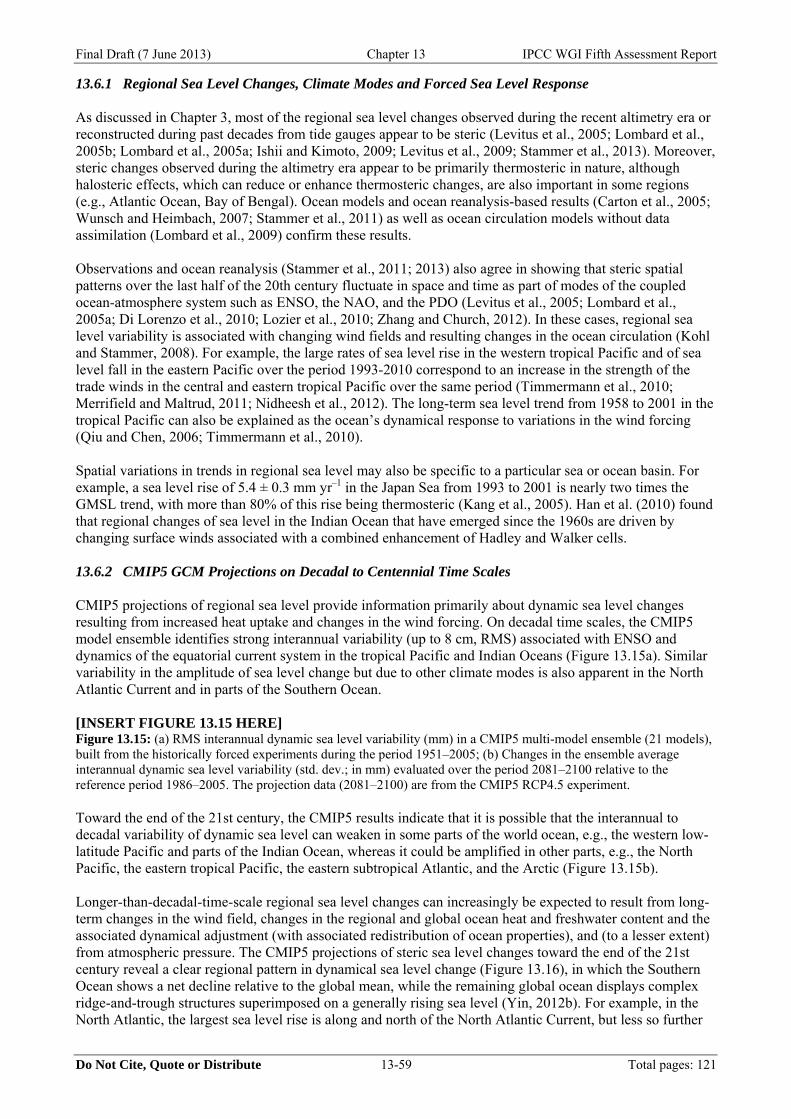
Final Draft (7 June 2013) Chapter 13 IPCC WGI Fifth Assessment Report
Do Not Cite, Quote or Distribute 13-59 Total pages: 121
13.6.1 Regional Sea Level Changes, Climate Modes and Forced Sea Level Response As discussed in Chapter 3, most of the regional sea level changes observed during the recent altimetry era or reconstructed during past decades from tide gauges appear to be steric (Levitus et al., 2005; Lombard et al., 2005b; Lombard et al., 2005a; Ishii and Kimoto, 2009; Levitus et al., 2009; Stammer et al., 2013). Moreover, steric changes observed during the altimetry era appear to be primarily thermosteric in nature, although halosteric effects, which can reduce or enhance thermosteric changes, are also important in some regions (e.g., Atlantic Ocean, Bay of Bengal). Ocean models and ocean reanalysis-based results (Carton et al., 2005; Wunsch and Heimbach, 2007; Stammer et al., 2011) as well as ocean circulation models without data assimilation (Lombard et al., 2009) confirm these results. Observations and ocean reanalysis (Stammer et al., 2011; 2013) also agree in showing that steric spatial patterns over the last half of the 20th century fluctuate in space and time as part of modes of the coupled ocean-atmosphere system such as ENSO, the NAO, and the PDO (Levitus et al., 2005; Lombard et al., 2005a; Di Lorenzo et al., 2010; Lozier et al., 2010; Zhang and Church, 2012). In these cases, regional sea level variability is associated with changing wind fields and resulting changes in the ocean circulation (Kohl and Stammer, 2008). For example, the large rates of sea level rise in the western tropical Pacific and of sea level fall in the eastern Pacific over the period 1993-2010 correspond to an increase in the strength of the trade winds in the central and eastern tropical Pacific over the same period (Timmermann et al., 2010; Merrifield and Maltrud, 2011; Nidheesh et al., 2012). The long-term sea level trend from 1958 to 2001 in the tropical Pacific can also be explained as the ocean’s dynamical response to variations in the wind forcing (Qiu and Chen, 2006; Timmermann et al., 2010). Spatial variations in trends in regional sea level may also be specific to a particular sea or ocean basin. For example, a sea level rise of 5.4 ± 0.3 mm yr–1 in the Japan Sea from 1993 to 2001 is nearly two times the GMSL trend, with more than 80% of this rise being thermosteric (Kang et al., 2005). Han et al. (2010) found that regional changes of sea level in the Indian Ocean that have emerged since the 1960s are driven by changing surface winds associated with a combined enhancement of Hadley and Walker cells. 13.6.2 CMIP5 GCM Projections on Decadal to Centennial Time Scales CMIP5 projections of regional sea level provide information primarily about dynamic sea level changes resulting from increased heat uptake and changes in the wind forcing. On decadal time scales, the CMIP5 model ensemble identifies strong interannual variability (up to 8 cm, RMS) associated with ENSO and dynamics of the equatorial current system in the tropical Pacific and Indian Oceans (Figure 13.15a). Similar variability in the amplitude of sea level change but due to other climate modes is also apparent in the North Atlantic Current and in parts of the Southern Ocean. [INSERT FIGURE 13.15 HERE] Figure 13.15: (a) RMS interannual dynamic sea level variability (mm) in a CMIP5 multi-model ensemble (21 models), built from the historically forced experiments during the period 1951–2005; (b) Changes in the ensemble average interannual dynamic sea level variability (std. dev.; in mm) evaluated over the period 2081–2100 relative to the reference period 1986–2005. The projection data (2081–2100) are from the CMIP5 RCP4.5 experiment. Toward the end of the 21st century, the CMIP5 results indicate that it is possible that the interannual to decadal variability of dynamic sea level can weaken in some parts of the world ocean, e.g., the western low-latitude Pacific and parts of the Indian Ocean, whereas it could be amplified in other parts, e.g., the North Pacific, the eastern tropical Pacific, the eastern subtropical Atlantic, and the Arctic (Figure 13.15b). Longer-than-decadal-time-scale regional sea level changes can increasingly be expected to result from long-term changes in the wind field, changes in the regional and global ocean heat and freshwater content and the associated dynamical adjustment (with associated redistribution of ocean properties), and (to a lesser extent) from atmospheric pressure. The CMIP5 projections of steric sea level changes toward the end of the 21st century reveal a clear regional pattern in dynamical sea level change (Figure 13.16), in which the Southern Ocean shows a net decline relative to the global mean, while the remaining global ocean displays complex ridge-and-trough structures superimposed on a generally rising sea level (Yin, 2012b). For example, in the North Atlantic, the largest sea level rise is along and north of the North Atlantic Current, but less so further
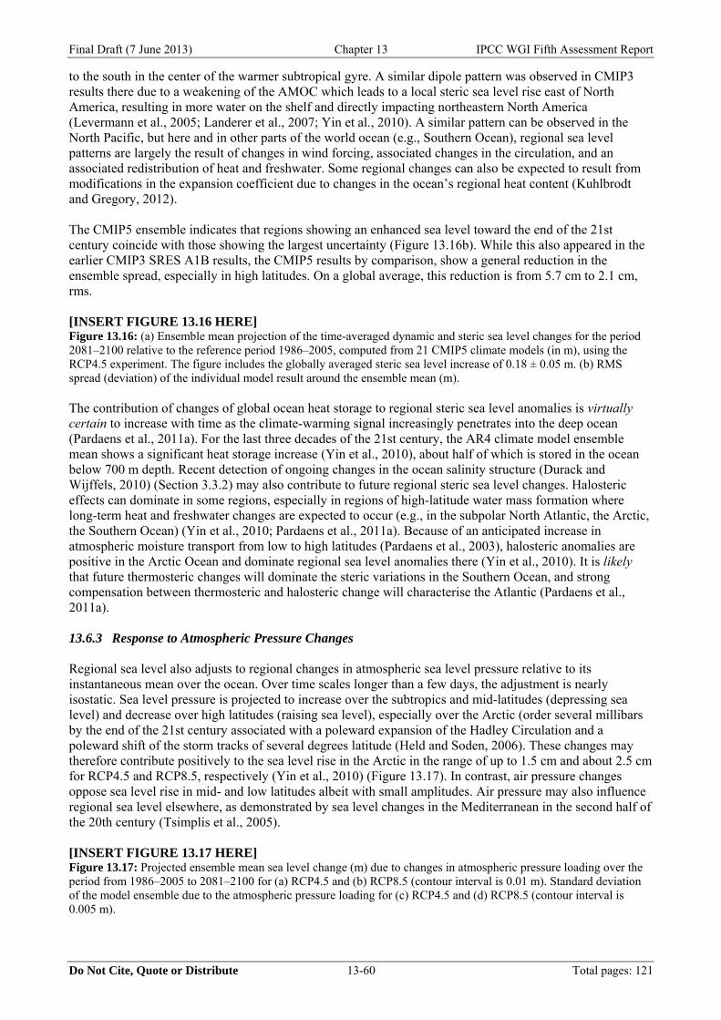
Final Draft (7 June 2013) Chapter 13 IPCC WGI Fifth Assessment Report
Do Not Cite, Quote or Distribute 13-60 Total pages: 121
to the south in the center of the warmer subtropical gyre. A similar dipole pattern was observed in CMIP3 results there due to a weakening of the AMOC which leads to a local steric sea level rise east of North America, resulting in more water on the shelf and directly impacting northeastern North America (Levermann et al., 2005; Landerer et al., 2007; Yin et al., 2010). A similar pattern can be observed in the North Pacific, but here and in other parts of the world ocean (e.g., Southern Ocean), regional sea level patterns are largely the result of changes in wind forcing, associated changes in the circulation, and an associated redistribution of heat and freshwater. Some regional changes can also be expected to result from modifications in the expansion coefficient due to changes in the ocean’s regional heat content (Kuhlbrodt and Gregory, 2012). The CMIP5 ensemble indicates that regions showing an enhanced sea level toward the end of the 21st century coincide with those showing the largest uncertainty (Figure 13.16b). While this also appeared in the earlier CMIP3 SRES A1B results, the CMIP5 results by comparison, show a general reduction in the ensemble spread, especially in high latitudes. On a global average, this reduction is from 5.7 cm to 2.1 cm, rms. [INSERT FIGURE 13.16 HERE] Figure 13.16: (a) Ensemble mean projection of the time-averaged dynamic and steric sea level changes for the period 2081–2100 relative to the reference period 1986–2005, computed from 21 CMIP5 climate models (in m), using the RCP4.5 experiment. The figure includes the globally averaged steric sea level increase of 0.18 ± 0.05 m. (b) RMS spread (deviation) of the individual model result around the ensemble mean (m). The contribution of changes of global ocean heat storage to regional steric sea level anomalies is virtually certain to increase with time as the climate-warming signal increasingly penetrates into the deep ocean (Pardaens et al., 2011a). For the last three decades of the 21st century, the AR4 climate model ensemble mean shows a significant heat storage increase (Yin et al., 2010), about half of which is stored in the ocean below 700 m depth. Recent detection of ongoing changes in the ocean salinity structure (Durack and Wijffels, 2010) (Section 3.3.2) may also contribute to future regional steric sea level changes. Halosteric effects can dominate in some regions, especially in regions of high-latitude water mass formation where long-term heat and freshwater changes are expected to occur (e.g., in the subpolar North Atlantic, the Arctic, the Southern Ocean) (Yin et al., 2010; Pardaens et al., 2011a). Because of an anticipated increase in atmospheric moisture transport from low to high latitudes (Pardaens et al., 2003), halosteric anomalies are positive in the Arctic Ocean and dominate regional sea level anomalies there (Yin et al., 2010). It is likely that future thermosteric changes will dominate the steric variations in the Southern Ocean, and strong compensation between thermosteric and halosteric change will characterise the Atlantic (Pardaens et al., 2011a). 13.6.3 Response to Atmospheric Pressure Changes Regional sea level also adjusts to regional changes in atmospheric sea level pressure relative to its instantaneous mean over the ocean. Over time scales longer than a few days, the adjustment is nearly isostatic. Sea level pressure is projected to increase over the subtropics and mid-latitudes (depressing sea level) and decrease over high latitudes (raising sea level), especially over the Arctic (order several millibars by the end of the 21st century associated with a poleward expansion of the Hadley Circulation and a poleward shift of the storm tracks of several degrees latitude (Held and Soden, 2006). These changes may therefore contribute positively to the sea level rise in the Arctic in the range of up to 1.5 cm and about 2.5 cm for RCP4.5 and RCP8.5, respectively (Yin et al., 2010) (Figure 13.17). In contrast, air pressure changes oppose sea level rise in mid- and low latitudes albeit with small amplitudes. Air pressure may also influence regional sea level elsewhere, as demonstrated by sea level changes in the Mediterranean in the second half of the 20th century (Tsimplis et al., 2005). [INSERT FIGURE 13.17 HERE] Figure 13.17: Projected ensemble mean sea level change (m) due to changes in atmospheric pressure loading over the period from 1986–2005 to 2081–2100 for (a) RCP4.5 and (b) RCP8.5 (contour interval is 0.01 m). Standard deviation of the model ensemble due to the atmospheric pressure loading for (c) RCP4.5 and (d) RCP8.5 (contour interval is 0.005 m).

Final Draft (7 June 2013) Chapter 13 IPCC WGI Fifth Assessment Report
Do Not Cite, Quote or Distribute 13-61 Total pages: 121
13.6.4 Response to Freshwater Forcing Enhanced freshwater fluxes derived from an increase in ice-sheet meltwater at high latitudes results in a regional pattern of sea level rise originating from adjustments in ocean dynamics and in the solid earth. Neither effect is included in CMIP5 models, although the latter adjustment is computed off line here. 13.6.4.1 Dynamic Ocean Response to Cryospheric Freshwater Forcing The addition of freshwater from glaciers and ice sheets to the ocean leads to an instantaneous increase in global mean sea level, but because it is communicated around the ocean basins via a dynamical adjustment, it is not instantaneously globally uniform (Kawase, 1987; Cane, 1989). For the addition of mass, the barotropic adjustment of the ocean takes place in a few days (Gower, 2010; Lorbacher et al., 2012). The addition of freshwater to the ocean from melting of the Greenland Ice Sheet results in an additional basin-wide steric response of the North Atlantic within months and is communicated to the global ocean via boundary waves, equatorial Kelvin waves, and westward propagating baroclinic Rossby waves on decadal time scales (Stammer, 2008). A similar response but with a different pattern can be observed from Antarctic meltwater input. In both cases, an associated complete baroclinic adjustment of the global ocean might take as long as several centuries. The adjustment of the ocean to high-latitude meltwater input also involves atmospheric teleconnections; such a response to Greenland meltwater pulses could lead to sea level changes in the Pacific within months (Stammer et al., 2011). On longer-than-decadal time scales, the freshwater input to the North Atlantic raises sea level in the Arctic Ocean and leads to an anomalous southward Bering Strait throughflow, transporting colder, fresher water from the Arctic Ocean into the North Pacific (Hu et al., 2010) and causing North Pacific cooling (Okumura et al., 2009). Meltwater forcing in the subpolar North Atlantic also causes changes of the AMOC (Section 12.4.7.2), which in turn causes dynamic changes of sea level in the North Atlantic, particularly in its northwestern region (Lorbacher et al., 2010). The combination of this dynamic sea level rise and the global mean sea level rise makes the northeastern North American coast vulnerable to some of the fastest and largest sea level rises during this century (Yin et al., 2009). 13.6.4.2 Earth and Gravitational Response to Contemporary Surface Water Mass Redistribution Deformational, rotational, and gravitational responses to mass redistribution between the cryosphere, the land, and the oceans produce distinctive regional departures from GMSL, referred to as sea level fingerprints (Mitrovica et al., 2001; Mitrovica et al., 2009; Gomez et al., 2010b; Riva et al., 2010) (Section 13.1, FAQ 13.1). Many existing studies of these effects have not defined a specific rate of ice-sheet mass loss (Mitrovica et al., 2001) or are based on end-member scenarios of ice retreat, such as from the West Antarctic Ice Sheet (Bamber et al., 2009; Mitrovica et al., 2009; Gomez et al., 2010b) and marine-based parts of the East Antarctic Ice Sheet (Gomez et al., 2010b). Bamber and Riva (2010) calculated the sea level fingerprint of all contemporary land-ice melt and each of its major components. Spada et al. (2013) examined the regional sea level pattern from future ice melt based on the A1B scenario. As can be seen from Figure 13.18, a characteristic of the sea level fingerprints is that regions adjacent to the source of the mass loss are subject to relative sea level fall of about an order of magnitude greater than the equivalent GMSL rise from these mass contributions, whereas in the far field the sea level rise is larger (up to about 30%) than the global average rise (Mitrovica et al., 2001; Mitrovica et al., 2009; Gomez et al., 2010b). Gomez et al. (2010b) and Mitrovica et al. (2011) showed that differences in the maximum predicted rise (relative to the global mean) between published results is due to the accuracy with which water expulsion from the deglaciated marine basins is calculated. These changes are in addition to the ongoing response to past changes (e.g., glacial isostatic adjustment in response to the last deglaciation). Mitrovica et al. (2001) suggested that the lower rates of sea level change inferred from tide gauge records at European sites relative to the global average were consistent with 20th century melting from Greenland. Similarly, Gehrels and Woodworth (2013) suggested that the larger magnitude of the early 20th century sea level acceleration observed in Australia and New Zealand, as compared with the North Atlantic, may represent a fingerprint of the increased melt contributions of Greenland and Arctic glaciers in the 1930s. Nevertheless, current rates of ice-sheet melting are difficult to distinguish from dynamic variability (Kopp et al., 2010; Hay et al., 2013), but it is likely that with further ice-sheet melting they will begin to dominate the regional patterns of sea level change toward the end of the 21st century, especially under climate forcing conditions for which ice-sheet melting contributes to more than 20-cm equivalent sea level rise (Kopp et al., 2010).
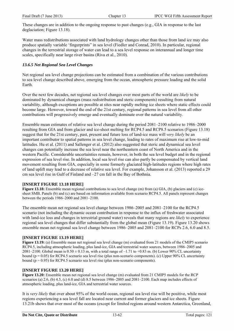
Final Draft (7 June 2013) Chapter 13 IPCC WGI Fifth Assessment Report
Do Not Cite, Quote or Distribute 13-62 Total pages: 121
These changes are in addition to the ongoing response to past changes (e.g., GIA in response to the last deglaciation; Figure 13.18). Water mass redistributions associated with land hydrology changes other than those from land ice may also produce spatially variable ‘fingerprints” in sea level (Fiedler and Conrad, 2010). In particular, regional changes in the terrestrial storage of water can lead to a sea level response on interannual and longer time scales, specifically near large river basins (Riva et al., 2010). 13.6.5 Net Regional Sea Level Changes Net regional sea level change projections can be estimated from a combination of the various contributions to sea level change described above, emerging from the ocean, atmospheric pressure loading and the solid Earth. Over the next few decades, net regional sea level changes over most parts of the world are likely to be dominated by dynamical changes (mass redistribution and steric components) resulting from natural variability, although exceptions are possible at sites near rapidly melting ice sheets where static effects could become large. However, toward the end of the 21st century, regional patterns in sea level from all other contributions will progressively emerge and eventually dominate over the natural variability. Ensemble mean estimates of relative sea level change during the period 2081–2100 relative to 1986–2000 resulting from GIA and from glacier and ice-sheet melting for RCP4.5 and RCP8.5 scenarios (Figure 13.18) suggest that for the 21st century, past, present and future loss of land-ice mass will very likely be an important contributor to spatial patterns in sea level change, leading to rates of maximum rise at low-to-mid latitudes. Hu et al. (2011) and Sallenger et al. (2012) also suggested that steric and dynamical sea level changes can potentially increase the sea level near the northeastern coast of North America and in the western Pacific. Considerable uncertainties remain, however, in both the sea level budget and in the regional expression of sea level rise. In addition, local sea level rise can also partly be compensated by vertical land movement resulting from GIA, especially in some formerly glaciated high-latitudes regions where high rates of land uplift may lead to a decrease of relative sea level. For example, Johansson et al. (2013) reported a 29 cm sea level rise in Gulf of Finland and –27 cm fall in the Bay of Bothnia. [INSERT FIGURE 13.18 HERE] Figure 13.18: Ensemble mean regional contributions to sea level change (m) from (a) GIA, (b) glaciers and (c) ice-sheet SMB. Panels (b) and (c) are based on information available from scenario RCP4.5. All panels represent changes between the periods 1986–2000 and 2081–2100. The ensemble mean net regional sea level change between 1986–2005 and 2081–2100 for the RCP4.5 scenario (not including the dynamic ocean contribution in response to the influx of freshwater associated with land-ice loss and changes in terrestrial ground water) reveals that many regions are likely to experience regional sea level changes that differ substantially from the global mean (Figure 13.19). Figure 13.20 shows ensemble mean net regional sea level change between 1986–2005 and 2081–2100 for RCPs 2.6, 6.0 and 8.5. [INSERT FIGURE 13.19 HERE] Figure 13.19: (a) Ensemble mean net regional sea level change (m) evaluated from 21 models of the CMIP5 scenario RCP4.5, including atmospheric loading, plus land-ice, GIA and terrestrial water sources, between 1986–2005 and 2081–2100. Global mean is 0.50 ± 0.13 m, with a total range of –1.71 to +0.83 m. (b) Lower 90% CL uncertainty bound (p = 0.05) for RCP4.5 scenario sea level rise (plus non-scenario components). (c) Upper 90% CL uncertainty bound (p = 0.95) for RCP4.5 scenario sea level rise (plus non-scenario components). [INSERT FIGURE 13.20 HERE] Figure 13.20: Ensemble mean net regional sea level change (m) evaluated from 21 CMIP5 models for the RCP scenarios (a) 2.6, (b) 4.5, (c) 6.0 and (d) 8.5 between 1986–2005 and 2081–2100. Each map includes effects of atmospheric loading, plus land-ice, GIA and terrestrial water sources. It is very likely that over about 95% of the world ocean, regional sea level rise will be positive, while most regions experiencing a sea level fall are located near current and former glaciers and ice sheets. Figure 13.21b shows that over most of the oceans (except for limited regions around western Antarctica, Greenland,
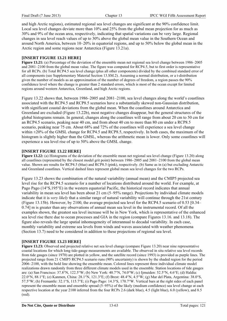
Final Draft (7 June 2013) Chapter 13 IPCC WGI Fifth Assessment Report
Do Not Cite, Quote or Distribute 13-63 Total pages: 121
and high Arctic regions), estimated regional sea level changes are significant at the 90% confidence limit. Local sea level changes deviate more than 10% and 25% from the global mean projection for as much as 30% and 9% of the ocean area, respectively, indicating that spatial variations can be very large. Regional changes in sea level reach values of up to 30% above the global mean value in the Southern Ocean and around North America, between 10–20% in equatorial regions, and up to 50% below the global mean in the Arctic region and some regions near Antarctica (Figure 13.21a). [INSERT FIGURE 13.21 HERE] Figure 13.21: (a) Percentage of the deviation of the ensemble mean net regional sea level change between 1986–2005 and 2081–2100 from the global mean value. The figure was computed for RCP4.5, but to first order is representative for all RCPs. (b) Total RCP4.5 sea level change (plus all other components) divided by the combined standard error of all components (see Supplementary Material Section 13.SM.2). Assuming a normal distribution, or a t-distribution given the number of models as an approximation of the number of degrees of freedom, a region passes the 90% confidence level where the change is greater than 2 standard errors, which is most of the ocean except for limited regions around western Antarctica, Greenland, and high Arctic regions. Figure 13.22 shows that, between 1986–2005 and 2081–2100, sea level changes along the world’s coastlines associated with the RCP4.5 and RCP8.5 scenarios have a substantially skewed non-Gaussian distribution, with significant coastal deviations from the global mean. When the coastlines around Antarctica and Greenland are excluded (Figure 13.22b), most negative changes disappear, but the general structures of the global histograms remain. In general, changes along the coastlines will range from about 20 cm to 50 cm for an RCP4.5 scenario, peaking near 40 cm, and from about 40 cm to more than 80 cm under a RCP8.5 scenario, peaking near 75 cm. About 68% and 72% of the coastlines will experience a sea level change within ±20% of the GMSL change for RCP4.5 and RCP8.5, respectively. In both cases, the maximum of the histogram is slightly higher than the GMSL, whereas the arithmetic mean is lower. Only some coastlines will experience a sea level rise of up to 50% above the GMSL change. [INSERT FIGURE 13.22 HERE] Figure 13.22: (a) Histograms of the deviation of the ensemble mean net regional sea level change (Figure 13.20) along all coastlines (represented by the closest model grit point) between 1986–2005 and 2081–2100 from the global mean value. Shown are results for RCP4.5 (blue) and RCP8.5 (pink), respectively. (b) Same as in (a) but excluding Antarctic and Greenland coastlines. Vertical dashed lines represent global mean sea level changes for the two RCPs. Figure 13.23 shows the combination of the natural variability (annual mean) and the CMIP5 projected sea level rise for the RCP4.5 scenario for a number of locations distributed around the world. For example, at Pago Pago (14°S,195°E) in the western equatorial Pacific, the historical record indicates that annual variability in mean sea level has been about 21 cm (5–95% range). Projections by individual climate models indicate that it is very likely that a similar range of natural variability will continue through the 21st century (Figure 13.15b). However, by 2100, the average projected sea level for the RCP4.5 scenario of 0.53 [0.34–0.74] m is greater than any observations of annual mean sea level in the instrumental record. Of all the examples shown, the greatest sea level increase will be in New York, which is representative of the enhanced sea level rise there due to ocean processes and GIA in the region (compare Figures 13.16. and 13.18). The figure also reveals the large spatial inhomogeneity of interannual to decadal variability. In each case, monthly variability and extreme sea levels from winds and waves associated with weather phenomena (Section 13.7) need to be considered in addition to these projections of regional sea level. [INSERT FIGURE 13.23 HERE] Figure 13.23: Observed and projected relative net sea level change (compare Figure 13.20) near nine representative coastal locations for which long tide-gauge measurements are available. The observed in situ relative sea level records from tide gauges (since 1970) are plotted in yellow, and the satellite record (since 1993) is provided as purple lines. The projected range from 21 CMIP5 RCP4.5 scenario runs (90% uncertainty) is shown by the shaded region for the period 2006–2100, with the bold line showing the ensemble mean. Colored lines represent three individual climate model realizations drawn randomly from three different climate models used in the ensemble. Station locations of tide gauges are: (a) San Francisco: 37.8°N, 122.5°W; (b) New York: 40.7°N, 74.0°W; (c) Ijmuiden: 52.5°N, 4.6°E; (d) Haldia: 22.0°N, 88.1°E; (e) Kanmen, China: 28.1°N, 121.3°E; (f) Brest: 48.4°N, 4.5°W; (g) Mar del Plata, Argentina: 38.0°S, 57.5°W; (h) Fremantle: 32.1°S, 115.7°E; (i) Pago Pago: 14.3°S, 170.7°W. Vertical bars at the right sides of each panel represent the ensemble mean and ensemble spread (5–95%) of the likely (medium confidence) sea level change at each respective location at the year 2100 inferred from the four RCPs 2.6 (dark blue), 4.5 (light blue), 6.0 (yellow), and 8.5 (red).
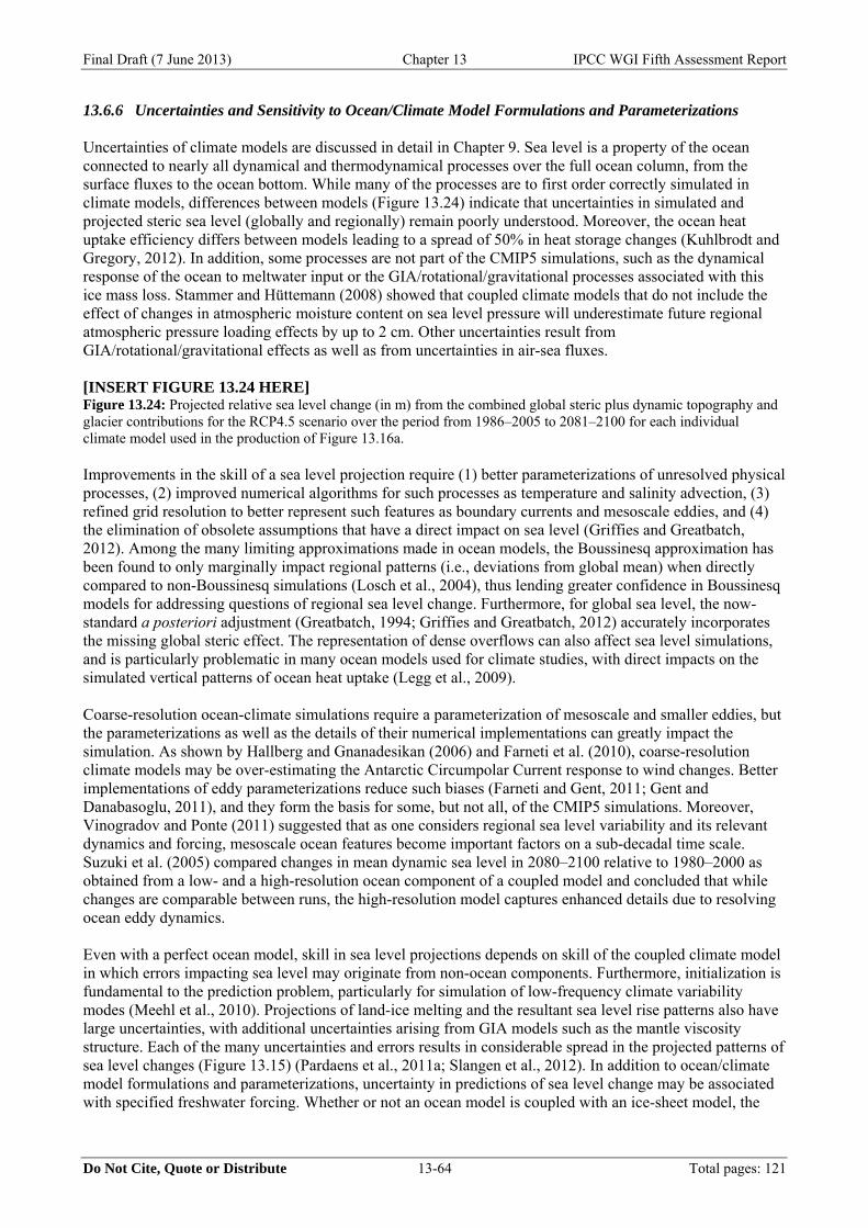
Final Draft (7 June 2013) Chapter 13 IPCC WGI Fifth Assessment Report
Do Not Cite, Quote or Distribute 13-64 Total pages: 121
13.6.6 Uncertainties and Sensitivity to Ocean/Climate Model Formulations and Parameterizations Uncertainties of climate models are discussed in detail in Chapter 9. Sea level is a property of the ocean connected to nearly all dynamical and thermodynamical processes over the full ocean column, from the surface fluxes to the ocean bottom. While many of the processes are to first order correctly simulated in climate models, differences between models (Figure 13.24) indicate that uncertainties in simulated and projected steric sea level (globally and regionally) remain poorly understood. Moreover, the ocean heat uptake efficiency differs between models leading to a spread of 50% in heat storage changes (Kuhlbrodt and Gregory, 2012). In addition, some processes are not part of the CMIP5 simulations, such as the dynamical response of the ocean to meltwater input or the GIA/rotational/gravitational processes associated with this ice mass loss. Stammer and Hüttemann (2008) showed that coupled climate models that do not include the effect of changes in atmospheric moisture content on sea level pressure will underestimate future regional atmospheric pressure loading effects by up to 2 cm. Other uncertainties result from GIA/rotational/gravitational effects as well as from uncertainties in air-sea fluxes. [INSERT FIGURE 13.24 HERE] Figure 13.24: Projected relative sea level change (in m) from the combined global steric plus dynamic topography and glacier contributions for the RCP4.5 scenario over the period from 1986–2005 to 2081–2100 for each individual climate model used in the production of Figure 13.16a. Improvements in the skill of a sea level projection require (1) better parameterizations of unresolved physical processes, (2) improved numerical algorithms for such processes as temperature and salinity advection, (3) refined grid resolution to better represent such features as boundary currents and mesoscale eddies, and (4) the elimination of obsolete assumptions that have a direct impact on sea level (Griffies and Greatbatch, 2012). Among the many limiting approximations made in ocean models, the Boussinesq approximation has been found to only marginally impact regional patterns (i.e., deviations from global mean) when directly compared to non-Boussinesq simulations (Losch et al., 2004), thus lending greater confidence in Boussinesq models for addressing questions of regional sea level change. Furthermore, for global sea level, the now- standard a posteriori adjustment (Greatbatch, 1994; Griffies and Greatbatch, 2012) accurately incorporates the missing global steric effect. The representation of dense overflows can also affect sea level simulations, and is particularly problematic in many ocean models used for climate studies, with direct impacts on the simulated vertical patterns of ocean heat uptake (Legg et al., 2009). Coarse-resolution ocean-climate simulations require a parameterization of mesoscale and smaller eddies, but the parameterizations as well as the details of their numerical implementations can greatly impact the simulation. As shown by Hallberg and Gnanadesikan (2006) and Farneti et al. (2010), coarse-resolution climate models may be over-estimating the Antarctic Circumpolar Current response to wind changes. Better implementations of eddy parameterizations reduce such biases (Farneti and Gent, 2011; Gent and Danabasoglu, 2011), and they form the basis for some, but not all, of the CMIP5 simulations. Moreover, Vinogradov and Ponte (2011) suggested that as one considers regional sea level variability and its relevant dynamics and forcing, mesoscale ocean features become important factors on a sub-decadal time scale. Suzuki et al. (2005) compared changes in mean dynamic sea level in 2080–2100 relative to 1980–2000 as obtained from a low- and a high-resolution ocean component of a coupled model and concluded that while changes are comparable between runs, the high-resolution model captures enhanced details due to resolving ocean eddy dynamics. Even with a perfect ocean model, skill in sea level projections depends on skill of the coupled climate model in which errors impacting sea level may originate from non-ocean components. Furthermore, initialization is fundamental to the prediction problem, particularly for simulation of low-frequency climate variability modes (Meehl et al., 2010). Projections of land-ice melting and the resultant sea level rise patterns also have large uncertainties, with additional uncertainties arising from GIA models such as the mantle viscosity structure. Each of the many uncertainties and errors results in considerable spread in the projected patterns of sea level changes (Figure 13.15) (Pardaens et al., 2011a; Slangen et al., 2012). In addition to ocean/climate model formulations and parameterizations, uncertainty in predictions of sea level change may be associated with specified freshwater forcing. Whether or not an ocean model is coupled with an ice-sheet model, the
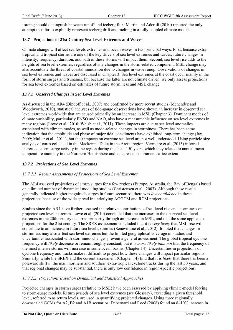
Final Draft (7 June 2013) Chapter 13 IPCC WGI Fifth Assessment Report
Do Not Cite, Quote or Distribute 13-65 Total pages: 121
forcing should distinguish between runoff and iceberg flux. Martin and Adcroft (2010) reported the only attempt thus far to explicitly represent iceberg drift and melting in a fully coupled climate model. 13.7 Projections of 21st Century Sea Level Extremes and Waves Climate change will affect sea levels extremes and ocean waves in two principal ways. First, because extra-tropical and tropical storms are one of the key drivers of sea level extremes and waves, future changes in intensity, frequency, duration, and path of these storms will impact them. Second, sea level rise adds to the heights of sea level extremes, regardless of any changes in the storm-related component. MSL change may also accentuate the threat of coastal inundation due to changes in wave runup. Observations of changes in sea level extremes and waves are discussed in Chapter 3. Sea level extremes at the coast occur mainly in the form of storm surges and tsunamis, but because the latter are not climate driven, we only assess projections for sea level extremes based on estimates of future storminess and MSL change. 13.7.1 Observed Changes in Sea Level Extremes As discussed in the AR4 (Bindoff et al., 2007) and confirmed by more recent studies (Menéndez and Woodworth, 2010), statistical analyses of tide-gauge observations have shown an increase in observed sea level extremes worldwide that are caused primarily by an increase in MSL (Chapter 3). Dominant modes of climate variability, particularly ENSO and NAO, also have a measureable influence on sea level extremes in many regions (Lowe et al., 2010; Walsh et al., 2011). These impacts are due to sea level anomalies associated with climate modes, as well as mode-related changes in storminess. There has been some indication that the amplitude and phase of major tidal constituents have exhibited long-term change (Jay, 2009; Muller et al., 2011), but their impacts on extreme sea level are not well understood. Using particle size analysis of cores collected in the Mackenzie Delta in the Arctic region, Vermaire et al. (2013) inferred increased storm surge activity in the region during the last ~150 years, which they related to annual mean temperature anomaly in the Northern Hemisphere and a decrease in summer sea-ice extent. 13.7.2 Projections of Sea Level Extremes 13.7.2.1 Recent Assessments of Projections of Sea Level Extremes The AR4 assessed projections of storm surges for a few regions (Europe, Australia, the Bay of Bengal) based on a limited number of dynamical modeling studies (Christensen et al., 2007). Although these results generally indicated higher magnitude surges in future scenarios, there was low confidence in these projections because of the wide spread in underlying AOGCM and RCM projections. Studies since the AR4 have further assessed the relative contributions of sea level rise and storminess on projected sea level extremes. Lowe et al. (2010) concluded that the increases in the observed sea level extremes in the 20th century occurred primarily through an increase in MSL, and that the same applies to projections for the 21st century. The SREX assessment concluded that it is very likely that MSL rise will contribute to an increase in future sea level extremes (Seneviratne et al., 2012). It noted that changes in storminess may also affect sea level extremes but the limited geographical coverage of studies and uncertainties associated with storminess changes prevent a general assessment. The global tropical cyclone frequency will likely decrease or remain roughly constant, but it is more likely than not that the frequency of the most intense storms will increase in some ocean basins (Chapter 14). Uncertainties in projections of cyclone frequency and tracks make it difficult to project how these changes will impact particular regions. Similarly, while the SREX and the current assessment (Chapter 14) find that it is likely that there has been a poleward shift in the main northern and southern extra-tropical cyclone tracks during the last 50 years, and that regional changes may be substantial, there is only low confidence in region-specific projections. 13.7.2.2 Projections Based on Dynamical and Statistical Approaches Projected changes in storm surges (relative to MSL) have been assessed by applying climate-model forcing to storm-surge models. Return periods of sea level extremes (see Glossary), exceeding a given threshold level, referred to as return levels, are used in quantifying projected changes. Using three regionally downscaled GCMs for A2, B2 and A1B scenarios, Debernard and Roed (2008) found an 8–10% increase in

Final Draft (7 June 2013) Chapter 13 IPCC WGI Fifth Assessment Report
Do Not Cite, Quote or Distribute 13-66 Total pages: 121
the 99th percentile surge heights between 1961–1990 and 2071–2100, mainly during the winter season, along the coastlines of the eastern North Sea and the northwestern British Isles, and decreases south of Iceland. Using a downscaled GCM under an A1B scenario, Wang et al. (2008) projected a significant increase in wintertime storm surges around most of Ireland between 1961–1990 and 2031–2060. Sterl et al. (2009) concatenated the output from a 17-member ensemble of A1B simulations from a GCM over the periods 1950–2000 and 2050–2100 into a single longer time series to estimate 10,000-year return levels of surge heights along the Dutch coastline. No statistically significant change in this value was projected for the 21st century because projected wind-speed changes were not associated with the maximum surge-generating northerlies. Using an ensemble of three climate models under A2 simulations, Colberg and McInnes (2012) found that changes in 95th percentile sea level height across the southern Australian coast in 2081–2100 compared to 1981–2000 were small (±0.1 m), mostly negative, and despite some inter-model differences, resembled the changes in wind patterns simulated by the climate models (McInnes et al., 2011). These studies demonstrate that the results are sensitive to the particular choice of GCM or RCM, therefore identifying uncertainties associated with the projections. For the tropical east coast of Australia, Harper et al. (2009) found that a 10% increase in tropical cyclone intensity for 2050 led to increases in the 100-year return level (including tides) that at most locations were smaller than 0.1 m. Several regional storm-surge studies have considered the relative contribution of the two main causative factors on changes in future sea level extremes (e.g., McInnes et al. (2009; 2013) for the southeastern coast of Australia; Brown et al. (2010) for the eastern Irish Sea; Woth et al. (2006) for the North Sea; Lowe et al. (2009) for the United Kingdom coast). They concluded that sea level rise has a greater potential than meteorological changes to increase sea level extremes by the end of the 21st century in these locations. Unnikrishnan et al. (2011) used RCM simulations to force a storm-surge model for the Bay of Bengal and found that the combined effect of MSL rise of 4 mm/yr and RCM projections for the A2 scenario (2071–2100) gave an increase in 100-year return levels of total sea level (including tides) between 0.40–0.67 m (about 15–20%) along the northern part of the east coast of India, except around the head of the bay, compared to those in the base line (1961–1990) scenario. Using six hypothetical hurricanes producing approximate 100-year return levels, Smith et al. (2010) found that in the regions of large surges on the southeastern Louisiana coast, the effect of MSL rise on simulated surges was linear. Yet in the regions of moderate surges (2–3 m), particularly in wetland-fronted areas, the increase in surges was larger by 1–3 m than the present values. They showed that sea level rise alters the speed of propagation of surges and their amplification in different regions of the coast. For the Gulf of Mexico, Mousavi et al. (2011) developed a simple relationship between hurricane-induced storm surges, sea level rise and hurricane intensification through increased SSTs for three modeled major historical cyclones, concluding that the dynamic interaction of surge and sea level rise lowered or amplified the surge at different points within a shallow coastal bay. Higher mean sea levels can significantly decrease the return period for exceeding given threshold levels. For a network of 198 tide gauges covering much of the globe, Hunter (2012) determined the factor by which the frequency of sea levels exceeding a given height would be increased for a MSL rise of 0.5 m (Figure 13.25a). The above calculations have been repeated here using regional RSL projections and their uncertainty using the RCP4.5 scenario (Section 13.6, Figure 13.19a). This multiplication factor depends exponentially on the inverse of the Gumbel scale parameter (a factor which describes the statistics of sea level extremes caused by the combination of tides and storm surges) (Coles and Tawn, 1990). The scale parameter is generally large where tides and/or storm surges are large, leading to a small multiplication factor, and vice versa. Figure 13.25a shows that a 0.5 m MSL rise would likely result in the frequency of sea level extremes increasing by an order of magnitude or more in some regions. The multiplication factors are found to be slightly higher, in general, when accounting for regional MSL projections (Figure 13.25b). However, in regions having higher regional projections of MSL, such as the east coast of Canada and the US (where GIA results in a larger sea level rise), the multiplication factor is higher, whereas in regions having lower regional projections of MSL, such as the northwest region of North America (where the land is rising due to present changes in glaciers and icecaps), the multiplication factor is lower. In another study, large increases in the frequency of sea level extremes for 2050 were found for a network of sites around the US coastline based on semi-empirical MSL rise projections and 20th century statistics of extremes (Tebaldi et al., 2012). Cayan et al. (2008) reached a similar conclusion for the California coast, using projected time series of tides, MSL rise, components for sea level fluctuations from projected MSLP and wind stress fields
Final Draft (7 June 2013) Chapter 13 IPCC WGI Fifth Assessment Report
Do Not Cite, Quote or Distribute 13-67 Total pages: 121
and a contribution for ENSO variability through projected SSTs for the 21st century, and showed that for high-end scenarios of MSL rise, the frequency and magnitude of extremes increases considerably relative to those experienced in the 20th century. [INSERT FIGURE 13.25 HERE] Figure 13.25: The estimated multiplication factor (shown at tide gauge locations by red circles and triangles), by which the frequency of flooding events of a given height increase for (a) a MSL rise of 0.5 m (b) using regional projections of MSL for the RCP4.5 scenario, shown in Figure13.19a. The Gumbel scale parameters are generally large in regions of large tides and/or surges resulting in a small multiplication factor and vice versa. 13.7.3 Projections of Ocean Waves Changes in ocean wave conditions are determined by changes in the major wind systems, especially in the main areas affected by tropical and extra-tropical storms. Based on in situ and satellite altimeter observations and wave-model hindcasts, it is likely that mean significant wave heights (SWH, defined as the average of the highest one-third of wave heights) have increased in regions of the North Pacific and the North Atlantic over the past half century, and in the Southern Ocean since the mid 1980s (Chapter 3, Seneviratne et al., 2012). The limited observational wave record makes it difficult to separate long-term trends from multi decadal variability (Young et al., 2011). A number of studies have related changes in wind-wave climatologies to modes of climate variability such as ENSO (Allan and Komar, 2006; Adams et al., 2008; Menéndez et al., 2008), the NAO (Woolf et al., 2002; Izaguirre et al., 2010), and the Southern Annular Mode (SAM) (Hemer et al., 2010; Izaguirre et al., 2011). Although anthropogenic influences have been considered (Wang et al., 2009), it is likely that reported SWH trends over the past half-century largely reflect natural variations in wind forcing. Recent reductions in summer sea-ice extent have resulted in enhanced wave activity in the Arctic Ocean due to increased fetch area and longer duration of the open-water season (Francis et al., 2011; Overeem et al., 2011). In general, there is low confidence in projections of future storm conditions (Chapters 12 and 14) and hence in projections of ocean waves. Nevertheless, there has been continued progress in translating climate model outputs into wind-wave projections. In the AR4, projected changes in global SWHs were based on a single statistical model (Wang and Swail, 2006). The projected conditions were consistent with increased wind speeds associated with mid-latitude storms, but they considered only a limited five-member ensemble for a single future emission scenario (SRES A2); wave parameters other than SWH were not considered. Since the AR4, global wave-climate projections for the end of the 21st century have been made by dynamically downscaling CMIP3 AOGCM results. A multi-model ensemble based on dynamical models forced with various greenhouse gas emission scenarios (SRES A1B: Mori et al. (2010), Fan et al. (2013), Semedo et al. (2013); SRES A2: Hemer et al. (2012a), as well as the statistical model of Wang and Swail (2006) forced with emission scenarios IS92a and SRES A2 and B2, has been constructed as part of the Coordinated Ocean Wave Climate Project (COWCLIP) (Hemer et al., 2013). In general, the ensemble projected changes of annual mean SWH (Figure 13.26a) resemble the statistical projections of Wang and Swail (2006) under an A2 scenario. The largest change is projected to be in the Southern Ocean, where mean SWHs at the end of the 21st century are approximately 5–10% higher than the present-day mean. SWH increase in this region reflects the projected strengthening of the westerlies over the Southern Ocean, particularly during austral winter (Figure 13.26c). Another region of SWH increase in the ensembles is in the tropical South Pacific associated with a projected strengthening of austral winter easterly trade winds in the CMIP3 multi-model dataset (Figure 13.26c). Negligible change or a mean SWH decrease is projected for all other ocean basins, with decreases identified in the trade wind region of the North Pacific, the mid-latitude westerlies in all basins, and in the trade and monsoon wind regions of the Indian Ocean. Hemer et al. (2013) found that variance of wave-climate projections associated with wave downscaling methodology dominated other sources of variance within the projections such as climate scenario of climate model uncertainties. Mori et al. (2013) reported similar findings. Three CMIP3-based model projections (Mori et al., 2010; Hemer et al., 2012b; Fan et al., 2013) were used to compare projections of wave direction and period (Hemer et al., 2013). Wave direction (Figure 13.26d) exhibits clockwise rotation in the tropics, consistent with a higher contribution from northward propagating swell from the Southern Ocean. Wave period (Figure 13.26e) shows an increase over the eastern Pacific,
Final Draft (7 June 2013) Chapter 13 IPCC WGI Fifth Assessment Report
Do Not Cite, Quote or Distribute 13-68 Total pages: 121
which is also attributed to enhanced wave generation in the Southern Ocean and northward swell propagation. A projected decrease in wave periods in the North Atlantic and western and central North Pacific is symptomatic of weaker wind forcing in these regions. SWH projections based on CMIP5 winds for emission scenarios RCP4.5 and RCP8.5 (Dobrynin et al., 2012) exhibit similar regional patterns for the end of the 21st century to the CMIP3 results presented in Figure 13.26A. Dobrynin et al. (2012) reported SWH increases in the Arctic Ocean, an area not considered by Hemer et al. (2013), and in basins connected to the Southern Ocean, particularly for RCP8.5. The probability of extreme wave heights is projected to increase in the Southern Hemisphere, the Arctic and Indian Oceans, but decrease in the North and Equatorial Atlantic and in the Pacific. In addition to wind changes, the projected loss of summer sea-ice extent in the Arctic Ocean is expected to increase overall wave activity there (Manson and Solomon, 2007; Overeem et al., 2011). Model intercomparisons are starting to identify common features of global wave projections yet in general there is low confidence in wave-model projections because of uncertainties regarding future wind states, particularly storm geography, the limited number of model simulations used in the ensemble averages, and the different methodologies used to downscale climate model results to regional scales (Hemer et al., 2012a). Despite these uncertainties, it appears likely (medium confidence) that enhanced westerly surface winds in the Southern Hemisphere (discussed in Chapter 12) will lead to enhanced wave generation in that region by the end of the 21st century. A number of dynamical wave-projection studies have been carried out with a regional focus. For the Mediterranean Sea, Lionello et al. (2008; 2010) projected a widespread shift of the wave-height distribution to lower values by the mid-21st century under an SRES A1B scenario, implying a decrease in mean and extreme wave heights. Caires et al. (2008) and Debernard and Røed (2008) reported a decrease (4–6% of present values) in the annual 99th percentile SWH south of Iceland by the end of the 21st century, and an increase (6–8%) along the North Sea east coast (SRES A2, B2, A1B scenarios). Grabemann and Weisse (2008) (Grabemann and Weisse, 2008) found increases (up to 18% of present values) in annual 99th percentile SWH in the North Sea by the end of the 21st century, with an increase in the frequency of extreme wave events over large areas of the southern and eastern North Sea (SRES A2, B2 scenarios). Charles et al. (2012) projected a general decrease in wave heights in the Bay of Biscay by the end of the 21st century (SRES A2, A1B, B1 scenarios), accompanied by clockwise rotations in winter swell (attributed to a projected northward shift in North Atlantic storm tracks) and summer sea and intermediate waves (attributed to a projected slackening of westerly winds). Along the Portuguese coast, Andrade et al. (2007) found little projected change in SWH and a tendency for a more northerly wave direction than present (SRES A2 scenario). In the Pacific, multi-model projections by Graham et al. (2013) (SRES A2 scenario) indicate a decrease in boreal winter upper-quantile SWHs over the mid-latitude North Pacific by the end of the 21st century associated with a projected decrease in wind speeds along the southern flank of the main westerlies. There is a less robust tendency for higher extreme waves at higher latitudes. On the southeastern Australian coast, Hemer et al. (2012b) used multi-model projections (SRES A2 and B1 scenarios) to identify a decrease in mean SWH (<0.2 m) by the end of the 21st century compared to present due to a projected decrease in regional storm wave energy, and a shift to a more southerly wave direction, consistent with a projected southward shift of the sub-tropical ridge in the forcing fields. [INSERT FIGURE 13.26 HERE] Figure 13.26: Projected changes in wind-wave conditions (~2075–2100 compared with ~1980–2009) derived from the Coordinated Ocean Wave Climate Projection (COWCLIP) Project (Hemer et al., 2013). (a) Percentage difference in annual mean significant wave height. (b) Percentage difference in January-March mean significant wave height. (c) Percentage difference in July-September mean significant wave height. Hashed regions indicate projected change is greater than the 5-member ensemble standard deviation. (d) As for (a), but displaying absolute changes in mean wave direction, with positive values representing projected clockwise rotation relative to displayed vectors, and colours shown only where ensemble members agree on sign of change. (e) As for (a), but displaying absolute changes in mean wave period. The symbol ~ is used to indicate that the reference periods differ slightly for the various model studies considered.

Final Draft (7 June 2013) Chapter 13 IPCC WGI Fifth Assessment Report
Do Not Cite, Quote or Distribute 13-69 Total pages: 121
13.8 Synthesis and Key Uncertainties There has been significant progress in our understanding of sea level change since the AR4. Paleo data now provide high confidence that sea levels were substantially higher when greenhouse gas concentrations were higher or surface temperatures were warmer than pre-industrial. The combination of paleo sea level data and long tide gauge records confirms that the rate of rise has increased from low rates of change during the late Holocene (order tenths of mm yr–1) to rates of almost 2 mm yr–1 averaged over the 20th century, with a likely continuing acceleration during the 20th century (Figure 13.27). Since 1993, the sum of observed contributions to sea level rise are in good agreement with the observed rise. [INSERT FIGURE 13.27 HERE] Figure 13.27: Compilation of paleo sea level data, tide gauge data, altimeter data (from Figure 13.3), and central estimates and likely ranges for projections of global-mean sea level rise for RCP2.6 (blue) and RCP8.5 (red) scenarios (Section 13.5.1), all relative to pre-industrial values. Understanding of the components that contribute to total sea level rise have improved significantly. For the 20th century, the range from an ensemble of such process-based models encompasses the observed rise when allowances are made for lack of inclusion of volcanic forcing in AOGCM control simulations, natural climate variability, and a possible small long-term ice-sheet contribution. Ice-sheet contributions to the 20th century sea level rise were small, however, and this agreement is thus not an evaluation of ice-sheet models. Nevertheless, there has been significant improvement in accounting for important physical processes in ice-sheet models, particularly of the dynamic response of individual glacier systems to warmer ocean waters in the immediate vicinity of the outlet glaciers. While there are as yet no complete simulations of regional ocean temperature changes and of the ice-sheet response to realistic climate change forcing, the publications to date have allowed an assessment of the likely range of sea level rise for the 21st century (Figure 13.27). These observations, together with our current scientific understanding and projections of future climate and sea level, imply that it is virtually certain that sea level will continue to rise during the 21st century and beyond. For the first few decades of the 21st century, regional sea level change will be dominated by climate variability superimposed on the climate change signal. For all scenarios, the rate of 21st century GMSL rise is very likely to exceed the average rate during the 20th century. For the RCP8.5 scenario, the projected rate of GMSL rise by the end of the 21st century will approach average rates experienced during the deglaciation of the Earth after the Last Glacial Maximum. These rates imply a significant transfer of mass from the ice sheets to the oceans and associated regional departures of sea level rise from the global average, in addition to the regional patterns from changing atmosphere-ocean interactions. Sea level rise has already led to a significant increase in the return frequency of extreme high sea levels at many locations, and this will continue during the 21st century, although there is low confidence in projections of changes in storminess. The first assessment of surface waves indicates a likely increase in the height of waves in the Southern Ocean. Despite this progress, significant uncertainties remain, particularly related to the magnitude and rate of the ice-sheet contribution for the 21st century and beyond, the regional distribution of sea level rise, and the regional changes in storm frequency and intensity. For coastal planning, sea level rise needs to be considered in a risk management framework, requiring knowledge of the frequency of sea level variability (from climate variability and extreme events) in future climates, projected changes in mean sea level, and the uncertainty of the sea level projections (Hunter, 2010, 2012), as well as local issues such as the compaction of sediments in deltaic regions and the changing supply of these sediments to maintain the height of the deltas (Syvitski et al., 2009). While improved understanding has allowed the projection of a likely range of sea level rise during the 21st century, it has not been possible to quantify a very likely range or give an upper bound to future rise. The potential collapse of ice shelves, as observed on the Antarctic Peninsula (Rignot et al., 2004; Scambos et al., 2004; Rott et al., 2011), could lead to a larger 21st century rise of up to several tenths of a meter. Sea level will continue to rise for centuries, even if greenhouse gas concentrations are stabilised, with the amount of sea level rise dependent on future greenhouse gas emissions. For higher emission scenarios and warmer temperatures, surface melting of the Greenland Ice Sheet is projected to exceed accumulation, leading to its long-term decay and a sea level rise of metres, consistent with paleo sea level data.
Final Draft (7 June 2013) Chapter 13 IPCC WGI Fifth Assessment Report
Do Not Cite, Quote or Distribute 13-70 Total pages: 121
Final Draft (7 June 2013) Chapter 13 IPCC WGI Fifth Assessment Report
Do Not Cite, Quote or Distribute 13-71 Total pages: 121
References Ablain, M., A. Cazenave, G. Valladeau, and S. Guinehut, 2009: A new assessment of the error budget of global mean
sea level rate estimated by satellite altimetry over 1993–2008. Ocean Science, 5, 193-201. Adams, P. N., D. L. Inman, and N. E. Graham, 2008: Southern California deep-water wave climate: characterization
and application to coastal processes. Journal of Coastal Research, 24, 1022-1035. Allan, J. C., and P. D. Komar, 2006: Climate controls on US West Coast erosion processes. Journal of Coastal
Research, 22, 511-529. Allen, M. R., D. J. Frame, C. Huntingford, C. D. Jones, J. A. Lowe, M. Meinshausen, and N. Meinshausen, 2009:
Warming caused by cumulative carbon emissions towards the trillionth tonne. Nature, 458, 1163-1166. Alley, R. B., S. Anandakrishnan, T. K. Dupont, B. R. Parizek, and D. Pollard, 2007: Effect of sedimentation on ice-
sheet grounding-line stability. Science, 315, 1838-1841. Andrade, C., H. O. Pires, R. Taborda, and M. C. Freitas, 2007: Projecting future changes in wave climate and coastal
response in Portugal by the end of the 21st century. Journal of Coastal Research, SI 50, 263-257. Anschütz, H., et al., 2009: Revisiting sites of the South Pole Queen Maud Land Traverses in East Antarctica:
accumulation data from shallow firn cores. Journal of Geophysical Research-Atmospheres, 114, D012204. Arendt, A., et al., 2012: Randolph Glacier Inventory [v2.0]: A Dataset of Global Glacier Outlines. Global Land Ice
Measurements from Space, Boulder Colorado, USA. Digital Media. Arthern, R., D. P. Winebrenner, and D. G. Vaughan, 2006: Antarctic snow accumulation mapped using polarization of
4.3-cm wavelength microwave emission. Journal of Geophysical Research-Atmospheres, 111, D06107. Bahr, D. B., and V. Radić, 2012: Significant contribution to total mass from very small glaciers. The Cryosphere, 6,
763-770. Bahr, D. B., M. Dyurgerov, and M. F. Meier, 2009: Sea-level rise from glaciers and ice caps: a lower bound.
Geophysical Research Letters, 36, L03501. Bales, R. C., et al., 2009: Annual accumulation for Greenland updated using ice core data developed during 2000-2006
and analysis of daily coastal meteorological data. Journal of Geophysical Research-Atmospheres, 114, D06116.
Bamber, J., and R. Riva, 2010: The sea level fingerprint of recent ice mass fluxes. Cryosphere, 4, 621-627. Bamber, J. L., and W. P. Aspinall, 2013: An expert judgement assessment of future sea level rise from the ice sheets.
Nature Climate Change, 3, 424-427. Bamber, J. L., R. E. M. Riva, B. L. A. Vermeersen, and A. M. LeBrocq, 2009: Reassessment of the potential sea-level
rise from a collapse of the West Antarctic Ice Sheet. Science, 324, 901-903. Bamber, J. L., et al., 2013: A new bed elevation dataset for Greenland. The Cryosphere, 7, 499-510. Banks, H. T., and J. M. Gregory, 2006: Mechanisms of ocean heat uptake in a coupled climate model and the
implications for tracer based predictions of ocean heat uptake. Geophysical Research Letters, 33. Barrand, N. E., et al., 2013: Computing the volume response of the Antarctic Peninsula ice sheet to warming scenarios
to 2200. Journal of Glaciology, doi:10.3189/2013JoG12J139, 397-409. Beckley, B. D., et al., 2010: Assessment of the Jason-2 Extension to the TOPEX/Poseidon, Jason-1 sea-surface height
time series for global mean sea level monitoring. Marine Geodesy, 33, 447-471. Bengtsson, L., S. Koumoutsaris, and K. Hodges, 2011: Large-scale surface mass balance of ice sheets from a
comprehensive atmosphere model. Surveys in Geophysics, 32, 459-474. Biancamaria, S., A. Cazenave, N. M. Mognard, W. Llovel, and F. Frappart, 2011: Satellite-based high latitude snow
volume trend, variability and contribution to sea level over 1989/2006. Global and Planetary Change, 75, 99-107.
Bindoff, N. L., et al., 2007: Observations: Oceanic climate change and sea level. Climate Change 2007: The Physical Science Basis, S. Solomon, et al., Eds., Cambridge University Press, 385-432.
Bindschadler, R. A., et al., 2013: Ice-sheet model sensitivities to environmental forcing and their use in projecting future sea level (The SeaRISE Project). Journal of Glaciology, 59, 195-224.
Bintanja, R., G. J. van Oldenborgh, S. S. Drijfhout, B. Wouters, and C. A. Katsman, 2013: Important role for ocean warming and increased ice-shelf melt in Antarctic sea-ice expansion. Nature Geoscience, 6, 376-379.
Bittermann, K., S. Rahmstorf, M. Perrette, and M. Vermeer, 2013: Predictability of 20th century sea-level rise from past data. Environmental Research Letters, doi:10.1088/1748-9326/8/1/014013.
Bjork, A. A., et al., 2012: An aerial view of 80 years of climate-related glacier fluctuations in southeast Greenland. Nature Geoscience, 5, 427-432.
Blum, M. D., and H. H. Roberts, 2009: Drowning of the Mississippi Delta due to insufficient sediment supply and global sea-level rise. Nature Geoscience, 2, 488-491.
Boening, C., J. K. Willis, F. W. Landerer, R. S. Nerem, and J. Fasullo, 2012: The 2011 La Niña: so strong, the oceans fell. Geophysical Research Letters, doi:10.1029/2012GL053055, L19602.
Boretti, A., 2011: The measured rate of rise of sea levels is not increasing and climate models should be revised to match the experimental evidence. Royal Society Publishing eLetter, July 12, 2011.
——, 2012a: Short term comparison of climate model predictions and satellite altimeter measurements of sea levels. Coastal Engineering, 60, 319-322.
Final Draft (7 June 2013) Chapter 13 IPCC WGI Fifth Assessment Report
Do Not Cite, Quote or Distribute 13-72 Total pages: 121
——, 2012b: Is there any support in the long term tide gauge data to the claims that parts of Sydney will be swamped by rising sea levels? Coastal Engineering, 64, 161-167.
——, 2013a: Discussion of Christine C. Shepard, Vera N. Agostini, Ben Gilmer, Tashya Allen, Jeff Stone, William Brooks and Michael W. Beck. Reply: Evaluating alternative future sea-level rise scenarios, Natural Hazards, 2012 doi:10.1007/s11069-012-0160-2. Natural Hazards, 65, 967-975.
——, 2013b: Discussion of J.A.G. Cooper, C. Lemckert, Extreme sea level rise and adaptation options for coastal resort cities: a qualitative assessment from the Gold Coast, Australia. Ocean and Coastal Management, 78, 132-135.
Boretti, A., and T. Watson, 2012: The inconvenient truth: ocean Levels are not accelerating in Australia or over the world. Energy and Environment, 23, 801-817.
Boretti, A. A., 2012c: Discussion of Natalya N. Warner, Philippe E. Tissot, "Storm flooding sensitivity to sea level rise for Galveston Bay, Texas", Ocean Engineering 44 (2012), 23-32. Ocean Engineering, 55, 235-237.
——, 2013c: Discussion of "Dynamic System Model to Predict Global Sea-Level Rise and Temperature Change" by Mustafa M. Aral, Jiabao Guan, and Biao Chang. Journal of Hydrologic Engineering, 18, 370-372.
Bougamont, M., et al., 2007: The impact of model physics on estimating the surface mass balance of the Greenland Ice Sheet. Geophysical Research Letters, 34, L17501.
Bouttes, N., J. M. Gregory, and J. A. Lowe, 2013: The reversibility of sea-level rise. Journal of Climate, doi:10.1175/JCLI-D-12-00285.1.
Box, J. E., 2002: Survey of Greenland instrumental temperature records: 1873-2001. International Journal of Climatology, 22, 1829-1847.
Box, J. E., 2013: Greenland ice sheet mass balance reconstruction. Part II: Surface mass balance (1840-2010). Journal of Climate, doi:10.1175/JCLI-D-12-00518.1.
Box, J. E., and W. Colgan, 2013: Greenland ice sheet mass balance reconstruction. Part III: Marine ice loss and total mass balance (1840-2010). Journal of Climate, doi:10.1175/JCLI-D-12-00546.1.
Box, J. E., L. Yang, D. H. Bromwich, and L. S. Bai, 2009: Greenland ice sheet surface air temperature variability: 1840-2007. Journal of Climate, 22, 4029-4049.
Box, J. E., X. Fettweis, J. C. Stroeve, M. Tedesco, D. K. Hall, and K. Steffen, 2012: Greenland ice sheet albedo feedback: thermodynamics and atmospheric drivers. The Cryosphere, 6, 821-839.
Box, J. E., et al., 2013: Greenland ice sheet mass balance reconstruction. Part I: net snow accumulation (1600-2009). Journal of Climate, doi:10.1175/JCLI-D-12-00373.1.
Bracegirdle, T. J., W. M. Connolley, and J. Turner, 2008: Antarctic climate change over the twenty first century. Journal of Geophysical Research-Atmospheres, 113, D03103.
Braithwaite, R. J., and O. B. Olesen, 1989: Calculation of glacier ablation from air temperature, West Greenland. Glacier Fluctuations and Climatic Change, J. Oerlemans, Ed., Kluwer Academic Publishers, 219-233.
Brierley, C., M. Collins, and A. Thorpe, 2010: The impact of perturbations to ocean-model parameters on climate and climate change in a coupled model. Climate Dynamics, 34, 325-343.
Broerse, D. B. T., L. L. A. Vermeersen, R. E. M. Riva, and W. van der Wal, 2011: Ocean contribution to co-seismic crustal deformation and geoid anomalies: Application to the 2004 December 26 Sumatra-Andaman earthquake. Earth and Planetary Science Letters, 305, 341-349.
Brohan, P., J. J. Kennedy, I. Harris, S. F. B. Tett, and P. D. Jones, 2006: Uncertainty estimates in regional and global observed temperature changes: A new data set from 1850. Journal of Geophysical Research-Atmospheres, 111, D12106.
Bromwich, D. H., J. P. Nicolas, and A. J. Monaghan, 2011: An assessment of precipitation changes over Antarctica and the Southern Ocean since 1989 in contemporary global reanalyses. Journal of Climate, 24, 4189-4209.
Bromwich, D. H., R. L. Fogt, K. I. Hodges, and J. E. Walsh, 2007: A tropospheric assessment of the ERA-40, NCEP, and JRA-25 global reanalyses in the polar regions. Journal of Geophysical Research-Atmospheres, 112, D10111.
Brown, J., A. Souza, and J. Wolf, 2010: Surge modelling in the eastern Irish Sea: present and future storm impact. Ocean Dynamics, 60, 227-236.
Burgess, E. W., R. R. Forster, J. E. Box, E. Mosley-Thompson, D. H. Bromwich, R. C. Bales, and L. C. Smith, 2010: A spatially calibrated model of annual accumulation rate on the Greenland Ice Sheet (1958-2007). Journal of Geophysical Research-Earth Surface, 115, F02004.
Caires, S., J. Groeneweg, and A. Sterl, 2008: Past and future changes in North Sea extreme waves. 31st International Conference on Coastal Engineering, Hamburg, 547-559.
Cane, M. A., 1989: A mathmatical note on Kawase study of deep ocean. Journal of Physical Oceanography, 19, 548-550.
Carton, J. A., B. S. Giese, and S. A. Grodsky, 2005: Sea level rise and the warming of the oceans in the Simple Ocean Data Assimilation (SODA) ocean reanalysis. Journal of Geophysical Research - Oceans, 110, C09006.
Cayan, D., P. Bromirski, K. Hayhoe, M. Tyree, M. Dettinger, and R. Flick, 2008: Climate change projections of sea level extremes along the California coast. Climatic Change, 87, 57-73.
Cazenave, A., et al., 2009: Sea level budget over 2003-2008: a reevaluation from GRACE space gravimetry, satellite altimetry and Argo. Global and Planetary Change, 65, 83-88.
Cazenave, A., et al., 2012: Estimating ENSO influence on the global mean sea level, 1993-2010. Marine Geodesy, 35 (sup1), 82-97.
Final Draft (7 June 2013) Chapter 13 IPCC WGI Fifth Assessment Report
Do Not Cite, Quote or Distribute 13-73 Total pages: 121
Chambers, D. P., 2006: Evaluation of new GRACE time‐variable gravity data over the ocean. Geophysical Research Letters, 33, L17603.
Chambers, D. P., J. Wahr, and R. S. Nerem, 2004: Preliminary observations of global ocean mass variations with GRACE. Geophysical Research Letters, 31, L13310.
Chambers, D. P., M. A. Merrifield, and R. S. Nerem, 2012: Is there a 60-year oscillation in global mean sea level? Geophysical Research Letters, 39.
Chambers, D. P., J. M. Wahr, M. Tamisiea, and R. S. Nerem, 2010: Ocean mass from GRACE and glacial isostatic adjustment. Journal of Geophysical Research, 115, B11415.
Chao, B. F., Y. H. Wu, and Y. S. Li, 2008: Impact of artificial reservoir water impoundment on global sea level. Science, 320, 212-214.
Charbit, S., D. Paillard, and G. Ramstein, 2008: Amount of CO2 emissions irreversibly leading to the total melting of Greenland. Geophysical Research Letters, 35, L12503.
Charles, E. D., D. Idier, P. Delecluse, M. Deque, and G. Le Cozannet, 2012: Climate change impact on waves in the Bay of Biscay, France. Ocean Dynamics, 62, 831-848.
Christensen, J. H., et al., 2007: Regional climate projections. Climate Change, 2007: The Physical Science Basis, 849-925.
Christoffersen, P., et al., 2011: Warming of waters in an East Greenland fjord prior to glacier retreat: mechanisms and connection to large-scale atmospheric conditions. The Cryosphere, 5, 701-714.
Church, J. A., and N. J. White, 2006: A 20th century acceleration in global sea-level rise. Geophysical Research Letters, 33, L01602.
——, 2011: Sea-level rise from the late 19th to the early 21st century. Surveys in Geophysics, 32, 585-602. Church, J. A., N. J. White, and J. M. Arblaster, 2005: Significant decadal-scale impact of volcanic eruptions on sea
level and ocean heat content. Nature, 438, 74-77. Church, J. A., P. L. Woodworth, T. Aarup, and W. S. Wildon, 2010: Understanding Sea-Level Rise and Variability,
428. Church, J. A., D. Monselesan, J. M. Gregory, and B. Marzeion, 2013: Evaluating the ability of process based models to
project sea-level change. Environmental Research Letters, 8, 015051. Church, J. A., J. M. Gregory, N. J. White, S. M. Platten, and J. X. Mitrovica, 2011a: Understanding and projecting sea
level change. Oceanography, 24, 130-143. Church, J. A., et al., 2001: Changes in sea level. Climate change 2001: The scientific basis. Contribution of Working
Group I to the Third Assessment Report of the Intergovernmental Panel on Climate Change, 639-693. Church, J. A., et al., 2011b: Revisiting the Earth's sea-level and energy budgets from 1961 to 2008. Geophysical
Research Letters, 38, L18601. Chylek, P., J. E. Box, and G. Lesins, 2004: Global warming and the Greenland ice sheet. Climatic Change, 63, 201-
221. Clark, J. A., and C. S. Lingle, 1977: Future sea-level changes due to West Antarctic ice sheet fluctuations. Nature, 269,
206-209. Clarke, P. J., D. A. Lavallee, G. Blewitt, T. M. van Dam, and J. M. Wahr, 2005: Effect of gravitational consistency and
mass conservation on seasonal surface mass loading models. Geophysical Research Letters, 32, L08306. Cogley, G., 2009a: Geodetic and direct mass-balance measurements: comparison and joint analysis. Annals of
Glaciology, 50, 96-100. Cogley, G., 2012: The Future of the World's Glaciers. Future Climates of the World, 2nd ed., A. Henderson-Sellers, and
K. McGuffie, Eds., Elsevier, 197-222. Cogley, J. G., 2009b: A more complete version of the World Glacier Inventory. Annals of Glaciology, 50, 32-38. Colberg, F., and K. L. McInnes, 2012: The impact of future changes in weather patterns on extreme sea levels over
southern Australia. Journal of Geophysical Research - Oceans, 117, C08001. Coles, S. G., and J. A. Tawn, 1990: Statistics of coastal flood prevention. Philosophical Transactions of the Royal
Society A -Mathematical Physical and Engineering Sciences, 332, 457-476. Connolley, W. M., and T. J. Bracegirdle, 2007: An Antarctic assessment of IPCC AR4 coupled models. Geophysical
Research Letters, 34. Conrad, C. P., and B. H. Hager, 1997: Spatial variations in the rate of sea level rise caused by the present-day melting
of glaciers and ice sheets. Geophysical Research Letters, 24, 1503-1506. Cook, A. J., and D. G. Vaughan, 2010: Overview of areal changes of the ice shelves on the Antarctic Peninsula over the
past 50 years. The Cryosphere, 4, 77-98. Cornford, S. L., et al., 2013: Adaptive mesh, finite volume modeling of marine ice sheets. Journal of Computational
Physics, 232, 529-549. Crowley, T., 2000: Causes of climate change over the past 1000 years. Science, 289, 270-277. Crowley, T. J., S. K. Baum, K.-Y. Kim, G. C. Hegerl, and W. T. Hyde, 2003: Modeling ocean heat content changes
during the last millennium. Geophysical Research Letters, 30, 1932. Debernard, J. B., and L. P. Røed, 2008: Future wind, wave and storm surge climate in the Northern Seas: a revisit.
Tellus A, 60, 427-438. Delworth, T. L., and T. R. Knutson, 2000: Simulation of early 20th century global warming. Science, 287, 2246-2250.
Final Draft (7 June 2013) Chapter 13 IPCC WGI Fifth Assessment Report
Do Not Cite, Quote or Distribute 13-74 Total pages: 121
Delworth, T. L., V. Ramaswamy, and G. L. Stenchikov, 2005: The impact of aerosols on simulated ocean temperature and heat content in the 20th century. Geophysical Research Letters, 32, L24709.
Di Lorenzo, E., et al., 2010: Central Pacific El Niño and decadal climate change in the North Pacific Ocean. Nature Geoscience, 3, 762-765.
Dobrynin, M., J. Murawsky, and S. Yang, 2012: Evolution of the global wind wave climate in CMIP5 experiments. Geophysical Research Letters, 39.
Dolan, A. M., A. M. Haywood, D. J. Hill, H. J. Dowsett, S. J. Hunter, D. J. Lunt, and S. J. Pickering, 2011: Sensitivity of Pliocene ice sheets to orbital forcing. Palaeogeography Palaeoclimatology Palaeoecology, 309, 98-110.
Domingues, C. M., J. A. Church, N. J. White, P. J. Gleckler, S. E. Wijffels, P. l. M. Barker, and J. R. Dunn, 2008: Improved estimates of upper-ocean warming and multi-decadal sea-level rise. Nature, 453, 1090-1093.
Donnelly, J. P., P. Cleary, P. Newby, and R. Ettinger, 2004: Coupling instrumental and geological records of sea-level change: Evidence from southern New England of an increase in the rate of sea-level rise in the late 19th century. Geophysical Research Letters, 31.
Douglas, B. C., 2001: Sea level change in the era of the recording tide gauge. Sea Level Rise, History and Consequences, International Geophysics Series, Volume 75, 37-64.
Driesschaert, E., et al., 2007: Modeling the influence of Greenland ice sheet melting on the Atlantic meridional overturning circulation during the next millennia. Geophysical Research Letters, 34, L10707.
Dufresne, J. L., and S. Bony, 2008: An assessment of the primary sources of spread of global warming estimates from coupled atmosphere-ocean models. Journal of Climate, 21, 5135-5144.
Dupont, T. K., and R. B. Alley, 2005: Assessment of the importance of ice-shelf buttressing to ice-sheet flow. Geophysical Research Letters, 32, L04503.
Durack, P. J., and S. E. Wijffels, 2010: Fifty-year trends in global ocean salinities and their relationship to broad-scale warming. Journal of Climate, 23, 4342-4362.
Durand, G., O. Gagliardini, T. Zwinger, E. Le Meur, and R. C. A. Hindmarsh, 2009: Full Stokes modeling of marine ice sheets: influence of the grid size. Annals of Glaciology, 50, 109-114.
Dutton, A., and K. Lambeck, 2012: Ice volume and sea level during the last interglacial. Science, 337, 216-219. Dyurgerov, M. B., and M. F. Meier, 2005: Glaciers and the Changing Earth System: A 2004 Snapshot. Occasional
Paper. Institute of Arctic and Alpine Research, University of Colorado. Easterling, D. R., and M. F. Wehner, 2009: Is the climate warming or cooling? Geophysical Research Letters, 36,
L08706. Ettema, J., M. R. van den Broeke, E. van Meijgaard, W. J. van de Berg, J. L. Bamber, J. E. Box, and R. C. Bales, 2009:
Higher surface mass balance of the Greenland ice sheet revealed by high-resolution climate modeling. Geophysical Research Letters, 36, L12501
Fan, Y., I. M. Held, S. J. Lin, and X. and Wang, 2013: Ocean warming effect on surface gravity wave climate change for the end of the 21st century. Journal of Climate, doi:10.1175/JCLI-D-12-00410.1.
Farneti, R., and P. R. Gent, 2011: The effects of the eddy-induced advection coefficient in a coarse-resolution coupled climate model. Ocean Modelling, 39, 135-145.
Farneti, R., T. L. Delworth, A. J. Rosati, S. M. Griffies, and F. Zeng, 2010: The role of mesoscale eddies in the rectification of the Southern Ocean response to climate change. Journal of Physical Oceanography, 40, 1539-1557.
Farrell, W. E., and J. A. Clark, 1976: On postglacial sea level. Geophysical Journal of the Royal Astronomical Society, 46, 647-667.
Fausto, R. S., A. P. Ahlstrom, D. van As, S. J. Johnsen, P. L. Langen, and K. Steffen, 2009: Improving surface boundary conditions with focus on coupling snow densification and meltwater retention in large-scale ice-sheet models of Greenland. Journal of Glaciology, 55, 869-878.
Favier, L., O. Gagliardini, G. Durand, and T. Zwinger, 2012: A three-dimensional full Stokes model of the grounding line dynamics: effect of a pinning point beneath the ice shelf. The Cryosphere, 6, 101-112.
Fettweis, X., E. Hanna, H. Gallee, P. Huybrechts, and M. Erpicum, 2008: Estimation of the Greenland ice sheet surface mass balance for the 20th and 21st centuries. The Cryosphere, 2, 117-129.
Fettweis, X., A. Belleflame, M. Erpicum, B. Franco, and S. Nicolay, 2011: Estimation of the sea level rise by 2100 resulting from changes in the surface mass balance of the Greenland ice sheet. Climate Change - Geophysical Foundations and Ecological Effects, 503-520.
Fettweis, X., B. Franco, M. Tedesco, J. H. van Angelen, J. T. M. Lenaerts, M. R. van den Broeke, and H. Gallee, 2013: Estimating Greenland ice sheet surface mass balance contribution to future sea level rise using the regional atmospheric model MAR. The Cryosphere, 7, 469-489.
Fiedler, J. W., and C. P. Conrad, 2010: Spatial variability of sea level rise due to water impoundment behind dams. Geophysical Research Letters, 37, L12603.
Fluckiger, J., R. Knutti, and J. W. C. White, 2006: Oceanic processes as potential trigger and amplifying mechanisms for Heinrich events. Paleoceanography, 21, PA2014.
Forest, C. E., P. H. Stone, and A. P. Sokolov, 2008: Constraining climate model parameters from observed 20th century changes. Tellus A, 60, 911-920.
Final Draft (7 June 2013) Chapter 13 IPCC WGI Fifth Assessment Report
Do Not Cite, Quote or Distribute 13-75 Total pages: 121
Forster, P. M., T. Andrews, I. Goodwin, J. M. Gregory, L. S. Jackson, and M. Zelinka, 2013: Evaluating adjusted forcing and model spread for historical and future scenarios in the CMIP5 generation of climate models. Journal of Geophysical Research, 118, 1139-1150.
Foster, G. L., and E. J. Rohling, 2013: Relationship between sea level and climate forcing by CO2 on geological timescales. Proceedings of the National Academy of Sciences of the United States of America, 110, 1209-1214.
Francis, O. P., G. G. Panteleev, and D. E. Atkinson, 2011: Ocean wave conditions in the Chukchi Sea from satellite and in situ observations. Geophysical Research Letters, 38.
Franco, B., X. Fettweis, and M. Erpicum, 2013: Future projections of the Greenland ice sheet energy balance driving the surface melt. The Cryosphere, 7, 1-18.
Franco, B., X. Fettweis, M. Erpicum, and S. Nicolay, 2011: Present and future climates of the Greenland ice sheet according to the IPCC AR4 models. Climate Dynamics, 36, 1897-1918.
Fretwell, P., et al., 2013: Bedmap2: improved ice bed, surface and thickness datasets for Antarctica. The Cryosphere, 7, 375-393.
Fyke, J. G., L. Carter, A. Mackintosh, A. J. Weaver, and K. J. Meissner, 2010: Surface melting over ice shelves and ice sheets as assessed from modeled surface air temperatures. Journal of Climate, 23, 1929-1936.
Gardner, A. S., et al., 2013: A reconciled estimate of glacier contributions to sea level rise: 2003 to 2009. Science. Gehrels, R., and P. L. Woodworth, 2013: When did modern rates of sea-level rise start? Global and Planetary Change,
100, 263-277. Gehrels, W. R., B. Hayward, R. M. Newnham, and K. E. Southall, 2008: A 20th century acceleration of sea-level rise in
New Zealand. Geophysical Research Letters, 35. Gehrels, W. R., D. A. Dawson, J. Shaw, and W. A. Marshall, 2011: Using Holocene relative sea-level data to inform
future sea-level predictions: An example from southwest England. Global and Planetary Change, 78, 116-126. Gehrels, W. R., et al., 2005: Onset of recent rapid sea-level rise in the western Atlantic Ocean. Quaternary Science
Reviews, 24, 2083-2100. Gehrels, W. R., et al., 2006: Rapid sea-level rise in the North Atlantic Ocean since the first half of the nineteenth
century. Holocene, 16, 949-965. Gehrels, W. R., et al., 2012: Nineteenth and twentieth century sea-level changes in Tasmania and New Zealand. Earth
and Planetary Science Letters, 315, 94-102. Gent, P. R., and G. Danabasoglu, 2011: Response to increasing southern hemisphere winds in CCSM4. Journal of
Climate, 24, 4992-4998. Genthon, C., G. Krinner, and H. Castebrunet, 2009: Antarctic precipitation and climate-change predictions: horizontal
resolution and margin vs plateau issues. Annals of Glaciology, 50, 55-60. Geoffroy, O., D. Saint-Martin, and A. Ribes, 2012: Quantifying the source of spread in climate change experiments.
Geophysical Research Letters, 39, L24703. Geoffroy, O., D. Saint-Martin, D. J. L. Olivie, A. Voldoire, G. Belon, and S. Tyteca, 2013: Transient climate response
in a two-box energy-balance model. Part I: analytical solution and parameter calibration using CMIP5. Journal of Climate, doi:10.1175/JCLI-D-12-00195.1.
Giesen, R. H., and J. Oerlemans, 2013: Climate-model induced differences in the 21st century global and regional glacier contributions to sea-level rise. Climate Dynamics, doi:10.1007/s00382-013-1743-7
Gillet-Chaulet, F., et al., 2012: Greenland ice sheet contribution to sea-level rise from a new-generation ice-sheet model. The Cryosphere, 6, 1561-1576.
Gillett, N. P., V. K. Arora, K. Zickfeld, S. J. Marshall, and A. J. Merryfield, 2011: Ongoing climate change following a complete cessation of carbon dioxide emissions. Nature Geoscience, 4, 83-87.
Gladstone, R. M., et al., 2012: Calibrated prediction of Pine Island Glacier retreat during the 21st and 22nd centuries with a coupled flowline model. Earth and Planetary Science Letters, 333, 191-199.
Gleckler, P. J., K. AchutaRao, J. M. Gregory, B. D. Santer, K. E. Taylor, and T. M. L. Wigley, 2006a: Krakatoa lives: The effect of volcanic eruptions on ocean heat content and thermal expansion. Geophysical Research Letters, 33, L17702.
Gleckler, P. J., T. M. L. Wigley, B. D. Santer, J. M. Gregory, K. AchutaRao, and K. E. Taylor, 2006b: Volcanoes and climate: Krakatoa's signature persists in the ocean. Nature, 439, 675.
Gleckler, P. J., et al., 2012: Human-induced global ocean warming on multidecadal timescales. Nature Climate Change, 2, 524-529.
Goelzer, H., P. Huybrechts, M. F. Loutre, H. Goosse, T. Fichefet, and A. Mouchet, 2011: Impact of Greenland and Antarctic ice sheet interactions on climate sensitivity. Climate Dynamics, 37, 1005-1018.
Goelzer, H., P. Huybrechts, S. C. B. Raper, M. F. Loutre, H. Goosse, and T. Fichefet, 2012: Millennial total sea-level commitments projected with the Earth system model of intermediate complexity LOVECLIM. Environmental Research Letters, 7.
Goelzer, H., et al., 2013: Sensitivity of Greenland ice sheet projections to model formulations. Journal of Glaciology, in press.
Goldberg, D., D. M. Holland, and C. Schoof, 2009: Grounding line movement and ice shelf buttressing in marine ice sheets. Journal of Geophysical Research-Earth Surface, 114, F04026.
Final Draft (7 June 2013) Chapter 13 IPCC WGI Fifth Assessment Report
Do Not Cite, Quote or Distribute 13-76 Total pages: 121
Goldberg, D. N., C. M. Little, O. V. Sergienko, A. Gnanadesikan, R. Hallberg, and M. Oppenheimer, 2012: Investigation of land ice-ocean interaction with a fully coupled ice-ocean model: 2. Sensitivity to external forcings. Journal of Geophysical Research-Earth Surface, 117.
Gomez, N., J. X. Mitrovica, P. Huybers, and P. U. Clark, 2010a: Sea level as a stabilizing factor for marine-ice-sheet grounding lines. Nature Geoscience, 3, 850-853.
Gomez, N., J. X. Mitrovica, M. E. Tamisiea, and P. U. Clark, 2010b: A new projection of sea level change in response to collapse of marine sectors of the Antarctic Ice Sheet. Geophysical Journal International, 180, 623-634.
Good, P., J. M. Gregory, and J. A. Lowe, 2011: A step-response simple climate model to reconstruct and interpret AOGCM projections. Geophysical Research Letters, 38, L01703.
Good, P., J. M. Gregory, J. A. Lowe, and T. Andrews, 2013: Abrupt CO2 experiments as tools for predicting and understanding CMIP5 representative concentration pathway projections. Climate Dynamics, 40, 1041-1053.
Goosse, H., H. Renssen, A. Timmermann, and R. S. Bradley, 2005: Internal and forced climate variability during the last millennium: a model-data comparison using ensemble simulations. Quaternary Science Reviews, 24, 1345-1360.
Gornitz, V., 2001: Impoundment, groundwater mining, and other hydrologic transformations: Impacts on global sea level rise. Sea Level Rise, History and Consequences, International Geophysics Series, Volume 75, 97-119.
Gouretski, V., and K. P. Koltermann, 2007: How much is the ocean really warming? Geophysical Research Letters, 34, L01610.
Gower, J. F. R., 2010: Comment on "Response of the global ocean to Greenland and Antarctic ice melting" by D. Stammer. Journal of Geophysical Research-Oceans, 115, C10009.
Grabemann, I., and R. Weisse, 2008: Climate change impact on extreme wave conditions in the North Sea: an ensemble study. Ocean Dynamics, 58, 199-212.
Graham, N. E., D. R. Cayan, P. Bromirski, and R. Flick, 2013: Multi-model projections of 21st century North Pacific winter wave climate under the IPCC A2 scenario. Climate Dynamics, 40:, 1335-1360.
Graversen, R. G., S. Drijfhout, W. Hazeleger, R. van de Wal, R. Bintanja, and M. Helsen, 2011: Greenland's contribution to global sea level rise by the end of the 21st century. Climate Dynamics, 37, 1427-1442.
Greatbatch, R. J., 1994: A note on the representation of steric sea-levels in models that conserve volume rather than mass. Journal of Geophysical Research-Oceans, 99, 12767-12771.
Gregory, J. M., 2000: Vertical heat transports in the ocean and their effect on time-dependent climate change. Climate Dynamics, 16, 501-515.
——, 2010: Long-term effect of volcanic forcing on ocean heat content. Geophysical Research Letters, 37, L22701. Gregory, J. M., and J. A. Lowe, 2000: Predictions of global and regional sea-level rise using AOGCMs with and
without flux adjustment. Geophysical Research Letters, 27, 3069-3072. Gregory, J. M., and P. Huybrechts, 2006: Ice-sheet contributions to future sea-level change. Philosophical Transactions
of the Royal Society of London A, 364, 1709-1731. Gregory, J. M., and P. M. Forster, 2008: Transient climate response estimated from radiative forcing and observed
temperature change. Journal of Geophysical Research - Atmospheres, 113, D23105. Gregory, J. M., J. A. Lowe, and S. F. B. Tett, 2006: Simulated global-mean sea-level changes over the last half-
millennium. Journal of Climate, 19, 4576-4591. Gregory, J. M., et al., 2013a: Climate models without pre-industrial volcanic forcing underestimate historical ocean
thermal expansion. Geophysical Research Letters, 40, 1-5. Gregory, J. M., et al., 2013b: Twentieth-century global-mean sea level rise: is the whole greater than the sum of the
parts? Journal of Climate, doi:0.1175/JCLI-D-12-00319.1. Greve, R., 2000: On the response of the Greenland ice sheet to greenhouse climate change. Climatic Change, 46, 289-
303. Griffies, S. M., and R. J. Greatbatch, 2012: Physical processes that impact the evolution of global mean sea level in
ocean climate models. Ocean Modelling, 51, 37-72. Grinsted, A., J. C. Moore, and S. Jevrejeva, 2010: Reconstructing sea level from paleo and projected temperatures 200
to 2100 AD. Climate Dynamics, 34, 461-472. Gudmundsson, G. H., J. Krug, G. Durand, F. L., and O. Gagliardini, 2012: The stability of grounding lines on
retrograde slopes. The Cryosphere Discussions, 6, 2597-2619. Hallberg, R., and A. Gnanadesikan, 2006: The role of eddies in determining the structure and response of the wind-
driven southern hemisphere overturning: Results from the Modeling Eddies in the Southern Ocean (MESO) project. Journal of Physical Oceanography, 36, 2232-2252.
Hallberg, R., A. Adcroft, J. Dunne, J. Krasting, and R. J. Stouffer, 2012: Sensitivity of 21st century global-mean steric sea level rise to ocean model formulation. Journal of Climate, doi:10.1175/JCLI-D-12-00506.1.
Han, W. Q., et al., 2010: Patterns of Indian Ocean sea-level change in a warming climate. Nature Geoscience, 3, 546-550.
Hanna, E., S. H. Mernild, J. Cappelen, and K. Steffen, 2012: Recent warming in Greenland in a long-term instrumental (1881-2012) climatic context: I. Evaluation of surface air temperature records. Environmental Research Letters, 7.
Hanna, E., P. Huybrechts, I. Janssens, J. Cappelen, K. Steffen, and A. Stephens, 2005: Runoff and mass balance of the Greenland ice sheet: 1958-2003. Journal of Geophysical Research-Atmospheres, 110, D13108.
Final Draft (7 June 2013) Chapter 13 IPCC WGI Fifth Assessment Report
Do Not Cite, Quote or Distribute 13-77 Total pages: 121
Hanna, E., et al., 2008: Increased runoff from melt from the Greenland Ice Sheet: A response to global warming. Journal of Climate, 21, 331-341.
Hanna, E., et al., 2011: Greenland Ice Sheet surface mass balance 1870 to 2100 based on twentieth century reanalysis, and links with global climate forcing. Journal of Geophysical Research, 116, D24121.
Hansen, J., M. Sato, P. Kharecha, and K. von Schuckmann, 2011: Earth's energy imbalance and implications. Atmospheric Chemistry and Physics, 11, 13421-13449.
Hansen, J., G. Russell, A. Lacis, I. Fung, D. Rind, and P. Stone, 1985: Climate response times - dependence on climate sensitivity and ocean mixing. Science, 229, 857-859.
Hansen, J., M. Sato, P. Kharecha, G. Russell, D. Lea, and M. Siddall, 2007: Climate change and trace gases. Philosophical Transactions of the Royal Society of London A, 365, 1925-1954.
Hansen, J., et al., 2005: Earth's energy imbalance: confirmation and implications. Science, 308, 1431-1435. Harper, B., T. Hardy, L. Mason, and R. Fryar, 2009: Developments in storm tide modelling and risk assessment in the
Australian region. Natural Hazards, 51, 225-238. Harper, J., N. Humphrey, W. T. Pfeffer, J. Brown, and X. Fettweis, 2012: Greenland ice-sheet contribution to sea-level
rise buffered by meltwater storage in firn. Nature, 491. Hay, C. C., E. Morrow, R. E. Kopp, and J. X. Mitrovica, 2013: Estimating the sources of global sea level rise with data
assimilation techniques. Proceedings of the National Academy of Sciences of the United States of America, 110, 3692-3699.
Hegerl, G. C., et al., 2007: Understanding and attributing climate change. Climate Change 2007: The Physical Science Basis. Contribution of Working Group I to the Fourth Assessment Report of the Intergovernmental Panel on Climate Change, 663-745.
Held, I. M., and B. J. Soden, 2006: Robust responses of the hydrological cycle to global warming. Journal of Climate, 19, 5686-5699.
Held, I. M., M. Winton, K. Takahashi, T. Delworth, F. R. Zeng, and G. K. Vallis, 2010: Probing the fast and slow components of global warming by returning abruptly to preindustrial forcing. Journal of Climate, 23, 2418-2427.
Hellmer, H. H., F. Kauker, R. Timmermann, J. Determann, and J. Rae, 2012: Twenty-first-century warming of a large Antarctic ice-shelf cavity by a redirected coastal current. Nature, 485, 225-228.
Hemer, M. A., J. A. Church, and J. R. Hunter, 2010: Variability and trends in the directional wave climate of the Southern Hemisphere. International Journal of Climatology, 30, 475-491.
Hemer, M. A., J. Katzfey, and C. Trenham, 2012a: Global dynamical projections of surface ocean wave climate for a future high greenhouse gas emission scenario. Ocean Modelling, doi:10.1016/j.ocemod.2012.09.008.
Hemer, M. A., K. L. McInnes, and R. Ranasinghe, 2012b: Projections of climate change-driven variations in the offshore wave climate off southeastern Australia. International Journal of Climatology, doi:10.1002/joc.3537.
Hemer, M. A., Y. Fan, N. Mori, A. Semedo, and X. L. Wang, 2013: Projected future changes in wind-wave climate in a multi-model ensemble. Nature Climate Change, 3, 471-476.
Hill, D. J., A. M. Dolan, A. M. Haywood, S. J. Hunter, and D. K. Stoll, 2010: Sensitivity of the Greenland Ice Sheet to Pliocene sea surface temperatures. Stratigraphy, 7, 111-121.
Hindmarsh, R. C. A., 1993: Qualitative dynamics of marine ice sheets. Ice in the Climate System I, 12, 68-99. Holgate, S., S. Jevrejeva, P. Woodworth, and S. Brewer, 2007: Comment on "A semi-empirical approach to projecting
future sea-level rise". Science, 317, 2. Holgate, S. J., 2007: On the decadal rates of sea level change during the twentieth century. Geophysical Research
Letters, 34, L01602. Holland, D. M., R. H. Thomas, B. De Young, M. H. Ribergaard, and B. Lyberth, 2008: Acceleration of Jakobshavn
Isbrae triggered by warm subsurface ocean waters. Nature Geoscience, 1, 659-664. Horton, R., C. Herweijer, C. Rosenzweig, J. P. Liu, V. Gornitz, and A. C. Ruane, 2008: Sea level rise projections for
current generation CGCMs based on the semi-empirical method. Geophysical Research Letters, 35, L02715. Hu, A., G. A. Meehl, W. Han, and J. Yin, 2011: Effect of the potential melting of the Greenland Ice Sheet on the
Meridional Overturning Circulation and global climate in the future. Deep-Sea Research Part Ii-Topical Studies in Oceanography, 58, 1914-1926.
Hu, A. X., et al., 2010: Influence of Bering Strait flow and North Atlantic circulation on glacial sea-level changes. Nature Geoscience, 3, 118-121.
Huber, M., and R. Knutti, 2012: Anthropogenic and natural warming inferred from changes in earth's energy balance. Nature Geoscience, 5, 31-36.
Hunter, J., 2010: Estimating sea-level extremes under conditions of uncertain sea-level rise. Climatic Change, 99, 331-350.
——, 2012: A simple technique for estimating an allowance for uncertain sea-level rise. Climatic Change, 113, 239-252.
Hunter, J. R., and M. J. I. Brown, 2013: Discussion of Boretti, A., ‘Is there any support in the long term tide gauge data to the claims that parts of Sydney will be swamped by rising sea levels?’. Coastal Engineering, 75, 1-3.
Huntington, T. G., 2008: Can we dismiss the effect of changes in land-based water storage on sea-level rise? Hydrological Processes, 22, 717-723.
Final Draft (7 June 2013) Chapter 13 IPCC WGI Fifth Assessment Report
Do Not Cite, Quote or Distribute 13-78 Total pages: 121
Huss, M., R. Hock, A. Bauder, and M. Funk, 2012: Conventional versus reference-surface mass balance. Journal of Glaciology, 58, 278-286.
Huybrechts, P., and J. De Wolde, 1999: The dynamic response of the Greenland and Antarctic ice sheets to multiple-century climatic warming. Journal of Climate, 12, 2169-2188.
Huybrechts, P., H. Goelzer, I. Janssens, E. Driesschaert, T. Fichefet, H. Goosse, and M. F. Loutre, 2011: Response of the Greenland and Antarctic ice sheets to multi-millennial greenhouse warming in the earth system model of intermediate complexity LOVECLIM. Surveys in Geophysics, 32, 397-416.
Ishii, M., and M. Kimoto, 2009: Reevaluation of historical ocean heat content variations with time-varying XBT and MBT depth bias corrections. Journal of Oceanography, 65, 287-299.
Izaguirre, C., F. J. Méndez, M. Menéndez, and I. J. Losada, 2011: Global extreme wave height variability based on satellite data. Geophysical Research Letters, 38, L10607.
Izaguirre, C., F. J. Méndez, M. Menéndez, A. Luceño, and I. J. Losada, 2010: Extreme wave climate variability in southern Europe using satellite data. Journal of Geophysical Research - Oceans, 115, C04009.
Jacobs, S. S., A. Jenkins, C. F. Giulivi, and P. Dutrieux, 2011: Stronger ocean circulation and increased melting under Pine Island Glacier ice shelf. Nature Geoscience, 4, 519-523.
Jay, D. A., 2009: Evolution of tidal amplitudes in the eastern Pacific Ocean. Geophysical Research Letters, 36. Jenkins, A., and D. Holland, 2007: Melting of floating ice and sea level rise. Geophysical Research Letters, 34. Jenkins, A., P. Dutrieux, S. S. Jacobs, S. D. McPhail, J. R. Perrett, A. T. Webb, and D. White, 2010: Observations
beneath Pine Island Glacier in West Antarctica and implications for its retreat. Nature Geoscience, 3, 468-472. Jevrejeva, S., A. Grinsted, and J. C. Moore, 2009: Anthropogenic forcing dominates sea level rise since 1850.
Geophysical Research Letters, 36, L20706. Jevrejeva, S., J. C. Moore, and A. Grinsted, 2010: How will sea level respond to changes in natural and anthropogenic
forcings by 2100? Geophysical Research Letters, 37, L07703. ——, 2012a: Sea level projections to AD 2500 with a new generation of climate change scenarios. Global and
Planetary Change, 80-81, 14-20. ——, 2012b: Potential for bias in 21st century semiempirical sea level projections. Journal of Geophysical Research,
117, D20116. Jevrejeva, S., A. Grinsted, J. C. Moore, and S. Holgate, 2006: Nonlinear trends and multiyear cycles in sea level
records. Journal of Geophysical Research-Oceans, 111, C09012. Jevrejeva, S., J. C. Moore, A. Grinsted, and P. L. Woodworth, 2008: Recent global sea level acceleration started over
200 years ago? Geophysical Research Letters, 35, L08715. Johansson, M. M., H. Pellikka, K. K. Kahma, and K. Ruosteenoja, 2013: Global sea level rise scenarios adapted to the
Finnish coast. Journal of Marine Systems, doi:10.1016/j.jmarsys.2012.08.007. Johnson, G. C., and N. Gruber, 2007: Decadal water mass variations along 20 W in the Northeastern Atlantic Ocean.
Progress in Oceanography, 73, 277-295. Johnson, G. C., S. Mecking, B. M. Sloyan, and S. E. Wijffels, 2007: Recent bottom water warming in the Pacific
Ocean. Journal of Climate, 20, 5365-5375. Joughin, I., and R. B. Alley, 2011: Stability of the West Antarctic ice sheet in a warming world. Nature Geoscience, 4,
506-513. Joughin, I., B. E. Smith, and D. M. Holland, 2010: Sensitivity of 21st century sea level to ocean-induced thinning of
Pine Island Glacier, Antarctica. Geophysical Research Letters, 37, L20502. Kang, S. K., J. Y. Cherniawsky, M. G. G. Foreman, H. S. Min, C. H. Kim, and H. W. Kang, 2005: Patterns of recent
sea level rise in the East/Japan Sea from satellite altimetry and in situ data. Journal of Geophysical Research-Oceans, 110, C07002.
Kaser, G., J. G. Cogley, M. B. Dyurgerov, M. F. Meier, and A. Ohmura, 2006: Mass balance of glaciers and ice caps: Consensus estimates for 1961-2004. Geophysical Research Letters, 33.
Kato, S., 2009: Interannual variability of the global radiation budget. Journal of Climate, 22, 4893-4907. Katsman, C., W. Hazeleger, S. Drijfhout, G. Oldenborgh, and G. Burgers, 2008: Climate scenarios of sea level rise for
the northeast Atlantic Ocean: a study including the effects of ocean dynamics and gravity changes induced by ice melt. Climatic Change, 91, 351-374.
Katsman, C. A., and G. J. van Oldenborgh, 2011: Tracing the upper ocean's missing heat. Geophysical Research Letters, 38, L14610.
Katsman, C. A., et al., 2011: Exploring high-end scenarios for local sea level rise to develop flood protection strategies for a low-lying delta - the Netherlands as an example. Climate Dynamics, 109, 617-645.
Kawase, M., 1987: Establishment of deep ocean circulation driven by deep-water. Journal of Physical Oceanography, 17, 2294-2317.
Kemp, A. C., B. P. Horton, J. P. Donnelly, M. E. Mann, M. Vermeer, and S. Rahmstorf, 2011: Climate related sea-level variations over the past two millennia. Proceedings of the National Academy of Sciences of the United States of America, 108, 11017-11022.
Knutti, R., and L. Tomassini, 2008: Constraints on the transient climate response from observed global temperature and ocean heat uptake. Geophysical Research Letters, 35, L09701.
Knutti, R., S. Krahenmann, D. J. Frame, and M. R. Allen, 2008: Comment on "Heat capacity, time constant, and sensitivity of Earth's climate system'' by S. E. Schwartz. Journal of Geophysical Research-Atmospheres, 113.
Final Draft (7 June 2013) Chapter 13 IPCC WGI Fifth Assessment Report
Do Not Cite, Quote or Distribute 13-79 Total pages: 121
Kohl, A., and D. Stammer, 2008: Decadal sea level changes in the 50-year GECCO ocean synthesis. Journal of Climate, 21, 1876-1890.
Konikow, L. F., 2011: Contribution of global groundwater depletion since 1900 to sea-level rise. Geophysical Research Letters, 38, L17401.
——, 2013: Comment on "Model estimates of sea-level change due to anthropogenic impacts on terrestrial water storage" by Pokhrel et al. Nature Geoscience, 6, 2.
Kopp, R. E., F. J. Simons, J. X. Mitrovica, A. C. Maloof, and M. Oppenheimer, 2009: Probabilistic assessment of sea level during the last interglacial stage. Nature, 462, 863-868.
——, 2013: A probabilistic assessment of sea level variations within the last interglacial stage. Geophysical Journal International, 193, 711-716.
Kopp, R. E., J. X. Mitrovica, S. M. Griffies, J. J. Yin, C. C. Hay, and R. J. Stouffer, 2010: The impact of Greenland melt on local sea levels: a partially coupled analysis of dynamic and static equilibrium effects in idealized water-hosing experiments. Climatic Change, 103, 619-625.
Körper, J., et al., 2013: The effect of aggressive mitigation on sea level rise and sea ice changes. Climate Dynamics, 40, 531-550.
Kouketsu, S., et al., 2011: Deep ocean heat content changes estimated from observation and reanalysis product and their influence on sea level change. Journal of Geophysical Research-Oceans, 116, C03012.
Krinner, G., O. Magand, I. Simmonds, C. Genthon, and J. L. Dufresne, 2007: Simulated Antarctic precipitation and surface mass balance at the end of the twentieth and twenty-first centuries. Climate Dynamics, 28, 215-230.
Krinner, G., B. Guicherd, K. Ox, C. Genthon, and O. Magand, 2008: Influence of oceanic boundary conditions in simulations of Antarctic climate and surface mass balance change during the coming century. Journal of Climate, 21, 938-962.
Kuhlbrodt, T., and J. M. Gregory, 2012: Ocean heat uptake and its consequences for the magnitude of sea level rise and climate change. Geophysical Research Letters, 39.
Lambeck, K., and S. M. Nakiboglu, 1984: Recent global changes in sea level. Geophysical Research Letters, 11, 959-961.
Lambeck, K., C. Smither, and M. Ekman, 1998: Tests of glacial rebound models for Fennoscandinavia based on instrumented sea- and lake-level records. Geophysical Journal International, 135, 375-387.
Lambeck, K., A. Purcell, and A. Dutton, 2012: The anatomy of interglacial sea levels: The relationship between sea levels and ice volumes during the Last Interglacial. Earth and Planetary Science Letters, 315, 4-11.
Lambeck, K., M. Anzidei, F. Antonioli, A. Benini, and A. Esposito, 2004: Sea level in Roman time in the Central Mediterranean and implications for recent change. Earth and Planetary Science Letters, 224, 563-575.
Landerer, F. W., J. H. Jungclaus, and J. Marotzke, 2007: Regional dynamic and steric sea level change in response to the IPCC-A1B scenario. Journal of Physical Oceanography, 37, 296-312.
Langen, P. L., A. M. Solgaard, and C. S. Hvidberg, 2012: Self-inhibiting growth of the Greenland Ice Sheet. Geophysical Research Letters, 39, L12502.
Leclercq, P. W., J. Oerlemans, and J. G. Cogley, 2011: Estimating the glacier contribution to sea-level rise for the period 1800-2005. Surveys in Geophysics, 32, 519-535.
Leclercq, P. W., A. Weidick, F. Paul, T. Bolch, M. Citterio, and J. Oerlemans, 2012: Brief communication "Historical glacier length changes in West Greenland". The Cryosphere, 6, 1339-1343.
Legg, S., et al., 2009: Improving oceanic overflow representation in climate models. Bulletin of the American Meteorological Society, 90, 657-.
Lemieux-Dudon, B., et al., 2010: Consistent dating for Antarctic and Greenland ice cores. Quaternary Science Reviews, 29, 8-20.
Lempérière, F., 2006: The role of dams in the XXI century: achieving a sustainable development target. International Journal on Hydropower and Dams, 13, 99-108.
Lenaerts, J. T. M., M. R. van den Broeke, W. J. van de Berg, E. van Meijgaard, and P. Kulpers Munneke, 2012: A new high-resolution surface mass balance map of Antarctica (1989-2009) based on regional atmospheric climate modeling. Geophysical Research Letters, 39, L04501.
Lenton, T. M., H. Held, E. Kriegler, J. W. Hall, W. Lucht, S. Rahmstorf, and H. J. Schellnhuber, 2008: Tipping elements in the Earth's climate system. Proceedings of the National Academy of Sciences of the United States of America, 105, 1786-1793.
Lettenmaier, D. P., and P. C. D. Milly, 2009: Land waters and sea level. Nature Geoscience, 2, 452-454. Leuliette, E. W., and L. Miller, 2009: Closing the sea level rise budget with altimetry, Argo, and GRACE. Geophysical
Research Letters, 36, L04608. Leuliette, E. W., and J. K. Willis, 2011: Balancing the sea level budget. Oceanography, 24, 122-129. Levermann, A., A. Griesel, M. Hofmann, M. Montoya, and S. Rahmstorf, 2005: Dynamic sea level changes following
changes in the thermohaline circulation. Climate Dynamics, 24, 347-354. Levermann, A., et al., 2012: Potential climatic transitions with profound impact on Europe Review of the current state
of six 'tipping elements of the climate system'. Climatic Change, 110, 845-878. Levitus, S., J. Antonov, and T. Boyer, 2005: Warming of the world ocean, 1955-2003. Geophysical Research Letters,
32, L02604.
Final Draft (7 June 2013) Chapter 13 IPCC WGI Fifth Assessment Report
Do Not Cite, Quote or Distribute 13-80 Total pages: 121
Levitus, S., J. I. Antonov, J. L. Wang, T. L. Delworth, K. W. Dixon, and A. J. Broccoli, 2001: Anthropogenic warming of Earth's climate system. Science, 292, 267-270.
Levitus, S., J. I. Antonov, T. P. Boyer, R. A. Locarnini, H. E. Garcia, and A. V. Mishonov, 2009: Global ocean heat content 1955-2008 in light of recently revealed instrumentation problems. Geophysical Research Letters, 36, L07608.
Li, C., J. S. von Storch, and J. Marotzke, 2013: Deep-ocean heat uptake and equilibrium climate response. Climate Dynamics, 40, 1071-1086.
Ligtenberg, S. R. M., W. J. van de Berg, M. R. van den Broeke, J. G. L. Rae, and E. van Meijgaard, 2013: Future surface mass balance of the Antarctic ice sheet and its influence on sea level change, simulated by a regional atmospheric climate model. Climate Dynamics, doi:10.1007/s00382-013-1749-1.
Lionello, P., M. B. Galati, and E. Elvini, 2010: Extreme storm surge and wind wave climate scenario simulations at the Venetian littoral. Physics and Chemistry of the Earth, Parts A/B/C, 40-41, 86-92.
Lionello, P., S. Cogo, M. B. Galati, and A. Sanna, 2008: The Mediterranean surface wave climate inferred from future scenario simulations. Global and Planetary Change, 63, 152-162.
Little, C. M., M. Oppenheimer, and N. M. Urban, 2013a: Upper bounds on twenty-first-century Antarctic ice loss assessed using a probabilistic framework. Nature Climate Change, doi:10.1038/NCLIMATE1845.
Little, C. M., N. M. Urban, and M. Oppenheimer, 2013b: Probabilistic framework for assessing the ice sheet contribution to sea level change. Proceedings of the National Academy of Sciences of the United States of America, 110, 3264-3269.
Llovel, W., S. Guinehut, and A. Cazenave, 2010: Regional and interannual variability in sea level over 2002-2009 based on satellite altimetry, Argo float data and GRACE ocean mass. Ocean Dynamics, 60, 1193-1204.
Llovel, W., et al., 2011: Terrestrial waters and sea level variations on interannual time scale. Global and Planetary Change, 75, 76-82.
Loeb, N. G., et al., 2009: Toward optimal closure of the earth's top-of-atmosphere radiation budget. Journal of Climate, 22, 748-766.
Loeb, N. G., et al., 2012: Observed changes in top-of-the-atmosphere radiation and upper-ocean heating consistent within uncertainty. Nature Geoscience, 5, 110-113.
Lombard, A., G. Garric, and T. Penduff, 2009: Regional patterns of observed sea level change: insights from a 1/4A degrees global ocean/sea-ice hindcast. Ocean Dynamics, 59, 433-449.
Lombard, A., A. Cazenave, P. Y. Le Traon, and M. Ishii, 2005a: Contribution of thermal expansion to present-day sea-level change revisited. Global and Planetary Change, 47, 1-16.
Lombard, A., A. Cazenave, K. DoMinh, C. Cabanes, and R. S. Nerem, 2005b: Thermosteric sea level rise for the past 50 years; comparison with tide gauges and inference on water mass contribution. Global and Planetary Change, 48, 303-312.
Lorbacher, K., J. Dengg, C. W. Boning, and A. Biastoch, 2010: Regional patterns of sea level change related to interannual variability and multidecadal trends in the Atlantic meridional overturning circulation. Journal of Climate, 23, 4243-4254.
Lorbacher, K., S. J. Marsland, J. A. Church, S. M. Griffies, and D. Stammer, 2012: Rapid barotrophic sea-level rise from ice-sheet melting scenarios. Journal of Geophysical Research, 117, C06003.
Losch, M., A. Adcroft, and J. M. Campin, 2004: How sensitive are coarse general circulation models to fundamental approximations in the equations of motion? Journal of Physical Oceanography, 34, 306-319.
Lowe, J. A., and J. M. Gregory, 2006: Understanding projections of sea level rise in a Hadley Centre coupled climate model. Journal of Geophysical Research-Oceans, 111, C11014.
Lowe, J. A., et al., 2009: UK Climate Projections science report: Marine and coastal projections. M. O. H. Centre, Ed. Lowe, J. A., et al., 2010: Past and future changes in extreme sea levels and waves. Understanding Sea-Level Rise and
Variability, doi:10.1002/9781444323276.ch11, 326-375. Lozier, M. S., V. Roussenov, M. S. C. Reed, and R. G. Williams, 2010: Opposing decadal changes for the North
Atlantic meridional overturning circulation. Nature Geoscience, 3, 728-734. MacAyeal, D. R., T. A. Scambos, C. L. Hulbe, and M. A. Fahnestock, 2003: Catastrophic ice-shelf break-up by an ice-
shelf-fragment- capsize mechanism. Journal of Glaciology, 49, 22-36. Machguth, H., et al., 2013: The future sea-level rise contribution of Greenland’s glaciers and ice caps. Environmental
Research Letters, doi:10.1088/1748-9326/8/2/025005. Manson, G. K., and S. M. Solomon, 2007: Past and future forcing of Beaufort sea coastal change. Atmosphere-Ocean,
45, 107-122. Marčelja, S., 2010: The timescale and extent of thermal expansion of the global ocean due to climate change. Ocean
Science, 6, 179-184. Martin, T., and A. Adcroft, 2010: Parameterizing the fresh-water flux from land ice to ocean with interactive icebergs
in a coupled climate model. Ocean Modelling, 34, 111-124. Marzeion, B., A. H. Jarosch, and M. Hofer, 2012a: Past and future sea-level changes from the surface mass balance of
glaciers. The Cryosphere, 6, 1295-1322. Marzeion, B., M. Hofer, A. H. Jarosch, G. Kaser, and T. Mölg, 2012b: A minimal model for reconstructing interannual
mass balance variability of glaciers in the European Alps. The Cryosphere, 6, 71-84.
Final Draft (7 June 2013) Chapter 13 IPCC WGI Fifth Assessment Report
Do Not Cite, Quote or Distribute 13-81 Total pages: 121
Masson-Delmotte, V., et al., 2010: EPICA Dome C record of glacial and interglacial intensities. Quaternary Science Reviews, 29, 113-128.
Masters, D., R. S. Nerem, C. Choe, E. Leuliette, B. Beckley, N. White, and M. Ablain, 2012: Comparison of global mean sea level time series from TOPEX/Poseidon, Jason-1, and Jason-2. Marine Geodesy, 35, 20-41.
McInnes, K., I. Macadam, G. Hubbert, and J. O’Grady, 2009: A modelling approach for estimating the frequency of sea level extremes and the impact of climate change in southeast Australia. Natural Hazards, 51, 115-137.
McInnes, K., I. Macadam, G. Hubbert, and J. G. O'Grady, 2013: An assessment of current and future vulnerability to coastal inundation due to sea level extremes in Victoria, southeast Australia. International Journal of Climatology, 33, 33-47.
McInnes, K. L., T. A. Erwin, and J. M. Bathols, 2011: Global climate model projected changes in 10 m wind due to anthropogenic climate change. Atmospheric Science Letters, 12, 325-333.
Meehl, G. A., A. X. Hu, and C. Tebaldi, 2010: Decadal Prediction in the Pacific Region. Journal of Climate, 23, 2959-2973.
Meehl, G. A., J. M. Arblaster, J. T. Fasullo, A. Hu, and K. E. Trenberth, 2011: Model-based evidence of deep-ocean heat uptake during surface-temperature hiatus periods. Nature Climate Change, 1, 360-364.
Meehl, G. A., et al., 2005: How much more global warming and sea level rise? Science, 307, 1769-1772. Meehl, G. A., et al., 2012: Relative outcomes of climate change mitigation related to global temperature versus sea-
level rise. Nature Climate Change, 2, 576-580. Meehl, G. A., et al., 2007: Global climate projections. Climate Change 2007: The Physical Science Basis, S. Solomon,
et al., Eds., Cambridge University Press, 755-828. Meier, M. F., 1984: Contribution of small glaciers to global sea level. Science, 226, 1418-1421. Meier, M. F., et al., 2007: Glaciers dominate eustatic sea-level rise in the 21st century. Science, 317, 1064-1067. Meinshausen, M., et al., 2011: The RCP greenhouse gas concentrations and their extensions from 1765 to 2300.
Climatic Change, 109, 213-241. Menéndez, M., and P. L. Woodworth, 2010: Changes in extreme high water levels based on a quasi-global tide-gauge
data set. Journal of Geophysical Research - Oceans, 115, C10011. Menéndez, M., F. J. Méndez, I. J. Losada, and N. E. Graham, 2008: Variability of extreme wave heights in the
northeast Pacific Ocean based on buoy measurements. Geophysical Research Letters, 35, L22607. Mercer, J. H., 1978: West Antarctic ice sheet and CO2 greenhouse effect: a threat of disaster. Nature, 271, 321-325. Mernild, S. H., and G. E. Liston, 2012: Greenland freshwater runoff. Part II: Distribution and trends, 1960-2010.
Journal of Climate, 25, 6015. Mernild, S. H., G. E. Liston, C. A. Hiemstra, and J. H. Christensen, 2010: Greenland Ice Sheet Surface Mass-Balance
Modeling in a 131-Yr Perspective, 1950-2080. Journal of Hydrometeorology, 11, 3-25. Merrifield, M. A., and M. E. Maltrud, 2011: Regional sea level trends due to a Pacific trade wind intensification.
Geophysical Research Letters, 38, L21605. Mikolajewicz, U., M. Vizcaíno, J. Jungclaus, and G. Schurgers, 2007a: Effect of ice sheet interactions in anthropogenic
climate change simulations. Geophysical Research Letters, 34, L18706. Mikolajewicz, U., M. Groger, E. Maier-Reimer, G. Schurgers, M. Vizcaíno, and A. Winguth, 2007b: Long-term effects
of anthropogenic CO2 emissions simulated with a complex earth system model. Climate Dynamics, 28, 599-634.
Miller, L., and B. C. Douglas, 2007: Gyre-scale atmospheric pressure variations and their relation to 19th and 20th century sea level rise. Geophysical Research Letters, 34, L16602.
Milly, P. C. D., A. Cazenave, and M. C. Gennero, 2003: Contribution of climate-driven change in continental water storage to recent sea-level rise. Proceedings of the National Academy of Sciences of the United States of America, 100, 13158-13161.
Milly, P. C. D., et al., 2010: Terrestrial water-storage contributions to sea-level rise and variability. Understanding Sea-Level Rise and Variability, J. A. Church, P. L. Woodworth, T. Aarup, and W. S. Wildon, Eds., Wiley-Blackwell, 226-255.
Milne, G. A., and J. X. Mitrovica, 1998: Postglacial sea-level change on a rotating Earth. Geophysical Journal International, 133, 1-19.
Milne, G. A., W. R. Gehrels, C. W. Hughes, and M. E. Tamisiea, 2009: Identifying the causes of sea-level change. Nature Geoscience, 2, 471-478.
Mitrovica, J. X., N. Gomez, and P. U. Clark, 2009: The Sea-Level Fingerprint of West Antarctic Collapse. Science, 323, 753-753.
Mitrovica, J. X., M. E. Tamisiea, J. L. Davis, and G. A. Milne, 2001: Recent mass balance of polar ice sheets inferred from patterns of global sea-level change. Nature, 409, 1026-1029.
Mitrovica, J. X., N. Gomez, E. Morrow, C. Hay, K. Latychev, and M. E. Tamisiea, 2011: On the robustness of predictions of sea-level fingerprints. Geophysical Journal International, 187, 729-742.
Moberg, A., D. M. Sonechkin, K. Holmgren, N. M. Datsenko, and W. Karlen, 2005: Highly variable Northern Hemisphere temperatures reconstructed from low- and high-resolution proxy data. Nature, 433, 613-617.
Monaghan, A. J., et al., 2006: Insignificant change in Antarctic snowfall since the International Geophysical Year. Science, 313, 827-831.
Final Draft (7 June 2013) Chapter 13 IPCC WGI Fifth Assessment Report
Do Not Cite, Quote or Distribute 13-82 Total pages: 121
Moore, J. C., S. Jevrejeva, and A. Grinsted, 2011: The historical global sea level budget. Annals of Glaciology, 52, 8-14.
Mori, N., T. Shimura, T. Yasuda, and H. Mase, 2013: Multi-model climate projections of ocean surface variables under different climate scenarios - Future change of waves, sea level, and wind. Ocean Engineering, doi:doi:10.3178/hrl.4.15.
Mori, N., T. Yasuda, H. Mase, T. Tom, and Y. Oku, 2010: Projection of extreme wave climate change under global warming. Hydrological Research Letters, 4, 15-19.
Morice, C. P., J. J. Kennedy, N. A. Rayner, and P. D. Jones, 2012: Quantifying uncertainties in global and regional temperature change using an ensemble of observational estimates: The HadCRUT4 data set. Journal of Geophysical Research-Atmospheres, 117.
Morlighem, M., E. Rignot, H. Seroussi, E. Larour, and H. Ben Dhia, 2010: Spatial patterns of basal drag inferred using control methods from a full-Stokes and simpler models for Pine Island Glacier, West Antarctica. Geophysical Research Letters, 37, L14502.
Moucha, R., A. M. Forte, J. X. Mitrovica, D. B. Rowley, S. Quere, N. A. Simmons, and S. P. Grand, 2008: Dynamic topography and long-term sea-level variations: there is no such thing as a stable continental platform. Earth and Planetary Science Letters, 271, 101-108.
Mousavi, M., J. Irish, A. Frey, F. Olivera, and B. Edge, 2011: Global warming and hurricanes: the potential impact of hurricane intensification and sea level rise on coastal flooding. Climatic Change, 104, 575-597.
Muhs, D. R., J. M. Pandolfi, K. R. Simmons, and R. R. Schumann, 2012: Sea-level history of past interglacial periods from uranium-series dating of corals, Curacao, Leeward Antilles islands. Quaternary Research, 78, 157-169.
Muller, M., B. K. Arbic, and J. X. Mitrovica, 2011: Secular trends in ocean tides: Observations and model results. Journal of Geophysical Research-Oceans, 116.
Murphy, D. M., S. Solomon, R. W. Portmann, K. H. Rosenlof, P. M. Forster, and T. Wong, 2009: An observationally based energy balance for the Earth since 1950. Journal of Geophysical Research - Oceans, 114, D17107.
Naish, T., et al., 2009: Obliquity-paced Pliocene West Antarctic ice sheet oscillations. Nature, 458, 322-328. National Research Council, 2012: Sea-Level Rise for the Coasts of California, Oregon, and Washington: Past, Present,
and Future. The National Academies Press. Nerem, R. S., D. P. Chambers, C. Choe, and G. T. Mitchum, 2010: Estimating mean sea level change from the TOPEX
and Jason altimeter missions. Marine Geodesy, 33, 435-446. Ngo-Duc, T., K. Laval, J. Polcher, A. Lombard, and A. Cazenave, 2005: Effects of land water storage on global mean
sea level over the past half century. Geophysical Research Letters, 32, L09704. Nicholls, R. J., et al., 2011: Sea-level rise and its possible impacts given a 'beyond 4 degrees C world' in the twenty-first
century. Philosophical Transactions of the Royal Society of London A, 369, 161-181. Nick, F. M., A. Vieli, I. M. Howat, and I. Joughin, 2009: Large-scale changes in Greenland outlet glacier dynamics
triggered at the terminus. Nature Geoscience, 2, 110-114. Nick, F. M., et al., 2013: Future sea-level rise from Greenland’s major outlet glaciers in a warming climate. Nature,
497, 235-238. Nick, F. M., et al., 2012: The response of Petermann Glacier, Greenland, to large calving events, and its future stability
in the context of atmospheric and oceanic warming. Journal of Glaciology, 58, 229-239. Nidheesh, A. G., M. Lengaine, J. Vialard, A. S. Unnikrishnam, and H. Dayan, 2012: Decadal and long-term sea level
variability in the tropical Indo-Pacific Ocean. Climate Dynamics, doi:10.1007/s00382-012-1463-4. Nowicki, S., et al., 2013: Insights into spatial sensitivities of ice mass response to environmental change from the
SeaRISE ice sheet modeling project I: Antarctica. Journal of Geophysical Research, doi:10.1002/jgrf.20081. Oerlemans, J., J. Jania, and L. Kolondra, 2011: Application of a minimal glacier model to Hansbreen, Svalbard. The
Cryosphere, 5, 1-11. Okumura, Y. M., C. Deser, A. Hu, A. Timmermann, and S. P. Xie, 2009: North Pacific climate response to freshwater
forcing in the Subarctic North Atlantic: oceanic and atmospheric pathways. Journal of Climate, 22, 1424-1445.
Olivié, D. J. L., G. P. Peters, and D. Saint-Martin, 2012: Atmosphere Response Time Scales Estimated from AOGCM Experiments. Journal of Climate, 25, 7956-7972.
Ollivier, A., Y. Faugere, N. Picot, M. Ablain, P. Femenias, and J. Benveniste, 2012: Envisat Ocean Altimeter Becoming Relevant for Mean Sea Level Trend Studies. Marine Geodesy, 35, 118-136.
Orlić, M., and Z. Pasarić, 2013: Semi-empirical versus process-based sea-level projections for the twenty-first century. Nature Climate Change, doi:10.1038/NCLIMATE1877.
Otto, A., et al., 2013: Energy budget contraints on climate response. Nature Geoscience, 6, 415-416. Overeem, I., R. S. Anderson, C. W. Wobus, G. D. Clow, F. E. Urban, and N. Matell, 2011: Sea ice loss enhances wave
action at the Arctic coast. Geophysical Research Letters, 38. Palmer, M. D., D. J. McNeall, and N. J. Dunstone, 2011: Importance of the deep ocean for estimating decadal changes
in Earth's radiation balance. Geophysical Research Letters, 38, L13707. Pardaens, A., J. M. Gregory, and J. Lowe, 2011a: A model study of factors influencing projected changes in regional
sea level over the twenty-first century. Climate Dynamics, 36, 2015-2033. Pardaens, A. K., H. T. Banks, J. M. Gregory, and P. R. Rowntree, 2003: Freshwater transports in HadCM3. Climate
Dynamics, 21, 177-195.
Final Draft (7 June 2013) Chapter 13 IPCC WGI Fifth Assessment Report
Do Not Cite, Quote or Distribute 13-83 Total pages: 121
Pardaens, A. K., J. A. Lowe, S. Brown, R. J. Nicholls, and D. de Gusmao, 2011b: Sea-level rise and impacts projections under a future scenario with large greenhouse gas emission reductions. Geophysical Research Letters, 38, L12604.
Parizek, B. R., et al., 2013: Dynamic (In)stability of Thwaites Glacier, West Antarctica. Journal of Geophysical Research-Earth Surface, doi:10.1002/jgrf.20044.
Parker, A., 2013a: Comment to M Lichter and D Felsenstein, Assessing the costs of sea-level rise and extreme flooding at the local level: A GIS-based approach. Ocean and Coastal Management, 78, 138-142.
Parker, A., 2013b: Sea level trends at locations of the United States with more than 100 years of recording. Natural Hazards, 65, 1011-1021.
——, 2013c: Comment to Shepard, CC, Agostini, VN, Gilmer, B., Allen, T., Stone, J., Brooks, W., Beck, MW: Assessing future risk: quantifying the effects of sea level rise on storm surge risk for the southern shores of Long Island. Natural Hazards, 65, 977-980.
Passchier, S., 2011: Linkages between East Antarctic Ice Sheet extent and Southern Ocean temperatures based on a Pliocene high-resolution record of ice-rafted debris off Prydz Bay, East Antarctica. Paleoceanography, 26.
Pattyn, F., A. Huyghe, S. De Brabander, and B. De Smedt, 2006: Role of transition zones in marine ice sheet dynamics. Journal of Geophysical Research-Earth Surface, 111, F02004.
Pattyn, F., et al., 2013: Grounding-line migration in plan-view marine ice-sheet models: results of the ice2sea MISMIP3d intercomparison. Journal of Glaciology, 59, 410-422.
Paulson, A., S. J. Zhong, and J. Wahr, 2007: Inference of mantle viscosity from GRACE and relative sea level data. Geophysical Journal International, 171, 497-508.
Peltier, W. R., 2004: Global glacial isostasy and the surface of the ice-age earth: the ICE-5G (VM2) model and GRACE. Annual Review of Earth and Planetary Sciences, 32, 111-149.
——, 2009: Closure of the budget of global sea level rise over the GRACE era: the importance and magnitudes of the required corrections for global glacial isostatic adjustment. Quaternary Science Reviews, 28, 1658-1674.
Peltier, W. R., and A. M. Tushingham, 1991: Influence of glacial isostatic-adjustment on tide gauge measurements of secular sea-level change. Journal of Geophysical Research-Solid Earth and Planets, 96, 6779-6796.
Perrette, M., F. W. Landerer, R. Riva, K. Frieler, and M. Meinshausen, 2013: A scaling approach to project regional sea level rise and its uncertainties. Earth System Dynamics, 4, 11-29.
Pfeffer, W. T., J. T. Harper, and S. O'Neel, 2008: Kinematic constraints on glacier contributions to 21st-century sea-level rise. Science, 321, 1340-1343.
Phillips, T., H. Rajaram, and K. Steffen, 2010: Cryo-hydrologic warming: a potential mechanism for rapid thermal response of ice sheets. Geophysical Research Letters, 37, L20503.
Phillips, T., H. Rajaram, W. Colgan, K. Steffen, and W. Abdalati, 2013: Evaluation of cryo-hydrologic warming as an explanation for increased ice velocities in the wet snow zone, Sermeq Avannarleq, West Greenland. Journal of Geophysical Research, doi:10.1002/jgrf.20079.
Pokhrel, Y. N., N. Hanasaki, P. J. F. Yeh, T. J. Yamada, S. Kanae, and T. Oki, 2012: Model estimates of sea-level change due to anthropogenic impacts on terrestrial water storage. Nature Geoscience, 5, 389-392.
Pokhrel, Y. N., N. Hanasaki, P. J. F. Yeh, T. J. Yamada, S. Kanae, and T. Oki, 2013: Overestimated water storage Reply. Nature Geoscience, 6, 2-3.
Pollard, D., and R. M. DeConto, 2009: Modelling West Antarctic ice sheet growth and collapse through the past five million years. Nature, 458, 329-332.
Polvani, L. M., M. Previdi, and C. Deser, 2011: Large cancellation, due to ozone recovery, of future Southern Hemisphere atmospheric circulation trends. Geophysical Research Letters, 38, L04707.
Price, S. F., A. J. Payne, I. M. Howat, and B. E. Smith, 2011: Committed sea-level rise for the next century from Greenland ice sheet dynamics during the past decade. Proceedings of the National Academy of Sciences of the United States of America, 108, 8978-8983.
Pritchard, H. D., R. J. Arthern, D. G. Vaughan, and L. A. Edwards, 2009: Extensive dynamic thinning on the margins of the Greenland and Antarctic ice sheets. Nature, 461, 971-975.
Pritchard, H. D., S. R. M. Ligtenberg, H. A. Fricker, D. G. Vaughan, M. R. van den Broeke, and L. Padman, 2012: Antarctic ice-sheet loss driven by basal melting of ice shelves. Nature, 484, 502-505.
Purkey, S. G., and G. C. Johnson, 2010: Warming of global abyssal and deep southern ocean waters between the 1990s and 2000s: contributions to global heat and sea level rise budgets. Journal of Climate, 23, 6336-6351.
Qiu, B., and S. M. Chen, 2006: Decadal variability in the large-scale sea surface height field of the South Pacific Ocean: observations and causes. Journal of Physical Oceanography, 36, 1751-1762.
Quinn, K. J., and R. M. Ponte, 2010: Uncertainty in ocean mass trends from GRACE. Geophysical Journal International, 181, 762-768.
Radic, V., and R. Hock, 2010: Regional and global volumes of glaciers derived from statistical upscaling of glacier inventory data. Journal of Geophysical Research-Earth Surface, 115, F01010.
Radić, V., and R. Hock, 2011: Regionally differentiated contribution of mountain glaciers and ice caps to future sea-level rise. Nature Geoscience, 4, 91-94.
Radić, V., A. Bliss, A. D. Beedlow, R. Hock, E. Miles, and J. G. Cogley, 2013: Regional and global projections of the 21st century glacier mass changes in response to climate scenarios from global climate models. Climate Dynamics, doi:10.1007/s00382-013-1719-7.
Final Draft (7 June 2013) Chapter 13 IPCC WGI Fifth Assessment Report
Do Not Cite, Quote or Distribute 13-84 Total pages: 121
Rae, J. G. L., et al., 2012: Greenland ice sheet surface mass balance: evaluating simulations and making projections with regional climate models. The Cryosphere, 6, 1275-1294.
Rahmstorf, S., 2007a: A semi-empirical approach to projecting future sea-level rise. Science, 315, 368-370. ——, 2007b: Response to comments on "A semi-empirical approach to projecting future sea-level rise". Science, 317,
1866. Rahmstorf, S., and A. Ganopolski, 1999: Long-term global warming scenarios computed with an efficient coupled
climate model. Climatic Change, 43, 353-367. Rahmstorf, S., M. Perrette, and M. Vermeer, 2012a: Testing the robustness of semi-empirical sea level projections.
Climate Dynamics, 39, 861-875. Rahmstorf, S., G. Foster, and A. Cazenave, 2012b: Comparing climate projections to observations up to 2011.
Environmental Research Letters, 7, 044035. Rahmstorf, S., A. Cazenave, J. A. Church, J. E. Hansen, R. F. Keeling, D. E. Parker, and R. C. J. Somerville, 2007:
Recent climate observations compared to projections. Science, 316, 709-709. Raper, S. C. B., and R. J. Braithwaite, 2005: The potential for sea level rise: new estimates from glacier and ice cap area
and volume distributions. Geophysical Research Letters, 32, L05502. Raper, S. C. B., J. M. Gregory, and R. J. Stouffer, 2002: The role of climate sensitivity and ocean heat uptake on
AOGCM transient temperature response. Journal of Climate, 15, 124-130. Rasmussen, L. A., H. Conway, R. M. Krimmel, and R. Hock, 2011: Surface mass balance, thinning and iceberg
production, Columbia Glacier, Alaska, 1948-2007. Journal of Glaciology, 57, 431-440. Ray, R. D., and B. C. Douglas, 2011: Experiments in reconstructing twentieth-century sea levels. Progress in
Oceanography, 91, 495-515. Raymo, M. E., and J. X. Mitrovica, 2012: Collapse of polar ice sheets during the stage 11 interglacial. Nature, 483,
453-456. Raymo, M. E., J. X. Mitrovica, M. J. O'Leary, R. M. DeConto, and P. L. Hearty, 2011: Departures from eustasy in
Pliocene sea-level records. Nature Geoscience, 4, 328-332. Ridley, J., J. M. Gregory, P. Huybrechts, and J. Lowe, 2010: Thresholds for irreversible decline of the Greenland ice
sheet. Climate Dynamics, 35, 1065-1073. Ridley, J. K., P. Huybrechts, J. M. Gregory, and J. A. Lowe, 2005: Elimination of the Greenland ice sheet in a high
CO2 climate. Journal of Climate, 18, 3409-3427. Rignot, E., 2001: Evidence for rapid retreat and mass loss of Thwaites Glacier, West Antarctica. Journal of Glaciology,
47, 213-222. Rignot, E., 2008: Changes in West Antarctic ice stream dynamics observed with ALOS PALSAR data. Geophysical
Research Letters, 35, L12505. Rignot, E., I. Velicogna, M. R. van den Broeke, A. Monaghan, and J. Lenaerts, 2011: Acceleration of the contribution
of the Greenland and Antarctic ice sheets to sea level rise. Geophysical Research Letters, 38, L05503. Rignot, E., G. Casassa, P. Gogineni, W. Krabill, A. Rivera, and R. Thomas, 2004: Accelerated ice discharge from the
Antarctic Peninsula following the collapse of Larsen B ice shelf. Geophysical Research Letters, 31, L18401. Rignot, E., J. L. Bamber, M. R. Van Den Broeke, C. Davis, Y. H. Li, W. J. Van De Berg, and E. Van Meijgaard, 2008:
Recent Antarctic ice mass loss from radar interferometry and regional climate modelling. Nature Geoscience, 1, 106-110.
Riva, R. E. M., J. L. Bamber, D. A. Lavallee, and B. Wouters, 2010: Sea-level fingerprint of continental water and ice mass change from GRACE. Geophysical Research Letters, 37, L19605.
Roberts, D. L., P. Karkanas, Z. Jacobs, C. W. Marean, and R. G. Roberts, 2012: Melting ice sheets 400,000 yr ago raised sea level by 13 m: Past analogue for future trends. Earth and Planetary Science Letters, 357, 226-237.
Robinson, A., R. Calov, and A. Ganopolski, 2012: Multistability and critical thresholds of the Greenland ice sheet. Nature Climate Change, 2, 429-432.
Rott, H., F. Muller, T. Nagler, and D. Floricioiu, 2011: The imbalance of glaciers after disintegration of Larsen-B ice shelf, Antarctic Peninsula. The Cryosphere, 5, 125-134.
Rugenstein, M., M. Winton, R. J. Stouffer, S. M. Griffies, and R. W. Hallberg, 2013: Northern high latitude heat budget decomposition and transient warming. Journal of Climate, 26.
Russell, G. L., V. Gornitz, and J. R. Miller, 2000: Regional sea-level changes projected by the NASA/GISS atmosphere-ocean model. Climate Dynamics, 16, 789-797.
Sahagian, D., 2000: Global physical effects of anthropogenic hydrological alterations: sea level and water redistribution. Global and Planetary Change, 25, 39-48.
Sallenger, A. H., K. S. Doran, and P. A. Howd, 2012: Hotspot of accelerated sea-level rise on the Atlantic coast of North America. Nature Climate Change, Advanced on line publication.
Santer, B. D., et al., 2011: Separating signal and noise in atmospheric temperature changes: The importance of timescale. Journal of Geophysical Research-Atmospheres, 116, D22105.
Sasgen, I., et al., 2012: Timing and origin of recent regional ice-mass loss in Greenland. Earth and Planetary Science Letters, 333, 293-303.
Scambos, T. A., J. A. Bohlander, C. A. Shuman, and P. Skvarca, 2004: Glacier acceleration and thinning after ice shelf collapse in the Larsen B embayment, Antarctica. Geophysical Research Letters, 31, L18402.
Final Draft (7 June 2013) Chapter 13 IPCC WGI Fifth Assessment Report
Do Not Cite, Quote or Distribute 13-85 Total pages: 121
Schaeffer, M., W. Hare, S. Rahmstorf, and M. Vermeer, 2012: Long-term sea-level rise implied by 1.5°C and 2°C warming levels. Nature Climate Change, 2, 867-870.
Schewe, J., A. Levermann, and M. Meinshausen, 2011: Climate change under a scenario near 1.5 °C of global warming: monsoon intensification, ocean warming and steric sea level rise. Earth System Dynamics, 2, 25-35.
Schmith, T., S. Johansen, and P. Thejll, 2007: Comment on "A semi-empirical approach to projecting future sea-level rise". Science, 317, 1866.
Schoof, C., 2007a: Marine ice-sheet dynamics. Part 1. the case of rapid sliding. Journal of Fluid Mechanics, 573, 27-55.
——, 2007b: Ice sheet grounding line dynamics: steady states, stability, and hysteresis. Journal of Geophysical Research-Earth Surface, 112, F03S28.
——, 2011: Marine ice sheet dynamics. Part 2. A Stokes flow contact problem. Journal of Fluid Mechanics, 679, 122–155.
Schwartz, S. E., 2012: Determination of Earth's transient and equilibrium climate sensitivities from observations over the twentieth century: Strong dependence on assumed forcing. Surveys in Geophysics, 33, 745-777.
Seddik, H., R. Greve, T. Zwinger, F. Gillet-Chaulet, and O. Gagliardini, 2012: Simulations of the Greenland ice sheet 100 years into the future with the full Stokes model Elmer/Ice. Journal of Glaciology, 58, 427-440.
Semedo, A., R. Weisse, A. Beherens, A. Sterl, L. Bengtson, and H. Gunther, 2013: Projection of global wave climate change towards the end of the 21st century. Journal of Climate, doi:10.1175/JCLI-D-12-00658.1.
Seneviratne, S., et al., 2012: Changes in Climate Extremes and Their Impacts on the Natural Physical Environment. Managing the Risks of Extreme Events and Disasters to Advance Climate Change Adaptation (SREX), 109-230.
Shepherd, A., and D. Wingham, 2007: Recent sea-level contributions of the Antarctic and Greenland ice sheets. Science, 315, 1529-1532.
Shepherd, A., et al., 2012: A reconciled estimate of ice-sheet mass balance. Science, 338, 1183-1189. Shuman, C. A., E. Berthier, and T. A. Scambos, 2011: 2001-2009 elevation and mass losses in the Larsen A and B
embayments, Antarctic Peninsula. Journal of Glaciology, 57, 737-754. Slangen, A. B. A., and R. S. W. van de Wal, 2011: An assessment of uncertainties in using volume-area modelling for
computing the twenty-first century glacier contribution to sea-level change. The Cryosphere, 5, 673-686. Slangen, A. B. A., C. A. Katsman, R. S. W. van de Wal, L. L. A. Vermeersen, and R. E. M. Riva, 2012: Towards
regional projections of twenty-first century sea-level change based on IPCC SRES scenarios. Climate Dynamics, 38, 1191-1209.
Smith, J. M., M. A. Cialone, T. V. Wamsley, and T. O. McAlpin, 2010: Potential impact of sea level rise on coastal surges in southeast Louisiana. Ocean Engineering, 37, 37-47.
Sokolov, A. P., C. E. Forest, and P. H. Stone, 2010: Sensitivity of climate change projections to uncertainties in the estimates of observed changes in deep-ocean heat content. Climate Dynamics, 34, 735-745.
Solgaard, A. M., and P. L. Langen, 2012: Multistability of the Greenland ice sheet and the effects of an adaptive mass balance formulation. Climate Dynamics, 39, 1599-1612.
Solomon, S., G.-K. Plattner, R. Knutti, and P. Friedlingstein, 2009: Irresversible climate change due to carbon dioxide emissions. Proceedings of the National Academy of Science, 106, 1704-1709.
Spada, G., J. L. Bamber, and R. T. W. L. Hurkmans, 2013: The gravitationally consistent sea-level fingerprint of future terrestrial ice loss. Geophysical Research Letters, 40, 482-486.
Sriver, R. L., N. M. Urban, R. Olson, and K. Keller, 2012: Toward a physically plausible upper bound of sea-level rise projections. Climatic Change, 115, 893-902.
Stackhouse, P. W., T. Wong, N. G. Loeb, D. P. Kratz, A. C. Wilber, D. R. Doelling, and L. C. Nguyen, 2010: Earth radiation budget at top-of-atmosphere. Bulletin of the American Meteorological Society, 90, S33-S34.
Stammer, D., 2008: Response of the global ocean to Greenland and Antarctic ice melting. Journal of Geophysical Research - Oceans, 113, C06022.
Stammer, D., and S. Huttemann, 2008: Response of regional sea level to atmospheric pressure loading in a climate change scenario. Journal of Climate, 21, 2093-2101.
Stammer, D., A. Cazenave, R. M. Ponte, and M. E. Tamisiea, 2013: Causes for contemporary regional sea level changes. Annual Review of Marine Science, Vol 5, C. A. Carlson, and S. J. Giovannoni, Eds., 21-46.
Stammer, D., N. Agarwal, P. Herrmann, A. Kohl, and C. R. Mechoso, 2011: Response of a coupled ocean-atmosphere model to Greenland ice melting. Surveys in Geophysics, 32, 621-642.
Stenni, B., et al., 2011: Expression of the bipolar see-saw in Antarctic climate records during the last deglaciation. Nature Geoscience, 4, 46-49.
Sterl, A., H. van den Brink, H. de Vries, R. Haarsma, and E. van Meijgaard, 2009: An ensemble study of extreme North Sea storm surges in a changing climate. Ocean Science Discussions, 6, 1031-1059.
Stouffer, R. J., 2004: Time scales of climate response. Journal of Climate, 17, 209-217. Straneo, F., et al., 2010: Rapid circulation of warm subtropical waters in a major glacial fjord in East Greenland. Nature
Geoscience, 3, 182-186. Suzuki, T., and M. Ishii, 2011: Regional distribution of sea level changes resulting from enhanced greenhouse warming
in the Model for Interdisciplinary Research on Climate version 3.2. Geophysical Research Letters, 38, L02601.
Final Draft (7 June 2013) Chapter 13 IPCC WGI Fifth Assessment Report
Do Not Cite, Quote or Distribute 13-86 Total pages: 121
Suzuki, T., et al., 2005: Projection of future sea level and its variability in a high-resolution climate model: ocean processes and Greenland and Antarctic ice-melt contributions. Geophysical Research Letters, 32, L19706.
Swingedouw, D., T. Fichefet, P. Huybrechts, H. Goosse, E. Driesschaert, and M. F. Loutre, 2008: Antarctic ice-sheet melting provides negative feedbacks on future climate warming. Geophysical Research Letters, 35, L17705.
Syvitski, J. P. M., and A. Kettner, 2011: Sediment flux and the Anthropocene. Philosophical Transactions of the Royal Society of London A, 369, 957-975.
Syvitski, J. P. M., et al., 2009: Sinking deltas due to human activities. Nature Geoscience, 2, 681-686. Tamisiea, M. E., 2011: Ongoing glacial isostatic contributions to observations of sea level change. Geophysical Journal
International, 186, 1036-1044. Tamisiea, M. E., E. M. Hill, R. M. Ponte, J. L. Davis, I. Velicogna, and N. T. Vinogradova, 2010: Impact of self
attraction and loading on the annual cycle in sea level. Journal of Geophysical Research, 115, C07004. Tebaldi, C., B. H. Strauss, and C. E. Zervas, 2012: Modelling sea level rise impacts on storm surges along US coasts.
Environmental Research Letters, 7, 2-11. Tett, S. F. B., et al., 2007: The impact of natural and anthropogenic forcings on climate and hydrology since 1550.
Climate Dynamics, 28, 3-34. Thoma, M., A. Jenkins, D. Holland, and S. Jacobs, 2008: Modelling circumpolar deep water intrusions on the
Amundsen Sea continental shelf, Antarctica. Geophysical Research Letters, 35, L18602. Thompson, W. G., H. A. Curran, M. A. Wilson, and B. White, 2011: Sea-level oscillations during the last interglacial
highstand recorded by Bahamas corals. Nature Geoscience, 4, 684-687. Timmermann, A., S. McGregor, and F. F. Jin, 2010: Wind effects on past and future regional sea level trends in the
Southern Indo-Pacific. Journal of Climate, 23, 4429-4437. Tsimplis, M., E. Alvarez-Fanjul, D. Gomis, L. Fenoglio-Marc, and B. Perez, 2005: Mediterranean Sea level trends:
Atmospheric pressure and wind contribution. Geophysical Research Letters, 32. Unnikrishnan, A. S., M. R. R. Kumar, and B. Sindhu, 2011: Tropical cyclones in the Bay of Bengal and extreme sea-
level projections along the east coast of India in a future climate scenario. Current Science (India), 101, 327-331.
Uotila, P., A. H. Lynch, J. J. Cassano, and R. I. Cullather, 2007: Changes in Antarctic net precipitation in the 21st century based on Intergovernmental Panel on Climate Change (IPCC) model scenarios. Journal of Geophysical Research-Atmospheres, 112, D10107.
van Angelen, J. H., et al., 2012: Sensitivity of Greenland ice sheet surface mass balance to surface albedo parameterization: a study with a regional climate model. The Cryosphere, 6, 1531-1562.
van de Berg, W. J., M. van den Broeke, J. Ettema, E. van Meijgaard, and F. Kaspar, 2011: Significant contribution of insolation to Eemian melting of the Greenland ice sheet. Nature Geoscience, 4, 679-683.
van den Broeke, M., W. J. van de Berg, and E. van Meijgaard, 2006: Snowfall in coastal West Antarctica much greater than previously assumed. Geophysical Research Letters, 33, L02505.
van den Broeke, M., et al., 2009: Partitioning recent Greenland mass loss. Science, 326, 984-986. Van Ommen, T. D., V. Morgan, and M. A. J. Curran, 2004: Deglacial and Holocene changes in accumulation at Law
Dome, East Antarctica. Annals of Glaciology, 39, 395-365. Vaughan, D. G., J. L. Bamber, M. Giovinetto, J. Russell, and A. P. R. Cooper, 1999: Reassessment of net surface mass
balance in Antarctica. Journal of Climate, 12, 933-946. Vellinga, M., and R. Wood, 2008: Impacts of thermohaline circulation shutdown in the twenty-first century. Climatic
Change, 91, 43-63. Vermaire, J. C., M. F. J. Pisaric, J. R. Thienpont, C. J. C. Mustaphi, S. V. Kokelj, and J. P. Smol, 2013: Arctic climate
warming and sea ice declines lead to increased storm surge activity. Geophysical Research Letters, doi:10.1002/grl.50191.
Vermeer, M., and S. Rahmstorf, 2009: Global sea level linked to global temperature. Proceedings of the National Academy of Science, 106, 21527-21532.
Vernon, C. L., J. L. Bamber, J. E. Box, M. R. van den Broeke, X. Fettweis, E. Hanna, and P. Huybrechts, 2013: Surface mass balance model intercomparison for the Greenland ice sheet. The Cryosphere, 7, 599-614.
Vieli, A., and F. M. Nick, 2011: Understanding and modelling rapid dynamic changes of tidewater outlet glaciers: issues and implications. Surveys in Geophysics, 32, 437-458.
Vinogradov, S. V., and R. M. Ponte, 2011: Low-frequency variability in coastal sea level from tide gauges and altimetry. Journal of Geophysical Research-Oceans, 116.
Vizcaíno, M., U. Mikolajewicz, J. Jungclaus, and G. Schurgers, 2010: Climate modification by future ice sheet changes and consequences for ice sheet mass balance. Climate Dynamics, 34, 301-324.
Vizcaíno, M., U. Mikolajewicz, M. Groger, E. Maier-Reimer, G. Schurgers, and A. M. E. Winguth, 2008: Long-term ice sheet-climate interactions under anthropogenic greenhouse forcing simulated with a complex Earth System Model. Climate Dynamics, 31, 665-690.
von Schuckmann, K., and P. Y. Le Traon, 2011: How well can we derive Global Ocean Indicators from Argo data? Ocean Science, 7, 783-791.
von Storch, H., E. Zorita, and J. F. Gonzalez-Rouco, 2008: Relationship between global mean sea-level and global mean temperature in a climate simulation of the past millennium. Ocean Dynamics, 58, 227-236.
Final Draft (7 June 2013) Chapter 13 IPCC WGI Fifth Assessment Report
Do Not Cite, Quote or Distribute 13-87 Total pages: 121
Wada, Y., L. P. H. van Beek, C. M. van Kempen, J. W. T. M. Reckman, S. Vasak, and M. F. P. Bierkens, 2010: Global depletion of groundwater resources. Geophysical Research Letters, 37, L20402.
Wada, Y., L. P. H. van Beek, F. C. S. Weiland, B. F. Chao, Y. H. Wu, and M. F. P. Bierkens, 2012: Past and future contribution of global groundwater depletion to sea-level rise. Geophysical Research Letters, 39, L09402.
Wake, L. M., P. Huybrechts, J. E. Box, E. Hanna, I. Janssens, and G. A. Milne, 2009: Surface mass-balance changes of the Greenland ice sheet since 1866. Annals of Glaciology, 50, 178-184.
Walsh, K. J. E., K. McInnes, and J. L. McBride, 2011: Climate change impacts on tropical cyclones and extreme sea levels in the South Pacific – a regional assessment. Global and Planetary Change, 80-81, 149-164.
Wang, S., R. McGrath, J. Hanafin, P. Lynch, T. Semmler, and P. Nolan, 2008: The impact of climate change on storm surges over Irish waters. Ocean Modelling, 25, 83-94.
Wang, X. L., and V. R. Swail, 2006: Climate change signal and uncertainty in projections of ocean wave heights. Climate Dynamics, 26, 109-126.
Wang, X. L., V. R. Swail, and A. Cox, 2010: Dynamical versus statistical downscaling methods for ocean wave heights. International Journal of Climatology, 30, 317-332.
Wang, X. L., V. R. Swail, F. Zwiers, X. Zhang, and Y. Feng, 2009: Detection of external influence on trends of atmospheric storminess and northern oceans wave heights. Climate Dynamics, 32, 189-203.
Warrick, R. A., and J. Oerlemans, 1990: Sea level rise. Climate Change, The IPCC Scientific Assessment, 260-281. Warrick, R. A., C. Le Provost, M. F. Meier, J. Oerlemans, and P. L. Woodworth, 1996: Changes in sea level. Climate
Change 1995, The Science of Climate Change, 359-405. Washington, W. M., et al., 2009: How much climate change can be avoided by mitigation? Geophysical Research
Letters, 36. Watson, C., et al., 2010: Twentieth century constraints on sea level change and earthquake deformation at Macquarie
Island. Geophysical Journal International, 182, 781-796. Weertman, J., 1961: Stability of Ice-Age ice sheets. Journal of Geophysical Research, 66, 3783-3792. ——, 1974: Stability of the junction of an ice sheet and an ice shelf. Journal of Glaciology, 13, 3-11. White, N. J., J. A. Church, and J. M. Gregory, 2005: Coastal and global averaged sea level rise for 1950 to 2000.
Geophysical Research Letters, 32, L01601. Winguth, A., U. Mikolajewicz, M. Groger, E. Maier-Reimer, G. Schurgers, and M. Vizcaíno, 2005: Centennial-scale
interactions between the carbon cycle and anthropogenic climate change using a dynamic Earth system model. Geophysical Research Letters, doi:10.1029/2005GL023681.
Winkelmann, R., A. Levermann, M. A. Martin, and K. Frieler, 2012: Increased future ice discharge from Antarctica owing to higher snowfall. Nature, 492, 239-242.
Wong, T., B. A. Wielecki, R. B. I. Lee, G. L. Smith, K. A. Bush, and J. K. Willis, 2006: Reexamination of the observed decadal variability of the earth radiation budget using altitude-corrected ERBE/ERBS nonscanner WFOV data. Journal of Climate, 19, 4028-4040.
Woodroffe, C. D., H. V. McGregor, K. Lambeck, S. G. Smithers, and D. Fink, 2012: Mid-Pacific microatolls record sea-level stability over the past 5000 yr. Geology, 40, 951-954.
Woolf, D. K., P. G. Challenor, and P. D. Cotton, 2002: Variability and predictability of the North Atlantic wave climate. Journal of Geophysical Research-Oceans, 107, C103145.
Woth, K., R. Weisse, and H. von Storch, 2006: Climate change and North Sea storm surge extremes: an ensemble study of storm surge extremes expected in a changed climate projected by four different regional climate models. Ocean Dynamics, 56, 3-15.
Wunsch, C., and D. Stammer, 1997: Atmospheric loading and the oceanic "inverted barometer" effect. Reviews of Geophysics, 35, 79-107.
Wunsch, C., and P. Heimbach, 2007: Practical global oceanic state estimation. Physica D-Nonlinear Phenomena, 230, 197-208.
Yin, J., 2012a: Century to multi-century sea level rise projections from CMIP5 models. Geophysical Research Letters, 39, L17709.
Yin, J. J., 2012b: Century to multi-century sea level rise projections from CMIP5 models. Geophysical Research Letters, 39.
Yin, J. J., M. E. Schlesinger, and R. J. Stouffer, 2009: Model projections of rapid sea-level rise on the northeast coast of the United States. Nature Geoscience, 2, 262-266.
Yin, J. J., S. M. Griffies, and R. J. Stouffer, 2010: Spatial variability of sea level rise in twenty-first century projections. Journal of Climate, 23, 4585-4607.
Yin, J. J., J. T. Overpeck, S. M. Griffies, A. X. Hu, J. L. Russell, and R. J. Stouffer, 2011: Different magnitudes of projected subsurface ocean warming around Greenland and Antarctica. Nature Geoscience, 4, 524-528.
Yoshimori, M., and A. Abe-Ouchi, 2012: Sources of spread in multi-model projections of the Greenland ice-sheet surface mass balance. Journal of Climate, 25, 1157-1175.
Young, I. R., S. Zieger, and A. V. Babanin, 2011: Global trends in wind speed and wave height. Science, 332, 451-455. Zhang, X. B., and J. A. Church, 2012: Sea level trends, interannual and decadal variability in the Pacific Ocean.
Geophysical Research Letters, 39. Zickfeld, K., V. K. Arora, and N. P. Gillett, 2012: Is the climate response to CO2 emissions path dependent?
Geophysical Research Letters, 39.
Final Draft (7 June 2013) Chapter 13 IPCC WGI Fifth Assessment Report
Do Not Cite, Quote or Distribute 13-88 Total pages: 121
Zickfeld, K., M. Eby, H. D. Matthews, and A. J. Weaver, 2009: Setting cumulative emissions targets to reduce the risk of dangerous climate change. Proceedings of the National Academy of Sciences of the United States of America, 106, 16129-16134.
Zickfeld, K., et al., 2013: Long-term climate change commitment and reversibility: An EMIC intercomparison. Journal of Climate, doi:10.1175/JCLI-D-12-00584.1.
Zwally, H. J., and M. B. Giovinetto, 2011: Overview and assessment of Antarctic Ice-Sheet mass balance estimates: 1992-2009. Surveys in Geophysics, 32, 351-376.

Final Draft (7 June 2013) Chapter 13 IPCC WGI Fifth Assessment Report
Do Not Cite, Quote or Distribute 13-89 Total pages: 121
Chapter 13: Sea Level Change
Coordinating Lead Authors: John A. Church (Australia), Peter U. Clark (USA) Lead Authors: Anny Cazenave (France), Jonathan M. Gregory (UK), Svetlana Jevrejeva (UK), Anders Levermann (Germany), Mark A. Merrifield (USA), Glenn A. Milne (Canada), R. Steven Nerem (USA), Patrick D. Nunn (Australia), Antony J. Payne (UK), W. Tad Pfeffer (USA), Detlef Stammer (Germany), Alakkat S. Unnikrishnan (India) Contributing Authors: David Bahr (USA), Jason E. Box (USA), David H. Bromwich (USA), Mark Carson (Germany), William Collins (UK), Xavier Fettweis (Belgium), Piers Forster (UK), Alex Gardner (USA), W. Roland Gehrels (UK), Rianne Giesen (Netherlands), Peter J. Gleckler (USA), Peter Good (UK), Rune Grand Graversen (Sweden), Ralf Greve (Japan), Stephen Griffies (USA), Edward Hanna (UK), Mark Hemer (Australia), Regine Hock (USA), Simon J. Holgate (UK), John Hunter (Australia), Philippe Huybrechts (Belgium), Gregory Johnson (USA), Ian Joughin (USA), Georg Kaser (Austria), Caroline Katsman (Netherlands), Leonard Konikow (USA), Gerhard Krinner (France), Anne Le Brocq (UK), Jan Lenaerts (Netherlands), Stefan Ligtenberg (Netherlands), Christopher M. Little (USA), Ben Marzeion (Austria), Kathleen L. McInnes (Australia), Sebastian H. Mernild (USA), Didier Monselesan (Australia), Ruth Mottram (Denmark), Tavi Murray (UK), Gunnar Myhre (Norway), J.P. Nicholas (USA), Faezeh Nick (Norway), Mahé Perrette (Germany), David Pollard (USA),Valentina Radić (Canada), Jamie Rae (UK), Markku Rummukainen (Sweden), Christian Schoof (Canada), Aimée Slangen (Netherlands), Jan H. van Angelen (Netherlands), Willem Jan van de Berg (Netherlands), Michiel van den Broeke (Netherlands), Miren Vizcaíno (Netherlands), Yoshihide Wada (Netherlands), Neil J. White (Australia), R.Winkelmann (Germany), Jianjun Yin (USA), Masakazu Yoshimori (Japan), Kirsten Zickfeld (Canada) Review Editors: Jean Jouzel (France), Roderik van de Wal (Netherlands), Philip L. Woodworth (UK), Cunde Xiao (China) Date of Draft: 7 June 2013
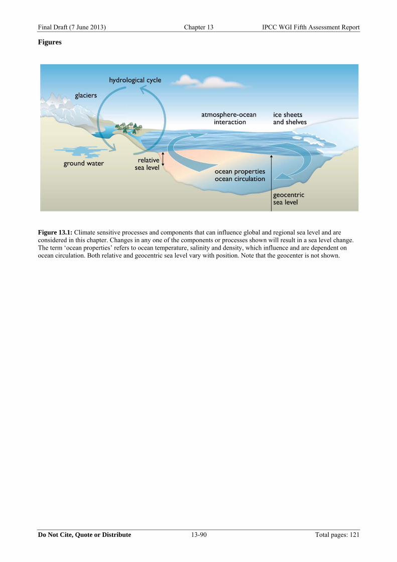
Final Draft (7 June 2013) Chapter 13 IPCC WGI Fifth Assessment Report
Do Not Cite, Quote or Distribute 13-90 Total pages: 121
Figures
Figure 13.1: Climate sensitive processes and components that can influence global and regional sea level and are considered in this chapter. Changes in any one of the components or processes shown will result in a sea level change. The term ‘ocean properties’ refers to ocean temperature, salinity and density, which influence and are dependent on ocean circulation. Both relative and geocentric sea level vary with position. Note that the geocenter is not shown.
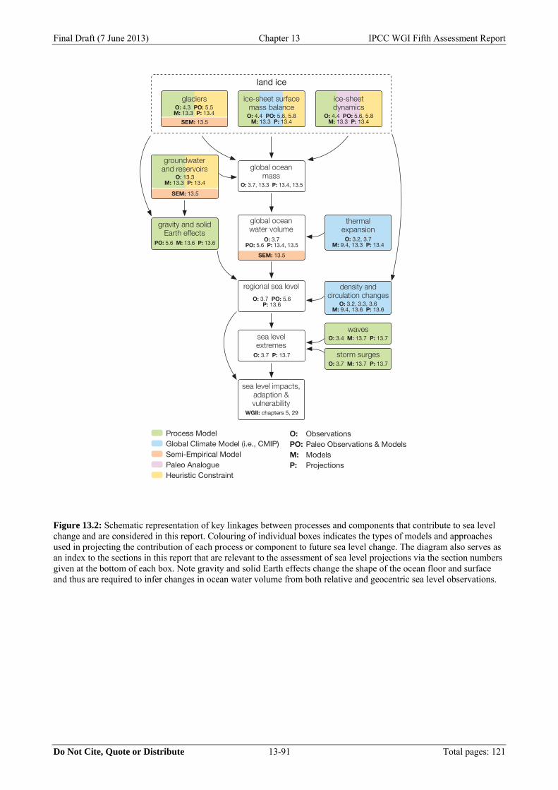
Final Draft (7 June 2013) Chapter 13 IPCC WGI Fifth Assessment Report
Do Not Cite, Quote or Distribute 13-91 Total pages: 121
Figure 13.2: Schematic representation of key linkages between processes and components that contribute to sea level change and are considered in this report. Colouring of individual boxes indicates the types of models and approaches used in projecting the contribution of each process or component to future sea level change. The diagram also serves as an index to the sections in this report that are relevant to the assessment of sea level projections via the section numbers given at the bottom of each box. Note gravity and solid Earth effects change the shape of the ocean floor and surface and thus are required to infer changes in ocean water volume from both relative and geocentric sea level observations.
ice-sheet surface mass balance
ice-sheet dynamics
thermal expansion
waves
storm surges
density and circulation changes
gravity and solid Earth effects
global ocean mass
regional sea level
sea level extremes
global ocean water volume
Process ModelGlobal Climate Model (i.e., CMIP)Semi-Empirical ModelPaleo AnalogueHeuristic Constraint
land iceglaciers
PO: 5.6 M: 13.6 P: 13.6
O: 3.7, 13.3 P: 13.4, 13.5
O: 3.7 PO: 5.6 P: 13.6
O: 3.7 P: 13.7
WGII: chapters 5, 29
O: 3.7 PO: 5.6 P: 13.4, 13.5
SEM: 13.5
SEM: 13.5
SEM: 13.5
O: 3.2, 3.7 M: 9.4, 13.3 P: 13.4
O: 3.4 M: 13.7 P: 13.7
O: 3.7 M: 13.7 P: 13.7
O: 3.2, 3.3, 3.6 M: 9.4, 13.6 P: 13.6
O: 4.4 PO: 5.6, 5.8M: 13.3 P: 13.4
O: 4.4 PO: 5.6, 5.8M: 13.3 P: 13.4
sea level impacts, adaption & vulnerability
O: ObservationsPO: Paleo Observations & ModelsM: ModelsP: Projections
O: 4.3 PO: 5.5M: 13.3 P: 13.4
groundwater and reservoirs
O: 13.3 M: 13.3 P: 13.4
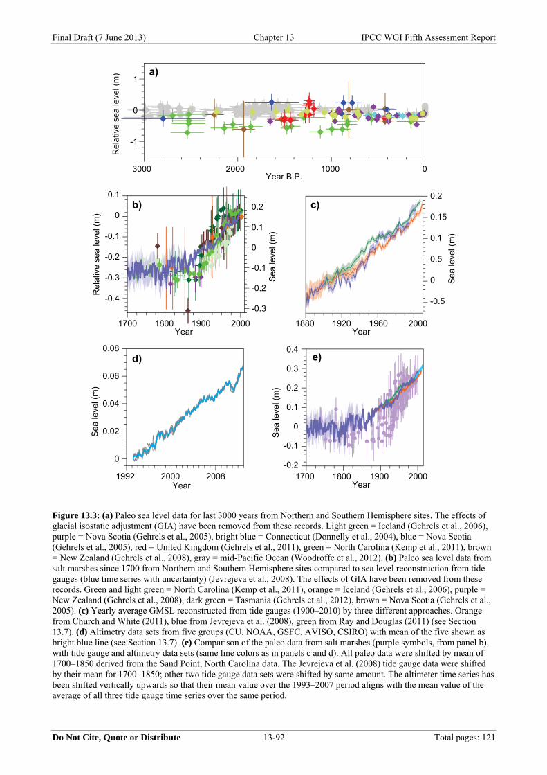
Final Draft (7 June 2013) Chapter 13 IPCC WGI Fifth Assessment Report
Do Not Cite, Quote or Distribute 13-92 Total pages: 121
Figure 13.3: (a) Paleo sea level data for last 3000 years from Northern and Southern Hemisphere sites. The effects of glacial isostatic adjustment (GIA) have been removed from these records. Light green = Iceland (Gehrels et al., 2006), purple = Nova Scotia (Gehrels et al., 2005), bright blue = Connecticut (Donnelly et al., 2004), blue = Nova Scotia (Gehrels et al., 2005), red = United Kingdom (Gehrels et al., 2011), green = North Carolina (Kemp et al., 2011), brown = New Zealand (Gehrels et al., 2008), gray = mid-Pacific Ocean (Woodroffe et al., 2012). (b) Paleo sea level data from salt marshes since 1700 from Northern and Southern Hemisphere sites compared to sea level reconstruction from tide gauges (blue time series with uncertainty) (Jevrejeva et al., 2008). The effects of GIA have been removed from these records. Green and light green = North Carolina (Kemp et al., 2011), orange = Iceland (Gehrels et al., 2006), purple = New Zealand (Gehrels et al., 2008), dark green = Tasmania (Gehrels et al., 2012), brown = Nova Scotia (Gehrels et al., 2005). (c) Yearly average GMSL reconstructed from tide gauges (1900–2010) by three different approaches. Orange from Church and White (2011), blue from Jevrejeva et al. (2008), green from Ray and Douglas (2011) (see Section 13.7). (d) Altimetry data sets from five groups (CU, NOAA, GSFC, AVISO, CSIRO) with mean of the five shown as bright blue line (see Section 13.7). (e) Comparison of the paleo data from salt marshes (purple symbols, from panel b), with tide gauge and altimetry data sets (same line colors as in panels c and d). All paleo data were shifted by mean of 1700–1850 derived from the Sand Point, North Carolina data. The Jevrejeva et al. (2008) tide gauge data were shifted by their mean for 1700–1850; other two tide gauge data sets were shifted by same amount. The altimeter time series has been shifted vertically upwards so that their mean value over the 1993–2007 period aligns with the mean value of the average of all three tide gauge time series over the same period.
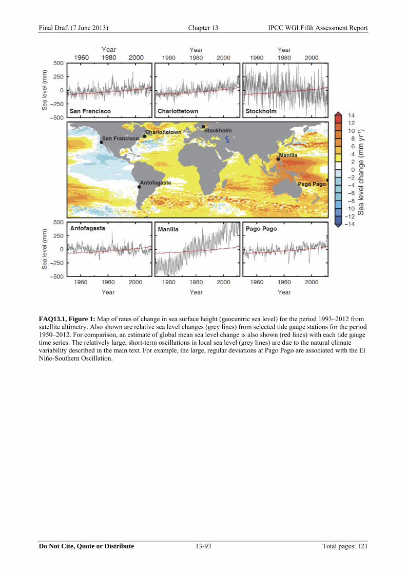
Final Draft (7 June 2013) Chapter 13 IPCC WGI Fifth Assessment Report
Do Not Cite, Quote or Distribute 13-93 Total pages: 121
FAQ13.1, Figure 1: Map of rates of change in sea surface height (geocentric sea level) for the period 1993–2012 from satellite altimetry. Also shown are relative sea level changes (grey lines) from selected tide gauge stations for the period 1950–2012. For comparison, an estimate of global mean sea level change is also shown (red lines) with each tide gauge time series. The relatively large, short-term oscillations in local sea level (grey lines) are due to the natural climate variability described in the main text. For example, the large, regular deviations at Pago Pago are associated with the El Niño-Southern Oscillation.
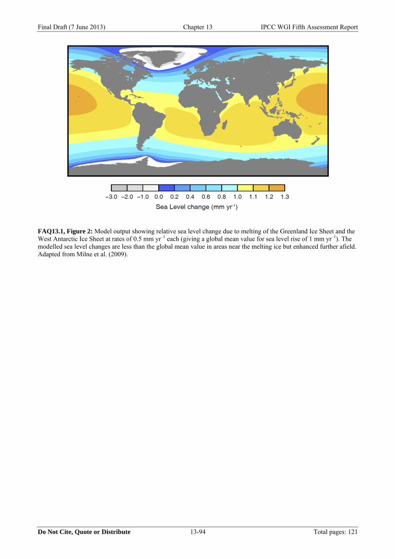
Final Draft (7 June 2013) Chapter 13 IPCC WGI Fifth Assessment Report
Do Not Cite, Quote or Distribute 13-94 Total pages: 121
FAQ13.1, Figure 2: Model output showing relative sea level change due to melting of the Greenland Ice Sheet and the West Antarctic Ice Sheet at rates of 0.5 mm yr–1 each (giving a global mean value for sea level rise of 1 mm yr–1). The modelled sea level changes are less than the global mean value in areas near the melting ice but enhanced further afield. Adapted from Milne et al. (2009).
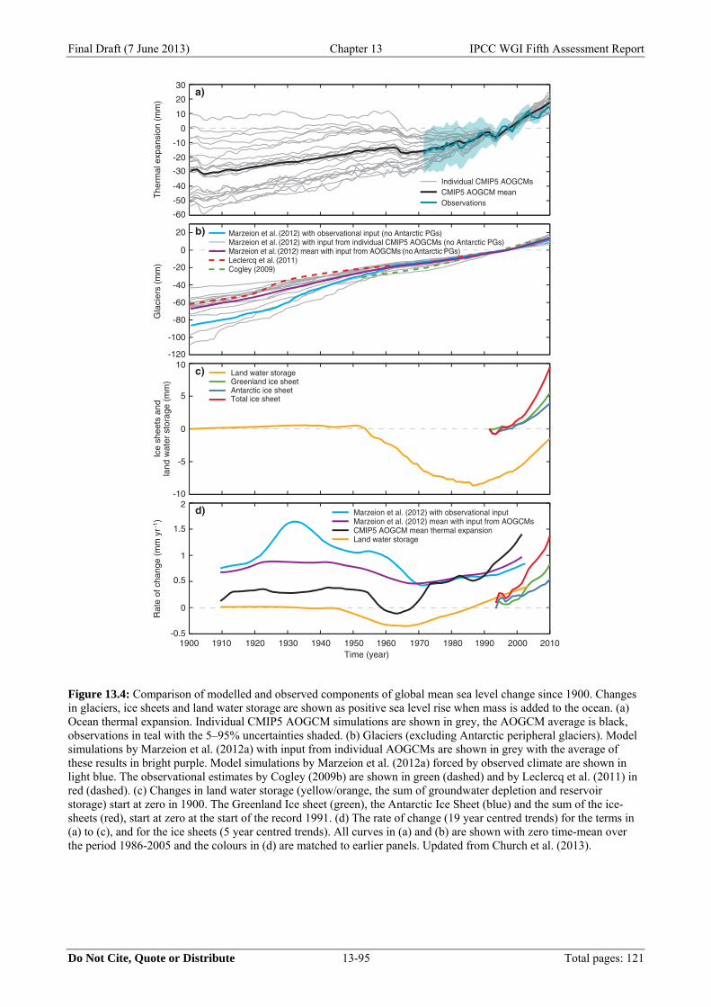
Final Draft (7 June 2013) Chapter 13 IPCC WGI Fifth Assessment Report
Do Not Cite, Quote or Distribute 13-95 Total pages: 121
Figure 13.4: Comparison of modelled and observed components of global mean sea level change since 1900. Changes in glaciers, ice sheets and land water storage are shown as positive sea level rise when mass is added to the ocean. (a) Ocean thermal expansion. Individual CMIP5 AOGCM simulations are shown in grey, the AOGCM average is black, observations in teal with the 5–95% uncertainties shaded. (b) Glaciers (excluding Antarctic peripheral glaciers). Model simulations by Marzeion et al. (2012a) with input from individual AOGCMs are shown in grey with the average of these results in bright purple. Model simulations by Marzeion et al. (2012a) forced by observed climate are shown in light blue. The observational estimates by Cogley (2009b) are shown in green (dashed) and by Leclercq et al. (2011) in red (dashed). (c) Changes in land water storage (yellow/orange, the sum of groundwater depletion and reservoir storage) start at zero in 1900. The Greenland Ice sheet (green), the Antarctic Ice Sheet (blue) and the sum of the ice-sheets (red), start at zero at the start of the record 1991. (d) The rate of change (19 year centred trends) for the terms in (a) to (c), and for the ice sheets (5 year centred trends). All curves in (a) and (b) are shown with zero time-mean over the period 1986-2005 and the colours in (d) are matched to earlier panels. Updated from Church et al. (2013).
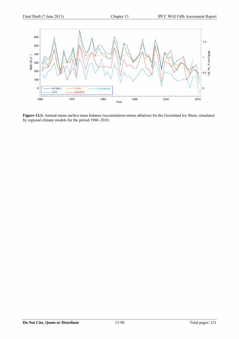
Final Draft (7 June 2013) Chapter 13 IPCC WGI Fifth Assessment Report
Do Not Cite, Quote or Distribute 13-96 Total pages: 121
Figure 13.5: Annual-mean surface mass balance (accumulation minus ablation) for the Greenland Ice Sheet, simulated by regional climate models for the period 1960–2010.
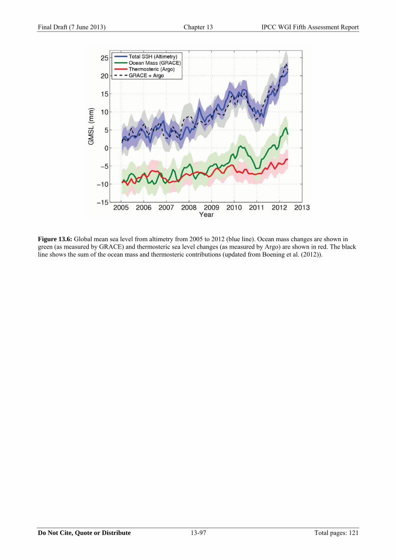
Final Draft (7 June 2013) Chapter 13 IPCC WGI Fifth Assessment Report
Do Not Cite, Quote or Distribute 13-97 Total pages: 121
Figure 13.6: Global mean sea level from altimetry from 2005 to 2012 (blue line). Ocean mass changes are shown in green (as measured by GRACE) and thermosteric sea level changes (as measured by Argo) are shown in red. The black line shows the sum of the ocean mass and thermosteric contributions (updated from Boening et al. (2012)).
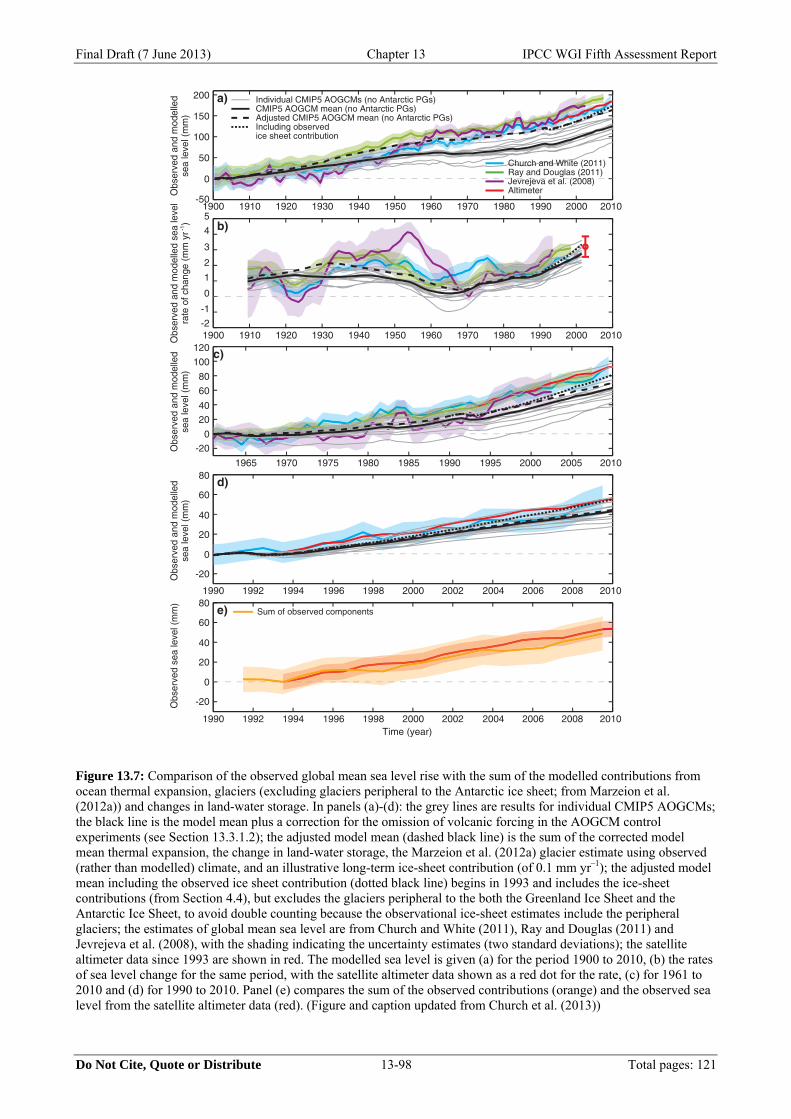
Final Draft (7 June 2013) Chapter 13 IPCC WGI Fifth Assessment Report
Do Not Cite, Quote or Distribute 13-98 Total pages: 121
Figure 13.7: Comparison of the observed global mean sea level rise with the sum of the modelled contributions from ocean thermal expansion, glaciers (excluding glaciers peripheral to the Antarctic ice sheet; from Marzeion et al. (2012a)) and changes in land-water storage. In panels (a)-(d): the grey lines are results for individual CMIP5 AOGCMs; the black line is the model mean plus a correction for the omission of volcanic forcing in the AOGCM control experiments (see Section 13.3.1.2); the adjusted model mean (dashed black line) is the sum of the corrected model mean thermal expansion, the change in land-water storage, the Marzeion et al. (2012a) glacier estimate using observed (rather than modelled) climate, and an illustrative long-term ice-sheet contribution (of 0.1 mm yr–1); the adjusted model mean including the observed ice sheet contribution (dotted black line) begins in 1993 and includes the ice-sheet contributions (from Section 4.4), but excludes the glaciers peripheral to the both the Greenland Ice Sheet and the Antarctic Ice Sheet, to avoid double counting because the observational ice-sheet estimates include the peripheral glaciers; the estimates of global mean sea level are from Church and White (2011), Ray and Douglas (2011) and Jevrejeva et al. (2008), with the shading indicating the uncertainty estimates (two standard deviations); the satellite altimeter data since 1993 are shown in red. The modelled sea level is given (a) for the period 1900 to 2010, (b) the rates of sea level change for the same period, with the satellite altimeter data shown as a red dot for the rate, (c) for 1961 to 2010 and (d) for 1990 to 2010. Panel (e) compares the sum of the observed contributions (orange) and the observed sea level from the satellite altimeter data (red). (Figure and caption updated from Church et al. (2013))
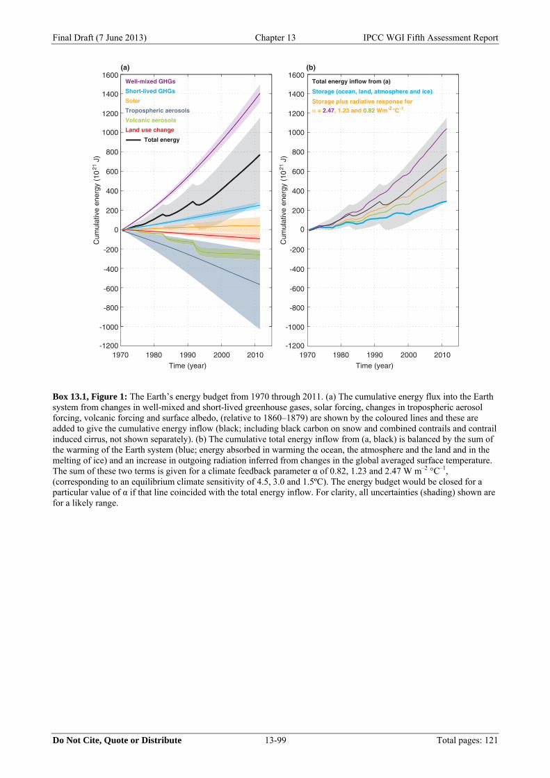
Final Draft (7 June 2013) Chapter 13 IPCC WGI Fifth Assessment Report
Do Not Cite, Quote or Distribute 13-99 Total pages: 121
Box 13.1, Figure 1: The Earth’s energy budget from 1970 through 2011. (a) The cumulative energy flux into the Earth system from changes in well-mixed and short-lived greenhouse gases, solar forcing, changes in tropospheric aerosol forcing, volcanic forcing and surface albedo, (relative to 1860–1879) are shown by the coloured lines and these are added to give the cumulative energy inflow (black; including black carbon on snow and combined contrails and contrail induced cirrus, not shown separately). (b) The cumulative total energy inflow from (a, black) is balanced by the sum of the warming of the Earth system (blue; energy absorbed in warming the ocean, the atmosphere and the land and in the melting of ice) and an increase in outgoing radiation inferred from changes in the global averaged surface temperature. The sum of these two terms is given for a climate feedback parameter α of 0.82, 1.23 and 2.47 W m–2 °C–1, (corresponding to an equilibrium climate sensitivity of 4.5, 3.0 and 1.5ºC). The energy budget would be closed for a particular value of α if that line coincided with the total energy inflow. For clarity, all uncertainties (shading) shown are for a likely range.
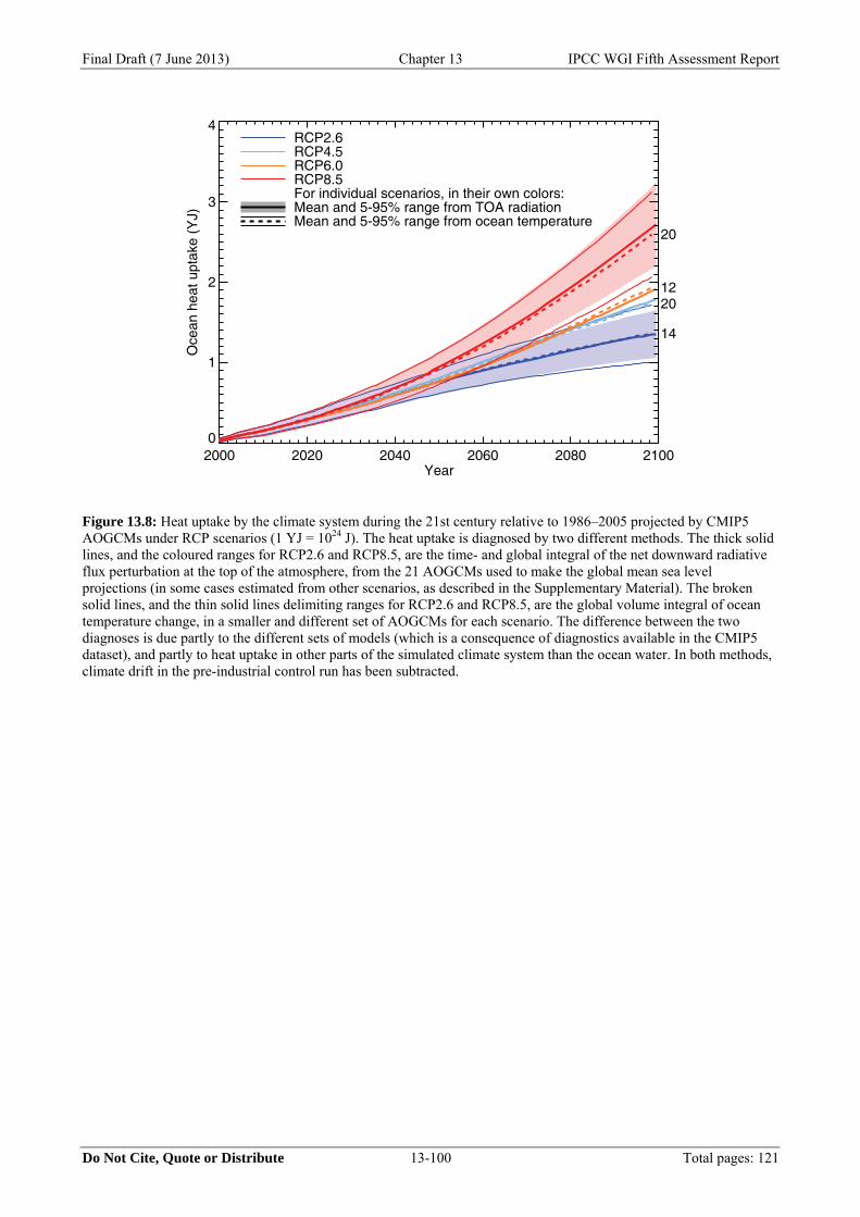
Final Draft (7 June 2013) Chapter 13 IPCC WGI Fifth Assessment Report
Do Not Cite, Quote or Distribute 13-100 Total pages: 121
Figure 13.8: Heat uptake by the climate system during the 21st century relative to 1986–2005 projected by CMIP5 AOGCMs under RCP scenarios (1 YJ = 1024 J). The heat uptake is diagnosed by two different methods. The thick solid lines, and the coloured ranges for RCP2.6 and RCP8.5, are the time- and global integral of the net downward radiative flux perturbation at the top of the atmosphere, from the 21 AOGCMs used to make the global mean sea level projections (in some cases estimated from other scenarios, as described in the Supplementary Material). The broken solid lines, and the thin solid lines delimiting ranges for RCP2.6 and RCP8.5, are the global volume integral of ocean temperature change, in a smaller and different set of AOGCMs for each scenario. The difference between the two diagnoses is due partly to the different sets of models (which is a consequence of diagnostics available in the CMIP5 dataset), and partly to heat uptake in other parts of the simulated climate system than the ocean water. In both methods, climate drift in the pre-industrial control run has been subtracted.
2000 2020 2040 2060 2080 2100Year
0
1
2
3
4
Oce
an h
eat u
ptak
e (Y
J)
14
RCP2.6
20
RCP4.5
12
RCP6.0
20
RCP8.5For individual scenarios, in their own colors:Mean and 5-95% range from TOA radiationMean and 5-95% range from ocean temperature
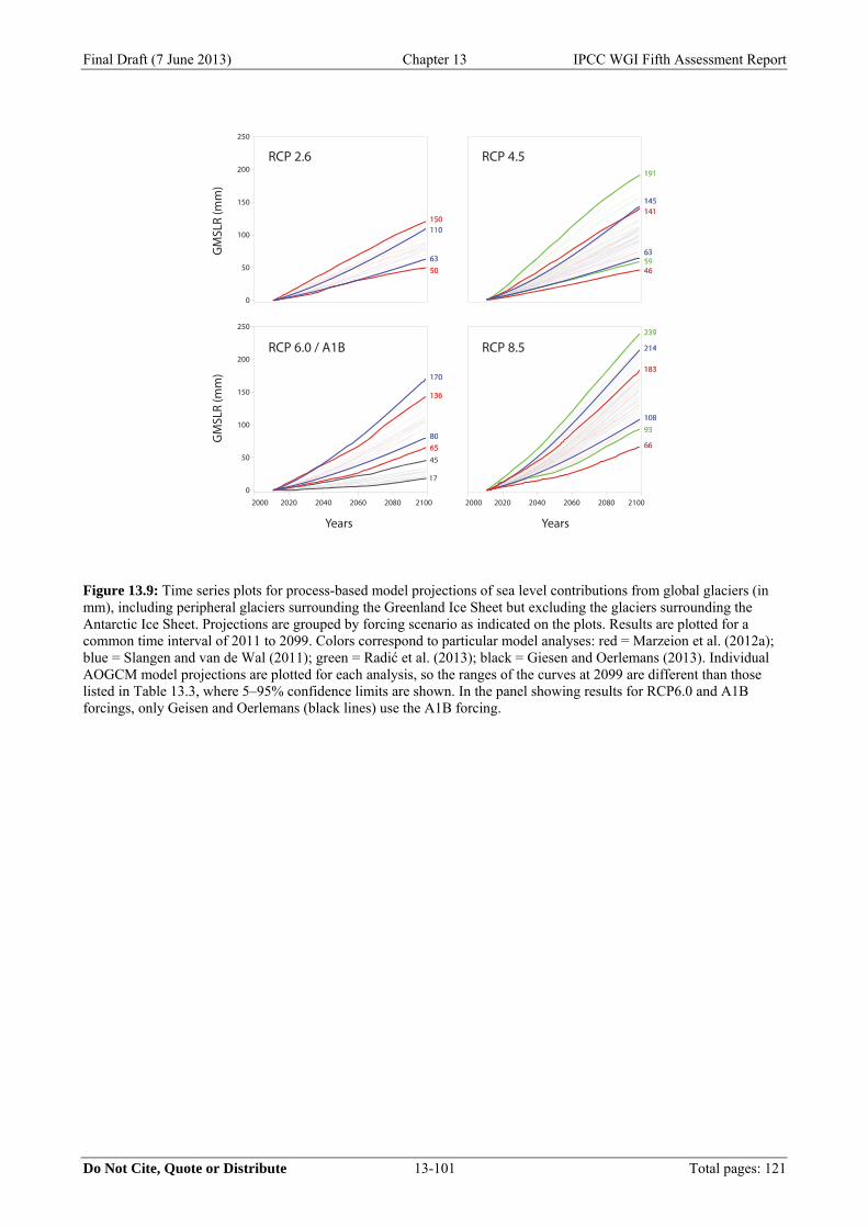
Final Draft (7 June 2013) Chapter 13 IPCC WGI Fifth Assessment Report
Do Not Cite, Quote or Distribute 13-101 Total pages: 121
Figure 13.9: Time series plots for process-based model projections of sea level contributions from global glaciers (in mm), including peripheral glaciers surrounding the Greenland Ice Sheet but excluding the glaciers surrounding the Antarctic Ice Sheet. Projections are grouped by forcing scenario as indicated on the plots. Results are plotted for a common time interval of 2011 to 2099. Colors correspond to particular model analyses: red = Marzeion et al. (2012a); blue = Slangen and van de Wal (2011); green = Radić et al. (2013); black = Giesen and Oerlemans (2013). Individual AOGCM model projections are plotted for each analysis, so the ranges of the curves at 2099 are different than those listed in Table 13.3, where 5–95% confidence limits are shown. In the panel showing results for RCP6.0 and A1B forcings, only Geisen and Oerlemans (black lines) use the A1B forcing.
0
50
100
150
200
250
0
50
100
150
200
250
2000 2020 2040 2060 2080 2100 2000 2020 2040 2060 2080 2100
RCP 2.6 RCP 4.5
RCP 8.5RCP 6.0 / A1B
5063
150110
6580
17
45
170
136
46
6359
145
191
141
66
108 93
214
239
183
50506363
150150110110
65658080
170170
136136
4646
63635959
145145
191191
141141
6666
1081089393
214214
239239
183183
Years Years
GM
SLR
(mm
)G
MSL
R (m
m)
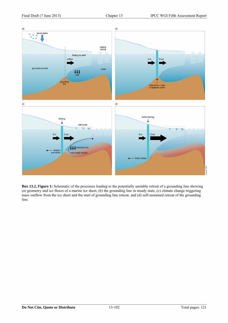
Final Draft (7 June 2013) Chapter 13 IPCC WGI Fifth Assessment Report
Do Not Cite, Quote or Distribute 13-102 Total pages: 121
Box 13.2, Figure 1: Schematic of the processes leading to the potentially unstable retreat of a grounding line showing (a) geometry and ice fluxes of a marine ice sheet, (b) the grounding line in steady state, (c) climate change triggering mass outflow from the ice sheet and the start of grounding line retreat, and (d) self-sustained retreat of the grounding line.
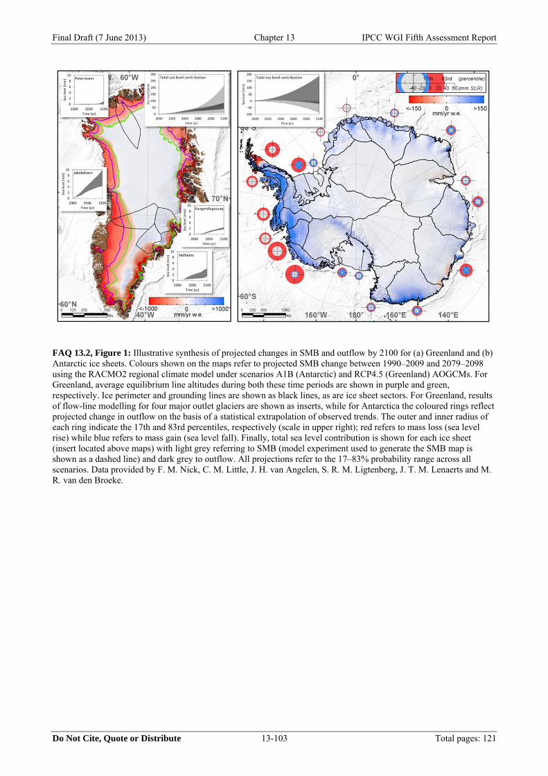
Final Draft (7 June 2013) Chapter 13 IPCC WGI Fifth Assessment Report
Do Not Cite, Quote or Distribute 13-103 Total pages: 121
FAQ 13.2, Figure 1: Illustrative synthesis of projected changes in SMB and outflow by 2100 for (a) Greenland and (b) Antarctic ice sheets. Colours shown on the maps refer to projected SMB change between 1990–2009 and 2079–2098 using the RACMO2 regional climate model under scenarios A1B (Antarctic) and RCP4.5 (Greenland) AOGCMs. For Greenland, average equilibrium line altitudes during both these time periods are shown in purple and green, respectively. Ice perimeter and grounding lines are shown as black lines, as are ice sheet sectors. For Greenland, results of flow-line modelling for four major outlet glaciers are shown as inserts, while for Antarctica the coloured rings reflect projected change in outflow on the basis of a statistical extrapolation of observed trends. The outer and inner radius of each ring indicate the 17th and 83rd percentiles, respectively (scale in upper right); red refers to mass loss (sea level rise) while blue refers to mass gain (sea level fall). Finally, total sea level contribution is shown for each ice sheet (insert located above maps) with light grey referring to SMB (model experiment used to generate the SMB map is shown as a dashed line) and dark grey to outflow. All projections refer to the 17–83% probability range across all scenarios. Data provided by F. M. Nick, C. M. Little, J. H. van Angelen, S. R. M. Ligtenberg, J. T. M. Lenaerts and M. R. van den Broeke.
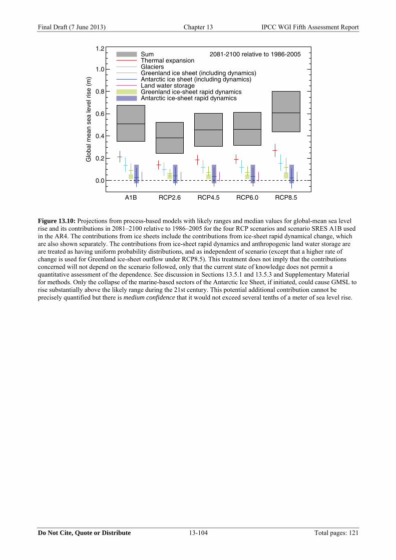
Final Draft (7 June 2013) Chapter 13 IPCC WGI Fifth Assessment Report
Do Not Cite, Quote or Distribute 13-104 Total pages: 121
Figure 13.10: Projections from process-based models with likely ranges and median values for global-mean sea level rise and its contributions in 2081–2100 relative to 1986–2005 for the four RCP scenarios and scenario SRES A1B used in the AR4. The contributions from ice sheets include the contributions from ice-sheet rapid dynamical change, which are also shown separately. The contributions from ice-sheet rapid dynamics and anthropogenic land water storage are are treated as having uniform probability distributions, and as independent of scenario (except that a higher rate of change is used for Greenland ice-sheet outflow under RCP8.5). This treatment does not imply that the contributions concerned will not depend on the scenario followed, only that the current state of knowledge does not permit a quantitative assessment of the dependence. See discussion in Sections 13.5.1 and 13.5.3 and Supplementary Material for methods. Only the collapse of the marine-based sectors of the Antarctic Ice Sheet, if initiated, could cause GMSL to rise substantially above the likely range during the 21st century. This potential additional contribution cannot be precisely quantified but there is medium confidence that it would not exceed several tenths of a meter of sea level rise.
A1B RCP2.6 RCP4.5 RCP6.0 RCP8.5
0.0
0.2
0.4
0.6
0.8
1.0
1.2
Glo
bal m
ean
sea
leve
l ris
e (m
)
2081-2100 relative to 1986-2005SumThermal expansionGlaciersGreenland ice sheet (including dynamics)Antarctic ice sheet (including dynamics)Land water storageGreenland ice-sheet rapid dynamicsAntarctic ice-sheet rapid dynamics
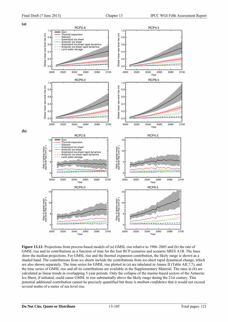
Final Draft (7 June 2013) Chapter 13 IPCC WGI Fifth Assessment Report
Do Not Cite, Quote or Distribute 13-105 Total pages: 121
(a)
(b)
Figure 13.11: Projections from process-based models of (a) GMSL rise relative to 1986–2005 and (b) the rate of GMSL rise and its contributions as a function of time for the four RCP scenarios and scenario SRES A1B. The lines show the median projections. For GMSL rise and the thermal expansion contribution, the likely range is shown as a shaded band. The contributions from ice sheets include the contributions from ice-sheet rapid dynamical change, which are also shown separately. The time series for GMSL rise plotted in (a) are tabulated in Annex II (Table AII.7.7), and the time series of GMSL rise and all its contributions are available in the Supplementary Material. The rates in (b) are calculated as linear trends in overlapping 5-year periods. Only the collapse of the marine-based sectors of the Antarctic Ice Sheet, if initiated, could cause GMSL to rise substantially above the likely range during the 21st century. This potential additional contribution cannot be precisely quantified but there is medium confidence that it would not exceed several tenths of a meter of sea level rise.
RCP2.6
0.0
0.2
0.4
0.6
0.8
1.0
Glo
bal m
ean
sea
leve
l ris
e (m
)
2000 2020 2040 2060 2080 2100Year
SumThermal expansionGlaciersGreenland ice sheetAntarctic ice sheetGreenland ice-sheet rapid dynamicsAntarctic ice-sheet rapid dynamicsLand water storage
RCP4.5
0.0
0.2
0.4
0.6
0.8
1.0
Glo
bal m
ean
sea
leve
l ris
e (m
)
2000 2020 2040 2060 2080 2100Year
RCP6.0
0.0
0.2
0.4
0.6
0.8
1.0
Glo
bal m
ean
sea
leve
l ris
e (m
)
2000 2020 2040 2060 2080 2100Year
RCP8.5
0.0
0.2
0.4
0.6
0.8
1.0
Glo
bal m
ean
sea
leve
l ris
e (m
)
2000 2020 2040 2060 2080 2100Year
RCP2.6
0
5
10
15
Rat
e of
glo
bal m
ean
sea
leve
l ris
e (m
m y
r-1)
2000 2020 2040 2060 2080 2100Year
SumThermal expansionGlaciersGreenland ice sheetAntarctic ice sheetGreenland ice-sheet rapid dynamicsAntarctic ice-sheet rapid dynamicsLand water storage
RCP4.5
0
5
10
15
Rat
e of
glo
bal m
ean
sea
leve
l ris
e (m
m y
r-1)
2000 2020 2040 2060 2080 2100Year
RCP6.0
0
5
10
15
Rat
e of
glo
bal m
ean
sea
leve
l ris
e (m
m y
r-1)
2000 2020 2040 2060 2080 2100Year
RCP8.5
0
5
10
15
Rat
e of
glo
bal m
ean
sea
leve
l ris
e (m
m y
r-1)
2000 2020 2040 2060 2080 2100Year
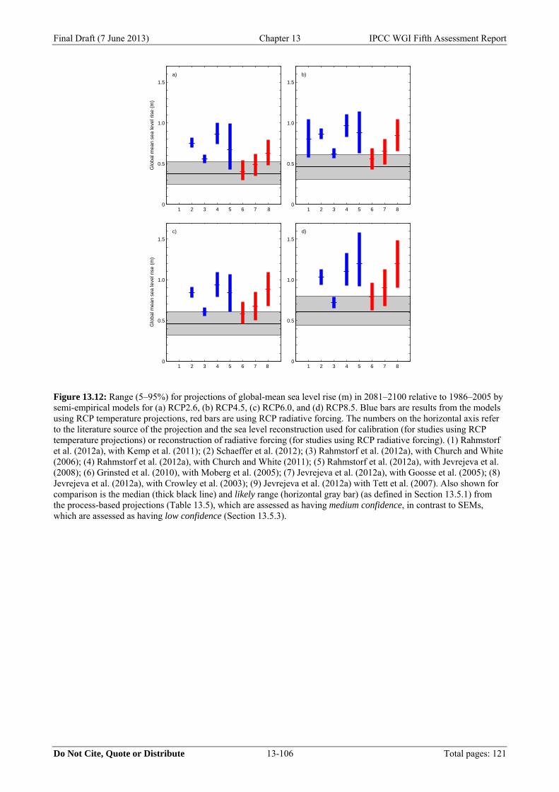
Final Draft (7 June 2013) Chapter 13 IPCC WGI Fifth Assessment Report
Do Not Cite, Quote or Distribute 13-106 Total pages: 121
Figure 13.12: Range (5–95%) for projections of global-mean sea level rise (m) in 2081–2100 relative to 1986–2005 by semi-empirical models for (a) RCP2.6, (b) RCP4.5, (c) RCP6.0, and (d) RCP8.5. Blue bars are results from the models using RCP temperature projections, red bars are using RCP radiative forcing. The numbers on the horizontal axis refer to the literature source of the projection and the sea level reconstruction used for calibration (for studies using RCP temperature projections) or reconstruction of radiative forcing (for studies using RCP radiative forcing). (1) Rahmstorf et al. (2012a), with Kemp et al. (2011); (2) Schaeffer et al. (2012); (3) Rahmstorf et al. (2012a), with Church and White (2006); (4) Rahmstorf et al. (2012a), with Church and White (2011); (5) Rahmstorf et al. (2012a), with Jevrejeva et al. (2008); (6) Grinsted et al. (2010), with Moberg et al. (2005); (7) Jevrejeva et al. (2012a), with Goosse et al. (2005); (8) Jevrejeva et al. (2012a), with Crowley et al. (2003); (9) Jevrejeva et al. (2012a) with Tett et al. (2007). Also shown for comparison is the median (thick black line) and likely range (horizontal gray bar) (as defined in Section 13.5.1) from the process-based projections (Table 13.5), which are assessed as having medium confidence, in contrast to SEMs, which are assessed as having low confidence (Section 13.5.3).
Glo
bal m
ean
sea
leve
l ris
e (m
)
a)
1 2 3 4 5 6 7 8 0
0.5
1.0
1.5
b)
1 2 3 4 5 6 7 8 0
0.5
1.0
1.5
Glo
bal m
ean
sea
leve
l ris
e (m
)
c)
1 2 3 4 5 6 7 8 0
0.5
1.0
1.5
d)
1 2 3 4 5 6 7 8 0
0.5
1.0
1.5
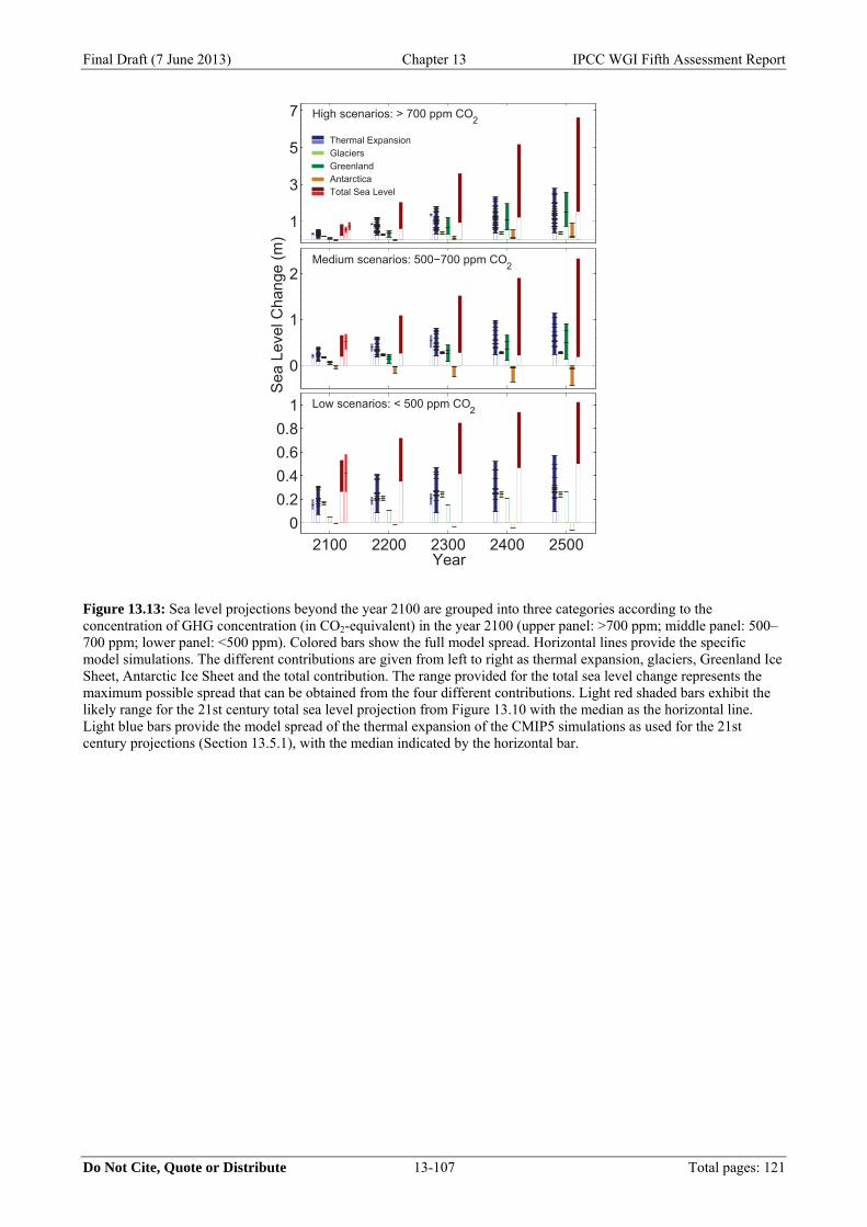
Final Draft (7 June 2013) Chapter 13 IPCC WGI Fifth Assessment Report
Do Not Cite, Quote or Distribute 13-107 Total pages: 121
Figure 13.13: Sea level projections beyond the year 2100 are grouped into three categories according to the concentration of GHG concentration (in CO2-equivalent) in the year 2100 (upper panel: >700 ppm; middle panel: 500–700 ppm; lower panel: <500 ppm). Colored bars show the full model spread. Horizontal lines provide the specific model simulations. The different contributions are given from left to right as thermal expansion, glaciers, Greenland Ice Sheet, Antarctic Ice Sheet and the total contribution. The range provided for the total sea level change represents the maximum possible spread that can be obtained from the four different contributions. Light red shaded bars exhibit the likely range for the 21st century total sea level projection from Figure 13.10 with the median as the horizontal line. Light blue bars provide the model spread of the thermal expansion of the CMIP5 simulations as used for the 21st century projections (Section 13.5.1), with the median indicated by the horizontal bar.
1
3
5
7
Thermal ExpansionGlaciersGreenlandAntarcticaTotal Sea Level
High scenarios: > 700 ppm CO2
0
1
2Medium scenarios: 500−700 ppm CO2
Year
2100 2200 2300 2400 25000
0.20.40.60.8
1
Year
Low scenarios: < 500 ppm CO2
Sea
Leve
l Cha
nge
(m)
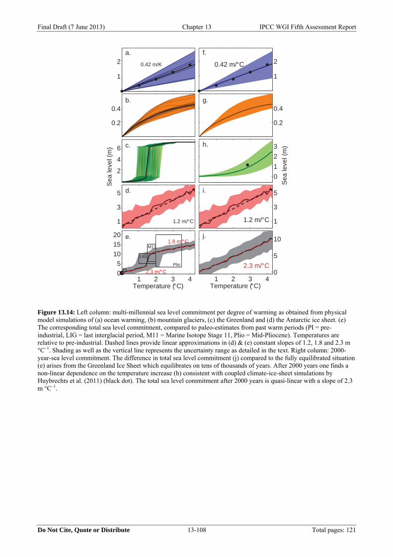
Final Draft (7 June 2013) Chapter 13 IPCC WGI Fifth Assessment Report
Do Not Cite, Quote or Distribute 13-108 Total pages: 121
Figure 13.14: Left column: multi-millennial sea level commitment per degree of warming as obtained from physical model simulations of (a) ocean warming, (b) mountain glaciers, (c) the Greenland and (d) the Antarctic ice sheet. (e) The corresponding total sea level commitment, compared to paleo-estimates from past warm periods (PI = pre-industrial, LIG = last interglacial period, M11 = Marine Isotope Stage 11, Plio = Mid-Pliocene). Temperatures are relative to pre-industrial. Dashed lines provide linear approximations in (d) & (e) constant slopes of 1.2, 1.8 and 2.3 m °C–1. Shading as well as the vertical line represents the uncertainty range as detailed in the text. Right column: 2000-year-sea level commitment. The difference in total sea level commitment (j) compared to the fully equilibrated situation (e) arises from the Greenland Ice Sheet which equilibrates on tens of thousands of years. After 2000 years one finds a non-linear dependence on the temperature increase (h) consistent with coupled climate-ice-sheet simulations by Huybrechts et al. (2011) (black dot). The total sea level commitment after 2000 years is quasi-linear with a slope of 2.3 m °C–1.
1
2f.
0.42 m/°C
0.2
0.4g.
0
1
2
3h.
1
3
5
1.2 m/°C
i.
1 2 3 40
5
10
2.3 m/°C
Temperature (°C)S
ea le
vel (
m)
j.
1
2a.
0.42 m/K
0.2
0.4b.
2
4
6 c.
1
3
5
1.2 m/°C
d.
1 2 3 40
5
10
15
201.8 m/°C
2.3 m/°C
Temperature (°C)
Sea
leve
l (m
)
e.
PI
LIG
M11
Plio
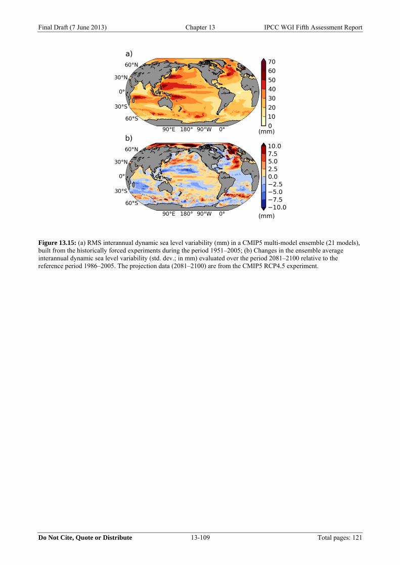
Final Draft (7 June 2013) Chapter 13 IPCC WGI Fifth Assessment Report
Do Not Cite, Quote or Distribute 13-109 Total pages: 121
Figure 13.15: (a) RMS interannual dynamic sea level variability (mm) in a CMIP5 multi-model ensemble (21 models), built from the historically forced experiments during the period 1951–2005; (b) Changes in the ensemble average interannual dynamic sea level variability (std. dev.; in mm) evaluated over the period 2081–2100 relative to the reference period 1986–2005. The projection data (2081–2100) are from the CMIP5 RCP4.5 experiment.
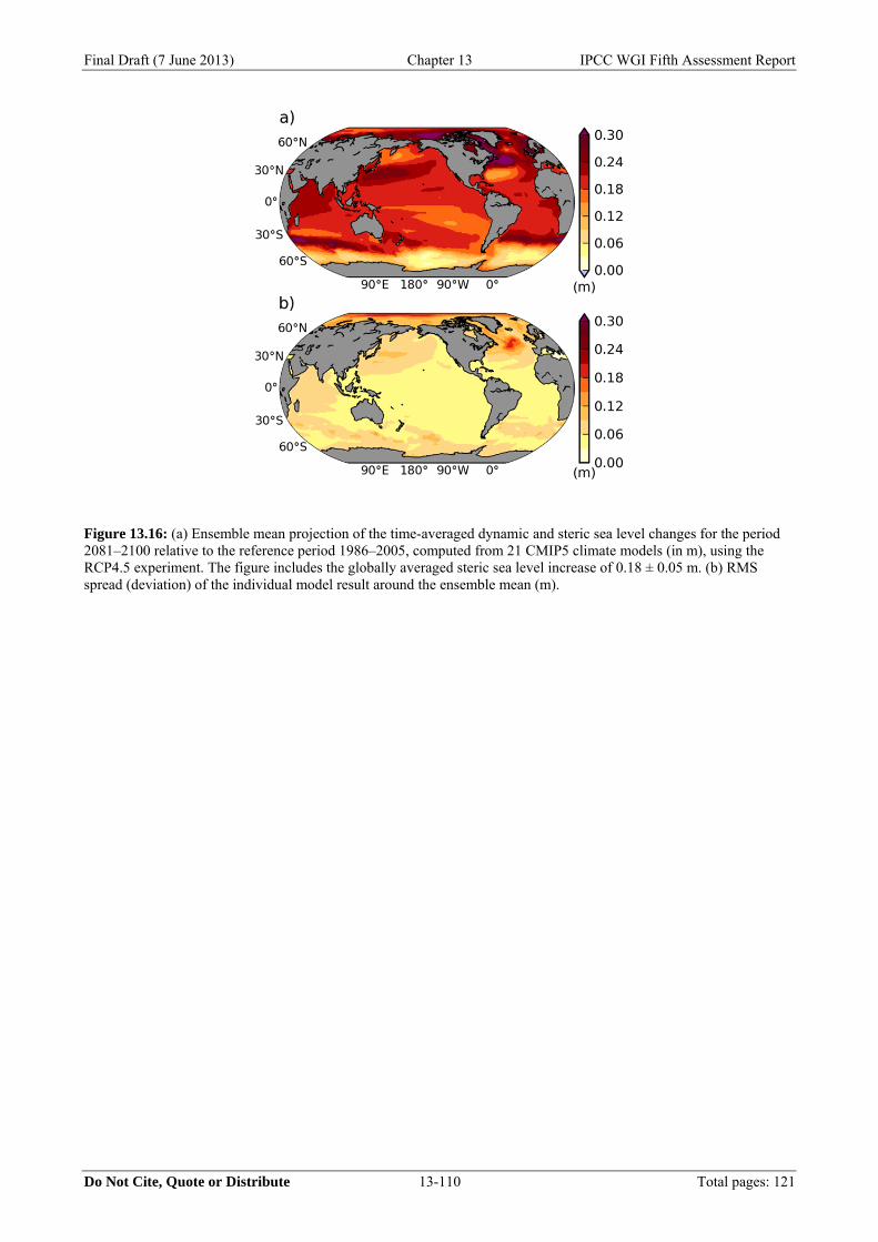
Final Draft (7 June 2013) Chapter 13 IPCC WGI Fifth Assessment Report
Do Not Cite, Quote or Distribute 13-110 Total pages: 121
Figure 13.16: (a) Ensemble mean projection of the time-averaged dynamic and steric sea level changes for the period 2081–2100 relative to the reference period 1986–2005, computed from 21 CMIP5 climate models (in m), using the RCP4.5 experiment. The figure includes the globally averaged steric sea level increase of 0.18 ± 0.05 m. (b) RMS spread (deviation) of the individual model result around the ensemble mean (m).

Final Draft (7 June 2013) Chapter 13 IPCC WGI Fifth Assessment Report
Do Not Cite, Quote or Distribute 13-111 Total pages: 121
Figure 13.17: Projected ensemble mean sea level change (m) due to changes in atmospheric pressure loading over the period from 1986–2005 to 2081–2100 for (a) RCP4.5 and (b) RCP8.5 (contour interval is 0.01 m). Standard deviation of the model ensemble due to the atmospheric pressure loading for (c) RCP4.5 and (d) RCP8.5 (contour interval is 0.005 m).
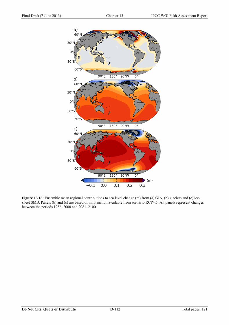
Final Draft (7 June 2013) Chapter 13 IPCC WGI Fifth Assessment Report
Do Not Cite, Quote or Distribute 13-112 Total pages: 121
Figure 13.18: Ensemble mean regional contributions to sea level change (m) from (a) GIA, (b) glaciers and (c) ice-sheet SMB. Panels (b) and (c) are based on information available from scenario RCP4.5. All panels represent changes between the periods 1986–2000 and 2081–2100.
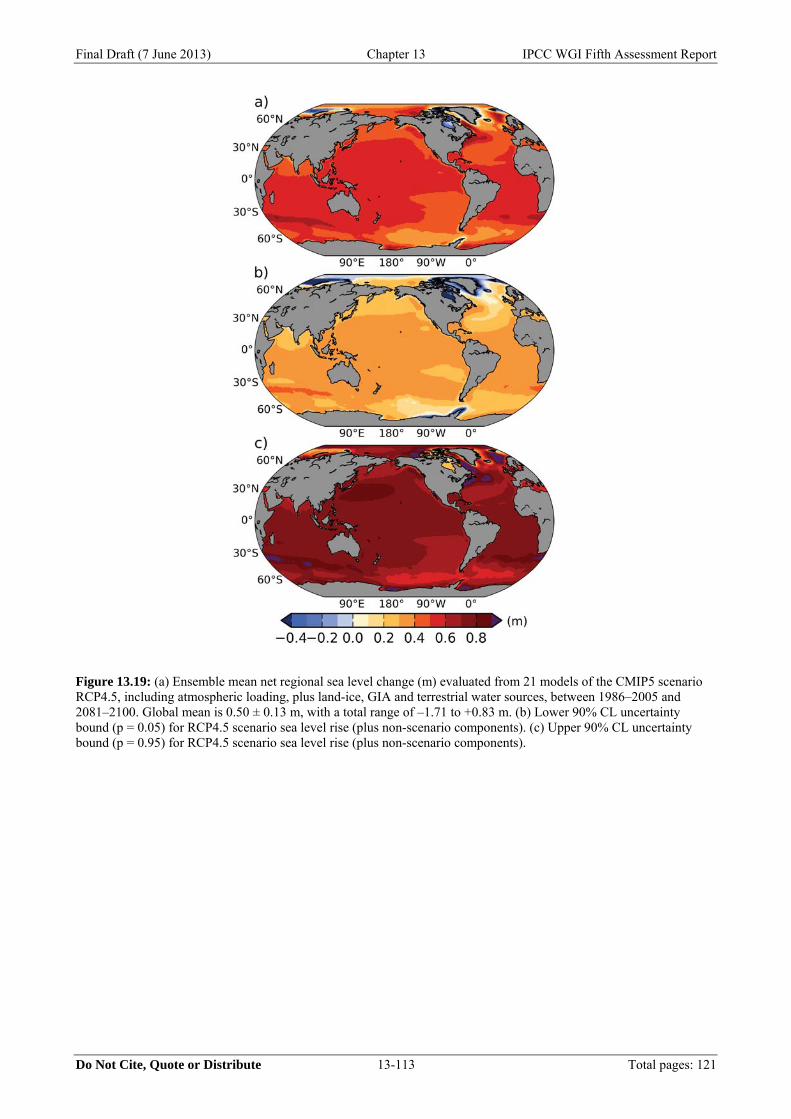
Final Draft (7 June 2013) Chapter 13 IPCC WGI Fifth Assessment Report
Do Not Cite, Quote or Distribute 13-113 Total pages: 121
Figure 13.19: (a) Ensemble mean net regional sea level change (m) evaluated from 21 models of the CMIP5 scenario RCP4.5, including atmospheric loading, plus land-ice, GIA and terrestrial water sources, between 1986–2005 and 2081–2100. Global mean is 0.50 ± 0.13 m, with a total range of –1.71 to +0.83 m. (b) Lower 90% CL uncertainty bound (p = 0.05) for RCP4.5 scenario sea level rise (plus non-scenario components). (c) Upper 90% CL uncertainty bound (p = 0.95) for RCP4.5 scenario sea level rise (plus non-scenario components).
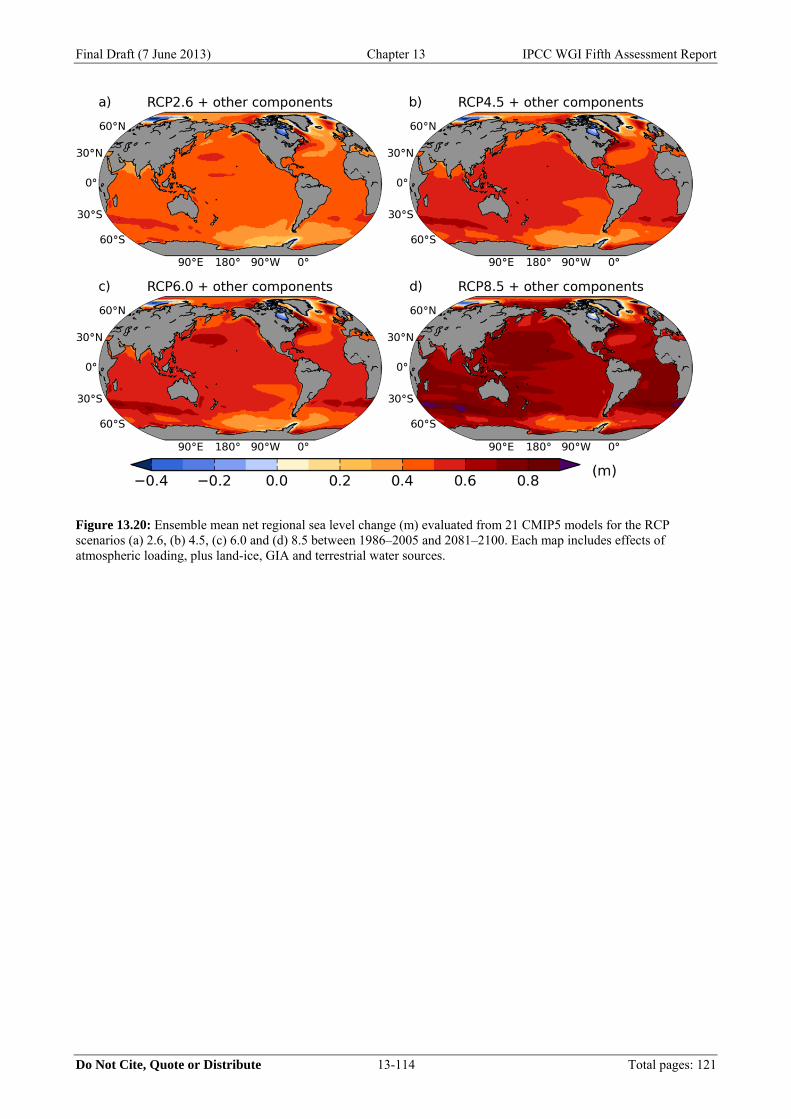
Final Draft (7 June 2013) Chapter 13 IPCC WGI Fifth Assessment Report
Do Not Cite, Quote or Distribute 13-114 Total pages: 121
Figure 13.20: Ensemble mean net regional sea level change (m) evaluated from 21 CMIP5 models for the RCP scenarios (a) 2.6, (b) 4.5, (c) 6.0 and (d) 8.5 between 1986–2005 and 2081–2100. Each map includes effects of atmospheric loading, plus land-ice, GIA and terrestrial water sources.
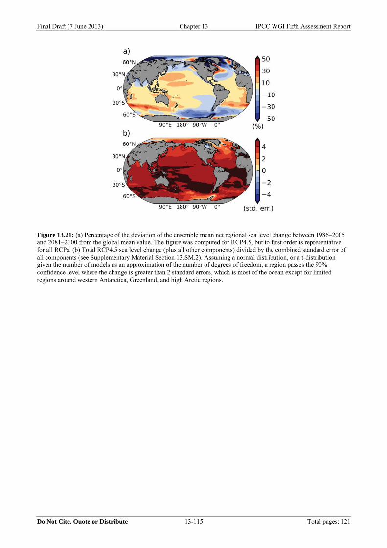
Final Draft (7 June 2013) Chapter 13 IPCC WGI Fifth Assessment Report
Do Not Cite, Quote or Distribute 13-115 Total pages: 121
Figure 13.21: (a) Percentage of the deviation of the ensemble mean net regional sea level change between 1986–2005 and 2081–2100 from the global mean value. The figure was computed for RCP4.5, but to first order is representative for all RCPs. (b) Total RCP4.5 sea level change (plus all other components) divided by the combined standard error of all components (see Supplementary Material Section 13.SM.2). Assuming a normal distribution, or a t-distribution given the number of models as an approximation of the number of degrees of freedom, a region passes the 90% confidence level where the change is greater than 2 standard errors, which is most of the ocean except for limited regions around western Antarctica, Greenland, and high Arctic regions.
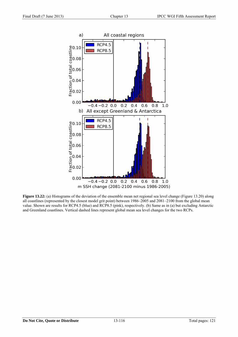
Final Draft (7 June 2013) Chapter 13 IPCC WGI Fifth Assessment Report
Do Not Cite, Quote or Distribute 13-116 Total pages: 121
Figure 13.22: (a) Histograms of the deviation of the ensemble mean net regional sea level change (Figure 13.20) along all coastlines (represented by the closest model grit point) between 1986–2005 and 2081–2100 from the global mean value. Shown are results for RCP4.5 (blue) and RCP8.5 (pink), respectively. (b) Same as in (a) but excluding Antarctic and Greenland coastlines. Vertical dashed lines represent global mean sea level changes for the two RCPs.
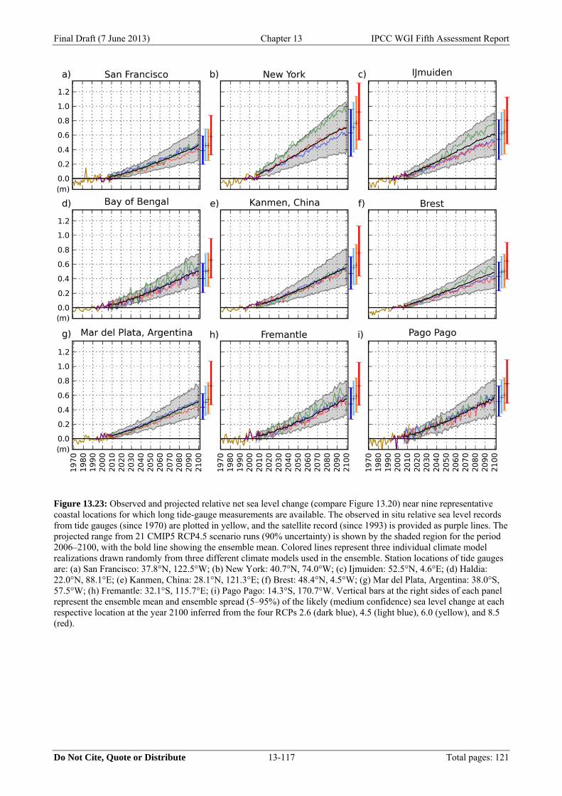
Final Draft (7 June 2013) Chapter 13 IPCC WGI Fifth Assessment Report
Do Not Cite, Quote or Distribute 13-117 Total pages: 121
Figure 13.23: Observed and projected relative net sea level change (compare Figure 13.20) near nine representative coastal locations for which long tide-gauge measurements are available. The observed in situ relative sea level records from tide gauges (since 1970) are plotted in yellow, and the satellite record (since 1993) is provided as purple lines. The projected range from 21 CMIP5 RCP4.5 scenario runs (90% uncertainty) is shown by the shaded region for the period 2006–2100, with the bold line showing the ensemble mean. Colored lines represent three individual climate model realizations drawn randomly from three different climate models used in the ensemble. Station locations of tide gauges are: (a) San Francisco: 37.8°N, 122.5°W; (b) New York: 40.7°N, 74.0°W; (c) Ijmuiden: 52.5°N, 4.6°E; (d) Haldia: 22.0°N, 88.1°E; (e) Kanmen, China: 28.1°N, 121.3°E; (f) Brest: 48.4°N, 4.5°W; (g) Mar del Plata, Argentina: 38.0°S, 57.5°W; (h) Fremantle: 32.1°S, 115.7°E; (i) Pago Pago: 14.3°S, 170.7°W. Vertical bars at the right sides of each panel represent the ensemble mean and ensemble spread (5–95%) of the likely (medium confidence) sea level change at each respective location at the year 2100 inferred from the four RCPs 2.6 (dark blue), 4.5 (light blue), 6.0 (yellow), and 8.5 (red).
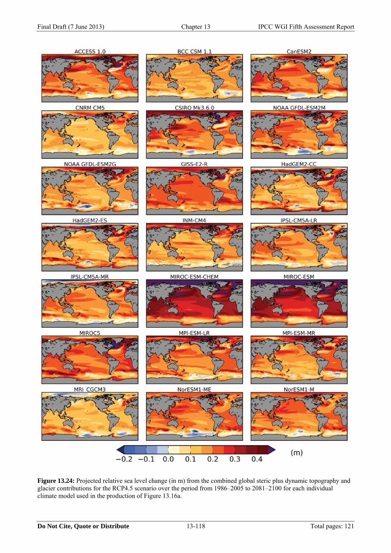
Final Draft (7 June 2013) Chapter 13 IPCC WGI Fifth Assessment Report
Do Not Cite, Quote or Distribute 13-118 Total pages: 121
Figure 13.24: Projected relative sea level change (in m) from the combined global steric plus dynamic topography and glacier contributions for the RCP4.5 scenario over the period from 1986–2005 to 2081–2100 for each individual climate model used in the production of Figure 13.16a.
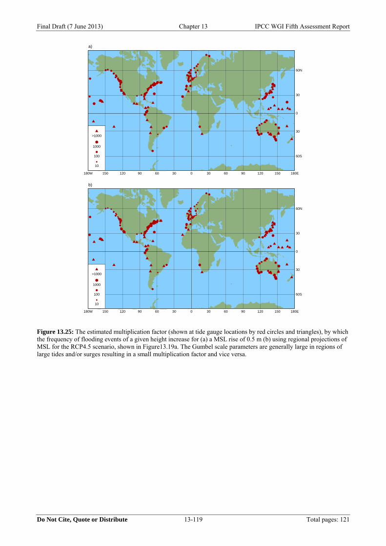
Final Draft (7 June 2013) Chapter 13 IPCC WGI Fifth Assessment Report
Do Not Cite, Quote or Distribute 13-119 Total pages: 121
Figure 13.25: The estimated multiplication factor (shown at tide gauge locations by red circles and triangles), by which the frequency of flooding events of a given height increase for (a) a MSL rise of 0.5 m (b) using regional projections of MSL for the RCP4.5 scenario, shown in Figure13.19a. The Gumbel scale parameters are generally large in regions of large tides and/or surges resulting in a small multiplication factor and vice versa.
0 30 60 90 150120 180E306090120180W 150
0
60S
60N
30
30
a)
10
100
1000
>1000
0 30 60 90 150120 180E306090120180W 150
0
60S
60N
30
30
b)
10
100
1000
>1000

Final Draft (7 June 2013) Chapter 13 IPCC WGI Fifth Assessment Report
Do Not Cite, Quote or Distribute 13-120 Total pages: 121
Figure 13.26: Projected changes in wind-wave conditions (~2075–2100 compared with ~1980–2009) derived from the Coordinated Ocean Wave Climate Projection (COWCLIP) Project (Hemer et al., 2013). (a) Percentage difference in annual mean significant wave height. (b) Percentage difference in January-March mean significant wave height. (c) Percentage difference in July-September mean significant wave height. Hashed regions indicate projected change is greater than the 5-member ensemble standard deviation. (d) As for (a), but displaying absolute changes in mean wave direction, with positive values representing projected clockwise rotation relative to displayed vectors, and colours shown only where ensemble members agree on sign of change. (e) As for (a), but displaying absolute changes in mean wave period. The symbol ~ is used to indicate that the reference periods differ slightly for the various model studies considered.
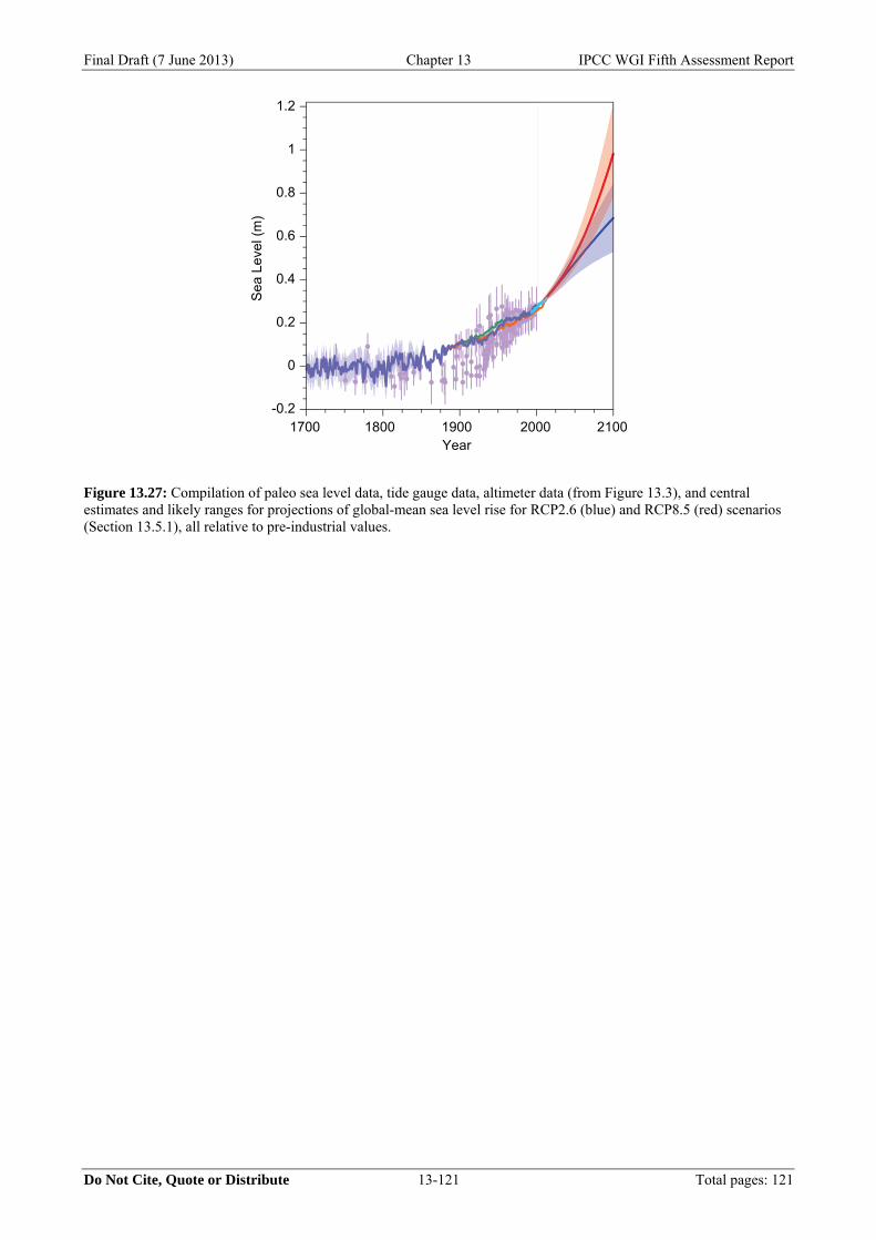
Final Draft (7 June 2013) Chapter 13 IPCC WGI Fifth Assessment Report
Do Not Cite, Quote or Distribute 13-121 Total pages: 121
Figure 13.27: Compilation of paleo sea level data, tide gauge data, altimeter data (from Figure 13.3), and central estimates and likely ranges for projections of global-mean sea level rise for RCP2.6 (blue) and RCP8.5 (red) scenarios (Section 13.5.1), all relative to pre-industrial values.
Related Documents