Worked Examples and Solutions for the Book: Adaptive Filtering Primer with MATLAB by Alexander Poularikas and Zayed Ramadan John L. Weatherwax ∗ December 13, 2015 ∗ [email protected] 1

Welcome message from author
This document is posted to help you gain knowledge. Please leave a comment to let me know what you think about it! Share it to your friends and learn new things together.
Transcript
Worked Examples and Solutions for the Book:
Adaptive Filtering Primer with MATLAB
by Alexander Poularikas and Zayed Ramadan
John L. Weatherwax∗
December 13, 2015
1

Text copyright c©2015 John L. WeatherwaxAll Rights Reserved
Please Do Not Redistribute Without Permission from the Author
2

Introduction
This is a wonderful little book on adaptive filtering. I found the examplesenjoyable and the text very easy to understand. To better facilitate myunderstanding of this material I wrote some notes on the main text andworked a great number of the problems while I worked through the book.For some of the problems I used MATLAB to perform any needed calculations.The code snippets for various exercises can be found at the following location:
http://waxworksmath.com/Authors/N_Z/Poularikas/poularikas.html
I’ve worked hard to make these notes as good as I can, but I have no illusionsthat they are perfect. If you feel that that there is a better way to accomplishor explain an exercise or derivation presented in these notes; or that one ormore of the explanations is unclear, incomplete, or misleading, please tellme. If you find an error of any kind – technical, grammatical, typographical,whatever – please tell me that, too. I’ll gladly add to the acknowledgmentsin later printings the name of the first person to bring each problem to myattention.
3

Chapter 2 (Discrete-time signal processing)
Problem 2.2.1 (a comparison between the FT and the DTFT)
The Fourier transform of the given signal x(t) is given by
X(ω) =
∫ ∞
−∞
x(t)e−jωtdt
=
∫ 0
−∞
e−|t|e−jωtdt +
∫ ∞
0
e−|t|e−jωtdt
=
∫ 0
−∞
ete−jωtdt+
∫ ∞
0
e−te−jωtdt
=
∫ ∞
0
e−tejωtdt+
∫ ∞
0
e−te−jωtdt
=
∫ ∞
0
e−(1−jω)tdt+
∫ ∞
0
e−(1+jω)tdt
=e−(1−jω)t
−(1− jω)
∣
∣
∣
∣
∞
0
+e−(1+jω)t
−(1 + jω)
∣
∣
∣
∣
∞
0
=1
1− jω+
1
1 + jω
=1 + jω
1 + ω2+
1− jω
1 + ω2
=2
1 + ω2.
Evaluating this expression at ω = 1.6 rad/s gives 0.5618.Next, we evaluate the discrete time Fourier transform (DTFT) of x(t) =
e−|t| with two different sampling intervals T = 1s and T = 0.1s. We beginby computing the DTFT of x(t) as
X(ejωT ) = T
∞∑
n=−∞
x(nT )e−jωnT
= T
(
−1∑
n=−∞
enT e−jωnT + 1 +∞∑
n=1
e−nT e−jωnT
)
= T
(
∞∑
n=1
e−nTejωnT +∞∑
n=0
e−nT e−jωnT
)
4

= T
(
∞∑
n=0
(e−T ejωT )n − 1 +
∞∑
n=0
(e−T e−jωT )n
)
= T
(
1
1− e−T ejωT− 1 +
1
1− e−T e−jωT
)
.
To convert this expression into its real and imaginary parts we will multiplyeach fraction above by a conjugate of its denominator. Denoting this commonproduct as D (for denominator) we have
D = (1− e−T ejωT )(1− e−T e−jωT )
= 1− e−T e−jωT − e−T ejωT + e−2T
= 1− e−T (e−jωT + ejωT ) + e−2T
= 1− 2e−T cos(ωT ) + e−2T .
So that the expression for the DTFT X(ejωT ) becomes
X(ejωT ) = T
(
1− e−T e−jωT
D+
1− e−T ejωT
D− 1
)
=T
D(2− 2e−T cos(ωT )−D)
=T
D(1− e−2T )
=T (1− e−2T )
1− 2e−T cos(ωT ) + e−2T.
When T = 1s and ω = 1.6 rad/s we find X(ej(1.6)) = 0.7475. When T = 0.1sthis expression becomes X(ej(0.16)) = 0.5635. The sampling interval withT = 0.1s is obviously a better approximation to the full Fourier transform atthis point.
Problem 2.2.2 (an example with the DFT)
See the MATLAB file prob 2 2 2.m for the calculations required for thisproblem. They basically follow the discussion in the book in the sectionentitled “the discrete Fourier transform (DFT)”. My results don’t exactlymatch the answer presented at the end of the chapter but I don’t see anythingincorrect with what I’ve done.
5

Problem 2.3.1 (examples with the z-transform)
For this problem using the definition of the z-transform we will directlycompute each of the requested expressions.Part (a): In this case we have
X(z) = Z{x(n)} =∞∑
n=−∞
x(n)z−n
=∞∑
n=−∞
cos(nωT )u(n)z−n =∞∑
n=0
cos(nωT )z−n
=1
2
∞∑
n=0
(ejnωT + e−jnωT )z−n
=1
2
(
∞∑
n=0
(ejωT z−1)n +
∞∑
n=0
(e−jωT z−1)n
)
=1
2
(
1
1− ejωT z−1+
1
1− e−jωTz−1
)
.
To further simplify this expression in each fraction above we will multiply bya “form of one” determined by the conjugate of the fractions denominator.In both cases this gives a denominator D given by
D = (1− ejωT z−1)(1− e−jωTz−1)
= 1− ejωT z−1 − e−jωT z−1 + z−2
= 1− 2z−1 cos(ωT ) + z−2 .
With this expression we obtain
X(z) =1
2D(2− 2z−1 cos(ωT ))
=z2 − z cos(ωT )
z2 − z cos(ωT ) + 1.
Part (b): In this case we find
X(z) = Z{x(n)} =
∞∑
n=−∞
nanu(n)z−n =
∞∑
n=0
nanz−n =
∞∑
n=0
n(a
z
)n
.
6

From the identityd
d(
az
)
(a
z
)n
= n(a
z
)n−1
,
we have(a
z
)
(
d
d(
az
)
(a
z
)n
)
= n(a
z
)n
,
and the above becomes
X(z) =(a
z
) d
d(
az
)
∞∑
n=0
(a
z
)n
=(a
z
) d
d(
az
)
(
1
1−(
az
)
)
=(a
z
) 1(
1− az
)
=az
(a− z)2.
7
Chapter 3 (Random variables, sequences, and
stochastic processes)
Problem 3.2.1 (an example of the autocorrelation function)
The autocorrelation function for this random process x(n) is defined as
rx(n,m) = E[x(n)x(m)]
= E[(a cos(nω + θ))(a cos(mω + θ))]
= a2∫ π
−π
cos(nω + θ) cos(mω + θ)
(
1
2π
)
dθ .
Using the fact that
cos(α) cos(β) =1
2(cos(α + β) + cos(α− β)) ,
the above becomes
rx(n,m) =a2
4π
∫ π
−π
(cos((n−m)ω) + cos((n+m)ω + 2θ))dθ .
Now∫ π
−π
cos((n+m)ω + 2θ)dθ =sin((n +m)ω + 2θ)
2
∣
∣
∣
∣
π
−π
= 0 .
Using this the above then gives for the autocorrelation the following
rx(n,m) =a2
4πcos((n−m)ω)(2π) =
a2
2cos((n−m)ω) .
8

0 50 100 150 200 250
−4
−3
−2
−1
0
1
2
3
4
n
mea
sure
d si
gnal
the pure signal and the signal with noise
d(n)d(n)+v
1(n)
0 50 100 150 200 250
−4
−3
−2
−1
0
1
2
3
4
n
appr
oxim
ate
sign
al
M=4
0 50 100 150 200 250
−4
−3
−2
−1
0
1
2
3
4
n
appr
oxim
ate
sign
al
M=8
0 50 100 150 200 250
−4
−3
−2
−1
0
1
2
3
4
n
appr
oxim
ate
sign
al
M=16
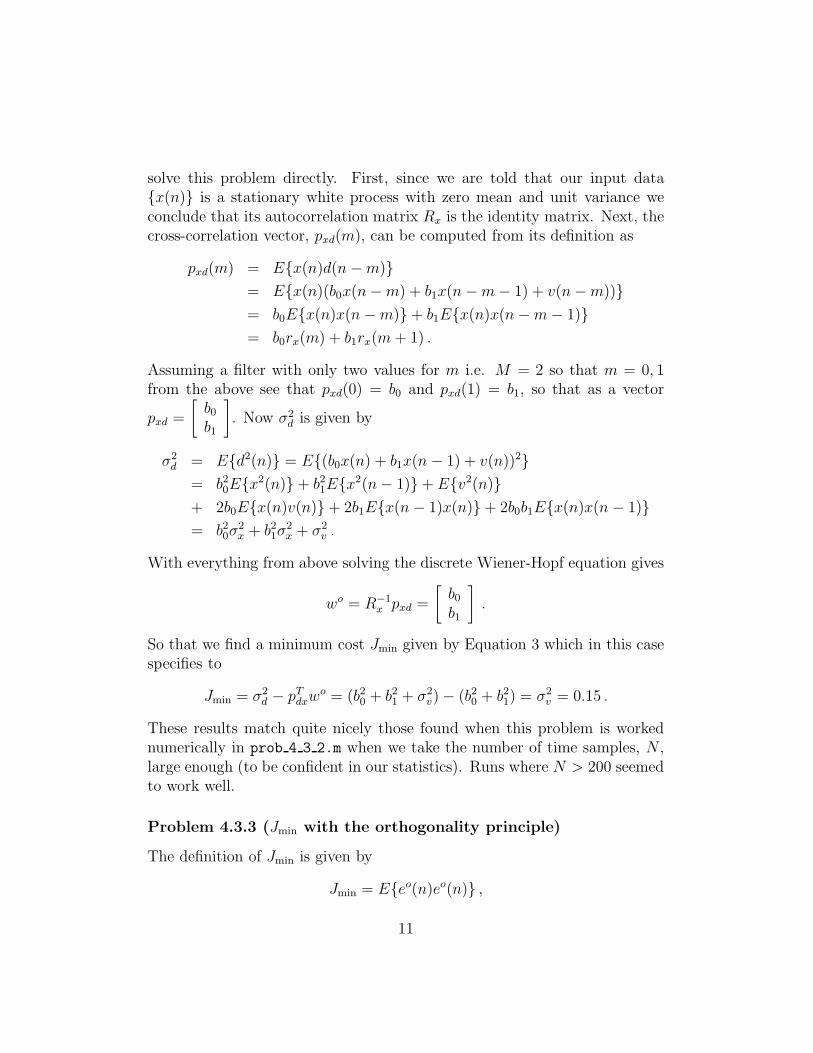
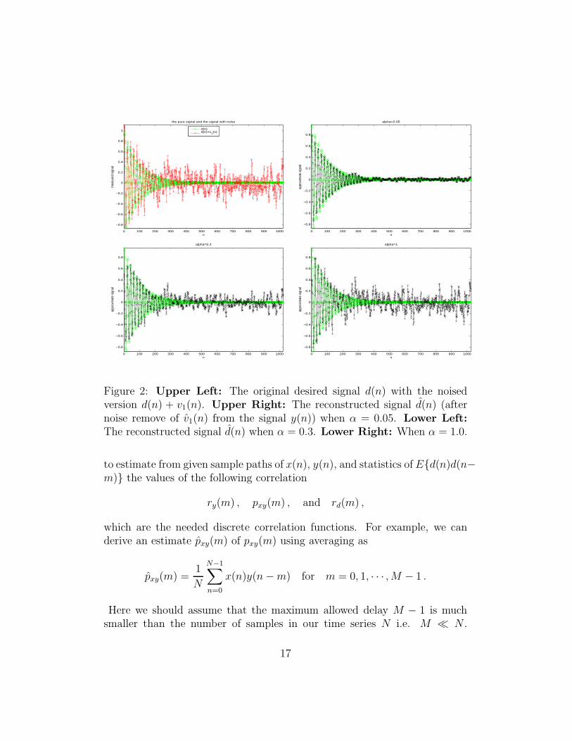
Figure 1: Upper Left: The pure signal d(n) in green and its noised coun-terpart d(n) + v1(n) in red. Upper Right: The Wiener filtered resultsusing M = 4 filter coefficients in black plotted with the signal d(n) in green.Lower Left: Using M = 8 filter coefficients. Lower Right: Using M = 16filter coefficients.
Chapter 4 (Wiener filters)
Notes on the Text
To aid in my understanding of this chapter I choose to duplicate the resultsfrom the book example that deals with the use of the Wiener filter to performnoise cancellation (Example 4.4.4). To do this I added several comments andfixed a few small bugs in the MATLAB function aawienernoisecancelor.m
supplied with the book . I then created a script noise canceling script.m
that performs the statements suggested in this section of the text. When thisis run it first plots the true signal d(n) along with the noised version d(n) +v1(n). Then for three choices of filter lengths M = 4, 8, 16 the estimated
9
signal d̂(n) is derived from the noised signal x(n) by removing an estimateof the noise v̂1(n). All of these results are shown in Figure 1.
Notice that when the number of filter coefficients becomes large enough(M ≥ 16) we are able to reconstruct the desired signal d(n) quite well giventhe amount of noise that is present.
Problem Solutions
Problem 4.3.1 (calculation of the minimum error)
We begin this problem by recalling that the optimum filter weights wo aregiven by
wo = R−1x pdx . (1)
Here Rx is the autocorrelation of the process x(n) and pdx is the cross-correlation vector between d(n) and x(n). We also recall the quadratic costJ(w) we sought to minimize is defined as
J(w) = E{(d(n)− d̂(n))2} = E{e2(n)} .
When represented in terms of the statistics of our desired signal d(n) andour observed signal x(n) becomes
J(w) = σ2d − 2wTpdx + wTRxw .
When this expression is evaluated at the optimum wo it becomes
J(wo) = σ2d − 2pTdxR
−1x pdx + pTdxR
−1x RxR
−1x pdx
= σ2d − pTdxR
−1x pdx (2)
= σ2d − pTdxw
o . (3)
In the above we have used the fact that the autocorrelation matrix, Rx, issymmetric.
Problem 4.3.2 (modeling an unknown system)
This problem can be worked numerically using code similar to that foundin Example 4.3.1 of the book. See the MATLAB script prob 4 3 2.m foran example of how this is done. Alternatively, one can compute many ofthe required correlations analytically due to the problem specification and
10
solve this problem directly. First, since we are told that our input data{x(n)} is a stationary white process with zero mean and unit variance weconclude that its autocorrelation matrix Rx is the identity matrix. Next, thecross-correlation vector, pxd(m), can be computed from its definition as
pxd(m) = E{x(n)d(n−m)}= E{x(n)(b0x(n−m) + b1x(n−m− 1) + v(n−m))}= b0E{x(n)x(n−m)}+ b1E{x(n)x(n−m− 1)}= b0rx(m) + b1rx(m+ 1) .
Assuming a filter with only two values for m i.e. M = 2 so that m = 0, 1from the above see that pxd(0) = b0 and pxd(1) = b1, so that as a vector
pxd =
[
b0b1
]
. Now σ2d is given by
σ2d = E{d2(n)} = E{(b0x(n) + b1x(n− 1) + v(n))2}
= b20E{x2(n)}+ b21E{x2(n− 1)}+ E{v2(n)}+ 2b0E{x(n)v(n)}+ 2b1E{x(n− 1)x(n)}+ 2b0b1E{x(n)x(n− 1)}= b20σ
2x + b21σ
2x + σ2
v .
With everything from above solving the discrete Wiener-Hopf equation gives
wo = R−1x pxd =
[
b0b1
]
.
So that we find a minimum cost Jmin given by Equation 3 which in this casespecifies to
Jmin = σ2d − pTdxw
o = (b20 + b21 + σ2v)− (b20 + b21) = σ2
v = 0.15 .
These results match quite nicely those found when this problem is workednumerically in prob 4 3 2.m when we take the number of time samples, N ,large enough (to be confident in our statistics). Runs where N > 200 seemedto work well.
Problem 4.3.3 (Jmin with the orthogonality principle)
The definition of Jmin is given by
Jmin = E{eo(n)eo(n)} ,
11

where the optimal error eo(n) is given by the difference between the desiredsignal, d(n), and the estimated signal d̂(n) =
∑M−1m=0 wmx(n−m) as
eo(n) = d(n)−M−1∑
m=0
wmx(n−m) .
Here wm are the optimal weights and the superscript o above stands for“optimal”. We can now compute the product of this expression directly witheo(n) “unexpanded” as
eo(n)eo(n) = eo(n)d(n)−M−1∑
m=0
wmeo(n)x(n−m) .
Taking the expectation of both sides of the above and using the orthogonalitycondition of E{eo(n)x(n − m)} = 0 for m = 0, 1, · · · ,M − 1 we find theexpectation of the second term vanish and we are left with
Jmin = E{eo(n)d(n)}
= E{(
d(n)−M−1∑
m=0
wmx(n−m)
)
d(n)}
= E{d(n)2 −M−1∑
m=0
wmx(n−m)d(n)}
= σ2d −
M−1∑
m=0
wmE{x(n−m)d(n)} .
By definition, this last expectation E{x(n−m)d(n)} is the cross-correlationbetween d(n) and x(n) or pdx(m) and the above becomes
Jmin = σ2d −
M−1∑
m=0
wmpdx(m) ,
the same result as Equation 3 but in terms of the components of the vectorswo and pdx.
Problem 4.4.1 (a specific Wiener filter)
For this problem we are told the autocorrelation function for the signal andthe noise are given by the quoted expressions for rd(m) and rv(m) respec-tively. Using these the cross-correlation function, pdx(m), can be computed
12

from its definition as
pdx(m) = E{d(n)x(n−m)}= E{d(n)(d(n−m) + v(n−m))}= E{d(n)d(n−m)}+ E{d(n)v(n−m)}= rd(m) .
Where we have used the fact that the term E{d(n)v(n − m)} = 0 sinceE{v(n)} = 0 and the processes d(n) and v(n) are uncorrelated. Recallthat the optimal Wiener filtering weights wo are given by wo = R−1
x pdx. Tocompute this expression we next need to compute the autocorrelation matrixRx. This is a Toeplitz matrix that has its (i, j) elements when |i − j| = m
given by rx(m). Here rx(m) is computed as
rx(m) = E{x(n)x(n−m)}= E{(d(n) + v(n))(d(n−m) + v(n−m))}= E{d(n)d(n−m) + d(n)v(n−m) + v(n)d(n−m) + v(n)v(n−m)}= rd(m) + rv(m) .
With the specified functional forms for rd(m) and rv(m) quoted in this prob-lem the autocorrelation matrix Rx looks like (assuming the length of thefilter M , is 4)
Rx =
rx(0) rx(1) rx(2) rx(3)rx(1) rx(0) rx(1) rx(2)rx(2) rx(1) rx(0) rx(1)rx(3) rx(2) rx(1) rx(0)
=
2 0.9 0.92 0.93
0.9 2 0.9 0.92
0.92 0.9 2 0.90.93 0.92 0.9 2
=
2.00 0.90 0.81 0.720.90 2.00 0.90 0.810.81 0.90 2.00 0.900.72 0.81 0.90 2.00
.
Since in practice we don’t know the optimal filter length M to use we letM = 2, 3, · · ·, compute the optimal filter weights wo, using the Wiener-HopfEquation 1, and for each evaluate the resulting Jmin using Equation 3. Onethen takes M to be the first value where where the Jmin first falls belowa fixed threshold, say 0.01. If we specify M = 2 the optimal weights wo
and minimum error Jmin are found in the MATLAB script prob 4 4 1.m.Running this gives numerical results identical to those found in the book.
13

We now compute the SNR of the original signal d(n) against the noisesignal v(n). Using the definition that the power a signal d(n) is given byE{d(n)2} see that
Power in the signal = E{d2(n)} = rd(0) = 1
Power in the noise = E{v2(n)} = rv(0) = 1 .
Since they have equal power, the SNR before filtering is then
SNR = 10 log10(1
1) = 0 .
Note: I don’t see any errors in my logic for computing the power inthe filtered signals below, but my results do not match the book exactly. Ifanyone sees anything wrong with what I have here please let me know. Sincethese topics are not discussed much in the book I’m going to pass on this fornow.
After filtering our observed signal x(n), to obtain d̂(n), we would like tocompute the power of the filtered signal d̂(n). This can be done by calculatingE{d̂2(n)}. We find
E{d̂2(n)} = E{(wTx)2} = E{(wTx)(wTx)T } = E{wTxxTwT}= wTE{xxT}w = wTRxw .
An estimate of the noise v̂(n) is given by subtracting the estimated signald̂(n) from our measured signal x(n) i.e.
v̂(n) = x(n)− d̂(n) .
Thus the power in the estimated noise is given by E{v̂2(n)}. We can computethis as follows
E{v̂2(n)} = E{(x(n)− d̂(n))2} = E{x2(n)− 2x(n)d̂(n) + d̂2(n)}= rx(0)− 2E{x(n)d̂(n)}+ rd̂(0) .
Now d̂(n) = wTx =∑M−1
m=0 wmx(n − m) so the middle expectation abovebecomes
E{x(n)d̂(n)} =M−1∑
m=0
wmE{x(n)x(n−m)} =M−1∑
m=0
wmrx(m) = wTrx .
Thus we findE{v̂2(n)} = rx(0)− 2wTrx + rd̂(0) .
Again, these results may be different than what the book has.
14

Problem 4.4.2 (signal leaking into our noise)
The optimal Wiener filter coefficients w in this case is given by solving
Rywo = pv1y ,
where we have defined our signal input, y(n), to be the additive noise v2(n)plus some amount, α, of our desired signal d(n). That is
y(n) = v2(n) + αd(n) .
Once these Wiener coefficients wo are found, they will be used to constructan estimate of v1(n) given the signal y(n). For this signal y(n) the auto-correlation matrix Ry has elements given by values from its autocorrelationfunction, ry(m). Since in operation we will be measuring the signal y(n) wecan compute its autocorrelation matrix using samples from our process. If,however, we desire to see how this autocorrelation matrix Ry depends on itscomponent parts v2(n) and d(n) we can decompose ry(m) as follows.
ry(m) = E{y(n)y(n−m)}= E{(v2(n) + αd(n))(v2(n−m) + αd(n−m))}= E{v2(n)v2(n−m)}+ α2E{d(n)d(n−m)} ,
since E{v2(n)d(n−m)} = 0. This shows that the autocorrelation matrix fory is related to that of v2 and d as
Ry = Rv2 + α2Rd .
It should be noted that in an implementation we don’t have access to d(n) andthus cannot form Ry using this decomposition. Instead we have to estimateRy using the input samples of y(n). After Ry to complete the Wiener filterwe need to compute the components of the cross-correlation vector pv1y(m).As any realizable implementation of this filter will need to estimate thiscross-correlation using the two signals y(n) and x(n). We can decompose thecross-correlation vector pv1y as follows
pv1y(m) = E{v1(n)y(n−m)}= E{(x(n)− d(n))y(n−m)}= E{x(n)y(n−m)} −E{d(n)y(n−m)}= E{x(n)y(n−m)} −E{d(n)(v2(n−m) + αd(n−m))}= E{x(n)y(n−m)} − αE{d(n)d(n−m))} .
15

The term (not shown) that would have had the product d(n)v2(n − m)vanished since v2(n) and d(n) are uncorrelated and the process v1(n) haszero mean. Since we don’t know the function d(n)1 we cannot calculateE{d(n)d(n − m)} using discrete samples. I see two ways to proceed withthis textbook exercise. The first is to assume we have access to the statisticsof d(n) i.e. to the expectation above. We could obtain this information by“training” on a pre-specified set of d(n) signals before the actual filters im-plementation. The second interpretation of this exercise would be to ignorethe term αE{d(n)d(n−m)} and show how much the performance of a noisecanceling algorithm will suffer from the fact that we are running it withoutthe correct system model. In that case we would expect that when α is smallthe error will be less since then the dropped term αE{d(n)d(n − m)} maybe negligible. That is, we could approximate pv1y with
pv1y ≈ pxy ,
in our Wiener filter implementation above.To finish this problem I’ll assume that we somehow have access to the
expectation E{d(n)d(n−m)} before running this filter live. If anyone sees away to compute the optimal filter coefficients wo directly from the the givensignals x(n) and y(n) please let me know.
From all of this discussion then our optimal filtering weights wo are givenby solving the Wiener-Hopf equation given by
Rywo = pxy − αpdd . (4)
In Example 4.4.4 we are told that d(n), v1(n), and v2(n) have analytic ex-pressions given by
d(n) = 0.99n sin(0.1nπ + 0.2π)
v1(n) = 0.8v1(n− 1) + v(n)
v2(n) = −0.95v2(n− 1) + v(n) .
Here v(n) a driving white noise process (a zero mean and unit variance Gaus-sian process). We then implement a modification of the book MATLAB func-tion aawienernoisecancelor.m here denoted aaWNC with leaking signal.m
1If we knew d(n) we would have the perfect noise canceler already!
16
0 100 200 300 400 500 600 700 800 900 1000
−0.8
−0.6
−0.4
−0.2
0
0.2
0.4
0.6
0.8
1
n
mea
sure
d si
gnal
the pure signal and the signal with noise
d(n)d(n)+v
1(n)
0 100 200 300 400 500 600 700 800 900 1000
−0.8
−0.6
−0.4
−0.2
0
0.2
0.4
0.6
0.8
n
appr
oxim
ate
sign
al
alpha=0.05
0 100 200 300 400 500 600 700 800 900 1000
−0.8
−0.6
−0.4
−0.2
0
0.2
0.4
0.6
0.8
n
appr
oxim
ate
sign
al
alpha=0.3
0 100 200 300 400 500 600 700 800 900 1000
−0.8
−0.6
−0.4
−0.2
0
0.2
0.4
0.6
0.8
n
appr
oxim
ate
sign
al
alpha=1
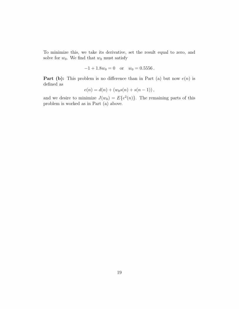
Figure 2: Upper Left: The original desired signal d(n) with the noisedversion d(n) + v1(n). Upper Right: The reconstructed signal d̂(n) (afternoise remove of v̂1(n) from the signal y(n)) when α = 0.05. Lower Left:The reconstructed signal d̂(n) when α = 0.3. Lower Right: When α = 1.0.
to estimate from given sample paths of x(n), y(n), and statistics ofE{d(n)d(n−m)} the values of the following correlation
ry(m) , pxy(m) , and rd(m) ,
which are the needed discrete correlation functions. For example, we canderive an estimate p̂xy(m) of pxy(m) using averaging as
p̂xy(m) =1
N
N−1∑
n=0
x(n)y(n−m) for m = 0, 1, · · · ,M − 1 .
Here we should assume that the maximum allowed delay M − 1 is muchsmaller than the number of samples in our time series N i.e. M ≪ N .
17

This problem as formulated is worked in the MATLAB script prob 4 4 2.m.The optimal coefficients wo as a function of the specified α are presented inFigure 2. There in the first plot in the upper left we see the desired signald(n) plotted along with its noised counter part d(n) + v1(n). We then plotthree reconstructions for α = 0.05, 0.3, 1.0. The reconstructions for small αseem to be much better.
Note: I’m not sure why the reconstructions for small α are better. In theformulation above the explicit dependence of α is be statistically consideredand should not present a problem for the reconstruction. I would expect thatif I had not modeled the α dependence I would see results like we are seeinghere. I’ve checked this code several times and have not been able to find anyerrors. If anyone sees anything wrong with what I have done here, please letme know.
Problem 4.4.3 (two example MSE surfaces)
Part (a): The diagram shown for this problem looks like what might be asystem modeling problem. In that we are seeking a coefficient w0 such thats(n) +w0s(n− 1) is an approximate d(n). Using this expression the value ofthe error at time step n can be written as
e(n) = d(n)− (s(n) + w0s(n− 1)) .
We then desire to find a value for w0 so that our estimate of d(n) (using thesignal s(n)) is as small as possible. In this case the cost function J(w0) wewant to minimize can be defined as
J(w0) = minw0
E{e2(n)} .
Where e2(n) is given by
e2(n) = d2(n)− 2d(n)(s(n) + w0s(n− 1))
+ s2(n) + 2w0s(n− 1)s(n) + w20s
2(n− 1) .
With this expression for e2(n) the expectation when we use the providedvalues then becomes
E{e2(n)} = 3− 2(−0.5 + w0(0.9)) + 0.9 + 2w0(0.4) + w20(0.9)
= 4.0− w0 + 0.9w20 .
18
To minimize this, we take its derivative, set the result equal to zero, andsolve for w0. We find that w0 must satisfy
−1 + 1.8w0 = 0 or w0 = 0.5556 .
Part (b): This problem is no difference than in Part (a) but now e(n) isdefined as
e(n) = d(n) + (w0s(n) + s(n− 1)) ,
and we desire to minimize J(w0) = E{e2(n)}. The remaining parts of thisproblem is worked as in Part (a) above.
19
Chapter 5 (Eigenvalues of Rx - properties of
the error surface)
Problem 5.1.1 (the correlation matrix R is positive definite)
From the definition of the autocorrelation matrix R, and with a is a constantvector we have that the product aTRa is given by
aTRa = aTE{xxT}a = E{aTxxTa} = E{(xTa)T (xTa)} = E{||xTa||2} ≥ 0 ,
since the last expression is the expectation of a positive quantity. SinceaTRa ≥ 0 for all a the autocorrelation matrix R is positive definite.
Problem 5.1.2 (eigenvalues of Rk)
If λi is an eigenvalue of R then by definition there exists an eigenvector qisuch that Rqi = λiqi. Then if k ≥ 1 multiplying this equation by the matrixRk−1 on both sides we obtain
Rkqi = λiRk−1qi
= λiRk−2(Rqi) = λiR
k−2λiqi
= λ2iR
k−2qi = · · · = λki qi ,
which shows that λki is an eigenvalue of Rk as claimed.
Problem 5.1.3 (distinct eigenvalues have independent eigenvectors)
To be linearly independent means that any finite (non-zero) sum of the givenvectors cannot be zero. Thus if ci for i = 1, 2, · · · ,M are non-zero constantswe require
∑M
i=1 ciqi 6= 0. Assume by way of contradiction that the ci are notall zero but that
M∑
i=1
ciqi = 0 . (5)
Then taking the dot-product of this equation with the vector qj gives
M∑
i=1
ciqTj qi = 0 .
20

Now from Problem 5.1.5 qTj qi = 0 for i 6= j and the above equation reducesto cj = 0 which is a contradiction. The book gives another solution wherewe generate M non-singular equations for ci by multiplying the Equation 5by Rx 0, 1, 2, · · · ,M times. The fact that the equations are non-singular andhave a zero right-hand-side implies again that ci = 0.
Problem 5.1.4 (the eigenvalues of R are real and non-negative)
We let q we be an eigenvector ofRx, then by definition Rxq = λq. Multiplyingthis expression by qH (the Hermitian conjugate of q) on both sides gives
qHRxq = λqHq or λ =qHRxq
qHq.
Since Rx is positive definite qHRxq ≥ 0 (by Problem 5.1.1) and qHq > 0everything in the ratio in the equation on the right hand side above is real andnon-negative. Thus we can conclude that λ must be real and non-negative.
Problem 5.1.5 (distinct eigenvalues have orthogonal eigenvectors)
Let qi and qj be two eigenvectors of Rx corresponding to distinct eigenvalues.Then by definition
Rxqi = λiqi and Rxqj = λjqj ,
Take the Hermitian inner product of qj with the first equation we find
qHj Rxqi = λiqHj qi ,
Taking the conjugate transpose of this expression and remembering that λ
is a real number we have
qHi Rxqj = λ̄iqHi qj = λiq
Hi qj . (6)
Now the left hand side of this expression (since qj is an eigenvector of Rx) isgiven by
qHi Rxqj = qHi λjqj = λjqHi qj , (7)
Thus subtracting Equation 6 from 7 we have shown the identity
λiqHi qj − λjq
Hi qj = 0 ,
21

or(λi − λj)q
Hi qj = 0 .
Since we are assuming that λi 6= λj the only way the above can be true is ifqHi qj = 0 that is the vector qi and qj are orthogonal.
Problem 5.1.6 (the eigenvector decomposition of Rx)
We begin by forming the matrix Q as suggested. Then it is easy to see thatwhen we left multiply by Rx we obtain
RxQ =[
Rxq1 Rxq2 · · · RxqM]
=[
λ1q1 λ2q2 · · · λMqM]
= QΛ .
Multiplying this last equation by QH on the left then because of the orthog-onality of qi and qj under the Hermitian inner product we find
QHRxQ = Λ ,
with Λ a diagonal matrix containing the eigenvalues of Rx. These manipula-tions assumes that the vectors qi and qj are orthogonal to each other. Thisin fact can be made true when these vectors are constructed.
Problem 5.1.7 (the trace of the matrix Rx)
Now from Problem 5.1.6 we know that
tr(QHRxQ) = tr(Λ) =
M∑
i=1
λi .
In addition to this identity, one can show that the trace operator satisfies atype of permutation identity in its arguments in that
tr(ABC) = tr(BCA) = tr(CAB) , (8)
provided that all of these products are defined. Using this identity we seethat
tr(QHRxQ) = tr(RxQQH) = tr(RxI) = tr(Rx) ,
the desired identity.
22

Problem 5.2.1 (the equation for the difference from optimal wo)
We begin by recalling the definition of our error function J(w) in terms ofsecond order statistics of our processes x(n) and d(n)
J(w) = σ2d − 2wTp+ wTRxw , (9)
orwTRxw − 2pTw − (J − σ2
d) = 0 .
We now “center” this equation about the optimal Wiener-Hopf solution wo
which is given by wo = R−1x pxd. We do this by introducing a vector ξ defined
as ξ = w−wo. This means that w = ξ+wo and our quadratic form equationabove becomes
(ξ + wo)TRx(ξ + wo)− 2pT (ξ + wo)− (J − σ2d) = 0 ,
or expanding everything
ξTRxξ + 2ξTRxwo + woTRxw
o − 2pT ξ − 2pTwo − (J − σ2d) = 0 .
Since Rxwo = p some terms cancel and we get
ξTRxξ − pTwo − (J − σ2d) = 0 . (10)
Recalling that
J(wo) = J(ξ = 0) = Jmin = σ2d − pTwo ,
we see that Equation 10 is given by
ξTRxξ − pTw0 − (J − σ2d) = ξTRxξ − J + Jmin = 0 .
Thus J − Jmin = ξTRxξ, which states by how much J is greater than thanJmin when ξ 6= 0.
23

Chapter 6 (Newton and steepest-decent method)
Problem 6.1.1 (convergence of w in the gradient search algorithm)
Recall that the difference equation satisfied by the one-dimensional filtercoefficients w(n) when using the gradient search algorithm is given by
w(n+ 1) = (1− 2µrx(0))w(n) + 2µrx(0)wo (11)
To solve this difference equation define v(n) as v(n) = w(n)− wo, so that win terms of v is given by w(n) = wo + v(n) and then Equation 11 becomes
wo + v(n+ 1) = (1− 2µrx(0))(wo + v(n)) + 2µrx(0)w
o ,
orv(n+ 1) = (1− 2µrx(0))v(n) . (12)
The solution of this last equation is
v(n) = (1− 2µrx(0))nv(0) ,
which can be proven using mathematical induction or by simply substitut-ing this expression into the difference equation 12 and verifying that it is asolution. Replacing v(n) with w(n)− wo we have that w(n) is given by
w(n) = wo + (1− 2µrx(0))n(w(0)− wo) ,
as we were to prove.
Problem 6.1.2 (visualizing convergence)
Equation 6.15. is the iterative solution to the one-dimensional gradient-decent search algorithm
w(n) = wo + (1− 2µrx(0))n(w(0)− wo) .
To generate these plots we took wo = 0.5, w(0) = −0.5, and rx(0) = 1 andseveral values for µ. We then plot the iterates of w(n) as a function of nin Figure 3 (left). These plots can be generated by running the MATLABscript prob 6 1 2.m.Part (a): When 0 ≤ µ ≤ 1
2rx(0)from the given plots we see that the conver-
gence is monotonic to the solution of 0.5.
24
Part (b): When µ ≈ 12rx(0)
we see that the convergence is also monotonicbut converges faster than before to the true solution.Part (c): When 1
2rx(0)< µ < 1
rx(0)the convergence is oscillatory around the
true solution and eventually converges to it.Part (d): When µ > 1
rx(0)the iterates oscillate and then diverge. That is
the iterates and don’t converge to the value of wo = 0.5. In the given plotwe only plot the first five samples so as to not clutter the graph.
Problem 6.1.3 (convergence of J in the gradient search algorithm)
Recall the solution to the iteration scheme for the weights w(n)
w(n) = wo + (1− 2µ)n(w(0)− wo) ,
When we put this into the books Equation 5.2.7 the shifted and rotated formfor J we obtain
J(w(n)) = Jmin + (w(n)− wo)TRx(w(n)− wo) (13)
= Jmin + (1− 2µ)2n(w(0)− wo)TRx(w(n)− wo) (14)
Evaluating Equation 13 when n = 0 results in
J(0) = J(w(0)) = Jmin + (w(0)− wo)TRx(w(0)− wo) .
or solving for the quadratic form the expression
(w(0)− wo)TRx(w(0)− wo) = J(0)− Jmin .
Using this result back in Equation 14 gives the desired form for the iteratesof J(n)
J(n) = J(w(n)) = Jmin + (1− 2µ)n(J(0)− Jmin) . (15)
Problem 6.2.1 (convergence of the vector SD algorithm)
The vector steepest-decent (SD) algorithm results in the iterative scheme forthe vector ξ′(n) defined as
ξ′(n) = QT (w(n)− wo) .
Here Rx = QΛQT . That is, Q is the orthogonal matrix that diagonalizesthe autocovariance matrix Rx. The iterative scheme that results for ξ′(n) isgiven by
ξ′(n+ 1) = (I − µ′Λ)ξ′(n) ,
25

Then taking the kth component of the above matrix expression results in thefollowing scalar iterative scheme
ξ′k(n+ 1) = (1− µ′λk)ξ′k(n) .
Problem 6.2.2 (the scalar equations in the vector GD algorithm)
The ith scalar equation in the vector gradient-decent algorithm is given byequation 6.2.25
w′i(n+ 1) = (1− µ′λi)w
′i(n) + µ′p′idx for 0 ≤ i ≤ M − 1 . (16)
Here µ′ = 2µ is the learning rate. Letting n = 0 in this equation we obtain
w′i(1) = (1− µ′λi)w
′i(0) + µ′p′idx .
Letting n = 1 we obtain
w′i(2) = (1− µ′λi)w
′i(1) + µ′p′idx
= (1− µ′λi)2w′
i(0) + µ′(1− µ′λi)p′idx + µ′p′idx ,
when we use the previously computed value of w′i(1). Continuing with w′
i(3)we let n = 2 in Equation 16 to obtain
w′i(3) = (1− µ′λi)w
′i(2) + µ′p′idx
= (1− µ′λi)3w′
i(0) + µ′(1− µ′λi)2p′idx + µ′(1− µ′λi)p
′idx + µ′p′idx .
By induction then we recognize that in the general case
w′i(n) = (1− µ′λi)
nw′i(0) + µ′p′idx
n−1∑
j=0
(1− µ′λj)j , (17)
as we were to show.
Problem 6.2.3 (analytic solutions for the iterates w(n))
The exact iterates for the transformed weight components w′i(n) satisfy (as-
suming we begin our iterations with w initialized to zero) the following
w′i(n) =
p′idxλi
(1− (1− µ′λi)n) . (18)
26
Using this expression and the given autocorrelation matrix R̂x and cross-correlation vector p̂dx we can analytically evaluate the transformed filterweights w′
i(n) as a function of n. From these we can translate w′i(n) into
analytic expressions for the filter weights wi(n) themselves. To do this werequire we see from Equation 18 requires the eigenvalues of the given R̂x.Computing them we find their values given by
λ1 = 0.3 and λ2 = 1.7 .
While the eigenvectors for Rx are given by the columns of a matrix say Q or
Q =
[
−0.7071 0.70710.7071 0.7071
]
.
We also require
p′xd = QTpxd =
[
−0.14140.8485
]
.
Using these (and recalling that µ′ = 2µ) we find
w′1(n) = −0.1414
0.3(1− (1− 2µ0.3)n) = −0.1414
0.3(1− (1− 0.6µ)n)
w′2(n) = +
0.8485
1.7(1− (1− 2µ1.7)n) = +
0.8485
1.7(1− (1− 3.4µ)n) ,
as the functional form for w′i(n). Given these expressions we can compute
the filter weights themselves wi(n) by multiplying them by the Q matrix2.In components then this is given by
w1(n) = −0.7071w′1(n) + 0.7071w′
2(n)
= +0.7071(0.1414)
0.3(1− (1− 0.6µ)n) +
0.7071(0.8485)
1.7(1− (1− 3.4µ)n)
w2(n) = +0.7071w′1(n) + 0.7071w′
2(n)
= −0.7071(0.1414)
0.3(1− (1− 0.6µ)n) +
0.7071(0.8485)
1.7(1− (1− 3.4µ)n) .
For convergence of this iterative scheme recall that the learning rate µ′ ≤2
λmax. Since µ′ = 2µ this means that
µ ≤ 1
λmax
= 0.5882 .
2Recall that the transformed weights w′(n) were obtained from the untransformedweights by w′(n) = QTw(n).
27
0 1 2 3 4 5 6 7−2
−1.5
−1
−0.5
0
0.5
1
1.5
2
n (index)
w(n
)
Part (a)Part (b)Part (c)Part (d)
5 10 15 20 25−1
−0.8
−0.6
−0.4
−0.2
0
0.2
0.4
0.6
0.8
1
n index
filte
r wei
ghts
w(n
)
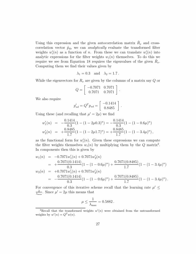
Figure 3: Left: Plots of iterates of the 1d gradient-search algorithm. Right:Plots of the two filter coefficients w1(n) and w2(n) as a function of n for twodifferent values of the learning parameter µ. See the text on Problem 6.2.3for more details.
These expressions for the weights wi are plotted in Figure 3 (right) for µ = 0.5and µ = 0.7 as a function of n. The two numerical values of µ were chosen tostraddle the stability threshold of µ ≈ 0.5882. The value of the iterates forµ = 0.5 is plotted in green while that for µ = 0.7 is plotted in red. We onlyplot the first ten elements of the µ = 0.7 curves since the large oscillationsthat result from the divergence would cloud the entire picture otherwise. Wealso clip the y-axis of the plot at reasonable limits since the diverging weightsquickly reach very large numbers. This plot can be generated and studiedby running the MATLAB script prob 6 2 3.m.
Problem 6.2.4 (J(w(n)) in terms of pdx(n) and Rx)
Given the expression for J(w(n))
J(w(n)) = Jmin + ξ′(n)TΛξ′(n) ,
expressed in terms of the rotated and translated vectors ξ′(n) = QT ξ(n) =QT (w(n)− wo) in terms of Q and w(n) this becomes
J(n) = Jmin + (w(n)− wo)TQΛQT (w(n)− wo)
= Jmin + (w(n)− wo)TRx(w(n)− wo) .
28
1 2 3 4 5 6 7 8 9 10−3.6
−3.4
−3.2
−3
−2.8
−2.6
−2.4
−2.2
−2
−1.8
n index
log(
J(n)
)
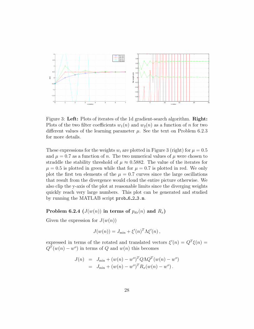
Figure 4: Plots of ln(J(n)) as a function of n for Problem 6.2.5.
Recalling that the optimal Wiener filter weights wo satisfy wo = R−1x pdx and
that Jmin = σ2d − pTdxw
o the above becomes
J(n) = σ2d − pTdx(Rx
−1pdx) + (w(n)− wo)TRx(w(n)− wo)
= σ2d − pTdxRx
−1pdx
+ w(n)TRxw(n)− w(n)TRxRx−1pdx − pTdxRx
−1Rxw(n) + pTdxRx−1RxRx
−1pdx
= σ2d − 2pTdxw(n) + w(n)TRxw(n) ,
or the desired expression.
Problem 6.2.5 (plots of the learning curve)
One form of the learning curve, J(n), in terms of the eigenvalues of theautocorrelation matrix Rx, is
J(n) = J(w(n)) = Jmin + ξ′(n)TΛξ′(n)
= Jmin +M−1∑
k=0
λk(1− µ′λk)2nξ′k(0)
2 .
For the correlation matrix with the given eigenvalues we have that the learn-ing curve has the following specific expression
J(n)− Jmin = 1.85(1− 1.85µ′)2nξ′1(0)2 + 0.15(1− 0.15µ′)2nξ′2(0)
2 .
The two values for the constants ξ′1(0)2 and ξ′1(0)
2 are determined by whatwe take for our initial guess at the filter coefficients (rotated by the eigenvec-tors of the system correlation matrix Rx). The value of µ′ must be selected
29

such that we have convergence of the gradient decent method which in thiscase means that
µ′ <2
λmax
=2
1.85= 1.0811 .
We plot the log of the expression J(n) for this problem in Figure 4 forµ′ = 0.4, ξ′1(0)
2 = 0.5, and ξ′1(0)2 = 0.75. The time constants, τk, for
the error decay are given by
τk = − 1
ln(1− µ′λk),
which in this case gives
τ1 = 0.7423 and τ2 = 16.1615 .
This plot can be generated by running the MATLAB command prob 6 2 5.
Problem 6.2.6 (the optimal value for µ′)
The optimal value for µ′ lies between 1λmin
and 1λmax
so that
|1− λminµ′| = λmin
∣
∣
∣
∣
1
λmin− µ′
∣
∣
∣
∣
= λmin
(
1
λmin− µ′
)
= 1− λminµ′ ,
since µ′ < 1λmin
. In the same way we have
|1− λmaxµ′| = λmax
∣
∣
∣
∣
1
λmax
− µ′
∣
∣
∣
∣
= λmax
(
µ′ − 1
λmax
)
= λmaxµ′ − 1 ,
since µ′ > 1λmax
. So solving |1−λminµ′| = |1−λmaxµ
′| is equivalent to solving
1− λminµ′ = λmaxµ
′ − 1 ,
30

or
µ′ =2
λmin + λmax.
With this optimal value of µ′ the convergence is determined by
α = 1− µ′optλmin = 1− 2λmin
λmax + λmin=
λmin
λmax− 1
λmin
λmax+ 1
,
as claimed in the book.
31
Chapter 7 (The least mean-square (LMS) al-
gorithm)
Notes From the Text
Using the LMS algorithm for linear prediction
In this subsection we will duplicate the linear prediction example from thebook. We assume we have a zero-mean white noise driving process v(n) andthat the observed process x(n) is given by an AR(2) model of the form
x(n) = 0.601x(n− 1)− 0.7225x(n− 2) + v(n) ,
We desire to predict the next value of x at the timestep n using the previoustwo values at n−1 and n−2. That is we desire to compute an estimate x̂(n)of x(n) from
x̂(n) =1∑
i=0
wi(n)x(n− 1− i) .
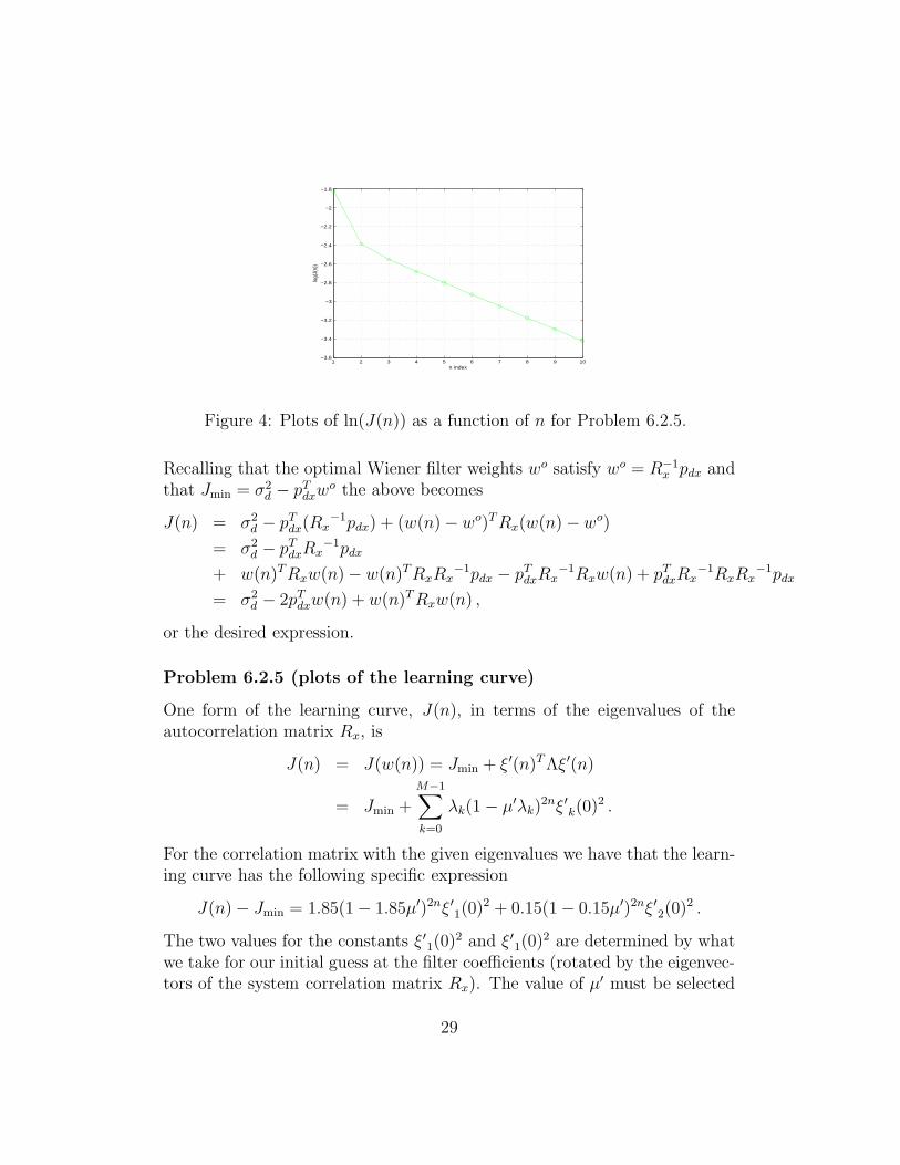
To do this we will use the LMS algorithm. The computations are performedin the MATLAB file linear prediction w lms.m. We perform lms learningwith two different learning rates µ = 0.02 and µ = 0.005. We expect that on“easy” problems all things begin equal lms algorithm with a larger learningrate µ will produce faster convergence and a give optimal results sooner. Theresults from this experiment are shown in Figure 5. There we plot the originalsignal x(n) and its prediction x̂(n) at the n-th step. We can see that after acertain amount of time we are predicting x(n) quite well. Next we plot theerror between the true observed value of x(n) and our estimate x̂. This erroris centered on zero and has the same variance as the unknown innovation termv(n) in our AR(2) model. Finally, we plot the estimates of the weights foundduring the lms learning procedure. We see nice convergence to the truthvalues (shown as horizontal green lines). Note that we are assuming thatwe are estimating M = 2 coefficients from the signal x(n). An attempt toestimate more coefficients M > 2 will work but the coefficients require moreiterations to estimate their values sufficiently. For example when M = 3 webegin to estimate the third weight w3 as zero after sufficient time.
32

550 600 650 700 750 800 850 900 950 1000−6
−4
−2
0
2
4
n
pre
dic
tio
ns
0 100 200 300 400 500 600 700 800 900 1000−3
−2
−1
0
1
2
3
4
5
n
pre
dic
tio
n e
rro
r
100 200 300 400 500 600 700 800 900 1000
−1
−0.5
0
0.5
1
1.5
n
we
igh
t co
nve
rge
nce
convergence of the weights
Figure 5: Using the LMS algorithm for linear prediction. Left: The signalx(n) from which we use the previous two time-steps x(n − 1) and x(n −2) in predicting the next value x(n). Center: The error x(n) − x̂(n) ateach timestep. Right: The convergence of the AR(2) weights [w1, w2]
T as afunction of timestep n.
Using the LMS algorithm for modeling unknown systems
In this subsection we will use the LMS algorithm to estimate the unknowncoefficients of a MA(3) model given the measured signal input signal d(n).That is we assume (this fact is unknown to the lms algorithm) that our ob-served signal d(n) is given by a MA(3) model based on x(n) with coefficients
d(n) = x(n)− 2x(n− 1) + 4x(n− 2) .
Here we will take x(n) to be the AR(2) signal model used in the previousexample. We then assume a model of our observed signal d(n) given by aMA(M) or
d̂(n) =M∑
i=0
wix(n− i) .
We will estimate the parameters wi using the lms algorithm and the bookMATLAB function aalms1.m. We do this in the MATLAB script calledmodeling w lms.m. The results from these experiments are shown in Fig-ure 6. If we specify to a MA(3) model of x(n) we see that our LMS algorithmis able to learn quite nicely the three weights wi.
33

0 100 200 300 400 500 600 700 800 900 1000
−15
−10
−5
0
5
10
15
n
pre
dic
tio
ns
0 100 200 300 400 500 600 700 800 900 1000
−6
−4
−2
0
2
4
6
n
pre
dic
tio
n e
rro
r
error under first learning rateerror under second learning rate
0 100 200 300 400 500 600 700 800 900 1000−2
−1
0
1
2
3
4
n
we
igh
t co
nve
rge
nce
convergence of the weights
Figure 6: Using the LMS algorithm for modeling. Left: The output signald(n) and our estimated signal d̂(n), which we assume is modeled as a MA(M)processed based on the input signal x(n). Center: The error x(n) − x̂(n)in our prediction at each timestep. Notice that as the number of time-stepsincreases the approximation gets better. Right: The convergence of theMA(3) weights [w0, w1, w2]
T as a function of timestep n.
Using the LMS algorithm for noise cancellation
In this example we will use the LMS algorithm for noise cancellation. Thismeans that we assume that we are given a signal s(n) that has been modifiedby additive noise s(n)+v(n). We then desire to use the previous sample s(n−1)+v(n−1) to predict the current sample s(n)+v(n). Here our filter input isx(n) = s(n−1)+v(n−1), while our desired signal is d(n) = s(n)+v(n). Thisexample is worked in the MATLAB script noise cancellation w lms.m.
Using the LMS algorithm for inverse system identification
For this subsection we will try to apply the LMS algorithm for numericallycomputing the inverse of an unknown system. To do this we will assume thatwe have a sinusoidal input signal s(n) given by
s(n) = sin(0.2πn) .
To this signal we add some random Gaussian noise v(n), that we are notable to predict. This modified signal m(n) ≡ s(n) + v(n) is then passedinto an unknown filter. For this example we will assume that this filter isMA(4) system the coefficients of which are unknown to our inverse system
34

0 500 1000 1500 2000 2500 3000 3500 4000−5
−4
−3
−2
−1
0
1
2
3
4
5
n index
ob
se
rve
d v
alu
es
s(n)+v(n) with y(n)
signal plus noiseLMS prediction #1LMS prediction #2
0 500 1000 1500 2000 2500 3000 3500
−2.5
−2
−1.5
−1
−0.5
0
0.5
1
1.5
2
2.5
n
pre
dic
tio
n e
rro
r
error under M=2error under M=6
0 500 1000 1500 2000 2500 3000 3500 4000−0.4
−0.2
0
0.2
0.4
0.6
0.8
1
n
we
igh
t co
nve
rge
nce
convergence of the weights
Figure 7: Using the LMS algorithm for inverse system identification. Left:A plot of the input signal x(n) and two reconstructions with different numberof coefficients M . The first has M = 2 while the second has M = 6. Center:The instantaneous error (m(n)−y(n))2 for each model. Note that the secondmodel withM = 6 ends with a smaller error overall. Right: The convergenceof the filter coefficients wi for each of the models.
algorithm. For this example we assume that we measure the output x(n) ofa MA(4) system given by
x(n) = 1.0m(n) + 0.2m(n− 1)− 0.5m(n− 2) + 0.75m(n− 3) .
Given this modified signal x(n), and the input signal, m(n) to the unknownfilter we want to construct a FIR filter that will estimate the inverse of theinput filter. That is we are looking for a set of filter coefficients wi such thatwe have an estimate m̂(n) of m(n)
y(n) = m̂(n) =
M∑
i=0
wix(n− i) .
Now in a physical realization of this filter because it will take four time-steps before the first output of our system x(n) appears and an additionalnumber M of steps before the output from our inverse system appears wewould need to compare the output of this combined filter system with avalue of m(n) that has already passed. The practical implementation of thisis that we would need to delay the signal m(n) by some amount before we cancalculate an error term. Strictly in a software digital environment this is notneeded since we desire to compare m(n) with the output the combined filter.
35

This example is implemented in the MATLAB script inv system w lms.m.The results obtained when running this code can be seen in Figure 7. Weplot the signal that is observed after obtained noise m(n) along with theLMS learned reconstructed signal for two filter designs y1(n) and y2(n). Thetwo filter designs are different in that they have a different number of filtercoefficients wi and in the learning rate used for each implementation. Thefirst experiment has M = 2 and µ = 0.01, while the second has more filtercoefficients at M = 6 and a smaller learning rate µ = 0.001 The consequenceof this is that the filter with M = 6 weights should do a better job atapproximating the inverse of our system. This can be seen when we considera plot of the error in the prediction y2(n) compared with that in y1(n). Theerror in y2(n) is uniformly smaller with a standard deviation of 0.637990compared to the same thing under the M = 2 filter coefficient where weobtain an error standard deviation of 0.831897. In addition, the smallerlearning rate in the second filter means that (all things begin equal) it willtake more time for the filter to obtain optimal performance. This can be seenin the signal plot where the first filter produces better approximations earlierand in the error plots where the second filter has a larger error initially. Wefinally plot the convergence of the filter coefficients where we see that theM = 6 filter’s initial two weights w0 and w1 converge to the same thing asthe M = 2’s filter’s weight.
The performance analysis of the LMS algorithm
In this subsection we expand and discuss the algebra and presentation on theLMS algorithm presented in the text. This section of the text was developedto further expand my understanding of these manipulations. We begin withequation 7.4.5 given by
ξ(n+ 1) = ξ(n) + 2µx(n)(eo(n)− x(n)T ξ(n)) . (19)
Where ξ(n) = w(n)−wo are the weight error vectors. We multiply this equa-tion on the left by Q, the matrix which orthogonalizes the autocorrelationmatrix for x(n), that is Rx = QΛQT . If we multiply Equation 19 on the leftby QT and recalling the definitions ξ′ = QT ξ and x′ = QTx and that Q is anorthogonal matrix we find
ξ′(n+ 1) = ξ′(n) + 2µx′(n)(eo(n)− (QTx)T (QT ξ))
= ξ′(n) + 2µx′(n)(eo(n)− x′(n)Tξ′
T)
36

= 2µx′(n)eo(n) + ξ′(n)− 2µx′(n)(x′T ξ′)
= (I − 2µx′(n)x′(n)T )ξ′(n) + 2µeo(n)x′(n) , (20)
which is equation 7.4.24 in the book. The transpose of Equation 20 is givenby
ξ′(n+ 1)T = ξ′(n)T (I − 2µx′(n)x′(n)T ) + 2µeo(n)x′(n)T .
Now for notational simplicity in the remaining parts of this derivation of anexpression for K ′(n) we will drop the prime on the vectors x and ξ. Thisprime notation was used to denote the fact that x and ξ are viewed in thespace rotated by the eigenvalues of Rx i.e. x′ = QTx with Rx = QΛQT .We will also drop the n notation which indicates that we have processedup to and including the nth sample, both notations would be present onall symbols and just seem to clutter the equations. Multiplying 20 by itstranspose (computed above) gives
ξ(n+ 1)ξ(n+ 1)T = (I − 2µxxT )ξξT (I − 2µxxT )
+ 2µeo(I − 2µxxT )ξxT
+ 2µeoxξT (I − 2µxxT )
+ 4µ2(eo)2xxT
= ξξT (21)
− 2µξξTxxT (22)
− 2µxxT ξξT (23)
+ 4µ2xxT ξξTxxT (24)
+ 2µeoξxT − 4µ2eoxxT ξxT (25)
+ 2µeoxξT − 4µ2eoxξTxxT (26)
+ 4µ2(eo)2xxT . (27)
We won’t use this fact but the above could be simplified by recalling thatthat inner products are symmetric that is xξT = ξxT . If we take the expec-tation E{·} of this expression we obtain the desired expression the the booksequation 7.4.25. To explicitly evaluate the above expectation we will use theindependence assumption, which basically states that the data, x(n), goinginto our filter is independent of the filter coefficient estimates, w(n), at leastwith respect to taking expectations. Since the filter coefficients and data arerepresented in the transformed space as ξ′(n) and x′(n), this means that the
37
expectation of the term 24 (equation 7.4.28 in the book) can be computedas
E{xxT ξξTxxT } = E{xxTE{ξξT}xxT } ,where we have used the independence assumption in passing an expecta-tion inside the outer expectation. Since E{ξ′(n)ξ′T (n)} = K ′(n) the abovebecomes
E{x′(n)x′(n)TK ′(n)x′(n)x′(n)T} .To further simplify this consider the quadratic part in the middle of thisexpression. That is write x′(n)TK ′(n)x′(n) in terms of the components ofx′(n) and K ′(n). In standard matrix component notation we have
x′(n)TK ′(n)x′(n) =
M−1∑
i=0
M−1∑
j=0
x′i(n)x
′j(n)K
′ij(n) .
Multiplying this inner product scalar by the vector x′(n) on the left, byx′(n)T on the right, and taking the lm-th component of the resulting matrixwe obtain
(x′(n)x′(n)TK ′(n)x′(n)x′(n)T )lm = x′l(n)x
′m(n)
M−1∑
i=0
M−1∑
j=0
x′i(n)x
′j(n)K
′ij(n) .
The expectation of the lm-th element is then given by
E{(·)lm} =
M−1∑
i=0
M−1∑
j=0
E{x′l(n)x
′m(n)x
′i(n)x
′j(n)K
′ij(n)}
=
M−1∑
i=0
M−1∑
j=0
K ′ij(n)E{x′
l(n)x′m(n)x
′i(n)x
′j(n)} .
This last expression involves evaluating the expectation of the product offour Gaussian random variables. Following the solution in the text we recallan identity that expands such products in terms of pairwise products. Wenote that this is an advantage of using Gaussian random variables in thatthe higher order moments can be determined explicitly from the second (andpossibly lower) moments. The needed identity is that the expectation of thefourth product of the xi’s is given by
E{x1x2x3x4} = E{x1x2}E{x3x4}+ E{x1x3}E{x2x4}+ E{x1x4}E{x2x3} .(28)
38
In the specific case considered here these pairwise products are given by
E{x′ix
′j} = (E{x′x′T})ij = (E{QTxxTQ})ij = (QTRxQ)ij = (Λ)ij = λiδ(i−j) .
Thus using Equation 28 the expectation of this lm-th component is given by
E{(·)lm} =M−1∑
i=0
M−1∑
j=0
K ′ij(n)λlλiδ(l −m)δ(i− j)
+M−1∑
i=0
M−1∑
j=0
K ′ij(n)λlλmδ(l − i)δ(m− j)
+
M−1∑
i=0
M−1∑
j=0
K ′ij(n)λlλmδ(l − j)δ(m− i)
= λlδ(l −m)
M−1∑
i=0
λiK′ii(n) + λlλmK
′lm(n) + λlλmK
′ml(n) .
As K ′(n) is symmetric K ′lm(n) = K ′
ml(n) and the last two terms are equaland we obtain
E{(·)lm} = λlδ(l −m)M−1∑
i=0
λiK′ii(n) + 2λlλmK
′lm(n) .
Now the diagonal sum over the elements of K ′(n) is the trace as
M−1∑
i=0
λiK′ii(n) = tr(ΛK ′(n)) = tr(K ′(n)Λ) .
Here ΛK ′(n) multiplies the ith row ofK ′(n) by λi where asK′(n)Λ multiplies
the i-th column of K ′(n) by λi, so that the diagonal terms of each productare identical. In matrix form then E{(·)lm} is given by
tr(ΛK ′(n))Λ + 2ΛK ′(n)Λ ,
or the expression 7.4.28.From the direct expectation of the component equations: 22, 23, 24, 25, 26, 27,
and what we calculated above for E{(·)lm}, the recursive equation for the
39

matrix K ′(n + 1) then becomes
K ′(n + 1) = K ′(n)− 2µ(ΛK ′(n) +K ′(n)Λ)
+ 4µ2(2ΛK ′(n)Λ + tr{ΛK ′(n)}Λ)+ 4µ2JminΛ ,
which is equation 7.4.34.To study convergence of the LMS algorithm as K ′(n) is a correlation
matrix we have, k′ij2 ≤ k′
iik′jj, so the off-diagonal terms are bounded by the
diagonal terms and it is sufficient to consider the iith element of K ′(n).From the above recursive expression for the entire matrix K ′(n) the ii-thcomponent of 7.4.34 is given by
k′ii(n + 1) = k′
ii(n)− 4µλik′ii(n) + 8µ2λ2
ik′ii(n)
+ 4µ2λi
M−1∑
j=0
λjk′jj(n) + 4µ2Jminλi
= (1− 4µλi + 8µ2λ2i )k
′ii(n)
+ 4µ2λi
M−1∑
j=0
λjk′jj(n) + 4µ2Jminλi , (29)
which is equation 7.4.35. To derive a matrix recursive relationship for thesecomponents k′
ii we place their values for i = 0, 1, · · · ,M − 1 in a vector
(denoted as k′(n) with no subscripts) and from the recursive scalar expressionjust considered we obtain a vector update equation as
k′00(n+ 1)
k′11(n+ 1)
...k′M−1,M−1(n + 1)
= F
k′00(n)
k′11(n)...
k′M−1,M−1(n)
+ 4µ2Jmin
λ0
λ1...
λM−1
+ 4µ2
λ0
λ1...
λM−1
[
λ0 λ1 · · · λM−1
]
k′00(n)
k′11(n)...
k′M−1,M−1(n)
.
40
Where we have defined the matrix F as
F =
1− 4µλ0 + 8µ2λ20 0 · · · 0
0 1− 4µλ1 + 8µ2λ21 0
.... . .
. . . 00 0 1− 4µλM−1 + 8µ2λ2
M−1
,
or a diagonal matrix with diagonal elements given by 1 − 4µλi + 8µ2λ2i .
Defining these elements as fi we find out matrix update equations becomes
k′(n+ 1) =(
diag(f0, f1, · · · , fM−1) + 4µλλT)
k′(n) + 4µ2Jminλ , (30)
which is equation 7.4.36 in the book. This completes our analysis of theconvergence of the weights in the LMS algorithm. We now consider how theerror functional J behaves as n → ∞.
We begin by defining Jex as the difference between the current iterate ofour error functional J(n) and the best possible value for this. Thus we have
Jex(∞) ≡ J(∞)− Jmin = tr(K(∞)Rx) ,
where we have used equation 7.4.17 to derive an expression for the excessmean square error Jex(∞) in terms of K(n) and the autocovariance matrixRx. As an aside it may help to discuss the motivation for these algorithmicsteps. We recognize that the LMS algorithm is an approximation to theoptimal Wiener filter and as an approximation will not be able to produce afilter with a minimum mean square error Jmin. The filter the LMS algorithmwill produce should have an error that larger than the smallest possible. Wedesire to study how this “excess error” behaves as we use the LMS algorithm.From the eigenvalue-eigenvector decomposition of Rx = QΛQT and the factthat tr(AB) = tr(BA) we can show that
tr(K(∞)Rx) = tr(K ′(∞)Λ) .
Since we have derived a recursive expression for the vector k′(n) in terms ofthis vector the above excess mean square error is given by
J(∞)− Jmin =
M−1∑
i=0
λkk′ii(∞) = λTk′(∞) .
41
To derive what the expression λTk′(∞) is. Assuming convergence of thevector k′(n) to some limiting vector (say k′(∞) as n → ∞) then Equation 30for this steady-state vector requires
k′(∞) = Fk′(∞) + 4µ2Jminλ ,
or solving for k′(∞)
k′(∞) = 4µ2Jmin(I − F )−1λ , (31)
which is the books equation 7.4.44. Thus taking the λT of this expression wehave we have an expression for the excess MSE given by
Jex(∞) = 4µ2JminλT (I − F )−1λ . (32)
Since Jmin depends on the problem considered (in regard to such things asthe signal-to-noise of the problem) we define a missadjustment factor M thatdepends on the other properties of LMS algorithm
M ≡ Jex(∞)
Jmin= 4µ2λT (I − F )−1λ . (33)
Matrix expressions like (I−F )−1 can often be simplified using the Woodburymatrix identity
(A+ CBCT )−1 = A−1 − A−1C(B−1 + CTA−1C)−1CTA−1 . (34)
In this case our matrix F is given by
F = diag(f0, f1, · · · , fM−1) + 4µ2λλT .
so that I − F becomes
I − F = I − diag(f0, f1, · · · , fM−1)− 4µ2λλT = F1 + aλλT .
Where in this last expression we have defined the matrix F1 and the constanta = −4µ2. If we define a vector v as v =
√aλ we see that the Woodbury
identity applied to the misadjustment factor M and in terms of F1 and v
becomes
M = −aλT (F1 + vvT )−1λ
= −aλT[
F1−1 − F1
−1v(I + vTF1−1v)−1vTF1
−1]
λ .
42

Now the inverse term inside the bracketed expression above is actually ascalar expression
(I + vTF1−1v)−1 =
1
1 + vTF1−1v
=1
1 + aλF1−1λT
.
Thus the misadjustment factor becomes since vvT = aλλT that
M = −aλT
(
F1−1 − F1
−1vvTF1−1
1 + aλTF1−1λ
)
λ = −aλT
(
F1−1 − aF1
−1λλTF1−1
1 + aλTF1−1λ
)
λ .
Combining the two terms in the parenthesis into one we find
F1−1 − aF1
−1λλTF1−1
1 + aλTF1−1λ
=F1
−1 + a(λTF1−1λ)F1
−1 − aF1−1λλTF1
−1
1 + aλTF1−1λ
.
If we take the product of this with λT on the left and λ on the right we seethat the numerator simplifies to
λTF1−1λ+ a(λTF1
−1λ)(λTF1−1λ)− aλTF1
−1λ λTF1−1λ = λTF1
−1λ .
This term in the numerator, λTF1−1λ, since F1 is a diagonal matrix can be
computed as
M−1∑
i=0
λ2i
1− fi=
M−1∑
i=0
λ2i
4µλi − 8µ2λ2i
=1
4µ
M−1∑
i=0
λi
1− 2µλi
.
While the denominator is given by
1 + aλTF1−1λ = 1− µ
M−1∑
i=0
λi
1− 2µλi
Thus the entire fraction for M is given by
M =−aλF1
−1λ
1 + aλTF1−1λ
=µ∑M−1
i=0λi
1−2µλi
1− µ∑M−1
i=0λi
1−2µλi
, (35)
as claimed in the book.
43

Problem Solutions
Problem 7.2.1 (the LMS algorithm for complex valued signals)
If we allow our process, x(n), to be complex our inner product becomesthe Hermitian inner product and we would compute for the autocorrelationmatrix
Rx = E{x(n)xH(n)} ,while for the cross-correlation pdx in the complex case we would use
pdx = d∗(n)x(n) ,
and finally for the filter output y(n) we would take
y(n) =
M−1∑
k=0
w∗k(n)x(n− k) ,
Thus setting up the expression for the error functional J(w(n)) we find
J(w(n)) = E{|e(n)|2} = E{e∗(n)e(n)}= E{(d(n)− w∗(n)x(n))∗(d(n)− w∗(n)x(n))}
= E{(
d(n)−M−1∑
k=0
w∗k(n)x(n− k)
)∗(
d(n)−M−1∑
k=0
w∗k(n)x
∗(n− k)
)
}
= E{(
d∗(n)−M−1∑
k=0
wk(n)x∗(n− k)
)(
d(n)−M−1∑
k=0
w∗k(n)x
∗(n− k)
)
}
= E{d∗(n)d(n)}
−M−1∑
k=0
E{wk(n)x∗(n− k)d(n)} −
M−1∑
k=0
E{d∗(n)w∗k(n)x(n− k)}
+
M−1∑
k=0
M−1∑
k′=0
E{wk(n)wk′∗(n)x(n− k′)x∗(n− k)} .
With this we see that taking the derivative of this expression with respect tothe filter coefficient wk gives
∂J(w(n))
∂wk
= −E{x∗(n− k)d(n)} − E{d∗(n)x(n− k)}∗
44

+M−1∑
k′=0
E{w∗k′(n)x(n− k′)x∗(n− k)}+
M−1∑
k=0
E{wk(n)x(n− k′)x∗(n− k)}∗
= −2E{x∗(n− k)d(n)}
+M−1∑
k′=0
E{w∗k′(n)x(n− k′)x∗(n− k)}+
M−1∑
k=0
E{w∗k(n)x(n− k)x∗(n− k′)}
= −2E{x∗(n− k)d(n)}+ 2E
{
x∗(n− k)M−1∑
k′=0
w∗k′(n)x(n− k′)
}
= −2E
{
x∗(n− k)
(
d(n)−M−1∑
k′=0
w∗k′(n)x(n− k′)
)}
= −2E{x∗(n− k)e(n)} .
From this derivative the filter update equations, using the gradient decentalgorithm are given by
wk(n+ 1) = wk(n)− µ∂J
∂wk
= wk(n) + 2µE{x∗(n− k)e(n)} .
If we use a point estimate to approximate the expectation in the above schemewe then take E{x∗(n−k)e(n)} ≈ x∗(n−k)e(n) and we arrive at the followingfilter update equations
wk(n+ 1) = wk(n) + 2µx∗(n− k)e(n) .
In vector form for the entire set of weights w this becomes
w(n+ 1) = w(n) + 2µe(n)x∗(n) .
Here the notation x∗(n) means that we take (conjugated) the lastM elementsof the signal x starting at position n i.e. the vector
(x∗(n), x∗(n− 1), x∗(n− 2), · · · , x∗(n−M + 1))T .
Problem 7.2.2 (the discrete-time representation of an AR system)
We are told that our AR system has poles at 0.85e±j π
4 and is driven by aninput v(n) given by discrete white noise. Then the z-transform of the output
45

of this system is given by the product of the system transfer function H(z)and the z-transform of the input to the system. Since our AR system haspoles at the given two points it has a system transfer function, H(z) givenby
H(z) =1
(
1− 0.85ejπ
4 z−1) (
1− 0.85e−j π
4 z−1)
=1
1− 0.85√2z−1 + 0.852z−2
=1
1− 1.2021z−1 + 0.7225z−2.
So that the z-transform of our system output X(z), assuming a z-transformof the system input given by σ2
vV (z) is given by X(z) = H(z)σ2vV (z) or the
input in terms of the output as
σ2vV (z) = H(z)−1X(x) = X(z)− 1.2021z−1X(z) + 0.7225z−2X(z) .
Taking the inverse z-transform of this expression and solving for x(n) gives
x(n) = 1.2021x(n− 1)− 0.7225x(n− 2) + σ2vv(n) ,
for the AR(2) process the discrete output signal x(n) satisfies.
Problem 7.4.1-7.4.5 (performance analysis of the LMS algorithm)
See the derivations in the section on the performance analysis of the LMSalgorithm which are presented in the notes above.
Problem 7.4.6 (the expressions for L and M)
Equation 7.4.54 in the book is given by
L =
M−1∑
i=0
µλi
1− 2µλi
.
Taking the derivative of L with respect to µ we obtain
∂L
∂µ=
M−1∑
i=0
(
λi
1− 2µλi
− µλi
(1− 2µλi)2(−2λi)
)
=
M−1∑
i=0
λi
(1− 2µλi)2> 0 .
46
so L is an increasing function of µ. Now equation 7.4.55 is M = L1−L
so
∂M∂L
=1
1− L− L(−1)
(1− L)2=
1
(1− L)2> 0 ,
so M is an increasing function of L.
Problem 7.4.8 (the effect of the initial guess at the weights)
To study the transient behavior means to study how J(n) trends to Jmin asn → ∞. Recalling the decomposition of J in terms of the eigenvalues of Rx
we have
J(n) = Jmin +M−1∑
k=0
λk(1− µ′λk)2nξ′
2k(0) ,
with ξ′(n) = QT ξ(n) = QT (w(n) − wo). With these expression we see thatthe initial scaled coordinate ξ is given by ξ′(0) = QT (w(0)−wo) so if we takean initial guess at our filter coefficients of zero i.e. w(0) = 0 then we have
ξ′(0) = −QTwo ,
and the equation for J(n) then becomes
J(n) = Jmin +
M−1∑
k=0
λk(1− µ′λk)2n(QTwo)k
2
= Jmin +M−1∑
k=0
λk(1− µ′λk)2nw′o
k2
with w′o defined as w′o = QTwo. Now how fast J(n) will converge to Jmin
will depend on how large the products λk(w′o)2k are. We know that for con-
vergence we must have|1− µ′λk| < 1 ,
so if we “tilt” the components of w′o to be close to zero for small eigenvaluesthe convergence will then depend primarily on the large eigenvalues andshould be fast since the corresponding time constants are small. If on theother hand the values of w′o happen to be such that they are near zero for thelarge eigenvalues, the convergence will be dominated by the small eigenvaluesand result in slow convergence.
47

Problem 7.4.9 (the LMS algorithm using E{e2(n)} ≈ e2(n))
For this problem we consider the cost functional J(n) defined as
J(n) = e2(n) = (d(n)− wT (n)x(n))2 .
Then the gradient decent method applied to J(n) results in updating w(n)with
w(n+ 1) = w(n)− µ∂J(w)
∂w,
We find for the first derivative of J(n) the following
∂J
∂w= 2(d(n)− wT (n)x(n))(−x(n))
= −2e(n)x(n) ,
so the gradient decent algorithm for w(n) then becomes
w(n+ 1) = w(n) + 2µe(n)x(n) .
Problem 7.4.10 (a linear system driven by a Bernoulli sequence)
Part (a): For the given specification of the filter coefficient weights h(k) wehave a discrete time representation of the system output given by
x(n) =
3∑
k=1
h(k)s(n− k) + v(n) .
Using this explicit representation of x(n) in terms of h(n) and s(n) we cancompute the autocorrelation for x(n) using its definition. We find
rx(m) = E{x(n)x(n−m)}
= E{(
3∑
k=1
h(k)s(n− k) + v(n)
)(
3∑
k′=1
h(k′)s(n−m− k′) + v(n−m)
)
}
=3∑
k=1
3∑
k′=1
h(k)h(k′)E{s(n− k)s(n−m− k′)}+ E{v(n)v(n−m)} .
Where we have used the fact that s(n) and v(n) are uncorrelated and havezero mean. The expectation of s(n) and v(n) against themselves can be
48
computed as
E{s(n− k)s(n−m− k′)} = σ2sδ(−k + k′ +m)
E{v(n)v(n−m)} = σ2vδ(m) .
Using these two results the above expression for rx(m) becomes
rx(m) = σ2s
3∑
k=1
3∑
k′=1
h(k)h(k′)δ(−k + k′ +m) + σ2vδ(m)
= σ2s
3∑
k=1
h(k)h(k −m) + σ2vδ(m)
= σ2srh(m) + σ2
vδ(m) .
Now computing each term rx(m) assuming a length five (M = 5 filter) re-quires us to evaluate rx(m) for m = 1, 2, 3, 4, 5. We find
rx(0) = 1rh(0) + σ2v = 1
3∑
k=1
h(k)2 + 0.01
= 0.222 + 12 + 0.222 + 0.01 = 1.1068
rx(1) = 13∑
k=1
h(k)h(k − 1) = h(1)h(0) + h(2)h(1) + h(3)h(2)
= 0 + 1(0.22) + (0.22)1 = 0.44
rx(2) =3∑
k=1
h(k)h(k − 2) = h(3)h(1) = 0.222 = 0.0484 ,
and rx(m) = 0 for m ≥ 3. Thus we get a matrix Rx given by
Rx =
1.1068 0.4400 0.0484 0 00.4400 1.1068 0.4400 0.0484 00.0484 0.4400 1.1068 0.4400 0.0484
0 0.0484 0.4400 1.1068 0.44000 0 0.0484 0.4400 1.1068
From which we find that λmax
λmin
= 4.8056 so that from stability considerationswe require
µ <1
3tr(Rx)= 0.0602 .
49

Chapter 8 (Variations of LMS algorithms)
Problem 8.1.1 (the step-size in the error sign algorithm)
The error sign algorithm is given by
w(n+ 1) = w(n) + 2µsign(e(n))x(n)
= w(n) +2µ
|e(n)|sign(e(n))|e(n)|x(n)
= w(n) +2µ
|e(n)|e(n)x(n) ,
which equals the normal LMS algorithm with a variable (dependent on n)step size parameter µ′(n) = µ
|e(n)|. Since |e(n)| → 0 as n → +∞ if we have
convergence we see that µ′(n) → +∞, so µ must be very small in the errorsign algorithm for convergence.
Problem 8.2.1 (a derivation of the normalized LMS algorithm)
We want to pick µ(n) in the generalized LMS recursion algorithm
w(n+ 1) = w(n) + 2µ(n)e(n)x(n) .
to minimize the a posteriori error
eps(n) = d(n)− w(n+ 1)Tx(n) .
when we put w(n+ 1) into the above we get
eps(n) = d(n)− w(n)Tx(n)− 2µ(n)e(n)xT (n)x(n)
= (1− 2µ(n)xT (n)x(n))e(n) .
Then
∂eps(n)
∂µ(n)= 2eps(n)
∂eps(n)
∂µ(n)
= 2eps(n)(−2xT (n)x(n)) ,
or when we set this equal to zero we have the equation
(1− 2µ(n)xT (n)x(n)) = 0 or µ(n) =1
2xT (n)x(n).
50
so the LMS algorithm becomes
w(n+ 1) = w(n) +e(n)x(n)
xT (n)x(n),
which is equation 8.2.3 in the book.
Problem 8.4.1 (a derivation of the leaky LMS algorithm)
If we take an error functional J(n) given by
J(n) = e2(n) + γwT (n)w(n)
= (d(n)− wT (n)x(n))2 + γwT (n)w(n) ,
then recalling that the LMS algorithm is given by the gradient decent algo-rithm applied to J(n) as
w(n+ 1) = w(n)− µ∂J(w(n))
∂w. (36)
Computing the w derivative we find
∂J(w(n))
∂w= −2e(n)x(n) + γw(n) + γw(n)
= 2(−e(n)x(n) + γw(n)) .
When we put this into Equation 36 above we obtain
w(n+ 1) = w(n) + 2µ(e(n)x(n)− γw(n))
= (1− 2µγ)w(n) + 2µe(n)x(n) ,
which is equation 8.4.9 or the leaky LMS algorithm.
Problem 8.5.1 (J for the linearly constrained LMS)
We desire to derive equation 8.5.5 a representation of the error functionalJc(n) in terms of centered coordinates ξ(n). Now in the linearly constrainedLMS algorithm we have a constraint functional Jc defined as
Jc = E{e2(n)}+ λ(cTw − a) ,
51

with the error e(n) given by e(n) = d(n)− wT (n)x(n). From the discussionearlier and problem 5.2.1 on page 21 we know that
E{e2(n)} = Jmin + ξTRxξ .
with ξ = w(n)−wo and wo = Rx−1pdx the optimal Wiener filtering weights.
Then to transform the additional Lagrange multiplier term in our cost func-tional, λ(cTw − a), into the same form we write it as
λ(cT (w − wo + wo)− a) = λ(cT ξ + cTwo − a)
= λ(cT ξ + a′) ,
where we have defined a′ as a′ = cTwo − a and we then obtain the followingcentered representation of the error criterion
Jc = Jmin + ξTRxξ + λ(cT ξ − a′) ,
the same expression as requested.
Problem 8.7.1 (the DFT of the filter coefficients w(n))
We have the discrete Fourier transform of the filter output given by Yi(k) =Wi,kXi(k) for k = 0, 1, 2, · · · ,M − 1 and we measure how well our filteredresult matches the desired signal as the difference between the Fourier trans-form of the desired signal Di(k) and the filtered output Yi(k). That is
Ei(k) = Di(k)− Yi(k)
= Di(k)−Wi,kXi(k) .
Then with the LMS iteration scheme for the filter coefficients given by equa-tion 8.7.7 we find the following recursion equation for Wi+1,k
Wi+1,k = Wi,k + 2µXi(k)∗Ei(k)
= Wi,k + 2µXi(k)∗(Di(k)−Wi,kXi(k))
= Wi,k + 2µXi(k)∗Di(k)− 2µWi,k|Xi(k)|2
= (1− 2µ|Xi(k)|2)Wi,k + 2µDi(k)Xi(k)∗ ,
which is equation 8.7.10.
52
Problem 8.7.2 (the steady-state value for Wi,k)
We desire to verify the recursive update equation 8.7.12 for the expectedFourier transform filter coefficients. The equation that these filter coefficientsWi,k satisfy is given by (repeated here for convenience)
E{Wi+1,k} = (1− 2µE{|Xi(k)|2})E{Wi,k}+ 2µE{Di(k)X∗i (k)} . (37)
We will take the z-transform of the above equation with respect to the indexi, under the assumption that that the two expectations E{|Xi(k)|2} andE{Di(k)X
∗i (k)} are independent of i. Recalling the z-transform identities
Z{1} =z
z − 1Z{x(n+ 1)} = z (Z{x(n)} − x(0)) ,
we can take the z-transform of Equation 37 to get
z(Wk(z)−W0,k) = (1− 2µE{|Xi(k)|2})Wk(z) +2µzE{Di(k)X
∗i (k)}
z − 1.
Solving this for Wk(z) we find
Wk(z) =2µzE{Di(k)X
∗i (k)}
(z − 1)(z − 1 + 2µE{|Xi(k)|2}).
Using this expression we can call on the final value theorem requires to findE{W∞
k } where we see that
E{W∞k } = lim
z→+1((z − 1)Wk(z)) = lim
z→+1
2µzE{Di(k)X∗i (k)}
(z − 1 + 2µE{|Xi(k)|2})
=E{Di(k)X
∗i (k)}
E{|Xi(k)|2},
the desired expression.
Problem 8.7.3 (the solution for Ei(k))
Recalling the steady state Fourier error given by Ei(k) = E{Wi,k}−E{W∞k }.
When we subtract E{W∞k }, which is equivalent to
E{Di(k)X∗
i(k)}
E{|Xi(k)|2}, from equa-
tion 8.7.11 the recursive expression for the error term we find
Ei+1(k) = (1− 2µE{|Xi(k)|2})E{Wi,k}
53

+ 2µE{Di(k)X∗i (k)} −
E{Di(k)X∗i (k)}
E{|Xi(k)|2}= (1− 2µE{|Xi(k)|2})E{Wi,k}
− (1− 2µE{|Xi(k)|2})E{Di(k)X
∗i (k)}
E{|Xi(k)|2}= (1− 2µE{|Xi(k)|2})(E{Wi,k} −E{W∞
k })= (1− 2µE{|Xi(k)|2})Ei(k) ,
which is equation 8.7.15.
54

Chapter 9 (Least squares and recursive
least-squares signal processing)
Additional Notes
For the weighted cost function JG given by
JG = eTGe = (y −Xw)TG(y −X) ,
we have on expanding this quadratic that
JG = yTGy − yTGXw − wTXTGy + wTXTGXw .
Then the derivative of this with respect to w is given by
∂JW
∂w= −(yTGX)T −XTGy + (XTGX + (XTGX)T )w
= −2XTGy + 2XTGXw .
Setting this expression equal to zero and solving for w we find
w = (XTGX)−1XTGy . (38)
which is equation 9.2.33.
Exercise Solutions
Problem 9.2.1 (a derivation of the least-squares solution)
From equation 9.2.15 in the book we have
J(w) = (d−Xw)T (d−Xw)
= dTd− 2pTw +wTRw .
Now we have the following identities of matrix derivatives so some commonscalar forms
∂(pTw)
∂w= p
∂(wTRw)
∂w= (R+RT )w .
55

Thus∇J(w∗) = −2p+ 2Rw∗ = 0 or w∗ = R−1p, ,
With this expression the minimum sum of square errors is given by
Jmin = J(w∗) = dTd− 2pTR−1p+ pTR−1RR−1p
= dTd− pTR−1p .
56
Related Documents


