WORK RELATED ATTITUDES AS PREDICTORS OF EMPLOYEE ABSENTEEISM by CHRISTELLE VAN DER WESTHUIZEN Submitted in part fulfilment of the requirements for the degree of MASTER OF COMMERCE in the subject INDUSTRIAL PSYCHOLOGY at the UNIVERSITY OF SOUTH AFRICA SUPERVISOR: PROF. AM VIVIERS MARCH 2006

Welcome message from author
This document is posted to help you gain knowledge. Please leave a comment to let me know what you think about it! Share it to your friends and learn new things together.
Transcript
WORK RELATED ATTITUDES AS PREDICTORS OF EMPLOYEE
ABSENTEEISM
by
CHRISTELLE VAN DER WESTHUIZEN
Submitted in part fulfilment of the requirements for
the degree of
MASTER OF COMMERCE
in the subject
INDUSTRIAL PSYCHOLOGY
at the
UNIVERSITY OF SOUTH AFRICA
SUPERVISOR: PROF. AM VIVIERS
MARCH 2006

Statement
I declare that Work Related Attitudes as Predictors of Employee Absenteeism is my own work and that all the sources that I have used or quoted
have been identified and acknowledged by means of complete references.

i
Acknowledgements
I would like to express my thanks to everyone who contributed to the completion of this
research.
I would like to thank the following in particular:
• to my Almighty Father, because without His mercy, grace and strength I would
not have complete this research;
• my husband for his love, understanding and encouragement over the past two
years;
• Prof. Rian Viviers for your patience and guidance over the past years;
• Mr. Cas Coetzee for the statistical analysis;
• Airports Company South Africa (ACSA) management and security staff who
made this research possible; and
• to my family and friends for the interest they have shown and continuous
encouragement.
ii
TABLE OF CONTENTS
Page
LIST OF FIGURES xi
LIST OF TABLES xii
SUMMARY xiii
CHAPTER 1
SCIENTIFIC OVERVIEW OF THE RESEARCH 1
1.1 BACKGROUND AND MOTIVATION FOR THE RESEARCH 1
1.2 PROBLEM STATEMENT 5
1.3 RESEARCH AIMS 8
1.3.1 General Aim 8
1.3.2 Specific Objectives 8
1.3.2.1 Literature objectives 8
1.3.2.2 Empirical objectives 9
1.4 RESEARCH MODEL 9
1.5 THE PARADIGMATIC PERSPECTIVE OF THE RESEARCH 12
1.5.1 Relevant Paradigms 13
1.5.2 Models 15
1.5.3 Theoretical statements and methodological convictions 17
1.5.3.1 Theoretical Statements 17
1.5.3.2 Methodological convictions 17
1.6 RESEARCH DESIGN 19
1.6.1 Unit of analysis 20
1.6.2 Typology of the research 20
1.6.3 Validity 20
iii
1.6.3.1 Validity in terms of the literature review 21
1.6.3.2 Validity in terms of the empirical study 22
1.6.4 Reliability 22
1.6.4.1 Reliability in terms of the literature review 22
1.6.4.2 Reliability in terms of the empirical research 22
1.6.5 Variables 23
1.6.6. Research Strategy 23
1.7 RESEARCH METHODOLOGY 23
1.8 CHAPTER ALLOCATION 25
1.9 CHAPTER SUMMARY 25
iv
CHAPTER 2
ABSENTEEISM 26
2.1 NATURE OF ABSENTEEISM 26
2.2 THEORIES OF ABSENTEEISM 29
2.2.1 Informal Contract 30
2.2.2 Resolving Perceived Inequity 31
2.2.3 Withdrawal from the stress of work situations 31
2.2.4 Dynamic Conflict 33
2.2.5 Social Exchange 33
2.2.6 Withdrawal 35
2.2.7 Non-attendance 35
2.2.8 Organisationally excused vs. organisationally
unexcused
36
2.2.9 Voluntary vs. involuntary 36
2.2.10 A four-category taxonomy 37
2.3 DEFINITIONS OF ABSENTEEISM 39
2.4 ORIGINS OF ABSENTEEISM 40
2.4.1 Personality 40
2.4.2 Demographics 41
2.4.3 Attitudes 42
2.4.4 Social Context 42
2.4.5 Decision-Making 43
2.5 CONSEQUENCES OF ABSENTEEISM 44
2.6 MODELS OF EMPLOYEE ABSENTEEISM 48
2.6.1 Absence as ‘approach-avoidance’ behaviour 49
2.6.2 Absence is the outcome of an adjustment process 51

v
2.7 CHAPTER SUMMARY 52
2.8 CHAPTER CONCLUSION 53
vi
CHAPTER 3 WORK RELATED ATTITUDES 54
3.1 THE NATURE OF THE RELATIONSHIP BETWEEN TWO
WORK RELATED ATTITUDES
54
3.2 JOB INVOLVEMENT 56
3.2.1 THEORETICAL FRAMEWORK OF JOB INVOLVEMENT 57
3.2.1.1 Individual difference variable 60
3.2.1.2 Job involvement as a function of the situation 62
3.2.1.3 Job involvement as an individual-situation interaction 63
3.2.1.4 Kanungo’s restricted approach to job involvement 64
3.2.2 DEFINITIONS OF JOB INVOLVEMENT 65
3.2.3 ANTECEDENTS OF JOB INVOLVEMENT 66
3.2.3.1 Personality variables 66
3.2.3.2 Motivation 67
3.2.3.3 Job characteristics and supervisory values 67
3.2.3.4 Role Perception 68
3.2.4 CORRELATES OF JOB INVOLVEMENT 68
3.2.5 CONSEQUENCES OF JOB INVOLVEMENT 69
3.2.5.1 Work behaviours and outcomes 69
3.2.5.2 Job attitudes 70
3.2.5.3 Side effects 70
3.2.6 SUMMARY 71
3.3 ORGANISATIONAL COMMITMENT 71
vii
3.3.1 THEORETICAL FRAMEWORK OF ORGANISATIONAL
COMMITMENT
72
3.3.1.1 Typologies 73
3.3.1.2 Sub-constructs 74
3.3.2 DEFINITIONS OF ORGANISATIONAL COMMITMENT 78
3.3.2.1 Affective Commitment 79
3.3.2.2 Normative Commitment 80
3.3.2.3 Continuance Commitment 81
3.3.3 ANTECEDENTS OF ORGANISATIONAL COMMITMENT 82
3.3.4 CORRELATES OF ORGANISATIONAL COMMITMENT 85
3.3.4.1 Personal correlates of commitment 86
3.3.4.2 Role correlates of commitment 87
3.3.4.3 Structural characteristics of commitment 87
3.3.4.4. Work experiences 88
3.3.5 CONSEQUENCES OF ORGANISATIONAL COMMITMENT 88
3.3.5.1 Commitment and job performance 90
3.3.5.2 Commitment and tenure 90
3.3.5.3 Commitment and absenteeism 90
3.3.5.4 Commitment and tardiness 90
3.3.5.5 Commitment and turnover 91
3.3.6 SUMMARY 91
3.4 CHAPTER INTEGRATION 92
3.5 CONCLUSION 93
viii
CHAPTER 4 EMPIRICAL STUDY 95
4.1 EMPIRICAL OBJECTIVES 95
4.2 STEPS IN THE EMPIRICAL STUDY 96
4.2.1 Step 1: Sample 96
4.2.2 Step 2: Describing the measuring instruments 98
4.2.2.1 Biographical questionnaire 98
4.2.2.2 Records of absenteeism 99
4.2.2.3 Job involvement questionnaire 103
4.2.2.4 Organisational commitment questionnaire 108
4.2.3 Step 3: Distribution of questionnaires to sample population 114
4.2.4 Step 4: Data gathering 115
2.2.4.1 Electronic capturing and processing of data 115
2.2.4.2 Descriptive statistics 115
2.2.4.3 Relations between variables 116
2.2.4.4 Internal consistency and reliability analysis of the scales 117
4.2.5 Step 5: Data processing 117
4.2.5.1 Factor analysis 117
4.2.5.2 Statistical computer package 119
4.2.5.3 Level of statistical significance 120
4.2.6 Step 6: Reporting and interpreting the results from the empirical
study
120
4.2.7 Step 7: Presentation of the combination of conclusions,
limitations and recommendations based on the research
120
4.3 FORMULATION OF RESEARCH HYPOTHESIS 120
4.5 CHAPTER SUMMARY 121
4.6 CHAPTER CONCLUSION 121
ix
CHAPTER 5 RESULTS 122
5.1 DESCRIPTION OF RESULTS 122
5.1.1 Composition of sample 122
5.1.1.1 Degree of absenteeism of sample population 123
5.1.1.2 Age distribution 124
5.1.1.3 Number of dependants 125
5.1.1.4 Distance travelled to work 126
5.1.1.5 Marital status 127
5.1.1.6 Gender composition 128
5.1.1.7 Ethnic origin 128
5.1.1.8 Mean scores and standard deviations 129
5.2 REPORTING OF INTERNAL CONSISTENCY, RELIABILITY
AND FACTORIAL VALIDITY OF SCALES
130
5.3 REPORTING OF BIOGRAPHICAL AND DEMOGRAPHICAL
PREDICTORS OF ABSENTEEISM
133
5.3.1 Gender 133
5.3.2 Marital status 135
5.3.3 Ethnic origin 136
5.3.4 Age 138
5.3.5 Number of dependants 139
5.3.6 Distance from work 140
5.4 JOB INVOLVEMENT AND ORGANISATIONAL COMMITMENT
AS PREDICTORS OF ABSENTEEISM
141
5.6 CHAPTER SUMMARY 145
x
CHAPTER 6 CONCLUSIONS, RECOMMENDATIONS AND LIMITATIONS 146
6.1 CONCLUSIONS 146
6.1.1 Conclusions relating to the literature review 146
6.1.2 Conclusions relating to the empirical study 148
6.1.3 Conclusions relating to the relationship between the literature
findings and the empirical findings
148
6.2 RECOMMENDATIONS 149
6.2.1 Recommendations related to the predictability of work-related
attitudes on absenteeism for Industrial Psychology
149
6.2.2 Recommendations for future research 149
6.3 LIMITATIONS OF THE RESEARCH 150
6.3.1 Sample
6.3.2 Measuring Instrument
150
151
6.4 CHAPTER SUMMARY 151
REFERENCES 152
xi
LIST OF FIGURES
Figure 1.1 An Integrated Model of Social Sciences research (Mouton &
Marais, 1996)
10
Figure 2.1 Steers and Rhodes’s (1978) model explaining employees’
attendance behaviour: major influences on employee attendance
49
Figure 3.1 Antecedents and Consequences of organizational commitment
(Kacmar, Carlson & Brymer, 1999)
83
Figure 5.1 Scree-plot of eigenvalues of ORGs of the job involvement and
organisational commitment ORGs (n=72)
131
xii
LIST OF TABLES Table 2.1 The toll of Absenteeism 45
Table 2. 2 Consequences of Absenteeism 47
Table 5.1 Degree of Absenteeism 123
Table 5.2 Age distribution 124
Table 5.3 Number of dependants 125
Table 5.4 Distance from work 126
Table 5.5 Marital status 127
Table 5.6 Gender composition 128
Table 5.7 Ethnic origin 129
Table 5.8 Average age, number of respondents and distance from work 129
Table 5.9 Promax-rotated two-factor matrix 132
Table 5.10 Distribution of males and females across the categories of
absenteeism
134
Table 5.11 Chi-square test for gender by category of absenteeism 134
Table 5.12 Distribution of the material status groups across the categories
of absenteeism
135
Table 5.13 Chi-square tests for marital status groups by category of
absenteeism
136
Table 5.14 Distribution of the ethnic origin groups across the categories of
absenteeism
137
Table 5.15 Chi-square tests for ethnic origin groups by category of
absenteeism
137
Table 5.16 Age by category of absenteeism 138
Table 5.17 Number of dependents by category of absenteeism 139
Table 5.18 Distance from work by category of absenteeism 140
Table 5.19 Zero order correlations between job involvement, organisational
commitment, sick leave and marital status and number of
dependent variables
142
Table 5.20 Partial correlations between job involvement, organisational
commitment and degree of absenteeism (controlling for marital
status, number of dependents and the interaction effect of these
two variables)
143
xiii
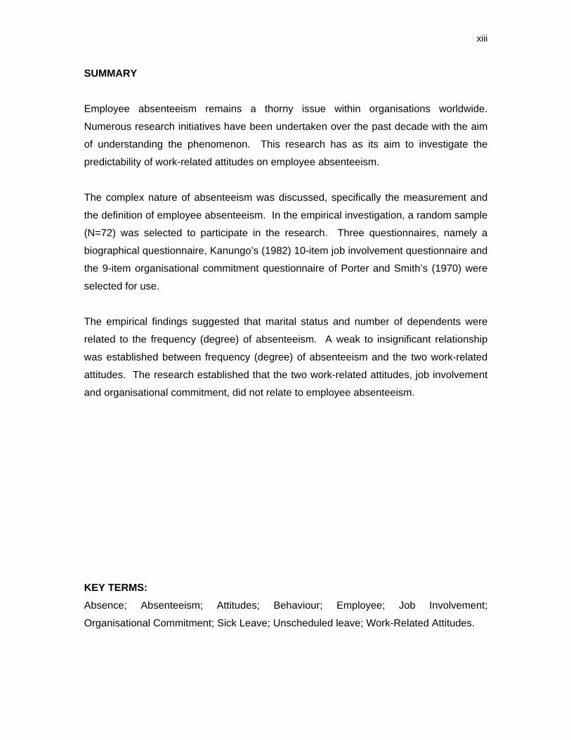
SUMMARY
Employee absenteeism remains a thorny issue within organisations worldwide.
Numerous research initiatives have been undertaken over the past decade with the aim
of understanding the phenomenon. This research has as its aim to investigate the
predictability of work-related attitudes on employee absenteeism.
The complex nature of absenteeism was discussed, specifically the measurement and
the definition of employee absenteeism. In the empirical investigation, a random sample
(N=72) was selected to participate in the research. Three questionnaires, namely a
biographical questionnaire, Kanungo’s (1982) 10-item job involvement questionnaire and
the 9-item organisational commitment questionnaire of Porter and Smith’s (1970) were
selected for use.
The empirical findings suggested that marital status and number of dependents were
related to the frequency (degree) of absenteeism. A weak to insignificant relationship
was established between frequency (degree) of absenteeism and the two work-related
attitudes. The research established that the two work-related attitudes, job involvement
and organisational commitment, did not relate to employee absenteeism.
KEY TERMS: Absence; Absenteeism; Attitudes; Behaviour; Employee; Job Involvement;
Organisational Commitment; Sick Leave; Unscheduled leave; Work-Related Attitudes.
1
CHAPTER 1
SCIENTIFIC OVERVIEW OF THE RESEARCH
This research will investigate the relationship between job involvement and
organisational commitment as work-related attitudes in predicting absenteeism.
The first chapter will provide a general background and motivation for the
research, including the initial problem formulation. The aims, in a practical
perspective, of the research will be discussed under the subcategories of
general, specific and theoretic. Paradigm perspectives will be discussed to
demarcate the boundaries of this research. The design and methodology are
outlined with a schematic flow diagram indicating the procedure for execution.
The outline of the chapters of this research and the chapter summary conclude
the first chapter.
1.1 BACKGROUND AND MOTIVATION FOR THE RESEARCH Absenteeism is considered to be one of the most complex employee problems
associated with a range of variables as well as an array of classifications. Years
of isolation and lack of global competition have let to extremely complacent
attitudes towards high and costly levels of absences in South African
organisations (Hamilton-Atwell, 2003). Such figures compare very unfavourably
with some of South Africa’s major international trading partners. South African
organisations are now faced with increased foreign competition and can only
elevate themselves to international standards by achieving a competitive
cost/productivity balance.
Employees are often considered to be a company’s most valuable assets and
one of the best ways to increase profitably is by increasing the returns on this
2
asset. Reducing absenteeism is one of the most overlooked methods of
reducing company costs (Hamilton-Atwell, 2003). The cost of absenteeism and
the impact thereof on productivity alone is enough to shock any human resources
manager out of complacency. For every 1% of the work force that is absent,
production levels will drop by 2,5%. But the toll of absent employees is
significantly more than only a 2,5% drop in production, such as friction in
employee relationships; impact on service delivery and poor employee attitudes
(Hamilton-Atwell, 2003).
Absenteeism is a phenomenon that affects businesses and countries worldwide.
According to an Unscheduled Absence Survey conducted by the CCH
Incorporated (Anonymous, 2000), unscheduled absenteeism by American
workers reached a seven-year high in 1998, resulting in the business and non-
profit sector suffering millions of dollars in losses. The survey revealed that the
rate of absenteeism increased by 25%, and the dollars lost due to absenteeism
rose 32 % compared to the previous year’s numbers.
For the first time personal illness was not the foremost reasons employees used
when calling in sick. Family issues headed the list at 26% of all unscheduled
absence, followed by personal illness with 22% and personal needs at 20%. The
report noted; that while personal illness absences reported a four-year low,
stress and “entitlement mentality” – taking sick days not because one is sick, but
because employers provided them – reached a four year high. For stress, the
numbers have almost doubled. (Anonymous, 2000)
A survey conducted in Canada during 2000 (Watson Wyatt, 2000) indicated that
the cost of employee absenteeism has risen and is having a greater impact on
the bottom line of companies than ever before. The results of the survey revealed
that a) short-term absences costs, as a percentage of total payroll costs, have
more than doubled from 2,0 % in 1997 to 4,2 %; b) the average direct cost of
employee absenteeism in Canada is now $ 3 550 per employee per year; c)

3
direct and indirect costs combined – including costs for replacement workers and
lost productivity – account for a staggering 17 % of the payroll.
In another survey conducted by CCH Incorporated during 2000 (Anonymous,
2001), unscheduled employee absenteeism declined, reaching the lowest levels
in 10 years, but the high cost of worker ‘no shows’ continued to be a major issue
for employers. While the average rate of absenteeism per employee dropped to
2,1 percent from 2,9 percent in 1999, the average cost per employee
absenteeism stayed at more than $ 600 per year, costing employers anywhere
from $ 10 000 for small companies to over $ 3 million annually for some large
organisations.
In South Africa the picture is no different and is fast joining the international
culture of escalating absenteeism. It was reported by Du Toit (Beeld, 2004) that
the direct cost of absenteeism due to illness for the South African economy is in
the region of R 12 million per annum. According to Du Toit (Beeld, 2004) the
total cost could be more than 200% if indirect costs were to be added. It was
also reported in the Cape Argus (2003) that teacher absenteeism is costing the
Education Department in the Eastern Cape R 5,3 million a day. According to the
Education MEC, Nomsa Jajula, absenteeism amongst teachers is running at
23% (Anonymous, 2003). The Sunday Times (2005) reported that a recent study
conducted by Occupational Care South Africa in conjunction with the University
of South Africa’s department of quantitative studies found that on average 6,3
days per employee per annum are lost to unapproved absences from work
(Vaida, 2005).
Airports Company South Africa (ACSA), is one of South Africa’s leading
parastatals which owns and manages the international and domestic airports in
South Africa. This research will be conducted within this company. Employee
absenteeism has been costing ACSA huge amounts of money in terms of work
hours lost. Almost all departments within the company are affected; however,
4
the security department have consistently shown the highest absenteeism
percentage (3%) over the last two years. The impact of this level of absenteeism
affects not only the company’s bottom line but due to strict legislative
prescriptions requiring that a specific number of personnel are present on the
airport at any given time, can cause serious penalties to the organisation, safety
of passengers and to the tourist industry in South Africa. As a result of this it is
imperative to investigate the causes of employee absenteeism within the security
department.
Based on the aforementioned it is clear that employee absenteeism is a costly
yet poorly understood organisational phenomenon (Johns & Nicholson, 1982;
Martocchio & Harrison, 1993; Mowday, Porter & Steers, 1982; Rhodes & Steers,
1990). Few studies have examined the effects of personal (e.g. age), job content
and organisational factors on absence (Porter & Steers, 1973; Steers & Rhodes,
1978). However a vast majority of absence research has focused on the effects
of work attitudes like job satisfaction (Fitzgibbons, 1992; Rhodes & Steers, 1990).
In recent independent reviews of the past 20 or so years of absence research,
both Harrison and Martocchio (1998) and Johns (1997) have concluded that
excellent progress has been made in understanding the behaviour.
From the literature review the researcher is especially interested to test Blau and
Boal’s (1987) conceptual model using job involvement and organisational
commitment to understand and predict employee absenteeism within ACSA’s
security department. It is in the above context, that this research will aim to
determine whether job involvement and organisational commitment predict
employee absenteeism of the security officers within ACSA.
5
1.2 PROBLEM STATEMENT The motivation for this research will be discussed by highlighting problems
related to employee absenteeism as experienced within ACSA.
Given the aforementioned discussion, it is clear that companies need to
determine the reasons for absenteeism and then implement processes to
address the absenteeism problem. In 2000 and 2001 the absenteeism rate
within the security department in ACSA have consistently exceeded 3% resulting
in a total of R1, 5 million lost in man-hours. This figure excludes the cost of
overtime and temporary staff. Several attempts have been made to address the
absenteeism problem, ranging from creating awareness, counselling, and strict
application of the disciplinary code to awards. None of the strategies has had any
significant affect in bringing the absenteeism percentage down. On reflection,
the interventions were aimed at managing the problem and not investigating the
causes of the absence behaviour.
Harrison and Martocchio (1998) point out that there are definitional,
methodological and statistical problems that imbue absenteeism research and
Rhodes and Steers (1990) agree that absenteeism in itself is quite complex.
According to Rhodes and Steers (1990), there are at least two reasons why the
study of attendance behaviour requires careful attention before reaching any
definite conclusions in a particular organisational situation. Firstly, there is often
a lack of clarity concerning the meaning or meanings attached to absence
behaviour. Absence frequently means different things to different people. The
meaning of absence to the manager is frequently seen as a problem to be
solved. Absence is a dysfunctional category of behaviour, and negative motives
are frequently imputed to the “violator”. “Good” employees come to work on a
consistent basis, “bad” ones stay away for the slightest reason (Rhodes &
Steers, 1990). Hence, absenteeism becomes a management problem, and good
managers solve the problems that confront them. To the employee, absence can
6
take on a very different meaning. Absenteeism can be symbolic of deeper
feelings of hostility or perceptions of inequitable treatment in the job situation
(Rhodes & Steers, 1990). Viewing absence as a social phenomenon, the focus
may need to be on improving work attractiveness and developing a culture that
facilitates attendance instead of absenteeism.
Secondly, it is necessary to recognise that there are multiple and often conflicting
ways to measure absenteeism and in order to understand the nature of
employee absenteeism, it must first be understood how (or whether) it is
measured in empirical studies. Mowday, Porter and Steers (1982) found that
very few organisations keep records of absenteeism. Assuming one wishes to
measure absenteeism, there are several methods that have been used to collect
such data. Unfortunately, there is no uniformly accepted classification scheme
for assessing this form of behaviour. Huse and Taylor (1962) examined four
indices, including the following:
1 absences frequency – total number of times absent;
2 absence severity – total number of days absent;
3 attitudinal absence – frequency of 1 day absence; and
4 medical absences – frequency of absences of three days or longer.
Chadwick-Jones, Brown, Nicholson, and Sheppard (1971) have taken a different
approach to measuring in which seven indices of absenteeism were used
namely:
1 absence frequency;
2 attitudinal absence;
3 other reasons – number of days lost in a week for any reason other than
holidays, rest days, and certified sickness;
4 worst day – difference score between number of individuals absent on any
week’s ‘best’ and ‘worst’ days;
5 time lost – number of days lost in a week for any reason other than leave;
6 lateness – number of instances of tardiness in any week; and
7
7 Blue Monday – number of individuals absent on a Monday minus number
of individuals absent on Friday of any week.
Further compounding the problem of measuring absenteeism is the fact that the
various measures used in empirical studies are not typically related to one
another. In addition to this, absence can be distinguished in various types.
Defining absenteeism has not changed much in the recent years and one simple
definition that is being used is that of organisationally excused versus
organisationally unexcused absences (Blau, 1985; Cheloha & Farr, 1980;
Fritzgibbons & Moch, 1980). Based upon these studies, it would seem that
organisations’ definitions of excused absence include (within defined limits)
categories such as personal sickness, jury duty, religious holidays, and funeral
leave and transportation problems.
By examining the different levels of job involvement and organisational
commitment and how these two variables jointly interact on absence behaviour,
the researcher, through this research, hopes to gain some insight understanding
the causes of absence behaviour within ACSA.
The motivation for this research will be discussed in terms of the research
questions, which are listed below.
• How can the construct of absenteeism be conceptualised through a literature
review?
• How can the construct of job involvement be conceptualised through a
literature review?
• How can the construct of organisational commitment be conceptualised
through a literature review?
• Do job involvement and organisational commitment serve as predictors of
absenteeism?
8
• Can recommendations be made regarding the predictive validity of job
involvement and organisational commitment on high levels of absenteeism?
In an effort to answer the research questions, the following objectives for the
research are set out. 1.3 RESEARCH AIMS
The aims for this research are discussed in terms of general and specific
objectives.
1.3.1 General Aim The general aim of this research is to determine whether work-related attitudes,
namely, job involvement and organisational commitment, predict employee
absenteeism.
The general objective consists of the specific objectives, which are presented
below.
1.3.2 Specific objectives
1.3.2.1 Literature Objectives
The specific literature objectives of this research entail the following:
(a) to conceptualise the construct employee absenteeism, the origins and
consequences in the workplace;
(b) to conceptualise the work-related attitudes of job involvement and
organisational commitment;
9
(c) to integrate the literature on job involvement and organisational
commitment and how job involvement and organisational commitment
impact on employee absenteeism.
1.3.2.2 Empirical Objectives
The specific empirical objectives of this research entail the following:
(a) to investigate whether biographical variables influence absenteeism;
(b) to investigate and analyse whether job involvement and organisational
commitment predict absenteeism in the organisation;
(c) to determine whether there is a correlation between employee absent
levels and job involvement and organisational commitment;
(d) to make recommendations related to the predictability of work-related
attitudes on absenteeism for Industrial Psychology and for future
research.
1.4 RESEARCH MODEL
Mouton and Marais (1996) provides a framework for social sciences, which
embodies a particular approach to the interpretation of the process of research in
the social sciences. The model can be used in distinguishing between good and
poor research in the social sciences. The research model of Mouton and Marais
(1996) serves as a framework for this particular research. It aims to incorporate
the five dimensions of social sciences, namely the sociological, ontological,
teleological, epistemological and methodological dimensions and to systematise
them in the framework of the research process. These are set out in figure 1.1
and also see 1.5.3.2.
10
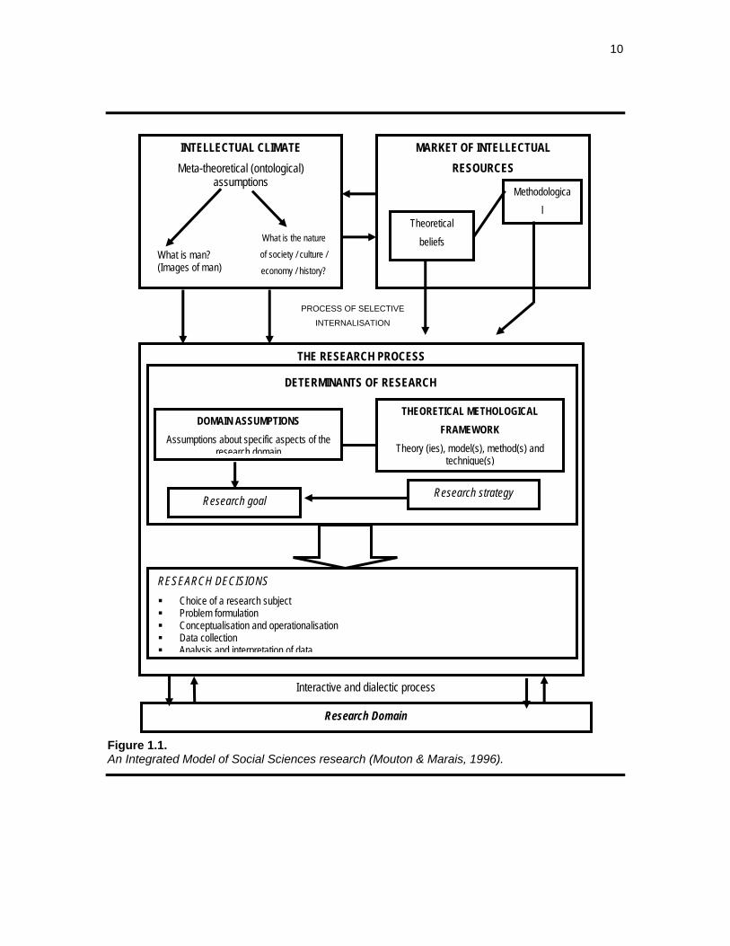
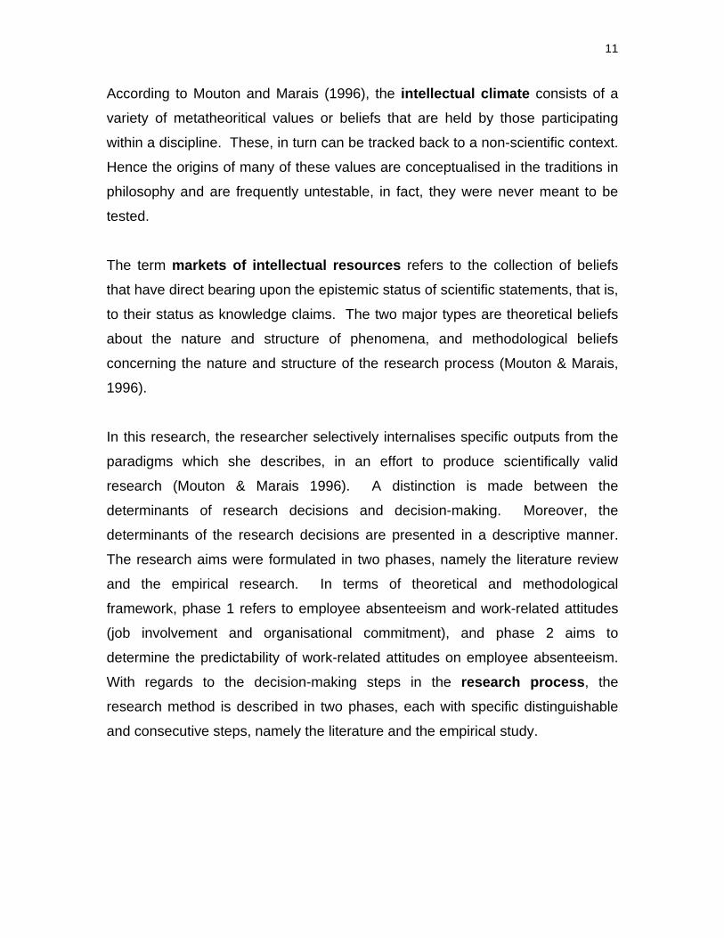
Figure 1.1. An Integrated Model of Social Sciences research (Mouton & Marais, 1996).
INTELLECTUAL CLIMATE Meta-theoretical (ontological)
assumptions
MARKET OF INTELLECTUAL RESOURCES
THE RESEARCH PROCESS
Research Domain
Methodological
What is man? (Images of man)
What is the nature of society / culture / economy / history?
PROCESS OF SELECTIVE
INTERNALISATION
DOMAIN ASSUMPTIONS Assumptions about specific aspects of the
research domain
THEORETICAL METHOLOGICAL FRAMEWORK
Theory (ies), model(s), method(s) and technique(s)
DETERMINANTS OF RESEARCH
Research goal Research strategy
RESEARCH DECISIONS Choice of a research subject Problem formulation Conceptualisation and operationalisation Data collection
Analysis and interpretation of data
Interactive and dialectic process
Theoretical beliefs
11
According to Mouton and Marais (1996), the intellectual climate consists of a
variety of metatheoritical values or beliefs that are held by those participating
within a discipline. These, in turn can be tracked back to a non-scientific context.
Hence the origins of many of these values are conceptualised in the traditions in
philosophy and are frequently untestable, in fact, they were never meant to be
tested.
The term markets of intellectual resources refers to the collection of beliefs
that have direct bearing upon the epistemic status of scientific statements, that is,
to their status as knowledge claims. The two major types are theoretical beliefs
about the nature and structure of phenomena, and methodological beliefs
concerning the nature and structure of the research process (Mouton & Marais,
1996).
In this research, the researcher selectively internalises specific outputs from the
paradigms which she describes, in an effort to produce scientifically valid
research (Mouton & Marais 1996). A distinction is made between the
determinants of research decisions and decision-making. Moreover, the
determinants of the research decisions are presented in a descriptive manner.
The research aims were formulated in two phases, namely the literature review
and the empirical research. In terms of theoretical and methodological
framework, phase 1 refers to employee absenteeism and work-related attitudes
(job involvement and organisational commitment), and phase 2 aims to
determine the predictability of work-related attitudes on employee absenteeism.
With regards to the decision-making steps in the research process, the
research method is described in two phases, each with specific distinguishable
and consecutive steps, namely the literature and the empirical study.
12
1.5 THE PARADIGMATIC PERSPECTIVE OF THE RESEARCH
The paradigmatic perspective of the research, the relevant paradigms,
metatheoretical statements and the market of intellectual resources are
examined next.
As mentioned in the previous section, Mouton and Marais (1996) describe social
science research as a collaborative human activity in which social reality is
studied objectively with the aim of gaining a valid understanding of it. This
research meets the said dimensions and will be approached from the discipline
of Psychology.
Plug, Meyer, Louw and Gouws (1986) define Psychology as a science that
studies human behaviour with the focus on the individual with the help of
methods like experiments, measurements and observation. This disciplinary
relationship focuses on Industrial Psychology, with Organisational Psychology as
a field of application. “Industrial Psychology is a branch of psychology that
applies the principles of psychology to the workplace” (Aamodt, 1991). In other
words, “anything that can be done to help workers realise their potential and
increase their satisfaction on the job will increase their productivity and their
value to the organisation” (Dawis, Fruehling & Oldham, 1989).
The field of Organisational Psychology is concerned with the organisation as a
system involving individuals and groups, and the structure and dynamics of the
organisation (Bergh & Theron, 1999). The basic aim is to foster worker
adjustment, satisfaction and productivity as well as organisational efficiency. As
absenteeism leads to lower productivity and lower efficiency, and job involvement
and organisational commitment deals with satisfaction this research will be
conducted within the field of Organisational Psychology.
13
1.5.1 Relevant Paradigms
Two paradigms are relevant to the literature review of this research. The
literature on absenteeism will be presented from the behaviouristic paradigm.
The literature on job involvement and organisational commitment will be
presented from the humanistic paradigm.
The applicable assumptions of the behaviouristic paradigm (Bergh & Theron,
1999) are presented below.
• Behaviourism is an entirely objective psychology, which aims at developing
general principles of behaviour based on the control and prediction of overt
behaviour.
• The subject matter of psychology is observable behaviour, since only what is
observable can be studied objectively.
• The environment determines behaviour.
• Humans are merely reactive beings and what they are and become is
determined by causes outside themselves.
Through the work of Tolman, Guthrie, Hull and Skinner (as cited in Berg &
Theron, 1999) Neo-behaviourism has introduced unobservable behaviour, the
stimulus – organism – response (S-O-R) approach. Tolman (as cited in Berg &
Theron, 1999) inferred that factors within the organism, such as memory,
thinking, emotion and needs are interfering variables i.e. factors that come
between the stimulus and the response and therefore influences the response.
For this research the factors within the organism, which influences absence
taking within the work context will be studied.
The applicable assumptions of the humanistic paradigm (Meyer, Moore & Viljoen,
1995) are listed below.
14
• The individual as an integrated whole: each individual should be studied as
an integrated, unique, organised whole or gestalt.
• The individual as a dignified human being: man is a unique being with
qualities, which distinguish him from lifeless objects like stones and trees, and
also from primitive animalistic beings.
• The positive nature of man: human nature is basically good, or at least
neutral.
• The conscious processes of the individual: humanists recognise the role of
conscious processes, especially conscious decision-making processes.
• The person is an active being: a person does not simply react to external
environmental stimuli, or merely submit to inherent drives over which he/she
has no control.
• Emphasis on psychic health: The humanists asserted that the psychologically
healthy person should be the criterion in examining human functioning, and
not the neurotic or psychotic person.
Based on this assumption, one can link Kanungo’s (1982) example that the job
itself can help an individual meet his/her intrinsic growth needs. Within this
context, job involvement and organisational commitment implies that a person
consciously and actively engages with his / her job and organisation.
The empirical study will be presented from the functionalistic paradigm. Listed
below are the assumptions of the functionalistic paradigm (Morgan, 1980).
• Society has a concrete, real existence and a systematic character orientated
towards producing an ordered and regulated state of affairs.
• Behaviour is always seen as being contextually bound in a real world of
concrete and tangible social relationships.
• Its basic foundation is primarily regulative and pragmatic.
15
• The focus is on understanding society in a way that generates useful
empirical knowledge.
• The focus is on understanding the role of human beings in society, which
encourages an approach to social theory.
1.5.2 Models
Kaplan (1964) indicates that a model is a particular mode of representation, so
that not all its features correspond to some characteristic of its subject matter.
Models do not pretend to be more than a partial representation of a given
phenomenon. A model merely agrees in broad outline with the phenomenon of
which it is a model (Mouton & Marais, 1996).
The literature component consists of three variables each having different
referents to orientations. According to Morrow (1983), job involvement and
organisational commitment are related, but distinct, types of work attitudes
because of their different referents. The first construct, namely absenteeism, has
through research, subsequently led to findings and theories that can be
categorised into various types of explanatory models.
Rhodes and Steers (1990) categorised absenteeism into three types of
explanatory models, the first model being the pain-avoidance, in which absence
behaviour is viewed as a flight from negative work experiences. Secondly in an
adjustment-to-work model, absence is seen as resulting largely from employee
responses to changes in job conditions leading to a re-negotiation of the
psychological contract. Thirdly in the decision models, absence behaviour is
viewed primarily as a rational (or at least quasi-rational) decision to attain valued
outcomes.
Rosse and Miller (1984) identified at least five implicit conceptual models relating
to absenteeism and turnover. These models are (a) independent forms model –
16
where absenteeism and turnover are viewed as unrelated to each other either
because of differences in causes or consequences; (b) spillover model – where
an adversive work environment is assumed to cause a generalised non-specific
avoidance response; (c) progression-of-withdrawal model – where individuals
engage in a hierarchically ordered sequence of withdrawal including absenteeism
and ending in quitting; (d1) behavioural alternate forms – where the likelihood of
one form of withdrawal, for example, absence, is a function of the constraints on
the alternative behaviour, for example, quitting; (d2) attitudinal alternate forms –
where a negative attitude may fail to translate into voluntary turnover if the
employee sees this response as inappropriate (e.g., if the employee does not
want to lose accumulated benefits); and (e) compensatory model – where
absence and turnover both represent means of avoiding an unpleasant work
environment. The researcher will be working within the pain-avoidance and
decision models provided by Rhodes and Steers (1990) and the spillover model,
behavioural alternate forms and compensatory model provided by Rosse and
Miller (1984).
This research will test the relationship between job involvement and
organisational commitment as related to absenteeism based on a model offered
by Blau and Boal (1987). Their conceptual model uses high and low
combinations of job involvement and organisational commitment to predict
turnover and absenteeism. Job involvement and organisational commitment are
partitioned into high and low categories, and then combined into four cells: (1)
high job involvement – high organisational commitment; (2) high job involvement
– low organisational commitment; (3) low job involvement – high organisational
commitment; (4) low job involvement – low organisational commitment. Each cell
is predicted to have a different impact on turnover and absenteeism.
17
1.5.3 Theoretical statements and methodological convictions
Theoretical statements and methodological convictions form part of the market of
intellectual resources. The market of intellectual resources, according to Mouton
and Marais (1996), refers to the collection of beliefs, which has a direct bearing
upon the epistemic status of scientific statements.
1.5.3.1 Theoretical Statements
The first statement is the theoretical beliefs about the nature and structure of
phenomena, i.e. those testable statements about social phenomena (Mouton &
Marais, 1996). Theoretical statements may be regarded as assertions about the
what (descriptive) and why (interpretive) aspects of human behaviour.
The central hypothesis for this research can be formulated as follows.
An interaction between job involvement and organisational commitment exists on
unexcused absence, such that individuals with higher levels of job involvement
and organisational commitment would exhibit less unexcused absence than
individuals with lower levels of job involvement and organisational commitment.
1.5.3.2 Methodological convictions
The next main epistemological conviction is that of methodological beliefs
concerning the nature of social science and scientific research, in other words
the preferences, assumptions and presuppositions about what ought to constitute
good research (Mouton & Marais, 1996). The aim of this research is to make use
of optimal research design and suitable methods to test the theoretical
hypothesis (Mouton & Marias, 1996).
18
In this research, the central hypothesis, namely that individuals with higher levels
of job involvement and organisational commitment would exhibit less unexcused
absences than individuals with lower levels of job involvement and organisational
commitment, is being tested.
(a) The Sociological Dimension
The sociological dimension conforms to the requirements of the sociological
research ethic. Within the bounds of the sociological dimensions the research is
experimental, analytical and exact. Since the problems that are being studied
are subject to quantitative research and analysis (Mouton & Marais 1996), the
focus of the research will be on the quantitative analysis of the variables and
concepts as described in chapters 4 and 5.
(b) The Ontological Dimension
The ontological dimension refers to the study of being or reality. The content of
this dimension may be regarded as humankind in all its diversity, which includes
human activities, characteristics and behaviour (Mouton & Marais, 1996). The
focus of this research is the predictability of work-related attitudes on employee
absenteeism. The specific aim of the research is to use work-related attitudes
jointly (in an interaction) to predict specific types of employee absence behaviour.
(c) The Teleological Dimension
The teleological dimension refers to human activity, its main aim being the
understanding of phenomena (Mouton & Marais, 1996). The goals of this
research are clear in that attempts are made to determine how work-related
attitudes interact in predicting absence behaviour.
(d) The Epistemological Dimension
The epistemological dimension refers to providing a valid and reliable
understanding of reality (Mouton & Marais, 1996). In this research, an attempt is
made to formulate an appropriate research design and achieve valid and reliable
19
results to determine whether work-related attitudes predict employee
absenteeism.
(e) The Methodological Dimension
The methodological dimension refers to the objectivity of the research – it should
be critical, balanced, unbiased, systematic and controllable (Mouton & Marais
1996). The research is therefore planned and structured, and executed to
comply with the criteria of science. It also relates to data collection through
questionnaires, the research and data analysis by means of the correlation of
quantitative data. The research design and research methods are structured to
ensure rational decision-making.
These five dimensions are core aspects of the same process – research. In
terms of the model, social science research is a collaborative human activity in
which social reality is studied with the aim of gaining valid understanding (Mouton
& Marais, 1996). In Figure 1.1 this model is described as a systems theoretical
model, with three subsystems that are interrelated and also relate to the research
domain of the specific domain – in this case, Industrial Psychology. The
subsystems represent the intellectual climate, the market of intellectual resources
and the research process itself (Mouton & Marais, 1996).
1.6 RESEARCH DESIGN
According to Mouton and Marais (1996), the aim of research design is to plan
and structure a given research project in such a manner that the eventual validity
of the research findings is maximised. They continue to describe it as
synonymous with rational decision-making during the research process and
points to three aspects that codetermine research design, namely the unit of
analysis, the type of objective and the research strategy. The research design is
discussed with reference to the aforementioned.
20
1.6.1 Unit of analysis
The unit of analysis, as it is refers to in the problem statement and the research
aims is the human being, namely security officers based at Johannesburg
International Airport.
1.6.2 Typology of the research
A distinction can be made between three types of research objectives, namely,
exploratory, descriptive and explanatory (Mouton & Marais, 1996). This research
is of an explanatory nature and the aim is to show that a relationship exists
between the variables, absenteeism and work-related attitudes namely,
organisational commitment and job involvement.
This research will be descriptive, in the presentation of the three constructs under
discussion, namely absenteeism, job involvement and organisational
commitment. The important consideration in descriptive research is to collect
accurate information on the domain phenomena that are under investigation.
1.6.3 Validity
According to Mouton and Mariais (1996) the aim of the research design is to plan
and structure the research project to ensure that the internal and external validity
of the research findings are maximised. Internal validity is the logical
predecessor of external validity and for this reason, the research findings can not
be based on external validity before the internal validity is established. Research
with a contextual aim places a high priority on internal validity (Mouton & Marias,
1996)
21
1.6.3.1 Validity in terms of the literature review
Internal validity for the literature review is ensured through:
• the definition of a central hypothesis which describes the aim of the
research (formulated in point 1.5.3.1);
• the provision of descriptions of all relevant concepts used in the research,
as it seen from a theoretical perspective and how it is measured
empirically (explained in point 1.3.2.1);
• choosing models which will support the literature review (explained in
point 1.5.2);
• using theories as a basic departure point which will explicitly explain
assumptions with regards to the human (explained in point 1.5.1);
• ensuring a comprehensive literature review by making use of a computer
search (discussed in point 1.7);
• selecting representative concepts with their respective measuring
instruments that touches on the theoretical field and to integrate it with the
literature review; and
• standardising the literature analysis and presentation according to a
systematic process. In the literature discussion on the various
constructs, the theoretical framework, definitions, causes, effects,
consequences and models will be provided. The discussion on the
measuring instruments will refer to the development and rationale,
description, interpretation, reliability and validity, and motivation for
selection.
The validity of the literature review can further be motivated by assuming that the
literature that is collected and used will be the most recent developments on the
field of study and will comply with the standards established for international and
local publication in journals and books.
22
1.6.3.2 Validity in terms of the empirical study
For the empirical study, validity is ensured through:
• the coding of responses and control thereof;
• the processing of statistics done by an expert with the help of the most
recent and sophisticated computer packages available;
• the reporting and interpreting of results according to standardised
procedures; and
• conclusions and recommendations will be made on the results.
Making use of questionnaires, which has already been tested in scientific
research and accepted as the most suitable, further ensures validity.
1.6.4 Reliability
The reliability within the research is assured by structuring the research model in
such a way that the disturbance variation is kept to a minimum and that the
research context of the research (Mouton & Marais 1996) is respected.
1.6.4.1 Reliability in terms of the literature review
Reliability of the literature review is ensured by the assumption that other subject
experts have access to the same literature and will therefore provide the same
theoretical information as well as the assumption that the research aims to put
forward the facts in as scientific a manner as possible.
1.6.4.2 Reliability in terms of the empirical research
The reliability in terms of the empirical research is ensured by making use of a
representative sample, to ensure that the results are not a reflection of a minority
23
group. The sample includes individuals from all ethnic origins and both sexes
within the organisation being used.
1.6.5 Variables
The aim of the research design is to determine if the specific chosen variable,
known as the independent variable, influences another variable, known as the
dependent variable (Huysamen, 1993). In this research the dependent variable
is unexcused absenteeism and the independent variable is work-related
attitudes, and more specifically, job involvement and organisational commitment.
1.6.6 Research strategy
Mouton and Marais (1996) distinguish between research with contextual and
general interest. Contextual research strategy refers to a study of phenomena or
events because of their intrinsic interest and is studied in terms of its immediate
context. This research is contextual of nature and focuses on the nature of
absence behaviour of security officers within a specific company.
1.7 RESEARCH METHODOLOGY
The aspects listed below represent the selected research methodology, which
will correspond with the specific literature and empirical aim of this research.
Two phases will apply.
PHASE 1 LITERATURE REVIEW Phase 1 contains the literature review of the research and includes all the steps
associated with the initial planning and execution of the research.
Step 1: Identification of key concepts of the independent and dependant
variables.
24
Step 2: Selection of relevant models, theories and measuring instruments.
Step 3: The gathering of relevant literature.
Step 4: Analysis of literature according to standardised procedures for
constructs, concepts and measuring instruments.
Step 5: Integration of job involvement and organisational commitment as
work-related attitudes and their relationship to absenteeism.
PHASE 2 EMPIRICAL STUDY Phase 2 consists of the empirical study and focuses on the steps associated with
the practical execution of the research.
Step 1: Describing the population and the sample.
Step 2: Describing the measuring instruments.
Step 3: Distribution of questionnaires to sample population.
Step 4: Data gathering.
Step 5: Data Processing.
Step 6: Reporting and interpreting the results from the empirical study.
Step 7: Presentation of the combination of conclusions, limitations and
recommendations based on the research.
25
1.8 CHAPTER ALLOCATION
The chapters for this research will be presented as follows:
Chapter 2: Absenteeism
Chapter 3: Work-Related Attitudes
Chapter 4: Empirical Study
Chapter 5: Results
Chapter 6: Conclusions, Limitations and Recommendations
1.9 CHAPTER SUMMARY
In this chapter, the scientific overview of the research, the background to, and
motivation for, this research were provided. The central problems to be
addressed, the aims, the research model, paradigm perspective, research design
and the research methodology were also discussed. Lastly the outline of the
chapters was presented.
In the next chapter, absenteeism will be examined from a theoretical perspective.
The concept and determinants of absenteeism will be defined and the complexity
of the construct will also be discussed.
26
CHAPTER 2
ABSENTEEISM
In this chapter, absenteeism will be discussed from a theoretical perspective
within the relevant literature. The nature of absenteeism, relevant theory,
definitions, origins, and consequences of absenteeism will be examined. Lastly
various models of absenteeism will be presented. This chapter will conclude with
a summary and chapter conclusion.
2.1 NATURE OF ABSENTEEISM
Over the years a vast volume of information has been collected about
absenteeism and numerous books have been written about the topic (e.g.
Goodman & Atkin, 1984; Rhodes & Steers, 1990). Research into absence
behaviour has proven problematic due to the complex nature of absenteeism
because of the wide range of variables, as well as an array of classifications
associated with the construct (Hamilton-Atwell, 2003). Johns (1994) points out
that there are some thorny definitional, methodological and statistical problems
that imbue absenteeism research. Steers and Rhodes (1984) have identified
four clearly defined areas in which absence behaviour is seen as complex, the
first being the pervasive nature of absenteeism across organisations and
international boundaries; the high cost involved; the many variables (several
hundred) researched in relation to it; and its potentially serious consequences for
the individual, co-workers and organisations alike. Johns and Nicholson (1982)
describe absence, as meaning “… different things to different people at different
times in different situations” (p.134), and this serves to illustrate the complexity of
absence behaviour. According to Johns and Nicholson (1982), an essential
problem is that absenteeism is actually a variety of behaviours with different
causes masquerading as a unitary phenomenon.
27
Landy, Vasey, & Smith (1984) commented that due to the complex nature of
absenteeism and the measurement around absenteeism, careful consideration
must be exercised in drawing comparisons between studies, since many studies
used differing definitions of absenteeism (Muchinsky, 1977). Muchinsky (1977)
pointed out that the single most vexing problem associated with absenteeism as
a meaningful concept involves the metric or measure of absenteeism. In chapter
1, section 1.2, the metric or measures of absenteeism as proposed by Huse and
Taylor (1962) and Chadwick-Jones, et al., (1971) were discussed. For the
purposes of this research attitudinal absence of Huse and Taylor (1962)
(frequency of 1 day absences) will be used.
Further compounding the problem of measuring absenteeism is the fact that the
various measures used in empirical studies are not typically related to one
another. Harrison and Martocchio (1998) indicated that researchers should
clearly describe their rationale for the timing of their measurements of other
variables, and the length of absence aggregation periods.
Chadwick-Jones et al., (1982) have through their study drawn a qualitative
distinction between longer and extremely short absences. The former tend to be
a result of serious illness and unavoidable incapacity. The latter, specifically
absences of one or two days’ duration, often seem to express employees’
decisions not to go to work. In practice, it is impossible to check whether ‘a slight
cold’ or a ‘muscular pain’ is simply a convenient excuse. It can thus be argued
that short absences are more likely to be under the employee’s own control,
resulting from his/her own decisions to take a day off (Chadwick-Jones et al.,
1982). Again, it is by no means certain that longer-term absences are
involuntary, but they are somewhat less likely to be voluntary. While some
longer sickness absences will no doubt be the result of malingering and some
very short absences will be unavoidable, it nevertheless seems justifiable to
make this important, if rather fallible, distinction between the two (Chadwick-
Jones et al., 1982).
28
In their research Harrison and Martocchio (1998) outlined the idea that the levels
of individual absenteeism accumulated over any time period are most likely to
reflect variables that are defined and relatively stable over that period. They
focused on three time periods as sources of variances in absenteeism, namely
long-term sources of variances, mid-term sources of variance and the short-term
source of variance. Long-term is defined as having a time span of more than one
year and, according to Harrison and Martocchio (1998), this aggregation period
for absenteeism has a degree of ecological validity. Variables likely to correlate
with a distribution of absence aggregated over a long-term period are themselves
stable in the long term. The few long-term studies that have appeared (e.g.
Thomas & Thomas, 1994) have mainly focused on demographic characteristics
such as gender and education.
The mid-term variance in absenteeism can be thought of as having a time span
of between three months and one year. Particularly the shorter end of the
interval, the notion of a mid-term level of time also corresponds to periods over
which global job attitudes remain fairly stable (Rosse & Hulin, 1985). Similar
patterns might be expected for absence cultures (Nicholson & Johns, 1985),
organisational commitment (Cohen, 1991), task characteristics (Fried & Ferris,
1987), and other constructs that are likely to show meaningful year-to-year, but
not day-to-day or week-to-week changes. The short-term variance in
absenteeism can be defined as having a time span of a few days to three
months. Variances can be attributed to attendance decision parameters
(Martocchio, 1992), acute work and life stressors (Theorell, Leymann, Jodko &
Konarski, 1992) or relative dissatisfaction (Rosse & Miller, 1984).
Remark For the purpose of this research absenteeism will be measured in the frequency
of absence spanning over a one-year period (mid-term source of variance).
29
In addition to the above, the issue of accurate record keeping of absenteeism
adds to the problem of effectively studying absenteeism. Fine-grained data can
provide a systematic variation in absenteeism over very short periods (Harrison &
Hulin, 1989). Very few organisations keep accurate records of employee
absenteeism, however in the organisation within which the research is being
conducted (ACSA), a record keeping system exists. Information from this system
was used to determine absence trends. The reliability of the information
captured in this system (especially referring to the reasons for sickness or
absence), as within any other system reliant on the human interface, will always
be questionable.
To meet the research aim namely, to conceptualise absenteeism from a
theoretical perspective, in the next section of this chapter theories on
absenteeism will be discussed in order to provide some depth of understanding.
It is noted that although there is generally a lack of theoretical support for
absenteeism, reviewing the literature has presented some theoretical views on
absenteeism. The theoretical viewpoints discussed are those most referred to in
recent research and have not changed over the past decade.
2.2 THEORIES OF ABSENTEEISM
Absence behaviour is discussed in terms of theories on absences such as the
notion of the informal contract, perceived inequity, and withdrawal from stressful
work situations, dynamic conflict, social exchange, withdrawal, non-attendance,
organisationally excused vs. organisationally unexcused, involuntary vs.
voluntary and lastly a four-category taxonomy. The relevance of each of these
perspectives to this specific research will also be discussed.
30
2.2.1 Informal Contract
Gibsson (1966) attempted to explain some of the main features of absence
behaviour by means of the notion of an informal contract. The contract is viewed
as being made between the individual and the organisation. Gibsson (1966) was
especially interested in absences that were not long enough to activate formal
legitimising (certification) procedures. He used the concept of valence, referring
to a person’s positive or negative relationships to a work situation and pointed
out that if the combined valences of a work situation are weak, it will be easier for
people to legitimise their absences to themselves.
Gibsson (1966) remarks that a plausible idea relating to the size of the
organisation influences absence rates; in larger organisations, since there is
greater division of labour, there is also more concealment of the contributions of
individuals, thus permitting latitude for absence from work. He also mentions the
importance of the employee’s identification with the organisation, as in the case
of longer-service employees, and argues for the importance of the “authenticity”
of the work contract (Gibsson, 1966). In other words, the organisation should be
seen to offer a fair deal to the individual, whose feelings of obligation would thus
be strengthened.
In this research Gibsson’s (1966) concept of valence, referring to an individual’s
positive and negative relationship toward a work situation has relevance, as the
aim of this research is to determine whether work-related attitudes (Job
Involvement and Organisational Commitment) predict employee absenteeism. It
is hypothesised that employees with low job involvement and organisational
commitment (negative relationship to the work situations) will have higher levels
of absenteeism.
31
2.1.2 Resolving Perceived Inequity
Adams (1965), Hill and Trist (1953) and Patchen (1960) have made notable
theoretical contributions towards the study of absenteeism. Although their
research is dated, it is included to add to the broader understanding of the
concept of absenteeism. No recent literature has been identified which has built
on this perspective. Adams (1965) suggested that absences may be a means of
resolving perceived inequity; the probability of absence behaviour will increase
with the magnitude of inequity and if other means of reducing inequity are not
available. Patchen (1960) had tested this kind of hypothesis; producing evidence
of a relationship between absences and perceived fairness of pay, that is,
employees’ feelings about how fairly they had been treated in regard to their pay
levels and promotions.
This research will not consider this perspective, as the security officers working
for ACSA are paid, on average, 30% higher than the norm in industry. The
author does not disregard the fact that in some employees’ mind this could be an
issue, as well as other procedures and process that could lead to a perception of
unfairness.
2.1.3 Withdrawal from the Stress of Work Situations
In their study on absence, Hill and Trist (1953; 1962) contributed a theory of
absence as being the withdrawal from the stress of work situations, claiming as
evidence for this proposition certain patterns of absence and accident rates
recorded over a four-year period in a large steel company. Withdrawal is the
central explanatory concept; thus, individuals experiencing conflicts of
satisfaction and obligations tend to express them through labour turnover,
accidents, and unsanctioned absences (this is, absences without formal
permission). Exactly how the conflict will be expressed depends on a sequence
of three phases in the employee-organisation relationship (Hill & Trist, 1962).
32
During the early stages of employment, the desire to withdraw is expressed
primarily in labour turnover (Hill & Trist, 1962). One important thing, as Hill and
Trist (1962) pointed out, in this period, is that newcomers are ignorant of the
prevalent norms of absences – they do not yet know how far they have this
means of withdrawal at their disposal.
After the initial ‘induction’ crisis, the ‘stayers’ have had time to learn the prevailing
absence culture to the point where they can operate it more freely (Hill & Trist
1962, p.340). Hill and Trist (1962) refer to this second phase as ‘differential
transit’. Subsequently the relationship stabilises, as the initial crisis recedes
further and the individual reaches a third phase of ‘settled connection’ that has
reduced levels of absence. Thus, the changes in withdrawal behaviour are
explained by the internalisation of norms as individuals become aware of, and
party to, the kinds of absence tolerated in the organisation.
However, if ‘available, sanctioned outlets for stress’ (absence that the employing
authority retrospectively excuses) are insufficient, then hostilities toward the job
environment are expressed in accidents and ‘ailments’. According to Hill and
Trist (1962), individuals accept that only so much absence without permission is
allowed, and therefore may have recourse to minor illness (which, by the
psychoanalytic interpretation, is characteristic of a depressive disorder). This is
in contrast with the other kind of absence without permission, which reflects a
more overt, paranoid expression of hostility.
Hill and Trist (1962) noted that the decline in accident rates with length of service
conceals a rise in the numbers of accidents that are under the control of the
individual. These represent a depressive mode of feeling and parallel the
increase in uncertified sickness absence as another means of ‘coping with
stress’. The main fault, however, with this research is that there is a large gap
between the level of explanation and the level of the empirical date, in other
33
words, the data consists of collective trends of accidents and absences, while the
explanation treats of individual reactions (Hill & Trist, 1962).
In addition to the views of Hill and Trist (1962), Hanisch and Hulin (1991)
theorised that absenteeism and other withdrawal behaviours (e.g., lateness and
turnover) reflect invisible attitudes such as job dissatisfaction, low level of
organisational commitment, or an intention to quit. According to this view, an
employee who is absent from work is consciously or unconsciously expressing
negative attachment to the organisation.
For this research, the perspective of Hanisch and Hulin (1991) on absence
behaviour is relevant, as the aim is to test the hypothesis that employees with
low job involvement and organisational commitment have higher levels of
absenteeism.
2.1.4 “Dynamic Conflict’
The ‘withdrawal’ explanation offered by Hill and Trist (1962) had some
subsequent influence on theoretical discussions by Ås (1962) and Knox (1961).
Gadourek (1965) described the latter as ‘dynamic conflict’ theories. The conflict
is located within the individual, and whether a person stays or withdraws is the
result of a complex in incentives and stresses. Within the scope of this research
the ‘dynamic conflict’ theory will not be addressed.
2.1.5 Social Exchange
Chadwick-Jones et al., (1982) presented a case for the theory of absenteeism
that is social, not individual in emphasis. As a first step Chadwick-Jones et al.,
(1982) assumed the interdependency of members of work organisations. It
seems obvious that individuals do have some mutual obligations to peers,
subordinates, and superiors (as well as other relationships outside the work
situation). In this context the rights and duties of individuals are both subject to,
34
and representative of, a set of rules about activities in the work situation. What
individuals do is therefore likely to be in answer to, on behalf of, in defence of, as
well as achieving a compromise with the rules of the group.
The second assumption made by Chadwick-Jones et al., (1982), is that under the
employment contract, some form of social exchange is taking place between
employers and employees. Whatever they exchange in this situation – whether it
be their time, effort, or skill or money, security, congenial friends, or anything else
- it will be only what is possible for employees in the organisation. Exchanges
may be conceived as between individuals and work groups, or between work
groups and management, but it would not be realistic to conceive of the
exchange between ‘the individual’ and ‘the organisation’ while disregarding the
social conditions and rules. In summary, then, the group is in the equation – on
one or both sides – and the explanation use must recognise it.
Chadwick-Jones et al., (1982) think of social exchange between employees and
employers as developing in, or as revealed by, a pattern of behaviour in the work
situation that includes absences with all the other factors that constitute the
contract, formal and informal, between employers and employees. Formal
factors include pay, hours, disciplinary rules, job duties, and promotion lines.
Informal ones include supervisory styles, peer group relations, and – salient to
their analysis – absence from work. Chadwick-Jones et al., (1982) however, do
point out that absences may not enter into the exchange at all, insofar as some
employees or employee groups, especially those with higher status – supervisors
in factories, managers in banks – are absent very little or hardly at all. It is quite
possible, however, that managers possess greater control over the allocation of
their working time and may take periods of ‘time out’ that are not recorded.
Absenteeism levels reflect the social exchange within an organisation and that it
is ‘agreed’ behaviour. This implies that employees understand that their
absences should fall within certain limits and, therefore, those employees’
35
decisions to be absent or to attend conform to a normative frequency level
(Chadwick-Jones et al., 1982). Employees can be expected to have a definite
notion of the appropriate frequency and duration of their absences. The question
for them is not only whether to be absent today, but how often they have already
been absent in this month or year.
Within the scope of this research the social exchange theory will not be
addressed.
2.1.6 Withdrawal
According to Chadwick-Jones et al., (1982), absence from work, where work is
defined by the employee’s presence at a particular location (office or workshop)
for a fixed period each day, can be interpreted as an individual act of choice
between alternative activities; as withdrawal or escape from surveillance; as
individual or group resistance to an inflexible system. Thus, absence may also
be viewed as a stratagem in inter-group relations, as a defensive or aggressive
act in inter-group conflict (Chadwick-Jones et al., 1982). For the purpose of this
research this theory has relevance, as the reasons for absence behaviour could
be related to a choice of alternative activities instead of attending work.
2.1.7 Non-attendance
Another definition of absenteeism refers to the non-attendance of employees for
scheduled work (Gibons, 1966; Johns, 1978; Jones, 1971). The definition
distinguishes absenteeism from other forms of non-attendance that are arranged
in advanced (e.g. vacations) and specifically avoids judgements of legitimacy
associated with absent events that are implied by as sick leave. This definitional
emphasis seeks to focus on the key organisational consequences of
unscheduled non-attendance – instability in the supply of labour to the
organisation resulting in the disruption of scheduled work processes and the loss
36
of under utilisation of productive capacity (Allen, 1981; Jones, 1971, Nicholson,
1977). For this research this definition will be applicable, as the researcher will
not take into account absences due to vacation leave and sick leave taken over
more than three days.
2.1.8 Organisationally excused vs. organisationally unexcused
In terms of distinguishing among types of absence, one simple distinction that
previous studies (Blau, 1985; Cheloha & Farr, 1980; Firzgibbons & Moch, 1980)
made is between organisationally excused versus organisationally unexcused
absences. Based on these studies, it seems that organisations operationalise
excused absence to include (within defined limits) categories such as personal
sickness, jury duty, religious holidays, funeral leave, and transportation problems.
However, as Johns and Nicholson (1982) noted, absence behaviour can have a
variety of meanings for individuals. This research will focus on the
organisationally unexcused type of absenteeism.
2.1.9 Involuntary vs. voluntary
March and Simon (1958) on the other hand, distinguished between two basic
types of absences: involuntary (e.g. certified sickness, funeral attendance) and
voluntary (e.g. vocation, uncertified sickness). Voluntary absences are under the
direct control of the employee and are frequently utilised for personal aims.
Conversely, involuntary absences are beyond the employee’s immediate control.
Hence, voluntary rather than involuntary absences from work may reflect job
dissatisfaction and lack of commitment to the organisation.
The theory of social exchange in this study will have relevance as, from the
analysis of the attendance records and the lack of action taken against the
employees, it would seem that within the security group at an ‘unwritten’ level a
37
certain amount of absence is tolerated (by the supervisors and not by the rest of
the organisation).
It can be seen from these definitions that an absent employee is one who should
be at work but has failed to attend. However, they do not specify whether that
absences is voluntary (under the control and motivation of the employee to
attend), or involuntary (beyond the control and ability of the employee to come to
work), both types being forms of unscheduled non-attendance which disrupt the
labour supply and consequently, the production process of the organisation
(Hammer and Landau, 1981). For this research, the focus will be on voluntary
absences.
2.1.10 A four-category taxonomy
Blau and Boal (1987) presented a four-category taxonomy describing the
meanings of absence. These categories are medical, career enhancing,
normative and calculative. In the medical category, absence is viewed as a
response to various infrequent and uncontrollable events (illness, injury, fatigue,
and family demands). If such an absence (medical) occurred, it probably would
be operationalised as a sporadically occurring excused absence (Blau & Boal,
1987). In the career-enhancing category, absence is depicted as a mechanism
that gives the employee a further choice to pursue task- and career-related goals
(Blau & Boal, 1987).
For the normative category, absence is viewed less as a motivated behaviour
and more as a habitual response to the norms of the work group (organisation)
regarding absence (Blau & Boal, 1987). As such, this type of absence probably
would operationalise as a consistently occurring excused absence. More
importantly, rather than absenteeism appearing as a random walk, as with the
medical category, definite patterns will emerge. Thus, for this group, it would be
expected not only to predict frequency, but also when absenteeism will happen.
38
Finally the calculative absence is viewed as a coin of exchange (Blau and Boal,
1987; Johns & Nicholson, 1982) in either fulfilling or modifying the implicit social
contract between the employee and employer, and as a time allocation strategy
for enhancing non-work outcomes. This type of absence would be
operationalised in terms of the employee using a certain number of excused and
unexcused absences permitted by the organisation, depending on how much the
employee felt he or she should modify the implicit social contract. It could be
predicted that an extremely apathetic employee (low job involvement and
organisational commitment) would take full advantage by using both kinds of
absence. Thus, the absolute frequency and total number of days absent should
be greatest for workers who are the most apathetic.
From the theoretical perspectives provided, the informal contract (Gibson, 1966)
and withdrawal from the stress of work situations (Hill & Trist, 1953, 1962) has
particular reference to this research. The “dynamic conflict” (Gadourek, 1965)
theory has some relevance. The research on absenteeism theories is relatively
dated and no new perspectives on absenteeism theory were evident from the
literature reviews. Research on absenteeism seemed to have built on the initial
theories and time and again highlighted the lack of theory formulation due to the
complexity of the absenteeism construct.
The meaning of absenteeism applied in this research refers to Blau and Boal’s
(1987) calculative category. The types of absenteeism that will be investigated
during this research refer to the organisationally unexcused, calculative and
voluntary absenteeism.
Based on the theoretical perspectives discussed, the definition formulation of
absenteeism will now be presented in section 2.3 of this chapter.
39
2.3 DEFINITIONS OF ABSENTEEISM
Owing to the large amount of research conducted on absenteeism, there are
many variations to the definition of absenteeism, each one specific to the work of
the researcher at the time. For the purpose of this research, an overview of the
various definitions of absenteeism being used in research will be presented.
Based on this, the researcher will provide a working definition of absenteeism
that will be applicable for this research.
• Absence constitutes a single day of missed work (Martocchio & Jimeno,
2003).
• Absence occurs whenever a person chooses to allocate time to activities that
compete with scheduled work, either to satisfy the waxing and waning of
underlying motivational rhythms (Fichman, 1984), or to maximise personal
utility (Chelius, 1981).
• An individual’s lack of physical presence at a given location and time when
there is a social expectation for him or her to be there (Martocchio & Harrison,
1993).
• Absenteeism refers to the non-attendance of employees for scheduled work
(Gibsson, 1966; John, 1978; Jones, 1971).
A working definition of absenteeism for this research is that absenteeism is
defined as a failure of an employee to report to work when he/she is scheduled to
do so (unexcused absence). The absence that occurs refers to short periods of
absence taken over a period of one year.
This contributes to the first literature aim, namely to conceptualise the construct
of employee absenteeism, the origins and consequences in the workplace (see
1.3.2.1 (a)).
40
A further aspect of this literature aim as outlined in chapter 1 section 1.3.1, is to
highlight the origins and consequences of employee absenteeism. These origins
will be discussed next.
2.4 ORIGINS OF ABSENTEEISM
Research on absenteeism over the past years, particularly conceptual work, has
focused on absenteeism’s origins or causes. The vast number of predictions
these theories and hypotheses make, the breadth of approaches they take, and
the scope of evidence they have generated all make on thing clear: absenteeism
does not have a simple etiology (Johns, 1997). Harrison and Martocchio (1998),
through their review of absenteeism research, indicated that literature suggests
five loosely defined classes of variables hypothesised to be origins of absence
which are (a) personality; (b) demographic characteristics; (c) job-related
attitudes; (d) social context and (e) decision-making mechanisms.
2.4.1 Personality
Researchers have suggested for decades that enduring personality traits account
for absenteeism’s moderate stability over time and situations. “Absence-
proneness” emerged as a term describing this idea (Harrison & Price, 1993).
Johns (1997) has labelled this perspective the “deviance” approach. Porter and
Steers (1973) proposed that employees with extreme levels of emotional
instability, anxiety, low achievement orientation, aggression, independence, and
sociability were likely to be the most frequent absentees. Hogan and Hogan
(1989) asserted that those who are at fairly high levels of hostility, impulsiveness,
social insensitivity, and alienation are more prone to engage in delinquent work
behaviours such as absenteeism. Ferris, Bergin and Wayne (1989) presented a
more differentiated view, proposing that personality dimensions also moderate
situational and attitudinal relationships with absenteeism.
41
2.4.2 Demographics
Many studies have accumulated in which gender, age, tenure, education level,
and family characteristics have been measured and as evidence accumulated,
demographic variables were brought into broadly inclusive and inductive
absenteeism models (Harrison & Martocchio, 1998). The most influential and
often cited example of such a model was developed by Steers and Rhodes
(1978, 1984), which introduced a series of propositions implying that an
individual’s demographic characteristics (personal factors, family characteristics)
indirectly influence absenteeism through sets of medial variables (such as
expectations and job satisfaction) and proximal constructs (attendance
motivation and ability to attend). These proximal constructs are also predicted to
interact – the effects of attendance motivation are tempered or neutralised by low
ability to attend. The underlying premise of Steers and Rhodes’ model (1978) is
that an employee’s short-term motivation and ability to attend work are the direct
precursors of attendance (Harrison & Martocchio, 1998).
Brooke (1986) proposed a revised and more extended model than that of Steers
and Rhodes (1978, 1984). He predicted additional, direct inputs of health-related
(e.g., alcohol use) and organisational constructs (e.g., permissiveness) to
absenteeism, formulated more precise definitions of existing constructs, and
argued for additive rather multiplicative effects. Marcus and Smith (1985)
presented a sociological model of absenteeism that included demographic
characteristics. Their basic contention was that previous research had
concentrated too heavily on attitudinal determinants of absenteeism, and that a
more fruitful approach would concentrate on absence norms, customs, and
socialisations.
42
2.4.3 Attitudes
The main conceptual paradigm for absenteeism was to treat absence taking as
individual-level avoidance or withdrawal from a disliked work situation (Harrison
& Martocchio, 1998). Steers and Rhodes (1978), however, assigned job
attitudes a central place in their early model, predicting that the effects of all other
job-related and organisational variables on absence would work their way
through job satisfaction. Job attitudes are the only mid-term engine driving
absenteeism in Rosse and Miller’s (1984) cybernetic theory of job adaptation,
and in the withdrawal theory of Hulin, Roznowski and Hachiya (1985), although
both models propose behavioural responses to dissatisfaction other than
absence. These models also include ‘evaluation of alternatives or ‘behavioural
intentions’ as penultimate steps to absence. Other job attitude theorist relegate a
much weaker role to job satisfaction. Blau and Boal (1987) omit it entirely,
instead emphasising two other forms of job-related attitudes as catalysts:
organisational commitment and job involvement. Their arguments focus on the
patterns of absenteeism and turnover likely to be manifest under combinations of
those two attitudes.
2.4.4 Social Context
Johns and Nicholson (1982) argued for a potent influence of the social environment on work absence, rejecting the traditional, implicit assumption that
absence was a private behaviour that occurred without regard to interpersonal
context. The influence of social context on absence is embodied in their
conception of an absence culture, defined as “the set of shared understanding
about absence legitimacy and the established ‘custom and practice’ of employee
absence behaviour and its control” (p.136). Nicholson and Johns (1985)
maintained that two factors shape absence cultures: (a) the values and beliefs of
the larger society and its subcultures, and (b) the unique set of beliefs shared by
virtue of membership in an organisation. Two themes, beliefs about absence
43
and assumptions about employment (psychological contract), describe the long-
term character of societal-level absence culture. For example, virtually all
cultures view serious illness as an acceptable reason for missing work
(Rushmore & Youngblood, 1979), and this position has held for decades
(Haccoun & Desgent, 1993). At the organisational level, the salience and nature
of absence cultures can vary over different units (Martocchio, 1994) and over
shorter, mid-term time periods.
2.4.5 Decision-making
Both economic (e.g., Chelius, 1981) and psychological (e.g., Harrison, 1995)
researchers have depicted absence as the result of a daily choice process. In
the economic approach, employees are assumed to make work attendance
decisions in a way that strives toward utility maximisation, making themselves as
happy as possible, given finite resources of time and money (Ehrensberg &
Smith, 1985). A variety of marginal utility and cost functions have been proposed
within this general axiom. For example, Winkler (1980) conceptualised absence
in terms of work-leisure trade-offs, through which individuals maximise utility,
subject to a budget constraint. A common prediction of the economic models is
that individuals would take as many fully paid absence days in a given period as
allowed or not penalised by their employers.
Although expected utility (anticipated affect) is part of the decision-making
process in psychological theories (Fichman, 1984), it is just one of many issues
thought to be considered by those facing the choices of absence or attendance
at work (Harrison, 1995, Nicholson, 1977). Instead of drawing from decision-
making constructs, however, Fichman’s (1984) theory drew on a general theory
of motivation, arguing that, to explain the timing of absence and attendance, the
dynamic strengths of motives to engage in work versus non-work activities must
be considered. Unfulfilled motives strengthen over time. This changing motive
strength leads to switches between attendance and absence. If there were no
44
external constraints on time allocation, and persons could act on their motives
without cost, then one could construct a deterministic model of the timing and
duration of absence and attendance (Harrison & Martocchio, 1998).
Nicholson (1977) proposed that absence events were based on the extent to
which an individual’s choice or decision preceded it. Labelling this an A
(unavoidable, no choice) - B (avoidance, choice) continuum of absence-inducing
events, he argued that the relationship between such events and the likelihood of
absence is influenced by attendance motivation or “work attachment”. In turn this
short-term construct is regarded as being a function of other mid-term and long-
term variables such as work involvement and facets of the employment
relationship. Martocchio and Harrison (1993) borrowed decision-making
elements from the social psychology theories of reasoned action (Ajzen &
Fishbein, 1980) and planned behaviour (Ajzen, 1991). These fluctuation
cognitions combine additively to shape attendance intention, which then
determines actual attendance. Harrison (1995) expanded this theory to include a
choice function among intentions for alternative settings, as feelings of moral
obligation as an input to attendance intentions and a feedback loop connecting
attendance to the effects of future attitude, subjective norm, perceived control,
and moral obligation.
This research will focus on job-related attitudes as the origin of absenteeism,
particularly focusing on Blau and Boal’s (1987) model (see section 1.5.2),
emphasising two forms of job-related attitudes, namely organisational
commitment and job involvement, as catalysts of absenteeism.
2.5 CONSEQUENCES OF ABSENTEEISM
Research over the past few years has yielded relatively little cumulative
knowledge regarding the consequences of employee absenteeism. Reviews of
literature have consistently attributed the usually weak, often contradictory, and
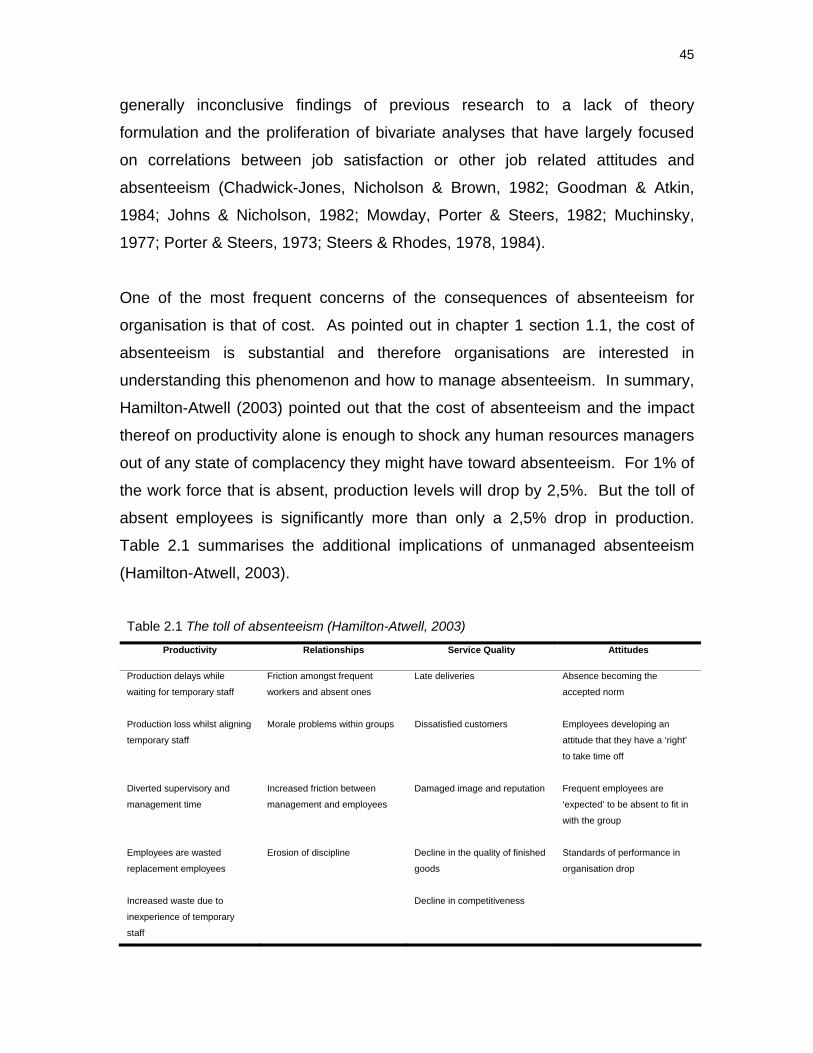
45
generally inconclusive findings of previous research to a lack of theory
formulation and the proliferation of bivariate analyses that have largely focused
on correlations between job satisfaction or other job related attitudes and
absenteeism (Chadwick-Jones, Nicholson & Brown, 1982; Goodman & Atkin,
1984; Johns & Nicholson, 1982; Mowday, Porter & Steers, 1982; Muchinsky,
1977; Porter & Steers, 1973; Steers & Rhodes, 1978, 1984).
One of the most frequent concerns of the consequences of absenteeism for
organisation is that of cost. As pointed out in chapter 1 section 1.1, the cost of
absenteeism is substantial and therefore organisations are interested in
understanding this phenomenon and how to manage absenteeism. In summary,
Hamilton-Atwell (2003) pointed out that the cost of absenteeism and the impact
thereof on productivity alone is enough to shock any human resources managers
out of any state of complacency they might have toward absenteeism. For 1% of
the work force that is absent, production levels will drop by 2,5%. But the toll of
absent employees is significantly more than only a 2,5% drop in production.
Table 2.1 summarises the additional implications of unmanaged absenteeism
(Hamilton-Atwell, 2003).
Table 2.1 The toll of absenteeism (Hamilton-Atwell, 2003)
Productivity Relationships Service Quality Attitudes
Production delays while
waiting for temporary staff
Friction amongst frequent
workers and absent ones
Late deliveries Absence becoming the
accepted norm
Production loss whilst aligning
temporary staff
Morale problems within groups Dissatisfied customers Employees developing an
attitude that they have a ‘right’
to take time off
Diverted supervisory and
management time
Increased friction between
management and employees
Damaged image and reputation Frequent employees are
‘expected’ to be absent to fit in
with the group
Employees are wasted
replacement employees
Erosion of discipline Decline in the quality of finished
goods
Standards of performance in
organisation drop
Increased waste due to
inexperience of temporary
staff
Decline in competitiveness
46
It is clear from table 2.1 that absence is a problem with costly and pervasive
implications, not only for effective functioning and productivity, but also for
relationships among people within the organisation.
Considering the cost associated with absenteeism, it is important to note that
absenteeism does not invariably lead to reduced operating efficiency. Staw and
Oldham (1978), for example pointed out that some absenteeism might actually
facilitate performance instead of inhibiting it. That is, absenteeism relieves
dissatisfied workers of job-related stress and in some cases may allow them to
be more productive when they return to work. This contention that absences
serve as safety valves for discharging accumulated stress is part of several
theories (Harrison & Martocchio, 1998). Harrison and Martocchio (1998) have
found little evidence that this is indeed experienced rather than being merely an
anticipated consequence of absenteeism. Hackett and Bycio (1996) noticed
downward and then upward shifts in affective and control variables in a small
sample of nurses going through working, then absent, then working day cycles.
They suggested that absenteeism served a maintenance rather than affect-
enhancing function.
Fitzgibbons and Moch (1980) have identified at least three conditions or
situations that might mitigate or even eliminate the consequences of
absenteeism on operating efficiency. These situations are (a) jobs that have
been ‘people proofed’ by automating production and reducing the role of
employees to machine motors; (b) work environments that anticipate and adjust
for expected absenteeism; (c) instances where employees have little direct effect
on plant-level efficiency. According to Fitzgibbons and Moch (1980), managers
can have a significant influence on improving operating efficiency in certain types
of work environments if they can succeed in reducing absenteeism.
Goodman and Atkin (1984) build on the earlier ideas of Mowday et al., (1982) to
bring together a broad array of possible positive and negative consequences of
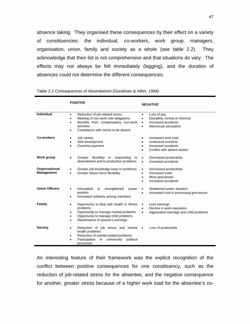
47
absence taking. They organised these consequences by their effect on a variety
of constituencies: the individual, co-workers, work group, managers,
organisation, union, family and society as a whole (see table 2.2). They
acknowledge that their list is not comprehensive and that situations do vary. The
effects may not always be felt immediately (lagging), and the duration of
absences could not determine the different consequences.
Table 2.2 Consequences of Absenteeism (Goodman & Atkin, 1984)
POSITIVE
NEGATIVE
Individual • Reduction of job-related stress
• Meeting of non-work role obligations • Benefits from compensatory non-work
activities • Compliance with norms to be absent
• Loss of pay • Discipline, formal or informal • Increased accidents • Altered job perception
Co-workers • Job variety • Skill development • Overtime payment
• Increased work load • Undesired overtime • Increased accidents • Conflict with absent worker
Work group • Greater flexibility in responding to absenteeism and to production problems
• Decreased productivity • Increased accidents
Organisational Management
• Greater job knowledge base in workforce • Greater labour-force flexibility
• Decreased productivity • Increased costs • More grievances • Increased accidents
Union Officers • Articulated & strengthened power position
• Increased solidarity among members
• Weakened power situation • Increased cost in processing grievances
Family • Opportunity to deal with health or illness problems
• Opportunity to manage marital problems • Opportunity to manage child problems • Maintenance of spouse’s earnings
• Less earnings • Decline in work reputation • Aggravated marriage and child problems
Society • Reduction of job stress and mental health problems
• Reduction of marital-related problems • Participation in community political
processes
• Loss of productivity
An interesting feature of their framework was the explicit recognition of the
conflict between positive consequences for one constituency, such as the
reduction of job-related stress for the absentee, and the negative consequence
for another, greater stress because of a higher work load for the absentee’s co-
48
workers, which creates a distinct social dilemma (Harrison & Martocchio, 1998)
within the organisation.
Another potential consequence of absenteeism is turnover. One perspective
casts absence as an alternative to turnover, rather than a precursor (Dalton &
Todor, 1993). Staw and Oldham (1978) have argued and found evidence that
absence provides coping opportunities outside the work place, especially when a
person holds a job that is incompatible with his or her abilities and preferences.
Mitra, Jenkins and Gupta (1992) on the other hand, found meta-analytic support
for the progression model, which presumes that the problems that instigated
absence will persist, leading to a move from temporary (absence) to permanent
(quitting) withdrawal.
It would seem that the predominant negative consequences of absenteeism
across all areas of the organisation are those of decreased productivity and
increased cost. ACSA has certainly felt these consequences; therefore the aim
of this research is to understand and possibly predict absenteeism in order to
manage it more effectively.
2.6 MODELS OF EMPLOYEE ABSENTEEISM
The dominant model of employee absenteeism in the academic literature is that
of Steers and Rhodes (1978, 1984). This model incorporates both voluntary and
involuntary absenteeism and was based on a review of over 100 studies of
absenteeism (Steers & Rhodes, 1978). Briefly stated, the model of Steers and
Rhodes (1978) posits that employee attendance is largely a function of two
important variables: a) an employee’s motivation to attend and b) an employee’s
ability to attend. Although not explicitly stated by them, the determinants of
attendance motivation appear to relate to “voluntary” absenteeism, whereas the
ability to attend variables seems to refer to “involuntary” absenteeism. Detail on
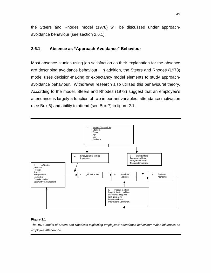
49
the Steers and Rhodes model (1978) will be discussed under approach-
avoidance behaviour (see section 2.6.1).
2.6.1 Absence as “Approach-Avoidance” Behaviour
Most absence studies using job satisfaction as their explanation for the absence
are describing avoidance behaviour. In addition, the Steers and Rhodes (1978)
model uses decision-making or expectancy model elements to study approach-
avoidance behaviour. Withdrawal research also utilised this behavioural theory.
According to the model, Steers and Rhodes (1978) suggest that an employee’s
attendance is largely a function of two important variables: attendance motivation
(see Box 6) and ability to attend (see Box 7) in figure 2.1.
Figure 2.1
The 1978 model of Steers and Rhodes’s explaining employees’ attendance behaviour: major influences on
employee attendance
1. Job Situation Job Scope Job level Role stress Work-group size Leader style Co-worker relations Opportunity for advancement
2. Employee values and Job Expectations
3. Personal Characteristics Education Tenure Age Sex Family size
7. Ability to Attend Illness and accidents Family responsibilities Transportation problems
4. Job Satisfaction 8. Employee Attendance
6. Attendance Motivation
5. Pressure to Attend Economic/market conditions Incentive/reward system Work-group norms Personal work ethic Organisational Commitment
50
Seven aspects of the job situation have been identified by Rhodes and Steers
(1981) as most likely to lead to increased job satisfaction (see Box 1). These
are: increased job scope and job level, reduced stress, smaller work group sizes,
considerate leadership, positive co-workers relations, and greater opportunities
for advancement. Not all companies have the same expectations from a job, and
individual values and expectations will determine how satisfaction is experienced
with the job situation (see Box 2). These values and expectations have been
shaped by the personal characteristics and backgrounds of the employees (see
Box 3) and will change over their career stage. During the selection of new
employees, the organisation should try to match individual and organisational
expectations to measure satisfaction with the job.
Five major “pressures to attend” have been recognised as enhancing attendance
motivation (Box 5), (Steers & Rhodes, 1978). These are economic and market
conditions, incentive and reward systems, work-group norms, personal work
ethic, and organisational commitment. Even if a person wants to go to work and
has a high attendance motivation (Box 6), there are instances where attendance
is not possible. The individual may not always have the choice of attendance.
There are three unavoidable limitations on attendance (Box 7): a) illness and
accidents; b) family responsibility; c) transportation problems.
The model described is a dynamic one, with employee absenteeism often
leading to a change in the job situation, which, in turn, may influence subsequent
attendance motivation. Steers and Rhodes (1978) felt that their model allowed
for management analysis and problem solving, primarily because the model
provides a diagnostic framework and identifies many areas in which major
problems may lie, thereby suggesting specific intervention strategies instead of
more general and costly ones. Brooke and Price (1989) provided a causal model
of absenteeism, which modifies and extends the conceptual framework of Steers
and Rhodes (1978). Their model includes routinisation, centralisation, pay,
distributive justice, work involvement, role ambiguity, conflict and overload,
51
kinship responsibility, organisational permissiveness, job satisfaction, job
involvement, organisational commitment, health status and alcohol involvement
as the determinants of absenteeism.
Over the years researchers have reviewed the model with mixed support. Steers
and Rhodes (1984) have suggested various modifications to improve the overall
utility of the model. Firstly, the modified model highlights the presence of work-
group norms and absence culture in recognition of the need to place absence
research in a social context. Secondly, to use the term work attitudes in place of
specifying only one of the attitudes in particular. Lastly, perceived ability
replaces actual ability to attend work.
Withdrawal research also utilises approach-avoidance behaviour. The
progression of the withdrawal hypothesis predicts a hierarchy among withdrawal
behaviours, with lateness being followed by absence, which in turn results in
resignation (Rosse, 1988). While Rosse (1988), Beehr and Gupta (1978) have
found some support for relating the forms of withdrawal behavioural, Clegg
(1983), concludes, “The generalisation notion of withdrawal is misleading” (p.88).
Though the dynamics and withdrawal models both fall within the approach-
avoidance models, there are several differences between them. In the dynamics
model, absence need not be a withdrawal from unpleasant work conditions but
an approach to a more attractive non-work situation (Fichman, 1984).
Withdrawal theory only allows for behaviour substitution in a compensatory
fashion and thus, if work is not aversive, cannot predict absences with increased
attendance duration as does the dynamics model (Fichman, 1989).
2.6.2 Absence is the outcome of an adjustment process
The models of Gibson (1966) and Hill and Trist (1953) can be described as
adjustment models. As job conditions change, the relationship between the
52
organisation and the employee is renegotiated. For example, absences are
compensation for unattractive aspects of the job. Cultural and social
expectations are included here in the employee’s control of absenteeism.
Hill and Trist (1953, 1955) introduced the concept of an “absence culture” to
describe how workers learn to adjust their behaviour to the stresses of remaining
in employment. An absenteeism culture is created by every organisation. Allen
and Higgens (1979) state that absenteeism has its own cultural norms that
constitute the expected supported and accepted ways of behaving with regard to
absences from work. These norms are often symptoms of larger organisational
problems (Allen & Higgens, 1979). Given the complex nature of absenteeism
antecedents, and the instability of absence phenomena, absenteeism needs to
be placed within a social context (Allen & Higgens, 1979).
2.7 CHAPTER SUMMARY The above literature review has attempted to give the reader a broad
conceptualisation of absenteeism and an indication of the size and complexity of
the subject. When studying absenteeism, the problem is not a lack of research
material but deciding what direction new work should take. Theories of
absenteeism were discussed which were: informal contract perspective;
perceived inequity; the withdrawal from the stress of work situations perspective;
dynamic conflict perspective and the social exchange perspective, as well as
withdrawal, non-attendance, organisationally excused vs. organisationally
unexcused, involuntary vs. voluntary and lastly a four-category taxonomy.
Definitions of absenteeism were also provided and the meanings of absenteeism
provided by Blau and Boal’s (1987) calculative category will be used in this
research. The positive and negative consequences introduced by Goodman and
Atkin (1984) were also included in this literature review. Models of employee
absenteeism were described, and for the purposes of this research the model
53
that of Steers and Rhodes (1978, 1984), focusing mainly on attendance
behaviour, is proposed.
Remark This chapter satisfies the first literature aim of conceptualising the construct
employee absenteeism, the origins and consequences in the workplace (see
1.3.2.1 (a)).
2.8 CHAPTER CONCLUSION
This chapter complied with the guidelines on the research design phase, namely
the literature review, discussed in chapter 1. It further followed the research
methodology indicated in chapter 1, following phase 1 step 1: an analysis and
integration of absenteeism, discussing the origins of absenteeism as well as the
consequences of absenteeism within organisations.
In chapter 3, the two work-related attitudes, namely job involvement and
organisational commitment, will be discussed from a theoretical perspective. The
two constructs will be dealt with separately and at the end of the chapter they will
be integrated in a conceptual framework indicating the relationship with
absenteeism.
54
CHAPTER 3
WORK-RELATED ATTITUDES
In this chapter the literature review of the two work-related attitudes namely, Job
Involvement and Organisational Commitment, will be presented. Each construct
will be discussed separately with reference to the theoretical framework, the
definition, antecedences, correlates and consequences of the construct. The two
constructs will then be integrated into a conceptual framework and the
relationship with the construct absenteeism will also be explained.
3.1 THE NATURE OF THE RELATIONSHIP BETWEEN TWO WORK RELATED ATTITUDES
This research will be testing the predictability of job involvement and
organisational commitment as work-related attitudes with absenteeism. Most of
the prior work on job involvement has focused on its ability to predict turnover
and absenteeism, with special interest on the interaction between job
involvement and organisational commitment as a predictor (Brown, 1996; Huselid
& Day, 1991). This is based on the conceptual framework presented by Blau and
Boal (1987), in which the framework emphasises the linking of job involvement
and organisational commitment as work-related attitudes to turnover and
absenteeism. The framework uses high and low combinations of job involvement
and organisational commitment to predict turnover and absenteeism. Support for
this interaction hypothesis has been found by field studies of turnover, turnover
intentions, and absenteeism (Blau, 1986; Blau & Boal, 1989; Martin & Hafer,
1995; Mathieu & Kohler, 1990). Steel and Rentsch (1995) found that job
involvement predicted low absenteeism over a 70-month period for U.S.
government employees.
55
Previous studies examined either the relationship between organisational
commitment, an organisational attitude, and absenteeism, or that between job
involvement, a job attitude, and absenteeism (Sagie, 1998). Although
organisational commitment and job involvement are closely correlated, they
constitute empirically distinct constructs (Brooke, Russel, & Price, 1988; Shore,
Newton, & Thornton, 1990). Gellatly’s (1995) theoretical approach sees absence
behaviour as a consequence of one’s work-related attitudes and it could be
expected that both organisational commitment and job involvement be negatively
correlated with volitional absenteeism.
Consequently, the relationship between the two attitudes is likely to have a
significant positive effect on absence. In other words, the total negative effect of
the two related attitudes on absence is lower than the sum of their negative
individual effects. Blau (1986), Blau and Boal (1989), as well as Mathieu and
Kohler (1990), observed similar effects concerning organisational commitment
and job involvement. Another work-related attitude generally referred to in
literature is the intention to leave the organisation, but this will not receive any
attention during this specific research.
In addition to the observation of work-related attitudes, Sagie (1998), Blau
(1986), Blau and Boal (1989), Mathieu and Kohler (1990), and Morrow (1983)
also indicated that job involvement and organisational commitment represent two
related but distinct types of work-related attitudes.
Literature suggests that the distinct different constructs of job involvement and
organisational commitment are viewed as work attitudes. It is however not clear
from the research done whether differences between these constructs are due to
the type of attitude (satisfaction vs. commitment) or the focus of the attitude (job
versus the organisation) (Shore, Newton & Thornton, 1990). According to Ajzen
and Fishbein (1977), attitudes are directed at entities that may be defined by four
different elements including attitudes towards targets, toward actions, toward
56
contexts, toward times, or toward any combination of elements. The work of
Ajzen and Fishbein (1977) suggests that attitudes with different targets are
distinct. Organisational attitudes may reflect more general employment policies
and practices. In contrast, job attitudes may reflect the type of work, task, and
immediate supervision experienced on the job.
The two work-related attitudes will be discussed in more detail in the following
sections, starting with job involvement.
3.2 JOB INVOLVEMENT
Since the job involvement construct was introduced by Lodahl and Kejner (1965),
hundreds of empirical studies relating to a variety of personal and situational
characteristics in a diversity of work settings have been conducted. From an
organisational perspective, job involvement has been considered the key to
activating employee motivation (Lawler, 1986) and a fundamental basis for
establishing competitive advantage in business markets (Lawler, 1992; Pfeffer,
1994). From an individual perspective, it has also been considered to be
essential to personal growth and satisfaction within the workplace, as well as to
motivation and goal-directed behaviour (Hackman & Lawler, 1971; Khan, 1990;
Lawler & Hall, 1970). Increasing job involvement can enhance organisational
effectiveness and productivity by engaging employees more completely in their
work and making work a more meaningful experience (Brown, 1996).
Job involvement is an important factor in the lives of most people. Work activities
consume a large proportion of time and constitute a fundamentally important
aspect of life for most people (Brown, 1996). People may be stimulated by and
drawn deeply into their work or alienated from it mentally and emotionally. The
quality of one’s entire life experience can be greatly affected by one’s degree of
involvement in, or alienation from, work (Argyris, 1964; Levinson, 1976). A state
of involvement implies a positive and relatively complete state of engagement of
57
core aspects of the self in the job, whereas alienation implies a loss of
individuality and separation of the self from the work environment (Argyris, 1964;
Kanungo, 1982b; McGregor, 1960). Kanungo (1979, 1982b) considered
involvement and alienation to be polar opposites.
In their review of literature, Rabinowitz and Hall (1977) pointed out that there is a
great deal of conceptual confusion and a proliferation of terms in theorising about
the construct labelled job involvement. Brown (1996) also stated that a number
of significant conceptual and methodological questions regarding job involvement
have been raised and debated but not resolved. These issues include specifying
the conceptual domain of job involvement, evaluating commonly used scales,
and building a conceptual framework for identifying related constructs as
antecedents, correlates or consequences (Brown, 1996).
In the following section a brief overview of the three theoretical perspectives on
job involvement as well as the definitions, the antecedents, correlates, and the
consequences of job involvement will be discussed. The connection between
these perspectives and the current research will also be examined.
3.2.1 Theoretical framework of job involvement
In the literature review that was conducted for this research, it was evident that
various theories and perspectives exist on job involvement, although somewhat
inconsistent, however, sufficient common ground was found between the most
important theoretical perspectives on the construct. These theoretical
perspectives presented by researchers such as Lodahl and Kejner (1965) and
Kanungo (1982) have been used as a basis for most of the empirical studies of
more resent research. The researcher, therefore, felt that it would still be
relevant to refer to these perspectives.
58
Kanungo’s (1982b) operationalisation of job involvement was a reaction against
several specific dimensions of excess meaning in Lodahl and Kejner’s (1965)
scale. These included the mixing of items tapping (a) cognitive and affective
states, (b) the individual’s involvement in work in general as well as in the
specific job, and (c) intrinsic motivation as well as job involvement. Kanungo
(1982b) argued that a person’s psychological identification with the job depended
on both need saliency and perceptions about the job’s potential for satisfying
salient needs.
Based on this way of defining job involvement, Kanungo (1982b) also argued that
existing scales were therefore inadequate to measure job involvement. Of the
commonly used scales to measure job involvement, Kanungo’s (1982b) scale is
based on the clearest and most precise conceptualisation of the construct. It
clearly identifies the core meaning of the construct as a cognitive state of the
individual, is not contaminated by items tapping concepts outside of this core
meaning, and separates job involvement from antecedent and consequent
constructs (Brown, 1996).
Influential contributions to the managerial literature (Lawler, 1986; Pfeffer, 1994)
have suggested that fostering job involvement is the key to unlocking employees’
motivational and performance potential, but empirical research has not
demonstrated how, or even whether, job involvement enhances individual
performance. Processes by which job involvement results in personal growth
and satisfaction for individuals are similarly unknown (Brown, 1996).
In a smaller number of studies, researchers have explicitly considered how job
involvement is causally related to other constructs. Cheloha and Farr (1980)
found that the relationship between job satisfaction and absenteeism was
mediated by job involvement in a study of state government employees.
However, Hammer, Landau, and Stern (1981) found that job involvement was not
related to absenteeism after controlling for job satisfaction, organisational
59
commitment, and demographic variables in an employee-owned firm. Smith and
Brannick (1990) concluded that job involvement influences job satisfaction both
directly and indirectly (i.e., through the mediation of both role conflict and
expectancy).
Kohler and Mathieu (1993) found that job involvement, along with other “affective
reactions” (e.g., organisational commitment, intrinsic and extrinsic job
satisfaction, and job tensions), fully mediated the effects of work perceptions on
absences in a sample of bus drivers. Noe and Schmitt (1986) discovered that
job involvement has a positive antecedent effect on career planning and learning
for educators in training for principals. Stumpf (1981) concluded that both work
performance and work satisfaction had antecedent influences on job
involvement.
The meta-analysis conducted by Brown (1996) strongly supported the
conceptualisation of personal and situational variables as antecedent influences
on job involvement. Although it is logical to posit that work outcomes, such as
performance, absenteeism, and turnover, are primarily consequences of job
involvement (Blau & Boal, 1987; 1989; Lawler, 1986), the aggregated data
revealed only weak relationships. It is likely that unidentified psychological and
behavioural linkages (e.g., emotion, motivation, effort, creativity, cooperation,
teamwork and isolation) mediate relationships between job involvement and work
outcomes (Brown, 1996).
Although it is more difficult to specify intuitively the ordering of relationships
between job involvement and other job attitudes, such as job satisfaction and
organisational commitment (Mathieu & Zajac, 1990), Brown’s (1996) conceptual
framework specifies job involvement as primarily an antecedent in these
relationships. Although these relationships are likely reciprocal, conceptual
grounds exist for positioning the casual priority of job involvement (Brown, 1996).
60
Rabinowitz and Hall (1977) reported that correlates have been used in support of
arguments that job involvement is determined by personal characteristics;
situational characteristics; both personal and situational characteristics and
personal and situational characteristics each independently. As some
researchers, such as Brown (1996), refer to these variables, the researcher
decided to describe each of the variables briefly.
3.2.1.1 Individual difference variable
The term “individual difference” variable is used frequently in the job involvement
literature (Morrow, 1983; Rabinowitz, Hall & Goodale, 1977). It refers to
variables upon which individuals may differ, even if environmental / contextual
factors remain constant.
Early researches (Dubin, 1956; & Lodahl, 1964) regarded job involvement as an
individual difference variable. They saw job involvement as a product of early
socialisation and an operationalisation of traditional work values such as the
“Protestant Work Ethic”. Dubin (1956) conceived job involvement as inherent in
the Protestant Work Ethic, the moral character of work and a sense of personal
responsibility. Anyone who has internalised these traditional values will probably
be “job involved”, regardless of the situational context within which he/she might
be employed (Runyon, 1973).
Lodahl (1964) hypothesised that the main determinant of job involvement is a
value orientation toward work that is learned early in the socialisation process.
Lodahl (1964) further believed that job involvement operationalises the
Protestant Ethic in some ways; since it is the result of the introjections of certain
values of work into the self, it is probably resistant to changes in the person due
to the nature of the particular job. Work done by Siegel (1969) concurred with
Lodahl’s (1964) point of view.

61
Hall and Mansfield (1971) suggested that if job involvement is indeed a personal
characteristic, then there should be little change in it during periods of
organisational stress. Hulin and Blood (1968) also focused on the notion of
individual differences. They felt that as a result of extra work socialisation
processes, many blue-collar workers in urban industrial environments have no
desire for ego need gratification while on the job. In contrast to the job-involved
individual, these workers mainly view their job as a means to an end – satisfying
their primary need off the job.
Support for this position was sought by investigating the correlations between job
involvement and quantifiable variables that might have represented individual
differences. Of these, the only variables showing fairly consistent correlations
with job involvement were age, education, internal locus of control, higher order
need strength and finally measures of the Protestant Work Ethic. All these
relationships were in a positive direction (Rabinowitz & Hall, 1977).
Morrow (1983) cited evidence supporting the hypothesis that job involvement is a
function of the person, and that it is determined independently of situational
variables. Morrow (1983) supported Rabinowitz and Hall (1977) finding
consistently positive relationships between job involvement, and age, internal
locus of control and higher order need strength.
The strongest support for the idea of job involvement being an individual
difference variable came from research into the stability of job involvement
scores over time. The rationale was that, if it is a personality factor, it should
remain fairly constant. Test-retest reliability coefficients indicated stability over
time, and coefficients of above 0,70 over a twenty month period were reported by
Rabinowitz and Hall (1977). This does indicate relative stability; however, they
gave little evidence of any strong situational changes that might have threatened
the stability, even if job involvement were entirely situationally determined.
62
In concluding this section, there is some evidence of job involvement as an
individual difference variable. Weak evidence exists for relating job involvement
with absenteeism. Stronger evidence exists showing job involvement may also
be a function of the situation.
3.2.1.2 Job Involvement as a function of the situation
Vroom (1962) has suggested that job factors can influence the degree to which
an employee is involved in his/her job. A person becomes ego-involved in
his/her work performance to the extent that performance is perceived to be
relevant to certain aptitudes, abilities, or other attributes that are central to his/her
self-conception.
Participative management theorists (Argyris, 1964, & McGregor, 1960) placed a
minimal emphasis on job involvement as a personal characteristic, and stress
involvement as a response to organisational conditions. They viewed the
organisation as blocking the gratification of ego and growth needs, a result that
leads to the decline or absence of individual involvement on the job. Specifically,
McGregor (1960) placed responsibility on the organisation for the behaviour of
employees, stating that how people behave is in large part dependent on the
assumptions management makes about them. According to McGregor (1960),
management draws from one of two sets of assumptions, Theory X or Theory Y.
Theory X assumptions (McGregor, 1960) hold that people have an inherent
dislike for work and must be forced to perform. Additionally, people avoid
responsibility, seeking only security. Theory Y, assumes that work is natural for
people, that they will exercise self-control without the threat of force.
Responsibility is sought rather than avoided. Theory Y, also suggests that
intellectual potential is only partially expended, given the present state of
organisational life. McGregor (1960) argues that the more management applies
63
Theory Y assumptions, the more it can expect improved worker involvement and
performance.
Argyris (1964) also placed the burden on the organisation. He argued that
although it is normal for individuals, as they mature, to develop desires for
independence, awareness of self, etc., the organisation does not recognise this
development. According to Argyris (1964), the organisation retards growth by
applying controls, demanding passivity, requiring only a few shallow abilities.
Thus, if an individual is to meet the demands of an organisation, he/she must, in
effect, consent to regress rather than mature. As a result, the individual will
become “psychologically” ill unless he/she finds some way of adapting to
conditions.
Bass (1965) concluded his discussion of job involvement by echoing the feeling
that six conditions lead to a strengthening of the variable: a) the opportunity to
make more of the job decisions; b) the feeling that one is making an important
contribution to company success; c) success; d) achievement; e) self-
determination; f) freedom to set one’s own work pace.
3.2.1.3 Job Involvement as an Individual – Situation interaction
Lawler and Hall (1970) suggested that the most realistic view of job involvement
would be that it is a function of an individual-job interaction. They support the
individual-difference point of view by expressing the feeling that people probably
do differ in the degree to which they are likely to become involved in their job as
a function of their backgrounds and personal situations. However, the situational
viewpoint is also alluded to, since it is also probably true that other things being
equal, more people will become more involved in a job that, allows them control
and a chance to use their abilities than will become involved in a job that is
lacking in these characteristics.
64
Farris (1971) assumed that job involvement was a function of the interaction of a
person with his/her environment, thus not considering it solely an individual
characteristic. Lodahl and Kejner (1965), although initially stating the individual
difference viewpoint, nonetheless concluded their study by declaring “It seems
clear that job involvement is affected by local organisational conditions (mostly
social ones), as well as by value orientations learned early in the socialisation
process”(p. 35).
Wanous (1974) theorised on the relationship between the individual’s
socialisation process and characteristics of the job. To Wanous (1974), one of
the earliest determinants of an individual’s work needs is his/her socialisation
environment. The result of an individual’s upbringing (Protestant Work Ethic
values) could cause an individual to develop a general value orientation toward
work that emphasises the importance of work in one’s total self-esteem and
reinforces the belief that work can hold intrinsic satisfaction.
Wanous (1974) speculated that the consequences of such values is that an
individual is likely to state his/her own particular desires for job characteristics,
such as autonomy, variety, challenge, feedback and task identity. Wanous
(1974) believed that it is likely that an involvement-prone individual will become
involved when holding a job with such characteristics.
3.2.1.4 Kanungo’s restricted approach to job involvement
Kanungo’s (1979) approach to job involvement can be founded in a motivational
framework which emphasises the analysis of the behavioural phenomenon at the
individual level. Kanungo’s (1979) restricted approach to job involvement
focuses on the psychological identification factor, which brings conceptual clarity
compared to the other approaches, and eliminates cultural biases related to self-
esteem and intrinsic motivation factors (Perrot, 2005).
65
Summary According to Brown (1996), Kanungo’s (1982a) scale of job involvement
identified the core meaning of the construct as a cognitive state of the individual.
In a small number of studies, the casual relation of job involvement and other
constructs, such as job satisfaction, absenteeism, demographic variables, career
planning and work performance, have been investigated with varying results.
Determinants of job involvement, individual/personal; situational; both personal
and situational characteristics have been discussed.
In this research the individual-situation interaction of Lawler and Hall (1970) will
be used in terms of the theoretical framework. The next section of this chapter
will focus on the antecedents, correlates and consequences of job involvement.
3.2.2 Definitions of job involvement
Different interpretations of job involvement have evolved while studying the
relationship of job involvement to numerous variables, including job
characteristics, performance, turnover and absenteeism (Kanungo, 1982a).
Kanungo (1982) conducted a literature review that revealed several different
conceptualisations of job involvement, including job involvement defined as:
• the degree of importance of one’s job to one’s self-image (Lodahl &
Kejner, 1965; Lawler & Hall, 1970);
• the degree to which an individual is actively participating in his/her job
(Allport, 1943; Bass, 1965);
• the degree to which an individual’s self-esteem or self-worth is affected by
his/her perceived performance level (French & Kahn, 1962; Gurin, Veroff,
& Feld, 1960); and
• generalised cognitive state of psychological identification with work,
insofar as work is perceived to have the potentiality to satisfy one’s salient
needs and expectations (Kanungo, 1979)
66
For the purpose of this research, job involvement is defined as the extent to
which the individual identifies psychologically with his/her job (Kanungo, 1979).
3.2.3 Antecedents of job involvement Brown’s (1996) conceptual framework classifies selected personality traits, an
array of job characteristics and supervisory behaviours, and role perceptions as
antecedent influences on job involvement. These antecedents’ influences
represent different conceptual perspectives on the nature and causation of job
involvement. Personality research illustrates the view that job involvement is
primarily an individual difference construct whose origins are deeply rooted in
individual disposition and socialisation (Brown, 1996). However, research
relating job involvement to job characteristics, supervisory behaviours, and role
perceptions assumes that situational influences determine the degree of job
involvement (Brown, 1996). The interactionist perspective posits that personality
and situational variables jointly influence the level of involvement (Rabinowitz &
Hall, 1977).
The antecedents of job involvement will now be discussed.
3.2.3.1 Personality variables
The individual difference perspective holds that job involvement results from
socialisation processes that inculcate the importance of work as a virtuous and
necessary activity as well as from other stable individual differences. Research
relating job involvement to work ethic, e.g., Brief & Aldag, 1977; Morrow &
McElroy, 1986; Saal, 1978 (as cited by Brown, 1996), illustrates this perspective.
Other personality variables have also been studied as antecedents of job
involvement. The most significant of these include locus of control, self-esteem,
growth need strength, and internal motivation.
67
3.2.3.2 Motivation
Theoretical perspectives differ in the causal precedence they ascribe tot
motivation in relation to job involvement. The individual-difference perspective
regards motivation primarily as an antecedent. The situationist perspective
however suggests that motivation is primarily a consequence rather than an
antecedent of job involvement. According to Brown (1996), the empirical
consideration of the relationship between motivation and job involvement has
been limited almost exclusively to the individual difference perspective.
Motivation is likely to be both an antecedent and a consequence of job
involvement, and theoretical assumptions and operationalisations are likely to
affect the order of the relationship between motivation and job involvement
specified and observed in individual studies. 3.2.3.3 Job Characteristics and Supervisory Variables
In an important stream of research, psychologists have also investigated job
involvement primarily as an outcome of situational characteristics. It has been
studied as a function of job characteristics, such as task autonomy, task
significance, task identity, skill variety, and feedback, and of supervisory
behaviours, such as leader consideration, participative decision-making, and
amount of communication. Contrary to the individual difference perspective, the
situationist perspective implies that job involvement changes when elements of
the job context change (Brown, 1996).
Work environments that (a) provide a sense of meaningfulness of one’s work, (b)
offer control over the methods by which work is accomplished, (c) maintain clear
and consistent behavioural norms, (d) include supportive relations with superiors
and co-workers, and (f) offer the opportunity for personal growth and
development are conducive to job involvement (Brown, 1996).
68
3.2.3.4 Role Perceptions
Role perceptions may affect a job’s potential for satisfying salient psychological
needs. To the extent that a worker experiences conflicting demands from
different role partners (role conflict) or uncertainty regarding role requirements
and expectations (role ambiguity), the job’s potential for satisfying salient
psychological needs is likely to be reduced. Thus role conflict and role ambiguity
should negatively affect job involvement (Fisher & Gitelson, 1983).
Summary Brown (1996) classified variables frequently studied in relation to job involvement
as antecedents, correlates or consequences. He remarked that in some cases
(e.g., motivation, job satisfaction, and organisational commitment), these
classifications are somewhat speculative and are based on theoretical premises
developed. He attempted to classify variables on theoretical grounds to stimulate
additional research seeking to clarify the structure of nomological relationships
involving job involvement.
3.2.4 Correlates of job involvement
Correlates of job involvement include demographic variables and involvement in
broader, work-related concepts, such as career and work. Brown (1996) regards
demographic variables as correlates rather than antecedents of job involvement,
even though they have temporal priority, because their conceptual links to job
involvement are generally weak and no necessarily causal relationship exist.
Numerous demographic variables have been studied in relation to job
involvement in a large number of studies. The most frequent studied
demographic characteristics include age, tenure, education, gender, salary, and
marital status. These have generally been weakly related to job involvement.
Other variables classified as correlates include career commitment and work
69
involvement. These constructs are closely related to job involvement in a
conceptual sense but they represent commitment to broader concepts than a
specific job (Brown, 1996). It is not clear whether commitment to a specific job
leads to greater commitment to work in general or to career commitment, or vice
versa. It is logical, however, that involvement in a specific job is positively
correlated with work and career commitment (Brown, 1996) and he considered
these constructs correlates of job involvement.
3.2.5 Consequences of job involvement
Work behaviours, job attitudes, and several important “side effects” of job
involvement (e.g., work-family conflict, stress, somatic health complaints, and
anxiety) are specified as consequences of job involvement (Brown, 1996). This
will now be discussed.
3.2.5.1 Work behaviours and outcomes
A dominant theoretical assumption underlies the classification of work behaviours
as consequences of job involvement. The assumption is that a cognitive state of
identification with the job, based on perceptions of its potential for satisfying
salient psychological needs, precedes and then triggers motivational processes
that influence motivation, effort, and ultimately performance, absenteeism and
turnover (Brown, 1996). This implies that some work behaviours (e.g., effort) are
more closely related to job involvement, whereas others (performance,
absenteeism, and turnover) are more distantly related (Brown, 1996). It further
implies that more close outcomes of job involvement mediate indirect
relationships with more distant outcomes (Brown, 1996). Such causal processes
have received negligible empirical attention.
70
3.2.5.2 Job attitudes
Previous research has not established the causal ordering of job involvement
with respect to job satisfaction and organisational commitment. Brown (1996)
classified job satisfaction as a consequence of job involvement, even though
reciprocal causation is likely. Brown (1996) regarded job satisfaction primarily as
a consequence because cognitive appraisal of the potential for need satisfaction
logically precedes actual needs satisfaction. It is also likely that actual
satisfaction then reciprocally influences job involvement (Brown, 1996).
Brown (1996) also considered organisational commitment a consequence of job
involvement, although the reverse order of causality may also occur. Prior
research has not clarified, or even addressed, the causal precedence of job
involvement with respect to organisational commitment. In most cases, it is likely
that workers first become familiar with, and involved in, particular jobs and then
develop commitment to the organisation as their psychological needs are
satisfied over time (Mowday, Porter, & Steers, 1982). Thus, even though the
process may occasionally work in the opposite direction (e.g., when a person
working in an uninvolving job becomes committed to the organisation and then
moves to a more involving job), organisational commitment is more often likely to
evolve form a state of job involvement (Brown, 1996).
3.2.5.3 Side effects
It is possible that high levels of job involvement may have negative social,
psychological, and even physiological side effects. In a number of studies, (e.g.,
Higgins, Duxbury, & Irving, 1992; Wiener, Vardi, & Muczyk, 1981), research has
investigated job involvement in relation to work-family conflict, stress, somatic
health complaints, and anxiety. Brown (1996) classifies these as consequences
of job involvement because excessive commitment of personal resources to, and
preoccupation with, work may cause or aggravate these negative outcomes.
71
High levels of job involvement could possibly lead to trading off family
commitments in favour of job commitments. Preoccupation with work may also
cause stress, anxiety, and health complaints (Brown, 1996).
3.2.6 Summary
The specific literature objective of conceptualising the two constructs of work-
related attitude has been met through a review of literature, explaining job
involvement. Conceptual frameworks on job involvement were presented, such
as job involvement as an individual difference, a function of the situation, and
individual-situation interaction. The individual-situation framework will be utilised
for this research. Definitions, antecedents, correlates, and consequences of job
involvement were also discussed. For the purpose of this research the definition
of Blau (1985), defining job involvement as “the extent to which the individual
identifies psychologically with his/her job” will be applied.
Remark
In the preceding sections of the chapter, the researcher satisfied the literature
review aims for job involvement, specifically steps 1 through to 4 as described in
chapter 1 section 1.7.
In order to meet the rest of the specific literature objectives, the second work-
related attitude, organisational commitment will now be examined.
3.3 ORGANISATIONAL COMMITMENT
The concept of organisational commitment has received considerable attention
from both managers and behavioural scientists. The interest has been
demonstrated not only in theoretical efforts to explain the construct but also in
empirical efforts to determine the primary antecedents and outcomes of
organisational commitment for example, Buchanan, 1974; Hall & Schneider,
72
1972; Hrebiniak & Alutto, 1972; Kanter,1968; Mowday, Porter, & Dubin, 1974;
Porter, Steers, & Boulian, 1974; Mathieu & Zajac, 1990; Meyer & Allen, 1991,
Randall, 1990; Salanick, 1977; Sheldon, 1971; Staw, 1977; Steers, 1977;
Stevens, Beyer, & Price, 1978 (as cited in Dunham, Grube, & Castañeda, 1994).
Throughout these studies, commitment has been repeatedly shown to be an
important factor in understanding the work behaviour of employees.
Over the decades of study, organisational commitment has been approached
from a variety of conceptual and operational perspectives (Dunham, Grube, &
Castañeda, 1994). Most commitment studies can be categorised as assuming
either an attitudinal or a behavioural perspective. The attitudinal variable is one
of the most frequently studied variables in organisational behaviour research
(Mathieu & Zajac, 1990; Meyer & Allen, 1997). Riketta (2002) proposes that the
main reason for the extensive and enduring research interest in attitudinal
organisational commitment is that this commitment is assumed to influence
almost any behaviour that is beneficial to the organisation such as performance,
attendance, and staying with the organisation (also see Matheiu & Zajac, 1990;
Meyer & Allen, 1997; Mowday, Porter, & Steers, 1982; Randall, 1990).
In this section of the chapter, the multidimensionality of organisational
commitment will be presented. Firstly, organisational commitment will be
discussed from a theoretical perspective followed by a definition of organisational
commitment. The antecedents, correlates and consequences of organisational
commitment will be briefly discussed. Finally, this information will then be
integrated and the relevance of the various approaches to this research will be
discussed.
3.3.1 Theoretical framework of organisational commitment
Studies have revealed that progress has been good in clarifying the confusion
about the meaning and characteristics of this concept (Steers, 1977). This has
73
largely been accomplished by the acceptance of the notion that no one view of
commitment is fundamentally “correct” (Meyer, Allen, & Gellantly, 1990). A
singular focus on a given view of commitment is, thus, gradually being replaced
with a multiple components model of commitment.
3.3.1.1. Typologies
Several researchers have suggested typologies into which the various
approaches to commitment can be categorised.
(a) Etzioni
Etzioni (1961) suggested that the power of authority that organisations have over
individuals is based on the nature of the individual’s involvement in the
organisation. Etzioni (1961) identifies three forms of involvement or commitment.
The first is moral involvement – based on the interaction of the organisation’s
goals, values, and norms and on an identification with authority. The second is
calculative involvement – based on an exchange relationship developed between
the individual and the organisation. The third is alienative involvement – a
negative orientation where individual behaviour is severely constrained.
(b) Kanter
Kanter (1968) also suggested three types of commitment. Kanter’s (1968) first
type is continuance commitment – the member’s dedication to the survival of the
organisation. The second is cohesion commitment – an attachment to social
relationships in the organisation brought about by the renunciation of previous
ties or ceremonies, which enhance group cohesion. The third type is control
commitment – the individual’s attachment to organisational norms that shape
behaviour in desired directions.
74
(c) Staw & Salanick
Staw (1980) and Salancik (1977) suggested the need to differentiate between
commitment from an organisational behaviour viewpoint (attitudinal viewpoint)
and commitment from a social psychological viewpoint (behavioural viewpoint).
Attitudinal commitment deals with the process through which the individual
comes to identify with the goals and values of the organisation and the
individual’s desire to maintain membership in the organisation. Blau and Boal
(1987) view this as a more positive individual orientation towards the
organisation. Behavioural commitment, however, deals with the process through
which the individual’s past behaviour binds that individual to the organisation.
Blau and Boal (1987) refer to past actions of “sunk costs” (fringe benefits, salary
as a function of age and tenure). According to Blau and Boal (1987), an
individual becomes “committed” to an organisation because it has become too
costly for him/her to leave.
3.3.1.2 Sub-Constructs of Commitment
Meyer and Allen (1984) conceptualised a multidimensional organisational
commitment measure that drew on the early works of such researchers as
Porter, Steers, Mowday, and Boulian (1974); Becker (1960); and Wiener and
Vardi (1980). Meyer and Allen (1991) proposed a three-component model for
organisational commitment that integrated a variety of alternative
conceptualisations. Affective commitment is the first of such approaches and can
be defined as an emotional attachment to the organisation via identification,
involvement and enjoyed membership (Allen & Meyer, 1990). Normative
commitment comprises a responsibility to the organisation and is an internalised
moral obligation. Lastly, continuance commitment is a cost-based association
developing form the magnitude and quantity of side-bet as well as the perceived
lack of alternatives (Allen & Meyer, 1990).
75
Allen and Meyer (1990) stated that each conceptual approach can be clearly
distinguished via measurement, and that these measures can be correlates to
the variety of antecedent variables in literature. These three sub-constructs of
commitment will now be briefly discussed.
(a) An affective perspective to organisational commitment
Porter, Crampon and Smith (1976) stated that two aspects indicate an affective
approach. Firstly commitment is a ‘global and stable alternative linkage’ between
the individual and the employing organisation and secondly, that the individual’s
feelings are representative by commitment, and these are connected to the
individual’s desire to be attached to the work situation.
(b) A normative view of organisational commitment
Wiener (1982) distinguished between identification and normative-instrumental
frameworks regarding commitment to the organisation. The identification
perspective implies commitment to be an ‘attitudinal intervening construct’, which
could range between antecedents and outcomes. These include the ‘personality-
need variables’, as well as the personal-demographic variables (for example age
and tenure).
By normative, Wiener (1982) implied that the commitment needs
conceptualisation within a motivational perspective, which clearly distinguishes
between normative and instrumental perspectives of behaviour in organisations.
Wiener (1982) state that behavioural intention is determined by the individual’s
perception of the ‘normative pressure’ concerning the conducting of the act.
Therefore as commitment increases, so too does the individual’s predisposition
to be led by actions, as opposed to the consequences of these actions.
Committed individuals enact specific behaviours due to the belief that these are
morally correct rather than personally beneficial. The individual’s moral
standards pertaining to the enactment are established when the individual
76
‘internalises expectations’ about this behaviour enactment. These acts, when
guided by normative pressures, are not dependent on original positive or
negative reinforcement. Wiener (1982) therefore stated that organisational
commitment must be defined from a subjective norm.
Wiener (1982) stated that the individual’s internalised normative pressures to
attain organisational goals and values must possess specific behavioural
characteristics. These include:
• a personal sacrifice on behalf of the organisation;
• perseverance which does not depend on positive and negative reinforcement;
and lastly
• personal preoccupation and devotion to organisational activities.
This implies that commitment is enhanced if the individual remains with the
organisation irrespective of opportunistic availabilities. Tenure therefore is an
insufficient predictor of overall commitment.
Allen and Meyer (1990) stated that the normative approach is a less common
approach to commitment. The internalised moral obligation is a contributor to
behaviour and is therefore, prominent in the individual’s terminating employment
with the organisation.
According to Wiener and Vardi (1980) in this type of commitment the individual
should feel loyal to the organisation, should make sacrifices on behalf of the
organisation, and lastly, that the individual should not oppose or criticise the
organisation.
(c) Perceived cost of continuance commitment to the organisation
Another view to organisational commitment is that of continuance commitment,
which implies that affective and normative commitment play only minor roles in
77
the conceptualisation of this variable (Allen & Meyer, 1990). Becker (1960), as
previously discussed, pursued a perceived costs approach to organisational
commitment based upon a series of side-bets.
Kanter (1968) refers to continuance commitment as a ‘cognitive orientation’,
where costs are considered when leaving or remaining with the organisation.
The cost or profit then compels departure or continued participation respectively.
Kanter (1968) states that ‘continuous commitment can be conceptualised as a
commitment to the role in a social system.’
Rusbult and Farrel (1983), in a technical worker study, found that, prior to
departing from the organisation, individuals experienced a decrease in rewards
and an increase in cost. Those declining aspects were used to predict job
commitment. Allen and Meyer (1990) integrated the side-bet viewpoint with the
findings of Rusbult and Farrel (1983) and found that continuance commitment will
develop due to the magnitude and quantity of side-bets, and secondly due to the
perceived lack of alternatives. The latter increases the cost associated with
departure. Continuance commitment will therefore be the strongest when
availability of alternatives is few and the number of investments is high.
Many studies have examined the relationship between the different kinds of
commitment and absenteeism. Overall, it appears that affective commitment has
the strongest relation with absence behaviour (Meyer, 1997). The results for
normative commitment are less consistent. Meyer, Allen & Smith (1993) found
that normative commitment was negatively related to absenteeism, while Somers
(1995) found no relationship between normative commitment and absenteeism.
Continuance commitment has not found strong support in the absenteeism
literature (e.g., Mayer & Schoorman, 1992).
78
Summary Various typologies have been presented in the previous section. Etzioni (1961)
postulated that an employee’s commitment is based on the nature of his/her
involvement in the organisation such as moral, calculative and alienative
involvement. Kanter (1968) suggested three types of commitment namely,
continuance, cohesion and control commitment. Staw (1980) and Salanick
(1977) indicated that organisational commitment should be viewed from an
organisational behaviour perspective or attitudinal view and from a social
psychological perspective or behavioural view. Meyer and Allen (1984)
developed a three-component model that integrated sub-constructs namely,
affective, normative and continuance commitment.
As the conceptual framework is used as basis for this research, linking job
involvement and organisational commitment as work-related attitudes to
absenteeism, the attitudinal approach of organisational commitment and the
affective dimension of commitment will be used for this research.
3.3.2 Definitions of organisational commitment
There is still disagreement among researchers over the definition of
organisational commitment (e.g. Cohen & Kirchmeyer, 1995; Dunham, Grube, &
Castañdeda, 1994; Hackett, Bycio & Hausdorf, 1994; Iverson & Roy, 1994;
Jaros, Jermier, Koehler & Sincich, 1993). However, most researchers consider
that commitment consists of two distinct but related concepts or components,
namely attitudinal and behavioural commitment. Attitudinal commitment (also
known as affective organisational commitment) represents the degree of loyalty
an individual has towards an organisation. This form of commitment emphasises
an individual’s identification and involvement in the organisation (Porter, Steers,
Mowday, & Boulian, 1974). Organisational commitment is viewed as a more
positive individual orientation toward the organisation; here, organisational
commitment is defined as a state in which an employee identifies with a
79
particular organisation and its goals, and he/she wishes to maintain membership
in the organisation in order to facilitate the organisation’s goals.
In contrast, behavioural commitment reflects the process by which individuals link
themselves to an organisation and focuses on the actions of the individuals. In
the behavioural approach, the individual is viewed as committed to an
organisation if he/she is bound by past actions of “sunk costs” (fringe benefits,
salary as a function of age and tenure). Thus, an individual becomes
“committed” to an organisation because it has become too costly for the
employee to leave. In this approach, organisational commitment is depicted as
more calculated in nature (Etzioni, 1961). Becker (1960) concentrated on what
he termed the ‘side-bet theory’, which attempted to explain the process by which
employees attached themselves to organisations through investments such as
time, effort and rewards.
Building on the side-bets tradition, Meyer and Allen and their colleagues (Allen &
Meyer, 1990; Meyer et al., 1993; Meyer, et al., 1990; Meyer, Paunonen,
Gellately, Goffin, & Jackson, 1989; Meyer and Allen, 1984, 1991) viewed
affective, normative and continuance commitment as components of attitudinal
commitment. Definitions of affective, normative and continuance commitment
will now be provided.
3.3.2.1 Affective Commitment
Buchanan (1974) integrated definitions of affective commitment prior to defining
the affective approach. Buchanan (1974) uses the perspectives listed below.
• Commitment is defined as the willingness to exert effort on behalf of the
organisation as well as an acceptance of the goals and values of that
organisation.
80
• Commitment is a favourable evaluation and intention to pursue the
organisation’s goals.
• Commitment is the willingness to exert energy and loyalty as an emotion to
the group.
• Commitment is the unwillingness to depart from the organisation.
• Lastly, commitment is an degree of belongingness.
Buchanan (1974) defined commitment as a ‘partisan, affective attachment’ to the
organisation’s goals and values, and the individual’s relation to these goals and
values. Commitment therefore has the components of identification, (with the
organisation’s goals), involvement, (in the work role in the organisation), and
loyalty, (an affective feeling for the organisation).
Cook and Wall (1980) also utilised an affective definition of commitment.
Organisational commitment refers to ‘an affective reaction to characteristics’ of
the organisation. Affective reactions encompass the feelings of attachment,
whilst the characteristics refer to the goals and values.
Allen and Meyer (1990) defined the affective component as an emotional
attachment to the organisation via identification, involvement and enjoyment
membership. Allen and Meyer (1990) emphasised that affective committed
individuals remain with the organisation because of a ‘want to’ desire.
3.3.2.2 Normative Commitment
Normative Commitment is described as the totality of internalised normative
pressure to act in a way that is conducive to the organisation’s goals and values
(Wiener, 1982).
81
3.3.2.3 Continuance Commitment
Stebbins (1970) defines continuance commitment as the awareness of being
unable to choose another social identity because of the penalties associated with
making alterations. It is a psychological state, which is not only present because
of tangible rewards but rather subjective penalties associated with the desire to
terminate employment with the organisation.
Widely divergent definitions for organisational commitment are found throughout
literature, specifically:
• an attitude or an orientation toward the organisation, which links or attaches
the identity of the person to the organisation (Sheldon, 1971);
• the willingness of social actors to give their energy and loyalty to social
systems, the attachment of personality systems to social relations which are
seen as self-expressive (Kanter, 1968);
• a structural phenomenon which occurs as a result of individual-organisational
transactions and alterations in side-bets or investments over time (Hrebiniak
& Alutto, 1972);
• a state of being which an individual becomes bound by his/her actions and
through these actions to beliefs that sustain the activities and his/her own
involvement (Salanick, 1977);
• the process by which the goals of the organisation and those of the individual
become increasingly integrated or congruent (Hall, Schneider, & Nygren,
1970);and
• the nature of the relationship of the member to the system as a whole
(Grusky, 1966).
Further features are listed below.
• (1) Commitment includes something of the notion of membership; (2) it
reflects the current position of the individual; (3) it has a special predictive
potential, providing predictions concerning certain aspects of performance,
82
motivation to work, spontaneous contribution, and other related outcomes;
and (4) it suggests the differential relevance of motivational factors (Brown,
1969).
• Commitments come into being when a person, by making a side-bet, links
extraneous interests with a consistent line of activity (Becker, 1960).
• Commitment behaviours are socially accepted behaviours that exceed formal
and/or normative expectations relevant to the object of commitment (Weiner
& Gechman, 1977).
• Also present is a partisan, affective attachment to the goals and values, and
to the organisation for its own sake, apart from its purely instrumental worth
(Buchanan, 1974).
Attitudinal organisational commitment defined by Mowday, Steers and Porter
(1979) as the a state in which an individual identifies with a particular
organisation and its goals and wishes to maintain membership in order to
facilitate these goals, will be used for the purpose of this research.
3.3.4 Antecedents of organisational commitment
Kacmar, Carlson and Brymer (1999) found through their research that
researchers in general have gained support for relationships between
organisational commitment and a variety of personality, demographic, and
organisational variables for example: Balfour & Wechler, 1990; Blau & Boal,
1989; Bennett & Linden, 1996; Luthans, Baack, & Taylor, 1987; McFarlin &
Sweetney, 1992; O’Reilly & Chatman, 1986; Settoon, Vandenberg, & Lance,
1992 (as cited by Kacmar, et al., 1999). Figure 3.1 diagrams the antecedents
and consequences of organisational commitment provided by Kacmar et al.,
(1999), of which the antecedents will be briefly discussed in the section below.
The consequences indicated in the diagram will be discussed in section 3.4.
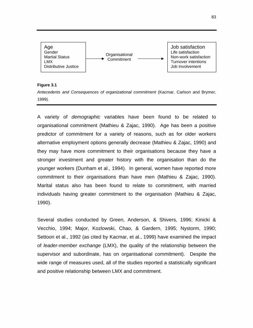
83
Figure 3.1 Antecedents and Consequences of organizational commitment (Kacmar, Carlson and Brymer,
1999).
A variety of demographic variables have been found to be related to
organisational commitment (Mathieu & Zajac, 1990). Age has been a positive
predictor of commitment for a variety of reasons, such as for older workers
alternative employment options generally decrease (Mathieu & Zajac, 1990) and
they may have more commitment to their organisations because they have a
stronger investment and greater history with the organisation than do the
younger workers (Dunham et al., 1994). In general, women have reported more
commitment to their organisations than have men (Mathieu & Zajac, 1990).
Marital status also has been found to relate to commitment, with married
individuals having greater commitment to the organisation (Mathieu & Zajac,
1990).
Several studies conducted by Green, Anderson, & Shivers, 1996; Kinicki &
Vecchio, 1994; Major, Kozlowski, Chao, & Gardern, 1995; Nystorm, 1990;
Settoon et al., 1992 (as cited by Kacmar, et al., 1999) have examined the impact
of leader-member exchange (LMX), the quality of the relationship between the
supervisor and subordinate, has on organisational commitment). Despite the
wide range of measures used, all of the studies reported a statistically significant
and positive relationship between LMX and commitment.
Age Gender Martial Status LMX Distributive Justice
Organisational Commitment
Job satisfaction Life satisfaction Non-work satisfaction Turnover intentions Job Involvement
84
Distributive justice refers to the perceived fairness or equity in the amount and
type of rewards organisational members receive (Folger & Konovsky, 1989).
Individuals will exhibit more commitment to an organisation they view as
providing fair and equitable rewards for their performance than will individuals
who feel cheated by their organisations. Although few studies have investigated
this relationship, some empirical support for this positive relationship exists
(McFarlin & Sweetney, 1992).
Iverson and Buttigieg (1999) have categorised antecedent variables for
organisational commitment. These are set out below.
First there are the Personal variables, comprising the individual characteristics
that employees bring to, or experience in the organisation. These consist of
education, tenure in the organisation, tenure in a particular location, kinship
responsibilities, job expectations, values, affectivity (positive and negative), and
work motivation.
Next are the Job-related variables, including job hazards, autonomy, co-worker
and supervisory support, job security, routinisation, stress, promotional
opportunities, pay, distributive justice, relationship with management, and
experiences of appreciation by the public.
Environmental variables relate to the non-work setting, including industrial
relations climate and job opportunities. Allen and Meyer (1990) have identified the following antecedents for affective
commitment as:
job challenge – the extent to which jobs are found to be challenging
role clarity
goal clarity
85
goal difficulty
receptiveness by management
peer cohesion
equity
personal importance
feedback
participation, and
dependence on the organisation.
These variables indicate that the individual requires a feeling of comfort in
relation to the organisation, coupled with a personal feeling of work role
competence.
3.3.4 Correlates of organisational commitment
Empirical studies carried out on the topic of organisational commitment represent
a rich collection of findings with respect to both the antecedents and
consequences of the construct. It was suggested that the major influences on
organisational commitment could be grouped into three categories: a) personal
characteristics; b) job- or role-related characteristics; and c) work experience. In
a study done by Mowday et al., (1980), commitment as measured by the
Organisational Commitment Questionnaire (OCQ) was regressed on several
personal characteristics, job characteristics and work experiences. Other
research suggested the need to add a fourth category of antecedents, namely,
structural characteristics (Morris & Steers, 1980; Stevens, Beyer, & Price 1978).
The categories of organisational commitment will now be briefly discussed as it
may help to explain the psychological and behavioural processes through which
commitment to an organisation develops over time.
86
3.3.4.1 Personal correlates of commitment
Personal characteristics studied have included, age, tenure, educational level,
gender, race and various personality factors. In general, commitment has been
positively related to both age and tenure (Angle & Perry, 1981; Brown, 1969;
Hall, Schneider & Nygren, 1970; Hrebiniak, 1974; Lee, 1971; Morris & Sherman,
1981; Sheldon, 1971). March and Simon (1958) noted that as age and tenure in
the organisation increase, the individual’s opportunities for alternative
employment become more limited. This decrease in an individual’s degrees of
freedom may increase the perceived attractiveness of the present employer,
thereby leading to increased psychological attachment.
In contrast to age and tenure, education has often been inversely related to
commitment (Angle & Perry, 1891; Morris & Sherman, 1981; Morris & Steers,
1980; Steers, 1977). It has been suggested that this inverse relationship may
result from the fact that more highly educated individuals have higher
expectations that the organisation may be unable to meet.
In other research, it has been fairly consistently found that gender is related to
commitment. In studies by Angle and Perry (1981), Grusky (1966), and
Hrebiniak and Alutto (1972), women as a group were found to be more
committed than men.
Finally, several of studies have examined various personality factors as they
relate to commitment. In isolated findings, commitment has been found to be
related to achievement motivation, sense of competence, and other higher-order
needs (Morris & Sherman, 1981; Steers, 1977; Steers & Spencer, 1977). It
would appear that commitment to the organisation could be supported to the
extent that employees see the organisation as a source of need satisfaction.
87
For the purpose of this research, only age will be examined. As the educational
level of employees employed within the security department is generally grade
10 to 12 it will be disregarded in this research. In terms of the gender and
personality, only gender will be examined.
3.3.4.2 Role-Related correlates of commitment
The second group of correlates of organisational commitment that have been
identified in the literature relate to employee roles and job characteristics. There
appear to be at least three related aspects of work role that have the potential to
influence commitment: job scope or challenge; role conflict; and role ambiguity
(Mowday et al., 1980).
For this research the above aspects will be excluded.
3.3.4.3 Structural characteristics of commitment
Structural variables that were considered in studies are organisation size, union
presence, span of control, and centralisation of authority. In a study carried out
by Stevens, Beyer & Price (1978) none of the variables were found to
significantly relate to commitment. In a study done by Morris and Steers (1980)
they found that formalisation, functional dependence and decentralisation were
related to commitment. Other variables such as worker ownership and
participation in decision-making were related to commitment (Rhodes & Steers,
1982).
This research will not exiling the effect of the structural variables of commitment.
88
3.3.4.4 Work experiences
Work experiences are viewed as a major socialising force and as such represent
an important influence on the extent to which psychological attachments are
formed with the organisation. Several work experience variables have been
found to be related to organisational commitment namely: a) organisational
dependability, b) personal importance to the organisation, c) the extent to which
employee expectations were met. A further factor relating to work experiences
focuses on the extent to which employees sense that their co-workers maintain
positive attitudes toward the organisation (Mowday et al., 1980).
Research by Rhodes and Steers (1982) found that perceived pay equity and
group norms regarding hard work were also related to commitment for a sample
of wood-products employees. Finally, an important factor in facilitating
commitment appears to be the degree of an employee’s social involvement in the
organisation (Rhodes & Steers, 1982).
3.3.5 Consequences of organisational commitment
Kacmar et al., (1999) described job satisfaction, intentions to turnover and job
involvement as consequences (see Figure 3.1) of organisational commitment. In
so far as job satisfaction is concerned, a positive relationship between job
satisfaction and organisational commitment, using a variety of satisfaction and
commitment measures, has been consistently reported in past research
conducted by Balfour & Wechsler, 1990; Cook & Wall, 1980; Green, Anderson, &
Shivers, 1996; Major, Kozlowski, Chao, & Gardner. 1995; McFarlin & Sweetney,
1992; Mowday et al., 1979 (as cited by Kacmar, et al. 1999). A positive
relationship was found to exist between job involvement and organisational
commitment (Kacmar et al., 1999; Cook & Wall, 1980; Mowday et al., 1979)
89
Based on the notion of Meyer and Allen (1991) that disparate outcomes or
behaviours are associated with the different factors motivating employees to
remain within organisations, Iverson and Bittigieg (1999) have hypothesised
consequences for the three components of commitment. Affective commitment
would have a negative effect on turnover intentions and absenteeism, and a
positive effect on the acceptance of change (Iverson, 1996; Mathieu & Zajac,
1990; Somers, 1995). Employees high in affective commitment demonstrate
emotional attachment, identification, with and involvement in, the organisation.
This explains why these employees are less likely to engage in withdrawal
behaviour and more willing to accept change (Meyer & Allen, 1997). Normative
commitment is also expected to have consequences similar to those of affective
commitment (Iverson & Buttigieg, 1999). This type of commitment focuses on
moral obligation, which derives in part from, the socialisation practices of
organisations. Employees have an obligation to reciprocate to the organisation
and will therefore be more receptive to change, be less likely to leave or to be
absent (Hackett et al., 1994; Meyer et al., 1993; Somers, 1995).
The third form of commitment, continuance, is anticipated to have the same
relationships as affective commitment, with both turnover intentions and
absenteeism (Hackett et al., 1994; Mathieu & Zajac, 1990). As employees would
feel a sense of being ‘locked’ into the organisation due to the high cost of leaving
(Jaros, Jermier, Koehler, Snicich, 1993), they would be less likely to leave or be
absent.
Mowday et al., (1982) have summarised five consequences of organisational
commitment (job performance, tenure with the organisation, absenteeism,
tardiness, and turnover) in the findings of their research and that of others. These
will now be discussed.
90
3.3.5.1 Commitment and Job Performance
Findings from studies on commitment reveal that there is a rather weak
relationship between commitment and job performance. Mowday et al., (1982)
pointed out that several factors might account for the weak relationship, in
particular the contemporary theories of employee motivation. Performance is
influenced by motivation level, role clarity, and ability (Porter & Lawler, 1968).
Attitudes like commitment would only be expected to influence one aspect of
actual job performance.
3.3.5.2 Commitment and Tenure
In a study done by Mowday et al., (1982) highly significant positive correlations
have been found between increased tenure and increased commitment. The
question they posed was: does commitment lead to increased tenure or does
increased tenure cause changes in commitment levels?
3.3.5.3 Commitment and Absenteeism
This research postulates that highly committed employees would be more
motivated to attend so they could facilitate organisational goal attainment. A
review of literature only provides modest support for this relationship (Smith,
1977; Steers, 1977). Mowday et al., (1982) suggest that commitment may
represent one influence on attendance motivation.
3.3.5.4 Commitment and Tardiness
In a study by Angle and Perry (1981), commitment was found to be strongly and
inversely related to employee tardiness. The theory underlying the construct
suggests that highly committed employees are likely to engage in behaviours
91
consistent with their attitudes toward the organisation. Coming to work on time
would certainly represent one such behaviour.
3.3.5.5 Commitment and Turnover
Following theory, Mowday et al., (1982) believe that the strongest or most
predictable behavioural outcome of employee commitment should be reduced
turnover. Highly committed employees are by definition desirous of remaining
with the organisation and working toward organisational goals and should hence
be less likely to leave.
3.3.6 Summary
In this section of the chapter the construct organisational commitment was
discussed. The various definitions of organisational commitment were presented
and for the purpose of this research, attitudinal organisational commitment
defined by Mowday, Steers and Porter (1979) as a state in which an individual
identifies with a particular organisation and its goals and wishes to maintain
membership in order to facilitate these goals, will be used. Theories were also
presented in which the various approaches to commitment can be categorised.
The construct organisational commitment was then conceptualised into two
approaches namely, the behavioural or attitudinal approach, after which the
antecedents, correlates and consequences of organisational commitment were
discussed.
Remark In the preceding sections of the chapter, the researcher satisfied the literature
review aims for organisational commitment, specifically steps 1 through to 4 as
described in chapter 1, section 1.7.
92
3.4 CHAPTER INTEGRATION
According to Morrow (1983), job involvement and organisational commitment are
related, but distinct, types of work attitudes because of their different referents.
For employees with a high level of involvement, the job is important to one’s self-
image (Kanungo, 1982a). Employees with a high level of organisational
commitment feel positively about the organisations for which they work. They
identify with a particular organisation and wish to maintain membership in it
(Porter, Crampon, & Smith 1976). Workers with high levels of both job
involvement and organisational commitment should be the most motivated
because they are attracted by both the job and the organisation.
Blau and Boal (1987) found that, based on empirical research, it seems that job
involvement and organisational commitment complement one another as
predictors of turnover and absenteeism. From either an analysis of variance or a
moderated regression standpoint (Saunders, 1956), Blau and Boal (1987) predict
that the job involvement and organisational commitment interaction terms will be
significant. Specific combinations of job involvement and organisational
commitment levels will help to predict particular types of turnover and absence
behaviour.
Brown’s (1996) meta-analysis and review of organisational research on job
involvement attempted to make a comparison to assess differences in
relationships between the two distinct but closely related attitudinal constructs.
The primary difference is that job involvement primarily reflects one attitude
toward a specific job, whereas organisational commitment refers to one’s
attachment to the organisation (Morrow, 1983,1993). It would be possible, for
example, to be very involved in a specific job but not be committed to the
organisation, or vice versa (Becker, 1992; Blau & Boal, 1987).
93
The results from Brown’s (1996) meta-analysis, found that the only relationship
that was significantly stronger for job involvement than for organisational
commitment involved participative decision-making. In addition, however, job
involvement was substantially more strongly related to work ethic endorsement
and skill variety than organisational commitment was. Job stress,
communication, salary, supervisory, co-worker, pay satisfaction, promotion
satisfaction, and turnover intentions were all strongly related to organisational
commitment than to job involvement.
For this research the conceptual framework of Blau and Boal (1987), using high
and low combinations of job involvement and organisational commitment to
predict turnover and absenteeism is particularly relevant. In their framework
(Blau & Boal, 1987) job involvement and organisational commitment are
partitioned into high and low categories and are then combined into four cells: 1)
high job involvement – high organisational commitment; 2) high job involvement
– low organisational commitment; 3) low job involvement – high organisational
commitment; and 4) low job involvement – low organisational commitment. Each
cell is predicted to have a different impact on absenteeism. Blau and Boal (1987)
derived these proposed categories using a median split on questionnaire scales,
for example, job involvement (Kanungo, 1982a) or organisational commitment
(Porter & Smith, 1970). Remark
With the preceding section the researcher has satisfied the specific literature
research aim (see section 1.3.2.1).
3.5 CONCLUSION
This chapter concluded the literature objectives as set out in section 1.3.2.1. (a)
and 1.3.2.1 (b). For phase 1, the literature review of the research methodology,
steps 1 through to 5 have been completed (see section 1.7).

94
In chapter 4, phase 2 of the research methodology, namely the empirical study
will be discussed. The sample, as well as the measuring instruments for
absenteeism, job involvement and organisational commitment, will be discussed
in detail, after which the data gathering and data processing will be explained.
95
CHAPTER 4
EMPIRICAL STUDY In chapter 2 and 3 a theoretical perspective of the constructs absenteeism and
work-related attitudes were provided. In this chapter, phase two of the research
methodology, the empirical study, will be discussed. An analysis of the
composition of the sample will be provided. In addition to this the motivation for
the selection of the measurement instruments as well as the reliability and
validity of the instruments will be discussed. The chapter will conclude by
outlining the data gathering and data processing steps followed.
4.1 EMPIRICAL OBJECTIVES
The following five empirical objectives have been developed for this study (see
1.3.2.2):
(a) to investigate what is regarded as high absenteeism, and evaluate the
current status within the organisation;
(b) to investigate whether biographical variables influence absenteeism;
(c) to investigate and analyse whether job involvement and organisational
commitment predict absenteeism in the organisation;
(d) to determine whether there is a correlation between employee absent
levels and job involvement and organisational commitment.
96
The following sample is a description of the steps in the empirical study.
4.2 STEPS IN THE EMPIRICAL STUDY The empirical study for this research consists of the steps described below (see
section 1.7, phase 2).
4.2.1 STEP 1: SAMPLE The sample will be discussed in this section. The basic idea of sampling is that
by selecting some of the elements in a population, conclusions may be drawn
about the entire population. A population element is the subject on which the
measurement is being taken. A population is the total collection of elements
about which the researcher is to make some inferences (Cooper & Schindler,
2004).
The population that was used for this research was the security employees of
Airports Company South Africa (ACSA) Ltd, who are based at Johannesburg
International Airport (JIA). The security department is mainly responsible for
passenger security, working inside the terminal buildings, searching passengers
as they enter the restricted area. The security department’s staff complement for
the year in which this research was conducted was 219. These employees are
all salaried staff and work eight hour shifts. The shift cycle consisted of two
morning-shifts (6 am to 2 pm), two afternoon-shifts (2 pm to 10 pm), two night
shifts (10 pm to 6 am) and two days off.
The first step of the sampling plan was to divide the target population into the
following categories:
(1) Aviation Security Officers who took no sick leave during a one-year period;
97
(2) Aviation Security Officers who took between one and five days non-
continuous sick leave during a period of one year;
(3) Aviation Security Officers who took between six and ten days non-
continuous sick leave during a period of one year; and
(4) Aviation Security Officers who took more that 10 days non-continuous sick
leave during a period of one year.
Once these groups had been identified, the individual members were ranked
according to age within each group. A systematic random sample was then
taken from each group, except for the category consisting of aviation security
officers who took more than 10 days non-continuous sick leave. In this category
all employees were included in the sample as they were such as small number.
This resulted in the sample total compromising of 72 population elements. The
reason why the entire population was not used for the research is that the union
and executive management agreed to the research being conducted within the
security department on condition that a sample was taken and questionnaires
were not distributed to all the security personnel.
In chapter 2, section 2.3, the construct “absenteeism” was defined. The
possibility of other variables that influence absenteeism, such as biographical
variables, e.g., age and gender, and demographic variables, such as distance
from work was also investigated.
4.2.2 Step 2: Describing the measuring instruments. The aim of this research is to test the predictability of job involvement and
organisational commitment on employee absenteeism as suggested by Blau and
Boal (1987). A measuring instrument for each of the independent variables was
utilised for this research. A biographical questionnaire was developed and given
98
to each of the sample subjects to collect data such as age, gender, marital
status, position held, years of experience, distance from work, and type of
transport used. The instruments used to measure job involvement and
organisational commitment respectively were Kanungo’s (1982a) 10-item Job
Involvement Questionnaire (JIQ) and the 9-item short form Organisational
Commitment Questionnaire (OCQ) of Porter and Smith’s (1970), which were
administered to the sample together with the biographical questionnaire.
The research on the measuring instruments will now be discussed separately.
The aim/development and rationale, scales and dimensions, administration,
interpretation, validity and reliability and justification of inclusion will be discussed
for each of the instruments.
4.2.2.1 Biographical questionnaire
The researcher developed a biographical questionnaire. This questionnaire
included questions about the biographical characteristics of the research
participants. The questionnaire was developed in such a way that research
participants merely had to tick the most applicable box for each question. The
questions aimed to determine whether biographical factors have a direct
correlation with absenteeism and whether job involvement and organisational
commitment predict when an individual will absent himself or herself from work.
Seven items were included in this biographical questionnaire, and these are
listed below.
(a) Name. This question was included to verify that the individual completing
the questionnaire was part of the randomly selected sample group.
(b) Job title. This question was included to verify that the individual completing
the questionnaire was an Aviation Security Officer and not employed in some
99
other capacity in the company. It was essential that the sample group comprise
only Aviation Security Officers.
(c) Age. This question was included to determine if there was any significant
difference in terms of age of Aviation Security Officers being absent from work.
(d) Marital status. This question was included to investigate if marital status
influenced the sample group’s levels of absenteeism in any way.
(e) Number of dependants. This question was included to investigate if the
number of dependants supported by the Aviation Security Officer influenced
levels of absenteeism in any way.
(f) Gender. This question was included to investigate if there was a difference
between gender groups in terms of absent behaviour.
(g) Distance travelled to work. This question was included to investigate
whether the distance the Aviation Security Officer had to travel to work would
impact on the level of absenteeism.
4.2.2.2 Records of Absenteeism
(a) Aim and Rationale
Absenteeism has been identified as an area of concern for the management of
ACSA, especially within the aviation security department at Johannesburg
International Airport, not only due to the cost of work hours lost, but also the
legislative implications it may have on the functioning of the airport if not enough
personnel are in place as any given time. The general aim for the research is to
investigate whether work-related attitudes, job involvement and organisational
commitment, can predict employee absenteeism (see section 1.3.1). In order to
establish this relationship, absenteeism records of all aviation security officers
100
were obtained from the Human Resources Department. The records collected
from the management information system mostly indicated reasons for absence.
For this research, the researcher specifically focused on the frequency of short
(one day) absences which, according to ACSA’s policy, employees were not
required to submit a medical certificate for their absence which meant that some
of the absence instances did not indicate reasons for the absence.
The absence records of the sample population were divided into four categories
as discussed under section 4.2.1 in this chapter. The categorisation was done
based on attitudinal absence (frequency of one day absences) over a mid-term
(i.e. 12-months) as discussed under section 2.1.
(b) Measures of absence
An absence is constitutively defined in a very small time period, usually a single
workday (Harrison & Martocchio, 1998). Echoing this definition, some theorists
have proposed that absences occur whenever a person chooses to allocate time
to activities that compete with scheduled work, either to satisfy the waxing and
waning of underlying motivational rhythms (Fichman, 1984) or to maximise
personal utility (Chelius, 1981). To understand the nature of employee
absenteeism in various organisations, researches must first understand how (or
whether) it is measured in empirical studies.
There is systematic variation in absenteeism over very short time periods
(Harrison & Hulin, 1989), but absence data are seldom available at such a fine-
grained level. When fine-grained data are available, their low base-rate
distributions usually suffer from severe discreteness, skewness, and kurtosis
(Hammer & Landau, 1981). Therefore, researchers often rely on absences
aggregated over convenient or arbitrarily longer times – typically one year (Mitra,
Jenkins & Gupta, 1992).
101
To compound the problem, sets of independent variables in absence research
carry a mix of dynamism. They range from demographic features such as sex
that are constant over a lifetime (Price, 1995), to constructs such as attendance
attitudes that fluctuate daily (Hackett, Bycio, & Guion, 1989). Absences clearly
do arise from a mix of causes, however different causes are more or less
detectable given the time frame over which absenteeism is cumulated (Epstein,
1983). The same is true for the consequences of absenteeism. The levels of
individual absenteeism cumulated over any time period are most likely to reflect
variables that are defined in and relatively stable over that period. Harrison and
Martocchio (1998) used a time-based system to help organise, summarise and
analyse research on employee absenteeism published from 1977 to 1996.
Section 1.2 explains that different approaches are propsed in measuring
absenteeism. The first approach was proposed by Huse and Taylor (1962),
examining four instances of absenteeism and the second, seven indices of
absenteeism proposed by Chadwick-Jones, Brown, Nicholson and Sheppard
(1971). It was noted in section 1.2 that the absence frequency measurement will
be applied to this research.
The one-day absence frequency rate has been named the “Attitudinal Index”
(Huse & Taylor, 1962) and is viewed as reflecting voluntary absenteeism
(Chadwick-Jones et al., 1982; Hackett & Guion, 1985). An employee may take
one day off work to do something enjoyable, otherwise the absence may be
motivated by negative attitudes to work (Huse & Taylor, 1962).
However, neither time lost, absence duration nor frequency indices alone provide
a representative picture of absence behaviour. Authors such as Cheloha and
Farr, 1980 and Muchinsky, 1977 suggested utilising multiple measures of
absenteeism in determining the existence of an absenteeism problem.
102
Van der Walt (1999) argued that grouping the causes of absenteeism into
different categories can not only shed more light on the causes themselves but is
also a good starting point to look for solutions to this problem. One such
classification method categorises the causes of absenteeism into personal
(income level, health, length of service, marital status, educational level and
gender), organisational (type of work, size of organisation and work groups,
nature of supervision, incentive schemes and shift work), attitudinal (job
satisfaction and general state of the economy) and social factors (child care
problems, religious beliefs and inclement weather).
For the purpose of this research the researcher used the mid-term variance in
absenteeism, generally referred to as having a time span of between three
months and one year. Rosse and Hulin (1985) reported that the notion of a mid-
term level of time also corresponds to periods over which global job attitudes
remain fairly stable. Thus, for mid-term periods, job attitudes will be at their peak
relevance for, and peak correlation with, absenteeism. Hackett (1985) and Steel
and Rentsch (1995) also provide support for this idea.
(c) Administration
The researcher downloaded the number of sick days taken from the Human
Resources System. Based on the information obtained from the HR system, the
respondents were categorised according to the number of one-day sick leave
days over a 12-month period.
(d) Interpretation
Employees in the fourth category (the highest number of one day instances of
sick days taken), are less committed and involved than the employees who have
taken no sick leave.
103
(e) Validity and Reliability
There is no information that could be found on the validity of sick leave days as a
measuring instrument. However, access to the companies’ HR system is limited
to authorised users only, who input sick leave and leave information where a
signed sick leave / leave form and certificate from the doctor are attached and
approved. Based on this, leave days taken by respondents can be a valid
predictor of sickness.
The information downloaded from the HR system is reliable, as all the
employee’s absences, be they sick leave or any other kind of leave, are recorded
on the system in term of ACSA’s conditions of service. The reliability is further
enhanced by the fact neither employees nor managers have access to the HR
system.
4.2.2.3 Job Involvement
(a) Development and Rationale
Various scales have been developed to measure job involvement of which some
are mentioned in the following paragraphs. Brown (1996) noted that in the article
by Lodhal and Kejner (1965) on the definition and measurement of job
involvement, they incorporated two conceptual dimensions into their definition
and scale of the construct. The first of these, stemming from the work of Allport
(1947), French and Kahn (1962), and Vroom (1962), related to the extent to
which job performance affected a person’s self-esteem (performance-self-esteem
contingency). A second dimension of job involvement, which was identified in
the abstract but not the text of the article of Lodahl and Kejner’s (1965),
concerned the extent to which a person identifies psychologically with his or her
work or the importance of work in total self-image. This second dimension grew
primarily out of earlier work by Dubin (1958, 1961). Both conceptual dimensions
were represented in the operational scale of job involvement devised by Lodahl
and Kejner’s (1965).
104
Saleh and Hosek (1976) also proposed a multidimensional scale of job
involvement, reflecting four dimensions:
(1) work as a central life interest;
(2) the extent of a person’s active participation in the job; (3) the extent of performance-self-esteem contingency, and (4) consistency of job performance with the self concept.
The Saleh and Hosek (1976) scale has been strongly criticised by Kanungo
(1979, 1981, 1982a, 1982b) as reflecting not only the psychological state of an
individual, but also the antecedent circumstances and consequent outcomes of
this psychological state. The measurement incorporates considerable extraneous
conceptual content, in addition to the core meaning of the cognitive state of
psychological identification with one’s job. It has seen relatively little empirical
usage and cannot be recommended as a measurement of involvement (Brown,
1996). Other scales have been developed by Farrell and Rusbult (1981), Jans
(1982), and Wollack, Goodale, Witjing and Smith (1971), but these too have seen
little use (Morrow, 1993).
Subsequent research has largely followed the definition of job involvement by
Lawler III and Hall’s (1970) as “psychological identification with one’s work” and
“the degree to which the job situation is central to the person and his or her
identity” (p. 310-311). Kanungo (1982b) advanced his scale based on the
conceptualisation of involvement as “a cognitive or belief state of psychological
identification’ (p. 342). Kanungo’s (1982b) operationalisation was a reaction
against several specific dimensions of excess meaning in Lodahl and Kejner’s
(1965) scale. These include the mixing of items tapping:
(i) cognitive and affective states;
(ii) the individual’s involvement in work in general as well as in the specific job;
and
(iii) intrinsic motivation as well as job involvement.
105
Kanungo (1982b) argued that a person’s psychological identification with the job
depends on both need salience and perceptions about the job’s potential for
satisfying salient needs. Kanungo (1982b) also argued the existing scales are
inadequate to measure job involvement defined in that way. Of the commonly
used scales of job involvement, that of Kanungo (1982b) is based on the clearest
and most precise conceptualisation of the construct. It clearly identifies the core
meaning of the construct as a cognitive state of the individual, is not
contaminated by items tapping on concepts of this core meaning, and separates
job involvement from antecedent and consequent constructs (Brown, 1996).
(b) Scales and dimensions
Kanungo’s (1982a) 10-item JIQ was used to measure the degree to which the
individual identifies with his or her present job. The responses were made on a
five-point, Likert-type scale, which ranged from “1” = strongly disagree to “5” =
strongly agree.
(c) Administration
The JIQ can be administered individually or with groups. The individual reads
the instructions on the questionnaire and then answers the ten items by deciding
to what extent he/she agrees with the statements made regarding the current job
he/she is engaged in as well as decide which point on the scale describes
him/her best, keeping in mind the description of the scales (Cook, Hepworth,
Wall, & Warr, 1981). Items scores are added to reach a total score.
(d) Interpretation
The total score is an indication of the degree to which the individual identifies
with his/her present job (Kanungo, 1982a). The higher the score the more
involved the individual is judged to be.
106
(e) Validity and Reliability
Kanungo (1982a) reported evidence supporting the reliability and validity of this
measure. Kanungo (1982a) reported that the internal consistency reliability for
the scale based on data from 703 respondents measured 0,87. The test-retest
reliability coefficients based on a separate sample of 63 respondents, who were
administered the questionnaire twice within a three-week interval, measured
0,85. The data of the 63 respondents used in the test-retest study was not very
different from the main sample of 703 respondents. The data suggests that both
the reliability of the repeated measurements and of the internal consistency of
items is adequate for the JIQ scales (Kanungo, 1982a).
Boshoff and Hoole (1998) tested the portability of Kanungo’s Job Involvement
Questionnaire between the United States and South Africa and found an internal
consistency of 0,83. All ten items loaded >0,30 on the one factor loadings
varying between 0,34 and 0,76. Riipinen (1997) tested the relationship between
job involvement and well-being and found the reliability coefficient of the scale to
be 0,86. In a study conducted by Van Wyk, Boshoff and Cilliers (2003) predicting
job involvement of pharmacists and accountants, the principal factor analysis
indicated a one-factor solution with the scale having a Cronbach Alpha coefficient
of 0,88. All items loaded >0,35 on the single dimension, except for one item,
item 7 which loaded 0,20. Blau (1985) found that nine items in Kanungo’s
(1982a) measure loaded sufficiently on the job involvement factor, while one item
(7) did not load highly on either factor.
Kanungo (1982a) tested the convergent and discriminant validity of six job
involvement measures by comparing the medial values of the off-diagonal
correlations among scale items under conditions: monotrait-heteromethod,
heterotrait-monomethod, and heterotrait-heteromethod (Campbell & Fiske,
1959). From the validity diagonals, all correlations are statistically significant (p <
0,01), suggesting the convergent validity of the scales. The magnitude of the
correlations suggests that the convergent validity of the JIQ of r = 0,80 is quite
107
high. The monotrait-heteromethod correlation for the JIQ reported 0,80, which is
substantially higher than the monomethod-heterotrait correlation of 0,36 and
heteromethod-heterotrait correlation of 0,33.
Various studies were conducted determining the correlation of job involvement
and other constructs. Van Wyk, Boshoff and Cilliers (2003) found a significantly
positive relationship between job involvement and job satisfaction (r = 0,23). In
their review of research they found that most studies confirm a positive significant
relationship between job satisfaction and job involvement, such as: Adams, King
& King, 1996; Batlis, 1980; Brown, Corn, & Leigh, 1993; Feldman & Turnley,
1995; George, 1995; Harris & Massholder, 1996; Heaven, 1994; Holton &
Russell, 1997; Jamal & Badawi, 1995; Jenkins & Maslach, 1994; Mael & Tetrick,
1992; Mishara, 1997; Newcombe, 1997; Parasuraman & Alutto, 1984; Riipinen,
1994; Riordian & Griffenth, 1995; Rosin & Korabik, 1995; Siegall & McDonald,
1995; Smart, 1998; Smith & Tisak, 1993; Strümpher, 1997 (as cited by Van Wyk,
Boshoff, & Cilliers, 2003). Low but significant correlations were found between
job involvement and entrepreneurial attitude orientations: economic innovation (r
= 0,29); achievement/ personal control (r = 0,12) and self-esteem (r = -0,11) (Van
Wyk, Boshoff, & Cilliers, 2003).
The relationship between job involvement and career orientations sub-scales
was significant in terms of service dedication (r = 0,31); entrepreneurship (r =
0,14) and life style integration (r = -0,16) (Van Wyk, Boshoff, & Cilliers, 2003).
The relationship between job involvement and the Type A total and sub-scale
scores was found to be significantly positive with achievement (r = 0,27); hard
driving / competitive (r = 0,19) and Jenkins total (r = 0,29) (Chusmir & Hood,
1986, 1988; Van Wyk, Boshoff & Cilliers, 2003). Van Wyk, Boshoff and Cilliers
(2003) found a significant positive relationship is indicated between job
involvement and internal locus of control (r = 0,26). This corresponds with
previous findings by Dailey, 1980; Edwards & Walters, 1980; Heaven, 1994;
Knoop, 1981; Parasuraman & Alutto, 1984; Remondet & Hansson, 1991. The
108
relationship between job involvement and the power self-concept sub-scale
indicated a significant correlation (r = 0,23) (Van Wyk, Boshoff, & Cillliers, 2003).
The study by Orpen (1982) also indicated a positive relationship between job
involvement and the self-concept of policemen (r = 0,05) and bank clerks (r =
0,05).
It would therefore seem that the JIQ is statistically acceptable for this research in
terms of validity and reliability. According to Boshoff and Hoole (1998) and Van
Wyk, Boshoff and Cilliers (2003), the JIQ seems to indicate that the measure is a
robust, probably unidimensional scale and the JIQ can be used with a great deal
of confidence in South Africa.
(f) Justification for inclusion
As pointed out in section 4.3.3.1, Kanungo’s (1982a) scales of the JIQ are
among the most commonly used and are based on the clearest and most precise
conceptualisation of the construct. It clearly identifies the core meaning of the
construct as a cognitive state of the individual, and is not contaminated by items
tapping concepts outside of this core meaning, and separates job involvement
from antecedent and consequent constructs (Brown 1996).
4.2.2.4 Organisational Commitment
(a) Development and rationale
Porter and Smith (1970) distinguished between the treatment of organisational
commitment as an attitude and as behaviour, and took the former approach. The
construct is thought to be more global than job satisfaction, being a generally
affective reaction to the organisation rather than specifically to the work.
Organisational commitment is also held to differ from job satisfaction in that it is
likely to be less subject to transitory changes associated with day-to-day events.
109
Organisational commitment is defined as the strength of an individual’s
identification, with and involvement in, a particular organisation, and is said to be
characterised by three factors; a strong belief in, and acceptance of the
organisation’s goals and values; a readiness to exert considerable effort on
behalf of the organisation; an a strong desire to remain a member of the
organisation (Mowday et al., 1982).
According to Buchanan (1974) and Porter, Steers, Mowday and Boulian (1974),
organisational commitment can be viewed in terms of three interrelated
components: identification: pride in the organisation, internalisation of the
organisation’s goals; involvement: willingness to invest personal effort as a
member of the organisation, for the sake of the organisation; and loyalty:
affection for and attachment to the organisation, a wish to remain a member of
the organisation.
Porter, Steers, Mowday and Boulian (1974), based on their own definition of
organisational commitment, developed the Organisational Commitment
Questionnaire, which can be used in two ways: in its full 15-item form or in its
reduced 9-item form. These authors characterised affective commitment in
terms of three factors, however, they measure it in a one-dimensional way,
having tested the internal consistency and reliability of the 15- and 9-item
versions of the OCQ. Commeiras and Fournier (2001) pointed out that many
studies have however observed the OCQ’s multidimensionality.
Angle and Perry (1981) made the distinction between ‘value commitment’ (items,
1,2,4,5,6,8,10,13 and 14); ‘commitment to stay’, the equivalent of Etzioni’s (1961)
calculative commitment (items 3, 7, 9,11, and 15) (see section 3.3.1.1); and the
third factor (item 12 only), which was eliminated due to its instability. Support for
these results is provided by other studies that distinguish an affective dimension
and a calculative dimension (Cohen & Gattiker, 1992; Tetrick & Farkas, 1988).
Although Tett and Meyer (1993) and Aktar and Tan (1994) confirm the
110
multidimensionality of the OCQ, they question the meaning of the calculative
commitment dimension.
Luthans, McCaul and Dodd (1985) found in their study of organisational
commitment among American, Japanese and Korean employees that the scale
yielded one factor for the American and Japanese samples and two factors for
the Korean sample. The studies conducted by Koh, Steers and Tergorg (1995);
Bar-Hayim and Berman (1992) reveal two factors. Benkhoff (1997) showed in a
confirmatory factor analysis that the 15-item version is composed of the three
factors stated in the definition by Porter et al., (1974). Koslowsky, Caspy, and
Lazar (1990) also found that the 15-item version of the scale yielded three
factors. According to the research of Commeiras and Fournier (2001), these
studies revealed that the make up of the dimensions differs and it would seem
that the factorial structure of the OQC is unstable.
Mathieu and Zajac (1990) along with Tetrick and Farkas (1988); Allen and Meyer
(1990); Meyer and Allen (1991); Morrow (1993); and McElroy, Morrow, Crum
Dooley (1995), recommended using the short version of the OCQ to measure
organisation commitment. This short version, however, only measures the
affective or behavioural dimension of organisational commitment, which is
acceptable in this research.
(b) Scales / dimensions
The 9-item short form OCQ of Porter and Smith (1970), as cited in Cook et al.,
(1981) was used for this research. The 9-item scale was developed with three
items tapping each of the components, as pointed out in 4.2.2.4: items 1, 5 and 8
cover Organisational Identification, items 3,6 and 9 cover Organisational
Involvement, and items 2, 4 and cover Organisational Loyalty.
The responses were made on a seven-point, Likert-type scale, which ranked
from “1” = strongly disagree to “7” = strongly agree and totalled across the items.
111
The higher the score, the more organisationally committed an individual is judged
to be (Porter & Smith, 1970).
(c) Administration
The OCQ can be administered individually or with groups. The individual reads
the instructions on the questionnaire and then answers the nine items by
deciding which point on the scale is more like him/her, keeping in mind the
description of the scales (Porter & Smith, 1970). Items scores are summed and
the mean is taken.
(d) Interpretation
The responses are on a seven-point dimension scored 1 to 7 respectively and
totalled across the items, so that the possible range of scores for the scale is
from 9 to 63. The higher the score, the more organisationally committed an
individual is judged to be.
(e) Validity and Reliability
According to Bagozzi, Yi and Philips (1991), a construct exhibits substantial
convergent validity if the t-test value associated with the factor loading of the
variables is above 1,96. Commeiras and Fournier (2001) found in their study that
certain items were not significantly correlated with the OCQ dimensions. Item 4
was poorly represented on the dimensions in both the samples for both the 15-
item and 9-item questionnaires in their study. Item 7 was poorly represented in
the second sample, and the t-values for all the other items were greater than
1,96. They concluded that the convergent validity of the constructs was good.
In so far as the reliability is concerned they found that the reliability of the
affective dimensions (measured by Cronbach’s alpha) was 0,81. This pattern is
consistent with the results of Peterson’s (1994) meta-analysis, where the
average alpha reliability in involvement studies was 0,79. For the calculative
dimensions, reliability was not nearly as good being only 0,66 for sample 1 and
112
0,73 for sample 2 (Commeiras & Fournier, 2001). As for the unidimentional
approach, Commeiras and Fournier (2001) found that the measurement reliability
was good in each sample for both the 15-item version (0,85 and 0,86 for samples
1 and 2 respectively) and the reduced version (9-item) 0,81 in both samples.
Commeiras and Fournier (2001) found that the results of their study indicated
good discordant validity for the organisational commitment and intent-to-leave
constructs. Predictive validity was tested by studying the correlation between
organisational commitment and intent-to-leave, and the correlation between the
two constructs was found to be significant, both on the affective dimension and
on the calculative dimension.
A study conducted by Randall (1990) to determine the relationship between
organisational commitment and different work outcomes, job performance, job
effort, attendance (or its converse, absenteeism), coming to work on time (or its
converse, tardiness) and remaining with an organisation (or its converse,
turnover), found that the relationship was generally positive and weak, but the
strength of the relationship varied by type of work outcome – from 0,80 for
attendance to 0,23 for remaining employed in an organisation. In the case of
attendance, Randall (1990) found that the confidence interval surrounding the
mean correlation coefficient did not rule out the possibility that the true
relationship between organisational commitment and attendance might be
negative. Randall (1990) found that the corrected mean coefficients varied
substantially between groups, from 0,21 for the attitudinal / moral organisational
commitment to 0,12 for the calculative commitment, suggesting that the
attitudinal conceptualisation of organisational commitment has a stronger
relationship with work outcomes.
Mowday et al., (1979) estimated the internal consistency through the use of three
methods namely, coefficient alpha, item analysis and factor analysis. The
coefficient alpha was found to be consistently high between 0,82 (Mowday et al,
113
1979) and 0,93 (Stumpf & Hartman, 1984) with a mean of 0,90. Mathieu and
Zajac (1989) also reviewed 13 studies, which used this measure and found an
average reliability of 0,86.
Item analysis indicated that, for each positively phrased item, there was a
positive correlation with the total score for the OCQ, with the extent of the
correlations between 0,36 and 0,72, with a mean correlation of 0,64. Factor
analysis was conducted with varimax-rotation and only one factor emerged and
where different, Mowday et al., (1979), indicated that it was rejected by general
psychometric rules.
Illustrative test-retest reliability coefficients from the review of Mowday et al.,
(1979) reviewed 0,72 across two months and 0,62 across three months.
Evidence for convergent validity of the OCQ comes from significant negative
correlations with the stated intention of leaving the organisation and positive
associations with work-orientated interests. Mowday et al., (1979) found
significant positive correlations across five studies. In another study Mowday et
al., (1979) found a strong correlation with employees’ estimation of how long they
would remain within an organisation. In general it was found that convergent
validity existed for the OCQ.
Mowday et al., (1979) concluded that relatively strong evidence could be found
that internal consistency and test-retest reliability exist for the OCQ. Evidence
also exists for satisfactory levels of convergent, discriminant and predictive
validity.
It would therefore seem that the OCQ is acceptable for this research in terms of
validity and reliability.
(f) Justification for Inclusion
For the purposes of this research, the short version of the OCQ of Porter and
Smith’s (1970), as in Cook et al.; (1981) was selected for this research as
114
organisational commitment is seen as an ‘attitude’ and not as behaviour. In
Chapter 3 (see section 3.3.6) the researcher indicated that the attitudinal
approach of organisational commitment would be applied in this research and
with this approach, organisational commitment is viewed as more of a positive
individual orientation toward the organisation. Organisational commitment is
defined as a state in which an employee has identified with a particular
organisation and its goals, and he/she wishes to maintain membership in the
organisation in order to facilitate its goals.
Many questionnaires are available to measure organisational commitment,
amongst others are the questionnaires by Hrebeniak and Alutto (1972),
Buchanan (1974), Frankiln (1975) and London and Howatt (1978) (as cited in
Cook et al., 1981). Some questionnaires have specific dimensions of
organisational commitment, such as the “Organisational Commitment Scale” of
Penley and Gould (1988) and the ACS-, CCS-, and NCS-questionnaires of Allen
and Meyer’s (1990). As the aim of this research is to determine the predictability
of job involvement and organisational commitment as work-related attitudes on
employee absenteeism, the extent to which an employee identifies with the
organisation is required, as opposed to specific aspects of organisational
commitment.
4.2.3 Step 3: Distribution of questionnaires to sample population
The questionnaires were printed and the selected employees were requested to
complete the questionnaires during their breaks on their shifts. Prior
arrangements with the shift supervisors had been made to ensure that as many
of the selected employees had the opportunity to complete the questionnaires.
115
4.2.4 Step 4: Data gathering The strategy followed to execute the research was to have appointments with the
respective shifts and ask the employees to complete the questionnaires. An
explanatory cover sheet was attached to the biographical questionnaire and to
each of the job involvement and organisational commitment questionnaires.
Spaces for answers was provided on the questionnaires.
All the questionnaires were in English. The procedure for execution consisted of
an explanation of the research’s purpose, and assurance of confidentiality and an
overview of each of the instruments and its completion process.
Once the completed questionnaires were collected the capturing and statistical
analysis was to begin.
4.2.4.1 Electronic capturing and processing of data
The responses of the 72 subjects to the biographical section of the questionnaire
and the items of the job involvement scale and the organisational commitment
scale were captured in a Statistical Package for the Social Sciences (SPSS)
(SPSS, 2001) database.
4.2.4.2 Descriptive statistics
Simple descriptive statistics were calculated for each variable in the research. In
the case of categorical data, this involved the calculation of the frequency
distribution of the responses to each category. A frequency distribution shows in
absolute or relative (percentage) terms how often (popular) the different values of
the variable are found among the respondents (Cooper & Schindler, 2003).
Biographical and organisational questions are generally categorical in nature as
were the case in the present research. In the case of interval-scaled variables
116
such as age and the two psychological scales used, the means and standard
deviations were calculated.
4.2.4.3 Relations between variables
In the final analysis, research is about relations between variables. The
appropriate statistical strategy necessary to ascertain the existence or not, of a
relation depends mostly on the measurement scale of the two variables involved
(Rosnow, 1996). The following scenarios are presented in this research.
(a) Both variables are categorical in nature. In such cases contingency tables of
frequencies are calculated between the two variables involved and the Chi-
square of independence (Rosnow, 1996) calculated to test whether the two
variables were related.
(b) Both variables are measured on an interval scale. In such cases the Pearson
product moment correlation coefficient (Rosnow, 1996) is calculated as a
measure of the linear relation between the two variables. Correlations
estimate the extent to which the changes in one variable are associated with
changes in the other variable and are indicated by the correlation coefficient
(r). Correlation coefficients can range from +1,00 to -1,00. A correlation of
+1,00 indicates a perfect positive relationship, a correlation of 0,00 indicates
no relationship and a correlation of -1,00 indicates a perfect negative
relationship (Rosnow, 1996).
(c) Both variables are measured on an interval scale but the influence of other
variables controlled. The relationship between two variables, such as job
involvement and organisational commitment, may depend on other variables
such as age, level of education, etc. To control these “other” variables, their
effect was partialled out by computing the correlation between job
involvement and organisational commitment while specifying these other
117
variables as variables to be partialled (Hays, 1963). The same strategy was
used when the relationship of job involvement and organisational commitment
with absenteeism was investigated.
4.2.4.4 Internal consistency and reliability analyses of the scales
In the present research the internal consistency reliability of the job involvement
and organisational commitment scale was calculated by calculating the Cronbach
Alpha as an index of the internal consistency reliability of the scales (Lemke &
Wiersma, 1976). According to Lemke and Wiersma (1976) “internal consistency”
means the degree to which the items inter-correlate or the degree to which the
items measure the same trait.
4.2.5 Step 5: Data processing In the section that follows, a description will be given of the statistical methods
that were followed when conducting the study.
4.2.5.1 Factor analysis
A statistical technique, which is particularly suited to the investigation of the
underlying structure of a questionnaire, is "factor analysis" (Kerlinger, 1986).
Factor analysis is especially useful when the purpose is to uncover dimensions in
a questionnaire. Those items that refer to the same dimension or share the same
dimension should correlate closely with one another and factor analysis uses this
to uncover factors or dimensions.
Kerlinger (1986, p.569) describes factor analysis as follows:
"Factor analysis serves the cause of scientific parsimony. It reduces the
multiplicity of tests or measures to greater simplicity. It tells us, in effect, what
tests or belong together - which ones virtually measure the same thing, in other
118
words, and how much they do so. It thus reduces the number of variables with
which the scientist must cope. It also helps the scientist locate and identify unities
or fundamental properties underlying tests and measures."
The strategy of this research was to perform a principle axis factor analysis
(Field, 2000; Morrison, 1976; Mulaik, 1972) on the items of the two
questionnaires, namely job involvement and organisational commitment. The
purpose was to ascertain whether a measure of divergent validity existed. In
other words: Are job involvement and organisational commitment two separate
factors? The factor analysis program of the statistical software package SPSS
(2001) was used for this purpose.
In the present research two factors were extracted as it was expected that the
items of each of the two scales would load on one of two factors. Hopefully, the
items of job involvement would all load on the same factor whereas the items of
organisational commitment would load on the other factor. The scree plot of
eigenvalues was nevertheless given and inspected for confirmation of the
existence of a two-factor structure. For the latter purpose, the eigenvalues
associated with underlying factors, were plotted against the factor numbers and
Cattell’s scree test (Stevens, 1992) was performed which involved studying the
slope of the plotted eigenvalues. The eigenvalue of a factor indicates the amount
of variance that factor explains of the data. The larger the eigenvalue of a factor,
relative to the size of the eigenvalues of the other factors, the more variance the
factor explains. Cattell (1979) suggested that one should extract factors that
account for the majority of the variability in the original data. An inspection of the
eigenvalues usually reveals that the initial drop in the eigenvalues of the first few
consecutive factors is large, but grows less and less as more factors are
considered.
At a particular stage, the drop becomes small and constant so that the shape of
the graph is that of a straight line with a gradual downward slope. This “straight-
line” segment is referred to as a “scree” and there can be more than one.
119
According to Cattell (1979), one should note the number of the factor at which
the first “scree” begins. Factors from this number onward represent minor or
error factors. The number of “real” factors are thus “the number of the factor
where the first scree begins minus 1”
The KMO and Bartlett test was also performed to establish whether the sample
data was adequate for factor analysis purposes. The Kaiser-Meyer-Olkin
measure of sampling adequacy tests whether the partial correlations among
variables are small. Bartlett's test of sphericity tests whether the correlation
matrix is an identity matrix, which would indicate that the factor model is
inappropriate (Field, 2000).
In the present research factor solutions were rotated obliquely according to the
promax criterion (Cureton & Mulaik, 1975), with KAPPA = 4 to obtain
interpretable solutions. Kappa = 4 is the default setting of the SPSS program
(Field, 2000) which allows factors to be moderately inter-correlated.
The promax oblique rotation results in several factor solution matrices of which
the so-called factor pattern solution matrix is the more important (Cattell, 1979)
and which is reported in the present study. The values in these factor pattern
solution matrices are called factor loadings and give the regression of the items
on the factors. These regression coefficients are also referred to as factor
loadings. As a rule-of-thumb factor loadings larger than 0,30 in absolute value
(Field, 2000) will be considered significant loadings.
4.2.5.2 Statistical Computer Package
All statistical analyses in the present research were computed using the SPSS
statistical package for Windows version 10.1. (SPSS, 2001)
120
4.2.5.3 Level of statistical significance
Conventionally, most researchers use the significance levels 0,05 and 0,01.
These are small values, as the researcher wishes to be sure before a significant
result can be concluded. The intention is to limit the risk of committing a so-
called Type I error, namely the rejection of the null hypothesis when in fact it is
true. It is as if the researcher would rather run the risk of missing a significant
result, than drawing a mistaken conclusion.
4.2.6 Step 6: Reporting and interpreting the results from the empirical
study This step consists of the reporting of statistical findings by means of tables.
Tables 5.1 to 5.8 provide descriptive statistics: while tables 5.9 to 5.20 illustrate
factor analysis, alpha coefficients and correlations.
The results will be interpreted and discussed by comparing findings with similar
studies in order to provide explanations for the results obtained.
4.2.7 Step 7: Presentation of the combination of conclusions, limitations
and recommendations based on the research The final step in the research will be achieved by providing conclusions regarding
the findings of the literature survey and the empirical study. Recommendations
will be made regarding aspects that require future investigation and research.
Limitations for the current research will also be outlined.
4.3 FORMULATION OF RESEARCH HYPOTHESIS
The following hypothesis is formulated for this research.
121
Job involvement and organisational commitment on the one hand are related to
non-continuous sick leave on the other hand.
4.4 CHAPTER SUMMARY
The empirical study was discussed in this chapter, firstly by describing the
empirical objectives of the research as well as the sample group used for this
research. The measuring instruments, the biographical questionnaire,
absenteeism and job involvement and organisational questionnaires, were then
discussed. The job involvement and organisational commitment questionnaires
were described in terms of their development, rationale, administration, reliability
and validity as well as the justification of inclusion. The chapter concluded with a
description of the statistical methods that were used during the research.
4.5 CHAPTER CONCLUSION This chapter satisfies steps one to six in phase two of the research methodology
as outlined under paragraph 1.7. Chapter 5 will deal with the reporting and
interpretation of the results from the empirical study.
122
CHAPTER 5
RESULTS
In this research the predictability of work-related attitudes (job involvement and
organisational commitment) as predictors of absenteeism is explored. In this
chapter the results of the empirical study are reported and interpreted. Although
the main focus was on the variables job involvement and organisational
commitment as predictors of absenteeism, the possibility that biographical
variables, such as gender and age, as well as some demographic variables such
as distance from work, may explain absenteeism, is also explored. The
composition of the sample will be given first, followed by the factorial validity and
the internal consistency reliability item analysis of each of the two scales (job
involvement and organisational commitment). Thereafter, an attempt is made to
explain absenteeism in terms of biographical and demographical factors and
finally, the predictive or explanatory values for job involvement and organisational
commitment are explored. The chapter will conclude with a summary.
5.1 DESCRIPTION OF RESULTS
In this section the following descriptive statistical analysis provides a profile of the
sample group, namely, the Aviation Security Officers in terms of age, number of
dependants, distance from work, marital status, gender composition and ethnic
origin.
5.1.1 Composition of sample
In section 4.2.1 the sampling plan was discussed. This sampling plan involved as
a first step the division of the target population into the following subgroups:
• those security officers who took no sick leave during a period of one year;
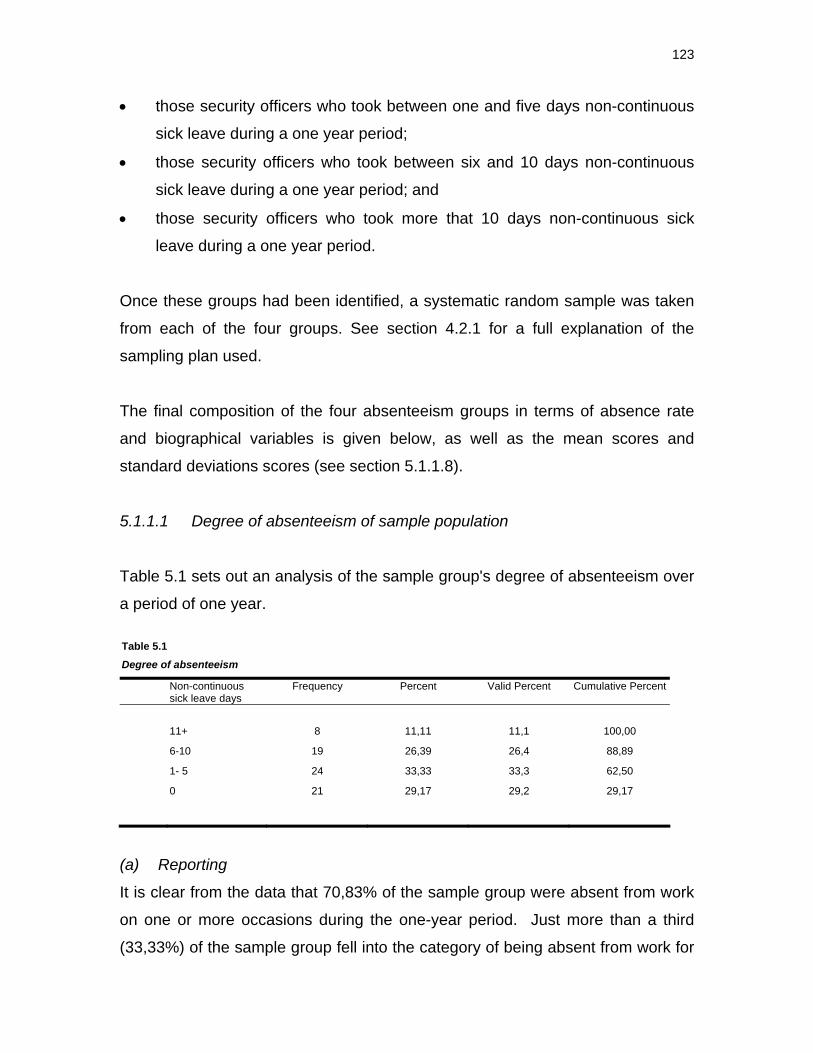
123
• those security officers who took between one and five days non-continuous
sick leave during a one year period;
• those security officers who took between six and 10 days non-continuous
sick leave during a one year period; and
• those security officers who took more that 10 days non-continuous sick
leave during a one year period.
Once these groups had been identified, a systematic random sample was taken
from each of the four groups. See section 4.2.1 for a full explanation of the
sampling plan used.
The final composition of the four absenteeism groups in terms of absence rate
and biographical variables is given below, as well as the mean scores and
standard deviations scores (see section 5.1.1.8).
5.1.1.1 Degree of absenteeism of sample population
Table 5.1 sets out an analysis of the sample group's degree of absenteeism over
a period of one year.
Table 5.1 Degree of absenteeism
Non-continuous sick leave days
Frequency Percent Valid Percent Cumulative Percent
11+ 8 11,11 11,1 100,00
6-10 19 26,39 26,4 88,89
1- 5 24 33,33 33,3 62,50
0 21 29,17 29,2 29,17
(a) Reporting
It is clear from the data that 70,83% of the sample group were absent from work
on one or more occasions during the one-year period. Just more than a third
(33,33%) of the sample group fell into the category of being absent from work for
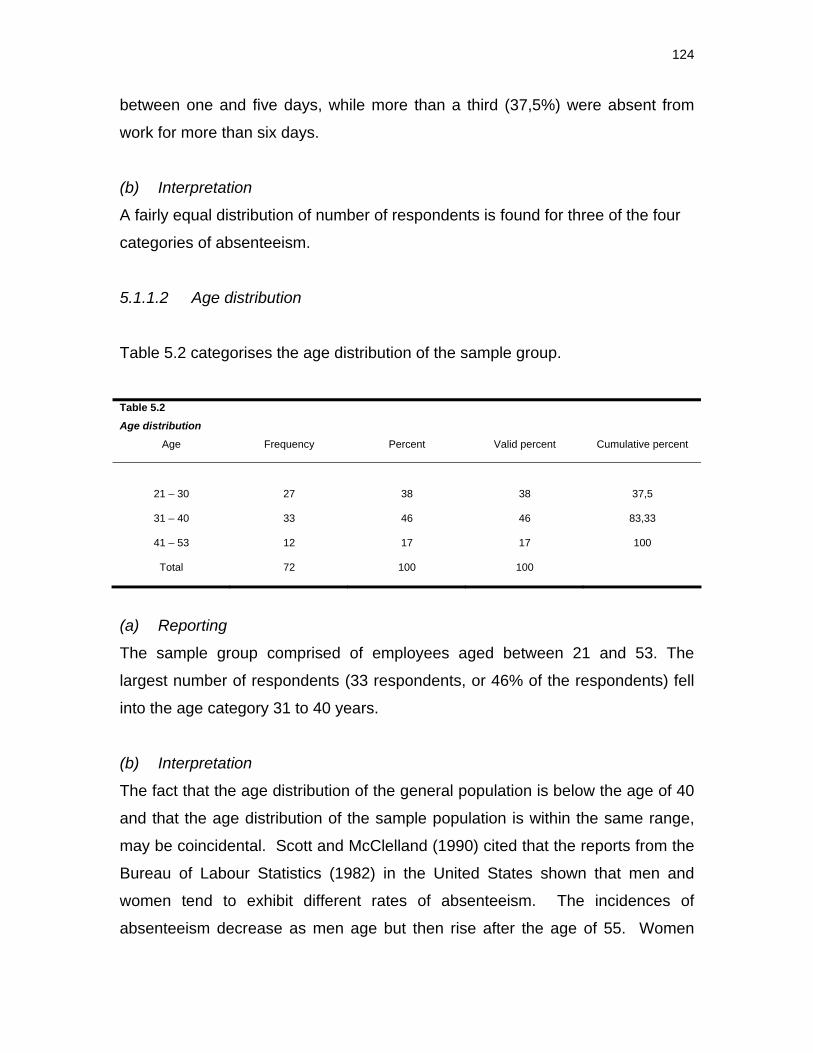
124
between one and five days, while more than a third (37,5%) were absent from
work for more than six days.
(b) Interpretation
A fairly equal distribution of number of respondents is found for three of the four
categories of absenteeism.
5.1.1.2 Age distribution
Table 5.2 categorises the age distribution of the sample group.
Table 5.2 Age distribution
Age Frequency Percent Valid percent Cumulative percent
21 – 30
27
38
38
37,5
31 – 40 33 46 46 83,33
41 – 53 12 17 17 100
Total 72 100 100
(a) Reporting
The sample group comprised of employees aged between 21 and 53. The
largest number of respondents (33 respondents, or 46% of the respondents) fell
into the age category 31 to 40 years.
(b) Interpretation
The fact that the age distribution of the general population is below the age of 40
and that the age distribution of the sample population is within the same range,
may be coincidental. Scott and McClelland (1990) cited that the reports from the
Bureau of Labour Statistics (1982) in the United States shown that men and
women tend to exhibit different rates of absenteeism. The incidences of
absenteeism decrease as men age but then rise after the age of 55. Women
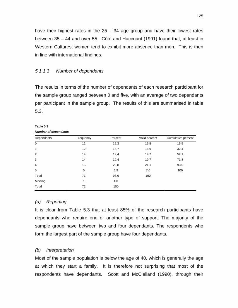
125
have their highest rates in the 25 – 34 age group and have their lowest rates
between 35 – 44 and over 55. Côté and Haccount (1991) found that, at least in
Western Cultures, women tend to exhibit more absence than men. This is then
in line with international findings.
5.1.1.3 Number of dependants
The results in terms of the number of dependants of each research participant for
the sample group ranged between 0 and five, with an average of two dependants
per participant in the sample group. The results of this are summarised in table
5.3.
Table 5.3 Number of dependants
Dependants Frequency Percent Valid percent Cumulative percent
0 11 15,3 15,5 15,5
1 12 16,7 16,9 32,4
2 14 19,4 19,7 52,1
3 14 19,4 19,7 71,8
4 15 20,8 21,1 93,0
5 5 6,9 7,0 100
Total 71 98,6 100
Missing 1 1,0 Total 72 100
(a) Reporting
It is clear from Table 5.3 that at least 85% of the research participants have
dependants who require one or another type of support. The majority of the
sample group have between two and four dependants. The respondents who
form the largest part of the sample group have four dependants.
(b) Interpretation
Most of the sample population is below the age of 40, which is generally the age
at which they start a family. It is therefore not surprising that most of the
respondents have dependants. Scott and McClelland (1990), through their
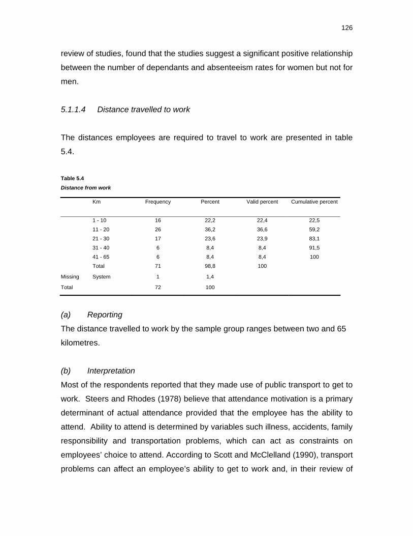
126
review of studies, found that the studies suggest a significant positive relationship
between the number of dependants and absenteeism rates for women but not for
men.
5.1.1.4 Distance travelled to work
The distances employees are required to travel to work are presented in table
5.4.
Table 5.4
Distance from work Km Frequency Percent Valid percent Cumulative percent
1 - 10 16 22,2 22,4 22,5
11 - 20 26 36,2 36,6 59,2
21 - 30 17 23,6 23,9 83,1
31 - 40 6 8,4 8,4 91,5
41 - 65 6 8,4 8,4 100
Total 71 98,8 100
Missing System 1 1,4
Total 72 100
(a) Reporting
The distance travelled to work by the sample group ranges between two and 65
kilometres.
(b) Interpretation
Most of the respondents reported that they made use of public transport to get to
work. Steers and Rhodes (1978) believe that attendance motivation is a primary
determinant of actual attendance provided that the employee has the ability to
attend. Ability to attend is determined by variables such illness, accidents, family
responsibility and transportation problems, which can act as constraints on
employees’ choice to attend. According to Scott and McClelland (1990), transport
problems can affect an employee’s ability to get to work and, in their review of
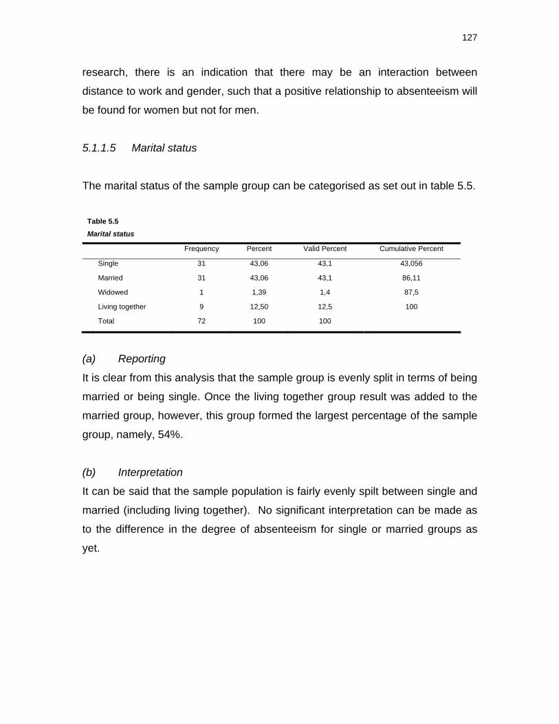
127
research, there is an indication that there may be an interaction between
distance to work and gender, such that a positive relationship to absenteeism will
be found for women but not for men.
5.1.1.5 Marital status
The marital status of the sample group can be categorised as set out in table 5.5.
Table 5.5 Marital status
Frequency Percent Valid Percent Cumulative Percent
Single 31 43,06 43,1 43,056
Married 31 43,06 43,1 86,11
Widowed 1 1,39 1,4 87,5
Living together 9 12,50 12,5 100
Total 72 100 100
(a) Reporting
It is clear from this analysis that the sample group is evenly split in terms of being
married or being single. Once the living together group result was added to the
married group, however, this group formed the largest percentage of the sample
group, namely, 54%.
(b) Interpretation
It can be said that the sample population is fairly evenly spilt between single and
married (including living together). No significant interpretation can be made as
to the difference in the degree of absenteeism for single or married groups as
yet.
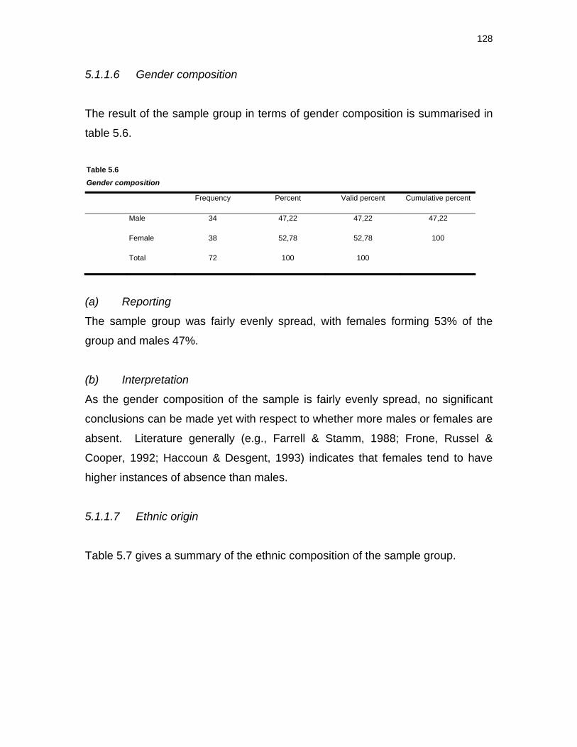
128
5.1.1.6 Gender composition
The result of the sample group in terms of gender composition is summarised in
table 5.6.
Table 5.6 Gender composition Frequency Percent Valid percent Cumulative percent
Male 34 47,22 47,22 47,22
Female 38 52,78 52,78 100
Total 72 100 100
(a) Reporting
The sample group was fairly evenly spread, with females forming 53% of the
group and males 47%.
(b) Interpretation
As the gender composition of the sample is fairly evenly spread, no significant
conclusions can be made yet with respect to whether more males or females are
absent. Literature generally (e.g., Farrell & Stamm, 1988; Frone, Russel &
Cooper, 1992; Haccoun & Desgent, 1993) indicates that females tend to have
higher instances of absence than males.
5.1.1.7 Ethnic origin
Table 5.7 gives a summary of the ethnic composition of the sample group.
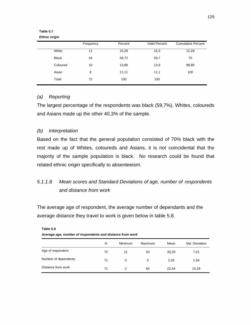
129
Table 5.7 Ethnic origin
Frequency Percent Valid Percent Cumulative Percent
White 11 15,28 15,3 15,28
Black 43 59,72 59,7 75
Coloured 10 13,89 13,9 88,89
Asian 8 11,11 11,1 100
Total 72 100 100
(a) Reporting
The largest percentage of the respondents was black (59,7%). Whites, coloureds
and Asians made up the other 40,3% of the sample.
(b) Interpretation
Based on the fact that the general population consisted of 70% black with the
rest made up of Whites, coloureds and Asians, it is not coincidental that the
majority of the sample population is black. No research could be found that
related ethnic origin specifically to absenteeism.
5.1.1.8 Mean scores and Standard Deviations of age, number of respondents
and distance from work
The average age of respondent, the average number of dependants and the
average distance they travel to work is given below in table 5.8.
Table 5.8 Average age, number of respondents and distance from work
N Minimum Maximum Mean Std. Deviation
Age of respondent 72 21 53 33,29 7,01
Number of dependents 71 0 5 2,35 1,54
Distance from work 71 2 65 22,54 15,29
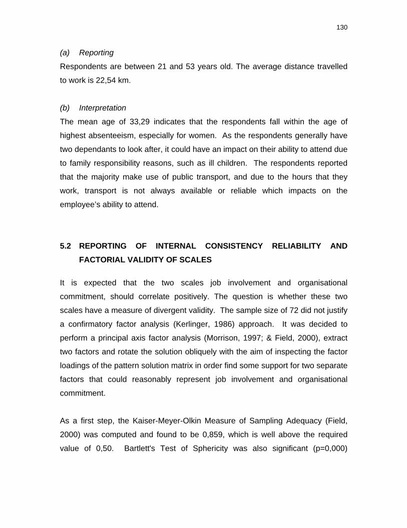
130
(a) Reporting
Respondents are between 21 and 53 years old. The average distance travelled
to work is 22,54 km.
(b) Interpretation
The mean age of 33,29 indicates that the respondents fall within the age of
highest absenteeism, especially for women. As the respondents generally have
two dependants to look after, it could have an impact on their ability to attend due
to family responsibility reasons, such as ill children. The respondents reported
that the majority make use of public transport, and due to the hours that they
work, transport is not always available or reliable which impacts on the
employee’s ability to attend.
5.2 REPORTING OF INTERNAL CONSISTENCY RELIABILITY AND FACTORIAL VALIDITY OF SCALES
It is expected that the two scales job involvement and organisational
commitment, should correlate positively. The question is whether these two
scales have a measure of divergent validity. The sample size of 72 did not justify
a confirmatory factor analysis (Kerlinger, 1986) approach. It was decided to
perform a principal axis factor analysis (Morrison, 1997; & Field, 2000), extract
two factors and rotate the solution obliquely with the aim of inspecting the factor
loadings of the pattern solution matrix in order find some support for two separate
factors that could reasonably represent job involvement and organisational
commitment.
As a first step, the Kaiser-Meyer-Olkin Measure of Sampling Adequacy (Field,
2000) was computed and found to be 0,859, which is well above the required
value of 0,50. Bartlett's Test of Sphericity was also significant (p=0,000)
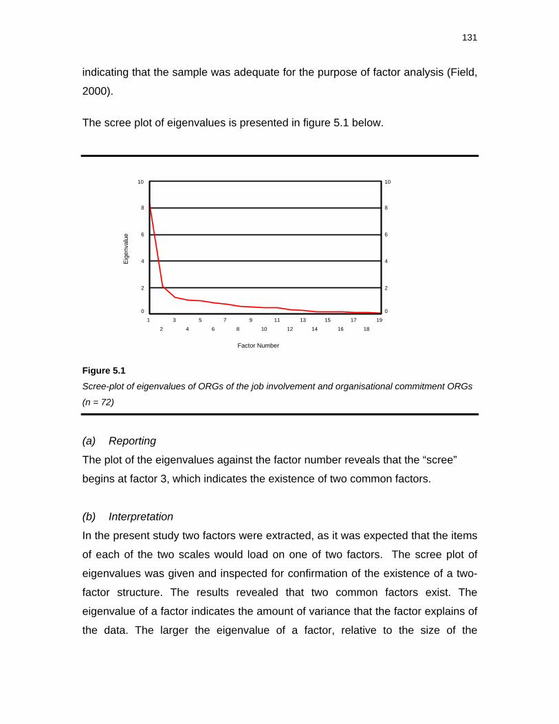
131
Factor Number
19
18
17
16
15
14
13
12
11
10
9
8
7
6
5
4
3
2
1
Eige
nval
ue
10
8
6
4
2
0
10
8
6
4
2
0
indicating that the sample was adequate for the purpose of factor analysis (Field,
2000).
The scree plot of eigenvalues is presented in figure 5.1 below.
Figure 5.1 Scree-plot of eigenvalues of ORGs of the job involvement and organisational commitment ORGs
(n = 72)
(a) Reporting
The plot of the eigenvalues against the factor number reveals that the “scree”
begins at factor 3, which indicates the existence of two common factors.
(b) Interpretation
In the present study two factors were extracted, as it was expected that the items
of each of the two scales would load on one of two factors. The scree plot of
eigenvalues was given and inspected for confirmation of the existence of a two-
factor structure. The results revealed that two common factors exist. The
eigenvalue of a factor indicates the amount of variance that the factor explains of
the data. The larger the eigenvalue of a factor, relative to the size of the
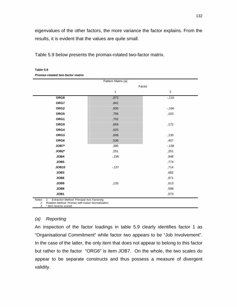
132
eigenvalues of the other factors, the more variance the factor explains. From the
results, it is evident that the values are quite small.
Table 5.9 below presents the promax-rotated two-factor matrix.
Table 5.9 Promax-rotated two-factor matrix
Pattern Matrix (a)
Factor
1 2
ORG8 ,873 -,116
ORG7 ,842
ORG2 ,830 -,166
ORG5 ,756 ,103
ORG1 ,702
ORG9 ,659 ,172
ORG4 ,620
ORG3 ,608 ,130
ORG6 ,536 ,407
JOB7* ,386 -,138
JOB2* ,251 ,251
JOB4 -,195 ,948
JOB5 ,774
JOB10 -,137 ,714
JOB3 ,682
JOB6 ,671
JOB9 ,133 ,613
JOB8 ,598
JOB1 ,573
Notes: 1. Extraction Method: Principal Axis Factoring. 2. Rotation Method: Promax with Kaiser Normalisation. 3. * Item reverse scored
(a) Reporting
An inspection of the factor loadings in table 5.9 clearly identifies factor 1 as
“Organisational Commitment” while factor two appears to be “Job Involvement”.
In the case of the latter, the only item that does not appear to belong to this factor
but rather to the factor “ORG6” is item JOB7. On the whole, the two scales do
appear to be separate constructs and thus possess a measure of divergent
validity.
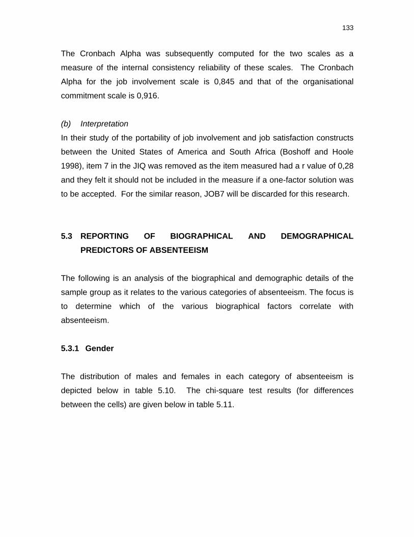
133
The Cronbach Alpha was subsequently computed for the two scales as a
measure of the internal consistency reliability of these scales. The Cronbach
Alpha for the job involvement scale is 0,845 and that of the organisational
commitment scale is 0,916.
(b) Interpretation
In their study of the portability of job involvement and job satisfaction constructs
between the United States of America and South Africa (Boshoff and Hoole
1998), item 7 in the JIQ was removed as the item measured had a r value of 0,28
and they felt it should not be included in the measure if a one-factor solution was
to be accepted. For the similar reason, JOB7 will be discarded for this research.
5.3 REPORTING OF BIOGRAPHICAL AND DEMOGRAPHICAL PREDICTORS OF ABSENTEEISM
The following is an analysis of the biographical and demographic details of the
sample group as it relates to the various categories of absenteeism. The focus is
to determine which of the various biographical factors correlate with
absenteeism.
5.3.1 Gender
The distribution of males and females in each category of absenteeism is
depicted below in table 5.10. The chi-square test results (for differences
between the cells) are given below in table 5.11.
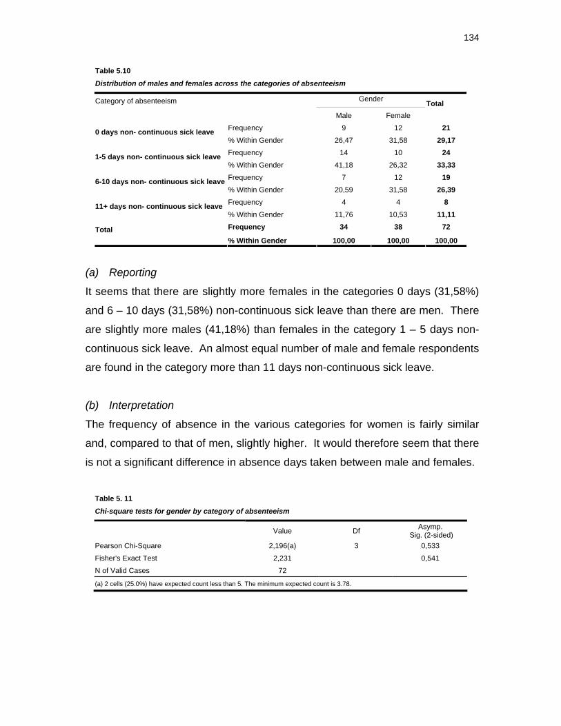
134
(a) Reporting
It seems that there are slightly more females in the categories 0 days (31,58%)
and 6 – 10 days (31,58%) non-continuous sick leave than there are men. There
are slightly more males (41,18%) than females in the category 1 – 5 days non-
continuous sick leave. An almost equal number of male and female respondents
are found in the category more than 11 days non-continuous sick leave.
(b) Interpretation
The frequency of absence in the various categories for women is fairly similar
and, compared to that of men, slightly higher. It would therefore seem that there
is not a significant difference in absence days taken between male and females.
Table 5. 11 Chi-square tests for gender by category of absenteeism
Value Df Asymp. Sig. (2-sided)
Pearson Chi-Square 2,196(a) 3 0,533
Fisher's Exact Test 2,231 0,541
N of Valid Cases 72
(a) 2 cells (25.0%) have expected count less than 5. The minimum expected count is 3.78.
Table 5.10 Distribution of males and females across the categories of absenteeism
Category of absenteeism Gender
Male Female Total
Frequency 9 12 21 0 days non- continuous sick leave % Within Gender 26,47 31,58 29,17 Frequency 14 10 24 1-5 days non- continuous sick leave % Within Gender 41,18 26,32 33,33 Frequency 7 12 19 6-10 days non- continuous sick leave % Within Gender 20,59 31,58 26,39 Frequency 4 4 8 11+ days non- continuous sick leave % Within Gender 11,76 10,53 11,11 Frequency 34 38 72 Total % Within Gender 100,00 100,00 100,00
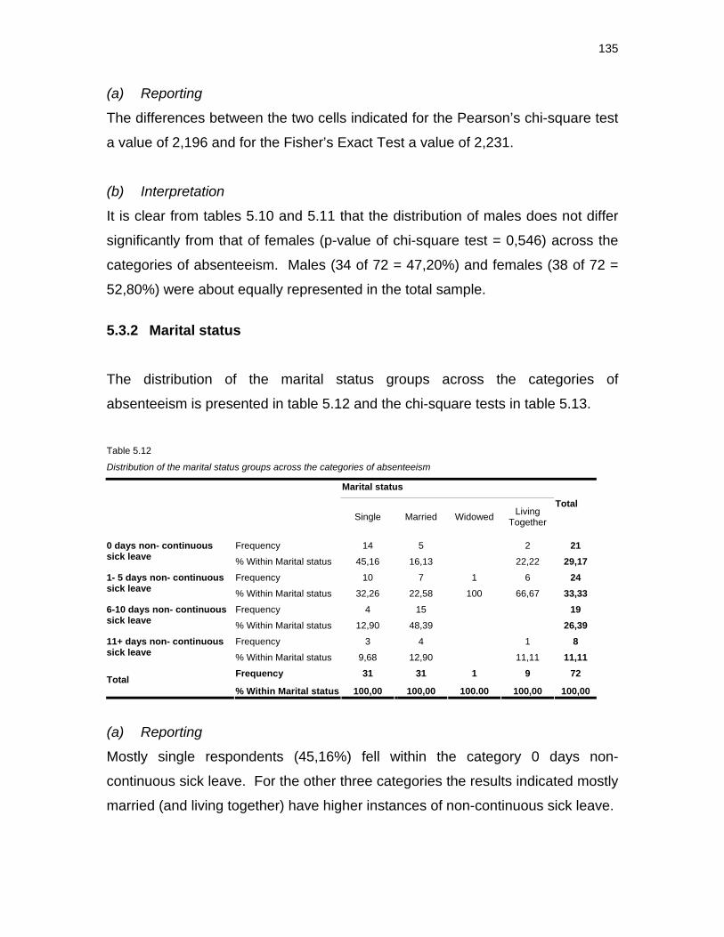
135
(a) Reporting
The differences between the two cells indicated for the Pearson’s chi-square test
a value of 2,196 and for the Fisher’s Exact Test a value of 2,231.
(b) Interpretation
It is clear from tables 5.10 and 5.11 that the distribution of males does not differ
significantly from that of females (p-value of chi-square test = 0,546) across the
categories of absenteeism. Males (34 of 72 = 47,20%) and females (38 of 72 =
52,80%) were about equally represented in the total sample.
5.3.2 Marital status
The distribution of the marital status groups across the categories of
absenteeism is presented in table 5.12 and the chi-square tests in table 5.13.
Table 5.12
Distribution of the marital status groups across the categories of absenteeism
Marital status
Single Married Widowed Living
Together
Total
Frequency 14 5 2 21 0 days non- continuous sick leave % Within Marital status 45,16 16,13 22,22 29,17
Frequency 10 7 1 6 24 1- 5 days non- continuous sick leave % Within Marital status 32,26 22,58 100 66,67 33,33
Frequency 4 15 19 6-10 days non- continuous sick leave % Within Marital status 12,90 48,39 26,39
Frequency 3 4 1 8 11+ days non- continuous sick leave % Within Marital status 9,68 12,90 11,11 11,11
Frequency 31 31 1 9 72 Total % Within Marital status 100,00 100,00 100.00 100,00 100,00
(a) Reporting
Mostly single respondents (45,16%) fell within the category 0 days non-
continuous sick leave. For the other three categories the results indicated mostly
married (and living together) have higher instances of non-continuous sick leave.
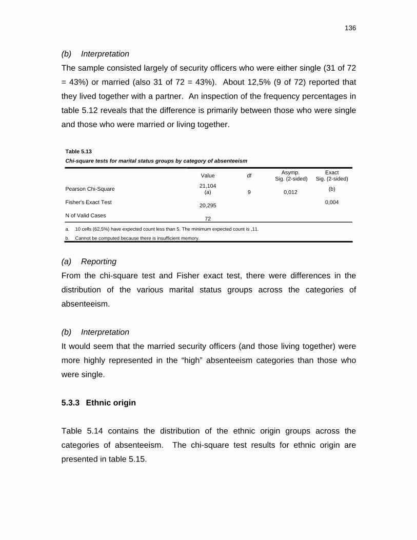
136
(b) Interpretation
The sample consisted largely of security officers who were either single (31 of 72
= 43%) or married (also 31 of 72 = 43%). About 12,5% (9 of 72) reported that
they lived together with a partner. An inspection of the frequency percentages in
table 5.12 reveals that the difference is primarily between those who were single
and those who were married or living together.
Table 5.13 Chi-square tests for marital status groups by category of absenteeism
Value df Asymp. Sig. (2-sided)
Exact Sig. (2-sided)
Pearson Chi-Square 21,104 (a) 9 0,012 (b)
Fisher's Exact Test 20,295 0,004
N of Valid Cases 72
a. 10 cells (62,5%) have expected count less than 5. The minimum expected count is ,11.
b. Cannot be computed because there is insufficient memory.
(a) Reporting
From the chi-square test and Fisher exact test, there were differences in the
distribution of the various marital status groups across the categories of
absenteeism.
(b) Interpretation
It would seem that the married security officers (and those living together) were
more highly represented in the “high” absenteeism categories than those who
were single.
5.3.3 Ethnic origin
Table 5.14 contains the distribution of the ethnic origin groups across the
categories of absenteeism. The chi-square test results for ethnic origin are
presented in table 5.15.
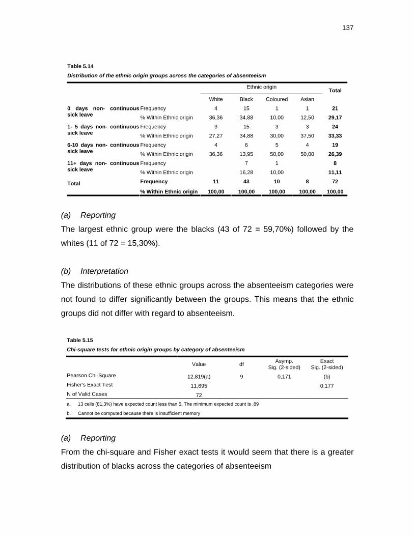
137
Table 5.14 Distribution of the ethnic origin groups across the categories of absenteeism
Ethnic origin
White Black Coloured Asian Total
Frequency 4 15 1 1 21 0 days non- continuous sick leave % Within Ethnic origin 36,36 34,88 10,00 12,50 29,17
Frequency 3 15 3 3 24 1- 5 days non- continuous sick leave % Within Ethnic origin 27,27 34,88 30,00 37,50 33,33
Frequency 4 6 5 4 19 6-10 days non- continuous sick leave % Within Ethnic origin 36,36 13,95 50,00 50,00 26,39
Frequency 7 1 8 11+ days non- continuous sick leave % Within Ethnic origin 16,28 10,00 11,11
Frequency 11 43 10 8 72 Total % Within Ethnic origin 100,00 100,00 100,00 100,00 100,00
(a) Reporting
The largest ethnic group were the blacks (43 of 72 = 59,70%) followed by the
whites (11 of 72 = 15,30%).
(b) Interpretation
The distributions of these ethnic groups across the absenteeism categories were
not found to differ significantly between the groups. This means that the ethnic
groups did not differ with regard to absenteeism.
Table 5.15 Chi-square tests for ethnic origin groups by category of absenteeism
Value df Asymp. Sig. (2-sided)
Exact Sig. (2-sided)
Pearson Chi-Square 12,819(a) 9 0,171 (b) Fisher's Exact Test 11,695 0,177 N of Valid Cases 72 a. 13 cells (81.3%) have expected count less than 5. The minimum expected count is .89
b. Cannot be computed because there is insufficient memory
(a) Reporting
From the chi-square and Fisher exact tests it would seem that there is a greater
distribution of blacks across the categories of absenteeism
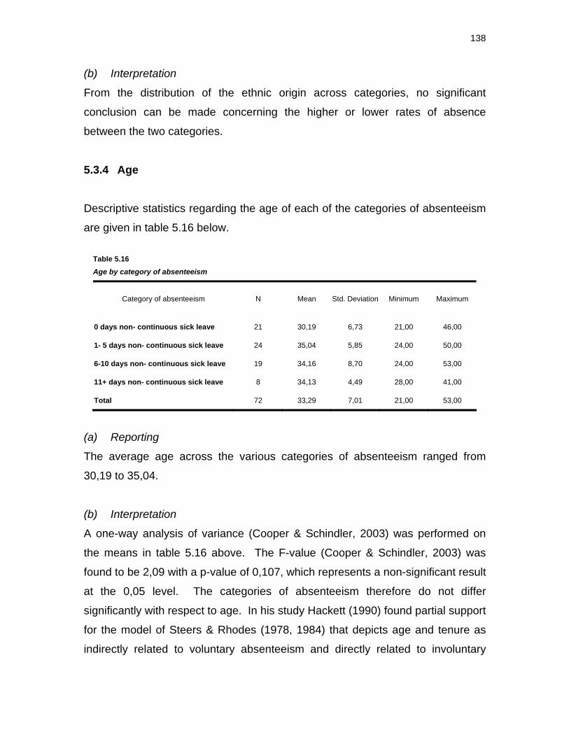
138
(b) Interpretation
From the distribution of the ethnic origin across categories, no significant
conclusion can be made concerning the higher or lower rates of absence
between the two categories.
5.3.4 Age
Descriptive statistics regarding the age of each of the categories of absenteeism
are given in table 5.16 below.
Table 5.16 Age by category of absenteeism
Category of absenteeism N Mean Std. Deviation Minimum Maximum
0 days non- continuous sick leave 21 30,19 6,73 21,00 46,00
1- 5 days non- continuous sick leave 24 35,04 5,85 24,00 50,00
6-10 days non- continuous sick leave 19 34,16 8,70 24,00 53,00
11+ days non- continuous sick leave 8 34,13 4,49 28,00 41,00
Total 72 33,29 7,01 21,00 53,00
(a) Reporting
The average age across the various categories of absenteeism ranged from
30,19 to 35,04.
(b) Interpretation
A one-way analysis of variance (Cooper & Schindler, 2003) was performed on
the means in table 5.16 above. The F-value (Cooper & Schindler, 2003) was
found to be 2,09 with a p-value of 0,107, which represents a non-significant result
at the 0,05 level. The categories of absenteeism therefore do not differ
significantly with respect to age. In his study Hackett (1990) found partial support
for the model of Steers & Rhodes (1978, 1984) that depicts age and tenure as
indirectly related to voluntary absenteeism and directly related to involuntary
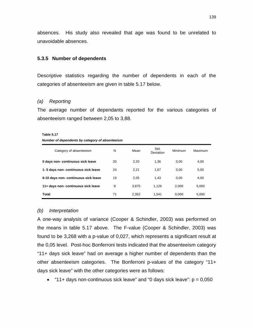
139
absences. His study also revealed that age was found to be unrelated to
unavoidable absences.
5.3.5 Number of dependents
Descriptive statistics regarding the number of dependents in each of the
categories of absenteeism are given in table 5.17 below.
(a) Reporting
The average number of dependants reported for the various categories of
absenteeism ranged between 2,05 to 3,88.
Table 5.17 Number of dependents by category of absenteeism
Category of absenteeism N Mean Std. Deviation Minimum Maximum
0 days non- continuous sick leave 20 2,20 1,36 0,00 4,00
1- 5 days non- continuous sick leave 24 2,21 1,67 0,00 5,00
6-10 days non- continuous sick leave 19 2,05 1,43 0,00 4,00
11+ days non- continuous sick leave 8 3,875 1,126 2,000 5,000
Total 71 2,352 1,541 0,000 5,000
(b) Interpretation
A one-way analysis of variance (Cooper & Schindler, 2003) was performed on
the means in table 5.17 above. The F-value (Cooper & Schindler, 2003) was
found to be 3,268 with a p-value of 0,027, which represents a significant result at
the 0,05 level. Post-hoc Bonferroni tests indicated that the absenteeism category
“11+ days sick leave” had on average a higher number of dependents than the
other absenteeism categories. The Bonferroni p-values of the category “11+
days sick leave” with the other categories were as follows:
• “11+ days non-continuous sick leave” and “0 days sick leave”: p = 0,050
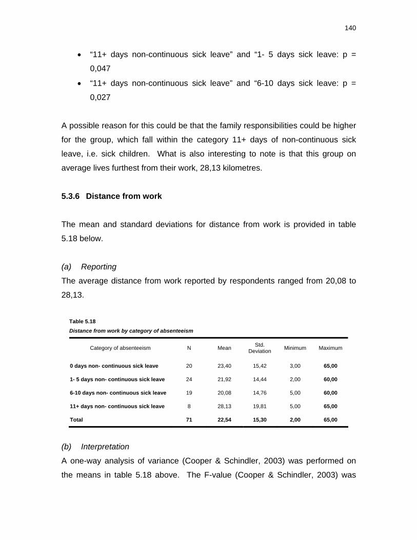
140
• “11+ days non-continuous sick leave” and “1- 5 days sick leave: p =
0,047
• “11+ days non-continuous sick leave” and “6-10 days sick leave: p =
0,027
A possible reason for this could be that the family responsibilities could be higher
for the group, which fall within the category 11+ days of non-continuous sick
leave, i.e. sick children. What is also interesting to note is that this group on
average lives furthest from their work, 28,13 kilometres.
5.3.6 Distance from work
The mean and standard deviations for distance from work is provided in table
5.18 below.
(a) Reporting
The average distance from work reported by respondents ranged from 20,08 to
28,13.
Table 5.18 Distance from work by category of absenteeism
Category of absenteeism N Mean Std. Deviation Minimum Maximum
0 days non- continuous sick leave 20 23,40 15,42 3,00 65,00
1- 5 days non- continuous sick leave 24 21,92 14,44 2,00 60,00
6-10 days non- continuous sick leave 19 20,08 14,76 5,00 60,00
11+ days non- continuous sick leave 8 28,13 19,81 5,00 65,00
Total 71 22,54 15,30 2,00 65,00
(b) Interpretation
A one-way analysis of variance (Cooper & Schindler, 2003) was performed on
the means in table 5.18 above. The F-value (Cooper & Schindler, 2003) was
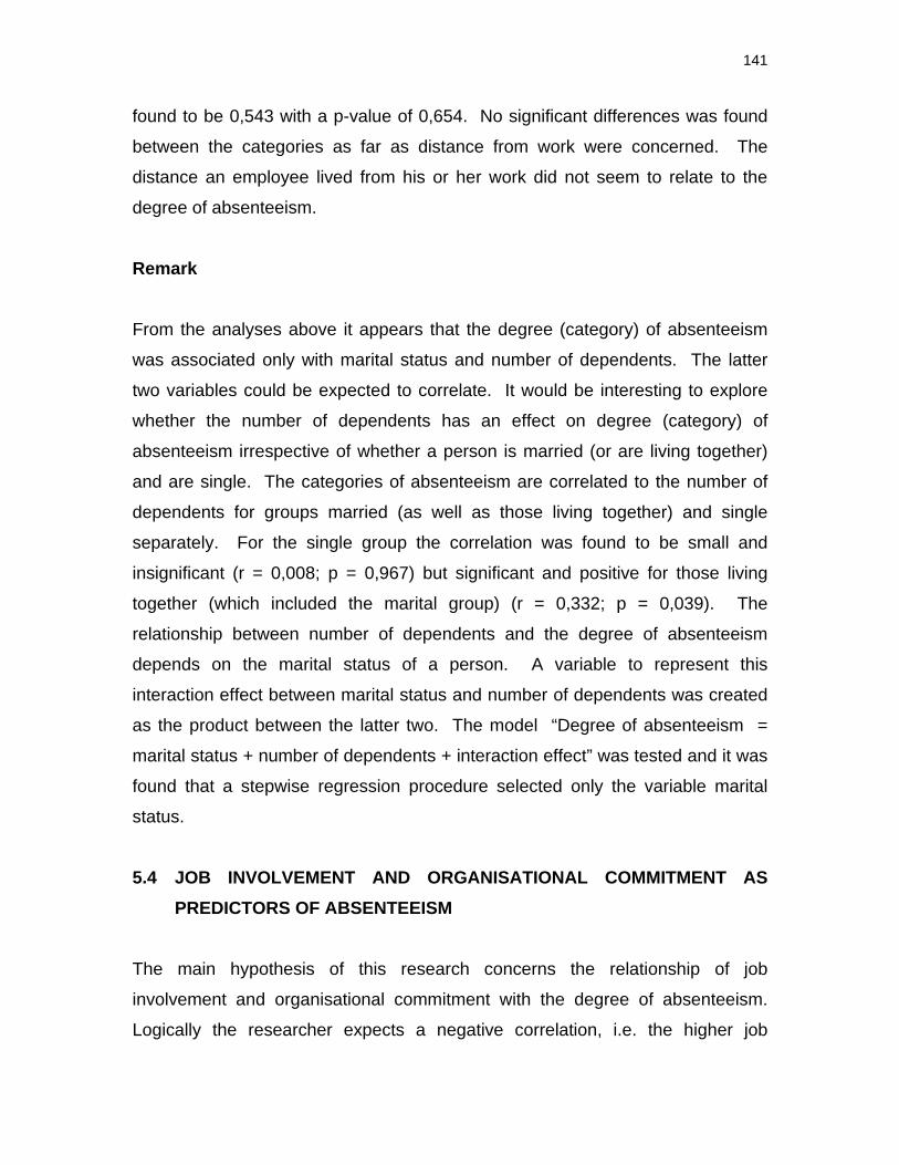
141
found to be 0,543 with a p-value of 0,654. No significant differences was found
between the categories as far as distance from work were concerned. The
distance an employee lived from his or her work did not seem to relate to the
degree of absenteeism.
Remark
From the analyses above it appears that the degree (category) of absenteeism
was associated only with marital status and number of dependents. The latter
two variables could be expected to correlate. It would be interesting to explore
whether the number of dependents has an effect on degree (category) of
absenteeism irrespective of whether a person is married (or are living together)
and are single. The categories of absenteeism are correlated to the number of
dependents for groups married (as well as those living together) and single
separately. For the single group the correlation was found to be small and
insignificant (r = 0,008; p = 0,967) but significant and positive for those living
together (which included the marital group) (r = 0,332; p = 0,039). The
relationship between number of dependents and the degree of absenteeism
depends on the marital status of a person. A variable to represent this
interaction effect between marital status and number of dependents was created
as the product between the latter two. The model “Degree of absenteeism =
marital status + number of dependents + interaction effect” was tested and it was
found that a stepwise regression procedure selected only the variable marital
status.
5.4 JOB INVOLVEMENT AND ORGANISATIONAL COMMITMENT AS PREDICTORS OF ABSENTEEISM
The main hypothesis of this research concerns the relationship of job
involvement and organisational commitment with the degree of absenteeism.
Logically the researcher expects a negative correlation, i.e. the higher job
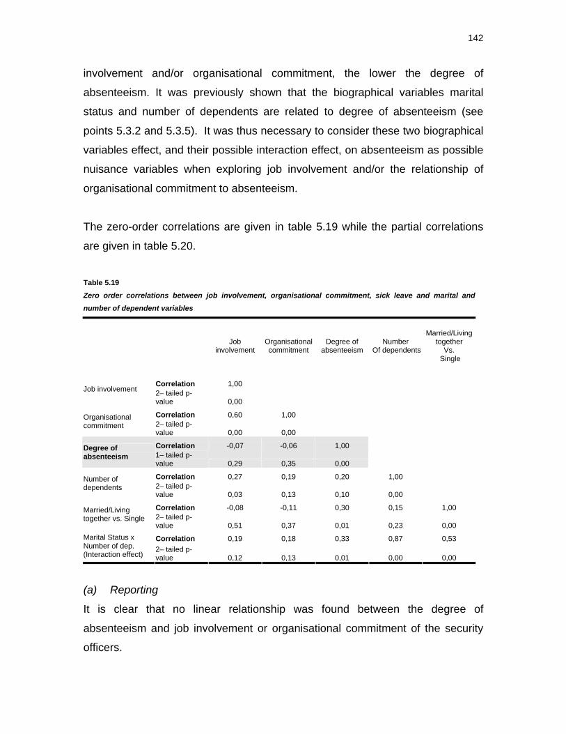
142
involvement and/or organisational commitment, the lower the degree of
absenteeism. It was previously shown that the biographical variables marital
status and number of dependents are related to degree of absenteeism (see
points 5.3.2 and 5.3.5). It was thus necessary to consider these two biographical
variables effect, and their possible interaction effect, on absenteeism as possible
nuisance variables when exploring job involvement and/or the relationship of
organisational commitment to absenteeism.
The zero-order correlations are given in table 5.19 while the partial correlations
are given in table 5.20. Table 5.19 Zero order correlations between job involvement, organisational commitment, sick leave and marital and
number of dependent variables
Job involvement
Organisational commitment
Degree of absenteeism
Number Of dependents
Married/Living together
Vs. Single
Correlation 1,00 Job involvement 2– tailed p-
value 0,00
Correlation 0,60 1,00 Organisational commitment 2– tailed p-
value 0,00 0,00
Correlation -0,07 -0,06 1,00 Degree of absenteeism 1– tailed p-
value 0,29 0,35 0,00
Correlation 0,27 0,19 0,20 1,00 Number of dependents 2– tailed p-
value 0,03 0,13 0,10 0,00
Correlation -0,08 -0,11 0,30 0,15 1,00 Married/Living together vs. Single 2– tailed p-
value 0,51 0,37 0,01 0,23 0,00
Correlation 0,19 0,18 0,33 0,87 0,53 Marital Status x Number of dep. (Interaction effect)
2– tailed p-value 0,12 0,13 0,01 0,00 0,00
(a) Reporting
It is clear that no linear relationship was found between the degree of
absenteeism and job involvement or organisational commitment of the security
officers.
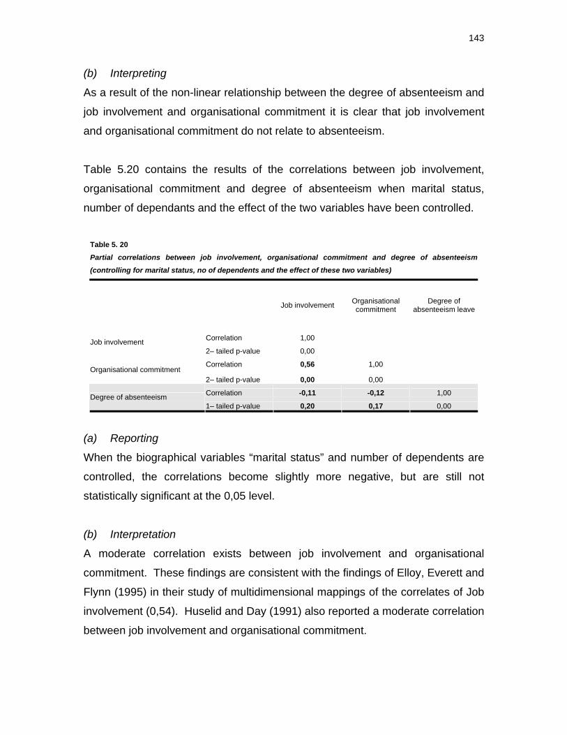
143
(b) Interpreting
As a result of the non-linear relationship between the degree of absenteeism and
job involvement and organisational commitment it is clear that job involvement
and organisational commitment do not relate to absenteeism.
Table 5.20 contains the results of the correlations between job involvement,
organisational commitment and degree of absenteeism when marital status,
number of dependants and the effect of the two variables have been controlled.
Table 5. 20 Partial correlations between job involvement, organisational commitment and degree of absenteeism
(controlling for marital status, no of dependents and the effect of these two variables)
Job involvement Organisational commitment
Degree of absenteeism leave
Correlation 1,00 Job involvement 2– tailed p-value 0,00
Correlation 0,56 1,00 Organisational commitment
2– tailed p-value 0,00 0,00
Correlation -0,11 -0,12 1,00 Degree of absenteeism 1– tailed p-value 0,20 0,17 0,00
(a) Reporting
When the biographical variables “marital status” and number of dependents are
controlled, the correlations become slightly more negative, but are still not
statistically significant at the 0,05 level.
(b) Interpretation
A moderate correlation exists between job involvement and organisational
commitment. These findings are consistent with the findings of Elloy, Everett and
Flynn (1995) in their study of multidimensional mappings of the correlates of Job
involvement (0,54). Huselid and Day (1991) also reported a moderate correlation
between job involvement and organisational commitment.
144
Summary The gender groups within the sample population were equally represented and
the largest ethnic group represented in the sample was blacks followed by
whites. In general, only marital status (whether the employee was single or
married) and number of dependents were related to the degree (category) of
absenteeism. It appeared that married employees (and those living together)
tended towards more absenteeism than did employees who are single. It was
also found that those employees in the higher levels of absenteeism, tended to
have more dependents. A possible relationship between marital status and the
number of independents was explored by correlating the degree of absenteeism
to the number of dependents for the marital groups separately. A significant
correlation was found for the marital group (which included the group “living
together”) but not for the single group – indicating that the relationship between
absenteeism and number of dependents depended on marital status.
In chapter 1 (see section 1.2) the problem statement was discussed which lead
to specific research questions. The research question relating to whether job
involvement and organisational commitment predict employee absenteeism, with
the results for this specific research presented in this chapter, can be concluded
as not achievable. The general aim and specific objectives set out in chapter 1
(see section 1.3.1 and 1.3.2) are herewith satisfied. The aim of the research
was achieved through the review of the literature, which presented support from
the literature for the predictability of job involvement and organisational
commitment on employee absenteeism. The hypothesis was tested through the
distribution of questionnaires and these were statistically processed, which
produced the results as set out in this chapter.
145
5.6 CHAPTER SUMMARY
In this chapter the results from the empirical study were reported and interpreted.
The composition of the sample and the factorial validity and the internal
consistency reliability item analysis of each of the two scales (job involvement
and organisational commitment) were set out in table form and interpreted.
Thereafter absenteeism was explained in terms of biographical and
demographical factors and finally, the predictive or explanatory value of job
involvement and organisational commitment was explored. The possibility that
the biographical variables, such as gender and age, as well as distance from
work, may explain absenteeism was also discussed.
In chapter 6 the conclusions on the research will be discussed, the shortcomings
of the research will be pointed out and recommendations for future research will
be provided.
146
CHAPTER 6
CONCLUSIONS, RECOMMENDATIONS AND LIMITATIONS
In this chapter conclusions relating to the literature findings, the results from the
empirical study and the integration of the literature and empirical results will first
be presented. Secondly, recommendations will be made relating to the findings
of the research for industrial psychology, after which recommendations relating to
future research will be discussed. The limitation of the research will then be
discussed and the chapter summary will conclude this chapter.
6.1 CONCLUSIONS
Conclusions will be made relating to the literature review that was conducted, as
well as the empirical study. Conclusions will also be made relating to the
relationship between the literature findings and the empirical findings.
6.1.1 Conclusions relating to the literature review
In chapter 2 the nature of absenteeism was explained and specifically the
complex issue of measuring absenteeism. The frequency of absence measured
over a mid-term variance of 12 months is identified as being the most accurate
measurement of employee behaviour. The theories presented indicated further
contributed to the complex nature of absenteeism in that the phenomenon cannot
be viewed from a one-dimensional aspect.
Certain conclusions can be made relating to the literature findings of chapter 2.
These are set out below.
Absenteeism carries a mixed dynamism in that sets of independent variables
range from demographic features such as gender that are constant over a
147
lifetime, to constructs such as attendance attitudes that fluctuate daily. Due to
this fluctuation in attitudes it becomes increasingly important to understand what
precedes the attendance instance. To achieve this, the timeframe within which
absenteeism is measured becomes quite significant, as does the accurate
recording of reasons for absence. Without this, it is difficult to come to any
meaningful conclusions as to what causes or affects employee absenteeism,
specifically voluntary or organisationally unexcused absenteeism.
In chapter 3 the work-related attitudes job involvement and organisational
commitment were conceptualised. The relationship of each of the work-related
attitudes with absenteeism were discussed. The literature suggested that there
exist a possibility that the two work-related attitudes could predict employee
absenteeism. Some evidence for the hypothesis that employees with high levels
of job involvement and high levels of organisational commitment will have low
levels or no absence instances were provided.
Certain conclusions can be made relating to the literature findings of chapter 3.
The two work-related attitudes, job involvement and organisational commitment,
are closely correlated but constitute empirically distinct constructs. This was
proven by the statistical analysis as discussed in chapter 5. Independently the
two constructs, job involvement and organisational commitment, have provided
varied results in their ability to predict absenteeism. The results in fact indicate a
weak predictability of absenteeism.
The integration of absenteeism and the work-related attitudes indicated that
absenteeism and work-related attitudes are very different constructs though
some research has indicated that there is some level of predictability toward
employee absenteeism.
148
6.1.2 Conclusions relating to the empirical study
In chapter 5 the results of the empirical study were reported and interpreted.
Conclusions will now be made regarding the outcomes of the empirical findings.
The conclusions will firstly be made in terms of job involvement, then
organisational commitment and finally in relation to absenteeism.
Through the empirical study, the construct job involvement was proven to be a
distinct construct. Sufficient evidence was provided to refer to job involvement as
a separate construct. The empirical study also proved that the organisational
commitment is distinctive and can be referred to as a separate construct.
The empirical study further found that a relationship exists between job
involvement and organisational commitment. Furthermore, it would seem that
marital status and number of dependants has some level of impact on employee
absenteeism.
6.1.3 Conclusions relating to the relationship between the literature findings and the empirical findings
The literature findings, that i.e., there is evidence that employees with high levels
of job involvement and high levels of organisational commitment have lower
levels of absence, are not supported by the empirical findings of this research.
Although the literature referred to the effect that demographic variables have on
employee absence, it was not the focus of this research. The hypothesis
presented in chapter 4 (see section 4.3) is therefore not proven.
Remark With this, the research hypothesis stated in chapter 4 (see section 4.3) namely
that job involvement and organisational commitment on the one hand are related
to non-continuous sick leave on the other hand.
149
6.2 RECOMMENDATIONS
Recommendations will now be made, firstly relating to the findings of the
research, and secondly relating to future research on the topic.
6.2.1 Recommendations related to the predictability of work-related attitudes on absenteeism for Industrial Psychology.
Absenteeism will remain a costly phenomenon for organisations and managers
and human resources professionals alike need to endeavour to understand what
within their organisations causes employee absenteeism or affects employee
attendance motivation.
Future research into employee motivation and other work-related attitudes might
shed some light onto understanding the dynamics of employee absenteeism.
Although research into absenteeism has produced significant insights, the
research efforts are quite diverse and it is difficult to draw meaningful general
conclusions or assumptions from the research. Future work needs to focus on
providing a robust theoretical base, which will incorporate the various definitions,
causes and antecedents of absenteeism.
6.2.2 Recommendations for future research.
Certain recommendations for future research pertaining to the topic are made.
These are listed below.
• Research incorporating a broader range of absence correlates will assist in a
more complete understanding of the factors that antecede and flow from
absence episodes.
• Research into attendance motivation, will assist in determining absence
behaviour.
150
• Research into accurate recording of absence reasons and using quantitative
study methods (interviews) will determine the real reasons for absence.
• Research could be undertaken with other questionnaires that measure
organisational commitment and job involvement.
• Research should be done to investigate the effect shift work has on the
attendance of employees.
6.3 LIMITATIONS OF THE RESEARCH
Although every effort has been made to plan and execute the research design
and research method (see section 1.6 and 1.7), some limitations are evident.
Although a variety of limitations can be highlighted, these are not that relevant for
this research, and only the most important limitations, namely sample and
measuring instruments will be discussed.
6.3.1 Sample
As a result of the discussions with management and the union at Johannesburg
International Airport (JIA), the researcher was only permitted to conduct this
survey with a sample of the broader security population at JIA. This resulted in a
small sample size of only 72 respondents and the findings can, therefore, not be
conclusive.
In addition to this, the sample consisted only of security officers at Johannesburg
International Airport and thus the conclusions made cannot be generalised for
the security departments within the other regions in South Africa. This limits the
depth of the research.
151
6.3.2 Measuring instruments
The measuring instruments used in this research have various inherent
shortcomings, which were discussed in chapter 4. In addition to this, further
shortcomings as outlined in chapter’s 2 and 3 with specific reference to the
theoretical basis of the constructs and questionnaires were also discussed.
In order to test the predictability of job involvement and organisational
commitment, other questionnaires available could have been used in this
research. This specifically refers to the use of the organisational commitment
questionnaire devised by Allen and Meyer (1990).
Not one of the questionnaires used in the research is South African or
standardised for South African usage, with the exception of the job involvement
questionnaire in which Boshoff and Hoole (1998), tested the portability of
Kanungo’s (1979) job involvement questionnaire between the United States and
South Africa.
6.4 CHAPTER SUMMARY
In this chapter conclusions were presented relating to the findings of the
research, firstly referring to the literature review, secondly relating to the
empirical study and finally regarding the relationship between the literature
findings and empirical findings. This was followed with recommendations for the
field of Industrial Psychology, as well as for future research into the predictability
of work-related attitudes and absenteeism. The chapter concluded with a
discussion of the most important limitations of the research.
152
REFERENCES
Aamodt, M.G. (1991). Applied Industrial / Organizational Psychology. California:
Wadsworth, Inc.
Adams, J.S. (1965). Inequity in social exchange. In: Berkowitz, L. (Ed.)
Advances in Experimental Psychology, Vol 2, Academic Press, San Diego, CA.
Ajzen, I. (1991). The theory of planned behaviour. Organizational Behaviour
and Human Decision Processes, 50, 179 – 211.
Ajzen, I., & Fishbein, M. (1980). Understanding attitudes and predicting social
behaviour. Englewood Cliffs, NJ: Prentice-Hall.
Allen, S.G. (1981). An empirical model of work attendance. Review of
Economics and Statistics, 63, 77-87.
Allen, S.G., & Higgens, (1979). An imperial model of work attendance. Review
of Economics and Statistics, 63, 83 –94.
Allen, N. & Meyer, J. (1990). The measurement and antecedents of affective,
continuance and normative commitment to the organization. Journal of
Occupational Psychology, 63, 1-18.
Allport, G.W. (1943). The ego in contemporary psychology. Psychological
Review, 50, 451 – 478.
Allport, G.W. (1947). The psychology of participation. Psychological Review, 52,
117 – 132.
153
Angle, H., & Perry, J. (1981). An empirical assessment of organizational
commitment and organizational effectiveness. Administrative Science
Quarterly, 26, 1-14.
Anonymous. (2000, April). Putting the brakes on employee absenteeism. USA
Today (Society for the Advancement of Education), April. Retrieved from
http://www.findarticles.com/cf_dls/m1272/2659_128/61586737/p1/article.jhtml.
Anonymous. (2001). U.S. Survey shows decline in absenteeism. Worklife
Report, 13 (1), 12 – 13.
Anonymous. (2003, April). Bunking teachers cost R5,3m a day. Cape Argus. 23
April.
Argyris, C. (1964). Integrating the individual and the organization. New York:
Wiley.
Arnond, H.J., & Feldman, D.C. (1982). A multivariate analysis of the
determinants of job turnover. Journal of Applied Psychology, 67, 350 – 360.
Ås, D. (1962). Absenteeism – a social fact in need of a theory. Acta Sociologica,
6, 278 – 285.
Atkar, S., & Tan, D. (1994). Reassessing and reconceptualizing the
multidimensional nature of organizational commitment. Psychological Reports,
75, 1379 – 1390.
Bagozzi, R.P., Yi., Y., & Phillips, L.W. (1991). Assessing Construct Validity in
Organizational Research. Administrative Science Quarterly, 36, 421 – 458.
154
Bar-Hayim, A., & Berman, G.S. (1992). The dimensions of organizational
commitment’. Journal of Organizational Behaviour, 13, 379 – 387.
Bass, B. (1965). Organizational Psychology. Boston: Allyn & Bacon.
Bateman, T.S., & Strasser, S. (1984). A longitudinal analysis of the antecedents
of organizational commitment. Academy of Management Journal, 27 (1), 95 –
112.
Becker, H. (1960). Notes on the concept of commitment. American Journal of
Sociology, 66, 32 – 42.
Becker, T.E. (1992). Foci and bases of commitment: Are they distinctions worth
making? Academy of Management Journal, 35, 232 – 244.
Beehr, T.A., & Gupta, N. (1978). A note on the structure of employee withdrawal.
Organisational Behaviour and Human Performance, 21, 73 – 79.
Benkhoff, B. (1997). Disentangling Organizational Commitment: The dangers of
OCQ for research and policy. Personnel Review, 26, 114 – 131.
Bergh, Z.C., & Theron, A.L. (1999). Psychology in the work context (Eds.).
Halfway House: International Thompson Publishing.
Blau, G. (1985). Relationships of extrinsic, intrinsic, and demographic predictors
to various types of withdrawal behaviours. Journal of Applied Psychology, 70,
442 – 450.
Blau, G.J. (1986). Job involvement and organizational commitment as interactive
predictors of tardiness and absenteeism. Journal of Management. 12(4), 577 –
584.
155
Blau, G.J., & Boal, K.B. (1987). Conceptualizing how job involvement and
organizational commitment affect turnover and absenteeism. Academy of
Management Review, 12, 288 – 300.
Blau, G.J., & Boal, K. (1989). Using job involvement and organizational
commitment interactively to predict turnover. Journal of Management, 15, 115 –
127.
Boal, K.B., & Cidambi, R. (1984). Attitudinal correlates of turnover and
absenteeism: A meta-analysis. Paper presented at the meeting of the
American Psychological Association, Toronto. Canada.
Boshoff, A.B., & Hoole, C. (1998). Portability of the Job Involvement and Job
Satisfaction constructs between the United States of America and South Africa.
Sateb, 1, 73 – 84.
Brayfield, A.H., & Crockett, W.H. (1955). Employee attitudes and employee
performance. Psychological Bulletin, 52, 396 – 424.
Brooke, P.B. (1986). Beyond the Steers and Rhodes model of employee
attendance. Academy of Management Review, 11, 345 – 361.
Brooke, P.B., & Price, J.L. (1989). The determinants of employee absenteeism:
An empirical test of a casual model. Journal of Occupational Psychology, 62, 1-
19.
Brooke, P.P., Russel, D.W., & Price, J.L. (1988). Discriminant validation of
measures of job satisfaction, job involvement, and organizational commitment.
Journal of Applied Psychology, 73, 139 – 145.
156
Brown, M. (1969). Identification and some conditions of organizational
commitment. Administrative Science Quarterly, 14, 346 – 355.
Brown, S.P. (1996). A meta-analysis and review of organizational research on
job involvement. Psychological Bulletin, 120, 235 – 255.
Buchanan, B. (1974). Building organization commitment: The socialization of
managers in work organizations. Administrative Science Quarterly, 22, 533 –
546.
Campbell, D.T, & Fiske, D.W. (1959). Convergent and discriminant validation by
the multitrait-multimethod matrix. Psychological Bulletin, 56, 81 – 105.
Cattell, R. B. (1979). The scientific use of factor analysis in behavioural and life
sciences. New York: Plemum Press.
Chadwick-Jones, J.K., Brown, C.A., Nicholson, N., & Sheppard, C. (1971).
Absence measures: Their reliability and stability in an industrial setting. Journal
of Applied Psychology, 65, 467 – 473.
Chadwick-Jones, J.K.; Nicholson, N. & Brown, C. (1982). Social Psychology of
Absenteeism. New York: Praeger Publishers.
Chelius, J.R. (1981). Understanding absenteeism: The potential contribution of
economic theory. Journal of Business Research, 9, 409 – 418.
Cheloha, R., & Farr, J. (1980). Absenteeism, job involvement, and job
satisfaction in an organisational setting. Journal of Applied Psychology, 65,
467 – 473.
157
Chusmir, L.H., & Hood, J.A. (1986). Relationship between Type A behaviour
pattern and motivational needs. Psychological Reports, 58 (3), 783 – 794.
Chusmir, L.H., & Hood, J.A. (1988). Predictive characteristics of Type A
behaviour among working men and women. Journal of Applied Social
Psychology. 18 (8), 688 – 698.
Clegg, C.W. (1983). Psychology of employee lateness, absence, and turnover: A
methodological critique and empirical study. Journal of Applied Psychology, 68,
88 – 101.
Cohen, A. (1991). Career stages as a moderator of the relationship between
organizational commitment and its outcomes: A meta-analysis. Journal of
Occupational Psychology, 64 (3), 253 – 268.
Cohen, A., & Gattiker, U.E. (1992). An empirical assessment of organizational
commitment: Using the side bet theory approach. Relations Industrielles, 47,
439 – 461.
Cohen, A., & Kirchmeyer, C. (1995). A multidimensional approach to the relation
between organizational commitment and non-work participation. Journal of
Vocational Behaviour, 46, 189 – 202.
Commeiras, N., & Fournier, C. (2001). Critical evaluation of Porter et al.,’s
organizational commitment questionnaire: Implications for researchers. The
Journal of Personal Selling & Sales Management, 21 (3), 239 – 245.
Cook, J., & Wall, T.D. (1980). New work attitude measures of trust,
organizational commitment and personal need non-fulfilment. Journal of
Occupational Psychology, 53, 39 – 52.
158
Cook, J.D., Hepworth, S.J., Wall, T.D., & Warr, P.B. (1981). The experience of
work. A compendium and review of 249 measures and their use. London:
Academic Press.
Cooper, D.R., & Schindler, P.S. (2003). Business research methods. New York:
McGraw-Hill / Irwin.
Côté, D., & Haccount, R.R. (1991). L’absentéism des femmes et des homes:
une méta-analyse. Canadian Journal of Administrative Sciences, 8, 130 – 139.
Cureton, E., &. Mulaik, S.A. (1975). The weighted varimax rotation and the
promax rotation. Psychometrika, 40 (2), 183 – 195.
Dailey, R.C. (1980). Relationship between Locus of Control, task characteristics
and work attitudes. Psychological Reports, 47, 855 – 861.
Dalton, D.R., & Todor, W.D. (1993). Turnover, transfer, absenteeism: An
interdependent perspective. Journal of Management, 19, 193 – 219.
Dawis, R.V., Fruehling, R.T., & Oldham, N.B. (1989). Psychology: human
relations and work adjustment (7th ed.) New York: Gregg Division, McGraw-Hill.
Dubin, R. (1956). Industrial workers’ worlds: A study of the central life interests
of industrial workers. Social Problems, 3, 131 – 142.
Dubin, R. (1958). The world of work. Englewood Cliffs, N.J.: Prentice-Hall.
Dubin, R. (1961). Human relations in administration. Englewood Cliffs, N.J.:
Prentice-Hall.
159
Dunham, R.B., Grube, J.A., & Castaneda, M.B. (1994). Organizational
Commitment: The utility of an integrative definition. Journal of Applied
Psychology, 79, 370 – 380.
Du Toit, J. (2004, October). Siek werkers kos SA jaarliks 12 mjd, Sake-Beeld, p
3.
Edwards, J.E., & Walters, L.K. (1980). Relationships of academic job
involvement to biographical data, personal characteristics, and academic
performance. Educational and Psychological Measurement, 40, 547 – 551.
Ehrensberg, R.G., & Smith, R.S. (1985). Modern labor economics (2nd. ed.).
Glenview, IL: Scott Foresman.
Elloy, D.F., Everett, J.E., & Flynn, W.R. (1995). Multidimensional mapping of the
correlates of job involvement. Journal of the Canadian Psychological
Association, 27, no page.
Epstein, S. (1983). Aggregation & beyond: Some basic issues in the prediction
of behaviour. Journal of Personality, 51, 360 – 392.
Etzioni, A. (1961). A comparative analysis of complex organisations. New York:
Free Press.
Farrell, D., & Rusbult, C.E. (1981). Exchange variables as predictors of job
satisfaction, job commitment, and turnover: The impact of rewards, cost,
alternatives, and investments. Organizational Behaviour and Human
Performance, 27, 78 – 95.
Farrell, D., & Stamm, C.L. (1988). Meta-analysis of the correlates of employee
absence. Human Relations, 41, 211 – 227.
160
Farris, G. (1971). A predictive study of turnover. Personnel Psychology, 24, 311
– 328.
Ferris, G.R., Bergin, T.G., & Wayne, S.J. (1989). Personal characteristics, job
performance, and absenteeism of public school teachers. Journal of Applied
Psychology, 18, 552 – 563.
Fichman, M. (1984). A theoretical approach toward understanding employee
attendance. In Goodman, P.S., & Atkin, R.S. (Eds), Absenteeism: New
approaches to understanding, measuring, and managing employee attendance
(pp. 1- 46). San Francisco: Jossey-Bass.
Fichman, M. (1989). Motivational consequences of absence and attendance:
Proportional hazard estimation of a dynamic motivation model. Journal of
Applied Psychology, 73, 119 – 134.
Field, A. (2000). Discovering Statistics using SPSS for Windows. London: SAGE
Publications Ltd.
Fisher, C., & Gitelson, R. (1983). A meta-analysis of the correlates of role
conflict and role ambiguity. Journal of Applied Social Issues, 18, 1 – 47.
Fitzgibbons, D.E. (1992). A critical re-examination of employee absence: The
impact of relational contracting, the negotiated order, and the employment
relationship. Research in Personnel and Human Resources Management, 10,
73 – 120.
Fitzgibbons, D., & Moch, M. (1980). Employee absenteeism: A multivariate
analysis with multivariate analysis with replication. Organisational Behaviour
and Human Performance, 26, 349 – 372.
161
Folger, R., & Konovsky, M.A. (1989). Effects of procedural and distributive
justice on reactions to pay raise decisions. Academy of Management Journal,
32, 115 – 130
Frankiln, J.L. (1975). Power and commitment: An empirical assessment. Human
Relations, 28, 737 – 753.
French, J.R.P., & Kahn, R. (1962). A programmatic approach to studying the
industrial environment and mental health. Journal of Social Issues, 18, 1 – 47.
Fried, Y., & Ferris, G.R. (1987). The validity of Job Characteristics Model: A
review of meta-analysis. Personnel Psychology, 73, 387 – 322.
Froggatt, P. (1970). Short-term absence from industry: I. Literature, definitions,
data, and effect of age and length of service. British Journal of Industrial
Medicine, 27, 199 – 210.
Frone, M.R., Russell, M., & Cooper, M.L. (1992). Job stressors, job involvement
and employee health: A test of identity theory. Journal of occupational and
organizational psychology. 68, 1 – 11.
Gallatly, I.R. (1995). Individual and group determinants of employee
absenteeism: A test of a causal model. Journal of Organizational Behaviour,
16, 469 – 485.
Gadourek, I. (1965). Absences and well-being of workers. Assen, Netherlands:
Van Gorcum.
Gibbons, J.O. (1966). Toward a conceptionalisation of absence behaviour of
personnel in organisations. Administrative Science Quarterly, 2, 107 – 133.
162
Glisson, C., & Durick, M. (1988). Predictors of job satisfaction and organizational
commitment in human service organizations. Administrative Science Quarterly,
33. 61 – 81.
Goodman, P.S., & Atkin, R.S. (1984). Effects of absenteeism on individuals and
organizations. In Goodman, P., & Atkin, R. (Eds.), Absenteeism. San
Francisco: Jossey-Bass.
Grusky, D. (1966). Career mobility and organizational commitment.
Administrative Science Quarterly, 10, 488 – 503.
Gurin, G., Veroff, J., & Feld, S. (1960). Americans view their mental health. New
York: Basic Books.
Haccoun, R.R., & Desgent, C. (1993). Perceived reasons and consequences for
absence: A survey of French speaking employees in Quebec. International
Journal of Psychology, 28 (1), 97 – 117.
Hackett, R. D. (1985). Age, tenure, and employee absenteeism. Paper
presented at the 49th Annual Convention of the Canadian Psychological
Association, Montreal.
Hackett, R.D. (1989). Work attitudes and employee absenteeism. A synthesis
of the literature. Journal of Occupational Psychology, 62, 235 – 248.
Hackett, R.D. (1990). Age, tenure, and employee absenteeism. Human
Relations, 43 (7), 601 – 619.
Hackett, R.D, and Guion, R.M. (1985). A re-evaluation of the absenteeism-job
satisfaction relationship. Organizational Behavior and Human Decisions
Processes, 35, 340 – 381.
163
Hackett, R.D., & Bycio, P. (1996). An evaluation of employee absenteeism as a
coping mechanism among hospital nurses. Journal of Occupational &
Organisational Psychology, 69 (4), 327 – 338.
Hackett, R.D., Bycio, P. & Guion, R.M. (1989). Absenteeism among hospital
nurses: An idiogrphic-longitudinal analysis. Academy of Management Journal,
32, 424 – 453.
Hackett, R.D., Bycio, P. and Hausdorf, P.A. (1994). Further assessments of
Meer and Allen’s (1991) three-component model of organizational commitment.
Journal of Applied Psychology, 79, 15 – 23.
Hackman, R., & Lawler, E.E. III. (1971). Employee reactions to job
characteristics. Journal of Applied Psychology Monograph, 55, 259 – 286.
Hall, D.T., & Mansfield, R. (1971). Organizational and individual responses to
external stress. Administrative Science Quarterly, 16, 533 – 547.
Hall, D.T., Schneider, B., & Nygren, H.T. (1970). Personal factors in
organisational identification. Administrative Science Quarterly, 15, 176 – 190.
Hamilton-Atwell, A (2003). Absenteeism: Managing it for organisational
improvement. Management Today, 18 (10), 56 – 61.
Hammer, T., & Landau, J. (1981). Methodological issues in the use of absence
data. Journal of Applied Psychology, 66, 574 – 581.
Hammer, T., Landau, J., & Stern, R. (1981). Absenteeism when workers have a
voice: The case of employee ownership. Journal of Applied Psychology, 66,
561 – 573.
164
Hanisch, K.A., & Hulin, C.L. (1991). General attitudes and organizational
withdrawal: A evaluation of the causal model. Journal of Vocational Behaviour,
39, 110 – 128.
Harrison, D.A. (1995). Volunteer motivation and attendance decisions:
Competitive theory testing in multiple samples from a homeless shelter. Journal
of Applied Psychology, 80, 371 – 385.
Harrison, D.A., & Hulin, C.L. (1989). Investigations of absenteeism: Using event
history models to study the absence-taking process. Journal of Applied
Psychology, 74, 300 – 316.
Harrison, D.A., & Martocchio, J.J. (1998). The time for absenteeism: A 20-year
review of origins, offshoots, and outcomes. Journal of Applied Psychology, 25,
305 – 350.
Harrison, D.A., & Price, K.H. (1993). Are some individuals absence and
lateness prone?: An idiographic, cross-situational analysis. Paper presented at
the National Academy of Management meetings, Atlanta, Georgia.
Hays, W. L. (1963). Statistics. New York: Holt, Rinehart and Winston.
Heaven, P.C.L. (1994). Occupational attributional style and attitudes to work: An
Australian study. Australian Psychologist, 29(1), 57 – 61.
Higgins, C.A., Duxbury, L.E., & Irving, R.H. (1992). Work-family conflict in the
dual-career family. Organizational Behavior and Human Decisions Processes,
51, 51 – 75.
Hill, J.M.M., & Trist, E.L. (1953). A consideration of industrial accidents as a
means of withdrawal from the work situation. Human Relations, 6, 357 – 380.
165
Hill, J.M.M., & Trist, E.L. (1955). Changes in accidents and other absences with
length of service. Human Relations, 8, 121 –152.
Hill, J.M.M. & Trist, E.L. (1962). A consideration of industrial accidents as a
means of withdrawal from the work situation. In F. Baker, P.J. M. McEwan &
A.C. Sheldon (Eds.). Industrial organisations and health. London: Travistock.
Hogan, J., & Hogan, R. (1989). How to measure employee reliability. Journal of
Applied Psychology, 74, 273 – 279.
Hrebiniak, L.G. (1974). Effects of job level and participation on employee
attitudes and perceptions of influence. Academy of Management Journal, 17,
649 – 662.
Hrebeniak, L.G. & Alutto, J.A. (1972). Personal and role-related factors in the
development of organizational commitment. Administrative Science Quarterly,
17, 555 – 573.
Hulin, C.L., & Blood, M.R. (1968). Job enlargement, individual differences, and
worker responses. Psychological Bulletin, 69, 41 – 55.
Hulin, C.L., Roznowski, M., & Hachiya, D. (1985). Alternative opportunities and
withdrawal decisions: Empirical and theoretical discrepancies and an
integration. Psychological Bulletin, 97, 233 – 250.
Huse, E.F., & Taylor, E.K. (1962). Reliability of absence measures. Journal of
Applied Psychology, 46 (3), 159 – 160.
Huselid, M.A., & Day, N.E. (1991). Organizational commitment, job involvement,
and turnover: A substantive and methodological analysis. Journal of Applied
Psychology, 76, 380 – 391.
166
Huysamen, G.K. (1993). Metodologie vir die sosiale en gedragswetenskappe.
Halweghuis: Southern Boekuitgewers.
Iverson, R.D. (1996). Employee acceptance of organizational change: the role of
organizational commitment. International Journal of Human Resources
Management, 7, 122 – 149.
Iverson, R.D., & Buttigieg, D.M. (1999). Affective, normative and continuance
commitment: Can the ‘right kind’ of commitment be managed? Journal of
Management Studies, 36 (3), 307 – 333.
Iverson, R.D., & Roy, P. (1994). A causal model of behavioural commitment:
evidence from a study of Australian blue-collar employees. Journal of
Management, 20 (1), 15 – 41.
Jans, N.A. (1982). The nature and measurement of work involvement. Journal
of Occupational Psychology, 55, 57 – 67.
Jaros, S.J., Jermier, J.M., Koehler, J.W., & Snicich, T. (1993). Effects of
continuance, affective, and moral commitment on the withdrawal process: An
evaluation of eight structural equation models. Academy of Management
Journal, 36 (5), 951 – 995.
Johns, G. (1978). Attitudinal and non-attitudinal predictors of two forms of
absence from work. Organizational Behavior and Human Performance, 22, 431
– 444.
Johns, G. (1994). How often are you absent? A review of the use of self-report
absence data. Journal of Applied Psychology, 79 (4), 574 – 591.
167
Johns, G. (1997). Contemporary research on absence from work: Correlates,
causes, and consequences. In Cooper, C.L., & Robertson, L.T. (Eds.).
International Review of Industrial and Organizational Psychology, 12, 115-173.
Johns, G. & Nicholson, N. (1982). The meanings of absence: New strategies for
theory and research. In Staw, B.M., & Cummings, L.L. (Eds.). Research in
organisational behaviour, 4, 127 – 172.
Jones, R.M. (1971). Absenteeism: Manpower papers no. 4. London: Her
Majesty’s Stationery Office.
Kacmar, K.M., Carlson, D.S., & Brymer, R.A. (1999). Antecedents and
consequences of organizational commitment: A comparison of two scales.
Educational and Psychological Measurement, 59 (6), 976 – 994.
Kahn, W.A. (1990). Psychological conditions of personal engagement and
disengagement at work. Academy of Management Journal, 33, 692 – 724.
Kanter, R.M. (1968). Commitment and social organization: A study of
commitment mechanisms in utopian communities. American Sociological
Review, 33, 499 – 517.
Kanugno, R.N. (1979). Work alienation and involvement: Problems and
prospects. International Review of Applied Psychology, 86, 119 – 138.
Kanungo, R.N. (1981). Work alienation and involvement: Problems and
prospects. International Review of Applied Psychology, 30, 1 – 15.
Kanungo, R.N. (1982a). Measurement of job and work involvement. Journal of
Applied Psychology, 67, 341 – 349.
168
Kanungo, R.N. (1982b). Work alienation: An integrative approach. New York:
Praeger.
Kaplan, R.A. (1964). The conduct of inquiry: methodology of behavioural
science. New York: Harper & Row.
Kerlinger F. N. (1986). Foundations of behavioral research (3rd ed.). New York:
Holt, Rinehart and Winston.
Khan, W.A. (1990). Psychological conditions of personal engagement and
disengagement at work. Academy of Management Journal, 33, 692 – 724.
Kholer, S.S., & Mathieu, S.E. (1993). Individual characteristics, work
perceptions, and affective reactions influences on differentiated absence
criteria. Journal of Organizational Behaviour, 14, 515 – 530.
Kim, J., & Mueller, C.W (1978). Introduction to Factor analysis: What it is and
how to do it. London: Sage Publications.
Knox, J.B. (1961). Absenteeism and turnover in an Argentine factory. American
Sociological Review, 26, 424-428.
Knoop, R. (1981). Age and correlates of locus of control. The Journal of
Psychology, 108, 103 – 106.
Koh, W.L., Steers, R.M., & Terborg, J.R. (1995). The effects of transformational
leadership on teacher attitudes and student performance in Singapore. Journal
of Occupational Behavior, 16, 319 – 333.
Koslowsky, M., Caspy, T., & Lazar, M. (1990). An empirical comparison of
commitment scales. Journal of Applied Social Psychology, 20, 1063 – 1075.
169
Landy, F., Vasey, J., & Smith, F. (1984). Methodological problems and
strategies in predicting absence. In Goodman, P., & Atkin, R. (Eds.),
Absenteeism. San Francisco: Jossey-Bass.
Lawler, E.E. (1986). High-involvement management: Participative strategies for
improving organizational performance. San Francisco: Jossey-Bass.
Lawler, E.E. (1992). Affective attachment to nested groups: A choice process
theory. American Sociological Review, 57, 327 – 339.
Lawler, E.E., & Hall, D.T. (1970). Relationships of job characteristics to job
involvement, satisfaction and intrinsic motivation. Journal of Applied
Psychology, 54, 305 – 312.
Lawler, E.E., III, & Hall, D.T. (1970). Relationship of job characteristics to job
involvement, satisfaction, and intrinsic motivation. Journal of Applied
Psychology, 54, 305 – 312.
Lee, S.M. (1971). An empirical analysis of organizational identification.
Academy of Management Journal, 14, 213 –226.
Lemke, E., & Wiersma, W. (1976). Principles of psychological measurement.
Chicago: Rand McNally College Publishing Company.
Levinson, H. (1976). Psychological man. Cambridge, MA:Levinson Institute.
Locke, E.A. (1976). The nature and causes of job satisfaction. In Dunette, M.D.
(Ed.), Handbook of industrial and organizational psychology. Chicago: Rand
McNally.
170
Lodahl, T. (1964). Patterns of job attitudes in two assembly technologies.
Administrative Science Quarterly, 8, 482 – 519.
Lodhal, T., & Kejner, M. (1965). The definition and measurement of job
involvement. Journal of Applied Psychology, 49, 24-33.
March, J. & Simon, H. (1958). Organisations. New York: Wiley.
Marcus, P.M., & Smit, C.B. (1985). Absenteeism in an organizational context.
Work & Occupations, 12(3): 251 – 268.
Martin, T.N., & Hafer, J.C. (1995). The multiplicative interaction effects of job
involvement and organizational commitment, job involvement and job
satisfaction. Journal of Vocational Behaviour, 44, 310 – 331.
Martocchio, J.J. (1992). The financial cost of absence decisions. Journal of
Management, 18, 133 –152.
Martocchio, J.J. (1994). The effects of absence culture on an individual’s
absence taking. Human Relations, 47, 243 – 262.
Martocchio, J.J., & Harrison, D.A. (1993). To be there or not to be there?
Questions, theories, and methods in absence research. Research in Personal
and Human Resources Management, 11, 259 – 329.
Martocchio, J.J., & Jimeno, D.I. (2003). Employee absenteeism as an affective
event. Human Resources Management Review, 13, 227 – 241.
Mathieu, J.E. & Zajac, D.M. (1990). A review and meta-analysis of the
antecedents, correlates, and consequences of organizational commitment.
Psychological Bulletin, 108, 171 –1194.
171
Mathieu, J.E., & Kohler, S.S. (1990). A test of the interactive effects of
organizational commitment and job involvement on various types of absence.
Journal of Vocational Behaviour, 36, 33 – 44.
Mathieu, J.E., & Zajac, D. (1990). A review and meta-analysis of the
antecedents, correlates and consequences of organizational commitment.
Psychological Bulletin, 108, 171 – 194.
Mayer, R.C., & Schoorman, F.D. (1992). Predicting participation and production
outcomes through a two-dimensional model of organizational commitment.
Academy of Management Journal, 35, 671– 684.
McElroy, J.C., Morrow, P.C., Crum, M.R., & Dooley, F.J. (1995). Railroad
employee commitment and work-related attitudes and perceptions.
Transportation Journal, 34, 13 – 24.
McGregor, D. (1960). The human side of enterprise. New York: McGraw-Hill.
Meyer, J.P., & Allen, N.J. (1984). Testing the side-bet theory of organisational
commitment: some methodological considerations. Journal of Applied
Psychology, 69, 372 – 378.
Meyer, J.P., & Allen, N.J. (1987). A longitudinal analysis of the early
development and consequences of organizational commitment. Canadian
Journal of Behvioural Science, 19, 199 – 215.
Meyer, J.P., & Allen, N.J. (1991). A three-component conceptualization of
organizational commitment, Human Resources Management Review, 1, 61 –
89.
172
Meyer, J.P., Allen, N.J., & Gellantly, I.R. (1990). Affective and continuance
commitment to the organization: Evaluation of measures and analysis of
concurrent and time-lagged relationships. Journal of Applied Psychology, 75,
710 – 720.
Meyer, J.P., Allen, N.J., & Smith, C.A. (1993). Commitment to organizations and
occupations: Extension and test of a three-component conceptualization.
Journal of Applied Psychology, 78, 538 – 551.
Meyer, J.P., Paunonen, S.V., Gellately, I.R., Goffin, R.D., & Jackson, D.N.
(1989). Organizational commitment and job performance: It’s the nature of the
commitment that counts. Journal of Applied Psychology, 74, 467 – 482.
Meyer, W.F., Moore, C., & Viljoen, H.G. (1995). Persoonlikheidsteorieë – van
Freud tot Frankl. Johnnesburg: Lexicon Uitgewers.
Mitra, A., Jenkins, G.D., & Gupta, N. (1992). A meta-analytic review of the
relationship between absence and turnover. Journal of Applied Psychology, 77,
879 – 889.
Mobley, W.H. (1977). Intermediate linkages in the relationship between job
satisfaction and employee turnover. Journal of Applied Psychology, 62, 237 –
240.
Morgan, G. (1980). Paradigms, metaphors and puzzle solving in organization
theory. Administrative Science Quarterly, 25 (4), 605 – 620.
Morris, J.H., & Sherman, J.D. (1981). Generalizability of an organizational
commitment model. Academy of Management Journal, 24, 512 – 526.
173
Morris, J.H., & Steers, R.M. (1980). Structural influences on organizational
commitment. Journal of Vocational Behaviour, 17, 50 – 57.
Morrison, D. (1976). Multivariate Statistical Methods, (2nd ed). New York:
McGraw-Hill.
Morrow, P. (1983). Concept redundancy in organizational research: The case of
work commitment. Academy of Management Review, 8, 486 – 500.
Morrow, P.C. (1993). The theory and measurement of work commitment.
Greenwich, CT: JAI Press.
Mouton, J., & Marais, H.C. (1996). Basic concepts in the methodology of the
social sciences. Pretoria: HSRC Publishers.
Mowday, R.T, Steers, R.M., and Porter, L.W. (1979). The measurement of
organisational commitment. Journal of Vocational Behaviour, 14, 224 – 247.
Mowday, R.T., Porter, L.W., & Steers, R.M. (1982). Employee-Organizational
linkages: The psychology of Commitment, Absenteeism and Turnover, New
York: Academic Press.
Muchinsky, P. (1977). Employee Absenteeism. A review of the literature.
Journal of Vocational Behaviour, 10, 316 – 334.
Nicholson, N. (1977). Absence behaviour and attendance motivation. A
conceptual synthesis. Journal of Management Studies, 14, 231 – 252.
Nicholson, N., & Johns, G. (1985). The absence culture and the psychological
contract: Who’s in control of absence? Academy of Management Review,
10(3): 397 – 407.
174
Noe, R.A., & Schmitt, N. (1986). The influence of trainee attitudes on training
effectiveness: Test of a model. Personnel Psychology, 39, 497 – 523.
Nord, W.R. (1970). Beyond the teaching machine. The neglected area of
operant conditioning in the theory and practice of management. In Nord, W.R.
(Ed.), Concepts and controversy in organizational behaviour. Pacific Palisades,
California: Goodyear.
Orpen, C. (1982). Effect of job involvement on the work-leisure relationship:
Correlational study among bank clerks and police officers. Psychological
Reports, 50, 355 – 364.
Parasuraman S., & Alutto, J.A. (1984). Sources and outcomes of stress in
organizational settings: toward the development of a structural model.
Academy of Management Journal, 27(2), 330 – 350.
Patchen, M. (1960). Absence and employee feelings about fair treatment.
Personnel Psychology, 13, 349 – 360.
Penley, L.E., & Gould, S. (1988). Etzioni’s model of organizational involvement:
A perspective for understanding commitment to organizations. Journal of
Organizational Behaviour, 9, 43 – 59.
Perrot, S. (2005). Using a 9-item version of Kanungo’s Job Involvement scale.
Working paper no 82, Paris Duphine University.
Peterson, R.A. (1994). A meta-analysis of Cronbach’s Coefficient Alpha.
Journal of Consumer Research, 21, 381 – 391.
Pfeffer, J. (1994). Competitive advantage through people: Unleashing the power
of the workforce. Boston: Harvard Business School Press.
175
Plug, C., Meyer, W.F., Louw, D.A., & Gouws, L.A. (1986). Psychology Dictionary
(2nd ed.). Johannesburg: McGraw-Hill.
Porter, L.W., & Lawler, E. E. (1968). Managerial attitudes and performance.
Homewood III: Irwin-Dorsey.
Porter, L.W., & Smith, F.J. (1970). The etiology of organizational commitment.
Unpublished paper, University of California at Irvine.
Porter, L.W., & Steers, R.M. (1973). Organizational, work, and personal factors
in employee turnover and absenteeism. Journal of Applied Psychology, 72, 275
– 286.
Porter, L.W., Crampon, W.J., & Smith, F.J. (1976). Organizational commitment:
Pre-employment propensity and initial work experiences. Journal of
Management, 13, 163 – 178.
Porter, L.W., Steers, R.M., & Boulian, P.V. (1974). Organizational commitment,
job satisfaction, and turnover among psychiatric technicians. Journal of Applied
Psychology, 59, 603 – 609.
Porter, L.W., Steers, R.M., Mowday, R.T., & Boulian, P.V. (1974). Organizational
Commitment, job satisfaction and turnover among psychiatric technicians.
Journal of Applied Psychology, 59, 603 – 609.
Price, J.L. (1995). A role for demographic variables in the study of absenteeism
and turnover. The International Journal of Career Management, 7, 26 – 32.
Rabinowitz, S., Hall, D.T. (1977). Organizational research on job involvement.
Psychological Bulletin, 84, 265 – 288.
176
Rabinowitz, S., Hall, D.T., & Goodale, T.G. (1977). Job scope and individual
differences as predictors of job involvement: Independent or interactive?
Academy of Management Journal, 20, 273 – 281.
Randall, D. (1990). The consequences of organizational commitment: A
methodological investigation. Journal of Organizational Behaviour, 11, 361 –
378.
Remondet, J.H., & Hansson, R.O. (1991). Job-related threats to control among
older employees. Journal of Social Issues, 47 (4), 129 – 141.
Rhodes, S., & Steers, R. (1981). Conventional versus worker owned
organisations. Human Relations, 34, 1013 – 1035.
Rhodes, S.R., & Steers, R.M. (1990). Managing Employee Absenteeism.
Massachusetts: Addison-Wesley, Reading.
Riipinen, M. (1997). The relationship between job involvement and well-being.
The Journal of Psychology, 131(1), 81 – 89.
Riketta, M. (2002). Attitudinal organizational commitment and job performance: a
meta-analysis. Journal of Organizational Behaviour, 23, 257 – 266.
Rosin, H., & Korabick, K. (1995). Organizational experiences and propensity to
leave: a multivariate investigation of men and women managers. Journal of
Vocational Behavior, 46, 1 – 16.
Rosnow, R.L. (1998). Beginning behavioural research: a conceptual primer /
Ralph L. Rosnow, Robert Rosenthal. Englewood Cliffs, N.J.: Prentice-Hall.
177
Rosse, J.G. (1988). Relationship among lateness, absence, and turnover: Is
there a progression of withdrawal? Human Relations, 41(7), 517 – 531.
Rosse, J.G., & Hulin, C.L. (1985). Adaptation on work: An analysis of employee
health, withdrawal, and change. Organizational Behavior and Human Decision
Processes, 36, 324 – 347.
Rosse, J.G., & Miller, H.E. (1984). Relationship of absenteeism and other
employee behaviours. In Goodman, P.S., Atkin, R.S., & Associates (Eds.),
Absenteeism: New approaches to understanding, measuring and managing
employee absence. San Francisco: Jossey-Bass
Runyon, K.E. (1973). Some interactions between personality variables and
management styles. Journal of Applied Psychology, 57, 288 – 294.
Rusbult, C.E., and Farrel, D. (1983). A longitudinal test of investment model: The
impact of job satisfaction, job commitment, and turnover of variations in
rewards, costs, alternatives, and investments. Journal of Applied Psychology,
68, 429 – 438.
Rushmore, C.H., & Youngblood, S.A. (1979). Medically-related absenteeism:
Random or motivated behaviour? Journal of Occupational Medicine, 21, 245 –
250.
Sagie, A. (1998). Employee Absenteeism, Organisational Commitment, and Job
Satisfaction: Another look. Journal of Vocational Behaviour, 52,156 – 171.
Salancik, G. (1977). Commitment and the control of organizational behaviour
and belief. In Staw, B., & Salancik, G. (Eds.), New directions in organizational
behaviour (pp. 1-21). Chicago: St. Clair Press.
178
Saleh, S.D., & Hosek, J. (1976). Job involvement: Concepts and measurements.
Academy of Management Journal, 19, 213 – 224.
Saunders, D.R. (1956). Moderator variables in prediction. Educational and
Psychological Measurement, 16, 209 – 222.
Scott, K.D., & McClelland, E.L. (1990). Gender differences in absenteeism.
Public Personnel Management, 19, 229 – 253.
Seeton, R.P., Bennett, N., & Linden, R.C. (1966). Social exchange in
organizations: Perceived Organizational Support, Leader-Member Exchange,
and Employee Reciprocity. Journal of Applied Psychology, 81: 219 – 227.
Sheldon, M. (1971). Investments and involvement as a mechanism producing
commitment to the organization. Administrative Science Quarterly, 16, 142 –
150.
Shore, L.M., Newton, L.A., & Thorton, G.C. (1990). Job and organizational
attitudes in relation to employee behavioural intentions. Journal of
Organizational Behavior, 11, 57 – 67.
Siegel, L. (1969). Industrial Psychology. (2nd ed.). Homewood, IL: Irwin.
Smith, F.J. (1977). Work attitudes as predictors of specific day absence. Journal
of Applied Psychology, 62, 16 –19.
Smith, C.S., & Barnnick, M.T. (1990). A role and expectancy model of
participative decision-making: A replication and theoretical extension. Journal
of Organizational Behavior, 11, 91 – 104.
179
Smith, C.S., & Brannick, M.T. (1990). A role and expectancy model of
participative decision-making: A replication and theoretical extension. Journal
of Organizational Behavior, 11, 91 – 104.
Smulders, P.G.W. (1980). Comments on employee absence/attendance as a
dependent variable in organizational research. Journal of Applied Psychology,
65, 368 - 371.
Somers M.J. (1995). Organizational commitment, turnover and absenteeism: an
examination of direct and interaction effects. Journal of Organizational
Behaviour, 16, 49 – 58.
SPSS. (2001). Stand for Statistical Package for the Social Sciences. SPSS Inc.
can be contacted at 444 North Michigan Avenue, Chicago, Illinois 60611 (USA).
Also see the website http://www.spss.com.
Staw, B.M. (1980). The consequences of turnover. Journal of Occupational
Behaviour, 1, 253 – 273.
Staw, B.M., & Oldham, G.R. (1978). Reconsidering our dependent variables: A
critique and empirical study. Academy of Management Journal, 21, 539 - 555.
Stebbins, R.A. (1970). On misunderstanding the concept of commitment: A
theoretical clarification, Social Forces, 48, 526 – 529.
Steel, R.P., & Rentsch, J.R. (1995). Influence of cumulation strategies on the
long-range prediction of absenteeism. Academy of Management Journal, 38,
1616 – 1634.
Steers, R.M. (1977). Antecedents and outcomes of organizational commitment.
Administrative Science Quarterly, 22, 46 – 56.
180
Steers, R. M., & Rhodes, S.R. (1978). Major influences of employee attendance:
A process model. Journal of Applied Psychology, 63, 391 – 407.
Steers, R. M., & Rhodes, S.R. (1984). Knowledge and speculation about
absenteeism. In Goodman, P.S., & Atkin, R.S. (Eds.), Absenteeism: New
approaches to understanding, measuring, and managing employee attendance
(pp. 229 – 275). San Francisco: Jossey-Bass.
Steers, R.M., & Porter, L. (1983). Employee commitment to organizations. In
Steers, R., & Porter, L. (Eds.), Motivation and work behaviour. New York:
McGraw-Hill.
Steers, R.M., & Spencer, D.G. (1977). The role of achievement motivation in job
design. Journal of Applied Psychology, 62, 472 – 479.
Stevens, J. (1992). Applied Statistics for the Social Sciences. (2nd ed.)
New Jersey, Hillsdale: Lawrence Erlbaum Associates, Publishers.
Stevens, J.M., Beyer, J.M., & Price, H.M. (1978). Assessing personal, role, and
organizational predictors of managerial commitment. Academy of Management
Journal, 21, 380 – 396.
Strümpher, D.J.W. (1997). The relation between religious motivation and work-
related variables amongst agricultural workers. South African Journal of
Psychology, 27(3), 134 – 142.
Stumpf, S.A. (1981). Career roles, psychological success, and job attitudes.
Journal of Vocational Behavior, 19, 98 – 112.
Stumpf, S.A., & Hartman, K. (1984). Individual exploration of organizational
commitment or withdrawal. Academy of Management Journal, 27, 308 – 329.
181
Tetrick, L.E., & Farkas, A. (1988). A longitudinal examination of the
dimensionality and stability of the OCQ. Educational and Psychological
Measurement, 48, 723 – 735.
Tett, R.P., & Meyer, J.P. (1993). Job satisfaction, organizational commitment,
turnover intention and turnover: Path analysis based on meta-analytic findings.
Personnel Psychology, 46, 259 – 293.
Theorell, T., Leymann, H., Jodko, M., & Konarski, K. (1992). “Person under train”
incidents: Medical consequences for subway drivers. Psychosomatic Medicine,
54 (4), 480 – 488.
Thomas, P.J., & Thomas, M.D. (1994). Effects of sex, marital status, and
parental status on absenteeism among Navy enlisted personnel. Special Issue:
Women in the Navy. Military Psychology, 6 (2), 95 – 108.
Van der Walt, R. (1999). Don’t take the ostrich approach to absenteeism. People
Dynamics , November / December, 49 – 51.
Van Wyk, R., Boshoff, A.B., & Cilliers, F.V.N. (2003). The prediction of job
involvement for pharmacists and accountants. SA Journal of Industrial
Psychology, 29 (3), 61 – 67.
Vandenberg, R.J., & Lance, C.E. (1992). Examining the causal order of job
satisfaction and organizational commitment. Journal of Management, 18, 153 –
167.
Vaida, Gearnor (2005). Sick leave costs SA millions. Sunday Times (Business
Times). 14 August.
182
Vroom, V.H. (1962). Ego-involvement, job satisfaction, and job performance.
Personnel Psychology, 15, 159 – 177.
Wanous, J.P. (1974). Individual differences and reactions to job characteristics.
Journal of Applied Psychology, 59, 616 – 622.
Watson Wyatt. 2002: Cost of employee absenteeism up. Canada: Watson
Wyatt
Wiener, Y. (1982). Commitment in organizations: A normative view. Academy of
Management Review, 7, 418 – 428.
Weiner, Y., & Gechman, A.S. (1977). Commitment: A behavioural approach to
job involvement. Journal of Vocational Behavior, 10, 47 – 52.
Wiener, Y., & Vardi, Y. (1980). Relationships between job, organization, and
career commitments and work outcomes: An integrative approach.
Organizational Behaviour and Human Performance, 26, 81 – 96.
Wiener, Y., Vardi, Y., & Muczyk, J. (1981). Antecedents of employee’s mental
health – The role of career and work satisfaction. Journal of Vocational
Behavior, 19, 50 – 60.
Winer, B. J. (1971). Statistical principles in experimental design. (2nd ed.).
Tokyo : McGraw-Hill.
Winkler, D.A. (1980). The effects of sick-leave policy on teacher absenteeism.
Industrial and Labor Relations Review, 33, 232 – 240.
Wollack, S., Goodale, J.G., Witjing, J.P., & Smith, P.D. (1971). Development of
the survey of work values. Journal of Applied Psychology, 55, 331 – 338.
Related Documents