Work Package (2) Final Report WP2A

1

Work Package (2) Final Report

WP2A: Development and Pilot Deployment of a Prototypic Autonomous Fisheries Data Harvesting System,

and

WP2B: Investigation into the Availability and Adaptability of Novel Technological Approaches to Data Collection.

Project codes: WP00(2A)SIFIDS and WP00(2B)SIFIDS

EMFF: SCO1434 This project was supported by a grant from the European Maritime and Fisheries Fund

2

Published by

This report/document is available on

Dissemination Statement

Disclaimer

This report was prepared for

The report was completed by

Recommended citation style

Marine Alliance for Science and Technology for Scotland (MASTS)

The MASTS website at http://www.masts.ac.uk/research/emff-sifids-project/ and via the British Lending Library.

Following the successful completion of the EMFF funded project ‘Scottish Inshore Fisheries Integrated Data System (SIFIDS)’ the University of St Andrews and Marine Scotland have consented to the free distribution/dissemination of the projects individual work package reports, in electronic format, via MASTS and the British Library.

This report reflects only the view(s) of the author(s) and the University of St Andrews, MASTS, Marine Scotland, the Scottish Government and the Commission are not responsible for any use that may be made of the information it contains.

University of St Andrews (UoSA)

Contact Dr. Mark James

Telephone +44 (0) 1334 467 312

Email [email protected]

SeaScope Fisheries Research Limited

Contact Grant Course

Telephone +44 (0) 1461 700309

Email [email protected]

EMFF: SCO1434

Ayers R., Course G.P. and Pasco G.R. (2019). Scottish Inshore Fisheries Integrated Data System (SIFIDS): Development of an Autonomous Fisheries Data Harvesting System and Investigations into Novel Technological Approaches to Fisheries Data Collection. Published by MASTS. 174pp.

This project was supported by a grant from the European Maritime and Fisheries Fund

3

EXECUTIVE SUMMARY To enhance sustainability and foster resilience within Scotland’s inshore fishing communities an effective system of collecting and sharing relevant data is required. To support business decisions made by vessel owners as well as informing fisheries managers and those involved in marine planning it will be vital to collect a range of information which will provide a robust understanding of fishing activity, the economic value of the sector and its importance within local communities.

The SIFIDS Project was conceived to assist in attaining these goals by working alongside fishers to develop and test technology to automatically collect and collate data on board vessels, thereby reducing the reporting burden on fishers. The project built upon previous research funded through the European Fisheries Fund (EFF) and was designed to deliver a step change in the way that inshore fisheries in Scotland could be managed in cooperation with the industry. The project focussed on inshore fishing vessels around Scotland, where spatio-temporal information on the distribution of vessels and associated fishing effort is data deficient.

The whole project was broken down into 12 highly integrated work packages. This is the integrated report for work packages 2A and 2B, entitled’ Development and Pilot Deployment of a Prototypic Autonomous Fisheries Data Harvesting System’ (2A) and ‘Investigation into the Availability and Adaptability of Novel Technological Approaches to Data Collection’ (2B).

Work package objective: The development and optimisation of a systematic approach to the acquisition, harvesting and collation of fisheries data leading to the production of a cost-effective On Board Central Data Collation System (OBCDCS) designed to harvest, store and forward a wide range of data streams from vessels operating in the Scottish inshore fisheries fleet.

The work packages can be broken down into 3 functional elements, the first addresses WP2A, the remaining two address WP2B. WP2B was broken into 2 elements based on the data streams required (effort and detailed catch), the complexity of the problem, the type and costs of the technology required and the likelihood of the successful development of a scalable solution:

1. Investigate and develop a system to acquire, store and forward ashore vessel positional data, provide a flexible method for acquiring additional sensor data, link this data to the positional records and include it in the forwarding process.

2. Investigate and develop a system for acquiring fishing activity and effort data that will integrate with element 1.

3. Investigate and develop a system to identify to species, allocate to sex and provide the standard measurement, or a suitable proxy, for Brown Crab and Lobster catches and integrate with element 1.

Element 1 – Positional data

The project designed, built and deployed 13 systems suited to the small vessels in the fleet; taking little power or space, being able to withstand the harsh environment and being simple to install. The systems are wholly constructed in a modular fashion using off-the-shelf components providing ease of maintenance should it be necessary.

The system provides a standard data package interface for the acquisition of sensor data and transmits both the positional and sensor data ashore utilising cellular (3G/4G) data. Providing the vessel has a mobile signal, the system uploads the positional and sensor in near real-time (every 5 minutes).

The system was configured in such a way that remote updates to the systems were possible via the cellular (3G/4G) networks used.

4

The systems were in the field for up to 1 year and the systems as a whole logged over 35 million individual positional pings.

The hardware and software elements of the system are detailed along with the challenges encountered during the design and operational phases.

Element 2 – Activity and effort data

A wide variety of sensors and methods for acquiring the necessary data streams were investigated and are presented in this report. A system utilising Radio Frequency Identification (RFID) tags and inductive sensing was developed and deployed on 5 vessels to record the hauling and shooting events for individual strings and to count creels as they were hauled aboard. The system is described in detail with background information on the operation of both RFID and inductive technology and why it is particularly suited to this application.

Element 3 – Catch data

The potential routes to acquiring the required data cover a range of technologies ranging from visual spectrum imagery, through near infrared spectroscopy, to cutting edge 3D laser scanning. The report explores the different technologies, assessing their suitability and how they may be applied to the project.

A system was developed using 3D laser technology to provide high resolution scans from which species, sex and measurements can be obtained. The resulting scans are presented along with discussion of the challenges encountered in achieving the aims of the element

The report concludes with a discussion on the performance of each of the systems developed, how they may be further developed and employed in a larger scale roll-out with a suggestion for a tiered approach to data collection across a fleet of vessels and a brief set of recommendations.

5

CONTENTS Acknowledgements .............................................................................................................. 12

1 Introduction .............................................................................................................. 13

1.1 The SIFIDS project ....................................................................................... 13

1.2 WP2a: “Development and Pilot Deployment of a Prototypic Autonomous Fisheries Data Harvesting System” .................................................................................. 13

1.3 WP2b: “Investigation into the Availability and Adaptability of Novel Technological Approaches to Data Collection” ................................................................. 15

1.4 Aims of Work Package 2 ............................................................................... 15

2 Methodology ............................................................................................................. 16

2.1 The Fishery and Data Requirements ............................................................. 16

2.1.1 Overview of a Creel Fishery Operation ......................................................... 16

2.1.2 Data Requirements ....................................................................................... 17

2.1.3 Opportunities for Data Collection .................................................................. 21

2.2 WP2a ............................................................................................................ 23

2.2.1 System Requirements ................................................................................... 23

2.2.2 System design – Concepts ........................................................................... 23

2.2.3 Option 1 – Central processor ........................................................................ 24

2.2.4 Option 2 – Central server .............................................................................. 25

2.2.5 Pathway selection ......................................................................................... 25

2.2.6 Hardware selection ....................................................................................... 26

2.2.7 The physical equipment ................................................................................ 28

2.2.8 Database functionality and logger software ................................................... 30

2.2.9 Local database functionality .......................................................................... 30

2.2.10 The reception database (AWS) ................................................................ 32

2.2.11 Logger software ....................................................................................... 32

2.2.11.1 Controller ................................................................................................. 33

2.2.11.2 MasterMonitor .......................................................................................... 33

2.2.11.3 UploadManager ....................................................................................... 34

2.2.11.4 SoftwareUpdater ...................................................................................... 35

2.2.11.5 SQLExecutor ........................................................................................... 36

2.2.11.6 SoftwareUpdater and SQLExecutor – Notes ............................................ 36

2.2.11.7 GNSSLogger ........................................................................................... 36

2.2.12 Vessel Selection ...................................................................................... 37

2.2.13 WP2a Installation ..................................................................................... 38

2.3 WP2b ............................................................................................................ 38

2.3.1 Phased Approach ......................................................................................... 38

2.4 WP2b – Phase 1 ........................................................................................... 38

2.4.1 Fishing Activity and Effort Data Collection ..................................................... 39

2.4.2 Fishing Activity Sensors ................................................................................ 39

2.4.2.1 Photo-electric Sensors ............................................................................. 39

6

2.4.2.2 Hydraulic Sensors .................................................................................... 41

2.4.3 Application of Fishing Activity Sensors within SIFIDS ................................... 41

2.4.4 Use of GNSS to determine activity ................................................................ 42

2.4.5 Collection of Effort data ................................................................................. 44

2.4.6 Self-reporting ................................................................................................ 44

2.4.7 RFID Tags .................................................................................................... 44

2.4.7.1 Recent Implementations of RFID in Fisheries .......................................... 46

2.4.7.2 Utilising RFID for SIFIDS ......................................................................... 48

2.4.8 Electro-Mechanical switches ......................................................................... 50

2.4.9 Non-Contact Proximity sensors ..................................................................... 51

2.4.9.1 Induction sensors ..................................................................................... 51

2.4.9.2 Capacitive sensors .................................................................................. 52

2.4.9.3 Combination system ................................................................................ 53

2.4.10 Machine vision systems ........................................................................... 54

2.4.11 Other data related to fishing activities ...................................................... 54

2.4.12 Additional Environmental Data ................................................................. 54

2.4.13 Data Storage Tags ................................................................................... 54

2.4.13.1 Challenges ............................................................................................... 56

2.4.13.2 Costs and Suppliers ................................................................................. 57

2.4.13.3 Conclusion ............................................................................................... 59

2.4.14 Meteorological (weather) data .................................................................. 59

2.4.15 Biological and Catch Data Capture .......................................................... 61

2.4.16 Changes to catch handling processes ..................................................... 61

2.4.17 Image and Video Analysis (Visual Spectrum) .......................................... 62

2.4.17.1 Object Detection ...................................................................................... 63

2.4.17.2 Feature Detection and Object Identification ............................................. 64

2.4.18 Obtaining Measurements from Images .................................................... 67

2.4.18.1 Calibration ............................................................................................... 68

2.4.18.2 3D calibration ........................................................................................... 68

2.4.18.3 Keeping on track ...................................................................................... 68

2.4.18.4 Throughput Rates .................................................................................... 70

2.4.18.5 Challenges ............................................................................................... 70

2.4.19 Stereoscopic Imaging to Obtain Object Distance and Measurement ........ 70

2.4.19.1 Challenges ............................................................................................... 71

2.4.19.2 Conclusion ............................................................................................... 71

2.4.20 Other implementations and research within fisheries and bio-sciences .... 71

2.4.21 Deep Learning for Electronic Monitoring in Fisheries ............................... 72

2.4.21.1 Origins ..................................................................................................... 72

2.4.21.2 Machine learning and neural networks ..................................................... 73

2.4.21.3 Applications ............................................................................................. 75

2.4.21.4 Requirements .......................................................................................... 75

7

2.4.21.5 Application within crab and lobster quantification ..................................... 76

2.4.22 Genetic Programming .............................................................................. 77

2.4.23 Photo-Electric Sensing ............................................................................. 78

2.4.24 3D Scanning Sensors .............................................................................. 84

2.4.25 3D structured light sensors ...................................................................... 84

2.4.26 Time of Flight (ToF) 3D sensors .............................................................. 85

2.4.27 Near Infrared Spectroscopy ..................................................................... 87

2.4.28 Weighing at Sea ...................................................................................... 92

2.4.29 Thermal Imagery ...................................................................................... 95

2.4.30 Bluetooth Callipers ................................................................................... 98

2.4.31 Sub-sampling the Catch ........................................................................... 99

2.4.32 Gesture Recognition .............................................................................. 100

2.4.33 Data Storage ......................................................................................... 101

2.4.34 Data Communication ............................................................................. 101

2.4.35 Engineering of a Handling and Delivery System .................................... 102

2.4.36 WP2b Phase 1 General Discussion ....................................................... 103

2.4.37 Effort Data ............................................................................................. 103

2.4.38 Biological Data ....................................................................................... 104

2.4.38.1 Individual counts of retained catch ......................................................... 104

2.4.38.2 Species identification and counts of retained catch ................................ 104

2.4.38.3 Species identification, sex and counts of retained catch ........................ 105

2.4.38.4 Species identification counts and measurements of retained catch........ 105

2.4.38.5 Applying the retained catch solutions to discarded catch ....................... 106

2.4.38.6 Engineering ........................................................................................... 106

2.4.39 WP2b Phase 1 Recommendations ........................................................ 106

2.5 WP2b – Phase 2 ......................................................................................... 109

2.5.1 Recommended Development ...................................................................... 109

2.5.2 Vessel Surveys, Recruitment and Selection ................................................ 109

2.5.3 Fishing Effort Data ...................................................................................... 110

2.5.4 String Haul and Shoot Detection ................................................................. 110

2.5.5 Creel Counts ............................................................................................... 111

2.5.5.1 .................................................................................................................... 112

2.5.6 Biological Catch Data .................................................................................. 113

2.5.6.1 Morphological Study .............................................................................. 113

2.5.7 ASSSID (Automated Species, Size and Sex Identification) ......................... 122

2.5.7.1 UK Industrial Vision Association Conference ......................................... 122

2.5.8 The Catch Scanning System ....................................................................... 124

2.5.8.1 LMI Gocator ........................................................................................... 124

2.5.8.2 Conveyor system and encoder .............................................................. 125

2.5.8.3 Embedded Windows PC ........................................................................ 125

2.5.8.4 System in general .................................................................................. 125

8

2.5.9 Environmental Data Collection .................................................................... 127

3 Results ................................................................................................................... 128

3.1 WP2A OBCDCS ......................................................................................... 128

3.1.1 Construction ................................................................................................ 128

3.1.2 Power and Space requirements .................................................................. 129

3.1.3 Costs .......................................................................................................... 129

3.1.4 Ease of Installation ...................................................................................... 130

3.1.5 Deployments ............................................................................................... 130

3.1.6 Variation in GNSS positional data ............................................................... 131

3.1.7 Data collected by OBCDCS ........................................................................ 132

3.1.8 Data transmission and monitoring incoming feeds ...................................... 136

3.1.9 OBCDCS Reliability .................................................................................... 136

3.2 Morphological Study ................................................................................... 137

3.2.1 Measurements ............................................................................................ 139

3.2.2 Analysis of Crab data .................................................................................. 141

3.2.3 Analysis of Lobster data .............................................................................. 143

3.2.4 Applying the findings to a technological solution ......................................... 146

3.2.4.1 Brown crabs ........................................................................................... 146

3.2.4.2 Lobsters ................................................................................................. 146

3.3 Fishing Effort ............................................................................................... 147

3.3.1 Construction ................................................................................................ 147

3.3.2 Power and Space requirements .................................................................. 147

3.3.3 Costs .......................................................................................................... 147

3.3.4 Ease of Installation ...................................................................................... 148

3.3.5 Deployments ............................................................................................... 148

3.4 Automated Species, Size and Sex Identification (ASSSID) ......................... 152

3.4.1 Replicability ................................................................................................. 155

3.4.2 Scallops ...................................................................................................... 156

3.4.3 Issues with the Sub-Contractor ................................................................... 157

3.4.4 ASSSID sea trials ....................................................................................... 157

3.4.5 Installation................................................................................................... 157

3.4.6 Day 1 – 20th May 2019 ................................................................................ 158

3.4.7 Day 2 – 21st May 2019 ................................................................................ 160

3.4.8 The skipper’s opinion of the systems trialled ............................................... 162

4 Discussion and Conclusions ................................................................................... 164

4.1 WP2A OBCDCS ......................................................................................... 164

4.2 WP2B Effort ................................................................................................ 165

4.3 ASSSID ...................................................................................................... 166

4.4 Environmental and other data ..................................................................... 167

4.5 Implementation and deployment on a larger scale ...................................... 167

5 Recommendations.................................................................................................. 169

9

6 References ............................................................................................................. 170

7 Annexes ................................................................................................................. 175

7.1 Annex 1: Glossary of Terms and Acronyms ................................................ 175

7.2 Annex 2: NMEA GNSS sentences .............................................................. 176

7.3 Annex 3: IP Ratings .................................................................................... 178

7.4 Annex 4: Data collection sheets .................................................................. 180

7.5 Annex 5: Primary Components ................................................................... 182

7.6 OBCDCS components ................................................................................ 182

7.7 WP2B Effort system components ................................................................ 182

List of Figures

Figure 1. A typical gear deployment from a creel fishing vessel (Montgomery, 2015)........... 16 Figure 2. Examples of creel vessels and the layout of hauling equipment and key operating areas. ................................................................................................................................... 17 Figure 3. Opportunities for data collection. Green oval = start trip, red oval = end trip. ........ 22 Figure 4. Central processor symbolic representation. ........................................................... 24 Figure 5. Central server symbolic representation. ................................................................ 25 Figure 6. Original IP67 connector assembly. ........................................................................ 28 Figure 7. Base of completed logger unit, note the incoming power and antennae leads were removed for clarity. .............................................................................................................. 28 Figure 8. The lid of a completed logger unit. ....................................................................... 29 Figure 9. The end panel of completed logger unit, showing gland connection options along with panel mount LAN connections. ..................................................................................... 29 Figure 10. Master monitor program flow. ............................................................................. 34 Figure 11. A winch rotation sensor with an attachable reflector. .......................................... 40 Figure 12. a winch sensor and reflectors fitted aboard a commercial Nephrops trawl fishing vessel (Course et al, 2015). ................................................................................................. 40 Figure 13. A hydraulic pressure sensor. .............................................................................. 41 Figure 14. GPS plots for 3 different creel vessels using different electronic monitoring systems, illustrating the range of patterns that can occur during hauling based on speed alone. ........ 43 Figure 15. An illustration of the different RFID frequencies available (AtlasRFIDstore 2017). ............................................................................................................................................ 45 Figure 16. Example of automated effort output data collected with RFID technology (McElderry, 2008). ............................................................................................................... 47 Figure 17. Comparison images of EM outputs from sensors and GPS, with one a standard output (top) and the other with additional RFID tag data overlaid (bottom). .......................... 48 Figure 18. Examples of electro mechanical switches that could potentially be utilised to record creel counts. A plunger type switch (a), a roller arm switch (b) and a pressure pad switch (c) (SICK AG 2017, Company products). .................................................................................. 50 Figure 19. Basic layout of an Induction sensor (Kinney, 2001). ........................................... 51 Figure 20. Induction sensor (Pepperl and Fuchs, 2017c). ................................................... 52 Figure 21. Capacitive sensor general working principal (Kinney, 2001). .............................. 53 Figure 22. A G5 data storage tag manufactured and supplied by Cefas Technology Ltd as used by Course et al (2015). Also shown is the data transfer dock and a British 5 pence coin for scale. .............................................................................................................................. 55 Figure 23. Example of a Furuno marine weather station (Furuno, 2017). ............................ 60

10

Figure 24. Current main Scottish weather station locations. Red points are manual weather stations, blue points are automatic weather stations and turquoise points are wind only weather stations (Met Office, 2018). .................................................................................................. 60 Figure 25. Image processing to extract vehicles from a road image set (Tamersoy, 2009).. 64 Figure 26. Haar Classifier output from field footage, note poor classification of some object areas. ................................................................................................................................... 66 Figure 27. The development and accuracy of deep learning over time. ............................... 73 Figure 28. The structure of a neural network, along with a visualisation of the response of layers within a network to patterns taken from an input image. ............................................ 75 Figure 29. The Pepperl & Fuchs 2D laser scanner OMD10M-R2000-B23-V1V1D, shown as a unit and with the 360o scanning field. (Pepperl and Fuchs 2017). ....................................... 79 Figure 30. Output from the Pepperl and Fuchs OMD10M-R2000-B23-V1V1D 360° 2-D scanner. Left image is raw data, right image has had a cleaning algorithm applied. Images supplied by Jon Rudd (Pepperl and Fuchs GB, pers comms; March 2017). ......................... 79 Figure 31. Scanner output with overlay describing carapace width (CW-red line) and carapace height (CD- blue line) parameters which could be exploited to determine sex. Source image supplied by Jon Rudd (Pepperl and Fuchs GB, pers comms; March 2017). ......................... 80 Figure 32. Image showing male (left) and female (right) brown crab specimens used in scanning demonstration and to illustrate the sexual dimorphism of the upper carapace. ...... 81 Figure 33. Scanner data output with overlay describing the carapace width (CW-red line). Source image supplied by Jon Rudd (Pepperl and Fuchs GB, pers. comms., March 2017). 82 Figure 34. The Pepperl and Fuchs SmartRunner light section sensor. Source image: www.pepperl-fuchs.smartrunner.com ................................................................................... 84 Figure 35. The step process required in the construction of virtual 3D objects utilising structured light scanning (Herakleous K and C Poullis, 2014). ............................................. 85 Figure 36. A graphical representation outlining the hardware set-up and structured light output in a typical structured light scanning application (Geng, 2011). ............................................ 85 Figure 37. Time of flight operating principal (Li, 2014). ........................................................ 86 Figure 38. Testing a processed fish fillet for species identification purposes, using near infrared spectroscopy. (O’Brian et al, 2013) ...................................................................................... 88 Figure 39. A diagrammatic description of the different methods of using near infrared analysis. (O’Brian et al, 2012) ............................................................................................................. 89 Figure 40. An example of a fibre optic accessory NIR measuring unit (O'Brien et al, 2012).91 Figure 41. A handheld microPHAZIRTM RX Analyser for use in pharmaceutical industries (Thermo Scientific TM , 2017). ............................................................................................... 91 Figure 42. A selection of different weighing solutions investigated online. Includes motion compensating platform scales (Marel 2017a), in-line conveyer scales (Marel 2017b), hopper scales (Tecnimodern, 2017) and in-line scales with air jets that “blow” items on different pathways based on individual item weight (Food MC, 2017) (clockwise from top right). ....... 94 Figure 43. A selection of thermal images of wildlife taken from various internet sources, to demonstrate the type of image and clarity one could expect from a thermal imaging system. (Pass 2017a, Pulsar 2017, Pass 2017b, McCafferty 2007). ................................................. 96 Figure 44, Two different types of thermal camera. the one on the left is a smartphone attachment, whilst the on in the right is a high-performance scientific camera (Flir, 2017) .... 97 Figure 45. Front and rear aspects of a set of electronic digital callipers fitted with a Bluetooth adaptor. The red and blue buttons allow two different species or sex to be measured concurrently. ........................................................................................................................ 98 Figure 46. RFID reader head (right) and associated tag (left). ............................................ 110 Figure 47. LED feedback panels, original polycarbonate (lower) and potted resin version (upper). .............................................................................................................................. 111

11

Figure 48. Original sensor (right) and current sensor (left) ................................................. 112 Figure 49, Sexual dimorphism between male (L) and female (R) brown crab in dome height and shape. ......................................................................................................................... 116 Figure 50. Proposed measurements of traits on Brown Crab, arrows indicate depth measurement points. Image adapted from portphillipmarinelife.net. ................................... 116 Figure 51. Ventral view of Brown Crab showing Abdomen Width to be measured along black line. Left image, male. Right image, female. ..................................................................... 117 Figure 52. Comparison of male (closest) and female tail carapace in Homarus gammarus. .......................................................................................................................................... 119 Figure 53. Proposed measurements of traits on common lobster. Arrows indicate depth measurement points. Image adapted from Debuse et al (2001). ....................................... 120 Figure 54. Gocator 2140, dimension sizes shown in mm. ................................................. 124 Figure 55. The completed ASSSID conveyor system on board the trials vessel. ............... 126 Figure 56. The ZebraTech WetTag; the blue cylinder at top of picture, installed in a creel . 127 Figure 57. The OBCDCS unit installed on wheelhouse roof. This unit was in place for over a year. ................................................................................................................................... 129 Figure 58. Bait fishing or drift angling. ................................................................................ 134 Figure 59. Track made by vessel when used to pick something or someone up from opposite Stromferry terminal. ........................................................................................................... 134 Figure 60. A "normal fishing day" GPS track associated with hauling and shooting creels. The string positions can be seen as the 90-degree deviations from the main track. Also shown is the data selection menu of the WP6 web-based tool. ......................................................... 135 Figure 61. Measuring the carapace width of a brown crab with digital callipers. ................. 138 Figure 62. Measuring the dome height of a brown crab with a profile gauge. ..................... 139 Figure 63. The cutting and crushing claws of lobster, note that the lobster on the left has a right claw that is the cutting one whilst the lobster on the right has a cutting claw on its left side. .......................................................................................................................................... 140 Figure 64. Regenerating claws on brown crab and lobster ................................................. 141 Figure 65. Relationship between dome height and carapace width of male and female brown crab. ................................................................................................................................... 142 Figure 66. Carapace width minus Tail width (CW-TW) as a sexual dimorphic feature in lobster. .......................................................................................................................................... 145 Figure 67. Track (purple) with fishing effort (red points are creels) for Vessel A, the creels detected close to the harbour are the keep-pots. ............................................................... 149 Figure 68. Track (green) with fishing effort (red points are creels) for Vessel F. ................. 150 Figure 69. Track (green) with fishing effort (red points are creels) for Vessel F, zoomed to show individual detections. .......................................................................................................... 150 Figure 70. Track (purple) with fishing effort (red points are string hauls) for Vessel A. ....... 151 Figure 71. Track (Blue) with intermittent fishing effort (creels) for Vessel I. ........................ 151 Figure 72. Track (Blue) with intermittent fishing effort (creel hauls) for Vessel I, zoomed to show single string of 25 creels with only 6 detections (red dots). ....................................... 152 Figure 73. Crab scan, showing top view as seen by the scanner. ...................................... 153 Figure 74. Crab scan rotated to show 3D. .......................................................................... 153 Figure 75. Lobster scan, top view as seen by the scanner. ................................................ 154 Figure 76. Lobster scan, raw view showing individual scan lines. ...................................... 154 Figure 77. Replicate scan data for crab carapace width. .................................................... 156 Figure 78. Scallop scan showing correct shell height measurement. .................................. 156 Figure 79. The ASSSID system and the water butt with a suspended fish basket inside, to catch animals undamaged once they have been scanned. ................................................ 158

12

Figure 80. Vessel track for Day 1 of the field trials. Note the absence of the effort sensor information. ........................................................................................................................ 159 Figure 81. Vessel track for Day 2 with the positions of strings hauled marked by the red points. .......................................................................................................................................... 161

List of Tables

Table 1. Data requirements for shellfish stock assessments in relation to this project, as supplied by Marine Scotland scientists and inshore fisheries managers............................... 18 Table 2. An example of an unassembled data stream. ......................................................... 30 Table 3. Technical and functional differences between passive and active RFID tags (modified from Savi Technologies 2007) .............................................................................................. 46 Table 4. Specification and cost information obtained from various DST type technology suppliers (pers. comms.). ..................................................................................................... 58 Table 5. A comparison of strengths and weaknesses across 3 types of 3D scanning technologies (Li, 2014). ........................................................................................................ 87 Table 6. Correlation of traits in brown crab carapace width from published studies, R squared values provided where available. ....................................................................................... 115 Table 7. Common lobster traits compared to Carapace Length (CL). ................................. 118 Table 8. Full list of measured characteristics for brown crabs and common lobsters. ......... 121 Table 9. Details of WP2A system installations.................................................................... 131 Table 10. Results of the GNSS consistency test. ............................................................... 132 Table 11. OBCDCS deployment data summary. ................................................................ 133 Table 12. Shellfish sampling achieved during each sampling visit. ..................................... 138 Table 13. Overall morphological sampling achieved by sample area. ................................ 139 Table 14. Crab measurement limits. ................................................................................... 141 Table 15. Lobster measurement limits. .............................................................................. 143 Table 16. Operational details for the WP2b fishing effort system. ...................................... 148 Table 17. Fishing effort data detected and reported during the sea trials with the ASSSID system. .............................................................................................................................. 162

ACKNOWLEDGEMENTS SeaScope would like to thank the following:

All the skippers, owners and crew of the trial vessels for their patience, commitment and invaluable insights and advice.

The SIFIDS facilitators for making the contacts and arrangements.

The technical staff at the manufacturers of the equipment, both used in the final products or otherwise.

13

1 INTRODUCTION

1.1 The SIFIDS project

The Scottish Inshore Fisheries Integrated Data System (SIFIDS) project was commissioned under the European Maritime Fisheries Fund (EMFF) and was coordinated by the University of St Andrews (USTAN). Its aim was to develop an integrated data collection system that could be used by fisheries scientists and policy makers to help manage the Scottish inshore shellfish fisheries. This project also aims to “support the development of a more sustainable, profitable and well managed inshore fisheries sector by modernising the management of inshore fisheries”, in line with Marine Scotland’s vision statements as outlined in their 2015 Scottish Inshore Fisheries Strategy.

The project was separated into 9 distinct work packages with the common link of using technology to improve the collection and analysis of inshore fisheries data. Full details of the different work packages (WP) are available on the SIFIDS website at https://www.masts.ac.uk/research/emff-sifids-project/;

Work Package 1 (WP1) – Review and Optimisation of Shellfish Data Collection Strategies for Scottish Inshore Waters.

Work Package 2A (WP2a) – Development and Pilot Deployment of an Autonomous Fisheries Data Harvesting System.

Work Package 2B (WP2b) – Investigation into the Availability and Adaptability of Novel Technological Approaches to Data Collection

Work Package 3 (WP3) – Development of a Novel, Automated Mechanism for the Collection of Scallop Stock Data

Work Package 4 (WP4) – Assessment of Socio-Economic and Cultural Characteristics of Scottish Inshore Fisheries

Work Package 5 (WP5) – Capture and Incorporation of Experiential Fisheries Data Work Package 6 (WP6) – Development of a Pilot Relational Data Resource for the

Collation and Interpretation of Inshore Fisheries Data Work Package 7 (WP7) – Engagement with Inshore Sector to Promote and Inform Work Package 8A (WP8a) – Provision of Onboard Observer Services Work Package 8B (WP8b) – Identifying Fishing Activities and their Associated Drivers Work Package 9 (WP9) – Project Management

Seascope Fisheries Research Limited were contracted to carry out the following two work packages:

1.2 WP2a: “Development and Pilot Deployment of a Prototypic Autonomous Fisheries Data Harvesting System”

Project Context and Purpose:

The geographical nature of Scotland and the scale and remoteness of the Scottish inshore shellfish fisheries makes data collection using traditional methods an expensive and difficult task. Sending observers to sea or scientific staff to ports in remote locations can add considerable cost to a sampling programme, which in turn will limit the quantity and potentially the quality, of the data collected. Large numbers of larger vessels operating out of large well-serviced ports are considerably easier to gather data from. Even when the data is collected delays can occur during the processing of this data which can lead to poor or late stock assessments and data deficient stocks. If data can be collected autonomously from these remotely located small vessels and uploaded to a database on a near real time basis, then management of these fisheries could be improved.

14

This work package specified that an On-Board Central Data Collection System (OBCDCS) be developed that can collect temporal and spatial data for each participating vessel for use in fisheries management, as well as link to other data sensors that are automatically collecting other relevant data at sea e.g. environmental and fishing effort data. In particular, the OBCDCS was to be able to link to all equipment that was being developed in WP2b to allow the collected data to be linked to time and location and stored locally or communicated back to shore via mobile phone technology. It should also be able to link to WP3 and potentially WP5.

All data collected and collated under WP2a would then need to be able to be communicated to the online tool being developed under WP6, which would allow the data to be displayed geographically and aggregated in an appropriate way depending on the permission granted to a user or user group. Access to this tool would be through the internet.

15

1.3 WP2b: “Investigation into the Availability and Adaptability of Novel Technological Approaches to Data Collection”

Project Context and Purpose:

Approximately 80% of the Scottish fishing fleet are under 12m in length and in many ports in the more remote areas of Scotland they can account for the majority of landings. These fleets are difficult to access and are spread over a wide geographical area. This makes it extremely difficult and expensive to gather representative usable fisheries data. These vessels mainly concentrate their fishing effort into targeting shellfish stocks with creels and the lack of data from these fleets has led to these stocks becoming data deficient. This impacts on the quality of the stock assessments which in turn can hinder management decisions and initiatives. This lack of data can also have a negative impact on the marketing of the catches, as it can make it difficult to label these fisheries as sustainable due to the lack of a credible stock assessment and lack of supporting data. Therefore, it is essential to try and improve data collection from these remote small vessels.

This work package investigated the potential for existing technological solutions to be utilised in the collection of fisheries data aboard small inshore vessels. The technology should be able to collect data on species, sex, quantity and size of shellfish caught; the fishing effort needed to catch these shellfish; and then be able to process these data and send it to the OBCDCS for linking to time and location information, storage and further communication to a shore-based hub. This work package was undertaken in 2 phases.

1.4 Aims of Work Package 2

The main aim of the Scottish Inshore Fisheries Integrated Data System (SIFIDS) project was to develop an integrated system for collecting and analysing data derived from the Scottish inshore fleet which has potential for scalability and can be used by fisheries managers to inform marine planning and strategies.

The specific aims of each of the WP2 projects were:

WP2a: To specify, design and build a vessel-based data hub (the OBCDCS) that was able to harvest data from a variety of sources, store the data securely, and transmit the data securely to a central server. It should be produced relatively cheaply and ideally the overall cost of the system to be deployed on a given vessel should not exceed £1000. The systems should be tested on 15 vessels spread around the Scottish coast and should be deployed for a period of 6 months.

WP2b: This work package was delivered in two phases.

Phase 1: A review of existing technologies was undertaken; this review identified technologies that had the potential to be utilised to gather fisheries effort and biological data on board inshore creel vessels targeting crabs and lobsters. This phase was considered successful, this led to Phase 2 being commissioned and undertaken. The phase 1 report forms part of this report and is also available as a separate document.

Phase 2 onwards: A survey of 50 volunteer inshore vessels was undertaken to help inform the design of a deck-based system that would gather fisheries catch and effort data. The survey comprised dockside visits and sea trips on the vessels where observers reviewed and documented normal operating procedures. Using the results of the survey, 2 systems were designed to capture the data, undertake some preliminary data processing and finally send the data to the OBCDCS developed in WP2a for storage and communication. Finally, the system was trialled on 5 vessels in the field.

16

2 METHODOLOGY The WP2 work streams were split into two separate but linked work packages as described in the introduction. Therefore, it has been necessary to present the methodology for each work stream separately to allow a thorough description of the approaches taken for each WP. The WP2a methodology concentrates on the development and installation of the OBCDCS and the WP2b methodology concentrates firstly on the review of technology and data requirements (Phase 1), which led to recommendations for the development and installation of the effort data gathering technology and the automated system for collection of catch and biological data (Phase 2).

For information, a description of creel fishing and the results of consultation with potential data end users are included within this section, as these helped inform the overall system design.

2.1 The Fishery and Data Requirements

2.1.1 Overview of a Creel Fishery Operation

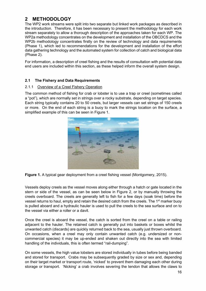
The common method of fishing for crab or lobster is to use a trap or creel (sometimes called a “pot”), which are normally set in strings over a rocky substrate, depending on target species. Each string typically contains 20 to 50 creels, but larger vessels can set strings of 150 creels or more. On the end of each string is a buoy to mark the strings location on the surface, a simplified example of this can be seen in Figure 1.

Figure 1. A typical gear deployment from a creel fishing vessel (Montgomery, 2015).

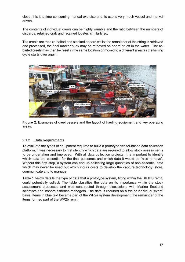
Vessels deploy creels as the vessel moves along either through a hatch or gate located in the stern or side of the vessel, as can be seen below in Figure 2, or by manually throwing the creels overboard. The creels are generally left to fish for a few days (soak time) before the vessel returns to haul, empty and retain the desired catch from the creels. The 1st marker buoy is pulled aboard and a hydraulic hauler is used to pull the creels to the sea surface and on to the vessel via either a roller or a davit. Once the creel is aboard the vessel, the catch is sorted from the creel on a table or railing adjacent to the hauler. The retained catch is generally put into baskets or boxes whilst the unwanted catch (discards) are quickly returned back to the sea, usually just thrown overboard. On occasions, when a creel may only contain unwanted catch (e.g. undersized or non-commercial species) it may be up-ended and shaken out directly into the sea with limited handling of the individuals, this is often termed “rail-dumping”. On some vessels, the high value lobsters are stored individually in tubes before being banded and stored for transport. Crabs may be subsequently graded by size or sex and, depending on their target market or transport route, ‘nicked’ to prevent them damaging each other during storage or transport. ‘Nicking’ a crab involves severing the tendon that allows the claws to

17

close, this is a time-consuming manual exercise and its use is very much vessel and market driven. The contents of individual creels can be highly variable and the ratio between the numbers of discards, retained crab and retained lobster, similarly so. The creels are then re-baited and stacked aboard whilst the remainder of the string is retrieved and processed, the final marker buoy may be retrieved on board or left in the water. The re-baited creels may then be reset in the same location or moved to a different area, as the fishing cycle starts over again.

Figure 2. Examples of creel vessels and the layout of hauling equipment and key operating areas.

2.1.2 Data Requirements

To evaluate the types of equipment required to build a prototype vessel-based data collection platform, it was necessary to first identify which data are required to allow stock assessments to be undertaken and improved. With all data collection projects, it is important to identify which data are essential for the final outcomes and which data it would be “nice to have”. Without this first step, a system can end up collecting large quantities of non-essential data which may never be used but which incurs costs to develop the capture technology, store, communicate and to manage.

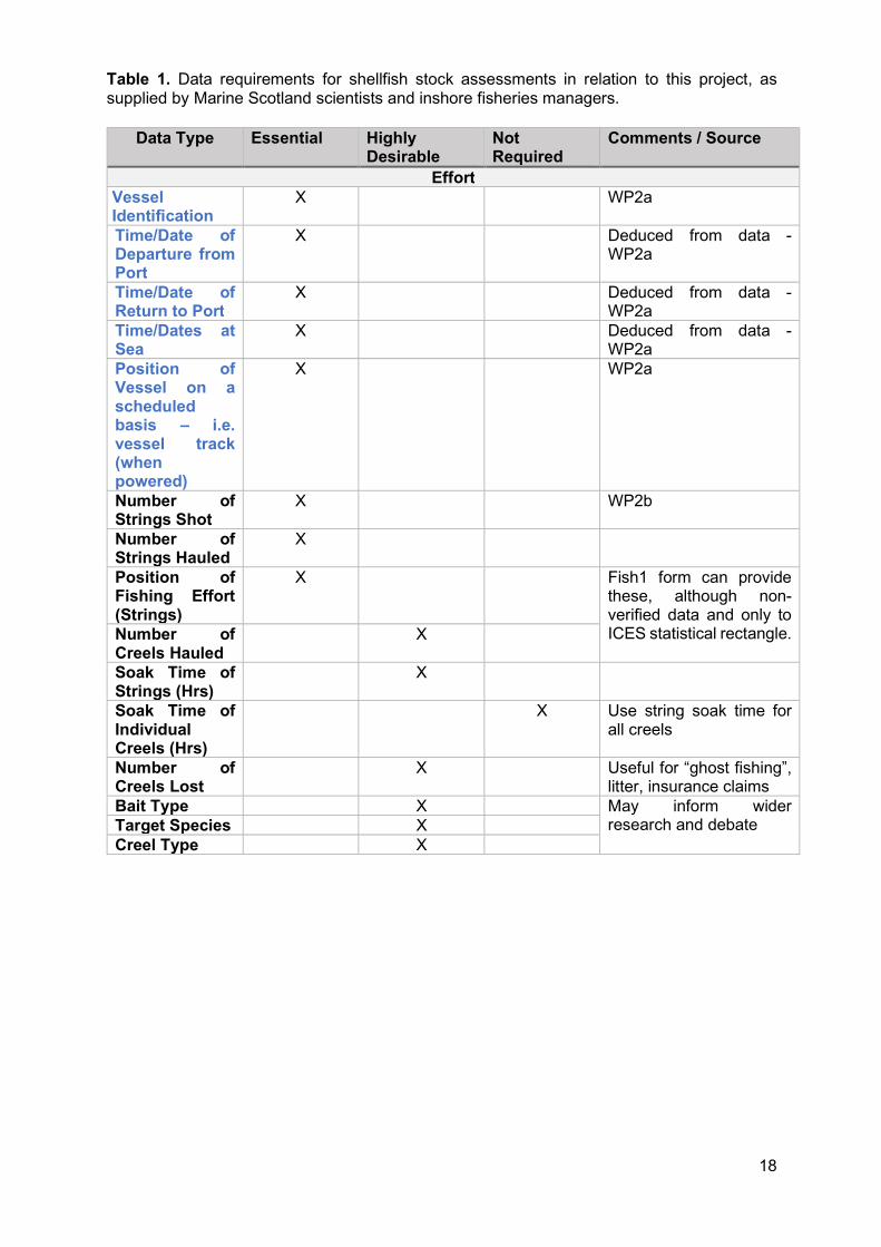
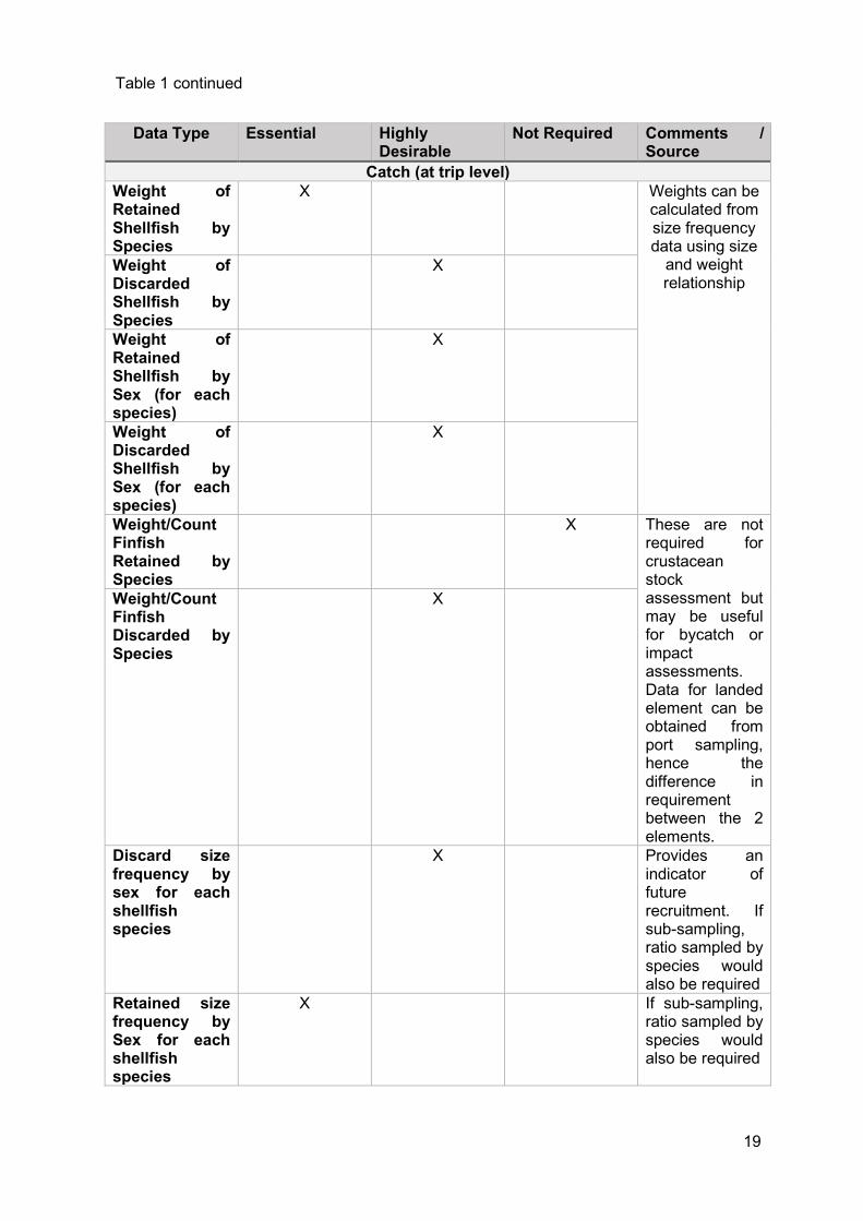
Table 1 below details the type of data that a prototype system, fitting within the SIFIDS remit, could potentially collect. The table classifies the data on its importance within the stock assessment processes and was constructed through discussions with Marine Scotland scientists and inshore fisheries managers. The data is required on a trip or individual ‘event’ basis. Items in blue text became part of the WP2a system development, the remainder of the items formed part of the WP2b remit.

18

Table 1. Data requirements for shellfish stock assessments in relation to this project, as supplied by Marine Scotland scientists and inshore fisheries managers.

Data Type Essential Highly Desirable

Not Required

Comments / Source

Effort Vessel Identification

X WP2a

Time/Date of Departure from Port

X Deduced from data -WP2a

Time/Date of Return to Port


Time/Dates at Sea


Position of Vessel on a scheduled basis – i.e. vessel track (when powered)

X WP2a

Number of Strings Shot

X WP2b

Number of Strings Hauled

X

Position of Fishing Effort (Strings)

X Fish1 form can provide these, although non-verified data and only to ICES statistical rectangle. Number of

Creels Hauled X

Soak Time of Strings (Hrs)

X

Soak Time of Individual Creels (Hrs)

X Use string soak time for all creels

Number of Creels Lost

X Useful for “ghost fishing”, litter, insurance claims

Bait Type X May inform wider research and debate Target Species X

Creel Type X

19


Not Required Comments / Source

Catch (at trip level) Weight of Retained Shellfish by Species

X Weights can be calculated from size frequency data using size

and weight relationship

Weight of Discarded Shellfish by Species

X

Weight of Retained Shellfish by Sex (for each species)

X

Weight of Discarded Shellfish by Sex (for each species)

X

Weight/Count Finfish Retained by Species

X These are not required for crustacean stock assessment but may be useful for bycatch or impact assessments. Data for landed element can be obtained from port sampling, hence the difference in requirement between the 2 elements.

Weight/Count Finfish Discarded by Species

X

Discard size frequency by sex for each shellfish species

X Provides an indicator of future recruitment. If sub-sampling, ratio sampled by species would also be required

Retained size frequency by Sex for each shellfish species

X If sub-sampling, ratio sampled by species would also be required

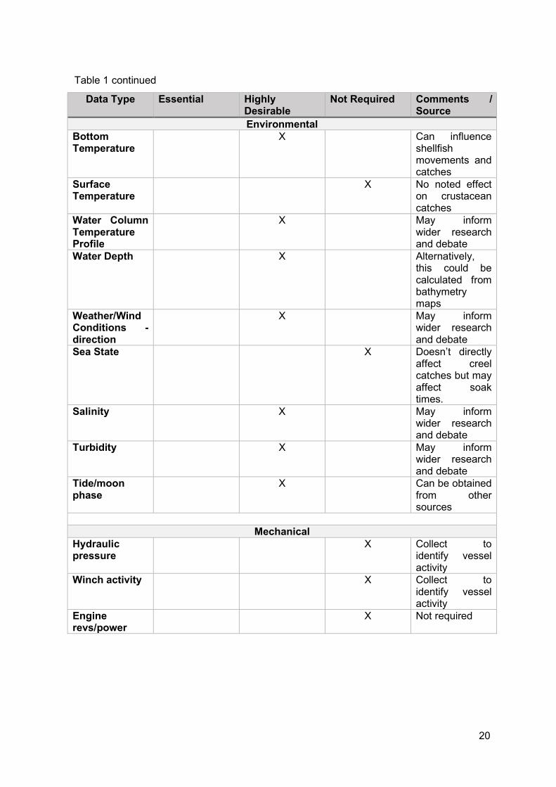
Table 1 continued

20


Not Required Comments / Source

Environmental Bottom Temperature

X Can influence shellfish movements and catches

Surface Temperature

X No noted effect on crustacean catches

Water Column Temperature Profile

X May inform wider research and debate

Water Depth X Alternatively, this could be calculated from bathymetry maps

Weather/Wind Conditions - direction

X May inform wider research and debate

Sea State X Doesn’t directly affect creel catches but may affect soak times.

Salinity X May inform wider research and debate

Turbidity X May inform wider research and debate

Tide/moon phase

X Can be obtained from other sources

Mechanical

Hydraulic pressure

X Collect to identify vessel activity

Winch activity X Collect to identify vessel activity

Engine revs/power

X Not required

Table 1 continued

21

2.1.3 Opportunities for Data Collection

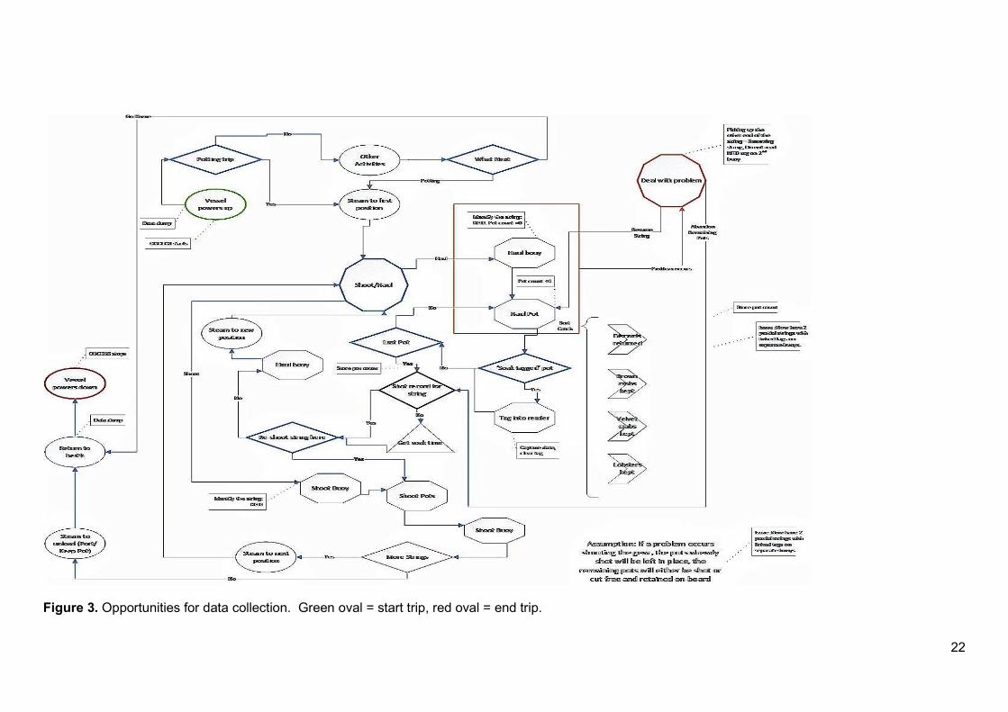
In order to identify potential data collection points within a vessel’s activity cycle an ‘activity model’ was developed to help clarify the processes, identify pinch points and focus activity onto the most practicable areas for implementation of technology solutions. Note; the activity model shown in Figure 3, below includes a single physical tag (soak tag) to obtain additional environmental data from a string. This is not an essential part of the model but is left in to show how this concept would fit into the activity cycle. This activity model is based on SeaScope's experience with the inshore creel fisheries and refined in conjunction with skippers as part of the Phase 2 vessel survey activities.

22

Figure 3. Opportunities for data collection. Green oval = start trip, red oval = end trip.

23

2.2 WP2a

2.2.1 System Requirements

The first stage of this project was to identify what data was required to be collected by the OBCDCS for the various end user groups and identify the functions the system would be required to perform. Discussions undertaken during the project steering meetings and additional discussions with Marine Scotland Compliance (MS), Marine Scotland Science (MSS), end users and the project managers, identified that the following information would be useful for informing fishery management decisions and should be collected by the OBCDCS:

Data – time and date of vessel activity Data – location of vessel Function – store additional sensor activity Function – store catch data from electronic catch system Function – link additional sensor, catch data and OBCDCS data together Function – communicate all data remotely to a cloud based central storage database Function – operate in the field for 6 months

At first glance this specification may resemble a simple tracking device such as AIS or a satellite tracker, but there are significant differences which impact on the complexity and cost of the system and the development processes. The requirements to link, store and forward the information collected from an unspecified range of sensors to a cloud-based server requires large capacity storage devices to be built into the system. The need to communicate this daily requires some form of communication device to allow data to be sent via low cost 3G/4G or Wi-Fi networks. Other methods of data collection (manual hard-drive swaps and satellite communications) were considered early on in the project but were subsequently discounted as suitable methods due to inefficiency and cost factors. The need to store data from a variety of sensor sources requires the design and development of a flexible local and cloud-based databases.

2.2.2 System design – Concepts

The requirement to geo and temporally tag data streams from a variety of sources can be achieved in many ways, these can effectively be condensed down to 2 generic pathways:

1. A central processor receives and processes the data feeds from all sensors including receiving and processing the Global Navigation Satellite System (GNSS) positional data. The processor would also manage the database storage and its subsequent communication ashore.

2. Using a central database server, receiving processed GNSS positional data and processed sensor data. Each sensor has its own interface unit to the server providing the processed or raw data via Transmission Control Protocol/Internet Protocol (TCP/IP) connections. The central server would link each sensor data package to the latest GNSS ‘ping’, a data management module would manage communication with the reception database.

24

Each of the pathways has advantages and disadvantages, the project team had to consider these alongside the requirements of the project to make an informed judgement as to which pathway to follow.

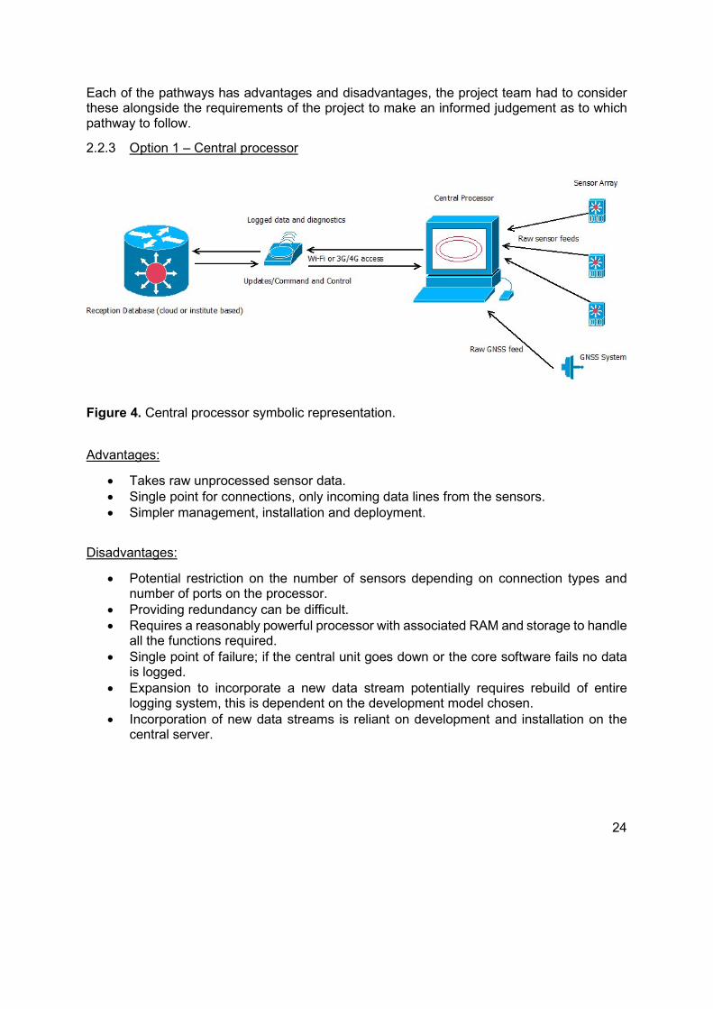
2.2.3 Option 1 – Central processor

Figure 4. Central processor symbolic representation.

Advantages:

Takes raw unprocessed sensor data. Single point for connections, only incoming data lines from the sensors. Simpler management, installation and deployment.

Disadvantages:

Potential restriction on the number of sensors depending on connection types and number of ports on the processor.

Providing redundancy can be difficult. Requires a reasonably powerful processor with associated RAM and storage to handle

all the functions required. Single point of failure; if the central unit goes down or the core software fails no data

is logged. Expansion to incorporate a new data stream potentially requires rebuild of entire

logging system, this is dependent on the development model chosen. Incorporation of new data streams is reliant on development and installation on the

central server.

25

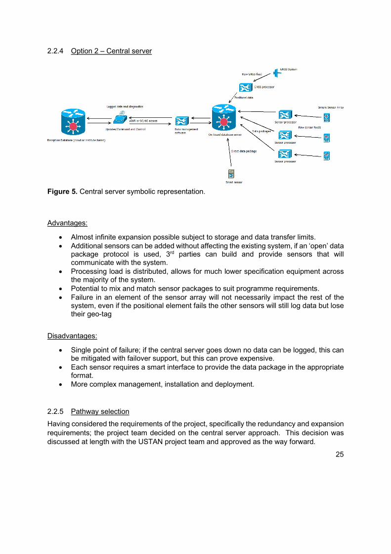
2.2.4 Option 2 – Central server

Advantages:

Almost infinite expansion possible subject to storage and data transfer limits. Additional sensors can be added without affecting the existing system, if an ‘open’ data

package protocol is used, 3rd parties can build and provide sensors that will communicate with the system.

Processing load is distributed, allows for much lower specification equipment across the majority of the system.

Potential to mix and match sensor packages to suit programme requirements. Failure in an element of the sensor array will not necessarily impact the rest of the

system, even if the positional element fails the other sensors will still log data but lose their geo-tag

Disadvantages:

Single point of failure; if the central server goes down no data can be logged, this can be mitigated with failover support, but this can prove expensive.

Each sensor requires a smart interface to provide the data package in the appropriate format.

More complex management, installation and deployment.

2.2.5 Pathway selection

Having considered the requirements of the project, specifically the redundancy and expansion requirements; the project team decided on the central server approach. This decision was discussed at length with the USTAN project team and approved as the way forward.

Figure 5. Central server symbolic representation.

26

2.2.6 Hardware selection

Selection of hardware was driven by 4 major factors; size, power requirements, initial cost and ongoing cost. The first two factors are related to installation and suitability for vessels in the under 12m fleet, the remaining factors are linked to budgetary constraints. Most of the vessels in the target fleet can only readily provide 12 or 24 volt DC supplies with limits on wattage available for the system, and have limited space available for installation of the equipment. Although the ability of the equipment to survive the harsh environment found on a fishing vessel is a major factor, it is relatively easily mitigated by selecting appropriate enclosures for the equipment and thus did not figure largely in the selection process. As the system is required to be autonomous with no human interaction on a regular basis there is no requirement for the system to support a complex Graphical User Interface (GUI) or provide a Human Machine Interface (HMI), this opened up the possibilities for the hardware. To provide the database server functionality two routes were explored; an embedded PC (Linux or Windows based) running the database engine with suitably sized storage onboard, or, an off-the-shelf Network Attached Storage (NAS) device providing the database engine and storage straight out of the box. For ease of installation, maintenance and replicability, the NAS route was chosen, exploration of the NAS offerings available resulted in the selection of Synology DS218+ systems with Solid State Hard-Drives (SSDs). This selection was made based on the power requirements (12V DC), physical size and the level of manufacturer and community support available. The units were specified with 2TB of storage to accommodate large volumes of data as at this point data volumes were unknown. SSDs were chosen over standard rotary hard drives as there is no danger of head-crashes in a vibration and movement intense environment, there is a downside to SSDs in that they have limited read/write cycles compared to a standard HDD, resulting in a shorter operational life, which is not ideal in a write intensive database environment, however this was outweighed by the environmental issues. The Synology devices support a variety of database engines, MariaDB (a MySQL fork) was chosen as it is supported by Synology as a recommended product, has no licence costs and has a large user base and associated support community. To provide the GNSS positional data an embedded PC system was required with a GNSS antenna and associated hardware to decode the GNSS signals. Raspberry Pis (model 3B) were chosen as the embedded system due to their cost, small footprint, low power requirements and extremely active support community. A number of GNSS solutions were explored with the final selection being a dedicated add-on board (RasPiGNSS) partnered with a Tallysman antenna. This route was chosen as it provided access to the GPS, GLONASS and Galileo GNSS systems as well as the possibility to incorporate Real Time Kinematic (RTK - a technique which can provide centimetre level accuracy for the position) functionality in the future if needed. Because the antenna is separate from the processing board it is possible to mount the antenna much further away from the processing unit than would be possible using a cheaper USB GPS only patch. 2 Raspberry Pis with GNSS capability were installed to provide redundancy for the critical data stream. The Raspberry Pis had their settings modified to allow them to boot from USB sticks rather than the standard Secure Digital (SD) cards as we experienced some issues with card corruption which may have been partially caused by uncontrolled shutdowns, i.e. when the

27

vessel powers down, the units effectively suffer a power-cut rather than a controlled shut-down. There are Uninterruptible Power Supplies (UPS) units available for the Rasberry Pis but they either use the communication lines already in use for the GNSS, are too expensive, or take too long to charge enough to support the device for the length of time needed to safely shut-down. All of the UPS devices provide functionality and features which are total unnecessary for this application. This application needs a simple device that charges quickly, monitors the incoming supply, switches seamlessly to UPS mode once the incoming supply drops and raises a signal to the Raspberry Pi to start a safe shut-down. Some exploratory development work was undertaken to pursue this using Super-Capacitors, which charge extremely quickly, and some straightforward electronics to provide the charging, switch-over and signalling. The signalling would be achieved using a single line to a spare General-Purpose Input Output (GPIO) pin on the Raspberry Pi. The power monitoring software was written and tested and a safe shut down can be achieved from a GPIO signal, the UPS board was designed in an electronics CAD package and works in theory, charging in under 10 minutes and providing 4 minutes backup power, a Pi shutdown takes 1 to 2 minutes. As the switch to USB stick booting seemed to largely mitigate the issue, the development was halted. For future iterations of the project it will be worth considering using a UPS within the system. 3G and 4G connectivity was provided using a Teltonika RUT955 router modem, again selected for power consumption and physical size. The RUT955 provides additional functionality allowing the data management software to interrogate the unit via Modbus protocol (amongst others) to obtain statistics about the connection, data transferred etc. The units were fitted with Vodafone data only SIM cards as these provided the best coverage within the target region. Due to the short-term nature of the project, the SIM cards were operated on a pay-as-you-go contract requiring regular monitoring and top-up. Network interconnectivity was achieved with the installation of Netgear GS108 unmanaged gigabit network switches, again chosen for power and size characteristics along with ease of maintenance and replicability. Power is provided to the different units using a set of buck-boost devices which can take an input voltage ranging from 9 to 36 VDC and provide the appropriate output voltage for each piece of equipment. All the equipment is housed in a single IP67 rated case measuring externally 48 x 36 x 19 cm, the case has 7 glanded entries for antenna, power and sensor feeds as well as an IP67 rated network connector. Should additional sensor feeds be required there is adequate space for further glanded entries to be fitted. A list of the core elements of a WP2A and 2B system can be found in Annex 5.

28

2.2.7 The physical equipment

The following figures show the equipment as deployed in the field trials, each unit deployed was internally identical, some units had additional connection options installed to suit the needs of the particular installation.

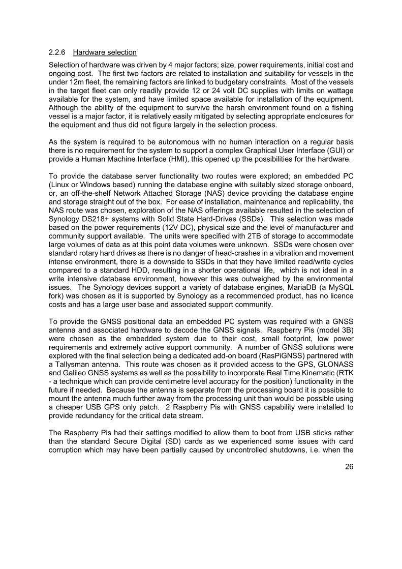
The very first build used IP67 rated panel mount connectors and their associated cable mount equivalents (Figure 6).

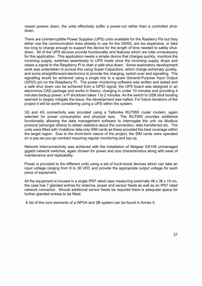
It was thought this would make for easy installs with the cabling being made up prior to visiting the vessel and just simply plugging everything in. However, it very soon became apparent that routing 4 or more 18mm connectors around the wheelhouse of an under 10m vessel is signficantly more difficult than just routing the 3mm diameter cables. There were no screw terminal connectors available that suited the cabling and boxes and attempting to solder the terminals, potentially on the roof of the wheelhouse or on the deck of a vessel, is not practical; so the glanded solution was chosen with the box using internal screw terminals that are easier to handle in the field. Figures 7 and 8 show the internal components of the OBCDCS.

Figure 6. Original IP67 connector assembly.

Figure 7. Base of completed logger unit, note the incoming power and antennae leads were removed for clarity.

29

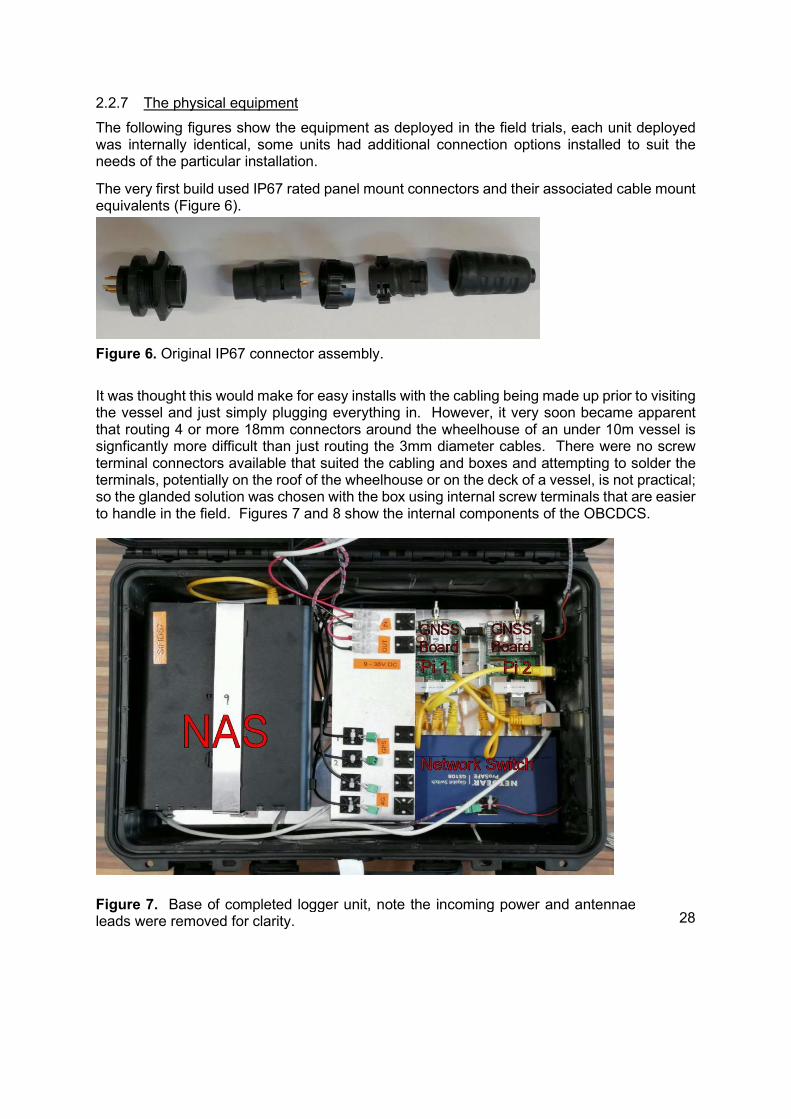
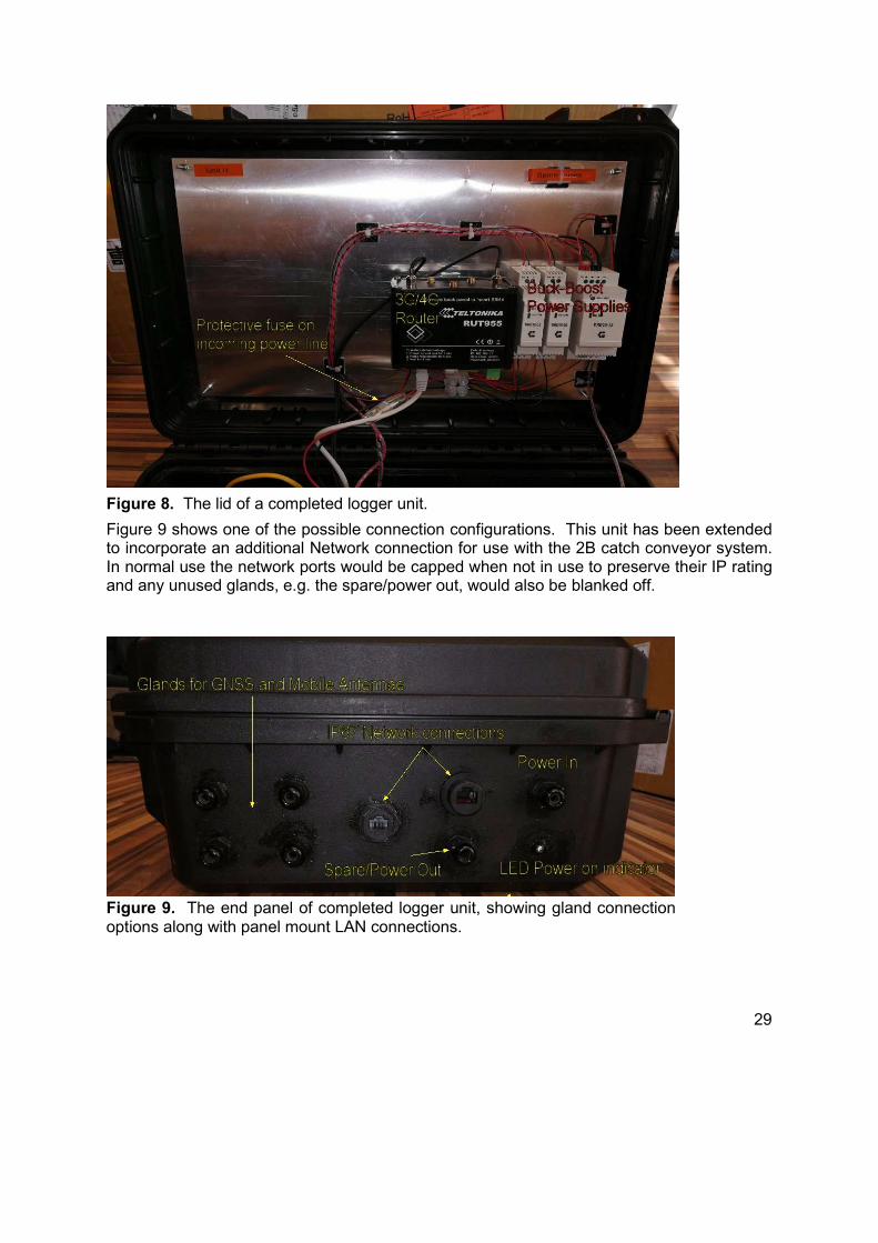
Figure 9 shows one of the possible connection configurations. This unit has been extended to incorporate an additional Network connection for use with the 2B catch conveyor system. In normal use the network ports would be capped when not in use to preserve their IP rating and any unused glands, e.g. the spare/power out, would also be blanked off.

Figure 9. The end panel of completed logger unit, showing gland connection options along with panel mount LAN connections.

Figure 8. The lid of a completed logger unit.

30

2.2.8 Database functionality and logger software

The system uses 2 database systems; as described previously, the local (on-board) database is MariaDB hosted on the NAS, the reception (“shore” based) database is hosted on a PostgreSQL instance provided in the cloud via Amazon Web Services (AWS).

2.2.9 Local database functionality

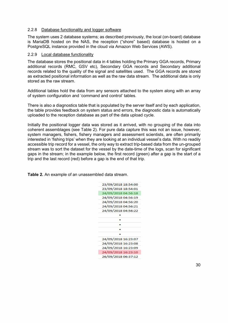
The database stores the positional data in 4 tables holding the Primary GGA records, Primary additional records (RMC, GSV etc), Secondary GGA records and Secondary additional records related to the quality of the signal and satellites used. The GGA records are stored as extracted positional information as well as the raw data stream. The additional data is only stored as the raw stream. Additional tables hold the data from any sensors attached to the system along with an array of system configuration and ‘command and control’ tables. There is also a diagnostics table that is populated by the server itself and by each application, the table provides feedback on system status and errors, the diagnostic data is automatically uploaded to the reception database as part of the data upload cycle. Initially the positional logger data was stored as it arrived, with no grouping of the data into coherent assemblages (see Table 2). For pure data capture this was not an issue, however, system managers, fishers, fishery managers and assessment scientists, are often primarily interested in ‘fishing trips’ when they are looking at an individual vessel’s data. With no readily accessible trip record for a vessel, the only way to extract trip-based data from the un-grouped stream was to sort the dataset for the vessel by the date-time of the logs, scan for significant gaps in the stream; in the example below, the first record (green) after a gap is the start of a trip and the last record (red) before a gap is the end of that trip.

Table 2. An example of an unassembled data stream.

31

Although a workable solution, it requires significant processing, careful definition of a ‘gap’ and realistically could not provide a ‘live’ trip-based data stream to WP6. To attempt to directly provide trip-based data grouping at the point of capture, the concept of a data-session was created; each time the server boots it creates a record in a control table that identifies the current session, it is a simple incrementing integer, the server also timestamps the session. Every GNSS log is associated with the current session, and from the GNSS log, every other record in the system is also associated with the session. When the data is uploaded to the reception database the session is prefixed with the vessel’s id within the project, thus creating a unique session ID within the whole WP2 data set. The concept works in general but as it is based on power cycles to the server it is affected by vessel behaviour;

Vessel powers up, fishes for the day, returns to port and powers down = 1 Session. Vessel powers up, fishes for 4 hours and then powers down for a peaceful lunch before

recommencing fishing and returning to port (genuine example) = 2 Sessions. In this example you could replace lunch with any number of reasons to fully power down including unexpected mechanical issues, resetting misbehaving electronics etc.

One of the trial fleet, for reasons we were never able to fully uncover, always started a session that lasted up to 10 minutes, followed by 1 or several very short sessions finally followed by a full day trip. It was thought that possibly the skipper powered the vessel up (including the logger system) without starting the engine, the drain of subsequently starting the engine caused such a voltage drop that the logger system powered off, once the engine was running, or the skipper waited to try starting it again, the logger system started up creating another new session until finally the day’s work commenced.

The data session concept is not a complete solution but combined with some post-processing, for example, if the next data session starts within 1 hour of the end of the last AND is within 0.25 nm of the last position then join them into a single session, it may prove to be the most appropriate. Other options to better define a trip could include geo-fencing functionality and/or using speed thresholds to identify fishing activity within a trip. As each primary GGA record is inserted to the database it is allocated a Globally Universally Unique Identifier (GUUID). This GUUID is subsequently used to link the additional and secondary positional records in the database back to the primary log. The GUUID is also used to link any sensor data back to the most recent primary GNSS record when the sensor data is received. The positional data is inserted to the tables directly by the loggers, sensor input is achieved using a stored procedure. The sensor stored procedure uses a simple eXtended Markup Language (XML) data package to transport the data. The XML can contain a single sensor value, a number of values or a 2D array of values. This single approach to a data package which can handle multiple data formats means new sensor data streams can be added without requiring further development work on the database. The stored procedure validates that the Media Access Control (MAC) address of the sensor providing the data package (all network adaptors have a unique MAC address) is in the system sensor list and that the parameters in the data package match those configured for the sensor. Once the data package is verified the stored procedure attaches

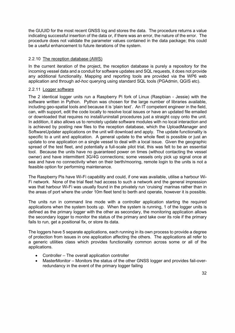
32

the GUUID for the most recent GNSS log and stores the data. The procedure returns a value indicating successful insertion of the data or, if there was an error, the nature of the error. The procedure does not validate the parameter values contained in the data package; this could be a useful enhancement to future iterations of the system.

2.2.10 The reception database (AWS)

In the current iteration of the project, the reception database is purely a repository for the incoming vessel data and a conduit for software updates and SQL requests, it does not provide any additional functionality. Mapping and reporting tools are provided via the WP6 web application and through ad-hoc querying using standard SQL tools (PGAdmin, QGIS etc).

2.2.11 Logger software

The 2 identical logger units run a Raspberry Pi fork of Linux (Raspbian - Jessie) with the software written in Python. Python was chosen for the large number of libraries available, including geo-spatial tools and because it is ‘plain text’. An IT competent engineer in the field, can, with support, edit the code locally to resolve local issues or have an updated file emailed or downloaded that requires no install/uninstall procedures just a straight copy onto the unit. In addition, it also allows us to remotely update software modules with no local interaction and is achieved by posting new files to the reception database, which the UploadManager and SoftwareUpdater applications on the unit will download and apply. The update functionality is specific to a unit and application. A general update to the whole fleet is possible or just an update to one application on a single vessel to deal with a local issue. Given the geographic spread of the test fleet, and potentially a full-scale pilot trial, this was felt to be an essential tool. Because the units have no guaranteed power on times (without contacting the vessel owner) and have intermittent 3G/4G connections; some vessels only pick up signal once at sea and have no connectivity when on their berth/mooring, remote login to the units is not a feasible option for performing maintenance. The Raspberry Pis have Wi-Fi capability and could, if one was available, utilise a harbour Wi-Fi network. None of the trial fleet had access to such a network and the general impression was that harbour Wi-Fi was usually found in the privately run ‘cruising’ marinas rather than in the areas of port where the under 10m fleet tend to berth and operate, however it is possible. The units run in command line mode with a controller application starting the required applications when the system boots up. When the system is running, 1 of the logger units is defined as the primary logger with the other as secondary, the monitoring application allows the secondary logger to monitor the status of the primary and take over its role if the primary fails to run, get a positional fix, or store its data. The loggers have 5 separate applications, each running in its own process to provide a degree of protection from issues in one application affecting the others. The applications all refer to a generic utilities class which provides functionality common across some or all of the applications.

Controller – The overall application controller MasterMonitor – Monitors the status of the other GNSS logger and provides fail-over-

redundancy in the event of the primary logger failing

33

UploadManager – Manages the upload of the data to the reception system, downloads software updates and Structured Query Language (SQL) requests

SoftwareUpdater – Executes software updates with roll-back support in case of failure to update

SQLExecutor – Executes SQL statements downloaded against the local NAS database

GNSSLogger – The actual logging application

2.2.11.1 Controller

The controller application is started as part of the system boot via a Bash (shell) script. It takes an array of command line parameters that control which applications it should start. If the controller is run by a logged in user from the command line rather than the Bash boot-up script it displays messages from all its child applications in the console window, this was incorporated to aid development and debugging. The messages are transferred from the child applications to the controller using Transmission Control Protocol/Internet Protocol (TCP/IP) port messaging.

2.2.11.2 MasterMonitor

The master monitor application runs to a schedule set in the configuration table in the database, for this project it was set at 300 seconds. Each time it runs it checks if the unit is the primary logger. If it is, it then checks whether it has been usurped by the secondary logger taking over the primary role. If the unit is the secondary logger the monitor program then checks the latest timestamps for the primary logger for activity, a good fix and a good log to the database. If the time elapsed since the timestamps were updated exceed the individual settings in the configuration table, the master monitor forces the secondary logger to become primary and sets a flag on the database so the next log from the original primary will become secondary.

As can be seen from the diagram (Figure 10), there is the potential for the 2 units to ‘flip-flop’ in situations where neither can successfully achieve a logged fix, this will continue until one of them does. Each time the secondary logger takes over from the primary it logs a diagnostic message on the NAS giving all the details. Once these diagnostic logs are uploaded to the reception database, they can be analysed to identify potential recurrent issues with systems and a technician could be scheduled to visit before a complete system failure occurs; if it was considered to be hardware issue rather than, for example, the issue always occurring in an area of poor reception.

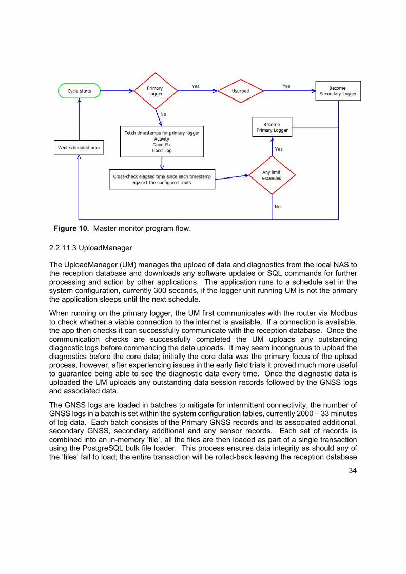
34

2.2.11.3 UploadManager

The UploadManager (UM) manages the upload of data and diagnostics from the local NAS to the reception database and downloads any software updates or SQL commands for further processing and action by other applications. The application runs to a schedule set in the system configuration, currently 300 seconds, if the logger unit running UM is not the primary the application sleeps until the next schedule.

When running on the primary logger, the UM first communicates with the router via Modbus to check whether a viable connection to the internet is available. If a connection is available, the app then checks it can successfully communicate with the reception database. Once the communication checks are successfully completed the UM uploads any outstanding diagnostic logs before commencing the data uploads. It may seem incongruous to upload the diagnostics before the core data; initially the core data was the primary focus of the upload process, however, after experiencing issues in the early field trials it proved much more useful to guarantee being able to see the diagnostic data every time. Once the diagnostic data is uploaded the UM uploads any outstanding data session records followed by the GNSS logs and associated data.

The GNSS logs are loaded in batches to mitigate for intermittent connectivity, the number of GNSS logs in a batch is set within the system configuration tables, currently 2000 – 33 minutes of log data. Each batch consists of the Primary GNSS records and its associated additional, secondary GNSS, secondary additional and any sensor records. Each set of records is combined into an in-memory ‘file’, all the files are then loaded as part of a single transaction using the PostgreSQL bulk file loader. This process ensures data integrity as should any of the ‘files’ fail to load; the entire transaction will be rolled-back leaving the reception database

Figure 10. Master monitor program flow.

35

in the same state as before the upload was attempted. The GNSS records are loaded oldest first so the system attempts to keep the data stream on the reception database consistent. The batch loading process continues as long as connectivity is available and there are logs to load, once all outstanding logs are loaded the UM proceeds to download software updates and SQL command requests, once complete, or if the connectivity drops out, the UM sleeps until the next cycle.

Given the current system configuration and a consistent good signal, the system theoretically provides a 1Hz (one record per second) positional and sensor data stream with a maximum lag of 5 minutes.

Although the GUUID system and transactional loading should ensure that entire GNSS record groups are loaded only once, we did experience issues with either roll-backs not occurring properly or a failure in the local flagging indicating that a primary GNSS record was uploaded. This caused data keying errors when attempting to load a primary GNSS record that already existed on the reception database. The underlying cause was never uncovered, the UM now implements a handling routine to deal with ‘duplicate key’ errors when loading primary GNSS records. The routine assumes that the data on the NAS is the correct data and that the reception database is in error, in the event of a duplicate key error the handling routine deletes ALL the primary GNSS records, the reception database cascades these deletes to incorporate all the linked records in the current batch from the reception database, before re-loading them in their entirety. This activity is logged in the diagnostics and can be further investigated if required.

Software updates are handled on a schedule by the SoftwareUpdater application, should SQL requests be received they are actioned immediately by the UM spawning a SQLExecutor process.

2.2.11.4 SoftwareUpdater

The SoftwareUpdater (SU) application runs to a schedule set in the system configuration, it runs irrelevant of the logger status (primary or secondary). Each software update targets a specific MAC address, thus allowing updates to be applied to specific units. The software updater can be implemented on any Raspberry Pi in the system, it is currently also used on the 2B effort systems. The SU checks the NAS for any updates specific to the MAC address of the unit it is running on, each update has a target filename and an associated Binary Large OBject (BLOB) which constitutes the updated file. BLOB was the chosen format as it can manage embedded special characters etc. that would not be acceptable in a plain text field. The updated file is not necessarily a Python program, it can be an update to one of the system scripts etc. If an applicable update is found, the SU first makes a backup copy of the original file before attempting to replace it and set the executable status of the file. Should either the overwrite or status change fail, the SU will use the backup copy to revert the system to its previous state. The SU will create diagnostic records indicating the result of the update process. Updates only take effect at the next system boot. It would be possible for the SU to either force a restart of the updated application/script or a system reboot, however, given the possible interdependencies between applications this functionality was not pursued as part of the trial project but could form part of a follow-on development.

36

2.2.11.5 SQLExecutor

The SQLExecutor (SE) is only run when the UploadManager encounters a SQL command that is applicable to the MAC address of the unit running. The SE takes in a single SQL statement from the NAS download tables and executes it against the NAS database. The statement is held in a plain text field to aid human readability in the field, however due to its plain text nature, certain special characters such as single and double quotes etc cannot easily be incorporated, these have been replaced by custom embedded sequences (**SQ, **DQ etc) which the SE interprets when building the statement to be executed. The SE is not, in this iteration, intended for day-to-day use, it was developed to allow remote control of local databases when problems were encountered. Its usefulness has been proven during the trials and it would be highly desirable for a full featured implementation to form part of any follow-on project.

2.2.11.6 SoftwareUpdater and SQLExecutor – Notes

These 2 applications have proven extremely useful during the development and field trials of the system, however, due to their ability to directly affect both the data integrity and operation of the systems their use should be carefully considered and the updates or SQL requests thoroughly tested on an accessible system before rolling out to remote systems. An inadvertent or ill-advised update could completely disable a system and require a technician visit to rectify.

2.2.11.7 GNSSLogger

Although the logger application is the core data source for the system, its operation is relatively straightforward compared to the other applications. Once the application starts it configures the GNSS board to provide the required data stream and collects the system parameter for log frequency from the NAS control table. The application then cycles, constantly reading the data stream from the GNSS board. The board provides the data stream via serial data (RS232) as standard National Marine Electronics Association (NMEA) sentences. The software reads each sentence and validates it against its embedded checksum. The positional sentences (GGA) are subjected to further validation using the embedded validity flags from within the sentence along with checks on the number of satellites providing the ‘fix’. Once a valid GGA has been received and it is required to be logged under the frequency requirement, the application checks its status (primary or secondary) and inserts the processed and raw GGA record into the appropriate table. The database on the NAS handles allocation of the log GUUID and linkages. For non-GGA records; if the previous GGA record was logged and the non-GGA sentence is in the list of additional sentences to be logged, it is logged to the appropriate table. For the purposes of this trial, the log frequency was set to 1 second, complementing with the work conducted under WP8a and WP8b. This allowed for detailed analysis of positional data to examine whether individual creel hauls could be identified purely from the positional data, as well as allowing for analysis to determine the most appropriate log frequency needed to achieve the aims of future projects.

37

2.2.12 Vessel Selection

As part of WP8a the at-sea-observers undertook questionnaire and physical surveys of the skippers and vessels that were being accompanied to sea. The purposes of these surveys was to identify the reason why fishers behave as they do and what drivers influence their decision making processes (for WP8b); to establish a pool of vessels that would be willing to participate in the WP2a trials of the OBCDCS; and to identify vessels within this pool of volunteers that would be willing and suitable to participate in the WP2b effort and catch trials. These were very basic surveys which were designed to allow an observer to record the physical configuration of a volunteer vessel which would allow a decision to be made on whether it was a suitable vessel to carry the WP2a/WP2b equipment. The full results can be found in the WP8a final report, available from USTAN.

Surveys were conducted in ports and at sea with each of the vessels, to ensure that the full spectrum of information on gear and catch handling under real conditions was captured. This allowed us to observe and document what the fishers do during full operational conditions, rather than what they “think” they do. Physical surveys included the following;

how the fishers operate their fishing gear and where on board it is stored under different scenarios

deck layout sketches, measurements and imagery potential sites for locating equipment power and communication facilities any potentially harvestable data streams already on the vessel any vessel limitations that could be problematic for installation or operation

Operational surveys included the following;

how the crew separate the catch into retained and discarded segments and how and where each segment is stored on board, or returned to the sea

how the crew think electronic monitoring (EM) could be implemented within their current working practices

the general pattern of activity of the vessel, anecdotal information regarding the local fishery and any relevant local knowledge that may benefit this and other work packages.

We also worked closely with the team working on the central database (WP6) to ensure that we incorporated any data, structures or formats needed to integrate with their systems. On completion of the surveys the skippers were also asked if they would like to participate in future trials, it was made clear there would be no financial incentive.

From the pool of volunteer vessels, a total of 15 vessels were selected to undertake the WP2a trials. The selection process was based on the responses received from the survey and took into account the vessel’s main operating port. This location criteria was necessary as it was assumed that during the trials there would be numerous visits to the vessels to update or modify the systems as development progressed or to rectify faults with the systems.

38

Five vessels from the 15 selected WP2a volunteers were approached to undertake the WP2b fishing effort trials and of these, one vessel was selected to trial the electronic catch enumeration system and the environmental data logger.

2.2.13 WP2a Installation

Installation on board the 15 vessels was arranged directly with the skippers. The OBCDCS was either wired directly to the vessel’s DC power supply or connected to a circuit board with its own designated breaker switch. For some vessels, final connection was undertaken by the vessel’s contracted engineer, on others it was completed by SeaScope staff in conjunction with the vessel owner or skipper. Depending on the vessel layout, wheelhouse space and ease of running cabling, the OBCDCS unit was either located internally in the wheelhouse or externally on top of the wheelhouse. The antennae for both the GNSS and 3G/4G systems were positioned to provide the best view of the sky whilst avoiding causing interference with existing vessel equipment e.g. radar, VHF, other GNSS systems etc. Depending on the complexity of the installation process, the need to remove panels etc., a vessel installation could take anywhere between 2 and 6 hours. Once a system was installed a full test was undertaken. For some vessels, due to the lack of 3G/4G signal at the mooring, the upload element of the test had to be skipped and the vessel’s data stream monitored once it was back fishing and able to communicate with the reception database.

2.3 WP2b

2.3.1 Phased Approach

It was decided at commencement of this element of the project that it would be prudent to take a phased approach to delivery. This was thought necessary because it was necessary to first review the different existing technologies available that could be adapted to collect this information autonomously in a fishing/marine environment. If no potential suitable technology could be identified, then there would be no point in progressing with Phase 2 of the project.

The following section details the technology review process and the recommendations from this review that determined the technologies that would be investigated in Phase 2.

2.4 WP2b – Phase 1

This first phase ran from 1st December 2016 to 30th April 2017, during this initial stage SeaScope undertook meetings with the other WP leaders, Marine Scotland Science, other partners and end users to ensure their needs and expectations of the project were accurately captured. We also undertook a thorough investigation and review of the technologies that may be transferrable to this project from other industrial sectors or those already being used in a fisheries monitoring context. As well as looking at stable, commercially available equipment we also reviewed current research and development (R&D) projects which may be able to make a significant contribution to this or future projects if they reach fruition. Although the R&D elements would, in all likelihood, not be available for use within this current project, their potential modes of operation or generalised concepts may be useful, and if considered appropriate, allowances could be made in the design at this early stage to allow for later incorporation.

39

As SeaScope were also successful in securing the development of the OBCDCS (WP2a) and the development of the central database (WP6), we were able to work closely with these work packages to ensure that we could incorporate any data, structures or formats needed to integrate with these systems.

The following section is reproduced, with some editing, from the phase 1 report which led onto the decisions regarding phase 2. It details the technology explored and evaluated and provides conclusions on its suitability. It should be noted that in some areas, especially image capture and processing and artificial intelligence (AI) and machine learning, the technology has seen considerable leaps forward since the review was undertaken.

2.4.1 Fishing Activity and Effort Data Collection

Through consultation with stock assessment scientists it has been possible to identify the data that it is essential to collect (see Table 1 in the Data Requirements section presented earlier). Some of these data requirements can be collected in other work packages. For example, having a GNSS capability incorporated into the OBCDCS being developed in WP2a will allow time and position data to be collected which can allow certain effort measure data, such as days at sea, to be collected. The deck-based system being developed in WP2b is focussed on the fishing gear, gear specific effort and the catch associated with its deployment. These data will be linked to the spatial/temporal data collected in WP2a through the logging functionality delivered as part of the OBCDCS.

2.4.2 Fishing Activity Sensors

Several different types of activity sensor could be utilised to collect activity data. These sensors detect the mechanical activity associated with deployment and retrieval of fishing gear.

2.4.2.1 Photo-electric Sensors

These sensors provide a means of non-contact range detection and/or presence/absence within the sensor’s field of view. In its most basic form, a photo-electric sensor operates by emitting a beam of light, usually from a laser or infra-red light, the light is reflected back to the sensor either from the object itself, or from a strategically placed reflector (Figure 11). Through assessment of the resultant reflected beam, be it the strength of the return signal or the time it takes to receive the reflected signal, determinations about presence or absence of objects and the distance the object is from the sensor, can be made.

In a simple form, this technology has been utilised in electronic monitoring (EM) projects previously. In both English and Scottish Catch Quota Trial projects and other studies (Course et al, 2015; McElderry et al, 2010), retro-reflective sensors were utilised to monitor fishing activity by installing sensors adjacent to winch drums. Simple plastic reflector plates were then aligned and affixed to the sides of the winch drums. When fishing activity occurs, these drums rotate, with the resultant sensor output giving a measure of activity, caused by the reflector passing directly in front of the sensor and a clean reflected signal being sent to the sensor. No reflected signal is sent when parts of the drum not fitted with reflectors are rotating in front

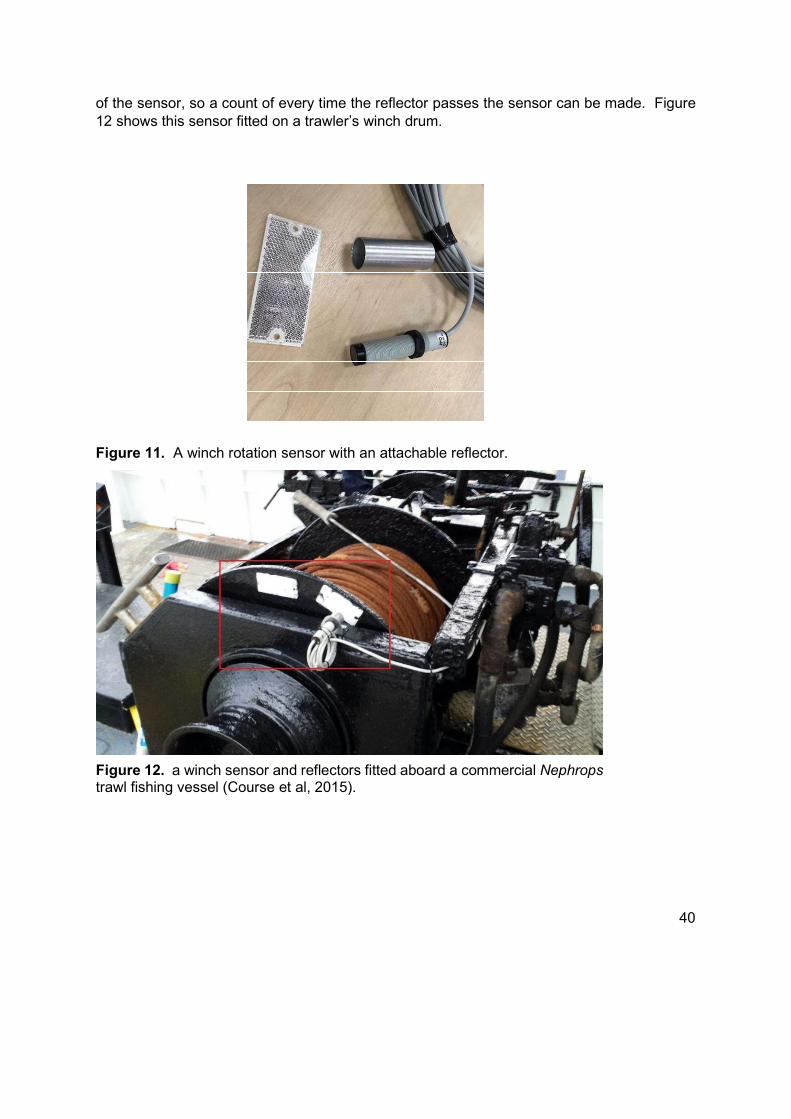
40

of the sensor, so a count of every time the reflector passes the sensor can be made. Figure 12 shows this sensor fitted on a trawler’s winch drum.

Figure 11. A winch rotation sensor with an attachable reflector.

Figure 12. a winch sensor and reflectors fitted aboard a commercial Nephropstrawl fishing vessel (Course et al, 2015).

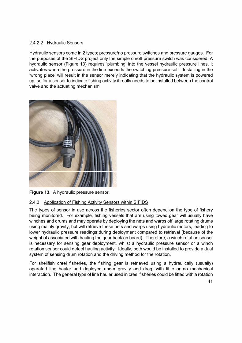
41

2.4.2.2 Hydraulic Sensors

Hydraulic sensors come in 2 types; pressure/no pressure switches and pressure gauges. For the purposes of the SIFIDS project only the simple on/off pressure switch was considered. A hydraulic sensor (Figure 13) requires ‘plumbing’ into the vessel hydraulic pressure lines, it activates when the pressure in the line exceeds the switching pressure set. Installing in the ‘wrong place’ will result in the sensor merely indicating that the hydraulic system is powered up, so for a sensor to indicate fishing activity it really needs to be installed between the control valve and the actuating mechanism.

2.4.3 Application of Fishing Activity Sensors within SIFIDS

The types of sensor in use across the fisheries sector often depend on the type of fishery being monitored. For example, fishing vessels that are using towed gear will usually have winches and drums and may operate by deploying the nets and warps off large rotating drums using mainly gravity, but will retrieve these nets and warps using hydraulic motors, leading to lower hydraulic pressure readings during deployment compared to retrieval (because of the weight of associated with hauling the gear back on board). Therefore, a winch rotation sensor is necessary for sensing gear deployment, whilst a hydraulic pressure sensor or a winch rotation sensor could detect hauling activity. Ideally, both would be installed to provide a dual system of sensing drum rotation and the driving method for the rotation.

For shellfish creel fisheries, the fishing gear is retrieved using a hydraulically (usually) operated line hauler and deployed under gravity and drag, with little or no mechanical interaction. The general type of line hauler used in creel fisheries could be fitted with a rotation

Figure 13. A hydraulic pressure sensor.

42

sensor to detect the hauling operation, but, given the protruding nature of the sensors it is likely that the sensor would get damaged or create an entanglement hazard that could catch on a creel rope or main line. A hydraulic pressure sensor could be fitted into the hydraulic circuit between the control valve and winch head and would be ideal for detecting winch activity, however, fitting of such a sensor is a specialist job.

Due to the deployment methods generally employed in creel fishing, neither a hydraulic pressure sensor nor a winch rotation sensor would be able to detect deployment activity.

The hauler-attached devices described could allow the number of strings hauled to be detected and recorded, but not the number of creels fished or soak time. It should be noted that the string count from these devices would be an estimate. There is an assumption that a given period of inactivity combined with a spatial/temporal threshold being exceeded, indicates the vessel has moved to a new string and begun a new hauling sequence. There are situations where this assumption will fail; a broken or ensnared string - where the vessel abandons hauling, travels to the other end of the string and begins hauling from that end could be counted as 2 strings if the temporal/spatial thresholds were exceeded. By the same token, 2 strings set very close together may be counted as a single string if the thresholds were set tight enough to eliminate scenario 1.

2.4.4 Use of GNSS to determine activity

Linking GNSS to the sensors as described above, can allow the data from the activity sensors to be time stamped and geographically plotted and thus allow fishing activity to be mapped. However, even by itself, GNSS is a useful tool in identifying fishing activity. In examples of using GNSS data to identify fishing activity the position of the vessel is logged, usually every 10 seconds, which allows the speed and direction of the vessel to be calculated. These data can then be interpreted based on prior knowledge of how the generic vessel type operates whilst at sea. For example, in towed gear fisheries, otter trawling for finfish, the vessel will usually steam to and from the grounds at in excess of 7-8 knots, they will then slow down to deploy the gear then speed up to let it stream out behind the vessel. When the gear finally settles on the seabed and is fishing the vessel speed generally settles to between 3 and 4.5 knots depending on the vessel, target species, sea conditions and currents. When a creeling vessel is deploying their gear, they let the drag of the water pull the gear out through a stern door (or over the side of the vessel) usually in a straight line (occasionally bending to follow a contour or underwater feature) and at a constant speed, unless there is an entanglement during the deployment process. When hauling the creels, the vessel is usually only holding station on the water or creeping very slowly when the hauler is operated, and the vessel is pulled towards the creels hanging in the water. Analysis of vessel movement characteristics can, in some circumstances, give a good interpretation of the activity at the time. There is potential that GNSS data could allow individual creels to be counted, based on the pattern described by the vessel during the hauling operation. Figure 14 shows an example of tracks described by 3 different vessels during their hauling operations. It can be seen that the tracks are very different but that string location and hauling activity can be easily discerned by eye, for all tracks. There is also the possibility that individual creels being hauled could be

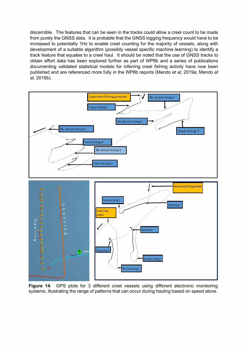
43

discernible. The features that can be seen in the tracks could allow a creel count to be made from purely the GNSS data. It is probable that the GNSS logging frequency would have to be increased to potentially 1Hz to enable creel counting for the majority of vessels, along with development of a suitable algorithm (possibly vessel specific machine learning) to identify a track feature that equates to a creel haul. It should be noted that the use of GNSS tracks to obtain effort data has been explored further as part of WP8b and a series of publications documenting validated statistical models for inferring creel fishing activity have now been published and are referenced more fully in the WP8b reports (Mendo et al, 2019a; Mendo et al, 2019b).

Figure 14. GPS plots for 3 different creel vessels using different electronic monitoring systems, illustrating the range of patterns that can occur during hauling based on speed alone.

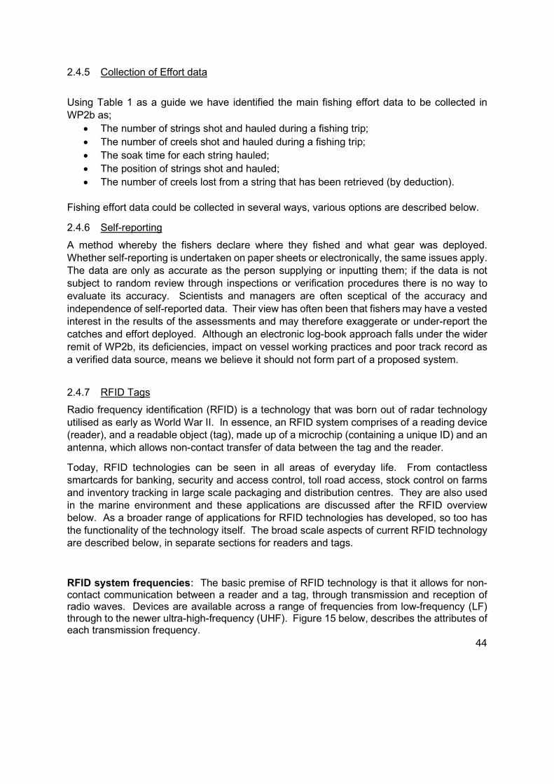
44

2.4.5 Collection of Effort data

Using Table 1 as a guide we have identified the main fishing effort data to be collected in WP2b as;

The number of strings shot and hauled during a fishing trip; The number of creels shot and hauled during a fishing trip; The soak time for each string hauled; The position of strings shot and hauled; The number of creels lost from a string that has been retrieved (by deduction).

Fishing effort data could be collected in several ways, various options are described below.

2.4.6 Self-reporting

A method whereby the fishers declare where they fished and what gear was deployed. Whether self-reporting is undertaken on paper sheets or electronically, the same issues apply. The data are only as accurate as the person supplying or inputting them; if the data is not subject to random review through inspections or verification procedures there is no way to evaluate its accuracy. Scientists and managers are often sceptical of the accuracy and independence of self-reported data. Their view has often been that fishers may have a vested interest in the results of the assessments and may therefore exaggerate or under-report the catches and effort deployed. Although an electronic log-book approach falls under the wider remit of WP2b, its deficiencies, impact on vessel working practices and poor track record as a verified data source, means we believe it should not form part of a proposed system.

2.4.7 RFID Tags

Radio frequency identification (RFID) is a technology that was born out of radar technology utilised as early as World War II. In essence, an RFID system comprises of a reading device (reader), and a readable object (tag), made up of a microchip (containing a unique ID) and an antenna, which allows non-contact transfer of data between the tag and the reader.

Today, RFID technologies can be seen in all areas of everyday life. From contactless smartcards for banking, security and access control, toll road access, stock control on farms and inventory tracking in large scale packaging and distribution centres. They are also used in the marine environment and these applications are discussed after the RFID overview below. As a broader range of applications for RFID technologies has developed, so too has the functionality of the technology itself. The broad scale aspects of current RFID technology are described below, in separate sections for readers and tags.

RFID system frequencies: The basic premise of RFID technology is that it allows for non-contact communication between a reader and a tag, through transmission and reception of radio waves. Devices are available across a range of frequencies from low-frequency (LF) through to the newer ultra-high-frequency (UHF). Figure 15 below, describes the attributes of each transmission frequency.

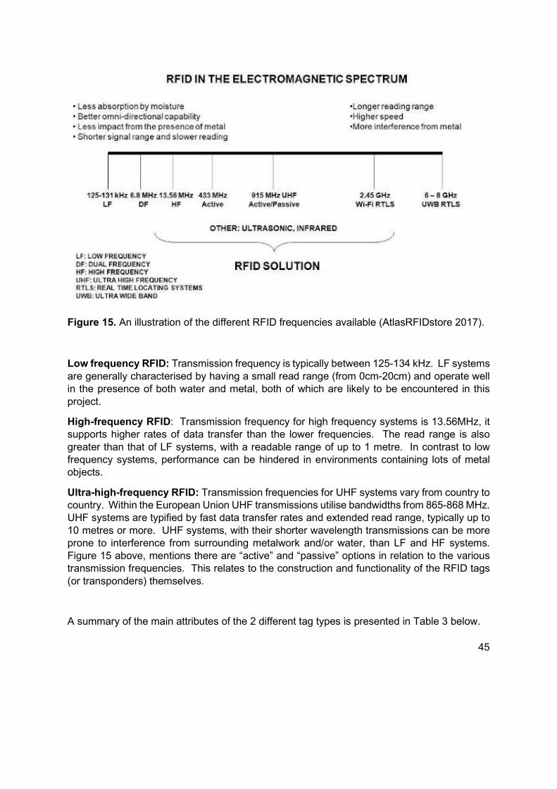
45

Low frequency RFID: Transmission frequency is typically between 125-134 kHz. LF systems are generally characterised by having a small read range (from 0cm-20cm) and operate well in the presence of both water and metal, both of which are likely to be encountered in this project.

High-frequency RFID: Transmission frequency for high frequency systems is 13.56MHz, it supports higher rates of data transfer than the lower frequencies. The read range is also greater than that of LF systems, with a readable range of up to 1 metre. In contrast to low frequency systems, performance can be hindered in environments containing lots of metal objects.

Ultra-high-frequency RFID: Transmission frequencies for UHF systems vary from country to country. Within the European Union UHF transmissions utilise bandwidths from 865-868 MHz. UHF systems are typified by fast data transfer rates and extended read range, typically up to 10 metres or more. UHF systems, with their shorter wavelength transmissions can be more prone to interference from surrounding metalwork and/or water, than LF and HF systems. Figure 15 above, mentions there are “active” and “passive” options in relation to the various transmission frequencies. This relates to the construction and functionality of the RFID tags (or transponders) themselves.

A summary of the main attributes of the 2 different tag types is presented in Table 3 below.

Figure 15. An illustration of the different RFID frequencies available (AtlasRFIDstore 2017).

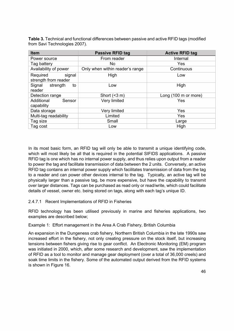
46

Table 3. Technical and functional differences between passive and active RFID tags (modified from Savi Technologies 2007).

Item Passive RFID tag Active RFID tag Power source From reader Internal Tag battery No Yes Availability of power Only when within reader’s range Continuous

Required signal strength from reader

High Low

Signal strength to reader

Low High

Detection range Short (<3 m) Long (100 m or more) Additional Sensor capability

Very limited Yes

Data storage Very limited Yes Multi-tag readability Limited Yes Tag size Small Large Tag cost Low High

In its most basic form, an RFID tag will only be able to transmit a unique identifying code, which will most likely be all that is required in the potential SIFIDS applications. A passive RFID tag is one which has no internal power supply, and thus relies upon output from a reader to power the tag and facilitate transmission of data between the 2 units. Conversely, an active RFID tag contains an internal power supply which facilitates transmission of data from the tag to a reader and can power other devices internal to the tag. Typically, an active tag will be physically larger than a passive tag, be more expensive, but have the capability to transmit over larger distances. Tags can be purchased as read only or read/write, which could facilitate details of vessel, owner etc. being stored on tags, along with each tag’s unique ID.

2.4.7.1 Recent Implementations of RFID in Fisheries

RFID technology has been utilised previously in marine and fisheries applications, two examples are described below;

Example 1: Effort management in the Area A Crab Fishery, British Columbia

An expansion in the Dungeness crab fishery, Northern British Columbia in the late 1990s saw increased effort in the fishery, not only creating pressure on the stock itself, but increasing tensions between fishers giving rise to gear conflict. An Electronic Monitoring (EM) program was initiated in 2000, which, after some research and development, saw the implementation of RFID as a tool to monitor and manage gear deployment (over a total of 36,000 creels) and soak time limits in the fishery. Some of the automated output derived from the RFID systems is shown in Figure 16.

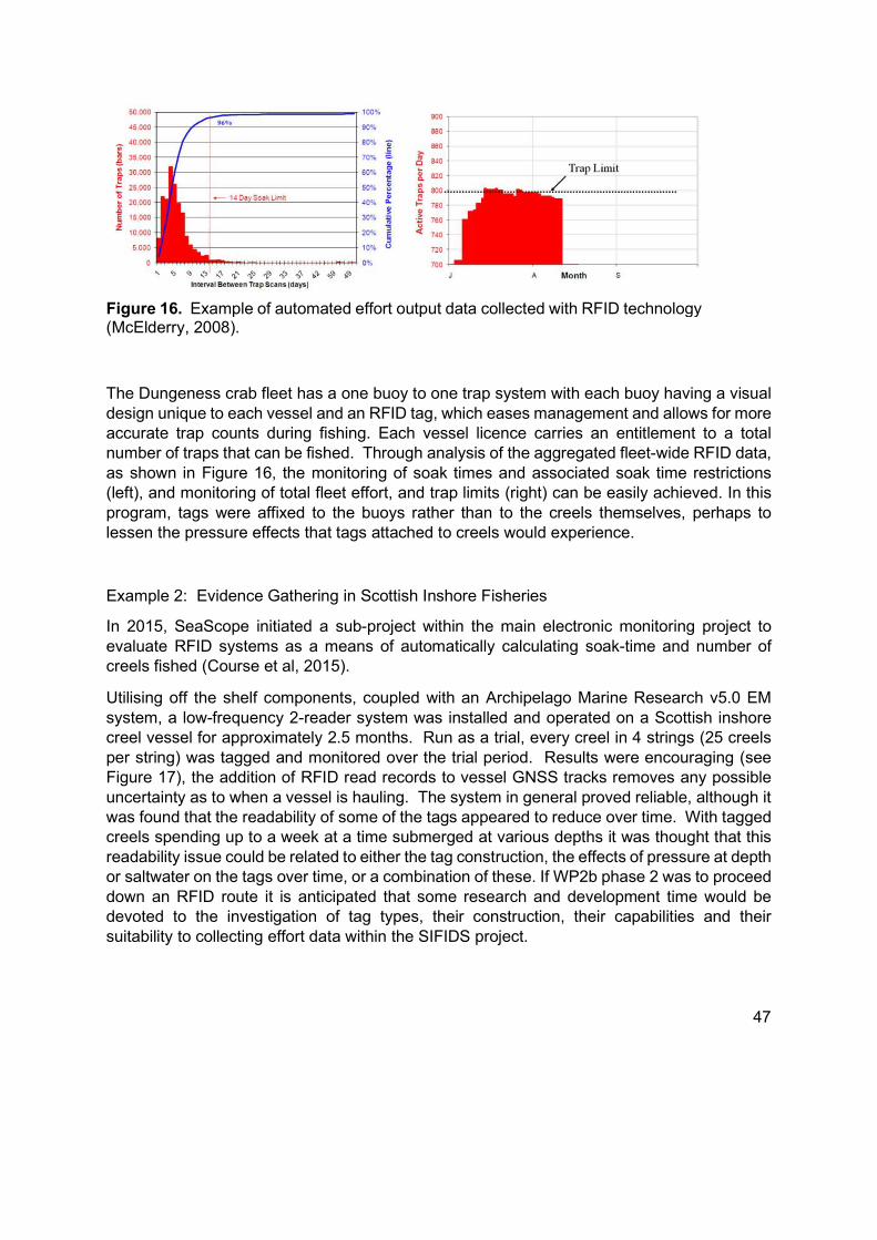
47

The Dungeness crab fleet has a one buoy to one trap system with each buoy having a visual design unique to each vessel and an RFID tag, which eases management and allows for more accurate trap counts during fishing. Each vessel licence carries an entitlement to a total number of traps that can be fished. Through analysis of the aggregated fleet-wide RFID data, as shown in Figure 16, the monitoring of soak times and associated soak time restrictions (left), and monitoring of total fleet effort, and trap limits (right) can be easily achieved. In this program, tags were affixed to the buoys rather than to the creels themselves, perhaps to lessen the pressure effects that tags attached to creels would experience.

Example 2: Evidence Gathering in Scottish Inshore Fisheries

In 2015, SeaScope initiated a sub-project within the main electronic monitoring project to evaluate RFID systems as a means of automatically calculating soak-time and number of creels fished (Course et al, 2015).

Utilising off the shelf components, coupled with an Archipelago Marine Research v5.0 EM system, a low-frequency 2-reader system was installed and operated on a Scottish inshore creel vessel for approximately 2.5 months. Run as a trial, every creel in 4 strings (25 creels per string) was tagged and monitored over the trial period. Results were encouraging (see Figure 17), the addition of RFID read records to vessel GNSS tracks removes any possible uncertainty as to when a vessel is hauling. The system in general proved reliable, although it was found that the readability of some of the tags appeared to reduce over time. With tagged creels spending up to a week at a time submerged at various depths it was thought that this readability issue could be related to either the tag construction, the effects of pressure at depth or saltwater on the tags over time, or a combination of these. If WP2b phase 2 was to proceed down an RFID route it is anticipated that some research and development time would be devoted to the investigation of tag types, their construction, their capabilities and their suitability to collecting effort data within the SIFIDS project.

Figure 16. Example of automated effort output data collected with RFID technology (McElderry, 2008).

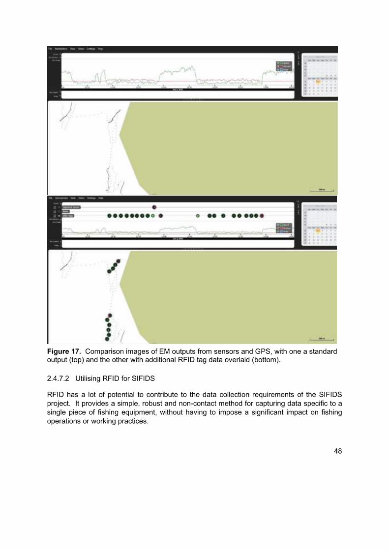
48

2.4.7.2 Utilising RFID for SIFIDS

RFID has a lot of potential to contribute to the data collection requirements of the SIFIDS project. It provides a simple, robust and non-contact method for capturing data specific to a single piece of fishing equipment, without having to impose a significant impact on fishing operations or working practices.

Figure 17. Comparison images of EM outputs from sensors and GPS, with one a standard output (top) and the other with additional RFID tag data overlaid (bottom).

49

The main ways RFID can benefit SIFIDS is to provide identification of strings and the individual creels within each string, with minimal or no impact on fishing operations.

String level data capture: By utilising RFID at a string level with cheaper passive tags attached to the surface buoys, combined with the spatial/temporal logging capability of the OBCDCS, the system would capture data on position and date/time of each string hauled and shot. From the shoot and haul data for each string the system would be able to calculate soak time.

It would be necessary to tag each buoy on the string so that at least one tag is on-board and can be read during a hauling or shooting operation. On occasions the fishers may leave the second end buoy for a string floating or trailing behind the vessel on the water rather than retrieving it on board every time.

A string level RFID system would require 2 tag readers to allow the fisher to scan the string (buoy) tag with either the ‘shooting’ or ‘hauling’ reader. It would be possible to implement this system using a single reader combined with a toggle mechanism to allow the fisher to set the system to shooting or hauling mode, a visual cue would need to be incorporated into the reader housing to indicate the current mode. The drawback of a toggle mechanism is that it relies on human interaction to set the mode, forgetting once and not noticing could result in the remaining strings for that day being logged in the opposite mode to their actual operation. A single reader may also not be appropriate in terms of working practice; the retrieved buoy may not be stored on deck in a position where it can easily be moved during the shooting operation to a reader which was suitably placed for hauling operations. Moving buoys and their associated ropes across the deck can cause potential hazards to those working on the deck and should be minimised.

Creel-level data capture: This would require a tag to be suitably fitted to each creel that a vessel uses along with a reader mounted in one of the retrieval, emptying, or rebaiting positions to mesh as seamlessly as possible with each vessel’s working practices. A creel-level system would only be capable of recording haul data; it is our opinion that it will be virtually impossible to implement creel-tag reading during the shooting operation without making major changes to vessel working practices or adding an unacceptably hazardous operation for the deck crew. Bearing this in mind it would still be likely that a string-based tag system would need to be implemented alongside a creel-tag system to provide shooting information to allow soak times to be calculated.

Setup and Running Costs for RFID: For the purpose of cost estimates, a vessel is expected to operate 30 strings of creels on a rotating basis, the costs provided are on a per vessel basis and allow for 10% loss of tags over the life of the trial.

It is likely that the working life of the reader components of any system would be approximately 2 years. Active tags should have a working life similar to that of the RFID readers, but this is highly dependent on suitable mounting, protection and considerate handling by the fishers. Passive tags should be almost considered as consumable items, we would expect to ‘issue’ each vessel with a surplus of tags and institute a process whereby the fisher could identify and replace defective tags easily in the field and provide substituted tag information back to the data collection team. This system could be further developed, whereby fishers have the

50

ability to change buoy tags (perhaps pre-defined by colour-coding) to indicate the main targeted species for that string.

Assuming a 2-reader system is required: Pricing ranged from £2600 for industrial grade high end specification, down to sub £1000 for an in-house system built using adapted RFID equipment currently marketed for and utilised in animal stock management.

If active tags were deployed on all strings to collect environmental data, the additional costs would be between £2216 and £3716 per vessel.

Alternatively, the individual RFID components; readers and bare antenna, can be purchased directly from suppliers allowing a custom system to be created to suit an individual vessel’s fishing practises and vessel structure. The individual systems would be built in-house to meet the exact needs of the vessel in terms of size, shape, antenna location, cabling etc., the completed systems would likely be embedded in high-resistance resin to provide a high level of ingress and mechanical protection. Due to the custom nature of this potential route it is not possible to give an indicative cost, but it is not expected to exceed the most expensive industrial grade complete system option.

2.4.8 Electro-Mechanical switches

Standard practice on creel vessels is for hauling, emptying and baiting of the creels to occur in virtually the same place each time on a vessel. By fitting a simple switch in this area which is activated by the creel being placed on or slid over it would allow creel counts to be obtained. The switch would be connected to a simple logger which records a count of switch actuations, the logger would need some inbuilt logic to ‘de-bounce’ the data and reject any potential ‘spurious’ actuations.

Some industrial switching options that could potentially be utilised are shown in Figure 18 below. These and other similar devices would be investigated and tested during the detailed design and build process in WP2b Phase 2.

a) b) c)

Figure 18. Examples of electro mechanical switches that could potentially be utilised to record creel counts. A plunger type switch (a), a roller arm switch (b) and a pressure pad switch (c) (SICK AG 2017, Company products).

51

2.4.9 Non-Contact Proximity sensors

As the title suggests, this type of sensor can detect objects within their ‘field-of-view’ without needing physical contact with the objects themselves. There are 2 primary types of this sensor that could be considered as potentially useful within the SIFIDS project.

2.4.9.1 Induction sensors

Inductive sensors detect when a ferrous metal object moves into the sensors range. Inside the sensor is a tight coil which produces a magnetic field, the sensor works by detecting any disturbance to the magnetic field caused by distortion from metal objects (see Figure 19). The sensor technology is mainly used in the manufacturing industry, where they perform tasks such as detecting when moving machinery parts are in the correct location; valve positions are aligned or detection of foreign metallic objects on a production line. Induction technology is also used in other fields, such as some types of metal detectors and larger scale sensors buried in roads to detect cars at traffic lights.

As the majority of shellfish creels are now constructed from steel, these sensors should be able to detect when a creel passes within range and provide a count. Most induction sensors emit a signal in a focused direction and so long as the sensor is mounted in a suitable location and orientation, false readings from other metal items on the vessel should be significantly reduced or even eliminated.

There are some challenges associated with using a ferrous detection sensor, including the use of non-metal creels, but we envisage that a small iron-based metal disk attached to the bottom of the creel, could allow it to be detected by the sensor. Other limitations of induction sensors can be the short detection range, usually 1 to 2cm, but sensors such as the one below can detect ferrous materials up to 6cm away.

Figure 19. Basic layout of an Induction sensor (Kinney, 2001).

52

Induction sensors (Figure 20) can cost as little as £20, but to ensure that the sensor can withstand the harsh conditions encountered on a fishing vessel, we would need to have a rugged and waterproof (minimum IP67) housing and each sensor will likely cost approximately £70. Each vessel will require only one sensor that will be used to count the creels being hauled aboard and there will be no cost associated with “tagging” the creels because they are usually constructed from iron. This cost will be per vessel and not related to the number of creels fished and the lifespan of a suitable sensor would be in the region of 2-3 years. These sensors may provide a good opportunity to collect creel count data at low cost.

2.4.9.2 Capacitive sensors

Capacitance is a measure of the electric charge stored within an object and is given the unit Farad. Although the charge in everyday objects is very small it can be picked up by a capacitive sensor (see Figure 21), which detects when objects are within range of two conductive wires and uses the electric change within the object to complete the circuit.

Figure 20. Induction sensor (Pepperl and Fuchs, 2017c).

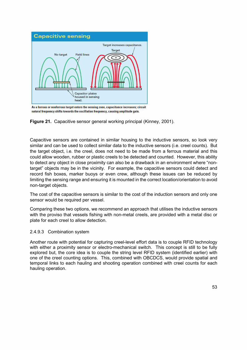
53

Figure 21. Capacitive sensor general working principal (Kinney, 2001).

Capacitive sensors are contained in similar housing to the inductive sensors, so look very similar and can be used to collect similar data to the inductive sensors (i.e. creel counts). But the target object, i.e. the creel, does not need to be made from a ferrous material and this could allow wooden, rubber or plastic creels to be detected and counted. However, this ability to detect any object in close proximity can also be a drawback in an environment where “non-target” objects may be in the vicinity. For example, the capacitive sensors could detect and record fish boxes, marker buoys or even crew, although these issues can be reduced by limiting the sensing range and ensuring it is mounted in the correct location/orientation to avoid non-target objects.

The cost of the capacitive sensors is similar to the cost of the induction sensors and only one sensor would be required per vessel.

Comparing these two options, we recommend an approach that utilises the inductive sensors with the proviso that vessels fishing with non-metal creels, are provided with a metal disc or plate for each creel to allow detection.

2.4.9.3 Combination system

Another route with potential for capturing creel-level effort data is to couple RFID technology with either a proximity sensor or electro-mechanical switch. This concept is still to be fully explored but, the core idea is to couple the string level RFID system (identified earlier) with one of the creel counting options. This, combined with OBCDCS, would provide spatial and temporal links to each hauling and shooting operation combined with creel counts for each hauling operation.

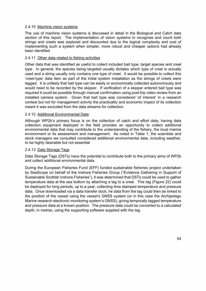
54

2.4.10 Machine vision systems

The use of machine vision systems is discussed in detail in the Biological and Catch data section of this report. The implementation of vision systems to recognise and count both strings and creels was explored and discounted due to the logical complexity and cost of implementing such a system when simpler, more robust and cheaper options had already been identified.

2.4.11 Other data related to fishing activities

Other data that was identified as useful to collect included bait type, target species and creel type. In general, the species being targeted usually dictates which type of creel is actually used and a string usually only contains one type of creel. It would be possible to collect this ‘creel-type’ data item as part of the initial system installation as the strings of creels were tagged. It is unlikely that bait type can be easily or economically collected autonomously and would need to be recorded by the skipper. If verification of a skipper entered bait type was required it could be possible through manual confirmation using post-trip video review from an installed camera system. Given that bait type was considered ‘of interest’ in a research context but not for management activity the practicality and economic impact of its collection meant it was excluded from the data streams for collection.

2.4.12 Additional Environmental Data

Although WP2b’s primary focus is on the collection of catch and effort data, having data collection equipment deployed in the field provides an opportunity to collect additional environmental data that may contribute to the understanding of the fishery, the local marine environment or its assessment and management. As noted in Table 1, the scientists and stock managers we consulted considered additional environmental data, including weather, to be highly desirable but not essential.

2.4.13 Data Storage Tags

Data Storage Tags (DSTs) have the potential to contribute both to the primary aims of WP2b and collect additional environmental data.

During the European Fisheries Fund (EFF) funded sustainable fisheries project undertaken by SeaScope on behalf of the Inshore Fisheries Group (“Evidence Gathering in Support of Sustainable Scottish Inshore Fisheries”), it was determined that DSTs could be used to gather temperature data at the sea bottom by attaching a tag to a creel. This tag (Figure 22) could be deployed for long periods, up to a year, collecting time stamped temperature and pressure data. Once downloaded via a data transfer dock, he data from the tag could then be linked to the position of the vessel using the vessel’s GNSS system (or in this case the Archipelago Marine research electronic monitoring system’s GNSS), giving temporally tagged temperature and pressure data at a known position. The pressure data could be converted to a calculated depth, in metres, using the supporting software supplied with the tag.

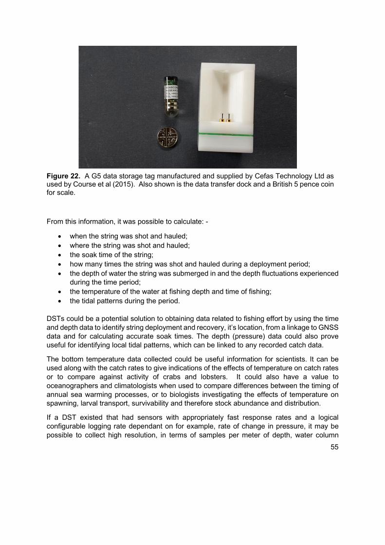
55

From this information, it was possible to calculate: -

when the string was shot and hauled; where the string was shot and hauled; the soak time of the string; how many times the string was shot and hauled during a deployment period; the depth of water the string was submerged in and the depth fluctuations experienced

during the time period; the temperature of the water at fishing depth and time of fishing; the tidal patterns during the period.

DSTs could be a potential solution to obtaining data related to fishing effort by using the time and depth data to identify string deployment and recovery, it’s location, from a linkage to GNSS data and for calculating accurate soak times. The depth (pressure) data could also prove useful for identifying local tidal patterns, which can be linked to any recorded catch data.

The bottom temperature data collected could be useful information for scientists. It can be used along with the catch rates to give indications of the effects of temperature on catch rates or to compare against activity of crabs and lobsters. It could also have a value to oceanographers and climatologists when used to compare differences between the timing of annual sea warming processes, or to biologists investigating the effects of temperature on spawning, larval transport, survivability and therefore stock abundance and distribution.

If a DST existed that had sensors with appropriately fast response rates and a logical configurable logging rate dependant on for example, rate of change in pressure, it may be possible to collect high resolution, in terms of samples per meter of depth, water column

Figure 22. A G5 data storage tag manufactured and supplied by Cefas Technology Ltd as used by Course et al (2015). Also shown is the data transfer dock and a British 5 pence coin for scale.

56

temperature profiles during shooting and hauling which may be of significant interest to oceanographers and biologists. DST’s capable of recording depth/temperature profiles do exist, but they are usually designed for high end use in oceanographic survey and research work. This function is reflected in the price which would preclude their widespread deployment in the context of an inshore fishery. A simple, low cost depth-temperature profile data logger is being developed as a prototype at USTAN. The prototype also includes a light sensor which may provide an indication of turbidity. Low cost and durable conductivity sensors needed to determine salinity remain a challenge.

2.4.13.1 Challenges

The main issues associated with DSTs are battery life, data storage/available memory, data transfer and cost. Although the example above focuses on the Cefas Technology DST that collects temperature and depth, other data storage tag manufacturers offer tags that can also collect additional environmental information e.g. salinity.

The costs, battery life, data storage capabilities and data transfer options are all dependent on what data is required to be collected. It is not cost effective to collect data every second if the data does not change greatly within an hour or will never be used at that frequency. High data collection rates will shorten the battery life and increase the amount of data that needs to be stored and transferred. Most manufacturers explored are listing a battery life of between 2-5 years, this is based on relatively slow data collection rates. If these are exceeded, then the battery life will be reduced.

A data recording rate set at 5 – 10 minute intervals would effectively record useful temperature and depth data and allow hauling and shooting operations to be detected and useable soak times calculated, probably for up to a year.

If profiles, salinity or other environmental data are not required under the primary programme it would be a worthwhile exercise to explore with potential partners e.g. UK Met. Office whether a market for the data is viable or additional funding could be provided to subsidise the additional data collection costs.

Transfer of data from the DST either direct to a shore-based system or to the on-board OBCDCS should also be considered. How often the data needs to be transferred will be governed by the requirements of the core data users; if the primary use is to collect fishing effort data to feed into a near real-time system then autonomous data offload to the OBCDCS is the only viable solution. If the primary aim is more inclined towards the environmental arena and the acceptable lag between collection and availability is long enough, then a regular manual offload either performed by the skipper or a technician visit, could be acceptable if an autonomous offload to OBCDCS is not viable.

Another consideration is the security of the DST. Fishing vessels can often lose a single creel or on occasions a whole string of creels. If the DST happens to be attached to the lost creel then it’s data will have been lost and it will need to be replaced. If the tags are expensive then this could rule DSTs out of the system build. The data loss could be quite significant if the DST is operating under a manual offload schedule rather than regular autonomous offload to

57

OBCDCS. Selection of a DST will need to consider the data loss risk, initial outlay plus the potential ongoing replacement costs as part of the system budget.

2.4.13.2 Costs and Suppliers

For the purpose of cost estimation, a vessel is expected to operate 30 strings of creels on a rotating basis. The costs provided are on a per vessel basis and allow for a 10% loss of tags over the life of the trial.

Temperature, depth and salinity (potentially) would appear to be the main environmental requirements of a DST if used as part of this system (based on the responses shown in Table 1). Several manufactures were contacted to provide a quote for data tags that could provide some of this information. Table 4 shows some examples of the suppliers and their equipment. It is worth noting that each vessel will need some form of communications hardware and software to download data from the tag and transmit it to the OBCDCS, either wirelessly or via a “tag-dock”.

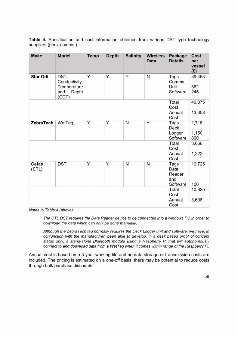
58

Table 4. Specification and cost information obtained from various DST type technology suppliers (pers. comms.).

Notes to Table 4 (above).

The CTL DST requires the Data Reader device to be connected into a windows PC in order to download the data which can only be done manually.

Although the ZebraTech tag normally requires the Deck Logger unit and software, we have, in conjunction with the manufacturer, been able to develop, in a desk based proof of concept status only, a stand-alone Bluetooth module using a Raspberry Pi that will autonomously connect to and download data from a WetTag when it comes within range of the Raspberry Pi.

Annual cost is based on a 3-year working life and no data storage or transmission costs are included. The pricing is estimated on a one-off basis, there may be potential to reduce costs through bulk purchase discounts.

Make Model Temp Depth Salinity Wireless Data

Package Details

Cost per vessel (£)

Star Odi DST-Conductivity Temperature and Depth (CDT)

Y Y Y N Tags Comms Unit Software

39,463 362 245

Total Cost

40,075

Annual Cost

13,358

ZebraTech WetTag Y Y N Y Tags Deck Logger Software

1,716 1,150 800

Total Cost

3,666

Annual Cost

1,222

Cefas (CTL)

DST Y Y N N Tags Data Reader and Software

10,725 100

Total Cost

10,825

Annual Cost

3,608

59

It can be seen from Table 4 that there is quite a wide range of prices depending on the options chosen. The most expensive of the 3 systems (Star Odi) includes salinity as an additional environmental parameter which is not available from the majority of other systems on the market.

The order of magnitude difference in annual cost between tags that provide temperature and depth only and those that can provide additional parameters highlights the need to ensure the data capture requirements are not over-specified and that data is not being collected just because it is possible.

2.4.13.3 Conclusion

DSTs are useful in two ways. Firstly, they can fulfil their primary design purpose and collect useful environmental data in the form of temperature and depth of deployment, as well as salinity if the sensor supports it. Secondly, their data can also be used to quantify fishing effort at location; analysing the time stamped pressure data alongside GNSS data allows data users to identify when and where a string was hauled to the surface or deployed to the seabed.

DSTs are not the cheapest option for solely collecting data on fishing effort and if that is the only function required, they would not be the recommended route. However, if the environmental data is important to the users and the additional cost of collecting this data is somehow underwritten by subsidy or data sale they could be incorporated into the system. The DSTs could be implemented to collect environmental data in a targeted manner in locations and at times when the data-cost-benefit assessment is positive.

2.4.14 Meteorological (weather) data

Mini weather stations generally include the same basic sensors, namely a barometer, temperature gauge, anemometer, humidity and rain fall gauge. To function aboard a small commercial fishing vessel, the system needs to be ruggedized, IP67 rated and the sensors need to be able to counteract external influencers, such as sea spray and vessel movement. Therefore, a specialist marine weather station would be required (Figure 23). During our investigations, we identified two possible suppliers, Furuno and Airmar Technology Corporation. Both systems utilise ultrasonic readings to obtain the different weather-related data and cost approximately £1,100. Any system such as these would need additional hardware and software to harvest their data and communicate it to the OBCDCS.

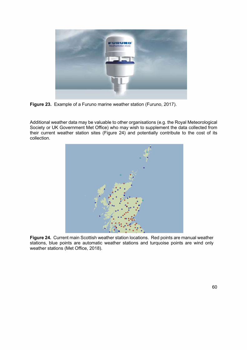
60

Additional weather data may be valuable to other organisations (e.g. the Royal Meteorological Society or UK Government Met Office) who may wish to supplement the data collected from their current weather station sites (Figure 24) and potentially contribute to the cost of its collection.

Figure 23. Example of a Furuno marine weather station (Furuno, 2017).

Figure 24. Current main Scottish weather station locations. Red points are manual weather stations, blue points are automatic weather stations and turquoise points are wind only weather stations (Met Office, 2018).

61

2.4.15 Biological and Catch Data Capture

From the discussions with Marine Scotland scientists and inshore fishery managers, only two catch data types were identified as essential to shellfish stock assessment scientists (see table 1);

Weight of retained shellfish catch by species Size frequency distributions for the retained shellfish catch by species

Other data that were identified as “Highly Desirable” were;

Weight of discarded shellfish by species Weight of discarded shellfish by sex (for each species) Weight of retained shellfish by sex (for each species) Weight/Count of finfish discarded (not retained) by species Size frequency distributions for the discarded shellfish catch by species

Some data can be calculated from other data which is more easily collected, for example; if count and sex/length frequency data are collected then the weight of the catch can be calculated using size weight relationships. As weighing individuals at sea is impractical, this provides a route to obtain the necessary weight information.

A variety of technologies that, on initial inspection, appeared to have potential for providing the catch and biological data required within the SIFIDS project were explored. Some of these technologies provide a result very similar to a ‘standard’ visual image, this means that a number of processes and approaches will cross boundaries between the technologies. These techniques for information extraction (features, measurements etc.) from a point cloud (an ‘image’) are explored in the visual-spectrum section, the technique exploration is implied and not repeated in the subsequent non-visual spectrum sections.

2.4.16 Changes to catch handling processes

As described in the creel fishery introduction, the discrete components of the catch are handled very differently, these different processes offer opportunities for capturing the data but also significant challenges;

Lobsters, due to their high value, are generally handled and stored individually and always banded. There are opportunities within this handling scenario where the individual can be presented to a technology solution in an appropriate orientation to enable data capture without significantly altering the handling process or causing an unacceptable delay.

Brown crabs, depending on their size and number may also be handled individually but may also be placed into bins in bulk. A more complex solution is required to limit changes to the handling process to enable a technology solution to capture data for this component.

Discarded individuals are generally returned directly to the sea in bulk. This component of the catch will need to be brought inboard, if only briefly, and lightly separated, to enable it to pass through a data capture solution. This will require the most significant change in working

62

practice aboard the vessels and presents the most significant technological and engineering challenge.

2.4.17 Image and Video Analysis (Visual Spectrum)

The field of computer vision (CV, see glossary) has seen huge advances in the last decade, consumer level vision systems are now widely available from numerous suppliers, standards have evolved, and a variety of open source platforms and libraries exist to allow the development of custom applications. CV is widely employed in a large proportion of industries, an essential part of manufacturing and inspection in automated factories. CV also appears in common consumer electronics; smile detection in digital cameras, games consoles (Xbox Kinect), motion detection in CCTV systems, facial recognition for mobile phone unlocking etc. CV systems come in 4 generic types

Smart Camera Systems; the camera, image processing and analysis software are bundled into a single unit providing a data feed to Programmable Logic Controllers (PLCs) or other manufacturing control/monitoring equipment. Smart camera systems are commonly used where a single view is sufficient, with no user interaction, display or complex algorithms and logic processing to undertake.

Compact vision systems; the controller is separate from the camera or cameras, as with smart camera systems the ability to run complex algorithms or processing logic is limited. The main advantage of compact systems is their ability to connect multiple cameras to a single controller, sharing the processor and storage of the controller. It is possible, with some systems, to have a PC or other higher spec hardware reading the image streams from the controller and providing image processing, analysis and program logic.

PC based systems; Camera(s) feed their image streams to a standard PC (windows, Linux, etc.) which performs the image processing and analysis functions using either bespoke or standard software modules. The results of the analysis are then recorded, actioned or passed to further control systems. The PC systems can be simple low cost machines; usually employed where speed is not a limiting factor or where the complexity of the process algorithms allow, or the PC systems can be a rack of multiple processors handling complex imaging requirements fast enough to allow a process line to run at maximum speed. All PC based systems require an interface between the camera and the system, some standard interfaces are supported by cameras; USB and FireWire, other systems require an additional piece of hardware (a frame-grabber) to be installed on the PC to allow it to access the image stream.

Bespoke systems; the entire system is built to achieve the required aims, using custom components, interconnects, processor arrays etc. These systems are usually phenomenally fast, accurate and precise. These advantages come at a price both in monetary terms and flexibility. The optimised algorithms are often written in low-level languages, compiled specifically for the hardware and cannot be quickly modified to account for changes in requirements etc.

There are CV systems available that can provide almost-off-the-shelf solutions that can be tailored by users with basic technical skills. These systems provide functionality that is common to the majority of general manufacturing systems and can be configured by users with little or no CV experience. All of these implementations employ concepts and processes discussed further in this report.

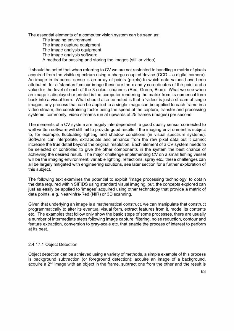
63

The essential elements of a computer vision system can be seen as: The imaging environment

The image capture equipment The image analysis equipment

The image analysis software A method for passing and storing the images (still or video) It should be noted that when referring to CV we are not restricted to handling a matrix of pixels acquired from the visible spectrum using a charge coupled device (CCD – a digital camera). An image in its purest sense is an array of points (pixels) to which data values have been attributed; for a ‘standard’ colour image these are the x and y co-ordinates of the point and a value for the level of each of the 3 colour channels (Red, Green, Blue). What we see when an image is displayed or printed is the computer rendering the matrix from its numerical form back into a visual form. What should also be noted is that a ‘video’ is just a stream of single images, any process that can be applied to a single image can be applied to each frame in a video stream, the constraining factor being the speed of the capture, transfer and processing systems; commonly, video streams run at upwards of 25 frames (images) per second. The elements of a CV system are hugely interdependent, a good quality sensor connected to well written software will still fail to provide good results if the imaging environment is subject to, for example, fluctuating lighting and shadow conditions (in visual spectrum systems). Software can interpolate, extrapolate and enhance from the raw pixel data but it cannot increase the true detail beyond the original resolution. Each element of a CV system needs to be selected or controlled to give the other components in the system the best chance of achieving the desired result. The major challenge implementing CV on a small fishing vessel will be the imaging environment; variable lighting, reflections, spray etc.; these challenges can all be largely mitigated with engineering solutions, see later section for a further exploration of this subject. The following text examines the potential to exploit ‘image processing technology’ to obtain the data required within SIFIDS using standard visual imaging, but, the concepts explored can just as easily be applied to ‘images’ acquired using other technology that provide a matrix of data points, e.g. Near-Infra-Red (NIR) or 3D scanning. Given that underlying an image is a mathematical construct, we can manipulate that construct programmatically to alter its eventual visual form, extract features from it, model its contents etc. The examples that follow only show the basic steps of some processes, there are usually a number of intermediate steps following image capture; filtering, noise reduction, contour and feature extraction, conversion to gray-scale etc. that enable the process of interest to perform at its best.

2.4.17.1 Object Detection

Object detection can be achieved using a variety of methods, a simple example of this process is background subtraction (or foreground detection); acquire an image of a background, acquire a 2nd image with an object in the frame, subtract one from the other and the result is

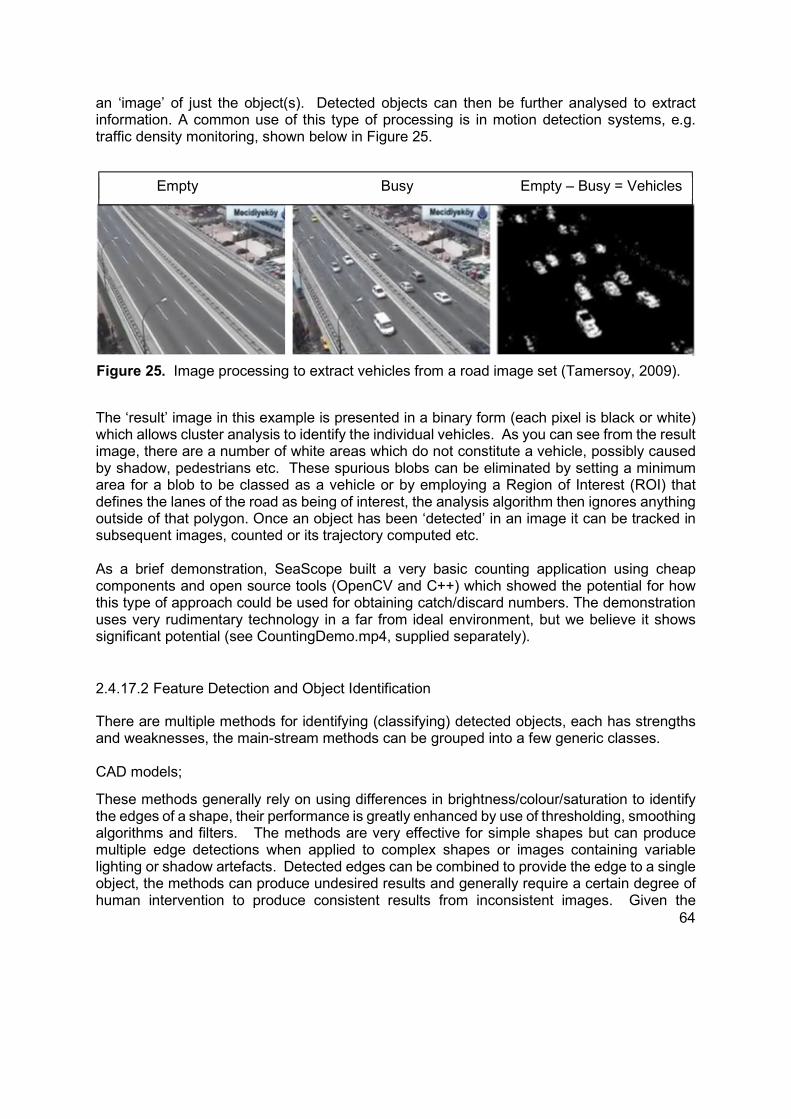
64

an ‘image’ of just the object(s). Detected objects can then be further analysed to extract information. A common use of this type of processing is in motion detection systems, e.g. traffic density monitoring, shown below in Figure 25.

The ‘result’ image in this example is presented in a binary form (each pixel is black or white) which allows cluster analysis to identify the individual vehicles. As you can see from the result image, there are a number of white areas which do not constitute a vehicle, possibly caused by shadow, pedestrians etc. These spurious blobs can be eliminated by setting a minimum area for a blob to be classed as a vehicle or by employing a Region of Interest (ROI) that defines the lanes of the road as being of interest, the analysis algorithm then ignores anything outside of that polygon. Once an object has been ‘detected’ in an image it can be tracked in subsequent images, counted or its trajectory computed etc. As a brief demonstration, SeaScope built a very basic counting application using cheap components and open source tools (OpenCV and C++) which showed the potential for how this type of approach could be used for obtaining catch/discard numbers. The demonstration uses very rudimentary technology in a far from ideal environment, but we believe it shows significant potential (see CountingDemo.mp4, supplied separately).

2.4.17.2 Feature Detection and Object Identification

There are multiple methods for identifying (classifying) detected objects, each has strengths and weaknesses, the main-stream methods can be grouped into a few generic classes. CAD models;

These methods generally rely on using differences in brightness/colour/saturation to identify the edges of a shape, their performance is greatly enhanced by use of thresholding, smoothing algorithms and filters. The methods are very effective for simple shapes but can produce multiple edge detections when applied to complex shapes or images containing variable lighting or shadow artefacts. Detected edges can be combined to provide the edge to a single object, the methods can produce undesired results and generally require a certain degree of human intervention to produce consistent results from inconsistent images. Given the

Empty Busy Empty – Busy = Vehicles

Figure 25. Image processing to extract vehicles from a road image set (Tamersoy, 2009).

65

complex shape, colour variation, missing limbs and the potential for non-target accretions (seaweed, barnacles etc.) on the individuals being imaged it is unlikely that a CAD based method of identification would produce acceptable results. Appearance based;

This technique uses a range of exemplar images, extracting key points and features from the target image, comparing this set of features to those in a database of the exemplar images, subsequently providing a probability of a match. This method requires the set of exemplars to cover all the possible variations of target object size, shape, lighting and orientation (which can be created programmatically) to be able to produce good results. As discussed earlier, the variation in the target images within SIFIDS would make this approach an unlikely candidate for this project. Feature based;

There are a variety of methods within this generic class, but they largely work on the same principles:

Take a set of exemplar images of the target object (the larger the better) Extract key features and descriptors for the target object Combine these features and descriptors from the ‘training’ images to create a ‘model’

classifier for the targets. Extract features and descriptors from the acquired target image, compare to the model

classifier and provide a probability that the object in the image fits the model. Many of these methods provide a ‘black-box’ approach, the eventual classifier model is largely unintelligible to a human operator without substantial work and cannot be ‘tweaked’. Some tools do provide visualisation applications which show the various stages of classification when applied to a sample image. Due to its ‘learning’ nature, a classifier can be subject to continuous improvement by re-running the training element with new images that the model incorrectly identified. The models may be available as an eXtended Markup Language (XML) file in their native form or can be exported and imported in a compressed form to enable remote updating of systems in the field. The training element of these methods can take up to several days to complete, dependant on the number and complexity of the exemplar images, the power of the processing machine etc. As the methods generally produce a model, this step can be run on powerful high spec machines with the resulting model being transferred to low-end recognition devices. An example of this type of machine learning can be seen across the web with several sites offering on-line image identification (see Wolfram Image Identify Project: https://www.imageidentify.com/). This approach has significant potential for the SIFIDS program. Morphometric and pixel analysis

Another alternative which bears further exploration is a simpler, less ‘black-box’, approach. Once an object has been detected by a simple method (such as background subtraction) it is possible to develop and apply a custom algorithm to identify the object as either Lobster, Brown Crab, Velvet Crab or ‘None of the above’. Most open-source libraries provide built-in

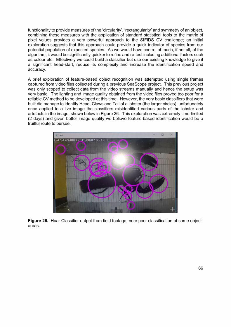
66

functionality to provide measures of the ‘circularity’, ‘rectangularity’ and symmetry of an object, combining these measures with the application of standard statistical tools to the matrix of pixel values provides a very powerful approach to the SIFIDS CV challenge; an initial exploration suggests that this approach could provide a quick indicator of species from our potential population of expected species. As we would have control of much, if not all, of the algorithm, it would be significantly quicker to refine and re-test including additional factors such as colour etc. Effectively we could build a classifier but use our existing knowledge to give it a significant head-start, reduce its complexity and increase the identification speed and accuracy. A brief exploration of feature-based object recognition was attempted using single frames captured from video files collected during a previous SeaScope project. This previous project was only scoped to collect data from the video streams manually and hence the setup was very basic. The lighting and image quality obtained from the video files proved too poor for a reliable CV method to be developed at this time. However, the very basic classifiers that were built did manage to identify Head, Claws and Tail of a lobster (the larger circles), unfortunately once applied to a live image the classifiers misidentified various parts of the lobster and artefacts in the image, shown below in Figure 26. This exploration was extremely time-limited (2 days) and given better image quality we believe feature-based identification would be a fruitful route to pursue.

Figure 26. Haar Classifier output from field footage, note poor classification of some object areas.

67

2.4.18 Obtaining Measurements from Images

Machine vision does not examine the object itself - measurements are made on the image of the object on the sensor. All of the factors that contribute to the quality of that image must be optimised, so careful consideration must be given to every element of the machine vision system, including lenses, illumination, camera type and resolution, image acquisition, measurement algorithms, as well as external factors such as vibrations, electromagnetic interference and heat. Measurements fall into 3 categories: 1D, 2D and 3D. 1D measurements are typically used to obtain the positions, distances, or angles of edges that are measured along a line or an arc. 2D measurements provide length and width information and are used for a host of measurements including area, shape, perimeter, centre of gravity, the quality of surface appearance, edge-based measurements and the presence and location of features. Image quality has a major influence on the resulting measurements and is dependent on resolution, contrast, depth of field, perspective and distortion. These, in turn, are determined by the choice of system components including cameras, lenses and illumination. Cost is also an important consideration. The best components for the application should be used but over-specifying them leads to unnecessary costs for no gain. Since all the components in a machine vision system must be perfectly coordinated it is essential to make an initial evaluation of the application:

What objects are to be measured? How large is the measurement area? What type of measurement is required? Are multiple views/measurements required? How fast are the objects moving? What measurement accuracy is needed? Is colour identification needed?

These and other factors help to determine the specification of the vision components needed, but there are also environmental issues that should be taken into account. These include physical constraints on positioning of components and environmental conditions such as ambient light etc. The resulting system does not need to be a complicated set-up, it simply needs to be fit for purpose. With 3D machine vision technology becoming much more widely available, a similar process should be adopted when specifying a system to make 3D measurements. Although 3D systems have become much more affordable in recent years, they are still generally more expensive than 2D systems and add more data and more complexity so should only be specified when the required measurement can’t be made using 2D methods. With a variety of 3D measurement techniques available, it is also important to choose the most appropriate method, this is often a case of trial and error.

68

2.4.18.1 Calibration

In order to make actual measurements, pixel positions must be converted into real world values, which means that system calibration is required, and the system must be set up to ensure that measurements can be made with the required accuracy, precision and repeatability. For the best repeatability, all of the set-up conditions for the vision system should be recorded. These include exposure time, camera gain, white balance of the camera, light intensity settings (and strobe, if used), working distances and angles and f-stop of the lens etc. A universal test chart can be used for quick and convenient system set-up and checking, for focus, system resolution, alignment, colour balance. Geometric distortions from the lens can usually be corrected in software.

2.4.18.2 3D calibration

Special 3D calibration bodies with known reference surfaces and angles allow metric calibration in combination with special software packages. They can be used for the simultaneous calibration of one or more cameras. In addition to metric calibration a plane fit for alignment of 3D point clouds is possible. This is important for 3D matching and for easy processing of range map images.

2.4.18.3 Keeping on track

It is important to check the accuracy and repeatability of a vision system. One way of doing this is to perform a series of measurements of the same object and check the variation of the results, this sets a benchmark for future measurements, many machine vision systems offer extra statistical information, such as minimum, maximum, mean, std. dev. of measured values from built-in calibration routines. It is also important to monitor machine vision results periodically to guarantee measurement reproducibility, this can be done by making test measurements with a reference object or calibration body. Measurement of objects detected using CV technology is a widely used standard process. As with all the CV techniques, it requires the selection and configuration of appropriate equipment to get the best possible results. It may be the case that the imaging technology that gives the best results for species identification will not be appropriate for accurate and repeatable measurements from those individuals, in which case a combination of technologies would need to be employed to achieve all the project aims. A 2007 study by Harbitz (2007) showed comparable length frequency results from automatic and manual measurement of Pandalus borealis carapace length. The automatic lengths were not measured directly but calculated from the pixel area of the entire animal and from the weight of the individual. The results show significant potential for deriving carapace length data indirectly. The study did highlight issues with the concept and also provides some potential solutions to those issues and investigations to pursue further. Obtaining measurements of crab and lobster from images presents a number of issues;

69

For all species, the distance to the points of measurement from the sensor will affect the accuracy of the measurement, pixels captured closer to the sensor will cover a smaller area of the individual than those captured further away. This can be mitigated by use of 3D imaging, Infra-Red (IR) distance measurement etc. to provide a measure of the sensor-object distance and then use a previously obtained calibration model to adjust the measurement. The sensor to measurement point issue may not need any attention if the requirements for accuracy and size-binning fit within the measurement parameters achievable without distance correction. The traditional measurement of lobster requires identifying the back of the eye-socket and taking a measurement at 90 degrees to the rear of the carapace. Identification of the 2 measuring points on a lobster image will present a challenge to CV technology, providing an image with appropriate resolution and contrast to identify those points is essential, once we have a workable image the challenge will be to develop an algorithm (possibly a combination of edge and feature detections) to identify the 2 points. Once the measurement points are identified it is simple mathematics to calculate the pixel distance between them and, from that value, the actual distance. As with Harbitz (2007), with detailed morphometric measurements and analysis we may find a measure that is simpler to obtain with CV but is well correlated to the required measurement. Measurement of crabs is less of a challenge; the measured dimension is more easily identifiable within an image once protruding legs, claws and extraneous artefacts have been removed. Having obtained a roughly ellipsoid object (the crab body) calculate its orientation. From the centre point of the object, segment it along the line of orientation (segment width to be determined by trial), obtain pixel distances for each segment, the largest should be the carapace width or a measure that can be correlated to carapace width. Extracting the body from the image could be accomplished by edge detection or feature detection, if these standard CV methods do not produce the desired result an alternative method will need to be developed. An initial idea to achieve this; find the approximate centre of the whole crab object and its orientation, create an ellipsoid object at the centre point, incrementally grow the ellipsoid object, moving its centre point if necessary, until it covers the body area (possibly by coinciding its perimeter with edge detections, percent coverage of the whole crab or some other measure to be determined with trials), the ellipsoid object will then be analysed to extract measurements. Industry implementations of traditional (visible spectrum) machine vision include: -

Sorting unripe tomatoes from ripe ones (colour recognition) Mis-shaped biscuits (shape recognition) Traffic density (object detection and tracking) General manufacturing: Presence verification (object detection and counting)

To verify parts, assemblies and packaged goods, vision systems provide high speed, reliable options for checking the presence, size, position, shape and completeness of features.

Surface inspection (edge detection, shape recognition, colour): - By pinpointing any contamination, scratches, cracks, discolouration or inclusions at high speeds, integrated vision systems enable quality control, increased yield, reduced waste and the delivery of superior products.

70

The systems allow irregular pattern structures and surface deviations to be assessed and measured and can be used to provide comprehensive reports and statistical process control (SPC) data on the size, position and structure of any defects detected.

2.4.18.4 Throughput Rates

Throughput rates in all the systems explored are constrained by the speed at which an image can be analysed to obtain the required result and the processing equipment’s ability to respond to the result. The analysis time is governed by the power of the image processing machine and the complexity of the algorithm in place, for example the ‘green tomato’ example only uses colour channels to separate ripe and unripe tomatoes, the algorithm for this is very simple allowing a phenomenally fast throughput especially as the low-level software is written specifically to achieve only this aim. As the SIFIDS project doesn’t require any physical action from the system as a result of its image analysis, there is the potential to capture images/video and process at a slower rate than the capture. Given the nature of vessel activity there is considerable ‘downtime’ where no individuals are being imaged, the system could run a continuous processing cycle dealing with a backlog of images during steams between strings and back to port.

2.4.18.5 Challenges

As discussed throughout the visual-spectrum section, controlling the imaging environment is key to providing images of a suitable nature for the subsequent analysis to achieve reliable identification, counts and measurements.

2.4.19 Stereoscopic Imaging to Obtain Object Distance and Measurement

Stereoscopy is a technique used for recording and representing stereoscopic (3D) images. There are two possible ways of taking stereoscopic pictures: by using special two-lens stereo cameras or systems with two single-lens cameras linked together to capture images simultaneously. Stereoscopic pictures allow us to calculate the distance from the camera(s) to a chosen object within the picture. The distance is calculated from differences between the pictures and additional technical data like focal length and distance between the cameras. The chosen object is selected on the left picture, while the same object on the right picture is automatically detected by means of optimisation algorithms which search for minimum difference between both pictures. The distance to the object can be calculated using standard geometrical derivations. The accuracy of the position depends on picture resolution, optical distortions and distance between the cameras. The results in Mrovlje and Vrančić (2008) showed that the calculated distance to the subject is relatively accurate. The calculated distance can be used to correct for object to camera distance in linear measurements taken from the image.

Harvey et al (2002) used manual measuring methods and commercial 3D software to study the accuracy and precision of single vs stereo imaging. Their results show that stereo imaging

71

provides improvements on single imaging but does highlight problems with the approach when the target object is not parallel to the imaging sensor.

Miura et al (2013) show a promising method for obtaining 3D object models using 2 still images of an object, the method uses Scale Invariant Feature Transform (SIFT) and Structure from Motion (SfM) approaches to compute the dense 3D point cloud. The method is targeted at providing lower computational cost 3D imaging from consumer level imaging equipment. The results show a 1mm accuracy for the test objects (when compared to a high-level laser scan of the same object), the object model took 20 seconds to compute once images were captured. The Chong and Stratford (2002) study showed that minor changes in photographic positioning relative to the initial calibration positions show insignificant changes in accuracy of measurement. Wehkamp and Fischer (2014) describe in great detail the process and issues involved in obtaining measurements from consumer-level digital imaging equipment. The study used a variety of imaging scenarios to explore the problem including use of wide-angle convertors to increase the field of view of the camera systems. The commercial software MatLab was used to correct the images for lens distortion and the subsequent image analysis, all the code and detailed documentation is freely available for download. The results of the study show a 1% to -4% error in measurements obtained from the corrected stereo images.

2.4.19.1 Challenges

The challenges for stereo vision are much the same as for standard visual imaging dependant on the method used to obtain the stereo images. Creating a custom-built stereo vision system isn’t as simple as adding a second camera, there is considerable work required in building the mounting to ensure correct alignment of lenses, creating software or engineering solutions to ensure simultaneous image capture from each camera and extraction of measurements from the custom built hardware. Stereo camera systems are available off-the-shelf, investigations into these systems show significant potential for incorporation into the SIFIDS project if the benefits of stereo-photogrammetry are considered necessary.

2.4.19.2 Conclusion

Stereo photogrammetry has significant potential for the SIFIDS project, the majority of the implementations explored used manual identification of the points from which to extract the measurements, which leads back to the issue identified in the visual 2D section; automatically identifying the points from which to extract the required measure. It could be possible to incorporate some of the techniques discussed in the 2D section with those from stereo-vision to achieve the project aims.

2.4.20 Other implementations and research within fisheries and bio-sciences

Wang (2014) evaluated a variety of classification methods to identify animals caught by camera traps around the province of Alberta. The problems encountered are remarkably

72

similar to some of those that will be encountered by the SIFIDS project, variable lighting conditions, orientation changes, partial images of animals etc. The work uses still images captured by motion triggered cameras. At the time of writing, the camera images were processed manually by experts to identify the species present in the image. The report presents comparisons of combinations of various methods to improve accuracy of identification, its approaches and conclusions can be used to inform and direct research within the SIFIDS CV work packages.

2.4.21 Deep Learning for Electronic Monitoring in Fisheries

Deep learning is a powerful and flexible technique that has achieved enormous success in solving a broad variety of computer vision problems, particularly when dealing with imagery acquired in challenging, real-world conditions. This makes deep learning a natural choice for quantifying and measuring the carapaces of crabs and lobsters.

First, we will describe the origins of deep learning. We will then discuss its internal operation and its applications within computer vision. Finally, we will discuss its requirements in terms of computer hardware and how it could be applied within an electronic monitoring system for fisheries.

2.4.21.1 Origins

Since 2012 deep learning (a term synonymous with deep neural networks) has risen to become the dominant approach to solving a wide variety of computer vision problems. Its rise started with the publication of Krizhevsky et al’s 2012 paper, in which they won the ImageNet 2012 image recognition challenge with a top-5 error rate of 15%, in contrast to a 25% error rate of competing hand-engineered approaches. Since then, researchers have proposed new neural network architectures that have further reduced error rates, with the most recent models achieving error rates as low as 3-4% (see Figure 27).

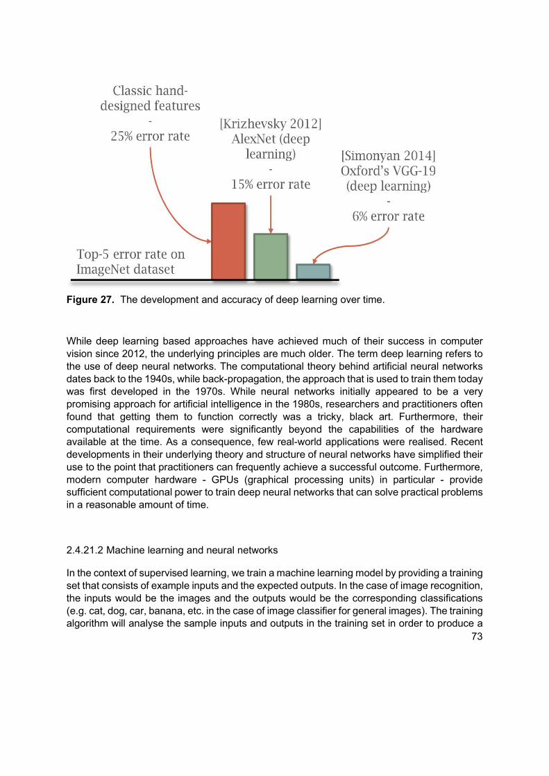
73

While deep learning based approaches have achieved much of their success in computer vision since 2012, the underlying principles are much older. The term deep learning refers to the use of deep neural networks. The computational theory behind artificial neural networks dates back to the 1940s, while back-propagation, the approach that is used to train them today was first developed in the 1970s. While neural networks initially appeared to be a very promising approach for artificial intelligence in the 1980s, researchers and practitioners often found that getting them to function correctly was a tricky, black art. Furthermore, their computational requirements were significantly beyond the capabilities of the hardware available at the time. As a consequence, few real-world applications were realised. Recent developments in their underlying theory and structure of neural networks have simplified their use to the point that practitioners can frequently achieve a successful outcome. Furthermore, modern computer hardware - GPUs (graphical processing units) in particular - provide sufficient computational power to train deep neural networks that can solve practical problems in a reasonable amount of time.

2.4.21.2 Machine learning and neural networks

In the context of supervised learning, we train a machine learning model by providing a training set that consists of example inputs and the expected outputs. In the case of image recognition, the inputs would be the images and the outputs would be the corresponding classifications (e.g. cat, dog, car, banana, etc. in the case of image classifier for general images). The training algorithm will analyse the sample inputs and outputs in the training set in order to produce a

Figure 27. The development and accuracy of deep learning over time.

74

set of numeric parameters that the model will use to predict outputs - the classification in the case of an image classifier - for novel sample inputs that it has not seen before, hopefully producing correct answers. Machine learning algorithms ‘learn’ from the samples in the training set, as opposed to typical computer programs where decision rules must be designed by hand. There are a variety of different kinds of machine learning models, each with its own strengths and weaknesses; neural networks are one such kind of model.

An artificial neural network consists of a number of layers. Typically, the layers are arranged in sequential fashion, each one receiving an input and passing its output to the next layer in the network. The first layer receives the input samples - images in our case - while the last layer emits the predicted outputs. Each layer in the network quantifies the presence of patterns within the input that it receives and passes its measurements to the next layer. The early layers in the network look for simple low-level patterns such as edges and colour. Further layers build on these early layers and look for small curves and simple textures. Mid-level layers look for small structures within the image, while later layers look for complex structures as parts. The final layers convert the pattern responses from the previous layer into the output prediction.

The diagram below (Figure 28) illustrates a simplified neural network. The image on the left is passed through the hidden layers in the middle, finally ending in a class prediction. The predictions take the form of probabilities, one for each class of object that the network was trained for. The palettes of layer activation images below each hidden layer show its response to various parts of the input image. Note that the first layer responds to very small simple patterns, while subsequent layers respond to more complex stimuli.

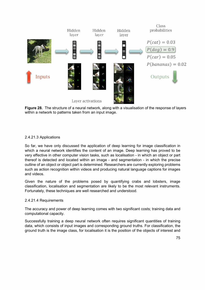
75

2.4.21.3 Applications

So far, we have only discussed the application of deep learning for image classification in which a neural network identifies the content of an image. Deep learning has proved to be very effective in other computer vision tasks, such as localisation - in which an object or part thereof is detected and located within an image - and segmentation - in which the precise outline of an object or object part is determined. Researchers are currently exploring problems such as action recognition within videos and producing natural language captions for images and videos.

Given the nature of the problems posed by quantifying crabs and lobsters, image classification, localisation and segmentation are likely to be the most relevant instruments. Fortunately, these techniques are well researched and understood.

2.4.21.4 Requirements

The accuracy and power of deep learning comes with two significant costs; training data and computational capacity.

Successfully training a deep neural network often requires significant quantities of training data, which consists of input images and corresponding ground truths. For classification, the ground truth is the image class, for localisation it is the position of the objects of interest and

Figure 28. The structure of a neural network, along with a visualisation of the response of layers within a network to patterns taken from an input image.

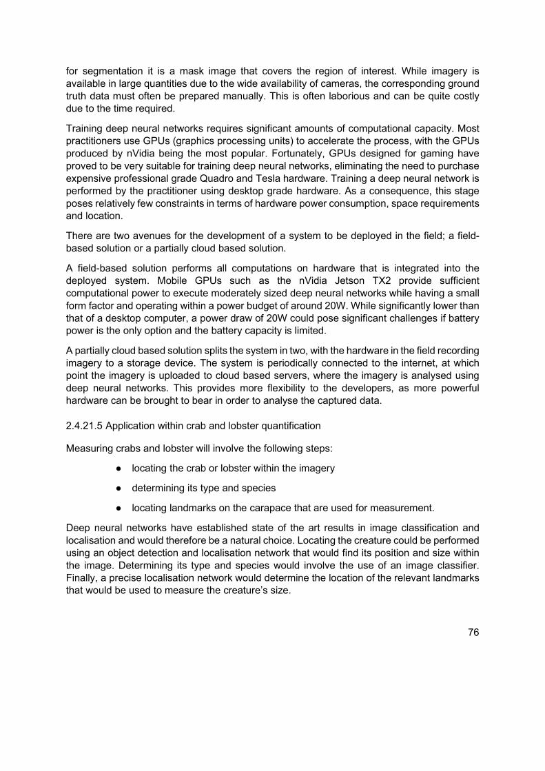
76

for segmentation it is a mask image that covers the region of interest. While imagery is available in large quantities due to the wide availability of cameras, the corresponding ground truth data must often be prepared manually. This is often laborious and can be quite costly due to the time required.

Training deep neural networks requires significant amounts of computational capacity. Most practitioners use GPUs (graphics processing units) to accelerate the process, with the GPUs produced by nVidia being the most popular. Fortunately, GPUs designed for gaming have proved to be very suitable for training deep neural networks, eliminating the need to purchase expensive professional grade Quadro and Tesla hardware. Training a deep neural network is performed by the practitioner using desktop grade hardware. As a consequence, this stage poses relatively few constraints in terms of hardware power consumption, space requirements and location.

There are two avenues for the development of a system to be deployed in the field; a field-based solution or a partially cloud based solution.

A field-based solution performs all computations on hardware that is integrated into the deployed system. Mobile GPUs such as the nVidia Jetson TX2 provide sufficient computational power to execute moderately sized deep neural networks while having a small form factor and operating within a power budget of around 20W. While significantly lower than that of a desktop computer, a power draw of 20W could pose significant challenges if battery power is the only option and the battery capacity is limited.

A partially cloud based solution splits the system in two, with the hardware in the field recording imagery to a storage device. The system is periodically connected to the internet, at which point the imagery is uploaded to cloud based servers, where the imagery is analysed using deep neural networks. This provides more flexibility to the developers, as more powerful hardware can be brought to bear in order to analyse the captured data.

2.4.21.5 Application within crab and lobster quantification

Measuring crabs and lobster will involve the following steps:

● locating the crab or lobster within the imagery

● determining its type and species

● locating landmarks on the carapace that are used for measurement.

Deep neural networks have established state of the art results in image classification and localisation and would therefore be a natural choice. Locating the creature could be performed using an object detection and localisation network that would find its position and size within the image. Determining its type and species would involve the use of an image classifier. Finally, a precise localisation network would determine the location of the relevant landmarks that would be used to measure the creature’s size.

77

One of the main challenges that developers face during the implementation of a system based on machine learning or computer vision is achieving reliable performance. The main cause of these problems arises from the system incorrectly handling unexpected circumstances. This manifests itself in two ways; events arising within a practical setting that were not anticipated by the developer; and the training data insufficiently representing the diversity of conditions that will be encountered in practice. Examples of the first include unanticipated actions of the fishers who are working with the system. Examples of the second include the variety of species and appearances of crabs and lobster and challenging conditions including extraneous material and detritus being visible to the camera.

Addressing the aforementioned challenges will most likely require that the prototype system should be heavily cloud based, with the field-based systems incorporating large quantities of storage so that most - if not all - images can be recorded for analysis on shore. This will allow the developers to evaluate the performance of the system in order to detect and fix erroneous operation.

2.4.22 Genetic Programming

A branch of Artificial Intelligence (AI) which allows a computer program to evolve to meet defined criteria using basic building blocks.

Approach, based on Langdon et al (2008)

1: Randomly create an initial population of programs from the available primitives (methods of classification in this context).

2: Execute each program and ascertain its fitness (ability to correctly identify individuals from a test library).

3: Select one or two program(s) from the population based on fitness (to achieve the aim) to participate in genetic operations.

4: Create new individual program(s) by applying genetic operations with specified probabilities. 5: Repeat until an acceptable solution is found or some other stopping condition is met (for example, reaching a maximum number of generations).

6: Return the best-so-far individual.

Steps 2 to 5 are completed automatically, allowing a large number of possible permutations of building blocks and parameters to be compared, improved on or rejected without human intervention.

Using this approach, it would be possible to create building blocks based on any/all of the methods detailed in the Object and Feature Detection section, allow the ‘program’ to evolve, the developer could add or refine building blocks if necessary, until an acceptable success rate is achieved.

78

2.4.23 Photo-Electric Sensing

A number of configurations of photo-electric sensors have been evaluated as part of this project, including arrays of individual laser sensors, light grid systems and colour sensors. Initial investigations indicate that many of these either won’t be applicable to the problems we are trying to address in WP2b or won’t be capable of delivering the accuracy that may be required when collecting size frequency data from shellfish species. For example, a sensor may be able to provide a count of individual objects moving past it, but, probably could not identify whether it is a “bundle” of crabs together or one large crab that has broken the light beam, a single beam sensor would not be able determine what species or sex is involved.

However, more applicable photo-electric sensor technology comes in the form of a 360° 2D-scanner. These scanners, with variable sampling frequency and variable and extended ranges are able to detect distance measurements almost continuously whilst the target objects are moving. These sensors are commonly deployed in a variety of applications related to storage, packing and distribution centres. Lower resolution models may be utilised for small object/hazard detection on a factory production line, whereas the ultra-high definition models are capable of assisting in robotic packing solutions and navigation in automated unmanned vehicles.

With most photo-electric systems, the range (distance) determination is achieved by measuring the time differential between light transmission and the reflected light being returned to the sensor’s receiver. Often, the transmitter and receiver are housed in the same sensor casing. The time differential can then be used to calculate the distance to any objects within range of the sensor. With appropriate hardware and software, this distance data can be reconstituted into an accurate 2D/3D model of the sensor’s scanning area.

Figure 29 shows an example of a scanning sensor used in a hazard alerting system installed on a forklift truck. This system allows broken pallets to be detected and avoided for safety reasons.

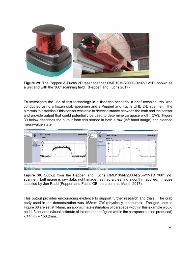
79

Figure 29. The Pepperl & Fuchs 2D laser scanner OMD10M-R2000-B23-V1V1D, shown as a unit and with the 360o scanning field. (Pepperl and Fuchs 2017).

To investigate the use of this technology in a fisheries scenario, a brief technical trial was conducted using a frozen crab specimen and a Pepperl and Fuchs UHD 2-D scanner. The aim was to establish if this sensor was able to detect distance between the crab and the sensor and provide output that could potentially be used to determine carapace width (CW). Figure 30 below describes the output from this sensor in both a raw (left hand image) and cleaned mean-value state.

Figure 30. Output from the Pepperl and Fuchs OMD10M-R2000-B23-V1V1D 360° 2-D scanner. Left image is raw data, right image has had a cleaning algorithm applied. Images supplied by Jon Rudd (Pepperl and Fuchs GB, pers comms; March 2017).

This output provides encouraging evidence to support further research and trials. The crab body used in the demonstration was 158mm CW (physically measured). The grid lines in Figure 30 are set at 14mm, an approximate estimation of carapace width in this example would be 11.3 squares (visual estimate of total number of grids within the carapace outline produced) x 14mm = 158.2mm.

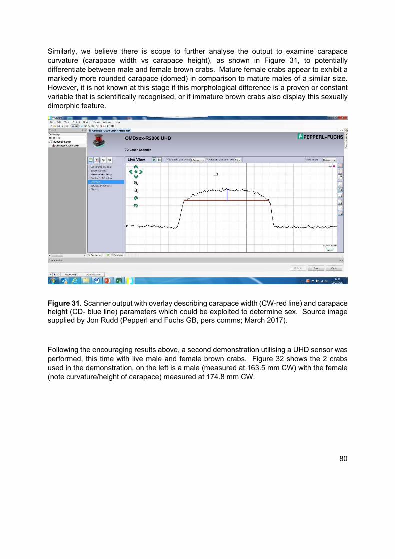
80

Similarly, we believe there is scope to further analyse the output to examine carapace curvature (carapace width vs carapace height), as shown in Figure 31, to potentially differentiate between male and female brown crabs. Mature female crabs appear to exhibit a markedly more rounded carapace (domed) in comparison to mature males of a similar size. However, it is not known at this stage if this morphological difference is a proven or constant variable that is scientifically recognised, or if immature brown crabs also display this sexually dimorphic feature.

Figure 31. Scanner output with overlay describing carapace width (CW-red line) and carapace height (CD- blue line) parameters which could be exploited to determine sex. Source image supplied by Jon Rudd (Pepperl and Fuchs GB, pers comms; March 2017).

Following the encouraging results above, a second demonstration utilising a UHD sensor was performed, this time with live male and female brown crabs. Figure 32 shows the 2 crabs used in the demonstration, on the left is a male (measured at 163.5 mm CW) with the female (note curvature/height of carapace) measured at 174.8 mm CW.

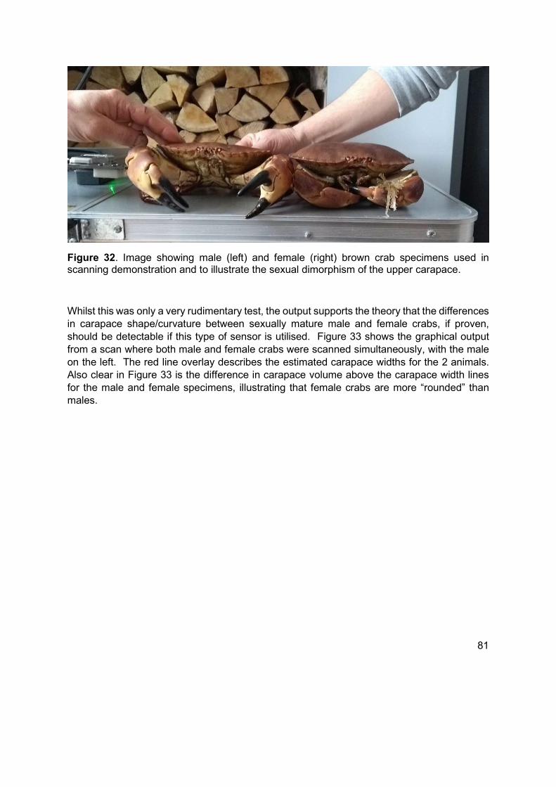
81

Figure 32. Image showing male (left) and female (right) brown crab specimens used in scanning demonstration and to illustrate the sexual dimorphism of the upper carapace.

Whilst this was only a very rudimentary test, the output supports the theory that the differences in carapace shape/curvature between sexually mature male and female crabs, if proven, should be detectable if this type of sensor is utilised. Figure 33 shows the graphical output from a scan where both male and female crabs were scanned simultaneously, with the male on the left. The red line overlay describes the estimated carapace widths for the 2 animals. Also clear in Figure 33 is the difference in carapace volume above the carapace width lines for the male and female specimens, illustrating that female crabs are more “rounded” than males.

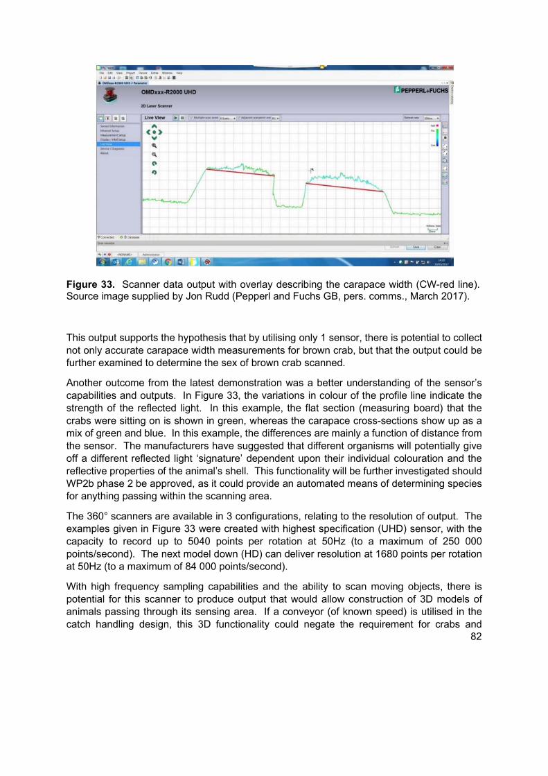
82

This output supports the hypothesis that by utilising only 1 sensor, there is potential to collect not only accurate carapace width measurements for brown crab, but that the output could be further examined to determine the sex of brown crab scanned.

Another outcome from the latest demonstration was a better understanding of the sensor’s capabilities and outputs. In Figure 33, the variations in colour of the profile line indicate the strength of the reflected light. In this example, the flat section (measuring board) that the crabs were sitting on is shown in green, whereas the carapace cross-sections show up as a mix of green and blue. In this example, the differences are mainly a function of distance from the sensor. The manufacturers have suggested that different organisms will potentially give off a different reflected light ‘signature’ dependent upon their individual colouration and the reflective properties of the animal’s shell. This functionality will be further investigated should WP2b phase 2 be approved, as it could provide an automated means of determining species for anything passing within the scanning area.

The 360° scanners are available in 3 configurations, relating to the resolution of output. The examples given in Figure 33 were created with highest specification (UHD) sensor, with the capacity to record up to 5040 points per rotation at 50Hz (to a maximum of 250 000 points/second). The next model down (HD) can deliver resolution at 1680 points per rotation at 50Hz (to a maximum of 84 000 points/second).

With high frequency sampling capabilities and the ability to scan moving objects, there is potential for this scanner to produce output that would allow construction of 3D models of animals passing through its sensing area. If a conveyor (of known speed) is utilised in the catch handling design, this 3D functionality could negate the requirement for crabs and

Figure 33. Scanner data output with overlay describing the carapace width (CW-red line). Source image supplied by Jon Rudd (Pepperl and Fuchs GB, pers. comms., March 2017).

83

lobsters to be oriented in a particular way to allow measurement of carapace width or length respectively. With respect to lobsters, this may also allow sex determination, by assessing the relationship between abdomen width and length, a methodology employed by Hold et el, (2015), although current understanding suggests this difference does not occur in immature lobsters.

With the potential to collect not only counts of objects (by species), but also collect accurate biological measurements (which may be further analysed to extract sex ratio data), this range of sensors (with costs ranging from £2800-£5000, dependent upon resolution) could provide most of the SIFIDS catch and biological data requirements, and thus warrant further research and investigation in WP2b Phase 2.

A similar sensor, without the 360° functionality (Smart Runner, see Figure 34) is likely to be available from Pepperl and Fuchs towards the end of 2019, it is still in development trials. This new sensor operates on a similar principle to the 2D sensor trialled above, but, rather than emitting individual beams of light, it emits a constant fixed beam (light section sensor). In-built sensors then analyse the reflected light and the distortions within that reflected light (caused by objects within the field) in much the same manner as the 2D-360°mentioned above. As this sensor is currently unavailable to purchase, an accurate estimate of price is not available at the time of writing, however, our contact within the company has indicated that it will likely be released with a list price of approximately £1000.

As the 360°functionality and high-resolution output of the Pepperl and Fuchs 2D laser scanner OMD10M-R2000-B23-V1V1D may not be required, the up-coming Smart Runner sensor may offer a considerable cost saving and still be capable of collecting the required data at suitable levels of accuracy.

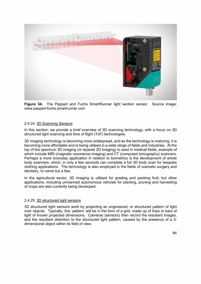
84

2.4.24 3D Scanning Sensors

In this section, we provide a brief overview of 3D scanning technology, with a focus on 3D structured light scanning and time of flight (ToF) technologies.

3D imaging technology is becoming more widespread, and as the technology is maturing, it is becoming more affordable and is being utilised in a wide range of fields and industries. At the top of the spectrum 3D imaging (or layered 2D imaging) is used in medical fields, example of which include MRI (magnetic resonance imaging) and CT (computed tomography) scanners. Perhaps a more everyday application in relation to biometrics is the development of whole body scanners, which, in only a few seconds can complete a full 3D body scan for bespoke clothing applications. The technology is also employed in the fields of cosmetic surgery and dentistry, to name but a few.

In the agricultural sector, 3D imaging is utilised for grading and packing fruit, but other applications, including unmanned autonomous vehicles for planting, pruning and harvesting of crops are also currently being developed.

2.4.25 3D structured light sensors

3D structured light sensors work by projecting an engineered, or structured pattern of light over objects. Typically, this ‘pattern’ will be in the form of a grid, made up of lines or bars of light of known projected dimensions. Cameras (sensors) then record the resultant images, and the resultant distortion to the structured light pattern, caused by the presence of a 3-dimensional object within its field of view.

Figure 34. The Pepperl and Fuchs SmartRunner light section sensor. Source image: www.pepperl-fuchs.smartrunner.com

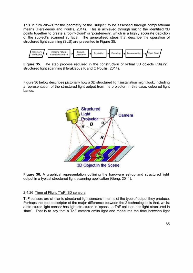
85

This in turn allows for the geometry of the ‘subject’ to be assessed through computational means (Herakleous and Poullis, 2014). This is achieved through linking the identified 3D points together to create a ‘point-cloud’ or ‘point-mesh’, which is a highly accurate depiction of the subject’s scanned surface. The generalised steps that describe the operation of structured light scanning (SLS) are presented in Figure 35.

Figure 36 below describes pictorially how a 3D structured light installation might look, including a representation of the structured light output from the projector, in this case, coloured light bands.

2.4.26 Time of Flight (ToF) 3D sensors

ToF sensors are similar to structured light sensors in terms of the type of output they produce. Perhaps the best descriptor of the major difference between the 2 technologies is that, whilst a structured light sensor has light structured in ‘space’, a ToF solution has light structured in ‘time’. That is to say that a ToF camera emits light and measures the time between light

Figure 35. The step process required in the construction of virtual 3D objects utilising structured light scanning (Herakleous K and C Poullis, 2014).

Figure 36. A graphical representation outlining the hardware set-up and structured light output in a typical structured light scanning application (Geng, 2011).

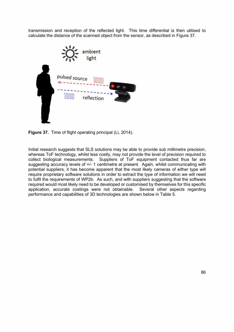
86

transmission and reception of the reflected light. This time differential is then utilised to calculate the distance of the scanned object from the sensor, as described in Figure 37.

Initial research suggests that SLS solutions may be able to provide sub millimetre precision, whereas ToF technology, whilst less costly, may not provide the level of precision required to collect biological measurements. Suppliers of ToF equipment contacted thus far are suggesting accuracy levels of +/- 1 centimetre at present. Again, whilst communicating with potential suppliers, it has become apparent that the most likely cameras of either type will require proprietary software solutions in order to extract the type of information we will need to fulfil the requirements of WP2b. As such, and with suppliers suggesting that the software required would most likely need to be developed or customised by themselves for this specific application, accurate costings were not obtainable. Several other aspects regarding performance and capabilities of 3D technologies are shown below in Table 5.

Figure 37. Time of flight operating principal (Li, 2014).

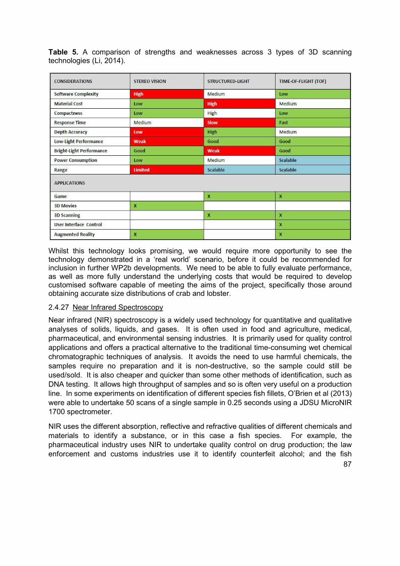
87

Table 5. A comparison of strengths and weaknesses across 3 types of 3D scanning technologies (Li, 2014).

Whilst this technology looks promising, we would require more opportunity to see the technology demonstrated in a ‘real world’ scenario, before it could be recommended for inclusion in further WP2b developments. We need to be able to fully evaluate performance, as well as more fully understand the underlying costs that would be required to develop customised software capable of meeting the aims of the project, specifically those around obtaining accurate size distributions of crab and lobster.

2.4.27 Near Infrared Spectroscopy

Near infrared (NIR) spectroscopy is a widely used technology for quantitative and qualitative analyses of solids, liquids, and gases. It is often used in food and agriculture, medical, pharmaceutical, and environmental sensing industries. It is primarily used for quality control applications and offers a practical alternative to the traditional time-consuming wet chemical chromatographic techniques of analysis. It avoids the need to use harmful chemicals, the samples require no preparation and it is non-destructive, so the sample could still be used/sold. It is also cheaper and quicker than some other methods of identification, such as DNA testing. It allows high throughput of samples and so is often very useful on a production line. In some experiments on identification of different species fish fillets, O’Brien et al (2013) were able to undertake 50 scans of a single sample in 0.25 seconds using a JDSU MicroNIR 1700 spectrometer.

NIR uses the different absorption, reflective and refractive qualities of different chemicals and materials to identify a substance, or in this case a fish species. For example, the pharmaceutical industry uses NIR to undertake quality control on drug production; the law enforcement and customs industries use it to identify counterfeit alcohol; and the fish

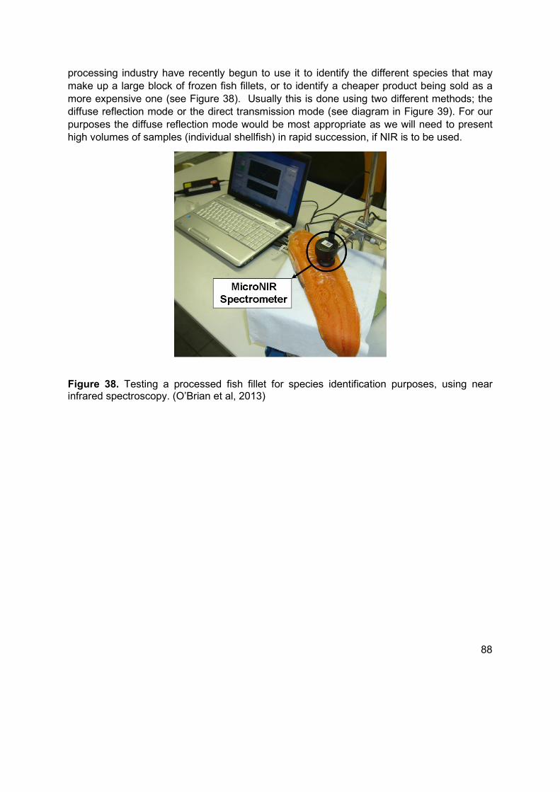
88

processing industry have recently begun to use it to identify the different species that may make up a large block of frozen fish fillets, or to identify a cheaper product being sold as a more expensive one (see Figure 38). Usually this is done using two different methods; the diffuse reflection mode or the direct transmission mode (see diagram in Figure 39). For our purposes the diffuse reflection mode would be most appropriate as we will need to present high volumes of samples (individual shellfish) in rapid succession, if NIR is to be used.

Figure 38. Testing a processed fish fillet for species identification purposes, using near infrared spectroscopy. (O’Brian et al, 2013)

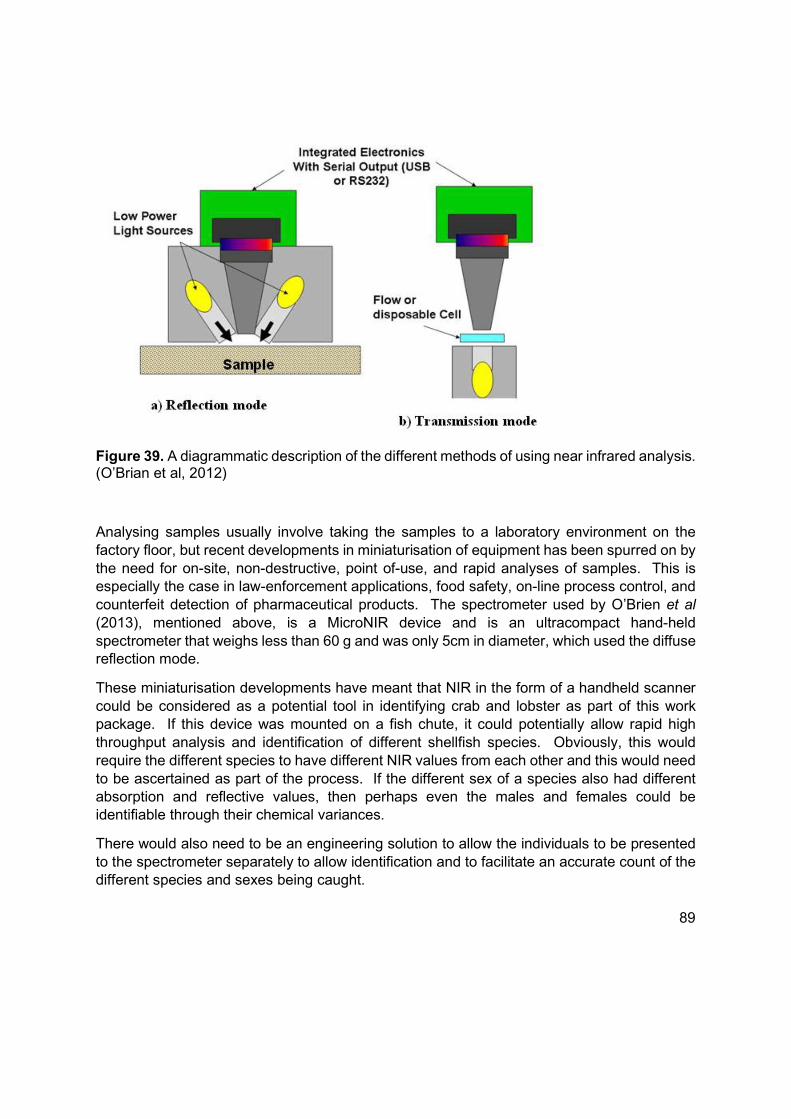
89

Figure 39. A diagrammatic description of the different methods of using near infrared analysis. (O’Brian et al, 2012)

Analysing samples usually involve taking the samples to a laboratory environment on the factory floor, but recent developments in miniaturisation of equipment has been spurred on by the need for on-site, non-destructive, point of-use, and rapid analyses of samples. This is especially the case in law-enforcement applications, food safety, on-line process control, and counterfeit detection of pharmaceutical products. The spectrometer used by O’Brien et al (2013), mentioned above, is a MicroNIR device and is an ultracompact hand-held spectrometer that weighs less than 60 g and was only 5cm in diameter, which used the diffuse reflection mode.

These miniaturisation developments have meant that NIR in the form of a handheld scanner could be considered as a potential tool in identifying crab and lobster as part of this work package. If this device was mounted on a fish chute, it could potentially allow rapid high throughput analysis and identification of different shellfish species. Obviously, this would require the different species to have different NIR values from each other and this would need to be ascertained as part of the process. If the different sex of a species also had different absorption and reflective values, then perhaps even the males and females could be identifiable through their chemical variances.

There would also need to be an engineering solution to allow the individuals to be presented to the spectrometer separately to allow identification and to facilitate an accurate count of the different species and sexes being caught.

90

NIR would not be able to undertake a length measurement of the individuals assessed, so NIR would need to be coupled with additional technology, such as video, laser or in line weighing devices, to enable a carapace length or an individual weight to be gathered or calculated.

If NIR was to be considered as an option going forward then this project would firstly need to establish whether crab shell and lobster shell were different and identifiable, irrespective of their state of moult. Whether sex could be identified for each species would also be established during these experiments.

In addition, for our purposes these devices will also need to be mounted inside a specially designed waterproof and robust casing to a specified standard (e.g. IP67 rating), to ensure that it could reliably operate in the marine environment and be built into the engineered solution. There would also need to be a reliable light source, fibre optic cabling, and on-board analysis capability with data storage.

The handling of the shellfish would need to facilitate rapid throughput by delivering the shellfish to the spectrometer in such a way as to allow rapid sampling.

Costs – The costs associated with NIR technology have reduced considerably in recent years, as has the size of the equipment required (Figure 40). Modern handheld devices are available and although the prices have reduced, they are still significant. Some systems also require additional equipment, an analytical suite, software and training and when these are added in, the costs can become high in relation to the fishery being targeted in this work package. One quote that was acquired from a leading company in the field, ThermoFisher for their microPHAZIR GP 4.2 handheld device (Figure 41) which comes in a storm proof case, with batteries, charger, data transfer cable, software, 1 day training and general ongoing support, was $US33,450. Obviously at this price NIR becomes infeasible, especially when it may not be able to provide all the data requirements e.g. carapace length frequency measurements.

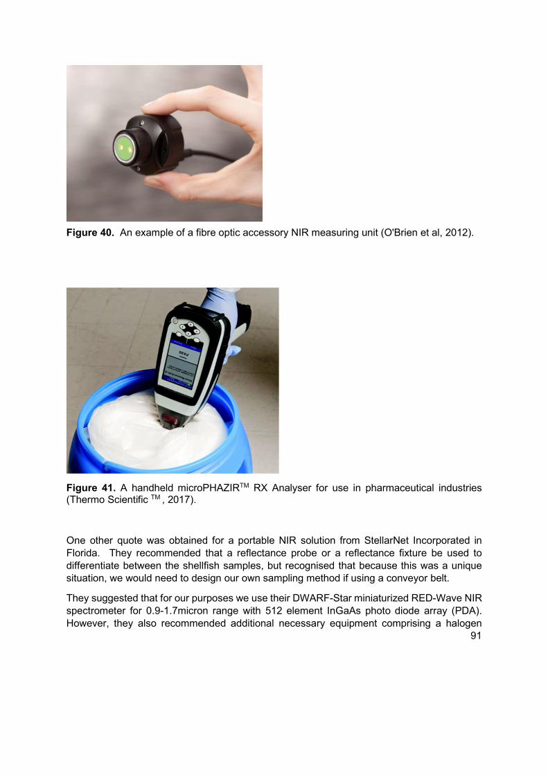
91

Figure 41. A handheld microPHAZIRTM RX Analyser for use in pharmaceutical industries (Thermo Scientific TM , 2017).

One other quote was obtained for a portable NIR solution from StellarNet Incorporated in Florida. They recommended that a reflectance probe or a reflectance fixture be used to differentiate between the shellfish samples, but recognised that because this was a unique situation, we would need to design our own sampling method if using a conveyor belt.

They suggested that for our purposes we use their DWARF-Star miniaturized RED-Wave NIR spectrometer for 0.9-1.7micron range with 512 element InGaAs photo diode array (PDA). However, they also recommended additional necessary equipment comprising a halogen

Figure 40. An example of a fibre optic accessory NIR measuring unit (O'Brien et al, 2012).

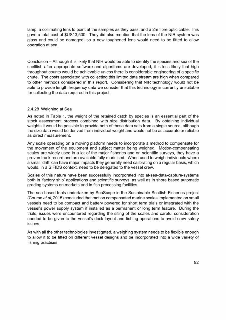
92

lamp, a collimating lens to point at the samples as they pass, and a 2m fibre optic cable. This gave a total cost of $US13,500. They did also mention that the lens of the NIR system was glass and could be damaged, so a new toughened lens would need to be fitted to allow operation at sea.

Conclusion – Although it is likely that NIR would be able to identify the species and sex of the shellfish after appropriate software and algorithms are developed, it is less likely that high throughput counts would be achievable unless there is considerable engineering of a specific chute. The costs associated with collecting this limited data stream are high when compared to other methods considered in this report. Considering that NIR technology would not be able to provide length frequency data we consider that this technology is currently unsuitable for collecting the data required in this project.

2.4.28 Weighing at Sea

As noted in Table 1, the weight of the retained catch by species is an essential part of the stock assessment process combined with size distribution data. By obtaining individual weights it would be possible to provide both of these data sets from a single source, although the size data would be derived from individual weight and would not be as accurate or reliable as direct measurement.

Any scale operating on a moving platform needs to incorporate a method to compensate for the movement of the equipment and subject matter being weighed. Motion-compensating scales are widely used in a lot of the major fisheries and on scientific surveys, they have a proven track record and are available fully marinised. When used to weigh individuals where a small ‘drift’ can have major impacts they generally need calibrating on a regular basis, which would, in a SIFIDS context, need to be delegated to the vessel crew.

Scales of this nature have been successfully incorporated into at-sea-data-capture-systems both in ‘factory ship’ applications and scientific surveys, as well as in shore based automatic grading systems on markets and in fish processing facilities.

The sea based trials undertaken by SeaScope in the Sustainable Scottish Fisheries project (Course et al, 2015) concluded that motion compensated marine scales implemented on small vessels need to be compact and battery powered for short term trials or integrated with the vessel’s power supply system if installed as a permanent or long term feature. During the trials, issues were encountered regarding the siting of the scales and careful consideration needed to be given to the vessel’s deck layout and fishing operations to avoid crew safety issues.

As with all the other technologies investigated, a weighing system needs to be flexible enough to allow it to be fitted on different vessel designs and be incorporated into a wide variety of fishing practises.

93

Capture of the data from a scale is relatively straightforward, the more complex challenge is the transporting of individuals to the weighing device and then onwards to their final destinations;

Manual transfer Single conveyor Multiple conveyors

Manual transfer would require the fisher to place each individual on a scale, wait for a weight to be obtained then move the individual to its destination. Given the impact these requirements would have on the fishing operation we have discounted this route.

Single conveyor systems carry each individual across a platform scale and then deposit them in a single bin at the end of the exit conveyor, requiring the fisher to effectively double handle the catch.

Weigh-checker or grading systems, employed in food packaging lines, offer additional functionality that could be of benefit to the fishers in addition to providing the data required for SIFIDS. These systems usually consist of a number of conveyors that take the individuals from a hopper, over a scale and then deposit them in the appropriate ‘bin’ based on weight. In a 3-belt system, the first belt feeds individuals (at variable speed) to the load cell conveyor where individual weight is assessed. The individual then passes onto the selection conveyor where individuals outside the specified weight parameters can be rejected. This approach could potentially be used to select marketable weight individuals from the catch and return the unwanted individuals (<Minimum Conservation Reference Size (MCRS)) to the sea.

The disadvantages of any conveyor-based system are its size compared to the available space on the deck of a small vessel, the power requirements to drive conveyors and actuators and the inherent problem of a mechanical failure without recourse to engineers or technicians in the short term.

Individual animal weights obtained from any suitable scale or weighing system would need to be combined with either output from another sensor, a complex engineering solution or direct input from the fisher to identify the species and sex that the captured weights refer to.

Previous experience has shown that motion compensated scales can often take several seconds to obtain a steady reliable weight measurement due to the violent and inconsistent nature of the motion of a vessel at sea. This time delay could, in some circumstances, be too long and create an unacceptable bottleneck in the processing of the catch.

As an alternative to individual weights and counts, the total catch weight and individual count could be achieved using a bulk weighing method combined with sub-sampling for numbers. This can be achieved through the use of multi-head hopper scales, normally used in packaging applications. These direct a product in bulk to several different chutes where the product is usually weighed and bagged (see Figure 42), however for this project it would direct the weighed shellfish to a specific storage facility or over the side of the vessel in the case of discards. Another option would be for the fisher to bulk weigh his catch at the end of a trip

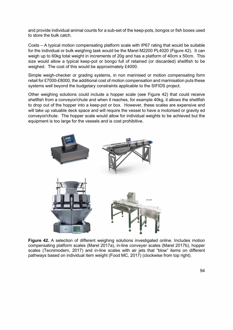
94

and provide individual animal counts for a sub-set of the keep-pots, bongos or fish boxes used to store the bulk catch. Costs – A typical motion compensating platform scale with IP67 rating that would be suitable for the individual or bulk weighing task would be the Marel M2200 PL4020 (Figure 42). It can weigh up to 60kg total weight in increments of 20g and has a platform of 40cm x 50cm. This size would allow a typical keep-pot or bongo full of retained (or discarded) shellfish to be weighed. The cost of this would be approximately £4000.

Simple weigh-checker or grading systems, in non marinised or motion compensating form retail for £7000-£8000, the additional cost of motion compensation and marinisation puts these systems well beyond the budgetary constraints applicable to the SIFIDS project.

Other weighing solutions could include a hopper scale (see Figure 42) that could receive shellfish from a conveyor/chute and when it reaches, for example 40kg, it allows the shellfish to drop out of the hopper into a keep-pot or box. However, these scales are expensive and will take up valuable deck space and will require the vessel to have a motorised or gravity ed conveyor/chute. The hopper scale would allow for individual weights to be achieved but the equipment is too large for the vessels and is cost prohibitive.

Figure 42. A selection of different weighing solutions investigated online. Includes motion compensating platform scales (Marel 2017a), in-line conveyer scales (Marel 2017b), hopper scales (Tecnimodern, 2017) and in-line scales with air jets that “blow” items on different pathways based on individual item weight (Food MC, 2017) (clockwise from top right).

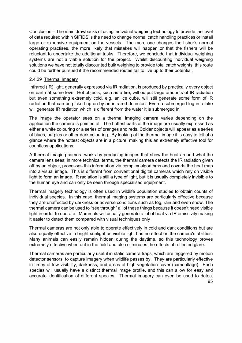
95

Conclusion – The main drawbacks of using individual weighing technology to provide the level of data required within SIFIDS is the need to change normal catch handling practices or install large or expensive equipment on the vessels. The more one changes the fisher’s normal operating practises, the more likely that mistakes will happen or that the fishers will be reluctant to undertake the additional tasks. Therefore, we conclude that individual weighing systems are not a viable solution for the project. Whilst discounting individual weighing solutions we have not totally discounted bulk weighing to provide total catch weights, this route could be further pursued if the recommended routes fail to live up to their potential.

2.4.29 Thermal Imagery

Infrared (IR) light, generally expressed via IR radiation, is produced by practically every object on earth at some level. Hot objects, such as a fire, will output large amounts of IR radiation but even something extremely cold, e.g. an ice cube, will still generate some form of IR radiation that can be picked up on by an infrared detector. Even a submerged log in a lake will generate IR radiation which is different from the water it is submerged in.

The image the operator sees on a thermal imaging camera varies depending on the application the camera is pointed at. The hottest parts of the image are usually expressed as either a white colouring or a series of oranges and reds. Colder objects will appear as a series of blues, purples or other dark colouring. By looking at the thermal image it is easy to tell at a glance where the hottest objects are in a picture, making this an extremely effective tool for countless applications.

A thermal imaging camera works by producing images that show the heat around what the camera lens sees; in more technical terms, the thermal camera detects the IR radiation given off by an object, processes this information via complex algorithms and coverts the heat map into a visual image. This is different from conventional digital cameras which rely on visible light to form an image. IR radiation is still a type of light, but it is usually completely invisible to the human eye and can only be seen through specialised equipment.

Thermal imagery technology is often used in wildlife population studies to obtain counts of individual species. In this case, thermal imaging systems are particularly effective because they are unaffected by darkness or adverse conditions such as fog, rain and even snow. The thermal camera can be used to “see through” all of these things because it doesn’t need visible light in order to operate. Mammals will usually generate a lot of heat via IR emissivity making it easier to detect them compared with visual techniques only

Thermal cameras are not only able to operate effectively in cold and dark conditions but are also equally effective in bright sunlight as visible light has no effect on the camera's abilities. Many animals can easily remain hidden during the daytime, so this technology proves extremely effective when out in the field and also eliminates the effects of reflected glare.

Thermal cameras are particularly useful in static camera traps, which are triggered by motion detector sensors, to capture imagery when wildlife passes by. They are particularly effective in times of low visibility, darkness, and areas of high vegetation cover (camouflage). Each species will usually have a distinct thermal image profile, and this can allow for easy and accurate identification of different species. Thermal imagery can even be used to detect

96

infections within an animal based on localised high temperature points. Figure 43 shows a selection of thermal images of wildlife for illustrative purposes. No images or experiments using thermal imagery with lobsters or crabs could be found. This could therefore be a very interesting and novel project in its own right.

Figure 43. A selection of thermal images of wildlife taken from various internet sources, to demonstrate the type of image and clarity one could expect from a thermal imaging system. (Pass 2017a, Pulsar 2017, Pass 2017b, McCafferty 2007).

However, there are limitations in using thermology for wildlife studies. Cilulko et al, (2013) describes how the weather conditions can affect the thermal pattern of the subject being studied. The effects of cold weather, solar radiation and precipitation can all chill or warm an animal’s surface body temperature which will change the distribution of emitted heat. So even the time of day will change the thermal radiation emitted. The greater the difference between the temperature of the animal and its surroundings, the more accurate the survey, which is why thermographic analyses are most effective at night or dawn (Butler et al., 2006). High levels of activity, stress or even illness can change the thermal pattern of a particular animal, so it is important to bear this in mind when designing surveys and identifying species.

The use of thermal imagery to identify and count different shellfish species is likely to be possible despite them being cold blooded, but it is also likely to be extremely problematic. Crab and lobster may have very different thermal profiles but so far these have not been documented. So, to use thermal imagery to provide high throughput counts for the different

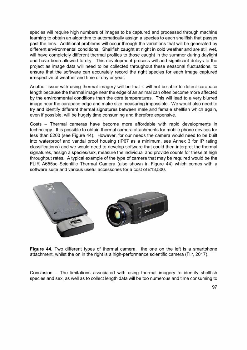
97

species will require high numbers of images to be captured and processed through machine learning to obtain an algorithm to automatically assign a species to each shellfish that passes past the lens. Additional problems will occur through the variations that will be generated by different environmental conditions. Shellfish caught at night in cold weather and are still wet, will have completely different thermal profiles to those caught in the summer during daylight and have been allowed to dry. This development process will add significant delays to the project as image data will need to be collected throughout these seasonal fluctuations, to ensure that the software can accurately record the right species for each image captured irrespective of weather and time of day or year.

Another issue with using thermal imagery will be that it will not be able to detect carapace length because the thermal image near the edge of an animal can often become more affected by the environmental conditions than the core temperatures. This will lead to a very blurred image near the carapace edge and make size measuring impossible. We would also need to try and identify different thermal signatures between male and female shellfish which again, even if possible, will be hugely time consuming and therefore expensive.

Costs – Thermal cameras have become more affordable with rapid developments in technology. It is possible to obtain thermal camera attachments for mobile phone devices for less than £200 (see Figure 44). However, for our needs the camera would need to be built into waterproof and vandal proof housing (IP67 as a minimum, see Annex 3 for IP rating classifications) and we would need to develop software that could then interpret the thermal signatures, assign a species/sex, measure the individual and provide counts for these at high throughput rates. A typical example of the type of camera that may be required would be the FLIR A655sc Scientific Thermal Camera (also shown in Figure 44) which comes with a software suite and various useful accessories for a cost of £13,500.

Figure 44. Two different types of thermal camera. the one on the left is a smartphone attachment, whilst the on in the right is a high-performance scientific camera (Flir, 2017).

Conclusion – The limitations associated with using thermal imagery to identify shellfish species and sex, as well as to collect length data will be too numerous and time consuming to

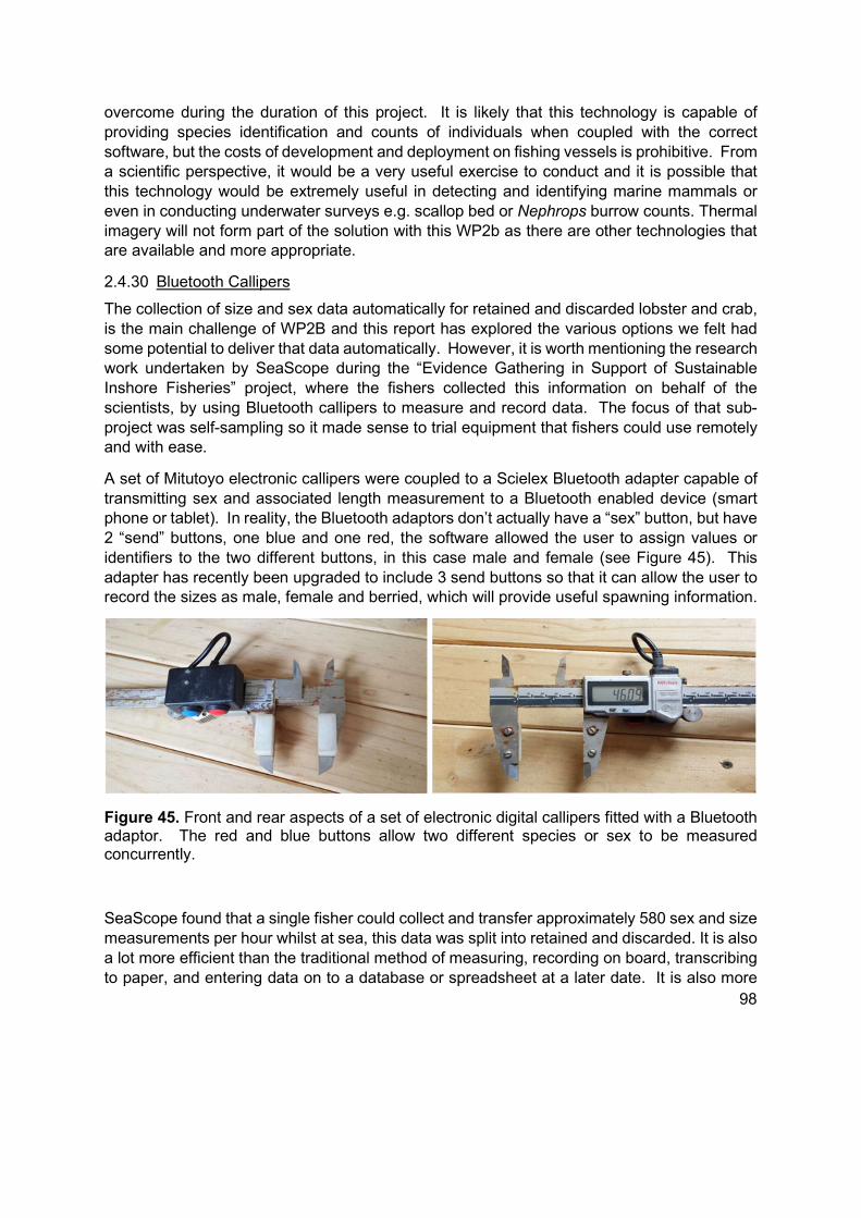
98

overcome during the duration of this project. It is likely that this technology is capable of providing species identification and counts of individuals when coupled with the correct software, but the costs of development and deployment on fishing vessels is prohibitive. From a scientific perspective, it would be a very useful exercise to conduct and it is possible that this technology would be extremely useful in detecting and identifying marine mammals or even in conducting underwater surveys e.g. scallop bed or Nephrops burrow counts. Thermal imagery will not form part of the solution with this WP2b as there are other technologies that are available and more appropriate.

2.4.30 Bluetooth Callipers

The collection of size and sex data automatically for retained and discarded lobster and crab, is the main challenge of WP2B and this report has explored the various options we felt had some potential to deliver that data automatically. However, it is worth mentioning the research work undertaken by SeaScope during the “Evidence Gathering in Support of Sustainable Inshore Fisheries” project, where the fishers collected this information on behalf of the scientists, by using Bluetooth callipers to measure and record data. The focus of that sub-project was self-sampling so it made sense to trial equipment that fishers could use remotely and with ease.

A set of Mitutoyo electronic callipers were coupled to a Scielex Bluetooth adapter capable of transmitting sex and associated length measurement to a Bluetooth enabled device (smart phone or tablet). In reality, the Bluetooth adaptors don’t actually have a “sex” button, but have 2 “send” buttons, one blue and one red, the software allowed the user to assign values or identifiers to the two different buttons, in this case male and female (see Figure 45). This adapter has recently been upgraded to include 3 send buttons so that it can allow the user to record the sizes as male, female and berried, which will provide useful spawning information.

Figure 45. Front and rear aspects of a set of electronic digital callipers fitted with a Bluetooth adaptor. The red and blue buttons allow two different species or sex to be measured concurrently.

SeaScope found that a single fisher could collect and transfer approximately 580 sex and size measurements per hour whilst at sea, this data was split into retained and discarded. It is also a lot more efficient than the traditional method of measuring, recording on board, transcribing to paper, and entering data on to a database or spreadsheet at a later date. It is also more

99

accurate as it removes the likelihood of transcription errors and the potential for data to be lost.

It would not be acceptable to ask a fisher to undertake an hour of sampling each day on top of their normal fishing activities and obviously, guidance or training should be given to ensure that sampling is random and representative. But, if a fisher could spend 15 minutes per day undertaking sampling on one or two components of the catch, it would be possible to collect about 600 to 800 sexed length samples of retained and discarded lobsters and crabs per week for each vessel in the programme.

Costs – A calliper setup costs in the region of £966 (£388 for the callipers, £467 for the adapter and £111 import duty), it would also require a device to accept the data and transmit it to the OBCDCS. In addition to the capital costs there would probably need to be a small incentive provided to the fishers to undertake this additional task. The hardware should have a working life of at least 3 years and therefore the annual hardware costs would be in the region of £322 per year.

Given that this is not a “fully automatic” system and would not be first choice as a size gathering tool in this work package, only a description and indicative costs have been included rather than a full search of the various suppliers. It is very likely that more developers and suppliers have entered the marketplace since the report for the EFF funded project was published and if callipers were to be seriously considered then a more in-depth market search should be undertaken.

Conclusion – As discussed earlier in this report, self-sampling is the least attractive solution to the SIFIDS data collection target but could be considered as a supplementary data source or used to verify data collected by the automatic solutions.

A significant challenge will be convincing fisheries scientists to accept the data for assessment purposes, some form of verification process would need to be included in the programme design, probably in the form of an installed camera system and random cross checking of reported size data.

We do not recommend this as a route forward for the main data collection aim of the SIFIDS project, but we do consider it a useful source for supplementary data or as a verification tool to use alongside the automatic systems.

2.4.31 Sub-sampling the Catch

All the implementations of technologies discussed in this report are targeted at sampling the entire catch, although this is the most preferable solution, sub-sampling is an accepted method across all fisheries population research and could be applied to the SIFIDS project.

Due to the catch handling process, described in the catch handling section, lobsters should present no problem in terms of sampling and will not require any sub-sampling process to be instigated.

100

Where large crabs are ‘nicked’ on a vessel, again the catch handling process lends itself to complete sampling of this component of the catch.

For bulk catches of crabs and discarded catch, sub-sampling may be the only viable solution to obtaining reliable and consistent data without significantly impacting the fishing operations.

Previous projects undertaking sampling at sea aboard shellfish creel vessels have allowed SeaScope to develop robust subsampling techniques specific to creel fisheries. These methods are different depending on whether one is subsampling the retained or discarded portion of the catch.

Once processed the retained bulk crab catch is stored in either keep-pots or fish boxes of a known average weight (e.g. 40kg). If subsampling of the retained catch was necessary then a keep-pot or box of each grade (by sex, or size or a combination) would be passed through the data capture system. The data from these sub-samples would then be raised to the total catch for the day, using standard procedures, either by using calculated sample weight and total estimated weight or number of creels or boxes sampled against total number of creels or boxes retained for each component. The totals could be input by the skipper or obtained later from the mandatory FISH1 forms submitted to Marine Scotland. Given the desire for near-real-time data, it would be preferable to obtain the total values directly from the skipper, this could be provided as functionality within the system that would also compile a FISH1 form for the skipper. By providing the FISH1 form as an output we reduce the paperwork burden on the skipper thus providing an incentive for them to provide the SIFIDS data in a timely manner. By using skipper obtained data we also introduce the possibility for finer detail sub-sampling; if the process was made relatively simple and quick, sub-sampling could be undertaken at a string level, or multiples of, e.g. every 5 strings, or when on a longer steam between strings.

Sub-sampling the discarded catch is more challenging because it is nearly impossible to get an accurate estimate of the total weight or volume of discards unless all the discards are boxed before being returned to the sea. This could potentially add an unacceptable burden on the skipper or crew. A potential solution to this would be to ask them to collect the discards from an agreed number of strings or creels selected randomly each day. The discarded catch from this sampling frame can then be raised to obtain total discards using the relationship between subsampled fishing effort and total fishing effort.

Ideally subsampling of crab catches would not be used because it doesn’t allow for different catch rates between the strings (and therefore local ground differences) to be detected. However, it could allow a good estimate for retained and discarded catches to be made should the overall catch volumes be unmanageable for the engineering/technology solution and it would still be a great improvement on current sampling levels. Therefore, it is important to also consider catch handling protocols that would enable subsampling if, and when necessary.

2.4.32 Gesture Recognition

There are various scenarios within this report which may require a degree of system input from the fishers, it would be possible to utilise machine vision techniques for gesture recognition to facilitate this input. For example, distinguishing between retained and discarded animals being put through a camera system could be achieved simply using a thumbs-up

101

signal to identify retained animals to follow or a flat palm to indicate discarded animals follow. Ideally, any process using gesture recognition would be supported by a visual cue to the operator to confirm the gesture was correctly interpreted.

2.4.33 Data Storage

Data, imagery and other binary objects generated by the system developed under WP2b will be eventually stored on the OBCDCS. It may be necessary to provide local storage within the 2B system to mitigate for any failure within the OBCDCS, the connection between the 2B system and OBCDCS or a fault within the 2B system preventing the communication from occurring. It is anticipated that the local storage would provide for a minimum number of days/hours local storage, until the exact nature and size of the data stream is defined a more specific offline capability cannot be defined. The offline mode would automatically transfer the local data to the OBCDCS once the connection is re-established.

2.4.34 Data Communication

Given the current (in draft) proposal for OBCDCS, all the data communication to the OBCDCS will be via a hard-wired standard network. Subsequent data transfer to the shore station will be managed by the OBCDCS. The proposal for OBCDCS allows for any data stream to be stored on the system with selected parameters uploaded automatically, other parameters uploaded only via high bandwidth Wi-Fi and other parameters only uploaded on demand. As an example, this functionality could be implemented in a video stream based 2B system as follows;

Sys2B Stores the full live video stream to OBCDCS in manageable chunks (5 to 10 min segments possibly).

Sys2B Extracts frames from the live video stream that contain an object of interest (a crab) and stores those on OBCDCS as a Frame of Interest (FoI).

Sys2B Extracts information (species, sex, size, discard or retained) from the FoI coupled with other sensors and stores that information as data parameters on OBCDCS.

The data parameters are set within OBCDCS as auto-upload and will be uploaded during the standard OBCDCS upload cycle.

The FoI images are set within OBCDCS as Wi-Fi or on-demand upload and will be uploaded only if a high bandwidth connection is detected OR a request is received to upload a specific set of FoI objects.

The video chunks are set within OBCDCS as on-demand and will only be uploaded if a request is received.

This scenario allows the developers and users of the system to analyse the result sets regularly, examine the extracted images (FoI) when available or request specific FoI images or full video to verify data or analyse system problems. This setup is targeted at minimising data transfer volumes therefore reducing system running costs.

102

2.4.35 Engineering of a Handling and Delivery System

Throughout the investigation into the different technology options it has become apparent that how the subject matter (e.g. a discarded crab) is presented to the technology, is as important as the technology itself. All potential technology solutions that we have identified have required the shellfish to be presented in a controlled way and in a reasonably consistent environment depending on what type of technology is being used.

If elements of the catch need to be quantified by count, or size frequency data needs to be obtained, then the shellfish need to be presented to the technology as individuals and usually held steady so that the required data can be collected.

If the technology solution involves visual spectrum image capture, either as video or stills, then the lighting conditions are also important and need to be controlled. The individual animals will need to be transported (by gravity and/or their own legs) through a short ‘tunnel’, which is externally light-proof and appropriately internally lit to provide optimum imaging conditions.

It may be that the ‘technology tunnel’ uses more than 1 type of technology to achieve the project aims; low resolution video for counting and/or triggering high resolution stills with different lighting or an entirely different technology for identification and measurement.

During the engineering design process, the method of transporting the animals and the data capture environment, as well as the technology selected to capture the data, will need to be considered together.

It is difficult to envisage an engineering solution for use on board an inshore vessel, that would allow discard and retained catch to be automatically identified and sorted. Crabs are often discarded for reasons other than size. They may be soft shelled or contain little meat due to a recent moulting process; they may have claws missing; they may be showing external signs of disease; or the carapace may be cracked and damaged. Therefore, it will be necessary to implement the solution into the catch handling process after the point that the fishers have made a decision on the fate of the individuals within the catch.

To avoid undue burden on the fishers the engineering solution will need to consider the current working practises of the fishers, the vessel’s deck layout, how the fishing gear is operated and stored, and where it would be possible to safely locate the handling system. Phase 1 of WP2b does not present an engineering solution because it is focussed on identifying the technology options for a Phase 2 work package, however this section will try and summarise our current thoughts on what the solution will need to provide.

Design Considerations

Construction will need to be of a material suitable for a marine environment such as stainless steel, aluminium or a hard plastic.

The footprint of the system will need to be as small as possible because deck space on the inshore fleets is extremely limited.

It will need to be as “snag-free” as possible to avoid entanglement with ropes.

103

Design will need to be versatile and allow it to be easily adapted to different vessel layouts and catch handling procedures.

The design should be portable to allow it to be moved round the deck of a fishing vessel to measure different catch segments if necessary, or even between different vessels and fleets.

The design should present the individual shellfish in a manner and environment suited to the technology chosen.

Once data capture is complete, the system should direct the individuals to the most appropriate destination without the need for additional handling

Further exploration, design and development of a handling system will be included within Phase 2 of WP2b should it proceed. It will include the design and building of prototypes that will be tested at sea aboard 5 commercial vessels along with the chosen biological sampling technology. The vessel surveys completed as part of Phase 2 (up to a maximum of 50 surveys) will help provide additional catch handling and gear deployment descriptions, along with input and suggestions from the fishers themselves, to help inform the design. Any required catch handling changes by the crew will also be described and a duty of care and training documentation will be produced.

2.4.36 WP2b Phase 1 General Discussion

There have been rapid developments over the last few years in technology, both hardware and software, that can be made relevant to gathering fisheries related data at sea. The miniaturisation and the introduction into everyday life of some of the technology described in this report, means that technology that was once limited to science laboratories and large-scale industrial use, is now a feasible option for gathering data at sea. Some of the technologies explored were capable of delivering the data requirements but their cost and/or implementation requirements ruled them out for use in the SIFIDS project.

2.4.37 Effort Data

There are many complex options available for detecting and recording the vessel activity associated with the retrieval of a buoy and its associated creels; image recognition, winch activity sensors, long range RFID systems and other electronic tagging, bar-codes or QR codes on the equipment etc. Each of these technological solutions has strengths and individual weaknesses but they all share the same inherent weakness; a high risk of spurious activations or missing activations. The technology recommended, although simple, requires minimal effort from the individuals working on the vessels, provides a technically and procedurally robust, and cost-effective mechanism for capturing the required data. The hardware side of the solution is well proven in harsh environments, requires minimal space on the vessel and draws little power. The most at-risk components (the RFID tags themselves) are cheap and require no technical knowledge to replace in the field. The remaining components are generic off-the-shelf items, can be suitably protected and, if necessary, can also be replaced in the field with minimal guidance. The software required to complete the system is, in software terms, quite simple; it has limited and well-defined functionality, simple

104

algorithms and no complex logic paths to follow and test. There is one unknown in the proposal, namely which detection mechanism to use for individual creels. We are confident that each of the proposed detection mechanisms can provide the creel count, it is purely a case of testing and selecting the best fit for ease of implementation and survivability in the field. Each of the creel detection options will provide the same indication back to the software, i.e. the device has been activated, this allows the string identification, the string associated activity (deployment or retrieval) and the creel counting elements of the software to be largely developed whilst the actuator testing and selection is underway, thus allowing the whole system to be available for desk and field testing much earlier in the project lifecycle.

2.4.38 Biological Data

The capture of biological data is significantly more complex than the effort data, and within the overall complexity there are further layers of added complexity. The traditional, human oriented methods of obtaining sex and size data do not lend themselves easily to a technical solution that can be implemented in a cost and space constrained way in a harsh and remote environment. There is the need to examine novel ways to obtain this data that can be used within the boundaries set by the SIFIDS project. We propose a multi-threaded approach that examines new measures and characteristics of the target species that will then enable development of technological solutions to the problem at hand. The technical solutions proposed use proven hardware, albeit in different scenarios, combined with cutting edge software techniques to extract the scientifically relevant data from the technical data stream. Using visible light cameras to identify (classify) objects is commonplace but implementing it to handle a high throughput of highly mobile individuals in a changing environment on a moving platform is a challenge. The discussion below assumes that the individual animals are presented the ‘right way up’. This, on the face of it, shouldn’t pose too much of an inconvenience to the crew, however, the surveys will confirm this. Should asking for the individuals to be put through the system the right way up cause issues, the proposal still stands but would require additional camera feeds and software logic to select the camera feed giving the most suitable view.

2.4.38.1 Individual counts of retained catch

As is shown in the demonstration video (supplied), counting of individual objects passing through the view of a camera is easily achieved without resorting to complex or proprietary software techniques. This simple approach could be implemented with 3 camera systems (1 per species – lobster, brown crab and velvet crab) to provide catch counts by species, using the humans on the vessel to undertake the easy, for a human, task of identifying to species. This approach does however come up against the constraint of the system requiring minimal space on the vessel.

2.4.38.2 Species identification and counts of retained catch

Again, using visible light vision systems, it will be possible to identify the individual species either through simple algorithms (shape and colour) or more complex machine learning techniques. The simple route will be tested first with development reverting to the complex

105

solution should the simple route fail. As discussed in detail in the relevant sections, we have no doubt that visual spectrum systems will be able to reliably deliver the data at this level. There are more unknowns with this part of the proposal; without field trials, we cannot confidently specify image quality, acceptable light fluctuations or the necessary processing power required to run the identification algorithms at an acceptable speed.

2.4.38.3 Species identification, sex and counts of retained catch

The addition of sex identification into the problem domain has significant impact on technology selection, system design and software development. Reliable, high hit-rate sex identification of lobsters using the normal ‘human’ method of examining the pleopods is near impossible with a technological solution. The need to turn the animal over, move legs and possibly tail out of the way to get a clear view of the pleopods, then applying an algorithm to identify where to find the pleopods before applying a further algorithm to differentiate between the sexes, rules this method out. It could be possible, with a lobster the ‘right way up’ walking over a camera system, to identify the pleopods and obtain a sex using visual systems. Our experience with lobster and crab chute systems suggests a large proportion of animals randomly placed at the top of a chute will slide down with legs and tail curled or be flicking themselves around on their sides. It would be possible to ask the fishers to try and ensure the lobsters are suitably calm and walk down a chute, but this would be pushing past the limits of acceptable change to working practices. Identifying the sex of crabs is less problematic, mainly due to the larger and more visible nature of the sexually identifying features. However, a crab with its legs curled under in defensive position will largely mask the area of interest. Although not entirely ruling out using visual systems to identify sex using the standard features, we feel exploring in more detail the morphometric features of the species in question may uncover a more technologically suited set of sexually dimorphic characteristics. Another solution which has been recommended for further investigation and possible development is the use of 2D/3D scanners. The implementation of these devices to identify sex would necessitate the discovery of detectable sexually dimorphic features, such as the (as yet only anecdotal) ‘domed’ carapace of female brown crab. Again, it is highly likely, guaranteed in the case of the ‘dome’, that features would only be detectable if the animal is presented in a particular rotational orientation, or a multitude of sensors were deployed to acquire the necessary profile irrelevant of the orientation of the individual.

2.4.38.4 Species identification counts and measurements of retained catch

As discussed in the detailed section, acquiring accurate measurements from visible spectrum images requires additional data as well as the image; to correctly calculate measurements from an image we need to know the distance between the subject matter and the sensor. This could be achieved in a number of ways within a visible spectrum system; a projected light beam with software analysing the resultant distortion or a laser or ultra-sonic range finder as a separate sensor proving input to the software. Once we start incorporating additional projection or sensors into a camera system it begs the question of whether we still need the visible spectrum image any longer. The 2D/3D scanning systems described provide the dense point cloud needed to allow measurement directly, with the addition of possibly being able to

106

provide sex identification (pending discovery of suitable characteristics). To a human, each of the target species has a very distinct shape, it is not outside the bounds of possibility that given a 2D/3D reconstruction of an entire individual it would be possible to develop a species identification algorithm. If the additional analysis methods can be developed for a 2D/3D point cloud then a single scanner could theoretically provide the whole individual data set – species, sex and size.

2.4.38.5 Applying the retained catch solutions to discarded catch

The discard portion of the catch adds yet another layer of complexity to the problem; non-target species (other crab species, whelks, fish etc.), other material (seaweed, discarded bait) and the physical bulk of the component. If the species identification algorithms are robust enough, they should be able to ignore the non-target species, if the engineering solution is appropriate and the processing speed of the hardware is fast enough the system should be able to manage the bulk. We are left with the significant change to work practices on the vessel, it will no longer be appropriate to shake out creels or throw discards directly over the side of the vessel, all the catch, whatever its fate, will need to pass through a data capture system. This is not an insurmountable problem. With engaged and willing fishers and a suitably flexible system we are confident a solution can be implemented. It is likely that the discard solution, certainly in engineering terms, will need to be customised to suit each vessel to make the change in working practice as small as possible.

2.4.38.6 Engineering

A recurrent theme throughout this report is engineering, any system put in place is reliant on individuals being presented to the technology in an appropriate fashion, and, in some cases, an appropriate environment (e.g. lighting). On top of the needs driven by the technology the engineering solution also has to have minimal impact on working practices, deck space and power drain. With input from the fishers, a carefully designed, well thought through design could make alterations to the catch handling processes beneficial to both the crew and the individual animals. This report does not attempt to address the engineering problem, but it has been considered for each of the technologies considered and we believe the proposed technology solutions all have applicable engineering solutions available to them.

2.4.39 WP2b Phase 1 Recommendations

As a result of our investigations, discussion with other scientists, manufacturers and researchers we propose the following be pursued as phase 2 of Work Package 2B. The recommendations regarding the biological data are split into 2 threads, it may be that after deeper investigation and development only 1 thread is pursued to completion or that both threads combine to provide the final product. Engineering solutions and vessel implementation survey

Conduct up to 50 vessel surveys and discussions with skippers and crew to ascertain;

107

the nature of the catch handling processes on the vessel and how they may fit with the technology solutions proposed.

how the selected technologies could be implemented. the engineering solution required for the vessel.

Effort data capture Development of a 2 reader RFID system to provide string level deployment and recovery flags associated with the spatial/temporal linkage provided by the OBCDCS. Laboratory and field trials of non-contact proximity sensors to provide creel counts. Followed by development and integration of the selected sensor with the RFID system to provide a single effort data collection system. Should proximity sensors fail to meet the needs of the project then to pursue further the use of electro-mechanical switching to provide the functionality.

Morphometric data collection

As development of the technological solutions may (evidence from our early trials suggest this is highly likely) require the collection of non-standard data items to provide the ‘standard’ measurements and sex of individuals, it is our recommendation that a program of detailed morphometric measurements is designed and undertaken across all 3 target species. These detailed data to be analysed to provide verified models and algorithms for the technology development team.

Biological data Thread 1 –

Develop visible spectrum machine vision system to provide species identification and counting for retained catch then discarded catch. Investigate and further develop, if appropriate, visual spectrum machine vision system to provide individual sex data Investigate and further develop, if appropriate, visual spectrum machine vision system to provide individual size data

Thread 2 –

Investigate and further develop 2D/3D scanning system to provide species identification, sex and size data

Both threads to be run in parallel until it becomes clear which thread is going to prove the most effective in delivering the required data, the time constraints on the project do not allow for exploration of a single thread, only to find it cannot fully deliver, leaving insufficient time for the other thread to reach completion. Both threads will use one or a combination of machine learning, deep neural networks and genetic programming to develop the required software.

Catch data capture

108

If the technology implemented for biological data is capable of full capture of the entire catch, the total catch data will be directly available from that system. However, if the biological system cannot provide total catch data then; Develop and implement a simple GUI that will enable the skipper to provide catch data at string or trip level and output that data as a FISH1 form as well as submitting it to OBCDCS.

Environmental data The scientists and fishery managers consulted, considered environmental data as useful or desirable, but not essential for stock assessment purposes. Investigations into the required technology to provide this information has led to the conclusion that the costs, in both monetary and time terms, of implementing this data stream capture programme, are too high to recommend its inclusion in Phase 2, as a primary target. Other data streams need to take priority. If these data had been specified as essential, then more emphasis could be put on collecting this data. If subsequent discussions re-prioritised this data stream and additional funding was agreed, then further investigation in to weather/environmental data collection could be considered. Perhaps a limited trial on a single vessel may prove useful as long as it does not jeopardise the collection of the data described as essential. It is also worth remembering that the OBCDCS being developed under WP2a will allow an appropriate stand-alone weather data collection device to connect directly to it, rather than have this data collected as part of WP2b. So, at this stage we recommend not including this within the WP2b development.

109

2.5 WP2b – Phase 2

2.5.1 Recommended Development

Undertaking Phase 1 allowed us to review a wide range of technologies that could potentially be employed in the development of the deck-based effort and catch data collection system and the OBCDCS. It also allowed us to discount some of those reviewed as impractical or incapable of collecting the data required.

The recommendations section from Phase 1 provided suggestions for the main direction of development. During the development process unexpected positive and negative results shaped the development direction and therefore the recommendations could not always be rigidly adhered to. Phase 1 recommended: -

Fishing effort data: develop an RFID reader system to provide string level deployment and recovery data that links to the spatial/temporal data collected by the OBCDCS. Test if non-contact proximity sensors to provide creel counts and integrate these with the RFID system to provide a single effort data collection system.

Biological data: o Undertake a morphological study to try and identify the physical characteristic

of crab and lobster that may differentiate the sexes and provide length data. o Investigate and develop a visible spectrum machine vision system to provide

species identification and counts of catch and if possible, sex and size. o Investigate and develop 2D/3D scanning system to provide species

identification, counts, sex and size data. o Choose most suitable system from above for the final chute design.

Environmental data: although this data was not deemed essential, it was recommended that a limited trial (one vessel) be undertaken to try and gather this data.

Attempt to deliver all solutions within specified cost limits.

2.5.2 Vessel Surveys, Recruitment and Selection

As detailed in the WP2a methodology section vessels that had agreed to participate in WP2a trials were also asked if they would like to participate in the WP2b trials where 5 vessels were needed (one of which would also undertake the trials with the electronic chute and the environmental data logger). It was necessary to only consider vessels that would be willing to carry both the OBCDCS (WP2a) and the WP2b effort logging system because the WP2b system needed to link to the OBCDCS to allow gathered data to be linked to the temporal and spatial data and to also be stored and communicated ashore on a regular basis.

A total of 64 vessels participated in the questionnaire surveys from WP8a and WP2b, and of these 18 vessels had indicated that they would be happy to carry both the OBCDCS and the WP2b fishing effort equipment. In addition to these vessels, a vessel in the Solway had expressed a desire to be fully involved in the project despite being slightly outside the originally preferred geographical areas. It was decided that this vessel would be the most suitable for

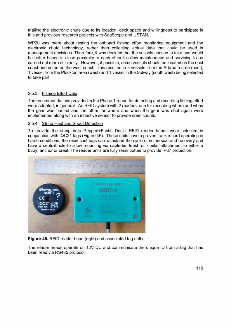
110

trialling the electronic chute due to its location, deck space and willingness to participate in this and previous research projects with SeaScope and USTAN.

WP2b was more about testing the onboard fishing effort monitoring equipment and the electronic chute technology, rather than collecting actual data that could be used in management decisions. Therefore, it was decided that the vessels chosen to take part would be better based in close proximity to each other to allow maintenance and servicing to be carried out more efficiently. However, if possible, some vessels should be located on the east coast and some on the west coast. This resulted in 3 vessels from the Arbroath area (east), 1 vessel from the Plockton area (west) and 1 vessel in the Solway (south west) being selected to take part.

2.5.3 Fishing Effort Data

The recommendations provided in the Phase 1 report for detecting and recording fishing effort were adopted, in general. An RFID system with 2 readers, one for recording where and when the gear was hauled and the other for where and when the gear was shot again were implemented along with an inductive sensor to provide creel counts.

2.5.4 String Haul and Shoot Detection

To provide the string data Pepperl+Fuchs Dent-I RFID reader heads were selected in conjunction with IQC21 tags (Figure 46). These units have a proven track record operating in harsh conditions, the resin cast tags can withstand the cycle of immersion and recovery and have a central hole to allow mounting via cable-tie, leash or similar attachment to either a buoy, anchor or creel. The reader units are fully resin potted to provide IP67 protection.

Figure 46. RFID reader head (right) and associated tag (left).

The reader heads operate on 12V DC and communicate the unique ID from a tag that has been read via RS485 protocol.

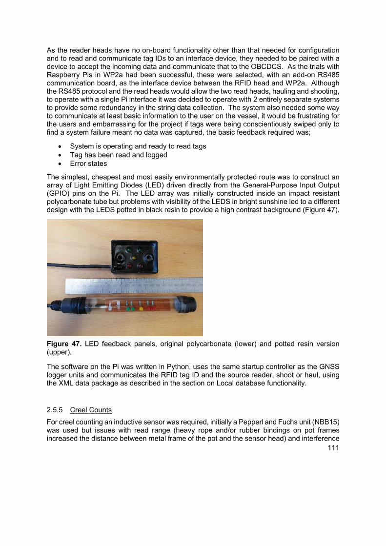
111

As the reader heads have no on-board functionality other than that needed for configuration and to read and communicate tag IDs to an interface device, they needed to be paired with a device to accept the incoming data and communicate that to the OBCDCS. As the trials with Raspberry Pis in WP2a had been successful, these were selected, with an add-on RS485 communication board, as the interface device between the RFID head and WP2a. Although the RS485 protocol and the read heads would allow the two read heads, hauling and shooting, to operate with a single Pi interface it was decided to operate with 2 entirely separate systems to provide some redundancy in the string data collection. The system also needed some way to communicate at least basic information to the user on the vessel, it would be frustrating for the users and embarrassing for the project if tags were being conscientiously swiped only to find a system failure meant no data was captured, the basic feedback required was;

System is operating and ready to read tags Tag has been read and logged Error states

The simplest, cheapest and most easily environmentally protected route was to construct an array of Light Emitting Diodes (LED) driven directly from the General-Purpose Input Output (GPIO) pins on the Pi. The LED array was initially constructed inside an impact resistant polycarbonate tube but problems with visibility of the LEDS in bright sunshine led to a different design with the LEDS potted in black resin to provide a high contrast background (Figure 47).

Figure 47. LED feedback panels, original polycarbonate (lower) and potted resin version (upper).

The software on the Pi was written in Python, uses the same startup controller as the GNSS logger units and communicates the RFID tag ID and the source reader, shoot or haul, using the XML data package as described in the section on Local database functionality.

2.5.5 Creel Counts

For creel counting an inductive sensor was required, initially a Pepperl and Fuchs unit (NBB15) was used but issues with read range (heavy rope and/or rubber bindings on pot frames increased the distance between metal frame of the pot and the sensor head) and interference

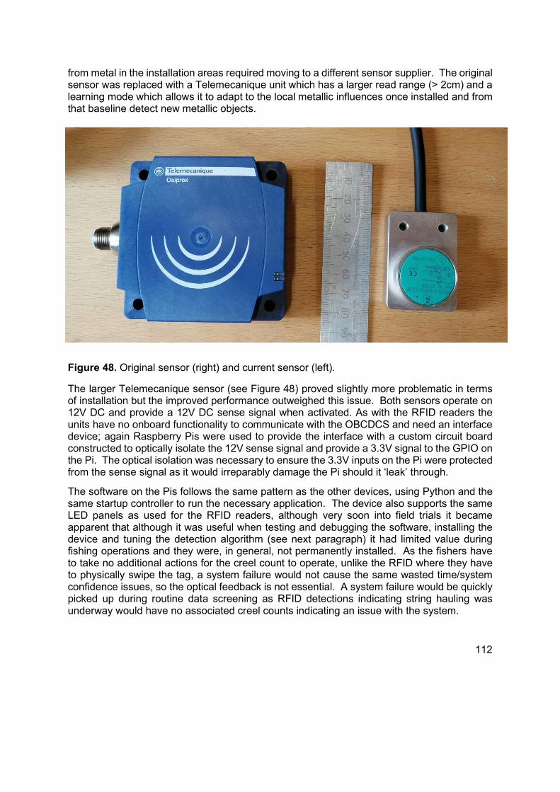
112

from metal in the installation areas required moving to a different sensor supplier. The original sensor was replaced with a Telemecanique unit which has a larger read range (> 2cm) and a learning mode which allows it to adapt to the local metallic influences once installed and from that baseline detect new metallic objects.

2.5.5.1

Figure 48. Original sensor (right) and current sensor (left).

The larger Telemecanique sensor (see Figure 48) proved slightly more problematic in terms of installation but the improved performance outweighed this issue. Both sensors operate on 12V DC and provide a 12V DC sense signal when activated. As with the RFID readers the units have no onboard functionality to communicate with the OBCDCS and need an interface device; again Raspberry Pis were used to provide the interface with a custom circuit board constructed to optically isolate the 12V sense signal and provide a 3.3V signal to the GPIO on the Pi. The optical isolation was necessary to ensure the 3.3V inputs on the Pi were protected from the sense signal as it would irreparably damage the Pi should it ‘leak’ through.

The software on the Pis follows the same pattern as the other devices, using Python and the same startup controller to run the necessary application. The device also supports the same LED panels as used for the RFID readers, although very soon into field trials it became apparent that although it was useful when testing and debugging the software, installing the device and tuning the detection algorithm (see next paragraph) it had limited value during fishing operations and they were, in general, not permanently installed. As the fishers have to take no additional actions for the creel count to operate, unlike the RFID where they have to physically swipe the tag, a system failure would not cause the same wasted time/system confidence issues, so the optical feedback is not essential. A system failure would be quickly picked up during routine data screening as RFID detections indicating string hauling was underway would have no associated creel counts indicating an issue with the system.

113

Due to the nature of the creels; they have multiple metallic cross bars, and the way they can be moved around in the ‘detection area’ when being emptied or rebaited, the software needed an algorithm to determine whether a detection signal from the sensor was a new creel or the same creel moving in and out of the ‘detection area’. The algorithm uses 2 values; the amount of time the detection signal lasted and the elapsed time since a new creel was logged. By altering these values it is possible to ‘tune’ the detection algorithm to suit both the creel type and handling practices for each vessel; for example on a vessel using creels with closely spaced cross bars, widely spaced creels on the string and limited movement when handling the creel for emptying and rebaiting; a detection time in excess of 4 seconds and an inter-creel interval of in excess of 9 seconds gave reliable counts. These time interval values were ascertained through a process of trial and error by observers on board vessels.

The Raspberry Pis, their associated power supplies and interface boards (RS485 and Optical Isolation) were mounted in a similar, but smaller (30 x 22.5 x 13.2 cms, 8.9 Litre) case as used in the 2A system. In addition to the sensing equipment another Netgear GS108 switch was mounted in the case to provide a network link to the 2A system.

2.5.6 Biological Catch Data

2.5.6.1 Morphological Study

As recommended in the Phase 1 report, ‘it is our recommendation that a program of detailed morphometric measurements is designed and undertaken across all 3 target species’, a programme of sampling was planned and undertaken. It was preceded by a literature review to gain a better understanding of the morphology of the species in question. The programme was undertaken in parallel with the work identifying the appropriate equipment to perform the scanning and processing of the scans to provide the biological data and as such was wide ranging to hopefully encompass the capabilities of the scanning equipment once identified.

The minimum size of crab allowed to be landed in Scotland is 140 mm carapace width, while for lobster it is 87 mm carapace length (specifically measured from behind the eye to the edge of the large segment, including soft frills between segments) (sizes correct at the start of 2017). These minimum sizes are set to allow at least one opportunity for reproduction before removal by fishing (Tully et al. 2001; Ungfors, 2007). It should be noted that the landing sizes changed during the project and were also location dependent. More accurate and up to date information is available at marine Scotland’s website at https://www2.gov.scot/Topics/marine/Sea-Fisheries/InshoreFisheries/crab-lobster-landing-controls

Maturity has been classified into four categories; behavioural, gonadal, morphometric and functional (Ungfors, 2007). Behavioural maturity is when mating behaviour occurs but may not include a successful mating. Gonadal maturity is then the gonads are mature enough for offspring to be produced. Morphological maturity is when morphological traits related to maturity change from isometric to allometric growth (Corgos & Freire, 2006). Functional maturity is when all three stages have occurred and allows successful mating (Ungfors 2007). An aspect of the catch that is rarely recorded is the sex. Males appear to mature at a smaller size than females (Debuse et al, 1999; Haig et al, 2016) and catches may selectively catch a

114

biased sex ratio (Thomas & Figueiredo, 1965; Woll et al, 2006). This may vary for a variety of factors such as geographical, catch size and sex (Woll et al., 2006).

The important aspect for the current study will be the use of morphological maturity to identify sexes via morphological differences in their secondary sexual traits. For the Automated Species, Size and Sex Identification (ASSSID) system to be able to determine the sex of different animals as they are scanned, it will be necessary for it to identify and measure the morphometrical features.WP2b will use a 2D or 3D scanner and/or the use of imaging technology (possibly combined with machine learning) to gather information on size and sex on board of a fishing vessel. The “standard” length measurements of carapace size and techniques for sex determination might not be easily captured by these new techniques so different proxies for carapace length and sex were investigated by undertaking sampling at shellfish merchants. The objectives of this was to determine:

Whether it is possible to use these potential proxies to gather information on carapace length and sex

How consistent these measurements are across different locations around Scotland

Many studies have investigated morphological maturity and measured a variety of traits in relation to each other to identify growth differences between males and females for brown crab and lobster (Tables 6 & 7). These traits were likely to provide morphological indicators of sex.

For the brown crab, measures of male weight, cheliped length, height and width, also female abdomen width and female pleopod weight have been correlated with carapace width (Table 6).

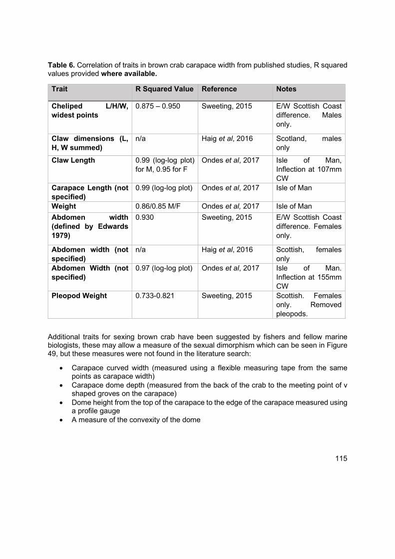
115

Table 6. Correlation of traits in brown crab carapace width from published studies, R squared values provided where available.

Trait R Squared Value Reference Notes

Cheliped L/H/W, widest points

0.875 – 0.950 Sweeting, 2015 E/W Scottish Coast difference. Males only.

Claw dimensions (L, H, W summed)

n/a Haig et al, 2016 Scotland, males only

Claw Length 0.99 (log-log plot) for M, 0.95 for F

Ondes et al, 2017 Isle of Man, Inflection at 107mm CW

Carapace Length (not specified)

0.99 (log-log plot) Ondes et al, 2017 Isle of Man

Weight 0.86/0.85 M/F Ondes et al, 2017 Isle of Man

Abdomen width (defined by Edwards 1979)

0.930 Sweeting, 2015 E/W Scottish Coast difference. Females only.

Abdomen width (not specified)

n/a Haig et al, 2016 Scottish, females only

Abdomen Width (not specified)

0.97 (log-log plot) Ondes et al, 2017 Isle of Man. Inflection at 155mm CW

Pleopod Weight 0.733-0.821 Sweeting, 2015 Scottish. Females only. Removed pleopods.

Additional traits for sexing brown crab have been suggested by fishers and fellow marine biologists, these may allow a measure of the sexual dimorphism which can be seen in Figure 49, but these measures were not found in the literature search:

Carapace curved width (measured using a flexible measuring tape from the same points as carapace width)

Carapace dome depth (measured from the back of the crab to the meeting point of v shaped groves on the carapace)

Dome height from the top of the carapace to the edge of the carapace measured using a profile gauge

A measure of the convexity of the dome

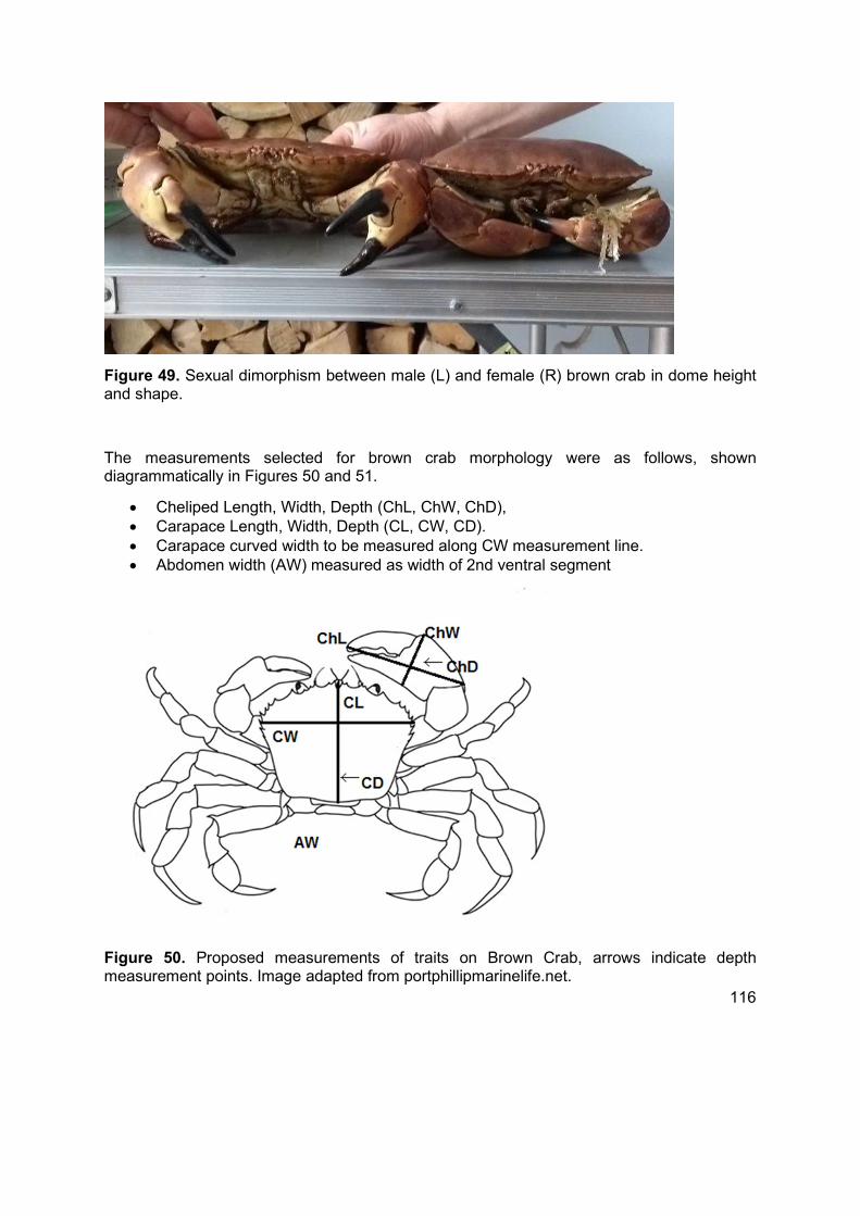
116

Figure 49. Sexual dimorphism between male (L) and female (R) brown crab in dome height and shape.

The measurements selected for brown crab morphology were as follows, shown diagrammatically in Figures 50 and 51.

Cheliped Length, Width, Depth (ChL, ChW, ChD), Carapace Length, Width, Depth (CL, CW, CD). Carapace curved width to be measured along CW measurement line. Abdomen width (AW) measured as width of 2nd ventral segment

Figure 50. Proposed measurements of traits on Brown Crab, arrows indicate depth measurement points. Image adapted from portphillipmarinelife.net.

117

Figure 51. Ventral view of Brown Crab showing Abdomen Width to be measured along black line. Left image, male. Right image, female.

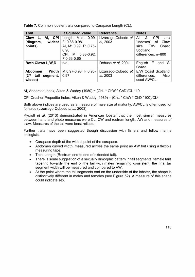
118

Table 7. Common lobster traits compared to Carapace Length (CL).

Trait R Squared Value Reference Notes Claw L, AI, CPI (diagram, widest points)

Length, Male: 0.99, F: 0.88-0.98. AI, M: 0.99, F: 0.75-0.96 CPI, M: 0.88-0.92, F:0.63-0.65

Lizarrago-Cubedo et al, 2003

AI & CPI are “indexes” of Claw size. E/W Coast Scotland differences. n=800

Both Claws L,W,D n/a Debuse et al, 2001 English E and S Coast.

Abdomen Width (2nd tail segment, widest)

M:0.97-0.98, F:0.95-0.97

Lizarrago-Cubedo et al, 2003

E/W Coast Scotland differences. Also used AW/CL.

AI, Anderson Index, Aiken & Waddy (1980) = (ChL * ChW * ChD)/CL *10

CPI Crusher Propodite Index, Aiken & Waddy (1989) = (ChL * ChW * ChD *100)/CL3

Both above indices are used as a measure of male size at maturity. AW/CL is often used for females (Lizarrago-Cubedo et al, 2003)

Rycroft et al, (2013) demonstrated in American lobster that the most similar measures between hand and photo measures were CL, CW and rostrum length, AW and measures of claw. Measures of the tail were least reliable.

Further traits have been suggested though discussion with fishers and fellow marine biologists.

Carapace depth at the widest point of the carapace. Abdomen curved width, measured across the same point as AW but using a flexible

measuring tape, Total Length (Rostrum end to end of extended tail). There is some suggestion of a sexually dimorphic pattern in tail segments; female tails

tapering towards the end of the tail with males remaining consistent, the final tail segment width will be measured and compared to AW.

At the point where the tail segments end on the underside of the lobster, the shape is distinctively different in males and females (see Figure 52). A measure of this shape could indicate sex.

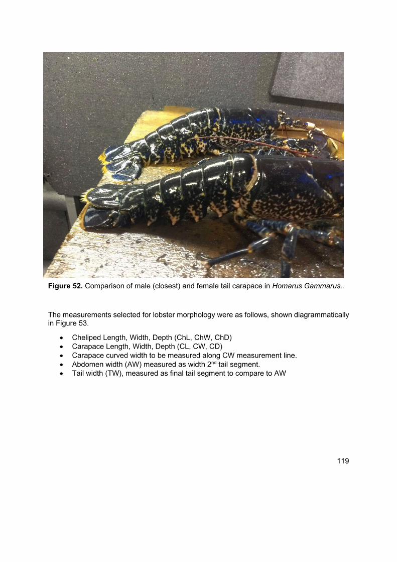
119

Figure 52. Comparison of male (closest) and female tail carapace in Homarus Gammarus..

The measurements selected for lobster morphology were as follows, shown diagrammatically in Figure 53.

Cheliped Length, Width, Depth (ChL, ChW, ChD) Carapace Length, Width, Depth (CL, CW, CD) Carapace curved width to be measured along CW measurement line. Abdomen width (AW) measured as width 2nd tail segment. Tail width (TW), measured as final tail segment to compare to AW

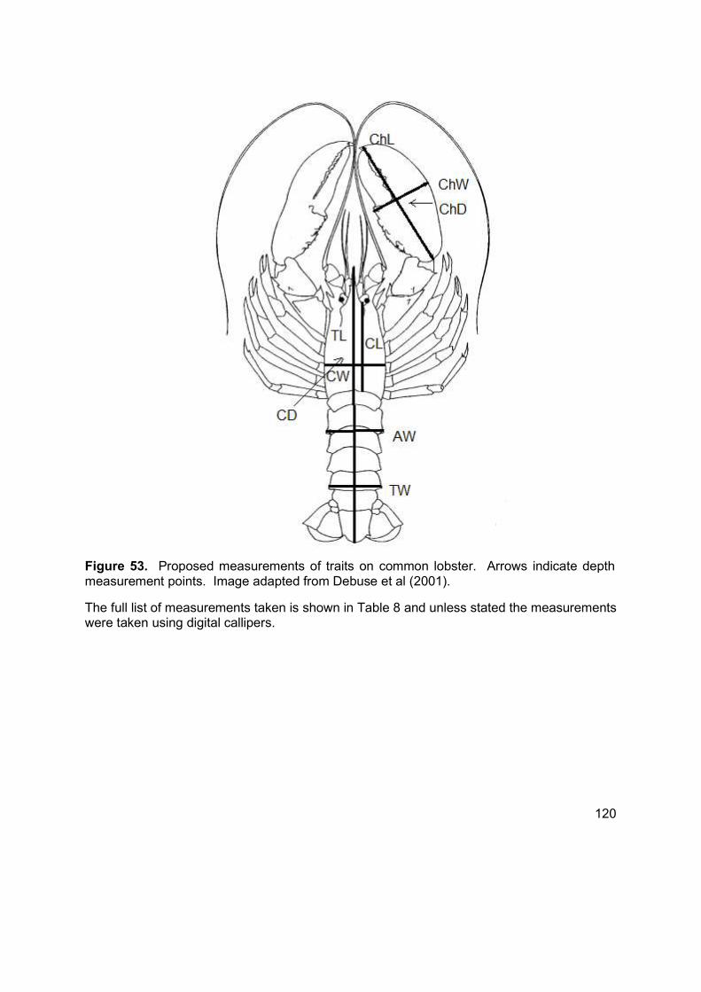
120

The full list of measurements taken is shown in Table 8 and unless stated the measurements were taken using digital callipers.

Figure 53. Proposed measurements of traits on common lobster. Arrows indicate depth measurement points. Image adapted from Debuse et al (2001).

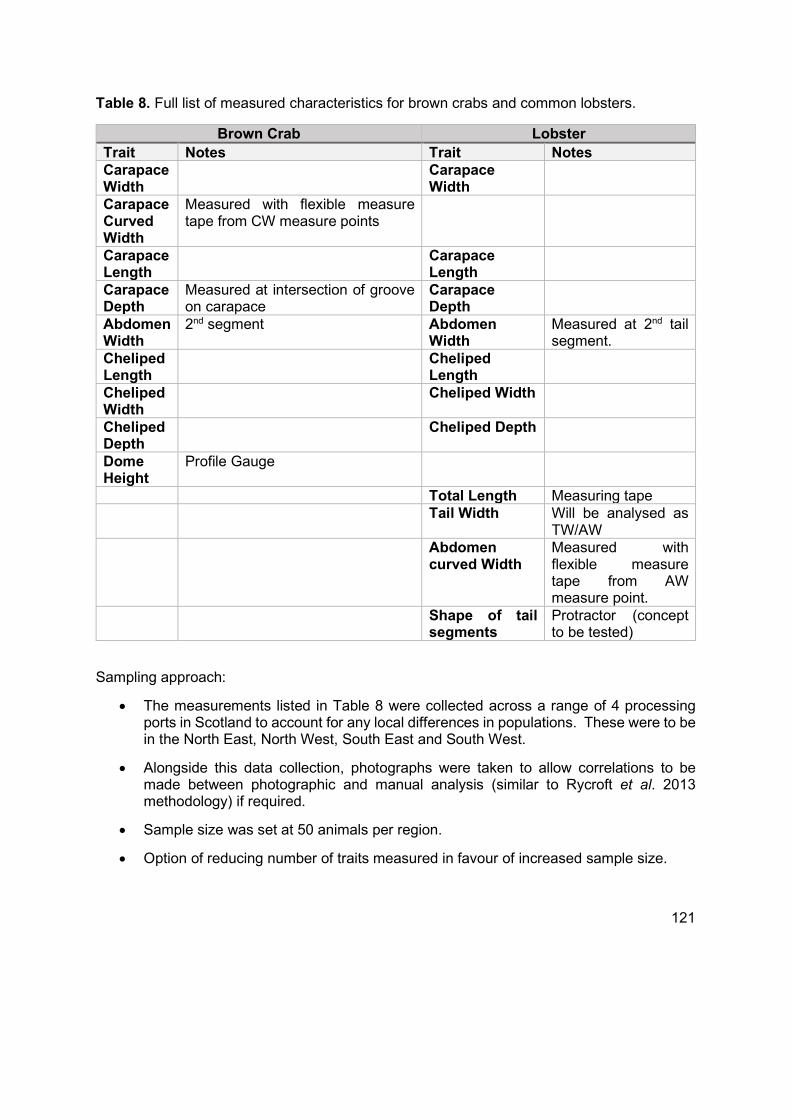
121

Table 8. Full list of measured characteristics for brown crabs and common lobsters.

Brown Crab Lobster Trait Notes Trait Notes Carapace Width

Carapace Width

Carapace Curved Width

Measured with flexible measure tape from CW measure points

Carapace Length

Carapace Length

Carapace Depth

Measured at intersection of groove on carapace

Carapace Depth

Abdomen Width

2nd segment Abdomen Width

Measured at 2nd tail segment.

Cheliped Length

Cheliped Length

Cheliped Width

Cheliped Width

Cheliped Depth

Cheliped Depth

Dome Height

Profile Gauge

Total Length Measuring tape Tail Width Will be analysed as

TW/AW Abdomen

curved Width Measured with flexible measure tape from AW measure point.

Shape of tail segments

Protractor (concept to be tested)

Sampling approach:

The measurements listed in Table 8 were collected across a range of 4 processing ports in Scotland to account for any local differences in populations. These were to be in the North East, North West, South East and South West.

Alongside this data collection, photographs were taken to allow correlations to be made between photographic and manual analysis (similar to Rycroft et al. 2013 methodology) if required.

Sample size was set at 50 animals per region.

Option of reducing number of traits measured in favour of increased sample size.

122

Lobster CL may be correlated against other traits to identify an alternative trait that would allow the ASSSID to generate size and sex data.

Sampling materials:

300mm Callipers

Profile Gauge

Flexible measuring tape

Waterproof Pad

Camera

Tripod

Grey background for photographs

2.5.7 ASSSID (Automated Species, Size and Sex Identification)

In Phase 1 of the WP2b project, two options were recommended for further investigation, these were:

a visible spectrum machine vision system and a 2D/3D scanner system

To begin investigations into these technologies, SeaScope staff attended a conference related to this type of technology.

2.5.7.1 UK Industrial Vision Association Conference

Subsequent to phase 1 completing, a member of SeaScope staff had the opportunity to attend the 2017 annual conference of the UK Industrial Vision Association (UKIVA). The conference (see UKIVA, 2017) brought together all the major manufacturers and integrators providing machine vision systems and the supporting equipment, e.g. robots, conveyors etc., in industrial and automation settings within and beyond the UK. Whereas manufacturers are focussed solely on the equipment they provide, integrators combine all the elements needed for a machine vision system providing complete solutions. The SeaScope delegate took the opportunity to take a model crab and lobster to the conference and discuss the challenge with a large number of the representatives and experts available.

We took 3 possible scenarios for the imaging environment; the following section summarises the responses on a technically feasible basis with limited consideration of practical implementation or budgetary constraints.

1. Uncontrolled lighting, variable distance to the crabs, probable occlusion of the individual (Basically an overhead camera system observing the fisher unloading the creels)

123

ID – Ranging from ‘Possible but very difficult’ through to ‘Not possible’ Sex – Not possible Measurement – Not possible

2. Uncontrolled lighting, fixed distance to the crabs, no occlusion of the individual (camera(s) observing the individuals from a fixed distance with a ‘clean’ view of the individual and an uncluttered background)

ID – Yes Sex from carapace shape – Possible with 3D imaging (structured light/line scan)

but problematic due to uncontrolled lighting, in all likelihood not possible Sex from lower shell features – Possible but would need 2 cameras (1 for

measuring, 1 for sex), unlikely to be successful where lower features occluded by legs etc

Measurement – Yes but problematic due to lighting conditions, ability to define carapace edge is still an issue if you can mitigate for the lighting in the processing

3. Controlled lighting, fixed distance to the crabs, no occlusion of the individual (camera(s) observing the individuals from a fixed distance with a ‘clean’ view of the individual and an uncluttered background)

ID – Yes, Note: This was previously proven with the SeaScope demonstration system

Sex from carapace shape: Possible with 3D imaging (structured light/line scan) Sex from lower shell features: Possible but would need 2 cameras (1 for measuring

1 for sex) Unlikely to be successful where lower features occluded by legs etc Measurement – Yes, ability to define carapace edge is biggest issue

The subject of the practical implementation of any solution in a field environment given the restrictions on space, power and limited impact on the working practices was also discussed, these discussions only served to underline what we already knew; the engineering challenge will be as great as the computer vision one.

Additional Notes

The ability to obtain a measurement is wholly driven by being able to identify the edge of the carapace, excluding legs, shadows etc.

Realistically the use of line-scan systems requires a conveyor to move the individuals past the scanner at a fixed speed, even then; individuals moving of their own accord on a slow conveyor will cause issues with accuracy.

The use of stereoscopic imaging was discounted by all the people spoken to but that may have been more to do with the industrial slant of the conference rather than its ability to provide what was needed.

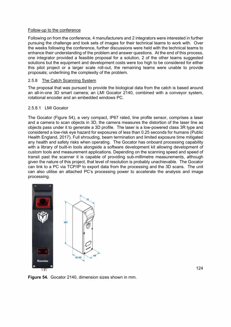
124

Follow-up to the conference

Following on from the conference, 4 manufacturers and 2 integrators were interested in further pursuing the challenge and took sets of images for their technical teams to work with. Over the weeks following the conference, further discussions were held with the technical teams to enhance their understanding of the problem and answer questions. At the end of this process, one integrator provided a feasible proposal for a solution, 2 of the other teams suggested solutions but the equipment and development costs were too high to be considered for either this pilot project or a larger scale roll-out, the remaining teams were unable to provide proposals; underlining the complexity of the problem.

2.5.8 The Catch Scanning System

The proposal that was pursued to provide the biological data from the catch is based around an all-in-one 3D smart camera; an LMI Gocator 2140, combined with a conveyor system, rotational encoder and an embedded windows PC.

2.5.8.1 LMI Gocator

The Gocator (Figure 54), a very compact, IP67 rated, line profile sensor, comprises a laser and a camera to scan objects in 3D, the camera measures the distortion of the laser line as objects pass under it to generate a 3D profile. The laser is a low-powered class 3R type and considered a low-risk eye hazard for exposures of less than 0.25 seconds for humans (Public Health England, 2017). Full shrouding, beam termination and limited exposure time mitigated any health and safety risks when operating. The Gocator has onboard processing capability with a library of built-in tools alongside a software development kit allowing development of custom tools and measurement applications. Depending on the scanning speed and speed of transit past the scanner it is capable of providing sub-millimetre measurements, although given the nature of this project, that level of resolution is probably unachievable. The Gocator can link to a PC via TCP/IP to export data from the processing and the 3D scans. The unit can also utilise an attached PC’s processing power to accelerate the analysis and image processing.

Figure 54. Gocator 2140, dimension sizes shown in mm.

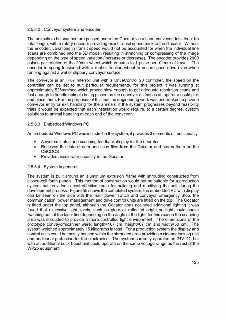
125

2.5.8.2 Conveyor system and encoder

The animals to be scanned are passed under the Gocator via a short conveyor, less than 1m total length, with a rotary encoder providing exact transit speed back to the Gocator. Without the encoder, variations in transit speed would not be accounted for when the individual line scans are combined into the 3D model, resulting in stretching or compressing of the image depending on the type of speed variation (increase or decrease). The encoder provides 2000 pulses per rotation of the 20mm wheel which equates to 1 pulse per .01mm of travel. The encoder is spring tensioned with a rubber traction wheel to ensure good drive even when running against a wet or slippery conveyor surface.

The conveyor is an IP67 Interroll unit with a DriveControl 20 controller, the speed on the controller can be set to suit particular requirements, for this project it was running at approximately 528mm/sec which proved slow enough to get adequate resolution scans and fast enough to handle animals being placed on the conveyer as fast as an operator could pick and place them. For the purposes of this trial, no engineering work was undertaken to provide conveyor entry or exit handling for the animals; if the system progresses beyond feasibility trials it would be expected that each installation would require, to a certain degree, custom solutions to animal handling at each end of the conveyor.

2.5.8.3 Embedded Windows PC

An embedded Windows PC was included in the system, it provides 3 elements of functionality:

A system status and scanning feedback display for the operator Receives the data stream and scan files from the Gocator and stores them on the

OBCDCS Provides accelerator capacity to the Gocator

2.5.8.4 System in general

The system is built around an aluminium extrusion frame with shrouding constructed from closed-cell foam panels. This method of construction would not be suitable for a production system but provided a cost-effective route for building and modifying the unit during the development process. Figure 55 shows the completed system, the embedded PC with display can be seen on the side with the main power switch and conveyor Emergency Stop, the communication, power management and drive control units are fitted on the top. The Gocator is fitted under the top panel, although the Gocator does not need additional lighting it was found that excessive light levels, such as glare or reflected bright sunlight could cause ‘washing out’ of the laser line depending on the angle of the light, for this reason the scanning area was shrouded to provide a more controlled light environment. The dimensions of the prototype conveyor/scanner were; length=107 cm, height=67 cm and width=50 cm. The system weighed approximately 15 kilograms in total. For a production system the display and control units could be mostly housed within the shrouded area providing a cleaner looking unit and additional protection for the electronics. The system currently operates on 24V DC but with an additional buck-boost unit could operate on the same voltage range as the rest of the WP2b equipment.

126

Figure 55. The completed ASSSID conveyor system on board the trials vessel.

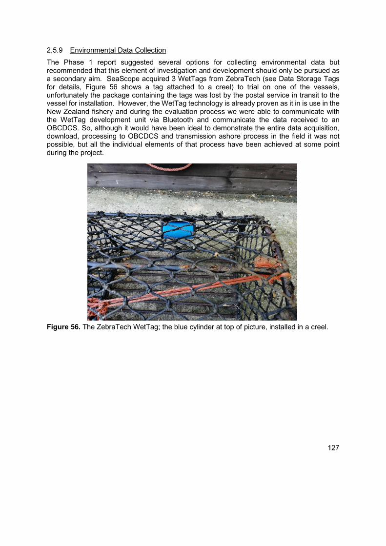
127

2.5.9 Environmental Data Collection

The Phase 1 report suggested several options for collecting environmental data but recommended that this element of investigation and development should only be pursued as a secondary aim. SeaScope acquired 3 WetTags from ZebraTech (see Data Storage Tags for details, Figure 56 shows a tag attached to a creel) to trial on one of the vessels, unfortunately the package containing the tags was lost by the postal service in transit to the vessel for installation. However, the WetTag technology is already proven as it in is use in the New Zealand fishery and during the evaluation process we were able to communicate with the WetTag development unit via Bluetooth and communicate the data received to an OBCDCS. So, although it would have been ideal to demonstrate the entire data acquisition, download, processing to OBCDCS and transmission ashore process in the field it was not possible, but all the individual elements of that process have been achieved at some point during the project.

Figure 56. The ZebraTech WetTag; the blue cylinder at top of picture, installed in a creel.

128

3 RESULTS

3.1 WP2A OBCDCS

3.1.1 Construction

The systems were constructed by SeaScope; as discussed in the methodology section, after initial trials on one vessel, the design was modified to aid installation. As required in the project specification, all the hardware elements of the WP2a system are widely available off-the-shelf items, even if the particular models used in this project were superseded or even withdrawn it is very likely that a functionally equivalent piece of equipment would be available. Provided functionally equivalent equipment can be sourced it is unlikely that software modifications would be required to incorporate the replacement equipment.

The modular nature of the construction means that should a component fail it is a relatively easy task to replace in the field without the need for specialist skills.

The majority of the systems were installed externally on the vessels, exposing them to the harshest conditions that could be expected. The longest deployment of a unit was on a wheelhouse roof (Figure 57) for over 1 year and it remained free from defects apart from the expected weathering of the case. One unit did suffer damage to a 4G aerial when it was snapped off by mackerel fishing gear, the aerial was replaced during a technician visit which took less than 30 minutes to achieve.

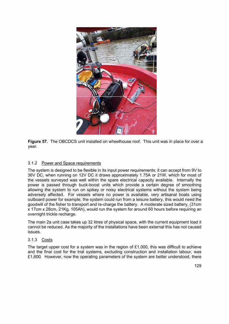
129

3.1.2 Power and Space requirements

The system is designed to be flexible in its input power requirements; it can accept from 9V to 36V DC, when running on 12V DC it draws approximately 1.75A or 21W, which for most of the vessels surveyed was well within the spare electrical capacity available. Internally the power is passed through buck-boost units which provide a certain degree of smoothing allowing the system to run on spikey or noisy electrical systems without the system being adversely affected. For vessels where no power is available, very artisanal boats using outboard power for example, the system could run from a leisure battery, this would need the goodwill of the fisher to transport and re-charge the battery. A moderate sized battery, (31cm x 17cm x 28cm, 21Kg, 105Ah), would run the system for around 60 hours before requiring an overnight trickle recharge.

The main 2a unit case takes up 32 litres of physical space, with the current equipment load it cannot be reduced. As the majority of the installations have been external this has not caused issues.

3.1.3 Costs

The target upper cost for a system was in the region of £1,000, this was difficult to achieve and the final cost for the trial systems, excluding construction and installation labour, was £1,600. However, now the operating parameters of the system are better understood, there

Figure 57. The OBCDCS unit installed on wheelhouse roof. This unit was in place for over a year.

130

are elements of it that could be considered over-specified, see the discussion for more detail. Having a specification more closely matched to program requirements and potentially bulk purchasing components could bring the system cost much closer to the target.

3.1.4 Ease of Installation

The aim was to develop a system that could be installed easily on a small vessel without the need for in-depth specialist skills. As the system is effectively fully built before being released for installation this aim was fully realised. Installation consists of:

Finding an appropriate location for the main unit taking into account cable routing and methods for mounting and securing the unit

Finding an appropriate location for the antennae for cellular data and GNSS reception, avoiding occlusion of the GNSS patches and taking into account the location of radar, VHF and any other equipment that could be affected by the cellular signal

Mounting the equipment and running cabling as necessary Completing power connection Testing the system

Installation should be undertaken in conjunction with the skipper/owner of the vessel to agree placement. Depending on the skill set of the technician, the electrical set-up on the vessel and requirements of the skipper/owner, the final power connection may have to made by the vessel’s designated engineer or marine electrician.

The logistics of organising technicians and equipment combined with vessel availability, due to scheduled downtime or forecast bad weather, meant the task was not straightforward. The nature of the fishing industry generally means when catches and weather are good the boats are fully occupied, and skippers/owners are not available after a full day at sea to oversee an installation. The wide geographic spread meant it was more cost and time efficient to schedule multiple vessels in the same port or area for installation during the same visit.

3.1.5 Deployments

The aim of WP2a was to have the OBCDCS deployed for 6 months on 15 vessels. Initially 18 vessels volunteered to take part in the trial, 15 were selected based on the criteria discussed in Vessel Selection, however, prior to installations commencing, two of the selected vessels had a change of heart and opted out of the trial. Rather than recruiting replacement vessels the OBCDCS system destined for, they were retained as spare systems to swap out another vessel’s system in the event of a failure. This approach was taken due to the time constraints related to achieving a 6-month deployment on replacement vessels.

The spare system approach proved its worth very early in the trials as a system was irreparably damaged when a 50v power surge on a vessel irreparably damaged the NAS component in the system during initial deployment.

As only 15 systems were built initially, this left 13 vessels with operational systems for the trial. Table 9 shows the details of the installation and removal date (as at end of April 2019). It shows most systems as having two different “System ID” codes, e.g. System K/KB; the systems were renamed with the “B” suffix when the boot method and logging software were upgraded from an SD storage card to a USB stick.

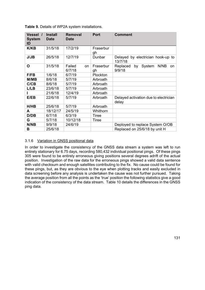
131

Table 9. Details of WP2A system installations.

Vessel / System ID

Install Date

Removal Date

Port Comment

K/KB 31/5/18 17/2/19 Fraserburgh

J/JB 26/5/18 12/7/19 Dunbar Delayed by electrician hook-up to 13/7/18

O 31/5/18 Failed on 6/7/18

Fraserburgh

Replaced by System N/NB on 9/9/18

F/FB 1/6/18 6/7/19 Plockton M/MB 8/6/18 5/7/19 Arbroath C/CB 8/6/18 5/7/19 Arbroath L/LB 23/6/18 5/7/19 Arbroath I 21/6/18 12/4/19 Arbroath E/EB 22/6/18 5/7/19 Arbroath Delayed activation due to electrician

delay H/HB 25/6/18 5/7/19 Arbroath A 18/12/17 24/5/19 Whithorn D/DB 6/7/18 6/3/19 Tiree G 5/7/18 10/12/18 Tiree N/NB 9/9/18 24/6/19 Deployed to replace System O/OB B 25/6/18 Replaced on 25/6/18 by unit H

3.1.6 Variation in GNSS positional data

In order to investigate the consistency of the GNSS data stream a system was left to run entirely stationary for 6.75 days, recording 580,432 individual positional pings. Of these pings 305 were found to be entirely erroneous giving positions several degrees adrift of the actual position. Investigation of the raw data for the erroneous pings showed a valid data sentence with valid checksum and enough satellites contributing to the fix. No cause could be found for these pings, but, as they are obvious to the eye when plotting tracks and easily excluded in data screening before any analysis is undertaken the cause was not further pursued. Taking the average position from all the points as the ‘true’ position the following statistics give a good indication of the consistency of the data stream. Table 10 details the differences in the GNSS ping data.

132

Table 10. Results of the GNSS consistency test.

Maximum difference (m) 3.292

Minimum difference (m) 0.134

Standard Deviation – Population (m) 0.436

Average Difference (m) 0.782

3.1.7 Data collected by OBCDCS

Table 11 shows the number of days each OBCDCS was deployed and the number of fishing days where data were recorded, where a day at sea was expected to be equivalent to a fishing trip. However, care should be taken when calculating how many days a vessel had completed at sea because the system powers up every time the vessel’s engines are switched on, irrespective of whether the vessel then left the harbour or not.

133

Table 11. OBCDCS deployment data summary.

Vessel System ID

First Trip Recorded

Days Deployed

Fishing Trips Data Recorded up to 19/04/19

Comments

K/KB 3/6/18 334 79 6-month deployment target exceeded

J/JB 16/7/18 339 49 6-month deployment target exceeded

O/OB and N/NB

1/6/18 334 38 + 67 = 105 System O/OB failed and was replaced by system N/NB. Resulted in 64 calendar days not monitored between 7/7/18 and 9/9/18. 6-month deployment target exceeded since 9/9/18.

F/FB 25/6/18 333 90 6-month deployment target exceeded

M/MB 9/6/18 326 196 6-month deployment target exceeded

C/CB 9/6/18 326 114 6-month deployment target exceeded

L/LB 26/6/18 311 72 6-month deployment target exceeded

I/IB 22/6/18 313 152 6-month deployment target exceeded

E/EB 5/7/18 312 98 6-month deployment target exceeded

H/HB 12/7/18 309 59 6-month deployment target exceeded

A 6/2/18 498 136 Deployed for over 1 year D/DB 6/7/18 298 65 6-month deployment target

exceeded G 5/7/18 299 83 6-month deployment target

exceeded

Due to the nature of how the fleet operates and that the OBCDCS starts recording positions every time the vessel powers up, not all sets of positional pings relate to a fishing trip. For example, some vessels appear to have been drifting to catch bait with handlines or rods (Figure 58), others used their boat as a “taxi” (Figure 59), some sailed out of the harbour to see if the weather was manageable, whilst others would sometimes sail only to haul keep-pots. On occasions more than one activity occurred during the same day with a vessel making multiple trips to the port. It is thought that perhaps this may be due to the vessel deploying new fleets of creels (or newly cleaned ones) or bringing in fleets of creels to be cleaned ashore.

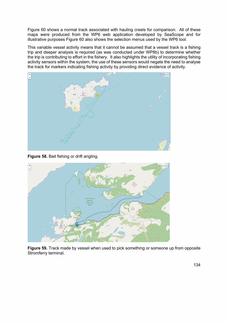
134

Figure 60 shows a normal track associated with hauling creels for comparison. All of these maps were produced from the WP6 web application developed by SeaScope and for illustrative purposes Figure 60 also shows the selection menus used by the WP6 tool.

This variable vessel activity means that it cannot be assumed that a vessel track is a fishing trip and deeper analysis is required (as was conducted under WP8b) to determine whether the trip is contributing to effort in the fishery. It also highlights the utility of incorporating fishing activity sensors within the system, the use of these sensors would negate the need to analyse the track for markers indicating fishing activity by providing direct evidence of activity.

Figure 58. Bait fishing or drift angling.

Figure 59. Track made by vessel when used to pick something or someone up from opposite Stromferry terminal.

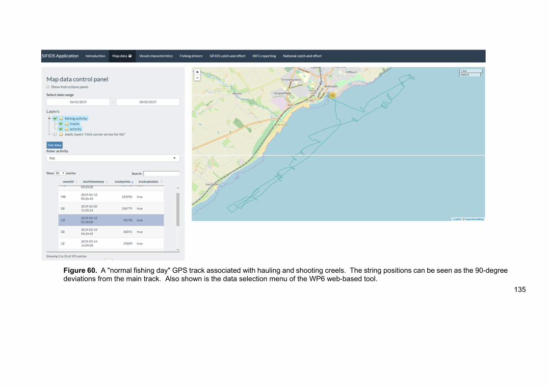
135

Figure 60. A "normal fishing day" GPS track associated with hauling and shooting creels. The string positions can be seen as the 90-degree deviations from the main track. Also shown is the data selection menu of the WP6 web-based tool.

136

3.1.8 Data transmission and monitoring incoming feeds

Due to the variable nature of the 3G/4G signal around the Scottish coast some vessels were only able to transmit data when they sailed into particular areas of their usual fishing grounds. This did not cause an issue for receiving data as the systems transmit all outstanding data once they acquire a usable connection to the reception database, this did however, cause a lag in data availability from the reception database, including the diagnostics. The lag in diagnostic data availability did result in delays identifying system issues as it was unknown whether the vessel had been at sea or just had not been into a good transmission area, it was only after contacting the fisher to ascertain whether the vessel had been fishing that issues became apparent.

The data communication between the on-board systems and the reception database is not particularly large but we saw significant data use at times with vessels using 15Gb of data over the period of a few weeks when it was expected to last 2-3 months. The operating system (Raspbian - Jessie) on the loggers does not automatically communicate with the internet, other than to obtain a time-signal on boot-up and the only other device within the system with built-in internet connectivity that could use the data credit is the NAS unit. The NAS units on the system were configured to keep their ‘personal’, e.g. auto-updates, manufacturer diagnostics etc., traffic to a minimum. Additional diagnostic routines were added to the UploadManager software which provided data traffic information from the router, via the Modbus link, at the start and end of each upload cycle. This additional diagnostic information allowed monitoring of traffic in between upload cycles where there should be limited or no traffic. The diagnostics showed additional unexpected traffic between the upload cycles, we were unable to uncover the source, but, as the only impact on the project was the limited cost of additional top-ups and staff resource was at a premium, a detailed investigation was discounted.

3.1.9 OBCDCS Reliability

It may be expected that an estimation of how many days were lost due to system failure could be made but calculating a malfunction rate is not realistically possible or appropriate during a project like this. The system was, initially, in a state of flux as issues not encountered in testing ashore became apparent once systems were in the field and modifications were rolled out. The system design that was initially installed on a vessel is not the same as the one that is currently operating.

When a performance issue occurred, the source of the fault had to be traced. This took varying durations dependent on whether it was a software issue or a hardware component failure somewhere within the system. In some circumstances faults appeared intermittent or were difficult to replicate on a shore-based system and required a technician visit to diagnose the problem.

The majority of the issues encountered were software or inter-connectivity issues between the components, all of which were resolved by adjusting the software, and the systems ran on stable releases in excess of the required time period specified in the project objectives.

There were some hardware failures; notably the SD card corruption issue discussed in the Hardware Selection element of this report. This issue could be considered less of a hardware failure but more as pushing the hardware well beyond its rated operational parameters. As

137

that element of the hardware is no longer part of the system, it was replaced with more robust USB sticks, and the issues occurred during the development phase, it can be ignored when considering the final system that the project produced.

One vessel caused considerable damage to a unit. The system stopped transmitting data, so a technician visited the vessel and found several components ‘fried’. On further investigation it was found that the DC circuit the unit was connected to was spiking to 50V which had caused the damage to the unit.

One NAS unit failed during the trials. After investigation it was found that the internal power supply board had failed, all the data from the unit was intact on the hard drive and had already been uploaded to the reception database, so the only data loss was for the time the system was unable to log whilst a replacement NAS was sourced and installed. The buck-boost unit that supplied the NAS was, and still is, operating normally so the fault lay fully with the NAS unit.

Of the 39 buck-boost units deployed within the units during the trials, 2 failed. On investigation, they had blown internal protection fuses designed to prevent them supplying over-voltage to the output. There appeared to be no external causal factor and the failure was attributed solely to the units themselves.

3.2 Morphological Study

Once the morphological sampling program began, it quickly became clear that poor weather and the associated lack of fishing effort was significantly reducing shellfish landings around the country. Therefore, the sampling regime was revised to 100 individuals from 3 regions; North (merchants based in Dingwall), South West (merchants based in Troon) and South East (merchants based in Eyemouth). Limited availability of velvet crabs saw this species dropped from the morphological study.

The main factors that limited sampling success were the low catches due to cold weather, persistent strong winds and the proximity of Christmas. The cold weather reduces the mobility of the shellfish so fewer animals move into the creels, whilst the windy weather stopped the fishers putting to sea to empty any creels that were being fished. In addition, the fishers were retaining their lobster catches in keep-pots to aggregate and land the catch when the prices would be at their highest just before Christmas.

The targets for sampling were originally set at 50 animals per species per region but subsequently revised due to the reasons noted above. Staff succeeded in undertaking sampling of lobster and crab at 3 shellfish merchant locations between the 19th October and 24th November 2017. Table 12 shows a summary of the sampling undertaken and examples of the field data log sheets used for the sampling can be found in Annex 4.

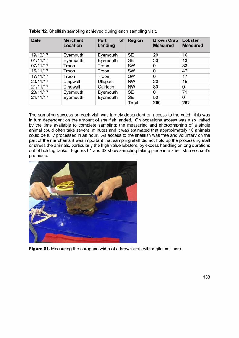
138

Table 12. Shellfish sampling achieved during each sampling visit.

Date Merchant Location

Port of Landing

Region Brown Crab Measured

Lobster Measured

19/10/17 Eyemouth Eyemouth SE 20 16 01/11/17 Eyemouth Eyemouth SE 30 13 07/11/17 Troon Troon SW 0 83 16/11/17 Troon Troon SW 0 47 17/11/17 Troon Troon SW 0 17 20/11/17 Dingwall Ullapool NW 20 15 21/11/17 Dingwall Gairloch NW 80 0 23/11/17 Eyemouth Eyemouth SE 0 71 24/11/17 Eyemouth Eyemouth SE 50 0 Total 200 262

The sampling success on each visit was largely dependent on access to the catch, this was in turn dependent on the amount of shellfish landed. On occasions access was also limited by the time available to complete sampling; the measuring and photographing of a single animal could often take several minutes and it was estimated that approximately 10 animals could be fully processed in an hour. As access to the shellfish was free and voluntary on the part of the merchants it was important that sampling staff did not hold up the processing staff or stress the animals, particularly the high value lobsters, by excess handling or long durations out of holding tanks. Figures 61 and 62 show sampling taking place in a shellfish merchant’s premises.

Figure 61. Measuring the carapace width of a brown crab with digital callipers.

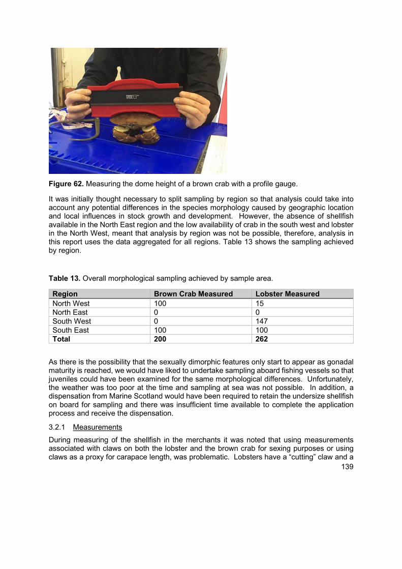
139

Figure 62. Measuring the dome height of a brown crab with a profile gauge.

It was initially thought necessary to split sampling by region so that analysis could take into account any potential differences in the species morphology caused by geographic location and local influences in stock growth and development. However, the absence of shellfish available in the North East region and the low availability of crab in the south west and lobster in the North West, meant that analysis by region was not be possible, therefore, analysis in this report uses the data aggregated for all regions. Table 13 shows the sampling achieved by region.

Table 13. Overall morphological sampling achieved by sample area.

Region Brown Crab Measured Lobster Measured North West 100 15 North East 0 0 South West 0 147 South East 100 100 Total 200 262

As there is the possibility that the sexually dimorphic features only start to appear as gonadal maturity is reached, we would have liked to undertake sampling aboard fishing vessels so that juveniles could have been examined for the same morphological differences. Unfortunately, the weather was too poor at the time and sampling at sea was not possible. In addition, a dispensation from Marine Scotland would have been required to retain the undersize shellfish on board for sampling and there was insufficient time available to complete the application process and receive the dispensation.

3.2.1 Measurements

During measuring of the shellfish in the merchants it was noted that using measurements associated with claws on both the lobster and the brown crab for sexing purposes or using claws as a proxy for carapace length, was problematic. Lobsters have a “cutting” claw and a

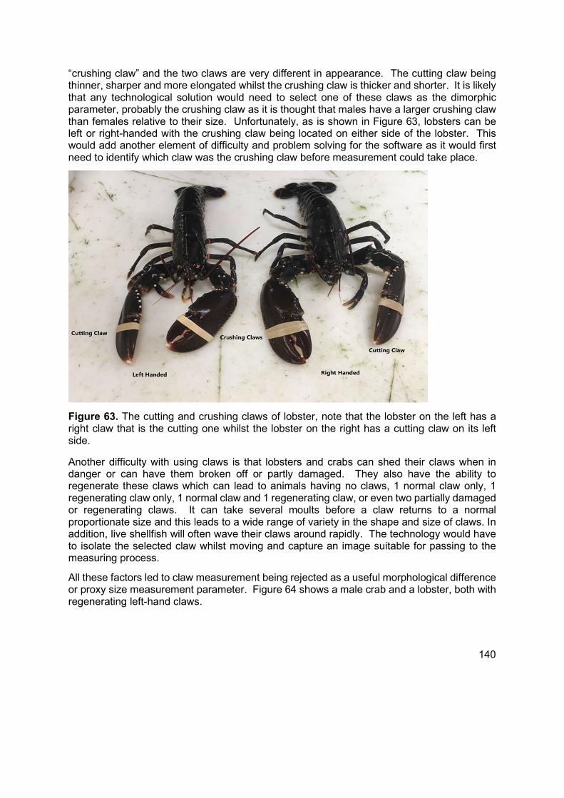
140

“crushing claw” and the two claws are very different in appearance. The cutting claw being thinner, sharper and more elongated whilst the crushing claw is thicker and shorter. It is likely that any technological solution would need to select one of these claws as the dimorphic parameter, probably the crushing claw as it is thought that males have a larger crushing claw than females relative to their size. Unfortunately, as is shown in Figure 63, lobsters can be left or right-handed with the crushing claw being located on either side of the lobster. This would add another element of difficulty and problem solving for the software as it would first need to identify which claw was the crushing claw before measurement could take place.

Figure 63. The cutting and crushing claws of lobster, note that the lobster on the left has a right claw that is the cutting one whilst the lobster on the right has a cutting claw on its left side.

Another difficulty with using claws is that lobsters and crabs can shed their claws when in danger or can have them broken off or partly damaged. They also have the ability to regenerate these claws which can lead to animals having no claws, 1 normal claw only, 1 regenerating claw only, 1 normal claw and 1 regenerating claw, or even two partially damaged or regenerating claws. It can take several moults before a claw returns to a normal proportionate size and this leads to a wide range of variety in the shape and size of claws. In addition, live shellfish will often wave their claws around rapidly. The technology would have to isolate the selected claw whilst moving and capture an image suitable for passing to the measuring process.

All these factors led to claw measurement being rejected as a useful morphological difference or proxy size measurement parameter. Figure 64 shows a male crab and a lobster, both with regenerating left-hand claws.

141

Figure 64. Regenerating claws on brown crab and lobster.

Having rejected claws as a useful morphological feature, we were left with examining the shape and size of the carapace for crabs and the shape and size of the fused segments of the head and thorax (cephalothorax, the main carapace), the tail segments (abdomen), or a relationship between the two for lobsters.

During any field work where measuring and transcribing takes place there can be an element of recording error introduced. The crab measurements were examined and of the 200 crabs measured, 5 were removed due to possible errors or obvious damage to the individuals, leaving 195 individuals for analysis. With the lobster measurements, 5 had to be removed from the original sample of 262, which left 257.

3.2.2 Analysis of Crab data

Of the 195 crabs measured, 92 were females and 103 were male. The male carapace widths ranged between 133 – 206mm and the females ranged between 137 – 213mm. This provided a good data set to investigate the theory that female crabs have a higher carapace peak, in relation to the edges of the carapace. For the remainder of this report, this is termed “dome height”. Table 14 shows the limits of the main measurements taken.

Table 14. Crab measurement limits.

Measured Parameter (mm) Male Female Min Carapace Width 133 137 Max Carapace Width 206 213 Min Dome Height 6 13.48 Max Dome Height 14 28 Average Carapace Width 161.1 166.15 Average Dome Height 9.9 19.42 Average Dome Height / Carapace Width 0.0618 0.1166 Min Abdomen Width 12 31 Max Abdomen Width 25 60 Average Abdomen Width 19.4 48.39 Abdomen Width / Carapace Width 0.0120 0.2901

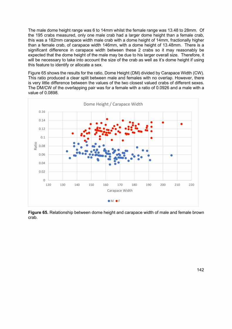
142

The male dome height range was 6 to 14mm whilst the female range was 13.48 to 28mm. Of the 195 crabs measured, only one male crab had a larger dome height than a female crab, this was a 182mm carapace width male crab with a dome height of 14mm, fractionally higher than a female crab, of carapace width 146mm, with a dome height of 13.48mm. There is a significant difference in carapace width between these 2 crabs so it may reasonably be expected that the dome height of the male may be due to his larger overall size. Therefore, it will be necessary to take into account the size of the crab as well as it’s dome height if using this feature to identify or allocate a sex.

Figure 65 shows the results for the ratio, Dome Height (DM) divided by Carapace Width (CW). This ratio produced a clear split between male and females with no overlap. However, there is very little difference between the values of the two closest valued crabs of different sexes. The DM/CW of the overlapping pair was for a female with a ratio of 0.0926 and a male with a value of 0.0898.

Figure 65. Relationship between dome height and carapace width of male and female brown crab.

0

0.02

0.04

0.06

0.08

0.1

0.12

0.14

0.16

120 130 140 150 160 170 180 190 200 210 220

Ratio

Carapace Width

Dome Height / Carapace Width

M F

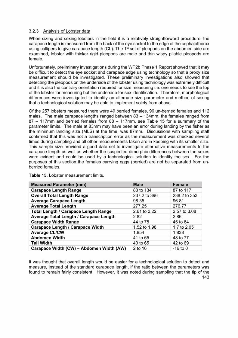
143

3.2.3 Analysis of Lobster data

When sizing and sexing lobsters in the field it is a relatively straightforward procedure; the carapace length is measured from the back of the eye socket to the edge of the cephalothorax using callipers to give carapace length (CL). The 1st set of pleopods on the abdomen side are examined, lobster with thicker rigid pleopods are male and thin wispy pliable pleopods are female.

Unfortunately, preliminary investigations during the WP2b Phase 1 Report showed that it may be difficult to detect the eye socket and carapace edge using technology so that a proxy size measurement should be investigated. These preliminary investigations also showed that detecting the pleopods on the underside of the lobster using technology was extremely difficult and it is also the contrary orientation required for size measuring i.e. one needs to see the top of the lobster for measuring but the underside for sex identification. Therefore, morphological differences were investigated to identify an alternate size parameter and method of sexing that a technological solution may be able to implement solely from above.

Of the 257 lobsters measured there were 49 berried females, 96 un-berried females and 112 males. The male carapace lengths ranged between 83 – 134mm, the females ranged from 87 – 117mm and berried females from 88 – 117mm, see Table 15 for a summary of the parameter limits. The male at 83mm may have been an error during landing by the fisher as the minimum landing size (MLS) at the time, was 87mm. Discussions with sampling staff confirmed that this was not a transcription error as the measurement was checked several times during sampling and all other measurements taken are in keeping with its smaller size. This sample size provided a good data set to investigate alternative measurements to the carapace length as well as whether the suspected dimorphic differences between the sexes were evident and could be used by a technological solution to identify the sex. For the purposes of this section the females carrying eggs (berried) are not be separated from un-berried females.

Table 15. Lobster measurement limits.

Measured Parameter (mm) Male Female Carapace Length Range 83 to 134 87 to 117 Overall Total Length Range 237.2 to 396 238.2 to 353 Average Carapace Length 98.35 96.81 Average Total Length 277.25 276.77 Total Length / Carapace Length Range 2.61 to 3.22 2.57 to 3.08 Average Total Length / Carapace Length 2.82 2.86 Carapace Width Range 44 to 75 45 to 64 Carapace Length / Carapace Width 1.52 to 1.98 1.7 to 2.05 Average CL/CW 1.854 1.838 Abdomen Width 41 to 65 48 to 77 Tail Width 40 to 65 42 to 69 Carapace Width (CW) – Abdomen Width (AW) 2 to 16 -16 to 0

It was thought that overall length would be easier for a technological solution to detect and measure, instead of the standard carapace length, if the ratio between the parameters was found to remain fairly consistent. However, it was noted during sampling that the tip of the

144

rostrum on some animals had often been damaged or was malformed and this would make any calculated carapace length from the total length of damaged individuals, incorrect.

Ignoring the issue noted above, a ratio of 2.82 for male and 2.86 for females or 2.84 combined sexes (not shown in Table 15) would allow the length of carapace to be estimated. Although, it should be noted that the spread of values between 2.57 to 3.22 for this ratio is probably too large to allow this to be used as a reliable proxy for length estimation. As no other potential proxies were identified, the technological solution will need to be able to detect the eye socket and edge of carapace to provide the standard measurement.

Additional measurements were taken during sampling to determine if there were any morphological differences between the sexes of lobsters that could potentially be detected by a technological solution. These included carapace width, abdomen width and tail width. Claws were also measured but these measurements were not explored due to the previously noted issues regarding damage, regeneration and ambidextrous-ness.

Anecdotal information from the fishing industry had suggested that female lobsters were often “wider” than males and found it harder to pass through the escape windows on creels. To explore this observation, the carapace width of the lobsters was measured. The ratio between carapace length (CL) and carapace width (CW) was compared, a ratio was used to take into account the overall size of the individuals; the resulting average CL/CW for males of 1.854 compared to 1.838 for females does support the anecdotal evidence, but, the difference is not large and the CL/CW ratio did not split the sample population by sex.

Another interesting observation made by the industry was that the tail of the female lobster is often wider, or more flared, than the tail of the male. The assumption is that the additional width in the female is linked to carrying eggs. Therefore, the abdomen width (AW) and tail width (TW) were measured as part of the sampling and subsequently compared between the sexes. Using these measurements directly didn’t allow the population to be separated into sex as a direct comparison doesn’t take into account the size of the individual lobster. So, several different relationships were examined:

AW/TW AW-TW CW-AW CW-TW CL/AW CL/TW CL-AW CL-TW

Of these, only one comparison resulted in consistent split between the sexes; Carapace Width (CW) – Abdomen Width (AW). The female lobsters always had an abdomen width that was greater than or equal to the width of the carapace, whereas the male’s abdomen was always less than (slimmer) than the carapace width, see Figure 66.

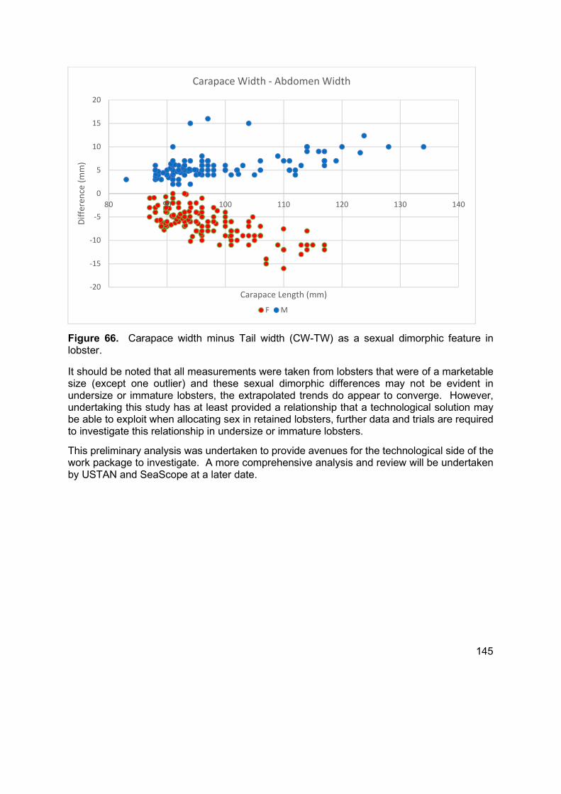
145

Figure 66. Carapace width minus Tail width (CW-TW) as a sexual dimorphic feature in lobster.

It should be noted that all measurements were taken from lobsters that were of a marketable size (except one outlier) and these sexual dimorphic differences may not be evident in undersize or immature lobsters, the extrapolated trends do appear to converge. However, undertaking this study has at least provided a relationship that a technological solution may be able to exploit when allocating sex in retained lobsters, further data and trials are required to investigate this relationship in undersize or immature lobsters.

This preliminary analysis was undertaken to provide avenues for the technological side of the work package to investigate. A more comprehensive analysis and review will be undertaken by USTAN and SeaScope at a later date.

-20

-15

-10

-5

0

5

10

15

20

80 90 100 110 120 130 140

Diff

eren

ce (m

m)

Carapace Length (mm)

Carapace Width - Abdomen Width

F M

146

3.2.4 Applying the findings to a technological solution

3.2.4.1 Brown crabs

The Phase 1 Report investigations showed that both image and scanner technology should be able to detect the edge of a brown crab’s carapace, in which case carapace width could be acquired directly and this route was to be taken in the technological element of the work package.

Abdomen width is the clearest way to sex crabs and given appropriate imagery or scans a technological solution should be able to implement a solution. Unfortunately, to measure abdomen width would require the technology to see the underside of the crabs, which is contrary to the requirements needed to measure carapace width where the technology needs the crabs to be presented so that the upper carapace is closest to the technology. This would then require additional technology sited with a view of the underside of the crab to obtain the abdomen imagery or scans and technology sited above to measure the carapace width. This is not a practical solution within the remit of this project due to:

Crabs often curl their legs under themselves, obscuring any viable view of the abdomen

The abdomen viewing lens/plate/scanner would very quickly be covered in a layer of dirt, debris and water which would cause occlusion of the features

The additional equipment would result in a significant increase in system cost

The only feasible solution for providing information on the sex of crabs is via the carapace width adjusted dome height value.

3.2.4.2 Lobsters

As no appropriate proxy could be found for carapace length, even though it is likely to be very difficult, the technological solution will have to find methods for detecting the eye socket and rear edge of the carapace to provide the required measurement.

As with crabs, the ‘from underneath view’ option has to be discounted for providing sex for exactly the same reasons, the technological solution will need to implement the carapace width minus abdomen width (CW-AW) proxy value.

147

3.3 Fishing Effort

3.3.1 Construction

Following the recommendations of the Phase 1 report, and as described in the methodology section, a system was built incorporating RFID technology to provide string haul and shoot logging alongside inductive sensing to count creels. The systems were built using the same off-the-shelf modular approach as the WP2a system, providing all the benefits previously described. Again, as with the WP2a systems, the main units were mounted externally and survived the environmental conditions.

Although the RFID heads and associated cabling came as IP67 rated from the manufacturer, 2 failures were encountered with the inline connectors leaking, becoming corroded and encrusted with salt residue. The subsequent replacement units had the connectors packed with silicon grease and wrapped in self-amalgamating tape which although not ideal resolved the issue.

The inductive sensors also suffered connector damage although this mainly came from impact damage from the creels (as well as corrosion). As this was a pilot project the mounting of these sensors had to be of a temporary nature and as such there was limited opportunity to construct and fit protective enclosures for the devices. In a longer term or permanent situation, appropriate installation and housing should mitigate this issue.

As the 2B sensor units and associated LED feedback units are, due to their interactions with the fishing gear, mounted in 3 different locations around the working deck of the vessel, there are some significant cable runs back to the main 2B unit. Again, due to the temporary nature of the installs, it wasn’t practical or possible to route and protect the cables in the same way a longer-term project would be able to. As a result, some cable failures were experienced due to physical damage through abrasion, damage through pinch points and general wear and tear. When replaced, alternate routes avoiding the high-risk area were avoided if possible or protection installed where practical.

3.3.2 Power and Space requirements

As described in the methodology, the 2b case takes up 8.9 litres of physical space. As the main unit is more closely associated with the working deck, finding an installation location suited to the cable runs for the sensors, power and the data feed back to the 2B system was more difficult than with the OBCDCS system of WP2a. However, as the system does not need a view of the sky it is possible to mount it under benches, in niches etc.

When running on 12V DC the system draws approximately 1.2A, it uses the same power technology as the OBCDCS system allowing it to operate from 9V to 36V DC and provides the same benefits.

3.3.3 Costs

The base cost of the prototype systems, without the RFID tags, was £1270. Each vessel needed a pair of tags for each string it operated plus spares, the tags were £3 each. Like the 2A system, now the practical implementation and operating parameters are understood in greater depth, this cost can be reduced by at least £400 by reducing to a single RFID (Haul only) reader. Additional savings could be made by selecting different RFID technology with

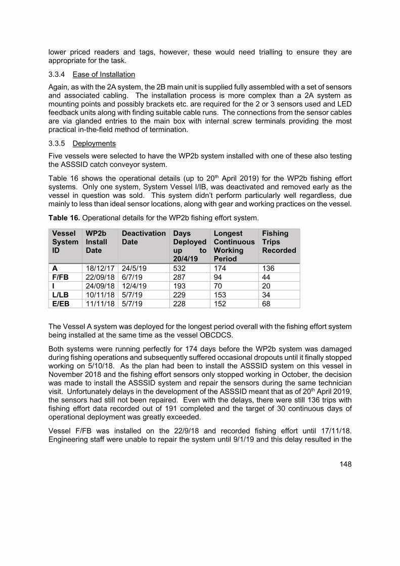
148

lower priced readers and tags, however, these would need trialling to ensure they are appropriate for the task.

3.3.4 Ease of Installation

Again, as with the 2A system, the 2B main unit is supplied fully assembled with a set of sensors and associated cabling. The installation process is more complex than a 2A system as mounting points and possibly brackets etc. are required for the 2 or 3 sensors used and LED feedback units along with finding suitable cable runs. The connections from the sensor cables are via glanded entries to the main box with internal screw terminals providing the most practical in-the-field method of termination.

3.3.5 Deployments

Five vessels were selected to have the WP2b system installed with one of these also testing the ASSSID catch conveyor system.

Table 16 shows the operational details (up to 20th April 2019) for the WP2b fishing effort systems. Only one system, System Vessel I/IB, was deactivated and removed early as the vessel in question was sold. This system didn’t perform particularly well regardless, due mainly to less than ideal sensor locations, along with gear and working practices on the vessel.

Table 16. Operational details for the WP2b fishing effort system.

Vessel System ID

WP2b Install Date

Deactivation Date

Days Deployed up to 20/4/19

Longest Continuous Working Period

Fishing Trips Recorded

A 18/12/17 24/5/19 532 174 136 F/FB 22/09/18 6/7/19 287 94 44 I 24/09/18 12/4/19 193 70 20 L/LB 10/11/18 5/7/19 229 153 34 E/EB 11/11/18 5/7/19 228 152 68

The Vessel A system was deployed for the longest period overall with the fishing effort system being installed at the same time as the vessel OBCDCS.

Both systems were running perfectly for 174 days before the WP2b system was damaged during fishing operations and subsequently suffered occasional dropouts until it finally stopped working on 5/10/18. As the plan had been to install the ASSSID system on this vessel in November 2018 and the fishing effort sensors only stopped working in October, the decision was made to install the ASSSID system and repair the sensors during the same technician visit. Unfortunately delays in the development of the ASSSID meant that as of 20th April 2019, the sensors had still not been repaired. Even with the delays, there were still 136 trips with fishing effort data recorded out of 191 completed and the target of 30 continuous days of operational deployment was greatly exceeded.

Vessel F/FB was installed on the 22/9/18 and recorded fishing effort until 17/11/18. Engineering staff were unable to repair the system until 9/1/19 and this delay resulted in the

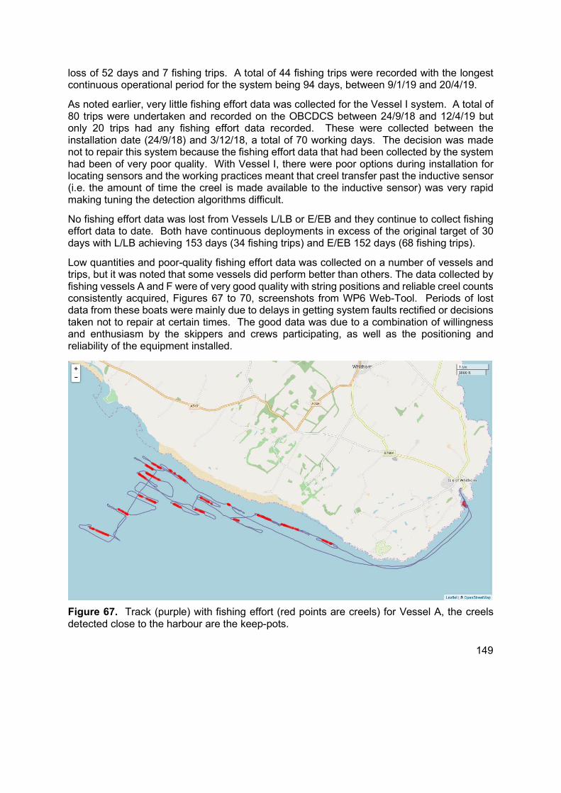
149

loss of 52 days and 7 fishing trips. A total of 44 fishing trips were recorded with the longest continuous operational period for the system being 94 days, between 9/1/19 and 20/4/19.

As noted earlier, very little fishing effort data was collected for the Vessel I system. A total of 80 trips were undertaken and recorded on the OBCDCS between 24/9/18 and 12/4/19 but only 20 trips had any fishing effort data recorded. These were collected between the installation date (24/9/18) and 3/12/18, a total of 70 working days. The decision was made not to repair this system because the fishing effort data that had been collected by the system had been of very poor quality. With Vessel I, there were poor options during installation for locating sensors and the working practices meant that creel transfer past the inductive sensor (i.e. the amount of time the creel is made available to the inductive sensor) was very rapid making tuning the detection algorithms difficult.

No fishing effort data was lost from Vessels L/LB or E/EB and they continue to collect fishing effort data to date. Both have continuous deployments in excess of the original target of 30 days with L/LB achieving 153 days (34 fishing trips) and E/EB 152 days (68 fishing trips).

Low quantities and poor-quality fishing effort data was collected on a number of vessels and trips, but it was noted that some vessels did perform better than others. The data collected by fishing vessels A and F were of very good quality with string positions and reliable creel counts consistently acquired, Figures 67 to 70, screenshots from WP6 Web-Tool. Periods of lost data from these boats were mainly due to delays in getting system faults rectified or decisions taken not to repair at certain times. The good data was due to a combination of willingness and enthusiasm by the skippers and crews participating, as well as the positioning and reliability of the equipment installed.

Figure 67. Track (purple) with fishing effort (red points are creels) for Vessel A, the creels detected close to the harbour are the keep-pots.

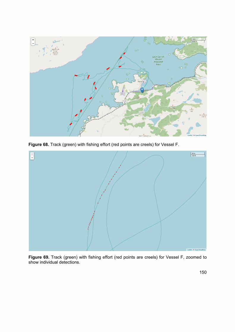
150

Figure 68. Track (green) with fishing effort (red points are creels) for Vessel F.

Figure 69. Track (green) with fishing effort (red points are creels) for Vessel F, zoomed to show individual detections.

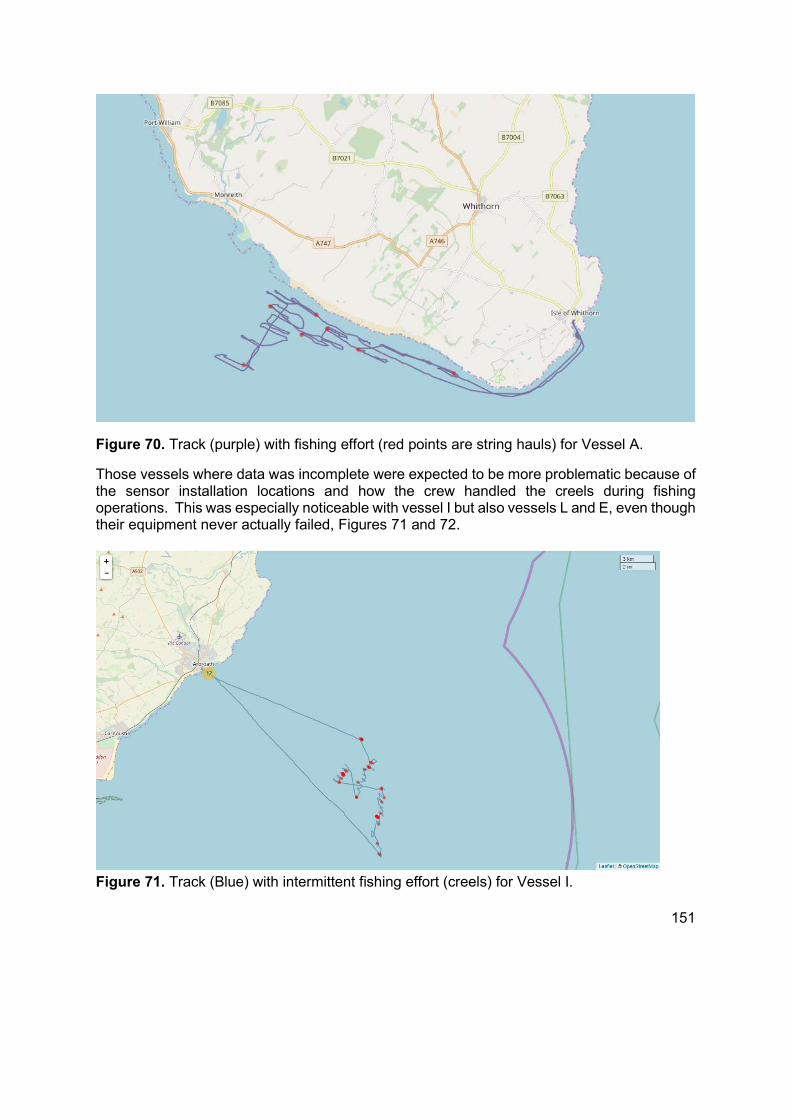
151

Figure 70. Track (purple) with fishing effort (red points are string hauls) for Vessel A.

Those vessels where data was incomplete were expected to be more problematic because of the sensor installation locations and how the crew handled the creels during fishing operations. This was especially noticeable with vessel I but also vessels L and E, even though their equipment never actually failed, Figures 71 and 72.

Figure 71. Track (Blue) with intermittent fishing effort (creels) for Vessel I.

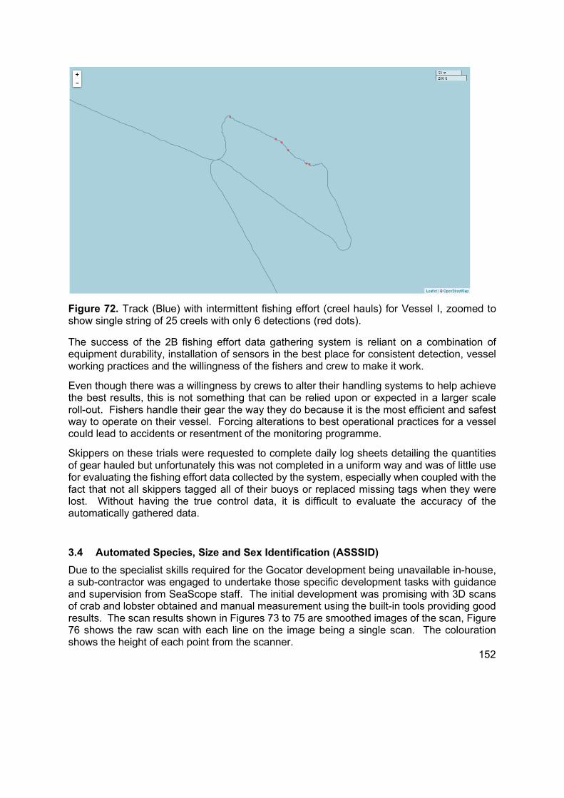
152

Figure 72. Track (Blue) with intermittent fishing effort (creel hauls) for Vessel I, zoomed to show single string of 25 creels with only 6 detections (red dots).

The success of the 2B fishing effort data gathering system is reliant on a combination of equipment durability, installation of sensors in the best place for consistent detection, vessel working practices and the willingness of the fishers and crew to make it work.

Even though there was a willingness by crews to alter their handling systems to help achieve the best results, this is not something that can be relied upon or expected in a larger scale roll-out. Fishers handle their gear the way they do because it is the most efficient and safest way to operate on their vessel. Forcing alterations to best operational practices for a vessel could lead to accidents or resentment of the monitoring programme.

Skippers on these trials were requested to complete daily log sheets detailing the quantities of gear hauled but unfortunately this was not completed in a uniform way and was of little use for evaluating the fishing effort data collected by the system, especially when coupled with the fact that not all skippers tagged all of their buoys or replaced missing tags when they were lost. Without having the true control data, it is difficult to evaluate the accuracy of the automatically gathered data.

3.4 Automated Species, Size and Sex Identification (ASSSID)

Due to the specialist skills required for the Gocator development being unavailable in-house, a sub-contractor was engaged to undertake those specific development tasks with guidance and supervision from SeaScope staff. The initial development was promising with 3D scans of crab and lobster obtained and manual measurement using the built-in tools providing good results. The scan results shown in Figures 73 to 75 are smoothed images of the scan, Figure 76 shows the raw scan with each line on the image being a single scan. The colouration shows the height of each point from the scanner.

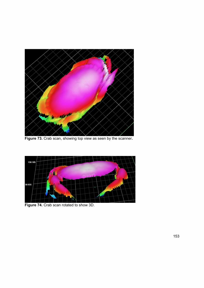
153

Figure 73. Crab scan, showing top view as seen by the scanner.

Figure 74. Crab scan rotated to show 3D.

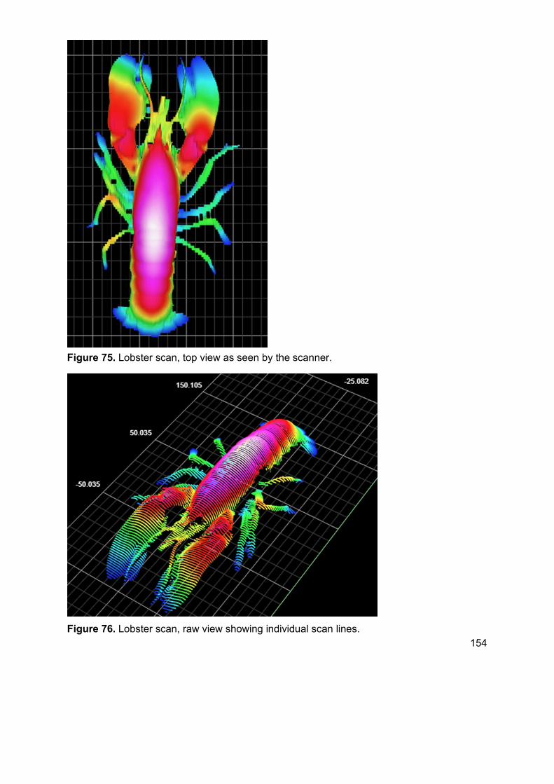
154

Figure 75. Lobster scan, top view as seen by the scanner.

Figure 76. Lobster scan, raw view showing individual scan lines.

155

Following good results from the manual Crab measurements, autonomous tools were developed to remove the legs etc. from the scan to effectively isolate the carapace ready to be passed to the measuring and sexing algorithms. Initially all the individual tools involved in the identification and measuring processes were developed to work with Crabs being scanned in a particular orientation with further tools planned for orientation correction.

After multiple iterations of built-in tools combined with custom tools built on the Gocator, a set of candidate tools were completed for testing.

The measuring tools identified the two extremes of the isolated carapace and directly extracted the distance between the two points ignoring any curvature of the surface.

Further tools then placed a 3D profile across the line between the measuring points, extracting the ‘angle of attack’ of the curvature, a line fit value for the curvature and the depth of the dome. These values along with the anchor points for all the tools and the raw scan data are then sent to the embedded PC for transmission to the OBCDCS.

A tool was developed that provided sex based purely on the ‘angle of attack’ value but this did not prove a robust enough method. It was apparent that sexing required a model-fit approach utilising some or all of the dome height, ‘angle-of-attack’, line-fit and carapace width parameters. This kind of model-fitting is beyond the capability of the Gocator internally but exporting the parameters would allow off-line sex allocation to be done once the data is available ashore. In order to build the sexing model a significant number of individuals will need to be scanned; this work is ongoing due to delays in the development of the remainder of the on-board side of the project.

A similar approach was taken for obtaining the lobster carapace length data, however, identifying the back of the eye socket is still proving very elusive, and as yet a reliable and lobster measuring tool is not available from the subcontractor.

3.4.1 Replicability

With the autonomous crab measuring tools in place, a series of replicate trials were undertaken to investigate the variability of the measurements acquired. Each of the trial animals were fed through the system 100 times and the measurement data collected. Although the crabs were fed through the system in generally the same orientation there was a certain degree of variability in the exact rotation. The data showed good consistency but also that the measuring tools were overestimating the carapace width. Figure 77 shows data for 1 individual; the 2 outliers at positions 1 and 87 were where the rotation of the individual was beyond the tool’s capability to handle. After removing the outliers, there is an average difference from the known carapace width of 2.05mm and a Standard Deviation (pop) of 0.32mm for the measurements.

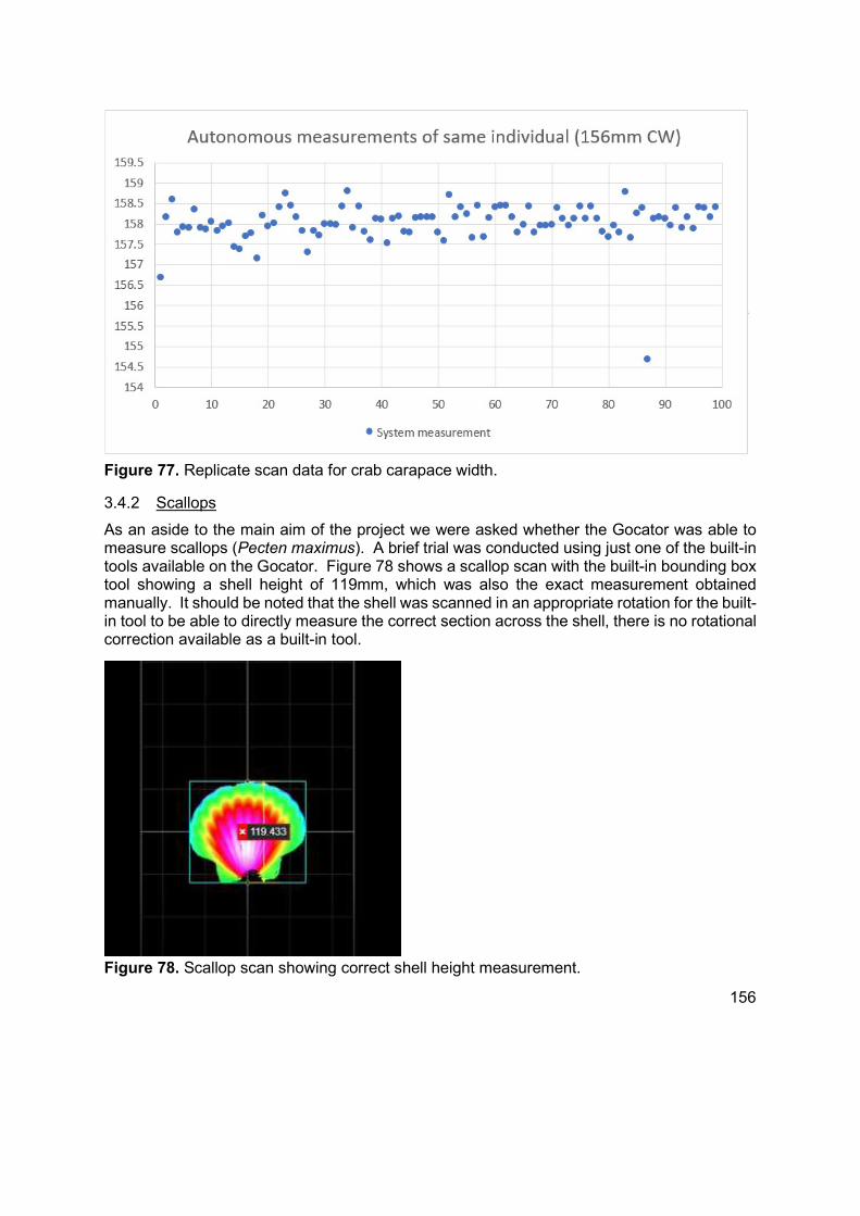
156

Figure 77. Replicate scan data for crab carapace width.

3.4.2 Scallops

As an aside to the main aim of the project we were asked whether the Gocator was able to measure scallops (Pecten maximus). A brief trial was conducted using just one of the built-in tools available on the Gocator. Figure 78 shows a scallop scan with the built-in bounding box tool showing a shell height of 119mm, which was also the exact measurement obtained manually. It should be noted that the shell was scanned in an appropriate rotation for the built-in tool to be able to directly measure the correct section across the shell, there is no rotational correction available as a built-in tool.

Figure 78. Scallop scan showing correct shell height measurement.

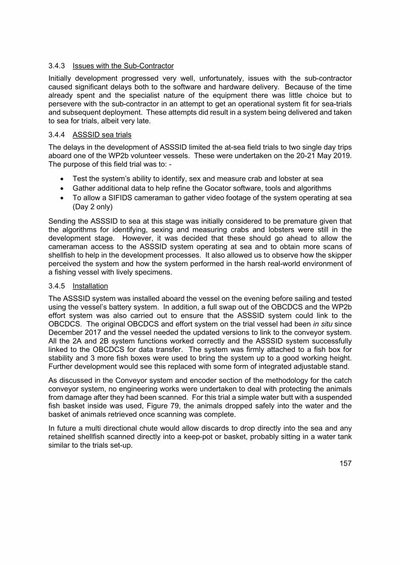
157

3.4.3 Issues with the Sub-Contractor

Initially development progressed very well, unfortunately, issues with the sub-contractor caused significant delays both to the software and hardware delivery. Because of the time already spent and the specialist nature of the equipment there was little choice but to persevere with the sub-contractor in an attempt to get an operational system fit for sea-trials and subsequent deployment. These attempts did result in a system being delivered and taken to sea for trials, albeit very late.

3.4.4 ASSSID sea trials

The delays in the development of ASSSID limited the at-sea field trials to two single day trips aboard one of the WP2b volunteer vessels. These were undertaken on the 20-21 May 2019. The purpose of this field trial was to: -

Test the system’s ability to identify, sex and measure crab and lobster at sea Gather additional data to help refine the Gocator software, tools and algorithms To allow a SIFIDS cameraman to gather video footage of the system operating at sea

(Day 2 only)

Sending the ASSSID to sea at this stage was initially considered to be premature given that the algorithms for identifying, sexing and measuring crabs and lobsters were still in the development stage. However, it was decided that these should go ahead to allow the cameraman access to the ASSSID system operating at sea and to obtain more scans of shellfish to help in the development processes. It also allowed us to observe how the skipper perceived the system and how the system performed in the harsh real-world environment of a fishing vessel with lively specimens.

3.4.5 Installation

The ASSSID system was installed aboard the vessel on the evening before sailing and tested using the vessel’s battery system. In addition, a full swap out of the OBCDCS and the WP2b effort system was also carried out to ensure that the ASSSID system could link to the OBCDCS. The original OBCDCS and effort system on the trial vessel had been in situ since December 2017 and the vessel needed the updated versions to link to the conveyor system. All the 2A and 2B system functions worked correctly and the ASSSID system successfully linked to the OBCDCS for data transfer. The system was firmly attached to a fish box for stability and 3 more fish boxes were used to bring the system up to a good working height. Further development would see this replaced with some form of integrated adjustable stand.

As discussed in the Conveyor system and encoder section of the methodology for the catch conveyor system, no engineering works were undertaken to deal with protecting the animals from damage after they had been scanned. For this trial a simple water butt with a suspended fish basket inside was used, Figure 79, the animals dropped safely into the water and the basket of animals retrieved once scanning was complete.

In future a multi directional chute would allow discards to drop directly into the sea and any retained shellfish scanned directly into a keep-pot or basket, probably sitting in a water tank similar to the trials set-up.

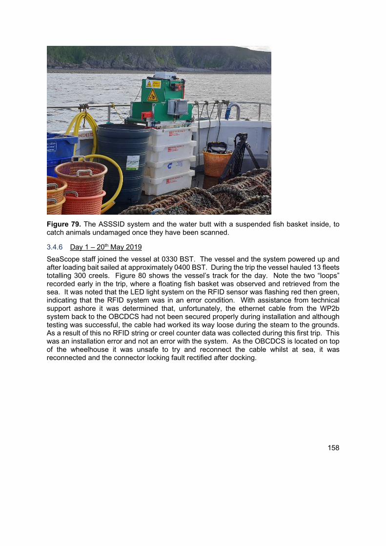
158

Figure 79. The ASSSID system and the water butt with a suspended fish basket inside, to catch animals undamaged once they have been scanned.

3.4.6 Day 1 – 20th May 2019

SeaScope staff joined the vessel at 0330 BST. The vessel and the system powered up and after loading bait sailed at approximately 0400 BST. During the trip the vessel hauled 13 fleets totalling 300 creels. Figure 80 shows the vessel’s track for the day. Note the two “loops” recorded early in the trip, where a floating fish basket was observed and retrieved from the sea. It was noted that the LED light system on the RFID sensor was flashing red then green, indicating that the RFID system was in an error condition. With assistance from technical support ashore it was determined that, unfortunately, the ethernet cable from the WP2b system back to the OBCDCS had not been secured properly during installation and although testing was successful, the cable had worked its way loose during the steam to the grounds. As a result of this no RFID string or creel counter data was collected during this first trip. This was an installation error and not an error with the system. As the OBCDCS is located on top of the wheelhouse it was unsafe to try and reconnect the cable whilst at sea, it was reconnected and the connector locking fault rectified after docking.

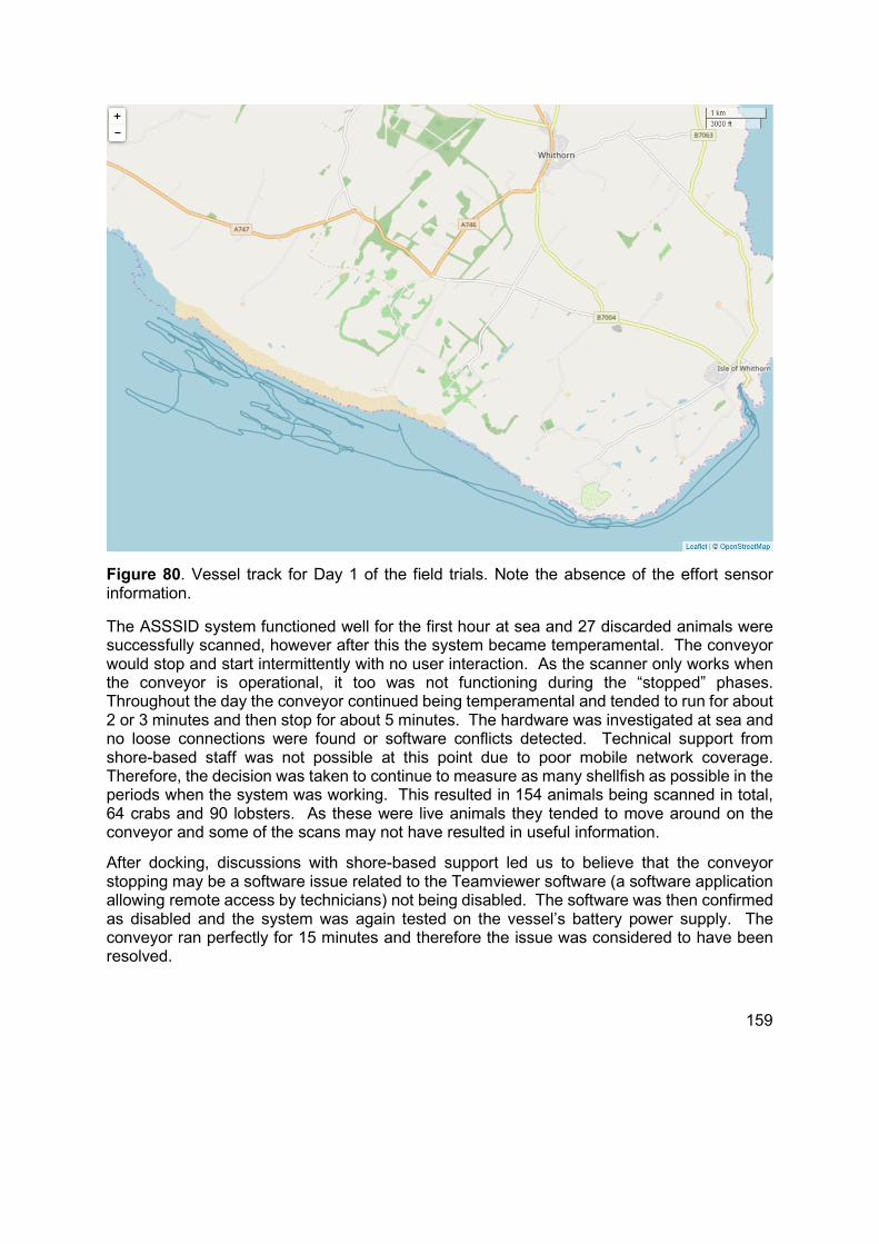
159

Figure 80. Vessel track for Day 1 of the field trials. Note the absence of the effort sensor information.

The ASSSID system functioned well for the first hour at sea and 27 discarded animals were successfully scanned, however after this the system became temperamental. The conveyor would stop and start intermittently with no user interaction. As the scanner only works when the conveyor is operational, it too was not functioning during the “stopped” phases. Throughout the day the conveyor continued being temperamental and tended to run for about 2 or 3 minutes and then stop for about 5 minutes. The hardware was investigated at sea and no loose connections were found or software conflicts detected. Technical support from shore-based staff was not possible at this point due to poor mobile network coverage. Therefore, the decision was taken to continue to measure as many shellfish as possible in the periods when the system was working. This resulted in 154 animals being scanned in total, 64 crabs and 90 lobsters. As these were live animals they tended to move around on the conveyor and some of the scans may not have resulted in useful information.

After docking, discussions with shore-based support led us to believe that the conveyor stopping may be a software issue related to the Teamviewer software (a software application allowing remote access by technicians) not being disabled. The software was then confirmed as disabled and the system was again tested on the vessel’s battery power supply. The conveyor ran perfectly for 15 minutes and therefore the issue was considered to have been resolved.

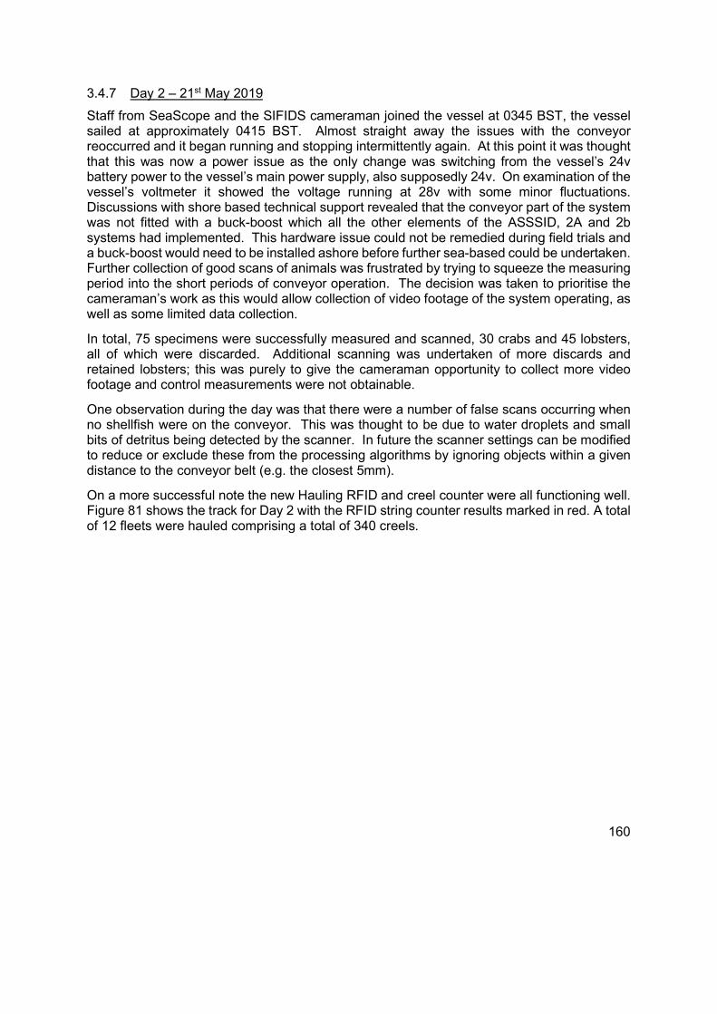
160

3.4.7 Day 2 – 21st May 2019

Staff from SeaScope and the SIFIDS cameraman joined the vessel at 0345 BST, the vessel sailed at approximately 0415 BST. Almost straight away the issues with the conveyor reoccurred and it began running and stopping intermittently again. At this point it was thought that this was now a power issue as the only change was switching from the vessel’s 24v battery power to the vessel’s main power supply, also supposedly 24v. On examination of the vessel’s voltmeter it showed the voltage running at 28v with some minor fluctuations. Discussions with shore based technical support revealed that the conveyor part of the system was not fitted with a buck-boost which all the other elements of the ASSSID, 2A and 2b systems had implemented. This hardware issue could not be remedied during field trials and a buck-boost would need to be installed ashore before further sea-based could be undertaken. Further collection of good scans of animals was frustrated by trying to squeeze the measuring period into the short periods of conveyor operation. The decision was taken to prioritise the cameraman’s work as this would allow collection of video footage of the system operating, as well as some limited data collection.

In total, 75 specimens were successfully measured and scanned, 30 crabs and 45 lobsters, all of which were discarded. Additional scanning was undertaken of more discards and retained lobsters; this was purely to give the cameraman opportunity to collect more video footage and control measurements were not obtainable.

One observation during the day was that there were a number of false scans occurring when no shellfish were on the conveyor. This was thought to be due to water droplets and small bits of detritus being detected by the scanner. In future the scanner settings can be modified to reduce or exclude these from the processing algorithms by ignoring objects within a given distance to the conveyor belt (e.g. the closest 5mm).

On a more successful note the new Hauling RFID and creel counter were all functioning well. Figure 81 shows the track for Day 2 with the RFID string counter results marked in red. A total of 12 fleets were hauled comprising a total of 340 creels.

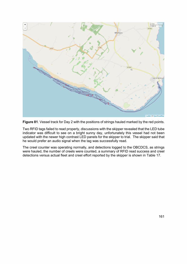
161

Figure 81. Vessel track for Day 2 with the positions of strings hauled marked by the red points.

Two RFID tags failed to read properly, discussions with the skipper revealed that the LED tube indicator was difficult to see on a bright sunny day, unfortunately this vessel had not been updated with the newer high contrast LED panels for the skipper to trial. The skipper said that he would prefer an audio signal when the tag was successfully read.

The creel counter was operating normally, and detections logged to the OBCDCS, as strings were hauled, the number of creels were counted, a summary of RFID read success and creel detections versus actual fleet and creel effort reported by the skipper is shown in Table 17.

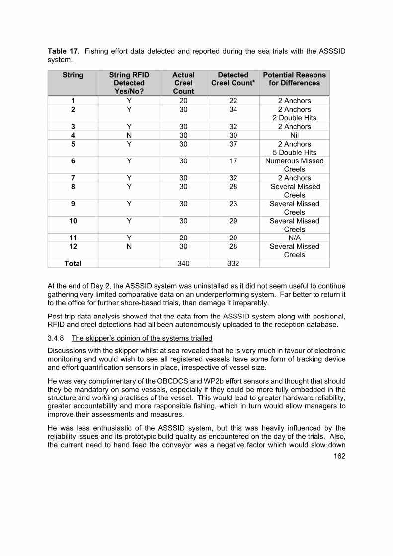
162

Table 17. Fishing effort data detected and reported during the sea trials with the ASSSID system.

String String RFID Detected Yes/No?

Actual Creel Count

Detected Creel Count*

Potential Reasons for Differences

1 Y 20 22 2 Anchors 2 Y 30 34 2 Anchors

2 Double Hits 3 Y 30 32 2 Anchors 4 N 30 30 Nil 5 Y 30 37 2 Anchors

5 Double Hits 6 Y 30 17 Numerous Missed

Creels 7 Y 30 32 2 Anchors 8 Y 30 28 Several Missed

Creels 9 Y 30 23 Several Missed

Creels 10 Y 30 29 Several Missed

Creels 11 Y 20 20 N/A 12 N 30 28 Several Missed

Creels Total 340 332

At the end of Day 2, the ASSSID system was uninstalled as it did not seem useful to continue gathering very limited comparative data on an underperforming system. Far better to return it to the office for further shore-based trials, than damage it irreparably.

Post trip data analysis showed that the data from the ASSSID system along with positional, RFID and creel detections had all been autonomously uploaded to the reception database.

3.4.8 The skipper’s opinion of the systems trialled

Discussions with the skipper whilst at sea revealed that he is very much in favour of electronic monitoring and would wish to see all registered vessels have some form of tracking device and effort quantification sensors in place, irrespective of vessel size.

He was very complimentary of the OBCDCS and WP2b effort sensors and thought that should they be mandatory on some vessels, especially if they could be more fully embedded in the structure and working practises of the vessel. This would lead to greater hardware reliability, greater accountability and more responsible fishing, which in turn would allow managers to improve their assessments and measures.

He was less enthusiastic of the ASSSID system, but this was heavily influenced by the reliability issues and its prototypic build quality as encountered on the day of the trials. Also, the current need to hand feed the conveyor was a negative factor which would slow down

163

fishing operations and increase workload. The system would need to be altered to reduce additional handling of the retained catch or discards. He also thought that no matter what alterations were made, the conveyor may always be too large for the very small vessels and that it would be necessary to incentivise skippers to take this to sea for management purposes.

164

4 DISCUSSION AND CONCLUSIONS

4.1 WP2A OBCDCS

The 2A systems deployed have recorded over 35 million positional pings, all autonomously transferred to the cloud reception database. The systems with attached 2B systems have also reliably received and transferred data streams from the additional systems using the standard package protocol. The ASSSID system has transferred multiple parameter data streams and desk testing has transferred multi-cell arrays of data. This variety of data formats shows the ability of the OBCDCS design to accept data streams from a large range of sensor packages provided they, or an attached interface, can provide the data package expected by the system.

The cost of the prototype system is over the target budget but as discussed there is scope to reduce the cost by, for example, reducing to a single GNSS receiver rather than keeping the redundant backup currently in the system, switching to a simpler GNSS system (USB), or reducing the available NAS storage from 2TB.

The individual hardware components that comprise the system have suffered few failures and withstood conditions well beyond their design capabilities. Installation, space and power requirements have met the required design parameters and posed few problems. There are alternatives to the majority of the components used and no doubt arguments could be made for and against the selections made, however, the individual components have integrated well to form a functional system.

The volume of both raw data and system diagnostics highlight the need for appropriate data reception, storage, monitoring and management infrastructure and processes to form an integral part of any larger scale implementation.

Due to the unobtrusive and autonomous nature of the system its deployment on the trial fleet raised no issues, however, the trial fleet were all volunteers, no incentives were offered to encourage participation. For a larger roll-out, covering an entire section of the fleet, resistance may be encountered, and incentives or national/local legislation may be required to ensure full coverage of the vessels of interest.

As with the hardware components, the selection of the development environment, Python, could provoke debate in a variety of directions. The final release of the software itself has proven robust in the field but should not be considered ‘production ready’. Having incorporated the SoftwareUpdater functionality, remote updates for either individual vessels or the whole fleet were made possible, reducing the need for technician visits in the field. For a larger scale roll-out, further work should be undertaken to enhance error handling, diagnostics and processing efficiency.

In discussion with a number of the fishers, the existence of third-party data that supported ‘track record’ of their fishing grounds and their routes to and from them was of significant interest given the pressure on use of the marine environment and potential for enforced displacement.

Overall the work package has shown it is possible to design, build and deploy an on-board autonomous data harvesting, storage and forwarding system suitable for the Scottish under 12m fleet.

165

4.2 WP2B Effort

The 2B systems deployed in the field focussed on detecting activity that could almost unequivocally, in the case of RFID this is absolute, be linked directly to creel fishing. Other activity sensors such as those running off vessel equipment, e.g. winch rotation, can only identify that the piece of equipment was in use and not what that use was.

The string RFID system worked well on the majority of the vessels; it does require a minor alteration to working practice and a little care and attention; swiping the tag and checking it read ok when the buoy, anchor or creel it is attached to is hauled aboard. The feedback mechanism, an LED panel, went through some iterations before a workable solution was found, for future development a combined audio/visual feedback system may be appropriate, with the option to turn off the audio element. The string ID system gives indication of fishing location and soak time, it does not give an absolute measure of effort in terms of number of creels; the number of creels on a given string could be collected at the time of tagging but creels can be added to or lost from a string at any time. If absolute up-to-date creel counts are a requirement, a notification system to allow fishers to update their creel counts would need to be implemented, adding to the administrative workload of running a fishing vessel and in all probability, it would not be updated regularly.

RFID tags did get lost at times when buoys broke away from the strings, but fortunately this was not a common occurrence. Skippers were issued spare sets of tags to deal with this eventuality, and, for the most part, lost tags were replaced and the project team notified of the new tags in use. In a future roll-out, a similar system would need to be implemented and resource allocated to manage the updates.

Initially, dual RFID readers were implemented to capture both the hauling and shooting position of a string. This is an ideal data set and provides a certain degree of redundancy; if one of the readers fails a record will still be provided by the other unit. Shooting position on one trip will become the hauling position on the next trip that recovers the string so the system in effect captures ‘duplicate’ data. On some vessels there was no appropriate location for a shooting sensor to be installed either due to vessel layout, working practice or the physical swiping of the tag during the shoot process would add an additional safety risk to the fisher (this was considered unacceptable), and for these vessels, only a haul sensor was installed. In any future roll-out consideration should be given to the need for dual sensors given the ‘duplicate data’ effect discussed above. It should be noted that the soak time calculation would be affected when using a single sensor as an assumption would have to be made about how long the gear was out of the water before shooting commenced

The inductive sensor system implemented to provide creel counts was less successful than the RFID system, this may in part be due to restrictions on installation locations combined with working practices and creel design. The inaccuracy in creel count worked both ways, over and under counting on a regular basis. The over-count was usually due to a creel being left in proximity to the sensor for too long, or the metal anchor weights triggering a count on the sensor. Under-counts were mainly due to creels not being sited close to the sensor to be detected or being moved away too quickly. If absolute creel counts are a necessity for assessment, management or licensing needs then this element of the work package probably needs a bottom-up review including examining other technological routes, although Phase 1

166

did not find an alternate practical solution at that time. Of course, RFID tags could be fitted to all creels and scanned as they come aboard, but this would be very expensive and many could be lost, creating plastic pollution.

Overall, the string RFID element of the system gives a clear indication of where and when fishing pressure is being exerted along with soak time and creel count estimates from the initial install.

4.3 ASSSID

The ASSSID system has been shown to work on fish markets and in an office environment, but its working life will be in a marine environment where it needs to withstand the rigours of operating on a working fishing vessel. It needs to be reliable and transferrable between vessels which may have different power supplies, deck space and operating conditions. Its primary purpose is to identify, measure and sex shellfish autonomously, passing the data and scan images on to the OBCDCS for storage and transmission. The prototype system has gone a long way to achieving these aims but is yet to achieve them all.

Fitting a buck-boost should remedy the power issues and along with further engineering work the physical issues with the unit itself can be resolved. Further discussion with fishers and subsequent engineering work is required to make the animal handling suitable, which may require a range of custom fittings to suit individual vessels.

The software is still in development, the challenges have been considerably more complex than originally thought and significant hurdles are yet to be cleared. Developmental progress suffered through failures of a 3rd party and any future work, if it occurred, would need to review this approach.

Unfortunately, there is no time to undertake the work required for the system to be able to meet all of its aims before the original deadline for this report (31st May 2019).

Discussion with the fisher involved in the trial highlighted that implementation of the system would definitely impact on working practices on almost every vessel involved and that for some vessels implementation may not be possible. This should not be seen as a barrier to implementation or further work but as an indicator that significant buy-in and committed support is required from all the stakeholders whether they are scientists, managers or fishers.

Working with live animals direct from the sea is very different to working with frozen or very docile stored animals. They try to grab hold of hardware whilst going along the conveyor, they rear up, squat down, flip over and wave appendages around. This was all expected behaviour, it was never an expectation that the system would be able to provide the full data set for every individual passed through the system, but as the software is refined it will be able to gather the required data for a large enough sub-sample of the catch, along with the number of un-processable animals, for the data to be considered representative.

Considerable work has gone into the current system to allow the measuring technology to be tested at sea, but it is clear that more work and investment is needed to bring this prototypic design up to the point where it is an operational, practical, deployable piece of equipment.

Without a doubt, the Gocator system could be an incredibly useful and versatile tool within shellfish monitoring programmes but its development and implementation will pose challenges.

167

4.4 Environmental and other data

Environmental data harvesting should also be considered more fully, by thorough and widespread surveying of potential end users and customers. This is a resource which could have a widespread interest beyond fisheries management and is a possible mechanism to recoup operational and development costs. Several institutes have already been in contact with USTAN to express an interest in the collection of data such as sea bottom temperature, surface temperature and temperature profiles.

4.5 Implementation and deployment on a larger scale

Throughout the development of all the systems, the question of how they could potentially be implemented within the fishing industry has been under consideration. It is unrealistic to think that every single vessel under 12m in Scottish waters would carry the full suite of equipment developed under this project. The cost for the equipment alone makes that an unrealistic proposition, without taking into account the amount of maintenance and project management required along with the vast amount of data that would be gathered and require storage and management.

An idea, initially proposed by USTAN, was discussed at various SIFIDS meetings, it may appear in different forms or levels of refinement in other work package reports, but it is particularly relevant to this work package.

If you take a fleet of vessels of interest, the fleet may be defined by geographic area, target species, main gear in use or a combination of parameters or even encompass the entire under 12m Scottish fleet. Once the fleet is defined, stratify it based on data needs and allocate each vessel to a stratum. The stratification may be based on the environmental risk posed by the gear in use, the ‘at-risk’ status of the stock being prosecuted or the proximity of a home port or main fishing grounds to a Marine Protected Area (MPA). For this example, we have defined 3 strata or tiers of data need which fit with the different data harvesting options available. The tiers are cumulative, i.e. a tier 2 vessel would collect all the data required for tier 1 plus the data required for tier 2, where necessary, the individual data items would be linked.

When defining the fleets and stratification, statisticians, managers and biologists would need to discuss and agree the parameter sets involved and the levels of sampling etc. required to meet the needs of the monitoring programme being considered. It would be perfectly feasible to move vessels between tiers on a regular basis to share the workload of tiers 2 and 3 data collection provided the data capture equipment lends itself to easy removal and installation.

Tier 1, the lowest level of data capture: It would require a vessel to carry a tracking device that streams position and time data at a relatively coarse interval into a central database. Basic trackers capable of doing this cost a few hundred pounds per year to buy and operate. The data would allow managers to see where the majority of fleet activity takes place and at what time of the year. There would be an element of installation, maintenance and fleet management required. Ideally the units would be solar powered or require minimal power and be installable by the fisher. Installation could be verified by the receipt of track data cross referenced to statutory reporting information or by inspection by a local fishery officer or fishers’ association representative etc.

168

Tier 2, intermediate data needs: Requires the collection of fishing effort data linked to position and time. This could be provided in the form of an OBCDCS with a 2B style fishing effort collection system. The exact type of sensors used would depend on the fishing gear being used. For example, a hydraulic pressure or rotational sensor may be the most appropriate for detecting trawl fishing, or RFID marked buoys for creel fishing.

Tier 3, highest level of data capture: Requires the collection of retained and discarded catch data, either as full data or sub-samples. This could consist of the OBCDCS and the ASSSID catch conveyor system being deployed together.

Implementing any of this technology in an operational monitoring programme will require careful management and planning. Reassurances regarding data privacy will need to be provided and data ownership agreements will need to be established. The purposes for which the data is being collected will also need to be clearly stated beforehand and consideration will need to be given as to whether participation is voluntary or mandatory. Fishers will need to know their legal standing if data collected with the equipment led to a prosecution. These topics are beyond the scope of this project but are integral to the successful implementation of such a program.

169

5 RECOMMENDATIONS The development of the OBCDCS, the incorporation of the fishing effort sensors and the development of the ASSSID system began nearly two years ago. Technological advancements have continued during this period and what was initially considered to be the most appropriate approach 2 years ago, may not still be the best approach or option today. It is likely that if we revisited the design process today, we would find cheaper, more efficient or more robust components that could be used in the building of the systems.

Before any of the resulting equipment, software or ideas from this project are considered for a larger scale project or further development, a review and revision process is highly recommended. Recent developments may reduce costs and lessons learned throughout this project will be invaluable in the review process. This is especially the case with the ASSSID system as by combining the scanner, or its improved successors with new camera technology and artificial intelligence systems there is scope to greatly improve the system’s abilities and performance.

A list of recommendations is provided below.

Recommendations: -

1. Review the current systems for improvements and value since project first commenced 2. Investigate cheap tracker devices for widespread vessel activity coverage 3. Combine the OBCDCS with the fishing effort sensor technology for a combined system 4. Review the ASSSID chute design from an engineering perspective to improve

usability, animal handling and automation 5. Review the ASSSID hardware components for improvements, alternatives and

complementary technology and consider a rebuild exercise 6. Continue the software development associated with the ASSSID system 7. Investigate the customer base for environmental data and potential to market these

data 8. Consider developing the ASSSID technology so that it can be used on other types of

fishing vessel and for other high value species e.g. scallops, razorfish, tuna.

170

6 REFERENCES Aiken, D. E., & Waddy, S. L. (1989). Interaction of temperature and photoperiod in the regulation of spawning by American lobsters (Homarus americanus). Canadian Journal of Fisheries and Aquatic Sciences, 46(1), 145-148. Aiken, D. E., & Waddy, A. S. (1980). Reproductive biology [Lobsters]. The biology and management of lobsters. AtlasRFIDstore., 2017. AtlasRFIDstore, Available at www.atlasrfidstore.com , [Accessed 02/03/2017] Butler, D.A., Ballard, W.B., Haskell, S.P. and Wallace, M.C., 2006. Limitations of thermal infrared imaging for locating neonatal deer in semiarid shrub communities. Wildlife Society Bulletin, 34(5), pp.1458-1462. Chong, A.K. and Stratford, P., 2002. Underwater digital stereo-observation technique for red hydrocoral study. Photogrammetric engineering and remote sensing, 68(7), pp.745-752. Cilulko, J., Janiszewski, P., Bogdaszewski, M. and Szczygielska, E., 2013. Infrared thermal imaging in studies of wild animals. European Journal of Wildlife Research, 59(1), pp.17-23. Corgos, A., & Freire, J. (2006). Morphometric and gonad maturity in the spider crab Maja brachydactyla: a comparison of methods for estimating size at maturity in species with determinate growth. ICES Journal of Marine Science, 63(5), 851-859. Course G., Pasco G., O’Brien M. and Addison J. 2015. Evidence Gathering in Support of Sustainable Scottish Inshore Fisheries: Monitoring Fishery Catch to Assist Scientific Stock Assessments in Scottish Inshore Fisheries – a Pilot Study and Identifying Catch Composition to Improve Scottish Inshore Fisheries Management using Technology to Enable Self-Reporting – a Pilot Study. Published by MASTS. 164pp Debuse, V. J., Addison, J. T., & Reynolds, J. D. (1999). The effects of sex ratio on sexual competition in the European lobster. Animal Behaviour, 58(5), 973-981. Debuse, V. J., Addison, J. T., & Reynolds, J. D. (2001). Morphometric variability in UK populations of the European lobster. Journal of the Marine Biological Association of the United Kingdom, 81(3), 469-474. Flir., 2017. Flir systems Inc. Available at http://www.flir.eu/home/. [Accessed 05/03/2017] Food MC., 2017. The Food Machinery Company Ltd. Available at https://www.foodmc.co.uk/check-weighers , [Accessed 14/02/2017] Furuno, 2017. The Furuno WS 200 weather station for marine vessels. http://www.furuno.dk/en/products/navigation/wind-system/airmar-ws-200wx/ [Accessed o6/o6/2017].

171

Geng, J., 2011. "Structured-light 3D surface imaging: a tutorial," Adv. Opt. Photon. 3, 128-160 (2011). Haig, J. A., Bakke, S., Bell, M. C., Bloor, I. S., Cohen, M., Coleman, M., ... & Salomonsen, H. (2016). Reproductive traits and factors affecting the size at maturity of Cancer pagurus across Northern Europe. ICES Journal of Marine Science, 73(10), 2572-2585. Harbitz, A., 2007. Estimation of shrimp (Pandalus borealis) carapace length by image analysis. ICES Journal of Marine Science: Journal du Conseil, 64(5), pp.939-944.

Harvey, E., Shortis, M., Stadler, M. and Cappo, M., 2002. A comparison of the accuracy and precision of measurements from single and stereo-video systems. Marine Technology Society Journal, 36(2), pp.38-49. Hernández-Serna, A. and Jiménez-Segura, L.F., 2014. Automatic identification of species with neural networks. PeerJ, 2, p.e563. Herakleous, K. and C. Poullis, 2014. “3DUNDERWORLD-SLS: An Open-Source Structured-Light Scanning System for Rapid Geometry Acquisition”, ICT-TR-2014-01 Hold, N., Murray, L.G., Pantin, J.R., Haig, J.A., Hinz, H. and Kaiser, M.J., 2015. Video capture of crustacean fisheries data as an alternative to on-board observers. ICES Journal of Marine Science: Journal du Conseil, p.fsv030. Kinney,T.A., 2001, Machine Design. Available at http://machinedesign.com/sensors/proximity-sensors-compared-inductive-capacitive-photoelectric-and-ultrasonic . [Accessed 03/04/2017] Krizhevsky, A., Sutskever, I. and Hinton, G.E., 2012. Imagenet classification with deep convolutional neural networks. In Advances in neural information processing systems (pp. 1097-1105). Langdon, W.B., Poli, R., McPhee, N.F. and Koza, J.R., 2008. Genetic programming: An introduction and tutorial, with a survey of techniques and applications. In Computational intelligence: A compendium (pp. 927-1028). Springer Berlin Heidelberg. Li, L., (2014). Time-of-Flight Camera – An Introduction. Technical White Paper, May 2014. http://www.ti.com/lit/wp/sloa190b/sloa190b.pdf (January 2015). Lizárraga-Cubedo, H. A., Tuck, I., Bailey, N., Pierce, G. J., & Kinnear, J. A. M. (2003). Comparisons of size at maturity and fecundity of two Scottish populations of the European lobster, Homarus gammarus. Fisheries Research, 65(1), 137-152. Marel., 2017a. Available at http://marel.com/fish-processing/systems-and-equipment/on-board/surimi/receiving--handling/weighing/marine-scales/303?prdct=1 , [Accessed 14/02/2017]

172

Marel., 2017b. Available at http://marel.com/fish-processing/systems-and-equipment/whitefish/pelagic/receiving--handling/grading--batching/compact-grader/1171?prdct=1&pc=wgb , [Accessed 14/02/2017] McCafferty, D.J., 2007. Hot biology: investigating the thermal physiology of birds and mammals. Available at http://www.flir.com/uploadedFiles/Thermography/MMC/Brochures/T820331/T820331_EN.pdf?_ga=1.178105703.332015088.1492005756 . [Accessed 05/03/2017]. McElderry, H., 2008, July. At-sea observing using video-based electronic monitoring. In Background paper prepared by Archipelago Marine Research Ltd. for the Electronic Monitoring Workshop July (pp. 29-30). McElderry, H., Beck, M., Pria, M.J., and Anderson, S., 2010. Electronic monitoring in the New Zealand inshore trawl fishery: A pilot study. Report by Archipelago Marine Research Ltd., Victoria, BC, Canada. Mendo, T., Smout, S., Photopoulou, T., and James, M. (2019a) Identifying fishing grounds from vessel tracks: model-based inference for small scale fisheries. Royal Society Open Science - Manuscript ID RSOS-191161. Accepted August 2019 Mendo, T., Smout, S., Russo, T., D’Andrea, L., and James, M. (2019b) Effect of temporal and spatial resolution on identification of fishing activities in small-scale fisheries using pots and traps. – ICES Journal of Marine Science, doi:10.1093/icesjms/fsz073. Met Office, 2018. Adapted from map of the UK Meteorological Office weather station locations. https://metofficenews.files.wordpress.com/2018/06/weather-observation-network.png?w=640. [Accessed 09/12/2018]. Miura, M., Sakai, S., Ishii, J., Ito, K. and Aoki, T., 2013. An easy-to-use and accurate 3D shape measurement system using two snapshots. In Proc. Int’l Workshop on Advanced Image Technology (pp. 1103-1106) Montgomery, M., 2015. Basic Fishing Methods – A comprehensive guide to commercial fishing methods. Seafish Industry Authority, 2015.

Mrovlje, J. and Vrancic, D., 2008, October. Distance measuring based on stereoscopic pictures. In 9th International PhD Workshop on Systems and Control: Young Generation Viewpoint (Vol. 2, pp. 1-6) NFFO - The National Federation of Fishers’s Organisation’s (2015). Atlantic crab resource users’ network. NFFO. Available at: http://nffo.org.uk/our-partnerships/acrunet O'Brien, N.A., Hulse, C.A., Friedrich, D.M., Van Milligen, F.J., von Gunten, M.K., Pfeifer, F. and Siesler, H.W., 2012. Miniature near-infrared (NIR) spectrometer engine for handheld applications. In SPIE Defense, Security, and Sensing (pp. 837404-837404). International Society for Optics and Photonics.

173

O’Brien, N., Hulse, C.A., Pfeifer, F. and Siesler, H.W., 2013. Near infrared spectroscopic authentication of seafood. J. Near Infrared Spectrosc, 21, p.299. Öndes, F., Kaiser, M. J., & Murray, L. G. (2017). Fish and invertebrate by-catch in the crab pot fishery in the Isle of Man, Irish Sea. Journal of the Marine Biological Association of the United Kingdom, 1-13. Pass, 2017a. Pass Thermal. Available at https://www.pass-thermal.co.uk/thermal-camera-applications-wildlife [Accessed 05/03/2017] Pass, 2017b Pass Thermal. Available at https://www.tester.co.uk/hunting-thermal-camera-comparison . [Accessed 05/03/2017] Pepperl and Fuchs., 2017, Pepperl and Fuchs GB Ltd. Available at https://files.pepperl-fuchs.com/webcat/navi/productInfo/doct/tdoct2584a_eng.pdf?v=20150417153628 . [Accessed 15/03/2017] Public Health England, 2017. Laser radiation safety advice. Uddated 15 August 2017. Available at https://www.gov.uk/government/publications/laser-radiation-safety-advice/laser-radiation-safety-advice#phe-advice . [Accessed 15/10/2019] Pulsar, 2017. Pulsar -nv.com. Available at http://www.pulsar-nv.com/products/thermal-imaging-scopes-quantum-xd/quantum-xd50s/ . [Accessed 05/03/2017]. Rycroft, N., Radcliffe, K., & Atema, J. (2013). A photographic method for lobster morphometry aimed at site discrimination. Canadian Journal of Fisheries and Aquatic Sciences, 70(11), 1658-1665. Savi Technologies., 2007. Savi Technology, Available at www.savi.com . [Accessed 03/03/2017]. Sick AG., 2017, SICK United Kingdom, Available at www.sick.com/gb/en/ , [Accessed 03/02/2017]. Sweeting, S. (2015). Maturity of brown crab (Cancer pagurus) in Scottish water. Master’s Thesis. University of Aberdeen, Aberdeen. Tamersoy, B., 2009. Vehicle detection and tracking in highway surveillance videos. University of Texas. Tecnimodern,. 2017. Tecnimodern Automotion. Available at http://www.tecnimodern.fr/index-famille-140126-lng-en-ID_MS-1394.html , [Accessed 14/02/2017]. Thermo Scientific TM., 2017. Thermo Fisher Scientific, Available at https://www.thermofisher.com/order/catalog/product/MICROPHAZIRRX , [Accessed 02/02/2017].

174

Thomas, H. J., & Figueiredo, M. J. (1965). Seasonal variations in the catch composition of the Norway lobster, Nephrops norvegicus (L.) around Scotland. ICES Journal of Marine Science, 30(1), 75-85. Tully, O., Roantree, V., & Robinson, M. (2001). Maturity, fecundity and reproductive potential of the European lobster (Homarus gammarus) in Ireland. Journal of the Marine Biological Association of the United Kingdom, 81(1), 61-68. UKIVA., 2017. United Kingdom Industrial Vision Association (UKIVA), Available at www.ukiva.org . [Accessed 10/03/2017]. Ungfors, A. (2007). Sexual maturity of the edible crab (Cancer pagurus) in the Skagerrak and the Kattegat, based on reproductive and morphometric characters. ICES Journal of Marine Science, 64(2), 318-327. Wang, B., 2014. Automatic Animal Species Identification Based on Camera Trapping Data. Doctoral dissertation, University of Alberta. Wehkamp, M. and Fischer, P., 2014. A practical guide to the use of consumer-level digital still cameras for precise stereogrammetric in situ assessments in aquatic environments. Underwater technology, 32(2), pp.111-128. Woll, A.K., van der Meeren, G.I., and Fossen, I. 2006. Spatial variation in abundance and catch composition of Cancer pagurus in Norwegian waters: biological reasoning and implications for assessment. ICES Journal of Marine Science: Journal du Conseil, 63(3): 421- 433.

175

7 ANNEXES

7.1 Annex 1: Glossary of Terms and Acronyms

Image Processing - the process of creating one image from another image or group of images.

CV/MV Computer or Machine Vision - the extraction of information from imaging technology which is subsequently passed to other processes for ‘action’

Banded – the act of restraining the claws on crabs and lobsters by applying a rubber band

Nicked – the practise of cutting a claw in a specific place to disable the claw from closing

EM – Electronic monitoring

GNSS – Global navigation satellite system

GPS – Global positioning system

GUI – Graphic user interface

HMI – Human machine interface

NIR – Near infrared spectroscopy

RFID – Radio Frequency Identification

176

7.2 Annex 2: NMEA GNSS sentences

The following table summarizes the range of possible NMEA messages, not all of these are supported by the receiver used

Message Function

ADV Position and satellite information for RTK network operations

DTM Datum reference information

GBS GNSS satellite fault detection (RAIM support)

GGA Time, position, and fix related data

GLL Position data: position fix, time of position fix, and status

GNS GNS Fix data

GRS GRS range residuals

GSA GPS DOP and active satellites

GST Position error statistics

GSV Number of SVs in view, PRN, elevation, azimuth, and SNR

HDT Heading from True North

LLQ Leica local position and quality

PFUGDP A proprietary message containing information about the type of positioning system, position, number of satellites and position statistics

PTNL,AVR Time, yaw, tilt, range, mode, PDOP, and number of SVs for Moving Baseline RTK

PTNL,BPQ Base station position and position quality indicator

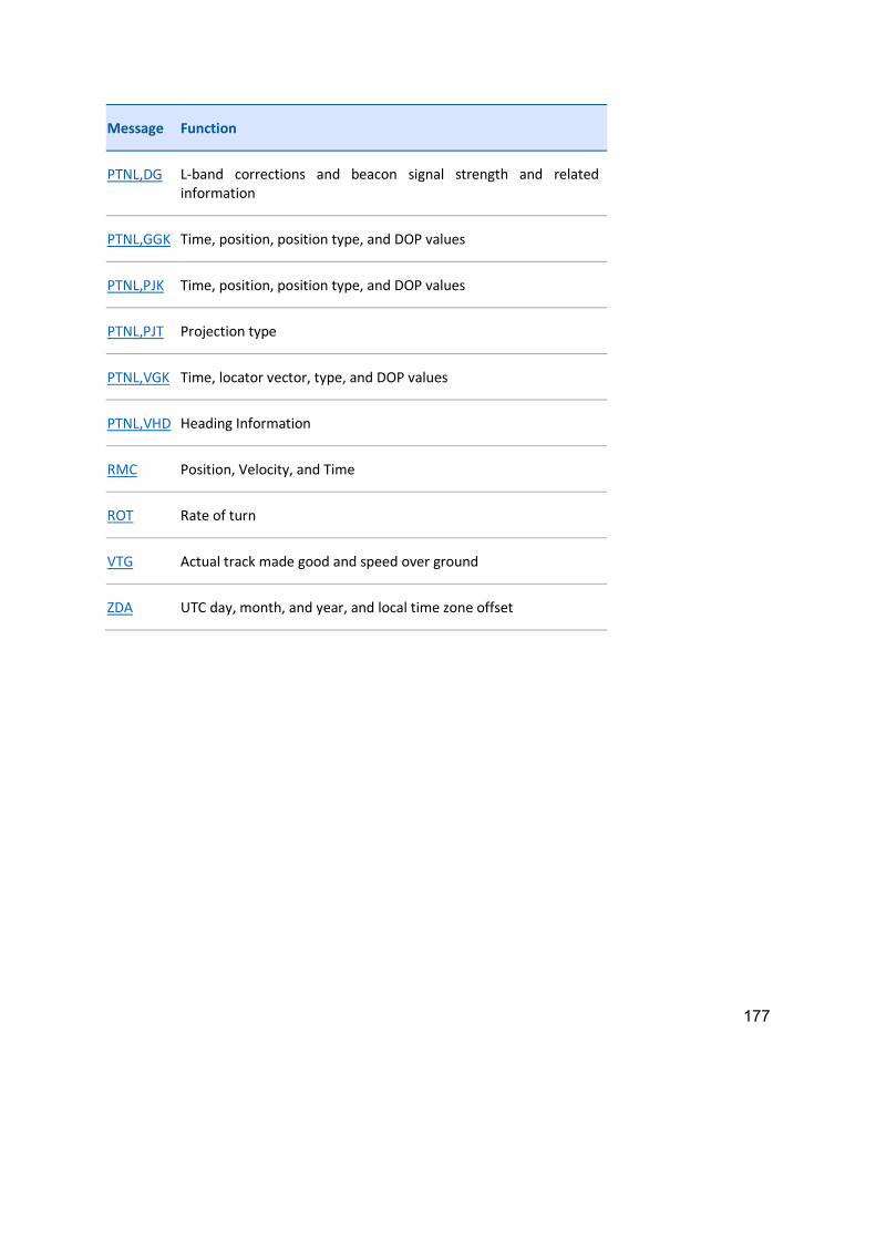
177

Message Function

PTNL,DG L-band corrections and beacon signal strength and related information

PTNL,GGK Time, position, position type, and DOP values

PTNL,PJK Time, position, position type, and DOP values

PTNL,PJT Projection type

PTNL,VGK Time, locator vector, type, and DOP values

PTNL,VHD Heading Information

RMC Position, Velocity, and Time

ROT Rate of turn

VTG Actual track made good and speed over ground

ZDA UTC day, month, and year, and local time zone offset

178

7.3 Annex 3: IP Ratings

The IP Code, International Protection Marking, IEC standard 60529, sometimes interpreted as Ingress Protection Marking, classifies and rates the degree of protection provided against intrusion (body parts such as hands and fingers), dust, accidental contact, and water by mechanical casings and electrical enclosures.

An IP rating is made up of 2 digits, the first indicating protection against solid matter, the second indicating protection against water.

First Digit:

0 No special protection

1 Protection from a large part of the body such as a hand (but no protection from deliberate access); from solid objects greater than 50mm in diameter.

2 Protection against fingers or other object not greater than 80mm in length and 12mm in diameter.

3 Protection from entry by tools, wires etc., with a diameter of 2.5 mm or more.

4 Protection against solid bodies larger than 1mm (e.g. fine tools/small etc.).

5 Protected against dust that may harm equipment.

6 Totally dust tight.

Second Digit:

0 No protection.

1 Protection against condensation.

2 Protection against water droplets deflected up to 15° from vertical

3 Protected against spray up to 60° from vertical.

4 Protected against water spray from all directions.

5 Protection against low pressure water jets (all directions)

6 Protection against strong water jets and waves.

7 Protected against temporary immersion.

8 Protected against prolonged effects of immersion under pressure.

Using the above definitions and given the harsh environment we are expecting deck-based equipment to operate in, IP66 is recommended as a minimum, with a preference for IP67 if cost effective, for the deck based equipment used in the SIFIDS project.

179

180

7.4 Annex 4: Data collection sheets

Brown Crab and Lobster morphological data collection sheets

Date

SEX CARAPACE WIDTHCARAPACE LENGTH MID-

EYES TO REAR

CARAPACE HEIGHT ABOVE CARAPACE

EDGE DOME HEIGHTCARAPACE CURVE

LENGTH ABDOMEN WIDTH CLAW LENGTH CLAW WIDTH CLAW DEPTHPHOTO TAKEN COMMENT

ID M/F CW CL CD DM CC AW ChL ChW ChD Y/N E.G. REGEN

BROWN CRAB (mm)

Sampler/s:Sample Port/Facility:Sample Area:

181

Lobster morphological data collection sheet

Date

SEX

TOTAL OVERALL LENGTH

CARAPACE LENGTH

CARAPACE WIDTH

CARAPACE DEPTH

CARAPACE LENGTH TO

ROSTRUM TIPABDOMEN

WIDTH TAIL WIDTH

ABDOMEN CURVE

LENGTH CLAW LENGTH CLAW WIDTH CLAW DEPTHPHOTO TAKEN COMMENT

ID M/F TL CL CW CD CLR AW TW ACL ChL ChW ChD Y/N e.g. REGEN

Sample Area: Sample Port/Facility: SAMPLER/S:

LOBSTER (mm)

182

7.5 Annex 5: Primary Components

The following are the primary components used in the OBCDCS system and the effort capture system. These components were supplemented with consumable items such as cabling, connectors, sealants etc. As a rough guide, the main components account for two thirds of the cost of the systems.

7.6 OBCDCS components

Item Case (Case farm – Dave range) Synology NAS DS218+ (NAS, SSD, Carrier) 2 x Raspberry Pi 2 x 32Gb SD 2 x PiGPS 2 x Antennae Netgear GS108 Teltonika Router 3 x 12V Buck Boost 2 x 5V Buck Boost

7.7 WP2B Effort system components

Item Case (Case farm – Dave range) 3 x Raspberry Pi 3 x 32Gb SD Netgear GS108 1 x 12V Buck Boost 3 x 5V Buck Boost 1 x 24V Buck Boost 2 x P & F RFID Head Telemechanique proximity sensor 2 x Pi-RS485 communications board 1 x 12v to 3v optically isolated convertor (in house build)

183

This project was supported by a grant from the European Maritime and Fisheries Fund

Marine Alliance for Science and Technology for Scotland C/O Scottish Oceans Institute East Sands University of St Andrews St Andrews Fife KY16 8LB Scotland/UK T: +44 (0) 1334 467 200 E: [email protected] W: www.masts.ac.uk

MASTS Company Number: SC485726; Charity Number: SC045259

ISBN

EMFF: SCO1434

Work Package (2) Final Report WP2A

Documents